transient stability improvement of multi-machine power ...transient stability improvement of...
TRANSCRIPT
IOSR Journal of Electrical and Electronics Engineering (IOSR-JEEE)
e-ISSN: 2278-1676,p-ISSN: 2320-3331, Volume 9, Issue 1 Ver. I (Jan. 2014), PP 28-40
www.iosrjournals.org
www.iosrjournals.org 28 | Page
Transient Stability Improvement of Multi-machine Power System
using Fuzzy Controlled TCSC
Mohammad Abdul Baseer Department of Electrical Engineering, College of Engineering/ Majmaah University, Saudi Arabia.
Abstract: Power system is subjected to sudden changes in load levels. Stability is an important concept which
determines the stable operation of power system. In general rotor angle stability is taken as index, but the
concept of transient stability, which is the function of operating condition and disturbances deals with the ability
of the system to remain intact after being subjected to abnormal deviations. A system is said to be synchronously
stable (i.e., retain synchronism) for a given fault if the system variables settle down to some steady-state values
with time, after the fault is removed.
For the improvement of transient stability the general methods adopted are fast acting exciters, circuit
breakers and reduction in system transfer reactance. The modern trend is to employ FACTS devices in the
existing system for effective utilization of existing transmission resources. These FACTS devices contribute to
power flow improvement besides they extend their services in transient stability improvement as well.
In this thesis, the studies had been carried out in order to improve the Transient Stability of WSCC 9
Bus System with Fixed Compensation on Various Lines and Optimal Location has been investigated using
trajectory sensitivity analysis for better results.
In this thesis, in order to improve the Transient Stability margin further series FACTS device has been
implemented. A fuzzy controlled Thyristor Controlled Series Compensation (TCSC) device has been used here
and the results highlight the effectiveness of the application of a TCSC in improving the transient stability of a
power system.
Keywords: faults, fuzzy logic, fuzzy controller, loads, multi-machine, Transient stability, TCSC.
I. Introduction 1.1 Transient Stability Analysis:
Transient stability studies provide information related to the capability of a power system to remain in
synchronism during major disturbances resulting from either the loss of generating or transmission facilities,
sudden or sustained load changes, or momentary faults. Specifically, these studies provide the changes in the
voltages, currents, powers, speeds, and torques of the machines of the power system, as well as the changes in
system voltages and power flows, during and immediately following a disturbance. The degree of stability of a
power system is an important factor in the planning of new facilities. In order to provide the reliability required
by the dependence on continuous electric service, it is necessary that power systems be designed to be stable
under any conceivable disturbance.
1.2 Methods for improving the transient stability limit of a power system.
Increase of system voltages, use of AVR.
Use of high speed excitation systems.
Reduction in system reactance.
Use of high speed reclosing breakers.
The operating characteristics of synchronous and induction machines are described by sets of
differential equations. The number of differential equations required for a machine depends on the details
needed to represent accurately the machine performance.
A transient stability analysis is performed by combining a solution of the algebraic equations
describing the network with a numerical solution of the differential equations. The solution of the network
equations retains the identity of the system and thereby provides access to system voltages and currents during
the transient period.
In order to perform Transient stability studies following concepts must be analyzed:
So many iterative algorithms for solving a set of non linear algebraic equations in the load flow studies,
for example Gauss method, Gauss Seidal method, Newton Raphson method etc.
Transient Stability Improvement of Multi-machine Power System using Fuzzy Controlled TCSC
www.iosrjournals.org 29 | Page
1.3 Gauss Seidal method
It is an iterative algorithm for solving set non-linear algebraic equations. To start with, a solution vector
is assumed, based on guidance from practical experience in a physical situation. One of the equations is then
used to obtain the revised value of a particular variable by substituting in it the present values of the remaining
variables.
It is almost impossible to say which one of the existing methods is the best. Choice of a particular
method in any given situation is normally a compromise between the various criteria of goodness of the load
flow methods.
1.4 Modeling of system:
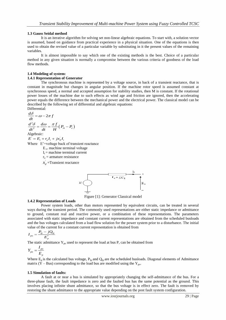
1.4.1 Representation of Generator
The synchronous machine is represented by a voltage source, in back of a transient reactance, that is
constant in magnitude but changes in angular position. If the machine rotor speed is assumed constant at
synchronous speed, a normal and accepted assumption for stability studies, then M is constant. If the rotational
power losses of the machine due to such effects as wind age and friction are ignored, then the accelerating
power equals the difference between the mechanical power and the electrical power. The classical model can be
described by the following set of differential and algebraic equations:
Differential:
2
2
2
m e
df
dt
d d fP P
dt dt H
Algebraic: ' '
t a t d tE E r I jx I
Where E’=voltage back of transient reactance
E t= machine terminal voltage
It = machine terminal current
ra = armature resistance
'
dx =Transient reactance
Figure [1]: Generator Classical model
1.4.2 Representation of Loads
Power system loads, other than motors represented by equivalent circuits, can be treated in several
ways during the transient period. The commonly used representations are either static impedance or admittance
to ground, constant real and reactive power, or a combination of these representations. The parameters
associated with static impedance and constant current representations are obtained from the scheduled busloads
and the bus voltages calculated from a load flow solution for the power system prior to a disturbance. The initial
value of the current for a constant current representation is obtained from
*
lp lp
po
p
P jQI
E
The static admittance Ypo used to represent the load at bus P, can be obtained from
po
po
p
IY
E
Where Ep is the calculated bus voltage, Plp and Qlp are the scheduled busloads. Diagonal elements of Admittance
matrix (Y – Bus) corresponding to the load bus are modified using the Ypo.
1.5 Simulation of faults:
A fault at or near a bus is simulated by appropriately changing the self-admittance of the bus. For a
three-phase fault, the fault impedance is zero and the faulted bus has the same potential as the ground. This
involves placing infinite shunt admittance, so that the bus voltage is in effect zero. The fault is removed by
restoring the shunt admittance to the appropriate value depending on the post fault system configuration.
Transient Stability Improvement of Multi-machine Power System using Fuzzy Controlled TCSC
www.iosrjournals.org 30 | Page
1.5.1 Simulation of fault in a power system studies: A symmetrical fault is simulated in one of the lines at a time. The simulation is done in three phases:
1. The pre-fault system is run for a small time (say 1 second) till the system is initialized.
2. The fault is then applied at one end of the line. Simulation of this faulted condition continues till the line is
disconnected from the buses at both the ends of the faulted line after a time tcl. The time gap between the
tripping of breakers at the two ends is negligible compared to the clearing time. Hence the disconnection of the
line at the two ends can be considered simultaneous.
3. Next is the post-fault system simulation where the faulted line is totally disconnected from the system.
Simulation is carried out for a longer time (say 10-20seconds) to observe the nature of the transients.
1.5.2 Runge-Kutta method
In the application of the Runge-Kutta fourth-order approximation, the changes in the internal voltage
angles and machine speeds, again for the simplified machine representation, are determined from
1 2 3 4
1 2 3 4
12 2
6
12 2
6
i i i ii t t
i i i ii t t
k k k k
l l l l
i=1,2,…,no. of generators.
The k’s and l’s are the changes in i and i respectively, obtained using derivatives evaluated at
predetermined points. For this procedure the network equations are to be solved four times.
1.6 Transient stability analysis:
Single machine connected to an infinite bus
Multi machine system
1.6.1 Multi machine system:
The following steps easily follow for determining multimachine stability.
1. From the prefault load flow data determine E'k voltage behind transient reactance for all generators.
This establishes generator emf magnitudes |E k| which remains constant during the study and initial
rotor angle δk° =∟Ek. Also record prime mover inputs to generators, Pmk=P°gk .
2. Augment the load flow network by the generator transient reactances. Shift network buses behind
the transient reactances.
3. Find Ybus for various network conditions –during fault, post fault (faulted line cleared), after line
reclosure.
4. For faulted mode, find generator outputs from power angle equations and solve swing equations step by
step (point by point method) or any integration algorithms such as modified Euler’s method, R.K fourth
order method etc.
5. Keep repeating the above step for post fault mode and after line reclosure mode.
6. Examine δ (t) plots for all the generators and establish the answer to the stability question.
II. Trajectory Sensitivity Analysis
2.1 Computation of Trajectory Sensitivity
Multi machine power system is represented by a set of differential equations
00 )(),,,( xtxxtfx (2.1)
Where x is a state vector and is a vector of system parameters. The sensitivities of state trajectories with
respect to system parameters can be found by perturbing from its nominal value 0 .The equations of
trajectory sensitivity can be found as
0)(,
otx
fx
x
fx (2.2)
Where /xx . Solution of (2.1) and (2.2) gives the state trajectory and trajectory sensitivity,
respectively. However sensitivities can also be found in a simpler way by using numerical method.
2.2 Simulation of fault
A symmetrical fault is simulated in one of the lines at a time. The simulation is done in three phases:
1. The pre-fault system is run for a small time (say 0.1 second).
Transient Stability Improvement of Multi-machine Power System using Fuzzy Controlled TCSC
www.iosrjournals.org 31 | Page
2. The fault is applied at one end of the line. Simulation of this faulted condition continues till the line is
disconnected from the buses at both the ends of the faulted line after a time tcl. The time gap between
the tripping of breakers at the two ends is negligible compared to the clearing time.Hence the
disconnection of the line at the two ends can be considered Simultaneous.
3. Next is the post-fault system simulation where the faulty line is totally disconnected from the system.
Simulation is carried out for a longer time (say 10seconds) to observe the nature of the transients.
Series controller:-
Static Synchronous Series Comparator
Inter line Power Flow Controller
Thyristor Controlled Series Capacitor
Thyristor Switched Series Capacitor
Thyristor Controlled Series Reactor
Thyristor Switch Series Reactor
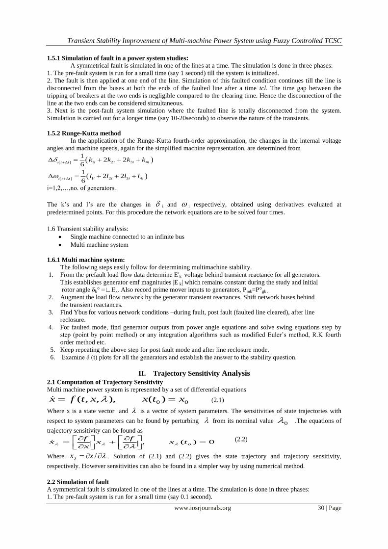
Thyristor-Controlled Series Capacitor (TCSC)
The basic Thyristor-Controlled Series Capacitor scheme, proposed in 1986 by Vithayathil with
others as a method of “rapid adjustment of network impedance,” is shown in the fig.[2].It consists of the series
compensating capacitor shunted by a Thyristor-Controlled Reactor. In a practical TCSC implementation, several
such basic compensators may be connected in series to obtain the desired voltage rating and operating
characteristics.
Fig 2 Equivalent circuit of TCSC
This arrangement is similar in structure to the TSSC and, if the impedance of the reactor, XL, is
sufficiently smaller than that of the capacitor, Xc, it can be operated in an on/off manner like the TSSC.
However, the basic idea behind the TCSC scheme is to provide a continuously variable capacitor by means of
partially canceling the effective compensating capacitance by the TCR.
The TCR at the fundamental system frequency is a continuously variable reactive impedance, controllable by
delay angle α, the steady state impedance of the TCSC is that of a parallel LC circuit, consisting of a fixed
capacitive impedance, Xc, and a variable inductive impedance, XL (α), that is,
XTCSC(α) = (Xc*XL)/(XL(α)-Xc) Where XL(α)=XL*π / (π-2 α-sin α), XL≤XL(α )≤∞
XL = ωL, and α is the delay angle measured from the crest of the capacitor voltage.
2.3 Modeling of the TCSC and the power system
The TCSC model is given in Fig. 2. The overall reactance XC of the TCSC is given in terms of the
firing angle α as
Let us denote the fundamental frequency capacitance of the TCSC, which is equal to 1/(ωsXC), as Ctcsc. It is to
be noted
That in this work the TCSC is operated only in the capacitive mode. The capacitive reactance XFC of the TCSC
is chosen as half of the reactance of the line in which the TCSC is placed and the TCR reactance XP is chosen to
be 1/3 of XFC.
Transient Stability Improvement of Multi-machine Power System using Fuzzy Controlled TCSC
www.iosrjournals.org 32 | Page
III. Fuzzy Logic Controller
3.1 INTRODUCTION
Most of the real-world processes that require automatic control are non-linear in nature. That is, their
parameter values alter as the operating point changes over time or both. In case of conventional control schemes,
as they are linear, a controller can only be tuned to give good performance at a particular operating point or for a
limited period of time. The controller needs to be retuned if the operating point changes with time. This
necessity to retune has driven the need for adaptive controllers that can automatically retune themselves to
match the current process characteristics.
Fuzzy logic is an innovative technology that enhances conventional system design with engineering
expertise. Using fuzzy logic, we can circumvent the need for rigorous mathematical modeling
During the past several years, FLC has emerged as one of the most active area of research for the
application of fuzzy set theory. A fuzzy set is a generalization of the concept of an ordinary set in which the
membership function (MF) values can be only one of the two values, 0 and 1. A fuzzy set can be defined as
below.
Fuzzy set A in a universe of discourse U is characterized by a MF A: U [0] [1] and associates with
each element x of U a number A (x) in the interval [0 1] representing the degree of membership of x in A.
3.2 Definition of Fuzzy Sets
Let X is a collection of objects, and then a fuzzy set is defined to be a set of ordered pairs. A = {(x,
A(x)), x X}, where A(x) is called the membership function x in A. The numerical interval X that is relevant
for the description of a fuzzy variable is commonly named as universe of discourse. The membership function
A(x) denotes the degree to which x belongs to A and is normally limited to values between 0 and 1. A value of
A(x) close to one means it is very likely for x to be in A and a value of A(x) near to zero denotes non-
membership. In case that the values of membership function are limited to zero or one, then A becomes a crisp
or non-fuzzy set.
3.3 Fuzzy Set Operations
It is well known that the membership functions play an important role in fuzzy sets. Therefore it is not
surprising to define fuzzy set operators based on their corresponding membership functions. Operations like
AND, OR and NOT are some the most important operations of the fuzzy sets.
Suppose A and B are two fuzzy sets with membership functions A(x) and B(x) respectively then.
a) The AND operator or the intersection of two fuzzy sets is the membership functions of the intersection of
these two fuzzy sets.
C = (AB), is defined by C(x) = min { A(x), B (x) }, x X
b) The OR operator or the union of two fuzzy sets is the membership function of the union of these two fuzzy
sets.
D (AB), is defined by C(x) = max { A(x), B (x) }, x X
The NOT operator or the complement of a fuzzy set is the membership function of the complement of
A is A1 is defined by
A1 (x) = {1 – A (x)}, x X
c) Fuzzy relation:
A fuzzy relation R from a and b can be consider as a fuzzy graph and characterized by membership
function R (x, y) which satisfies the composition rules as follows. R (x) = max {min [R (x, y), A (x)]}, x
X
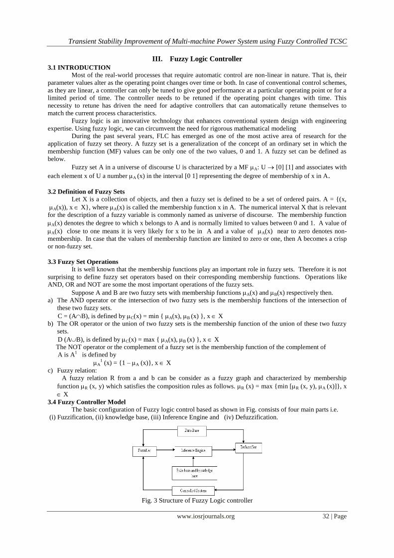
3.4 Fuzzy Controller Model
The basic configuration of Fuzzy logic control based as shown in Fig. consists of four main parts i.e.
(i) Fuzzification, (ii) knowledge base, (iii) Inference Engine and (iv) Defuzzification.
Fig. 3 Structure of Fuzzy Logic controller
Transient Stability Improvement of Multi-machine Power System using Fuzzy Controlled TCSC
www.iosrjournals.org 33 | Page
3.4.1 Fuzzification
1. Performs a scale mapping that transfers the range of values of input variables into corresponding universe of
discourse.
2. Performs the function of Fuzzification that converts input data into suitable linguistic variables,
which may be viewed as labels of fuzzy sets.
3.4.2 Knowledge Base (KB)
Knowledge base comprises of the definitions of fuzzy MFs for the input and output variables and the
necessary control rules, which specify the control action by using linguistic terms.
3.4.3 Inference Mechanism
The Decision – Making Logic Which plays an essential role and contains a set of fuzzy if-then rules
such as IF x is A and y is B then z is C
Where x, y and z are linguistic variables representing two input variables and one control output: A, B and C
are linguistic values.
It is kernel of an FLC, it has the capability of simulating human decision making based on fuzzy
control actions employing fuzzy implication and the rules of inference in fuzzy logic.
3.4.4 Defuzzification
Defuzzification coverts the linguistic variables to determine numerical values. Centroid method of
defuzzification is used in this study.
(1) A scale mapping, which converts the range of values of input variables into corresponding universe of
discourse?
(2) Defuzzification, which yields a non-fuzzy control action from an inferred fuzzy control action.
We defuzzify the output distribution B to produce a single numerical output, a single value in the
output universe of discourse Y = {y1, y2…yp}. The information in the output waveform B resides largely in the
relative values of membership degrees. The simplest deuzzificatioin scheme chooses that, element Ymax. That
has maximal membership put in the output fuzzy ser B. MB (ymax) = max mB (yj); 1 j k. The maximum
membership defuzzificatioin scheme has two fundamental problems. First, the mode of the B distribution is not
unique. In practice B is often highly asymmetric; even if it is unimodal infinitely many output distributions can
share the same mode. The maximum membership scheme ignores the information in much of the waveform B.
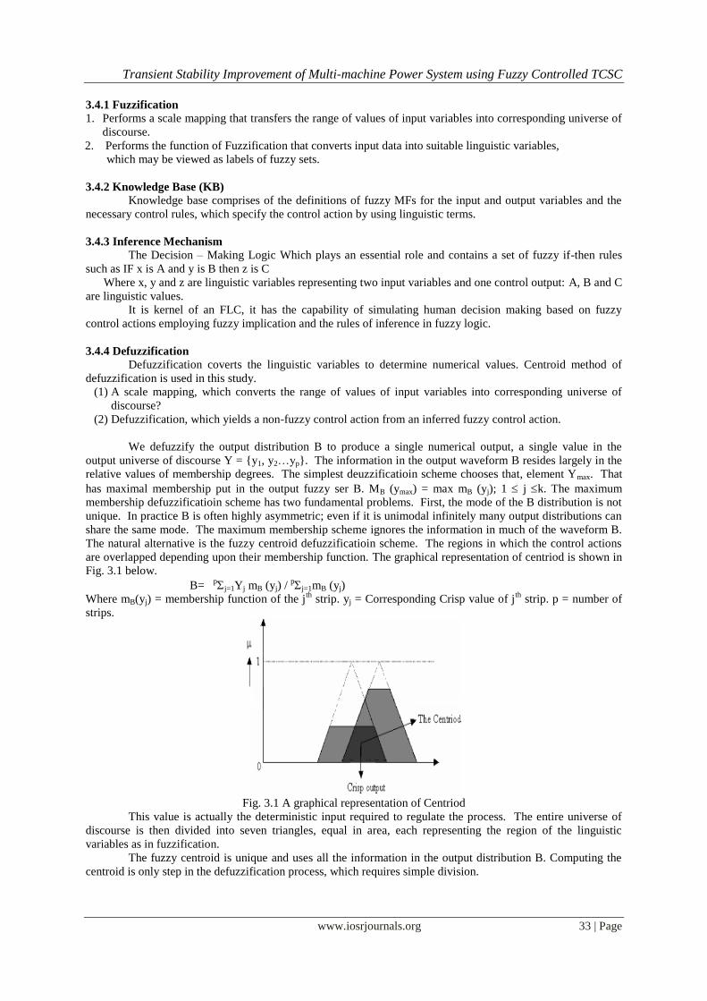
The natural alternative is the fuzzy centroid defuzzificatioin scheme. The regions in which the control actions
are overlapped depending upon their membership function. The graphical representation of centriod is shown in
Fig. 3.1 below.
B= pj=1Yj mB (yj) /
pj=1mB (yj)
Where mB(yj) = membership function of the jth
strip. yj = Corresponding Crisp value of jth
strip. p = number of
strips.
Fig. 3.1 A graphical representation of Centriod
This value is actually the deterministic input required to regulate the process. The entire universe of
discourse is then divided into seven triangles, equal in area, each representing the region of the linguistic
variables as in fuzzification.
The fuzzy centroid is unique and uses all the information in the output distribution B. Computing the
centroid is only step in the defuzzification process, which requires simple division.
Transient Stability Improvement of Multi-machine Power System using Fuzzy Controlled TCSC
www.iosrjournals.org 34 | Page
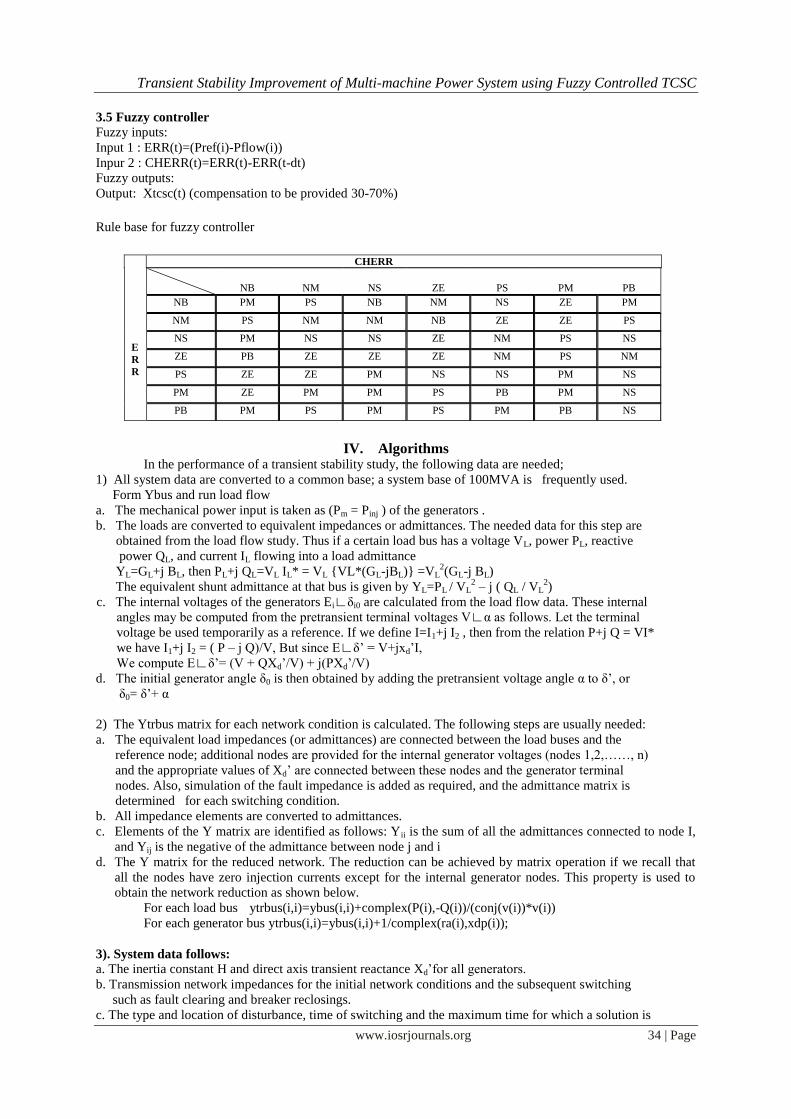
3.5 Fuzzy controller
Fuzzy inputs:
Input 1 : ERR(t)=(Pref(i)-Pflow(i))
Inpur 2 : CHERR(t)=ERR(t)-ERR(t-dt)
Fuzzy outputs:
Output: Xtcsc(t) (compensation to be provided 30-70%)
Rule base for fuzzy controller
IV. Algorithms
In the performance of a transient stability study, the following data are needed;
1) All system data are converted to a common base; a system base of 100MVA is frequently used.
Form Ybus and run load flow
a. The mechanical power input is taken as (Pm = Pinj ) of the generators .
b. The loads are converted to equivalent impedances or admittances. The needed data for this step are
obtained from the load flow study. Thus if a certain load bus has a voltage VL, power PL, reactive
power QL, and current IL flowing into a load admittance
YL=GL+j BL, then PL+j QL=VL IL* = VL {VL*(GL-jBL)} =VL2(GL-j BL)
The equivalent shunt admittance at that bus is given by YL=PL / VL2 – j ( QL / VL
2)
c. The internal voltages of the generators Ei∟δi0 are calculated from the load flow data. These internal
angles may be computed from the pretransient terminal voltages V∟α as follows. Let the terminal
voltage be used temporarily as a reference. If we define I=I1+j I2 , then from the relation P+j Q = VI*
we have I1+j I2 = ( P – j Q)/V, But since E∟δ’ = V+jxd’I,
We compute E∟δ’= (V + QXd’/V) + j(PXd’/V)
d. The initial generator angle δ0 is then obtained by adding the pretransient voltage angle α to δ’, or
δ0= δ’+ α
2) The Ytrbus matrix for each network condition is calculated. The following steps are usually needed:
a. The equivalent load impedances (or admittances) are connected between the load buses and the
reference node; additional nodes are provided for the internal generator voltages (nodes 1,2,……, n)
and the appropriate values of Xd’ are connected between these nodes and the generator terminal
nodes. Also, simulation of the fault impedance is added as required, and the admittance matrix is
determined for each switching condition.
b. All impedance elements are converted to admittances.
c. Elements of the Y matrix are identified as follows: Yii is the sum of all the admittances connected to node I,
and Yij is the negative of the admittance between node j and i
d. The Y matrix for the reduced network. The reduction can be achieved by matrix operation if we recall that
all the nodes have zero injection currents except for the internal generator nodes. This property is used to
obtain the network reduction as shown below.
For each load bus ytrbus(i,i)=ybus(i,i)+complex(P(i),-Q(i))/(conj(v(i))*v(i))
For each generator bus ytrbus(i,i)=ybus(i,i)+1/complex(ra(i),xdp(i));
3). System data follows:
a. The inertia constant H and direct axis transient reactance Xd’for all generators.
b. Transmission network impedances for the initial network conditions and the subsequent switching
such as fault clearing and breaker reclosings.
c. The type and location of disturbance, time of switching and the maximum time for which a solution is
E
R
R
CHERR
NB NM NS ZE PS PM PB
NB PM PS NB NM NS ZE PM
NM PS NM NM NB ZE ZE PS
NS PM NS NS ZE NM PS NS
ZE PB ZE ZE ZE NM PS NM
PS ZE ZE PM NS NS PM NS
PM ZE PM PM PS PB PM NS
PB PM PS PM PS PM PB NS

Transient Stability Improvement of Multi-machine Power System using Fuzzy Controlled TCSC
www.iosrjournals.org 35 | Page
to be considered.
4) Find Ytrbus for various network conditions –during fault, post fault (faulted line cleared), after line
reclosure.
5) For faulted mode, find generator outputs from power angle equations and solve swing equations by R.K
fourth order method etc.
Voltages at each bus is obtained by v=inv(ytrbus)*Inor
6) Keep repeating the above step for post fault mode and after line reclosure mode.
7) Examine δ (t) plots for all the generators and establish the answer to the stability question.
Case i
Fixed compensation
Compensation of 50% is provided in the line where Tcsc is placed by reducing the line reactance and change
the ybus in step1
Case ii
Variable compensation (PI)
a. Initial compensation of (30-50%) is provided in the line where Tcsc is to be placed by reducing the
line reactance and change ybus in step 1.
b. For fault mode (step 5)
ytrbus(fb,fb)=ytrbus(fb,fb)+complex(0.0,-999999999), where fb is fault bus. for each time step solve
swing equations using R.K. fourth order and calculate deltas of generators pid controller
error(1)=(Pf(ltc)-Pref(ltc)), where ltc=line having tcsc calculate Xtcsc, the line impedance becomes
zl(ltc)=complex(r(ltc),-Xtcsc),change elements in ytransbus
c. For post fault mode (step 6)
ytransbus is as in prefault mode.
Case iii
4.2 Fuzzy controller
a. Initial compensation of (30-50%) is provided in the line where Tcsc is to be placed by reducing the
line reactance and change ybus in step 1.
b. For fault mode (step 5)
ytrbus(fb,fb)=ytrbus(fb,fb)+complex(0.0,-999999999), where fb is fault bus.
for each time step
Solve swing equations using R.K. fourth order and calculate deltas of generators for fuzzy
controller take error(1)=(Pf(ltc)-Pref(ltc)), where ltc=line having tcscdelerr=error(1)-error(0) as inputs
and output of Xtcsc gives the compensation to be provided. The line impedance becomes.
zl(ltc)=complex(r(ltc),x(ltc)-Xtcsc), change elements in ytransbus
c. For fault mode (step 5)
ytrbus(fb,fb)=ytrbus(fb,fb)+complex(0.0,-999999999), where fb is fault bus
V. Results Static transient stability results for WSCC 9 bus system:
Case (1) No Damping in the system (Self clearing type), Fault at Bus 5
Here Fault is at Bus 5 and Fault is self cleared and fault clearance time is 0.2 sec and here no damping
in the system, such that oscillations continues.
Case (2) With Damping in the system (Self Clearing type) Fault at Bus 5
0 1 2 3 4 5 6 7 8 9 10-50
0
50
100
time in sec
del21
,del31
(in de
grees
)
Relative Rotor angle Vs Time
0 1 2 3 4 5 6 7 8 9 10-2
0
2
4
time in sec
Activ
e pow
er in
p.u
Active power generation Vs Time
del21
del31
P1
P2
P3
Transient Stability Improvement of Multi-machine Power System using Fuzzy Controlled TCSC
www.iosrjournals.org 36 | Page
By observing the above two cases, we can say that by providing damping to the system the oscillations
will die out and they will settle to a final steady state value with in a very short time duration.
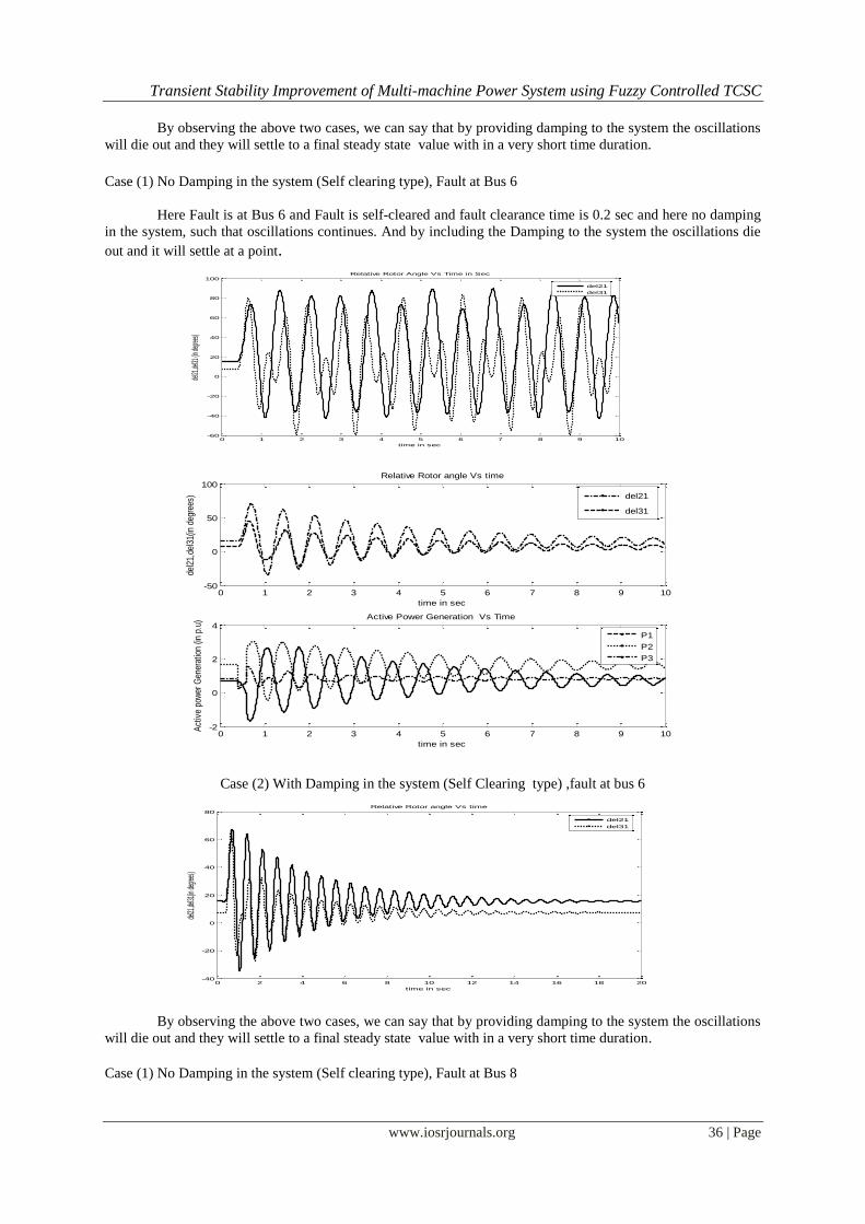
Case (1) No Damping in the system (Self clearing type), Fault at Bus 6
Here Fault is at Bus 6 and Fault is self-cleared and fault clearance time is 0.2 sec and here no damping
in the system, such that oscillations continues. And by including the Damping to the system the oscillations die
out and it will settle at a point.
Case (2) With Damping in the system (Self Clearing type) ,fault at bus 6
By observing the above two cases, we can say that by providing damping to the system the oscillations
will die out and they will settle to a final steady state value with in a very short time duration.
Case (1) No Damping in the system (Self clearing type), Fault at Bus 8
0 1 2 3 4 5 6 7 8 9 10-50
0
50
100
time in sec
del2
1,de
l31(
in d
egre
es)
Relative Rotor angle Vs time
0 1 2 3 4 5 6 7 8 9 10-2
0
2
4
time in sec
Act
ive
pow
er G
ener
atio
n (in
p.u
) Active Power Generation Vs Time
P1
P2
P3
del21
del31
0 1 2 3 4 5 6 7 8 9 10-60
-40
-20
0
20
40
60
80
100
time in sec
del21
,del31
(in de
grees
)
Relative Rotor Angle Vs Time in Sec
del21
del31
0 2 4 6 8 10 12 14 16 18 20-40
-20
0
20
40
60
80
time in sec
del21
,del31
(in de
grees
)
Relative Rotor angle Vs time
del21
del31
Transient Stability Improvement of Multi-machine Power System using Fuzzy Controlled TCSC
www.iosrjournals.org 37 | Page
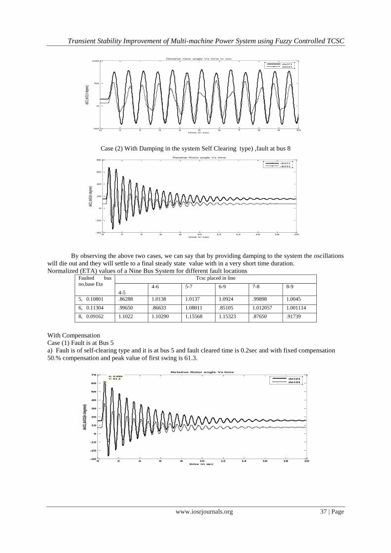
Case (2) With Damping in the system Self Clearing type) ,fault at bus 8
By observing the above two cases, we can say that by providing damping to the system the oscillations
will die out and they will settle to a final steady state value with in a very short time duration.
Normalized (ETA) values of a Nine Bus System for different fault locations Faulted bus
no,base Eta
Tcsc placed in line
4-5
4-6 5-7 6-9 7-8 8-9
5, 0.10801 .86288 1.0138 1.0137 1.0924 .99898 1.0045
6, 0.11304 .99650 .86633 1.08011 .85105 1.012057 1.001114
8, 0.09162 1.1022 1.10290 1.15568 1.15323 .87650 .91739
With Compensation
Case (1) Fault is at Bus 5
a) Fault is of self-clearing type and it is at bus 5 and fault cleared time is 0.2sec and with fixed compensation
50.% compensation and peak value of first swing is 61.3.
0 1 2 3 4 5 6 7 8 9 10-50
0
50
100
time in sec
del21,
del31(
in degr
ees)
Relative rotor angle Vs time in sec
del21
del31
0 2 4 6 8 10 12 14 16 18 20-40
-20
0
20
40
60
80
time in sec
del21
,del31
(in de
grees
)
Relative Rotor angle Vs time
del21
del31
0 2 4 6 8 10 12 14 16 18 20-30
-20
-10
0
10
20
30
40
50
60
70
time in sec
del21
,del31
(in de
gree
s)
Relative Rotor angle Vs time
X: 0.695
Y: 61.3 del21
del31
Transient Stability Improvement of Multi-machine Power System using Fuzzy Controlled TCSC
www.iosrjournals.org 38 | Page
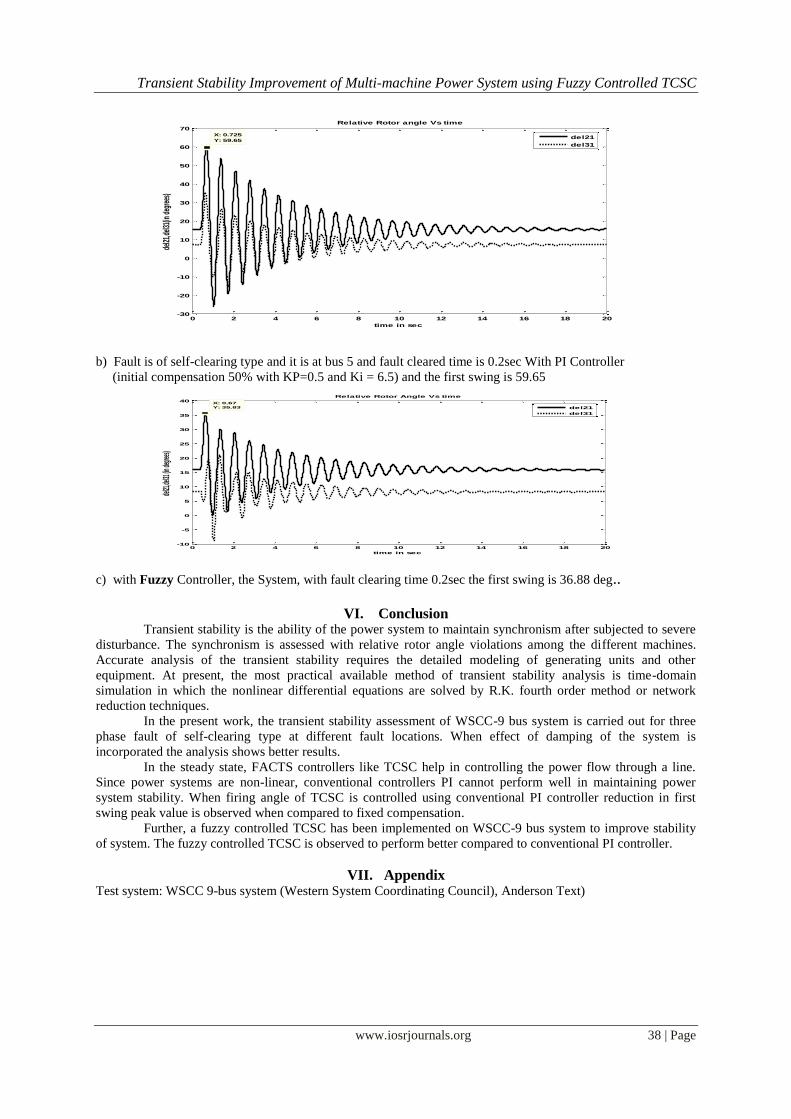
b) Fault is of self-clearing type and it is at bus 5 and fault cleared time is 0.2sec With PI Controller
(initial compensation 50% with KP=0.5 and Ki = 6.5) and the first swing is 59.65
c) with Fuzzy Controller, the System, with fault clearing time 0.2sec the first swing is 36.88 deg..
VI. Conclusion Transient stability is the ability of the power system to maintain synchronism after subjected to severe
disturbance. The synchronism is assessed with relative rotor angle violations among the different machines.
Accurate analysis of the transient stability requires the detailed modeling of generating units and other
equipment. At present, the most practical available method of transient stability analysis is time-domain
simulation in which the nonlinear differential equations are solved by R.K. fourth order method or network
reduction techniques.
In the present work, the transient stability assessment of WSCC-9 bus system is carried out for three
phase fault of self-clearing type at different fault locations. When effect of damping of the system is
incorporated the analysis shows better results.
In the steady state, FACTS controllers like TCSC help in controlling the power flow through a line.
Since power systems are non-linear, conventional controllers PI cannot perform well in maintaining power
system stability. When firing angle of TCSC is controlled using conventional PI controller reduction in first
swing peak value is observed when compared to fixed compensation.
Further, a fuzzy controlled TCSC has been implemented on WSCC-9 bus system to improve stability
of system. The fuzzy controlled TCSC is observed to perform better compared to conventional PI controller.
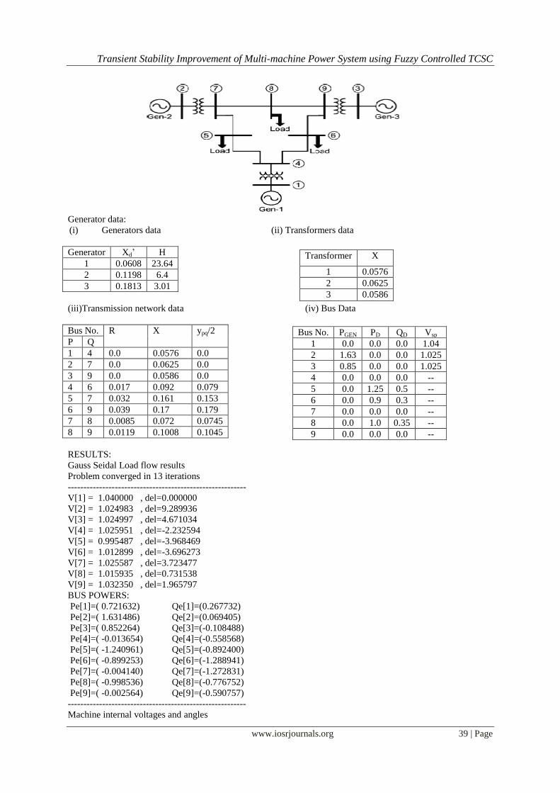
VII. Appendix Test system: WSCC 9-bus system (Western System Coordinating Council), Anderson Text)
0 2 4 6 8 10 12 14 16 18 20-30
-20
-10
0
10
20
30
40
50
60
70 Relative Rotor angle Vs time
time in sec
del
21,d
el31
(in d
egre
es)
X: 0.725
Y: 59.65del21
del31
0 2 4 6 8 10 12 14 16 18 20-10
-5
0
5
10
15
20
25
30
35
40X: 0.67
Y: 35.83
time in sec
del21
,del31
(in de
grees
)
Relative Rotor Angle Vs time
del21
del31
Transient Stability Improvement of Multi-machine Power System using Fuzzy Controlled TCSC
www.iosrjournals.org 39 | Page
Generator data:
(i) Generators data (ii) Transformers data
Generator Xd’ H
1 0.0608 23.64
2 0.1198 6.4
3 0.1813 3.01
(iii)Transmission network data (iv) Bus Data
Bus No. R X ypq/2
P Q
1 4 0.0 0.0576 0.0
2 7 0.0 0.0625 0.0
3 9 0.0 0.0586 0.0
4 6 0.017 0.092 0.079
5 7 0.032 0.161 0.153
6 9 0.039 0.17 0.179
7 8 0.0085 0.072 0.0745
8 9 0.0119 0.1008 0.1045
RESULTS:
Gauss Seidal Load flow results
Problem converged in 13 iterations
---------------------------------------------------------
V[1] = 1.040000 , del=0.000000
V[2] = 1.024983 , del=9.289936
V[3] = 1.024997 , del=4.671034
V[4] = 1.025951 , del=-2.232594
V[5] = 0.995487 , del=-3.968469
V[6] = 1.012899 , del=-3.696273
V[7] = 1.025587 , del=3.723477
V[8] = 1.015935 , del=0.731538
V[9] = 1.032350 , del=1.965797
BUS POWERS:
Pe[1]=( 0.721632) Qe[1]=(0.267732)
Pe[2]=( 1.631486) Qe[2]=(0.069405)
Pe[3]=( 0.852264) Qe[3]=(-0.108488)
Pe[4]=( -0.013654) Qe[4]=(-0.558568)
Pe[5]=( -1.240961) Qe[5]=(-0.892400)
Pe[6]=( -0.899253) Qe[6]=(-1.288941)
Pe[7]=( -0.004140) Qe[7]=(-1.272831)
Pe[8]=( -0.998536) Qe[8]=(-0.776752)
Pe[9]=( -0.002564) Qe[9]=(-0.590757)
---------------------------------------------------------
Machine internal voltages and angles
Transformer X
1 0.0576
2 0.0625
3 0.0586
Bus No. PGEN PD QD Vsp
1 0.0 0.0 0.0 1.04
2 1.63 0.0 0.0 1.025
3 0.85 0.0 0.0 1.025
4 0.0 0.0 0.0 --
5 0.0 1.25 0.5 --
6 0.0 0.9 0.3 --
7 0.0 0.0 0.0 --
8 0.0 1.0 0.35 --
9 0.0 0.0 0.0 --
Transient Stability Improvement of Multi-machine Power System using Fuzzy Controlled TCSC
www.iosrjournals.org 40 | Page
Eint[1]=(1.056495), del[1]=(2.288525)°
Eint[2]=(1.107851), del[2]=(18.544415)°
Eint[3]=(1.041663), del[3]=(13.053976)°
Acknowledgements When I was a teaching the course power system protection and fault location I found an interesting job
after commencing my career. However, the development in digital signal processing and numerical techniques
applied to protection systems motivated me to study this subject area. Till now, I consider the subject of power
system protection as a hobby. I found that accurate location of power line faults is a crucial point in deregulated
electricity networks. At this point, I would like to express my sincere gratitude to Dr. Muhammad Al-Salamah
(Dean of College of Engineering), Dr. Tawfeeq Kanhal (Vice-Dean of College of Engineering) Dr Ahmad Galal
(Head of the Department) for their invaluable guidance, encouragement, and support throughout this work.
Also, the fruitful discussions with Dr. Omar have been greatly helpful in preparing this article. My deepest
thanks also go to my wife and son's for their patience and support during the preparation and writing of this
article.
References [1] P. Kundur, “Power System Stability and Control”, McGraw- Hill, Inc., 1994
[2] Prabha Kundur, John Paserba, “Definition and Classification of Power System Stability”, IEEE Trans. on Power Systems., Vol. 19,
No. 2, pp 1387- 1401, May 2004. [3] Stagg and El- Abiad, “Computer Methods in Power System Analysis”, International Student Edition, McGraw- Hill,Book
Company, 1968.
[4] K. R. Padiyar, “HVDC Power Transmission Systems”, New Age International (P) Ltd., 2004. [5] P.M.Anderson and A.A.Foud, “power system control and stability”, Iowa state University Press, Ames, Iowa, 1977.
[6] Dheeman Chatterjee, Arindam Ghosh∗, “TCSC control design for transient stability improvement of a multi-machine power system using trajectory sensitivity”, Department of Electrical Engineering, Indian Institute of Technology, Kanpur 208 016, India
[7] P.W. Sauer, M.A. Pai, Power System Dynamics and Stability, Prentice Hall, Upper Saddle River, 1998.
[8] Dheeman Chatterjee , Arindam Ghosh*, “Application of Trajectory Sensitivity for the Evaluation of the Effect of TCSC Placement on Transient Stability” International Journal of Emerging Electric Power Systems, Volume 8, Issue 1 2007 Article 4, The Berkeley
Electronic Press