software quality assurance methodologies and...
TRANSCRIPT

Software Quality Assurance Methodologies and Techniques
Guest Editors: Chin-Yu Huang, Hareton Leung, Wu-Hon Francis Leung, and Osamu Mizuno
Advances in Software Engineering

Software Quality Assurance Methodologiesand Techniques

Advances in Software Engineering
Software Quality Assurance Methodologiesand Techniques
Guest Editors: Chin-Yu Huang, Hareton Leung,Wu-Hon Francis Leung, and Osamu Mizuno

Copyright © 2012 Hindawi Publishing Corporation. All rights reserved.
This is a special issue published in “Advances in Software Engineering.” All articles are open access articles distributed under the CreativeCommons Attribution License, which permits unrestricted use, distribution, and reproduction in any medium, provided the originalwork is properly cited.

Editorial Board
Pekka Abrahamsson, ItalyReda A. Ammar, USALerina Aversano, ItalyXiaoying Bai, ChinaKamel Barkaoui, FranceJan A. Bergstra, The NetherlandsGerardo Canfora, ItalyChristine W. Chan, CanadaAlexander Chatzigeorgiou, GreeceGabriel Ciobanu, RomaniaAndrea De Lucia, ItalyMourad Debbabi, CanadaGiuseppe A. Di Lucca, ItalyWilhelm Hasselbring, Germany
Xudong He, USAChin-Yu Huang, TaiwanMichael N. Huhns, USASuresh Jagannathan, USAJan Jurjens, GermanyDae-Kyoo Kim, USAChristoph Kirsch, AustriaNicholas A. Kraft, USARalf Lammel, GermanyFilippo Lanubile, ItalyPhillip A. Laplante, USALuigi Lavazza, ItalyJeff (Yu) Lei, USADavid Lo, Singapore
Moreno Marzolla, ItalyE. Mendes, BrazilJose Merseguer, SpainHenry Muccini, ItalyRocco Oliveto, ItalySooyong Park, Republic of KoreaHoang Pham, USAAndrea Polini, ItalyHouari Sahraoui, CanadaHossein Saiedian, USAMichael H. Schwarz, GermanyWei-Tek Tsai, USARobert J. Walker, Canada

Contents
Software Quality Assurance Methodologies and Techniques, Chin-Yu Huang, Hareton Leung,Wu-Hon Francis Leung, and Osamu MizunoVolume 2012, Article ID 872619, 2 pages
An Empirical Study on the Impact of Duplicate Code, Keisuke Hotta, Yui Sasaki, Yukiko Sano,Yoshiki Higo, and Shinji KusumotoVolume 2012, Article ID 938296, 22 pages
A Comparative Study of Data Transformations for Wavelet Shrinkage Estimation with Application toSoftware Reliability Assessment, Xiao Xiao and Tadashi DohiVolume 2012, Article ID 524636, 9 pages
Can Faulty Modules Be Predicted by Warning Messages of Static Code Analyzer?, Osamu Mizuno andMichi NakaiVolume 2012, Article ID 924923, 8 pages
Specifying Process Views for a Measurement, Evaluation, and Improvement Strategy, Pablo Becker,Philip Lew, and Luis OlsinaVolume 2012, Article ID 949746, 28 pages
Program Spectra Analysis with Theory of Evidence, Rattikorn HewettVolume 2012, Article ID 642983, 12 pages

Hindawi Publishing CorporationAdvances in Software EngineeringVolume 2012, Article ID 872619, 2 pagesdoi:10.1155/2012/872619
Editorial
Software Quality Assurance Methodologies and Techniques
Chin-Yu Huang,1 Hareton Leung,2 Wu-Hon Francis Leung,3 and Osamu Mizuno4
1 Department of Computer Science and Institute of Information Systems and Applications, National Tsing Hua University,Hsinchu 30013, Taiwan
2 Department of Computing, Hong Kong Polytechnic University, Kowloon, Hong Kong3 Department of Computer Science, Illinois Institute of Technology, Chicago, IL 60616, USA4 Graduate School of Science and Technology, Kyoto Institute of Technology, Kyoto 606-8585, Japan
Correspondence should be addressed to Chin-Yu Huang, [email protected]
Received 18 July 2012; Accepted 18 July 2012
Copyright © 2012 Chin-Yu Huang et al. This is an open access article distributed under the Creative Commons AttributionLicense, which permits unrestricted use, distribution, and reproduction in any medium, provided the original work is properlycited.
Software quality assurance (SQA) is a planned and systematicpattern of actions necessary to provide adequate confidencethat a software product conforms to requirements duringsoftware development. SQA consists of methodologies andtechniques of assessing the software development processesand methods, tools, and technologies used to ensure thequality of the developed software. SQA is typically achievedthrough the use of well-defined standard practices, includingtools and processes, for quality control to ensure the integrityand reliability of software. This special issue presents newresearch works along these directions, and we received 21submissions and accepted five of them after a thorough peer-review process. The acceptance rate of this special issue isaround 24%. The resultant collection provides a number ofuseful results. These accepted papers cover a broad range oftopics in the research field of SQA, including software valida-tion, verification, and testing, SQA modeling, certification,evaluation, and improvement, SQA standards and models,SQA case studies, data analysis and risk management.
For example, in “Specifying process views for a mea-surement, evaluation, and improvement strategy,” P. Becker,P. Lew, and L. Olsina developed a specific strategy calledSIQinU (strategy for understanding and improving qual-ity in use), which recognizes problems of quality in usethrough evaluation of a real system-in-use situation andproposes product improvements by understanding andmaking changes to the product’s attributes. They used UML2.0 activity diagrams and the SPEM profile to stress thefunctional, informational, organizational, and behavioralviews for the SIQinU process.
In the paper “Program spectra analysis with theory ofevidence,” R. Hewett proposed a spectrum-based approachto fault localization using the Dempster-Shaffer theoryof evidence. Using mathematical theories of evidence foruncertainty reasoning, the proposed approach estimatesthe likelihood of faulty locations based on evidence fromprogram spectra. Evaluation results show that their approachis at least as effective as others with an average effectivenessof 85.6% over 119 versions of the programs.
In the paper entitled “An empirical study on the impactof duplicate code,” K. Hotta et al. presented an empiricalstudy on the impact of the presence of duplicate code onsoftware evolution. They assumed that if duplicate codeis modified more frequently than nonduplicate code, thepresence of duplicate code affects software evolution, andcompared the stability of duplicate code and non-duplicatecode. They conducted an experiment on 15 open-sourcesoftware systems, and the result showed that duplicatecode was less frequently modified than nonduplicate codeand, in some cases, duplicate code was intensively mod-ified in a short period though duplicate code was morestable than nonduplicate code in the whole developmentperiod.
The next paper by X. Xiao and T. Dohi, “A comparativestudy of data transformations for wavelet shrinkage estimationwith application to software reliability assessment,” appliedthe wavelet-based techniques to estimate the software inten-sity function. Some data transformations were employedto preprocess the software-fault count data. Throughoutthe numerical evaluation, the authors concluded that the
2 Advances in Software Engineering
wavelet-based estimation methods have much more poten-tial applicability than the other data transformations to thesoftware reliability assessment.
In the last paper “Can faulty modules be predicted bywarning messages of static code analyzer?,” O. Mizuno and M.Nakai proposed a detection method of fault-prone modulesbased on the spam filtering technique—fault-prone filtering.For the analysis, the authors tried to state two questions: “canfault-prone modules be predicted by applying a text filter tothe warning messages of static code analyzer?” and “is theperformance of the fault-prone filtering becomes better withthe warning messages of a static code analyzer?”. The resultsof experiments show that the answer to the first question is“yes.” But for the second question, the authors found that therecall becomes better than the original approach.
In summary, this special issue serves as a platformfor researchers and practitioners to present theory, results,experience, and other advances in SQA. Hopefully, you willenjoy this publication, and we look forward to your feedbackand comments.
Chin-Yu HuangHareton Leung
Wu-Hon Francis LeungOsamu Mizuno

Hindawi Publishing CorporationAdvances in Software EngineeringVolume 2012, Article ID 938296, 22 pagesdoi:10.1155/2012/938296
Research Article
An Empirical Study on the Impact of Duplicate Code
Keisuke Hotta, Yui Sasaki, Yukiko Sano, Yoshiki Higo, and Shinji Kusumoto
Graduate School of Information Science and Technology, Osaka University, Osaka 565-0871, Japan
Correspondence should be addressed to Keisuke Hotta, [email protected]
Received 4 January 2012; Accepted 5 March 2012
Academic Editor: Osamu Mizuno
Copyright © 2012 Keisuke Hotta et al. This is an open access article distributed under the Creative Commons Attribution License,which permits unrestricted use, distribution, and reproduction in any medium, provided the original work is properly cited.
It is said that the presence of duplicate code is one of the factors that make software maintenance more difficult. Many researchefforts have been performed on detecting, removing, or managing duplicate code on this basis. However, some researchers doubtthis basis in recent years and have conducted empirical studies to investigate the influence of the presence of duplicate code. In thisstudy, we conduct an empirical study to investigate this matter from a different standpoint from previous studies. In this study, wedefine a new indicator “modification frequency” to measure the impact of duplicate code and compare the values between duplicatecode and nonduplicate code. The features of this study are as follows the indicator used in this study is based on modification placesinstead of the ratio of modified lines; we use multiple duplicate code detection tools to reduce biases of detection tools; and wecompare the result of the proposed method with other two investigation methods. The result shows that duplicate code tendsto be less frequently modified than nonduplicate code, and we found some instances that the proposed method can evaluate theinfluence of duplicate code more accurately than the existing investigation methods.
1. Introduction
Recently, duplicate code has received much attention. Dupli-cate code is also called as “code clone.” Duplicate code isdefined as identical or similar code fragments to each otherin the source code, and they are generated by various reasonssuch as copy-and-paste programming. It is said that thepresence of duplicate code has negative impacts on softwaredevelopment and maintenance. For example, they increasebug occurrences: if an instance of duplicate code is changedfor fixing bugs or adding new features, its correspondentshave to be changed simultaneously; if the correspondentsare not changed inadvertently, bugs are newly introduced tothem.
Various kinds of research efforts have been performedfor resolving or improving the problems caused by thepresence of duplicate code. For example, there are currentlya variety of techniques available to detect duplicate code[1]. In addition, there are many research efforts for mergingduplicate code as a single module like function or method,or for preventing duplications from being overlooked inmodification [2, 3]. However, there are precisely the oppositeopinions that code cloning is a good choice for design of thesource code [4].
In order to answer the question whether duplicate codeis harmful or not, several efforts have proposed comparisonmethods between duplicate code and nonduplicate code.Each of them compares a characteristic of duplicate codeand nonduplicate code instead of directly investigating theirmaintenance cost. This is because measuring the actualmaintenance cost is quite difficult. However, there is noconsensus on this matter.
In this paper, we conduct an empirical study thatcompares duplicate code to nonduplicate code from adifferent standpoint of previous research and reports theexperimental result on open source software. The features ofthe investigation method in this paper are as follows:
(i) every line of code is investigated whether it is dupli-cate code or not; such a fine-grained investigationcan accurately judge whether every modificationconducted to duplicate code or to nonduplicate code;
(ii) maintenance cost consists of not only source codemodification but also several phases prior to it; inorder to more appropriately estimate maintenancecost, we define an indicator that is not based onmodified lines of code but the number of modifiedplaces;

2 Advances in Software Engineering
(iii) we evaluate and compare modifications of duplicatecode and nonduplicate code on multiple open sourcesoftware systems with multiple duplicate code detec-tion tools, that is, because every detection tool detectsdifferent duplicate code from the same source code.
We also conducted a comparison experiment with twoprevious investigation methods. The purpose of this exper-iment is to reveal whether comparisons between duplicatecode and nonduplicate code with different methods yield thesame result or not. In addition, we carefully analyzed theresults in the cases that the comparison results were differentfrom each method to reveal the causes behind the differences.
The rest of this paper is organized as follows: Section 2describes related works and our motivation of this study.Section 3 introduces the preliminaries. We situate ourresearch questions and propose a new investigation methodin Section 4. Section 5 describes the design of our exper-iments, then we report the results in Sections 6 and 7.Section 8 discusses threats to validity, and Section 9 presentsthe conclusion and future work of this study.
2. Motivation
2.1. Related Work. At present, there is a huge body of work onempirical evidence on duplicate code shown in Table 1. Thepioneering report in this area is Kim et al.’s study on clonegenealogies [5]. They have conducted an empirical study ontwo open source software systems and found 38% or 36%of groups of duplicate code were consistently changed atleast one time. On the other hand, they observed that therewere groups of duplicate code that existed only for a shortperiod (5 or 10 revisions) because each instance of the groupswas modified inconsistently. Their work is the first empiricalevidence that a part of duplicate code increases the cost ofsource code modification.
However, Kapser and Godfrey have different opinionsregarding duplicate code. They reported that duplicate codecan be a reasonable design decision based on the empiricalstudy on two large-scale open source systems [4]. They builtseveral patterns of duplicate code in the target systems, andthey discussed the pros and cons of duplicate code using thepatterns. Bettenburg et al. also reported that duplicate codedoes not have much a negative impact on software quality[6]. They investigated inconsistent changes to duplicate codeat release level on two open software systems, and they foundthat only 1.26% to 3.23% of inconsistent changes introducedsoftware errors into the target systems.
Monden et al. investigated the relation between softwarequality and duplicate code on the file unit [7]. They usethe number of revisions of every file as a barometer ofquality: if the number of revisions of a file is great, itsquality is low. Their experiment selected a large-scale legacysystem, which was being operated in a public institution,as the target. The result showed that modules that includedduplicate code were 40% lower quality than modules that didnot include duplicate code. Moreover, they reported that thelarger duplicate code a source file included, the lower qualityit was.
Lozano et al. investigated whether the presence ofduplicate code was harmful or not [8]. They developed a tool,CloneTracker, which traces which methods include duplicatecode (in short, duplicate method) and which methods aremodified in each revision. They conducted a pilot study, andfound that: duplicate methods tend to be more frequentlymodified than nonduplicate methods; however, duplicatemethods tend to be modified less simultaneously thannonduplicate methods. The fact implies that the presenceof duplicate code increased cost for modification, andprogrammers were not aware of the duplication, so thatthey sometimes overlooked code fragments that had to bemodified simultaneously.
Also, Lozano and Wermelinger investigated the impactof duplicate code on software maintenance [9]. Threebarometers were used in the investigation. The first one islikelihood, which indicates the possibility that the methodis modified in a revision. The second one is impact, whichindicates the number of methods that are simultaneouslymodified with the method. The third one is work, whichcan be represented as a product of likelihood and impact(work = likelihood × impact). They conducted a case studyon 4 open source systems for comparing the three barometersof methods including and not including duplicate code. Theresult was that likelihood of methods including duplicatecode was not so different from one of methods not includingduplicate code; there were some instances that impact ofmethods including duplicate code were greater than oneof methods not including duplicate code; if duplicate codeexisted in methods for a long time, their work tended toincrease greatly.
Moreover, Lozano et al. investigated the relation betweenduplicate code, features of methods, and their changeability[10]. Changeability means the ease of modification. Ifchangeability decreased, it will be a bottleneck of soft-ware maintenance. The result showed that the presenceof duplicate code can decrease changeability. However,they found that changeability was more greatly affected byother properties such as length, fan-out, and complexityof methods. Consequently, they concluded that it was notnecessary to consider duplicate code as a primary option.
Krinke hypothesized that if duplicate code is less stablethan nonduplicate code, maintenance cost for duplicatecode is greater than for nonduplicate code. He conducteda case study in order to investigate whether the hypothesisis true or not [11]. The targets are 200 revisions (a versionper week) of source code of 5 large-scale open-sourcesystems. He measured added, deleted, and changed LOCson duplicate code and nonduplicate code and comparedthem. He reported that nonduplicate code was more added,deleted, and changed than duplicate code. Consequently,he concluded that the presence of duplicate code did notnecessarily make it more difficult to maintain source code.
Gode and Harder replicated Krinke’s experiment [12].Krinke’s original experiment detected line-based duplicatecode meanwhile their experiment detected token-basedduplicate code. The experimental result was the same asKrinke’s one. Duplicate code is more stable than nondu-plicate code in the viewpoint of added and changed. On

Advances in Software Engineering 3
Table 1: Summarization of related work.
How to investigate Impact of duplicate code
Kim et al. [5] Using clone linages and clone genealogies A part of duplicate code is negative
Kapser and Godfrey [4] Build several patterns of duplicate code and discuss about them Nonnegative
Bettenburg et al. [6] Investigate inconsistent changes to duplicate code at the release revel Nonnegative
Monden et al. [7] Calculate the number of revisions on every file Negative
Lozano et al. [8] Count the number of modifications on methods including duplicate code Negative
Lozano and Wermelinger[9]
Using work A part of duplicate code is negative
Lozano et al. [10] Using changeability (the ease of modification) Negative but not so high
Krinke [11] Using stability (line level) Nonnegative
Gode and Harder [12] Using stability (token level) Nonnegative
Krinke [13] Using ages Nonnegative
Rahman et al. [14] Investigate the relationship between duplicate code and bugs Nonnegative
Gode and Koschke [15] Count the number of changes on clone genealogies A part of duplicate code is negative
the other hand, from the deleted viewpoint, nonduplicatecode is more stable than duplicate code.
Also, Krinke conducted an empirical study to investigateages of duplicate code [13]. In this study, he calculated andcompared average ages of duplicate lines and nonduplicatelines on 4 large-scale Java software systems. He found thatthe average age of duplicate code is older than nonduplicatecode, which implies duplicate code is more stable thannonduplicate code.
Eick et al. investigated whether source code decays whenit is operated and maintained for a long time [16]. Theyselected several metrics such as the amount of added anddeleted code, the time required for modification, and thenumber of developers as indicators of code decay. The experi-mental result on a 15-year-operated large system showed thatcost required for completing a single requirement tendS toincrease.
Rahman et al. investigated the relationship betweenduplicate code and bugs [14]. They analyzed 4 softwaresystems written in C language with bug information stored inBugzilla. They use Deckard, which is an AST-based detectiontool, to detect duplicate code. They reported that only a smallpart of the bugs located on duplicate code, and the presenceof duplicate code did not dominate bug appearances.
Gode modeled how type-1 code clones are generated andhow they evolved [17]. Type-1 code clone is a code clone thatis exactly identical to its correspondents except white spacesand tabs. He applied the model to 9 open-source softwaresystems and investigated how code clones in them evolved.The result showed that the ratio of code duplication wasdecreasing as time passed; the average life time of code cloneswas over 1 year; in the case that code clones were modifiedinconsistently, there were a few instances that additionalmodifications were performed to restore their consistency.
Also, Gode and Koschke conducted an empirical studyon clone evolution and performed a detailed tracking todetect when and how clones had been changed [15]. In theirstudy, they traced clone evolution and counted the numberof changes on each clone genealogy. They manually inspected
the result in one of the target systems and categorized allthe modifications on clones into consistent or inconsistent.In addition, they carefully categorized inconsistent changesinto intentional or unintentional. They reported that almostall clones were never changed or only once during theirlifetime, and only 3% of the modifications had high severity.Therefore, they concluded that many of clones do not causeadditional change effort, and it is important to identify theclones with high threat potential to manage duplicate codeeffectively.
As described above, some empirical studies reported thatduplicate code should have a negative impact on softwareevolution meanwhile the others reported the opposite result.At present, there is no consensus on the impact of the pres-ence of duplicate code on software evolution. Consequently,this research is performed as a replication of the previousstudies with solid settings.
2.2. Motivating Example. As described in Section 2.1, manyresearch efforts have been performed on evaluating theinfluence of duplicate code. However, these investigationmethods still have some points that they did not evaluate. Weexplain these points with the example shown in Figure 1. Inthis example, there are two similar methods and some placesare modified. We classified these modifications into 4 parts,modification A, B, C, and D.
Investigated Units. In some studies, large units (e.g., filesor methods) are used as their investigation units. In thoseinvestigation methods, it is assumed that duplicate code hasa negative impact if files or methods having a certain amountof duplicate code are modified, which can cause a problem.The problem is the incorrectness of modifications count. Forexample, if modifications are performed on a method whichhas a certain amount of duplicate code, all the modificationsare assumed as performed on the duplicate code even ifthey are actually performed on nonduplicate code of themethod. Modification C in Figure 1 is an instance of thisproblem. This modification is performed on nonduplicate

4 Advances in Software Engineering
Revision R
public void highlight(Graph target) {if (target.isEmpty()) {
return;}Set<Node> nodes = target.getNodes();
uninterestNodes.add(node);
}}nodes.removeAll(uninterestNodes);
for(Node node : uninterestNodes) {drawLineThrough (node);
}
addHighlight(node, Color.red);}
}
Set<Node> uninterestNodes =new HashSet<Node>();
for (Node node : target.getNodes()) {if (node.getEdges().isEmpty()) {
for (Node node : nodes) {
Revision R + 1
public void highlight(Graph target) {
return;}Set<Node> nodes = target.getNodes(); Set<Node> nodes = target.getNodes();
Set<Node> uninterestNodes =new HashSet<Node>();
for (Node node : target.getNodes()) {if (node.getEdges().isEmpty()) {
uninterestNodes.add(node);
}}nodes.removeAll(uninterestNodes);
for(Node node : uninterestNodes) {paint (node, getPaintColor());
}
for (Node node : nodes) {addHighlight(node, getColor());
for (Node node : nodes)
addHighlight(node, getColor());
}}
}}
Modification A
if (target== null || target.isEmpty()) {public void highlight(Graph target) {
return;}
if (target== null || target.isEmpty()) {
public void highlight(Graph target) {if (target.isEmpty()) {
return;}
Set<Node> nodes = target.getNodes();Set<Node> uninterestNodes =
new HashSet<Node>();
for (Node node : target.getNodes()) {if (node.getEdges().isEmpty()) {
uninterestNodes.add(node);
}}nodes.removeAll(uninterestNodes);
for (Node node : nodes) {addHighlight(node, Color.red);
}}
Duplicate code detected by only Scorpio
Duplicate code detected by both CCFinder &Scorpio
Modification B
Modification C
Modification D
System.out.println(“Processing Nodes”);
System.out.println(“Processing Nodes”);
Figure 1: Motivating example.

Advances in Software Engineering 5
code; nevertheless, it is regarded that this modification isperformed on duplicate code if we use method as theinvestigation units.
Line-Based Barometers. In some studies, line-based barom-eters are used to measure the influence of duplicate codeon software evolution. Herein, the line-based barometerindicates a barometer calculated with the amount of added/changed/deleted lines of code. However, line-based barome-ter cannot distinguish the following two cases: the first case isthat consecutive 10 lines of code were modified for fixing a singlebug; the second case is that 1 line modification was performedon different 10 places of code for fixing 10 different bugs. Inreal software maintenance, the latter requires much morecost than the former because we have to conduct severalsteps before the actual source code modification such asidentifying buggy module, informing the maintainer aboutthe bugs, and identifying buggy instruction.
In Figure 1, Modification A is 1 line modification, andperformed on 2 places, meanwhile Modification B is 7 linesmodification on a single place. With line-based barometers,it is regarded that Modification B has the impact 3.5 timeslarger than Modification A. However, this is not true becausewe have to identify 2 places of code for modifying Ameanwhile 1 place identification is required for B.
A Single Detection Tool. In the previous studies, a singledetection tool was used to detect duplicate code. However,there is neither a generic nor strict definition of duplicatecode. Each detection tool has its own unique definition ofduplicate code, and it detects duplicate code based on theown definition. Consequently, different duplicate code isdetected by different detection tools from the same sourcecode. Therefore, the investigation result with one detector isdifferent from the result from another detector. In Figure 1,a detector CCFinder detects lines highlighted with red asduplicate code, and another detector Scorpio detects notonly lines highlighted with red but also lines highlighted withorange before modification. Therefore, if we use Scorpio,Modification D is regarded as being affected with duplicatecode, nevertheless, it is regarded as not being affectedwith duplicate code if we use CCFinder. Consequently, theinvestigation with a single detector is not sufficient to get thegeneric result about the impact of duplicate code.
2.2.1. Objective of This Study. In this paper, we conductedan empirical study from a different standpoint of previousresearch. The features of this study are as follows.
Fine-Grained Investigation Units. In this study, every line ofcode is investigated whether it is duplicate code or not, whichenables us to judge whether every modification is conductedon duplicate code or nonduplicate code.
Place-Based Indicator. We define a new indicator based onthe number of modified places, not the number of modifiedlines. The purpose of place-based indicator is to evaluatethe impact of the presence of duplicate code with differentstandpoints from the previous research.
Multiply Detector. In this study, we use 4 duplicate codedetection tools to reduce biases of each detection method.
3. Preliminaries
In this section, we describe preliminaries used in this paper.
3.1. Duplicate Code Detection Tools. There are currentlyvarious kinds of duplicate code detection tools. The detectiontools take the source code as their input data, and theyprovide the position of the detected duplicate code in it. Thedetection tools can be categorized based on their detectiontechniques. Major categories should be line based, tokenbased, metrics based, AST (Abstract Syntax Tree) based, andPDG (Program Dependence Graph) based. Each techniquehas merits and demerits, and there is no technique thatis superior to any other techniques in every way [1, 18].The following subsections describe 4 detection tools thatare used in this research. We use two token-based detectiontools, which is for investigating whether both the token-based detection tools always introduce the same result or not.
3.1.1. CCFinder. CCFinder is a token-based detection tool[19]. The major features of CCFinder are as follows.
(i) CCFinder replaces user-defined identifiers such asvariable names or function names with specialtokens before the matching process. Consequently,CCFinder can identify code fragments that usedifferent variables as duplicate code.
(ii) Detection speed is very fast. CCFinder can detectsduplicate code from millions lines of code within anhour.
(iii) CCFinder can handle multiple popular program-ming languages such as C/C++, Java, and COBOL.
3.1.2. CCFinderX. CCFinderX is a major version up fromCCFinder [20]. CCFinderX is a token-based detection toolas well as CCFinder, but the detection algorithm waschanged to bucket sort to suffix tree. CCFinderX can handlemore programming languages than CCFinder. Moreover, itcan effectively use resources of multi core CPUs for fasterdetection.
3.1.3. Simian. Simian is a line-based detection tool [21].As well as CCFinder family, Simian can handle multipleprogramming languages. Its line-based technique realizesduplicate code detection on small memory usage and shortrunning time. Also, Simian allows fine-grained settings. Forexample, we can configure that duplicate code is not detectedfrom import statements in the case of Java language.
3.1.4. Scorpio. Scorpio is a PDG-based detection tool[22, 23]. Scorpio builds a special PDG for duplicate codedetection, not traditional one. In traditional PDGs, there aretwo types of edge representing data dependence and controldependence. The special PDG used in Scorpio has one

6 Advances in Software Engineering
(a) before modification(1) A(2) B(3) line will be changed 1(4) line will be changed 2(5) C(6) D(7) line will be deleted 1(8) line will be deleted 2(9) E(10) F(11) G(12) H
(b) after modification(1) A(2) B(3) line changed 1(4) line changed 2(5) C(6) D(7) E(8) F(9) G(10) line added 1(11) line added 2(12) H
(c) diff output3,4c3,4< line will be changed 1< line will be changed 2---> line changed 1> line changed 27,8d6< line will be deleted 1< line will be deleted 211a10,11> line added 1> line added 2
Algorithm 1: A simple example of comparing two source files withdiff (changed region is represented with identifier “c” like 3,4c3,4;deleted region is represented with identifier “d” like 7,8d6, addedregion is represented with identifier “a” like 11a10,11). The numberbefore and after the identifier shows the correspond lines.
more edge, execution-next link, which allows detecting moreduplicate code than traditional PDG. Also, Scorpio adoptssome heuristics for filtering out false positives. Currently,Scorpio can handle only Java language.
3.2. Revision. In this paper, we analyze historical datamanaged by version control systems for investigation. Ver-sion control systems store information about changes todocuments or programs. We can specify changes by usinga number, “revision”. We can get source code in arbitraryrevision, and we can also get modified files, change logs, and
the name of developers who made changes in arbitrary twoconsecutive revisions with version control systems.
Due to the limit of implementation, we restrict the targetversion control system to Subversion. However, it is possibleto use other version control systems such as CVS.
3.3. Target Revision. In this study, we are only interestedin changes in source files. Therefore, we find out revisionsthat have some modifications in source files. We call suchrevisions as target revisions. We regard a revision R as thetarget revision, if at least one source file is modified from Rto R + 1.
3.4. Modification Place. In this research, we use the numberof places of modified code, instead lines of modified code.That is, even if multiple consecutive lines are modified,we regard it as a single modification. In order to identifythe number of modifications, we use UNIX diff command.Algorithm 1 shows an example of diff output. In thisexample, we can find 3 modification places. One is a changein line 3 and 4, another is a deletion in line 7 and 8, and theother is an addition at line 11. As shown in the algorithm,it is very easy to identify multiple consecutive modified linesas a single modification; all we have to do is just parsing theoutput of diff so that the start line and end line of all themodifications are identified.
4. Proposed Method
This section describes our research questions and the inves-tigation method.
4.1. Research Questions and Hypotheses. The purpose of thisresearch is to reveal whether the presence of duplicate codereally affects software evolution or not. We assume that ifduplicate code is more frequently modified than nonduplicatecode, the presence of duplicate code has a negative impact onsoftware evolution. This is because if much duplicate code isincluded in source code though, it is never modified duringits lifetime, the presence of duplicate code never causesinconsistent changes or additional modification efforts. Ourresearch questions are as follows.
RQ1: Is duplicate code more frequently modified than non-duplicate code?
RQ2: Are the comparison results of stability betweenduplicate code and nonduplicate code different frommultiple detection tools?
RQ3: Is duplicate code modified uniformly throughout itslifetime?
RQ4: Are there any differences in the comparison results onmodification types?
To answer these research questions, we define an indica-tor, modification frequency (in short, MF). We measure andcompare MF of duplicate code (in short, MFd) and MF ofnonduplicate code (in short, MFn) for investigation.

Advances in Software Engineering 7
4.2. Modification Frequency
4.2.1. Definition. As described above, we use MF to estimatethe influence of duplicate code. MF is an indicator basedon the number of modified code, not lines of modifiedcode. This is because this research aims to investigate froma different standpoint from previous research.
We define MFd in the formula:
MFd =∑
r∈R MCd(r)|R| , (1)
where R is a set of target revisions, MCd(r) is the number ofmodifications on duplicate code between revision r and r+1.We also define MFn in the formula:
MFn =∑
r∈R MCn(r)|R| , (2)
where MCn(r) is the number of modifications on nondupli-cate code between revision r and r + 1.
These values mean the average number of modificationson duplicate code or nonduplicate code per revision. How-ever, in these definitions, MFd and MFn are very affected bythe amount of duplicate code included the source code. Forexample, if the amount of duplicate code is very small, it isquite natural that the number of modifications on duplicatecode is much smaller than nonduplicate code. However,if a small amount of duplicate code is included but it isquite frequently modified, we need additional maintenanceefforts to judge whether its correspondents need the samemodifications or not. We cannot evaluate the influence ofduplicate code in these situations in these definitions.
In order to eliminate the bias of the amount of duplicatecode, we normalize the formulae (1) and (2) with the ratio ofduplicate code. Here, we assume that
(i) LOCd(r) is the total lines of duplicate code in revisionr,
(ii) LOCn(r) is the total lines of nonduplicate code on r,
(iii) LOC(r) is the total lines of code on r, so that thefollowing formula is satisfied:
LOC(r) = LOCd(r) + LOCn(r). (3)
Under these assumptions, the normalized MFd and MFn
are defined in the following formula:
normalized MFd =∑
r∈R MCd(r)|R| ×
∑r∈R LOC(r)
∑r∈R LOCd(r)
,
normalized MFn =∑
r∈R MCn(r)|R| ×
∑r∈R LOC(r)
∑r∈R LOCn(r)
.(4)
In the reminder of this paper, the normalized MFd andMFn are called as just MFd and MFn, respectively.
4.2.2. Measurement Steps. The MFd and MFn are measuredwith the following steps,
Step 1. It identifies target revisions from the repositories oftarget software systems. Then, all the target revisions arechecked out into the local storage.
Step 2. It normalized all the source files in every targetrevision.
Step 3. It detects duplicate code within every target revision.Then, the detection result is analyzed in order to identify thefile path, the lines of all the detected duplicate code.
Step 4. It identifies differences between two consecutiverevisions. The start lines and the end lines of all thedifferences are stored.
Step 5. It counts the number of modifications on duplicatecode and nonduplicate code.
Step 6. It calculates MFd and MFn.
In the reminder of this subsection, we explain each stepof the measurement in detail.
Step 1. It obtains Target Revisions. In order to measure MFd
and MFn, it is necessary to obtain the historical data of thesource code. As described above, we used a version controlsystem, Subversion, to obtain the historical data.
Firstly, we identify which files are modified, added, ordeleted in each revision and find out target revisions. Afteridentifying all the target revision from the historical data,they are checked out into the local storage.
Step 2. It normalizes Source Files. In the Step 2, every sourcefile in all the target revisions is normalized with the followingrules:
(i) deletes blank lines, code comments, and indents,
(ii) deletes lines that consist of only a single open/closebrace, and the open/close brace is added to the end ofthe previous line.
The presence of code comments influences the measure-ment of MFd and MFn. If a code comment is located within aduplicate code, it is regarded as a part of duplicate code evenif it is not a program instruction. Thus, the LOC of duplicatecode is counted greater than it really is. Also, there is nocommon rule how code comments should be treated if theyare located in the border of duplicate code and nonduplicatecode, which can cause a problem that a certain detection toolregards such a code comment as duplicate code meanwhileanother tool regards it as nonduplicate code.
As mentioned above, the presence of code commentsmakes it more difficult to identify the position of duplicatecode accurately. Consequently, all the code comments areremoved completely. As well as code comments, differentdetection tools handle blank lines, indents, lines includingonly a single open or close brace in different ways, whichalso influence the result of duplicate code detection. For thisreason, blank lines and indents are removed, and lines thatconsist of only a single open or close brace are removed, and

8 Advances in Software Engineering
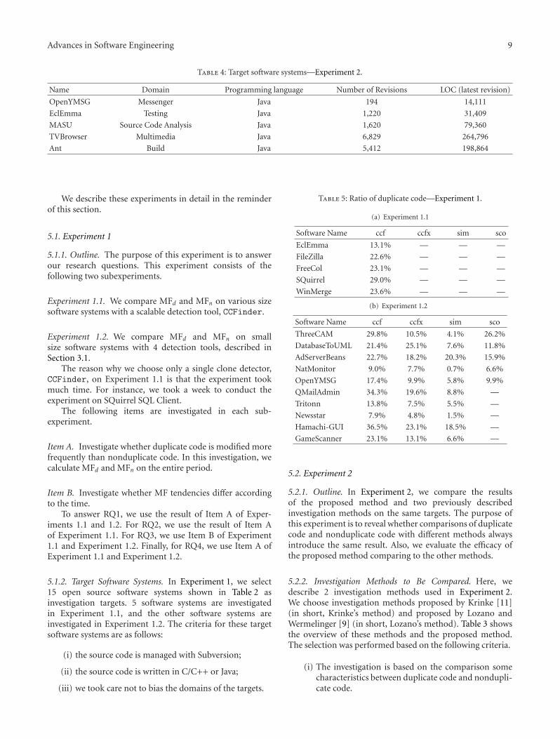
Table 2: Target software systems—Experiment 1.
(a) Experiment 1.1
Name Domain Programming language Number of Revisions LOC (latest revision)
EclEmma Testing Java 788 15,328
FileZilla FTP C++ 3,450 87,282
FreeCol Game Java 5,963 89,661
SQuirrel SQL Client Database Java 5,351 207,376
WinMerge Text Processing C++ 7,082 130,283
(b) Experiment 1.2
Name Domain Programming language Number of Revisions LOC (latest revision)
ThreeCAM 3D Modeling Java 14 3,854
DatabaseToUML Database Java 59 19,695
AdServerBeans Web Java 98 7,406
NatMonitor Network (NAT) Java 128 1,139
OpenYMSG Messenger Java 141 130,072
QMailAdmin Mail C 312 173,688
Tritonn Database C/C++ 100 45,368
Newsstar Network (NNTP) C 165 192,716
Hamachi-GUI GUI, Network (VPN) C 190 65,790
GameScanner Game C/C++ 420 1,214,570
Table 3: Overview of Investigation Methods.
Method Krinke [11]Lozano and
Wermelinger[9]
Proposed method
TargetRevisions
A revision perweek
All All
InvestigationUnit
Line MethodPlace (consecutive
lines)
Measureratio of
Modified linesWork
Modificationfrequency
the removed open or close brace is added to the end of theprevious line.
Step 3. It detects Duplicate Code. In this step, duplicate code isdetected from every target revision, and the detection resultsare stored into a database. Each detected duplicate code isidentified by 3-tuple (v, f , l), where v is the revision numberthat a given duplicate code was detected; f is the absolutepath to the source file where a given duplicate code exists;l is a set of line numbers where duplicate code exists. Notethat storing only the start line and the end line of duplicatecode is not feasible because a part of duplicate code is non-contiguous.
This step is very time consuming. If the history ofthe target software includes 1,000 revisions, duplicate codedetection is performed 1,000 times. However, this step is fullyautomated, and no manual work is required.
Step 4. It identifies Differences between Two ConsecutiveRevisions. In Step 4, we find out modification places between
two consecutive revisions with UNIX diff command. Asdescribed above, we can get this information by just parsingthe output of diff.
Step 5. It Counts the Number of Modifications. In this step,we count the number of modifications of duplicate codeand nonduplicate code with the results of the previoustwo steps. Here, we assume the variable for the number ofmodifications of duplicate code is MCd, and the variablefor nonduplicate code is MCn. Firstly, MCd and MCn areinitialized with 0, then they are increased as follows; ifthe range of specified modification is completely includedin duplicate code, MCd is incremented; if it is completelyincluded in nonduplicate code, MCn is incremented; if it isincluded in both of duplicate code and nonduplicate code,both MCd and MCn are incremented. All the modificationsare processed with the above algorithm.
Step 6. It calculates MFd and MFn. Finally, MFd and MFn
defined in the formula (4) are calculated with the result ofthe previous step.
5. Design of Experiment
In this paper, we conduct the following two experiments.
Experiment 1. Compare MFd and MFn on 15 open-sourcesoftware systems.
Experiment 2. Compare the result of the proposed methodwith 2 previous investigation methods on 5 open-sourcesoftware systems.
Advances in Software Engineering 9
Table 4: Target software systems—Experiment 2.
Name Domain Programming language Number of Revisions LOC (latest revision)
OpenYMSG Messenger Java 194 14,111
EclEmma Testing Java 1,220 31,409
MASU Source Code Analysis Java 1,620 79,360
TVBrowser Multimedia Java 6,829 264,796
Ant Build Java 5,412 198,864
We describe these experiments in detail in the reminderof this section.
5.1. Experiment 1
5.1.1. Outline. The purpose of this experiment is to answerour research questions. This experiment consists of thefollowing two subexperiments.
Experiment 1.1. We compare MFd and MFn on various sizesoftware systems with a scalable detection tool, CCFinder.
Experiment 1.2. We compare MFd and MFn on smallsize software systems with 4 detection tools, described inSection 3.1.
The reason why we choose only a single clone detector,CCFinder, on Experiment 1.1 is that the experiment tookmuch time. For instance, we took a week to conduct theexperiment on SQuirrel SQL Client.
The following items are investigated in each sub-experiment.
Item A. Investigate whether duplicate code is modified morefrequently than nonduplicate code. In this investigation, wecalculate MFd and MFn on the entire period.
Item B. Investigate whether MF tendencies differ accordingto the time.
To answer RQ1, we use the result of Item A of Exper-iments 1.1 and 1.2. For RQ2, we use the result of Item Aof Experiment 1.1. For RQ3, we use Item B of Experiment1.1 and Experiment 1.2. Finally, for RQ4, we use Item A ofExperiment 1.1 and Experiment 1.2.
5.1.2. Target Software Systems. In Experiment 1, we select15 open source software systems shown in Table 2 asinvestigation targets. 5 software systems are investigatedin Experiment 1.1, and the other software systems areinvestigated in Experiment 1.2. The criteria for these targetsoftware systems are as follows:
(i) the source code is managed with Subversion;
(ii) the source code is written in C/C++ or Java;
(iii) we took care not to bias the domains of the targets.
Table 5: Ratio of duplicate code—Experiment 1.
(a) Experiment 1.1
Software Name ccf ccfx sim sco
EclEmma 13.1% — — —
FileZilla 22.6% — — —
FreeCol 23.1% — — —
SQuirrel 29.0% — — —
WinMerge 23.6% — — —
(b) Experiment 1.2
Software Name ccf ccfx sim sco
ThreeCAM 29.8% 10.5% 4.1% 26.2%
DatabaseToUML 21.4% 25.1% 7.6% 11.8%
AdServerBeans 22.7% 18.2% 20.3% 15.9%
NatMonitor 9.0% 7.7% 0.7% 6.6%
OpenYMSG 17.4% 9.9% 5.8% 9.9%
QMailAdmin 34.3% 19.6% 8.8% —
Tritonn 13.8% 7.5% 5.5% —
Newsstar 7.9% 4.8% 1.5% —
Hamachi-GUI 36.5% 23.1% 18.5% —
GameScanner 23.1% 13.1% 6.6% —
5.2. Experiment 2
5.2.1. Outline. In Experiment 2, we compare the resultsof the proposed method and two previously describedinvestigation methods on the same targets. The purpose ofthis experiment is to reveal whether comparisons of duplicatecode and nonduplicate code with different methods alwaysintroduce the same result. Also, we evaluate the efficacy ofthe proposed method comparing to the other methods.
5.2.2. Investigation Methods to Be Compared. Here, wedescribe 2 investigation methods used in Experiment 2.We choose investigation methods proposed by Krinke [11](in short, Krinke’s method) and proposed by Lozano andWermelinger [9] (in short, Lozano’s method). Table 3 showsthe overview of these methods and the proposed method.The selection was performed based on the following criteria.
(i) The investigation is based on the comparison somecharacteristics between duplicate code and nondupli-cate code.

10 Advances in Software Engineering
(ii) The method has been published at the time when ourresearch started (at 2010/9).
In the experiments of Krinke’s and Lozano’s papers, onlya single detection tool Simian or CCFinder was selected.However, in this experiment, we selected 4 detection toolsfor bringing more valid results.
We developed software tools for Krinke’s and Lozano’smethods based on their papers. We describe Krinke’s methodand Lozano’s method briefly.
Krinke’s Method. Krinke’s method compares stability ofduplicate code and nonduplicate code [11]. Stability iscalculated based on ratios of modified duplicate code andmodified nonduplicate code. This method uses not all therevisions but a revision per week.
First of all, a revision is extracted from every weekhistory. Then, duplicate code is detected from every of theextracted revisions. Next, every consecutive two revisionsare compared for obtaining where added lines, deleted lines,and changed lines are. With this information, the ratios ofadded lines, deleted lines, and changed lines on duplicate andnonduplicate code are calculated and compared.
Lozano’s Method. Lozano’s method categorized Java meth-ods, then compare distributions of maintenance cost basedon the categories [9].
Firstly, Java methods are traced based on their ownerclass’s full qualified name, start/end lines, and signatures.Methods are categorized as follows:
AC-Method. Methods that always had duplicate codeduring their lifetime;
NC-Method. Methods that never had duplicate codeduring their lifetime;
SC-Method. Methods that sometimes had duplicatecode and sometimes did not.
Lozano’s method defines the followings where m is amethod, P is a period (a set of revisions), and r is a revision.
(i) ChangedRevisions(m,P): a set of revisions thatmethod m is modified in period P,
(ii) Methods(r): a set of methods that exist in revision r,
(iii) ChangedMethods(r): a set of methods that weremodified in revision r,
(iv) CoChangedMethods(m, r): a set of methods thatwere modified simultaneously with method m inrevision r. If method m is not modified in revisionr, it becomes 0. If modified, the following formula issatisfied:
ChangedMethod(r) = m∪ CoChangedMethod(m, r).(5)
Table 6: Overall results—Experiment 1.
(a) Experiment 1.1
Software Name ccf ccfx sim sco
EclEmma N — — —
FileZilla N — — —
FreeCol N — — —
SQuirrel N — — —
WinMerge N — — —
(b) Experiment 1.2
Software Name ccf ccfx sim sco
ThreeCAM N C N N
DatabaseToUML N N N N
AdServerBeans N N N N
NatMonitor C C N C
OpenYMSG C C C N
QMailAdmin C C C —
Tritonn N C N —
Newsstar N N N —
Hamachi-GUI N N N —
GameScanner C C N —
Then, this method calculates the following formulae withthe above definitions. Especially, work is an indicator of themaintenance cost:
likelihood(m,P) = ChangedRevisions(m,P)∑
r∈P∣∣ChangedMethods(r)
∣∣ ,
impact(m,P)
=∑
r∈P∣∣CoChangedMethods(m, r)
∣∣/|Methods(r)|
∣∣ChangedRevisions(m,P)
∣∣ ,
work(m,P) = likelihood(m,P)× impact(m,P).(6)
In this research, we compare work between AC-Methodand NC-Method. In addition, we also compare SC-Methods’work on duplicate period and nonduplicate period.
5.2.3. Target Software Systems. We chose 5 open-sourcesoftware systems in Experiment 2. Table 4 shows them. Twotargets, OpenYMSG and EclEmma, are selected as well asExperiment 1. Note that the number of revisions and LOCof the latest revision of these two targets are different fromTable 2. This is because they had been being in developmentbetween the time-lag in Experiments 1 and 2. Every sourcefile is normalized with the rules described in Section 4.2.2 aswell as Experiment 1. In addition, automatically generatedcode and testing code are removed from all the revisionsbefore the investigation methods are applied.
6. Experiment 1—Result and Discussion
6.1. Overview. Table 5 shows the average ratio for each targetof Experiment 1. Note that “ccf,” “ccfx,” “sim,” and “sco” in

Advances in Software Engineering 11
EclEmma FileZilla FreeCol Squirrel
DeleteAdd
201510
50
WinMerge
Change
d n d n d n d n d n
Figure 2: Result of Item A on Experiment 1.1.
Table 7: The average values of MF in Experiment 1.1.
Modification TypeMF
Duplicate code Nonduplicate code
Change 7.0337 8.1039
Delete 1.0216 1.4847
Add 1.9539 3.7378
ALL 10.0092 13.3264
the table are the abbreviated form of CCFinder, CCFinderX,Simian, and Scorpio, respectively.
Table 6 shows the overall result of Experiment 1. Inthis table, “C” means MFd > MFn in that case, and “N”means the opposing result. For example, the comparisonresult in ThreeCAM with CCFinder is MFd < MFn, whichmeans duplicate code is not modified more frequently thannonduplicate code. Note that “—” means the cases that wedo not consider because of the following reasons: (1) inExperiment 1.1, we use only CCFinder, so that the cases withother detectors are not considered; (2) Scorpio can handleonly Java, so that the cases in software systems written inC/C++ with Scorpio are not considered.
We describe the results in detail in the following subsec-tions.
6.2. Result of Experiment 1.1. Figure 2 shows all the resultsof Item A on Experiment 1.1. The labels “d” and “n” in X-axis means MF in duplicate code and nonduplicate code,respectively, and every bar consists of three parts, whichmeans change, delete, and add. As shown in Figure 2, MFd
is lower than MFn on all the target systems. Table 7 shows theaverage values of MF based on the modification types. Thecomparison results of MFd and MFn show that MFd is lessthan MFn in the cases of all the modification types. However,the degrees of differences between MFd and MFn are differentfor each modification type.
For Item B on Experiment 1.1, first, we divide the entireperiod into 10 sub-periods and calculate MF on every of thesub periods. Figure 3 shows the result. X-axis is the dividedperiods. Label “1” is the earliest period of the development,and label “10” is the most recent period. In the case ofEclEmma, the number of periods that MFd is greater thanMFn is the same as the number of periods that MFn is greaterthan MFd. In the case of FileZilla, FreeCol, and WinMerge,there is only a period that MFd is greater than MFn. In
1 2 3 4 5 6 7 8 9 10
Time period
25201510
50
d n d n d n d n d n d n d n d n d n d n
MF
(a) EclEmma
1 2 3 4 5 6 7 8 9 10
Time period
d n d n d n d n d n d n d n d n d n d n
20
15
10
5
0
MF
(b) FileZilla
1 2 3 4 5 6 7 8 9 10
Time period
d n d n d n d n d n d n d n d n d n d n
25201510
50
MF
(c) FreeCol
1 2 3 4 5 6 7 8 9 10
Time period
d n d n d n d n d n d n d n d n d n d n
40
30
20
10
0
MF
(d) SQuirrel
25201510
50
1 2 3 4 5 6 7 8 9 10
Time period
d n d n d n d n d n d n d n d n d n d n
MF
(e) WinMerge
Figure 3: Result of Item B on Experiment 1.1 (divided into 10periods).
the case of Squirrel SQL Client, MFn is greater than MFd
in all the periods. This result implies that if the numberof revisions becomes large, duplicate code tends to becomemore stable than nonduplicate code. However, the shapes ofMF transitions are different from every software system.
For WinMerge, we investigated period “2,” where MFn ismuch greater than MFd, and period “10,” where is only the

12 Advances in Software Engineering
Table 8: Comparing MFs based on programming language anddetection tool.
(a) Comparison on programming language
Programming languageMF
Duplicate code Nonduplicate code
Java 20.4370 24.1739
C/C++ 49.4868 57.2246
ALL 32.8869 38.3384
(b) Comparison on detection tool
Detection toolMF
Duplicate code Nonduplicate code
CCFinder 38.2790 40.7211
CCFinderX 40.3541 40.0774
Simian 26.0084 42.1643
Scorpio 20.9254 24.1628
ALL 32.8869 38.3384
Table 9: The average values of MF in Experiment 1.2.
Modification typeMF
Duplicate code Nonduplicate code
Change 26.8065 29.2549
Delete 3.8706 3.5228
Add 2.2098 5.5608
ALL 32.8869 38.3384
period that MFd is greater than MFn. In period “10,” there aremany modifications on test cases. The number of revisionsthat test cases are modified is 49, and the ratio of duplicatecode in test cases is 88.3%. Almost all modifications for testcases are performed on duplicate code, so that MFd is greaterthan MFn. Omitting the modifications for test cases, MFd
and MFn became inverted. However, there is no modificationon test cases in period “2,” so that MFd is less than MFn in thiscase.
Moreover, we divide the entire period by release dates andcalculate MF on every period. Figure 4 shows the result. Asthe figure shows, MFd is less than MFn in all the cases forFileZilla, FreeCol, SQuirrel, and WinMerge. For EclEmma,there are some cases that MFd > MFn at the release level.Especially, duplicate code is frequently modified in the earlyreleases.
Although MFd is greater than MFn in the period “6”in Freecol and the period “10” in WinMerge, MFd is lessthan MFn in all cases at the release level. This indicates thatduplicate code is sometimes modified intensively in a shortperiod, nevertheless it is stable than nonduplicate code in along term.
The summary of Experiment 1 is that duplicate codedetected by CCFinder was modified less frequently thannonduplicate code. Consequently, we conclude that duplicatecode detected by CCFinder does not have a negative impacton software evolution even if the target software is large andits period is long.
12
8
4
0
0.1.1–1.0.0 1.0.0–1.1.0 1.1.0–1.2.0 1.2.0–1.3.0 1.3.0–1.4.0
d n d n d n d n d n
Version
MF
(a) EclEmma
12
8
4
0d n d n d n
Version
Beta–3.0.0 3.0.0–3.1.0 3.1.0–3.2.0
MF
(b) FileZilla
d n d n d n d n d n
0.3.0–0.4.0 0.4.0–0.5.0 0.5.0–0.6.0 0.6.0–0.7.0 0.7.0–0.8.0
Version
30
20
10
0
MF
(c) FreeCol
1.1–2.0 2.0–2.1 2.1–2.2 2.2–2.3 2.3–2.4 2.4–2.5 2.5–2.6 2.6–3.0
Version
30
20
10
0d n d n d n d n d nd n d n d n
MF
(d) SQuirrel
1.7–2.0 2.0–2.2 2.2–2.4 2.4–2.6 2.6–2.8 2.8–2.10 2.10–2.12
Version
20
15
10
5
0d n d n d n d nd n d n d n
MF
(e) WinMerge
Figure 4: Result of Item B on Experiment 1.1 (divided by releases).
6.3. Result of Experiment 1.2. Figure 5 shows all the results ofItem A on Experiment 1.2. In Figure 5, the detection toolsare abbreviated as follows: CCFinder→C; CCFinderX →X; Simian→Si;Scorpio→Sc. There are the results of 3detection tools except Scorpio on C/C++ systems, becauseScorpio does not handle C/C++. MFd is less than MFn inthe 22 comparison results out of 35. In the 4 target systemsout of 10, duplicate code is modified less frequently than

Advances in Software Engineering 13
8070605040302010
0
ChangeDeleteAdd
ThreeCAM DatabaseToUML AdserverBeans NatMonitor OpenYMSG
d n d n d n d n d n d n d n d n d n d n d n d n d n d n d n d n d n d n d n d n
MF
C X Si Sc C X Si Sc C X Si Sc C X Si Sc C X Si Sc
(a) Java software
C X Si C X Si C X Si C X Si C X Si
d n d n d n d n d n d n d n d n d n d n d n d n d n d n d n
QMailAdmin Tritonn Newsstar Hamachi-GUI GameScanner
250
200
150
100
50
0
MF
(b) C/C++ Software
Figure 5: Result of Item A on Experiment 1.2.
nonduplicate code in the cases of all the detection tools.In the case of the other 1 target system, MFd is greaterthan MFn in the cases of all the detection tools. In theremaining systems, the comparison result is different for thedetection tools. Also, we compared MFd and MFn based onprogramming language and detection tools. The comparisonresult is shown in Table 8. The result shows that MFd is lessthan MFn on all the programming language, and MFd isless than MFn on the 3 detectors, CCFinder, Simian, andScorpio, meanwhile the opposing result is shown in the caseof CCFinderX. We also compared MFd and MFn based onmodification types. The result is shown in Table 9. As shownin Table 9, MFd is less than MFn in the cases of change andaddition, meanwhile the opposing result is shown in the caseof deletion.
We investigated whether there is a statistically significantdifference between MFd and MFn by t-test. The result isthat, there is no difference between them where the levelof significance is 5%. Also, there is no significant differencein the comparison based on programming language anddetection tool.
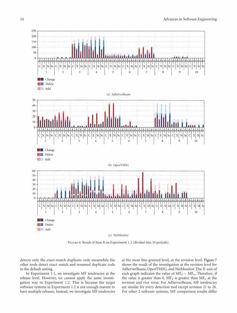
For Item B on Experiment 1.2, we divide the wholeperiod into 10 subperiods likewise Experiment 1.1. Figure 6shows the result. In this experiment, we observed that thetendencies of MF transitions loosely fall into three categories:(1) MFd is lower than MFn almost of all the divisions; (2)MFd is greater than MFn in the early divisions, meanwhile theopposite tendency is observed in the late divisions; (3) MFd isless than MFn in the early divisions, meanwhile the opposite
tendency is observed in the late divisions. Figure 6 shows theresult of the 3 systems on which we observed remarkabletendencies of every category.
In Figure 6(a), period “4” shows that MFn is greater thanMFd on all the detection tool meanwhile period “7” showsexactly the opposite result. Also, in period “5,” there arehardly differences between duplicate code and nonduplicatecode. We investigated the source code of period “4.” Inthis period, many source files were created by copy-and-paste operations, and a large amount of duplicate code wasdetected by each detection tool. The code generated by copy-and-paste operations was very stable meanwhile the othersource files were modified as usual. This is the reason whyMFn is much greater than MFd in period “4.”
Figure 6(b) shows that duplicate code tends to be modi-fied more frequently than nonduplicate code in the anteriorhalf of the period meanwhile the opposite occurred in theposterior half. We found that there was a large number ofduplicate code that was repeatedly modified in the anteriorhalf. On the other hand, there was rarely such duplicate codein the posterior half.
Figure 6(c) shows the opposite result of Figure 6(b). Thatis, duplicate code was modified more frequently in theposterior half of the period. In the anterior half, the amountof duplication was very small, and modifications were rarelyperformed on it. In the posterior half, amount of duplicatecode became large, and modifications were performed onit repeatedly. In the case of Simian detection, no duplicatecode was detected except period “5.” This is because Simian
14 Advances in Software Engineering
250
200
150
100
50
0
Change
Delete
Add
1 2 3 4 5 6 7 8 9 10
dndndndndndndndndndndndndndndndndndndndndndndndndndndndndndndndndndndndndndndndn
C X Si Sc C X Si Sc C X Si Sc C X Si Sc C X Si Sc C X Si Sc C X Si Sc C X Si Sc C X Si Sc C X Si Sc
(a) AdServerBeans
Change
Delete
Add
1 2 3 4 5 6 7 8 9 10
dndndndndndndndndndndndndndndndndndndndndndndndndndndndndndndndndndndndndndndndn
50
40
30
20
10
0
C X Si Sc C X Si Sc C X Si Sc C X Si Sc C X Si Sc C X Si Sc C X Si Sc C X Si Sc C X Si Sc C X Si Sc
(b) OpenYMSG
Change
Delete
Add
1 2 3 4 5 6 7 8 9 10
dndndndndndndndndndndndndndndndndndndndndndndndndndndndndndndndndndndndndndndndn
60
50
40
30
20
10
0
C X Si Sc C X Si Sc C X Si Sc C X Si Sc C X Si Sc C X Si Sc C X Si Sc C X Si Sc C X Si Sc C X Si Sc
(c) NatMonitor
Figure 6: Result of Item B on Experiment 1.2 (divided into 10 periods).
detects only the exact-match duplicate code meanwhile theother tools detect exact match and renamed duplicate codein the default setting.
In Experiment 1.1, we investigate MF tendencies at therelease level. However, we cannot apply the same investi-gation way to Experiment 1.2. This is because the targetsoftware systems in Experiment 1.2 is not enough mature tohave multiple releases. Instead, we investigate MF tendencies
at the most fine-grained level, at the revision level. Figure 7shows the result of the investigation at the revision level forAdServerBeans, OpenYMSG, and NatMonitor. The X-axis ofeach graph indicates the value of MFd − MFn. Therefore, ifthe value is greater than 0, MFd is greater than MFn at therevision and vice versa. For AdServerBeans, MF tendenciesare similar for every detection tool except revision 21 to 26.For other 2 software systems, MF comparison results differ

Advances in Software Engineering 15
1 11 21 31 41 51 61 918171
250200150100
500
−50−100−150−200
MF d−
MF n
(a) AdServerBeans
1 11 21 31 41 51 61 918171
200
150
100
50
0
−50
−100
101 111 121 131 141MF d−
MF n
(b) OpenYMSG
120
80
40
0
−40
−80
1 11 21 31 41 51 61 71 81 91 101 111 121
AverageIndividual tool (4 lines)
MF d−
MF n
(c) NatMonitor
Figure 7: Result of Item B on Experiment 1-2 (for each revision).
from each detection tool in most of the revisions. As thefigures show, tendencies of MF transition differ from clonedetectors nevertheless there seems to be small differencesbetween clone detectors in 10 sub-periods division. However,these graphs do not consider modification types. Therefore,we cannot judge what type of modification frequentlyoccurred from the graphs.
The summary of Experiment 1.2 is as follows: we foundsome instances that duplicate code was modified morefrequently than nonduplicate code in a short period oneach detection tool; however, in the entire period, duplicatecode was modified less frequently than nonduplicate codeon every target software with all the detection tools. Conse-quently, we conclude that the presence of duplicate code doesnot have a seriously-negative impact on software evolution.
6.4. Answers for RQs
RQ1: Is duplicate code more frequently modified than nondu-plicate code? The answer is No. In Experiment 1.1, we foundthat MFd is lower than MFn in all the target systems. Also,
we found a similar result in Experiment 1.2: 22 comparisonresults out of 35 show that MFd is lower than MFn, also MFd
is lower than MFn in average. This result indicates that thepresence of duplicate code does not seriously affect softwareevolution, which is different from the common belief.
RQ2: Are the comparison results of stability between duplicatecode and nonduplicate code different from multiple detectiontools? The answer is Yes. In Experiment 1.2, the comparisonresults with CCFinderX are different from the results withother 3 detectors. Moreover, MFn is much greater than MFd
in the case of Simian. At present, we cannot find the causesof the difference of the comparison results. One of the causesmay be the ratio of duplicate code. The ratio of duplicatecode is quite different for each detection tool on the samesoftware. However, we cannot see any relation between theratio of duplicate code and MF.
RQ3: Is duplicate code modified uniformly throughout itslifetime? The answer is No. In Item B of Experiments 1.1

16 Advances in Software Engineering
and 1.2, there are some instances that duplicate code wasmodified more frequently than nonduplicate code in a shortperiod though MFd is less than MFn in the whole period.However, these MFs tendencies depend on target softwaresystems, so that we cannot find characteristics of suchvariability.
RQ4: Are there any differences in the comparison results onmodification types? The answer is Yes. In Experiment 1.1,MFd is less than MFn on all the modification types. However,there is a small difference between MFd and MFn in the caseof deletion, meanwhile there is a large difference in the caseof addition. In Experiment 1.2, MFd is less than MFn in thecases of change and addition. Especially, MFn is more thantwice as large as MFd in the case of addition. However, MFd
is greater than MFn in the case of deletion. These resultsshow that deletion tends to be affected by duplicate code,meanwhile addition tends not to be affected by duplicatecode.
6.5. Discussion. In Experiment 1, we found that duplicatecode tends to be more stable than nonduplicate code, whichindicates that the presence of duplicate code does not have anegative impact on software evolution. We investigated howthe software evolved in the period, and we found that thefollowing activities should be a part of factors that duplicatecode is modified less frequently than nonduplicate code.
Reusing Stable Code. When implementing new functionali-ties, reusing stable code is a good way to reduce the numberof introduced bugs. If most of duplicate code is reused stablecode, MFd becomes less than MFn.
Using Generated Code. Automatically generated code israrely modified manually. Also, the generated code tends tobe duplicate code. Consequently, if the amount of generatedcode is high, MFd will become less than MFn.
On the other hand, there are some cases that duplicatecode was more frequently modified than nonduplicate codein a short period. The period “7” on AdServerBeans (Exper-iment 1.2, Item B) is one of these instances. We analyzed thesource code of this period to detect why MFd was greater thanMFn in this period though the opposite results were shown inthe other periods. Through the analysis, we found that thereare some instances that the same modifications were appliedto multiple places of code.
Algorithm 2 shows an example of unstable duplicatecode. There are 5 code fragments that are similar tothis fragment. Firstly, lines labeled with “%” (shown inAlgorithm 2(b)) were modified to replace the getter methodsinto directly accesses to fields. In the next, a line labeledwith “#” is removed (shown in Algorithm 2(c)). These twomodifications were concentrically conducted in period “7.”Reusing unstable code like this example can cause additionalcosts for software maintenance. Moreover, a code fragmentwas not simultaneously changed with its correspondents atthe second modification. If this inconsistent change wasintroduced unintentionally, it might cause a bug. If so, this
Table 10: Ratio of duplicate code—Experiment 2.
Software Name ccf ccfx sim sco
OpenYMSG 12.4% 6.2% 2.7% 5.5%
EclEmma 6.9% 4.8% 2.0% 3.7%
MASU 25.6% 26.5% 11.3% 15.4%
TVBrowser 13.6% 10.9% 5.4% 19.0%
Ant 13.9% 12.1% 6.2% 15.6%
Table 11: Overall results—Experiment 2.
Software Name MethodTools
ccf ccfx sim sco
OpenYMSGProposed N C C N
Krinke N C C N
Lozano — — N —
EclEmmaProposed N N N N
Krinke N N N C
Lozano N N — —
MASUProposed C N C C
Krinke C C C C
Lozano C C C C
TVBrowserProposed N N N N
Krinke C C C C
Lozano C C C C
AntProposed N N N N
Krinke C C C C
Lozano C C C C
is a typical situation that duplicate code affects softwareevolution.
7. Experiment 2—Result and Discussion
7.1. Overview. Table 10 shows the average ratios of duplicatecode in each target, and Table 11 shows the comparisonresults of all the targets. In Table 11, “C” means that duplicatecode requires more cost than nonduplicate code, and “N”means its opposite. The discriminant criteria of “C” and “N”are different in each investigation method.
In the proposed method, if MFd is lower than MFn, thecolumn is labeled with “C,” and the column is labeled with“N” in its opposite case.
In Krinke’s method, if the ratio of changed and deletedlines of code on duplicate code is greater than changed anddeleted lines on nonduplicate code, the column is labeledwith “C,” and in its opposite case the column is labeled with“N.” Note that herein we do not consider added lines becausethe amount of add is the lines of code added in the nextrevision, not in the current target revision.
In Lozano’s method, if work in AC-Method is statisticallygreater than one in NC-Method, the column is labeled with“C.” On the other hand, if work in NC-Method is statisticallygreater than one in AC-Method, the column is labeled with“N.” Here, we use Mann-Whitney’s U test under setting

Advances in Software Engineering 17
(a) Before Modificationint offsetTmp = dataGridDisplayCriteria
.getItemsPerPage() ∗(dataGridDisplayCriteria.getPage() -1);
if (offsetTmp > 0) --offsetTmp;if (offsetTmp < 0) offsetTmp = 0;
final int offset = offsetTmp;String sortColumn =
dataGridDisplayCriteria.getSortColumn();Order orderTmp =
dataGridDisplayCriteria.getOrder().equals(AdServerBeansConstants.ASC) ?
Order.asc(sortColumn) :Order.desc(sortColumn);
(b) After 1st Modificationint offsetTmp = dataGridDisplayCriteria
.getItemsPerPage() ∗(dataGridDisplayCriteria.getPage() -1);
if (offsetTmp > 0) --offsetTmp;if (offsetTmp < 0) offsetTmp = 0;
final int offset = offsetTmp;String sortColumn =
% dataGridDisplayCriteria.sortColumn;Order orderTmp =
% dataGridDisplayCriteria.order.equals(AdServerBeansConstants.ASC) ?
Order.asc(sortColumn) :Order.desc(sortColumn);
(c) After 2nd Modificationint offsetTmp = dataGridDisplayCriteria
.getItemsPerPage() ∗(dataGridDisplayCriteria.getPage() -1);
#if (offsetTmp < 0) offsetTmp = 0;
final int offset = offsetTmp;String sortColumn =
dataGridDisplayCriteria.sortColumn;Order orderTmp =
dataGridDisplayCriteria.order.equals(AdServerBeansConstants.ASC) ?
Order.asc(sortColumn) :Order.desc(sortColumn);
Algorithm 2: An example of unstable duplicate code.
5% as the level of significance. If there is no statisticallysignificant difference in AC- and NC-Method, we comparework in duplicate period and nonduplicate period in SC-Method with Wlcoxon’s singed-rank test. We also set 5% asthe level of significance. If there is no statistically significantdifference, the column is labeled with “—.”
As this table shows, different methods and different toolsbrought almost the same result in the case of EclEmma andMASU. On the other hand, in the case of other targets, weget different results with different methods or different tools.Especially, in the case of TVBrowser and Ant, the proposedmethod brought the opposite result to Lozano’s and Krinke’smethod.
7.2. Result of MASU. Herein, we show comparison figures ofMASU. Figure 8 shows the results of the proposed method. Inthis case, all the detection tools except CCFinderX broughtthe same result that duplicate code is more frequentlymodified than nonduplicate code. Figure 9 shows the resultsof Krinke’s method on MASU. As this figure shows, thecomparison of all the detection detectors brought the sameresult that duplicate code is less stable than nonduplicatecode. Figure 10 shows the results of Lozano’s method onMASU with Simian. Figure 10(a) compares AC-Methodand NC-Method. X-axis indicates maintenance cost (work)and Y-axis indicates cumulated frequency of methods. Forreadability, we adopt logarithmic axis on X-axis. In this

18 Advances in Software Engineering
ccf ccfx sim sco
d n d n d n d n
ChangeDeleteAdd
25
20
15
10
5
0
Figure 8: Result of the proposed method on MASU.
ChangeDeleteAdd
ccf ccfx sim sco
1.41.2
10.80.60.40.2
0d n d n d n d n
Figure 9: Result of Krinke’s method on MASU.
case, AC-Method requires more maintenance cost thanNC-Method. Also, Figure 10(b) compares duplicate periodand nonduplicate period of SC-Method. In this case, themaintenance cost in duplicate period is greater than innonduplicate period.
In the case of MASU, Krinke’s method and Lozano’smethod regard duplicate code as requiring more cost thannonduplicate code in the cases of all the detection tools.The proposed method indicates that duplicate code is morefrequently modified than nonduplicate code with CCFinder,Simian, and Scorpio. In addition, there is little differencesbetween MFd and MFn in the result of the proposed methodwith CCFinderX, which is the only case that duplicate codeis more stable than nonduplicate code. Considering all theresults, we can say that duplicate code has a negative impacton software evolution on MASU. This result is reliablebecause all the investigation methods show such tendencies.
7.3. Result of OpenYMSG. Figures 11, 12, and 13 showthe result of the proposed method, Krinke’s method, andLozano’s method on OpenYMSG. In the cases of theproposed method and Krinke’s method, duplicate code isregarded as having a negative impact with CCFinderX andSimian, meanwhile the opposing results are shown withCCFinder and Scorpio. In Lozano’s method with Simian,duplicate code is regarded as not having a negative impact.Note that we omit the comparison figure on SC-Method
1 10 100 1000
100
80
60
40
20
0
(%)
AC-methodNC-method
(a) AC-Method versus NC-Method
Duplicate periodNonduplicate period
1 10 100 1000
100
80
60
40
20
0
(%)
(b) SC-Method
Figure 10: Result of Lozano’s Method on MASU with Simian.
because there are only 3 methods that are categorized intoSC-Method.
As these figures show, the comparison results are differentfor detection tools or investigation methods. Therefore, wecannot judge whether the presence of duplicate code has anegative impact or not on OpenYMSG.
7.4. Discussion. In the case of OpenYMSG, TVBrowser,and Ant, different investigation methods and differenttools brought opposing results. Figure 14 shows an actualmodification in Ant. Two methods were modified in thismodification. The hatching parts are detected duplicate codeand frames in them mean pairs of duplicate code betweentwo methods. Vertical arrows show modified lines betweenthis modification and the next (77 lines of code weremodified).
This modification is a refactoring, which extracts theduplicate instructions from the two methods and mergesthem as a new method. In the proposed method, thereare 2 modification places in duplicate code and 4 placesin nonduplicate code, so that MFd and MFn become 51.13and 18.13, respectively. In Krinke’s method, DC + CC and

Advances in Software Engineering 19
30
25
20
15
10
5
0
ccf ccfx sim sco
d n d n d n d n
ChangeDeleteAdd
Figure 11: Result of the proposed method on OpenYMSG.
ChangeDeleteAdd
ccf ccfx sim sco
1.61.41.2
10.80.60.40.2
0d n d n d n d n
Figure 12: Result of Krinke’s method on OpenYMSG.
DN + CN become 0.089 and 0.005, where DC, CC, DN,and CN indicate the ratio of deleted lines on duplicatecode, changed lines on duplicate code, deleted lines onnonduplicate code, and deleted lines on nonduplicate code,respectively.
In this case, both the proposed method and Krinke’smethod regard duplicate code requiring more maintenancecost than nonduplicate code. However, there is a greatdifference in Krinke’s method than the proposed method:in the proposed method, duplicate code is modified about2.8 times as frequently as nonduplicate code; meanwhile,in Krinke’s method, duplicate code is modified 17.8 timesas frequently as nonduplicate code. This is caused by thedifference of the barometers used in each method. InKrinke’s method, the barometer depends on the amount ofmodified lines, meanwhile the barometer depends on theamount of modified places in the proposed method. Thisexample is one of the refactorings on duplicate code. InKrinke’s method, if removed duplicate code is large, duplicatecode is regarded as having more influence. However, inthe cases of duplicate code removal, we have to spendmuch effort if the number of duplicate fragments is high.Therefore, we can say that the proposed method canaccurately measure the influence of duplicate code in thiscase.
1 10 100 1000
AC-methodNC-method
100
80
60
40
20
0
(%)
Figure 13: Result of Lozano’s method on OpenYMSG with Simian.
This is an instance that is advantageous for the proposedmethod. However, we cannot investigate all the experimentaldata because the amount of the data is too vast to conductmanual checking for all the modifications. There is apossibility that the proposed method cannot accuratelyevaluate the influence of duplicate code in some situations.
In Experiment 2, we found that the different investiga-tion methods or different detectors draw different resultson the same target systems. In Experiment 1, we found thatduplicate code is less frequently modified than nonduplicatecode. However, the result of Experiment 2 shows that wecannot generalize the result of Experiment 1. We have toconduct more experiments and analyze the results of themin detail to gain more generic.
8. Threats to Validity
This section describes threats to validity of this study.
8.1. Features of Every Modification. In this study, we assumethat cost required for every modification is equal to oneanother. However, the cost is different between every mod-ification in the actual software evolution. Consequently, thecomparison based on MF may not appropriately representthe cost required for modifying duplicate code and nondu-plicate code.
Also, when we modify duplicate code, we have toconsider maintaining the consistency between the modifiedduplicate code and its correspondents. If the modificationlacks the consistency by error, we have to remodify them forrepairing the consistency. The effort for consistency is notnecessary for modifying nonduplicate code. Consequently,the average cost required for duplicate code may be differentfrom the one required for nonduplicate code. In order tocompare them more appropriately, we have to consider thecost for maintaining consistency.
Moreover, distribution of source code that should bemodified are not considered. However, it differs from

20 Advances in Software Engineering
Clone pair relationship
Modified lines between this revision and the next
Code fragment 1 Code fragment 2
private void doClassicCompile() throws BuildException { private void doClassicCompile() throws BuildException {log(“Using classic compiler”, Project.MSG VERBOSE);
log(“Using classic compiler”, Project.MSG VERBOSE);Path classPath = getCompileClasspath(false);. . .
7 lines
argList.addElement(“-classpath”);Path classPath = getCompileClasspath(false);. . .
7 lines
argList.addElement(“-classpath”);if (. . .) { . . .} else {
. . .. . .
}if (debug) { . . . }. . .log(“Compilation args: ” + argList.toString(),
Project.MSG VERBOSE);
. . .
Enumeration enum = compileList.elements();
while (enum.hasMoreElements()) { . . . }log(niceSourceList.toString(), Project.MSG VERBOSE);ByteArrayOutputStream out = new ByteArrayOutputStream();. . .. . .
}
. . .
. . .
}
String[] args = new String[argList.size() + compileList.size()];32lines
. . .
17 lines
if (debug) { . . . }. . .log(“Compilation args: ” + argList.toString(),Project.MSG VERBOSE);
. . .
Enumeration enum = compileList.elements();
while (enum.hasMoreElements()) { . . . }log(niceSourceList.toString(), Project.MSG VERBOSE);
String[] args = new String[argList.size() + compileList.size()];
17 lines
38
lines
Figure 14: An Example of Modification.
every modification, thus we may get different results byconsidering the distribution of source code.
8.2. Identifying the Number of Modifications. In this study,modifying consecutive multiple lines are regarded as asingle modification. However, it is possible that such anautomatically processing identifies the incorrect number ofmodifications. If multiple lines that were not contiguousare modified for fixing a single bug, the proposed methodpresumes that multiple modifications were performed. Also,if multiple consecutive lines were modified for fixing two ormore bugs by chance, the proposed method presumes thatonly a single modification was performed. Consequently, itis necessary to manually identify modifications if we have touse the exactly correct number of modifications.
Besides, we investigated how many the identified modifi-cations occurred across the boundary of duplicate code andnonduplicate code. If this number is high, then the analysissuspects because such modifications increase both the countsat the same time. The investigation result is that, in thehighest case, the ratio of such modifications is 4.8%. Thatmeans that almost all modifications occurred within eitherduplicate code or nonduplicate code.
8.3. Category of Modifications. In this study, we counted allthe modifications, regardless of their categories. As a result,the number of modifications might be incorrectly increasedby unimportant modifications such as format transfor-mation. A part of unimportant modifications remainedeven if we had used the normalized source code describedin Section 4.2.2. Consequently, manual categorization forthe modifications is required for using the exactly correctnumber of modifications.
Also, the code normalization that we used in this studyremoved all the comments in the source files. If considerablecost was expended to make or change code comments on thedevelopment of the target systems, we incorrectly missed thecost.
8.4. Property of Target Software. In this study, we used onlyopen-source software systems, so that different results maybe shown with industrial software systems. Some researcherspointed out that industrial software systems include muchduplicate code [24, 25]. Consequently, duplicate code maynot be managed well in industrial software, which mayincrease MFd. Also, properties of industrial software arequite different from ones of open source software. In orderto investigate the impact of duplicate code on industrialsoftware, we have to compare MF on industrial softwareitself.
8.5. Settings of Detection Tools. In this study, we used defaultsettings for all the detection tools. If we change the settings,different results will be shown.
9. Conclusion
This paper presented an empirical study on the impact ofthe presence of duplicate code on software evolution. Weassumed that if duplicate code is modified more frequentlythan nonduplicate code, the presence of duplicate codeaffects software evolution and compared the stability ofduplicate code and nonduplicate code. To evaluate from adifferent standpoint from previous studies, we used a newindicator, modification frequency, which is calculated withthe number of modified places of code. Also, we used 4
Advances in Software Engineering 21
duplicate code detection tools to reduce the bias of duplicatecode detectors. We conducted an experiment on 15 open-source software systems, and the result showed that duplicatecode was less frequently modified than nonduplicate code.We also found some cases that duplicate code was intensivelymodified in a short period though duplicate code was stablethan nonduplicate code in the whole development period.
Moreover, we compared the proposed method to other2 investigation methods to evaluate the efficacy of theproposed method. We conducted an experiment on 5 open-source software systems, and in the cases of 2 targets, we gotthe opposing results to other 2 methods. We investigated theresult in detail and found some instances that the proposedmethod could evaluate more accurately than other methods.
In this study, we found that duplicate code tends to bestable than nonduplicate code. However, more studies arerequired to generalize this result, because we found thatdifferent investigation methods may bring different results.As future work, we are going to conduct more studies withother settings to get the characteristics of harmful duplicatecode.
Acknowledgments
This research is being conducted as a part of the Stage Project,the Development of Next Generation IT Infrastructure,supported by the Ministry of Education, Culture, Sports,Science, and Technology of Japan. This study has beensupported in part by Grant-in-Aid for Scientific Research(A) (21240002) and Grant-in-Aid for Exploratory Research(23650014) from the Japan Society for the Promotion of Sci-ence, and Grant-in-Aid for Young Scientists (B) (22700031)from Ministry of Education, Science, Sports and Culture.This paper is an extended version of earlier conference papers[26, 27].
References
[1] S. Bellon, R. Koschke, G. Antoniol, J. Krinke, and E. Merlo,“Comparison and evaluation of clone detection tools,” IEEETransactions on Software Engineering, vol. 32, no. 10, pp. 804–818, 2007.
[2] M. D. Wit, A. Zaidman, and A. V. Deursen, “Managingcode clones using dynamic change tracking and resolution?”in Proceedings of the 25th IEEE International Conference onSoftware Maintenance (ICSM ’09), pp. 169–178, September2009.
[3] M. P. Robillard, W. Coelho, and G. C. Murphy, “How effectivedevelopers investigate source code: an exploratory study,” IEEETransactions on Software Engineering, vol. 30, no. 12, pp. 889–903, 2004.
[4] C. J. Kapser and M. W. Godfrey, “‘cloning considered harmful’considered harmful: patterns of cloning in software,” EmpiricalSoftware Engineering, vol. 13, no. 6, pp. 645–692, 2008.
[5] M. Kim, V. Sazawal, D. Notkin, and G. C. Murphy, “Anempirical study of code clone genealogies,” in Proceedings ofthe 13th ACM SIGSOFT Symposium on the Foundations ofSoftware Engineering, pp. 187–196, September 2005.
[6] N. Bettenburg, W. Shang, W. M. Ibrahim, B. Adams, Y.Zou, and A. E. Hassan, “An empirical study on inconsistent
changes to code clones at the release level,” Science of ComputerProgramming, vol. 77, no. 6, pp. 760–776, 2012.
[7] A. Monden, D. Nakae, T. Kamiya, S. Sato, and K. Matsumoto,“Software quality analysis by code clones in industrial legacysoftware,” in Proceedings of the 8th IEEE International SoftwareMetrics Symposium, pp. 87–94, June 2002.
[8] A. Lozano, M. Wermelinger, and B. Nuseibeh, “Evaluatingthe harmfulness of cloning: a change based experiment,”in Proceedings of the 4th International Workshop on MiningSoftware Repositories (MSR ’07), May 2007.
[9] A. Lozano and M. Wermelinger, “Assessing the effect of cloneson changeability,” in Proceedings of the 24th InternationalConference on Software Maintenance, pp. 227–236, September2008.
[10] A. Lozano, M. Wermelinger, and B. Nuseibeh, “Evaluating therelation between changeability decay and the characteristicsof clones and methods,” in Proceedings of the 23rd IEEE/ACMInternational Conference on Automated Software Engineering,pp. 100–109, September 2008.
[11] J. Krinke, “Is cloned code more stable than non-cloned code?”in Proceedings of the 8th IEEE International Working Conferenceon Source Code Analysis and Manipulation, SCAM 2008, pp.57–66, September 2008.
[12] N. Gode and J. Harder, “Clone stability,” in Proceedings ofthe 15th European Conference on Software Maintenance andReengineering (CSMR ’11), pp. 65–74, March 2011.
[13] J. Krinke, “Is cloned code older than non-cloned code?” in Pro-ceedings of the 5th International Workshop on Software Clones(IWSC ’11), pp. 28–33, May 2011.
[14] F. Rahman, C. Bird, and P. Devanbu, “Clones: what is thatsmell?” in Proceedings of the 7th IEEE Working Conference onMining Software Repositories, pp. 72–81, May 2010.
[15] N. Gode and R. Koschke, “Frequency and risks of changesto clones,” in 33rd International Conference on SoftwareEngineering (ICSE ’11), pp. 311–320, May 2011.
[16] S. G. Eick, T. L. Graves, A. F. Karr, U. S. Marron, andA. Mockus, “Does code decay? Assessing the evidence fromchange management data,” IEEE Transactions on SoftwareEngineering, vol. 27, no. 1, pp. 1–12, 2001.
[17] N. Gode, “Evolution of type-1 clones,” in Proceedings of the 9thIEEE International Working Conference on Source Code Analysisand Manipulation (SCAM ’09), pp. 77–86, September 2009.
[18] E. Burd and J. Bailey, “Evaluating clone detection tools foruse during preventative maintenance,” in Proceedings of the2nd IEEE International Workshop on Source Code Analysis andManipulation, pp. 36–43, October 2002.
[19] T. Kamiya, S. Kusumoto, and K. Inoue, “CCFinder: a multilin-guistic token-based code clone detection system for large scalesource code,” IEEE Transactions on Software Engineering, vol.28, no. 7, pp. 654–670, 2002.
[20] CCFinderX, http://www.ccfinder.net/ccfinderx.html/.[21] Simian, http://www.harukizaemon.com/simian/.[22] Y. Higo and S. Kusumoto, “Code clone detection on special-
ized PDGs with heuristics,” in Proceedings of the 15th Euro-pean Conference on Software Maintenance and Reengineering(CSMR ’11), pp. 75–84, March 2011.
[23] Scorpio, http://sdl.ist.osaka-u.ac.jp/∼higo/cgi-bin/moin.cgi/Scorpio/.
[24] S. Ducasse, M. Rieger, and S. Demeyer, “Language indepen-dent approach for detecting duplicated code,” in Proceedingsof the 15th IEEE International Conference on Software Mainte-nance (ICSM ’99), pp. 109–118, September 1999.
22 Advances in Software Engineering
[25] S. Uchida, A. Monden, N. Ohsugi, T. Kamiya, K. I. Matsumoto,and H. Kudo, “Software analysis by code clones in open sourcesoftware,” Journal of Computer Information Systems, vol. 45,no. 3, pp. 1–11, 2005.
[26] K. Hotta, Y. Sano, Y. Higo, and S. Kusumoto, “Is duplicate codemore frequently modified than non-duplicate code in softwareevolution?: an empirical study on open source software,” inProceedings of the 4th the International Joint ERCIM Workshopon Software Evolution and International Workshop on Principlesof Software Evolution, September 2010.
[27] Y. Sasaki, K. Hotta, Y. Higo, and S. Kusumoto, “Is duplicatecode good or bad? an empirical study with multiple investi-gation methods and multiple detection tools,” in Proceedingsof the 22nd International Symposium on Software ReliabilityEngineering (ISSRE ’11), Hiroshima, Japan, November 2011.

Hindawi Publishing CorporationAdvances in Software EngineeringVolume 2012, Article ID 524636, 9 pagesdoi:10.1155/2012/524636
Research Article
A Comparative Study of Data Transformations forWavelet Shrinkage Estimation with Application toSoftware Reliability Assessment
Xiao Xiao and Tadashi Dohi
Department of Information Engineering, Graduate School of Engineering, Hiroshima University, 1-4-1 Kagamiyama,Higashi-Hiroshima 739-8527, Japan
Correspondence should be addressed to Xiao Xiao, [email protected]
Received 6 January 2012; Revised 6 March 2012; Accepted 6 March 2012
Academic Editor: Chin-Yu Huang
Copyright © 2012 X. Xiao and T. Dohi. This is an open access article distributed under the Creative Commons Attribution License,which permits unrestricted use, distribution, and reproduction in any medium, provided the original work is properly cited.
In our previous work, we proposed wavelet shrinkage estimation (WSE) for nonhomogeneous Poisson process (NHPP)-basedsoftware reliability models (SRMs), where WSE is a data-transform-based nonparametric estimation method. Among manyvariance-stabilizing data transformations, the Anscombe transform and the Fisz transform were employed. We have shown thatit could provide higher goodness-of-fit performance than the conventional maximum likelihood estimation (MLE) and theleast squares estimation (LSE) in many cases, in spite of its non-parametric nature, through numerical experiments with realsoftware-fault count data. With the aim of improving the estimation accuracy of WSE, in this paper we introduce other three datatransformations to preprocess the software-fault count data and investigate the influence of different data transformations to theestimation accuracy of WSE through goodness-of-fit test.
1. Introduction
In the field of software reliability engineering, the quan-titative assessment of software reliability has become oneof the main issues of this area. Especially, people areinterested in finding several software intensity functions fromthe software-fault count data observed in the software testingphases, since the software intensity function in discrete timedenotes the number of software faults detected per unittime. This directly makes it possible to estimate the num-ber of remaining software faults and the quantitative softwarereliability, which is defined as the probability that softwaresystem does not fail during a specified time period undera specified operational environment. Moreover, these eval-uation measures can be used in the decision making suchas allocation of development resources and software releasescheduling. Therefore, we are interested in developing ahigh-accuracy estimation method for the software intensityfunction.
Among over hundreds of software reliability models(SRMs) [1–3], nonhomogeneous Poisson process (NHPP)-based SRMs have gained much popularity in actual softwaretesting phases. In many cases, the NHPP-based SRM isformulated as a parametric model, where the mean valuefunction or its difference in discrete time or derivativein continuous time, called “software intensity function,”can be considered as a unique parameter to govern theprobabilistic property. One class of parametric NHPP-basedSRMs is concerned with modeling the number of softwarefaults detected in testing phases, initiated by Goel andOkumoto [4]. Afterwards, many parametric NHPP-basedSRMs were proposed in the literatures [5–8] from variouspoints of view. However, it is well known in the softwarereliability engineering community that there does not exista uniquely best parametric NHPP-based SRM which can fitevery type of software-fault count data. This fact impliesthat nonparametric methods without assuming parametricform should be used to describe the software debuggingphenomenon which is different in each testing phase.

2 Advances in Software Engineering
Apart from the traditional Bayesian framework, somefrequentist approaches based on non-parametric statisticswere introduced to estimate the quantitative software reli-ability. Sofer and Miller [9] used an elementary piecewiselinear estimator of the NHPP intensity function from thesoftware-fault detection time data and proposed a smoothingtechnique by means of quadratic programming. Gandy andJensen [10] applied the kernel-based estimator to estimatethe NHPP intensity function in a non-parametric way.Barghout et al. [11] also proposed a kernel-based non-parametric estimation for the order statistics-based SRMs,where the likelihood cross-validation and the prequentiallikelihood approaches were used to estimate the bandwidth.Wang et al. [12] applied the similar kernel method tothe NHPP-based SRMs, where they focused on the locallikelihood method with a locally weighted log-likelihoodfunction. By combining the non-parametric estimation withthe Bayesian framework, El-Aroui and Soler [13] and Wilsonand Samaniego [14] developed non-parametric Bayesianestimation methods. It should be noted that, generally, thesenon-parametric estimation methods require high computa-tional cost, which, in some cases, may be almost similar to orgreater than an effort on model selection in the parametricSRMs.
Another class of non-parametric estimation methods forNHPP-based SRMs is the wavelet analysis-based approach,initiated by Xiao and Dohi [15]. They proposed the waveletshrinkage estimation (WSE), which does not require solvingany optimization problem, so that the implementation ofestimation algorithms is rather easy than the other non-parametric methods. They compared their method withthe conventional maximum likelihood estimation (MLE)and the least squares estimation (LSE) through goodness-of-fit test. It has been shown that WSE could providehigher goodness-of-fit performance than MLE and LSE inmany cases, in spite of its non-parametric nature, throughnumerical experiments with real software-fault count data.
The fundamental idea of WSE is to remove the noiseincluded in the observed software-fault count data to geta noise-free estimate of the software intensity function. Itis performed through the following three-step procedure.First, the noise variance is stabilized by applying the datatransformation to the data. This produces a time-series datain which the noise can be treated as Gaussian white noise.Second, the noise is removed using “Haar-wavelet” baseddenoising algorithm. Third, an inverse data transformationis applied to the denoised time-series data, obtaining theestimate of the software intensity function. Among manyvariance-stabilizing data transformations, the Anscombetransform [16] and the Fisz transform [17] were employedin the previous work [15]. The other well-known squareroot data transformations are Bartlett transform [18] andFreeman transform [19]. Both Anscombe transform andFreeman transform are actually natural extensions of theBartlett transform.
This paper focuses on the first step of WSE andaims at identifying and emphasizing the influence that thedata transformation exerts on the accuracy of WSE. Theremaining part of this paper is planned as follows. In
Section 2, we give a preliminary on NHPP-based softwarereliability modeling. Section 3 is devoted to introduce datatransformations. Section 4 describes the WSE for NHPP-based SRMs in details. In Section 5, we carry out the realproject data analysis and illustrate numerical examples toexamine the effectiveness of the proposed methods. Finallythe paper is concluded with future researches in Section 6.
2. NHPP-Based Software Reliability Modeling
Suppose that the number of software faults detected througha system test is observed at discrete time i = 0, 1, 2, . . . . LetYi and Ni =
∑ik=0 Yk denote the number of software faults
detected at testing date i and its cumulative value, whereY0 = N0 = 0 is assumed without any loss of generality.The stochastic process {Ni : i = 0, 1, 2, . . .} is said to be adiscrete non-homogeneous Poisson process (D-NHPP) if theprobability mass function at time i is given by
Pr{Ni = m} = {Λi}mm!
exp{−Λi}, m = 0, 1, 2, . . . , (1)
where Λi = E[Ni] is called the mean value function of aD-NHPP and means the expected cumulative number ofsoftware faults detected by testing date i. The function λi =Λi −Λi−1 (i ≥ 1) is called the discrete intensity function andimplies the expected number of faults detected at testing datei, say λi = E[Yi].
MLE is one of the most commonly used parametricestimation method. Let θ denote the vector of parameters inthe mean value function Λi = Λi(θ), and xi(yi) denote therealization of Ni(Yi). When n software faults are detected, thelog-likelihood function of a D-NHPP is given by
LLF (θ) =n∑
i=1
(xi − xi−1) ln[Λi(θ)−Λi−1(θ)]−Λn(θ)
−n∑
i=1
ln[(xi − xi−1)!],
(2)
where xi =∑i
k=0 yk and y0 = x0 = 0. Then, the maximum
likelihood estimate of θ, say θ, is given by the solution ofargmaxθ LLF (θ). Therefore, the estimate of the softwareintensity function λi = λi(θ) (i = 0, 1, 2, . . .) can be obtained
by λi = Λi(θ)−Λi−1(θ) (i ≥ 1) with λ0 = 0. In the followingsections, we consider the problem of estimating the softwareintensity function from the noise-involved observation yi, ina non-parametric way.
3. Variance Stabilizing Data Transformation
It is very familiar to make use of data transformations (DTs)to stabilize the variance of Poisson data. By using DT, thesoftware-fault count data which follow the D-NHPP areapproximately transformed to the Gaussian data. The mostfundamental data-transform tool in statistics is the Bartletttransform (BT) [18]. Let ηi denote the Poisson white noise,that is,
Yi = λi + ηi, i = 1, 2 . . . ,n. (3)
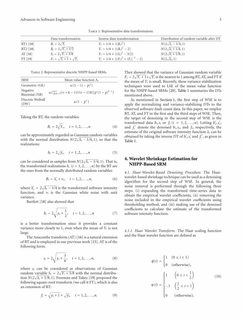
Advances in Software Engineering 3
Table 1: Representative data transformaions.
Data transformation Inverse data transformation Distribution of random variable after DT
BT1 [18] Bi = 2√Yi Yi = 1/4× {(Bi)
2} N(2√λi − 1/4, 1)
BT2 [18] Bi = 2√Yi + 1/2 Yi = 1/4× {(Bi)
2 − 2} N(2√λi + 1/4, 1)
AT [16] Si = 2√Yi + 3/8 Yi = 1/4× {(Si)2 − 3/2} N(2
√λi + 1/8, 1)
FT [19] Fi =√Yi + 1 +
√Yi Yi = 1/4× {(Fi)2 + (Fi)
−2 − 2} N(2√λi, 1)
Table 2: Representative discrete NHPP-based SRMs.
SRM Mean value function Λi
Geometric (GE) ω{1− (1− p)i}NegativeBinomial (NB)
ω{∑ik=1((r + k − 1)!/(r − 1)!k!)pr(1− p)k−1}
Discrete Weibull(DW)
ω{1− pir }
Taking the BT, the random variables:
Bi = 2√Yi, i = 1, 2, . . . ,n (4)
can be approximately regarded as Gaussian random variableswith the normal distribution N(2
√λi − 1/4, 1), so that the
realizations:
bi = 2√yi, i = 1, 2, . . . ,n (5)
can be considered as samples from N(2√λi − 1/4, 1). That is,
the transformed realizations bi (i = 1, 2, . . . ,n) by the BT arethe ones from the normally distributed random variables:
Bi = λ′i + νi, i = 1, 2, . . . ,n, (6)
where λ′i = 2√λi − 1/4 is the transformed software intensity
function, and νi is the Gaussian white noise with unitvariance.
Bartlett [18] also showed that
bi = 2
√
yi +12
, i = 1, 2, . . . ,n (7)
is a better transformation since it provides a constantvariance more closely to 1, even when the mean of Yi is notlarge.
The Anscombe transform (AT) [16] is a natural extensionof BT and is employed in our previous work [15]. AT is of thefollowing form:
si = 2
√
yi +38
, i = 1, 2, . . . ,n, (8)
where si can be considered as observations of Gaussianrandom variable Si = 2
√Yi + 3/8 with the normal distribu-
tion N(2√λi + 1/8, 1). Freeman and Tukey [19] proposed the
following square-root transform (we call it FT), which is alsoan extension of BT:
fi =√yi + 1 +
√yi, i = 1, 2, . . . ,n. (9)
They showed that the variance of Gaussian random variableFi = 2
√Yi + 1+
√Yi is the nearest to 1 among BT, AT, and FT if
the mean of Yi is small. Recently, these variance stabilizationtechniques were used to LSE of the mean value functionfor the NHPP-based SRMs [20]. Table 1 summaries the DTsmentioned above.
As mentioned in Section 1, the first step of WSE is toapply the normalizing and variance-stabilizing DTs to theobserved software-fault count data. In this paper, we employBT, AT, and FT in the first and the third steps of WSE. Then,the target of denoising in the second step of WSE is thetransformed data bi, si or fi (i = 1, 2, . . . ,n). Letting b′i , s
′i ,
and f ′i denote the denoised bi, si, and fi, respectively, theestimate of the original software intensity function λi can beobtained by taking the inverse DT of b′i , s
′i and f ′i , as given in
Table 1.
4. Wavelet Shrinkage Estimation forNHPP-Based SRM
4.1. Haar-Wavelet-Based Denoising Procedure. The Haar-wavelet-based shrinkage technique can be used as a denoisingalgorithm for the second step of WSE. In general, thenoise removal is performed through the following threesteps: (i) expanding the transformed time-series data toobtain the empirical wavelet coefficients, (ii) removing thenoise included in the empirical wavelet coefficients usingthresholding method, and (iii) making use of the denoisedcoefficients to calculate the estimate of the transformedsoftware intensity function.
4.1.1. Haar Wavelet Transform. The Haar scaling functionand the Haar wavelet function are defined as
φ(i) =⎧⎨
⎩
1 (0 ≤ i < 1)
0 (otherwise),
ψ(i) =
⎧⎪⎪⎪⎪⎪⎪⎪⎨
⎪⎪⎪⎪⎪⎪⎪⎩
1(
0 ≤ i <12
)
−1(
12≤ i < 1
)
0 (otherwise),
(10)

4 Advances in Software Engineering
Table 3: Goodness-of-fit test results for different data transformations. (Threshold level: universal threshold.)
DS1 MSE1 MSE2 LL
HBT1(h, ut) 4.180 0.327 −153.759
HBT2(h, ut) 2.401 0.316 −144.850
HAT(h, ut) 2.573 0.317 −145.390
HFT(h, ut) 9.842 0.403 −383.785
HBT1(s, ut) 4.180 0.327 −153.759
HBT2(s, ut) 2.401 0.316 −144.850
HAT(s, ut) 2.573 0.317 −145.390
HFT(s, ut) 3.231 0.320 −148.023
DS2 MSE1 MSE2 LL
HBT1(h, ut) 12.449 1.141 −197.109
HBT2(h, ut) 11.600 1.138 −196.904
HAT(h, ut) 11.725 1.138 −196.953
HFT(h, ut) 11.847 1.138 −196.806
HBT1(s, ut) 12.450 1.141 −197.109
HBT2(s, ut) 11.600 1.138 −196.904
HAT(s, ut) 11.725 1.138 −196.953
HFT(s, ut) 11.847 1.138 −196.806
DS3 MSE1 MSE2 LL
HBT1(h, ut) 10.159 0.719 −143.181
HBT2(h, ut) 9.055 0.791 −192.903
HAT(h, ut) 9.286 0.793 −193.178
HFT(h, ut) 9.653 0.796 −167.025
HBT1(s, ut) 12.954 1.037 −212.321
HBT2(s, ut) 10.528 1.035 −213.978
HAT(s, ut) 10.813 1.035 −213.496
HFT(s, ut) 11.496 1.037 −213.419
DS4 MSE1 MSE2 LL
HBT1(h, ut) 2.065 0.304 −171.605
HBT2(h, ut) 1.781 0.304 −171.491
HAT(h, ut) 1.822 0.304 −171.504
HFT(h, ut) 1.864 0.304 −171.516
HBT1(s, ut) 2.065 0.304 −171.605
HBT2(s, ut) 1.781 0.304 −171.491
HAT(s, ut) 1.822 0.304 −171.504
HFT(s, ut) 1.864 0.304 −171.516
DS5 MSE1 MSE2 LL
HBT1(h, ut) 14.013 0.586 −304.198
HBT2(h, ut) 12.781 0.581 −301.073
HAT(h, ut) 12.941 0.581 −301.447
HFT(h, ut) 13.200 0.582 −301.841
HBT1(s, ut) 14.054 0.601 −312.551
HBT2(s, ut) 12.804 0.596 −309.709
HAT(s, ut) 12.968 0.597 −310.005
HFT(s, ut) 13.227 0.598 −310.480
DS6 MSE1 MSE2 LL
HBT1(h, ut) 12.707 0.521 −378.932
HBT2(h, ut) 11.899 0.525 −380.497
HAT(h, ut) 12.053 0.526 −380.987

Advances in Software Engineering 5
Table 3: Continued.
DS6 MSE1 MSE2 LL
HFT(h, ut) 12.186 0.526 −381.071
HBT1(s, ut) 13.546 0.585 −423.335
HBT2(s, ut) 12.505 0.584 −421.480
HAT(s, ut) 12.670 0.584 −421.729
HFT(s, ut) 12.810 0.584 −421.866
respectively. By introducing the scaling parameter j andshifting parameter k, the Haar father wavelet and the Haarmother wavelet are defined by
φj,k(i) = 2− j/2φ(
2− j i− k)
,
ψj,k(i) = 2− j/2ψ(
2− j i− k)
,(11)
respectively. Then the target function, transformed softwareintensity function λ′i (i = 1, 2, . . . ,n), can be expressed in thefollowing equation:
λ′i =2 j0−1∑
k=0
αj0,kφj0,k(i) +∞∑
j= j0
2 j−1∑
k=0
βj,kψj,k(i), (12)
where
αj0,k =n∑
i=1
λ′i φ j0,k(i), (13)
βj,k =n∑
i=1
λ′iψj,k(i) (14)
are called the scaling coefficients and the wavelet coefficients,respectively, for any primary resolution level j0(≥ 0). Due tothe implementability, it is reasonable to set an upper limitinstead of ∞ for the resolution level j. In other words, thehighest resolution level must be finite in practice. We use Jto denote the highest resolution level. That is, the range ofj in the second term of (12) is j ∈ [ j0, J]. The mappingfrom function λ′i to coefficients (αj0,k,βj,k) is called the Haarwavelet transform (HWT).
Since bi, si or fi (i = 1, 2, . . . ,n) can be considered as theobservation of λ′i , the empirical scaling coefficients cj0,k andthe empirical wavelet coefficients dj,k of λ′i can be calculatedby (13) and (14) with λ′i replaced by bi, si or fi. The noisesinvolved in the empirical wavelet coefficients dj,k can beremoved by the thresholding method that we will introducelater. Finally, the estimate of λ′i can be obtained by taking theinverse HWT with denoised empirical coefficients.
4.1.2. Thresholding. In denoising the empirical wavelet coef-ficients, the common choices of thresholding method are thehard thresholding:
δτ(u) = u1|u|>τ , (15)
and the soft thresholding:
δτ(u) = sgn(u)(|u| − τ)+, (16)
for a fixed threshold level τ(> 0), where 1A is the indicatorfunction of an event A, sgn(u) is the sign function of u and(u)+ = max(0,u). There are many methods to determine thethreshold level τ. In this paper, we use the universal threshold[21] and the “leave-out-half” cross-validation threshold[22]:
τ =√
2 logn,
τ =(
1− log 2logn
)−1/2
τ(n
2
)
,(17)
where n is the length of the observation si. Hard thresholdingis a “keep” or “kill” rule, while soft thresholding is a “shrink”or “kill” rule. Both thresholding methods and both thresholdlevels will be employed to work on the empirical waveletcoefficients dj,k for denoising.
4.2. Wavelet Shrinkage Estimation for NHPP-Based SRM.Since the software-fault count data is Poisson data, thepreprocessing is necessary before making use of the Haar-wavelet-based denoising procedure. Xiao and Dohi [15]combined data transformation and the standard denoisingprocedure to propose the wavelet shrinkage estimation(WSE) for the D-NHPP-based SRMs. They call the HWTcombined with AT, the Haar-Anscombe transform (HAT).Similarly, we call the HWT combined with BT and FT,the Haar-Bartlett transform (HBT) and the Haar-Freemantransform (HFT), respectively. In the numerical study, weinvestigate the goodness-of-fit performance of HBT- andHFT-based WSEs and compare them with the HAT-basedWSE [15].
5. Numerical Study
5.1. Data Sets and Measures. We use six real project datasets cited from reference [1], where they are named asJ1, J3, DATA14, J5, SS1, and DATA8. These data sets aresoftware-fault count data (group data). We rename them forconvenience as DS1∼DS6 in this paper. Let (n, xn) denotethe pair of the final testing date and the total number ofdetected fault. Then these data sets are presented by (62, 133),(41, 351), (46, 266), (73, 367), (81, 461), and (111, 481),

6 Advances in Software Engineering
Table 4: Goodness-of-fit test results for different data transformations. (Threshold level: “leave-out-half” cross-validation threshold.)
DS1 MSE1 MSE2 LL
HBT1(h, lht) 0.112 0.015 −59.704
HBT2(h, lht) 0.131 0.017 −60.634
HAT(h, lht) 0.114 0.014 −60.324
HFT(h, lht) 8.079 0.343 −216.320
HBT1(s, lht) 0.159 0.010 −59.581
HBT2(s, lht) 0.109 0.010 −60.195
HAT(s, lht) 0.115 0.010 −60.118
HFT(s, lht) 0.151 0.010 −59.609
DS2 MSE1 MSE2 LL
HBT1(h, lht) 0.477 0.102 −70.438
HBT2(h, lht) 0.225 0.072 −70.227
HAT(h, lht) 0.263 0.077 −70.663
HFT(h, lht) 0.552 0.125 −71.041
HBT1(s, lht) 0.342 0.027 −69.407
HBT2(s, lht) 0.363 0.030 −69.781
HAT(s, lht) 0.364 0.030 −69.731
HFT(s, lht) 0.351 0.028 −69.446
DS3 MSE1 MSE2 LL
HBT1(h, lht) 0.208 0.032 −55.829
HBT2(h, lht) 0.275 0.041 −56.767
HAT(h, lht) 0.902 0.074 −57.614
HFT(h, lht) 0.323 0.048 −56.411
HBT1(s, lht) 0.573 0.040 −55.847
HBT2(s, lht) 0.486 0.037 −56.649
HAT(s, lht) 0.496 0.037 −56.551
HFT(s, lht) 0.537 0.037 −55.922
DS4 MSE1 MSE2 LL
HBT1(h, lht) 0.288 0.015 −121.008
HBT2(h, lht) 0.132 0.007 −120.942
HAT(h, lht) 0.232 0.013 −121.031
HFT(h, lht) 0.281 0.014 −121.004
HBT1(s, lht) 0.097 0.005 −120.893
HBT2(s, lht) 0.046 0.003 −120.906
HAT(s, lht) 0.050 0.003 −120.907
HFT(s, lht) 0.064 0.004 −120.888
DS5 MSE1 MSE2 LL
HBT1(h, lht) 0.055 0.012 −120.869
HBT2(h, lht) 0.221 0.016 −121.205
HAT(h, lht) 0.228 0.017 −121.195
HFT(h, lht) 0.219 0.017 −120.890
HBT1(s, lht) 0.174 0.007 −120.805
HBT2(s, lht) 0.149 0.006 −120.913
HAT(s, lht) 0.151 0.006 −120.898
HFT(s, lht) 0.158 0.006 −120.806
DS6 MSE1 MSE2 LL
HBT1(h, lht) 0.778 0.025 −166.906
HBT2(h, lht) 0.558 0.017 −166.816
HAT(h, lht) 0.548 0.017 −166.767
HFT(h, lht) 0.540 0.017 −166.673

Advances in Software Engineering 7
Table 4: Continued.
DS6 MSE1 MSE2 LL
HBT1(s, lht) 0.288 0.009 −166.432
HBT2(s, lht) 0.282 0.009 −166.532
HAT(s, lht) 0.289 0.010 −166.540
HFT(s, lht) 0.294 0.009 −166.440
16 32 48 64
50
100
150
Cu
mu
lati
ve n
um
ber
of s
oftw
are
fau
lts
Testing date
0
MLE (GE, DW)
MLE (NB)
Observed data
WSE (HBT2(h, lht))
(a) HBT2-based WSE(h, lht) versus MLE
16 32 48 64
4
12
Nu
mbe
r of
sof
twar
e fa
ult
sTesting date
0
8
Observed data
MLE (GE, DW)
MLE (NB)
WSE (HBT2(h, lht))
(b) HBT2-based WSE(h, lht) versus MLE
Figure 1: Behavior of estimates with MLE and WSE using hard thresholding (DS1).
respectively. We employ the MSE (mean squares error) as thegoodness-of-fit measures, where
MSE1 =√∑n
i=1 (Λi − xi)2
n,
MSE2 =√∑n
i=1
(λi − yi
)2
n.
(18)
Additionally, we calculate LL (Log Likelihood), which isdefined as
LL =n∑
i=1
(xi − xi−1) ln[Λi − Λi−1
]− Λn(θ)
−n∑
i=1
ln[(xi − xi−1)!],
(19)
where Λi =∑i
k=1 λk (i = 1, 2, . . . ,n), and λi is the WSEestimate of the software intensity function λi.
5.2. Goodness-of-Fit Test. A total of 16 wavelet-based estima-tion methods are examined in this paper since the WSE isapplied with four thresholding techniques: hard thresholding(h) versus soft thresholding (s); universal threshold (ut)versus “leave-out-half,” cross-validation threshold (lht). LetHBT(·, ·), HAT(·, ·) and HFT(·, ·) denote the WSEs basedon Haar-Bartlett Transform, Haar-Anscombe Transformand Haar-Freeman Transform, respectively. HBT1(·, ·), andHBT2(·, ·) correspond to the transforms in (5) and (7),respectively. Additionally, the result of HAT-based WSE was
introduced in [15], but they only showed the results of HAT-based WSE with hard thresholding. Here, we present com-prehensively all the results of them for a further discussion.
We present the goodness-of-fit results based on differentthreshold levels in Tables 3 and 4, respectively. HBT2provides smaller MSE and larger MLL than the otherswhen “ut” is used, regardless of the thresholding methodemployed. It is worth mentioning that “ut” provides the sameestimates with hard or soft thresholding in three data sets(DS1, DS2, and DS4). This is due to the relatively large valueof “ut”, since when threshold is set to be 0, the output ofthresholding δτ(dj,k) is the wavelet coefficient dj,k itself. Inour numerical experiments, “ut” is relatively large in these 3software-fault count data sets, which result in δut(dj,k) = 0whichever hard or soft thresholding is applied. HBT2 alsolooks better than the others when software thresholding isapplied with “lht.” However, when “lht” is combined withhard thresholding, HBT1 (HAT; HFT) possesses the bestresults in DS3 and DS5 (DS1; DS6), respectively. Since “lht”is considered as a much more proper threshold level than“ut” in analyzing of software-fault count data, we suggest thatHBT2 should be selected as an appropriate DT for the WSE.
5.3. Comparison with MLE. Our concern in this section isthe comparison of WSE with MLE. We estimate the softwareintensity function by using three parametric D-NHPP-basedSRMs listed in Table 2, where the MLE is applied to estimatethe model parameters for comparison. HBT2-based WSE isselected as a representative one among the 16 wavelet-basedestimation methods. Figures 1 and 2 depict the estimationbehavior of cumulative number of software faults and itsincrement per testing date (individual number of software

8 Advances in Software Engineering
16 32 48 64
50
100
150
Cu
mu
lati
ve n
um
ber
of s
oftw
are
fau
lts
Testing date0
MLE (GE, DW)
MLE (NB)
WSE (HBT2(s, lht))
Observed data
(a) HBT2-based WSE(s, lht) versus MLE
16 32 48 64
4
12
Nu
mbe
r of
sof
twar
e fa
ult
s
Testing date
0
8
Observed data
WSE (HBT2(s, lht))
MLE (GE, DW)
MLE (NB)
(b) HBT2-based WSE(s, lht) versus MLE
Figure 2: Behavior of estimates with MLE and WSE using soft thresholding (DS1).
faults detected per testing date) with DS1. The observed datais plotted in bar graph in both figures. Looking at (i) and(iii) in these figures, it is clear that the parametric D-NHPP-based SRMs with maximum likelihood estimator can fitthe real data. However, since the parametric D-NHPP-basedSRMs assume the software intensity function as smoothfunction, they can estimate only the average tendency ofthe individual number of software faults detected at eachtesting date, but cannot follow the microscopic fluctuatedbehavior in (ii) and (iv) of Figures 1 and 2. In other words,the estimation accuracy based on the cumulative number offaults is embedded in “cumulative effects” in (i) and (iii).The experimental results performed here give the potentialapplicability of the wavelet-based estimation methods withdifferent thresholding schemes. Our methods employed heredo not need the expensive computational cost comparingwith the MLE (within less than one second to get anestimate). This is a powerful advantage in applying the D-NHPP-based SRMs, in addition to the fact that practitionersdo not request much time and effort to implement thewavelet-based estimation algorithms.
6. Concluding Remarks
In this paper, we have applied the wavelet-based techniquesto estimate the software intensity function. Four datatransformations were employed to preprocess the software-fault count data. Throughout the numerical evaluation, wecould conclude that the wavelet-based estimation methodswith Bartlett transform 2
√Yi have much more potential
applicability than the other data transformations to thesoftware reliability assessment practice because practitionersare not requested to carry out troublesome procedures onmodel selection and to take care of computational efficiencysuch as judgment of convergence and selecting initialguess of parameters in the general purpose of optimizationalgorithms. Note that, the result obtained here does not meanthat the other data transformations are not good becausethe performance evaluation was executed only through
goodness-of-fit test. Although the prediction ability of theproposed methods is out of focus of this paper at thepresent, the predictive performance should be consideredand compared in the future.
References
[1] M. R. Lyu, Ed., Handbook of Software Reliability Engineering,McGraw-Hill, New York, NY, USA, 1996.
[2] J. D. Musa, A. Iannino, and K. Okumoto, Software Reliabil-ity, Measurement, Prediction, Application, McGraw-Hill, NewYork, NY, USA, 1987.
[3] H. Pham, Software Reliability, Springer, Singapore, Singapore,2000.
[4] A. L. Goel and K. Okumoto, “Time-dependent error-detectionrate model for software reliability and other performancemeasures,” IEEE Transactions on Reliability, vol. R-28, no. 3,pp. 206–211, 1979.
[5] A. L. Goel, “Software reliability models: assumptions, lim-itations and applicability,” IEEE Transactions on SoftwareEngineering, vol. SE-11, no. 12, pp. 1411–1423, 1985.
[6] X. Xiao and T. Dohi, “Estimating software reliability usingextreme value distribution,” in Proceedings of the InternationalConference on Advances in Software Engineering and ItsApplications (ASEA ’11), vol. CCIS 257, pp. 399–406, Springer,2011.
[7] X. Xiao, H. Okamura, and T. Dohi, “NHPP-based softwarereliability models using equilibrium distribution,” IEICETransactions of the Fundamentals A, vol. E95-A, no. 5, pp. 894–902, 2012.
[8] S. Yamada, M. Ohba, and S. Osaki, “S-shaped reliabilitygrowth modeling for software error detection,” IEEE Transac-tions on Reliability, vol. R-32, no. 5, pp. 475–484, 1983.
[9] A. Sofer and D. R. Miller, “A non-parametric softwarereliability growth model,” IEEE Transactions on Reliability, vol.R-40, no. 3, pp. 329–337, 1991.
[10] A. Gandy and U. Jensen, “A non-parametric approach tosoftware reliability,” Applied Stochastic Models in Business andIndustry, vol. 20, no. 1, pp. 3–15, 2004.
[11] M. Barghout, B. Littlewood, and A. Abdel-Ghaly, “A non-parametric order statistics software reliability model,” Software

Advances in Software Engineering 9
Testing Verification and Reliability, vol. 8, no. 3, pp. 113–132,1998.
[12] Z. Wang, J. Wang, and X. Liang, “Non-parametric estimationfor NHPP software reliability models,” Journal of AppliedStatistics, vol. 34, no. 1, pp. 107–119, 2007.
[13] M. A. El-Aroui and J. L. Soler, “A bayes nonparametricframework for software-reliability analysis,” IEEE Transactionson Reliability, vol. 45, no. 4, pp. 652–660, 1996.
[14] S. P. Wilson and F. J. Samaniego, “Nonparametric analysisof the order-statistic model in software reliability,” IEEETransactions on Software Engineering, vol. 33, no. 3, pp. 198–208, 2007.
[15] X. Xiao and T. Dohi, “Wavelet-based approach for estimatingsoftware reliability,” in Proceedings of the 20th InternationalSymposium on Software Reliability Engineering (ISSRE ’09), pp.11–20, IEEE CS Press, November 2009.
[16] F. J. Anscombe, “The transformation of Poisson, binomial andnegative binomial data,” Biometrika, vol. 35, no. 3-4, pp. 246–254, 1948.
[17] M. Fisz, “The limiting distribution of a function of twoindependent random variables and its statistical application,”Colloquium Mathematicum, vol. 3, pp. 138–146, 1955.
[18] M. S. Bartlett, “The square root transformation in the analysisof variance,” Journal of the Royal Statistical Society, vol. 3, no.1, pp. 68–78, 1936.
[19] M. F. Freeman and J. W. Tukey, “Transformations related tothe angular and the square root,” The Annals of MathematicalStatistics, vol. 21, no. 4, pp. 607–611, 1950.
[20] H. Ishii, T. Dohi, and H. Okamura, “Software reliability pre-diction based on least squares estimation,” Quality Technologyand Quantitative Management Journal. In press.
[21] D. L. Donoho and J. M. Johnstone, “Ideal spatial adaptationby wavelet shrinkage,” Biometrika, vol. 81, no. 3, pp. 425–455,1994.
[22] G. P. Nason, “Wavelet shrinkage using cross-validation,”Journal of the Royal Statistical Society B, vol. 58, no. 2, pp. 463–479, 1996.

Hindawi Publishing CorporationAdvances in Software EngineeringVolume 2012, Article ID 924923, 8 pagesdoi:10.1155/2012/924923
Research Article
Can Faulty Modules Be Predicted by Warning Messages ofStatic Code Analyzer?
Osamu Mizuno and Michi Nakai
Kyoto Institute of Technology, Matsugasaki Goshokaido-cho, Sakyo-ku, Kyoto 606-8585, Japan
Correspondence should be addressed to Osamu Mizuno, [email protected]
Received 5 January 2012; Accepted 24 February 2012
Academic Editor: Chin-Yu Huang
Copyright © 2012 O. Mizuno and M. Nakai. This is an open access article distributed under the Creative Commons AttributionLicense, which permits unrestricted use, distribution, and reproduction in any medium, provided the original work is properlycited.
We have proposed a detection method of fault-prone modules based on the spam filtering technique, “Fault-prone filtering.” Fault-prone filtering is a method which uses the text classifier (spam filter) to classify source code modules in software. In this study, wepropose an extension to use warning messages of a static code analyzer instead of raw source code. Since such warnings includeuseful information to detect faults, it is expected to improve the accuracy of fault-prone module prediction. From the result ofexperiment, it is found that warning messages of a static code analyzer are a good source of fault-prone filtering as the originalsource code. Moreover, it is discovered that it is more effective than the conventional method (that is, without static code analyzer)to raise the coverage rate of actual faulty modules.
1. Introduction
Recently, machine learning approaches have been widelyused for fault-proneness detection [1]. We have introduceda text feature-based approach to detect fault-prone modules[2]. In this approach, we extract text features from the freq-uency information of words in source code modules. In otherwords, we construct a large metrics set representing the freq-uency of words in source code modules. Once the text fea-tures are obtained, the Bayesian classifier is constructed fromtext features. In the fault-prone module detection of newmodules, we also extract text features from source code mod-ules, and Bayesian model classifies modules into either fault-prone or nonfault-prone. Since less effort or cost needed tocollect text feature metrics than other software metrics, itmay be applied to software development projects easily.
On the other hand, since this approach accepts any inputwith text files, the accuracy of prediction could be improvedby selecting appropriate input other than raw source code.We then try to find another input but source code. In thisstudy, we use warning messages of a static code analyzer.Among many static code analyzers, we used PMD in thisstudy. By replacing the input of fault-prone filtering from raw
source code to warning messages of PMD, we can get the re-sults of prediction by PMD and fault-prone filtering.
The rest of this paper is organized as follows. Section 2describes the objective of this research. Section 3 shows abrief summary of the fault-prone filtering technique withPMD. In Section 4, the experiments conducted in this studyare described. Section 5 discusses the result of the experi-ments. Finally, Section 6 concludes this study.
2. Objective
2.1. Fault-Prone Module Filtering. The basic idea of fault-prone filtering is inspired by the spam mail filtering. In thespam e-mail filtering, a spam filter first trains both spam andham e-mail messages from the training data set. Then, anincoming e-mail is classified into either ham or spam by thespam filter.
This framework is based on the fact that spam e-mailusually includes particular patterns of words or sentences.From the viewpoint of source code, a similar situationusually occurs in faulty software modules. That is similarfaults may occur in similar contexts. We thus guessed thatsimilar to spam e-mail messages, faulty software modules

2 Advances in Software Engineering
have similar patterns of words or sentences. To obtain suchfeatures, we adopted a spam filter in fault-prone moduleprediction.
In other words, we try to introduce a new metric as afault-prone predictor. The metric is “frequency of particularwords.” In detail, we do not treat a single word, but use com-binations of words for the prediction. Thus, the frequencyof a certain length of words is the only metric used in ourapproach.
From a viewpoint of effort, conventional fault-prone de-tection techniques require relatively much effort for applica-tion because they have to measure various metrics. Of course,metrics are useful for understanding the property of sourcecode quantitatively. However, measuring metrics usuallyneeds extra effort and translating the values of metrics intomeaningful result also needs additional effort. Thus, easy-to-use technique that does not require much effort will be usefulin software development.
We then try to apply a spam filter to identification offault-prone modules. We named this approach as “fault-prone filtering.” That is, a learner first trains both faulty andnonfaulty modules. Then, a new module can be classifiedinto fault-prone or notfault-prone using a classifier. In thisstudy, we define a software module as a Java class file.
Essentially, the fault-prone filtering does the text classifi-cation on the source codes. Of course, the text classificationcan be applied to the text information other than the sourcecodes. We guessed that there is the other input for the textclassification to achieve higher prediction accuracy. We thenstarted seeking such information.
2.2. Static Code Analysis. The static code analysis is a methodof analyzing without actually running software and findingthe problem and faults in a software. By analyzing a sourcecode structurally, we can find potential faults, violation ofcoding conventions, and so on. The static code analysis thuscan assure the safety of software, reliability, and quality. Italso reduces the cost of maintenance. In recent years, theimportance of static code analysis has been emerging sincefinding potential faults or security hole is required at an earlystage of the development. There are many kinds of tools forthe static code analysis available [3]. Among them, we usedthe PMD (the meaning of PMD is not determined. “We havebeen trying to find the meaning of the letters PMD—becausefrankly, we do not really know. We just think the letters soundgood together” [4]), since it can be applicable to the sourcecode directly.
The PMD is one of static code analysis tools [5]. It is anopen-source software and written in Java, and it is used foranalyzing programs written in Java. PMD can find the codepieces that may cause the potential faults such as an unusedvariable and an empty catch block by analyzing the sourcecode of Java. To do so, PMD has a variety of rule sets. Accord-ing to the rule sets to be used, a broad range of purposes fromthe inspection of coding conventions to find potential faultscan be used.
2.3. Characteristics of the Warning Messages of the Static CodeAnalyzer. Warning messages of a static code analyzer include
rich information about potential faults in source codes.Figure 1 shows an example of warning messages. Usually, thenumber of warning messages generated by the static codeanalyzer becomes large in proportion to the length of sourcecode. Since most of the messages are not harmful or trivial,warning messages are often ignored. It can be considered thatthese warning messages are quality aspects of the sourcecode. Thus, we consider that the warning messages have lessnoise for fault-prone module prediction.
As mentioned in Section 2.1, applying the text informa-tion to the text classifier is an easy task. We thus implementthe fault-prone filtering technique to use the warning mes-sages of the static code analyzer. We then conduct experi-ments to confirm the effects of the warning messages to theperformance of the fault-prone filtering approach.
2.4. Research Questions. In this study, we aim at answeringthe following research questions:
RQ1: “can fault-prone modules be predicted by ap-plying a text filter to the warning messages of a staticcode analyzer?”
RQ2: “if RQ1 is true, is the performance of the fault-prone filtering becomes better with the warning mes-sages of a static code analyzer?”
RQ1 tries to find a possibility to apply the warning mes-sages to the fault-prone filtering technique. RQ2 investigatesthe prediction performance.
3. Fault-Prone Filtering with PMD
3.1. Applying PMD to Source Code. We used 10 rule sets ofPMD in a standard rule sets: Basic, Braces, Code Size, Coupl-ing, Design, Naming, Optimizations, Strict Exception,Strings, and Unused Code. These rule sets are frequently usedfor investigation of the quality of software. We apply PMDwith 10 rule sets to all source code modules and get warningmessages of PMD.
3.2. Classification Techniques. In this study, we used CRM114(the controllable regex mutilator) spam filtering software [6]for its versatility and accuracy. Since CRM114 is implement-ed as a language to classify text files for general purpose, ap-plying source code modules is easy. Furthermore, the classi-fication techniques implemented in CRM114 are basedmainly on Markov random field model instead of the naiveBayesian classifier.
In this experiment, we used the orthogonal sparse bi-grams Markov model built in CRM114.
Orthogonal Sparse Bigrams Markov model (OSB)
Basically, CRM114 uses sparse binary polynomialHash Markov model (SBPH). It is an extension of theBayesian classification, and it maps features in theinput text into a markov random field [7]. In thismodel, tokens are constructed from combinations ofn words (n-grams) in a text file. Tokens are then
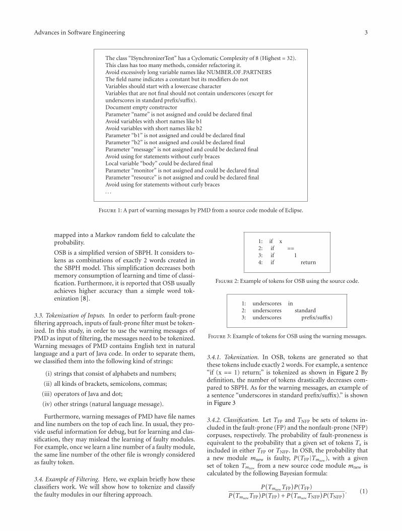
Advances in Software Engineering 3
The class “ISynchronizerTest” has a Cyclomatic Complexity of 8 (Highest = 32).This class has too many methods, consider refactoring it.Avoid excessively long variable names like NUMBER OF PARTNERSThe field name indicates a constant but its modifiers do notVariables should start with a lowercase characterVariables that are not final should not contain underscores (except forunderscores in standard prefix/suffix).Document empty constructorParameter “name” is not assigned and could be declared finalAvoid variables with short names like b1Avoid variables with short names like b2Parameter “b1” is not assigned and could be declared finalParameter “b2” is not assigned and could be declared finalParameter “message” is not assigned and could be declared finalAvoid using for statements without curly bracesLocal variable “body” could be declared finalParameter “monitor” is not assigned and could be declared finalParameter “resource” is not assigned and could be declared finalAvoid using for statements without curly braces. . .
Figure 1: A part of warning messages by PMD from a source code module of Eclipse.
mapped into a Markov random field to calculate theprobability.
OSB is a simplified version of SBPH. It considers to-kens as combinations of exactly 2 words created inthe SBPH model. This simplification decreases bothmemory consumption of learning and time of classi-fication. Furthermore, it is reported that OSB usuallyachieves higher accuracy than a simple word tok-enization [8].
3.3. Tokenization of Inputs. In order to perform fault-pronefiltering approach, inputs of fault-prone filter must be token-ized. In this study, in order to use the warning messages ofPMD as input of filtering, the messages need to be tokenized.Warning messages of PMD contains English text in naturallanguage and a part of Java code. In order to separate them,we classified them into the following kind of strings:
(i) strings that consist of alphabets and numbers;
(ii) all kinds of brackets, semicolons, commas;
(iii) operators of Java and dot;
(iv) other strings (natural language message).
Furthermore, warning messages of PMD have file namesand line numbers on the top of each line. In usual, they pro-vide useful information for debug, but for learning and clas-sification, they may mislead the learning of faulty modules.For example, once we learn a line number of a faulty module,the same line number of the other file is wrongly consideredas faulty token.
3.4. Example of Filtering. Here, we explain briefly how theseclassifiers work. We will show how to tokenize and classifythe faulty modules in our filtering approach.
1: if x2: if ==3: if 14: if return
Figure 2: Example of tokens for OSB using the source code.
1: underscores in2: underscores standard3: underscores prefix/suffix)
Figure 3: Example of tokens for OSB using the warning messages.
3.4.1. Tokenization. In OSB, tokens are generated so thatthese tokens include exactly 2 words. For example, a sentence“if (x == 1) return;” is tokenized as shown in Figure 2 Bydefinition, the number of tokens drastically decreases com-pared to SBPH. As for the warning messages, an example ofa sentence “underscores in standard prefix/suffix).” is shownin Figure 3
3.4.2. Classification. Let TFP and TNFP be sets of tokens in-cluded in the fault-prone (FP) and the nonfault-prone (NFP)corpuses, respectively. The probability of fault-proneness isequivalent to the probability that a given set of tokens Tx isincluded in either TFP or TNFP. In OSB, the probability thata new module mnew is faulty, P(TFP|Tmnew ), with a givenset of token Tmnew from a new source code module mnew iscalculated by the following Bayesian formula:
P(TmnewTFP
)P(TFP)
P(TmnewTFP
)P(TFP) + P
(TmnewTNFP
)P(TNFP)
. (1)

4 Advances in Software Engineering
Table 1: Target project: Eclipse BIRT plugin.
Name Eclipse BIRT plugin
Language Java
Revision control cvs
Type of faults Bugs
Status of faultsResolved;Verified;closed
Resolution of faults Fixed
SeverityBlocker; critical;major; normal
Priority of faults All
Total number of faults 4708
Table 2: The number of modules in Eclipse BIRT.
Number of modules (files)
Nonfaulty 42,503
Faulty 27,641
Total 70,144
Intuitively speaking, this probability denotes that the newcode is classified into FP. According to P(TFP | Tmnew ) andpredefined threshold tFP, classification is performed.
4. Experiment
4.1. The Outline of the Experiment. In this experiment, warn-ing messages of PMD are used for fault-prone filtering as aninput instead of a source code module, and Fault-pronemodule is predicted. And it is the purpose to evaluate thepredictive accuracy of the proposed method. Therefore, twoexperiments using raw source code modules and the warningmessages by the PMD as inputs are conducted. We then com-pare these results to each other.
4.2. Target Project. In this experiment, we use the source codemodule of an open source project, Eclipse BIRT (businessintelligence and reporting tools). The source code module isobtained from this project by the SZZ (Sliwerski et al.) algo-rithm [9]. The summary of Eclipse BIRT project is shown inTable 1. All software modules in this project are used for bothlearning and classification by the procedure called trainingonly errors (TOE). The number of modules is shown inTable 2.
4.3. Procedure of Filtering (Training on Errors). Experiment 1performs the original fault-prone module prediction usingthe raw source code and OSB classifier by the followingprocedures:
(1) apply the FP classifier to a newly created softwaremodule (say, method in Java, function in C, and soon), Mi, and obtain the probability to be fault-prone;
Modules sorted by date
Get nextmoduleFP classifier
Prediction(FP/NFP)
Corpus ofFPCorpus of
NFP Yes
No
FP trainerTraining
Correctprediction?
Figure 4: Outline of fault-prone filtering by training on errors.
(2) by the predetermined threshold tFP (0 < tFP < 1),classify the module Mi into FP or NFP;
(3) when the actual fault-proneness of Mi is revealed byfault report, investigate whether the predicted resultfor Mi was correct or not;
(4) if the predicted result was correct, go to step 1;otherwise, apply FP trainer toMi to learn actual fault-proneness and go to step 1.
This procedure is called “training on errors (TOE)”procedure because training process is invoked only whenclassification errors happen. The TOE procedure is quitesimilar to actual classification procedure in practice. Forexample, in actual e-mail filtering, e-mail messages are classi-fied when they arrive. If some of them are misclassified,actual results (spam or nonspam) should be trained.
Figure 4 shows an outline of this approach. At this point,we consider that the fault-prone filtering can be applied tothe sets of software modules which are developed in the same(or similar) project.
Experiment 2 is an extension of Experiment 1 by append-ing additional steps as the first step as follows:
(1) obtain warning messages Wi of PMD by applyingPMD to a newly created software module Mi;
(2) apply the FP classifier to the warning messages, Wi,and obtain the probability to be fault-prone;
(3) by the predetermined threshold tFP (0 < tFP < 1),classify the warning messages Wi into FP or NFP;
(4) when the actual fault-proneness of Mi is revealed byfault report, investigate whether the predicted resultfor Wi was correct or not;
(5) if the predicted result was correct, go to step (1); oth-erwise, apply FP trainer to Wi to learn actual fault-proneness and go to step (1).

Advances in Software Engineering 5
Table 3: Classification result matrix.
Prediction
Nonfault-prone Fault-prone
Actual Nonfaulty True negative (tn) False positive ( f p)
Faulty False negative (fn) True positive (tp)
4.4. Procedure of TOE Experiment. In the experiment, wehave to simulate actual TOE procedure in the experimentalenvironment. To do so, we first prepare a list of all modulesfound in Section 4.2. The list is sorted by the last modifieddate (di) of each module so that the first element of the listis the oldest module. We then start simulated experiment inthe procedure shown in Algorithm 1. During the simulation,modules are classified by the order of date. If the predictedresult s
pi differs from actual status sai , the training procedure
is invoked.
4.5. Evaluation Measures. Table 3 shows a classification resultmatrix. True negative (tn) shows the number of modules thatare classified as nonfault-prone, and are actually nonfaulty.False positive ( f p) shows the number of modules that areclassified as fault-prone, but are actually nonfaulty. On thecontrary, false negative shows the number of modules thatare classified as nonfault-prone, but are actually faulty. Final-ly, true positive shows the number of modules that are classi-fied as fault-prone which are actually faulty.
In order to evaluate the results, we prepare two measures:recall and precision. Recall is the ratio of modules correctlyclassified as fault-prone to the number of entire faulty modu-les Recall is defined as tp/(tp + f n). Precision is the ratio ofmodules correctly classified as fault-prone to the number ofentire modules classified fault-prone. Precision is defined astp/(tp+ f p). Accuracy is the ratio of correctly classified mod-ules to the entire modules. Accuracy is defined as (tp +tn)/(tn + tp + f p + f n). Since recall and precision are in thetrade-off, F1-measure is used to combine recall and precision[10]. F1-measure is defined as (2×recall×precision)/(recall+precision). In this definition, recall and precision are evenlyweighed.
From the viewpoint of the quality assurance, it is recom-mended to achieve higher recall, since the coverage of actualfaults is of importance. On the other hand, from the view-point of the project management, it is recommended to focuson the precision, since the cost of the software unit test isdeeply related to the number of modules to be tested. In thisstudy, we mainly focus on the recall from the viewpoint ofthe quality assurance.
4.6. Result of Experiments. Tables 4 and 5 show the result ofexperiment using the original approach without PMD andthe approach with PMD, respectively. Table 6 summarizes theevaluation measures for these experiments.
From Table 6, we can see that the approach with PMD hasalmost the same capability to predict fault-prone modulesas the approach without PMD. For example, F1 for the ap-proach without PMD is 0.779, and for the approach with
Table 4: Result of prediction in Experiment 1 (without PMD).
Prediction
Nonfault-prone Fault-prone
Actual Nonfaulty 30,521 11,982
Faulty 2,360 25,281
Total 32,821 37,263
Table 5: Result of prediction in Experiment 2 (with PMD).
Prediction
Nonfault-prone Fault-prone
Actual Nonfaulty 22,982 19,521
Faulty 1,674 25,967
Total 24,656 45,488
Table 6: Evaluation measures of the results of experiments.
Precision Recall Accuracy F1
Experiment 1(without PMD)
0.678 0.915 0.796 0.779
Experiment 2(with PMD)
0.571 0.939 0.698 0.710
PMD is 0.710. The result shows that the original approachwithout PMD is relatively better than the approach withPMD in precision, accuracy, and F1 measures. The recall ofthe approach with PMD is better than the approach withoutPMD.
Figures 5 and 6 show the result of TOE history for theapproaches without and with PMD, respectively. From thisgraph, we can see that evaluation measures first to decrease atthe beginning of TOE procedure, then increase and becomestable after learning and classification of 15,000 modules.
5. Discussions
At first, we discuss the advantage of the approach with PMD.From Table 6, we can see that the result of Experiment 2 hashigher recall and lower precision than that of Experiment 1.Generally speaking, the recall is an important measure for thefault-prone module prediction because it implies how manyactual faults can be detected by the prediction. Therefore,higher recall can be an advantage of the approach with PMD.However, the difference of the recalls between two experi-ments is rather small.
When we focus on the graphs of TOE histories shown inFigures 5 and 6, the difference between two experiments canbe seen clearly. The transition of recall in Experiment 2 keepshigher than that of Experiment 1 from an early stage of theexperiment. That is the recall of Experiment 2 reaches 0.90 at10,000 modules learning. From this fact, we can say that theapproach with PMD is efficient especially at an early stage ofdevelopment. It can be considered as another advantage ofthe approach with PMD.
We discuss the reasons of the result that the approachwith PMD does not shows a good evaluation measures at
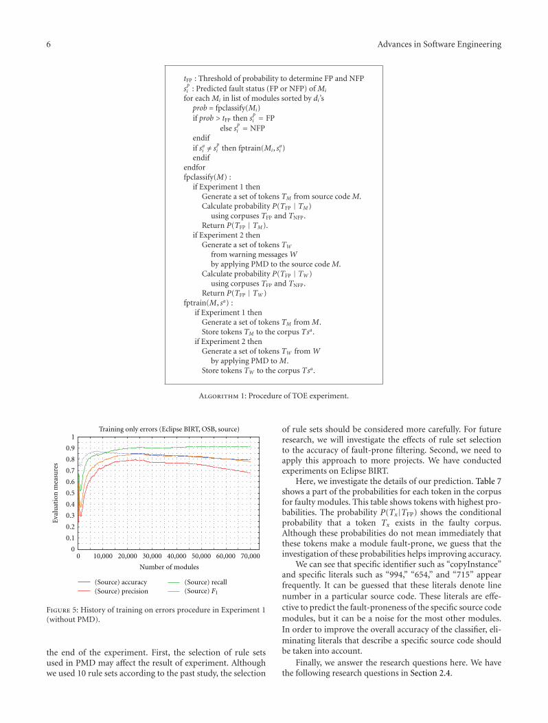
6 Advances in Software Engineering
tFP : Threshold of probability to determine FP and NFPspi : Predicted fault status (FP or NFP) of Mi
for each Mi in list of modules sorted by di’sprob = fpclassify(Mi)if prob > tFP then s
pi = FP
else spi = NFP
endifif sai /= s
pi then fptrain(Mi, sai )
endifendforfpclassify(M) :
if Experiment 1 thenGenerate a set of tokens TM from source code M.Calculate probability P(TFP | TM)
using corpuses TFP and TNFP.Return P(TFP | TM).
if Experiment 2 thenGenerate a set of tokens TW
from warning messages Wby applying PMD to the source code M.
Calculate probability P(TFP | TW )using corpuses TFP and TNFP.
Return P(TFP | TW )fptrain(M, sa) :
if Experiment 1 thenGenerate a set of tokens TM from M.Store tokens TM to the corpus Tsa.
if Experiment 2 thenGenerate a set of tokens TW from W
by applying PMD to M.Store tokens TW to the corpus Tsa.
Algorithm 1: Procedure of TOE experiment.
(Source) accuracy(Source) precision
(Source) recall(Source) F1
Training only errors (Eclipse BIRT, OSB, source)
Eval
uat
ion
mea
sure
s
Number of modules
1
0.9
0.8
0.7
0.6
0.5
0.4
0.3
0.2
0.1
070,00060,00050,00040,00030,00020,00010,0000
Figure 5: History of training on errors procedure in Experiment 1(without PMD).
the end of the experiment. First, the selection of rule setsused in PMD may affect the result of experiment. Althoughwe used 10 rule sets according to the past study, the selection
of rule sets should be considered more carefully. For futureresearch, we will investigate the effects of rule set selectionto the accuracy of fault-prone filtering. Second, we need toapply this approach to more projects. We have conductedexperiments on Eclipse BIRT.
Here, we investigate the details of our prediction. Table 7shows a part of the probabilities for each token in the corpusfor faulty modules. This table shows tokens with highest pro-babilities. The probability P(Tx|TFP) shows the conditionalprobability that a token Tx exists in the faulty corpus.Although these probabilities do not mean immediately thatthese tokens make a module fault-prone, we guess that theinvestigation of these probabilities helps improving accuracy.
We can see that specific identifier such as “copyInstance”and specific literals such as “994,” “654,” and “715” appearfrequently. It can be guessed that these literals denote linenumber in a particular source code. These literals are effe-ctive to predict the fault-proneness of the specific source codemodules, but it can be a noise for the most other modules.In order to improve the overall accuracy of the classifier, eli-minating literals that describe a specific source code shouldbe taken into account.
Finally, we answer the research questions here. We havethe following research questions in Section 2.4.

Advances in Software Engineering 7Ev
alu
atio
n m
easu
res
Number of modules
1
0.9
0.8
0.7
0.6
0.5
0.4
0.3
0.2
0.1
070,00060,00050,00040,00030,00020,00010,0000
(PMD) accuracy(PMD) precision(PMD) recall(PMD) F1
Training only errors (PMD with Eclipse BIRT, OSB)
Figure 6: History of training on errors procedure in Experiment 2(with PMD).
Table 7: Probabilities for each token in the corpus for faultymodules. The “�” denotes any words.
P (Tx | TFP) Tx
0.56229 line 654
0.56229 715 Local
0.56229 “copyInstance” has
0.56229 654 Local
0.56229 instanceof The
0.56229 method copyInstance ()
0.56229 255 Parameter
0.56229 method “copyInstance”
0.56229 489 Avoid
0.56229 line 715
0.56229 copyInstance () has
0.56229 line 994
0.56229 line 474
0.56229 994 The
0.56215 715 � variable
0.56215 blocks � “pageNumber”
0.56215 on � 994
0.56215 bb � instantiating
0.56215 on � 654
0.56215 The � “copyInstance”
0.56215 654 � variable
0.56215 994 � String
0.56215 The � copyInstance ()
0.56215 “copyInstance” � a
0.56215 on � 715
0.56215 on � 474
0.56215 300 � variables
0.56215 copyInstance () � an
RQ1: “can fault-prone modules be predicted by ap-plying a text filter to the warning messages of a staticcode analyzer?”
For this question, we can answer “yes” from the resultsin Table 5 and Table 6. It is obvious that the approach withPMD has prediction capability of the fault-prone modules ata certain degree.
RQ2: “if RQ1 is true, is the performance of the fault-prone filtering becomes better with the warning mes-sages of a static code analyzer?”
For this question, we can say that the recall of the ap-proach with PMD becomes higher and more stable duringthe development than the approach without PMD as shownin Table 6 and Figures 5 and 6. From the viewpoint of thequality assurance, it is a preferred property. We then con-clude that the proposed approach has better performance toassure the software quality.
6. Conclusion
In this paper, we proposed an approach to predict fault-prone modules using warning messages of PMD and a textfiltering technique. For the analysis, we stated two researchquestions: “can fault-prone modules be predicted by apply-ing a text filter to the warning messages of static code analyz-er?” and “is the performance of the fault-prone filtering be-comes better with the warning messages of a static code ana-lyzer?” We tried to answer this question by conducting ex-periments on the open source software. The results of experi-ments show that the answer to the first question is “yes.” Asfor the second question, we can find that the recall becomesbetter than the original approach.
Future work includes investigating which parts of warn-ing messages are really effective for fault-prone moduleprediction. Selection of rule sets of PMD is an interestingfuture research.
References
[1] C. Catal and B. Diri, “A systematic review of software faultprediction studies,” Expert Systems with Applications, vol. 36,no. 4, pp. 7346–7354, 2009.
[2] O. Mizuno and T. Kikuno, “Training on errors experiment todetect fault-prone software modules by spam filter,” in Pro-ceedings of the 6th Joint Meeting of the European Software En-gineering Conference and the ACM SIGSOFT Symposium on theFoundations of Software Engineering, pp. 405–414, 2007.
[3] N. Rutar, C. B. Almazan, and J. S. Foster, “A comparison of bugfinding tools for java,” in Proceedings of the 15th InternationalSymposium on Software Reliability Engineering, pp. 245–256,IEEE Computer Society, Washington, DC, USA, 2004.
[4] T. Copeland, PMD—What does “PMD” mean?, http://pmd.sourceforge.net/meaning.html .
[5] T. Copeland, PMD Applied, Centennial Books, Arexandria, Va,USA, 2005.
[6] W. S. Yerazunis, CRM114—the Controllable Regex Mutilator,http://crm114.sourceforge.net/.

8 Advances in Software Engineering
[7] S. Chhabra, W. S. Yerazunis, and C. Siefkes, “Spam filtering us-ing a markov random field model with variable weightingschemas,” in Proceedings of the 4th IEEE International Confer-ence on Data Mining, (ICDM ’04), pp. 347–350, Riverside,Calif, USA, November 2004.
[8] C. Siefkes, F. Assis, S. Chhabra, and W. S. Yerazunis, “Combin-ing winnow and orthogonal sparse bigrams for incrementalspam filtering,” in Proceedings of the Conference on MachineLearning/European Conference on Principles and Practice ofKnowledge Discovery in Databases (ECML PKDD ’04), 2004.
[9] J. Sliwerski, T. Zimmermann, and A. Zeller, “When do changesinduce fixes? (on Fridays),” in Proceedings of the 2nd Interna-tional Workshop on Mining Software Repositories, pp. 24–28, St.Louis, Mo, USA, May 2005.
[10] C. J. van Rijsbergen, Information Retrieval, Butterworth, Bos-ton, Mass, USA, 2nd edition, 1979.
Hindawi Publishing CorporationAdvances in Software EngineeringVolume 2012, Article ID 949746, 28 pagesdoi:10.1155/2012/949746
Research Article
Specifying Process Views for a Measurement, Evaluation,and Improvement Strategy
Pablo Becker,1 Philip Lew,2 and Luis Olsina1
1 GIDIS Web, Engineering School, Universidad Nacional de La Pampa, General Pico, Argentina2 School of Software, Beihang University, Beijing, China
Correspondence should be addressed to Luis Olsina, [email protected]
Received 24 August 2011; Revised 12 November 2011; Accepted 8 December 2011
Academic Editor: Osamu Mizuno
Copyright © 2012 Pablo Becker et al. This is an open access article distributed under the Creative Commons Attribution License,which permits unrestricted use, distribution, and reproduction in any medium, provided the original work is properly cited.
Any organization that develops software strives to improve the quality of its products. To do this first requires an understandingof the quality of the current product version. Then, by iteratively making changes, the software can be improved with subsequentversions. But this must be done in a systematic and methodical way, and, for this purpose, we have developed a specific strategycalled SIQinU (Strategy for understanding and Improving Quality in Use). SIQinU recognizes problems of quality in use throughevaluation of a real system-in-use situation and proposes product improvements by understanding and making changes to theproduct’s attributes. Then, reevaluating quality in use of the new version, improvement gains can be gauged along with the changesthat led to those improvements. SIQinU aligns with GOCAME (Goal-Oriented Context-Aware Measurement and Evaluation), amultipurpose generic strategy previously developed for measurement and evaluation, which utilizes a conceptual framework (withontological base), a process, and methods and tools. Since defining SIQinU relies on numerous phase and activity definitions, inthis paper, we model different process views, for example, taking into account activities, interdependencies, artifacts, and roles,while illustrating them with excerpts from a real-case study.
1. Introduction
Even though software product launches now may consistof “continuous beta,” users expect more and better func-tionality, combined with increased quality from the user’sperception. Methodically improving the perceived quality,that is, its quality in use (QinU) particularly for web applica-tions (WebApps), is not an easy job. WebApps—a kindof software applications—are no longer simple websitesconveying information. Rather, they have become fullyfunctional software applications often with complex businesslogic and sometimes critical to operating the business. Users,in addition, are becoming more demanding and diversein their requirements. Consequently, WebApp quality andespecially the quality in use, namely, the perceived qualityby the end user has taken on increased significance asweb and now cloud deployment have become mainstreamdelivery methods. Systematic means for evaluating QinUis important because it enables understanding the qualitysatisfaction level achieved by the application and provides
useful information for recommendation and improvementprocesses in a consistent manner over time. Coincident withconsistent and systematic evaluation of WebApp quality, themain goal is to ultimately improve its QinU.
This leads to our strategy with the objectives ofunderstanding and improving the QinU—as nonfunctionalrequirements—of WebApps. QinU is currently redefined inthe ISO 25010 standard [1], which was reused and enlargedby the 2Q2U (internal/external Quality, Quality in use, actualUsability, and User experience) quality framework—see [2]for an in-depth discussion. QinU from the actual usabilitystandpoint (that embraces performance or “do” goals incontrast to hedonic or “be” goals [3]) is defined as the degreeto which specified users can achieve specified goals witheffectiveness in use, efficiency in use, learnability in use, andaccessibility in use in a specified context of use [2].
Utilizing 2Q2U quality models, we developed SIQinU asan integrated means to evaluate and find possible problemsin QinU which are then related to external quality (EQ)characteristics and attributes (by doing a mapping between

2 Advances in Software Engineering
Reuses
SIQinUprocess
WebQEM,parser tool,
code restructuring,refactoring,
others.
SIQinU strategy
conceptualframework
Process Methods/tools
conceptualframework
Process Methods/tools
GOCAME WebQEM,
GOCAME strategy
C-INCAMI
C-INCAMI
C-INCAMI tool
M & E
M & E
M & E process
Figure 1: Allegory of the three GOCAME pillars, which are reused to a great extent by SIQinU.
QinU problems and EQ). This is followed by evaluatingthe application from the EQ standpoint and then makingrecommendations for improvements if necessary. The newversion, based on recommended improvements, is reevalu-ated to gauge the improvement gain from both the EQ andQinU point of views. One aspect of SIQinU’s uniquenessis that it collects user usage data from WebApps in a realcontext of use whereby code snippets are inserted (or usingsimilar techniques) to gather data related to the task beingexecuted by users at the subtask level enabling nonintrusiveevaluations.
It is worth mentioning that SIQinU aligns with theGOCAME strategy [4]. GOCAME, a multipurpose goal-oriented strategy, was previously developed for supportingmeasurement and evaluation (M&E) programs and projects.Its rationale is based on three main pillars or principles,namely, (i) a conceptual framework utilizing an ontologicalbase; (ii) a well-defined measurement and evaluation pro-cess; (iii) quality evaluation methods and tools instantiatedfrom both the framework and process. This is allegoricallydepicted in Figure 1.
GOCAME’s first principle is that designing and imple-menting a robust M&E program require a sound conceptualframework. Often times, organizations conduct start andstop measurement programs because they do not pay enoughattention to the way nonfunctional requirements, contextualproperties, metrics, and indicators should be designed,implemented, and analyzed. Any M&E effort requires anM&E framework built on a sound conceptual base, thatis, on an ontological base, which explicitly and formallyspecifies the main agreed concepts, properties, relationships,and constraints for a given domain. To accomplish this,we utilize the C-INCAMI (Contextual-Information Need,
Concept model, Attribute, Metric, and Indicator) frameworkand its components [4, 5] based on our metrics andindicators ontology.
GOCAME’s second principle requires a well-establishedM&E process in order to guarantee repeatability in per-forming activities and consistency of results. A processprescribes a set of phases, activities, inputs and outputs,interdependencies, sequences and parallelisms, check points,and so forth. Frequently, process specifications state what todo but do not mention the particular methods and toolsto perform specific activity descriptions. Thus, to providerepeatability and replicability in performing activities, aprocess model for GOCAME was proposed in [6], which isalso compliant with both the C-INCAMI conceptual baseand components. Finally, methods and tools—the thirdpillar in the GOCAME strategy—can be instantiated fromboth the conceptual framework and process, for example, theWebQEM (Web Quality Evaluation) methodology [7] and itstool called C-INCAMI tool [4].
SIQinU utilizes the above three GOCAME principleswhile also reusing the C-INCAMI conceptual base andprocess. However, since SIQinU is a specific-purpose goal-oriented strategy, it has specific processes, methods, andprocedures that are not specified in GOCAME. Since theprocess aspect is critical in specifying SIQinU, given ofits numerous interrelated phases and activities, this workdefines its process model in detail through illustration withexcerpts of a real case study. This case study was thoroughlyillustrated in [8], and also aspects of its internal and externalvalidity were considered in [9] as well.
Note that processes can be modeled taking into accountdifferent views [10] such as (i) functional that includes theactivities’ structure, inputs, and outputs; (ii) informational

Advances in Software Engineering 3
that includes the structure and interrelationships amongartifacts produced or consumed by the activities; (iii)behavioral that models the dynamic view of processes; (iv)organizational that deals with agents, roles, and responsi-bilities. Additionally, a methodological view is described in[11], which is used to represent the process constructors(e.g., specific methods) that can be applied to differentdescriptions of activities. In order to specify all these views,different modeling languages can be used. However, nomodeling language fits all needs and preferences. Each hasits own strengths and weaknesses, which can make it moresuitable for modeling certain views than others [12].
This paper using UML 2.0 activity diagrams [13] andthe SPEM profile [14] stresses the functional, informational,organizational, and behavioral views for the SIQinU process.Modeling its process helps to (i) ease the repeatabilityand understandability among practitioners, (ii) integrateand formalize different activities that are interrelated indifferent phases, and (iii) promote the learnability andinteroperability by reusing the same ontological base comingfrom the C-INCAMI framework. This paper is an extensionof the work presented in [15] elaborating on new aspectsand views (e.g., informational and organizational) for bothGOCAME and SIQinU process, as we remark later on.Summarizing, the main contributions of this paper are
(i) a six-phased strategy (SIQinU) useful for under-standing and improving the QinU for WebApps,which is specified and illustrated from the processviewpoint regarding activities (i.e., the functionalview), interdependencies (behavioral view), arti-facts (informational view), and roles (organizationalview).
(ii) foundations for reusing a multipurpose goal-oriented strategy (i.e., GOCAME) to derive andintegrate more specific-purpose strategies (e.g.,SIQinU) regarding its conceptual M&E framework,methods, and process views.
The remainder of this paper is organized as follows. Section 2gives an overview of the six-phased SIQinU strategy.Section 3 provides the GOCAME rationale considering itsthree pillars, which are to a great extent reused by SIQinU;particularly, in Section 3.4, we discuss why SIQinU is inalignment with GOCAME regarding its conceptual M&Eframework (Section 3.1), its process views (Section 3.2), andits methods (Section 3.3). Section 4 models and illustratesthe six-phased SIQinU process from the above-mentionedprocess views. Section 5 analyzes related work consideringthe two quoted contributions, and, finally, in Section 6,concluding remarks as well as future work are discussed.
2. Overview of the SIQinU Strategy
SIQinU is an evaluation-driven strategy to iteratively andincrementally improve a WebApp’s QinU by means ofmapping actual system-in-use problems—that happenedwhile real users were performing common WebApp tasks—to measurable EQ product attributes and by then improving
the current WebApp and assessing the gain both at EQ andQinU levels. SIQinU can be implemented in an economicand systematic manner that alleviates most of the problemsidentified with typical usability testing studies which canbe expensive, subjective, nonrepeatable, time consuming,and unreliable due to users being observed in an intrusiveway. This is accomplished through utilizing server-sidecapabilities to collect user usage data from log files adding,for example, snippets of code in the application to specificallyrecord data used to calculate measures and indicator valuesfor QinU in a nonintrusive way.
Note that SIQinU can apply to systems in use otherthan WebApps if data can be collected for analysis regardinguser activities. This may be possible in client-server networkenvironments where the developer has control over the servercode and the activities of users at their client workstationscan be collected. Therefore, the major constraint is incollecting easily large amounts of data in a nonintrusivemanner from which to measure and evaluate the QinUserving as the basis for improvement.
The SIQinU strategy uses quality models such as thosespecified in the ISO 25010 standard [1] and its enhancement,that is, the 2Q2U quality framework [2]. Once the QinUmodel has been established, the data collected, and metricsand indicators calculated, a preliminary analysis is made.If the agreed QinU level is not met, then EQ requirementsare derived considering the application’s QinU problems andits tasks, subtasks, and associated screens. In turn, takinginto account the derived EQ requirements, an evaluation ofthe WebApp attributes is performed by inspection. Thus aproduct analysis regarding the EQ evaluation is performed,and changes for improvement are recommended. If theimprovement actions have been implemented, then the newversion is reevaluated to gauge the improvement gain bothfrom the EQ and the QinU standpoint. Ultimately, SIQinUis a useful strategy not only for understanding but also—andmost importantly—for improvement purposes.
SIQinU uses the concepts for nonfunctional require-ments specification, measurement, and evaluation design,and so forth, established in the C-INCAMI framework as wewill see in Section 3.1. Also, SIQinU has an integrated, well-defined, and repeatable M&E process, which follows to greatextent the GOCAME process as we will discuss in Sections3.2 and 3.3. Specifically, the SIQinU process embraces sixphases as shown in Figure 2, which stresses the main phasesand interdependencies.
Additionally, Table 1 provides, with Phase (Ph.) referencenumbers as per Figure 2, a brief description of each phase,the involved activities, and main artifacts. Section 4 thor-oughly illustrates phases, activities, interdependencies, arti-facts, as well as roles taking into account aspects of the func-tional, behavioral, informational, and organizational views.
Lastly, in the Introduction, we stated as contribution thatGOCAME—a previously developed strategy—can be reusedto derive and integrate more specific-purpose strategies (asis the case of SIQinU) regarding its conceptual M&E frame-work, process, and methods. Therefore, in the followingsection, the GOCAME strategy regarding these principles isoutlined.

4 Advances in Software Engineering
Specify requirements
and evaluation criteria
for QinU (Ph. I)
Perform QinUevaluation(Ph. II/VI)
[else]
[true]
Were improvement actionsperformed for the product?
Derive/specifyrequirements and
evaluation criteria forEQ (Ph. III)
[else] [else]
[true]
Should improvement actionsbe performed for the product?
Perform EQ evaluationand analysis (Ph. IV)
Recommend and performimprovement actions for
EQ (Ph. V)
Conduct improvementactions analysis (Ph. VI)
Conduct preliminaryanalysis (Ph. II)
Does product’s QinUsatisfy requirements?
Do you want to derive/specify other
requirements for EQ?
[true]
[else]
[true]
Ph.: phaseEQ: external qualityQinU: quality in use
≪ decision input ≫
≪ decision input ≫
≪ decision input ≫
≪ decision input ≫
Figure 2: Process overview of SIQinU stressing phases and interdependencies.
3. GOCAME Strategy
GOCAME is a multipurpose M&E strategy that followsa goal-oriented and context-sensitive approach in definingprojects. It allows the definition of M&E projects includingwell-specified context descriptions, providing therefore morerobust evaluation interpretations among different projectresults at intra- and interorganization levels.
GOCAME is based on the three above-mentioned pillars,namely, a conceptual framework (described in Section 3.1); aM&E process (Section 3.2); methods and tools (Section 3.3).Finally, in Section 3.4, we discuss why SIQinU is in alignmentwith GOCAME regarding these capabilities.
3.1. C-INCAMI Conceptual Framework. The C-INCAMIframework provides a domain (ontological) model definingall the concepts and relationships needed to design andimplement M&E processes. It is an approach in which therequirements specification, M&E design, and analysis ofresults are designed to satisfy a specific information need ina given context. In C-INCAMI, concepts and relationshipsare meant to be used along all the M&E activities. This way,a common understanding of data and metadata is sharedamong the organization’s projects lending to more consistentanalysis and results across projects.
Following the main activities of the process (shown inSection 3.2), the framework—that is, the related conceptsand relationships—is structured in six components ormodules, namely,
(i) measurement and evaluation project definition;
(ii) nonfunctional requirements specification;
(iii) context specification;
(iv) measurement design and implementation;
(v) evaluation design and implementation;
(vi) analysis and recommendation specification.
For illustration purposes, Figure 3 shows the main conceptsand relationships for four components (i.e., from (ii) to (v)),and Table 2 defines the used terms, stressed in italic in thefollowing text). The entire modeling of components can befound in [4, 5].
Briefly outlined, the GOCAME strategy follows a goal-oriented approach in which all the activities are guidedby agreed Information Needs; these are intended to satisfyparticular nonfunctional requirements of some Entity for aparticular purpose and stakeholder’s viewpoint. The non-functional requirements are represented by Concept Modelsincluding high-level Calculable Concepts, as in ISO 25010’squality models [1], which, in turn, measurable Attributesof the entity under analysis are combined. The instantiatedquality models are the backbone for measurement andevaluation. Measurement is specified and implemented byusing Metrics, which define how to represent and collectattributes’ values; Evaluation is specified and implementedby using Indicators, which define how to interpret attributes’values and calculate higher-level calculable concepts of thequality model.
Since each MEProject does not occur in isolation, wetherefore say that measurement and evaluation should besupported by Context; thus, context specifications may be

Advances in Software Engineering 5
Table 1: SIQinU phases, activities, and artifacts.
Phases (Ph.) Phase description and activities involved Artifacts (work products)
Ph. ISpecify requirementsand evaluationcriteria for QinU
Taking into account the recorded data of the WebApp’s usage, wereengineer QinU requirements. This embraces designing tasks,defining user type, specifying usage context and characteristics.Activities include (see Figure 8) (i) establish information need; (ii)specify project context; (iii) design tasks; (iv) select QinU conceptmodel; (v) design QinU measurement and evaluation; (vi) designPreliminary Analysis
(1) Information Needspecification
(2) Context specification(3) Task/subtasks specification(4) QinU NFR tree(5) QinU metrics and indicators
specification(6) Analysis design
Ph. IIPerform QinUevaluation andconduct preliminaryanalysis
As per Ph. I, data is collected purposely targeting QinU attributes forimprovement. Depending on the WebApp’s data collectioncapabilities, we collect data such as the date/time, the data is gathered,errors, task, and subtask completion and accuracy, and so forth. Itincludes (see Figure 12) (i) collect and parse data pertaining to taskswith their subtasks; (ii) quantify QinU attributes; (iii) calculate QinUindicators; (iv) conduct preliminary analysis
(1) Parsed data file(2) Measure and indicator values
for QinU(3) QinU preliminary analysis
report
Ph. IIIDerive/SpecifyRequirements andEvaluation Criteriafor EQ
Based on Ph. I and II, we derive EQ requirements, that is,characteristics and attributes, with their metrics and indicators inorder to understand the current WebApp’s quality. Activities include(see Figure 13) (i) select EQ concept model; (ii) design EQmeasurement; (iii) design EQ evaluation
(1) EQ NFR tree(2) EQ metrics and indicators
specification
Ph. IVPerform EQevaluation andanalysis
Activities include (see Figure 15) (i) quantify EQ attributes; (ii)calculate EQ indicators; (iii) conduct an EQ analysis and identifyparts of the WebApp that need improvement
(1) Measure and indicator valuesfor EQ
(2) EQ analysis report (and newreport after reevaluation)
Ph. VRecommend, performimprovement actions,and reevaluate EQ
Using the EQ attributes that require improvement, we makeimprovement recommendations for modifying the WebApp, that is,version 1 to 1.1. Activities include (see Table 9) (i) recommendimprovement actions; (ii) design improvement actions; (iii) performimprovement actions; (iv) evaluate improvement gain to noteimprovement from benchmark in Ph. IV. Note that once changeswere made on the WebApp (Phase V), evaluators could detect thatother EQ attributes (from problems identified in QinU) should bederived—under the premise that if further EQ improvement in thesenew attributes will result in greater impact on the improvement gainin QinU. This concern is taken into account in the process as shownin Figure 2
(1) EQ recommendations report(2) Improvement plan(3) New application version
Ph. VIReevaluate QinU andanalyze improvementactions
Once the new version has been used by real users, we evaluate QinUagain to determine the influence of what was improved for theWebApp’s EQ on QinU. This provides insight to further develop thedepends-on and influences relationships [8]. Activities include (i)evaluate QinU again to determine level of improvement from Ph. II;(ii) conduct improvement action analysis, which includes developingdepends-on and influences relationships between EQ improvementsand QinU
(1) New measure and indicatorvalues for QinU
(2) QinU improvement analysisreport
(3) EQ/QinU attributerelationship table (see Table 11)
provided in order to support sounder analysis, interpreta-tions, and recommendations. A summarized description foreach component is provided below.
3.1.1. M&E Project Definition Component. This componentdefines and relates a set of Project concepts needed to articu-late M&E activities, roles, and artifacts.
A clear separation of concerns among NonfunctionalRequirements Project, Measurement Project, and EvaluationProject concepts is made for reuse purposes as well as for
easing management’s role. The main concept in this compo-nent is a measurement and evaluation project (MEProject),which allows defining a concrete requirement project withthe information need and the rest of the nonfunctionalrequirements information. From this requirement project,one or more measurement projects can be defined andassociated; in turn, for each measurement project, oneor more evaluation projects could be defined. Hence, foreach measurement and evaluation project we can manageassociated subprojects accordingly. Each project also hasinformation such as responsible person’s name and contact

6 Advances in Software Engineering
Table 2: Some M&E terms—see [4] for more details.
Concept Definition
Project terms
Evaluation projectA project that allows, starting from a measurement project and a conceptmodel of a nonfunctional requirement project, assigning indicators, andperforming the calculation in an evaluation process.
Measurement projectA project that allows, starting from a nonfunctional requirements project,assigning metrics to attributes, and recording the values in a measurementprocess.
MEProject (i.e., measurement and evaluationproject)
A project that integrates related nonfunctional requirements, measurement andevaluation projects, and then allows managing and keeping track of all relatedmetadata and data.
ProjectPlanned temporal effort, which embraces the specification of activities andresources constraints performed to reach a particular goal.
Nonfunctional requirements projectA project that allows specifying nonfunctional requirements for measurementand evaluation activities.
Nonfunctional requirements terms
Attribute (synonyms: property, feature) A measurable physical or abstract property of an entity category.
Calculable concept (synonym: characteristic,dimension)
Abstract relationship between attributes of entities and information needs.
Concept model (synonyms: factor, feature model)The set of subconcepts and the relationships between them, which provide thebasis for specifying the concept requirement and its further evaluation orestimation.
Entity A concrete object that belongs to an entity category.
Entity category (synonym: object) Object category that is to be characterized by measuring its attributes.
Information need Insight necessary to manage objectives, goals, risks, and problems.
Requirement treeA requirement tree is a constraint to the kind of relationships among theelements of the concept model, regarding the graph theory.
Context terms
Context
A special kind of entity representing the state of the situation of an entity,which is relevant for a particular information need. The situation of an entityinvolves the task, the purpose of that task, and the interaction of the entity withother entities as for that task and purpose.
Context property (synonyms: context attribute,feature)
An attribute that describes the context of a given entity; it is associated to oneof the entities that participates in the described context.
Measurement terms
Calculation methodA particular logical sequence of operations specified for allowing the realizationof a formula or indicator description by a calculation.
Direct metric (synonyms: base, single metric)A metric of an attribute that does not depend upon a metric of any otherattribute.
Indirect metric (synonyms: derived, hybrid metric)A metric of an attribute that is derived from metrics of one or more otherattributes.
MeasureThe number or category assigned to an attribute of an entity by making ameasurement.
Measurement An activity that uses a metric definition in order to produce a measure’s value.
Measurement method (synonyms: counting rule,protocol)
The particular logical sequence of operations and possible heuristics specifiedfor allowing the realization of a direct metric description by a measurement.
Metric The defined measurement or calculation method and the measurement scale.
Scale
A set of values with defined properties. Note. The scale type depends on thenature of the relationship between values of the scale. The scale types mostlyused in software engineering are classified into nominal, ordinal, interval, ratio,and absolute.
UnitA particular quantity defined and adopted by convention, with which otherquantities of the same kind are compared in order to express their magnituderelative to that quantity.
Advances in Software Engineering 7
Table 2: Continued.
Concept Definition
Evaluation terms
Decision criterion (synonym: acceptability level)Thresholds, targets, or patterns used to determine the need for action orfurther investigation, or to describe the level of confidence in a given result.
Elementary indicator (synonyms: elementarypreference, criterion)
An indicator that does not depend upon other indicators to evaluate orestimate a calculable concept.
Elementary model (synonym: elementary criterionfunction)
Algorithm or function with associated decision criteria that model anelementary indicator.
Evaluation (synonym: calculation)Activity that uses an indicator definition in order to produce an indicator’svalue.
Global indicator (synonyms: global preference,criterion)
An indicator that is derived from other indicators to evaluate or estimate acalculable concept.
Global model (synonyms: scoring, aggregationmodel, or function)
Algorithm or function with associated decision criteria that model a globalindicator.
Indicator (synonym: criterion)The defined calculation method and scale in addition to the model anddecision criteria in order to provide an estimate or evaluation of a calculableconcept with respect to defined information needs.
Indicator value (synonym: preference value)The number or category assigned to a calculable concept by making anevaluation.
information, starting and ending date, amongst other rele-vant information. Ultimately, this separation of concerns foreach MEProject facilitates the traceability and consistency forintra- and interproject analysis.
3.1.2. Nonfunctional Requirements Specification Component.This component includes concepts and relationships neededto define the nonfunctional requirements for measurementand evaluation. One key concept is the Information Need,which specifies (see Figure 3)
(i) the purpose for performing the evaluation (whichcan be for instance “understand,” “predict,”“improve,” “control,” etc.);
(ii) the focus concept (CalculableConcept) to be assessed(e.g., “operability,” “quality in use,” “actual usability,”etc.);
(iii) the category of the entity (EntityCategory) that willbe assessed, for example, a “Web application” (whichits superCategory is a “product” or “informationsystem”) and the concrete Entities (such as “JIRA,”“Mantis” WebApps, etc.). Other super categories forentities can be “resource,” “process,” “informationsystem-in-use” (e.g., as a Web application-in-use),and “project”
(iv) the userViewpoint (i.e., the intended stakeholder as“developer,” “final user,” etc.) from which the focusconcept (and model) will be evaluated;
(v) the Context that characterizes the situation defined bythe previous items to a particular MEProject.
The focus concept constitutes the higher-level concept of thenonfunctional requirements; in turn, a calculable conceptand its subconcepts are related by means of a Concept Model.
This model may be a tree-structured representation in termsof related mid-level calculable concepts and lower-levelmeasurable Attributes, which are associated to the targetentity. Predefined instances of metadata for informationneeds, entities, and entity categories, calculable concepts,attributes, and so forth, and its corresponding data canbe obtained from an organizational repository to supportreusability and consistency in the requirements specificationalong the organizational projects.
3.1.3. Context Specification Component. This componentincludes concepts and relationships dealing with the contextinformation specification. The main concept is Context,which represents the relevant state of the situation of theentity to be assessed with regard to the stated informationneed. We consider Context as a special kind of Entity inwhich related relevant entities are involved. Consequently,the context can be quantified through its related entities. Byrelevant entities, we mean those that could affect how thefocus concept of the assessed entity is interpreted (examplesof relevant entities of the context may include resources as anetwork infrastructure, a working team, lifecycle types, theorganization, or the project itself, among others).
In order to describe the situation, attributes of therelevant entities (involved in the context) are used. Theseare also Attributes called Context Properties and can bequantified to describe the relevant context of the entity underanalysis. A context property inherits the metadata fromthe Attribute class such as name, definition, and objective,and also adds other information (see Figure 3). All thesecontext properties’ metadata are meant to be stored inthe organizational repository, and, for each MEProject, theparticular metadata and its values are stored as well. Adetailed illustration of context and the relationship withother C-INCAMI components can be found in [5].

8 Advances in Software Engineering
requirements characterizedBy
InformationNeed
purposeuserViewpoint
relatedEntity1
1
1
1
1
1
1
1
1
1
1
1
1
1
1
1
11
1
1
1
1
1
1
1
11
1
specifies
focus
CalculableConcept
name
definition
references
subconcept
object
EntityCategory
name
description
superCategory
Entity
name
description
combines
evaluates
ConceptModel
namespecificationreferencesconstraints
Attribute
namedefinitionobjective
quantifies
context
Context
actualContext
describedBy
ContextProperty
weight
relevance
evaluationevaluates
GlobalModel
interpretedUsing interpretedUsing
modeledBy
GlobalIndicator
operator
DecisionCriterion
name
description
lowerThreshold
upperThreshold
ElementaryModel
relatedIndicators
IndicatorValue
value
modeledBy
ElementaryIndicator
Indicator
nameweightauthorversion
contains
relatedTo
produces
Evaluation
timestamp
measurement
MeasurementMethod CalculationMethod
measuredUsing
DirectMetric
Method
namespecificationreferences
calculatedUsing
IndirectMetric
formula
relatedMetric
refersTo
Measurement
timeStampdataCollectorNamecollector ContactInfo
contains
Scale
scaleType
Unit
name
description
acronym
produces
Measure
value
expressedIn
includes
relatedTo
Metric
name
objective
author
version
described by
0..∗
0..∗
0..∗
0..∗
0..∗
0..∗
0..∗
0..∗
1..∗
1..∗
1..∗
1..∗
1..∗ 1..∗1..∗
1..∗
1..∗
1..∗
1..∗
1..∗ 2..∗
1..∗1..∗
associated with
belongs to
relatedContextProperty
represneted by
Figure 3: Main concepts and relationships of the C-INCAMI framework. Four out of six C-INCAMI components are depicted as packages,namely, nonfunctional requirements specification, context specification, measurement design and implementation, and evaluation designand implementation.
3.1.4. Measurement Design and Implementation Compo-nent. This module includes the concepts and relationshipsintended to specify the measurement design and imple-mentation, for instance, the concrete Entities that will bemeasured, the selected Metric for each attribute, and so on.
Regarding measurement design, a metric provides aMeasurement specification of how to quantify a particularattribute of an entity, using a particular Method, and how torepresent its values, using a particular Scale. The propertiesof the measured values in the scale with regard to theallowed mathematical and statistical operations and analysisare given by the scaleType [16]. Two types of metrics aredistinguished. Direct Metrics are those for which values areobtained directly from measuring the corresponding entity’sattribute, by using a Measurement Method. On the otherhand, Indirect Metrics’ values are calculated from othersdirect metrics’ values following a function specification anda particular Calculation Method.
For measurement implementation, a Measurement spec-ifies the activity by using a particular metric description in
order to produce a Measure value. Other associated metadatais the data collector name and the timestamp in which themeasurement was performed.
3.1.5. Evaluation Design and Implementation Component.This component includes the concepts and relationshipsintended to specify the evaluation design and implemen-tation. Indicator is the main term, which allows specifyinghow to calculate and interpret the attributes and calculableconcepts of nonfunctional requirement models.
Two types of indicators are distinguished. First, Ele-mentary Indicators that evaluate lower-level requirements,namely, attributes combined in a concept model. Eachelementary indicator has an Elementary Model that pro-vides a mapping function from the metric’s measures (thedomain) to the indicator’s scale (the range). The new scaleis interpreted using agreed Decision Criteria, which helpanalyze the level of satisfaction reached by each elemen-tary nonfunctional requirement, that is, by each attribute.Second, Partial/Global Indicators, which evaluate mid-level
Advances in Software Engineering 9
and higher-level requirements, that is, subcharacteristics andcharacteristics in a concept model. Different aggregationmodels (GlobalModel), like logic scoring of preference mod-els, neuronal networks models, and fuzzy logic models, canbe used to perform evaluations. The global indicator’s valueultimately represents the global degree of satisfaction inmeeting the stated information need for a given purpose anduser viewpoint.
As for the implementation, an Evaluation represents theactivity involving a single calculation, following a partic-ular indicator specification—either elementary or global—producing an Indicator Value.
It is worthy to mention that the selected metrics areuseful for a measurement process as long as the selectedindicators are useful for an evaluation process in order tointerpret the stated information need.
3.1.6. Analysis and Recommendation Specification Compo-nent. This component includes concepts and relationshipsdealing with analysis design and implementation as wellas conclusion and recommendation. Analysis and recom-mendation component uses information coming from eachMEProject (which includes requirements, context, measure-ment, and evaluation data and metadata). By storing allthis information and by using different kinds of statisticaltechniques and visualization tools, stakeholders can analyzethe assessed entities’ strengths and weaknesses with regard toestablished information needs, and justify recommendationsin a consistent way. Note this component is not shown inFigure 3. However, it is shown in Table 5 from the processspecification standpoint.
3.2. GOCAME Measurement and Evaluation Process. Whenmodeling a process, often engineers think more about whata process must do rather than how activities should beperformed. In order to foster repeatability and reproducibil-ity, a process specifies (i.e., prescribes or informs) a set ofphases and activities, inputs and outputs, interdependencies,among other concerns. Also, to deal with the inherentcomplexity of processes, process views—also quoted inprocess modeling literature as perspectives—are used. A viewis a particular model or approach to represent, specify, andcommunicate regarding the process. For instance, accordingto [10], a process can be modeled taking into account fourviews, namely, functional, behavioral, informational, andorganizational.
Considering these process views, the functional per-spective for GOCAME represents what activities and tasks(instead of the often-used term “task” in process modeling,which represents a fine grained or atomic activity, we will usethe term “sub-activity” in the rest of the text, since, inSection 4, for QinU modeling, the term task has a veryspecific meaning) should be specified, what hierarchicalactivities structure (also known as task breakdown structure)there exists, what conditions (pre- and postconditions)should be accomplished, and what inputs and outputs(artifacts) will be required. Taking into account the termi-nology and components used in the C-INCAMI framework(Section 3.1), the integrated process of GOCAME embraces
the following core activities: (i) Define Non-FunctionalRequirements; (ii) Design the Measurement; (iii) Design theEvaluation; (iv) Implement the Measurement; (v) Implementthe Evaluation; (vi) Analyze and Recommend as shown inFigure 4. In addition, in Table 3, we enumerate these sixactivities, their involved subactivities, and the main outputartifacts.
The behavioral view represents the dynamics of theprocess, that is, the sequencing and synchronization of activ-ities, parallelisms, iterations, feedback loops, beginning andending conditions, among other issues. The core GOCAMEactivities as well as sequences, parallelisms, main inputs,and outputs are depicted in Figure 4. The �datastore�stereotype shown in the figure represents repositories; forinstance, the Metrics repository stores the metadata for thepreviously designed metrics. More details for the GOCAMEfunctional and behavioral process views can be found in [6].
On the other hand, the informational view is concernedwith those artifacts produced or required (consumed) byactivities, the artifact breakdown structure, strategies of con-figuration management, and traceability models. For exam-ple, for illustration purpose, in Figure 5, the structure forthe Non-Functional Requirements Specification, and MetricsSpecification documents, which are outputs of A.1 and A.2activities (see Table 3) is modeled. As the reader can observein Figure 5(a), the Non-Functional Requirements Specificationartifact is composed of the Information Need Specification,the Context Specification and the Non-Functional Require-ments Tree documents. Besides, the Metrics Specification arti-fact (Figure 5(b)) is composed of a set of one or more MetricSpecification, which in turn is composed of a Scale and aCalculation or Measurement Method descriptions. Note that,aimed at easing the communication among stakeholdersthese models can complement the textual specification madein the third column of Table 3.
Finally, the organizational view deals with what agentsand their associated resources participate-plan-execute-control what activities; which roles (in terms of respon-sibilities and skills) are assigned to agents; what groups’dynamic and communication strategies are used, amongother aspects. To illustrate this, Figure 6 depicts the differentroles and their associated GOCAME activities. In Table 4,each role definition and its involved activities are also listed.Note that we have used italics in the definition column (inTable 4) to show the terminological correspondence betweenthe process role definition and the C-INCAMI conceptualframework. It is important to remark that a role can beassumed by a human or an automated agent. And a humanagent can be embodied by one or more persons, that is, ateam.
In order to combine the above views, Table 5 presentsa template which specifies just the Analyze and Recommendactivity. The template specifies the activity name, objectiveand description, the subactivities and involved roles, inputand output artifacts, pre- and postconditions. Also a diagramrepresenting the Analyze and Recommend activity is attachedas well to enable understanding and communicability.
Summarizing, the GOCAME M&E process can bedescribed as follows. Once the nonfunctional requirements
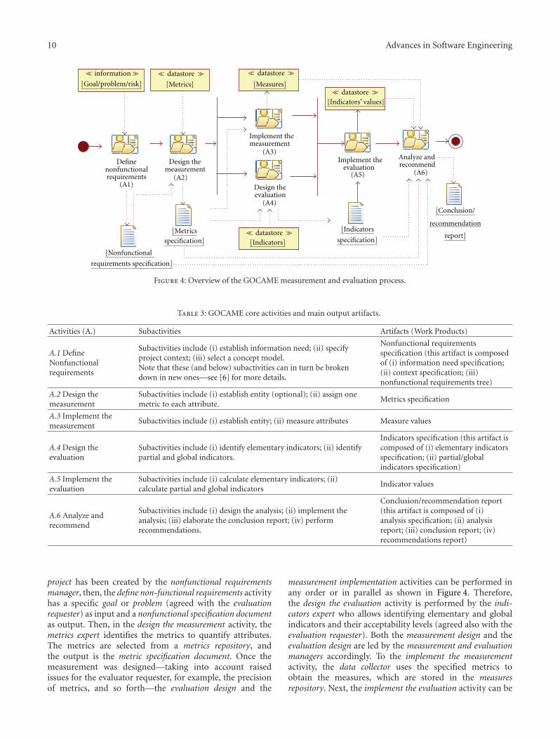
10 Advances in Software Engineering
Define
requirements
Design themeasurement
Design theevaluation
Implement themeasurement
Implement theevaluation
Analyze andrecommend
(A1)(A2)
(A4)
(A3)
(A5) (A6)
[Metrics]
[Indicators]
[Metricsspecification]
[Indicators
specification]
[Nonfunctional
requirements specification]
[Measures]
[Indicators’ values]
[Goal/problem/risk]
[Conclusion/
recommendation
report]
nonfunctional
≪ information≫ ≪ datastore ≫ ≪ datastore ≫
≪ datastore ≫
≪ datastore ≫
Figure 4: Overview of the GOCAME measurement and evaluation process.
Table 3: GOCAME core activities and main output artifacts.
Activities (A.) Subactivities Artifacts (Work Products)
A.1 DefineNonfunctionalrequirements
Subactivities include (i) establish information need; (ii) specifyproject context; (iii) select a concept model.Note that these (and below) subactivities can in turn be brokendown in new ones—see [6] for more details.
Nonfunctional requirementsspecification (this artifact is composedof (i) information need specification;(ii) context specification; (iii)nonfunctional requirements tree)
A.2 Design themeasurement
Subactivities include (i) establish entity (optional); (ii) assign onemetric to each attribute.
Metrics specification
A.3 Implement themeasurement
Subactivities include (i) establish entity; (ii) measure attributes Measure values
A.4 Design theevaluation
Subactivities include (i) identify elementary indicators; (ii) identifypartial and global indicators.
Indicators specification (this artifact iscomposed of (i) elementary indicatorsspecification; (ii) partial/globalindicators specification)
A.5 Implement theevaluation
Subactivities include (i) calculate elementary indicators; (ii)calculate partial and global indicators
Indicator values
A.6 Analyze andrecommend
Subactivities include (i) design the analysis; (ii) implement theanalysis; (iii) elaborate the conclusion report; (iv) performrecommendations.
Conclusion/recommendation report(this artifact is composed of (i)analysis specification; (ii) analysisreport; (iii) conclusion report; (iv)recommendations report)
project has been created by the nonfunctional requirementsmanager, then, the define non-functional requirements activityhas a specific goal or problem (agreed with the evaluationrequester) as input and a nonfunctional specification documentas output. Then, in the design the measurement activity, themetrics expert identifies the metrics to quantify attributes.The metrics are selected from a metrics repository, andthe output is the metric specification document. Once themeasurement was designed—taking into account raisedissues for the evaluator requester, for example, the precisionof metrics, and so forth—the evaluation design and the
measurement implementation activities can be performed inany order or in parallel as shown in Figure 4. Therefore,the design the evaluation activity is performed by the indi-cators expert who allows identifying elementary and globalindicators and their acceptability levels (agreed also with theevaluation requester). Both the measurement design and theevaluation design are led by the measurement and evaluationmanagers accordingly. To the implement the measurementactivity, the data collector uses the specified metrics toobtain the measures, which are stored in the measuresrepository. Next, the implement the evaluation activity can be

Advances in Software Engineering 11
requirementsspecification
Informationneed
specification
Contextspecification
requirementstree
Nonfunctional
Nonfunctional
(a)
Metricsspecification
Metric specification
NameObjectiveAuthorVersion
Method
Name
Specification
Reference
Scale
Scale type
Unit
1..∗
(b)
Figure 5: Excerpt of the informational view for A.1 and A.2 in Table 3, regarding artifact composition. (a) Nonfunctional requirementsspecification documents; (b) metrics specification document.
Design themeasurement
(A2)
Evaluationmanager
Measurementmanager
Nonfunctionalrequirements
manager
Metricsexpert
Resultscommunicator
Recommender
Evaluationrequester Data
collectorIndicators
expertData
analyzerIndicatorcalculator
Implement themeasurement
(A3)
Definenonfunctionalrequirements
(A1)
Analyze andrecommend
(A6)
Design theevaluation
(A4)
Implement theevaluation (A5)
Analysisdesigner
QA manager
Figure 6: The organizational view: roles assigned to the GOCAME activities.
carried out by the indicator calculator—this role usually isenacted by a tool. Finally, analyze and recommend activity isperformed by analysis designer, data analyzer, recommender,and results communicator roles. This activity has as inputsmeasures and indicators values (i.e., data), the requirementsspecification document, and the associated metrics andindicators specifications (i.e., metadata) in order to producea conclusion/recommendation report.
3.3. GOCAME Methods and Tools: WebQEM and C-INCAMI Tool. While activities state “what” to do, methodsdescribe “how” to perform these activities accomplished byagents and roles, which in turn can be automated by tools.In addition, a methodology is a set of related methods.Since the above M&E process includes activities such asspecify the requirements tree and identify metrics, we haveenvisioned a methodology that integrates all these aspectsand tools that automate them; that is, a set of well-defined
and cooperative methods, models, techniques, and tools that,applied consistently to the process activities, produces thedifferent outcomes.
Particularly, the WebQEM and its associated tool the so-called C-INCAMI Tool (see screenshots in Figure 7) wereinstantiated from the conceptual framework and process.The methodology supports an evaluation-driven approach,relying on experts and/or end users to evaluate and analyzedifferent views of quality such as EQ and QinU for softwareand system-in-use applications. Note that GOCAME strategyand its methodology can be used to evaluate not onlysoftware/WebApps but also other entity categories, such asresources and processes.
In addition to the above-mentioned views, a method-ological view is presented in [11]. This represents the processconstructors to be applied to the different descriptions ofactivities in a given process. Note that, for a specific activitydescription, we can have one or more methods that give
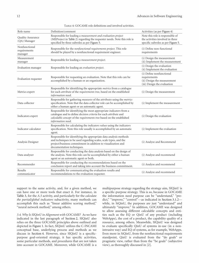
12 Advances in Software Engineering
Table 4: GOCAME role definitions and involved activities.
Role name Definition/comment Activities (as per Figure 4)
Quality Assurance(QA) Manager
Responsible for leading a measurement and evaluation project(MEProject in Table 2) regarding the requester needs. Note this role isspecified by three subroles as per Figure 5.
Note this role is responsible ofthe activities involved in threespecific subroles as per Figure 5.
Nonfunctionalrequirementsmanager
Responsible for the nonfunctional requirements project. This roleshould be played by a nonfunctional requirement engineer.
(i) Define non-functionalrequirements
Measurementmanager
Responsible for leading a measurement project.(i) Design the measurement(ii) Implement the measurement
Evaluation manager Responsible for leading an evaluation project.(i) Design the evaluation(ii) Implement the evaluation
Evaluation requesterResponsible for requesting an evaluation. Note that this role can beaccomplished by a human or an organization.
(i) Define nonfunctionalrequirements(ii) Design the measurement(iii) Design the evaluation
Metrics expertResponsible for identifying the appropriate metrics from a cataloguefor each attribute of the requirements tree, based on the establishedinformation need.
(i) Design the measurement
Data collectorResponsible for gathering measures of the attributes using the metricsspecification. Note that the data collector role can be accomplished byeither a human agent or an automatic agent.
(i) Implement the measurement
Indicators expert
Responsible for identifying the most appropriate indicators from acatalogue and to define decision criteria for each attribute andcalculable concept of the requirements tree based on the establishedinformation need.
(i) Design the evaluation
Indicator calculatorResponsible for calculating the indicators values using the indicatorsspecification. Note this role usually is accomplished by an automaticagent.
(i) Implement the evaluation
Analysis Designer
Responsible for identifying the appropriate data analysis methodsand techniques to be used regarding scales, scale types, and theproject/business commitment in addition to visualization anddocumentation techniques.
(i) Analyze and Recommend
Data analyzerResponsible for conducting the data analysis based on the design ofthe analysis. Note this role can be accomplished by either a humanagent or an automatic agent or both.
(i) Analyze and recommend
RecommenderResponsible for conducting the recommendations based on theconclusion report and taking into account the business commitment.
(i) Analyze and recommend
Resultscommunicator
Responsible for communicating the evaluation results andrecommendations to the evaluation requester.
(i) Analyze and recommend
support to the same activity, and, for a given method, wecan have one or more tools that enact it. For instance, inTable 3, for the A.5 activity, and particularly for the calculatethe partial/global indicators subactivity, many methods canaccomplish this such as “linear additive scoring method,”“neural network method,” among others.
3.4. Why Is SIQinU in Alignment with GOCAME? As we haveindicated in the last paragraph of Section 2, SIQinU alsorelies on the three GOCAME principles above outlined anddepicted in Figure 1. In fact, SIQinU utilizes the C-INCAMIconceptual base, underlying process and methods as wediscuss in Section 4. However, since SIQinU is a specific-purpose goal-oriented strategy, it has specific activities,some particular methods, and procedures that are not takeninto account in GOCAME. Moreover, while GOCAME is a
multipurpose strategy regarding the strategy aim, SIQinU isa specific-purpose strategy. This is so, because in GOCAMEthe information need purpose can be “understand,” “pre-dict,” “improve,” “control”—as indicated in Section 3.1.2—while, in SiQinU, the purposes are just “understand” andultimately “improve.” In addition, GOCAME was designedto allow assessing different calculable concepts and enti-ties such as the EQ or QinU of any product (includingWebApps), the cost of a product, the capability quality of aresource, among others. Meanwhile, SIQinU was designedto evaluate specifically QinU of systems in-use (in a non-intrusive way) and EQ of systems, as for example, WebApps.Even more in SiQinU, from the nonfunctional requirementsstandpoint, QinU is evaluated from the “do goals” orpragmatic view, rather than from the “be goals” (subjectiveview), as thoroughly discussed in [2].
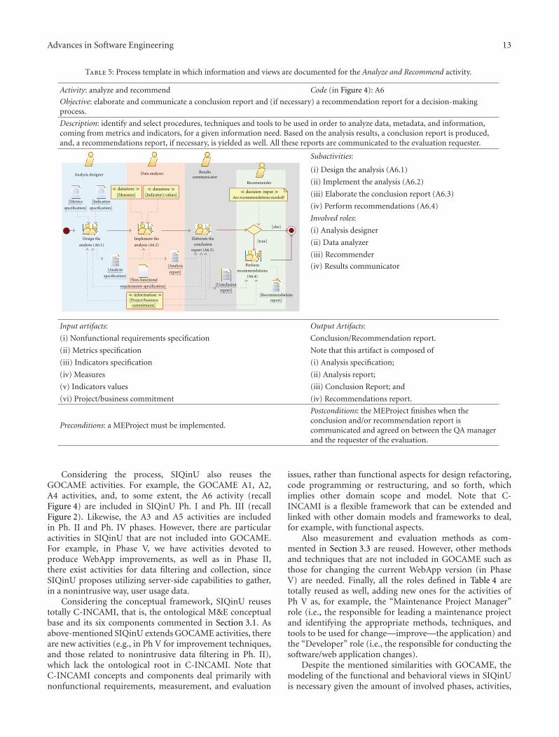
Advances in Software Engineering 13
Table 5: Process template in which information and views are documented for the Analyze and Recommend activity.
Activity: analyze and recommend Code (in Figure 4): A6
Objective: elaborate and communicate a conclusion report and (if necessary) a recommendation report for a decision-makingprocess.
Description: identify and select procedures, techniques and tools to be used in order to analyze data, metadata, and information,coming from metrics and indicators, for a given information need. Based on the analysis results, a conclusion report is produced,and, a recommendations report, if necessary, is yielded as well. All these reports are communicated to the evaluation requester.
Design the
analysis (A6.1)
Implement the
analysis (A6.2)
Elaborate the
conclusion
report (A6.3)
Perform
recommendations
(A6.4)
[Metrics
specification]
[Indicators
specification]
[Conclusion
report]
[Analysis
report]
[Non-functional
requirements specification]
[Recommendationsreport]
[Indicator’s values][Measures]
[Project/businesscommitment]
Are recommendations needed?
[Analysis
specification]
[true]
[else]
Analysis designer Data analyzer Resultscommunicator
Recommender
≪ datastore≫≪ datastore≫
≪ information≫
≪ decision input≫
Subactivities:
(i) Design the analysis (A6.1)
(ii) Implement the analysis (A6.2)
(iii) Elaborate the conclusion report (A6.3)
(iv) Perform recommendations (A6.4)
Involved roles:
(i) Analysis designer
(ii) Data analyzer
(iii) Recommender
(iv) Results communicator
Input artifacts: Output Artifacts:
(i) Nonfunctional requirements specification Conclusion/Recommendation report.
(ii) Metrics specification Note that this artifact is composed of
(iii) Indicators specification (i) Analysis specification;
(iv) Measures (ii) Analysis report;
(v) Indicators values (iii) Conclusion Report; and
(vi) Project/business commitment (iv) Recommendations report.
Preconditions: a MEProject must be implemented.
Postconditions: the MEProject finishes when theconclusion and/or recommendation report iscommunicated and agreed on between the QA managerand the requester of the evaluation.
Considering the process, SIQinU also reuses theGOCAME activities. For example, the GOCAME A1, A2,A4 activities, and, to some extent, the A6 activity (recallFigure 4) are included in SIQinU Ph. I and Ph. III (recallFigure 2). Likewise, the A3 and A5 activities are includedin Ph. II and Ph. IV phases. However, there are particularactivities in SIQinU that are not included into GOCAME.For example, in Phase V, we have activities devoted toproduce WebApp improvements, as well as in Phase II,there exist activities for data filtering and collection, sinceSIQinU proposes utilizing server-side capabilities to gather,in a nonintrusive way, user usage data.
Considering the conceptual framework, SIQinU reusestotally C-INCAMI, that is, the ontological M&E conceptualbase and its six components commented in Section 3.1. Asabove-mentioned SIQinU extends GOCAME activities, thereare new activities (e.g., in Ph V for improvement techniques,and those related to nonintrusive data filtering in Ph. II),which lack the ontological root in C-INCAMI. Note thatC-INCAMI concepts and components deal primarily withnonfunctional requirements, measurement, and evaluation
issues, rather than functional aspects for design refactoring,code programming or restructuring, and so forth, whichimplies other domain scope and model. Note that C-INCAMI is a flexible framework that can be extended andlinked with other domain models and frameworks to deal,for example, with functional aspects.
Also measurement and evaluation methods as com-mented in Section 3.3 are reused. However, other methodsand techniques that are not included in GOCAME such asthose for changing the current WebApp version (in PhaseV) are needed. Finally, all the roles defined in Table 4 aretotally reused as well, adding new ones for the activities ofPh V as, for example, the “Maintenance Project Manager”role (i.e., the responsible for leading a maintenance projectand identifying the appropriate methods, techniques, andtools to be used for change—improve—the application) andthe “Developer” role (i.e., the responsible for conducting thesoftware/web application changes).
Despite the mentioned similarities with GOCAME, themodeling of the functional and behavioral views in SIQinUis necessary given the amount of involved phases, activities,

14 Advances in Software Engineering
Figure 7: Snapshots of the C-INCAMI tool.
subactivities, and their workflows. These issues will behighlighted in the next section.
4. A Process Model View for SIQinU
Process modeling is rather a complex endeavor. Given theinherent complexity of the process domain, a process canbe modeled taking into account different views as analyzedin Section 3.2 for GOCAME. With the aim to model theSIQinU phases and activities, their inputs and outputs,sequences, parallelism, and iterations, we specify below usingUML activity diagrams and the SPEM profile [14], thefunctional view taking into account behavioral concerns aswell. Aspects of the organizational and informational viewsare to a lesser extent specified in the following diagrams,since as indicated in Section 3.4 many of the roles andartifacts are reused from the GOCAME strategy. Note that,in order to facilitate the communication, automation, andcollaboration, different modeling languages and tools can beused to specify all the views. Each has its own strengths andweaknesses, which can make it more suitable for modelingcertain views than others [12]. However, nowadays, SPEMis widely used and according to [17] can be adopted byresearchers and practitioners for different disciplines, notjust software engineering.
Also in Section 2 (Figure 2 and Table 1), we depicted theSIQinU phases, so below we concentrate on the specificationsof activities and their descriptions. In order to illustratethe SIQinU process, excerpts of a case study conducted inmid-2010 are used (see details of the case study in [8]).This case study examined JIRA (http://www.atlassian.com/),a defect reporting WebApp in commercial use in over 24,000organizations in 138 countries around the globe. JIRA’smost common task, Entering a new defect, was evaluatedin order to provide the most benefit, since entering a newdefect represents a large percentage of the total usage of theapplication. We studied 50 beginner users in a real workenvironment in their daily routine of testing software andreporting defects in a software testing department of ABC,a company (with fictitious name but real one) specializing insoftware quality and testing. The beginner users were testers
which were the majority of users. Although there are otheruser categories such as test managers, QA managers, andadministrators, testers are the predominant user type, so wechose beginner testers as our user viewpoint.
4.1. Phase I: Specify Requirements and Evaluation Criteriafor QinU. Once the requirements project has been created,using the data of the WebApp’s usage recorded in log files,we reengineer and establish QinU requirements, that is,characteristics with measurable attributes, with the objectiveof not only understanding but also improving the system-in-use with real users. From observations of the actualWebApp, this phase embraces defining user type, designingtasks, specifying usage context and dimensions for QinU(e.g., actual usability) and their attributes. Based on thesespecifications, metrics (for measurement) and indicators (forevaluation) are selected. Below we describe the seven coreactivities (see the flow in Figure 8) involved in Ph. I.
4.1.1. Establish Information Need. This activity, according tothe C-INCAMI framework (recall requirements package inFigure 3), involves Define the purpose and the user viewpoint,establish the object and the entity under study, and identifythe focus of the evaluation (see Figure 9). These activitiesare accomplished by the NFR manager role considering theevaluation requester’s needs. In the case study, the purposefor performing the evaluation is to “understand” and“improve” the WebApp being used from the userViewpointof a “beginner tester.” The category of the entity (i.e., theobject) assessed was a “defect tracking WebApp” while theentity being studied was “JIRA” (called in our study JIRA v.1).The focus (CalculableConcept) assessed is “actual usability”and its subcharacteristics, “effectiveness in use,” “efficiency inuse,” and “learnability in use” [2].
4.1.2. Specify Project Context. Once the information needspecification document is yielded, we optionally can SpecifyProject Context as shown in Figure 8. It involves the Selectrelevant Context Properties subactivity—from the organiza-tional repository of context properties [5], and, for each
Advances in Software Engineering 15
Establishinformation
need
Specify projectcontext
Selectconcept model
Design tasks
Designmeasurement
DesignevaluationDesign preliminary
analysis
[Information needspecification]
[Context specification] [Tasks/subtasks specification]
[QinU NFRtree]
[QinU metricsspecification]
[QinUindicators
specification]
[Goal/problem/risk] [Context properties] [Concept models]
[Metrics][Indicators]
[Analysis
design]
[define context]
[else]
≪ information≫ ≪ datastore ≫ ≪ datastore ≫
≪ datastore ≫≪ datastore ≫
Figure 8: Overview for the specify requirements and evaluation criteria for QinU process (Ph. I).
Establish information need
Define purpose Define userviewpoint
Establish object Establish entity Identify focus
≪Workdefinition ≫
Figure 9: Activities for establish information need.
selected property, the Quantify Context Property activitymust be performed—based on the associated metric. In theend, we get as output a context specification document forthe specific project.
4.1.3. Design Tasks. In this activity, the most common andrepresentative task or tasks should be designed. It is alsoimportant to choose a task that is performed for whichsufficient data can be collected. In our case study, the selectedtask by the evaluation requester was “entering a new defect,”as indicated above. This JIRA task included 5 subtasksspecified by the task designer, namely: (i) Summary, steps,and results; (ii) Add Detail Info; (iii) Add Environment Info;(iv) Add Version Info; (v) Add Attachment (see details oftasks and screens in [8]).
4.1.4. Select QinU Concept Model. It involves both Selecta Model and Edit the Model subactivities. Concept modelsare chosen from an organizational repository regarding the
quality focus. For example, in our case study, the NFRmanager based on the previously stated information needand taking into account the concept focus to evaluate actualusability, he instantiated a concept model for the “do goals”of the user [2]. Then, if the selected model is not totallysuitable, for example, some subcharacteristics or attributesare missing, it is necessary to Edit the Model, adding orremoving subconcepts, and/or attributes accordingly.
Finally, a requirements tree where attributes are the leavesand the concept focus is the root is yielded. For the selectedconcept model and regarding the information need andtask at hand, the NFR manager instantiated the model asshown in Table 6 (attributes are in italic). Basically, the NFRmanager, in the end, needs to satisfy the objectives of thesponsoring organization, that is, the evaluation requester.
4.1.5. Design QinU Measurement. For each attribute ofthe requirements tree—highlighted in italic in Table 6—weIdentify a Metric to quantify them. The appropriate metrics
16 Advances in Software Engineering
Table 6: Instantiated QinU NFR tree for JIRA case study.
1. Actual usability
1.1. Effectiveness in use
1.1.1. Subtask correctness
1.1.2. Subtask completeness
1.1.3. Task successfulness
1.2. Efficiency in use
1.2.1. Subtask correctness efficiency
1.2.2. Subtask completeness efficiency
1.2.3. Task successfulness efficiency
1.3. Learnability in use
1.3.1. Subtask correctness learnability
1.3.2. Subtask completeness learnability
1.3.3. Task successfulness learnability
are selected from a repository. In the C-INCAMI framework,two types of metrics are specified, a direct metric whichapplies a measurement method, that is, our data collectionprocedures from log files, and an indirect metric which usesa formula (based on other direct and/or indirect metrics)and calculation method (recall measurement package inFigure 3). If the metric is indirect, it is necessary identifyrelated metrics and identify attributes quantified by relatedMetrics (see Figure 10). These two subactivities allow identi-fying the extra attributes and metrics for the indirect metricso that data collector may later gather the data accordingly.
In the JIRA case study, the metrics used to measureattributes were selected by the metrics expert from a metriccatalogue which contains over 30 indirect metrics and theirassociated direct metrics. Below we illustrate the selectedindirect metric for the subtask completeness efficiency(coded 1.2.2 in Table 6) attribute:
Metric: average ratio of subtasks that are completedincorrectly or correctly per unit of time to do it(AvgRCput).
Interpretation: 0 <= AvgRCput, more is better.
Objective: calculate the overall average proportion ofthe subtasks that are completed, whether correct orincorrect, per time unit (usually seconds or minutes).
Calculation Method (Formula): AvgRCput =AvgRC/AvgTC
AvgRC = Average ratio of subtasks that arecompleted incorrectly or correctlyAvgTC = Average time for a complete subtask,correct or incorrect
Scale: numeric
Type of Scale: ratio
Unit (type, description): subtasks effectiveness/time,subtask completeness effectiveness per time unit(usually seconds or minutes).
As final output of these activities, we get the QinUmetrics specification document.
4.1.6. Design QinU Evaluation. Once the metric specifica-tions have been completed, we can design an indicator foreach attribute and calculable concept of the requirementstree. Taking into account the C-INCAMI framework (recallevaluation package in Figure 3), there are two indicatortypes: elementary and global indicators. The elementaryIndicators evaluate attributes and map to a new scale basedon the metric’s measures. The new scale is interpreted toanalyze the level of satisfaction reached by each attribute.On the other hand, the global indicators (also calledpartial indicator if it evaluates a subcharacteristic) evaluatecharacteristics in a concept model and serve to analyze thelevel of global (or partial) satisfaction achieved.
Following the activities flow depicted in Figure 11, foreach attribute of the requirements tree, the indicators expertshould specify an elementary indicator by means of the nextiterative activities: establish the elementary model, establish thecalculation method (optional), and identify the scale.
The first activity (establish the elementary model) involvesestablishing a function to map between measure andindicator values and define the associated decision criteriaor acceptability levels (see Section 3.1.5). In our case, theindicators expert and the evaluation requester defined threeacceptability ranges in the indicator percentage scale, namely,a value within 70–90 (a marginal—bold—range) indicatesa need for improvement actions; a value within 0–70(an unsatisfactory—italic—range) means changes must takeplace with high priority; a score within 90–100 indicatesa satisfactory level—bold italic—for the analyzed attribute.The acceptance levels in this case study were the same for allindicators, both elementary and partial/global, but could bedifferent depending on the needs of the evaluation requester.
Note that the establish the calculation method activity isnot mandatory because usually the model used is an easilyinterpreted function. In other cases, the calculation methodshould be specified.
Regarding to the partial/global indicators, these arespecified in a similar way to the elementary indicators, as wecan see in Figure 11. For example, in the JIRA case study,a global (linear additive) aggregation model to calculatethe requirements tree was selected, with equal weights fortheir elements. This approach was used given that it wasan exploratory study. Different weights would be assignedbased on the requester’s objectives to reflect the differentlevels of importance relative to one another. For example, foreffectiveness in use, some organizations may weigh mistakesor correctness more heavily than completeness dependingon the domain. A pharmacy or accounting application, forexample, may have a higher weighting for accuracy.
The final output for the QinU evaluation design isan indicators specification document for quality in use.An artifact hierarchy (i.e., the informational view) of theindicators specification document is shown in Figure 12.
4.1.7. Design Preliminary Analysis. Taking into account theunderlying SIQinU improvement objective, the specificQinU requirements for the project, the task, the metrics andindicators specifications, as well as the data properties with

Advances in Software Engineering 17
[attributes]
[QinU NFR
tree]
Identifya metric
[is indirect metric]
[QinU metrics
specification]Identify
attributes
quantified by
related metrics
Identify
related
metrics
[else]
[Metric]
[Metric]
≪ iterative≫≪ datastore ≫
Figure 10: Design QinU Measurement activity.
[QinU NFR tree]
Establish thecalculation method
Identifythe scale
Establish the
partial/global model
Establish thecalculation method
Identify
the scaleAssign values
to theparameters of
the model
Establish theelementary model
[QinU elementary
indicatorsspecification]
[QinU
partial/global
indicators
specification]
Do you want specifythe calculation method?
Do you want specify
the calculation method?
[Indicators]
[QinU metrics
specification]
[attributes]
[true]
[else]
[concepts]
[else]
[true]
≪iterative≫ ≪iterative≫
≪decision input≫ ≪decision input≫
≪ datastore≫
Figure 11: Design QinU evaluation activity.
regard to the scale, a preliminary analysis design should bedrawn by the analysis designer role. This activity involvesdeciding on the allowable mathematical and statisticalmethods and techniques for analysis regarding the scale type,dataset properties, and so forth, the suitable tools for thekinds of analysis at hand, the presentation, and visualizationmechanisms, and so forth.
4.2. Phase II: Perform QinU Evaluation and Analysis. Thisphase involves the basic activities to accomplish the firstpurpose of the SIQinU strategy, namely, understand thecurrent QinU satisfaction level of the actual WebApp in use.To achieve this, the next four activities (see Figure 13) shouldbe performed.
4.2.1. Collect Data. Taking into account the tasks specifica-tion, the log files with the user usage data are analyzed andthe relevant data is filtered and organized to facilitate themeasurement for each attribute in the next activity. Note thata tool can be used to process the log file for extracting therelevant data from user records.
4.2.2. Quantify Attributes. After collecting the data, wederive measurement values for each attribute in the QinUrequirements tree. The values are obtained based on themeasurement or calculation methods specified in QinU met-rics specification according to the design QinU measurementactivity (Figure 10).
4.2.3. Calculate Indicators. Taking into account the measures(values) and the indicators specification, the indicatorsvalues are calculated by the indicators calculator. The globalindicator value ultimately represents the degree of satisfac-tion in meeting the stated information need for a concreteentity, for a given purpose, and user viewpoint. Within thecalculate indicators activity, first, the calculate elementaryindicator activity should be performed for each attributeof the requirements tree, and then, using these indicators’values and the specified partial or global model, the partialand global indicators are calculated by performing theCalculate Partial/Global Indicator activity for each calculableconcept. Table 7, columns 2 and 3, shows each element of theQinU nonfunctional requirements tree evaluated at task level

18 Advances in Software Engineering
Elementaryindicator
specification
Indicators
specification
Partialindicator
specification
Globalindicator
specification
Scale
Scale typeunit
Decisioncriterion
specification
Name
Description
Lower threshold
Upper threshold
Elementary model
Global model
Model
Namespecification
Indicatorspecification
Nameobjective
1..∗
1..∗
Figure 12: An informational view of the QinU indicators specification document.
This activity implies
data filtering and
organization
[Parser tool]
Collect data Quantify
attributes
[Parsed
data file]
[QinU measures]
[QinU metrics
specification] [QinU indicators’ values]
Calculateindicators
[QinU NFR tree] [QinU indicatorsspecification]
Conductpreliminary
analysis
[Tasks/subtasks
specification]
[QinUpreliminary
analysisreport]
[Log files]≪ datastore ≫
≪ datastore ≫
≪ datastore ≫
Figure 13: Overview for the perform QinU evaluation and analysis phase (Ph. II).
with elementary, partial and global indicators for the currentversion of JIRA (i.e., v.1).
4.2.4. Conduct Preliminary Analysis. After calculating indi-cators at all levels, that is, elementary, partial, and global,a preliminary analysis on the current JIRA WebApp taskis conducted by the data analyzer role. Basically, it followsthe analysis design (produced in the design preliminaryanalysis activity, in Ph. I), that is, implementing the designedprocedures and planned tools, and storing results accordingto established formats in order to produce the preliminaryanalysis report. The analysis allows us to understand how theapplication performs overall (globally) and also with respect
to each particular attribute for each part of the task (i.e., atsubtask levels) being executed by a given user group type.
In the case study, the preliminary analysis was conductedfor the above-mentioned task, its five subtasks, and theirassociated screens in JIRA, for the beginner user type. Thisallows the recommender to gauge more specifically whereusers had difficulty, for example, low task successfulness, lowcompletion rate in using the application, among others.
4.3. Phase III: Derive/Specify Requirements and EvaluationCriteria for EQ. Taking into account the preliminary analysisreport yielded in Phase II for QinU and the requirementstree defined in Phase I, in Phase III, a requirements tree for
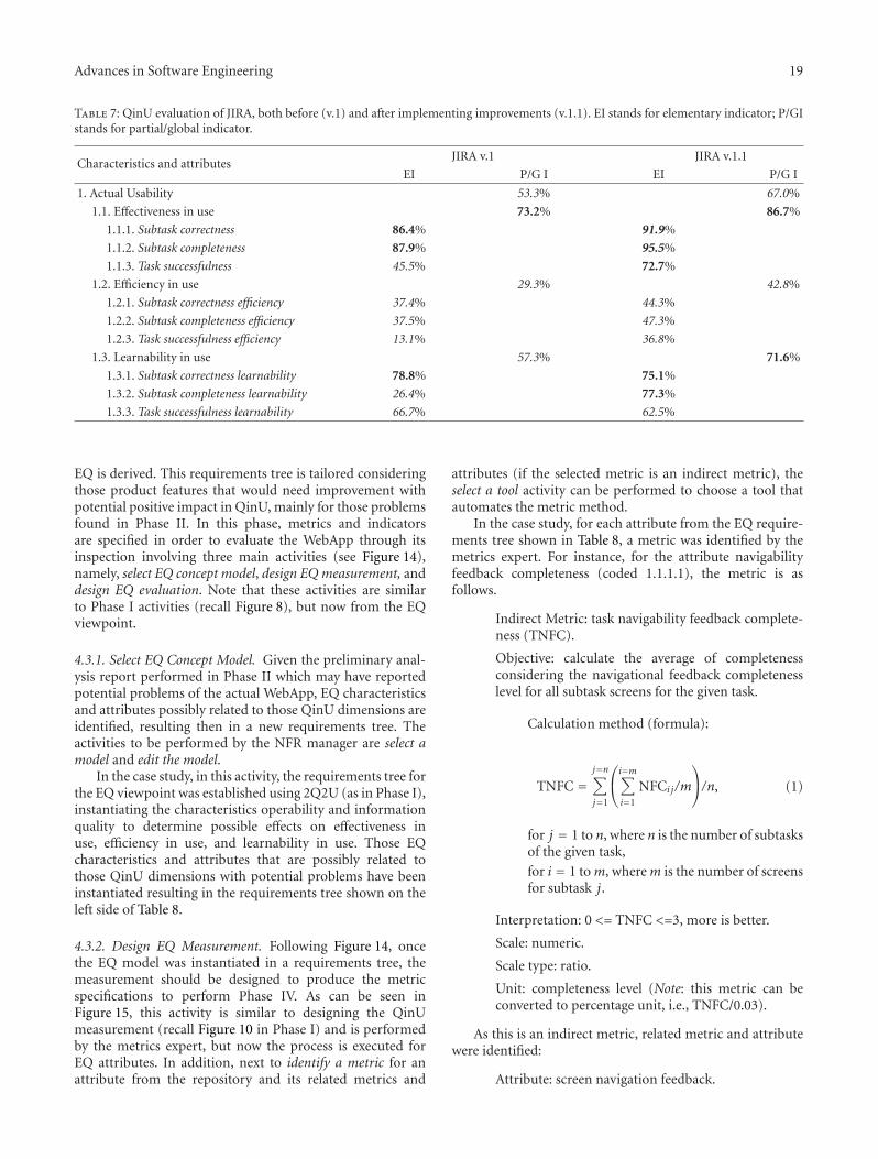
Advances in Software Engineering 19
Table 7: QinU evaluation of JIRA, both before (v.1) and after implementing improvements (v.1.1). EI stands for elementary indicator; P/GIstands for partial/global indicator.
Characteristics and attributesJIRA v.1 JIRA v.1.1
EI P/G I EI P/G I
1. Actual Usability 53.3% 67.0%
1.1. Effectiveness in use 73.2% 86.7%
1.1.1. Subtask correctness 86.4% 91.9%
1.1.2. Subtask completeness 87.9% 95.5%
1.1.3. Task successfulness 45.5% 72.7%
1.2. Efficiency in use 29.3% 42.8%
1.2.1. Subtask correctness efficiency 37.4% 44.3%
1.2.2. Subtask completeness efficiency 37.5% 47.3%
1.2.3. Task successfulness efficiency 13.1% 36.8%
1.3. Learnability in use 57.3% 71.6%
1.3.1. Subtask correctness learnability 78.8% 75.1%
1.3.2. Subtask completeness learnability 26.4% 77.3%
1.3.3. Task successfulness learnability 66.7% 62.5%
EQ is derived. This requirements tree is tailored consideringthose product features that would need improvement withpotential positive impact in QinU, mainly for those problemsfound in Phase II. In this phase, metrics and indicatorsare specified in order to evaluate the WebApp through itsinspection involving three main activities (see Figure 14),namely, select EQ concept model, design EQ measurement, anddesign EQ evaluation. Note that these activities are similarto Phase I activities (recall Figure 8), but now from the EQviewpoint.
4.3.1. Select EQ Concept Model. Given the preliminary anal-ysis report performed in Phase II which may have reportedpotential problems of the actual WebApp, EQ characteristicsand attributes possibly related to those QinU dimensions areidentified, resulting then in a new requirements tree. Theactivities to be performed by the NFR manager are select amodel and edit the model.
In the case study, in this activity, the requirements tree forthe EQ viewpoint was established using 2Q2U (as in Phase I),instantiating the characteristics operability and informationquality to determine possible effects on effectiveness inuse, efficiency in use, and learnability in use. Those EQcharacteristics and attributes that are possibly related tothose QinU dimensions with potential problems have beeninstantiated resulting in the requirements tree shown on theleft side of Table 8.
4.3.2. Design EQ Measurement. Following Figure 14, oncethe EQ model was instantiated in a requirements tree, themeasurement should be designed to produce the metricspecifications to perform Phase IV. As can be seen inFigure 15, this activity is similar to designing the QinUmeasurement (recall Figure 10 in Phase I) and is performedby the metrics expert, but now the process is executed forEQ attributes. In addition, next to identify a metric for anattribute from the repository and its related metrics and
attributes (if the selected metric is an indirect metric), theselect a tool activity can be performed to choose a tool thatautomates the metric method.
In the case study, for each attribute from the EQ require-ments tree shown in Table 8, a metric was identified by themetrics expert. For instance, for the attribute navigabilityfeedback completeness (coded 1.1.1.1), the metric is asfollows.
Indirect Metric: task navigability feedback complete-ness (TNFC).
Objective: calculate the average of completenessconsidering the navigational feedback completenesslevel for all subtask screens for the given task.
Calculation method (formula):
TNFC =j=n∑
j=1
⎛
⎝i=m∑
i=1
NFCi j /m
⎞
⎠/n, (1)
for j = 1 to n, where n is the number of subtasksof the given task,
for i = 1 to m, where m is the number of screensfor subtask j.
Interpretation: 0 <= TNFC <=3, more is better.
Scale: numeric.
Scale type: ratio.
Unit: completeness level (Note: this metric can beconverted to percentage unit, i.e., TNFC/0.03).
As this is an indirect metric, related metric and attributewere identified:
Attribute: screen navigation feedback.

20 Advances in Software Engineering
Select conceptmodel
Designmeasurement
Designevaluation
[EQ NFR tree][EQ metrics
specification]
[EQ indicators
specification]
[Concept models] [Metrics] [Indicators]
[QinU
preliminaryanalysis report]
≪ datastore ≫ ≪ datastore ≫ ≪ datastore ≫
Figure 14: Overview for the derive/specify requirements and evaluation criteria for EQ process (Ph. III).
[EQ NFR tree]
[attributes]
[EQ metrics
specification]Identify related
metrics
Identify attributes
quantified by
related metrics[Metric] [is indirect metric]
[else]
Identifya Metric
[else]
Is there a tool thatautomates the method?
Select atool
[Metrics]
[true]
≪ datastore ≫
≪ decision input ≫
≪ iterative≫
Figure 15: Activity flow involved in design external quality measurement activity.
Direct metric: navigation feedback completenesslevel (NFC).
Objective: determine the screen meets the criteriafor navigation feedback completeness. Note: Thismetric is similar to the breadcrumb or path capabilityavailable in many WebApps.
Measurement method (type: objective): the screen isinspected to determine the rating (0–3), where eval-uators through inspection observe the availability ofthe previous (backward), current, and next location(forward) mechanism. Screens should support thecompleteness of this navigation feedback.
Scale: numerical.
Scale type: ratio.
Allowed values: (0) has none; (1) has one of them; (2)has two of them; (3) has all of them.
Unit: completeness level.
4.3.3. Design EQ Evaluation. Similar to Phase I, one indicatorper each attribute and concept of the EQ requirements
tree should be identified by the indicators expert. In ourcase, when elementary, partial, and global indicators weredesigned, new acceptability ranges (DecisionCriterion inFigure 3) were agreed between the evaluation requester andthe indicators expert. The three acceptability ranges in theindicator percentage scale were as follows: a value within 60–80 (a marginal—bold—range) indicates a need for improve-ment actions; a value within 0–60 (an unsatisfactory—italic—range) means changes must take place with highpriority; a score within 80–100 indicates a satisfactorylevel—bold italic—for the analyzed attribute. Note thatthis indicator mapping does not necessarily have to be thesame as the QinU mapping (e.g., may have different rangethresholds) but rather should meet the information need andgoals of the evaluation requester.
4.4. Phase IV: Perform EQ Evaluation and Analysis. Based onmetric and indicator specifications obtained in Phase III, themeasurement and evaluation of the EQ requirements and theanalysis of the current product situation are performed. Thisphase is similar to Phase II, but now for EQ. The involved

Advances in Software Engineering 21
activities are shown in Figure 16. Note the similarity withPhase II (recall Figure 13), but, for Phase IV, the collect dataactivity is not performed, that is, it is just carried out in PhaseII to obtain user data usage from log files in a nonintrusiveway. In this phase, the measurement and evaluation activitiesare done by inspection.
Once each attribute is measured by the data collector inquantify attributes activity, and all indicators are calculatedin calculate indicators activity, the data analyzer role shouldconduct EQ analysis. The latter activity generates an EQanalysis report with information that allows us to identify,for instance, parts of the application that needs improvementfrom the EQ viewpoint. In Table 8 (columns 2 and 3),we can see the EQ evaluation results from JIRA (v.1) casestudy. Note, for example, that some attributes such aserror prevention (coded 1.2.2.1.) and context-sensitive helpavailability (coded 1.1.2.1) need improvement with highpriority. Also, we can observe that, for some elementaryindicators (attributes), no improvement is needed, forexample, stability of main control (coded 1.2.1.2).
4.5. Phase V: Recommend, Perform Improvement Actions,and Reevaluate EQ. Considering the previous EQ analysisreport generated in Conduct EQ Analysis activity (PhaseIV), we make recommendations to improve the applicationfor those EQ attributes that needed improvement. Afterthe recommended changes were completed in the currentWebApp and a new version generated, we reevaluate the EQto determine the improvement gain between both productversions. The activities for this phase are shown in Table 9and described below.
4.5.1. Recommend Improvement Actions. Based on the EQanalysis report generated in Phase IV, the recommendimprovement actions activity is carried out by the recom-mender in order to produce a recommendations report. Thisdocument has a set of recommendations for which attributesof the WebApp can be improved. For instance, a rankingof elementary indicators scored from weaker—that is, thatfell in the unsatisfactory acceptability level—to stronger, butwhich did not fall in the satisfactory or bold italic levels canbe listed.
Then, the evaluation requester can prioritize recommen-dations made for improvement action. Considering the casestudy, in this activity, some of the recommendations listed inthe recommendations report were the following:
(i) for increasing the satisfaction level of defaultsattribute (1.2.3.1) change fields to have default andmake mandatory because they are critical defectdescription correctness and completeness;
(ii) for increasing the satisfaction level of Error Preven-tion attribute (1.2.2.1) add context sensitive help andeliminate nonvalid platform combinations.
4.5.2. Design Improvement Actions. Based on the previousrecommendations report, the maintenance project manager
produces an improvement plan indicating how to actu-ally change the application. This “how” implies planningmethods and techniques to be used to actually accomplishthe improvement actions in the next activity (performimprovement actions). Methods and techniques for changingthe WebApp can range from parameterized reconfigurations,code restructuring, refactoring (as made in [18]) to archi-tectural redesign. The eventual method employed dependson the scope of the improvement recommendation as wellas the resources of the evaluation requester and the desiredeffect. The expected effect may include an application easierto operate and learn, faster to run, more secure, among manyother aspects.
For example, taking into account the two improvementrecommendations listed in the above activity, the improve-ment plan included the following.
(i) Recommendation: add context sensitive help toimprove the error prevention (1.2.2.1) attribute.Action taken: defect steps moved to next screen onadd detail info, with help, examples shown to aid user.
(ii) Recommendation: eliminate nonvalid platform com-binations to improve error prevention (1.2.2.1).Action taken: help provided and invalid combinationsnot allowed.
(iii) Recommendation: change fields to have default andmake mandatory because they are critical defectdescription correctness and completeness to improvethe defaults (1.2.3.1) attribute. Action taken: donewhere possible.
4.5.3. Perform Improvement Actions. With the improvementplan, the developer of the WebApp performs changes accord-ingly, resulting in a new application version (see the activityflow in Table 9). The ABC developer of our JIRA case studymade some of the recommended changes, including thoseshown above, resulting in a new product version termed JIRAv.1.1. This new JIRA version had many other improvementsnot shown, one of which was the reduction of workloadthrough eliminating one subtask and moving more relateditems together to make the overall task design more efficient.Thus, JIRA v.1.1 only has 4 subtasks, instead of 5. BecauseJIRA does not give access to its source code, the developercould not enact all the changes that were recommended;so only some improvements were made. Rather, throughchanging its configuration, they were able to perform mostof the changes. Note that some recommended changes thatcould not be made were due to the application under study,and not due to SIQinU.
4.5.4. Evaluate Improvement Gain. Once changes were made,the WebApp can be reevaluated by inspection to determinewhich attributes have been improved, which have not, andget a score which can be compared to the outcomes ofPhase IV. The activities involved are quantify attributes,calculate indicators, and conduct EQ analysis. The outputis a new EQ analysis report in which the changes made

22 Advances in Software Engineering
Quantifyattributes
Calculateindicators
Conductanalysis
[EQ metrics
specification]
[EQ NFR tree] [EQ indicatorsspecification]
[EQ measures]
[EQ indicators’ values]
[EQ analysis
report]
≪ datastore ≫
≪ datastore ≫
Figure 16: Overview for perform EQ evaluation and analysis phase (Ph. IV).
Table 8: EQ evaluation of JIRA, both before (v.1) and after (v.1.1) implementing improvements.
JIRA v.1 JIRA v.1.1
Characteristics and attributes EI P/G I EI P/G I
External Quality 38% 74%
1. Operability 30% 60%
1.1. Learnability 26% 59%
1.1.1. Feedback suitability 38% 38%
1.1.1.1. Navigability feedback completeness 33% 33%
1.1.1.2. Task progress feedback appropriateness 30% 30%
1.1.1.3. Entry form feedback awareness 50% 50%
1.1.2. Helpfulness 15% 80%
1.1.2.1. Context-sensitive help availability 20% 80%
1.1.2.2. Help completeness 10% 80%
1.2. Ease of use 34% 61%
1.2.1. Controllability 80% 80%
1.2.1.1. Permanence of main controls 60% 60%
1.2.1.2. Stability of main controls 100% 100%
1.2.2. Error management 0% 30%
1.2.2.1. Error prevention 0% 30%
1.2.3. Data entry ease 23% 73%
1.2.3.1. Defaults 10% 50%
1.2.3.2. Mandatory entry 10% 80%
1.2.3.3. Control appropriateness 50% 90%
2. Information quality 45% 88%
2.1. Information suitability 45% 88%
2.1.1. Consistency 40% 90%
2.1.2. Information coverage 50% 85%
2.1.2.1. Appropriateness 50% 90%
2.1.2.2. Completeness 50% 80%
between the WebApp versions are compared to determine theimprovement gain.
In Table 8 (columns 4 and 5), we can see the resultsobtained when JIRA v.1.1 was evaluated from EQ viewpoint.As can be seen from comparing the 2 evaluations (columns2 and 3 with 4 and 5), the overall partial indicator forease of use improved significantly from 34% to 61% withimprovements in many of the individual attributes and
an overall improvement in the global indicator from 38%to 74%. The next and final phase examines how theseimprovements in EQ affect QinU in a real context of use.
4.6. Phase VI: Reevaluate Quality in Use and Analyze Improve-ment Actions. Once the new application version (generatedin Phase V, particularly in perform improvement actionsactivity) has been used by the same user group type in its

Advances in Software Engineering 23
Table 9: Process template in which information and views are documented for the recommend, perform improvement actions, and reevaluateEQ activities.
Activity: recommend, perform improvement actions, and reevaluate EQ code (in Figure 2): Ph. V
Objective: improve the current application version and determine the improvement gain from the EQ standpoint.
Description: Considering the EQ analysis report generated in conduct EQ analysis activity (Phase IV), the recommender makesrecommendations to improve the current application, and the maintenance project manager produces an improvement plan to enhancethe current WebApp. After the recommended changes were implemented by the developer and a new version generated, a reevaluation ofthe EQ is performed to determine the improvement gain between both application versions.
Recommendimprovement
actions
Performimprovement
actions
Evaluateimprovement
gain
[Recommendationsreport]
[ImprovementPlan]
[EQ analysisreport]
[New EQanalysis report]
Designimprovement
actions
[Newapplication
version]
[Currentapplication
version]
It implies re-evaluation,i.e., performing again the
phase IV activities
Should improvement
action be performed
again for the product?
[true]
[else]
Recommender Maintenanceproject manager
Developer Data analyzer
≪decision input≫
Subactivities:
(i) Recommend improvement actions
(ii) Design improvement actions
(iii) Perform improvement actions
(iv) Evaluate improvement gain (i.e., in Phase IV)
Involved roles:
(i) Recommender
(ii) Maintenance project manager
(iii) Developer
(iv) Data analyzer
Input artifacts: Output artifacts:
(i) EQ analysis report (i) EQ recommendations report
(ii) Current application version (ii) Improvement plan
(iii) New application version
(iv) New EQ analysis report (from Phase IV)
Preconditions: there are EQ attributes with low level of satisfaction met, soimprovement actions are needed to enhance the current software/webapplication version.
Postconditions: the Phase V finishes when the EQattributes met the agreed satisfaction level.
same real context of use that the previous version, then,we are able to perform the QinU reevaluation (in a similarway to Phase II, recall Figure 13) to determine if what wasimproved from the EQ viewpoint had a positive quality-in-use effect using the identical tasks.
The activities involved are the same that in Phase II(see Figure 2), namely, collect data, quantify attributes andcalculate indicators. Finally, conduct improvement actionsanalysis activity is performed to determine the improvementgain and also to hypothesize EQ/QinU relationships. Theseactivities are described below according to the JIRA casestudy.
4.6.1. Collect Data, Quantify Attributes, and Calculate Indica-tors. When JIRA v.1.1 was evaluated from the EQ viewpoint,and its satisfaction level was achieved, then this new releasewas used by real users in the same real context of use as JIRAv.1. After 12 weeks (the same time period), we performedthe QinU reevaluation (using the same nonfunctionalrequirements, metrics, and indicators designed in Phase I) todetermine if what was improved from the EQ viewpoint hada positive quality-in-use effect with the same task (Enteringa new defect). Following the SIQinU activities involved inPhase VI, we collect the data (i.e., the data collector using
the same parser tool), quantify the attributes, and calculateall the indicators in a similar way as in Phase II. In Table 7,columns 4 and 5, we show the evaluation results for JIRAv.1.1.
4.6.2. Conduct Improvement Actions Analysis. Once all indi-cators were calculated, data analyzer looks at each particularattribute’s change for each part of the task being executed bythe user group noting the difference to calculate quantifiedimprovement between both WebApp versions from the QinUviewpoint. Table 10 shows the attributes and indicator valuesregarding the QinU requirements tree depicted in Table 6 forJIRA v.1 and JIRA v.1.1 with the right most columns showingthe change.
As we can see from Table 10, all attributes noted improve-ment with the exception of task successfulness learnabilityand subtask correctness learnability. A possible explanationfor this is that due to metric design with data collected over a12-week period that the learning process did not improve asmuch as expected. Remembering our earlier comments thattemporal analysis over time is important as user behaviorcan change over time, these beginning users possibly werenot able to ramp up their learning during this time period.And, on the other hand, if the case study had been longer, we
24 Advances in Software Engineering
may have seen different behavior and hence measurements.However, their negative change was small compared to thepositive changes in the other attributes resulting in an overallaverage change of attributes evaluation of 13.7%. While theindicators show that most of the attributes in JIRA v.1.1still need some or significant improvement, there has beennotable improvement from JIRA v.1. Again, as previouslymentioned, due to the limitations in changing code inJIRA, configurations changes enabled many changes andimprovements, but not all, it is possible that JIRA v.1.1 couldbe even better if more changes could be made. In otherinstances, depending on the software under evaluation, thetools/methods available to the maintenance project manager,and the time/resources available, more improvements couldbe made.
4.6.3. Develop “Depends-on” and “Influences” Relationships.A final action of Ph. VI (recall Table 1) is to develop depends-on and influences relationships between EQ improvementsand QinU, which outputs the EQ/QinU attribute relation-ship table. These come also from the “influences” and“depends-on” relationships stated in the ISO 25010 standard.Table 11 summarizes the relationships found in this firstcase study. We discovered through our EQ evaluation, thatsome attributes could be improved and lead to specificimprovements in QinU given the context of testers executingthe specific task of entering a new defect in JIRA. Incarrying out SIQinU, we were able to map EQ attributesto QinU attributes with the goal of ultimately achievingreal improvement not only for JIRA but for WebApps andsoftware design in general.
The weakness of our analysis is that we are only able tohypothesize the precise relationships between EQ and QinUattributes, but we cannot quantify the exact contributionfrom each because we made more than one change at atime. If we made only one change and then measuredQinU for JIRA v.1.1, then we could make a more precisehypothesis for a one-to-one or one-to-many relationship.Most likely, those uncovered would be one-to-many, as one-to-one relationships probably are rare in this situation.
Regarding the hypothetical EQ/QinU relationshipsfound in the JIRA case study, they can be further validatedthrough additional case studies; case studies that can becarried out using our proposed SIQinU strategy groundedon a conceptual M&E framework (C-INCAMI), processes,and methods, which ensure repeatability and consistency ofresults. By doing this, we can generalize the conclusions offound relationships, that is, whether real improvements canbe achieved not only for JIRA but for WebApps and softwaresystems in general.
On the other hand, we are aware that this paper doesnot answer, from the experimental software engineeringstandpoint, the question of the effectiveness of the proposedstrategy to accomplish similar or better objectives and resultsthan using, for example, other strategies for improvement.The JIRA case study was made in a real context of a company,where beginner testers were performing their daily task andexperts using SIQinU, as a first study. An experimental studyto compare the effectiveness of SIQinU with another strategy
should be performed as future work. Nevertheless, we canstate that SIQinU is quite scalable in terms of amount oftasks and users performing tasks, and amount of metrics andindicators as well. Once the nonfunctional requirements aredeveloped and data collection procedure is set, that is, theparser tool that filter and organize data from log files whichserve as input to get the metrics values, then any numberof metrics (and indicators) can be determined across anunlimited number of users. That is the scalability power ofthis nonintrusive strategy versus using usability observationand heuristic techniques.
5. Related Work
In recent years, the ISO/IEC has worked on a new project,called SQuaRE (Software product Quality Requirements andEvaluation), that proposes integrating many ISO standardsrelated to quality models, M&E processes, and so forth.Although ISO 25000 [19] has guidelines for the use of thenew series of standards, the documents aimed at specifyingM&E processes are not issued yet. So the standards forsoftware measurement process (ISO 15939 [20]) and theprocess for evaluators (ISO 14598-5 [21]) are still ineffect and considered the most recent. Taking into accountthese standards, the process for measurement has two coreactivities, namely, plan the measurement process and performthe measurement process [20].The evaluation process involvesfive activities: establishment of evaluation requirements, speci-fication of the evaluation, design of the evaluation, execution ofthe evaluation plan, and conclusion of the evaluation [21]. Wehave observed that there is so far no single ISO standard thatspecifies in an integrated way the M&E process and approachas a whole.
Other work, worthy to mention, is the CMMI (capabilitymaturity model integration) [22] de facto standard, whichprovides support for process areas such as measurementand analysis, among others. It aligns information needsand measurement objectives with a focus on goal-orientedmeasurement—following to some extent the GQM (goalquestion metric) [23] approach and the [20] measurementprocess. Although CMMI specifies (specific/generic) prac-tices to accomplish the given process area goals, a processmodel itself is not defined. To a certain extent, it representspractices (i.e., actions/activities) without explicitly establish-ing sequences, parallelisms, control points, and so forth.Some specific practices for measurement and analysis are forexample, establish measurement objectives, specify measures,obtain measurement data, and analyze measurement data.However, a clear distinction between M&E processes ismissing in addition to lacking a robust conceptual base forits terms.
Regarding improvement strategies for evaluation ofWebApps, we can consider the work in [18], where authorspresent an approach for incremental EQ improvementwhereby the results from EQ evaluation were used to makechanges and improvements in a WebApp through WMR(web model refactoring) in a systematic way. But althougha set of activities is considered, the underlying process is

Advances in Software Engineering 25
Table 10: QinU attributes satisfaction level for JIRA v.1 and JIRA v.1.1 with improvements.
Attributes v.1 v.1.1 Change
1.1.1. Subtask correctness 86.4% 91.9% 5.5% ↑1.1.2. Subtask completeness 87.9% 95.5% 7.6% ↑1.1.3. Task successfulness 45.5% 72.7% 27.2% ↑1.2.1. Subtask correctness efficiency 37.4% 44.3% 6.9% ↑1.2.2. Subtask completeness efficiency 37.5% 47.3% 9.8% ↑1.2.3. Task successfulness efficiency 13.1% 36.8% 23.7% ↑1.3.1. Subtask correctness learnability 78.8% 75.1% −3.7% ↓1.3.2. Subtask completeness learnability 26.4% 77.3% 50.9% ↑1.3.3. Task successfulness learnability 66.7% 62.5% −4.2% ↓
Average change 13.7%
Table 11: Summary of the influence relationships between EQ and QinU attributes.
EQ attribute QinU attribute
1.1.2.2 Operability.Learnability.Helpfulness.HelpCompleteness Learnability in Use. Subtask completeness learnability
2.1.1 Information Quality.InfoSuitability.Consistency
1.2.1.2 Operability.EaseOfUse.Controllability.StabilityMainControls Effectiveness in Use. Task Successfulness
1.1.1.2 Operability.Learnability.FeedbackSuitability.TaskProgressFeedbackAppropriateness
1.1.1.3 Operability.Learnability.FeedbackSuitability.EntryFormFeedbackAwareness
1.1.2.1 Operability.Learnability.Helpfulness.Context-sensitiveHelpAvailability
1.2.3.1 Operability.EaseOfUse.DataEntryEase.Defaults Efficiency in Use. Subtask completeness efficiency
1.2.3.2 Operability.EaseOfUse.DataEntryEase.MandatoryEntry
1.2.3.3 Operability.EaseOfUse.DataEntryEase.ControlAppropriateness
2.1.1 Information Quality.InfoSuitability.Consistency Effectiveness in Use.Subtask completeness
1.1.2.2 Operability.Learnability.Helpfulness.HelpCompleteness
1.2.2.1 Operability.EaseOfUse.Error Mgmt.Error Prevention
1.2.3.1 Operability.EaseOfUse.DataEntryEase.Defaults
1.2.3.3 Operability.EaseOfUse.DataEntryEase.ControlAppropriateness Effectiveness in Use.Sub-task correctness
2.1.2.2 Information quality.InfoSuitability.InfoCoverage.Completeness
2.1.2.2 Information quality.InfoSuitability.InfoCoverage.Appropriateness
neither well defined nor modeled regarding process views.On the other hand, in [24], a systematic approach to specify,measure, and evaluate QinU was discussed. However, theprocess used is not explicitly shown, and the outcomes wereused just for understanding the current situation of theQinU for an e-learning application, without proposing anyimprovement strategy.
With the aim of developing quality software, there areseveral works that focus on improving and controlling thedevelopment process and the intermediate products becausethe quality of the final product is strongly dependent onthe qualities of intermediate products and their respectivecreation processes. For example [25], deal with the use of asoftware project control center (SPCC) as a means for on-linecollecting, interpreting, and visualizing measurement data inorder to provide purpose- and role-oriented information toall involved parties (e.g., project manager, quality assurancemanager) during the execution of a development project. On
the other hand, in [26], the authors considered introducingusability practices into the defined software developmentprocess. With this goal in mind, authors offer to softwaredevelopers a selection of human-computer interface (HCI)techniques which are appropriate to be incorporated into adefined software process. The HCI techniques are integratedinto a framework organized according to the kind of softwareengineering activities in an iterative development wheretheir application yields a higher usability improvement. Also,in the usability field, in [27], authors explore how someopen source projects address issues of usability and describethe mechanisms, techniques, and technology used by opensource communities to design and refine the interfacesto their programs. In particular, they consider how thesedevelopers cope with their distributed community, lack ofdomain expertise, limited resources, and separation fromtheir users. However, in SIQinU, we start identifying prob-lems in systems in-use, that is, with running applications
26 Advances in Software Engineering
used by real users in a real context. Therefore, SIQinU isnot focused on early stages of the development process buton how we can understand the current application-in-use’sQinU and how we can change the attributes of a softwaresystem to improve its QinU.
Taking into account the complexity of processes, in [28],authors propose the use of an electronic process guide toprovide a one-off improvement opportunity through thebenefits of declaring a defined, systematic, and repeatableapproach to software development. An electronic processguide offers several advantages over a printed processhandbook, including easy access over the web for the mostup-to-date version of the guide, electronic search facilitiesand hypernavigation to ease browsing information. In thiswork, authors combine the electronic process guide with theexperience management, which refers to approaches to struc-ture and store reusable experiences. It aims at reducing theoverhead of information searching that can support softwaredevelopment activities. Experience management also appearsto be more effective when it is process centric. Thus, the twoconcepts have a symbiotic relationship in that the processguide is more useful when supported by experiences and theexperience base is more useful when it is process focused. Theelectronic process guide/experience repository (EPG/ER) isan implementation of this relationship and supports usersthrough provision of guidance that is supplemented bytask-specific experiences. However, our process specificationis devoted specifically to represent the different views (asproposed in [10]) for measurement and evaluation activitiesrather than software development activities.
Regarding integrated strategies for M&E, it is worthy tomention the GQM+ Strategies [29]—which are based onthe GQM approach—as an approach that allows definingand assessing measurement goals at different organizationlevels, but it does not specify formal process views to conductthe evaluation and improvement lifecycle as we have shownas an integral component of SiQinU. Also, since issued,the GQM model was at different moments enlarged withproposals of processes and methods. However, [30] pointedout GQM is not intended to define metrics at a level of detailsuitable to ensure that they are trustworthy, in particular,whether or not they are repeatable. Moreover, an interestingGQM enhancement, which considers indicators, has recentlybeen issued as a technical report [31]. This approach usesboth the balanced scorecard and the goal-question-indicator-measurement methods, in order to purposely derive therequired enterprise goal-oriented indicators and metrics. Itis a more robust approach for specifying enterprise-wideinformation needs and deriving goals and subgoals and thenoperationalizing questions with associated indicators andmetrics. However, this approach is not based on a soundontological conceptualization of metrics and indicators as inour research. Furthermore, the terms “measure” and “indi-cator” are sometimes used ambiguously, which inadvertentlycan result in datasets and metadata recorded inconsistently,and so it cannot assure that measurement values (and theassociated metadata like metric version, scale, scale type,unit, measurement method, etc.) are trustworthy, consistent,and repeatable for further analysis among projects.
Finally, in [32], authors propose the CQA approach,consisting of a methodology (CQA-Meth) and a tool thatimplements it (CQA-Tool). They have applied this approachin the evaluation of the quality of UML models such asuse cases, class, and statechart diagrams. Also authors haveconnected CQA-Tool to the different tools needed to assessthe quality of models. CQA-Tool, apart from implementingthe methodology, provides the capacity for building a cata-logue of evaluation techniques that integrates the evaluationtechniques (e.g., metrics, checklists, modeling conventions,guidelines, etc.), which are available for each softwareartifact. Compared with our strategies, the CQA approachlacks for instance an explicit conceptual framework from aterminological base. On the other hand, other related work inwhich authors try to integrate strategic management, processimprovement, and quantitative measurement for managingthe competitiveness of software engineering organizationsis documented in [33]. In this work, a process template tospecify activities from different views is considered. However,the integration of the three capabilities as made in GOCAMEand SIQinU is not explicit and formalized.
6. Concluding Remarks
Ultimately, the main contribution of this paper is SIQinU,an integrated specific-purpose strategy—that is, for under-standing and improving QinU—whose rationale is based onwell-defined M&E processes, founded on a M&E conceptualframework backed up by an ontological base, and supportedby methods and tools.
In this paper, we have specified the process of theSIQinU strategy modeled stressing the functional, informa-tional, organizational, and behavioral views. Moreover, toillustrate the SIQinU process, excerpts from a JIRA casestudy were used where real users were employed to collectdata and ultimately prove the usefulness of the strategy inimproving the application in a process-oriented systematicmeans. We have also shown SIQinU, to be a derivation ofGOCAME, based on three foundations, namely, the process,the conceptual framework, and methods/tools. Relying onthe GOCAME foundation, SIQinU has been defined as asystematic approach with the appropriate recorded metadataof concrete projects’ information needs, context proper-ties, attributes, metrics, and indicators. This ensures thatcollected data are repeatable and comparable among theorganization’s projects. Otherwise, analysis, comparisons,and recommendations can be made in a less robust, noncon-sistent, or even incorrect way.
SIQinU, although reusing the general principles ofGOCAME, is a specific-purpose goal-oriented strategy withspecific activities and methods that are not taken intoaccount in GOCAME. Where GOCAME is a multipurposestrategy with general purposes such as “understand,” “pre-dict,” “improve,” and “control,” SiQinU objectives are tar-geted to “understand” and ultimately “improve.” In addition,as discussed in Section 3.4, SIQinU was specifically designedto evaluate QinU and EQ for WebApps, from the “do goals”perspective rather than from the “be goals.”

Advances in Software Engineering 27
As future work, we are planning to extend SIQinU toinclude processes and methods not only to gather data ina nonintrusive way (as currently it does) but also to gatherdata using more traditional intrusive methods such as videorecording, observations, and questionnaires. This could notonly help to add robustness to Phase III particularly in thederivation process from QinU problems to EQ attributes butalso supplement the analysis in Phase II and VI.
Acknowledgment
This work and line of research is supported by the PAE2007 PICT 2188 project at UNLPam, from the Science andTechnology Agency, Argentina.
References
[1] ISO/IEC CD 25010.3. Systems and software engineering.Systems and software Quality Requirements and Evaluation(SQuaRE). System and software quality models, 2009.
[2] P. Lew, L. Olsina, and L. Zhang, “Quality, quality in use, actualusability and user experience as key drivers for web applicationevaluation,” in Proceedings of the 10th International Conferenceon Web Engineering (ICWE ’10), vol. 6189 of Lecture Notesin Computer Science, pp. 218–232, Springer, Vienne, Austria,2010.
[3] N. Bevan, “Extending quality in use to provide a frameworkfor usability measurement,” in Proceedings of the 1st Interna-tional Conference on Human Centered Design (HCD ’09), vol.5619 of Lecture Notes in Computer Science, pp. 13–22, Springer,San Diego, Calif, USA, 2009.
[4] L. Olsina, F. Papa, and H. Molina, “How to measure andevaluate web applications in a consistent way,” in WebEngineering: Modeling and Implementing Web Applications,G. Rossi, O. Pastor, D. Schwabe, and L. Olsina, Eds., HCIS,chapter 13, pp. 385–420, Springer, London, UK, 2008.
[5] H. Molina and L. Olsina, “Assessing web applications consis-tently: a context information approach,” in Proceedings of the8th International Conference on Web Engineering (ICWE ’08),pp. 224–230, Yorktown Heights, NJ, USA, July 2008.
[6] P. Becker, H. Molina, and L. Olsina, “Measurement and eval-uation as quality driver,” Journal ISI (Ingenierie des Systemesd’Information), vol. 15, no. 6, pp. 33–62, 2010.
[7] L. Olsina and G. Rossi, “Measuring Web application qualitywith WebQEM,” IEEE Multimedia, vol. 9, no. 4, pp. 20–29,2002.
[8] P. Lew, L. Olsina, P. Becker, and L. Zhang, “An integratedstrategy to understand and manage quality in use for webapplications,” Requirements Engineering Journal, vol. 16, no. 3,2011.
[9] E. Mendes, “The need for empirical web engineering: anIntroduction,” in Web Engineering: Modelling and Implement-ing Web Applications, G. Rossi, O. Pastor, D. Schwabe, andL. Olsina, Eds., HCIS, chapter 14, pp. 421–447, Springer,London, UK, 2008.
[10] B. Curtis, M. Kellner, and J. Over, “Process modelling,”Communications of the ACM, vol. 35, no. 9, pp. 75–90, 1992.
[11] L. Olsina, “Applying the flexible process model to buildhypermedia products,” in Proceedings of the Hypertext andHypermedia: Tools, Products, Methods (HHTPM ’97), pp. 211–221, Hermes Ed., Paris, France, 1997.
[12] S. Acuna, N. Juristo, A. Merona, and A. Mon, A SoftwareProcess Model Handbook for Incorporating People’s Capabilities,Springer, 1st edition, 2005.
[13] UML.Unified Modeling Language Specification, Version 2.0.Document/05-07-04, 2004.
[14] SPEM. Software Process Engineering Metamodel Specifica-tion. Doc./02-11-14., Ver.1.0, 2002.
[15] P. Becker, P. Lew, and L. Olsina, “Strategy to improve qualityfor software applications: a process view,” in Proceedings of theInternational Conference of Software and System Process (ICSSP’11), pp. 129–138, ACM, Honolulu, Hawaii, USA, 2011.
[16] N. E. Fenton and S. L. Pfleeger, Software Metrics: a Rigorousand Practical Approach, PWS Publishing Company, 2ndedition, 1997.
[17] F. Garcıa, A. Vizcaino, and C. Ebert, “Process managementtools,” IEEE Software, vol. 28, no. 2, pp. 15–18, 2011.
[18] L. Olsina, G. Rossi, A. Garrido, D. Distante, and G. Canfora,“Web applications refactoring and evaluation: a quality-oriented improvement approach,” Journal of Web Engineering,Rinton Press, US, vol. 7, no. 4, pp. 258–280, 2008.
[19] ISO/IEC 25000. Software Engineering—Software productQuality Requirements and Evaluation (SQuaRE)—Guide toSQuaRE, 2005.
[20] ISO/IEC 15939. Software Engineering—Software Measure-ment Process, 2002.
[21] ISO/IEC 14598-5. International Standard, Informationtechnology—Software product evaluation—Part 5: processfor evaluators, 1999.
[22] CMMI Product Team. CMMI for Development Version 1.3(CMMI-DEV, V.1.3) CMU/SEI-2010-TR-033, SEI Carnegie-Mellon University, 2010.
[23] R. Basili, G. Caldiera, and H. D. Rombach, “The goal questionmetric approach,” in Encyclopedia of Software Engineering, J. J.Marciniak, Ed., vol. 1, pp. 528–532, John Wiley & Sons, 1994.
[24] G. Covella and L. Olsina, “Assessing quality in use in aconsistent way,” in Proceedings of the International Conferenceon Web Engineering (ICWE ’06), pp. 1–8, ACM, San Francisco,Calif, USA, July 2006.
[25] J. Munch and J. Heidrich, “Software project control centers:concepts and approaches,” Journal of Systems and Software, vol.70, no. 1-2, pp. 3–19, 2004.
[26] X. Ferre, N. Juriste, and A. M. Moreno, “Framework forintegrating usability practices into the software process,” inProceedings of the 6th International Conference on ProductFocused Software Process Improvement (PROFES ’05), vol. 3547of Lecture Notes in Computer Science, pp. 202–215, Springer,2005.
[27] D. M. Nichols and M. B. Twidale, “Usability processes in opensource projects,” Software Process Improvement and Practice,vol. 11, no. 2, pp. 149–162, 2006.
[28] F. Kurniawati and R. Jeffery, “The use and effects of an elec-tronic process guide and experience repository: a longitudinalstudy,” Information and Software Technology, vol. 48, no. 7, pp.566–577, 2006.
[29] V. R. Basili, M. Lindvall, M. Regardie et al., “Linking softwaredevelopment and business strategy through measurement,”Computer, vol. 43, no. 4, pp. 57–65, 2010.
[30] B. A. Kitchenham, R. T. Hughes, and S. G. Linkman,“Modeling software measurement data,” IEEE Transactions onSoftware Engineering, vol. 27, no. 9, pp. 788–804, 2001.
[31] W. Goethert and M. Fisher, Deriving Enterprise-Based Mea-sures Using the Balanced Scorecard and Goal-Driven Mea-surement Techniques. Software Engineering Measurementand Analysis Initiative, CMU/SEI-2003-TN-024, 2003.

28 Advances in Software Engineering
[32] M. Rodrıguez, M. Genero, D. Torre, B. Blasco, and M. Piattini,“A methodology for continuos quality assessment of softwareartefacts,” in Proceedings of the 10th International Conferenceon Quality Software (QSIC ’10), pp. 254–261, Zhangjiajie,China, July 2010.
[33] J. G. Guzman, H. Mitre, A. Seco, and M. Velasco, “Integrationof strategic management, process improvement and quan-titative measurement for managing the competitiveness ofsoftware engineering organizations,” Software Quality Journal,vol. 18, no. 3, pp. 341–359, 2010.

Hindawi Publishing CorporationAdvances in Software EngineeringVolume 2012, Article ID 642983, 12 pagesdoi:10.1155/2012/642983
Research Article
Program Spectra Analysis with Theory of Evidence
Rattikorn Hewett
Department of Computer Science, Texas Tech University, Lubbock, TX 79409-3104, USA
Correspondence should be addressed to Rattikorn Hewett, [email protected]
Received 30 August 2011; Revised 4 January 2012; Accepted 8 January 2012
Academic Editor: Chin-Yu Huang
Copyright © 2012 Rattikorn Hewett. This is an open access article distributed under the Creative Commons Attribution License,which permits unrestricted use, distribution, and reproduction in any medium, provided the original work is properly cited.
This paper presents an approach to automatically analyzing program spectra, an execution profile of program testing results for faultlocalization. Using a mathematical theory of evidence for uncertainty reasoning, the proposed approach estimates the likelihoodof faulty locations based on evidence from program spectra. Our approach is theoretically grounded and can be computedonline. Therefore, we can predict fault locations immediately after each test execution is completed. We evaluate the approachby comparing its performance with the top three performing fault localizers using a benchmark set of real-world programs. Theresults show that our approach is at least as effective as others with an average effectiveness (the reduction of the amount of codeexamined to locate a fault) of 85.6% over 119 versions of the programs. We also study the quantity and quality impacts of programspectra on our approach where the quality refers to the spectra support in identifying that a certain unit is faulty. The results showthat the effectiveness of our approach slightly improves with a larger number of failed runs but not with a larger number of passedruns. Program spectra with support quality increases from 1% to 100% improves the approach’s effectiveness by 3.29%.
1. Introduction
Identifying location of faulty software is notoriously knownto be among the most costly and time-consuming processin software development [1, 2]. As software gets larger andmore complex, the task can be daunting even with the helpof debugging tools. Over the decades, many approaches tosoftware fault localization have been studied including diag-nostic reasoning [3], program slicing [4], nearest neighbor[5], and statistical analysis [6, 7].
Recent fault localization techniques have focused onautomatically analyzing program behaviors observed fromthe execution of a suite of test cases on the tested programcalled program spectra [8]. For each run of the test case,certain program units (e.g., statements or blocks of code) areexecuted and result in either a passed test (run, or execution)when the output of the program’s execution is the same asthe expected output, or a failed test, otherwise. A collectionof program spectra contains execution profiles that indicatewhich part of the program is involved in each test run andwhether it is passed or failed.
Spectrum-based fault localization basically tries to iden-tify the part of the program whose activity correlates most
with the resulting passed or failed test runs. Most existingspectrum-based approaches rely on similarity measures tolocate faulty software units by identifying the units thatmost resemble the spectra error outcomes [9–15]. Thetechnique has been used for fault localization in variousapplications including the Pinpoint tool [12] for largedynamic online transaction processing systems and AMPLE[16] for objected-oriented software. Spectrum-based faultlocalization is relatively efficient to compute and doesnot require modeling of the program under investigation.Therefore, it is a popular fault localization technique that caneasily be integrated into testing procedures [10].
The current top three performing spectrum-based faultlocalizers include Ochiai [14], Jaccard [12], and Tarantula[13]. Tarantula uses a heuristic function adapted from avisualization technique while Jaccard and Ochiai employdifferent similarity measures, both of which are widely usedin other domains such as biology and ecology. While theseapproaches are useful, most lack theoretical foundation andthe ability to immediately incorporate new testing resultsinto the fault localization process. Furthermore, they are noteasily extensible to new findings of contributing factors. Ourresearch aims to alleviate these shortcomings.

2 Advances in Software Engineering
This paper presents a spectrum-based fault localiza-tion technique for pinpointing locations of faulty softwareunits. The approach employs the theory of evidence calledDempster-Shafer Theory [17] for uncertainty reasoningto estimate the likelihood of faulty locations based onevidence gathered from program spectra. Our approachis theoretically grounded and computed online instead ofbatch. Thus, it allows the prediction of fault locations to beidentified immediately as the execution of each test case iscompleted without having to wait to collect a set of programspectra that is large enough to be statistically valid. Ourcontribution also includes a study of the influences of thetheory of evidence on fault localization effectiveness as wellas the influences of the quantity and quality of the programspectra used in the analysis.
The rest of the paper is organized as follows: Section 2describes preliminary concepts and terminology includingbasic mechanisms for software fault localization, the threespectrum-based fault localizers used in our comparisonstudy, and the Dempster-Shafer Theory along with itsfundamental elements. Section 3 presents our approach toprogram spectra analysis, an illustration on a small exampleprogram, and some characteristic comparisons. Section 4evaluates the proposed technique and discusses the empiricalstudy using a set of standard benchmarks to compare theproposed method against the other three prominent softwarefault localizers. Section 5 presents an empirical study toanswer questions whether the performance of the proposedapproach relies on the quality or quantity of the programspectra or not. Section 6 discusses the work related to faultlocalization and the method proposed in this paper. Section 7concludes the paper.
2. Preliminaries
This section describes terms, concepts of spectrum-basedfault localization technique, the three fault localizers and thebasic foundations of the mathematical theory of evidence.
2.1. Concepts, Terms, and Notations. Following the terminol-ogy in [10], a software failure occurs when the actual programoutput, for a given input, deviates from the correspondingspecified output. Software errors, however, define defects thatmay or may not cause a failure. Thus, in practice, we may notbe able to detect all errors. Defects that result in failures arereferred to as software faults (or bugs).
Program spectra [8] are execution profiles of the programresulting from test runs. In particular, suppose we run m testcases on a program of n units (e.g., statements, blocks, andmodules). The hit spectra can be represented as an m × nmatrix R = (ri j), where ri j = 1 if test i involves execution ofunit j of the program, otherwise it is 0 (i.e., if test i does notinvolve execution of unit j). In addition, for each run of testi, we define a corresponding error ei to be 1 if the test failed,and 0, otherwise (i.e., when the test was passed or successful).Program spectra include both the hit spectra and the error.To collect program spectra, we run a suite of test cases andobserve execution results where the test can be performed at
Table 1: Different types of test run frequency count.
Software UnitTest run
Passed Failed
Not Executed a00 a01
Executed a10 a11
various levels of software units (e.g., code lines or statements,blocks of code, or modules). Much research has studied faultlocalization in code blocks [9, 15]. Though we illustrate ourapproach at a code statement (or line) level, the approach isgeneral for application in any level of software unit.
Conceptually, fault localization is an attempt to identifya software unit whose behaviors in all relevant test casesare most similar to the errors observed in a given programspectra. To do this, the following notations are defined. For agiven test run i and a software unit j, let p and q be a binaryvariable signifying whether run i involves execution of unit j,and, respectively, whether run i fails or not. Here p is 1 if runi involves execution of unit j, and 0, otherwise. On the otherhand, q is 1 if run i fails and 0, otherwise. Next we relate pand q to observations in the program spectra.
For each software unit j, we define the frequency of runsapq( j) = |{i | ri j = p, ei = q}|. Recall that ri j representsthe result of test run i on unit j (whether it executes unit j ornot), and ei represents the output error of test run i (whetherthe test is passed or failed). Thus, for a given software unit,we can summarize the interpretations of all possible cases ofapq’s in Table 1. For example, a01( j) represents the numberof failed test runs (i.e., q = 1) that did not execute (i.e.,p = 0) unit j. Note that in general a00( j) is not of interestto fault localization since a successful test run that does notinvolve the execution of the software unit does not provideany useful information for detecting faults. It does not raiseany suspicion that the unit under investigation is faulty nordoes it confirm that it is not faulty. On the other hand, a11( j)is an important indicator for identifying faulty units.
2.2. Spectrum-Based Fault Localizers. In spectrum-basedfault localization techniques, software units are ranked basedon their corresponding similarity coefficients (e.g., see [5,10]). A similarity coefficient of a software unit measureshow closely the execution runs of the test cases that involvethe considering unit resemble the errors observed [9]. Thesoftware unit that has a high similarity to the output errorsis assumed to have a high probability that the unit would bethe cause of such errors. Thus, a unit with a larger similarity-coefficient value would rank higher in terms of its chance tobe faulty. Let Si denote a similarity coefficient for softwareunit i.
Next we describe the current top three fault localizersthat mainly differ by the similarity coefficient Si. A popularTarantula [13] has been shown to be the best performingspectrum-based fault localizer in [18]. Abreu et al. [9] haverecently shown that the Jaccard coefficient [12] and Ochiaicoefficient [14] marginally outperform Tarantula. Mostsimilarity coefficients utilize the frequency of occurrences of
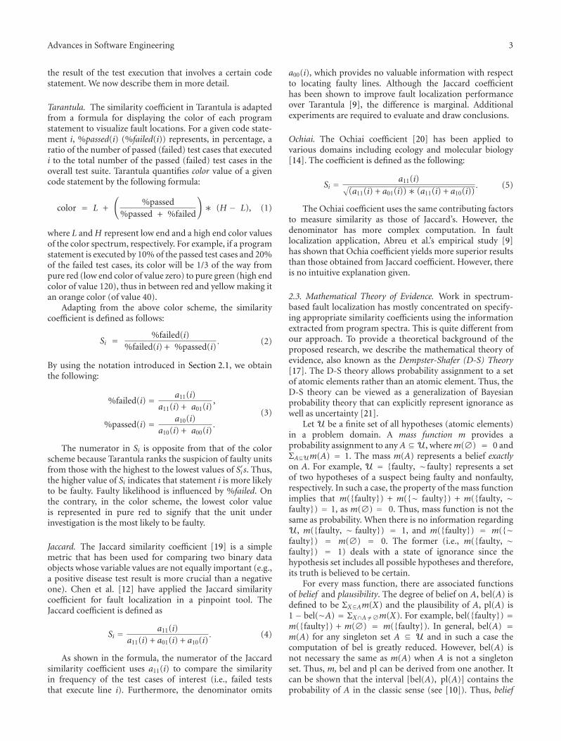
Advances in Software Engineering 3
the result of the test execution that involves a certain codestatement. We now describe them in more detail.
Tarantula. The similarity coefficient in Tarantula is adaptedfrom a formula for displaying the color of each programstatement to visualize fault locations. For a given code state-ment i, %passed(i) (%failed(i)) represents, in percentage, aratio of the number of passed (failed) test cases that executedi to the total number of the passed (failed) test cases in theoverall test suite. Tarantula quantifies color value of a givencode statement by the following formula:
color = L +
(%passed
%passed + %failed
)
∗ (H − L), (1)
where L and H represent low end and a high end color valuesof the color spectrum, respectively. For example, if a programstatement is executed by 10% of the passed test cases and 20%of the failed test cases, its color will be 1/3 of the way frompure red (low end color of value zero) to pure green (high endcolor of value 120), thus in between red and yellow making itan orange color (of value 40).
Adapting from the above color scheme, the similaritycoefficient is defined as follows:
Si = %failed(i)%failed(i) + %passed(i)
. (2)
By using the notation introduced in Section 2.1, we obtainthe following:
%failed(i) = a11(i)a11(i) + a01(i)
,
%passed(i) = a10(i)a10(i) + a00(i)
.(3)
The numerator in Si is opposite from that of the colorscheme because Tarantula ranks the suspicion of faulty unitsfrom those with the highest to the lowest values of S′i s. Thus,the higher value of Si indicates that statement i is more likelyto be faulty. Faulty likelihood is influenced by %failed. Onthe contrary, in the color scheme, the lowest color valueis represented in pure red to signify that the unit underinvestigation is the most likely to be faulty.
Jaccard. The Jaccard similarity coefficient [19] is a simplemetric that has been used for comparing two binary dataobjects whose variable values are not equally important (e.g.,a positive disease test result is more crucial than a negativeone). Chen et al. [12] have applied the Jaccard similaritycoefficient for fault localization in a pinpoint tool. TheJaccard coefficient is defined as
Si = a11(i)a11(i) + a01(i) + a10(i)
. (4)
As shown in the formula, the numerator of the Jaccardsimilarity coefficient uses a11(i) to compare the similarityin frequency of the test cases of interest (i.e., failed teststhat execute line i). Furthermore, the denominator omits
a00(i), which provides no valuable information with respectto locating faulty lines. Although the Jaccard coefficienthas been shown to improve fault localization performanceover Tarantula [9], the difference is marginal. Additionalexperiments are required to evaluate and draw conclusions.
Ochiai. The Ochiai coefficient [20] has been applied tovarious domains including ecology and molecular biology[14]. The coefficient is defined as the following:
Si = a11(i)√
(a11(i) + a01(i))∗ (a11(i) + a10(i)). (5)
The Ochiai coefficient uses the same contributing factorsto measure similarity as those of Jaccard’s. However, thedenominator has more complex computation. In faultlocalization application, Abreu et al.’s empirical study [9]has shown that Ochia coefficient yields more superior resultsthan those obtained from Jaccard coefficient. However, thereis no intuitive explanation given.
2.3. Mathematical Theory of Evidence. Work in spectrum-based fault localization has mostly concentrated on specify-ing appropriate similarity coefficients using the informationextracted from program spectra. This is quite different fromour approach. To provide a theoretical background of theproposed research, we describe the mathematical theory ofevidence, also known as the Dempster-Shafer (D-S) Theory[17]. The D-S theory allows probability assignment to a setof atomic elements rather than an atomic element. Thus, theD-S theory can be viewed as a generalization of Bayesianprobability theory that can explicitly represent ignorance aswell as uncertainty [21].
Let U be a finite set of all hypotheses (atomic elements)in a problem domain. A mass function m provides aprobability assignment to any A ⊆U, where m(∅) = 0 andΣA⊆Um(A) = 1. The mass m(A) represents a belief exactlyon A. For example, U = {faulty, ∼ faulty} represents a setof two hypotheses of a suspect being faulty and nonfaulty,respectively. In such a case, the property of the mass functionimplies that m({faulty}) + m({∼ faulty}) + m({faulty, ∼faulty}) = 1, as m(∅) = 0. Thus, mass function is not thesame as probability. When there is no information regardingU, m({faulty, ∼ faulty}) = 1, and m({faulty}) = m({∼faulty}) = m(∅) = 0. The former (i.e., m({faulty, ∼faulty}) = 1) deals with a state of ignorance since thehypothesis set includes all possible hypotheses and therefore,its truth is believed to be certain.
For every mass function, there are associated functionsof belief and plausibility. The degree of belief on A, bel(A) isdefined to be ΣX⊆Am(X) and the plausibility of A, pl(A) is1 − bel(∼A) = ΣX∩A /=∅m(X). For example, bel({faulty}) =m({faulty}) + m(∅) = m({faulty}). In general, bel(A) =m(A) for any singleton set A ⊆ U and in such a case thecomputation of bel is greatly reduced. However, bel(A) isnot necessary the same as m(A) when A is not a singletonset. Thus, m, bel and pl can be derived from one another. Itcan be shown that the interval [bel(A), pl(A)] contains theprobability of A in the classic sense (see [10]). Thus, belief

4 Advances in Software Engineering
and probability are different measures. In this paper, we usethe terms likelihood and belief synonymously.
A mass function can be combined using various rulesincluding the popular Dempster’s Rule of Combination, whichis a generalization of the Bayes rule. For X ,A,B ⊆ U, acombination rule of mass functions m1 and m2, denoted bym1 ⊕m2 (or m1,2) is defined as the following:
m1,2(X) = m1 ⊕m2(X) =∑
A∩B=X m1(A)m2(B)1− K
, (6)
where K = ΣA∩B=∅m1(A)m2(B) and m1 ⊕m2(∅) = 0.The combination rule can be applied in pairs repeatedly
to obtain a combination of multiple mass functions. Theabove rule strongly emphasizes the agreement betweenmultiple sources of evidence and ignores the disagreementby the use of a normalization factor.
3. Proposed Approach
By exploiting program spectra, the proposed approach to theway an automated fault localizer builds on the concepts ofDempster-Shafer theory will be described. Section 3.1 dis-cusses the formulation of mass functions, which are our maincontributions. Section 3.2 discusses some characteristics ofdifferent fault localizers and how the proposed approach canbe extended. Section 3.3 illustrates the approach in a smallexample along with intuitive justifications.
3.1. Mass Functions and Combination Rule. Mass functionsare essential elements in estimating the likelihood of thecode statement being faulty based on evidences from theprogram spectra described in Section 2. For any statement jof a tested program, let U j = { f j , ∼ f j}, where f j representsthe hypothesis that j is faulty and similarly,∼ f j for nonfaulty.For each test run, we are concerned with whether the test wassuccessful or not and what code statements were executedduring the test. There are two possibilities.
Case 1 (failed test). A failed test that involves the execution ofthe statement under investigation is evidence that supportsthat the statement is likely to be faulty. In such a case, thelikelihood of the statement being nonfaulty is zero. On theother hand, its likelihood of being faulty can be estimated bya ratio of one over the total number of statements involvedin this test run. We can formulate this formally as follows
Recall that in the program spectra, ri j = 1 if test i involvesexecution of unit j of the program, and it is 0, otherwise.Thus, a total number of units executed in test run i can berepresented by Σ j ri j . We now define mi, the mass functionof failed test i for all possible nonempty subsets of thehypotheses in U j as follows:
mi
({∼ f j
})= 0, (7)
mi
({f j})= α ∗
(ri jΣ j ri j
)
, where 0 < α ≤ 1, (8)
mi
(U j
)= 1−mi
({f j})
. (9)
The third equation is derived from the property thatm(∅) = 0 and ΣA⊆Um(A) = 1. Based on the secondequation, it should be easy to see that the likelihood of astatement being faulty can only be influenced by the (failed)test that executes that statement. The parameter α is anadjusted value that represents the strength of the propertyof “failed test” in determining if statement j is faulty.
Case 2 (passed test). If a test involving the execution ofthe statement in question is successful, it is evidence thatsupports that this statement behaves correctly. Thus, thelikelihood of it being faulty is zero. On the other hand, thelikelihood of this statement being correct (i.e., nonfaulty)can be estimated by a ratio of one over the total numberof statements involved in this test run. We now define mi,the mass function of passed test i for all possible nonemptysubsets of the hypotheses in U j as follows:
mi
({f j})= 0, (10)
mi
({∼ f j
})= β ∗
(ri jΣ j ri j
)
where 0 < β ≤ 1, (11)
mi
(U j
)= 1− mi
({∼ f j
}). (12)
It should be easy to see that in this case the likelihoodof a statement being correct can only be influenced bythe (successful) test that executes it. Analogous to α, theparameter β is an adjusted value that represents the strengthof the property of “passed test” in determining if statement jis not faulty.
In general, the appropriate values of the adjusted valuesα and β are determined empirically since they are likely todepend on the size of the program, the number of testsand the ratios of failed to passed tests (see an example inSection 3.3). The more precision the values of α and β are, themore likely we can discriminate faulty belief values amonga large number of software units. In this paper, α and βare estimated conservatively to one and 0.0001, respectively,in order to yield a sufficient power of discrimination for avery large program. The intuitive reason behind this is thefact that when a test fails, we can guarantee the existenceof at least one faulty line. Thus, we should give very highstrength to such evidence. This justifies α having the highestpossible strength of one. However, when a test is successful,there is no guarantee that there is no faulty statement sincethe particular test may not have executed faulty statementsand detected the faults. Thus, a successful test does notcontribute to the belief of a statement being faulty as much asa failed test does. Nevertheless, when a statement is executedin a successful test, one may be inclined to believe that thestatement is probably not likely to be faulty. As the numberof such successful tests increases, we gain more confidenceof such belief and thus, the successful test results have acontributing factor (although small) to the belief and cannotbe ignored. In practice, the number of failed tests is typicallymuch less than that of successful ones. Thus, each successfultest should have less strength compared to that of each failedtest. This explains why β takes a very small value that is as
Advances in Software Engineering 5
close to zero as possible. We conjecture that the larger the sizeof the program and the smaller ratio of the number of failedtests to the number of successful tests would likely requiremuch smaller β. However, to conclude such a statementrequires further experiments.
Recall that a mass function of a singleton set hypothesisis the same as the degree of belief of the hypothesis. Applyingone of the above two cases, a mass function is created for eachof the supporting evidences (i.e., a test result, which eithersupports faulty or nonfaulty) of each program statement.Thus, the likelihood of a statement being faulty is estimatedby combining the beliefs obtained from corresponding massfunctions for each of the supporting pieces of evidence. Todefine the rule for combining mass functions, suppose thatm1 and m2 are two distinct mass functions of a particularcode statement i. Dempster’s rule of combination can beapplied as shown below. For readability, we omit i and replace{ fi}, {∼ fi} and Ui by f , ∼ f and U, respectively.
m1,2(f) =
(m1(f)m2(f)
+m1(f)m2(U)+m1(U)m2
(f))
1− K,
m1,2(∼f ) =m1
(∼f )m2(∼f )+m1
(∼f )m2(U)+m1(U)m2(∼f)
1−K ,
m1,2(U) = m1(U)m2(U)1− K
,
(13)
where K = m1( f )m2(∼ f ) + m1(∼ f )m2( f ).This combination rule can be applied repeatedly pair-
wise until evidence from all test runs has been incorporatedinto the computation of the likelihood of each statement.Unlike other spectrum-based fault localizers discussed inSection 2.2, instead of ranking the lines based on thesimilarity coefficient values, our proposed approach ranksthe lines based on the corresponding likelihood of thembeing faulty using the beliefs combined from all of the testevidence.
3.2. Characteristic Comparisons and Generalization. Thissection discusses and compares some characteristics of theproposed approach with other fault localizers: Tarantula,Jaccard, and Ochiai. Our approach is based on the principleof uncertainty reasoning, while the others are based onsimilarity coefficients, which share common characteristics.We now describe them below assuming that a code statementin question is given.
Suppose we classify test runs into those that failed andthose that executed the code statement. The coefficient ofeach of the three localizers reaches its minimum value ofzero when there is no test in both groups (i.e., a11 = 0). Thismeans that there is no association between failed tests andtests that executed the code statement. On the other hand,the coefficient reflects a maximum association with a valueone when all tests are in both groups. In other words, there isno failed test that did not execute the statement (i.e., a01 = 0)and no passed test that executed the statement (i.e., a10 = 0).
Unlike Tarantula, Jaccard, and Ochiai do not use a00 tocompute the similarity coefficient. The denominator of theJaccard coefficient represents the “sum” of all failed (i.e.,
a11+a01) and all executed tests (i.e., a11+a10) but not both(i.e., excluding a11). On the other hand, the denominatorof the Ochiai coefficient, which is derived from a geometricmean of a11/failed and a11/executed, is a square root of a“product” of executed and failed tests. Thus, the Ochiai coef-ficient amplifies the distinction between failed and executedtests more than the Jaccard coefficient. Therefore, the Ochiaicoefficient is expected to provide a better discriminator forlocating fault units.
Recall that the similarity coefficient of Tarantula is%failed/(%failed + %passed). This seems reasonable. How-ever, note that when %passed value is zero, the coefficientvalue is one regardless of the %failed value. Suppose thatthe two code statements both have zero %passed but onewas executed in one out of 100 failed tests and the otherwas executed in 90 out of the 100 failed tests. The chanceof the latter statement being faulty should be greater than theother but Tarantula would rank the two statements as equallylikely to be faulty. This explains why Ochiai and Jaccard canoutperform Tarantula as reported in [10].
Our approach uses the Dempster-Shafer Theory ofEvidence to account for each test run to accumulativelysupport the hypothesis about the statement. This makesour approach applicable for online computation. As shownin (8), each failed test adds belief to the statement beingfaulty. Similarly, in (10), each passed test adds belief to thestatement being correct. The belief is contributed to by aprobability factor that depends on the number of timesthat the test executed the statement and an overall numberof statements executed in that test. Thus, our reasoning isin a finer grain size than the others since it focuses on aspecific test (i.e., the mass functions) and the contributingfactors are not necessarily expressible in terms of ai j ’s as withother similarity coefficients. Thus, it would be interesting tocompare the performance among these approaches.
The proposed approach can be generalized to accommo-date evidence of new properties. That is, we can, respectively,generalize (8) and (10) to
m({
fi}) = α ∗ f , where 0 < α ≤ 1,
m({∼ fi
}) = β ∗ g, where 0 < β ≤ 1,(14)
where function f (function g) quantifies evidential supportfor statement i being faulty (correct). Thus, the proposedapproached is easily extensible.
3.3. Illustrated Example. To demonstrate our approach,Algorithm 1 shows a small faulty program introduced in[10]. The program is supposed to sort a list of n rationalnumbers using a bubble sort algorithm. There is a total offive blocks (the last block corresponding to the body of theRationalSort function is not shown here). Block 4 is faultysince when we swap the order of the two rational numbers,their denominators (den) need to be swapped as well as thenumerators (num).
The program spectra can be constructed after running sixtests with various inputs as shown in Table 2. Tests 1, 2, and 6are already sorted and so they result in no error. Test 3 is notsorted but because the input denominators are of the same

6 Advances in Software Engineering
void rationalsort (int n, int∗ num, int∗ den)
{/∗ block 1 ∗/int i, j, temp;
for (i = n − 1; i >= 0; i--) {/∗ block 2 ∗/for (j = 0; j < i; j++) {
/∗ block 3 ∗/if (RationalGT(num[j], den[j],
num[j + 1], den[j + 1])) {/∗ block 4 ∗/temp = num[j];
num[j] = num[j + 1];
num[j + 1] = temp;
}}
}}
Algorithm 1: Example of a faulty program.
value, no error occurs. However, double errors occur duringTest 4’s execution and so errors go undetected and Test 4 ispassed. Finally, Test 5 failed since it resulted in erroneousoutput of 〈1/1 2/2 4/3 3/4〉.
In this small set of program spectra we use the adjustedstrength α of value one and the adjusted strength β of value1/6 to reflect the ratio of the number of failed test to overallnumber of test runs. Applying our approach, since Test 1 isa passed test (i.e., error = 0), we compute the belief of eachhypothesis using the mass functions (10), (11) and (12). Forexample, the beliefs of hypotheses related to Block 1 afterTest 1 are
m1({
f1}) = 0,
m1({∼ f1
}) = β ∗(
r11
Σ j r1 j
)
=(
16
)
∗(
11
)
= 0.167,
m1(U1) = 1− m1({∼ f1
}) = 0.833.
(15)
Similarly, for Test 2, which is a passed test, we can applythe mass functions (10), (11) and (12) to compute the beliefof each hypothesis. For example, the beliefs of hypothesesrelated to Block 1 after Test 2 are
m2({
f1}) = 0,
m2({∼ f1
}) = β ∗(
r21
Σ j r2 j
)
=(
16
)
∗(
12
)
= 0.083,
m2 (U1) = 1−m2({∼ f1
}) = 0.917.(16)
Now we can apply the Dempster’s rule of combinationto update the new beliefs as evidenced by the two tests. Forsimplicity, we omit the subscript representing software unit
of Block 1. Here K = m1( f )m2(∼ f ) + m1(∼ f )m2( f ) = 0and we have
m1,2(f) = m1
(f)m2(f)
+ m1(f)m2(U)
+ m1(U)m2(f) = 0,
m1,2(∼ f
) =m1(∼ f
)m2(∼ f
)+m1
(∼ f)m2(U)
+m1(U)m2(∼ f
)=0.236,
m1,2(U) = m1(U)m2(U) = 0.764.
(17)
Next consider Test 3, which is again a passed test. Byapplying the mass functions (10), (11), and (12), we obtainthe following:
m3({
f1}) = 0,
m3({∼ f1
}) = β ∗(
r31
Σ j r3 j
)
=(
16
)
∗(
15
)
= 0.333
m3(U1) = 1−m3({∼ f1
}) = 0.967.
, (18)
By applying the Dempster’s combination rule to m1,2 andm3, we have the following:
m1,2,3(f) = m1
(f)m2(f)
+ m1(f)m2(U)
+ m1(U)m2(f) = 0,
m1,2,3(∼ f
) = m1(∼ f
)m2(∼ f
)+m1
(∼ f)m2(U)
+m1(U)m2(∼ f
) =0.262,
m1,2,3(U) = m1(U)m2(U) = 0.738.
(19)
The above belief computation repeats until no moreevidence from the test runs is to be considered. Thus,the belief of the hypothesis that Block 1 being faulty iscalculated in accumulative fashion. For each block, theprocess continues for each test to accumulate the new beliefsof each hypothesis until all tests have been considered. Eachnew test run can be immediately integrated into the fault

Advances in Software Engineering 7
Table 2: Program spectra and results.
Test input Block 1 Block 2 Block 3 Block 4 Block 5 Error
(1)〈〉 1 0 0 0 0 0
(2)〈1/4〉 1 1 0 0 0 0
(3)〈2/1 1/1〉 1 1 1 1 1 0
(4)〈4/1 2/2 0/1〉 1 1 1 1 1 0
(5)〈3/1 2/2 4/3 1/4〉 1 1 1 1 1 1
(6)〈1/4 1/3 1/2 1/1〉 1 1 1 0 1 0
No. of matches 1 2 3 4 3 6
Fault Likelihood 0.15 0.17 0.18 0.19 0.18
Table 3: Belief values using different adjusted strengths.
Unit α = 0.9, β = 0.1 α = 0.99, β = 0.01 α = 1, β = 0.0001
Block 1 0.149 0.1946 0.1999656
Block 2 0.163 0.1962 0.1999816
Block 3 0.170 0.1969 0.1999896
Block 4 0.174 0.1973 0.1999936
Block 5 0.170 0.1969 0.1999896
localization process. It is clear that our approach supportsonline computing. In this example, Test 5 is the only failedtest to which we apply the mass functions (7), (8) and (9).
The final results obtained for the beliefs of each blockbeing faulty are shown in the last row of Table 2. Rankingthe beliefs obtained, Block 4 is identified to be the mostlikely faulty location. This is as expected. In fact, as shownin the second-to-bottom line of Table 2, Block 4 has thehighest number of matched executions with the error resultsobtained from the six tests. Thus, the approach produces theresult that is also in line with the concept of finding the blockthat corresponds most to the error results in the spectra.
As mentioned earlier that the adjusted strength valuesof α and β can be determined empirically for each specificprogram to obtain the best discriminative power amongbeliefs of each software unit. For example, Table 3 shows thebelief values obtained for this small program using variousadjusted strength values.
As shown in Table 3, all cases of the strength values areable to correctly identify Block 4 as a faulty unit. However,different strength values give different precision on the beliefvalues, which can be critical for large-scale program spectra.
4. Evaluation and Comparison Study
To evaluate our approach, we compare the results of ourapproach with the top three state-of-the-art spectrum-basedfault localizers using a popular benchmark data set.
4.1. Benchmark Data and Acquisition. The Siemens ProgramSuite [22], which has been widely used as a benchmarkfor testing fault localizer effectiveness [9–11]. The suite hasseven programs with multiple versions that reflect real-worldscenarios. Most versions contain a single fault except a few
Table 4: Siemens program suite.
ProgramName
Versions omittedNo.
versionsNo.lines
No. testcases
print tokens 4, 6 7 475 4130
print tokens2 10 10 401 4115
replace 27, 32 32 512 5542
schedule 3, 5, 6, 7, 8, 9 9 292 2649
schedule2 9 10 297 2710
tcas 38 41 135 1608
tot info none 23 346 1052
containing two faults. However, since we typically locate onefault at a time, most studies including ours focus on methodsfor locating a single fault. The GNU Compiler Collection(GCC) 4.4.0 compiler was used to compile the programs andthe GNU Coverage (GCov) extension was used to generatecode coverage information to construct the program spectra.
For data preparation, we omit 13 out of a total of 132faulty program versions due to inappropriate changes inthe header file, lack of failure test results, and crash beforeGCov could produce a trace file. Thus, we use the remainingtotal of 119 versions in the experiment. Table 4 summarizesthe information of the Siemens program suite including theprogram names, versions excluded and their correspondingnumber of (faulty) versions, executable lines of code, and testcases.
4.2. Evaluation Metric. Based on the standard method forevaluating fault localizers, we use effectiveness [18] as ourevaluation metric. Effectiveness is defined to be the percent-age of unexamined code (saved efforts) when identifyingfault location. More precisely, suppose P = 〈p1, p2, . . . , pn〉is a list of program statements (units, blocks) ranking ina descending order of similarity coefficient or likelihoodvalues. The effectiveness, which signifies the reduction of theamount of code examined to locate a single fault in thesoftware, can be specified as
effectiveness =(
1− k
n
)
∗ 100%, (20)
where k = min1≤ j≤n{ j | pj in P is actually a faulty line}.In other words, k is the first code statement found in P that

8 Advances in Software Engineering
actually is faulty. This is an optimistic measure that gives amaximum amount of unexamined code or effectiveness.
Because ranking can result in different findings for faultlocation, an issue of how to define the effectiveness whenmultiple lines have the same value of similarity coefficient orbelief, can be crucial. Taking the first actual faulty statementfound would be too optimistic and taking the last one foundwould be too pessimistic. Instead, Ali et al. [11] has proposedthe midline adjustment, which appears to be a practicalcompromise. The midline takes the average rank of all thestatements that have the same measure, which gives
midline effectiveness =(
1− τ
n
)
∗ 100%, (21)
where τ = (k + m− 1)/2, where k is defined above and m =max1≤ j≤n{ j | pj in P & pj′s measure = pk′s measure}.
Our experiments employ the effectiveness metric in bothconventional and adjusted midline measures of effectivenessas described above to compare the performance of ourapproach with those of other three fault localizers, namely,Tarantura, Jaccard, and Ochiai.
4.3. Experimental Results. We implemented the four meth-ods in C++. The experimental results show that in a totalof 119 versions, our approach gives better or the sameeffectiveness as those of the other three 100% of the time.In fact, in about 40% of all cases, our results have highereffectiveness than those of the rest; specifically they are higherthan those of Tarantura, Jaccard, and Ochiai in 61, 59, and 48versions, respectively.
Figure 1 shows the results obtained for midline effective-ness, which is less optimistic than the conventional effec-tiveness. By ranking program versions based on theircorresponding effectiveness, Figure 1 compares the averagepercentages, over all 119 versions, of midline effectivenessobtained by our approach to those of the others. For easyvisualization, because Tarantula has the lowest performancein all versions, Figure 1 displays the resulting average midlineeffectiveness of all versions performed by Tarantula inincreasing order.
As shown in Figure 1, our approach results in slightlyhigher average midline effectiveness than those of Tarantula,Jaccard, and Ochiai. In particular, compared with Tarantula,our approach approximately shows up to an average of 3%increase in the midline effectiveness. Thus, the proposedapproach is competitive with top performing fault localizers.
To see how the midline effectiveness differs from theconventional “optimistic” effectiveness, we compare theresults obtained from each metric. Figure 2 shows the averagepercentages of both types of effectiveness obtained by ourapproach in each of the programs in the Siemens set.As expected, the midline effectiveness gives slightly lessoptimistic effectiveness than those of the conventional ones.
Table 5 compares the average effectiveness of overallversions for each approach (in percentages). The numbersafter “±” represent variances. The conventional effective-ness is higher than that of the midline effectiveness. Allmethods perform competitively with no more than 0.5%
1 21 41 61 81 101
OursOchiai
JaccardTarantula
60
70
80
90
100
(%)
Ours
OchiaiJaccardTarantula
Figure 1: Comparison of average midline effectiveness.
Table 5: Average effectiveness in percentages.
Fault Localizer % Avg. effectiveness % Avg. midline effectiveness
Tarantula 88.10 ± 0.094 86.04 ± 0.088
Jaccard 88.14 ± 0.094 86.07 ± 0.088
Ochiai 88.34 ± 0.093 86.30 ± 0.087
Ours 88.47 ± 0.092 86.53 ± 0.086
difference of the effectiveness and all perform well withover 88% and 86% on the average of the conventional andmidline effectiveness, respectively. As shown in Table 5, theproposed method gives the highest average percentage ofeffectiveness of both types, followed in order by Ochiai,Jaccard, and Tarantula. The proposed method also showsthe least variance, so it performs consistently. However, thedifferences are marginal.
5. Impacts of Program Spectra
This section studies the impacts of program spectra onthe effectiveness of fault localization. In previous sections,although our approach shows promising and competitiveresults on the Siemens benchmark data, one may questionwhether it performs well in general, regardless of what pro-gram spectra we use. It raises the issue whether the spectraquality or quantity have any impact on the effectiveness ofthe proposed fault localizer. To better understand how theproposed approach performs under different conditions ofprogram spectra, we further perform our experiments usingthe same concepts and methodologies introduced in [10].The effectiveness measure in this section refers to the midlineeffectiveness described earlier.
5.1. Quality Measure and Impacts. In a collection of programspectra as defined in Section 2, a software unit whose columnvector exactly matches with the error vector has moreassurance of being faulty. This is because the program fails(represented by a value one in a corresponding error vectorentry) if and only if it is executed (represented by a valueone in a corresponding entry of the software unit vector).

Advances in Software Engineering 9
70
80
90
100
EffectivenessMidline effectiveness
Pri
nt
toke
ns
Pri
nt
toke
ns2
Rep
lace
Sch
edu
le
Sch
edu
le2
tcas
tot
info
Figure 2: Comparison of two effectiveness measures.
Locating faults in such a case can be easily achieved. However,in practice inexact matches are quite common because aprogram may not fail even when a faulty unit is executed.It is possible to have a faulty unit executed in a successful testrun since the run may not involve a condition that introduceserrors or the errors may not propagate far enough to resultin a program failure. Unfortunately, the ratio between thesetwo cases is often unknown making fault localization morecomplex and difficult. In fact, the higher the number ofsuccessful test runs that involved the execution of softwareunit i is, the less confident we are that unit i is faulty. Inother words, a10(i) is inversely proportional to the supportin locating software fault at unit i. On the other hand, aspointed out earlier, fault localization of a software unit iseasy if the program fails only whenever it is executed. Thus,the number of failed test runs that involved the executionof software unit i provides support in identifying unit i asfaulty. That is, a11(i) is proportional to the support of faultlocalization at unit i. Based on the above arguments, wedefine a support for locating fault at software unit i, denotedby support (i), as follows:
support(i) = a11(i)a11(i) + a10(i)
. (22)
In other words, the percentage of support for locating afaulty software unit is quantified by the ratio of the numberof its executions in failed test runs to the total number ofits executions. The support measure can be computed usinginformation obtained from the set of program spectra usedfor locating faults. The higher the support value is, the moreconfident it is to locate the fault. Therefore, the supportmeasure is an indicator of the quality of the program spectrain facilitating fault localization. When a fault location isknown, we can compute the quality of support for locatingthe fault.
Each faulty version of a program in the benchmarkset has an inherent support, whose value depends onvarious attributes including the type of fault and runningenvironments of the test cases as reflected on the resultingprogram spectra. In the Siemens set, the support values ofdifferent faulty units range from 1.4% to 20.3%. We wantto see how the quality of program spectra, as indicated
80
82
84
86
88
90
1 20 40 60 80 100
Ave
rage
eff
ecti
ven
ess
(%)
Support quality (%)
Ours TarantulaJaccard Ochiai
Figure 3: Quality impacts on effectiveness.
by varying support values, impacts the effectiveness of theproposed fault localization approach. To do this, for eachgiven faulty location, a different support value can beobtained by excluding runs that contribute either to a11 (toobtain a series of smaller support values) or a10 (to obtaina series of larger support values). The passed or failed runsfor exclusion are randomly selected from the available setwhen there are too many choices. In this experiment, eachcontrolled support value is obtained by using the maximumnumber of relevant runs. For example, suppose a faulty unitis executed in 10 failed and 30 passed runs. A support valueof 25% would be generated from all of the available runsinstead of say one passed and three failed runs. As observed in[10], although there are alternatives (e.g., setting failed runsto passed or vice versa) for controlling the support values,excluding runs is a preferred method because it maintainsintegrity and consistency of the data. Using the exclusionmethod, we obtained support values ranging from 1% to100% (in a 10% increment).
Figure 3 shows the % of average effectiveness over all 120faulty program versions for each approach under the studyand for the support values ranging from 1% to 100%. Asshown in Figure 3, the proposed approach outperformed therest regardless of the support quality of the program spectra.As support value increases, Jaccard’s effectiveness movestoward that of the Ochiai, which consistently performedbetter than Tarantura. Each of the approaches providesthe effectiveness of at least about 84% even at only 1%of quality support. Comparing these values with 100%of quality support from program spectra, the effectivenessobtained by our approach, Ochiai, Jaccard, and Tarantulaincreases by 3.29%, 3.35%, 3.42%, and 2.56%, respectively.The improvement of our proposed approach over Ochiai,the second best performing approach, ranges from 0.19%to 0.58%. The small improvements are obtained for higherquality support of 90%–100% and large improvement forlower support values of 20%–50%. This implies that theproposed approach performs more consistently and is morerobust to the support quality of the program spectra thanthe Ochiai approach. As expected, the effectiveness of each
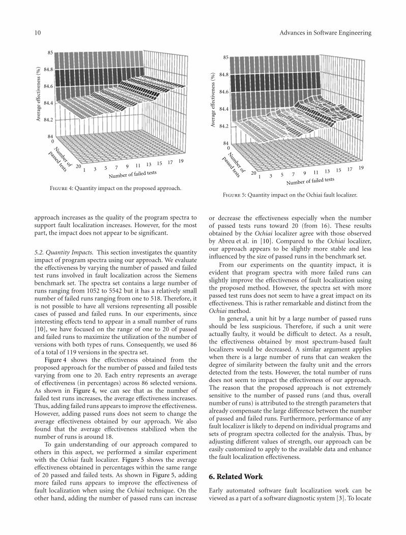
10 Advances in Software Engineering
1 3 5 7 9 11 13 15 17 19
84
84.2
84.4
84.6
84.8
85
0
20
Num
ber of
passed tests
Number of failed tests
Ave
rage
eff
ecti
ven
ess
(%)
Figure 4: Quantity impact on the proposed approach.
approach increases as the quality of the program spectra tosupport fault localization increases. However, for the mostpart, the impact does not appear to be significant.
5.2. Quantity Impacts. This section investigates the quantityimpact of program spectra using our approach. We evaluatethe effectiveness by varying the number of passed and failedtest runs involved in fault localization across the Siemensbenchmark set. The spectra set contains a large number ofruns ranging from 1052 to 5542 but it has a relatively smallnumber of failed runs ranging from one to 518. Therefore, itis not possible to have all versions representing all possiblecases of passed and failed runs. In our experiments, sinceinteresting effects tend to appear in a small number of runs[10], we have focused on the range of one to 20 of passedand failed runs to maximize the utilization of the number ofversions with both types of runs. Consequently, we used 86of a total of 119 versions in the spectra set.
Figure 4 shows the effectiveness obtained from theproposed approach for the number of passed and failed testsvarying from one to 20. Each entry represents an averageof effectiveness (in percentages) across 86 selected versions.As shown in Figure 4, we can see that as the number offailed test runs increases, the average effectiveness increases.Thus, adding failed runs appears to improve the effectiveness.However, adding passed runs does not seem to change theaverage effectiveness obtained by our approach. We alsofound that the average effectiveness stabilized when thenumber of runs is around 18.
To gain understanding of our approach compared toothers in this aspect, we performed a similar experimentwith the Ochiai fault localizer. Figure 5 shows the averageeffectiveness obtained in percentages within the same rangeof 20 passed and failed tests. As shown in Figure 5, addingmore failed runs appears to improve the effectiveness offault localization when using the Ochiai technique. On theother hand, adding the number of passed runs can increase
1 3 5 7 9 11 13 15 17 19
84
84.2
84.4
84.6
84.8
85
0
20N
umber of
passed tests
Number of failed tests
Ave
rage
eff
ecti
ven
ess
(%)
Figure 5: Quantity impact on the Ochiai fault localizer.
or decrease the effectiveness especially when the numberof passed tests runs toward 20 (from 16). These resultsobtained by the Ochiai localizer agree with those observedby Abreu et al. in [10]. Compared to the Ochiai localizer,our approach appears to be slightly more stable and lessinfluenced by the size of passed runs in the benchmark set.
From our experiments on the quantity impact, it isevident that program spectra with more failed runs canslightly improve the effectiveness of fault localization usingthe proposed method. However, the spectra set with morepassed test runs does not seem to have a great impact on itseffectiveness. This is rather remarkable and distinct from theOchiai method.
In general, a unit hit by a large number of passed runsshould be less suspicious. Therefore, if such a unit wereactually faulty, it would be difficult to detect. As a result,the effectiveness obtained by most spectrum-based faultlocalizers would be decreased. A similar argument applieswhen there is a large number of runs that can weaken thedegree of similarity between the faulty unit and the errorsdetected from the tests. However, the total number of runsdoes not seem to impact the effectiveness of our approach.The reason that the proposed approach is not extremelysensitive to the number of passed runs (and thus, overallnumber of runs) is attributed to the strength parameters thatalready compensate the large difference between the numberof passed and failed runs. Furthermore, performance of anyfault localizer is likely to depend on individual programs andsets of program spectra collected for the analysis. Thus, byadjusting different values of strength, our approach can beeasily customized to apply to the available data and enhancethe fault localization effectiveness.
6. Related Work
Early automated software fault localization work can beviewed as a part of a software diagnostic system [3]. To locate

Advances in Software Engineering 11
known faults, the system exploits knowledge about faultsand their associated possible causes obtained from previousexperience. For novel faults, the diagnostic system employsinferences based on the software model that contains pro-gram structure and functions along with heuristics to searchfor likely causes (and locations of faulty units). However,modeling the program behavior and functions is a majorbottleneck in applying this technique in practice.
Agrawal et al. [23] introduced the fault localizationapproach based on execution slices, each of which refers tothe set of a program’s basic blocks executed by a test input.Weiser [4] introduced the concept of a program slice as anabstract used by programmers in locating bugs. Agrawal etal.’s approach assumes that the fault resides in the slice ofa failed test and not in the slice of a successful test. Byrestricting the attention to the statements in the failed slicethat do not appear in the successful slice, called dice, the faultis likely to be found. However, the technique does not fullyexploit program spectra as it only uses a single failed (passed)test case’s execution slice to locate faults [18]. Consequently,program statements that are executed by one passed testcase and a different number of failed test cases would havean equal likelihood to be faulty if both were executed bythe failed test case for the considered dice. Our approach,however, makes use of all the test cases in the test suite, bothpassed or failed, to estimate fault locations.
Recent spectrum-based fault localization techniquesinclude nearest neighbor queries [5], Tarantula [13], Jaccard[12], and Ochiai [14]. These approaches use some measureof similarity to compare the units executed in a failed testto those of a passed test. The unit that results in the mostsimilar behaviors to errors in all the test runs is likely to befaulty. Other fault localization techniques employ statistical[6, 7] and neural net models [24] to analyze source codes andprogram spectra, respectively. However, the performance ofthe former heavily relies on the quality of data, whereas thelatter suffers from classic limitations such as local minima.Unlike these approaches, our approach is not similarity basedor statistical based, but estimates the likelihoods or beliefs ofunits being faulty. The computation is based on a theory thatis widely used for reasoning under uncertainty.
7. Discussion and Conclusions
Our approach is fundamentally different from existingmethods. Although the results of the proposed approach onthe benchmark data are marginally better than state-of-the-art approaches, it should be emphasized that the proposedapproach provides useful aspects for software testing inpractice. Its ability to do online computation to locate faultsas soon as each test run is executed is particularly novelin that testing of large program can be performed moreefficiently since it does not have to wait for all testingprogram spectral data to be completed. The intermediateresults obtained can also influence the configuration ordesign of subsequent tests. This is useful for real-time systemswhere system configurations tend to be highly adaptable andit is hard to predict the program behaviors.
In summary, this paper presents a spectrum-basedapproach to fault localization using the Dempster-Shaffertheory of evidence. Other than its competitive performanceto state-of-the-art techniques, our approach has severalunique benefits. First, it is theoretically grounded andtherefore it has a solid foundation for handling uncertaintyin fault location. Second, it supports an online computationthat allows the prediction of fault locations to be updatedimmediately as the execution of each test case is completedwithout having to wait for completion of a large enoughset of program spectrum to be statistically valid. Suchcomputation adapts well to real-time systems. Finally, theapproach can be extended easily by adding new massfunctions to represent additional evidence for use in theprobability assignment of faulty hypotheses.
Future work includes more experiments to gain under-standing of the characteristics of the proposed approach,for example, what types of program spectra on whichthe proposed approach would perform best or performsignificantly better than the other three approaches, and howwe can extend the approach so that it can deal with softwarewith multiple faults. More experiments can be performedto see if different types of software units impact the results.These are among our ongoing and future research.
Acknowledgments
Thanks are due to Adam Jordan for his help on theexperiments and to Phongphun Kijsanayothin for his helpfuldiscussion and comments on earlier versions of this paper.The author would also like to thank the reviewers whosecomments have helped improve the quality of the paper.
References
[1] B. Hailpern and P. Santhanam, “Software debugging, testing,and verification,” IBM Systems Journal, vol. 41, no. 1, pp. 4–12,2002.
[2] I. Vessey, “Expertise in debugging computer programs: ananalysis of the content of verbal protocols,” IEEE Transactionson Systems, Man and Cybernetics, vol. 16, no. 5, pp. 621–637,1986.
[3] R. Sedlmeyer, W. B. Thompson, and P. E. Johnson, “Diagnosticreasoning in software fault localization,” in Proceedings of the8th International Joint Conference on Artificial Intelligence, vol.1, pp. 29–31, Morgan Kaufmann, San Francisco, Calif, USA,1983.
[4] M. Weiser, “Programmers use slices when debugging,” Com-munications of the ACM, vol. 25, no. 7, pp. 446–452, 1982.
[5] M. Renieres and S. P. Reiss, “Fault localization with nearestneighbor queries,” in Proceedings of the 18th IEEE InternationalConference on Automated Software Engineering, pp. 30–39,Providence, RI, USA, 2003.
[6] B. Liblit, M. Naik, A. X. Zheng, A. Aiken, and M. I.Jordan, “Scalable statistical bug isolation,” in Proceedings of theACM SIGPLAN Conference on Programming Language Designand Implementation, pp. 15–26, Association for ComputingMachinery, New York, NY, USA, 2005.

12 Advances in Software Engineering
[7] C. Liu, L. Fei, X. Yan, J. Han, and S. P. Midkiff, “Statisticaldebugging: a hypothesis testing-based approach,” IEEE Trans-actions on Software Engineering, vol. 32, no. 10, pp. 831–848,2006.
[8] T. Reps, T. Ball, M. Das, and J. Larus, “The use of programprofiling for software maintenance with applications to theyear 2000 problem,” in Proceedings of the 6th EuropeanSoftware Engineering Conference, pp. 432–449, Springer, NewYork, NY, USA, 1997.
[9] R. Abreu, P. Zoeteweij, and A. van Gemund, “An evaluationof similarity coefficients for software fault localization,” inProceedings of the 12th Pacific Rim International Symposiumon Dependable Computing, pp. 39–46, IEEE Computer SocietyPress, Riverside, Calif, USA, 2006.
[10] R. Abreu, P. Zoeteweij, and A. van Gemund, “On the Accu-racy of Spectrum-based Fault Localization,” in Proceedingsof the Testing: Academic and Industrial Conference Practiceand Research Techniques (MUTATION ’07), pp. 89–98, IEEEComputer Society Press, Washington, DC, USA, 2007.
[11] S. Ali, J. H. Andrews, T. Dhandapani, and W. Wang,“Evaluating the accuracy of fault localization techniques,”in Proceedings of the IEEE/ACM International Conference onAutomated Software Engineering, pp. 76–87, IEEE ComputerSociety Press, Washington, DC, USA, 2009.
[12] M. Y. Chen, E. Kiciman, E. Fratkin, A. Fox, and E. Brewer,“Pinpoint: problem determination in large, dynamic internetservices,” in Proceedings of the International Conference onDependable Systems and Networks (DSN ’02), pp. 595–604,Berkeley, Calif, USA, 2002.
[13] J. Jones, M. J. Harrold, and J. Stasko, “Visualization of testinformation to assist fault localization,” in Proceedings of the24th International Conference on Software Engineering, pp.467–477, Association for Computing Machinery, New York,NY, USA, 2002.
[14] A. Meyer, A. Garcia, A. Souza, and C. Souza Jr., “Comparisonof similarity coefficients used for cluster analysis with domi-nant markers in maize (Zea mays L),” Genetics and MolecularBiology, vol. 27, no. 1, pp. 83–91, 2004.
[15] S. Nessa, M. Abedin, E. W. Wong, L. Khan, and Y. Qi, “Soft-ware fault localization using N-gram analysis,” in Proceedingsof the 3rd International Conference on Wireless Algorithms,Systems, and Applications, pp. 548–559, Springer, Berlin,Germany, 2008.
[16] V. Dallmeier, C. Lindig, and A. Zeller, “Lightweight defectlocalization for Java,” in Proceedings of the 19th EuropeanConference on Object-Oriented Programming, vol. 3568 ofLecture Notes in Computer Science, pp. 528–550, Springer,Glasgow, UK, 2005.
[17] G. Shafer, A Mathematical Theory of Evidence, PrincetonUniversity Press, Princeton, NJ, USA, 1976.
[18] J. Jones and M. J. Harrold, “Empirical evaluation of the taran-tula automatic fault-localization technique,” in Proceedings ofthe 20th IEEE/ACM International Conference on AutomatedSoftware Engineering, pp. 273–282, Association for ComputingMachinery, New York, NY, USA, 2005.
[19] P. Jaccard, “Etude comparative de la distribution florale dansune portion des Alpes et des Jura,” Bulletin de la SocieteVaudoise des Sciences Naturelles, vol. 37, pp. 547–579, 1901.
[20] A. Ochiai, “Zoogeographic studies on the soleoid fishes foundin Japan and its neighbouring regions,” Bulletin of the JapaneseSociety for the Science of Fish, vol. 22, pp. 526–530, 1957.
[21] J. Pearl, Causality: Models, Reasoning, and Inference, Cam-bridge University Press, 2000.
[22] M. Hutchins, H. Foster, T. Goradia, and T. Ostrand, “Experi-ments of the effectiveness of dataflow- and control flow-basedtest adequacy criteria,” in Proceedings of the 6th InternationalConference on Software Engineering, pp. 191–200, IEEE Com-puter Society Press, Sorrento , Italy, 1994.
[23] H. Agrawal, J. R. Horgan, S. London, and W. E. Wong,“Fault localization using execution slices and dataflow tests,”in Proceedings of the 6th International Symposium on SoftwareReliability Engineering, pp. 143–151, Toulouse , France, 1995.
[24] W. Wong and Y. Qi, “BP neural network-based effective faultlocalization,” International Journal of Software Engineering andKnowledge Engineering, vol. 19, no. 4, pp. 573–597, 2009.