semiconductor yield modeling using generalized linear …...semiconductor fabrication process. in an...
TRANSCRIPT
Semiconductor Yield Modeling Using Generalized Linear Models
by
Dana Cheree Krueger
A Dissertation Presented in Partial Fulfillment
of the Requirements for the Degree
Doctor of Philosophy
Approved March 2011 by the
Graduate Supervisory Committee:
Douglas C. Montgomery, Chair
John Fowler
Rong Pan
Michele Pfund
ARIZONA STATE UNIVERSITY
May 2011

ii
ABSTRACT
Yield is a key process performance characteristic in the capital-intensive
semiconductor fabrication process. In an industry where machines cost millions
of dollars and cycle times are a number of months, predicting and optimizing
yield are critical to process improvement, customer satisfaction, and financial
success. Semiconductor yield modeling is essential to identifying processing
issues, improving quality, and meeting customer demand in the industry.
However, the complicated fabrication process, the massive amount of data
collected, and the number of models available make yield modeling a complex
and challenging task.
This work presents modeling strategies to forecast yield using generalized
linear models (GLMs) based on defect metrology data. The research is divided
into three main parts. First, the data integration and aggregation necessary for
model building are described, and GLMs are constructed for yield forecasting.
This technique yields results at both the die and the wafer levels, outperforms
existing models found in the literature based on prediction errors, and identifies
significant factors that can drive process improvement. This method also allows
the nested structure of the process to be considered in the model, improving
predictive capabilities and violating fewer assumptions.
To account for the random sampling typically used in fabrication, the
work is extended by using generalized linear mixed models (GLMMs) and a
larger dataset to show the differences between batch-specific and population-
averaged models in this application and how they compare to GLMs. These

iii
results show some additional improvements in forecasting abilities under certain
conditions and show the differences between the significant effects identified in
the GLM and GLMM models. The effects of link functions and sample size are
also examined at the die and wafer levels.
The third part of this research describes a methodology for integrating
classification and regression trees (CART) with GLMs. This technique uses the
terminal nodes identified in the classification tree to add predictors to a GLM.
This method enables the model to consider important interaction terms in a
simpler way than with the GLM alone, and provides valuable insight into the
fabrication process through the combination of the tree structure and the statistical
analysis of the GLM.

iv
DEDICATION
This work is dedicated to my husband, Chad, who has encouraged me, sacrificed
with me, and loved me throughout this special season of our lives together.

v
ACKNOWLEDGMENTS
I would first like to thank Dr. Montgomery for teaching me, mentoring
me, and believing in me. Your enduring patience and gentle encouragement have
been invaluable to me, both in completing this work and in my own role as a
teacher and scholar. I am also thankful for the helpful contributions from my
committee members Dr. Pfund, Dr. Pan, and Dr. Fowler. Your questions and
comments have made me a better researcher.
I am grateful for the support of my parents, who stood behind me as I took
a leap of faith and pursued this degree. Without your encouragement, I would not
dare to dream, and I wouldn’t appreciate the value of taking the scenic route.
I have no words to express how grateful I am to my husband, Chad, who
has sacrificed so much along with me to allow me to have time to work on this
dissertation. Also, many thanks to Clara who has provided a strong and very
special motivation for me to finish this race.
I am also thankful for the support of my friends and colleagues who have
encouraged me through this extended process. Andrea, Shilpa, Busaba, Nat, Jing,
Linda, Donita, Chwen, Diane, and many others have helped me persevere.
I would also like to acknowledge the organizations that supported me
financially in this research. This work was sponsored in part by NSF and SRC
(DMI-0432395). Also, the support I received through the Intel Foundation Ph.D.
Fellowship and ASQ’s Statistics Division’s Ellis R. Ott Scholarship enabled me to
continue and complete this research.

vi
Most of all, this work would not have been possible without the Lord
Jesus Christ, who called me to this degree, opened unexpected doors, carried me
through many challenges, and continues to be at work in my life. Your love and
faithfulness amaze me. May this work and my life glorify You.

vii
TABLE OF CONTENTS
Page
LIST OF TABLES ....................................................................................................... x
LIST OF FIGURES ................................................................................................... xii
CHAPTER
1 INTRODUCTION .................................................................................. 1
2 LITERATURE REVIEW ...................................................................... 6
Semiconductor Yield Modeling ......................................................... 8
Statistical Approaches ...................................................................... 29
3 DATA REFINING FOR MODEL BUILDING .................................. 43
Overall Description of Data.............................................................. 43
Process Data ................................................................................. 44
Defectivity Data ........................................................................... 47
Class Probe ................................................................................... 49
Unit Probe .................................................................................... 50
Use of the Dataset ............................................................................. 52
Data Refining for GLM Model Building ......................................... 52
Data Integration ........................................................................... 52
Data Aggregation ......................................................................... 53
Managing Outliers ....................................................................... 56
4 SEMICONDUCTOR YIELD MODELING USING GENERALIZED
LINEAR MODELS ....................................................................... 58
Introduction ....................................................................................... 58
viii
CHAPTER Page
Model Buiding Using Logistic Regression ...................................... 60
Results ............................................................................................... 61
Die-Level Logistic Regression .................................................... 61
Die-Level Logistic Regression Validation .................................. 66
Wafer-Level Logistic Regression................................................ 73
Wafer-Level Logistic Regression Validation ............................. 75
Summary ........................................................................................... 80
5 SEMICONDUCTOR YIELD MODELING USING GENERALIZED
LINEAR MIXED MODELS ......................................................... 83
Introduction ....................................................................................... 83
Data Description ............................................................................... 85
Model Building ................................................................................. 85
Results ............................................................................................... 88
Die-Level Model Results ............................................................. 88
Die-Level Model Validation ....................................................... 98
Wafer-Level Model Results ...................................................... 103
Wafer-Level Model Validation ................................................. 109
Summary ......................................................................................... 114
6 SEMICONDUCTOR YIELD MODELING INTEGRATING CART
AND GENERALIZED LINEAR MODELS .............................. 118
Introduction ..................................................................................... 118
Methodology ................................................................................... 123

ix
CHAPTER Page
Building Trees ............................................................................ 123
Creating Models ......................................................................... 129
Results ............................................................................................. 137
Validation ................................................................................... 139
Terminal Nodes and Interactions .............................................. 146
Summary ......................................................................................... 151
7 CONCLUSIONS ................................................................................ 153
Limitations ...................................................................................... 156
Future Work .................................................................................... 156
References .............................................................................................................. 160
Appendix
A SAS CODE ..................................................................................... 167
Biographical Sketch ................................................................................................. 180

x
LIST OF TABLES
Table Page
2.1 Relationships between negative binomial model and other models
based on values for alpha................................................................... 14
3.1 Process measurements in dataset ........................................................ 46
3.2 Description of the layers involved in defectivity scans ...................... 48
3.3 Raw data for each defect after integration .......................................... 54
3.4 Aggregated data for individual dice ................................................... 55
3.5 Subset of data for analysis .................................................................. 55
4.1 Die-level non-nested logistic regression model results for full training
data set (N=2967) .............................................................................. 63
4.2 Comparison of link functions and outlier methods ............................ 64
4.3 Existing yield models .......................................................................... 69
4.4 Mean squared error (MSE) and mean absolute deviation (MAD) for
model comparisons at the die level using test data .......................... 71
4.5 Comparison of link functions and outlier methods (wafer-level, not
nested) ............................................................................................... 75
4.6 Comparison of Pearson correlation coefficients between models and
actual yields using test data ............................................................... 79
4.7 Mean squared error (MSE) and mean absolute deviation (MAD) for
model comparisons at the wafer level .............................................. 80
5.1 Models analyzed for comparisons ...................................................... 86
5.2 Significant fixed effects for die-level GLM models from t-tests ....... 89
xi
Table Page
5.3 Significant effects for die-level GLMM models from t-tests ............ 90
5.4 Die-level significant factors for GLM models using various sample
sizes .................................................................................................95
5.5 Die-level significant factors for GLMM batch-specif models using
various sample sizes (logit link function) ........................................97
5.6 Die-level significant factors for GLMM population-averaged models
using various sample sizes (logit link function) ..............................98
5.7 Significant fixed effects for wafer-level models from t-tests ..........104
5.8 Significant effects for wafer-level models from t-tests (logit link) .108
6.1 Die-level predictors .........................................................................125
6.2 Preliminary tree building results .....................................................127
6.3 Terminal node information for Tree 3 .............................................132
6.4 Coefficients and p-values ofr GLM models ....................................138
6.5 Recipes and classification results for terminal nodes 1, 2, 4, 5, 7, 9,
and 11 ............................................................................................147
6.6 Recipes and classification results for terminal nodes 12, 14, 15, 16,
18, 19, 22, and 24 ..........................................................................147
6.7 Significant interaction terms and the terminal nodes that contain both
factors ............................................................................................151

xii
LIST OF FIGURES
Figure Page
1.1 Semiconductor manufacturing process ................................................ 2
2.1 The binary tree structure of CART ..................................................... 25
3.1 Cross section of semiconductor device ............................................... 44
3.2 X-bar and R chart for defect densities for the device studied ............46
3.3 Sampling strategies by lot for different data types ............................... 49
3.4 A wafer map .......................................................................................... 51
3.5 Summary statistics for total defects per die .......................................... 57
4.1. Nested structure for wafers ................................................................. 59
4.2. Nested structure for dice ....................................................................... 59
4.3 Residual plots for a multiple linear regression model based on the
training dataset with no outliers removed .......................................... 62
4.4 Predicted vs. actual yield for die-level logistic regression models ...... 68
4.5 Expected probabilities of dice passing vs. number of defects per die . 70
4.6 Mean absolute deviation (MAD) and mean squared error (MSE) results
comparing GLM models with other models from the literature ....... 72
4.7 Number of dice predicted to pass compared to actual passing dice and
failing dice with defects ...................................................................... 73
4.8 Predicted vs. actual yield of dice with defects ..................................... 78
4.9 Wafer-level yield model predictions for the test data .......................... 78

xiii
Figure Page
4.10 Mean squared error (MSE) and mean absolute deviation (MAD)
measures for the nine models from the literature and the GLM
models ................................................................................................. 80
5.1 Significant wafer maps comparing 30-wafer logit models .................. 93
5.2 Significant wafer maps comparing 168-wafer complimentary log-log
models ................................................................................................. 94
5.3 Mean absolute deviation (MAD) for die-level yield models ............. 100
5.4 Mean squared error (MSE) for die-level yield models ...................... 101
5.5 Predicted vs. actual number of passing dice on a waer for the 30-wafer
models using the logit link................................................................ 102
5.6 Predicted vs. actual number of passing dice on a wafer of the 168-
wafer models using the logit link ..................................................... 103
5.7 Mean absolute deviation (MAD) for wafer-level yield models......... 111
5.8 Mean squared error (MSE) for wafer-level models ........................... 112
5.9 Predicted vs. actual wafer yields for wafer-level historical models
Y1-Y9 ................................................................................................. 113
5.10 Predicted vs. actual wafer yields for adjusted wafer-level GLM and
GLMM models ................................................................................. 113
6.1 Preliminary tree structures using different predictors ........................ 128
6.2 Tree 3 structure .................................................................................... 131
6.3 CART tree showing interactions between factors .............................. 135
6.4 Bottom of CART tree showing interactions between factors ............ 136

xiv
Figure Page
6.5 Die-level MAD and MSE for model comparisons ............................ 141
6.6 Wafer-level MAD and MSE for model comparisons ........................ 141
6.7 Wafer-level predictions for test dataset using CART alone .............. 142
6.8 Wafer-level predictions for test dataset – Main effects only ............. 143
6.9 Wafer-level predictions for test dataset – Main effects plus CART
terminal nodes ................................................................................... 143
6.10 Wafer-level predictions for test dataset – Main effects plus CART-
selected terminal nodes ..................................................................... 144
6.11 Wafer-level predictions for test dataset – Main effects pluc
interactions from CART ................................................................... 145
6.12 Wafer-level predictions for test dataset – Main effects plus all two-
way interactions reduced model ....................................................... 145
6.13 Wafer map showing the radial and quadrant regions that apply to
terminal nodes 1-8 from the CART tree .......................................... 149
7.1 Actual and calculated yields for wafers ............................................ 159

1
Chapter 1
INTRODUCTION
Yield is a key process performance characteristic in the capital-intensive
semiconductor fabrication process. Semiconductor yield may be defined as the
fraction of total input transformed into shippable output (Cunningham, Spanos, &
Voros, 1995). Hu (2009) points out that yield analysis usually has two purposes:
to determine the root cause of yield loss and to build accurate models to predict
yield. From a manufacturing viewpoint, it is also extremely important to predict
yield impact based on in-line inspections (Nurani, Strojwas, Maly, Ouyang,
Shindo, Akella, et al. (1998). In an industry where machines cost millions of
dollars and cycle times are a number of months, predicting and optimizing yield
are critical to process improvement, customer satisfaction, and financial success.
Since the 1960s, semiconductor yield models have been used in the
planning, optimization, and control of the fabrication process (Stapper, 1989). A
comprehensive review of these methods is given by Kumar, Kennedy,
Gildersleeve, Albeson, Mastrangelo, and Montgomery (2006). Many of these
methods focus on using defect metrology information, sometimes referred to as
defectivity data, to predict yield. While several other measurements, such as
critical dimensions and electrical tests, are taken as wafers are fabricated,
defectivity data seem to be the most influential in current yield modeling practice.
Defectivity measures come from a wafer-surface scan that identifies
unusual patterns such as particles, scratches, or pattern defects. These scans are
performed after different layers of the wafer have completed processing (see
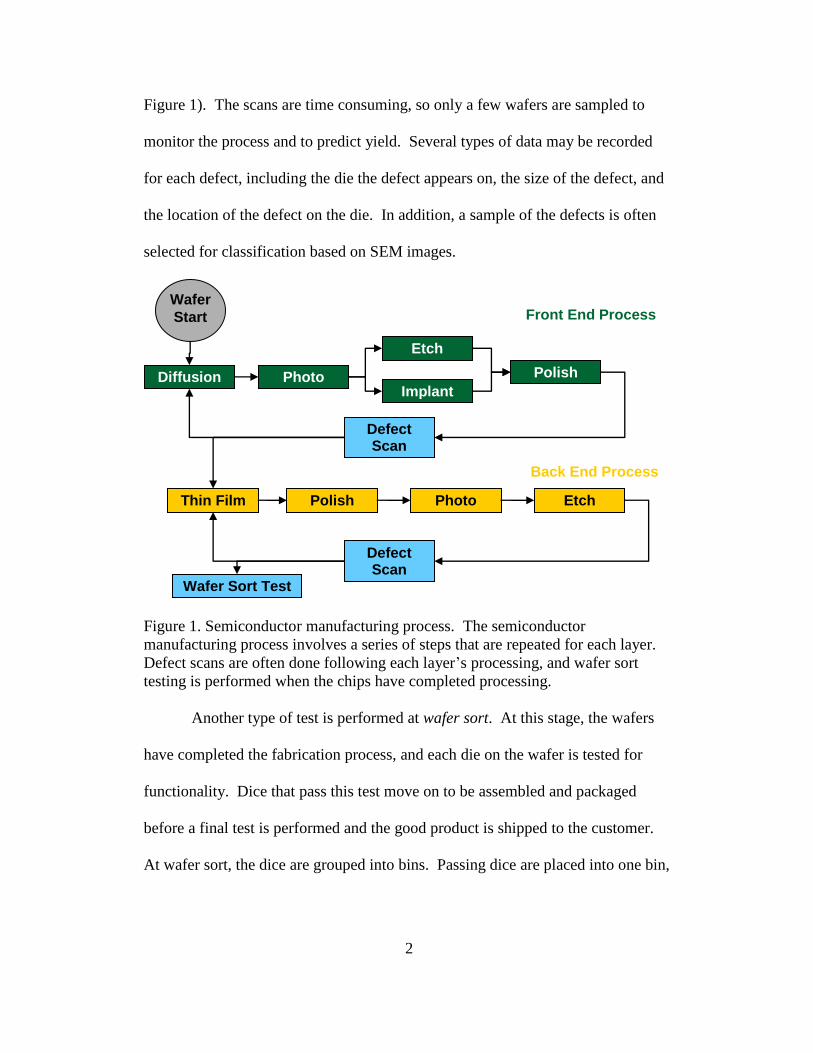
2
Figure 1). The scans are time consuming, so only a few wafers are sampled to
monitor the process and to predict yield. Several types of data may be recorded
for each defect, including the die the defect appears on, the size of the defect, and
the location of the defect on the die. In addition, a sample of the defects is often
selected for classification based on SEM images.
Figure 1. Semiconductor manufacturing process. The semiconductor
manufacturing process involves a series of steps that are repeated for each layer.
Defect scans are often done following each layer’s processing, and wafer sort
testing is performed when the chips have completed processing.
Another type of test is performed at wafer sort. At this stage, the wafers
have completed the fabrication process, and each die on the wafer is tested for
functionality. Dice that pass this test move on to be assembled and packaged
before a final test is performed and the good product is shipped to the customer.
At wafer sort, the dice are grouped into bins. Passing dice are placed into one bin,
Wafer
Start
Diffusion
Etch
Photo Implant
Polish
Defect Scan
Front End Process
Thin Film Etch Polish Photo
Defect Scan
Back End Process
Wafer Sort Test

3
while failing dice are separated by their failure modes into a number of different
bins.
One of the challenges of working with semiconductor measurements is the
size of the massive datasets available with computer-aided manufacturing. While
these data record many important process parameters and test results, integrating
them into a usable form is a considerable problem. Often, process data from tools
are stored in one database, defectivity data in another database, and electrical and
wafer sort data in yet a third database. Obtaining a dataset that contains
defectivity data and the corresponding wafer sort data can require skilled
knowledge of two different systems and the ability to query in both. Aggregating
the data into a more useable form for model building is also a time-consuming
task.
Another challenge is developing an adequate yield model. Yield models
in the literature that use defect metrology data have neglected to properly account
for the nested structure of the data and have assumed independence among the
data. Dice are grouped together on wafers, and wafers are processed together as
lots, making this assumption questionable at best. The yield models in the
literature have overlooked this potential source of variation. Also, most current
modeling is done at the wafer level, which loses the vast amounts of information
available at the die level. In industry, many companies develop their own
proprietary yield models that are not available in published literature. Some of
the most common methodologies used for these models include employing
classical linear regression and tree-based classification using various predictors.

4
Additional approaches used to predict yield and improve processing
include using kill ratios (Lorenzo, Oter, Cruceta, Valtuena, Gonzalez, & Mata,
1999; Yeh, Chen, & Chen, 2007), using unified defect and parametric data
(Burglund, 1996) and using process and parametric data in a hierarchical
generalized linear model (GLM) (Kumar, 2006). Defectivity data have also been
used to identify gross failures due to clusters of defects. Spatial filters (Wang,
2008) and tests for spatial randomness (Fellows, Mastrangelo, & White, Jr., 2009)
have been developed to help identify non-random clusters. Supervised learning
can also be beneficial, as shown by Skinner, Montgomery, Runger, Fowler,
McCarville, Rhoads, et al. (2002) and Hu (2009), for yield models that use
parametric data as predictors. Classification and regression tree (CART)
techniques are recommended as a means to develop a “best path” to high-yield
outputs and a path to avoid for low-yield outcomes (Skinner, et al., 2002).
However, the predictive power of CART models is limited (Hu, 2009) and can
have limitations due to the process parameters data not being available at the
same time and due to the process and design interactions that are not considered
in this approach (Bergeret & Le Gall, 2003).
The literature suggests GLMs have not been applied to model
semiconductor yield from defectivity data, yet this approach is appealing because
GLMs are most appropriate for response data that follow a distribution in the
exponential family (i.e. binomial or Poisson) and can handle the nested data
structure and the die-level data (Montgomery, Peck, & Vining, 2006).

5
The purpose of this dissertation is to present a modeling strategy that
guides practitioners to develop die- and wafer-level GLM- or generalized linear
mixed model (GLMM)-based yield models using defect metrology data. An
example using real semiconductor yield data is presented that illustrates the
strengths of this approach in comparison to other yield models. This work also
explores the effects of outliers on GLM models and the impact of using nested
models at the die level, the differences between die- and wafer- level modeling,
the differences between population-averaged and batch-specific random effects
modeling, and the impact of integrating CART methods with logistic regression.
These GLM models can be applied to determine which process steps are
significant, to identify specific wafers or locations on wafers that warrant further
investigation for improvements, and to predict future yields based on intermediate
data, thus fulfilling the two purposes of yield analysis mentioned by Hu (2009)
with a strategy that is easy for practitioners to use and implement.
This work is organized by first presenting a review of the literature in
Chapter 2 and by describing the data and the methods used to develop a useful
dataset for modeling in Chapter 3. Chapter 4 shows the results of applying GLMs
to model these yield data. Chapter 5 considers random effects by applying
GLMM techniques and showing differences between population-averaged and
batch-specific approaches. Chapter 6 discusses a methodology of integrating
CART techniques with those of logistic regression for improved models. The
conclusions are presented in Chapter 7 along with recommendations for future
work.

6
Chapter 2
LITERATURE REVIEW
While there are many measures of process performance, the number one
index of success in the industry is yield (J. A. Cunningham, 1990). There is some
skepticism amongst practitioners when it comes to yield modeling techniques;
still, their usefulness in the planning, optimization, and control of semiconductor
fabrication cannot be overlooked (Stapper, 1989). As improving productivity and
cost effectiveness in the industry become more critical with increasing market
competition, improving productivity and cost effectiveness is vital (Nag, Maly, &
Jacobs, 1998).
There are many challenges in creating a reasonable yield model. One of
these is utilizing the massive datasets available with computer-aided
manufacturing. Process parameters are constantly being recorded for each layer
of fabrication. Defects are found and classified at each layer as well. Electrical
test data and bin sort counts are also recorded, usually all in different databases.
Since ownership of these data collection tools is usually segmented, the
integration of the many types of data is no small task (Braun, 2002). Other
challenges arise with computational complexity of the models and with ensuring
the assumptions made in yield formulas accurately represent the process.
Despite the challenges, yield models have the opportunity to reap large
rewards for semiconductor manufacturers. Dance & Jarvis (1992) state that
implementing yield models has “made it possible for process engineers to
quantify their own process sector’s influence on [electrical] test yield” (p. 42).

7
Instead of waiting months to get final test results, the model can be used to insure
process improvement. This is possible when the yield models are linked with
statistical process control methods, driving process improvement (Dance & Jarvis,
1992).
Yield models are an important part of yield learning, which consists of
eliminating one source of faults after another until an overwhelming portion of
manufactured units function according to specification (Weber, 2004). Yield
learning is especially important as new products start up. Companies must
maximize yield as early as possible while still releasing a product before
competitors launch. Weber (2004) states that the yield-learning rate tends to be
the most significant contributor to profitability in the semiconductor industry. If
the yield-learning ramp could be improved by six months, the cumulative net
profit would more than double; if the yield ramp is delayed by six months, two-
thirds of the profit is eliminated (Weber, 2004).
According to Nag et al. (1998), the yield learning rate depends on the
relationship between particles, defects, and faults and the ease of defect
localization that in turn depends on the following:
1. Size, layer and type of defect
2. Ability to analyze the IC design
3. Probability of occurrence of catastrophic events
4. The effectiveness of the corrective actions performed
5. The timing of each of the events mentioned
6. The rate of wafer movement through the process (p. 164).

8
Because yield models reflect the relationships between particles, defects, and
faults, they are important tools in yield learning and, consequently, profitability.
Semiconductor Yield Modeling
Many different yield models have been developed and used since the
1960s. Stapper (1989) provided a history of many of these models, and Kumar, et
al. (2006) also briefly discussed historical models before expanding the discussion
to more recent models. In understanding the changes in yield modeling
throughout the years, it is valuable to observe how yield modeling began and how
it has changed to better account for the rapidly-changing semiconductor
fabrication processes. This review will also demonstrate that, while advances are
still being made, improved models that utilize the vast amount of data available
and provide decision rules early in the process have not yet been developed.
Initial Yield Models
As Wallmark (1960) examined the effects of shrinkage in integrated
circuits, he calculated yield using
N
i SY )100/1( (2.1)
for an N-stage device that has shrinkage such that S out of every 100 stages
cannot be used. Wallmark used this result in a binomial distribution to estimate
yield of an integrated circuit (IC) with redundant transistors. While this model

9
became inappropriate in later years as the interconnect wiring evolved from
repairable methods to IC methods because this yield loss was not considered in
the model, Wallmark was the first to model the IC yield of circuits with fault
tolerance (Stapper, 1989).
Hofstein and Heiman also examined the problems of yield and tolerance.
They observed the primary failure mechanism at the time to be a faulty gate
insulator, likely caused by pinholes in the oxide layer that led to a short circuit
(Hofstein & Heiman, 1963). Assuming the oxide defects were randomly
distributed on the surface of the silicon crystal and that the area of the pinhole was
much smaller than the area of the gate electrodes, they used the Poisson model to
predict yield for a device with N transistors,
)( DAN GeY
(2.2)
where AG is the active area of the gate in each transistor and D is the average
surface density of the defects. While later work showed the assumptions used in
this model to be incorrect, the relationship between defects and gate area has been
useful as yield models evolve with the complexity of the process.
Murphy’s Yield Model
Murphy (1964) constructed a yield model that accounted for variations in
defect densities from wafer to wafer and die to die. Using f(D) as the normalized

10
distribution function of dice in defect densities, Murphy proposed the overall
device yield to be
0
)( dDDfeY DA (2.3)
where D is again the density of defects per unit area, and A is the susceptible area
of the device. Murphy observed that distribution was bell-shaped, but due to the
variation expected with the distribution from production line to production line,
he used the triangular distribution as an approximation to simplify the
calculations,
2
0
01
AD
eY
AD
(2.4)
where D0 is the mean defect density. This equation assumed that only one type of
spot defect occurred. Murphy (1964) noted this limitation, knowing that the
occurrence of different types of defects may or may not be independent.
The defect density distribution, f(D), later became known as a compounder
or mixing function with the yield formula being referred to as a compound or
mixed Poisson yield model (Stapper, 1989).
11
Seeds’ Yield Formula
Seeds (1967), like Murphy, also assumed that the defect densities vary
from wafer to wafer and from die to die. He used the exponential distribution to
model defect densities where 0
//)( 0 DeDf
DD and produced the yield formula
ADY
01
1
. (2.5)
Seeds’ method of determining yield for blocks of chips has since come to be
known as the window method, where an overlay of windows is made for each set
of chip multiples. The number of defect-free windows is counted and the yield
determined for each window size (Stapper, 1989).
Seeds’ data confirmed Murphy’s predictions, but showed that Murphy’s
yield formula underestimated the yield due to the larger standard deviation in the
triangular distribution.
Dingwall’s Model
In 1968, A. G. F. Dingwall (as cited by Cunningham, 1990) presented a
yield model in the form
3
01 / 3Y D A
. (2.6)

12
Moore’s Model
Moore (as cited by Cunningham, 1990) published a yield model that he
claimed was most representative of Intel’s processing in the form of
0D AY e
. (2.7)
Cunningham (1990) compares several of these models and concluded Moore’s
and Seeds’ models can be grossly inaccurate.
Price’s Model
Price (1970) criticized prior models that used an initial model that
predicted yield falling off exponentially as circuit area increased, stating that this
decay was less than exponential. Price argued the previous use of Boltzmann
statistics, considering all spot defects to be distinguishable was inappropriate. He
proposed using Bose-Einstein statistics to first derive Seeds’ model and then for r
independent defect-producing mechanisms having defect densities D1, D2, …, Dr
modeled yield as
)/11()/11)(/11(
)/11(
21 NADNADNAD
NY
r
r
. (2.8)
Price stated the experimental measurement of defect densities due to a single
defect-producing mechanism was made more tractable with this model.

13
While this approach was used in practice for a time, the assumption that
the defects are indistinguishable was found to be inappropriate for IC fabrication.
Murphy (1971) pointed out Price’s error lay in confusing the highly specialized
quantum mechanics terms “distinguishable” and “particle” with their everyday
usage. In general, when defects are counted, they are distinguishable (Stapper,
1989). Price’s model has not stood the test of time and has not been developed
further.
Okabe’s Model
Okabe, Nagata, and Shimada (1972) proposed a model that took into
account different processing steps, assuming that critical areas and defect
densities were the same for all layers. For a process with n process steps, the
model had the form
nnADY
)/1(
1
0 (2.9)
and was derived from Murphy’s model using the Erlang distribution for the
compounder.

14
Negative Binomial Yield Model
The negative binomial yield model was the first model to consider defect
clustering. This model is also derived from Murphy’s but uses the gamma
distribution as the compounder. This produces
)/1( ADY (2.10)
where is a parameter related to the coefficient of variation of the gamma
distribution that is a rational number greater than zero (Stapper, 1989). Stapper
(1976) was one of the first to consider defect clustering. The negative binomial
model’s parameter was used to represent a clustering parameter. The negative
binomial model has been used extensively, though when severe clustering is
present, the formula becomes inadequate (Stapper, 1989).
Another concern with the negative binomial model is how should be
determined. Cunningham (1990) relates values of to different levels of
clustering and connects them to other yield models. This is shown in Table 2.
Table 2.1. Relationships between negative binomial model and other models
based on values for alpha.
Clustering Value of Yield Model
None About 10 to Poisson
Some 4.2 Murphy
Some 3 Dingwall
Much 1 Seeds

15
If the company has similar, mature products, may be determined by curve
fitting for that factory environment. For different or new products, Cunningham
(1990) describes a method for determining , but the approach is not straight
forward. Cunningham (1990) gives a formula for calculating , as
2
(2.11)
where is the mean of the number of defects per die, and 2 is the variance, but
he mentions that this calculation can yield results that are quite scattered and
sometimes negative. Cunningham describes how may be determined using the
defects on the wafers by using surface particle maps and an overlaid grid of
different sizes. Using averages of defect densities from these grids, Cunningham
(1990) proposed using
2
2
1/
1 /avgavg
. (2.12)
This approach does not always give positive values either, though, and produces
different calculated values for for the different grids.
16
Poisson Mixture Yield Models
Reghavachari, Srinivasan, and Sullo (1997) developed the Poisson-
Rayleigh and Poisson-inverse Gaussian models furthering the expansion of
Murphy’s model. With the Poisson-Rayleigh model, they investigate the special
case of using a Weibull distribution with =2. This results in the yield model
2 1/ 2
0 0 01 exp / /Y AD AD erfc AD
(2.13)
Using the inverse-Gaussian distribution, Reghavachari, et al. (1997) constructed
the Poisson-inverse Gaussian mixture yield model of
1/ 2
02( ) exp 1 1A
ADY L A
(2.14)
where is a shape parameter and 0D is a scale parameter. In comparisons with
other mixing distributions, such as the exponential, half Gaussian, triangular,
degenerate and gamma, Reghavachari, et al. (1997) showed the Poisson-gamma
(negative binomial yield model) and the Poisson-inverse Gaussian mixtures are
sufficiently robust to emulate all the other models, supporting the prevalent use of
the negative binomial model. Reghavachari, et al. (1997) point out the limitations
of these models through a discussion on the impact of reference regions used in
the models, which may be chip die areas, specific regions within wafers such as

17
groups of chip areas, entire wafers, or even batches of wafers. They show these
models are not sufficient to completely characterize the spatial patterns of defects
generated and that different specifications of such regions lead to different levels
of aggregations in the spatial distribution of defects, which must be well
understood to properly estimate the parameters of the model and to obtain good
results.
Clustering and Critical Area Analysis
The type, size, and arrangement of defects have played a part in more
recent yield models and process-improvement efforts. Nahar (1993) points out
that defects may be classified into one of three categories. Point defects include
oxide pinholes, isolated particles, or process-induced defects. Line defects can be
scratches, step lines, or other defects that have high length-to-width ratios. Area
defects are a third category and include misalignment, stains, and wafer cleaning
problems. Kuo and Kim (1999) indicate it is useful to classify defects as random
or nonrandom. Random defects occur by chance, such as shorts and opens or
local crystal defects. Nonrandom defects include gross defects and parametric
defects.
These different classifications of defects support the development of
models that take into account clustering in methods different from the negative
binomial model in Equation 2.10. Clusters of defects can be, in general, classified
as either particle or process related, with particle-related clusters being assignable
to individual machines and process-related clusters being attributable to one or

18
more process steps not meeting specification requirements (Hansen, Nair, &
Friedman, 1997; Fellows, Mastrangelo, & White, Jr., 2009). Hansen, Nair, and
Friedman (1997) developed methods for routinely monitoring wafer-map data to
detect significant spatially clustered defects that are of interest in yield prediction
and process improvement. White, Jr., Kundu, and Mastrangelo (2008) show how
the Hough transformation can be used to automatically detect such defect clusters
as stripes, horizontal and vertical scratches, and diagonal scratches at 45° and
135° from the horizontal. This technique also works well to detect defect patterns
such as scratches at arbitrary angles, center defects, and edge defects, but is not
useful in detecting defect clusters that cannot be so characterized, such as ring
defects. Fellows, Mastrangelo, and White, Jr. (2009) compare a spatially
homogeneous Bernoulli process (SHBP) and a Markov random field (MRF) for
testing the randomness of defects on a wafer. Wang (2008) proposes an approach
that applies a spatial filter to the defect scan data, then uses kernel eigen-
decomposition of the affinity matrix for systematic components to determine the
number of clusters embedded in the dataset. Spectral clustering is applied to
group the data in a high-dimensional kernel space before a decision tree is used to
generate the final classification results. These detections techniques have not yet
been incorporated into formal yield models and are more applicable currently in
process improvement and problem solving in the fab.
The size and location of defects is considered in critical area analysis.
Zhou, Ross, Vickery, Metteer, Gross, and Verret (2002) discuss using critical area
analysis (CAA) to help quantify how susceptible a device may be to particle

19
defects. The critical area of a die is described as the area where, if the center of a
particle of a given size lands, the die will fail. (See Stapper, 1989, for a helpful
illustration.) The probability of failure depends on the defect size, the layout
feature density, and the failure modes, such as short or open (Zhou, et al., 2002).
There is a unique critical area for each defect size and for each layer in the die
(Nurani, et al., 1998). Yield is estimated by using a generalized Poisson-based
model, given as
N
i
i
crit
ii dRRfRADY1
0exp (2.15)
where i is the layer index, N is the number of layers, R is the defect radius, D is
the defect density, and , critA R f R are the critical area and the defect size
probability density functions of the defect radius, respectively (Nurani, et al.,
1998).
Zhou, et al. (2002) describe the unique benefits of this approach due to it
allowing factory planners to anticipate yields for a new product more precisely
than the simple estimation using die area and defect density. This approach
requires much information, though. The architecture of the device must be known
and assessed as to what size of defects may cause faults in the various layers. The
defect size distribution, while widely believed to be of 31/ x type for smaller
defects (Stapper, Armstrong, & Saji, 1983) is variable (Stapper & Rosner, 1995)
and must be known or estimated. Scaling must be done to manipulate the critical

20
area as suggested by Zhou, et al. (2002). Defect types may need to be considered
for different yield impacts (Nurani, et al., 1998), and all failure modes may not be
considered. Thus, this modeling approach is complex and limiting.
Kill Ratios
Defect type and size can be used to determine a measure called a kill ratio
which is also used in industry to estimate yield and to enable engineers to find
processing problems. Kill ratios link defectivity data and unit probe data.
Lorenzo, et al. (1999) define a kill ratio as bad chips with one defect divided by the
sum of bad chips with one defect and good chips with one defect. Kill ratios can be
used whether assuming the visual defects are randomly distributed on a wafer or
assuming the presence of defect clustering (Yeh, Chen, Wu, & Chen, 2007).
These ratios have been praised for their impact in providing trend charts of “dead
chips,” in identifying “losing layers” of processing, and in examining yield losses
for a single wafer (Lorenzo, et al., 1999).
A limitation with kill ratios is they, like many of the yield models that rely
only on defect data, only consider cosmetic defects while other problems can also
lead to failure. They also do not consider the impact of a die having multiple
defects or where the defects occur in the process. Another drawback is that as
process technologies change, defect densities and their yield impact also change,
so kill-ratios must be regenerated for each new product generation (Nurani, et al.,
1998).

21
Unified Defect and Parametric Model
As the semiconductor industry moves to smaller design rules, process
parameter variations now cause significant and functional yield problems (Braun,
2002). Parametric yield loss problems also dominate over defect-related yield,
particularly during the early start-up phase of a new process (Berglund, 1996).
This suggests both defect management and parametric control are necessary for
effective yield management, rather than a single focus on defect problems. In
prior models, a constant multiplier, called the area usage factor (AUF), has been
used to account for parametric defects (Ham, 1978). This model is given by
dDeDfYY AD)(0 (2.16)
or can also be used presented using the negative-binomial model:
)/1( 00 ADYY . (2.17)
Berglund (1996) suggests the assumption of a die-size-independent area
usage factor fails to accommodate the die-size dependence of the total failure
area. He takes the parametric data into consideration in the formula where L is
length of the die, W is width of the die, D0 is the mean defect density and s is the
defect size

22
})2/()((exp{}exp{ 2
0000 ssWLDLWDY . (2.18)
This two-parameter model is easier to use for analysis and provides good
agreement with the data. It is also applicable to both point defect yield problems
as well as combinations of defects, larger size defects, and parametric yield
limiters (Berglund, 1996).
Hierarchical Generalized Linear Yield Model
Kumar (2006) focuses on process and parametric data to introduce the
concept of using a hierarchical generalized linear model (hGLM) approach to
model yield in the form of bin counts. To overcome the problems of infeasibility
of using all process and test variables in a model, Kumar (2006) proposes to break
the system into smaller, more manageable subprocess models, estimate the key
characteristics for each subprocess, and combine all the information to estimate
the higher-level key performance characteristics, such as yield. The subprocess
modeling is begun by exploratory data analysis, by discussions with process
experts in the industry, and by review of process reports. The relationships
between the key subprocess and the in-line electrical (or parametric) test are
modeled. These submodels are then combined into a metamodel that is used to
estimate bin count. Kumar (2006) shows the expected value and variance of the
parameters associated with the submodels and with the metamodel are unbiased
when the submodels are assumed to be orthogonal to each other. These are also
unbiased under the independence assumption. His results also show that the

23
expected bias or residual in the metamodel is reduced with each additional
inclusion of an independent submodel. The use of the metamodel shows better
results than using the parametric data alone to model yield.
This work was expanded by Chang (2010) to make it more general and
applicable, using GLMs rather than assuming normality as Kumar (2006) did.
Chang (2010) also proposed a method that does not require orthogonality,
expanding the application to those beyond designed experiments and develops a
model selection technique based on information criterion to find the best sub-
process for the intermediate variables.
Before this hGLM method was introduced, all yield models have included
defect data in their calculations. However, Kumar (2006) and Chang (2010) don’t
include this element in their models, relying on process data and parametric data
to make the prediction. Chang (2010) indicates that defectivity data were not
included in the model due to the small number of lots available that had
defectivity, parametric, and process data available for the hGLM. Still, the use of
the process data introduces the ability for practitioners to make decisions
regarding continued processing given low yield probabilities much sooner,
enabling savings of time and money (Cunningham et al., 1995).
Classification and Regression Trees (CART)
Skinner, et al. (2002) examine modeling and analysis of wafer probe data
using parametric electrical tests as predictors by applying traditional statistical
approaches, such as clustering and principal components and regression-based

24
methods, and introducing the application of classification and regression trees
(CART). CART produces a decision tree built by recursive partitioning with
predictor variables being used to split the data points into regions with similar
responses, allowing the modeler to approximate more general response surfaces
than standard regression methods (Skinner, et al., 2002). While CART did not
provide a more accurate prediction than the regression methods used in the study,
the model is easier to interpret and can provide a “recipe” for both high-yield and
low-yield situations, which are some of its prime advantages (Skinner, et al.,
2002).
Data mining has also been used in other areas of the semiconductor
industry. Hu (2009) uses CART to detect the source of yield variation from
electrical test parameters and equipment, and Braha and Shmilovici (2002) use
data mining techniques to improve a cleaning process that removes micro-
contaminants.
Data mining can be defined as an activity of extracting information from
observational databases, wherein the goal is to discover hidden facts (Anderson,
Hill, & Mitchell, 2002). Some of the advantages of the CART method are that
this approach does not contain distribution assumptions and that these trees can
handle data with fewer observations than input variables. CART is also robust to
outliers and can handle missing values (Anderson, et al., 2002). It can be used
effectively as an exploratory tool (Hu, 2009), which is of considerable interest
when dealing with such large datasets. The goal with CART is to minimize
25
model deviance and to maximize node purity without over-fitting the model
(Skinner, et al., 2002).
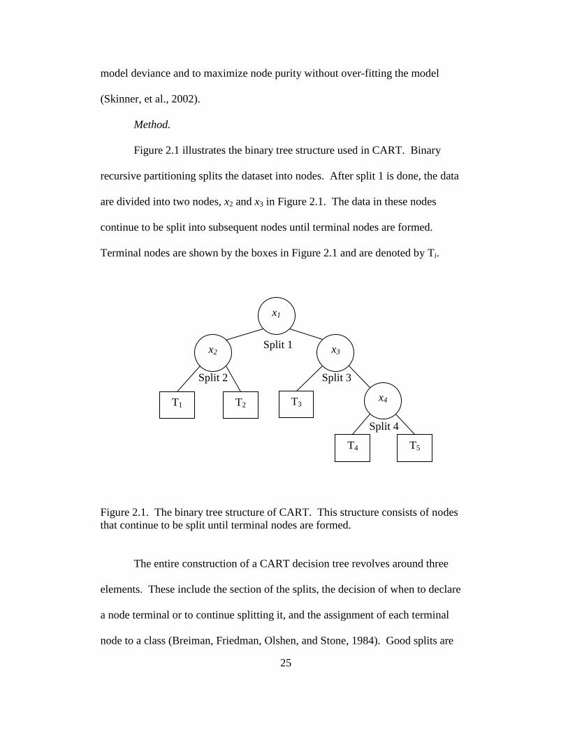
Method.
Figure 2.1 illustrates the binary tree structure used in CART. Binary
recursive partitioning splits the dataset into nodes. After split 1 is done, the data
are divided into two nodes, x2 and x3 in Figure 2.1. The data in these nodes
continue to be split into subsequent nodes until terminal nodes are formed.
Terminal nodes are shown by the boxes in Figure 2.1 and are denoted by Ti.
Figure 2.1. The binary tree structure of CART. This structure consists of nodes
that continue to be split until terminal nodes are formed.
The entire construction of a CART decision tree revolves around three
elements. These include the section of the splits, the decision of when to declare
a node terminal or to continue splitting it, and the assignment of each terminal
node to a class (Breiman, Friedman, Olshen, and Stone, 1984). Good splits are
x1
x2 x3
T1 T2 T3 x4
T4 T5
Split 1
Split 2 Split 3
Split 4
26
defined by their purity. The impurity of a node for a classification tree can be
defined as
( ) (1| ), (2 | ),..., ( | )i t p t p t p j t (2.19)
where i(t) is a measure of impurity of node t, p(j|t) is the node proportions (e.g.,
the cases in node t belonging to a certain class j), and is a non-negative
function (Brieman, et al., 1984). The measure of node impurity by the Gini index
of diversity (Brieman, et al., 1984) is defined as
( ) ( | ) ( | )j i
i t p i t p j t
. (2.20)
This Gini method is the default for CART 5.0 (CART for Windows user’s guide
(Version 5.0), 2002). Other splitting criteria have been developed and used and
are described in depth in Brieman, et al. (1984).
Terminal nodes are created when there is no significant decrease in
impurity by splitting the node. This is measured by
( , ) ( ) ( ) ( )R R L Li s t i t p i t p i t (2.21)
27
where s is a candidate split, and Rp and Lp are the proportions of observations of
the parent node t that go to the child node tR and tL, respectively (Chang & Chen,
2005). The best splitter is one that maximizes ( , )i s t .
Once a tree is “grown,” the next step is to prune the tree. This creates a
sequence of simpler trees. This process begins with the saturated tree with very
few observations in each terminal node and, selectively pruning upward, produces
a sequence of sub-trees until the tree eventually collapses to the tree off the root
node (Chang & Chen, 2005). This pruning is done to guard against overfitting
(Brown, Pittard, & Park, 1996). Overfitting occurs when the decision tree
constructed classifies the training examples perfectly, but fails to accurately
classify new unseen instances (Braha & Shmilovici, 2002). Pruning relies on a
complexity parameter which can be calculated through a cost function of the
misclassification of the data and the size of the tree (Chang & Chen, 2005). To
determine this cost-complexity parameter, first, the misclassification cost for a
node and a tree must be determined. The node misclassification cost can be
defined as
( ) 1 ( | )r t p j t (2.22)
and the tree misclassification cost can be defined as
( ) ( ) ( )r T
R T r t p t
(2.23)
28
The cost-complexity measure for each subtree T, R(T), can be defined, then, as
( ) ( ) | |R T R T T (2.24)
Where | |T is the tree complexity, which is equal to the number of terminal nodes
of the subtree, and is the complexity parameter which measures how much
additional accuracy is added to the tree to warrant additional complexity (Chang
& Chen, 2005). Alpha varies between 0 and 1, and by gradually increasing this
parameter, the smaller | |T becomes to minimize ( )R T , and a sequence of
pruned subtrees is generated (Chang & Chen, 2005).
To choose the best pruned tree that avoids overfitting, cross-validation is
conducted. This may be done by using techniques such as resubstitution, test
sample estimation, V-fold cross validation, or N-fold cross-validation (Brieman,
et al., 1984).
Other Applications.
CART has been used to model a variety of data in applications.
Khoshgoftaar and Allen (2002) apply CART to predicting fault-prone software
modules in embedded systems, and Khoshgoftaar and Seliya (2003) compare two
CART models with other approaches for modeling software quality. Neagu and
Hoerl (2005) use CART methods to define a “yellow zone” for predicting
corporate defaults. Scheetz, Zhang, and Kolassa (2009) apply classification trees

29
to identify severe and moderate vehicular injuries, and Chang and Chen (2005)
use tree-based data mining models to analyze freeway accident frequencies in
Taiwan. CART is commonly applied to medical studies as well. For example,
Kurt, Ture, and Kurum (2008) use CART to predict coronary heart disease, and
Ture, Kurt, Kurum, and Ozdamar (2005) use this approach to predict
hypertension. These two papers show how the decision tree structure of CART is
similar to medical reasoning and how it can be used to complement statistical
approaches such as logistic regression.
Statistical Approaches
Though many yield models have been introduced over the last five
decades, there is still a need for a model that can accurately model yield for a
semiconductor process for both purposes of process improvement and of
forecasting yield. The assumptions made in these past models are not generally
valid, and the complexity of some approaches and the data required can also be
limiting factors. An approach is needed that examines the impact of a defect
being located on a specific processing layer to help detect significant yield
impacts for those layers. Also, these models of the past do not model yield at the
die level, losing much of the information that is captured during expensive defect
scans, and forcing modelers to use average defect densities across wafers or lots.
The past models also do not consider the nested structure of the process, where
dice are fabricated together on wafers, and wafers are processed together in lots.

30
In addition, interactions between various factors are not considered, such as
considering the impact of having a defect on a die on multiple layers. For
additional discussion of the assumptions made in yield models, see Ferris-Prabhu
(1992). Statistical approaches, such as using regression techniques, offer a
solution for these problems. Ordinary least squares (OLS) regression, GLMs, and
GLMMs are described in this section.
Ordinary Least Squares Regression
For response data that are normally distributed, linear regression models
often fit well. These models are in the form
0 1 1 ... p py x x . (2.25)
The coefficients, 0 1, , p , are estimated using the method of least squares.
These models assume the residuals to be normally distributed with mean equal to
zero and constant variance as well as independence between the observations. If
these assumptions are violated, the model is not adequate (Montgomery, Peck &
Vining, 2006).
Generalized Linear Models (GLMs)
Due to the non-normality of the pass/fail response variable for yield,
techniques such as ordinary least squares regression are not adequate for
semiconductor yield models. To properly model a non-normal response whose

31
distribution is a member of the exponential family, generalized linear models may
be successfully employed. The exponential family includes the normal, Poisson,
binomial, exponential, and gamma distributions.
Generalized linear models (GLMs) were introduced by Nelder and
Wedderburn (1972). They combined the systematic and random (error)
components of a model characterized by a dependent variable, a set of
independent variables, and a linking function. The systematic component is the
linear predictor part of the model, the random component is the response variable
distribution (or error structure), and the link function between them defines the
relationship between the mean of the ith observation and its linear predictor
(Skinner, et al., 2002). This approach uses the maximum likelihood equations,
which are solved using an iterative weighted least squares procedure (Nelder and
Wedderburn, 1972). GLMs provide an alternative to data transformation methods
when the assumptions of normality and constant variance are not satisfied
(Montgomery, Peck, & Vining, 2006). One of the most commonly used
generalized linear models is logistic regression.
Logistic regression accounts for cases that have a binomial response, such
as proportion or pass/fail data. The logistic model for the mean response ( )E y is
given by
0 1 1( ... )'
1 1( )
1 1 p pi x xE y
e e
x β. (2.26)

32
The parameters are estimated using maximum likelihood.
There are three links commonly used in logistic regression models: the
logit, the probit, and the complimentary log-log links. These are expressed as
Logit
exp( ) 1( )
1 exp( ) 1 exp( )E y
'
' '
x β
x β x β (2.27)
Probit ( ) ( )E y 'xβ (2.28)
Complimentary Log-Log ( ) 1 exp[ exp( )]E y 'xβ . (2.29)
For the logit link, odds ratios are calculated that aid interpretation of the
predictors. The odds ratio can be interpreted as the estimated increase in the
probability of success associated with a one-unit change in the value of the
predictor variable (Montgomery, Peck, & Vining, 2006). Odds ratios are
calculated for each predictor by
ˆ1ˆ i i
i
x
R
x
oddsO e
odds
(2.30)
where ˆRO is the odds ratio for the predictor variable being examined, and ˆ
i is
the coefficient in the model corresponding to the predictor variable. For example,

33
if a model predicting failing dice has defectsx985.046.2 βx'
, an increase of one
defect will have an impact of an increased probability of failing dice of
exp(0.985) = 2.678. These ratios are not calculated for the probit or
complimentary log-log links.
For each of the link functions, the significance of individual regressors is
determined using Wald inference, which yields z-statistics and p-values similar to
the t-tests done in linear regression to test
0 : 0jH (2.31)
1 : 0jH . (2.32)
Model adequacy is determined by goodness-of-fit tests. Three statistics
are often used: the Pearson , Deviance, and the Hosmer-Lemeshow values.
Deviance can also be used to evaluate possible overdispersion, which can
underestimate regressors’ standard errors. For more on the theory and application
of logistic regression models, see McCullagh and Nelder (1989), Hosmer and
Lemeshow (2000), and Myers, Montgomery, Vining, and Robinson (2010).
Logistic regression is used more often than any other member in the
family of generalized linear models with wide applications to biomedical,
business management, biological, and industrial problems. GLMs have also been
applied to design experiments with non-normal responses (Lewis, Montgomery,

34
& Myers, 2001), to monitor multi-stage processes (Jearkpaporn, Borror, Runger,
& Montgomery, 2007) and to analyze reliability data (Lee & Pan, 2010). Software
packages such as Minitab and JMP simplify developing such models.
Generalized Linear Mixed Models (GLMMs)
One of the assumptions with GLMs is that the data are independent,
suggesting the experimental run has been completely randomized. In many cases,
factors in a process or experiment may be difficult or costly to change, making
this randomization impractical. Observations within these groups, which may be
split plots of split-plot designs or longitudinal data where an individual is tracked
over time, for example, are correlated, thus violating this assumption (Robinson,
Myers, and Montgomery, 2004).
Generalized linear mixed models (GLMMs) extend the GLM to include
various covariance patterns, enabling the GLM to account for correlation present
in random effects (Robinson, et al., 2004). The random effects models can also
relate to methods of dealing with forms of missing data or with random
measurement error in the explanatory variables (Agresti, 2002).
Breslow and Clayton (1993) first proposed GLMMs, and work by
Wolfinger and O’Connell (1993) refined the technique. This advance has had a
significant impact on research, demonstrated by the 2004 ISI Essential Science
Indicator identifying Breslow and Clayton (1993) as the most cited paper in
mathematics in the previous decade (Dean & Nielson, 2007). The GLMMs
explicitly model variance components and can be written as a batch-specific

35
model or as a population-averaged model. These two approaches have different
methods and scopes of inference for prediction.
Batch-specific model.
Also known as subject-specific models, batch-specific models are most
useful in repeated measures studies where individual profiles of subjects across
time are of interest (Myers, et al., 2010). These models produce estimates of the
mean conditional on the levels of the random effects.
Similar to linear mixed models, random effects GLMs are defined by
y = μ+ε , where
ZγXβμ )(g . (2.33)
Here, g is the appropriate link function, and γ and ε are assumed to be
independent. This gives the conditional mean for the thj cluster as
jjjjjn ggE
iγZβXηγy 11| (2.34)
where jny is the vector of responses at the thj cluster, g is the link function, jη is
the linear predictor, jX is the jn p matrix of fixed effect model terms
associate with the thj cluster, and β is the corresponding 1p vector of fixed
effect regression coefficients. For the random effect portion, jγ is the 1q

36
vector of random factor levels associated with the thj cluster, and jZ is the
corresponding matrix of predictors for the thj cluster (Myers, et al., 2010). The
thj cluster has jn observations.
This mixed model involves some assumptions as well. The conditional
response, γy | , is assumed to have an exponential family distribution, and each of
the random effects are assumed to be normally distributed with mean zero and the
variance-covariance matrix of the vector of random effects in the thj cluster is
denoted jG . The jG is typically assumed to be the same for each cluster
(Myers, et al., 2010).
Population-averaged model.
When interest is in estimating more general trends across the entire
population of random effects rather than at the specific levels, a population-
averaged model is more appropriate (Myers, et al., 2010). While a popular
approach for estimating the marginal mean using the batch-specific models is to
set 0ˆ γ since 0γ )(E , this estimate of the marginal mean will differ from that
found using the population-averaged approach, and the estimated fixed effect
parameters will also differ for the two approaches (Myers, et al., 2010) with the
conditional effects usually being larger than the marginal effects, though the
significance of the effects is usually similar (Agresti, 2002).
The marginal mean is more tedious to obtain due to the nonlinearity in
GLMMs, so often approximations must be used. This is done by linearizing the

37
conditional mean using a first-order Taylor series expansion about ( )E η Xβ and
gives the approximation of the unconditional process mean as
Xβγ|yy 1 gEEE . (2.35)
This approximation will be exact for a linear link function and is more accurate
when the variance components associated with δ are close to zero (Myers, et al.,
2010).
The population-averaged model requires that a covariance structure be
defined for the error term. This is a major difference from the batch-specific
approach. For split-plot designs, the correlation matrix, R , generally has a
compound symmetric structure (Robinson, et al., 2004). For a random effect such
as following a subject over time in a longitudinal study, R may take on a first-
order autoregressive (AR-1) structure.
Robinson, et al. (2004) found that in examining the application of both
approaches to a split plot experiment, that when the prediction of an average
across all subjects (batches, in this case) is of interest, it is better to model the
unconditional expectation of the response than the conditional expectation. The
population-averaged model is appealing for prediction purposes, but the quality of
this model is heavily dependent on the assumption that the group of random
subjects or clusters is a true representation of the whole (Robinson, et al., 2004).

38
Parameter estimation.
With GLMs, the independence of the data makes the log likelihood well-
defined and the objective function for estimating the parameters simple to
construct (SAS, 2006). This is not the case for GLMMs. The objective function
may not be able to be computed due to cases:
1. where no valid joint distribution can be constructed,
2. where the dependency between the mean and the variance places
constraints on the possible correlation models that simultaneously
yield valid joint distributions and desired conditional distributions, or
3. where the joint distribution may be mathematically feasible but
computationally impractical (SAS, 2006).
Two basic parameter estimation approaches have been suggested in the
literature: to approximate the objective function and to approximate the model
(SAS, 2006). Integral approximation methods approximate the log likelihood of
the GLMM and use the approximated function in numerical optimization using
techniques such as Laplace methods, quadrature methods, Monte Carlo
integration, and Markov Chain Monte Carlo methods (SAS, 2006). The
advantage of this approach is that it provides an actual objective function for
optimization. This singly iterative approach has difficulty in dealing with crossed
random effects, multiple subject effects, and complex marginal covariance
structures (SAS, 2006).
Linearization methods are used to approximate the model, using
expansions to approximate the model by one based on pseudo-data with fewer
39
nonlinear components (SAS, 2006). These fitting methods are usually doubly
iterative. First, the GLMM is approximated by a linear mixed model based on
current values of the covariance parameter estimates. The resulting linear mixed
model is then fit, also using an iterative process. Upon convergence, the new
parameter estimates are used to update the linearlization. The process continues
until the paramenter estimates between successive linear mixed model fits change
within a specified tolerance (SAS, 2006).
Linearization-based methods have the advantage of including a relatively
simple form of the linearized model, allowing it to fit models for which the joint
distribution is difficult or impossible to obtain (SAS, 2006). While this approach
handles models with correlated errors, a large number of random effects, crossed
random effects, and multiple types of subjects well, the method does not use a
true objective function for the overall optimation process, and the estimates of the
covariance paramenters can be potentially biased, especially for binary data (SAS,
2006). PROC GLIMMIX uses linearizations to fit GLMMs.
The default estimation technique, restricted pseudo-likelihood (RPL), is
based on the work of Wolfinger and O’Connell (1993). The Pseudo-Model
begins with
μηZγXβγ|Y 11 ggE 2.36
where )(~ G0,γ N and 2/121var RAAγ|Y / .

40
The first-order Taylor series of μ about β~
and γ~ yields
γγZΔββXΔηη ~~~~~11 gg 2.37
where
~,
~
~
η
Δ1g
is a diagonal matrix of derivatives of the conditional
mean evaluated at the expansion locus (Wolfinger & O’Connell, 1993). This can
also be expressed as
ZγXβγZβXημΔ1 ~~~~ 1g 2.38
The left-hand side is the expected value, conditional on γ , of
PγZβXηYΔ1 ~~~~ 1g 2.39
and
11/21/21ΔRAAΔγ|P
~~
var . 2.40
Thus, the model
εZγXβP 2.41

41
can be considered. This is a linear mixed model with pseudo-response P , fixed
effects β , random effects γ , and γ|Pε varvar .
Now, the marginal variance in the linear mixed pseudo-model is defined
as
12/12/1 ~~' ΔRAAΔZGZθV 2.42
where θ is the 1q parameter vector containing all unknowns in G and R .
Assuming the distribution of P is known, an objective function can be defined
based on this linearized model. The restricted log pseudo-likelihood (RxPL) for
P is
2log2
log2
1
2
1log
2
1 11 kflR
XθVX'rθVr'θVpθ, 2.43
With pVX'XVX'Xpr11 . f denotes the sum of the frequencies used in
the analysis, and k denotes the rank of X . The fixed effects parameters β are
profiled from these expressions, and the parameters in θ are estimated by
optimization techniques, such as Newton-Raphson. The objective function for
minimization is pθ,Rl2 . At convergence, the profiled parameters are
estimated as

42
pθVXXθVXβ11
ˆˆˆ 2.44
and the random effects are predicted as
rθVZGγ ˆˆˆˆ1
. 2.45
Using these statistics, the pseudo-response and error weights of the linearlized
model are recomputed and the objective function is minimized again until the
relative change between parameter estimates at two successive iterations is
sufficiently small (SAS, 2006). For more on parameter estimation, see Wolfinger
and O’Connell (1993), SAS (2006), and Myers, et al. (2010).
Applications.
GLMMs have been applied widely in epidemiology (Fotouhi, 2008), but
have also been used to model events such as post-earthquake fire ignitions
(Davidson, 2009), electrical power outages due to severe weather events (Liu,
Davidson, & Apanasovich, 2007), credit defaults (Czado & Pfluger, 2008), plant
disease (Madden, Turecheck, & Nita, 2002), and workers’ compensation
insurance claims (Antonio & Beirlant, 2007). GLMMs can also be used in
designed experiments (Robinson, et al., 2004) and robust design and analysis of
signal-response systems (Gupta, Kulahci, Montgomery, & Borror, 2010). Myers,
et al. (2010) and Agresti (2002) include additional examples of applications of
GLMMs.

43
Chapter 3
DATA REFINING FOR MODEL BUILDING
The semiconductor industry is rich in data with many measurements being
taken at hundreds of points throughout the fabrication process. Analyzing these
data begins to become troublesome due to the amount of data available. The first
step in preparing to develop any semiconductor yield model is to collect,
integrate, and aggregate the data. Often, this can be the most time-consuming
step in model creation. The datasets collected in computer-aided manufacturing
are massive in size and complex due to the sampling strategies used that do not
necessarily correspond with one another in levels of aggregation, the number of
sample wafers selected for different tests, or the actual sample wafers used. This
chapter describes the data that were collected from an SRC-member company that
were used in the analysis provided in Chapters 4-6. The data collection,
integration, and aggregation process is described in detail to aid practitioners in
completing these steps in following the modeling strategies described in the
following chapters.
Overall Description of Data
The device studied is a non-volatile memory chip with RAM, ROM, and
flash components. It has a 32-bit microcontroller and is used in applications such
as engines, tractors, printers, and basically anything that is not a personal
computer. It uses communication design rule (CDR1) technology. Each 8” wafer

44
contains 226 dice and takes 10-12 weeks to process. A cross section of the device
is provided in Figure 3.1.
Figure 3.1. Cross section of semiconductor device from an SRC-member
company. The different layers of processing are shown.
In developing a data test bed for this and future research, four areas of evaluation
were considered: 1) process data, 2) defectivity data, 3) class probe, and 4) unit
probe.
Process Data.
As lots move through the fabrication process, many measurements are
taken at different stages to gauge how the process is performing. For example,
critical dimension measurements may be taken after an etching process to ensure
the correct amount of material was etched. These process measurements also
measure critical dimensions and overlay for the photo processes, remaining

45
oxides at etch, changes in oxide thicknesses, etch endpoint times, and more.
Several process parameters are recorded at each layer of fabrication.
Process data are automatically recorded in a tool, such as DataLog.
Though DataLog can have data integrity issues, it is used commonly in examining
process data in SPC graphs. DataLog isn’t a tool often used by the device
engineer. He or she relies more on the defectivity, class probe (also referred to as
parametric or electrical test), and yield data. If there is a processing concern, he
or she directs questions to the process owner.
Data are pulled from DataLog by using what is known as an Area –
Logbook – Process or ALP. An area will usually denote the type of process and
measurement. For instance, E_CD_SEM measures the critical dimensions for the
etch process. The “logbook” is often a specified piece of equipment or a specified
layer for the part. Often the “process” is the part name or an equipment name.
Queries can be used to extract raw or summary data and can be limited by date.
The process data extracted for this project are those applicable to the device of
interest during the time period of April 1, 2006 through September 30, 2006.
Process data are measured on two wafers from each lot after each layer of
fabrication (see Figure 3.3). The data files compiled for this project include both
the raw and summary data for each process parameter. This allows researchers to
examine the control charts, such as the one shown in Figure 3.2 for defect density,
as well as using the raw or summary data for modeling purposes. Some of the
process measurements included in this data set are given in Table 3.1.
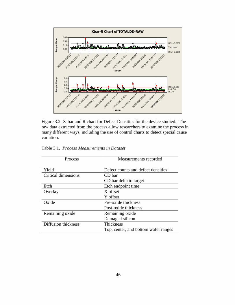
46
ST OP
Sa
mp
le M
ea
n
09/2
6/20
06 19:
35:5
7
09/1
2/20
06 2
3:48
:19
08/2
3/20
06 9:5
6:09
07/2
8/20
06 1
4:48
:04
07/1
5/20
06 17:
43:5
1
06/2
6/20
06 2:2
3:42
06/06/
2006
22:33
:30
05/2
3/20
06 21:
43:5
0
05/04/
2006
7:40:
11
04/22/
2006
15:54
:44
04/01/
2006
6:14:
11
0.45
0.30
0.15
0.00
__X=0.0595
UC L=0.2267
LC L=-0.1076
ST OP
Sa
mp
le R
an
ge
09/2
6/20
06 19:
35:5
7
09/1
2/20
06 2
3:48
:19
08/2
3/20
06 9:5
6:09
07/2
8/20
06 1
4:48
:04
07/1
5/20
06 17:
43:5
1
06/2
6/20
06 2
:23:
42
06/06/
2006
22:33
:30
05/2
3/20
06 21:
43:5
0
05/04/
2006
7:40:
11
04/22/
2006
15:54
:44
04/01/
2006
6:14:
11
2.0
1.5
1.0
0.5
0.0
_R=0.346UC L=0.693
LC L=0
11
1
11
111
1
1
11
Xbar-R Chart of TOTALDD-RAW
Figure 3.2. X-bar and R chart for Defect Densities for the device studied. The
raw data extracted from the process allow researchers to examine the process in
many different ways, including the use of control charts to detect special cause
variation.
Table 3.1. Process Measurements in Dataset
Process Measurements recorded
Yield Defect counts and defect densities
Critical dimensions CD bar
CD bar delta to target
Etch Etch endpoint time
Overlay X offset
Y offset
Oxide Pre-oxide thickness
Post-oxide thickness
Remaining oxide Remaining oxide
Damaged silicon
Diffusion thickness Thickness
Top, center, and bottom wafer ranges

47
Defectivity.
Defects are detected by comparative techniques using high-powered visual
equipment. Defects are found by a machine comparing one die to the next and
noting any differences. If there is a difference between the two die, a third dice is
checked to determine which one contains the defect. These data are often used to
look at significant problems with a wafer.
At the SRC-member company contributing to this project, defectivity is
measured using KLA machines and is recorded in a system called KLARITY.
KLARITY stores both die- and wafer-level data. However, KLARITY is not
directly linked to the database that contains the unit probe data for the die. A
program has been written to link the two when both types of corresponding data
are needed.
The size of the defect is usually not of concern to the engineers. However,
the visual images produced from selected defects are often key in determining the
root causes for problems. Device engineers can access these images from their
computers easily. Defects such as scratches can be easily seen at a high level, and
SEM (Scanning Electron Microscope) images are also available. These images
help the engineer quickly determine if the defect will cause a fatal flaw in the
dice. Sometimes defects will cause a die to fail at unit probe (known as a fault),
but other times (this is somewhat dependent on the location on the die and the
critical area), the die will function properly regardless of the defect.
KLA data are recorded at ten layers of this device. They are given in
Table 3.2.

48
Table 3.2. Description of the Layers Involved in Defectivity Scans
Layer Description
Layer 1 Active
Layer 2 Poly 1
Layer 3 Flash
Layer 4 Flash Drain
Layer 5 Salicide
Layer 6 Contact
Layer 7 Metal 1
Layer 8 Via 1
Layer 9 Metal 2
Layer 10 Metal 3
Defectivity measures are not performed on every wafer. For this device,
they are usually conducted on every tenth lot that is fabricated. From each of
these test lots, two wafers (#2 and #21) are tested (see Figure 3.3). The dataset
includes the wafers that had KLA data that were tested at unit probe between June
1, 2006 and September 30, 2006. This dataset includes 136 lots.
The KLA data in the dataset compiled include the lot number, wafer
number, x- and y- coordinates of the die, the layer where the testing was
performed, the defect number (such as the 10th
defect found, etc.), the
classification if the defect was classified, and the corresponding bin code from
unit probe.
The process data and the defectivity data are the two types of in-line test
measures available in the dataset. Toward the end of the fabrication process, class
probe and bin data are collected. Figure 3.3 shows the frequency of the wafer
testing for the various data types and the inconsistencies present in the sampling
structure across the different data types.
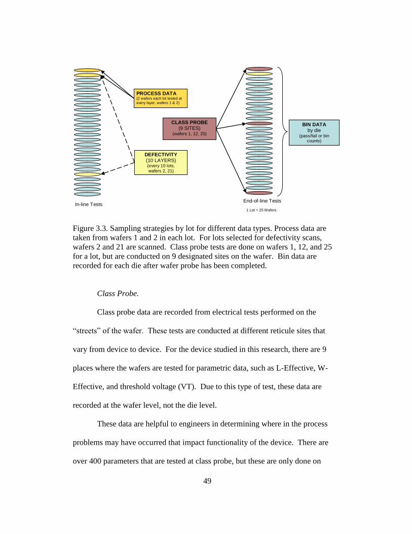
49
CLASS PROBE (9 SITES)
(wafers 1, 12, 25)
DEFECTIVITY (10 LAYERS) (every 10 lots,
wafers 2, 21)
1 Lot = 25 Wafers
BIN DATA by die
(pass/fail or bin counts)
PROCESS DATA (2 wafers each lot tested at every layer, wafers 1 & 2)
In-line Tests End-of-line Tests
Figure 3.3. Sampling strategies by lot for different data types. Process data are
taken from wafers 1 and 2 in each lot. For lots selected for defectivity scans,
wafers 2 and 21 are scanned. Class probe tests are done on wafers 1, 12, and 25
for a lot, but are conducted on 9 designated sites on the wafer. Bin data are
recorded for each die after wafer probe has been completed.
Class Probe.
Class probe data are recorded from electrical tests performed on the
“streets” of the wafer. These tests are conducted at different reticule sites that
vary from device to device. For the device studied in this research, there are 9
places where the wafers are tested for parametric data, such as L-Effective, W-
Effective, and threshold voltage (VT). Due to this type of test, these data are
recorded at the wafer level, not the die level.
These data are helpful to engineers in determining where in the process
problems may have occurred that impact functionality of the device. There are
over 400 parameters that are tested at class probe, but these are only done on

50
wafers 1, 12, and 25 for each lot. However, reliability tests, which include 17 or
18 parameters, are performed on 5 sites on every wafer for this device. These are
stored differently in dataPOWER so device engineers as well as process engineers
are able to use the information.
Some parameters are closely linked to specific processes. For instance, if
a problem occurs with the L-Effective, the device engineer knows the process
most likely responsible for this deviation, whereas when problems occur with W-
Effective, which is formed in several different steps, it is harder to determine the
root cause.
The dataset compiled includes class probe data for all wafers tested
between June 1, 2006 and September 30, 2006. In addition, the company
provided a list of 109 “watchdog” parameters that are more important to refine the
search from the 400+ to these. The engineer also provided a list of about 40 of
these “watchdog” parameters that he considers most important.
Unit Probe.
The unit probe (sometimes called wafer sort) data are needed to determine
the final adequacy of the product. Testing is performed to determine if the die are
good or bad. When a die fails, its failure is categorized into a specific “bin.”
These various bins are coded for a variety of failure modes. These failures can be
viewed on a wafer map as shown in Figure 3. 4.

51
Figure 3.4. A wafer map. Different colors of dice on the wafer map indicated
different failure bin assignments based on unit probe tests.
For this device, two passes of testing are required. The first pass includes
all functional testing. If a wafer passes the first pass of testing, each die is
classified into BIN 250, and it is baked for 72 hours before the memory is
checked for retention. If a die passes this second test, it is classified as “BIN 1”
and is shippable. If the wafer fails the first pass, it will be scrapped unless there
are special circumstances such as the engineer hasn’t readjusted the specification
limits after a change. The engineer may indicate if the wafer should be retested.
Hence, sometimes there are multiple sets of bin data for the same wafer. The
failure limits for specific bins are kept in a specific program where the data can be
easily accessed by the engineer to examine specific failures.

52
Use of the Dataset
As described in Chapter 1, this dissertation focuses on developing
modeling strategies using GLMs to predict wafer sort outcomes at unit probe
testing based on defect counts on the process layers. The other components of
this dataset (class probe and process data) have been useful in furthering the work
of Kumar (2006) through the work of Chang (2010) at the University of
Washington. These data have been used to help further advance the methodology
of hGLMs described in Chapter 2. The remainder of this chapter will describe the
steps taken to refine the defect count and wafer sort data from their raw forms in
the dataset to a useable form for modeling purposes.
Data Refining for GLM Model Building
Data Integration.
For GLM models that use defectivity data for predictors, the defect
metrology data and the wafer sort yield data first need to be integrated by die for
die-level analyses to be performed. This can be done a number of ways, including
automatic or manual methods. If using software such as DataPower, these data
may already be integrated and be easy to extract together. If multiple databases
are used to store the various types of data recorded during the fabrication and
testing process, though, running queries in both can sometimes require advanced
coding expertise, especially if the location coordinates of the dice are constructed
differently for different tests, specifically, defect metrology and wafer sort.

53
Data Aggregation.
Perhaps the most time-consuming task is taking the integrated data and
aggregating them into a form that will be usable for model building. Table 3.3
contains an example of raw, integrated data extracted from a database. Rows
showing dice with multiple defects on a layer are highlighted in bold text. While
these integrated data contain the lot number, wafer number, layer number, die
location (given in x- and y-coordinates), and the final bin assigned at wafer sort
for each identified defect found during the scan, this arrangement of the data is
not useful for common statistical packages such as Minitab or JMP that can create
the desired models. For example, in Table 3.3, the die from Lot 1, Wafer 2, with
coordinates (9, 1) has one defect on Layer 1 and three defects on Layer 2, so it is
displayed on four different rows. The data need to be aggregated such that each
die (or wafer for wafer-level modeling) is a row, and the total number of defects
in each layer is given in a separate column with the column containing the wafer
sort test result remaining. An example of the necessary aggregation is shown in
Table 3.4. Here, the die from Lot 1, Wafer 2 with coordinates (9, 1) is
summarized in a single row showing it had one defect detected in Layer 1 and
three defects on Layer 2. Also, if using a binomial response (pass or fail), the
failure bin data should be converted to reflect the appropriate binomial response
rather than a specific bin number as shown in the far right column.
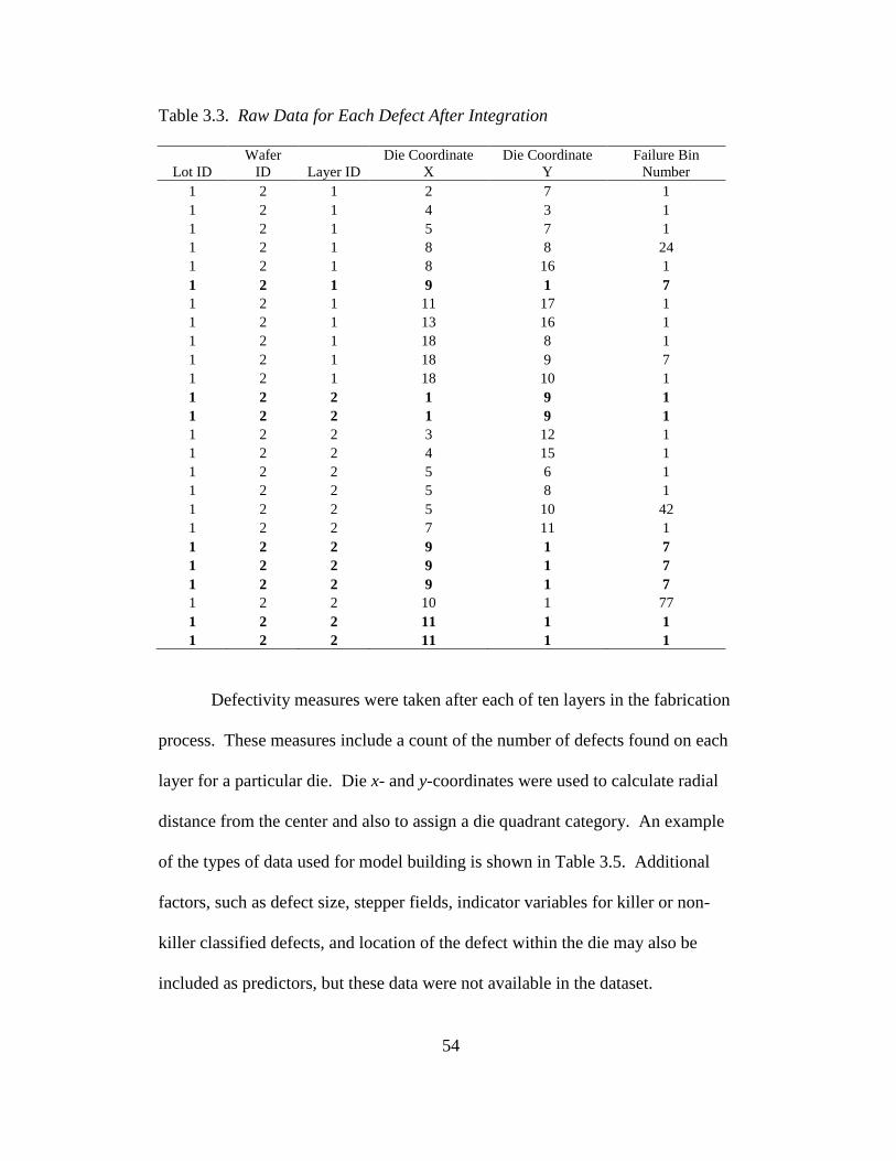
54
Table 3.3. Raw Data for Each Defect After Integration
Lot ID
Wafer
ID Layer ID
Die Coordinate
X
Die Coordinate
Y
Failure Bin
Number
1 2 1 2 7 1
1 2 1 4 3 1
1 2 1 5 7 1
1 2 1 8 8 24
1 2 1 8 16 1
1 2 1 9 1 7
1 2 1 11 17 1
1 2 1 13 16 1
1 2 1 18 8 1
1 2 1 18 9 7
1 2 1 18 10 1
1 2 2 1 9 1
1 2 2 1 9 1
1 2 2 3 12 1
1 2 2 4 15 1
1 2 2 5 6 1
1 2 2 5 8 1
1 2 2 5 10 42
1 2 2 7 11 1
1 2 2 9 1 7
1 2 2 9 1 7
1 2 2 9 1 7
1 2 2 10 1 77
1 2 2 11 1 1
1 2 2 11 1 1
Defectivity measures were taken after each of ten layers in the fabrication
process. These measures include a count of the number of defects found on each
layer for a particular die. Die x- and y-coordinates were used to calculate radial
distance from the center and also to assign a die quadrant category. An example
of the types of data used for model building is shown in Table 3.5. Additional
factors, such as defect size, stepper fields, indicator variables for killer or non-
killer classified defects, and location of the defect within the die may also be
included as predictors, but these data were not available in the dataset.
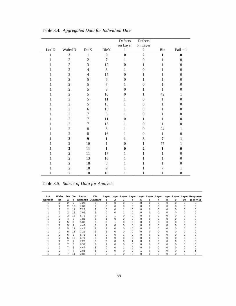
55
Table 3.4. Aggregated Data for Individual Dice
LotID WaferID DieX DieY
Defects
on Layer
1
Defects
on Layer
2 Bin Fail = 1
1 2 1 9 0 2 1 0
1 2 2 7 1 0 1 0
1 2 3 12 0 1 1 0
1 2 4 3 1 0 1 0
1 2 4 15 0 1 1 0
1 2 5 6 0 1 1 0
1 2 5 7 1 0 1 0
1 2 5 8 0 1 1 0
1 2 5 10 0 1 42 1
1 2 5 11 1 0 1 0
1 2 5 15 1 0 1 0
1 2 6 15 1 0 1 0
1 2 7 3 1 0 1 0
1 2 7 11 0 1 1 0
1 2 7 15 1 0 1 0
1 2 8 8 1 0 24 1
1 2 8 16 1 0 1 0
1 2 9 1 1 3 7 1
1 2 10 1 0 1 77 1
1 2 11 1 0 2 1 0
1 2 11 17 1 1 1 0
1 2 13 16 1 1 1 0
1 2 18 8 1 1 1 0
1 2 18 9 1 1 7 1
1 2 18 10 1 1 1 0
Table 3.5. Subset of Data for Analysis
Lot
Number
Wafer
ID
Die
X
Die
Y
Radial
Distance
Die
Quadrant
Layer
1
Layer
2
Layer
3
Layer
4
Layer
5
Layer
6
Layer
7
Layer
8
Layer
9
Layer
10
Response
(Fail = 1)
1 2 2 7 7.28 3 1 0 0 0 0 0 0 0 0 0 0
1 2 2 10 7.07 2 0 0 0 0 0 1 0 0 0 0 0
1 2 2 11 7.28 2 0 0 1 0 0 0 0 0 0 0 0
1 2 2 12 7.62 2 0 0 1 0 0 0 0 0 0 0 0
1 2 3 12 6.71 2 0 1 0 0 0 0 0 0 0 0 0
1 2 4 3 7.81 3 1 0 0 0 0 0 0 0 0 0 0
1 2 5 6 5.00 3 0 1 0 0 0 0 0 0 0 0 0
1 2 5 7 4.47 3 1 0 0 0 0 0 0 0 0 0 0
1 2 5 11 4.47 2 1 0 0 0 0 0 0 0 0 0 0
1 2 5 15 7.21 2 1 0 0 0 0 0 0 0 0 0 0
1 2 6 3 6.71 3 0 0 1 0 0 0 0 0 0 0 0
1 2 6 15 6.71 2 1 0 0 0 0 0 0 0 0 0 0
1 2 7 2 7.28 3 0 0 0 1 0 0 0 0 0 0 0
1 2 7 3 6.32 3 1 0 0 0 0 0 0 0 0 0 0
1 2 7 5 4.47 3 0 0 1 0 0 0 0 0 0 0 0
1 2 7 7 2.83 3 0 0 0 0 1 0 0 0 0 0 1
1 2 7 11 2.83 2 0 1 0 0 0 0 0 0 0 0 0

56
Managing outliers.
With the large quantities of data available in the semiconductor industry,
there is a question of which data, if any, should be removed for model building.
While many algorithms exist to detect outliers, clear cutoffs for removing data are
difficult to determine. Figure 3.4 illustrates the large number of possible outliers
looking at the total number of defects per die. For the die-level training set, the
median is 1.0, but the mean is 2.571 defects per die. Also, the third quartile is 2.0
and the maximum value is 218. This demonstrates the presence of unusual
observations that may have a strong impact on model building.
To explore the effects of removing outliers, the models built in the study
described in Chapter 4 were built three times from the training dataset. The
distribution for the die-level training dataset showed the 97.5th
percentile to be 9
total defects on a die, and the 95th
percentile was 5 total defects on a die. The dice
with more than 9 and more than 5 total defects were removed from the data set
using a one-sided trimmed means outlier detection approach with p=0.025 and
p=0.05, respectively. Hu and Sung (2004) show trimmed means to be an
appropriate method for outlier detection that has higher efficiency than using
median. This method unifies mean and median in a dataset. While their study
uses two-sided trimmed means with p=0.15, this more conservative approach will
allow the most common occurrences of defect distributions on layers to be
examined while constructing useful models. No points were removed from the
test dataset that was used for validation purposes described in Chapters 4, 5, and
6.
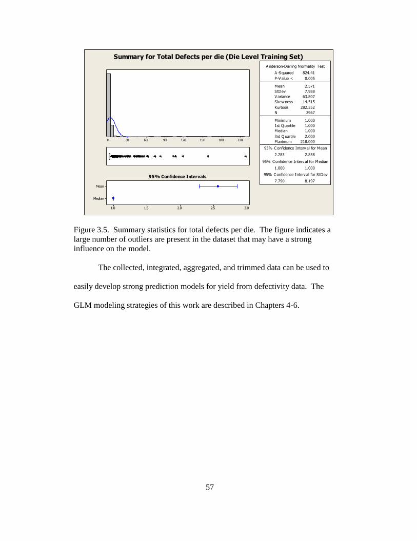
57
2101801501209060300
Median
Mean
3.02.52.01.51.0
A nderson-Darling Normality Test
V ariance 63.807
Skewness 14.515
Kurtosis 282.352
N 2967
Minimum 1.000
A -Squared
1st Q uartile 1.000
Median 1.000
3rd Q uartile 2.000
Maximum 218.000
95% C onfidence Interv al for Mean
2.283
824.41
2.858
95% C onfidence Interv al for Median
1.000 1.000
95% C onfidence Interv al for StDev
7.790 8.197
P-V alue < 0.005
Mean 2.571
StDev 7.988
95% Confidence Intervals
Summary for Total Defects per die (Die Level Training Set)
Figure 3.5. Summary statistics for total defects per die. The figure indicates a
large number of outliers are present in the dataset that may have a strong
influence on the model.
The collected, integrated, aggregated, and trimmed data can be used to
easily develop strong prediction models for yield from defectivity data. The
GLM modeling strategies of this work are described in Chapters 4-6.

58
Chapter 4
SEMICONDUCTOR YIELD MODELING USING GENERALIZED LINEAR
MODELS
Introduction
As shown in Chapter 2, many approaches have been taken to model
semiconductor yield, but these models make a number of assumptions that are not
valid for the nature of the process and the data being collected. Ferris-Prabhu
(1992) shows the accuracy of yield predictions depends just as much on the
accuracy of the assumed average defect densities as upon the choice of yield
model. Generalized linear models (GLMs), described in Chapter 2, offer a way to
construct models making fewer assumptions as well as a means of modeling the
data in more detail by creating die-level models that can take advantage of the raw
data available, instead of relying on lot- or wafer-level summaries. This approach
of die-level modeling can also consider nested effects.
In some multi-factor experiments, the levels of one factor are similar but
not identical for different levels of another factor. This is called a nested (or
hierarchical) design. Nested designs are often used in analyzing processes to
identify the major sources of variability in the output. In a two-stage nested
design, the levels of factor B are nested under the levels of factor A. That is, the
levels of B are unique for each level of A. For example, for the semiconductor
industry, wafers are nested within lots.
Since the dice are processed together on a wafer, and wafers are grouped
together in a lot, independence from die to die cannot be assumed. To account for
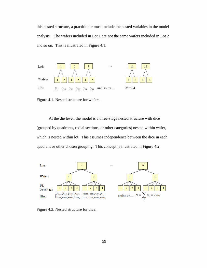
59
this nested structure, a practitioner must include the nested variables in the model
analysis. The wafers included in Lot 1 are not the same wafers included in Lot 2
and so on. This is illustrated in Figure 4.1.
Figure 4.1. Nested structure for wafers.
At the die level, the model is a three-stage nested structure with dice
(grouped by quadrants, radial sections, or other categories) nested within wafer,
which is nested within lot. This assumes independence between the dice in each
quadrant or other chosen grouping. This concept is illustrated in Figure 4.2.
Figure 4.2. Nested structure for dice.

60
Model Building Using Logistic Regression
The dataset used in this phase of the research consisted of defectivity data
for 36 wafers from 18 lots and the corresponding wafer sort data given for each
die on those wafers that had at least one defect recorded. This included 4,413
dice. These wafers were found to be an appropriate random sample of wafers
produced over time for the industrial product’s dataset. In order to assess the
validity of the models, the dataset of 18 lots was divided into a training dataset of
12 lots and a test dataset of 6 lots. The 12 lots used for the training dataset were
chosen at random from the 18 lots. The data from these 12 selected lots were
used consistently to construct the wafer- and die-level models.
Both die- and wafer-level models were developed using the training data
set of 24 wafers (12 lots). For the die-level model, predictor variables included
lot, wafer, radial distance, die quadrant, and the count of defects found on each of
the ten layers. Non-nested and nested models were created to observe differences
between the two, with the nested model created by nesting wafer within lot and
die quadrant within wafer, assuming independence between the die within a die
quadrant. For the wafer-level model, predictor variables included lot, wafer, and
the count of defects found on each of the ten layers of the wafer. No nested
models were created at the wafer level due to a lack of degrees of freedom with
the current sampling structure. Minitab software was used to build these logistic
regression models. Full models used all predictor variables, and reduced models
were created through backward elimination using factors found to be significant
at the =0.1 level. All factors were considered to be fixed in these analyses.

61
Results
The results and discussion are organized primarily into examining the die-
level analysis and the wafer-level analysis. Within each one, the nested structure
is discussed, the significance of outliers is examined, and the different link
functions used in logistic regression are compared. Validation is assessed, and a
comparison to other yield models from the literature is also provided.
Die-Level Logistic Regression.
To demonstrate the problems with using standard linear regression models
for this binary response, the entire training dataset (N=2967) was first analyzed
using multiple linear regression. Figure 4.3 shows the residual plots for this
model. The normal probability plot indicates that the errors are not normally
distributed. The residuals versus the fitted values plot shows a distinct pattern,
rather than showing random behavior. The histogram of the residuals again
shows non-normality. These results indicate the linear model is inadequate since
the assumptions for this model, including:
1. The relationship between the response and the regressors is linear, at
least approximately,
2. The error term has zero mean,
3. The error term has constant variance 2,
4. The errors are uncorrelated, and
5. The errors are normally distributed (Montgomery, Peck, & Vining,
2006)
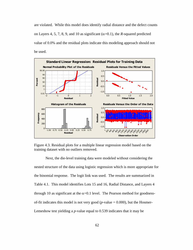
62
are violated. While this model does identify radial distance and the defect counts
on Layers 4, 5, 7, 8, 9, and 10 as significant (=0.1), the R-squared predicted
value of 0.0% and the residual plots indicate this modeling approach should not
be used.
Residual
Pe
rce
nt
210-1-2
99.99
99
90
50
10
1
0.01
Fitted ValueR
esid
ua
l2.01.51.00.50.0
1.0
0.5
0.0
-0.5
-1.0
Residual
Fre
qu
en
cy
0.750.500.250.00-0.25-0.50-0.75-1.00
800
600
400
200
0
Observation Order
Re
sid
ua
l
2800
2600
2400
2200
2000
1800
1600
1400
1200
100080
060
040
020
01
1.0
0.5
0.0
-0.5
-1.0
Normal Probability Plot of the Residuals Residuals Versus the Fitted Values
Histogram of the Residuals Residuals Versus the Order of the Data
Standard Linear Regression: Residual Plots for Training Data
Figure 4.3. Residual plots for a multiple linear regression model based on the
training dataset with no outliers removed.
Next, the die-level training data were modeled without considering the
nested structure of the data using logistic regression which is more appropriate for
the binomial response. The logit link was used. The results are summarized in
Table 4.1. This model identifies Lots 15 and 16, Radial Distance, and Layers 4
through 10 as significant at the =0.1 level. The Pearson method for goodness-
of-fit indicates this model is not very good (p-value = 0.000), but the Hosmer-
Lemeshow test yielding a p-value equal to 0.539 indicates that it may be

63
adequate. This model, however, assumes independence between the die, which is
not valid considering the nature of the fabrication process.
Table 4.1. Die-Level Non-Nested Logistic Regression Model Results for Full
Training Data Set (N=2967)
Significant Factors
(alpha = 0.1)
p-value
Lot 15 0.040
Lot 16 0.010
Radial Distance 0.001
Layer 4 0.003
Layer 5 0.001
Layer 6 0.002
Layer 7 0.000
Layer 8 0.071
Layer 9 0.000
Layer 10 0.000
Next, the nested structure was modeled using the entire training dataset.
This analysis gives much more information. Instead of only identifying
significant lots, this model shows there to be a significant difference between
Wafer 1 and Wafer 2 in Lots 4 and 16. The logit link model also shows 6 die
quadrants to be significantly different from Die Quadrant 1 on the same wafer
(=0.1). This model again indicates Radial Distance is significant, and lists
Layers 4 through 10 as significant predictors.
All three link functions were used to build models with the nested
structure using the entire training dataset as well as with the two trimmed training
datasets. These results are presented in Table 4.2. While the results were similar
among the links, the probit model did not converge after 5000 iterations, and did
not identify Layer 7 as significant at the 0.1 level for the full training dataset.

64
Also, the complimentary log-log link shows the best value for the Hosmer-
Lemeshow goodness-of-fit test. It also found an additional die quadrant to be
significant.
Table 4.2. Comparison of Link Functions and Outlier Methods (Die-level,
Nested)
All Training Set Data
N=2967
Outliers Removed (2.5%
trimmed)
N=2896
Outliers Removed (5%
trimmed)
N=2845 Logit Probit Complime
ntary Log-
Log
Logit Probit Complimen
tary Log-
Log
Logit Probit Complimen
tary Log-
Log Significa
nt Factors
Wafer
2(4)
Wafer
2(16)
Rad. Dist.
6 Die
Quadrants
Layers 4-
10
Wafer
2(4)
Wafer
2(16)
Rad. Dist.
6 Die
Quadrants
Layers 4-
6, 8-10
Wafer 2(4)
Wafer 2(16)
Rad. Dist.
7 Die
Quadrants
Layers 4-10
Wafer
2(4)
Wafer
2(16)
Rad. Dist.
6 Die
Quadrants
Layers 2-
10
Wafer
2(4)
Wafer
2(16)
Rad.
Dist.
8 Die
Quadrant
s
Layers 2-
10
Wafer 2(4)
Wafer 2(14)
Wafer 2(16)
Rad. Dist.
7 Die
Quadrants
Layers 2-10
Wafer
2(4)
Wafer
2(16)
Rad. Dist.
7 Die
Quadrants
Layers 2-
10
Wafer 2(4)
Wafer
2(16)
Rad. Dist.
8 Die
Quadrants
Layers 2-
10
Wafer 2(4)
Wafer 2(14)
Wafer 2(16)
Rad. Dist.
7 Die
Quadrants
Layers 2-10
G
(p-value)
301.988
(0.000)
292.343
(0.000)
250.004
(0.000)
314.462
(0.000)
312.256
(0.000)
261.638
(0.000)
319.679
(0.000)
321.005
(0.000)
318.729
(0.000)
Pearson
(p-value)
1837716
(0.000)
3143.77
(0.000)
2 x 10¹²
(0.000)
2930.44
(0.005)
2914.42
(0.009)
1 x 10¹²
(0.000)
2771.85
(0.121)
2770.59
(0.125)
2769.46
(0.128)
Deviance
(p-value)
3427
(0.000)
3436.21
(0.000)
3478.56
(0.000)
3288.97
(0.000)
3291.18
(0.000)
3341.8
(0.000)
3202.48
(0.000)
3201.16
(0.000)
3203.43
(0.000)
Hosmer-
Lemesho
w (p-
value)
8
(0.463)
8.95
(0.347)
5.1079
(0.746)
4.04
(0.853)
2.26
(0.972)
3.254
(0.917)
7.42
(0.492)
6.24
(0.620)
5.79
(0.671)
Somers’
D
0.38 0.36 0.38 0.38 0.38 0.37 0.39 0.39 0.38
Notes: Probit link did not converge within 5000
iterations.
Complimentary Log-Log link converged
within 100 iterations.
Complimentary Log-Log link converged
within 100 iterations.
One disadvantage of the use of the nested model is the number of degrees
of freedom required for analysis. Many more parameters are estimated using the
nested structure. At the die level, the replication needed is available within the
die quadrant groupings (if the practitioner is willing to assume that dice within the
same quadrant are independent). In this study, for the 12 lots of training data, 107
parameters are estimated, requiring 1 degree of freedom (df) for the intercept, 11
df for lot, 12 df for wafer (1 df for every lot), 72 df for die quadrant (3 df for
every lot/wafer combination), plus 1 df for every covariate added to the model (11
df total for radial distance plus defect counts from 10 layers). While this nested

65
approach works well for the die-level analysis with dice grouped into quadrants,
there are problems when modeling the wafer level. This will be discussed in
more detail with the wafer-level analysis.
Removing outliers also had an impact on the models. When all dice
having more than 9 total defects were removed from the dataset, there were still
2896 dice in the training data. Using nested models, the logit, probit, and
complimentary log-log link functions were compared. A summary of the results
is given in Table 4.3. These results show two more layers (Layers 2 and 3) to be
significant at the =0.1 level. Also, the Pearson goodness-of-fit tests show
improvement in the logit and probit models. The Hosmer-Lemeshow goodness-
of-fit statistics are also improved over keeping the outliers in the dataset.
Removing 5% of the outliers (die with more than 5 total defects) left 2845
dice in the dataset. The analyses were conducted again with these data using the
nested structure and all three link functions. These results are also presented in
Table 4.3. These models produce the same significant factors as the model that
uses 97.5% of the data with the exception of this logit model identifying an
additional die quadrant as significant. The Pearson goodness-of-fit tests are
improved to show these models to be adequate at the 0.05 level of significance.
The Hosmer-Lemeshow statistics show lower p-values for these models,
compared to those from the 97.5 percentile data, suggesting that this test may be
more robust when including outliers.
When used for predictive purposes, the model does not need to include
variables for specific lots, wafers, and die quadrants since they will not be the
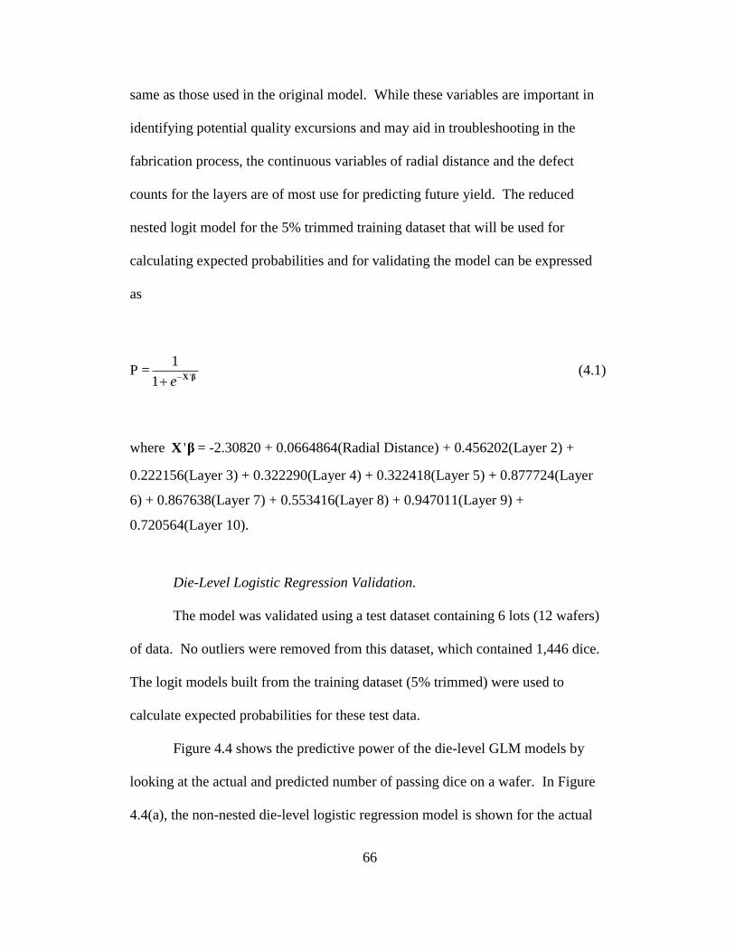
66
same as those used in the original model. While these variables are important in
identifying potential quality excursions and may aid in troubleshooting in the
fabrication process, the continuous variables of radial distance and the defect
counts for the layers are of most use for predicting future yield. The reduced
nested logit model for the 5% trimmed training dataset that will be used for
calculating expected probabilities and for validating the model can be expressed
as
P ='
1
1 e X β (4.1)
where 'X β = -2.30820 + 0.0664864(Radial Distance) + 0.456202(Layer 2) +
0.222156(Layer 3) + 0.322290(Layer 4) + 0.322418(Layer 5) + 0.877724(Layer
6) + 0.867638(Layer 7) + 0.553416(Layer 8) + 0.947011(Layer 9) +
0.720564(Layer 10).
Die-Level Logistic Regression Validation.
The model was validated using a test dataset containing 6 lots (12 wafers)
of data. No outliers were removed from this dataset, which contained 1,446 dice.
The logit models built from the training dataset (5% trimmed) were used to
calculate expected probabilities for these test data.
Figure 4.4 shows the predictive power of the die-level GLM models by
looking at the actual and predicted number of passing dice on a wafer. In Figure
4.4(a), the non-nested die-level logistic regression model is shown for the actual

67
and predicted values from both the training data (5% trimmed) used to create the
model and to the test data. Results from Seeds’ Model (Y4) are also shown for
comparison. (Seeds’ Model was chosen as a baseline due its lower MAD and
MSE measures, shown in Figure 4.6.) This figure shows the model fits the
training data very well, but the predictive power is less with the model applied to
the test data showing the predictions to underestimate the actual yield. This
model significantly outperforms Seeds’ model in predictive power, though.
Figure 4.4(b) is a similar chart that shows the nested, reduced die-level
model applied to the training and test data. Here, the nested GLM model predicts
higher values than actual for the training data, but the predicted values are very
near the actual results for the test dataset, which is a demonstration of the
predictive power of this approach. Again, Seeds’ Model is shown for
comparison.
There have been several yield models proposed in the literature that use
defect count data to predict performance as described in Chapter 2. Many of these
models are described in (Kumar, Kennedy, Gildersleeve, Abelson, Mastrangelo,
& Montgomery, 2006) and are briefly shown in Table 4.3. In these models, the
variables used are defined as:
0 defects per area
defects per area from process step
area of a die
area of a wafer
=number of processing steps
=clustering parameter
i
w
D
D i
A
A
n
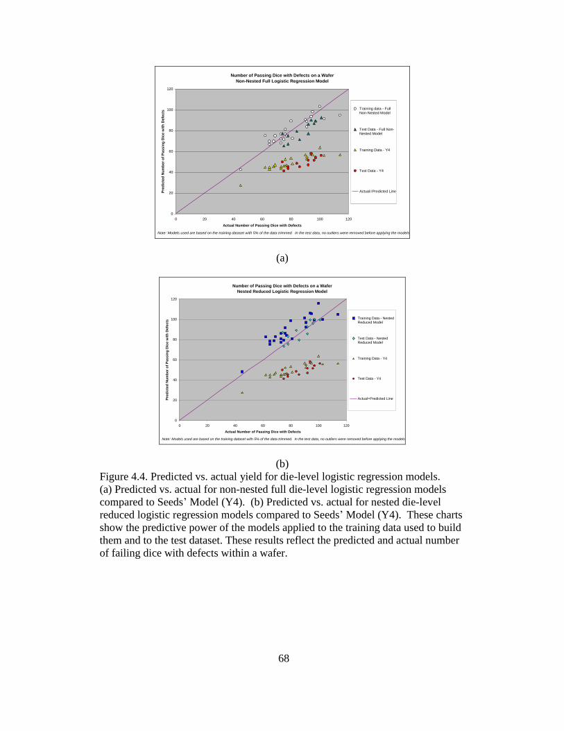
68
Number of Passing Dice with Defects on a Wafer
Non-Nested Full Logistic Regression Model
0
20
40
60
80
100
120
0 20 40 60 80 100 120
Actual Number of Passing Dice with Defects
Pre
dic
ted
Nu
mb
er
of
Passin
g D
ice w
ith
Defe
cts
Training data - FullNon-Nested Model
Test Data - Full Non-Nested Model
Training Data - Y4
Test Data - Y4
Actual=Predicted Line
Note: Models used are based on the training dataset with 5% of the data trimmed. In the test data, no outliers were removed before applying the models.
(a)
Number of Passing Dice with Defects on a Wafer
Nested Reduced Logistic Regression Model
0
20
40
60
80
100
120
0 20 40 60 80 100 120
Actual Number of Passing Dice with Defects
Pre
dic
ted
Nu
mb
er
of
Passin
g D
ice w
ith
Defe
cts
Training Data - NestedReduced Model
Test Data - NestedReduced Model
Training Data - Y4
Test Data - Y4
Actual=Predicted Line
Note: Models used are based on the training dataset with 5% of the data trimmed. In the test data, no outliers were removed before applying the models.
(b)
Figure 4.4. Predicted vs. actual yield for die-level logistic regression models.
(a) Predicted vs. actual for non-nested full die-level logistic regression models
compared to Seeds’ Model (Y4). (b) Predicted vs. actual for nested die-level
reduced logistic regression models compared to Seeds’ Model (Y4). These charts
show the predictive power of the models applied to the training data used to build
them and to the test dataset. These results reflect the predicted and actual number
of failing dice with defects within a wafer.

69
Table 4.3. Existing Yield Models
Popular Name Model
Classic Poisson Model 0
1
D AY e
Binomial Yield Model 0
2 1 /wD A
wY A A
Murphy’s Yield Model: 02
3
0
1D A
eY
D A
Seeds’ Yield Model: 4
0
1
1Y
D A
Dingwall’s Yield Model: 3
5 01 / 3Y D A
Moore’s Yield Model: 0
6
D AY e
Price’s Yield Model: 7
1
1
1
n
i i
YD A
Price’s General Model: 8 01 /n
Y D A n
Negative Binomial Model: 9 0(1 / )Y D A
In Figures 4.5 and 4.6, the die-level GLM models are compared to those
from the literature. Figure 4.5 shows the expected probability for each of the nine
models given in Table 4.3 at the die level. The value for the negative binomial
(Y9) clustering parameter () was calculated using the method proposed by
Cunningham (1990) shown in Equation 2.12. This produced an average alpha
value of 3.33. Figure 4.5 shows the actual performance of the die either passing
(1) or failing (0). While earlier models have been formed to handle wafer-level
analysis, they can be applied at the die-level to predict a yield percentage for all
the dice on a wafer. The GLM model gives a range of yield probabilities that
more closely reflect expected behavior without the degree of underestimation that
the earlier models produce, as demonstrated in Figure 4.5. These GLM models,
which consider which layer the defects are found on, can give a more precise
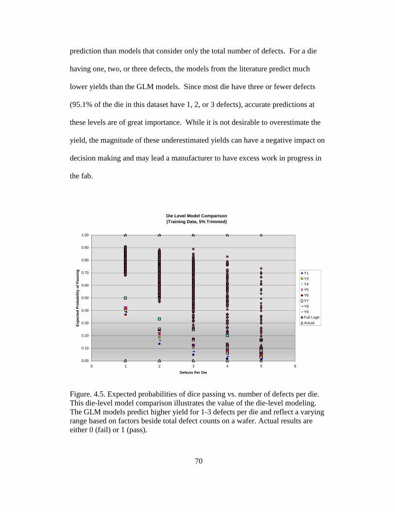
70
prediction than models that consider only the total number of defects. For a die
having one, two, or three defects, the models from the literature predict much
lower yields than the GLM models. Since most die have three or fewer defects
(95.1% of the die in this dataset have 1, 2, or 3 defects), accurate predictions at
these levels are of great importance. While it is not desirable to overestimate the
yield, the magnitude of these underestimated yields can have a negative impact on
decision making and may lead a manufacturer to have excess work in progress in
the fab.
Die Level Model Comparison
(Training Data, 5% Trimmed)
0.00
0.10
0.20
0.30
0.40
0.50
0.60
0.70
0.80
0.90
1.00
0 1 2 3 4 5 6
Defects Per Die
Exp
ecte
d P
rob
ab
ilit
y o
f P
assin
g
Y1
Y3
Y4
Y5
Y6
Y7
Y8
Y9
Full Logit
Actual
Figure. 4.5. Expected probabilities of dice passing vs. number of defects per die.
This die-level model comparison illustrates the value of the die-level modeling.
The GLM models predict higher yield for 1-3 defects per die and reflect a varying
range based on factors beside total defect counts on a wafer. Actual results are
either 0 (fail) or 1 (pass).

71
Additional advantages of this die-level GLM approach can also be seen
when comparing the mean absolute deviation (MAD) and the mean squared error
(MSE) for the models. These are shown Table 4.4 and illustrated in Figure 4.6
with the MSE and MAD values being found by applying the models to the test
data and assessing how well the predicted values fit the actual results. MAD is
the average of the absolute deviations for each die, and the MSE is the average of
the squared errors (the actual minus predicted value) for the dice. The lower the
number for either of these measures, the better the model matches the actual data.
Both Seeds’ Model (Y4) and the Negative Binomial (Y9, =3.3) show good
performance for the literature models, but the Reduced Nested Logit GLM model
shows a 34.6% improvement in MSE and a 31.1% improvement in MAD over the
best-performing Seeds’ Model (Y4).
Table 4.4. Mean Squared Error (MSE) and Mean Absolute Deviation (MAD) for
Model Comparisons at the Die Level Using Test Data
Y1 Y3 Y4 Y5 Y6 Y7 Y8 Y9
Full
Nested
Logit
Reduced
Nested
Logit
Full
Non-
Nested
Die-
Level
Logit
Multiple
Linear
Regressi
on
MSE 0.412 0.377 0.289 0.358 0.371 0.309 0.394 0.362 0.190 0.189 0.188 0.592
MAD 0.583 0.566 0.517 0.556 0.572 0.522 0.574 0.558 0.356 0.356 0.397 0.650

72
Die-Level Error Measures for Models Using Test Data for Predictors
(No Outliers Removed)
0.000
0.100
0.200
0.300
0.400
0.500
0.600
0.700
Y1
Y3
Y4
Y5
Y6
Y7
Y8
Y9
Full N
este
d Lo
git
Red
uced
Nes
ted
Logit
Full N
on-N
este
d Die-L
evel L
ogit
Multip
le L
inea
r Reg
ress
ion
Predictive Model
Mean
Sq
uare
d E
rro
r (M
SE
), M
ean
Ab
so
lute
Devia
tio
n (
MA
D)
MSE
MAD
Figure 4.6. Mean Absolute Deviation (MAD) and Mean Squared Error (MSE)
results comparing GLM models with other models from the literature and
multiple linear regression when applied to the test dataset with no outliers
removed. Lower values of MAD and MSE indicate the model is closer to the
actual yield values.
The predictive power of these GLM models can also be seen by examining
the predicted probabilities for the various models summed together at a high level
of aggregation. Figure 4.7 shows the predicted number of passing dice for each
model for the entire test dataset (1446 dice). For each model, the actual number
of passing and failing dice for the 6 lots in this dataset is shown to demonstrate
which models best predict the actual yield of dice that have at least one defect.
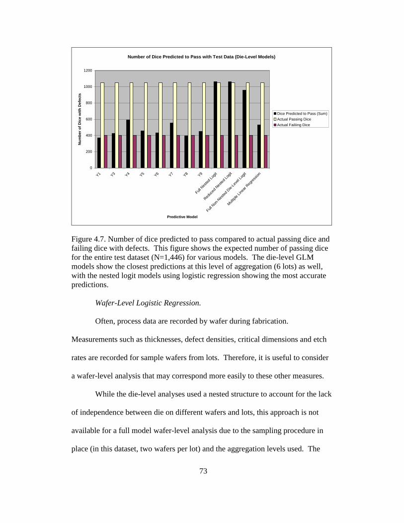
73
Number of Dice Predicted to Pass with Test Data (Die-Level Models)
0
200
400
600
800
1000
1200
Y1
Y3
Y4
Y5
Y6
Y7
Y8
Y9
Full N
este
d Lo
git
Red
uced
Nes
ted
Logit
Full N
on-N
este
d Die-L
evel L
ogit
Multip
le L
inea
r Reg
ress
ion
Predictive Model
Nu
mb
er
of
Dic
e w
ith
Defe
cts
Dice Predicted to Pass (Sum)
Actual Passing Dice
Actual Failiing Dice
Figure 4.7. Number of dice predicted to pass compared to actual passing dice and
failing dice with defects. This figure shows the expected number of passing dice
for the entire test dataset (N=1,446) for various models. The die-level GLM
models show the closest predictions at this level of aggregation (6 lots) as well,
with the nested logit models using logistic regression showing the most accurate
predictions.
Wafer-Level Logistic Regression.
Often, process data are recorded by wafer during fabrication.
Measurements such as thicknesses, defect densities, critical dimensions and etch
rates are recorded for sample wafers from lots. Therefore, it is useful to consider
a wafer-level analysis that may correspond more easily to these other measures.
While the die-level analyses used a nested structure to account for the lack
of independence between die on different wafers and lots, this approach is not
available for a full model wafer-level analysis due to the sampling procedure in
place (in this dataset, two wafers per lot) and the aggregation levels used. The

74
training dataset for the wafer level contains twelve lots (24 wafers). To utilize the
nested structure for modeling, one degree of freedom is needed for estimating the
constant, eleven degrees of freedom for the lots, twelve for the wafers, and ten for
the product layers. Even if only the lots and wafers are considered in the nested
model, the model is saturated, and goodness-of-fit statistics cannot be calculated.
While adding more lots to the dataset may seem like a feasible solution to this
problem, as additional lots of data are added (2 wafers each), two more
parameters need to be estimated, so the full model will always be saturated.
While other standard diagnostics, such as absolute deviation, can be used to
evaluate the usefulness of these models in the absence of goodness-of-fit
statistics, a nested model at the wafer level is not recommended as a strong
approach due to the limited helpful information that it would provide given these
constraints.
Non-nested models were created for the training dataset at the wafer-level
using the three link functions and predictors of Lot, Wafer, and the defect counts
from the ten process layers. The results are shown in Table 4.5. The logit and
probit models identify Lots 6 and 8 as significantly different from Lot 1 and also
indicate that Layer 8 is statistically significant. The complimentary log-log model
indicates the same two lots as significant, but does not show Layer 8 to be
significant at the =0.1 level. The goodness-of-fit tests are favorable for all three
links, indicating these should be good models.
Though these models appear to be good, outliers may be impacting the
results. Table 4.5 also shows the results of the models created after the dice with

75
more than 9 total defects (upper 2.5%) were removed from the dataset. These
analyses show no lots are significantly different from Lot 1, and a different layer,
Layer 9, is identified as significant (=0.1).
Table 4.5. Comparison of Link Functions & Outlier Methods (Wafer-level, Not-
nested)
All Training Set Data
N= 24 wafers (2967 dice) Outliers Removed (97.5th
percentile)
N= 24 wafers (2896 dice)
Outliers Removed (95th
percentile)
N= 24 wafers (2845 dice) Logit Probit Complimen
tary Log-
Log
Logit Probit Complimen
tary Log-
Log
Logit Probit Complimen
tary Log-
Log
Significant
Factors
(=0.10)
Lot 6
Lot 8
Layer 8
Lot 6
Lot 8
Layer 8
Lot 6
Lot 8
Layer 9 Layer 9 Layer 9 Layer 9 Layer 9 Layer 9
G
(p-value)
52.381
(0.000)
52.368
(0.000)
52.337
(0.000)
51.402
(0.000)
51.399
(0.000)
51.392
(0.000)
51.168
(0.000)
51.158
(0.000)
51.137
(0.000)
Pearson
(p-value)
0.0280972
(0.867)
0.0401750
(0.841)
0.0713576
(0.789)
0.0341
(0.853)
0.0370
(0.847)
0.0440120
(0.834)
0.0239
(0.877)
0.0334
(0.855)
0.0547531
(0.815)
Deviance
(p-value)
0.0281218
(0.867)
0.0402199
(0.841)
0.0714682
(0.789)
0.0341
(0.853)
0.0370
(0.847)
0.0440098
(0.834)
0.0239
(0.877)
0.0334
(0.855)
0.0547564
(0.815)
Hosmer-
Lemeshow
(p-value)
0.0151858
(1.000)
0.0211868
(1.000)
0.0358298
(1.000)
0.0064
(1.000)
0.0068
(1.000)
0.0075645
(1.000)
0.0062
(1.000)
0.0086
(1.000)
0.0187298
(1.000)
Somers’ D 0.16 0.16 0.16 0.16 0.16 0.16 0.16 0.16 0.16
Similar results were obtained from the training dataset with the upper 5%
of the outliers removed (more than 5 total defects in a die). These results are
presented in Table 4.5 as well. Goodness-of-fit measures have not improved
considerably, so the wafer-level analysis seems to be more robust against outliers
than the die-level study, but there are differences in which predictors are
identified as significant.
Wafer-Level Logistic Regression Validation.
Since the results were similar for both of the refined datasets, the model
for the training set with 5% of the outliers removed was used for validation.
Since there were no significant differences between the links, the logit link was

76
used to form the full model using Equation 4.1 where 'X β =1.40356 -
0.027(Layer 1) + 0.00393(Layer 2) + 0.002937(Layer 3) + 0.01582(Layer 4) -
0.038756(Layer 5) + 0.0237897(Layer 6) - 0.005593(Layer 7) - 0.00848(Layer
8) - 0.041995(Layer 9) + 0.030685(Layer 10).
The reduced model for the wafer level was formed using backward
elimination. Using this method, the predictors were eliminated one by one
according to which had the smallest z-statistic (largest p-value). First, due to their
high p-values and inability to be used in predictive modeling, Lot and Wafer were
removed, followed by Layer 2, Layer 1, Layer 4, Layer 8, Layer 3, Layer 6, Layer
5, and Layer 10, respectively. A cutoff value of =0.1 was used, as done with the
previous models. This reduced model takes the form
)9*0174814.07*0065599.0917234.0(1
1LLe
P
(4.3)
to predict the proportion of dice that will pass. This reduced model had p-values
of 0.030, 0.027, and 0.555 for the Pearson, Deviance, and Hosmer-Lemeshow
goodness-of-fit tests, respectively.
The validity of the wafer-level GLM models can be assessed in ways
similar to those used for the die-level models. Figure 4.8 shows a plot of the
actual yields compared to the predicted yield values for dice with defects from the
wafer-level full and reduced models, the die-level nested reduced model, and
Seeds’ Model. As seen in the die-level plot, the GLM models are closer to the
actual values than the underestimating Seeds’ Model, but a good amount of
variability is seen in the wafer-level results. Figure 4.8 demonstrates that the die-

77
level nested GLM model has the greatest and most consistent predictive power for
these data.
Figure 4.9 shows the predicted yields for each model as well as the actual
yield for each of the 24 wafers in the dataset. In this chart, it is clear that the
models from the literature consistently underestimate the yield. While the GLM
models (full logit and reduced logit) are closer to the actual yields, their behaviors
are not as smooth as the other models. This can be explained both by the fact that
these models take into account more specific information (the number of defects
on specific layers on a die rather than the average defects per die) and by the fact
that there can be other contributors to yield loss other than defect counts alone.
The die-level nested reduced logit model shows very good performance to these
test data, though, both in being nearest to the actual yield and in showing more
stable behavior as is also shown in Figure 4.8.
The behavior of the models shown in Figure 4.9 shows varying levels of
correlation to the actual yield results. To assess correlation, Pearson correlation
coefficients may be calculated and compared for the different models. These
results are shown in Table 4.6. The results show the models from the literature
(Y1 through Y9) are significantly correlated to the actual results at the =0.1
level of significance. The wafer-level GLM models do not share this distinction.
The highest correlation is seen with the die-level nested reduced logit GLM model
with a Pearson correlation coefficient of 0.819 and a p-value of 0.001 showing
this model has by far the strongest correlation to the actual results.
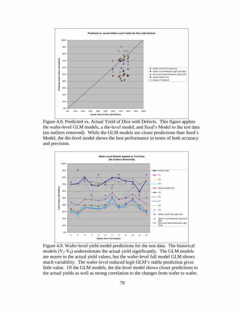
78
Predicted vs. Actual Wafer-Level Yields for Dice with Defects
0%
10%
20%
30%
40%
50%
60%
70%
80%
90%
100%
0% 10% 20% 30% 40% 50% 60% 70% 80% 90% 100%
Actual Yield of Dice with Defects
Pre
dic
ted
Yie
ld o
f D
ice w
ith
Defe
cts
Wafer-Level Full Logit GLM
Wafer-Level Reduced Logit GLM (BE)
Die-Level Nested Reduced Logit GLM
Seed's Model (Y4)
Actual = Predicted
Figure 4.8. Predicted vs. Actual Yield of Dice with Defects. This figure applies
the wafer-level GLM models, a die-level model, and Seed’s Model to the test data
(no outliers removed). While the GLM models are closer predictions than Seed’s
Model, the die-level model shows the best performance in terms of both accuracy
and precision.
Wafer-Level Models Applied to Test Data
(No Outliers Removedl)
0%
10%
20%
30%
40%
50%
60%
70%
80%
90%
100%
1 2 3 4 5 6 7 8 9 10 11 12
Wafers from Test Dataset
Yie
ld o
f D
ice w
ith
Defe
cts
Actual Yield
Y1
Y2
Y3
Seed's Model (Y4)
Y5
Y6
Y7
Y8
Y9
Wafer-Level Full Logit GLM
Wafer-Level Reduced Logit GLM(BE)Die-Level Nested Reduced LogitGLM
Figure 4.9. Wafer-level yield model predictions for the test data. The historical
models (Y1-Y9) underestimate the actual yield significantly. The GLM models
are nearer to the actual yield values, but the wafer-level full model GLM shows
much variability. The wafer-level reduced logit GLM’s stable prediction gives
little value. Of the GLM models, the die-level model shows closer predictions to
the actual yields as well as strong correlation to the changes from wafer to wafer.
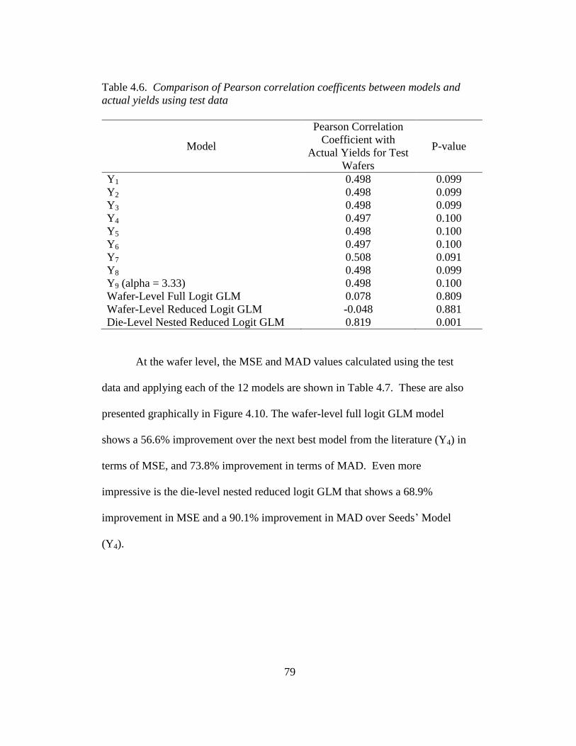
79
Table 4.6. Comparison of Pearson correlation coefficents between models and
actual yields using test data
Model
Pearson Correlation
Coefficient with
Actual Yields for Test
Wafers
P-value
Y1 0.498 0.099
Y2 0.498 0.099
Y3 0.498 0.099
Y4 0.497 0.100
Y5 0.498 0.100
Y6 0.497 0.100
Y7 0.508 0.091
Y8 0.498 0.099
Y9 (alpha = 3.33) 0.498 0.100
Wafer-Level Full Logit GLM 0.078 0.809
Wafer-Level Reduced Logit GLM -0.048 0.881
Die-Level Nested Reduced Logit GLM 0.819 0.001
At the wafer level, the MSE and MAD values calculated using the test
data and applying each of the 12 models are shown in Table 4.7. These are also
presented graphically in Figure 4.10. The wafer-level full logit GLM model
shows a 56.6% improvement over the next best model from the literature (Y4) in
terms of MSE, and 73.8% improvement in terms of MAD. Even more
impressive is the die-level nested reduced logit GLM that shows a 68.9%
improvement in MSE and a 90.1% improvement in MAD over Seeds’ Model
(Y4).

80
Table 4.7. Mean Squared Error (MSE) and Mean Absolute Deviation (MAD) for
Model Comparisons at the Wafer Level (%)
Y1 Y2 Y3 Y4 Y5 Y6 Y7 Y8 Y9
Wafer-Level
Full
Logit GLM
Wafer-
Level Reduced
Logit
GLM (BE)
Die-Level Nested
Reduced
Logit GLM
MAD 0.52 0.52 0.48 0.37 0.46 0.50 0.49 0.50 0.46 0.162 0.219 0.116
MSE 0.27 0.27 0.23 0.14 0.21 0.25 0.24 0.25 0.22 0.037 0.057 0.014
Wafer-Level Error Measures for Models Using Test Data for Predictors
(No Outliers Removed)
0.00
0.10
0.20
0.30
0.40
0.50
0.60
Y1 Y2 Y3 Y4 Y5 Y6 Y7 Y8 Y9 Wafer-
Level Full
Logit
GLM
Wafer-
Level
Reduced
Logit
GLM
(BE)
Die-Level
Nested
Reduced
Logit
GLM
Predictive Model
Mean
Ab
so
lute
Devia
tio
n (
MA
D),
Mean
Sq
uare
d E
rro
r (M
SE
)
MAD
MSE
Figure 4.10. Mean Squared Error (MSE) and Mean Absolute Deviation (MAD)
measures for the nine models from the literature and the GLM models. The GLM
models significantly outperform previous models in these measurements of error
with the best model being the die-level nested reduced logit GLM.
Summary
A number of conclusions are drawn from this phase of study. First,
generalized linear models, such as logistic regression, can be used to successfully
model semiconductor yield based on defect data. This empirical modeling
approach can be applied to devices of various sizes and types. While this

81
approach does not develop a general model that can be used across different
products, the simplicity of this modeling strategy makes it easy to apply to
individual products to optimize yield prediction accuracy.
These generalized linear models have two primary advantages. First, the
die-level models created can predict yield very well. This can be beneficial in
product planning (for both the product and the process) and for yield
improvement efforts for the device. While this approach is recommended
primarily for application to ongoing products, the models may provide a good
basis for predicting yield for new products that are similar to a device already
modeled. A second advantage is in the power these models have to identify
significant predictor variables. This can be helpful in diagnosing problems and
finding areas of improvement that can improve quality and reduce testing time.
For example, in the die-level nested GLM models, defects found in Layer 1 were
not found to be significant. This suggests that defects on Layer 1 may not need to
be scanned and detected for this device. Elimination of these measures for a layer
can save valuable processing time and improve overall equipment effectiveness
(OEE). In addition, the layers or even specific wafers that are identified as
significant in the building the model can be explored in more detail to better
understand their influences on yield, and any process problems may be corrected.
This information can be especially helpful for processing new devices as yields
usually start lower and improve as the new process is optimized. Identifying and
solving process and quality issues early in a product’s life cycle can help a
company reduce costs.

82
While this modeling strategy using GLMs is shown to be very effective, a
practitioner needs to carefully consider and evaluate the types of models
constructed and selected for use. Wafer-level GLM analyses, while showing
adequate goodness-of-fit results, can be misleading and are not as accurate at
prediction as die-level models in this study. At the wafer level, very few
fabrication layers are identified as significant, and the predictive power of these
models is limited. Also, the nested structure cannot be used at the wafer level
unless more wafers are sampled and are sorted into groups. Given constraints on
scan equipment and process times, regularly testing additional wafers is not a
feasible option for semiconductor manufacturers.
Die-level nested models are most effective for these data. There are not
significant differences between the different link functions, even with the large
sample sizes used. The nested structure provides more detailed information about
significant predictors, including specific wafers and die quadrants, and it removes
the need to assume independence between all dice. The nested die-level logistic
regression models also show the best predictive power at both the die- and wafer-
levels of aggregation.
Outliers can have a strong impact on model adequacy and on which
predictors are significant for the model. The best results were obtained by
removing the dice that had more than 5 total defects. (This corresponded to the
top 5% of the total defects per die.) Validation testing on this model using a test
dataset that included outliers proved the predictive capability of these models.

83
Chapter 5
SEMICONDUCTOR YIELD MODELING USING GENERALIZED LINEAR
MIXED MODELS
Introduction
The results shown in Chapter 4 indicate the promise of using GLMs for
semiconductor yield modeling. These fixed-effects models do not have the ability
to account for the random sampling that is necessary in a fab environment,
though. GLMs assume complete randomization, but commonly in practice only
certain lots and/or wafers are sampled for defect scans. For the data studied in
this research, only two wafers of twenty-five in every tenth lot were scanned for
defects. While the nested GLM models account for the hierarchical structure of
the sampling, they do not consider the nested effects as random. This suggests a
violation of the GLM assumptions and indicates generalized linear mixed models
(GLMMs) should be used to account for random effects such as lot and wafer.
Recall from Chapter 2 that there are two approaches when using GLMMs,
the batch-specific model and the population-averaged model. The formulas for
the expected values for these models are found in Equations 2.34 and 2.35 for the
batch-specific and the population-averaged models, respectively. The batch-
specific approach includes the random effects and provides predictions for each
different random factors setting. Population-averaged models are designed to
provide a more general trend across an entire population. In modeling
semiconductor yield, both these approaches are appropriate for different types of
applications. Batch-specific models allow estimates of slopes and/or intercepts

84
for each random factor setting, which can be helpful in identifying significant
differences or in creating models for those specific effects (i.e. locations, patients,
etc.). The population-averaged models create a marginal model that accounts for
the random factors but does not provide estimates for them in the model and is
used primarily for predicting across the population as a whole.
In some GLMM modeling applications, the random effects are clear. For
example, a medical study may follow a particular participant over time, or a
designed experiment may need to be run in split plots for hard-to-change factors.
Sometimes, though, the random effects modeling may not be this straightforward.
Especially with a case having multiple random effects, determining which random
effects should be used in modeling and which GLMM structure is most
appropriate must be carefully considered.
A modeling strategy for using GLMMs to model semiconductor yield can
be useful to practitioners and may also provide guidelines that can be applied in
other areas and industries as well. The advantages of this approach include being
able to identify random effects, such as specific lots or wafers, that are
significantly different from a baseline and to account for the random effects in the
model without incorrectly assuming them to be fixed as with a GLM approach.
This research extends that from Chapter 4 by using an extended dataset to
study the impact of using GLMMs, both batch-specific and population-averaged
models, in various forms to model semiconductor yield. The effects of using
different link functions and using different sample sizes will also be studied and
discussed. This chapter is organized to first describe the dataset used in the

85
analysis. The model building approach is described in the next section. Next, the
die-level results for the models are presented, followed by the wafer-level results
and a summary.
Data Description
The data used in this phase of the research were obtained and cleaned as
described in Chapter 3 and as used in Chapter 4, but this dataset is larger than the
one used in Chapter 4 to advance the study. The data used in this phase included
126 lots (252 wafers) for the device described in Chapter 3. Of these, 168 wafers
(84 lots) were randomly selected to be used for training the data, and 84 wafers
(42 lots) were chosen for testing the models. At the die-level, 23,296 dice were
used as the training dataset, after removing outliers that contained more than nine
defects. The test dataset was made up of 11,240 dice. No outliers were removed
from the test dataset to better assess model validity.
Model Building
Several models were constructed using the training dataset. These models
were examined at both the die and wafer levels and were analyzed for
comparisons at various sample sizes and using different link functions. A matrix
displaying the models developed is shown in Table 5.1. The GLM models and
the GLM nested models are analogous to those described in Chapter 4. As in
Chapter 4, predictor variables for the die-level models included Lot, Wafer,
Radial Distance, Die Quadrant, the number of layers with defects, and the count
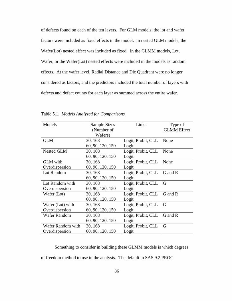
86
of defects found on each of the ten layers. For GLM models, the lot and wafer
factors were included as fixed effects in the model. In nested GLM models, the
Wafer(Lot) nested effect was included as fixed. In the GLMM models, Lot,
Wafer, or the Wafer(Lot) nested effects were included in the models as random
effects. At the wafer level, Radial Distance and Die Quadrant were no longer
considered as factors, and the predictors included the total number of layers with
defects and defect counts for each layer as summed across the entire wafer.
Table 5.1. Models Analyzed for Comparisons
Models Sample Sizes
(Number of
Wafers)
Links Type of
GLMM Effect
GLM 30, 168
60, 90, 120, 150
Logit, Probit, CLL
Logit
None
Nested GLM 30, 168
60, 90, 120, 150
Logit, Probit, CLL
Logit
None
GLM with
Overdispersion
30, 168
60, 90, 120, 150
Logit, Probit, CLL
Logit
None
Lot Random 30, 168
60, 90, 120, 150
Logit, Probit, CLL
Logit
G and R
Lot Random with
Overdispersion
30, 168
60, 90, 120, 150
Logit, Probit, CLL
Logit
G
Wafer (Lot) 30, 168
60, 90, 120, 150
Logit, Probit, CLL
Logit
G and R
Wafer (Lot) with
Overdispersion
30, 168
60, 90, 120, 150
Logit, Probit, CLL
Logit
G
Wafer Random 30, 168
60, 90, 120, 150
Logit, Probit, CLL
Logit
G and R
Wafer Random with
Overdispersion
30, 168
60, 90, 120, 150
Logit, Probit, CLL
Logit
G
Something to consider in building these GLMM models is which degrees
of freedom method to use in the analysis. The default in SAS 9.2 PROC

87
GLIMMIX for GLMs and GLMs with overdispersion is the RESIDUAL method.
The default for random-effects models with only R-side effects and the subject
option specified (population-averaged models) is the BETWITHIN method,
which divides the residual degrees of freedom into between-subject and within-
subject components. For G-side random effects (batch-specific models), the
default method is CONTAIN, which uses the containment method. Another
option for modeling is the KENWARDROGER option, which involves inflating
the estimated variance-covariance matrix of the fixed and random effects and then
computes Satterthwaite-type degrees of freedom from the adjustment.
Sattherthwaite degrees of freedom require more computing time, and the small
sample properties are not extensively studied (SAS, 2006). For the models
presented in this chapter, the default degrees of freedom methods were used in
SAS.
Another option in the model building requires selecting the type of the
covariance structure. The default method in SAS PROC GLIMMIX for the
RANDOM statement is TYPE=VC, or variance components, which uses a simple
diagonal covariance matrix and models a different variance component for each
random effect (SAS, 2006). For random effects that follow a subject over time,
AR(1) or ARMA(1,1) may be desirable types to specify. Another option is the
TYPE=CS, which specifies the compound-symmetry structure and has constant
variance and constant covariance. This structure arises naturally with nested
random effects, such as split-plot experiments (SAS, 2006). For the models
described in this chapter, the G-side random effects (batch-specific models) used

88
TYPE=VC, and the R-side random effects (population-averaged) models used
TYPE=CS to indicate the nested structure of the data. Examples of the SAS code
used for these models are included in Appendix A.
Results
To help develop a strategy for using GLMMs in semiconductor yield
modeling, many models were built in order to answer the following questions:
1. What are the differences between different GLMM modeling approaches
and how do they compare to GLM models?
2. How does using different link functions affect GLMM models?
3. How does sample size impact GLMM model results?
The first question was addressed by modeling the data with different random
effects and comparing them to GLM models. Logit, probit, and complimentary
log-log functions (Eq. 2.27, 2.28, and 2.29, respectively) were used to compare
the differences at samples sizes of 30 wafers and 168 wafers. To examine the
impact of using different sample sizes on the models, subsets of the training
dataset were used: 30 wafers (3797 dice), 60 wafers (7900 dice), 90 wafers
(11,868 dice), 120 wafers (16,537 dice), and 150 wafers (20,872 dice). The
results of the study are broken up in to die- and wafer-level results.
Die-Level Model Results
The die-level models with different link functions were very similar within
the sample size used. The significant factors (=0.1) in the models are given for
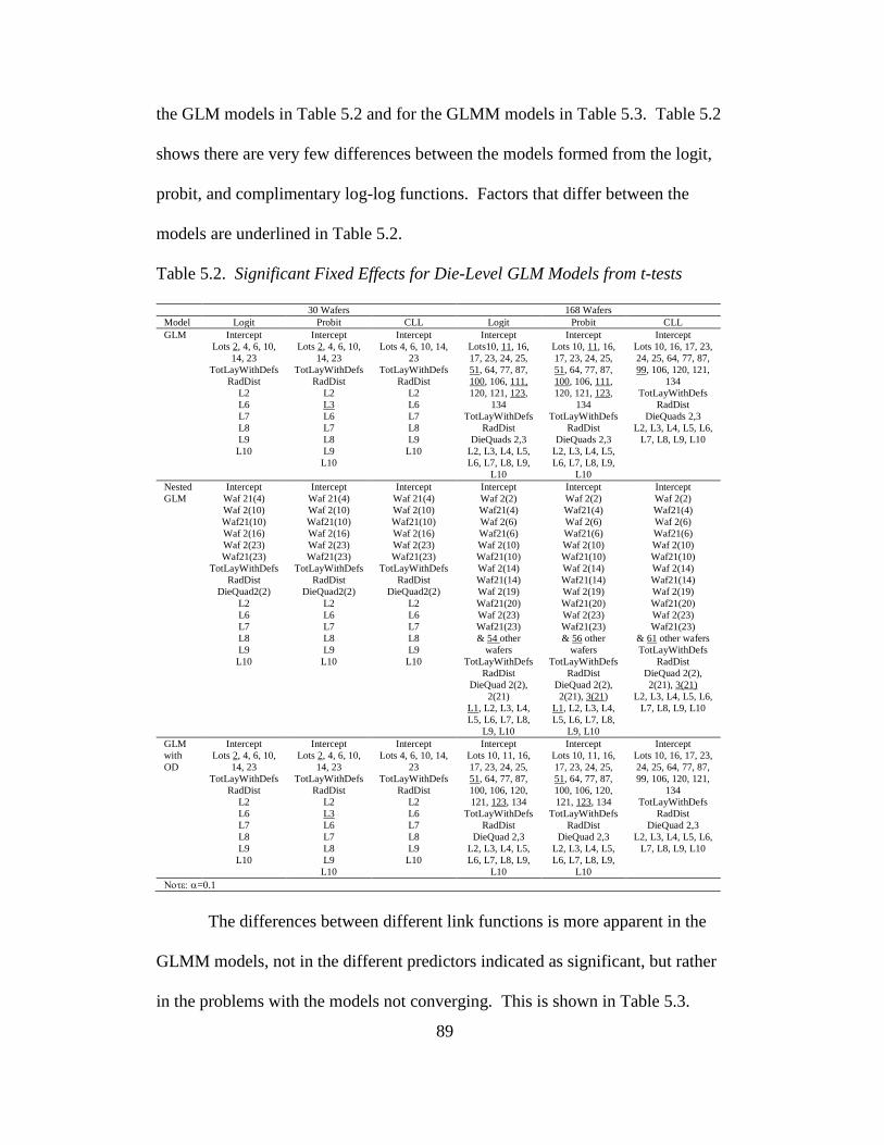
89
the GLM models in Table 5.2 and for the GLMM models in Table 5.3. Table 5.2
shows there are very few differences between the models formed from the logit,
probit, and complimentary log-log functions. Factors that differ between the
models are underlined in Table 5.2.
Table 5.2. Significant Fixed Effects for Die-Level GLM Models from t-tests
30 Wafers 168 Wafers
Model Logit Probit CLL Logit Probit CLL
GLM Intercept
Lots 2, 4, 6, 10,
14, 23
TotLayWithDefs
RadDist
L2
L6
L7
L8
L9
L10
Intercept
Lots 2, 4, 6, 10,
14, 23
TotLayWithDefs
RadDist
L2
L3
L6
L7
L8
L9
L10
Intercept
Lots 4, 6, 10, 14,
23
TotLayWithDefs
RadDist
L2
L6
L7
L8
L9
L10
Intercept
Lots10, 11, 16,
17, 23, 24, 25,
51, 64, 77, 87,
100, 106, 111,
120, 121, 123,
134
TotLayWithDefs
RadDist
DieQuads 2,3
L2, L3, L4, L5,
L6, L7, L8, L9,
L10
Intercept
Lots 10, 11, 16,
17, 23, 24, 25,
51, 64, 77, 87,
100, 106, 111,
120, 121, 123,
134
TotLayWithDefs
RadDist
DieQuads 2,3
L2, L3, L4, L5,
L6, L7, L8, L9,
L10
Intercept
Lots 10, 16, 17, 23,
24, 25, 64, 77, 87,
99, 106, 120, 121,
134
TotLayWithDefs
RadDist
DieQuads 2,3
L2, L3, L4, L5, L6,
L7, L8, L9, L10
Nested
GLM
Intercept
Waf 21(4)
Waf 2(10)
Waf21(10)
Waf 2(16)
Waf 2(23)
Waf21(23)
TotLayWithDefs
RadDist
DieQuad2(2)
L2
L6
L7
L8
L9
L10
Intercept
Waf 21(4)
Waf 2(10)
Waf21(10)
Waf 2(16)
Waf 2(23)
Waf21(23)
TotLayWithDefs
RadDist
DieQuad2(2)
L2
L6
L7
L8
L9
L10
Intercept
Waf 21(4)
Waf 2(10)
Waf21(10)
Waf 2(16)
Waf 2(23)
Waf21(23)
TotLayWithDefs
RadDist
DieQuad2(2)
L2
L6
L7
L8
L9
L10
Intercept
Waf 2(2)
Waf21(4)
Waf 2(6)
Waf21(6)
Waf 2(10)
Waf21(10)
Waf 2(14)
Waf21(14)
Waf 2(19)
Waf21(20)
Waf 2(23)
Waf21(23)
& 54 other
wafers
TotLayWithDefs
RadDist
DieQuad 2(2),
2(21)
L1, L2, L3, L4,
L5, L6, L7, L8,
L9, L10
Intercept
Waf 2(2)
Waf21(4)
Waf 2(6)
Waf21(6)
Waf 2(10)
Waf21(10)
Waf 2(14)
Waf21(14)
Waf 2(19)
Waf21(20)
Waf 2(23)
Waf21(23)
& 56 other
wafers
TotLayWithDefs
RadDist
DieQuad 2(2),
2(21), 3(21)
L1, L2, L3, L4,
L5, L6, L7, L8,
L9, L10
Intercept
Waf 2(2)
Waf21(4)
Waf 2(6)
Waf21(6)
Waf 2(10)
Waf21(10)
Waf 2(14)
Waf21(14)
Waf 2(19)
Waf21(20)
Waf 2(23)
Waf21(23)
& 61 other wafers
TotLayWithDefs
RadDist
DieQuad 2(2),
2(21), 3(21)
L2, L3, L4, L5, L6,
L7, L8, L9, L10
GLM
with
OD
Intercept
Lots 2, 4, 6, 10,
14, 23
TotLayWithDefs
RadDist
L2
L6
L7
L8
L9
L10
Intercept
Lots 2, 4, 6, 10,
14, 23
TotLayWithDefs
RadDist
L2
L3
L6
L7
L8
L9
L10
Intercept
Lots 4, 6, 10, 14,
23
TotLayWithDefs
RadDist
L2
L6
L7
L8
L9
L10
Intercept
Lots 10, 11, 16,
17, 23, 24, 25,
51, 64, 77, 87,
100, 106, 120,
121, 123, 134
TotLayWithDefs
RadDist
DieQuad 2,3
L2, L3, L4, L5,
L6, L7, L8, L9,
L10
Intercept
Lots 10, 11, 16,
17, 23, 24, 25,
51, 64, 77, 87,
100, 106, 120,
121, 123, 134
TotLayWithDefs
RadDist
DieQuad 2,3
L2, L3, L4, L5,
L6, L7, L8, L9,
L10
Intercept
Lots 10, 16, 17, 23,
24, 25, 64, 77, 87,
99, 106, 120, 121,
134
TotLayWithDefs
RadDist
DieQuad 2,3
L2, L3, L4, L5, L6,
L7, L8, L9, L10
=0.1
The differences between different link functions is more apparent in the
GLMM models, not in the different predictors indicated as significant, but rather
in the problems with the models not converging. This is shown in Table 5.3.
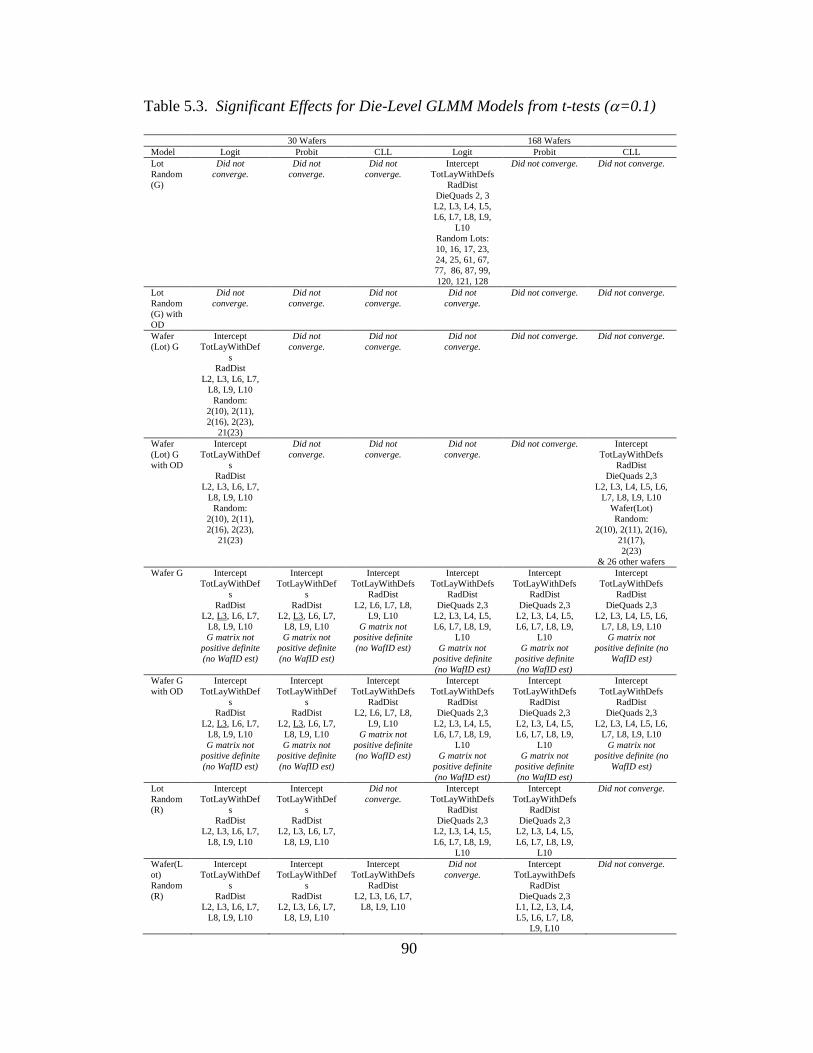
90
Table 5.3. Significant Effects for Die-Level GLMM Models from t-tests (=0.1)
30 Wafers 168 Wafers
Model Logit Probit CLL Logit Probit CLL
Lot
Random
(G)
Did not
converge.
Did not
converge.
Did not
converge.
Intercept
TotLayWithDefs
RadDist
DieQuads 2, 3
L2, L3, L4, L5,
L6, L7, L8, L9,
L10
Random Lots:
10, 16, 17, 23,
24, 25, 61, 67,
77, 86, 87, 99,
120, 121, 128
Did not converge. Did not converge.
Lot
Random
(G) with
OD
Did not
converge.
Did not
converge.
Did not
converge.
Did not
converge.
Did not converge. Did not converge.
Wafer
(Lot) G
Intercept
TotLayWithDef
s
RadDist
L2, L3, L6, L7,
L8, L9, L10
Random:
2(10), 2(11),
2(16), 2(23),
21(23)
Did not
converge.
Did not
converge.
Did not
converge.
Did not converge. Did not converge.
Wafer
(Lot) G
with OD
Intercept
TotLayWithDef
s
RadDist
L2, L3, L6, L7,
L8, L9, L10
Random:
2(10), 2(11),
2(16), 2(23),
21(23)
Did not
converge.
Did not
converge.
Did not
converge.
Did not converge. Intercept
TotLayWithDefs
RadDist
DieQuads 2,3
L2, L3, L4, L5, L6,
L7, L8, L9, L10
Wafer(Lot)
Random:
2(10), 2(11), 2(16),
21(17),
2(23)
& 26 other wafers
Wafer G Intercept
TotLayWithDef
s
RadDist
L2, L3, L6, L7,
L8, L9, L10
G matrix not
positive definite
(no WafID est)
Intercept
TotLayWithDef
s
RadDist
L2, L3, L6, L7,
L8, L9, L10
G matrix not
positive definite
(no WafID est)
Intercept
TotLayWithDefs
RadDist
L2, L6, L7, L8,
L9, L10
G matrix not
positive definite
(no WafID est)
Intercept
TotLayWithDefs
RadDist
DieQuads 2,3
L2, L3, L4, L5,
L6, L7, L8, L9,
L10
G matrix not
positive definite
(no WafID est)
Intercept
TotLayWithDefs
RadDist
DieQuads 2,3
L2, L3, L4, L5,
L6, L7, L8, L9,
L10
G matrix not
positive definite
(no WafID est)
Intercept
TotLayWithDefs
RadDist
DieQuads 2,3
L2, L3, L4, L5, L6,
L7, L8, L9, L10
G matrix not
positive definite (no
WafID est)
Wafer G
with OD
Intercept
TotLayWithDef
s
RadDist
L2, L3, L6, L7,
L8, L9, L10
G matrix not
positive definite
(no WafID est)
Intercept
TotLayWithDef
s
RadDist
L2, L3, L6, L7,
L8, L9, L10
G matrix not
positive definite
(no WafID est)
Intercept
TotLayWithDefs
RadDist
L2, L6, L7, L8,
L9, L10
G matrix not
positive definite
(no WafID est)
Intercept
TotLayWithDefs
RadDist
DieQuads 2,3
L2, L3, L4, L5,
L6, L7, L8, L9,
L10
G matrix not
positive definite
(no WafID est)
Intercept
TotLayWithDefs
RadDist
DieQuads 2,3
L2, L3, L4, L5,
L6, L7, L8, L9,
L10
G matrix not
positive definite
(no WafID est)
Intercept
TotLayWithDefs
RadDist
DieQuads 2,3
L2, L3, L4, L5, L6,
L7, L8, L9, L10
G matrix not
positive definite (no
WafID est)
Lot
Random
(R)
Intercept
TotLayWithDef
s
RadDist
L2, L3, L6, L7,
L8, L9, L10
Intercept
TotLayWithDef
s
RadDist
L2, L3, L6, L7,
L8, L9, L10
Did not
converge.
Intercept
TotLayWithDefs
RadDist
DieQuads 2,3
L2, L3, L4, L5,
L6, L7, L8, L9,
L10
Intercept
TotLayWithDefs
RadDist
DieQuads 2,3
L2, L3, L4, L5,
L6, L7, L8, L9,
L10
Did not converge.
Wafer(L
ot)
Random
(R)
Intercept
TotLayWithDef
s
RadDist
L2, L3, L6, L7,
L8, L9, L10
Intercept
TotLayWithDef
s
RadDist
L2, L3, L6, L7,
L8, L9, L10
Intercept
TotLayWithDefs
RadDist
L2, L3, L6, L7,
L8, L9, L10
Did not
converge.
Intercept
TotLaywithDefs
RadDist
DieQuads 2,3
L1, L2, L3, L4,
L5, L6, L7, L8,
L9, L10
Did not converge.
91
For the GLMM models shown in Table 5.3, the logit link seems to work
best for nested random effects in batch-specific models with smaller sample size,
since it is the only link function that returned a solution with Wafer(Lot) random
for 30 wafers. The complimentary log-log function was the only link function to
converge with the Wafer(Lot) random effect for the 168-wafer sample size,
though. At the larger sample size, at least one of the link functions gave a
solution, except in the cases when Lot was a random G-side effect with
overdispersion and when Wafer(Lot) was a G-side random effect. Since the
significant factors are so similar between the different link functions when they do
converge, if convergence is an issue, changing the link function may be the best
adjustment to make first.
None of the link functions used in Table 5.3 were able to estimate random
intercepts for Wafer due to the G matrix not being positive definite for the batch-
specific models. The population-averaged models with Wafer as a random effect
also had problems as they did not converge within reasonable computing time,
even with the small samples. This may be due to only having two wafers (2 and
21) identified to compare since the Wafer(Lot) random effects, which consider
each wafer individually rather than simply the position of the wafer in the lot,
produced meaningful results.
In comparing the GLM models to the GLMM models, there are some
interesting similarities. The same factors are identified as significant in the GLM
and GLM with overdispersion as with the population-averaged models (for both
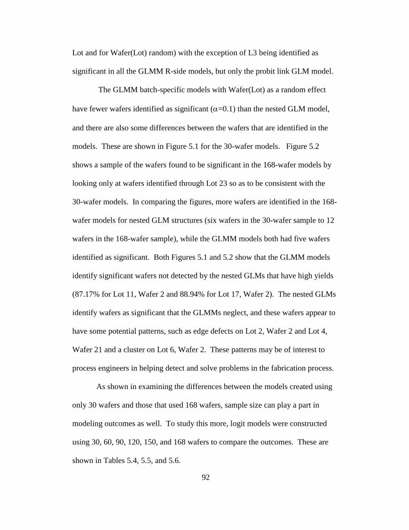
92
Lot and for Wafer(Lot) random) with the exception of L3 being identified as
significant in all the GLMM R-side models, but only the probit link GLM model.
The GLMM batch-specific models with Wafer(Lot) as a random effect
have fewer wafers identified as significant (=0.1) than the nested GLM model,
and there are also some differences between the wafers that are identified in the
models. These are shown in Figure 5.1 for the 30-wafer models. Figure 5.2
shows a sample of the wafers found to be significant in the 168-wafer models by
looking only at wafers identified through Lot 23 so as to be consistent with the
30-wafer models. In comparing the figures, more wafers are identified in the 168-
wafer models for nested GLM structures (six wafers in the 30-wafer sample to 12
wafers in the 168-wafer sample), while the GLMM models both had five wafers
identified as significant. Both Figures 5.1 and 5.2 show that the GLMM models
identify significant wafers not detected by the nested GLMs that have high yields
(87.17% for Lot 11, Wafer 2 and 88.94% for Lot 17, Wafer 2). The nested GLMs
identify wafers as significant that the GLMMs neglect, and these wafers appear to
have some potential patterns, such as edge defects on Lot 2, Wafer 2 and Lot 4,
Wafer 21 and a cluster on Lot 6, Wafer 2. These patterns may be of interest to
process engineers in helping detect and solve problems in the fabrication process.
As shown in examining the differences between the models created using
only 30 wafers and those that used 168 wafers, sample size can play a part in
modeling outcomes as well. To study this more, logit models were constructed
using 30, 60, 90, 120, 150, and 168 wafers to compare the outcomes. These are
shown in Tables 5.4, 5.5, and 5.6.
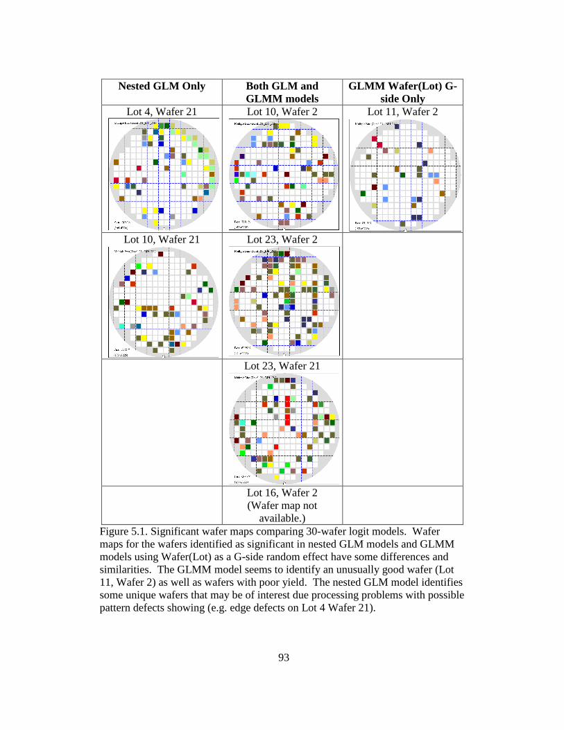
93
Nested GLM Only Both GLM and
GLMM models
GLMM Wafer(Lot) G-
side Only
Lot 4, Wafer 21
Lot 10, Wafer 2
Lot 11, Wafer 2
Lot 10, Wafer 21
Lot 23, Wafer 2
Lot 23, Wafer 21
Lot 16, Wafer 2
(Wafer map not
available.)
Figure 5.1. Significant wafer maps comparing 30-wafer logit models. Wafer
maps for the wafers identified as significant in nested GLM models and GLMM
models using Wafer(Lot) as a G-side random effect have some differences and
similarities. The GLMM model seems to identify an unusually good wafer (Lot
11, Wafer 2) as well as wafers with poor yield. The nested GLM model identifies
some unique wafers that may be of interest due processing problems with possible
pattern defects showing (e.g. edge defects on Lot 4 Wafer 21).
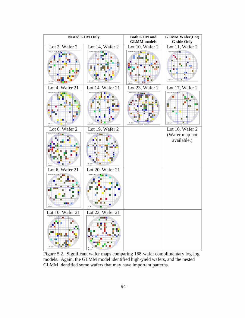
94
Nested GLM Only Both GLM and
GLMM models
GLMM Wafer(Lot)
G-side Only
Lot 2, Wafer 2
Lot 14, Wafer 2
Lot 10, Wafer 2
Lot 11, Wafer 2
Lot 4, Wafer 21
Lot 14, Wafer 21
Lot 23, Wafer 2
Lot 17, Wafer 2
Lot 6, Wafer 2
Lot 19, Wafer 2
Lot 16, Wafer 2
(Wafer map not
available.)
Lot 6, Wafer 21
Lot 20, Wafer 21
Lot 10, Wafer 21
Lot 23, Wafer 21
Figure 5.2. Significant wafer maps comparing 168-wafer complimentary log-log
models. Again, the GLMM model identified high-yield wafers, and the nested
GLMM identified some wafers that may have important patterns.
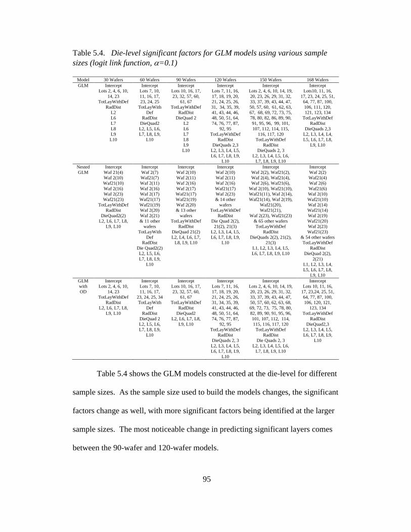
95
Table 5.4. Die-level significant factors for GLM models using various sample
sizes (logit link function, =0.1)
Model 30 Wafers 60 Wafers 90 Wafers 120 Wafers 150 Wafers 168 Wafers
GLM Intercept
Lots 2, 4, 6, 10,
14, 23
TotLayWithDef
RadDist
L2
L6
L7
L8
L9
L10
Intercept
Lots 7, 10,
11, 16, 17,
23, 24, 25
TotLayWith
Def
RadDist
DieQuad2
L2, L5, L6,
L7, L8, L9,
L10
Intercept
Lots 10, 16, 17,
23, 32, 57, 60,
61, 67
TotLayWithDef
RadDist
DieQuad 2
L2
L6
L7
L8
L9
L10
Intercept
Lots 7, 11, 16,
17, 18, 19, 20,
21, 24, 25, 26,
31, 34, 35, 39,
41, 43, 44, 46,
48, 50, 51, 64,
74, 76, 77, 87,
92, 95
TotLayWithDef
RadDist
DieQuads 2,3
L2, L3, L4, L5,
L6, L7, L8, L9,
L10
Intercept
Lots 2, 4, 6, 10, 14, 19,
20, 23, 26, 29, 31, 32,
33, 37, 39, 43, 44, 47,
50, 57, 60, 61, 62, 63,
67, 68, 69, 72, 73, 75,
78, 80, 82, 86, 89, 90,
91, 95, 96, 99, 101,
107, 112, 114, 115,
116, 117, 120
TotLayWithDef
RadDist
DieQuads 2, 3
L2, L3, L4, L5, L6,
L7, L8, L9, L10
Intercept
Lots10, 11, 16,
17, 23, 24, 25, 51,
64, 77, 87, 100,
106, 111, 120,
121, 123, 134
TotLayWithDef
RadDist
DieQuads 2,3
L2, L3, L4, L4,
L5, L6, L7, L8,
L9, L10
Nested
GLM
Intercept
Waf 21(4)
Waf 2(10)
Waf21(10)
Waf 2(16)
Waf 2(23)
Waf21(23)
TotLayWithDef
RadDist
DieQuad2(2)
L2, L6, L7, L8,
L9, L10
Intercept
Waf 2(7)
Waf21(7)
Waf 2(11)
Waf 2(16)
Waf 2(17)
Waf21(17)
Waf21(19)
Waf 2(20)
Waf 2(21)
& 11 other
wafers
TotLayWith
Def
RadDist
Die Quad2(2)
L2, L5, L6,
L7, L8, L9,
L10
Intercept
Waf 2(10)
Waf 2(11)
Waf 2(16)
Waf 2(17)
Waf21(17)
Waf21(19)
Waf 2(20)
& 13 other
wafers
TotLayWithDef
RadDist
DieQuad 21(2)
L2, L4, L6, L7,
L8, L9, L10
Intercept
Waf 2(10)
Waf 2(11)
Waf 2(16)
Waf21(17)
Waf 2(23)
& 14 other
wafers
TotLayWithDef
RadDist
Die Quad 2(2),
21(2), 21(3)
L2, L3, L4, L5,
L6, L7, L8, L9,
L10
Intercept
Waf 2(2), Waf21(2),
Waf 2(4), Waf21(4),
Waf 2(6), Waf21(6),
Waf 2(10), Waf21(10),
Waf21(11), Waf 2(14),
Waf21(14), Waf 2(19),
Waf21(20),
Waf21(21),
Waf 2(23), Waf21(23)
& 65 other wafers
TotLayWithDef
RadDist
DieQuads 2(2), 21(2),
21(3)
L1, L2, L3, L4, L5,
L6, L7, L8, L9, L10
Intercept
Waf 2(2)
Waf21(4)
Waf 2(6)
Waf21(6)
Waf 2(10)
Waf21(10)
Waf 2(14)
Waf21(14)
Waf 2(19)
Waf21(20)
Waf 2(23)
Waf21(23)
& 54 other wafers
TotLayWithDef
RadDist
DieQuad 2(2),
2(21)
L1, L2, L3, L4,
L5, L6, L7, L8,
L9, L10
GLM
with
OD
Intercept
Lots 2, 4, 6, 10,
14, 23
TotLayWithDef
RadDist
L2, L6, L7, L8,
L9, L10
Intercept
Lots 7, 10,
11, 16, 17,
23, 24, 25, 34
TotLayWith
Def
RadDist
DieQuad 2
L2, L5, L6,
L7, L8, L9,
L10
Intercept
Lots 10, 16, 17,
23, 32, 57, 60,
61, 67
TotLayWithDef
RadDist
DieQuad2
L2, L6, L7, L8,
L9, L10
Intercept
Lots 7, 11, 16,
17, 18, 19, 20,
21, 24, 25, 26,
31, 34, 35, 39,
41, 43, 44, 46,
48, 50, 51, 64,
74, 76, 77, 87,
92, 95
TotLayWithDef
RadDist
DieQuads 2, 3
L2, L3, L4, L5,
L6, L7, L8, L9,
L10
Intercept
Lots 2, 4, 6, 10, 14, 19,
20, 23, 26, 29, 31, 32,
33, 37, 39, 43, 44, 47,
50, 57, 60, 62, 63, 68,
69, 72, 73, 75, 78, 80,
82, 89, 90, 91, 95, 96,
101, 107, 112, 114,
115, 116, 117, 120
TotLayWithDef
RadDist
Die Quads 2, 3
L2, L3, L4, L5, L6,
L7, L8, L9, L10
Intercept
Lots 10, 11, 16,
17, 23,24, 25, 51,
64, 77, 87, 100,
106, 120, 121,
123, 134
TotLayWithDef
RadDist
DieQuad2,3
L2, L3, L4, L5,
L6, L7, L8, L9,
L10
Table 5.4 shows the GLM models constructed at the die-level for different
sample sizes. As the sample size used to build the models changes, the significant
factors change as well, with more significant factors being identified at the larger
sample sizes. The most noticeable change in predicting significant layers comes
between the 90-wafer and 120-wafer models.

96
Table 5.5 also shows the differences across these different sample sizes,
but this table highlights the factors found to be significant in batch-specific
GLMM models using the logit link function. As with the link model comparisons
in Table 5.3, convergence was again an issue for these GLMM models. None of
the models using a 90-wafer sample converged using the logit link. The sample
sizes over 60 wafers had convergence issues for the Wafer(Lot) random effect
models, and the G-matrix was not positive definite for any of the models using
Wafer as a random effect, thus preventing any wafer position (2 or 21) from being
identified as significant. Including the overdispersion parameter does not have an
impact on these die-level models, suggesting there is not overdispersion present in
the GLMM models, and Table 5.4 shows only very slight differences between the
GLM and the GLM with overdispersion (OD) models.
Table 5.6 shows the population-averaged GLMM models using the
different sample sizes and the logit link. Convergence issues again hindered
drawing many conclusions. The 30-wafer model using Wafer as an R-side
random effect took considerable computing time before producing the output that
the model did not converge, so large sample sizes were not tried for this type of
model. For the models that did converge, there seems to be very little difference
between the significant fixed factors identified in the batch-specific GLMM and
the population-averaged GLMM models.
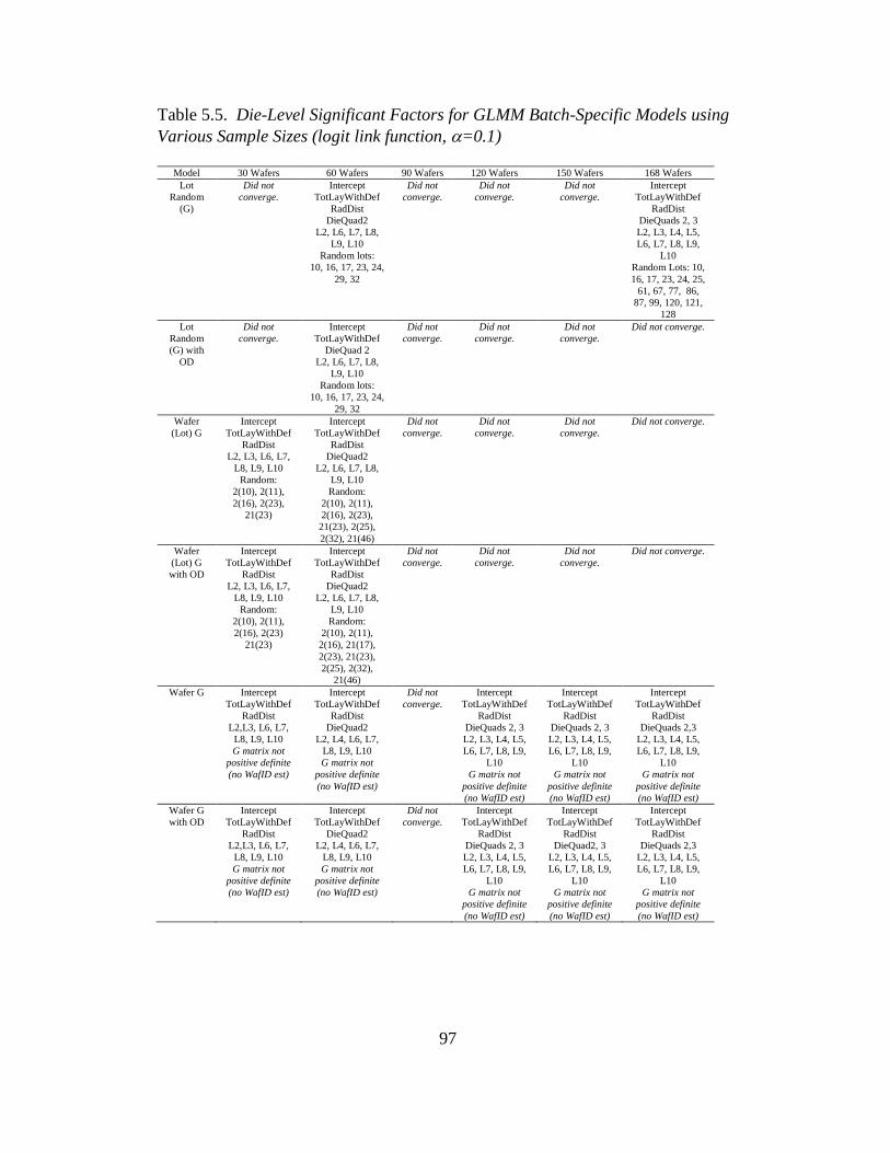
97
Table 5.5. Die-Level Significant Factors for GLMM Batch-Specific Models using
Various Sample Sizes (logit link function, =0.1)
Model 30 Wafers 60 Wafers 90 Wafers 120 Wafers 150 Wafers 168 Wafers
Lot
Random
(G)
Did not
converge.
Intercept
TotLayWithDef
RadDist
DieQuad2
L2, L6, L7, L8,
L9, L10
Random lots:
10, 16, 17, 23, 24,
29, 32
Did not
converge.
Did not
converge.
Did not
converge.
Intercept
TotLayWithDef
RadDist
DieQuads 2, 3
L2, L3, L4, L5,
L6, L7, L8, L9,
L10
Random Lots: 10,
16, 17, 23, 24, 25,
61, 67, 77, 86,
87, 99, 120, 121,
128
Lot
Random
(G) with
OD
Did not
converge.
Intercept
TotLayWithDef
DieQuad 2
L2, L6, L7, L8,
L9, L10
Random lots:
10, 16, 17, 23, 24,
29, 32
Did not
converge.
Did not
converge.
Did not
converge.
Did not converge.
Wafer
(Lot) G
Intercept
TotLayWithDef
RadDist
L2, L3, L6, L7,
L8, L9, L10
Random:
2(10), 2(11),
2(16), 2(23),
21(23)
Intercept
TotLayWithDef
RadDist
DieQuad2
L2, L6, L7, L8,
L9, L10
Random:
2(10), 2(11),
2(16), 2(23),
21(23), 2(25),
2(32), 21(46)
Did not
converge.
Did not
converge.
Did not
converge.
Did not converge.
Wafer
(Lot) G
with OD
Intercept
TotLayWithDef
RadDist
L2, L3, L6, L7,
L8, L9, L10
Random:
2(10), 2(11),
2(16), 2(23)
21(23)
Intercept
TotLayWithDef
RadDist
DieQuad2
L2, L6, L7, L8,
L9, L10
Random:
2(10), 2(11),
2(16), 21(17),
2(23), 21(23),
2(25), 2(32),
21(46)
Did not
converge.
Did not
converge.
Did not
converge.
Did not converge.
Wafer G Intercept
TotLayWithDef
RadDist
L2,L3, L6, L7,
L8, L9, L10
G matrix not
positive definite
(no WafID est)
Intercept
TotLayWithDef
RadDist
DieQuad2
L2, L4, L6, L7,
L8, L9, L10
G matrix not
positive definite
(no WafID est)
Did not
converge.
Intercept
TotLayWithDef
RadDist
DieQuads 2, 3
L2, L3, L4, L5,
L6, L7, L8, L9,
L10
G matrix not
positive definite
(no WafID est)
Intercept
TotLayWithDef
RadDist
DieQuads 2, 3
L2, L3, L4, L5,
L6, L7, L8, L9,
L10
G matrix not
positive definite
(no WafID est)
Intercept
TotLayWithDef
RadDist
DieQuads 2,3
L2, L3, L4, L5,
L6, L7, L8, L9,
L10
G matrix not
positive definite
(no WafID est)
Wafer G
with OD
Intercept
TotLayWithDef
RadDist
L2,L3, L6, L7,
L8, L9, L10
G matrix not
positive definite
(no WafID est)
Intercept
TotLayWithDef
DieQuad2
L2, L4, L6, L7,
L8, L9, L10
G matrix not
positive definite
(no WafID est)
Did not
converge.
Intercept
TotLayWithDef
RadDist
DieQuads 2, 3
L2, L3, L4, L5,
L6, L7, L8, L9,
L10
G matrix not
positive definite
(no WafID est)
Intercept
TotLayWithDef
RadDist
DieQuad2, 3
L2, L3, L4, L5,
L6, L7, L8, L9,
L10
G matrix not
positive definite
(no WafID est)
Intercept
TotLayWithDef
RadDist
DieQuads 2,3
L2, L3, L4, L5,
L6, L7, L8, L9,
L10
G matrix not
positive definite
(no WafID est)
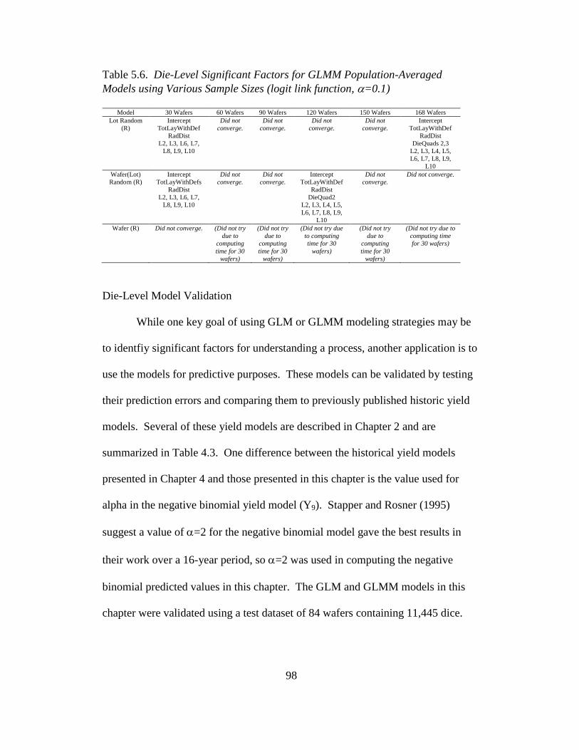
98
Table 5.6. Die-Level Significant Factors for GLMM Population-Averaged
Models using Various Sample Sizes (logit link function, =0.1)
Model 30 Wafers 60 Wafers 90 Wafers 120 Wafers 150 Wafers 168 Wafers
Lot Random
(R)
Intercept
TotLayWithDef
RadDist
L2, L3, L6, L7,
L8, L9, L10
Did not
converge.
Did not
converge.
Did not
converge.
Did not
converge.
Intercept
TotLayWithDef
RadDist
DieQuads 2,3
L2, L3, L4, L5,
L6, L7, L8, L9,
L10
Wafer(Lot)
Random (R)
Intercept
TotLayWithDefs
RadDist
L2, L3, L6, L7,
L8, L9, L10
Did not
converge.
Did not
converge.
Intercept
TotLayWithDef
RadDist
DieQuad2
L2, L3, L4, L5,
L6, L7, L8, L9,
L10
Did not
converge.
Did not converge.
Wafer (R) Did not converge. (Did not try
due to
computing
time for 30
wafers)
(Did not try
due to
computing
time for 30
wafers)
(Did not try due
to computing
time for 30
wafers)
(Did not try
due to
computing
time for 30
wafers)
(Did not try due to
computing time
for 30 wafers)
Die-Level Model Validation
While one key goal of using GLM or GLMM modeling strategies may be
to identfiy significant factors for understanding a process, another application is to
use the models for predictive purposes. These models can be validated by testing
their prediction errors and comparing them to previously published historic yield
models. Several of these yield models are described in Chapter 2 and are
summarized in Table 4.3. One difference between the historical yield models
presented in Chapter 4 and those presented in this chapter is the value used for
alpha in the negative binomial yield model (Y9). Stapper and Rosner (1995)
suggest a value of =2 for the negative binomial model gave the best results in
their work over a 16-year period, so =2 was used in computing the negative
binomial predicted values in this chapter. The GLM and GLMM models in this
chapter were validated using a test dataset of 84 wafers containing 11,445 dice.
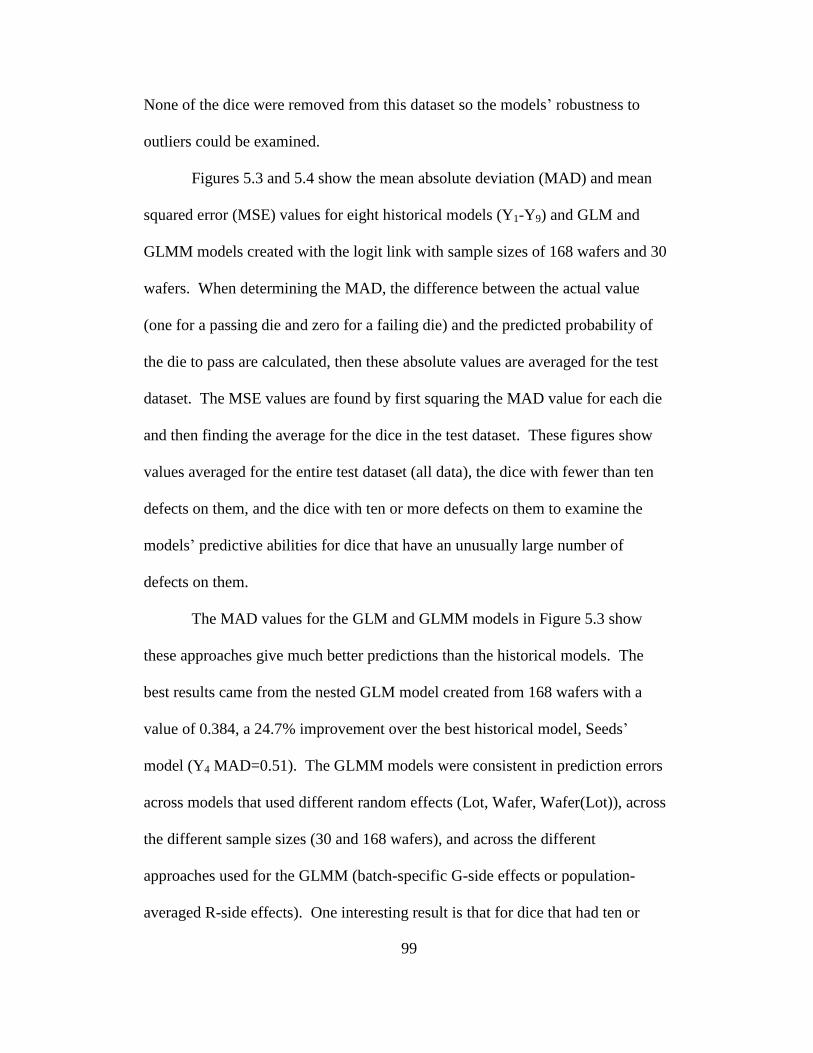
99
None of the dice were removed from this dataset so the models’ robustness to
outliers could be examined.
Figures 5.3 and 5.4 show the mean absolute deviation (MAD) and mean
squared error (MSE) values for eight historical models (Y1-Y9) and GLM and
GLMM models created with the logit link with sample sizes of 168 wafers and 30
wafers. When determining the MAD, the difference between the actual value
(one for a passing die and zero for a failing die) and the predicted probability of
the die to pass are calculated, then these absolute values are averaged for the test
dataset. The MSE values are found by first squaring the MAD value for each die
and then finding the average for the dice in the test dataset. These figures show
values averaged for the entire test dataset (all data), the dice with fewer than ten
defects on them, and the dice with ten or more defects on them to examine the
models’ predictive abilities for dice that have an unusually large number of
defects on them.
The MAD values for the GLM and GLMM models in Figure 5.3 show
these approaches give much better predictions than the historical models. The
best results came from the nested GLM model created from 168 wafers with a
value of 0.384, a 24.7% improvement over the best historical model, Seeds’
model (Y4 MAD=0.51). The GLMM models were consistent in prediction errors
across models that used different random effects (Lot, Wafer, Wafer(Lot)), across
the different sample sizes (30 and 168 wafers), and across the different
approaches used for the GLMM (batch-specific G-side effects or population-
averaged R-side effects). One interesting result is that for dice that had ten or
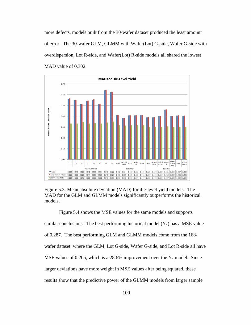
100
more defects, models built from the 30-wafer dataset produced the least amount
of error. The 30-wafer GLM, GLMM with Wafer(Lot) G-side, Wafer G-side with
overdispersion, Lot R-side, and Wafer(Lot) R-side models all shared the lowest
MAD value of 0.302.
Y1 Y3 Y4 Y5 Y6 Y7 Y8 Y9 GLMNested
GLMLot G
Wafer G
Lot R GLMNested
GLMWafer(Lot) G
Wafer G
Wafer G with
ODLot R
Wafer(Lot) R
Historical Models 168 Wafers 30 wafers
All data 0.562 0.549 0.510 0.540 0.553 0.514 0.640 0.622 0.412 0.384 0.407 0.408 0.409 0.389 0.390 0.402 0.461 0.402 0.407 0.404
Fewer than 10 defs/die 0.566 0.553 0.513 0.544 0.557 0.517 0.645 0.627 0.413 0.385 0.409 0.409 0.411 0.391 0.392 0.404 0.464 0.404 0.408 0.406
10 or more defs/die 0.332 0.333 0.345 0.333 0.336 0.332 0.343 0.351 0.317 0.315 0.317 0.317 0.317 0.302 0.303 0.302 0.307 0.302 0.302 0.302
0.00
0.10
0.20
0.30
0.40
0.50
0.60
0.70
Me
an A
bso
lute
De
viat
ion
(M
AD
)
MAD for Die-Level Yield
Figure 5.3. Mean absolute deviation (MAD) for die-level yield models. The
MAD for the GLM and GLMM models significantly outperforms the historical
models.
Figure 5.4 shows the MSE values for the same models and supports
similar conclusions. The best performing historical model (Y4) has a MSE value
of 0.287. The best performing GLM and GLMM models come from the 168-
wafer dataset, where the GLM, Lot G-side, Wafer G-side, and Lot R-side all have
MSE values of 0.205, which is a 28.6% improvement over the Y4 model. Since
larger deviations have more weight in MSE values after being squared, these
results show that the predictive power of the GLMM models from larger sample
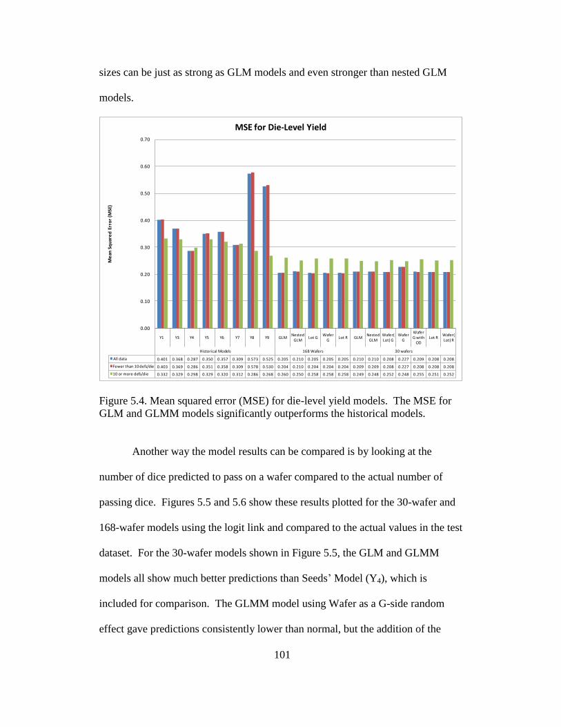
101
sizes can be just as strong as GLM models and even stronger than nested GLM
models.
Y1 Y3 Y4 Y5 Y6 Y7 Y8 Y9 GLMNested
GLMLot G
Wafer G
Lot R GLMNested
GLMWafer(Lot) G
Wafer G
Wafer G with
ODLot R
Wafer(Lot) R
Historical Models 168 Wafers 30 wafers
All data 0.401 0.368 0.287 0.350 0.357 0.309 0.573 0.525 0.205 0.210 0.205 0.205 0.205 0.210 0.210 0.208 0.227 0.209 0.208 0.208
Fewer than 10 defs/die 0.403 0.369 0.286 0.351 0.358 0.309 0.578 0.530 0.204 0.210 0.204 0.204 0.204 0.209 0.209 0.208 0.227 0.208 0.208 0.208
10 or more defs/die 0.332 0.329 0.298 0.329 0.320 0.312 0.286 0.268 0.260 0.250 0.258 0.258 0.258 0.249 0.248 0.252 0.248 0.255 0.251 0.252
0.00
0.10
0.20
0.30
0.40
0.50
0.60
0.70
Me
an S
qu
are
d E
rro
r (M
SE)
MSE for Die-Level Yield
Figure 5.4. Mean squared error (MSE) for die-level yield models. The MSE for
GLM and GLMM models significantly outperforms the historical models.
Another way the model results can be compared is by looking at the
number of dice predicted to pass on a wafer compared to the actual number of
passing dice. Figures 5.5 and 5.6 show these results plotted for the 30-wafer and
168-wafer models using the logit link and compared to the actual values in the test
dataset. For the 30-wafer models shown in Figure 5.5, the GLM and GLMM
models all show much better predictions than Seeds’ Model (Y4), which is
included for comparison. The GLMM model using Wafer as a G-side random
effect gave predictions consistently lower than normal, but the addition of the

102
overdispersion factor to this model improved the performance to be much closer
to the actual values and more in line with the other GLMM models. From this
figure, the GLM and nested GLM models appear to give higher predicted values
than the GLMM models.
0
20
40
60
80
100
120
140
0 20 40 60 80 100 120 140
Pre
dic
ted
Nu
mb
er
of
Pas
sin
g D
ice
Wit
h D
efe
cts
Actual Number of Passing Dice With Defects
Number of Passing Dice with Defects on a Wafer
30-Wafer Models
Values Actual=Pred
Values Sum of Y4
30 Wafers GLM
30 Wafers Nested GLM
30 Wafers Wafer(Lot) G
30 Wafers Wafer G
30 Wafers Wafer G with OD
30 Wafers Lot R
30 Wafers Wafer(Lot) R
Figure 5.5. Predicted vs. actual number of passing dice on a wafer for the 30-
wafer models using the logit link. Seeds’ model (Y4) is shown for comparison.
Figure 5.6 shows a similar chart for the models created with the 168-wafer
training dataset. Again, the GLM and GLMM models clearly provide better
predictions than the best historical model, Y4, for these data. With this larger
sample size, the Wafer G-side random effect model does not underestimate as it
did for the smaller sample size. This shows at larger sample sizes, the model is
robust even when the G matrix is not positive definite. Also, in this figure the
overestimation by the nested GLM model is more apparent. These figures show

103
the predictive power of the GLMM models, both batch-specific and population-
averaged, is strong and outperforms historical models, such as Seeds’ model.
0
20
40
60
80
100
120
140
0 20 40 60 80 100 120 140
Pre
dic
ted
Nu
mb
er
of
Pas
sin
g D
ice
Wit
h D
efe
cts
Actual Number of Passing Dice With Defects
Number of Passing Dice with Defects on a Wafer
168-Wafer Models
Values Actual=Pred
Historic Model Y4
168 Wafers GLM
168 Wafers Nested GLM
168 Wafers Lot G
168 Wafers Wafer G
168 Wafers Lot R
Figure 5.6. Predicted vs. actual number of passing dice on a wafer for the 168-
wafer models using the logit link. Seeds’ model (Y4) is shown for comparison.
Wafer-Level Model Results
Wafer-level analyses may be beneficial as well, and studying the different
levels of aggregation in this research helps determine the advantages of both
approaches. At the wafer level, the nested GLM models cannot be constructed, as
in Chapter 4, due to a lack of degrees of freedom with the particular nested
structure and sampling used. With this exception, all the models in Table 5.1
were run at the wafer level to study the effects of sample size and link functions
as well as the differences between the GLM and various GLMM models. The
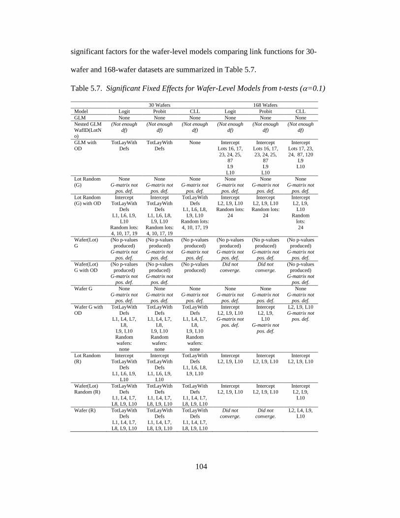
104
significant factors for the wafer-level models comparing link functions for 30-
wafer and 168-wafer datasets are summarized in Table 5.7.
Table 5.7. Significant Fixed Effects for Wafer-Level Models from t-tests (=0.1)
30 Wafers 168 Wafers
Model Logit Probit CLL Logit Probit CLL
GLM None None None None None None
Nested GLM
WafID(LotNo)
(Not enough
df)
(Not enough
df)
(Not enough
df)
(Not enough
df)
(Not enough
df)
(Not enough
df)
GLM with
OD
TotLayWith
Defs
TotLayWith
Defs
None Intercept
Lots 16, 17,
23, 24, 25, 87
L9
L10
Intercept
Lots 16, 17,
23, 24, 25, 87
L9
L10
Intercept
Lots 17, 23,
24, 87, 120 L9
L10
Lot Random
(G)
None
G-matrix not
pos. def.
None
G-matrix not
pos. def.
None
G-matrix not
pos. def.
None
G-matrix not
pos. def.
None
G-matrix not
pos. def.
None
G-matrix not
pos. def.
Lot Random (G) with OD
Intercept TotLayWith
Defs
L1, L6, L9, L10
Random lots: 4, 10, 17, 19
Intercept TotLayWith
Defs
L1, L6, L8, L9, L10
Random lots: 4, 10, 17, 19
TotLayWithDefs
L1, L6, L8,
L9, L10 Random lots:
4, 10, 17, 19
Intercept L2, L9, L10
Random lots:
24
Intercept L2, L9, L10
Random lots:
24
Intercept L2, L9,
L10
Random lots:
24
Wafer(Lot)
G
(No p-values
produced)
G-matrix not pos. def.
(No p-values
produced)
G-matrix not pos. def.
(No p-values
produced)
G-matrix not pos. def.
(No p-values
produced)
G-matrix not pos. def.
(No p-values
produced)
G-matrix not pos. def.
(No p-values
produced)
G-matrix not pos. def.
Wafer(Lot)
G with OD
(No p-values
produced) G-matrix not
pos. def.
(No p-values
produced) G-matrix not
pos. def.
(No p-values
produced)
Did not
converge.
Did not
converge.
(No p-values
produced) G-matrix not
pos. def.
Wafer G None
G-matrix not pos. def.
None
G-matrix not pos. def.
None
G-matrix not pos. def.
None
G-matrix not pos. def.
None
G-matrix not pos. def.
None
G-matrix not pos. def.
Wafer G with
OD
TotLayWith
Defs L1, L4, L7,
L8,
L9, L10 Random
wafers:
none
TotLayWith
Defs L1, L4, L7,
L8,
L9, L10 Random
wafers:
none
TotLayWith
Defs L1, L4, L7,
L8,
L9, L10 Random
wafers:
none
Intercept
L2, L9, L10 G-matrix not
pos. def.
Intercept
L2, L9, L10
G-matrix not
pos. def.
L2, L9, L10
G-matrix not pos. def.
Lot Random (R)
Intercept TotLayWith
Defs
L1, L6, L9, L10
Intercept TotLayWith
Defs
L1, L6, L9, L10
TotLayWithDefs
L1, L6, L8,
L9, L10
Intercept L2, L9, L10
Intercept L2, L9, L10
Intercept L2, L9, L10
Wafer(Lot)
Random (R)
TotLayWith
Defs L1, L4, L7,
L8, L9, L10
TotLayWith
Defs L1, L4, L7,
L8, L9, L10
TotLayWith
Defs L1, L4, L7,
L8, L9, L10
Intercept
L2, L9, L10
Intercept
L2, L9, L10
Intercept
L2, L9, L10
Wafer (R) TotLayWithDefs
L1, L4, L7,
L8, L9, L10
TotLayWithDefs
L1, L4, L7,
L8, L9, L10
TotLayWithDefs
L1, L4, L7,
L8, L9, L10
Did not converge.
Did not converge.
L2, L4, L9, L10
105
There are several interesting differences to observe in these model
comparisons. First, at the wafer level, neither the GLM model nor the batch-
specific GLMM models identified any effects as significant unless the
overdispersion parameter was included in the model. Also, the GLM model with
overdispersion for the 30-wafer models only identified at most one significant
factor. From a process improvement standpoint, this is a limitation of the GLM
models at small sample sizes. At larger sample size (168 wafers), the GLM
models were able to identify more significant factors, but they did not identify
Layer 2 as significant like the GLMM models for the 168-wafer dataset did. They
did, though, identify more lots as significant (considering them as fixed effects)
than the batch-specific GLMM did.
As shown in Table 5.7, there are very few differences in significant factors
across link functions at either the small or the large sample size. There are not as
many convergence problems with these wafer-level models as there were with the
die-level models, which enable better understanding of the differences between
the links. These wafer-level data suggest the complimentary log-log link seems to
work better than the probit or logit links for the large sample size of 168 wafers in
delivering a solution.
There are also some interesting similarities and differences in comparing
the GLMM models. In comparing the batch-specific (including the
overdispersion parameter) and the population-averaged GLMM models, the same
predictive factors were identified as statistically significant in both types of
GLMM for random effects of Lot and of Wafer. The batch-specific model was
106
able to identify specific significant lots. This suggest there is some robustness in
model selection since choosing either the batch-specific or the population-
averaged approach delivered the same results in terms of identifying the same
significant fixed effects. For the 30-wafer models, there were differences in the
results between the GLMM models that used only Lot as a random effect and
those that used Wafer or Wafer(Lot) as a random effect. These differences are
not seen in the 168-wafer models, with the exception of the complimentary log-
log link with Wafer as an R-side random effect identifying an additional
significant layer (L4). This consistency suggests that at large sample sizes, the
choice of the random effect used in the model may not be critical to obtaining
useful results.
The GLMM models in Table 5.7 that included Wafer(Lot) or Wafer as
random G-side effects had problems with the G matrix not being positive definite
(except for the 30-wafer models that included Wafer as a G-side random effect
and included an overdispersion parameter). The wafer-level population-averaged
GLMM models did not not have as many convergence issues as the die-level
models did, though two of the links did not converge for the 168-wafer models
using Wafer as an R-side random effect. None of the die-level models converged
using Wafer as an R-side random effect, so the ability to obtain results for this
model at the wafer level is an important difference to consider.
Since the nested GLM model cannot be assessed at the wafer level, it was
interesting to see these results show that the nested Wafer(Lot) random effect
could produce results for the population-averaged model. Also, these results were
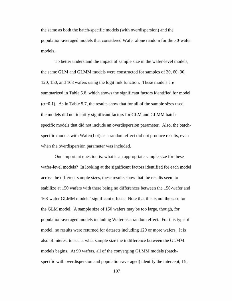
107
the same as both the batch-specific models (with overdispersion) and the
population-averaged models that considered Wafer alone random for the 30-wafer
models.
To better understand the impact of sample size in the wafer-level models,
the same GLM and GLMM models were constructed for samples of 30, 60, 90,
120, 150, and 168 wafers using the logit link function. These models are
summarized in Table 5.8, which shows the significant factors identified for model
(=0.1). As in Table 5.7, the results show that for all of the sample sizes used,
the models did not identify significant factors for GLM and GLMM batch-
specific models that did not include an overdispersion parameter. Also, the batch-
specific models with Wafer(Lot) as a random effect did not produce results, even
when the overdispersion parameter was included.
One important question is: what is an appropriate sample size for these
wafer-level models? In looking at the significant factors identified for each model
across the different sample sizes, these results show that the results seem to
stabilize at 150 wafers with there being no differences between the 150-wafer and
168-wafer GLMM models’ significant effects. Note that this is not the case for
the GLM model. A sample size of 150 wafers may be too large, though, for
population-averaged models including Wafer as a random effect. For this type of
model, no results were returned for datasets including 120 or more wafers. It is
also of interest to see at what sample size the indifference between the GLMM
models begins. At 90 wafers, all of the converging GLMM models (batch-
specific with overdispersion and population-averaged) identify the intercept, L9,
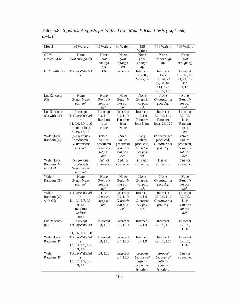
108
Table 5.8. Significant Effects for Wafer-Level Models from t-tests (logit link,
=0.1)
Model 30 Wafers 60 Wafers 90 Wafers 120
Wafers
150 Wafers 168 Wafers
GLM None None None None None None
Nested GLM (Not enough df) (Not
enough
df)
(Not
enough
df)
(Not
enough
df)
(Not enough
df)
(Not
enough df)
GLM with OD TotLayWithDef
s
L6 Intercept
Intercept
Lots 16,
24, 25, 87
Intercept
Lots
10, 14, 23
57, 61, 67,
114, 120
L2, L9, L10
Intercept
Lots 16, 17,
23, 24, 25,
87
L9, L10
Lot Random
(G)
None
G-matrix not
pos. def.
None
G-matrix
not pos.
def.
None
G-matrix
not pos.
def.
None
G-matrix
not pos.
def.
None
G-matrix not
pos. def.
None
G-matrix
not pos.
def.
Lot Random
(G) with OD
Intercept
TotLayWithDef
s
L1, L6, L9, L10
Random lots:
4, 10, 17, 19
Intercept
L8, L10
Random
lots:
None
Intercept
L9, L10
Random
lots:
None
Intercept
L2, L9
Random
lots: None
Intercept
L2, L9, L10
Random
lots: 24, 120
Intercept
L2, L9,
L10
Random
lots:
24
Wafer(Lot)
Random (G)
(No p-values
produced)
G-matrix not
pos. def.
(No p-
values
produced)
G-matrix
not pos.
def.
(No p-
values
produced)
G-matrix
not pos.
def.
(No p-
values
produced)
G-matrix
not pos.
def.
(No p-values
produced)
G-matrix not
pos. def.
(No p-
values
produced)
G-matrix
not pos.
def.
Wafer(Lot)
Random (G)
with OD
(No p-values
produced)
G-matrix not
pos. def.
Did not
converge.
Did not
converge.
Did not
converge.
Did not
converge.
Did not
converge.
Wafer
Random (G)
None
G-matrix not
pos. def.
None
G-matrix
not pos.
def.
None
G-matrix
not pos.
def.
None
G-matrix
not pos.
def.
None
G-matrix not
pos. def.
None
G-matrix
not pos.
def.
Wafer
Random (G)
with OD
TotLayWithDef
s
L1, L4, L7, L8,
L9, L10
Random
wafers:
none
L10
G-matrix
not pos.
def.
Intercept
L9, L10
G-matrix
not pos.
def.
Intercept
L4, L9
G-matrix
not pos.
def.
Intercept
L2, L9, L10
G-matrix not
pos. def.
Intercept
L2, L9,
L10
G-matrix
not pos.
def.
Lot Random
(R)
Intercept
TotLayWithDef
s
L1, L6, L9, L10
Intercept
L8, L10
Intercept
L9, L10
Intercept
L2, L9
Intercept
L2, L9, L10
Intercept
L2, L9,
L10
Wafer(Lot)
Random (R)
TotLayWithDef
s
L1, L4, L7, L8,
L9, L10
Intercept
L8, L10
Intercept
L9, L10
Intercept
L4, L9
Intercept
L2, L9, L10
Intercept
L2, L9,
L10
Wafer
Random (R)
TotLayWithDef
s
L1, L4, L7, L8,
L9, L10
L8, L10 Intercept
L9, L10
Stopped
because of
infinite
objective
function.
Stopped
because of
infinite
objective
function.
Did not
converge.

109
and L10 as significant. There are some slight differences for the 120-wafer
models with the models using Lot as a random effect identifying the intercept, L2,
and L9 as significant while the Wafer (G-side) and Wafer(Lot) (R-side) models
show the intercept, L2, and L9 to be significant. Any differences between
significant factors across different types of GLMM models appear to be resolved
for models containing 150 wafers or more.
Wafer-Level Model Validation
As with the die-level models, MAD and MSE can help compare the
predictive power of the GLM and GLMM models compared to the historical
models. At the wafer-level, these comparisons were made using the models
developed for the 30-wafer and 168-wafer datasets. Adjusted models were also
considered. These adjusted wafer-level models took the wafer-level GLM or
GLMM and adjusted the forecasted yield from predicting that of the entire wafer
to instead forecast the yield for only the defective dice. For example, the wafer-
level GLMM prediction may be 75% yield for a wafer. This prediction, however,
is really modeling the proportion of dice that have defects and pass, not a
proportion of all the dice on the wafer. The adjusted models take this into account
and assume that all non-defective dice will pass. To illustrate this, consider a
wafer (Lot 8, Wafer 2 in the training dataset) that has 226 total dice on the wafer,
154 of them with detectable defects on at least one layer. Of these defective dice,
101 of them pass. The wafer-level GLM predicts 63.7% yield. The adjusted
yield is found simply by taking:

110
%.26.75226
)154226(154*637.0
waferon the dice Total
dice defective-non ofnumber dice defective passing ofnumber Predictedyield model Adjusted
The actual yield for this wafer is 76.11% (172 passing dice), so the adjusted yield
gives a much more accurate forecast and is fitting, considering the data used to
build the GLM and GLMM models is based only on dice containing defects.
Die-level models were also included in these comparisons by summing the
prediction probabilities for all the dice on a wafer to predict how many dice on the
wafer would pass. These values were also adjusted while assuming non-defective
dice will pass. For example, for Lot 8, Wafer 2, the die-level nested GLM
predicted probabilities sum to 106.38 for the wafer. The adjustment simply takes:
%.9.78226
)154226(38.106
Figure 5.7 displays the mean absolute deviation (MAD) values for the
historical yield models Y1-Y9, the wafer-level GLM and GLMM models from
both the 30-wafer and 168-wafer datasets, the adjusted wafer-level models, and
the adjusted die-level models. These values are calculated using the actual yields
from the wafers in the test dataset (84 wafers). The chart shows that all the GLM
and GLMM models signficantly outperform the historical models. The best of the
previously published models is Y4, Seeds’ model, with a MAD value of 0.336 and
an MSE value of 0.1205. Figure 5.7 shows a number of interesting relationships
between the models. First, wafer-level GLM and GLMM models from the larger
sample size (168 wafers) are very consistent in their prediction errors, regardless
of the form of the model. This is not the case for the 30-wafer models, where
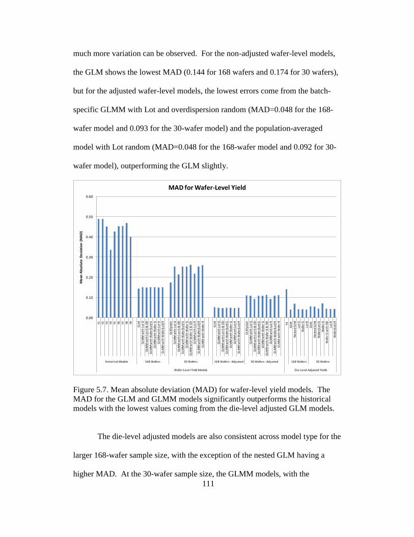
111
much more variation can be observed. For the non-adjusted wafer-level models,
the GLM shows the lowest MAD (0.144 for 168 wafers and 0.174 for 30 wafers),
but for the adjusted wafer-level models, the lowest errors come from the batch-
specific GLMM with Lot and overdispersion random (MAD=0.048 for the 168-
wafer model and 0.093 for the 30-wafer model) and the population-averaged
model with Lot random (MAD=0.048 for the 168-wafer model and 0.092 for 30-
wafer model), outperforming the GLM slightly.
0.00
0.10
0.20
0.30
0.40
0.50
0.60
Y1 Y2 Y3 Y4 Y5 Y6 Y7 Y8 Y9
GLM
GLM
M w
ith
Lo
t G
GLM
M w
ith
Lo
t G
& O
DG
LMM
wit
h W
afe
r(Lo
t) G
GLM
M w
ith
Waf
er
GG
LMM
wit
h L
ot
RG
LMM
wit
h W
afe
r(Lo
t) R
GLM
pla
inG
LMM
wit
h L
ot
GG
LMM
wit
h L
ot
G &
OD
GLM
M w
ith
Waf
er(
Lot)
GG
LMM
wit
h W
afe
r G
GLM
M w
ith
Waf
er
G &
OD
GLM
M w
ith
Lo
t R
GLM
M w
ith
Waf
er(
Lot)
RG
LMM
wit
h W
afe
r R
GLM
GLM
M w
ith
Lo
t G
GLM
M w
ith
Lo
t G
& O
DG
LMM
wit
h W
afe
r(Lo
t) G
GLM
M w
ith
Waf
er
GG
LMM
wit
h L
ot
RG
LMM
wit
h W
afe
r(Lo
t) R
GLM
pla
inG
LMM
wit
h L
ot
GG
LMM
wit
h L
ot
G &
OD
GLM
M w
ith
Waf
er(
Lot)
GG
LMM
wit
h W
afe
r G
GLM
M w
ith
Waf
er
G &
OD
GLM
M w
ith
Lo
t R
GLM
M w
ith
Waf
er(
Lot)
RG
LMM
wit
h W
afe
r R
Y4
GLM
N
est
ed
GLM
Lot
GW
afe
r G
Lot
RG
LM
Ne
ste
d G
LMW
afe
r(Lo
t) G
Waf
er
GW
afe
r G
wit
h O
DLo
t R
Waf
er(
Lot)
R
Historical Models 168 Wafers 30 Wafers 168 Wafers - Adjusted 30 Wafers - Adjusted 168 Wafers 30 Wafers
Wafer-Level Yield Models Die-Level Adjusted Yields
Me
an A
bso
lute
De
viat
ion
(M
AD
)
MAD for Wafer-Level Yield
Figure 5.7. Mean absolute deviation (MAD) for wafer-level yield models. The
MAD for the GLM and GLMM models significantly outperforms the historical
models with the lowest values coming from the die-level adjusted GLM models.
The die-level adjusted models are also consistent across model type for the
larger 168-wafer sample size, with the exception of the nested GLM having a
higher MAD. At the 30-wafer sample size, the GLMM models, with the
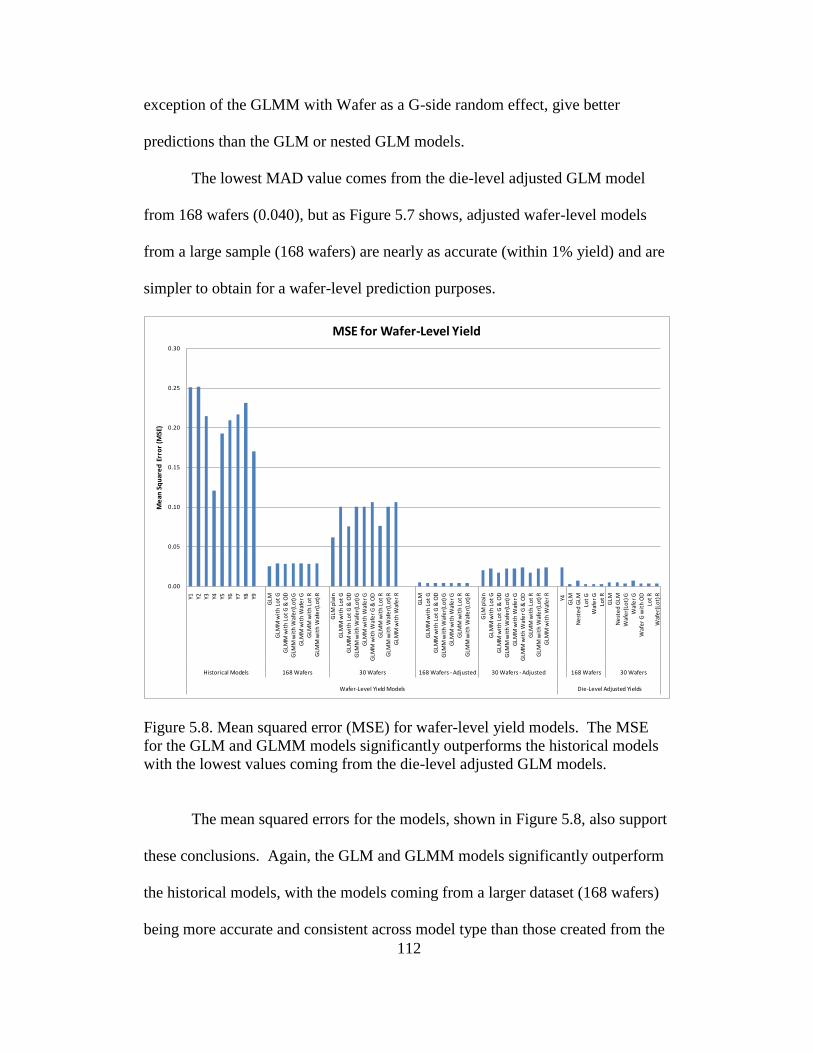
112
exception of the GLMM with Wafer as a G-side random effect, give better
predictions than the GLM or nested GLM models.
The lowest MAD value comes from the die-level adjusted GLM model
from 168 wafers (0.040), but as Figure 5.7 shows, adjusted wafer-level models
from a large sample (168 wafers) are nearly as accurate (within 1% yield) and are
simpler to obtain for a wafer-level prediction purposes.
0.00
0.05
0.10
0.15
0.20
0.25
0.30
Y1 Y2 Y3 Y4 Y5 Y6 Y7 Y8 Y9
GLM
GLM
M w
ith
Lo
t G
GLM
M w
ith
Lo
t G
& O
DG
LMM
wit
h W
afe
r(Lo
t) G
GLM
M w
ith
Waf
er
GG
LMM
wit
h L
ot
RG
LMM
wit
h W
afe
r(Lo
t) R
GLM
pla
inG
LMM
wit
h L
ot
GG
LMM
wit
h L
ot
G &
OD
GLM
M w
ith
Waf
er(
Lot)
GG
LMM
wit
h W
afe
r G
GLM
M w
ith
Waf
er
G &
OD
GLM
M w
ith
Lo
t R
GLM
M w
ith
Waf
er(
Lot)
RG
LMM
wit
h W
afe
r R
GLM
GLM
M w
ith
Lo
t G
GLM
M w
ith
Lo
t G
& O
DG
LMM
wit
h W
afe
r(Lo
t) G
GLM
M w
ith
Waf
er
GG
LMM
wit
h L
ot
RG
LMM
wit
h W
afe
r(Lo
t) R
GLM
pla
inG
LMM
wit
h L
ot
GG
LMM
wit
h L
ot
G &
OD
GLM
M w
ith
Waf
er(
Lot)
GG
LMM
wit
h W
afe
r G
GLM
M w
ith
Waf
er
G &
OD
GLM
M w
ith
Lo
t R
GLM
M w
ith
Waf
er(
Lot)
RG
LMM
wit
h W
afe
r R
Y4
GLM
Ne
ste
d G
LMLo
t G
Waf
er
GLo
t R
GLM
Ne
ste
d G
LMW
afe
r(Lo
t) G
Waf
er
GW
afe
r G
wit
h O
DLo
t R
Waf
er(
Lot)
R
Historical Models 168 Wafers 30 Wafers 168 Wafers - Adjusted 30 Wafers - Adjusted 168 Wafers 30 Wafers
Wafer-Level Yield Models Die-Level Adjusted Yields
Me
an S
qu
are
d E
rro
r (M
SE)
MSE for Wafer-Level Yield
Figure 5.8. Mean squared error (MSE) for wafer-level yield models. The MSE
for the GLM and GLMM models significantly outperforms the historical models
with the lowest values coming from the die-level adjusted GLM models.
The mean squared errors for the models, shown in Figure 5.8, also support
these conclusions. Again, the GLM and GLMM models significantly outperform
the historical models, with the models coming from a larger dataset (168 wafers)
being more accurate and consistent across model type than those created from the
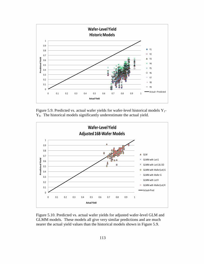
113
0
0.1
0.2
0.3
0.4
0.5
0.6
0.7
0.8
0.9
1
0 0.1 0.2 0.3 0.4 0.5 0.6 0.7 0.8 0.9 1
Pre
dic
ted
Yie
ld
Actual Yield
Wafer-Level YieldHistoric Models
Y1
Y2
Y3
Y4
Y5
Y6
Y7
Y8
Y9
Actual = Predicted
Figure 5.9. Predicted vs. actual wafer yields for wafer-level historical models Y1-
Y9. The historical models significantly underestimate the actual yield.
0
0.1
0.2
0.3
0.4
0.5
0.6
0.7
0.8
0.9
1
0 0.1 0.2 0.3 0.4 0.5 0.6 0.7 0.8 0.9 1
Pre
dic
ted
Yie
ld
Actual Yield
Wafer-Level YieldAdjusted 168-Wafer Models
GLM
GLMM with Lot G
GLMM with Lot G & OD
GLMM with Wafer(Lot) G
GLMM with Wafer G
GLMM with Lot R
GLMM with Wafer(Lot) R
Actual=Pred
Figure 5.10. Predicted vs. actual wafer yields for adjusted wafer-level GLM and
GLMM models. These models all give very similar predictions and are much
nearer the actual yield values than the historical models shown in Figure 5.9.
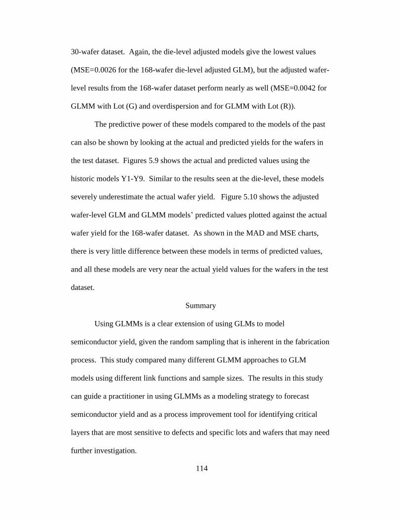
114
30-wafer dataset. Again, the die-level adjusted models give the lowest values
(MSE= 0.0026 for the 168-wafer die-level adjusted GLM), but the adjusted wafer-
level results from the 168-wafer dataset perform nearly as well (MSE=0.0042 for
GLMM with Lot (G) and overdispersion and for GLMM with Lot (R)).
The predictive power of these models compared to the models of the past
can also be shown by looking at the actual and predicted yields for the wafers in
the test dataset. Figures 5.9 shows the actual and predicted values using the
historic models Y1-Y9. Similar to the results seen at the die-level, these models
severely underestimate the actual wafer yield. Figure 5.10 shows the adjusted
wafer-level GLM and GLMM models’ predicted values plotted against the actual
wafer yield for the 168-wafer dataset. As shown in the MAD and MSE charts,
there is very little difference between these models in terms of predicted values,
and all these models are very near the actual yield values for the wafers in the test
dataset.
Summary
Using GLMMs is a clear extension of using GLMs to model
semiconductor yield, given the random sampling that is inherent in the fabrication
process. This study compared many different GLMM approaches to GLM
models using different link functions and sample sizes. The results in this study
can guide a practitioner in using GLMMs as a modeling strategy to forecast
semiconductor yield and as a process improvement tool for identifying critical
layers that are most sensitive to defects and specific lots and wafers that may need
further investigation.

115
One limitation of the study was the lack of convergence in many of the
models examined. This may be due to the degrees of freedom method used.
Preliminary models using the Sattherwaite degrees of freedom method (ddfm) for
wafer-level models did not have as many problems with convergence, so using
this method or the Kenward-Rogers approach, both available in PROC
GLIMMIX in SAS, may provide more conclusive results when the default
settings do not.
The results from this research can provide a meaningful modeling strategy
for yield modeling or other applications, but the approach depends on the
researcher’s objectives. Different information is provided by the models at
different levels of aggregation and through the different model types.
For a focus on process improvement, the die-level models described here
can be very helpful in identifying significant process layers impacted by defects
and in distinguishing important wafers or lots for further investigation. The
GLMM models include high-yield wafers in those found to be significant, while
the GLM models identify more wafers and tend to identify more low-yield wafers
as significant. Some of the wafers identified by the GLM model appear to have
some pattern defects, so this identification, either done at the end of the line as
with this study or earlier in the fabrication process, may be helpful in detecting
processing issues that can be resolved to boost yield on future wafers.
Conversely, the high-yield wafers identified by the GLMM model may be helpful
in studying optimal operating conditions that can be replicated in future
fabrication. Also, at the die level GLM models identified a much larger number

116
of lots or wafers as significant compared to the GLMM models. This additional
detection may lead to some false alarms in process improvement efforts, meaning
some of the wafers or lots identified may actually be different from the baseline
due to random effects rather than systematic problems.
Due to the convergence issues, it is not clear if one link function
consistently outperforms the others at the die level, but there were very few
differences between the results using different link functions when they all
provided results. The die-level models did give the best predictions of wafer yield
in terms of MAD and MSE, even for the small 30-wafer sample size. This
suggests that if only a small dataset is available for modeling, die-level models
should be used to predict wafer yield.
For a focus on wafer-level predictions that have little error and are robust
as to model type, adjusted wafer-level models from large sample datasets can
work very well. Sample sizes over 150 wafers seem to work best for wafer-level
modeling, and the complimentary log-log link seems to work best for generating
results at this larger sample size.
The wafer-level GLM and GLMM models all identified fewer significant
factors than the die-level models, with the 150-wafer models selecting only L2,
L9, and L10 as significant. These differences between the die- and wafer-level
modeling may make a strong difference in detecting problems, and since the die-
level models take advantage of more complete and specific information, the die-
level models are most useful for process and yield improvement efforts.

117
The GLM and GLMM models significantly outperformed the models of
the past in terms of prediction error. GLMM models offer a modeling approach
that accounts for the random factors in a system without violating the assumptions
of the model. This work shows that the GLMM models do this while providing
additional insight into the process and maintaining or even improving prediction
power compared to using GLMs.

118
Chapter 6
SEMICONDUCTOR YIELD MODELING INTEGRATING CART AND
GENERALIZED LINEAR MODELS
Introduction
The approach used in building classification and regression trees (CART)
is described in Chapter 2 and in full detail by Brieman, et al. (1984). Recall the
main steps involved in CART are (1) building the tree through binary recursive
partitioning by minimizing the impurity of the nodes, (2) pruning the tree using a
cost-complexity parameter, and (3) selecting the best tree to avoid overfitting by
using cross-validation techniques. This approach has shown promise in a variety
of applications.
Many articles have been published that compare the use of classification
trees with other approaches such as logistic regression. Costanza and Paccaud
(2004) compare the use of linear regression, logistic regression, classification
trees, and regression trees to predict occurrences of dyslipidemia. Skinner, et al.
(2002) compare the use of cluster analysis, principal components, ordinary least
squares regression, logistic regression, and CART to determine the cause of low
yield wafers from unit probe testing. Chang and Chen (2005) consider CART
models and negative binomial regression models to analyze freeway accident
frequency. Khoshgoftaar and Seliya (2003) use CART-least squares, CART-least
absolute deviation, S-PLUS, multiple linear regression, artificial neural networks,
and case-based reasoning and compare these modeling techniques applied to

119
predicting software quality. Predicting essential hypertension was studied by
Ture, et al. (2005) as they applied CART, Quick, Unbiased, Efficient Statistical
Tree (QUEST), logistic regression, Flexible Discriminant Analysis (FDA),
Multivariate Addititve Regression Splines (MARS), Multi-Layer Perceptron
(MLP) and Radial Basis Function (RBF) neural networks to compare the models.
These studies demonstrate the value of CART for handling large datasets that do
not fit the assumptions required for more traditional statistical techniques.
CART’s tree structure is easy for users to interpret and understand. If
sufficient data are available to form the model, good predictions can be achieved
using CART. The CART approach also is beneficial as a supplemental tool to
other modeling techniques that provides a different type of information through
the trees that are generated, including a “recipe” for groups such as high yield.
Limitations mentioned include the limited predictive power of CART and the
need for large datasets to construct meaningful models.
Some work has also been done to integrate CART or decision trees with
other techniques to build new modeling approaches. Choi and Lee (2010)
develop a method for selecting retaining wall systems to prevent failures. While
previous studies in this area have used machine-learning techniques, the training
datasets had to be very large to produce adequate prediction values. These large
amounts of data are not feasible in the excavation area, so Choi and Lee (2010)
demonstrate a different approach. They first use a series of logistic regression to
determine significant factors, reduce multicollinearity, and adjust certain outcome
groups. Next, the derived explanatory variables were examined against general

120
findings documented in the literature and were reviewed by process experts (Choi
& Lee, 2010). The third step of the process was to develop these explanatory
variables into a binary decision tree based on their impact on outcomes.
Threshold values at each node were determined using ROC curves. The resulting
decision tree showed high prediction rates (82.6% for retaining walls), which was
much improved over using a data-mining algorithm along that produced a
decision tree with accuracy of 58.7% (Choi & Lee, 2010).
Chandra, et al. (2009) use a variety of approaches to determine important
factors and prediction accuracy for survival of dotcom companies, also called
“click-and-mortar” corporations. They compare using multilayer perceptrons
(MLP), CART, support vector machines (SVM), random forest (RF), and logistic
regression (LR) to their dataset of 24 financial ratios for 240 dotcom companies.
They compared both full and reduced (10 of the 24 financial ratios determined
from t-tests) models and also explored the use of ensembling and boosting to
improve the accuracy of the method. Ensembling, which aims to exploit each
constituent model’s unique features to capture different patterns in the dataset
(Chandra, et al., 2009), was used to combine the results from RF, CART, and
SVM by majority voting. For the dotcom data, Chandra, et al. (2009) found this
ensembling approach did not improve the accuracy of the model compared to the
individual classifying methods. Boosting focuses on producing a series of
classifiers and attempts to produce new classifiers that are better able to predict
examples for which the current ensemble’s performance is not adequate (Chandra,
et al., 2009). This is a more hierarchical approach where the misclassified

121
samples from using one approach, such as RF, are then modeled using another
approach, such as CART. Any samples that are still misclassified by the second
step (CART) are modeled using yet as third approach, such as MLP. Chandra, et
al. (2009) found that this technique of boosting using RF+SVM+MLP to give the
most accurate predictions.
Kuhnert, Do, and McClure (2000) consider combining CART,
multivariate adaptive regression splines (MARS), and logistic regression to
improve on logistic regression modeling by using the variable importance
rankings from CART to aid in identifying important variables and also in
visualizing each variable’s contribution to the response being modeled. As they
apply their approach to motor vehicle accident data, they show how using these
approaches together can improve understanding of significant factors (risk factors
such as seat belts and speeding), interactions (age and experience), and groups of
special interest (middle-aged “rural” drivers). The approach of modeling with all
three methods first contributed to a stronger logistic regression model by using the
age*experience interaction identified by MARS and creating two logistic
regression models after splitting the data into groups determined by CART
(splitting by age < 27.5 years and age > 27.5 years), which allowed for better
interpretation of the interaction (Kuhnert, et al., 2000).
Fu (2004) took a similar approach by using loglinear models and CART
together to examine occurrences of low birth weight and preterm birth. The use
of both CART and loglinear models produced more information about potential

122
relationships between the variables than using either approach alone. Using these
methods jointly produced the benefits of both, including the odds ratios and
ability to deal with multiple responses simultaneously for the loglinear model and
the strength of being able to be used for predictive classification from the CART
model. These methods are complementary for data analysis (Fu, 2004).
These integrated techniques show promise but do not fully explore the
ways CART can be used with GLMs. For semiconductor yield modeling using
defectivity data, Krueger, Montgomery, and Mastrangelo (2011) found die-level
GLM models to best outperform yield models of the past (also described in
Chapter 4), but interaction terms between the process layers were not considered.
This is also the case for the GLMM models described in Chapter 5. Considering
all the two-way interaction terms in the model would require an additional 45
predictor variables, significantly adding to the complexity of the model.
Additional interactions may be present as well. CART’s tree structure classifies
each data point into a terminal node that is reached by following a series of
splitting nodes. These terminal nodes form groups that may be statistically
significant (as mentioned in Skinner, et al., 2002) and can be detected as such
using a GLM. These groups may be of particular interest in developing “recipes”
for reproducing those outcomes. Also, the CART tree can quickly identify which
interactions may be of most interest to include in the GLM as predictors.
The purpose of this chapter is to describe a methodology that integrates
CART and GLMs in a way that enhances the modeling results and interpretation

123
for process improvement and outcome prediction. An example using
semiconductor yield data is provided to demonstrate the benefits of this integrated
approach. This chapter is organized to first describe the methodology, then
discuss the results, and summarize the findings.
Methodology
This integrated approach includes two main components: first, building
decision trees using a method such as CART to determine terminal nodes and
important interaction terms in the dataset and, second, building a GLM model
using the factors in the dataset as well as indicator variables from the terminal
nodes of the classification trees. The approach is described in detail and
demonstrated through an example using semiconductor yield data.
Building Trees
Often in exploratory data mining, prior knowledge of the data may not
exist. While a process owner may understand the important process factors and
logical interactions, sometimes this information is unknown, such as for a new
product or process or when only limited previous analyses have been performed.
Recall from Chapter 2 that nodes are split to minimize impurity based on a
given method. The Gini splitting method is a well-known and commonly used
standard splitting rule (see Equation 2.20). Other possible splitting criteria
include symmetric Gini, entropy, class probability, twoing, and ordered twoing
(CART for Windows User’s Guide, Version 5.0, 2002).

124
An Example from Semiconductor Yield Modeling.
For the die-level data, the dataset included 18 possible predictors. These
are shown and described in Table 6.1. Dice with more than nine defects were
removed as outliers based on the results described in Chapter 4, leaving a training
dataset of 23,296 dice that were used to build the trees. The number of defects on
layers is found from a wafer scan performed after certain processing steps have
been completed as described in Chapter 3. Krueger, et al. (2011) found the die-
level data to be most accurate in GLM predictions for semiconductor yield
modeling of this type, so the die-level data, rather than wafer-level data are used
in this modeling approach.
Classification trees may be built in a number of different ways, and
several options can be specified in the CART 5.0 software from Salford Systems
based on methods developed by Breiman, Friedman, Olshen, and Stone (1984).
To begin the tree building, this step is assumed to be exploratory in nature,
without detailed prior knowledge. Due to the binary nature of the data,
classification trees were chosen for the modeling. Case weights, prior
probabilities, and misclassification costs were not specified for the dataset. Since
the dataset of 23,296 records was well over 3,000 records, 10-fold cross-
validation was selected to evaluate the performance of the results. The Gini
splitting rule is the default splitting technique, and was selected for this work,
though since “Favor even splits” was set to zero and a unit cost matrix used, the
Gini, symmetric Gini, twoing, and ordered twoing splitting methods will produce

125
identical results. These splitting rules provide the greatest variety of differences
for multilevel targets (CART for Windows User’s Guide (Version 5.0), 2002).
For these binomial data, the splitting rule choice is not as critical. Gini splitting
works to produce small nodes with only one target class prevailing and works best
for binary responses.
Table 6.1. Die-Level Predictors
Predictor Variable Description Predictor Variable Description
Lot Classification
variable (84 levels in
training data) that
indicates which
sampled lot the data
are from.
Wafer Classification variable
(2 levels) that indicates
which sampled wafer
the data are from.
Die X x-coordinate for the
die.
Die Y y-coordinate for the die.
Die
Quadrant
From the (x,y)
coordinates, dice
were assigned a
quadrant.
Radial
Distance
From the (x,y)
coordinates, a radial
distance was calculated.
Total
Layers
with
Defects
A count of the
number of layers
that contain at least
one defect.
Total
Defects
per Die
A count of the total
defects present on the
die.
L1 Number of defects
detected on Layer 1.
L2 Number of defects
detected on Layer 2.
L3 Number of defects
detected on Layer 3.
L4 Number of defects
detected on Layer 4.
L5 Number of defects
detected on Layer 5.
L6 Number of defects
detected on Layer 6.
L7 Number of defects
detected on Layer 7.
L8 Number of defects
detected on Layer 8.
L9 Number of defects
detected on Layer 9.
L10 Number of defects
detected on Layer 10.
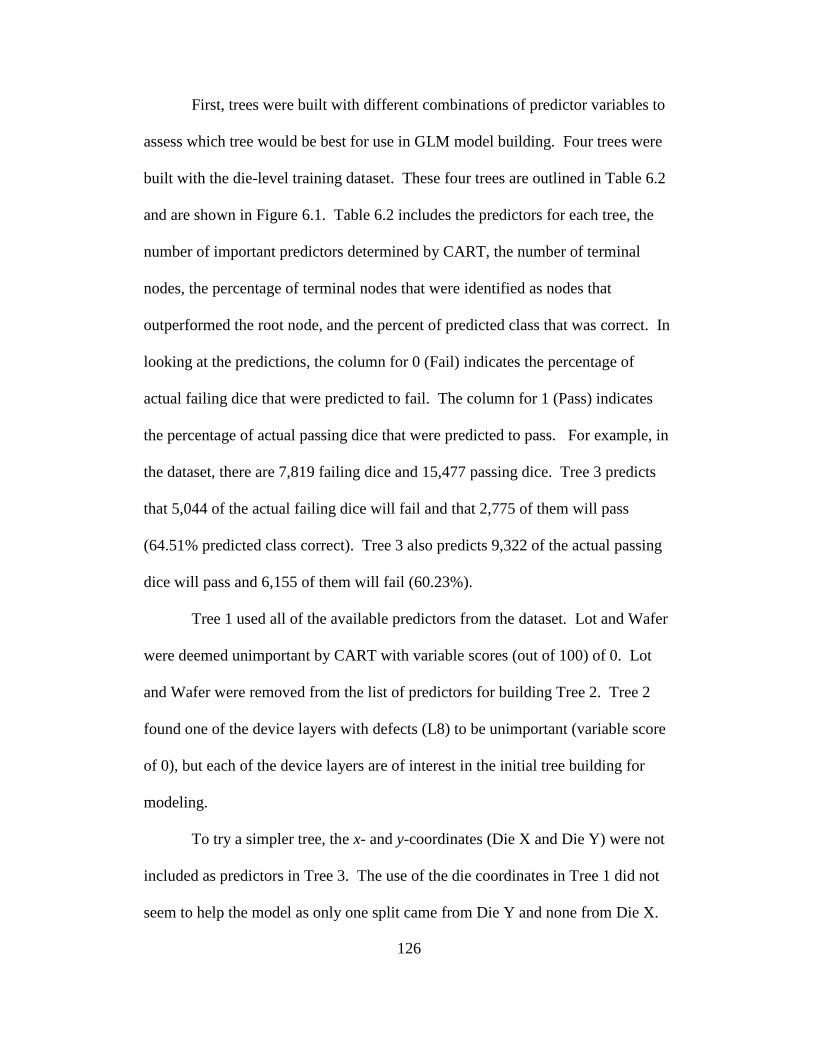
126
First, trees were built with different combinations of predictor variables to
assess which tree would be best for use in GLM model building. Four trees were
built with the die-level training dataset. These four trees are outlined in Table 6.2
and are shown in Figure 6.1. Table 6.2 includes the predictors for each tree, the
number of important predictors determined by CART, the number of terminal
nodes, the percentage of terminal nodes that were identified as nodes that
outperformed the root node, and the percent of predicted class that was correct. In
looking at the predictions, the column for 0 (Fail) indicates the percentage of
actual failing dice that were predicted to fail. The column for 1 (Pass) indicates
the percentage of actual passing dice that were predicted to pass. For example, in
the dataset, there are 7,819 failing dice and 15,477 passing dice. Tree 3 predicts
that 5,044 of the actual failing dice will fail and that 2,775 of them will pass
(64.51% predicted class correct). Tree 3 also predicts 9,322 of the actual passing
dice will pass and 6,155 of them will fail (60.23%).
Tree 1 used all of the available predictors from the dataset. Lot and Wafer
were deemed unimportant by CART with variable scores (out of 100) of 0. Lot
and Wafer were removed from the list of predictors for building Tree 2. Tree 2
found one of the device layers with defects (L8) to be unimportant (variable score
of 0), but each of the device layers are of interest in the initial tree building for
modeling.
To try a simpler tree, the x- and y-coordinates (Die X and Die Y) were not
included as predictors in Tree 3. The use of the die coordinates in Tree 1 did not
seem to help the model as only one split came from Die Y and none from Die X.
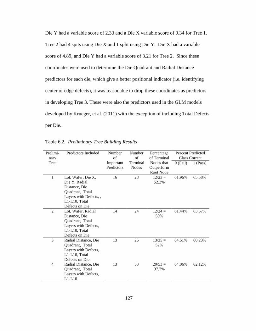
127
Die Y had a variable score of 2.33 and a Die X variable score of 0.34 for Tree 1.
Tree 2 had 4 spits using Die X and 1 split using Die Y. Die X had a variable
score of 4.89, and Die Y had a variable score of 3.21 for Tree 2. Since these
coordinates were used to determine the Die Quadrant and Radial Distance
predictors for each die, which give a better positional indicator (i.e. identifying
center or edge defects), it was reasonable to drop these coordinates as predictors
in developing Tree 3. These were also the predictors used in the GLM models
developed by Krueger, et al. (2011) with the exception of including Total Defects
per Die.
Table 6.2. Preliminary Tree Building Results
Prelimi-
nary
Tree
Predictors Included Number
of
Important
Predictors
Number
of
Terminal
Nodes
Percentage
of Terminal
Nodes that
Outperform
Root Node
Percent Predicted
Class Correct
0 (Fail) 1 (Pass)
1 Lot, Wafer, Die X,
Die Y, Radial
Distance, Die
Quadrant, Total
Layers with Defects, ,
L1-L10, Total
Defects on Die
16 23 12/23 =
52.2%
61.96% 65.58%
2 Lot, Wafer, Radial
Distance, Die
Quadrant, Total
Layers with Defects,
L1-L10, Total
Defects on Die
14 24 12/24 =
50%
61.44% 63.57%
3 Radial Distance, Die
Quadrant, Total
Layers with Defects,
L1-L10, Total
Defects on Die
13 25 13/25 =
52%
64.51% 60.23%
4 Radial Distance, Die
Quadrant, Total
Layers with Defects,
L1-L10
13 53 20/53 =
37.7%
64.06% 62.12%
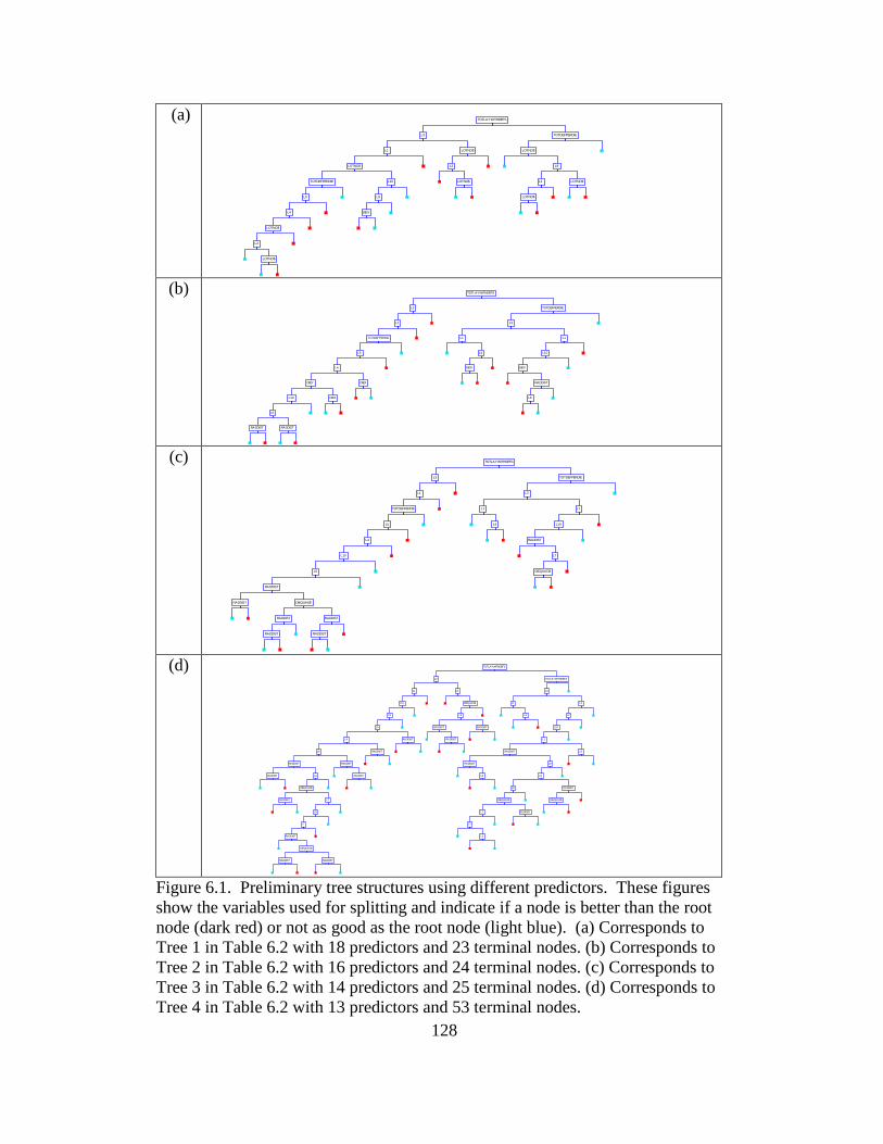
128
(a)
LOTNO$
L2
LOTNO$
L4
L5
TOTDEFPERDIE
DIEY
L9
L10
LOTNO$
L1
LOTNO$
L3
LOTNO$
L3
LOTNO$
L1
LOTNO$
L8
LOTNO$
TOTDEFPERDIE
TOTLAYWITHDEFS
(b)
RADDIST
RADDIST
L6
L10
DIEX
DIEY
DIEX
L4
L5
TOTDEFPERDIE
L1
L3
DIEX
L4
L1
L6
RADDIST
DIEX
L10
L1
L3
TOTDEFPERDIE
TOTLAYWITHDEFS
(c)
RADDIST
RADDIST
RADDIST
RADDIST
RADDIST
DIEQUAD$
RADDIST
L6
L10
L4
L5
TOTDEFPERDIE
L1
L3
L4
L1
DIEQUAD$
L7
RADDIST
L10
L1
L3
TOTDEFPERDIE
TOTLAYWITHDEFS
(d)
RADDIST
RADDIST
RADDIST
RADDIST
DIEQUAD$
RADDIST
L7
L8
L7
DIEQUAD$
L2
RADDIST
RADDIST
RADDIST
L6
RADDIST
L4
RADDIST
L5
L9
L10
L1
RADDIST
RADDIST
RADDIST
L3
DIEQUAD$
L3
L3
L4
L1
L9
RADDIST
L3
L7
L7
RADDIST
DIEQUAD$
L9
DIEQUAD$
RADDIST
L5
L6
RADDIST
L3
L1
L10
L2
L3
L3
TOTLAYWITHDEFS
TOTLAYWITHDEFS
Figure 6.1. Preliminary tree structures using different predictors. These figures
show the variables used for splitting and indicate if a node is better than the root
node (dark red) or not as good as the root node (light blue). (a) Corresponds to
Tree 1 in Table 6.2 with 18 predictors and 23 terminal nodes. (b) Corresponds to
Tree 2 in Table 6.2 with 16 predictors and 24 terminal nodes. (c) Corresponds to
Tree 3 in Table 6.2 with 14 predictors and 25 terminal nodes. (d) Corresponds to
Tree 4 in Table 6.2 with 13 predictors and 53 terminal nodes.

129
Tree 4, shown in Figure 6.1(d), used the same predictors as Tree 3, except
Total Defects per Die was removed as a predictor. This change had a strong
impact on the tree, creating 53 terminal nodes and a much more complex structure
than the other trees.
From these four trees, Tree 3 was chosen to be the best. This tree includes
the predictors used in Krueger, et al. (2011), plus the “Total Defects per Die”
count. The inclusion of “Total Defects per Die” simplifies the tree considerably
from what is seen in Tree 4. Also, of Trees 1 through 3, Tree 3 has the largest
number of nodes that are identified as being better than the root node with only a
small increase in the number of terminal nodes needed. The details of Tree 3 are
shown in Figure 6.2. The information displayed included the splitting values for
nodes, the tree structure, and the number of passing, failing, and total dice in each
terminal node. Each terminal node also includes a bar at the bottom that indicates
the proportion of passing dice in the node. In the bars, the royal blue (black)
portion is the proportion of passing dice, and the red (gray) portion is the
proportion of failing dice.
Creating Models
Once the appropriate tree has been selected, the information from the tree
can be used in developing a generalized linear model. This can be done in
different ways. When the goals of the study may include learning about certain
groups (such as high-yield or low-yield, high-risk or low-risk) to determine a
“recipe” for achieving or avoiding these outcomes, the terminal nodes from

130
CART are quite helpful. These terminal nodes can be used as indicator variables
that give information about important interactions for these groups that are then
included in the GLM. The use of indicator variables is well described in Chapter
8 of Montgomery, Peck, and Vining (2006). This approach can determine which
terminal nodes are statistically significant and help the user by providing a better
understanding of the important factors and interactions for those particular
groups.
Another approach is to use the CART-constructed tree to identify
important two-way interactions more quickly by looking at the splits and
implementing these interaction terms into the GLM model as predictors. This
can simplify model building if a large number of factors and interactions are part
of the dataset by letting the modeler avoid having to include all the interaction
terms and then reducing the model through backward elimination or other
techniques.
Reduced models, using the terminal nodes or the interaction terms from
the CART tree, can be developed to achieve parsimony using backward
elimination techniques. Using this approach, factors are eliminated one-by-one
from the model on the basis of their p-values, starting with the highest p-values,
and proceeding until all the factors in the model have the desired level of
significance. Forward selection and step-wise regression may also be used
(Montgomery, Peck, & Vining, 2006).
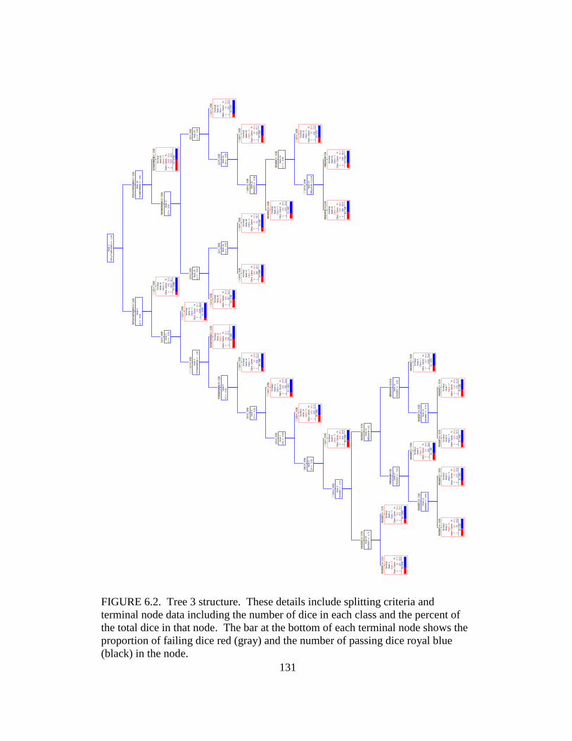
131
RA
DD
IST <
= 1
.71
Term
inal
Node 1
Cla
ss =
0
Cla
ss
Cases
%
066
37.5
1110
62.5
N =
176
RA
DD
IST >
1.7
1
Term
inal
Node 2
Cla
ss =
1
Cla
ss
Cases
%
0311
26.3
1871
73.7
N =
1182
RA
DD
IST <
= 4
.74
Node 1
0
RA
DD
IST <
= 1
.71
RA
DD
IST <
= 5
.52
Term
inal
Node 3
Cla
ss =
0
Cla
ss
Cases
%
050
39.1
178
60.9
N =
128
RA
DD
IST >
5.5
2
Term
inal
Node 4
Cla
ss =
1
Cla
ss
Cases
%
071
29.1
1173
70.9
N =
244
RA
DD
IST <
= 7
.04
Node 1
3
RA
DD
IST <
= 5
.52
RA
DD
IST >
7.0
4
Term
inal
Node 5
Cla
ss =
0
Cla
ss
Cases
%
0117
41.8
1163
58.2
N =
280
DIE
QU
AD
$ =
(2)
Node 1
2
RA
DD
IST <
= 7
.04
RA
DD
IST <
= 5
.74
Term
inal
Node 6
Cla
ss =
1
Cla
ss
Cases
%
0130
29.3
1314
70.7
N =
444
RA
DD
IST >
5.7
4
Term
inal
Node 7
Cla
ss =
0
Cla
ss
Cases
%
0110
38.6
1175
61.4
N =
285
RA
DD
IST <
= 6
.20
Node 1
5
RA
DD
IST <
= 5
.74
RA
DD
IST >
6.2
0
Term
inal
Node 8
Cla
ss =
1
Cla
ss
Cases
%
0477
29.2
11154
70.8
N =
1631
DIE
QU
AD
$ =
(1,3
,4)
Node 1
4
RA
DD
IST <
= 6
.20
RA
DD
IST >
4.7
4
Node 1
1
DIE
QU
AD
$ =
(2)
L6 <
= 0
.50
Node 9
RA
DD
IST <
= 4
.74
L6 >
0.5
0
Term
inal
Node 9
Cla
ss =
0
Cla
ss
Cases
%
0169
39.2
1262
60.8
N =
431
L10 <
= 0
.50
Node 8
L6 <
= 0
.50
L10 >
0.5
0
Term
inal
Node 1
0
Cla
ss =
0
Cla
ss
Cases
%
0360
38.1
1585
61.9
N =
945
L4 <
= 0
.50
Node 7
L10 <
= 0
.50
L4 >
0.5
0
Term
inal
Node 1
1
Cla
ss =
1
Cla
ss
Cases
%
0246
23.6
1795
76.4
N =
1041
L5 <
= 0
.50
Node 6
L4 <
= 0
.50
L5 >
0.5
0
Term
inal
Node 1
2
Cla
ss =
1
Cla
ss
Cases
%
092
18.8
1398
81.2
N =
490
TO
TD
EFPER
DIE
<= 1
.50
Node 5
L5 <
= 0
.50
TO
TD
EFPER
DIE
> 1.5
0
Term
inal
Node 1
3
Cla
ss =
0
Cla
ss
Cases
%
0404
42.1
1555
57.9
N =
959
L1 <
= 0
.50
Node 4
TO
TD
EFPER
DIE
<= 1
.50
L1 >
0.5
0
Term
inal
Node 1
4
Cla
ss =
1
Cla
ss
Cases
%
0204
15.7
11099
84.3
N =
1303
L3 <
= 0
.50
Node 3
L1 <
= 0
.50
L3 >
0.5
0
Term
inal
Node 1
5
Cla
ss =
1
Cla
ss
Cases
%
0896
19.9
13603
80.1
N =
4499
TO
TLA
YW
ITH
DEFS
<= 1
.50
Node 2
L3 <
= 0
.50
L1 <
= 0
.50
Term
inal
Node 1
6
Cla
ss =
0
Cla
ss
Cases
%
0809
45.8
1957
54.2
N =
1766
L4 <
= 0
.50
Term
inal
Node 1
7
Cla
ss =
0
Cla
ss
Cases
%
0190
35.3
1348
64.7
N =
538
L4 >
0.5
0
Term
inal
Node 1
8
Cla
ss =
1
Cla
ss
Cases
%
019
21.3
170
78.7
N =
89
L1 >
0.5
0
Node 1
9
L4 <
= 0
.50
L3 <
= 0
.50
Node 1
8
L1 <
= 0
.50
RA
DD
IST <
= 4
.36
Term
inal
Node 1
9
Cla
ss =
1
Cla
ss
Cases
%
0112
29.1
1273
70.9
N =
385
DIE
QU
AD
$ =
(1,2
,4)
Term
inal
Node 2
0
Cla
ss =
0
Cla
ss
Cases
%
0278
38.2
1450
61.8
N =
728
DIE
QU
AD
$ =
(3)
Term
inal
Node 2
1
Cla
ss =
1
Cla
ss
Cases
%
075
30.7
1169
69.3
N =
244
L7 <
= 0
.50
Node 2
4
DIE
QU
AD
$ =
(1,2
,4)
L7 >
0.5
0
Term
inal
Node 2
2
Cla
ss =
1
Cla
ss
Cases
%
079
29.0
1193
71.0
N =
272
RA
DD
IST >
4.3
6
Node 2
3
L7 <
= 0
.50
L10 <
= 0
.50
Node 2
2
RA
DD
IST <
= 4
.36
L10 >
0.5
0
Term
inal
Node 2
3
Cla
ss =
0
Cla
ss
Cases
%
099
42.3
1135
57.7
N =
234
L1 <
= 0
.50
Node 2
1
L10 <
= 0
.50
L1 >
0.5
0
Term
inal
Node 2
4
Cla
ss =
1
Cla
ss
Cases
%
063
23.1
1210
76.9
N =
273
L3 >
0.5
0
Node 2
0
L1 <
= 0
.50
TO
TD
EFPER
DIE
<= 2
.50
Node 1
7
L3 <
= 0
.50
TO
TD
EFPER
DIE
> 2.5
0
Term
inal
Node 2
5
Cla
ss =
0
Cla
ss
Cases
%
02392
50.6
12337
49.4
N =
4729
TO
TLA
YW
ITH
DEFS
> 1.5
0
Node 1
6
TO
TD
EFPER
DIE
<= 2
.50
Node 1
TO
TLA
YW
ITH
DEFS
<= 1
.50
FIGURE 6.2. Tree 3 structure. These details include splitting criteria and
terminal node data including the number of dice in each class and the percent of
the total dice in that node. The bar at the bottom of each terminal node shows the
proportion of failing dice red (gray) and the number of passing dice royal blue
(black) in the node.
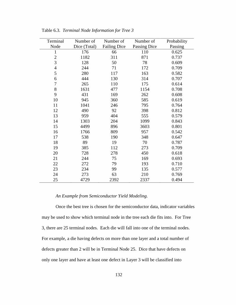
132
Table 6.3. Terminal Node Information for Tree 3
Terminal
Node
Number of
Dice (Total)
Number of
Failing Dice
Number of
Passing Dice
Probability
Passing
1 176 66 110 0.625
2 1182 311 871 0.737
3 128 50 78 0.609
4 244 71 172 0.709
5 280 117 163 0.582
6 444 130 314 0.707
7 265 110 175 0.614
8 1631 477 1154 0.708
9 431 169 262 0.608
10 945 360 585 0.619
11 1041 246 795 0.764
12 490 92 398 0.812
13 959 404 555 0.579
14 1303 204 1099 0.843
15 4499 896 3603 0.801
16 1766 809 957 0.542
17 538 190 348 0.647
18 89 19 70 0.787
19 385 112 273 0.709
20 728 278 450 0.618
21 244 75 169 0.693
22 272 79 193 0.710
23 234 99 135 0.577
24 273 63 210 0.769
25 4729 2392 2337 0.494
An Example from Semiconductor Yield Modeling.
Once the best tree is chosen for the semiconductor data, indicator variables
may be used to show which terminal node in the tree each die fits into. For Tree
3, there are 25 terminal nodes. Each die will fall into one of the terminal nodes.
For example, a die having defects on more than one layer and a total number of
defects greater than 2 will be in Terminal Node 25. Dice that have defects on
only one layer and have at least one defect in Layer 3 will be classified into

133
Terminal Node 15. Indicator variables can be quickly constructed in Excel by
using the splitting criteria and “If” statements to give values of “1” for the
terminal node a row of data falls into and a value of “0” for all other terminal
nodes. For 25 terminal nodes, 24 indicator variables are used for a full model.
GLM models can be constructed by adding these indicator variables as
predictors in the model. Several models were constructed using SAS 9.2 and
PROC GLIMMIX (see Appendix A for SAS code) to compare various
approaches. These GLM models included full and reduced logit models with only
the main effects used as predictors, full and reduced models using the main effects
and the terminal node indicator variables as predictors, full and reduced models
using the main effects and the terminal nodes identified by CART as
outperforming the root node (red nodes) as predictors, a reduced model from
using the main effects and the interactions identified in the CART tree for the
predictors, and a reduced model using the main effects and all two-way
interactions in the model as predictors. The terms used in these models are shown
in more detail in Table 6.4.
The models constructed using only the main effects are similar to those
described in Chapter 4 but are built using this larger dataset. The models built
with the terminal nodes develop a model that is adjusted by the coefficient for the
terminal node a row of data falls into, giving the resulting models a form that
resembles having different intercepts for a line. The significant terminal nodes
can be determined by reducing the model through backward selection or another
method.

134
CART also provides information that describes each terminal node as
being a better or worse classifier than the root node. (Recall this percentage was
used to help select the best tree in Table 6.2.) Nodes that outperform the root
node are marked in different shades of red on the resulting tree while nodes that
do not outperform the root node are marked in blue. These selected terminal
nodes may also be of interest in model building, and reduced models can again be
formed from these predictors. All of the models described to this point were
reduced through backward elimination using the t-test values and a level of
significance of =0.1 since the F-test and t-test p-values are the same for the
GLM with only the main effects, and the models with terminal nodes included did
not produce F-values.
While the use of terminal nodes themselves give an increased
understanding into significant groupings and interactions that pertain to them,
more general modeling can be done with the interaction terms from the CART
tree. By following the various branches of the tree, different interaction terms can
be quickly identified. For example, Figure 6.3 shows L1 branching off an L3
node in two places, indicating a possibly significant interaction between these two
factors. This branching occurs near the root node, suggesting this interaction term
(L1*L3) may be one of the strongest for these data. Including this interaction
term in the GLM model can confirm this through the t-test and F-test results.
Another example of finding possible interactions from the CART tree is shown in
Figure 6.4, which shows in more detail the bottom, left-hand side of the tree and
the relevant interactions. This figure shows interactions L5* L4, L4* L10,
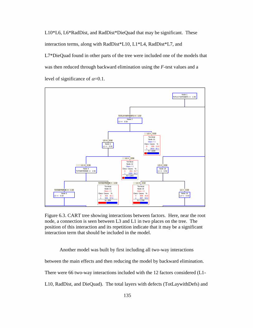
135
L10*L6, L6*RadDist, and RadDist*DieQuad that may be significant. These
interaction terms, along with RadDist*L10, L1*L4, RadDist*L7, and
L7*DieQuad found in other parts of the tree were included one of the models that
was then reduced through backward elimination using the F-test values and a
level of significance of =0.1.
Figure 6.3. CART tree showing interactions between factors. Here, near the root
node, a connection is seen between L3 and L1 in two places on the tree. The
position of this interaction and its repetition indicate that it may be a significant
interaction term that should be included in the model.
Another model was built by first including all two-way interactions
between the main effects and then reducing the model by backward elimination.
There were 66 two-way interactions included with the 12 factors considered (L1-
L10, RadDist, and DieQuad). The total layers with defects (TotLaywithDefs) and
RADDIST <= 1.71
Terminal
Node 1
Class = 0
Class Cases %
0 66 37.5
1 110 62.5
N = 176
RADDIST > 1.71
Terminal
Node 2
Class = 1
Class Cases %
0 311 26.3
1 871 73.7
N = 1182
RADDIST <= 4.74
Node 10
RADDIST <= 1.71
RADDIST <= 5.52
Terminal
Node 3
Class = 0
Class Cases %
0 50 39.1
1 78 60.9
N = 128
RADDIST > 5.52
Terminal
Node 4
Class = 1
Class Cases %
0 71 29.1
1 173 70.9
N = 244
RADDIST <= 7.04
Node 13
RADDIST <= 5.52
RADDIST > 7.04
Terminal
Node 5
Class = 0
Class Cases %
0 117 41.8
1 163 58.2
N = 280
DIEQUAD$ = (2)
Node 12
RADDIST <= 7.04
RADDIST <= 5.74
Terminal
Node 6
Class = 1
Class Cases %
0 130 29.3
1 314 70.7
N = 444
RADDIST > 5.74
Terminal
Node 7
Class = 0
Class Cases %
0 110 38.6
1 175 61.4
N = 285
RADDIST <= 6.20
Node 15
RADDIST <= 5.74
RADDIST > 6.20
Terminal
Node 8
Class = 1
Class Cases %
0 477 29.2
1 1154 70.8
N = 1631
DIEQUAD$ = (1,3,4)
Node 14
RADDIST <= 6.20
RADDIST > 4.74
Node 11
DIEQUAD$ = (2)
L6 <= 0.50
Node 9
RADDIST <= 4.74
L6 > 0.50
Terminal
Node 9
Class = 0
Class Cases %
0 169 39.2
1 262 60.8
N = 431
L10 <= 0.50
Node 8
L6 <= 0.50
L10 > 0.50
Terminal
Node 10
Class = 0
Class Cases %
0 360 38.1
1 585 61.9
N = 945
L4 <= 0.50
Node 7
L10 <= 0.50
L4 > 0.50
Terminal
Node 11
Class = 1
Class Cases %
0 246 23.6
1 795 76.4
N = 1041
L5 <= 0.50
Node 6
L4 <= 0.50
L5 > 0.50
Terminal
Node 12
Class = 1
Class Cases %
0 92 18.8
1 398 81.2
N = 490
TOTDEFPERDIE <= 1.50
Node 5
L5 <= 0.50
TOTDEFPERDIE > 1.50
Terminal
Node 13
Class = 0
Class Cases %
0 404 42.1
1 555 57.9
N = 959
L1 <= 0.50
Node 4
TOTDEFPERDIE <= 1.50
L1 > 0.50
Terminal
Node 14
Class = 1
Class Cases %
0 204 15.7
1 1099 84.3
N = 1303
L3 <= 0.50
Node 3
L1 <= 0.50
L3 > 0.50
Terminal
Node 15
Class = 1
Class Cases %
0 896 19.9
1 3603 80.1
N = 4499
TOTLAYWITHDEFS <= 1.50
Node 2
L3 <= 0.50
L1 <= 0.50
Terminal
Node 16
Class = 0
Class Cases %
0 809 45.8
1 957 54.2
N = 1766
L4 <= 0.50
Terminal
Node 17
Class = 0
Class Cases %
0 190 35.3
1 348 64.7
N = 538
L4 > 0.50
Terminal
Node 18
Class = 1
Class Cases %
0 19 21.3
1 70 78.7
N = 89
L1 > 0.50
Node 19
L4 <= 0.50
L3 <= 0.50
Node 18
L1 <= 0.50
RADDIST <= 4.36
Terminal
Node 19
Class = 1
Class Cases %
0 112 29.1
1 273 70.9
N = 385
DIEQUAD$ = (1,2,4)
Terminal
Node 20
Class = 0
Class Cases %
0 278 38.2
1 450 61.8
N = 728
DIEQUAD$ = (3)
Terminal
Node 21
Class = 1
Class Cases %
0 75 30.7
1 169 69.3
N = 244
L7 <= 0.50
Node 24
DIEQUAD$ = (1,2,4)
L7 > 0.50
Terminal
Node 22
Class = 1
Class Cases %
0 79 29.0
1 193 71.0
N = 272
RADDIST > 4.36
Node 23
L7 <= 0.50
L10 <= 0.50
Node 22
RADDIST <= 4.36
L10 > 0.50
Terminal
Node 23
Class = 0
Class Cases %
0 99 42.3
1 135 57.7
N = 234
L1 <= 0.50
Node 21
L10 <= 0.50
L1 > 0.50
Terminal
Node 24
Class = 1
Class Cases %
0 63 23.1
1 210 76.9
N = 273
L3 > 0.50
Node 20
L1 <= 0.50
TOTDEFPERDIE <= 2.50
Node 17
L3 <= 0.50
TOTDEFPERDIE > 2.50
Terminal
Node 25
Class = 0
Class Cases %
0 2392 50.6
1 2337 49.4
N = 4729
TOTLAYWITHDEFS > 1.50
Node 16
TOTDEFPERDIE <= 2.50
Node 1
TOTLAYWITHDEFS <= 1.50
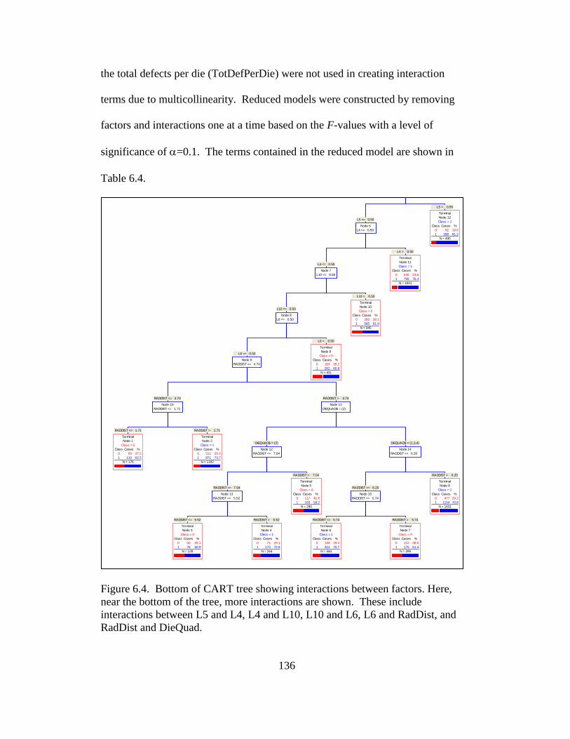
136
the total defects per die (TotDefPerDie) were not used in creating interaction
terms due to multicollinearity. Reduced models were constructed by removing
factors and interactions one at a time based on the F-values with a level of
significance of =0.1. The terms contained in the reduced model are shown in
Table 6.4.
Figure 6.4. Bottom of CART tree showing interactions between factors. Here,
near the bottom of the tree, more interactions are shown. These include
interactions between L5 and L4, L4 and L10, L10 and L6, L6 and RadDist, and
RadDist and DieQuad.
RADDIST <= 1.71
Terminal
Node 1
Class = 0
Class Cases %
0 66 37.5
1 110 62.5
N = 176
RADDIST > 1.71
Terminal
Node 2
Class = 1
Class Cases %
0 311 26.3
1 871 73.7
N = 1182
RADDIST <= 4.74
Node 10
RADDIST <= 1.71
RADDIST <= 5.52
Terminal
Node 3
Class = 0
Class Cases %
0 50 39.1
1 78 60.9
N = 128
RADDIST > 5.52
Terminal
Node 4
Class = 1
Class Cases %
0 71 29.1
1 173 70.9
N = 244
RADDIST <= 7.04
Node 13
RADDIST <= 5.52
RADDIST > 7.04
Terminal
Node 5
Class = 0
Class Cases %
0 117 41.8
1 163 58.2
N = 280
DIEQUAD$ = (2)
Node 12
RADDIST <= 7.04
RADDIST <= 5.74
Terminal
Node 6
Class = 1
Class Cases %
0 130 29.3
1 314 70.7
N = 444
RADDIST > 5.74
Terminal
Node 7
Class = 0
Class Cases %
0 110 38.6
1 175 61.4
N = 285
RADDIST <= 6.20
Node 15
RADDIST <= 5.74
RADDIST > 6.20
Terminal
Node 8
Class = 1
Class Cases %
0 477 29.2
1 1154 70.8
N = 1631
DIEQUAD$ = (1,3,4)
Node 14
RADDIST <= 6.20
RADDIST > 4.74
Node 11
DIEQUAD$ = (2)
L6 <= 0.50
Node 9
RADDIST <= 4.74
L6 > 0.50
Terminal
Node 9
Class = 0
Class Cases %
0 169 39.2
1 262 60.8
N = 431
L10 <= 0.50
Node 8
L6 <= 0.50
L10 > 0.50
Terminal
Node 10
Class = 0
Class Cases %
0 360 38.1
1 585 61.9
N = 945
L4 <= 0.50
Node 7
L10 <= 0.50
L4 > 0.50
Terminal
Node 11
Class = 1
Class Cases %
0 246 23.6
1 795 76.4
N = 1041
L5 <= 0.50
Node 6
L4 <= 0.50
L5 > 0.50
Terminal
Node 12
Class = 1
Class Cases %
0 92 18.8
1 398 81.2
N = 490
TOTDEFPERDIE <= 1.50
Node 5
L5 <= 0.50
TOTDEFPERDIE > 1.50
Terminal
Node 13
Class = 0
Class Cases %
0 404 42.1
1 555 57.9
N = 959
L1 <= 0.50
Node 4
TOTDEFPERDIE <= 1.50
L1 > 0.50
Terminal
Node 14
Class = 1
Class Cases %
0 204 15.7
1 1099 84.3
N = 1303
L3 <= 0.50
Node 3
L1 <= 0.50
L3 > 0.50
Terminal
Node 15
Class = 1
Class Cases %
0 896 19.9
1 3603 80.1
N = 4499
TOTLAYWITHDEFS <= 1.50
Node 2
L3 <= 0.50
L1 <= 0.50
Terminal
Node 16
Class = 0
Class Cases %
0 809 45.8
1 957 54.2
N = 1766
L4 <= 0.50
Terminal
Node 17
Class = 0
Class Cases %
0 190 35.3
1 348 64.7
N = 538
L4 > 0.50
Terminal
Node 18
Class = 1
Class Cases %
0 19 21.3
1 70 78.7
N = 89
L1 > 0.50
Node 19
L4 <= 0.50
L3 <= 0.50
Node 18
L1 <= 0.50
RADDIST <= 4.36
Terminal
Node 19
Class = 1
Class Cases %
0 112 29.1
1 273 70.9
N = 385
DIEQUAD$ = (1,2,4)
Terminal
Node 20
Class = 0
Class Cases %
0 278 38.2
1 450 61.8
N = 728
DIEQUAD$ = (3)
Terminal
Node 21
Class = 1
Class Cases %
0 75 30.7
1 169 69.3
N = 244
L7 <= 0.50
Node 24
DIEQUAD$ = (1,2,4)
L7 > 0.50
Terminal
Node 22
Class = 1
Class Cases %
0 79 29.0
1 193 71.0
N = 272
RADDIST > 4.36
Node 23
L7 <= 0.50
L10 <= 0.50
Node 22
RADDIST <= 4.36
L10 > 0.50
Terminal
Node 23
Class = 0
Class Cases %
0 99 42.3
1 135 57.7
N = 234
L1 <= 0.50
Node 21
L10 <= 0.50
L1 > 0.50
Terminal
Node 24
Class = 1
Class Cases %
0 63 23.1
1 210 76.9
N = 273
L3 > 0.50
Node 20
L1 <= 0.50
TOTDEFPERDIE <= 2.50
Node 17
L3 <= 0.50
TOTDEFPERDIE > 2.50
Terminal
Node 25
Class = 0
Class Cases %
0 2392 50.6
1 2337 49.4
N = 4729
TOTLAYWITHDEFS > 1.50
Node 16
TOTDEFPERDIE <= 2.50
Node 1
TOTLAYWITHDEFS <= 1.50
137
All of the models were built using the logit link in PROC GLIMMIX. Though
PROC GLIMMIX is designed to analyze GLMMs, if no random effects are
specified, SAS runs in GLM mode and provides the same analysis as PROC
GENMOD.
Results
Table 6.4 displays the model coefficients and p-values for significant
factors and interactions obtained from the t-tests for the different models using a
level of significance of 0.1. There are some interesting differences between the
models. In considering the reduced models, the models with only the main effects
or the main effects with the terminal nodes from CART included eliminate Layer
1 as significant while the models containing interaction terms retain Layer 1. The
reduced models using the CART terminal nodes eliminate radial distance as a
significant predictor, suggesting that this location parameter is important only in
connection with the other variables as described through the terminal node
recipes. Radial distance is included as a splitting factor in terminal nodes 1-8 and
19-22, several of which are included in the reduced models containing terminal
nodes. The reduced model from including all the possible two-way interactions
deems Layer 8 as insignificant, but interactions between Layers 8 and Layer 1,
Layer 2, and Radial Distance are significant in the model. The reduced model
using interactions taken from the CART tree indicated 11 interactions to be
significant, matching with 11 of the 21 identified through backward elimination
from the model that examined all two-way interactions.
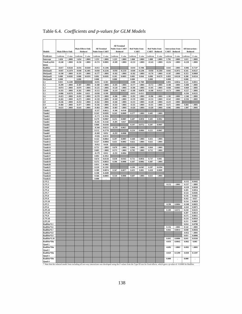
138
Table 6.4. Coefficients and p-values for GLM Models
Models Predictors Coefficient P-value Coefficient P-value Coefficient P-value Coefficient P-value Coefficient P-value Coefficient P-value Coefficient P-value Coefficient P-value Intercept 1.656 <.0001 1.654 <.0001 1.253 <.0001 1.225 <.0001 1.068 <.0001 1.008 <.0001 1.781 <.0001 1.611 <.0001 TotalLayWit hDefs
-0.248 <.0001 -0.236 <.0001 -0.174 0.0001 -0.189 <.0001 -0.133 <.0001 -0.143 <.0001 -0.234 <.0001 -0.228 <.0001
RadDist -0.017 0.0244 -0.016 0.0269 -0.013 0.1206 -0.010 0.1986 -0.043 <.0001 -0.006 0.714* DieQuad1 -0.047 0.2479 -0.048 0.2401 -0.050 0.2236 -0.050 0.2218 -0.049 0.2296 -0.050 0.2284 -0.043 0.2972 0.341 0.0127 DieQuad2 -0.190 <.0001 -0.191 <.0001 -0.177 <.0001 -0.182 <.0001 -0.182 <.0001 -0.176 <.0001 -0.187 <.0001 0.353 0.0069 DieQuad3 0.089 0.0283 0.088 0.0293 0.091 0.0285 0.105 0.0093 0.083 0.044 0.090 0.0279 0.093 0.0218 0.280 0.0214 DieQuad4 0.000 . 0.000 . 0.000 . 0.000 . 0.000 . 0.000 . 0.000 . 0.000 . L1 0.035 0.2289 -0.035 0.303 -0.008 0.7989 0.093 0.0054 0.121 0.0011 L2 -0.299 <.0001 -0.307 <.0001 -0.180 <.0001 -0.185 <.0001 -0.177 <.0001 -0.172 <.0001 -0.306 <.0001 -0.408 <.0001 L3 -0.074 <.0001 -0.079 <.0001 -0.125 <.0001 -0.128 <.0001 -0.106 <.0001 -0.105 <.0001 -0.060 0.0003 -0.069 <.0001 L4 -0.193 <.0001 -0.202 <.0001 -0.113 0.009 -0.119 0.0027 -0.108 0.0078 -0.100 0.0113 -0.174 <.0001 -0.227 <.0001 L5 -0.086 0.0376 -0.094 0.021 -0.038 0.399 -0.033 0.4513 -0.294 0.0225 L6 -0.423 <.0001 -0.431 <.0001 -0.278 <.0001 -0.286 <.0001 -0.291 <.0001 -0.286 <.0001 -1.302 <.0001 -1.346 <.0001 L7 -0.265 <.0001 -0.273 <.0001 -0.159 <.0001 -0.169 <.0001 -0.159 <.0001 -0.155 <.0001 -0.545 <.0001 -0.594 <.0001 L8 -0.246 <.0001 -0.251 <.0001 -0.162 <.0001 -0.166 <.0001 -0.155 <.0001 -0.149 <.0001 -0.255 <.0001 L9 -0.468 <.0001 -0.477 <.0001 -0.336 <.0001 -0.343 <.0001 -0.335 <.0001 -0.331 <.0001 -0.472 <.0001 -0.881 <.0001 L10 -0.633 <.0001 -0.643 <.0001 -0.464 <.0001 -0.483 <.0001 -0.426 <.0001 -0.420 <.0001 -0.902 <.0001 -1.007 <.0001 Tnode1 -0.337 0.0651 -0.306 0.0549 Tnode2 0.243 0.0281 0.245 0.0009 0.377 <.0001 0.405 <.0001 Tnode3 -0.173 0.3926 Tnode4 0.279 0.0967 0.251 0.0887 0.407 0.0058 0.403 0.0062 Tnode5 -0.241 0.1142 -0.285 0.027 Tnode6 0.068 0.6184 0.197 0.0752 0.207 0.0607 Tnode7 -0.344 0.0215 -0.378 0.0027 Tnode8 0.112 0.2778 0.234 0.0004 0.221 0.0007 Tnode9 -0.269 0.051 -0.293 0.0088 Tnode10 -0.026 0.8232 Tnode11 0.322 0.0063 0.297 0.0007 0.448 <.0001 0.451 <.0001 Tnode12 0.527 0.0004 0.451 0.0002 0.652 <.0001 0.625 <.0001 Tnode13 -0.052 0.626 Tnode14 0.751 <.0001 0.670 <.0001 0.846 <.0001 0.844 <.0001 Tnode15 0.605 <.0001 0.573 <.0001 0.705 <.0001 0.712 <.0001 Tnode16 -0.179 0.011 -0.191 0.0004 Tnode17 0.092 0.3952 Tnode18 0.674 0.0118 0.630 0.0165 0.731 0.0056 0.737 0.005 Tnode19 0.372 0.0033 0.396 0.0006 0.447 0.0002 0.487 <.0001 Tnode20 0.051 0.5882 Tnode21 0.229 0.1291 0.299 0.0387 0.297 0.0394 Tnode22 0.389 0.0074 0.367 0.0077 0.455 0.001 0.458 0.0009 Tnode23 0.108 0.4589 Tnode24 0.566 0.0003 0.510 0.0006 0.607 <.0001 0.615 <.0001 Tnode25 0.000 . L1*L2 -0.152 0.0442 L1*L3 -0.132 <.0001 -0.137 <.0001 L1*L8 -0.229 0.0038 L2*L4 0.205 0.0054 L2*L7 0.124 0.0585 L2*L8 0.156 0.0465 L2*L9 0.162 0.027 L2*L10 0.154 0.0829 L4*L5 -0.390 0.0004 -0.348 0.0025 L4*L6 -0.263 0.0875 L4*L10 0.189 0.0372 0.210 0.0225 L5*L10 0.207 0.0614 L7*L9 0.175 0.0011 L7*L10 0.124 0.0934 L9*L10 0.211 0.0087 RadDist*L5 0.034 0.0798 RadDist*L6 0.136 <.0001 0.142 <.0001 RadDist*L7 0.042 0.0014 0.040 0.0026 RadDist*L8 -0.052 <.0001 RadDist*L9 0.051 0.0006 RadDist*L10 0.045 0.0086 0.041 0.0184 RadDist*Die Quad 1
-0.059 0.0045 -0.062 0.003
RadDist*Die Quad 2
-0.092 <.0001 -0.092 <.0001
RadDist*Die Quad 3
-0.029 0.1299 -0.030 0.1297
RadDist*Die Quad 4
0.000 . 0.000 .
* Note that the reduced model from including all two-way interactions was developed using the F-values from the Type III test for fixed effects, which gave a p-value of <0.0000 for RadDist.
Main Effects Only Main Effects Only
- Reduced All Terminal
Nodes from CART
All Terminal Nodes from CART
- Reduced Red Nodes from
CART Red Nodes from CART - Reduced
Interactions from CART - Reduced
All Interactions - Reduced

139
Validation
The models were tested for validity by using a test set of data consisting of
11,445 dice with defects from 84 wafers. No outliers were removed from the test
dataset. The model coefficients were used to determine prediction probabilities
for each die. These predicted values were compared to the actual pass or fail
outcomes, and measures of mean absolute deviation (MAD) and mean squared
error (MSE) were calculated. The MAD and MSE values were also calculated at
the wafer level by summing the expected probabilities for each wafer and
comparing that value to the actual number of passing dice on the wafer in the test
dataset. The charts showing the MAD and MSE values for each of the models
used is shown for the die level in Figure 6.5, and the MAD and MSE values for
each model at the wafer level is presented in Figure 6.6.
The MAD and MSE values for the die level in Figure 6.5 show that the
differences between the models’ predictive powers are very small. Also, recall
from Chapter 4 that the main effects GLM model outperformed the existing
semiconductor yield models significantly. Figure 4.6 compared the die-level
MAD and MSE of GLM models against historical yield models, showing the die-
level full nested, reduced nested, and full non-nested GLMs to have nearly the
same amount of error from the actual results. (Note that the full, non-nested logit
GLM shown in Figure 4.6 is the same as the model referred to as “Main Effects
Only” in this study.) Figure 4.10 showed the wafer-level comparisons, with the
die-level nested reduced GLM having the least amount of error. Figure 6.6 shows
the wafer-level comparisons for the models from this study, furthering the work

140
of Chapter 4. At the die-level, all of the models in this study have nearly the same
predictive power, with the best model in terms of MAD being the model
containing only the main effect with a value of 0.3995. The worst MAD value
was from the model that included the interactions taken from examining the
CART tree and using them as predictors in the model, giving a value of 0.4240.
One result to note here is that the use of the terminal nodes, either all of the
terminal nodes or only those shown by CART to be better than the root node, with
the main effects as predictors in the model outperformed the predictive ability of
CART alone. This is true for the MSE values as well as the MAD values. The
best MSE value came from the model that included all the two-way interactions
and was then reduced (MSE=0.2048), but was followed closely by the main
effects only reduced model, the main effects plus terminal nodes reduced model,
and the main effects plus CART-selected terminal nodes full and reduced models,
all with MSE=0.2049. The MSE values give more weight to larger errors because
the values are squared, suggesting that the models with lower MSE values are
closer to the predicted values more often.
As Figures 6.5 and 6.6 show, adding the terminal nodes from CART does
not improve the predictive strength of the model, though this addition does not
significantly diminish the predictive strength either. The advantage of including
these terminal nodes lies in being able to determine which nodes are significant
and can be most helpful in process improvement efforts. With CART able to
produce many nodes in an optimal tree (i.e. Tree 4 in Figure 6.1), this can be of
great value to practitioners.
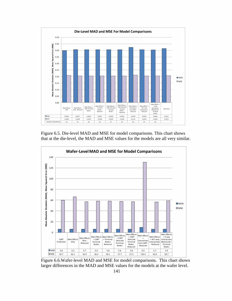
141
Main Effects Only
Main Effects Only - Reduced
Main Effects + CART Terminal
Nodes
Main Effects + Terminal
Nodes-Reduced
Main Effects + CART Selected
Terminal Nodes
Main Effects + CART Selected
Terminal Nodes -Reduced
Main Effects + Interactions
from CART -Reduced
Main Effects + All 2-way
Interactions -Reduced
Main Effects + 2-way
Interactions (Reduced) +
Terminal
Nodes
CART Only
MAD 0.3995 0.4077 0.4056 0.4057 0.4058 0.4059 0.4240 0.4063 0.4044 0.4147
MSE 0.2090 0.2049 0.2050 0.2049 0.2049 0.2049 0.2110 0.2050 0.2048 0.2079
Number of Parameters 14 13 38 26 27 24 20 35 59
0.00
0.05
0.10
0.15
0.20
0.25
0.30
0.35
0.40
0.45
0.50
Me
an A
bso
lute
De
viat
ion
(M
AD
), M
ean
Sq
uar
ed
Err
or
(MSE
)
Die-Level MAD and MSE For Model Comparisons
MAD
MSE
Figure 6.5. Die-level MAD and MSE for model comparisons. This chart shows
that at the die-level, the MAD and MSE values for the models are all very similar.
CART Prediction
Main Effects Only
Main Effects Only -
Reduced
Main Effects + CART
Terminal Nodes
Main Effects + Terminal
Nodes-Reduced
Main Effects + CART
Selected Terminal
Nodes
Main Effects + CART
Selected Terminal Nodes -
Reduced
Main Effects +
Interactions from CART -
Reduced
Main Effects + All 2-way
Interactions - Reduced
Main Effects + 2-way
Interactions (Reduced) +
Terminal Nodes
MAD 5.8 6.2 5.7 5.9 5.8 5.8 5.8 9.5 5.7 5.9
MSE 59.7 66.1 56.9 58.4 58.1 57.7 57.5 130.4 56.8 58.7
0
20
40
60
80
100
120
140
Me
an A
bso
lute
De
viat
ion
(M
AD
), M
ean
Sq
uar
ed
Err
or
(MSE
)
Wafer-Level MAD and MSE for Model Comparisons
MAD
MSE
Figure 6.6.Wafer-level MAD and MSE for model comparisons. This chart shows
larger differences in the MAD and MSE values for the models at the wafer level.
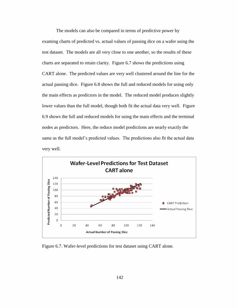
142
The models can also be compared in terms of predictive power by
examing charts of predicted vs. actual values of passing dice on a wafer using the
test dataset. The models are all very close to one another, so the results of these
charts are separated to retain clarity. Figure 6.7 shows the predictions using
CART alone. The predicted values are very well clustered around the line for the
actual passing dice. Figure 6.8 shows the full and reduced models for using only
the main effects as predictors in the model. The reduced model produces slightly
lower values than the full model, though both fit the actual data very well. Figure
6.9 shows the full and reduced models for using the main effects and the terminal
nodes as predictors. Here, the reduce model predictions are nearly exactly the
same as the full model’s predicted values. The predictions also fit the actual data
very well.
Figure 6.7. Wafer-level predictions for test dataset using CART alone.

143
Figure 6.8. Wafer-level predictions for test dataset – Main effects only. This
shows the preadicted values from using GLM full and reduced models with only
the main effects as predictors.
Figure 6.9. Wafer-level predictions for test dataset – Main effects plus CART
terminal nodes. This shows the predicted values from using GLM full and
reduced models with the main effects and the terminal nodes from CART as
predictors.

144
Figure 6.10 displays the predictive power of the models containing the
main effects plus the terminal nodes that CART identified as being better than the
root node. Again, the reduced model points are centered on the full model points
with both fittin the data well. Figure 6.11 shows the model that contains the main
effects plus the interactions taken from the CART tree as predictors. This model
consistently underestimates the actual yield of the wafer. It appears that it may be
a better predictor for low-yield wafers (<70 wafers passing) than the other
models, but at higher yields, this is the worst-performing model. The full and
reduced models that included the main effects plus the two-way interactions is
shown in Figure 6.12. Here again, the reduced model predictions are nearly the
same as the full model, and there is no significant visual difference between these
models and those in Figures 6.9 and 6.10. All of the models show strong
predictive power with the exception of the models shown in Figure 6.11.
Figure 6.10. Wafer-level predictions for test dataset – Main effects plus CART-
selected terminal nodes. This shows the preadicted values from using GLM full
and reduced models with the main effects and the terminal nodes (selected by
CART as being better than the root node) as predictors.
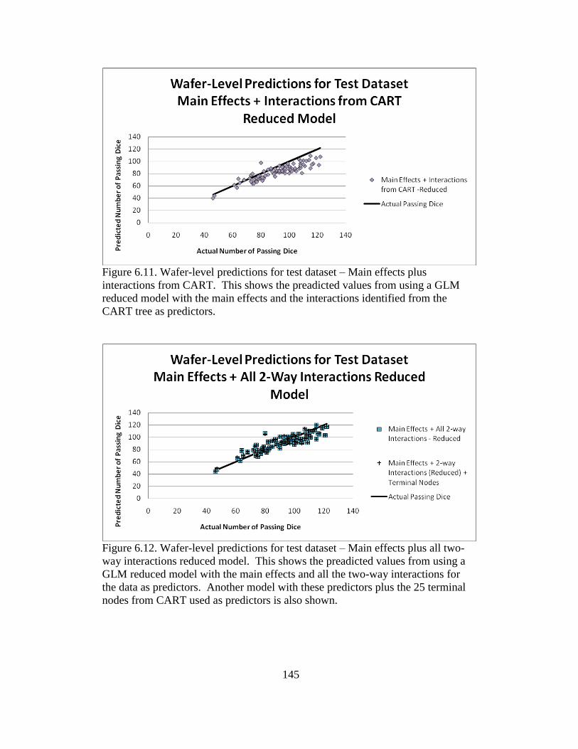
145
Figure 6.11. Wafer-level predictions for test dataset – Main effects plus
interactions from CART. This shows the preadicted values from using a GLM
reduced model with the main effects and the interactions identified from the
CART tree as predictors.
Figure 6.12. Wafer-level predictions for test dataset – Main effects plus all two-
way interactions reduced model. This shows the preadicted values from using a
GLM reduced model with the main effects and all the two-way interactions for
the data as predictors. Another model with these predictors plus the 25 terminal
nodes from CART used as predictors is also shown.

146
Terminal Nodes and Interactions
The reduced model that contained the main effects and the terminal node
indicator variables from CART included 15 of the terminal nodes as statistically
significant (=0.1). Terminal nodes 1, 2, 4, 5, 7, 9, 11, 12, 14, 15, 16, 18, 19, 22,
and 24 were included in the reduced model. These terminal nodes, their recipes,
and the percent of passing dice that fall into the nodes in both the training and the
test datasets are shown in Tables 6.5 and 6.6. Recall the main effects of radial
distance and the defect counts of Layer 1 and Layer 5 were eliminated from the
reduced model due to lack of significance. This indicates that the contribution of
these factors may be well accounted for by the interactions contained in the
terminal nodes. Indeed, Layer 1 occurs as part of the recipe in 14 of the 15
terminal nodes in the reduced model, and Layer 5 is present in seven of the 15
terminal nodes included in the reduced model.
Much can be learned by reading the tree from CART and should be
considered when drawing conclusions about the results. Terminal Node 25 is
selected when there are at least two layers with defects and at least three defects
on the die. Of the dice falling into this node in the training dataset, only 49.4%
pass. Thus, the terminal nodes in this tree focus on the occurrences where there
are very few(less than three) defects present and can help focus improvement
efforts for these areas. Practitioners may also be interested in learning more about
the interactions present with these dice in Terminal Node 25. The data may be
separated, and an additional tree or GLM could be constructed for this purpose.
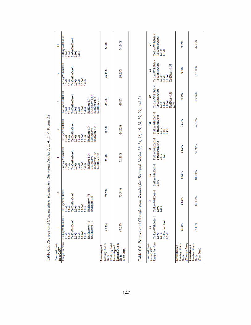
147

148
Terminal nodes 1-15 all have defects on only one layer while terminal
nodes 16-25 have defects on at least 2 different layers. The interactions suggested
by the recipes, then, have interesting interpretations. For example, the recipe for
Terminal Node 1 includes dice that have only one defect that is on Layer 2, Layer
7, Layer 8, or Layer 9, and falls between the center of the wafer and a radial
distance of 1.71. From the training data, only 62.5% of these dice pass. Because
L1, L3, L4, L5, L6, and L10 are included in the recipe for Terminal Node 1,
interactions between these effects may seem likely, but since the splits indicate
that for this node, these layers all have zero defects, any interaction between them
is difficult to interpret. One advantage is that the early processing layers (Layer 1
is the first layer of the die.) are part of the terminal node recipes, so it may be
possible to predict yield earlier in the production process using only the data from
these steps.
Another advantage may be in using the splitting criteria toward the bottom
of the tree to learn more about potential processing issues. Figure 6.14 illustrates
a wafer map showing the areas for the location of the dice for the first eight
terminal nodes from the CART tree. The percentage of dice that passed in each of
the nodes using the training dataset is also included. These nodes include radial
distance in their branches and have only one defect on one layer and have no
defects on Layers 1, 3, 4, 5, 6, and 10. This indicates that for dice with a defect
on Layer 2, 7, 8, or 9, the position of the defect makes the largest impact on the
resulting yield. The figure indicates that there may be processing issues that
impact yield when a defect from these layers is found in the outer radius in

149
Quadrant 2 (Terminal Node 5, 58.2% passing) or in the center of the die
(Terminal Node 1, 62.5% passing). There is also a small region in Quadrant 2
that has lower yield (Terminal Node 3, 60.9% passing) and in Quadrants 1, 3, and
4 (Terminal Node 7, 61.4% passing) that may be of help to process and defect
metrology engineers in identifying potential causes for the problems. This type of
analysis can be very constructive for practitioners.
Figure 6.13. Wafer map showing the radial and quadrant regions that apply to
terminal nodes 1-8 from the CART tree. These terminal nodes include dice that
have only one defect occurring on layer 2, 7, 8, or 9. The percentages shown
indicate the proportion of dice predicted to pass in that node.

150
Another interesting finding of this study is that the GLM model that used
all the terminal nodes from CART and was then reduced identified different
terminal nodes than the model that used the terminal nodes that CART identified
as being better than the root node. While there was some consistency between the
two, there were only 13 CART-identified nodes, compared to the 15 nodes
reduced from the model that contained all 25. Both approaches identified
Terminal Nodes 2, 4, 11, 12, 14, 15, 18, 19, 22, and 24 as significant. Differences
include the reduced model from using all the terminal nodes identified Terminal
Nodes 1, 5, 7, 9, and 16 as significant, while the CART-identified node model
included Terminal Nodes 6, 8, and 21. These differences suggest it may be
beneficial for practitioners to use GLMs to identify important terminal nodes
instead of relying solely on CART’s identification of the better terminal nodes.
Another interesting difference between the models is seen in comparing
the model that was reduced after starting with all the two-factor interactions with
those using CART terminal nodes. The interactions found to be statistically
significant were not all described by the branching of the CART tree. Table 6.7
shows the interaction terms and the terminal nodes from CART that contain both
of the factors in the interactions (not necessarily immediately following each
other). Interactions containing L2, L8, and L9 are not included in the criteria for
terminal nodes in the CART tree. This may indicate that these layers show
important interactions with defects on other layers when there are more total
defects on the die. Recall that any die with three or more defects was classified
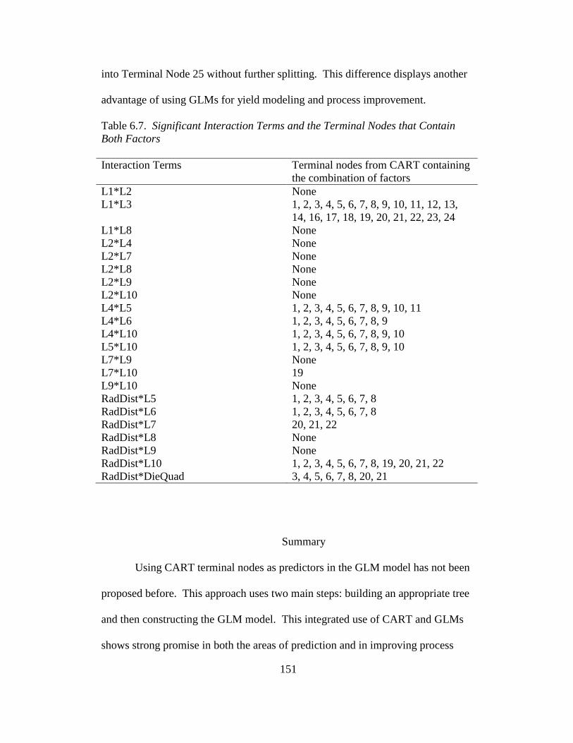
151
into Terminal Node 25 without further splitting. This difference displays another
advantage of using GLMs for yield modeling and process improvement.
Table 6.7. Significant Interaction Terms and the Terminal Nodes that Contain
Both Factors
Interaction Terms Terminal nodes from CART containing
the combination of factors
L1*L2 None
L1*L3 1, 2, 3, 4, 5, 6, 7, 8, 9, 10, 11, 12, 13,
14, 16, 17, 18, 19, 20, 21, 22, 23, 24
L1*L8 None
L2*L4 None
L2*L7 None
L2*L8 None
L2*L9 None
L2*L10 None
L4*L5 1, 2, 3, 4, 5, 6, 7, 8, 9, 10, 11
L4*L6 1, 2, 3, 4, 5, 6, 7, 8, 9
L4*L10 1, 2, 3, 4, 5, 6, 7, 8, 9, 10
L5*L10 1, 2, 3, 4, 5, 6, 7, 8, 9, 10
L7*L9 None
L7*L10 19
L9*L10 None
RadDist*L5 1, 2, 3, 4, 5, 6, 7, 8
RadDist*L6 1, 2, 3, 4, 5, 6, 7, 8
RadDist*L7 20, 21, 22
RadDist*L8 None
RadDist*L9 None
RadDist*L10 1, 2, 3, 4, 5, 6, 7, 8, 19, 20, 21, 22
RadDist*DieQuad 3, 4, 5, 6, 7, 8, 20, 21
Summary
Using CART terminal nodes as predictors in the GLM model has not been
proposed before. This approach uses two main steps: building an appropriate tree
and then constructing the GLM model. This integrated use of CART and GLMs
shows strong promise in both the areas of prediction and in improving process

152
understanding and root cause analysis for occurrences of interest. This technique
does not have a significant impact on yield prediction, producing only slightly
more error than the GLM with main effects alone, suggesting CART trees may be
used well for prediction in this way.
Though the differences in prediction are minute between models
including terminal nodes and those containing two-way interactions, the process
implications and understanding can differ between these models and should be
strongly considered when choosing a final approach. For example, if terminal
node of interest is not split in the CART tree, interactions important for these
observations will not be shown on the tree. If using two-way interactions directly
in a model, it is best to include all possible interactions and then reduce the model
rather than relying on CART branches to help identify important interactions.
This latter approach resulted in the worst prediction errors seen in this study.
As shown in Chapter 4, the application of GLMs to semiconductor yield
modeling is a much-improved approach over yield models of the past. The work
shown in this chapter demonstrates other approaches that can produce nearly as
accurate predictions while providing additional information critical to process
improvement.

153
Chapter 7
CONCLUSIONS
This research contributes to the existing literature in a number of ways.
This work uses generalized linear models, in different forms, to predict
semiconductor yield based on defect count data, an approach to yield modeling
that has not been explored before. This exploration has been done to understand
how different GLM approaches can aid practitioners in problem solving and
decision making. The validity of these GLM modeling strategies has been
demonstrated by applying GLMs to a test dataset with success and by comparing
the predicted values with those from models in the literature.
The use of fixed-effects GLM models showed an advantage in using die-
level data to model yield, with this approach producing less forecasting error than
both wafer-level models and historical models. The die-level models identified
several fixed factors as significant, which could lead to better process
understanding and improvement. The die-level modeling approach also allows
the practitioner to consider the nested structure of the data, accurately reflecting
the process of dice being produced together on a wafer, and wafers being
processed together in a lot. Models built by trimming 5% of a training dataset as
outliers produced the best goodness-of-fit results, but trimming 2.5% of the data
produced very similar models. These models, created using 24 wafers as a
training dataset and tested using 12 additional wafers of data, showed a 34.6%
improvement in MSE and 31.1% improvement in MAD for the reduced, nested
die-level GLM models compared to the best-performing historical model, Seeds’
154
model. These results demonstrate the potential of applying GLMs to these data
for the purposes of accurate yield forecasting and process improvement.
While the GLM models account for the binomial response data, they
assume all factors to be fixed. This assumption is not true for the random
sampling that is commonly used in the fabrication process. A GLMM model
allows a modeler to identify both random and fixed effects and to create models
using a batch-specific or population-averaged approach, depending on the
modeling objectives. GLMM models created using a large dataset of 168 wafers
demonstrated this approach yields similar prediction error to the GLM models,
even improving them under some conditions. The GLMM model results differ
from the GLM results in a number of ways. First, different wafers are identified
as significant, with the GLMM models identifying fewer wafers and including
wafers with high yields as well as low yields. The GLM models selected more
wafers as significant, but these were all lower-yield wafers. These GLM-
identified wafers appeared to display some pattern defects, which may be helpful
in process improvement and trouble-shooting, but the larger number of lots and
wafers identified may also lead to false alarms by indicating a wafer to be
significant when, in fact, it has no substantial problems.
The GLMM study showed differences between link functions used in the
model (logit, probit, and complimentary log-log) to be very minor when all three
link functions produced results. Convergence issued plagued the die-level study,
and changing the degrees of freedom method may be useful in obtaining results if
the default settings do not work. Also, if one link function doesn’t return results
155
due to convergence concerns, another link function can be easily tried and trusted
to produce meaningful output. As with the GLM study, the die-level GLMM
models produced the best results in terms of prediction error, but they were
closely followed by wafer-level adjusted models that account for the dice without
defects on the wafer as well as the dice with defects that were considered in the
model. Wafer-level models are consistent across model type (batch-specific or
population-averaged; lot, wafer, or wafer(lot) modeled as a random effect) for
large sample sizes over 150 wafers.
Finally, this research contributes to the literature by introducing a method
for integrating CART with GLMs. This technique uses the terminal nodes from a
classification tree as indicator variables for prediction in the GLM model. This
approach adds value to the practitioner by providing prediction results nearly as
good as those produced by the GLM alone while giving additional insight into
potential process interactions that can be valuable in process improvement. This
integrated approach takes advantage of both the easy-to-understand tree structure
of the classification tree and the statistical analysis of the GLM to identify
significant interactions and to construct an accurate yield forecasting model.
This work has potential use for practitioners and researchers alike. While
this study showed the validity of these approaches by applying the methods to
semiconductor yield modeling, these same techniques can be applied in other
areas that also exhibit non-normal responses. The improvements in forecast
accuracy and value in identifying key process factors may be important for many
different applications.

156
Limitations
This study, which describes a modeling strategy using GLMs, does have
limitations. In exploring and developing this strategy, data from only one
semiconductor device were used to build and validate the models. This was a
mature device, so this approach may not work well for new products without
considering additional factors. The data for this device was from a four-month
period and did not include information on defect size, defect type, or defect
location on the die for the dice.
The response variable used for this work was the pass/fail result for each
die (or proportion of passing dice for the wafer) and did not consider different
types of failure modes. A similar approach may be employed to predict bin
counts (counts of specific failure modes) using Poisson regression.
This research focused on using defect scan data for yield modeling and did
not consider the process or parametric data for the wafers. Die failure can be due
to non-defect related causes, but these were not considered in this modeling
approach due to the limited corresponding data available.
Future Work
While this work illustrates the potential of using GLMs to model
semiconductor yield, there are many ways this research can be extended. Using
more or different predictor variables, such as defect type (killer or non-killer),
defect size, and the location of the defect within a chip (within critical area or
not), may improve the prediction capabilities of these models even more. These

157
predictors may add value to the models also in the process insight they could
contribute by identifying which of these additional factors are critical in
fabrication. In addition, the device studied in this research was a mature product.
Evaluating these modeling strategies for newer products in early stages of their
life cycles can provide more direction on how generally these techniques may be
applied to forecast yield.
Models that focus on using only intermediate factors from early in the
process (such as front-end processing layers) may also be of interest in guiding
processing and scheduling decisions. For example, early prediction during the
process can help practitioners to decide whether to continue processing wafers
with a number of early defects or to instead start fabricating new wafers, to create
forecasts designed more for planning purposes, and to reliably meet customer
demand. These models may take into account process data recorded during
fabrication as well as the defect counts detected on the front-end layers of the
wafer.
Practitioners may also find useful a method that would identify at which
prediction probabilities a die should be classified as “passing” or “failing” dice for
prediction purposes. These cutoffs can be created based on the models described
in this research. Different cutoff values could be compared using sensitivity and
specificity measures and by comparing the areas under ROC curves (see Hosmer
& Lemeshow, 2000). These cutoff values could be use to make decisions
concerning continued processing for wafers that have already been impacted by
defects.

158
Another area of future work may be in creating systems that can automate
data collection, integration, and cleaning for the purposes of forming these types
of models, making them more accessible to practitioners and more user-friendly.
This automation could also be extended to include coding that would create the
models (GLM, GLMM, CART, etc.) of interest to the user as well as model
comparisons that could suggest the best performing models for the specific
application. This coding may also include creating methods for integrating
classification trees and GLMs (or GLMMs) in SAS or other software.
Another area of extention may be in using GLMs and GLMMs to detect
special differences on wafers. Currently, gross failure defect patterns on wafers
are often manually identified in industry, though research has been published that
studies automating this process (Hansen, Nair, and Friedman, 1997; Fellows,
Mastrangelo, and White, Jr., 2009). GLMMs may be used to consider the
clustering of defects as random effects that can give more information about
predicted yields as well as in automatically identifying these clusters that are
usually caused by processing issues.
Finally, the actual yield and the yield values calculated from the dice with
defects are different, as shown in Figure 7.1, suggesting that factors other than
defects contribute to yield losses. Other types of data are recorded during wafer
fabrication, including process data and parametric electrical test data. Integrating
these process or parametric data with the defectivity data may produce even
stronger and more useful GLM models for decision making. This integration may
be done with a hierarchical approach, as suggested by Kumar (2006), or through
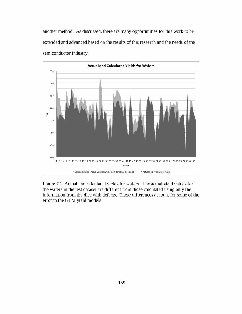
159
another method. As discussed, there are many opportunities for this work to be
extended and advanced based on the results of this research and the needs of the
semiconductor industry.
60%
65%
70%
75%
80%
85%
90%
95%
1 3 5 7 9 11 13 15 17 19 21 23 25 27 29 31 33 35 37 39 41 43 45 47 49 51 53 55 57 59 61 63 65 67 69 71 73 75 77 79 81 83
Yie
ld
Wafer
Actual and Calculated Yields for Wafers
Calculated Yield (Actual yield assuming non-defective dice pass) Actual Yield from wafer maps
Figure 7.1. Actual and calculated yields for wafers. The actual yield values for
the wafers in the test dataset are different from those calculated using only the
information from the dice with defects. These differences account for some of the
error in the GLM yield models.
160
REFERENCES
Agresti, A. (2002). Categorical data analysis (2nd ed.). Hoboken, New Jersey:
John Wiley & Sons, Inc.
Anderson, K., Hill, E., & Mitchell, A. (2002). Spelunking in the data mine: On
data mining as an analysis tool for the optimization of microprocessor speed.
IEEE/SEMI Advanced Semiconductor Manufacturing Conference. 193-198.
Antonio, K. & Beirlant, J. (2007). Actuarial statistics with generalized linear
mixed models. Insurance: Mathematics and Economics, 40, 58-76.
Bergeret, F., & Le Gall, C. (2003). Yield improvement using statistical analysis of
process dates. IEEE Transactions on Semiconductor Manufacturing, 16, 535-
542.
Berglund, C. N. (1996). Unified yield model incorporating both defect and
parametric effects. IEEE Transactions on Semiconductor Manufacturing, 9,
447-454.
Braun, A. E. (2002). Yield management: no longer a closed system.
Semiconductor International, 25(1), 49-54.
Braha, D. & Shmilovici, A. (2002). Data mining for improving a cleaning process
in the semiconductor industry. IEEE Transactions on Semiconductor
Manufacturing, 15(1), 91-101.
Breslow, N. E., & Clayton, D. G. (1993). Approximate inference in generalized
linear mixed models. Journal of the American Statistical Association, 88
(421), 9-25.
Brieman, L., Friedman, J., Olshen, R., & Stone, C. (1984). Classification and
regression trees. Pacific Grove: Wadsworth.
Brown, D. E., Pittard, C. L., & Park, H. (1996). Classification trees with optimal
multivariate decision nodes. Pattern Recognition Letters, 17, 699-703.
CART for Windows user’s guide (Version 5.0). (2002). San Diego, CA: Salford
Systems.
Chandra, D. K., Ravi, V. & Bose, I. (2009). Failure prediction of dotcom
companies using hybrid intelligent techniques. Expert Systems with
Applications, 36, 4830-4837.
Chang, L. Y. & Chen, W. C. (2005). Data mining of tree-based models to analyze
freeway accident frequency. Journal of Safety Research, 36, 365-375.
161
Chang, Y. C. (2010). Hierarchical approach to semiconductor yield modeling:
Applications of generalized linear models. Ph.D. dissertation, University of
Washington, United States -- Washington. Retrieved January 2, 2011, from
Dissertations & Theses: Full Text.(Publication No. AAT 3421548).
Choi, M. & Lee, G. (2010). Decision tree for selecting retaining wall systems
based on logistic regression analysis. Automation in Construction, 19, 917-
928.
Costanza, M.C.; Paccaud, F. (2004). Binary classification of dyslipidemia from
the waist-to-hip ratio and body mass index: a comparison of linear, logistic,
and CART models. BMC Medical Research Methodology, 4(7). Retrieved
January 2, 2011, from http://www.biomedcentral.com/1471-2288/4/7.
Cunningham, J. A. (1990). The use and evaluation of yield models in integrated
circuit manufacturing. IEEE Transactions on Semiconductor Manufacturing,
3, 60-71.
Cunningham, S. P., Spanos, C. J., & Voros, K. (1995). Semiconductor yield
improvement: results and best practices. IEEE Transactions on
Semiconductor Manufacturing, 8, 103-9.
Czado, C. & Pfluger, C. (2008). Modeling dependencies between rating
categories and their effects on prediction in a credit risk portfolio. Applied
Stochastic Models in Business and Industry, 24, 237-259.
Dance, D. L., & Jarvis, R. (1992). Application of yield models for semiconductor
yield improvement. IEEE Transactions on Semiconductor Manufacturing, 5,
41-46.
Davidson, R. A. (2009). Modeling postearthquake fire ignitions using generalized
linear (mixed) models. Journal of Infrastructure Systems, 15(4), 351-360.
Dean, C. B. & Nielsen, J. D. (2007). Generalized linear mixed models: a review
and some extensions. Lifetime Data Analysis, 13, 497-512.
Dingwall, A. G. F. (1968, October). High-yield-processed bipolor LSI arrays.
Paper presented at the IEEE International Electron Devices Meeting,
Washington, D.C.
Fellows, H. H., Mastrangelo, C. M., & and White, Jr., K. P. (2009). An empirical
comparison of spatial randomness models for yield analysis. IEEE Trans. on
Electrononics Packaging Manufacturing, 32, 115-120.
162
Ferris-Prabhu, A. V. (1992). On the assumptions contained in semiconductor
yield models. IEEE Transactions on Computer-Aided Design, 11(8), 966-
975.
Fotouhi, A. R. (2008). Modelling overdispersion in longitudinal count data in
clinical trials with application to epileptic data. Contemporary Clinical
Trials, 29, 547-554.
Fu, C. Y. (2004). “Combining loglinear model with classification and regression
tree (CART): an application to birth data”. Computational Statistics & Data
Analysis, 45, 865-874.
Gupta, S., Kulahci, M, Montgomery, D. C., & Borror, C. M. (2010). Analysis of
signal-response systems using generalized linear mixed models. Quality and
Reliability Engineering International, 26, 375-385.
Ham, W. E. (1978). Yield-area analysis. I. A diagnostic tool for fundamental
integrated-circuit process problems. RCA Review, 39, 231-49.
Hansen, M. H., Nair, V. N., & Friedman, D. J. (1997). Monitoring wafer map data
from integrated circuit fabrication processes for spatially clustered defects.
Technometrics, 39(3), 241-253.
Hofstein, S. R., & Heiman, F. P. (1963). The silicon insulated-gate field-effect
transistor. Proceedings of the IEEE, 51(9), 1190-1202.
Hosmer, D. W., & Lemeshow, S. (2000). Applied logistic regression (2nd
ed.).
Hoboken, New Jersey: John Wiley & Sons, Inc.
Hu, H. (2009) Supervised learning models in sort yield modeling. 2009 Advanced
Semiconductor Manufacturing Conference Proceedings, 133-136.
Hu, T. & Sung, S. Y. (2004). A trimmed mean approach to finding spatial
outliers, Intelligent Data Analysis, 8(1), 79-95.
Jearkpaporn, D., Borror, C. M., Runger, G. C., & Montgomery, D. C. (2007).
Process monitoring for mean shifts for multiple stage processes. International
Journal of Production Research, 45(23), 5547-5570.
Khoshgoftaar, T., M. & Allen, E. B. (2002). Predicting fault-prone software
modules in embedded systems with classification trees. International Journal
of Reliability, Quality and Safety Engineering, 9(1), 1-16.
Khoshgoftaar, T. M., Seliya, N. (2003). Fault prediction modeling for software
quality estimation: Comparing commonly used techniques. Empirical
Software Engineering, 8, 255-283.
163
Krueger, D. C., Montgomery, D. C., & Mastrangelo, C. M. (2011). Application of
generalized linear models to predict semiconductor yield data using defect
metrology data. IEEE Transactions on Semiconductor Manufacturing, 24(1),
44-58.
Kuhnert, P.M., Do, K.A., & McClure, R. (2000). Combining non-parametric
models with logistic regression: an application to motor vehicle injury data.
Computational Statistics & Data Analysis, 34, 371-386.
Kumar, N. (2006). Hierarchical modeling approach to improve factory operations
in semiconductor manufacturing. (Doctoral dissertation, University of
Washington). Dissertation Abstracts International, 67, 06.
Kumar, N., Kennedy, K., Gildersleeve, K., Abelson, R., Mastrangelo, C. M., &
Montgomery, D. C. (2006). A review of yield modelling techniques for
semiconductor manufacturing. International Journal of Production Research,
44(2), 5019-5036.
Kuo, W. & Kim, T. (1999). An overview of manufacturing yield and reliability
modeling for semiconductor products. Proceedings of the IEEE, 87(8), 1329-
1344.
Lee, J., & Pan, R. (2010). Analyzing step-stress accelerated life testing data using
generalized linear models. IIE Transactions, 42, 589-598.
Lewis, S. L., Montgomery, D. C., & Myers, R. H. (2001). Examples of designed
experiments with nonnormal responses. Journal of Quality Technology,
33(3), 265-278.
Lorenzo, A., Oter, D., Cruceta, S., Valtuena, J. F., Gonzalez, G., & Mata, C.
(1999). Kill ratio calculation for in line yield prediction. Proceedings of SPIE
- The International Society for Optical Engineering, 3743, 258-266.
Liu, H., Davidson, R. A., Apanasovich, T. V. (2007). Spatial generalized linear
mixed models of electric power outages due to hurricanes and ice storms.
Reliability Engineering and System Safety, 93, 875-890.
Madden, L. V., Turechek, W. W., Nita, M. (2002). Evaluation of generalized
linear mixed models for analyzing disease incidence data obtained in
designed experiments. Plant Disease, 86, 316-325.
McCullagh, P. & Nelder, J. A. (1989). Generalized linear models (2nd
ed.). New
York: Chapman and Hall.
Montgomery, D. C., Peck, E. A., & Vining, G. G. (2006). Introduction to linear
regression analysis (4th ed.). Hoboken, New Jersey: John Wiley & Sons, Inc.

164
Moore, G. E. (1970). What level of LSI is best for you? Electronics, 43, 126-130.
Murphy, B. T. (1964). Cost-size optima of monolithic integrated circuits.
Proceedings of the IEEE, 52(12), 1537-1545.
Murphy, B. T. (1971). Comments on "A new look at yield of integrated circuits".
Proceedings of the IEEE, 59(7), 1128-1128.
Myers, R. H., Montgomery, D. C., Vining, G. G., and Robinson, T. J. ( 2010).
Generalized linear models with applications in engineering and the sciences
(2nd
ed.). Hoboken, New Jersey: John Wiley & Sons, Inc.
Nag, P. K., Maly, W., & Jacobs, H. (1998). Advanced forecasting of cost and
yield. Semiconductor International, 21, 163-70.
Nahar, R. K., (1993). The yield models and defect density monitors for integrated
circuit diagnosis. Microelectronics Reliability, 33(14), 2153-2159.
Neagu, R. & Hoerl, R. (2005). A Six Sigma approach to predicting corporate
defaults. Quality and Reliability Engineering International, 21, 293-309.
Nelder, J.A., & Wedderburn, R. W. M. (1972). Generalized linear models.
Journal of the Royal Statistical Society. Series A (General), 135(3), 370-384.
Nurani, R. K., Strojweas, A. J., Maly, W. P., Ouyang, C., Shindo, W., Akella, R.,
et al. (1998). In-line yield prediction methodologies using patterned wafer
inspection information. IEEE Transactions on Semiconductor
Manufacturing, 11(1), 40-47.
Okabe, T., Nagata, M., & Shimada, S. (1972). Analysis on yield of integrated
circuits and a new expression for the yield. Electrical Engineering in Japan,
92, 135-41.
Price, J. E. (1970). A new look at yield of integrated circuits. Proceedings of the
IEEE, 58(8), 1290-1291.
Raghavachari, M., Srinivasan, A. & Sullo, P. (1997) Poisson mixture yield
models for integrated circuits: A critical review. Microelectronics Reliability,
37(4), 565-580.
Robinson, T. J., Myers, R. H., Montgomery, D. C. (2004). Analysis
considerations in industrial split-plot experiments with non-normal responses.
Journal of Quality Technology, 36(2), 180-192.
SAS. (2006, June). The GLIMMIX procedure. Retrieved January 31, 2011, from
http://support.sas.com/rnd/app/papers/glimmix.pdf
165
Scheetz, L. J., Zhang, J. & Kolassa, J. (2009). Classification tree modeling to
identify severe and moderate vehicular injuries in young and middle-aged
adults. Artificial Intelligence in Medicine, 45, 1-10.
Seeds, R. B. (1967). Yield and cost analysis of bipolar LSI. , International
Electron Device Meeting Keynote Section, (Abstract p. 12 of the meeting
record).
Skinner, K. R., Montgomery, D. C., Runger, G. C., Fowler, J. W., McCarville, D.
R., Rhoads, T. R., et al. (2002). Multivariate statistical methods for modeling
and analysis of wafer probe test data, IEEE Transactions on Semiconductor
Manufacturing, 15(4), 523-530.
Stapper, C. H. (1976). LSI yield modeling and process monitoring. IBM Journal
of Research and Development, 20, 228-34.
Stapper, C. H. (1989). Fact and fiction in yield modeling. Microelectronics
Journal, 20(1), 129-51.
Stapper, C. H., Armstrong, R.M., & Saji, K. (1983). Integrated circuit yield
statistics. Proceedings of the IEEE, 71, 453-470.
Stapper, C. H. & Rosner, R. J. (1995). Integrated circuit yield management and
yield analysis: Development and implementation. IEEE Transactions on
Semiconductor Manufacturing, 8(2), 95-102.
Ture, M., Kurt, I., & Kurum, A. T. (2008). Comparing performances of logistic
regression, classification and regression tree, and neural networks for
predicting coronary artery disease. Expert Systems with Applications, 34,
366-374.
Ture, M., Kurt, I., Kurum, A. T., & Ozdamar, K. (2005). Comparing classification
techniques for predicting essential hypertension. Expert Systems with
Applications, 29, 583-588.
Wallmark, J. T. (1960). Design Considerations for Integrated Electronic Devices.
Proceedings of the IRE, 48(3), 293-300.
Wang, C. H. (2008). Recognition of semiconductor defect patterns using spatial
filtering and spectral clustering. Expert Systems with Applications, 34, 1914-
1923.
Weber, C. (2004). Yield learning and the sources of profitability in semiconductor
manufacturing and process development. IEEE Transactions on
Semiconductor Manufacturing, 17, 590-6.

166
White, Jr., K. P., Kundu, B., & Mastrangelo, C. M. (2008). Classification of
defect clusters on semiconductor wafers via the Hough transformation. IEEE
Transactions on Semiconductor Manufacturing, 21(2), 272-278.
Wolfinger, R. & O’Connell, M. (1993). Generealized linear models: A pseudo-
likelihood approach. Journal of Statistical Computation and Simulation, 48,
233-243.
Yeh, C., Chen, C., Wu, F., & Chen, K. (2007). Validation and evaluation for
defect-kill-rate and yield estimation models in semiconductor manufacturing.
International Journal of Production Research, 45, 829-844.
Zhou, C., Ross, R., Vickery, C., Metteer, B., Gross, S. & Verret, D. (2002,
August). Yield prediction using critical area analysis with inline defect data.
Advanced Semiconductor Manufacturing IEEE/SEMI Conference and
Workshop, 82-86.

167
APPENDIX A
SAS CODE
168
SAS CODE
SAS Code for Chapter 5
Die Level
GLM
ods html;
ods graphics on;
proc glimmix data=sasuser.thirtywafersdielevel method=RsPL
plots=(residualpanel(type=noblup unpack)
residualpanel(type=blup)
studentpanel(type=noblup));
*Method=RSPL for G-side, RMPL for R-side;
class WafID LotNo DieQuad;
model Pass = LotNo WafID TotLayWithDefs RadDist DieQuad L1 L2 L3
L4 L5 L6 L7 L8 L9 L10/
dist=binomial link=probit solution;
run;
ods graphics off;
ods html close;
Nested GLM ods html;
ods graphics on;
proc glimmix data=sasuser.thirtywafersdielevel method=RsPL
plots=(residualpanel(type=noblup unpack)
residualpanel(type=blup)
studentpanel(type=noblup));
*Method=RSPL for G-side, RMPL for R-side;
class WafID LotNo DieQuad;
model Pass = WafID(LotNo) TotLayWithDefs RadDist DieQuad(WafID)
L1 L2 L3 L4 L5 L6 L7 L8 L9 L10/
dist=binomial link=logit solution;
run;
ods graphics off;
ods html close;
169
GLM with Overdispersion ods html;
ods graphics on;
proc glimmix data=sasuser.thirtywafersdielevel method=RsPL
plots=(residualpanel(type=noblup unpack)
residualpanel(type=blup)
studentpanel(type=noblup));
*Method=RSPL for G-side, RMPL for R-side;
class WafID LotNo DieQuad;
model Pass = LotNo WafID TotLayWithDefs RadDist DieQuad L1 L2 L3
L4 L5 L6 L7 L8 L9 L10/
dist=binomial link=logit solution;
random _residual_;
run;
ods graphics off;
ods html close;
Lot Random G ods html;
ods graphics on;
proc glimmix data=sasuser.thirtywafersdielevel method=RsPL
plots=(residualpanel(type=noblup unpack)
residualpanel(type=blup)
studentpanel(type=noblup));
*Method=RSPL for G-side, RMPL for R-side;
class WafID LotNo DieQuad;
model Pass = TotLayWithDefs RadDist DieQuad L1 L2 L3 L4 L5 L6 L7
L8 L9 L10/
dist=binomial link=probit solution ;
random int / subject = LotNo g s;
run;
ods graphics off;
ods html close;
Lot Random with Overdispersion G ods html;
ods graphics on;
proc glimmix data=sasuser.thirtywafersdielevel method=RsPL
plots=(residualpanel(type=noblup unpack)
residualpanel(type=blup)
studentpanel(type=noblup));
*Method=RSPL for G-side, RMPL for R-side;
class WafID LotNo DieQuad;
model Pass = TotLayWithDefs RadDist DieQuad L1 L2 L3 L4 L5 L6 L7
L8 L9 L10/
dist=binomial link=cll solution ;
random int / subject = LotNo g s;
random _residual_;
run;
ods graphics off;
ods html close;
170
Wafer(Lot) G
ods html;
ods graphics on;
proc glimmix data=sasuser.thirtywafersdielevel method=RsPL
plots=(residualpanel(type=noblup unpack)
residualpanel(type=blup)
studentpanel(type=noblup));
*Method=RSPL for G-side, RMPL for R-side;
class WafID LotNo DieQuad;
model Pass = TotLayWithDefs RadDist DieQuad L1 L2 L3 L4 L5 L6 L7
L8 L9 L10/
dist=binomial link=logit solution ;
random int / subject =WafID(LotNo) g s;
run;
ods graphics off;
ods html close;
Wafer(Lot) with Overdispersion G ods html;
ods graphics on;
proc glimmix data=sasuser.thirtywafersdielevel method=RsPL
plots=(residualpanel(type=noblup unpack)
residualpanel(type=blup)
studentpanel(type=noblup));
*Method=RSPL for G-side, RMPL for R-side;
class WafID LotNo DieQuad;
model Pass = TotLayWithDefs RadDist DieQuad L1 L2 L3 L4 L5 L6 L7
L8 L9 L10/
dist=binomial link=logit solution ;
random int / subject =WafID(LotNo) g s;
random _residual_;
run;
ods graphics off;
ods html close;
Wafer G ods html;
ods graphics on;
proc glimmix data=sasuser.thirtywafersdielevel method=RsPL
plots=(residualpanel(type=noblup unpack)
residualpanel(type=blup)
studentpanel(type=noblup));
*Method=RSPL for G-side, RMPL for R-side;
class WafID LotNo DieQuad;
model Pass = TotLayWithDefs RadDist DieQuad L1 L2 L3 L4 L5 L6 L7
L8 L9 L10/
dist=binomial link=cll solution ;
random int / subject = WafID g s;
run;
ods graphics off;
ods html close;
171
Wafer with Overdispersion G ods html;
ods graphics on;
proc glimmix data=sasuser.thirtywafersdielevel method=RsPL
plots=(residualpanel(type=noblup unpack)
residualpanel(type=blup)
studentpanel(type=noblup));
*Method=RSPL for G-side, RMPL for R-side;
class WafID LotNo DieQuad;
model Pass = TotLayWithDefs RadDist DieQuad L1 L2 L3 L4 L5 L6 L7
L8 L9 L10/
dist=binomial link=probit solution ;
random int / subject =WafID g s;
random _residual_;
run;
ods graphics off;
ods html close;
Lot Random R ods html;
ods graphics on;
proc glimmix data=sasuser.thirtywafersdielevel method=RmPL
plots=(residualpanel(type=noblup unpack)
residualpanel(type=blup)
studentpanel(type=noblup));
*Method=RSPL for G-side, RMPL for R-side;
class WafID LotNo DieQuad;
model Pass = TotLayWithDefs RadDist DieQuad L1 L2 L3 L4 L5 L6
L7 L8 L9 L10/
dist=binomial link=logit solution ;
random _residual_ / sub=LotNo type=cs rside cl s;
run;
ods graphics off;
ods html close;
Wafer(Lot) R ods html;
ods graphics on;
proc glimmix data=sasuser.thirtywafersdielevel method=RmPL
plots=(residualpanel(type=noblup unpack)
residualpanel(type=blup)
studentpanel(type=noblup));
*Method=RSPL for G-side, RMPL for R-side;
class WafID LotNo DieQuad;
model Pass = TotLayWithDefs RadDist DieQuad L1 L2 L3 L4 L5 L6
L7 L8 L9 L10/
dist=binomial link=logit solution ;
random _residual_ / sub=WafID(LotNo) type=cs rside cl s;
run;
ods graphics off;
ods html close;
172
Wafer R ods html;
ods graphics on;
proc glimmix data=sasuser.thirtywafersdielevel method=RmPL
plots=(residualpanel(type=noblup unpack)
residualpanel(type=blup)
studentpanel(type=noblup));
*Method=RSPL for G-side, RMPL for R-side;
class WafID LotNo DieQuad;
model Pass = TotLayWithDefs RadDist DieQuad L1 L2 L3 L4 L5 L6
L7 L8 L9 L10/
dist=binomial link=logit solution ;
random _residual_ / sub=WafID type=cs rside cl s;
run;
ods graphics off;
ods html close;
173
Wafer level
GLM
ods html;
ods graphics on;
proc glimmix data=waferleveltrainingdata310 method=RsPL
plots=(residualpanel(type=noblup unpack)
residualpanel(type=blup)
studentpanel(type=noblup));
class WafID LotNo;
PropPassed = PassingDice/DiceWithDef;
model PropPassed = LotNo WafID TotLayWithDefs L1 L2 L3 L4 L5 l6
L7 L8 L9 L10/
dist=binomial link=probit solution ;
run;
ods graphics off;
ods html close;
Nested GLM ods html;
ods graphics on;
proc glimmix data=waferleveltrainingdata310 method=RsPL
plots=(residualpanel(type=noblup unpack)
residualpanel(type=blup)
studentpanel(type=noblup));
class WafID LotNo;
PropPassed = PassingDice/DiceWithDef;
model PropPassed = WafID(LotNo) TotLayWithDefs L1 L2 L3 L4 L5
l6 L7 L8 L9 L10/
dist=binomial link=logit solution ;
run;
ods graphics off;
ods html close;
GLM with OD: ods html;
ods graphics on;
proc glimmix data=waferleveltrainingdata310 method=RsPL
plots=(residualpanel(type=noblup unpack)
residualpanel(type=blup)
studentpanel(type=noblup));
class WafID LotNo;
PropPassed = PassingDice/DiceWithDef;
model PropPassed = LotNo WafID TotLayWithDefs L1 L2 L3 L4 L5 l6
L7 L8 L9 L10/
dist=binomial link=probit solution ;
random _residual_;
run;
ods graphics off;
ods html close;
174
Lot Random (G-side) ods html;
ods graphics on;
proc glimmix data=waferleveltrainingdata310 method=RsPL
plots=(residualpanel(type=noblup unpack)
residualpanel(type=blup)
studentpanel(type=noblup));
class WafID LotNo;
PropPassed = PassingDice/DiceWithDef;
model PropPassed = TotLayWithDefs L1 L2 L3 L4 L5 l6 L7 L8 L9
L10/
dist=binomial link=logit solution ;
random int / subject = LotNo g s;
run;
ods graphics off;
ods html close;
Lot Random (G-side) with Overdispersion
ods html;
ods graphics on;
proc glimmix data=waferleveltrainingdata310 method=RsPL
plots=(residualpanel(type=noblup unpack)
residualpanel(type=blup)
studentpanel(type=noblup));
class WafID LotNo;
PropPassed = PassingDice/DiceWithDef;
model PropPassed = TotLayWithDefs L1 L2 L3 L4 L5 l6 L7 L8 L9
L10/
dist=binomial link=cll solution ;
random int / subject = LotNo g s;
random _residual_;
run;
ods graphics off;
ods html close;
Wafer(Lot) Random (G-side) ods html;
ods graphics on;
proc glimmix data=waferleveltrainingdata310 method=RsPL
plots=(residualpanel(type=noblup unpack)
residualpanel(type=blup)
studentpanel(type=noblup));
class WafID LotNo;
PropPassed = PassingDice/DiceWithDef;
model PropPassed = TotLayWithDefs L1 L2 L3 L4 L5 l6 L7 L8 L9
L10/
dist=binomial link=logit solution ;
random int / subject = WafID(LotNo) g s;
run;
ods graphics off;
ods html close;
175
Wafer(Lot) Random (G-side) with Overdispersion ods html;
ods graphics on;
proc glimmix data=waferleveltrainingdata310 method=RsPL
plots=(residualpanel(type=noblup unpack)
residualpanel(type=blup)
studentpanel(type=noblup));
class WafID LotNo;
PropPassed = PassingDice/DiceWithDef;
model PropPassed = TotLayWithDefs L1 L2 L3 L4 L5 l6 L7 L8 L9
L10/
dist=binomial link=logit solution ;
random int / subject = WafID(LotNo) g s;
random _residual_;
run;
ods graphics off;
ods html close;
Wafer Random (G-side) ods html;
ods graphics on;
proc glimmix data=waferleveltrainingdata310 method=RsPL
plots=(residualpanel(type=noblup unpack)
residualpanel(type=blup)
studentpanel(type=noblup));
class WafID LotNo;
PropPassed = PassingDice/DiceWithDef;
model PropPassed = TotLayWithDefs L1 L2 L3 L4 L5 l6 L7 L8 L9
L10/
dist=binomial link=logit solution ;
random int / subject = WafID g s;
run;
ods graphics off;
ods html close;
Wafer Random (G-side) with Overdispersion ods html;
ods graphics on;
proc glimmix data=waferleveltrainingdata310 method=RsPL
plots=(residualpanel(type=noblup unpack)
residualpanel(type=blup)
studentpanel(type=noblup));
class WafID LotNo;
PropPassed = PassingDice/DiceWithDef;
model PropPassed = TotLayWithDefs L1 L2 L3 L4 L5 l6 L7 L8 L9
L10/
dist=binomial link=logit solution ;
random int / subject = WafID g s;
random _residual_;
run;
ods graphics off;
ods html close;
176
Lot Random (R-side) ods html;
ods graphics on;
proc glimmix data=waferleveltrainingdata310 method=RmPL
plots=(residualpanel(type=noblup unpack)
residualpanel(type=blup)
studentpanel(type=noblup));
class WafID LotNo;
PropPassed = PassingDice/DiceWithDef;
model PropPassed = TotLayWithDefs L1 L2 L3 L4 L5 l6 L7 L8 L9
L10/
dist=binomial link=logit solution ;
random _residual_ / sub=LotNo type=cs rside cl s;
run;
ods graphics off;
ods html close;
Wafer(Lot) Random (R-side)
ods html;
ods graphics on;
proc glimmix data=waferleveltrainingdata310 method=RmPL
plots=(residualpanel(type=noblup unpack)
residualpanel(type=blup)
studentpanel(type=noblup));
class WafID LotNo;
PropPassed = PassingDice/DiceWithDef;
model PropPassed = TotLayWithDefs L1 L2 L3 L4 L5 l6 L7 L8 L9
L10/
dist=binomial link=logit solution ;
random _residual_ / sub=WAfID(LotNo) type=cs rside cl s;
run;
ods graphics off;
ods html close;
Wafer Random (R-side)
ods html;
ods graphics on;
proc glimmix data=waferleveltrainingdata310 method=RmPL
plots=(residualpanel(type=noblup unpack)
residualpanel(type=blup)
studentpanel(type=noblup));
class WafID LotNo;
PropPassed = PassingDice/DiceWithDef;
model PropPassed = TotLayWithDefs L1 L2 L3 L4 L5 l6 L7 L8 L9
L10/
dist=binomial link=cll solution ;
random _residual_ / sub=WAfID type=cs rside cl s;
run;
ods graphics off;
ods html close;
177
SAS Code for Chapter 6
Die-Level Model with Fixed Effects and Terminal Nodes
ods html;
ods graphics on;
proc glimmix data=sasuser.cartdiedata method=RsPL
plots=(residualpanel(type=noblup unpack)
residualpanel(type=blup)
studentpanel(type=noblup));
*Method=RSPL for G-side, RMPL for R-side;
class WafID LotNo DieQuad;
model Pass1 = TotalLayWithDefs RadDist DieQuad L1 L2 L3 L4 L5 L6
L7 L8 L9 L10
Tnode1 Tnode2 Tnode3 Tnode4 Tnode5 Tnode6 Tnode7 Tnode8 Tnode9
Tnode10 Tnode11 Tnode12 Tnode13 Tnode14
Tnode15 Tnode16 Tnode17 Tnode18 Tnode19 Tnode20 Tnode21 Tnode22
Tnode23 Tnode24 Tnode25
/ dist=binomial link=logit solution ddfm=kr;
run;
proc print data=glimmixout;
run;
ods graphics off;
ods html close;
Die-Level Full Model with Interactions from CART Tree 3
ods html;
ods graphics on;
proc glimmix data=sasuser.cartprobdiedata method=RsPL
plots=(residualpanel(type=noblup unpack)
residualpanel(type=blup)
studentpanel(type=noblup));
class WafID LotNo DieQuad;
model Pass1 = TotalLayWithDefs RadDist DieQuad L1 L2 L3 L4 L5
L6 L7 L8 L9 L10
L1*L3 L4*L5 L4*L10 L10*L6 L6*RadDist RadDist*DieQuad L1*L4
L1*L10 L10*RadDist L7*RadDist L7*DieQuad
/ dist=binomial link=logit solution ;
run;
ods graphics off;
ods html close;
178
Die-Level Reduced Model with Interactions from CART Tree 3
ods html;
ods graphics on;
proc glimmix data=sasuser.cartprobdiedata method=RsPL
plots=(residualpanel(type=noblup unpack)
residualpanel(type=blup)
studentpanel(type=noblup));
class WafID LotNo DieQuad;
model Pass1 = TotalLayWithDefs RadDist DieQuad L1 L2 L3 L4 L6
L7 L8 L9 L10
L1*L3 L4*L5 L4*L10 L6*RadDist RadDist*DieQuad L10*RadDist
L7*RadDist
/ dist=binomial link=logit solution ;
run;
ods graphics off;
ods html close;
Die-Level Model with All 2-way interactions
ods html;
ods graphics on;
proc glimmix data=sasuser.cartprobdiedata method=RsPL
plots=(residualpanel(type=noblup unpack)
residualpanel(type=blup)
studentpanel(type=noblup));
class WafID LotNo DieQuad;
model Pass1 = TotalLayWithDefs RadDist DieQuad L1 L2 L3 L4 L5
L6 L7 L8 L9 L10
L1*L2 L1*L3 L1*L4 L1*L5 L1*L6 L1*L7 L1*L8 L1*L9 L1*L10
L2*L3 L2*L4 L2*L5 L2*L6 L2*L7 L2*L8 L2*L9 L2*L10
L3*L4 L3*L5 L3*L6 L3*L7 L3*L8 L3*L9 L3*L10
L4*L5 L4*L6 L4*L7 L4*L8 L4*L9 L4*L10
L5*L6 L5*L7 L5*L8 L5*L9 L5*L10
L6*L7 L6*L8 L6*L9 L6*L10
L7*L8 L7*L9 L7*L10
L8*L9 L8*L10
L9*L10
RadDist*L1 RadDist*L2 RadDist*L3 RadDist*L4 RadDist*L5 RadDist*L6
RadDist*L7 RadDist*L8 RadDist*L9 RadDist*L10
DieQuad*RadDist DieQuad*L1 DieQuad*L2 DieQuad*L3 DieQuad*L4
DieQuad*L5 DieQuad*L6 DieQuad*L7 DieQuad*L8 DieQuad*L9
DieQuad*L10
/ dist=binomial link=logit solution ;
run;
ods graphics off;
ods html close;
179
Die-Level Reduced Model with Interactions
ods html;
ods graphics on;
proc glimmix data=sasuser.cartprobdiedata method=RsPL
plots=(residualpanel(type=noblup unpack)
residualpanel(type=blup)
studentpanel(type=noblup));
class WafID LotNo DieQuad;
model Pass1 = TotalLayWithDefs RadDist DieQuad L1 L2 L3 L4 L5
L6 L7 L9 L10
L1*L2 L1*L3 L1*L8 L2*L4 L2*L7 L2*L8 L2*L9 L2*L10 L4*L5 L4*L6
L4*L10 L5*L10 L7*L9 L7*L10 L9*L10
RadDist*L5 RadDist*L6 RadDist*L7 RadDist*L8 RadDist*L9
RadDist*L10 DieQuad*RadDist
/ dist=binomial link=logit solution ;
run;
ods graphics off;
ods html close;

180
BIOGRAPHICAL SKETCH
Dana Cheree Fritzemeier Krueger is a native of Stafford, KS. She earned
her B.S. in chemical engineering from Kansas State University, Manhattan, KS in
1999 and worked for The Goodyear Tire & Rubber Co., Lincoln, NE for over five
years as a development engineer for power transmission products. While with
Goodyear, Mrs. Krueger was trained as a Six Sigma Black Belt, and she earned
her M.S. in Industrial and Management Systems Engineering from the University
of Nebraska – Lincoln in 2005 with an emphasis in engineering management.
Her doctoral studies at Arizona State University, Tempe, AZ, focused on quality
and reliability engineering. Mrs. Krueger is currently an instructor at Kansas
State University in the Department of Management and resides with her husband
and daughter in Manhattan, KS. Her research interests include applied statistics,
designed experiments, and generalized linear models.

181
181
This document was generated using the Graduate College Format Advising tool. Please
turn a copy of this page in when you submit your document to Graduate College format
advising. You may discard this page once you have printed your final
document. DO NOT TURN THIS PAGE IN WITH YOUR FINAL
DOCUMENT!
181
181
181