scheduling algorithms -...
TRANSCRIPT

Scheduling Algorithms
Peter Brucker
SchedulingAlgorithms
Fifth Edition
With 77 Figures and 32 Tables
123

Professor Dr. Peter BruckerUniversität OsnabrückFachbereich Mathematik/InformatikAlbrechtstraße 28a49069 Osnabrü[email protected]
Library of Congress Control Number: 2006940721
ISBN 978-3-540-69515-8 Springer Berlin Heidelberg New YorkISBN 978-3-540-20524-1 4th ed. Springer Berlin Heidelberg New York
This work is subject to copyright. All rights are reserved, whether the whole or part of the material isconcerned, specifically the rights of translation, reprinting, reuse of illustrations, recitation, broad-casting, reproduction on microfilm or in any other way, and storage in data banks. Duplication ofthis publication or parts thereof is permitted only under the provisions of the German CopyrightLaw of September 9, 1965, in its current version, and permission for use must always be obtainedfrom Springer. Violations are liable to prosecution under the German Copyright Law.
Springer is part of Springer Science+Business Media
springer.com
© Springer-Verlag Berlin Heidelberg 2001, 2004, 2007
The use of general descriptive names, registered names, trademarks, etc. in this publication doesnot imply, even in the absence of a specific statement, that such names are exempt from the relevantprotective laws and regulations and therefore free for general use.
Production: LE-TEX Jelonek, Schmidt & Vockler GbR, LeipzigCover-design: WMX Design GmbH, Heidelberg
SPIN 11970705 42/3100YL - 5 4 3 2 1 0 Printed on acid-free paper
¨
Preface of the Fifth and Fourth Edition
In these editions new results have been added to the complexity columns.Furthermore, the bibliographies have been updated.
Again many thanks go to Marianne Gausmann for the typesetting andto Dr. Sigrid Knust for taking care of the complexity columns which canbe found under the www-address
http://www.mathematik.uni-osnabrueck.de/research/OR/class.
Osnabruck, October 2006 Peter Brucker
vi Preface
Preface of the Third Edition
In this edition again the complexity columns at the end of each chap-ter and the corresponding references have been updated. I would liketo express may gratitude to Dr. Sigrid Knust for taking care of a cor-responding documentation of complexity results for scheduling problemsin the Internet. These pages can be found under the world-wide-webaddress http://www.mathematik.uni-osnabrueck.de/research/OR/class.
In addition to the material of the second edition some new results onscheduling problems with release times and constant processing timesand on multiprocessor task problems in which each task needs a certainnumber of processors have been included.
The new edition has been rewritten in LATEX2ε. Many thanks go toMarianne Gausmann for the new typesetting and to Christian Strotmannfor creating the bibliography database files.
Osnabruck, March 2001 Peter Brucker
Preface of the Second Edition
In this revised edition new material has been added. In particular, thechapters on batching problems and multiprocessor task scheduling havebeen augmented. Also the complexity columns at the end of each chap-ter have been updated. In this connection I would like thank Jan KarelLenstra for providing the current results of the program MSPCLASS.I am grateful for the constructive comments of Jacek Blazewicz, Jo-hann Hurink, Sigrid Knust, Svetlana Kravchenko, Erwin Pesch, Mau-rice Queyranne, Vadim Timkowsky, Jurgen Zimmermann which helpedto improve the first edition.
Finally, again special thanks go to Marianne Gausmann and Teresa Gehrsfor the TEX typesetting and for improving the English.
Osnabruck, November 1997 Peter Brucker
Preface vii
Preface
This is a book about scheduling algorithms. The first such algorithmswere formulated in the mid fifties. Since then there has been a growinginterest in scheduling. During the seventies, computer scientists discov-ered scheduling as a tool for improving the performance of computersystems. Furthermore, scheduling problems have been investigated andclassified with respect to their computational complexity. During the lastfew years, new and interesting scheduling problems have been formulatedin connection with flexible manufacturing.
Most parts of the book are devoted to the discussion of polynomial algo-rithms. In addition, enumerative procedures based on branch & boundconcepts and dynamic programming, as well as local search algorithms,are presented.
The book can be viewed as consisting of three parts. The first part,Chapters 1 through 3, covers basics like an introduction to and classi-fication of scheduling problems, methods of combinatorial optimizationthat are relevant for the solution procedures, and computational com-plexity theory.
The second part, Chapters 4 through 6, covers classical scheduling algo-rithms for solving single machine problems, parallel machine problems,and shop scheduling problems.
The third and final part, Chapters 7 through 11, is devoted to problemsdiscussed in the more recent literature in connection with flexible man-ufacturing, such as scheduling problems with due dates and batching.Also, multiprocessor task scheduling is discussed.
Since it is not possible to cover the whole area of scheduling in one book,some restrictions are imposed. Firstly, in this book only machine orprocessor scheduling problems are discussed. Secondly, some interestingtopics like cyclic scheduling, scheduling problems with finite input and/oroutput buffers, and general resource constrained scheduling problems arenot covered in this book.
I am indebted to many people who have helped me greatly in preparingthis book. Students in my courses during the last three years at the Uni-versity of Osnabruck have given many suggestions for improving earlierversions of this material. The following people read preliminary drafts ofall or part of the book and made constructive comments: Johann Hurink,Sigrid Knust, Andreas Kramer, Wieslaw Kubiak, Helmut Mausser.

viii Preface
I am grateful to the Deutsche Forschungsgemeinschaft for supportingthe research that underlies much of this book. I am also indebted to theMathematics and Computer Science Department of the University of Os-nabruck, the College of Business, University of Colorado at Boulder, andthe Computer Science Department, University of California at Riversidefor providing me with an excellent environment for writing this book.
Finally, special thanks go to Marianne Gausmann for her tireless effortsin translating my handwritten hieroglyphics and figures into input forthe TEX typesetting system.
Osnabruck, April 1995 Peter Brucker
Contents
Preface v
1 Classification of Scheduling Problems 1
1.1 Scheduling Problems . . . . . . . . . . . . . . . . . . . . 1
1.2 Job Data . . . . . . . . . . . . . . . . . . . . . . . . . . . 2
1.3 Job Characteristics . . . . . . . . . . . . . . . . . . . . . 3
1.4 Machine Environment . . . . . . . . . . . . . . . . . . . 5
1.5 Optimality Criteria . . . . . . . . . . . . . . . . . . . . . 6
1.6 Examples . . . . . . . . . . . . . . . . . . . . . . . . . . 7
2 Some Problems in Combinatorial Optimization 11
2.1 Linear and Integer Programming . . . . . . . . . . . . . 11
2.2 Transshipment Problems . . . . . . . . . . . . . . . . . . 12
2.3 The Maximum Flow Problem . . . . . . . . . . . . . . . 13
2.4 Bipartite Matching Problems . . . . . . . . . . . . . . . 14
2.5 The Assignment Problem . . . . . . . . . . . . . . . . . . 18
2.6 Arc Coloring of Bipartite Graphs . . . . . . . . . . . . . 22
2.7 Shortest Path Problems and Dynamic Programming . . . 26
3 Computational Complexity 37
3.1 The Classes P and NP . . . . . . . . . . . . . . . . . . . 37
3.2 NP-complete and NP-hard Problems . . . . . . . . . . 41
3.3 Simple Reductions Between Scheduling Problems . . . . 48
3.4 Living with NP-hard Problems . . . . . . . . . . . . . . 51
3.4.1 Local Search Techniques . . . . . . . . . . . . . . 51
x Contents
3.4.2 Branch-and-Bound Algorithms . . . . . . . . . . . 56
4 Single Machine Scheduling Problems 61
4.1 Minimax Criteria . . . . . . . . . . . . . . . . . . . . . . 62
4.1.1 Lawler’s Algorithm for 1 | prec | fmax . . . . . . . 62
4.1.2 1 |prec; pj = 1; rj | fmax and 1 | prec; pmtn; rj | fmax 63
4.2 Maximum Lateness and Related Criteria . . . . . . . . . 67
4.3 Total Weighted Completion Time . . . . . . . . . . . . . 73
4.3.1 1 | tree | ∑wjCj . . . . . . . . . . . . . . . . . . 73
4.3.2 1 | sp-graph | ∑wjCj . . . . . . . . . . . . . . . . 79
4.4 Weighted Number of Late Jobs . . . . . . . . . . . . . . 84
4.4.1 1 | rj ; pj = 1 | ∑wjUj . . . . . . . . . . . . . . . 84
4.4.2 1 | pj = 1 | ∑wjUj . . . . . . . . . . . . . . . . . 85
4.4.3 1 || ∑Uj . . . . . . . . . . . . . . . . . . . . . . . 86
4.4.4 1 | rj ; pmtn | ∑wjUj . . . . . . . . . . . . . . . . 88
4.5 Total Weighted Tardiness . . . . . . . . . . . . . . . . . 93
4.6 Problems with Release Times and Identical ProcessingTimes . . . . . . . . . . . . . . . . . . . . . . . . . . . . 98
4.6.1 1 | rj ; pj = p | ∑wjUj . . . . . . . . . . . . . . . 98
4.6.2 1 | rj ; pj = p | ∑wjCj and 1 | rj; pj = p | ∑
Tj . . 101
4.7 Complexity of Single Machine Problems . . . . . . . . . 104
5 Parallel Machines 107
5.1 Independent Jobs . . . . . . . . . . . . . . . . . . . . . . 107
5.1.1 Identical Machines . . . . . . . . . . . . . . . . . 107
5.1.2 Uniform Machines . . . . . . . . . . . . . . . . . 124
5.1.3 Unrelated Machines . . . . . . . . . . . . . . . . . 136
5.2 Jobs with Precedence Constraints . . . . . . . . . . . . . 139
5.2.1 P | tree; pi = 1 | Lmax-Problems . . . . . . . . . . 140
5.2.2 Problem P2 | prec; pi = 1 | Lmax . . . . . . . . . . 145
5.3 Complexity Results . . . . . . . . . . . . . . . . . . . . . 150
6 Shop Scheduling Problems 155
Contents xi
6.1 The Disjunctive Graph Model . . . . . . . . . . . . . . . 156
6.2 Open Shop Problems . . . . . . . . . . . . . . . . . . . . 158
6.2.1 Arbitrary Processing Times . . . . . . . . . . . . 158
6.2.2 Unit Processing Times . . . . . . . . . . . . . . . 161
6.3 Flow Shop Problems . . . . . . . . . . . . . . . . . . . . 174
6.3.1 Minimizing Makespan . . . . . . . . . . . . . . . 174
6.4 Job Shop Problems . . . . . . . . . . . . . . . . . . . . . 178
6.4.1 Problems with Two Machines . . . . . . . . . . . 179
6.4.2 Problems with Two Jobs. A Geometric Approach 186
6.4.3 Job Shop Problems with Two Machines . . . . . . 196
6.4.4 A Branch-and-Bound Algorithm . . . . . . . . . . 202
6.4.5 Applying Tabu-Search to the Job Shop Problem . 221
6.5 Mixed Shop Problems . . . . . . . . . . . . . . . . . . . 226
6.5.1 Problems with Two Machines . . . . . . . . . . . 226
6.5.2 Problems with Two Jobs . . . . . . . . . . . . . . 227
6.6 Complexity of Shop Scheduling Problems . . . . . . . . . 232
7 Due-Date Scheduling 243
7.1 Problem 1 | dopt |∑
wi|Lσ(i)| + w0 · d . . . . . . . . . . . 244
7.2 Problem 1|dopt|wE
∑Ei+wT
∑Ti + w0d . . . . . . . . . 247
7.3 Problem 1 | d | ∑wi|Lσ(i)| . . . . . . . . . . . . . . . . . 249
7.4 Problem 1 | d | wE
∑Ei + wT
∑Ti . . . . . . . . . . . . 255
7.5 Problem 1 | d | |Li|max and 1 | dopt | |Li|max . . . . . . . . 257
7.6 Problem 1 | dopt |∑
wi|Li| . . . . . . . . . . . . . . . . . 259
7.7 Problem 1 | d | ∑wi|Li| . . . . . . . . . . . . . . . . . . 262
8 Batching Problems 267
8.1 Single Machine s-Batching Problems . . . . . . . . . . . 267
8.2 Single Machine p-Batching Problems . . . . . . . . . . . 271
8.2.1 The Unbounded Model . . . . . . . . . . . . . . . 272
8.2.2 The Bounded Model . . . . . . . . . . . . . . . . 276
8.3 Complexity Results for Single Machine Batching Problems 277
xii Contents
9 Changeover Times and Transportation Times 281
9.1 Single Machine Problems . . . . . . . . . . . . . . . . . . 282
9.2 Problems with Parallel Machines . . . . . . . . . . . . . 286
9.3 General Shop Problems . . . . . . . . . . . . . . . . . . . 290
10 Multi-Purpose Machines 293
10.1 MPM Problems with Identical and Uniform Machines . 294
10.2 MPM Problems with Shop Characteristics . . . . . . . . 300
10.2.1 Arbitrary Processing Times . . . . . . . . . . . . 300
10.2.2 Unit Processing Times . . . . . . . . . . . . . . . 311
10.3 Complexity Results . . . . . . . . . . . . . . . . . . . . . 315
11 Multiprocessor Tasks 317
11.1 Multiprocessor Task Systems . . . . . . . . . . . . . . . . 318
11.2 Shop Problems with MPT : Arbitrary Processing Times 323
11.3 Shop Problems with MPT : Unit Processing Times . . . 329
11.4 Multi-Mode Multiprocessor-Task Scheduling Problems . 335
11.5 Complexity Results . . . . . . . . . . . . . . . . . . . . . 342
Bibliography 347
Index 367
Chapter 1
Classification of SchedulingProblems
The theory of scheduling is characterized by a virtually unlimited numberof problem types (see, e.g. Baker [12], Blazewicz et al. [27], Coffman [69],Conway et al. [72], French [93], Lenstra [151] , Pinedo [180], RinnooyKan [181], Tanaev et al. [193], Tanaev et al. [194]). In this chapter, abasic classification for the scheduling problems covered in the first partof this book will be given. This classification is based on a classificationscheme widely used in the literature (see, e.g. Lawler et al. [145]). Inlater chapters we will extend this classification scheme.
1.1 Scheduling Problems
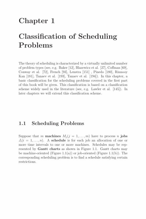
Suppose that m machines Mj(j = 1, . . . , m) have to process n jobsJi(i = 1, . . . , n). A schedule is for each job an allocation of one ormore time intervals to one or more machines. Schedules may be rep-resented by Gantt charts as shown in Figure 1.1. Gantt charts maybe machine-oriented (Figure 1.1(a)) or job-oriented (Figure 1.1(b)). Thecorresponding scheduling problem is to find a schedule satisfying certainrestrictions.
2 Classification of Scheduling Problems
�M1
M2
M3
J1
J2
J2 J1 J3
J3
J3 J1 J4
t(a)
�J4
J3
J2
J1
M1
M3 M1 M2
M2 M3
M1 M2 M1
t(b)
Figure 1.1: Machine- and job-oriented Gantt charts.
1.2 Job Data
A job Ji consists of a number ni of operations Oi1, . . . , Oi,ni. Asso-
ciated with operation Oij is a processing requirement pij. If job Ji
consists of only one operation (ni = 1), we then identify Ji with Oi1 anddenote the processing requirement by pi. Furthermore, a release dateri, on which the first operation of Ji becomes available for processing maybe specified. Associated with each operation Oij is a set of machinesμij ⊆ {M1, . . . , Mm}. Oij may be processed on any of the machines inμij. Usually, all μij are one element sets or all μij are equal to the setof all machines. In the first case we have dedicated machines. Inthe second case the machines are called parallel. The general case isintroduced here to cover problems in flexible manufacturing where ma-chines are equipped with different tools. This means that an operationcan be processed on any machine equipped with the appropriate tool.We call scheduling problems of this type problems with multi-purposemachines (MPM).
It is also possible that all machines in the set μij are used simultane-ously by Oij during the whole processing period. Scheduling problemsof this type are called multiprocessor task scheduling problems.Scheduling problems with multi-purpose machines and multiprocessortask scheduling problems will be classified in more detail in Chapters 10and 11.
1.3. Job Characteristics 3
Finally, there is a cost function fi(t) which measures the cost of com-pleting Ji at time t. A due date di and a weight wi may be used indefining fi.
In general, all data pi, pij, ri, di, wi are assumed to be integer. A sched-ule is feasible if no two time intervals overlap on the same machine, ifno two time intervals allocated to the same job overlap, and if, in addi-tion, it meets a number of problem-specific characteristics. A schedule isoptimal if it minimizes a given optimality criterion.
Sometimes it is convenient to identify a job Ji by its index i. We will usethis brief notation in later chapters.
We will discuss a large variety of classes of scheduling problems which dif-fer in their complexity. Also the algorithms we will develop are quite dif-ferent for different classes of scheduling problems. Classes of schedulingproblems are specified in terms of a three-field classification α|β|γ whereα specifies the machine environment , β specifies the job character-istics , and γ denotes the optimality criterion. Such a classificationscheme was introduced by Graham et al. [108].
1.3 Job Characteristics
The job characteristics are specified by a set β containing at the mostsix elements β1, β2, β3, β4, β5, and β6.
β1 indicates whether preemption (or job splitting) is allowed. Preemp-tion of a job or operation means that processing may be interruptedand resumed at a later time, even on another machine. A job or opera-tion may be interrupted several times. If preemption is allowed, we setβ1 = pmtn. Otherwise β1 does not appear in β.
β2 describes precedence relations between jobs. These precedencerelations may be represented by an acyclic directed graph G = (V, A)where V = {1, . . . , n} corresponds with the jobs, and (i, k) ∈ A iff Ji
must be completed before Jk starts. In this case we write Ji → Jk. IfG is an arbitrary acyclic directed graph we set β2 = prec. Sometimeswe will consider scheduling problems with restricted precedences givenby chains, an intree, an outtree, a tree or a series-parallel directed graph.In these cases we set β2 equal to chains, intree, outtree, and sp-graph.
If β2 = intree (outtree), then G is a rooted tree with an outdegree(indegree) for each vertex of at the most one. Thus, in an intree (outtree)

4 Classification of Scheduling Problems
all arcs are directed towards (away from) a root. If β2 = tree, then Gis either an intree or an outtree. A set of chains is a tree in which theoutdegree and indegree for each vertex is at the most one. If β2 = chains,then G is a set of chains.
Series-parallel graphs are closely related to trees. A graph is calledseries-parallel if it can be built by means of the following rules:
Base graph. Any graph consisting of a single vertex is series-parallel.Let Gi = (Vi, Ai) be series-parallel (i = 1, 2).
Parallel composition. The graph G = (V1 ∪ V2, A1 ∪ A2) formed fromG1 and G2 by joining the vertex sets and arc sets is series parallel.
Series composition. The graph G = (V1∪V2, A1∪A2∪T1×S2) formedfrom G1 and G2 by joining the vertex sets and arc sets and adding allarcs (t, s) where t belongs to the set T1 of sinks of G1 (i.e. the set ofvertices without successors) and s belongs to the set S2 of sources of G2
(i.e. the set of vertices without predecessors) is series parallel.
We set β2 = sp-graph if G is series parallel. If there are no precedenceconstraints, then β2 does not appear in β.
If β3 = ri, then release dates may be specified for each job. If ri = 0 forall jobs, then β3 does not appear in β.
β4 specifies restrictions on the processing times or on the number ofoperations. If β4 is equal to pi = 1(pij = 1), then each job (operation)has a unit processing requirement. Similarly, we may write pi =p(pij = p). Occasionally, the β4 field contains additional characteristicswith an obvious interpretation such as pi ∈ {1, 2} or di = d.
If β5 = di, then a deadline di is specified for each job Ji, i.e. job Ji mustfinish not later than time di.
In some scheduling applications, sets of jobs must be grouped into bat-ches. A batch is a set of jobs which must be processed jointly on amachine. The finishing time of all jobs in a batch is defined as equalto the finishing time of the batch. A batch may consist of a single jobup to n jobs. There is a set-up time s for each batch. We assume thatthis set-up time is the same for all batches and sequence independent.A batching problem is to group the jobs into batches and to sched-ule these batches. There are two types of batching problems, denotedby p-batching problems, and s-batching problems. For p-batchingproblems (s batching-problems) the length of a batch is equal to the max-imum (sum) of processing times of all jobs in the batch. β6 = p-batch
1.4. Machine Environment 5
or β6 = s-batch indicates a batching problem. Otherwise β6 does notappear in β.
1.4 Machine Environment
The machine environment is characterized by a string α = α1α2 of twoparameters. Possible values of α1 are ◦, P, Q, R, PMPM, QMPM, G, X,O, J, F . If α1 ∈ {◦, P, Q, R, PMPM, QMPM}, where ◦ denotes theempty symbol (thus, α = α2 if α1 = ◦), then each Ji consists of a singleoperation.
If α1 = ◦, each job must be processed on a specified dedicated machine.
If α1 ∈ {P, Q, R}, then we have parallel machines, i.e. each job can beprocessed on each of the machines M1, . . . , Mm. If α1 = P , then thereare identical parallel machines. Thus, for the processing time pij ofjob Ji on Mj we have pij = pi for all machines Mj . If α1 = Q, then thereare uniform parallel machines, i.e. pij = pi/sj where sj is the speedof machine Mj . Finally, if α1 = R, then there are unrelated parallelmachines, i.e. pij = pi/sij for job-dependent speeds sij of Mj .
If α1 = PMPM and α1 = QMPM , then we have multi-purpose ma-chines with identical and uniform speeds, respectively.
If α1 ∈ {G, X, O, J, F}, we have a multi-operation model, i.e. associatedwith each job Ji there is a set of operations Oi1, . . . , Oi,ni
. The machinesare dedicated, i.e. all μij are one element sets. Furthermore, there areprecedence relations between arbitrary operations. This general model iscalled a general shop. We indicate the general shop by setting α1 = G.Job shops, flow shops, open shops, and mixed shops are special cases ofthe general shop. In a job shop , indicated by α1 = J , we have specialprecedence relations of the form
Oi1 → Oi2 → Oi3 → . . . → Oi,nifor i = 1, . . . , n.
Furthermore, we generally assume that μij �= μi,j+1 for j = 1, . . . , ni − 1.We call a job shop in which μij = μi,j+1 is possible a job shop withmachine repetition.
The flow shop, indicated by α1 = F , is a special case of the job-shop inwhich ni = m for i = 1, . . . , n and μij = {Mj} for each i = 1, . . . , n andj = 1, . . . , m. The open shop , denoted by α1 = O, is defined as the flowshop, with the exception that there are no precedence relations between
6 Classification of Scheduling Problems
�M4
M3
M2
M1
t
O14 O24 O34
O13 O23 O33
O12 O22 O32
O11 O21 O31
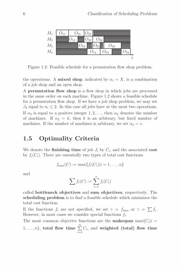
Figure 1.2: Feasible schedule for a permutation flow shop problem.
the operations. A mixed shop, indicated by α1 = X, is a combinationof a job shop and an open shop.
A permutation flow shop is a flow shop in which jobs are processedin the same order on each machine. Figure 1.2 shows a feasible schedulefor a permutation flow shop. If we have a job shop problem, we may setβ4 equal to ni ≤ 2. In this case all jobs have at the most two operations.
If α2 is equal to a positive integer 1, 2, . . ., then α2 denotes the numberof machines. If α2 = k, then k is an arbitrary, but fixed number ofmachines. If the number of machines is arbitrary, we set α2 = ◦.
1.5 Optimality Criteria
We denote the finishing time of job Ji by Ci, and the associated costby fi(Ci). There are essentially two types of total cost functions
fmax(C) := max{fi(Ci)|i = 1, . . . , n}and
∑fi(C) :=
n∑
i=1
fi(Ci)
called bottleneck objectives and sum objectives, respectively. Thescheduling problem is to find a feasible schedule which minimizes thetotal cost function.
If the functions fi are not specified, we set γ = fmax or γ =∑
fi.However, in most cases we consider special functions fi.
The most common objective functions are the makespan max{Ci|i =
1, . . . , n}, total flow timen∑
i=1
Ci, and weighted (total) flow time

1.6. Examples 7
n∑
i=1
wiCi. In these cases we write γ = Cmax, γ =∑
Ci, and γ =∑
wiCi,
respectively.
Other objective functions depend on due dates di which are associatedwith jobs Ji. We define for each job Ji:
Li := Ci − di lateness
Ei := max{0, di − Ci} earliness
Ti := max{0, Ci − di} tardiness
Di := |Ci − di| absolute deviation
Si := (Ci − di)2 squared deviation
Ui :=
{0 if Ci ≤ di
1 otherwiseunit penalty.
With each of these functions Gi we get four possible objectives γ =max Gi, max wiGi,
∑Gi,
∑wiGi. The most important bottleneck ob-
jective besides Cmax is maximum lateness Lmax :=n
maxi=1
Li. Other ob-
jective functions which are widely used are∑
Ti,∑
wiTi,∑
Ui,∑
wiUi,∑Di,
∑wiDi,
∑Si,
∑wiSi,
∑Ei,
∑wiEi. Linear combinations of
these objective functions are also considered.
An objective function which is nondecreasing with respect to all variablesCi is called regular. Functions involving Ei, Di, Si are not regular. Theother functions defined so far are regular.
A schedule is called active if it is not possible to schedule jobs (op-erations) earlier without violating some constraint. A schedule is calledsemiactive if no job (operation) can be processed earlier without chang-ing the processing order or violating the constraints.
1.6 Examples
To illustrate the three-field notation α|β|γ we present some examples. Ineach case we will describe the problem. Furthermore, we will specify an
8 Classification of Scheduling Problems
instance and present a feasible schedule for the instance in the form of aGantt chart.
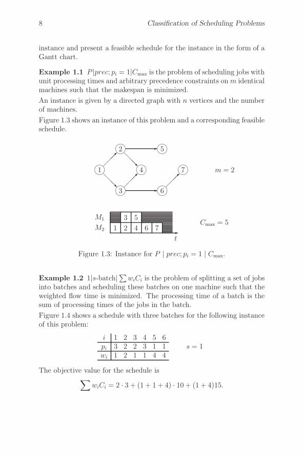
Example 1.1 P |prec; pi = 1|Cmax is the problem of scheduling jobs withunit processing times and arbitrary precedence constraints on m identicalmachines such that the makespan is minimized.
An instance is given by a directed graph with n vertices and the numberof machines.
Figure 1.3 shows an instance of this problem and a corresponding feasibleschedule.
��
��
3��
��
6
��
��
1��
��
4��
��
7
��
��
2��
��
5
m = 2
�
�
����
����
����
����
����
�M2
M1
t
1 2 4 6 7
3 5Cmax = 5
Figure 1.3: Instance for P | prec; pi = 1 | Cmax.
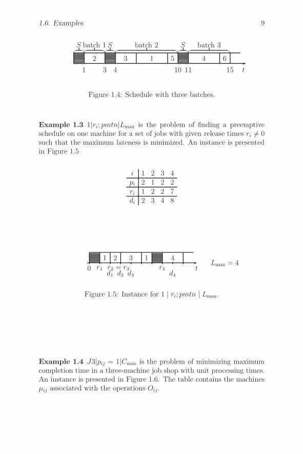
Example 1.2 1|s-batch|∑wiCi is the problem of splitting a set of jobsinto batches and scheduling these batches on one machine such that theweighted flow time is minimized. The processing time of a batch is thesum of processing times of the jobs in the batch.
Figure 1.4 shows a schedule with three batches for the following instanceof this problem:
i 1 2 3 4 5 6pi 3 2 2 3 1 1 s = 1wi 1 2 1 1 4 4
The objective value for the schedule is∑
wiCi = 2 · 3 + (1 + 1 + 4) · 10 + (1 + 4)15.
1.6. Examples 9
�1 3 4 10 11 15 t
2 3 1 5 4 6
� �S
� �batch 1
� �S
� �batch 2
� �S
� �batch 3
Figure 1.4: Schedule with three batches.
Example 1.3 1|ri; pmtn|Lmax is the problem of finding a preemptiveschedule on one machine for a set of jobs with given release times ri �= 0such that the maximum lateness is minimized. An instance is presentedin Figure 1.5
i 1 2 3 4pi 2 1 2 2ri 1 2 2 7di 2 3 4 8
�1 2 3 1 4Lmax = 4
0 r1 r2 = r3 r4d1 d2 d3 d4
t
Figure 1.5: Instance for 1 | ri; pmtn | Lmax.
Example 1.4 J3|pij = 1|Cmax is the problem of minimizing maximumcompletion time in a three-machine job shop with unit processing times.An instance is presented in Figure 1.6. The table contains the machinesμij associated with the operations Oij.
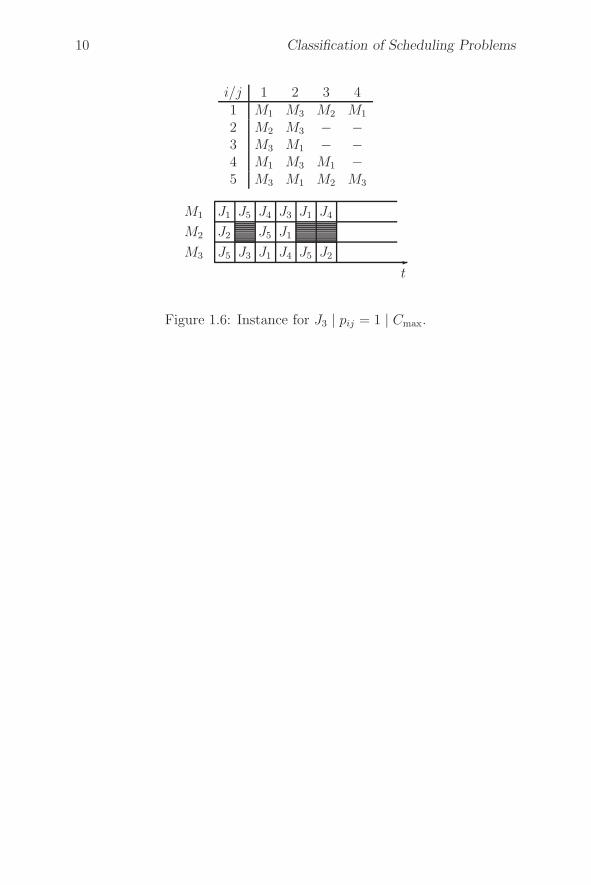
10 Classification of Scheduling Problems
i/j 1 2 3 41 M1 M3 M2 M1
2 M2 M3 − −3 M3 M1 − −4 M1 M3 M1 −5 M3 M1 M2 M3
�M3
M2
M1
J5 J3 J1 J4 J5 J2
J2 J5 J1
J1 J5 J4 J3 J1 J4
t
Figure 1.6: Instance for J3 | pij = 1 | Cmax.

Chapter 2
Some Problems inCombinatorial Optimization
Some scheduling problems can be solved efficiently by reducing themto well-known combinatorial optimization problems, such as linear pro-grams, maximum flow problems, or transportation problems. Others canbe solved by using standard techniques, such as dynamic programmingand branch-and-bound methods. In this chapter we will give a brief sur-vey of these combinatorial optimization problems. We will also discusssome of the methods.
2.1 Linear and Integer Programming
A linear program is an optimization problem of the form
minimize z(x) = c1x1 + . . . + cnxn (2.1)
subject to (s.t.)
a11x1 + . . . + a1nxn ≥ b1
... (2.2)
am1x1 + . . . + amnxn ≥ bm
xi ≥ 0 for i = 1, . . . , n.
A vector x = (x1, . . . , xn) satisfying (2.2) is called a feasible solution.The problem is to find a feasible solution which minimizes (2.1). A linear
12 Some Problems in Combinatorial Optimization
program that has a feasible solution is called feasible. A linear programmay also be unbounded, which means that for each real number Kthere exists a feasible solution x with z(x) < K. Linear programs whichhave a feasible solution and are not unbounded always have an optimalsolution.
The most popular method for solving linear programs is the simplexalgorithm. It is an iterative procedure which finds an optimal solutionor detects infeasibility or unboundedness after a finite number of steps.Although the number of iteration steps may be exponential, the simplexalgorithm is very efficient in practice.
An integer linear program is a linear program in which all variablesxi are restricted to integers. If the variables xi can only take the values0 or 1, then the corresponding integer linear program is called a binarylinear program. If in a linear program only some variables are restrictedto integers, then we have a mixed integer linear program.
Many books exist on linear and integer programming. The interestedreader is referred to the more recent books by Chvatal [67], Nemhauser& Wolsey [175], and Schrijver [182].
2.2 Transshipment Problems
The transshipment problem is a special linear program. Let G = (V, A)be a directed graph with vertex set V = {1, . . . , n} and arc set A. Arcsare denoted by (i, j) with i, j ∈ V . A transshipment problem is givenby
minimize∑
(i,j)∈A
cijxij
s.t.∑
j(j,i)∈A
xji −∑
j(i,j)∈A
xij = bi for all i ∈ V (2.3)
lij ≤ xij ≤ uij for all (i, j) ∈ A. (2.4)
Graph G may be interpreted as a transportation network. The bi-valueis the demand for or the supply of some goods in vertex i. If bi > 0,we have a demand of bi units. If bi < 0, we have a supply of −bi units.
2.3. The Maximum Flow Problem 13
Notice that either the demand in i or the supply in i may be zero. Thegoods may be transported along the arcs. cij are the costs of shippingone unit of the goods along arc (i, j). xij denotes the number of unitsto be shipped from vertex i to vertex j. Equations (2.3) are balancingequations: in each vertex i, the amount shipped to i plus the supplyin i must be equal to the amount shipped away from i, or the amountshipped to i must be equal to the demand plus the amount shipped away.By (2.4) the amount shipped along (i, j) is bounded from below by lijand from above by uij. We may set lij = −∞ or uij = ∞, which meansthat there are no bounds. A vector x = (xij) satisfying (2.3) and (2.4)is called a feasible flow. The problem is to find a feasible flow whichminimizes the total transportation costs. We assume that
n∑
i=1
bi = 0, (2.5)
i.e. the total supply is equal to the total demand. A transshipmentproblem with bi = 0 for all i ∈ V is called a circulation problem .
Standard algorithms for the transshipment problem are the network sim-plex method (Dantzig [74]), and the out-of-kilter algorithm, which wasdeveloped independently by Yakovleva [207], Minty [168], and Fulkerson[94]. Both methods have the property of calculating an integral flow ifall finite bi, lij, and uij are integers. These algorithms and other morerecent algorithms can be found in a book by Ahuja et al. [6]. Complex-ity results for the transshipment problem and the equivalent circulationproblem will be discussed in Chapter 3. In the next two sections wediscuss special transshipment problems.
2.3 The Maximum Flow Problem
A flow graph G = (V, A, s, t) is a directed graph (V, A) with a sourcevertex s, and a sink vertex t. Associated with each arc (i, j) ∈ A isa nonnegative capacity uij, which may also be ∞. The maximum flowproblem is to send as much flow as possible from the source to the sinkwithout violating capacity constraints in the arcs. For this problem, we
14 Some Problems in Combinatorial Optimization
have the linear programming formulation
maximize vs.t.
∑
j(j,i)∈A
xji −∑
j(i,j)∈A
xij =
⎧⎨
⎩
−v for i = sv for i = t0 otherwise
0 ≤ xij ≤ uij for all (i, j) ∈ A.
The maximum flow problem may be interpreted as a transshipment prob-lem with exactly one supply vertex s and exactly one demand vertex t,and variable supply (demand) v which should be as large as possible. Itcan be formulated as a minimum cost circulation problem by adding anarc (t, s) with uts = ∞ and cost cts = −1. The cost of all other arcs(i, j) ∈ A should be equal to zero.
The first algorithm for the maximum flow problem was the augment-ing path algorithm of Ford and Fulkerson [91]. Other algorithms andtheir complexity are listed in Chapter 3. All these algorithms provide anoptimal solution which is integral if all capacities are integers.
2.4 Bipartite Matching Problems
The bipartite maximum cardinality matching problem is a specialmaximum flow problem which can be formulated as follows:
Consider a bipartite graph, i.e. a graph G = (V1 ∪ V2, A) where thevertex set V is the union of two disjoint sets V1 and V2, and A ⊆ V1 ×V2.A matching is a set M ⊆ A of arcs such that no two arcs in M havea common vertex, i.e. if (i, j), (i′, j′) ∈ M with (i, j) �= (i′, j′), theni �= i′ and j �= j′. The problem is to find a matching M with maximalcardinality.
The maximum cardinality bipartite matching problem may be reducedto a maximum flow problem by adding a source s with arcs (s, i), i ∈ V1
and a sink t with arcs (j, t), j ∈ V2 to the bipartite graph. Furthermore,we associate unit capacities with all arcs in the augmented network. Itis not difficult to see that a maximal integer flow from s to t correspondswith a maximum cardinality matching M . This matching is given by allarcs (i, j) ∈ A carrying unit flow.
The maximum cardinality bipartite matching problem can be solved in
2.4. Bipartite Matching Problems 15
O(min{|V1|, |V2|} · |A|) steps by maximum flow calculations. Hopcroft
and Karp [114] developed an O(n12 r) (see Section 3.1 for a definition of
this O-notation) algorithm for the case n = |V1| ≤ |V2| and r = |A|.Now, consider a bipartite graph G = (V1 ∪ V2, A) with |V1| ≥ |V2| = m.For each j ∈ V2 let P (j) be the set of predecessors of j, i.e. P (j) ={i ∈ V1 | (i, j) ∈ A}. Clearly, m is an upper bound for the cardinalityof a maximal cardinality matching in G. The following theorem due toHall [110] gives necessary and sufficient conditions for the existence of amatching with cardinality m.
Theorem 2.1 Let G = (V1 ∪ V2, A) be a bipartite graph with |V1| ≥|V2| = m. Then there exists in G a matching with cardinality m if andonly if
|⋃
i∈N
P (i) |≥| N | for all N ⊆ V2.
�
Next we will show how to use this theorem and network flow theory tosolve an open shop problem.
O | pmtn | Cmax
This preemptive open shop problem can be formulated in the follow-ing way: n jobs J1, . . . , Jn are given to be processed on m machinesM1, . . . , Mm. Each job Ji consists of m operations Oij (j = 1, . . . , m)where Oij must be processed on machine Mj for pij time units. Preemp-tion is allowed and the order in which the operations of Ji are processedis arbitrary. The only restriction is that a machine cannot process twojobs simultaneously and a job cannot be processed by two machines atthe same time. We have to find a schedule with minimal makespan.
For each machine Mj(j = 1, . . . , m) and each job Ji(i = 1, . . . , n) define
Tj :=n∑
i=1
pij and Li :=m∑
j=1
pij.
Tj is the total time needed on machine Mj , and Li is the length of jobJi.
Clearly,
T = max{ nmaxi=1
Li,m
maxj=1
Tj} (2.6)
16 Some Problems in Combinatorial Optimization
is a lower bound for the Cmax-value.
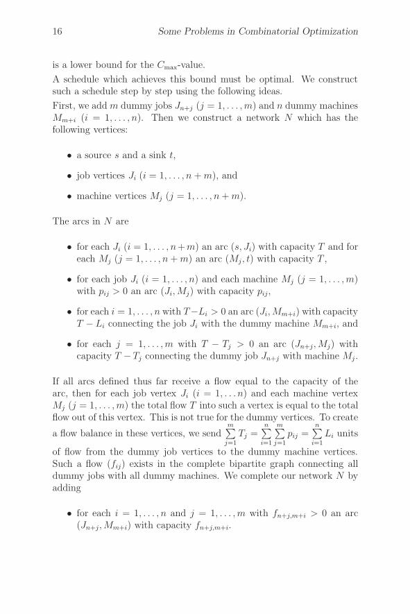
A schedule which achieves this bound must be optimal. We constructsuch a schedule step by step using the following ideas.
First, we add m dummy jobs Jn+j (j = 1, . . . , m) and n dummy machinesMm+i (i = 1, . . . , n). Then we construct a network N which has thefollowing vertices:
• a source s and a sink t,
• job vertices Ji (i = 1, . . . , n + m), and
• machine vertices Mj (j = 1, . . . , n + m).
The arcs in N are
• for each Ji (i = 1, . . . , n+m) an arc (s, Ji) with capacity T and foreach Mj (j = 1, . . . , n + m) an arc (Mj , t) with capacity T ,
• for each job Ji (i = 1, . . . , n) and each machine Mj (j = 1, . . . , m)with pij > 0 an arc (Ji, Mj) with capacity pij,
• for each i = 1, . . . , n with T−Li > 0 an arc (Ji, Mm+i) with capacityT − Li connecting the job Ji with the dummy machine Mm+i, and
• for each j = 1, . . . , m with T − Tj > 0 an arc (Jn+j, Mj) withcapacity T −Tj connecting the dummy job Jn+j with machine Mj .
If all arcs defined thus far receive a flow equal to the capacity of thearc, then for each job vertex Ji (i = 1, . . . n) and each machine vertexMj (j = 1, . . . , m) the total flow T into such a vertex is equal to the totalflow out of this vertex. This is not true for the dummy vertices. To create
a flow balance in these vertices, we sendm∑
j=1
Tj =n∑
i=1
m∑
j=1
pij =n∑
i=1
Li units
of flow from the dummy job vertices to the dummy machine vertices.Such a flow (fij) exists in the complete bipartite graph connecting alldummy jobs with all dummy machines. We complete our network N byadding
• for each i = 1, . . . , n and j = 1, . . . , m with fn+j,m+i > 0 an arc(Jn+j, Mm+i) with capacity fn+j,m+i.
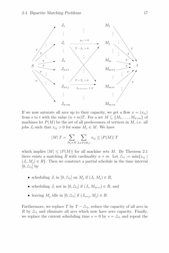
2.4. Bipartite Matching Problems 17
M1
Mj
Mm
Mm+n
Ji
Jn
Jn+m
S t
...
...
...
......
...
...
...
...
...
...
...
...
...
...
...
...
...
...
pij > 0
fn+j,m+i > 0
...
T − Li > 0
T − Tj > 0T
T T
T
T
T
T
T
T
T
T
T
Jn+j Mm+i
Jn+1
J1
Mm+1
If we now saturate all arcs up to their capacity, we get a flow x = (xij)from s to t with the value (n + m)T . For a set M ⊆ {M1, . . . , Mn+m} ofmachines let P (M) be the set of all predecessors of vertices in M , i.e. alljobs Ji such that xij > 0 for some Mj ∈ M . We have
|M | T =∑
Mj∈M
∑
Ji∈P (Mj)
xij ≤ |P (M)| T
which implies |M | ≤ |P (M)| for all machine sets M . By Theorem 2.1there exists a matching R with cardinality n + m. Let �1 := min{xij |(Ji, Mj) ∈ R}. Then we construct a partial schedule in the time interval[0,�1] by
• scheduling Ji in [0,�1] on Mj if (Ji, Mj) ∈ R,
• scheduling Ji not in [0,�1] if (Ji, Mm+i) ∈ R, and
• leaving Mj idle in [0,�1] if (Jn+j, Mj) ∈ R.
Furthermore, we replace T by T −�1, reduce the capacity of all arcs inR by �1 and eliminate all arcs which now have zero capacity. Finally,we replace the current scheduling time s = 0 by s = �1 and repeat the

18 Some Problems in Combinatorial Optimization
process to schedule the next interval [s, s+�2], etc. The whole procedurestops if T = 0, providing a schedule of length T which is optimal.
After each step at least one arc is eliminated. Thus, if r is the numberof operations Oij with pij > 0, then we have at the most O(r) steps (weassume that r ≥ n and r ≥ m). A matching can be calculated in O(r(n+m)0.5) steps (Hopcroft and Karp [114]). Thus, the total complexity isO(r2(n+m)0.5). The complexity can be reduced to O(r2) due to the factthat in each step the matching from the previous step may be used tocalculate the new matching.
2.5 The Assignment Problem
Consider the complete bipartite graph, G = (V1 ∪ V2, V1 × V2) withV1 = {v1, . . . , vn} and V2 = {w1, . . . , wm}. Assume w.l.o.g. that n ≤ m.Associated with each arc (vi, wj) there is a real number cij. An assign-ment is given by a one-to-one mapping ϕ : V1 → V2. The assignmentproblem is to find an assignment ϕ such that
∑
v∈V1
cvϕ(v)
is minimized.
We may represent the assignment problem by the n×m-matrix C = (cij)and formulate it as a linear program with 0-1-variables xij :
minimizen∑
i=1
m∑
j=1
cijxij (2.7)
s.t.m∑
j=1
xij = 1 i = 1, . . . , n (2.8)
n∑
i=1
xij ≤ 1 j = 1, . . . , m (2.9)
xij ∈ {0, 1} i = 1, . . . , n; j = 1, . . . , m. (2.10)
Here xij = 1 if and only if vi is assigned to wj . Due to (2.8) and (2.9)each vi ∈ V1 is assigned to a unique element in V2, and each wj ∈ V2 isinvolved in at the most one assignment.
The assignment problem may be reduced to the transshipment problemby adding a source vertex s with arcs (s, vi), vi ∈ V1 and a sink t with
2.5. The Assignment Problem 19
arcs (wj, t), wj ∈ V2 to the bipartite graph. All costs of the new arcsare defined as zero, and the lower and upper capacities are zero and one,respectively. Finally, we let s be the only supply node, and t the onlydemand node. Both supply and demand are equal to n.
Any integer solution provided by an algorithm which solves this trans-shipment problem is feasible for (2.7) to (2.10). Thus, we may solve theassignment problem by solving the corresponding transshipment prob-lem. The first algorithm for the assignment problem was the Hungarianmethod introduced by Kuhn [132]. It solves the assignment problem inO(n2m) steps by exploiting its special structure.
Next we show that single machine problems with unit processing timescan be reduced to assignment problems.
1|ri;pi = 1|∑ fi
To solve problem 1|ri; pi = 1|∑ fi, where the fi are monotone functionsof the finishing times Ci of jobs i = 1, . . . , n, we have to assign to the jobsn different time slots. If we assign time slot t to job i, the correspondingcosts are fi(t + 1). Next we will show that at the most n time slots areto be considered. Thus, the corresponding assignment problem can besolved in O(n3) time.
Because functions fi are monotone nondecreasing, the jobs should bescheduled as early as possible. The n earliest time slots ti for schedulingall n jobs may be calculated using the following algorithm, in which weassume that the jobs are enumerated in such a way that
r1 ≤ r2 ≤ . . . ≤ rn.
Algorithm Time Slots1. t1 := r1;2. FOR i := 2 TO n DO
ti := max{ri, ti−1 + 1}
There exists an optimal schedule which occupies all of the time slots ti(i =1, . . . , n). To see this, consider an optimal schedule S which occupies timeslots t1, . . . , tj where j < n is maximal. According to the construction ofthe ti-values, tj+1 is the next time slot in which a job can be scheduled.If time slot tj+1 in S is empty, a job scheduled later in S can be movedto tj+1 without increasing the objective value. Thus, the new schedule is
20 Some Problems in Combinatorial Optimization
optimal, too, and we have a contradiction to the maximality of j. Noticethat the schedule created this way defines time intervals Iν in which themachine is busy. These intervals are separated by idle periods of themachine.
The complete bipartite graph which defines the corresponding assignmentproblem is given by
V1 = {1, . . . , n}V2 = {t1, . . . , tn}.
For the cij-values we choose
cij =
{fi(tj + 1) if ri ≤ tj∞ otherwise.
Next we consider an assignment problem which has a very simple solu-tion.
Let V1 = {v1, . . . , vn} and V2 = {w1, . . . , wm} and consider the corre-sponding complete bipartite graph G = (V1 ∪ V2, V1 × V2). Then the cor-responding assignment problem is specified by a n × m array C = (cij).C is called a Monge array if
cik + cjl ≤ cil + cjk for all i < j and k < l. (2.11)
Theorem 2.2 Let (cij) be a Monge array of dimension n × m wheren ≤ m. Furthermore, let cij ≤ cik for all i and j < k. Then
xij =
{1 if i = j0 otherwise
is an optimal solution for the assignment problem.
Proof: Let y = (yij) be an optimal solution of the assignment problemwith yνν = 1 for ν = 1, . . . , i where i is as large as possible. Assume thati < n (if i = n we have finished). Because yi+1,i+1 = 0, there exists anindex l > i + 1 with yi+1,l = 1. Now we consider two cases.
Case 1: There exists an index j > i + 1 with yj,i+1 = 1.
(2.11) yieldsci+1,i+1 + cjl ≤ ci+1,l + cj,i+1.
Thus, if we set
yrs =
⎧⎨
⎩
1 if r = s = i + 1 or r = j, s = l0 if r = i + 1, s = l or r = j, s = i + 1yrs otherwise
2.5. The Assignment Problem 21
then yrs is again an optimal solution of the assignment problem, contra-dicting the maximality of i.
Case 2: yν,i+1 = 0 for all ν ≥ i + 1.
There exists an l > i + 1 with yi+1,l = 1. Furthermore, ci+1,i+1 ≤ ci+1,l.Thus, yrs defined by
yrs =
⎧⎨
⎩
1 if r = s = i + 10 if r = i + 1, s = lyrs otherwise
is again an optimal solution, contradicting the maximality of i. �
Corollary 2.3 Let C = (cij) be a Monge array of dimension n×n. Then
xij =
{1 if i = j0 otherwise
is an optimal solution for the assignment problem.
Proof: If m = n, then all wj ∈ V2 must be assigned. Thus, we only haveCase 1 and therefore we do not need the rows of C to be monotone.
�
Corollary 2.4 Let (ai) and (bj) be arrays of real numbers a1 ≥ a2 ≥. . . ≥ an ≥ 0 and 0 ≤ b1 ≤ b2 ≤ . . . ≤ bm where n ≤ m. Then theassignment problem given by the array
C = (cij)n×m with cij = aibj
has an optimal solution given by
xij =
{1 if i = j0 otherwise.
Proof: We have cij = aibj ≤ aibk = cik for all i and j < k. Furthermore,C is a Monge array because if i < j and k < l, then ai ≥ aj and bk ≤ bl.Thus,
aibl + ajbk − aibk − ajbl = (ai − aj)(bl − bk) ≥ 0,
i.e.aibk + ajbl ≤ aibl + ajbk.
�
Due to Corollary 2.4 we may efficiently solve the following schedulingproblem.
22 Some Problems in Combinatorial Optimization
P||∑Ci
n jobs i = 1, . . . , n with processing times pi are to be processed on midentical parallel machines j = 0, . . . , m− 1 to minimize mean flow time.There are no precedence constraints between the jobs.
A schedule S is given by a partition of the set of jobs into m disjointsets I0, . . . , Im−1 and for each Ij, a sequence of the jobs in Ij . Assumethat Ij contains nj elements and that j(i)(i = 1, . . . , nj) is the job to bescheduled in position nj − i+1 on machine Mj . We assume that the jobsin Ij are scheduled on Mj starting at zero time without idle times. Thenthe value of the objective function is
n∑
i=1
Ci =m−1∑
j=0
nj∑
i=1
i · pj(i). (2.12)
Now consider the assignment problem with cik = aibk where ai = pi fori = 1, . . . , n, and bk = � k
m 1 for k = 1, . . . , n. A schedule S corresponds
with an assignment with objective value (2.12). In this schedule job i isassigned to the bk-last position on a machine if i is assigned to k.
If we assume thatp1 ≥ p2 ≥ . . . ≥ pn,
then we get an optimal assignment by assigning ai = pi to bi(i =1, . . . , n). This assignment corresponds with a schedule in which jobi is scheduled on machine (i−1)mod(m). Furthermore, on each machinethe jobs are scheduled according to nondecreasing processing times. Sucha schedule can be calculated in O(n log n)-time, which is the time to sortthe jobs according to their processing times.
2.6 Arc Coloring of Bipartite Graphs
Consider again a directed bipartite graph G = (V1 ∪ V2, A) with V1 ={v1, . . . , vn} and V2 = {w1, . . . , wm}. (Arc) coloring is the assignmentof a color to each arc of G such that arcs incident to any vertex (i.e.arcs (vi, wk), (vi, wl) with k �= l or arcs (vk, wj), (vl, wj) with l �= k) havedistinct colors. Minimum coloring uses as few colors as possible. Theproblem we address in this section is to find a minimum coloring for abipartite graph.
1�x is the smallest integer greater or equal to x
2.6. Arc Coloring of Bipartite Graphs 23
For each v ∈ V1 ∪ V2 let deg(v) be the number of arcs incident with v(i.e. arcs of the form (vi, wk) if v = vi ∈ V1 or arcs of the form (vk, wi)if v = wi ∈ V2). deg(v) is called the degree of node v. The maximumdegree
� := max{deg(v) | v ∈ V1 ∪ V2}of G is a lower bound for the number of colors needed for coloring. Next,we describe an algorithm to construct a coloring using � colors.
It is convenient to represent G by its adjacency matrix A = (aij) where
aij =
{1 if (vi, wj) ∈ A0 otherwise.
By definition of � we have
m∑
j=1
aij ≤ � for all i = 1, . . . , n (2.13)
andn∑
i=1
aij ≤ � for all j = 1, . . . , m. (2.14)
Entries (i, j) with aij = 1 are called occupied cells. We have to assigncolors c ∈ {1, . . . ,�} to the occupied cells in such a way that the samecolor is not assigned twice in any row or column of A. This is done byvisiting the occupied cells of A row by row from left to right. Whenvisiting the occupied cell (i, j) a color c not yet assigned in column j isassigned to (i, j). If c is assigned to another cell in row i, say to (i, j∗),then there exists a color c not yet assigned in row i and we can replacethe assignment c of (i, j∗) by c. If again a second cell (i∗, j∗) in column j∗
also has the assignment c, we replace this assignment by c, etc. We stopthis process when there is no remaining conflict. If the partial assignmentbefore coloring (i, j) was feasible (i.e. no color appears twice in any rowor column) then this conflict resolution procedure ends after at the mostn steps with feasible coloring. We will prove this after giving a moreprecise description of the algorithm.
Algorithm Assignment1. For i := 1 TO n DO2. While in row i there exists an uncolored occupied cell DO
BEGIN
24 Some Problems in Combinatorial Optimization
3. Find a first uncolored occupied cell (i, j);4. Find a color c not assigned in column j;5. Assign c to (i, j);6. IF c is assigned twice in row i THEN
BEGIN7. Find a color c that is not assigned in row i;8. Conflict (i, j, c, c)
ENDEND
Conflict(i, j, c, c) is a conflict resolution procedure which applies to asituation in which c is assigned to cell (i, j). It is convenient to writeConflict(i, j, c, c) as a recursive procedure.
Procedure Conflict (i, j, c, c)1. IF c is assigned to some cell (i, j∗) with j∗ �= j
THEN assign c to (i, j∗)2. ELSE RETURN;3. IF c is assigned to some cell (i∗, j∗) with i∗ �= i THEN
BEGIN4. Assign c to (i∗, j∗);5. Conflict (i∗, j∗, c, c)
END6. ELSE RETURN
Due to (2.14), a color c can always be found in Step 4 of AlgorithmAssignment. Furthermore, due to (2.13), in Step 7 there exists a color cwhich is not yet assigned to a cell in row i. Next, if there is a c-conflictin column j∗ due to the fact that c is replaced by c, then c cannotappear in this column again if we assume that previous conflicts havebeen resolved. Thus, it is correct to resolve the c-conflict by replacingthe other c-value by c (Step 4 of Procedure Conflict(i, j, c, c)). Similarly,Step 1 of Procedure Conflict(i∗, j∗, c, c)) is correct.
Finally, we claim that the Procedure Conflict terminates after at themost n recursive calls. To prove this, it is sufficient to show that if colorc of cell (i, j∗) is replaced by c, then it is impossible to return to a cellin row i again. The only way to do so is by having a c-conflict in somecolumn s where c is the color of (i, s) and (k, s) with i �= k. Consider asituation where this happens the first time. We must have s = j∗ because
2.6. Arc Coloring of Bipartite Graphs 25
otherwise c is the color of two different cells in row i, which contradictsthe correctness of previous steps. Because s = j∗ we must have visitedcolumn j∗ twice, the first time when moving from cell (i, j∗) to some cell(i∗, j∗). (i∗, j∗) cannot be visited a second time due to the assumptionthat row i is the first row which is revisited. Thus, when visiting columnj∗ a second time we visit some cell (k, j∗) which is different from (i, j∗)and (i∗, j∗). At that time cells (i∗, j∗) and (k, j∗) are colored c, whichagain contradicts the fact that the algorithm maintains feasibility.
Next we show that Algorithm Assignment has a running time of O((n +�)e), where e is the number of occupied cells.
We use a data structure with the following components:
• An n ×�-array J-INDEX where
J-INDEX(i, l)=
{j if (i, j) is the l-th occupied cell in row i0 if there are less than l occupied cells in row i.
• For each column j, a list COLOR(j) containing all color numbersassigned to cells in column j in increasing order.
• For each row i, a double linked list FREE(i) containing all colorsnot yet assigned to cells in row i. Moreover, we use a �-vector ofpointers to this list such that deletion of a color can be done inconstant time.
• An �× m-array I-INDEX where
I-INDEX(c, j) =
{i if color c is assigned to cell (i, j)0 if no cell in column j is assigned to c.
Using the array J-INDEX Step 3 of Algorithm Assignment can be donein constant time. In Step 4 color c is found in O(�) time using thelist COLOR(j) because this list contains at the most � elements. Step5 is done by updating COLOR(j), FREE(i), and I-INDEX in O(�)steps. Step 6 is done in O(�)-time using the arrays J-INDEX and I-INDEX. Furthermore, the color c in Step 7 is found in constant timeusing FREE(i).
During the recursive processing of the Procedure Conflict, the list FREEis not changed. Moreover, the list COLOR(j) only changes if a columnnot already containing color c is found (in this case Conflict terminates).
26 Some Problems in Combinatorial Optimization
A cell (i∗, j∗) already colored by c (Step 3 of Conflict) can be foundin constant time using the array I-INDEX. Because each change of thearray I-INDEX only needs a constant amount of time and Conflict alwaysterminates after n steps, we get an overall complexity of O((n + �)e).
Another more sophisticated algorithm for solving the arc coloring prob-lem for bipartite graphs can be found in Gabow & Kariv [95]. It improvesthe complexity to O(e log2(n + m)).
2.7 Shortest Path Problems and Dynamic
Programming
Another method for solving certain scheduling problems is dynamic pro-gramming, which enumerates in an intelligent way all possible solutions.During the enumeration process, schedules which cannot be optimal areeliminated. We shall explain the method by solving the following schedul-ing problems:
1||∑wiUi
Given n jobs i = 1, . . . , n with processing times pi and due dates di,
we have to sequence these jobs such thatn∑
i=1
wiUi is minimized where
wi ≥ 0 for i = 1, . . . , n. Assume that the jobs are enumerated accordingto nondecreasing due dates:
d1 ≤ d2 ≤ . . . ≤ dn. (2.15)
Then there exists an optimal schedule given by a sequence of the form
i1, i2, . . . , is, is+1, . . . , in
where jobs i1 < i2 < . . . < is are on time and jobs is+1, . . . , in arelate. This can be shown easily by applying the following interchangearguments. If a job i is late, we may put i at the end of the schedulewithout increasing the objective function. If i and j are early jobs withdi ≤ dj such that i is not scheduled before j, then we may shift the blockof all jobs scheduled between j and i jointly with i to the left by pj timeunits and schedule j immediately after this block. Because i was not lateand di ≤ dj this creates no late job.
2.7. Shortest Path Problems and Dynamic Programming 27
To solve the problem, we calculate recursively for t = 0, 1, . . . , T :=n∑
i=1
pi
and j = 1, . . . , n the minimum criterion value Fj(t) for the first j jobs,subject to the constraint that the total processing time of the on-timejobs is at the most t. If 0 ≤ t ≤ dj and job j is on time in a schedulewhich corresponds with Fj(t), then Fj(t) = Fj−1(t − pj). OtherwiseFj(t) = Fj−1(t) + wj . If t > dj, then Fj(t) = Fj(dj) because all jobs1, 2, . . . , j finishing later than dj ≥ . . . ≥ d1 are late. Thus, for j =1, . . . , n we have the recursion
Fj(t) =
{min{Fj−1(t − pj), Fj−1(t) + wj} for 0 ≤ t ≤ dj
Fj(dj) for dj < t < T
with Fj(t) = ∞ for t < 0, j = 0, . . . , n and F0(t) = 0 for t ≥ 0.
Notice that Fn(dn) is the optimal solution to the problem.
The following algorithm calculates all values Fj(t) for j = 1, . . . , n andt = 0, . . . , dj. We assume that the jobs are enumerated such that (2.15)holds. pmax denotes the largest processing time.
Algorithm 1||∑wiUi
1. FOR t := −pmax TO -1 DO2. FOR j := 0 TO n DO
Fj(t) := ∞;3. FOR t := 0 TO T DO F0(t) := 0;4. FOR j := 1 TO n DO
BEGIN5. FOR t := 0 TO dj DO6. IFFj−1(t) + wj < Fj−1(t − pj) THEN Fj(t) := Fj−1(t) + wj
ELSE Fj(t) := Fj−1(t − pj);7. FOR t := dj + 1 TO T DO
Fj(t) := Fj(dj)END
The computational time of this algorithm is bounded by O(nn∑
i=1
pi).
To calculate an optimal schedule it is sufficient to calculate the set L oflate jobs in an optimal schedule. Given all Fj(t)-values this can be doneby the following algorithm.
28 Some Problems in Combinatorial Optimization
Algorithm Backward Calculationt := dn; L := φFOR j := n DOWN TO 1 DOBEGINt := min{t, dj};IF Fj(t) = Fj−1(t) + wj THEN L := L ∪ {j}ELSE t := t − pj
END
P||∑wiCi
n jobs 1, . . . , n are to be processed on m identical parallel machines such
thatn∑
i=1
wiCi is minimized. All wi are assumed to be positive.
We first consider the problem 1||∑wiCi. An optimal solution of thisone machine problem is obtained if we sequence the jobs according tonondecreasing ratios pi/wi. The following interchange argument provesthis. Let j be a job which is scheduled immediately before job i. If weinterchange i and j, the objective function changes by
wipi + wj(pi + pj) − wjpj − wi(pi + pj) = wjpi − wipj
which is nonpositive if and only if pi/wi ≤ pj/wj. Thus, the objectivefunction does not increase if i and j are interchanged.
A consequence of this result is that in an optimal solution of problemP ||∑wiCi, jobs to be processed on the same machine must be processedin order of nondecreasing ratios pi/wi. Therefore we assume that all jobsare indexed such that
p1/w1 ≤ p2/w2 ≤ . . . ≤ pn/wn.
Let T be an upper bound on the completion time of any job in an optimalschedule. Define Fi(t1, . . . , tm) to be the minimum cost of a schedulewithout idle time for jobs 1, . . . , i subject to the constraint that the lastjob on Mj is completed at time tj for j = 1, . . . , m. Then
Fi(t1, . . . , tm) =m
minj=1
{witj + Fi−1(t1, . . . , tj−1, tj − pi, tj+1, . . . , tm)}.(2.16)
2.7. Shortest Path Problems and Dynamic Programming 29
The initial conditions are
F0(t1, . . . , tm) =
{0 if tj = 0 for j = 1, . . . , m∞ otherwise .
(2.17)
Starting with (2.17), for i = 1, 2, . . . , n the Fi(t)-values are calculated forall t ∈ {1, 2, . . . , T}m in a lexicographic order of the integer vectors t. At∗ ∈ {1, 2, . . . , T}m with Fn(t) minimal provides the optimal value of theobjective function. The computational complexity of this procedure isO(mnT m).
Similar techniques may be used to solve problem Q||∑wjCj .
A Shortest Path Algorithm
Next we will introduce some shortest path problems and show how theseproblems can be solved by dynamic programming.
A network N = (V, A, c) is a directed graph (V, A) together with a func-tion c which associates with each arc (i, j) ∈ A a real number cij . A(directed) path p in N is a sequence of arcs:
p : (i0, i1), (i1, i2, ) . . . , (ir−1, ir).
p is called an s-t–path if i0 = s and ir = t. p is a cycle if i0 = ir. Thelength l(p) of a path p is defined by
l(p) = ci0i1 + ci1i2 + . . . + cir−1ir .
Assume that N = (V, A, c) has no cycles, and |V | = n. Then the verticescan be enumerated by numbers 1, . . . , n such that i < j for all (i, j) ∈ A.Such an enumeration is called topological. If (i, j) is an arc, then i isthe predecessor of j, and j is the successor of i. Using this notion, analgorithm for calculating a topological enumeration α(v)(v ∈ V ) may beformulated as follows.
Algorithm Topological Enumeration1. i := 1;2. WHILE there exists a vertex v ∈ V without predecessor DO
BEGIN3. α(v) := i;4. Eliminate vertex v from V and all arcs (v, j) from A;5. i := i + 1
END6. If V �= ∅ then (V, A) has a cycle and there exists no
topological enumeration.
30 Some Problems in Combinatorial Optimization
Using an appropriate data structure this algorithm can be implementedin such a way that the running time is O(|A|).The problem shortest paths to s is to find for each vertex i ∈ V ashortest i-s–path. We solve this problem for networks without cyclesby a dynamic programming approach. Assume that the vertices areenumerated topologically, and that s = n. If we denote by F (i) thelength of a shortest i-n–path, then we have the recursion
F (n) := 0F (i) = min{cij + F (j)|(i, j) ∈ A, j > i} for i = n − 1, . . . , 1.
(2.18)
This leads to
Algorithm Shortest Path 11. F (n) := 0;2. FOR i := n − 1 DOWN TO 1 DO
BEGIN3. F (i) := ∞;4. FOR j := n DOWN TO i + 15. IF (i, j) ∈ A AND cij + F (j) < F (i) THEN
BEGIN6. F (i) := cij + F (j);7. SUCC(i) := j
ENDEND
SUCC(i) is the successor of i on a shortest path from i to n. Thus,shortest paths can be constructed using this successor array. The runningtime of this algorithm is O(n2).
A Special Structured Network
Now we consider an even more special situation. Let N = (V, A, c) be anetwork with
V = {1, . . . , n}(i, j) ∈ A if and only if i < j (2.19)
cil − cik = r(k, l) + f(i)h(k, l) for i < k < l
2.7. Shortest Path Problems and Dynamic Programming 31
where f(i) is nonincreasing, the values r(k, l) are arbitrary, and h(k, l) ≥0 for all k, l. The last property is called the product property. It isnot difficult to show that an array C = (cij) which satisfies the productproperty also satisfies the Monge property, i.e. is a Monge array.
Next we will develop an O(n)-algorithm for finding shortest paths in anetwork satisfying (2.19). Later we will apply this algorithm to certainbatching problems.
Again we use the recursion formulas (2.18). However, due to the specialproperties of the cij-values the computational complexity decreases fromO(n2) to O(n).
As before, let F (i) be the length of a shortest path from i to n and set
F (i, k) = cik + F (k) for i < k.
Thus, we have
F (i) =n
mink=i+1
F (i, k).
First, we assume that h(k, l) > 0 for all k < l. The relation
F (i, k) ≤ F (i, l) i < k < l (2.20)
stating that k is as good as l as a successor of i is equivalent to
F (k) − F (l) ≤ cil − cik = r(k, l) + f(i)h(k, l)
or
ϑ(k, l) :=F (k) − F (l) − r(k, l)
h(k, l)≤ f(i). (2.21)
Lemma 2.5 Assume that ϑ(k, l) ≤ f(i) for some 1 ≤ i < k < l ≤ n.Then F (j, k) ≤ F (j, l) for all j = 1, . . . , i.
Proof: Because f is monotonic nonincreasing for all j ≤ i, the inequalityϑ(k, l) ≤ f(i) ≤ f(j) holds, which implies F (j, k) ≤ F (j, l). �
Lemma 2.6 Assume that ϑ(i, k) ≤ ϑ(k, l) for some 1 ≤ i < k < l ≤ n.Then for each j = 1, . . . , i we have F (j, i) ≤ F (j, k) or F (j, l) ≤ F (j, k).
Proof: Let 1 ≤ j ≤ i. If ϑ(i, k) ≤ f(j), then F (j, i) ≤ F (j, k). Oth-erwise we have f(j) < ϑ(i, k) ≤ ϑ(k, l), which implies F (j, l) < F (j, k).
�

32 Some Problems in Combinatorial Optimization
An Efficient Shortest Path Algorithm
As Algorithm Shortest Path 1, the efficient algorithm to be developednext calculates the F (i)-values for i = n down to 1. When calculatingF (i) all values F (i+1), . . . , F (n) are known. Furthermore, a queue Q ofthe form
Q : ir, ir−1, . . . , i2, i1
withir < ir−1 < . . . < i2 < i1 (2.22)
is used as a data structure. i1 is the head and ir is the tail of this queue.Vertices not contained in the queue are no longer needed as successorson shortest paths from 1, . . . , i to n. Furthermore, the queue satisfies thefollowing invariance property
ϑ(ir, ir−1) > ϑ(ir−1, ir−2) > . . . > ϑ(i2, i1). (2.23)
In the general iteration step we have to process vertex i and calculateF (i):
If f(i) ≥ ϑ(i2, i1), then by Lemma 2.5 we have F (j, i2) ≤ F (j, i1) forall j ≤ i. Thus, vertex i1 is deleted from Q. We continue with thiselimination process until we reach some t ≥ 1 such that
ϑ(ir, ir−1) > . . . > ϑ(it+1, it) > f(i)
which implies
F (i, iν+1) > F (i, iν) for ν = t, . . . , r − 1.
This implies that it must be a successor of i on a shortest path from i ton, i.e. F (i) = ciit + F (it).
Next we try to append i at the tail of the queue. If ϑ(i, ir) ≤ ϑ(ir, ir−1),then by Lemma 2.6 vertex ir can be eliminated from Q. We continuethis elimination process until we reach some ν with ϑ(i, iν) > ϑ(iν , iν−1).When we now add i at the tail of the queue the invariance property (2.23)remains satisfied.
Details are given by the following algorithm. In this algorithm, head(Q)and tail(Q) denote the head and tail of the queue. In SUCC(i) we storethe successor of i in a shortest path from i to n. Next(j) and previous(j)are the elements immediately after and immediately before, respectively,the element j in the queue when going from head to tail.

2.7. Shortest Path Problems and Dynamic Programming 33
Algorithm Shortest Path 21. Q := {n}; F (n) := 0;2. FOR i := n − 1 DOWN TO 1 DO
BEGIN3. WHILE head(Q) �= tail(Q) and f(i) ≥ ϑ (next(head(Q)), head(Q))
DO delete head(Q) from the queue;4. SUCC(i) :=head(Q);5. j := SUCC(i);6. F (i) := cij + F (j);7. WHILE head(Q) �= tail(Q) and ϑ(i, tail (Q)) ≤ ϑ(tail(Q),
previous(tail(Q))) DO delete tail(Q) from the queue;8. Add i to the queue
END
Each vertex is added and deleted once at the most. Thus, the algorithmruns in O(n) time if the necessary ϑ-values can be computed in totaltime O(n), which is the case in many applications.
If h(k, l) = 0, then ϑ(k, l) is not defined. Therefore Steps 7 and 8 ofthe Algorithm Shortest Path 2 must be modified if h(i, k) = 0 and k =tail(Q):
For all j < i we have with (2.19) the equations
F (j, k) − F (j, i) = cjk − cji + F (k) − F (i) = F (k) − F (i) + r(i, k).
If F (k) − F (i) + r(i, k) ≥ 0, then F (j, i) ≤ F (j, k) for all j < i. Thusk = tail(Q) can be deleted from the queue. Otherwise F (j, i) > F (j, k)for all j < i, and i is not added to the queue. Furthermore, in Step 3the condition f(i) ≥ ϑ(iν+1, iν) must be replaced by F (iν+1) − F (iν) −r(iν+1, iν) ≤ 0.
1 | s − batch | ∑Ci and 1 | pi = p; s − batch | ∑
wiCi
Single machine s-batching problems can be formulated as follows. n jobsJi are given with processing times pi (i = 1, . . . , n). Jobs are scheduledin so-called s-batches. Recall that an s-batch is a set of jobs which areprocessed jointly. The length of an s-batch is the sum of the processingtime of jobs in the batch. The flow time Ci of a job coincides with thecompletion time of the last scheduled job in its batch and all jobs inthis batch have the same flow time. The production of a batch requires
34 Some Problems in Combinatorial Optimization
a machine set-up S of s ≥ 0 time units. We assume that the machineset-ups are both sequence independent and batch independent, i.e. theydepend neither on the sequence of batches nor on the number of jobs ina batch. The single machine s-batching problem we consider is tofind a sequence of jobs and a collection of batches that partitions thissequence of jobs such that the weighted flow time
n∑
i=1
wiCi
is minimized. We assume that all weights wi are non-negative and con-sider also the case that all wi = 1.
Consider a fixed, but arbitrary job sequence J1, J2, . . . , Jn of the singlemachine s-batching problem. Any solution is of the form
BS : SJi(1) . . . Ji(2)−1SJi(2) . . . . . . Ji(k)−1SJi(k) . . . Jn
where k is the number of batches and
1 = i(1) < i(2) < . . . < i(k) ≤ n.
Notice that this solution is completely characterized by the job sequenceand a sequence of batch sizes n1, . . . , nk with nj = i(j + 1) − i(j)where i(k + 1) := n + 1. We now calculate the
∑wiCi value F (BS) for
BS. The processing time of the jth batch equals
Pj = s +
i(j+1)−1∑
ν=i(j)
pν .
Thus,
F (BS) =n∑
i=1
wiCi =k∑
j=1
(n∑
ν=i(j)
wν)Pj =k∑
j=1
(n∑
ν=i(j)
wν)(s +
i(j+1)−1∑
ν=i(j)
pν).
In order to solve the batch sizing problem, we obviously have to find aninteger 1 ≤ k ≤ n and a sequence of indices
1 = i(1) < i(2) < . . . < i(k) < i(k + 1) = n + 1
such that the above objective function value is minimized. This problemcan be reduced to the specially structured shortest path problem.
2.7. Shortest Path Problems and Dynamic Programming 35
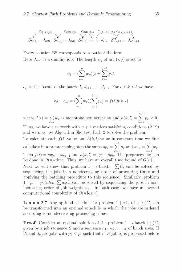
S S S SJi(1) Ji(2)−1 Ji(2) Ji(3)−1 Ji(3) Ji(k)−1 Ji(k) JnJn+1· · · · · · · · · · · · · · ·�
ci(1),i(2)
��
ci(2),i(3)
�� ci(k),i(k+1)
��
ci(3),i(4)
�� ci(k−1),i(k)
�
Every solution BS corresponds to a path of the form
Here Jn+1 is a dummy job. The length cij of arc (i, j) is set to
cij = (n∑
ν=i
wν)(s +
j−1∑
ν=i
pν).
cij is the “cost” of the batch Ji, Ji+1, . . . , Jj−1. For i < k < l we have
cil − cik = (n∑
ν=i
wν)(l−1∑
ν=k
pν) = f(i)h(k, l)
where f(i) =n∑
ν=i
wν is monotone nonincreasing and h(k, l) =l−1∑
ν=k
pν ≥ 0.
Thus, we have a network with n + 1 vertices satisfying conditions (2.19)and we may use Algorithm Shortest Path 2 to solve the problem.
To calculate each f(i)-value and h(k, l)-value in constant time we first
calculate in a preprocessing step the sums spi =i−1∑
ν=1
pν and swi =i∑
ν=1
wν .
Then f(i) = swn − swi−1 and h(k, l) = spl − spk. The preprocessing canbe done in O(n)-time. Thus, we have an overall time bound of O(n).
Next we will show that problem 1 | s-batch | ∑Ci can be solved by
sequencing the jobs in a nondecreasing order of processing times andapplying the batching procedure to this sequence. Similarly, problem1 | pi = p; batch|∑ wiCi can be solved by sequencing the jobs in non-increasing order of job weights wi. In both cases we have an overallcomputational complexity of O(n log n).
Lemma 2.7 Any optimal schedule for problem 1 | s-batch | ∑Ci can
be transformed into an optimal schedule in which the jobs are orderedaccording to nondecreasing processing times.
Proof: Consider an optimal solution of the problem 1 | s-batch | ∑Ci
given by a job sequence S and a sequence n1, n2, . . . , nk of batch sizes. IfJi and Jk are jobs with pk < pi such that in S job Ji is processed before
36 Some Problems in Combinatorial Optimization
Jk, then we may swap Ji and Jk and move the block of jobs in S betweenJi and Jk by pi − pk time units to the left. Furthermore, we keep thesequence of batch sizes unchanged. This does not increase the value ofthe objective function because the new Ci-value is the old Ck-value, thenew Ck-value is less than or equal to the old Ci-value, and the Cj-valuesof the other jobs are not increased. Iterating such changes leads to anoptimal solution with the desired property. �
Lemma 2.8 Any optimal schedule for problem 1 | pi = p; s-batch |∑wiCi can be transformed into an optimal schedule in which the jobs
are ordered according to nonincreasing job weights wi.
Proof: Consider an optimal solution and let Ji and Jk be two jobs withwi < wk, where Ji is scheduled preceding Jk. Interchanging Ji and Jk
does not increase the value of the objective function and iterating suchinterchanges leads to an optimal solution with the desired property. �

Chapter 3
Computational Complexity
Practical experience shows that some computational problems are easierto solve than others. Complexity theory provides a mathematical frame-work in which computational problems are studied so that they can beclassified as “easy” or “hard”. In this chapter we will describe the mainpoints of such a theory. A more rigorous presentation can be found inthe fundamental book of Garey & Johnson [99].
3.1 The Classes P and NPA computational problem can be viewed as a function h that maps eachinput x in some given domain to an output h(x) in some given range.We are interested in algorithms for solving computational problems. Suchan algorithm computes h(x) for each input x. For a precise discussion,a Turing machine is commonly used as a mathematical model of an al-gorithm. For our purposes it will be sufficient to think of a computerprogram written in some standard programming language as a model ofan algorithm. One of the main issues of complexity theory is to measurethe performance of algorithms with respect to computational time. Tobe more precise, for each input x we define the input length |x| as thelength of some encoding of x. We measure the efficiency of an algorithmby an upper bound T (n) on the number of steps that the algorithm takeson any input x with |x| = n. In most cases it will be difficult to calculatethe precise form of T . For these reasons we will replace the precise formof T by its asymptotic order. Therefore, we say that T (n) ∈ O(g(n))if there exist constants c > 0 and a nonnegative integer n0 such that
38 Computational Complexity
T (n) ≤ cg(n) for all integers n ≥ n0. Thus, rather than saying that thecomputational complexity is bounded by 7n3 + 27n2 + 4, we say simplythat it is O(n3).
Example 3.1 Consider the problem 1 ‖ ∑wiCi. The input x for this
problem is given by the number n of jobs and two n-dimensional vectors(pi) and (wi). We may define |x| to be the length of a binary encodedinput string for x. The output f(x) for the problems is a schedule min-
imizingn∑
i=1
wiCi. It can be represented by an n-vector of all Ci-values.
The following algorithm calculates these Ci-values (see Section 4.3).
Algorithm 1||∑wiCi
1. Enumerate the jobs such thatw1/p1 ≥ w2/p2 ≥ . . . ≥ wn/pn;
2. C0 := 0;3. FOR i := 1 TO n DO
Ci := Ci−1 + pi
The number of computational steps in this algorithm can be boundedas follows. In Step 1 the jobs have to be sorted. This takes O(n logn)steps. Furthermore, Step 3 can be done in O(n) time. Thus, we haveT (n) ∈ O(n log n). If we replace n by the input length |x|, the bound isstill valid because we always have n ≤ |x|. �A problem is called polynomially solvable if there exists a polynomialp such that T (|x|) ∈ O(p(|x|)) for all inputs x for the problem, i.e. if thereis a k such that T (|x|) ∈ O(|x|k). Problem 1 ‖ ∑
wiCi is polynomiallysolvable, as we have shown in Example 3.1
Important classes of problems which are polynomially solvable are linearprogramming problems (Khachiyan [125]) and integer linear program-ming problems with a fixed number of variables (Lenstra [149]).
The fastest currently known algorithms for network flow problems arepresented in Tables 3.1 and 3.2. In these tables n and m denote thenumber of vertices and arcs in the underlying network.
Table 3.1 contains the running times of maximum flow algorithms andcorresponding references.
U denotes the maximum of all arc capacities.
Table 3.2 contains running times of algorithms for the minimum-costcirculation problem.
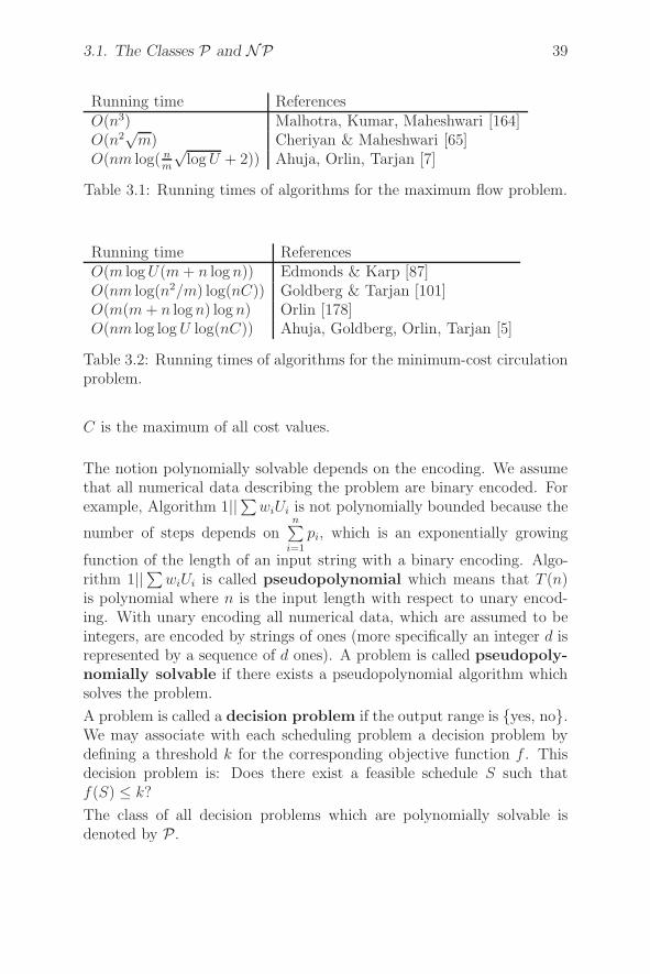
3.1. The Classes P and NP 39
Running time ReferencesO(n3) Malhotra, Kumar, Maheshwari [164]O(n2
√m) Cheriyan & Maheshwari [65]
O(nm log( nm
√log U + 2)) Ahuja, Orlin, Tarjan [7]
Table 3.1: Running times of algorithms for the maximum flow problem.
Running time ReferencesO(m log U(m + n log n)) Edmonds & Karp [87]O(nm log(n2/m) log(nC)) Goldberg & Tarjan [101]O(m(m + n log n) log n) Orlin [178]O(nm log log U log(nC)) Ahuja, Goldberg, Orlin, Tarjan [5]
Table 3.2: Running times of algorithms for the minimum-cost circulationproblem.
C is the maximum of all cost values.
The notion polynomially solvable depends on the encoding. We assumethat all numerical data describing the problem are binary encoded. Forexample, Algorithm 1||∑wiUi is not polynomially bounded because the
number of steps depends onn∑
i=1
pi, which is an exponentially growing
function of the length of an input string with a binary encoding. Algo-rithm 1||∑wiUi is called pseudopolynomial which means that T (n)is polynomial where n is the input length with respect to unary encod-ing. With unary encoding all numerical data, which are assumed to beintegers, are encoded by strings of ones (more specifically an integer d isrepresented by a sequence of d ones). A problem is called pseudopoly-nomially solvable if there exists a pseudopolynomial algorithm whichsolves the problem.
A problem is called a decision problem if the output range is {yes, no}.We may associate with each scheduling problem a decision problem bydefining a threshold k for the corresponding objective function f . Thisdecision problem is: Does there exist a feasible schedule S such thatf(S) ≤ k?
The class of all decision problems which are polynomially solvable isdenoted by P.
40 Computational Complexity
When a scheduling problem is formulated as a decision problem thereis an important asymmetry between those inputs whose output is “yes”and those whose output is “no”. A “yes”-answer can be certified by asmall amount of information: the feasible schedule S with f(S) ≤ k.Given this certificate, the “yes”-answer can be verified in polynomialtime. This is not the case for the “no”-answer.
In general, let NP denote the class of decision problems where each “yes”input x has a certificate y, such that |y| is bounded by a polynomial in|x| and there is a polynomial-time algorithm to verify that y is a validcertificate for x.
Example 3.2 Consider the decision version of problem P |prec|Cmax:Given m machines, n jobs Ji with processing times pi(i = 1, . . . , n),precedence relations between the jobs, and a threshold value k. Doesthere exist a schedule such that the corresponding Cmax-value is less thanor equal to k?
A certificate is given by a vector (Ci) of finishing times and a vector (μi)where μi is the machine on which Ji is processed. Clearly, (Ci) and (μi)have binary encodings which are bounded by polynomials in the inputlength of the problem. Furthermore, it can be checked in polynomialtime whether (Ci) and (μi) define a feasible schedule with Cmax-value≤ k. This is done by checking that
– Ci ≤ Cj − pj for all jobs Ji, Jj with Ji → Jj,
–n
maxi=1
Ci ≤ k, and
– the intervals [Ci − pi, Ci[, [Cj − pj, Cj[ do not overlap for all i �= jwith μi = μj.
Thus, problem P |prec|Cmax belongs to NP. �Similarly, it can be shown that other scheduling problems when consid-ered as decision problems belong to NP.
Every decision problem solvable in polynomial time belongs to NP. Ifwe have such a problem P and an algorithm which calculates for eachinput x the answer h(x) ∈ {yes, no} in a polynomial number of steps,then this answer h(x) may be used as a certificate. This certificate can beverified by the algorithm. Thus P is also in NP which implies P ⊆ NP.
3.2. NP-complete and NP-hard Problems 41
One of the major open problems of modern mathematics is whether Pequals NP. It is generally conjectured that this is not the case. There isa beautiful theory developed by Cook [73], Karp [124], and Levin [159]which provides some strong evidence that P �= NP. We will discuss thistheory in the next section.
3.2 NP-complete and NP-hard Problems
The principal notion in defining NP-completeness is that of a reduction.For two decision problems P and Q, we say that P reduces to Q (denotedP ∝ Q) if there exists a polynomial-time computable function g thattransforms inputs for P into inputs for Q such that x is a ‘yes’-input forP if and only if g(x) is a ‘yes’-input for Q.
To illustrate these concepts we first introduce some decision problemswhich play an important role in proving that decision versions of schedul-ing problems are NP-complete.
PARTITION (PART)
Given n positive integer numbers s1, s2, . . . , sn, is there a subset J ⊆ I ={1, . . . , n} such that ∑
i∈J
si =∑
i∈I\Jsi?
3-DIMENSIONAL MATCHING (3DM)
We are given a set N ⊆ W ×X ×Y where W, X, and Y are disjoint setswith the same number of q elements.
Does N contain a matching, that is, a subset M ⊆ N with q elementssuch that no two elements of M agree in any coordinate?
VERTEX COVER (VC)
We are given an undirected graph G = (V, E) and a positive integerk ≤ |V |.Is there a vertex cover of size k or less for G, that is, a subset C ⊆ Vwith at the most k elements such that for each edge {u, v} ∈ E, at least
42 Computational Complexity
one of u and v belongs to C?
CLIQUE
We are given an undirected graph G = (V, E) and a positive integerk ≤ |V |.Does G contain a clique of size k or more, that is, a subset C ⊆ V withat least k elements such that every two vertices in C are joined by anedge in E?
HAMILTON CIRCUIT (HC)
We are given an undirected graph G = (V, E).
Does G contain a Hamiltonian circuit,that is, an ordering v1, v2,. . . , vn of the vertices of G, where n = |V |, such that {vn, v1} ∈ Eand {vi, vi+1} ∈ E for i = 1, . . . , n − 1?
In the following examples we will illustrate some reductions.
Example 3.3 The partitioning problem is reducible to the decision ver-sion of problem F3 ‖ Cmax: PARTITION ∝ F3 ‖ Cmax. To prove this, weconsider a 3-machine flow shop problem with n + 1 jobs i = 1, . . . , n + 1,where the processing times of the operations are of the form
pi1 = 0, pi2 = si, pi3 = 0 for i = 1, . . . , n
pn+1,1 = pn+1,2 = pn+1,3 = b := 12
n∑
i=1
si.
We choose k = 3b as the threshold for the corresponding decision prob-lem.
If PARTITION has a solution, then there exists an index set J ⊆{1, . . . , n} such that ∑
i∈J
si = b.
In this case the schedule shown in Figure 3.1 solves the decision versionof problem F3 ‖ Cmax.
If, on the other hand, the flow-shop problem has a solution with Cmax ≤3b, then job n+1 must be scheduled as shown in Figure 3.1. Furthermore,J = {i| job finishes not later than b} solves the partitioning problem.

3.2. NP-complete and NP-hard Problems 43
0 b 2b 3b
Job n + 1
Job n + 1
Job n + 1
Jobs i ∈ J Jobs i /∈ J
Figure 3.1: Feasible schedule.
Finally, the input of the flow-shop problem can be computed in polyno-mial time given the input of the partitioning problem. �
Example 3.4 We show that CLIQUE ∝ P2|prec; pi ∈ {1, 2}|Cmax. Theinput of CLIQUE is given by an undirected graph G = (V, E) withvertices v1, . . . , vq and edges e1, . . . , er, and a threshold value p (0 < p ≤q). We must polynomially transform this input into an instance of theP2|prec; pi ∈ {1, 2}|Cmax-problem such that there is a clique C with|C| ≥ p if and only if there is a schedule with Cmax ≤ k for a suitablevalue k.
We set k = q + 2r + (q − p + 1) and define the scheduling problem asfollows: Consider jobs denoted by
v1, . . . , vq, e1, . . . , er, w1 . . . , wt with t = k + (q − p + 1),
i.e. we have v-jobs and e-jobs which correspond with the vertices andedges of G and dummy jobs wi.
Let the processing time of all e-jobs be equal to 2. The processing timesof v-jobs and dummy jobs are 1. Furthermore, define vi → ej if and onlyif vi is an endpoint of ej . We only have additional precedence relationsbetween dummy jobs. They are chosen in such a way that, under theassumption that Cmax ≤ k in each time period, at least one dummy jobmust be scheduled, say on machine 2, and that on machine 1 free blocksare created, as shown in Figure 3.2.
In the first block there is exactly space for the p vertex jobs and 12p(p−1)
edge jobs which correspond to a clique with p vertices. Thus the length ofthis block is p+2 · 1
2p(p−1) = p2. In the following q−p unit time blocks
which are separated by dummy jobs, there is space for the remainingvertex jobs. In the last block, which starts at time p2 + 2(q − p) + 1and ends at time k, there is exactly space for the remaining edge jobs.
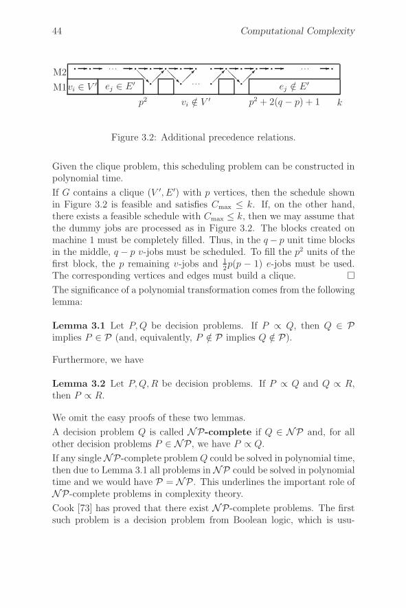
44 Computational Complexity
M1
M2
vi ∈ V ′ ej ∈ E ′ ej /∈ E ′
� �
������
� � � � �
������ ��� ���
���
� � � � � �� � � � � �
� � �
p2 vi /∈ V ′ p2 + 2(q − p) + 1 k
Figure 3.2: Additional precedence relations.
Given the clique problem, this scheduling problem can be constructed inpolynomial time.
If G contains a clique (V ′, E ′) with p vertices, then the schedule shownin Figure 3.2 is feasible and satisfies Cmax ≤ k. If, on the other hand,there exists a feasible schedule with Cmax ≤ k, then we may assume thatthe dummy jobs are processed as in Figure 3.2. The blocks created onmachine 1 must be completely filled. Thus, in the q − p unit time blocksin the middle, q − p v-jobs must be scheduled. To fill the p2 units of thefirst block, the p remaining v-jobs and 1
2p(p − 1) e-jobs must be used.
The corresponding vertices and edges must build a clique. �The significance of a polynomial transformation comes from the followinglemma:
Lemma 3.1 Let P, Q be decision problems. If P ∝ Q, then Q ∈ Pimplies P ∈ P (and, equivalently, P /∈ P implies Q /∈ P).
Furthermore, we have
Lemma 3.2 Let P, Q, R be decision problems. If P ∝ Q and Q ∝ R,then P ∝ R.
We omit the easy proofs of these two lemmas.
A decision problem Q is called NP-complete if Q ∈ NP and, for allother decision problems P ∈ NP, we have P ∝ Q.
If any single NP-complete problem Q could be solved in polynomial time,then due to Lemma 3.1 all problems in NP could be solved in polynomialtime and we would have P = NP. This underlines the important role ofNP-complete problems in complexity theory.
Cook [73] has proved that there exist NP-complete problems. The firstsuch problem is a decision problem from Boolean logic, which is usu-
3.2. NP-complete and NP-hard Problems 45
ally referred to as the satisfiability problem. The terms we shall use indescribing it are defined as follows.
Let U = {u1, u2, . . . , um} be a set of Boolean variables . A truthassignment for U is a function t : U → { true, false }. u ∈ U is true(false) if and only if t(u) = true (false). If u ∈ U , then u and u areliterals over U , where u is true iff u is false.
A clause over U is a set of literals over U (such as {u1, u2, u7}). Itrepresents the disjunction of those literals and is satisfied by a truthassignment if and only if at least one of its members is true under theassignment. A collection C of clauses over U is satisfiable if and only ifthere exists some truth assignment for U that simultaneously satisfies allthe clauses in C. Such a truth assignment is called a satisfying truthassignment for C. The satisfiability problem is specified as follows.
SATISFIABILITY (SAT)
We are given a set U of Boolean variables and a collection C of clausesover U .
Is there a satisfying truth assignment for C?
The problem in which each clause contains exactly 3 literals is called the3-SATISFIABILITY problem (3-SAT).
The important theorem of Cook [73] can now be stated:
Theorem 3.3 (Cook’s Theorem) SAT is NP-complete.
For a proof of this theorem we refer to Garey & Johnson [99].
The following lemma gives us a straightforward approach for proving newproblems to be NP-complete.
Lemma 3.4 If P and Q belong to NP, P is NP-complete, and P ∝ Q,then Q is NP-complete.
Proof: Since Q ∈ NP, all we need to do is to show that, for every R ∈NP, R ∝ Q. However, because P is NP-complete, we have R ∝ P ∝ Qand thus by Lemma 3.2, R ∝ Q for every R ∈ NP. �
Usually it is an easy task to show that Q ∈ NP. Therefore, when provingNP-completeness the main task is to find an NP-complete problem Psuch that P ∝ Q.
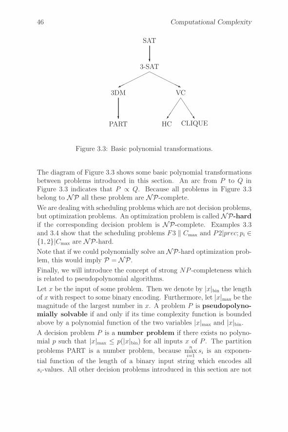
46 Computational Complexity
PART HC CLIQUE�
��
��
�
3DM VC
������
�������
3-SAT�
SAT
Figure 3.3: Basic polynomial transformations.
The diagram of Figure 3.3 shows some basic polynomial transformationsbetween problems introduced in this section. An arc from P to Q inFigure 3.3 indicates that P ∝ Q. Because all problems in Figure 3.3belong to NP all these problem are NP-complete.
We are dealing with scheduling problems which are not decision problems,but optimization problems. An optimization problem is called NP-hardif the corresponding decision problem is NP-complete. Examples 3.3and 3.4 show that the scheduling problems F3 ‖ Cmax and P2|prec; pi ∈{1, 2}|Cmax are NP-hard.
Note that if we could polynomially solve an NP-hard optimization prob-lem, this would imply P = NP.
Finally, we will introduce the concept of strong NP -completeness whichis related to pseudopolynomial algorithms.
Let x be the input of some problem. Then we denote by |x|bin the lengthof x with respect to some binary encoding. Furthermore, let |x|max be themagnitude of the largest number in x. A problem P is pseudopolyno-mially solvable if and only if its time complexity function is boundedabove by a polynomial function of the two variables |x|max and |x|bin.
A decision problem P is a number problem if there exists no polyno-mial p such that |x|max ≤ p(|x|bin) for all inputs x of P . The partition
problems PART is a number problem, becausen
maxi=1
si is an exponen-
tial function of the length of a binary input string which encodes allsi-values. All other decision problems introduced in this section are not
3.2. NP-complete and NP-hard Problems 47
number problems because no numbers are used to define them (in whichcase we set |x|max = 1).
An NP-complete problem P which is not a number problem cannotbe solved by a pseudopolynomial algorithm unless P = NP. Other-wise, there exists a monotone polynomial function h such that the timecomplexity is bounded by h(|x|max, |x|bin) ≤ h(p(|x|bin), |x|bin), i.e. theNP-complete problem P would be polynomially solvable.
For any decision problem P and any polynomial q let Pq denote thesubproblem of P obtained by restricting P to those instances satisfying|x|max ≤ q(|x|bin). Then Pq is not a number problem. A decision problemP is NP-complete in the strong sense if P belongs to NP and thereexists a polynomial q for which Pq is NP-complete.
Lemma 3.5 If P is NP-complete in the strong sense, then P cannot besolved by a pseudopolynomial time algorithm unless P = NP.
Proof: Let q be a polynomial such that Pq is NP-complete. Pq is not anumber problem. Thus, the existence of a pseudopolynomial algorithmfor P (which is also pseudopolynomial for Pq) would imply P = NP. �
This lemma implies that it is very unlikely that problems which are NP-complete in the strong sense can be solved pseudopolynomially.
The most straightforward way to prove that a number problem P isNP-complete in the strong sense is simply to prove for some specificpolynomial q that Pq is NP-complete. In this way we conclude thatNP-complete problems which do not involve numbers are NP-completein the strong sense. With the exception of PART, all basic problemsintroduced in this section are NP-complete in the strong sense for thisreason. PART can be proved to be pseudopolynomially solvable (Garey &Johnson [99]). Thus, by Lemma 3.5 it is not NP-complete in the strongsense (unless P = NP). Another way to prove NP-completeness in thestrong sense is to use pseudopolynomial reductions (Garey & Johnson[99]): P is NP-complete in the strong sense if P belongs to NP andthere exists a pseudopolynomial reduction from a problem Q, which isNP-complete in the strong sense, to P .
A pseudopolynomial reduction from a problem Q to a problem P usesa pseudopolynomial time computable function g (i.e. g(x) is computablein time polynomial in two variables |x|max and |x|bin.) Furthermore, gmust satisfy the following two conditions:
48 Computational Complexity
• there exists a polynomial q1 such that q1(|g(x)|′bin) ≥ |x|bin for allinputs x of Q, and
• there exists a two-variable polynomial q2 such that
|g(x)|′max ≤ q2(|x|max, |x|bin)
for all inputs x of Q.
The first condition is almost always satisfied. It requires that g does notcause a substantial decrease in the input length. The second conditionensures that the magnitude of the largest number in g(x) does not blowup exponentially.
3.3 Simple Reductions Between Schedul-
ing Problems
If in a description of a scheduling problem we replace F by J , we get asimple reduction because the flow shop is a special case of a job shop.Similarly, we get a simple reduction if we replace tree by prec. Possiblesimple reductions are shown by the reduction graphs Gi(i = 1, . . . , 8) inFigure 3.4.
Note that the reduction of G8 only holds if the objective function isregular. In this case, s-batching with set-up time s = 0 means that wemay consider only one-element batches, which is equivalent to having nobatches at all.
There are similar relations between objective functions. These relationsare shown in Figure 3.5.∑
fj reduces to∑
wjfj by setting wj = 1 for all j. Cmax,∑
Cj, and∑wjCj reduce to Lmax,
∑Tj , and
∑wjTj , respectively, by setting dj = 0
for all j. Furthermore, we have
max Lj ≤ k ⇔ Cj − dj ≤ k for all j
⇔ Cj − (dj + k) ≤ 0 for all j
⇔ max{0, Cj − (dj + k)} ≤ 0 for all j
⇔ ∑Tj =
∑max{0, Cj − (dj + k)} ≤ 0
⇔ ∑Uj ≤ 0.
Thus Lmax reduces to∑
Tj and∑
Uj .
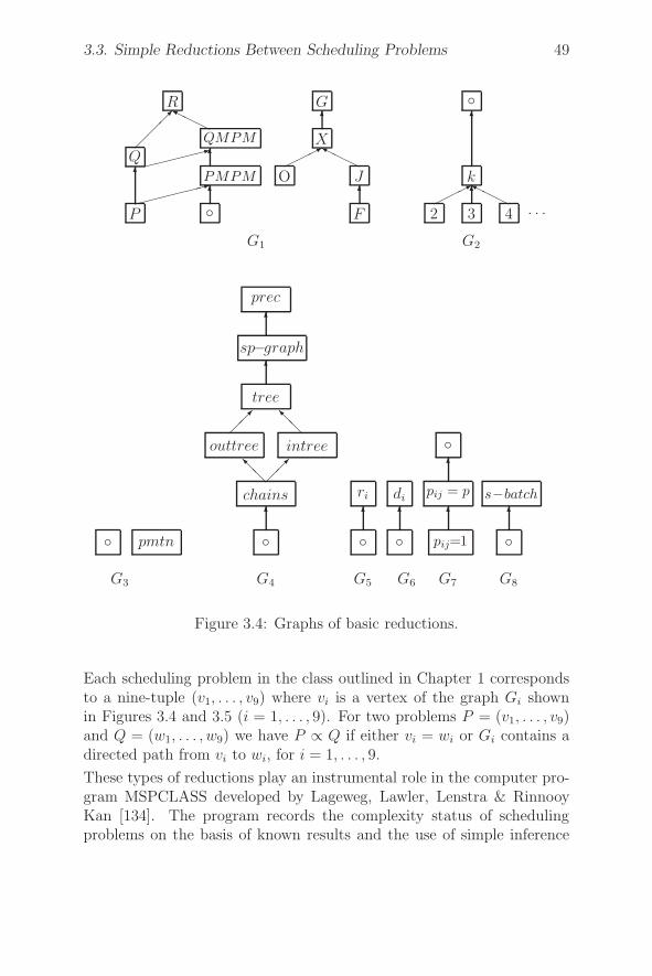
3.3. Simple Reductions Between Scheduling Problems 49
P ◦ F 2 3 4 . . .
PMPM O J k
QQMPM X
R G ◦
�
�������� � ����� ����
� ��������
�
��
��
������
���� �
G1 G2
◦ pmtn ◦ ◦ ◦ pij=1 ◦
chains
◦outtree intree
ri dipij = p s−batch
tree
sp−graph
prec
�
���
���
���
���
�
�
� �
�
� �
G3 G4 G5 G6 G7 G8
Figure 3.4: Graphs of basic reductions.
Each scheduling problem in the class outlined in Chapter 1 correspondsto a nine-tuple (v1, . . . , v9) where vi is a vertex of the graph Gi shownin Figures 3.4 and 3.5 (i = 1, . . . , 9). For two problems P = (v1, . . . , v9)and Q = (w1, . . . , w9) we have P ∝ Q if either vi = wi or Gi contains adirected path from vi to wi, for i = 1, . . . , 9.
These types of reductions play an instrumental role in the computer pro-gram MSPCLASS developed by Lageweg, Lawler, Lenstra & RinnooyKan [134]. The program records the complexity status of schedulingproblems on the basis of known results and the use of simple inference
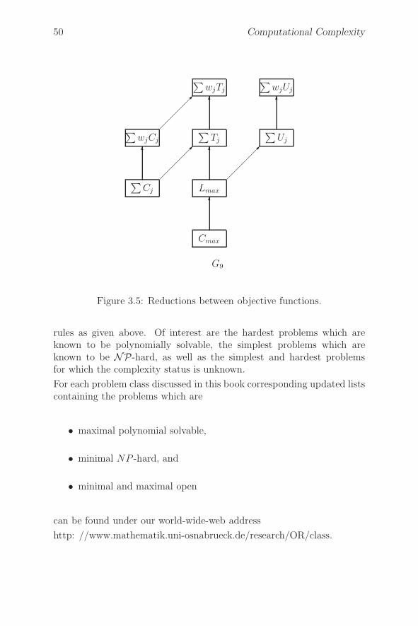
50 Computational Complexity
Cmax
�
∑Cj Lmax
� �
��
���
��
���
∑wjCj
∑Tj
∑Uj
� �
��
���
∑wjTj
∑wjUj
G9
Figure 3.5: Reductions between objective functions.
rules as given above. Of interest are the hardest problems which areknown to be polynomially solvable, the simplest problems which areknown to be NP-hard, as well as the simplest and hardest problemsfor which the complexity status is unknown.
For each problem class discussed in this book corresponding updated listscontaining the problems which are
• maximal polynomial solvable,
• minimal NP -hard, and
• minimal and maximal open
can be found under our world-wide-web address
http: //www.mathematik.uni-osnabrueck.de/research/OR/class.
3.4. Living with NP-hard Problems 51
3.4 Living with NP-hard Problems
The knowledge that a scheduling problem is NP-hard is little consolationfor the algorithm designer who needs to solve the problem. Fortunately,despite theoretical equivalence, not all NP-hard problems are equallyhard from a practical perspective. We have seen that some NP-hardproblems can be solved pseudopolynomially using dynamic programming.Such an approach may provide satisfactory results if the problems to besolved are not too large. A method related to dynamic programmingis branch-and-bound, which will be discussed at the end of this section.The branch-and-bound method is based on the idea of intelligently enu-merating all feasible solutions.
Another possibility is to apply approximation algorithms. These algo-rithms produce solutions that are guaranteed to be within a fixed per-centage of the actual optimum. One of the most successful methods ofattacking hard combinatorial optimization problems is the discrete ana-log of “hill climbing”, known as local (or neighborhood) search, whichwill be discussed at the beginning of this section. Local search methodsgenerally only provide feasible solutions which are not guaranteed to beoptimal. However, for minimization (maximization) problems, a possibledeviation from the optimal objective value can be bounded if a lower(upper) bound is available.
Any approach without formal guarantee of performance can be consid-ered a “heuristic”. Such approaches are useful in practical situations ifno better methods are available.
3.4.1 Local Search Techniques
In this section we will study local search techniques which are useful toolsfor solving discrete optimization problems. A discrete optimizationproblem can be described as follows. For a given finite set S and a givenfunction c : S → R, one has to find a solution s∗ ∈ S with
c(s∗) ≤ c(s) for all s ∈ S.
All nonpreemptive scheduling problems introduced thus far are discreteoptimization problems. Local search is an iterative procedure whichmoves from one solution in S to another as long as necessary. In orderto systematically search through S, the possible moves from a solution s
52 Computational Complexity
to the next solution should be restricted in some way. To describe suchrestrictions, we introduce a neighborhood structure N : S → 2S onS. For each s ∈ S, N(s) describes the subset of solutions which canbe reached in one step by moving from s. The set N(s) is called theneighborhood of s.
A neighborhood structure N may be represented by a directed graphG = (V, A) where V = S and
(s, t) ∈ A iff t ∈ N(s).
G is called the neighborhood graph of the neighborhood structure.
Usually it is not possible to store the neighborhood graph because S hasan exponential size. To overcome this difficulty, a set AM of allowedmodifications F : S → S is introduced. For a given solution s, theneighborhood of s can now be defined by
N(s) = {F (s) | F ∈ AM}.Using these definitions, a local search method may be described asfollows. In each iteration we start with a solution s ∈ S and choose asolution s′ ∈ N(s) (or a modification F ∈ AM which provides s′ = F (s)).Based on the values c(s) and c(s′), we choose a starting solution of thenext iteration. According to different criteria used for the choice of thestarting solution of the next iteration, we get different types of localsearch techniques.
The simplest choice is to take the solution with the smallest value of thecost function. This choice leads to the well-known iterative improvementmethod which may be formulated as follows.
Algorithm Iterative Improvement1. Choose an initial solution s′ ∈ S;2. REPEAT3. s := s′
4. Generate the best solution s′ ∈ N(s);5. UNTIL c(s′) ≥ c(s)
This algorithm will terminate with some solution s∗. In general, s∗ isonly a local minimum with respect to the neighborhood N (i.e. asolution such that no neighbor is better than this solution) and maydiffer considerably from the global minimum.
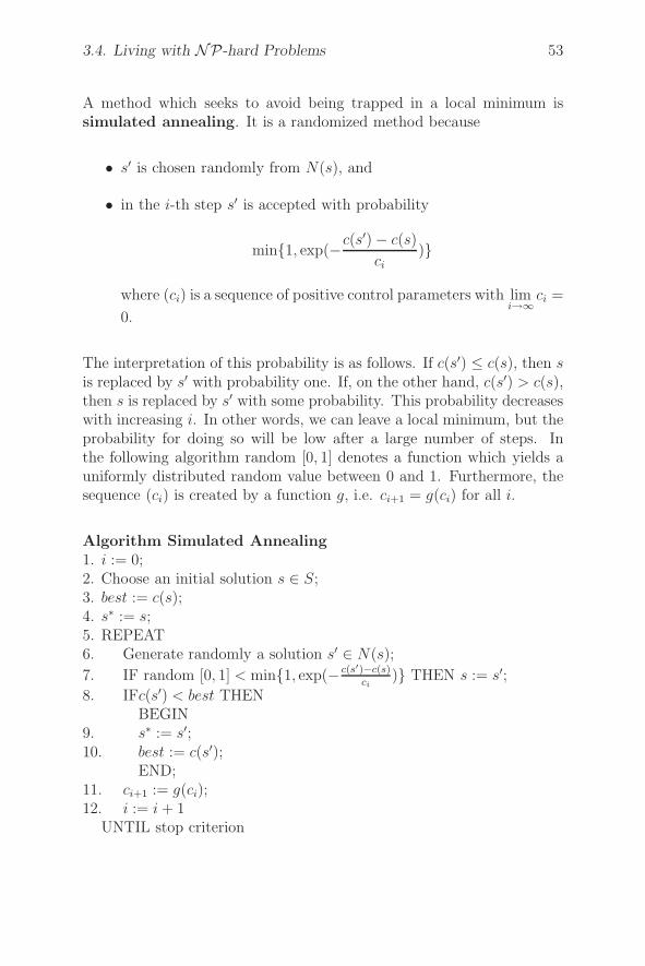
3.4. Living with NP-hard Problems 53
A method which seeks to avoid being trapped in a local minimum issimulated annealing. It is a randomized method because
• s′ is chosen randomly from N(s), and
• in the i-th step s′ is accepted with probability
min{1, exp(−c(s′) − c(s)
ci)}
where (ci) is a sequence of positive control parameters with limi→∞
ci =
0.
The interpretation of this probability is as follows. If c(s′) ≤ c(s), then sis replaced by s′ with probability one. If, on the other hand, c(s′) > c(s),then s is replaced by s′ with some probability. This probability decreaseswith increasing i. In other words, we can leave a local minimum, but theprobability for doing so will be low after a large number of steps. Inthe following algorithm random [0, 1] denotes a function which yields auniformly distributed random value between 0 and 1. Furthermore, thesequence (ci) is created by a function g, i.e. ci+1 = g(ci) for all i.
Algorithm Simulated Annealing1. i := 0;2. Choose an initial solution s ∈ S;3. best := c(s);4. s∗ := s;5. REPEAT6. Generate randomly a solution s′ ∈ N(s);
7. IF random [0, 1] < min{1, exp(− c(s′)−c(s)ci
)} THEN s := s′;8. IFc(s′) < best THEN
BEGIN9. s∗ := s′;10. best := c(s′);
END;11. ci+1 := g(ci);12. i := i + 1
UNTIL stop criterion
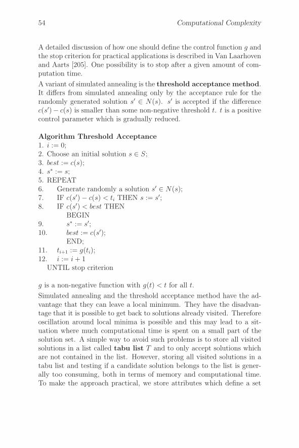
54 Computational Complexity
A detailed discussion of how one should define the control function g andthe stop criterion for practical applications is described in Van Laarhovenand Aarts [205]. One possibility is to stop after a given amount of com-putation time.
A variant of simulated annealing is the threshold acceptance method.It differs from simulated annealing only by the acceptance rule for therandomly generated solution s′ ∈ N(s). s′ is accepted if the differencec(s′)− c(s) is smaller than some non-negative threshold t. t is a positivecontrol parameter which is gradually reduced.
Algorithm Threshold Acceptance1. i := 0;2. Choose an initial solution s ∈ S;3. best := c(s);4. s∗ := s;5. REPEAT6. Generate randomly a solution s′ ∈ N(s);7. IF c(s′) − c(s) < ti THEN s := s′;8. IF c(s′) < best THEN
BEGIN9. s∗ := s′;10. best := c(s′);
END;11. ti+1 := g(ti);12. i := i + 1
UNTIL stop criterion
g is a non-negative function with g(t) < t for all t.
Simulated annealing and the threshold acceptance method have the ad-vantage that they can leave a local minimum. They have the disadvan-tage that it is possible to get back to solutions already visited. Thereforeoscillation around local minima is possible and this may lead to a sit-uation where much computational time is spent on a small part of thesolution set. A simple way to avoid such problems is to store all visitedsolutions in a list called tabu list T and to only accept solutions whichare not contained in the list. However, storing all visited solutions in atabu list and testing if a candidate solution belongs to the list is gener-ally too consuming, both in terms of memory and computational time.To make the approach practical, we store attributes which define a set
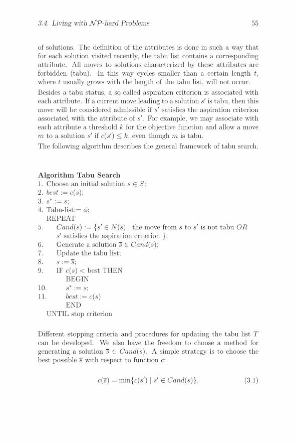
3.4. Living with NP-hard Problems 55
of solutions. The definition of the attributes is done in such a way thatfor each solution visited recently, the tabu list contains a correspondingattribute. All moves to solutions characterized by these attributes areforbidden (tabu). In this way cycles smaller than a certain length t,where t usually grows with the length of the tabu list, will not occur.
Besides a tabu status, a so-called aspiration criterion is associated witheach attribute. If a current move leading to a solution s′ is tabu, then thismove will be considered admissible if s′ satisfies the aspiration criterionassociated with the attribute of s′. For example, we may associate witheach attribute a threshold k for the objective function and allow a movem to a solution s′ if c(s′) ≤ k, even though m is tabu.
The following algorithm describes the general framework of tabu search.
Algorithm Tabu Search1. Choose an initial solution s ∈ S;2. best := c(s);3. s∗ := s;4. Tabu-list:= φ;
REPEAT5. Cand(s) := {s′ ∈ N(s) | the move from s to s′ is not tabu OR
s′ satisfies the aspiration criterion };6. Generate a solution s ∈ Cand(s);7. Update the tabu list;8. s := s;9. IF c(s) < best THEN
BEGIN10. s∗ := s;11. best := c(s)
ENDUNTIL stop criterion
Different stopping criteria and procedures for updating the tabu list Tcan be developed. We also have the freedom to choose a method forgenerating a solution s ∈ Cand(s). A simple strategy is to choose thebest possible s with respect to function c:
c(s) = min{c(s′) | s′ ∈ Cand(s)}. (3.1)
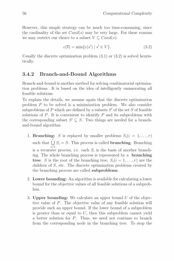
56 Computational Complexity
However, this simple strategy can be much too time-consuming, sincethe cardinality of the set Cand(s) may be very large. For these reasonswe may restrict our choice to a subset V ⊆ Cand(s):
c(s) = min{c(s′) | s′ ∈ V }. (3.2)
Usually the discrete optimization problem (3.1) or (3.2) is solved heuris-tically.
3.4.2 Branch-and-Bound Algorithms
Branch-and-bound is another method for solving combinatorial optimiza-tion problems. It is based on the idea of intelligently enumerating allfeasible solutions.
To explain the details, we assume again that the discrete optimizationproblem P to be solved is a minimization problem. We also considersubproblems of P which are defined by a subsets S ′ of the set S of feasiblesolutions of P . It is convenient to identify P and its subproblems withthe corresponding subset S ′ ⊆ S. Two things are needed for a branch-and-bound algorithm.
1. Branching: S is replaced by smaller problems Si(i = 1, . . . , r)
such thatr⋃
i=1
Si = S. This process is called branching. Branching
is a recursive process, i.e. each Si is the basis of another branch-ing. The whole branching process is represented by a branchingtree. S is the root of the branching tree, Si(i = 1, . . . , r) are thechildren of S, etc. The discrete optimization problems created bythe branching process are called subproblems.
2. Lower bounding: An algorithm is available for calculating a lowerbound for the objective values of all feasible solutions of a subprob-lem.
3. Upper bounding: We calculate an upper bound U of the objec-tive value of P . The objective value of any feasible solution willprovide such an upper bound. If the lower bound of a subproblemis greater than or equal to U , then this subproblem cannot yielda better solution for P . Thus, we need not continue to branchfrom the corresponding node in the branching tree. To stop the
3.4. Living with NP-hard Problems 57
branching process in many nodes of the branching tree, the boundU should be as small as possible. Therefore, at the beginning ofthe branch-and-bound algorithm we apply some heuristic to find agood feasible solution with small value U . After branching manytimes we may reach a situation in which the subproblem has onlyone feasible solution. Then the lower bound LB of the subproblemis set equal to the objective value of this solution and we replace Uby LB if LB < U .
Algorithm Branch-and-Bound summarizes these basic ideas. In this al-gorithm, LIST contains all subproblems for which we have to continuethe branching process.
Algorithm Branch-and-Bound1. LIST:={S};2. U := value of some heuristic solution;
currentbest:= heuristic solution;3. WHILE LIST �= φ DO
BEGIN4. Choose a branching node k from LIST;5. Remove k from LIST;6. Generate children child (i) for i = 1, . . . , nk and calculate
corresponding lower bounds LBi;7. For i := 1 TO nk DO8. IF LBi < U THEN9. IF child (i) consists of a single solution THEN
BEGIN10. U := LBi;11. currentbest := solution corresponding with
child (i)END
12. ELSE add child (i) to LISTEND
As an example, we will present a branch-and-bound algorithm for prob-lem F2||∑Ci which is known to be NP-hard (Garey et al. [100]).
Example 3.5 Problem F2||∑Ci is defined as follows. We are given njobs i = 1, . . . , n. Each job has two operations to be performed on one of
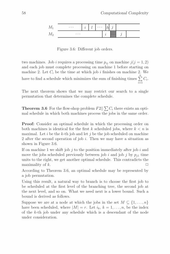
58 Computational Complexity
M1
M2
· · · i l · · · h j
· · · i j
Figure 3.6: Different job orders.
two machines. Job i requires a processing time pij on machine j(j = 1, 2)and each job must complete processing on machine 1 before starting onmachine 2. Let Ci be the time at which job i finishes on machine 2. We
have to find a schedule which minimizes the sum of finishing timesn∑
i=1
Ci.
The next theorem shows that we may restrict our search to a singlepermutation that determines the complete schedule.
Theorem 3.6 For the flow-shop problem F2||∑Ci there exists an opti-mal schedule in which both machines process the jobs in the same order.
Proof: Consider an optimal schedule in which the processing order onboth machines is identical for the first k scheduled jobs, where k < n ismaximal. Let i be the k-th job and let j be the job scheduled on machine2 after the second operation of job i. Then we may have a situation asshown in Figure 3.6.
If on machine 1 we shift job j to the position immediately after job i andmove the jobs scheduled previously between job i and job j by pj1 timeunits to the right, we get another optimal schedule. This contradicts themaximality of k. �
According to Theorem 3.6, an optimal schedule may be represented bya job permutation.
Using this result, a natural way to branch is to choose the first job tobe scheduled at the first level of the branching tree, the second job atthe next level, and so on. What we need next is a lower bound. Such abound is derived as follows.
Suppose we are at a node at which the jobs in the set M ⊆ {1, . . . , n}have been scheduled, where |M | = r. Let ik, k = 1, . . . , n, be the indexof the k-th job under any schedule which is a descendant of the nodeunder consideration.

3.4. Living with NP-hard Problems 59
The cost of this schedule, which we wish to bound, is
S =∑
i∈M
Ci +∑
i/∈M
Ci. (3.3)
For the second sum in (3.3) we will derive two possible lower bounds.
(1) If every job i /∈ M could start its processing on machine 2 immedi-ately after completing its processing on machine 1, the second sumin (3.3) would become
S1 =
n∑
k=r+1
[∑
i∈M
pi1 + (n − k + 1)pik1 + pik2].
If that is not possible, then we have
∑
i/∈M
Ci ≥ S1.
The bound S1 depends on the way the jobs not in M are scheduled.This dependence can be eliminated by noting that S1 is minimizedby scheduling jobs i /∈ M in an order of nondecreasing pi1-values(compare to solution of P ‖ ∑
Ci in Section 2.5). Call the resultingminimum value S∗
1 .
(2) max{Cir ,∑
i∈M
pi1 +mini/∈M
pi1} is a lower bound on the start of the first
job i /∈ M on machine 2. Thus, the second sum in (3.3) would bebounded by
S2 =n∑
k=r+1
[max{Cir ,∑
i∈M
pi1 + mini/∈M
pi1} + (n − k + 1)pik2].
Again, S2 is minimized by scheduling jobs i /∈ M in an order ofnondecreasing pi2-values. Call the resulting minimum value S∗
2 .
Combining the two lower bounds we get
∑
i∈M
Ci + max{S∗1 , S
∗2} (3.4)
which is an easily computed lower bound.
60 Computational Complexity
Algorithm Branch-and-Bound may be implemented using lower bound(3.4) and the simple branching rule. This algorithm can be improved byexploiting a natural dominance relation introduced by Ignall and Schrage[117]:
Suppose we have two nodes t and u representing partial sequencesi1, . . . , ir and j1, . . . , jr of the same set of jobs, M . Denote by Ci(t)and Cj(u) the corresponding finishing times. If
Cir(t) ≤ Cjr(u) (3.5)
and if the accumulated cost under the partial schedule t is no more thanunder u, ∑
i∈M
Ci(t) ≤∑
j∈M
Cj(u) (3.6)
then the best completion of schedule t is at least as good as the best com-pletion of u. Checking conditions (3.5) and (3.6) for nodes with identicalsets M , nodes may be eliminated from LIST in Algorithm Branch-and-Bound. �There are many alternatives to implement a branch-and-bound algo-rithm. There may be many possibilities to organize the branching. Whencalculating lower bounds, one often has a choice between bounds that arerelatively tight, but require much computation time, and bounds that arenot so tight but can be computed quickly. A similar trade-off may exist inchoosing a dominance relation. At each branching step, it is necessary toselect the branching node. The usual alternatives are least-lower-bound-next, last-in-first-out, or first-in-first-out.
Finally, we should mention that the branch-and-bound algorithm is oftenterminated before optimality is reached. In this case we have a completesolution with cost U , and the lowest lower bound LB of all nodes in thelist provides a lower bound on the optimal cost.
Note that if OPT is the optimal solution value, then U−OPTOPT
≤ U−LBLB
,i.e. U−LB
LBis an upper bound for the performance ratio for the heuristic
we get by terminating the branch-and-bound procedure before reachingthe optimum.
Which design strategy is taken depends very much on the problem andits data. Designing a good branch-and-bound procedure usually requiressome computational experience.
Chapter 4
Single Machine SchedulingProblems
The single machine case has been the subject of extensive research eversince the early work of Jackson [118] and Smith [188]. In this chapter,we will present algorithms for single machine scheduling problems whichare polynomial or pseudopolynomial. It is useful to note the followinggeneral result which holds for single machine problems: if all rj = 0 andif the objective function is a monotone function of the finishing timesof the jobs, then only schedules without preemption and without idletime need to be considered. This follows from the fact that the optimalobjective value does not improve if preemption is allowed. To see this,consider a schedule in which some job i is preempted, i.e.
• i is scheduled in [t1, t2[ and [t3, t4[ where t1 < t2 < t3 < t4, and
• i is neither scheduled in [t2, t3[ nor immediately before t1.
If we reschedule so that the part of i occurring in [t1, t2[ is scheduledbetween t3 − (t2 − t1) and t3, and so that anything scheduled between t2and t3 is moved back t2 − t1 units of time, we eliminate this preemptionof i without increasing the objective function. Furthermore, no newpreemption is created. Continuing this process, we obtain an optimalsolution for the preemptive problem where no preemption is necessary.
Note that this transformation generally creates infeasibility if rj �= 0 forsome jobs j.
62 Single Machine Scheduling Problems
4.1 Minimax Criteria
4.1.1 Lawler’s Algorithm for 1 | prec | fmax
To solve problem 1 | prec | fmax with fmax =n
maxj=1
fj(Cj) and fj monotone
for j = 1, . . . , n, it is sufficient to construct an optimal sequence π :π(1), π(2), . . . , π(n) (π(i) denotes the job in position i). Lawler [135]developed a simple algorithm which constructs this sequence in reverseorder.
Let N = {1, . . . , n} be the set of all jobs and denote by S ⊆ N theset of unscheduled jobs. Furthermore, define p(S) =
∑
j∈S
pj . Then the
scheduling rule may be formulated as follows: Schedule a job j ∈ S,which has no successor in S and has a minimal fj(p(S))-value, as thelast job in S.
To give a precise description of the algorithm, we represent the prece-dence constraints by the corresponding adjacency matrix A = (aij)where aij = 1 if and only if j is a direct successor of i. By n(i) we denotethe number of immediate successors of i.
Algorithm 1 | prec | fmax
1. FOR i := 1 TO n DO n(i) :=n∑
j=1
aij ;
2. S := {1, . . . , n}; p :=n∑
j=1
pj ;
3. FOR k := n DOWN TO 1 DOBEGIN
4. Find job j ∈ S with n(j) = 0 and minimal fj(p)-value;5. S := S\{j};6. n(j) := ∞;7. π(k) := j;8. p := p − pj ;9. FOR i := 1 to n DO
IF aij = 1 THEN n(i) := n(i) − 1END
The complexity of this algorithm is O(n2).
Theorem 4.1 Algorithm 1 | prec | fmax constructs an optimal sequence.
4.1. Minimax Criteria 63
Proof: Enumerate the jobs in such a way that 1, 2, . . . , n is the sequenceconstructed by the algorithm. Let σ : σ(1), . . . , σ(n) be an optimal se-quence with σ(i) = i for i = n, n− 1, . . . , r and σ(r − 1) �= r − 1 where ris minimal. We have the following situation
σ : . . . r − 1 k . . . j r . . . n
It is possible to schedule r−1 immediately before r. Therefore, r−1 andj have no successor in the set {1, . . . , r−1}. This implies fr−1(p) ≤ fj(p)
with p =r−1∑
i=1
pi because 1, . . . , n was constructed by the algorithm. Thus,
the schedule we get by shifting the block of jobs between r − 1 and r anamount of pr−1 units to the left and processing r− 1 immediately beforer is again optimal. This contradicts the minimality of r. �
In the next section, we show that the problem can also be solved effi-ciently if we have release times rj and either preemption is allowed or alljobs have unit processing times.
4.1.2 1 |prec;pj =1; rj | fmax and 1 | prec;pmtn; rj | fmax
We assume again that fmax is the maximum of monotone functions. Thefirst step in solving these problems is to modify the release times rj . Ifi → j (i.e. if j is a successor of i) and ri +pi > rj , then job j cannot startbefore r′j = ri + pi. Thus, we may replace rj by r′j. The release timescan be modified in a systematic way using the following algorithm. Weassume that the jobs are enumerated topologically (i.e. for all jobs i, jwith i → j we have i < j). If this is not the case, we apply the algorithmpresented in Section 2.7.
Algorithm Modify rj
1. FOR i := 1 TO n − 1 DO2. FOR j := i + 1 TO n DO3. IF i → j THEN rj := max{rj, ri + pi}
We denote the modified release time by r′j. Note that if the processingtimes are nonzero, then we have
r′j > r′i if i → j. (4.1)
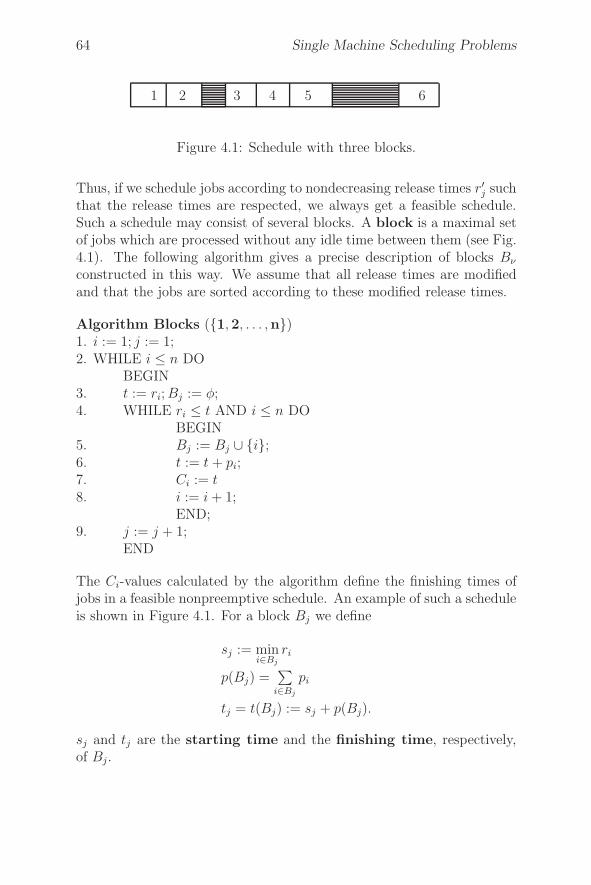
64 Single Machine Scheduling Problems
1 2 3 4 5 6
Figure 4.1: Schedule with three blocks.
Thus, if we schedule jobs according to nondecreasing release times r′j suchthat the release times are respected, we always get a feasible schedule.Such a schedule may consist of several blocks. A block is a maximal setof jobs which are processed without any idle time between them (see Fig.4.1). The following algorithm gives a precise description of blocks Bν
constructed in this way. We assume that all release times are modifiedand that the jobs are sorted according to these modified release times.
Algorithm Blocks ({1, 2, . . . ,n})1. i := 1; j := 1;2. WHILE i ≤ n DO
BEGIN3. t := ri; Bj := φ;4. WHILE ri ≤ t AND i ≤ n DO
BEGIN5. Bj := Bj ∪ {i};6. t := t + pi;7. Ci := t8. i := i + 1;
END;9. j := j + 1;
END
The Ci-values calculated by the algorithm define the finishing times ofjobs in a feasible nonpreemptive schedule. An example of such a scheduleis shown in Figure 4.1. For a block Bj we define
sj := mini∈Bj
ri
p(Bj) =∑
i∈Bj
pi
tj = t(Bj) := sj + p(Bj).
sj and tj are the starting time and the finishing time, respectively,of Bj.
4.1. Minimax Criteria 65
The discussion thus far is valid for nonpreemptive schedules with jobshaving arbitrary processing times.
Now we turn to problem 1 | prec; pmtn; rj | fmax.
Lemma 4.2 For problem 1 | prec; pmtn; rj | fmax there exists an optimalschedule such that the intervals [sj, tj ] (j = 1, . . . , k) constructed byAlgorithm Blocks are completely occupied by jobs.
Proof: Consider an optimal schedule with the property that [s, t] issome idle interval contained in some block interval [sj , tj]. Furthermore,assume that in this schedule [s, t] is the first such interval. We claimthat there exists some job i with ri ≤ s which finishes later than times. Otherwise, for the set T of jobs which are processed in time periodslater than time s we would have
r = min{rk | k ∈ T} > s
and in the schedule created by Algorithm Blocks interval [s, r] must bean idle interval, which is a contradiction.
We move job i into the idle interval so that either [s, t] is completely filledor job i finishes in [s, t]. Continuing this process, after a finite number ofsteps we get a schedule with the desired properties. �
Due to Lemma 4.2 we may treat each block separately. The optimalsolution value for the whole problem is given by the maximum of thesolution values of all blocks.
Let B be such a block. Denote by f ∗max(B) the optimal solution value
for the jobs in this block. Furthermore, let f ∗max(B\{j}) be the optimal
solution value for the jobs in B\{j}. Clearly, f ∗max(B\{j}) ≤ f ∗
max(B) forall j scheduled in B and thus
f ∗max(B) ≥ max
j∈B{f ∗
max(B\{j})}. (4.2)
Furthermore,
fl(t(B)) := min{fj(t(B)) | j ∈ B without successors in B} ≤ f ∗max(B)
(4.3)because in an optimal schedule one job k ∈ B without successors in Bfinishes at time t(B).
A schedule is now constructed as follows. We solve the problem for theset of jobs B\{l}. The optimal solution of this problem again has a
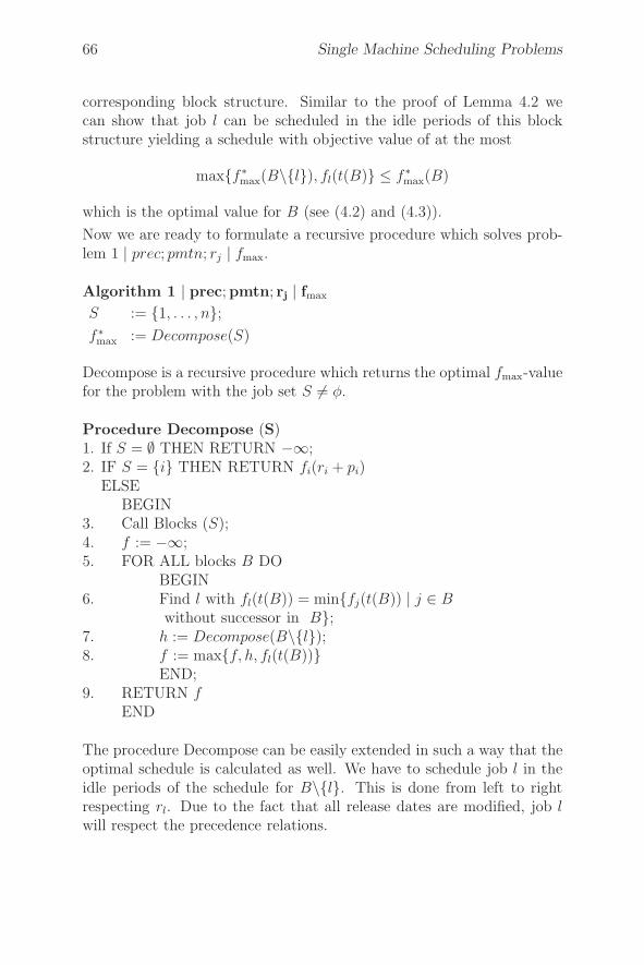
66 Single Machine Scheduling Problems
corresponding block structure. Similar to the proof of Lemma 4.2 wecan show that job l can be scheduled in the idle periods of this blockstructure yielding a schedule with objective value of at the most
max{f ∗max(B\{l}), fl(t(B)} ≤ f ∗
max(B)
which is the optimal value for B (see (4.2) and (4.3)).
Now we are ready to formulate a recursive procedure which solves prob-lem 1 | prec; pmtn; rj | fmax.
Algorithm 1 | prec;pmtn; rj | fmax
S := {1, . . . , n};f ∗
max := Decompose(S)
Decompose is a recursive procedure which returns the optimal fmax-valuefor the problem with the job set S �= φ.
Procedure Decompose (S)1. If S = ∅ THEN RETURN −∞;2. IF S = {i} THEN RETURN fi(ri + pi)
ELSEBEGIN
3. Call Blocks (S);4. f := −∞;5. FOR ALL blocks B DO
BEGIN6. Find l with fl(t(B)) = min{fj(t(B)) | j ∈ B
without successor in B};7. h := Decompose(B\{l});8. f := max{f, h, fl(t(B))}
END;9. RETURN f
END
The procedure Decompose can be easily extended in such a way that theoptimal schedule is calculated as well. We have to schedule job l in theidle periods of the schedule for B\{l}. This is done from left to rightrespecting rl. Due to the fact that all release dates are modified, job lwill respect the precedence relations.

4.2. Maximum Lateness and Related Criteria 67
The complexity of the algorithm is O(n2). This can be seen as follows.If we exclude the recursive calls in Step 7, the number of steps for theProcedure Decompose is O(|S|). Thus, for the number f(n) of computa-tional steps we have the recursion f(n) = cn +
∑f(ni) where ni is the
number of jobs in the i-th block and∑
ni ≤ n.
The number of preemptions is bounded by n−1 because each preemptioninduces a splitting of blocks.
If all data are integer, then all starting and finishing times of the blocksare also integer. Thus, if we apply the algorithm to a problem with unitprocessing times, no preemption is necessary. Therefore, our algorithmalso solves problem 1 | prec; pj = 1; rj | fmax.
Finally, we would like to mention that when applying Algorithm 1 |prec; pmtn; rj | fmax to problem 1 | prec | fmax Lawler’s algorithm isyielded.
4.2 Maximum Lateness and Related Crite-
ria
Problem 1 | rj | Lmax is NP-hard. However, each of the following threespecial cases is polynomial solvable:
(a) rj = r for all j = 1, . . . , n.
We get an optimal schedule by applying Jackson’s scheduling rule:
Schedule jobs in order of nondecreasing due dates. (4.4)
This rule is also called the earliest due date (EDD-) rule. It is aconsequence of Lawler’s algorithm.
(b) dj = d for all j = 1, . . . , n.
We get an optimal schedule by applying the following rule:
Schedule jobs in order of nondecreasing release dates. (4.5)
(c) pj = 1 for all j = 1, . . . , n.
For this case Horn [115] formulated the following scheduling rule:
At any time schedule an available job with the smallest due date.(4.6)
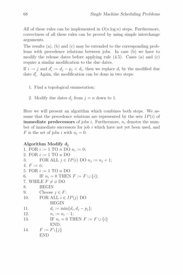
68 Single Machine Scheduling Problems
All of these rules can be implemented in O(n log n) steps. Furthermore,correctness of all these rules can be proved by using simple interchangearguments.
The results (a), (b) and (c) may be extended to the corresponding prob-lems with precedence relations between jobs. In case (b) we have tomodify the release dates before applying rule (4.5). Cases (a) and (c)require a similar modification to the due dates.
If i → j and d′i := dj − pj < di, then we replace di by the modified due
date d′i. Again, the modification can be done in two steps:
1. Find a topological enumeration;
2. Modify due dates dj from j = n down to 1.
Here we will present an algorithm which combines both steps. We as-sume that the precedence relations are represented by the sets IP (i) ofimmediate predecessors of jobs i. Furthermore, ni denotes the num-ber of immediate successors for job i which have not yet been used, andF is the set of jobs i with ni = 0.
Algorithm Modify dj
1. FOR i := 1 TO n DO ni := 0;2. FOR i := 1 TO n DO3. FOR ALL j ∈ IP (i) DO nj := nj + 1;4. F := φ;5. FOR i := 1 TO n DO6. IF ni = 0 THEN F := F ∪ {i};7. WHILE F �= φ DO8. BEGIN9. Choose j ∈ F ;10. FOR ALL i ∈ IP (j) DO
BEGIN11. di := min{di, dj − pj};12. ni := ni − 1;13. IF ni = 0 THEN F := F ∪ {i}
END;14. F := F\{j}
END
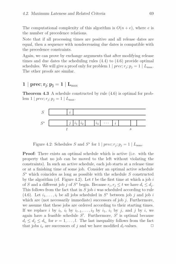
4.2. Maximum Lateness and Related Criteria 69
The computational complexity of this algorithm is O(n + e), where e isthe number of precedence relations.
Note that if all processing times are positive and all release dates areequal, then a sequence with nondecreasing due dates is compatible withthe precedence constraints.
Again, we can prove by exchange arguments that after modifying releasetimes and due dates the scheduling rules (4.4) to (4.6) provide optimalschedules. We will give a proof only for problem 1 | prec; rj; pj = 1 | Lmax.The other proofs are similar.
1 | prec; rj;pj = 1 | Lmax
Theorem 4.3 A schedule constructed by rule (4.6) is optimal for prob-lem 1 | prec; rj; pj = 1 | Lmax.
S∗
S
t s
j
i
i1 i2 i3 . . . i
Figure 4.2: Schedules S and S∗ for 1 | prec; rj; pj = 1 | Lmax.
Proof: There exists an optimal schedule which is active (i.e. with theproperty that no job can be moved to the left without violating theconstraints). In such an active schedule, each job starts at a release timeor at a finishing time of some job. Consider an optimal active scheduleS∗ which coincides as long as possible with the schedule S constructedby the algorithm (cf. Figure 4.2). Let t be the first time at which a job iof S and a different job j of S∗ begin. Because ri, rj ≤ t we have di ≤ dj.This follows from the fact that in S job i was scheduled according to rule(4.6). Let i1, . . . , il be all jobs scheduled in S∗ between job j and job iwhich are (not necessarily immediate) successors of job j. Furthermore,we assume that these jobs are ordered according to their starting times.If we replace i by il, il by il−1, . . . , i2 by i1, i1 by j, and j by i, weagain have a feasible schedule S ′. Furthermore, S ′ is optimal becausedi ≤ dj ≤ diν for ν = 1, . . . , l. The last inequality follows from the factthat jobs iν are successors of j and we have modified di-values. �
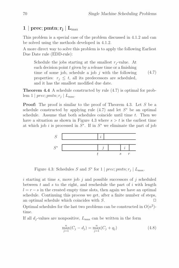
70 Single Machine Scheduling Problems
1 | prec;pmtn; rj | Lmax
This problem is a special case of the problem discussed in 4.1.2 and canbe solved using the methods developed in 4.1.2.
A more direct way to solve this problem is to apply the following EarliestDue Date rule (EDD-rule):
Schedule the jobs starting at the smallest rj-value. Ateach decision point t given by a release time or a finishingtime of some job, schedule a job j with the followingproperties: rj ≤ t, all its predecessors are scheduled,and it has the smallest modified due date.
(4.7)
Theorem 4.4 A schedule constructed by rule (4.7) is optimal for prob-lem 1 | prec; pmtn; rj | Lmax.
Proof: The proof is similar to the proof of Theorem 4.3. Let S be aschedule constructed by applying rule (4.7) and let S∗ be an optimalschedule. Assume that both schedules coincide until time t. Then wehave a situation as shown in Figure 4.3 where s > t is the earliest timeat which job i is processed in S∗. If in S∗ we eliminate the part of job
S∗
S
j
i
i
t s r
Figure 4.3: Schedules S and S∗ for 1 | prec; pmtn; rj | Lmax.
i starting at time s, move job j and possible successors of j scheduledbetween t and s to the right, and reschedule the part of i with lengthl = r− s in the created empty time slots, then again we have an optimalschedule. Continuing this process we get, after a finite number of steps,an optimal schedule which coincides with S. �
Optimal schedules for the last two problems can be constructed in O(n2)-time.
If all dj-values are nonpositive, Lmax can be written in the form
nmaxj=1
(Cj − dj) =n
maxj=1
(Cj + qj) (4.8)
4.2. Maximum Lateness and Related Criteria 71
where qj = −dj ≥ 0 for all j = 1, . . . , n. qj is called the tail of jobj. (4.8) is the finishing time, including post processing times qj , of alljobs j. Single machine problems with an objective function (4.8) play animportant role in connection with job-shop problems, whereby the releasetimes rj are called heads. The head-tail problem involves finding aschedule which is feasible with respect to the heads and minimizes (4.8).
We have the following result.
Corollary 4.5 (a) A preemptive schedule for the one machine head-tail problem with precedence constraints can be constructed inO(n2) time using the following rule:
At each time given by a head t or a finishing time tof some job, schedule a precedence feasible job j withrj ≤ t which has a largest tail.
(4.9)
(b) If there are no precedence constraints between jobs, then an optimalschedule for the head-tail problem can be found in O(n log n) time.
Proof: An earliest due date ordering corresponds with a largest tailordering. Thus, (a) follows from the results in this section.
To get the O(n logn)-algorithm in (b) we first sort the jobs according tonondecreasing heads. In addition to this sorted list, we keep a priorityqueue with the tails as keys. At each time t this priority queue holds allunfinished jobs j with rj ≤ t. It allows us to find an available job withlargest tail in constant time. Jobs which become available are insertedinto the queue and a job is deleted after finishing. Insertion and deletionof a job takes O(logn) time. �
Finally, we will present an efficient algorithm for the problem
1 | prec;pj = 1 | Lmax
This problem, which is a special case of problem 1 | prec; rj; pj = 1 | Lmax,can be solved more efficiently using an idea of Monma [169].
The first step is to modify the due dates in such a way that they are com-patible with the precedence relations. This is done by applying AlgorithmModify dj. Additionally, we assume that all modified due dates are non-negative. If this is not the case, we subtract the minimum modified duedate dmin from all modified due dates. This decreases the Lmax-value by
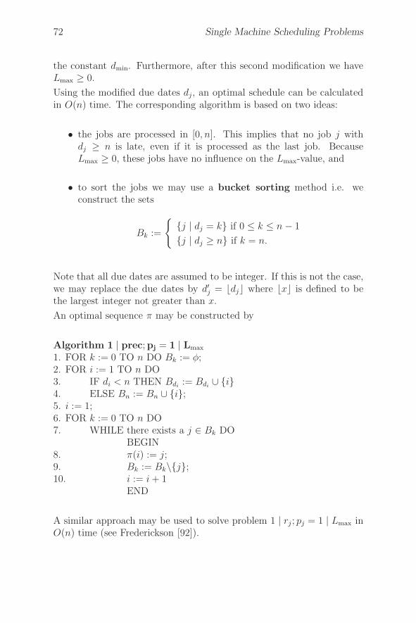
72 Single Machine Scheduling Problems
the constant dmin. Furthermore, after this second modification we haveLmax ≥ 0.
Using the modified due dates dj, an optimal schedule can be calculatedin O(n) time. The corresponding algorithm is based on two ideas:
• the jobs are processed in [0, n]. This implies that no job j withdj ≥ n is late, even if it is processed as the last job. BecauseLmax ≥ 0, these jobs have no influence on the Lmax-value, and
• to sort the jobs we may use a bucket sorting method i.e. weconstruct the sets
Bk :=
{{j | dj = k} if 0 ≤ k ≤ n − 1
{j | dj ≥ n} if k = n.
Note that all due dates are assumed to be integer. If this is not the case,we may replace the due dates by d′
j = �dj� where �x� is defined to bethe largest integer not greater than x.
An optimal sequence π may be constructed by
Algorithm 1 | prec;pj = 1 | Lmax
1. FOR k := 0 TO n DO Bk := φ;2. FOR i := 1 TO n DO3. IF di < n THEN Bdi
:= Bdi∪ {i}
4. ELSE Bn := Bn ∪ {i};5. i := 1;6. FOR k := 0 TO n DO7. WHILE there exists a j ∈ Bk DO
BEGIN8. π(i) := j;9. Bk := Bk\{j};10. i := i + 1
END
A similar approach may be used to solve problem 1 | rj ; pj = 1 | Lmax inO(n) time (see Frederickson [92]).
4.3. Total Weighted Completion Time 73
4.3 Total Weighted Completion Time
We will first discuss problem 1 | tree | ∑wjCj and some of its special
cases. Problem 1 | sp-graph | ∑wjCj will be discussed in 4.3.2. We allow
negative wj-values. However, in this case all jobs must be scheduled in
the time interval [0,n∑
j=1
pj ].
4.3.1 1 | tree | ∑wjCj
We have to schedule jobs with arbitrary processing times on a singlemachine so that a weighted sum of completion times is minimized. Theprocessing times are assumed to be positive. Precedence constraints aregiven by a tree. We first assume that the tree is an outtree (i.e. eachnode in the tree has at the most one predecessor). Later we will dealwith intrees (in which each node has at the most one successor). Thealgorithms presented are due to Adolphson and Hu [3].
Before presenting an algorithm for outtrees, we will prove some basicproperties of optimal schedules, which motivate the algorithm and areuseful for the correctness proof.
First we need to introduce some notation. For each job i = 1, . . . , n,define qi = wi/pi and let S(i) be the set of (not necessarily immediate)successors of i including i. For a set of jobs I ⊆ {1, . . . , n} define
w(I) :=∑
i∈I
wi, p(I) =∑
i∈I
pi, and q(I) := w(I)/p(I).
Two subsets I, J ⊆ {1, . . . , n} are parallel (I ∼ J) if, for all i ∈ I, j ∈ J ,neither i is a successor of j nor vice versa. The parallel sets must bedisjoint. In the case {i} ∼ {j} we simply write i ∼ j.
Each schedule is given by a sequence π.
Lemma 4.6 Let π be an optimal sequence and let I, J represent twoblocks (sets of jobs to be processed consecutively) of π such that I isscheduled immediately before J . Let π′ be the sequence we get from πby swapping I and J . Then
(a) I ∼ J implies q(I) ≥ q(J),
(b) if I ∼ J and q(I) = q(J), then π′ is also optimal.
74 Single Machine Scheduling Problems
Proof:
(a) Denote by f the objective function∑
wjCj . We have f(π) ≤ f(π′),because π is optimal. Thus
0 ≤ f(π′) − f(π) = w(I)p(J) − w(J)p(I).
Division by p(I)p(J) yields
q(I) = w(I)/p(I) ≥ w(J)/p(J) = q(J).
(b) If q(I) = q(J), then f(π) = f(π′) and π′ is also optimal.
�
Theorem 4.7 Let i, j be jobs with i → j and qj = max{qk | k ∈ S(i)}.Then there exists an optimal schedule in which i is processed immediatelybefore j.
Proof: Each schedule can be represented by a sequence. Let π be anoptimal sequence with the property that the number l of jobs scheduledbetween i and j is minimal. Assume l > 0. Then we have the followingsituation:
i · · · k j
We consider two cases.
Case 1: k ∈ S(i)j is not a successor of k because otherwise j would have at least twopredecessors. Thus, k ∼ j and Lemma 4.6 imply q(k) ≥ q(j). Bydefinition of j we also have q(j) ≥ q(k) which implies q(j) = q(k). Again,by Lemma 4.6, jobs j and k can be interchanged without destroyingoptimality. This contradicts the minimality of l.
Case 2: k /∈ S(i)Let h be the last job scheduled between i and j (i included) which belongsto S(i), i.e. for jobs r in the set K of jobs scheduled between h and j wehave r /∈ S(i). The outtree structure and i → j imply that a predecessorof j is also a predecessor of i. Thus, a job in K cannot be a predecessorof j, and we have K ∼ j. This implies q(K) ≥ q(j).
h ∈ S(i) is not a predecessor of some r ∈ K because this would implyr ∈ S(i). Therefore h ∼ K, which implies q(h) ≥ q(K) ≥ q(j). By
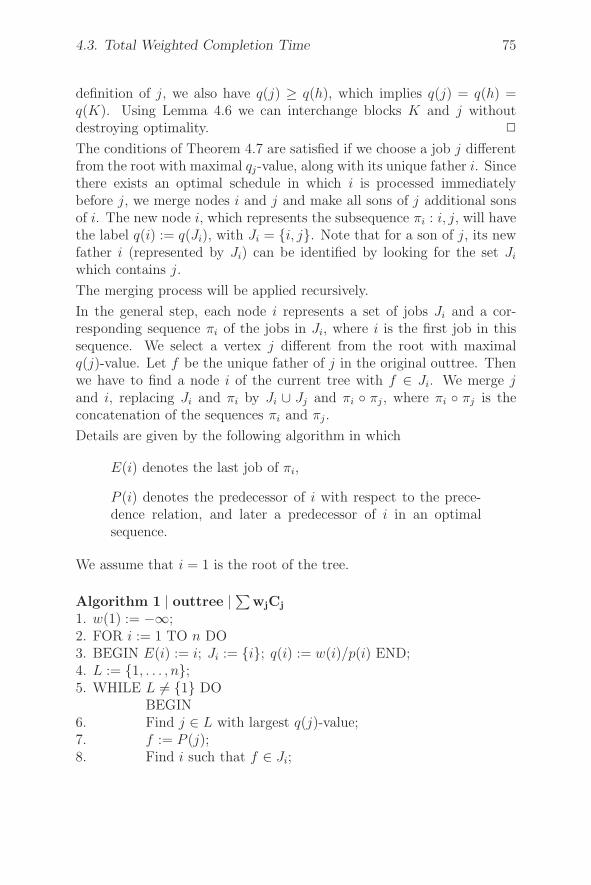
4.3. Total Weighted Completion Time 75
definition of j, we also have q(j) ≥ q(h), which implies q(j) = q(h) =q(K). Using Lemma 4.6 we can interchange blocks K and j withoutdestroying optimality. �
The conditions of Theorem 4.7 are satisfied if we choose a job j differentfrom the root with maximal qj-value, along with its unique father i. Sincethere exists an optimal schedule in which i is processed immediatelybefore j, we merge nodes i and j and make all sons of j additional sonsof i. The new node i, which represents the subsequence πi : i, j, will havethe label q(i) := q(Ji), with Ji = {i, j}. Note that for a son of j, its newfather i (represented by Ji) can be identified by looking for the set Ji
which contains j.
The merging process will be applied recursively.
In the general step, each node i represents a set of jobs Ji and a cor-responding sequence πi of the jobs in Ji, where i is the first job in thissequence. We select a vertex j different from the root with maximalq(j)-value. Let f be the unique father of j in the original outtree. Thenwe have to find a node i of the current tree with f ∈ Ji. We merge jand i, replacing Ji and πi by Ji ∪ Jj and πi ◦ πj , where πi ◦ πj is theconcatenation of the sequences πi and πj .
Details are given by the following algorithm in which
E(i) denotes the last job of πi,
P (i) denotes the predecessor of i with respect to the prece-dence relation, and later a predecessor of i in an optimalsequence.
We assume that i = 1 is the root of the tree.
Algorithm 1 | outtree | ∑wjCj
1. w(1) := −∞;2. FOR i := 1 TO n DO3. BEGIN E(i) := i; Ji := {i}; q(i) := w(i)/p(i) END;4. L := {1, . . . , n};5. WHILE L �= {1} DO
BEGIN6. Find j ∈ L with largest q(j)-value;7. f := P (j);8. Find i such that f ∈ Ji;
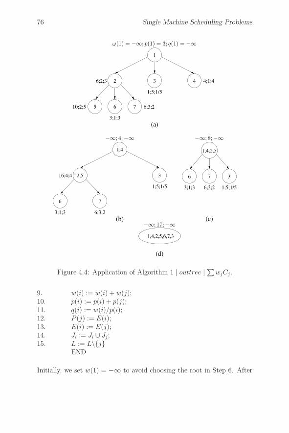
76 Single Machine Scheduling Problems
6 7 3
1;5;1/56;3;23;1;3
1,4,2,5
5 6 7
4
3;1;3
6;3;2
1;5;1/5
4;1;46;2;3
10;2;5
32
1
(a)
7
16;4;4
1,4
2,5
6
3;1;3 6;3;2
3
1;5;1/5
(b) (c)
(d)
1,4,2,5,6,7,3
−∞; 8;−∞
ω(1) = −∞; p(1) = 3; q(1) = −∞
−∞; 4;−∞
−∞; 17;−∞
Figure 4.4: Application of Algorithm 1 | outtree | ∑wjCj .
9. w(i) := w(i) + w(j);10. p(i) := p(i) + p(j);11. q(i) := w(i)/p(i);12. P (j) := E(i);13. E(i) := E(j);14. Ji := Ji ∪ Jj;15. L := L\{j}
END
Initially, we set w(1) = −∞ to avoid choosing the root in Step 6. After
4.3. Total Weighted Completion Time 77
termination, the optimal sequence π∗ may be constructed using E(1)and the array P (i). This is done by constructing π∗ from right to left:j := E(1) is the last job in π∗, P (j) is the predecessor of j in π∗, etc.The example in Figure 4.4 shows how the algorithm works. Fig. 4.4(a)shows a problem with 7 jobs. Fig. 4.4(b) i presents the tree after twoiterations. The result after the next operations is shown in Figs 4.4(c)and (d). The optimal sequence is 1,4,2,5,6,7,3.
Algorithm 1 | outtree | ∑wjCj can be implemented in O(n log n)-time
if a priority queue is used for the q(i)-values and an efficient union-findalgorithm for sets is used in Steps 8 and 14 (see Aho, Hopcroft, Ullmann[4]). It remains to prove that an optimal sequence is constructed.
Theorem 4.8 Algorithm 1 | outtree | ∑wjCj calculates an optimal
sequence in O(n log n)-time.
Proof: We prove optimality by induction on the number of jobs.
Clearly the algorithm is correct if we have only one job. Let P be aproblem with n jobs. Assume that i, j are the first jobs merged by thealgorithm. Let P ′ be the resulting problem with n − 1 jobs, where i isreplaced by I := (i, j) with w(I) = w(i) + w(j) and p(I) = p(i) + p(j).
Let R be the set of sequences of the form
π : π(1), . . . , π(k), i, j, π(k + 3), . . . , π(n)
and let R′ be the set of sequences of the form
π′ : π(1), . . . , π(k), I, π(k + 3), . . . , π(n).
Note that by Theorem 4.7 set R contains an optimal schedule. Further-more, for the corresponding objective function values fn(π) and fn−1(π
′)we have
fn(π) − fn−1(π′)
= w(i)p(i) + w(j)(p(i) + p(j)) − (w(i) + w(j))(p(i) + p(j))
= −w(i)p(j).
We conclude that π ∈ R is optimal if and only if the correspondingπ′ ∈ R′ is optimal. However, π′ has only n − 1 jobs. Thus, by theinduction hypothesis, the sequence constructed by our algorithm mustbe optimal. �
To solve a 1 | intree | ∑wjCj-problem P , we reduce P to a 1 | outtree |∑
w′jCj-problem P ′ with
78 Single Machine Scheduling Problems
• i is a successor of j in P ′ if and only if j is a successor of i in P ,and
• w′j = −wj for j = 1, . . . , n.
Then a sequence π : 1, . . . , n is feasible for P if and only if π′ : n, . . . , 1is feasible for P ′. Furthermore, we have
f ′(π′) =n∑
i=1
(−wi)(∑
j≥i
pj) =n∑
i=1
(−wi)(∑
j>i
pj) −n∑
i=1
wipi
=n∑
i=1
wi(∑
j≤i
pj) − (n∑
i=1
wi)(n∑
j=1
pj) −n∑
i=1
wipi
= f(π) − a
where a does not depend on the sequence π. Thus a sequence π for P isoptimal if and only if the reverse sequence π′ is optimal for P ′.
An instance of problem 1 || ∑wjCj can be reduced to an instance of
problem 1 | outtree | ∑wjCj by adding a root r with very small pro-
cessing time as a dummy job. After calculating an optimal sequence,we have to eliminate r to get an optimal sequence for the instance of1 || ∑
wjCj . This process leads to
Smith’s ratio rule: Put the jobs in order of nondecreasing ratios pj/wj ,which applies if all wj > 0.
That Smith’s ratio rule leads to an optimal sequence can also be shownby a simple interchange argument.
If all weights are equal to one, we have problem 1 || ∑Cj which is solved
by
Smith’s rule: Put the jobs in order of nondecreasing processing times(“shortest processing time first” -rule).
A related problem is
1 | rj;pmtn | ∑Cj
This problem can be solved by constructing a schedule from left to rightusing:
Modified Smith’s rule: At each release time or finishing time of ajob, schedule an unfinished job which is available and has the smallestremaining processing time.
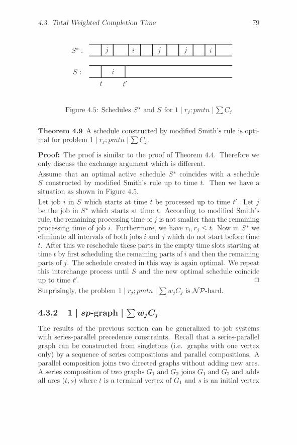
4.3. Total Weighted Completion Time 79
S :
S∗ : j i j j i
i
t t′
Figure 4.5: Schedules S∗ and S for 1 | rj; pmtn | ∑Cj
Theorem 4.9 A schedule constructed by modified Smith’s rule is opti-mal for problem 1 | rj; pmtn | ∑
Cj.
Proof: The proof is similar to the proof of Theorem 4.4. Therefore weonly discuss the exchange argument which is different.
Assume that an optimal active schedule S∗ coincides with a scheduleS constructed by modified Smith’s rule up to time t. Then we have asituation as shown in Figure 4.5.
Let job i in S which starts at time t be processed up to time t′. Let jbe the job in S∗ which starts at time t. According to modified Smith’srule, the remaining processing time of j is not smaller than the remainingprocessing time of job i. Furthermore, we have ri, rj ≤ t. Now in S∗ weeliminate all intervals of both jobs i and j which do not start before timet. After this we reschedule these parts in the empty time slots starting attime t by first scheduling the remaining parts of i and then the remainingparts of j. The schedule created in this way is again optimal. We repeatthis interchange process until S and the new optimal schedule coincideup to time t′. �
Surprisingly, the problem 1 | rj ; pmtn | ∑wjCj is NP-hard.
4.3.2 1 | sp-graph | ∑wjCj
The results of the previous section can be generalized to job systemswith series-parallel precedence constraints. Recall that a series-parallelgraph can be constructed from singletons (i.e. graphs with one vertexonly) by a sequence of series compositions and parallel compositions. Aparallel composition joins two directed graphs without adding new arcs.A series composition of two graphs G1 and G2 joins G1 and G2 and addsall arcs (t, s) where t is a terminal vertex of G1 and s is an initial vertex
80 Single Machine Scheduling Problems
of G2. Note that unlike parallel composition, a series composition is nota symmetric operation.
Figure 4.6(a) shows a series-parallel graph which is constructed by thefollowing operations. First we build G1 and G2 by a parallel compositionof the singletons 2,3 and 5,6, respectively. Then we construct G3 andG4, composing the singleton 1 in series with G1 and G3 in series with thesingleton 4. Finally, we get the graph shown in Figure 4.6(a) by seriescomposition of G4 and G2.
A series-parallel graph may be represented by its decomposition tree,which is a binary tree, with singletons as leaves. Each inner node ofthe tree represents a composition. Parallel and series composition arelabeled P and S, respectively. Figure 4.6(b) shows a decomposition treefor the graph in Figure 4.6(a). The algorithm which solves problem1 | sp-graph | ∑
wjCj works from the bottom of the tree upward, mergingsequences of jobs in an appropriate way. These sequences are associatedwith the leaves of the tree. All sequences are disjoint subsequences ofan optimal sequence which can be constructed by concatenating thesesubsequences. Initially, we associate with a leaf representing job i theone element set Si := {i}, consisting of the subsequence i of length 1. Inthe general step of the algorithm, two leaves with the same father f aremerged, creating a new set Sf of subsequences. Furthermore, the fatherturns into a leaf with subsequences set Sf . The merging process dependson the type of composition represented by the father.
To describe this composition in more detail we need some further nota-tions. Let π be a subsequence. Then p(π) and w(π) denote the sum ofprocessing times and weights of all jobs in subsequence π. Furthermore,let q(π) = w(π)/p(π). The concatenation of two subsequences π1 and π2
is denoted by π1 ◦ π2.
Let Si(Sj) be the set of subsequences of the left (right) child of f . Thenthe following two procedures calculate the set of subsequences of thefather f depending on the label of f .
If f is a parallel node, then we simply have
Parallel (Si,Sj)1.RETURN Si ∪ Sj
The procedure in the case of a series composition is more involved.
4.3. Total Weighted Completion Time 81
Series (Si,Sj)1. Find πi ∈ Si with q(πi) = min{q(π) | π ∈ Si};2. Find πj ∈ Sj with q(πj) = max{q(π) | π ∈ Sj};3. IF q(πi) > q(πj) THEN RETURN Si ∪ Sj
ELSEBEGIN
4. π := πi ◦ πj ;5. Si := Si\{πi};6. Find πi ∈ Si with q(πi) = min{q(π) | π ∈ Si};7. Sj := Sj\{πj};8. Find πj ∈ Sj with q(πj) = max{q(π) | π ∈ Sj};9. WHILE q(π) ≥ q(πi) OR q(πj) ≥ q(π) DO10. IFq(π) ≥ q(πi) THEN
BEGIN11. π := πi ◦ π; Si := Si\{πi};12. Find πi ∈ Si with q(πi) = min{q(π) | π ∈ Si}
ENDELSE
BEGIN13. π := π ◦ πj ; Sj := Sj\{πj};14. Find πj ∈ Sj with q(πj) = max{q(π) | π ∈ Sj}
END;15. RETURN Si ∪ Sj ∪ {π}
END
Note that after applying Series (Si, Sj), for all πi ∈ Si and πj ∈ Sj ,the inequalities q(πi) > q(πj) or q(πi) > q(π) > q(πj) hold. Thus, if asubsequence πi must be processed before a subsequence πj , we must haveq(πi) > q(πj). The following algorithm calculates an optimal sequenceπ∗ for problem 1 | sp-graph | ∑
wjCj.
Algorithm 1 | sp-graph | ∑wjCj
1. FOR ALL leaves i of the decomposition tree DO Si := {i};2. WHILE there exists a vertex f with two leaves as children DO
BEGIN3. i := leftchild(f); j := rightchild(f);4. IF f has label P THEN5. Sf := Parallel (Si, Sj)
ELSE
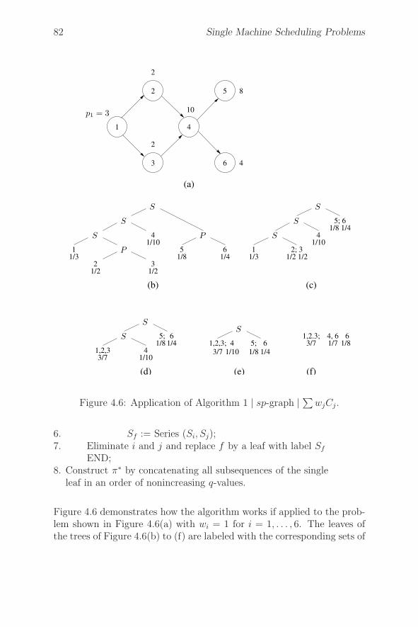
82 Single Machine Scheduling Problems
(a)
4
8
1
10
2
2
2
4
3
5
6
(c)
21/2
41/10
1/23
(b)
11/3
51/8
61/4
41/10
1/8 1/4
1/32; 3
1/2 1/21
41/10
1,2,33/7
(d) (e) (f)
5; 6
3/71,2,3; 44, 61/76
1,2.3;1/8
1/8 1/45;
6
3/7 1/10
5; 61/8 1/4
p1 = 3
S
S
P
S
P
S
S
S
SS
S
Figure 4.6: Application of Algorithm 1 | sp-graph | ∑wjCj.
6. Sf := Series (Si, Sj);7. Eliminate i and j and replace f by a leaf with label Sf
END;8. Construct π∗ by concatenating all subsequences of the single
leaf in an order of nonincreasing q-values.
Figure 4.6 demonstrates how the algorithm works if applied to the prob-lem shown in Figure 4.6(a) with wi = 1 for i = 1, . . . , 6. The leaves ofthe trees of Figure 4.6(b) to (f) are labeled with the corresponding sets of
4.3. Total Weighted Completion Time 83
sequences. The corresponding q(π)-value is shown below each sequenceπ. If we concatenate the three sequences shown in Figure 4.6(f) in sucha way that the sequence with the larger q-value is first, we get the opti-mal sequence π∗ : 1, 2, 3, 4, 6, 5. The algorithm runs in O(n log n) time ifimplemented appropriately (Aho et al. [4]).
To prove that Algorithm 1 | sp-graph | ∑wjCj is correct, we first show
that it satisfies the following invariance property: There exists an opti-mal solution which can be constructed by concatenating all subsequencesassociated with the leaves of the current decomposition tree (i.e. all sub-sequences σ ∈ ⋃
Si).
The invariance property holds initially, when each job corresponds with aone element subsequence associated with some leaf of the decompositiontree. Furthermore, a parallel composition keeps the invariance propertysatisfied.
Lemma 4.10 The invariance property is satisfied during all steps ofAlgorithm 1 | sp-graph | ∑
wjCj.
Proof: If the invariance property is violated, it will be violated whenconcatenating two subsequences. Consider the first concatenation violat-ing the invariance property. We assume that this is a concatenation πi◦πj
done in Step 4 of the procedure Series(Si, Sj). Concatenations of Steps11 and 13 are treated similarly. The subsequence πi ◦πj is not containedin an optimal solution σ but all subsequences created previously are con-tained in some σ. Thus, σ contains πi with q(πi) = min{q(π) | π ∈ Si}and πj with q(πj) = max{q(π) | π ∈ Sj}. Furthermore, in σ, sub-sequence πi is scheduled before πj and between πi and πj we have asequence σ1, σ2, . . . , σr. Additionally, q(πi) ≤ q(πj) holds. We assumethat the optimal solution σ is chosen in such a way that the number r ofsubsequences σν between πi and πj is minimal.
If σ1 ∈ Si, then q(σ1) ≥ min{q(π) | π ∈ Si} = q(πi) and we can swap σ1
and πi without increasing the objective value. This follows from the factthat σ1 can be processed before πi because q(σ1) ≥ q(πi). Furthermore,according to the proof of Lemma 4.6, the objective function does notincrease when swapping σ1 and πi. Thus, the new sequence is optimal,contradicting the minimality of r. Similarly, we can swap σr and πj ifσr ∈ Sj . Because σs ∈ Si and σt ∈ Sj imply s < t, the only cases left are:
Case 1: σt ∈ Sj and σt+1, . . . , σr /∈ Si ∪ Sj .
Let ρ := σt+1 ◦ . . . ◦ σr. If q(σt) ≤ q(ρ), we may swap σt with ρ, and σt
84 Single Machine Scheduling Problems
with πj without increasing the objective function. This follows from thefact that there is no job k in one of the subsequences σt+1, . . . , σr whichis a successor of a job in σt ∈ Sj. Otherwise, due to the constructionof the series parallel graph, such a job k would also be a successor ofa job in πj ∈ Sj, which is impossible. If q(ρ) ≤ q(πj), we may swap ρwith πj and then σt with πj . The remaining case q(σt) > q(ρ) > q(πj)contradicts the definition of πj .
Case 2: σ1, . . . , σs−1 /∈ Si ∪ Sj and σs ∈ Si is symmetric to Case 1.
Case 3: σ1, . . . , σr /∈ Si ∪ Sj.
Let ρ := σ1 ◦ . . .◦σr. If q(ρ) ≥ q(πi), then we may swap ρ and πi withoutincreasing the objective function. If q(ρ) < q(πi) ≤ q(πj), then we mayswap ρ and πj . �
Theorem 4.11 Algorithm 1 | sp-graph | ∑wjCj is correct.
Proof: Due to Lemma 4.10 there exists an optimal sequence σ whichcontains all subsequences created by the algorithm. If, in σ, we permutethese subsequences according to nonincreasing q-values, the objectivevalue will not increase. Furthermore, the subsequences are constructedin such a way that the sequence resulting from this permutation is com-patible with the precedence constraints. Hence, it must be optimal. �
4.4 Weighted Number of Late Jobs
In this section we will discuss problems with objective function∑
wjUj .Karp [124] has shown that problem 1 || ∑
wjUj is NP-hard. In Sec-tion 2.7 we presented a pseudopolynomial algorithm based on dynamicprogramming for this problem. In connection with this algorithm, wehave shown that an optimal schedule is defined by the set of early jobsscheduled in order of nondecreasing due dates. In this section we willconsider special cases of problem 1 ‖ ∑
wjUj . Furthermore, we willdiscuss preemptive versions of the problem.
4.4.1 1 | rj;pj = 1 | ∑wjUj
In Section 2.5 we showed that problem 1 | rj; pj = 1 | ∑wjUj can be
reduced to an assignment problem that can be solved in time O(n3). In
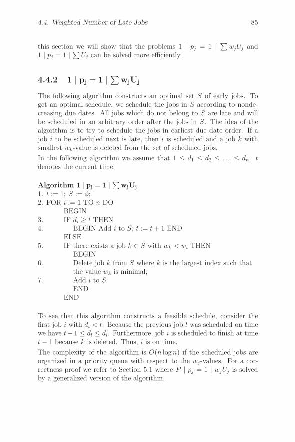
4.4. Weighted Number of Late Jobs 85
this section we will show that the problems 1 | pj = 1 | ∑wjUj and
1 | pj = 1 | ∑Uj can be solved more efficiently.
4.4.2 1 | pj = 1 | ∑wjUj
The following algorithm constructs an optimal set S of early jobs. Toget an optimal schedule, we schedule the jobs in S according to nonde-creasing due dates. All jobs which do not belong to S are late and willbe scheduled in an arbitrary order after the jobs in S. The idea of thealgorithm is to try to schedule the jobs in earliest due date order. If ajob i to be scheduled next is late, then i is scheduled and a job k withsmallest wk-value is deleted from the set of scheduled jobs.
In the following algorithm we assume that 1 ≤ d1 ≤ d2 ≤ . . . ≤ dn. tdenotes the current time.
Algorithm 1 | pj = 1 | ∑wjUj
1. t := 1; S := φ;2. FOR i := 1 TO n DO
BEGIN3. IF di ≥ t THEN4. BEGIN Add i to S; t := t + 1 END
ELSE5. IF there exists a job k ∈ S with wk < wi THEN
BEGIN6. Delete job k from S where k is the largest index such that
the value wk is minimal;7. Add i to S
ENDEND
To see that this algorithm constructs a feasible schedule, consider thefirst job i with di < t. Because the previous job l was scheduled on timewe have t−1 ≤ dl ≤ di. Furthermore, job i is scheduled to finish at timet − 1 because k is deleted. Thus, i is on time.
The complexity of the algorithm is O(n logn) if the scheduled jobs areorganized in a priority queue with respect to the wj-values. For a cor-rectness proof we refer to Section 5.1 where P | pj = 1 | wjUj is solvedby a generalized version of the algorithm.
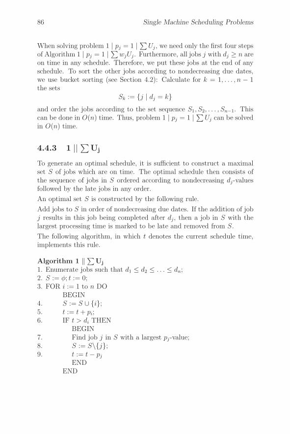
86 Single Machine Scheduling Problems
When solving problem 1 | pj = 1 | ∑Uj , we need only the first four steps
of Algorithm 1 | pj = 1 | ∑wjUj . Furthermore, all jobs j with dj ≥ n are
on time in any schedule. Therefore, we put these jobs at the end of anyschedule. To sort the other jobs according to nondecreasing due dates,we use bucket sorting (see Section 4.2): Calculate for k = 1, . . . , n − 1the sets
Sk := {j | dj = k}and order the jobs according to the set sequence S1, S2, . . . , Sn−1. Thiscan be done in O(n) time. Thus, problem 1 | pj = 1 | ∑
Uj can be solvedin O(n) time.
4.4.3 1 || ∑Uj
To generate an optimal schedule, it is sufficient to construct a maximalset S of jobs which are on time. The optimal schedule then consists ofthe sequence of jobs in S ordered according to nondecreasing dj-valuesfollowed by the late jobs in any order.
An optimal set S is constructed by the following rule.
Add jobs to S in order of nondecreasing due dates. If the addition of jobj results in this job being completed after dj, then a job in S with thelargest processing time is marked to be late and removed from S.
The following algorithm, in which t denotes the current schedule time,implements this rule.
Algorithm 1 ‖ ∑Uj
1. Enumerate jobs such that d1 ≤ d2 ≤ . . . ≤ dn;2. S := φ; t := 0;3. FOR i := 1 to n DO
BEGIN4. S := S ∪ {i};5. t := t + pi;6. IF t > di THEN
BEGIN7. Find job j in S with a largest pj-value;8. S := S\{j};9. t := t − pj
ENDEND
4.4. Weighted Number of Late Jobs 87
Theorem 4.12 Algorithm 1 || ∑Uj constructs the set S of early jobs
in an optimal schedule.
Proof: We denote a schedule by P = (S, F ), where S is the set of earlyjobs and F is the set of the late jobs.
Let j be the first job which, in Step 8 of the algorithm, is deleted fromset S. We first prove that there exists an optimal schedule P = (S, F )with j ∈ F . Denote by k the job which was added to S in the precedingStep 4. Then
pj =k
maxi=1
pi.
Furthermore, when scheduling the partial sequence 1, 2, . . . , j − 1, j +1, . . . , k no job is late. This follows from the fact that in 1, 2, . . . , k − 1no job is late and pk ≤ pj . We replace j by k and reorder jobs accordingto nondecreasing due dates.
Now consider an optimal schedule P ′ = (S ′, F ′) with j ∈ S ′. There existsa sequence
π : π(1), . . . , π(m), . . . , π(r), π(r + 1), . . . , π(n)
with
F ′ = {π(r + 1), . . . , π(n)} (4.10)
dπ(1) ≤ . . . ≤ dπ(r) (4.11)
{π(1), . . . , π(m)} ⊆ {1, . . . , k} (4.12)
{π(m + 1), . . . , π(r)} ⊆ {k + 1, . . . , n} (4.13)
j ∈ {π(1), . . . , π(m)}. (4.14)
Since d1 ≤ d2 ≤ . . . ≤ dn, there always exists m such that (4.12) and(4.13) are satisfied. Furthermore, (4.14) holds because j ∈ S ′∩{1, . . . , k}.Since {π(1), . . . , π(m)} ⊆ S ′, no job in {π(1), . . . , π(m)} is late. On theother hand, there is a late job in {1, . . . , k} in any schedule. Thus wehave
{π(1), . . . , π(m)} � {1, . . . , k},which implies that we have a job h(1 ≤ h ≤ k) with h /∈ {π(1), . . . ,π(m)}. We delete job j from {π(1), . . . , π(m)} and replace it by h. If weorder all jobs in {π(1), . . . , π(m)} ∪ {h}\{j} ⊆ {1, . . . , k}\{j} accordingto nondecreasing due dates, all jobs are on time because {1, . . . , k}\{j}
88 Single Machine Scheduling Problems
has this property. If we add the jobs π(m + 1), . . . , π(r) to the set{π(1), . . . , π(m)} ∪ {h}\{j} and sort all jobs according to nondecreas-ing due dates, all jobs are on time because ph ≤ pj implies
m∑
i=1
pπ(i) − pj + ph ≤m∑
i=1
pπ(i).
Thus we get an optimal schedule P = (S, F ) with j ∈ F .
Now it is not difficult to prove the theorem by induction on the number nof jobs. Clearly the algorithm is correct if n = 1. Assume the algorithmis correct for all problems with n−1 jobs. Let P = (S, F ) be the scheduleconstructed by the algorithm and let P ′ = (S ′, F ′), an optimal schedulewith j ∈ F ′.
Then, by optimality, we have | S |≤| S ′ |.If we apply the algorithm to the set of jobs {1, . . . , j−1, j +1, . . . , n} weget an optimal schedule of the form (S, F\{j}). Because (S ′, F ′\{j}) isfeasible for the reduced problem, we have | S ′ |≤| S |. Thus | S ′ |=| S |and P is optimal. �
4.4.4 1 | rj;pmtn | ∑wjUj
Karp [124] has shown that problem 1 ‖ ∑wjUj is NP-hard. At the
beginning of this chapter, we saw that a preemptive schedule for a onemachine problem with monotone objective function and rj = 0 for alljobs j can be polynomially transformed into a nonpreemptive schedulewithout increasing the objective function. This implies that 1 | pmtn |∑
wjUj is NP-hard as well. In this section we present an O(nk2W 2)-algorithm for problem 1 | rj; pmtn | ∑
wjUj where k is the number of
distinct release dates and W =n∑
j=1
wj. This gives an O(n5)-algorithm for
problem 1 | rj; pmtn | ∑Uj.
We assume that all data are integer and that wj > 0 for j = 1, . . . , n.
A set of jobs S is feasible if there exists a schedule for S in which alljobs are completed on time. To check whether a set is feasible, we mayapply the following simplified version of the EDD rule (see 4.7):
Schedule the jobs in time starting with the smallest rj-value.At each decision point given by a release time or a finish timeof some job, schedule a job with smallest due date.
(4.15)
4.4. Weighted Number of Late Jobs 89
S is feasible if and only if there are no late jobs in the EDD schedule forS. This is an immediate consequence of Theorem 4.4. If S has n jobs,the corresponding EDD schedule can be constructed in O(n logn) time.Our problem reduces to that of finding a maximum-weight feasible setS.
For a given nonempty feasible set S define
r(S) = minj∈S
rj ; p(S) =∑
j∈S
pj ; w(S) =∑
j∈S
wj .
Furthermore, let C(S) be the completion time of the last job in S in anEDD schedule.
An EDD schedule consists of periods of continuous processing, separatedby periods of idle time during which no job is available for processing.This means that S can be partitioned into subsets S1, S2, . . . , Sl withC(Si) = r(Si)+p(Si) < r(Si+1) for i = 1, . . . , l−1. A feasible subset S isa block if S is processed continuously from start to finish and S cannotbe decomposed into subsets that are schedule-disjoint, i.e. C(S) = r(S)+p(S), and S is not the union of subsets S1, S2 such that C(S1) < r(S2).
Next we will present a dynamic programming solution for problem 1 |rj ; pmtn | ∑
wjUj . Again, we assume that
d1 ≤ d2 ≤ . . . ≤ dn.
Let k denote the number of distinct release dates.
For a release date r and an integer w with 0 ≤ w ≤ W define
Cj(r, w) := min{C(S) | S ⊆ {1, . . . , j} is feasible; r(S) ≥ r; w(S) ≥ w}
if there exists a feasible set S ⊆ {1, . . . , j} with r(S) ≥ r, w(S) ≥ w andCj(r, w) = ∞ otherwise.
The maximum weight of a feasible set is given by the largest value of w
such that Cn(rmin, w) is finite, where rmin :=n
minj=1
rj .
We compute the values Cj(r, w) in n iterations, j = 1, 2, . . . , n, startingwith the initial conditions
C0(r, 0) = r for all r,
C0(r, w) = ∞ for all r and w > 0.
90 Single Machine Scheduling Problems
j cannot be contained in a feasible set S with r(S) > rj. Hence,
Cj(r, w)
{= Cj−1(r, w) if r > rj
≤ Cj−1(r, w) otherwise .
It follows that at iteration j we have only to compute the value of Cj(r, w)for which r ≤ rj .
Let S ⊆ {1, 2, . . . , j} with Cj(r, w) = C(S). If j /∈ S, then we haveCj(r, w) = Cj−1(r, w). If j ∈ S, we consider two cases.
Case 1: Job j starts after C(S\{j}).Either C(S\{j}) ≤ rj , or C(S\{j}) > rj . In the first case, we haveC(S) = rj + pj . In the second case, jobs in S\{j} are processed con-tinuously in the interval [rj , C(S\{j})] because otherwise j would startbefore C(S\{j}). We conclude that
Cj(r, w) = max{rj, C(S\{j})} + pj .
We may assume that S\{j} is such that
C(S\{j}) = Cj−1(r, w − wj).
If this is not so, replace S\{j} by a feasible subset of {1, 2, . . . , j−1} forwhich this is satisfied.
It follows that
Cj(r, w) = max{rj, Cj−1(r, w − wj)} + pj.
Case 2: Job j starts before C(S\{j}).In this case there is idle time in the EDD schedule for the set S\{j}after rj . Let S ′ be the last block in S\{j}, i.e. r(S ′) = max{r(B) | Bis a block of S\{j}}. Then r(S ′) ≥ rj, and it must be the case thatC(S ′) = Cj−1(r(S
′), w(S ′)), otherwise S is not optimal.
Also, we may assume that the total amount of processing done on jobs in(S\{j})\S ′ in the interval [rj , r(S
′)] is minimal, with respect to all fea-sible sets S ′′ ⊆ {1, 2, . . . , j − 1} with r(S ′′) ≥ r, C(S ′′) ≤ r(S ′), w(S ′′) ≥w − wj − w(S ′).
Let r, r′ be release dates with r ≤ rj < r′, and w′′ be an integer with0 ≤ w′′ < W . Define Pj−1(r, r
′, w′′) to be the minimum amount ofprocessing done in the interval [rj , r
′] with respect to feasible sets S ′′ ⊆
4.4. Weighted Number of Late Jobs 91
{1, 2, . . . , j − 1} with r(S ′′) ≥ r, C(S ′′) ≤ r′, w(S ′′) ≥ w′′. If there is nosuch feasible set S ′′, then let Pj−1(r, r
′, w′′) = ∞.
Using this notation, the amount of time available for processing job j inthe interval [rj , r(S
′)] is
(r(S ′) − rj) − Pj−1(r, r(S′), w − wj − w(S ′)).
The amount of processing done on j after time r(S ′) is
max{0, pj − (r(S ′) − rj) + Pj−1(r, r(S′), w − wj − w(S ′))}
and the completion time of the last job in S is
Cj(r, w) = minr′,w′
{Cj−1(r′, w′)
+ max{0, pj − r′ + rj + Pj−1(r, r′, w − wj − w′)}}. (4.16)
Putting all of the above observations together, we obtain the recurrencerelation
Cj(r, w) = min
⎧⎪⎪⎪⎪⎨
⎪⎪⎪⎪⎩
Cj−1(r, w)
max{rj, Cj−1(r, w − wj)} + pj
minr′,w′
{Cj−1(r′, w′) + max{0, pj − r′ + rj
+Pj−1(r, r′, w − wj − w′)}},
(4.17)
where the inner minimization is taken over all distinct release dates r′ >rj such that r′ = r(S ′) ∈ {r1, . . . , rj−1} and all integers w′, 0 ≤ w′ <w−wj . It is important to note that (4.17) is valid only if the right-handside does not exceed dj; if this is not so we set Cj(r, w) = ∞.
Now we have to consider how to compute the values Pj−1(r, r′, w′′) for
r ≤ rj < r′ and 0 ≤ w′′ < W . If w′′ = 0, then Pj−1(r, r′, w′′) = 0. If w′′ >
0, then Pj−1(r, r′, w′′) is realized by a nonempty set S ′′ ⊆ {1, . . . , j − 1}.
If r(S ′′) > r, then Pj−1(r, r′, w′′) = Pj−1(r(S
′′), r′, w′′). Also, in general,we observe that
Pj−1(r, r′, w′′) ≤ Pj−1(r
+, r′, w′′)
where r+ is the smallest distinct release date, if any, larger than r.
If r(S ′′) = r, then let S ′ ⊆ S ′′ be the block of S ′′ such that r(S ′) = r.We may assume that C(S ′) = Cj−1(r, w(S ′)). Hence, the total amountof processing done on S ′ in the interval [rj , r
′] is
max{0, Cj−1(r, w(S ′)) − rj}.
92 Single Machine Scheduling Problems
Let r′′ be the smallest release date greater than or equal to Cj−1(r, w(S ′)).Then the total amount of processing done on S ′′\S ′ in the interval [rj , r
′]is Pj−1(r
′′, r′, w′′ − w(S ′)). Hence, the total amount of processing doneon S ′′ in the interval [rj , r
′] is
max{0, Cj−1(r, w(S ′)) − rj} + Pj−1(r′′, r′, w′′ − w(S ′)). (4.18)
The right-hand side of (4.18) must be minimal with respect to setsS ′, S ′′\S ′, with r(S ′) = r, C(S ′) ≤ r(S ′′\S ′) = r′′, w(S ′)+w(S ′′\S ′) = w′′.It follows that we now have
Pj−1(r, r′, w′′) = min
⎧⎪⎪⎨
⎪⎪⎩
Pj−1(r+, r′, w′′)
min0<w′≤w′′
{max{0, Cj−1(r, w′) − rj}
+Pj−1(r′′, r′, w′′ − w′)}
(4.19)
with the initial conditions
Pj−1(r, r′, 0) = 0 for j = 1, . . . , n
P0(r, r′, w′′) = ∞ for w′′ > 0.
We now analyze the time complexity of the dynamic programming com-putation.
At each of n iterations j = 1, . . . , n, there are O(k2W ) of the Pj−1(r, r′,
w′′) values to compute, one for each combination of r, r′, w′′. By (4.19),each Pj−1(r, r
′, w′′) is found by minimization over O(W ) choices of w′ ≤w′′. Hence, the time required to compute the Pj−1(r, r
′, w′′) values ateach iteration is bounded by O(k2W 2). There are O(kW ) of the Cj(r, w)values to compute, one for each combination of r and w. By (4.17), eachCj(r, w) is found by minimization over O(kW ) choices of r′, w′. Hence,the time required to compute the Cj(r, w) values at each iteration isbounded by O(k2W 2). The maximum weight of a feasible subset canbe obtained by finding the maximum value w such that Cn(rmin, w) isfinite. This takes O(W ) time. It follows that the overall time bound isO(nk2W 2).
To construct a maximum-weight feasible set, we compute an incidencevector of the set realizing each Pj−1(r, r
′, w′′) and Cj(r, w) value. Thecomputation of these incidence vectors can be carried out in O(n2k2W )time, which is dominated by the O(nk2W 2) time bound obtained above.
Finally, we will discuss some special cases. When release dates and duedates are similarly ordered, i.e. when
r1 ≤ r2 ≤ . . . ≤ rn and d1 ≤ d2 ≤ . . . ≤ dn,
4.5. Total Weighted Tardiness 93
then Case 2 never applies. In such a situation the recurrence relations(4.17) simplify to
Cj(r, w) = min
{Cj−1(r, w)
max{rj, Cj−1(r, w − wj)} + pj
or, if we set Cj(w) := Cj(rmin, w), to
Cj(w) = min
{Cj−1(w)
max{rj , Cj−1(w − wj)} + pj .
This means that we have an O(nW ) computation for this special case,with the maximum weight of a feasible set being given by the largest wsuch that Cn(w) is finite. When all job weights are equal, the time boundbecomes O(n2).
When all release dates are equal to zero, the recurrence further simplifiesto
Cj(w) = min{Cj−1(w), Cj−1(w − wj) + pj}which, due to the fact that preemption does not improve the optimal solu-tion value, leads to an alternative algorithm for the 1 ‖ ∑
wjUj-problemwhich has complexity O(n
∑wj) (compare Algorithm 1 ‖ ∑
wjUj inSection 2.7 with complexity O(n
∑pj)).
4.5 Total Weighted Tardiness
In this section we consider the problem of scheduling n jobs j = 1, . . . , n
on one machine such thatn∑
j=1
wjTj is minimized, where Tj = max{0, Cj −dj} is the tardiness of job j. As before, dj denotes the due date of job j.
If we have arbitrary processing times, then there is no hope of findingpolynomial algorithms because problem 1 ‖ ∑
Tj is NP-hard. This hasbeen shown by Du & Leung [81]. Due to the remark at the beginning ofthis chapter, this implies that 1 | pmtn | ∑
Tj is NP-hard as well.
On the other hand problem 1 | rj; pj = 1 | ∑wjTj can be solved in O(n3)
time using the matching model we introduced for solving the more generalproblem 1 | rj; pj = 1 | ∑
fj with monotone functions fj . However,1 | prec; pj = 1 | ∑
Tj has been shown to be NP-hard (Lenstra &Rinnooy Kan [152]).
94 Single Machine Scheduling Problems
Finally, we will present a pseudopolynomial algorithm for problem 1 ‖∑Tj which is due to Lawler [136]. This algorithm is also applicable to the
problem 1 ‖ ∑wjTj if the weights wj are agreeable with the processing
times pj (i.e. if pi < pj implies wi ≥ wj for j = 1, . . . , n), which areassumed to be integer. Clearly the weights wj = 1 are agreeable.
The algorithm is based on the following results.
Lemma 4.13 Let the jobs have arbitrary weights. Let π be any sequencewhich is optimal with respect to given due dates d1, d2, . . . , dn, and letCj be the completion time of job j(j = 1, . . . , n) for this sequence. Letd′
j be chosen such that
min{dj, Cj} ≤ d′j ≤ max{dj, Cj}.
Then any sequence π′ which is optimal with respect to the due datesd′
1, d′2, . . . , d
′n is also optimal with respect to d1, d2, . . . , dn.
Proof: Let T denote total weighted tardiness with respect to d1, d2, . . . ,dn and let T ′ denote total weighted tardiness with respect to d′
1, d′2, . . . ,
d′n. Let π′ be any sequence which is optimal with respect to d′
1, d′2, . . . , d
′n
and let C ′j be the completion time of job j for this sequence. We have
T (π) = T ′(π) +
n∑
j=1
Aj (4.20)
T (π′) = T ′(π′) +
n∑
j=1
Bj (4.21)
where, if Cj ≤ dj
Aj = 0
Bj = −wj max{0, min{C ′j, dj} − d′
j}and if Cj ≥ dj
Aj = wj(d′j − dj)
Bj = wj max{0, min{C ′j, d
′j} − dj}.
(4.20) holds, because if Cj ≤ dj , then
Cj = min{dj, Cj} ≤ d′j ≤ max{dj, Cj} = dj
4.5. Total Weighted Tardiness 95
which implies
wj max{0, Cj − dj} = wj max{0, Cj − d′j} = 0.
If, on the other hand, dj ≤ Cj, then
dj = min{dj, Cj} ≤ d′j ≤ max{dj, Cj} = Cj
which implies
wj max{0, Cj − dj} = wj max{0, Cj − d′j} + wj(d
′j − dj).
(4.21) holds because if Cj ≤ dj, then Cj ≤ d′j ≤ dj and, by considering
the cases C ′j ≤ d′
j, d′j ≤ C ′
j ≤ dj, and dj ≤ C ′j, we verify
wj max{0, C ′j − dj} = wj max{0, C ′
j − d′j}−wj max{0, min{C ′
j, dj}− d′j}.
If dj ≤ Cj, then dj ≤ d′j ≤ Cj and we have
wj max{0, C ′j − dj} = wj max{0, C ′
j − d′j}+ wj max{0, min{C ′
j, d′j}− dj}.
Clearly, Aj ≥ Bj for all j and thereforen∑
j=1
Aj ≥n∑
j=1
Bj. Moreover,
T ′(π) ≥ T ′(π′) because π′ minimizes T ′. Therefore, the right-hand sideof (4.20) dominates the right-hand side of (4.21). It follows that T (π) ≥T (π′) and π′ is optimal with respect to d1, d2, . . . , dn. �
Lemma 4.14 Suppose the jobs are agreeably weighted. Then there ex-ists an optimal sequence π in which job i precedes job j if di ≤ dj andpi < pj , and in which all on time jobs are in nondecreasing due dateorder.
Proof: Let π be an optimal sequence. Suppose that i follows j in π,where di ≤ dj and pi < pj. Because the jobs are agreeably weighted, pi <pj implies wj ≤ wi. Therefore, wj max{0, T − dj} ≤ wi max{0, T − di}holds for all T . Thus, if we shift job j to the position immediately afterjob i, then this new schedule must also be optimal.
Furthermore, if job i follows job j where di ≤ dj and i and j are bothon time, then moving j to the position immediately following i keeps jon time. Thus, we get a sequence for which the total weighted tardinessdoes not increase.
96 Single Machine Scheduling Problems
Repeated application of these two rules yields an optimal sequence sat-isfying the conditions of the lemma. �
In order to simplify exposition somewhat, let us assume that all process-ing times are distinct. If this is not the case, then they may be perturbedinfinitesimally without violating the assumption of agreeable weightingand without changing the problem significantly.
Theorem 4.15 Let j = 1, . . . , n be jobs with d1 ≤ d2 ≤ . . . ≤ dn andwith agreeable weights. Let k be a job with a largest processing time.Then there exists a job j∗ ≥ k such that in an optimal schedule all jobsν = 1, . . . , j∗ with ν �= k are scheduled before k and the remaining jobsare scheduled after k.
Proof: Let C ′k be the latest possible completion time of job k in any
sequence which is optimal with respect to due dates d1, d2, . . . , dn. Let πbe a sequence which is optimal with respect to the due dates
d1, d2, . . . , dk−1, d′k = max{C ′
k, dk}, dk+1, . . . , dn
and which satisfies the conditions of Lemma 4.15. Let Ck be the com-pletion time of job k for π. By Lemma 4.13, the sequence π is optimalwith respect to the original due dates d1, d2, . . . , dn. Thus, by definitionof C ′
k, we have Ck ≤ C ′k ≤ max{C ′
k, dk} = d′k.
Therefore, job k cannot be preceded by any job j such that dj > d′k.
Otherwise, job j would also be on time, in violation of the conditionsof Lemma 4.15. On the other hand, job k must be preceded by all jobsj �= k such that dj ≤ d′
k because pj < pk. If we choose j∗ to be thelargest integer such that dj∗ ≤ d′
k = max{C ′k, dk}, then j∗ ≥ k because
dk ≤ d′k and j∗ has the desired properties. �
The algorithm calculates, for each j ≥ k, an optimal schedule in whichthe job set I1 = {1, . . . , j}\{k} is scheduled before k and the set I2 ={j + 1, . . . , n} is scheduled after k. Thus, for each j, the problem splitsinto two subproblems. In the first problem, jobs in I1 are to be scheduled
Sequence (t, I)1. IF I = φ THEN σ∗ :=empty sequence
ELSEBEGIN
2. Let i1 < i2 < . . . < ir be the jobs in I;3. Find ik with pik := max{pi | i ∈ I};
4.5. Total Weighted Tardiness 97
4. f ∗ := ∞;5. FOR j = k TO r DO
BEGIN6. I1 := {iν | 1 ≤ ν ≤ j; ν �= k}; t1 := t;7. σ1 := Sequence (t1, I1);
8. I2 := {iν | j < ν ≤ r}; t2 := t +j∑
ν=1
piν ;
9. σ2 := Sequence (t2, I2);10. σ := σ1 ◦ ik ◦ σ2;11. Calculate the objective value f(σ, t) for σ;12. IFf(σ, t) < f ∗ THEN
BEGIN13. σ∗ := σ;14. f ∗ := f(σ, t)
ENDEND
END;15. RETURN (σ∗)
optimally starting at time t1 = 0. In the second problem, jobs in I2 are
to be scheduled optimally starting at time t2 =j∑
i=1
pi. This suggests the
recursive procedure Sequence (t, I), which calculates an optimal sequenceσ∗ for the job set I starting at time t.
Algorithm 1 ‖ ∑wjTj
σ∗ := Sequence (0, {1, . . . , n})
calculates an optimal sequence σ∗ if the weights are agreeable with theprocessing times.
Assume that all processing times are different. Then it is easy to estab-lish a time bound for this algorithm. The sets I which appear in thearguments of the recursive procedure are of the form
Ii,j,k := {ν | i ≤ ν ≤ j; pν < pk},i.e. they are completely characterized by the index triples i, j, k. We
also have at the most p :=n∑
j=1
pj different t-values. Thus, we need to
call procedure Sequence (t, I) at the most O(n3p) times. Furthermore,
98 Single Machine Scheduling Problems
for fixed k, all values max{pν | ν ∈ Iijk} for i, j = 1, . . . , n, i < j canbe calculated in O(n2) time. Thus, the computational complexity for allSteps 3 is O(n3). For each call of the recursive procedure the other stepscan be done in constant time. Thus, we have an O(n3p)-algorithm or
O(n4pmax)-algorithm where pmax =n
maxi=1
pi.
4.6 Problems with Release Times and Iden-
tical Processing Times
In this section we consider the problem of scheduling jobs j with integerrelease times rj and pj = p for all j where p is an arbitrary integer. If therelease times are not multiples of p such problems are in general morecomplex than problems with unit processing times pj = 1.
4.6.1 1 | rj;pj = p | ∑wjUj
A schedule for a subset X of jobs is said to be feasible if and only if
• all jobs in X start after or at their release date and are completedbefore or at their due date, and
• jobs do not overlap in time.
We have to find a feasible set X of jobs such that the total weight∑
j∈X
wj
is maximal.
This problem can be solved by a dynamic programming algorithm. Forthis algorithm we assume that jobs are indexed in an non-decreasingorder of due dates. The following lemma shows that the starting timesof all jobs can be restricted to a set of at most n2 values.
Lemma 4.16 An optimal schedule exists in which each job starts at atime belonging to the set
T := {rj + lp | j = 1, . . . , n; l = 0, . . . , n − 1}
Proof: Consider an optimal schedule S. Let j1, j2, . . . , jn be the corre-sponding processing order of the jobs in S. By the following procedure S
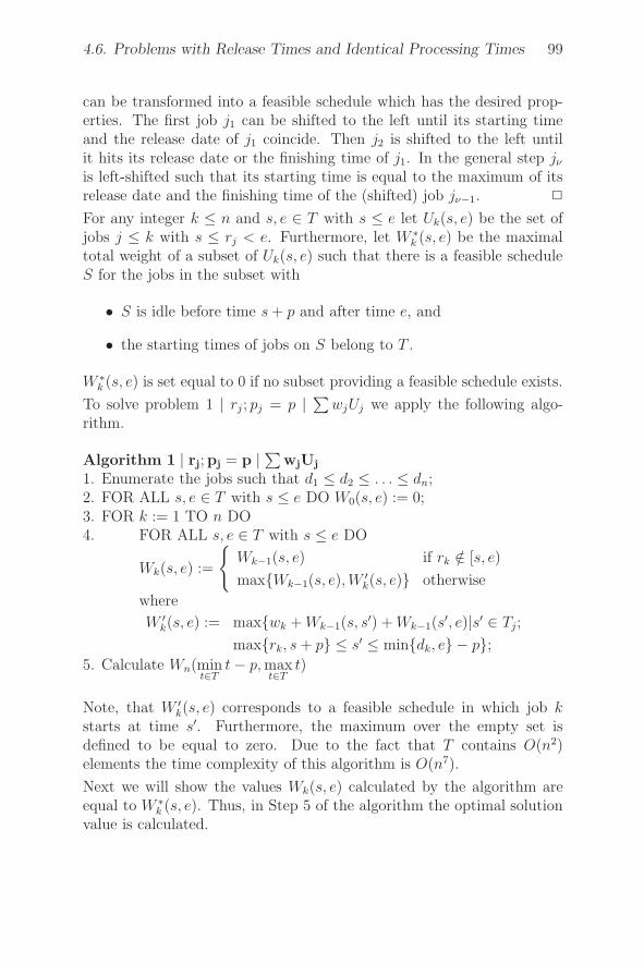
4.6. Problems with Release Times and Identical Processing Times 99
can be transformed into a feasible schedule which has the desired prop-erties. The first job j1 can be shifted to the left until its starting timeand the release date of j1 coincide. Then j2 is shifted to the left untilit hits its release date or the finishing time of j1. In the general step jν
is left-shifted such that its starting time is equal to the maximum of itsrelease date and the finishing time of the (shifted) job jν−1. �
For any integer k ≤ n and s, e ∈ T with s ≤ e let Uk(s, e) be the set ofjobs j ≤ k with s ≤ rj < e. Furthermore, let W ∗
k (s, e) be the maximaltotal weight of a subset of Uk(s, e) such that there is a feasible scheduleS for the jobs in the subset with
• S is idle before time s + p and after time e, and
• the starting times of jobs on S belong to T .
W ∗k (s, e) is set equal to 0 if no subset providing a feasible schedule exists.
To solve problem 1 | rj ; pj = p | ∑wjUj we apply the following algo-
rithm.
Algorithm 1 | rj;pj = p | ∑wjUj
1. Enumerate the jobs such that d1 ≤ d2 ≤ . . . ≤ dn;2. FOR ALL s, e ∈ T with s ≤ e DO W0(s, e) := 0;3. FOR k := 1 TO n DO4. FOR ALL s, e ∈ T with s ≤ e DO
Wk(s, e) :=
{Wk−1(s, e) if rk /∈ [s, e)
max{Wk−1(s, e), W′k(s, e)} otherwise
where
W ′k(s, e) := max{wk + Wk−1(s, s
′) + Wk−1(s′, e)|s′ ∈ Tj;
max{rk, s + p} ≤ s′ ≤ min{dk, e} − p};5. Calculate Wn(min
t∈Tt − p, max
t∈Tt)
Note, that W ′k(s, e) corresponds to a feasible schedule in which job k
starts at time s′. Furthermore, the maximum over the empty set isdefined to be equal to zero. Due to the fact that T contains O(n2)elements the time complexity of this algorithm is O(n7).
Next we will show the values Wk(s, e) calculated by the algorithm areequal to W ∗
k (s, e). Thus, in Step 5 of the algorithm the optimal solutionvalue is calculated.
100 Single Machine Scheduling Problems
Theorem 4.17 For k = 0, . . . , n and all s, e ∈ T with s ≤ e the equality
Wk(s, e) = W ∗k (s, e) (4.22)
holds.
Proof: We prove (4.22) by the induction on k. Clearly, the assertion istrue for k = 0. Assume that (4.22) holds for k − 1.
If rk /∈ [s, e) then Uk(s, e) = Uk−1(s, e) which implies Wk(s, e) = Wk−1
(s, e) = W ∗k−1(s, e) = W ∗
k (s, e). It remains to show that
max{Wk−1(s, e), W′k(s, e)} = W ∗
k (s, e) if rk ∈ [s, e). (4.23)
This is accomplished in two steps by showing that each side of (4.23) issmaller or equal than the other side.
We first prove
max{Wk−1(s, e),W′k(s, e)} ≤ W∗
k(s, e).
We have Wk−1(s, e) = W ∗k−1(s, e) ≤ W ∗
k (s, e) because Uk−1(s, e) ⊆Uk(s, e). Furthermore, if W ′
k(s, e) > 0 then there exists some s′ with
max{rk, s + p} ≤ s′ ≤ min{dk, e} − p
such that
W ′k(s, e) = wk + Wk−1(s, s
′) + Wk−1(s′, e)
= wk + W ∗k−1(s, s
′) + W ∗k−1(s
′, e)
≤ W ∗k (s, s′).
The inequality holds because wk + W ∗k−1(s, s
′) + W ∗k−1(s
′, e) is the totalweight of a schedule of
• job k scheduled in [s′, s′ + p],
• a subset of jobs of Uk−1(s, s′) scheduled in [s + p, s′], and
• a subset of jobs of Uk−1(s′, e) scheduled in [s′ + p, e].
Finally, we prove
4.6. Problems with Release Times and Identical Processing Times 101
W∗k(s, e) ≤ max{Wk−1(s, e),W′
k(s, e)}.Let Z be a subset of Uk(s, e) corresponding with W ∗
k (s, e). If k /∈ Z thenW ∗
k (s, e) = W ∗k−1(s, e) = Wk−1(s, e) and we finished the proof. Other-
wise, let S∗ be the schedule realizing W ∗k (s, e) and let s′ be the starting
time of job k. We must have max{rk, s + p} ≤ s′ ≤ min{dk, e} − p.
We denote by Zb and Za the subset of jobs in Z which in S∗ are scheduledbefore and after job k, respectively. We may assume that the release datesof all jobs in Za are greater than the starting time s′ of job k. Otherwiselet i be a job in Za with ri ≤ s′. Because the jobs are ordered accordingto non-decreasing due-dates we have di ≤ dk. Thus, by swapping jobs iand k in S∗ the total weight does not change. We continue this processuntil the new schedule S∗ has the desired property. We now have
W ∗k (s, e)=
∑
j∈Z
wj =∑
j∈Zb
wj+wk+∑
j∈Za
wj ≤ W ∗k−1(s, s
′)+wk+W ∗k−1(s
′, e)
= Wk−1(s, s′) + wk + Wk−1(s
′, e) ≤ W ′k(s, e) (4.24)
because clearly Zb ⊆ Uk−1(s, s′) and, due to our assumption, Za ⊆
Uk−1(s′, e). holds. �
The ideas of this section can be extended to the preemptive case. Baptiste[15] has shown that the corresponding problem 1 | rj ; pj = p; pmtn |∑
wjUj can be solved in time O(n10).
4.6.2 1 | rj;pj = p | ∑wjCj and 1 | rj;pj = p | ∑
Tj
To derive polynomial algorithms for the problems 1 | rj; pj = p | γ withγ ∈ {∑wjCj,
∑Tj} where wj ≥ 0 for all jobs j we use techniques similar
to those derived in the previous section. We apply these techniques to amore general objective function
∑fj(Cj) where the functions f1, . . . , fn
have the following properties:
• fj is non-decreasing for j = 1, . . . , n (4.25)
• fi−fj is non-decreasing for all i, j = 1, . . . , n with i < j. (4.26)
∑wjCj and
∑Tj =
∑max{0, Cj − dj} are functions of the form∑
fj(Cj) satisfying (4.25) and (4.26) if the jobs are enumerated in sucha way that w1 ≥ w2 ≥ . . . ≥ wn and d1 ≤ d2 ≤ . . . ≤ dn, respectively.

102 Single Machine Scheduling Problems
Due to the fact that the functions fj satisfy (4.25), for problem 1 | rj ; pj =p | ∑
fj there exists an optimal schedule in which each job starts at atime belonging to the set
T := {rj + lp | j = 1, . . . , n; l = 0, . . . , n − 1}The proof of this claim is identical with the proof of Lemma 4.16.
For any integer k ≤ n and s, e ∈ T with s ≤ e let Uk(s, e) be the set ofjobs j ≤ k with s ≤ rj < e. Furthermore, let F ∗
k (s, e) be the minimalvalue that the function ∑
j∈Uk(s−p,e)
fj(Cj)
can take among the feasible schedules S of all jobs in Uk(s − p, e) suchthat
• S is idle before time s and after time e, and
• the starting times of jobs on S belong to T .
If non such schedule S exists then we define F ∗k (s, e) := ∞.
The following dynamic programming algorithm which solves problem 1 |rj; pj = p | ∑
fj is similar to the algorithm formulated in Section 4.6.1.
Algorithm 1 | rj;pj = p | ∑fj
1. Enumerate the jobs such that condition (4.26) holds;2. FOR ALL s, e ∈ T with s ≤ e DO F0(s, e) := 0;3. FOR k := 1 TO n DO4. FOR ALL s, e ∈ T with s ≤ e DO
Fk(s, e) =
{Fk−1(s, e) if rk /∈ [s − p, e)
F ′k(s, e) otherwise
where
F ′k(s, e) = min {Fk−1(s, tk) + Fk−1(tk + p, e) + fk(tk + p) | tk ∈ T ;
max{s, rk} ≤ tk ≤ e − p} ;
5. Calculate Fn
(n
mini=1
ri, maxt∈T t + p
)
The time complexity of this algorithm which calculates the optimal so-lution value in Step 5 is O(n7).
The next theorem shows that the algorithm is correct.
4.6. Problems with Release Times and Identical Processing Times 103
Theorem 4.18 For k = 0, . . . , n and all s, e ∈ T with s ≤ e
Fk(s, e) = F ∗k (s, e) (4.27)
holds.
Proof: The proof is similar to the proof of Theorem 4.17. Assume that(4.27) is true for k − 1 (clearly (4.27) is true for k = 0).
If rk /∈ [s−p, e) then Uk(s−p, e) = Uk−1(s−p, e) which implies (4.27). Itremains to show that (a) F ∗
k (s, e) ≤ F ′k(s, e) and (b) F ′
k(s, e) ≤ F ∗k (s, e)
when rk ∈ [s − p, e).
(a) Assume that F ′k(s, e) is finite. Then some tk ∈ T with max{s, tk} ≤
tk ≤ e − p exists such that
F ′k(s, e)=Fk−1(s, tk) + Fk−1(tk + p, e) + fk(tk + p)
=F ∗k−1(s, tk) + F ∗
k−1(tk + p, e) + fk(tk + p) ≥ F ∗k (s, e).
(b) Assume that F ∗k (s, e) is finite. Among all feasible schedules pro-
viding the value F ∗k (s, e) we choose a schedule S such that the cor-
responding vector (Ci1, Ci2 , . . . , Cil) of finishing times where i1 <i2 < . . . < il is lexicographic minimal. Let tk ∈ T be the startingtime of job k in S. Then
F ∗k (s, e)=
∑
j∈Uk(s−p,e)
fj(Cj)
=∑
j∈Uk(s−p,tk)
fj(Cj) +∑
j∈Uk(tk ,e)
fj(Cj) + fk(tk + p)
≥Fk−1(s, tk) + Fk−1(tk + p, e) + fk(tk + p)
≥F ′k(s, e).
To prove that the first inequality holds we have to show that alljobs of Uk−1(s − p, tk) are scheduled in S in the interval [s, tk] andall jobs of Uk−1(tk, e) are scheduled in S in the interval [tk + p, e].We prove the first assertion (the second follows similarly).
Assume there is a job j with s − p ≤ rj < tk starting in S at atime tj > tk, i.e. starting after job k. By swapping k and j we get
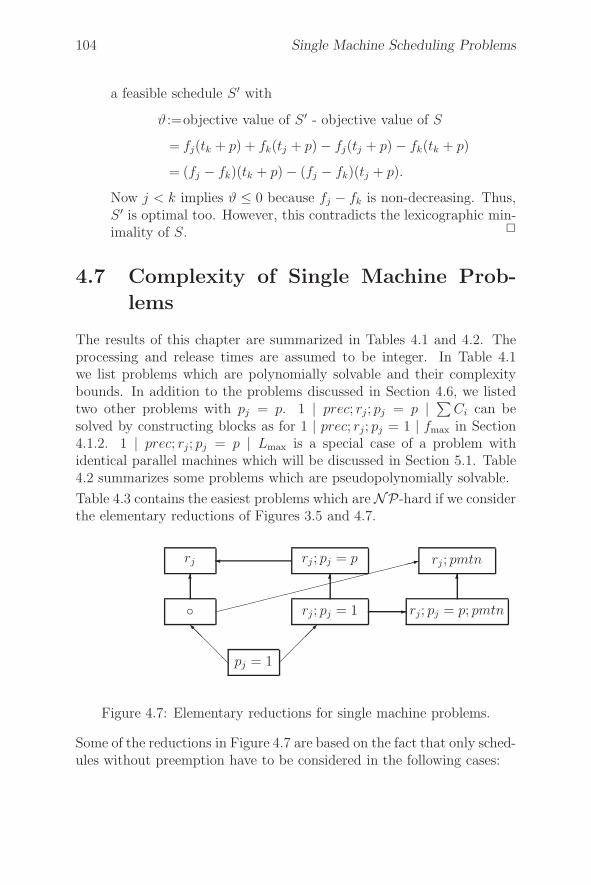
104 Single Machine Scheduling Problems
a feasible schedule S ′ with
ϑ :=objective value of S ′ - objective value of S
= fj(tk + p) + fk(tj + p) − fj(tj + p) − fk(tk + p)
= (fj − fk)(tk + p) − (fj − fk)(tj + p).
Now j < k implies ϑ ≤ 0 because fj − fk is non-decreasing. Thus,S ′ is optimal too. However, this contradicts the lexicographic min-imality of S. �
4.7 Complexity of Single Machine Prob-
lems
The results of this chapter are summarized in Tables 4.1 and 4.2. Theprocessing and release times are assumed to be integer. In Table 4.1we list problems which are polynomially solvable and their complexitybounds. In addition to the problems discussed in Section 4.6, we listedtwo other problems with pj = p. 1 | prec; rj; pj = p | ∑
Ci can besolved by constructing blocks as for 1 | prec; rj; pj = 1 | fmax in Section4.1.2. 1 | prec; rj; pj = p | Lmax is a special case of a problem withidentical parallel machines which will be discussed in Section 5.1. Table4.2 summarizes some problems which are pseudopolynomially solvable.
Table 4.3 contains the easiest problems which are NP-hard if we considerthe elementary reductions of Figures 3.5 and 4.7.
pj = 1
◦
rj
rj; pj = 1
rj ; pj = p
rj; pj = p; pmtn
rj ; pmtn
� � �
�
��
���
��
���
��������������������
Figure 4.7: Elementary reductions for single machine problems.
Some of the reductions in Figure 4.7 are based on the fact that only sched-ules without preemption have to be considered in the following cases:
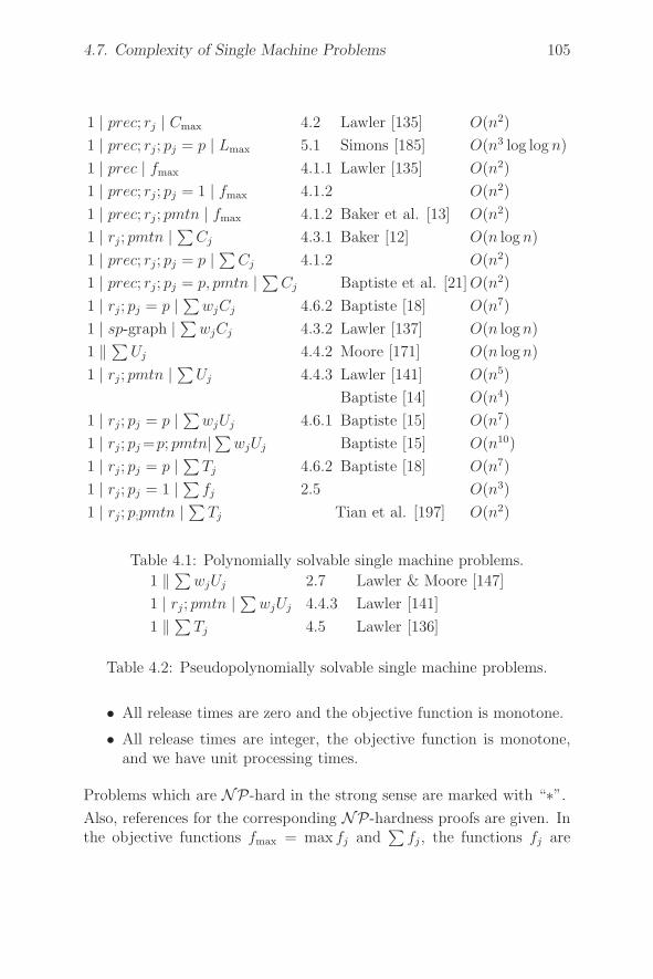
4.7. Complexity of Single Machine Problems 105
1 | prec; rj | Cmax 4.2 Lawler [135] O(n2)
1 | prec; rj; pj = p | Lmax 5.1 Simons [185] O(n3 log log n)
1 | prec | fmax 4.1.1 Lawler [135] O(n2)
1 | prec; rj; pj = 1 | fmax 4.1.2 O(n2)
1 | prec; rj; pmtn | fmax 4.1.2 Baker et al. [13] O(n2)
1 | rj; pmtn | ∑Cj 4.3.1 Baker [12] O(n log n)
1 | prec; rj; pj = p | ∑Cj 4.1.2 O(n2)
1 | prec; rj; pj = p, pmtn | ∑Cj Baptiste et al. [21] O(n2)
1 | rj; pj = p | ∑wjCj 4.6.2 Baptiste [18] O(n7)
1 | sp-graph | ∑wjCj 4.3.2 Lawler [137] O(n log n)
1 ‖ ∑Uj 4.4.2 Moore [171] O(n log n)
1 | rj; pmtn | ∑Uj 4.4.3 Lawler [141] O(n5)
Baptiste [14] O(n4)
1 | rj; pj = p | ∑wjUj 4.6.1 Baptiste [15] O(n7)
1 | rj; pj =p; pmtn|∑ wjUj Baptiste [15] O(n10)
1 | rj; pj = p | ∑Tj 4.6.2 Baptiste [18] O(n7)
1 | rj; pj = 1 | ∑fj 2.5 O(n3)
1 | rj; p;pmtn | ∑Tj Tian et al. [197] O(n2)
Table 4.1: Polynomially solvable single machine problems.
1 ‖ ∑wjUj 2.7 Lawler & Moore [147]
1 | rj; pmtn | ∑wjUj 4.4.3 Lawler [141]
1 ‖ ∑Tj 4.5 Lawler [136]
Table 4.2: Pseudopolynomially solvable single machine problems.
• All release times are zero and the objective function is monotone.
• All release times are integer, the objective function is monotone,and we have unit processing times.
Problems which are NP-hard in the strong sense are marked with “∗”.
Also, references for the corresponding NP-hardness proofs are given. Inthe objective functions fmax = max fj and
∑fj , the functions fj are
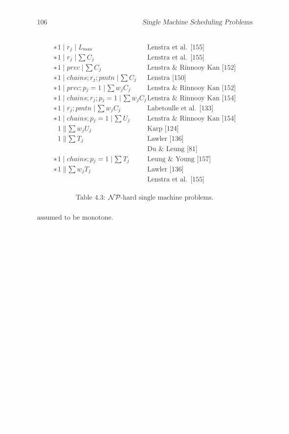
106 Single Machine Scheduling Problems
∗1 | rj | Lmax Lenstra et al. [155]
∗1 | rj |∑
Cj Lenstra et al. [155]
∗1 | prec | ∑Cj Lenstra & Rinnooy Kan [152]
∗1 | chains; rj ; pmtn | ∑Cj Lenstra [150]
∗1 | prec; pj = 1 | ∑wjCj Lenstra & Rinnooy Kan [152]
∗1 | chains; rj ; pj = 1 | ∑wjCj Lenstra & Rinnooy Kan [154]
∗1 | rj; pmtn | ∑wjCj Labetoulle et al. [133]
∗1 | chains; pj = 1 | ∑Uj Lenstra & Rinnooy Kan [154]
1 ‖ ∑wjUj Karp [124]
1 ‖ ∑Tj Lawler [136]
Du & Leung [81]
∗1 | chains; pj = 1 | ∑Tj Leung & Young [157]
∗1 ‖ ∑wjTj Lawler [136]
Lenstra et al. [155]
Table 4.3: NP-hard single machine problems.
assumed to be monotone.
Chapter 5
Parallel Machines
In this chapter, we discuss the problem of scheduling jobs on parallelmachines. Problem P ‖ ∑
Ci and, more generally, problem R ‖ ∑Ci
are the only nonpreemptive problems with arbitrary processing timesknown to be known polynomially solvable. Problems P2 ‖ Cmax and P2 ‖∑
wiCi are NP-hard. For these reasons, we essentially discuss problemsin which preemption is possible or in which all jobs have unit processingtimes. In the first section of this chapter, problems with independentjobs are discussed. In the second section, we permit precedence relationsbetween jobs.
5.1 Independent Jobs
In the following three sections, problems with identical, uniform, andunrelated parallel machines are discussed separately.
5.1.1 Identical Machines
Consider n jobs Ji(i = 1, . . . , n) with processing times pi (i = 1, . . . , n)to be processed on m identical parallel machines M1, . . . , Mm. Then thefollowing problem can be solved polynomially.
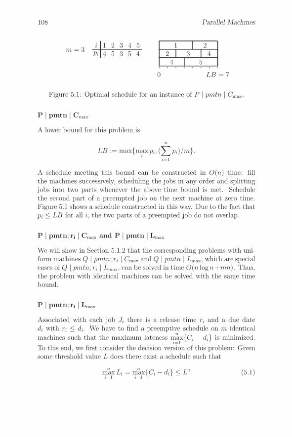
108 Parallel Machines
m = 3ipi
14
25
33
45
54
1 22 3 44 5
LB = 70
Figure 5.1: Optimal schedule for an instance of P | pmtn | Cmax.
P | pmtn | Cmax
A lower bound for this problem is
LB := max{maxi
pi, (n∑
i=1
pi)/m}.
A schedule meeting this bound can be constructed in O(n) time: fillthe machines successively, scheduling the jobs in any order and splittingjobs into two parts whenever the above time bound is met. Schedulethe second part of a preempted job on the next machine at zero time.Figure 5.1 shows a schedule constructed in this way. Due to the fact thatpi ≤ LB for all i, the two parts of a preempted job do not overlap.
P | pmtn; ri | Cmax and P | pmtn | Lmax
We will show in Section 5.1.2 that the corresponding problems with uni-form machines Q | pmtn; ri | Cmax and Q | pmtn | Lmax, which are specialcases of Q | pmtn; ri | Lmax, can be solved in time O(n logn+mn). Thus,the problem with identical machines can be solved with the same timebound.
P | pmtn; ri | Lmax
Associated with each job Ji there is a release time ri and a due datedi with ri ≤ di. We have to find a preemptive schedule on m identical
machines such that the maximum latenessn
maxi=1
{Ci − di} is minimized.
To this end, we first consider the decision version of this problem: Givensome threshold value L does there exist a schedule such that
nmaxi=1
Li =n
maxi=1
{Ci − di} ≤ L? (5.1)
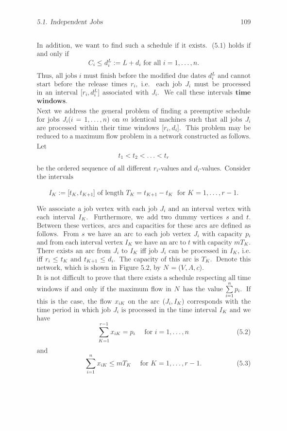
5.1. Independent Jobs 109
In addition, we want to find such a schedule if it exists. (5.1) holds ifand only if
Ci ≤ dLi := L + di for all i = 1, . . . , n.
Thus, all jobs i must finish before the modified due dates dLi and cannot
start before the release times ri, i.e. each job Ji must be processedin an interval [ri, d
Li ] associated with Ji. We call these intervals time
windows.
Next we address the general problem of finding a preemptive schedulefor jobs Ji(i = 1, . . . , n) on m identical machines such that all jobs Ji
are processed within their time windows [ri, di]. This problem may bereduced to a maximum flow problem in a network constructed as follows.
Let
t1 < t2 < . . . < tr
be the ordered sequence of all different ri-values and di-values. Considerthe intervals
IK := [tK , tK+1] of length TK = tK+1 − tK for K = 1, . . . , r − 1.
We associate a job vertex with each job Ji and an interval vertex witheach interval IK . Furthermore, we add two dummy vertices s and t.Between these vertices, arcs and capacities for these arcs are defined asfollows. From s we have an arc to each job vertex Ji with capacity pi
and from each interval vertex IK we have an arc to t with capacity mTK .There exists an arc from Ji to IK iff job Ji can be processed in IK , i.e.iff ri ≤ tK and tK+1 ≤ di. The capacity of this arc is TK . Denote thisnetwork, which is shown in Figure 5.2, by N = (V, A, c).
It is not difficult to prove that there exists a schedule respecting all time
windows if and only if the maximum flow in N has the valuen∑
i=1
pi. If
this is the case, the flow xiK on the arc (Ji, IK) corresponds with thetime period in which job Ji is processed in the time interval IK and wehave
r−1∑
K=1
xiK = pi for i = 1, . . . , n (5.2)
andn∑
i=1
xiK ≤ mTK for K = 1, . . . , r − 1. (5.3)
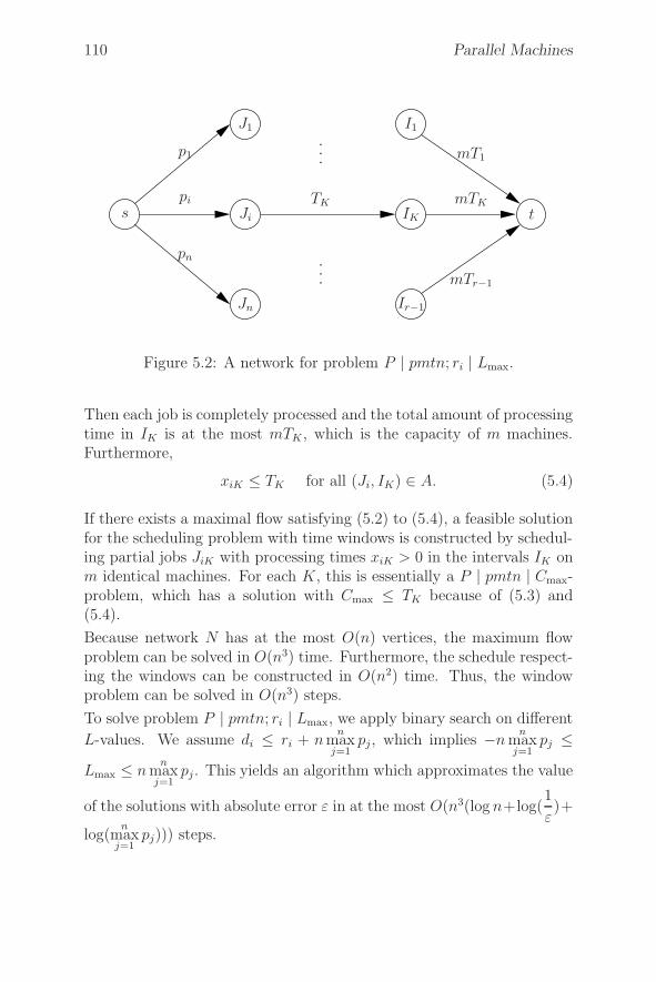
110 Parallel Machines
s Ji
J1
Jn
IK
I1
Ir−1
tTK
···
···
pi
p1
pn
mTK
mT1
mTr−1
Figure 5.2: A network for problem P | pmtn; ri | Lmax.
Then each job is completely processed and the total amount of processingtime in IK is at the most mTK , which is the capacity of m machines.Furthermore,
xiK ≤ TK for all (Ji, IK) ∈ A. (5.4)
If there exists a maximal flow satisfying (5.2) to (5.4), a feasible solutionfor the scheduling problem with time windows is constructed by schedul-ing partial jobs JiK with processing times xiK > 0 in the intervals IK onm identical machines. For each K, this is essentially a P | pmtn | Cmax-problem, which has a solution with Cmax ≤ TK because of (5.3) and(5.4).
Because network N has at the most O(n) vertices, the maximum flowproblem can be solved in O(n3) time. Furthermore, the schedule respect-ing the windows can be constructed in O(n2) time. Thus, the windowproblem can be solved in O(n3) steps.
To solve problem P | pmtn; ri | Lmax, we apply binary search on different
L-values. We assume di ≤ ri + nn
maxj=1
pj, which implies −nn
maxj=1
pj ≤Lmax ≤ n
nmaxj=1
pj . This yields an algorithm which approximates the value
of the solutions with absolute error ε in at the most O(n3(log n+log(1
ε)+
log(n
maxj=1
pj))) steps.

5.1. Independent Jobs 111
P | pi = 1; ri | Lmax
It is convenient to assume that the jobs are indexed in such a way that
r1 ≤ r2 ≤ . . . ≤ rn.
The problem has an easy solution if all release times ri are integer. In thiscase, we get an optimal schedule by scheduling available jobs in the orderof nondecreasing due dates. More specifically, if at the current time t notall machines are occupied and there is an unscheduled job Ji with ri ≤ t,we schedule such a job with the smallest due date. Technical detailsare given by the following algorithm in which K counts the number ofmachines occupied immediately after Step 7 at current time t, m is thenumber of machines, M is the set of unscheduled jobs available at timet, and j is a counter for the number of scheduled jobs.
Algorithm P | pi = 1; ri integer | Lmax
1. j := 1;2. WHILE j ≤ n DO
BEGIN3. t := rj; M := {Ji | Ji is not scheduled; ri ≤ t}; K := 1;4. WHILE M �= φ DO
BEGIN5. Find job Ji in M with smallest due date;6. M := M\{Ji};7. Schedule Ji at time t;8. j := j + 1;9. IF K + 1 ≤ m THEN K := K + 1
ELSEBEGIN
10. t := t + 1;11. K := 1;12. M := M ∪ {Ji | Ji in not scheduled; ri ≤ t}
ENDEND
END
The inner “while”-loop creates blocks of jobs which are processed with-out idle time on the machines between the scheduled jobs. After finishingsuch a block, the current rj-value is the starting time of the next block.
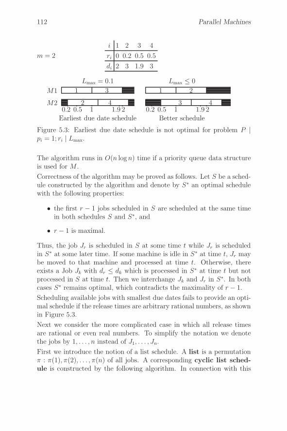
112 Parallel Machines
m = 2
i 1 2 3 4
ri 0 0.2 0.5 0.5
di 2 3 1.9 3
M2
M1
0.2 0.5 1 1.9 22 4
1 3
Earliest due date schedule
Lmax = 0.1
0.2 0.5 1 1.9 23 4
1 2
Better schedule
Lmax ≤ 0
Figure 5.3: Earliest due date schedule is not optimal for problem P |pi = 1; ri | Lmax.
The algorithm runs in O(n log n) time if a priority queue data structureis used for M .
Correctness of the algorithm may be proved as follows. Let S be a sched-ule constructed by the algorithm and denote by S∗ an optimal schedulewith the following properties:
• the first r − 1 jobs scheduled in S are scheduled at the same timein both schedules S and S∗, and
• r − 1 is maximal.
Thus, the job Jr is scheduled in S at some time t while Jr is scheduledin S∗ at some later time. If some machine is idle in S∗ at time t, Jr maybe moved to that machine and processed at time t. Otherwise, thereexists a Job Jk with dr ≤ dk which is processed in S∗ at time t but notprocessed in S at time t. Then we interchange Jk and Jr in S∗. In bothcases S∗ remains optimal, which contradicts the maximality of r − 1.
Scheduling available jobs with smallest due dates fails to provide an opti-mal schedule if the release times are arbitrary rational numbers, as shownin Figure 5.3.
Next we consider the more complicated case in which all release timesare rational or even real numbers. To simplify the notation we denotethe jobs by 1, . . . , n instead of J1, . . . , Jn.
First we introduce the notion of a list schedule. A list is a permutationπ : π(1), π(2), . . . , π(n) of all jobs. A corresponding cyclic list sched-ule is constructed by the following algorithm. In connection with this
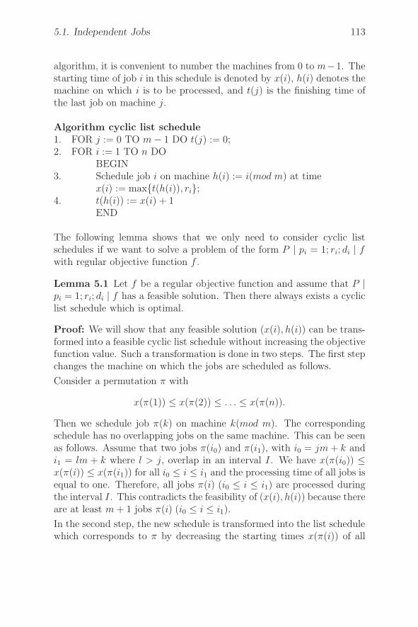
5.1. Independent Jobs 113
algorithm, it is convenient to number the machines from 0 to m−1. Thestarting time of job i in this schedule is denoted by x(i), h(i) denotes themachine on which i is to be processed, and t(j) is the finishing time ofthe last job on machine j.
Algorithm cyclic list schedule1. FOR j := 0 TO m − 1 DO t(j) := 0;2. FOR i := 1 TO n DO
BEGIN3. Schedule job i on machine h(i) := i(mod m) at time
x(i) := max{t(h(i)), ri};4. t(h(i)) := x(i) + 1
END
The following lemma shows that we only need to consider cyclic listschedules if we want to solve a problem of the form P | pi = 1; ri; di | fwith regular objective function f .
Lemma 5.1 Let f be a regular objective function and assume that P |pi = 1; ri; di | f has a feasible solution. Then there always exists a cycliclist schedule which is optimal.
Proof: We will show that any feasible solution (x(i), h(i)) can be trans-formed into a feasible cyclic list schedule without increasing the objectivefunction value. Such a transformation is done in two steps. The first stepchanges the machine on which the jobs are scheduled as follows.
Consider a permutation π with
x(π(1)) ≤ x(π(2)) ≤ . . . ≤ x(π(n)).
Then we schedule job π(k) on machine k(mod m). The correspondingschedule has no overlapping jobs on the same machine. This can be seenas follows. Assume that two jobs π(i0) and π(i1), with i0 = jm + k andi1 = lm + k where l > j, overlap in an interval I. We have x(π(i0)) ≤x(π(i)) ≤ x(π(i1)) for all i0 ≤ i ≤ i1 and the processing time of all jobs isequal to one. Therefore, all jobs π(i) (i0 ≤ i ≤ i1) are processed duringthe interval I. This contradicts the feasibility of (x(i), h(i)) because thereare at least m + 1 jobs π(i) (i0 ≤ i ≤ i1).
In the second step, the new schedule is transformed into the list schedulewhich corresponds to π by decreasing the starting times x(π(i)) of all

114 Parallel Machines
jobs. Thus, the regular objective function does not increase during thetransformation. �
We will present an algorithm which constructs a schedule (x(i), h(i))respecting all time windows [ri, di] (i.e. with ri ≤ x(i) < x(i) + 1 ≤ di
for i = 1, . . . , n) or finds that such a schedule does not exist. If such aschedule exists, then the schedule constructed by the algorithm minimizes∑
Ci as well as Cmax.
The idea of the algorithm is to construct an optimal list π(1), π(2), . . . ,π(n). This is done by trying to schedule at the current time t an availablejob i with the smallest deadline. However, this is not always correct, aswe have seen in Figure 5.3. For these reasons, if di < t + 1 (i.e. if jobi is late) we have to call a crisis subroutine. The crisis subroutinebacktracks over the current partial schedule π(1), . . . , π(k − 1) searchingfor a job π(j) with a highest position j that has a deadline greater thanthat of the crisis job i. If such a job π(j) does not exist, the subroutineconcludes that there is no feasible schedule and halts. Otherwise, we calljob π(j) a pull job and the set of all jobs in the partial schedule withpositions greater than j a restricted set. The subroutine determinesthe minimum release time r of all jobs in the restricted set and createsa barrier (j, r). This barrier is an additional restriction to the startingtime of jobs scheduled in positions k ≥ j. It is added to a barrier listwhich is used to calculate the current scheduling time. Finally, π(j) andall jobs in the restricted set are eliminated from the partial schedule andwe continue with the partial schedule π(1), . . . , π(j − 1).
If di ≥ t+1, then job i is scheduled at time t on machine h(i) = i(mod m).
Details are given below. U is the set of unscheduled jobs, the barrier list
Algorithm P | pi = 1; ri;di |∑
Ci,Cmax
1. Initialize;2. WHILE there are unscheduled jobs DO
BEGIN3. Calculate current time t;4. Find unscheduled job i available at time t
with smallest due date;5. If di ≥ t + 1 THEN schedule job i
ELSE6. crisis (i)
END
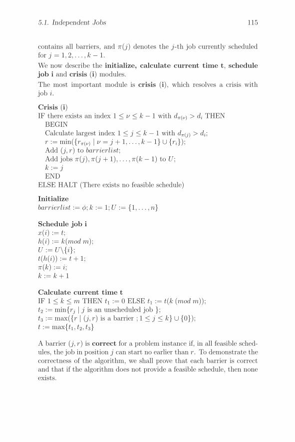
5.1. Independent Jobs 115
contains all barriers, and π(j) denotes the j-th job currently scheduledfor j = 1, 2, . . . , k − 1.
We now describe the initialize, calculate current time t, schedulejob i and crisis (i) modules.
The most important module is crisis (i), which resolves a crisis withjob i.
Crisis (i)IF there exists an index 1 ≤ ν ≤ k − 1 with dπ(ν) > di THEN
BEGINCalculate largest index 1 ≤ j ≤ k − 1 with dπ(j) > di;r := min({rπ(ν) | ν = j + 1, . . . , k − 1} ∪ {ri});Add (j, r) to barrierlist;Add jobs π(j), π(j + 1), . . . , π(k − 1) to U ;k := jEND
ELSE HALT (There exists no feasible schedule)
Initializebarrierlist := φ; k := 1; U := {1, . . . , n}
Schedule job ix(i) := t;h(i) := k(mod m);U := U\{i};t(h(i)) := t + 1;π(k) := i;k := k + 1
Calculate current time tIF 1 ≤ k ≤ m THEN t1 := 0 ELSE t1 := t(k (mod m));t2 := min{rj | j is an unscheduled job };t3 := max({r | (j, r) is a barrier ; 1 ≤ j ≤ k} ∪ {0});t := max{t1, t2, t3}
A barrier (j, r) is correct for a problem instance if, in all feasible sched-ules, the job in position j can start no earlier than r. To demonstrate thecorrectness of the algorithm, we shall prove that each barrier is correctand that if the algorithm does not provide a feasible schedule, then noneexists.
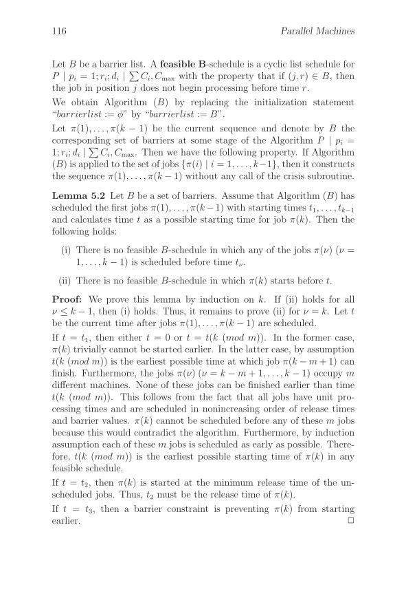
116 Parallel Machines
Let B be a barrier list. A feasible B-schedule is a cyclic list schedule forP | pi = 1; ri; di |
∑Ci, Cmax with the property that if (j, r) ∈ B, then
the job in position j does not begin processing before time r.
We obtain Algorithm (B) by replacing the initialization statement“barrierlist := φ” by “barrierlist := B”.
Let π(1), . . . , π(k − 1) be the current sequence and denote by B thecorresponding set of barriers at some stage of the Algorithm P | pi =1; ri; di |
∑Ci, Cmax. Then we have the following property. If Algorithm
(B) is applied to the set of jobs {π(i) | i = 1, . . . , k−1}, then it constructsthe sequence π(1), . . . , π(k − 1) without any call of the crisis subroutine.
Lemma 5.2 Let B be a set of barriers. Assume that Algorithm (B) hasscheduled the first jobs π(1), . . . , π(k−1) with starting times t1, . . . , tk−1
and calculates time t as a possible starting time for job π(k). Then thefollowing holds:
(i) There is no feasible B-schedule in which any of the jobs π(ν) (ν =1, . . . , k − 1) is scheduled before time tν .
(ii) There is no feasible B-schedule in which π(k) starts before t.
Proof: We prove this lemma by induction on k. If (ii) holds for allν ≤ k − 1, then (i) holds. Thus, it remains to prove (ii) for ν = k. Let tbe the current time after jobs π(1), . . . , π(k − 1) are scheduled.
If t = t1, then either t = 0 or t = t(k (mod m)). In the former case,π(k) trivially cannot be started earlier. In the latter case, by assumptiont(k (mod m)) is the earliest possible time at which job π(k −m + 1) canfinish. Furthermore, the jobs π(ν) (ν = k − m + 1, . . . , k − 1) occupy mdifferent machines. None of these jobs can be finished earlier than timet(k (mod m)). This follows from the fact that all jobs have unit pro-cessing times and are scheduled in nonincreasing order of release timesand barrier values. π(k) cannot be scheduled before any of these m jobsbecause this would contradict the algorithm. Furthermore, by inductionassumption each of these m jobs is scheduled as early as possible. There-fore, t(k (mod m)) is the earliest possible starting time of π(k) in anyfeasible schedule.
If t = t2, then π(k) is started at the minimum release time of the un-scheduled jobs. Thus, t2 must be the release time of π(k).
If t = t3, then a barrier constraint is preventing π(k) from startingearlier. �
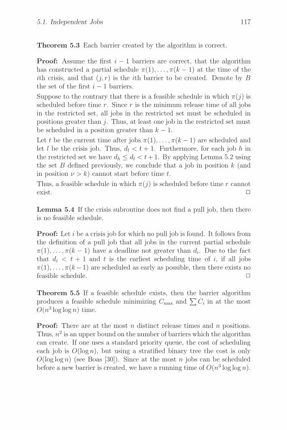
5.1. Independent Jobs 117
Theorem 5.3 Each barrier created by the algorithm is correct.
Proof: Assume the first i − 1 barriers are correct, that the algorithmhas constructed a partial schedule π(1), . . . , π(k − 1) at the time of theith crisis, and that (j, r) is the ith barrier to be created. Denote by Bthe set of the first i − 1 barriers.
Suppose to the contrary that there is a feasible schedule in which π(j) isscheduled before time r. Since r is the minimum release time of all jobsin the restricted set, all jobs in the restricted set must be scheduled inpositions greater than j. Thus, at least one job in the restricted set mustbe scheduled in a position greater than k − 1.
Let t be the current time after jobs π(1), . . . , π(k − 1) are scheduled andlet l be the crisis job. Thus, dl < t + 1. Furthermore, for each job h inthe restricted set we have dh ≤ dl < t+1. By applying Lemma 5.2 usingthe set B defined previously, we conclude that a job in position k (andin position ν > k) cannot start before time t.
Thus, a feasible schedule in which π(j) is scheduled before time r cannotexist. �
Lemma 5.4 If the crisis subroutine does not find a pull job, then thereis no feasible schedule.
Proof: Let i be a crisis job for which no pull job is found. It follows fromthe definition of a pull job that all jobs in the current partial scheduleπ(1), . . . , π(k − 1) have a deadline not greater than di. Due to the factthat di < t + 1 and t is the earliest scheduling time of i, if all jobsπ(1), . . . , π(k−1) are scheduled as early as possible, then there exists nofeasible schedule. �
Theorem 5.5 If a feasible schedule exists, then the barrier algorithmproduces a feasible schedule minimizing Cmax and
∑Ci in at the most
O(n3 log log n) time.
Proof: There are at the most n distinct release times and n positions.Thus, n2 is an upper bound on the number of barriers which the algorithmcan create. If one uses a standard priority queue, the cost of schedulingeach job is O(log n), but using a stratified binary tree the cost is onlyO(log log n) (see Boas [30]). Since at the most n jobs can be scheduledbefore a new barrier is created, we have a running time of O(n3 log log n).
118 Parallel Machines
Let B be the set of all barriers created by the algorithm. If we applyLemma 5.2 with this set B, we conclude that the algorithm minimizesCmax as well as
∑Ci. �
We may replace the restrictions that pi = 1 and that ri, di are rationalby the equivalent restrictions that pi = p and ri, di are integers. Thus,we have shown that P | pi = p; ri; di | f with f ∈ {Cmax,
∑Ci} can be
solved in O(n3 log log n) time.
Problem P | pi = p; ri | Lmax can be solved using binary search.
P | pi = 1 | ∑wiUi
An optimal schedule for P | pi = 1 | ∑wiUi is given by a set S of jobs
which are early. The late job can be scheduled at the end in an arbitraryorder. Furthermore, we may assume that the early jobs are scheduled inthe following way: Sort the jobs according to nondecreasing due datesand schedule the jobs in this order, i.e. schedule the first m jobs in S attime 0, the next m jobs at time 1, etc.
To calculate an optimal set S of early jobs we add jobs to S in non-decreasing order of their due dates (and try to schedule them) and assoon as some job appears late we delete from S a job with minimal wi-value.
More specifically, assume that we have jobs 1, . . . , n with d1 ≤ d2 ≤. . . ≤ dn. Then the following algorithm calculates an optimal set S ofearly jobs.
Algorithm P | pi = 1 | ∑wiUi
1. S := φ;2. FOR i := 1 TO n DO3. IF i is late when scheduled in the earliest empty time slot on a
machineTHEN
BEGIN4. Find a job i∗ with wi∗ = min
i∈Swi;
5. IF wi∗ < wi THEN replace i∗ by i in the schedule and in SEND
6. ELSE add i to S and schedule i in the earliest time slot.
Clearly, this algorithm can be implemented in O(n log n) time if appro-priate data structures are used.

5.1. Independent Jobs 119
Theorem 5.6 Algorithm P | pi = 1 | ∑wiUi is correct.
Proof: Let S be the set of the jobs calculated by the algorithm. Thenall jobs in S are early because if job i replaces an early job k then i mustbe early as well. This follows from the fact that dk ≤ di. Let S∗ be theset of early jobs of an optimal schedule with the following properties:
• l is the first job in S with l /∈ S∗, and
• k is the first job in S∗ with k /∈ S.
We may assume that such jobs l and k exist because
• S ⊂ S∗ would lead to a contradiction to the construction of S, and
• if S∗ ⊆ S then S must be optimal too and the theorem is proven.
We show that in S∗ job k can be replaced by l without increasing theobjective function which is a contradiction to the definition of S∗. Thereare two cases to be considered.
Case 1: l < kThe job which eliminates k in S must be considered later than job l.Thus, we must have wl ≥ wk. Due to the definition of k all jobs i ∈ S∗
with i < k must belong to S. Therefore, S∗ remains feasible if l replacesk.
Case 2: k < lIf in S∗ job k is replaced by l then l is on time because k is on time anddk ≤ dl. Therefore, all we have to prove is that wl ≥ wk holds.
Let ki0 := k be eliminated by i0 and let ki1, . . . , kir be the sequence ofjobs which are eliminated afterwards from S, where kiν is eliminated byiν (ν = 1, . . . , r). Then i0 < i1 < . . . < ir. We say “iν dominates iμ”(μ < ν) if kiν ≤ iμ. In this case the inequality wkiν
≥ wkiμholds (Figure
5.4).
kiν kiμ iμ iν
Figure 5.4: iν dominates iμ.
If a subsequence j0 = i0 < j1 < . . . js of i0 < i1 < . . . < ir exists whichhas the properties
120 Parallel Machines
• jν+1 dominates jν for ν = 0, 1, . . . , s − 1, and
• js−1 < l ≤ js
thenwl ≥ wkjs
≥ . . . ≥ wkj0= wk
and the theorem is proven.
Otherwise a job it with smallest index t exists which is not dominatedby a job iν with ν > t and it < l. Thus, after it is added to S no jobi ≤ it will be deleted from S. Because it < l all jobs which belong to Swhen it is added must also belong to S∗. This contradicts the fact thatk ∈ S∗ and S∗ contains no late jobs.
To derive such a contradiction let St be set S after deleting kit and addingit. We consider two cases.
If k′ := kit > k, i.e. dk′ ≥ dk then we may replace k by k′ in S∗ withoutproviding late jobs. Thus, St ∪ {k′} has no late jobs which contradictsthe construction of S. Otherwise, k′ < k. Then all jobs in St∪{k} can bescheduled early. Furthermore, all jobs in {j ∈ St | j < k} ∪ {k′} can bescheduled early. This implies that all jobs in St ∪ {k′} can be scheduledearly which again is a contradiction. �
P ‖ ∑Ci
We will show in the next section that the corresponding problem withuniform machines can be solved by a polynomial algorithm, which pro-vides the complexity bound O(n logn) for problem P ‖ ∑
Ci.
P | pi = 1 | ∑wiCi and P | pi = 1;pmtn | ∑
wiCi
We get an optimal schedule for problem P | pi = 1 | ∑wiCi by scheduling
the jobs in order of nonincreasing weights wi. To give a more precisedescription of such an optimal schedule S, it is convenient to representthe jobs by numbers 0, . . . , n − 1 such that
w0 ≥ w1 ≥ . . . ≥ wn−1
and to denote the machines by 0, . . . , m − 1. In S, job i is scheduled attime �i/m� on machine i(mod m). It can be shown by simple interchangearguments that S is an optimal schedule.
5.1. Independent Jobs 121
The following theorem shows that an optimal schedule for P | pi = 1 |∑wiCi is optimal even if preemption is allowed.
Theorem 5.7 For P | pmtn | ∑wiCi there exists an optimal schedule
without preemption.
Proof: It is sufficient to show that an arbitrary schedule with a finitenumber of preemptions can be transformed into a nonpreemptive sched-ule without increasing the value of the objective function.
By preemption, a job i may be split at some time s, i.e. processing job iat some machine is stopped and either continued at time s on a differentmachine or at some time s′ > s on the same or a different machine.
Consider an optimal preemptive schedule S with a minimal number l ofpreemption times. If l = 0, we have finished. Otherwise, let t′ < t be thetwo greatest splitting times of S (if l = 1, we set t′ = 0).
We show that by transforming S into a schedule S ′, all preemptions attime t can be eliminated without creating new preemptions. Further-more, the objective value for S ′ is not greater than the objective valuefor S which contradicts the fact that S is an optimal schedule with aminimal number of preemptions.
If a job i processed on machine Mj is preempted at time t and continuedat time t on a different machine Mk, then we may interchange the sched-ule after time t on Mj and the schedule after t on Mk. This reduces thenumber of preemptions at time t of this type.
Therefore, we may assume that all jobs iν(ν = 1, . . . , r) preempted attime t are continued at some time tν > t on some machine until com-pleted. We assume w.l.o.g. that iν is preempted at time t on machineMν (ν = 1, . . . , r). Now we consider two cases.
Case 1: Each job preemption at time t is continued on a machine whichis different to the first r machines M1, . . . , Mr.
Let Mk, k > r be one of the machines having at least one of the jobsi1, . . . , ir scheduled on it . Suppose that il (1 ≤ l ≤ r) is the earliestsuch job to be scheduled on Mk after time t. Then il is scheduled on Ml
between time q and t where q ≥ t′( if il is processed from time q < t′ totime t on Ml we preempt il at time t′) and on Mk between times u andu′ where t ≤ u < u′. Let c = t− q, d = u′ − u, and e = u− t (see Figure5.5(a)).
Let S1 be like S, except that il is not scheduled on Ml at all after time
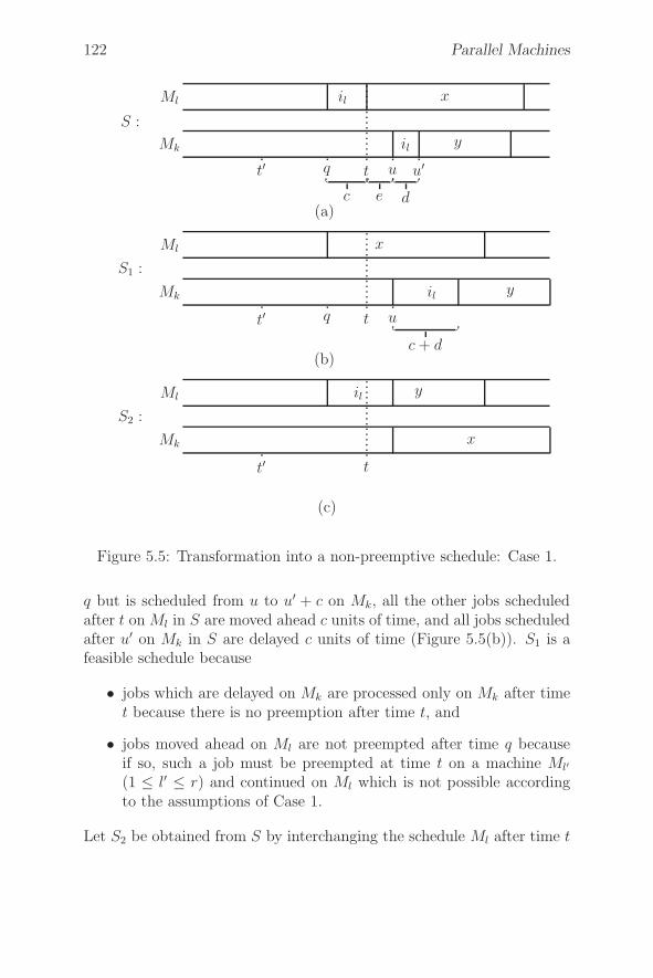
122 Parallel Machines
Mk
Ml
S :
il y
il x
t′ q t u u′�
c�
e�
d(a)
Mk
Ml
S1 :
il y
x
t′ q t u�
c + d(b)
Mk
Ml
S2 :
x
il y
t′ t
(c)
Figure 5.5: Transformation into a non-preemptive schedule: Case 1.
q but is scheduled from u to u′ + c on Mk, all the other jobs scheduledafter t on Ml in S are moved ahead c units of time, and all jobs scheduledafter u′ on Mk in S are delayed c units of time (Figure 5.5(b)). S1 is afeasible schedule because
• jobs which are delayed on Mk are processed only on Mk after timet because there is no preemption after time t, and
• jobs moved ahead on Ml are not preempted after time q becauseif so, such a job must be preempted at time t on a machine Ml′
(1 ≤ l′ ≤ r) and continued on Ml which is not possible accordingto the assumptions of Case 1.
Let S2 be obtained from S by interchanging the schedule Ml after time t
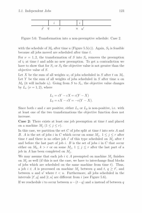
5.1. Independent Jobs 123
i i
t′ q t u u′
Figure 5.6: Transformation into a non-preemptive schedule: Case 2.
with the schedule of Mk after time u (Figure 5.5(c)). Again, S2 is feasiblebecause all jobs moved are scheduled after time t.
For ν = 1, 2, the transformation of S into Sν removes the preemptionof il at time t and adds no new preemption. To get a contradiction wehave to show that for S1 or S2 the objective value is not greater than theobjective value of S.
Let X be the sum of all weights wi of jobs scheduled in S after t on Ml.Let Y be the sum of all weights of jobs scheduled in S after time u onMk (it will include il). Going from S to Sν , the objective value changesby Lν (ν = 1, 2), where
L1 = cY − cX = c(Y − X)
L2 = eX − eY = −e(Y − X).
Since both c and e are positive, either L1 or L2 is non-positive, i.e. withat least one of the two transformations the objective function does notincrease.
Case 2: There exists at least one job preemption at time t and placedon a machine Mj (1 ≤ j ≤ r).
In this case, we partition the set C of jobs split at time t into sets A andB. A is the set of jobs i in C which occur on some Mj , 1 ≤ j ≤ r aftertime t and there is no other job i′ of this type scheduled on Mj after tand before the last part of job i. B is the set of jobs i in C that occureither on Mk, k > r or on some Mj, 1 ≤ j ≤ r after the last part of ajob in A has been completed on Mj .
We may assume that each job i ∈ A preempted on machine Mj finisheson Mj as well (if this is not the case, we have to interchange final blocksof jobs which are scheduled on the same machine from time t). Thus,a job i ∈ A is processed on machine Mj between q and t, q ≥ t′, andbetween u and u′ where t < u. Furthermore, all jobs scheduled in theintervals [t′, q] and [t, u] are different from i (see Figure 5.6).
If we reschedule i to occur between u− (t−q) and u instead of between q

124 Parallel Machines
and t and move ahead t−q units of time all that has occurred between in[t, u], we get a feasible schedule with an objective value not greater thanbefore (note that jobs scheduled in [t, u] can be moved ahead becausethese jobs are not preempted at time t).
By such a rescheduling procedure, jobs in A are eliminated. On theother hand, jobs in C finished after a job in A must be added to A. Therescheduling process ends after a finite number of steps with a Case 1situation. �
P | pi = 1; ri |∑
fi can be solved by a network flow algorithm. P2 | pi =p; pmtn; ri | ∑
Ci has been solved polynomially by Herrbach & Leung[111].
The following problems are NP-hard:P2 ‖ Cmax, P2 ‖ ∑
wiCi, P2 | pmtn; ri |∑
Ci, P2 | pmtn | ∑wiCi, P2 |
pmtn; ri |∑
Ui, P | pmtn | ∑Ui.
5.1.2 Uniform Machines
In this section we consider n jobs Ji(i = 1, . . . , n) to be processed onm parallel uniform machines Mj(j = 1, . . . , m). The machines havedifferent speeds sj(j = 1, . . . , m). Each job Ji has a processing re-quirement pi(i = 1, . . . , n). Execution of job Ji on machine Mj requirespi/sj time units. If we set sj = 1 for j = 1, . . . , m, we have m parallelidentical machines. All problems with parallel identical machines whichare NP-hard are also NP-hard if we replace the machines by uniformmachines. Therefore, we first consider problems with preemptions. Wealso assume that 1 = s1 ≥ s2 ≥ . . . ≥ sm and p1 ≥ p2 ≥ . . . ≥ pn.
Q | pmtn | Cmax
We will present a lower bound w for the objective value of problem Q |pmtn | Cmax. In a second step, we will give an algorithm which constructsa schedule of length w (i.e. an optimal schedule). Let
Pi = p1 + . . . + pi and Sj = s1 + . . . + sj
for i = 1, . . . , n and j = 1, . . . , m. Furthermore, we assume that n ≥ m.If n < m, we only have to consider the n fastest machines. A necessarycondition for processing all jobs in the interval [0, T ] is
Pn = p1 + . . . + pn ≤ s1T + . . . + smT = SmT
5.1. Independent Jobs 125
orPn/Sm ≤ T.
Similarly, we must have Pj/Sj ≤ T for j = 1, . . . , m− 1 because Pj/Sj isa lower bound on the length of a schedule for the jobs J1, . . . , Jj. Thus,
w := max{m−1maxj=1
Pj/Sj, Pn/Sm} (5.5)
is a lower bound for the Cmax-values.
Next we will construct a schedule which achieves this bound. The corre-sponding algorithm is called the level algorithm. Given a partial scheduleup to time t, the level pi(t) of job i at time t is the portion of pi notprocessed before t. At time t, the level algorithm calls a procedure as-sign (t) which assigns jobs to machines. The machines are run with thisassignment until some time s > t. A new assignment is done at time s,and the process is repeated.
Algorithm level1. t := 0;2. WHILE there exist jobs with positive level DO
BEGIN3. Assign(t);4. t1 := min{s > t | a job completes at time s};5. t2 := min{s > t | there are jobs i, j with pi(t) > pj(t) and
pi(s) = pj(s)};6. t := min{t1, t2}
END7. Construct the schedule.
The procedure assign(t) is given by
Assign (t)1. J := {i | pi(t) > 0};2. M := {M1, . . . , Mm};3. WHILE J �= ∅ and M �= ∅ DO
BEGIN4. Find the set I ⊆ J of jobs with highest level;5. r := min{|M |, |I|};6. Assign jobs in I to be processed jointly on the r fastest
machines in M ;
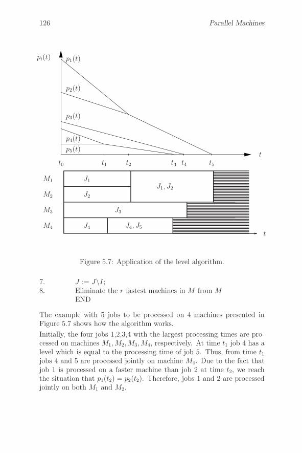
126 Parallel Machines
t0 t1 t2 t3 t4 t5
t
pi(t)
p5(t)
p4(t)
p3(t)
p2(t)
p1(t)
M4
M3
M2
M1
�
J1
J1, J2
J2
J3
J4 J4, J5
t
Figure 5.7: Application of the level algorithm.
7. J := J\I;8. Eliminate the r fastest machines in M from M
END
The example with 5 jobs to be processed on 4 machines presented inFigure 5.7 shows how the algorithm works.
Initially, the four jobs 1,2,3,4 with the largest processing times are pro-cessed on machines M1, M2, M3, M4, respectively. At time t1 job 4 has alevel which is equal to the processing time of job 5. Thus, from time t1jobs 4 and 5 are processed jointly on machine M4. Due to the fact thatjob 1 is processed on a faster machine than job 2 at time t2, we reachthe situation that p1(t2) = p2(t2). Therefore, jobs 1 and 2 are processedjointly on both M1 and M2.
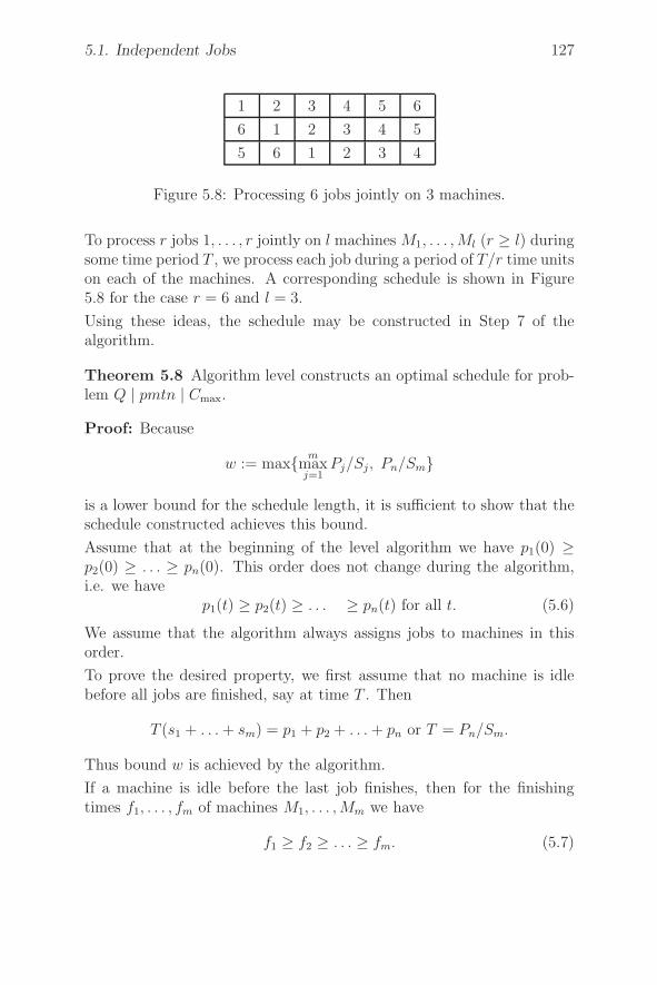
5.1. Independent Jobs 127
1 2 3 4 5 6
6 1 2 3 4 5
5 6 1 2 3 4
Figure 5.8: Processing 6 jobs jointly on 3 machines.
To process r jobs 1, . . . , r jointly on l machines M1, . . . , Ml (r ≥ l) duringsome time period T , we process each job during a period of T/r time unitson each of the machines. A corresponding schedule is shown in Figure5.8 for the case r = 6 and l = 3.
Using these ideas, the schedule may be constructed in Step 7 of thealgorithm.
Theorem 5.8 Algorithm level constructs an optimal schedule for prob-lem Q | pmtn | Cmax.
Proof: Because
w := max{ mmaxj=1
Pj/Sj, Pn/Sm}
is a lower bound for the schedule length, it is sufficient to show that theschedule constructed achieves this bound.
Assume that at the beginning of the level algorithm we have p1(0) ≥p2(0) ≥ . . . ≥ pn(0). This order does not change during the algorithm,i.e. we have
p1(t) ≥ p2(t) ≥ . . . ≥ pn(t) for all t. (5.6)
We assume that the algorithm always assigns jobs to machines in thisorder.
To prove the desired property, we first assume that no machine is idlebefore all jobs are finished, say at time T . Then
T (s1 + . . . + sm) = p1 + p2 + . . . + pn or T = Pn/Sm.
Thus bound w is achieved by the algorithm.
If a machine is idle before the last job finishes, then for the finishingtimes f1, . . . , fm of machines M1, . . . , Mm we have
f1 ≥ f2 ≥ . . . ≥ fm. (5.7)
128 Parallel Machines
Otherwise, if fi < fi+1 for some 1 ≤ i ≤ m − 1, the level of the lastjob processed on Mi at some time fi − ε, where ε > 0 is sufficientlysmall, is smaller than the level of the last job on Mi+1 at the same time.This is a contradiction. Furthermore, in (5.7) we have at least one strictinequality.
Assume that T := f1 = f2 = . . . = fj > fj+1 with j < m. The jobsfinishing at time T must have been started at time 0. If this is not thecase, then we have a job i which starts at time t > 0 and finishes at timeT . This implies that at time 0 at least m jobs, say jobs 1, . . . , m, arestarted and processed together on all machines. We have p1(0) ≥ . . . ≥pm(0) ≥ pi(0), which implies p1(T −ε) ≥ . . . ≥ pm(T −ε) ≥ pi(T −ε) > 0for all ε with 0 ≤ ε < T − t. Thus, until time T no machine is idle, whichis a contradiction. We conclude T = Pj/Sj. �
The level algorithm calls the procedure assign(t) at the most O(n) times.The computational effort for assigning jobs to machines after each callis bounded by O(nm). Thus, we get a total complexity of O(n2m) (thetotal work for calculating all t-values is dominated by this).
Unfortunately, the algorithm generates schedules with an excessive num-ber of preemptions. Also the complexity can be improved. This hasbeen shown by Gonzalez & Sahni [106], who developed an algorithmwhich needs O(n + m log n) steps to construct an optimal schedule withat the most 2(m − 1) preemptions.
Problem Q | pmtn; chains | Cmax which is equivalent to Q | pmtn | Cmax
can be solved with the same complexity.
Next we will derive necessary and sufficient conditions for scheduling aset of jobs in a time interval of length T which will be used in the nextsection.
We have seen that jobs 1, 2, . . . , n with processing times p1 ≥ p2 ≥ . . . ≥pn can be scheduled on machines M1, . . . , Mm with speeds s1 ≥ s2 ≥. . . ≥ sm within an interval of length T if and only if the followinginequalities hold:
j∑
i=1
pi ≤ Tj∑
i=1
si = TSj for j = 1, . . . , min{n, m}n∑
i=1
pi ≤ Tm∑
i=1
si = TSm if n > m.
Due to the monotonicity of the pi-values, for an arbitrary subset A ⊆
5.1. Independent Jobs 129
{1, . . . , n}, we have
∑
i∈A
pi ≤|A|∑
i=1
pi ≤ Th(A)
where
h(A) =
{S|A| if |A| ≤ m
Sm otherwise .
Thus, jobs 1, . . . , n with processing requirements p1, . . . , pn can be sched-uled within an interval of length T if and only if
∑
i∈A
pi ≤ Th(A) for all A ⊆ {1, . . . , n}. (5.8)
Finally, we would like to mention that Q | pmtn; ri | Cmax and Q | pi =1; ri | Cmax has been solved polynomially by Labetoulle et al. [133] andDessouky et al. [76], respectively.
Q | pmtn; ri | Lmax
Again, we first consider the problem of finding a schedule with the prop-erty that each job i is processed in the time window [ri, di] defined bya release time ri and a deadline di of job i. We call such a schedulefeasible with respect to the time windows [ri, di]. In a second step,we apply binary search to solve the general problem.
As in Section 5.1.1 for identical machines, we solve the feasibility problemby reducing it to a network flow problem. Again, let
t1 < t2 < . . . < tr
be the ordered sequence of all different ri-values and di-values and defineIK := [tK−1, tK ], TK = tK − tK−1 for K = 2, . . . , r. Next we expand thenetwork shown in Figure 5.2 in the following way.
Let IK be an arbitrary interval node in Figure 5.2 and denote by Ji1 , Ji2,. . . , Jis the set of predecessors of node IK . Then we replace the subnet-work defined by IK , Ji1 , Ji2, . . . , Jis which is shown in Figure 5.9(a) bythe expanded network shown in Figure 5.9(b).
Again, we assume that the machines are indexed in nonincreasing orderof speeds
s1 ≥ s2 ≥ . . . ≥ sm.
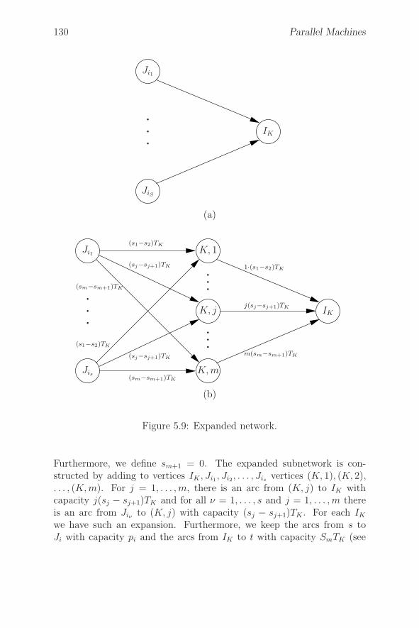
130 Parallel Machines
JiS
Ji1
IK
(a)
Jis K, m
K, j IK
Ji1 K, 1
m(sm−sm+1)TK
j(sj−sj+1)TK
1·(s1−s2)TK
(sm−sm+1)TK
(sj−sj+1)TK
(sm−sm+1)TK
(s1−s2)TK
(sj−sj+1)TK
(s1−s2)TK
(b)
Figure 5.9: Expanded network.
Furthermore, we define sm+1 = 0. The expanded subnetwork is con-structed by adding to vertices IK , Ji1, Ji2, . . . , Jis vertices (K, 1), (K, 2),. . . , (K, m). For j = 1, . . . , m, there is an arc from (K, j) to IK withcapacity j(sj − sj+1)TK and for all ν = 1, . . . , s and j = 1, . . . , m thereis an arc from Jiν to (K, j) with capacity (sj − sj+1)TK . For each IK
we have such an expansion. Furthermore, we keep the arcs from s toJi with capacity pi and the arcs from IK to t with capacity SmTK (see
5.1. Independent Jobs 131
Figure 5.2). The network constructed in this way is called an expandednetwork.
The following theorem shows that we can check feasibility by solving amaximum flow problem in the expanded network.
Theorem 5.9 The following properties are equivalent:
(a) There exists a feasible schedule.
(b) In the expanded network there exists a flow from s to t with valuen∑
i=1
pi.
Proof: (b) ⇒ (a): Consider a flow with valuen∑
i=1
pi in the expanded
network. Denote by xiK the total flow which goes from Ji to IK . Thenn∑
i=1
r∑
K=2
xiK =n∑
i=1
pi. It is sufficient to show that for each subset A ⊆{1, . . . , n} we have ∑
i∈A
xiK ≤ TKh(A).
This means that condition (5.8) holds and the processing requirementsx1K , . . . , xnK can be scheduled in IK for K = 2, . . . , r.
Consider in the expanded network the subnetwork induced by A and thecorresponding partial flow. The portion of this partial flow which goesthrough (K, j) is bounded by
min{j(sj − sj+1)TK , |A|(sj − sj+1)TK} = TK(sj − sj+1) min{j, |A|}.Thus, we have
∑
i∈A
xiK ≤ TK
m∑
j=1
(sj − sj+1) min{j, |A|} = TKh(A). (5.9)
That the equality in (5.9) holds can be seen as follows. If |A| > m, wehave
m∑
j=1
min{j, |A|}(sj − sj+1)= s1 − s2 + 2s2 − 2s3 + 3s3 − 3s4
+ . . . + msm − msm+1
= Sm = h(A).
132 Parallel Machines
Otherwise
m∑
j=1
min{j, |A|}(sj − sj+1)
= s1 − s2 + 2s2 − 2s3 + 3s3 − . . . + (|A| − 1)s|A|−1
−(|A| − 1)s|A| + |A|(s|A| − s|A|+1 + s|A|+1 − . . . − sm + sm − sm+1)
= S|A| = h(A).
(a) ⇒ (b): Assume that a feasible schedule exists. For i = 1, . . . , nand K = 2, . . . , r let xiK be the “amount of work” to be performed onjob i in the interval IK according to this feasible schedule. Then for allK = 2, . . . , r and arbitrary sets A ⊆ {1, . . . , n}, the inequality
∑
i∈A
xiK ≤ TKh(A) (5.10)
holds. Furthermore, for i = 1, . . . , n we have pi =r∑
K=2
xiK . It remains
to show that it is possible to send xiK units of flow from Ji to IK (i =1, . . . , n; K = 2, . . . , r) in the expanded network. A sufficient conditionfor the existence of such a flow is that for arbitrary A ⊆ {1, . . . , n} andK = 2, . . . , r the value
∑
i∈A
xiK is bounded by the value of a minimum cut
in the partial network with sources Ji(i ∈ A) and sink IK . However, thisvalue is
TK
m∑
j=1
min{j, |A|}(sj − sj+1).
Using (5.10) and the right-hand side of (5.9), we get
∑
i∈A
xiK ≤ TKh(A) = TK
m∑
j=1
min{j, |A|}(sj − sj+1)
which is the desired inequality. �
Because a maximal flow in the expanded network can be calculated inO(mn3) steps, a feasibility check can be done with the same complexity.To solve problem Q | pmtn; ri | Lmax we do binary search. This yieldsan ε-approximation algorithm with complexity O(mn3(log n+log(1/ε)+
log(n
maxi=1
pi)) because Lmax is certainly bounded by nn
maxi=1
pi if s1 = 1.
Because (5.10) holds for all K, the partial jobs with processing require-ments xiK can be scheduled in IK with the level algorithm. Problem

5.1. Independent Jobs 133
Q | pmtn; ri | Cmax, which is a special case of Q | pmtn; ri | Lmax,can be solved more efficiently. Labetoulle, Lawler, Lenstra, and RinnooyKan [133] have developed an O(n log n + mn)-algorithm for this specialcase. Also problem Q | pmtn | Lmax can be solved in O(n log n + mn)steps. This is a consequence of the following considerations.
Problem Q | pmtn; ri | Cmax is equivalent to finding a smallest T ≥ 0 suchthat the problem with time windows [ri, T ] (i = 1, . . . , n) has a feasiblesolution. On the other hand, problem Q | pmtn | Lmax is equivalentto finding a smallest T ≥ 0 such that the problem with time windows[0, di + T ] or with time windows [−T, di] has a feasible solution. Thus,the problems Q | pmtn; ri | Cmax and Q | pmtn | Lmax are symmetrical.
Q ‖ ∑Ci
Assume that i1, i2, . . . , ir is the sequence of jobs to be processed on ma-chine Mj . Then the contribution of these jobs on machine Mj in theobjective function is given by
pi1
r
sj
+ pi2
r − 1
sj
+ . . . + pir
1
sj
.
This implies that in an optimal schedule the jobs on machine Mj aresequenced according to nondecreasing processing requirements pi.
To find an optimal distribution of jobs to machines we may proceed asfollows. Let t1, . . . , tn be a nondecreasing sequence of the n smallestnumbers in the set { 1
s1, 1
s2, . . . , 1
sm, 2
s1, 2
s2, . . . , 2
sm, 3
s1, . . .}. If ti = k
sj, then
schedule job i on Mj as the k-th last job because we assume p1 ≥ p2 ≥. . . ≥ pn. Optimality of this strategy is a consequence of the results inSection 2.5.
These ideas lead to the following algorithm in which, for j = 1, . . . , m,we denote by Πj the sequence of jobs currently scheduled at machine Mj .
Each minimal w-value can be calculated in O(log m) time if we use apriority queue. Thus, the overall complexity is O(n log m) if the pi-valuesare sorted. Otherwise, we have a total complexity of O(n log n) if n > m.
Next we will consider the preemptive version of this problem.
Algorithm Q ‖ ∑Ci
1. FOR j = 1 TO m DO2. BEGIN Πj := φ; wj := 1
sjEND;
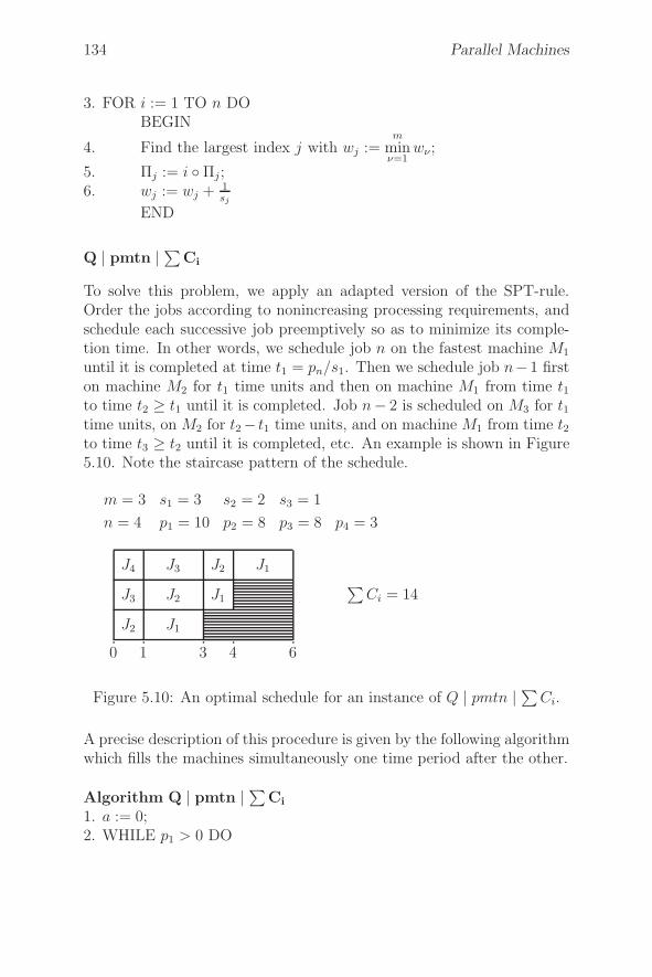
134 Parallel Machines
3. FOR i := 1 TO n DOBEGIN
4. Find the largest index j with wj :=m
minν=1
wν ;
5. Πj := i ◦ Πj ;6. wj := wj + 1
sj
END
Q | pmtn | ∑Ci
To solve this problem, we apply an adapted version of the SPT-rule.Order the jobs according to nonincreasing processing requirements, andschedule each successive job preemptively so as to minimize its comple-tion time. In other words, we schedule job n on the fastest machine M1
until it is completed at time t1 = pn/s1. Then we schedule job n−1 firston machine M2 for t1 time units and then on machine M1 from time t1to time t2 ≥ t1 until it is completed. Job n− 2 is scheduled on M3 for t1time units, on M2 for t2− t1 time units, and on machine M1 from time t2to time t3 ≥ t2 until it is completed, etc. An example is shown in Figure5.10. Note the staircase pattern of the schedule.
m = 3 s1 = 3 s2 = 2 s3 = 1
n = 4 p1 = 10 p2 = 8 p3 = 8 p4 = 3
0 1 3 4 6
∑Ci = 14
J2 J1
J3 J2 J1
J4 J3 J2 J1
Figure 5.10: An optimal schedule for an instance of Q | pmtn | ∑Ci.
A precise description of this procedure is given by the following algorithmwhich fills the machines simultaneously one time period after the other.
Algorithm Q | pmtn | ∑Ci
1. a := 0;2. WHILE p1 > 0 DO
5.1. Independent Jobs 135
BEGIN3. Find the largest index i with pi > 0;4. �t := pi/s1;5. For ν := i DOWN TO k := max{1, i − m + 1} DO
BEGIN6. Schedule job ν on M1+i−ν during [a, a + �t];7. pν := pν −�t · s1+i−ν
END8. a := a + �t
END
The computational complexity is O(n log n + mn). The number of pre-emptions is bounded by (m−1)n−[1+2+. . .+(m−1)] = (m−1)(n−m
2).
A simple interchange argument may be used to prove the correctness ofthe algorithm .
Q | pi = 1 | ∑fi and Q | pi = 1 | fmax
In this section we consider the problem of scheduling n jobs with unitprocessing requirements on m uniform machines with speeds s1, . . . , sm.
The objective functions aren∑
i=1
fi(Ci) andn
maxi=1
fi(Ci), where fi(Ci) are
monotone nondecreasing functions depending on the finishing times Ci
of jobs i. These problems are easily solved in polynomial time. First, ob-serve that there exists an optimal schedule in which the jobs are executedin time periods with the n earliest possible completion times. These com-pletion times can be generated in O(n log m) time: initialize a priorityqueue with completion times 1/sj(j = 1, . . . , m) and, at a general step,remove the smallest completion time from the queue. If this smallestcompletion time is k/sj, then (k + 1)/sj is inserted.
Let t1, . . . , tn denote the n smallest completion times in nondecreasingorder.
An optimal solution of problem Q | pi = 1 | ∑fi can be found by solving
an n × n-assignment problem with cost coefficients cik = fi(tk)(i, k =1, . . . , n). The overall complexity is O(n3).
To solve problem Q | pi = 1 | fmax, Lawler’s algorithm can be adaptedin the following way.
136 Parallel Machines
Algorithm Q | pi = 1 | fmax
1. J := {1, . . . , n};2. FOR i := n DOWN TO 1 DO
BEGIN3. Find a job j ∈ J with minimal fj(ti)-value;4. Schedule job j finishing at time ti;5. J := J\{j}
END
The correctness of this algorithm follows in a similar way as for Lawler’salgorithm. The overall complexity is O(n2).
There are several special cases which can be solved more quickly. Q |pi = 1 | ∑
wiCi is solved by assigning the job with the k-th largest weightto tk, and Q | pi = 1 | ∑
Ti is solved by assigning the job with the k-thsmallest due date to tk. The time required is O(n log n).
Q | pi = 1 | Lmax can be solved by simply matching the k-th smallest duedate with tk. Again the complexity is O(n logn). Q | ri, pi = 1 | Cmax
can be solved symmetrically.
To procedure for calculating the tk-value can be adapted if we have pi = pinstead of pi = 1 for all jobs i. Thus, also the problems Q | pi = p | Lmax
and Q | pi = p; ri | Cmax can be solved with time complexity O(n logn).
5.1.3 Unrelated Machines
We have n independent jobs i = 1, . . . , n to be processed on m machines.The processing time of job i on machine Mj is pij (i = 1, . . . , n; j =1, . . . , m). This model is a generalization of the uniform machine modelwe get by setting pij = pi/sj. In this case, problem Q ‖ ∑
Ci was theonly problem which was polynomially solvable in the case of nonpre-emptable jobs with arbitrary processing times. Next we will show thata polynomial algorithm also exists for the corresponding problem withunrelated machines.
R ‖ ∑Ci
We reduce this problem to an assignment problem. Again, if i1, i2, . . . , iris the sequence of jobs processed at machine Mj , then the contribution
5.1. Independent Jobs 137
of these jobs in the objective function is
rpi1j + (r − 1)pi2j + . . . + 1pirj .
We define a position of a job on a machine by considering the job pro-cessed last on the first position, the job processed second from last onthe second position, etc. To solve problem R ‖ ∑
Ci we have to assignthe jobs i to positions k on machines j. The cost of assigning job i to(k, j) is kpij . Note that an optimal solution of this assignment problemhas the following property: if some job i is assigned to position k > 1on machine j, then there is also a job assigned to position k − 1 on ma-chine j. Otherwise, scheduling job i in position k − 1 would improve thetotal assignment cost (provided that pij > 0). Thus, a solution of theassignment problem always yields an optimal solution of our schedulingproblem.
R | pmtn | Cmax, R | pmtn | Lmax and R | pmtn; ri | Lmax
We solve problem R | pmtn | Cmax in two steps. In the first step weformulate a linear program to calculate for each job i and each machinej the amount of time tij machine j works on job i in an optimal schedule.In a second step, a corresponding schedule in constructed.
First we give the linear programming formulation. Problem R | pmtn |Cmax is given by nm positive integers pij, which represents the totalprocessing time of job i on machine Mj . Let tij be the processing time ofthat part of job i which is processed on Mj . Then tij/pij is the fractionof time that job i spends on machine j, and the equation
m∑
j=1
tijpij
= 1
must hold in order for job i to be completed (i = 1, . . . , n).
138 Parallel Machines
This leads to the following formulation of the problem:
minimize Cmax
subject tom∑
j=1
tijpij
=1, i = 1, . . . , n (5.11)
m∑
j=1
tij≤Cmax, i = 1, . . . , n (5.12)
n∑
i=1
tij≤Cmax, j = 1, . . . , m (5.13)
tij≥0, i = 1, . . . , n; j = 1, . . . , m.
The left-hand side of (5.12) represents the time job i (i = 1, . . . , n) spendson all machines. The left-hand side of (5.13) represents the total timemachine Mj (j = 1, . . . , m) spends processing jobs. Note that for anoptimal solution of this linear program we have
Cmax = max{ nmaxi=1
m∑
j=1
tij ,m
maxj=1
n∑
i=1
tij}. (5.14)
The problem of finding a corresponding schedule is equivalent to theproblem of finding a solution to the preemptive open shop problem withprocessing times tij (i = 1, . . . , n; j = 1, . . . , m) which has a Cmax-valuegiven by (5.14). In Section 2.4, we presented a polynomial algorithmfor solving this problem. We conclude that problem R | pmtn | Cmax ispolynomially solvable.
A similar approach may be used to solve R | pmtn | Lmax. We formulatea linear programming problem to minimize Lmax.
Assume that the jobs are numbered in nondecreasing due date order, i.e.d1 ≤ d2 ≤ . . . ≤ dn.
Let t(1)ij be the total amount of time that machine Mj spends on job i
in time period I1 = [0, d1 + Lmax]. Furthermore, for k = 2, . . . , n let t(k)ij
be the total amount of time that machine Mj spends on job i within thetime period Ik = [dk−1 + Lmax, dk + Lmax]. Then we have to solve
5.2. Jobs with Precedence Constraints 139
minimize Lmax
subject tom∑
j=1
i∑
k=1
t(k)ij
pij= 1, i = 1, . . . , n
m∑
j=1
t(1)ij ≤ d1 + Lmax, i = 1, . . . , n
m∑
j=1
t(k)ij ≤ dk − dk−1, i = k, . . . , n; k = 2, . . . , n
n∑
i=1
t(1)ij ≤ d1 + Lmax, j = 1, . . . , m
n∑
i=k
t(k)ij ≤ dk − dk−1, j = 1, . . . , m; k = 2, . . . , n
t(k)ij ≥ 0, j = 1, . . . , m; i, k = 1, . . . , n.
Given an optimal solution of this linear programming problem, an Lmax-optimal schedule can be obtained by constructing for each of the timeperiods Ik (k = 1, . . . , n) a corresponding schedule using the data given
by the matrix Tk = (t(k)ij ). We again conclude that problem R | pmtn |
Lmax is polynomially solvable.
In a similar way, we may solve problem R | pmtn; ri | Lmax by consideringintervals [tk, tk+1], k = 1, . . . , r − 1, where
t1 < t2 < . . . < tr
is the ordered sequence of all ri-values and di +Lmax values. In this case,we have the variables t
(k)ij and Lmax where t
(k)ij is the processing time of
job i on Mj within the interval [tk, tk+1].
5.2 Jobs with Precedence Constraints
In this section we consider problems with n jobs i = 1, . . . , n with prece-dence constraints between these jobs. We write i → j if j is an immediatesuccessor of i or, equivalently, i is an immediate predecessor of j. Theset IP (i) (IS(i)) of all immediate predecessors (successors) of job i isgiven by
IP (i) = {j | j → i} (IS(i) = {j | i → j}).Besides scheduling problems with arbitrary precedence constraints, weconsider intrees (outtrees) which are precedence constraints with the
140 Parallel Machines
property that each IS(i) (IP (i)) contains at the most one job. Givenan intree (outtree), we denote by s(i) (p(i)) the unique successor (pre-decessor) of i if such a successor (predecessor) exists. Otherwise we sets(i) = 0 (p(i) = 0).
Release times ri of the jobs are called consistent with the precedenceconstraints if ri + pi ≤ rj whenever i → j. Similarly, due dates di arecalled consistent with the precedence constraints if di ≤ dj −pj wheneveri → j.
5.2.1 P | tree;pi = 1 | Lmax-Problems
We now consider the problem in which unit time jobs with precedenceconstraints are to be scheduled on identical parallel machines. The prece-dence constraints are either intrees or outtrees.
P | intree;pi = 1 | Lmax
The procedure which solves this problem has two steps. In the firststep, the due dates of the jobs are modified in such a way that they areconsistent with the precedence constraints.
In the second step, jobs are scheduled in an order of nondecreasing mod-ified due dates.
The due date modification procedure is a special case of a correspondingprocedure already introduced in the last chapter. The idea is to replacedi by min{di, dj − 1} whenever i → j. This is done in a systematic waygoing from the roots (vertices i with s(i) = 0) to the leaves (verticesi with IP (i) = φ) of the intree. After modifying the due date di, weeliminate i from the intree. T denotes the set of roots in the current tree.Details are described by the following algorithm.
Algorithm Due Date Modification 11. T := {i | i has no successor};2. WHILE T �= φ DO
BEGIN3. Choose a job i in T ;4. FOR ALL j ∈ IP (i) DO
BEGIN5. dj := min{dj, di − 1};
5.2. Jobs with Precedence Constraints 141
6. T := T ∪ {j}END;
7. T := T\{i}END
Implementing Algorithm Due Date Modification 1 in an appropriate wayyields an O(n)-algorithm if applied to intrees.
We denote the modified due dates by d′i. Note that d′
i < d′j whenever
i → j. Furthermore, the following lemma holds.
Lemma 5.10 A schedule has no late jobs with respect to the originaldue dates di if and only if it has no late jobs with respect to the modifieddue dates.
Proof: Because d′i ≤ di for all jobs i, a schedule without late jobs with
respect to the d′i-values has no late jobs with respect to the di-values.
To prove the other direction, assume w.l.o.g. that n, n − 1, . . . , 1 is theorder in which the due dates are modified by Algorithm Due Date Modi-fication 1. Consider a schedule with finishing times C1, . . . , Cn satisfyingCi ≤ di for i = 1, . . . , n. Then Cn ≤ dn = d′
n. If for some 1 < r ≤ n wehave Ci ≤ d′
i for i = r, . . . , n, and there exists a job j ∈ {r, . . . , n} withs(r − 1) = j then we have Cr−1 ≤ min{dr−1, d
′j − 1} = d′
r−1. �
In the second step the jobs are scheduled sequentially in order of non-decreasing modified due dates. This is done by scheduling each job atthe earliest available starting time, i.e. the earliest time at which lessthan m tasks are scheduled to start and all predecessors of the job havebeen completed. A more precise description is given by the followingalgorithm. We assume that the jobs are numbered in such a way thatd′
1 ≤ d′2 ≤ . . . , d′
n. Furthermore, F denotes the earliest time at which amachine is available, and r(i) is the latest finishing time of a predecessorof job i. n(t) counts the number of jobs scheduled at time t and x(i) isthe starting time of job i. As before, s(i) is the successor of i.
Algorithm P | intree;pi = 1 | Lmax
1. F := 0;2. FOR i := 1 TO n DO r(i) := 0;3. FOR t := 0 TO n DO n(t) := 0;4. FOR i := 1 TO n DO
142 Parallel Machines
BEGIN5. t := max{r(i), F};6. x(i) := t;7. n(t) := n(t) + 1;8. IF n(t) = m THEN F := t + 1;9. j := s(i);10. r(j) := max{r(j), t + 1}
END
The schedule constructed by this algorithm has the important propertythat the number of tasks scheduled at any time is never less than thenumber scheduled at a later time. This can be seen as follows. Supposek tasks are scheduled to start at a time t and at least k + 1 tasks arescheduled to start at time t + 1. Since the procedure schedules jobs atthe earliest available starting time and less than m jobs are scheduled attime t, the k+1 jobs scheduled at time t+1 must each have an immediatepredecessor scheduled to start at time t. This is impossible because, dueto the intree property, each job starting at time t has at the most onesuccessor.
The running time of Algorithm P | intree; pi = 1 | Lmax is O(n). Thus,problem P | intree; pi = 1 | Lmax can be solved in O(n log n) time.
We still have to prove that Algorithm P | intree; pi = 1 | Lmax is correct.
Lemma 5.11 If there exists a schedule in which no job is late, then aschedule constructed by Algorithm P | intree; pi = 1 | Lmax has thisproperty.
Proof: Assume that there is a late job in the schedule x(1), . . . , x(n)constructed by the algorithm. Then there is also a late job with respectto the modified due dates. Consider the smallest i with x(i) + 1 > d′
i.
Let t < d′i be the largest integer with the property that | {j | x(j) =
t, d′j ≤ d′
i} |< m.
Such a t exists because otherwise md′i jobs j with d′
j ≤ d′i are scheduled
before d′i. Job i does not belong to this set because x(i) + 1 > d′
i. Thismeans that at least md′
i + 1 jobs must be scheduled in the time interval[0, d′
i] if no job is late. This is a contradiction.
Each job j with d′j ≤ d′
i and x(j) > t must have a (not necessarilyimmediate) predecessor starting at time t. Now we consider two cases.
5.2. Jobs with Precedence Constraints 143
Case 1: t = d′i − 1
We have x(i) > d′i − 1 = t. Thus, a predecessor k of i must start at time
t and finish at time d′i. Because d′
k ≤ d′i − 1 < d′
i = x(k) + 1, job k islate, too. However, this is a contradiction to the minimality of i.
Case 2: t < d′i − 1
Exactly m jobs j with d′j ≤ d′
i start at time t + 1, each of them havinga predecessor starting at time t. Due to the intree structure, all thesepredecessors must be different. Furthermore, if k is such a predecessorof a job j, then d′
k ≤ d′j − 1 < d′
j ≤ d′i which contradicts the definition of
t. �
Theorem 5.12 The Algorithm P | intree; pi = 1 | Lmax is correct.
Proof: Let L∗max be the optimal solution value. Then there exists a
schedule satisfyingn
maxi=1
{Ci − di} ≤ L∗max (5.15)
which is equivalent to
Ci ≤ di + L∗max for i = 1, . . . , n. (5.16)
Due to Lemma 5.10, a schedule S constructed by the algorithm for thedue dates di +L∗
max satisfies (5.16) or equivalently (5.15). Thus it is opti-mal. However, S is identical to a schedule constructed by the algorithmfor the due dates di because (di + L∗
max)′ = d′
i + L∗max for i = 1, . . . , n. �
If we use the same idea we applied for solving problem 1 | prec; pi =1 | Lmax, the complexity of problem P | intree; pi = 1 | Lmax can beimproved to O(n) as well.
To get this result, we first calculate the modified due dates d′j using Al-
gorithm Due Date Modification 1. We may assume that the smallestmodified due date d′
j∗ = min{d′j | j = 1, . . . , n} is equal to one. Other-
wise, we replace the original due dates by dj − d′j∗ +1 which implies that
(dj − d′j∗ + 1)′ = d′
j − d′j∗ + 1. We conclude that
Lmax =n
maxj=1
(Cj − d′j) ≥ Cj∗ − d′
j∗ ≥ 0
for any schedule.
144 Parallel Machines
Next we partially sort the jobs according to modified due dates in O(n)time by partitioning the set of jobs into sets Sk, defined by
Sk =
{{j | d′
j = k} if 1 ≤ k ≤ n − 1
{j | d′j ≥ n} if k = n.
Then we apply Algorithm P | intree; pi = 1 | Lmax to the job setn−1⋃
k=1
Sk
by first scheduling the jobs in S1 in an arbitrary order, then the jobs inS2 in an arbitrary order, etc. We extend the partial schedule constructedthis way by scheduling the jobs in Sn in an order of nondecreasing d′
j-values according to algorithm P | intree; pi = 1 | Lmax. The resultingschedule must be optimal because all jobs are scheduled in an order ofnondecreasing d′
j-values. Denote the corresponding objective value byL∗
max.
Unfortunately, the jobs in Sn must be sorted, which takes O(n logn)time. We can avoid this by ordering the jobs in Sn consistently with theprecedence constraints and scheduling them in this order. The resultingschedule must be optimal because
nmaxj=1
{Cj − d′j}= max(max{Cj − d′
j | j ∈n−1⋃
k=1
Sk},max{Cj − d′
j | j ∈ Sn})= max{Cj − d′
j | j ∈n−1⋃
k=1
Sk} ≤ L∗max.
The last equality follows from the fact that Cj ≤ n ≤ d′j for all j ∈ Sn.
P | intree; pi = p | Lmax can be solved with the same complexitybecause by scaling with factor 1/p this problem is transformed intothe corresponding equivalent problems with pi = 1. Symmetrically toP | intree; pi = p | Lmax, problem P | outtree; pi = p; ri | Cmax can besolved in linear time.
P | tree;pi = 1 | Cmax
Clearly, P | outtree; pi = 1 | Cmax can be solved in time O(n) as well. P |intree; pi = 1 | Cmax has the same complexity because it is symmetricalto P | outtree; pi = 1 | Cmax. Thus, P | tree; pi = 1 | Cmax can be solvedin linear time. However, problem P | outtree; pi = 1 | Lmax is NP-hard.
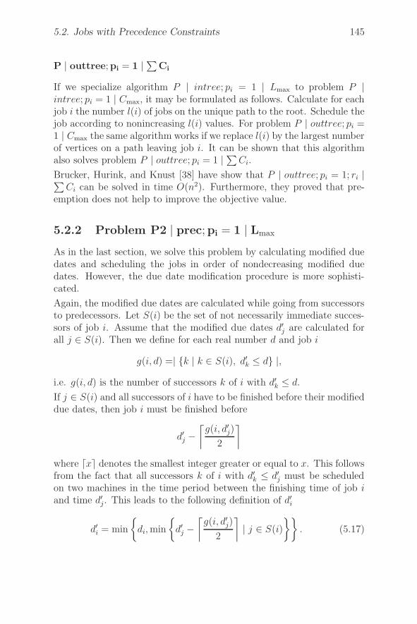
5.2. Jobs with Precedence Constraints 145
P | outtree;pi = 1 | ∑Ci
If we specialize algorithm P | intree; pi = 1 | Lmax to problem P |intree; pi = 1 | Cmax, it may be formulated as follows. Calculate for eachjob i the number l(i) of jobs on the unique path to the root. Schedule thejob according to nonincreasing l(i) values. For problem P | outtree; pi =1 | Cmax the same algorithm works if we replace l(i) by the largest numberof vertices on a path leaving job i. It can be shown that this algorithmalso solves problem P | outtree; pi = 1 | ∑
Ci.
Brucker, Hurink, and Knust [38] have show that P | outtree; pi = 1; ri |∑Ci can be solved in time O(n2). Furthermore, they proved that pre-
emption does not help to improve the objective value.
5.2.2 Problem P2 | prec;pi = 1 | Lmax
As in the last section, we solve this problem by calculating modified duedates and scheduling the jobs in order of nondecreasing modified duedates. However, the due date modification procedure is more sophisti-cated.
Again, the modified due dates are calculated while going from successorsto predecessors. Let S(i) be the set of not necessarily immediate succes-sors of job i. Assume that the modified due dates d′
j are calculated forall j ∈ S(i). Then we define for each real number d and job i
g(i, d) =| {k | k ∈ S(i), d′k ≤ d} |,
i.e. g(i, d) is the number of successors k of i with d′k ≤ d.
If j ∈ S(i) and all successors of i have to be finished before their modifieddue dates, then job i must be finished before
d′j −
⌈g(i, d′
j)
2
⌉
where �x denotes the smallest integer greater or equal to x. This followsfrom the fact that all successors k of i with d′
k ≤ d′j must be scheduled
on two machines in the time period between the finishing time of job iand time d′
j. This leads to the following definition of d′i
d′i = min
{
di, min
{
d′j −
⌈g(i, d′
j)
2
⌉
| j ∈ S(i)
}}
. (5.17)
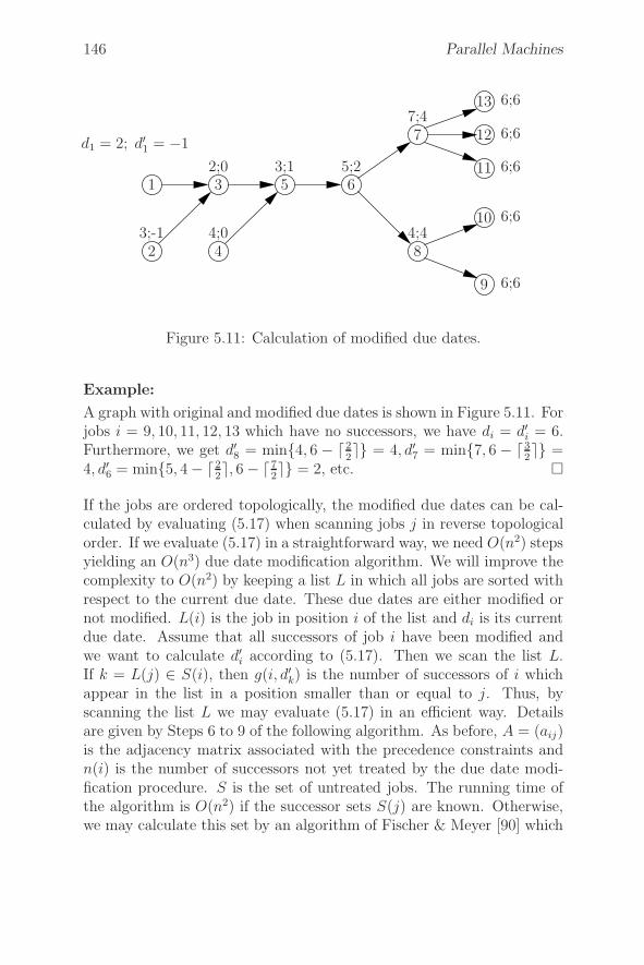
146 Parallel Machines
1
2
3
4
5 6
7
13
12
11
8
10
9
d1 = 2; d′1 = −1
2;0 3;1 5;2
3;-1 4;0 4;4
7;46;6
6;6
6;6
6;6
6;6
Figure 5.11: Calculation of modified due dates.
Example:
A graph with original and modified due dates is shown in Figure 5.11. Forjobs i = 9, 10, 11, 12, 13 which have no successors, we have di = d′
i = 6.Furthermore, we get d′
8 = min{4, 6 − �22 } = 4, d′
7 = min{7, 6 − �32 } =
4, d′6 = min{5, 4 − �2
2 , 6 − �7
2 } = 2, etc. �
If the jobs are ordered topologically, the modified due dates can be cal-culated by evaluating (5.17) when scanning jobs j in reverse topologicalorder. If we evaluate (5.17) in a straightforward way, we need O(n2) stepsyielding an O(n3) due date modification algorithm. We will improve thecomplexity to O(n2) by keeping a list L in which all jobs are sorted withrespect to the current due date. These due dates are either modified ornot modified. L(i) is the job in position i of the list and di is its currentdue date. Assume that all successors of job i have been modified andwe want to calculate d′
i according to (5.17). Then we scan the list L.If k = L(j) ∈ S(i), then g(i, d′
k) is the number of successors of i whichappear in the list in a position smaller than or equal to j. Thus, byscanning the list L we may evaluate (5.17) in an efficient way. Detailsare given by Steps 6 to 9 of the following algorithm. As before, A = (aij)is the adjacency matrix associated with the precedence constraints andn(i) is the number of successors not yet treated by the due date modi-fication procedure. S is the set of untreated jobs. The running time ofthe algorithm is O(n2) if the successor sets S(j) are known. Otherwise,we may calculate this set by an algorithm of Fischer & Meyer [90] which

5.2. Jobs with Precedence Constraints 147
takes O(nlog 7) steps.
Algorithm Due Date Modification 2
1. FOR i := 1 TO n DO n(i) :=n∑
j=1
aij;
2. Calculate a list L of all jobs ordered according to nondecreasingdi-values;
3. S := {1, . . . , n};4. WHILE S �= φ DO
BEGIN5. Find job i ∈ S with n(i) = 0;6. count := 1;7. FOR j := 1 TO n DO IF k := L(j) ∈ S(i) THEN
BEGIN8. di := min{di, dk − � count
2 };
9. count := count + 1;END
10. Eliminate i from L and insert i according to its currentdi-value;
11. FOR j := 1 TO n DO IF aji = 1 THEN n(j) := n(j) − 1;12 S := S\{i}
END
The final list L will be input to a second algorithm which constructs anoptimal schedule by scheduling jobs in order of nondecreasing modifieddue dates. Each job is scheduled as early as possible on one of the two
Algorithm P2 | prec;pi = 1 | Lmax
1. FOR j := 1 TO n DO v(j) =n∑
i=1
aij ;
2. T := 0;3. M := φ;4. WHILE L �= φ DO
BEGIN5. IF |M | = 2 OR there is no job in L with v(j) = 0 THEN
BEGIN6. T := T + 1;7. WHILE there exists i ∈ M DO
BEGIN

148 Parallel Machines
8. FOR j := 1 TO n DOIF aij = 1 THEN v(j) := v(j) − 1;
9. M := M\{i}END
END10. Find the first job j in L with v(j) = 0;11. x(j) := T ;12. M := M ∪ {j};13. L := L\{j}
END
machines. The variables used in this algorithm are
• the current time T ,
• the number v(i) of predecessors of job i which are not scheduledyet,
• the starting time x(i) of job i in the schedule to be constructed,and
• a set M of at the most two jobs and at least one job to be scheduledat current time T .
The complexity of this algorithm is O(n2). Thus, the total time forsolving problem P2 | prec; pi = 1 | Lmax is O(n2) or O(nlog 7) if thesuccessor sets S(j) must be calculated.
We still have to prove the correctness of this procedure.
The following lemma is an immediate consequence of the discussions inthis section.
Lemma 5.13 A schedule has no late jobs with respect to the originaldue dates di if and only if it has no late jobs with respect to the modifieddue dates d′
i. �
Lemma 5.14 If there exists a schedule without late jobs then AlgorithmP2 | prec; pi = 1 | Lmax calculates such a schedule.
Proof: Assume that a schedule x(1), . . . , x(n) constructed by AlgorithmP2 | prec; pi = 1 | Lmax has a late job with respect to the d-values. By
5.2. Jobs with Precedence Constraints 149
Lemma 5.13, this schedule also has a job which is late with respect to thed′-values. Let i be a job with the smallest x-value satisfying d′
i < x(i)+1.Due to the algorithm, at each time t < x(i) at least one job j with d′
j ≤ d′i
must be processed. We consider two cases.
Case 1: At some time t < x(i) only one job k with d′k ≤ d′
i is processed.
We choose a maximal t < x(i) with this property. Then for all jobs jprocessed in the interval [t + 1, x(i)] we have d′
j ≤ d′i. Furthermore, no
machine is idle during this period. All jobs j processed in [t + 1, x(i)]and job i must be successors of k, because otherwise such a j must beprocessed before t + 1. We have
⌈g(k, d′
i)
2
⌉
≥⌈
2(x(i) − t) − 1
2
⌉
= x(i) − t
which implies
d′k ≤ d′
i −⌈
g(k, d′i)
2
⌉
≤ d′i − x(i) + t < x(i) + 1 − x(i) + t = t + 1.
We conclude that job k is also late which contradicts the minimality ofx(i).
Case 2: At each time 0 ≤ t < x(i), two jobs are scheduled and for allthese jobs j the inequality d′
j ≤ d′i holds.
Then we have d′j ≤ d′
i < x(i) + 1 for at least 2x(i) + 1 jobs, which meansthat in each schedule there exists a late job. �
The following lemma shows that the schedule constructed by the algo-rithm will not change if all original due dates are shifted by a constant l.
Lemma 5.15 If d′i(i = 1, . . . , n) are the modified due dates for di(i =
1, . . . , n), then d′i + l are the modified due dates for di + l(i = 1, . . . , n)
for any real number l.
Proof: The assertion is clearly true for all jobs without successors. Oth-erwise, we have by induction
(di + l)′= min{di + l, min{d′j + l − �g(i,d′j)
2 | j ∈ S(i)}
= d′i + l
because
{k | k ∈ S(i), d′k + l ≤ d′
j + l} = {k | k ∈ S(i), d′k ≤ d′
j}.�
150 Parallel Machines
Theorem 5.16 Algorithm P2 | prec; pi = 1 | Lmax is correct.
Proof: Similar to proof of Theorem 5.12.
The procedure can be generalized to an O(n3 log n)-procedure whichsolves problem P2 | prec; pi = 1; ri | Lmax (Garey & Johnson [97]).
�
5.3 Complexity Results
In Tables 5.1 and 5.2 we summarize scheduling problems to be processedwithout preemption on parallel machines which are polynomially solv-able and pseudopolynomially solvable, respectively. In connection with“chains” l denotes the number of chains. In Table 5.3 we will also give alist of related NP-hard problems.
Tables 5.4 to 5.6 summarize the corresponding complexity results forparallel machine problems with preemptions.
Tables 5.1 and 5.6 show that P | pi = p | ∑wiUi is polynomially solvable
but P | pi = p; pmtn | ∑wiUi is NP-hard. This is very surprising be-
cause in the other cases if a problem with pi = p or pi = 1 is polynomiallysolvable then the corresponding preemptive problem is also polynomiallysolvable even with arbitrary processing times. Another result of this typewas provided more recently by Sitters [187].
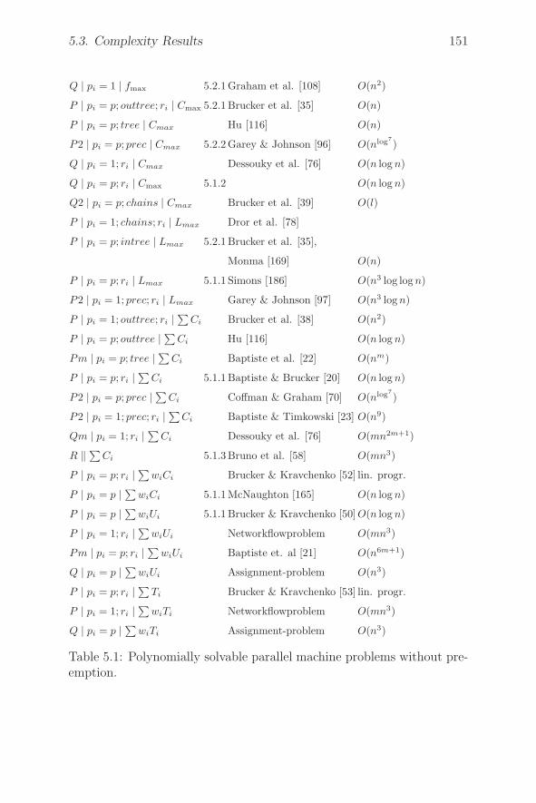
5.3. Complexity Results 151
Q | pi = 1 | fmax 5.2.1Graham et al. [108] O(n2)
P | pi = p; outtree; ri | Cmax 5.2.1Brucker et al. [35] O(n)
P | pi = p; tree | Cmax Hu [116] O(n)
P2 | pi = p; prec | Cmax 5.2.2Garey & Johnson [96] O(nlog7)
Q | pi = 1; ri | Cmax Dessouky et al. [76] O(n log n)
Q | pi = p; ri | Cmax 5.1.2 O(n log n)
Q2 | pi = p; chains | Cmax Brucker et al. [39] O(l)
P | pi = 1; chains; ri | Lmax Dror et al. [78]
P | pi = p; intree | Lmax 5.2.1Brucker et al. [35],
Monma [169] O(n)
P | pi = p; ri | Lmax 5.1.1 Simons [186] O(n3 log log n)
P2 | pi = 1; prec; ri | Lmax Garey & Johnson [97] O(n3 log n)
P | pi = 1; outtree; ri |∑
Ci Brucker et al. [38] O(n2)
P | pi = p; outtree | ∑Ci Hu [116] O(n log n)
Pm | pi = p; tree | ∑Ci Baptiste et al. [22] O(nm)
P | pi = p; ri |∑
Ci 5.1.1Baptiste & Brucker [20] O(n log n)
P2 | pi = p; prec | ∑Ci Coffman & Graham [70] O(nlog7
)
P2 | pi = 1; prec; ri |∑
Ci Baptiste & Timkowski [23] O(n9)
Qm | pi = 1; ri |∑
Ci Dessouky et al. [76] O(mn2m+1)
R ‖ ∑Ci 5.1.3Bruno et al. [58] O(mn3)
P | pi = p; ri |∑
wiCi Brucker & Kravchenko [52] lin. progr.
P | pi = p | ∑wiCi 5.1.1McNaughton [165] O(n log n)
P | pi = p | ∑wiUi 5.1.1Brucker & Kravchenko [50] O(n log n)
P | pi = 1; ri |∑
wiUi Networkflowproblem O(mn3)
Pm | pi = p; ri |∑
wiUi Baptiste et. al [21] O(n6m+1)
Q | pi = p | ∑wiUi Assignment-problem O(n3)
P | pi = p; ri |∑
Ti Brucker & Kravchenko [53] lin. progr.
P | pi = 1; ri |∑
wiTi Networkflowproblem O(mn3)
Q | pi = p | ∑wiTi Assignment-problem O(n3)
Table 5.1: Polynomially solvable parallel machine problems without pre-emption.

152 Parallel Machines
Qm | ri | Cmax Lawler et al. [145]
Qm ‖ ∑wiCi Lawler et al. [145]
Qm ‖ ∑wiUi Lawler et al. [145]
Table 5.2: Pseudopolynomially solvable parallel machine problems with-out preemption.
P2 ‖ Cmax Lenstra et al. [155]
∗ P ‖ Cmax Garey & Johnson [98]
∗ P | pi = 1; intree; ri | Cmax Brucker et al. [35]
∗ P | pi = 1; prec | Cmax Ullman [203]
∗ P2 | chains | Cmax Du et al. [86]
∗ Q | pi = 1; chains | Cmax Kubiak [129]
∗ P | pi = 1; outtree | Lmax Brucker et al. [35]
∗ P | pi = 1; intree; ri |∑
Ci Lenstra [150]
∗ P | pi = 1; prec | ∑Ci Lenstra & Rinnooy Kan [152]
∗ P2 | chains | ∑Ci Du et al. [86]
∗ P2 | ri |∑
Ci Single-machine problem
P2 ‖ ∑wiCi Bruno et al. [58]
∗ P ‖ ∑wiCi Lenstra [150]
∗ P2 | pi = 1; chains | ∑wiCi Timkovsky [201]
∗ P2 | pi = 1; chains | ∑Ui Single-machine problem
∗ P2 | pi = 1; chains | ∑Ti Single-machine problem
Table 5.3: NP-hard parallel machine problems without preemption.
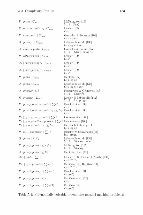
5.3. Complexity Results 153153
P | pmtn | Cmax McNaughton [165]5.1.1 O(n)
P | outtree; pmtn; ri | Cmax Lawler [139]O(n2)
P | tree; pmtn | Cmax Gonzalez & Johnson [103]O(n log m)
Q | pmtn; ri | Cmax Labetoulle et al. [133]O(n log n + mn)
Q | chains; pmtn | Cmax Gonzalez & Sahni [105]5.1.2 O(n + m log n)
P | intree; pmtn | Lmax Lawler [139]O(n2)
Q2 | prec; pmtn; rj | Lmax Lawler [139]O(n2)
Q2 | prec; pmtn; ri | Lmax Lawler [139]O(n6)
P | pmtn | Lmax Baptiste [17]O(n log n)
Q | pmtn | Lmax Labetoulle et al. [133]O(n log n + mn)
Q | pmtn, ri; di | − Federgruen & Gronevelt [89]5.1.2 O(mn3)
R | pmtn; ri | Lmax Lawler & Labetoulle [142]5.1.3 lin. progr.
P | pi = p; outtree; pmtn | ∑Ci Brucker et al. [38]
O(n2)P | pi = 1; outtree; pmtn; ri |
∑Ci Brucker et al. [38]
O(n2)P2 | pi = p; prec; ; pmtn | ∑
Ci Coffman et al. [68]P2 | pi = p; outtree; pmtn; ri |
∑Ci Lushchakova [163]
P2 | pi = p; pmtn; ri |∑
Ci Herrbach & Leung [111]O(n log n)
P | pi = p; pmtn; ri |∑
Ci Brucker & Kravchenko [52]lin. progr.
Q | pmtn | ∑Ci Labetoulle et al. [133]
5.1.2 O(n log n + mn)P | pi = p; pmtn | ∑
wiCi McNaughton [165]5.1.1 O(n log n)
Q | pi = p; pmtn | ∑Ui Baptiste et al. [21]
Qm | pmtn | ∑Ui Lawler [138], Lawler & Martel [146]
O(n3(m−1))Pm | pi = p; pmtn | ∑
wiUi Baptiste [18], Baptiste [17]O(n3m+4)
P | pi = 1; pmtn; ri |∑
wiUi Brucker et al. [37]O(mn3)
P | pi = p; pmtn | ∑Ti Baptiste et al. [21]
O(n3)P | pi = 1; pmtn; ri |
∑wiTi Baptiste [19]
O(mn3)
Table 5.4: Polynomially solvable preemptive parallel machine problems.

154 Parallel Machines
Pm | pmtn | ∑wiCi McNaughton [165], Lawler et al. [145]
Qm | pmtn | ∑wiUi Lawler [138] , Lawler & Martel [146]
Table 5.5: Pseudopolynomially solvable preemptive parallel machineproblems.
∗ P | intree; pmtn; ri | Cmax Lenstra [150]
∗ P | pi = 1; prec; pmtn | Cmax Ullman [204]
∗ R2 | chains; pmtn | Cmax Lenstra [150]
∗ P | outtree; pmtn | Lmax Lenstra [150]
P2 | pmtn; ri |∑
Ci Du et al. [85]
∗ P2 | chains; pmtn | ∑Ci Du et al. [86]
∗ P | pmtn; ri |∑
Ci Brucker & Kravchenko [51]
∗ R | pmtn | ∑Ci Sitters [187]
∗ P2 | pi = 1; chains; pmtn | ∑wiCi Du et al. [86]
P2 | pmtn | ∑wiCi Bruno et al. [58]
∗ P | pi = p; pmtn; ri |∑
wiCi Leung & Young [158]
∗ P | pmtn | ∑wiCi Lenstra [150]
∗ P2 | pmtn; ri |∑
wiCi Labetoulle et al. [133]
P | pmtn | ∑Ui Lawler [140]
P2 | pmtn; ri |∑
Ui Du et al. [84]
∗ P2 | pi = 1; chains; pmtn | ∑Ui Baptiste et al. [21]
∗ R | pmtn; ri |∑
Ui Du & Leung [82]
∗ R | pmtn | ∑Ui Sitters [187]
P | pi = p; pmtn | ∑wiUi Brucker & Kravchenko [50]
P2 | pmtn | ∑wiUi Single-machine problem
Table 5.6: NP-hard preemptive parallel machine problems.

Chapter 6
Shop Scheduling Problems
In this chapter we will discuss shop scheduling problems, such asopen shop problems, flow shop problems, job shop problems, and mixedshop problems, which are widely used for modeling industrial productionprocesses. All of these problems are special cases of the general shopproblem.
The general shop problem may be defined as follows. We have n jobsi = 1, . . . , n and m machines M1, . . . , Mm. Each job i consists of a set ofoperations Oij (j = 1, . . . , ni) with processing times pij. Each operationOij must be processed on a machine μij ∈ {M1, . . . , Mm}. There maybe precedence relations between the operations of all jobs. Each job canonly be processed only by one machine at a time and each machine canonly process one job at a time. The objective is to find a feasible schedulethat minimizes some objective function of the finishing times Ci of thejobs i = 1, . . . , n. The objective functions are assumed to be regular.
In Section 6.1 we will introduce disjunctive graphs, which are a use-ful tool for representing feasible schedules for shop problems. In sub-sequent sections we will discuss open shop problems (Section 6.2), flowshop problems (Section 6.3), job shop problems (Section 6.4), and mixedshop problems (Section 6.5). In Section 6.6 complexity results for shopscheduling problems are presented. Unless otherwise stated, preemptionis not allowed.
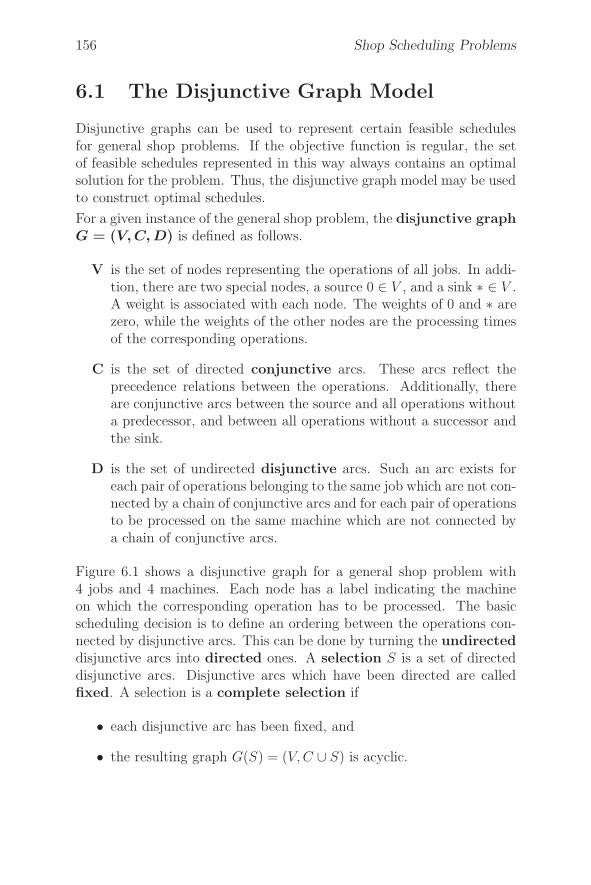
156 Shop Scheduling Problems
6.1 The Disjunctive Graph Model
Disjunctive graphs can be used to represent certain feasible schedulesfor general shop problems. If the objective function is regular, the setof feasible schedules represented in this way always contains an optimalsolution for the problem. Thus, the disjunctive graph model may be usedto construct optimal schedules.
For a given instance of the general shop problem, the disjunctive graphG = (V, C, D) is defined as follows.
V is the set of nodes representing the operations of all jobs. In addi-tion, there are two special nodes, a source 0 ∈ V , and a sink ∗ ∈ V .A weight is associated with each node. The weights of 0 and ∗ arezero, while the weights of the other nodes are the processing timesof the corresponding operations.
C is the set of directed conjunctive arcs. These arcs reflect theprecedence relations between the operations. Additionally, thereare conjunctive arcs between the source and all operations withouta predecessor, and between all operations without a successor andthe sink.
D is the set of undirected disjunctive arcs. Such an arc exists foreach pair of operations belonging to the same job which are not con-nected by a chain of conjunctive arcs and for each pair of operationsto be processed on the same machine which are not connected bya chain of conjunctive arcs.
Figure 6.1 shows a disjunctive graph for a general shop problem with4 jobs and 4 machines. Each node has a label indicating the machineon which the corresponding operation has to be processed. The basicscheduling decision is to define an ordering between the operations con-nected by disjunctive arcs. This can be done by turning the undirecteddisjunctive arcs into directed ones. A selection S is a set of directeddisjunctive arcs. Disjunctive arcs which have been directed are calledfixed. A selection is a complete selection if
• each disjunctive arc has been fixed, and
• the resulting graph G(S) = (V, C ∪ S) is acyclic.
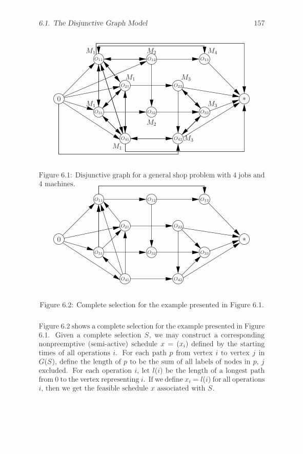
6.1. The Disjunctive Graph Model 157
O41 O42
O31 O32 O33
0 ∗O21 O22
O11 O12 O13
M1
M1
M1
M1
M2
M2
M3
M3
M3
M4
Figure 6.1: Disjunctive graph for a general shop problem with 4 jobs and4 machines.
O41 O42
O31 O32 O33
0 ∗O21 O22
O11 O12 O13
Figure 6.2: Complete selection for the example presented in Figure 6.1.
Figure 6.2 shows a complete selection for the example presented in Figure6.1. Given a complete selection S, we may construct a correspondingnonpreemptive (semi-active) schedule x = (xi) defined by the startingtimes of all operations i. For each path p from vertex i to vertex j inG(S), define the length of p to be the sum of all labels of nodes in p, jexcluded. For each operation i, let l(i) be the length of a longest pathfrom 0 to the vertex representing i. If we define xi = l(i) for all operationsi, then we get the feasible schedule x associated with S.
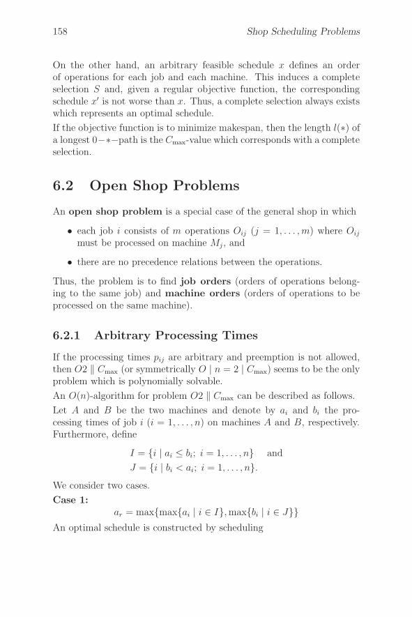
158 Shop Scheduling Problems
On the other hand, an arbitrary feasible schedule x defines an orderof operations for each job and each machine. This induces a completeselection S and, given a regular objective function, the correspondingschedule x′ is not worse than x. Thus, a complete selection always existswhich represents an optimal schedule.
If the objective function is to minimize makespan, then the length l(∗) ofa longest 0−∗−path is the Cmax-value which corresponds with a completeselection.
6.2 Open Shop Problems
An open shop problem is a special case of the general shop in which
• each job i consists of m operations Oij (j = 1, . . . , m) where Oij
must be processed on machine Mj , and
• there are no precedence relations between the operations.
Thus, the problem is to find job orders (orders of operations belong-ing to the same job) and machine orders (orders of operations to beprocessed on the same machine).
6.2.1 Arbitrary Processing Times
If the processing times pij are arbitrary and preemption is not allowed,then O2 ‖ Cmax (or symmetrically O | n = 2 | Cmax) seems to be the onlyproblem which is polynomially solvable.
An O(n)-algorithm for problem O2 ‖ Cmax can be described as follows.
Let A and B be the two machines and denote by ai and bi the pro-cessing times of job i (i = 1, . . . , n) on machines A and B, respectively.Furthermore, define
I = {i | ai ≤ bi; i = 1, . . . , n} and
J = {i | bi < ai; i = 1, . . . , n}.We consider two cases.
Case 1:ar = max{max{ai | i ∈ I}, max{bi | i ∈ J}}
An optimal schedule is constructed by scheduling
6.2. Open Shop Problems 159
B
A
r I\{r} J
I\{r} J r
(a)
B
A
J\{r} I r
r J\{r} I
(b)
Figure 6.3: Optimal schedules for O2 ‖ Cmax.
• first all jobs in I\{r} in an arbitrary order on machine A, then alljobs in J in an arbitrary order, and, finally, job r,
• first job r on machine B, then all jobs in I\{r} in the same orderas jobs in I\{r} are scheduled on A, and, finally, all jobs in J inthe same order as on machine A, and
• first job r on machine B and then on machine A, while all otherjobs are first scheduled on machine A (see Figure 6.3(a)).
Case 2:br = max{max{ai | i ∈ I}, max{bi | i ∈ J}}
We have to interchange the machines and sets I and J before applyingthe same rule (see Figure 6.3(b)).
The complexity of this procedure is O(n).
To prove the correctness of this procedure we consider only Case 1 (Case2 is similar).
Let G(S) be the network induced by the solution S. Then it is sufficientto show that one of the following paths is a longest path in G(S):
(i) 0 → ai (i ∈ I\{r}) −→ ai (i ∈ J) −→ ar → ∗(ii) 0 → br −→ bi (i ∈ I\{r}) −→ bi(i ∈ J) → ∗(iii) 0 → br −→ ar → ∗
160 Shop Scheduling Problems
Here ai (I\{r}), ai (i ∈ J), etc. stand for corresponding subpaths.
Because the length of each of these three paths is a lower bound for theopen shop problem, the solution must be optimal.
To simplify the notation we assume that the jobs are enumerated accord-ing to the sequence on machine A. Thus, I\{r} = {1, . . . , |I|−1}, J ={|I|, . . . , n − 1}, and r = n.
The only paths other than (i), (ii), and (iii) that exist in G(S) are pathsof the form
0 → a1 → . . . → ai → bi → . . . → bn−1 → ∗ (i = 1, . . . , n − 1).
We show that none of these paths is longer than the longest of (i), (ii),(iii).
If i ∈ I, then
i∑
j=1
aj +n−1∑
j=i
bj ≤i−1∑
j=1
bj + ai +n−1∑
j=i
bj ≤n∑
j=1
bj
because ai ≤ max{aj | j ∈ I} = an ≤ bn.
If i ∈ J , then
i∑
j=1
aj +
n−1∑
j=i
bj ≤i∑
j=1
aj + bi +
n−1∑
j=i+1
aj ≤n∑
j=1
aj
because bi ≤ max{bj | j ∈ J} ≤ max{max{ai | i ∈ I}, max{bj | j ∈J}} = an. �
In Section 2.4 we showed that problem O | pmtn | Cmax can be solved inO(n5/2m) time. Similar results can be obtained for the minimization ofmaximum lateness if preemption is allowed. Lawler, Lenstra & RinnooyKan [144] give an O(n) time algorithm for O2 | pmtn | Lmax and, bysymmetry, for O2 | pmtn, ri | Cmax. For O | ri; pmtn | Lmax Cho &Sahni [66] show that a trial value of Lmax can be tested for feasibility bylinear programming; binary search is then applied to minimize Lmax inpolynomial time.
The following problems are NP-hard: O | pmtn | ∑Ci, O2 | pmtn; di |∑
Ci (Liu & Bulfin [160]), and O2 | pmtn | ∑Ci (Du & Leung [83]).
6.2. Open Shop Problems 161
6.2.2 Unit Processing Times
To solve an open shop problem P with unit processing times we proceedas follows.
We transform P into a problem P by replacing
• the machines by m identical parallel machines, and
• each job i by a chain of m unit time jobs Oik (k = 1, . . . , m),
and solve problem P .
A schedule for problem P may be represented by a binary matrix A =(ait) where ait = 1 iff Oik is scheduled in time period t for some k (k =1, . . . , m). Such a schedule can be transformed into a feasible schedule ofthe original open shop problem by assigning machines to the unit timeoperations in such a way that
• all m unit time operations belonging to the same chain are assignedto different machines, and
• all unit time operations scheduled at the same time are assigned todifferent machines.
This machine assignment problem is equivalent to coloring the arcs of thebipartite graph G defined by A with exactly m colors. According to theresults in Section 2.6, this is always possible because m is the maximumdegree of G. Note that G has nm edges. Furthermore, we assume thatm ≤ n. Then the machine assignment can be done in O(n2m) timeusing the edge coloring algorithm of Section 2.6. If we use the moresophisticated algorithm of Gabow & Kariv [95], we get a time bound ofO(nm log2(nm)) because the number of columns in A are bounded byO(nm).
An optimal solution of P yields an optimal solution of the original prob-lem P . This follows from the fact that P is a relaxation of P and that asolution of P also defines a solution for P .
Problem P is equivalent to the problem P of scheduling identical jobswith processing time m on m identical machines where preemption andrestart is only allowed at integer times.
We have considered the case m ≤ n. If n < m, then it is always possibleto construct a schedule in which job i finishes at time ri + m. Such a
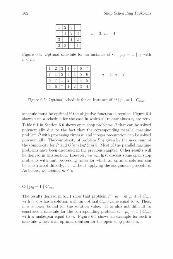
162 Shop Scheduling Problems
1 2 3
1 2 3 n = 3, m = 4
3 1 2
2 3 1
Figure 6.4: Optimal schedule for an instance of O | pij = 1 | γ withn < m.
1 2 3 4 5 6 7
7 1 2 3 4 5 6 m = 4, n = 7
6 7 1 2 3 4 5
5 6 7 1 2 3 4
Figure 6.5: Optimal schedule for an instance of O | pij = 1 | Cmax.
schedule must be optimal if the objective function is regular. Figure 6.4shows such a schedule for the case in which all release times ri are zero.
Table 6.1 in Section 6.6 shows open shop problems P that can be solvedpolynomially due to the fact that the corresponding parallel machineproblem P with processing times m and integer preemption can be solvedpolynomially. The complexity of problem P is given by the maximum ofthe complexity for P and O(nm log2(nm)). Most of the parallel machineproblems have been discussed in the previous chapter. Other results willbe derived in this section. However, we will first discuss some open shopproblems with unit processing times for which an optimal solution canbe constructed directly, i.e. without applying the assignment procedure.As before, we assume m ≤ n.
O | pij = 1 | Cmax
The results derived in 5.1.1 show that problem P | pi = m; pmtn | Cmax
with n jobs has a solution with an optimal Cmax-value equal to n. Thus,n is a lower bound for the solution value. It is also not difficult toconstruct a schedule for the corresponding problem O | pij = 1 | Cmax
with a makespan equal to n. Figure 6.5 shows an example for such aschedule which is an optimal solution for the open shop problem.

6.2. Open Shop Problems 163
Block 1 Block 2 Block 3 Block 4
1 2 3 4 5 6 7 8 9 10 11
3 1 2 6 4 5 9 7 8 10 11
2 3 1 5 6 4 8 9 7 11 10
Figure 6.6: Optimal schedule for an instance of O | pij = 1 | ∑wiCi.
O | pij = 1 | ∑wiCi
We first investigate how to solve the corresponding problem P | pi =m; pmtn | ∑
wiCi. In Section 5.1.1, we saw that preemptions are notadvantageous when solving P | pmtn | ∑
wiCi, i.e. an instance ofP ‖ ∑
wiCi has the same optimal objective value as the correspond-ing instance of P | pmtn | ∑
wiCi.
Thus, it is sufficient to solve P | pi = m | ∑wiCi. This is accomplished
by scheduling the jobs in order of nonincreasing wi-values (see 5.1.1). Ifwe assume that n = lm + r with r < m, we get l blocks of jobs, eachconsisting of exactly m jobs, and a block l+1 consisting of the remainingr jobs. All jobs of block k (k = 1, . . . , l + 1) are scheduled in the timeinterval [(k − 1)m, km]. To construct a schedule for the correspondingO | pij = 1 | ∑
wiCi-problem, we schedule each of the first l blocks asshown in Figure 6.5 and the last block as shown in Figure 6.4. Figure6.6 shows the total schedule for the case m = 3 and n = 11.
Problem O | pij = 1; di |- is to determine whether a feasible scheduleexists for the open shop problem with unit processing times in which nojobs finish later than their deadlines.
In the next sections we will present algorithms for this problem andother problems involving due dates. We will assume that the jobs areenumerated in such a way that
d1 ≤ d2 ≤ . . . ≤ dn. (6.1)
O | pij = 1;di | −If d1 < m, then C1 > d1 in any schedule for O | pij = 1; di | −. Thus, wemay assume that m ≤ di for all i = 1, . . . , n.
Algorithm O | pij = 1; di | − solves problem O | pij = 1; di | − for

164 Shop Scheduling Problems
m machines. Later we will show that this algorithm has an O(nm)-implementation.
The idea of Algorithm O | pij = 1; di | − is to assign the m unit opera-tions of each job to the time slots [t − 1, t] for t = 1, . . . , T := max{di |i = 1, . . . , n}. Job i is first assigned to time slots di − m + 1, . . . , di. Ifsome time slot t > 1 contains m + 1 operations, then an operation fromthe smallest time slot t > 1 with this property is moved one unit to theleft and the process is repeated if necessary. Thus, only the first timeslot may accumulate more than m operations and this happens if andonly if the decision problem O | pij = 1; di | − has a negative answer.We denote by h(t) the number of operations accumulated in time slot[t − 1, t].
Algorithm O | pij = 1;di | −1. T := max{di | i = 1, . . . , n};2. FOR t := 1 TO T DO h(t) := 0;3. FOR i := 1 TO n DO
BEGIN4. FOR j := di DOWN TO di − m + 1 DO h(j) := h(j) + 1;5. WHILE there exists a t > 1 with h(t) = m + 1 DO
BEGIN6. Find a minimal t0 > 1 with h(t0) = m + 1;7. h(t0 − 1) := h(t0 − 1) + 1;8. h(t0) := m
ENDEND
9. IF h(1) ≤ m THEN there exists a schedule without late jobs
We call the vector h calculated by the algorithm the frequency vector.The frequency vector does not depend on the numeration of jobs.
It remains to show that Algorithm O | pij = 1; di | − is correct.
Lemma 6.1 For a set of jobs with deadlines d1, . . . , dn problem O | pij =1; di | − has a feasible solution if and only if h(1) ≤ m holds.
Proof: If h(1) > m, the capacity of machines is not sufficient to performall operations in time.
Algorithm O | pij = 1; di | − initially assigns all operations of the samejob to pairwise different time slots. If there is a t > 1 with h(t) = m + 1
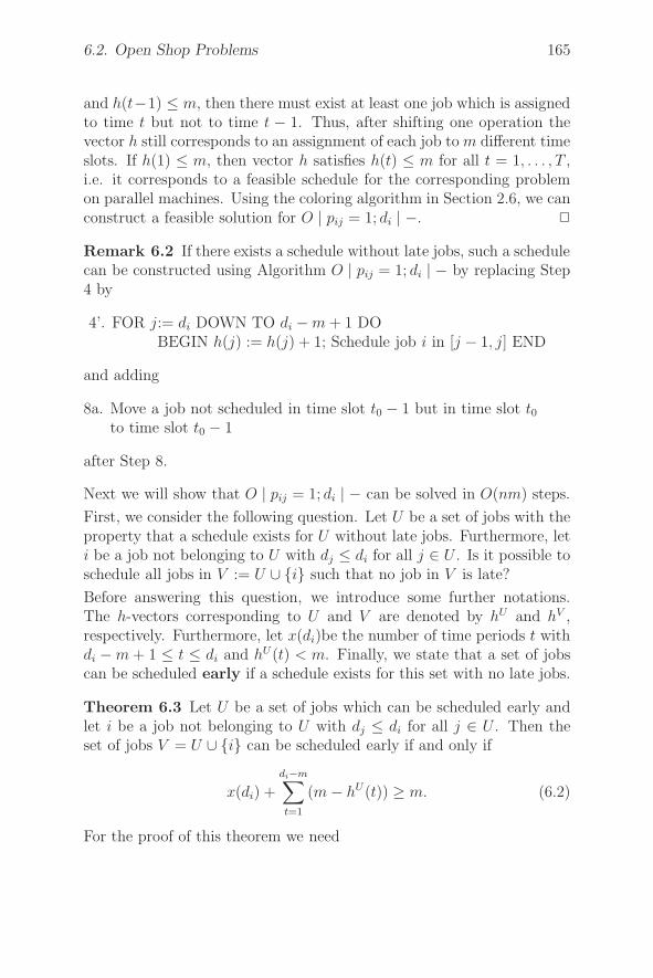
6.2. Open Shop Problems 165
and h(t−1) ≤ m, then there must exist at least one job which is assignedto time t but not to time t − 1. Thus, after shifting one operation thevector h still corresponds to an assignment of each job to m different timeslots. If h(1) ≤ m, then vector h satisfies h(t) ≤ m for all t = 1, . . . , T ,i.e. it corresponds to a feasible schedule for the corresponding problemon parallel machines. Using the coloring algorithm in Section 2.6, we canconstruct a feasible solution for O | pij = 1; di | −. �
Remark 6.2 If there exists a schedule without late jobs, such a schedulecan be constructed using Algorithm O | pij = 1; di | − by replacing Step4 by
4’. FOR j:= di DOWN TO di − m + 1 DOBEGIN h(j) := h(j) + 1; Schedule job i in [j − 1, j] END
and adding
8a. Move a job not scheduled in time slot t0 − 1 but in time slot t0to time slot t0 − 1
after Step 8.
Next we will show that O | pij = 1; di | − can be solved in O(nm) steps.
First, we consider the following question. Let U be a set of jobs with theproperty that a schedule exists for U without late jobs. Furthermore, leti be a job not belonging to U with dj ≤ di for all j ∈ U . Is it possible toschedule all jobs in V := U ∪ {i} such that no job in V is late?
Before answering this question, we introduce some further notations.The h-vectors corresponding to U and V are denoted by hU and hV ,respectively. Furthermore, let x(di)be the number of time periods t withdi − m + 1 ≤ t ≤ di and hU(t) < m. Finally, we state that a set of jobscan be scheduled early if a schedule exists for this set with no late jobs.
Theorem 6.3 Let U be a set of jobs which can be scheduled early andlet i be a job not belonging to U with dj ≤ di for all j ∈ U . Then theset of jobs V = U ∪ {i} can be scheduled early if and only if
x(di) +
di−m∑
t=1
(m − hU(t)) ≥ m. (6.2)
For the proof of this theorem we need
166 Shop Scheduling Problems
Lemma 6.4 Consider jobs 1, 2, . . . , i with d1 ≤ d2 ≤ . . . ≤ di and letU := {1, . . . , i − 1}, V := U ∪ {i}. Then for all j = di − m + 1, . . . , di
with hU(j) < m we have hV (j) = hU(j) + 1.
Proof: We get vectors hU and hV after i−1 and i iterations of AlgorithmO | pij = 1; di | −. During the algorithm, components of the h-vectorwith h(j) ≤ m never decrease.
Thus, if di −m+1 ≤ j ≤ di and hU(j) < m, then hV (j) ≥ hU (j)+ 1. Toprove that hV (j) ≥ hU(j) + 2 is not possible for di −m + 1 ≤ j ≤ di, weconsider the schedule which can be constructed by Algorithm O | pij =1; di | − (see Remark 6.2).
If hV (j) ≥ hU(j) + 2, then during the i-th iteration an operation of job iis added to time slot j and at least one operation of some other job, sayk, is moved from time slot j +1 to time slot j. This is only possible if nooperation of job k is scheduled before time slot j (no operation is movedfrom j to j − 1 as long as h(j) < m). Thus, job k is scheduled in timeslot j and time slots ν > j +1 which implies j < dk −m+1 ≤ di−m+1,i.e. a contradiction. �
Proof of Theorem 6.3: Condition (6.2) is equivalent to
(di − m)m ≥di−m∑
i=1
hU(t) + m − x(di). (6.3)
Due to Lemma 6.4 we have
di∑
j=di−m+1
hV (j) =
di∑
j=di−m+1
hU(j) + x(di).
Subtracting this equation from
di∑
j=1
hV (j) =
di∑
j=1
hU(j) + m
we getdi−m∑
t=1
hV (t) = m − x(di) +
di−m∑
t=1
hU (t).
Thus, (6.2) or (6.3) is equivalent to
Tm ≥T∑
t=1
hV (t) (6.4)

6.2. Open Shop Problems 167
with T := di − m.
It remains to show that if (6.4) holds for T = di − m, then (6.4) alsoholds for T = 1, . . . , di − m − 1. By Lemma 6.1 hV (1) ≤ m implies thatall jobs in V can be scheduled early. If, on the other hand, hV (1) ≤ m,then (6.4) holds because hV (t) ≤ m for all t ≥ 2 by construction of hV .
We prove that (6.4) holds for all T = 1, . . . , di − m by induction on T .
Assume that (6.4) holds for some T with 1 < T ≤ di − m. We considertwo cases depending on the value hV (T ).
Case 1: hV (T ) = mBecause (6.4) holds for T we have
(T − 1)m ≥T∑
t=1
hV (t) − m =
T−1∑
t=1
hV (t),
i.e. (6.4) holds for T − 1.
Case 2: hV (T ) < mIn the V -schedule all operations of job i must have been assigned to[T − 1, di] because T ≤ di − m and there is an idle machine during [T −1, T ]. By the same reasoning, all operations in the U-schedule assignedto [T − 1, di] are also assigned to [T − 1, di] by the V -schedule.
Thus, we have
(T − 1)m ≥T−1∑
t=1
hU(t) =T−1∑
t=1
hV (t),
i.e. (6.4) holds for T − 1. Note that the last inequality holds, since afeasible schedule exists for the jobs of U . �
Let k be the cardinality of the set U . Then we have
di−m∑
j=1
(m − hU(j))= m(di − m) −di−m∑
j=1
hU (j)
= m(di − m) − (km −di∑
j=di−m+1
hU(j))
and (6.2) becomes
m(di − m) − (km −m∑
j=1
hU(di − m + j)) + x(di) ≥ m. (6.5)
168 Shop Scheduling Problems
We conclude that we only need to know the values hU(di − m + 1),. . . , hU(di) and the cardinality k of the set U to check whether (6.5)holds, i.e. whether V = U ∪ {i} can be scheduled early. Furthermore,(6.5) can be checked in O(m) time.
To solve problem O | pij = 1; di | − for jobs i = 1, . . . , n with d1 ≤ d2 ≤. . . ≤ dn for each i = 1, . . . , n we check whether the job set Ui = {1, . . . , i}can be scheduled early if Ui−1 can be scheduled early. This is done inO(m) time by checking (6.5). Furthermore, due to Lemma 6.4, the valueshUi(di − m + 1), . . . , hUi(di) can be updated in O(m) time. Therefore,Algorithm O | pij = 1; di | − can be implemented such that the runningtime is O(nm) if the jobs are ordered according to nondecreasing duedates.
The O(nm)-algorithm for solving O | pij = 1; di | − may be used tocalculate the optimal objective value of O | pij = 1 | ∑
Ui in O(mn log n)time. This will be discussed in the next section.
O | pij = 1 | ∑Ui
We will first solve the parallel machine problem corresponding to O |pij = 1 | ∑
Ui. An optimal schedule of this problem consists of a schedulefor the set E of early jobs followed by the set L := {1, . . . , n}\E of tardyjobs scheduled arbitrarily.
Again we assume that (6.1) holds. An easy exchange argument showsthat a maximal set E∗ of early jobs has the form E∗ = {k∗, k∗+1, . . . , n}.We can calculate k∗ by binary search using the O(nm)-algorithm which solves O | pij = 1 | di | − as a subroutine. This providesan O(mn log n)-algorithm for solving the parallel machine problem.
To construct a schedule in which all jobs in E∗ are early, we may applyan O(nm log2(nm))-algorithm to be discussed later in this section, whichsolves problem O | pij = 1 | ∑
Ti.
Finally, we would like to mention that Tautenhahn [195] has developedan O(nm + n log n)-algorithm for solving problem O | pij = 1; ri |
∑Ui.
O | pij = 1 | ∑wiUi
To solve this problem we have to find a set U∗ of jobs which can bescheduled early such that
∑
i/∈U∗wi, i.e. the sum of the weights of jobs
6.2. Open Shop Problems 169
not scheduled in U∗ is minimized. We solve this problem by dynamicprogramming using the results developed in connection with problemO | pij = 1; di | −.
Again, assume that d1 ≤ d2 ≤ . . . ≤ dn. For each job i we have todecide whether it should be scheduled early or late. Assume that wehave already made this decision for jobs 1, 2, . . . , i − 1, i.e. we have asubset U ⊆ {1, . . . , i − 1} of jobs which can be scheduled early. LethU be the frequency vector for U . To decide whether U ∪ {i} can bescheduled early we have to check condition (6.5):
m(di − m) − (km −m∑
j=1
hU(di − m + j)) + x(di) ≥ m
where k is the cardinality of U and x(di) denotes the number of timeperiods di − m + 1 ≤ t ≤ di with hU(t) < m. U ∪ {i} can be scheduledearly iff (6.5) holds. To check this, we only need m components hU(t), t =di − m + 1, . . . , di. Therefore, we introduce the variables
kj :=
{hU(di − m + j) if j ∈ {1, . . . , m}0 otherwise.
Furthermore, it is convenient to define additional variables.
lj :=
{1 if j ∈ {1, . . . , m} and kj < m
0 otherwise.
Note that x(di) =m∑
j=1
lj. Therefore, (6.5) implies
m(di − m) − (km −m∑
j=1
kj) +
m∑
j=1
lj ≥ m
or
m(di − m − k) +
m∑
j=1
(kj + lj) ≥ m. (6.6)
For the dynamic programming approach, we define fi(k, k1, . . . , km) tobe the minimum cost of scheduling jobs i, i + 1, . . . , n given that a set Uof k jobs in {1, . . . , i−1} is scheduled early, and kj = hU(di−m+ j)(j =
170 Shop Scheduling Problems
1, . . . , m). Moreover, let p := di+1 − di. Then we have the followingrecurrence relations:
fi(k, k1, . . . , km) =
⎧⎪⎪⎪⎪⎪⎪⎪⎪⎪⎪⎪⎪⎪⎪⎪⎪⎨
⎪⎪⎪⎪⎪⎪⎪⎪⎪⎪⎪⎪⎪⎪⎪⎪⎩
fi+1(k, k1+p, k2+p, . . . , km+p) + wi (6.7)
if m(di − m − k) +m∑
j=1
(kj + lj) < m
min{fi+1(k, k1+p, k2+p, . . . , km+p) + wi,
fi+1(k + 1, k1+p + l1+p, k2+p + l2+p, . . . (6.8)
. . . , km+p + lm+p)} otherwise.
The boundary conditions are
fn+1(k, k1, . . . , km) = 0 (k, k1, . . . , km = 0, 1, . . . , m).
(6.7) describes the case in which job i cannot be scheduled early due toinequality (6.5). Thus, the objective value increases by wi. The frequencyvector does not change but the indices of the variables kj have to beincreased by p because, when considering job i + 1, the new variablesmust reflect the frequency vector at positions t = di+1 −m + 1, . . . , di+1.
In the second case (see (6.8)), job i may be scheduled early or late. If jobi is scheduled early, then there is no increase in the objective function,but the frequency vector changes. This is reflected by increasing eachvariable kj by lj(j = 1, . . . , m). Moreover, analogously to the first case,the indices of the variables kj have to be increased by p. If job i isscheduled late, we get the same formula as in the first case (namelyformula (6.7)).
Note that the values fi(k, k1, . . . , km) can only be calculated if all valuesfi+1(k, k1, . . . , km) are already known. Therefore, the recurrence relationsare first evaluated for i = n, then for i = n − 1, etc. The cost of theoptimal schedule is f1(0, 0, . . . , 0).
To calculate the time complexity of this dynamic program, note that therange of i and k is 0, . . . , n and the range of kj is 0, . . . , m for each j =1, . . . , m. Each fi(k, k1, . . . , km)-value may be calculated in O(m) time.Thus, the complexity of the algorithm is O(n2mm+1), which is O(n2) for afixed number of machines. The final calculation of a feasible schedule forthe early jobs can be done in O(mn log2(mn)) time using an algorithm
6.2. Open Shop Problems 171
to be derived in the next section for solving problem O | pij = 1 | ∑Ti.
O | pij = 1 | ∑Ti
Again, we consider the corresponding parallel machine problem. Thismeans that we have to schedule n jobs, each consisting of m unit time
operations, in such a way thatn∑
i=1
max{0, Ci − di} is minimized, where
Ci is the finishing time of the last operation of job i(i = 1, . . . , n). Recallthat the operations have to be scheduled in such a way that no twooperations of the same job are processed in the same time slot and thatat the most m jobs are scheduled in each time slot.
As before, we assume that d1 ≤ d2 ≤ . . . ≤ dn. Then the following lemmaholds.
Lemma 6.5 An optimal schedule always exists with C1 ≤ C2 ≤ . . . ≤Cn.
Proof: By a simple exchange argument. �
Next we consider only optimal schedules with C1 ≤ C2 ≤ . . . ≤ Cn. Thenwe have:
Theorem 6.6 An optimal schedule always exists with Ci ≤ m + i − 1for i = 1, . . . , n.
Proof: Consider an optimal schedule B with Ci ≤ m + i − 1 for i =1, . . . , k − 1 and Ck > m + k − 1 where k is maximal.
k is at least two, because if we have an optimal schedule with C1 > mand job 1 is scheduled in period t but not in period t − 1, then thereexists a (possibly empty) operation scheduled in period t − 1 and notscheduled in period t. We exchange this operation with the operation ofjob 1 scheduled in period t. The Ci-values do not increase because C1
is the smallest Ci-value. If we continue this process, we get an optimalschedule with C1 = m.
Now let Ck = m+k + t, t ≥ 0. Let W be the set of all operations of jobsi = 1, 2, . . . , k− 1, let X be the set of all operations scheduled after timek + m + t in schedule B, and let Y be the set of operations of jobs i =k+1, . . . , n which were scheduled by time k+m+ t in schedule B. Thesesets are mutually exclusive and, with job k, are collectively exhaustive.
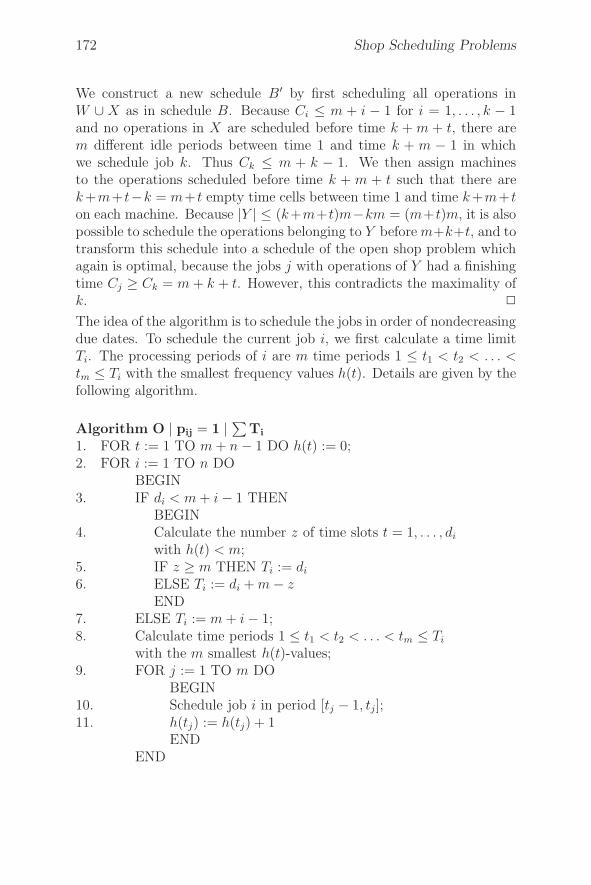
172 Shop Scheduling Problems
We construct a new schedule B′ by first scheduling all operations inW ∪ X as in schedule B. Because Ci ≤ m + i − 1 for i = 1, . . . , k − 1and no operations in X are scheduled before time k + m + t, there arem different idle periods between time 1 and time k + m − 1 in whichwe schedule job k. Thus Ck ≤ m + k − 1. We then assign machinesto the operations scheduled before time k + m + t such that there arek+m+ t−k = m+ t empty time cells between time 1 and time k+m+ ton each machine. Because |Y | ≤ (k+m+t)m−km = (m+t)m, it is alsopossible to schedule the operations belonging to Y before m+k+t, and totransform this schedule into a schedule of the open shop problem whichagain is optimal, because the jobs j with operations of Y had a finishingtime Cj ≥ Ck = m + k + t. However, this contradicts the maximality ofk. �
The idea of the algorithm is to schedule the jobs in order of nondecreasingdue dates. To schedule the current job i, we first calculate a time limitTi. The processing periods of i are m time periods 1 ≤ t1 < t2 < . . . <tm ≤ Ti with the smallest frequency values h(t). Details are given by thefollowing algorithm.
Algorithm O | pij = 1 | ∑Ti
1. FOR t := 1 TO m + n − 1 DO h(t) := 0;2. FOR i := 1 TO n DO
BEGIN3. IF di < m + i − 1 THEN
BEGIN4. Calculate the number z of time slots t = 1, . . . , di
with h(t) < m;5. IF z ≥ m THEN Ti := di
6. ELSE Ti := di + m − zEND
7. ELSE Ti := m + i − 1;8. Calculate time periods 1 ≤ t1 < t2 < . . . < tm ≤ Ti
with the m smallest h(t)-values;9. FOR j := 1 TO m DO
BEGIN10. Schedule job i in period [tj − 1, tj];11. h(tj) := h(tj) + 1
ENDEND
6.2. Open Shop Problems 173
The algorithm can be implemented in such a way that its running time isO(nm). To get an algorithm with this complexity, we schedule the jobssuch that after each step i the following invariance property holds: l1 ≥l2 ≥ . . . ≥ lm exists with l1 ≤ Ti such that on machine Mj (j = 1, . . . , m)all time slots 1, . . . , lj are occupied.
Clearly, the invariance property is initially satisfied with l1 = l2 = . . . =lm = 0. Assume that the invariance property holds after step i−1. Thenwe have Ti−1 ≤ Ti and schedule job i by filling time slots in the followingorder
l1 + 1, . . . , Ti on M1,
l2 + 1, . . . , l1 on M2,...
lm + 1, . . . , lm−1 on Mm.
We still have to prove the correctness of the algorithm.
Theorem 6.7 Algorithm O | pij = 1 | ∑Ti calculates an optimal
schedule for the parallel machine problem corresponding with problemO | pij = 1 | ∑
Ti.
Proof: We use interchange arguments to prove this theorem. Accordingto Lemma 6.5 and Theorem 6.6, an optimal schedule exists with C1 ≤C2 ≤ . . . ≤ Cn and
Ci ≤ m + i − 1 for i = 1, . . . , n. (6.9)
Let B be an optimal schedule satisfying (6.9) with the property that jobs1, . . . , k − 1 are scheduled in the same time slots as in the schedule Aconstructed by Algorithm O | pij = 1 | ∑
Ti. Furthermore, assume thatB is chosen such that k is maximal.
Assume that Ck > Tk. Since job k is scheduled before Tk in A, a timeslot t ≤ Tk exists in which job k is not processed in B. Thus, in B thistime slot is either empty or it is occupied by a job r > k. If this timeslot is empty, we move the operation of k scheduled in time slot Ck tothis time slot. If job r is scheduled at time t but not at time Ck, thenwe switch the operations of jobs k and r. If job r is scheduled at times tand Ck, then either there is an empty slot at Cr + 1 or there must be ajob, say v, which is scheduled at time Cr + 1 but not scheduled at timeCk. This must be possible since r and k are scheduled at time Ck butnot at time Cr + 1.
174 Shop Scheduling Problems
If there is an empty slot at Cr + 1, move job r from time t to Cr + 1 andjob k from time Ck to t. If there is no empty slot at Cr +1, we can mover from t to Cr + 1, k from Ck to t, and v from Cr + 1 to Ck. Since Ck
must improve by at least one unit and Cr increases by at the most oneunit the new schedule is as good as the old one.
If we continue this process, we get an optimal schedule B′ with Ck ≤ Tk
in which jobs 1, . . . , k − 1 are scheduled as in A.
Now let h be the frequency vector for the partial schedule for jobs1, . . . , k−1. Assume that h(t′) < h(t) and job k is scheduled in time slott but not in time slot t′ in B′. If in B′ a machine is idle at time t′, wecan move job k from time slot t to time slot t′. Otherwise a job r > k isscheduled in time slot t′ but not in time slot t. We can move r to t and kto t′ without increasing
∑Ti because Ck ≤ Cr. Continuing in this way,
we reach an optimal schedule in which jobs 1, . . . , k are scheduled as inA. This is a contradiction to the maximality of k. �
Again, the coloring algorithm of Gabow & Kariv [GK82] can be used toprovide an optimal solution for the open shop problem. This shows thatproblem O | pij = 1 | ∑
Ui can be solved in O(nm log2(nm)) time.
6.3 Flow Shop Problems
The flow shop problem is a general shop problem in which
• each job i consists of m operations Oij with processing times pij
(j = 1, . . . , m) where Oij must be processed on machine Mj, and
• there are precedence constraints of the form Oij → Oi,j+1 (i =1, . . . , m − 1) for each i = 1, . . . , n, i.e. each job is first processedon machine 1, then on machine 2, then on machine 3, etc.
Thus, the problem is to find a job order πj for each machine j. We willrestrict our discussion to flow shop problems with Cmax-objective func-tion. All other problems turn out to be NP-hard if we admit arbitraryprocessing times.
6.3.1 Minimizing Makespan
Problem F2 ‖ Cmax is the only flow shop problem with Cmax-criterionwhich is polynomially solvable if the processing times are arbitrary. A

6.3. Flow Shop Problems 175
corresponding algorithm has been developed by Johnson [120].
To find an optimal solution for problem F2 ‖ Cmax we may restrict ourattention to schedules in which the job sequence on both machines is thesame. This is an immediate consequence of the following lemma.
Lemma 6.8 For problem Fm ‖ Cmax an optimal schedule exists withthe following properties:
(i) The job sequence on the first two machines is the same.
(ii) The job sequence on the last two machines is the same.
Proof: The proof of (i) is similar to the proof of Theorem 3.5. The proofof (ii) is symmetric to the proof of (i). �
A flow shop is called a permutation flow shop if solutions are restrictedto job sequences π1, . . . , πm with π1 = π2 = . . . = πm. Lemma 6.8 showsthat for two or three machines the optimal solution of the flow shopproblem is not better than that of the corresponding permutation flowshop. This is not the case if there are more than three machines.
Next we will present Johnson’s algorithm for solving the two-machineflow shop problem. We have to find a permutation
L : L(1), . . . , L(n)
of all jobs such that if all jobs are scheduled in this order on both ma-chines, then the makespan is minimized.
An optimal order is constructed by calculating a left list T : L(1), . . . ,L(t) and a right list R : L(t+1), . . . , L(n), and then concatenating themto obtain L = T ◦R := L(1), . . . , L(n). The lists T and R are constructedstep by step.
At each step we consider an operation Oi∗j∗ with the smallest pi∗j∗-value.If j∗ = 1, then we put job i∗ at the end of list T , i.e. we replace T byT ◦ i∗. Otherwise we put i∗ at the beginning of list R, i.e. we replace Rby i∗ ◦R. Job i∗ and processing times pi∗1 and pi∗2 are then deleted fromconsideration.
Algorithm F2 ‖ Cmax
1. X := {1, . . . , n}; T := φ; R := φ;2. While X �= φ DO
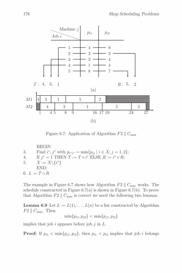
176 Shop Scheduling Problems
��������
Machine j
Job ipi1 pi2
1
2
3
4
5
4
3
3
1
8
8
3
4
4
7
T : 4, 3, 1 R : 5, 2
��� � �
(a)
�M2
M1�
1 4 5 8 9 16 17 19 24 27
4 3 1 5 2
4 3 1 5 2
(b)
Figure 6.7: Application of Algorithm F2 ‖ Cmax
BEGIN3. Find i∗, j∗ with pi∗j∗ = min{pij | i ∈ X; j = 1, 2};4. If j∗ = 1 THEN T := T ◦ i∗ ELSE R := i∗ ◦ R;5. X := X\{i∗}
END;6. L := T ◦ R
The example in Figure 6.7 shows how Algorithm F2 ‖ Cmax works. Theschedule constructed in Figure 6.7(a) is shown in Figure 6.7(b). To provethat Algorithm F2 ‖ Cmax is correct we need the following two lemmas.
Lemma 6.9 Let L := L(1), . . . , L(n) be a list constructed by AlgorithmF2 ‖ Cmax. Then
min{pi1, pj2} < min{pj1, pi2}implies that job i appears before job j in L.
Proof: If pi1 < min{pj1, pi2}, then pi1 < pi2 implies that job i belongs

6.3. Flow Shop Problems 177
M2
M1
· · · i j · · ·· · · i j · · ·
(a)
M2
M1
· · · i j · · ·· · · i j · · ·
(b)
M2
M1
· · · i j · · ·· · · i j · · ·
� �
x(c)
Figure 6.8: Three possible cases if j is scheduled immediately after i.
to T . If j is added to R, we have finished. Otherwise j appears after i inT because pi1 < pj1. If pj2 < min{pj1, pi2}, we argue in a similar way. �
Lemma 6.10 Consider a schedule in which job j is scheduled immedi-ately after job i. Then
min{pj1, pi2} ≤ min{pi1, pj2} (6.10)
implies that i and j can be swapped without increasing the Cmax-value.
Proof: If j is scheduled immediately after i, then we have three possiblecases which are shown in Figure 6.8. Denote by wij the length of thetime period from the start of job i to the finishing time of job j in thissituation. We have
wij = max{pi1 + pj1 + pj2, pi1 + pi2 + pj2, x + pi2 + pj2}= max{pi1 + pj2 + max{pj1, pi2}, x + pi2 + pj2}
Similarly, we have
wji = max{pj1 + pi2 + max{pi1, pj2}, x + pi2 + pj2}
178 Shop Scheduling Problems
if i is scheduled immediately after j.
Now (6.10) implies
max{−pi1,−pj2} ≤ max{−pj1,−pi2}.
Adding pi1 + pi2 + pj1 + pj2 to both sides of this inequality, we get
pj1 + pi2 + max{pi1, pj2} ≤ pi1 + pj2 + max{pj1, pi2},
which implies wji ≤ wij.
Thus, swapping i and j will not increase the Cmax-value. �
Now it is not difficult to prove the correctness of Algorithm F2 ‖ Cmax.
Theorem 6.11 The sequence L : L(1), . . . , L(n) constructed by Algo-rithm F2 ‖ Cmax is optimal.
Proof: Let L be the set of all optimal sequences and assume that L /∈ L.Then we consider a sequence R ∈ L with
L(ν) = R(ν) for ν = 1, . . . , s − 1 and i := L(s) �= R(s) =: j
where s is maximal. Then job i is a (not necessarily immediate) successorof j in R. Let k be a job scheduled between job j and job i or k = j inR. In L, job k is scheduled after job i. Thus, by Lemma 6.9 we musthave
min{pk1, pi2} ≥ min{pi1, pk2} (6.11)
(otherwise job i would follow job k in L).
(6.11) holds for each such job k. Applying Lemma (6.10) to R, we mayswap each immediate predecessor k of job i with i without increasing theobjective value. We finally get a sequence R ∈ L with R(ν) = L(ν) forν = 1, . . . , s which contradicts the maximality of s. �
6.4 Job Shop Problems
The job shop problem is a special case of the general shop problemwhich generalizes the flow shop problem. We are given n jobs i = 1, . . . , nand m machines M1, . . . , Mm. Job i consists of a sequence of ni operations
Oi1, Oi2, . . . , Oini

6.4. Job Shop Problems 179
which must be processed in this order, i.e. we have precedence constraintsof the form Oij → Oi,j+1 (j = 1, . . . , ni − 1). There is a machine μij ∈{M1, . . . , Mm} and a processing time pij associated with each operationOij. Oij must be processed for pij time units on machine μij. Theproblem is to find a feasible schedule which minimizes some objectivefunction depending on the finishing times Ci of the last operations Oi,ni
of the jobs. If not stated differently we assume that μij �= μi,j+1 forj = 1, . . . , ni − 1.
In Sections 6.4.1 and 6.4.2 we will discuss job shop problems which arepolynomially solvable. In Section 6.4.3, a branch-and-bound method forthe general problem J ‖ Cmax will be developed. This method solvesthe famous 10x10 problem given in Muth & Thompson [174] in less than15 minutes. Section 6.4.4 is devoted to heuristics based on iterativeimprovement.
6.4.1 Problems with Two Machines
There are only a few special job shop problems which can be solvedpolynomially or pseudopolynomially.
J2 | ni ≤ 2 | Cmax
This two-machine job shop problem with at the most two operations perjob can be solved by a reduction to the two-machine flow shop problem.To describe this reduction, it is convenient to divide the set of jobs intothe following subsets:
I1 jobs which are processed only on machine 1
I2 jobs which are processed only on machine 2
I1,2 jobs which are processed first on machine 1 and then onmachine 2
I2,1 jobs which are processed first on machine 2 and then onmachine 1
Note that jobs in I1 and I2 consist of only one operation.
To construct an optimal solution for problem J2 | ni ≤ 2 | Cmax we haveto apply the following steps.
1. Calculate an optimal sequence R1,2 for the flow shop problem withjob set I1,2.
180 Shop Scheduling Problems
2. Calculate an optimal sequence R2,1 for the flow shop problem withjob set I2,1.
3. On machine 1 first schedule I1,2 according to R1,2, then all jobs inI1 in an arbitrary order, and, finally, I2,1 according to R2,1.
4. On machine 2 first schedule I2,1 according to R2,1, then all jobs inI2 in an arbitrary order, and, finally, I1,2 according to R1,2.
We may assume that the schedule constructed in this way is active. Thenat least one machine processes the jobs without idle time. More specifi-cally, if ∑
i∈I2,1
pi2 ≤∑
i∈I1,2
pi1 +∑
i∈I1
pi1
then there is no idle time on machine 1. Otherwise there is no idle timeon machine 2.
To prove that the schedule is optimal we assume w.l.o.g. that there is noidle time on machine 1. If there is also no idle time on machine 2 or if
nmaxi=1
Ci =∑
i∈I1,2∪I1∪I2,1
pi1,
then we have finished. Otherwise the solution value is equal to that ofthe problem restricted to I1,2, which is also optimal.
A related problem is
J2 | pij = 1 | Lmax
Given are n jobs i = 1, . . . , n and two machines denoted by A and B.Job i has ni unit time operations Oij, j = 1, . . . , ni. If operation Oij isprocessed on machine A (B), then operation Oi,j+1 must be processed onmachine B (A) (j = 1, . . . , ni − 1). Thus, job i may be characterized bythe number ni of operations and the machine on which the first operation
must be processed. Let r =n∑
i=1
ni be the total number of operations.
Again, assume that zero time is the earliest time an operation can bestarted. Furthermore, let tmax be an upper bound for the latest startingtime of any operation. For example, we may choose tmax = r. Then aschedule may be defined by two arrays A(t) and B(t) (t = 0, . . . , tmax)where A(t) = Oij if operation Oij is to be processed on machine A at
6.4. Job Shop Problems 181
time t and A(t) = φ if machine A is idle during the time period from tto t + 1. We call φ an empty operation. For each operation Oij to beprocessed on machine A, there exists a time t with A(t) = Oij . B(t)is defined similarly. A schedule is feasible if and only if A(t) = Oij
(B(t) = Oij) with 1 < j ≤ ni implies that Oi,j−1 = B(s) (Oi,j−1 = A(s))for some s < t, and the first operation of each job is scheduled on theright machine. A permutation of all operations is called a list. Givena list L, a feasible schedule can be constructed in the following way.Schedule the operations in the order given by L, where each operation isscheduled as early as possible. Such a schedule is called a list schedulecorresponding to L.
The finishing time Ci of job i in a feasible schedule y = (A(t), B(t)) isgiven by
Ci := max{t + 1 | A(t) or B(t) is an operation of job i}.
Given a due date di ≥ 0 associated with each job i, the problem we con-sider in this section is to find a feasible schedule such that the maximumlateness
max{Ci − di | i = 1, . . . , n}is minimized.
The following algorithm solves this problem.
Algorithm 1 J2 | pij = 1 | Lmax
1. Associate with each operation Oij the label l(Oij) = di − ni + j;
2. Construct a list L of all operations ordered according to nonde-creasing l(Oij)-values;
3. Find a list schedule corresponding to L.
This algorithm can be implemented in O(r log r) time. However, we willuse hash techniques (compare Section 4.2, 1 | prec; pj = 1 | Lmax) toderive an O(r)-implementation of this algorithm.
As in Section 4.2, we may assume that di ≥ 0 for i = 1, . . . , n anddi = 0 for at least one job i. Otherwise, replace di by d′
i = di − d whered = min{di | i = 1, . . . , n}.
182 Shop Scheduling Problems
Because Ci ≥ 1 for all i = 1, . . . , n and di = 0 for at least one i, wehave Li = Ci − di ≥ 1 for at least one i. Furthermore, we may assumethat Ci ≤ r. Thus, jobs with di > r − 1, i.e. with Li = Ci − di < 1may be ignored. They do not contribute to the objective function maxLi
because Li ≥ 1 for some i. We may schedule these jobs after all othersin an arbitrary order. For the operations Oij of the remaining jobs wehave
−r + 1 ≤ l(Oij) = di − ni + j ≤ r − 1.
We put each of these operations in a corresponding bucket L(k) wherek = l(Oij) = di − ni + j (−r + 1 ≤ k ≤ r − 1). In a second step, weschedule the operations according to increasing bucket numbers k whereoperations from the same bucket may be scheduled in an arbitrary order.
Details are given by the following algorithm. In this algorithm T1 and T2denote the first period t ≥ 0 where machines A and B, respectively, areidle. LAST (i) denotes the finishing time of the last scheduled operationof job i. Z denotes the set of jobs i with di ≥ r.
Algorithm 2 J2 | pij = 1 | Lmax
1. FOR k := −r + 1 TO r − 1 DO L(k) := φ; Z := φ;2. FOR i := 1 TO n DO3. IF di < r THEN4. FOR j := 1 TO ni DO add Oij to L(di − ni + j)
ELSE5. add job i to Z;6. FOR i := 1 TO n DO LAST (i) := 0;7. T1 := 0; T2 := 0;8. FOR k := −r + 1 TO r − 1 DO9. WHILE L(k) �= φ DO
BEGIN10. Choose a task Oij from L(k);11. L(k) := L(k)\{Oij};12. Schedule Oij
END13.WHILE Z �= φ DO
BEGIN14. Choose job i from Z;15. Z := Z\{i};16. FOR j := 1 TO ni Schedule Oij
END
6.4. Job Shop Problems 183
The module Schedule Oij schedules operation Oij. It may be formulatedas follows.
Scheduled Oij
1. IF μij = A THEN DO2. IF T1 < LAST (i) THEN
BEGIN3. t := LAST (i);4. A(t) := Oij
ENDELSE
BEGIN5. t := T1;6. A(t) := Oij;7. WHILE A(T1) �= φ DO T1 := T1 + 1
ENDELSE {μij = B}
8. IF T2 < LAST (i) THENBEGIN
9. t := LAST (i);10. B(t) := Oij
ENDELSE
BEGIN11. t := T2;12. B(t) := Oij;13. WHILE B(T2) �= φ DO T2 := T2 + 1
END;14. LAST (i) := t + 1
Clearly, the number of steps of Algorithm 2 J2 | pij = 1 | Lmax is boundedby O(r).
To prove that Algorithm 2 J2 | pij = 1 | Lmax is correct we first haveto show that a feasible schedule is constructed. This is true if and onlyif, before setting A(t) := Oij and B(t) := Oij in Steps 4 and 10 of themodule Schedule Oij, we have A(t) = φ and B(t) = φ, respectively.Otherwise two different operations would be scheduled at the same timeon the same machine.
To show feasibility we first prove

184 Shop Scheduling Problems
Lemma 6.12 Let Y = (A(t), B(t)) be a list schedule with B(t) = φ(A(t) = φ). Then for each s > t with B(s) = Oij (A(s) = Oij) we haveA(s − 1) = Oi,j−1 (B(s − 1) = Oi,j−1).
Proof: We show by induction on s that B(s) = Oij, s > t implies A(s−1) = Oi,j−1. This is certainly true for s = t + 1 because if B(t + 1) = Oij
and A(t) does not belong to job i, then B(t) = φ implies that operationOij must be scheduled earlier in the list schedule.
Now, assume that Lemma 6.12 holds for all v with t < v < s and thatB(s) = Oij. Choose a maximal l with t ≤ l < s and B(l) = φ. Bythe induction assumption, A(v − 1) and B(v) belong to the same job forv = l + 1, . . . , s − 1. Suppose that A(s − 1) does not belong to job i.Then for each v ∈ {l, l + 1, . . . , s − 1} operation A(v) does not belongto job i for v = l, . . . , s − 1. Thus Oij can be processed at time l, whichcontradicts the fact that Y is a list schedule. �
Theorem 6.13 Let Oij be the operation scheduled in Step 4 (Step 10)of the module Schedule Oij and assume that t = LAST (i) > T1(T2).Then A(t) = φ (B(t) = φ).
Proof: Assume that A(t) �= φ (B(t) �= φ). Because A(T1) = φ (B(T2) =φ), the previous Lemma implies that A(t) and B(t−1) (B(t) and A(t−1))are operations of the same job k. Because LAST (i) = t, we must havek �= i. This is not possible because LAST (i) = t and μij = A(μij = B)imply that B(t − 1) = Oi,j−1 (A(t − 1) = Oi,j−1). �
Finally, we show that the list schedule constructed by the algorithm isoptimal.
Lemma 6.14 If a schedule exists in which no job is late, then the sched-ule Y = (A(t), B(t)) constructed by Algorithm 2 J2 | pij = 1 | Lmax hasthis property.
Proof: We will show that if there is a late job in the schedule constructedby Algorithm 2 J2 | pij = 1 | Lmax, then there is a late job in eachschedule.
If there is a late job in Y = (A(t), B(t)), then there exists an operationA(t) or B(t) with l(A(t)) < t + 1 or l(B(t)) < t + 1. For example, thisinequality is true for the last operation in a late job. Choose a minimalt with this property and assume that l(A(t)) < t + 1.
6.4. Job Shop Problems 185
Then we will prove that
l(A(v)) ≤ l(A(t)) for v = 1, . . . , t − 1
l(A(0)) ≤ l(A(t)) if A(0) �= φ.(6.12)
Thus, in each schedule at least one late job must exist because A(0) �= φimplies l(A(v)) < t + 1 for v = 0, . . . , t and we must schedule t + 1operations in the time interval [0, t], which is impossible. If, on the otherhand, A(0) = φ, then all jobs start on machine B and t operations mustbe processed in the time interval [1, t], which again is not possible.
To prove (6.12), note that (6.12) is true if A(t) is the first operation of ajob, for if
l(A(t)) < l(A(v)) for some v = 0 . . . , t − 1,
then the algorithm must schedule A(t) before A(v).
Now let
A(t) = Oi,j for some i and j > 1.
Then we have
Oi,j−1 = B(s) with s < t − 1
because s = t − 1 implies l(B(s)) = l(A(t)) − 1 < t = s + 1, whichcontradicts the minimality of t. It follows that
l(A(v)) ≤ l(A(t)) for v = s + 1, . . . , t − 1
because otherwise A(t) must be scheduled earlier. Also
l(A(s)) ≤ l(A(s + 1))
because otherwise A(s + 1) should be scheduled at time s since A(s + 1)and B(s) are operations of different jobs. If s = 0, we have alreadyproved (6.12). Otherwise let A(s) = Oi′,j′. If A(s) is the first operationof a job, we have finished. Otherwise, if
Oi′,j′−1 = B(r) with r < s − 1,
we again have
l(A(v)) ≤ l(A(s)) for v = r, . . . , s − 1.
186 Shop Scheduling Problems
If, however, Oi′,j′−1 = B(s − 1), then we let r ≤ s − 1 be the smallestinteger with the property that B(v) and A(v+1) are successive operationsof the same job for v = r, . . . , s − 1. A(s + 1) does not belong to job iand we again have l(A(v)) ≤ l(A(s + 1)) for v = r, . . . , s. If r = 0, wehave finished. If r > 0, we continue in the same way. �
Theorem 6.15 A schedule constructed by Algorithm 2 J2 | pij = 1 |Lmax is optimal.
Proof: Let l be the maximum lateness of an optimal schedule. Then
nmaxi=1
L(i) =n
maxi=1
{Ci − di} ≤ l,
which is equivalent to
nmaxi=1
{Ci − (di + l)} ≤ 0.
Due to Lemma 6.14, Algorithm 2 J2 | pij = 1 | Lmax applied to theproblem with due dates di + l yields an optimal schedule for the originalproblem. Furthermore, this schedule is the same as the schedule we getby applying Algorithm 2 J2 | pij = 1 | Lmax to the due dates di. �
Note that the algorithm, although fast, is not polynomial if we encodethe problem by the numbers ni and, for each job i, the machine numberon which the first operation of job i has to be processed. It is only apseudopolynomial algorithm. Timkovsky [199] and Kubiak et al. [130]presented algorithms which are polynomial even for this encoding for thespecial case with Cmax objective function. The following more generalresult has been derived by Timkovsky [199]: J2 | pij = 1 | Lmax (andsymmetrically J2 | pij = 1; ri | Cmax) can be solved in O(n2) time. ThatJ2 | pij = 1 | ∑
Ci can be solved in O(n logn) time has been shown byKubiak & Timkovsky [131]. An O(n6)-algorithm for J2 | pij = 1
∑Ui is
due to Kravchenko [126]. The problems J2 | pij = 1; ri |∑
Ci, J2 | pij =1 | ∑
wiCi, and J2 | pij = 1 | ∑Ti are NP-hard.
6.4.2 Problems with Two Jobs. A Geometric Ap-
proach
Job shop problems with two jobs can be solved polynomially even withobjective functions f(C1, C2) which are regular, i.e. monotone nonde-creasing functions of the finishing times C1 and C2 of both jobs. These
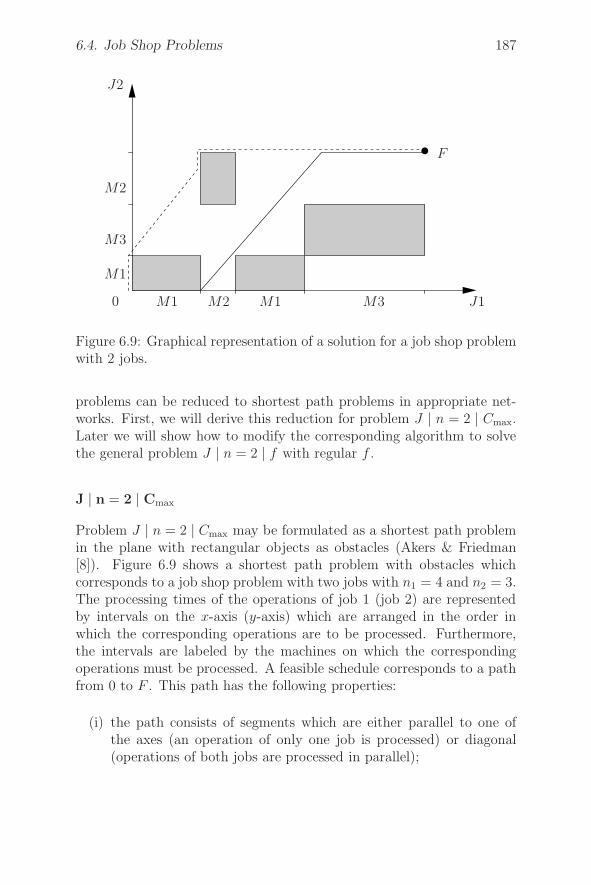
6.4. Job Shop Problems 187
F
J1M3M1M2M10
M1
M3
M2
J2
Figure 6.9: Graphical representation of a solution for a job shop problemwith 2 jobs.
problems can be reduced to shortest path problems in appropriate net-works. First, we will derive this reduction for problem J | n = 2 | Cmax.Later we will show how to modify the corresponding algorithm to solvethe general problem J | n = 2 | f with regular f .
J | n = 2 | Cmax
Problem J | n = 2 | Cmax may be formulated as a shortest path problemin the plane with rectangular objects as obstacles (Akers & Friedman[8]). Figure 6.9 shows a shortest path problem with obstacles whichcorresponds to a job shop problem with two jobs with n1 = 4 and n2 = 3.The processing times of the operations of job 1 (job 2) are representedby intervals on the x-axis (y-axis) which are arranged in the order inwhich the corresponding operations are to be processed. Furthermore,the intervals are labeled by the machines on which the correspondingoperations must be processed. A feasible schedule corresponds to a pathfrom 0 to F . This path has the following properties:
(i) the path consists of segments which are either parallel to one ofthe axes (an operation of only one job is processed) or diagonal(operations of both jobs are processed in parallel);
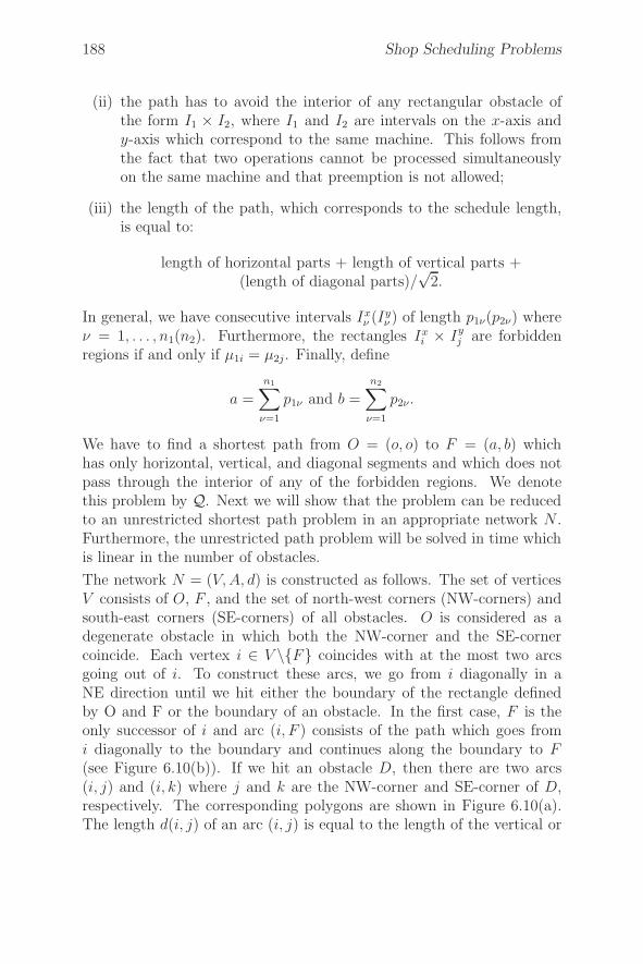
188 Shop Scheduling Problems
(ii) the path has to avoid the interior of any rectangular obstacle ofthe form I1 × I2, where I1 and I2 are intervals on the x-axis andy-axis which correspond to the same machine. This follows fromthe fact that two operations cannot be processed simultaneouslyon the same machine and that preemption is not allowed;
(iii) the length of the path, which corresponds to the schedule length,is equal to:
length of horizontal parts + length of vertical parts +(length of diagonal parts)/
√2.
In general, we have consecutive intervals Ixν (Iy
ν ) of length p1ν(p2ν) whereν = 1, . . . , n1(n2). Furthermore, the rectangles Ix
i × Iyj are forbidden
regions if and only if μ1i = μ2j. Finally, define
a =
n1∑
ν=1
p1ν and b =
n2∑
ν=1
p2ν .
We have to find a shortest path from O = (o, o) to F = (a, b) whichhas only horizontal, vertical, and diagonal segments and which does notpass through the interior of any of the forbidden regions. We denotethis problem by Q. Next we will show that the problem can be reducedto an unrestricted shortest path problem in an appropriate network N .Furthermore, the unrestricted path problem will be solved in time whichis linear in the number of obstacles.
The network N = (V, A, d) is constructed as follows. The set of verticesV consists of O, F , and the set of north-west corners (NW-corners) andsouth-east corners (SE-corners) of all obstacles. O is considered as adegenerate obstacle in which both the NW-corner and the SE-cornercoincide. Each vertex i ∈ V \{F} coincides with at the most two arcsgoing out of i. To construct these arcs, we go from i diagonally in aNE direction until we hit either the boundary of the rectangle definedby O and F or the boundary of an obstacle. In the first case, F is theonly successor of i and arc (i, F ) consists of the path which goes fromi diagonally to the boundary and continues along the boundary to F(see Figure 6.10(b)). If we hit an obstacle D, then there are two arcs(i, j) and (i, k) where j and k are the NW-corner and SE-corner of D,respectively. The corresponding polygons are shown in Figure 6.10(a).The length d(i, j) of an arc (i, j) is equal to the length of the vertical or
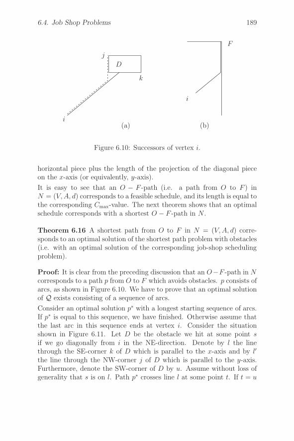
6.4. Job Shop Problems 189
D
i
j
k
F
i
(a) (b)
Figure 6.10: Successors of vertex i.
horizontal piece plus the length of the projection of the diagonal pieceon the x-axis (or equivalently, y-axis).
It is easy to see that an O − F -path (i.e. a path from O to F ) inN = (V, A, d) corresponds to a feasible schedule, and its length is equal tothe corresponding Cmax-value. The next theorem shows that an optimalschedule corresponds with a shortest O − F -path in N .
Theorem 6.16 A shortest path from O to F in N = (V, A, d) corre-sponds to an optimal solution of the shortest path problem with obstacles(i.e. with an optimal solution of the corresponding job-shop schedulingproblem).
Proof: It is clear from the preceding discussion that an O−F -path in Ncorresponds to a path p from O to F which avoids obstacles. p consists ofarcs, as shown in Figure 6.10. We have to prove that an optimal solutionof Q exists consisting of a sequence of arcs.
Consider an optimal solution p∗ with a longest starting sequence of arcs.If p∗ is equal to this sequence, we have finished. Otherwise assume thatthe last arc in this sequence ends at vertex i. Consider the situationshown in Figure 6.11. Let D be the obstacle we hit at some point sif we go diagonally from i in the NE-direction. Denote by l the linethrough the SE-corner k of D which is parallel to the x-axis and by l′
the line through the NW-corner j of D which is parallel to the y-axis.Furthermore, denote the SW-corner of D by u. Assume without loss ofgenerality that s is on l. Path p∗ crosses line l at some point t. If t = u

190 Shop Scheduling Problems
D
j
il′
u s k t l
Figure 6.11: Proof of Theorem 6.16.
and p∗ continues to k or if t is between u and k or t = k, then we mayreplace the part of p∗ going from i to k by arc i, s, k without increasingthe length of p∗. If t is to the right of k, then we may replace the part ofp∗ between i and t by i, s, k, t without increasing the length of p∗. In bothcases we get an optimal path with a longer beginning sequence of arcswhich contradicts the maximality assumption. Finally, if t is to the leftof u, then p∗ crosses l′ at some point t′ above u and a similar argument(but now using t′ and l′) leads to a contradiction. �
To find a shortest path from O to F in the network N = (V, A, d), wefirst order the forbidden regions according to the lexicographic order oftheir NW-corners (i.e. Di < Dj if for the corresponding NW-corners(xi, yi) and (xj , yj) we have yi < yj or yi = yj, xi < xj).
Assume that we have r forbidden regions and that they are indexed suchthat
D1 < D2 < . . . < Dr.
Then the following algorithm calculates the length d∗ of a shortest pathfrom O to F .
Algorithm J | n = 2 | Cmax
1. FOR ALL vertices i ∈ V DO d(i) := ∞;2. FOR ALL successors j of O DO d(j) := d(O, j);3. FOR i := 1 TO r DO
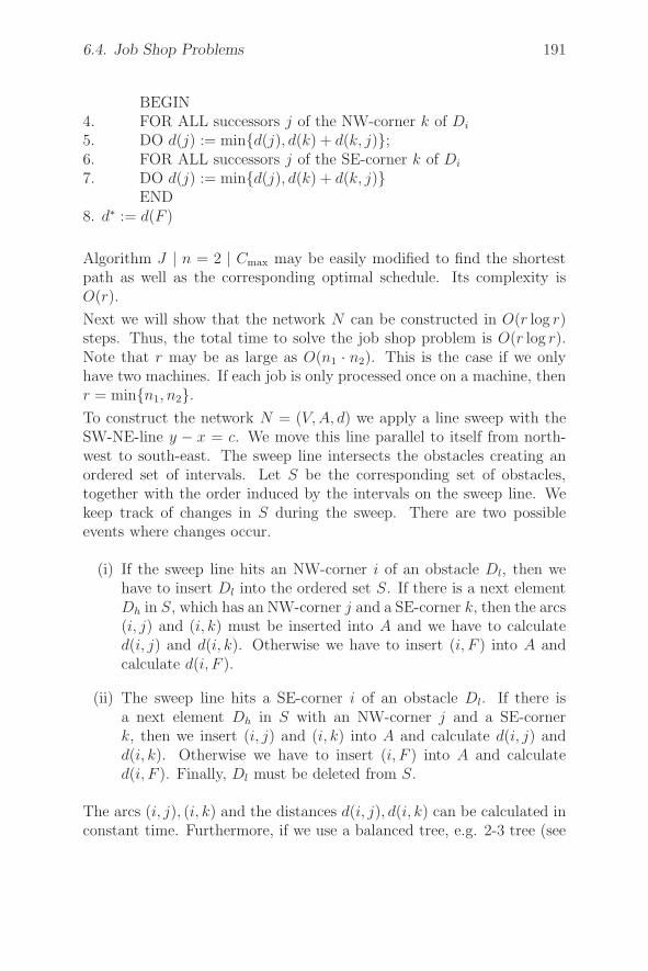
6.4. Job Shop Problems 191
BEGIN4. FOR ALL successors j of the NW-corner k of Di
5. DO d(j) := min{d(j), d(k) + d(k, j)};6. FOR ALL successors j of the SE-corner k of Di
7. DO d(j) := min{d(j), d(k) + d(k, j)}END
8. d∗ := d(F )
Algorithm J | n = 2 | Cmax may be easily modified to find the shortestpath as well as the corresponding optimal schedule. Its complexity isO(r).
Next we will show that the network N can be constructed in O(r log r)steps. Thus, the total time to solve the job shop problem is O(r log r).Note that r may be as large as O(n1 · n2). This is the case if we onlyhave two machines. If each job is only processed once on a machine, thenr = min{n1, n2}.To construct the network N = (V, A, d) we apply a line sweep with theSW-NE-line y − x = c. We move this line parallel to itself from north-west to south-east. The sweep line intersects the obstacles creating anordered set of intervals. Let S be the corresponding set of obstacles,together with the order induced by the intervals on the sweep line. Wekeep track of changes in S during the sweep. There are two possibleevents where changes occur.
(i) If the sweep line hits an NW-corner i of an obstacle Dl, then wehave to insert Dl into the ordered set S. If there is a next elementDh in S, which has an NW-corner j and a SE-corner k, then the arcs(i, j) and (i, k) must be inserted into A and we have to calculated(i, j) and d(i, k). Otherwise we have to insert (i, F ) into A andcalculate d(i, F ).
(ii) The sweep line hits a SE-corner i of an obstacle Dl. If there isa next element Dh in S with an NW-corner j and a SE-cornerk, then we insert (i, j) and (i, k) into A and calculate d(i, j) andd(i, k). Otherwise we have to insert (i, F ) into A and calculated(i, F ). Finally, Dl must be deleted from S.
The arcs (i, j), (i, k) and the distances d(i, j), d(i, k) can be calculated inconstant time. Furthermore, if we use a balanced tree, e.g. 2-3 tree (see
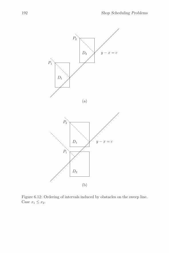
192 Shop Scheduling Problems
P1
P2
D1
D2 y − x = c
(a)
P2
P1
D2
D1 y − x = c
(b)
Figure 6.12: Ordering of intervals induced by obstacles on the sweep line.Case x1 ≤ x2.
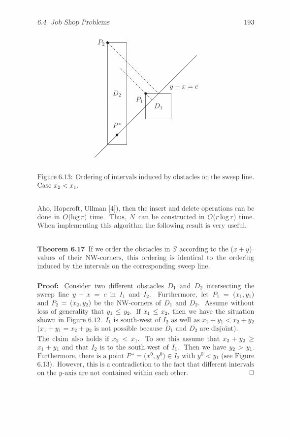
6.4. Job Shop Problems 193
P1
P2
P ∗
D1
D2
y − x = c
Figure 6.13: Ordering of intervals induced by obstacles on the sweep line.Case x2 < x1.
Aho, Hopcroft, Ullman [4]), then the insert and delete operations can bedone in O(log r) time. Thus, N can be constructed in O(r log r) time.When implementing this algorithm the following result is very useful.
Theorem 6.17 If we order the obstacles in S according to the (x + y)-values of their NW-corners, this ordering is identical to the orderinginduced by the intervals on the corresponding sweep line.
Proof: Consider two different obstacles D1 and D2 intersecting thesweep line y − x = c in I1 and I2. Furthermore, let P1 = (x1, y1)and P2 = (x2, y2) be the NW-corners of D1 and D2. Assume withoutloss of generality that y1 ≤ y2. If x1 ≤ x2, then we have the situationshown in Figure 6.12. I1 is south-west of I2 as well as x1 + y1 < x2 + y2
(x1 + y1 = x2 + y2 is not possible because D1 and D2 are disjoint).
The claim also holds if x2 < x1. To see this assume that x2 + y2 ≥x1 + y1 and that I2 is to the south-west of I1. Then we have y2 > y1.Furthermore, there is a point P ∗ = (x0, y0) ∈ I2 with y0 < y1 (see Figure6.13). However, this is a contradiction to the fact that different intervalson the y-axis are not contained within each other. �
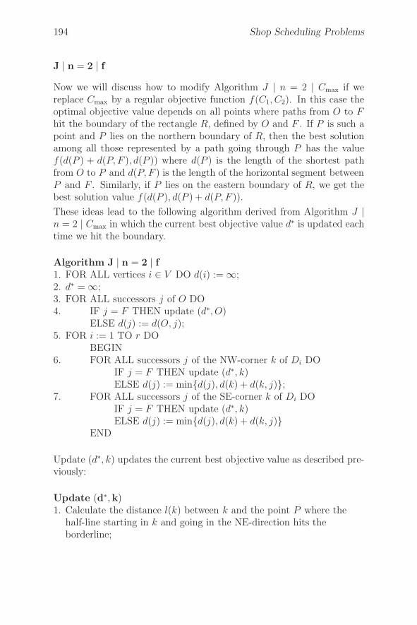
194 Shop Scheduling Problems
J | n = 2 | fNow we will discuss how to modify Algorithm J | n = 2 | Cmax if wereplace Cmax by a regular objective function f(C1, C2). In this case theoptimal objective value depends on all points where paths from O to Fhit the boundary of the rectangle R, defined by O and F . If P is such apoint and P lies on the northern boundary of R, then the best solutionamong all those represented by a path going through P has the valuef(d(P ) + d(P, F ), d(P )) where d(P ) is the length of the shortest pathfrom O to P and d(P, F ) is the length of the horizontal segment betweenP and F . Similarly, if P lies on the eastern boundary of R, we get thebest solution value f(d(P ), d(P ) + d(P, F )).
These ideas lead to the following algorithm derived from Algorithm J |n = 2 | Cmax in which the current best objective value d∗ is updated eachtime we hit the boundary.
Algorithm J | n = 2 | f1. FOR ALL vertices i ∈ V DO d(i) := ∞;2. d∗ = ∞;3. FOR ALL successors j of O DO4. IF j = F THEN update (d∗, O)
ELSE d(j) := d(O, j);5. FOR i := 1 TO r DO
BEGIN6. FOR ALL successors j of the NW-corner k of Di DO
IF j = F THEN update (d∗, k)ELSE d(j) := min{d(j), d(k) + d(k, j)};
7. FOR ALL successors j of the SE-corner k of Di DOIF j = F THEN update (d∗, k)ELSE d(j) := min{d(j), d(k) + d(k, j)}
END
Update (d∗, k) updates the current best objective value as described pre-viously:
Update (d∗,k)1. Calculate the distance l(k) between k and the point P where the
half-line starting in k and going in the NE-direction hits theborderline;

6.4. Job Shop Problems 195
i
j
v(a)
i
j
v(b)
Figure 6.14: Successors of vertex v if preemption is allowed.
2. IF P lies on the northern borderline THENd∗ := min{d∗, f(d(k) + d(k, F ), d(k) + l(k))}
ELSE {P lies on the eastern borderline}d∗ := min{d∗, f(d(k) + l(k), d(k) + d(k, F ))}
If the function f(C1, C2) can be evaluated in constant time, this algorithmhas the same complexity as the previous one.
Preemptive job shop problems with two jobs can be solved similarly.
J | n = 2;pmtn | fIf preemption is allowed in the previous problem, then we may go hor-izontally or vertically through obstacles. For this reason, the networkN = (V, A, d) must be defined differently.
The vertex set is defined recursively by
(i) O is a vertex.
(ii) If v is a vertex and the half-line starting from v and going in aNE-direction hits an obstacle, then v has the two successors i andj shown in Figure 6.14(a) or (b).
(iii) If v is a vertex and the half-line starting from v and going in aNE-direction hits the borderline given by the rectangle defined byO and F , then F is the only successor of v.
We denote the modified network by N .
196 Shop Scheduling Problems
Arcs (i, j) and arc lengths d(i, j) are defined as before. If in AlgorithmJ | n = 2 | f the “NW-corner” and “SE-corner” are replaced by “northboundary point” and “east boundary point”, respectively, this modifiedalgorithm applied to N solves problem J | n = 2; pmtn | f . The runningtime of this modified algorithm is bounded by O(n3
max) where nmax =max{n1, n2}. This can be seen as follows.
Consider for each SE-corner or NW-corner v, which can be reached fromO, the unique path starting from v which avoids the boundaries of theobstacles it hits. If such a path hits the SW-corner t of an obstacle (ora boundary point t′ of the rectangle R, defined by O and F ), this pathterminates in t (or in F ). There are at most O(n1, n2) of these paths andeach has at the most n1 +n2 arcs. Furthermore, the set of all these pathscovers all arcs going through the interior of obstacles. Thus, the totalnumber of arcs which go through the interior of obstacles is bounded byO(n3
max). Because the number of arcs not going through the interior ofobstacles is bounded by O(n1n2) and the total computation time of theshortest path algorithm is proportional to the number of all arcs, we havean O(n3
max)-algorithm.
Finally, we remark that all of the geometric methods also work if we dropthe assumption that μij �= μi,j+1 for all i and j = 1, . . . , ni − 1.
6.4.3 Job Shop Problems with Two Machines
In the previous section we showed that job shop problems with two jobsare polynomially solvable. Sotskov & Shakhlevich [190] showed that theproblems J3 | n = 3 | Cmax and J3 | n = 3 | ∑
Ci are NP-hard.Also J2 ‖ Cmax is NP-hard (Lenstra & Rinnooy Kan [153]). Thus,the complexity of the job shop problem with two machines and a fixednumber k of jobs remains open. In this section we will show that problemJ2 | n = k | Cmax is polynomially solvable even if machine repetition isallowed, i.e. if μij = μi,j+1 is possible for jobs i.
We first show that J2 | n = k | Cmax can be reduced to a shortest path
problem in an acyclic network with O(rk) vertices where r =n
maxi=1
ni.
Then we show that this network can be constructed in O(r2k) steps,providing an overall complexity of O(r2k). Finally, we present a sim-ple O(r4)-algorithm for problem J2 | n = 3 | Cmax with no machinerepetition.
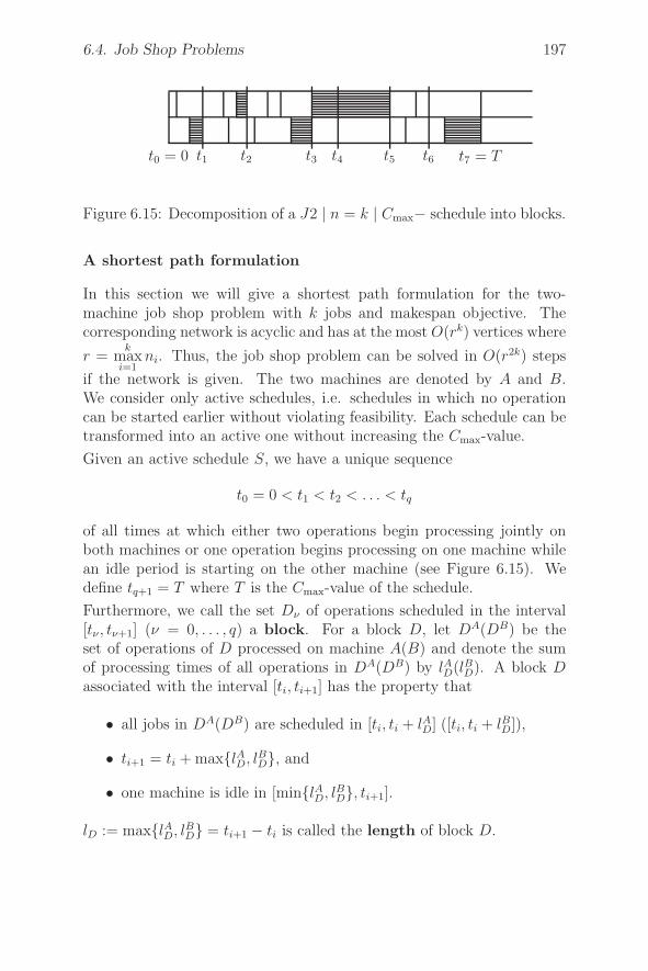
6.4. Job Shop Problems 197
t0 = 0 t1 t2 t3 t4 t5 t6 t7 = T
Figure 6.15: Decomposition of a J2 | n = k | Cmax− schedule into blocks.
A shortest path formulation
In this section we will give a shortest path formulation for the two-machine job shop problem with k jobs and makespan objective. Thecorresponding network is acyclic and has at the most O(rk) vertices where
r =k
maxi=1
ni. Thus, the job shop problem can be solved in O(r2k) steps
if the network is given. The two machines are denoted by A and B.We consider only active schedules, i.e. schedules in which no operationcan be started earlier without violating feasibility. Each schedule can betransformed into an active one without increasing the Cmax-value.
Given an active schedule S, we have a unique sequence
t0 = 0 < t1 < t2 < . . . < tq
of all times at which either two operations begin processing jointly onboth machines or one operation begins processing on one machine whilean idle period is starting on the other machine (see Figure 6.15). Wedefine tq+1 = T where T is the Cmax-value of the schedule.
Furthermore, we call the set Dν of operations scheduled in the interval[tν , tν+1] (ν = 0, . . . , q) a block. For a block D, let DA(DB) be theset of operations of D processed on machine A(B) and denote the sumof processing times of all operations in DA(DB) by lAD(lBD). A block Dassociated with the interval [ti, ti+1] has the property that
• all jobs in DA(DB) are scheduled in [ti, ti + lAD] ([ti, ti + lBD]),
• ti+1 = ti + max{lAD, lBD}, and
• one machine is idle in [min{lAD, lBD}, ti+1].
lD := max{lAD, lBD} = ti+1 − ti is called the length of block D.

198 Shop Scheduling Problems
It follows that a schedule is defined by a sequence of blocks and theschedule length is the sum of the lengths of all blocks in that sequence.To formulate problem J2 | n = k | Cmax as a shortest path problem insome network N = (V, A, l), we characterize blocks in a different way.For each job i, let jν(i) be the index of the last operation Oi,jν(i) whichis processed before tν and define jν := (jν(i))
ki=1. Then Dν is defined by
jν and jν+1. Generally, blocks can be described by pairs (j,h) of indextuples j = (j(i)), h = (h(i)) with 0 ≤ j(i) ≤ h(i) ≤ ni for i = 1, . . . , k.However, not all pairs of index tuples (j,h) define blocks.
The network N = (V, A, l) is defined by
• the set V of all index tuples j = (j(i)) with 0 ≤ j(i) ≤ ni fori = 1, . . . , k. The vertex s = j with j(i) = 0 for all i = 1, . . . , kis called the initial vertex. The vertex t = j, with j(i) = ni fori = 1, . . . , k, is called the terminal vertex,
• (u,v) ∈ A if and only if u < v and the set of operations
{Oi,j(i) | i = 1, . . . , k; u(i) < j(i) ≤ v(i)}defines a block, and
• for each (u,v) ∈ A, its length l(u,v) is the length of the blockcorresponding to (u,v).
In N , each s− t-path p corresponds to a feasible schedule and the lengthof p is equal to the makespan of this schedule. We obtain this scheduleby scheduling the blocks corresponding to the arcs in p consecutively asshown in Figure 6.15. Furthermore, there is an s− t-path correspondingto an optimal schedule. Thus, to solve the job shop problem we have tofind a shortest s− t-path in N .
It remains to show that the network can be constructed in polynomialtime. This is the case if, for each vertex u ∈ V , all successors of ucanbe calculated in polynomial time. In the next section we will derive analgorithm which does this in O(rk) time for each vertex. Thus, the totaltime needed to construct the network is O(r2k).
Constructing the network N
In this section we will present an O(rk) algorithm which, for a givenvertex u, finds all arcs (u,v) which define a block. W.l.o.g. let u = swhere s is the starting vertex defined in the previous section.
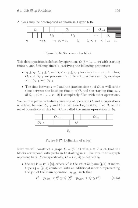
6.4. Job Shop Problems 199
A block may be decomposed as shown in Figure 6.16.
s1 s2 t1 s3 s4 = t2 t3 t4 sr−1 sr tr−1 tr
O1
O2
O3
O4
· · ·· · ·
Or−1
Or
Figure 6.16: Structure of a block.
This decomposition is defined by operations Oi(i = 1, . . . , r) with startingtimes si and finishing times ti satisfying the following properties:
• s1 ≤ s2, tr−1 ≤ tr and si < ti−1 ≤ si+1 for i = 2, 3, . . . , r−1. Thus,Oi and Oi+1 are processed on different machines and Oi overlapswith Oi−1 and Oi+1.
• The time between t = 0 and the starting time s2 of O2 as well as thetime between the finishing time ti of Oi and the starting time si+2
of Oi+2 (i = 1, . . . , r− 2) is completely filled with other operations.
We call the partial schedule consisting of operation Oi and all operationsscheduled between Oi−2 and Oi a bar (see Figure 6.17). Let Bi be theset of operations in this bar. Oi is called the main operation of Bi.
Oi−2
Oi−1
Oi
Oi+1
Bi
� �
Figure 6.17: Definition of a bar.
Next we will construct a graph G = (V , A) with s ∈ V such that theblocks correspond with paths in G starting in s. The arcs in this graphrepresent bars. More specifically, G = (V , A) is defined by
• the set V = V ′∪{s}, where V ′ is the set of all pairs (j, h) of index-tupels j = (j(i)) combined with an additional index h representingthe job of the main operation Oh,j(h) such that
tAj − ph,j(h) < tBj ≤ tAj (tBj − ph,j(h) < tAj ≤ tBj ) (6.13)
200 Shop Scheduling Problems
if Oh,j(h) is processed on machine A(B). Here tAj (tBj ) is the sumof the processing times of all operations Oij (i = 1, . . . , k; j =1, . . . , j(i)) which are processed on machine A(B). If tAj − ph,j(h) =0 (tBj − ph,j(h) = 0), the strict inequality in condition (6.13) isreplaced by “≤”,
• (u, v) with u = (u, h), v = (v, l) ∈ V ′ is an arc if and only if (u, v)defines a bar, and
• (s, v) with v = (v, l) ∈ V ′ is an arc if and only if
v(j) =
{1if j = l
0otherwise
for some job index l.
To construct all blocks, we have to find all paths in G starting from s.Because G is acyclic and has at the most O(rk) vertices, this can bedone in O(r2k) time. However, the complexity can be reduced by addinga single operation in each step of the search process. There are at themost k operations which can be added. Thus, the total complexity isO(krk) = O(rk) because k is fixed.
Problem J2 | n = 3 | Cmax with no machine repetition
In this section we will show that a simple O(r4)-algorithm for problemJ2 | n = 3 | Cmax with no machine repetition can be easily derived usingthe concepts introduced previously.
As before, we denote the two machines by A and B. Furthermore, assumethat the three jobs denoted by 1,2,3 have operations Oij where i = 1, 2, 3and j = 1, . . . , ni. pij is the processing time of operations Oij, whichmust be processed on machine μij. We assume that
μij �= μi,j+1 for i = 1, 2, 3 and j = 1, . . . , ni − 1.
We use the algorithm presented in the previous section to solve thisproblem. However, due to the fact that machine repetition is not allowed,blocks containing at least two operations have a special structure whichmay be characterized by the following two properties (see Figure 6.18):

6.4. Job Shop Problems 201
. . .j i k j
i k j k
Figure 6.18: Block structure for J2 | n = 3 | Cmax.
(a) With the exception of a first and a last operation, each operationin the block overlaps exactly two other operations.
(b) The job indices are repeated periodically, i.e. the operations or-dered according to increasing starting times yield a sequence
Oir, Ojs, Okt, Oi,r+1, Oj,s+1, Ok,t+1, Oi,r+2, . . .
These properties follow from the fact that if two operations O and Pof jobs i and j with finishing times t1 and t2, respectively, overlap andt1 < t2, then the first operation Q of job k scheduled at time t1 or laterin the same block must be processed starting at time t1. Furthermore,the block ends at time t2 if the processing time of Q is not larger thant2 − t1.
However, it is also possible that a block consists of exactly one operation.
For a block B there are at the most three one-element blocks which maybe a successor of B. In a successor block of B containing more thanone operation, two operations begin at the same time. Given these twooperations, there is a unique maximal block satisfying conditions (a) and(b) and this maximal block can be constructed in O(r) time. Each initialpart of this maximal block may be a successor of B. Due to the fact thatthere are only these two possibilities to start a successor block of B, itfollows that block B has at the most O(r) successors and these successorscan be constructed in O(r) time.
This implies that the network has at the most O(r4) arcs and can beconstructed in O(r4) time. Thus, we have an O(r4)-algorithm to solveJ2 | n = 3 | Cmax.
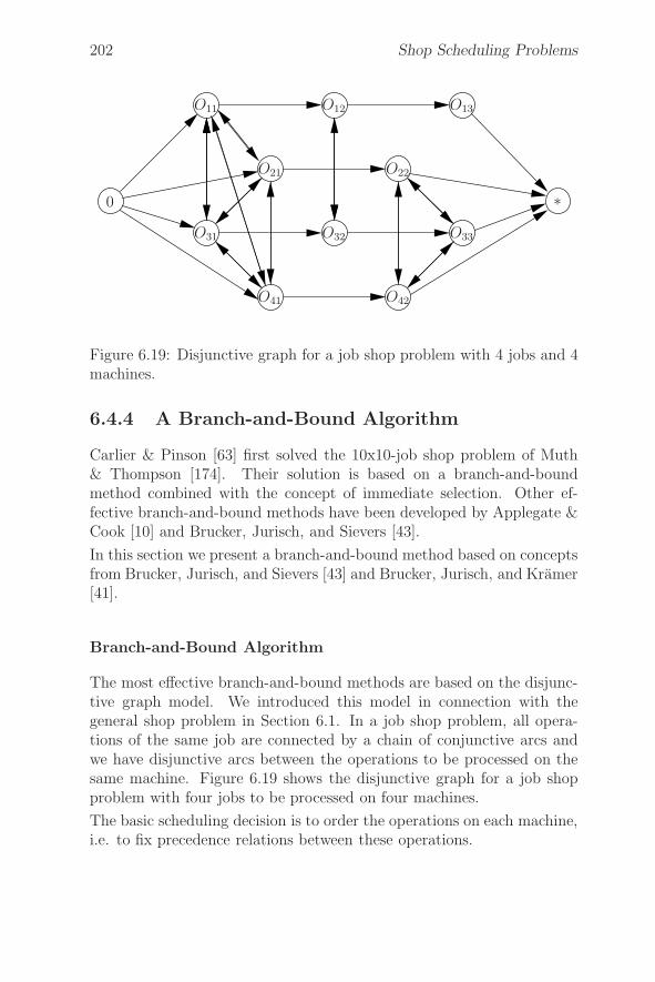
202 Shop Scheduling Problems
O41 O42
O31 O32 O33
0 ∗O21 O22
O11 O12 O13
Figure 6.19: Disjunctive graph for a job shop problem with 4 jobs and 4machines.
6.4.4 A Branch-and-Bound Algorithm
Carlier & Pinson [63] first solved the 10x10-job shop problem of Muth& Thompson [174]. Their solution is based on a branch-and-boundmethod combined with the concept of immediate selection. Other ef-fective branch-and-bound methods have been developed by Applegate &Cook [10] and Brucker, Jurisch, and Sievers [43].
In this section we present a branch-and-bound method based on conceptsfrom Brucker, Jurisch, and Sievers [43] and Brucker, Jurisch, and Kramer[41].
Branch-and-Bound Algorithm
The most effective branch-and-bound methods are based on the disjunc-tive graph model. We introduced this model in connection with thegeneral shop problem in Section 6.1. In a job shop problem, all opera-tions of the same job are connected by a chain of conjunctive arcs andwe have disjunctive arcs between the operations to be processed on thesame machine. Figure 6.19 shows the disjunctive graph for a job shopproblem with four jobs to be processed on four machines.
The basic scheduling decision is to order the operations on each machine,i.e. to fix precedence relations between these operations.
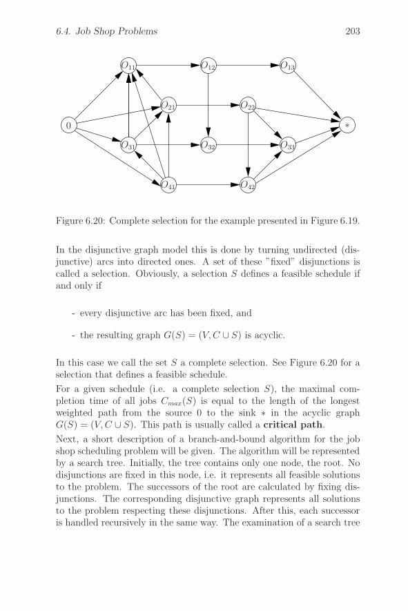
6.4. Job Shop Problems 203
O41 O42
O31 O32 O33
0 ∗O21 O22
O11 O12 O13
Figure 6.20: Complete selection for the example presented in Figure 6.19.
In the disjunctive graph model this is done by turning undirected (dis-junctive) arcs into directed ones. A set of these ”fixed” disjunctions iscalled a selection. Obviously, a selection S defines a feasible schedule ifand only if
- every disjunctive arc has been fixed, and
- the resulting graph G(S) = (V, C ∪ S) is acyclic.
In this case we call the set S a complete selection. See Figure 6.20 for aselection that defines a feasible schedule.
For a given schedule (i.e. a complete selection S), the maximal com-pletion time of all jobs Cmax(S) is equal to the length of the longestweighted path from the source 0 to the sink ∗ in the acyclic graphG(S) = (V, C ∪ S). This path is usually called a critical path.
Next, a short description of a branch-and-bound algorithm for the jobshop scheduling problem will be given. The algorithm will be representedby a search tree. Initially, the tree contains only one node, the root. Nodisjunctions are fixed in this node, i.e. it represents all feasible solutionsto the problem. The successors of the root are calculated by fixing dis-junctions. The corresponding disjunctive graph represents all solutionsto the problem respecting these disjunctions. After this, each successoris handled recursively in the same way. The examination of a search tree
204 Shop Scheduling Problems
node stops if it represents only one solution (i.e. the set S of fixed dis-junctive arcs is a complete selection), or it can be shown that the nodedoes not contain an optimal solution.
More precisely: A search tree node r corresponds to a graph G(Fr) =(V, C ∪ Fr). Fr denotes the set of fixed disjunctive arcs in node r. Thenode represents all solutions Y (r) respecting the partial order given byFr. Branching is done by dividing Y (r) into disjoint subsets Y (s1), ...,Y (sq). Each Y (si) is the solution set of a problem with a graph G(Fsi
) =(V, C ∪ Fsi
) where Fr ⊂ Fsi, which means that G(Fsi
) is derived fromG(Fr) by fixing additional disjunctions. This branching creates immedi-ate successors s1, ..., sq of node r in the branching tree which are treatedrecursively. For each node r, a value LB(r), bounding from below theobjective values of all solutions in Y (r), is calculated. We set LB(r) = ∞if the corresponding graph G(Fr) has a cycle. Furthermore, we have anupper bound UB for the solution value of the original problem. UB isupdated whenever a new feasible solution is found which improves UB.
The following recursive procedure describes a branch-and-bound schemebased on depth-first search. Initially, we set UB = ∞ and Fr = ∅.
PROCEDURE Branch-and-Bound (r)1. Calculate a solution S ∈ Y (r) using heuristics;2. IF Cmax(S) < UB THEN UB := Cmax(S);3. WHILE there is a successor s of r which has not yet been examined
DO4. IF LB(s) < UB THEN Branch-and-Bound (s)
To specify the branch-and-bound procedure in more detail we have to
(a) introduce a branching scheme, and
(b) discuss methods for calculating bounds.
The next sections are devoted to these issues.
A branching scheme
The branching scheme presented here is based on an approach used byGrabowski et al. [107] in connection with single-machine scheduling with
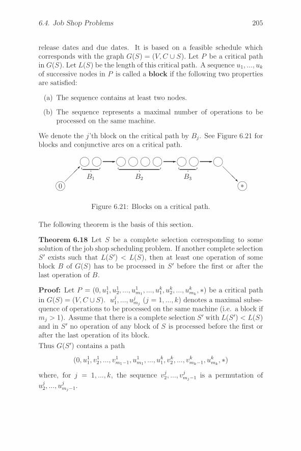
6.4. Job Shop Problems 205
release dates and due dates. It is based on a feasible schedule whichcorresponds with the graph G(S) = (V, C ∪ S). Let P be a critical pathin G(S). Let L(S) be the length of this critical path. A sequence u1, ..., uk
of successive nodes in P is called a block if the following two propertiesare satisfied:
(a) The sequence contains at least two nodes.
(b) The sequence represents a maximal number of operations to beprocessed on the same machine.
We denote the j’th block on the critical path by Bj . See Figure 6.21 forblocks and conjunctive arcs on a critical path.
�0
� � � � � � � � �
�∗���� �
���
� � ��
B1
�
B2
�
B3
Figure 6.21: Blocks on a critical path.
The following theorem is the basis of this section.
Theorem 6.18 Let S be a complete selection corresponding to somesolution of the job shop scheduling problem. If another complete selectionS ′ exists such that L(S ′) < L(S), then at least one operation of someblock B of G(S) has to be processed in S ′ before the first or after thelast operation of B.
Proof: Let P = (0, u11, u
12, ..., u
1m1
, ..., uk1, u
k2, ..., u
kmk
, ∗) be a critical path
in G(S) = (V, C ∪ S). uj1, ..., u
jmj
(j = 1, ..., k) denotes a maximal subse-quence of operations to be processed on the same machine (i.e. a block ifmj > 1). Assume that there is a complete selection S ′ with L(S ′) < L(S)and in S ′ no operation of any block of S is processed before the first orafter the last operation of its block.
Thus G(S ′) contains a path
(0, u11, v
12, ..., v
1m1−1, u
1m1
, ..., uk1, v
k2 , ..., v
kmk−1, u
kmk
, ∗)where, for j = 1, ..., k, the sequence vj
2, ..., vjmj−1 is a permutation of
uj2, ..., u
jmj−1.
206 Shop Scheduling Problems
The length of the critical path in G(S ′) is not less than the length of thispath. We have:
L(S ′)≥k∑
j=1
(
puj1+
mj−1∑
i=2
pvji+ puj
mj
)
=k∑
j=1
(
puj1+
mj−1∑
i=2
puji+ puj
mj
)
=L(S)
which is a contradiction. �
The following fact is an immediate consequence of the previous theorem:
If there are two complete selections S, S ′ with L(S ′) < L(S), then atleast one of the two conditions (i) or (ii) holds.
(i) At least one operation of one block B in G(S), different from thefirst operation in B, has to be processed before all other operationsof B in the schedule defined by G(S ′).
(ii) At least one operation of one block B in G(S), different from thelast operation in B, has to be processed after all other operationsof B in the schedule defined by G(S ′).
Now consider a node r of the search tree and a solution y ∈ Yr. Usuallyy is calculated using some heuristic. Let S be the complete selectioncorresponding to y. A critical path in G(S) defines blocks B1, ..., Bk. Forblock Bj : uj
1, ..., ujmj
, the jobs in
EBj := Bj \ {uj
1} and EAj := Bj \ {uj
mj}
are called before-candidates and after-candidates.
At least one of the candidates must be moved in order to improve S.
Furthermore, we define the arc-sets
Fj := {uj1 −→ | = uj
2, ..., ujmj}
Lj := { −→ ujmj
| = uj1, ..., u
jmj−1}
for j = 1, ..., k and consider a permutation
R1, R2, ..., R2k (6.14)
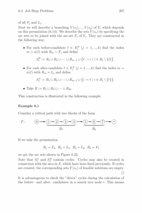
6.4. Job Shop Problems 207
of all Fj and Lj.
Next we will describe a branching Y (s1), ..., Y (sq) of Yr which dependson this permutation (6.14). We describe the sets Y (sν) by specifying thearc sets to be joined with the arc-set Fr of Yr. They are constructed inthe following way:
• For each before-candidate ∈ EBj (j = 1, ..., k) find the index
m = α( ) with Rm = Fj and define
SB� := R1 ∪ R2 ∪ · · · ∪ Rm−1 ∪
{ → i | i ∈ Bj \ { }
}.
• For each after-candidate ∈ EAj (j = 1, ..., k) find the index m =
α( ) with Rm = Lj and define
SA� := R1 ∪ R2 ∪ · · · ∪ Rm−1 ∪
{i → | i ∈ Bj \ { }
}.
• Take R := R1 ∪ R2 ∪ · · · ∪ R2k.
This construction is illustrated in the following example.
Example 6.1
Consider a critical path with two blocks of the form.
P : �0 �1 �2 �3 �4 �5 �6 �7 �∗� � �� � � � ��
B1
�
B2
If we take the permutation
R1 = F2, R2 = L1, R3 = L2, R4 = F1
we get the arc sets shown in Figure 6.22.
Note that SA5 and SB
4 contain cycles. Cycles may also be created inconnection with the arcs in Fr which have been fixed previously. If cyclesare created, the corresponding sets Y (sν) of feasible solutions are empty.
�It is advantageous to check the ”direct” cycles during the calculation ofthe before– and after– candidates in a search tree node r. This means
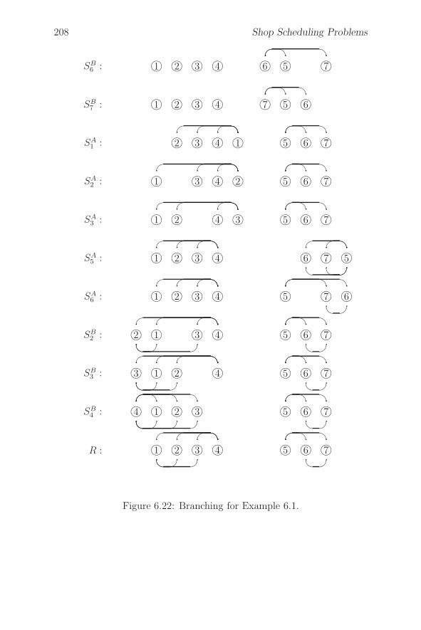
208 Shop Scheduling Problems
SB6 : �1 �2 �3 �4 �6 �5 �7
� �� �
SB7 : �1 �2 �3 �4 �7 �5 �6
� �� �
SA1 : �2 �3 �4 �1 �5 �6 �7
� � � �� � � �� �
SA2 : �1 �3 �4 �2 �5 �6 �7
� � � �� � � �� �
SA3 : �1 �2 �4 �3 �5 �6 �7
� � � �� �� �� �
SA5 : �1 �2 �3 �4 �6 �7 �5
� � � �
� �
� � � �
� �
� �
SA6 : �1 �2 �3 �4 �5 �7 �6
� �
� �
� � � �� � � �
SB2 : �2 �1 �3 �4 �5 �6 �7
� � � �
� � � �
� �� �
� �
� �
SB3 : �3 �1 �2 �4 �5 �6 �7
� �
� � � �
� � � �
� �
� �� �
SB4 : �4 �1 �2 �3 �5 �6 �7
� � � �
� � � �
� � � �
� �
� �
� �
R : �1 �2 �3 �4 �5 �6 �7
� � � �
� � � �
� � � �
� �
� �
Figure 6.22: Branching for Example 6.1.
6.4. Job Shop Problems 209
that for the block B� : u�1, ..., u
�m�
if a disjunctive arc i → j (i, j ∈ B�) isalready fixed in the actual search tree node, then operation j (operation i)is not inserted into the set EB
� (EA� ). The cycles in the preceding example
can be eliminated by this method. A complete cycle-check is done duringthe computation of heads and tails which will be introduced in the nextsection.
The resulting solution sets created by this branching rule are pairwisedisjoint. This can be seen as follows. If we have two sets SB
� and SB�′ with
, ′ ∈ EBj , then ( , ′) ∈ SB
� and ( ′, ) ∈ SB�′ . Thus, the corresponding
sets Y (sν) have an empty intersection. The same reasoning applies ifwe have sets SA
� and SA�′ with , ′ ∈ EA
j . Note that these two casesare characterized by the fact that α( ) = α( ′). If, on the other hand, wehave two sets Sν
� and Sν′�′ with α( ) < α( ′), then if is a before-candidate
(after-candidate) in the block Bj , we have −→ uj1 (uj
mj−→ ) in Sν
�
but uj1 −→ ( −→ uj
mj) in Sν′
�′ .
By Theorem 6.18, solutions associated with R do not improve the solutionS. Thus, the corresponding successor node of r will not be considered.
We have not yet specified how to choose the permutation R1, ..., R2k
of the sets Fj and Lj (j = 1, ..., k). The objective is to fix a largenumber of disjunctive arcs as early as possible. Hence we arrange thesets Fj and Lj (j = 1, ..., k) according to nonincreasing cardinalities ofthe corresponding blocks. Additionally, we always take the set Lj as adirect successor of the set Fj . More precisely, we choose
R2i−1 := Fπ(i), R2i := Lπ(i) (i = 1, ..., k)
where π is a permutation of 1, ..., k such that |Bπ(i)| ≥ |Bπ(j)| if i < j.
Now it is possible to formulate a branch-and-bound procedure based onthe branching rule introduced in this section.
PROCEDURE Branch-and-Bound (r)1. Calculate a solution S ∈ Y (r) using heuristics;2. IF Cmax(S) < UB THEN UB := Cmax(S);3. Calculate a critical path P ;4. Calculate the blocks of P ;5. Calculate the sets EB
j and EAj ;
6. WHILE an operation i ∈ Eνj exists with j = 1, ..., k and
ν = A, B DOBEGIN
210 Shop Scheduling Problems
7. Delete i from Eνj ;
8. Fix disjunctions for the corresponding successor s;9. Calculate a lower bound LB(s) for node s;10. IF LB(s) < UB THEN Branch-and-Bound (s)
END
Note that the handling of a node s terminates if
• the lower bound LB(s) is greater than or equal to the best solutionvalue (this is the case if the corresponding disjunctive graph hascycles, i.e. LB(s) = ∞) or
• the critical path of the heuristic solution calculated for S does notcontain any blocks or
• the sets EBj and EA
j are empty for all blocks Bj .
We did not specify in which order the operations i ∈ Eνj are chosen, i.e.
the order of the successors of a search tree node r. The following ruleseems to be promising. Sort the candidates according to nondecreasingheads of before-candidates and tails of after-candidates and deal withthe successors of a search tree node in this order. Heads and tails areexplained below.
Heads and tails
With each operation i we may associate a head and a tail. Heads andtails are important for lower bound calculations. They are also used inheuristics.
A head ri of operation i is a lower bound for an earliest possible startingtime of i.
A tail qi of operation i is a lower bound for the time period between thefinishing time of operation i and the optimal makespan.
Calculations of heads and tails are based on all conjunctive arcs and thefixed disjunctive arcs. Thus, they depend on the specific search tree noder.
A simple way to get heads ri for operation i would be to calculate thelength of the longest weighted path from 0 to i in the disjunctive graphG = (V, C ∪ Fr). Similarly, for each i the tail qi could be calculated asthe length of the longest weighted path from i to ∗ in G = (V, C ∪ Fr).
6.4. Job Shop Problems 211
A more sophisticated method for calculating heads is as follows.
If P (i) is the set of disjunctive predecessors of operation i in a searchtree node, the value
maxJ⊆P (i)
{
minj∈J
rj +∑
j∈J
pj
}
defines a lower bound for the earliest possible starting time of operationi. Using the head of the conjunctive predecessor h(i) of i, we get thelower bound rh(i) + ph(i). Using these formulas, we may define the headri of an operation i recursively:
r0 :=0;
ri :=max
{
rh(i) + ph(i); maxJ⊆P (i)
{
minj∈J
rj +∑
j∈J
pj
}}
The same ideas lead to a formula for the tails qi of all operations:
q∗ :=0;
qi :=max
{
pk(i) + qk(i); maxJ⊆S(i)
{∑
j∈J
pj + minj∈J
qj
}}
Here k(i) is the conjunctive successor of i, and S(i) denotes the set ofdisjunctive successors of i.
The calculation of heads can be combined with a cycle-check. We callan operation a labeled operation if its head is calculated. Furthermore,we keep a set D of all operations which can be labeled next, i.e. allunlabeled operations with the property that all their predecessors arelabeled. Initially, D = {0}. If we label an operation i ∈ D, then i iseliminated from D and all successors of i are checked for possible insertioninto D. The procedure continues until D is empty. The disjunctive graphG = (V, C ∪F ) contains a cycle if and only if no head has been assignedto the dummy operation ∗ by this procedure. It is not difficult to provethis property which is a consequence of the special structure of G.
In the following sections we will see how to use heads and tails in differentparts of the branch-and-bound algorithm.
212 Shop Scheduling Problems
Immediate Selection
One of the objectives of the introduced branching scheme was to addlarge numbers of fixed disjunctions to the set Fr when going from noder to its successors. A fast increase of the sets of fixed disjunctions isessential for the quality of a branch-and-bound algorithm because
• more successors s of r contain cycles in the disjunctive graph andneed not be inspected ,
• generally, the value of the lower bound increases because more fixeddisjunctive arcs have to be respected, and
• if we have the additional information that j succeeds i in a solutionwhich improves a current upper bound, then a heuristic will notlook for schedules where j is processed before i. Therefore, such aheuristic generally calculates better solutions.
In this section we will present a method due to Carlier and Pinson [63]which fixes additional disjunctive arcs between jobs belonging to a setof operations to be processed on the same machine. The method, calledimmediate selection, is independent of the branching process. It usesan upper bound UB for the optimal makespan and simple lower bounds.From now on we assume that I is the set of all operations to be processedon a given machine. Furthermore, let n be the number of elements in I.
Let J ⊂ I and c ∈ I\J . If condition
minj∈J∪{c}
rj +∑
j∈J∪{c}pj + min
j∈Jqj ≥ UB (6.15)
holds, then all operations j ∈ J must be processed before operation c ifwe want to improve the current upper bound UB. This follows from thefact that the left-hand side of (6.15) is a lower bound for all schedulesin which c does not succeed all jobs in J . Due to integrality, (6.15) isequivalent to
minj∈J∪{c}
rj +∑
j∈J∪{c}pj + min
j∈Jqj > UB − 1
ormin
j∈J∪{c}rj +
∑
j∈J∪{c}pj > max
j∈Jdj (6.16)
6.4. Job Shop Problems 213
where dj := UB − qj − 1.
(J, c) is called a primal pair if (6.15) or, equivalently, (6.16) holds. Thecorresponding arcs j → c with j ∈ J are called primal arcs. Similarly,(c, J) is called a dual pair and arcs c → j are called dual arcs if
minj∈J
rj +∑
j∈J∪{c}pj > max
j∈J∪{c}dj (6.17)
holds. In this case all operations j ∈ J must be processed after operationc if we want to improve the current solution value UB.
If J is a one-element set, then (6.15) may be replaced by the weakercondition
rc + pc + pj + qj ≥ UB (6.18)
which is equivalent topc + pj > dj − rc. (6.19)
If these conditions hold, then we can fix the disjunction j → c. Thecorresponding arc is called a direct arc.
In (6.16), (6.17), and (6.19) the dj-values may be interpreted as deadlines.Next we will present an algorithm for fixing all primal and dual arcs inO(n2) time. This algorithm is based on a method for improving headsand due dates.
Improving Heads and Deadlines
In this section we consider the problem of finding a feasible schedule fora set I of n operations with processing times pk, heads rk, and deadlinesdk to be scheduled on one machine.
We assume that the corresponding problem with preemption has a fea-sible solution. Such a solution can be found by calculating Jackson’sPreemptive Schedule (JPS) (Carlier [62]). JPS is calculated from leftto right by applying the following rule: At each time t, which is givenby a head or a completion time of an operation, schedule an unfinishedoperation i with ri ≤ t and di = min{dj|rj ≤ t; j is not finished}. Figure6.23(a) shows an example for JPS. Note that the starting and restartingtimes of the operations are always integer if rk, pk are integer. Thereis a dual version of JPS which calculates a schedule from right to leftapplying the following dual rule: At each time t, which is given by adeadline or a starting time of an operation, schedule backwards a not
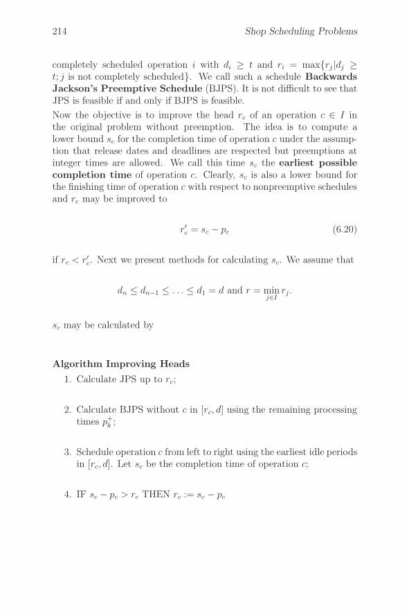
214 Shop Scheduling Problems
completely scheduled operation i with di ≥ t and ri = max{rj |dj ≥t; j is not completely scheduled}. We call such a schedule BackwardsJackson’s Preemptive Schedule (BJPS). It is not difficult to see thatJPS is feasible if and only if BJPS is feasible.
Now the objective is to improve the head rc of an operation c ∈ I inthe original problem without preemption. The idea is to compute alower bound sc for the completion time of operation c under the assump-tion that release dates and deadlines are respected but preemptions atinteger times are allowed. We call this time sc the earliest possiblecompletion time of operation c. Clearly, sc is also a lower bound forthe finishing time of operation c with respect to nonpreemptive schedulesand rc may be improved to
r′c = sc − pc (6.20)
if rc < r′c. Next we present methods for calculating sc. We assume that
dn ≤ dn−1 ≤ . . . ≤ d1 = d and r = minj∈I
rj .
sc may be calculated by
Algorithm Improving Heads
1. Calculate JPS up to rc;
2. Calculate BJPS without c in [rc, d] using the remaining processingtimes p+
k ;
3. Schedule operation c from left to right using the earliest idle periodsin [rc, d]. Let sc be the completion time of operation c;
4. IF sc − pc > rc THEN rc := sc − pc

6.4. Job Shop Problems 215
i 1 2 3 4 5
ri 117 7 3 5
pi 4 2 3 5 3
di2019151210
�1 4 5 4 3 1 20 1 3 5 8 11 14 1617 19
(a)
Step 1: �1 4 50 1 7
�r3
p+1 = 2, p+
2 = 2, p+4 = 3, p+
5 = 1
Step 2: �1 4 5 4 5 4 1 2 10 7 10 12 1617 1920
Step 3: �3 30 14
�s3
(b)
�1 4 5 5 4 2 10 10 12 15 1920
(c)
Figure 6.23: Calculation of earliest completion times rc.
Figure 6.23(b) shows the results of the three steps of this algorithm ap-plied to c = 3.
216 Shop Scheduling Problems
Theorem 6.19 (i) The schedule S calculated by Algorithm Improv-ing Heads is feasible.
(ii) Algorithm Improving Heads provides a lower bound for the com-pletion time of operation c under the assumption that preemptionat integer times is allowed.
Proof:
(i) We only need to consider the interval [rc, d].By assumption JPS is feasible. Thus, we have a feasible preemptiveschedule in [rc, d] for the processing times p+
k and BJPS providessuch a feasible schedule even if c is included. Let f denote thecompletion time of operation c in this BJPS. Then sc ≤ f ≤ dc andthus operation c also respects its release time and deadlines in S.
(ii) We use simple exchange arguments.Assume that a feasible schedule exists in which the finishing timef1 of c is smaller than sc. Among all such schedules consider oneS1 coinciding with S as long as possible, i.e. S and S1 coincide on[r, t] with t maximal. Due to the fact that we have to consider onlyschedules with preemptions on integer times, such a t exists and isinteger. Suppose t < rc. If no operation in S is scheduled in [t, t+1],then no operation can be scheduled in [t, t + 1] in S1, contradictingmaximality of t. Now assume that in S operation j is scheduledin [t, t + 1] and in S1 operation k �= j is scheduled in [t, t + 1].Then a time unit [t′, t′ + 1], t′ > t exists in which j is scheduledin S1. Since dj ≤ dk, operations j and k may be exchanged inS1. f1 does not change because t < rc implies k �= c and j �= c.This again contradicts the maximality of t. Similarly, we have acontradiction if in S1 no operation is scheduled in [t, t + 1]. HenceS1 and S coincide at least in [r, rc]. With the same argument itcan be shown that a schedule S2 exists coinciding with S at leaston [r, rc] ∪ [sc, d] in which the finishing time f2 of c is smaller thansc. Now the total remaining processing time of all operations to bescheduled in [rc, sc] is exactly sc − rc because S has this property.Only operation c may be scheduled in [sc − 1, sc]. So it must bescheduled in [sc − 1, sc] which contradicts the fact that f2 < sc.
�
6.4. Job Shop Problems 217
The calculation of the earliest possible completion time sc for a givenoperation c ∈ I can be simplified due to the following ideas.
To apply Step 3 of Algorithm Improving Heads we only need to knowthe idle periods which are generated by BJPS in Step 2 of the algorithm.These idle periods can also be calculated using the following modifiedStep 2.
2. Starting from time d, schedule backwards in an order of nonin-creasing deadlines the operations j ∈ I\{c} with processing timesp+
j without preemption.
It is easy to see that this algorithm generates the same idle periods asBJPS. Figure 6.23(c) shows the resulting schedule after applying themodified Step 2.
The deadlines can be improved (decreased) in a similar way. The cor-responding procedures are symmetric to those derived for the releasetimes.
Fixing all Primal and Dual Arcs
The following simple procedure fixes all direct arcs associated with theset I of n jobs in O(n2) time.
Procedure Select1. FOR ALL c, j ∈ I, c �= j DO2. IF pc + pj > dj − rc THEN3. fix direct arc j → c;
Next we will prove that Procedure Select calculates all primal and dualpairs associated with I if we replace the rj-values and dj-values by themodified rj-values and dj-values, respectively (see previous section).
Let r′i and d′i denote the release date and deadlines of operation i that
are improved by the procedure given in the last section (note that r′i ≥ ri
and d′i ≤ di for i = 1, . . . , n).
We get the following
Theorem 6.20 Let I be a set of operations to be processed on onemachine with release dates ri, deadlines di, modified release dates r′i, andmodified deadlines d′
i for i = 1, . . . , n.
218 Shop Scheduling Problems
(a) For each primal pair (J, c) with J ⊂ I, c ∈ I\J we have
r′c + pc + pj > dj ≥ d′j
for all j ∈ J .
(b) For each dual pair (c, J) with J ⊂ I, c ∈ I\J we have
r′j + pj + pc ≥ rj + pj + pc > d′c
for all j ∈ J .
(a) means that we can calculate all disjunctive arcs associated with primalarcs using Procedure Select with modified release dates r′i (i = 1, . . . , n).The corresponding result for dual pairs is given by (b).
Proof: We will only prove (a). (b) can be proved similarly. Let (J, c) bea primal pair, i.e.
minj∈J∪{c}
rj +∑
j∈J∪{c}pj > max
j∈Jdj.
This implies that in all feasible preemptive schedules parts of c have tobe processed after max
j∈Jdj .
In the last section we calculated a feasible preemptive schedule in whichoperation c finished as early as possible. We thereby obtained an earliestpossible finishing time sc for operation c and the modified release dater′c = sc−pc. By the arguments given above, we have sc > dj for all j ∈ Jand
dj − r′c= dj − (sc − pc)
= (dj − sc) + pc
< pc
< pc + pj .
�
Combining the results of this section and the last section we get an O(n2)-procedure for fixing all primal arcs and dual arcs for a set I of n jobs tobe processed on the same machine. The time bound can be reduced toO(max{n log n, d}) (see Brucker et al. [41]) where d denotes the numberof arcs to be fixed by the algorithm.
6.4. Job Shop Problems 219
Application of Immediate Selection
The calculation of all disjunctive arcs by immediate selection is under-taken before the computation of a heuristic solution. One may proceedas follows:
(1) Calculation of all primal arcs for all machines.
(2) Calculation of new heads and deadlines.
(3) Calculation of all dual arcs for all machines.
(4) Calculation of new heads and deadlines.
In (1) and (3) we improve heads and deadlines, respectively, and applyProcedure Select. The computation of new heads and deadlines in steps(2) and (4) is undertaken because the additional arcs influence the headsand deadlines of all operations. Steps (1) to (4) are repeated as long asnew disjunctive arcs are fixed.
Calculation of Lower Bounds
Let r be a search tree node with a set Fr of fixed disjunctive arcs. Basedon the arcs in Fr, a head ri and a tail qi is given for each operation i. Alower bound LB(s) is calculated for each successor s of r. If this valueexceeds or is equal to the actual upper bound UB, then an inspection ofs is not necessary.
Different methods for calculating lower bounds have been tested. Thebest strategy was to compute different lower bounds at different placesof the algorithm:
(1) Lower bound calculation during the computation of the sets EB� and
EA� : If operation i should be moved before block B, all disjunctive
arcs{i → j : j ∈ B \ {i}} are fixed. Thus the value
ri + pi + max
⎧⎨
⎩max
j∈B\{i}(pj + qj);
∑
j∈B\{i}pj + min
j∈B\{i}qj
⎫⎬
⎭
220 Shop Scheduling Problems
is a simple lower bound for the search tree node s. Similarly, thevalue
max
⎧⎨
⎩max
j∈B\{i}(rj + pj); min
j∈B\{i}rj +
∑
j∈B\{i}pj
⎫⎬
⎭+ pi + qi
is a lower bound for the node s if i should be moved after block B.
(2) Lower bound calculation during the computation of heads and tails:If the value ri + pi + qi of an operation i exceeds the actual upperbound, the node need not be inspected. Also the head r∗ of thesink and the tail q0 of the source of the disjunctive graph are usedas lower bounds for all solutions in the search tree node s.
(3) Lower bound calculation after the computation of heads and tails:The Jackson Preemptive Schedule is calculated for each machine.The maximal makespan of these schedules gives a lower bound forthe search tree node s.
Note that the value of the lower bound LB(s) may increase if additionaldisjunctions are fixed. Thus, it is advantageous to check LB(s) each timeadditional disjunctive arcs are fixed.
The calculation of all these lower bounds is advantageous because ev-ery time a lower bound exceeds or is equal to an upper bound, a time-consuming part of the algorithm (e.g. the computation of heads and tailsor the fixation of disjunctions) is no longer necessary.
Calculation of heuristic solutions
The branching scheme we used was based on a heuristic solution of theproblem.
In connection with the 10×10-problem, a priority dispatching rule basedheuristic gave the best result (see Jurisch & Sievers [43]). The heuristicsuccessively calculates the operation to be scheduled next. This is donein the following way:
• Calculate the set C of all operations which can be scheduled next,i.e. C is the set of operations c with the property that all prede-cessors of c are already scheduled. Initially, C contains the source0 of the disjunctive graph.
6.4. Job Shop Problems 221
• Let u ∈ C be the operation with minimal value ru+pu, i.e. ru+pu =minc∈C
{rc+pc}. Let Mk be the machine which has to process operation
u. We define the set C by
C := {s ∈ C | rs < ru + pu; s has to be processed on Mk}.
• For each operation c ∈ C we calculate a lower bound for themakespan of the schedule if we schedule c next. We choose theoperation c ∈ C with minimal lower bound to be scheduled next.
• The set C is updated by inspecting all successors s of c. If allpredecessors of s have already been scheduled, we set C = C ∪{s}.After this, c is deleted from C and we start again.
Different methods to calculate lower bounds for the operations c ∈ Chave been tested. The bound which gave the best results was calculatedas follows.
Let T be the set of operations on machine Mk that are not yet scheduled(note that C is a subset of T ). Take as a lower bound the solution valueof Jackson’s Preemptive Schedule for the set T assuming that c has tobe scheduled first.
6.4.5 Applying Tabu-Search to the Job Shop Prob-
lem
In this section we will describe how the Algorithm Tabu-Search presentedin Section 3.4.1 can be implemented for the job shop problem. Firstly,several neighborhoods will be discussed. These neighborhoods can alsobe used in connection with other local search methods. Then, followingDell’Amico & Trubian [75], we will describe the organization of the tabu-list and the aspiration criterion to be used. For a more detailed discussionof the application of simulated annealing and tabu-search to the job shopscheduling problem we refer to Van Laarhoven et al. [206] and Dell’Amico& Trubian [75].
All processing times pij considered in this section are assumed to bepositive.
222 Shop Scheduling Problems
Neighborhood Structures
The quality of local search heuristics strongly depends on the neighbor-hood used. In this section we will define neighborhoods that yield goodresults for simulated annealing and tabu-search methods. Again we usedisjunctive graphs G = (V, C, D) for representing job shop schedulingproblems. Thus, solutions can be represented by complete selections. Acomplete selection S induces the acyclic graph G(S) = (V, C ∪ S).
The following Lemma motivates the first neighborhood N1.
Lemma 6.21 Let S be a complete selection and let p be a longest pathin G(S). Let (v, w) be an arc of p such that v and w are processed onthe same machine. Then S ′ derived from S by reversing (v, w) is againa complete selection.
Proof: We have to show that G(S ′) is acyclic. If G(S ′) is cyclic, then(w, v) must be belong to a cycle c because G(S) has no cycles. (v, w) doesnot belong to c. Thus, c contains at least three vertices. Furthermore,v and w are the only vertices which belong to both c and p. If we nowreplace the arc (v, w) in p by the subpath of c going from v to w, we havein G(S) a path which is longer than p. This contradicts the fact that pis a longest path in G(S). �
For a complete selection S we now denote by N1(S) the set of all completeselections derived from S by reversing an arc (v, w) on a critical path inG(S), where v and w are to be processed on the same machine. Thus,the moves corresponding to N1 are reversals of certain critical arcs.
A neighborhood N is called opt-connected if, from each solution S,some optimal solution can be reached by a finite sequence of moves, i.e.there exists a sequence of complete selections S0, S1, . . . , Sk with S0 = S,Sk is optimal, and Si+1 ∈ N(Si) for i = 0, 1, . . . , k − 1.
Connectivity is a desired property for local search methods, such as sim-ulated annealing and tabu-search. In connection with simulated anneal-ing and tabu-search, connected neighborhoods generally provide betterresults.
Theorem 6.22 N1 is opt-connected.
Proof: We have to show that we can get from an arbitrary completeselection S to an optimal selection by a finite sequence of moves. This is
6.4. Job Shop Problems 223
accomplished by the following procedure which is guided by an arbitrarybut given optimal selection Sopt.
1. i = 0; Si := S;2. WHILE Si is not optimal DO
BEGIN3. Find (v, w) ∈ Si on a critical path in G(Si) such that
(v, w) does not belong to Sopt;4. Si+1 := (Si\{(v, w)}) ∪ {(w, v)};5. i := i + 1
END
In Step 3 of this procedure we can always find an arc (v, w) on a criticalpath with respect to Si which does not belong to Sopt. Otherwise allarcs on a critical path in G(Si) belong to Sopt which implies Cmax(Si) ≤Cmax(Sopt) and Si must be optimal, too. Thus the procedure must reachSopt after a finite number of steps unless some Si �= Sopt is optimal. �
A disadvantage of N1 is that for all (v, w) on a critical path where v and wbelong to the same block and neither v is the first operation in the blocknor w is the last operation in the block, the move which corresponds to(v, w) does not improve the Cmax-value. Thus, generally several movesare necessary to improve the objective value. To decrease this number ofmoves, N1 can be extended in the following way.
Let (v, w) be on a critical path with respect to S, where v and w are tobe processed on the same machine, and denote by PM(v) (SM(w)) theimmediate disjunctive predecessor (successor) of v(w), if it exists. Insteadof the reversal of (v, w), we consider as moves all possible permutations of{PM(v), v, w} and {v, w, SM(w)} in which arc (v, w) is inverted. Denotethis neighborhood by N2. Then we clearly have N1(S) ⊆ N2(S) for allcomplete selections S. Thus, N2 is also opt-connected.
Another alternative would be to consider the neighborhood N3 definedby all moves shifting an operation of some block at the beginning or theend of the block. Such moves are not defined if the resulting selections arenot complete, i.e. contain cycles. Unfortunately, it is an open questionwhether N3 is opt-connected.
N3 can be extended to a neighborhood N4 which is opt-connected bydefining neighbors S ′ of S in the following way.
Let p be a critical path in G(S). Then S ′ is derived from S by movingone operation of a block B of p, which is different from the first (last)
224 Shop Scheduling Problems
operation j in B, before (after) all other operations in B if the resultingselection is feasible. Otherwise j is moved to the position inside block Bclosest to the first (last) position of B such that the resulting schedule isfeasible. Note that N3(S) ⊆ N4(S) for all complete selections S.
Theorem 6.23 N4 is opt-connected.
Proof: Let Sopt be an optimal solution and, for an arbitrary complete se-lection S, denote by n(S) the number of disjunctive arcs fixed in differentdirections in S and Sopt.
If S is not optimal, then according to Theorem 6.18 a block B exists ina critical path of S such that at least one operation j in B is processedbefore or after all other operations of B in Sopt. Assume w.l.o.g. thatj has to be processed before all other operations of B. Then we movej to the position closest to the beginning of B such that the resultingschedule S ′ is feasible. This is one of the moves in N4. Note that dueto Lemma 6.21 it is always possible to move j to the position of itsimmediate predecessor in B. Furthermore, n(S ′) < n(S). �
Organization of the Tabu-List
The main components of a tabu-search algorithm are memory structures,in order to have a trace of the evolution of the search, and strategies forusing the memory information in the best possible way.
The fundamental memory structure is a so-called tabu list, which storesattributes characterizing solutions that should not be considered againfor a certain length of time. Usually a first-in-first-out (FIFO) strategyis applied to the list. Old attributes are deleted as new attributes areinserted.
In connection with the job shop scheduling problem and the neighbor-hoods N1 to N4, disjunctive arcs (i, j) reversed by recent moves will beused as attributes. A solution S is defined to be tabu if an arc belongingto the attribute set is contained in S.
As a supporting data structure we may use a square matrix A = (aij) witha dimension equal to the maximum number of operations. aij containsthe count of the iteration in which arc (i, j) was last reversed. We forbidthe swapping of arc (i, j) if the previous aij-value aold
ij plus the length l ofthe tabu list is greater than the count anew
ij of the current iteration, i.e.
6.4. Job Shop Problems 225
l > anewij − aold
ij . Thus, a solution is not considered again after less than literations.
Dell’Amico & Trubian [75] suggest using a variable length l for the tabulist, defined according to the following rules:
• if the current objective function value is less than the best valuefound before, then set l = 1.
• if we are in an improving phase of the search (i.e. the value of theobjective function of the current solution is less than the value atthe previous iteration) and the length of the list is greater than athreshold MIN, then decrease the list length by one unit.
• if we are not in an improving phase of the search (i.e. the valueof the objective function of the current solution is greater than orequal to the value at the previous iteration) and the length of thelist is less than a given MAX, then increase the length by one unit.
Such a tabu list is called dynamic.
Finally, we note that A is usually sparse and can be stored in a compactway if its dimension is large.
Aspiration Criterion
An aspiration criterion is introduced as a condition for cancelling theeffect of tabu status on a move. A basic condition for allowing a forbiddenmove from solution S to solution S ′ is:
An estimation estim(S, S ′) for the solution value S ′ which depends onS is less than the value of the best solution found before the currentiteration.
One may define estim(S, S ′) as follows. Let B(S, S ′) be the set of alloperations j such that (i, j) or (j, i) is reversed by the move from S toS ′. Furthermore, for each operation i, let ri(r
′i) be the length of the
longest path from 0 to i in G(S) (G(S ′)) and let qi(q′i) be the length of
the longest path from i to � in G(S) (G(S ′)). Then we set
estim(S, S ′) = max{r′j + pj + q′j | j ∈ B(S, S ′)}. (6.21)
The values r′j and q′j can be calculated using the rj- and qj-values. Therj- and qj-values are found by longest path calculations in G(S) (seeDell’Amico & Trubian [75]).
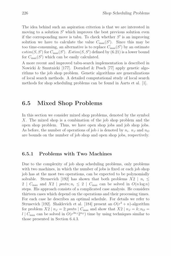
226 Shop Scheduling Problems
The idea behind such an aspiration criterion is that we are interested inmoving to a solution S ′ which improves the best previous solution evenif the corresponding move is tabu. To check whether S ′ is an improvingsolution we have to calculate the value Cmax(S
′). Since this may betoo time-consuming, an alternative is to replace Cmax(S
′) by an estimateestim(S, S ′) for Cmax(S
′). Estim(S, S ′) defined by (6.21) is a lower boundfor Cmax(S
′) which can be easily calculated.
A more recent and improved tabu-search implementation is described inNowicki & Smutnicki [177]. Dorndorf & Pesch [77] apply genetic algo-rithms to the job shop problem. Genetic algorithms are generalizationsof local search methods. A detailed computational study of local searchmethods for shop scheduling problems can be found in Aarts et al. [1].
6.5 Mixed Shop Problems
In this section we consider mixed shop problems, denoted by the symbolX. The mixed shop is a combination of the job shop problem and theopen shop problem. Thus, we have open shop jobs and job shop jobs.As before, the number of operations of job i is denoted by ni. nJ and nO
are bounds on the number of job shop and open shop jobs, respectively.
6.5.1 Problems with Two Machines
Due to the complexity of job shop scheduling problems, only problemswith two machines, in which the number of jobs is fixed or each job shopjob has at the most two operations, can be expected to be polynomiallysolvable. Strusevich [192] has shown that both problems X2 | ni ≤2 | Cmax and X2 | pmtn; ni ≤ 2 | Cmax can be solved in O(n logn)steps. His approach consists of a complicated case analysis. He considersthirteen cases which depend on the operations and their processing times.For each case he describes an optimal schedule. For details we refer toStrusevich [192]. Shaklevich et al. [184] present an O(r3 + n)-algorithmfor problem X2 | nJ = 2; pmtn | Cmax and show that X2 | nJ = k; nO =l | Cmax can be solved in O(r3nJ2nO) time by using techniques similar tothose presented in Section 6.4.3.
6.5. Mixed Shop Problems 227
6.5.2 Problems with Two Jobs
Shakhlevich & Sotskov [183] have shown that the problems X | n =2 | Cmax and X | n = 2 | ∑
Ci are NP-hard. They also suggested anO(r)-algorithm for the preemptive problem consisting of one open shopjob and one job shop job with an arbitrary regular objective functionf(C1, C2). As before, r is the maximum number of operations of bothjobs. This algorithm will be presented in this section.
Assume that we have two jobs, J1 and J2. Let J1 be a job shop jobwith operations O1j (j = 1, . . . , n1). O1j has the processing time p1j andis to be processed on machine μj ∈ {M1, . . . , Mm}. Job J2 is an openshop job with operations O2j (j = 1, . . . , n2 = m), where O2j has theprocessing time p2j and must be processed on Mj . The order in whichthe operations O2j are processed is arbitrary.
Let ti =ni∑
j=1
pij be the total processing time of Ji (i = 1, 2). We consider
the two cases t2 ≤ t1 and t1 < t2.
Case: t2 ≤ t1
We assume that an index l (1 ≤ l < n1) exists withl∑
j=1
p1j = t2. Other-
wise we split an operation of J1 into two operations.
For each k = 1, . . . , m we define
sk = p2k +∑
μj=Mk
j≤l
p1j
and set s = sk∗ :=n
maxk=1
sk.
We consider two subcases.
Subcase: s ≤ t2
We will construct a schedule with C1 = t1 and C2 = t2 which is optimal.
It is sufficient to show that for the truncated problem obtained by re-placing J1 by O11, . . . , O1l a schedule S exists which finishes at time t2.If, additionally, the remaining operations O1,l+1, . . . , O1,n1 are processed
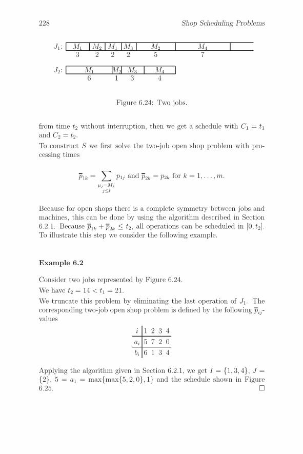
228 Shop Scheduling Problems
J2:
J1:
M1 M2 M3 M4
M1 M2 M1 M3 M2 M4
6 1 3 4
3 2 2 2 5 7
Figure 6.24: Two jobs.
from time t2 without interruption, then we get a schedule with C1 = t1and C2 = t2.
To construct S we first solve the two-job open shop problem with pro-cessing times
p1k =∑
μj=Mk
j≤l
p1j and p2k = p2k for k = 1, . . . , m.
Because for open shops there is a complete symmetry between jobs andmachines, this can be done by using the algorithm described in Section6.2.1. Because p1k + p2k ≤ t2, all operations can be scheduled in [0, t2].To illustrate this step we consider the following example.
Example 6.2
Consider two jobs represented by Figure 6.24.
We have t2 = 14 < t1 = 21.
We truncate this problem by eliminating the last operation of J1. Thecorresponding two-job open shop problem is defined by the following pij-values
i 1 2 3 4
ai 5 7 2 0
bi 6 1 3 4
Applying the algorithm given in Section 6.2.1, we get I = {1, 3, 4}, J ={2}, 5 = a1 = max{max{5, 2, 0}, 1} and the schedule shown in Figure6.25. �
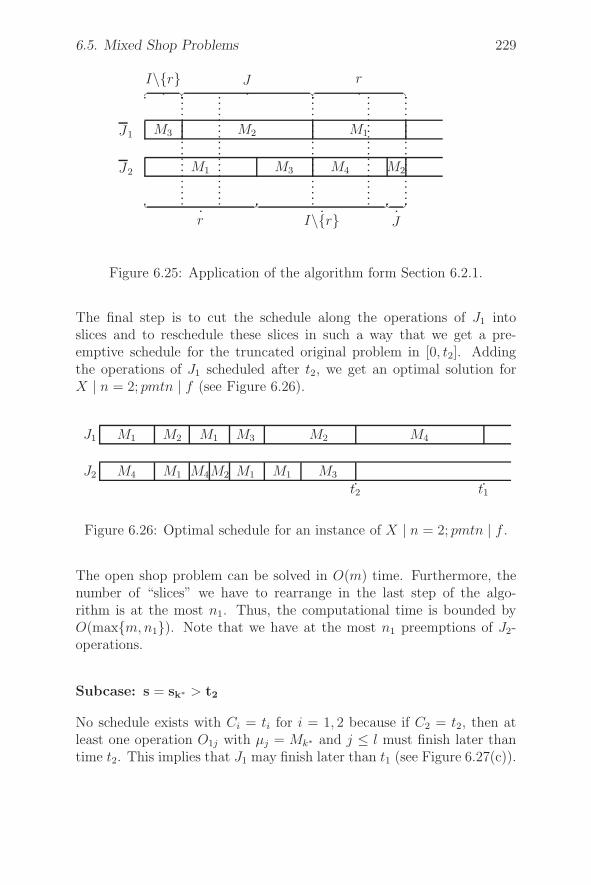
6.5. Mixed Shop Problems 229
J2
J1
M1 M3 M4 M2
M3 M2 M1
�
r�
I\{r}�
J
� �I\{r}
� �J
� �r
Figure 6.25: Application of the algorithm form Section 6.2.1.
The final step is to cut the schedule along the operations of J1 intoslices and to reschedule these slices in such a way that we get a pre-emptive schedule for the truncated original problem in [0, t2]. Addingthe operations of J1 scheduled after t2, we get an optimal solution forX | n = 2; pmtn | f (see Figure 6.26).
J2
J1
M4 M1 M4M2 M1 M1 M3
M1 M2 M1 M3 M2 M4
t2 t1
Figure 6.26: Optimal schedule for an instance of X | n = 2; pmtn | f .
The open shop problem can be solved in O(m) time. Furthermore, thenumber of “slices” we have to rearrange in the last step of the algo-rithm is at the most n1. Thus, the computational time is bounded byO(max{m, n1}). Note that we have at the most n1 preemptions of J2-operations.
Subcase: s = sk∗ > t2
No schedule exists with Ci = ti for i = 1, 2 because if C2 = t2, then atleast one operation O1j with μj = Mk∗ and j ≤ l must finish later thantime t2. This implies that J1 may finish later than t1 (see Figure 6.27(c)).

230 Shop Scheduling Problems
J2
J1
t1 t∗2
machine 1 machine 2 machine 3
(a)
J2
J1
t(1)2
(b)
J2
J1
t2 t∗1(c)
Figure 6.27: An example for Subcase s > t2 of Case t2 ≤ t1.
To avoid excessive formalism, we will use the example in Figure 6.27 toexplain how to proceed in this case. In the example, k∗ = 1. We firstconsider the two extreme cases in which
(1) C1 = t1 and C2 is minimized (see Figure 6.27(a)) or
(2) C2 = t2 and C1 is minimized (see Figure 6.27(c)).
Denote the minimal C2-value in Case (1) by t∗2 and the minimal C1-valuein Case (2) by t∗1 .
For each t2 ≤ t ≤ t∗2 define
f(t) = min{f(s, t) | t1 ≤ s ≤ t∗1}.
Then f(t∗) = min{f(t) | t2 ≤ t ≤ t∗2} is the optimal solution of theproblem. To calculate t∗ we need to consider at the most n1 differentt-values which can be calculated in O(n1) time. This can be explainedas follows using Figure 6.27.
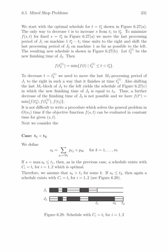
6.5. Mixed Shop Problems 231
We start with the optimal schedule for t = t∗2 shown in Figure 6.27(a).The only way to decrease t is to increase s from t1 to t∗2. To minimizef(s, t) for fixed s = t∗2 in Figure 6.27(a) we move the last processingperiod of J1 on machine 1 t∗2 − t1 time units to the right and shift thelast processing period of J2 on machine 1 as far as possible to the left.The resulting new schedule is shown in Figure 6.27(b). Let t
(1)2 be the
new finishing time of J2. Then
f(t(1)2 ) = min{f(t) | t
(1)2 ≤ t < t∗2}.
To decrease t = t(1)2 we need to move the last M1-processing period of
J1 to the right in such a way that it finishes at time t(1)2 . Also shifting
the last M1-block of J2 to the left yields the schedule of Figure 6.27(c)in which the new finishing time of J2 is equal to t2. Thus, a furtherdecrease of the finishing time of J2 is not possible and we have f(t∗) =
min{f(t∗2), f(t(1)2 ), f(t2)}.
It is not difficult to write a procedure which solves the general problem inO(n1) time if the objective function f(s, t) can be evaluated in constanttime for given (s, t).
Next we consider the
Case: t1 < t2
We define
sk =∑
μj=Mk
p1j + p2k for k = 1, . . . , m.
If s = max sk ≤ t1, then, as in the previous case, a schedule exists withCi = ti for i = 1, 2 which is optimal.
Therefore, we assume that sk > t1 for some k. If sk ≤ t2, then again aschedule exists with Ci = ti for i = 1, 2 (see Figure 6.28).
J2
J1
t1 sk t2
Figure 6.28: Schedule with Ci = ti for i = 1, 2
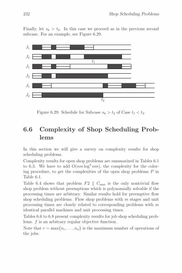
232 Shop Scheduling Problems
Finally, let sk > t2. In this case we proceed as in the previous secondsubcase. For an example, see Figure 6.29.
J2
J1
t1
J2
J1
J2
J1
t2
Figure 6.29: Schedule for Subcase sk > t2 of Case t1 < t2.
6.6 Complexity of Shop Scheduling Prob-
lems
In this section we will give a survey on complexity results for shopscheduling problems.
Complexity results for open shop problems are summarized in Tables 6.1to 6.3. We have to add O(nm log2 nm), the complexity for the color-ing procedure, to get the complexities of the open shop problems P inTable 6.1.
Table 6.4 shows that problem F2 ‖ Cmax is the only nontrivial flowshop problem without preemptions which is polynomially solvable if theprocessing times are arbitrary. Similar results hold for preemptive flowshop scheduling problems. Flow shop problems with m stages and unitprocessing times are closely related to corresponding problems with midentical parallel machines and unit processing times.
Tables 6.6 to 6.8 present complexity results for job shop scheduling prob-lems. f is an arbitrary regular objective function.
Note that r = max{ni, . . . , nn} is the maximum number of operations ofthe jobs.
6.6. Complexity of Shop Scheduling Problems 233
Tables 6.9 and 6.10 present complexity results for mixed shop problems.Again f is an arbitrary regular function and r = max{n1, . . . , nk}. Weassume that f(C1, C2) can be evaluated in constant time.
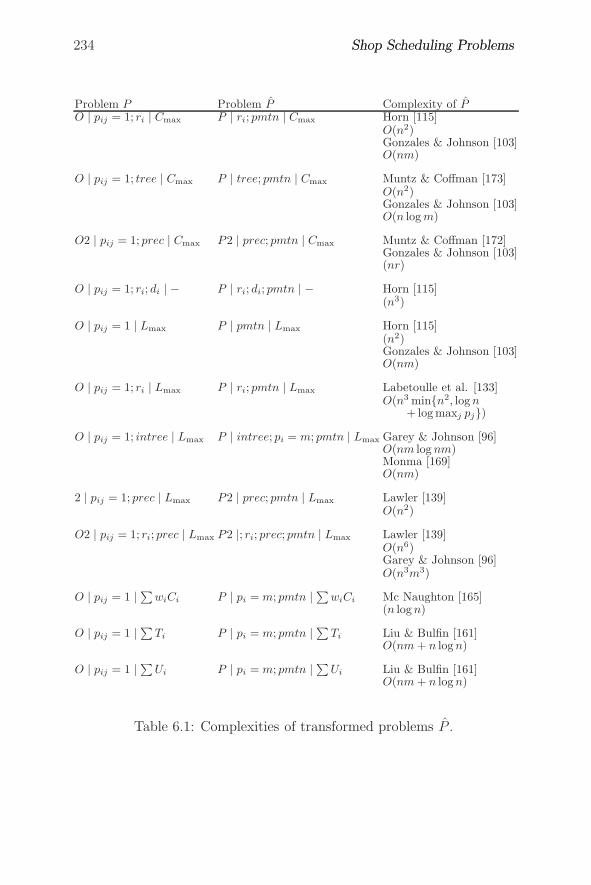
234 Shop Scheduling ProblemsShop Scheduling Problems
Problem P Problem P Complexity of PO | pij = 1; ri | Cmax P | ri; pmtn | Cmax Horn [115]
O(n2)Gonzales & Johnson [103]O(nm)
O | pij = 1; tree | Cmax P | tree; pmtn | Cmax Muntz & Coffman [173]O(n2)Gonzales & Johnson [103]O(n log m)
O2 | pij = 1; prec | Cmax P2 | prec; pmtn | Cmax Muntz & Coffman [172]Gonzales & Johnson [103](nr)
O | pij = 1; ri; di | − P | ri; di; pmtn | − Horn [115](n3)
O | pij = 1 | Lmax P | pmtn | Lmax Horn [115](n2)Gonzales & Johnson [103]O(nm)
O | pij = 1; ri | Lmax P | ri; pmtn | Lmax Labetoulle et al. [133]O(n3 min{n2, log n
+ log maxj pj})O | pij = 1; intree | Lmax P | intree; pi = m; pmtn | Lmax Garey & Johnson [96]
O(nm log nm)Monma [169]O(nm)
2 | pij = 1; prec | Lmax P2 | prec; pmtn | Lmax Lawler [139]O(n2)
O2 | pij = 1; ri; prec | Lmax P2 |; ri; prec; pmtn | Lmax Lawler [139]O(n6)Garey & Johnson [96]O(n3m3)
O | pij = 1 | ∑wiCi P | pi = m; pmtn | ∑
wiCi Mc Naughton [165](n log n)
O | pij = 1 | ∑Ti P | pi = m; pmtn | ∑
Ti Liu & Bulfin [161]O(nm + n log n)
O | pij = 1 | ∑Ui P | pi = m; pmtn | ∑
Ui Liu & Bulfin [161]O(nm + n log n)
Table 6.1: Complexities of transformed problems P .
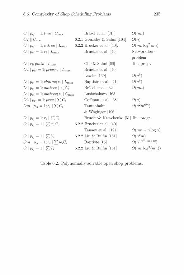
6.6. Complexity of Shop Scheduling Problems 235
O | pij = 1; tree | Cmax Brasel et al. [31] O(nm)O2 ‖ Cmax 6.2.1 Gonzalez & Sahni [104] O(n)O | pij = 1; intree | Lmax 6.2.2 Brucker et al. [40], O(mn log2 mn)O | pij = 1; ri | Lmax Brucker et al. [40] Networkflow-
problemO | ri; pmtn | Lmax Cho & Sahni [66] lin. progr.O2 | pij = 1; prec; ri | Lmax Brucker et al. [40]
Lawler [139] O(n6)O | pij = 1; chains; ri | Lmax Baptiste et al. [21] O(n9)O | pij = 1; outtree | ∑
Ci Brasel et al. [32] O(nm)O | pij = 1; outtree; ri | Cmax Lushchakova [163]O2 | pij = 1; prec | ∑
Ci Coffman et al. [68] O(n)Om | pij = 1; ri |
∑Ci Tautenhahn O(n2m6m)
& Woginger [196]O | pij = 1; ri |
∑Ci Brucker& Kravchenko [51] lin. progr.
O | pij = 1 | ∑wiCi 6.2.2 Brucker et al. [40]
Tanaev et al. [194] O(mn + n log n)O | pij = 1 | ∑
Ui 6.2.2 Liu & Bulfin [161] O(n2m)Om | pij = 1; ri |
∑wiUi Baptiste [15] O(n4m2−m+10)
O | pij = 1 | ∑Ti 6.2.2 Liu & Bulfin [161] O(nm log2(mn))
Table 6.2: Polynomially solvable open shop problems.
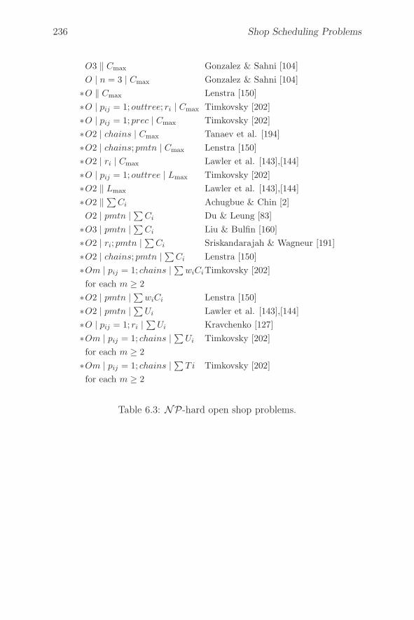
236 Shop Scheduling Problems
O3 ‖ Cmax Gonzalez & Sahni [104]O | n = 3 | Cmax Gonzalez & Sahni [104]
∗O ‖ Cmax Lenstra [150]∗O | pij = 1; outtree; ri | Cmax Timkovsky [202]∗O | pij = 1; prec | Cmax Timkovsky [202]∗O2 | chains | Cmax Tanaev et al. [194]∗O2 | chains; pmtn | Cmax Lenstra [150]∗O2 | ri | Cmax Lawler et al. [143],[144]∗O | pij = 1; outtree | Lmax Timkovsky [202]∗O2 ‖ Lmax Lawler et al. [143],[144]∗O2 ‖ ∑
Ci Achugbue & Chin [2]O2 | pmtn | ∑
Ci Du & Leung [83]∗O3 | pmtn | ∑
Ci Liu & Bulfin [160]∗O2 | ri; pmtn | ∑
Ci Sriskandarajah & Wagneur [191]∗O2 | chains; pmtn | ∑
Ci Lenstra [150]∗Om | pij = 1; chains | ∑
wiCiTimkovsky [202]for each m ≥ 2
∗O2 | pmtn | ∑wiCi Lenstra [150]
∗O2 | pmtn | ∑Ui Lawler et al. [143],[144]
∗O | pij = 1; ri |∑
Ui Kravchenko [127]∗Om | pij = 1; chains | ∑
Ui Timkovsky [202]for each m ≥ 2
∗Om | pij = 1; chains | ∑T i Timkovsky [202]
for each m ≥ 2
Table 6.3: NP-hard open shop problems.
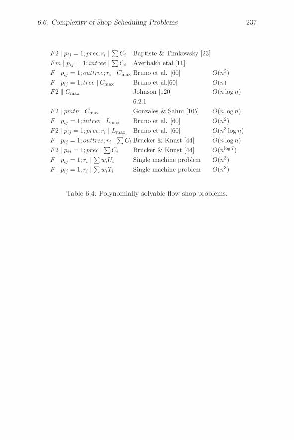
6.6. Complexity of Shop Scheduling Problems 237
F2 | pij = 1; prec; ri |∑
Ci Baptiste & Timkowsky [23]Fm | pij = 1; intree | ∑
Ci Averbakh etal.[11]F | pij = 1; outtree; ri | Cmax Bruno et al. [60] O(n2)F | pij = 1; tree | Cmax Bruno et al.[60] O(n)F2 ‖ Cmax Johnson [120] O(n log n)
6.2.1F2 | pmtn | Cmax Gonzales & Sahni [105] O(n log n)F | pij = 1; intree | Lmax Bruno et al. [60] O(n2)F2 | pij = 1; prec; ri | Lmax Bruno et al. [60] O(n3 log n)F | pij = 1; outtree; ri |
∑Ci Brucker & Knust [44] O(n log n)
F2 | pij = 1; prec | ∑Ci Brucker & Knust [44] O(nlog 7)
F | pij = 1; ri |∑
wiUi Single machine problem O(n3)F | pij = 1; ri |
∑wiTi Single machine problem O(n3)
Table 6.4: Polynomially solvable flow shop problems.
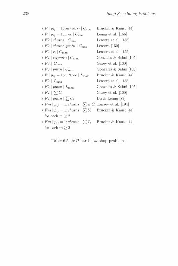
238 Shop Scheduling Problems
∗ F | pij = 1; intree; ri | Cmax Brucker & Knust [44]∗ F | pij = 1; prec | Cmax Leung et al. [156]∗ F2 | chains | Cmax Lenstra et al. [155]∗ F2 | chains; pmtn | Cmax Lenstra [150]∗ F2 | ri | Cmax Lenstra et al. [155]∗ F2 | ri; pmtn | Cmax Gonzales & Sahni [105]∗ F3 ‖ Cmax Garey et al. [100]∗ F3 | pmtn | Cmax Gonzales & Sahni [105]∗ F | pij = 1; outtree | Lmax Brucker & Knust [44]∗ F2 ‖ Lmax Lenstra et al. [155]∗ F2 | pmtn | Lmax Gonzales & Sahni [105]∗ F2 ‖ ∑
Ci Garey et al. [100]∗ F2 | pmtn | ∑
Ci Du & Leung [83]∗ Fm | pij = 1; chains | ∑
wiCi Tanaev et al. [194]∗ Fm | pij = 1; chains | ∑
Ui Brucker & Knust [44]for each m ≥ 2
∗ Fm | pij = 1; chains | ∑Ti Brucker & Knust [44]
for each m ≥ 2
Table 6.5: NP-hard flow shop problems.
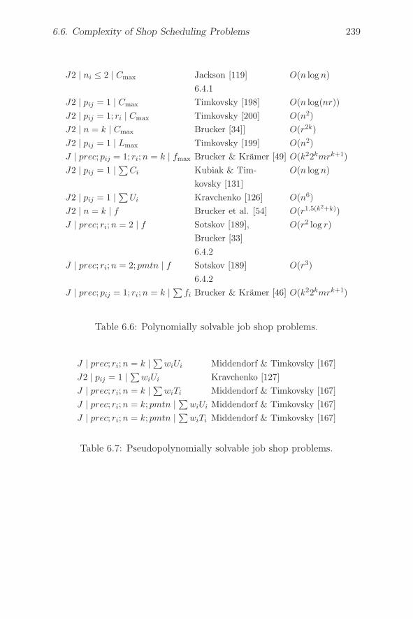
6.6. Complexity of Shop Scheduling Problems 239
J2 | ni ≤ 2 | Cmax Jackson [119] O(n log n)6.4.1
J2 | pij = 1 | Cmax Timkovsky [198] O(n log(nr))J2 | pij = 1; ri | Cmax Timkovsky [200] O(n2)J2 | n = k | Cmax Brucker [34]] O(r2k)J2 | pij = 1 | Lmax Timkovsky [199] O(n2)J | prec; pij = 1; ri;n = k | fmax Brucker & Kramer [49] O(k22kmrk+1)J2 | pij = 1 | ∑
Ci Kubiak & Tim- O(n log n)kovsky [131]
J2 | pij = 1 | ∑Ui Kravchenko [126] O(n6)
J2 | n = k | f Brucker et al. [54] O(r1.5(k2+k))J | prec; ri;n = 2 | f Sotskov [189], O(r2 log r)
Brucker [33]6.4.2
J | prec; ri;n = 2; pmtn | f Sotskov [189] O(r3)6.4.2
J | prec; pij = 1; ri;n = k | ∑fi Brucker & Kramer [46] O(k22kmrk+1)
Table 6.6: Polynomially solvable job shop problems.
J | prec; ri;n = k | ∑wiUi Middendorf & Timkovsky [167]
J2 | pij = 1 | ∑wiUi Kravchenko [127]
J | prec; ri;n = k | ∑wiTi Middendorf & Timkovsky [167]
J | prec; ri;n = k; pmtn | ∑wiUi Middendorf & Timkovsky [167]
J | prec; ri;n = k; pmtn | ∑wiTi Middendorf & Timkovsky [167]
Table 6.7: Pseudopolynomially solvable job shop problems.
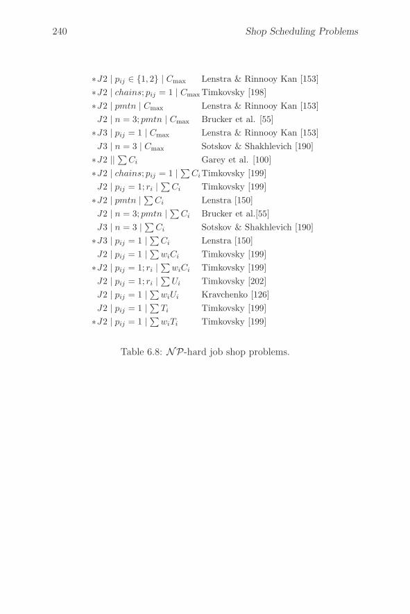
240 Shop Scheduling Problems
∗J2 | pij ∈ {1, 2} | Cmax Lenstra & Rinnooy Kan [153]∗J2 | chains; pij = 1 | Cmax Timkovsky [198]∗J2 | pmtn | Cmax Lenstra & Rinnooy Kan [153]J2 | n = 3; pmtn | Cmax Brucker et al. [55]
∗J3 | pij = 1 | Cmax Lenstra & Rinnooy Kan [153]J3 | n = 3 | Cmax Sotskov & Shakhlevich [190]
∗J2 || ∑Ci Garey et al. [100]
∗J2 | chains; pij = 1 | ∑CiTimkovsky [199]
J2 | pij = 1; ri |∑
Ci Timkovsky [199]∗J2 | pmtn | ∑
Ci Lenstra [150]J2 | n = 3; pmtn | ∑
Ci Brucker et al.[55]J3 | n = 3 | ∑
Ci Sotskov & Shakhlevich [190]∗J3 | pij = 1 | ∑
Ci Lenstra [150]J2 | pij = 1 | ∑
wiCi Timkovsky [199]∗J2 | pij = 1; ri |
∑wiCi Timkovsky [199]
J2 | pij = 1; ri |∑
Ui Timkovsky [202]J2 | pij = 1 | ∑
wiUi Kravchenko [126]J2 | pij = 1 | ∑
Ti Timkovsky [199]∗J2 | pij = 1 | ∑
wiTi Timkovsky [199]
Table 6.8: NP-hard job shop problems.
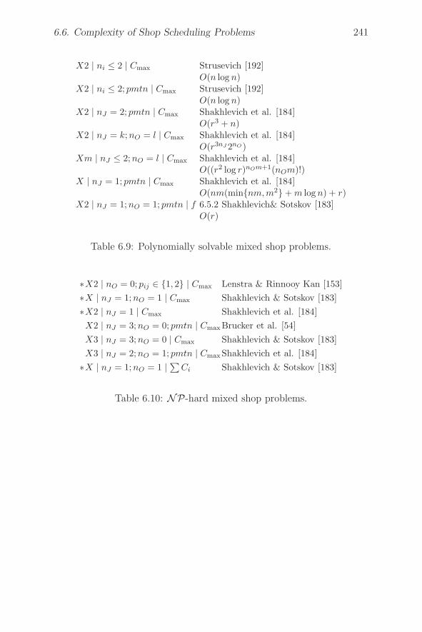
6.6. Complexity of Shop Scheduling Problems 241
X2 | ni ≤ 2 | Cmax Strusevich [192]O(n log n)
X2 | ni ≤ 2; pmtn | Cmax Strusevich [192]O(n log n)
X2 | nJ = 2; pmtn | Cmax Shakhlevich et al. [184]O(r3 + n)
X2 | nJ = k;nO = l | Cmax Shakhlevich et al. [184]O(r3nJ 2nO)
Xm | nJ ≤ 2;nO = l | Cmax Shakhlevich et al. [184]O((r2 log r)nOm+1(nOm)!)
X | nJ = 1; pmtn | Cmax Shakhlevich et al. [184]O(nm(min{nm,m2} + m log n) + r)
X2 | nJ = 1;nO = 1; pmtn | f 6.5.2 Shakhlevich& Sotskov [183]O(r)
Table 6.9: Polynomially solvable mixed shop problems.
∗X2 | nO = 0; pij ∈ {1, 2} | Cmax Lenstra & Rinnooy Kan [153]∗X | nJ = 1;nO = 1 | Cmax Shakhlevich & Sotskov [183]∗X2 | nJ = 1 | Cmax Shakhlevich et al. [184]X2 | nJ = 3;nO = 0; pmtn | CmaxBrucker et al. [54]X3 | nJ = 3;nO = 0 | Cmax Shakhlevich & Sotskov [183]X3 | nJ = 2;nO = 1; pmtn | CmaxShakhlevich et al. [184]
∗X | nJ = 1;nO = 1 | ∑Ci Shakhlevich & Sotskov [183]
Table 6.10: NP-hard mixed shop problems.
Chapter 7
Due-Date Scheduling
New production technologies like “just-in-time” production lead to spe-cial scheduling problems involving due dates di. Contrary to classicalscheduling problems where the objective function simply involves late-ness Li = Ci − di or tardiness Ti = max{0, Ci − di} penalties, earlinessEi = max{0, di−Ci} is now also of importance. Objective functions suchas
∑wi | Li | and
∑wiL
2i are typical of “just-in-time” situations. Note
that Li = Ti + Ei and L2i = T 2
i + E2i . From the practical and theoretical
point of view, situations in which all due dates are equal are of impor-tance. This due date d may be a given parameter of the problem or itmay be a variable, i.e. we are interested in an optimal due date dopt withrespect to the objective function. To indicate these special situations weadd d or dopt to the job characteristics of the problem. If the due dateis a variable, then we may add due-date assignment costs wd · d to theobjective function.
Another objective function considered in the literature in connection withsingle-machine problems is
∑wi | Lσ(i) |, where σ : σ(1), . . . , σ(n) de-
notes the sequence in which the jobs are processed on the machine. Inthis case the weights wi do not correspond with the jobs but with thepositions in which the jobs are scheduled.
In this chapter we will present polynomial and pseudo-polynomial algo-rithms for such due-date scheduling problems. In general, we will restrictourselves to the one-machine case. Furthermore, we assume that thereare no precedence constraints between jobs and that preemption is notallowed.
In the next sections we show that the dopt-version of the problem with
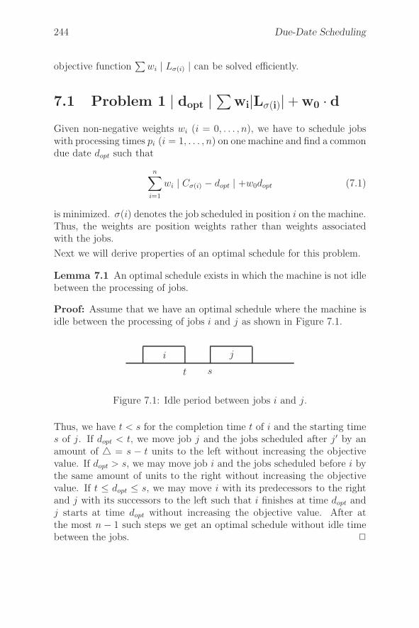
244 Due-Date Scheduling
objective function∑
wi | Lσ(i) | can be solved efficiently.
7.1 Problem 1 | dopt |∑
wi|Lσ(i)| + w0 · dGiven non-negative weights wi (i = 0, . . . , n), we have to schedule jobswith processing times pi (i = 1, . . . , n) on one machine and find a commondue date dopt such that
n∑
i=1
wi | Cσ(i) − dopt | +w0dopt (7.1)
is minimized. σ(i) denotes the job scheduled in position i on the machine.Thus, the weights are position weights rather than weights associatedwith the jobs.
Next we will derive properties of an optimal schedule for this problem.
Lemma 7.1 An optimal schedule exists in which the machine is not idlebetween the processing of jobs.
Proof: Assume that we have an optimal schedule where the machine isidle between the processing of jobs i and j as shown in Figure 7.1.
t s
i j
Figure 7.1: Idle period between jobs i and j.
Thus, we have t < s for the completion time t of i and the starting times of j. If dopt < t, we move job j and the jobs scheduled after j′ by anamount of � = s − t units to the left without increasing the objectivevalue. If dopt > s, we may move job i and the jobs scheduled before i bythe same amount of units to the right without increasing the objectivevalue. If t ≤ dopt ≤ s, we may move i with its predecessors to the rightand j with its successors to the left such that i finishes at time dopt andj starts at time dopt without increasing the objective value. After atthe most n − 1 such steps we get an optimal schedule without idle timebetween the jobs. �
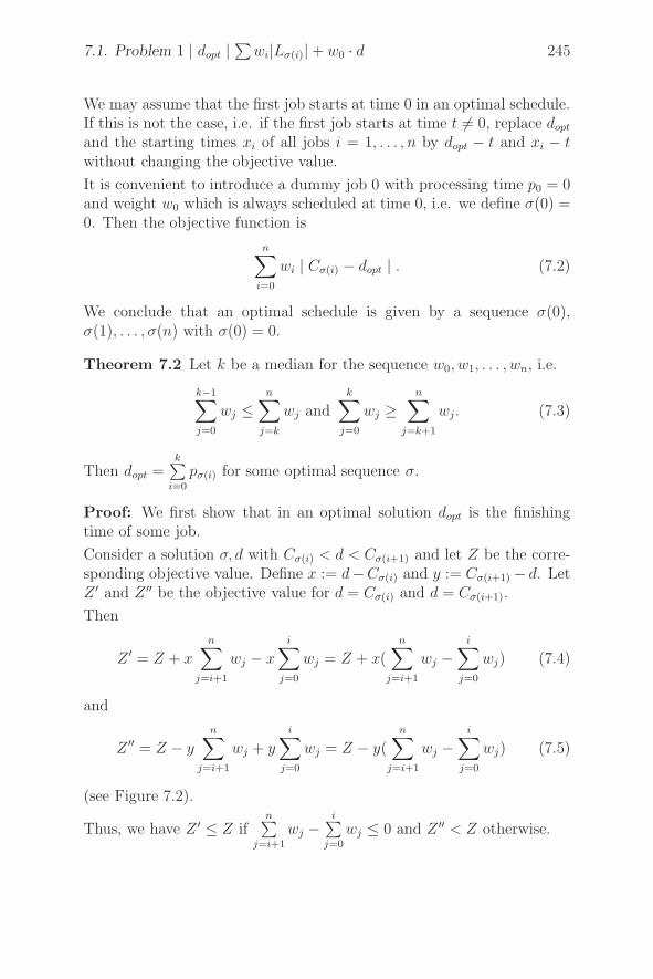
7.1. Problem 1 | dopt |∑
wi|Lσ(i)| + w0 · d 245
We may assume that the first job starts at time 0 in an optimal schedule.If this is not the case, i.e. if the first job starts at time t �= 0, replace dopt
and the starting times xi of all jobs i = 1, . . . , n by dopt − t and xi − twithout changing the objective value.
It is convenient to introduce a dummy job 0 with processing time p0 = 0and weight w0 which is always scheduled at time 0, i.e. we define σ(0) =0. Then the objective function is
n∑
i=0
wi | Cσ(i) − dopt | . (7.2)
We conclude that an optimal schedule is given by a sequence σ(0),σ(1), . . . , σ(n) with σ(0) = 0.
Theorem 7.2 Let k be a median for the sequence w0, w1, . . . , wn, i.e.
k−1∑
j=0
wj ≤n∑
j=k
wj and
k∑
j=0
wj ≥n∑
j=k+1
wj. (7.3)
Then dopt =k∑
i=0
pσ(i) for some optimal sequence σ.
Proof: We first show that in an optimal solution dopt is the finishingtime of some job.
Consider a solution σ, d with Cσ(i) < d < Cσ(i+1) and let Z be the corre-sponding objective value. Define x := d−Cσ(i) and y := Cσ(i+1) − d. LetZ ′ and Z ′′ be the objective value for d = Cσ(i) and d = Cσ(i+1).
Then
Z ′ = Z + x
n∑
j=i+1
wj − x
i∑
j=0
wj = Z + x(
n∑
j=i+1
wj −i∑
j=0
wj) (7.4)
and
Z ′′ = Z − y
n∑
j=i+1
wj + y
i∑
j=0
wj = Z − y(
n∑
j=i+1
wj −i∑
j=0
wj) (7.5)
(see Figure 7.2).
Thus, we have Z ′ ≤ Z ifn∑
j=i+1
wj −i∑
j=0
wj ≤ 0 and Z ′′ < Z otherwise.
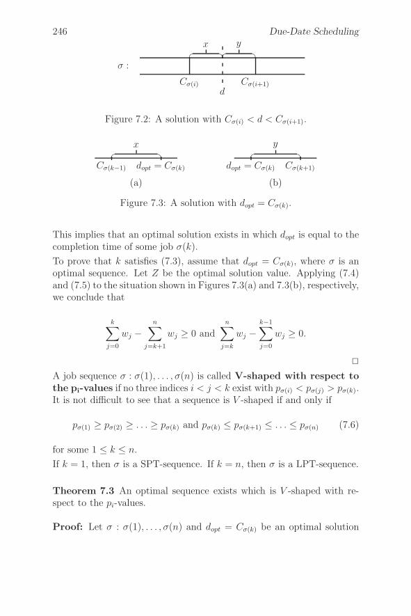
246 Due-Date Scheduling
σ :
Cσ(i)
dCσ(i+1)
� �x
� �y
Figure 7.2: A solution with Cσ(i) < d < Cσ(i+1).
Cσ(k−1) dopt = Cσ(k)
� �x
(a)
dopt = Cσ(k) Cσ(k+1)
� �y
(b)
Figure 7.3: A solution with dopt = Cσ(k).
This implies that an optimal solution exists in which dopt is equal to thecompletion time of some job σ(k).
To prove that k satisfies (7.3), assume that dopt = Cσ(k), where σ is anoptimal sequence. Let Z be the optimal solution value. Applying (7.4)and (7.5) to the situation shown in Figures 7.3(a) and 7.3(b), respectively,we conclude that
k∑
j=0
wj −n∑
j=k+1
wj ≥ 0 and
n∑
j=k
wj −k−1∑
j=0
wj ≥ 0.
�
A job sequence σ : σ(1), . . . , σ(n) is called V-shaped with respect tothe pi-values if no three indices i < j < k exist with pσ(i) < pσ(j) > pσ(k).It is not difficult to see that a sequence is V -shaped if and only if
pσ(1) ≥ pσ(2) ≥ . . . ≥ pσ(k) and pσ(k) ≤ pσ(k+1) ≤ . . . ≤ pσ(n) (7.6)
for some 1 ≤ k ≤ n.
If k = 1, then σ is a SPT-sequence. If k = n, then σ is a LPT-sequence.
Theorem 7.3 An optimal sequence exists which is V -shaped with re-spect to the pi-values.
Proof: Let σ : σ(1), . . . , σ(n) and dopt = Cσ(k) be an optimal solution
7.2. Problem 1|dopt|wE
∑Ei+wT
∑Ti + w0d 247
such that (7.3) is satisfied. For the corresponding objective value we have
k∑
j=0
wj(Cσ(k) − Cσ(j)) +n∑
j=k+1
wj(Cσ(j) − Cσ(k)) =k∑
j=0
wj
k∑
ν=j+1
pσ(ν)
+n∑
j=k+1
wj
j∑
ν=k+1
pσ(ν) =k∑
ν=1
pσ(ν)(ν−1∑
j=0
wj) +n∑
ν=k+1
pσ(ν)(n∑
j=ν
wj).
=n∑
j=1
pσ(j)λj
with
λj =
⎧⎪⎪⎨
⎪⎪⎩
j−1∑
ν=0
wν for j = 1, . . . , k
n∑
ν=j
wν for j = k + 1, . . . , n.(7.7)
Because λ1 ≤ λ2 ≤ . . . ≤ λk and λk+1 ≥ λk+2 ≥ . . . ≥ λn, the ob-jective value does not increase if we reorder σ in such a way that in
the sumn∑
j=1
pσ(j)λj the smallest pi-values are assigned to the largest λj-
values. This yields a sequence which is V -shaped with respect to thepi-values. �
To solve problem 1 | dopt | ∑wi | Lσ(i) | +w0d, we first calculate k
according to (7.3) and the corresponding λj-values. Using the λj-values,
an optimal sequence σ is constructed and dopt =k∑
j=1
pσ(j) is calculated.
σ is constructed by matching the smallest pi-values with the largest λj .More specifically, we compare λk and λk+1. If λk ≥ λk+1, then a job withthe smallest processing time is scheduled in position k and λk is replacedby λk−1. Otherwise such a job is scheduled in position k + 1, and λk+1 isreplaced by λk+2, etc.
The computational complexity of this algorithm is O(n log n).
7.2 Problem 1|dopt|wE
∑Ei+wT
∑Ti + w0d
In “just-in-time” production models we have to consider a penalty notonly if a job is late but also if a job is early with respect to a givendue date d. A simple objective function modeling such a situation iswE
∑Ei + wT
∑Ti + w0d, where Ei = max{0,−Li} = max{0, di − Ci},
Ti = max{0, Li} = max{0, Ci − di}, and wE , wT > 0. Problem 1 | dopt |
248 Due-Date Scheduling
wE
∑Ei + wT
∑Ti + w0d can be solved using techniques described in
the last section.
This is due to the fact that each solution of problem 1 | dopt | wE
∑Ei +
wT
∑Ti +w0d is a solution of problem 1 | dopt |
∑wi | Lσ(i) | +w0d with
special weights (namely w0 for the dummy job, wE for each of the firstjobs which is early, and wT for each of the last jobs which is late).
Again, if we have an optimal solution, there is no idle time between two
jobs and dopt is equal to the finishing time of some job. If dopt =k∑
ν=1
pσ(ν),
then the following inequalities hold
w0 + (k − 1)wE ≤ (n − k + 1)wT (7.8)
w0 + kwE ≥ (n − k)wT (7.9)
(compare (7.3) and the proof of Theorem 7.2).
Inequalities (7.8) and (7.9) are equivalent to
nwT − w0
wE + wT
≤ k ≤ nwT − w0
wE + wT
+ 1. (7.10)
We have to find an integer k satisfying (7.10). If nwT−w0
wE+wTis not integer,
then
k :=
⌈nwT − w0
wE + wT
⌉
(7.11)
is the only k satisfying (7.10). Otherwise we have two solutions k and
k +1 where k is given by (7.11). In this case, each d withk∑
ν=1
pσ(ν) ≤ d ≤k+1∑
ν=1
pσ(ν) provides the same objective value. This can be seen as follows.
Let Z(σ, d) be the objective value for the sequence σ : σ(1), . . . , σ(n) and
the due-date d. Then for d∗ = Cσ(k) :=k∑
j=1
pσ(ν) we have
Z(σ, d∗) = wE
k∑
j=1
| Cσ(j) − d∗ | +wT
n∑
j=k+1
| Cσ(j) − d∗ | +w0d∗.
7.3. Problem 1 | d | ∑wi|Lσ(i)| 249
Replacing d∗ by d∗ + � with 0 ≤ � ≤ pσ(k+1) yields
Z(σ, d∗ + �)= Z(σ, d∗) + wEk �−wT (n − k) � +w0�= Z(σ, d∗) + �(k(wE + wT ) + w0 − nwT )
= Z(σ, d∗) + � · (nwT−w0
wE+wT(wE + wT ) + w0 − nwT )
= Z(σ, d∗).
Therefore, regardless of whether k is integer or not, we may choose k asdefined by (7.11). However, for large w0 this value may be negative. Inthis case, we have to replace k by
k := max
{
0,
⌈nwT − w0
wE + wT
⌉}
. (7.12)
Given k, for the corresponding λj-values we have
λj =
{wE(j − 1) + w0 for 1 ≤ j ≤ k
wT (n − j + 1) for k + 1 ≤ j ≤ n(7.13)
(see (7.7)).
Using (7.12) and (7.13), an optimal solution for problem 1 | dopt |wE
∑Ei +wT
∑Ti +w0d can be found using the algorithm described at
the end of Section 7.2. The corresponding algorithm was first formulatedby Panwalkar et al. [179].
If we set wE = wT = 1 and w0 = 0, we get problem 1 | dopt |∑ | Li |.
Our algorithm also solves this problem if we set
k :=⌈n
2
⌉
and
λj =
{j − 1 for 1 ≤ j ≤ k
n − j + 1 for k + 1 ≤ j ≤ n
(see Kanet [123]).
Finally, we mention that problem P2 | dopt |∑ | Li | is NP-hard.
7.3 Problem 1 | d | ∑wi|Lσ(i)|
If in problem 1 | dopt |∑ | Lσ(i) | we replace dopt by d, i.e. if the due
date is given and a job cannot start before time t = 0, then the problembecomes NP-hard (Kahlbacher [122]).
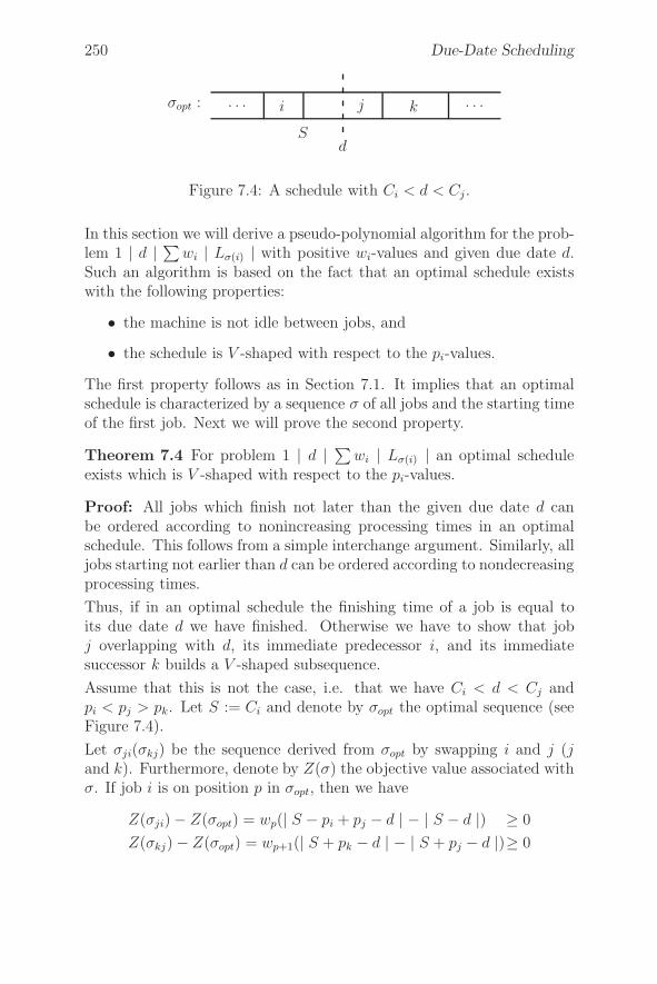
250 Due-Date Scheduling
σopt :
S
. . . i j k . . .
d
Figure 7.4: A schedule with Ci < d < Cj .
In this section we will derive a pseudo-polynomial algorithm for the prob-lem 1 | d | ∑
wi | Lσ(i) | with positive wi-values and given due date d.Such an algorithm is based on the fact that an optimal schedule existswith the following properties:
• the machine is not idle between jobs, and
• the schedule is V -shaped with respect to the pi-values.
The first property follows as in Section 7.1. It implies that an optimalschedule is characterized by a sequence σ of all jobs and the starting timeof the first job. Next we will prove the second property.
Theorem 7.4 For problem 1 | d | ∑wi | Lσ(i) | an optimal schedule
exists which is V -shaped with respect to the pi-values.
Proof: All jobs which finish not later than the given due date d canbe ordered according to nonincreasing processing times in an optimalschedule. This follows from a simple interchange argument. Similarly, alljobs starting not earlier than d can be ordered according to nondecreasingprocessing times.
Thus, if in an optimal schedule the finishing time of a job is equal toits due date d we have finished. Otherwise we have to show that jobj overlapping with d, its immediate predecessor i, and its immediatesuccessor k builds a V -shaped subsequence.
Assume that this is not the case, i.e. that we have Ci < d < Cj andpi < pj > pk. Let S := Ci and denote by σopt the optimal sequence (seeFigure 7.4).
Let σji(σkj) be the sequence derived from σopt by swapping i and j (jand k). Furthermore, denote by Z(σ) the objective value associated withσ. If job i is on position p in σopt, then we have
Z(σji) − Z(σopt) = wp(| S − pi + pj − d | − | S − d |) ≥ 0
Z(σkj) − Z(σopt) = wp+1(| S + pk − d | − | S + pj − d |)≥ 0
7.3. Problem 1 | d | ∑wi|Lσ(i)| 251
because σopt is optimal. This implies
| S − pi + pj − d |≥ d − S (7.14)
| S + pk − d | ≥ S + pj − d (7.15)
because S < d < S + pj.
We must have S−pi+pj−d ≥ 0 because otherwise (7.14) is equivalent to−S +pi−pj +d ≥ d−S, i.e. pi ≥ pj, which is a contradiction. Similarly,due to (7.15), we must have S + pk − d ≤ 0. Thus, (7.14) and (7.15) canbe written in the form
S − pi + pj − d≥ d − S (7.16)
−S − pk + d ≥ S + pj − d. (7.17)
Adding inequalities (7.16) and (7.17) gives pi + pk ≤ 0, which impliespi = pk = 0. Thus we can swap i with j or i with k without increasingthe objective value. If we continue this process, we get a V -shapedsequence. �
Let d∗ be the optimal due date for the corresponding problem 1 | dopt |∑wi | Lσ(i) |. We may assume that the optimal schedule of this problem
starts at time t = 0. Let σ∗ be the optimal sequence of the jobs.
If d ≥ d∗, then the starting time d−d∗ and σ∗ define an optimal schedulefor our problem 1 | d | ∑
wi | Lσ(i) |. If d < d∗, then we can show thatan optimal schedule starts at time t = 0. However, finding an optimalsequence is NP-hard. We solve this problem by dynamic programming.
We assume that the jobs are indexed according to nondecreasing pro-cessing time, i.e. that
p1 ≤ p2 ≤ . . . ≤ pn
holds. Since an optimal solution exists which is V -shaped, we may as-sume that in an optimal solution jobs 1, . . . , k(1 ≤ k ≤ n) are scheduledas a contiguous block.
Let S(k, i, e) be an optimal schedule for jobs 1, . . . , k with positionalweights wi, wi+1, . . . , wi+k−1 and due date e starting at time 0. Letσ(k, i, e) be the corresponding sequence and let Z(k, i, e) be the cor-responding objective value.
We will now derive a recursion for the Z(k, i, e)-values and correspondingsequences σ(k, i, e), where 1 ≤ k ≤ n, 1 ≤ i ≤ n − k + 1, and 0 ≤ e ≤ d.
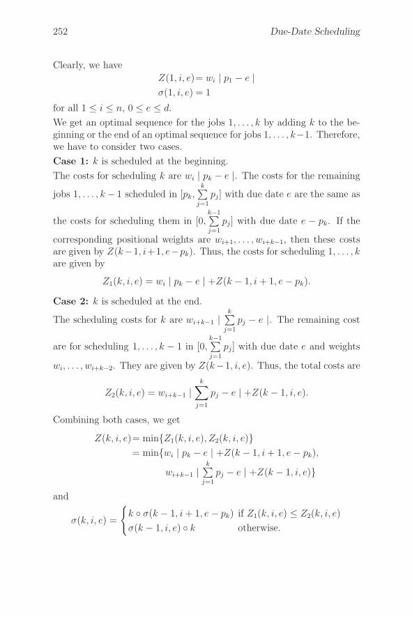
252 Due-Date Scheduling
Clearly, we have
Z(1, i, e)= wi | p1 − e |σ(1, i, e) = 1
for all 1 ≤ i ≤ n, 0 ≤ e ≤ d.
We get an optimal sequence for the jobs 1, . . . , k by adding k to the be-ginning or the end of an optimal sequence for jobs 1, . . . , k−1. Therefore,we have to consider two cases.
Case 1: k is scheduled at the beginning.
The costs for scheduling k are wi | pk − e |. The costs for the remaining
jobs 1, . . . , k − 1 scheduled in [pk,k∑
j=1
pj] with due date e are the same as
the costs for scheduling them in [0,k−1∑
j=1
pj] with due date e − pk. If the
corresponding positional weights are wi+1, . . . , wi+k−1, then these costsare given by Z(k−1, i+1, e−pk). Thus, the costs for scheduling 1, . . . , kare given by
Z1(k, i, e) = wi | pk − e | +Z(k − 1, i + 1, e − pk).
Case 2: k is scheduled at the end.
The scheduling costs for k are wi+k−1 |k∑
j=1
pj − e |. The remaining cost
are for scheduling 1, . . . , k − 1 in [0,k−1∑
j=1
pj ] with due date e and weights
wi, . . . , wi+k−2. They are given by Z(k−1, i, e). Thus, the total costs are
Z2(k, i, e) = wi+k−1 |k∑
j=1
pj − e | +Z(k − 1, i, e).
Combining both cases, we get
Z(k, i, e)= min{Z1(k, i, e), Z2(k, i, e)}= min{wi | pk − e | +Z(k − 1, i + 1, e − pk),
wi+k−1 |k∑
j=1
pj − e | +Z(k − 1, i, e)}
and
σ(k, i, e) =
{k ◦ σ(k − 1, i + 1, e − pk) if Z1(k, i, e) ≤ Z2(k, i, e)
σ(k − 1, i, e) ◦ k otherwise.
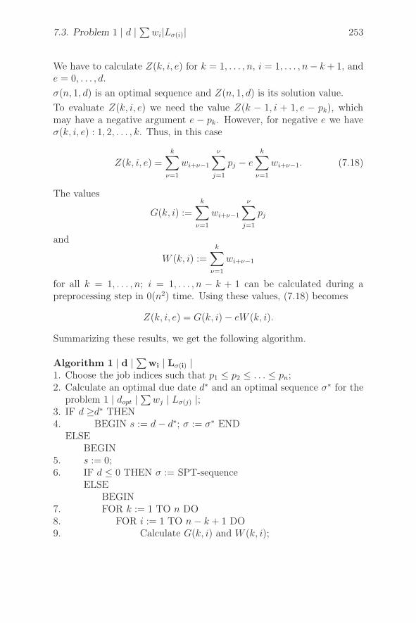
7.3. Problem 1 | d | ∑wi|Lσ(i)| 253
We have to calculate Z(k, i, e) for k = 1, . . . , n, i = 1, . . . , n− k + 1, ande = 0, . . . , d.
σ(n, 1, d) is an optimal sequence and Z(n, 1, d) is its solution value.
To evaluate Z(k, i, e) we need the value Z(k − 1, i + 1, e − pk), whichmay have a negative argument e − pk. However, for negative e we haveσ(k, i, e) : 1, 2, . . . , k. Thus, in this case
Z(k, i, e) =
k∑
ν=1
wi+ν−1
ν∑
j=1
pj − e
k∑
ν=1
wi+ν−1. (7.18)
The values
G(k, i) :=
k∑
ν=1
wi+ν−1
ν∑
j=1
pj
and
W (k, i) :=
k∑
ν=1
wi+ν−1
for all k = 1, . . . , n; i = 1, . . . , n − k + 1 can be calculated during apreprocessing step in 0(n2) time. Using these values, (7.18) becomes
Z(k, i, e) = G(k, i) − eW (k, i).
Summarizing these results, we get the following algorithm.
Algorithm 1 | d | ∑wi | Lσ(i) |
1. Choose the job indices such that p1 ≤ p2 ≤ . . . ≤ pn;2. Calculate an optimal due date d∗ and an optimal sequence σ∗ for the
problem 1 | dopt |∑
wj | Lσ(j) |;3. IF d ≥d∗ THEN4. BEGIN s := d − d∗; σ := σ∗ END
ELSEBEGIN
5. s := 0;6. IF d ≤ 0 THEN σ := SPT-sequence
ELSEBEGIN
7. FOR k := 1 TO n DO8. FOR i := 1 TO n − k + 1 DO9. Calculate G(k, i) and W (k, i);
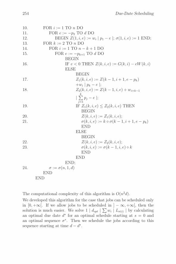
254 Due-Date Scheduling
10. FOR i := 1 TO n DO11. FOR e := −p2 TO d DO12. BEGIN Z(1, i, e) := wi | p1 − e |; σ(1, i, e) := 1 END;13. FOR k := 2 TO n DO14. FOR i := 1 TO n − k + 1 DO15. FOR e := −pk+1 TO d DO
BEGIN16. IF e < 0 THEN Z(k, i, e) := G(k, i) − eW (k, i)
ELSEBEGIN
17. Z1(k, i, e) := Z(k − 1, i + 1, e − pk)+wi | pk − e |;
18. Z2(k, i, e) := Z(k − 1, i, e) + wi+k−1
|k∑
j=1
pj − e |;19. IF Z1(k, i, e) ≤ Z2(k, i, e) THEN
BEGIN20. Z(k, i, e) := Z1(k, i, e);21. σ(k, i, e) := k ◦ σ(k − 1, i + 1, e − pk)
ENDELSE
BEGIN22. Z(k, i, e) := Z2(k, i, e);23. σ(k, i, e) := σ(k − 1, i, e) ◦ k
ENDEND
END;24. σ := σ(n, 1, d)
ENDEND
The computational complexity of this algorithm is O(n2d).
We developed this algorithm for the case that jobs can be scheduled onlyin [0, +∞[. If we allow jobs to be scheduled in ] − ∞, +∞[, then thesolution is much easier. We solve 1 | dopt |
∑wi | Lσ(i) | by calculating
an optimal due date d∗ for an optimal schedule starting at s = 0 andan optimal sequence σ∗. Then we schedule the jobs according to thissequence starting at time d − d∗.
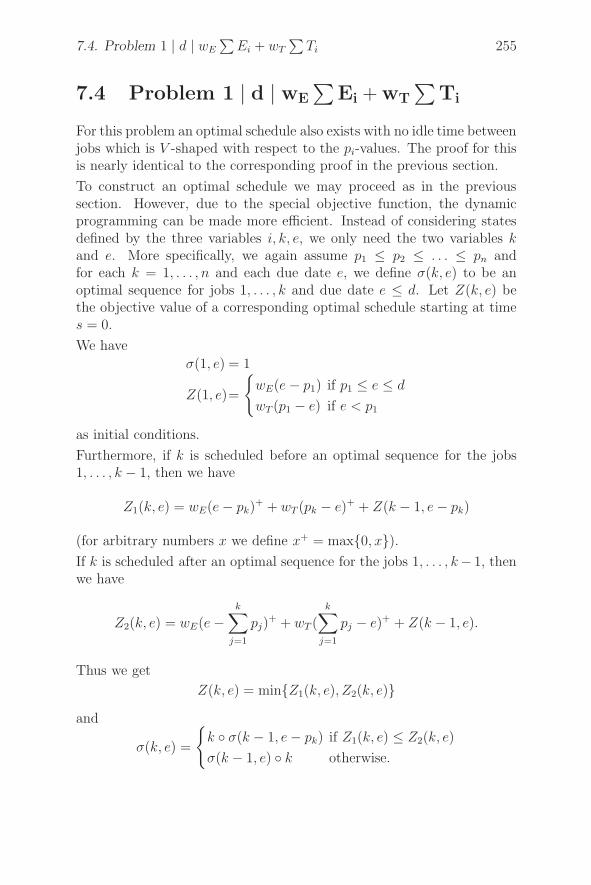
7.4. Problem 1 | d | wE
∑Ei + wT
∑Ti 255
7.4 Problem 1 | d | wE
∑Ei + wT
∑Ti
For this problem an optimal schedule also exists with no idle time betweenjobs which is V -shaped with respect to the pi-values. The proof for thisis nearly identical to the corresponding proof in the previous section.
To construct an optimal schedule we may proceed as in the previoussection. However, due to the special objective function, the dynamicprogramming can be made more efficient. Instead of considering statesdefined by the three variables i, k, e, we only need the two variables kand e. More specifically, we again assume p1 ≤ p2 ≤ . . . ≤ pn andfor each k = 1, . . . , n and each due date e, we define σ(k, e) to be anoptimal sequence for jobs 1, . . . , k and due date e ≤ d. Let Z(k, e) bethe objective value of a corresponding optimal schedule starting at times = 0.
We have
σ(1, e) = 1
Z(1, e)=
{wE(e − p1) if p1 ≤ e ≤ d
wT (p1 − e) if e < p1
as initial conditions.
Furthermore, if k is scheduled before an optimal sequence for the jobs1, . . . , k − 1, then we have
Z1(k, e) = wE(e − pk)+ + wT (pk − e)+ + Z(k − 1, e − pk)
(for arbitrary numbers x we define x+ = max{0, x}).If k is scheduled after an optimal sequence for the jobs 1, . . . , k− 1, thenwe have
Z2(k, e) = wE(e −k∑
j=1
pj)+ + wT (
k∑
j=1
pj − e)+ + Z(k − 1, e).
Thus we get
Z(k, e) = min{Z1(k, e), Z2(k, e)}and
σ(k, e) =
{k ◦ σ(k − 1, e − pk) if Z1(k, e) ≤ Z2(k, e)
σ(k − 1, e) ◦ k otherwise.
256 Due-Date Scheduling
These recursions hold for k = 2, . . . , n and 0 ≤ e ≤ d. If e < 0, then theSPT-sequence is optimal and we have
Z(k, e) = wT (k∑
ν=1
ν∑
j=1
pj − ke).
If all values
G(k) :=
k∑
ν=1
ν∑
j=1
pj k = 1, 2, . . . , n
are calculated during a preprocessing step, then each value
Z(k, e) = wT (G(k) − k · e)can be calculated in constant time. The preprocessing can be done inO(n) time.
It is not difficult to formulate the algorithm along the lines of the previoussection.
Algorithm 1 | d | wE
∑Ei + wT
∑Ti
1. Choose the job indices such that p1 ≤ p2 ≤ . . . ≤ pn;2. Calculate an optimal due date d∗ and an optimal sequence σ∗ for
the corresponding problem 1 | dopt | wE
∑Ei + wT
∑Ti;
3. IF d ≥d∗ THEN4. BEGIN s := d − d∗; σ := σ∗ END
ELSEBEGIN
5. s := 0;6. IF d ≤ 0 THEN σ := SPT-sequence
ELSEBEGIN
7. FOR k = 1 TO n DO calculate G(k);8. FOR e := −p2 TO d DO
BEGIN9. σ(1, e) = 1;10. IF e < p1 THEN Z(1, e) := wT (p1 − e)
ELSE Z(1, e) := wE(e − p1);END;
11. FOR k := 2 TO n DO12. FOR e := −pk+1 TO d DO
7.5. Problem 1 | d | |Li|max and 1 | dopt | |Li|max 257
BEGIN13. IF e < 0 THEN Z(k, e) := wT (G(k) − ke)
ELSEBEGIN
14. Z1(k, e) := wE(e − pk)+ + wT (pk − e)+
+Z(k − 1, e − pk);
15. Z2(k, e) := wE(e −k∑
j=1
pj)+ + wT (
k∑
j=1
pj − e)+
+Z(k − 1, e);16. IF Z1(k, e) ≤ Z2(k, e) THEN
BEGIN17. Z(k, e) := Z1(k, e);18. σ(k, e) := k ◦ σ(k − 1, e − pk)
ENDELSE
BEGIN19. Z(k, e) := Z2(k, e);20. σ(k, e) := σ(k − 1, e) ◦ k
ENDEND
END;21. σ := σ(n, d)
ENDEND
The complexity of this algorithm is O(n log n + nd).
7.5 Problem 1 |d | |Li|max and 1 |dopt | |Li|max
We now consider the objective functionn
maxi=1
| Ci − d | (Kahlbacher
[122]). As before, for variable and fixed d there exists an optimal schedulewithout idle time between jobs.
We first consider problem 1 | d | | Li |max. If σ(1) is the first job and thisjob starts at time s, then the objective value can be written in the form
| Li |max=n
maxi=1
| Ci−d |= max{| s+pσ(1) −d |, | s+
n∑
i=1
pi−d |} (7.19)
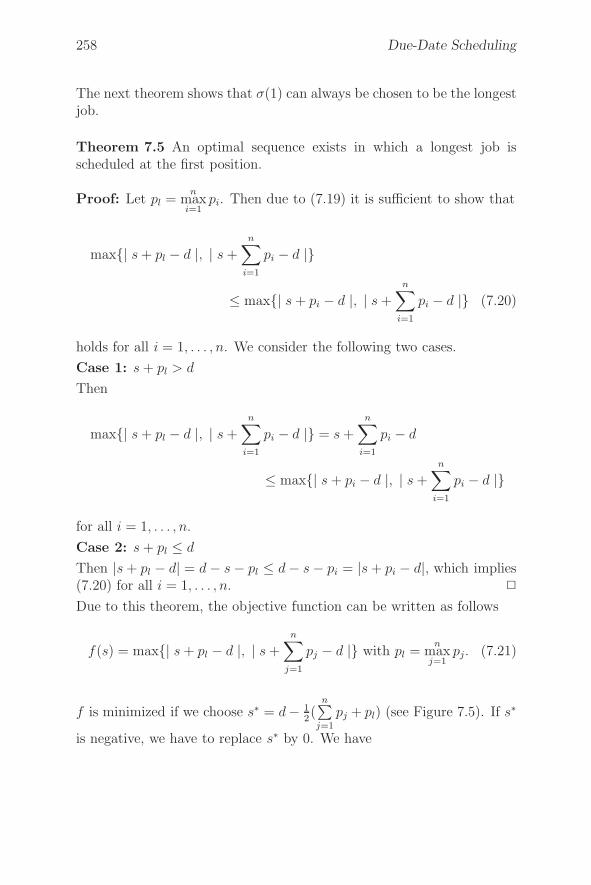
258 Due-Date Scheduling
The next theorem shows that σ(1) can always be chosen to be the longestjob.
Theorem 7.5 An optimal sequence exists in which a longest job isscheduled at the first position.
Proof: Let pl =n
maxi=1
pi. Then due to (7.19) it is sufficient to show that
max{| s + pl − d |, | s +n∑
i=1
pi − d |}
≤ max{| s + pi − d |, | s +
n∑
i=1
pi − d |} (7.20)
holds for all i = 1, . . . , n. We consider the following two cases.
Case 1: s + pl > d
Then
max{| s + pl − d |, | s +
n∑
i=1
pi − d |} = s +
n∑
i=1
pi − d
≤ max{| s + pi − d |, | s +n∑
i=1
pi − d |}
for all i = 1, . . . , n.
Case 2: s + pl ≤ d
Then |s + pl − d| = d − s − pl ≤ d − s − pi = |s + pi − d|, which implies(7.20) for all i = 1, . . . , n. �
Due to this theorem, the objective function can be written as follows
f(s) = max{| s + pl − d |, | s +n∑
j=1
pj − d |} with pl =n
maxj=1
pj. (7.21)
f is minimized if we choose s∗ = d− 12(
n∑
j=1
pj + pl) (see Figure 7.5). If s∗
is negative, we have to replace s∗ by 0. We have
7.6. Problem 1 | dopt |∑
wi|Li| 259
d −n∑
j=1
pj s∗ d − pl
| s +n∑
j=1
pj − d | | s + pl − d |
f(s)
Figure 7.5: Function f .
Theorem 7.6 Any schedule which starts with a job l with a largestprocessing time at time
t := max{0, d − 1
2(
n∑
j=1
pj + pl)}
and processes the other jobs without idle time after l in an arbitrarysequence is optimal for problem 1 | d | | Li |max. �
Note that such an optimal schedule can be found in O(n) time.
To solve problem 1 | dopt | | Li |max, we have to find a value d∗ whichminimizes (7.21). We may assume that s = 0. In other words, we geta solution for problem 1 | dopt | | Li |max if we set d = 0 and s = −d in(7.21). This leads to
Theorem 7.7 An optimal solution for problem 1 | dopt | | Li |max isobtained by scheduling a longest job l as the first job starting at times = 0 and setting
dopt =1
2(
n∑
j=1
pj + pl).
�
7.6 Problem 1 | dopt |∑
wi|Li|In this problem we assume that all wj-values are positive integers. Hall &Posner [109] have shown that problem 1 | dopt |
∑wi | Li | is NP-hard.
260 Due-Date Scheduling
We will develop two pseudo-polynomial algorithms for this problem. One
has complexity O(nn∑
i=1
pi), the other has complexity O(nn∑
i=1
wi). The fol-
lowing theorems are the basis for these algorithms. Again, it is sufficientto consider only schedules without idle time between jobs in which thefirst job starts at time 0. We have to find an optimal sequence σ∗ andan optimal due date d∗.
Theorem 7.8 Given a sequence σ(1), . . . , σ(n), a corresponding optimaldue date is given by the finishing time Cσ(r) of a job σ(r). Moreover,
r−1∑
j=1
wσ(j) ≤n∑
j=r
wσ(j) and
r∑
j=1
wσ(j) ≥n∑
j=r+1
wσ(j).
Proof: Similar to the proof of Theorem 7.2. �
The next theorem states that an optimal sequence exists which is V -shaped with respect to the ratios pi/wi.
Theorem 7.9 An optimal sequence exists in which the early jobs aresequenced according to nonincreasing (pi/wi)-values and the late jobsare sequenced according to nondecreasing (pi/wi)-values.
Proof: By a simple exchange argument (see also Smith’s ratio rule inSection 4.3.1). �
Again, we use dynamic programming approaches to solve problem 1 |dopt |
∑wi | Li |. We assume that the jobs are numerated such that
p1/w1 ≤ p2/w2 ≤ . . . ≤ pn/wn.
In the first approach, we define for each k = 1, . . . , n and integer p with
0 ≤ p ≤k∑
i=1
pi the optimal value Z(k, p) for scheduling jobs 1, . . . , k under
the condition that the total processing time of all early jobs, i.e. the duedate, equals p.
For k = 1 we set
Z(1, p) =
{0 if p ∈ {0, p1, . . . , pn}∞ otherwise .
Now assume that Z(k − 1, p) is known for each p. We get an optimalsequence for jobs 1, . . . , k by adding job k either at the beginning or at
7.6. Problem 1 | dopt |∑
wi|Li| 261
the end of the optimal sequence for the jobs 1, . . . , k−1. In the first casewe have
Z1(k, p) = Z(k − 1, p − pk) + wk(p − pk).
In the second case we get
Z2(k, p) = Z(k − 1, p) + wk(
k∑
i=1
pi − p).
Combining both cases yields the recursion
Z(k, p)= min{Z1(k, p), Z2(k, p)}= min{Z(k − 1, p − pk) + wk(p − pk),
Z(k − 1, p) + wk(k∑
i=1
pi − p)}
which holds for k = 2, . . . , n and 0 ≤ p ≤k∑
i=1
pi.
Note that Z(k, p) is finite only if p =∑
i∈E
pi for some set E of (early) jobs.
The optimal solution value is given by
Z∗ = min{Z(n, p) | p = 0, . . . ,
n∑
i=1
pi}.
Clearly, the computational time needed to calculate Z∗ is O(nn∑
i=1
pi).
The second approach is based on the fact that, given an optimal sequence
σ and an optimal due date d =r∑
i=1
pσ(i), the objective value can be written
as follows
pσ(2)wσ(1) + pσ(3)(wσ(1) + wσ(2)) + . . . + pσ(r)
r−1∑
i=1
wσ(i)+
pσ(r+1)
n∑
i=r+1
wσ(i) + . . . + pσ(n)wσ(n).
For each k = n, n − 1, . . . , 1 and integer 0 ≤ w ≤n∑
i=k
wi, let Z(k, w) be
the optimal objective value for scheduling jobs k, k + 1, . . . , n under thecondition that the total weight of all early jobs equals w.
262 Due-Date Scheduling
For k = n we set
Z(n, w) =
{0 if w ∈ {0, w1, . . . , wn}∞ otherwise.
We get an optimal sequence for jobs k . . . , n from an optimal sequencefor jobs k +1, . . . , n by considering k as either the last early job or as thefirst late job. In the first case we have
Z1(k, w) = Z(k + 1, w − wk) + pk(w − wk).
In the second case we get
Z2(k, w) = Z(k + 1, w) + pk(
n∑
i=k
wi − w).
Combining both yields
Z(k, w) = min{Z1(k, w), Z2(k, w)}.
The optimal solution value is given by
Z∗ = min{Z(1, w) | w = 0, . . . ,
n∑
i=1
wi}
and can be calculated in O(nn∑
i=1
wi) time.
Notice the close relationship and high symmetry between both approa-ches.
7.7 Problem 1 | d | ∑wi|Li|
Contrary to problem 1 | dopt |∑
wi | Li |, for problem 1 | d | ∑wi | Li |
there need not exist an optimal solution which is V -shaped with respectto the (pi/wi)-values, as the following example shows.
Example 7.1: Consider a problem with 3 jobs where p1 = 4, p2 = 5, p3 =2, w1 = 5, w2 = 7, w3 = 3, and d = 7.5. Then p1/w1 > p2/w2 > p3/w3,but σ∗ : 2, 1, 3 is the only optimal solution. �However, we have the following result.
7.7. Problem 1 | d | ∑wi|Li| 263
Theorem 7.10 An optimal sequence exists in which all jobs finishingnot later than time d are scheduled according to nonincreasing (pi/wi)-values and all jobs starting not earlier than time d are scheduled accordingto nondecreasing (pi/wi)-values.
Proof: By an exchange argument (see Smith’s rule in Section 4.3.1). �
Thus, one job at the most starts before and finishes after d which, to-gether with its predecessors and successor, violates the V -shape property.We call this job a d-job.
We solve the problem again by dynamic programming, assuming that
p1/w1 ≥ p2/w2 ≥ . . . ≥ pn/wn.
We consider two cases.
Case 1: An optimal solution exists in which d is the finishing time orthe starting time of a job.
Then the corresponding optimal sequence is V -shaped. In this case wedenote, by F (k, t) for each integer 0 ≤ t ≤ d and k = 1, . . . , n the optimalsolution value for the problem of scheduling jobs n − k + 1, . . . , n in theinterval
[d − t, d − t +n∑
i=n−k+1
pi],
i.e. starting at time d − t.
We define
F (k, t) =
{0 if t = 0, k = 0
∞ otherwise.
The recursion is
F (k, t)= min{F (k − 1, t − pn−k+1) + wn−k+1(t − pn−k+1),
F (k − 1, t) + wn−k+1 |n∑
i=n−k+1
pi − t |} (7.22)
for k = 1, 2, . . . , n and 0 ≤ t ≤ d.
In (7.22) the minimum is taken from the optimal solution value if jobn − k + 1 is scheduled first, and the optimal solution value if n − k + 1is scheduled at the end.
The optimal solution value for scheduling all jobs is given by
F ∗ =d
mint=0
F (n, t).
264 Due-Date Scheduling
It can be calculated in O(nd) time.
If in an optimal solution the first job starts later than time t = 0, thenwe must have Case 1. To prove this, consider the optimal due date d∗
for problem 1 | dopt | ∑wi | Li |. If d∗ = d, we have finished (see
Theorem 7.8). Otherwise we may improve the objective value by movingthe starting time of the first job, which is a contradiction.
Case 2: The first job in an optimal schedule starts at time 0.
Under the assumption that job h is the d-job for k = 1, . . . , n and 0 ≤t ≤ d, let G(h, k, t) be the optimal solution value for scheduling the jobsin {1, . . . , k}\{h} in the intervals
[0, t] and [t +n∑
i=ki�=h
pi + ph,n∑
i=1
pi].
We define
G(h, k, t) =
{0 if t = 0, k = 0
∞ otherwise.
To derive a recursion formula for G(h, k, t), we consider two cases.
(a) Job k is scheduled as the last job in [0, t]. Then the G(h, k, t)-valueis
G1(h, k, t) = G(h, k − 1, t − pk) + wk(d − t).
(b) Job k is scheduled as the first job in [t +n∑
i=k+1i�=h
pi + ph,n∑
i=1
pi]. Then
the G(h, k, t)-value is
G2(h, k, t) = G(h, k − 1, t) + wk | t +
n∑
i=ki�=h
npi + ph − d | .
Note that if t < pk, then only case (b) can occur and ifn∑
i=1
pi− t−n∑
i=ki�=h
pi−
ph < pk, then only case (a) can occur. Finally, we have G(h, h, t) =
7.7. Problem 1 | d | ∑wi|Li| 265
G(h, h − 1, t). Summarizing, we get
G(h, k, t) =
⎧⎪⎪⎪⎪⎪⎪⎨
⎪⎪⎪⎪⎪⎪⎩
G(h, k − 1, t) if k = h
G1(h, k, t) ifn∑
i=1
pi − t −n∑
i=ki�=h
pi−ph <pk
G2(h, k, t) if t < pk
min{G1(h, k, t), G2(h, k, t)} otherwise
for h = 1, . . . , n, k = 1, . . . , n, 0 ≤ t ≤ d.
Finally,
G∗(h) = min{G(h, n, t) + wh(t + ph − d) | d − ph ≤ t ≤ d}
is the optimal solution value under the constraint that h is a d-job and
G∗ =n
minh=1
G∗(h)
is the optimal value in Case 2.
G∗ can be calculated in 0(n2d) time.
If we combine Case 1 and Case 2, we get the overall optimal solutionvalue
H∗ = min{F ∗, G∗}in O(n2d) time.
Chapter 8
Batching Problems
Batching means that sets of jobs which are processed on the same ma-chine must be grouped into batches. A batch is a set of jobs which mustbe processed jointly. The finishing time of all jobs in a batch is defined tobe equal to the finishing time of the last job in the batch. There is a set-up time s for each batch, which is assumed to be the same for all batches.A batching problem is to group the jobs on each machine into batchesand to schedule these batches. Depending on the calculation of the lengthof a batch, two types of batching problems have been considered. For s-batching (p-batching) problems the length is the sum (maximum) of theprocessing times of the jobs in the batch. Batching problems have beenidentified by adding the symbol “s-batch” or “p-batch” to the β-field ofour classification scheme.
In the next two sections we discuss single machine s-batching and p-batching problems. Section 8.3 presents some complexity results for suchbatching problems.
8.1 Single Machine s-Batching Problems
In Section 2.7 we discussed single machine s-batching problems withobjective function
∑wiCi. We have shown that, given a sequence of n
jobs, an optimal partitioning of this sequence into s-batches can be foundby solving a special shortest path problem in O(n) time. Furthermore, weshowed that for the problems 1 | s−batch | ∑
Ci and 1 | pi = p; s−batch |∑wiCi optimal sequences can be found by ordering the jobs according to
268 Batching Problems
nondecreasing processing times and nonincreasing weights, respectively.Similarly, the problem 1 | prec; pi = p; s − batch | ∑
Ci can be solved:Find a sequence which is compatible with the precedence constraints andcalculate an optimal partitioning for this sequence. The first step can bedone in O(n2) time by sorting the jobs topologically.
Next we will present two dynamic programming algorithms for the prob-lem 1 | s − batch | ∑
wiUi which lead to polynomial algorithms for thespecial cases in which pi = p or wi = 1 for all jobs i.
1 | s − batch | ∑wiUi
Before presenting the two dynamic programming algorithms, we derivesome properties of an optimal schedule for problem 1 | s−batch | ∑
wiUi.The first property is that we can put all late jobs into one batch scheduledafter all other “early” batches. In the following, we assume that the jobsare enumerated such that
d1 ≤ d2 ≤ . . . ≤ dn (8.1)
holds and that for at least one i we have s + pi ≤ di. Then we have
Lemma 8.1 For 1 | s− batch | ∑wiUi there exists an optimal schedule
S with the property: if i belongs to batch Bl, job j belongs to batch Bt,both are early, and Bl is scheduled before Bt, then i < j.
Proof: Consider an optimal schedule for which the property of Lemma8.1 does not hold, i.e. we have batch Bl scheduled before batch Bt withi ∈ Bl, j ∈ Bt, and i > j. Then dj ≤ di. Furthermore, because j ∈ Bt
and all jobs in Bt are early, the finishing time of batch Bt is not greaterthan dj. Thus, if we move job i from Bl to Bt, we get a schedule in whichthe early batches remain early. Continuing this exchange process we getan optimal schedule with the desired properties. �
For the first dynamic programming algorithm we assume that all weightswi are integer. We define Cj(w, d) to be the minimal completion time ofthe last early job in a schedule S for jobs 1, . . . , j, which has the followingproperties:
• the∑
wiUi-value of S is w, and
• the earliest due date in the last early batch of S is equal to d.
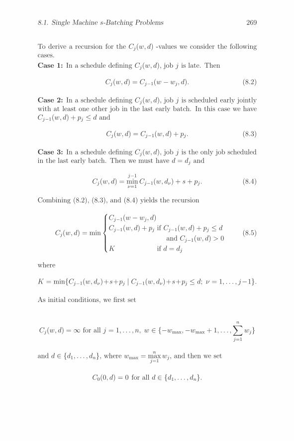
8.1. Single Machine s-Batching Problems 269
To derive a recursion for the Cj(w, d) -values we consider the followingcases.
Case 1: In a schedule defining Cj(w, d), job j is late. Then
Cj(w, d) = Cj−1(w − wj, d). (8.2)
Case 2: In a schedule defining Cj(w, d), job j is scheduled early jointlywith at least one other job in the last early batch. In this case we haveCj−1(w, d) + pj ≤ d and
Cj(w, d) = Cj−1(w, d) + pj . (8.3)
Case 3: In a schedule defining Cj(w, d), job j is the only job scheduledin the last early batch. Then we must have d = dj and
Cj(w, d) =j−1
minν=1
Cj−1(w, dν) + s + pj . (8.4)
Combining (8.2), (8.3), and (8.4) yields the recursion
Cj(w, d) = min
⎧⎪⎪⎪⎨
⎪⎪⎪⎩
Cj−1(w − wj, d)
Cj−1(w, d) + pj if Cj−1(w, d) + pj ≤ d
and Cj−1(w, d) > 0
K if d = dj
(8.5)
where
K = min{Cj−1(w, dν)+s+pj | Cj−1(w, dν)+s+pj ≤ d; ν = 1, . . . , j−1}.
As initial conditions, we first set
Cj(w, d) = ∞ for all j = 1, . . . , n, w ∈ {−wmax,−wmax + 1, . . . ,n∑
j=1
wj}
and d ∈ {d1, . . . , dn}, where wmax =n
maxj=1
wj, and then we set
C0(0, d) = 0 for all d ∈ {d1, . . . , dn}.
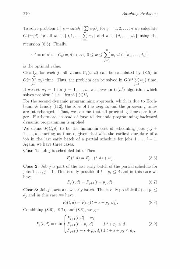
270 Batching Problems
To solve problem 1 | s − batch | ∑wjUj for j = 1, 2, . . . , n we calculate
Cj(w, d) for all w ∈ {0, 1, . . . ,n∑
j=1
wj} and d ∈ {d1, . . . , dn} using the
recursion (8.5). Finally,
w∗ = min{w | Cn(w, d) < ∞, 0 ≤ w ≤n∑
j=1
wj, d ∈ {d1, . . . , dn}}
is the optimal value.
Clearly, for each j, all values Cj(w, d) can be calculated by (8.5) in
O(nn∑
j=1
wj) time. Thus, the problem can be solved in O(n2n∑
j=1
wj) time.
If we set wj = 1 for j = 1, . . . , n, we have an O(n3) algorithm whichsolves problem 1 | s − batch | ∑
Uj .
For the second dynamic programming approach, which is due to Hoch-baum & Landy [112], the roles of the weights and the processing timesare interchanged. Thus, we assume that all processing times are inte-ger. Furthermore, instead of forward dynamic programming backwarddynamic programming is applied.
We define Fj(t, d) to be the minimum cost of scheduling jobs j, j +1, . . . , n, starting at time t, given that d is the earliest due date of ajob in the last early batch of a partial schedule for jobs 1, . . . , j − 1.Again, we have three cases.
Case 1: Job j is scheduled late. Then
Fj(t, d) = Fj+1(t, d) + wj . (8.6)
Case 2: Job j is part of the last early batch of the partial schedule forjobs 1, . . . , j − 1. This is only possible if t + pj ≤ d and in this case wehave
Fj(t, d) = Fj+1(t + pj , d). (8.7)
Case 3: Job j starts a new early batch. This is only possible if t+s+pj ≤dj and in this case we have
Fj(t, d) = Fj+1(t + s + pj , dj). (8.8)
Combining (8.6), (8.7), and (8.8), we get
Fj(t, d) = min
⎧⎪⎨
⎪⎩
Fj+1(t, d) + wj
Fj+1(t + pj , d) if t + pj ≤ d
Fj+1(t + s + pj, dj)if t + s + pj ≤ dj .
(8.9)
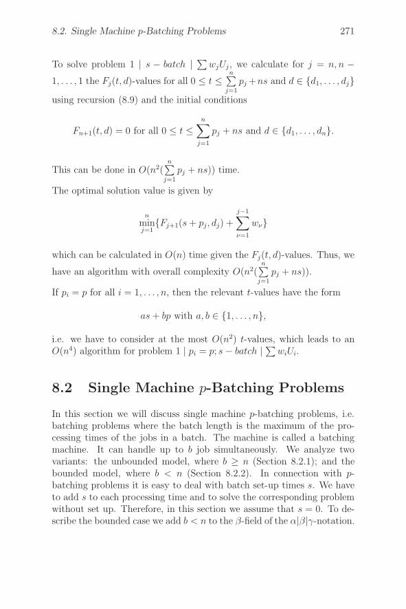
8.2. Single Machine p-Batching Problems 271
To solve problem 1 | s − batch | ∑wjUj , we calculate for j = n, n −
1, . . . , 1 the Fj(t, d)-values for all 0 ≤ t ≤n∑
j=1
pj +ns and d ∈ {d1, . . . , dj}using recursion (8.9) and the initial conditions
Fn+1(t, d) = 0 for all 0 ≤ t ≤n∑
j=1
pj + ns and d ∈ {d1, . . . , dn}.
This can be done in O(n2(n∑
j=1
pj + ns)) time.
The optimal solution value is given by
n
minj=1
{Fj+1(s + pj, dj) +
j−1∑
ν=1
wν}
which can be calculated in O(n) time given the Fj(t, d)-values. Thus, we
have an algorithm with overall complexity O(n2(n∑
j=1
pj + ns)).
If pi = p for all i = 1, . . . , n, then the relevant t-values have the form
as + bp with a, b ∈ {1, . . . , n},
i.e. we have to consider at the most O(n2) t-values, which leads to anO(n4) algorithm for problem 1 | pi = p; s − batch | ∑
wiUi.
8.2 Single Machine p-Batching Problems
In this section we will discuss single machine p-batching problems, i.e.batching problems where the batch length is the maximum of the pro-cessing times of the jobs in a batch. The machine is called a batchingmachine. It can handle up to b job simultaneously. We analyze twovariants: the unbounded model, where b ≥ n (Section 8.2.1); and thebounded model, where b < n (Section 8.2.2). In connection with p-batching problems it is easy to deal with batch set-up times s. We haveto add s to each processing time and to solve the corresponding problemwithout set up. Therefore, in this section we assume that s = 0. To de-scribe the bounded case we add b < n to the β-field of the α|β|γ-notation.
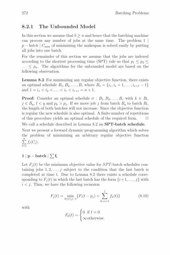
272 Batching Problems
8.2.1 The Unbounded Model
In this section we assume that b ≥ n and hence that the batching machinecan process any number of jobs at the same time. The problem 1 |p − batch | Cmax of minimizing the makespan is solved easily by puttingall jobs into one batch.
For the remainder of this section we assume that the jobs are indexedaccording to the shortest processing time (SPT) rule so that p1 ≤ p2 ≤. . . ≤ pn. The algorithms for the unbounded model are based on thefollowing observation.
Lemma 8.2 For minimizing any regular objective function, there existsan optimal schedule B1, B2, . . . , Br where Bν = {iν , iν + 1, . . . , iν+1 − 1}and 1 = i1 < i2 < . . . < ir < ir+1 = n + 1.
Proof: Consider an optimal schedule σ : B1, B2, . . . , Br with k ∈ Bl,j ∈ Bq, l < q and pk > pj. If we move job j from batch Bq to batch Bl,the length of both batches will not increase. Since the objective functionis regular the new schedule is also optimal. A finite number of repetitionsof this procedure yields an optimal schedule of the required form. �
We call a schedule described in Lemma 8.2 an SPT-batch schedule.
Next we present a forward dynamic programming algorithm which solvesthe problem of minimizing an arbitrary regular objective functionn∑
i=1
fi(Ci).
1 | p− batch | ∑fi
Let Fj(t) be the minimum objective value for SPT -batch schedules con-taining jobs 1, 2, . . . , j subject to the condition that the last batch iscompleted at time t. Due to Lemma 8.2 there exists a schedule corre-sponding to Fj(t) in which the last batch has the form {i+1, . . . , j} withi < j. Thus, we have the following recursion
Fj(t) = min0≤i≤j−1
{Fi(t − pj) +
j∑
k=i+1
fk(t)} (8.10)
with
F0(t) =
{0 if t = 0
∞otherwise.
8.2. Single Machine p-Batching Problems 273
To solve the problem we evaluate (8.10) for j = 1, . . . , n and t = pj, . . . ,j∑
k=1
pk. The optimal solution value is equal to min{Fn(t) | pn ≤ t ≤ P}
where P =n∑
k=1
pk.
To implement the algorithm efficiently, the partial sumsj∑
k=1
fk(t) are
evaluated and stored for j = 1, . . . , n and t = pj , . . . ,j∑
k=1
pk in a pre-
processing step in O(nP ) time. Then each application of the recursionequation (8.10) requires O(n) time. Thus, the dynamic programmingalgorithm requires O(n2P ) time and O(nP ) space.
1 | p − batch | ∑Ui
To solve this problem in polynomial time we use the objective value asthe state variable and the makespan as the value of a state. Furthermore,we build the schedule by adding single jobs instead of complete batchesand fix the last job to be scheduled in the current batch.
More specifically, we define a schedule for jobs 1, 2, . . . , j to be in state(j, u, k) where u ≤ j ≤ k if it contains exactly u tardy jobs. Additionally,the last batch, if completed, contains the additional jobs j+1, . . . , k whichare contained in the same batch, and this batch has processing time pk.Let Fj(u, k) be the minimum makespan for SPT -batch schedules in state(j, u, k). A schedule in state (j, u, k) with value Fj(u, k) is created bytaking one of the following decisions in a previous state:
• add job j so that it does not start the last batch.
In this case j − 1 and j belong to the last batch with processingtime pk. This processing time contributes to the makespan of theprevious state, which is Fj−1(u, k) or Fj−1(u − 1, k) depending onwhether j is on time or tardy. If Fj−1(u, k) ≤ dj, then we consider(j − 1, u, k) as a previous state in which j is scheduled on timeand Fj(u, k) = Fj−1(u, k). If Fj−1(u − 1, k) > dj, then j must betardy. Thus, (j − 1, u − 1, k) is considered as a previous state andFj(u, k) = Fj−1(u − 1, k).
• add job j so that it starts the last batch.
274 Batching Problems
The previous batch ends with job j − 1 and the processing timeof the new batch is pk. After adding the contribution from theprevious state, the makespan becomes Fj−1(u, j−1)+pk or Fj−1(u−1, j − 1) + pk, depending on whether j is on time or tardy. IfFj−1(u, j − 1) + pk ≤ dj, then we consider (j − 1, u, j − 1) as aprevious state (the last batch ends with j − 1) with j scheduledto be on time. If Fj−1(u − 1, j − 1) + pk > dj , then we consider(j−1, u−1, j−1) as a previous state with j scheduled to be tardy.
Summarizing, we have the recursion for j = 1, . . . , n, u = 0, . . . , j, andk = j, . . . , n:
Fj(u, k) = min
⎧⎪⎪⎪⎪⎪⎪⎨
⎪⎪⎪⎪⎪⎪⎩
Fj−1(u, k), if Fj−1(u, k) ≤ dj
Fj−1(u − 1, k), if Fj−1(u − 1, k) > dj
Fj−1(u, j − 1) + pk, if Fj−1(u, j − 1) + pk ≤ dj
Fj−1(u − 1, j − 1) + pk, if Fj−1(u − 1, j − 1) + pk > dj
∞, otherwise.
The initialization is
F0(u, k) =
{0, if u = 0 and k = 0
∞,otherwise.
The minimum number of tardy jobs is then equal to the smallest value ufor which Fn(u, n) < ∞. The algorithm requires O(n3) time and O(n3)space.
1 | p− batch | ∑wiCi
To solve this problem we apply backward dynamic programming. Let Fj
be the minimum total weighted completion time for SPT -batch schedulescontaining the last n−j+1 jobs j, j+1, . . . , n. Processing of the first batchin the schedule starts at zero time. Furthermore, whenever a new batch isadded to the beginning of this schedule, there is a corresponding delay tothe processing of all batches. Suppose that a batch {j, . . . , k− 1}, whichhas processing time pk−1, is inserted at the start of a schedule for jobsk, . . . , n. The total weighted completion time of jobs k, . . . , n increases by
pk−1
n∑
ν=k
wν , while the total weighted completion time for jobs j, . . . , k−1
8.2. Single Machine p-Batching Problems 275
is pk−1
k−1∑
ν=j
wν . Thus, the overall increase in total weighted completion
time is pk−1
n∑
ν=j
wν .
The dynamic programming recursion can now be formulated as follows.The initialization is
Fn+1 = 0
and for j = n, n − 1, . . . , 1 we have
Fj = minj<k≤n+1
{Fk + pk−1
n∑
ν=j
wν}.
The optimal solution value is equal to F1.
Fj can be interpreted as the length of a shortest path from j to n+1 in anetwork with vertices 1, . . . , n + 1, arcs (j, k) with j < k and arc lengths
cjk = pk−1
n∑
ν=j
wν .
The arc lengths cjk satisfy the product property
cjl − cjk = (pl−1 − pk−1)
n∑
ν=j
wν = h(k, l)f(j), j < k < l
with h(k, l) ≥ 0 and f(j) nonincreasing. Thus, all values Fj(j = n,n − 1, . . . , 1) can be calculated in O(n) time (see Section 2.7) if the jobsare enumerated according to nondecreasing pi-values. Therefore, theproblem can be solved in time O(n log n).
1 | p − batch | Lmax
Again, we apply backward dynamic programming. Let Fj be the mini-mum value for the maximum lateness for SPT -batch schedules containingjobs j, . . . , n, where processing starts at zero time. If batch {j, . . . , k−1},which has processing time pk−1, is inserted at the start of a schedule forjobs k, . . . , n, then the maximum lateness of jobs k, . . . , n increases bypk−1, while the maximum lateness for jobs j, . . . , k is max
j≤ν≤k−1(pk−1 − dν).
276 Batching Problems
We are now ready to give the dynamic programming recursion. Theinitialization is
Fn+1 = −∞,
and the recursion for j = n, n − 1, . . . , 1 is
Fj = minj<k≤n+1
max{Fk + pk−1, maxj≤ν≤k−1
{pk−1 − dν}}.
The optimal solution is then equal to F1. Clearly, the algorithm requiresO(n2) time and O(n) space.
Next we will show that this algorithm for the Lmax-problem can be usedas a subroutine for solving the fmax-problem.
1 | p− batch | fmax
Let fmax =n
maxi=1
fi(Ci), where each fi is a nondecreasing function of the
finishing time of job i. We assume that the optimal solution value of theproblem is an integer whose logarithm is polynomially bounded in thesize of the input. Then 1 | p − batch | fmax can be solved polynomiallyif, for any integer k, there is a polynomial algorithm which solves thedecision problem P (k): Does there exist a solution with fmax ≤ k?
Such an algorithm for solving P (k) can be obtained as follows. A sched-ule satisfies the condition fmax ≤ k if and only if fj(Cj) ≤ k for allj = 1, . . . , n. The condition fj(Cj) ≤ k induces a deadline dj on thecompletion time of job j which can be determined in O(log P ) time by
binary search over the P +1 possible completion times where P :=n∑
ν=1
pν .
Once the deadlines have been determined, we can use the algorithm forminimizing Lmax to find out if there is a solution with fj(Cj) ≤ k bychecking the condition Lmax ≤ 0. Hence, the question “is fmax ≤ k?”can be answered in O(n2 + n log P ) time.
This is almost as far as we can get with polynomial algorithms becausethe problems 1 | p− batch | ∑
wiUi and 1 | p− batch | ∑wiTi have been
shown to be NP -hard.
8.2.2 The Bounded Model
It is easy to show that 1 | p − batch; b < n | Cmax can be solved inO(n logn) time: We assume that n is a multiple of b. If this is not the
8.3. Complexity Results for Single Machine Batching Problems 277
case, we add dummy jobs with zero processing times. Now the batchesare constructed as follow. Assign the b jobs with smallest processingtimes to the first batch B1, then b jobs with the next smallest processingtimes to B2, and so on, until all jobs are assigned. An easy exchangeargument shows that this must be optimal.
On the other hand, problems of type 1 | p−batch; b = 1 | f are equivalentto the corresponding single machine problems. Thus, NP -hardness re-sults for single machine problems are also valid for p-batching problemswith bounded batch size. Furthermore, 1 | p − batch; b = 2 | Lmax isstrongly NP -hard.
8.3 Complexity Results for Single Machine
Batching Problems
Tables 8.1 and 8.2 present complexity results for single machine s-bat-ching problems. Several problems are NP-hard because the correspond-ing single machine problem without batching (i.e. with s = 0) are NP-hard.
Tables 8.3 and 8.4 contain complexity results for single machine p-bat-ching problems. Note that we have shown that 1 | p−batch | ∑
fi can besolved in time O(n2P ). Serial batching problems and bounded parallelbatching problems with constant processing times, release dates, andthe objective function
∑wiCi,
∑wiUi,
∑Ti can be solved polynomially
using a dynamic programming approach related to the one discussed inSection 4.6.
Complexity results for some bounded parallel batching problems withconstant processing times are derived from the fact that these prob-lems are equivalent to corresponding problems with identical parallelmachines.
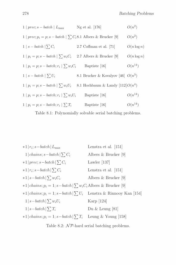
278 Batching Problems
1 | prec; s − batch | Lmax Ng et al. [176] O(n2)
1 | prec; pi = p; s − batch | ∑Ci8.1 Albers & Brucker [9] O(n2)
1 | s − batch |∑Ci 2.7 Coffman et al. [71] O(n log n)
1 | pi = p; s − batch | ∑wiCi 2.7 Albers & Brucker [9] O(n log n)
1 | pi = p; s − batch; ri |∑
wiCi Baptiste [16] O(n14)
1 | s − batch | ∑Ui 8.1 Brucker & Kovalyov [46] O(n3)
1 | pi = p; s − batch | ∑wiUi 8.1 Hochbaum & Landy [112]O(n4)
1 | pi = p; s − batch; ri |∑
wiUi Baptiste [16] O(n14)
1 | pi = p; s − batch; ri |∑
Ti Baptiste [16] O(n14)
Table 8.1: Polynomially solvable serial batching problems.
∗1 |ri; s−batch |Lmax Lenstra et al. [151]
1 |chains; s−batch |∑ Ci Albers & Brucker [9]
∗1 |prec; s−batch |∑Ci Lawler [137]
∗1 |ri; s−batch |∑ Ci Lenstra et al. [151]
∗1 |s−batch |∑ wiCi Albers & Brucker [9]
∗1 |chains; pi = 1; s−batch |∑ wiCiAlbers & Brucker [9]
∗1 |chains; pi = 1; s−batch |∑ Ui Lenstra & Rinnooy Kan [154]
1 |s−batch |∑ wiUi Karp [124]
1 |s−batch |∑ Ti Du & Leung [81]
∗1 |chains; pi = 1; s−batch |∑ Ti Leung & Young [158]
Table 8.2: NP-hard serial batching problems.

8.3. Complexity Results for Single Machine Batching Problems 279
1 | p − batch | Cmax 8.2.1 Brucker et al. [36]O(n)
1 | outtree; pi = p; p − batch; ri; b < n | Cmax Brucker et al. [35]O(n)
1 | p − batch; b < n | Cmax 8.2.1 Brucker et al. [36]O(n log n)
1 | tree; pi = p; p − batch; b < n | Cmax Hu [116]O(n)
1 | p − batch | Lmax 8.2.1 Brucker et al. [36]O(n log n)
1 | chains; pi = 1; p − batch; ri; b < n | Lmax Parallel machine problem1 | intree; pi = p; p − batch; b < n | Lmax Brucker et al. [35]
O(n)1 | outtree; pi = 1; p − batch; ri; b < n | ∑
Ci Brucker et al. [38]O(n2)
1 | tree; pi = p; p − batch; b < n | ∑Ci Parallel machine problem
1 | p − batch | ∑wiCi 8.2.1 Brucker et al. [36]
O(n log n)1 | pi = p; p − batch; ri; b < n | ∑
wiCi Baptiste [16]O(n8)
1 | p − batch | ∑Ui 8.2.1 Brucker et al. [36]
O(n3)1 | pi = p; p − batch; ri; b < n | ∑
wiUi Baptiste [16]O(n8)
1 | prec; pi = p; p − batch | ∑wiUi Earliest Start Schedule
O(n2)1 | pi = p; p − batch; ri; b < n | ∑
Ti Baptiste [16]O(n8)
1 | pi = 1; p − batch; ri; b < n | ∑wiTi Network flow problem
1 | pi = p; p − batch; b < n | ∑wiTi Network flow problem
1 | pi = p; p − batch; ri; |∑
wiUi Baptiste et al. [21]O(n11)
1 | prec; pi = p; p − batch | ∑wiTi Earliest Start Schedule
O(n2)
Table 8.3: Polynomially solvable parallel batching problems.
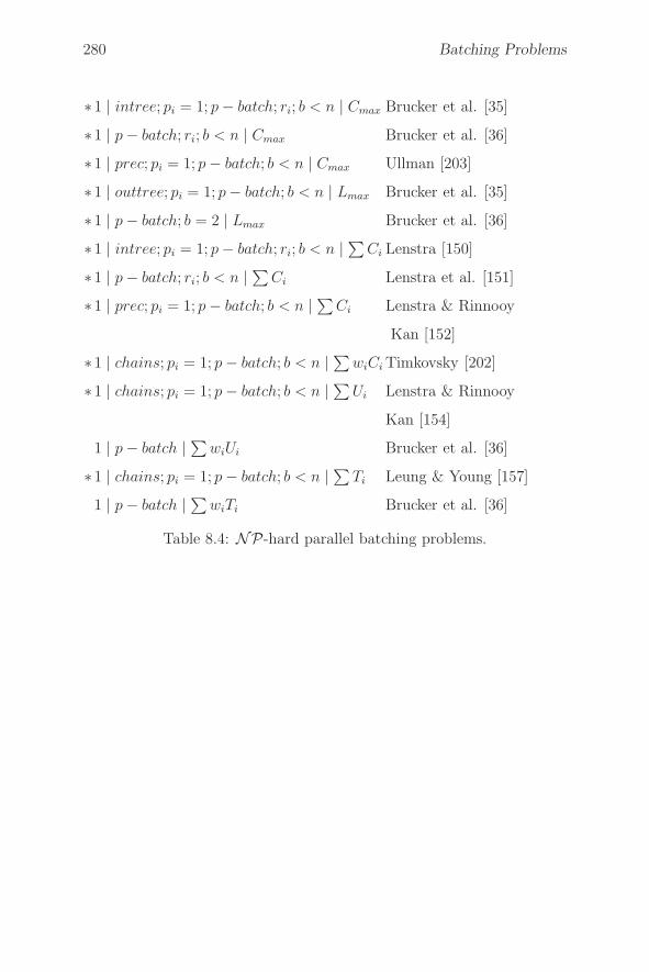
280 Batching Problems
∗1 | intree; pi = 1; p − batch; ri; b < n | Cmax Brucker et al. [35]
∗1 | p − batch; ri; b < n | Cmax Brucker et al. [36]
∗1 | prec; pi = 1; p − batch; b < n | Cmax Ullman [203]
∗1 | outtree; pi = 1; p − batch; b < n | Lmax Brucker et al. [35]
∗1 | p − batch; b = 2 | Lmax Brucker et al. [36]
∗1 | intree; pi = 1; p − batch; ri; b < n | ∑Ci Lenstra [150]
∗1 | p − batch; ri; b < n | ∑Ci Lenstra et al. [151]
∗1 | prec; pi = 1; p − batch; b < n | ∑Ci Lenstra & Rinnooy
Kan [152]
∗1 | chains; pi = 1; p − batch; b < n | ∑wiCi Timkovsky [202]
∗1 | chains; pi = 1; p − batch; b < n | ∑Ui Lenstra & Rinnooy
Kan [154]
1 | p − batch | ∑wiUi Brucker et al. [36]
∗1 | chains; pi = 1; p − batch; b < n | ∑Ti Leung & Young [157]
1 | p − batch | ∑wiTi Brucker et al. [36]
Table 8.4: NP-hard parallel batching problems.
Chapter 9
Changeover Times andTransportation Times
In this chapter we consider scheduling problems in which the set I of alljobs or all operations (in connection with shop problems) is partitionedinto disjoint sets I1, . . . , Ir called groups, i.e. I = I1 ∪ I2 ∪ . . . ∪ Ir andIf ∩ Ig = φ for f, g ∈ {1, . . . , r}, f �= g. Let Nj be the number of jobsin Ij . Furthermore, we have the additional restrictions that for any twojobs (operations) i, j with i ∈ If and j ∈ Ig to be processed on the samemachine Mk, job (operation) j cannot be started until sfgk time unitsafter the finishing time of job (operation) i, or job (operation) i cannotbe started until sgfk time units after the finishing time of job (operation)j. In a typical application, the groups correspond to different types ofjobs (operations) and sfgk may be interpreted as a machine dependentchangeover time. During the changeover period, the machine cannotprocess another job. We assume that sfgk = 0 for all f, g ∈ {1, . . . , r},k ∈ {1, . . . , m} with f = g, and that the triangle inequality holds:
sfgk + sghk ≥ sfhk for all f, g, h ∈ {1, . . . , r}, k ∈ {1, . . . , m}. (9.1)
Both assumptions are realistic in practice.
If we consider single machine problems or if the changeover times are ma-chine independent, we replace sfgk by sfg. If the changeover times do notdepend on both groups If and Ig, but only on the group Ig to which thejob to be processed next belongs, then we replace sfg by sg. In the lattercase, the changeover times are called sequence independent, contraryto the general case in which they are called sequence dependent. If

282 Changeover Times and Transportation Times
sfg = s for all f, g = 1, . . . , r, then we have constant changeover times.
To indicate problems with changeover times, we add β7 ∈ {sfgk, sfg, sg, s}to the β-part of our general classification scheme.
In Section 9.1, single machine problems with changeover times will bediscussed. Section 9.2 describes some results on parallel machine prob-lems with changeover times, while in the last section, shop problems withchangeover and/or transportation times are introduced.
9.1 Single Machine Problems
While problems 1 | sfg | Cmax and 1 | sg | Lmax are NP-hard (Bruno& Downey [59]), problem 1 | sg | Cmax can be solved polynomially byscheduling the jobs group by group in any order.
Next we will present dynamic programming procedures for the problems1 | sfg | Lmax, 1 | sfg | ∑
wiCi, and 1 | sfg | ∑wiUi, which are due
to Monma & Potts [170]. The following theorem is the basis for theseprocedures.
Theorem 9.1 (a) For problem 1 | sfg | ∑wiUi, there exists an opti-
mal schedule where the early jobs within each group are orderedaccording to nondecreasing due dates.
(b) For problem 1 | sfg | ∑wiCi, there exists an optimal schedule
where the jobs within each group are ordered according to nonde-creasing pi/wi-values.
(c) For problem 1 | sfg | Lmax, there exists an optimal schedule wherethe jobs within each group are ordered according to nondecreasingdue dates.
Proof: Consider a schedule of the form D, j, E, i, F , where jobs i andj are from the same group and D, E, F represent arbitrary blocks, i.e.partial sequences of jobs. Due to the triangle inequality (9.1), the totalchangeover times will not increase if D, j, E, i, F is replaced by D, E, i, j,F or D, i, j, E, F . We have to show that if di < dj for early jobs i, j, orpi/wi < pj/wj, or di < dj , then
∑wiUi, or
∑wiCi, or the Lmax-value
will not increase when moving from the sequence D, j, E, i, F to one ofthe two sequences D, E, i, j, F or D, i, j, E, F .
9.1. Single Machine Problems 283
(a) If we have the objective function∑
wiUi, then the fact that i isearly in D, j, E, i, F implies that i, j are early in D, E, i, j, F be-cause di < dj.
(b) Consider the objective function∑
wiCi and let pi/wi < pj/wj.
It is convenient to replace changeover times by set-up jobs with pro-cessing time equal to the changeover time and zero weight. Further-more, we assume that all set ups after j and before i in D, j, E, i, Fare included in the partial sequence E. Define
p(E) =∑
i∈E
pi and w(E) =∑
i∈E
wi.
Then an easy calculation shows that job j and block E can beswapped without increasing the objective value if pj/wj > p(E)/w(E). Similarly, i and E can be swapped if p(E)/w(E) > pi/wi.In the first case we first swap j and E and then j and i with-out increasing the objective value. This provides the sequenceD, E, i, j, F . If pj/wj ≤ p(E)/w(E), then pi/wi < p(E)/w(E)and we get D, i, j, E, F after two swaps.
(c) Consider the objective function Lmax and let di < dj. Again,changeover times are replaced by set-up jobs with the changeovertime as the processing time and a very large due date. To see theeffect of swapping a job j scheduled before a block E = ir, ir−1, . . . ,i1, we replace E by a job with processing time pir ,ir−1,...,i1 = p(E)and a due date dir,ir−1,...,i1, where dir,ir−1,...,i1 is calculated by therecursion
diϑ+1,...,i1 = min{diϑ,...,i1, diϑ+1+
ϑ∑
k=1
pik} for ϑ = 1, 2, . . . , r − 1.
This follows by induction using the fact that, for two jobs i and jwith finishing times Cj and Ci = Cj − pj , we have
max{Cj − dj, Cj − pj − di} = Cj − min{dj, di + pj}.Now we can proceed as in Part (b). If dj > dE := dir ,ir−1,...,i1, thenwe can first swap j and E and then j and i without increasing theobjective value. Otherwise, we have di < dj ≤ dE and we can firstswap i and E and then j and i. �
284 Changeover Times and Transportation Times
For the following dynamic programming algorithms, we assume that thejobs in each group are ordered according to Theorem 9.1. We first derivean algorithm for problem 1 | sfg | ∑
wiCi.
We define C(n1, n2, . . . , nr, t, h) to be the minimum cost of a partialschedule containing the first nj jobs of group Ij (j = 1, . . . , r), wherethe last job scheduled comes from group Ih and is completed at time t.We have
0 ≤ nj ≤ Nj for j = 1, . . . , r
and
0 ≤ t ≤ T :=∑
i∈I
pi +r∑
j=1
Nj max{sfj | 1 ≤ f ≤ r}.
The recursion is
C(n1, n2, . . . , nr, t, h)
= min{C(n′1, n
′2, . . . , n
′r, t
′, f) + whnh
t | 1 ≤ f ≤ r} (9.2)
where n′j = nj for j �= h, n′
h = nh − 1, t′ = t− phnh
− sfh, and whnh
and phnh
are the weight and processing time of the nh-th job in group Ih.
Initially, we set C(0, 0, . . . , 0, 0, 0) = 0 and all other C-values to infinity.
The optimal schedule cost is found by selecting the smallest value of theform C(N1, . . . , Nr, t, h) for some schedule completion time 0 ≤ t ≤ Tand some group Ih to which the final job belongs.
Because the number of states is bounded by O(rnrT ) and (9.2) can becalculated in O(r) steps, we have an O(r2nrT )-algorithm.
Alternatively, we can replace the state variable t by variables tfh (f, h =1, . . . , r) representing the number of set ups from group f to group h.Note that t is readily computed from the state variables using
t =
r∑
f,h=1
tfhsfh +
r∑
h=1
nh∑
ν=1
phν .
The complexity of this version is O(r2nr+s), where s is the number ofdifferent values for changeover times. Note that s ≤ r2 in general ands ≤ r in the case of sequence-independent changeover times. If thenumber of groups is fixed, we have a polynomial algorithm.
9.1. Single Machine Problems 285
Similarly, we solve problem 1 | sfg | Lmax. In this case (9.2) is replacedby
C(n1, n2, . . . , nr, t, h)
= min{max{C(n′1, n
′2, . . . , n
′r, t
′, f), t − dhnk} | 1 ≤ f ≤ r}. (9.3)
The problem with the weighted number of late jobs is solved differently.By Theorem 9.1(a), we only know an order for early jobs; those jobs thatare late must also be determined by the algorithm. The late jobs maybe appended in any order to the schedule of on-time jobs.
We define C(n1, n2, . . . , nr, t, h) to be the minimum weighted number oflate jobs for the partial schedule containing the first nj jobs of groupIj (j = 1, . . . , r), where the last on-time job comes from group Ih and iscompleted at time t. We have
0 ≤ nj ≤ Nj for j = 1, . . . , r
and
0 ≤ t ≤ T := min{maxi∈I
di,∑
i∈I
pi +r∑
j=1
Nj max{sfj | 1 ≤ f ≤ r}}.
The recursion is
C(n1, n2, . . . , nr, t, h) =
⎧⎪⎪⎪⎨
⎪⎪⎪⎩
min{ min1≤f≤r
C(n′1, n
′2, . . . , n
′r, t
′, f),
C(n′1, n
′2, . . . , n
′r, t, h) + wh
nh} if t ≤ dh
nh
C(n′1, n
′2, . . . , n
′r, t, h) + wh
nhif t > dh
nh
(9.4)where n′
j = nj if j �= h, n′h = nh − 1, t′ = t − ph
nh− sfh.
The initial values are
C(n1, n2, . . . , nr, 0, 0) =r∑
j=1
nj∑
ν=1
wjν
for 0 ≤ nj ≤ Nj , where j = 1, . . . , r. All other initial values are set toinfinity.
The minimum weighted number of late jobs is found by selecting thesmallest value of the form C(N1, N2, . . . , Nr, t, h) for some completion
286 Changeover Times and Transportation Times
time of on-time jobs, where 0 ≤ t ≤ T , and for some group Ih containingthe final on-time job.
The complexity is O(r2nrT ). Again, it may be desirable to eliminate thestate variable t from the recursion. To achieve this, we switch the statevariable t with the objective function value as follows.
Define C(n1, n2, . . . , nr, w, h) to be the minimum completion time of on-time jobs for a partial schedule containing the first nj jobs of each groupIj, where the weighted number of late jobs is equal to w, and the laston-time job comes from group Ih. The initial values are C(n1, n2, . . . , nr,
w, 0) = 0, where w =r∑
j=1
nj∑
ν=1
wjν for 0 ≤ nj ≤ Nj (j = 1, . . . , r), and all
other values are set to infinity.
The recursion is
C(n1, n2, . . . , nr, w, h) = min{ min1≤f≤r
{C(n′1, n
′2, . . . , n
′r, w, f) + p′fh |
C(n′1, n
′2, . . . , n
′r, w, f) + p′fh ≤ dh
nh}, C(n′
1, n′2, . . . , n
′r, w
′, h)}
where n′j = nj if j �= h, n′
h = nh − 1, p′fh = phnh
+ sfh and w′ = w − whnh
.
As in (9.4), the first term in the minimization chooses the nh-th job ingroup Ih to be scheduled on time, if possible, and chooses the previouson-time job from group If ; the second term selects the nh-th job of groupIh to be late.
The minimum weighted number of late jobs is found by selecting thesmallest w for which min
0≤h≤rC(N1, N2, . . . , Nr, w, h) is finite.
The complexity is O(r2nrW ), where W =∑
i∈I
wi. It reduces to O(r2nr+1)
for the total number of late jobs problem.
9.2 Problems with Parallel Machines
In this section we consider changeover times in connection with parallel,identical (uniform, unrelated) machines. For unrelated machines, wehave machine dependent changeover times sfgk. In the case of uniformmachines, the changeover time depends on the speed rk of machine k,more specifically sfgk = sfg/rk.
We saw in the last section that even in the one machine case, problemswith sequence dependent changeover times are NP-hard in all but trivial
9.2. Problems with Parallel Machines 287
cases. Therefore, we restrict ourselves to parallel machine problems withsequence independent changeover times sgk, sgk = sg/rk, or sg for unre-lated, uniform, or identical machines. As before, there are r job groupsI1, . . . , Ir, where Nj is the number of jobs in group Ij.
The two problems P2 | pj = 1; sg = 1 | Cmax and Q | pj = 1; sg = 1; Nj =h | Cmax are NP-hard (Brucker et al. [47]). Thus, we can only expectpolynomial algorithms in special situations.
One such problem is P | pj = p; sg = p; Nj = h | Cmax, i.e. a problemwith identical parallel machines where all groups have equal sizes and allprocessing and changeover times are equal to p.
Let P (y) be the problem of finding a schedule for P | pj = p; sg = p; Nj =h | Cmax with Cmax ≤ y if such a schedule exists. P (y) can be solved byapplying Mc Naughton’s Wrapping Around Rule: Schedule the groupsone after the other in the interval [0, y] by filling this interval for eachmachine, one machine after the other. Continue to schedule a groupon the next machine if the group cannot be completed on the currentmachine.
Theorem 9.2 Problem P (y) has a solution if and only if all jobs can bescheduled by applying the Wrapping Around Rule.
Proof: Consider a feasible schedule. Assume that all groups scheduledcompletely on M1 are scheduled at the beginning of the interval [0, y].Let i be the first group not completely scheduled on M1 and assume thatthe i-jobs, i.e. the jobs belonging to group i, are scheduled immediatelyafter the last complete group on M1. Let c be the completion time ofthe last i-job.
There exists a machine, say M2, on which other i-jobs are scheduled.Assume that on M2 all i-jobs are scheduled at the beginning of [0, y] andthat the last i-job on M2 finishes at time a. Then we consider three cases.
Case 1: y − c < 2p
If y − c < p, no further job can be scheduled on M1. If y − c ≥ p, thenwe move one i-job from M2 to M1.
Case 2: y − c ≥ 2p and a ≤ y − c
We exchange the jobs (including set-up jobs) scheduled on M1 in theinterval [c, c + a] with the i-jobs and the set-up job scheduled on M2 in[0, a] as shown in Figures 9.1(a) and 9.1(b).

288 Changeover Times and Transportation Times
i i · · ·· · · i i ∗ ∗
M2
M1
(a)
� �a
� �(y − c)
∗ ∗i i i i
M2
M1
y(b)
Figure 9.1: Extending group of i-job on M1: Case 2.
Case 3: y − c ≥ 2p and a > y − c
We have the situation as shown in Figure 9.2(a) and transform this sched-ule into the one in Figure 9.2(b).
i i i · · ·· · · i i ∗ ∗
M2
M1
(a)
∗ ∗· · · i i i i i
M2
M1
(b)y
Figure 9.2: Extending group of i-job on M1: Case 3.
The whole process is repeated until after a finite number of steps we geta schedule with the desired properties.
Due to the fact that all job groups have equal sizes and all machines areidentical, the wrapping around rule creates a feasible schedule. �

9.2. Problems with Parallel Machines 289
The computation time of the Wrapping Around Algorithm is boundedby O(m). To find an optimal Cmax-value C∗, we exploit the followingfacts:
• L := � r(h+1)m
p is a lower bound for C∗, and
• L+p is an upper bound for C∗ (the Wrapping Around schedule fory = L + p is always feasible because the extra p-value allows for anadditional set up on each machine).
Thus, we only need to solve the two problems P (L) and P (L + p). Thisprovides us with O(m)-algorithm.
Mc Naughton’s Wrapping Around Rule solves the problem even if thechangeover time is a multiple of the processing time p, i.e. if pj = pand sg = lp where l is an arbitrary positive integer. The interchangearguments in the proof of Theorem 9.2 are almost the same.
If we replace the identical machines by uniform machines, then the ex-change arguments of Theorem 9.2 are still valid. However, Mc Naugh-ton’s Wrapping Around Rule does not solve the corresponding problemQ | pj = p; sg = lp; Nj = h; dj = y | −. The reason for this is that theWrapping Around Rule depends on the order of the uniform machines.To solve the problem we may apply the Wrapping Around Rule to eachof the m! possible orders which yields an O(mm!)-algorithm. This algo-rithm is polynomial if m is fixed.
Finally, note that the O(m)-algorithm which solves P (y) by applyingthe Wrapping Around Rule is not a polynomial one. Next, an O(log m)-algorithm will be presented which solves problem P (y). This algorithmcan be described as follows.
Let s = lp. In the interval [0, Y ] with Y = (hp+s)�y/(hp+s)� we scheduleas many groups as possible without splitting them into subgroups. Ifall groups can be scheduled, we have finished. Otherwise each of theremaining groups is divided into subgroups including U := �(y−Y −s)/p�jobs, except possibly the last subgroups including Q < U jobs. Weschedule the subgroups with U jobs without splitting them on the mavailable machines. If all of these subgroups are scheduled and Q = 0,we have finished. If the number r of these subgroups is greater thanm or r = m and Q > 0, no feasible schedule exists. Otherwise, we setm′ = m − r, y′ = y − Y, p′ = p, h′ = Q and apply the same procedurerecursively to the problem specified by m′, y′, p′, h′.
290 Changeover Times and Transportation Times
Note that we may assume that r > �m2�, because otherwise all batches
with Q jobs can be scheduled in [Y, y] on the remaining m′ = m−r > �m2�
machines and we have finished. Thus, the number of recursive calls isat the most O(log m). In each recursive step the corresponding schedulecan be calculated in constant time.
Using the interchange techniques described in the proof of Theorem 9.2,it can be shown that an optimal schedule exists with the described struc-ture. This leads to
Theorem 9.3 Problem P | pj = p; sg = lp; Nj = h | Cmax can be solvedin time O(log m).
9.3 General Shop Problems
In connection with general shop problems, we may have changeover timesand transportation times. For changeover times, we have a partition ofthe set I = {1, . . . , t} of operations of all jobs into disjoint sets I1, . . . , Ir.Again, we call these sets groups. If, on a specific machine Mk, an op-eration i from group Ih is processed immediately after an operation jfrom group Il, a changeover time tlhk occurs between i and j. In thedisjunctive graph model we can take care of the changeover time fromoperation j to operation i by labeling the fixed disjunctive arc (j, i) withtlhk. Furthermore, the length of a path in the corresponding network isnow equal to the sum of all vertex labels and arc labels on the path.Using these concepts, it is possible to generalize the branch-and-boundmethod presented in Section 6.4.3 to this more general situation (seeBrucker & Thiele [57]).
If in the general shop model we replace “sets of operations to be processedon the same machine” by “sets of operations belonging to the same job”and introduce a changeover time tlhi if an operation of job i belonging togroup Il is processed immediately before an operation of job i belongingto group Ih, then we get a model which is mathematically equivalent tothe previous one. If group Ik is the set of operations to be processed onmachine Mk, then tlhi may be interpreted as the time to transport job ifrom machine Ml to machine Mh. Due to the equivalence of both models,an algorithm which solves the general shop problem with changeovertimes solves the general shop problem with transportation times. Itshould be noted that in the transportation model we assume that there
9.3. General Shop Problems 291
is sufficient transportation capacity to handle all jobs to be transportedsimultaneously.
We can go a step further by considering problems with both changeovertimes and transportation times.
Chapter 10
Multi-Purpose Machines
In a multi-purpose machine (MPM) model there is a set of machinesμi(μij) ⊆ {M1, . . . , Mm} associated with a job Ji (operation Oij).Ji(Oij) has to be processed by one machine in the set μi(μij). Thus,scheduling problems with multi-purpose machines combine assignmentand scheduling problems: we have to schedule each job Ji (operationOij) on exactly one machine from the set μi(μij).
If we have single operation jobs and the multi-purpose machines haveidentical (uniform) speeds, we denote the corresponding situation byPMPM (QMPM). Note that P (Q) is the special case of PMPM(QMPM) in which all machine sets μi contain all m machines. Fur-thermore, PMPM is a special case of QMPM . We also may introduceRMPM to denote MPM problems with unrelated machines which gen-eralize QMPM problems. However in combination with regular objec-tive functions RMPM is equivalent to R because we may set pij = ∞ ifMj /∈ μi.
Shop problems with MPM are defined similarly. In a general shop withMPM , denoted by GMPM , there is a machine set μij associated witheach operation. The MPM job shop problem, denoted by JMPM , is thecorresponding special case of GMPM . For MPM flow shop problemsand MPM open shops, denoted by FMPM and OMPM , respectively,we need special definitions. For the MPM flow shop problem, each job Ji
has exactly r operations Oij (j = 1, . . . , r) and there is the same machineset μj associated with the j-th operation of each job. r is called thenumber of stages of the problem. Furthermore, all machine sets areassumed to be different, i.e. μj �= μk for j �= k. As in the classical case
294 Multi-Purpose Machines
for j = 2, . . . , r, Oij cannot start before Oi,j−1 is completed.
MPM open shop problems are defined like MPM flow shop problems.However, there are no precedence constraints between the operations ofan MPM open shop. In connection with FMPM problems and OMPMproblems, r is called the number of stages. Shop problems are MPMshop problems with one-element machine sets μij.
To describe and classify MPM problems, we combine PMPM , QMPM ,GMPM , JMPM , etc. with the other symbols used for the classificationof scheduling problems.
In Section 10.1, MPM problems with identical and uniform machineswill be discussed. Section 10.2 is devoted to MPM shop problems.
10.1 MPM Problems with Identical and
Uniform Machines
Problem RMPM‖∑Ci is equivalent to problem R‖∑
Ci. This problemcan be formulated as a weighted matching problem in a bipartite graphand can be solved in O(n3) time.
All other problems with arbitrary processing times and parallel multi-purpose machines are NP-hard because P2‖Cmax and P2‖∑
wiCi areNP-hard (Garey and Johnson [99] and Bruno et al. [58]).
Now let us consider problems with unit processing times.
Problems QMPM | pi = 1 | ∑wiUi(
∑wiTi)
Again, we reduce the problems to minimum cost bipartite matching prob-lems. Consider first problem QMPM | pi = 1 | ∑
wiUi. The correspond-ing bipartite graph is (V1 ∪ V2, A), where
• V1 is the set of jobs,
• V2 is the set of all pairs (j, t), where j represents Mj and t representsunit-time period [(t − 1)/sj, t/sj] (j = 1, . . . , m; t = 1, . . . , n),
• for each t = 1, . . . , n an arc from i to (j, t) exists if Mj ∈ μi, and
• the cost associated with the arc from i to (j, t) is given by wi ift/sj > dj and 0 otherwise.

10.1. MPM Problems with Identical and Uniform Machines 295
Problem QMPM | pi = 1 | ∑wiTi can be solved in the same way if we
replace the cost associated with the arc from i to (j, t) by
wi · max{0, t/sj − di}.
Problems PMPM | pi = 1; ri |∑
wiUi(∑
wiTi)
These problems are also formulated as minimum cost matching problemsin bipartite graphs which are nearly identical with those defined above.The main difference is that the time slots t = 1, . . . , n have to be replacedby different time slots t1, t2, . . . , tn, which are the earliest possible timeslots for scheduling n unit-time jobs with release times r1, . . . , rn on onemachine. Furthermore, we have to set sj = 1 for j = 1, . . . , m.
Problems PMPM2 | pi = 1; chains | Cmax
Surprisingly, problem PMPM 2 | pi = 1; chains | Cmax is NP-hard.This follows from an NP-hardness proof for problem PMPT 2 | pi =1; chains | Cmax given by Hoogeveen et al. [113].
Now let us consider
QMPM- and PMPM Problems with Preemption
Problem PMPM | pmtn | ∑Ci
We will show that every schedule with a finite number of preemptions canbe transformed into a nonpreemptive one without increasing the objectivevalue. Thus, the problem can be solved in O(n3) time by applying thealgorithm for R||∑Ci.
Theorem 10.1 Any schedule for problem PMPM | pmtn | ∑Ci can
be transformed into a nonpreemptive one without increasing the objectivevalue.
Proof: Consider an arbitrary schedule S for an instance of problemPMPM | pmtn | ∑
Ci with a finite number of preemptions. Since theclaim clearly holds for single machine problems, it suffices to transformthis schedule into a preemptive one where every job is processed by onlyone machine.
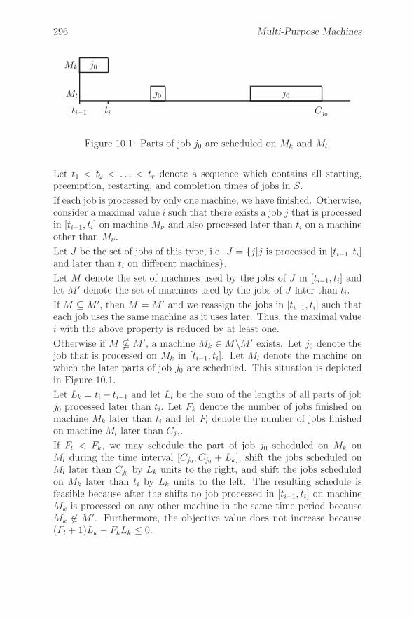
296 Multi-Purpose Machines
Mk
Ml j0 j0
j0
ti−1 ti Cj0
Figure 10.1: Parts of job j0 are scheduled on Mk and Ml.
Let t1 < t2 < . . . < tr denote a sequence which contains all starting,preemption, restarting, and completion times of jobs in S.
If each job is processed by only one machine, we have finished. Otherwise,consider a maximal value i such that there exists a job j that is processedin [ti−1, ti] on machine Mν and also processed later than ti on a machineother than Mν .
Let J be the set of jobs of this type, i.e. J = {j|j is processed in [ti−1, ti]and later than ti on different machines}.Let M denote the set of machines used by the jobs of J in [ti−1, ti] andlet M ′ denote the set of machines used by the jobs of J later than ti.
If M ⊆ M ′, then M = M ′ and we reassign the jobs in [ti−1, ti] such thateach job uses the same machine as it uses later. Thus, the maximal valuei with the above property is reduced by at least one.
Otherwise if M � M ′, a machine Mk ∈ M\M ′ exists. Let j0 denote thejob that is processed on Mk in [ti−1, ti]. Let Ml denote the machine onwhich the later parts of job j0 are scheduled. This situation is depictedin Figure 10.1.
Let Lk = ti − ti−1 and let Ll be the sum of the lengths of all parts of jobj0 processed later than ti. Let Fk denote the number of jobs finished onmachine Mk later than ti and let Fl denote the number of jobs finishedon machine Ml later than Cj0.
If Fl < Fk, we may schedule the part of job j0 scheduled on Mk onMl during the time interval [Cj0, Cj0 + Lk], shift the jobs scheduled onMl later than Cj0 by Lk units to the right, and shift the jobs scheduledon Mk later than ti by Lk units to the left. The resulting schedule isfeasible because after the shifts no job processed in [ti−1, ti] on machineMk is processed on any other machine in the same time period becauseMk �∈ M ′. Furthermore, the objective value does not increase because(Fl + 1)Lk − FkLk ≤ 0.
10.1. MPM Problems with Identical and Uniform Machines 297
Conversely, if Fl ≥ Fk, we may schedule the parts of job j0 scheduledlater than ti on Ml in [ti, ti + Ll] on Mk, shift the jobs scheduled onMk later than ti by Ll units to the right, and shift the remaining jobsscheduled on Ml later than ti as far to the left as possible. Due to themaximality of i, the resulting schedule is feasible. The objective valuedoes not increase because FkLl − FlLl ≤ 0.
Thus, we have reduced the set J by one element. This process can berepeated until the set J is empty. Hence the maximal value i with theabove property is again reduced by at least one. �
P 2 | pmtn | ∑wiCi is NP-hard since for problem P | pmtn | ∑
wiCi
preemptive schedules do not yield a smaller optimal objective value thannonpreemptive schedules (see Theorem 5.6) and P 2 || ∑
wiCi is NP-hard (Bruno et al. [58]).
QMPM and PMPM Problems with Preemption and ReleaseDates
Problem R | pmtn; ri | Lmax can be formulated as a linear program(see Section 5.1.3). This implies that QMPM | pmtn; ri | L max ispolynomially solvable. However, this is as far as we can get becausePMPM2 | pmtn; ri | ∑
Ci and PMPM2 | pmtn; ri | ∑Ui are NP-
hard. These NP-hardness results are a consequence of the fact that thecorresponding parallel machine problems are NP-hard (Du et al. [85],Du et al. [84]).
In this section we will derive an ε-approximation algorithm for problemPMPM | pmtn; ri | Lmax which is based on network flow concepts.
For a given threshold value L, we consider the decision problem of whe-ther a feasible solution exists with Lmax ≤ L. Because Lmax ≤ L isequivalent to
Ci ≤ dLi := di + L for i = 1, . . . , n
this problem is equivalent to the time window problem: Given releasetimes ri and deadlines di for each job, does there exist a feasible schedulewith
Ci ≤ di for i = 1, . . . , n?
To solve the time window problem, we generalize the network flow ap-proach described in Section 5.1.1.
Let t1, t2, . . . , tp+1 be a sequence of the release times ri and the due dates
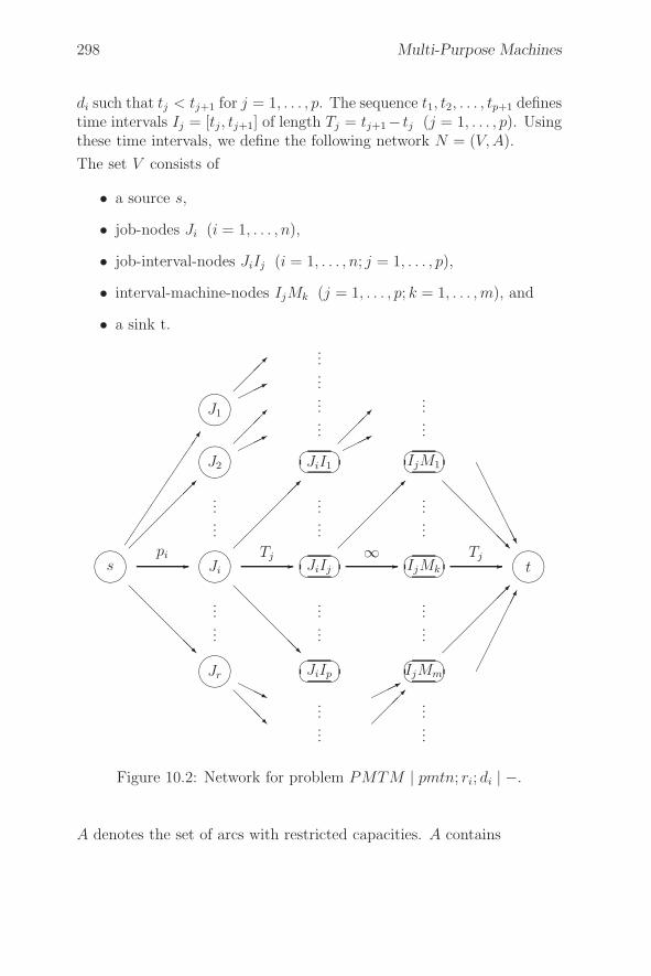
298 Multi-Purpose Machines
di such that tj < tj+1 for j = 1, . . . , p. The sequence t1, t2, . . . , tp+1 definestime intervals Ij = [tj , tj+1] of length Tj = tj+1− tj (j = 1, . . . , p). Usingthese time intervals, we define the following network N = (V, A).
The set V consists of
• a source s,
• job-nodes Ji (i = 1, . . . , n),
• job-interval-nodes JiIj (i = 1, . . . , n; j = 1, . . . , p),
• interval-machine-nodes IjMk (j = 1, . . . , p; k = 1, . . . , m), and
• a sink t.
��
��
s
��
��
J1
��
��
J2
��
��
Ji
��
��
Jr
�
�
�
�JiI1
�
�
�
�JiIj
�
�
�
�JiIp
�
�
�
�IjM1
�
�
�
�IjMk
�
�
�
�IjMm
��
��
t
��
���
��
���
��
��
���
�pi
��
��
���
����
����
����
����
��
��
���
�Tj
��
��
���
��������
����
����
��
��
���
�∞
��������
��������
��
��
����
Tj
��
��
���
��������
...
...
...
...
...
...
...
...
...
...
...
...
...
...
...
...
...
...
...
...
...
...
Figure 10.2: Network for problem PMTM | pmtn; ri; di | −.
A denotes the set of arcs with restricted capacities. A contains
10.1. MPM Problems with Identical and Uniform Machines 299
• arcs (s, Ji) with capacity pi (i = 1, . . . , n),
• arcs (Ji, JiIj) with capacity Tj if Ji can be processed in time intervalIj , i.e. ri ≤ tj and di ≥ tj+1 (i = 1, . . . , n; j = 1, . . . , p),
• arcs (JiIj, IjMk) with infinite capacity if Mk ∈ μi (i = 1, . . . , n;j = 1, . . . , p; k = 1, . . . , m), and
• arcs (IjMk, t) with capacity Tj (j = 1, . . . , p; k = 1, . . . , m).
Figure 10.2 shows a part of the resulting network.
We have the following
Theorem 10.2 For a given instance of PMPM |pmtn; ri; di|−, there ex-ists a feasible schedule if and only if there exists a flow from s to t in the
corresponding network N = (V, A) with flow valuer∑
i=1
pi.
Proof: First assume that there exists a feasible flow x = (x(i, j) :
(i, j) ∈ A) with flow value P :=r∑
i=1
pi. For all job-nodes Ji (i =
1, . . . , n) we have x(s, Ji) = pi because P =r∑
i=1
pi. A feasible sched-
ule of PMPM |pmtn; ri; di|− can be defined as follows.
(i) If x(Ji, JiIj) = l, then we schedule l time units of Ji in time intervalIj . This is possible because x(Ji, JiIj) ≤ Tj .
(ii) If x(JiIj, IjMk) = l, then we schedule l time units of Ji in timeinterval Ij on machine Mk. Because x(IjMk, t) ≤ Tj , machine Mk
is busy for at the most Tj time units during time interval Ij .
We obtain a classical open shop problem O|pmtn|Cmax in each time in-terval Ij by defining
pik := x(JiIj, IjMk) (i = 1, . . . , n; k = 1, . . . , m).
Because of (i) we have
Ai :=
m∑
k=1
pik ≤ Tj (i = 1, . . . , n; j = 1, . . . , p).
300 Multi-Purpose Machines
Moreover, because of (ii) we have
Bk :=
r∑
i=1
pik ≤ Tj (k = 1, . . . , m; j = 1, . . . , p).
As shown in Section 2.4, the optimal solution value of the open shop
problem is given by max{ nmaxi=1
Ai,m
maxk=1
Bk} ≤ Tj . Therefore, we can
schedule x(JiIj, IjMk) time units of job Ji on machine Mk in time in-terval Ij without violating any capacity constraints. By combining theschedules obtained in all time intervals, we get a feasible schedule forPMPM |pmtn; ri; di|−.
Now let there be a feasible schedule for a given instance of PMPM|pmtn; ri; di|−. Using (i) and (ii), it is easy to define a feasible flow
x = (x(i, j) : (i, j) ∈ A) with flow value P =r∑
i=1
pi based on this
schedule. �
To find a solution with an objective value that differs from the optimalobjective value by at the most ε time units, we do binary search on theset of values Llow + iε(i = 1, . . . , �Lup−Llow
ε ), where Llow(Lup) is a lower
(upper) bound for the optimal Lmax-value.
10.2 MPM Problems with Shop Charac-
teristics
In this section we study job shop, flow shop, and open shop problemswith multi-purpose machines. In Section 10.2.1, problems with arbitraryprocessing times are discussed. Section 10.2.2 is devoted to problemswith unit-processing times.
10.2.1 Arbitrary Processing Times
Job shop, flow shop, and open shop problems without preemption areinvestigated first. Then preemptive open shop scheduling problems areanalyzed.

10.2. MPM Problems with Shop Characteristics 301
MPM Job Shop Problems
First we consider job shop problems with a fixed number of jobs to beprocessed on multi-purpose machines. Contrary to the classical job shopproblem, the MPM job shop problem with two machines and three jobsis already NP-hard. On the other hand, the geometrical approach de-scribed in Section 6.4.2 can be extended to problem JMPM | n = 2 |Cmax. This can be seen as follows.
Assume that we have two jobs J1 and J2, and that μ assigns a machineμ(Oij) to each of the operations Oij of both jobs. For a fixed assignmentμ, the problem may be formulated as a shortest path problem in theplane with rectangular objects as obstacles. The obstacles are of the formI1i × I2j with μ(O1i) = μ(O2j), where I1i(I2j) are consecutive intervalsof length p1i(p2j) on the x-axis (y-axis). The path goes either diagonallyor parallel to the axes and has to avoid the interior of the obstacles (seeFigure 6.9).
As shown in Section 6.4.2, this shortest path problem can be reduced tothe problem of finding a shortest path from an origin to some destinationin a network N(μ) = (V (μ), A(μ), l(μ)), where
(i) V (μ) = {O, F}∪{ north-west corners of obstacles}∪{ south-east corners of obstacles}.
(ii) Each vertex i has at the most two immediate successors which arecalculated as follows. Assume R is the obstacle we hit first if wego diagonally starting in i. Then the north-west corner and south-east corner of R are immediate successors of i. If we do not hit anyobstacle, then F is the immediate successor of i.
(iii) O is the origin and F is the destination.
(vi) The length lij(μ) = lij of arc (i, j) is defined by lij = max{pxij, py
ij},where px
ij and pyij are the lengths of the two projections of the line
segment connecting i and j.
N(μ) can be constructed in O(r2 log r) time, where r = max{n1, n2}.Let A be the set of all possible assignments μ. Then we define the networkN = (V, A, l) by setting
V =⋃
μ∈AV (μ), A =
⋃
μ∈AA(μ).
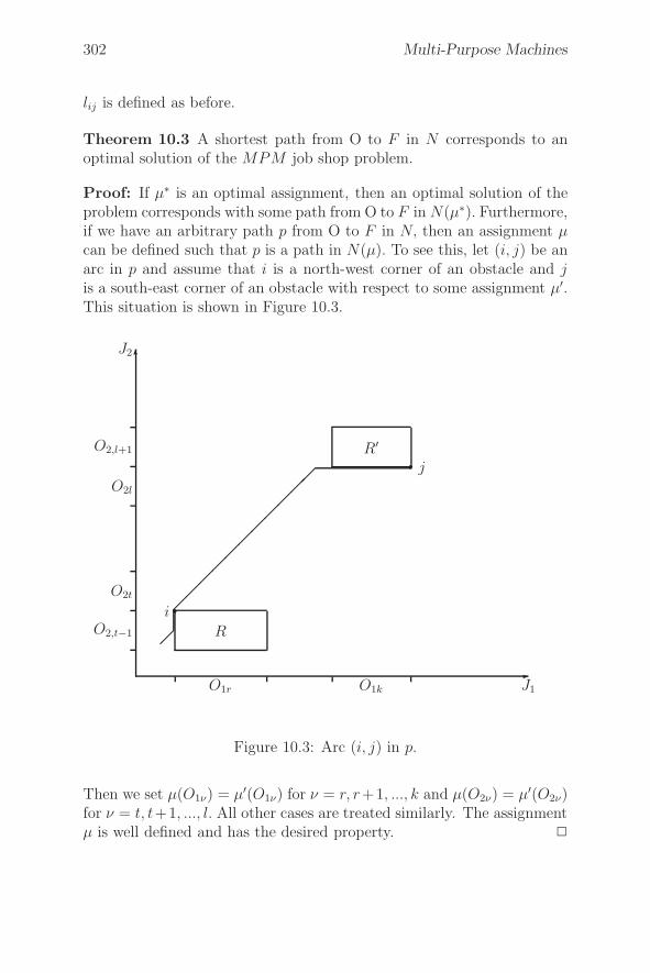
302 Multi-Purpose Machines
lij is defined as before.
Theorem 10.3 A shortest path from O to F in N corresponds to anoptimal solution of the MPM job shop problem.
Proof: If μ∗ is an optimal assignment, then an optimal solution of theproblem corresponds with some path from O to F in N(μ∗). Furthermore,if we have an arbitrary path p from O to F in N, then an assignment μcan be defined such that p is a path in N(μ). To see this, let (i, j) be anarc in p and assume that i is a north-west corner of an obstacle and jis a south-east corner of an obstacle with respect to some assignment μ′.This situation is shown in Figure 10.3.
�
�J2
J1
� j
�i
O1r O1k
O2,t−1
O2t
O2l
O2,l+1
R
R′
�
��
��
��
��
��
�
Figure 10.3: Arc (i, j) in p.
Then we set μ(O1ν) = μ′(O1ν) for ν = r, r+1, ..., k and μ(O2ν) = μ′(O2ν)for ν = t, t+1, ..., l. All other cases are treated similarly. The assignmentμ is well defined and has the desired property. �
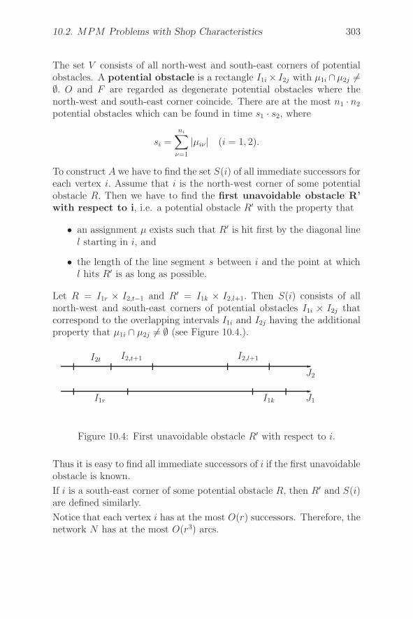
10.2. MPM Problems with Shop Characteristics 303
The set V consists of all north-west and south-east corners of potentialobstacles. A potential obstacle is a rectangle I1i × I2j with μ1i ∩μ2j �=∅. O and F are regarded as degenerate potential obstacles where thenorth-west and south-east corner coincide. There are at the most n1 · n2
potential obstacles which can be found in time s1 · s2, where
si =
ni∑
ν=1
|μiν| (i = 1, 2).
To construct A we have to find the set S(i) of all immediate successors foreach vertex i. Assume that i is the north-west corner of some potentialobstacle R. Then we have to find the first unavoidable obstacle R’with respect to i, i.e. a potential obstacle R′ with the property that
• an assignment μ exists such that R′ is hit first by the diagonal linel starting in i, and
• the length of the line segment s between i and the point at whichl hits R′ is as long as possible.
Let R = I1r × I2,t−1 and R′ = I1k × I2,l+1. Then S(i) consists of allnorth-west and south-east corners of potential obstacles I1i × I2j thatcorrespond to the overlapping intervals I1i and I2j having the additionalproperty that μ1i ∩ μ2j �= ∅ (see Figure 10.4.).
�
�
J1
J2
I1r I1k
I2t I2,t+1 I2,l+1
Figure 10.4: First unavoidable obstacle R′ with respect to i.
Thus it is easy to find all immediate successors of i if the first unavoidableobstacle is known.
If i is a south-east corner of some potential obstacle R, then R′ and S(i)are defined similarly.
Notice that each vertex i has at the most O(r) successors. Therefore, thenetwork N has at the most O(r3) arcs.
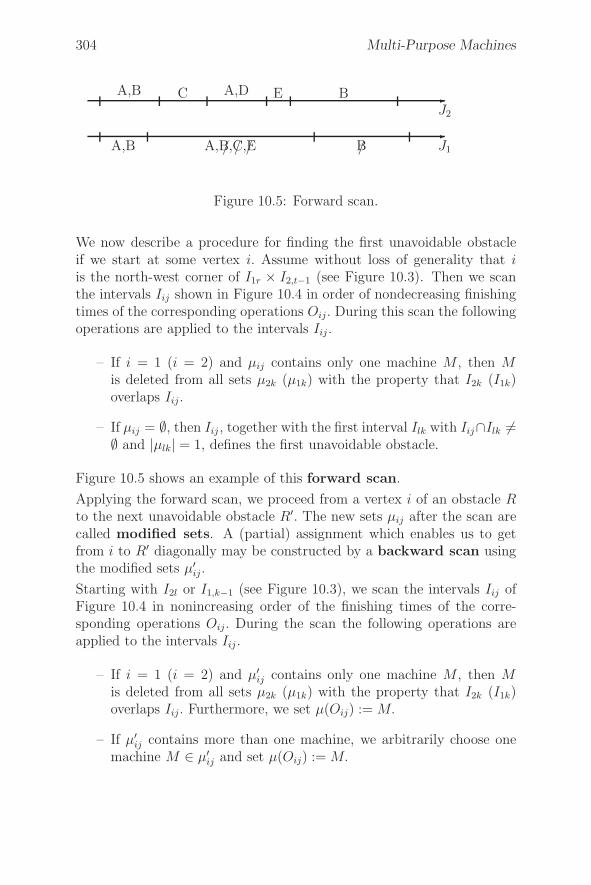
304 Multi-Purpose Machines
�
�
J1
J2
A,B A,B,C,E/ / / B/
A,B C A,D E B
Figure 10.5: Forward scan.
We now describe a procedure for finding the first unavoidable obstacleif we start at some vertex i. Assume without loss of generality that iis the north-west corner of I1r × I2,t−1 (see Figure 10.3). Then we scanthe intervals Iij shown in Figure 10.4 in order of nondecreasing finishingtimes of the corresponding operations Oij. During this scan the followingoperations are applied to the intervals Iij .
– If i = 1 (i = 2) and μij contains only one machine M , then Mis deleted from all sets μ2k (μ1k) with the property that I2k (I1k)overlaps Iij.
– If μij = ∅, then Iij , together with the first interval Ilk with Iij∩Ilk �=∅ and |μlk| = 1, defines the first unavoidable obstacle.
Figure 10.5 shows an example of this forward scan.
Applying the forward scan, we proceed from a vertex i of an obstacle Rto the next unavoidable obstacle R′. The new sets μij after the scan arecalled modified sets. A (partial) assignment which enables us to getfrom i to R′ diagonally may be constructed by a backward scan usingthe modified sets μ′
ij.
Starting with I2l or I1,k−1 (see Figure 10.3), we scan the intervals Iij ofFigure 10.4 in nonincreasing order of the finishing times of the corre-sponding operations Oij. During the scan the following operations areapplied to the intervals Iij .
– If i = 1 (i = 2) and μ′ij contains only one machine M , then M
is deleted from all sets μ2k (μ1k) with the property that I2k (I1k)overlaps Iij. Furthermore, we set μ(Oij) := M.
– If μ′ij contains more than one machine, we arbitrarily choose one
machine M ∈ μ′ij and set μ(Oij) := M.
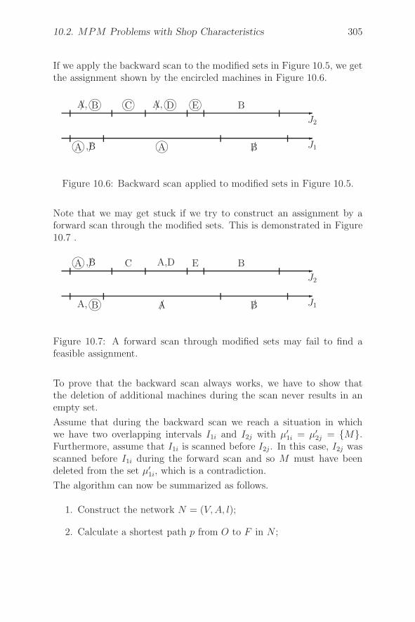
10.2. MPM Problems with Shop Characteristics 305
If we apply the backward scan to the modified sets in Figure 10.5, we getthe assignment shown by the encircled machines in Figure 10.6.
�
�
J1
J2
�A ,B/ �A B/
�BA,/ �C �DA,/ �E B
Figure 10.6: Backward scan applied to modified sets in Figure 10.5.
Note that we may get stuck if we try to construct an assignment by aforward scan through the modified sets. This is demonstrated in Figure10.7 .
�
�
J1
J2
�A, B A/ B/
�A ,B/ C A,D E B
Figure 10.7: A forward scan through modified sets may fail to find afeasible assignment.
To prove that the backward scan always works, we have to show thatthe deletion of additional machines during the scan never results in anempty set.
Assume that during the backward scan we reach a situation in whichwe have two overlapping intervals I1i and I2j with μ′
1i = μ′2j = {M}.
Furthermore, assume that I1i is scanned before I2j . In this case, I2j wasscanned before I1i during the forward scan and so M must have beendeleted from the set μ′
1i, which is a contradiction.
The algorithm can now be summarized as follows.
1. Construct the network N = (V, A, l);
2. Calculate a shortest path p from O to F in N ;

306 Multi-Purpose Machines
3. Calculate an assignment corresponding to p by backward scanningthrough p.
Steps 1 and 2 can be combined. Starting from O, we may construct onlythat part of the network which is relevant while simultaneously doing theshortest path calculation. This is possible since N is acyclic. If we donot count the work for doing operations on the sets μij, the complexityof the algorithm is O(r3).
A further generalization leads to an O(max{n1, n2}5)-algorithm forJMPM | n = 2; prec; ri | Lmax (Jurisch [121]). Multi-purpose machineproblems with 3 jobs are NP-hard even if the number of machines isrestricted to 2 (Brucker et al. [42]).
MPM Flow Shop and Open Shop Problems
Proceeding as for problem JMPM2|n = 3|Cmax, FMPM |n = 3|Cmax
and OMPM |n = 3|Cmax can be shown to be NP-hard. If we fix the num-ber of machines, even the simplest problems FMPM2|stages = 1|Cmax
and OMPM2|stages = 1|Cmax are also NP-hard since they generalizeproblem P2||Cmax. Here stage = 1 indicates that we have only one stage.
Next we consider open shop problems where preemption is allowed. Wewill show that the decision version of OMPM |pmtn|Cmax for a thresh-
old value T is solvable in O((m +n∑
i=1
ni)3 + (min{m, n})4) time. This
yields an ε-approximation algorithm for problem OMPM |pmtn|Cmax.Furthermore, an ε-approximation algorithm is presented for problemOMPM |pmtn, ri|Lmax.
OMPM|pmtn|Cmax
Let there be a given threshold value T . We denote the corresponding de-cision problem by OMPM |pmtn; Ci ≤ T |−. To answer the question ofwhether there exists a feasible schedule for an instance of OMPM |pmtn;Ci ≤ T |− with makespan less than or equal to T , we consider the follow-ing network NT = (V, A).
V , the set of vertices, consists of different types of nodes:
• a source s,
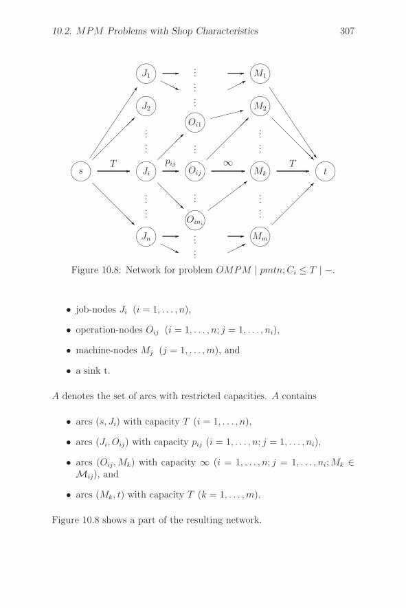
10.2. MPM Problems with Shop Characteristics 307
��
��
s
��
��
J1
��
��
J2
��
��
Ji
��
��
Jn
��
��
Oi1
��
��
Oij
��
��
Oini
��
��
M1
��
��
M2
��
��
Mk
��
��
Mm
��
��
t
����
���
���
��
��
���
�T
��
��
���
�����
��
���
�pij
��
���
�����
�
����
�����
��
��
���
�∞
��
����
�
����
�
��
��
����T
��
��
���
...
...
...
...
...
...
...
...
...
...
...
...
...
...
...
Figure 10.8: Network for problem OMPM | pmtn; Ci ≤ T | −.
• job-nodes Ji (i = 1, . . . , n),
• operation-nodes Oij (i = 1, . . . , n; j = 1, . . . , ni),
• machine-nodes Mj (j = 1, . . . , m), and
• a sink t.
A denotes the set of arcs with restricted capacities. A contains
• arcs (s, Ji) with capacity T (i = 1, . . . , n),
• arcs (Ji, Oij) with capacity pij (i = 1, . . . , n; j = 1, . . . , ni),
• arcs (Oij, Mk) with capacity ∞ (i = 1, . . . , n; j = 1, . . . , ni; Mk ∈Mij), and
• arcs (Mk, t) with capacity T (k = 1, . . . , m).
Figure 10.8 shows a part of the resulting network.
308 Multi-Purpose Machines
We will show that there exists a solution of a given instance of OMPM|pmtn|Cmax with makespan less than or equal to T if and only if thereexists a feasible flow from s to t in the corresponding network NT with
flow valuen∑
i=1
ni∑
j=1
pij.
First assume that for a given instance of OMPM |pmtn|Cmax there existsa feasible schedule y with makespan less than or equal to T . We obtain
a feasible flow x from s to t in NT with value P =n∑
i=1
ni∑
j=1
pij as follows:
• x(s, Ji) =ni∑
j=1
pij (i = 1, . . . , n).
• x(Ji, Oij) = pij (i = 1, . . . , n; j = 1, . . . , ni).
• Define x(Oij , Mk) to be the time during which operation Oij isprocessed on Mk in schedule y (i = 1, . . . , n; j = 1, . . . , ni; k =1, . . . , m).
• Define x(Mk, t) to be the length of all parts of operations which areprocessed on Mk in y (k = 1, . . . , m).
Because no machine has to work for more than T time units (Cmax ≤ T ),the flow x is a feasible flow from s to t in NT with flow value P .
Now assume that there is a feasible flow x from s to t in NT with flowvalue P . We obtain a classical open-shop problem by defining
pik =
ni∑
j=1
x(Oij , Mk) (i = 1, . . . , n; k = 1, . . . , m).
As shown in Section 2.4, this problem has a solution with makespan lessthan or equal to T . This solution defines a feasible schedule for the giveninstance of O MPM |pmtn|Cmax.
The max-flow problem in NT can be solved with time complexity O((n+
m+n∑
i=1
ni)3) (e.g. Malhotra, Kumar, Maheshwari [164]). The calculation
of a feasible schedule by solving the classical open-shop problem needsO((min{n, m})4) (Gonzalez [102]). Thus, we obtain an overall complexity
of O((m +n∑
i=1
ni)3 + (min{m, n})4) to decide if a feasible schedule exists
and to calculate such a schedule.
10.2. MPM Problems with Shop Characteristics 309
Of course, the solution of OMPM |pmtn; di = T |− can be used for an ε-approximation algorithm for OMPM |pmtn|Cmax. To find a solution forOMPM |pmtn|Cmax which differs from the optimal objective value by atthe most ε time units, we do binary search on the set of values
Clow + iε (i = 1, . . . , �Cup − Clow
ε ),
where Clow(Cup) is a lower (upper) bound for the optimal Cmax-value.
OMPM|pmtn; ri|Lmax
Now we will present an ε-approximation algorithm for O MPM |pmtn;ri|Lmax.
For a given threshold value T we consider the decision problem of whe-ther there exists a feasible solution with Lmax ≤ T . This problem isequivalent to the time window problem: Given release dates ri and duedates di for each job, does there exist a feasible schedule with Ci ≤ di fori = 1, . . . , n? The time window problem is denoted by OMPM |pmtn; ri;di|−. It can be solved by linear programming.
Let t1, . . . , tp+1 be a sequence of release dates and due dates such thattl < tl+1 for l = 1, . . . , p. The sequence t1, . . . , tp+1 defines time intervalsIl = [tl, tl+1] of length Tl = tl+1 − tl for l = 1, . . . , p.
We use a linear program with variables
xijkl (i = 1, . . . , n; (job indices)
j = 1, . . . , ni; (operation indices)
k = 1, . . . , m;(machine indices)
l = 1, . . . , p (time-interval indices)).
The 4-tuple (i, j, k, l) is called feasible if and only if Oij can be processedon Mk in time interval Il, i.e. if
• Mk ∈ Mij, and
• ri ≤ tl and di ≥ tl+1.
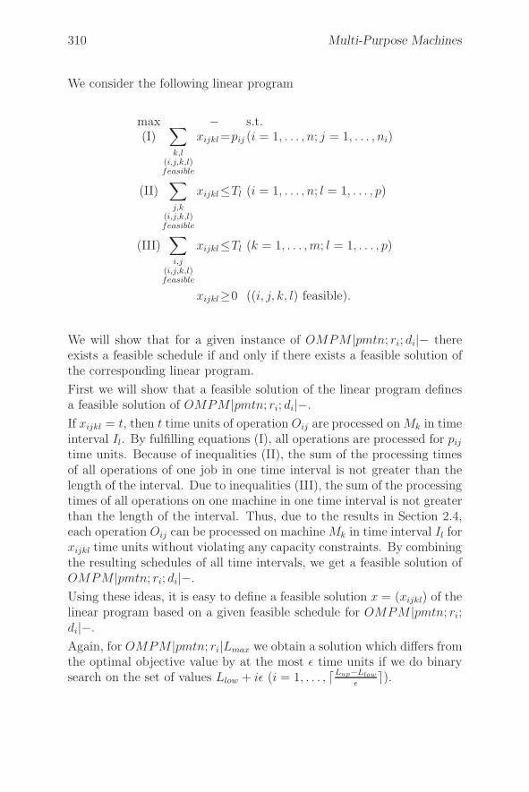
310 Multi-Purpose Machines
We consider the following linear program
max − s.t.(I)
∑
k,l(i,j,k,l)feasible
xijkl =pij (i = 1, . . . , n; j = 1, . . . , ni)
(II)∑
j,k(i,j,k,l)feasible
xijkl≤Tl (i = 1, . . . , n; l = 1, . . . , p)
(III)∑
i,j(i,j,k,l)feasible
xijkl≤Tl (k = 1, . . . , m; l = 1, . . . , p)
xijkl≥0 ((i, j, k, l) feasible).
We will show that for a given instance of OMPM |pmtn; ri; di|− thereexists a feasible schedule if and only if there exists a feasible solution ofthe corresponding linear program.
First we will show that a feasible solution of the linear program definesa feasible solution of OMPM |pmtn; ri; di|−.
If xijkl = t, then t time units of operation Oij are processed on Mk in timeinterval Il. By fulfilling equations (I), all operations are processed for pij
time units. Because of inequalities (II), the sum of the processing timesof all operations of one job in one time interval is not greater than thelength of the interval. Due to inequalities (III), the sum of the processingtimes of all operations on one machine in one time interval is not greaterthan the length of the interval. Thus, due to the results in Section 2.4,each operation Oij can be processed on machine Mk in time interval Il forxijkl time units without violating any capacity constraints. By combiningthe resulting schedules of all time intervals, we get a feasible solution ofOMPM |pmtn; ri; di|−.
Using these ideas, it is easy to define a feasible solution x = (xijkl) of thelinear program based on a given feasible schedule for OMPM |pmtn; ri;di|−.
Again, for OMPM |pmtn; ri|Lmax we obtain a solution which differs fromthe optimal objective value by at the most ε time units if we do binarysearch on the set of values Llow + iε (i = 1, . . . , �Lup−Llow
ε ).
10.2. MPM Problems with Shop Characteristics 311
10.2.2 Unit Processing Times
In this section we show that some MPM shop problems with unit pro-cessing times can be formulated as shortest path problems in suitablenetworks.
MPM Job Shop Problems
We generalize an approach of Meyer [166] for problem J MPM | pij =1; n = k|Cmax.
JMPM | pij = 1; ri;prec;n = k|max fi (∑
fi)
Here fi denotes a monotonic nondecreasing function of the completiontime of job i.
To solve this problem, we first determine time slots t1, . . . , tl (l =k∑
i=1
ni)
which are sufficient to schedule all jobs in some active schedule for theproblem. To calculate such time slots we may assume ri < rj wheneveri precedes j, and schedule jobs with processing time ni (i = 1, . . . , k)on one machine in order of nondecreasing release dates ri. t1, . . . , tl aredefined by all the time slots occupied by this schedule.
Now the original problem will be formulated as the problem of findinga shortest path from some initial vertex to some terminal vertex in thefollowing network N = (V, A, l). In this network each path from theinitial vertex to the terminal vertex corresponds to a feasible schedule.
• The set V of vertices consists of (k + 1)-tupels (tj , i1, . . . , ik) forj = 1, . . . , l and 0 ≤ iν ≤ nν(ν = 1, . . . , k). Such a vertex representsa partial schedule for the interval [0, tj], where iν indicates the lastoperation of job ν which is already scheduled. We also have an ini-tial vertex (t1−1, 0, . . . , 0) and a terminal vertex (tl+1, n1, . . . , nk).
• We have arcs between vertices (tj , i1, . . . , ik) and (tj+1, i′1, . . . , i
′k)
representing the operations scheduled in time slot tj+1. Thus, wehave an arc between two vertices if a k-tupel (x1, . . . , xk) ∈ {0, 1}k
exists with i′ν = iν + xν , ν = 1, . . . , k such that:
– the operations of S = {Oν,iν+1|xν = 1} can be processed inparallel, i.e. a feasible assignment of the operations of S to
312 Multi-Purpose Machines
the machines exists. This can be checked by constructing a bi-partite graph in O(km) time and finding a maximal matchingin O(m2.5) time (Even & Kariv [88]),
– the release dates are respected, i.e. Oν,iν+1 ∈ S implies rν <tj+1, and
– the precedences are respected, i.e. if job μ precedes job ν andxν = 1, the value of iμ must equal nμ.
• The arcs are weighted with the maximum (sum) of all fν(tj+1)-values of jobs finishing exactly at time tj+1, i.e. jobs ν with xν = 1and iν + xν = nν . If no job finishes at time tj+1, the arc weight isset to −∞(0).
Each feasible schedule corresponds to a path from the initial vertex tothe terminal vertex and vice versa. The corresponding objective valueis given by the length of the path, which is the maximum (sum) of allarc values. Thus, we only need to find a shortest path which takes
O((km + m2.5)2kk∑
i=1
ni
k∏
i=1
ni) time since we have O(k∑
i=1
ni
k∏
i=1
ni) vertices
and O(2k) arcs incident at each vertex. Thus we obtain O(2kk∑
i=1
ni
k∏
i=1
ni)
arcs. Since the inspection of an arc takes O(km + m2.5) time, we get thegiven complexity.
MPM Flow Shop Problems
First we consider the flow shop problem
FMPM | pij = 1; stages = r | ∑wiCi
We may assume w1 ≥ w2 ≥ . . . ≥ wn. Then there always exists anoptimal schedule in which job i finishes not later than job j if i < j.
We define a network as follows.
The set V of vertices consists of (2r + 2)-tupels (i, i0, . . . , ir, j1, . . . , jr)for i = 1, . . . , nr, ik = 0, . . . , n (k = 0, . . . , r), and jk = 0, . . . , m (k =
1, . . . , r). Additionally, we assumer∑
n=0
ik = n and jk ≤ ik for all k =
1, . . . , r.
10.2. MPM Problems with Shop Characteristics 313
A vertex represents a partial schedule for the interval [0, i]. Here ikindicates the number of jobs which are finished up to stage k. The entryjk denotes the number of jobs of this partial schedule which are processedin stage k in [i − 1, i]. We consider only vertices such that j1 operationsof stage 1, j2 operations of stage 2, . . . , and jr operations of stage r can
be processed in parallel, i.e. a feasible assignment of ther∑
k=1
jk operations
to the m machines exists. This can be checked in O(mr + m2.5) time byconstructing a bipartite graph and finding a maximal matching (Even &Kariv [88]).
Note that ir equals the number of jobs which are completely finished.Additionally, we have an initial vertex (0, n, 0, . . . , 0). The vertex (nr +1, 0, . . . , 0, ir, 0, . . . , 0) with ir = n is defined as the terminal vertex.
The set A of arcs consists of two different types of arcs. Arcs of thefirst type are between vertices (i, i0, . . . , ir, j1, . . . , jr) and (i, i′0, . . . , i
′r, j
′1,
. . . , j′r) belonging to the same time i. They represent the processingof a job in stage k in interval [i − 1, i]. Hence we have an arc if i′k =ik + 1, i′k−1 = ik−1 − 1, j′k = jk + 1 and i′ν = iν , j
′ν = jν otherwise. This
arc is weighted with 0 if k < r. If k = r, a job is finished and this arcis weighted with iwir+1. Arcs of the second type are between vertices(i, i0, . . . , ir, j1, . . . , jr) and (i + 1, i0, . . . , ir, 0, . . . , 0). In this situation nooperation is scheduled. Hence these arcs are weighted with 0.
Now each schedule in which the jobs are finished in order of nonincrea-sing weights corresponds to a path from the initial vertex to the terminalvertex. The objective value is given by the length of the path. Conversely,from each such path a schedule with objective value equal to the lengthof the path can be constructed. Note that we may always construct apermutation flow-shop schedule, i.e. a schedule in which the job orderfor each stage is the same.
The network has O(nrnrmr) vertices since ir is uniquely determined byi0, . . . , ir−1. Hence the network has O(r2mrnr+1) arcs. Calculating amaximal matching for each vertex takes O(rm + m2.5) time. Inspectingan arc takes O(r) time since a vertex has O(r) entries, implying that O(r)binary symbols are needed to encode a vertex. Thus, it takes O((r2 +rm + m2.5)r ·mr · nr+1) time to construct the network and to calculate ashortest path, i.e. an optimal schedule.
By modifying this approach as described in Section 11.3, FMPM | pij =1; stages = r | ∑
Ti(∑
wiUi) and FMPM | pij = 1; stages = r; ri |
314 Multi-Purpose Machines
∑Ci(Cmax) can be solved in O(r(r2 + rm + m2.5)mrnr+1) time.
Recall that a fixed number of machines induces a bounded number ofstages of a flow shop problem. Thus, the problems FMPM m | pij =1 | f for f ∈ {∑ wiCi,
∑Ti,
∑wiUi} and FMPM m | pij = 1; ri | f for
f ∈ {Cmax,∑
Ci} are also solvable in polynomial time.
MPM Open Shop Problems
In an open shop problem, the tasks of a job might be processed in an ar-bitrary order. By prespecifying for each possible order the number of jobswhich have to be processed according to this order, we obtain a schedul-ing problem which can be solved by generalizations of the approaches forflow shop problems presented in the last section.
In such a problem each job is processed according to one of the C = r!possible (stage) orders π1, . . . , πC . Thus each schedule defines a C-tupel(n1, . . . , nC), where ni denotes the number of jobs which are processed ac-cording to πi. Hence we have to calculate all different tupels (n1, . . . , nC)
with 0 ≤ ni ≤ n for all i = 1, . . . , C andC∑
i=1
ni = n, and solve for each
such tupel the corresponding optimization problem. Then the best sched-ule of all these subproblems gives the optimal schedule of the open-shopproblem.
Based on these ideas, but using more complicated networks (see Section11.3), problems OMPM | pij = 1; stages = r | f for f ∈ {∑ wiCi,
∑Ti,∑
wiUi} and OMPM | pij = 1; stages = r; ri | f for f ∈ {Ci, Cmax} canbe solved polynomially. These networks have O(r·mr ·nr!r+1) vertices andO(r!r) arcs incident at each vertex. The consideration of arcs and thefeasibility check takes O(m2.5+mr!r) time per arc. Hence these problemscan be solved in O(r2 · r!(mr!r + m2.5)mr · nr!r+1) time. Similar to theflow shop situation, we conclude that problem OMPM m | pij = 1 | ffor f ∈ {∑uiCi,
∑Ti,
∑wiUi} and OMPM m | pij = 1; ri | f for
f ∈ {Cmax,∑
Ci} are also solvable in polynomial time.
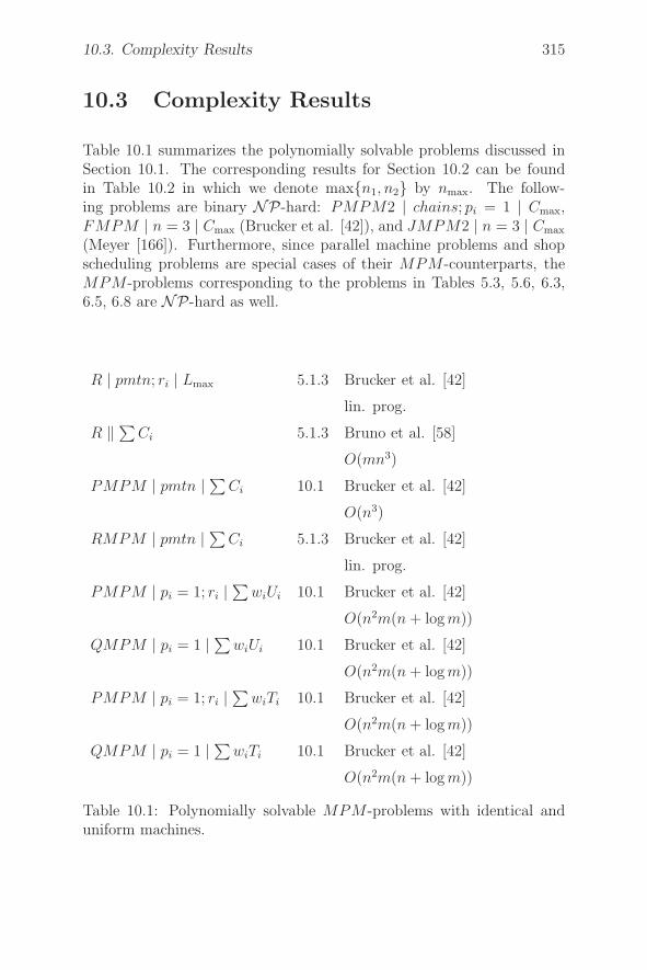
10.3. Complexity Results 315
10.3 Complexity Results
Table 10.1 summarizes the polynomially solvable problems discussed inSection 10.1. The corresponding results for Section 10.2 can be foundin Table 10.2 in which we denote max{n1, n2} by nmax. The follow-ing problems are binary NP-hard: PMPM2 | chains; pi = 1 | Cmax,FMPM | n = 3 | Cmax (Brucker et al. [42]), and JMPM2 | n = 3 | Cmax
(Meyer [166]). Furthermore, since parallel machine problems and shopscheduling problems are special cases of their MPM-counterparts, theMPM-problems corresponding to the problems in Tables 5.3, 5.6, 6.3,6.5, 6.8 are NP-hard as well.
R | pmtn; ri | Lmax 5.1.3 Brucker et al. [42]
lin. prog.
R ‖ ∑Ci 5.1.3 Bruno et al. [58]
O(mn3)
PMPM | pmtn | ∑Ci 10.1 Brucker et al. [42]
O(n3)
RMPM | pmtn | ∑Ci 5.1.3 Brucker et al. [42]
lin. prog.
PMPM | pi = 1; ri |∑
wiUi 10.1 Brucker et al. [42]
O(n2m(n + log m))
QMPM | pi = 1 | ∑wiUi 10.1 Brucker et al. [42]
O(n2m(n + log m))
PMPM | pi = 1; ri |∑
wiTi 10.1 Brucker et al. [42]
O(n2m(n + log m))
QMPM | pi = 1 | ∑wiTi 10.1 Brucker et al. [42]
O(n2m(n + log m))
Table 10.1: Polynomially solvable MPM-problems with identical anduniform machines.
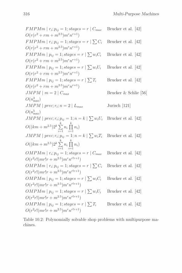
316 Multi-Purpose Machines
FMPMm | ri; pij = 1; stages = r | Cmax Brucker et al. [42]
O(r(r2 + rm + m2.5)mrnr+1)
FMPMm | ri; pij = 1; stages = r | ∑Ci Brucker et al. [42]
O(r(r2 + rm + m2.5)mrnr+1)
FMPMm | pij = 1; stages = r | ∑wiCi Brucker et al. [42]
O(r(r2 + rm + m2.5)mrnr+1)
FMPMm | pij = 1; stages = r | ∑wiUi Brucker et al. [42]
O(r(r2 + rm + m2.5)mrnr+1)
FMPMm | pij = 1; stages = r | ∑Ti Brucker et al. [42]
O(r(r2 + rm + m2.5)mrnr+1)
JMPM | m = 2 | Cmax Brucker & Schlie [56]
O(n3max)
JMPM | prec; ri; n = 2 | Lmax Jurisch [121]
O(n5max)
JMPM | prec; ri; pij = 1; n = k | ∑wiUi Brucker et al. [42]
O((km + m2.5)2kk∑
i=1
ni
k∏
i=1
ni)
JMPM | prec; ri; pij = 1; n = k | ∑wiTi Brucker et al. [42]
O((km + m2.5)2kk∑
i=1
ni
k∏
i=1
ni)
OMPMm | ri; pij = 1; stages = r | Cmax Brucker et al. [42]
O(r2r!(mr!r + m2.5)mrnr!r+1)
OMPMm | ri; pij = 1; stages = r | ∑Ci Brucker et al. [42]
O(r2r!(mr!r + m2.5)mrnr!r+1)
OMPMm | pij = 1; stages = r | ∑wiCi Brucker et al. [42]
O(r2r!(mr!r + m2.5)mrnr!r+1)
OMPMm | pij = 1; stages = r | ∑wiUi Brucker et al. [42]
O(r2r!(mr!r + m2.5)mrnr!r+1)
OMPMm | pij = 1; stages = r | ∑Ti Brucker et al. [42]
O(r2r!(mr!r + m2.5)mrnr!r+1)
Table 10.2: Polynomially solvable shop problems with multipurpose ma-chines.
Chapter 11
Multiprocessor Tasks
Contrary to the scheduling problems discussed thus far in which each job(or task) is processed by at the most one machine (processor) at a time,in a system with multiprocessor tasks (MPT ) tasks require one ormore processors at a time.
More specifically, we have m different processors M1, . . . , Mm and n tasksi = 1, . . . , n. Each task i requires during a processing period pi allprocessors belonging to a subset μi ⊆ {M1, . . . , Mm}. Tasks requiringthe same processor cannot be processed simultaneously. Such tasks arecalled incompatible. Otherwise they are called compatible.
The general shop problem with multiprocessor tasks is definedsimilarly. Each job i consists of ni multiprocessor tasks Oi1, . . . , Oi,ni
with processing times pij and processor sets μij ⊆ {M1, . . . , Mm}. Duringthe processing period pij , Oij requires each processor in the set μij. Themultiprocessor task job shop problem is a special case of the generalshop problem with MPT in which each job consists of a chain of tasks.The flow shop problem with MPT is a special case of the job shopproblem with MPT in which ni = r for i = 1, . . . , n. Furthermore, weassume that μij = μj ⊆ {M1, . . . , Mm} for stages j = 1, . . . , r and μj �= μl
for j �= l.
Open shop problems with MPT are defined as flow shop problemswith MPT but without precedence constraints between tasks. However,no pair of tasks of the same job can be processed simultaneously.
To describe different types of multiprocessor task scheduling problems,we modify the α-field of the α|β|γ-notation introduced in Chapter 1.We set α = MPT if we have a task system with an arbitrary number
318 Multiprocessor Tasks
of processors. Shop problems with multiprocessor tasks are denoted byGMPT, JMPT, FMPT, OMPT . If the number of processors is fixed,we add the symbol m after the symbol MPT .
11.1 Multiprocessor Task Systems
In this section we consider the problem of scheduling a set of multipro-cessor tasks. MPT2 ‖ Cmax is the simplest problem of this type. Due tothe fact that there are only two processors, we have only three types oftasks: bi-processor tasks and two types of single-processor tasks. Clearly,we get an optimal schedule by first scheduling each single-processor taskon its processor without causing idle time.
This, however, is as far as we can get with polynomial algorithms for mul-tiprocessor task systems with arbitrary processing times. Hoogeveen etal. [113] have shown that the following problems are NP-hard: MPT3 ‖Cmax, MPT2 ‖ ∑
Ci, MPT2 | ri | Cmax.
The situation is different if we consider task systems with unit processingtimes. Blazewicz & Ecker [26] have shown that MPTm | pi = 1 | Cmax
can be solved in time which is linear in the number of jobs. The moregeneral problem MPTm | pi = 1; ri | Cmax, as well as MPTm | pi =1; ri |
∑Ci, had open complexity status (Hoogeveen et al. [113]).
We will show that these and other related open problems can be solvedpolynomially by reductions to shortest (or longest) path problems. Weshow this reduction for problem MPTm | pi = 1 | ∑
wiCi. Reduc-tions for the problems mentioned above and for the additional problemsPMPTm | pi = 1 | ∑
Ti and MPTm | pi = 1 | ∑wiUi are very similar
and will be explained later.
MPTm | pi = 1 | ∑wiCi
We have n multiprocessor tasks i = 1, . . . , n with unit processing times.Associated with task i is a set μi of processors which are all needed toprocess task i. The set μi defines the type of task i. Let R ≤ 2m−1 be thenumber of different types in the system and denote by Ij(j = 1, . . . , R)the set of all tasks of type j. Let nj be the number of tasks in Ij. Byexchange arguments one can show that there exists an optimal schedule Ssuch that the following property holds for each j = 1, . . . , R (see Section

11.1. Multiprocessor Task Systems 319
4.3): The tasks in Ij are processed in order of nonincreasing weights wi.
For each Ij , letj1, j2, . . . , jnj
be an ordered sequence of all tasks from Ij . For technical reasons we adda dummy task j0 at the beginning of the sequence. Next we show thatproblem MPTm | pi = 1 | ∑
wiCi can be formulated as a shortest pathproblem in some network N = (V, A, l). This network is defined by:
• The set V of vertices consisting of (R+1)-tuples (t; i1, . . . , iR) where0 ≤ t ≤ n and 0 ≤ ij ≤ nj . (t; i1, . . . , iR) represents a partialschedule consisting of all tasks jν with 1 ≤ j ≤ R and 1 ≤ ν ≤ ijscheduled in the time interval [0, t]. (0; 0, . . . , 0) is the initial vertexand (n; n1, . . . , nR) is the terminal vertex.
• The immediate successors of vertex u = (t; i1, . . . , iR) are given byall v = (t + 1; i1 + x1, . . . , iR + xR) where x1, . . . , xR satisfy thefollowing conditions:
– xν ∈ {0, 1} for ν = 1, . . . , R
– during one time period, exactly one task from each set Iν withxν = 1 can be scheduled, i.e. for each pair (ν, α) with ν �= αand xν = xα = 1, tasks from Iν and Iα are compatible.
• The cost l(u, v) associated with arc (u, v) is given by
∑
i∈S
wi(t + 1) (11.1)
where S = {jiν+1 | xν = 1; 1 ≤ ν ≤ R}.
Clearly, a feasible schedule corresponds to a path in N from (0; 0, . . . , 0)to (n; n1, . . . , nR) and vice versa. The shortest such path provides anoptimal solution of the problem.
In a preprocessing step, all feasible (x1, . . . , xR)-tupels are calculated.
The number of vertices is bounded by nR∏
j=1
nj ≤ nR+1 and each vertex
has at the most 2R successors. Thus, the network has at the most 2RnR+1
arcs, which means that a shortest path can be calculated in O(R2RnR+1)time where R ≤ 2m −1. The factor R takes care of the calculation of arcweights.
320 Multiprocessor Tasks
MPTm | pi = 1 | ∑Ti
To solve this problem we have to order the tasks in each set Ij accordingto nondecreasing due dates. Furthermore, the cost (11.1) is replaced by
∑
i∈S
max{0, t + 1 − di}.
MPTm | pi = 1; ri | Cmax and MPTm | pi = 1; ri |∑
Ci
To solve these problems the tasks are ordered according to nondecreasingrelease times ri in each set Ij (see Sections 4.2 and 4.3). Furthermore, wemay restrict the schedule to a set of at the most n time periods [t− 1, t].Let T be the set of corresponding t-values (see Section 4.1.2). The setV of vertices is given by all (R + 1)-tuples (t; i1, . . . , iR) with t ∈ T andrij ≤ t − 1 for j = 1, . . . , R. In the definition of the terminal vertex, nmust be replaced by n∗ = maxT . In the definition of successors of somevertex (t; i1, . . . , iR), the first component t + 1 must be replaced by thesmallest number s ∈ T which is greater than t.
For the∑
Ci-problem the costs are given by (11.1) with wi = 1 for alli = 1, . . . , n.
For the Cmax-problem, the cost associated with an arc (u, v), where u =(t; i1, . . . , iR) and v = (s; i1 + x1, . . . , iR + xR), is equal to zero if iν = nν
for ν = 1, . . . , R. Otherwise the cost is equal to s − t.
MPTm | pi = 1 | ∑wiUi
To solve this problem we need to determine a feasible schedule for the on-time tasks such that the sum of the weights of the late tasks is minimal.Late tasks can be scheduled at the end of the schedule in an arbitraryorder. We may assume that an optimal schedule for the on-time tasks ex-ists in which tasks of the same type are finished in order of nondecreasingdue dates. Thus, let
Jj1, Jj2, . . . , Jjnj
be a sequence of all tasks in Ij ordered according to nondecreasing duedates. We define the network N = (V, A, l) as follows:
• The set V of vertices consists of (R + 1)-tupels (t; i1, . . . , iR) fort = 0, . . . , n and ij = 0, . . . , nj . A vertex represents a partial
11.1. Multiprocessor Task Systems 321
schedule in which the first ij tasks of the set Ij for j = 1, . . . , R areeither scheduled late or in time interval [0, t]. We define (0; . . . , 0)to be the initial vertex and (n; n1, . . . , nR) to be the terminal vertex.
• We have two different types of arcs. Arcs of the first type arebetween vertices u = (t; i1, . . . , iR) and v = (t + 1; i1 + x1, . . . , iR +xR). They are defined as in problem MPTm | pi = 1 | sumwiCi
but under the additional restriction that the scheduled tasks areon time, i.e. djij+1
≥ t + 1 if xj = 1 for j = 1, . . . , R. These arcshave zero weight since they represent tasks which are on time.
The arcs of the second type are between vertices belonging to thesame time t. They represent the tasks which are scheduled late, i.e.we have arcs from (t; i1, . . . , ij, . . . , iR) to (t; i1, . . . , ij + 1, . . . , iR)with weight wjij+1
for all j = 1, . . . , R.
Each schedule in which the on-time tasks of the same type are finishedaccording to nondecreasing due dates corresponds to a path from thestarting vertex to the terminal vertex. The length of the path denotesthe corresponding objective value. On the other hand, each path definesa feasible schedule for the on-time tasks. Thus, by calculating a shortestpath we obtain the optimal objective value and a corresponding schedulein O(R2RnR+1) steps if the feasible tupels (x1, . . . , xR) are calculated ina preprocessing step.
If the number m of processors is small, more efficient algorithms can begiven. This is illustrated by the following two examples.
MPT2 | pi = 1 | ∑Ci Simple exchange arguments show that an optimal
schedule for this problem can be constructed by first scheduling the singleprocessor tasks and then all bi-processor tasks.
MPT2 | pi = 1; ri | Cmax and MPMPT2 | pi = 1 | Lmax
To solve problem MPT2 | pi = 1; ri | Cmax, all bi-processor tasks are firstscheduled according to nondecreasing ri-values. Then, on each processor,we schedule the corresponding single-processor tasks again in an orderof nondecreasing ri-values using the idle time slots left by bi-processortasks.
Problem MPT2 | pi = 1 | Lmax can be solved similarly.
322 Multiprocessor Tasks
MPT-Problems with Preemption
Concerning the preemptive case, Kubale [128] has shown that MPM |pmtn | Cmax is strongly NP-hard. On the other hand, MPTm | pmtn |Cmax can be solved polynomially using linear programming (Bianco et al.[24]). For MPT2 | pmtn | Lmax a linear time algorithm exists (Biancoet al. [25]). MPT2 | pmtn | ∑
Ci can be solved by a reduction to thesingle-machine problem 1 | chains | ∑
Ci (Cai et al. [61]). This can beseen as follows.
Let M1 and M2 be the two machines. Then we have three types of tasks:M1-tasks, M2-tasks, and bi-processor tasks.
Lemma 11.1 An optimal schedule exists with the following properties.
(a) There is no idle time on processor M1(M2) before the completiontime of the last M1-task (M2-task).
(b) The M1-tasks (M2-tasks) are sequenced according to the shortestprocessing time (SPT ) rule. The bi-processor tasks are sequencedaccording to the SPT rule.
(c) None of the bi-processor tasks is preempted by other jobs.
Proof:
(a) If there is idle time on M1(M2) before the completion time of thelast M1-task (M2-task), we shift this task to the left.
(b) If two Mi-tasks are not sequenced according to the SPT rule, elim-inate both tasks and reschedule them in the created slot accordingto the SPT rule.
(c) Apply transformation to bi-processor tasks which is similar to theone described in (b).
None of the transformations described in (a), (b), and (c) increase the∑Ci-value. Thus, there exists an optimal schedule with the described
properties. �
Lemma 11.2 In any optimal schedule if a bi-processor task is not thefirst task, its starting time must be equal to the completion time of someother tasks.
11.2. Shop Problems with MPT : Arbitrary Processing Times 323
Proof: Assume that some bi-processor task J starts at time t and t isnot the finishing time of some task. Then at time t at least one task ispreempted and if only one task is preempted on one processor at time t,then the other processor has an idle interval finishing at time t. MovingJ slightly to the left will decrease the
∑Ci-value. Thus, an optimal
schedule has the described properties. �
Due to Lemmas 11.1 and 11.2, an optimal schedule can be constructedby first scheduling the M1-tasks and M2-tasks in SPT -order on theircorresponding processors. Then we have to insert the bi-processor tasks,again in SPT -order, starting at the finishing times of the single-processortasks. This insertion problem may be solved by solving a correspondingproblem 1 | chains | ∑
Ci which is constructed in the following way.
Let t1 < t2 < . . . < tq be the time instances where a task finishes in theSPT -schedule for the M1-tasks and M2-tasks. Define two chains of jobs.The first chain consists of q tasks
J ′1 → J ′
2 → . . . → J ′q
where J ′i has the processing time ti − ti−1 and t0 = 0.
The second chainJ ′′
1 → J ′′2 → . . . → J ′′
r
contains the bi-processor tasks ordered according to the SPT -rule. Con-sider the 1 | chains | ∑
Ci problem which is provided by these twochains.
11.2 Shop Problems with MPT :Arbitrary
Processing Times
In this section we will discuss polynomial algorithms for open shop, flowshop, and job shop problems with multiprocessor tasks with arbitraryprocessing times.
Open Shop Problems
We will first discuss the complexity of MPT open shop problems withan arbitrary number of machines and Cmax-criterion. The complexitydepends on the compatibility structure of the stages of the problem.
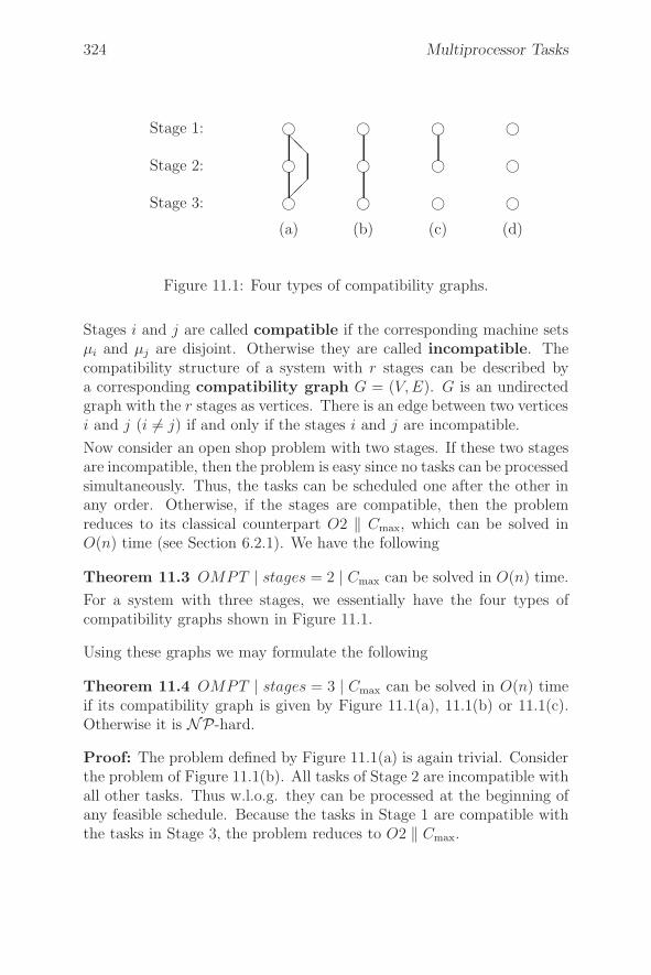
324 Multiprocessor Tasks
Stage 3:
Stage 2:
Stage 1:
(a) (b) (c) (d)
�
�
�
�
�
�
�
�
�
�
�
�
��
��
Figure 11.1: Four types of compatibility graphs.
Stages i and j are called compatible if the corresponding machine setsμi and μj are disjoint. Otherwise they are called incompatible. Thecompatibility structure of a system with r stages can be described bya corresponding compatibility graph G = (V, E). G is an undirectedgraph with the r stages as vertices. There is an edge between two verticesi and j (i �= j) if and only if the stages i and j are incompatible.
Now consider an open shop problem with two stages. If these two stagesare incompatible, then the problem is easy since no tasks can be processedsimultaneously. Thus, the tasks can be scheduled one after the other inany order. Otherwise, if the stages are compatible, then the problemreduces to its classical counterpart O2 ‖ Cmax, which can be solved inO(n) time (see Section 6.2.1). We have the following
Theorem 11.3 OMPT | stages = 2 | Cmax can be solved in O(n) time.
For a system with three stages, we essentially have the four types ofcompatibility graphs shown in Figure 11.1.
Using these graphs we may formulate the following
Theorem 11.4 OMPT | stages = 3 | Cmax can be solved in O(n) timeif its compatibility graph is given by Figure 11.1(a), 11.1(b) or 11.1(c).Otherwise it is NP-hard.
Proof: The problem defined by Figure 11.1(a) is again trivial. Considerthe problem of Figure 11.1(b). All tasks of Stage 2 are incompatible withall other tasks. Thus w.l.o.g. they can be processed at the beginning ofany feasible schedule. Because the tasks in Stage 1 are compatible withthe tasks in Stage 3, the problem reduces to O2 ‖ Cmax.
11.2. Shop Problems with MPT : Arbitrary Processing Times 325
For a problem given by Figure 11.1(c) we proceed as follows. We con-catenate Stages 1 and 2 to one stage, where the processing time of a jobin this stage is given by the sum of its processing times of Stage 1 andStage 2. Thus, we obtain the classical problem O2 ‖ Cmax where, addi-tionally, one special preemption per job is allowed. Since any solutionof the problem O2 | pmtn | Cmax can be transformed into one withoutpreemption without increasing the makespan (Gonzalez & Sahni [104]),this additional condition may be dropped.
The classical problem O3 ‖ Cmax is represented by the graph in Figure11.1(d). Thus, this case is NP-hard (Gonzalez & Sahni [104]). �
A consequence of Theorems 11.3 and 11.4 is that OMPT2 ‖ Cmax canbe solved in O(n) time. If we have three stages, the compatibility graphis given by Figure 11.1(b) and Theorem 11.4 applies. If there are twostages, Theorem 11.3 applies.
The following problems are NP-hard since the corresponding problemswithout multiprocessor tasks are NP-hard: OMPT2 | ri | Cmax,OMPT2 ‖ Lmax, OMPT3 ‖ Cmax, OMPT2 ‖ ∑
Ci, OMPT2 | tree |Cmax, OMPT | n = 3 | Cmax.
If the number of machines is fixed, then the number of possible stagesis also fixed. Thus, the general problems OMPTm | n = k; prec; ri |∑
wiUi and OMPTm | n = k; prec; ri |∑
wiTi are solvable in constanttime.
Flow Shop Problems
Again, we classify MPT flow shop problems according to the compati-bility structure of the stages.
Similar to the MPT open shop problem, the MPT flow shop problemwith two stages is either trivial or it reduces to problem F2 ‖ Cmax, whichcan be solved in O(n logn) time (see Section 6.3).
Theorem 11.5 FMPT | stages = 2 | Cmax can be solved in O(n log n)time.
The possible compatibility graphs for MPT flow shop problems withthree stages are shown in Figure 11.2.
Obviously, the problems described by Figures 11.2(c) and 11.2(d) (Fi-gures 11.2(e) and 11.2(f)) are symmetric to each other.
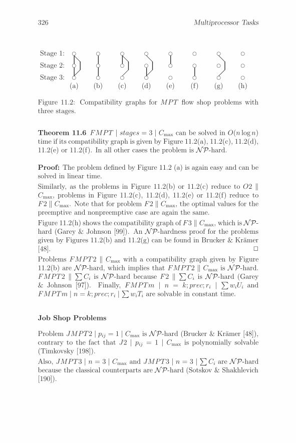
326 Multiprocessor Tasks
Stage 3:
Stage 2:
Stage 1:
(a) (b) (c) (d) (e) (f) (g) (h)
�
�
�
�
�
�
�
�
�
�
�
�
�
�
�
�
�
�
�
�
�
�
�
�
��
��
��
��
��
��
��
��
Figure 11.2: Compatibility graphs for MPT flow shop problems withthree stages.
Theorem 11.6 FMPT | stages = 3 | Cmax can be solved in O(n logn)time if its compatibility graph is given by Figure 11.2(a), 11.2(c), 11.2(d),11.2(e) or 11.2(f). In all other cases the problem is NP-hard.
Proof: The problem defined by Figure 11.2 (a) is again easy and can besolved in linear time.
Similarly, as the problems in Figure 11.2(b) or 11.2(c) reduce to O2 ‖Cmax, problems in Figure 11.2(c), 11.2(d), 11.2(e) or 11.2(f) reduce toF2 ‖ Cmax. Note that for problem F2 ‖ Cmax, the optimal values for thepreemptive and nonpreemptive case are again the same.
Figure 11.2(h) shows the compatibility graph of F3 ‖ Cmax, which is NP-hard (Garey & Johnson [99]). An NP-hardness proof for the problemsgiven by Figures 11.2(b) and 11.2(g) can be found in Brucker & Kramer[48]. �
Problems FMPT2 ‖ Cmax with a compatibility graph given by Figure11.2(b) are NP-hard, which implies that FMPT2 ‖ Cmax is NP-hard.FMPT2 ‖ ∑
Ci is NP-hard because F2 ‖ ∑Ci is NP-hard (Garey
& Johnson [97]). Finally, FMPTm | n = k; prec; ri | ∑wiUi and
FMPTm | n = k; prec; ri |∑
wiTi are solvable in constant time.
Job Shop Problems
Problem JMPT2 | pij = 1 | Cmax is NP-hard (Brucker & Kramer [48]),contrary to the fact that J2 | pij = 1 | Cmax is polynomially solvable(Timkovsky [198]).
Also, JMPT3 | n = 3 | Cmax and JMPT3 | n = 3 | ∑Ci are NP-hard
because the classical counterparts are NP-hard (Sotskov & Shakhlevich[190]).

11.2. Shop Problems with MPT : Arbitrary Processing Times 327
However, it is possible to extend the other known polynomial time algo-rithms for the classical job shop problem to the MPT case.
Theorem 11.7 The following job shop problems with MPT are poly-nomially solvable:
(a) JMPT2 | ni ≤ 2 | Cmax,
(b) JMPT | n = 2 | f if f is regular, and
(c) JMPT2 | n = k | Cmax.
Proof: (a) If the first (last) task of a job requires both processors, itcan be moved to the beginning (end) of the schedule without changingthe schedule length. Thus, the problem is equivalent to scheduling thesingle-processor tasks, which is equivalent to the classical problem J2 |ni ≤ 2 | Cmax. Because the classical problem can be solved in O(n log n)time (Jackson [119]), JMPT2 | ni ≤ 2 | Cmax can be solved with thesame complexity.
(b) Like the classical problem J | n = 2 | f , problem JMPT | n = 2 | fcan be formulated as a shortest path problem. It can be solved by themethods developed in Section 6.4.2.
(c) As in Section 6.4.3, we reduce JMPT2 | n = k | Cmax to a shortestpath problem in an acyclic network N = (V, A, l). The construction ofN can be described as follows.
The two processors are denoted by A and B. We consider only activeschedules , i.e. schedules in which no task can be started earlier withoutviolating feasibility. Given an active schedule, we have a unique sequence
t0 = 0 < t1 < t2 < . . . < tq
of times at which one of the following conditions holds:
• two single-processor tasks start to be processed jointly on bothprocessors,
• a bi-processor task starts, or
• a single-processor task starts to be processed on one processor andon the other processor an idle period starts (see Figure 11.3).
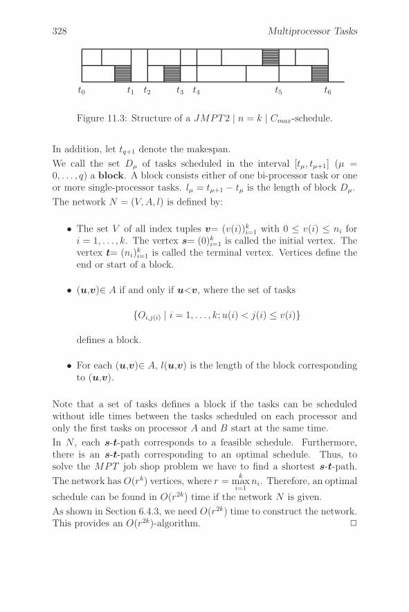
328 Multiprocessor Tasks
t0 t1 t2 t3 t4 t5 t6
Figure 11.3: Structure of a JMPT2 | n = k | Cmax-schedule.
In addition, let tq+1 denote the makespan.
We call the set Dμ of tasks scheduled in the interval [tμ, tμ+1] (μ =0, . . . , q) a block. A block consists either of one bi-processor task or oneor more single-processor tasks. lμ = tμ+1 − tμ is the length of block Dμ.
The network N = (V, A, l) is defined by:
• The set V of all index tuples v= (v(i))ki=1 with 0 ≤ v(i) ≤ ni for
i = 1, . . . , k. The vertex s= (0)ki=1 is called the initial vertex. The
vertex t= (ni)ki=1 is called the terminal vertex. Vertices define the
end or start of a block.
• (u,v)∈ A if and only if u<v, where the set of tasks
{Oi,j(i) | i = 1, . . . , k; u(i) < j(i) ≤ v(i)}
defines a block.
• For each (u,v)∈ A, l(u,v) is the length of the block correspondingto (u,v).
Note that a set of tasks defines a block if the tasks can be scheduledwithout idle times between the tasks scheduled on each processor andonly the first tasks on processor A and B start at the same time.
In N , each s-t-path corresponds to a feasible schedule. Furthermore,there is an s-t-path corresponding to an optimal schedule. Thus, tosolve the MPT job shop problem we have to find a shortest s-t-path.
The network has O(rk) vertices, where r =k
maxi=1
ni. Therefore, an optimal
schedule can be found in O(r2k) time if the network N is given.
As shown in Section 6.4.3, we need O(r2k) time to construct the network.This provides an O(r2k)-algorithm. �
11.3. Shop Problems with MPT : Unit Processing Times 329
11.3 Shop Problems with MPT: Unit Pro-
cessing Times
Job Shop Problems
We consider a job shop problem with a fixed number of jobs consistingof unit time tasks. The algorithm we will present is a straightforwardgeneralization of an algorithm for the problem without multiprocessortasks due to Meyer [166]. This algorithm can be applied to the generalobjective functions max fi and
∑fi where fi denotes a monotonous non-
decreasing function of the completion time of job i. Furthermore, wemay have release times and precedence constraints between jobs.
JMPT | pij = 1;prec; ri;n = k | max fi (∑
fi)
To solve this problem we first determine time slots t1, . . . , tl (l =k∑
i=1
ni)
which are sufficient for some active schedule for the problem. Then theproblem will be formulated as a shortest path problem in a suitablenetwork.
We may assume ri < rj whenever i precedes j. If we assume that alltasks must be processed on the same processor, we obtain the time slotst1, . . . , tl by scheduling the k jobs in order of nondecreasing release dateswith processing times ni.
A feasible schedule defines a path in the following network N = (V, A, d)from some initial vertex to a terminal vertex:
• The set V of vertices consists of (k + 1)-tupels (tj , i1, . . . , ik) forj = 1, . . . , l and 0 ≤ iν ≤ nν(ν = 1, . . . , k). Such a vertex rep-resents a partial schedule for the interval [0, tj] where iν indicatesthe last task of job ν which is already scheduled. Additionally,we have an initial vertex (t1 − 1, 0, . . . , 0) and a terminal vertex(tl + 1, n1, . . . , nk).
• We have arcs between nodes (tj , i1, . . . , ik) and (tj+1, i′1, . . . , i
′k) rep-
resenting the tasks scheduled in time slot tj+1. There is an arcbetween two vertices if a k-tupel (x1, . . . , xk) ∈ {0, 1}k exists withi′ν = iν + xν , ν = 1, . . . , k such that:
330 Multiprocessor Tasks
– the tasks of S = {Oν,iν+1 | xν = 1} can be processed inparallel,
– the release dates are respected, i.e. Oν,iν+1 ∈ S implies rν <tj+1, and
– the precedences are respected, i.e. if job μ precedes job ν andxν = 1, then the value of iμ must equal nμ.
• The arcs are weighted with the maximum (sum) of all fν(tj+1)-values of jobs finishing exactly at time tj+1, i.e. jobs ν with xν = 1and iν + xν = nν . If no job finishes at time tj+1, the arc weight isset to −∞(0).
Each feasible schedule corresponds to a path from the initial vertex tothe terminal vertex and vice versa. The corresponding objective valueis given by the length of the path, where the length of a path is themaximum (sum) of all arc values. Thus, we only need to find a shortest
path which takes O(k2kmk∑
i=1
ni
k∏
i=1
ni) time since we have O(k∑
i=1
ni
k∏
i=1
ni)
vertices, O(2k) arcs incident at each vertex, and the inspection of an arctakes O(km) time.
Flow Shop Problems
We solve different flow shop problems with multiprocessor unit time tasksand a fixed number of stages.
FMPT | pij = 1; stages = r | ∑wiCi
We may assume w1 ≥ w2 . . . ≥ wn. Then there always exists an optimalschedule in which job i finishes before job j if i < j.
We define the network as follows:
• The set V of vertices consists of (r + 2)-tupels (i, i0, . . . , ir) for
i = 1, . . . , nr and 0 ≤ ik ≤ n (k = 0, . . . , r) withr∑
k=0
ik = n. It
represents a partial schedule for the interval [0, i] where ik indicatesthe number of jobs that are finished up to stage k. Thus, ir equalsthe number of jobs that are completely finished. We have an initial
11.3. Shop Problems with MPT : Unit Processing Times 331
vertex (0, n, 0, . . . , 0). The vertex (nr, 0, . . . , 0, n) is defined to bethe terminal vertex.
• The arcs between vertices (i, i0, . . . , ir) and (i + 1, i′0, . . . , i′r) repre-
sent the tasks scheduled in time slot i + 1. Hence we have an arcbetween two nodes if an r-tupel (x1, . . . , xr) ∈ {0, 1}r, representingthe stages processed in time slot i + 1, exists such that
– the processor requirements of the stages, i.e. the sets μj withxj = 1, are pairwise disjoint,
– a job is processed in stage k only if at least one job was pro-cessed up to stage k − 1, i.e. xk = 1 only if ik−1 > 0, and
– i′k equals the sum of the number of jobs already processed upto stage k in [0, i] and the number of jobs which are processedin stage k in [i, i + 1] minus the number of jobs which areprocessed in stage k + 1 in [i, i + 1], i.e. i′k = ik + xk − xk+1
for all k = 1, . . . , r − 1, i′0 = i0 − x1 and i′r = ir + xr.
• The arcs have zero weight if xr = 0. If xr = 1, the weight equals(i+1)wir+1 because we may assume that job ir +1 is now finished.
Each schedule in which the jobs are finished in order of nonincreasingweights corresponds to a path from the initial vertex to the terminalvertex. The objective value is given by the length of the path. Conversely,from each such path, a schedule with objective value equal to the lengthof the path can be constructed as follows. For each arc (x1, . . . , xr) ofthe shortest path ending at a node (i + 1, i′0, . . . , i
′r), schedule for xj = 1
job (i′j + . . . + i′r) in stage j in time slot [i, i + 1]. Note that the resultingschedule is always a permutation flow shop schedule, i.e. a schedule inwhich the job order for each stage is the same.
In a preprocessing step we calculate all feasible (x1, . . . , xr)-tupels inO(2r(r + m)) steps. The network has O(nrnr) vertices since the valueof ir is uniquely determined by i0, . . . , ir−1, and hence O(r2rnr+1) arcs.Inspection of an arc takes O(r) steps. Thus, it takes O(r22rnr+1 +2r(r+m)) time to calculate a shortest path, i.e. an optimal schedule.
Using similar techniques, FMPT | pij = 1; stages = r | ∑Ti and
FMPT | pij = 1; stages = r; ri |∑
Ci(Cmax) can be solved in O(r22r
nr+1 +2r(r +m)) time. For the latter, we may assume that jobs are pro-cessed in order of nondecreasing release dates. Furthermore, time slots
332 Multiprocessor Tasks
are calculated as described for problem JMPT | pij = 1; prec; ri; n = k |maxfi by computing an earliest possible starting schedule. Then the net-work can be defined as for problem FMPT | pij = 1; stages = r | ∑
wiCi
with the following additional restriction. Arcs with x1 = 1 are only al-lowed to end at a node (tj+1, i
′0, . . . , i
′r) if rn−i′0 ≤ tj+1 − 1. Here we
assume that r1 ≤ r2 ≤ . . . ≤ rn.
FMPT | pij = 1; stages = r | ∑wiUi
We proceed in a similar way as for problem MPTm | pi = 1 | ∑wiUi.
We are interested in finding a feasible schedule for the on-time jobs. Weassume that d1 ≤ . . . ≤ dn since the on-time jobs can be finished in orderof nondecreasing due dates. The network is defined as follows:
• The set V of vertices consists of (r + 2)-tupels (i, i0, . . . , ir) for
i = 1, . . . , nr and 0 ≤ ik ≤ n (k = 0, . . . , r) withr∑
k=0
ik = n.
Furthermore, we have vertices (0, n − i, 0, . . . , 0, i) for i = 0, . . . , n.A vertex represents a partial schedule for the on-time jobs scheduledin interval [0, i] and the late jobs scheduled in [dn,∞[. Here ik(k = 0, . . . , r − 1) indicates the number of jobs which have beenprocessed up to stage k. The value of ir indicates the number ofjobs which are either finished on time in [0, i] or scheduled late.(0, n − i, 0, . . . , 0, i) indicates that the first i jobs are scheduledlate. The vertex (0, n, 0, . . . , 0) is defined as the initial vertex while(nr, 0, . . . , 0, n) is the terminal vertex.
• The arcs are defined as in problem FMPT | pij = 1; stages =r | ∑
wiCi under the restriction that arcs with xr = 1 are onlyallowed to end at a vertex (i + 1, i′0, . . . , i
′r) with di′r ≥ i + 1. These
arcs have zero weight since they represent jobs which are on time.Additionally, we have arcs between vertices belonging to the sametime slot i. They represent the jobs which are scheduled late, i.e.for i0 > 0 we have arcs from (i, i0, . . . , ir) to (i, i0 − 1, . . . , ir + 1)with weight wir+1.
Each schedule in which the on-time jobs are finished according to non-decreasing due dates corresponds to a path from the initial vertex to theterminal vertex. The length of the path denotes the corresponding objec-tive value. On the other hand, each path defines a feasible schedule for the
11.3. Shop Problems with MPT : Unit Processing Times 333
on-time jobs. Thus, by calculating a shortest path we obtain the optimalobjective value and a corresponding schedule in O(r22rnr+1 +2r(r +m))time.
Recall that a fixed number of processors induces a bounded number ofstages of a flow shop problem. Thus, the problems FMPTm | pij = 1 |∑
wiCi, FMPTm | pij = 1 | ∑Ti, FMPTm | pij = 1; ri |
∑Ci(Cmax),
and FMPTm | pij = 1 | ∑wiUi are also solvable in polynomial time.
Open Shop Problems with Multiprocessor Tasks
In an open shop problem, tasks of a job might be processed in an arbitraryorder. By prespecifying for each possible order the number of jobs whichhave to be processed according to this order, we obtain a schedulingproblem which can be solved by generalizations of the approaches forflow shop problems presented in the last section.
OMPT | pij = 1; stages = r | ∑wiCi
In this problem each job is processed according to one of the C = r!possible (stage) orders π1, . . . , πC . Thus, each schedule defines a C-tupel(n1, . . . , nC), where ni denotes the number of jobs which are processed ac-cording to πi. Hence, we have to calculate all different tupels (n1, . . . , nC)
with 0 ≤ ni ≤ n for all i = 1, . . . , C andC∑
i=1
ni = n, and solve the cor-
responding optimization problem for each such tupel. Then the bestschedule of all these subproblems gives the optimal schedule of the openshop problem.
We may assume w1 ≥ . . . ≥ wn. Then an optimal schedule exists withC1 ≤ . . . ≤ Cn. We generalize the definition of the network for problemFMPT | pij = 1; stages = r | ∑
wiCi as follows:
• The vertices are (1 + C(r + 1) + r)-tupels (i, i1,0, . . . , i1,r, i2,0,. . . , iC,r, j1, . . . , jr) for i = 0, . . . , nr − 1, 0 ≤ iμ,ν ≤ nμ (μ =1, . . . , C;ν = 0, . . . , r) and jk ∈ {0, 1} (k = 1, . . . , r). Furthermore,
we assumer∑
ν=0
iμ,ν = nμ for μ = 1, . . . , C. A vertex represents a
partial schedule for the interval [0, i + 1], where iμ,ν indicates thenumber of jobs which have to be scheduled according to πμ andhave been processed up to stage πμ(ν). The entry jk denotes the
334 Multiprocessor Tasks
number of tasks processed in stage k in [i, i + 1]. The initial vertexis given by (0, i1,0, . . . , i1,r, i2,0, . . . , iC,r, j1, . . . , jr) with jk = 0 fork = 1, . . . , r, iμ,0 = nμ for μ = 1, . . . , C, and iμ,ν = 0 for ν �= 0.The vertex (nr, i1,0, . . . , i1,r, i2,0, . . . , iC,r, j1, . . . , jr) with jk = 0 fork = 1, . . . , r, iμ,r = nμ for μ = 1, . . . , C, and iμ,ν = 0 for ν �= r isdefined as the terminal vertex.
• The set A consists of two different types of arcs. Arcs of thefirst type are between vertices (i, . . . , iμ,ν , . . . , j1, . . . , jr) and (i, . . . ,i′μ,ν , . . . , j
′1, . . . , j
′r) belonging to the same time i. They represent the
scheduling of a task in stage πq(s) in [i, i + 1]. Hence, we have anarc if i′q,s = iq,s + 1, i′q,s−1 = iq,s−1 − 1 and i′μ,ν = iμ,ν otherwise.Furthermore, we have j′πq(s) = jπq(s) + 1 and j′k = jk otherwise. Wemust ensure that no processor is required more than once. Thischeck takes O(r) time if we assume a preprocessing as in the flowshop section. These arcs have zero weight if no job is finished, i.e.
s < r. Otherwise we may assume that jobs 1, 2, . . . ,C∑
μ=1
iμ,r are al-
ready finished in [0, i+1]. Hence, the jobC∑
μ=1
iμ,r +1 finishes at time
i + 1 and the weight of the arc equals (i + 1)wPCμ=1 iμ,r+1. Arcs of
the second type are between vertices (i, . . . , iμ,ν , . . . , iC,r, j1, . . . , jr)and (i + 1, . . . , iμ,ν , . . . , iC,r, 0, . . . , 0). In this situation no task isscheduled. Thus they have zero weight.
Thus, by calculating a shortest path we get an optimal schedule forthe subproblem. All O(nr!) subproblems have a total of O(nrnr!r2r) =O(r2rnr!r+1) nodes. At the most O(r!r) arcs start from each node andthe inspection of an arc takes O(rr!) time. As in the flow shop section,we calculate all feasible (j1, . . . , jr)-tupels in O(2r(r + m)) time in a pre-processing step. Thus, problem OMPT | pij = 1; stages = r | ∑
wiCi
can be solved in O(r3(r!)22rnr!r+1 + 2r(r + m)) time.
Now observe that the subproblems of the open shop problems with ob-jective function
∑Ti,
∑wiUi and
∑Ci(Cmax) with release dates can be
solved by similar generalizations of the corresponding flow shop prob-lems. Hence, we conclude that OMPT | pij = 1; stages = r | ∑
Ti,OMPT | pij = 1; stages = r; ri | ∑
Ci(Cmax) and OMPT | pij =1; stages = r | ∑
wiUi can also be solved in O(r3(r!)22rnr!r+1+2r(r+m))time.
11.4. Multi-Mode Multiprocessor-Task Scheduling Problems 335
Similar to the flow shop situation, we conclude that the problemsOMPTm | pij = 1 | ∑
wiCi, OMPTm | pij = 1 | ∑Ti, OMPTm |
pij = 1; ri | ∑Ci(Cmax) and OMPTm | pij = 1 | ∑
wiUi are alsosolvable in polynomial time.
We are interested in classifying shop problems with multiprocessor tasksand unit processing times with respect to their complexity status. Thus,we remark that open shop problems with 2 jobs and unit processing timetasks, i.e. OMPT | pij = 1; n = 2 | Cmax, can be reduced to a matchingproblem in a bipartite graph G = (V ∪ W, A) as follows. Each task ofjob 1 (job 2) corresponds to a vertex of V (W ). An edge between avertex of V and a vertex of W exists if the represented tasks can beprocessed in parallel. An optimal schedule for the open shop problemcorresponds to a maximal matching in the graph G and vice versa. Thusit can be calculated in O(r2.5) time (Even & Kariv [88]), where r denotesthe number of stages. Note that this approach can be generalized in astraightforward way to solve OMPT | pij = 1; ri; n = 2 | maxfi (
∑fi)
in O(r2.5) time if the fi are monotonic nondecreasing.
11.4 Multi-Mode Multiprocessor-Task
Scheduling Problems
In a multi-mode multiprocessor-task scheduling problem (MMPT -pro-blem) there is set Ai = {A1
i , . . . , Amik }(Aij = {A1
ij, . . . , Amij
ij }) of machinesets Aν
i (Aνij) and corresponding processing times pν
i (pνij) associated with
each task i (operation Oij). We have to assign a set Aνi (A
νij) to each
task i (operation Oij). If Aνi (A
νij) is assigned to i (Oij), then task i
(operation Oij) occupies all processors in the set Aνi (A
νij) for pν
i (pνij) time
units. Thus, after the assignment we have a multiprocessor task problem.The MMPT -problem consists of finding an assignment and schedulingthe tasks (operations) on the assigned machines such that some objec-tive function is minimized. In the α|β|γ-notation, MMPT -problemsare characterized by α1 ∈ {MMPT, MGMPT, MJMPT, MFMPT,MOMPT}. The sets Ai(Aij) may be restricted. For example, we mayassume that each task requires a fixed number q of processors. ThenAi is the set of all subsets of processors of size q. In this case we usu-ally assume that the processing time depends only on this number ofprocessors. To indicate such a model we add “sizei” to the β-field. In

336 Multiprocessor Tasks
connection with models for parallel computing other restrictions are pos-sible (see Blazewicz et al. [27]). Next we will briefly discuss knowncomplexity results for MMPT -problems.
Problem MMPT2 ‖ Cmax is NP-hard because the NP-hard problemP2 ‖ Cmax is a special case of this problem. However, it can be solved
with complexity O(nT ) where T =n∑
i=1
pmin(i) is the sum of minimal
processing times
pmin(i) =mi
minν=1
pνi
of tasks i. The special case of MMPT3 ‖ Cmax in which only two ma-chines are involved in the bi-machine sets can also be solved pseudopoly-nomially with complexity O(nT 2) (see Chen & Lee [64]).
In the remaining part of this section we discuss polynomial algorithmsfor “sizei”-problems. Firstly, two-processor problems are considered. Inthis case we have 1-tasks and 2-tasks depending on the number ofprocessors needed. Denote by n1 and n2 the number of 1-tasks and 2-tasks, respectively.
MPT2 | ri;pi = p; sizei | Cmax
It can be easily shown by exchange arguments that the following algo-rithm solves this problem.
Algorithm MPT2 | ri;pi = p; sizei | Cmax
1. t :=n
minr=1
rν ;
2. WHILE not all tasks are scheduled DOBEGIN
3. IF an unscheduled 2-task j with rj ≤ t exists THEN schedulej at time t
4. ELSE schedule a largest possible number of 1-tasks j withrj ≤ t at time t;
5. t := max{t + p; min{rν | ν is unscheduled }END
The multiprocessor tasks problem
11.4. Multi-Mode Multiprocessor-Task Scheduling Problems 337
MPT2 | ri;pi = 1; sizei |∑
Ci
can be solved by a similar algorithm. All we have to do is to replaceStatements 3 and 4 by the following statement:
If at least two 1-tasks are available at time t, then assign any two suchtasks for processing from time t. Otherwise, assign any available 2-taskfor processing, or, if there is no such 2-task available, assign any available1-task for processing.
Theorem 11.8 Any schedule constructed by the algorithm above is op-timal.
Proof: Let Cj be the completion times in a schedule S constructed bythe algorithm above, and let S∗ be an optimal schedule. Let t be thefirst point in time where these two schedules differ. We will show by aninterchange argument that in this case S∗ can be converted to an optimalschedule S that coincides with S at least up to point t + 1.
Note that, since S and S∗ coincide up to the point t, any task j that isprocessed in schedule S in the interval [t, t + 1] satisfies
rj ≤ t ≤ Cj(S∗).
Suppose that according to S two 1-tasks j1 and j2 are processed in theinterval [t, t + 1]. If Cj1(S
∗) = Cj2(S∗), then S can be obtained by
swapping j1 and j2 with tasks processed in schedule S∗ in the interval[t, t + 1]. If Cj1(S
∗) < Cj2(S∗), we first swap j2 with a task processed
in parallel with j1, and then again swap j1 and j2 with tasks processedin schedule S∗ in the interval [t, t + 1]. Suppose that only one task j isprocessed in schedule S in the interval [t, t+1]. Observe that in this casedue to the construction of S exactly one task must be processed in thisinterval in the optimal schedule S∗. Moreover, if sizej = 1, then thistask is also a 1-task. Hence, S can be obtained from S∗ by swapping jand the task processed in the interval [t, t + 1]. It is easy to see that
n∑
j=1
Cj(S∗) =
n∑
j=1
Cj(S∗),
in each case and the optimality of S follows by a simple inductive argu-ment. �
338 Multiprocessor Tasks
MPT2 | pi = p; sizei |∑
Ui
Task j is early in some schedule S if Cj(S) ≤ di, otherwise this task islate. By simple interchange arguments it is easy to prove the following.
Lemma 11.9 There is an optimal schedule such that
• all late tasks are scheduled (in any order) after all early tasks,
• all early tasks with the same size are scheduled according to non-decreasing due dates and 1-tasks precede 2-tasks with the same duedate, and
• if a 1-task j is late, then all 2-tasks with due dates less than orequal to dj are also late.
The following algorithm constructs an optimal schedule which has theproperties of Lemma 11.9.
Algorithm MPT2 | pi = p; sizei |∑
Ui
1. Calculate a list L in which the tasks are ordered according tonon-decreasing due dates. If 1-tasks and 2-tasks have the samedue date then place the 1-tasks before the 2-tasks;
2. WHILE L is not empty DOBEGIN
3. Select the first task j in L;4. IF task j is a 2-task THEN5. IF j late if added to the partial schedule of early tasks THEN
add j to the set of late tasksELSE schedule j;
6. IF task j is a 1-task which can be scheduled on time THEN insertj into the partial schedule of early tasks in the first time slotELSE
7. IF the partial schedule of early tasks contains a 2-task THENeliminate the 2-task k scheduled last among all 2-tasks, addit to the set of late tasks, move all early tasks scheduled afterk one unit to the left, and schedule task jELSE add j to the set of late tasks
END
11.4. Multi-Mode Multiprocessor-Task Scheduling Problems 339
Using two lists (a doubly-linked one for the current partial schedule ofearly tasks and another list containing the early 2-tasks from right to left)and storing the first free time periods for 1- and 2-tasks in the currentpartial schedule respectively, the algorithm can be implemented in such away that it runs in O(n log n) time. To show that this algorithm providesan optimal schedule, let S be a schedule for early tasks constructed bythe algorithm and let S∗ be an optimal schedule satisfying Lemma 11.9which coincides with S in the interval [0, t], where t is maximal. Weconsider two cases.
Case 1: In S two 1-tasks i and j are scheduled at time t. Then for all1-tasks l in S∗ with starting time greater than or equal to t we must havemax {di, dj} ≤ dl, since otherwise l must have been scheduled at or beforetime t in S. If in S∗ a 2-task k is scheduled at time t and i or j is scheduledas a late task, then we replace k by i and j and schedule k as a late task.If both i and j are scheduled early, then we may assume that both arescheduled at the same time and we swap i, j and k. After this swap i, jand k will be early in the resulting schedule because max {di, dj} ≤ dk
which can be seen as follows. Assume that dk < di. Then k must havebeen deleted from S. Because dk < di all 1-tasks h with starting times≥ t in S must belong to S∗ (otherwise we may replace k by h in S∗ andwe have Case 2 which will be considered later). Let l be the 1-task whicheliminates k from S. Then all tasks scheduled before l in S as well ask belong to S∗ which contradicts the fact that k is eliminated in S. Ineach case we have a contradiction to the maximality of t because afterthese modifications the schedule derived remains optimal. If in S∗ oneor two 1-tasks are scheduled, then again we can swap tasks such that iand j will be scheduled at time t.
Case 2: In S a 2-task j is scheduled at time t. If in S∗ a 2-task kwith dj ≤ dk is scheduled at time t, then j and k can be swapped. Ifin S∗ a 2-task k with dk < dj is scheduled, then in S task k must havebeen eliminated by some 1-task l and as in Case 1 we may assume thatall 1-tasks scheduled before l as well as k belong to S∗ which again is acontradiction. If in S∗ one or two 1-tasks are scheduled at time t and jis scheduled early, then these 1-tasks and j can be swapped. Otherwise,j is scheduled late and we consider the first time t′ > t where a 2-task lis scheduled early in S∗ (if no such 2-task exists, let t′ be the completiontime of the last early task in S∗). Let T be the set of tasks scheduledin S∗ in the time interval [t, t′]. If we now eliminate l from S∗, scheduleall tasks in T one time unit later, and schedule j at time t, we then get

340 Multiprocessor Tasks
another optimal schedule, because no rescheduled task in T is late. Thiscan be seen as follows. In S, after scheduling the 2-task j, no 1-task willbe scheduled late. Because S and S∗ coincide up to time t, all tasks in Tare scheduled early in S after time t + 1. Thus, they are also scheduledearly in S∗ if moved one time unit to the right.
MPT2 | pi = p; sizei |∑
Ti
We consider the case pi = 1. Problems with pi = p are solved similarly.Because the functions Ti(t) = max{0, t − dj} are non-decreasing, in anoptimal schedule all tasks are processed within [0, Cmax] where
Cmax :=⌈n1
2
⌉+ n2.
Assume that i1, . . . , in1 is a sequence of all 1-tasks and j1, . . . , jn2 is a se-quence of all 2-tasks, each ordered according to non-decreasing due dates.It can be shown by exchange arguments that in an optimal schedule the1-tasks and 2-tasks are scheduled in these orders. Thus, we only have tomerge these two sequences into a single sequence specifying the order inwhich the tasks should be allocated for processing. We will show thatthis can be accomplished by a dynamic programming procedure.
Let t = Cjkthe finish time of the 2-task jk in some optimal schedule S∗.
Then αk(t) := min{2(t−k), n1} 1-tasks are processed in the interval [0, t].If in S∗ task jk−1 finishes at time t′ and jk finishes at time t > t′ thenαk(t) − αk−1(t
′) 1-tasks are scheduled in the interval [t′, t] in the givenorder. The corresponding costs for scheduling these 1-tasks are denotedby ηk(t
′, t).
For t = Cjkwhere 1 ≤ k ≤ n2 and k ≤ t ≤ Cmax − (n2 − k) denote
by Fk(t) the minimal costs associated with the tasks processed in theinterval [0, t] when 2-task jk finishes at time t.
All relevant Fk(t)-values can be calculated by the following recursion.
Initialization
F1(1) = Tj1(1)
F1(t) = Tj1(t) +
α1(t)∑
ν=1
Tiν
(⌈ν
2
⌉)for 1 < t ≤ Cmax − (n2 − 1)
11.4. Multi-Mode Multiprocessor-Task Scheduling Problems 341
Iteration
Fk(t) = mint′<t
{Fk−1(t′) + ηk(t
′, t) + Tjk(t)}
for 2 ≤ k ≤ n2 and k ≤ t ≤ Cmax − (n2 − k).
The optimal solution value is given by
minη2≤t≤Cmax
Fn2(t) + ηn2(t, Cmax).
It is easy to see that the computational complexity of the whole procedureis O(n3).
MPT2 | prec; pi = p; sizei | Cmax
Lloyd [162] has shown that the procedure for solving the identical par-allel machine problem P2 | prec; pi = 1 | Cmax can be adapted to solvethe corresponding multiprocessor-task scheduling problem with “size”-characteristic.
Finally, we consider problems of type
MPTm | pi = p; sizei | fwith f ∈ {∑ wiCi,
∑wiUi,
∑Ti}. These problems can be reduced to the
corresponding multiprocessor task scheduling problems with m dedicatedprocessors as follows. Let nk be the number of tasks i with sizei = k ∈{1, . . . , m}. There are
(mk
)possibilities to assign k processors to each of
these nk tasks. Thus, the number of all possible assignments for the set of
all tasks i with sizei = k is certainly bounded by n(m
k)k . This implies that
the number of all possible assignments for the set of all tasks 1, . . . , n isbounded by
m∏
k=1
n(m
k)k ≤
m∏
k=1
n(mk) ≤ n2m
.
Furthermore, the size problem can be solved by solving all these possi-ble multiprocessor task scheduling problems. Due to these observations,problems MPTm | pi = 1, sizei | γ with γ ∈ {∑ wiCi,
∑wiUi,
∑Ti}
are polynomially solvable since the corresponding multiprocessor taskproblems with dedicated processors are polynomially solvable. Although
342 Multiprocessor Tasks
these problems are polynomially solvable for a fixed number m, thecomplexity of the corresponding algorithms grows exponentially with m.
11.5 Complexity Results
Tables 11.1 to 11.3 show complexity results for multiprocessor-task sche-duling problems with dedicated processors. In Tables 11.1 and 11.2 poly-nomially solvable and NP-hard problems for single stage problems arelisted. Table 11.3 contains multi-stage problems which are polynomiallysolvable. There is no table for corresponding NP-hard multi-stage prob-lems which are NP-hard because most of these problems can be foundin Tables 6.3, 6.5 and 6.8. Additionally, in Kramer [48] it is shown thatFMPT | n = 3 | Cmax is NP-hard and proofs that FMPT2 ‖ Cmax andJMPT2 | pij = 1 | Cmax are strongly NP-hard can be found in Brucker& Kramer [48].
Table 11.4 contains multiprocessor-task scheduling problems of type“sizei” which are polynomially solvable. Table 11.5 contains corres-ponding NP-hard problems. NP-hard parallel scheduling problems, i.e.problems with sizei = 1 for all jobs i, are not listed in Table 11.5.
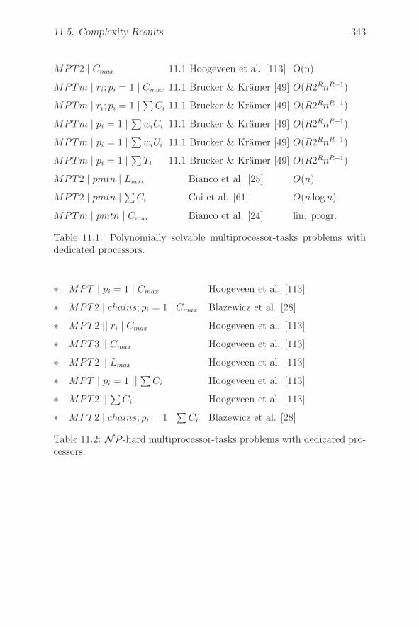
11.5. Complexity Results 343
MPT2 | Cmax 11.1 Hoogeveen et al. [113] O(n)
MPTm | ri; pi = 1 | Cmax 11.1 Brucker & Kramer [49] O(R2RnR+1)
MPTm | ri; pi = 1 | ∑Ci 11.1 Brucker & Kramer [49] O(R2RnR+1)
MPTm | pi = 1 | ∑wiCi 11.1 Brucker & Kramer [49] O(R2RnR+1)
MPTm | pi = 1 | ∑wiUi 11.1 Brucker & Kramer [49] O(R2RnR+1)
MPTm | pi = 1 | ∑Ti 11.1 Brucker & Kramer [49] O(R2RnR+1)
MPT2 | pmtn | Lmax Bianco et al. [25] O(n)
MPT2 | pmtn | ∑Ci Cai et al. [61] O(n log n)
MPTm | pmtn | Cmax Bianco et al. [24] lin. progr.
Table 11.1: Polynomially solvable multiprocessor-tasks problems withdedicated processors.
∗ MPT | pi = 1 | Cmax Hoogeveen et al. [113]
∗ MPT2 | chains; pi = 1 | Cmax Blazewicz et al. [28]
∗ MPT2 || ri | Cmax Hoogeveen et al. [113]
∗ MPT3 ‖ Cmax Hoogeveen et al. [113]
∗ MPT2 ‖ Lmax Hoogeveen et al. [113]
∗ MPT | pi = 1 || ∑Ci Hoogeveen et al. [113]
∗ MPT2 ‖ ∑Ci Hoogeveen et al. [113]
∗ MPT2 | chains; pi = 1 | ∑Ci Blazewicz et al. [28]
Table 11.2: NP-hard multiprocessor-tasks problems with dedicated pro-cessors.
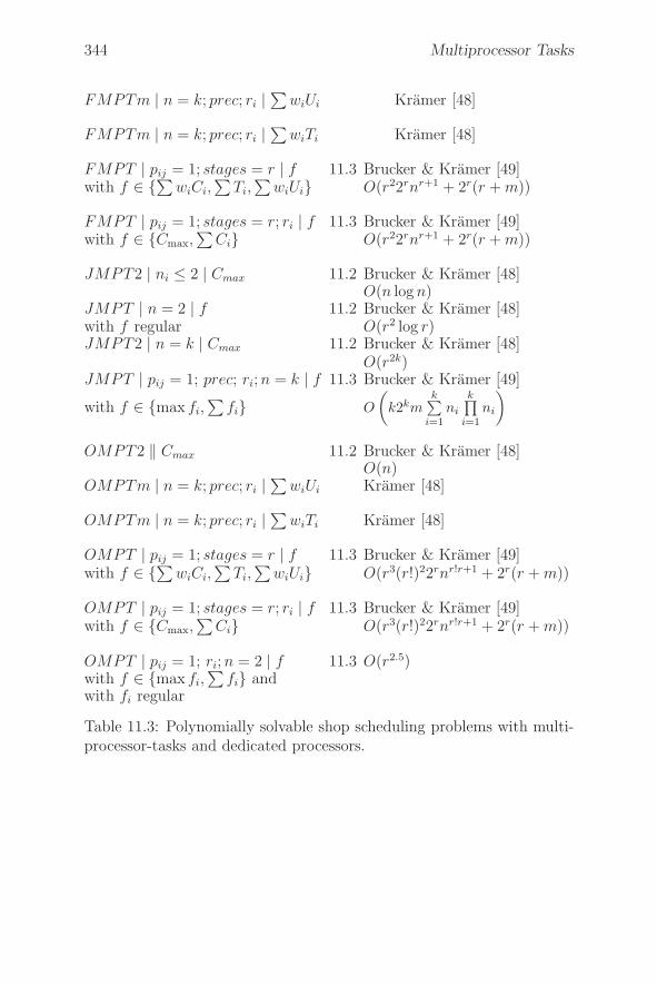
344 Multiprocessor Tasks
FMPTm | n = k; prec; ri |∑
wiUi Kramer [48]
FMPTm | n = k; prec; ri |∑
wiTi Kramer [48]
FMPT | pij = 1; stages = r | f 11.3 Brucker & Kramer [49]with f ∈ {∑ wiCi,
∑Ti,
∑wiUi} O(r22rnr+1 + 2r(r + m))
FMPT | pij = 1; stages = r; ri | f 11.3 Brucker & Kramer [49]with f ∈ {Cmax,
∑Ci} O(r22rnr+1 + 2r(r + m))
JMPT2 | ni ≤ 2 | Cmax 11.2 Brucker & Kramer [48]O(n log n)
JMPT | n = 2 | f 11.2 Brucker & Kramer [48]with f regular O(r2 log r)JMPT2 | n = k | Cmax 11.2 Brucker & Kramer [48]
O(r2k)JMPT | pij = 1; prec; ri; n = k | f 11.3 Brucker & Kramer [49]
with f ∈ {max fi,∑
fi} O
(
k2kmk∑
i=1ni
k∏
i=1ni
)
OMPT2 ‖ Cmax 11.2 Brucker & Kramer [48]O(n)
OMPTm | n = k; prec; ri |∑
wiUi Kramer [48]
OMPTm | n = k; prec; ri |∑
wiTi Kramer [48]
OMPT | pij = 1; stages = r | f 11.3 Brucker & Kramer [49]with f ∈ {∑ wiCi,
∑Ti,
∑wiUi} O(r3(r!)22rnr!r+1 + 2r(r + m))
OMPT | pij = 1; stages = r; ri | f 11.3 Brucker & Kramer [49]with f ∈ {Cmax,
∑Ci} O(r3(r!)22rnr!r+1 + 2r(r + m))
OMPT | pij = 1; ri; n = 2 | f 11.3 O(r2.5)with f ∈ {max fi,
∑fi} and
with fi regular
Table 11.3: Polynomially solvable shop scheduling problems with multi-processor-tasks and dedicated processors.
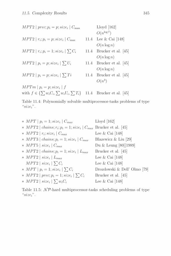
11.5. Complexity Results 345
MPT2 | prec; pi = p; sizei | Cmax Lloyd [162]
O(nlog 7)
MPT2 | ri; pi = p; sizei | Cmax 11.4 Lee & Cai [148]
O(n log n)
MPT2 | ri; pi = 1; sizei |∑
Ci 11.4 Brucker et al. [45]
O(n log n)
MPT2 | pi = p; sizei |∑
Ui 11.4 Brucker et al. [45]
O(n log n)
MPT2 | pi = p; sizei |∑
T i 11.4 Brucker et al. [45]
O(n3)
MPTm | pi = p; sizei | f
with f ∈ {∑wiCi,∑
wiUi,∑
Ti} 11.4 Brucker et al. [45]
Table 11.4: Polynomially solvable multiprocessor-tasks problems of type“sizei”.
∗ MPT | pi = 1; sizei | Cmax Lloyd [162]
∗ MPT2 | chains; ri; pi = 1; sizei | Cmax Brucker et al. [45]
∗ MPT2 | ri; sizei | Cmax Lee & Cai [148]
∗ MPT3 | chains; pi = 1; sizei | Cmax Blazewicz & Liu [29]
∗ MPT5 | sizei | Cmax Du & Leung [80][1989]
∗ MPT2 | chains; pi = 1; sizei | Lmax Brucker et al. [45]
∗ MPT2 | sizei | Lmax Lee & Cai [148]
MPT2 | sizei |∑
Ci Lee & Cai [148]
∗ MPT | pi = 1; sizei |∑
Ci Drozdowski & Dell’ Olmo [79]
∗ MPT2 | prec; pi = 1; sizei |∑
Ci Brucker et al. [45]
∗ MPT2 | sizei |∑
wiCi Lee & Cai [148]
Table 11.5: NP-hard multiprocessor-tasks scheduling problems of type“sizei”.
Bibliography
[1] E.H.L. Aarts, P.J.M. van Laarhoven, J.K. Lenstra, and N.L.J. Ul-der. A computational study of local search algorithms for job shopscheduling. ORSA Journal on Computing, 6(2):118–125, 1994.
[2] J.O. Achugbue and F.Y. Chin. Scheduling the open shop to min-imize mean flow time. SIAM Journal on Computing, 11:709–720,1982.
[3] D. Adolphson and T.C. Hu. Optimal linear ordering. SIAM Journalof Applied Mathematics, 25:403–423, 1973.
[4] A.V. Aho, J.E. Hopcroft, and J.D. Ullman. The design and analysisof computer algorithms. Adisson-Wesley, Reading, Mass., 1974.
[5] R.K. Ahuja, A.V. Goldberg, J.B. Orlin, and R.E. Tarjan. Findingminimum-cost flows by double scaling. Mathematical Programming,Ser. A, 53(3):243–266, 1992.
[6] R.K. Ahuja, T.L. Magnanti, and J.B. Orlin. Network Flows. Pren-tice Hall, Englewood Cliffs, 1993.
[7] R.K. Ahuja, J.B. Orlin, and R.E. Tarjan. Improved time boundsfor the maximum flow problem. SIAM Journal on Computing,18(5):939–954, 1989.
[8] S.B. Akers and J. Friedman. A non-numerical approach to produc-tion scheduling problems. Operations Research, 3:429–442, 1955.
[9] S. Albers and P. Brucker. The complexity of one-machine batch-ing problems. Discrete Applied Mathematics. Combinatorial Algo-rithms, Optimization and Computer Science, 47(2):87–107, 1993.

348 Bibliography
[10] D. Applegate and W. Cook. A computational study of the job-shopscheduling problem. ORSA Journal on Computing, 3(2):149–156,1991.
[11] I. Averbakh, O. Berman, and I. Chernykh. The m machine flowshopproblem with unit-time operations and precedence constraints. Op-erations Research Letters, 33(3):263–266, 2005.
[12] K.R. Baker. Introduction to Sequencing and Scheduling. John Wi-ley & Sons, New York, 1974.
[13] K.R. Baker, E.L. Lawler, J.K. Lenstra, and A.H.G. Rinnooy Kan.Preemptive scheduling of a single machine to minimize maximumcost subject to release dates and precedence constraints. OperationsResearch, 31:381–386, 1983.
[14] P. Baptiste. An 0(n4) algorithm for preemptive scheduling of asingle machine to minimize the number of late jobs. OperationsResearch Letters, 24:175–180, 1999.
[15] P. Baptiste. Polynomial time algorithms for minimizing theweighted number of late jobs on a single machine with equal pro-cessing times. Journal of Scheduling, 2:245–252, 1999.
[16] P. Baptiste. Batching identical jobs. Mathematical Methods ofOperations Research, 53(3):355–367, 2000.
[17] P. Baptiste. Preemptive scheduling of identical machines. TechnicalReport 2000-314, Universite de Technologie de Compiegne, France,2000.
[18] P. Baptiste. Scheduling equal-length jobs on identical parallel ma-chines. Discrete Applied Mathematics, 103(1):21–32, 2000.
[19] P. Baptiste. On preemption redundancy. BM research report, 2002.
[20] P. Baptiste and P. Brucker. Scheduling equal processing time jobs:a survey. In J. Y.-P. Leung, editor, Handbook of Scheduling, pages14.1–14.37. Chapman & Hall/CRC, New York, 2004.
[21] P. Baptiste, P. Brucker, S. Knust, and V.G. Timkovsky. Fourteennotes on equal-processing-times scheduling. OSM Reihe P, Heft246, Universitat Osnabruck, Fachbereich Mathematik/Informatik,2002.
Bibliography 349
[22] P. Baptiste, P. Brucker, S. Knust, and V.G. Timkovsky. Ten noteson equal-execution-times scheduling. 4 OR, 2:111–127, 2004.
[23] P. Baptiste and V.G. Timkovsky. Shortest path to nonpreemp-tive schedules of unit-time jobs on two identical parallel machineswith minimum total completion time. Math. Methods Oper. Res.,60(1):145–153, 2004.
[24] L. Bianco, J. Blazewicz, P. Dell’Olmo, and M. Drozdowski.Scheduling preemptive multiprocessor tasks on dedicated proces-sors. Performance Evaluation, 20(4):361–371, 1994.
[25] L. Bianco, J. Blazewicz, P. Dell’Olmo, and M. Drozdowski. Lin-ear algorithms for preemptive scheduling of multiprocessor taskssubject to minimal lateness. Discrete Applied Mathematics, 72(1-2):25–46, 1997.
[26] J. Blazewicz and K. Ecker. A linear time algorithm for restrictedbin packing and scheduling problems. Operations Research Letters,2:80–83, 1983.
[27] J. Blazewicz, K. H. Ecker, E. Pesch, G. Schmidt, and J. Weglarz.Scheduling computer and manufacturing processes. Springer Verlag,Berlin, 1996.
[28] J. Blazewicz, J.K. Lenstra, and A.H.G. Rinnooy Kan. Schedul-ing subject to resource constraints: classification and complexity.Discrete Applied Mathematics, 5(1):11–24, 1983.
[29] J. Blazewicz and Z. Liu. Scheduling multiprocessor tasks with chainconstraints. European Journal of Operational Research, 94(2):231–241, 1996.
[30] P.V.E. Boas. Preserving order in a forest in less than logarith-mic time. In 16th Annual Symposium of Foundations of ComputerScience, pages 75–84, Long Beach, 1978. IEEE Computer Society.
[31] H. Brasel, D. Kluge, and F. Werner. A polynomial algorithm for the[n/m/0, tij = 1, tree/Cmax] open shop problem. European Journalof Operational Research, 72(1):125–134, 1994.
350 Bibliography
[32] H. Brasel, D. Kluge, and F. Werner. A polynomial algorithm for anopen shop problem with unit processing times and tree constraints.Discrete Applied Mathematics, 59(1):11–21, 1995.
[33] P. Brucker. An efficient algorithm for the job-shop problem withtwo jobs. Computing, 40(4):353–359, 1988.
[34] P. Brucker. A polynomial algorithm for the two machine job-shopscheduling problem with a fixed number of jobs. Operations Re-search Spektrum, 16(1):5–7, 1994.
[35] P. Brucker, M.R. Garey, and D.S. Johnson. Scheduling equal-lengthtasks under treelike precedence constraints to minimize maximumlateness. Mathematics of Operations Research, 2(3):275–284, 1977.
[36] P. Brucker, A. Gladky, H. Hoogeveen, M.Y. Kovalyov, C.N. Potts,T. Tautenhahn, and S.L. van de Velde. Scheduling a batchingmachine. Journal of Scheduling, 1(1):31–54, 1998.
[37] P. Brucker, S. Heitmann, and J. Hurink. How useful are preemptiveschedules? Operations Research Letters 31, 31:129–136, 2003.
[38] P. Brucker, J. Hurink, and S. Knust. A polynomial algorithm forP |pj = 1, rj, outtree|∑Cj. Mathematical Methods of OperationsResearch, 56:407–412, 2002.
[39] P. Brucker, J. Hurink, and W. Kubiak. Scheduling identical jobswith chain precedence constraints on two uniform machines. Math-ematical Methods of Operations Research, 49(2):211–219, 1999.
[40] P. Brucker, B. Jurisch, and M. Jurisch. Open shop problems withunit time operations. Zeitschrift fur Operations Research. Methodsand Models of Operations Research, 37(1):59–73, 1993.
[41] P. Brucker, B. Jurisch, and A. Kramer. The job-shop problem andimmediate selection. Annals of Operations Research, 50:73–114,1994.
[42] P. Brucker, B. Jurisch, and A. Kramer. Complexity of schedul-ing problems with multi-purpose machines. Annals of OperationsResearch, 70:57–73, 1997.
Bibliography 351
[43] P. Brucker, B. Jurisch, and B. Sievers. A branch and bound algo-rithm for the job-shop scheduling problem. Discrete Applied Math-ematics, 49(1-3):107–127, 1994.
[44] P. Brucker and S. Knust. Complexity results for single-machineproblems with positive finish-start time-lags. Computing, 63:299–316, 1999.
[45] P. Brucker, S. Knust, D. Roper, and Y. Zinder. Scheduling UETtask systems with concurrency on two parallel identical proces-sors. Mathematical Methods of Operations Research, 53(3):369–387,2000.
[46] P. Brucker and M.Y. Kovalyov. Single machine batch scheduling tominimize the weighted number of late jobs. Mathematical Methodsof Operations Research, 43(1):1–8, 1996.
[47] P. Brucker, M.Y. Kovalyov, Y.M. Shafransky, and F. Werner.Batch scheduling with deadlines on parallel machines. Annals ofOperations Research, 83:23–40, 1998.
[48] P. Brucker and A. Kramer. Shop scheduling problems with mul-tiprocessor tasks on dedicated processors. Annals of OperationsResearch, 57:13–27, 1995.
[49] P. Brucker and A. Kramer. Polynomial algorithms for resource-constrained and multiprocessor task scheduling problems. Euro-pean Journal of Operational Research, 90:214–226, 1996.
[50] P. Brucker and S.A. Kravchenko. Preemption can make parallelmachine scheduling problems hard. OSM Reihe P, Heft 211, Uni-versitat Osnabruck, Fachbereich Mathematik/Informatik, 1999.
[51] P. Brucker and S.A. Kravchenko. of mean flow timescheduling problems with release dates. OSM Reihe P, Heft 251,Universitat Osnabruck, Fachbereich Mathematik/Informatik, 2004.
[52] P. Brucker and S.A. Kravchenko. Scheduling jobs with equal pro-cessing times and time window on identical parallel machine. OSMReihe P, Heft 257, Universitat Osnabruck, Fachbereich Mathe-matik/Informatik, 2004.
Complexity
352 Bibliography
[53] P. Brucker and S.A. Kravchenko. Scheduling jobs with releasetimes on parallel machines to minimize total tardiness. OSMReihe P, Heft 258, Universitat Osnabruck, Fachbereich Mathe-matik/Informatik, 2005.
[54] P. Brucker, S.A. Kravchenko, and Y.N. Sotskov. On the com-plexity of two machine job-shop scheduling with regular objectivefunctions. Operations Research Spektrum, 19(1):5–10, 1997.
[55] P. Brucker, S.A. Kravchenko, and Y.N. Sotskov. Preemptive job-shop scheduling problems with a fixed number of jobs. Mathemat-ical Methods of Operations Research, 49(1):41–76, 1999.
[56] P. Brucker and R. Schlie. Job-shop scheduling with multi-purposemachines. Computing, 45(4):369–375, 1990.
[57] P. Brucker and O. Thiele. A branch & bound method for thegeneral-shop problem with sequence dependent setup-times. Oper-ations Research Spektrum, 18(3):145–161, 1996.
[58] J. Bruno, E.G. Coffman, Jr., and R. Sethi. Scheduling independenttasks to reduce mean finishing time. Communications of the ACM,17:382–387, 1974.
[59] J. Bruno and P. Downey. Complexity of task sequencing with dead-lines, set-up times and changeover costs. SIAM Journal on Com-puting, 7:393–403, 1978.
[60] J. Bruno, J.W. Jones, III, and K. So. Deterministic scheduling withpipelined processors. IEEE Transactions on Computers, 29(4):308–316, 1980.
[61] X. Cai, C.-Y. Lee, and C.-L. Li. Minimizing total completiontime in two-processor task systems with prespecified processorallocations. Naval Research Logistics. An International Journal,45(2):231–242, 1998.
[62] J. Carlier. The one-machine sequencing problem. European Journalof Operational Research, 11:42–47, 1982.
[63] J. Carlier and E. Pinson. An algorithm for solving the job-shopproblem. Management Science, 35(2):164–176, 1989.
Bibliography 353
[64] J. Chen and C.-Y. Lee. General multiprocessor task scheduling.Naval Research Logistics, 46(1):57–74, 1999.
[65] J. Cheriyan and S.N. Maheshwari. Analysis of preflow push algo-rithms for maximum network flow. SIAM Journal on Computing,18(6):1057–1086, 1989.
[66] Y. Cho and S. Sahni. Preemptive scheduling of independent jobswith release and due times on open, flow and job shops. OperationsResearch, 29(3):511–522, 1981.
[67] V. Chvatal. Linear programming. W. H. Freeman and Company,New York - San Francisco, 1983.
[68] E. G. Coffman, Jr., J. Sethuraman, and V.G. Timkovsky. Ideal pre-emptive schedules on two processors. Technical report, ColumbiaUniversity, 2002.
[69] E.G. Coffman, Jr. Scheduling in Computer and Job Shop Systems.J.Wiley, New York, 1976.
[70] E.G. Coffman, Jr. and R.L. Graham. Optimal scheduling for two-processor systems. Acta Informatica, 1:200–213, 1971/1972.
[71] E.G. Coffman, Jr., M. Yannakakis, M.J. Magazine, and C. Santos.Batch sizing and job sequencing on a single machine. Annals ofOperations Research, 26(1-4):135–147, 1990.
[72] R.W. Conway, W.L. Maxwell, and L.W. Miller. Theory of Schedul-ing. Addison Wesley, Reading, Mass., USA, 1967.
[73] S.A. Cook. The complexity of theorem-proving procedures. In Pro-ceedings of the 3rd Annual ACM Symposium on Theory of Com-puting, pages 151–158. ACM-Press, 1971.
[74] G.B. Dantzig. Application of the simplex method to a transporta-tion problem. In T.C. Koopmans, editor, Activity analysis of pro-duction and allocation, pages 359–373. John Wiley & Sons, Inc.,1951.
[75] M. Dell’Amico and M. Trubian. Applying tabu search to the job-shop scheduling problem. Annals of Operations Research, 41(1-4):231–252, 1993.
354 Bibliography
[76] M.I. Dessouky, B.J. Lageweg, J.K. Lenstra, and S.L. van de Velde.Scheduling identical jobs on uniform parallel machines. StatisticaNeerlandica, 44(3):115–123, 1990.
[77] U. Dorndorf and E. Pesch. Evolution based learning in a jobshop scheduling environment. Computers & Operations Research,22(1):25–40, 1995.
[78] M. Dror, W. Kubiak, and P. Dell’Olmo. Strong-weak chain con-strained scheduling. Ricerca Operativa, 27:35–49, 1998.
[79] M. Drozdowski and P. Dell’ Olmo. Scheduling multiprocessor tasksfor mean flow time criterion. Technical Report RA-003/98, Insti-tute of Computing Science, Poznan University of Technology, 1998.
[80] J. Du and J.Y.-T. Leung. Complexity of scheduling parallel tasksystems. SIAM Journal on Discrete Mathematics, 2(4):473–487,1989.
[81] J. Du and J.Y.-T. Leung. Minimizing total tardiness on one ma-chine is NP-hard. Mathematics of Operations Research, 15(3):483–495, 1990.
[82] J. Du and J.Y.-T. Leung. Minimizing the number of late jobs onunrelated machines. Operations Research Letters, 10(3):153–158,1991.
[83] J. Du and J.Y.-T. Leung. Minimizing mean flow time in two-machine open shops and flow shops. Journal of Algorithms,14(1):24–44, 1993.
[84] J. Du, J.Y.-T. Leung, and C.S. Wong. Minimizing the number oflate jobs with release time constraint. Journal of CombinatorialMathematics and Combinatorial Computing, 11:97–107, 1992.
[85] J. Du, J.Y.-T. Leung, and G.H. Young. Minimizing mean flowtime with release time constraint. Theoretical Computer Science,75(3):347–355, 1990.
[86] J. Du, J.Y.-T. Leung, and G.H. Young. Scheduling chain-structured tasks to minimize makespan and mean flow time. In-formation and Computation, 92(2):219–236, 1991.
Bibliography 355
[87] J. Edmonds and R.M. Karp. Theoretical improvements in algorith-mic efficiency for network flow problems. Journal of the Associationfor Computing Machinery, 19:248–264, 1972.
[88] S. Even and O. Kariv. An o(n2.5) algorithm for maximum matchingin general graphs. In Proceedings of the 16th Annual Symposiumof Foundations of Computer Science, pages 100–112, Long Beach,1975. IEEE Computer Society.
[89] A. Federgruen and H. Groenevelt. Preemptive scheduling of uni-form machines by ordinary network flow techniques. ManagementScience, 32:341–349, 1986.
[90] M.J. Fischer and A.R. Meyer. Boolean matrix multiplication andtransitive closure. In Proceedings Twelfth Annual Symposium onSwitching and Automata Theory, pages 129–137, East Lansing,Mich., 1971.
[91] L.R.jun. Ford and D.R. Fulkerson. Maximal flow through a net-work. Canadian Journal of Mathematics, 8:399–404, 1956.
[92] G.N. Frederickson. Scheduling unit-time tasks with integer releasetimes and deadlines. Information Processing Letters, 16:171–173,1983.
[93] S. French. Sequencing and scheduling: an introduction to the math-ematics of the job- shop. Ellis Horwood Limited, New York, 1982.
[94] D.R. Fulkerson. An out-of-kilter method for minimal-cost flowproblems. SIAM Jouranl of Applied Mathematics, 9:18–27, 1961.
[95] H.N. Gabow and O. Kariv. Algorithms for edge coloring bipartitegraphs and multigraphs. SIAM Journal on Computing, 11:117–129,1982.
[96] M.R. Garey and D.S. Johnson. Scheduling tasks with nonuniformdeadlines on two processors. Journal of the Association for Com-puting Machinery, 23:461–467, 1976.
[97] M.R. Garey and D.S. Johnson. Two-processor scheduling withstart-times and deadlines. SIAM Journal on Computing, 6(3):416–426, 1977.
356 Bibliography
[98] M.R. Garey and D.S. Johnson. “Strong” NP-completeness results:motivation, examples, and implications. Journal of the Associationfor Computing Machinery, 25(3):499–508, 1978.
[99] M.R. Garey and D.S. Johnson. Computers and intractability. Aguide to the theory of NP-completeness. W. H. Freeman and Com-pany, San Francisco, 1979.
[100] M.R. Garey, D.S. Johnson, and R. Sethi. The complexity of flow-shop and jobshop scheduling. Mathematics of Operations Research,1(2):117–129, 1976.
[101] A.V. Goldberg and R.E. Tarjan. Finding minimum-cost circula-tions by successive approximation. Mathematics of Operations Re-search, 15(3):430–466, 1990.
[102] T. Gonzalez. A note on open shop preemptive schedules. IEEETransactions on Computers C-28, pages 782–786, 1979.
[103] T. Gonzalez and D.B. Johnson. A new algorithm for preemptivescheduling of trees. Journal of the Association for Computing Ma-chinery, 27(2):287–312, 1980.
[104] T. Gonzalez and S. Sahni. Open shop scheduling to minimize fin-ish time. Journal of the Association for Computing Machinery,23(4):665–679, 1976.
[105] T. Gonzalez and S. Sahni. Flowshop and jobshop schedules: com-plexity and approximation. Operations Research, 26(1):36–52,1978.
[106] T. Gonzalez and S. Sahni. Preemptive scheduling of uniform pro-cessor systems. Journal of the Association for Computing Machin-ery, 25:92–101, 1978.
[107] J. Grabowski, E. Nowicki, and S. Zdrzalka. A block approachfor single-machine scheduling with release dates and due dates.European Journal of Operational Research, 26:278–285, 1986.
[108] R.L. Graham, E.L. Lawler, J.K. Lenstra, and A.H.G. Rinnooy Kan.Optimization and approximation in deterministic sequencing andscheduling: A survey. Annals of Discrete Mathematics, 5:287–326,1979.
Bibliography 357
[109] N.G. Hall and M.E. Posner. Earliness-tardiness scheduling prob-lems. I: Weighted deviation of completion times about a commondue data. Operations Research, 39(5):836–846, 1991.
[110] P. Hall. On representatives of subsets. Journal of the LondonMathematical Society, 10:26–30, 1935.
[111] L.A. Herrbach and J.Y.-T. Leung. Preemptive scheduling of equallength jobs on two machines to minimize mean flow time. Opera-tions Research, 38(3):487–494, 1990.
[112] D.S. Hochbaum and D. Landy. Scheduling with batching: mini-mizing the weighted number of tardy jobs. Operations ResearchLetters, 16(2):79–86, 1994.
[113] J.A. Hoogeveen, S.L. van de Velde, and B. Veltman. Complexityof scheduling multiprocessor tasks with prespecified processor allo-cations. Discrete Applied Mathematics. Combinatorial Algorithms,Optimization and Computer Science, 55(3):259–272, 1994.
[114] J.E. Hopcroft and R.M. Karp. A n5/2 algorithm for maximummatchings in bipartite graphs. SIAM Journal on Computing,2:225–231, 1973.
[115] W.A. Horn. Some simple scheduling algorithms. Naval ResearchLogistics Quarterly, 21:177–185, 1974.
[116] T.C. Hu. Parallel sequencing and assembly line problems. Opera-tions Research, 9:841–848, 1961.
[117] E. Ignall and L. Schrage. Apllications of the branch and boundtechnique to some flow-shop scheduling problems. Operations Re-search, 13:400–412, 1965.
[118] J.R. Jackson. Scheduling a production to minimize maximum tar-diness. Research Report 43, Management Science Research Project,University of California at Los Angeles, 1955.
[119] J.R. Jackson. An extension of johnson’s results on job lot schedul-ing. Naval Research Logistic Quaterly, 3:201–203, 1956.
358 Bibliography
[120] S.M. Johnson. Optimal two-and-three-stage production scheduleswith set-up times included. Naval Research Logistic Quaterly, 1:61–68, 1954.
[121] B. Jurisch. Lower bounds for the job-shop scheduling problem onmulti-purpose machines. Discrete Applied Mathematics. Combina-torial Algorithms, Optimization and Computer Science, 58(2):145–156, 1995.
[122] H. Kahlbacher. Termin- und Ablaufplanung - ein analytischer Zu-gang. PhD thesis, University Kaiserslautern, 1992.
[123] J.J. Kanet. Minimizing the average deviation of job completiontimes about a common due date. Naval Research Logistic Quaterly,28:643–651, 1981.
[124] R.M. Karp. Reducibility among combinatorial problems. In Com-plexity of computer computations (Proc. Sympos., IBM Thomas J.Watson Res. Center, Yorktown Heights, N.Y., 1972), pages 85–103. Plenum, New York, 1972.
[125] L.G. Khachiyan. A polynomial algorithm in linear programming.Doklasy Akademii Nauk SSSR, 244:1093–1096, 1979.
[126] S.A. Kravchenko. Minimizing the number of late jobs for the two-machine unit-time job-shop scheduling problem. Discrete AppliedMathematics, 98(3):209–217, 1999.
[127] S.A. Kravchenko. On the complexity of minimizing the number oflate jobs in unit time open shops. Discrete Applied Mathematics,100(2):127–132, 1999.
[128] M. Kubale. Preemptive scheduling of two processor tasks on ded-icated processors. Zeszyty Naukowe Politechnik: Slaskiej, Seria:Automatyka Z. 100, 1082:145–153, 1990.
[129] W. Kubiak. Exact and approximate algorithms for schedulingunit time tasks with tree-like precedence constraints. In AbstractsEURO IX - TIMS XXVIII Paris, 195, 1988.
[130] W. Kubiak, S. Sethi, and C. Sriskandarajah. An efficient algorithmfor a job shop problem. Annals of Operations Research, 57:203–216,1995.
Bibliography 359
[131] W. Kubiak and V.G. Timkovsky. A polynomial-time algorithm fortotal completion time minimization in two-machine job-shop withunit-time operations. European Journal of Operational Research,94:310–320, 1996.
[132] H.W. Kuhn. The Hungarian method for the assignment problem.Naval Research Logistics, 2, 1955.
[133] J. Labetoulle, E.L. Lawler, J.K. Lenstra, and A.H.G. Rinnooy Kan.Preemptive scheduling of uniform machines subject to releasedates. In Progress in combinatorial optimization (Waterloo, Ont.,1982), pages 245–261. Academic Press, Toronto, Ont., 1984.
[134] B.J. Lageweg, J.K. Lenstra, E.L. Lawler, and A.H.G. Rinnooy Kan.Computer-aided complexity classification of combinatorial prob-lems. Communications of the ACM, 25:817–822, 1982.
[135] E.L. Lawler. Optimal sequencing of a single machine subject toprecedence constraints. Management Science, 19:544–546, 1973.
[136] E.L. Lawler. A “pseudopolynomial” algorithm for sequencing jobsto minimize total tardiness. Annals of Discrete Mathematics,1:331–342, 1977.
[137] E.L. Lawler. Sequencing jobs to minimize total weighted comple-tion time subject to precedence constraints. Annals of DiscreteMathematics, 2:75–90, 1978.
[138] E.L. Lawler. Preemptive scheduling of uniform parallel machinesto minimize the weighted number of late jobs. Report BW 105,Centre for Mathematics and Computer Science, Amsterdam, 1979.
[139] E.L. Lawler. Preemptive scheduling of precedence-constrainedjobs on parallel machines. In M.A.H. Dempster, J.K. Lenstra,and A.H.G. Rinnooy Kan, editors, Deterministic and stochasticscheduling, Proceedings of the NATO Advanced Study and ResearchInstitute on Theoretical Approaches to Scheduling Problems held inDurham, July 6–17, 1981, volume 84 of NATO Advanced Study In-stitute Series C: Mathematical and Physical Sciences, pages 101–123, Dordrecht, 1982. D. Reidel Publishing Co.
360 Bibliography
[140] E.L. Lawler. Recent results in the theory of machine scheduling.In A. Bachem, M. Groetschel, and B. Korte, editors, Mathematicalprogramming: the state of the art (Bonn, 1982), pages 202–234.Springer, Berlin, 1983.
[141] E.L. Lawler. A dynamic programming algorithm for preemptivescheduling of a single machine to minimize the number of late jobs.Annals of Operations Research, 26(1-4):125–133, 1990.
[142] E.L. Lawler and J. Labetoulle. On preemptive scheduling of un-related parallel processors by linear programming. Journal of theAssociation for Computing Machinery, 25(4):612–619, 1978.
[143] E.L. Lawler, J.K. Lenstra, and A.H.G. Rinnooy Kan. Minimizingmaximum lateness in a two-machine open shop. Mathematics ofOperations Research, 6(1):153–158, 1981.
[144] E.L. Lawler, J.K. Lenstra, and A.H.G. Rinnooy Kan. Erra-tum: “Minimizing maximum lateness in a two-machine open shop”[Math. Oper. Res. 6 (1981), no. 1, 153-158]. Mathematics of Oper-ations Research, 7(4):635, 1982.
[145] E.L. Lawler, J.K. Lenstra, A.H.G. Rinnooy Kan, and D.B. Shmoys.Sequencing and Scheduling: Algorithmus and Complexity, vol-ume 4 of Handbook in Operations Research and Managment Sci-ence. North-Holland, Amsterdam, 1993.
[146] E.L. Lawler and C.U. Martel. Preemptive scheduling of two uni-form machines to minimize the number of late jobs. OperationsResearch, 37(2):314–318, 1989.
[147] E.L. Lawler and J.M. Moore. A functional equation and its applica-tion to resource allocation and sequencing problems. ManagementScience, 16:77–84, 1969.
[148] C.-Y. Lee and X. Cai. Scheduling one and two-processor taskson two parallel processors. IIE Transactions on Scheduling andLogistics, 31:445–455, 1999.
[149] H.W. Lenstra, Jr. Integer programming with a fixed number ofvariables. Mathematics of Operations Research, 8:538–548, 1983.
[150] J.K. Lenstra. Not published.
Bibliography 361
[151] J.K. Lenstra. Sequencing by enumerative methods. MathematicalCentre Tracts. 69, 1977.
[152] J.K. Lenstra and A.H.G. Rinnooy Kan. Complexity of schedulingunder precedence constraints. Operations Research, 26(1):22–35,1978.
[153] J.K. Lenstra and A.H.G. Rinnooy Kan. Computational complexityof discrete optimization problems. Annals of Discrete Mathematics,4:121–140, 1979.
[154] J.K. Lenstra and A.H.G. Rinnooy Kan. Complexity results forscheduling chains on a single machine. European Journal of Oper-ational Research, 4(4):270–275, 1980.
[155] J.K. Lenstra, A.H.G. Rinnooy Kan, and P. Brucker. Complexityof machine scheduling problems. Annals of Discrete Mathematics,1:343–362, 1977.
[156] J.Y.-T. Leung, O. Vornberger, and J.D. Witthoff. On some vari-ants of the bandwidth minimization problem. SIAM Journal onComputing, 13(3):650–667, 1984.
[157] J.Y.-T. Leung and G.H. Young. Minimizing total tardiness ona single machine with precedence constraints. ORSA Journal onComputing, 2(4):346–352, 1990.
[158] J.Y.-T. Leung and G.H. Young. Preemptive scheduling to minimizemean weighted flow time. Information Processing Letters, 34(1):47–50, 1990.
[159] L.A. Levin. Universal sorting problems. Problemy Peredachi In-formatsii, 9:265–266, 1973.
[160] C.Y. Liu and R.L. Bulfin. On the complexity of preemptive open-shop scheduling problems. Operations Research Letters, 4(2):71–74,1985.
[161] C.Y. Liu and R.L. Bulfin. Scheduling open shops with unit execu-tion times to minimize functions of due dates. Operations Research,36(4):553–559, 1988.
362 Bibliography
[162] E.L. Lloyd. Concurrent task systems. Operations Research. TheJournal of the Operations Research Society of America, 29(1):189–201, 1981.
[163] I. Lushchakova. Two machine preemptive scheduling problem withrelease dates, equal processing times and precedence constraints.European J. Oper. Res., 171(1):107–122, 2006.
[164] V.M. Malhotra, M.P. Kumar, and S.N. Maheshwari. An O(|V |3)algorithm for finding maximum flows in networks. InformationProcessing Letters, 7:277–278, 1978.
[165] R. McNaughton. Scheduling with deadlines and loss functions.Management Science, 6:1–12, 1959/1960.
[166] W. Meyer. Geometrische Methoden zur Losung von Job-Shop Prob-lemen und deren Verallgemeinerungen. PhD thesis, UniversitatOsnabruck, Fachbereich Mathematik/Informatik, 1992.
[167] M. Middendorf and V.G. Timkovsky. Transversal graphs for par-tially ordered sets: sequencing, merging and scheduling problems.Journal of Combinatorial Optimization, 3(4):417–435, 1999.
[168] G.J. Minty. Monotone networks. Proceedings of the London Math-ematical Society, 257:194–212, 1960.
[169] C.L. Monma. Linear-time algorithms for scheduling on parallelprocessors. Operations Research, 30:116–124, 1982.
[170] C.L. Monma and C.N. Potts. On the complexity of scheduling withbatch setup times. Operations Research, 37(5):798–804, 1989.
[171] J.M. Moore. An n job, one machine sequencing algorithm for min-imizing the number of late jobs. Management Science, 15:102–109,1968.
[172] R.R. Muntz and E.G. Coffman, Jr. Optimal preemptive schedulingon two-processor systems. IEEE Transactions on Computers, pages1014–1020, 1969.
[173] R.R. Muntz and E.G. Coffman, Jr. Preemptive scheduling of real-time tasks on multiprocessor systems. Journal of the Associationfor Computing Machinery, 17:324–338, 1970.
Bibliography 363
[174] J.F. Muth and G.L. Thompson. Industrial Scheduling. Wiley, NewYork, 1963.
[175] G.L. Nemhauser and L.A. Wolsey. Integer and combinatorial opti-mization. Wiley, New York, 1988.
[176] C.T. Ng, T.C.E. Cheng, and J.J. Yuan. A note on the single ma-chine serial batching scheduling problem to minimize maximumlateness with precedence constraints. Operations Research Letters,30:66–68, 2002.
[177] E. Nowicki and C. Smutnicki. A fast tabu search algorithm for thejob shop problem. Management Science, 42(6):797–813, 1996.
[178] J.B. Orlin. A faster strongly polynomial minimum cost flow algo-rithm. Operations Research, 41(2):338–350, 1993.
[179] S.S. Panwalkar, M.L. Smith, and A. Seidmann. Common due dateassignment to minimize total penalty for the one machine schedul-ing problem. Operations Research, 30:391–399, 1982.
[180] M. Pinedo. Scheduling: Theory, Algorithms and Systems. PrenticeHall, Englewood Cliffs N.J., 1995.
[181] A.H.G. Rinnooy Kan. Machine Scheduling Problems: Classifica-tion, Complexity and Computations. Martinus Nijhoff, The Hague,1976.
[182] A. Schrijver. Theory of linear and integer programming. Wiley,Chichester, 1986.
[183] N.V. Shakhlevich and Yu.N. Sotskov. Scheduling two jobs withfixed and nonfixed routes. Computing, 52(1):17–30, 1994.
[184] N.V. Shakhlevich, Yu.N. Sotskov, and F. Werner. Shop schedulingproblems with fixed and non-fixed machine orders of jobs. Annalsof Operations Research, 92:281–304, 1999.
[185] B. Simons. A fast algorithm for single processor scheduling. In 19thAnnual Symposium on Foundations of Computer Science (Ann Ar-bor, Mich., 1978), pages 246–252. IEEE, Long Beach, Calif., 1978.
364 Bibliography
[186] B. Simons. Multiprocessor scheduling of unit-time jobs with arbi-trary release times and deadlines. SIAM Journal on Computing,12(2):294–299, 1983.
[187] R.A. Sitters. Two NP-hardness results for preemptive minisumscheduling for unreleated parallel machines. In Proc. 8th Interna-tional IPCO Conference, volume 2081 of Lecture Notes in Com-puter Science, pages 396–405. Springer, 2001.
[188] W.E. Smith. Various optimizers for single-stage production. NavalResearch Logistics Quarterly, 3:59–66, 1956.
[189] Y.N. Sotskov. The complexity of shop-scheduling problems withtwo or three jobs. European Journal of Operational Research,53(3):326–336, 1991.
[190] Y.N. Sotskov and N.V. Shakhlevich. NP-hardness of shop-scheduling problems with three jobs. Discrete Applied Mathemat-ics, 59(3):237–266, 1995.
[191] C. Sriskandarajah and E. Wagneur. On the complexity of preemp-tive openshop scheduling problems. European Journal of Opera-tional Research, 77(3):404–414, 1994.
[192] V.A. Strusevich. Two-machine super-shop scheduling problem.Journal of the Operational Research Society, 42(6):479–492, 1991.
[193] V.S. Tanaev, V.S. Gordon, and Y.M. Shafransky. Scheduling the-ory. Single-stage systems. Vol. 1. Kluwer Academic Publishers.,Dordrecht, 1994.
[194] V.S. Tanaev, Y.N. Sotskov, and V.A. Strusevich. Scheduling the-ory. Multi-stage systems, volume 285 of Mathematics and its Ap-plications. Kluwer Academic Publishers Group, Dordrecht, 1994.Translated and revised from the 1989 Russian original by the au-thors.
[195] T. Tautenhahn. Open-shop-Probleme mit Einheitsbearbeitungszei-ten. PhD thesis, Fakultat fur Mathematik, Otto-von-Guericke-Uni-versitat Magdeburg, 1993.
Bibliography 365
[196] T. Tautenhahn and G.J. Woeginger. Minimizing the total comple-tion time in a unit-time open shop with release times. OperationsResearch Letters, 20(5):207–212, 1997.
[197] Z. Tian, C.T. Ng, and T.C.E. Cheng. An O(n2) algorithm forscheduling equal-length preemptive jobs on a single machine tominimze total tardiness. Journal of Scheduling, 9(4):343–364, 2006.
[198] V.G. Timkovsky. On the complexity of scheduling an arbitrary sys-tem. Soviet Journal of Computer and Systems Sciences, 23(5):46–52, 1985.
[199] V.G. Timkovsky. The complexity of unit-time job-shop schedul-ing. Technical Report 93-09, Department of Computer Science andSystems, McMaster Univ. Hamilton, 1993.
[200] V.G. Timkovsky. A polynomial-time algorithm for the two-machineunit-time release-date job-shop schedule-length problem. DiscreteApplied Mathematics. Combinatorial Algorithms, Optimization andComputer Science, 77(2):185–200, 1997.
[201] V.G. Timkovsky. Identical parallel machines vs. unit-time shops,preemptions vs. chains, and other offsets in scheduling complexity.Technical Report, Department of Computer Science and Systems,McMaster Univ. Hamilton, 1998.
[202] V.G. Timkovsky. Is a unit-time job shop not easier than identicalparallel machines? Discrete Applied Mathematics. CombinatorialAlgorithms, Optimization and Computer Science, 85(2):149–162,1998.
[203] J.D. Ullman. NP-complete scheduling problems. Journal of Com-puter and System Sciences, 10:384–393, 1975.
[204] J.D. Ullman. Complexity of sequencing problems. In J.L. Bruno,E.G. Coffman, Jr., R.L. Graham, W.H. Kohler, R. Sethi, K. Stei-glitz, and J.D. Ullman, editors, Computer and Job/Shop SchedulingTheory. John Wiley & Sons Inc., New York, 1976.
[205] P.J.M. van Laarhoven and E.H.L. Aarts. Simulated annealing: the-ory and applications. D. Reidel Publishing Company, Dordrecht,1987.
366 Bibliography
[206] P.J.M. van Laarhoven, E.H.L. Aarts, and J.K. Lenstra. Jobshop scheduling by simulated annealing. Operations Research,40(1):113–125, 1992.
[207] M.A. Yakovleva. A problem on minimum transportation cost. InApplications of mathematics in economic research, pages 390–399.Izdat. Social’no - Ekon Lit., Moscow, 1959.
Index
MMPT -problem, 335MPT , 317V -shaped, 246, 250, 255, 260NP, 40NP-complete, 44NP-complete in the strong sense,
47NP-hard, 46P, 39p-batching problem, 4s-t-path, 29s-batch, 33s-batching problem, 4, 341-tasks, 3362-tasks, 3363-DIMENSIONAL MATCHING, 413-SATISFIABILITY, 45
absolute deviation, 7active, 157active schedule, 7, 180, 197acyclic graph, 156adjacency matrix, 23, 62after-candidates, 206agreeable weights, 94allowed modifications, 52arc coloring, 22, 161aspiration criterion, 55, 225assignment, 18assignment problem, 18, 135, 137augmenting path algorithm, 14
backward calculation, 28
backward scan, 304backwards Jackson’s preemptive sched-
ule, 214bar, 199barrier, 114barrier list, 114barrier-correct, 115batch, 4batching, 267batching problem, 4before-candidates, 206binary linear program, 12bipartite graph, 14, 18, 20, 22, 161bipartite matching, 14block, 64, 89, 111, 197, 205, 328Boolean variable, 45bottleneck objective, 6branch-and-bound algorithm, 56, 202branching, 56branching scheme, 204branching tree, 56bucket sorting, 72, 86
certificate, 40chains, 4changeover time, 281, 290circulation problem, 13classification, 1clause, 45CLIQUE, 42clique, 42compatibility graph, 324
368 Index
compatible stages, 324compatible tasks, 317complete selection, 156, 203complexity of single machine prob-
lems, 104computational problem, 37conflict resolution procedure, 24conjunctive arc, 156constant changeover time, 282cost, 6cost function, 3crisis job, 114crisis subroutine, 114critical path, 203, 205cycle, 29cyclic list schedule, 112
deadline, 4decision problem, 39, 41decomposition tree, 80dedicated machine, 2degree, 23demand, 12direct arc, 213discrete optimization problem, 51disjunctive arc, 156disjunctive graph, 156disjunctive graph model, 202dual arc, 213dual pair, 213due date, 3due date modification, 140due date scheduling, 243dynamic programming, 26, 29, 98,
282dynamic tabu list, 225
earliest possible completion time, 214earliness, 7, 243early set of jobs, 165
EDD rule, 67, 70, 88expanded network, 131
feasible B-schedule, 116feasible flow, 13feasible solution, 11feasible with respect to the time win-
dows, 129finishing time, 6fixed arc, 156flexible manufacturing, 2flow graph, 13flow shop, 5flow shop problem, 174, 232flow shop problem with MPT , 317flow shop with MPT , 325, 330flow-shop problem, 58forward scan, 304frequency vector, 164
Gantt chart, 1general shop, 5general shop problem, 155, 290general shop problem with multi-
processor tasks, 317geometric approach, 186
HAMILTON CIRCUIT, 42head, 71, 210head-tail problem, 71
identical machines, 107identical parallel machine, 28identical processing times, 98immediate predecessor, 68, 139immediate selection, 212immediate successor, 139incompatible stages, 324incompatible tasks, 317initial vertex, 198
Index 369
input length, 37integer linear program, 12intree, 3, 77, 140invariance property, 83iterative improvement, 52
Jackson’s preemptive schedule, 213Jackson’s scheduling rule, 67job, 1job characteristics, 3job shop, 5job shop problem with MPT , 317job shop scheduling problem, 178,
232job shop with MPT , 326, 329job shop with machine repetition, 5just-in-time production, 243
lateness, 7, 243Lawler’s algorithm, 135length of a path, 29length of block, 197level, 125level algorithm, 125linear program, 11, 12, 137linear programming formulation, 14,
18list, 112literals, 45local minimum, 52local search, 51lower bound, 56LPT-sequence, 246
machine, 1machine environment, 3, 5machine repetition, 196machine-dedicated, 5machine-identical parallel, 5machine-uniform parallel, 5
machine-unrelated parallel, 5main operation, 199makespan, 6matching, 14, 15, 18maximum flow algorithm, 38maximum flow problem, 13, 109maximum lateness, 7, 67Mc Naughton’s wrapping around rule,
287mean flow time, 22median, 245minimax criterion, 62minimum coloring, 22minimum-cost circulation problem,
38mixed integer linear program, 12mixed shop, 6mixed shop problem, 226, 233modification of due dates, 68modification of release times, 63modified due date, 145modified sets, 304modified Smith’s rule, 78Monge array, 20MSPCLASS, 49multi-mode multiprocessor-task sche-
duling problem, 335multi-purpose machine, 2, 5multiprocessor task, 2multiprocessor tasks, 317
neighborhood, 52neighborhood graph, 52neighborhood structure, 52, 222network simplex method, 13number of operations, 2number problem, 46
occupied cells, 23open shop, 5
370 Index
open shop problem, 138, 158, 232open shop problems with MPT , 317open shop with MPT , 323, 333opt-connected, 222optimality criterion, 3, 6out-of-kilter algorithm, 13outtree, 3, 73, 140
parallel composition, 4parallel jobsets, 73parallel machines, 2, 107parallel uniform machines, 124PARTITION, 41path, 29permutation flow shop, 6, 175polynomially solvable, 38potential obstacle, 303precedence relations, 3predecessor, 29preemption, 3preemptive open shop problem, 15primal arc, 213primal pair, 213procedure select, 217processing requirement, 2product property, 31pseudopolynomial, 39pseudopolynomial reduction, 47pseudopolynomially solvable, 39, 46pull job, 114
reduction, 41reduction graph, 48regular objective functions, 7release date, 2restricted set, 114
SATISFIABILITY, 45satisfied, 45schedule, 1
schedule-feasible, 3schedule-jobs, 7schedule-optimal, 3scheduling problem, 6search tree, 203selection, 156, 203semiactive schedule, 7sequence dependent changeover time,
281sequence independent changeover time,
281sequence of batch sizes, 34series composition, 4series-parallel graph, 4, 79set of machines, 2set-up time, 267shop problems with MPT , 323shop scheduling problem, 155shortest path algorithm, 29, 32shortest path problem, 187, 198, 318shortest paths to s, 30simplex algorithm, 12simulated annealing, 53single machine batching problem, 34single machine problem, 19single machine scheduling, 26, 61sink, 156sink vertex, 13sizei, 335Smith’s ratio rule, 78Smith’s rule, 78source, 156source vertex, 13speed-of machine, 5SPT-rule, 134SPT-sequence, 246squared deviation, 7successor, 29sum objective, 6
Index 371
supply, 12
tabu-list, 54, 224tabu-search, 55, 221tail, 71, 210tardiness, 7, 243terminal vertex, 198threshold, 39threshold acceptance method, 54time window problem, 297time windows, 109tool, 2topological enumeration, 29total flow time, 6total weighted completion time, 73total weighted tardiness, 93transportation network, 12transportation time, 290transshipment problem, 12truth assignment, 45type of task, 318
unary encoding, 39unavoidable obstacle, 303unbounded problem, 12unit penalty, 7unit processing requirement, 4unrelated machines, 136upper bound, 56
VERTEX COVER, 41vertex cover, 41
weight, 3weighted flow time, 7, 34weighted number of late jobs, 84