Proof Complexity Lower Bounds from Algebraic Circuit Complexity

Michael A. Forbes ∗ Amir Shpilka † Iddo Tzameret ‡ Avi Wigderson §

June 17, 2016

Abstract

We give upper and lower bounds on the power of subsystems of the Ideal Proof System (IPS),the algebraic proof system recently proposed by Grochow and Pitassi [GP14], where the circuitscomprising the proof come from various restricted algebraic circuit classes. This mimics anestablished research direction in the boolean setting for subsystems of Extended Frege proofs,where proof-lines are circuits from restricted boolean circuit classes. Except one, all of thesubsystems considered in this paper can simulate the well-studied Nullstellensatz proof system,and prior to this work there were no known lower bounds when measuring proof size by thealgebraic complexity of the polynomials (except with respect to degree, or to sparsity).

We give two general methods of converting certain algebraic lower bounds into proof complexityones. Our methods require stronger notions of lower bounds, which lower bound a polynomialas well as an entire family of polynomials it defines. Our techniques are reminiscent of existingmethods for converting boolean circuit lower bounds into related proof complexity results, suchas feasible interpolation. We obtain the relevant types of lower bounds for a variety of classes(sparse polynomials, depth-3 powering formulas, read-once oblivious algebraic branching programs,and multilinear formulas), and infer the relevant proof complexity results. We complement ourlower bounds by giving short refutations of the previously-studied subset-sum axiom using IPSsubsystems, allowing us to conclude strict separations between some of these subsystems.

Our first method is a functional lower bound, a notion of Grigoriev and Razborov [GR00],which is a function f : 0, 1n → F such that any polynomial f agreeing with f on the booleancube requires large algebraic circuit complexity. For our classes of interest, we develop functionallower bounds where f(x) equals 1/p(x) where p is a constant-degree polynomial, which in turnyield corresponding IPS lower bounds for proving that p is nonzero over the boolean cube. Inparticular, we show super-polynomial lower bounds for refuting variants of the subset-sum axiomin various IPS subsystems.

Our second method is to give lower bounds for multiples, that is, to give explicit polynomialswhose all (nonzero) multiples require large algebraic circuit complexity. By extending knowntechniques, we are able to obtain such lower bounds for our classes of interest, which we then useto derive corresponding IPS lower bounds. Such lower bounds for multiples are of independentinterest, as they have tight connections with the algebraic hardness versus randomness paradigm.

∗Email: miforbes@csail.mit.edu. Department of Computer Science, Princeton University. Supported by thePrinceton Center for Theoretical Computer Science.†Email: shpilka@post.tau.ac.il. Department of Computer Science, Tel Aviv University, Tel Aviv, Israel. The

research leading to these results has received funding from the European Community’s Seventh Framework Programme(FP7/2007-2013) under grant agreement number 257575.‡Email: iddo.tzameret@rhul.ac.uk. Department of Computer Science, Royal Holloway, University of London,

UK.§Email: avi@math.ias.edu. Institute for Advanced Study, Princeton. This research was partially supported by

NSF grant CCF-1412958.

1

arX

iv:1

606.

0505

0v1

[cs

.CC

] 1

6 Ju

n 20

16

Contents

Contents 2

1 Introduction 41.1 Algebraic Proof Systems . . . . . . . . . . . . . . . . . . . . . . . . . . . . . . . . . . 51.2 Algebraic Circuit Classes . . . . . . . . . . . . . . . . . . . . . . . . . . . . . . . . . 7

1.2.1 Low Depth Classes . . . . . . . . . . . . . . . . . . . . . . . . . . . . . . . . . 71.2.2 Oblivious Algebraic Branching Programs . . . . . . . . . . . . . . . . . . . . 81.2.3 Multilinear Formulas . . . . . . . . . . . . . . . . . . . . . . . . . . . . . . . . 9

1.3 Our Results and Techniques . . . . . . . . . . . . . . . . . . . . . . . . . . . . . . . . 91.3.1 Upper Bounds for Proofs within Subclasses of IPS . . . . . . . . . . . . . . . 101.3.2 Linear-IPS Lower Bounds via Functional Lower Bounds . . . . . . . . . . . . 111.3.3 Lower Bounds for Multiples . . . . . . . . . . . . . . . . . . . . . . . . . . . . 13

1.4 Organization . . . . . . . . . . . . . . . . . . . . . . . . . . . . . . . . . . . . . . . . 16

2 Notation 16

3 Algebraic Complexity Theory Background 163.1 Polynomial Identity Testing . . . . . . . . . . . . . . . . . . . . . . . . . . . . . . . . 173.2 Coefficient Dimension and roABPs . . . . . . . . . . . . . . . . . . . . . . . . . . . . 183.3 Evaluation Dimension . . . . . . . . . . . . . . . . . . . . . . . . . . . . . . . . . . . 193.4 Multilinear Polynomials and Multilinear Formulas . . . . . . . . . . . . . . . . . . . 203.5 Depth-3 Powering Formulas . . . . . . . . . . . . . . . . . . . . . . . . . . . . . . . . 213.6 Monomial Orders . . . . . . . . . . . . . . . . . . . . . . . . . . . . . . . . . . . . . . 21

4 Upper Bounds for Linear-IPS 234.1 Simulating IPS Proofs with Linear-IPS . . . . . . . . . . . . . . . . . . . . . . . . . . 234.2 Multilinearizing roABP-IPSLIN . . . . . . . . . . . . . . . . . . . . . . . . . . . . . . 284.3 Multilinear-Formula-IPSLIN′ . . . . . . . . . . . . . . . . . . . . . . . . . . . . . . . . 314.4 Refutations of the Subset-Sum Axiom . . . . . . . . . . . . . . . . . . . . . . . . . . 35

5 Lower Bounds for Linear-IPS via Functional Lower Bounds 405.1 The Strategy . . . . . . . . . . . . . . . . . . . . . . . . . . . . . . . . . . . . . . . . 405.2 Degree of a Polynomial . . . . . . . . . . . . . . . . . . . . . . . . . . . . . . . . . . . 425.3 Sparse polynomials . . . . . . . . . . . . . . . . . . . . . . . . . . . . . . . . . . . . . 445.4 Coefficient Dimension in a Fixed Partition . . . . . . . . . . . . . . . . . . . . . . . . 455.5 Coefficient Dimension in any Variable Partition . . . . . . . . . . . . . . . . . . . . . 47

6 Lower Bounds for Multiples of Polynomials 506.1 Connections to Hardness versus Randomness and Factoring Circuits . . . . . . . . . 506.2 Lower Bounds for Multiples via PIT . . . . . . . . . . . . . . . . . . . . . . . . . . . 526.3 Lower Bounds for Multiples via Leading/Trailing Monomials . . . . . . . . . . . . . 55

6.3.1 Depth-3 Powering Formulas . . . . . . . . . . . . . . . . . . . . . . . . . . . . 556.3.2

∑∧∑∏O(1) Formulas . . . . . . . . . . . . . . . . . . . . . . . . . . . . . . . 566.3.3 Sparse Polynomials . . . . . . . . . . . . . . . . . . . . . . . . . . . . . . . . . 56

6.4 Lower Bounds for Multiples of Sparse Multilinear Polynomials . . . . . . . . . . . . 576.5 Lower Bounds for Multiples by Leading/Trailing Diagonals . . . . . . . . . . . . . . 58

2

6.5.1 Leading and Trailing Diagonals . . . . . . . . . . . . . . . . . . . . . . . . . . 586.5.2 Lower Bounds for Multiples for Read-Once and Read-Twice ABPs . . . . . . 60

7 IPS Lower Bounds via Lower Bounds for Multiples 62

8 Discussion 64

References 65

A Relating IPS to Other Proof Systems 70A.1 Polynomial Calculus Refutations . . . . . . . . . . . . . . . . . . . . . . . . . . . . . 70A.2 roABP-PC . . . . . . . . . . . . . . . . . . . . . . . . . . . . . . . . . . . . . . . . . 72A.3 Multilinear Formula PC . . . . . . . . . . . . . . . . . . . . . . . . . . . . . . . . . . 72

B Explicit Multilinear Polynomial Satisfying a Functional Equation 76

3

1 Introduction

Propositional proof complexity aims to understand and analyze the computational resources requiredto prove propositional tautologies, in the same way that circuit complexity studies the resourcesrequired to compute boolean functions. A typical goal would be to establish, for a given proofsystem, super-polynomial lower bounds on the size of any proof of some propositional tautology.The seminal work of Cook and Reckhow [CR79] showed that this goal relates quite directly tofundamental hardness questions in computational complexity such as the NP vs. coNP question:establishing super-polynomial lower bounds for every propositional proof system would separateNP from coNP (and thus also P from NP). We refer the reader to Krajıcek [Kra95] for more on thissubject.

Propositional proof systems come in a large variety, as different ones capture different formsof reasoning, either reasoning used to actually prove theorems, or reasoning used by algorithmictechniques for different types of search problems (as failure of the algorithm to find the desiredobject constitutes a proof of its nonexistence). Much of the research in proof complexity dealswith propositional proof systems originating from logic or geometry. Logical proof systems includesuch systems as resolution (whose variants are related to popular algorithms for automated theoryproving and SAT solving), as well as the Frege proof system (capturing the most common logictext-book systems) and its many subsystems. Geometric proof systems include cutting-plane proofs,capturing reasoning used in algorithms for integer programming, as well as proof systems arising fromsystematic strategies for rounding linear- or semidefinite-programming such as the lift-and-projector sum-of-squares hierarchies.

In this paper we focus on algebraic proof systems, in which propositional tautologies (or rathercontradictions) are expressed as unsatisfiable systems of polynomial equations and algebraic toolsare used to refute them. This study originates with the work of Beame, Impagliazzo, Krajıcek,Pitassi and Pudlak [BIK+96a], who introduced the Nullstellensatz refutation system (based onHilbert’s Nullstellensatz), followed by the Polynomial Calculus system of Clegg, Edmonds, andImpagliazzo [CEI96], which is a “dynamic” version of Nullstellensatz. In both systems the mainmeasures of proof size that have been studied are the degree and sparsity of the polynomials appearingin the proof. Substantial work has lead to a very good understanding of the power of these systemswith respect to these measures (see for example [BIK+96b,Raz98,Gri98, IPS99,BGIP01,AR01] andreferences therein).

However, the above measures of degree and sparsity are rather rough measures of a complexity ofa proof. As such, Grochow and Pitassi [GP14] have recently advocated measuring the complexity ofsuch proofs by their algebraic circuit size and shown that the resulting proof system can polynomiallysimulate strong proof systems such as the Frege system. This naturally leads to the question ofestablishing lower bounds for this stronger proof system, even for restricted classes of algebraiccircuits.

In this work we establish such lower bounds for previously studied restricted classes of algebraiccircuits, and show that these lower bounds are interesting by providing non-trivial upper boundsin these proof systems for refutations of interesting sets of polynomial equations. This provideswhat are apparently the first examples of lower bounds on the algebraic circuit size of propositionalproofs in the Ideal Proof System (IPS) framework of Grochow and Pitassi [GP14].

We note that obtaining proof complexity lower bounds from circuit complexity lower bounds isan established tradition that takes many forms. Most prominent are the lower bounds for subsystemsof the Frege proof system defined by low-depth boolean circuits, and lower bounds of Pudlak [Pud97]on Resolution and Cutting Planes system using the so-called feasible interpolation method. Werefer the reader again to Krajıcek [Kra95] for more details. Our approach here for algebraic systems

4

shares features with both of these approaches.The rest of this introduction is arranged as follows. In Section 1.1 we give the necessary

background in algebraic proof complexity, and explain the IPS system. In Section 1.2 we define thealgebraic complexity classes that will underlie the subsystems of IPS we will study. In Section 1.3we state our results and explain our techniques, for both the algebraic and proof complexity worlds.

1.1 Algebraic Proof Systems

We now describe the algebraic proof systems that are the subject of this paper. If one has aset of polynomials (called axioms) f1, . . . , fm ∈ F[x1, . . . , xn] over some field F, then (the weakversion of) Hilbert’s Nullstellensatz shows that the system f1(x) = · · · = fm(x) = 0 is unsatisfiable(over the algebraic closure of F) if and only if there are polynomials g1, . . . , gm ∈ F[x] such that∑

j gj(x)fj(x) = 1 (as a formal identity), or equivalently, that 1 is in the ideal generated by thefjj .

Beame, Impagliazzo, Krajıcek, Pitassi, and Pudlak [BIK+96a] suggested to treat these gjj asa proof of the unsatisfiability of this system of equations, called a Nullstellensatz refutation. Thisis in particular relevant for complexity theory as one can restrict attention to boolean solutionsto this system by adding the boolean axioms, that is, adding the polynomials x2

i − xini=1 to thesystem. As such, one can then naturally encode NP-complete problems such as the satisfiability of3CNF formulas as the satisfiability of a system of constant-degree polynomials, and a Nullstellensatzrefutation is then an equation of the form

∑mj=1 gj(x)fj(x)+

∑ni=1 hi(x)(x2

i −xi) = 1 for gj , hi ∈ F[x].This proof system is sound (only refuting unsatisfiable systems over 0, 1n) and complete (refutingany unsatisfiable system, by Hilbert’s Nullstellensatz).

Given that the above proof system is sound and complete, it is then natural to ask what isits power to refute unsatisfiable systems of polynomial equations over 0, 1n. To understand thisquestion one must define the notion of the size of the above refutations. Two popular notions arethat of the degree, and the sparsity (number of monomials). One can then show (see for examplePitassi [Pit97]) that for any unsatisfiable system which includes the boolean axioms, there exist arefutation where the gj are multilinear and where the hi have degree at most O(n+ d), where eachfj has degree at most d. In particular, this implies that for any unsatisfiable system with d = O(n)there is a refutation of degree O(n) and involving at most exp(O(n)) monomials. This intuitivelyagrees with the fact that coNP is a subset of non-deterministic exponential time.

Building on the suggestion of Pitassi [Pit97] and various investigations into the power ofstrong algebraic proof systems ([GH03,RT08a,RT08b]), Grochow and Pitassi [GP14] have recentlyconsidered more succinct descriptions of polynomials where one measures the size of a polynomialby the size of an algebraic circuit needed to compute it. This is potentially much more powerful asthere are polynomials such as the determinant which are of high degree and involve exponentiallymany monomials and yet can be computed by small algebraic circuits. They named the resultingsystem the Ideal Proof System (IPS) which we now define.Definition 1.1 (Ideal Proof System (IPS), Grochow-Pitassi [GP14]). Let f1(x), . . . , fm(x) ∈F[x1, . . . , xn] be a system of polynomials. An IPS refutation for showing that the polynomials fjjhave no common solution in 0, 1n is an algebraic circuit C(x, y, z) ∈ F[x, y1, . . . , ym, z1, . . . , zn],such that

1. C(x, 0, 0) = 0.

2. C(x, f1(x), . . . , fm(x), x21 − x1, . . . , x

2n − xn) = 1.

The size of the IPS refutation is the size of the circuit C. If C is of individual degree ≤ 1 in each yjand zi, then this is a linear IPS refutation (called Hilbert IPS by Grochow-Pitassi [GP14]), which

5

we will abbreviate as IPSLIN. If C is of individual degree ≤ 1 only in the yj then we say this is aIPSLIN′ refutation. If C comes from a restricted class of algebraic circuits C, then this is a called aC-IPS refutation, and further called a C-IPSLIN refutation if C is linear in y, z, and a C-IPSLIN′

refutation if C is linear in y. ♦

Notice also that our definition here by default adds the equations x2i − xii to the system

fjj . For convenience we will often denote the equations x2i − xii as x2 − x. One need not add

the equations x2 − x to the system in general, but this is the most interesting regime for proofcomplexity and thus we adopt it as part of our definition.

The C-IPS system is sound for any C, and Hilbert’s Nullstellensatz shows that C-IPSLIN iscomplete for any complete class of algebraic circuits C (that is, classes which can compute anypolynomial, possibly requiring exponential complexity). We note that we will also consider non-complete classes such as multilinear-formulas (which can only compute multilinear polynomials,but are complete for multilinear polynomials), where we will show that the multilinear-formula-IPSLIN system is not complete for the language of all unsatisfiable sets of multilinear polynomials(Example 4.10), while the stronger multilinear-formula-IPSLIN′ version is complete (Corollary 4.15).However, for the standard conversion of unsatisfiable CNFs into polynomial systems of equations,the multilinear-formula-IPSLIN system is complete (Theorem 1.2).

Grochow-Pitassi [GP14] proved the following theorem, showing that the IPS system has surprisingpower and that lower bounds on this system give rise to computational lower bounds.Theorem 1.2 (Grochow-Pitassi [GP14]). Let ϕ = C1 ∧ · · · ∧ Cm be an unsatisfiable CNF on n-variables, and let f1, . . . , fm ∈ F[x1, . . . , xm] be its encoding as a polynomial system of equations.If there is a size-s Frege proof (resp. Extended Frege) that fjj , x2

i − xii is unsatisfiable, thenthere is a formula-IPSLIN (resp. circuit-IPSLIN) refutation of size poly(n,m, s) that is checkable inrandomized poly(n,m, s) time.1

Further, fjj , x2i − xii has a IPSLIN refutation, where the refutation uses multilinear polyno-

mials in VNP. Thus, if every IPS refutation of fjj , x2i − xii requires formula (resp. circuit) size

≥ s, then there is an explicit polynomial (that is, in VNP) that requires size ≥ s algebraic formulas(resp. circuits).Remark 1.3. One point to note is that the transformation from Extended Frege to IPS refutationsyields circuits of polynomial size but without any guarantee on their degree. In particular, suchcircuits can compute polynomials of exponential degree. In contrast, the conversion from Fregeto IPS refutations yields polynomial sized algebraic formulas and those compute polynomials ofpolynomially bounded degree. This range of parameters, polynomials of polynomially boundeddegree, is the more common setting studied in algebraic complexity. ♦

The fact that C-IPS refutations are efficiently checkable (with randomness) follows from thefact that we need to verify the polynomial identities stipulated by the definition. That is, oneneeds to solve an instance of the polynomial identity testing (PIT) problem for the class C: given acircuit from the class C decide whether it computes the identically zero polynomial. This problem issolvable in probabilistic polynomial time (BPP) for general algebraic circuits, and there are variousrestricted classes for which deterministic algorithms are known (see Section 3.1).

Motivated by the fact that PIT of non-commutative formulas 2 can be solved deterministically([RS05]) and admit exponential-size lower bounds ([Nis91]), Li, Tzameret and Wang [LTW15] haveshown that IPS over non-commutative polynomials (along with additional commutator axioms)

1We note that Grochow and Pitassi [GP14] proved this for Extended Frege and circuits, but essentially the sameproof relates Frege and formula size.

2These are formulas over a set of non-commuting variables.

6

can simulate Frege (they also provided a quasipolynomial simulation of IPS over non-commutativeformulas by Frege; see Li, Tzameret and Wang [LTW15] for more details).Theorem 1.4 (Li, Tzameret and Wang [LTW15]). Let ϕ = C1 ∧ · · · ∧ Cm be an unsatisfiableCNF on n-variables, and let f1, . . . , fm ∈ F[x1, . . . , xm] be its encoding as a polynomial system ofequations. If there is a size-s Frege proof that fjj , x2

i − xii is unsatisfiable, then there is a non-commutative-IPS refutation of formula-size poly(n,m, s), where the commutator axioms xixj − xjxiare also included in the polynomial system being refuted. Further, this refutation is checkable indeterministic poly(n,m, s) time.

The above results naturally motivate studying C-IPS for various restricted classes of algebraiccircuits, as lower bounds for such proofs then intuitively correspond to restricted lower boundsfor the Extended Frege proof system. In particular, as exponential lower bounds are known fornon-commutative formulas ([Nis91]), this possibly suggests that such methods could even attack thefull Frege system itself.

1.2 Algebraic Circuit Classes

Having motivated C-IPS for restricted circuit classes C, we now give formal definitions of thealgebraic circuit classes of interest to this paper, all of which were studied independently in algebraiccomplexity. Some of them capture the state-of-art in our ability to prove lower bounds and provideefficient deterministic identity tests, so it is natural to attempt to fit them into the proof complexityframework. We define each and briefly explain what we know about it. As the list is long, thereader may consider skipping to the results (Section 1.3), and refer to the definitions of these classesas they arise.

Algebraic circuits and formula (over a fixed chosen field) compute polynomials via addition andmultiplication gates, starting from the input variables and constants from the field. For backgroundon algebraic circuits in general and their complexity measures we refer the reader to the surveyof Shpilka and Yehudayoff [SY10]. We next define the restricted circuit classes that we will bestudying in this paper.

1.2.1 Low Depth Classes

We start by defining what are the simplest and most restricted classes of algebraic circuits. Thefirst class simply represents polynomials as a sum of monomials. This is also called the sparserepresentation of the polynomial. Notationally we call this model

∑∏formulas (to capture the

fact that polynomials computed in the class are represented simply as sums of products), but wewill more often call these polynomials “sparse”.Definition 1.5. The class C =

∑∏compute polynomials in their sparse representation, that is,

as a sum of monomials. The graph of computation has two layers with an addition gate at thetop and multiplication gates at the bottom. The size of a

∑∏circuit of a polynomial f is the

multiplication of the number of monomials in f , the number of variables, and the degree. ♦

This class of circuits is what is used in the Nullstellensatz proof system. In our terminology∑∏-IPSLIN is exactly the Nullstellensatz proof system.

Another restricted class of algebraic circuits is that of depth-3 powering formulas (sometimesalso called “diagonal depth-3 circuits”). We will sometimes abbreviate this name as a “

∑∧∑formula”, where

∧denotes the powering operation. Specifically, polynomials that are efficiently

computed by small formulas from this class can be represented as sum of powers of linear functions.This model appears implicitly in Shpilka [Shp02] and explicitly in the work of Saxena [Sax08].

7

Definition 1.6. The class of depth-3 powering formulas, denoted∑∧∑

, computes polynomials ofthe following form

f(x) =s∑i=1

`i(x)di ,

where `i(x) are linear functions. The degree of this∑∧∑

representation of f is maxidi and itssize is n ·

∑si=1(di + 1). ♦

One reason for considering this class of circuits is that it is a simple, but non-trivial model that issomewhat well-understood. In particular, the partial derivative method of Nisan-Wigderson [NW96]implies lower bounds for this model and efficient polynomial identity testing algorithms are known([Sax08,ASS13,FS13a,FS13b,FSS14], as discussed further in Section 3.1).

We also consider a generalization of this model where we allow powering of low-degree polynomials.Definition 1.7. The class

∑∧∑∏t computes polynomials of the following form

f(x) =s∑i=1

fi(x)di ,

where the degree of the fi(x) is at most t. The size of this representation is(n+tt

)·∑si=1(di + 1). ♦

We remark that the reason for defining the size this way is that we think of the fi as representedas sum of monomials (there are

(n+tt

)n-variate monomials of degree at most t) and the size captures

the complexity of writing this as an algebraic formula. This model is the simplest that requires themethod of shifted partial derivatives of Kayal [Kay12,GKKS14] to establish lower bounds, and thishas recently been generalized to obtain polynomial identity testing algorithms ([For15], as discussedfurther in Section 3.1).

1.2.2 Oblivious Algebraic Branching Programs

Algebraic branching programs (ABPs) form a model whose computational power lies between thatof algebraic circuits and algebraic formulas, and certain read-once and oblivious ABPs are a naturalsetting for studying the partial derivative matrix lower bound technique of Nisan [Nis91].Definition 1.8 (Nisan [Nis91]). An algebraic branching program (ABP) with unrestrictedweights of depth D and width ≤ r, on the variables x1, . . . , xn, is a directed acyclic graph suchthat:

• The vertices are partitioned in D + 1 layers V0, . . . , VD, so that V0 = s (s is the sourcenode), and VD = t (t is the sink node). Further, each edge goes from Vi−1 to Vi for some0 < i ≤ D.

• max |Vi| ≤ r.

• Each edge e is weighted with a polynomial fe ∈ F[x].

The (individual) degree d of the ABP is the maximum (individual) degree of the edge polynomialsfe. The size of the ABP is the product n · r · d ·D,

Each s-t path is said to compute the polynomial which is the product of the labels of its edges,and the algebraic branching program itself computes the sum over all s-t paths of such polynomials.

There are also the following restricted ABP variants.

• An algebraic branching program is said to be oblivious if for every layer `, all the edge labelsin that layer are univariate polynomials in a single variable xi`.

8

• An oblivious branching program is said to be a read-once oblivious ABP (roABP) if each xiappears in the edge label of exactly one layer, so that D = n. That is, each xi appears in theedge labels in at exactly one layer. The layers thus define a variable order, which will bex1 < · · · < xn if not otherwise specified.

• An oblivious branching program is said to be a read-k oblivious ABP if each variable xiappears in the edge labels of exactly k layers, so that D = kn.

• An ABP is non-commutative if each fe is from the ring F〈x〉 of non-commuting variablesand has deg fe ≤ 1, so that the ABP computes a non-commutative polynomial. ♦

Intuitively, roABPs are the algebraic analog of read-once boolean branching programs, thenon-uniform model of the class RL, which are well-studied in boolean complexity. Algebraically,roABPs are also well-studied. In particular, roABPs are essentially equivalent to non-commutativeABPs ([FS13b]), a model at least as strong as non-commutative formulas. That is, as an roABP readsthe variables in a fixed order (hence not using commutativity) it can be almost directly interpretedas a non-commutative ABP. Conversely, as non-commutative multiplication is ordered, one caninterpret a non-commutative polynomial in a read-once fashion by (commutatively) exponentiatinga variable to its index in a monomial. For example, the non-commutative xy− yx can be interpretedcommutatively as x1y2 − y1x2 = xy2 − x2y, and one can show that this conversion preserves therelevant ABP complexity ([FS13b]). The study of non-commutative ABPs dates to Nisan [Nis91],who proved lower bounds for non-commutative ABPs (and thus also for roABPs, in any order).In a sequence of more recent papers, polynomial identity testing algorithms were devised forroABPs ([RS05,FS12,FS13b,FSS14,AGKS15], see also Section 3.1). In terms of proof complexity,Tzameret [Tza11] studied a proof system with lines given by roABPs, and recently Li, Tzameretand Wang [LTW15] (Theorem 1.4) showed that IPS over non-commutative formulas is essentiallyequivalent in power to the Frege proof system. Due to the close connections between non-commutativeABPs and roABPs, this last result suggests the importance of proving lower bounds for roABP-IPS as a way of attacking lower bounds for the Frege proof system (although our work obtainsroABP-IPSLIN lower bounds without obtaining non-commutative-IPSLIN lower bounds).

Finally, we mention that recently Anderson, Forbes, Saptharishi, Shpilka, and Volk [AFS+16]obtained exponential lower bounds for read-k oblivious ABPs (when k = o(logn/ log logn)) as wellas a slightly subexponential polynomial identity testing algorithm.

1.2.3 Multilinear Formulas

The last model that we consider is that of multilinear formulas.Definition 1.9 (Multilinear formula). An algebraic formula is a multilinear formula if thepolynomial computed by each gate of the formula is multilinear (as a formal polynomial, that is, asan element of F[x1, . . . , xn]). The product depth is the maximum number of multiplication gateson any input-to-output path in the formula. ♦

Raz [Raz09,Raz06] proved quasi-polynomial lower bounds for multilinear formulas and separatedmultilinear formulas from multilinear circuits. Raz and Yehudayoff proved exponential lower boundsfor small depth multilinear formulas [RY09]. Only slightly sub-exponential polynomial identitytesting algorithms are known for small-depth multilinear formulas ([OSV15]).

1.3 Our Results and Techniques

We now briefly summarize our results and techniques, stating some results in less than full generalityto more clearly convey the result. We present the results in the order that we later prove them. We

9

start by giving upper bounds for the IPS (Section 1.3.1). We then describe our functional lowerbounds and the IPSLIN lower bounds they imply (Section 1.3.2). Finally, we discuss lower boundsfor multiples and state our lower bounds for IPS (Section 1.3.3).

1.3.1 Upper Bounds for Proofs within Subclasses of IPS

Various previous works have studied restricted algebraic proof systems and shown non-trivialupper bounds. The general simulation (Theorem 1.2) of Grochow and Pitassi [GP14] showedthat the formula-IPS and circuit-IPS systems can simulate powerful proof systems such as Fregeand Extended Frege, respectively. The work of Li, Tzameret and Wang [LTW15] (Theorem 1.4)show that even non-commutative-formula-IPS can simulate Frege. The work of Grigoriev andHirsch [GH03] showed that proofs manipulating depth-3 algebraic formulas can refute hard axiomssuch as the pigeonhole principle, the subset-sum axiom, and Tseitin tautologies. The work of Raz andTzameret [RT08a,RT08b] somewhat strengthened their results by restricting the proof to depth-3multilinear proofs (in a dynamic system, see Appendix A).

However, these upper bounds are for proof systems (IPS or otherwise) for which no proof lowerbounds are known. As such, in this work we also study upper bounds for restricted subsystems ofIPS. In particular, we compare linear-IPS versus the full IPS system, as well as showing that even forrestricted C, C-IPS can refute interesting unsatisfiable systems of equations arising from NP-completeproblems (and we will obtain corresponding proof lower bounds for these C-IPS systems).

Our first upper bound is to show that linear-IPS can simulate the full IPS proof system whenthe axioms are computationally simple, which essentially resolves a question of Grochow andPitassi [GP14, Open Question 1.13].Theorem (Proposition 4.4). For |F| ≥ poly(d), if f1, . . . , fm ∈ F[x1, . . . , xn] are degree-d polynomialscomputable by size-s algebraic formulas (resp. circuits) and they have a size-t formula-IPS (resp.circuit-IPS) refutation, then they also have a size-poly(d, s, t) formula-IPSLIN (resp. circuit-IPSLIN)refutation.

This theorem is established by pushing the “non-linear” dependencies on the axioms into theIPS refutation itself, which is possible as the axioms are assumed to themselves be computable bysmall circuits. We note that Grochow and Pitassi [GP14] showed such a conversion, but only forIPS refutations computable by sparse polynomials. Also, we remark that this result holds even forcircuits of unbounded degree, as opposed to just those of polynomial degree.

We then turn our attention to IPS involving only restricted classes of algebraic circuits, andshow that they are complete proof systems. This is clear for complete models of algebraic circuitssuch as sparse polynomials, depth-3 powering formulas 3 and roABPs. The models of sparse-IPSLINand roABP-IPSLIN can efficiently simulate the Nullstellensatz proof system measured in terms ofnumber of monomials, as the former is equivalent to this system, and the latter follows as sparsepolynomials have small roABPs. Note that depth-3 powering formulas cannot efficiently computesparse polynomials in general (Corollary 6.9) so cannot efficiently simulate the Nullstellensatz system.For multilinear formulas, showing completeness (much less an efficient simulation of sparse-IPSLIN)is more subtle as not every polynomial is multilinear, however the result can be obtained by acareful multilinearization.Theorem (Example 4.10, Corollary 4.15). The proof systems of sparse-IPSLIN,

∑∧∑-IPSLIN (in

large characteristic fields), and roABP-IPSLIN are complete proof systems (for systems of polynomialswith no boolean solutions). The multilinear-formula-IPSLIN proof system is not complete, but the

3Showing that depth-3 powering formulas are complete (in large characteristic) can be seen from the fact that anymultilinear monomial can be computed in this model, see for example Fischer [Fis94].

10

depth-2 multilinear-formula-IPSLIN′ proof system is complete (for multilinear axioms) and canpolynomially simulate sparse-IPSLIN (for low-degree axioms).

However, we recall that multilinear-formula-IPSLIN is complete when refuting unsatisfiable CNFformulas (Theorem 1.2).

We next consider the equation∑ni=1 αixi−β along with the boolean axioms x2

i −xii. Decidingwhether this system of equations is satisfiable is the NP-complete subset-sum problem, and as suchwe do not expect small refutations in general (unless NP = coNP). Indeed, Impagliazzo, Pudlak, andSgall [IPS99] (Theorem A.4) have shown lower bounds for refutations in the polynomial calculussystem (and thus also the Nullstellensatz system) even when α = 1. Specifically, they showedthat such refutations require both Ω(n)-degree and exp(Ω(n))-many monomials, matching theworst-case upper bounds for these complexity measures. In the language of this paper, they gaveexp(Ω(n))-size lower bounds for refuting this system in

∑∏-IPSLIN (which is equivalent to the

Nullstellensatz proof system). In contrast, we establish here poly(n)-size refutations for α = 1 inthe restricted proof systems of roABP-IPSLIN and depth-3 multilinear-formula-IPSLIN (despite thefact that multilinear-formula-IPSLIN is not complete).Theorem (Corollary 4.18, Proposition 4.19). Let F be a field of characteristic char(F) > n. Thenthe system of polynomial equations

∑ni=1 xi − β, x2

i − xini=1 is unsatisfiable for β ∈ F \ 0, . . . , n,and there are explicit poly(n)-size refutations within roABP-IPSLIN, as well as within depth-3multilinear-formula-IPSLIN.

This theorem is proven by noting that the polynomial p(t) :=∏nk=0(t − k) vanishes on

∑i xi

modulo x2i −xini=1, but p(β) is a nonzero constant. This implies that

∑i xi− β divides p(

∑i xi)−

p(β). Denoting the quotient by f(x), it follows that 1−p(β) · f(x) · (

∑i xi− β) ≡ 1 mod x2

i −xini=1,which is nearly a linear-IPS refutation except for the complexity of establishing this relation overthe boolean cube. We show that the quotient f is easily expressed as a depth-3 powering circuit.Unfortunately, proving the above equivalence to 1 modulo the boolean cube is not possible in thedepth-3 powering circuit model. However, by moving to more powerful models (such as roABPsand multilinear formulas) we can give proofs of this multilinearization to 1 and thus give properIPS refutations.

1.3.2 Linear-IPS Lower Bounds via Functional Lower Bounds

Having demonstrated the power of various restricted classes of IPS refutations by refuting thesubset-sum axiom, we now turn to lower bounds. We give two paradigms for establishing lowerbounds, the first of which we discus here, named a functional circuit lower bound. This idea appearedin the work of Grigoriev and Razborov [GR00] as well as in the recent work of Forbes, Kumar andSaptharishi [FKS16]. We briefly motivate this type of lower bound as a topic of independent interestin algebraic circuit complexity, and then discuss the lower bounds we obtain and their implicationsto obtaining proof complexity lower bounds.

In boolean complexity, the primary object of interest are functions. Generalizing slightly, one caneven seek to compute functions f : 0, 1n → F for some field F. In contrast, in algebraic complexityone seeks to compute polynomials as elements of the ring F[x1, . . . , xn]. These two regimes are tiedby the fact that every polynomial f ∈ F[x] induces a function f : 0, 1n → F via the evaluationf : x 7→ f(x). That is, the polynomial f functionally computes the function f . As an example,x2 − x functionally computes the zero function despite being a nonzero polynomial.

Traditional algebraic circuit lower bounds for the n × n permanent are lower bounds forcomputing permn as an element in the ring F[xi,j1≤i,j≤n]. This is a strong notion of “computingthe permanent”, while one can consider the weaker notion of functionally computing the permanent,

11

that is, a polynomial f ∈ F[xi,j] such that f = permn over 0, 1n×n, where f is not requiredto equal permn as a polynomial. As permn : 0, 1n×n → F is #P-hard (for fields of largecharacteristic), assuming plausible conjectures (such as the polynomial hierarchy being infinite)it follows that any polynomial f which functionally computes permn must require large algebraiccircuits. Unconditionally obtaining such a result is what we term a functional lower bound.Goal 1.10 (Functional Circuit Lower Bound ([GR00, FKS16])). Obtain an explicit function f :0, 1n → F such that for any polynomial f ∈ F[x1, . . . , xn] satisfying f(x) = f(x) for all x ∈ 0, 1n,it must be that f requires large algebraic circuits. ♦

Obtaining such a result is challenging, in part because one must lower bound all polynomialsagreeing with the function f (of which there are infinitely many). Prior work ([GK98,GR00,KS15])has established functional lower bounds for functions when computing with polynomials overconstant-sized finite fields, and the recent work of Forbes, Kumar and Saptharishi [FKS16] hasestablished some lower bounds for any field.

While it is natural to hope that existing methods would yield such lower bounds, many lowerbound techniques inherently use that algebraic computation is syntactic. In particular, techniquesinvolving partial derivatives (which include the partial derivative method of Nisan-Wigderson [NW96]and the shifted partial derivative method of Kayal [Kay12,GKKS14]) cannot as is yield functionallower bounds as knowing a polynomial on 0, 1n is not enough to conclude information about itspartial derivatives.

We now explain how functional lower bounds imply lower bounds for linear-IPS refutations incertain cases. Suppose one considers refutations of the unsatisfiable polynomial system f(x), x2

i −xini=1. A linear-IPS refutation would yield an equation of the form g(x)·f(x)+

∑i hi(x)·(x2

i−xi) = 1for some polynomials g, hi ∈ F[x]. Viewing this equation modulo the boolean cube, we have thatg(x) · f(x) ≡ 1 mod x2

i − xii. Equivalently, since f(x) is unsatisfiable over 0, 1n, we see thatg(x) = 1/f(x) for x ∈ 0, 1n, as f(x) is never zero so this fraction is well-defined. It follows that ifthe function x 7→ 1/f(x) induces a functional lower bound then g(x) must require large complexity,yielding the desired linear-IPS lower bound.

Thus, it remains to instantiate this program. While we are successful, we should note that thisapproach as is seems to only yield proof complexity lower bounds for systems with one non-booleanaxiom and thus cannot encode polynomial systems where each equation depends on O(1) variables(such as those naturally arising from 3CNFs).

Our starting point is to observe that the subset-sum axiom already induces a weak form offunctional lower bound, where the complexity is measured by degree.Theorem (Corollary 5.4). Let F be a field of a characteristic at least poly(n) and β /∈ 0, . . . , n.Then

∑i xi−β, x2

i −xii is unsatisfiable and any polynomial f ∈ F[x1, . . . , xn] with f(x) = 1∑ixi−β

for x ∈ 0, 1n, satisfies deg f ≥ n.A lower bound of dn2 e+ 1 was previously established by Impagliazzo, Pudlak, and Sgall [IPS99]

(Theorem A.4), but the bound of ‘n’ (which is tight) will be crucial for our results.We then lift this result to obtain lower bounds for stronger models of algebraic complexity. In

particular, by replacing “xi” with “xiyi” we show that the function 1∑ixiyi−β

has maximal evaluationdimension between x and y, which is some measure of interaction between the variables in x andthose in y (see Section 3.3). This measure is essentially functional, so that one can lower boundthis measure by understanding the functional behavior of the polynomial on finite sets such as theboolean cube. Our lower bound for evaluation dimension follows by examining the above degreebound. Using known relations between this complexity measure and algebraic circuit classes, wecan obtain lower bounds for depth-3 powering linear-IPS.

12

Theorem (Corollary 5.10). Let F be a field of characteristic ≥ poly(n) and β /∈ 0, . . . , n. Then∑ni=1 xiyi − β, x2

i − xii, y2i − yii is unsatisfiable and any

∑∧∑-IPSLIN refutation requires size

≥ exp(Ω(n)).The above axiom only gets maximal interaction between the variables across a fixed partition of

the variables. By introducing auxiliary variables we can create such interactions in variables acrossany partition of (some) of the variables. By again invoking results showing such structure impliescomputational hardness we obtain more linear-IPS lower bounds.Theorem (Corollary 5.15). Let F be a field of characteristic ≥ poly(n) and β /∈ 0, . . . ,

(2n2). Then∑

i<j zi,jxixj −β, x2i −xini=1, z2

i,j − zi,ji<j is unsatisfiable, and any roABP-IPSLIN refutation (inany variable order) requires exp(Ω(n))-size. Further, any multilinear-formula-IPS refutation requiresnΩ(logn)-size, and any product-depth-d multilinear-formula-IPS refutation requires nΩ((n/logn)1/d/d2)-size.

Note that our result for multilinear-formulas is not just for the linear-IPS system, but actuallyfor the full multilinear-formula-IPS system. Thus, we show that even though roABP-IPSLIN anddepth-3 multilinear formula-IPSLIN′ can refute the subset-sum axiom in polynomial size, slightvariants of this axiom do not have polynomial-size refutations.

1.3.3 Lower Bounds for Multiples

While the above paradigm can establish super-polynomial lower bounds for linear-IPS, it doesnot seem able to establish lower bounds for the general IPS proof system over non-multilinearpolynomials, even for restricted classes. This is because such systems would induce equations suchas h(x)f(x)2 + g(x)f(x) ≡ 1 mod x2

i − xini=1, where we need to design a computationally simpleaxiom f so that this equation implies at least one of h or g is of large complexity. In a linear-IPSproof it must be that h is zero, so that for any x ∈ 0, 1n we can solve for g(x), that is, g(x) = 1/f(x).However, in general knowing f(x) does not uniquely determine g(x) or h(x), which makes thisapproach significantly more complicated. Further, even though we can efficiently simulate IPS bylinear-IPS (Proposition 4.4) in general, this simulation increases the complexity of the proof so thateven if one started with a C-IPS proof for a restricted circuit class C the resulting IPSLIN proof maynot be in C-IPSLIN.

As such, we introduce a second paradigm, called lower bounds for multiples, which can yieldC-IPS lower bounds for various restricted classes C. We begin by defining this question.Goal 1.11 (Lower Bounds for Multiples). Design an explicit polynomial f(x) such that for anynonzero g(x) we have that the multiple g(x)f(x) is hard to compute. ♦

We now explain how such lower bounds yield IPS lower bounds. Consider the system f, x2i −xii

with a single non-boolean axiom. An IPS refutation is a circuit C(x, y, z) such that C(x, 0, 0) = 0and C(x, f, x2−x) = 1, where (as mentioned) x2−x denotes x2

i −xii. Expressing C(x, f, x2−x) asa univariate in f , we obtain that

∑i≥1Ci(x, x2−x)f i = 1−C(x, 0, x2−x) for some polynomials Ci.

For most natural measures of circuit complexity 1−C(x, 0, x2−x) has complexity roughly bounded bythat of C itself. Thus, we see that a multiple of f has a small circuit, as

(∑i≥1Ci(x, x2 − x)f i−1

)·f =

1− C(x, 0, x2 − x), and one can use the properties of the IPS refutation to show this is in fact anonzero multiple. Thus, if we can show that all nonzero multiples of f require large circuits thenwe rule out a small IPS refutation.

We now turn to methods for obtaining polynomials with hard multiples. Intuitively if apolynomial f is hard then so should small modifications such as f2 + x1f , and this intuition issupported by the result of Kaltofen [Kal89] which shows that if a polynomial has a small algebraic

13

circuit then so do all of its factors. As a consequence, if a polynomial requires super-polynomiallylarge algebraic circuits then so do all of its multiples. However, Kaltofen’s [Kal89] result is aboutgeneral algebraic circuits, and there are very limited results about the complexity of factors ofrestricted algebraic circuits ([DSY09,Oli15b]) so that obtaining polynomials for hard multiples viafactorization results seems difficult.

However, note that lower bound for multiples has a different order of quantifiers than thefactoring question. That is, Kaltofen’s [Kal89] result speaks about the factors of any small circuit,while the lower bound for multiples speaks about the multiples of a single polynomial. Thus, itseems plausible that existing methods could yield such explicit polynomials, and indeed we showthis is the case.

We begin by noting that obtaining lower bounds for multiples is a natural instantiation ofthe algebraic hardness versus randomness paradigm. In particular, Heintz-Schnorr [HS80] andAgrawal [Agr05] showed that obtaining deterministic (black-box) polynomial identity testing algo-rithms implies lower bounds (see Section 3.1 for more on PIT), and we strengthen that connectionhere to lower bounds for multiples. We can actually instantiate this connection, and we use slightmodifications of existing PIT algorithms to show that multiples of the determinant are hard in somemodels.Theorem (Informal Version of Lemma 6.2, Corollary 6.7). Let C be a restricted class of n-variatealgebraic circuits. Full derandomization of PIT algorithms for C yields a (weakly) explicit polynomialwhose nonzero multiples require exp(Ω(n))-size as C-circuits.

In particular, when C is the class of sparse polynomials, depth-3 powering formulas,∑∧∑∏O(1)

formulas (in characteristic zero), or “every-order” roABPs, then all nonzero multiples of the n× ndeterminant are exp(Ω(n))-hard in these models.

The above statement shows that derandomization implies hardness. We also partly address theconverse direction by arguing (Section 6.1) that hardness-to-randomness construction of Kabanetsand Impagliazzo [KI04] only requires lower bounds for multiples to derandomize PIT. Unfortunately,this direction is harder to instantiate for restricted classes as it requires lower bounds for classeswith suitable closure properties.4

Unfortunately the above result is slightly unsatisfying from a proof complexity standpoint as the(exponential-size) lower bounds for the subclasses of IPS one can derive from the above result wouldinvolve the determinant polynomial as an axiom. While the determinant is efficiently computable,it is not computable by the above restricted circuit classes (indeed, the above result proves that).As such, this would not fit the real goal of proof complexity which seeks to show that there arestatements whose proofs must be super-polynomial larger than the length of the statement. Thus, ifwe measure the size of the IPS proof and the axioms with respect to the same circuit measure, thelower bounds for multiples approach cannot establish such super-polynomial lower bounds.

However, we believe that lower bounds for multiples could lead, with further ideas, to proofcomplexity lower bounds in the conventional sense. That is, it seems plausible that by addingextension variables we can convert complicated axioms to simple, local axioms by tracing throughthe computation of that axiom. That is, consider the axiom xyzw. This can be equivalently writtenas a− xy, b− zw, c− ab, c, where this conversion is done by considering a natural algebraic circuitfor xyzw, replacing each gate with a new variable, and adding an axiom ensuring the new variablesrespect the computation of the circuit. While we are unable to understand the role of extensionvariables in this work, we aim to give as simple axioms as possible whose multiples are all hard as

4Although, we note that one can instantiate this connection with depth-3 powering formulas (or even∑∧∑∏O(1)

formulas) using the lower bounds for multiples developed in this paper, building on the work of Forbes [For15]. However,the resulting PIT algorithms are worse than those developed by Forbes [For15].

14

this may facilitate future work on extension variables.We now discuss the lower bounds for multiples we obtain.5

Theorem (Corollaries 6.9, 6.11, 6.13, 6.21, and 6.23). We obtain the following lower bounds formultiples.

• All nonzero multiples of x1 · · ·xn require exp(Ω(n))-size as a depth-3 powering formula (overany field), or as a

∑∧∑∏O(1) formula (in characteristic zero).

• All nonzero multiples of (x1 + 1) · · · (xn + 1) require exp(Ω(n))-many monomials.

• All nonzero multiples of∏i(xi + yi) require exp(Ω(n))-width as an roABP in any variable

order where x precedes y.

• All nonzero multiples of∏i<j(xi + xj) require exp(Ω(n))-width as an roABP in any variable

order, as well as exp(Ω(n))-width as a read-twice oblivious ABP.

We now briefly explain our techniques for obtaining these lower bounds, focusing on the simplestcase of depth-3 powering formulas. It follows from the partial derivative method of Nisan andWigderson [NW94] (see Kayal [Kay08]) that such formulas require exponential size to compute themonomial x1 . . . xn exactly. Forbes and Shpilka [FS13a], in giving a PIT algorithm for this class,showed that this lower bound can be scaled down and made robust. That is, if one has a size-sdepth-3 powering formula, it follows that if it computes a monomial xi1 · · ·xi` for distinct ij then` ≤ O(log s) (so the lower bound is scaled down). One can then show that regardless of what thisformula actually computes the leading monomial xai1i1 · · ·x

ai`i`

(for distinct ij and positive aij ) musthave that ` ≤ O(log s). One then notes that leading monomials are multiplicative. Thus, for anynonzero g the leading monomial of g ·x1 . . . xn involves n variables so that if g ·x1 . . . xn is computedin size-s then n ≤ O(log s), giving s ≥ exp(Ω(n)) as desired. One can then obtain the other lowerbounds using the same idea, though for roABPs one needs to define a leading diagonal (refining anargument of Forbes-Shpilka [FS12]).

We now conclude our IPS lower bounds.Theorem (Corollary 7.2, Corollary 7.3). We obtain the following lower bounds for subclasses ofIPS.

• In characteristic zero, the system of polynomials x1 · · ·xn, x1 + · · ·+ xn − n, x2i − xini=1 is

unsatisfiable, and any∑∧∑

-IPS refutation requires exp(Ω(n))-size.

• In characteristic > n, the system of polynomials,∏i<j(xi + xj − 1), x1 + · · ·+ xn − n, x2

i −xii is unsatisfiable, and any roABP-IPS refutation (in any variable order) must be of sizeexp(Ω(n)).

Note that the first result is a non-standard encoding of 1 = AND(x1, . . . , xn) = 0. Similarly, thesecond is a non-standard encoding of AND(x1, . . . , xn) = 1 yet XOR(xi, xj) = 1 for all i, j.

5While we discussed functional lower bounds for multilinear formulas, this class is not interesting for the lowerbounds for multiples question. This is because a multiple of a multilinear polynomial may not be multilinear, andthus clearly cannot have a multilinear formula.

15

1.4 Organization

The rest of the paper is organized as follows. Section 2 contains the basic notation for the paper. InSection 3 we give background from algebraic complexity, including several important complexitymeasures such as coefficient dimension and evaluation dimension (see Section 3.2 and Section 3.3).We present our upper bounds for IPS in Section 4. In Section 5 we give our functional lower boundsand from them obtain lower bounds for IPSLIN. Section 6 contains our lower bounds for multiplesof polynomials and in Section 7 we derive lower bounds for IPS using them. In Section 8 we listsome problems which were left open by this work.

In Appendix A we describe various other algebraic proof systems and their relations to IPS,such as the dynamic Polynomial Calculus of Clegg, Edmonds, and Impagliazzo [CEI96], the orderedformula proofs of Tzameret [Tza11], and the multilinear proofs of Raz and Tzameret [RT08a]. InAppendix B we give an explicit description of a multilinear polynomial occurring in our IPS upperbounds.

2 Notation

In this section we briefly describe notation used in this paper. We denote [n] := 1, . . . , n. For avector a ∈ Nn, we denote xa := xa1

1 · · ·xann so that in particular x1 =∏ni=1 xi. The (total) degree of a

monomial xa, denoted deg xa, is equal to |a|1 :=∑i ai, and the individual degree, denoted ideg xa, is

equal to |a|∞ := maxaii. A monomial xa depends on |a|0 := |i : ai 6= 0| many variables. Degreeand individual degree can be defined for a polynomial f , denoted deg f and ideg f respectively, bytaking the maximum over all monomials with nonzero coefficients in f . We will sometimes comparevectors a and b as “a ≤ b”, which is to be interpreted coordinate-wise. We will use ≺ to denote amonomial order on F[x], see Section 3.6.

Polynomials will often be written out in their monomial expansion. At various points we willneed to extract coefficients from polynomials. When “taking the coefficient of yb in f ∈ F[x, y]” wemean that both x and y are treated as variables and thus the coefficient returned is a scalar in F,and this will be denoted Coeffyb(f). However, when “taking the coefficient of yb in f ∈ F[x][y]” wemean that x is now part of the ring of scalars, so the coefficient will be an element of F[x], and thiscoefficient will be denoted Coeff

x|yb(f).For a vector a ∈ Nn we denote a≤i ∈ Ni to be the restriction of a to the first i coordinates. For

a set S ⊆ [n] we let S denote the complement set. We will denote the size-k subsets of [n] by([n]k

).

We will use ml : F[x]→ F[x] to denote the multilinearization operator, defined by Fact 3.12. Wewill use x2 − x to denote the set of equations x2

i − xii.To present algorithms that are field independent, this paper works in a model of computation

where field operations (such as addition, multiplication, inversion and zero-testing) over F can becomputed at unit cost, see for example Forbes [For14, Appendix A]. We say that an algebraic circuitis t-explicit if it can be constructed in t steps in this unit-cost model.

3 Algebraic Complexity Theory Background

In this section we state some known facts regarding the algebraic circuit classes that we will bestudying. We also give some important definitions that will be used later in the paper.

16

3.1 Polynomial Identity Testing

In the polynomial identity testing (PIT) problem, we are given an algebraic circuit computing somepolynomial f , and we have to determine whether “f ≡ 0”. That is, we are asking whether f is the zeropolynomial in F[x1, . . . , xn]. By the Schwartz-Zippel-DeMillo-Lipton Lemma [Zip79,Sch80,DL78],if 0 6= f ∈ F[x] is a polynomial of degree ≤ d and S ⊆ F, and α ∈ Sn is chosen uniformly atrandom, then f(α) = 0 with probability at most 6 d/|S|. Thus, given the circuit, we can performthese evaluations efficiently, giving an efficient randomized procedure for deciding whether “f ≡ 0?”.It is an important open problem to find a derandomization of this algorithm, that is, to find adeterministic procedure for PIT that runs in polynomial time (in the size of circuit).

Note that in the randomized algorithm of Schwartz-Zippel-DeMillo-Lipton we only use the circuitto compute the evaluation f(α). Such algorithms are said to run in the black-box model. In contrast,an algorithm that can access the internal structure of the circuit runs in the white-box model. It isa folklore result that efficient deterministic black-box algorithms are equivalent to constructions ofsmall hitting sets. That is, a hitting set is set of inputs so that any nonzero circuit from the relevantclass evaluates to nonzero on at least one of the inputs in the set. For more on PIT we refer to thesurvey of Shpilka and Yehudayoff [SY10].

A related notion to that of a hitting set is that of a generator, which is essentially a low-dimensional curve whose image contains a hitting set. The equivalence between hitting sets andgenerators can be found in the above mentioned survey.Definition 3.1. Let C ⊆ F[x1, . . . , xn] be a set of polynomials. A polynomial G : F` → Fn is agenerator for C with seed length ` if for all f ∈ C, f ≡ 0 iff f G ≡ 0. That is, f(x) = 0 inF[x] iff f(G(y)) = 0 in F[y]. ♦

In words, a generator for a circuit class C is a mapping G : F` → Fn, such that for any nonzeropolynomial f , computed by a circuit from C, it holds that the composition f(G) is nonzero as well.By considering the image of G on S`, where S ⊆ F is of polynomial size, we obtain a hitting set forC.

We now list some existing work on derandomizing PIT for some of the classes of polynomials westudy in this paper.Sparse Polynomials: There are many papers giving efficient black-box PIT algorithms for

∑∏formulas. For example, Klivans and Spielman [KS01] gave a hitting set of polynomial size.Depth-3 Powering Formulas: Saxena [Sax08] gave a polynomial time white-box PIT algorithmand Forbes, Shpilka, and Saptharishi [FSS14] gave a sO(lg lg s)-size hitting set for size-s depth-3powering formulas.∑∧∑∏O(1) Formulas: Forbes [For15] gave an sO(lg s)-size hitting set for size-s

∑∧∑∏O(1)

formulas (in large characteristic).Read-once Oblivious ABPs: Raz and Shpilka [RS05] gave a polynomial time white-box PITalgorithm. A long sequence of papers calumniated in the work of Agrawal, Gurjar, Korwar, andSaxena [AGKS15], who gave a sO(lg s)-sized hitting set for size-s roABPs.Read-k Oblivious ABPs: Recently, Anderson, Forbes, Saptharishi, Shpilka and Volk [AFS+16]obtained a white-box PIT algorithm running in time 2O(n1−1/2k−1 ) for n-variate poly(n)-sized read-koblivious ABPs.

6Note that this is non-trivial only if d < |S| ≤ |F|, which in particular implies that f is not the zero function.

17

3.2 Coefficient Dimension and roABPs

This paper proves various lower bounds on roABPs using a complexity measures known as coefficientdimension. In this section, we define this measures and recall basic properties. Full proofs of theseclaims can be found for example in the thesis of Forbes [For14].

We first define the coefficient matrix of a polynomial, called the “partial derivative matrix” in theprior work of Nisan [Nis91] and Raz [Raz09]. This matrix is formed from a polynomial f ∈ F[x, y]by arranging its coefficients into a matrix. That is, the coefficient matrix has rows indexed bymonomials xa in x, columns indexed by monomials yb in y, and the (xa, yb)-entry is the coefficientof xayb in the polynomial f . We now define this matrix, recalling that Coeff

xayb(f) is the coefficient

of xayb in f .Definition 3.2. Consider f ∈ F[x, y]. Define the coefficient matrix of f as the scalar matrix

(Cf )a,b := Coeffxayb

(f) ,

where coefficients are taken in F[x, y], for |a|1, |b|1 ≤ deg f . ♦

We now give the related definition of coefficient dimension, which looks at the dimension of therow- and column-spaces of the coefficient matrix. Recall that Coeff

x|yb(f) extracts the coefficient of

yb in f as a polynomial in F[x][y].Definition 3.3. Let Coeffx|y : F[x, y]→ 2F[x] be the space of F[x][y] coefficients, defined by

Coeffx|y(f) :=

Coeffx|yb(f)

b∈Nn

,

where coefficients of f are taken in F[x][y].Similarly, define Coeffy|x : F[x, y]→ 2F[y] by taking coefficients in F[y][x]. ♦

The following basic lemma shows that the rank of the coefficient matrix equals the coefficientdimension, which follows from simple linear algebra.Lemma 3.4 (Nisan [Nis91]). Consider f ∈ F[x, y]. Then the rank of the coefficient matrix Cf obeys

rankCf = dim Coeffx|y(f) = dim Coeffy|x(f) .

Thus, the ordering of the partition ((x, y) versus (y, x)) does not matter in terms of the resultingdimension. The above matrix-rank formulation of coefficient dimension can be rephrased in termsof low-rank decompositions.Lemma 3.5. Let f ∈ F[x, y]. Then dim Coeffx|y(f) equals the minimum r such that there areg ∈ F[x]r and h ∈ F[y]r such that f can be written as f(x, y) =

∑ri=1 gi(x)hi(y).

We now state a convenient normal form for roABPs (see for example Forbes [For14, Corollary4.4.2]).Lemma 3.6. A polynomial f ∈ F[x1, . . . , xn] is computed by width-r roABP iff there exist matricesAi(xi) ∈ F[xi]r×r of (individual) degree ≤ deg f such that f = (

∏ni=1Ai(xi))1,1. Further, this

equivalence preserves explicitness of the roABPs up to poly(n, r,deg f)-factors.By splitting an roABP into such variable-disjoint inner-products one can obtain a lower bound

for roABP width via coefficient dimension. In fact, this complexity measure characterizes roABPwidth.Lemma 3.7. Let f ∈ F[x1, . . . , xn] be a polynomial. If f is computed by a width-r roABP then r ≥maxi dim Coeffx≤i|x>i(f). Further, f is computable width-

(maxi dim Coeffx≤i|x>i(f)

)roABP.

18

Using this complexity measure it is rather straightforward to prove the following closure propertiesof roABPs.Fact 3.8. If f, g ∈ F[x] are computable by width-r and width-s roABPs respectively, then

• f + g is computable by a width-(r + s) roABP.

• f · g is computable by a width-(rs) roABP.

Further, roABPs are also closed under the follow operations.

• If f(x, y) ∈ F[x, y] is computable by a width-r roABP in some variable order then the partialsubstitution f(x, α), for α ∈ F|y|, is computable by a width-r roABP in the induced order onx, where the degree of this roABP is bounded by the degree of the roABP for f .

• If f(z1, . . . , zn) is computable by a width-r roABP in variable order z1 < · · · < zn, thenf(x1y1, . . . , xnyn) is computable by a poly(r, ideg f)-width roABP in variable order x1 < y1 <· · · < xn < yn.

Further, these operations preserve the explicitness of the roABPs up to polynomial factors in allrelevant parameters.

We now state the extension of these techniques which yield lower bounds for read-k obliviousABPs, as recently obtained by Anderson, Forbes, Saptharishi, Shpilka and Volk [AFS+16].Theorem 3.9 ([AFS+16]). Let f ∈ F[x1, . . . , xn] be a polynomial computed by a width-w read-koblivious ABP. Then there exists a partition x = (u, v, w) such that

1. |u|, |v| ≥ n/kO(k).

2. |w| ≤ n/10.

3. dimF(w) Coeffu|v(fw) ≤ w2k, where fw is f as a polynomial in F(w)[u, v].

3.3 Evaluation Dimension

While coefficient dimension measures the size of a polynomial f(x, y) by taking all coefficients iny, evaluation dimension is a complexity measure due to Saptharishi [Sap12] that measures thesize by taking all possible evaluations in y over the field. This measure will be important for ourapplications as one can restrict such evaluations to the boolean cube and obtain circuit lower boundsfor computing f(x, y) as a polynomial via its induced function on the boolean cube. We begin withthe definition.Definition 3.10 (Saptharishi [Sap12]). Let S ⊆ F. Let Evalx|y,S : F[x, y]→ 2F[x] be the space ofF[x][y] evaluations over S, defined by

Evalx|y,S(f(x, y)) :=f(x, β)

β∈S|y|

.

Define Evalx|y : F[x, y]→ 2F[x] to be Evalx|y,S when S = F.Similarly, define Evaly|x,S : F[x, y]→ 2F[y] by replacing x with all possible evaluations α ∈ S|x|,

and likewise define Evaly|x : F[x, y]→ 2F[y]. ♦

The equivalence between evaluation dimension and coefficient dimension was shown by Forbes-Shpilka [FS13b] by appealing to interpolation.

19

Lemma 3.11 (Forbes-Shpilka [FS13b]). Let f ∈ F[x, y]. For any S ⊆ F we have that Evalx|y,S(f) ⊆span Coeffx|y(f) so that dim Evalx|y,S(f) ≤ dim Coeffx|y(f). In particular, if |S| > ideg f thendim Evalx|y,S(f) = dim Coeffx|y(f).

While evaluation dimension and coefficient dimension are equivalent when the field is largeenough, when restricting our attention to inputs from the boolean cube this equivalence no longerholds (in particular, we have to consider all polynomials that obtain the same values on the booleancube and not just one polynomial), but evaluation dimension will be still be helpful as it will alwayslower bound coefficient dimension.

3.4 Multilinear Polynomials and Multilinear Formulas

We now turn to multilinear polynomials and classes that respect multilinearity such as multilinearformulas. We first state some well-known facts about multilinear polynomials.Fact 3.12. For any two multilinear polynomials f, g ∈ F[x1, . . . , xn], f = g as polynomials iff theyagree on the boolean cube 0, 1n. That is, f = g iff f |0,1n = g|0,1n.

Further, there is a multilinearization map ml : F[x]→ F[x] such that for any f, g ∈ F[x],

1. ml(f) is multilinear.

2. f and ml(f) agree on the boolean cube, that is, f |0,1n = ml(f)|0,1n.

3. deg ml(f) ≤ deg f .

4. ml(fg) = ml(ml(f) ml(g)).

5. ml is linear, so that for any α, β ∈ F, ml(αf + βg) = αml(f) + βml(g).

6. ml(xa11 · · ·xann ) =

∏i x

maxai,1i .

7. If f is the sum of at most s monomials (s-sparse) then so is ml(f).

Also, if f is a function 0, 1n → F that only depends on the coordinates in S ⊆ [n], then the uniquemultilinear polynomial f agreeing with f on 0, 1n is a polynomial only in xii∈S.

One can also extend the multilinearization map ml : F[x] → F[x] to matrices ml : F[x]r×r →F[x]r×r by applying the map entry-wise, and the above properties still hold.

Throughout the rest of this paper ‘ml’ will denote the multilinearization operator. Raz [Raz09,Raz06] gave lower bounds for multilinear formulas using the above notion of coefficient dimension,and Raz-Yehudayoff [RY08,RY09] gave simplifications and extensions to constant-depth multilinearformulas.Theorem 3.13 (Raz-Yehudayoff [Raz09,RY09]). Let f ∈ F[x1, . . . , x2n, z] be a multilinear polyno-mial in the set of variables x and auxiliary variables z. Let fz denote the polynomial f in the ringF[z][x]. Suppose that for any partition x = (u, v) with |u| = |v| = n that

dimF(z) Coeffu|vfz ≥ 2n .

Then f requires ≥ nΩ(logn)-size to be computed as a multilinear formula, and for d = o(logn/log logn),f requires nΩ((n/logn)1/d/d2)-size to be computed as a multilinear formula of product-depth-d.

20

3.5 Depth-3 Powering Formulas

In this section we review facts about depth-3 powering formulas. We begin with the duality trick ofSaxena [Sax08], which shows that one can convert a power of a linear form to a sum of products ofunivariate polynomials.Theorem 3.14 (Saxena’s Duality Trick [SW01,Sax08,FGS13]). Let n ≥ 1, and d ≥ 0. If |F| ≥ nd+1,then there are poly(n, d)-explicit univariates fi,j ∈ F[xi] such that

(x1 + · · ·+ xn)d =s∑i=1

fi,1(x1) · · · fi,n(xn) ,

where deg fi,j ≤ d and s = (nd+ 1)(d+ 1).The original proof of Saxena [Sax08] only worked over fields of large enough characteristic, and

gave s = nd+ 1. A similar version of this trick also appeared in Shpilka-Wigderson [SW01]. Theparameters we use here are from the proof of Forbes, Gupta, and Shpilka [FGS13], which has theadvantage of working over any large enough field.

Noting that the product fi,1(x1) · · · fi,n(xn) trivially has a width-1 roABP (in any variable order),it follows that (x1 + · · ·+ xn)d has a poly(n, d)-width roABP over a large enough field. Thus, size-s∑∧∑

formulas have poly(s)-size roABPs over large enough fields by appealing to closure propertiesof roABPs (Fact 3.8). As it turns out, this result also holds over any field as Forbes-Shpilka [FS13b]adapted Saxena’s [Sax08] duality to work over any field. Their version works over any field, butloses the above clean form (sum of product of univariates).Theorem 3.15 (Forbes-Shpilka [FS13b]). Let f ∈ F[x] be expressed as f(x) =

∑si=1(αi,0 + αi,1xi +

· · ·+ αi,nxn)di . Then f is computable by a poly(r, n)-explicit width-r roABP of degree maxidi, inany variable order, where r =

∑i(di + 1).

One way to see this claim is to observe that for any variable partition, a linear function canbe expressed as the sum of two variable-disjoint linear functions `(x1, x2) = `1(x1) + `2(x2). Bythe binomial theorem, the d-th power of this expression is a summation of d+ 1 variable-disjointproducts, which implies a coefficient dimension upper bound of d+ 1 (Lemma 3.5) and thus also anroABP-width upper bound (Lemma 3.7). One can then sum over the linear forms.

While this simulation suffices for obtaining roABP upper bounds, we will also want the cleanform obtained via duality for application to multilinear-formula IPS proofs of the subset-sum axiom(Proposition 4.19).

3.6 Monomial Orders

We recall here the definition and properties of a monomial order, following Cox, Little andO’Shea [CLO07]. We first fix the definition of a monomial in our context.Definition 3.16. A monomial in F[x1, . . . , xn] is a polynomial of the form xa = xa1

1 · · ·xann fora ∈ Nn. ♦

We will sometimes abuse notation and associate a monomial xa with its exponent vector a, sothat we can extend this order to the exponent vectors. Note that in this definition “1” is a monomial,and that scalar multiples of monomials such as 2x are not considered monomials. We now define amonomial order, which will be total order on monomials with certain natural properties.Definition 3.17. A monomial ordering is a total order ≺ on the monomials in F[x] such that

• For all a ∈ Nn \ 0, 1 ≺ xa.

21

• For all a, b, c ∈ Nn, xa ≺ xb implies xa+c ≺ xb+c.

For nonzero f ∈ F[x], the leading monomial of f (with respect to a monomial order≺), denoted LM(f), is the largest monomial in Supp(f) := xa : Coeffxa(f) 6= 0 with respect to themonomial order ≺. The trailing monomial of f , denoted TM(f), is defined analogously to bethe smallest monomial in Supp(f). The zero polynomial has neither leading nor trailing monomial.

For nonzero f ∈ F[x], the leading (resp. trailing) coefficient of f , denoted LC(f) (resp.TC(f)), is Coeffxa(f) where xa = LM(f) (resp. xa = TM(f)). ♦

Henceforth in this paper we will assume F[x] is equipped with some monomial order ≺. Theresults in this paper will hold for any monomial order. However, for concreteness, one can considerthe lexicographic ordering on monomials, which is easily seen to be a monomial ordering (see alsoCox, Little and O’Shea [CLO07]).

We begin with a simple lemma about how taking leading or trailing monomials (or coefficients)is homomorphic with respect to multiplication.

Lemma 3.18. Let f, g ∈ F[x] be nonzero polynomials. Then the leading monomial and trailingmonomials and coefficients are homomorphic with respect to multiplication, that is, LM(fg) =LM(f) LM(g) and TM(fg) = TM(f) TM(g), as well as LC(fg) = LC(f) LC(g) and TC(fg) =TC(f) TC(g).

Proof: We do the proof for leading monomials and coefficients, the claim for trailing monomials andcoefficients is symmetric.

Let f(x) =∑a αax

a and g(x) =∑b βbx

b. Isolating the leading monomials,

f(x) = LC(f) · LM(f) +∑

xa≺LM(f)

αaxa, g(x) = LC(g) · LM(g) +

∑xb≺LM(g)

βbxb,

with LC(f) = αLM(f) and LC(g) = βLM(g) being nonzero. Thus,

f(x)g(x) = LC(f) LC(g) · LM(f) LM(g) + LC(f) LM(f)

∑xb≺LM(g)

βbxb

+ LC(g) LM(g)

∑xa≺LM(f)

αaxa

+

∑xa≺LM(f)

αaxa

∑xb≺LM(g)

βbxb

.Using that xaxb ≺ LM(f) LM(g) whenever xa ≺ LM(f) or xb ≺ LM(g) due to the definition of amonomial order, we have that LM(f) LM(g) is indeed the maximal monomial in the above expressionwith nonzero coefficient, and as its coefficient is LC(f) LC(g).

We now recall the well-known fact that for any set of polynomials the dimension of their span inF[x] is equal to the number of distinct leading or trailing monomials in their span.Lemma 3.19. Let S ⊆ F[x] be a set of polynomials. Then dim spanS = |LM(spanS)| =|TM(spanS)|. In particular, dim spanS ≥ |LM(S)| , |TM(S)|.

22

4 Upper Bounds for Linear-IPS

While the primary focus of this work is on lower bounds for restricted classes of the IPS proof system,we begin by discussing upper bounds to demonstrate that these restricted classes can prove theunsatisfiability of non-trivial systems of polynomials equations. In particular we go beyond existingwork on upper bounds ([GH03, RT08a, RT08b, GP14, LTW15]) and place interesting refutationsin IPS subsystems where we will also prove lower bounds, as such upper bounds demonstrate thenon-triviality of our lower bounds.

We begin by discussing the power of the linear-IPS proof system. While one of the most novelfeatures of IPS proofs is their consideration of non-linear certificates, we show that in powerfulenough models of algebraic computation, linear-IPS proofs can efficiently simulate general IPSproofs, essentially answering an open question of Grochow and Pitassi [GP14]. A special case of thisresult was obtained by Grochow and Pitassi [GP14], where they showed that IPSLIN can simulate∑∏

-IPS. We then consider the subset-sum axioms, previously considered by Impagliazzo, Pudlak,and Sgall [IPS99], and show that they can be refuted in polynomial size by the C-IPSLIN proofsystem where C is either the class of roABPs, or the class of multilinear formulas.

4.1 Simulating IPS Proofs with Linear-IPS

We show here that general IPS proofs can be efficiently simulated by linear-IPS, assuming thatthe axioms to be refuted are described by small algebraic circuits. Grochow and Pitassi [GP14]showed that whenever the IPS proof computes sparse polynomials, one can simulate it by linear-IPSusing (possibly non-sparse) algebraic circuits. We give here a simulation of IPS when the proofs usegeneral algebraic circuits.

To give our simulation, we will need to show that if a small circuit f(x, y) is divisible by y, thenthe quotient f(x,y)/y also has a small circuit. Such a result clearly follows from Strassen’s [Str73]elimination of divisions in general, but we give two constructions for the quotient which tailorStrassen’s [Str73] technique to optimize certain parameters.

The first construction assumes that f has degree bounded by d, and produces a circuit for thequotient whose size depends polynomially on d. This construction is efficient when f is computedby a formula or branching program (so that d is bounded by the size of f). In particular, thisconstruction will preserve the depth of f in computing the quotient, and as such we only present itfor formulas. The construction proceeds via interpolation to decompose f(x, y) =

∑i fi(x)yi into

its constituent parts fi(x)i and then directly constructs f(x,y)/y =∑i fi(x)yi−1.

Lemma 4.1. Let F be a field with |F| ≥ d + 1. Let f(x, y) ∈ F[x1, . . . , xn, y] be a degree ≤ dpolynomial expressible as f(x, y) =

∑0≤i≤d fi(x)yi for fi ∈ F[x]. Assume f is computable by a size-s

depth-D formula. Then for a ≥ 1 one can computed∑i=a

fi(x)yi−a ,

by a poly(s, a, d)-size depth-(D + 2) formula. Further, given d and the formula for f , the resultingformula is poly(s, a, d)-explicit. In particular, if ya|f(x, y) then the quotient f(x,y)/ya has a formulaof these parameters.Proof: Express f(x, y) ∈ F[x][y] by f(x, y) =

∑0≤i≤d fi(x)yi. As |F| ≥ 1 + degy f , by interpolation

there are poly(d)-explicit constants αi,j , βj ∈ F such that

fi(x) =d∑j=0

αi,jf(x, βj) .

23

It then follows that

d∑i=a

fi(x)yi−a =d∑i=a

d∑j=0

αi,jf(x, βj)

yi−a =d∑i=a

d∑j=0

αi,jf(x, βj)yi−a ,

which is clearly a formula of the appropriate size, depth, and explicitness. The claim aboutthe quotient f(x,y)/ya follows from seeing that if the quotient is a polynomial then f(x,y)/ya =∑di=a fi(x)yi−a.

The above construction suffices in the typical regime of algebraic complexity where the circuitscompute polynomials whose degree is polynomially-related to their circuit size. However, thesimulation of Extended Frege by general IPS proved by Grochow-Pitassi [GP14] (Theorem 1.2)yields IPS refutations with circuits of possibly exponential degree (see also Remark 1.3). As such,this motivates the search for an efficient division lemma in this regime. We now provide such alemma, which is a variant of Strassen’s [Str73] homogenization technique for efficiently computingthe low-degree homogeneous components of an unbounded degree circuit. As weaker models ofcomputation (such as formulas and branching programs) cannot compute polynomials of degreeexponential in their size, we only present this lemma for circuits.

Lemma 4.2. Let f(x, y) ∈ F[x1, . . . , xn, y] be a polynomial expressible as f(x, y) =∑i fi(x)yi for

fi ∈ F[x], and assume f is computable by a size-s circuit. Then for a ≥ 1 there is an O(a2s)-sizecircuit with outputs gates computing

f0(x), . . . , fa−1(x),∑i≥a

fi(x)yi−a .

Further, given a and the circuit for f , the resulting circuit is poly(s, a)-explicit. In particular, ifya|f(x, y) then the quotient f(x,y)/ya has a circuit of these parameters.

Proof: The proof proceeds by viewing the computation in the ring F[x][y], and splitting each gate inthe circuit for f into its coefficients in terms of y. However, to avoid a dependence on the degree, weonly split out the coefficients of y0, y1, . . . , ya−1, and then group together the rest of the coefficientstogether. That is, for a polynomial g(x, y) =

∑i≥0 gi(x)yi, we can split this into g =

∑0≤i<a gi(x)yi+(∑

i≥a gi(x)yi−a)ya to obtain the constituent parts g0(x), . . . , ga−1(x),

∑i≥a gi(x)yi−a. We can then

locally update this split by appropriately keeping track of how addition and multiplication affectsthis grouping of coefficients. We note that we can assume without loss of generality that the circuitfor f has fan-in 2, as this only increases the size of the circuit by a constant factor (measuring thesize of the circuit in number of edges) and simplifies the construction.

construction: Let Φ denote the circuit for f . For a gate v in Φ, denote Φv to be the configurationof v in Φ and let fv to be the polynomial computed by the gate v. We will define the new circuitΨ, which will be defined by the gates (v, i) : v ∈ Φ, 0 ≤ i ≤ a and the wiring between them, asfollows.

• Φv ∈ F: Ψ(v,0) := Φv, Ψ(v,i) := 0 for i ≥ 1.

• Φv = xi: Ψ(v,0) := xi, Ψ(v,i) := 0 for i ≥ 1.

• Φv = y: Ψ(v,1) := 1, Ψ(v,i) := 0 for i 6= 1.

• Φv = Φu + Φw: Ψ(v,i) := Ψ(u,i) + Ψ(w,i), all i.

24

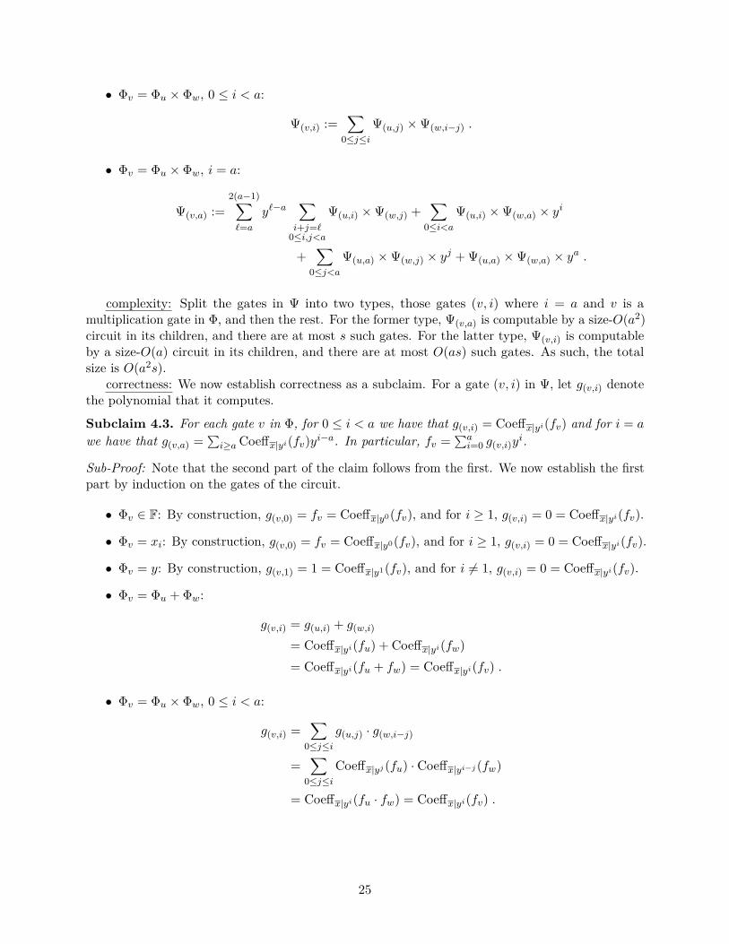
• Φv = Φu × Φw, 0 ≤ i < a:

Ψ(v,i) :=∑

0≤j≤iΨ(u,j) ×Ψ(w,i−j) .

• Φv = Φu × Φw, i = a:

Ψ(v,a) :=2(a−1)∑`=a

y`−a∑i+j=`

0≤i,j<a

Ψ(u,i) ×Ψ(w,j) +∑

0≤i<aΨ(u,i) ×Ψ(w,a) × yi

+∑

0≤j<aΨ(u,a) ×Ψ(w,j) × yj + Ψ(u,a) ×Ψ(w,a) × ya .

complexity: Split the gates in Ψ into two types, those gates (v, i) where i = a and v is amultiplication gate in Φ, and then the rest. For the former type, Ψ(v,a) is computable by a size-O(a2)circuit in its children, and there are at most s such gates. For the latter type, Ψ(v,i) is computableby a size-O(a) circuit in its children, and there are at most O(as) such gates. As such, the totalsize is O(a2s).

correctness: We now establish correctness as a subclaim. For a gate (v, i) in Ψ, let g(v,i) denotethe polynomial that it computes.

Subclaim 4.3. For each gate v in Φ, for 0 ≤ i < a we have that g(v,i) = Coeffx|yi(fv) and for i = a

we have that g(v,a) =∑i≥a Coeffx|yi(fv)yi−a. In particular, fv =

∑ai=0 g(v,i)y

i.

Sub-Proof: Note that the second part of the claim follows from the first. We now establish the firstpart by induction on the gates of the circuit.

• Φv ∈ F: By construction, g(v,0) = fv = Coeffx|y0(fv), and for i ≥ 1, g(v,i) = 0 = Coeffx|yi(fv).

• Φv = xi: By construction, g(v,0) = fv = Coeffx|y0(fv), and for i ≥ 1, g(v,i) = 0 = Coeffx|yi(fv).

• Φv = y: By construction, g(v,1) = 1 = Coeffx|y1(fv), and for i 6= 1, g(v,i) = 0 = Coeffx|yi(fv).

• Φv = Φu + Φw:

g(v,i) = g(u,i) + g(w,i)

= Coeffx|yi(fu) + Coeffx|yi(fw)= Coeffx|yi(fu + fw) = Coeffx|yi(fv) .

• Φv = Φu × Φw, 0 ≤ i < a:

g(v,i) =∑

0≤j≤ig(u,j) · g(w,i−j)

=∑

0≤j≤iCoeffx|yj (fu) · Coeffx|yi−j (fw)

= Coeffx|yi(fu · fw) = Coeffx|yi(fv) .

25

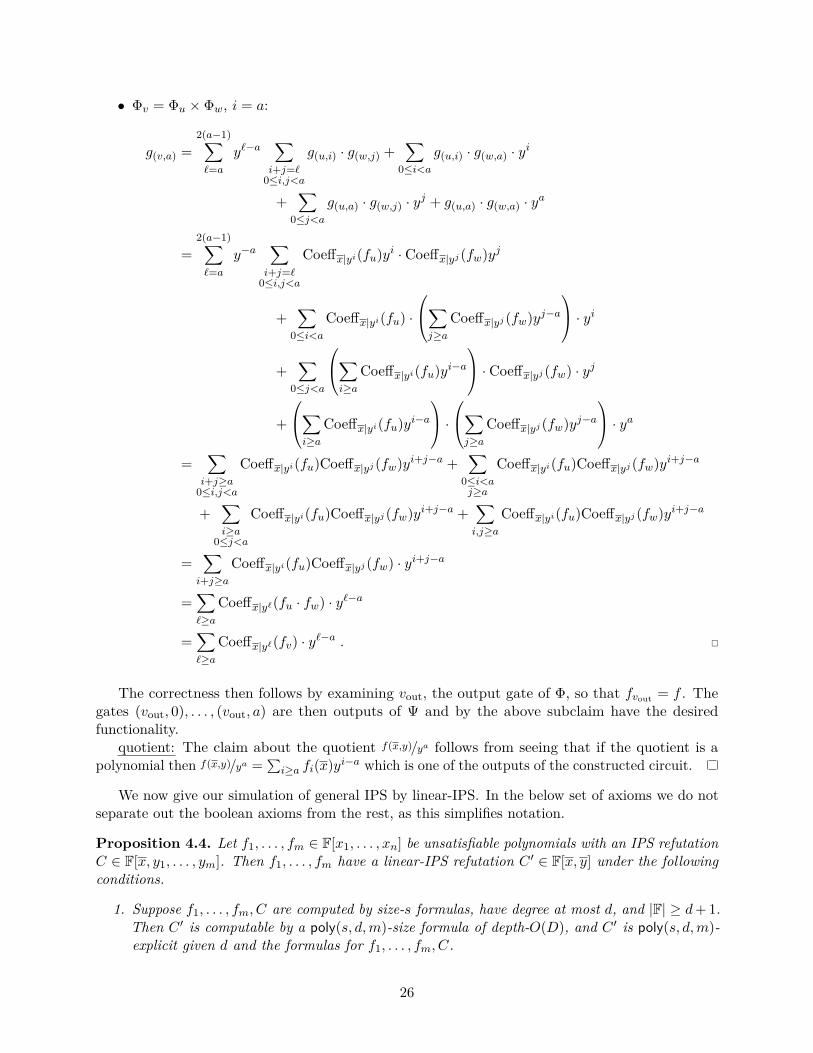
• Φv = Φu × Φw, i = a:

g(v,a) =2(a−1)∑`=a

y`−a∑i+j=`

0≤i,j<a

g(u,i) · g(w,j) +∑

0≤i<ag(u,i) · g(w,a) · yi

+∑

0≤j<ag(u,a) · g(w,j) · yj + g(u,a) · g(w,a) · ya

=2(a−1)∑`=a

y−a∑i+j=`

0≤i,j<a

Coeffx|yi(fu)yi · Coeffx|yj (fw)yj

+∑

0≤i<aCoeffx|yi(fu) ·

∑j≥a

Coeffx|yj (fw)yj−a · yi

+∑

0≤j<a

∑i≥a

Coeffx|yi(fu)yi−a · Coeffx|yj (fw) · yj

+

∑i≥a

Coeffx|yi(fu)yi−a ·

∑j≥a

Coeffx|yj (fw)yj−a · ya

=∑i+j≥a

0≤i,j<a

Coeffx|yi(fu)Coeffx|yj (fw)yi+j−a +∑

0≤i<aj≥a

Coeffx|yi(fu)Coeffx|yj (fw)yi+j−a

+∑i≥a

0≤j<a

Coeffx|yi(fu)Coeffx|yj (fw)yi+j−a +∑i,j≥a

Coeffx|yi(fu)Coeffx|yj (fw)yi+j−a

=∑i+j≥a

Coeffx|yi(fu)Coeffx|yj (fw) · yi+j−a

=∑`≥a

Coeffx|y`(fu · fw) · y`−a

=∑`≥a

Coeffx|y`(fv) · y`−a .

The correctness then follows by examining vout, the output gate of Φ, so that fvout = f . Thegates (vout, 0), . . . , (vout, a) are then outputs of Ψ and by the above subclaim have the desiredfunctionality.

quotient: The claim about the quotient f(x,y)/ya follows from seeing that if the quotient is apolynomial then f(x,y)/ya =

∑i≥a fi(x)yi−a which is one of the outputs of the constructed circuit.

We now give our simulation of general IPS by linear-IPS. In the below set of axioms we do notseparate out the boolean axioms from the rest, as this simplifies notation.

Proposition 4.4. Let f1, . . . , fm ∈ F[x1, . . . , xn] be unsatisfiable polynomials with an IPS refutationC ∈ F[x, y1, . . . , ym]. Then f1, . . . , fm have a linear-IPS refutation C ′ ∈ F[x, y] under the followingconditions.

1. Suppose f1, . . . , fm, C are computed by size-s formulas, have degree at most d, and |F| ≥ d+ 1.Then C ′ is computable by a poly(s, d,m)-size formula of depth-O(D), and C ′ is poly(s, d,m)-explicit given d and the formulas for f1, . . . , fm, C.

26

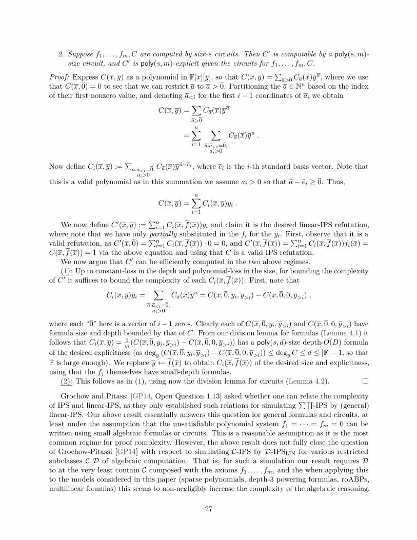
2. Suppose f1, . . . , fm, C are computed by size-s circuits. Then C ′ is computable by a poly(s,m)-size circuit, and C ′ is poly(s,m)-explicit given the circuits for f1, . . . , fm, C.

Proof: Express C(x, y) as a polynomial in F[x][y], so that C(x, y) =∑a>0Ca(x)ya, where we use

that C(x, 0) = 0 to see that we can restrict a to a > 0. Partitioning the a ∈ Nn based on the indexof their first nonzero value, and denoting a<i for the first i− 1 coordinates of a, we obtain

C(x, y) =∑a>0

Ca(x)ya

=n∑i=1

∑a:a<i=0,ai>0

Ca(x)ya .

Now define Ci(x, y) :=∑a:a<i=0,ai>0

Ca(x)ya−ei , where ei is the i-th standard basis vector. Note that

this is a valid polynomial as in this summation we assume ai > 0 so that a− ei ≥ 0. Thus,

C(x, y) =n∑i=1

Ci(x, y)yi .

We now define C ′(x, y) :=∑ni=1Ci(x, f(x))yi and claim it is the desired linear-IPS refutation,

where note that we have only partially substituted in the fi for the yi. First, observe that it is avalid refutation, as C ′(x, 0) =

∑ni=1Ci(x, f(x)) · 0 = 0, and C ′(x, f(x)) =

∑ni=1Ci(x, f(x))fi(x) =

C(x, f(x)) = 1 via the above equation and using that C is a valid IPS refutation.We now argue that C ′ can be efficiently computed in the two above regimes.(1): Up to constant-loss in the depth and polynomial-loss in the size, for bounding the complexity

of C ′ it suffices to bound the complexity of each Ci(x, f(x)). First, note that

Ci(x, y)yi =∑

a:a<i=0,ai>0

Ca(x)ya = C(x, 0, yi, y>i)− C(x, 0, 0, y>i) ,

where each “0” here is a vector of i− 1 zeros. Clearly each of C(x, 0, yi, y>i) and C(x, 0, 0, y>i) haveformula size and depth bounded by that of C. From our division lemma for formulas (Lemma 4.1) itfollows that Ci(x, y) = 1

yi(C(x, 0, yi, y>i)− C(x, 0, 0, y>i)) has a poly(s, d)-size depth-O(D) formula

of the desired explicitness (as degy(C(x, 0, yi, y>i)− C(x, 0, 0, y>i)

)≤ degy C ≤ d ≤ |F| − 1, so that

F is large enough). We replace y ← f(x) to obtain Ci(x, f(x)) of the desired size and explicitness,using that the fj themselves have small-depth formulas.

(2): This follows as in (1), using now the division lemma for circuits (Lemma 4.2).

Grochow and Pitassi [GP14, Open Question 1.13] asked whether one can relate the complexityof IPS and linear-IPS, as they only established such relations for simulating

∑∏-IPS by (general)

linear-IPS. Our above result essentially answers this question for general formulas and circuits, atleast under the assumption that the unsatisfiable polynomial system f1 = · · · = fm = 0 can bewritten using small algebraic formulas or circuits. This is a reasonable assumption as it is the mostcommon regime for proof complexity. However, the above result does not fully close the questionof Grochow-Pitassi [GP14] with respect to simulating C-IPS by D-IPSLIN for various restrictedsubclasses C,D of algebraic computation. That is, for such a simulation our result requires Dto at the very least contain C composed with the axioms f1, . . . , fm, and the when applying thisto the models considered in this paper (sparse polynomials, depth-3 powering formulas, roABPs,multilinear formulas) this seems to non-negligibly increase the complexity of the algebraic reasoning.

27

4.2 Multilinearizing roABP-IPSLIN

We now exhibit instances where one can efficiently prove that a polynomial equals its multilineariza-tion modulo the boolean axioms. That is, for a polynomial f computed by a small circuit we wishto prove that f ≡ ml(f) mod x2 − x by expressing f −ml(f) =

∑i hi · (x2

i − xi) so that the hi alsohave small circuits. Such a result will simplify the search for linear-IPS refutations by allowing usto focus on the non-boolean axioms. That is, if we are able to find a refutation of f, x2 − x given by∑

j

gjfj ≡ 1 mod x2 − x ,

where the gj have small circuits, multilinearization results of the above form guarantee that thereare hi so that ∑

j

gjfj +∑i

hi · (x2i − xi) = 1 ,

which is a proper linear-IPS refutation.We establish such a multilinearization result when f is an roABP in this section, and consider

when f the product of a low-degree multilinear polynomial and a multilinear formula in the nextsection. We will use these multilinearization results in our construction of IPS refutations of thesubset-sum axiom (Section 4.4).

We begin by noting that multilinearization for these two circuit classes is rather special, asthese classes straddle the conflicting requirements of neither being too weak nor too strong. Thatis, some circuit classes are simply too weak to compute their multilinearizations. An exampleis the class of depth-3 powering formulas, where (x1 + · · · + xn)n has a small

∑∧∑formula,

but its multilinearization has the leading term n!x1 · · ·xn and thus requires exponential size asa∑∧∑

formula (by appealing to Theorem 6.8). On the other hand, some circuit classes aretoo strong to admit efficient multilinearization (under plausible complexity assumptions). Thatis, consider an n × n symbolic matrix X where (X)i,j = xi,j and the polynomial f(X, y) :=(x1,1y1 + · · ·+ x1,nyn) · · · (xn,1y1 + · · ·+ xn,nyn), which is clearly a simple depth-3 (

∏∑∏) circuit.

Viewing this polynomial in F[X][y], one sees that CoeffX|y1···ynf = perm(X), where perm(X) is then× n permanent. Viewing ml(f), the multilinearization of f , in F[X][y] one sees that ml(f) is ofdegree n and its degree n component is the coefficient of y1 · · · yn in ml(f), which is still perm(X).Hence, by interpolation, one can extract this degree n part and thus can compute a circuit forperm(X) given a circuit for ml(f). Since we believe perm(X) does not have small algebraic circuitsit follows that the multilinearization of f does not have small circuits. These examples show thatefficient multilinearization is a somewhat special phenomenon.

We now give our result for multilinearizing roABPs, where we multilinearize variable by variablevia telescoping.

Proposition 4.5. Let f ∈ F[x1, . . . , xn] be computable by a width-r roABP in variable orderx1 < · · · < xn, so that f(x) = (

∏ni=1Ai(xi))1,1 where Ai ∈ F[xi]r×r have degAi ≤ d. Then

ml(f) has a poly(r, n, d)-explicit width-r roABP in variable order x1 < · · · < xn, and there arepoly(r, n, d)-explicit width-r roABPs h1, . . . , hn ∈ F[x] in variable order x1 < · · · < xn such that

f(x) = ml(f) +n∑j=1

hj · (x2j − xj) .

Further, ideg hj ≤ ideg f and the individual degree of the roABP for ml(f) is ≤ 1.

28

Proof: We apply the multilinearization map ml : F[x]→ F[x] to matrices ml : F[x]r×r → F[x]r×r byapplying the map entry-wise (Fact 3.12). It follows then that Ai(xi)−ml(Ai(xi)) ≡ 0 mod x2

i−xi, sothat Ai(xi)−ml(Ai(xi)) = B(xi)·(x2

i−xi) for some Bi(xi) ∈ F[xi]r×r where idegBi(xi) ≤ idegAi(xi).Now define ml≤i be the map which multilinearizes the first i variables and leaves the others intact,so that ml≤0 is the identity map and ml≤n = ml. Telescoping,

n∏i=1

Ai(xi) = ml<1

(n∏i=1

Ai(xi))

= ml≤n

(n∏i=1

Ai(xi))

+n∑j=1

[ml<j

(n∏i=1

Ai(xi))−ml≤j

(n∏i=1

Ai(xi))]

using that the identity ml(gh) = ml(ml(g) ml(h)) (Fact 3.12) naturally extends from scalars tomatrices, and also to partial-multilinearization (by viewing ml≤i as multilinearization in F[x>i][x≤i]),

= ml≤n

(n∏i=1

ml≤nAi(xi))

+n∑j=1

ml<j

∏i<j

ml<j(Ai(xi))∏i≥j

Ai(xi)

−ml≤j

∏i≤j

ml≤j(Ai(xi))∏i>j

Ai(xi)

dropping the outside ml<j and ml≤j as the inside polynomials are now multilinear in the appropriatevariables, and replacing them with ml as appropriate,

=n∏i=1

ml(Ai(xi)) +n∑j=1

∏i<j

ml(Ai(xi))∏i≥j

Ai(xi)

−∏i≤j

ml(Ai(xi))∏i>j

Ai(xi)

=

n∏i=1

ml(Ai(xi)) +n∑j=1

∏i<j

ml(Ai(xi)) ·(Aj(xj)−ml(Aj(xj))

)·∏i>j

Ai(xi)

=

n∏i=1

ml(Ai(xi)) +n∑j=1

∏i<j

ml(Ai(xi)) ·Bj(xj) ·∏i>j

Ai(xi) · (x2j − xj)

.

Taking the (1, 1)-entry in the above yields that

f(x) =(

n∏i=1

Ai(xi))

1,1

=(

n∏i=1

ml(Ai(xi)))

1,1+

n∑j=1

∏i<j

ml(Ai(xi)) ·Bj(xj) ·∏i>j

Ai(xi)

1,1

· (x2j − xj) .

Thus, define

f :=(

n∏i=1

ml(Ai(xi)))

1,1, hj :=

∏i<j

ml(Ai(xi)) ·Bj(xj) ·∏i>j

Ai(xi)

1,1

.

29

It follows by construction that f and each hj are computable by width-r roABPs of the desiredexplicitness in the correct variable order. Further, ideg hj ≤ ideg f and f has individual degree ≤ 1.Thus, the above yields that f = f +

∑j hj · (x2

j − xj), from which it follows that ml(f) = f , asdesired.

We now conclude that in designing an roABP-IPSLIN refutation∑j gj · fj +

∑i hi · (x2

i − xi) off1(x), . . . , fm(x), x2 − x, it suffices to bound the complexity of the gj ’s.

Proposition 4.6. Let f1, . . . , fm ∈ F[x1, . . . , xn] be unsatisfiable polynomials over x ∈ 0, 1ncomputable by width-s roABPs in variable order x1 < · · · < xn. Suppose that there are gj ∈ F[x]such that

m∑i=1

gj(x)fj(x) ≡ 1 mod x2 − x ,

where the gj have width-r roABPs in the variable order x1 < · · · < xn. Then there is anroABP-IPSLIN refutation C(x, y, z) of individual degree at most 1 + ideg f and computable inwidth-poly(s, r, n,m) in any variable order where x1 < · · · < xn. Furthermore, this refutation ispoly(s, r, ideg g, ideg f, n,m)-explicit given the roABPs for fj and gj.

Proof: We begin by noting that we can multilinearize the gj , so that∑mi=1 ml(gj(x))fj(x) ≡ 1

mod x2 − x, and that ml(gj) are poly(r, ideg g, n,m)-explicit multilinear roABPs of width-r byProposition 4.5. Thus, we assume going forward that the gj are multilinear.

As gj , fj are computable by roABPs, their product gjfj is computable by a width-rs roABP inthe variable order x1 < · · · < xn (Fact 3.8) with individual degree at most 1 + ideg fj (Lemma 3.6).Thus, by the above multilinearization (Proposition 4.5), there are hj,i ∈ F[x] such that

gj(x)fj(x) = ml(gjfj) +n∑i=1

hj,i(x) · (x2i − xi) .

where the hj,i are computable by width-rs roABPs of individual degree at most 1 + ideg fj . Wenow define

C(x, y, z) :=m∑j=1

gj(x)yj −n∑i=1

m∑j=1

hj,i(x)

zi .By the closure operations of roABPs (Fact 3.8) it follows that C is computable the appropriately-sized roABPs in the desired variable orders, has the desired individual degree, and that C has thedesired explicitness.

We now show that this is a valid IPS refutation. Observe that C(x, 0, 0) = 0 and that

C(x, f, x2 − x) =m∑j=1

gj(x)fj(x)−n∑i=1

m∑j=1

hj,i(x)

(x2i − xi) (4.7)

=m∑j=1

(gj(x)fj(x)−

n∑i=1

hj,i(x)(x2i − xi)

)(4.8)

=m∑j=1

ml(gjfj) (4.9)

30

as∑mi=1 gj(x)fj(x) ≡ 1 mod x2 − x we have that

m∑j=1

ml(gjfj) = ml(

m∑i=1

gj(x)fj(x))

= 1 ,

where we appealed to linearity of multilinearization (Fact 3.12), so that

C(x, f, x2 − x) =m∑j=1

ml(gjfj) = 1 ,

as desired.

4.3 Multilinear-Formula-IPSLIN′

We now turn to proving that g ·f ≡ ml(g ·f) mod x2−x when f is low-degree and g is a multilinearformula. This multilinearization can be used to complete our construction of multilinear-formula-IPSrefutations of subset-sum axiom (Section 4.4), though our actual construction will multilinearizemore directly (Proposition 4.19).

More importantly, the multilinearization we establish here shows that multilinear-formula-IPS can efficiently simulate sparse-IPSLIN (when the axioms are low-degree and multilinear).Such a simulation holds intuitively, as multilinear formulas can efficiently compute any sparse(multilinear) polynomial, and as we work over the boolean cube we are morally working withmultilinear polynomials. While this intuition suggests that such a simulation follows immediately,this intuition is false. Specifically, while sparse-IPSLIN is a complete refutation system for anysystem of unsatisfiable polynomials over the boolean cube, multilinear-formula-IPSLIN is incompleteas seen by the following example (though, by Theorem 1.2, multilinear-formula-IPSLIN is completefor refuting unsatisfiable CNFs).Example 4.10. Consider the unsatisfiable system of equations xy+ 1, x2 − x, y2 − y. A multilinearlinear-IPS proof is a tuple of multilinear polynomials (f, g, h) ∈ F[x, y] such that f ·(xy+1)+g ·(x2−x) + h · (y2 − y) = 1. In particular, f(x, y) = 1

xy+1 for x, y ∈ 0, 1, which implies by interpolationover the boolean cube that f(x, y) = 1·(1−x)(1−y)+1·(1−x)y+1·x(1−y)+ 1

2 ·xy = 1− 12 ·xy. Thus

f · (xy + 1) contains the monomial x2y2. However, as g, h are multilinear we see that x2y2 cannotappear in g · (x2−x) +h · (y2− y)− 1, so that the equality f · (xy+ 1) + g · (x2−x) +h · (y2− y) = 1cannot hold. Thus, xy + 1, x2 − x, y2 − y has no linear-IPS refutation only using multilinearpolynomials. ♦

Put another way, the above example shows that in a linear-IPS refutation∑j gjfj +

∑i hi ·

(x2i − xi) = 1, while one can multilinearize the gj (with a possible increase in complexity) and still

retain a refutation, one cannot multilinearize the hi in general.As such, to simulate sparse-IPSLIN (a complete proof system) we must resort to using the

more general IPSLIN′ over multilinear formulas, where recall that the IPSLIN′ refutation systemconsiders refutes f, x2 − x with a polynomial C(x, y, z) where C(x, 0, 0) = 0, C(x, f, x2 − x) = 1,with the added restriction that when viewing C ∈ F[x, z][y] that the degree of C with respect to they-variables is at most 1, that is, degy C ≤ 1. In fact, we in fact establish such a simulation usingthe subclass of refutations of the form C(x, y, z) =

∑j gjyj + C ′(x, z) where C ′(x, 0) = 0. Note

that such refutations are only linear in the non-boolean axioms, which allows us to circumventExample 4.10.

We now show how to prove g · f ≡ ml(g · f) mod x2 − x when f is low-degree and g is amultilinear formula, where the proof is supplied by the equality g · f − ml(g · f) = C(x, x2 − x)

31

where C(x, 0) = 0, and where we seek to show that C has a small multilinear formula. We beginwith the special case of f and g being the same monomial.Lemma 4.11. Let x1 =

∏ni=1 xi. Then,

(x1)2 − x1 = C(x, x2 − x) ,

where C(x, z) ∈ F[x, z1, . . . , zn] is defined by

C(x, z) := (z + x)1 − x1 =∑

0<a≤1

zax1−a ,

so that C(x, 0) = 0.Note that the first expression for C is a poly(n)-sized depth-3 expression, while the second

is an exp(n)-sized depth-2 expression. This difference will, going forward, show that we canmultilinearize efficiently in depth-3, but can only efficiently multilinearize low-degree monomials indepth-2. We now give an IPS proof for showing how a monomial times a multilinear formula equalsits multilinearization.

Lemma 4.12. Let g ∈ F[x1, . . . , xn, y1, . . . , yd] be a multilinear polynomial. Then there is aC ∈ F[x, y, z1, . . . , zd] such that

g(x, y) · y1 −ml(g(x, y) · y1) = C(x, y, y2 − y) ,

and C(x, y, 0) = 0.If g is t-sparse, then C is computable as a poly(t, n, 2d)-size depth-2 multilinear formula (which is

poly(t, n, 2d)-explicit given the computation for g), as well as being computable by a poly(t, n, d)-sizedepth-3 multilinear formula with a +-output-gate (which is poly(t, n, d)-explicit given the computationfor g). If g is computable by a size-t depth-D multilinear formula, then C is computable by apoly(t, 2d)-size depth-(D + 2) multilinear formula with a +-output-gate (which is poly(t, 2d)-explicitgiven the computation for g).

Proof: defining C: Express g as g =∑

0≤a≤1 ga(x)ya in the ring F[x][y], so that each ga is multilinear.Then

g(x, y) · y1 −ml(g(x, y) · y1) =∑a

ga(x)ya · y1 −ml(∑

a

ga(x)ya · y1)

=∑a

ga(x)(ya+1 − y1

)=∑a

ga(x)y1−a((ya)2 − ya

),

and appealing to Lemma 4.11,

=∑a

ga(x)y1−a(((y2 − y) + y)a − ya

)= C(x, y, y2 − y) ,

where we defineC(x, y, z) :=

∑a

ga(x)y1−a((z + y)a − ya

).

As (z + y)a = ya under z ← 0 we have that C(x, y, 0) = 0.

32

g is t-sparse: As g is t-sparse and multilinear, so are each ga, so that ga =∑ti=1 αa,ix

ca,i , andthus

C(x, y, z) =∑a

t∑i=1

αa,ixca,iy1−a

((z + y)a − ya

)

=∑a

t∑i=1

αa,ixca,iy1−a(z + y)a −

∑a

t∑i=1

αa,ixca,iy1 ,

where this is clearly an explicit depth-3 (∑∏∑

) multilinear formula (as y1−a is variable-disjointfrom (z+ y)a), and the size of this formula is poly(n, t, d) as there are at most t such a where ga 6= 0as g is t-sparse. Continuing the expansion, appealing to Lemma 4.11,

=∑a

t∑i=1

αa,ixca,iy1−a ∑

0≤b≤a

zbya−b −∑a

t∑i=1

αa,ixca,iy1

=∑a

t∑i=1

αa,ixca,i

∑0<b≤a

zbya−b

=∑a

t∑i=1

∑0<b≤a

αa,ixca,izbya−b ,

which is then easily seen to be explicit and poly(n, t, 2d)-sparse appealing to the above logic.g a multilinear formula: By interpolation, it follows that for each a there are poly(2d)-explicit

constants αa,β such that ga(x) =∑β∈0,1d αa,βg(x, β). From this it follows that ga is computable

by a depth D + 1 multilinear formula of size poly(t, 2d). Expanding the definition of C we get that

C(x, y, z) =∑a

ga(x)y1−a((z + y)a − ya

)=∑a

ga(x)y1−a(z + y)a −∑a

ga(x)y1

=∑a

∑β∈0,1d

αa,βg(x, β)y1−a(z + y)a −∑a

∑β∈0,1d

αa,βg(x, β)y1 ,

which is clearly an explicit depth D + 2 multilinear formula of size poly(t, 2d), as D ≥ 1 so that thecomputation of the zi + yi is parallelized with computing g(x, β), and we absorb the subtractioninto the overall top-gate of addition.

We can then straightforwardly extend this to multilinearizing the product of a low-degree sparsemultilinear polynomial and a multilinear formula, as we can use that multilinearization is linear.Corollary 4.13. Let g ∈ F[x1, . . . , xn] be a multilinear polynomial and f ∈ F[x] a s-sparse multi-linear polynomial of degree ≤ d. Then there is a C ∈ F[x, z1, . . . , zn] such that

g · f −ml(g · f) = C(x, x2 − x) ,

and C(x, 0) = 0.If g is t-sparse, then C is computable as a poly(s, t, n, 2d)-size depth-2 multilinear formula

(which is poly(s, t, n, 2d)-explicit given the computations for f, g), as well as being computable by a

33

poly(s, t, n, d)-size depth-3 multilinear formula with a +-output-gate (which is poly(s, t, n, d)-explicitgiven the computations for f, g). If g is computable by a size-t depth-D multilinear formula, then Cis computable by a poly(s, t, 2d)-size depth-(D + 2) multilinear formula with a +-output-gate (whichis poly(s, t, 2d)-explicit given the computations for f, g).

We now show how to derive multilinear-formula-IPSLIN′ refutations for f, x2 − x from equationsof the form

∑j gjfj ≡ 1 mod x2 − x.

Corollary 4.14. Let f1, . . . , fm ∈ F[x1, . . . , xn] be degree at most d multilinear s-sparse polynomialswhich are unsatisfiable over x ∈ 0, 1n. Suppose that there are multilinear gj ∈ F[x] such that

m∑i=1

gj(x)fj(x) ≡ 1 mod x2 − x .

Then there is a multilinear-formula-IPSLIN′ refutation C(x, y, z) such that

• If the gj are t-sparse, then C is computable by a poly(s, t, n,m, 2d)-size depth-2 multilin-ear formula (which is poly(s, t, n,m, 2d)-explicit given the computations for the fj , gj), aswell as being computable by a poly(s, t, n,m, d)-size depth-3 multilinear formula (which ispoly(s, t, n,m, d)-explicit given the computations for fj , gj).

• If the gj are computable by size-t depth-D multilinear formula, then C is computable by apoly(s, t,m, 2d)-size depth-(D + 2) multilinear formula (which is poly(s, t,m, 2d)-explicit giventhe computations for fj , gj).

Proof: construction: By the above multilinearization (Corollary 4.13), there are Cj ∈ F[x, z] suchthat

gj(x)fj(x) = ml(gjfj) + Cj(x, x2 − x) .

where Cj(x, 0) = 0. We now define

C(x, y, z) :=m∑j=1

(gj(x)yj − Cj(x, z)) .

We now show that this is a valid IPS refutation. Observe that C(x, 0, 0) = 0 and that

C(x, f, x2 − x) =m∑j=1

(gj(x)fj(x)− Cj(x, x2 − x)

)

=m∑j=1

ml(gjfj)

as∑mi=1 gj(x)fj(x) ≡ 1 mod x2 − x we have that

m∑j=1

ml(gjfj) = ml(

m∑i=1

gj(x)fj(x))

= 1 ,

where we appealed to linearity of multilinearization (Fact 3.12), so that

C(x, f, x2 − x) =m∑j=1

ml(gjfj) = 1 .

34

complexity: The claim now follows from appealing to Corollary 4.13 for bounding the complexityof the Cj . That is, if the gj are t-sparse then

∑mj=1 gj(x)yj is tm-sparse and thus computable

by a poly(t,m)-size depth-2 multilinear formula with +-output-gate. As each Cj is computableby a poly(s, t, n, 2d)-size depth-2 or poly(s, t, n, d)-size depth-3 multilinear formula (each having a+-output-gate), it follows that C(x, y, z) :=

∑mj=1 (gj(x)yj − Cj(x, z)) can be explicitly computed

by a poly(s, t, n,m, 2d)-size depth-2 or poly(s, t, n,m, d)-size depth-3 multilinear formula (collapsingaddition gates into a single level).

If the gj are computable by size-t depth-D multilinear formula then∑mj=1 gj(x)yj is computable

by size poly(m, t)-size depth-(D + 2) multilinear formula (with a +-output-gate), and each Cjis computable by a poly(s, t, 2d)-size depth-(D + 2) multilinear formula with a +-output-gate,from which it follows that C(x, y, z) :=

∑mj=1 (gj(x)yj − Cj(x, z)) can be explicitly computed by a

poly(s, t,m, 2d)-size depth-(D + 2) multilinear formula by collapsing addition gates.

We now conclude by showing that multilinear-formula-IPSLIN′ can efficiently simulate sparse-IPSLIN when the axioms are low-degree. As this latter system is complete, this shows the former isas well. That is, we allow the refutation to depend non-linearly on the boolean axioms, but onlylinearly on the other axioms.

Corollary 4.15. Let f1, . . . , fm ∈ F[x1, . . . , xn] be degree at most d s-sparse polynomials unsatisfiableover x ∈ 0, 1n. Suppose they have an

∑∏-IPSLIN refutation, that is, that there are t-sparse

polynomials g1, . . . , gm, h1, . . . , hn ∈ F[x] such that∑mj=1 gjfj+

∑ni=1 hi ·(x2

i −xi) = 1. Then f, x2−xcan be refuted by a depth-2 multilinear-formula-IPSLIN′ proof of poly(s, t, n,m, 2d)-size, or by adepth-3 multilinear-formula-IPSLIN′ proof of poly(s, t, n,m, d)-size.

Proof: This follows from Corollary 4.14 by noting that∑j ml(gj)fj ≡ 1 mod x2 − x, and that the

ml(gj) are multilinear and t-sparse.

4.4 Refutations of the Subset-Sum Axiom

We now give efficient IPS refutations of the subset-sum axiom, where these IPS refutations can be evenplaced in the restricted roABP-IPSLIN or multilinear-formula-IPSLIN subclasses. That is, we give suchrefutations for whenever the polynomial

∑i αixi − β is unsatisfiable over the boolean cube 0, 1n,

where the size of the refutation is polynomial in the size of the set A := ∑i αixi : x ∈ 0, 1n. A

motivating example is when α = 1 so that A = 0, . . . , n.To construct our refutations, we first show that there is an efficiently computable polynomial f

such that f(x) · (∑i αixi − β) ≡ 1 mod x2 − x. This will be done by considering the univariate

polynomial p(t) :=∏α∈A(t− α). Using that for any univariate p(x) that x− y divides p(x)− p(y),

we see that p(∑i αixi)− p(β) is a multiple of

∑i αixi − β. As

∑i αixi − β is unsatisfiable it must

be that β /∈ A. This implies that p(∑i αixi) ≡ 0 mod x2 − x while p(β) 6= 0. Consequently,

p(∑i αixi)− p(β) is equivalent to a nonzero constant modulo x2 − x, yielding the Nullstellensatz

refutation1

−p(β) ·p(∑i αixi)− p(β)∑i αixi − β

· (∑iαixi − β) ≡ 1 mod x2 − x .

By understanding the quotient p(∑

iαixi)−p(β)∑iαixi−β

we see that it can be efficiently computed by asmall

∑∧∑formula and thus an roABP, so that using our multilinearization result for roABPs

(Proposition 4.5) this yields the desired roABP-IPSLIN refutation. However, this does not yield thedesired multilinear-formula-IPSLIN refutation. For this, we need to (over a large field) convert theabove quotient to a sum of products of univariates using duality (Theorem 3.14). We can then

35

multilinearize this to a sum of products of linear univariates, which is a depth-3 multilinear formula.By appealing to our proof-of-multilinearization result for multilinear formula (Corollary 4.14) oneobtains a multilinear-formula-IPSLIN′ refutation, and we give a direct proof which actually yieldsthe desired multilinear-formula-IPSLIN refutation.

We briefly remark that for the special case of α = 1, one can explicitly describe the unique multi-linear polynomial f such that f(x)(

∑i xi − β) ≡ 1 mod x2 − x. This description (Proposition B.1)

shows that f is a linear combination of elementary symmetric polynomials, which implies the desiredcomplexity upper bounds for this case via known bounds on the complexity of elementary symmetricpolynomials ([NW96]). However, this proof strategy is more technical and thus we pursue the moreconceptual outline given above to bound the complexity of f for general A.

Proposition 4.16. Let α ∈ Fn, β ∈ F and A := ∑ni=1 αixi : x ∈ 0, 1n be so that β /∈ A. Then

there is a multilinear polynomial f ∈ F[x] such that

f(x) · (∑iαixi − β) ≡ 1 mod x2 − x .

For any |F|, f is computable by a poly(|A|, n)-explicit poly(|A|, n)-width roABP of individual degree≤ 1.

If |F| ≥ poly(|A|, n), then f is computable as a sum of product of linear univariates (and hencea depth-3 multilinear formula)

f(x) =s∑i=1

fi,1(x1) · · · fi,n(xn) ,

where each fi,j ∈ F[xi] has deg fi,j ≤ 1, s ≤ poly(|A|, n), and this expression is poly(|A|, n)-explicit.

Proof: computing A: We first note that A can be computed from α in poly(|A|, n)-steps (as opposedto the naive 2n steps). That is, define Aj :=

∑ji=1 αixi : x1, . . . , xj ∈ 0, 1, so that A0 = ∅

and An = A. It follows that for all j, we have that Aj ⊆ A and thus |Aj | ≤ |A|, and thatAj+1 ⊆ Aj ∪ (Aj + αj). It follows that we can compute Aj+1 from Aj in poly(|A|) time, so thatA = An can be computed in poly(|A|, n)-time.

defining f : Define p(t) ∈ F[t] by p :=∏α∈A(t − α), so that p(A) = 0 and p(β) 6= 0. Express

p(t) in its monomial representation as p(t) =∑|A|k=0 γkt

k, where the γk can be computed in poly(|A|)time from α by computing A as above. Then observe that

p(t)− p(β) =

|A|∑k=0

γktk − βk

t− β

(t− β)

=

|A|∑k=0

γk

k−1∑j=0

tjβ(k−1)−j

(t− β)

=

|A|−1∑j=0

|A|∑k=j+1

γkβ(k−1)−j

tj (t− β) .

Thus, plugging in t←∑i αixi, we can define the polynomial g(x) ∈ F[x] by

g(x) := p(∑i αixi)− p(β)∑i αixi − β

=|A|−1∑j=0

|A|∑k=j+1

γkβ(k−1)−j

(∑i

αixi

)j. (4.17)

36

Hence,

g(x)(∑iαixi − β) = p(

∑iαixi)− p(β) .

For any x ∈ 0, 1n we have that∑i αixi ∈ A. As p(A) = 0 it follows that p(

∑i αixi) = 0 for all

x ∈ 0, 1n. This implies that p(∑i αixi) ≡ 0 mod x2 − x, yielding

g(x)(∑iαixi − β) ≡ −p(β) mod x2 − x .

As −p(β) ∈ F \ 0, we have that

1−p(β) · g(x) · (

∑iαixi − β) ≡ 1 mod x2 − x .

We now simply multilinearize, and thus define the multilinear polynomial

f(x) := ml( 1−p(β) · g(x)

).

First, we see that this has the desired form, using the interaction of multilinearization and multipli-cation (Fact 3.12).

1 = ml( 1−p(β)g(x) · (

∑iαixi − β)

)= ml

(ml( 1−p(β) · g(x)

)ml(

∑iαixi − β)

)= ml

(f ·ml(

∑iαixi − β)

)= ml

(f · (

∑iαixi − β)

)Thus, f · (

∑iαixi − β) ≡ 1 mod x2 − x as desired.

computing f as an roABP: By Equation 4.17 we see that g(x) is computable by a poly(|A|, n)-size∑∧∑-formula, and by the efficient simulation of

∑∧∑-formula by roABPs (Theorem 3.15) g(x)

and thus 1−p(β) · g(x) are computable by poly(|A|, n)-width roABPs of poly(|A|, n)-degree. Noting

that roABPs can be efficiently multilinearized (Proposition 4.5) we see that f = ml( 1−p(β) · g(x))

can thus be computed by such an roABP also, where the individual degree of this roABP is at most1. Finally, note that each of these steps has the required explicitness.

computing f via duality: We apply duality (Theorem 3.14) to see that over large enough fieldsthere are univariates gj,`,i of degree at most |A|, where

g(x) =|A|−1∑j=0

|A|∑k=j+1

γkβ(k−1)−j

(∑i

αixi

)j

=|A|−1∑j=0

|A|∑k=j+1

γkβ(k−1)−j

(nj+1)(j+1)∑`=1

gj,`,1(x1) · · · gj,`,n(xn)

Absorbing the constant(∑|A|

k=j+1 γkβ(k−1)−j

)into these univariates and re-indexing,

=s∑i=1

gi,1(x1) · · · gi,n(xn)

37

for some univariates gi,j , where s ≤ |A|(n|A|+ 1)(|A|+ 1) = poly(|A|, n).We now obtain f by multilinearizing the above expression, again appealing to multilinearization

(Fact 3.12).

f = ml( 1−p(β)g(x)

)= ml

(1

−p(β)

s∑i=1

gi,1(x1) · · · gi,n(xn))

absorbing the constant 1/−p(β) and renaming,

= ml(

s∑i=1

g′i,1(x1) · · · g′i,n(xn))

= ml(

s∑i=1

ml(g′i,1(x1)) · · ·ml(g′i,n(xn)))

defining fi,j(xj) := ml(gi,j(xj)), so that deg fi,j ≤ 1,

= ml(

s∑i=1

fi,1(x1) · · · fi,n(xn))

and we can drop the outside ml as this expression is now multilinear,

=s∑i=1

fi,1(x1) · · · fi,n(xn) ,

showing that f is computable as desired, noting that this expression has the desired explicitness.

Note that computing f via duality also implies an roABP for f , but only in large enough fields|F| ≥ poly(|A|, n). Of course, the field must at least have |F| ≥ |A|, but by using the field-independentconversion of

∑∧∑to roABP (Theorem 3.15) this shows that F need not be any larger than A for

the refutation to be efficient.The above shows that one can give an “IPS proof” g(x)(

∑i αixi − β) +

∑i hi(x)(x2

i − xi) = 1,where g is efficiently computable. However, this is not yet an IPS proof as it does not bound thecomplexity of the hi. We now extend this to an actual IPS proof by using the above multilinearizationresults for roABPs (Proposition 4.6), leveraging that

∑i αixi − β is computable by an roABP in

any variable order (and that the above result works in any variable order).Corollary 4.18. Let α ∈ Fn, β ∈ F and A :=

∑ni=1 αixi : x ∈ 0, 1n be so that β /∈ A.

Then∑i αixi − β, x2 − x has a poly(|A|, n)-explicit roABP-IPSLIN refutation of individual degree 2

computable in width-poly(|A|, n) in any variable order.Note that while the above results give a small

∑∧∑formula g such that g ·(

∑i αixi−β) ≡ −p(β)

mod x2 − x for nonzero scalar −p(β), this does not translate to a∑∧∑

-IPS refutation as∑∧∑

formulas cannot be multilinearized efficiently (see the discussion in Section 4.2).We now turn to refuting the subset-sum axioms by multilinear-formula-IPSLIN (which is not

itself a complete proof system, but will suffice here). While one can use the multilinearizationtechniques for multilinear-formula-IPSLIN′ of Corollary 4.14 it gives slightly worse results due to itsgenerality, so we directly multilinearize the refutations we built above using that the subset-sumaxiom is linear.

38

Proposition 4.19. Let α ∈ Fn, β ∈ F and A := ∑ni=1 αixi : x ∈ 0, 1n be so that β /∈ A.

If |F| ≥ poly(|A|, n), then∑i αixi − β, x2 − x has a poly(|A|, n)-explicit poly(|A|, n)-size depth-3

multilinear-formula-IPSLIN refutation.

Proof: By Proposition 4.16, there is a multilinear polynomial f ∈ F[x] such that f(x)·(∑iαixi − β) ≡

1 mod x2 − x, and f is explicitly given as

f(x) =s∑i=1

fi,1(x1) · · · fi,n(xn) ,

where each fi,j ∈ F[xi] has deg fi,j ≤ 1 and s ≤ poly(|A|, n).We now efficiently prove that f(x) · (

∑ni=1 αixi − β) is equal to its multilinearization (which is

1) modulo the boolean cube. The key step is that for a linear function p(x) = γx+ δ we have that(γx+ δ)x = (γ + δ)x+ γ(x2 − x) = p(1)x+ (p(1)− p(0))(x2 − x).

Thus,

f(x) · (∑iαixi − β)

=(

s∑i=1

fi,1(x1) · · · fi,n(xn))· (∑iαixi − β)

=s∑i=1−βfi,1(x1) · · · fi,n(xn)

+s∑i=1

n∑j=1

αj∏k 6=j

fi,k(xk) ·(fi,j(1)xj + (fi,j(1)− fi,j(0))(x2

j − xj))

=s∑i=1−βfi,1(x1) · · · fi,n(xn) +

s∑i=1

n∑j=1

αj∏k 6=j

fi,k(xk) · fi,j(1)xj

+s∑i=1

n∑j=1

αj∏k 6=j

fi,k(xk) · (fi,j(1)− fi,j(0)) · (x2j − xj)

absorbing constants and renaming, using j = 0 to incorporate the above term involving β,

=s∑i=1

n∑j=0

n∏k=1

fi,j,k(xk) +n∑j=1

(s∑i=1

n∏k=1

hi,j,k(xk))

(x2j − xj)

where each fi,j,k and hi,j,k are linear univariates. As f(x) · (∑ni=1 αixi − β) ≡ 1 mod x2 − x it

follows that∑i

∑j

∏k fi,j,k(xk) ≡ 1 mod x2 − x, but as each fi,j,k is linear it must actually be

that∑i

∑j

∏k fi,j,k(xk) = 1, so that,

= 1 +n∑j=1

(s∑i=1

n∏k=1

hi,j,k(xk))

(x2j − xj) .

Define C(x, y, z) := f(x)y −∑nj=1 hj(x)zj , where hj(x) :=

∑si=1

∏nk=1 hi,j,k(xk). It follows that

C(x, 0, 0) = 0 and that C(x,∑i αixi − β, x2 − x) = 1, so that C is a linear-IPS refutation. Further,

as each f, hj is computable as a sum of products of linear univariates, these are depth-3 multilinearformulas. By distributing the multiplication of the variables y, z1, . . . , zn to the bottom multiplicationgates, we see that C itself has a depth-3 multilinear formula of the desired complexity.

39

5 Lower Bounds for Linear-IPS via Functional Lower Bounds

In this section we give functional circuit lower bounds for various measures of algebraic complexity,such as degree, sparsity, roABPs and multilinear formulas. That is, while algebraic complexitytypically treats a polynomial f ∈ F[x1, . . . , xn] as a syntactic object, one can also see that it definesa function on the boolean cube f : 0, 1n → F. If this function is particularly complicated then onewould expect that this implies that the polynomial f requires large algebraic circuits. In this sectionwe obtain such lower bounds, showing that for any polynomial f (not necessarily multilinear) thatagrees with a certain function on the boolean cube must in fact have large algebraic complexity.

Our lower bounds will proceed by first showing that the complexity of f is an upper boundfor the complexity of its multilinearization ml(f). While such a statement is known to be falsefor general circuits (under plausible assumptions, see Section 4.2), such efficient multilinearizationcan be shown for the particular restricted models of computation we consider. In particular, thismultilinearization is easy for degree and sparsity, for multilinear formulas f is already multilinear,and for roABPs this is seen in Section 4.2. As then ml(f) is uniquely defined by the function f(Fact 3.12), we then only need to lower bound the complexity of ml(f) using standard techniques. Weremark that the actual presentation will not follow the above exactly, as for roABPs and multilinearformulas it is just as easy to just work directly with the underlying lower bound technique.

We then observe that by deriving such lower bounds for carefully crafted functions f : 0, 1n → Fone can easily obtain linear-IPS lower bounds for the above circuit classes. That is, consider thesystem of equations f(x), x2−x, where f(x) is chosen so this system is unsatisfiable, hence f(x) 6= 0for all x ∈ 0, 1n. Any linear-IPS refutation yields an equation g(x) · f(x) +

∑i hi(x)(x2

i − xi) = 1,which implies that g(x) = 1/f(x) for all x ∈ 0, 1n (that this system is unsatisfiable allows us toavoid division by zero). It follows that the polynomial g(x) agrees with the function f(x) := 1/f(x)on the boolean cube. If the function f has a functional lower bound then this implies g must havelarge complexity, giving the desired lower bound for the linear-IPS refutation.

The section proceeds as follows. We begin by detailing the above strategy for convertingfunctional lower bounds into lower bounds for linear-IPS. We then derive a tight functional lowerbound of n for the degree of 1/(

∑ixi+1). We then extend this via random restrictions to a functional

lower bound of exp(Ω(n)) on the sparsity of 1/(∑

ixi+1). We can then lift this degree bound to a

functional lower bound of 2n on the evaluation dimension of 1/(∑

ixiyi+1) in the x|y partition, which

we then symmetrize to obtain a functional lower bound on the evaluation dimension in any partitionof the related function 1/

(∑i<j

zi,jxixj+1). In each case, the resulting linear-IPS lower bounds are

immediate via the known relations of these measures to circuit complexity classes (Section 3).

5.1 The Strategy

We give here the key lemma detailing the general reduction from linear-IPS lower bounds tofunctional lower bounds.

Lemma 5.1. Let C ⊆ F[x1, . . . , xn] be a set of polynomials closed under partial evaluation. Letf ∈ F[x], where the system f(x), x2 − x is unsatisfiable. Suppose that for all g ∈ F[x] with

g(x) = 1f(x) , ∀x ∈ 0, 1n ,

that g /∈ C. Then f(x), x2 − x does not have C-IPSLIN refutations.

Proof: Suppose for contradiction that f(x), x2 − x has the C-IPSLIN refutation C(x, y, z) = g(x) ·y +

∑i hi(x) · zi where C(x, f, x2 − x) = 1 (and clearly C(x, 0, 0) = 0). As g = C(x, 1, 0), it follows

40

that g ∈ C from the closure properties we assumed of C. Thus,

1 = C(x, f, x2 − x)= g(x) · f(x) +

∑i

hi(x)(x2i − xi)

≡ g(x) · f(x) mod x2 − x .

Thus, for any x ∈ 0, 1n, as f(x) 6= 0,

g(x) = 1/f(x) .

However, this yields the desired contradiction, as this contradicts the assumed functional lowerbound for 1/f.

We now note that the lower bound strategy of using functional lower bounds actually produceslower bounds for IPSLIN′ (and even for the full IPS system if we have multilinear polynomials),and not just IPSLIN. This is because we work modulo the boolean axioms, so that any non-lineardependence on these axioms vanishes, only leaving a linear dependence on the remaining axioms.This slightly stronger lower bound is most interesting for multilinear-formulas, where the IPSLINversion is not complete in general (Example 4.10) (though it is still interesting due to its shortrefutations of the subset-sum axiom (Proposition 4.19)), while the IPSLIN′ version is complete(Corollary 4.15).

Lemma 5.2. Let C ⊆ F[x1, . . . , xn] be a set of polynomials closed under evaluation, and let D bethe set of differences of C, that is, D := p(x) − q(x) : p, q ∈ C. Let f ∈ F[x], where the systemf(x), x2 − x is unsatisfiable. Suppose that for all g ∈ F[x] with

g(x) = 1f(x) , ∀x ∈ 0, 1n ,

that g /∈ D. Then f(x), x2 − x does not have C-IPSLIN′ refutations.Furthermore, if C (and thus D) are a set of multilinear polynomials, then f(x), x2 − x does not

have C-IPS refutations.

Proof: Suppose for contradiction that f(x), x2 − x has the C-IPSLIN′ refutation C(x, y, z). Thatdegy C(x, y, z) ≤ 1 implies there is the decomposition C(x, y, z) = C1(x, z)y+C0(x, z). As C1(x, 0) =C(x, 1, 0)−C(x, 0, 0), the assumed closure properties imply that C1(x, 0) ∈ D. By the definition of anIPS refutation, we have that 0 = C(x, 0, 0) = C1(x, 0)·0+C0(x, 0), so that C0(x, 0) = 0. By using thedefinition of an IPS refutation again, we have that 1 = C(x, f, x2−x) = C1(x, x2−x)·f+C0(x, x2−x),so that modulo the boolean axioms,

1 = C1(x, x2 − x) · f + C0(x, x2 − x)≡ C1(x, 0) · f + C0(x, 0) mod x2 − x

using that C0(x, 0) = 0,

≡ C1(x, 0) · f mod x2 − x .

Thus, for every x ∈ 0, 1n we have that C1(x, 0) = 1/f(x) so that by the assumed functional lowerbound C1(x, 0) /∈ D, yielding the desired contradiction to the above C1(x, 0) ∈ D.

Now suppose that C is a set of multilinear polynomials. Any C-IPS refutation C(x, y, z) off(x), x2 − x thus must have degy C ≤ 1 as C is multilinear, so that C is actually a C-IPSLIN′

refutation, thus the above lower bound applies.

41

5.2 Degree of a Polynomial

We now turn to obtaining functional lower bounds, and deriving the corresponding linear-IPS lowerbounds. We begin with a particularly weak form of algebraic complexity, the degree of a polynomial.While it is trivial to obtain such bounds in some cases (as any polynomial that agrees with the ANDfunction on the boolean cube 0, 1n must have degree ≥ n), for our applications to proof complexitywe will need such degree bounds for functions defined by f(x) = 1/f(x) for simple polynomials f(x).

We show that any multilinear polynomial agreeing with 1/f(x), where f(x) is the subset-sumaxiom

∑i xi − β, must have the maximal degree n. We note that a degree lower bound of dn/2e+ 1

was established by Impagliazzo, Pudlak, and Sgall [IPS99] (Theorem A.4). They actually establishedthis degree bound 7 when f(x) =

∑i αixi−β for any α, while we only consider α = 1 here. However,

we need the tight bound of n here as it will be used crucially in the proof of Proposition 5.8.

Proposition 5.3. Let n ≥ 1 and F be a field with char(F) > n. Suppose that β ∈ F \ 0, . . . , n.Let f ∈ F[x1, . . . , xn] be a multilinear polynomial such that

f(x)(∑

i

xi − β)

= 1 mod x2 − x .

Then deg f = n.

Proof: ≤ n: This is clear as f is multilinear.≥ n: Begin by observing that as β /∈ 0, . . . , n, this implies that

∑i xi − β is never zero on the

boolean cube, so that the above functional equation implies that for x ∈ 0, 1n the expression

f(x) = 1∑i xi − β

,

is well defined.Now observe that this implies that f is a symmetric polynomial. That is, define the multilinear

polynomial g by symmetrizing f ,

g(x1, . . . , xn) := 1n!

∑σ∈Sn

f(xσ(1), . . . , xσ(n)) ,

where Sn is the symmetric group on n symbols. Then we see that f and g agree on x ∈ 0, 1n, as

g(x) = 1n!

∑σ∈Sn

f(xσ(1), . . . , xσ(n))

= 1n!

∑σ∈Sn

1∑i xσ(i) − β

= 1n!

∑σ∈Sn

1∑i xi − β

= 1n! · n! · 1∑

i xi − β= 1∑

i xi − β= f(x) .

It follows then that g = f as polynomials, since they are multilinear and agree on the boolean cube(Fact 3.12). As g is clearly symmetric, so is f . Thus f can be expressed as f =

∑dk=0 γkSn,k(x),

7The degree lower bound of Impagliazzo, Pudlak, and Sgall [IPS99] (Theorem A.4) actually holds for the (dynamic)polynomial calculus proof system (see section Appendix A), while we only consider the (static) Nullstellensatz proofsystem here. Note that for polynomial calculus Impagliazzo, Pudlak, and Sgall [IPS99] also showed a matching upperbound of dn/2e+ 1 for α = 1.

42

where d := deg f , Sn,k :=∑S⊆([n]

k )∏i∈S xi is the k-th elementary symmetric polynomial, and γk ∈ F

are scalars with γd 6= 0.Now observe that for k < n, we can understand the action of multiplying Sn,k by

∑i xi − β.

(∑i xi − β)Sn,k(x) =

∑S∈([n]

k )(∑i xi − β)

∏j∈S xj

=∑

S∈([n]k )

(∑i/∈S xi

∏j∈S xj +

∑i∈S xi

∏j∈S xj − β

∏j∈S xj

)

=∑

S∈([n]k )

∑|T |=k+1T⊇S

∏j∈T

xj + (k − β)∏j∈S

xj

mod x2 − x

= (k + 1)Sn,k+1 + (k − β)Sn,k mod x2 − x .

Note that we used that each subset of [n] of size k + 1 contains exactly k + 1 subsets of size k.Putting the above together, suppose for contradiction that d < n. Then,

1 = f(x)(∑

i

xi − β)

mod x2 − x

=(

d∑k=0

γkSn,k

)(∑i

xi − β)

mod x2 − x

=(

d∑k=0

γk((k + 1)Sn,k+1 + (k − β)Sn,k

))mod x2 − x

= γd(d+ 1)Sn,d+1 + (degree ≤ d) mod x2 − x

However, as γd 6= 0, d + 1 ≤ n (so that d + 1 6= 0 in F and Sn,d+1 is defined) this shows that 1(a multilinear degree 0 polynomial) equals γd(d + 1)Sn,d+1 + (degree ≤ d) (a multilinear degreed+ 1 polynomial) modulo x2 − x, which is a contradiction to the uniqueness of representation ofmultilinear polynomials modulo x2 − x. Thus, we must have d = n.

To paraphrase the above argument, it shows that for multilinear f of deg f < n with ml(f(x) ·(∑i xi − β)) = 1 it holds that deg ml(f(x) · (

∑i xi − β)) = deg f + 1. This contradicts the

fact that deg 1 = 0, so that deg f = n. It is tempting to attempt to argue this claim withoutusing that ml(f(x) · (

∑i xi − β)) = 1 in some way. That is, one could hope to argue that

deg(ml(f(x) · (∑i xi − β))) = deg f + 1 directly. Unfortunately this is false, as seen by the example

ml((x+ y)(x− y)) = ml(x2 − y2) = x− y. However, one can make this approach work to obtain adegree lower bound of dn/2e+ 1, as shown by Impagliazzo, Pudlak, and Sgall [IPS99].

Putting the above together with the fact that multilinearization is degree non-increasing(Fact 3.12) we obtain that any polynomial agreeing with 1∑

ixi−β

on the boolean cube mustbe of degree ≥ n.

Corollary 5.4. Let n ≥ 1 and F be a field with char(F) > n. Suppose that β ∈ F \ 0, . . . , n. Letf ∈ F[x1, . . . , xn] be a polynomial such that

f(x)(∑

i

xi − β)

= 1 mod x2 − x .

Then deg f ≥ n.

43

Proof: Multilinearizing (Fact 3.12) we see that 1 = ml(f(x)·(

∑i xi − β)

)= ml

(ml(f)·(

∑i xi − β)

),

so that ml(f) · (∑i xi − β) = 1 mod x2−x. Thus deg f ≥ deg ml(f) (Fact 3.12) and deg ml(f) = n

by the above Proposition 5.3, yielding the claim.

The above proof shows that the unique multilinear polynomial f agreeing with 1/(∑

ixi−β)

on the hypercube has degree n, but does so without actually specifying the coefficients of f . InProposition B.1 we compute the coefficients of this polynomial, giving an alternate proof that ithas degree n (Corollary B.3). In particular, this computation yields a small algebraic circuit for f ,expressing it as an explicit linear combination of elementary symmetric polynomials (which havesmall algebraic circuits).

5.3 Sparse polynomials

We now use the above functional lower bounds for degree, along with random restrictions, to obtainfunctional lower bounds for sparsity. We then apply this to obtain exponential lower bounds forsparse-IPSLIN refutations of the subset-sum axiom. Recall that sparse-IPSLIN is equivalent to theNullstellensatz proof system when we measure the size of the proof in terms of the number ofmonomials. While we provide the proof here for completeness, we note that this result has alreadybeen obtained by Impagliazzo-Pudlak-Sgall [IPS99], who also gave such a lower bound for thestronger polynomial calculus proof system.

We first recall the random restrictions lemma. This lemma shows that by randomly settinghalf of the variables to zero, sparse polynomials become sums of monomials involving few variables,which after multilinearization is a low-degree polynomial.

Lemma 5.5. Let f ∈ F[x1, . . . , xn] be an s-sparse polynomial. Let ρ : F[x]→ F[x] be the homomor-phism induced by randomly and independently setting each variable xi to 0 with probability 1/2 andleaving xi intact with probability 1/2. Then with probability ≥ 1/2, each monomial in ρ(f(x)) involves≤ lg s+ 1 variables. Thus, with probability ≥ 1/2, deg ml(ρ(f)) ≤ lg s+ 1.

Proof: Consider a monomial xa involving ≥ t variables, t ∈ R. Then the probability that ρ(xa) isnonzero is at most 2−t. Now consider f(x) =

∑sj=1 αjx

aj . By a union bound, the probability thatany monomial xaj involving at least t variables survives the random restriction is at most s2−t. Fort = lg s+1 this is at most 1/2. The claim about the multilinearization of ρ(f(x)) follows by observingthat for a monomial xa involving ≤ lg s + 1 variables it must be that deg ml(ρ(xa)) ≤ lg s + 1(Fact 3.12).

We now give our functional lower bound for sparsity. This follows from taking any refutation ofthe subset-sum axiom and applying a random restriction. The subset-sum axiom will be relativelyunchanged, but any sparse polynomial will become (after multilinearization) low-degree, to whichour degree lower bounds (Section 5.2) can then be applied.

Proposition 5.6. Let n ≥ 8 and F be a field with char(F) > n. Suppose that β ∈ F \ 0, . . . , n.Let f ∈ F[x1, . . . , xn] be a polynomial such that

f(x) = 1∑i xi − β

,

for x ∈ 0, 1n. Then f requires ≥ 2n/4−1 monomials.

44

Proof: Suppose that f is s-sparse so that f(x) =∑sj=1 αjx

aj . Take a random restriction ρ as inLemma 5.5, so that with probability at least 1/2 we have that deg ml(ρ(f)) ≤ lg s+1. By the Chernoffbound,8 we see that ρ keeps alive at least n/4 variables with probability at least 1− e−2·(1/4)2·n, whichis ≥ 1 − e−1 for n ≥ 8. Thus, by a union bound the probability that ρ fails to have either thatdeg ml(ρ(f)) ≤ lg s+ 1 or that it keeps at least n/4 variables alive is at most 1/2 + e−1 < 1. Thus a ρexists obeying both properties.

Thus, the functional equation for f implies that

f(x)(∑

i

xi − β)

= 1 +∑i

hi(x)(x2i − xi) ,

for some hi ∈ F[x]. Applying the random restriction and multilinearization to both sizes of thisequation, we obtain that

ml(ρ(f)) ·

∑ρ(xi) 6=0

xi − β

≡ 1 mod x2i − xiρ(xi)6=0 .

Thus, by appealing to the degree lower bound for this functional equation (Proposition 5.3) weobtain that lg s + 1 ≥ deg ml(ρ(f)) is at least the number of variables which is ≥ n/4, so thats ≥ 2n/4−1 as desired.

We remark that one can actually improve the sparsity lower bound to the optimal “≥ 2n”by computing the sparsity of the unique multilinear polynomial satisfying the above functionalequation (Corollary B.3). We now apply these functional lower bounds to obtain lower bounds forsparse-IPSLIN refutations of

∑i xi − β, x2 − x via our reduction (Lemma 5.1).

Corollary 5.7. Let n ≥ 1 and F be a field with char(F) > n. Suppose that β ∈ F \ 0, . . . , n. Then∑ni=1 xi − β, x2 − x is unsatisfiable and any sparse-IPSLIN refutation requires size exp(Ω(n)).

5.4 Coefficient Dimension in a Fixed Partition

We now seek to prove functional circuit lower bounds for more powerful models of computation suchas roABPs and multilinear formulas. As recalled in Section 3, the coefficient dimension complexitymeasure can give lower bounds for such models. However, by definition it is a syntactic measureas it speaks about the coefficients of a polynomial. Unfortunately, knowing that a polynomialf ∈ F[x] agrees with a function f : 0, 1n → F on the boolean cube 0, 1n does not in general giveenough information to determine its coefficients. In contrast, the evaluation dimension measureis concerned with evaluations of a polynomial (which is functional). Obtaining lower bounds forevaluation dimension, and leveraging the fact that the evaluation dimension lower bounds coefficientdimension (Lemma 3.11) we can obtain the desired lower bounds for this complexity measure.

We now proceed to the lower bound. It will follow from the degree lower bound for the subset-sumaxiom (Corollary 5.4). That is, this degree bound shows that if f(z) · (

∑i zi − β) ≡ 1 mod z2 − z

then f must have degree ≥ n. We can then “lift” this lower bound by the use of a gadget, inparticular by replacing z ← x y, where ‘’ is the Hadamard (entry-wise) product. Because thedegree of f is maximal, this gadget forces x and y to maximally “interact”, and hence the evaluationdimension is large in the x versus y partition.

8For independent [0, 1]-valued random variables X1, . . . ,Xn, Pr[∑

iXi −

∑iE[Xi] ≤ −εn

]≤ e−2ε2n.

45

Proposition 5.8. Let n ≥ 1 and F be a field with char(F) > n. Suppose that β ∈ F \ 0, . . . , n.Let f ∈ F[x1, . . . , xn, y1, . . . , yn] be a polynomial such that

f(x, y) = 1∑i xiyi − β

,

for x, y ∈ 0, 1n. Then dim Coeffx|yf ≥ 2n.

Proof: By lower bounding coefficient dimension by the evaluation dimension over the boolean cube(Lemma 3.11),

dim Coeffx|yf ≥ dim Evalx|y,0,1f= dimf(x,1S) : S ⊆ [n]≥ dimml(f(x,1S)) : S ⊆ [n] ,

where 1S ∈ 0, 1n is the indicator vector for a set S, and ml is the multilinearization operator.Note that we used that multilinearization is linear (Fact 3.12) and that dimension is non-increasingunder linear maps. Now note that for x ∈ 0, 1n,

f(x,1S) = 1∑i∈S xi − β

,

It follows then ml(f(x,1S)) is a multilinear polynomial only depending on x|S (Fact 3.12), and byits functional behavior it follows from Proposition 5.3 that deg ml(f(x,1S)) = |S|. As ml(f(x,1S))is multilinear it thus follows that the leading monomial of ml(f(x,1S)) is

∏i∈S xi, which is distinct

for each distinct S. This is also readily seen from the explicit description of ml(f(x,1S)) given byProposition B.1. Thus, we can lower bound the dimension of this space by the number of leadingmonomials (Lemma 3.19),

dim Coeffx|yf ≥ dimml(f(x,1S)) : S ⊆ [n]

≥∣∣∣LM

(ml(f(x,1S)) : S ⊆ [n]

)∣∣∣=∣∣∣∣∣∏i∈S

xi : S ⊆ [n]∣∣∣∣∣

= 2n .

Note that in the above proof we crucially leveraged that the degree bound of Proposition 5.3 isexactly n, not just Ω(n). This exact bound allows us to determine the leading monomials of thesepolynomials, which seems not to follow from degree lower bounds of Ω(n).

As coefficient dimension lower bounds roABP-width (Lemma 3.7) and depth-3 powering formulascan be computed by roABPs in any variable order (Theorem 3.15), we obtain as a corollary ourfunctional lower bound for these models.Corollary 5.9. Let n ≥ 1 and F be a field with char(F) > n. Suppose that β ∈ F \ 0, . . . , n. Letf ∈ F[x1, . . . , xn, y1, . . . , yn] be a polynomial such that

f(x, y) = 1∑i xiyi − β

,

for x, y ∈ 0, 1n. Then f requires width ≥ 2n to be computed as an roABP in any variable orderwhere x precedes y. In particular, f requires exp(Ω(n))-size as a depth-3 powering formula.

46

We now conclude with a lower bound for linear-IPS over roABPs in certain variable orders, andthus also for depth-3 powering formulas, by appealing to our reduction to functional lower bounds(Lemma 5.1).

Corollary 5.10. Let n ≥ 1 and F be a field with char(F) > n. Suppose that β ∈ F \ 0, . . . , n.Then

∑ni=1 xiyi − β, x2 − x, y 2 − y is unsatisfiable and any roABP-IPSLIN refutation, where the

roABP reads x before y, requires width ≥ exp(Ω(n)). In particular, any∑∧∑

-IPSLIN refutationrequires size ≥ exp(Ω(n)).

Proof: That this system is unsatisfiable is clear from construction. The proof then follows fromapplying our functional lower bound (Corollary 5.9) to our reduction strategy (Lemma 5.1), wherewe use that partial evaluations of small roABPs yield small roABPs in the induced variableorder (Fact 3.8), and that depth-3 powering formulas are a subclass of roABPs (in any order)(Theorem 3.15).

The above result shows an roABP-IPSLIN lower bound for variable orders where x precedes y,and we complement this by giving an upper bound showing there are small roABP-IPSLIN upperbounds for variable orders where x and y are tightly interleaved. This is achieved by taking theroABP-IPSLIN upper bound of Corollary 4.18 for

∑i zi − β, z2 − z under the substitution zi ← xiyi,

and observing that such substitutions preserve roABP width in the x1 < y1 < · · · < xn < yn order(Fact 3.8). In particular, as

∑∧∑formulas are small roABPs in every variable order, this allows

us to achieve an exponential separation between∑∧∑

-IPSLIN and roABP-IPSLIN.

Corollary 5.11. Let n ≥ 1 and F be a field with char(F) > n. Suppose that β ∈ F \ 0, . . . , n.Then

∑ni=1 xiyi− β, x2− x, y2− y is unsatisfiable, has a poly(n)-explicit poly(n)-size roABP-IPSLIN

refutation in the variable order x1 < y1 < · · · < xn < yn, and every∑∧∑

-IPSLIN refutationrequires size ≥ exp(Ω(n)).

Proof: Corollary 5.10 showed that this system is unsatisfiable and has the desired∑∧∑

-IPSLINlower bound, so that it remains to prove the roABP upper bound.

By Proposition 4.16 the unique multilinear polynomial f ∈ F[z] such that f(z) · (∑ni=1 zi−β) ≡ 1

mod z2 − z has a multilinear poly(n)-size roABP in the variable order z1 < · · · < zn. Applying thevariable substitution zi ← xiyi, it follows that f ′(x, y) := f(x1y1, . . . , xnyn) obeys f ′ · (

∑ni=1 xiyi −

β) ≡ 1 mod x2 − x, y2 − y (as z2i − zi ≡ 0 mod x2 − x, y2 − y under the substitution zi ← xiyi)

and that f ′ is computable by a poly(n)-size roABP in the variable order x1 < y1 < · · · < xn < yn(Fact 3.8, using that f has individual degree 1). Appealing to the efficient multilinearization ofroABPs (Proposition 4.6) completes the claim as

∑i xiyi−β is computable by a poly(n)-size roABP

(in any order).

5.5 Coefficient Dimension in any Variable Partition

The previous section gave functional lower bounds for coefficient dimension, and thus roABP width,in the x|y variable partition. However, this lower bound fails for other variable orderings where xand y are interleaved because of corresponding upper bounds (Corollary 5.11). In this section weextend the lower bound to any variable ordering by using suitable auxiliary variables to plant theprevious lower bound into any partition we desire by suitably evaluating the auxiliary variables.

We begin by developing some preliminaries for how coefficient dimension works in the presenceof auxiliary indicator variables. That is, consider a polynomial f(x, y, z) where we wish to study thecoefficient dimension of f in the x|y partition. We can view this polynomial as lying in F[z][x, y] sothat its coefficients are polynomials in z and one studies the dimension of the coefficient space in

47

the field of rational functions F(z). Alternatively one can evaluate z at some point z ← α so thatf(x, y, α) ∈ F[x, y] and study its coefficient dimension over F. The following straightforward lemmashows the first dimension over F(z) is lower-bounded by the second dimension over F.

Lemma 5.12. Let f ∈ F[x, y, z]. Let fz denote f as a polynomial in F[z][x, y], so that for anyα ∈ F|z| we have that fα ∈ F[x, y]. Then for any such α,

dimF(z) Coeffx|yfz(x, y) ≥ dimF Coeffx|yfα(x, y) .

Proof: Let f(x, y, z) be written in F[x, y, z] as f =∑a,b fa,b(z)x

ay b. By Lemma 3.4 we see thatdimF(z) Coeffx|yfz(x, y) is equal to the rank (over F(z)) of the coefficient matrix Cfz , so that itsentries (Cfz)a,b = fa,b(z) are in F[z]. Similarly, dimF Coeffx|yfα(x, y) is equal to the rank (over F)of the coefficient matrix Cfα , so that as f(x, y, α) =

∑a,b fa,b(α)xayb we have that (Cfα)a,b = fa,b(α),

which is in F. Thus, it follows that Cfz |z←α = Cfα .The claim then follows by noting that for a matrixM(w) ∈ F[w]r×r it holds that rankF(w)M(w) ≥

rankFM(β) for any β ∈ F|w|. This follows as the rank of M(w) is equal to the maximum size of aminor with a non-vanishing determinant. As such determinants are polynomials in w, they can onlyfurther vanish when w ← β.

We now use auxiliary variables to embed the coefficient dimension lower bound from Propo-sition 5.8 into any variable order. We do this by viewing the polynomial

∑i uivi − β as using a

matching between variables in u and v. We then wish to embed this matching graph-theoreticallyinto a complete graph, where nodes are labelled with the variables x. Any equipartition of this graphwill induce many edges across this cut, and we can drop edges to find a large matching betweenthe x variables which we then identify as instance of

∑i uivi − β. We introduce one new auxiliary

variable zi,j per edge which, upon setting it to 0 or 1, allows us to have this edge (respectively)dropped from or kept in the desired matching. This leads to the new (symmetrized) equation∑i<j zi,jxixj − β, for which we now give the desired lower bound.

Proposition 5.13. Let n ≥ 1 and F be a field with char(F) >(2n

2). Suppose that β ∈ F\0, . . . ,

(2n2).

Let f ∈ F[x1, . . . , x2n, z1, . . . , z(2n2 )] be a polynomial such that

f(x, z) = 1∑i<j zi,jxixj − β

,

for x ∈ 0, 12n, z ∈ 0, 1(2n2 ). Let fz denote f as a polynomial in F[z][x]. Then for any partition

x = (u, v) with |u| = |v| = n,dimF(z) Coeffu|vfz ≥ 2n .

Proof: We wish to embed∑i uivi − β in this instance via a restriction of z. Define the z-evaluation

α ∈ 0, 1(2n2 ) to restrict f to sum over those xixj in the natural matching between u an v, so that

αi.j =

1 xi = uk, xj = vk

0 else.

It follows then that f(u, v, α) = 1∑n

k=1 ukvk−βfor u, v ∈ 0, 1n. Thus, by appealing to our lower

bound for a fixed partition (Proposition 5.8) and the relation between the coefficient dimension infz versus fα (Lemma 5.12),

dimF(z) Coeffu|vfz(u, v) ≥ dimF Coeffu|vfα(u, v)≥ 2n .

48

We remark that this lower bound is only exp(Ω(√m)) where m = 2n+

(2n2)

is the number oftotal variables, while one could hope for an exp(Ω(m)) lower bound as 2m is the trivial upper boundfor multilinear polynomials. One can achieve such a lower bound by replacing the above auxiliaryvariable scheme (which corresponds to a complete graph) with one derived from a constant-degreeexpander graph. That is because in such graphs any large partition of the vertices induces a largematching across that partition, where one can then embed the fixed-partition lower bounds of theprevious section (Section 5.4). However, we omit the details as this would not qualitatively changethe results.

We now obtain our desired functional lower bounds for roABPs and multilinear formulas.

Corollary 5.14. Let n ≥ 1 and F be a field with char(F) >(2n

2). Suppose that β ∈ F \ 0, . . . ,

(2n2).

Let f ∈ F[x1, . . . , x2n, z1, . . . , z(2n2 )] be a polynomial such that

f(x, z) = 1∑i<j zi,jxixj − β

,

for x ∈ 0, 12n, z ∈ 0, 1(2n2 ). Then f requires width ≥ 2n to be computed by an roABP in

any variable order. Also, f requires nΩ(logn)-size to be computed as a multilinear formula. Ford = o(logn/log logn), f requires nΩ((n/logn)1/d/d2)-size multilinear formulas of product-depth-d.

Proof: roABPs: Suppose that f(x, z) is computable by a width-r roABP in some variable order.By pushing the z variables into the fraction field, it follows that fz (f as a polynomial in F[z][x]) isalso computable by a width-r roABP over F(z) in the induced variable order on x (Fact 3.8). Bysplitting x in half along its variable order one obtains the lower bound by combining the coefficientdimension lower bound of Proposition 5.13 with its relation to roABPs (Lemma 3.7).

multilinear formulas: This follows immediately from our coefficient dimension lower bound(Proposition 5.13) and the Raz [Raz09] and Raz-Yehudayoff [RY09] results (Theorem 3.13).

As before, this immediately yields the desired roABP-IPSLIN and multilinear-formula-IPS lowerbounds.

Corollary 5.15. Let n ≥ 1 and F be a field with char(F) >(2n

2). Suppose that β ∈ F \ 0, . . . ,

(2n2).

Then∑i<j zi,jxixj − β, x2− x, z2− z ∈ F[x1, . . . , x2n, z1, . . . , z(2n

2 )] is unsatisfiable, and any roABP-IPSLIN refutation (in any variable order) requires exp(Ω(n))-size. Further, any multilinear-formula-IPS refutation requires nΩ(logn)-size, and any product-depth-d multilinear-formula-IPS refutationrequires nΩ((n/logn)1/d/d2)-size.

Proof: The system is unsatisfiable as any setting of x ∈ 0, 1n yields a sum over at most(2n

2)

z-variables, which must be in 0, . . . ,(2n

2) which by hypothesis does not contain β.

The roABP-IPSLIN lower bound follows immediately from the above functional lower bound(Corollary 5.14) along with our reduction (Lemma 5.1), just as in Corollary 5.10.

The multilinear-formula-IPS lower bound also follows immediately from the above functionallower bound (Corollary 5.14) along with our reduction from IPS lower bounds to functional lowerbounds for multilinear polynomials (Lemma 5.2). In particular, this application uses that multilinearformulas are closed under partial evaluations, and that taking the difference of two formulas willonly double its size and does not change the product depth.

49

6 Lower Bounds for Multiples of Polynomials

In this section we consider the problem of finding explicit polynomials whose nonzero multiples areall hard. Such polynomials are natural to search for, as intuitively if f is hard to compute then soshould small modifications such as x1f

2 + 4f3. This intuition is buttressed by Kaltofen’s [Kal89]result that if a polynomial has a small algebraic circuit then so do all of its factors (up to somepathologies in small characteristic). Taken in a contrapositive, this says that if a polynomial frequires super-polynomial size algebraic circuits, then so must all of its nonzero multiples. Thus, forgeneral circuits the question of lower bounds for multiples reduces to the standard lower boundsquestion.

Unfortunately, for many restricted classes of circuits where lower bounds are known (depth-3powering formulas, sparse polynomials, roABPs) Kaltofen’s [Kal89] result produces circuits for thefactors which do not fall into (possibly stronger) restricted classes of circuits where lower boundsare still known.9 As such, developing lower bounds for multiples against these restricted classesseems to require further work beyond the standard lower bound question.

We will begin by discussing the applications of this problem to the hardness versus randomnessparadigm in algebraic complexity. We then use existing derandomization results to show thatmultiples of the determinant are hard for certain restricted classes. However, this method is veryrigidly tied to the determinant. Thus, we also directly study existing lower bound techniques forrestricted models of computation (depth-3 powering formulas, sparse polynomials, and roABPs) andextend these results to also apply to multiples. We will show the applications of such polynomialsto proof complexity in Section 7.

6.1 Connections to Hardness versus Randomness and Factoring Circuits

To motivate the problem of finding polynomials with hard multiples, we begin by discussing thehardness versus randomness approach to derandomizing polynomial identity testing. That is,Kabanets and Impagliazzo [KI04] extended the hardness versus randomness paradigm of Nisanand Wigderson [NW94] to the algebraic setting, showing that sufficiently good algebraic circuitlower bounds for an explicit polynomial would qualitatively derandomize PIT. While much ofthe construction is similar (using combinatorial designs, hybrid arguments, etc.) to the approachof Nisan and Wigderson [NW94] for boolean derandomization, there is a key difference. In theboolean setting, obtaining a hardness versus randomness connection requires converting worst-casehardness (no small computation can compute the function everywhere) to average-case hardness(no small computation can compute the function on most inputs). Such a reduction (obtained byImpagliazzo and Wigderson [IW97]) can in fact be obtained using certain error-correcting codesbased on multivariate polynomials (as shown by Sudan, Trevisan and Vadhan [STV01]).

Such a worst-case to average-case reduction is also needed in the algebraic setting, but asmultivariate polynomials are one source of this reduction in the boolean regime, it is natural toexpect it to be easier in the algebraic setting. Specifically, the notion of average-case hardness for apolynomial f(x) used in Kabanets-Impagliazzo [KI04] is that for any g(x, y) satisfying g(x, f(x)) = 0,it must be that g then requires large algebraic circuits (by taking g(x, y) := y − f(x) this implies fitself requires large circuits). This can be interpreted as average-case hardness because if such a gexisted with a small circuit, then for any value α we have that g(α, y) is a univariate polynomialthat vanishes on f(α). By factoring this univariate (which can be done efficiently), we see that suchg give a small list (of size at most deg g) of possible values for f(α). By picking a random element

9While some results ([DSY09,Oli15b]) can bound the depth of the factors in terms of the depth of the input circuit,there are only very weak lower bounds known for constant-depth algebraic circuits.

50

from this list, one can correctly compute f(x) with noticeable probability, which by an averagingargument one can convert to a (non-uniform) deterministic procedure to compute f(x) on mostinputs (over any fixed finite set). While this procedure (involving univariate factorization) is notan algebraic circuit, the above argument shows that the Kabanets-Impagliazzo [KI04] notion is anatural form of average case hardness.

To obtain this form of average-case hardness from worst-case hardness, Kabanets and Impagli-azzo [KI04] used a result of Kaltofen [Kal89], who showed that (up to pathologies in low-characteristicfields), factors of small (general) circuits have small circuits. As g(x, f(x)) = 0 iff y − f(x) dividesg(x, y), it follows that if g(x, y) has a small circuit then so does y − f(x), and thus so does f(x).Taking the contrapositive, if f requires large circuits (worst-case hardness) then any such g(x, y)with g(x, f(x)) = 0 also requires large circuits (average-case hardness). Note that this says that anyworst-case hard polynomial is also average-case hard. In contrast, this is provably false for booleanfunctions, where such worst-case to average-case reductions thus necessarily modify the originalfunction.

Unfortunately, Kaltofen’s [Kal89] factoring algorithm does not preserve structural restrictions(such as multilinearity, homogeneousness, low-depth, read-once-ness, etc.) of the original circuit, sothat obtaining average-case hardness for restricted classes of circuits requires worst-case hardnessfor much stronger classes. While follow-up work has reduced the complexity of the circuits resultingfrom Kaltofen’s [Kal89] algorithm (Dvir-Shpilka-Yehudayoff [DSY09] and Oliveira [Oli15b] extendedKaltofen’s [Kal89] to roughly preserve the depth of the original computation) these works are limitedto factoring polynomials of small individual degree and do not seem applicable to other types ofcomputations such as roABPs. Indeed, it even remains an open question to show any non-trivialupper bounds on the complexity of the factors of sparse polynomials. In fact, we actually have non-trivial lower bounds. Specifically, von zur Gathen and Kaltofen [vzGK85] gave an explicit s-sparsepolynomial (over any field) which has a factor with sΩ(log s) monomials, and Volkovich [Vol15b] gave,for a prime p, an explicit n-variate n-sparse polynomial of degree-p which in characteristic p has afactor with

(n+p−2n−1

)monomials (an exponential separation for p ≥ poly(n)). We refer the reader

to the survey of Forbes and Shpilka [FS15] for more on the challenges in factoring small algebraiccircuits.

While showing the equivalence of worst-case and average-case hardness for restricted circuitclasses seems difficult, to derandomize PIT via Kabanets-Impagliazzo [KI04] only requires a singlepolynomial which is average case hard. To facilitate obtaining such hard polynomials, we now recordan easy lemma showing that polynomials with only hard multiples are average-case hard.

Lemma 6.1. Let f(x) ∈ F[x] and g(x, y) ∈ F[x, y] both be nonzero, where g(x, 0) 6= 0 also. Ifg(x, f(x)) = 0 then g(x, 0) is a nonzero multiple of f(x).

Proof: Let g(x, y) =∑i gi(x)yi and g0(x) := g(x, 0). That g(x, f(x)) = 0 implies that

0 = g(x, f(x)) =∑i

gi(x)(f(x))i = g0(x) +∑i≥1

gi(x)(f(x))i

so that g0(x) = f(x) ·(−∑i≥1 gi(x)(f(x))i−1

)as desired.

That is, saying that f(x) is not average-case hard means that g(x, f(x)) = 0 for a nonzero g(x, y).One can assume that g(x, 0) 6= 0, as otherwise one can replace g by g/yi for some i ≤ deg g, as thisonly mildly increases the size for most measures of circuit size (see for example Section 4.1). As thenthe complexity of g(x, 0) is bounded by that of g(x, y) (for natural measures), the lemma shows thenthat f has a nonzero multiple of low-complexity. Taken contrapositively, if f only has hard nonzero

51

multiples then it is average-case hard in the sense needed for Kabanets-Impagliazzo [KI04]. Thisshows that lower bounds for multiples is essentially the lower bound needed for algebraic hardnessversus randomness.10

While in the below sections we are able to give explicit polynomials with hard multiples forvarious restricted classes of algebraic circuits, some of these classes (such as sparse polynomials androABPs) still do not have the required closure properties to use Kabanets-Impagliazzo [KI04] toobtain deterministic PIT algorithms. Even for classes with the needed closure properties (such as∑∧∑∏O(1) formulas, where the hard polynomial is the monomial), the resulting PIT algorithmsare only worse than existing results (which for

∑∧∑∏O(1) formulas is the result of Forbes [For15]).However, it seems likely that future results establishing polynomials with hard multiples wouldimply new PIT algorithms.

6.2 Lower Bounds for Multiples via PIT

This above discussion shows that obtaining lower bounds for multiples is sufficient for instantiatingthe hardness versus randomness paradigm. We now observe the converse, showing that one canobtain such polynomials with hard multiples via derandomizing (black-box) PIT, or equivalently,producing generators with small seed-length. That is, Heintz-Schnorr [HS80] and Agrawal [Agr05]showed that one can use explicit generators for small circuits to obtain hard polynomials, and weobserve here that the resulting polynomials also have only hard multiples.

Thus the below claim shows that obtaining black-box PIT yields the existence of a polynomialwith hard multiples, which yields average-case hardness, which (for general enough classes) willallow the Kabanets-Impagliazzo [KI04] reduction to again yield black-box PIT. Thus, we see thatobtaining such polynomials with hard multiples is essentially what is needed for this hardness versusrandomness approach.

Note that we give the construction based on a non-trivial generator for a class of circuits. Whileone can analogously prove the hitting-set version of this claim, it is weaker. That is, it is possibleto consider classes C of unbounded degree and still have generators with small seed-length (see forexample Corollary 6.5 below), but for such classes one must have hitting sets with infinite size (ashitting univariate polynomials of unbounded degree requires an infinite number of points).

Lemma 6.2. Let C ⊆ F[x] be a class of polynomials and let G : F` → Fx be a generator for C.Suppose 0 6= h ∈ F[x] has h G = 0. Then for any nonzero g ∈ F[x] we have that g · h /∈ C.

Proof: By definition of G, for any f ∈ C, f = 0 iff f G = 0. Then for any nonzero g, g · h 6= 0 and(g · h) G = (g G) · (h · G) = (g G) · 0 = 0. Thus, we must have that g · h /∈ C.

That is, if ` < n then such an h exists (as the coordinates of G are algebraically dependent) andsuch an h can be found in exponential time by solving an exponentially-large linear system. Assuch, h is a weakly-explicit polynomial with only hard multiples, which is sufficient for instantiatinghardness versus randomness.

While there are now a variety of restricted circuit classes with non-trivial (black-box) PITresults, it seems challenging to find for any given generator G an explicit nonzero polynomial f withf G = 0. Indeed, to the best of our knowledge no such examples have ever been furnished forinteresting generators. Aside from the quest for polynomials with hard multiples, this question isindependently interesting as it demonstrates the limits of the generator in question, especially forgenerators that are commonly used. There is not even a consensus as to whether the generators

10However, it is not an exact equivalence between lower bounds for multiples and average case hardness, as theconverse to Lemma 6.1 is false, as seen by considering g(x, y) := y − x(x+ 1), so that x|g(x, 0) but g(x, x) 6= 0.

52

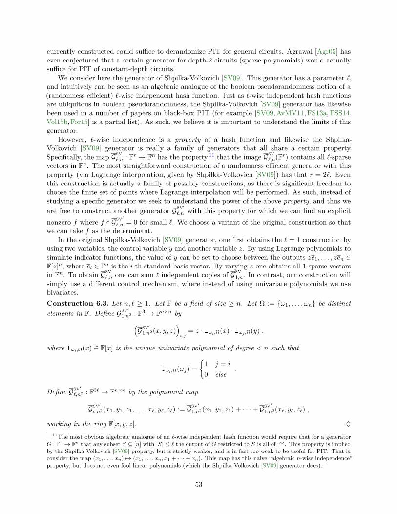
currently constructed could suffice to derandomize PIT for general circuits. Agrawal [Agr05] haseven conjectured that a certain generator for depth-2 circuits (sparse polynomials) would actuallysuffice for PIT of constant-depth circuits.

We consider here the generator of Shpilka-Volkovich [SV09]. This generator has a parameter `,and intuitively can be seen as an algebraic analogue of the boolean pseudorandomness notion of a(randomness efficient) `-wise independent hash function. Just as `-wise independent hash functionsare ubiquitous in boolean pseudorandomness, the Shpilka-Volkovich [SV09] generator has likewisebeen used in a number of papers on black-box PIT (for example [SV09, AvMV11, FS13a, FSS14,Vol15b,For15] is a partial list). As such, we believe it is important to understand the limits of thisgenerator.

However, `-wise independence is a property of a hash function and likewise the Shpilka-Volkovich [SV09] generator is really a family of generators that all share a certain property.Specifically, the map GSV

`,n : Fr → Fn has the property 11 that the image GSV`,n(Fr) contains all `-sparse

vectors in Fn. The most straightforward construction of a randomness efficient generator with thisproperty (via Lagrange interpolation, given by Shpilka-Volkovich [SV09]) has that r = 2`. Eventhis construction is actually a family of possibly constructions, as there is significant freedom tochoose the finite set of points where Lagrange interpolation will be performed. As such, instead ofstudying a specific generator we seek to understand the power of the above property, and thus weare free to construct another generator GSV′

`,n with this property for which we can find an explicitnonzero f where f GSV′

`,n = 0 for small `. We choose a variant of the original construction so thatwe can take f as the determinant.

In the original Shpilka-Volkovich [SV09] generator, one first obtains the ` = 1 construction byusing two variables, the control variable y and another variable z. By using Lagrange polynomials tosimulate indicator functions, the value of y can be set to choose between the outputs ze1, . . . , zen ∈F[z]n, where ei ∈ Fn is the i-th standard basis vector. By varying z one obtains all 1-sparse vectorsin Fn. To obtain GSV

`,n one can sum ` independent copies of GSV1,n. In contrast, our construction will

simply use a different control mechanism, where instead of using univariate polynomials we usebivariates.Construction 6.3. Let n, ` ≥ 1. Let F be a field of size ≥ n. Let Ω := ω1, . . . , ωn be distinctelements in F. Define GSV′

1,n2 : F3 → Fn×n by(GSV′

1,n2(x, y, z))i,j

= z · 1ωi,Ω(x) · 1ωj ,Ω(y) .

where 1ωi,Ω(x) ∈ F[x] is the unique univariate polynomial of degree < n such that

1ωi,Ω(ωj) =

1 j = i

0 else.

Define GSV′

`,n2 : F3` → Fn×n by the polynomial map

GSV′

`,n2(x1, y1, z1, . . . , x`, y`, z`) := GSV′

1,n2(x1, y1, z1) + · · ·+ GSV′

1,n2(x`, y`, z`) ,

working in the ring F[x, y, z]. ♦

11The most obvious algebraic analogue of an `-wise independent hash function would require that for a generatorG : Fr → Fn that any subset S ⊆ [n] with |S| ≤ ` the output of G restricted to S is all of FS . This property is impliedby the Shpilka-Volkovich [SV09] property, but is strictly weaker, and is in fact too weak to be useful for PIT. That is,consider the map (x1, . . . , xn) 7→ (x1, . . . , xn, x1 + · · ·+ xn). This map has this naive “algebraic n-wise independence”property, but does not even fool linear polynomials (which the Shpilka-Volkovich [SV09] generator does).

53

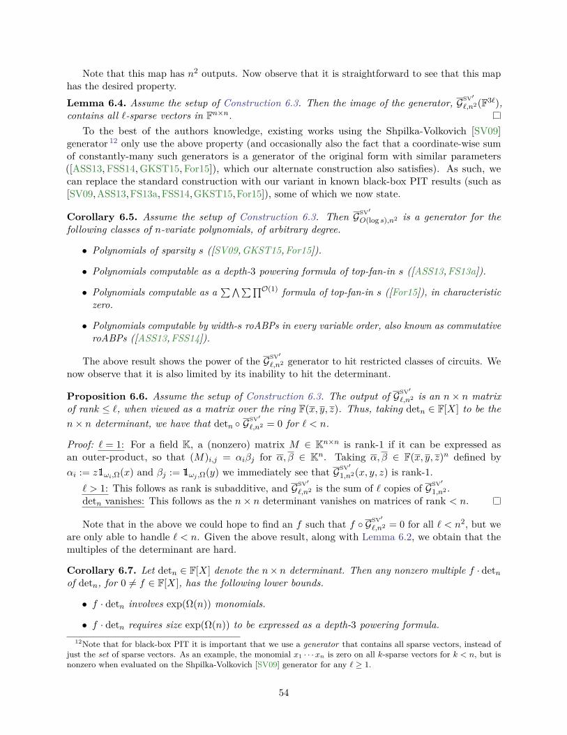
Note that this map has n2 outputs. Now observe that it is straightforward to see that this maphas the desired property.Lemma 6.4. Assume the setup of Construction 6.3. Then the image of the generator, GSV′

`,n2(F3`),contains all `-sparse vectors in Fn×n.

To the best of the authors knowledge, existing works using the Shpilka-Volkovich [SV09]generator 12 only use the above property (and occasionally also the fact that a coordinate-wise sumof constantly-many such generators is a generator of the original form with similar parameters([ASS13, FSS14, GKST15, For15]), which our alternate construction also satisfies). As such, wecan replace the standard construction with our variant in known black-box PIT results (such as[SV09,ASS13,FS13a,FSS14,GKST15,For15]), some of which we now state.

Corollary 6.5. Assume the setup of Construction 6.3. Then GSV′

O(log s),n2 is a generator for thefollowing classes of n-variate polynomials, of arbitrary degree.

• Polynomials of sparsity s ([SV09, GKST15, For15]).

• Polynomials computable as a depth-3 powering formula of top-fan-in s ([ASS13, FS13a]).

• Polynomials computable as a∑∧∑∏O(1) formula of top-fan-in s ([For15]), in characteristic

zero.

• Polynomials computable by width-s roABPs in every variable order, also known as commutativeroABPs ([ASS13, FSS14]).

The above result shows the power of the GSV′

`,n2 generator to hit restricted classes of circuits. Wenow observe that it is also limited by its inability to hit the determinant.

Proposition 6.6. Assume the setup of Construction 6.3. The output of GSV′

`,n2 is an n× n matrixof rank ≤ `, when viewed as a matrix over the ring F(x, y, z). Thus, taking detn ∈ F[X] to be then× n determinant, we have that detn G

SV′

`,n2 = 0 for ` < n.

Proof: ` = 1: For a field K, a (nonzero) matrix M ∈ Kn×n is rank-1 if it can be expressed asan outer-product, so that (M)i,j = αiβj for α, β ∈ Kn. Taking α, β ∈ F(x, y, z)n defined byαi := z1ωi,Ω(x) and βj := 1ωj ,Ω(y) we immediately see that GSV′

1,n2(x, y, z) is rank-1.` > 1: This follows as rank is subadditive, and GSV′

`,n2 is the sum of ` copies of GSV′

1,n2 .detn vanishes: This follows as the n× n determinant vanishes on matrices of rank < n.

Note that in the above we could hope to find an f such that f GSV′

`,n2 = 0 for all ` < n2, but weare only able to handle ` < n. Given the above result, along with Lemma 6.2, we obtain that themultiples of the determinant are hard.

Corollary 6.7. Let detn ∈ F[X] denote the n× n determinant. Then any nonzero multiple f · detnof detn, for 0 6= f ∈ F[X], has the following lower bounds.

• f · detn involves exp(Ω(n)) monomials.

• f · detn requires size exp(Ω(n)) to be expressed as a depth-3 powering formula.12Note that for black-box PIT it is important that we use a generator that contains all sparse vectors, instead of

just the set of sparse vectors. As an example, the monomial x1 · · ·xn is zero on all k-sparse vectors for k < n, but isnonzero when evaluated on the Shpilka-Volkovich [SV09] generator for any ` ≥ 1.

54

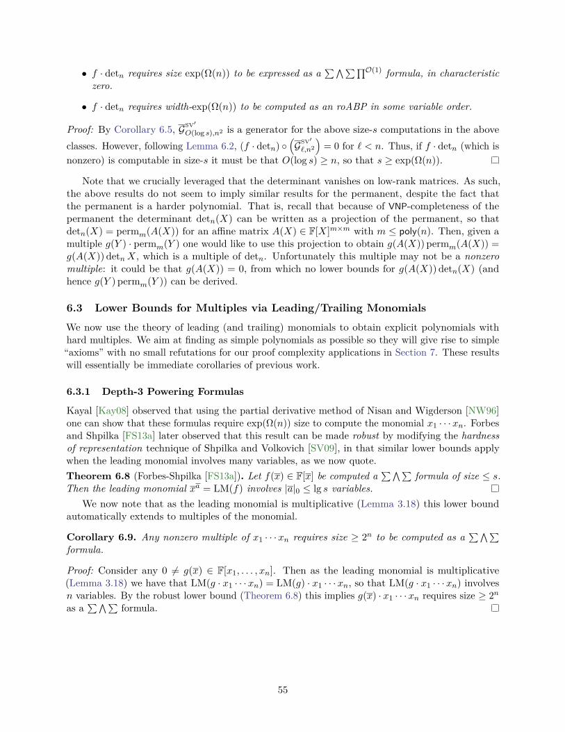
• f · detn requires size exp(Ω(n)) to be expressed as a∑∧∑∏O(1) formula, in characteristic

zero.

• f · detn requires width-exp(Ω(n)) to be computed as an roABP in some variable order.

Proof: By Corollary 6.5, GSV′

O(log s),n2 is a generator for the above size-s computations in the aboveclasses. However, following Lemma 6.2, (f · detn)

(GSV′

`,n2

)= 0 for ` < n. Thus, if f · detn (which is

nonzero) is computable in size-s it must be that O(log s) ≥ n, so that s ≥ exp(Ω(n)).

Note that we crucially leveraged that the determinant vanishes on low-rank matrices. As such,the above results do not seem to imply similar results for the permanent, despite the fact thatthe permanent is a harder polynomial. That is, recall that because of VNP-completeness of thepermanent the determinant detn(X) can be written as a projection of the permanent, so thatdetn(X) = permm(A(X)) for an affine matrix A(X) ∈ F[X]m×m with m ≤ poly(n). Then, given amultiple g(Y ) · permm(Y ) one would like to use this projection to obtain g(A(X)) permm(A(X)) =g(A(X)) detnX, which is a multiple of detn. Unfortunately this multiple may not be a nonzeromultiple: it could be that g(A(X)) = 0, from which no lower bounds for g(A(X)) detn(X) (andhence g(Y ) permm(Y )) can be derived.

6.3 Lower Bounds for Multiples via Leading/Trailing Monomials

We now use the theory of leading (and trailing) monomials to obtain explicit polynomials withhard multiples. We aim at finding as simple polynomials as possible so they will give rise to simple“axioms” with no small refutations for our proof complexity applications in Section 7. These resultswill essentially be immediate corollaries of previous work.

6.3.1 Depth-3 Powering Formulas

Kayal [Kay08] observed that using the partial derivative method of Nisan and Wigderson [NW96]one can show that these formulas require exp(Ω(n)) size to compute the monomial x1 · · ·xn. Forbesand Shpilka [FS13a] later observed that this result can be made robust by modifying the hardnessof representation technique of Shpilka and Volkovich [SV09], in that similar lower bounds applywhen the leading monomial involves many variables, as we now quote.Theorem 6.8 (Forbes-Shpilka [FS13a]). Let f(x) ∈ F[x] be computed a

∑∧∑formula of size ≤ s.

Then the leading monomial xa = LM(f) involves |a|0 ≤ lg s variables.We now note that as the leading monomial is multiplicative (Lemma 3.18) this lower bound

automatically extends to multiples of the monomial.

Corollary 6.9. Any nonzero multiple of x1 · · ·xn requires size ≥ 2n to be computed as a∑∧∑

formula.

Proof: Consider any 0 6= g(x) ∈ F[x1, . . . , xn]. Then as the leading monomial is multiplicative(Lemma 3.18) we have that LM(g · x1 · · ·xn) = LM(g) · x1 · · ·xn, so that LM(g · x1 · · ·xn) involvesn variables. By the robust lower bound (Theorem 6.8) this implies g(x) · x1 · · ·xn requires size ≥ 2nas a

∑∧∑formula.

55

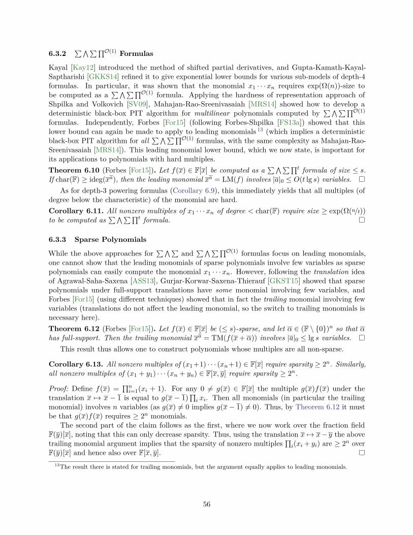
6.3.2∑∧∑∏O(1) Formulas

Kayal [Kay12] introduced the method of shifted partial derivatives, and Gupta-Kamath-Kayal-Saptharishi [GKKS14] refined it to give exponential lower bounds for various sub-models of depth-4formulas. In particular, it was shown that the monomial x1 · · ·xn requires exp(Ω(n))-size tobe computed as a

∑∧∑∏O(1) formula. Applying the hardness of representation approach ofShpilka and Volkovich [SV09], Mahajan-Rao-Sreenivasaiah [MRS14] showed how to develop adeterministic black-box PIT algorithm for multilinear polynomials computed by

∑∧∑∏O(1)

formulas. Independently, Forbes [For15] (following Forbes-Shpilka [FS13a]) showed that thislower bound can again be made to apply to leading monomials 13 (which implies a deterministicblack-box PIT algorithm for all

∑∧∑∏O(1) formulas, with the same complexity as Mahajan-Rao-Sreenivasaiah [MRS14]). This leading monomial lower bound, which we now state, is important forits applications to polynomials with hard multiples.Theorem 6.10 (Forbes [For15]). Let f(x) ∈ F[x] be computed as a

∑∧∑∏t formula of size ≤ s.If char(F) ≥ ideg(xa), then the leading monomial xa = LM(f) involves |a|0 ≤ O(t lg s) variables.

As for depth-3 powering formulas (Corollary 6.9), this immediately yields that all multiples (ofdegree below the characteristic) of the monomial are hard.Corollary 6.11. All nonzero multiples of x1 · · ·xn of degree < char(F) require size ≥ exp(Ω(n/t))to be computed as

∑∧∑∏t formula.

6.3.3 Sparse Polynomials

While the above approaches for∑∧∑

and∑∧∑∏O(1) formulas focus on leading monomials,

one cannot show that the leading monomials of sparse polynomials involve few variables as sparsepolynomials can easily compute the monomial x1 · · ·xn. However, following the translation ideaof Agrawal-Saha-Saxena [ASS13], Gurjar-Korwar-Saxena-Thierauf [GKST15] showed that sparsepolynomials under full-support translations have some monomial involving few variables, andForbes [For15] (using different techniques) showed that in fact the trailing monomial involving fewvariables (translations do not affect the leading monomial, so the switch to trailing monomials isnecessary here).Theorem 6.12 (Forbes [For15]). Let f(x) ∈ F[x] be (≤ s)-sparse, and let α ∈ (F \ 0)n so that αhas full-support. Then the trailing monomial xa = TM(f(x+ α)) involves |a|0 ≤ lg s variables.

This result thus allows one to construct polynomials whose multiples are all non-sparse.

Corollary 6.13. All nonzero multiples of (x1 +1) · · · (xn+1) ∈ F[x] require sparsity ≥ 2n. Similarly,all nonzero multiples of (x1 + y1) · · · (xn + yn) ∈ F[x, y] require sparsity ≥ 2n.

Proof: Define f(x) =∏ni=1(xi + 1). For any 0 6= g(x) ∈ F[x] the multiple g(x)f(x) under the

translation x 7→ x − 1 is equal to g(x − 1)∏i xi. Then all monomials (in particular the trailing

monomial) involves n variables (as g(x) 6= 0 implies g(x− 1) 6= 0). Thus, by Theorem 6.12 it mustbe that g(x)f(x) requires ≥ 2n monomials.

The second part of the claim follows as the first, where we now work over the fraction fieldF(y)[x], noting that this can only decrease sparsity. Thus, using the translation x 7→ x− y the abovetrailing monomial argument implies that the sparsity of nonzero multiples

∏i(xi + yi) are ≥ 2n over

F(y)[x] and hence also over F[x, y].13The result there is stated for trailing monomials, but the argument equally applies to leading monomials.

56

Note that it is tempting to derive the second part of the above corollary from the first, using thatthe substitution y ← 1 does not increase sparsity. However, this substitution can convert nonzeromultiples of

∏i(xi + yi) to zero multiples of

∏i(xi + 1), which ruins such a reduction, as argued in

the discussion after Corollary 6.7.

6.4 Lower Bounds for Multiples of Sparse Multilinear Polynomials

While the previous section established that all multiples of (x1 + 1) · · · (xn + 1) are non-sparse, theargument was somewhat specific to that polynomial and fails to obtain an analogous result for(x1 + 1) · · · (xn + 1) + 1. Further, while that argument can show for example that all multiples of then× n determinant or permanent require sparsity ≥ exp(Ω(n)), this is the best sparsity lower boundobtainable for these polynomials with this method.14 In particular, one cannot establish a sparsitylower bound of “n!” for the determinant or permanent (which would be tight) via this method.

We now give a different argument, due to Oliveira [Oli15a] that establishes a much more generalresult showing that multiples of any multilinear polynomial have at least the sparsity of the originalpolynomial. While Oliveira [Oli15a] gave a proof using Newton polytopes, we give a more compactproof here using induction on variables (loosely inspired by a similar result of Volkovich [Vol15a] onthe sparsity of factors of multi-quadratic polynomials).

Proposition 6.14 (Oliveira [Oli15a]). Let f(x) ∈ F[x1, . . . , xn] be a nonzero multilinear polynomialwith sparsity exactly s. Then any nonzero multiple of f has sparsity ≥ s.

Proof: By induction on variables.n = 0: Then f is a constant, so that s = 1 as f 6= 0. All nonzero multiples are nonzero

polynomials so have sparsity ≥ 1.n ≥ 1: Partition the variables x = (y, z), so that f(y, z) = f1(y)z + f0(y), where fi(y) has

sparsity si and s = s1 + s0. Consider any nonzero g(y, z) =∑d1i=d0

gi(y)zi with gd0(y), gd1(y) 6= 0(possibly with d0 = d1). Then

g(y, z)f(y, z) =(f1(y)z + f0(y)

)·

d1∑i=d0

gi(y)zi

= f1(y)gd1(y)zd1+1 +

∑d0<i≤d1

(f1(y)gi−1(y) + f0(y)gi(y)

)zi

+ f0(y)gd0(y)zd0 .

By partitioning this sum by powers of z so that there is no cancellation, and then discarding themiddle terms, ∣∣∣Supp

(g(y, z)f(y, z)

)∣∣∣ ≥ ∣∣∣Supp(f1(y)gd1(y)

)∣∣∣+ ∣∣∣Supp(f0(y)gd0(y)

)∣∣∣so that appealing to the induction hypothesis, as f0 and f1 are multilinear polynomials of sparsitys0 and s1 respectively,

≥ s1 + s0 = s .

14Specifically, as the determinant and permanent are degree n multilinear polynomials, and thus so are theirtranslations, their monomials always involve ≤ n variables so no sparsity bound better than 2n can be obtained byusing Theorem 6.12.

57

We note that multilinearity is essential in the above lemma, even for univariates. This is seen bynoting that the 2-sparse polynomial xn − 1 is a multiple of xn−1 + · · ·+ x+ 1.

Thus, the above not only gives a different proof of the non-sparsity of multiples of∏i(xi + 1)

(Corollary 6.13), but also establishes that nonzero multiples of∏i(xi + 1) + 1 are ≥ 2n sparse, and

nonzero multiples of the determinant or permanent are n! sparse, which is tight. Note further thatthis lower bound proof is “monotone” in that it applies to any polynomial with the same support,whereas the proof of Corollary 6.13 is seemingly not monotone as seen by contrasting

∏i(xi + 1)

and∏i(xi + 1) + 1.

6.5 Lower Bounds for Multiples by Leading/Trailing Diagonals

In the previous sections we obtained polynomials with hard multiples for various circuit classes byappealing to the fact that lower bounds for these classes can be reduced to studying the number ofvariables in leading or trailing monomials. Unfortunately this approach is restricted to circuit classeswhere monomials (or translations of monomials) are hard to compute, which in particular rules outthis approach for roABPs. Thus, to develop polynomials with hard multiples for roABPs we needto develop a different notion of a “leading part” of a polynomial. In this section, we define such anotion called a leading diagonal, establish its basic properties, and obtain the desired polynomialswith hard multiples. The ideas of this section are a cleaner version of the techniques used in thePIT algorithm of Forbes and Shpilka [FS12] for commutative roABPs.

6.5.1 Leading and Trailing Diagonals

We begin with the definition of a leading diagonal, which is a generalization of a leading monomial.Definition 6.15. Let f ∈ F[x1, . . . , xn, y1, . . . , yn] be nonzero. The leading diagonal of f , denotedLD(f), is the leading coefficient of f(x z, y z) when this polynomial is considered in the ringF[x, y][z1, . . . , zn], and where x z denotes the Hadamard product (x1z1, . . . , xnzn). The trailingdiagonal of f is defined analogously. The zero polynomial has no leading or trailing diagonal. ♦

As this notion has not explicitly appeared prior in the literature, we now establish severalstraightforward properties. The first is that extremal diagonals are homomorphic with respect tomultiplication.

Lemma 6.16. Let f, g ∈ F[x1, . . . , xn, y1, . . . , yn] be nonzero. Then LD(fg) = LD(f) LD(g) andTD(fg) = TD(f) TD(g).

Proof: As LD(f) = LCx,y|z(f(xz, yz)), where this leading coefficient is taken in the ring F[x, y][z],this automatically follows from the fact that leading coefficients are homomorphic with respect tomultiplication (Lemma 3.18). The result for trailing diagonals is symmetric.

We now show how to relate the leading monomials of the coefficient space of f to the respectivemonomials associated to the leading diagonal of f .

Proposition 6.17. Let f ∈ F[x1, . . . , xn, y1, . . . , yn]. For any b, if Coeffx|yb(LD(f)) 6= 0, then

LM(Coeff

x|yb(LD(f)))

= LM(Coeff

x|yb(f)).

The respective trailing statement also holds.

58

Proof: We prove the leading statement, the trailing version is symmetric. Let f =∑a,b αa,bx

ay b.We can then expand f(x z, y z) as follows.

f(x z, y z) =∑c

(∑a+b=c αa,bx

ayb)zc

choose c0 so that LCx,y|z(f) = Coeffx,y|zc0 (f), we get that

=(∑

a+b=c0αa,bx

ayb)zc0 +

∑c≺c0

(∑a+b=c αa,bx

ayb)zc ,

where LD(f) =∑a+b=c0

αa,bxay b and

∑a+b=c αa,bx

ay b = 0 for c c0. In particular, this meansthat for any b we have that αa,b = 0 for a c0 − b.

Thus we have that

LM(Coeff

x|yb(LD(f)))

= LM(Coeff

x|yb

(∑a+b=c0

αa,bxayb))

= LM(αc0−b,bx

c0−b)

= xc0−b ,

as we assume this leading monomial exists, which is equivalent here to αc0−b,b 6= 0.In comparison,

LM(Coeff

x|yb(f))

= LM(Coeff

x|yb

(∑a,b αa,bx

ayb))

= LM(∑

a αa,bxa)

= LM(∑

ac0−b αa,bxa + αc0−b,bx

c0−b +∑a≺c0−b αa,bx

a)

as αa,b = 0 for a c0 − b,

= LM(αc0−b,bx

c0−b +∑a≺c0−b αa,bx

a)

= xc0−b ,

where in the last step we again used that αc0−b,b 6= 0. This establishes the desired equality.

We now relate the extremal monomials of the coefficient space of f to the monomials of thecoefficient space of the extremal diagonals of f .

Corollary 6.18. Let f ∈ F[x1, . . . , xn, y1, . . . , yn]. Then

LM(Coeffx|y(f)) ⊇ LM(Coeffx|y(LD(f))) .

The respective trailing statement also holds.

Proof: This follows as LM(Coeffx|y(LD(f))) is equal toLM

(Coeff

x|yb(

LD(f))) ∣∣∣ Coeff

x|yb(

LD(f))6= 0

,

but by Proposition 6.17 this set equalsLM

(Coeff

x|yb(f)) ∣∣∣ Coeff

x|yb(

LD(f))6= 0

,

which is clearly contained in LM(Coeffx|y(f)).

59

We now observe that the number of leading monomials of the coefficient space of a leadingdiagonal is equal to its sparsity.

Lemma 6.19. Let f ∈ F[x1, . . . , xn, y1, . . . , yn]. For a polynomial g, let |g|0 denotes its sparsity.Then ∣∣∣LM

(Coeffx|y

(LD(f)

))∣∣∣ = |LD(f)|0 .

The respective trailing statement also holds.

Proof: We prove the claim for the leading diagonal, the trailing statement is symmetric. Notethat the claim is a vacuous “0=0” if f is zero. For nonzero f , express it as f =

∑a,b αa,bx

ay b sothat LD(f) =

∑a+b=c0

αa,bxay b =

∑b αc0−b,bx

c0−by b for some c0 ∈ Nn. Then Coeffx|yb(LD(f)) =

αc0−b,bxc0−b. As the monomials xc0−b are distinct and hence linearly independent for distinct b, it

follows that dim Coeffx|y(LD(f)) = |b|αc0−b,b 6= 0|, which is equal the sparsity |LD(f)|0.

Finally, we now lower bound the coefficient dimension of a polynomial by the sparsity of itsextremal diagonals.Corollary 6.20. Let f ∈ F[x1, . . . , xn, y1, . . . , yn]. Then

dim Coeffx|y(f) ≥ |LD(f)|0, |TD(f)|0 ,

where for a polynomial g, |g|0 denotes its sparsity.

Proof: We give the proof for the leading diagonal, the trailing diagonal is symmetric. By the above,

dim Coeffx|y(f) ≥∣∣∣LM

(Coeffx|y(f)

)∣∣∣ ≥ ∣∣∣LM(Coeffx|y

(LD(f)

))∣∣∣ = |LD(f)|0 ,

where we passed from span to number of leading monomials (Lemma 3.19), and then passed tothe leading monomials of the leading diagonal (Corollary 6.18), and then passed to sparsity of theleading diagonal (Lemma 6.19).

6.5.2 Lower Bounds for Multiples for Read-Once and Read-Twice ABPs

Having developed the theory of leading diagonals in the previous section, we now turn to usingthis theory to obtain explicit polynomials whose nonzero multiples all require large roABPs. Wealso generalize this to read-O(1) oblivious ABPs, but only state the results for k = 2 as this hasa natural application to proof complexity (Section 7). As the restricted computations consideredabove (

∑∧∑formulas and sparse polynomials) have small roABPs, the hard polynomials in

this section will also have multiples requiring large complexity in these models as well and thusqualitatively reprove some of the above results. However, we included the previous sections as thehard polynomials there are simpler (being monomials or translations of monomials), and moreimportantly we will need those results for the proofs below.

The proofs will use the characterization of roABPs by their coefficient dimension (Lemma 3.7),the lower bound for coefficient dimension in terms of the sparsity of the extremal diagonals(Corollary 6.20), and polynomials whose multiples are all non-sparse (Corollary 6.13).

Proposition 6.21. Let f(x, y) :=∏ni=1(xi + yi + αi) ∈ F[x1, . . . , xn, y1, . . . , yn], for αi ∈ F. Then

for any 0 6= g ∈ F[x, y],dim Coeffx|y(g · f) ≥ 2n .

In particular, all nonzero multiples of f require width at least 2n to be computed by an roABP inany variable order where x ≺ y.

60

Proof: Observe that leading diagonal of f is insensitive to the αi. That is, LD(xi+yi+αi) = xi+yi,so by multiplicativity of the leading diagonal (Lemma 6.16) we have that LD(f) =

∏i(xi + yi).

Thus, appealing to Corollary 6.20 and Corollary 6.13,

dim Coeffx|y(g · f) ≥ |LD(g · f)|0= |LD(g) · LD(f)|0= |LD(g) ·

∏i(xi + yi)|0

≥ 2n .

The claim about roABP width follows from Lemma 3.7.

Note that this lower bound actually works in the “monotone” setting (if we replace Corollary 6.13with the monotone Proposition 6.14), as the result only uses the zero/nonzero pattern of thecoefficients.

The above result gives lower bounds for coefficient dimension in a fixed variable partition. Wenow symmetrize this construction to get lower bounds for coefficient dimension in any variablepartition. We proceed as in Section 5.5, where we plant the fixed-partition lower bound into anarbitrary partition. Note that unlike that construction, we will not need auxiliary variables here.

Corollary 6.22. Let f ∈ F[x1, . . . , xn] be defined by f(x) :=∏i<j(xi+xj +αi,j) for αi,j ∈ F. Then

for any partition x = (u, v, w) with m := |u| = |v|, and any 0 6= g ∈ F[x],

dimF(w) Coeffu|v(g · f) ≥ 2m ,

where we treat g · f as a polynomial in F(w)[u, v]. In particular, all nonzero multiples of f requirewidth ≥ 2n to be computed by an roABP in any variable order.

Proof: We can factor f into a copy of the hard polynomial from Proposition 6.21, and the rest.That is,

f(x) =∏i<j

(xi + xj + αi,j) =m∏i=1

(ui + vi + βi) · f ′(u, v, w) ,

for some βi ∈ F and nonzero f ′(u, v, w) ∈ F[u, v, w]. Thus,

g · f =(g(u, v, w) · f ′(u, v, w)

)·m∏i=1

(ui + vi + βi) .

Noting that g, f ′ are nonzero in F[u, v, w], they are also nonzero in F(w)[u, v], so that g ·f is nonzeromultiple of

∏mi=1(ui + vi + βi) in F(w)[u, v]. Appealing to our lower bound for (nonzero) multiples

of coefficient dimension (Proposition 6.21), we have that

dimF(w) Coeffu|v(g · f) = dimF(w) Coeffu|v

(g · f ′ ·

m∏i=1

(ui + vi + βi))≥ 2m .

The statement about roABPs follows from Lemma 3.7.

We briefly remark that the above bound does not match the naive bound achieved by writingthe polynomial

∏i<j(xi + xj + αi,j) in its sparse representation, which has 2Θ(n2) terms. The gap

between the lower bound (2Ω(n)) and the upper bound (2O(n2)) is explained by our use of a complete

61

graph to embed the lower bounds of Proposition 6.21 into an arbitrary partition. As discussed afterProposition 5.13 one can use expander graphs to essentially close this gap.

We now observe that the above lower bounds for coefficient dimension suffices to obtain lowerbounds for read-twice oblivious ABPs, as we can appeal to the structural result of Anderson, Forbes,Saptharishi, Shpilka and Volk [AFS+16] (Theorem 3.9). This result shows that for any read-twiceoblivious ABP that (after discarding some variables) there is a partition of the variables acrosswhich has small coefficient dimension, which is in contrast to the above lower bound.

Corollary 6.23. Let f ∈ F[x1, . . . , xn] be defined by f(x) :=∏i<j(xi+xj +αi,j) for αi,j ∈ F. Then

for any 0 6= g ∈ F[x], g · f requires width-2Ω(n) as a read-twice oblivious ABP.

Proof: Suppose that g · f has a read-twice oblivious ABP of width-w. By the lower-bound ofAnderson, Forbes, Saptharishi, Shpilka and Volk [AFS+16] (Theorem 3.9), there exists a partitionx = (u, v, w) where |u|, |v| ≥ Ω(n), and such that dimF(w) Coeffu|v(g · f) ≤ w4 (where we treatg · f as a polynomial in F(w)[u, v]). Note that we can take enforce that the partition obeysm := |u| = |v| ≥ Ω(n), as we can balance u and v by pushing variables into w, as this cannotincrease the coefficient dimension (Fact 3.8). However, appealing to our coefficient dimension bound(Corollary 6.22)

w4 ≥ dimF(w) Coeffu|v(g · f) ≥ 2m ≥ 2Ω(n) ,

so that w ≥ 2Ω(n) as desired.

7 IPS Lower Bounds via Lower Bounds for Multiples

In this section we use the lower bounds for multiples of Section 6 to derive lower bounds for C-IPSproofs for various restricted algebraic circuit classes C. The advantage of this approach over thefunctional lower bounds strategy of Section 5 is that we derive lower bounds for the general IPSsystem, not just its subclass linear-IPS. While our equivalence (Proposition 4.4) of C-IPS andC-IPSLIN holds for any strong-enough class C, the restricted classes we consider here (depth-3powering formulas and roABPs) 15 are not strong enough to use Proposition 4.4 to lift the results ofSection 5 to lower bounds for the full IPS system. However, as discussed in the introduction, thetechniques of this section can only yield lower bounds for C-IPS refutations of systems of equationswhich are hard to compute within C (though our examples are computable by small (general)circuits).

We begin by first detailing the relation between IPS refutations and multiples. We then useour lower bounds for multiples (Section 6) to derive as corollaries lower bounds for

∑∧∑-IPS and

roABP-IPS refutations.

Lemma 7.1. Let f, g, x2−x ∈ F[x1, . . . , xn] be an unsatisfiable system of equations, where g, x2−xis satisfiable. Let C ∈ F[x, y, z, w] be an IPS refutation of f, g, x2 − x. Then

1− C(x, 0, g, x2 − x)

is a nonzero multiple of f .15As in Section 6, we will not treat multilinear formulas in this section as they are less natural for the techniques

under consideration. Further, IPS lower bounds for multilinear formulas can be obtained via functional lower bounds(Corollary 5.15).

62

Proof: That C is an IPS refutation means that

C(x, f, g, x2 − x) = 1, C(x, 0, 0, 0) = 0 .

We first show that 1− C(x, 0, g, x2 − x) is a multiple of f , using the first condition on C. ExpandC(x, y, z, w) as a univariate in y, so that

C(x, y, z, w) =∑i≥0

Ci(x, z, w)yi ,

for Ci ∈ F[x, z, w]. In particular, C0(x, z, w) = C(x, 0, z, w). Thus,

1− C(x, 0, g, x2 − x) = C(x, f, g, x2 − x)− C(x, 0, g, x2 − x)

=(∑

i≥0Ci(x, g, x2 − x)f i)− C0(x, g, x2 − x)

=∑i≥1Ci(x, g, x2 − x)f i

=(∑

i≥1Ci(x, g, x2 − x)f i−1)· f .

Thus, 1− C(x, 0, g, x2 − x) is a multiple of f as desired.We now show that this is a nonzero multiple, using the second condition on C and the satisfiability

of g, x2 − x. That is, the second condition implies that 0 = C(x, 0, 0, 0) = C0(x, 0, 0). If 1 −C(x, 0, g, x2 − x) is zero, then by the above we have that C0(x, g, x2 − x) = 1, so that C0(x, z, w)is an IPS refutation of g, x2 − x, which contradicts the satisfiability of g, x2 − x as IPS is a soundproof system. So it must then be that 1− C(x, 0, g, x2 − x) is nonzero.

That is, take an α satisfying g, x2 − x so that g(α) = 0, α2 − α = 0. Substituting this α intoC0(x, g, x2−x), we have that C0(x, g, x2−x)|x←α = C0(α, 0, 0), and because C0(x, 0, 0) ≡ 0 in F[x] viathe above we have that C0(α, 0, 0) = 0. Thus, we have that 1−C(x, 0, g, x2−x) = 1−C0(x, g, x2−x)is a nonzero polynomial as its evaluation at x← α is 1.

The above lemma thus gives a template for obtaining lower bounds for IPS. First, obtain a“hard” polynomial f whose nonzero multiples are hard for C, where f is hopefully also computable bysmall (general) circuits. Then find additional (simple) polynomials g such that g, x2−x is satisfiableyet f, g, x2 − x is unsatisfiable. By the above lemma one then has the desired IPS lower boundfor refuting f, g, x2 − x, assuming that C is sufficiently general. However, for our results we needto more careful as even though C(x, y, z, w) is from the restricted class C, the derived polynomialC(x, 0, g, x2 − x) may not be, and as such we will need to appeal to lower bounds for strongerclasses.

We now instantiate this template, first for depth-3 powering formulas, where we use lower boundsfor multiples of the stronger

∑∧∑∏2 model.

Corollary 7.2. Let F be a field with char(F) = 0. Let f := x1 · · ·xn and g := x1 + · · · + xn − nwith f, g ∈ F[x1, . . . , xn]. Then f, g, x2 − x are unsatisfiable and any

∑∧∑-IPS refutation requires

size at least exp(Ω(n)).

Proof: The hypothesis char(F) = 0 implies that 0, . . . , n are distinct numbers. In particular,the system g(x) = 0 and x2 − x = 0 is satisfiable and has the unique satisfying assignment 1.However, this single assignment does not satisfy f as f(1) =

∏ni=1 1 = 1 6= 0, so the entire system is

unsatisfiable. Thus, applying our strategy (Lemma 7.1), we see that for any∑∧∑

-IPS refutationC(x, y, z, w) of f, g, x2 − x that 1− C(x, 0, g, x2 − x) is a nonzero multiple of f .

63

Let s be the size of C as a∑∧∑

formula. As g is linear and the boolean axioms x2 − x arequadratic, it follows that 1− C(x, 0, g, x2 − x) is a sum of powers of quadratics (

∑∧∑∏2) of sizepoly(s). As nonzero multiples of f requires exp(Ω(n))-size as a

∑∧∑∏2 formula (Corollary 6.11)it follows that poly(s) ≥ exp(Ω(n)), so that s ≥ exp(Ω(n)) as desired.

We similarly obtain a lower bound for roABP-IPS, where here we use lower bounds for multiplesof read-twice oblivious ABPs.

Corollary 7.3. Let F be a field with char(F) > n. Let f :=∏i<j(xi+xj−1) and g := x1+· · ·+xn−n

with f, g ∈ F[x1, . . . , xn]. Then f, g, x2 − x are unsatisfiable and any roABP-IPS refutation (in anyvariable order) requires size ≥ exp(Ω(n)).

Proof: The hypothesis char(F) > n implies that 0, . . . , n are distinct numbers. In particular, thesystem g(x) = 0 and x2 − x = 0 is satisfiable and has the unique satisfying assignment 1. However,this single assignment does not satisfy f as f(1) =

∏i<j(1 + 1− 1) = 1 6= 0, so the entire system is

unsatisfiable. Thus, applying our strategy (Lemma 7.1), we see that for any roABP-IPS refutationC(x, y, z, w) of f, g, x2 − x that 1− C(x, 0, g, x2 − x) is a nonzero multiple of f .

Let s be the size of C as an roABP, and we now argue that 1− C(x, 0, g, x2 − x) has a smallread-twice oblivious ABP. First, note that we can expand C(x, 0, z, w) into powers of z, so thatC(x, 0, z, w) =

∑0≤i≤sCi(x,w)zi (where we use that s bounds the width and degree of the roABP

C). Each Ci(x,w) has a poly(s)-size roABP (in the variable order of C where z is omitted) as wecan compute Ci via interpolation over z, using that each evaluation preserves roABP size (Fact 3.8).Further, as g is linear, for any i we see that gi can be computed by a poly(n, i)-size roABP (in anyvariable order) (Theorem 3.15). Combining these facts using closure properties of roABPs underaddition and multiplication (Fact 3.8), we see that C(x, 0, g, w), and hence 1 − C(x, 0, g, w), hasa poly(s, n)-size roABP in the variable order that C induces on x,w. Next observe, that as eachboolean axiom x2

i − xi only refers to a single variable, substituting w ← x2 − x in the roABP for1−C(x, 0, g, w) will preserve obliviousness of the ABP, but now each variable will be read twice, sothat 1− C(x, 0, g, x2 − x) has a poly(s, n)-size read-twice oblivious ABP.

Now, using that nonzero multiples of f requires exp(Ω(n))-size to be computed as read-twiceoblivious ABPs (Corollary 6.23) it follows that poly(s, n) ≥ exp(Ω(n)), so that s ≥ exp(Ω(n)) asdesired.

We note that the above lower bound is for the size of the roABP. One can also obtain thestronger result (for similar but less natural axioms) showing that the width (and hence also the size)of the roABP must be large, but we do not pursue this as it does not qualitatively change the result.

8 Discussion

In this work we proved new lower bounds for various natural restricted versions of the Ideal ProofSystem (IPS) of Grochow and Pitassi [GP14]. While existing work in algebraic proof complexityshowed limitations of weak measures of complexity such as the degree and sparsity of a polynomial,our lower bounds are for stronger measures of circuit size that match many of the frontier lowerbounds in algebraic circuit complexity. However, our work leaves several open questions anddirections for further study, which we now list.

1. Can one obtain proof complexity lower bounds from the recent techniques for lower boundsfor depth-4 circuits, such as the results of Gupta, Kamath, Kayal and Saptharishi [GKKS14]?Neither of our approaches (functional lower bounds or lower bounds for multiples) currentlyextend to their techniques.

64

2. Many proof complexity lower bounds are for refuting unsatisfiable k-CNFs, where k = O(1),which can be encoded as systems of polynomial equations where each equation involves O(1)variables. Can one obtain interesting IPS lower bounds for such systems? Our techniques onlyestablish exponential lower bounds where there is at least one axiom involving Ω(n) variables.

3. Given an equation f(x) = 0 where f has a size-s circuit, there is a natural way to convertthis equation to poly(s)-many equations on O(1) extension variables by tracing throughthe computation of f . Can one understand how introducing extension variables affects thecomplexity of refuting polynomial systems of equations? This seems a viable approach to theprevious question when applied to our technique of using lower bounds for multiples.

4. We have shown various lower bounds for multiples by invoking the hardness of the determinant(Corollary 6.7), but this does not lead to satisfactory proof lower bounds as the axioms arecomplicated. Can one implicitly invoke the hardness of the determinant? For example, considerthe hard matrix identities suggested by Cook and Rackoff (see for example the survey ofBeame and Pitassi [BP98]) and later studied by Soltys and Cook [SC04]. That is, considerunsatisfiable equations such as XY − In, Y X − 2 · In, where X and Y are symbolic n × nmatrices and In is the n × n identity matrix. The simplest refutations known involve thedeterminant (see Hrubes-Tzameret [HT15], and the discussion in Grochow-Pitassi [GP14]),can one provide evidence that computing the determinant is intrinsic to such refutations?

5. The lower bounds of this paper are for the static IPS system, where one cannot simplifyintermediate computations. There are also dynamic algebraic proof systems (see Appendix A),can one extend our techniques to that setting?

Acknowledgments

We would like to thank Rafael Oliviera for telling us of Proposition 6.14, Mrinal Kumar andRamprasad Saptharishi for conversations [FKS16] clarifying the roles of functional lower bounds inthis work, as well as Avishay Tal for pointing out how Proposition B.1 implies an optimal functionallower bound for sparsity (Corollary B.3). We would also like to thank Joshua Grochow for helpfuldiscussions regarding this work. We are grateful for the anonymous reviewers for their careful readof the paper and for their comments.

References[AFS+16] Matthew Anderson, Michael A. Forbes, Ramprasad Saptharishi, Amir Shpilka, and Ben Lee Volk. Identity

testing and lower bounds for read-k oblivious algebraic branching programs. In Proceedings of the 31st

Annual Computational Complexity Conference (CCC 2016), volume 50 of Leibniz International Proceedingsin Informatics (LIPIcs), pages 30.1–30.25, 2016. Full version at arXiv:1511.07136.

[AGKS15] Manindra Agrawal, Rohit Gurjar, Arpita Korwar, and Nitin Saxena. Hitting-sets for ROABP and sum ofset-multilinear circuits. SIAM J. Comput., 44(3):669–697, 2015. Preliminary version at arXiv:1406.7535.

[Agr05] Manindra Agrawal. Proving lower bounds via pseudo-random generators. In Proceedings of the 25th

International Conference on Foundations of Software Technology and Theoretical Computer Science(FSTTCS 2005), pages 92–105, 2005.

[AR01] Michael Alekhnovich and Alexander A. Razborov. Lower bounds for polynomial calculus: Non-binomialcase. In Proceedings of the 42nd Annual IEEE Symposium on Foundations of Computer Science (FOCS2001), pages 190–199, 2001.

[ASS13] Manindra Agrawal, Chandan Saha, and Nitin Saxena. Quasi-polynomial hitting-set for set-depth-∆formulas. In Proceedings of the 45th Annual ACM Symposium on Theory of Computing (STOC 2013),pages 321–330, 2013. Full version at arXiv:1209.2333.

65

[AvMV11] Matthew Anderson, Dieter van Melkebeek, and Ilya Volkovich. Derandomizing polynomial identitytesting for multilinear constant-read formulae. In Proceedings of the 26th Annual IEEE Conference onComputational Complexity (CCC 2011), pages 273–282, 2011. Full version in the Electronic Colloquiumon Computational Complexity (ECCC), Technical Report TR10-188.

[BGIP01] Samuel R. Buss, Dima Grigoriev, Russell Impagliazzo, and Toniann Pitassi. Linear gaps between degreesfor the polynomial calculus modulo distinct primes. J. Comput. Syst. Sci., 62(2):267–289, 2001. Preliminaryversion in the 14th Annual IEEE Conference on Computational Complexity (CCC 1999).

[BIK+96a] Paul Beame, Russell Impagliazzo, Jan Krajıcek, Toniann Pitassi, and Pavel Pudlak. Lower boundson Hilbert’s Nullstellensatz and propositional proofs. Proc. London Math. Soc. (3), 73(1):1–26, 1996.Preliminary version in the 35th Annual IEEE Symposium on Foundations of Computer Science (FOCS1994).

[BIK+96b] Samuel R. Buss, Russell Impagliazzo, Jan Krajıcek, Pavel Pudlak, Alexander A. Razborov, and JirıSgall. Proof complexity in algebraic systems and bounded depth Frege systems with modular counting.Computational Complexity, 6(3):256–298, 1996.

[BP98] Paul Beame and Toniann Pitassi. Propositional proof complexity: Past, present and future. Bulletinof the European Association for Theoretical Computer Science (EATCS), 65:66–89, 1998. Preliminaryversion in the Electronic Colloquium on Computational Complexity (ECCC), Technical Report TR98-067.

[CEI96] Matthew Clegg, Jeff Edmonds, and Russell Impagliazzo. Using the Groebner basis algorithm to findproofs of unsatisfiability. In Proceedings of the 28th Annual ACM Symposium on Theory of Computing(STOC 1996), pages 174–183, 1996.

[CLO07] David Cox, John Little, and Donal O’Shea. Ideals, varieties, and algorithms. Undergraduate Texts inMathematics. Springer, New York, third edition, 2007.

[CR74a] Stephen A. Cook and Robert A. Reckhow. On the lengths of proofs in the propositional calculus(preliminary version). In Proceedings of the 6th Annual ACM Symposium on Theory of Computing (STOC1974), pages 135–148, 1974. For corrections see Cook-Reckhow [CR74b].

[CR74b] Stephen A. Cook and Robert A. Reckhow. Corrections for “On the lengths of proofs in the propositionalcalculus (preliminary version)”. SIGACT News, 6(3):15–22, July 1974.

[CR79] Stephen A. Cook and Robert A. Reckhow. The relative efficiency of propositional proof systems. J. Symb.Log., 44(1):36–50, 1979. This is a journal-version of Cook-Reckhow [CR74a] and Reckhow [Rec76].

[DL78] Richard A. DeMillo and Richard J. Lipton. A probabilistic remark on algebraic program testing. Inf.Process. Lett., 7(4):193–195, 1978.

[DSY09] Zeev Dvir, Amir Shpilka, and Amir Yehudayoff. Hardness-randomness tradeoffs for bounded deptharithmetic circuits. SIAM J. Comput., 39(4):1279–1293, 2009. Preliminary version in the 40th AnnualACM Symposium on Theory of Computing (STOC 2008).

[FGS13] Michael A. Forbes, Ankit Gupta, and Amir Shpilka. Personal Communication to Gupta, Kamath, Kayal,Saptharishi [GKKS13], 2013.

[Fis94] Ismor Fischer. Sums of like powers of multivariate linear forms. Mathematics Magazine, 67(1):59–61, 1994.[FKS16] Michael A. Forbes, Mrinal Kumar, and Ramprasad Saptharishi. Functional lower bounds for arithmetic

circuits and connections to boolean circuit complexity. In Proceedings of the 31st Annual ComputationalComplexity Conference (CCC 2016), volume 50 of Leibniz International Proceedings in Informatics(LIPIcs), pages 33.1–33.19, 2016. Full version at arXiv:1605.04207.

[For14] Michael A. Forbes. Polynomial Identity Testing of Read-Once Oblivious Algebraic Branching Programs.PhD thesis, Massachusetts Institute of Technology, June 2014.

[For15] Michael A. Forbes. Deterministic divisibility testing via shifted partial derivatives. In Proceedings of the56th Annual IEEE Symposium on Foundations of Computer Science (FOCS 2015), pages 451–465, 2015.

[FS12] Michael A. Forbes and Amir Shpilka. On identity testing of tensors, low-rank recovery and compressedsensing. In Proceedings of the 44th Annual ACM Symposium on Theory of Computing (STOC 2012), pages163–172, 2012. Full version at arXiv:1111.0663.

[FS13a] Michael A. Forbes and Amir Shpilka. Explicit Noether Normalization for simultaneous conjugation viapolynomial identity testing. In Proceedings of the 17th International Workshop on Randomization andComputation (RANDOM 2013), pages 527–542, 2013. Full version at arXiv:1303.0084.

66

[FS13b] Michael A. Forbes and Amir Shpilka. Quasipolynomial-time identity testing of non-commutative andread-once oblivious algebraic branching programs. In Proceedings of the 54th Annual IEEE Symposium onFoundations of Computer Science (FOCS 2013), pages 243–252, 2013. Full version at arXiv:1209.2408.

[FS15] Michael A. Forbes and Amir Shpilka. Complexity theory column 88: Challenges in polynomial factorization.SIGACT News, 46(4):32–49, 2015.

[FSS14] Michael A. Forbes, Ramprasad Saptharishi, and Amir Shpilka. Hitting sets for multilinear read-oncealgebraic branching programs, in any order. In Proceedings of the 46th Annual ACM Symposium on Theoryof Computing (STOC 2014), pages 867–875, 2014. Full version at arXiv:1309.5668.

[GH03] Dima Grigoriev and Edward A. Hirsch. Algebraic proof systems over formulas. Theoretical ComputerScience, 1(303):83–102, 2003. Preliminary version in the Electronic Colloquium on ComputationalComplexity (ECCC), Technical Report TR01-011.

[GK98] Dima Grigoriev and Marek Karpinski. An exponential lower bound for depth 3 arithmetic circuits. InProceedings of the 30th Annual ACM Symposium on Theory of Computing (STOC 1998), pages 577–582,1998.

[GKKS13] Ankit Gupta, Pritish Kamath, Neeraj Kayal, and Ramprasad Saptharishi. Arithmetic circuits: A chasmat depth three. In Proceedings of the 54th Annual IEEE Symposium on Foundations of Computer Science(FOCS 2013), pages 578–587, 2013. Full version in the Electronic Colloquium on Computational Complexity(ECCC), Technical Report TR13-026.

[GKKS14] Ankit Gupta, Pritish Kamath, Neeraj Kayal, and Ramprasad Saptharishi. Approaching the chasm atdepth four. J. ACM, 61(6):33:1–33:16, December 2014. Preliminary version in the 28th Annual IEEEConference on Computational Complexity (CCC 2013).

[GKST15] Rohit Gurjar, Arpita Korwar, Nitin Saxena, and Thomas Thierauf. Deterministic identity testing for sumof read-once oblivious arithmetic branching programs. In Proceedings of the 30th Annual ComputationalComplexity Conference (CCC 2015), volume 33 of Leibniz International Proceedings in Informatics(LIPIcs), pages 323–346, 2015. Full version at arXiv:1411.7341.

[GP14] Joshua A. Grochow and Toniann Pitassi. Circuit complexity, proof complexity, and polynomial identitytesting. In Proceedings of the 55th Annual IEEE Symposium on Foundations of Computer Science (FOCS2014), pages 110–119, 2014. Full version at arXiv:abs/1404.3820.

[GR00] Dima Grigoriev and Alexander A. Razborov. Exponential lower bounds for depth 3 arithmetic circuitsin algebras of functions over finite fields. Appl. Algebra Eng. Commun. Comput., 10(6):465–487, 2000.Preliminary version in the 39th Annual IEEE Symposium on Foundations of Computer Science (FOCS1998).

[Gri98] Dima Grigoriev. Tseitin’s tautologies and lower bounds for Nullstellensatz proofs. In Proceedings of the39th Annual IEEE Symposium on Foundations of Computer Science (FOCS 1998), pages 648–652, 1998.

[HS80] Joos Heintz and Claus-Peter Schnorr. Testing polynomials which are easy to compute (extended abstract).In Proceedings of the 12th Annual ACM Symposium on Theory of Computing (STOC 1980), pages 262–272,1980.

[HT15] Pavel Hrubes and Iddo Tzameret. Short proofs for the determinant identities. SIAM J. Comput., 44(2):340–383, 2015. Preliminary version in the 44th Annual ACM Symposium on Theory of Computing (STOC2012). arXiv:1112.6265.

[IPS99] Russell Impagliazzo, Pavel Pudlak, and Jirı Sgall. Lower bounds for the polynomial calculus and theGrobner basis algorithm. Computational Complexity, 8(2):127–144, 1999. Preliminary version in theElectronic Colloquium on Computational Complexity (ECCC), Technical Report TR97-042.

[IW97] Russell Impagliazzo and Avi Wigderson. P=BPP if E requires exponential circuits: Derandomizing theXOR lemma. In Proceedings of the 29th Annual ACM Symposium on Theory of Computing (STOC 1997),pages 220–229, 1997.

[Kal89] Erich L. Kaltofen. Factorization of polynomials given by straight-line programs. In Silvio Micali, editor,Randomness and Computation, volume 5 of Advances in Computing Research, pages 375–412. JAI Press,Inc., Greenwich, CT, USA, 1989.

[Kay08] Neeraj Kayal. Personal Communication to Saxena [Sax08], 2008.[Kay12] Neeraj Kayal. An exponential lower bound for the sum of powers of bounded degree polynomials. Electronic

Colloquium on Computational Complexity (ECCC), 19(81), 2012.

67

[KI04] Valentine Kabanets and Russell Impagliazzo. Derandomizing polynomial identity tests means provingcircuit lower bounds. Computational Complexity, 13(1-2):1–46, 2004. Preliminary version in the 35th

Annual ACM Symposium on Theory of Computing (STOC 2003).[Kra95] Jan Krajıcek. Bounded arithmetic, propositional logic, and complexity theory, volume 60 of Encyclopedia

of Mathematics and its Applications. Cambridge University Press, Cambridge, 1995.[KS01] Adam Klivans and Daniel A. Spielman. Randomness efficient identity testing of multivariate polynomials.

In Proceedings of the 33rd Annual ACM Symposium on Theory of Computing (STOC 2001), pages 216–223,2001.

[KS15] Mrinal Kumar and Ramprasad Saptharishi. An exponential lower bound for homogeneous depth-5 circuitsover finite fields. arXiv, 1507.00177, 2015.

[LTW15] Fu Li, Iddo Tzameret, and Zhengyu Wang. Non-commutative formulas and Frege lower bounds: a newcharacterization of propositional proofs. In Proceedings of the 30th Annual Computational ComplexityConference (CCC 2015), volume 33 of Leibniz International Proceedings in Informatics (LIPIcs), pages412–432, 2015. Full version at arXiv:1412.8746.

[MRS14] Meena Mahajan, B.V. Raghavendra Rao, and Karteek Sreenivasaiah. Building above read-once polynomials:Identity testing and hardness of representation. In Proceedings of Computing and Combinatorics - 20th

International Conference (COCOON 2014), volume 8591 of Lecture Notes in Computer Science, pages1–12, 2014. Full version in the Electronic Colloquium on Computational Complexity (ECCC), TechnicalReport TR15-202.

[Nis91] Noam Nisan. Lower bounds for non-commutative computation. In Proceedings of the 23rd Annual ACMSymposium on Theory of Computing (STOC 1991), pages 410–418, 1991.

[NW94] Noam Nisan and Avi Wigderson. Hardness vs randomness. J. Comput. Syst. Sci., 49(2):149–167, 1994.Preliminary version in the 29th Annual IEEE Symposium on Foundations of Computer Science (FOCS1988).

[NW96] Noam Nisan and Avi Wigderson. Lower bounds on arithmetic circuits via partial derivatives. ComputationalComplexity, 6(3):217–234, 1996. Preliminary version in the 36th Annual IEEE Symposium on Foundationsof Computer Science (FOCS 1995).

[Oli15a] Rafael Oliveira. Personal Communication, 2015.[Oli15b] Rafael Oliveira. Factors of low individual degree polynomials. In Proceedings of the 30th Annual

Computational Complexity Conference (CCC 2015), volume 33 of Leibniz International Proceedings inInformatics (LIPIcs), pages 198–216, 2015.

[OSV15] Rafael Oliveira, Amir Shpilka, and Ben Lee Volk. Subexponential size hitting sets for bounded depthmultilinear formulas. In Proceedings of the 30th Annual Computational Complexity Conference (CCC2015), volume 33 of Leibniz International Proceedings in Informatics (LIPIcs), pages 304–322, 2015. Fullversion at arXiv:1411.7492.

[Pit97] Toniann Pitassi. Algebraic propositional proof systems. In Descriptive Complexity and Finite Models,volume 31 of DIMACS Series in Discrete Mathematics and Theoretical Computer Science, pages 215–244,1997.

[Pud97] Pavel Pudlak. Lower bounds for resolution and cutting plane proofs and monotone computations. J.Symb. Log., 62(3):981–998, 1997.

[Raz98] Alexander A. Razborov. Lower bounds for the polynomial calculus. Computational Complexity, 7(4):291–324, 1998.

[Raz06] Ran Raz. Separation of multilinear circuit and formula size. Theory of Computing, 2(6):121–135, 2006.Preliminary version in the 45th Annual IEEE Symposium on Foundations of Computer Science (FOCS2004).

[Raz09] Ran Raz. Multi-linear formulas for permanent and determinant are of super-polynomial size. J. ACM,56(2), 2009. Preliminary version in the 36th Annual ACM Symposium on Theory of Computing (STOC2004).

[Rec76] Robert A. Reckhow. On the lengths of proofs in the propositional calculus. PhD thesis, University ofToronto, 1976.

[RS05] Ran Raz and Amir Shpilka. Deterministic polynomial identity testing in non-commutative models.Comput. Complex., 14(1):1–19, April 2005. Preliminary version in the 19th Annual IEEE Conference onComputational Complexity (CCC 2004).

68

[RT08a] Ran Raz and Iddo Tzameret. The strength of multilinear proofs. Computational Complexity, 17(3):407–457,2008. Preliminary version in the Electronic Colloquium on Computational Complexity (ECCC), TechnicalReport TR06-001.

[RT08b] Ran Raz and Iddo Tzameret. Resolution over linear equations and multilinear proofs. Ann. Pure Appl.Logic, 155(3):194–224, 2008. Preliminary version at arXiv:0708.1529.

[RY08] Ran Raz and Amir Yehudayoff. Balancing syntactically multilinear arithmetic circuits. ComputationalComplexity, 17(4):515–535, 2008.

[RY09] Ran Raz and Amir Yehudayoff. Lower bounds and separations for constant depth multilinear circuits.Computational Complexity, 18(2):171–207, 2009. Preliminary version in the 23rd Annual IEEE Conferenceon Computational Complexity (CCC 2008).

[Sap12] Ramprasad Saptharishi, 2012. Personal communication to Forbes-Shpilka [FS13b].[Sax08] Nitin Saxena. Diagonal circuit identity testing and lower bounds. In Proceedings of the 35th International

Colloquium on Automata, Languages and Programming (ICALP 2008), pages 60–71, 2008. Preliminaryversion in the Electronic Colloquium on Computational Complexity (ECCC), Technical Report TR07-124.

[SC04] Michael Soltys and Stephen A. Cook. The proof complexity of linear algebra. Ann. Pure Appl. Logic,130(1-3):277–323, 2004. Preliminary version in 17th IEEE Symposium on Logic in Computer Science(LICS 2002).

[Sch80] J. T. Schwartz. Fast probabilistic algorithms for verification of polynomial identities. J. ACM, 27(4):701–717, October 1980. Preliminary version in the International Symposium on Symbolic and AlgebraicComputation (EUROSAM 1979).

[Shp02] Amir Shpilka. Affine projections of symmetric polynomials. J. Comput. Syst. Sci., 65(4):639–659, 2002.Preliminary version in the 16th Annual IEEE Conference on Computational Complexity (CCC 2001).

[Str73] Volker Strassen. Vermeidung von divisionen. J. Reine Angew. Math., 264:184–202, 1973.[STV01] Madhu Sudan, Luca Trevisan, and Salil P. Vadhan. Pseudorandom generators without the XOR lemma.

J. Comput. Syst. Sci., 62(2):236–266, 2001. Preliminary version in the 31st Annual ACM Symposium onTheory of Computing (STOC 1999).

[SV09] Amir Shpilka and Ilya Volkovich. Improved polynomial identity testing for read-once formulas. InProceedings of the 13th International Workshop on Randomization and Computation (RANDOM 2009),volume 5687 of Lecture Notes in Computer Science, pages 700–713, 2009. Full version in the ElectronicColloquium on Computational Complexity (ECCC), Technical Report TR10-011.

[SW01] Amir Shpilka and Avi Wigderson. Depth-3 arithmetic circuits over fields of characteristic zero. Com-putational Complexity, 10(1):1–27, 2001. Preliminary version in the 14th Annual IEEE Conference onComputational Complexity (CCC 1999).

[SY10] Amir Shpilka and Amir Yehudayoff. Arithmetic circuits: A survey of recent results and open questions.Foundations and Trends in Theoretical Computer Science, 5(3-4):207–388, 2010.

[Tza11] Iddo Tzameret. Algebraic proofs over noncommutative formulas. Information and Computation,209(10):1269–1292, 2011. Preliminary version in Theory and Applications of Models of Computation —7th Annual Conference (TAMC 2010). arXiv:1004.2159.

[Vol15a] Ilya Volkovich. Computations beyond exponentiation gates and applications. Electronic Colloquium onComputational Complexity (ECCC), 22:42, 2015.

[Vol15b] Ilya Volkovich. Deterministically factoring sparse polynomials into multilinear factors and sums of univariatepolynomials. In Proceedings of the 19th International Workshop on Randomization and Computation(RANDOM 2015), volume 40 of Leibniz International Proceedings in Informatics (LIPIcs), pages 943–958,2015. Preliminary version in the Electronic Colloquium on Computational Complexity (ECCC), TechnicalReport TR14-168.

[vzGK85] Joachim von zur Gathen and Erich L. Kaltofen. Factoring sparse multivariate polynomials. J. Comput.Syst. Sci., 31(2):265–287, 1985. Preliminary version in the 24th Annual IEEE Symposium on Foundationsof Computer Science (FOCS 1983).

[Zip79] Richard Zippel. Probabilistic algorithms for sparse polynomials. In Proceedings of the InternationalSymposium on Symbolic and Algebraic Computation (EUROSAM 1979), pages 216–226. Springer-Verlag,1979.

69

A Relating IPS to Other Proof Systems

In this section we summarize some existing work on algebraic proof systems and how these otherproof systems compare to IPS. In particular, we define the (dynamic) Polynomial Calculus refutationsystem over circuits (related to but slightly different than the system of Grigoriev and Hirsch [GH03])and relate it to the (static) IPS system ([Pit97,GP14]) considered in this paper. We then examinethe roABP-PC system, essentially considered by Tzameret [Tza11], and its separations from sparse-PC. Finally, we consider multilinear-formula-PC as studied by Raz and Tzameret [RT08a,RT08b]and show that its tree-like version simulates multilinear-formula-IPS, and is hence separated fromsparse-PC.

A.1 Polynomial Calculus Refutations

A substantial body of prior work considers dynamic proof systems, which are systems that allowsimplification of intermediate polynomials in the proof. In contrast, IPS is a static system where theproof is single object with no “intermediate” computations to simplify. We now define the principledynamic system of interest, the Polynomial Calculus system. We give a definition over an arbitrarycircuit class, which generalizes the definition of the system as introduced by Clegg, Edmonds, andImpagliazzo [CEI96].Definition A.1. Let f1(x), . . . , fm(x) ∈ F[x1, . . . , xn] be a system of polynomials. A PolynomialCalculus (PC) proof for showing that p ∈ F[x] is in the ideal generated by f, x2 − x is a directedacyclic graph with a single sink, where

• Leaves are labelled with an equation from f, x2 − x.

• An internal node v with children u1, . . . , uk for k > 1 is labelled with a linear combinationv = α1u1 + · · ·+ αkuk for αi ∈ F.

• An internal node v with a single child u is labelled with the product g · u for some g ∈ F[x].

The value of a node in the proof is defined inductively via the above labels interpreted as equations,and the value of the output node is required to be the desired polynomial p. The proof is tree-like ifthe underlying graph is a tree, and is otherwise dag-like. A PC refutation of f, x2 − x is a proofthat 1 is in the ideal of f, x2 − x so that f, x2 − x is unsatisfiable.

The size of each node is defined inductively as follows.

• The size of a leaf v is the size of the minimal circuit agreeing with the value of v.

• The size of an addition node v = α1u1 + · · ·+αkuk is k plus the size of each child ui, plus thesize of the minimal circuit agreeing with the value of v.

• The size of a product node v = g · u is the size of the child u plus the size of the minimalcircuit agreeing with the value of v.

The size of the proof is the sum of the sizes of each node in the proof. For a restricted algebraiccircuit class C, a C-PC proof is a PC proof where the circuits are measured as their size comingfrom the restricted class C. ♦

As with IPS, one can show this is a sound and complete proof system for unsatisfiability ofequations. Also as with IPS, in our definition of PC we included the boolean axioms x2 − x as thisin the most common regime.

70

An important aspect of the above proof system is that it is semantic, as the polynomials derivedin the proof are simplified to their smallest equivalent algebraic circuit. This is a valid in thatsuch simplifications can be efficiently verified (with randomness) using polynomial identity testing(which can sometimes be derandomized, see Section 3). In contrast, one could instead require asyntactic proof system, which would have to provide a proof via syntactic manipulation of algebraiccircuits that such simplifications are valid. We will focus on semantic systems as they more naturallycompare with IPS, which also requires polynomial identity testing for verification.

While many priors work ([Pit97,RT08a,RT08b,Tza11,GP14]) considered algebraic proof systemswhose verification relied on polynomial identity testing (because of semantic simplification orotherwise), we note that the system of Grigoriev and Hirsch [GH03] (which they called “formula-PC”) is actually a syntactic system and as such is deterministically checkable. Despite their systembeing restricted to being syntactic, it is still strong enough to simulate Frege and obtain low-depthrefutations of the subset-sum axiom, the pigeonhole principle, and Tseitin tautologies.Remark A.2. Note that our definition here varies slightly from the definition of Clegg, Edmonds,and Impagliazzo [CEI96], in that we allow products by an arbitrary polynomial g instead of onlyallowing products of a single variable xi. For some circuit classes C these two definitions arepolynomially equivalent (see for example the discussion in Raz and Tzameret [RT08a]). In generalhowever, using the product rule f ` xi · f in a tree-like proof can only yield g · f where g is a smallformula. However, we will be interested in algebraic circuit classes not known to be simulated bysmall formulas (such as roABPs, which can compute iterated matrix products which are believed torequire super-polynomial-size formulas) and as such will consider this stronger product rule. ♦

We now observe that tree-like C-PC can simulate C-IPSLIN for natural restricted circuit classesC.

Lemma A.3. Let C be a restricted class of circuits computing polynomials in F[x1, . . . , xn], andsuppose that C-circuits grow polynomially in size under multiplication and addition, that is,

• sizeC(f · g) ≤ poly(sizeC(f), sizeC(g)).

• sizeC(f + g) ≤ poly(sizeC(f)) + poly(sizeC(g)).

In particular, one can take C to be sparse polynomials, depth-3 powering formulas (in characteristiczero), or roABPs.

Then if f, x2 − x are computable by size-t C-circuits and have a C-IPSLIN refutation of size-s,then f, x2−x have a tree-like C-PC refutation of size-poly(s, t, n), which is poly(s, t, n)-explicit giventhe IPS refutation.

Proof: That the relevant classes obey these closure properties is mostly immediate. See for exampleFact 3.8 for roABPs. For depth-3 powering formulas, the closure under addition is immediate andfor multiplication it follows from Fischer [Fis94].

Turning to the simulation, such an IPS refutation is an equation of the form∑j gjfj+

∑i hi ·(x2

i −xi) = 1. Using the closure properties of C, one can compute the expression

∑j gjfj +

∑i hi · (x2

i −xi)in the desired size, which yields the required (explicit) derivation of 1.

Note that the above claim does not work for multilinear formulas, as multilinear polynomialsare not closed under multiplication. That tree-like multilinear-formula-PC simulates multilinear-formula-IPSLIN is more intricate, and is given in Corollary A.11.

The Polynomial Calculus proof system has received substantial attention since its introductionby Clegg, Edmonds, and Impagliazzo [CEI96], typically when the complexity of the proofs are

71

measured in terms of the number of monomials. In particular, Impagliazzo, Pudlak and Sgall [IPS99]showed an exponential lower bound for the subset-sum axiom.Theorem A.4 (Impagliazzo, Pudlak and Sgall [IPS99]). Let F be a field of characteristic zero. Letα ∈ Fn, β ∈ F and A :=

∑ni=1 αixi : x ∈ 0, 1n be so that β /∈ A. Then α1x1+· · ·+αnxn−β, x2−x

is unsatisfiable and any PC refutation requires degree ≥ dn/2e+1 and exp(Ω(n))-many monomials.

A.2 roABP-PC

The class of roABPs are a natural restricted class of algebraic computation that non-trivially goesbeyond sparse polynomials. In proof complexity, roABP-PC was explored by Tzameret [Tza11](under the name of ordered formulas, a formula-variant of roABPs, but the results there apply toroABPs as well). In particular, Tzameret [Tza11] observed that roABP-PC can be deterministicallychecked using the efficient PIT algorithm for roABPs due to Raz and Shpilka [RS05].

Given the Impagliazzo, Pudlak and Sgall [IPS99] lower bound for the subset-sum axiom (Theo-rem A.4), our roABP-IPS upper bound for this axiom (Corollary 4.18), and the relation betweenIPSLIN and tree-like PC (Lemma A.3), we can conclude the following exponential separation.Corollary A.5. Let F be a field of characteristic zero. Then x1 + · · ·+xn+1, x2−x is unsatisfiable,requires sparse-PC refutations of size-exp(Ω(n)), but has poly(n)-explicit poly(n)-size roABP-IPSLINand tree-like roABP-PC refutations.

This strengthens a result of Tzameret [Tza11], who separated dag-like roABP-PC from sparse-PC. However, we note that it is not clear whether sparse-PC can be efficiently simulated byroABP-IPSLIN.

A.3 Multilinear Formula PC

We now proceed to study algebraic proofs defined in terms of multilinear formulas, as explored by Razand Tzameret [RT08a,RT08b]. We seek to show that the tree-like version of this system can simulatemultilinear-formula-IPSLIN. While tree-like C-PC can naturally simulate C-IPSLIN if C is closedunder multiplication (Lemma A.3), the product of two multilinear polynomials may not multilinear.As such, the simulation we derive is more intricate, and is similar to the efficient multilinearizationresults for multilinear formulas from Section 4.3. We first define the Raz-Tzameret [RT08a,RT08b]system (which they called fMC ).Definition A.6. Let f1(x), . . . , fm(x) ∈ F[x1, . . . , xn] be a system of polynomials. A multilinear-formula-PC ¬ refutation for showing that the system f, x2 − x is unsatisfiable is a multilinear-formula-PC refutation of f(x), x2−x,¬x2−¬x, x¬x in the ring F[x1, . . . , xn,¬x1, . . . ,¬xn], where‘’ denotes the entry-wise product so that x ¬x = (x1¬x1, . . . , xn¬xn). ♦

That is, a multilinear-formula-PC¬ refutation of f, x2 − x is a multilinear-formula-PC refutationwith the additional variables ¬x := (¬x1, . . . ,¬xn) which are constrained so that ¬xi = 1− xi (sothat ‘¬’ here is simply a modifier of the symbol ‘x’ as opposed to being imbued with mathematicalmeaning). These additional variables are important, as without them the system is not complete. Forexample, in attempting to refute the subset-sum axiom

∑i xi + 1, x2 − x in multilinear-formula-PC

alone, one can never multiply the axiom∑i xi + 1 by another (non-constant) polynomial as it would

ruin multilinearity. However, in multilinear-formula-PC¬ one can instead multiply by polynomials in¬x and appropriately simplify. We now formalize this by showing that tree-like multilinear-formula-PC¬ can simulate multilinear-formula-IPSLIN′ (which is complete (Corollary 4.15)).

We begin by proving a lemma on how the ¬x variables can help multilinearize products. Inparticular, if we have a monomial (1− ¬x)a (which is meant to be equal to xa) and multiply by x1

72

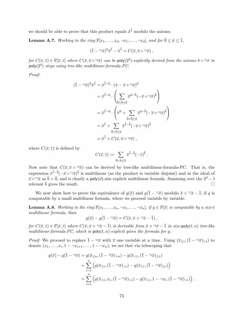
we should be able to prove that this product equals x1 modulo the axioms.

Lemma A.7. Working in the ring F[x1, . . . , xd,¬x1, . . . ,¬xd], and for 0 ≤ a ≤ 1,

(1− ¬x)ax1 − x1 = C(x, x ¬x) ,

for C(x, z) ∈ F[x, z] where C(x, x ¬x) can be poly(2d)-explicitly derived from the axioms x ¬x inpoly(2d) steps using tree-like multilinear-formula-PC.

Proof:

(1− ¬x)ax1 = x1−a · (x− x ¬x)a

= x1−a ·

∑0≤b≤a

xa−b(−x ¬x)b

= x1−a ·

xa +∑

0<b≤a

xa−b(−x ¬x)b

= x1 +∑

0<b≤a

x1−b(−x ¬x)b

= x1 + C(x, x ¬x) ,

where C(x, z) is defined byC(x, z) :=

∑0<b≤a

x1−b(−z)b .

Now note that C(x, x ¬x) can be derived by tree-like multilinear-formula-PC. That is, theexpression x1−b(−x ¬x)b is multilinear (as the product is variable disjoint) and in the ideal ofx ¬x as b > 0, and is clearly a poly(d)-size explicit multilinear formula. Summing over the 2d − 1relevant b gives the result.

We now show how to prove the equivalence of g(x) and g(1− ¬x) modulo x+ ¬x− 1, if g iscomputable by a small multilinear formula, where we proceed variable by variable.

Lemma A.8. Working in the ring F[x1, . . . , xn,¬x1, . . . ,¬xn], if g ∈ F[x] is computable by a size-tmultilinear formula, than

g(x)− g(1− ¬x) = C(x, x+ ¬x− 1) ,

for C(x, z) ∈ F[x, z] where C(x, x+ ¬x− 1) is derivable from x+ ¬x− 1 in size-poly(t, n) tree-likemultilinear-formula-PC, which is poly(t, n)-explicit given the formula for g.

Proof: We proceed to replace 1 − ¬x with x one variable at a time. Using (x≤i, (1 − ¬x)>i) todenote (x1, . . . , xi, 1− ¬xi+1, . . . , 1− ¬xn), we see that via telescoping that

g(x)− g(1− ¬x) = g(x≤n, (1− ¬x)>n)− g(x<1, (1− ¬x)≥1)

=n∑i=1

(g(x≤i, (1− ¬x)>i)− g(x<i, (1− ¬x)≥i)

)=

n∑i=1

(g(x<i, xi, (1− ¬x)>i)− g(x<i, 1− ¬xi, (1− ¬x)>i)

).

73

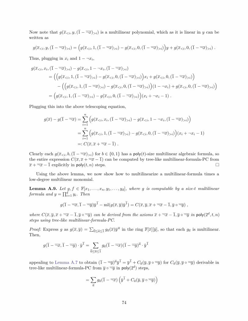
Now note that g(x<i, y, (1 − ¬x)>i) is a multilinear polynomial, which as it is linear in y can bewritten as

g(x<i, y, (1− ¬x)>i) =(g(x<i, 1, (1− ¬x)>i)− g(x<i, 0, (1− ¬x)>i)

)y + g(x<i, 0, (1− ¬x)>i) .

Thus, plugging in xi and 1− ¬xi,

g(x<i, xi, (1− ¬x)>i)− g(x<i, 1− ¬xi, (1− ¬x)>i)

=((g(x<i, 1, (1− ¬x)>i)− g(x<i, 0, (1− ¬x)>i)

)xi + g(x<i, 0, (1− ¬x)>i)

)−((g(x<i, 1, (1− ¬x)>i)− g(x<i, 0, (1− ¬x)>i)

)(1− ¬xi) + g(x<i, 0, (1− ¬x)>i)

)=(g(x<i, 1, (1− ¬x)>i)− g(x<i, 0, (1− ¬x)>i)

)(xi + ¬xi − 1) .

Plugging this into the above telescoping equation,

g(x)− g(1− ¬x) =n∑i=1

(g(x<i, xi, (1− ¬x)>i)− g(x<i, 1− ¬xi, (1− ¬x)>i)

)=

n∑i=1

(g(x<i, 1, (1− ¬x)>i)− g(x<i, 0, (1− ¬x)>i)

)(xi + ¬xi − 1)

=: C(x, x+ ¬x− 1) .

Clearly each g(x<i, b, (1− ¬x)>i) for b ∈ 0, 1 has a poly(t)-size multilinear algebraic formula, sothe entire expression C(x, x+ ¬x− 1) can be computed by tree-like multilinear-formula-PC fromx+ ¬x− 1 explicitly in poly(t, n) steps.

Using the above lemma, we now show how to multilinearize a multilinear-formula times alow-degree multilinear monomial.

Lemma A.9. Let g, f ∈ F[x1, . . . , xn, y1, . . . , yd], where g is computable by a size-t multilinearformula and y =

∏di=1 yi. Then

g(1− ¬x, 1− ¬y)y1 −ml(g(x, y)y1) = C(x, y, x+ ¬x− 1, y ¬y) ,

where C(x, y, x+ ¬x− 1, y ¬y) can be derived from the axioms x+ ¬x− 1, y ¬y in poly(2d, t, n)steps using tree-like multilinear-formula-PC.

Proof: Express g as g(x, y) =∑

0≤a≤1 ga(x)y a in the ring F[x][y], so that each ga is multilinear.Then,

g(1− ¬x, 1− ¬y) · y1 =∑

0≤a≤1

ga(1− ¬x)(1− ¬y)a · y1

appealing to Lemma A.7 to obtain (1− ¬y)ay1 = y1 + Ca(y, y ¬y) for Ca(y, y ¬y) derivable intree-like multilinear-formula-PC from y ¬y in poly(2d) steps,

=∑a

ga(1− ¬x)(y1 + Ca(y, y ¬y)

)

74

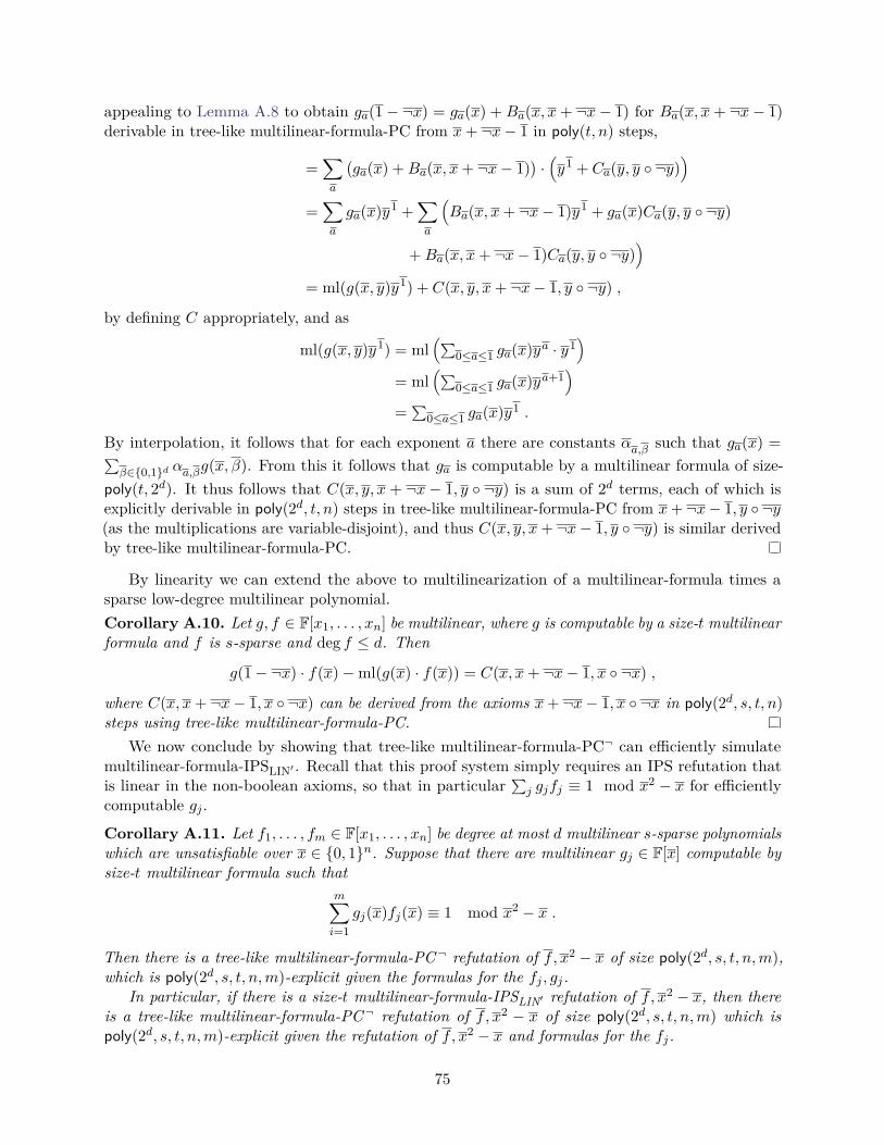
appealing to Lemma A.8 to obtain ga(1− ¬x) = ga(x) + Ba(x, x+ ¬x− 1) for Ba(x, x+ ¬x− 1)derivable in tree-like multilinear-formula-PC from x+ ¬x− 1 in poly(t, n) steps,

=∑a

(ga(x) +Ba(x, x+ ¬x− 1)

)·(y1 + Ca(y, y ¬y)

)=∑a

ga(x)y1 +∑a

(Ba(x, x+ ¬x− 1)y1 + ga(x)Ca(y, y ¬y)

+Ba(x, x+ ¬x− 1)Ca(y, y ¬y))

= ml(g(x, y)y1) + C(x, y, x+ ¬x− 1, y ¬y) ,

by defining C appropriately, and as

ml(g(x, y)y1) = ml(∑

0≤a≤1 ga(x)ya · y1)

= ml(∑

0≤a≤1 ga(x)ya+1)

=∑

0≤a≤1 ga(x)y1 .

By interpolation, it follows that for each exponent a there are constants αa,β such that ga(x) =∑β∈0,1d αa,βg(x, β). From this it follows that ga is computable by a multilinear formula of size-

poly(t, 2d). It thus follows that C(x, y, x + ¬x − 1, y ¬y) is a sum of 2d terms, each of which isexplicitly derivable in poly(2d, t, n) steps in tree-like multilinear-formula-PC from x+ ¬x− 1, y ¬y(as the multiplications are variable-disjoint), and thus C(x, y, x+ ¬x− 1, y ¬y) is similar derivedby tree-like multilinear-formula-PC.

By linearity we can extend the above to multilinearization of a multilinear-formula times asparse low-degree multilinear polynomial.Corollary A.10. Let g, f ∈ F[x1, . . . , xn] be multilinear, where g is computable by a size-t multilinearformula and f is s-sparse and deg f ≤ d. Then

g(1− ¬x) · f(x)−ml(g(x) · f(x)) = C(x, x+ ¬x− 1, x ¬x) ,

where C(x, x+ ¬x− 1, x ¬x) can be derived from the axioms x+ ¬x− 1, x ¬x in poly(2d, s, t, n)steps using tree-like multilinear-formula-PC.

We now conclude by showing that tree-like multilinear-formula-PC¬ can efficiently simulatemultilinear-formula-IPSLIN′ . Recall that this proof system simply requires an IPS refutation thatis linear in the non-boolean axioms, so that in particular

∑j gjfj ≡ 1 mod x2 − x for efficiently

computable gj .

Corollary A.11. Let f1, . . . , fm ∈ F[x1, . . . , xn] be degree at most d multilinear s-sparse polynomialswhich are unsatisfiable over x ∈ 0, 1n. Suppose that there are multilinear gj ∈ F[x] computable bysize-t multilinear formula such that

m∑i=1

gj(x)fj(x) ≡ 1 mod x2 − x .

Then there is a tree-like multilinear-formula-PC ¬ refutation of f, x2 − x of size poly(2d, s, t, n,m),which is poly(2d, s, t, n,m)-explicit given the formulas for the fj , gj.

In particular, if there is a size-t multilinear-formula-IPSLIN′ refutation of f, x2 − x, then thereis a tree-like multilinear-formula-PC ¬ refutation of f, x2 − x of size poly(2d, s, t, n,m) which ispoly(2d, s, t, n,m)-explicit given the refutation of f, x2 − x and formulas for the fj.

75

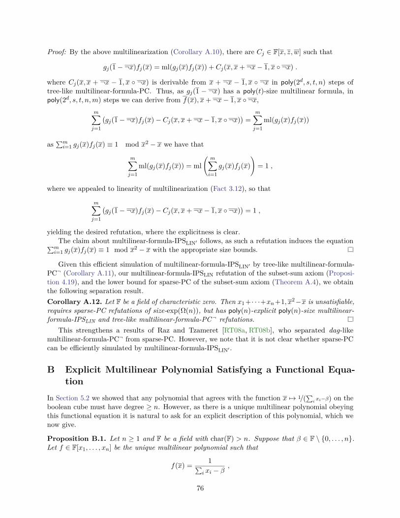
Proof: By the above multilinearization (Corollary A.10), there are Cj ∈ F[x, z, w] such that

gj(1− ¬x)fj(x) = ml(gj(x)fj(x)) + Cj(x, x+ ¬x− 1, x ¬x) .

where Cj(x, x + ¬x − 1, x ¬x) is derivable from x + ¬x − 1, x ¬x in poly(2d, s, t, n) steps oftree-like multilinear-formula-PC. Thus, as gj(1 − ¬x) has a poly(t)-size multilinear formula, inpoly(2d, s, t, n,m) steps we can derive from f(x), x+ ¬x− 1, x ¬x,

m∑j=1

(gj(1− ¬x)fj(x)− Cj(x, x+ ¬x− 1, x ¬x)

)=

m∑j=1

ml(gj(x)fj(x))

as∑mi=1 gj(x)fj(x) ≡ 1 mod x2 − x we have that

m∑j=1

ml(gj(x)fj(x)) = ml(

m∑i=1

gj(x)fj(x))

= 1 ,

where we appealed to linearity of multilinearization (Fact 3.12), so that

m∑j=1

(gj(1− ¬x)fj(x)− Cj(x, x+ ¬x− 1, x ¬x)

)= 1 ,

yielding the desired refutation, where the explicitness is clear.The claim about multilinear-formula-IPSLIN′ follows, as such a refutation induces the equation∑m

i=1 gj(x)fj(x) ≡ 1 mod x2 − x with the appropriate size bounds.

Given this efficient simulation of multilinear-formula-IPSLIN′ by tree-like multilinear-formula-PC¬ (Corollary A.11), our multilinear-formula-IPSLIN refutation of the subset-sum axiom (Proposi-tion 4.19), and the lower bound for sparse-PC of the subset-sum axiom (Theorem A.4), we obtainthe following separation result.Corollary A.12. Let F be a field of characteristic zero. Then x1 + · · ·+xn+1, x2−x is unsatisfiable,requires sparse-PC refutations of size-exp(Ω(n)), but has poly(n)-explicit poly(n)-size multilinear-formula-IPSLIN and tree-like multilinear-formula-PC ¬ refutations.

This strengthens a results of Raz and Tzameret [RT08a, RT08b], who separated dag-likemultilinear-formula-PC¬ from sparse-PC. However, we note that it is not clear whether sparse-PCcan be efficiently simulated by multilinear-formula-IPSLIN′ .

B Explicit Multilinear Polynomial Satisfying a Functional Equa-tion

In Section 5.2 we showed that any polynomial that agrees with the function x 7→ 1/(∑

ixi−β) on the

boolean cube must have degree ≥ n. However, as there is a unique multilinear polynomial obeyingthis functional equation it is natural to ask for an explicit description of this polynomial, which wenow give.

Proposition B.1. Let n ≥ 1 and F be a field with char(F) > n. Suppose that β ∈ F \ 0, . . . , n.Let f ∈ F[x1, . . . , xn] be the unique multilinear polynomial such that

f(x) = 1∑i xi − β

,

76

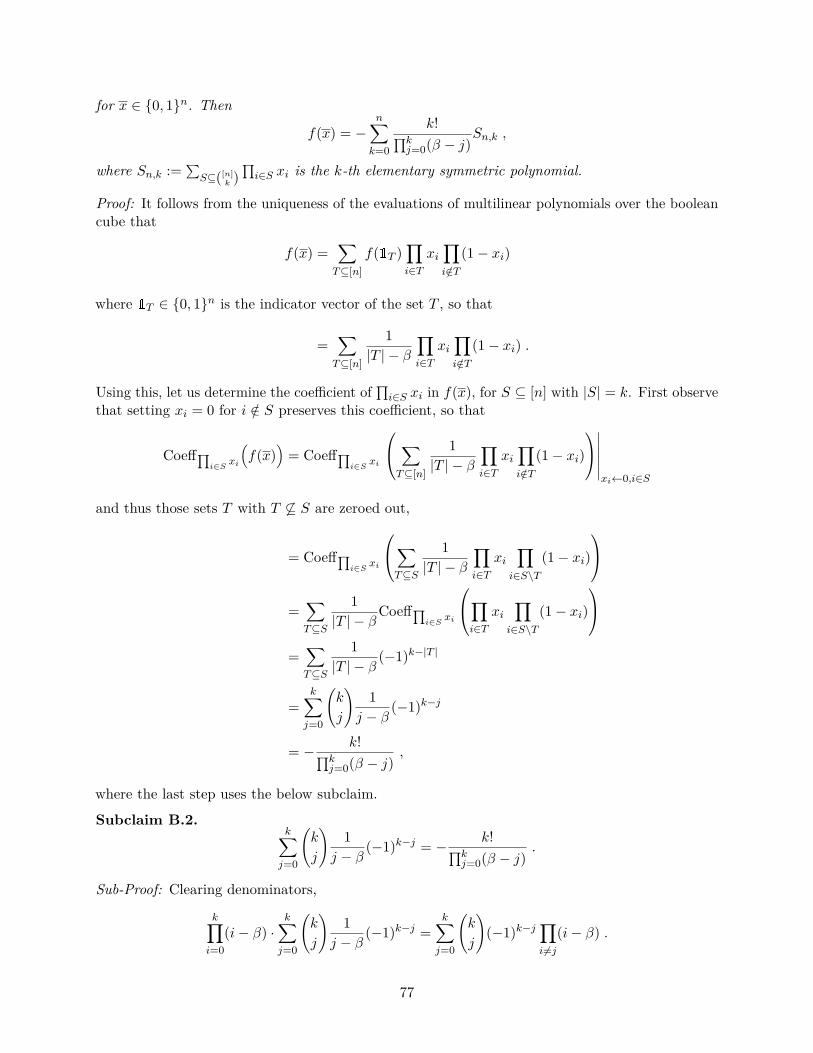
for x ∈ 0, 1n. Then

f(x) = −n∑k=0

k!∏kj=0(β − j)

Sn,k ,

where Sn,k :=∑S⊆([n]

k )∏i∈S xi is the k-th elementary symmetric polynomial.

Proof: It follows from the uniqueness of the evaluations of multilinear polynomials over the booleancube that

f(x) =∑T⊆[n]

f(1T )∏i∈T

xi∏i/∈T

(1− xi)

where 1T ∈ 0, 1n is the indicator vector of the set T , so that

=∑T⊆[n]

1|T | − β

∏i∈T

xi∏i/∈T

(1− xi) .

Using this, let us determine the coefficient of∏i∈S xi in f(x), for S ⊆ [n] with |S| = k. First observe

that setting xi = 0 for i /∈ S preserves this coefficient, so that

Coeff∏i∈S xi

(f(x)

)= Coeff∏

i∈S xi

∑T⊆[n]

1|T | − β

∏i∈T

xi∏i/∈T

(1− xi)

∣∣∣∣∣∣xi←0,i∈S

and thus those sets T with T 6⊆ S are zeroed out,

= Coeff∏i∈S xi

∑T⊆S

1|T | − β

∏i∈T

xi∏

i∈S\T(1− xi)

=∑T⊆S

1|T | − β

Coeff∏i∈S xi

∏i∈T

xi∏

i∈S\T(1− xi)

=∑T⊆S

1|T | − β

(−1)k−|T |

=k∑j=0

(k

j

)1

j − β(−1)k−j

= − k!∏kj=0(β − j)

,

where the last step uses the below subclaim.

Subclaim B.2.k∑j=0

(k

j

)1

j − β(−1)k−j = − k!∏k

j=0(β − j).

Sub-Proof: Clearing denominators,

k∏i=0

(i− β) ·k∑j=0

(k

j

)1

j − β(−1)k−j =

k∑j=0

(k

j

)(−1)k−j

∏i 6=j

(i− β) .

77

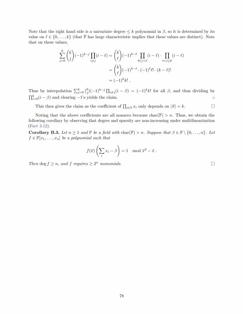
Note that the right hand side is a univariate degree ≤ k polynomial in β, so it is determined by itsvalue on ` ∈ 0, . . . , k (that F has large characteristic implies that these values are distinct). Notethat on these values,

k∑j=0

(k

j

)(−1)k−j

∏i 6=j

(i− `) =(k

`

)(−1)k−`

∏0≤i<`

(i− `) ·∏

`<i≤k(i− `)

=(k

`

)(−1)k−` · (−1)``! · (k − `)!

= (−1)kk! .

Thus by interpolation∑kj=0

(kj

)(−1)k−j

∏i 6=j(i − β) = (−1)kk! for all β, and thus dividing by∏k

i=0(i− β) and clearing −1’s yields the claim.

This then gives the claim as the coefficient of∏i∈S xi only depends on |S| = k.

Noting that the above coefficients are all nonzero because char(F) > n. Thus, we obtain thefollowing corollary by observing that degree and sparsity are non-increasing under multilinearization(Fact 3.12).Corollary B.3. Let n ≥ 1 and F be a field with char(F) > n. Suppose that β ∈ F \ 0, . . . , n. Letf ∈ F[x1, . . . , xn] be a polynomial such that

f(x)(∑

i

xi − β)

= 1 mod x2 − x .

Then deg f ≥ n, and f requires ≥ 2n monomials.

78