optimization of municipal solid waste collection routes ... · optimization of municipal solid...

FACULDADE DE ENGENHARIA DA UNIVERSIDADE DO PORTO

Optimization of municipal solid wastecollection routes based on the

containers’ fill status data

Hugo Miguel Pereira Peixoto

Master in Informatics and Computing Engineering

Supervisor: Luís Paulo Gonçalves dos Reis (Professor Auxiliar)

Second Supervisor: Ana Cristina Costa Aguiar (Professor Auxiliar Convidado)

28th June, 2010

Optimization of municipal solid waste collection routesbased on the containers’ fill status data

Hugo Miguel Pereira Peixoto

Master in Informatics and Computing Engineering

Approved in oral examination by the committee:

Chair: Armando Jorge Miranda de Sousa (Professor Auxiliar)

External Examiner: Pedro Miguel do Vale Moreira (Professor Adjunto)

Supervisor: Luís Paulo Gonçalves dos Reis (Professor Auxiliar)

26th July, 2010

Abstract

Fraunhofer Portugal Research Center for Assistive Information and Communication Solutions iscurrently developing a system to monitor the fill status of waste containers. The introduction ofa waste container fill status monitoring system in the city of Porto, Portugal, gives rise to severalopportunities. For example, it allows the development of a detailed analysis of the city’s wastegeneration distribution and the optimization of waste collection routes.

This document describes the architecture design of the information system to store and retrievedata regarding the containers’ status. Furthermore, it provides a description of several algorithmsthat can be used to obtain efficient collection routes. This optimization problem is modeled as theCapacitated Vehicle Routing Problem. To address this problem, two approaches were analyzed;the first involves solving the associated Asymmetric Traveling Salesman Problem — in whichvehicle capacity constraints are ignored — followed by clustering the resulting tour into feasibleroutes. This approach is called route-first-cluster-second. The second approach relies on the usageof a construction heuristic by Clarke and Wright.

Regarding the optimization of the Asymmetric Traveling Salesman Problem solution, thisstudy compares several techniques: two construction heuristics — greedy and repetitive near-est neighbor — and three meta-heuristics — hill climbing, genetic algorithms and MAX-MIN antsystem. Additionally, MAX-MIN ant system was subjected to a parameter sensibility analysis.

Results show that MAX-MIN ant system achieves more efficient routes when the number ofants is higher, although it increases the algorithm’s running time. When dealing with a scenarioin which there is a limited time-frame, it is recommended that a low number of ants is used. Thealgorithm was also shown to be very sensitive to changes in parameter β , which indicates if an antshould give more importance to the distance between two vertices or to the pheromone levels inthat arc. This analysis suggests that β should be close to 20.

When evaluating the performance of the presented techniques applied to the Capacitated Ve-hicle Routing Problem, MAX-MIN ant system produced, in average, more efficient routes than theother approaches.

i

Resumo

O Centro de Pesquisa para Soluções de Informação e Comunicação Assistiva da Fraunhofer Por-tugal está a desenvolver um sistema de monitorização do estado de enchimento dos contentoresde lixo. A introdução deste sistema na cidade do Porto dá origem a várias oportunidades. Por ex-emplo, torna-se possível fazer uma análise detalhada da distribuição da geração do lixo na cidade.Este projecto permite, também, implementar um sistema de optimização das rotas de recolha dolixo.

Este documento descreve o desenho da arquitectura do sistema de informação que permitiráarmazenar — e disponibilizar — a informação referente ao estado dos contentores. O documentooferece também uma descrição de vários algoritmos que podem ser utilizados para obter rotasde recolha eficientes. Este problema de optimização pode ser modelado como um problema deplaneamento de rotas de veículos com capacidade limitada (CVRP). Neste estudo, foram anal-isadas duas abordagens para a resolução do CVRP. A primeira começa por resolver o problema docaixeiro viajante em grafos assimétricos (ATSP) — ignorando as restrições de capacidade — e,subsequentemente, divide o circuito obtido em rotas que respeitem as restrições de capacidade dosveículos. Esta técnica chama-se route-first-cluster-second. A segunda abordagem para resolver oCVRP é baseada numa heurística construtiva, por Clarke e Wright.

Relativamente ao problema de optimização do problema do caixeiro viajante em grafos as-simétricos, foram comparadas várias técnicas: duas heurísticas construtivas — gulosa e vizinhomais próximo repetitivo — e três meta-heurísticas — subir-a-colina, algoritmos genéticos e umsistema de formigas chamado MAX-MIN ant system (MMAS). Além da comparação dos váriosalgoritmos entre si, foi também feita uma análise de sensibilidade aos parâmetros do MMAS.

Os resultados mostram que o MMAS calcula rotas mais eficientes quando o número de formi-gas é mais elevado, apesar de levar a um aumento no tempo de execução do algoritmo. Quandoaplicado a um cenário em que o tempo de execução disponível é limitado, é recomendado que seutilize um número reduzido de formigas. Também foi possível mostrar que o algoritmo é bastantesensível a variações no parâmetro β , que decide se uma formiga deve dar mais importância à dis-tância entre dois vértices ou à quantidade de feromonas existente nesse arco. Esta análise mostrouque o parâmetro β deve tomar valores perto de 20.

A análise do desempenho dos vários algoritmos, relativamente ao problema de planeamentode rotas de veículos de capacidade limitada, mostrou que o sistema de formigas obtém, em média,rotas mais eficientes.

iii

Acknowledgements

I thank both my supervisors, Prof. Luís Paulo Reis and Prof. Ana Cristina Aguiar, for their guid-ance and support.

To Júlio Santos, for providing me with an awesome working environment, and for his excellentcooking abilities.

To Raquel Rios Correira, for forcing me to work and keeping me company — I learned a lotabout radiation from her.

To NIFEUP, for all the random stuff.

Hugo “Wiki” Peixoto

v

“In computing, elegance is not a dispensable luxurybut a quality that decides between success and failure”

Edsger W. Dijkstra

vii

Contents

1 Introduction 11.1 Context and motivation . . . . . . . . . . . . . . . . . . . . . . . . . . . . . . . 11.2 Fill status monitoring . . . . . . . . . . . . . . . . . . . . . . . . . . . . . . . . 11.3 Optimization of waste collection routes . . . . . . . . . . . . . . . . . . . . . . 21.4 Objectives . . . . . . . . . . . . . . . . . . . . . . . . . . . . . . . . . . . . . . 21.5 Document structure . . . . . . . . . . . . . . . . . . . . . . . . . . . . . . . . . 3

2 State of the art 52.1 General problem description . . . . . . . . . . . . . . . . . . . . . . . . . . . . 5

2.1.1 City graph . . . . . . . . . . . . . . . . . . . . . . . . . . . . . . . . . 62.2 Overview of routing problems . . . . . . . . . . . . . . . . . . . . . . . . . . . 72.3 Waste collection scenarios . . . . . . . . . . . . . . . . . . . . . . . . . . . . . 8

2.3.1 Residential scenario . . . . . . . . . . . . . . . . . . . . . . . . . . . . 82.3.2 Commercial scenario . . . . . . . . . . . . . . . . . . . . . . . . . . . . 112.3.3 Rollon-Rolloff scenario . . . . . . . . . . . . . . . . . . . . . . . . . . 13

2.4 Chapter summary . . . . . . . . . . . . . . . . . . . . . . . . . . . . . . . . . . 16

3 Problem description 173.1 Waste collection in Porto, Portugal . . . . . . . . . . . . . . . . . . . . . . . . . 173.2 Asymmetric capacitated vehicle routing problem . . . . . . . . . . . . . . . . . 183.3 Chapter summary . . . . . . . . . . . . . . . . . . . . . . . . . . . . . . . . . . 18

4 Solution architecture 194.1 Framework workflow . . . . . . . . . . . . . . . . . . . . . . . . . . . . . . . . 194.2 Implementation details . . . . . . . . . . . . . . . . . . . . . . . . . . . . . . . 214.3 Data formats . . . . . . . . . . . . . . . . . . . . . . . . . . . . . . . . . . . . . 21

4.3.1 City map format . . . . . . . . . . . . . . . . . . . . . . . . . . . . . . 224.3.2 Containers status format . . . . . . . . . . . . . . . . . . . . . . . . . . 234.3.3 Dataset format . . . . . . . . . . . . . . . . . . . . . . . . . . . . . . . 234.3.4 Routes format . . . . . . . . . . . . . . . . . . . . . . . . . . . . . . . . 234.3.5 Statistics format . . . . . . . . . . . . . . . . . . . . . . . . . . . . . . 24

4.4 Evaluation metrics . . . . . . . . . . . . . . . . . . . . . . . . . . . . . . . . . 254.5 Datasets . . . . . . . . . . . . . . . . . . . . . . . . . . . . . . . . . . . . . . . 25

4.5.1 Validation datasets . . . . . . . . . . . . . . . . . . . . . . . . . . . . . 254.5.2 Realistic city datasets . . . . . . . . . . . . . . . . . . . . . . . . . . . . 27

4.6 Chapter summary . . . . . . . . . . . . . . . . . . . . . . . . . . . . . . . . . . 28

ix

CONTENTS

5 Algorithms 295.1 Construction heuristics for the ATSP . . . . . . . . . . . . . . . . . . . . . . . . 295.2 Hill climbing for the ATSP . . . . . . . . . . . . . . . . . . . . . . . . . . . . . 315.3 Genetic algorithm for the ATSP . . . . . . . . . . . . . . . . . . . . . . . . . . 335.4 Ant colony algorithms . . . . . . . . . . . . . . . . . . . . . . . . . . . . . . . 36

5.4.1 Ant system . . . . . . . . . . . . . . . . . . . . . . . . . . . . . . . . . 365.4.2 MAX-MIN ant system . . . . . . . . . . . . . . . . . . . . . . . . . . . 37

5.5 Complexity overview of ATSP algorithms . . . . . . . . . . . . . . . . . . . . . 405.6 Split clustering algorithm . . . . . . . . . . . . . . . . . . . . . . . . . . . . . . 405.7 Clarke-Wright savings heuristic for the ACVRP . . . . . . . . . . . . . . . . . . 425.8 Approach overview . . . . . . . . . . . . . . . . . . . . . . . . . . . . . . . . . 445.9 Validation of algorithm implementations . . . . . . . . . . . . . . . . . . . . . . 45

5.9.1 ATSP validation . . . . . . . . . . . . . . . . . . . . . . . . . . . . . . 455.9.2 ACVRP validation . . . . . . . . . . . . . . . . . . . . . . . . . . . . . 46

5.10 Chapter summary . . . . . . . . . . . . . . . . . . . . . . . . . . . . . . . . . . 47

6 Results 496.1 Sensitivity of MAX-MIN ant system to algorithm parameters . . . . . . . . . . . 49

6.1.1 Parameter β sensitivity . . . . . . . . . . . . . . . . . . . . . . . . . . . 506.1.2 Trade-off between ants and iterations . . . . . . . . . . . . . . . . . . . 51

6.2 Algorithm performance on large ACVRP instances . . . . . . . . . . . . . . . . 536.2.1 ATSP solutions . . . . . . . . . . . . . . . . . . . . . . . . . . . . . . . 546.2.2 ACVRP solutions . . . . . . . . . . . . . . . . . . . . . . . . . . . . . . 556.2.3 Route improvement . . . . . . . . . . . . . . . . . . . . . . . . . . . . . 57

6.3 Chapter summary . . . . . . . . . . . . . . . . . . . . . . . . . . . . . . . . . . 59

7 Conclusions 617.1 Conclusions . . . . . . . . . . . . . . . . . . . . . . . . . . . . . . . . . . . . . 61

7.1.1 Sensitivity analysis of MMAS . . . . . . . . . . . . . . . . . . . . . . . 627.1.2 Comparison of methods for the ACVRP . . . . . . . . . . . . . . . . . . 62

7.2 Future work . . . . . . . . . . . . . . . . . . . . . . . . . . . . . . . . . . . . . 63

References 65

A Submitted article 71

x

List of Figures

2.1 Graph for the Rollon-Rolloff problem. Thick vertices (except v0) represent nodesfrom which the vehicle leaves loaded. Thin vertices are the ones from which itleaves unloaded. . . . . . . . . . . . . . . . . . . . . . . . . . . . . . . . . . . . 15

4.1 Project architecture . . . . . . . . . . . . . . . . . . . . . . . . . . . . . . . . . 204.2 An example city topology map and its JSON equivalent. . . . . . . . . . . . . . 224.3 An example containers’ fill status JSON file. . . . . . . . . . . . . . . . . . . . . 234.4 Complete dataset example object, constructed from previous examples. . . . . . 244.5 Rollon-Rolloff set of routes example, representing two vehicles. . . . . . . . . . 244.6 The city of Porto, Portugal, retrieved from OpenStreetMap.org and loaded onto

the current framework viewer. . . . . . . . . . . . . . . . . . . . . . . . . . . . 27

6.1 Variations in final route performance when varying beta in the MAX-MIN antsystem for datasets ftv35, ftv70 and ftv170. Performance is given in the formof the ratio between the heuristic’s route average cost and the dataset optimum(minimum) cost. . . . . . . . . . . . . . . . . . . . . . . . . . . . . . . . . . . . 50

6.2 Evolution of final route performance when varying the number of ants and numberof iterations for the MAX-MIN ant system on dataset ftv170. Performance is givenin the form of the ratio between the heuristic’s route average cost and the datasetoptimum (minimum) cost. . . . . . . . . . . . . . . . . . . . . . . . . . . . . . 51

6.3 Evolution of final tour length when varying the number of ants and number ofiterations for the MAX-MIN ant system a dataset with 1287 vertices. . . . . . . . 52

6.4 Evolution of final tour length when varying the number of ants and number ofiterations for the MAX-MIN ant system a dataset with 6247 vertices. . . . . . . . 52

xi

LIST OF FIGURES

xii

List of Tables

4.1 Asymmetric Traveling Salesman Problem datasets, presenting the number of ver-tices and the optimum route cost. . . . . . . . . . . . . . . . . . . . . . . . . . . 26

4.2 Capacitated Vehicle Routing Problem datasets, presenting the number of verticesand a reference route cost. . . . . . . . . . . . . . . . . . . . . . . . . . . . . . 26

4.3 Large realistic Capacitated Vehicle Routing Problem datasets . . . . . . . . . . . 28

5.1 Bounds for ATSP algorithms. There is a tight bound whenever both the lowerand upper bounds are the same. R represents the number of iterations of a givenalgorithm. H is the time complexity for a chosen heuristic, such as the repetitivenearest neighbor or the greedy algorithm . . . . . . . . . . . . . . . . . . . . . . 40

5.2 Summary of the ACVRP techniques evaluated during this study. RNN: repetitivenearest neighbor; GA: genetic algorithm; MMAS: MAX-MIN ant system . . . . . 44

5.3 Performance of our heuristic and meta-heuristic implementations using the datasetsfrom TSPLIB. Performance is given in the form of the ratio between the heuristic’sroute average cost and the dataset optimum (minimum) cost. . . . . . . . . . . . 45

5.4 Performance of our heuristic and meta-heuristic implementations using the datasetsfrom TSPLIB. Performance is given in the form of the ratio between the heuristic’sroute average cost and the dataset reference solution’s cost. . . . . . . . . . . . . 46

6.1 Trade-off between running time and route efficiency, when varying the number ofants in dataset hp6247. . . . . . . . . . . . . . . . . . . . . . . . . . . . . . . . 53

6.2 Performance of ATSP heuristic and meta-heuristic implementations using realisti-cally large datasets. Minimum values for each dataset are highlighted. . . . . . . 54

6.3 Normalized performance of ATSP techniques. Each value expressed as the per-centage excess relative to the minimum value for its dataset. . . . . . . . . . . . 55

6.4 Performance of heuristic and meta-heuristic implementations using realisticallylarge datasets. Minimum values for each dataset are highlighted. . . . . . . . . . 56

6.5 Average route efficiency excess when comparing each algorithm to the best solu-tion found for each dataset. . . . . . . . . . . . . . . . . . . . . . . . . . . . . . 56

6.6 Final ACVRP solutions’ performance, after the application of the 2-opt improve-ment technique. Minimum values for each dataset are highlighted. . . . . . . . . 57

6.7 Final ACVRP solutions’ performance, after applying the final route optimizationtechnique. Values are normalized by calculating the excess between a given algo-rithm’s performance and the best value found for its dataset. . . . . . . . . . . . 58

6.8 Summary of the several techniques’ performance, over the three optimization stages. 59

xiii

LIST OF TABLES

xiv

List of Algorithms

1 Repetitive nearest neighbor heuristic . . . . . . . . . . . . . . . . . . . . . . . . 302 Greedy heuristic . . . . . . . . . . . . . . . . . . . . . . . . . . . . . . . . . . . 313 Steep ascent hill climbing using a 2-cut neighborhood (2-opt algorithm) . . . . . 324 Mutation operator used in the ATSP genetic algorithm . . . . . . . . . . . . . . . 345 ATSP genetic algorithm . . . . . . . . . . . . . . . . . . . . . . . . . . . . . . . 356 Ant vertex selection used in max-min ant system . . . . . . . . . . . . . . . . . 387 Max-min ant system . . . . . . . . . . . . . . . . . . . . . . . . . . . . . . . . 398 ACVRP clustering algorithm . . . . . . . . . . . . . . . . . . . . . . . . . . . . 419 Clarke-Wright savings heuristic for the ACVRP . . . . . . . . . . . . . . . . . . 43

xv

LIST OF ALGORITHMS

xvi

Abbreviations

1-SCP 1-Skip Collection ProblemACO Ant Colony OptimizationACVRP Asymmetric Capacitated Vehicle Routing ProblemARP Arc Routing ProblemAS Ant SystemATSP Asymmetric Traveling Salesman ProblemAVRP Asymmetric Vehicle Routing ProblemBPP Bin Packing ProblemCARP Capacitated Arc Routing ProblemCGRP-m see MCGRPCPP Chinese Postman ProblemCVRP Capacitated Vehicle Routing ProblemGA Genetic AlgorithmGTSP Graphical Traveling Salesman ProblemGRP General Routing ProblemHC Hill ClimbingJSON JavaScript Object NotationMMAS MAX-MIN Ant SystemMCGRP Mixed-graph Capacitated General Routing ProblemM-RRVRP Multiple Rollon-Rolloff Vehicle Routing ProblemMSW Municipal Solid WasteRPP Rural Postman ProblemRRVRP Rollon-Rolloff Vehicle Routing ProblemSGTSP Steiner Graphical Traveling Salesman ProblemTSP Traveling Salesman ProblemVRP Vehicle Routing ProblemXML Extensible Markup LanguageWDF Waste Disposal Facility

xvii

ABBREVIATIONS

xviii

Chapter 1

Introduction

This chapter introduces this work, by presenting its context and motivation. Finally, it presents the

project’s objectives and the document structure.

1.1 Context and motivation

Municipal solid waste (MSW) production has been increasing in the last few years, along with

economic growth [McC94]. This has led to the need — and subsequent development — of efficient

waste management solutions. Waste management involves not only the collection, but also the

transportation, recycling and disposal of generated waste.

According to [Bha96], municipal solid waste collection and disposal represents up to 85% of

some cities’ waste management budget. With this in mind, route optimization is as an important

field of study regarding the improvement of MSW management processes.

Many cities around the world have studied and applied optimization techniques to their collec-

tion scenarios, which are usually very different from each other. In Portugal, however, there seems

to be little research regarding this subject. [Pá03] describes the waste management scenario in Por-

tugal from 1996 and 2002, a period in which several improvements were made due to changes in

the legislation. In 2006, [MDS06] further report the legislation trends and present some statistics

on the average MSW generation rate. Concerning collection routing, [TAdS04] describes a study

for optimizing the collection of urban recyclable waste in the center-littoral region of Portugal.

1.2 Fill status monitoring

The Municipality of Porto, Portugal, is working together with the Fraunhofer Portugal Research

Center for Assistive Information and Communication Solutions (FhP-AICOS) in order to im-

plement a platform that allows the real-time measurement of waste containers’ fill status. This

1

Introduction

requires the deployment of low cost sensors in each container and the development of a commu-

nication system to gather information. On top of this platform, several applications will then be

possible. As an example, this will allow researchers to study waste generation behaviors on a more

detailed level. These monitoring systems have been studied in places, such as Pudong New Area,

in Shanghai, China [RXV+09, VGR+09] and Sweden [Joh06].

Another application for this system is the optimization of waste collection routes.

1.3 Optimization of waste collection routes

The problem of optimizing waste collection routes involves deciding, for example, which streets

must each garbage truck follow, which containers should each one of them collect and how many

trucks should a fleet for a given city have.

One of the first articles regarding this subject was done in 1974 [Bel74], and it was applied

to both New York and Washington D.C., United States of America. Since then, other cities have

tried to minimize the costs by optimizing collection routes: Trabon, Turkey [AG07]; Barcelona,

Spain [BP04]; Athens, Greece [Kar05]; Hanoi, Vietnam [TP00]; Porto Alegre, Brazil [LBM08]

and many others.

However, many of these studies do not have real-time information of the containers’ fill status.

Usually, they are either based on statistical data (surveys), or they ignore the containers’ fill status

and simply collect the waste in every container.

Combining these techniques with the Fill Status Monitoring platform described in section 1.2,

the municipality of Porto, Portugal might reduce even further the collection costs.

1.4 Objectives

With the deployment of a fill status monitoring solution in the municipality of Porto, there is the

opportunity to develop an optimization framework for the waste collection routes.

The first challenge is to devise and implement an architecture to store and retrieve, when

necessary, the information obtained from the container fill sensors. This includes specifying the

information workflow, the database schema and formats to exchange data between modules.

The second goal is to analyze and compare different algorithms for the optimization of waste

collection routes so that an efficient itinerary can be calculated within a time-frame of two hours,

given the containers’ fill status and the collection vehicles’ capacities.

2

Introduction

1.5 Document structure

The next chapter on this document, chapter 2, provides an overview of waste collection route

optimization approaches. First, an informal description of each scenario is given. Then, each

one of the scenarios is exposed as a mathematical formulation, followed by possible techniques

that can be applied to them. Chapter 3 summarizes the problem statement, using the definitions

presented by chapter 2.

Chapter 4 introduces the architecture proposal for the management of waste containers’ fill

status information — modules, workflow and information interchange formats. It also presents

the technologies used to implement this system. Finally, this chapter presents the metrics and

datasets used for both algorithm validation and analysis.

Chapter 5 describes the algorithms used to optimize collection routes and shows their vali-

dation results. Chapter 6 presents a comparative analysis of the chosen algorithms’ performance.

Chapter 7 finalizes this document by presenting the conclusions of this project, along with possible

further developments and future work.

3

Introduction

4

Chapter 2

State of the art

This chapter describes several studies regarding the optimization of solid waste collection routes.

It reviews the mathematical models used in these studies and provides alternative optimization

techniques that can be applied to each one.

In section 2.1, the waste collection problem will be detailed. Section 2.2 provides a back-

ground on the categorization of routing problems. As a final introductory section, section 2.1.1

exposes the basic data structure used in waste collection problems.

Sections 2.3.1, 2.3.2 and 2.3.3 describe each one of the three possible scenarios. Each section

presents a mathematical formulation of the problem, along with techniques for solving it.

As seen in section 2.3.2, waste collection in a commercial scenario can be divided into two

common subproblems; one of them is modeled as the Traveling Salesman Problem (TSP).

2.1 General problem description

Authors of [GAW01] divided waste collection routing problems into three main categories. First,

the commercial collection contemplates waste collection from businesses and organizations like

malls, factories and such. Second, the residential collection problem involves collecting household

generated waste, usually stored in containers along the streets of a city. Comparatively, the number

of containers in the commercial problem is significantly smaller than in the residential case.

In both of these two variants, each waste collection vehicle travels to a container, loads its con-

tents into its hopper and moves on to the next container. As soon as the hopper is full, the vehicle

travels to a disposal facility (such as a landfill, or a recycling/treatment facility) and deposits the

collected waste.

The third variant — named Rollon-Rolloff, which is described in [BMBB00] — involves large

containers, which must be transported to the disposal facilities and replaced by empty ones. Their

dimensions impose that each vehicle can only transport a single container (either full or empty) at

a time.

5

State of the art

In the Rollon-Rolloff original description, each waste collection vehicle can perform four basic

operations:

• Insertion trip — the vehicle brings an empty container from the waste disposal facility

(WDF) to a new location;

• Removal trip — the vehicle picks up a full container from a location and leaves it at the

WDF;

• Round trip — the vehicle picks up a container, brings it to a waste disposal facility (WDF)

for emptying and returns it to its original location;

• Exchange trip — the vehicle leaves the WDF with an empty container, travels to a location

with a full one and switches them, bringing it back to the WDF.

Although round and exchange trips could be considered as being composed by insertion and

removal operations, the authors considered them as separate actions to avoid the need for modeling

extra constraints. For example, in round trips the same container is brought back to its original

place, while minimizing the time that location stays without a container. In exchange trips, the

target location may not have room for two containers, so an extra restriction would have to be

added, forcing vehicles to pick up the full one before delivering the new, empty container.

In each of these three main variants, extra parameters can vary. For example, consider a

scenario with either a single or multiple waste disposal facilities. In the multiple facilities case, an

extra restriction may be to balance the waste disposed at each location.

2.1.1 City graph

All three variants described in section 2.1 have a common base for their mathematical models —

waste collection vehicles that travel along the streets of a given city. To model a city, the common

approach is to define a graph in which each street is represented by one or two arcs (depending

if the street is one or both ways), with street intersections being the vertices. Each arc may have

several associated weights, reflecting the street distance, the time it takes to transverse it, or some

other metric. As such, a city graph is defined as the ordered tuple G=(V,E∪A), where V represent

the vertices, E the (undirected) edges and A the (directed) arcs.

This definition alone does not suffice to realistically represent the possible vehicle routes,

as there are extra restrictions which must be considered, specially regarding traffic signs. For

example: at a given intersection, it may not be possible to take a left turn if you are arriving from

a specific street. U-turns may also be forbidden, in certain intersections.

These restrictions can be specified by defining a cost for every pair of arcs that intersect at a

given vertex. tava′ is denoted as being the cost to go from the arc a to arc a′ by making a turn at v.

If the arcs do not intersect at that vertex, or if the traffic signs forbid such a turn, set tava′ = +∞.

Further details on this approach can be seen in [CMMS02].

6

State of the art

For now, consider the case in which there is a depot facility, located in vertex v0 ∈V , and that

all waste collection vehicles start and finish their routes there. Consider that there are K vehicles

available, and that each of the K routes can be defined as a set of round trips, each starting at the

depot. The number of round trips in each vehicle route may or may not be limited. Furthermore,

consider vehicles being limited to an amount Q of waste that they can carry at any given time.

This can be either measured in weight or in volume.

2.2 Overview of routing problems

Before presenting the mathematical formulations that can be used to model our three waste collect-

ing scenarios, this section provides a background on routing problems. This is useful to understand

the concepts applied in the following sections. Routing problems are an important field in opti-

mization, with many different applications. Its first formulation is usually attributed to Euler’s

article on the briges of Königsberg [Eul36].

The usual underlying structure for these problems is a strongly connected mixed graph. A

mixed graph, G = (V,E ∪A), contains both undirected and directed links (edges and arcs, respec-

tively). Being strongly connected means that there is a directed path between every pair of vertices

in V . With each link, there is an associated value that represents the cost of transversing it.

The Mixed-graph Capacitated General Routing Problem (CGRP-m, or MCGRP), defined in

[CGSH02, PM95], aims to find a set of K routes that start and end in a specific vertex vd ∈ V ,

which is called the depot. Additionally, these routes must respect the following set of constraints.

Consider the following subsets ER ⊆ E, AR ⊆ A and VR ⊆ V . With each element of these subsets

— which shall be called requests — there is an associated positive demand (qa, qe or qv). These

requests must all be serviced by one and just one of the K routes exactly once. A request being

serviced implies that a route, at some point, visits it. Note that while each request may only be

serviced once, its associated element (vertex or link) may be visited multiple times; transversing a

link without servicing it is called deadheading. Furthermore, for each one of the K routes, the sum

of the serviced requests’ demands should not exceed a fixed capacity Q — hence the designation

of capacitated.

In order for this problem to have feasible solutions, the service demands must fulfill two con-

ditions. First, each demand must not be superior to the capacity Q. Second, there must be a way

to partition the requests into no more than K subsets, such that the total demand for each subset

does not exceed Q. These two conditions can be specified by the expressions (2.1) and (2.2).

∀s ∈ ER∪AR∪VR : qs ≤ Q (2.1)

∃P :⋃

P = ER∪AR∪VR∧|P| ≤ K

∀A,B ∈ P : A∩B = /0∧∀A ∈ P : ∑

s∈Aqs ≤ Q (2.2)

7

State of the art

The CGRP-m, as its name states, is a general routing problem. This means that it is a general-

ization of several known and analyzed routing problems. A short list of CGRP-m specializations

is now presented. In each of them, the previously stated conditions must always be respected.

These specializations can be divided into two main categories: capacitated arc routing prob-

lems (CARP), with VR = /0, and node routing problems, with ER = AR = /0.

In the CARP category, the special case where K = 1 is called the Rural Postman Problem

(RPP). In addition, if AR∪ER = E ∪A, the Chinese Postman Problem (CPP) is obtained [PM95].

They can be classified as Directed (DRPP and DCPP), Undirected (URPP and UCPP) or Mixed

(MRPP and MCPP), if E = /0, A = /0 or A 6= /0∧E 6= /0, respectively. DCPP and UCPP have been

proven to be solvable in polynomial time by [Jac73], using a matching algorithm. Mixed CPP and

all RPP are part of the NP-complete complexity class [PM95].

The second category represents node routing problems. Letting K = 1 yields the Steiner

Graphical Traveling Salesman Problem (SGTSP) [Let99]. When a SGTSP also satisfies the con-

dition VR = V , it is called the Graphical Traveling Salesman Problem (GTSP). Finally, if the

underlying graph is complete, the problem becomes the classical Traveling Salesman Problem

(TSP).

On the other hand, the instances with VR =V form a widely studied variant — the Capacitated

Vehicle Routing Problem (CVRP). This category, along with several of its variants, is described in

[TV01b].

2.3 Waste collection scenarios

2.3.1 Residential scenario

In the residential scenario, due to the container density per street, it is usual to consider that

vehicles should serve arcs instead of individual nodes. Oppositely, in the commercial scenario

dealt with in the next section, vehicles will serve vertices.

2.3.1.1 Mathematical Formulation

Since each vehicle is also limited in its capacity, it is considered to be a problem in the CARP

category. More specifically, it can be modeled as a Mixed Capacitated Arc Routing Problem

(MCARP).

A recent survey on CARP can be found in [San08]. The problem was first suggested and mod-

eled, in its undirected variant, by [Gol81], with Belenguer et al. providing a different mathematical

model, as well as an algorithm for determining lower and upper bounds [BB98, BB03].

With respect to CARP on mixed graphs (MCARP), Belenguer et al. [BBLP06] provide a

relaxed linear formulation, lower bounds for it and several heuristics. Recently, Gouveia et

al. [GMP10] provided a valid linear formulation for the MCARP and presented benchmarks on

large datasets. This formulation will be now described.

8

State of the art

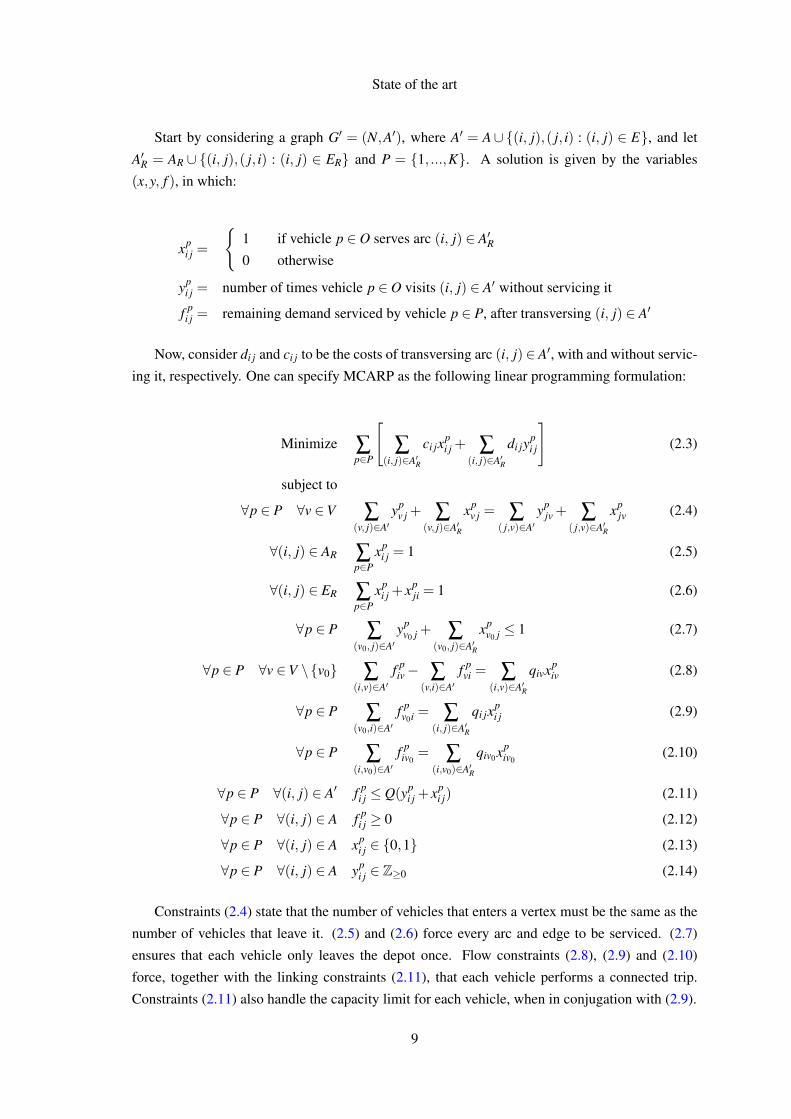
Start by considering a graph G′ = (N,A′), where A′ = A∪(i, j),( j, i) : (i, j) ∈ E, and let

A′R = AR ∪ (i, j),( j, i) : (i, j) ∈ ER and P = 1, ...,K. A solution is given by the variables

(x,y, f ), in which:

xpi j =

1 if vehicle p ∈ O serves arc (i, j) ∈ A′R0 otherwise

ypi j = number of times vehicle p ∈ O visits (i, j) ∈ A′ without servicing it

f pi j = remaining demand serviced by vehicle p ∈ P, after transversing (i, j) ∈ A′

Now, consider di j and ci j to be the costs of transversing arc (i, j)∈ A′, with and without servic-

ing it, respectively. One can specify MCARP as the following linear programming formulation:

Minimize ∑p∈P

[∑

(i, j)∈A′R

ci jxpi j + ∑

(i, j)∈A′R

di jypi j

](2.3)

subject to

∀p ∈ P ∀v ∈V ∑(v, j)∈A′

ypv j + ∑

(v, j)∈A′R

xpv j = ∑

( j,v)∈A′yp

jv + ∑( j,v)∈A′R

xpjv (2.4)

∀(i, j) ∈ AR ∑p∈P

xpi j = 1 (2.5)

∀(i, j) ∈ ER ∑p∈P

xpi j + xp

ji = 1 (2.6)

∀p ∈ P ∑(v0, j)∈A′

ypv0 j + ∑

(v0, j)∈A′R

xpv0 j ≤ 1 (2.7)

∀p ∈ P ∀v ∈V \v0 ∑(i,v)∈A′

f piv− ∑

(v,i)∈A′f pvi = ∑

(i,v)∈A′R

qivxpiv (2.8)

∀p ∈ P ∑(v0,i)∈A′

f pv0i = ∑

(i, j)∈A′R

qi jxpi j (2.9)

∀p ∈ P ∑(i,v0)∈A′

f piv0

= ∑(i,v0)∈A′R

qiv0xpiv0

(2.10)

∀p ∈ P ∀(i, j) ∈ A′ f pi j ≤ Q(yp

i j + xpi j) (2.11)

∀p ∈ P ∀(i, j) ∈ A f pi j ≥ 0 (2.12)

∀p ∈ P ∀(i, j) ∈ A xpi j ∈ 0,1 (2.13)

∀p ∈ P ∀(i, j) ∈ A ypi j ∈ Z≥0 (2.14)

Constraints (2.4) state that the number of vehicles that enters a vertex must be the same as the

number of vehicles that leave it. (2.5) and (2.6) force every arc and edge to be serviced. (2.7)

ensures that each vehicle only leaves the depot once. Flow constraints (2.8), (2.9) and (2.10)

force, together with the linking constraints (2.11), that each vehicle performs a connected trip.

Constraints (2.11) also handle the capacity limit for each vehicle, when in conjugation with (2.9).

9

State of the art

Further details regarding the theory of arc routing problems, along with possible approaches

for solving them, can be found in [Mos00, AG95].

2.3.1.2 Solving approaches

In [BBLP06], the authors describe three fast heuristics, adapted from studies on the undirected

version of CARP: path scanning, augment-merge and Ulusoy’s heuristic.

Path scanningthis heuristic builds routes sequentially. In each step, the current route is extended (until the

capacity constraints are violated) by adding the arcs that lead to the closest arc v∈ A′R which

needs to be serviced. In case of ties, the heuristic may use randomly one of five criteria:

F1 maximize the cost to return to the depot;

F2 minimize the cost to return to the depot;

F3 maximize the ratio qv/cv;

F4 minimize the ratio qv/cv;

F5 if the vehicle is less than half-full, use F2 and otherwise use F1.

Augment-mergeA route is created for each required link e∈ AR∪ER, minimizing the deadheading cost (This

can easily be done using shortest path algorithms). The next step, called Augment phase,

verifies if there are routes which include required links in their deadheading arcs. When it

happens, they are merged together, if the capacity constraints hold.

The second phase, Merge, takes every pair of routes (r0,r1) and checks if their concatenation

yields a better result (while respecting the capacity constraints), and merges them. The

concatenation process is done by finding the shortest path between the last served arc in r0

to the first served arc in r1.

Ulusoy’s heuristicThis heuristic builds a single route containing all arcs in A′R, ignoring the capacity con-

straints, and subsequently divides it into several feasible routes.

The first step does not need to produce an optimal route, so the authors suggest the usage of

the path-scanning heuristic and disregarding the capacity limit. This route defines the order

in which the arcs will be serviced, so let pos(a) be the arc’s position on this route.

Next, the route is subdivided. This step can be done using a simple dynamic programming

technique.

In the same study, the authors propose new linear relaxed formulation which can is used to-

gether with a cutting plane algorithm to determine a lower bound for MCARP instances.

Belenguer et al. also mention several metaheuristics applied to UCARP that solve a majority

of instances optimally [BBLP06, BB03]. These could be adapted to solve MCARP.

10

State of the art

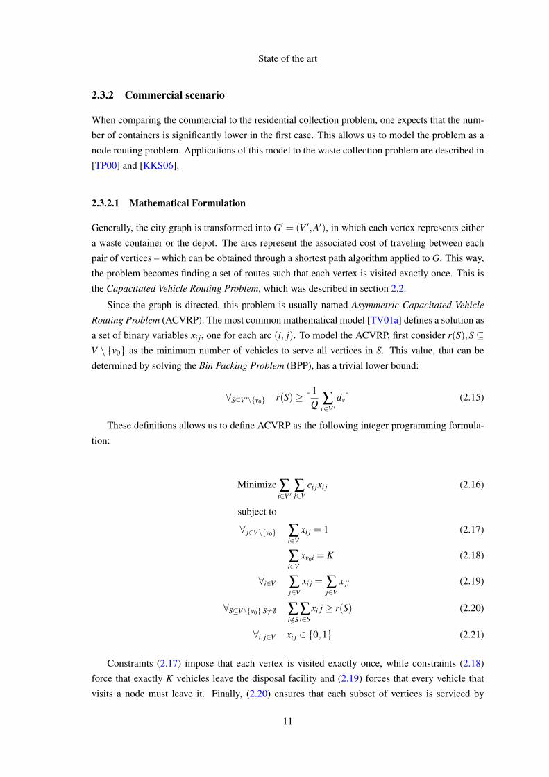
2.3.2 Commercial scenario

When comparing the commercial to the residential collection problem, one expects that the num-

ber of containers is significantly lower in the first case. This allows us to model the problem as a

node routing problem. Applications of this model to the waste collection problem are described in

[TP00] and [KKS06].


Generally, the city graph is transformed into G′ = (V ′,A′), in which each vertex represents either

a waste container or the depot. The arcs represent the associated cost of traveling between each

pair of vertices – which can be obtained through a shortest path algorithm applied to G. This way,

the problem becomes finding a set of routes such that each vertex is visited exactly once. This is

the Capacitated Vehicle Routing Problem, which was described in section 2.2.

Since the graph is directed, this problem is usually named Asymmetric Capacitated Vehicle

Routing Problem (ACVRP). The most common mathematical model [TV01a] defines a solution as

a set of binary variables xi j, one for each arc (i, j). To model the ACVRP, first consider r(S),S ⊆V \ v0 as the minimum number of vehicles to serve all vertices in S. This value, that can be

determined by solving the Bin Packing Problem (BPP), has a trivial lower bound:

∀S⊆V ′\v0 r(S)≥ d 1Q ∑

v∈V ′dve (2.15)

These definitions allows us to define ACVRP as the following integer programming formula-

tion:

Minimize ∑i∈V ′

∑j∈V

ci jxi j (2.16)

subject to

∀ j∈V\v0 ∑i∈V

xi j = 1 (2.17)

∑i∈V

xv0i = K (2.18)

∀i∈V ∑j∈V

xi j = ∑j∈V

x ji (2.19)

∀S⊆V\v0,S 6= /0 ∑i/∈S

∑i∈S

xi j ≥ r(S) (2.20)

∀i, j∈V xi j ∈ 0,1 (2.21)

Constraints (2.17) impose that each vertex is visited exactly once, while constraints (2.18)

force that exactly K vehicles leave the disposal facility and (2.19) forces that every vehicle that

visits a node must leave it. Finally, (2.20) ensures that each subset of vertices is serviced by

11

State of the art

at least the minimum number of vehicles required to fulfill their demands, thus respecting the

capacity constraints.


In the book by Toth and Vigo [TV01b], CVRP is described with great detail. They divide methods

into the following categories:

• Branch-and-bound

• Branch-and-cut

• Set-covering based algorithms

• Heuristics

• Metaheuristics

The first three categories are exact methods, based on relaxations of linear formulations and

the determination of lower bounds. Some of these approaches have been used to solve optimally

problem instances with up to 135 nodes [NR01]. These involve the study of polytopes defined by

linear formulations and cutting plane algorithms.

In the heuristics field, there are three subcategories [LS01]. Constructive heuristics gradually

build a feasible solution, minimizing the cost in a greedy fashion. Two-phase heuristics divide

the problem into two: clustering the vertices in K clusters and constructing a route from each

cluster. Some methods do clustering first (cluster-first-route-second), while others build a single

tour — containing all vertices and ignoring capacity constraints — and consequently divide it

into vehicle routes (route-first-cluster-second) [TB]. The latter approach is similar to Ulusoy’s

heuristic, described in section 2.3.1.2. The third category, containing Improvement methods, is

applied over the two first categories. Improvement methods can be applied either by changing the

order in which vertices are visited in a vehicle route or by switching vertices between routes. In

the first case, this technique is the same as optimizing a single route in a subgraph — resulting in

the Traveling Salesman Problem.

The last category of methods encompasses metaheuristics, which are general optimization

methods. Metaheuristics are said to produce better results than the previous set of methods [GLP01].

These techniques are no more than Improvement methods.

Examples of metaheuristics applied to VRP, are Simulated Annealing, Deterministic Anneal-

ing, Tabu Search, Genetic Algorithms and Ant Systems. The first three approaches start by building

an initial solution (using a heuristic) and search its neighborhood for a better solution. The neigh-

borhood is usually defined by some swap operator; for example, exchanging a subset of serviced

vertices between routes.

Genetic Algorithms start by generating a set of initial solutions, and proceeds to the next step

by combining solutions between them, and discarding the worst. Ant systems work by applying

12

State of the art

concepts based on the ants’ pheromone system for marking paths [CDM91]. These two approaches

will be described further in chapter 5.

2.3.3 Rollon-Rolloff scenario

Regarding the Rollon-Rolloff case, some of the earlier studies found on the literature are [G.94,

dML97, BMBB00]. According to Bodin et al., the first three papers assume that it is known

beforehand which trip type (see section 2.1) must serve each container. This problem is named

Rolloff-Rollon Vehicle Routing Problem (RRVRP).


Each given trip t ∈ T is defined by its type and by a tuple of vertices to visit, in a specific order.

The problem of assigning trips to vehicles can be formulated as an Asymmetric Vehicle Routing

Problem (AVRP). AVRP is similar to the ACVRP without the vehicle capacity constraints, but

differs in that the number of vehicles is not given — it is a value which must be minimized.

Usually, the number of vehicles must be bounded by a given interval [L,U ].

In order to model the RRVRP as a AVRP, admit a new graph, G′ = (V ′,A′). One vertex

represents the disposal facility, while the others represent trips that need to be serviced. Each arc

(i, j) ∈ A′ represents the transition between trip i and trip j. When i = 0, consider this transition to

be the start of a route; when j = 0, consider it as the end. The costs of going from the end location

of a given trip to the start location of another one are given by ca,a ∈ A′.

The AVRP formulation for the RRVRP can now be defined as:

Minimize KA ∑i∈V ′

∑j∈V

ci jxi j +KB ∑j∈V

xv0 j (2.22)

subject to

∀ j∈V\v0 ∑i∈V

xi j = 1 (2.23)

∀i∈V ∑j∈V

xi j = ∑j∈V

x ji (2.24)

∑j∈V

xv0 j ≤U (2.25)

∑j∈V

xv0 j ≥ L (2.26)

∀i, j∈V xi j ∈ 0,1 (2.27)

Another formulation is provided in [BBM06]. This paper does not assume, as the previous

ones, that the trips to be serviced are predefined. Furthermore, it addresses the problem of having

multiple disposal facilities and multiple inventory locations (where empty containers are stored).

The authors named this as the Multiple Rollon-Rolloff Vehicle Routing Problem (M-RRVRP). The

13

State of the art

M-RRVRP can be converted to a Vehicle Routing Problem with Time Windows (VRPTW). This

makes it possible to model the problem as a Set Partitioning (SP) formulation.

A similar problem is defined by [Arc05], named 1-Skip (container) Collection Problem (1-

SCP). Here, multiple disposal facilities are available, and there are compatibility constraints be-

tween the facilities and the containers. The trips that each vehicle can perform are different from

the four types defined in the RRVRP. Each vehicle starts its tour from a depot with an empty con-

tainer and travels to a location where there is a full one. The two containers are then exchanged,

and the vehicle proceeds with the full container to a compatible disposal facility. It then proceeds

to another trip, with a new empty container. This model also considers time windows for picking

up and emptying containers.

The authors of [ABMN04] also present a rather interesting alternative for the Rollon-Rolloff

model. They start by considering that there is a finite number of available empty containers at the

depot, KC, and that compatibility constraints defined in the 1-SCP model are also present. Each

request for collection i ∈ I, I = 1, ...,n is characterized by its location (γi), container type (βi) and

waste material type (µi).

The graph model G = (V,A) defines its vertices as representations of collection requests. For

each request i, there are two nodes ei and fi in V , that represent the full container to be collected

and an empty container to be delivered. As usual, vertex v0 represents the depot from where the

vehicles must begin and end their tours. There are also KC vertices (the set D′), representing the

possible pick up of an empty container at the depot, and KC vertices (the set D′′) representing

their delivery. No nodes will be added to represent the disposal facilities; this information will be

embed in the graph arcs.

Let E = ei : i∈ I, F = fi : i∈ I. Defining the set of vertices as V = v0∪E∪F∪D′∪D′′,

we now need to specify the arcs connecting them.

There is an arc between fi ∈ F and e j ∈ E if both services have the same container type

(βi = β j). These arcs correspond to picking up a full container at γi, taking it to a disposal facility

of type µi for emptying and deploying it at location γ j.

Between every ei ∈E and f ∈F there is also an arc. It represents deploying an empty container

at location γi and travelling to γ j to pick up its full container.

At the start of a tour, a vehicle starts at the depot node, v0, unloaded. From here, there are

two alternatives: it travels to a location with a full container or it picks up an empty container.

These operations are represented by the arcs (v0, f ), f ∈ F and (v0,d′),∈ D′. Analogously, there

are arcs that represent unloading an empty container and finishing the tour. These arcs are defined

by (e,v0),e ∈ E and (d′′,v0),d′′ ∈ D′′.

Picking up an empty container from the depot and deploying it is represented by the arcs

(d′,e),d′ ∈ D′∧ e ∈ E. Picking up a full container, emptying it at a disposal facility and dropping

it at the depot is modeled by the arcs ( f ,d′′), f ∈ F ∧ d′′ ∈ D′′. Finally, there are cases where a

vehicle drops an empty container at the depot to pick up another empty one, of another type, or a

full one: (d′′,d′),d′′ ∈ D′′∧d′ ∈ D′ and (d′′, f ),d′′ ∈ D′′∧ f ∈ F .

14

State of the art

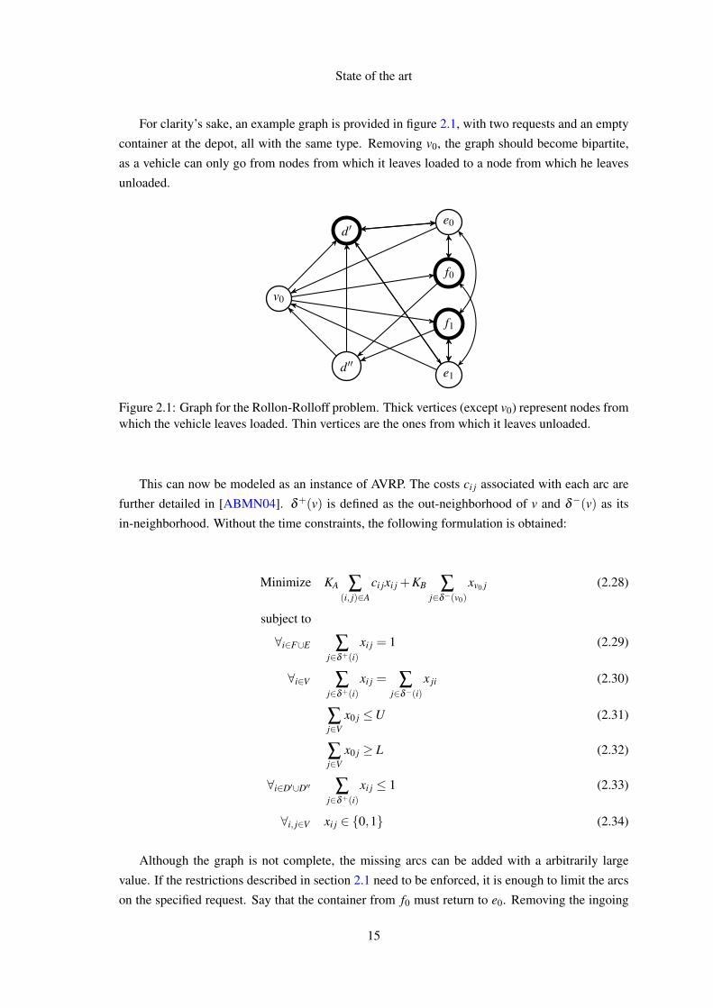
For clarity’s sake, an example graph is provided in figure 2.1, with two requests and an empty

container at the depot, all with the same type. Removing v0, the graph should become bipartite,

as a vehicle can only go from nodes from which it leaves loaded to a node from which he leaves

unloaded.

v0

d′′

e0

e1

d′

f0

f1

Figure 2.1: Graph for the Rollon-Rolloff problem. Thick vertices (except v0) represent nodes fromwhich the vehicle leaves loaded. Thin vertices are the ones from which it leaves unloaded.

This can now be modeled as an instance of AVRP. The costs ci j associated with each arc are

further detailed in [ABMN04]. δ+(v) is defined as the out-neighborhood of v and δ−(v) as its

in-neighborhood. Without the time constraints, the following formulation is obtained:

Minimize KA ∑(i, j)∈A

ci jxi j +KB ∑j∈δ−(v0)

xv0 j (2.28)

subject to

∀i∈F∪E ∑j∈δ+(i)

xi j = 1 (2.29)

∀i∈V ∑j∈δ+(i)

xi j = ∑j∈δ−(i)

x ji (2.30)

∑j∈V

x0 j ≤U (2.31)

∑j∈V

x0 j ≥ L (2.32)

∀i∈D′∪D′′ ∑j∈δ+(i)

xi j ≤ 1 (2.33)

∀i, j∈V xi j ∈ 0,1 (2.34)

Although the graph is not complete, the missing arcs can be added with a arbitrarily large

value. If the restrictions described in section 2.1 need to be enforced, it is enough to limit the arcs

on the specified request. Say that the container from f0 must return to e0. Removing the ingoing

15

State of the art

edges to e0 and the outgoing edges from f0 (except the one that connects f0 to e0) is enough to

ensure this constraint.


Solving RRVRP instances, as modeled in the previous section, can be done using the algorithms

described in section 2.3.2.2.

2.4 Chapter summary

This chapter presented some background information regarding waste collection problems. It

followed by giving a general overview of the modelation of route optimization problems.

Finally, section 2.3 presents the application of route optimization models to waste collection

vehicle route optimization problem. Three different scenarios were introduced.

In the residential scenario, there are several approaches applied to the directed CARP. Al-

though some have been adapted to the undirected variant, further study could be made regarding

the remaining algorithms — namely, the usage of metaheuristics.

The Rollon-rolloff scenario was formulated as a AVRP instance. Although the authors pro-

vided preliminary computational results using an heuristic, further computations could be made,

comparing several other heuristics, metaheuristics and exact methods.

The commercial scenario is modeled as a Capacitated Vehicle Routing Problem. This model

is used whenever the density of waste containers per street is low.

The next chapter, chapter 3, uses the definitions introduced in these sections to explicitly state

the goals of this study.

16

Chapter 3

Problem description

This chapter provides a description of the problem being addressed.

3.1 Waste collection in Porto, Portugal

The municipal council of the city of Porto is interested in implementing a platform that measures

the fill status of the containers in real-time, so that the evolution of waste can be monitored,

the quality and efficiency of the collection can be increased, and the sums paid to subcontractor

companies by amount of km traveled each month reduced. The system should work as follows:

containers send an alarm when they are full, and everyday in the evening the waste collection

routes are calculated with the static values available at a certain time.

This project’s scope is to build a framework that stores container fill status and that uses that

information to calculate efficient collection routes. Routes have to be provided every day, based on

recent fill information; although there is no need to calculate routes in real-time, a solution must be

provided within 1 to 2 hours. This constraint requires that an efficient solution is found within that

time frame for graphs of large cities, which are composed of several thousand vertices. To decide

which algorithm should be used to calculate the routes, it was necessary to do a comparative study

to evaluate the performance of several techniques.

As stated in the previous chapter, a residential waste collection scenario is modeled as a Capac-

itated Arc Routing Problem (CARP), due to high number of containers per street. CARP consists

of, in summary, finding a set of vehicle routes that visit a subset of a given graph’s arcs. With each

arc, there is an associated demand, which must be serviced by exactly one vehicle. The sum of the

demands that a given vehicle services must not exceed a fixed limit.

Although residential waste collection scenarios are usually modeled as a CARP, it must be

taken into account that in Porto, containers service several homes and that containers fill status

will be monitored. With this in mind, it becomes more natural to use a Asymmetric Capacitated

Vehicle Routing Problem (ACVRP) model. This model is similar to that of CARP, with a simple

difference: instead of servicing arcs, in ACVRP vehicles must service vertices instead.

17

Problem description

3.2 Asymmetric capacitated vehicle routing problem

As exposed in the previous chapter, there are three non-exact methods to address the Asymmetric

Capacitated Vehicle Routing Problem. One of them, route-first-cluster-second, first solves the

associated Asymmetric Traveling Salesman Problem (ATSP); this implies finding the shortest tour

that visits every vertice exactly once. This process is followed by the partitioning of the tour into

routes that respect vehicle capacity constraints (henceforth called clustering).

Another method, cluster-first-route-second, first clusters the containers and then attempts to

find an optimum route for each cluster. This method usually requires that one predefines the

number of vehicles to use.

The third method to address the ACVRP is to use constructive heuristics, that build all the

vehicle routes in parallel.

This work will focus on the comparison of the first and third methods, using different ap-

proaches to solve the ATSP. Additionally, special focus will be given to the MAX-MIN ant system

(MMAS) — which is described in section 5.4.2 — and its sensibility to certain parameters.

3.3 Chapter summary

This chapter summarized the motivation, goals and approach of this project. The next chapter

will focus on the definition of the architecure for the waste sensor framework. It also presents the

evaluation metrics and validation datasets to analyse the optimization process.

18

Chapter 4

Solution architecture

This chapter describes the proposed architecture for managing waste containers fill status and cal-

culating efficient routes. It starts by specifying, in section 4.1, all the modules and the information

workflow of the framework. Section 4.2 presents the technologies used to implement each module,

while section 4.3 specifies the data formats in which information is exchanged between modules.

Section 4.4 defines the metrics chosen to evaluate the optimization algorithms, so that they

may be quantified and properly compared.

Section 4.5 introduces the datasets used throughout this study. Implemented algorithms will

be applied to these datasets, and the resulting routes will be evaluated using the metrics previously

defined in section 4.4.

A subset of these datasets, defined in section 4.5.1, will be used to validate the algorithms’ im-

plementations. These datasets are widely used throughout the literature to benchmark algorithms,

and their optimal solutions has usually already been determined.

Section 4.5.2 presents a second subset of datasets, whose properties are similar to those of the

datasets obtained when the monitoring system is deployed. These will be used to compare the

algorithms’ performance.

4.1 Framework workflow

This project is structured in a modular way; this chapter enumerates and describes each one of the

modules, defining what is required and produced in each step.

To understand the following architecture and underlying information flow, one must have in

mind that this project has two major components. First, several optimization algorithms must be

compared, using both real and fabricated scenarios. In second place, the system must be ready

to be integrated with the fill status monitoring solution being developed at Fraunhofer Portugal

AICOS.

19


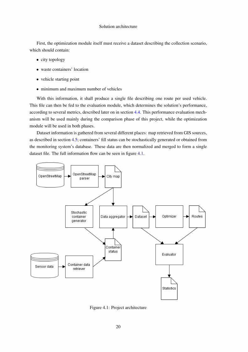
First, the optimization module itself must receive a dataset describing the collection scenario,

which should contain:

• city topology

• waste containers’ location

• vehicle starting point

• minimum and maximum number of vehicles

With this information, it shall produce a single file describing one route per used vehicle.

This file can then be fed to the evaluation module, which determines the solution’s performance,

according to several metrics, described later on in section 4.4. This performance evaluation mech-

anism will be used mainly during the comparison phase of this project, while the optimization

module will be used in both phases.

Dataset information is gathered from several different places: map retrieved from GIS sources,

as described in section 4.5; containers’ fill status can be stochastically generated or obtained from

the monitoring system’s database. These data are then normalized and merged to form a single

dataset file. The full information flow can be seen in figure 4.1.

Figure 4.1: Project architecture

20


Note that there is the need to manage independent city and containers’ status files before

creating a normalized dataset. This happens because the stochastic container generator depends

on the city file to create valid scenarios.

4.2 Implementation details

To implement this framework, there was the need to decide which technologies to use, regarding

several modules.

Figure 4.1 shows the necessity of a database management system (DBMS), to maintain infor-

mation about the containers’ fill status. Due to the simple nature of the information model stored

in the database, the choice of which DBMS to use is not critical. Additionally, the load of the

DBMS will not be too high, as the optimization process is only run once per day. With this in

mind, it was decided to use the MySQL DBMS, as it is both free and widely used in high profile

projects, such as the Wikimedia Foundation and Yahoo! Finance [BD08].

Modules such as the data aggregator, OpenStreetMap parser, Container data retriever and

Stochastic container generator were developed using a combination of C++ and bash scripting.

C++ was used to apply complex transformations to the data, which involved handling large files.

Bash scripting was used as an utility to invoke MySQL queries and convert the retrieved data into

a more convenient format.

All the algorithms in the optimization module were implemented in C++. As the algorithm

implementations need to be efficient (both regarding running time and memory), the usage of

interpreted languages, such as Ruby or Python, was discarded. C++ was chosen due to the author’s

familiarity with the language, thus accelerating the development phase.

The evaluation module was also implemented in C++, so that its code could be shared with

the optimization module.

4.3 Data formats

As seen in figure 4.1, there are five different files that carry information from one module to the

next. To ease implementation, all five formats were specified using the same notation.

Examples of common data interchange formats are XML (Extensible Markup Language) and

JSON (JavaScript Object Notation). Advantages of such standards are, for example, the ready

availability of several parsers for a great number of languages [Cro09b, Rob09], their openness

and simplicity.

Between these two notations, it was decided to use the JSON format. It was chosen because it

is simpler than XML and because it was specifically designed to be a lightweight computer data

interchange format, whereas XML was designed to be a document interchange format [Cro09b].

JSON is based on two universal data structures: ordered lists and keyed lists (from here on

out called objects). The latter structure is also known in various programming languages as a

21


dictionary, hash table, associative array and others. There are also primitive types available, such

as strings, numbers and three constants: true, false and null.

While objects’ keys must be strings, their values can be of any type, either primitive or not.

The same is true for ordered lists’ elements. Further details regarding JSON syntax can be found

in the RFC 4627 [Cro09a].

The following sections in this chapter will describe each one of the five formats present in this

system’s architecture.

4.3.1 City map format

To simulate the waste generation and collection, there is the need to provide a topological city map.

This topological map must be represented as a directed weighted graph, so that routing algorithms

may be applied. A city is usually a sparse graph — each vertex, representing a street intersection,

has a reduced number of arcs. This leads to the conclusion that a adjacency list representation

should be used.

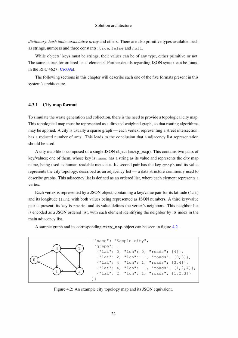
A city map file is composed of a single JSON object (city_map). This contains two pairs of

key/values; one of them, whose key is name, has a string as its value and represents the city map

name, being used as human-readable metadata. Its second pair has the key graph and its value

represents the city topology, described as an adjacency list — a data structure commonly used to

describe graphs. This adjacency list is defined as an ordered list, where each element represents a

vertex.

Each vertex is represented by a JSON object, containing a key/value pair for its latitude (lat)

and its longitude (lon), with both values being represented as JSON numbers. A third key/value

pair is present; its key is roads, and its value defines the vertex’s neighbors. This neighbor list

is encoded as a JSON ordered list, with each element identifying the neighbor by its index in the

main adjacency list.

A sample graph and its corresponding city_map object can be seen in figure 4.2.

0

1

2

3

4

"name": "Sample city","graph": ["lat": 0, "lon": 0, "roads": [4],"lat": 2, "lon": -1, "roads": [0,3],"lat": 4, "lon": 1, "roads": [3,4],"lat": 4, "lon": -1, "roads": [1,2,4],"lat": 2, "lon": 1, "roads": [1,2,3]

]

Figure 4.2: An example city topology map and its JSON equivalent.

22


4.3.2 Containers status format

The containers’ fill status file contains, for each container, its location — latitude and longitude

— and the current amount of waste stored in it. This is represented by a JSON ordered list, with

an element per container. Each container element is a JSON object and contains three key/value

pairs: one for its latitude (lat), one for its longitude (lon) and one for its current fill (fill). An

example JSON object is available in figure 4.3.

["lat": 0.0, "lon": 0.0, "fill": 43.01,"lat": 4.1, "lon": -0.9, "fill": 18.47]

Figure 4.3: An example containers’ fill status JSON file.

4.3.3 Dataset format

After obtaining both the city map file and the containers’ status file, they must be merged together

to form a single dataset file. This action is performed by the normalizer module, shown previously

in figure 4.1.

This format contains both features regarding the city topology and the containers’ fill status.

Each container geographical position is matched against the graph’s vertices and its fill status

information is added to the closest vertex.

The dataset schema is similar to the one presented in section 4.3.1, with a few changes. First,

for each vertex in which a waste container is present, there is an additional key/value pair repre-

senting its fill status, as defined in section 4.3.2. Second, two new key/value pairs must be added

to the main JSON object; one regarding the maximum number of trucks to use (max_trucks)

and one regarding the starting/ending node (depot). These two extra parameters must be de-

fined when running the normalization process, and are not present in any of the previous data file

formats.

Taking the examples presented in the two previous sections, they could be normalized into the

dataset file present in figure 4.4.

4.3.4 Routes format

The optimization module must process a single dataset file and determine a near-optimal set of

routes — one for each vehicle. Each vehicle route can be defined as an ordered list of references

to the city vertices.

When dealing with commercial scenarios, each vertex there should be paired with a boolean

indicator that tells if the vehicle must empty the waste container present at that location. In the

Rollon-Rolloff scenario, this additional flag indicates if the vehicle should load/unload a container

at that location.

23


"name": "Sample city","max_trucks": 3,"depot": 1,"graph": ["lat": 0, "lon": 0, "roads": [4], "fill": 43.01,"lat": 2, "lon": -1, "roads": [0,3],"lat": 4, "lon": 1, "roads": [3,4],"lat": 4, "lon": -1, "roads": [1,2,4], 18.47,"lat": 2, "lon": 1, "roads": [1,2,3]

]

Figure 4.4: Complete dataset example object, constructed from previous examples.

The set of routes can be defined as a JSON ordered list, with each element defining a single

route. Each route can also be represented by an ordered list of vertex references. These are

themselves defined as ordered lists of two values; the first value represents the vertex index, while

the second is a boolean value, determining if the vehicle should or should not act on that specific

location.

Figure 4.5 shows an example of a two-vehicle routes file, in the Rollon-Rolloff scenario, after

applying an optimization technique to the previously shown dataset. Each vehicle starts by loading

an empty container at vertex 1, moves to a location with a full container and switches the empty

with the full one. Then, both vehicles proceed back to the depot location, where they deposit the

picked up containers.

[[[1, true], [4, true], [4, true], [0, false], [1, true]],[[1, true], [3, true], [3, true], [1, true]]

]

Figure 4.5: Rollon-Rolloff set of routes example, representing two vehicles.

4.3.5 Statistics format

The fifth data format regards the statistics obtained when evaluating the routes obtained by a given

optimization module. These metrics are calculated based on the routes and the dataset files. The

output object is represented as a JSON object, where each key/value pair represents a different

metric. This representation is left open, as metrics may be added and/or removed during the

algorithm comparison phase.

24


4.4 Evaluation metrics

Performance evaluation of the implemented optimization framework requires the definition of

quantifiable metrics. As the goal is to reduce collection costs, an important metric is the total

number of kilometers that vehicles travel during waste collection. The lower the number of kilo-

meters is, the better.

Although the total distance is the main evaluation metric, there are additional metrics that may

be used to evaluate a solution. The average ratio between a vehicle’s capacity and the total urban

waste it collects may be important to evaluate collection efficiency.

4.5 Datasets

This section will present datasets used for algorithm validation. This will be followed by the

description of the methods used to obtain large datasets that share the same properties as the ones

to be used in production, when the monitoring system is deployed.

4.5.1 Validation datasets

Routing problems have been widely studied over the last decades; this has led to the establishment

of standard datasets for benchmarking algorithms and implementations, one of them being the

TSPLIB[Rei91]. There are datasets for the Capacitated Vehicle Routing Problem, both Symmetric

and Asymmetric Traveling Salesman Problem and other related routing problems. ATSP instances

have been solved optimally; as such, they are accompanied by their respective optimum route cost.

This library can be used to validate the algorithm implementations described in chapter 5, as

it allows one to measure the performance gap between a given solution and the optimal route.

Table 4.1 shows the ATSP validation instances, including the number of nodes and the op-

timum route cost, while table 4.2 shows the CVRP validation instances. In the latter case, an

optimum route cost is not available. This is due to the fact that these datasets can be used to for-

mulate several problems. For example, one might consider the number of vehicles specified in the

dataset as a fixed, minimum or maximum value. It might also be possible to disregard the number

of vehicles specified by the dataset. As such, table 4.2 only presents reference values obtained

when considering a fixed number of vehicles.

25


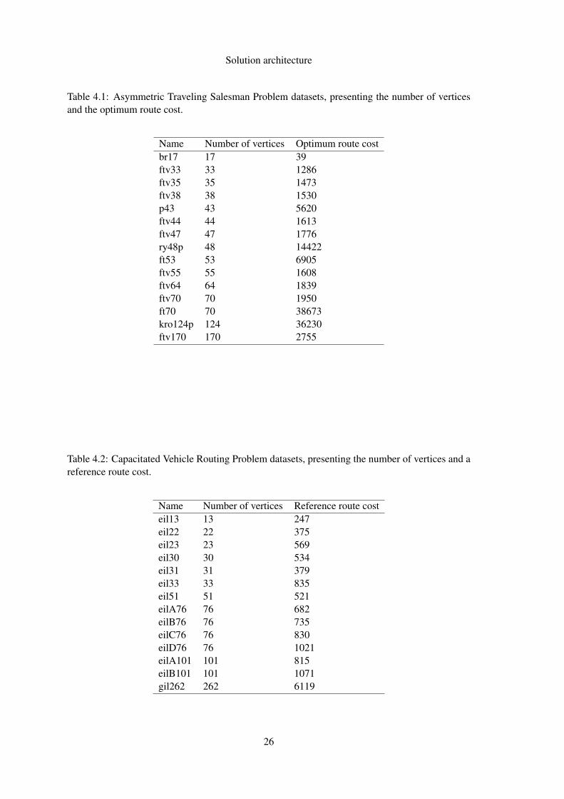
Table 4.1: Asymmetric Traveling Salesman Problem datasets, presenting the number of verticesand the optimum route cost.

Name Number of vertices Optimum route costbr17 17 39ftv33 33 1286ftv35 35 1473ftv38 38 1530p43 43 5620ftv44 44 1613ftv47 47 1776ry48p 48 14422ft53 53 6905ftv55 55 1608ftv64 64 1839ftv70 70 1950ft70 70 38673kro124p 124 36230ftv170 170 2755

Table 4.2: Capacitated Vehicle Routing Problem datasets, presenting the number of vertices and areference route cost.

Name Number of vertices Reference route costeil13 13 247eil22 22 375eil23 23 569eil30 30 534eil31 31 379eil33 33 835eil51 51 521eilA76 76 682eilB76 76 735eilC76 76 830eilD76 76 1021eilA101 101 815eilB101 101 1071gil262 262 6119

26


4.5.2 Realistic city datasets

In order to properly evaluate the developed algorithms, there was the need to obtain realistic

datasets that represented the street topology of real cities. These datasets must be similar to those

to be obtained by the monitoring system, so that results are as reliable as possible.

4.5.2.1 OpenStreetMap.org

To obtain realistic city maps, a tool to extract and convert topological maps from OpenStreetMap.org

was developed. OpenStreetMap.org is an collaborative and open source initiative which aims to

create a free editable map of the world [Hak08]. Users may add information by editing the world

map manually — using the web editor — or by submitting data from GPS devices.

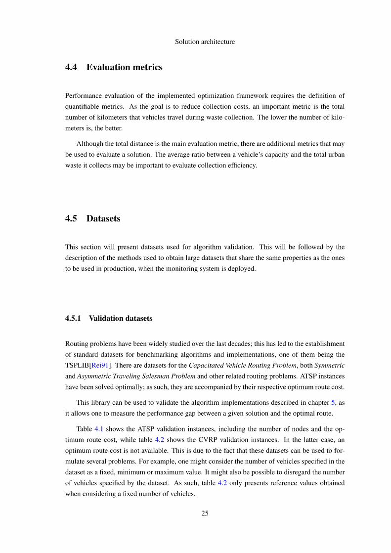
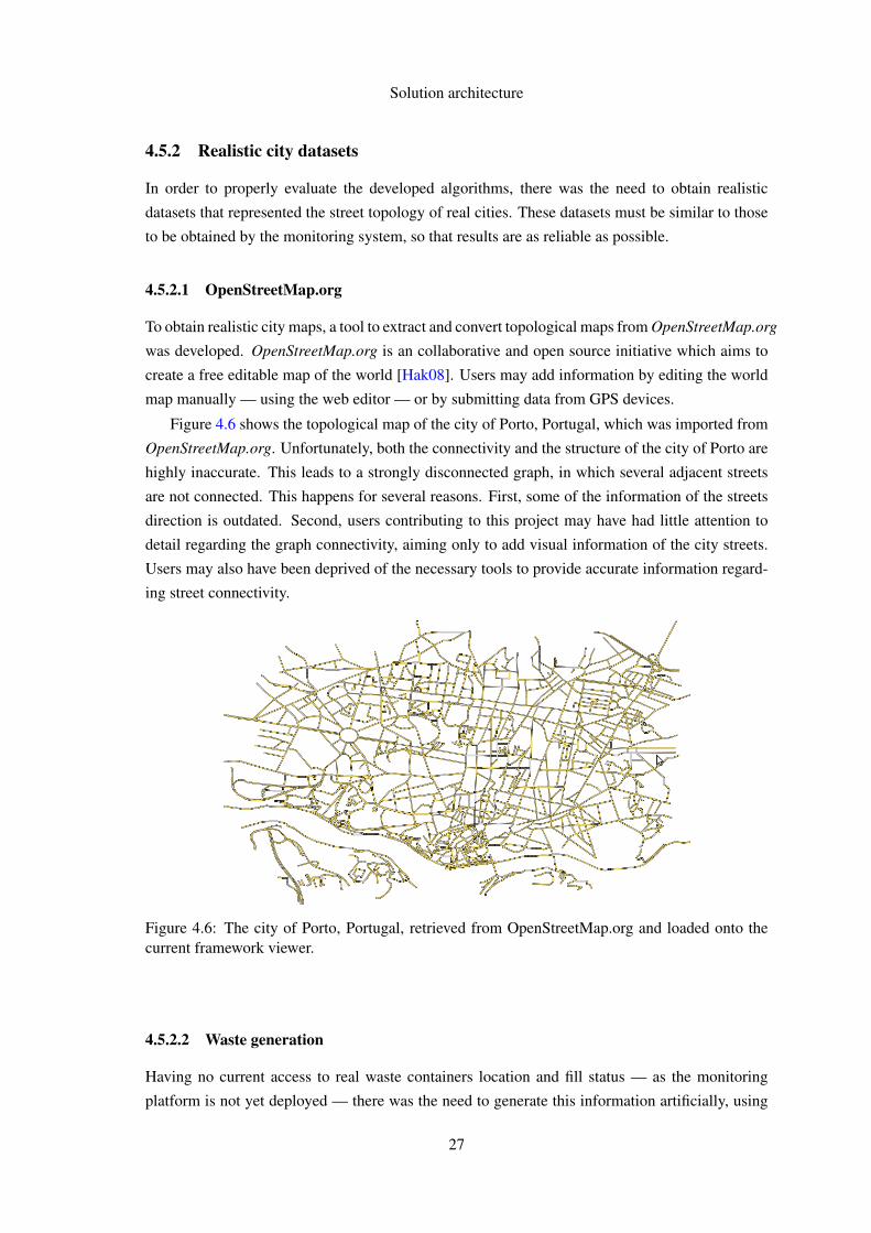
Figure 4.6 shows the topological map of the city of Porto, Portugal, which was imported from

OpenStreetMap.org. Unfortunately, both the connectivity and the structure of the city of Porto are

highly inaccurate. This leads to a strongly disconnected graph, in which several adjacent streets

are not connected. This happens for several reasons. First, some of the information of the streets

direction is outdated. Second, users contributing to this project may have had little attention to

detail regarding the graph connectivity, aiming only to add visual information of the city streets.

Users may also have been deprived of the necessary tools to provide accurate information regard-

ing street connectivity.

Figure 4.6: The city of Porto, Portugal, retrieved from OpenStreetMap.org and loaded onto thecurrent framework viewer.

4.5.2.2 Waste generation

Having no current access to real waste containers location and fill status — as the monitoring

platform is not yet deployed — there was the need to generate this information artificially, using

27


a stochastic approach. Waste containers were scattered in street intersections following different

patterns according to the following process:

The algorithm starts by selecting k road intersections (represented by a graph vertex) on the

city map as cluster centers. A number di in the range [0,1] is assigned to each cluster, representing

the cluster’s waste container density. Then, until all intersections belong to a cluster, k vertices

are chosen arbitrarily from each of the clusters’ neighborhood and added to the respective cluster.

When a vertex is added to a cluster it is decided, with probability di, if it should contain a full

waste container.

4.5.2.3 Generated datasets

This approach was applied to three different city topological maps — Leeds, Lisbon and London

— using different clustering parameter configurations. This yielded fifteen large datasets, whose

number of vertices ranges from 518 to 7628. Table 4.3 shows information about these datasets —

both the number of nodes and the cities in which their topology was based.

Table 4.3: Large realistic Capacitated Vehicle Routing Problem datasets

Name Number of vertices Cityhp518 518 Leedshp841 841 Leedshp904 904 Leedshp1287 1287 Leedshp1175 1175 Londonhp1849 1849 Londonhp2038 2038 Londonhp2206 2206 Londonhp2561 2561 Lisbonhp3481 3481 Lisbonhp3859 3859 Lisbonhp4109 4109 Lisbonhp4628 4628 Lisbonhp6247 6247 Lisbonhp7628 7628 Lisbon

4.6 Chapter summary

This chapter presented the design for the fill status monitoring framework — the information

workflow, data interchange formats and the technologies have been specified. Additionally, sec-

tions 4.4 and 4.5 specified the metrics and datasets with which to validate the waste collection

route optimization approaches.

The following chapter will introduce the optimization algorithms used throughout this study.

28

Chapter 5

Algorithms

As seen in section 2.3.2.2, one way to tackle the Asymmetric Capacitated Vehicle Routing Problem

is to first build a tour over graph G and to divide it into routes that respect the vehicle capacity

constraints. The problem of finding a tour in a directed graph is called Asymmetric Traveling

Salesman Problem.

The first sections in this chapter describe several algorithms used for solving Asymmetric Trav-

eling Salesman Problem instances. A comparative analysis of their complexity is shown in sec-

tion 5.5. Section 5.6 presents an algorithm for dividing a tour — a route that visits all vertices in

a graph — into several routes that respect vehicle capacity constraints.

Section 5.9 explains the process with which the implemented algorithms were validated. It

reports the results regarding the benchmarks done using standard Asymmetric Traveling Salesman

Problem and Capacitated Vehicle Routing Problem instances.

This chapter shows the algorithms’ characterization, by using asymptotic notation (also known

as Bachmann-Landau notation) to represent bounds on time complexities. For a description of

asymptotic notation used throughout this chapter, see [Knu76].

5.1 Construction heuristics for the ATSP

Two classical construction heuristics for the ATSP are the nearest neighbor and the greedy heuris-

tics [GPB+02].

Nearest neighbor (NN) starts by picking an arbitrary vertex, usually chosen at random. It

proceeds by advancing to the nearest unvisited neighbor, until all vertices are visited. A tour is

then completed by returning to the first visited vertex. When applied to a complete graph — where

|E|= |V |2 — this heuristic has a time complexity of O(|V |2). Instead of simply picking an arbitrary

vertex at first, one can start NN from every vertex and return the best final tour. This variation is

called repetitive nearest neighbor (RNN) [GPB+02]. Algorithm 1 describes the repetitive nearest

neighbor heuristic. Lines 4 through 15 apply the nearest neighbor heuristic starting in vertex v.

29

Algorithms

Algorithm 1 Repetitive nearest neighbor heuristicInput: A complete graph G = (V,E)Output: An ATSP route

1: minimum←+∞

2: best_route← nil3: for all v ∈ V do // calculate the NN for each vertex4: route← []5: current← v6: while |route| 6= |V | do7: route.append(current)8: closest← nil9: for all w ∈ V do // determine the closest non-visited vertex

10: if w 6∈ route∧ (closest = nil∨ cost(v,w)< cost(v,closest)) then11: closest← w12: end if13: end for14: current← closest15: end while16: if best_route = nil∨ cost(route)< cost(best_route) then17: best_route← route18: end if19: end for20: return best_route

The greedy heuristic (GR) works in a similar way than that of Kruskal’s minimum spanning

tree algorithm [Kru56]. It starts by creating an auxiliary directed graph with no arcs, G′ = (V,)and sorts all the arcs in G by their weight, which are then iterated in ascending order. Each arc

is added to G′ if and only if its vertices are not already connected in G′ and both the outdegree

(number of outgoing arcs) of the source vertex and the indegree (number of incoming arcs) of the

destination vertex are exactly 0. This process will yield a spanning tree which can be converted

to a tour by adding the arc that connects the only two vertices whose degree is less than 2. Its

time complexity is equal to that of Kruskal’s algorithm: Θ(|E|log|E|). When dealing with a

complete graph, where |E| = |V |2, the time complexity can be expressed as Θ(|V |2log(|V |2)) =Θ(|V |2log|V |).

The pseudo-code for this heuristic is presented in algorithm 2. Two arrays, prev and next, are

used to maintain information about each vertex’s incoming and outgoing connections. The f irst

and last arrays serve to determine if two vertices are already connected or not.

30

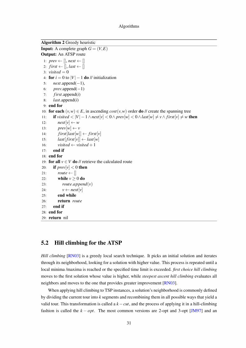
Algorithms

Algorithm 2 Greedy heuristicInput: A complete graph G = (V,E)Output: An ATSP route

1: prev← [], next← []2: f irst← [], last← []3: visited = 04: for i = 0 to |V |−1 do // initialization5: next.append(−1),6: prev.append(−1)7: f irst.append(i)8: last.append(i)9: end for

10: for each (v,w) ∈ E, in ascending cost(v,w) order do // create the spanning tree11: if visited < |V |−1∧next[v]< 0∧ prev[w]< 0∧ last[w] 6= v∧ f irst[v] 6= w then12: next[v]← w13: prev[w]← v14: f irst[last[w]]← f irst[v]15: last[ f irst[v]]← last[w]16: visited← visited +117: end if18: end for19: for all v ∈V do // retrieve the calculated route20: if prev[v]< 0 then21: route← []22: while v≥ 0 do23: route.append(v)24: v← next[v]25: end while26: return route27: end if28: end for29: return nil

5.2 Hill climbing for the ATSP

Hill climbing [RN03] is a greedy local search technique. It picks an initial solution and iterates

through its neighborhood, looking for a solution with higher value. This process is repeated until a

local minima /maxima is reached or the specified time limit is exceeded. first choice hill climbing

moves to the first solution whose value is higher, while steepest ascent hill climbing evaluates all

neighbors and moves to the one that provides greater improvement [RN03].

When applying hill climbing to TSP instances, a solution’s neighborhood is commonly defined

by dividing the current tour into k segments and recombining them in all possible ways that yield a

valid tour. This transformation is called a k− cut, and the process of applying it in a hill-climbing

fashion is called the k− opt. The most common versions are 2-opt and 3-opt [JM97] and an

31

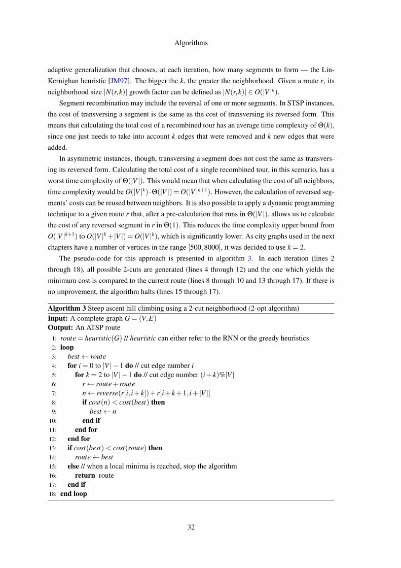
Algorithms

adaptive generalization that chooses, at each iteration, how many segments to form — the Lin-

Kernighan heuristic [JM97]. The bigger the k, the greater the neighborhood. Given a route r, its

neighborhood size |N(r,k)| growth factor can be defined as |N(r,k)| ∈ O(|V |k).Segment recombination may include the reversal of one or more segments. In STSP instances,

the cost of transversing a segment is the same as the cost of transversing its reversed form. This

means that calculating the total cost of a recombined tour has an average time complexity of Θ(k),

since one just needs to take into account k edges that were removed and k new edges that were

added.

In asymmetric instances, though, transversing a segment does not cost the same as transvers-

ing its reversed form. Calculating the total cost of a single recombined tour, in this scenario, has a

worst time complexity of Θ(|V |). This would mean that when calculating the cost of all neighbors,

time complexity would be O(|V |k) ·Θ(|V |) =O(|V |k+1). However, the calculation of reversed seg-

ments’ costs can be reused between neighbors. It is also possible to apply a dynamic programming

technique to a given route r that, after a pre-calculation that runs in Θ(|V |), allows us to calculate

the cost of any reversed segment in r in Θ(1). This reduces the time complexity upper bound from

O(|V |k+1) to O(|V |k+ |V |) = O(|V |k), which is significantly lower. As city graphs used in the next

chapters have a number of vertices in the range [500,8000], it was decided to use k = 2.

The pseudo-code for this approach is presented in algorithm 3. In each iteration (lines 2

through 18), all possible 2-cuts are generated (lines 4 through 12) and the one which yields the

minimum cost is compared to the current route (lines 8 through 10 and 13 through 17). If there is

no improvement, the algorithm halts (lines 15 through 17).

Algorithm 3 Steep ascent hill climbing using a 2-cut neighborhood (2-opt algorithm)Input: A complete graph G = (V,E)Output: An ATSP route

1: route = heuristic(G) // heuristic can either refer to the RNN or the greedy heuristics2: loop3: best← route4: for i = 0 to |V |−1 do // cut edge number i5: for k = 2 to |V |−1 do // cut edge number (i+ k)%|V |6: r← route+ route7: n← reverse(r[i, i+ k])+ r[i+ k+1, i+ |V |]8: if cost(n)< cost(best) then9: best← n

10: end if11: end for12: end for13: if cost(best)< cost(route) then14: route← best15: else // when a local minima is reached, stop the algorithm16: return route17: end if18: end loop

32

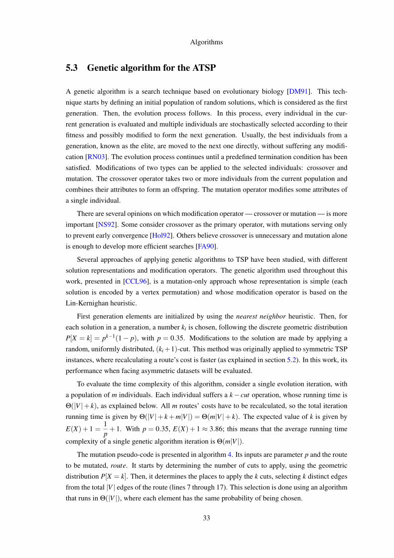
Algorithms

5.3 Genetic algorithm for the ATSP

A genetic algorithm is a search technique based on evolutionary biology [DM91]. This tech-

nique starts by defining an initial population of random solutions, which is considered as the first

generation. Then, the evolution process follows. In this process, every individual in the cur-

rent generation is evaluated and multiple individuals are stochastically selected according to their

fitness and possibly modified to form the next generation. Usually, the best individuals from a

generation, known as the elite, are moved to the next one directly, without suffering any modifi-

cation [RN03]. The evolution process continues until a predefined termination condition has been

satisfied. Modifications of two types can be applied to the selected individuals: crossover and

mutation. The crossover operator takes two or more individuals from the current population and

combines their attributes to form an offspring. The mutation operator modifies some attributes of

a single individual.

There are several opinions on which modification operator — crossover or mutation — is more

important [NS92]. Some consider crossover as the primary operator, with mutations serving only

to prevent early convergence [Hol92]. Others believe crossover is unnecessary and mutation alone

is enough to develop more efficient searches [FA90].

Several approaches of applying genetic algorithms to TSP have been studied, with different

solution representations and modification operators. The genetic algorithm used throughout this

work, presented in [CCL96], is a mutation-only approach whose representation is simple (each

solution is encoded by a vertex permutation) and whose modification operator is based on the

Lin-Kernighan heuristic.

First generation elements are initialized by using the nearest neighbor heuristic. Then, for

each solution in a generation, a number ki is chosen, following the discrete geometric distribution

P[X = k] = pk−1(1− p), with p = 0.35. Modifications to the solution are made by applying a

random, uniformly distributed, (ki+1)-cut. This method was originally applied to symmetric TSP

instances, where recalculating a route’s cost is faster (as explained in section 5.2). In this work, its

performance when facing asymmetric datasets will be evaluated.

To evaluate the time complexity of this algorithm, consider a single evolution iteration, with

a population of m individuals. Each individual suffers a k− cut operation, whose running time is

Θ(|V |+ k), as explained below. All m routes’ costs have to be recalculated, so the total iteration

running time is given by Θ(|V |+ k+m|V |) = Θ(m|V |+ k). The expected value of k is given by

E(X)+ 1 =1p+ 1. With p = 0.35, E(X)+ 1 ≈ 3.86; this means that the average running time

complexity of a single genetic algorithm iteration is Θ(m|V |).The mutation pseudo-code is presented in algorithm 4. Its inputs are parameter p and the route

to be mutated, route. It starts by determining the number of cuts to apply, using the geometric

distribution P[X = k]. Then, it determines the places to apply the k cuts, selecting k distinct edges

from the total |V | edges of the route (lines 7 through 17). This selection is done using an algorithm

that runs in Θ(|V |), where each element has the same probability of being chosen.

33

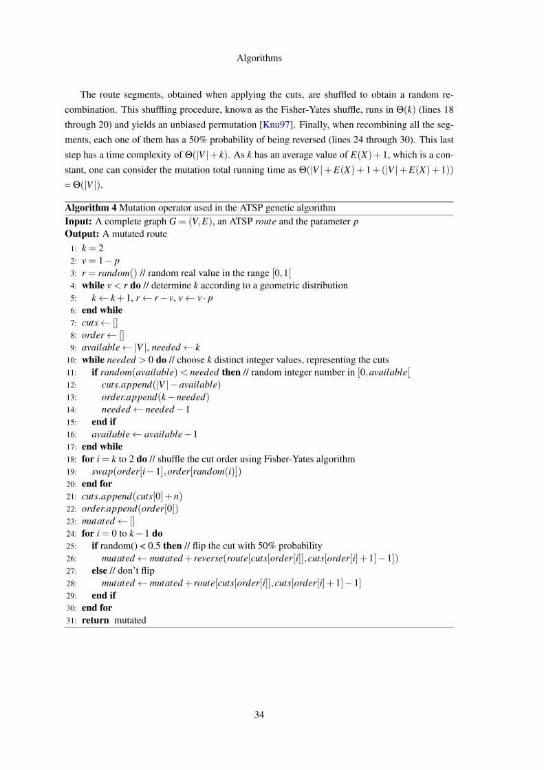
Algorithms

The route segments, obtained when applying the cuts, are shuffled to obtain a random re-

combination. This shuffling procedure, known as the Fisher-Yates shuffle, runs in Θ(k) (lines 18

through 20) and yields an unbiased permutation [Knu97]. Finally, when recombining all the seg-

ments, each one of them has a 50% probability of being reversed (lines 24 through 30). This last

step has a time complexity of Θ(|V |+ k). As k has an average value of E(X)+1, which is a con-

stant, one can consider the mutation total running time as Θ(|V |+E(X)+ 1+(|V |+E(X)+ 1))

= Θ(|V |).

Algorithm 4 Mutation operator used in the ATSP genetic algorithmInput: A complete graph G = (V,E), an ATSP route and the parameter pOutput: A mutated route

1: k = 22: v = 1− p3: r = random() // random real value in the range [0,1[4: while v < r do // determine k according to a geometric distribution5: k← k+1, r← r− v, v← v · p6: end while7: cuts← []8: order← []9: available← |V |, needed← k

10: while needed > 0 do // choose k distinct integer values, representing the cuts11: if random(available)< needed then // random integer number in [0,available[12: cuts.append(|V |−available)13: order.append(k−needed)14: needed← needed−115: end if16: available← available−117: end while18: for i = k to 2 do // shuffle the cut order using Fisher-Yates algorithm19: swap(order[i−1],order[random(i)])20: end for21: cuts.append(cuts[0]+n)22: order.append(order[0])23: mutated← []24: for i = 0 to k−1 do25: if random() < 0.5 then // flip the cut with 50% probability26: mutated← mutated + reverse(route[cuts[order[i]],cuts[order[i]+1]−1])27: else // don’t flip28: mutated← mutated + route[cuts[order[i]],cuts[order[i]+1]−1]29: end if30: end for31: return mutated

34

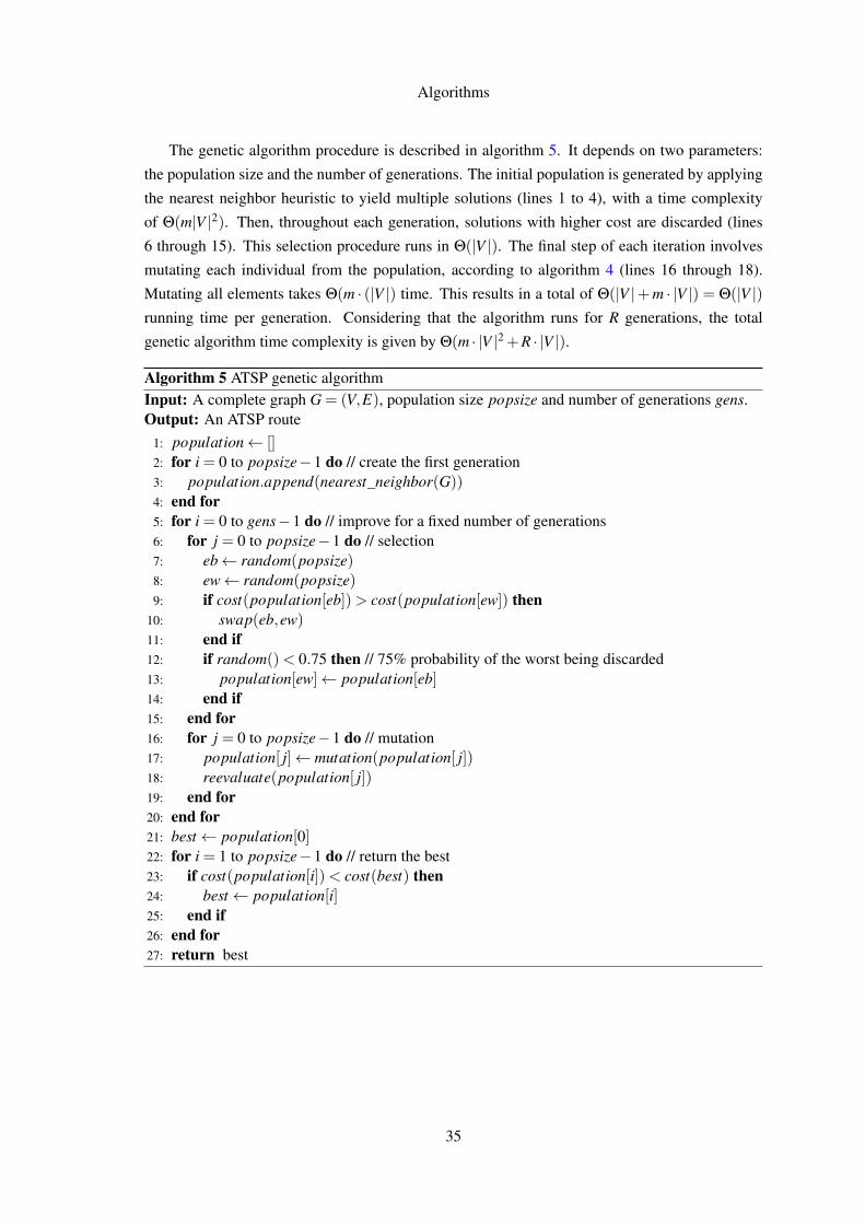
Algorithms

The genetic algorithm procedure is described in algorithm 5. It depends on two parameters:

the population size and the number of generations. The initial population is generated by applying

the nearest neighbor heuristic to yield multiple solutions (lines 1 to 4), with a time complexity

of Θ(m|V |2). Then, throughout each generation, solutions with higher cost are discarded (lines

6 through 15). This selection procedure runs in Θ(|V |). The final step of each iteration involves

mutating each individual from the population, according to algorithm 4 (lines 16 through 18).

Mutating all elements takes Θ(m · (|V |) time. This results in a total of Θ(|V |+m · |V |) = Θ(|V |)running time per generation. Considering that the algorithm runs for R generations, the total

genetic algorithm time complexity is given by Θ(m · |V |2 +R · |V |).

Algorithm 5 ATSP genetic algorithmInput: A complete graph G = (V,E), population size popsize and number of generations gens.Output: An ATSP route

1: population← []2: for i = 0 to popsize−1 do // create the first generation3: population.append(nearest_neighbor(G))4: end for5: for i = 0 to gens−1 do // improve for a fixed number of generations6: for j = 0 to popsize−1 do // selection7: eb← random(popsize)8: ew← random(popsize)9: if cost(population[eb])> cost(population[ew]) then

10: swap(eb,ew)11: end if12: if random()< 0.75 then // 75% probability of the worst being discarded13: population[ew]← population[eb]14: end if15: end for16: for j = 0 to popsize−1 do // mutation17: population[ j]← mutation(population[ j])18: reevaluate(population[ j])19: end for20: end for21: best← population[0]22: for i = 1 to popsize−1 do // return the best23: if cost(population[i])< cost(best) then24: best← population[i]25: end if26: end for27: return best

35

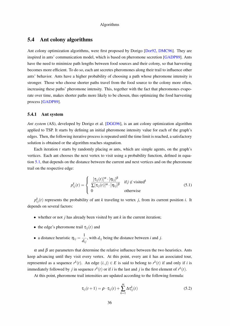
Algorithms

5.4 Ant colony algorithms

Ant colony optimization algorithms, were first proposed by Dorigo [Dor92, DMC96]. They are

inspired in ants’ communication model, which is based on pheromone secretion [GADP89]. Ants

have the need to minimize path lengths between food sources and their colony, so that harvesting

becomes more efficient. To do so, each ant secretes pheromones along their trail to influence other

ants’ behavior. Ants have a higher probability of choosing a path whose pheromone intensity is

stronger. Those who choose shorter paths travel from the food source to the colony more often,

increasing these paths’ pheromone intensity. This, together with the fact that pheromones evapo-

rate over time, makes shorter paths more likely to be chosen, thus optimizing the food harvesting

process [GADP89].

5.4.1 Ant system

Ant system (AS), developed by Dorigo et al. [DGG96], is an ant colony optimization algorithm

applied to TSP. It starts by defining an initial pheromone intensity value for each of the graph’s

edges. Then, the following iterative process is repeated until the time limit is reached, a satisfactory

solution is obtained or the algorithm reaches stagnation.

Each iteration t starts by randomly placing m ants, which are simple agents, on the graph’s

vertices. Each ant chooses the next vertex to visit using a probability function, defined in equa-

tion 5.1, that depends on the distance between the current and next vertices and on the pheromone

trail on the respective edge:

pki j(t) =

[τi j(t)]α · [ηi j]

β

∑[τi j(t)]α · [ηi j]βif j 6∈ visitedk

0 otherwise(5.1)

pki j(t) represents the probability of ant k traveling to vertex j, from its current position i. It

depends on several factors:

• whether or not j has already been visited by ant k in the current iteration;

• the edge’s pheromone trail τi j(t) and

• a distance heuristic ηi j =1

di j, with di j being the distance between i and j.

α and β are parameters that determine the relative influence between the two heuristics. Ants

keep advancing until they visit every vertex. At this point, every ant k has an associated tour,

represented as a sequence rk(t). An edge (i, j) ∈ E is said to belong to rk(t) if and only if i is

immediately followed by j in sequence rk(t) or if i is the last and j is the first element of rk(t).

At this point, pheromone trail intensities are updated according to the following formula:

τi j(t +1) = ρ · τi j(t)+m

∑k=1

∆τki j(t) (5.2)

36

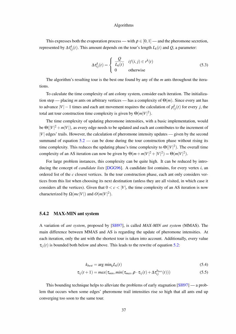
Algorithms

This expresses both the evaporation process — with ρ ∈ [0,1] — and the pheromone secretion,

represented by ∆τki j(t). This amount depends on the tour’s length Lk(t) and Q, a parameter:

∆τki j(t) =

Q

Lk(t)i f (i, j) ∈ rk(t)

0 otherwise(5.3)

The algorithm’s resulting tour is the best one found by any of the m ants throughout the itera-

tions.

To calculate the time complexity of ant colony system, consider each iteration. The initializa-

tion step — placing m ants on arbitrary vertices — has a complexity of Θ(m). Since every ant has

to advance |V |−1 times and each ant movement requires the calculation of pki j(t) for every j, the

total ant tour construction time complexity is given by Θ(m|V |2).The time complexity of updating pheromone intensities, with a basic implementation, would

be Θ(|V |2 +m|V |), as every edge needs to be updated and each ant contributes to the increment of

|V | edges’ trails. However, the calculation of pheromone intensity updates — given by the second

summand of equation 5.2 — can be done during the tour construction phase without rising its

time complexity. This reduces the updating phase’s time complexity to Θ(|V |2). The overall time

complexity of an AS iteration can now be given by Θ(m+m|V |2 + |V |2) = Θ(m|V |2).For large problem instances, this complexity can be quite high. It can be reduced by intro-

ducing the concept of candidate lists [DGG96]. A candidate list contains, for every vertex i, an

ordered list of the c closest vertices. In the tour construction phase, each ant only considers ver-

tices from this list when choosing its next destination (unless they are all visited, in which case it

considers all the vertices). Given that 0 < c < |V |, the time complexity of an AS iteration is now

characterized by Ω(mc|V |) and O(m|V |2).

5.4.2 MAX-MIN ant system

A variation of ant system, proposed by [SH97], is called MAX-MIN ant system (MMAS). The

main difference between MMAS and AS is regarding the update of pheromone intensities. At

each iteration, only the ant with the shortest tour is taken into account. Additionally, every value

τi j(t) is bounded both below and above. This leads to the rewrite of equation 5.2:

kbest = arg minkLk(t) (5.4)

τi j(t +1) = max(τmin,min(τmax,ρ · τi j(t)+∆τkbesti j (t))) (5.5)

This bounding technique helps to alleviate the problems of early stagnation [SH97] — a prob-

lem that occurs when some edges’ pheromone trail intensities rise so high that all ants end up

converging too soon to the same tour.

37

Algorithms

Additionally, MMAS is stated to be one of the best performing ant colony algorithms [SH00]

and its convergence has been proved [SD02]. This led to the choosing of MMAS for further

analysis and comparison with other approaches.

The pseudo-code for the algorithm used when deciding which vertex an ant should move to is

given in algorithm 6. It starts by gathering the first c vertices that are to be visited, while calculating

the probability of each one being chosen (lines 3 through 12). This probability depends on both

distance and pheromone intensity of the arc, as well as on two parameters that determine the

influence of each heuristic: α and β . Lines 13 through 19 implement the selection based on the

probabilities. The time complexity for the vertex selection is given by the lower bound Ω(c) and

the upper bound O(|V |).

Algorithm 6 Ant vertex selection used in max-min ant systemInput: A graph G = (V,E), pheromone levels pheromones, ant’s visited vertices route and pa-rameters α and β

Output: The next vertex to be visited by the ant1: candidates← [], odds← []2: total← 0, current← route[|route|−1]3: for all v ∈V do4: if v 6∈ route then5: candidates.append(v)6: r← cost(current,v)α · (pheromones[current][v])β

7: total← total + r8: odds.append(r)9: end if

10: if |candidates|== c then10: break11: end if12: end for13: r← random() · total14: for k = 0 to |odds|−1 do15: r← r−odds[k]16: if r ≤ 0 then17: return candidates[k]18: end if19: end for

The pseudo-code for MMAS is given by algorithm 7. First, it initializes the pheromone values

for each edge, each represented by a pair of vertices, in Θ(|V |2) time (lines 2 through 7). Then,

in each iteration, m ants are placed in randomly chosen vertices (lines 10 through 12), in Θ(m)

time. Each ant then procedes to move to the next vertex (using algorithm 6) until all vertices are

visited. The vertex selection method is executed Θ(m|V |) times, yielding a total time complexity

described by the bounds Ω(mc|V |) and O(m|V |2). This is followed by the evaporation process

(lines 18 through 22), that runs in Θ(|V |2). The final step regards pheromone update using the

lowest cost route obtained in this iteration (lines 24 through 32), and it runs in Θ(|V |+m).

38

Algorithms

Considering that MAX-MIN ant system runs for R iterations, using m ants, a candidate list of

size c and that the heuristic used in line 1 runs in Θ(H) time, the total running time is given by the

bounds Ω(H +(|V |2 +mc|V |) ·R) and O(H +m|V |2 ·R).

Algorithm 7 Max-min ant systemInput: A complete graph G = (V,E)Output: An ATSP route

1: best← heuristic(G)2: pheromones← []3: for all v ∈V do // pheromone initialization4: for all w ∈V do5: pheromones[v][w]← τmin

6: end for7: end for8: for r = 1 to iterations do9: routes← []

10: for i = 0 to m−1 do // ant initialization, starting in a random vertex11: routes.append([random(|V |)])12: end for13: for i = 1 to |V |−1 do // each ant must advance |V |−1 times14: for j = 0 to m−1 do15: routes[ j].append(ant_selection(G, pheromones,routes[ j],al pha,beta))16: end for17: end for18: for all v ∈V do // pheromone evaporation19: for all w ∈V do20: pheromones[v][w]← max(τmin, pheromones[v][w] ·ρ)21: end for22: end for23: route← routes[0]24: for i = 1 to m−1 do25: if cost(routes[i])< cost(route) then26: route← routes[i]27: end if28: end for29: for i = 0 to |V |−1 do // pheromone update30: v← route[i], w← route[(i+1)%|V |]31: pheromone[v][w]← min(τmax, pheromones[v][w]+ cost(route)−1)32: end for33: if cost(route)< cost(best) then34: best← route35: end if36: end for37: return best

39

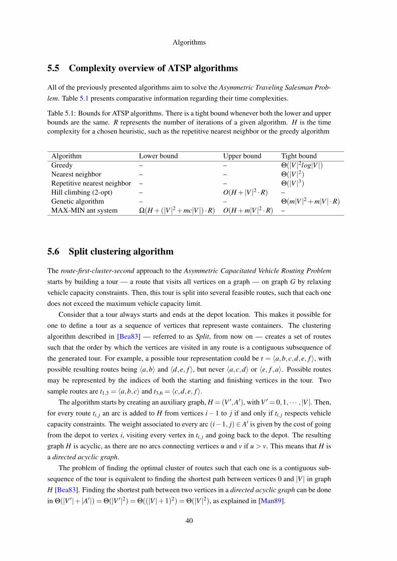
Algorithms

5.5 Complexity overview of ATSP algorithms

All of the previously presented algorithms aim to solve the Asymmetric Traveling Salesman Prob-

lem. Table 5.1 presents comparative information regarding their time complexities.

Table 5.1: Bounds for ATSP algorithms. There is a tight bound whenever both the lower and upperbounds are the same. R represents the number of iterations of a given algorithm. H is the timecomplexity for a chosen heuristic, such as the repetitive nearest neighbor or the greedy algorithm

Algorithm Lower bound Upper bound Tight boundGreedy – – Θ(|V |2log|V |)Nearest neighbor – – Θ(|V |2)Repetitive nearest neighbor – – Θ(|V |3)Hill climbing (2-opt) – O(H + |V |2 ·R) –Genetic algorithm – – Θ(m|V |2 +m|V | ·R)MAX-MIN ant system Ω(H +(|V |2 +mc|V |) ·R) O(H +m|V |2 ·R) –

5.6 Split clustering algorithm

The route-first-cluster-second approach to the Asymmetric Capacitated Vehicle Routing Problem

starts by building a tour — a route that visits all vertices on a graph — on graph G by relaxing

vehicle capacity constraints. Then, this tour is split into several feasible routes, such that each one

does not exceed the maximum vehicle capacity limit.

Consider that a tour always starts and ends at the depot location. This makes it possible for

one to define a tour as a sequence of vertices that represent waste containers. The clustering

algorithm described in [Bea83] — referred to as Split, from now on — creates a set of routes

such that the order by which the vertices are visited in any route is a contiguous subsequence of

the generated tour. For example, a possible tour representation could be t = 〈a,b,c,d,e, f 〉, with

possible resulting routes being 〈a,b〉 and 〈d,e, f 〉, but never 〈a,c,d〉 or 〈e, f ,a〉. Possible routes

may be represented by the indices of both the starting and finishing vertices in the tour. Two

sample routes are t1,3 = 〈a,b,c〉 and t3,6 = 〈c,d,e, f 〉.The algorithm starts by creating an auxiliary graph, H = (V ′,A′), with V ′= 0,1, · · · , |V |. Then,

for every route ti, j an arc is added to H from vertices i− 1 to j if and only if ti, j respects vehicle

capacity constraints. The weight associated to every arc (i−1, j)∈ A′ is given by the cost of going

from the depot to vertex i, visiting every vertex in ti, j and going back to the depot. The resulting

graph H is acyclic, as there are no arcs connecting vertices u and v if u > v. This means that H is

a directed acyclic graph.

The problem of finding the optimal cluster of routes such that each one is a contiguous sub-

sequence of the tour is equivalent to finding the shortest path between vertices 0 and |V | in graph

H [Bea83]. Finding the shortest path between two vertices in a directed acyclic graph can be done

in Θ(|V ′|+ |A′|) = Θ(|V ′|2) = Θ((|V |+1)2) = Θ(|V |2), as explained in [Man89].

40

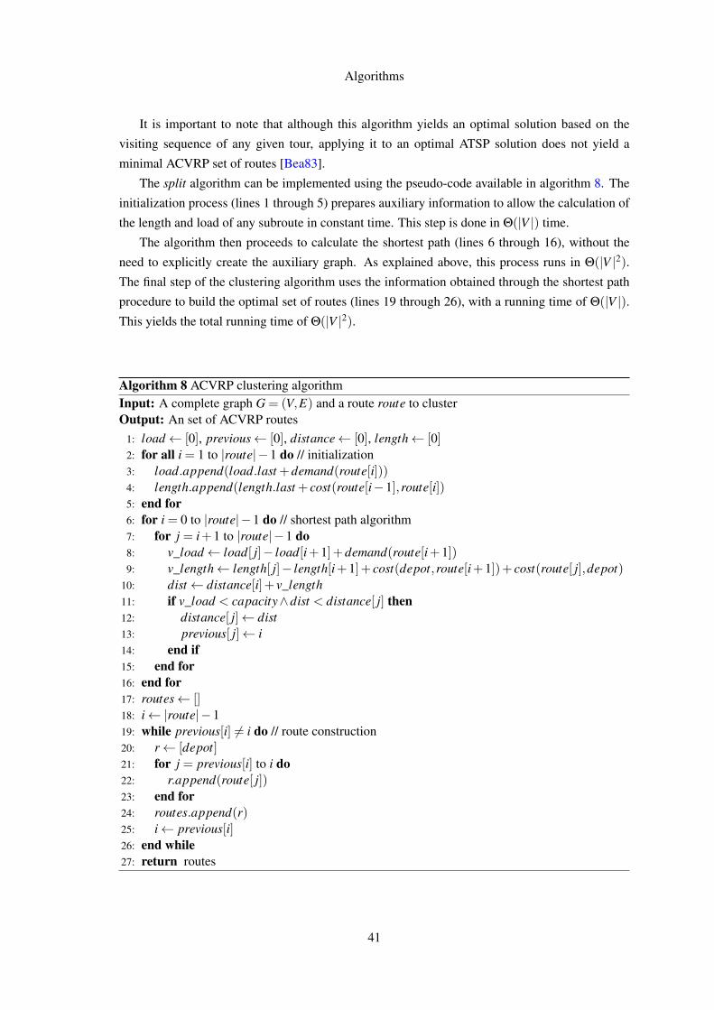
Algorithms

It is important to note that although this algorithm yields an optimal solution based on the

visiting sequence of any given tour, applying it to an optimal ATSP solution does not yield a

minimal ACVRP set of routes [Bea83].

The split algorithm can be implemented using the pseudo-code available in algorithm 8. The

initialization process (lines 1 through 5) prepares auxiliary information to allow the calculation of

the length and load of any subroute in constant time. This step is done in Θ(|V |) time.

The algorithm then proceeds to calculate the shortest path (lines 6 through 16), without the

need to explicitly create the auxiliary graph. As explained above, this process runs in Θ(|V |2).The final step of the clustering algorithm uses the information obtained through the shortest path

procedure to build the optimal set of routes (lines 19 through 26), with a running time of Θ(|V |).This yields the total running time of Θ(|V |2).

Algorithm 8 ACVRP clustering algorithmInput: A complete graph G = (V,E) and a route route to clusterOutput: An set of ACVRP routes

1: load← [0], previous← [0], distance← [0], length← [0]2: for all i = 1 to |route|−1 do // initialization3: load.append(load.last +demand(route[i]))4: length.append(length.last + cost(route[i−1],route[i])5: end for6: for i = 0 to |route|−1 do // shortest path algorithm7: for j = i+1 to |route|−1 do8: v_load← load[ j]− load[i+1]+demand(route[i+1])9: v_length← length[ j]− length[i+1]+ cost(depot,route[i+1])+ cost(route[ j],depot)

10: dist← distance[i]+ v_length11: if v_load < capacity∧dist < distance[ j] then12: distance[ j]← dist13: previous[ j]← i14: end if15: end for16: end for17: routes← []18: i← |route|−119: while previous[i] 6= i do // route construction20: r← [depot]21: for j = previous[i] to i do22: r.append(route[ j])23: end for24: routes.append(r)25: i← previous[i]26: end while27: return routes

41

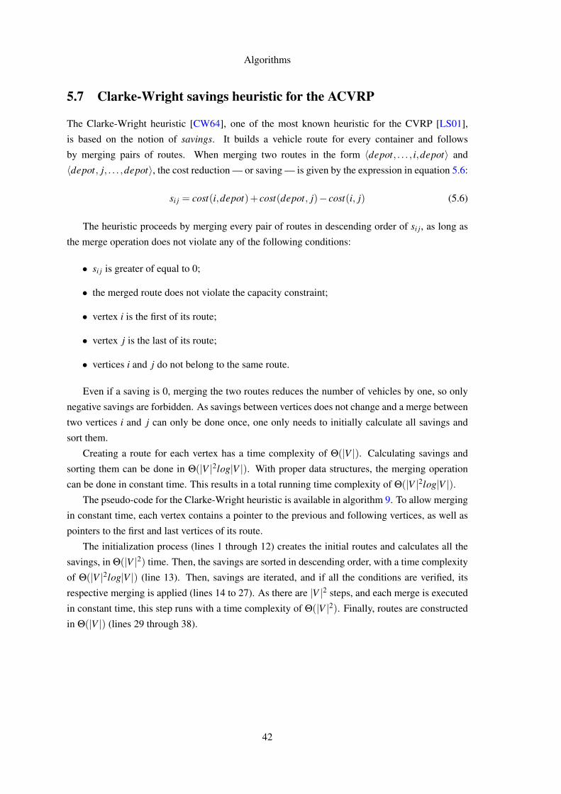
Algorithms

5.7 Clarke-Wright savings heuristic for the ACVRP

The Clarke-Wright heuristic [CW64], one of the most known heuristic for the CVRP [LS01],

is based on the notion of savings. It builds a vehicle route for every container and follows

by merging pairs of routes. When merging two routes in the form 〈depot, . . . , i,depot〉 and

〈depot, j, . . . ,depot〉, the cost reduction — or saving — is given by the expression in equation 5.6:

si j = cost(i,depot)+ cost(depot, j)− cost(i, j) (5.6)

The heuristic proceeds by merging every pair of routes in descending order of si j, as long as

the merge operation does not violate any of the following conditions:

• si j is greater of equal to 0;

• the merged route does not violate the capacity constraint;

• vertex i is the first of its route;

• vertex j is the last of its route;

• vertices i and j do not belong to the same route.

Even if a saving is 0, merging the two routes reduces the number of vehicles by one, so only

negative savings are forbidden. As savings between vertices does not change and a merge between

two vertices i and j can only be done once, one only needs to initially calculate all savings and

sort them.

Creating a route for each vertex has a time complexity of Θ(|V |). Calculating savings and

sorting them can be done in Θ(|V |2log|V |). With proper data structures, the merging operation

can be done in constant time. This results in a total running time complexity of Θ(|V |2log|V |).The pseudo-code for the Clarke-Wright heuristic is available in algorithm 9. To allow merging

in constant time, each vertex contains a pointer to the previous and following vertices, as well as

pointers to the first and last vertices of its route.

The initialization process (lines 1 through 12) creates the initial routes and calculates all the

savings, in Θ(|V |2) time. Then, the savings are sorted in descending order, with a time complexity

of Θ(|V |2log|V |) (line 13). Then, savings are iterated, and if all the conditions are verified, its

respective merging is applied (lines 14 to 27). As there are |V |2 steps, and each merge is executed

in constant time, this step runs with a time complexity of Θ(|V |2). Finally, routes are constructed

in Θ(|V |) (lines 29 through 38).

42

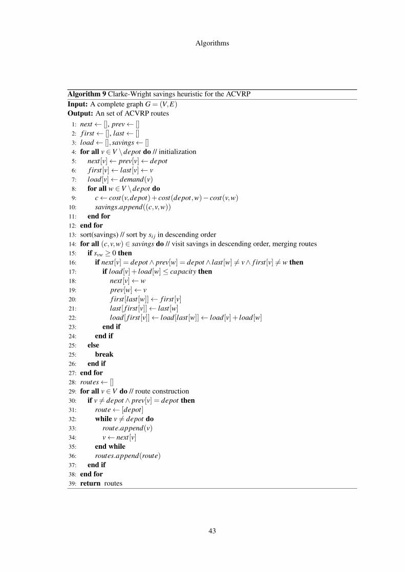
Algorithms

Algorithm 9 Clarke-Wright savings heuristic for the ACVRPInput: A complete graph G = (V,E)Output: An set of ACVRP routes

1: next← [], prev← []2: f irst← [], last← []3: load← [],savings← []4: for all v ∈V \depot do // initialization5: next[v]← prev[v]← depot6: f irst[v]← last[v]← v7: load[v]← demand(v)8: for all w ∈V \depot do9: c← cost(v,depot)+ cost(depot,w)− cost(v,w)

10: savings.append((c,v,w))11: end for12: end for13: sort(savings) // sort by si j in descending order14: for all (c,v,w) ∈ savings do // visit savings in descending order, merging routes15: if svw ≥ 0 then16: if next[v] = depot ∧ prev[w] = depot ∧ last[w] 6= v∧ f irst[v] 6= w then17: if load[v]+ load[w]≤ capacity then18: next[v]← w19: prev[w]← v20: f irst[last[w]]← f irst[v]21: last[ f irst[v]]← last[w]22: load[ f irst[v]]← load[last[w]]← load[v]+ load[w]23: end if24: end if25: else25: break26: end if27: end for28: routes← []29: for all v ∈V do // route construction30: if v 6= depot ∧ prev[v] = depot then31: route← [depot]32: while v 6= depot do33: route.append(v)34: v← next[v]35: end while36: routes.append(route)37: end if38: end for39: return routes

43

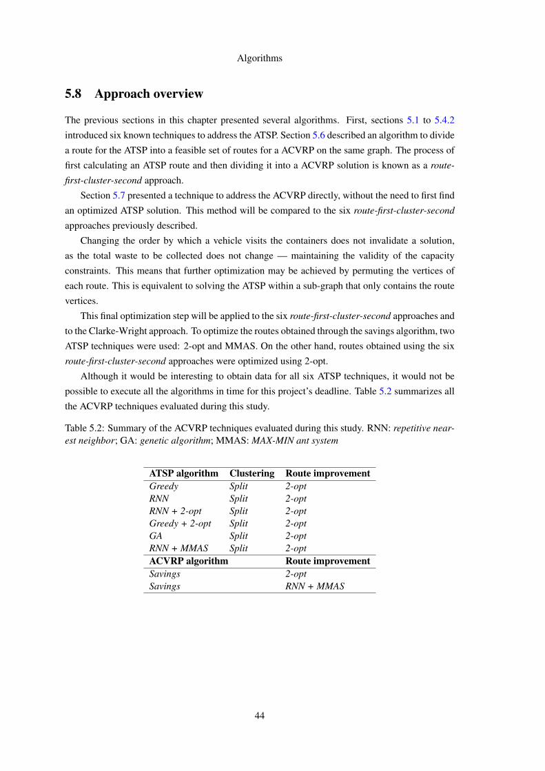
Algorithms

5.8 Approach overview

The previous sections in this chapter presented several algorithms. First, sections 5.1 to 5.4.2

introduced six known techniques to address the ATSP. Section 5.6 described an algorithm to divide

a route for the ATSP into a feasible set of routes for a ACVRP on the same graph. The process of

first calculating an ATSP route and then dividing it into a ACVRP solution is known as a route-

first-cluster-second approach.

Section 5.7 presented a technique to address the ACVRP directly, without the need to first find

an optimized ATSP solution. This method will be compared to the six route-first-cluster-second

approaches previously described.

Changing the order by which a vehicle visits the containers does not invalidate a solution,

as the total waste to be collected does not change — maintaining the validity of the capacity

constraints. This means that further optimization may be achieved by permuting the vertices of

each route. This is equivalent to solving the ATSP within a sub-graph that only contains the route

vertices.

This final optimization step will be applied to the six route-first-cluster-second approaches and

to the Clarke-Wright approach. To optimize the routes obtained through the savings algorithm, two

ATSP techniques were used: 2-opt and MMAS. On the other hand, routes obtained using the six

route-first-cluster-second approaches were optimized using 2-opt.

Although it would be interesting to obtain data for all six ATSP techniques, it would not be

possible to execute all the algorithms in time for this project’s deadline. Table 5.2 summarizes all

the ACVRP techniques evaluated during this study.

Table 5.2: Summary of the ACVRP techniques evaluated during this study. RNN: repetitive near-est neighbor; GA: genetic algorithm; MMAS: MAX-MIN ant system

ATSP algorithm Clustering Route improvementGreedy Split 2-optRNN Split 2-optRNN + 2-opt Split 2-optGreedy + 2-opt Split 2-optGA Split 2-optRNN + MMAS Split 2-optACVRP algorithm Route improvementSavings 2-optSavings RNN + MMAS

44

Algorithms

5.9 Validation of algorithm implementations

After implementing the algorithms described in this chapter, there was the need to validate their

results. Validation is done by applying these algorithms to standard TSPLIB datasets and com-

paring the results to either the optimum route cost (when known) or to the best route found so

far.

5.9.1 ATSP validation

First, construction heuristics — greedy and repetitive nearest neighbor —, hill climbing, the ge-

netic algorithm and MAX-MIN ant system were validated against ATSP instances. This allows one

to verify if these techniques successfully build a near-optimal tour.

It is important to note that, as hill climbing and MAX-MIN ant system both depend on the

repetitive nearest neighbor technique, their resulting routes are always better or equal to the one

obtained by this construction heuristic.

Results are presented in table 5.3. All parameters used to obtain these values are according to

the original authors of each algorithm. Both GA and MMAS were executed for 1000 iterations.

GA was run with a population of 100 and p = 0.35. MMAS was run with 200 ants and β = 5.

Table 5.3: Performance of our heuristic and meta-heuristic implementations using the datasetsfrom TSPLIB. Performance is given in the form of the ratio between the heuristic’s route averagecost and the dataset optimum (minimum) cost.

Dataset Vertices Optimum Greedy RNN Greedy+ 2-opt

RNN +2-opt

GA MMAS

br17 17 39 1.97 1.43 1.00 1.00 1.00 1.00ftv33 33 1286 1.16 1.23 1.14 1.17 1.17 1.00ftv35 35 1473 1.30 1.13 1.31 1.13 1.13 1.04ftv38 38 1530 1.25 1.14 1.24 1.08 1.08 1.07

p43 43 5620 1.03 1.01 1.00 1.00 1.00 1.00ftv44 44 1613 1.23 1.14 1.24 1.14 1.09 1.03ftv47 47 1776 1.27 1.22 1.27 1.20 1.15 1.11ry48p 48 14422 1.32 1.07 1.04 1.02 1.05 1.02

ft53 53 6905 1.77 1.24 1.54 1.18 1.19 1.15ftv55 55 1608 1.40 1.21 1.34 1.21 1.13 1.07ftv64 64 1839 1.36 1.19 1.29 1.17 1.16 1.04ftv70 70 1950 1.30 1.17 1.26 1.17 1.16 1.09ft70 70 38673 1.14 1.08 1.11 1.06 1.05 1.04

kro124p 124 36230 1.21 1.19 1.15 1.17 1.15 1.08ftv170 170 2755 1.43 1.30 1.40 1.28 1.24 1.18

Table 5.3 shows that 2-opt, GA and MMAS yield significantly better results than the heuristics.

MMAS, using only 1000 iterations, produces results within 5% of the optimal solution for half of

the datasets.

45

Algorithms

5.9.2 ACVRP validation

Having validated the six ATSP techniques, it is necessary to validate the eight ACVRP approaches

described in section 5.8 (table 5.2). These approaches were applied to the CVRP datasets available

in TSPLIB to obtain the benchmarks in table 5.4.

Table 5.4: Performance of our heuristic and meta-heuristic implementations using the datasetsfrom TSPLIB. Performance is given in the form of the ratio between the heuristic’s route averagecost and the dataset reference solution’s cost.

Vertices Greedy RNN Greedy+ 2-opt

RNN +2-opt

GA MMAS Savings+ 2-opt

Savings+ MMAS

13 1.223 1.198 1.198 1.193 1.223 1.190 1.174 1.17422 1.204 1.122 1.068 1.046 1.012 1.062 1.037 1.03723 1.172 1.066 1.012 1.030 1.066 1.007 1.013 0.99930 0.961 0.961 0.954 0.979 0.946 0.946 1.001 0.95231 1.472 1.631 1.760 1.548 1.451 1.310 1.657 1.61733 1.066 1.042 1.034 1.037 1.033 1.033 1.010 1.00951 1.148 1.137 1.139 1.110 1.087 1.095 1.136 1.12576 1.408 1.346 1.346 1.342 1.319 1.348 1.332 1.30676 1.593 1.573 1.515 1.498 1.518 1.491 1.471 1.47176 1.053 0.994 1.031 0.990 0.977 0.989 0.951 0.93576 0.772 0.759 0.780 0.746 0.732 0.757 0.747 0.719

101 1.217 1.167 1.168 1.123 1.070 1.093 1.090 1.076101 1.176 1.136 1.141 1.120 1.130 1.072 1.076 1.066262 1.019 1.013 1.036 0.998 0.986 0.996 0.952 0.945

It is important to remember that the reference values for these datasets represent solutions

for a fixed number of vehicles, specified in the dataset. When applied to this specific problem,

the number of vehicles is a decision variable, and not a fixed number. This explains why some

algorithms yield solutions with ratios below 1.0, as it may be possible to obtain routes that are

more efficient by using a different number of vehicles.

This values show that the route-first-cluster-second approach, using any of the six ATSP tech-

niques, is surpassed by the savings heuristic in most of the CVRP datasets. However, there are

two facts that must be taken into account. First, all of TSPLIB’s CVRP datasets are symmetric.

Second, these datasets only go up to 262 vertices. Datasets used in chapter 6 are asymmetric and

contain a much higher number of vertices. With this in mind, the values in table 5.4 are insufficient

to determine if the savings approach is better or not than the route-first-cluster-second approaches.

46

Algorithms

5.10 Chapter summary

This chapter described a set of algorithms that can be used to address the Asymmetric Capacitated

Vehicle Routing Problem. Most of these start by solving the associated Asymmetric Traveling

Salesman Problem, by ignoring capacity constraints, and subsequently split the resulting tour into

vehicle routes using the algorithm described in section 5.6. Additionally, a heuristic for the CVRP

was also described — the Clarke-Wright savings heuristic. This technique does not start by solving

the ATSP, and therefore it is not a route-first-cluster-second approach.

The following chapter presents the results for a sensitivity analysis on MAX-MIN ant system’s

parameters, to maximize its performance. This is followed by an exposition of the results obtained

when applying the eight techniques for the ACVRP to the large datasets. Although this chapter

already provided some results regarding their comparative performance, the validation datasets are

quite different from the ones to be used when the optimization framework is deployed.

47

Algorithms

48

Chapter 6

Results

This chapter reports several benchmarks analyzing the performance of several algorithms, as well

as benchmarks to analyze the influence of several parameters of the MAX-MIN ant system.

The first section, section 6.1, presents the sensitivity analysis on MAX-MIN ant system’s pa-

rameters. It provides information that allows one to balance the trade-off between route efficiency

and running time.

Section 6.2 presents the benchmark results that compare the techniques described in the previ-

ous chapter when applied to the large Asymmetric Capacitated Vehicle Routing Problem datasets.

Unless specified otherwise, all benchmarks shown are obtained through averaging ten runs for

each algorithm/dataset. All running times were obtained by running the algorithms on the same

hardware and platform. The CPU was an Intel R© Xeon R©, running at 2.33 GHz with 1 GB of RAM,

running on the Ubuntu operating system, a Linux distribution.

6.1 Sensitivity of MAX-MIN ant system to algorithm parameters

To understand how MMAS parameters influence the performance of the resulting routes, there

was the need to execute a series of benchmarks and comparisons. These were done by varying the

target parameter’s value and by using the validation datasets. This analysis will aid in configuring

the parameters for the application of this technique to larger datasets.

49

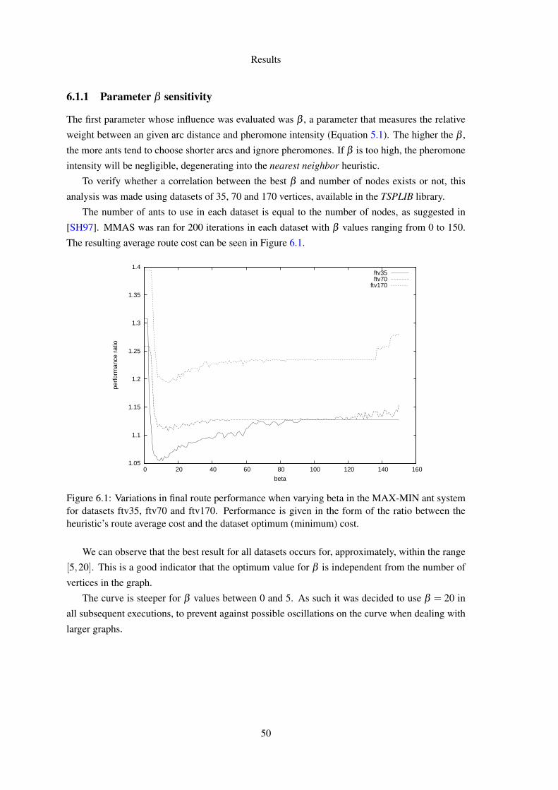
Results

6.1.1 Parameter β sensitivity

The first parameter whose influence was evaluated was β , a parameter that measures the relative

weight between an given arc distance and pheromone intensity (Equation 5.1). The higher the β ,

the more ants tend to choose shorter arcs and ignore pheromones. If β is too high, the pheromone

intensity will be negligible, degenerating into the nearest neighbor heuristic.

To verify whether a correlation between the best β and number of nodes exists or not, this

analysis was made using datasets of 35, 70 and 170 vertices, available in the TSPLIB library.

The number of ants to use in each dataset is equal to the number of nodes, as suggested in

[SH97]. MMAS was ran for 200 iterations in each dataset with β values ranging from 0 to 150.

The resulting average route cost can be seen in Figure 6.1.

1.05

1.1

1.15

1.2

1.25

1.3

1.35

1.4

0 20 40 60 80 100 120 140 160

perf

orm

ance

rat

io

beta

ftv35ftv70

ftv170

Figure 6.1: Variations in final route performance when varying beta in the MAX-MIN ant systemfor datasets ftv35, ftv70 and ftv170. Performance is given in the form of the ratio between theheuristic’s route average cost and the dataset optimum (minimum) cost.

We can observe that the best result for all datasets occurs for, approximately, within the range

[5,20]. This is a good indicator that the optimum value for β is independent from the number of

vertices in the graph.

The curve is steeper for β values between 0 and 5. As such it was decided to use β = 20 in

all subsequent executions, to prevent against possible oscillations on the curve when dealing with

larger graphs.

50

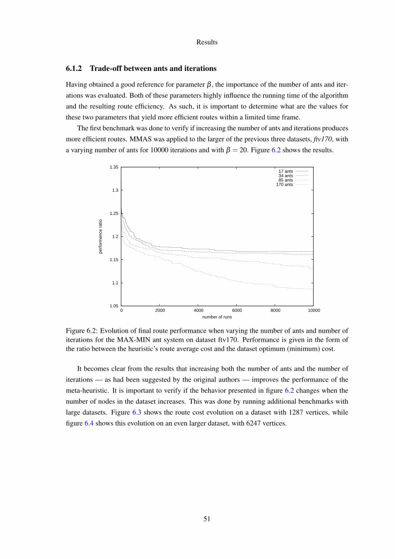
Results

6.1.2 Trade-off between ants and iterations

Having obtained a good reference for parameter β , the importance of the number of ants and iter-

ations was evaluated. Both of these parameters highly influence the running time of the algorithm

and the resulting route efficiency. As such, it is important to determine what are the values for

these two parameters that yield more efficient routes within a limited time frame.

The first benchmark was done to verify if increasing the number of ants and iterations produces

more efficient routes. MMAS was applied to the larger of the previous three datasets, ftv170, with

a varying number of ants for 10000 iterations and with β = 20. Figure 6.2 shows the results.

1.05

1.1

1.15

1.2

1.25

1.3

1.35

0 2000 4000 6000 8000 10000

perf

orm

ance

rat

io

number of runs

17 ants34 ants85 ants

170 ants

Figure 6.2: Evolution of final route performance when varying the number of ants and number ofiterations for the MAX-MIN ant system on dataset ftv170. Performance is given in the form ofthe ratio between the heuristic’s route average cost and the dataset optimum (minimum) cost.

It becomes clear from the results that increasing both the number of ants and the number of

iterations — as had been suggested by the original authors — improves the performance of the

meta-heuristic. It is important to verify if the behavior presented in figure 6.2 changes when the

number of nodes in the dataset increases. This was done by running additional benchmarks with

large datasets. Figure 6.3 shows the route cost evolution on a dataset with 1287 vertices, while

figure 6.4 shows this evolution on an even larger dataset, with 6247 vertices.

51

Results

94000

95000

96000

97000

98000

99000

100000

0 1000 2000 3000 4000 5000 6000 7000 8000 9000 10000

tour

leng

th

number of runs


1000 ants

Figure 6.3: Evolution of final tour length when varying the number of ants and number of iterationsfor the MAX-MIN ant system a dataset with 1287 vertices.

590000

595000

600000

605000

610000

615000

620000

625000

630000

635000

0 1000 2000 3000 4000 5000 6000 7000 8000 9000 10000

tour

leng

th

number of runs


1000 ants2000 ants

Figure 6.4: Evolution of final tour length when varying the number of ants and number of iterationsfor the MAX-MIN ant system a dataset with 6247 vertices.

The two figures 6.3 and 6.4 show that the behavior that occurred in figure 6.2 occurs, indepen-

dently of the number of vertices in the graph. The difference in the route efficiency, when varying

the number of ants, is more prominent for large number of iterations. The larger the dataset, the

higher the number of iterations has to be in order for this difference to be noticeable.

52

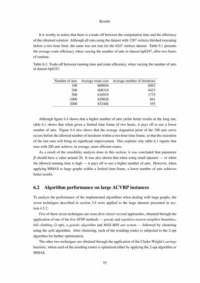
Results

It is worthy to notice that there is a trade-off between the computation time and the efficiency

of the obtained solution. Although all runs using the dataset with 1287 vertices finished executing

before a two hour limit, the same was not true for the 6247 vertices dataset. Table 6.1 presents

the average route efficiency when varying the number of ants in dataset hp6247, after two hours

of runtime.

Table 6.1: Trade-off between running time and route efficiency, when varying the number of antsin dataset hp6247.

Number of ants Average route cost Average number of iterations100 609056 6963200 608310 4423500 616919 1775

1000 629026 8412000 632468 355

Although figure 6.4 shows that a higher number of ants yields better results in the long run,

table 6.1 shows that when given a limited time frame of two hours, it pays off to use a lower

number of ants. Figure 6.4 also shows that the average stagnation point of the 100 ants curve

occurs before the allowed number of iterations within a two hour time-frame, so that the execution

of the last runs will bring no significant improvement. This explains why table 6.1 reports that

runs with 200 ants achieve, in average, more efficient routes.

As a result of the sensibility analysis done in this section, it was concluded that parameter

β should have a value around 20. It was also shown that when using small datasets — or when

the allowed running time is high — it pays off to use a higher number of ants. However, when

applying MMAS to large graphs within a limited time-frame, a lower number of ants achieves

better results.

6.2 Algorithm performance on large ACVRP instances

To analyze the performance of the implemented algorithms when dealing with large graphs, the

seven techniques described in section 5.8 were applied to the large datasets presented in sec-

tion 4.5.2.

Five of these seven techniques are route-first-cluster-second approaches, obtained through the

application of one of the five ATSP methods — greedy and repetitive nearest neighbor heuristics,

hill climbing (2-opt), a genetic algorithm and MAX-MIN ant system — followed by clustering

using the split algorithm. After clustering, each of the resulting routes is subjected to the 2-opt

algorithm for further optimization.

The other two techniques are obtained through the application of the Clarke-Wright’s savings

heuristic, where each of the resulting routes is optimized either by applying the 2-opt algorithm or

MMAS.

53

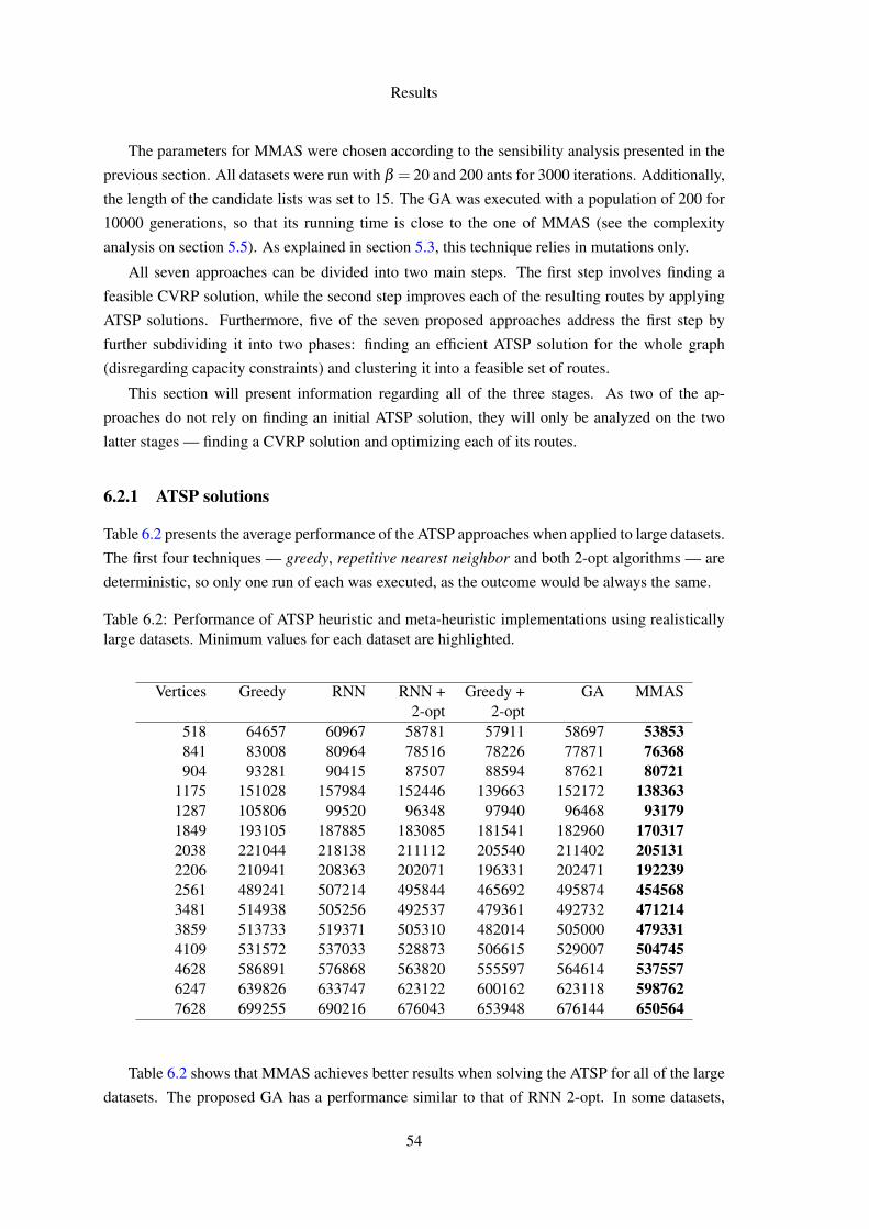
Results

The parameters for MMAS were chosen according to the sensibility analysis presented in the

previous section. All datasets were run with β = 20 and 200 ants for 3000 iterations. Additionally,

the length of the candidate lists was set to 15. The GA was executed with a population of 200 for

10000 generations, so that its running time is close to the one of MMAS (see the complexity

analysis on section 5.5). As explained in section 5.3, this technique relies in mutations only.

All seven approaches can be divided into two main steps. The first step involves finding a

feasible CVRP solution, while the second step improves each of the resulting routes by applying

ATSP solutions. Furthermore, five of the seven proposed approaches address the first step by

further subdividing it into two phases: finding an efficient ATSP solution for the whole graph

(disregarding capacity constraints) and clustering it into a feasible set of routes.

This section will present information regarding all of the three stages. As two of the ap-

proaches do not rely on finding an initial ATSP solution, they will only be analyzed on the two

latter stages — finding a CVRP solution and optimizing each of its routes.

6.2.1 ATSP solutions

Table 6.2 presents the average performance of the ATSP approaches when applied to large datasets.

The first four techniques — greedy, repetitive nearest neighbor and both 2-opt algorithms — are

deterministic, so only one run of each was executed, as the outcome would be always the same.

Table 6.2: Performance of ATSP heuristic and meta-heuristic implementations using realisticallylarge datasets. Minimum values for each dataset are highlighted.

Vertices Greedy RNN RNN +2-opt

Greedy +2-opt

GA MMAS

518 64657 60967 58781 57911 58697 53853841 83008 80964 78516 78226 77871 76368904 93281 90415 87507 88594 87621 80721

1175 151028 157984 152446 139663 152172 1383631287 105806 99520 96348 97940 96468 931791849 193105 187885 183085 181541 182960 1703172038 221044 218138 211112 205540 211402 2051312206 210941 208363 202071 196331 202471 1922392561 489241 507214 495844 465692 495874 4545683481 514938 505256 492537 479361 492732 4712143859 513733 519371 505310 482014 505000 4793314109 531572 537033 528873 506615 529007 5047454628 586891 576868 563820 555597 564614 5375576247 639826 633747 623122 600162 623118 5987627628 699255 690216 676043 653948 676144 650564

Table 6.2 shows that MMAS achieves better results when solving the ATSP for all of the large

datasets. The proposed GA has a performance similar to that of RNN 2-opt. In some datasets,

54

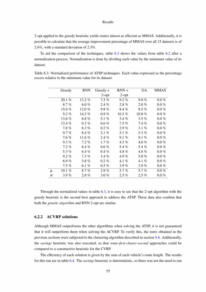
Results

2-opt applied to the greedy heuristic yields routes almost as efficient as MMAS. Additionally, it is

possible to calculate that the average improvement percentage of MMAS over all 15 datasets is of

2.6%, with a standard deviation of 2.5%.

To aid the comparison of the techniques, table 6.3 shows the values from table 6.2 after a

normalization process. Normalization is done by dividing each value by the minimum value of its

dataset.

Table 6.3: Normalized performance of ATSP techniques. Each value expressed as the percentageexcess relative to the minimum value for its dataset.

Greedy RNN Greedy +2-opt

RNN +2-opt

GA MMAS

20.1 % 13.2 % 7.5 % 9.2 % 9.0 % 0.0 %8.7 % 6.0 % 2.4 % 2.8 % 2.0 % 0.0 %

15.6 % 12.0 % 9.8 % 8.4 % 8.5 % 0.0 %9.2 % 14.2 % 0.9 % 10.2 % 10.0 % 0.0 %

13.6 % 6.8 % 5.1 % 3.4 % 3.5 % 0.0 %13.4 % 0.3 % 6.6 % 7.5 % 7.4 % 0.0 %

7.8 % 6.3 % 0.2 % 2.9 % 3.1 % 0.0 %9.7 % 8.4 % 2.1 % 5.1 % 5.3 % 0.0 %7.6 % 11.6 % 2.4 % 9.1 % 9.1 % 0.0 %9.3 % 7.2 % 1.7 % 4.5 % 4.6 % 0.0 %7.2 % 8.4 % 0.6 % 5.4 % 5.4 % 0.0 %5.3 % 6.4 % 0.4 % 4.8 % 4.8 % 0.0 %9.2 % 7.3 % 3.4 % 4.9 % 5.0 % 0.0 %6.9 % 5.8 % 0.2 % 4.1 % 4.1 % 0.0 %7.5 % 6.1 % 0.5 % 3.9 % 3.9 % 0.0 %

µ 10.1 % 8.7 % 2.9 % 5.7 % 5.7 % 0.0 %σ 3.9 % 2.8 % 3.0 % 2.5 % 2.5 % 0.0 %

Through the normalized values in table 6.3, it is easy to see that the 2-opt algorithm with the

greedy heuristic is the second best approach to address the ATSP. These data also confirm that

both the genetic algorithm and RNN 2-opt are similar.

6.2.2 ACVRP solutions

Although MMAS outperforms the other algorithms when solving the ATSP, it is not guaranteed

that it will outperform them when solving the ACVRP. To verify this, the tours obtained in the

previous sections were subjected to the clustering algorithm described in section 5.6. Additionally,

the savings heuristic was also executed, so that route-first-cluster-second approaches could be

compared to a constructive heuristic for the CVRP.

The efficiency of each solution is given by the sum of each vehicle’s route length. The results

for this run are in table 6.4. The savings heuristic is deterministic, so there was not the need to run

55

Results

it more than once. The genetic algorithm and max-min ant system had to be run multiple times,

due to their stochastic nature.

Table 6.4: Performance of heuristic and meta-heuristic implementations using realistically largedatasets. Minimum values for each dataset are highlighted.

Vertices Greedy RNN Greedy +2-opt

RNN +2-opt

GA MMAS Savings

518 78072 77564 71521 75933 75448 70640 93759841 114308 110422 109654 111192 107092 104913 115576904 120087 120124 112396 117111 116067 113603 124092

1175 223817 234530 224408 232428 232154 212875 1943121287 133382 132784 125682 129607 129669 126473 1522291849 263830 273410 257318 263879 263935 249708 2381012038 332029 333665 316529 317786 318345 304314 2810312206 319361 325752 303652 313078 319353 304754 2913172561 766226 777766 745094 767076 765974 733627 8319863481 903800 905700 865213 894672 894868 876834 9942993859 910598 917740 880713 904655 903134 879900 10400894109 1062410 1071682 1038768 1062764 1062898 1044653 11932484628 1099846 1104546 1067747 1091359 1095330 1070835 12452846247 1381520 1379607 1339356 1369770 1369637 1353391 16390087628 1579516 1595006 1537125 1577184 1577286 1556051 1912985

Table 6.4 shows that there is no direct relationship between the ATSP solution efficiency and

its respective ACVRP efficiency. Nevertheless, MMAS yields more efficient routes in some of the

datasets. The other two techniques that achieve the efficient routes for some datasets are the 2-opt

algorithm, when used with the greedy heuristic, and the savings construction heuristic.

Another important conclusion that the results on table 6.4 allow one to make is that although

the greedy heuristic has the lowest performance on the ATSP, this gap is greatly reduced after

applying the clustering algorithm.

This is better described by quantifying the difference between algorithms when transforming

ATSP solutions to ACVRP solutions. Table 6.5 shows, for each algorithm, the average excess

when compared to the best solution found for each dataset.

Table 6.5: Average route efficiency excess when comparing each algorithm to the best solutionfound for each dataset.

Greedy RNN Greedy +2-opt

RNN +2-opt

GA MMAS

ATSP 10.1 % 8.7 % 2.9 % 5.7 % 5.7 % 0.0 %ACVRP 7.3 % 8.1 % 3.2 % 6.1 % 5.9 % 2.2 %

56

Results

Table 6.5 show that the greedy has the highest improvement, even surpassing the repetitive

nearest neighbor heuristic. MMAS no longer dominates all the other algorithms (as shown in

table 6.4), but it is the algorithm with the lowest gap.

6.2.3 Route improvement

At this stage, each algorithm has already produced a feasible ACVRP solution, composed of sev-

eral routes. Each of the routes may be further optimized using the previously mentioned ATSP

techniques.

As shown in table 5.2, the six route-first-cluster-second approaches’ solutions will be opti-

mized using the 2-opt improvement technique. On the other hand, the savings constructive heuris-

tic will be optimized using two techniques: 2-opt and MMAS. Table 6.6 shows the final solution

costs for all techniques.

Table 6.6: Final ACVRP solutions’ performance, after the application of the 2-opt improvementtechnique. Minimum values for each dataset are highlighted.

2-opt improvement MMASGreedy RNN Greedy +

2optRNN +

2-optGA MMAS Savings Savings

70534 74469 70588 74917 74422 70161 91899 79032107288 103128 107304 106233 102727 103291 112972 108669112511 111993 109614 111479 113266 110986 120648 120223212389 225613 221932 230153 229544 208737 189620 190846124957 128623 124510 128624 128700 125161 149926 140379248255 264648 253844 259096 259068 247085 233170 236821309866 323190 310721 312768 312855 300796 276362 280927301713 312762 300303 306855 313087 301897 284023 284310740730 764905 740815 763068 761945 729603 823621 832580865570 887982 859474 885902 885972 873044 975839 965098874926 896603 871511 895631 893888 871832 1026658 987353

1030661 1056671 1033678 1053607 1053741 1041138 1179891 11548231058717 1088214 1057246 1085945 1090055 1064012 1212899 12162221332414 1360244 1328719 1360440 1360441 1344851 1620740 15823201518843 1565735 1520317 1562099 1562200 1544687 1894903 1840384

The information on table 6.6 shows that the minimum values for each dataset are now scattered

throughout the eight approaches. To help with the analysis between the approaches, table 6.7

presents a normalization of these results.

57

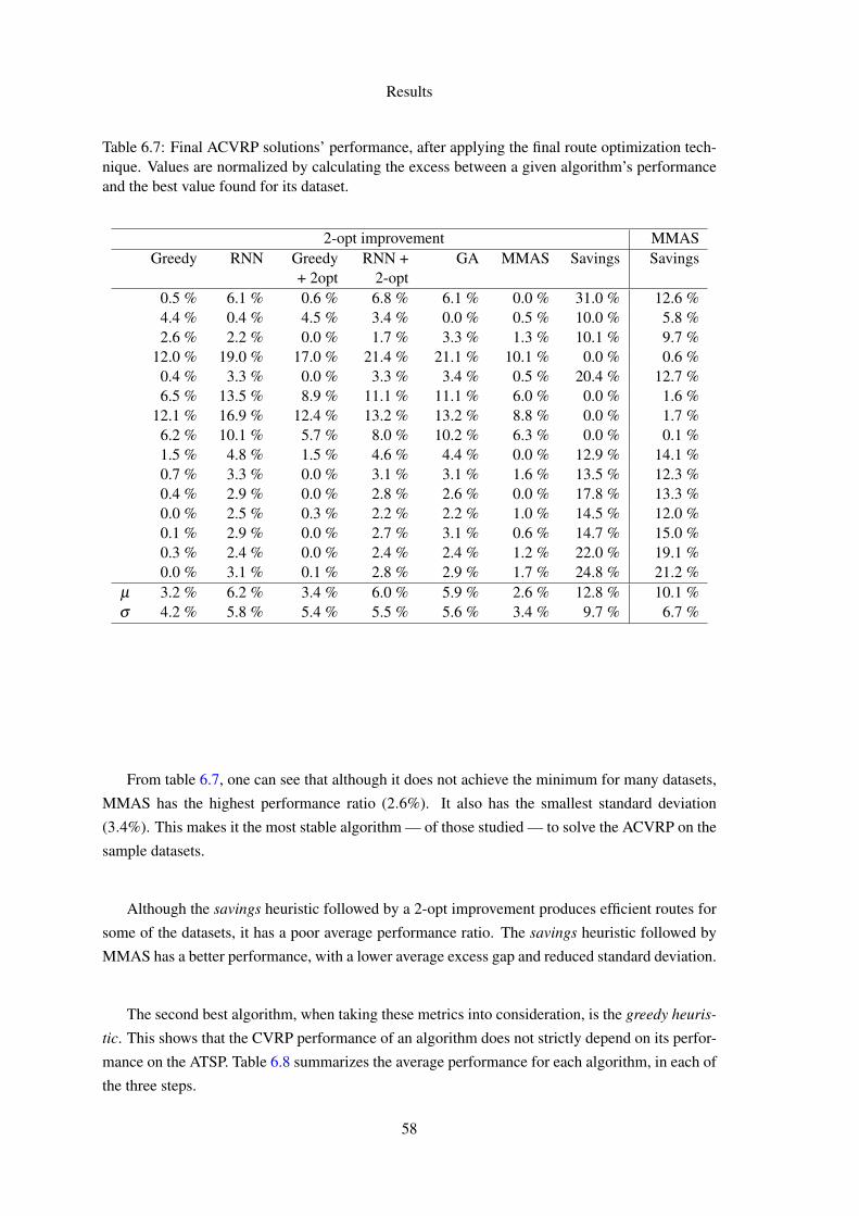
Results

Table 6.7: Final ACVRP solutions’ performance, after applying the final route optimization tech-nique. Values are normalized by calculating the excess between a given algorithm’s performanceand the best value found for its dataset.

2-opt improvement MMASGreedy RNN Greedy

+ 2optRNN +

2-optGA MMAS Savings Savings

0.5 % 6.1 % 0.6 % 6.8 % 6.1 % 0.0 % 31.0 % 12.6 %4.4 % 0.4 % 4.5 % 3.4 % 0.0 % 0.5 % 10.0 % 5.8 %2.6 % 2.2 % 0.0 % 1.7 % 3.3 % 1.3 % 10.1 % 9.7 %

12.0 % 19.0 % 17.0 % 21.4 % 21.1 % 10.1 % 0.0 % 0.6 %0.4 % 3.3 % 0.0 % 3.3 % 3.4 % 0.5 % 20.4 % 12.7 %6.5 % 13.5 % 8.9 % 11.1 % 11.1 % 6.0 % 0.0 % 1.6 %

12.1 % 16.9 % 12.4 % 13.2 % 13.2 % 8.8 % 0.0 % 1.7 %6.2 % 10.1 % 5.7 % 8.0 % 10.2 % 6.3 % 0.0 % 0.1 %1.5 % 4.8 % 1.5 % 4.6 % 4.4 % 0.0 % 12.9 % 14.1 %0.7 % 3.3 % 0.0 % 3.1 % 3.1 % 1.6 % 13.5 % 12.3 %0.4 % 2.9 % 0.0 % 2.8 % 2.6 % 0.0 % 17.8 % 13.3 %0.0 % 2.5 % 0.3 % 2.2 % 2.2 % 1.0 % 14.5 % 12.0 %0.1 % 2.9 % 0.0 % 2.7 % 3.1 % 0.6 % 14.7 % 15.0 %0.3 % 2.4 % 0.0 % 2.4 % 2.4 % 1.2 % 22.0 % 19.1 %0.0 % 3.1 % 0.1 % 2.8 % 2.9 % 1.7 % 24.8 % 21.2 %

µ 3.2 % 6.2 % 3.4 % 6.0 % 5.9 % 2.6 % 12.8 % 10.1 %σ 4.2 % 5.8 % 5.4 % 5.5 % 5.6 % 3.4 % 9.7 % 6.7 %

From table 6.7, one can see that although it does not achieve the minimum for many datasets,

MMAS has the highest performance ratio (2.6%). It also has the smallest standard deviation

(3.4%). This makes it the most stable algorithm — of those studied — to solve the ACVRP on the

sample datasets.

Although the savings heuristic followed by a 2-opt improvement produces efficient routes for

some of the datasets, it has a poor average performance ratio. The savings heuristic followed by

MMAS has a better performance, with a lower average excess gap and reduced standard deviation.

The second best algorithm, when taking these metrics into consideration, is the greedy heuris-

tic. This shows that the CVRP performance of an algorithm does not strictly depend on its perfor-

mance on the ATSP. Table 6.8 summarizes the average performance for each algorithm, in each of

the three steps.

58

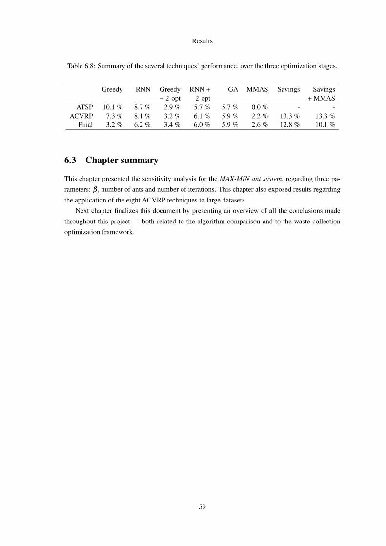
Results

Table 6.8: Summary of the several techniques’ performance, over the three optimization stages.

Greedy RNN Greedy+ 2-opt

RNN +2-opt

GA MMAS Savings Savings+ MMAS

ATSP 10.1 % 8.7 % 2.9 % 5.7 % 5.7 % 0.0 % - -ACVRP 7.3 % 8.1 % 3.2 % 6.1 % 5.9 % 2.2 % 13.3 % 13.3 %

Final 3.2 % 6.2 % 3.4 % 6.0 % 5.9 % 2.6 % 12.8 % 10.1 %

6.3 Chapter summary

This chapter presented the sensitivity analysis for the MAX-MIN ant system, regarding three pa-

rameters: β , number of ants and number of iterations. This chapter also exposed results regarding

the application of the eight ACVRP techniques to large datasets.

Next chapter finalizes this document by presenting an overview of all the conclusions made

throughout this project — both related to the algorithm comparison and to the waste collection

optimization framework.

59

Results

60

Chapter 7

Conclusions

This final chapter presents a review of the relevant information obtained from this study and an

exposition of further research that could be done in this area. Section 7.1 presents the sensibility

analysis results regarding the MAX-MIN ant system and describes results on the application of the

route-first-cluster-second approach to the waste collection scenario.

Section 7.2 exposes some thoughts on how to further extend the study on both the Asymmet-

ric Traveling Salesman Problem and the Capacitated Vehicle Routing Problem. It also finalizes

this document by presenting the next stages of implementing the waste collectionwaste collection

optimization framework.

7.1 Conclusions

This document presented an architecture proposal for the storage and retrieval of containers’ status,

together with formats for information interchange. These formats are built on top of JSON, an

open standard that can be used to represent simple data structures. An alternative would be to use

XML; however, JSON was preferred over XML due to the following reasons:

• JSON has a simpler notation than that of XML;

• JSON was designed to serve as a data interchange format, whereas XML was designed to

be a document interchange format.

The second goal of this work is to provide insight on existing algorithms to calculate efficient

routes for waste collection. This problem is modeled as an Asymmetric Capacitated Vehicle Rout-

ing Problem (ACVRP). Several methods have been proposed, in the literature, on how to approach

the ACVRP.

To solve the ACVRP, there are construction heuristics (such as the one by Clarke-Wright).

These yield a set of vehicle routes, which can be further optimized by applying ATSP solving

techniques.

61

Conclusions

Another method to address the ACVRP involves solving the associated Asymmetric Travel-

ing Salesman Problem (ATSP) and dividing the resulting tour into routes that respect the vehicle

capacity constraints. This is called a route-first-cluster-second approach.

To solve the ATSP, several techniques were compared: two construction heuristics — greedy

and repetitive nearest neighbor (RNN) — and three meta-heuristics — hill climbing (2-opt), ge-

netic algorithms (GA) and MAX-MIN ant system (MMAS). Apart from their comparison regarding

the efficiency of resulting routes, MMAS was also targeted for a parameter sensibility analysis.

7.1.1 Sensitivity analysis of MMAS

As a result of the parameter sensitivity analysis for the MAX-MIN ant system, it was shown that,

for the given datasets, the optimum value for parameter β lies in the interval [5,20]. Although the

optimum value appears to be located closed to the lower side of this interval, it is recommended

that higher values are used. The rationale for this is that there is a significantly steep ascent for

values close to β = 5. Thus, it was chosen to use β = 20 during this study. This helps to prevent

against possible oscillations in the β optimization curve, when applying MMAS to larger graphs.

Regarding the number of ants and iterations, it was shown that increasing both parameters

increases the resulting route efficiency. When applying this algorithm with a limited time frame,

though, it is preferable to have a low number of ants and a high number of iterations. However, one

must take into consideration that using MMAS with a low number of ants may lead to convergence

too soon. Early convergence causes the algorithm not to take full advantage of the total available

running time.

7.1.2 Comparison of methods for the ACVRP

When comparing the five methods to solve the ATSP, MMAS obtained more efficient routes than

the other four methods. In average, the improvement of MMAS over the best route obtained using

the other methods is of 2.6%.

Although MMAS outperforms the other techniques in solving the ATSP, the same needs not

to hold for the ACVRP solutions. Immediately after clustering, the hill climbing approach ap-

plied to the greedy heuristic produces more efficient routes for half of the fifteen large datasets.

Nevertheless, MMAS only exceeds the best solution for each dataset, in average, by 2.2%.

The third step of the optimization consists of applying an ATSP technique to each of the

vehicle routes obtained from the previous step. After this step, MMAS is still the approach that

yields better results, with an average excess of 2.6%. This technique also has the lowest standard

deviation (σ = 3.4%), which means that it is the most stable algorithm.

In terms of solution efficency, MMAS is followed by the greedy heuristic, which has an aver-

age excess of 3.2% (σ = 4.2%). This shows that the initial ATSP solution performance does not

directly influence the efficiency of the final ACVRP set of routes.

62

Conclusions

It was also shown that the savings heuristic performs better when followed by a MMAS op-

timization, rather than the 2-opt technique. This is consistent with the fact that MMAS had per-

formed better than 2-opt when applied to ATSP instances. This leads to the conclusion that it

would be possible to further reduce the route costs by applying MMAS at the final optimization

step, instead of 2-opt.

A 12-page article summarizing the results of this study was submitted to an international work-

shop on algorithmic approaches for transportation modeling. The preliminary version can be seen

in appendix A.

7.2 Future work

Regarding route optimization, this study analyzed a constructive heuristic and several route-first-

cluster-second approaches for solving the Capacitated Vehicle Routing Problem. It would be

possible to apply cluster-first-route-second methods to these approaches, although most of them

rely on predefining a fixed number of vehicles to use.

It would also be interesting to apply MMAS and other techniques at the last optimization step,

instead of simply using 2− opt. This task was not done due to the time it would take to run all

benchmarks.

Having designed the architecture for information management regarding waste containers’ fill

status, the next step is to implement a web service application layer between the central server

and the sensors. This would consist of sending the container’s fill status using through an HTTP

request. Depending on the sensors’ network architecture — currently being studied in Fraunhofer

Portugal Research Center — authorization policies and mechanisms might have to be designed.

63

Conclusions

64

References

[ABMN04] Roberto Aringhieri, Maurizio Bruglieri, Federico Malucelli, and Maddalena Nonato.An asymmetric vehicle routing problem arising in the collection and disposal of spe-cial waste. Electronic Notes in Discrete Mathematics, 17:41 – 47, 2004. Workshopon Graphs and Combinatorial Optimization.

[AG95] Arjang A. Assad and Bruce L. Golden. Chapter 5 arc routing methods and appli-cations. In C.L. Monma M.O. Ball, T.L. Magnanti and G.L. Nemhauser, editors,Network Routing, volume 8 of Handbooks in Operations Research and ManagementScience, pages 375 – 483. Elsevier, 1995.

[AG07] O. Apaydin and M.T. Gonullu. Route optimization for solid waste collection: Trab-zon (Turkey) case study. Global Nest Journal, 9:6 – 11, 2007.

[Arc05] M.G. Speranza Archetti. Collection of waste with single load trucks: a real case. InB. Fleischmann and A. Klose, editors, Distribution Logistics: Advanced Solutions toPractical Problems, pages 105–119, Berlin Heidelberg, 2005. Springer-Verlag.

[BB98] J. M. Belenguer and E. Benavent. The Capacitated Arc Routing Problem: ValidInequalities and Facets. Comput. Optim. Appl., 10(2):165–187, 1998.

[BB03] José M. Belenguer and Enrique Benavent. A cutting plane algorithm for the capac-itated arc routing problem. Computers & Operations Research, 30(5):705 – 728,2003.

[BBLP06] José-Manuel Belenguer, Enrique Benavent, Philippe Lacomme, and Christian Prins.Lower and upper bounds for the mixed capacitated arc routing problem. Comput-ers & Operations Research, 33(12):3363 – 3383, 2006. Part Special Issue: RecentAlgorithmic Advances for Arc Routing Problems.

[BBM06] Roberto Baldacci, Lawrence Bodin, and Aristide Mingozzi. The multiple disposal fa-cilities and multiple inventory locations rollon-rolloff vehicle routing problem. Com-put. Oper. Res., 33(9):2667–2702, 2006.

[BD08] Emilian Balanescu and Cristian Darie. Beginning PHP and MySQL E-Commerce:From Novice to Professional, Second Edition (Beginners / Beginning Guide). APress,2008.

[Bea83] JE Beasley. Route first–cluster second methods for vehicle routing. Omega,11(4):403–408, 1983.

[Bel74] Beltrami, E.J., Bodin, L.D. Networks and Vehicle Routing for Municipal WasteCollection. Networks, 4(1):65–94, 1974.

65

REFERENCES

[Bha96] Vasanthakumar N. Bhat. A Model for the Optimal Allocation of Trucks for SolidWaste Management. Waste Management Research, 14(1):87–96, 1996.

[BMBB00] Lawrence Bodin, Aristide Mingozzi, Roberto Baldacci, and Michael Ball.The Rollon-Rolloff Vehicle Routing Problem. TRANSPORTATION SCIENCE,34(3):271–288, 2000.

[BP04] Joaquín Bautista and Jordi Pereira. Ant Algorithms for Urban Waste Collection Rout-ing. In ANTS Workshop, pages 302–309, 2004.

[CCL96] Sangit Chatterjee, Cecilia Carrera, and Lucy A. Lynch. Genetic algorithms and trav-eling salesman problems. European Journal of Operational Research, 93(3):490 –510, 1996.

[CDM91] Alberto Colorni, Marco Dorigo, and Vittorio Maniezzo. Distributed optimization byant colonies. In European Conference on Artificial Life, pages 134–142, 1991.

[CGSH02] Julio César, Angel Gutiérrez, David Soler, and Antonio Hervás. The capacitatedgeneral routing problem on mixed graphs. Investigaciones Operacionales, 23:15–26,2002.

[CMMS02] Angel Corberán, Rafael Martí, Eulalia Martínez, and David Soler. The Rural PostmanProblem on mixed graphs with turn penalties. Computers & Operations Research,29(7):887 – 903, 2002.

[Cro09a] Douglas Crockford. The application/json Media Type for JavaScript Object Notation(JSON). http://www.ietf.org/rfc/rfc4627.txt?number=4627, March2009. Last accessed on 20th July 2010.

[Cro09b] Douglas Crockford. Introducing JSON. http://json.org/, March 2009. Lastaccessed on 20th July 2010.

[CW64] G. Clarke and J. W. Wright. Scheduling of vehicles from a central depot to a numberof delivery points. OPERATIONS RESEARCH, 12(4):568–581, July 1964.

[DGG96] Marco Dorigo, L.M. Gambardella, and Luca Maria Gambardella. Ant colony system:A cooperative learning approach to the traveling salesman problem. 1996.

[DM91] L. D. Davis and Melanie Mitchell. Handbook of genetic algorithms. Van NostrandReinhold, 1991.

[DMC96] Marco Dorigo, Vittorio Maniezzo, and Alberto Colorni. The ant system: Optimiza-tion by a colony of cooperating agents. IEEE Transactions on Systems, Man, andCybernetics-Part B, 26:29–41, 1996.

[dML97] de Meulemeester L. Optimal sequencing of skip collections and deliveries. Journalof the Operational Research Society, 48:57–64(8), 1 January 1997.

[Dor92] M. Dorigo. Optimization, Learning and Natural Algorithms. PhD thesis, Politecnicodi Milano, Italy, 1992.

[Eul36] Leonhard Euler. Solutio problematis ad geometriam situs pertinentis. Comment.Academiae Sci. J. Petropolitanae, 8:128–140, 1736.

66

http://www.ietf.org/rfc/rfc4627.txt?number=4627

http://json.org/

REFERENCES

[FA90] D. B. Fogel and J.W. Atmar. Comparing genetic operators with gaussian mutationsin simulated evolutionary processes using linear systems. Biological Cybernetics,63:111–114, 1990.

[G.94] Cristallo G. Optimisation de Tournées de Véhicules de Transport Container. Mémoirede license en Sciences Economique et Sociales, Facultés Universitaires Notre-Damede la Paix, 1994.

[GADP89] S. Goss, S. Aron, J. Deneubourg, and J. Pasteels. Self-organized shortcuts in theargentine ant. Naturwissenschaften, 76(12):579–581, 1989.

[GAW01] B. L. Golden, A. A. Assad, and E. A. Wasil. Routing vehicles in the real world: ap-plications in the solid waste, beverage, food, dairy, and newspaper industries, pages245–286. In [TV01b], 2001.

[GLP01] M. Gendreau, G. Laporte, and J.-Y. Potvin. Metaheuristics for the capacitated VRP.[TV01b], pages 129–154.

[GMP10] Luís Gouveia, Maria Cândida Mourão, and Leonor Santiago Pinto. Lower boundsfor the mixed capacitated arc routing problem. Computers & Operations Research,37(4):692 – 699, 2010.

[Gol81] Wong Richard T. Golden, Bruce L. Capacitated arc routing problems. Networks,11(3):305–315, 1981.

[GPB+02] Gregory Gutin, Abraham Punnen, Alexander Barvinok, Edward Kh. Gimadi, andAnatoliy I. Serdyukov. The Traveling Salesman Problem and Its Variations. 2002.

[Hak08] Mordechai (Muki) Haklay. Openstreetmap: User-generated street maps. IEEE Per-vasive Computing, 7:12–18, 2008.

[Hol92] John H. Holland. Adaptation in natural and artificial systems. MIT Press, Cambridge,MA, USA, 1992.

[Jac73] Jack Edmonds. Matching, Euler tours and the Chinese postman. Mathematical Pro-gramming, 5:88–124, 1973.

[JM97] David S. Johnson and Lyle A. Mcgeoch. The Traveling Salesman Problem: A CaseStudy in Local Optimization. 1997.

[Joh06] Ola M. Johansson. The effect of dynamic scheduling and routing in a solid wastemanagement system. Waste Management, 26(8):875 – 885, 2006.

[Kar05] Karadimas, N.V., Kouzas, G., Anagnostopoulos, I. and Loumos, V. Urban SolidWaste Collection and Routing: the Ant Colony Strategic Approach. InternationalJournal of Simulation: Systems, Science & Technology, 6:45–53, 2005.

[KKS06] Byung-In Kim, Seongbae Kim, and Surya Sahoo. Waste collection vehicle rout-ing problem with time windows. Computers & Operations Research, 33(12):3624– 3642, 2006. Part Special Issue: Recent Algorithmic Advances for Arc RoutingProblems.

[Knu76] Donald E. Knuth. Big omicron and big omega and big theta. SIGACT News, 8(2):18–24, 1976.

67

REFERENCES

[Knu97] Donald E. Knuth. The art of computer programming, volume 2 (3rd ed.): seminu-merical algorithms. Addison-Wesley Longman Publishing Co., Inc., 1997.

[Kru56] Joseph B. Kruskal. On the Shortest Spanning Subtree of a Graph and the TravelingSalesman Problem. Proceedings of the American Mathematical Society, 7(1):48–50,February 1956.

[LBM08] Jing-Quan Li, Denis Borenstein, and Pitu B. Mirchandani. Truck scheduling for solidwaste collection in the City of Porto Alegre, Brazil. Omega, 36(6):1133–1149, 2008.

[Let99] Adam N. Letchford. The general routing polyhedron: A unifying framework. Euro-pean Journal of Operational Research, 112(1):122 – 133, 1999.

[LS01] G. Laporte and F. Semet. Classical heuristics for the capacitated VRP, pages 109–128. In [TV01b], 2001.

[Man89] Udi Manber. Introduction to Algorithms: A Creative Approach. Addison-WesleyLongman Publishing Co., Inc., Boston, MA, USA, 1989.

[McC94] J.E. McCarthy. The municipal solid waste problem in the main industrialized coun-tries. In Curzio, A.Q., Prosperetti, L., Zoboli, R., editor, The Management of Munic-ipal Solid Waste in Europe: Economic, Technological and Environmental Perspec-tives, Amsterdam, 1994.

[MDS06] Alexandre Magrinho, Filipe Didelet, and Viriato Semiao. Municipal solid waste dis-posal in Portugal. Waste Management, 26(12):1477 – 1489, 2006.

[Mos00] Moshe Dror, editor. Arc Routing: Theory, Solutions and Applications. 2000.

[NR01] D. Naddef and G. Rinaldi. Branch-and-cut algorithms for the capacitated VRP, pages53–84. In [TV01b], 2001.

[NS92] William Spears Navy and William M. Spears. Crossover or mutation? In Foundationsof Genetic Algorithms 2, pages 221–237. Morgan Kaufmann, 1992.

[PM95] Ram Pandit and B. Muralidharan. A capacitated general routing problem on mixednetworks. Computers & Operations Research, 22(5):465 – 478, 1995.

[Pá03] D. A. Pássaro. Report: waste management in Portugal between 1996 and 2002. WasteManagement, 23(1):97 – 99, 2003.

[Rei91] Gerhard Reinelt. TSPLIB–A Traveling Salesman Problem Library. INFORMSJOURNAL ON COMPUTING, 3(4):376–384, 1991.

[RN03] Stuart J. Russell and Peter Norvig. Artificial Intelligence: A Modern Approach. Pear-son Education, 2003.

[Rob09] Robin Cover. XML Applications and Initiatives. http://xml.coverpages.org/xmlApplications.html, March 2009. Last accessed on 15th March 2010.

[RXV+09] Alberto Rovetta, Fan Xiumin, Federico Vicentini, Zhu Minghua, Alessandro Giusti,and He Qichang. Early detection and evaluation of waste through sensorized contain-ers for a collection monitoring application. Waste Management, 29(12):2939 – 2949,2009.

68

http://xml.coverpages.org/xmlApplications.html

http://xml.coverpages.org/xmlApplications.html

REFERENCES

[San08] Sanne Wøhlk. A Decade of Capacitated Arc Routing. 2008.

[SD02] Thomas Stutzle and Marco Dorigo. A short convergence proof for a class of antcolony optimization algorithms. IEEE Transactions on Evolutionary Computation,2002:358–365, 2002.

[SH97] T. Stutzle and H. Hoos. Max-min ant system and local search for the traveling sales-man problem. Evolutionary Computation, 1997., IEEE International Conference on,pages 309–314, 1997.

[SH00] Thomas Stützle and Holger H. Hoos. Max-min ant system. Future Gener. Comput.Syst., 16(9):889–914, 2000.

[TAdS04] Joao Teixeira, Antonio Pais Antunes, and Jorge Pinho de Sousa. Recyclable wastecollection planning–a case study. European Journal of Operational Research,158(3):543–554, November 2004.

[TB] A. Tucker and L. Bodin. A model for municipal street sweeping operations, pages107–150.

[TP00] Dang Vu Tung and Anulark Pinnoi. Vehicle routing-scheduling for waste collectionin Hanoi. European Journal of Operational Research, 125(3):449–468, 2000.

[TV01a] P. Toth and D. Vigo. An overview of vehicle routing problems, pages 1–26. In[TV01b], 2001.

[TV01b] P. Toth and D. Vigo. The vehicle routing problem. Society for Industrial and AppliedMathematics, Philadelphia, PA, USA, 2001.

[VGR+09] F. Vicentini, A. Giusti, A. Rovetta, X. Fan, Q. He, M. Zhu, and B. Liu. Sensorizedwaste collection container for content estimation and collection optimization. WasteManagement, 29(5):1467 – 1472, 2009. First international conference on environ-mental management, engineering, planning and economics.

69

REFERENCES

70

Appendix A

Submitted article

71

Metaheuristics for the ATSP Problem Appliedto Urban Waste Collection

Hugo Peixoto1,2 and Ana Aguiar2

1 Fraunhofer Portugal AICOS, Rua do Campo Alegre 1021,4169-007 Porto, Portugal

2 Faculdade de Engenharia da Universidade do Porto, Rua Dr. Roberto Frias, s/n,4200-465 Porto, Portugal

Abstract. Real-time fill status of the waste containers can be used toreduce collection costs if this data is used to calculate efficient wastecollection routes. This problem can be modeled as a dynamic stochasticvehicle routing and scheduling problem. One of the ways to tackle thisproblem is to use a route-first cluster-second approach.This article contains a comparative analysis of several route optimizationalgorithms, with a focus on the sensitivity analysis of the MAX-MINant system. Our results show that usage of the MAX-MIN ant systemprovides competitive results on large datasets and also suggests there isroom for further improvement.

Keywords: asymmetric traveling salesman problem, ant systems, urbanwaste collection

1 Introduction

Municipal solid waste (MSW) production has constantly increased since the1960s as a consequence of economic growth [13], leading to the need for efficientwaste management solutions. These involve collection, transportation, recyclingand disposal of solid urban waste waste. A study by Johansson [7], shows thatcost reductions of up to 20% can be achieved by taking into account the real-time fill status of the waste containers and defining collection policies appropriatefor each specific case. In that study, calculating efficient waste collection routesis modeled as a dynamic stochastic vehicle routing and scheduling problem,assuming that the waste collection is done during the day, as need arises forwaste containers to be emptied, signaled by level sensors in the containers.

In the specific case of Porto, Portugal, the residential solid urban waste collec-tion is done once a day in the evening, with the vehicles picking up trash regularlyfrom containers, based on experience-based values for trash generation. In thisscenario, sometimes some full containers wait one day or more for being pickedup, and sometimes partially full containers are picked up, both situation beinginefficient. The city hall is interested in implementing a platform that measuresthe actual fill status of the containers, so that the evolution of trash can be mon-itored, the quality and efficiency of the collection can be increased, and the sums

2

paid to subcontractor companies by amount of km traveled each month reduced.The system should wok as follows: containers send an alarm when they are full,and everyday in the evening the waste collection routes are calculated with thestatic values available at a certain time. The problem that has to be solved everyday within 1 to 2 hours is a classical vehicle routing and scheduling problem,as defined and classified in [2], and differs from the dynamic stochastic vehiclerouting problem above. The 1 to 2 hours available to find the solution, thoughnot imposing a real-time constraint, do require an efficient solution that can befound within that time frame for graphs of large cities, with several thousandsof nodes.

We use a Capacitated Vehicle Routing Problem (CVRP) model for the prob-lem described and solve it by solving the associated Asymmetric Traveling Sales-man Problem (ATSP) first, followed by partitioning the resulting route into thetours for each truck subject to truck capacity (henceforth called clustering),being aware that the results of the serialized problem is suboptimal. Since thesecond problem can be solved optimally, we will focus on improving the approx-imate solutions for the ATSP. Using real city maps and Monte Carlo simula-tions, we study the application to the ATSP problem of the max-min ant systemproposed by Stuetzle [17], showing results of a parameter sensitivity analysis.Moreover, we compare the results obtained with commonly used heuristics andmeta-heuristics for the ATSP problem, evaluating them in comparable scenar-ios. Our results show that the max-min ant system always delivers the bestperformance among the meta-heuristics studied on the datasets of the TSPLIB,but the improvement never not exceeds 10%. Moreover, the performance of theMMAS on large datasets typical for current cities does not show significantimprovement compared to other metaheuristics, although our parameter sensi-tivity analysis shows that further improvements could be achieved using otheralgorithm parameters at the cost of higher computation cost.

In the next section, we present related work and justify the choice of theCVRP model for the problem, in Section 3 we elaborate on our approach to solveit and we briefly describe the details of the meta-heuristics studied with strongerfocus on the ant colony algorithm used. This is followed by the validation of ouralgorithm implementations in Section 4. In Section 5 we describe the frameworkand datasets for the Monte Carlo simulations used in the evaluation. Section 6shows the results of the sensitivity analysis for the ant colony algorithm chosen,Section 7 shows the results and discussion of the comparative evaluation of themeta-heuristics and we conclude the paper in Section 8.

2 Related Work

The work by Johansson [7] studies the scenario of routing vehicles with real-time data from the containers, changing the routes when vehicles are alreadyunder way. They model the systems as a dynamic/stochastic routing problemand focus the study not only on heuristics for optimizing the result, but also onthe influence of system parameters on the result of applying different policies. For

3

example, the best choice between collecting only full containers or also partiallyfull containers depends on the total number of containers in the area covered.

The problem we are faced with is not dynamic, as the data for calculating thecollection routes will be taken from a snapshot of the system at a certain time ofthe day. Hence, we are dealing with a static vehicle scheduling routing problemas in [2] and our goal is to compare heuristics that minimize the sum of thedistances of all collection vehicle tours needed to collect the trash from full binsper day, using recently developed meta-heuristics which, to our best knowledge,have not been comparatively evaluated in other studies. We focus specifically onthe sensitivity analysis of an ant colony algorithm, the MAX-MIN Ant Systemwhich will be described in the next section, and its performance on large graphs,such as those of cities.

Waste collecting can be seen a Vehicle Routing Problem[19], where eachcontainer is represented by a vertex that needs to be serviced, with it’s currentfill status representing the vertex demand. Each arc between vertices representsthe distance, respecting the city’s roads and traffic rules, between two containers.As several waste collection vehicles are available, and as they have a limit onhow much waste it can carry, this problem is modeled as a Capacitated VehicleRouting Problem (CVRP).

Two common approaches to solve a Capacitated Vehicle Routing Problemare to either cluster the customers and then calculate an optimized route for eachone (cluster-first route-second) or to determine a single route passing throughall the costumers and then divide it into feasible subroutes (route-first cluster-second) [19]. In the first scenario, clustering can be done, for example, by solvinga Generalized Assignment Problem, while building each individual route can bedone by solving a Traveling Salesman Problem (TSP) instance. In the secondscenario, the tour passing all nodes can be constructed by solving a TSP instance,while its optimal clustering can be done using a standard dynamic programmingapproach.

3 Our Approach

We started by comparing route-first cluster-second approaches. The first stage —building a single tour — is equivalent to solve a TSP instance where each graph’svertex represents a waste container or the depot location and where each graph’sarc weight represents the cost of traveling from one location to another. Sincearc transversal represents the transversal of multiple city roads, it follows thatthe graph weight matrix may be asymmetric, as we may have one way streetsalong the way. This leads to the conclusion that these specific TSP instances areactually Asymmetric Traveling Salesman Problem (ATSP) instances, which areharder to solve than the symmetric version [20].

Having obtained a single tour that visits every of the graph’s vertices, clus-tering it into several routes in which vertex visiting order is not altered andwhere capacity constraints (due to the limited truck capacity) are satisfied canbe done by applying a shortest path algorithm on an auxiliary directed acyclic

4

graph, where each arc represents a feasible route composed by a subsequenceof the tour, as proposed by Beasley [1]. Since this clustering method is bothoptimal and polynomially bounded — its time complexity is O(|V |2), with Vbeing the set of vertices in the graph — we focus on solving ATSP instances.It is important to note that while the clustering algorithm is optimal, it doesnot mean that solving the ATSP optimally and applying this method yields anoptimal CVRP solution[12].

There are two main methods to solve TSP instances. First, there are routeconstruction heuristics, which are usually greedy in some fashion and may berandomized. Then, there are improvement techniques which can be used on topof these heuristics to further improve their results. Two commonly known routeconstruction heuristics are the nearest neighbor and the greedy heuristic.

The nearest neighbor heuristic (NN) starts by picking a (usually random)vertex. It follows by choosing the closest unvisited vertex, until all vertices arevisited. Applied to a complete graph, this heuristic runs in O(|V |2). Instead ofsimply picking the first vertex randomly, we decided to apply the heuristic toevery starting vertex and return the best route. This creates a longer runningtime of O(|V |3), but yields better results, as will be shown in Section 7. We willrefer to this heuristic as the Best NN heuristic.

The greedy heuristic works in a similar way to Kruskal’s minimum spanningtree algorithm [9]. It starts by creating an auxiliary directed graph with no arcs,G′ = (V, ), and then sorts all the arcs by their weight, which are then iteratedin ascending order. For each arc, we add it to G′ if and only if its verticesare not already connected in G′ and both the outdegree (number of outgoingarcs) of the source vertex and the indegree (number of incoming arcs) of thedestination vertex are exactly 0. This process will yield a spanning tree whichcan be converted to a tour by adding the arc that connects the only two verticeswhose degree is less than 2.

Metaheuristics such as hill climbing, genetic algorithms and ant systems canbe applied to the ATSP problem to improve the results obtained by the heuristicsabove.

Hill climbing Hill climbing[16] is a greedy local search technique. It picks aninitial solution and iterates through its neighborhood, looking for a solution thatyields a better value. As soon as it finds one, it halts its search and moves on tothe newly found solution. This process is repeated until a local minima/maximais reached or the specified time limit is exceeded.

When applying hill climbing to TSP instances, a solution’s neighborhood iscommonly defined by dividing the current route into k segments and recombiningthem in all possible ways that yield a tour. This is called the k− opt technique.The most common versions are 2-opt and 3-opt [8] and an adaptive generalizationthat chooses, at each iteration, how many segments to form — the Lin-Kernighanheuristic[8]. The bigger the k, the greater the neighborhood and the algorithmrunning time. In asymmetric instances, the neighborhood evaluation takes longerthan in symmetric, hence we decided to use 2-opt techniques, to keep a lowrunning time.

5

Genetic algorithm A genetic algorithm is a search technique based on evolution-ary biology [3]. This technique starts by defining an initial population of randomsolutions, which is considered as the first generation. Then, the evolution processfollows. In this process, every individual in the current generation is evaluatedand multiple individuals are stochastically selected according to their fitness andpossibly modified to form the next generation. Usually, the best individuals froma generation, known as the elite, are moved to the next one directly, without suf-fering any modification[16]. The evolution process continues until a predefinedtermination condition has been satisfied. Modifications of two types can be ap-plied to the selected inviduals: crossover and mutation. The crossover operatortakes two or more individuals from the current population and combines theirattributes to form an offspring. The mutation operator randomly modifies at-tributes of any individual. In this project, we simply use the mutation operator,which is defined by selecting two vertices in the route at random and switchingthem.

MAX-MIN Ant System Ant systems, first proposed by Dorigo[4, 5], are based inant colony communications and pheromone trail techniques. Ants are able to findshort paths between food sources and their colony by leaving pheromone markson their trails. Ants tend to follow paths where the pheromone intensity is higher,and the more ants follow a path, more pheromones are laid on it. These conceptswere adapted into a class of probabilistic techniques for solving problems ofcombinatorial optimization [10, 11, 14]. Several ant systems have been proposedover the last years and we chose MAX-MIN Ant System (MMAS) [17], as itshows better results than the original ant system proposed by Dorigo and itsconvergence has been proved [18].

To apply MMAS to ATSP, a fixed amount of pheromones is placed in eachof the graph’s edges. Then, the following procedure is applied iteratively, until itconverges or reaches a maximum number of steps or time limit. Each iterationstarts by placing K ants in random vertices. Then, each ant starts constructinga tour by choosing the next node probabilistically according to two factors:pheromone strength in the arc and its distance. The probability is 0 if the nodeis already visited. Otherwise, it is proportional to:

pij ∼ ταijηβij , (1)

where τij is the pheromone strength in the arc and ηij is the inverse of thedistance between i and j. α and β are parameters that determine the relativeinfluence of τij and ηij . When all ants finish constructing their routes, the onewith the shortest tour lays down pheromones along its path, which is equivalentto updating the pheromones along the trail, according to [17]:

τnewij = ρ · τoldij +∆τij (2)

∆τij equals to 0 if the arc from i to j does not belong to the tour of the bestant, or a fixed positive amount if it does. This amount is inversely proportionalto the ant’s tour length. Additionally, MMAS bounds pheromone values in each

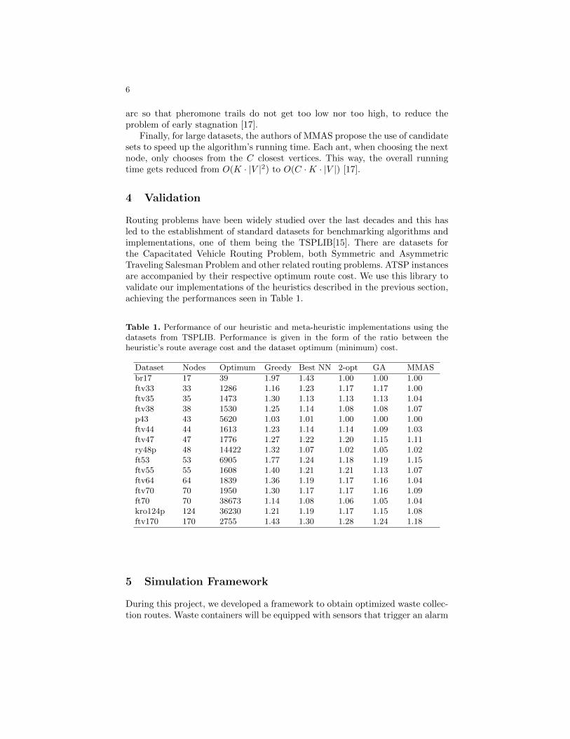
6

arc so that pheromone trails do not get too low nor too high, to reduce theproblem of early stagnation [17].

Finally, for large datasets, the authors of MMAS propose the use of candidatesets to speed up the algorithm’s running time. Each ant, when choosing the nextnode, only chooses from the C closest vertices. This way, the overall runningtime gets reduced from O(K · |V |2) to O(C ·K · |V |) [17].

4 Validation

Routing problems have been widely studied over the last decades and this hasled to the establishment of standard datasets for benchmarking algorithms andimplementations, one of them being the TSPLIB[15]. There are datasets forthe Capacitated Vehicle Routing Problem, both Symmetric and AsymmetricTraveling Salesman Problem and other related routing problems. ATSP instancesare accompanied by their respective optimum route cost. We use this library tovalidate our implementations of the heuristics described in the previous section,achieving the performances seen in Table 1.

Table 1. Performance of our heuristic and meta-heuristic implementations using thedatasets from TSPLIB. Performance is given in the form of the ratio between theheuristic’s route average cost and the dataset optimum (minimum) cost.

Dataset Nodes Optimum Greedy Best NN 2-opt GA MMAS

br17 17 39 1.97 1.43 1.00 1.00 1.00ftv33 33 1286 1.16 1.23 1.17 1.17 1.00ftv35 35 1473 1.30 1.13 1.13 1.13 1.04ftv38 38 1530 1.25 1.14 1.08 1.08 1.07p43 43 5620 1.03 1.01 1.00 1.00 1.00ftv44 44 1613 1.23 1.14 1.14 1.09 1.03ftv47 47 1776 1.27 1.22 1.20 1.15 1.11ry48p 48 14422 1.32 1.07 1.02 1.05 1.02ft53 53 6905 1.77 1.24 1.18 1.19 1.15ftv55 55 1608 1.40 1.21 1.21 1.13 1.07ftv64 64 1839 1.36 1.19 1.17 1.16 1.04ftv70 70 1950 1.30 1.17 1.17 1.16 1.09ft70 70 38673 1.14 1.08 1.06 1.05 1.04kro124p 124 36230 1.21 1.19 1.17 1.15 1.08ftv170 170 2755 1.43 1.30 1.28 1.24 1.18

5 Simulation Framework

During this project, we developed a framework to obtain optimized waste collec-tion routes. Waste containers will be equipped with sensors that trigger an alarm

7

whenever they are full. This information is stored in a centralized database, readyto be used when the route optimization process starts.

Every day, two to three hours before collection starts, urrent fill status dataof all of the city’s containers is retrieved from the database, along with theirlocation. This is then merged with the city’s topological map — which can beobtained in OpenStreetMaps, for example — to form a standard CVRP dataset.Finally, meta-heuristics are applied to this dataset, yielding an optimized setof routes. This set can then be visualized and distributed to collection trucks’operators.

Realistic Graph Datasets While TSPLIB instances can be useful to provide afast validation of implemented algorithms, available instances are limited in thenumber of vertices: ATSP instances only go up to 443 vertices and CVRP in-stances only go up to 101. Since instances corresponding to actual cities will havethousands of nodes, to compare the performance of the optimization heuristicsin realistic scenarios we generated additional datasets based on the topology ofcities such as Leeds, London and Lisbon. This information was obtained fromthe collaborative and open source initiative OpenStreetMap which aims to createa free editable map of the world [6]. We obtained 15 new CVRP datasets rangingfrom 518 to 7628 vertices. A sample dataset can be seen in figure 1.

Fig. 1. Part of London with scattered waste containers. Yellow lines represent roadswhile black dots represent full waste containers. Road direction is not differentiated,in this image.

Waste Generation Having no access to real waste containers location and fillstatus, we also had to generate this information artificially, using a stochasticapproach. Waste containers were scattered in street intersections following differ-ent patterns according to the following process. The algorithm starts by selectingk road intersections (represented by a graph vertex) on the city map as cluster

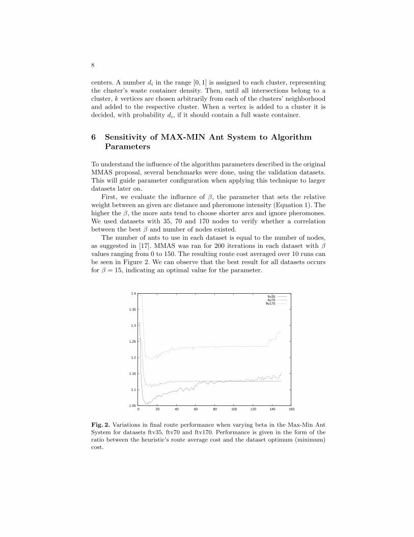
8

centers. A number di in the range [0, 1] is assigned to each cluster, representingthe cluster’s waste container density. Then, until all intersections belong to acluster, k vertices are chosen arbitrarily from each of the clusters’ neighborhoodand added to the respective cluster. When a vertex is added to a cluster it isdecided, with probability di, if it should contain a full waste container.

6 Sensitivity of MAX-MIN Ant System to AlgorithmParameters

To understand the influence of the algorithm parameters described in the originalMMAS proposal, several benchmarks were done, using the validation datasets.This will guide parameter configuration when applying this technique to largerdatasets later on.

First, we evaluate the influence of β, the parameter that sets the relativeweight between an given arc distance and pheromone intensity (Equation 1). Thehigher the β, the more ants tend to choose shorter arcs and ignore pheromones.We used datasets with 35, 70 and 170 nodes to verify whether a correlationbetween the best β and number of nodes existed.

The number of ants to use in each dataset is equal to the number of nodes,as suggested in [17]. MMAS was ran for 200 iterations in each dataset with βvalues ranging from 0 to 150. The resulting route cost averaged over 10 runs canbe seen in Figure 2. We can observe that the best result for all datasets occursfor β = 15, indicating an optimal value for the parameter.

1.05

1.1

1.15

1.2

1.25

1.3

1.35

1.4

0 20 40 60 80 100 120 140 160

ftv35ftv70

ftv170

Fig. 2. Variations in final route performance when varying beta in the Max-Min AntSystem for datasets ftv35, ftv70 and ftv170. Performance is given in the form of theratio between the heuristic’s route average cost and the dataset optimum (minimum)cost.

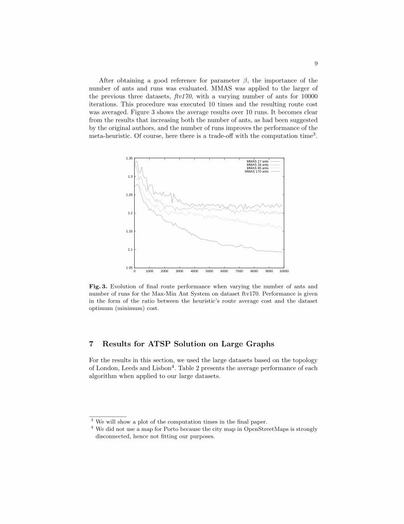
9

After obtaining a good reference for parameter β, the importance of thenumber of ants and runs was evaluated. MMAS was applied to the larger ofthe previous three datasets, ftv170, with a varying number of ants for 10000iterations. This procedure was executed 10 times and the resulting route costwas averaged. Figure 3 shows the average results over 10 runs. It becomes clearfrom the results that increasing both the number of ants, as had been suggestedby the original authors, and the number of runs improves the performance of themeta-heuristic. Of course, here there is a trade-off with the computation time3.

1.05

1.1

1.15

1.2

1.25

1.3

1.35

0 1000 2000 3000 4000 5000 6000 7000 8000 9000 10000

MMAS 17 antsMMAS 34 antsMMAS 85 ants

MMAS 170 ants

Fig. 3. Evolution of final route performance when varying the number of ants andnumber of runs for the Max-Min Ant System on dataset ftv170. Performance is givenin the form of the ratio between the heuristic’s route average cost and the datasetoptimum (minimum) cost.

7 Results for ATSP Solution on Large Graphs

For the results in this section, we used the large datasets based on the topologyof London, Leeds and Lisbon4. Table 2 presents the average performance of eachalgorithm when applied to our large datasets.

3 We will show a plot of the computation times in the final paper.4 We did not use a map for Porto because the city map in OpenStreetMaps is strongly

disconnected, hence not fitting our purposes.

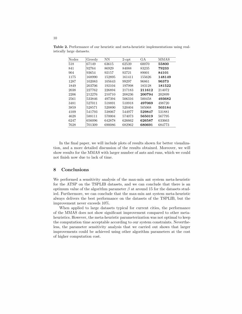
10

Table 2. Performance of our heuristic and meta-heuristic implementations using real-istically large datasets.

Nodes Greedy NN 2-opt GA MMAS

518 67149 63615 62539 60070 55800841 92764 86929 84088 83235 79233904 93654 92157 92721 89001 841011175 168990 152895 161411 155626 1481491287 102083 105643 99297 96861 963731849 203706 192104 197998 183128 1815222038 227762 226894 217183 211612 2140722206 212276 210710 208236 200794 2028992561 533846 497394 506316 500458 4936823481 527011 518891 510918 497069 4987203859 528571 520890 520404 505068 5031844109 541793 538067 544977 529847 5318814628 588111 570004 574073 565019 5677956247 656096 642878 626662 626587 6336637628 701309 690086 682962 680691 684773

In the final paper, we will include plots of results shown for better visualiza-tion, and a more detailed discussion of the results obtained. Moreover, we willshow results for the MMAS with larger number of ants and runs, which we couldnot finish now due to lack of time.

8 Conclusions

We performed a sensitivity analysis of the max-min ant system meta-heuristicfor the ATSP on the TSPLIB datasets, and we can conclude that there is anoptimum value of the algorithm parameter β at around 15 for the datasets stud-ied. Furthermore, we can conclude that the max-min ant system meta-heuristicalways delivers the best performance on the datasets of the TSPLIB, but theimprovement never exceeds 10%.

When applied to large datasets typical for current cities, the performanceof the MMAS does not show significant improvement compared to other meta-heuristics. However, the meta-heuristic parameterization was not optimal to keepthe computation time acceptable according to our system constraints. Neverthe-less, the parameter sensitivity analysis that we carried out shows that largerimprovements could be achieved using other algorithm parameters at the costof higher computation cost.

11

References

1. JE Beasley. Route first–cluster second methods for vehicle routing. Omega,11(4):403–408, 1983.

2. Bodin, L. Classification in Vehicle Routing and Scheduling. Networks, 11(2):97–108, 1981.

3. L. D. Davis and Melanie Mitchell. Handbook of genetic algorithms. Van NostrandReinhold, 1991.

4. M. Dorigo. Optimization, Learning and Natural Algorithms. PhD thesis, Politec-nico di Milano, Italy, 1992.

5. Marco Dorigo, Vittorio Maniezzo, and Alberto Colorni. The ant system: Opti-mization by a colony of cooperating agents. IEEE Transactions on Systems, Man,and Cybernetics-Part B, 26:29–41, 1996.

6. Mordechai (Muki) Haklay. Openstreetmap: User-generated street maps. IEEEPervasive Computing, 7:12–18, 2008.

7. Ola M. Johansson. The effect of dynamic scheduling and routing in a solid wastemanagement system. Waste Management, 26(8):875 – 885, 2006.

8. David S. Johnson and Lyle A. Mcgeoch. The Traveling Salesman Problem: A CaseStudy in Local Optimization. 1997.

9. Joseph B. Kruskal. On the Shortest Spanning Subtree of a Graph and the TravelingSalesman Problem. Proceedings of the American Mathematical Society, 7(1):48–50,February 1956.

10. G. Leguizamon and Z. Michalewicz. A new version of ant system for subset prob-lems. Proceedings of the 1999 Congress on Evolutionary Computation, 2:1458–1464,1999.

11. Helena R. Loureno and Daniel Serra. Adaptive search heuristics for the generalizedassignment problem. Mathware and Soft Computing, 9:209–234, 2002.

12. M. Haimovich. Bounds and Heuristics for Capacitated Routing Problems. Math-ematics of Operations Research, 10(4):527–542, 1985.

13. J.E. McCarthy. The municipal solid waste problem in the main industrializedcountries. In Curzio, A.Q., Prosperetti, L., Zoboli, R., editor, The Managementof Municipal Solid Waste in Europe: Economic, Technological and EnvironmentalPerspectives, Amsterdam, 1994.

14. S. Meshoul and M. Batouche. Ant colony system with extremal dynamics for pointmatching and pose estimation. In ICPR ’02: Proceedings of the 16 th InternationalConference on Pattern Recognition (ICPR’02) Volume 3, page 30823, Washington,DC, USA, 2002. IEEE Computer Society.

15. Gerhard Reinelt. TSPLIB–A Traveling Salesman Problem Library. INFORMSJOURNAL ON COMPUTING, 3(4):376–384, 1991.

16. Stuart J. Russell and Peter Norvig. Artificial Intelligence: A Modern Approach.Pearson Education, 2003.

17. T. Stutzle and H. Hoos. Max-min ant system and local search for the travelingsalesman problem. Evolutionary Computation, 1997., IEEE International Confer-ence on, pages 309–314, 1997.

18. Thomas Stutzle and Marco Dorigo. A short convergence proof for a class of antcolony optimization algorithms. IEEE Transactions on Evolutionary Computation,2002:358–365, 2002.

19. P. Toth and D. Vigo. The vehicle routing problem. Society for Industrial andApplied Mathematics, Philadelphia, PA, USA, 2001.

20. David P. Williamson. ”Analysis of the Held-Karp lower bound for the asymmetricTSP”. Operations Research Letters, 12(2):83 – 88, 1992.

optimization of municipal solid waste collection routes ... · optimization of municipal solid...

Documents