mobile robot navigation - dtu orbitorbit.dtu.dk/files/4724729/oersted-dtu2868.pdf · technical...
TRANSCRIPT

General rights Copyright and moral rights for the publications made accessible in the public portal are retained by the authors and/or other copyright owners and it is a condition of accessing publications that users recognise and abide by the legal requirements associated with these rights.
• Users may download and print one copy of any publication from the public portal for the purpose of private study or research. • You may not further distribute the material or use it for any profit-making activity or commercial gain • You may freely distribute the URL identifying the publication in the public portal
If you believe that this document breaches copyright please contact us providing details, and we will remove access to the work immediately and investigate your claim.
Downloaded from orbit.dtu.dk on: Sep 11, 2018
Mobile Robot Navigation
Andersen, Jens Christian; Ravn, Ole; Andersen, Nils Axel
Publication date:2007
Document VersionPublisher's PDF, also known as Version of record
Link back to DTU Orbit
Citation (APA):Andersen, J. C., Ravn, O., & Andersen, N. A. (2007). Mobile Robot Navigation.

Jens Christian Andersen
Mobile Robot Navigation
PhD thesis, September 2006

2

Technical University of Denmark
Mobile Robot Navigation
PhD thesisJens Christian Andersen
September 2006
Supervisors: Associate Professor Ole Ravn,Associate Professor Nils A. Andersenboth at Automation Ørsted•DTU
ISBN: 87-91184-64-9

4

Preface
This thesis is submitted in partial fulfilment of the requirements for thePhD degree at the Technical University of Denmark. The work was performedin the period March 2003–September 2006 at Automation Ørsted•DTU .
The supervisors have been Associate Professor Ole Ravn and AssociateProfessor Nils A. Andersen both Automation Ørsted•DTU.
Working with robots is an inspiring, satisfactory occupation and a constantsource of enjoyment. Especially I remember a small event where a class ofabout 10-year-old pupils visited our lab. I gave a short demonstration of a fewof our robots, and one of the boys asked with wide open eyes: ’Is this a sort ofplayground for adults?’ And when I confirmed with a smile, he replied: ’Thisis where I want to go when I get older.’
I would like to thank both supervisors for the cooperation and encourage-ments in the project period and for the gentle pushes – especially in situationswhere details became prohibitive for progress.
Additionally I would like to thank the other members of the robotics groupfor the many informal discussions which have been a source of inspirationthroughout the years, and to the service-minded workshop for assistance andideas with the mechanical, electronic and logistic issues when needed.
A special thank to Lisbeth Winter for her (patient) proofreading assistanceduring the writing of this thesis.
And finally: this project would never have been possible without the supportand encouragement from my beloved family: my wife Birte and my son Mikkel.
Kgs. Lyngby, September 2006
J. Christian Andersen
5

6

Abstract
Robots will soon take part in everyone’s daily life. In industrial productionthis has been the case for many years, but up to now the use of mobile robotshas been limited to a few and isolated applications like lawn mowing, surveil-lance, agricultural production and military applications. The research is nowprogressing towards autonomous robots which will be able to assist us in ourdaily life. One of the enabling technologies is navigation, and navigation is thesubject of this thesis.
Navigation of an autonomous robot is concerned with the ability of therobot to direct itself from the current position to a desired destination. Thisthesis present and experimentally validates solutions for road classification,obstacle avoidance and mission execution. The road classification is based onlaser scanner measurements and supported at longer ranges by vision. The roadclassification is sufficiently sensitive to separate the road from flat roadsides,and to distinguish asphalt roads from gravelled roads. The vision-based roaddetection uses a combination of chromaticity and edge detection to outline thetraversable part of the road based on a laser scanner classified sample area.
The perception of these two sensors are utilised by a path planner to allowa number of drive modes, and especially the ability to follow road edges areinvestigated.
The navigation mission is controlled by a script language. The navigationscript controls route sequencing, junction detection, junction crossing calcula-tions and drive mode selection.
The entire system is tested on a combination of narrow asphalt and gravelledroads connected by a number of junctions. Missions of up to 3 km in lengthhave been successfully completed using the described system.
The main focus of the thesis has been the experimental validation of theimplemented solutions and the ability of the methods to solve real world prob-lems.
The amount of software needed by an autonomous robot can be overwhelm-ing. Software reuse and distributed development are therefore important issues.The thesis describes a new component architecture for robotics software thatpromotes software reuse and distributed development and maintenance.
7

8

Dansk Resume
Robotter vil om fa ar blive en del af vores daglige liv. Inden for pro-duktionsindustrien har det allerede være tilfældet i mange ar, men anven-delsen af mobile robotter har hidtil været henvist til isolerede omrader somgræsslaning, overvagning, landbrugsproduktion og militære funktioner. Frem-skridt i forskningen der gør, at robotter vil kunne assistere os i mange af voredaglige gøremal i en ikke safjern fremtid. En af de teknologier, der skal gøredette muligt, er navigation, og navigation er emnet for denne afhandling.
Navigation for autonome robotter handler om robottens evne til autonomtat manøvrere fra den nuværende position til et ønsket bestemmelsessted. Denneafhandling præsenterer og validerer eksperimentelt løsninger til detektering affarbar vej, omgaelse af forhindringer og gennemførelse af missioner. Vejklassi-fikationen er baseret pa laserscanner malinger og assisteret med vision for læn-gere rækkevidde. Vejklassifikationen er tilstrækkelig selektiv til at kunne ad-skille selv flade vejrabatter fra selve vejen og kan isolere asfaltveje fra grusveje.Vejgenkendelse ud fra kamera billeder tager udgangspunkt i klassifikationenfra laserscanneren og bruger en kombination af farve og kantdetektering til atestimere farbar vej pa længere afstande.
Resultatet af disse to sensorer anvendes under planlægning af en farbar rute,og her er det især robottens evne til at følge vejens kanter, der er undersøgt.
Navigationen i en mission er styret af et sekventielt manuskript. Manuskr-iptsproget giver mulighed for detektering af vejkryds, for beregninger til brugunder passagen af disse kryds og til valg a styringsmetode iøvrigt.
Det samlede system er testet pa en kombination af asfalt- og grusveje, medet antal forgreninger og vejkryds. Missioner pa op til 3 km længde er gen-nemkørt autonomt med det beskrevne system.
Fokus i afhandlingen har været den eksperimentelle validering af de im-plementerede metoder og metodernes evne til at løse problemer i en virkeligeverden.
Der skal en betydelig mængde software til for at styre en autonom robot, em-ner som software genbrug og distribueret udvikling er derfor essentielle. Denneafhandling beskriver yderligere en komponentbaseret arkitektur for robotter,som kan fremme software genbrug og distribueret udvikling og vedligeholdelse.
9

10
Contents
1 Introduction 17
1.1 State of the art . . . . . . . . . . . . . . . . . . . . . . . . . . . 17
1.2 Unsolved aspects . . . . . . . . . . . . . . . . . . . . . . . . . . 20
1.3 Objectives . . . . . . . . . . . . . . . . . . . . . . . . . . . . . . 22
1.4 Navigation disciplines . . . . . . . . . . . . . . . . . . . . . . . . 23
1.5 Navigation platform elements . . . . . . . . . . . . . . . . . . . 24
1.6 Contributions . . . . . . . . . . . . . . . . . . . . . . . . . . . . 25
1.7 Thesis structure . . . . . . . . . . . . . . . . . . . . . . . . . . . 25
2 Overview 27
2.1 Introduction . . . . . . . . . . . . . . . . . . . . . . . . . . . . . 27
2.2 Robot conceptual model . . . . . . . . . . . . . . . . . . . . . . 27
2.3 Task breakdown . . . . . . . . . . . . . . . . . . . . . . . . . . . 29
2.3.1 Behaviour generation . . . . . . . . . . . . . . . . . . . . 29
2.3.2 World model and value judgement . . . . . . . . . . . . . 30
2.3.3 Sensor processing . . . . . . . . . . . . . . . . . . . . . . 31
2.4 Experimental platform . . . . . . . . . . . . . . . . . . . . . . . 32
2.4.1 Mechanical capabilities . . . . . . . . . . . . . . . . . . . 32
2.4.2 Posture detector . . . . . . . . . . . . . . . . . . . . . . 33
2.4.3 GPS . . . . . . . . . . . . . . . . . . . . . . . . . . . . . 35
2.4.4 Laser scanner . . . . . . . . . . . . . . . . . . . . . . . . 35
2.4.5 Camera . . . . . . . . . . . . . . . . . . . . . . . . . . . 36
2.4.6 Computer . . . . . . . . . . . . . . . . . . . . . . . . . . 36
2.4.7 Security . . . . . . . . . . . . . . . . . . . . . . . . . . . 37
2.5 Approach . . . . . . . . . . . . . . . . . . . . . . . . . . . . . . 37
2.5.1 Road navigation . . . . . . . . . . . . . . . . . . . . . . . 37
2.5.2 Vision support . . . . . . . . . . . . . . . . . . . . . . . 38
2.5.3 Sensor fusion . . . . . . . . . . . . . . . . . . . . . . . . 38
2.5.4 Behaviour decisions . . . . . . . . . . . . . . . . . . . . . 39
2.5.5 Software architecture . . . . . . . . . . . . . . . . . . . . 39
11
12 CONTENTS
3 Laser scanner based perception 433.1 Introduction . . . . . . . . . . . . . . . . . . . . . . . . . . . . . 433.2 Related work . . . . . . . . . . . . . . . . . . . . . . . . . . . . 443.3 Overview . . . . . . . . . . . . . . . . . . . . . . . . . . . . . . . 443.4 Laser scanner use . . . . . . . . . . . . . . . . . . . . . . . . . . 45
3.4.1 Obstacle detection . . . . . . . . . . . . . . . . . . . . . 463.4.2 Security distance . . . . . . . . . . . . . . . . . . . . . . 473.4.3 Scan rate requirement . . . . . . . . . . . . . . . . . . . 473.4.4 Laser scanner tilt . . . . . . . . . . . . . . . . . . . . . . 483.4.5 Wet surface reflection . . . . . . . . . . . . . . . . . . . . 503.4.6 Spurious detections . . . . . . . . . . . . . . . . . . . . . 503.4.7 Summary . . . . . . . . . . . . . . . . . . . . . . . . . . 50
3.5 Traversability . . . . . . . . . . . . . . . . . . . . . . . . . . . . 503.5.1 Measurements . . . . . . . . . . . . . . . . . . . . . . . . 523.5.2 Feature membership functions . . . . . . . . . . . . . . . 523.5.3 Invalid data . . . . . . . . . . . . . . . . . . . . . . . . . 533.5.4 Raw height feature . . . . . . . . . . . . . . . . . . . . . 543.5.5 Roughness feature . . . . . . . . . . . . . . . . . . . . . 543.5.6 Step size . . . . . . . . . . . . . . . . . . . . . . . . . . . 573.5.7 Curvature . . . . . . . . . . . . . . . . . . . . . . . . . . 593.5.8 Slope and width . . . . . . . . . . . . . . . . . . . . . . . 593.5.9 Single scan classification . . . . . . . . . . . . . . . . . . 61
3.6 Road detection . . . . . . . . . . . . . . . . . . . . . . . . . . . 613.6.1 Segment correlation . . . . . . . . . . . . . . . . . . . . . 623.6.2 Corridor generation . . . . . . . . . . . . . . . . . . . . . 633.6.3 Road lines . . . . . . . . . . . . . . . . . . . . . . . . . . 653.6.4 Road type . . . . . . . . . . . . . . . . . . . . . . . . . . 663.6.5 Results . . . . . . . . . . . . . . . . . . . . . . . . . . . . 703.6.6 Quality . . . . . . . . . . . . . . . . . . . . . . . . . . . 72
3.7 Obstacle detection . . . . . . . . . . . . . . . . . . . . . . . . . 723.7.1 Wall detect . . . . . . . . . . . . . . . . . . . . . . . . . 74
3.8 Summary . . . . . . . . . . . . . . . . . . . . . . . . . . . . . . 753.9 Further improvements . . . . . . . . . . . . . . . . . . . . . . . 76
4 Vision based perception 774.1 Introduction . . . . . . . . . . . . . . . . . . . . . . . . . . . . . 774.2 Related work . . . . . . . . . . . . . . . . . . . . . . . . . . . . 784.3 Limitations and possibilities . . . . . . . . . . . . . . . . . . . . 794.4 Road outline . . . . . . . . . . . . . . . . . . . . . . . . . . . . . 80
4.4.1 Shadows . . . . . . . . . . . . . . . . . . . . . . . . . . . 824.4.2 Road-outline polygon . . . . . . . . . . . . . . . . . . . . 834.4.3 Projection to robot plane . . . . . . . . . . . . . . . . . . 84
CONTENTS 13
4.4.4 Road outline results . . . . . . . . . . . . . . . . . . . . 854.5 Guidemark recognition . . . . . . . . . . . . . . . . . . . . . . . 90
4.5.1 The landmark . . . . . . . . . . . . . . . . . . . . . . . . 914.5.2 Corner detection . . . . . . . . . . . . . . . . . . . . . . 924.5.3 Frame detection . . . . . . . . . . . . . . . . . . . . . . . 944.5.4 Code detection . . . . . . . . . . . . . . . . . . . . . . . 964.5.5 Guidemark position . . . . . . . . . . . . . . . . . . . . . 97
4.6 Guidemark results . . . . . . . . . . . . . . . . . . . . . . . . . 1014.7 Summary . . . . . . . . . . . . . . . . . . . . . . . . . . . . . . 1034.8 Further improvements . . . . . . . . . . . . . . . . . . . . . . . 103
5 Obstacle avoidance 1055.1 Introduction . . . . . . . . . . . . . . . . . . . . . . . . . . . . . 1055.2 Obstacle avoidance methods . . . . . . . . . . . . . . . . . . . . 105
5.2.1 Design decisions . . . . . . . . . . . . . . . . . . . . . . . 1075.3 Obstacle detection . . . . . . . . . . . . . . . . . . . . . . . . . 1075.4 Integration of vision data . . . . . . . . . . . . . . . . . . . . . . 108
5.4.1 Extended road corridor . . . . . . . . . . . . . . . . . . . 1085.5 Exit posture . . . . . . . . . . . . . . . . . . . . . . . . . . . . . 111
5.5.1 Exit posture results . . . . . . . . . . . . . . . . . . . . . 1125.6 Obstacle maintenance . . . . . . . . . . . . . . . . . . . . . . . . 1125.7 Obstacle avoidance routes . . . . . . . . . . . . . . . . . . . . . 1165.8 Posture to posture manoeuvre . . . . . . . . . . . . . . . . . . . 118
5.8.1 Right, straight and then right . . . . . . . . . . . . . . . 1185.8.2 Right, straight and then left . . . . . . . . . . . . . . . . 119
5.9 Route selection . . . . . . . . . . . . . . . . . . . . . . . . . . . 1205.10 Drive commands . . . . . . . . . . . . . . . . . . . . . . . . . . 1225.11 Summary . . . . . . . . . . . . . . . . . . . . . . . . . . . . . . 124
6 Mission planning and execution 1276.1 Introduction . . . . . . . . . . . . . . . . . . . . . . . . . . . . . 1276.2 Mission . . . . . . . . . . . . . . . . . . . . . . . . . . . . . . . 1286.3 Navigation scheduler . . . . . . . . . . . . . . . . . . . . . . . . 128
6.3.1 Drive commands and stop conditions . . . . . . . . . . . 1296.3.2 Stop conditions . . . . . . . . . . . . . . . . . . . . . . . 1316.3.3 Sensor control . . . . . . . . . . . . . . . . . . . . . . . . 1326.3.4 Control decisions . . . . . . . . . . . . . . . . . . . . . . 1336.3.5 Watch functions . . . . . . . . . . . . . . . . . . . . . . . 1346.3.6 Support functions . . . . . . . . . . . . . . . . . . . . . . 135
6.4 Mission assignment - operator interface . . . . . . . . . . . . . . 1386.5 Mission planning . . . . . . . . . . . . . . . . . . . . . . . . . . 1396.6 Summary . . . . . . . . . . . . . . . . . . . . . . . . . . . . . . 142

14 CONTENTS
7 Software architecture 1437.1 Introduction . . . . . . . . . . . . . . . . . . . . . . . . . . . . . 1437.2 Related work . . . . . . . . . . . . . . . . . . . . . . . . . . . . 1437.3 Software architecture requirements . . . . . . . . . . . . . . . . 1447.4 Design decisions . . . . . . . . . . . . . . . . . . . . . . . . . . . 1457.5 Communication . . . . . . . . . . . . . . . . . . . . . . . . . . . 1477.6 Component structure . . . . . . . . . . . . . . . . . . . . . . . . 148
7.6.1 Client connections . . . . . . . . . . . . . . . . . . . . . 1507.6.2 Mission monitoring . . . . . . . . . . . . . . . . . . . . . 150
7.7 Simulation . . . . . . . . . . . . . . . . . . . . . . . . . . . . . . 1507.8 Full component structure . . . . . . . . . . . . . . . . . . . . . . 1517.9 Results . . . . . . . . . . . . . . . . . . . . . . . . . . . . . . . . 1527.10 Summary . . . . . . . . . . . . . . . . . . . . . . . . . . . . . . 153
8 Results and discussion 1558.1 Introduction . . . . . . . . . . . . . . . . . . . . . . . . . . . . . 155
8.1.1 Test route . . . . . . . . . . . . . . . . . . . . . . . . . . 1558.2 Road line quality . . . . . . . . . . . . . . . . . . . . . . . . . . 1568.3 Excessive roll . . . . . . . . . . . . . . . . . . . . . . . . . . . . 1578.4 Excessive tilt . . . . . . . . . . . . . . . . . . . . . . . . . . . . 1588.5 Open areas . . . . . . . . . . . . . . . . . . . . . . . . . . . . . 1598.6 Flat roadsides . . . . . . . . . . . . . . . . . . . . . . . . . . . . 1608.7 Side roads . . . . . . . . . . . . . . . . . . . . . . . . . . . . . . 1618.8 Convex obstacles . . . . . . . . . . . . . . . . . . . . . . . . . . 1628.9 Road ridge . . . . . . . . . . . . . . . . . . . . . . . . . . . . . . 1638.10 Odometry navigation . . . . . . . . . . . . . . . . . . . . . . . . 1648.11 Discussion . . . . . . . . . . . . . . . . . . . . . . . . . . . . . . 164
9 Conclusion 1679.1 Perception . . . . . . . . . . . . . . . . . . . . . . . . . . . . . . 167
9.1.1 Laser scanner perception . . . . . . . . . . . . . . . . . . 1679.1.2 Vision-based perception . . . . . . . . . . . . . . . . . . 169
9.2 Behaviour generation . . . . . . . . . . . . . . . . . . . . . . . . 1709.3 Architecture . . . . . . . . . . . . . . . . . . . . . . . . . . . . . 1719.4 Results . . . . . . . . . . . . . . . . . . . . . . . . . . . . . . . . 1729.5 Future work . . . . . . . . . . . . . . . . . . . . . . . . . . . . . 173
Bibliography 175
A Trinocular stereovision 181A.1 Introduction . . . . . . . . . . . . . . . . . . . . . . . . . . . . . 181A.2 Objectives and Overview . . . . . . . . . . . . . . . . . . . . . . 182A.3 Feature filtering . . . . . . . . . . . . . . . . . . . . . . . . . . . 183

CONTENTS 15
A.4 Stereoscopic scanning . . . . . . . . . . . . . . . . . . . . . . . . 185A.5 Camera calibration . . . . . . . . . . . . . . . . . . . . . . . . . 188A.6 Results . . . . . . . . . . . . . . . . . . . . . . . . . . . . . . . . 189A.7 Conclusion . . . . . . . . . . . . . . . . . . . . . . . . . . . . . . 191
A.7.1 Next step . . . . . . . . . . . . . . . . . . . . . . . . . . 191
B Navigation script definition 193B.1 Introduction . . . . . . . . . . . . . . . . . . . . . . . . . . . . . 193B.2 Assignments . . . . . . . . . . . . . . . . . . . . . . . . . . . . . 194B.3 Execute statement . . . . . . . . . . . . . . . . . . . . . . . . . 194
B.3.1 Drive command FWD . . . . . . . . . . . . . . . . . . . 195B.3.2 Drive command GOTOWAYPOINT . . . . . . . . . . . 196B.3.3 Drive command IDLE . . . . . . . . . . . . . . . . . . . 196
B.4 Drive command SMRCL . . . . . . . . . . . . . . . . . . . . . . 196B.5 Function definition . . . . . . . . . . . . . . . . . . . . . . . . . 197B.6 Flow control . . . . . . . . . . . . . . . . . . . . . . . . . . . . . 197B.7 Skip statement . . . . . . . . . . . . . . . . . . . . . . . . . . . 198B.8 Remarks . . . . . . . . . . . . . . . . . . . . . . . . . . . . . . . 198B.9 Library functions . . . . . . . . . . . . . . . . . . . . . . . . . . 199B.10 Special functions . . . . . . . . . . . . . . . . . . . . . . . . . . 199
B.10.1 Guidemark functions . . . . . . . . . . . . . . . . . . . . 200B.11 System defined variables . . . . . . . . . . . . . . . . . . . . . . 200B.12 Examples . . . . . . . . . . . . . . . . . . . . . . . . . . . . . . 204
B.12.1 A 4m square . . . . . . . . . . . . . . . . . . . . . . . . 204B.12.2 Up and down the hallway . . . . . . . . . . . . . . . . . 205B.12.3 Up and down the hallway with stops . . . . . . . . . . . 205B.12.4 Test area navigation script . . . . . . . . . . . . . . . . . 207

16 CONTENTS
Chapter 1
Introduction
Navigation is in Encyclopædia Britannica defined as ’science of directing acraft by determining its position, course, and distance travelled. Navigation isconcerned with finding the way to the desired destination, avoiding collisions,conserving fuel, and meeting schedules’. Mobile robot navigation is thus theability of a mobile robot to get from one place to another in an orderly manner.
For a navigation robot the purpose is to get to a destination, but you donot buy a robot for this purpose alone. To solve real problems the robot mustbe able to do something, a gardening robot must be able to do some gardeninglike cutting the hedges, and a delivery robot must be able to deliver items likemail or groceries, a surveillance robot must report on the surveillance findings.Navigation is the common ability that enables the robot to reach the destinationrequired by the job.
This thesis deals with the enabling technologies needed by a navigatingrobot. The method is to research methods and test their ability to cope in realworld situations.
1.1 State of the art
The UN publishes annually a status report World Robotics (2005) on the useof robotics – covering both industrial and service robots – based on contribu-tions from the member countries. The service robot area is small compared tothe industrial robots, but it is a fast growing area and is expected to exceedthe market size for industrial robots within the next few years. The groth isestimated by the Japan Robotics Association as shown in Fig. 1.1(a).
The European Union has established the European Robotics Platform (EU-ROP) (Barontini et al. (2005)) to promote the robotics area, and expects Eu-rope to play a major role especially in the area of non-military service robots.At present the USA is dominating the area of military robotics and Japan thearea of domestic (entertainment) robots.
17

18 CHAPTER 1. INTRODUCTION
Robots for autonomous lawn moving and vacuum cleaning have been avail-able commercially for a number of years; two recent examples of products areshown in Fig. 1.1(b) and Fig. 1.2(b). The solutions have very limited percep-tion of the working area, and the working area is covered using a random ratherthan a systematic and optimised method.
(a) (b)
Fig. 1.1: The service robot market is expected to exceed the market for in-dustrial robots within the next few years (a). Automatic lawn mower fromBelrobotics (b).
Within the agricultural area GPS1 has made a spectrum of field roboticapplications attractive, an example of a robot in the area of crops and plantnursing is shown in Fig. 1.2(a) from the Danish Royal Veterinary and Agricul-tural University (KVL) and is described in Mejnertsen & Reske-Nielsen (2006).
Robots for storage and recovery of goods in storage systems are already inplace, and robots for delivery to and from end users in hospitals are seen atplaces. In the future such systems could be expanded to deliver mail in officebuildings, or to deliver the ordinary mail and other commodities to privatehouses.
Potentially computer-driven cars could make the traffic on highways andmotorways more efficient, some results have been demonstrated by Thorpe etal. (1997), and an image from this event is shown in Fig. 1.3(a), where a numberof cars are driven at high speed with short separation.
1GPS: Global Positioning System

1.1. STATE OF THE ART 19
(a) (b)
Fig. 1.2: Autonomous tractor (a) from the Royal Veterinary and AgriculturalUniversity (KVL); an Electrolux robotic cleaner (b).
Surveillance of areas of high value is an area for robots when camera surveil-lance or guard dogs are either impractical or insufficient. The present tech-nology in the area has a limited autonomy though, like the OFRO robot byRobowatch (2006) shown in Fig. 1.3(b) this was used during the football worldcup event 2006 in Germany. Other areas could be monitoring of agriculturalcrops, inspection of deserted mines, areas with dangerous chemicals (like nearan active volcano) or radioactive waste (a depot or after an accident).
Handicap assistance is expected to be a major area for robots in general,but also for autonomous robots, and could help a number of elderly or disabledpeople to be less dependent on human assistance. One of the future examplesin this area could be a robot acting as a guide dog for blind people.
Search and rescue are areas, where robots could save lives without puttingthe rescue workers at risk. The rescue robots on the accident scene are primarilyenvisaged as guided robots, but autonomous robots could be beneficial if largeareas were to be searched for survivors, like in an avalanche area.
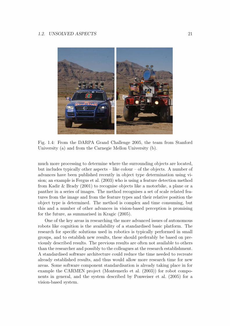
The military applications include ground transportation of goods acrosspotential hostile areas to support friendly units or own troops. One of theprojects that aim for this segment is described in Aufrere et al. (2003) where alarge number of sensors is used in an attempt to create an autonomous outdoorplatform. The USA defence organisation DARPA2 has sponsored a number ofprojects in the area and has organised the Grand Challenge 2004 and 2005events for autonomous vehicles. Five teams completed in 2005 the 132 milesdesert terrain route; the top two of the participants are shown in Fig. 1.4. A
2DARPA: Defence Advanced Research Projects Agency

20 CHAPTER 1. INTRODUCTION
(a) (b)
Fig. 1.3: Demonstration of computer-driven cars travelling at 65miles per hourin San Diego 1997 (a). Surveillance robot used during the football world cupgames in Germany 2006 (b).
number of papers and reports are released from these events, eg Behringer etal. (2005), Xiang & Ozguner (2005), and the winner from Stanford Universitydescribed in Thrun et al. (2006).
1.2 Unsolved aspects
The EUROP describes in Barontini et al. (2005) cognition as one of the mainareas where further research is needed. The cognitive system must base itsdecisions on situation awareness. And situation awareness requires for a robot aqualified perception of the surroundings. Most of the future robots are expectedto operate in an unstructured environment where such skills are needed.
In research work published over the last 20 to 30 years there are sugges-tions to solutions in almost any of the individual disciplines needed to buildan autonomous robot. A plenitude of drive system solutions is available. Sen-sor solutions based on sonar, laser, vision, radar, telemetry, odometry, inertiaand others are described, and each description presents aspects that may bebeneficial for an autonomous robot. When entering into the higher levels ofabstraction in perception and cognition there are less published results.
The perception needed by an autonomous robot is primarily the positioningof nearby objects and a qualified type identification of the objects. When on ahighway with objects in front of the vehicle and on the right side, it is importantto know that the object in front is a car and the object on the right is the roadedge – and not vice versa.
The question as to the position of the objects is often readily solvable bysensors like a laser scanner, whereas the determination of object types oftenrequires more data processing and often more data. A vision sensor requires
1.2. UNSOLVED ASPECTS 21
Fig. 1.4: From the DARPA Grand Challenge 2005, the team from StanfordUniversity (a) and from the Carnegie Mellon University (b).
much more processing to determine where the surrounding objects are located,but includes typically other aspects – like colour – of the objects. A number ofadvances have been published recently in object type determination using vi-sion; an example is Fergus et al. (2003) who is using a feature detection methodfrom Kadir & Brady (2001) to recognise objects like a motorbike, a plane or apanther in a series of images. The method recognises a set of scale related fea-tures from the image and from the feature types and their relative position theobject type is determined. The method is complex and time consuming, butthis and a number of other advances in vision-based perception is promisingfor the future, as summarised in Kragic (2005).
One of the key areas in researching the more advanced issues of autonomousrobots like cognition is the availability of a standardised basic platform. Theresearch for specific solutions used in robotics is typically performed in smallgroups, and to establish new results, these should preferably be based on pre-viously described results. The previous results are often not available to othersthan the researcher and possibly to the colleagues at the research establishment.A standardised software architecture could reduce the time needed to recreatealready established results, and thus would allow more research time for newareas. Some software component standardisation is already taking place in forexample the CARMEN project (Montemerlo et al. (2003)) for robot compo-nents in general, and the system described by Ponweiser et al. (2005) for avision-based system.
22 CHAPTER 1. INTRODUCTION
The conclusion is that especially within the perception and cognitive disci-plines there are many unsolved aspects, and these are the areas that suffer mostfrom the lack of a standardised component framework. A number of such com-ponents – like sensor interface, drive control, simulation and mission scheduler– are needed before perception and cognition components can be integratedand tested in a real world situation.
It will still take a number of years before robots are able to navigate au-tonomously and safely in populated areas.
1.3 Objectives
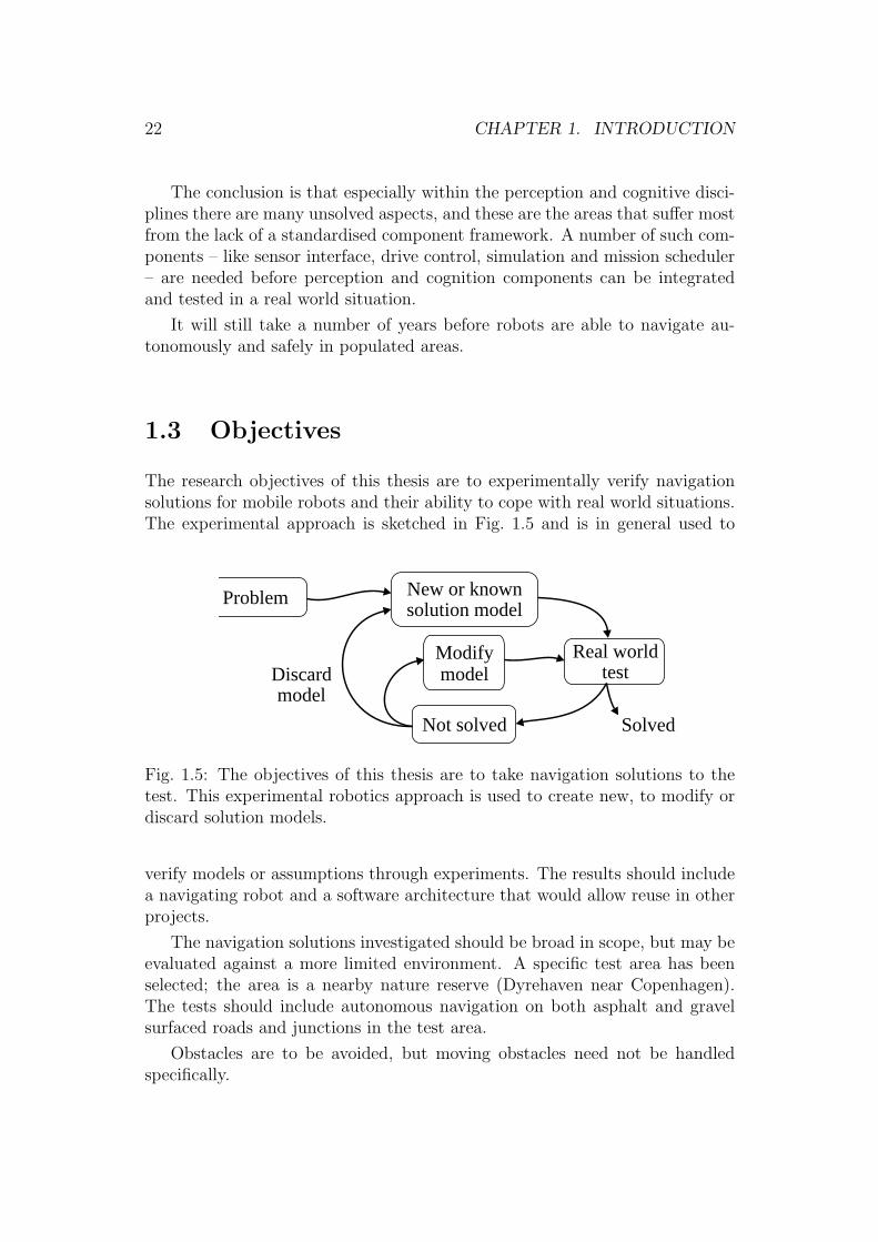
The research objectives of this thesis are to experimentally verify navigationsolutions for mobile robots and their ability to cope with real world situations.The experimental approach is sketched in Fig. 1.5 and is in general used to
Problem
Solved
Modifymodel
Not solved
New or knownsolution model
Discardmodel
Real worldtest
Fig. 1.5: The objectives of this thesis are to take navigation solutions to thetest. This experimental robotics approach is used to create new, to modify ordiscard solution models.
verify models or assumptions through experiments. The results should includea navigating robot and a software architecture that would allow reuse in otherprojects.
The navigation solutions investigated should be broad in scope, but may beevaluated against a more limited environment. A specific test area has beenselected; the area is a nearby nature reserve (Dyrehaven near Copenhagen).The tests should include autonomous navigation on both asphalt and gravelsurfaced roads and junctions in the test area.
Obstacles are to be avoided, but moving obstacles need not be handledspecifically.

1.4. NAVIGATION DISCIPLINES 23
1.4 Navigation disciplines
Navigation is concerned with finding the way to a desired destination. This canbe divided into three parts: the localisation, where am I; the mission, wheredo I want to go; and finally how do I get there.
Where am I
I am at 55.7986N and 12.5456E or at 346145.264E 6183922.977N in zone 33of the UTM3 projection heading 72.5, may be an accurate positioning, buta position like ’facing building 326’ or ’eastbound on route 20’ may be muchmore useful as navigation reference – dependent on the situation.
The important issue is a knowledge of own position relative to the destina-tion.
Where do I want to go
The mission objectives for a navigating robot are to get to a different place.It could be to a position far away, or a position with a number of specificwaypoints, it could be just to explore the surroundings, or search an area untilsome success criterion is met.
There may be a number of competing missions, eg the main mission maybe to explore the area to the left, but the batteries may be almost flat and thecharging station is to the right.
These mission types can all be broken down into a sub mission of the type:bring the robot from A to B.
How to get there
An old Chinese proverb says: ‘Even the longest journey begins with a firststep’. This could be translated as: get moving in the right direction, avoidingobstacles as they are detected. This reactive approach may work well, and isin the spirit of Allan Brooks (MIT 1987) ‘Planning is just a way of avoidingfiguring out what to do next’, but a plan may be needed in some situations, egwhen the robot has met a dead end and the final destination is further ahead.
If a map of the area from A to B is available, with traversable terraininformation, then it may be possible to make an overall plan to get to B, andpossibly to select the most appropriate from a number of alternative routes.But as the obstacle situation along the route most likely is unknown the detailedplanning must wait until the obstacle situation is detected.
3UTM: Universal Trans Mercator

24 CHAPTER 1. INTRODUCTION
Thus a solution should combine long term planning – based on past expe-rience, eg a map – and a short term reactive behaviour to cope with detectedobstacles and situations not foreseen in the map.
1.5 Navigation platform elements
The elements needed for a navigation robot are (see also Fig. 1.6):
• a mechanical system that is capable of making the move from A to B,
• sensors to get impressions from the current situation,
• cognition to perceive the sensed information and to decide on a behaviour,and
• a control system to implement the desired behaviour.
Cognition Sensors
Mechanical platformControl
Fig. 1.6: The main elements of a navigating robot are: sensors, a cognitivefunction, a control system and a mechanical platform.
Cognition is (in this sense) the process of reasoning on the perceived infor-mation and from the reasoning the making of intelligent behaviour decisions.Perception is the interpreting and organising of the sensory information.
A car is a mechanical system capable of making the move from A to B, andit has a control system to implement the desired behaviour. The driver handlesthe remaining elements: the sensors (primarily using the eyes and ears) and theperception of the sensor data (into road and traffic and the interpretation ofsignposts) as well as the decision of an appropriate behaviour (eg take the nextexit and stop when the target position (B) is reached). A normal car is thusnot a navigation robot, as the car does not handle the sensing and cognition.
A (modern) cruise missile has all it takes to get from A to B autonomously,it has sensors that allow perception of the current situation, it has sufficientcognition to correct the course as needed and to take the appropriate actionwhen the target is reached. A cruise missile is thus a navigating robot.

1.6. CONTRIBUTIONS 25
1.6 Contributions
This thesis focuses on the autonomous navigation problem with special em-phasis on outdoor navigation in the semi-structured environment of the testarea.
The main contributions from this thesis are:
• A laser scanner (2D) based perception of road surface and obstacles. Thisis the main sensor for obstacle avoidance and environment perception.The classification into traversable road surface and nontraversable terrainis in short form described in the papers (Blas et al. 2005) and (Andersenet al. 2006).
• A vision-based perception of the available road in front of the robot. Thepurpose is to extend the decision range for direction decisions beyond thelaser scanner range. The results were presented at the 10th InternationalSymposium on Experimental Robotics 2006 (Andersen et al. (2006)).
• A guidemark solution to detect artificial 2D guidemarks using vision.The solution can evaluate the robot position relative to the guidemarkposition. The guidemark includes a (unique) code and can thus be usedas fixed reference points in the navigation process.
• A behaviour control scheduler, where a sequence of prepared navigationroutes can be executed, including decisions based on events on the route,eg detection of guidemark, or calculations based on sensor measurementsetc. This is the human interface point for the implemented navigationsolution, and is intended as the interface point for a mission plannerabove the navigation level. The navigation system has proved its valueon a 3 km autonomous drive on different road types within the test area.
• A software component architecture dividing the software complexity intoa client server structure where the server components complexity is fur-ther reduced by moving parts of the functionality to plugins. The clientserver interface uses an XML4 type text interface, this allows easy exten-sion, monitoring and debugging.
1.7 Thesis structure
The thesis is divided into an
4XML: Extensible Markup Language.

26 CHAPTER 1. INTRODUCTION
Overview chapter of the used robot solution, and is describing the overallfunctionality decisions and design.
Following the overview chapter a separate chapter is allocated for each ofthe main functional areas:
Laser scanner based sensing includes the feature extraction used to sep-arate traversable road areas from nontraversable road sides and otherobstacles.
Vision-based feature extraction describes the determination of availableroad area at longer ranges and the position determination of artificialguidemarks.
Obstacle avoidance includes obstacle management, sensor fusion and deter-mination of the short term path planning in reaction to the detectedobstacles.
Mission planning and execution include the navigation scheduler whichcombines the planned mission with obstacle avoidance.
Following these functional chapters a separate chapter is allocated for aproposal for a new standardised system architecture.
Software architecture is proposing a new division of the robot functionalityinto separately maintainable components and functional modules.
Each of these chapters includes some test results for the described subsys-tem. The final two chapters primarily deal with the full system.
Results where the results obtained on the full system are discussed.
Conclusion which is a summary of the results.
The appendices hold sections describing results and detailed informationexpanding on the results in the main chapters.

Chapter 2
Overview
2.1 Introduction
Outdoor navigation in open terrain requires sensors that can detect obstaclesand traversable terrain directly or indirectly, it requires sensors to determineown position relative to the obstacles and relative to desired target position,and finally to implement the navigation decisions, it requires mobility abilitiesin the desired terrain.
These requirements are discussed in this chapter and are used to determinea set of requirements for an outdoor navigation solution.
Some navigation subsystems are then described in the following chaptersand tested against the requirements.
2.2 Robot conceptual model
The National Aeronautics and Space Administration (NASA) and the US Na-tional Institute of Standards and Technology (NIST) have developed a StandardReference Model Telerobot Control System Architecture (NASREM) describedin Albus et al. (1986) and extended it for intelligent system design as in Albus(1992). This model has been used as the conceptual framework for many robotprojects since then. The basic structure for this model is shown in Fig. 2.1.
The right column in Fig. 2.1 holds the behaviour generation functions, wherethe overall mission is sequenced into a specific behaviour to achieve the missiongoal. The mission assignment is entered at the top to the task scheduler thatimplements the tasks needed to progress the mission and reflects on the currentstate of the system. The relevant system state is supplied by the world model,eg the current position on the navigation map.
The obstacle avoidance block takes the task assigned from the task sched-uler, eg follow road 200m forward, and decides on a route that brings the robot
27

28 CHAPTER 2. OVERVIEW
Mapsensing
Posesensing
Navigatemap
Obstaclemap
Robotstate
Obstacleavoidance
Drivecontrol
Taskscheduler
Behaviourgeneration
World model &value judgement
Sensorprocess
Mission
Obstaclesensing
Drive systemSensor
Operator interface
Fig. 2.1: The conceptual architecture for the robot. The sensors with basic dataextraction are in the left sensor column, the centre column holds the model ofthe world and the robot as well as the current state. The right column is thetasks that control the robot behaviour from the more abstract level on top tothe detailed motion control at the bottom.
in the right direction considering the current obstacles, terrain and robot state.
The drive control implements the drive command by controlling the indi-vidual actuators in the drive system, eg implementing the requested speed andheading.
The sensor process blocks extract the needed data from the real world; theintention is that this information can be used to maintain a model of the worldthat is sufficient for the behaviour decisions.
The value judgement part of the world model column can evaluate alterna-tive plans in terms of cost, risks and benefits, add uncertainty, attractivenessand desirability to measurements and states in the world model. The result ofthe value judgement can then be used to improve behaviour decisions.
In the behaviour generation column the planning horizon will decrease asthe task decomposition gets closer to the drive system actuators. The taskdecomposition may be hierarchical, so that the task scheduler may issue nav-igation tasks to the obstacle avoidance planner and at the same time relatedtasks to a manipulator or some other subsystem of the robot. The obstacleavoidance task may issue commands to both the drive system and other sys-tems like eg an audible alarm or an obstacle movement system. The drivecontrol – most likely – will control a number of actuators.

2.3. TASK BREAKDOWN 29
2.3 Task breakdown
The task breakdown shown in Fig. 2.2 is an expansion of the conceptual modelpresented in Fig. 2.1. The experimental platform (described in section 2.4) setssome of the possibilities and limitations, and these are included in parts of theargumentation for the task breakdown.
Guidemarkextract Navigation
scheduler
Behaviourgeneration
World model &value judgement
Sensorprocess
Mission
Terrainclassify
Drive system
Operator interface
CameraRoad
extend
Obstacledetect
Pose
UTMGPS
Laserscanner
Gyro
Odometry
World pose
Posehistory
Traversablemap layer
Obstaclemap layer
Kinematicmodel
Avoidobstacles
Driveschedule
Drivecontrol
Guidemarkmap layer
Missionmap Mission
decision
Fig. 2.2: The conceptual architecture expanded to include first level of func-tional breakdown. The implemented sensors with data extraction are in the leftcolumn, the centre column holds current state and the model of the world asgenerated by the sensors and the planned behaviour. The right column holdsthe tasks that control the robot behaviour. The mission map and the missionassignment blocks are not implemented. The operator interface is availableprimarily to initiate and monitor the functionality.
2.3.1 Behaviour generation
Missions are loaded to the mission decision block and are assigned to thetask scheduler after some sort of priority scheme. These parts, neither themission map nor the mission decision blocks, are implemented or investigatedin this thesis. The mission priority list could eg hold: go to position B, C orD, explore new roads around position E or return to docking station. The top
30 CHAPTER 2. OVERVIEW
priority mission should then be compiled into a mission sequence of navigationcommands – eg covering the route from current position to point C – andpresent this to the task scheduler.
The implemented navigation command set in the task scheduler includes:’follow road (left, right or centre)’, ’goto (relative) position’ and a set of condi-tions that determine when a command is finished (ie a stop criterion). Addi-tionally, any of the behaviour primitives provided by the drive scheduler maybe used too. The command set supports relative or topological navigation com-mands, either relative to the road or relative to the current posture or to theposture history. When following roads and crossing junctions this command setshould be sufficient. The only GPS support implemented is as a stop condition,where it can be used to determine when to expect eg a junction or a new roadtype.
The navigation scheduler will then in sequence present a method totraverse part of the route – eg keep left on this road or how to cross a square –to the avoid obstacle function, and monitor the available progress indications(used as a stop criterion) before continuing to the next part in the sequence. Astop criterion could be: detection of a vision-based guidemark, that the robotis near a given GPS position, that the robot has travelled a given distance orthat no route is available. The task scheduler will then decide what to do next,according to the assignment. This area is covered in detail in chapter 6.
The avoid obstacles function will attempt to follow the directions pre-sented by the task scheduler by planning a route that follows traversable areasof the terrain and avoids obstacles. The found route is formed as a sequence ofdrive commands – like ’forward 1m’ and then ’turn 20 right’ – and presented tothe drive scheduler replacing the previously assigned drive schedule. Obstaclemanagement and avoidance are the subjects of chapter 5.
The drive scheduler implements the drive schedule taking the currentstate and kinematics model of the robot into account, ie aiming for a desiredspeed at an acceptable acceleration. The result is then presented to the drivecontrol for the relevant part of the drive system. The interface to the drivescheduler is described in chapter 5.
The drive scheduler (named SMRDEMO) and the drive control are notdeveloped as parts of this thesis.
2.3.2 World model and value judgement
The world posture is intended to maintain a global reference to the missionmap using a GPS. The primary purpose of the world posture is to be able todetermine if a reference point is reached in the mission map. Aiming directlyfor a position in GPS coordinates is not implemented, but could be an extensionto the allowed command set. For this purpose a standard GPS unit is available

2.3. TASK BREAKDOWN 31
and allows the robot to get a reference position in absolute coordinates.
The guidemark map layer holds information about detected guidemarks,ie which guidemarks are observed where. A number of guidemark types couldbe interesting, eg a road sign, a wall, a house, a road or a tree, or other objectsthat could be used to recognize a given position. Of these guidemark types onlyroads are implemented, and the available information includes estimated roadwidth and the estimation quality. A vision-based artificial guidemark sensoris available; this detects an artificial two-dimensional barcode (a checkerboardcode). The guidemark code as well as its (3D) position and orientation aredetected. The guidemark extraction is discussed in chapter 4.
The traversable map and the obstacle map are parts of the featuremap used for local navigation for obstacle avoidance. Lack of obstacles is notthe same as good traversable terrain. The roads in the test area are typicallyedged by slightly rougher grass areas, some of which may be traversable bythe robot, but the robot should preferably stay on the roads. Obstacles, onthe other hand, are defined as areas that hinder progress and thus should beavoided at all times. The traversable map can therefore be used in the valuejudgement for possible alternative routes.
The pose history holds the newest posture history of the robot. Theintention of this history is recognition of road curves and the average roaddirection. This information is available to the task scheduler and may be usedto determine when to advance to the next command in the navigation sequence.
The kinematics model is needed to generate smooth and controlled ma-noeuvres.
2.3.3 Sensor processing
The laser scanner is selected as the main sensor for terrain following andobstacle avoidance. As the terrain is primarily flat, the laser scanner is tilteddownwards to get measurements from the road and roadsides. The measure-ments are used for terrain classification and for obstacle detection. This is thesubject of chapter 3.
The vision sensor is used for road detection beyond the reach of the laserscanner and for detection of artificial guidemarks. This issue is discussed inchapter 4.
A gyro is used to supplement the wheel odometry sensor to get a morestable heading. The odometry based heading is very sensitive to terrain cur-vature and structure. The combined wheel odometry and gyro sensor providesstable posture estimate in the tested environment.
32 CHAPTER 2. OVERVIEW
2.4 Experimental platform
The robot platform used for the tests was constructed as part of a master’sthesis Nielsen & Breiting (2004) in 2004.
2.4.1 Mechanical capabilities
cg
41 cm9°
86 cm
15°
15 cm
43 cm
22°
45°90 cm
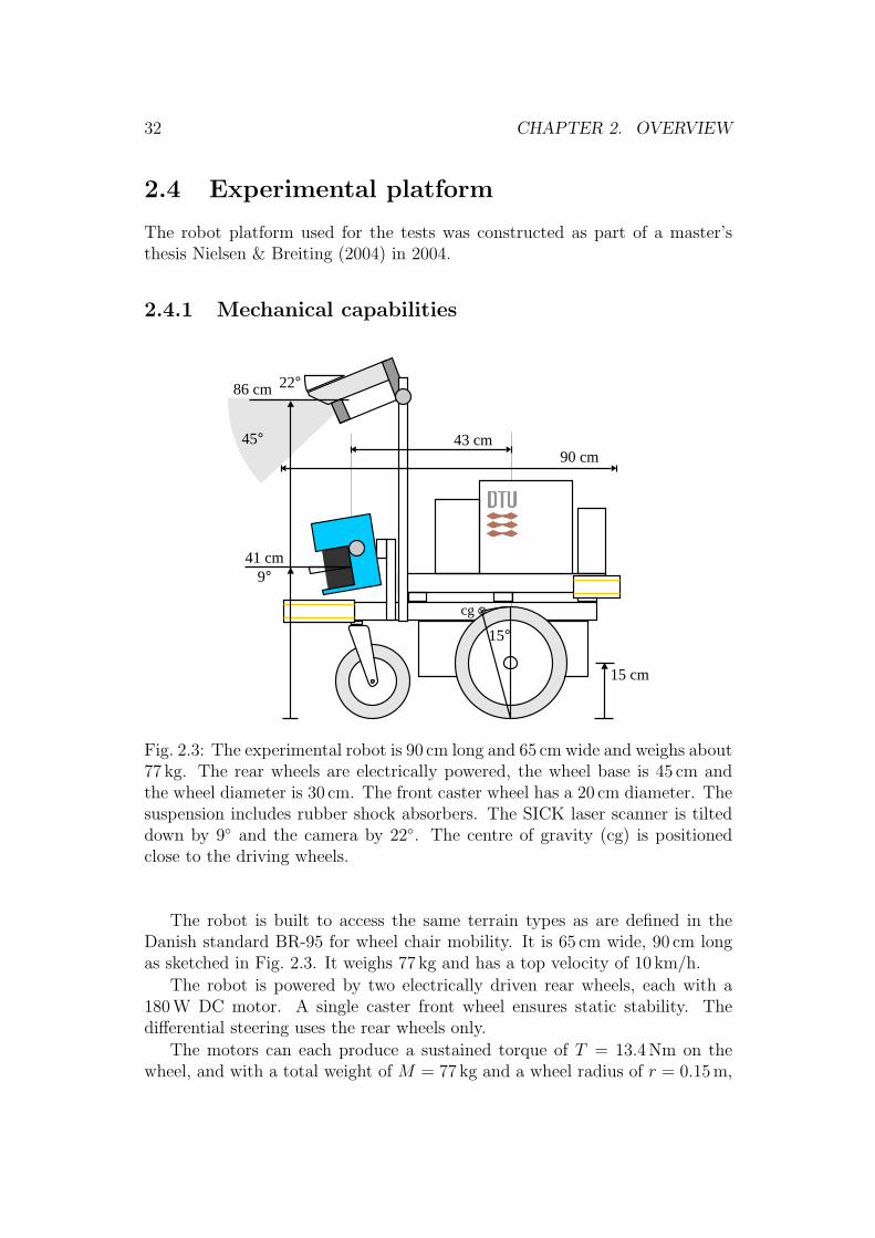
Fig. 2.3: The experimental robot is 90 cm long and 65 cm wide and weighs about77 kg. The rear wheels are electrically powered, the wheel base is 45 cm andthe wheel diameter is 30 cm. The front caster wheel has a 20 cm diameter. Thesuspension includes rubber shock absorbers. The SICK laser scanner is tilteddown by 9 and the camera by 22. The centre of gravity (cg) is positionedclose to the driving wheels.
The robot is built to access the same terrain types as are defined in theDanish standard BR-95 for wheel chair mobility. It is 65 cm wide, 90 cm longas sketched in Fig. 2.3. It weighs 77 kg and has a top velocity of 10 km/h.
The robot is powered by two electrically driven rear wheels, each with a180W DC motor. A single caster front wheel ensures static stability. Thedifferential steering uses the rear wheels only.
The motors can each produce a sustained torque of T = 13.4Nm on thewheel, and with a total weight of M = 77 kg and a wheel radius of r = 0.15m,

2.4. EXPERIMENTAL PLATFORM 33
the maximum road inclination that the robot can climb is Ri = 13.6 as shownin (2.1).
Ri = sin −1 2T
rMg= sin −1 2× 13.4
0.15× 77× 9.8= 13.6 (2.1)
This is approximately the same as the angle to the centre of gravity seenfrom the rear wheels. This indicates that the robot in this configuration willbe able to do a wheelie (lifting the front wheel), especially as the motors willbe able to deliver a higher peek torque.
To avoid a wheelie the total torque should be limited to Tw = 31.4Nm asshown in (2.2), or 15.3Nm each wheel. This corresponds to a wheelie acceler-ation aw = 2.7ms−2 as shown in (2.3)
Mgxcg =Tw
rhcg
Tw =Mgxcgr
hcg
=77× 9.8× 0.15× 0.075
0.27= 31.4 Nm,
(2.2)
where xcg = 0.075 m is the position of the centre of gravity in front of the rearwheels, and hcg = 0.27m is the height of the centre of gravity, as shown in (2.3)
aw =Tw
rM=
31.4
0.15× 77= 2.7ms−2. (2.3)
The weight distribution is approximately 13 kg on the caster wheel and 32 kgon each of the rear wheels.
The robot is equipped with a 38Ah 24 V power pack; this should ensurecontinuous driving for about 7.5 hours at a speed of about 1.5ms−1. The elec-tronics alone uses approximately 50W corresponding to about 18 hours of idleoperation time.
2.4.2 Posture detector
Wheel encoders on both driving wheels ensure odometry distance measure-ments for each wheel. The difference in wheel distance can be used to estimateheading change, but this estimate is dependent on a known wheel diameter.The air-filled tires allow for some compression if the load increases, and thiswill influence the effective wheel radius and hence the odometry accuracy. Ona curved road as shown in Fig. 2.4 the roll angle results in an uneven weightdistribution as shown in table 2.1.
The wheel depression is measured to approximately 0.0001mkg−1 (derivedfrom variations in distance driven with different loads) at a tire inflation pres-sure of (about) 1.5 bar. The difference in wheel radius (rl − rr) relative to the

34 CHAPTER 2. OVERVIEW
MMR
cg
45 cm
10°
27 cm
17.0 cm27.3 cm
Fig. 2.4: On curved roads the roll of the robot will shift the weight balanceresulting in a change in wheel compression and thereby influence the effectivewheel radius used in the odometry.
wheel base (B = 0.45) is the same as the average wheel radius (r = 0.15) rel-ative to the turn radius (R), as shown in (2.4) and exemplified for a roll angleof 10
rl − rr
B=
r
R
R =Br
rl − rr
=0.45× 0.15
0.15065− 0.14935= 52 m.
(2.4)
In outdoor terrain a roll angle of 2–5 on either side of an asphalt or gravelled
Table 2.1: The effective wheel radius of the wheels depends on the tyre depres-sion due to load. When the road profile is curved and the wheels are turning atthe same rotation speed, the robot will follow a curve with the shown turn ra-dius, or suffer the shown systematic heading error (tyre depression effect only).
Roll Load [kg] Radius [cm] Turn Turn err.angle left right left right radius [m] [deg/m]
0 30.5 30.5 15.00 15.000 ∞ 05 27.3 33.7 15.032 14.968 105 0.5410 24.0 37.0 15.065 14.935 52 1.1

2.4. EXPERIMENTAL PLATFORM 35
road is typical, sometimes – typically close to junctions – the roll angle mayreach 10.
The effect of tyre depression may be reduced by increasing the tyre pres-sure, but effects from loose gravel (or soft soil), slippage and stepping effect onthe tyre treads (as there is a turn momentum from the weight on the casterfront wheel) influence the effective wheel radius too. All in all the headingestimate based on difference in travelled distance is systematically dependenton parameters that cannot be deduced from the odometry.
A heading error of more than 1m−1 is not satisfactory. On a flat surfacethe heading stability is about 0.2 m−1 (based on calibration figures in Nielsen& Breiting (2004)).
Detection of roll angle could be obtained by using a tilt sensor and therebyreducing one of the error sources. A gyro measuring the heading change ratewould however be able to measure the heading change independent of theseerror sources (but introduce others like drift as a function of temperature andtime).
The used gyro reaches a heading stability matching the odometry on a flatsurface at a speed of about 1ms−1. When the robot is stationary or at very lowspeed the time drifting error from the gyro exceeds the odometry error, andthus a combination of the two sensors should produce a superior result. Theused implementation is a combination that uses the odometry heading whenthe wheels are stationary and uses the gyro when the wheels are moving. Atthe robot minimum speed (about 0.2 ms−1) the gyro accuracy should still besuperior to the odometry-based heading at a 10 roll angle, so a more balanceduse of the odometry and gyro headings is expected to produce minor accuracyimprovements only.
2.4.3 GPS
A GlobalSat GPS BU303 is available on the robot, this device supports EG-NOS1 and WAAS2 (America only), this enables the device to obtain an about5m accuracy in open areas, compared to about 30m when EGNOS/WAAS isnot available (ref. Nielsen & Breiting (2004)).
2.4.4 Laser scanner
The laser scanner used is a SICK LMS-200; it is interfaced using a high speedUSB-serial connection. This allows a scan rate of up to 72 scans/s with 181measurements each scan. The used range is 8 m, at this range the absoluterange accuracy is about 1 cm. The laser scanner is mounted on bas that allows
1EGNOS: European Geostationary Navigation Overlay Service2WAAS: Wide Area Augmentation System
36 CHAPTER 2. OVERVIEW
variable pitch. For the experiments in this thesis the tilt control is fixated at9. The laser scanner is mounted 41 cm above the terrain.
2.4.5 Camera
A single camera is used for vision purposes. A Philips 840K USB webcam isused, the camera is fitted with a non standard CAML12 fixed wide-angle lens.In this configuration the focal length is found to be 576 pixels for a 640× 480image.
The radial distortion constants are estimated to be K1 = 1.29 · 10−6 andK2 = 1.78 · 10−13 (K1 is a proportional factor for r3 and K2 for r5, where r isthe radial distance (in pixels) from the image centre).
The camera is mounted at a height of 86 cm and is tilted downwards withan angle of 22. The opening angles ϕv vertically and ϕh horizontally arecalculated in (2.5)
ϕv = 2 tan−1 240
576= 45
ϕh = 2 tan−1 320
576= 58.
(2.5)
The camera tilt therefore ensures – in a flat terrain – that the horizon isat the top edge of the image. This is to reduce the effects of image saturationwhen too much of a bright sky is visible in the image.
The out-of-band filtering – infrared and ultraviolet – was implemented asa coating on the original lens. An infrared filter is attached as a replacementto maintain a reasonable colour balance, but especially in sunshine the coloursaturation is limited suggesting that the out-of-band filtering is less than opti-mal.
The automatic white balance filtering provided by the camera is used toadapt to the changing colour temperature under changing weather conditions.This is sufficient for the currently implemented usage, and is visually appealing.Manual operation modes are available.
2.4.6 Computer
The robot has an on-board computer (a mini ATX with a 1.2 GHz VIA proces-sor). This integrates all sensors and the drive control systems. The operationsystem is Linux (in a slackware distribution) on a 1GB flash disk. A RAM-diskis used for data logging during missions.
2.5. APPROACH 37
2.4.7 Security
The weight and speed of the platform allows it to inflict some limited damageon material and persons directly. The robot is therefore equipped with bothan emergency stop switch – that removes power from the driving wheels – anda hand-held remote control capable of taking control of the vehicle wheneverneeded. The remote control must further be within radio coverage at all timesto allow the on-board computer to control the robot.
2.5 Approach
The first attempt was to analyze the laser scanner data to separate traversablefrom nontraversable terrain and then follow a sequence of GPS positions to getto the destination driving on the traversable terrain only. This attempt wasperformed as part of the Master’s thesis Riisgaard & Blas (2005), and someresults were obtained. The terrain analysis used was not efficient on all theterrain types needed for this thesis, and the control strategy, in combinationwith the odometry-based posture sensing, was insufficient to successfully com-plete the navigation objectives. However the basic approach is continued inthis thesis.
The objective is to navigate the different road types, as they are found inthe test area, and be able to do so most of the year.
2.5.1 Road navigation
The approach is to be able to distinguish between road surface and road edgesbased on an analysis of the laser data supplemented by analysis of images fromthe camera. With the road detection in place a method should be found todrive the robot steadily on the road and to detect transitions in road topology– eg at a road junction or when entering open areas – where the control strategyshould be changed.
The robot is capable of passing terrain with steps or obstacles with a heightof less than 5 cm and a terrain inclination of less than 10%, this will allow itto drive on almost all roads and pass most of the obstacles found on the road,eg stones, erosions from rainfall, leaves and small branches. Some of the roadedges are relative flat from wear or with cut grass; these areas are in manycases traversable by the robot, but the robot should, whenever possible, preferthe road over the grass edges.
Obstacle larger than 5 cm should be detected and avoided. Moving obstacleslike pedestrians, bicycles and cars should be avoided too, but detection ofmoving obstacles are outside the scope of this thesis.
38 CHAPTER 2. OVERVIEW
Some of the roads are rather wide (5 m) and here the robot should stickto normal traffic rules and keep to either the left or right side of the road, toallow passage of other traffic. On narrower roads it may be more appropriateto drive in the middle of the road.
The navigation approach is therefore to use the developed algorithms tofollow a road edge or a road centre. This topological approach is independentof GPS coverage and GPS accuracy. The approach requires detection of changein topology, eg when the road ends or joins with another road. The navigationapproach is thus to follow a sequence of topological features (eg roads) sup-plemented by odometry-controlled transitions from one road to the next whenneeded.
2.5.2 Vision support
This experimental platform uses a laser scanner to detect the road at a distanceof about 2.5–3 m in front of the robot. This is sufficient for obstacle avoidanceand road detection in most cases, but detection of junctions and obstacles atlonger distances would improve navigation quality as manoeuvring could beinitiated at an earlier stage. The approach is to isolate the extend of the roadfrom images taken by a forward looking camera. The assumption is that ahomogeneous road surface can be isolated from non-road areas, as the non-road areas are assumed to have a different colour or structure, or is detectableat the transition from road to non-road.
The algorithm uses a sample area in the image already classified by the laserscanner. This sample area is analyzed for colour and intensity profile, and thearea in the image that matches this profile, within an allowed deviation, andnot crossing clear edges, is taken as the road extend.
The reliability of this vision method is – for a number of reasons – less thanthe laser scanner method and is therefore used as a support function only.
2.5.3 Sensor fusion
The laser scanner classifies the terrain up to 2.5–3m with a high probability ofcorrect classification, the vision system has longer range, but both the accuracyand the detection probability are inferior to the laser scanner, the vision data istherefore used at ranges beyond the laser scanner range only. The basis for routeplanning is a traversable corridor; this corridor is based on the laser scannertraversable terrain classification and is extended using the vision data. Theadvantage of the extended range is that the manoeuvre planning may includeavoidance of obstacles that is yet unseen by the laser scanner. In junctions theavailable exit roads may be visible by the vision sensor and the route thereforebe adjusted in time to reach the desired exit. At places where the roadsides

2.5. APPROACH 39
are as smooth as the road itself (eg warn down grass from next to a gravelledroad), the vision may be able to improve the separation.
When the vision part fails, eg is unable to find the extend of the road suc-cessfully, either finding too much (including the roadsides) or too little (hin-dered by eg surface change or hard shadows), the planning reduces to the laserscanner only.
The update rate of the laser scanner (about 6Hz) is higher than the visionanalysis (about 1 Hz), as the vision covers a longer range segment and thereforestays valid for a longer period of time.
2.5.4 Behaviour decisions
A number of traversable corridors may be identified, eg left and right of obsta-cles, side roads and main roads, or just flat areas in the roadside. A manoeuvreroute is planned for all identified corridors, and the decision on which to followis made based on the route attributes and navigation objectives.
When manoeuvring is required an attempt is made to limit the resultingcentripetal acceleration maintaining the desired velocity (where possible).
When no corridor is available the robot will stop, following part of the lastfree route planned. If the obstacle disappears the robot will resume the routeafter an obstacle timeout period.
2.5.5 Software architecture
The software architecture implemented should be reusable and expandable forother than the original developers. It should not be needed to know the detailsof the reused code to use it, and the maintenance of the reusable code and newdevelopment should be separable. At the same time the interface points shouldbe simple, fast and allow easy debug and function monitoring.
The component structure in Orca Brooks et al. (2005) was investigated butwas not adopted, primarily for three reasons: the communication structureseemed too complicated (too much overhead for high data rate connections andtoo limited in data content resulting in too many connections), the extensivelibrary dependency gave implementation difficulties in our Linux distribution,and the available components were not sufficiently attractive to overcome theother limitations.
The proposed component structure is based on a number of servers pro-ducing, where each server may have client connections to other servers. Thisstructure, as well as the basic communication methods – server-push and client-pull – is taken from the Orca terminology. The communication media is selectedto be socket-based TCP/IP. Our existing software is focused on socket-basedIP-communication. The communication data formatting is selected to follow a

40 CHAPTER 2. OVERVIEW
Cameraserver
Laserserver
Operator interface
Camera(s)
Road outline
Driveserver
GPSserverGPS
Laserscanner
GyroOdometry
Guidemark
Emerg. stop
Behaviourserver
SequencerTerrain class.
ObstacleDrive
Drivesystem
Missionassignment
Fig. 2.5: The software architecture is based on a number of server functionsthat allows connection from clients (at points marked with a circle). Some ofthe servers allow increased functionality by plugins shown as a square attachedto the server. The communication media uses IP, and the message data isformatted using XML (with a few exceptions).
subset of the XML defined in the World Wide Web Consordium (2004) recom-mendation. XML is selected as it is well defined, it remains compatible evenif extended, it is text based allowing for interface debugging by use of sim-ple tools, and a number of parsers and coders exist in different programminglanguages.
Transfer of large data structures (eg a camera image) over a socket connec-tion is relative slow, XML coded or not, compared to data transfer internallyin one application or using shared memory. An internal data transfer rate maybe up to 4 bytes for each CPU clock cycle. Transfer of the same data on asocket connection is often at least 10–40 times slower.
A server handling large data structures like a camera server or a laser scan-ner server should therefore include as much data reduction as possible beforedelivering data to a client. That is, the server should hold the data analysisfunctionality so that only the result is transferred to the client. Much of thenew data analysis functionality should therefore preferably be built into theserver directly. To do this without sacrificing separate maintenance of reusedcode and new functionality, the new functionality should be added to the serveras a plugin.
This set of selected communication and structure methods has led to theblock structure shown in Fig. 2.5. Each server serves a unique purpose and mayprovide access to a limited set of resources – ie sensors or actuators. A servertypically provides all its services on one line (shown as a small circle). Eachclient attached decides on the communication method and content from the

2.5. APPROACH 41
available options provided by the server. The operator interface may connectto servers for monitoring or configuration. The operator interface may be simpletools as the text-based TELNET application or more advanced with graphicaldata monitoring and control, possibly with capabilities like teleoperation.

42 CHAPTER 2. OVERVIEW

Chapter 3
Laser scanner based perception
3.1 Introduction
The laser scanner is by far the most common sensor used in mobile roboticsto support obstacle avoidance and path finding. The laser scanner measuresdirection and distance directly, and is thus an easy starting point for the nav-igation software. Almost all other sensors need significant processing beforecomparable data quality can be obtained.
Two main objectives can be fulfilled by the laser scanner in support ofnavigation: detection of obstacles that need to be avoided and detection of tra-versable areas. Detecting obstacles and defining lack of obstacles as traversableareas is one solution. The opposite – detection of traversable areas and definingnon traversable areas as obstacles – is another. In an indoor environment thefirst method – obstacle detection only – is usually sufficient. In an outdoorenvironment the transition from traversable and obstacles is more fluent, andtraversable areas may be more or less desirable for route planning.
Obstacles may be just obstacles – something to avoid – and traversable areasjust for route planning, but they may also be used as guidemarks that can assistthe navigation decisions. This will require that the obstacles or traversableareas are recognisable, in shape or position, either as unique guidemarks – likea unique signpost on a highway – or unique within a limited search area – likea house number when the search area is limited to one road.
This chapter focuses on positive sensing of traversable areas and obstaclesfrom one and the same laser scanner sensor. The use of the data in navigationterms is deferred to a later chapter.
43

44 CHAPTER 3. LASER SCANNER BASED PERCEPTION
3.2 Related work
Current work in the area tends to focus on using 3D laser scanners or a com-bination of 3D laser scanners and vision.
Using 3D laser scanner solutions has been proposed by Vandapel et al.(2004) by transforming point clouds into linear features, surfaces, and scatter.These were classified by using a Bayesian filter based on a manually classifiedtraining set.
Identification of navigable terrain using a 3D laser scanner by checking ifall height measurements in the vicinity of a range reading had less than a fewcentimetres deviation is described in Montemerlo & Thrun (2004).
An algorithm that distinguished compressible grass (which is traversable)from obstacles such as rocks using spatial coherence techniques with an omni-directional single line laser is described in Macedo et al. (2000).
A method for detection and tracking the vertical edges of the curbstonesbordering the road, using a 2D laser scanner, described in Wijesoma et al.(2004) is a way of indirect road detection.
Detection of borders or obstacles using laser scanners is often used bothindoors and in populated outdoor environments, and is the favoured methodwhen the purpose includes map building, as in Guivant et al. (2001) and Klooret al. (1993).
Detection of nontraversable terrain shapes like steps using laser scanner forplanetary exploration is described in Henriksen & Krotkov (1997).
The DARPA Grand Challenge 2004 race demonstrated the difficulties inemploying road following and obstacle avoidance for autonomous vehicles Urm-son et al. (2004). This situation seems to be improved in the 2005 version ofthe race, where five autonomous vehicles completed the 212 km planned route.The winning team from Stanford perceived the environment through four laserrange finders, a radar system, and a monocular vision system. Other teams,like the gray team Trepagnier et al. (2005) also use laser scanners as the mainsensor for traversability sensing supplemented by (stereo) vision. The solutionof the winning team in 2005 is described in Thrun et al. (2006); a 2D laserscanner detects traversable road based on the vertical distance between mea-surements, this solution is combined with vision and radar for longer rangedetections.
3.3 Overview
As in most of the related work, the primary navigation sensor for this thesis isthe laser scanner. It supports the two main drive methods: road following anda direct to destination mode.

3.4. LASER SCANNER USE 45
• Road following attempts to keep a fixed position relative to the road, oraims for a fixed position following the most appropriate of the detectedroads.
• Direct to destination mode is intended for tight manoeuvres where theroad information is either irrelevant or just seen as obstacles.
The same laser scanner data is used for both road finding and for obstacledetection.
• The road finding is based on a series of connected traversable segmentsfrom successive laser scans; this series is assumed to form a corridor thatdescribes the road. The traversable segments are found by analysing thelaser scanner data for a set of features that combined describes traversableterrain.
• Obstacles are found in the part of the laser scanner measurements clas-sified as nontraversable. These single scan obstacles are then combinedwith obstacles found in previous scans into confirmed obstacles. Twoobstacle modes are used when obstacles are correlated with confirmedobstacles: indoor or outdoor.
The laser scanner positioning and scan rate requirements are discussed first,and then the data is analyzed for traversable corridors and for obstacles.
The use of the detected road corridor and obstacles are deferred to chapter 5.
3.4 Laser scanner use
To detect the road the laser scanner must be tilted towards the road. Thisfurther allows detection of obstacles up to the road detection distance.
The optimal positioning and tilt of the sensor is a compromise betweenlaser scanner sensitivity and range, the required obstacle warning distance, theminimum obstacle size and the required scan rate. The used setup is shown inFig. 3.1.
The longer warning distance required the smaller the angle between thelaser beam and the road surface. A small angle reduces the amount of returnedlaser light and thus reduces sensitivity. This is especially a problem on awet surface, eg pits filled with water and wet asphalt. A small angle and ahigh scan rate both results in better obstacle detection capability and longerobstacle detection range. A higher laser scanner mounting height results in alonger warning distance. The laser scanner range – 8m in the used mode –further sets a limit for the angle of tilt.

46 CHAPTER 3. LASER SCANNER BASED PERCEPTION
Fig. 3.1: The robot used in the experiments has a laser scanner at a heightof 41 cm looking downwards in an angle of θL = 9. A flat road is thereforedetected at 2.6m. The position of the last scan (scan n − 1) is shown toillustrate the largest undetected obstacle. The unseen object is not detected inscan n− 1 and is too short to be seen by scan n.
3.4.1 Obstacle detection
The largest obstacle Do that can remain undetected is a function of robotvelocity V , the tilt-angle of the laser scanner ΘL, the scan rate fs and thedistance xj required to separate the obstacle from the road. The obstacle sizeDo can be calculates as shown in (3.1), or as a limitation on the scan rate in(3.2)
Do = (V
fs
+ xj) tan ΘL (3.1)
fs = V/(Do
tan ΘL
− xj). (3.2)
This scan rate fs corresponds to a required distance between scans Ds main-taining the obstacle detection capability
Ds =V
fs
=Do
tan ΘL
− xj. (3.3)
For an obstacle size of Do = 5 cm, a detection distance of xj = 15 cm and alaser scanner tilt-angle of 9 the required distance between scans is 16 cm.
Further the obstacle detection distance xj = 15 cm has the consequence thatobstacles down to 2.5 cm (xj tan(9)) may be detected as obstacles. This meansthat obstacles that can be ignored may trigger an unnecessary manoeuvre.

3.4. LASER SCANNER USE 47
3.4.2 Security distance
The maximum allowable robot velocity Vmax depends on the maximum brakeacceleration ab and the available brake distance Sb as shown in (3.4)
Vmax =√
2abSb. (3.4)
The available breaking distance Sb is shorter than the road detection dis-tance Sr by: a guard distance Sg, the distance required to detect the obstaclexj, the distance travelled in the reaction time tr and the scan rate fs, as shownin (3.5)
Sb = Sr − Sg − xj − V (tr + f−1s )
Sr =hL
tan ΘL
,(3.5)
where hL is the laser scanner height.
3.4.3 Scan rate requirement
(3.5) and (3.4) can be expressed as a scan rate requirement as shown in (3.6)
fs = V (Sr − Sg − xj − V tr − V 2
2ab
)−1. (3.6)
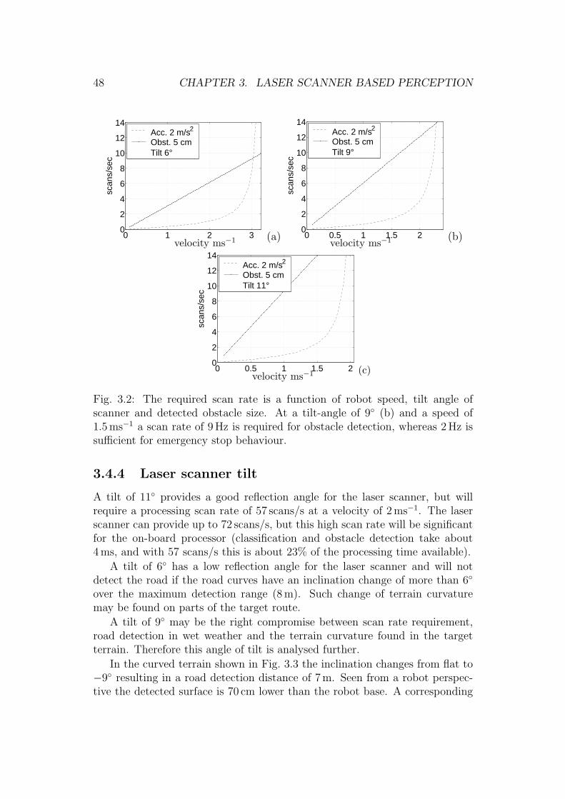
The scan rate requirements are shown in Fig. 3.2 for three different laserscanner tilt-angles: 6 (a), 9 (b) and 11 (c), all with a laser scanner height of41 cm. A breaking acceleration of 2 ms−2 is about the maximum obtainable ona gravelled surface.
The maximum usable cruise speed for the robot is about 1.5–2ms−1 (5.4–7.2 kmh−1). For 1.5 ms−1 the detection range and required scan rate are shownin table 3.1 for the tree cases shown in Fig. 3.2.
Table 3.1: The scan rate and detection range are a function of the tilt-angle ofthe laser scanner and the robot velocity.
1.5 ms−1 2ms−1
Scanner tilt 6 9 11 6 9 11 unitObstacle detect 5 9 14 6 12 18 scan/sEmergency stop 1 1.5 2.5 1 4 57 scan/sDetect range 3.9 2.6 2.1 3.9 2.6 2.1 m
48 CHAPTER 3. LASER SCANNER BASED PERCEPTION
0 1 2 30
2
4
6
8
10
12
14
scan
s/se
c
Acc. 2 m/s2
Obst. 5 cmTilt 6°
(a) 0 0.5 1 1.5 20
2
4
6
8
10
12
14
scan
s/se
c
Acc. 2 m/s2
Obst. 5 cmTilt 9°
(b)velocity ms−1 velocity ms−1
0 0.5 1 1.5 20
2
4
6
8
10
12
14
scan
s/se
c
Acc. 2 m/s2
Obst. 5 cmTilt 11°
(c)velocity ms−1
Fig. 3.2: The required scan rate is a function of robot speed, tilt angle ofscanner and detected obstacle size. At a tilt-angle of 9 (b) and a speed of1.5ms−1 a scan rate of 9 Hz is required for obstacle detection, whereas 2Hz issufficient for emergency stop behaviour.
3.4.4 Laser scanner tilt
A tilt of 11 provides a good reflection angle for the laser scanner, but willrequire a processing scan rate of 57 scans/s at a velocity of 2ms−1. The laserscanner can provide up to 72 scans/s, but this high scan rate will be significantfor the on-board processor (classification and obstacle detection take about4ms, and with 57 scans/s this is about 23% of the processing time available).
A tilt of 6 has a low reflection angle for the laser scanner and will notdetect the road if the road curves have an inclination change of more than 6
over the maximum detection range (8m). Such change of terrain curvaturemay be found on parts of the target route.
A tilt of 9 may be the right compromise between scan rate requirement,road detection in wet weather and the terrain curvature found in the targetterrain. Therefore this angle of tilt is analysed further.
In the curved terrain shown in Fig. 3.3 the inclination changes from flat to−9 resulting in a road detection distance of 7 m. Seen from a robot perspec-tive the detected surface is 70 cm lower than the robot base. A corresponding

3.4. LASER SCANNER USE 49
7 m
0.7m
2.0 m
9°
0.1 m
Fig. 3.3: The road inclination may change from flat and down to about −9
in just 7m, and the road will still be detected. A corresponding increase ininclination reduces the detection range to about 2m.
(a) (b)
Fig. 3.4: The wet parking lot (a) seen by the robot camera is detected by thelaser scanner as shown in (b). The small circles and crosses in (b) are the lasermeasurements. In some areas left and right the returned laser beam is too weekto be detected. The nonvalid measurements are returned as maximum range(just above 8 m). The area to the left – where the detections start to fade –corresponds to the more wet area in image (a). The measurements (crosses)left and right are parked cars not visible in the camera image (a).
increase in inclination results in a road detection distance of about 2.0m (com-pared to 2.6 m for a flat road).
An obstacle with a height of 5 cm below the front or rear wheels will resultin a robot tilt of about ±6.5 of the robot. At a nominal laser tilt of 9 theresulting tilt of the laser scanner will be from 2.5 to 15.5. An otherwiseflat surface will in this case be detected at a distance from 10m (beyond laserscanner range) down to 1.5 m. Detection of a road at just 1.5m corresponds toa terrain elevation of 17 cm when the laser scanner tilt is assumed to be 9.

50 CHAPTER 3. LASER SCANNER BASED PERCEPTION
3.4.5 Wet surface reflection
On a wet surface – especially pits filled with water and wet asphalt – the usedlaser scanner has difficulties in detecting the surface at the narrow angles used.An example is shown in Fig. 3.4(a) from a wet parking lot where there are signsof blank water in the left side of the image; the laser scanner measurementsfails in parts of this area, as shown in Fig. 3.4(b). Just in front of the robotand at some areas to the right, the wet surface is detected.
3.4.6 Spurious detections
The laser scanner is seen to return spurious detections, the origin of the spuriousdetections may be raindrops, insects, snowflakes or just spurious. Typicallythere is only one detection at the particular position and it is not repeated inthe following scan.
A thin fence pole or a chair leg are also often seen by one measurement only,so to avoid the spurious detections isolated measurements are to be trusted asobstacles if they persist in more than one scan only.
3.4.7 Summary
A laser scanner tilt of 9 is about right, it allows detection of terrain curvatureto the degree found in the target area, it allows a manageable scan rate ofabout 9 scans/s for obstacle detection at a velocity of 1.5m/s, and 2 scans/s formanoeuvre planning (especially emergency stopping). When the robot climbsobstacles, the robot tilt will add to the laser scanner tilt temporarily, andobstacles larger than the allowed size may pass unnoticed at the calculatedscan rate. The calculated scan rate for obstacle detection should therefore beexceeded to allow such rough conditions. As the tilt variations due to obstaclesare assumed to be temporary, the effect on the required scan rate for manoeuvreplanning is not expected to be influenced significantly.
The wet asphalt problem is not fully solvable, but as shown in Fig. 3.4 theroad just in front of the robot is usually detected and, if the missing rangemeasurements are ignored, a reasonable road width can be detected.
3.5 Traversability
The assumption is that the measurements can be divided into traversable andnontraversable based on the measurement range values from one single laserscan. By looking at the measurements in Fig. 3.5 this assumption seems rea-sonable. A number of exceptions need to be considered though, like roughgravelled road surfaces, relative smooth road sides, stones and branches on

3.5. TRAVERSABILITY 51
(a)
(b)
Fig. 3.5: Measurements from the laser scanner from an asphalt road. The mea-surements are – as expected – more homogeneous from the road surface thanfrom the grass edges. On the robot top view (b) the circles are measurementsclassified as road (traversable), and the crosses as nontraversable. From themeasurements it is clearly seen that the road is about 5m wide and slightlycurved.

52 CHAPTER 3. LASER SCANNER BASED PERCEPTION
the road, ditches and the road profile, as well as wet reflecting surfaces andpits filled with water. The traversability classification is therefore a bit morecomplicated than might be expected.
The traversability analysis described here is accepted for publication in thejournal paper Andersen et al. (2006). The work was initiated in the master’sthesis Riisgaard & Blas (2005), improved in the paper Blas et al. (2005) andnow further improved as described here.
3.5.1 Measurements
With laser scan readings given in the plane of the laser sensor, each laserscan PL(di, φi) comprises a set of range readings di, i ∈ [1, N ] and the anglesφi ∈ [−90, 90] associated with these. A laser scan PL is hence represented inpolar coordinates in the laser scanner frame. A single element of PL is denotedPL
i . A measurement can be transformed to a robot fixed frame by an R2 → R3
mappingMRL(hL, θL) : PL(di, φi)→ P (xi, yi, zi) as shown in (3.7). The robotframe has body-fixed axes x, y, z pointing forward, left and up, respectively.Scanner measurement angle φi is zero forward and positive to the left
Pi =
xi
yi
zi
=
di cos ΘL cos φi
di sin φi
hL − di sin ΘL cos φi
. (3.7)
With a constant laser tilt-angle ΘL the coordinates xi and zi are fully cor-related as zi = hL − xi tan ΘL, and thus carry the same terrain information.In the calculations below the xi values are used primarily, as this value is di-rectly visible in an x–y map projection, but especially if a controlled tilt wasto be implemented, the zi values would be preferable over xi as these are moreindependent of the laser scanner tilt.
In the sequel, PL(k) will denote a full set of range measurements from asingle laser scan at time k, and P (k) the scan converted to the robot fixed,cartesian frame.
3.5.2 Feature membership functions
The description is based on two main assumptions, a classification assumptionand a mapping assumption:
Classification assumption: Each 3D reading can be categorized as belong-ing to either of three classes, Pi(k) ∈ C, C = Ct, Cn, CØ where Ct :traversable, Cn : nontraversable and CØ : invalid data.
Each Pi(k) ∈ Ct will belong to one traversable segment Sj(k) of the setof traversable segments S in the scan k.

3.5. TRAVERSABILITY 53
Mapping assumption: Seven main features characterise the natural environ-ment, : Fh : raw height, Fσ : roughness, Fz : step size, Fc : curvature,Fw : slope and width, and FØ : invalid data. A unique mapping existsMCF (F) : F → C that categorisation can be uniquely determined from.
Further a mapping existsMSF (F) : F → S for measurements in categoryCt.
Testing each measurement Pi and associating a membership function witheach feature, the aim is to determine a classification into traversable and non-traversable segments and let this information navigate the robot. The formalprocedures of feature extraction and test of hypotheses about categorisationare pursued in the following subsections, starting with a formal statement ofthe problem. It is a prerequisite that scan readings PL(k) are transformed tothe appropriate body coordinates P (k). Let Fi ⊆ Fh,Fσ,Fz,Fc,Fw,FØ andCi ∈ Ct, Cn, CØ,
problem: Given 2D laser readings P (k), determine membership of a featurefunction Fi(Pi(k)) and determine a mapping MCF (F) : F → C to cate-gorise Pi(k) ∈ Ci, and for Pi ∈ Ct a mappingMSF (F) : F → S.
For the sake of brevity, and because feature extraction and classificationare done on single scans in this context, the scan index k is omitted in theremainder of this section.
3.5.3 Invalid data
The laser scanner detects the surface at a small angle, but in most cases thesurface is sufficiently rough to get stable range measurements. On smoothsurfaces the laser scanner is often unable to detect the surface, as shown insection 3.4.5.
In these cases the laser scanner returns maximum range, the same value asif the reflecting surface was further away than the maximum range (8m).
The feature extraction for invalid data is
FØ(PLi ) = dinf ≤ di . (3.8)
The limit is set to the maximum range for the laser scanner dinf = 8m.
These measurements are now classified and are disregarded from the re-maining classification process.

54 CHAPTER 3. LASER SCANNER BASED PERCEPTION
3.5.4 Raw height feature
The feature extraction for valid data starts with the raw height of the mea-surement, h(Pi)
Fh(Pi) = hinf < h(Pi) < hsup . (3.9)
The limits hinf and hsup depend on the expected terrain variations as de-scribed in section 3.4.4 and further on the robot sensitivity to tilt and yaw.
This hsup = 0.2m threshold will limit erroneous classification of flat surfaces,eg a wall in front of the robot, and allow true road detection in a reasonablecombination of robot tilt and road curvature. The lower threshold is moresensitive to road curvature in combination with tilt and yaw of the robot. Thelower limit was set to hinf = −0.7 m in the experiments; this should ensureroad detection in the road curvature situations of the test area – see Fig. 3.3– but not in all combinations of robot tilt and road curvature. The robot tiltsituation is expected to be of temporary nature, so a situation without roaddetection should be temporary and thus recoverable when the robot tilt is backto normal.
3.5.5 Roughness feature
Roughness of data in a 2D laser scan is defined as the square root of localvariance of distance to reflections along the scan. A general estimation of localroughness was given in Blas et al. (2005) using a singular value decomposi-tion approach. However, an alternative and less computationally demandingalgorithm were implemented as described below.
Roughness algorithm
Select a consecutive point set Pn,m from Pn covering a width Wfit = B or widerto the nearest measurement. B is the wheel base (0.45m).
Pn,m =
Pi ∈ P
∣∣∣∣n ≤ i ≤ mm = mmin
where
mmin = MIN(m)
∣∣∣∣| Pm − Pn |≥ Wfit
∧ m− n ≥ 3
(3.10)
Calculate the best fitted line Ln in the x, y plane for the points in Pn,m asshown in (3.11). A least square fit of the deviation in the x-direction is used

3.5. TRAVERSABILITY 55
Fig. 3.6: The laser measurements from Fig. 3.5 are shown in measurement order(−90 to 90) in order to show the roughness estimate at each angle.
for simplicity.
Ln =
x = an + bny
∣∣∣∣∣∣∣∣
an = x− bybn = σ2
xyσ−2yy
σ2xy =
∑(xi − x)(yi − y)
σ2yy =
∑(yi − y)2
(3.11)
Calculate roughness Rn in the Pn,m interval as the average deviation fromthe fitted line
Rn =
√√√√ 1
m− n
m∑i=n
(bnyi − xi + an)2
b2n + 1
. (3.12)
The length of the fitted line Wfit = B = 0.45m is selected to emphasiseterrain variation with a spatial period shorter than this distance and wideenough to allow at least three measurements – in most cases – within thisdistance. Soft curves with a spatial period longer than the robot width willresult in a relatively small roughness value. An example of the roughness valueis shown in Fig. 3.6 for the scene from Fig. 3.5. The roughness is the full line atthe bottom, and the corresponding laser scanner measurements xi are shownabove.

56 CHAPTER 3. LASER SCANNER BASED PERCEPTION
Roughness groups
The intention is to group measurement into traversable segments. If there aremore types of traversable segments these should be grouped separately. Anexample of traversable segment types could be an asphalt road edged by cutgrass, both segment types are traversable, but it would – in most cases – bepreferable for the robot to keep to the asphalt. This is accomplished in threesteps. First the measurements are divided into homogeneous groups (usingheight and roughness). These groups are then combined using the classifiersfor step size Fz and curvature Fc. Finally the resulting groups are filteredbased on slope and width Fw to a set of traversable segments S.
Neighbouring traversable points Pi in Pn to Pm are said to belong to groupGj if their roughness values Ri are relatively homogeneous – as defined in (3.13)
Gj =
Pi ∈ Pn,m
∣∣∣∣∣∣∣∣
hinf < zi < hsup
∧Ri < Rsup
∧ E(Pn−1, Ln) < Rlimj
∧ E(Pm+1, Ln) < Rlimj
where
E(Pi, Ln) =
∣∣∣∣∣bnyi − xi + an√
b2n + 1
∣∣∣∣∣Rlim
j = α MIN(Ri |Pi ∈ Pn,m ).
(3.13)
This implement an adaptive threshold based on the point with the minimumroughness. The interval is then expanded to the point where the distance tothe next measurement is above the adaptive threshold. The distance E(Pi, Ln)is taken from the next measurement Pm+1 or Pn−1 to the fitted line Ln used tocalculate Rn. The threshold limit Rlim
j is set to α times the minimum roughnessinside the interval.
The value of the roughness threshold Rlimj was found experimentally to be
α = 4.5 by optimizing for large group size and to avoid combination of differentterrain types.
Finally, association of a point to the feature Fσ is obtained as
∀j : Fσ(Pi) = Pi ∈ Gj (3.14)
Figure 3.6 is an example of the resulting grouping, using data from theasphalt road with rough grass edges shown in Fig. 3.5. The groupings areshown below the laser measurements. The groupings include the asphalt area(from about −50 to 20), as well as a number of short segments in the rough

3.5. TRAVERSABILITY 57
grass. The asphalt area has a very low roughness (less than 0.01 m), but alignedmeasurements, with a roughness below the hard threshold Rsup = 0.1 m, arealso found outside the road area.
3.5.6 Step size
The surface of gravelled roads and areas are often a combination of smoothareas separated by small objects like stones or tracks. The adaptive thresholdtypically separates such intervals. Branches, leaves and stones also tend tobreak up otherwise smooth roads into separate segments.
The produced groups are therefore inspected and flagged for possible com-bination if they are likely to be from the same surface and the area betweenthe groups is traversable.
The step size feature ensures that two segments are not combined if theyare separated by an obstacle, or separated in height, ie a sidewalk should notbe combined with the road.
Included in the step size feature Fz is also a step in roughness, as defined in(3.15); this prohibits combination of a segment representing a road with a seg-ment representing a traversable roadside (eg cut grass) into just one traversablesegment.
Further, group Gj (with measurements from Pn to Pm) may be combinedwith group Gj+1 (with measurements Pp to Pq) under the following condition
Fz(Pi) =
Pi ∈ Gj
Pi ∈ Gj+1
p > m
∣∣∣∣∣∣∣∣∣∣∣∣∣∣∣
p−m ≤ 4
∧R−1lim <
(Rk
Rk+1
)2
< Rlim
∧ |xm − xp| < Dlim
∧ |xd − xg| < Dlim
wherexd ∈ Pm+1,p−1
xg = xm+xp
2
.(3.15)
This step criterion allows groups to be separated by up to 3 measurements,as long as the x value of these measurement points Pm+1 to Pp−1 are not toofar away (Dlim = 15 cm) from the average of the two end points. The groupsmay not be combined if the roughness Rj and Rj+1, associated with groups Gj
and Gj+1, differ by more than a factor Rlim = 1.8. The x difference betweenthe near end points of the groups may be separated by no more than 15 cm(corresponding to a difference in height of 2.5 cm with the sensor tilt chosen).
An example is shown in Fig. 3.7. This is from a rather flat gravelled area.The area was divided into 6 roughness groups, but all were allowed to becombined.

58 CHAPTER 3. LASER SCANNER BASED PERCEPTION
(a)
(b)
Fig. 3.7: Measurements from a relatively flat gravelled terrain is shown relativeto the robot in (a). The traversable area is divided into a number of roughnessgroups, as shown below the measurement points in (b). These groups are thencombined to one traversable segment (shown above the measurement points).

3.5. TRAVERSABILITY 59
3.5.7 Curvature
A curvature criterion ensures that a road with a high convex profile can be clas-sified as one traversable segment, whereas concave profiles that often describea ditch cannot.
The feature Fc defined in (3.16) checks for curvature and allows combinationof two groups Gj (Pi ∈ Pn,m) and Gj+1 (Pi ∈ Pp,q) based on the vertical anglebetween the groups. The vertical angle of the two groups may be concavewith an angle of no more than ∆sup = 3. For convex groups, the criterion is∆inf = −10
Fc(Pi) =
Pi ∈ Gj
Pi ∈ Gj+1
p > m
∣∣∣∣∣∣Aj+1 − Aj < ∆sup
∧ Aj − Aj+1 < ∆inf
where
Aj = tan−1
(zm − zn
ym − yn
)
Aj+1 = tan−1
(zq − zp
yq − yp
).
(3.16)
An example of this group combination and prohibited combination can beseen in Fig. 3.8, where the high profile road is crossed by a bridle path. Thebridle path is separated from the road, but both parts are smooth enough tobe classified traversable.
3.5.8 Slope and width
Consecutive groups formed by points that posses the features Fz (step) and Fc
(curvature) are merged to one group Gj. Each group Gj (with measurementsPi ∈ Pp,m) must further fulfil a combined slope and width criterion to becomefully qualified traversable segments Sj.
The slope of a traversable segment must be less than ∆yz = 10 vertically(in the y-z plane), and the width of a traversable segment must be wider thanthe robot (WR =robot width)
Fw(Pi) =
Pi ∈ Gj
∣∣∣∣|Pm − Pp| > WR
∧ | Aj |< ∆yz
where
Aj = tan−1
(zm − zq
ym − yq
).
(3.17)

60 CHAPTER 3. LASER SCANNER BASED PERCEPTION
(a)
(b)
Fig. 3.8: Data from a gravelled road crossed by a bridle path. The road isthe area with the high profile (about 15 cm higher at the centre). There arerelatively flat areas from the bridle path on both sides. Rough grass on thepath edges before the bridle path is just visible on both sides of the robot(a). The segmentation algorithm separates the road from the bridle path, andmarks both as traversable (b). The resulting segments are shown above themeasurements.
3.6. ROAD DETECTION 61
The groups that are left out by the criterion Fw are typically originatingfrom a few aligned measurements in the rough vegetation. In Fig. 3.6 thegroups in the rough edges are all removed with the exception of a relativelyflat – and probably traversable – area at the right roadside. The resultingtraversable segments are shown above the measurement points.
3.5.9 Single scan classification
The classification of points of the single laser scan is finally obtained as
CØ(Pi) =FØ(Pi) (3.18)
Ct(Pi) =Fh(Pi) ∩ Fσ(Pi) ∩ Fz(Pi)∩Fc(Pi) ∩ Fw(Pi)
Cn(Pi) = (Ct(Pi) ∪ CØ(Pi)) ,
and the formation of traversable segments from the defined groups as
Sj = Fw(Pi ∈ Gj) . (3.19)
3.6 Road detection
Road detection is used for two purposes:
• To determine where the robot should be positioned on the road, this couldbe on the left side, the right side, at the centre of the road, or at somedistance from these road lines.
• To get road information usable for planning decisions, especially thewidth, eg the road width could indicate that the robot has entered ajunction, or has entered a narrow road.
A quality value is associated with the road lines (left, right and centre) aswell as the width; this quality value is indicating the steadiness of the lines.These quality values can be used as an indication of the fact that the roadedges are valid and not just parked bicycles or other obstacles.
The number of traversable segments in the most recent scan is used asan indication of the number of possible roads or traversable corridors visiblein front of the robot. More than one segment may be found, it could be: asidewalk and a road as shown in Fig. 3.9, a road split, a road with traversableroadsides or just an error. In any case the road quality and roughness valueswill be valuable, when the robot has to determine where to go.

62 CHAPTER 3. LASER SCANNER BASED PERCEPTION
Fig. 3.9: View from the robot camera while driving on a bicycle path with theroad to the left and a sidewalk to the right. The laser scanner measurementsare shown in Fig. 3.10.
The road is detected by correlating traversable segments over a number ofscans from the most recent and some distance back. Each set of correlatedsegments is called a corridor. The road lines are then calculated from the left,right and centre of these corridors.
The corridors – possibly extended by vision-based road detection (see chap-ter 4) – are further used when determining the best route for the robot tofollow, as described in chapter 5.
3.6.1 Segment correlation
The segments found in laser scan k is Skj | j ∈ [1,m], where m is the number of
traversable segments found in scan k, m may typically range from 1 to 3 withextremes being 0 (no traversable segment) and up to 4–5.
A segment Skj may correlate with a corresponding segment in the previous
scans to form a corridor
Bi =Sk
j , Sk−1j1
, Sk−2j2
, ..., Sk−njn
(3.20)
formed by segments from scan k back to scan k − n.Each segment is represented by a parameter line segment of length l
Sj = x + vt | t ∈ [0, l] , (3.21)
where x = [xx, xy]T is the (right) end of the segment and v = [vx, vy]
T is a unitvector in the direction of the line fitted for the segment. The parameter t isused to represent a position sj(t) on the segment for t ∈ [0, l].
The correlation of two line segments is accepted if there is an overlap ofat least the robot width WR between the segments. The overlap is tested byprojecting t0 → t1, where t0 is a position on segment Sk
j and t1 the projected

3.6. ROAD DETECTION 63
position on segment Sk−1j1
; this projected point or the reversely projected pointt1 → t0 should overlap with at least the robot width.
The projected position t1(t0) = t0 → t1 of the point sj(t0) from segment Skj
on segment Sk−1j1
is
t1(t0) = vT · (sj(t0)− x). (3.22)
The overlap is tested by projecting both the end point ta = 0 and a robotwidth into segment ta = WR, both projected positions should be inside theother segment, or alternatively from ta = la to ta = la −WR should be insidethe other segment. The complete test function Fo(Sja , Sjb
) for overlap betweensegment Sja and Sjb
is shown in (3.23)
Fo(Sja , Sjb) =
Sja , Sjb
∈ Bi
∣∣∣∣∣∣∣∣
(tb(0) ∈ [0, lb] ∧ tb(WR)) ∈ [0, lb])∨(tb(la) ∈ [0, lb] ∧ tb(la −WR)) ∈ [0, lb])∨(ta(0) ∈ [0, la] ∧ ta(WR)) ∈ [0, la])∨(ta(lb) ∈ [0, la] ∧ ta(lb −WR)) ∈ [0, la])
.(3.23)
3.6.2 Corridor generation
On every new scan the found traversable segments are linked to the traversablesegments in the previous scan where the Fo(S
kj , Sk−1
j1) ((3.23)) is fulfilled.
The desired result is that corridors are formed for each traversable roadtype visible. An example is shown in Fig. 3.10 where a sidewalk, a bicycle pathand a road are visible.
A set of corridors Bi ∈ B are therefore found by following a unique set oflinks, as described in (3.24)
Bj =Sk
j , Sk−1j1
, ..., Sk−njn
∣∣∣∣∣∣∣∣∣∣∣∣
Fo(Sk−aja
, Sk−(a+1)ja+1
)
ja ∈ [1..ma]ja+1 ∈ [1..ma+1]a ∈ [0..n− 1]∧ age(Sk−n) < Tfade
∧ |Sk−n − Probot|s > Dr
(3.24)
where ma and ma+1 are the numbers of traversable segments found in scan aand a+1. The links are followed back until the segment has reached the robotposition Probot within a (signed) distance Dr ≤ 0.5m, or the oldest scan hasreached a time limit Tfade = 4.5 s.
There may be more than one possible corridor originating from the sametraversable segment Sk
1 , eg one segment in scan k could correlate with twosegments in scan k− 1, and further each of these could correlate with multiplesegments in the previous scan.

64 CHAPTER 3. LASER SCANNER BASED PERCEPTION
S3k
S2k
S2k-1
S2k-2
S2k-3
S2k-4
S2k-5
S2k-6
S2k-7
S2k-8
S2k-9
S1k
S1k-1
S1k-2
S3k-1
S3k-2
S3k-3
S3k-7
S3k-4
S3k-5
S3k-6
S3k-8
S3k-9
Road
Bicycle path
Sidewalk
Fig. 3.10: Traversable segments from the most recent 10 scans. The mea-surements are shown below the lines, as circles (traversable) and crosses (non-traversable) for the most recent scan, and as dots for older scans. The scene isshown in figure 3.9 as seen by the robot camera.
In Fig. 3.10 a corridor is formed for each of the three road types. But thesegments Sk−7
2 and Sk−83 are extra wide and have an overlap that fulfils the
criterion, this adds a fourth corridor that switches from the bicycle path to theroad at this point.
The situation in Fig. 3.10 will therefore produce the corridors shown in(3.25), where B2,a and B2,b are equal except for the last two scans
B1,a =Sk
1 , Sk−11 , Sk−2
1 , Sk−31 , Sk−4
1 , Sk−51 , Sk−6
1 , Sk−71 , Sk−8
1 , Sk−91
B2,a =Sk
2 , Sk−12 , Sk−2
2 , Sk−32 , Sk−4
2 , Sk−52 , Sk−6
2 , Sk−72 , Sk−8
2 , Sk−92
B2,b =Sk
2 , Sk−12 , Sk−2
2 , Sk−32 , Sk−4
2 , Sk−52 , Sk−6
2 , Sk−72 , Sk−8
3 , Sk−93
B3,a =Sk
3 , Sk−13 , Sk−2
3 , Sk−33 , Sk−4
3 , Sk−53 , Sk−6
3 , Sk−73 , Sk−8
3 , Sk−93
.
(3.25)
When there are multiple corridors from the same segment (as B2,a and B2,b
in (3.25)), the best qualified corridor will be maintained only.
The qualification has two parameters: stability in roughness and stabil-ity in width. Every traversable segment has a minimum roughness valuemin(Rn) ∈ Sj (see section 3.5.5), the standard deviation σB of this value forall the segments in a corridor B generates a roughness quality Qr ∈]0, 1]
Qr(B) = (1 + σB · wσ)−1 , (3.26)
3.6. ROAD DETECTION 65
where wσ = 1/0.05 to scale the quality relative to the minimum obstacle sizeto get a reasonable quality interval.
If the traversable segments start on a smooth road and then switches to arough bridle path alongside the road, then the corridor with the switch willhave a lower quality than a the corridor following either the bridle path all theway or the smooth road all the way.
The road width quality Qw ∈]0, 1] is formed by the standard deviation ofthe width of the n segments in the corridor
Qw(B) =
(1 + w−1
B
√1
nΣn
i=1(w2B)− w 2
B
)−1
, (3.27)
where wB is the average width of the corridor B.
The available road corridors are then
Bj = Bj,i |min(Qr(Bj,i) + Qw(Bj,i)), i ∈ [1, N ] (3.28)
3.6.3 Road lines
The road lines include the left, the right and the centre road line. These lines areestimated from the laser scanner based road corridor described in the previoussection.
The end point of the segments in a corridor S is fitted to a straight line.This line is taken as the road edge line (Ll or Lr) and the deviation of thesegment end points from these lines is used as a measure of the edge detectionquality LQ ∈]0, 1] as shown in (3.29)
LQ = (1 +σr
σmax
)−1, (3.29)
where σmax = 0.8m is a scale value.
Road lines with a road edge quality LQ < 0.5 are discarded, and a quality ofLQ > 0.8 indicates a stable, reliable road line. A road edge quality is calculatedfor the left and the right edge individually. The road edge lines are used asreference when the robot is to follow a specific position on the road. Twoexamples are shown in Fig. 3.11 where the high quality (LQ > 0.8) road edgelines are shown as solid lines, and edges with less quality (0.7 < LQ < 0.8) areshown as dots.
The centre of the road is often the best place to drive on narrow gravelledroads. The road centre line Lc is defined as the highest point on the road.The highest point is calculated, relative to the traversable segment, as themeasurement with the longest signed distance (longer in the z-direction, shorter
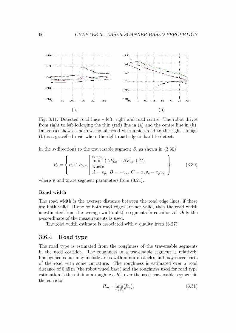
66 CHAPTER 3. LASER SCANNER BASED PERCEPTION
(a) (b)
Fig. 3.11: Detected road lines – left, right and road centre. The robot drivesfrom right to left following the thin (red) line in (a) and the centre line in (b).Image (a) shows a narrow asphalt road with a side-road to the right. Image(b) is a gravelled road where the right road edge is hard to detect.
in the x-direction) to the traversable segment S, as shown in (3.30)
Pc =
Pi ∈ Pn,m
∣∣∣∣∣∣∣
i∈[n,m]
min (APi,x + BPi,y + C)whereA = vy, B = −vx, C = xxvy − xyvx
(3.30)
where v and x are segment parameters from (3.21).
Road width
The road width is the average distance between the road edge lines, if theseare both valid. If one or both road edges are not valid, then the road widthis estimated from the average width of the segments in corridor B. Only they-coordinate of the measurements is used.
The road width estimate is associated with a quality from (3.27).
3.6.4 Road type
The road type is estimated from the roughness of the traversable segmentsin the used corridor. The roughness in a traversable segment is relativelyhomogeneous but may include areas with minor obstacles and may cover partsof the road with some curvature. The roughness is estimated over a roaddistance of 0.45m (the robot wheel base) and the roughness used for road typeestimation is the minimum roughness Rm over the used traversable segment inthe corridor
Rm = minn∈Sj
(Rn). (3.31)

3.6. ROAD DETECTION 67
Fig. 3.12: Roughness estimate for the smoothest part of the used traversablesegments. From 1100–1770m and again from 1860–2190m the road surface isasphalt (blue), the rest has a gravel surface (red). A Gauss distribution withthe same mean and variance is shown to the right.
Table 3.2: Roughness estimation of asphalt and gravel road types based onlaser scanner measurements.
Road type Average Deviation UnitAsphalt µa = 0.0025 σa = 0.00059 mGravel µg = 0.0045 σg = 0.0015 m
This roughness estimate Rm is shown in Fig. 3.12 for a distance where therobot starts on an asphalt road, crosses a gravelled square, drives on to a narrowasphalt road for some 400m and then continues on a gravelled road.
The roughness value clearly changes with the road type, but the variation ofthe roughness is larger than the change in mean value. The laser scanner reso-lution is 1 mm and the accuracy about 10 mm, so quantisation error and sensornoise are expected to be significant parts of the asphalt roughness especially.
The average roughness and standard deviation of the two road types are forthe data in Fig. 3.12 as shown in Table 3.6.4.
Assuming a Gaussian distribution of the roughness for both the asphaltand the gravel road, the distribution is as shown to the right in Fig. 3.12. Thepoint with equal probability for the two road types can then be found by solving

68 CHAPTER 3. LASER SCANNER BASED PERCEPTION
(3.32)
N(µa, σa) = N(µg, σg)
1√2πσa
exp
(−(req − µa)
2
2σ2a
)=
1√2πσg
exp
(−(req − µg)
2
2σ2g
)
req = 0.0034 m .
(3.32)
Determination of road type clearly requires averaging over some measure-ments to maintain a stable road type estimate. A cumulative sum (CUSUM)algorithm may be used to determine state change between such two probabilitydistribution functions Blanke et al. (2003), and this algorithm seems applicablefor the problem.
The CUSUM algorithm sums the log likelihood ratio for a series of mea-surements (r(i) for i ∈ [1, k]) of a stochastic variable, as shown in (3.33)
s(k) =k∑
i=1
s(r(i)) =k∑
i=1
lnpg(r(i))
pa(r(i)). (3.33)
This function value s(k) is expected to decrease if the measurement r(i)belongs to the asphalt probability pa and to increase if it belongs to the gravelprobability pg. When the probability density functions are Gaussian and withequal variance, the expression can be simplified as in (3.34) (from Blanke et al.(2003))
s(k) =k∑
i=1
µg − µa
σ2a
(r(i)− req). (3.34)
The gravel distribution adapted with the same variance as the asphalt road,positioned symmetrically on the other side of the equal probability line req givesan µ′g = req + (rex − µa) = 0.0043 and σ′g = σa = 0.00059.
When the sum s(k) increases (from a minimum value) by a value hg theestimate is that the measurements belong to probability function pg. The valuehg determines the time to detect a change and the false alarm ratio. Thesevalues can be determined by the runlength function L(µs, σs, h) as shown in(3.35) (from Blanke et al. (2003)

3.6. ROAD DETECTION 69
Table 3.3: Average ’false alarm rate’ and ’time to detect’ for the estimationof road type. Both values are in measurement counts. The h value associatedwith the CUSUM threshold.
Transition h false alarm time torate detect
asphalt→gravel 7 38700 2.4gravel→asphalt 10 1700 6.0
L(µs, σs, h) =
(e−2(µsh
σ2s
+µsσs
1.166) − 1 + 2(µsh
σ2s
+µs
σs
1.166)
)σ2
s
2µ2s
(3.35)
where
µs = −(µg − µa)2
2σ2a
false alarm rate (3.36)
µs =(µg − µa)
2
2σ2a
time to detect (3.37)
σs =
∣∣∣∣µg − µa
σa
∣∣∣∣ . (3.38)
The same calculations can be performed for the change from gravel to as-phalt; there the variance σ2
g = 0.00142 is used for both probability functions.The hg and ha values have been selected to provide for a reasonable detectiontime and false alarm rate for both transitions. The result is shown in Table 3.3
With h = 7 the average time to detect is 2.5 measurements and the averagefalse alarm rate is one in 38700 measurements, all assuming that the measuredvalues follow the used distribution functions.
The state change from asphalt to gravel is determined from the function in(3.39), following the CUSUM function in (3.34) but is limiting the minimumvalue to zero. The state change detection from gravel to asphalt is shown in(3.40)
state:asphalt→ gravel
∣∣∣∣∣∣
state = asphaltb(k) = max0, r(k)− req + b(k − 1)∧ µg−µa
σ2a
b(k) >= hg
(3.39)
state:gravel→ asphalt
∣∣∣∣∣∣
state = gravelb(k) = min0, r(k)− req + b(k − 1)∧ µg−µa
σ2g
b(k) <= −ha
. (3.40)
The resulting road type estimation can be seen in Fig. 3.13. The change
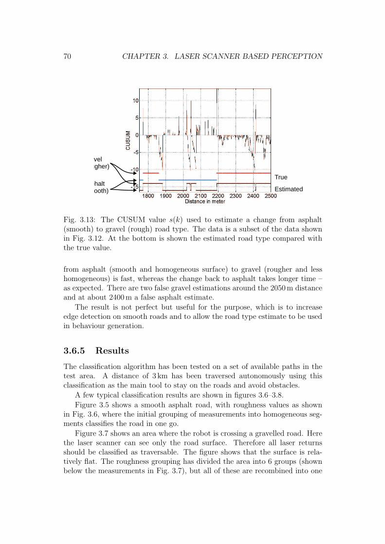
70 CHAPTER 3. LASER SCANNER BASED PERCEPTION
Gravel(rougher)
Asphalt(smooth)
True
Estimated
Fig. 3.13: The CUSUM value s(k) used to estimate a change from asphalt(smooth) to gravel (rough) road type. The data is a subset of the data shownin Fig. 3.12. At the bottom is shown the estimated road type compared withthe true value.
from asphalt (smooth and homogeneous surface) to gravel (rougher and lesshomogeneous) is fast, whereas the change back to asphalt takes longer time –as expected. There are two false gravel estimations around the 2050m distanceand at about 2400m a false asphalt estimate.
The result is not perfect but useful for the purpose, which is to increaseedge detection on smooth roads and to allow the road type estimate to be usedin behaviour generation.
3.6.5 Results
The classification algorithm has been tested on a set of available paths in thetest area. A distance of 3 km has been traversed autonomously using thisclassification as the main tool to stay on the roads and avoid obstacles.
A few typical classification results are shown in figures 3.6–3.8.
Figure 3.5 shows a smooth asphalt road, with roughness values as shownin Fig. 3.6, where the initial grouping of measurements into homogeneous seg-ments classifies the road in one go.
Figure 3.7 shows an area where the robot is crossing a gravelled road. Herethe laser scanner can see only the road surface. Therefore all laser returnsshould be classified as traversable. The figure shows that the surface is rela-tively flat. The roughness grouping has divided the area into 6 groups (shownbelow the measurements in Fig. 3.7), but all of these are recombined into one
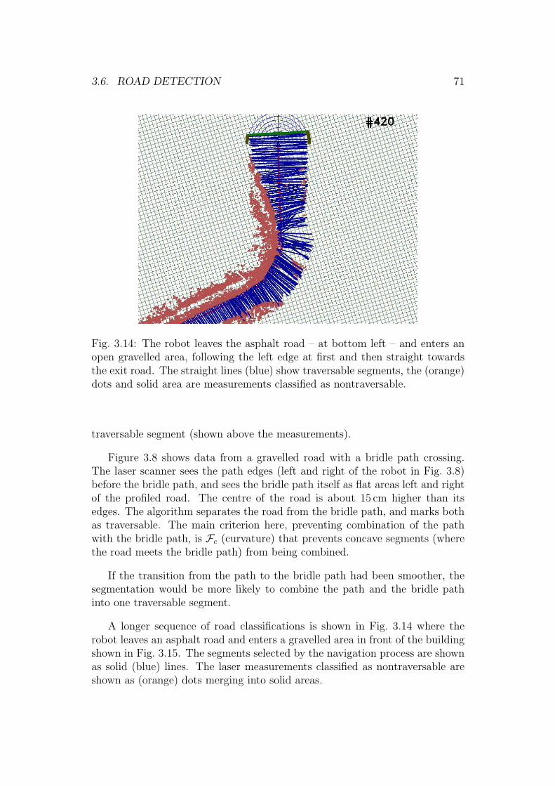
3.6. ROAD DETECTION 71
Fig. 3.14: The robot leaves the asphalt road – at bottom left – and enters anopen gravelled area, following the left edge at first and then straight towardsthe exit road. The straight lines (blue) show traversable segments, the (orange)dots and solid area are measurements classified as nontraversable.
traversable segment (shown above the measurements).
Figure 3.8 shows data from a gravelled road with a bridle path crossing.The laser scanner sees the path edges (left and right of the robot in Fig. 3.8)before the bridle path, and sees the bridle path itself as flat areas left and rightof the profiled road. The centre of the road is about 15 cm higher than itsedges. The algorithm separates the road from the bridle path, and marks bothas traversable. The main criterion here, preventing combination of the pathwith the bridle path, is Fc (curvature) that prevents concave segments (wherethe road meets the bridle path) from being combined.
If the transition from the path to the bridle path had been smoother, thesegmentation would be more likely to combine the path and the bridle pathinto one traversable segment.
A longer sequence of road classifications is shown in Fig. 3.14 where therobot leaves an asphalt road and enters a gravelled area in front of the buildingshown in Fig. 3.15. The segments selected by the navigation process are shownas solid (blue) lines. The laser measurements classified as nontraversable areshown as (orange) dots merging into solid areas.
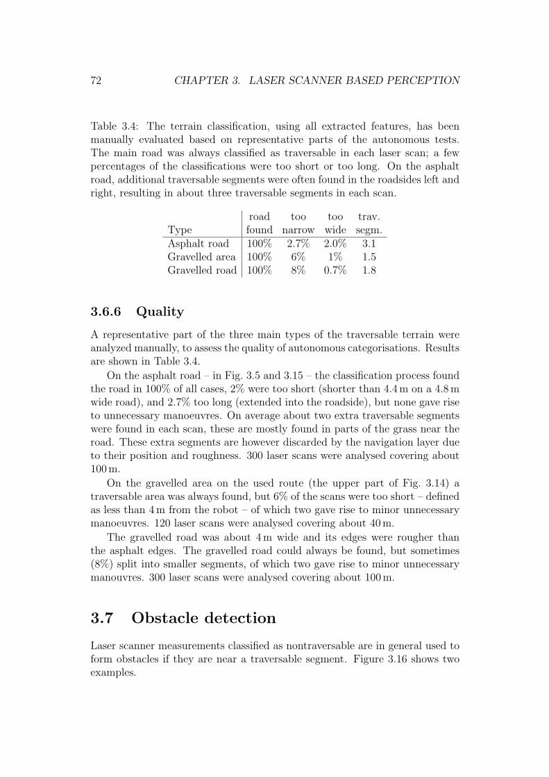
72 CHAPTER 3. LASER SCANNER BASED PERCEPTION
Table 3.4: The terrain classification, using all extracted features, has beenmanually evaluated based on representative parts of the autonomous tests.The main road was always classified as traversable in each laser scan; a fewpercentages of the classifications were too short or too long. On the asphaltroad, additional traversable segments were often found in the roadsides left andright, resulting in about three traversable segments in each scan.
road too too trav.Type found narrow wide segm.Asphalt road 100% 2.7% 2.0% 3.1Gravelled area 100% 6% 1% 1.5Gravelled road 100% 8% 0.7% 1.8
3.6.6 Quality
A representative part of the three main types of the traversable terrain wereanalyzed manually, to assess the quality of autonomous categorisations. Resultsare shown in Table 3.4.
On the asphalt road – in Fig. 3.5 and 3.15 – the classification process foundthe road in 100% of all cases, 2% were too short (shorter than 4.4m on a 4.8mwide road), and 2.7% too long (extended into the roadside), but none gave riseto unnecessary manoeuvres. On average about two extra traversable segmentswere found in each scan, these are mostly found in parts of the grass near theroad. These extra segments are however discarded by the navigation layer dueto their position and roughness. 300 laser scans were analysed covering about100m.
On the gravelled area on the used route (the upper part of Fig. 3.14) atraversable area was always found, but 6% of the scans were too short – definedas less than 4 m from the robot – of which two gave rise to minor unnecessarymanoeuvres. 120 laser scans were analysed covering about 40 m.
The gravelled road was about 4m wide and its edges were rougher thanthe asphalt edges. The gravelled road could always be found, but sometimes(8%) split into smaller segments, of which two gave rise to minor unnecessarymanouvres. 300 laser scans were analysed covering about 100m.
3.7 Obstacle detection
Laser scanner measurements classified as nontraversable are in general used toform obstacles if they are near a traversable segment. Figure 3.16 shows twoexamples.
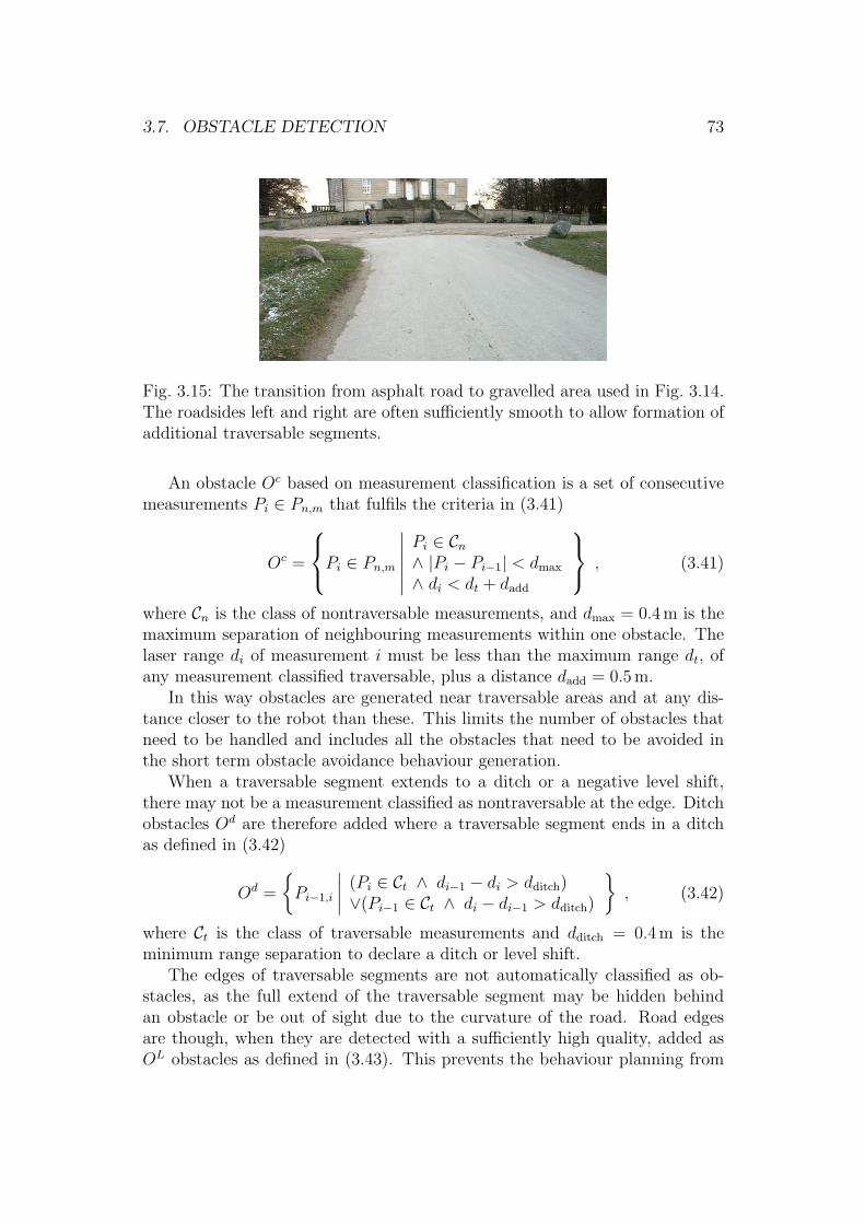
3.7. OBSTACLE DETECTION 73
Fig. 3.15: The transition from asphalt road to gravelled area used in Fig. 3.14.The roadsides left and right are often sufficiently smooth to allow formation ofadditional traversable segments.
An obstacle Oc based on measurement classification is a set of consecutivemeasurements Pi ∈ Pn,m that fulfils the criteria in (3.41)
Oc =
Pi ∈ Pn,m
∣∣∣∣∣∣
Pi ∈ Cn∧ |Pi − Pi−1| < dmax
∧ di < dt + dadd
, (3.41)
where Cn is the class of nontraversable measurements, and dmax = 0.4m is themaximum separation of neighbouring measurements within one obstacle. Thelaser range di of measurement i must be less than the maximum range dt, ofany measurement classified traversable, plus a distance dadd = 0.5m.
In this way obstacles are generated near traversable areas and at any dis-tance closer to the robot than these. This limits the number of obstacles thatneed to be handled and includes all the obstacles that need to be avoided inthe short term obstacle avoidance behaviour generation.
When a traversable segment extends to a ditch or a negative level shift,there may not be a measurement classified as nontraversable at the edge. Ditchobstacles Od are therefore added where a traversable segment ends in a ditchas defined in (3.42)
Od =
Pi−1,i
∣∣∣∣(Pi ∈ Ct ∧ di−1 − di > dditch)∨(Pi−1 ∈ Ct ∧ di − di−1 > dditch)
, (3.42)
where Ct is the class of traversable measurements and dditch = 0.4m is theminimum range separation to declare a ditch or level shift.
The edges of traversable segments are not automatically classified as ob-stacles, as the full extend of the traversable segment may be hidden behindan obstacle or be out of sight due to the curvature of the road. Road edgesare though, when they are detected with a sufficiently high quality, added asOL obstacles as defined in (3.43). This prevents the behaviour planning from

74 CHAPTER 3. LASER SCANNER BASED PERCEPTION
Mainroad
Bicycleroad
Sidewalk
Level-shiftobstacle
Classifiedobstacles
RobotCorridorlines
Classifiedobstacles(pedestrians)
Road-sideobstacle
Classifiedobstacles
(a) (b)
Fig. 3.16: Detection of obstacles. The laser measurements classified as non-traversable are divided into obstacle polygons. Additionally if a traversablesegment ends with a level shift to a lower level the positions around the levelshift are marked as obstacles as shown in (a) where the level goes down to themain road. In (b) the road edge has a high quality (the residual from the linefitting is low) and is included as an obstacle.
crossing road boundaries even if the area on the other side of the road boundaryis classified as traversable (deliberate crossing of a road boundary is thereforenot supported)
OL = L ∈ Lr, Ll |LQ > Qmin , (3.43)
where Qmin = 0.9 is the required quality limit for addition of road edge lines asobstacles.
The measurements in an obstacle are reduced to a convex polygon. Thisreduces the amount of data needed to describe the obstacle and simplifies cal-culations. Further, the amount of vertices needed to describe the obstacle isreduced, so that close vertices are removed (reduction limit set to 0.03 m).
The obstacles will be further processed when merged with obstacles fromprevious scans as described in chapter 5.
3.7.1 Wall detect
When the robot drives directly towards a wall the first detection of the wallwill look like a flat road surface – only slightly elevated. When the robot movesthe elevation increases until the height threshold hsup = 0.2 is passed, the wallis now about 1.3m from the robot.
A wall detection function is therefore added that invalidates a corridor ifit ends in a wall. The wall test compares the position and orientation of two
3.8. SUMMARY 75
consecutive traversable segments while the robot has moved (at least 0.05m).The two segments must be within 0.04m of each other and their orientationmust be within 2.3.
When the wall in this way is detected twice (using three consecutive scans)the corridor is assumed to end in a wall, and thus invalidated as a traversablecorridor.
In a rough outdoor environment it happens that the road detection getscloser – due to robot tilt – at the same speed as the robot movement, there isthus a possibility that the corridor is mistaken to be a wall. A few instances ofthis type have been recorded, typically resulting in an erroneous stop.
If a corridor flagged to be a wall continues to correlate without furthertriggering of the wall detector, the wall flagging is removed after four non-wallscans.
3.8 Summary
This chapter has described a comprehensive set of features extracted fromthe laser scanner measurements. These should form a solid base for obstacleavoidance and behaviour generation. The features extracted include:
Traversable segments describing parts of the surface that is evaluated to betraversable. Each segment is further qualified with a roughness estimate.
Traversable corridors generated from a set of correlated traversable seg-ments. The corridors describe a part of the road – primarily in front ofthe robot – that is traversable; there may be multiple of such corridors,eg describing a road fork or multiple lanes originating from eg a road anda sidewalk.
Road lines are generated as a by-product of the corridors. The road lines arecalculated from the left, right and centre of the corridor. A quality valueis associated with each line to allow discrimination of lines influenced byobstacles or partially out of laser scanner range.
Road type estimate based on roughness. The tested road types include as-phalt (smooth) and gravelled (rough) roads, and the road type is esti-mated reasonably well.
Obstacles describing areas that should be avoided by the behaviour genera-tion function.
Requirements for laser scanner positioning and scan rate are further eval-uated to allow sufficient obstacle detection ability and sufficient warning timefor manoeuvring.

76 CHAPTER 3. LASER SCANNER BASED PERCEPTION
The limitations of the laser scanner are primarily the limited range (theroad is detected at a distance of about 2.6m in front of the robot) and in thelimited ability to discriminate a road from its sides in the cases where the sidesare rather flat and smooth.
3.9 Further improvements
Further improvements are expected to be obtainable especially in the followingareas:
Road line detection is not continued from one scan to the next, but calcu-lated anew using the most recent corridor only. A method of estimatingthe road edge continuously using eg a Kalman filter is expected to pro-duce superior results and may enable continued road edge detection whenpassing obstacles. Such road edges would be valuable, especially if therobot was to perform mapping.
A Roll and pitch sensors would allow for slightly better estimation of roadcurvature, and this could allow for better qualification of a number of theused thresholds in the classification process.
Obstacle detection at times detect obstacles near maximum range in openareas or when passing a side road, this could probably be avoided byusage of some of the partial results from the filtering.

Chapter 4
Vision based perception
4.1 Introduction
The objective for any sensor is to extract useful information.
A vision sensor has the potential to extract any visible feature inside thecamera view, but especially two limitations make vision-based sensors difficultto use for navigation purposes:
A camera sensor is an angle-only sensor. This first limitation necessitatesthat the sensor must have additional information to be able to deliver 3Dpositions of the features. This additional information could be knowledge of thesize of a feature, the distance from camera to the feature, or angle informationfrom a sensor at another position, eg another vision sensor.
The second limitation is the use of illumination of opportunity. An image ofa stationary scene looks different in different illuminations, the shadows change,the colour changes with the colour of the illumination, bright illumination ofsome features and week illumination of objects in the shadows make it difficultfor the camera to get sufficient detail in both situations.
When the illumination is controlled and the scene has known features, egan orange ball of a known size on a horizontal green surface, then the detectionis simplified, but parts of the ball may not seem orange as part of the surface –the highlight area – just reflects the illumination and thus has the same colouras the illumination.
In an outdoor environment the illumination is changing and the size of theseen objects is mostly unknown. The use of vision for navigation in such anenvironment poses a significant challenge. This chapter presents vision-basedsolutions and discusses the obtained results.
77
78 CHAPTER 4. VISION BASED PERCEPTION
4.2 Related work
The use of cameras to aid robot navigation has been described in a number ofpapers using a large number of different approaches.
Stereo vision is one of the fundamental methods to create a 3D model of theangle-only measurements from the camera. The basic method is to recognisethe same features in two or more images, and from accurate knowledge ofthe camera position and orientation to calculate the triangulation points toreconstruct the distance to the feature. One project described in Loaıza etal. (1999) and Loaıza et al. (2001) uses two cameras mounted on top of eachother and does stereoscopic calculation on contrast straight lines found in theimages, the Loaıza et al. (2001) project puts emphasis in colour on each sideof the extracted lines to improve correlation. The project Se et al. (2001)uses three cameras in a right angle triangular configuration to remove falsecorrelations. The project also extracts a number of (scale invariant) featuresbefore stereo calculation and then stores these points (about 3000 for one room)for the ongoing navigation.
A camera with fish-eye lenses that cover 360 around and above the robotcan be very useful for localisation, especially in an indoor environment. Shah& Aggarwal (1997) use this configuration to find significant lines ending ingeometric vanishing points and from these and vertical lines build a model ofthe traversed corridor.
In vision solutions Bertozzi & Broggi (1997) argue that this problem canbe divided into two subproblems: lane following and obstacle detection, anddescribe a stereo-vision based solution for both. The lane following dependon the bright lane markings and a stereo-based solution to detect the angle tomoving obstacles (cars).
Edge detection in vision systems is one of the possibilities to identify roadborders and had some success already in 1986, as described in Wallace et al.(1986).
A method for road following using vision and neural network to estimate themain road direction was developed by Jochem et al. (1993) for lane following,and in Jochem et al. (1995) expanded to detect side roads and ’Y’ junctions.
A simple method – with the same basic principle as used in this project –is described in Horswill (1994), where the edges of a homogenous structurelessarea in front of the robot is taken as obstacle free area for navigation.
Lane following using single camera solution is also described in Liatsis etal. (2003), where edges are detected and tracked from one frame to the nextusing edge magnitude and orientation in the area of the image, where the roadedge is expected.
The DARPA Grand Challenge 2004 race demonstrated great difficulties inroad following and obstacle avoidance for autonomous vehicles as described in
4.3. LIMITATIONS AND POSSIBILITIES 79
eg Behringer et al. (2005).
4.3 Limitations and possibilities
Vision depends on ambient light and provides a 2D colour and texture view ofparts of the surroundings.
The image colour depends on the illumination (eg sunlight and shadows),the time of year (eg trees are green in the summer, red or yellow in the falland partially transparent in the winter) and weather conditions (eg roads areoften black when it rains, grey when they are dry and possibly white during thewinter). The camera may lack dynamic range to detect colours in both sunnyand shaded parts of an image. Limited illumination at night and weatherconditions like fog, rain or snow will further limit the results of vision-basedsolutions.
Some of these factors may have little or no influence on some vision sensorsor solutions may be available to avoid or compensate for the effects.
A vision sensor is an angle-only sensor, and the 3D reconstruction of thescene therefore requires additional information, typically in the form of multipleimages from different locations, assistance from other sensors, or assumptionsrelated to the features seen in the image.
The possibilities of using vision are – despite the limitations mentionedabove – almost endles. Evolution has proved the success of vision, as largegroups of the living creatures on earth use vision as one of their main sensors.
The solutions can be divided into two groups, one group uses images frommore locations to place the objects seen in a 3D environment eg stereovisionand structure from motion; the other group makes assumptions on the seenfeatures, being objects of a known size or an assumption of the layout of thescene, eg roads are predominantly flat and has mostly parallel edges.
Stereovision was initially evaluated for this project, but the tested solutionwas temporarily discarded due to experienced problems during robot move-ment (the solution is described in appendix A). Stereovision units for robotnavigation are becoming commercially available and may in time replace theneed for laser scanner based obstacle detection – especially at short ranges.
For this project the near obstacle detection and the road detection arehandled by a laser scanner. The prime purpose for a vision system is thereforeto assist where the laser scanner comes short, ie at longer ranges and wherethere are ambiguities in the laser scanner detections.
The two vision sensor methods presented here are both based on presump-tions of the viewed features to reconstruct a 3D world model: a road outlinesensor that assumes the road seen by the camera to be flat and in the sameplane as the robot base and a guidemark recognition solution that requires the
80 CHAPTER 4. VISION BASED PERCEPTION
physical size of the recognized artificial guidemark to be known in advance.The first solution should supplement the laser scanner sensor and the seconduniquely identify the robot position, once a guidemark is recognised.
4.4 Road outline
The assumption is that it is possible to estimate the outline of the road byanalysing the image, based on an appropriate seed area. Such a seed area maybe provided by the laser scanner.
The main features describing the road are its homogeneity. But there maybe variation in the visual expression due to eg shadows, sunlight, specularreflections, surface granularity, flaws, partially wet or dry surface and minorobstacles like leaves on the road.
The road detection is therefore based on two features: the chromaticity Cand the intensity gradient ∇I.
The chromaticity is colour stripped from intensity as shown in (4.1) basedon a RGB (Red, Green, Blue) image
c =
[cred
cgreen
]=
[r/(r + g + b)g/(r + g + b)
]. (4.1)
Each pixel position Hi,j is classifiable into class R =road, not road. TheRroad classification is defined as in (4.2) and the Rnot road = Rroad holds theremaining pixels
Rroad(Hi,j) =
Hi,j
∣∣∣∣∣∣
(1−Kbal)Pc(C(Hi,j))+KbalPe(∇I(Hi,j))> Klim
, (4.2)
where Kbal = 0.43 gives the balance between chromaticity and edge sensitivity,and Klim = 0.65 the detection sensitivity. Both values are found experimentally.A sample filtering is shown in Fig. 4.1 for each of the two components as wellas combined.
Pc(·) is a probability function based on the Mahalanobi distance of thechromaticity relative to the seed area
Pc(i, j) =(1 + wc(c
′i,j − c)TQ−1(c
′i,j − c)
)−1
, (4.3)
where Q is the chromaticity covariance for the seed area, c is the averagechromaticity in the seed area, and wc = 0.022 ensures appropriate numericalvalues for the result.

4.4. ROAD OUTLINE 81
(a) (b)
(c)
Fig. 4.1: Road outline extraction based on chromaticity (a), on gradient de-tection (b) and combined (c). In the top left corner there is a stone fence;this is not distinguished from the gravel road surface using the chromaticityfilter in (a). The gradient filter (b) makes a border to the pit (bottom left).The combined filter (c) outlines the traversable area as desired. The seed areaclassified by the laser scanner is shown as a (thin) rectangle. The part of theimage below the seed area is not analysed.
Pe(·) is a function based on the intensity gradient ∇I(Hi,j)
Pe(i, j) =
(1 + we
[∣∣∣∣∂I(i, j)
∂i
∣∣∣∣2
+
∣∣∣∣∂I(i, j)
∂j
∣∣∣∣2])−1
, (4.4)
where we = 0.067 is a weight factor (the image intensity has the value range[0,255]).
The intensity gradient is calculated using a Sobel operator. The Sobelkernel size is selected as appropriate for the position in the image, ie the lowerin the image (closer and more detailed) the larger the kernel (5 × 5 pixels atthe bottom and 3× 3 at the top for the used 320× 240 image resolution).
The pixels at the road contour are evaluated only, ie from the seed area
82 CHAPTER 4. VISION BASED PERCEPTION
pixels are tested towards the image edge or road border, the road border isthen followed (clockwise) back to the seed area. This is a very computationallyefficient analysis method as only a subset of the pixels in the image are anal-ysed and no filtering is needed on the full image. A disadvantage is that smallobstacles (lower than the camera height) in the middle of the road may remainundetected, when all surrounding pixels indicate traversable road. This disad-vantage could be avoided by testing pixels inside the road outline at appropriateintervals.
4.4.1 Shadows
Shadows are a problem as the colour information in the shade is more bluishfrom the blue sky whereas the colour in the sun is more reddish – and thus maynot match the seed area. In full sunshine and full shadow the automatic whitebalance of the camera will compensate for this, but when both are presentin the same image it needs to be considered. The white balance in sun andshadows influences the balance between red and blue chromaticity values only,whereas the green is relatively unaffected. The intensity in the shade is lowerthan in the sun, and the intensity is therefore a first choice for a correlatedvalue that could be used to compensate for the shift in white balance.
In Fig. 4.2(b) the blue and red chromaticity is shown as a function of inten-sity for a part of the road area in the image shown in Fig. 4.2(a) with mixedshade and sun (on the asphalt road part of the image).
The figure shows that darker areas have an increased blue and decreasedred component – as expected. The difference in colour balance is a function ofthe used camera and the colour of the sky, but the tendency shown in Fig. 4.2is taken to be representative for this camera. The chromaticity value uses thered and green values only, therefore the red chromaticity value cred is adjustedas defined in (4.5)
c′=
[cred + (I − I)gred
cgreen
], (4.5)
where I = (r + g + b) is the intensity, I = 1.5 × 256 is the average intensity(the linearization point) and gred = 0.066 is the linearized gradient of the redchromaticity as a function of intensity – derived from Fig. 4.2.
This shade-compensated c′is used as the basis for calculation of c and the
covariance matrix Q.The seed area is taken from the most recent laser scan, and the traversable
segment with the least roughness is used. The seed area is taken as the centralthird of this segment; this will in most cases avoid the areas near the roadborders, which may not be representative for the road. This central part isprojected into the image and used as a seed area.
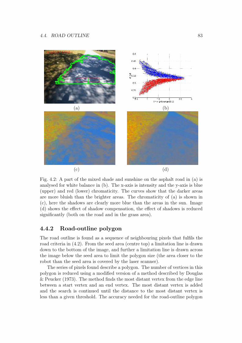
4.4. ROAD OUTLINE 83
(a) (b)
(c) (d)
Fig. 4.2: A part of the mixed shade and sunshine on the asphalt road in (a) isanalysed for white balance in (b). The x-axis is intensity and the y-axis is blue(upper) and red (lower) chromaticity. The curves show that the darker areasare more bluish than the brighter areas. The chromaticity of (a) is shown in(c), here the shadows are clearly more blue than the areas in the sun. Image(d) shows the effect of shadow compensation, the effect of shadows is reducedsignificantly (both on the road and in the grass area).
4.4.2 Road-outline polygon
The road outline is found as a sequence of neighbouring pixels that fulfils theroad criteria in (4.2). From the seed area (centre top) a limitation line is drawndown to the bottom of the image, and further a limitation line is drawn acrossthe image below the seed area to limit the polygon size (the area closer to therobot than the seed area is covered by the laser scanner).
The series of pixels found describe a polygon. The number of vertices in thispolygon is reduced using a modified version of a method described by Douglas& Peucker (1973). The method finds the most distant vertex from the edge linebetween a start vertex and an end vertex. The most distant vertex is addedand the search is continued until the distance to the most distant vertex isless than a given threshold. The accuracy needed for the road-outline polygon

84 CHAPTER 4. VISION BASED PERCEPTION
changes with the position in the image: one pixel covers a larger road area atthe top of the image than at the bottom, on the other hand pixels at the bottomdescribe positions that are closer to the robot and are thus more relevant forobstacle avoidance. The threshold used is one pixel at the top of the imageand 4.5 pixels at the bottom with a linear scaling between these values.
4.4.3 Projection to robot plane
The pixel coordinates in the reduced polygon needs to be projected to the robotplane to be comparable with the laser scanner solution. This is done in threesteps: compensation for radial lens error, finding a vector in the pixel directionand finally finding the position where this vector crosses the robot base plane.
• The pixel position pe = [pex, p
ey]
T found in the image is adjusted for radiallens error to p = [px, py]
T using the two major radial error parameters K1
and K2 for the lens (values are found in section 2.4.5). The adjustmentis performed as in (4.6) – from Carstensen (2001)
r2 = (pe − h)T (pe − h)
dr = K1r2 + K2r
4
p = pe + (pe − h)dr ,
(4.6)
where h = [hx, hy] is the head point in the image (the geometric imagecentre is used).
• A 3D line a = [xa + tva] from the projection centre in the direction of thepixel coordinate p is found (in camera-oriented coordinates) ac = [0+tvc
a]as in (4.7)
vca =
vcx
vcy
vcz
=
1−(px − hx)/c−(py − hy)/c
, (4.7)
where c is the focal length, and the vector end position is taken at anarbitrary fixed x-distance of 1m.
The line origin and orientation vector are then coordinate converted torobot-oriented coordinates as in (4.8)
a = [xc + t(va)]
va = Rcvca ,
(4.8)
where xc == [xx, xy, xz] = [0.43, 0, 0.86] is the camera position, Rc =RκRϕRΩ is the camera rotation matrix where primarily Rϕ has a valuedifferent from unity, as the camera is rotated along the y-axis by ϕ = 22
as from section 2.4.5.

4.4. ROAD OUTLINE 85
• The line from the camera to the pixel position is crossing the robot planein the searched position b (unless parallel with robot plane), and b isfound as in (4.9) utilising that the robot plane is the x, y plane
b = [xc + tbva]
tb = −xz |va|vz
,(4.9)
where va = [vx, vy, vz].
If vz is positive or zero then there is no crossing (at least not in front ofthe robot), such results are replaced with a position close to the horizonin order to get a proper polygon in robot-oriented coordinates. Positionsabove the horizon of the robot plane may be classified as road when therobot tilt (or roll) places parts of the real horizon above the robot planeor if objects in the horizon (erroneously) are taken as road.
The road-outline polygon is now in robot-oriented coordinates and is readyfor use by the navigation and obstacle avoidance functions.
4.4.4 Road outline results
The road width estimate and the road width stability can be taken as a perfor-mance measure of the vision and laser scanner sensors. The method is testedprimarily on a 3 km route in the test area. The navigation is guided by a scriptspecifying how to follow the roads and for how long. Parts of this route areanalysed.
An analysis is shown in Fig. 4.3 for an asphalt road and in Fig. 4.4 for agravelled road. The weather conditions were overcast with mild showers. Theroad width is estimated in front of the robot based on the available data atthe time of manoeuvre decision. The vision-based road width is taken as theaverage distance between the road lines, where both road lines are inside theimage (see next chapter for more details).
The road width data in Fig. 4.3 covers a distance of about 500 m, and showsa stable road detection both by the laser scanner sensor and by the visionsenor, the vision with a slightly higher uncertainty, but with good correlationbetween the two sensors. The road-outline estimate in Fig. 4.3(b) shows analmost perfect correlation with the road edges. There is a slight tendency thatthe vision estimate shows a narrower road width than the laser scanner.
The gravelled road in Fig. 4.4 shows data from a distance of about 300mwith a side road about halfway. The road width seen by the vision sensor isclearly narrower than the width from the laser scanner. The reason is twofold:the vision estimate is too narrow and the laser scanner estimate is too wide.

86 CHAPTER 4. VISION BASED PERCEPTION
0 100 200 300 400 5003.5
4
4.5
5
5.5
Roa
d w
idth
[m]
(a) (b)
Fig. 4.3: Road width estimation (a) based on laser scanner (solid black) andvision-based (red with dots). A 500m section of an about 5m wide asphaltroad. The vision-based outline for the first part of the road is shown in (b).
The width seen by the vision system is projected to a plane at the robotbase, and as the road profile is convex, the true road width is slightly wider.Typically the road is 10 cm higher at the centre, and with a true road widthof 3.5 m (as it is most of the way), the projection would show a road width of3.13m. This corresponds nicely with the measured value.
The laser scanner estimated a road width of typically 3.5 to 4 m with onlylittle correlation with the vision-based road width. The reason is mostly thatthe road roughness is not much lower than the roughness of the near part of theroadsides. Figure 4.5 shows a set of measurements from the early part of thedata series in Fig. 4.4. The blue lines (in Fig. 4.5(a)) between the robot and thelaser scanner measurements are the traversable segments used for calculatingthe road width. Especially the right roadside shows variations in the segmentwidth, none is too short, but some are too wide. The thin green lines show theestimated road lines. This effect is mostly significant where the roadside is inthe same plane as the road (especially in the early part of the data series inFig. 4.4).
Seasonal variation
An about 600 m section of the route are shown in Fig. 4.6(a) and (c) taken inthe spring (early May) in sunshine and in Fig. 4.6(b) and (d) the same roadsection in midsummer (late July) during an overcast weather condition. Thefirst part of the section is a narrow asphalt road (up to about 300m) and then

4.4. ROAD OUTLINE 87
550 600 650 700 750
2
3
4
5
6
7
Roa
d w
idth
[m]
Fig. 4.4: Road width estimation based on laser scanner (solid black) and vision-based (red). A section from an about 3.5 m wide gravelled road (a). At about675m a side road makes the road estimate wider.
a gravelled road for the remaining part. Two side roads are passed at about100m and 500 m.
The width of the asphalt road (about 3 m) is detected equally well in springand in summer. The gravelled road appears wider in early spring than mid-summer, and the uncertainty seems much higher, both for the laser scannerbased width and the vision-based width.
The laser scanner estimate is wider as the grass is still relative flat aftera long winter, so the roughness difference between the road and the roadsideis marginal. In midsummer the grass is higher and the border thus easier todistinguish.
For the vision sensor the partially gray grass (from the winter) is muchharder to distinguish from the road than at midsummer. An example can beseen in Fig. 4.7(h), where especially the right roadside is problematic.
Another issue is sunshine and shadows. Below open trees in sunshine, likein Fig. 4.7(c) and in Fig. 4.6(c) – both from the early part of the data series –the road width estimation is more difficult resulting in a more insecure estimate(visible at about 50m in Fig. 4.6(a)).
Summary
The road width estimates are summarised in table 4.1 for the laser scanner andvision sensor, respectively. The first two rows are from the same test but atdifferent road types – asphalt and gravel, respectively. The last two rows in

88 CHAPTER 4. VISION BASED PERCEPTION
(a) (b)
Fig. 4.5: A set of measurements at the early part of the data series used inFig. 4.4. Both laser scanner data and the vision road outline is shown in (a).The vision-based outline is shown in (b).
Table 4.1 are from a narrow asphalt road segment that is partially below largetrees and here the road outline estimates failed in 16% of the measurements on aday with sunshine, compared to just 2% under gray and wet weather condition.Failed measurements are counted as a too wide or too narrow estimate (> 20%of true value).
The conclusion is that the vision sensor performs reasonably well, and some-times better than the laser scanner. The performance is slightly better on as-phalt roads than on gravelled roads. Gray grass and scattered shadows reducethe performance.
Shadows
Most road outline situations are handled reasonably well, the shadows fromoverhanging trees in Fig. 4.7(a), (b) and (c) and from the lightpole in (d)produce usable results. The partially wet asphalt in (e) is handled. The tiledsidewalk in (f) is only partially solved, especially the sunny spots in a ratherdark image as in (c) and (f) are difficult. The gravel road in (h) and (i) arebasically fine, but the sharp shadow in (i) is taken as an obstacle. In (h) theside road to the left is partially found, but part of the right roadside is takenas road. Painted road markings are normally taken as obstacles.
All the shown images in Fig. 4.7 are produced with the same algorithm andthe same weight and threshold settings.
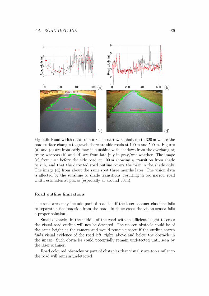
4.4. ROAD OUTLINE 89
0 200 400 6000
2
4
6
8
Roa
d w
idth
[m]
(a) 0 200 400 6001
2
3
4
5
6
Roa
d w
idth
[m]
(b)
(c) (d)
Fig. 4.6: Road width data from a 3–4 m narrow asphalt up to 320m where theroad surface changes to gravel; there are side roads at 100m and 500m. Figures(a) and (c) are from early may in sunshine with shadows from the overhangingtrees; whereas (b) and (d) are from late july in gray/wet weather. The image(c) from just before the side road at 100 m showing a transition from shadeto sun, and that the detected road outline covers the part in the shade only.The image (d) from about the same spot three months later. The vision datais affected by the sunshine to shade transitions, resulting in too narrow roadwidth estimates at places (especially at around 50m).
Road outline limitations
The seed area may include part of roadside if the laser scanner classifier failsto separate a flat roadside from the road. In these cases the vision sensor failsa proper solution.
Small obstacles in the middle of the road with insufficient height to crossthe visual road outline will not be detected. The unseen obstacle could be ofthe same height as the camera and would remain unseen if the outline searchfinds visual evidence of the road left, right, above and below the obstacle inthe image. Such obstacles could potentially remain undetected until seen bythe laser scanner.
Road coloured obstacles or part of obstacles that visually are too similar tothe road will remain undetected.

90 CHAPTER 4. VISION BASED PERCEPTION
Table 4.1: Road width estimate summary from the data shown in Fig. 4.4and Fig. 4.3 is in the first two rows. The last two rows are from the narrowasphalt road segment in the early part of Fig. 4.6 both in the early spring, thefirst under overcast (wet) weather and the last under clear sunshine. The ’w/n’column is the too wide or too narrow count as a percentage of the measurementcount N.
Road True Laser based Vision basedsegment width mean σ N mean σ w/n N refAsphalt 4.9 4.7 0.17 1200 4.5 0.24 1% 474 4.3Gravelled 3.5 3.7 0.48 600 3.2 0.32 3% 245 4.4Asphalt 3–4 3.5 0.63 890 2.8 0.36 2% 224 wetAsphalt 3–4 3.3 0.46 482 2.8 0.53 16% 79 sun
Road paintings will typically be detected as obstacles (not part of the road).
Sharp shadows may trigger the edge detector sufficiently to be taken as anobstacle.
Change in road surface type, eg change from asphalt to gravel, may limitthe road outline.
Sensor saturation may occur, especially in sunny spots in an otherwise dom-inantly shady area.
4.5 Guidemark recognition
Landmark navigation is based on the assumption that the robot from recog-nising a landmark can get a localisation reference. The landmark could beartificial and placed to be recognised by the robot, ie for indoor applicationsa method is to place unique landmarks on the ceiling and let a robot cameralook for these landmarks, and further place the landmarks at so short intervalsthat the robot could navigate from one landmark to the next with sufficientaccuracy to be able to find the next guidemark.
The guidemark itself could be at a known position, or just act as a uniquereference position so that any ambiguity or accumulating errors could be re-solved or reduced when recognising the guidemark.
The initial position of the robot could be resolved by recognition of a uniqueartificial landmark. This landmark could refer to an entry in the robot databasewith knowledge of that specific area. One or more landmarks could be placedclose to a charging station that may require accurate navigation.
For these purposes a camera-based landmark system has been designed toexplore the possibilities.
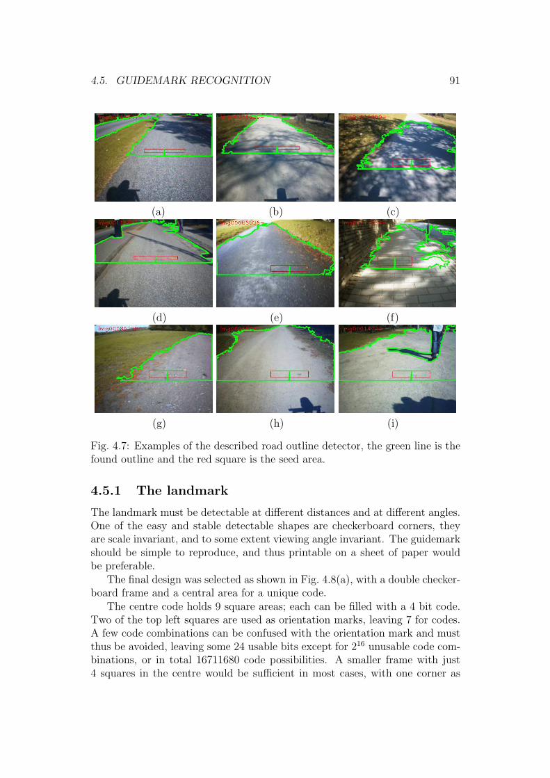
4.5. GUIDEMARK RECOGNITION 91
(a) (b) (c)
(d) (e) (f)
(g) (h) (i)
Fig. 4.7: Examples of the described road outline detector, the green line is thefound outline and the red square is the seed area.
4.5.1 The landmark
The landmark must be detectable at different distances and at different angles.One of the easy and stable detectable shapes are checkerboard corners, theyare scale invariant, and to some extent viewing angle invariant. The guidemarkshould be simple to reproduce, and thus printable on a sheet of paper wouldbe preferable.
The final design was selected as shown in Fig. 4.8(a), with a double checker-board frame and a central area for a unique code.
The centre code holds 9 square areas; each can be filled with a 4 bit code.Two of the top left squares are used as orientation marks, leaving 7 for codes.A few code combinations can be confused with the orientation mark and mustthus be avoided, leaving some 24 usable bits except for 216 unusable code com-binations, or in total 16711680 code possibilities. A smaller frame with just4 squares in the centre would be sufficient in most cases, with one corner as

92 CHAPTER 4. VISION BASED PERCEPTION
y1
y2 y4
y3 y1
y2
y4
y3
(a) (b) (c)
Fig. 4.8: The guidemark in consist of a checkerboard frame and a central code.The camera view of the lower left part is shown in (b) and (c). The cornerfilter uses four 3× 3 areas to detect a corner at the centre position.
orientation mark, and at maximum 3 bits used in the remaining a total of 9bits or 512 codes would be available.
The guidemark in Fig. 4.8(a) has two black bits set in each of the two leastsignificant squares – bottom right inside the frame – corresponding to the value9Chex or 156 decimal.
The guidemark is detected in four steps: corner detection, frame detection,code detection and frame localisation, each of these steps are described in thefollowing.
4.5.2 Corner detection
The corner detection is done by performing a comparison of four areas in theimage expected to match two black areas and two white areas.
The full image is first filtered using a 3× 3 pixel Gaussian kernel, summingthe pixels inside the kernel area – in a G(i, j) function – to the centre pixelposition (i, j) (eg the y1 area in Fig. 4.8(b)). The summation uses a Gaussiandistribution for weights with a σ = 0.95. This yields the central pixel a weightof about as much as the sum of weights of the remaining 8 pixels.
A set of corner pixels C1 at pixel positions a = [r, c] ∈ C1 are found in theimage as defined in (4.10)

4.5. GUIDEMARK RECOGNITION 93
C1 =
a = [r, c], wr, c ∈ image
w = y1 + y4 − y2 − y3
∣∣∣∣∣∣∣∣
y1 − y2 > kc
∧ y1 − y3 > kc
∧ y4 − y2 > kc
∧ y4 − y3 > kc
, (4.10)
where
y1 = G(r − 2, c− 2) (4.11)
y2 = G(r + 2, c− 2) (4.12)
y3 = G(r − 2, c + 2) (4.13)
y4 = G(r + 2, c + 2) (4.14)
kc =1
3[max(y1, y2, y3, y4)−min(y1, y2, y3, y4)] + kI . (4.15)
An intensity difference is thus required from all bright corners to all blackcorners. This difference kc is increased with the intensity difference from thebrightest to the darkest block as in (4.15) and includes a fixed minimum thresh-old kI = 7 (the intensity coding is 255 for white and 0 for black). This ensuresthat a guidemark in both bright areas and darker areas are detectable.
The filter will detect a corner that is bright in the upper-left and lower-rightpart. Intensity-reversed corners are found in the same way by exchanging thecalculation of y1, y4 with y2, y3 in (4.11) to (4.14) for the second corner setC2.
The guidemark may however be observed at different orientations dependingon the positioning of the guidemark and the camera. By adding a guard bandof one pixel between the 4 corner areas, the filter will be relatively insensitiveto viewing angle rotation of the guidemark relative to the camera, the cornerdetection sensitivity will be reduced as the angle increases, and at 45 thesensitivity will be zero.
To be able to detect guidemarks at any rotation angle a second set of filtermasks (rotated 45) is added as shown in Fig. 4.8(c), using the same filterfunction as in (4.10), except that the relative positioning of the four areasy1, y2, y3, y4, is replaced with (4.16) to (4.19) producing a third corner set C3
y1 = G(r − 3, c) (4.16)
y2 = G(r, c− 3) (4.17)
y3 = G(r, c + 3) (4.18)
y4 = G(r + 3, c) . (4.19)
Again replacing the calculation of y1, y4 with y2, y3 in (4.16) to (4.19)yields the fourth corner set C4.

94 CHAPTER 4. VISION BASED PERCEPTION
The distance between the four summed areas is in the 45 version 4.2 pixelsand in the not rotated version 4 pixels. When the block size in the image is lessthan four pixels (or 4.2 when rotated) the detection probability will decrease.A not rotated guidemark can thus be detected at slightly longer distancescompared to a rotated guidemark.
The corner pixels in C1, C2, C3, C4 are then enumerated individually using8-connectivity into the total set of corner groups Hn. The centre of each cornergroup hn(Hn) is found as shown in (4.20)
hn(Hn) =1∑
i∈Hn(wi)
∑i∈Hn
(aiwi) , (4.20)
where the accuracy improvement by using the intensity weight wi derived in(4.10) is not quantified nor optimised.
In Fig. 4.8(b) and (c) the detected corner pixels are shown as bright squaresin yellow and green, where green marks the pixel closest to found corner posi-tion.
When a guidemark is rotated approximately 22.5 it happens that the samecorner is detected by two filters, ie one of C1, C2 and one of C3, C4, suchcorners are combined to one if the distance between the centres ha − hb <2.9 pixels.
4.5.3 Frame detection
The corner positions have to match the frame of the guidemark, ie from aframe corner there should be two sets of 6 corners each describing a straightline following a frame edge, and further the corners should have almost the sameseparation. Figure 4.9 shows an example with three guidemarks – rotated atdifferent angles. The original image is shown faintly in the background. Thecorner pixels are colour coded, each colour corresponds to one of the four filters.The pixel closest to the detected corner is shown in a darker colour.
From all corner positions the up to eight closest neighbours are found withina maximum distance – of 1
5image height – allowing a guidemark to fill the whole
image. A frame edge corner set fj is therefore described as six corners on anapproximately straight line fulfilling the requirements in (4.21)
fj =
hii ∈ [1, 2, .., 6]hi ∈ hn
∣∣∣∣∣∣∣∣∣∣∣∣∣
v2 = h2 − h1
h2 = h2
hi+1 = hi + vi
vi+1 = vi + kg(hi − hi)
|hi − hi| < klim|vi|i ∈ [2, 5]
, (4.21)

4.5. GUIDEMARK RECOGNITION 95
Fig. 4.9: The corner pixels from three guidemarks are shown. The differentcolours correspond to the four used corner filters.
where klim = 0.37 and kg = 0.5.
A frame corner should be the end point of at least two frame edges. In thisway a full frame F is a set of four frame edges as described in (4.22) with thecorners in each edge ordered as described in frame conditions
F =
f1, f2, f3, f4
∣∣∣∣∣∣∣∣∣∣∣∣∣∣
Fn,m = hm ∈ fnF1,1 = F2,1
F2,6 = F3,1
F1,6 = F4,1
vn = Fn,6 − Fn,1
|v1 − v3| < kp|v1||v2 − v4| < kp|v2|
, (4.22)
where the frame is described counter-clockwise, so that f1 is the topmost edgeand f2 is the leftmost edge. The edges of a frame should in pairs be approx-imately parallel and of equal lengths, ie f1 ‖ f3 and f2 ‖ f4 with the limitskp = 0.5.
The six corners h1 to h6 are fitted to a straight line, and the crossing ofthis line with the line from one of the adjacent edges is used as the true framecorner. The frame can then alternatively be described by these four framecorners as defined in (4.23), describing the frame counter-clockwise with h
′1 as

96 CHAPTER 4. VISION BASED PERCEPTION
the topmost corner
F =h′1,h
′2,h
′3,h
′4
. (4.23)
4.5.4 Code detection
The code in the guidemark requires detection of black and white areas in thecentre of the frame, and each of the code bits cover an area of only a quarterof the blocks in the frame. The intensity level that separates a black bit froma white bit must further be determined.
The size of the code bits are selected so that the probability of detectionfor the frame and the code vanishes at about the same distance. At the dis-tance where the frame is detected with a 95% probability, the code is correctlydetected with a probability of about 95% (of the instances where the frame isdetected).
A frame grid is constructed by dividing the distance between two adjacentcorners on every frame edge in two. The corners are projected to the fittedline edge, but the distance between the corners are not equalised. The correctdistance between the corners may change over the frame if the guidemark isseen in perspective, but this effect is mostly significant if part of the guidemarkis very close to the camera, and being close to the camera the code detection isusually easy, as a high number of pixels are available for each code bit. At longerdistances all cells in the grid will be very close to the same size, and here thegrid accuracy is more important for code recognition. A minor improvement incode detection may therefore be obtainable if the grid spacing along the edgeswas made equal.
Figure 4.10 shows an example of some detected guidemarks. The code gridis painted in green and includes the inner part of the frame blocks as well asthe code area itself. All pixels inside the green area are evaluated as belongingto one of the cells, and the average intensity of the pixels inside the cell is usedto estimate its value.
Half of the cells covering the frame blocks are always white, the other halfblack. The average intensity for these cells is used as a threshold value whenclassifying bits as black or white in the code area. The histograms in thebottomleft corner of Fig. 4.10 show the distribution of intensity values for eachof the three detected guidemarks. Left is black, right is white on the histogramline. The histogram colour should match the grid colour painted on top of theguidemark.
The two all black code areas for the orientation mark are located, and thecode values in the remaining code area are ordered accordingly. The two FFhex
squares mark the top left corner of the code area, and in this orientation thefour bits in each block are coded as follows:
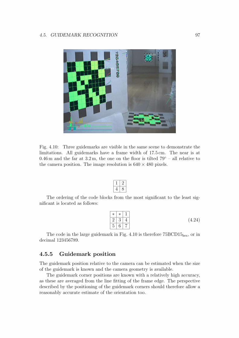
4.5. GUIDEMARK RECOGNITION 97
Fig. 4.10: Three guidemarks are visible in the same scene to demonstrate thelimitations. All guidemarks have a frame width of 17.5 cm. The near is at0.46m and the far at 3.2m, the one on the floor is tilted 79 – all relative tothe camera position. The image resolution is 640× 480 pixels.
1 24 8
The ordering of the code blocks from the most significant to the least sig-nificant is located as follows:
∗ ∗ 12 3 45 6 7
(4.24)
The code in the large guidemark in Fig. 4.10 is therefore 75BCD15hex, or indecimal 123456789.
4.5.5 Guidemark position
The guidemark position relative to the camera can be estimated when the sizeof the guidemark is known and the camera geometry is available.
The guidemark corner positions are known with a relatively high accuracy,as these are averaged from the line fitting of the frame edge. The perspectivedescribed by the positioning of the guidemark corners should therefore allow areasonably accurate estimate of the orientation too.

98 CHAPTER 4. VISION BASED PERCEPTION
The guidemark position and orientation is estimated using least square pa-rameter estimation. From the frame extraction algorithm above the positionin the image of the frame corners are known h′i = (hr, hc). The position of thecorners on the guidemark surface is known from the guidemark design as fourcoordinate pairs.
The coordinates on the guidemark is selected as being seen in the same wayas a robot, that is x being forward (in front of the guidemark), z being up, andwhen looking in the direction of x (from behind the guidemark) y is to the left.When looking at the guidemark on a wall, then z is up and y is right.
The centre of the guidemark is taken as the reference position, ie the topright frame corner has the frame coordinate B = [0, by, bz]
T with positive valuesfor both by and bz.
A guidemark may be at any position gt = [x, y, z]T relative to the robot androtated following the normal convention: first turned κ around the vertical zaxis with positive being counter-clockwise, then tilted Φ around the y axis withpositive being a down tilt and finally roll Ω around the x axis with positivebeing a roll to the right.
When a point on the guidemark surface B = [0, by, bz]T is being seen at
the 3D position A = [ax, ay, az, 1]T in robot coordinates, then A and B arerelated with the guidemarks orientation and position (x, y, z, Ω, Φ, κ) (also inrobot coordinates) as in (4.25)
0bywbzww
= RΩRΦRκTA , (4.25)
where RΩ, RΦ and Rκ are rotation matrices in homogeneous coordinates andT is a translation matrix as shown below:
RΩ =
1 0 0 00 cos(Ω) sin(Ω) 00 − sin(Ω) cos(Ω) 00 0 0 1
(4.26)
RΦ =
cos(Φ) 0 − sin(Φ) 00 1 0 0
sin(Φ) 0 cos(Ω) 00 0 0 1
(4.27)
Rκ =
cos(κ) sin(κ) 0 0− sin(κ) cos(κ) 0 0
0 0 1 00 0 0 1
(4.28)
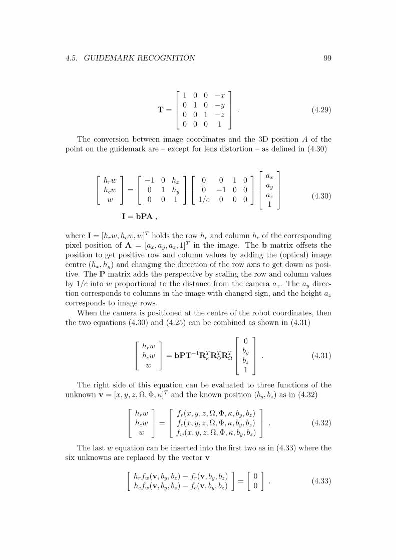
4.5. GUIDEMARK RECOGNITION 99
T =
1 0 0 −x0 1 0 −y0 0 1 −z0 0 0 1
. (4.29)
The conversion between image coordinates and the 3D position A of thepoint on the guidemark are – except for lens distortion – as defined in (4.30)
hrwhcww
=
−1 0 hx
0 1 hy
0 0 1
0 0 1 00 −1 0 0
1/c 0 0 0
ax
ay
az
1
I = bPA ,
(4.30)
where I = [hrw, hcw,w]T holds the row hr and column hc of the correspondingpixel position of A = [ax, ay, az, 1]T in the image. The b matrix offsets theposition to get positive row and column values by adding the (optical) imagecentre (hx, hy) and changing the direction of the row axis to get down as posi-tive. The P matrix adds the perspective by scaling the row and column valuesby 1/c into w proportional to the distance from the camera ax. The ay direc-tion corresponds to columns in the image with changed sign, and the height az
corresponds to image rows.
When the camera is positioned at the centre of the robot coordinates, thenthe two equations (4.30) and (4.25) can be combined as shown in (4.31)
hrwhcww
= bPT−1RT
κRTΦRT
Ω
0by
bz
1
. (4.31)
The right side of this equation can be evaluated to three functions of theunknown v = [x, y, z, Ω, Φ, κ]T and the known position (by, bz) as in (4.32)
hrwhcww
=
fr(x, y, z, Ω, Φ, κ, by, bz)fc(x, y, z, Ω, Φ, κ, by, bz)fw(x, y, z, Ω, Φ, κ, by, bz)
. (4.32)
The last w equation can be inserted into the first two as in (4.33) where thesix unknowns are replaced by the vector v
[hrfw(v, by, bz)− fr(v, by, bz)hcfw(v, by, bz)− fc(v, by, bz)
]=
[00
]. (4.33)

100 CHAPTER 4. VISION BASED PERCEPTION
To solve for the six unknowns at least six equations are needed, so the fourcorners of the guidemark frame yield eight equations by substituting by, bz, hr
and hc in (4.33) with the values from the remaining three corners. The problemmay then be solvable. The eight functions on the left side of (4.33) should allevaluate to zero with the correct value of the six unknowns
F = 0 . (4.34)
As the functions are nonlinear the six unknown parameters are estimatedusing Newton’s iteration method.
With an initial guess of the vector v the equations will (probably) not bezero, but assuming that the errors are small and the equations are approxi-mately linear at the guessed position, the error can be compensated for by alinear adjustment ∆v as shown in (4.35)
F(v) + J(v)∆v = 0 . (4.35)
where F(v) is the value of the eight equations evaluated with the guessed setof parameters v and J(v) is the Jacobian of F with respect to the unknownsin v taken at v, finally ∆v is the adjustment to the guess needed to get therequired zero result.
A better guess of v would therefore be v2 as shown in (4.36)
v2 = v + ∆v . (4.36)
The estimated adjustment ∆v is found by solving (4.35) as:
∆v = −(JTJ)−1JTF . (4.37)
Equations (4.35), (4.36) and (4.37) are then repeated, setting v = v2 forthe next iteration, until the estimated parameters have converged sufficiently.
The pixel position in the image is adjusted for radial lens error (as in (4.6))prior to insertion into the functions in F.
The iteration is terminated when the parameter change ∆vn in iteration nis significantly small according to the stop criteria in (4.38)
stop criteria =
∣∣∣∣∣∣∣∣
[x, y, z, Ω, Φ, κ
]
| [x, y, z] | < Pinf ∧∣∣∣[Ω, Φ, κ
] ∣∣∣ < Rinf
. (4.38)
When looking at a guidemark that is tilted slightly forward or backward itmay be difficult to see the difference, this could indicate local optimum thatcould trap the parameter estimation. Figure 4.11 shows the pixel error as afunction of a combination of turn (κ) and tilt (Φ). This shows the correct value
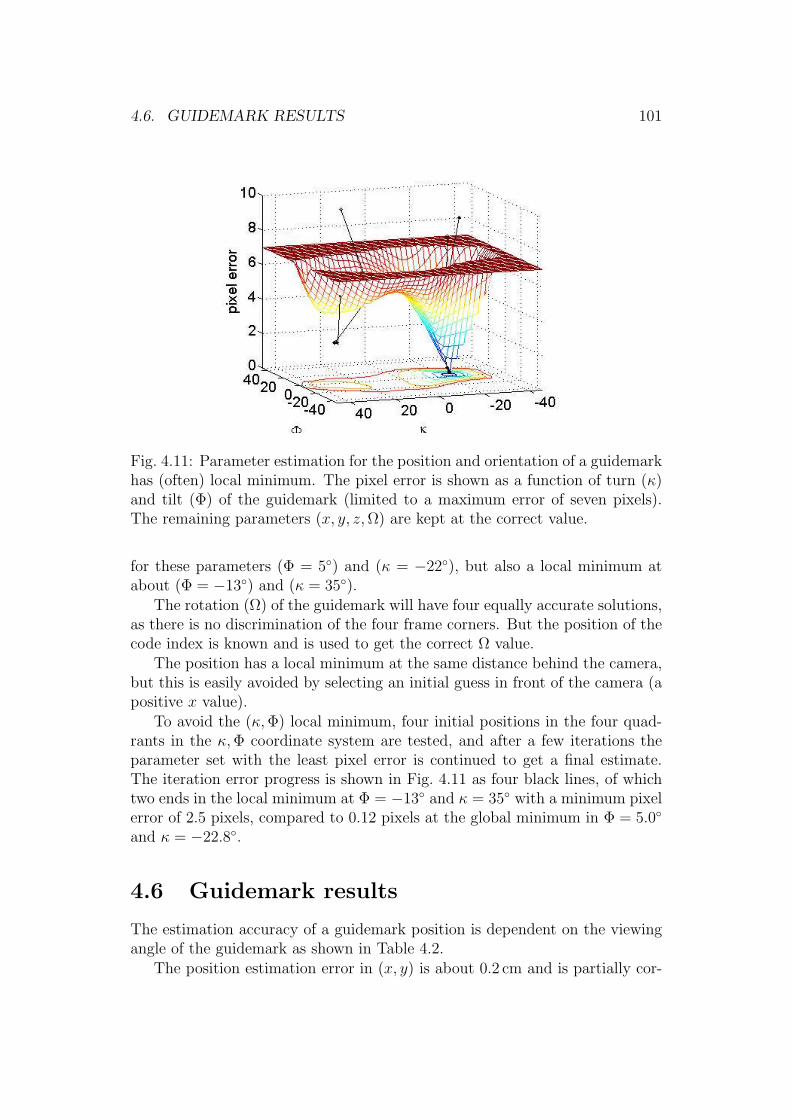
4.6. GUIDEMARK RESULTS 101
Fig. 4.11: Parameter estimation for the position and orientation of a guidemarkhas (often) local minimum. The pixel error is shown as a function of turn (κ)and tilt (Φ) of the guidemark (limited to a maximum error of seven pixels).The remaining parameters (x, y, z, Ω) are kept at the correct value.
for these parameters (Φ = 5) and (κ = −22), but also a local minimum atabout (Φ = −13) and (κ = 35).
The rotation (Ω) of the guidemark will have four equally accurate solutions,as there is no discrimination of the four frame corners. But the position of thecode index is known and is used to get the correct Ω value.
The position has a local minimum at the same distance behind the camera,but this is easily avoided by selecting an initial guess in front of the camera (apositive x value).
To avoid the (κ, Φ) local minimum, four initial positions in the four quad-rants in the κ, Φ coordinate system are tested, and after a few iterations theparameter set with the least pixel error is continued to get a final estimate.The iteration error progress is shown in Fig. 4.11 as four black lines, of whichtwo ends in the local minimum at Φ = −13 and κ = 35 with a minimum pixelerror of 2.5 pixels, compared to 0.12 pixels at the global minimum in Φ = 5.0
and κ = −22.8.
4.6 Guidemark results
The estimation accuracy of a guidemark position is dependent on the viewingangle of the guidemark as shown in Table 4.2.
The position estimation error in (x, y) is about 0.2 cm and is partially cor-

102 CHAPTER 4. VISION BASED PERCEPTION
Table 4.2: Relative estimation accuracy of a sequence of 100 position requestsof a guidemark at 2.2m at different turn angles of the guidemark. All sourceimages are of size 640 × 320 pixels, the guidemark has a frame block size of2.5 cm, and each frame block is covered by at least the stated number of pixels.The used USB camera has a focal length of 1050 pixels.
Viewing Position Orientation Block Nangle κ σ|x,y| σΩ (roll) σΦ (tilt) σκ (turn) pixels samples
0 1.7 mm 0.04 1.55 0.61 11.9 10010 1.3 mm 0.06 0.72 0.27 11.7 10030 2.2 mm 0.12 0.21 0.12 10.3 10060 2.5 mm 0.10 0.11 0.06 5.9 24
related with an estimation error in the guidemark orientation; typically a smalltilt combined with a slight turn makes the guidemark seem slightly smallerand thus further away. When the turn angle is zero (guidemark is facing thecamera) the relative estimation error in roll (σΩ) is uncorrelated with the othererrors and thus small, at larger turn angles the roll error increases and the errorvalue is now correlated with the other estimated parameters.
The obtainable absolute position accuracy is dependent on the mountingaccuracy of the camera, the focal length of the lens and the accuracy of theestimated lens (radial) errors. With the used USB camera an absolute positionaccuracy of less than 5 cm and an angle accuracy of less than 5 are obtainedwithin the camera coverage area.
When a guidemark is viewed with a rotation of 22.5 – just in between thetwo sets of corner filters (C1,2 and C3,4) – the sensitivity is slightly reduced. Theeffect is a reduction of the distance at which the guidemark can be detected.
The number of pixels needed for each of the squares in the frame to be ableto detect the guidemark is shown in table 4.3 as ’block pixels’.
Table 4.3: The number of pixels needed for each frame block to detect guide-marks at different rotation angles relative to camera. The distance in metre isfor a camera with a focal length of 525 pixels and an image size of 320 × 240pixels.
Orientation pd = 0.5 pd = 0.95of grid pixels metre pixels metre
0 3.8 3.4 3.9 3.322.5 4.6 2.8 4.8 2.745 4.2 3.1 4.3 3.0
When the probability of detection (pd) is about 0.95 the code is evaluatedcorrectly with a probability of about 0.95 too (for the detected guidemarks).

4.7. SUMMARY 103
Stable guidemark detection requires that each of the blocks in the guidemarkframe should be covered by at least five pixels. When the guidemark is not atthe distance with the optimal focus the detection distance will decrease further.
The used camera has a configurable contour enhancement feature intendedto compensate for limited bandwidth in an analogue video signal and to en-hance the image sharpness visually. This feature is turned off to improve theguidemark detection capability.
4.7 Summary
Two vision sensors are presented in this chapter: a road outline sensor and aguidemark sensor.
The road outline sensor is able to extend a sample area to cover the visiblearea with the same properties as the sample area. The visual appearance ofa road changes with the illumination and the surface type, but the presentedsensor that combines a colour (chromaticity) analysis with edge detection is ableto detect the road outline in many surface type and illumination combinations:gravelled roads, wet and dry asphalt roads with a range of sunshine and shadowillumination. The method is fast, simple and efficient as long as the seed areais representative for the road.
The sensor fails if the seed area is not representative for the road andadditionally very sharp shadows are excluded from the road outline, and thusboth false positives (non-road included) and false negatives (road excluded)may occur. For these reasons the sensor is not recommendable as a stand alonesensor for detection of obstacles and traversable terrain. The sensor is howeveran excellent supplement to the laser scanner based road detector described inchapter 3, and provides supplementary road classification, obstacle and junctiondetection beyond the laser scanner range.
The guidemark detection capability is primarily a supplement intended toimprove the robot localisation and may solve positional ambiguities. In theinitial phase for the robot, the start posture may be determined from a guide-mark. Where accurate localisation is needed – eg when approaching a doggingstation – a guidemark may provide the needed accuracy.
4.8 Further improvements
Further cameras and possibly manoeuvrable cameras may further improve theability to detect side roads and interesting objects like natural or artificialguidemarks.
The vision-based perception process could include is much more then thetwo sensor types presented in this chapter. Further segmentation of the camera

104 CHAPTER 4. VISION BASED PERCEPTION
image may provide additional information valuable for the navigation process.A combination with ’structure from motion’ or stereovision techniques the po-sitioning of the seen objects may be improved, and thus qualitatively improvethe perception.

Chapter 5
Obstacle avoidance
5.1 Introduction
Obstacles are from the definition something that hinders progress, and in thisproject obstacles are primarily maintained for the purpose of obstacle avoid-ance.
The obstacle avoidance behaviour decisions should obey to overall behaviourrequirements – eg follow left side of road – while avoiding detected obstacles.The data source is a number of possible corridors based on laser scanner tra-versable segments wide enough to allow passage by the robot, a vision-basedroad outline, and a number of detected obstacles that should be avoided. Theresult of obstacle avoidance should be a path within the area covered by thesensors that avoids the detected obstacles and brings the robot closer to thedesired destination.
5.2 Obstacle avoidance methods
A number of methods for path planning to avoid obstacles are described in theliterature and is adequately summarized by Siegwart & Nourbakhsh (2004).The methods describe different methods to calculate a route from current posi-tion to an exit position, the exit position being either the destination positionor a position that would bring the robot closer to the desired destination.
The obstacle avoidance methods are divided into four groups:
• Road map: identify a route in the identified traversable area to a targetposition. Two basic methods are described: the direct visibility graphmethod and a Veroni diagram method.
The visibility graph method connects all vertices of the obstacles withall visible vertices of all other obstacles including the current position
105

106 CHAPTER 5. OBSTACLE AVOIDANCE
and the exit position. The shortest graph from the current position andthe exit position is then the optimal route. If the number of obstacles issparse the method is efficient, but the computation time grows fast withthe number of obstacles.
The Veroni diagram makes a path from current position to the exit po-sition following lines where there is equal distance to the two closestobstacles. If there is a route to the destination the method will find it,but the distance is not optimal, and especially in sparse environments,the solution is far from optimal.
• Cell decomposition: divide the area that includes the current and theexit position into obstacle cells and traversable cells. Two basic methodsare described: exact cell decomposition and approximated cell decompo-sition.
The exact cell decomposition divides the area between obstacles into ar-eas, each cell has three or four sides, each cell is either traversable oran obstacle, and thus each side of a traversable cell is shared with an-other traversable cell or an obstacle. A graph can then connect the cellwith the current position to the cell with the exit position, and an op-timal sequence of cells be found. The method is efficient in large sparseenvironments, but rarely used due to implementation complexity.
The approximate cell decomposition method uses square cells, where a cellis declared nontraversable if parts of the cell is occupied by an obstacle.The traversable cells are then searched from current position in a breastfirst search until the destination cell is found. The cell size should besmall, so that narrow passages are not lost due to the cell approximation,but the cell count should be kept low to reduce the memory and processingtime is needed. The implementation is simple and the method is popular.
The cell size of the approximate cell decomposition method may be se-lected to be variable. Large free areas are then represented by one largesquare cell, and if obstacles are found inside this area then the area issplit into four smaller cells. This cell splitting can be continued until thedesired accuracy is obtained. The number of required cells is in this wayreduced at the expense of implementation complexity.
• Potential field: using mathematical functions describing a field wherethe destination is attractive and the obstacles are repulsive. The currentposition is then a particle in this field, and the steepest decent is then theoptimal route to the destination. Concave obstacles or obstacle groupsmay introduce local minima and thus trap the robot.

5.3. OBSTACLE DETECTION 107
• Bug navigation: aiming for the destination and dealing with one obstacleat a time as they come. These methods may get to the exit position, butthe route may be far from optimal.
5.2.1 Design decisions
The selected method is based on the visible graph method. The method ismodified to ignore obstacles too far away and to start the path search with thedirect route. The search may end here if no obstacles are found, or may beextended when the direct route crosses or gets too near an obstacle. The pathis further including robot dynamics during the search.
The reasoning is that the method is intuitive simple, based on a graph ofvisible segments from current position to the exit position. The environmentused by the robot is – apart from the road sides – a sparse environment, andthus a method favouring sparse environments could be selected. The methodis scalable and allows the exit position to be far away from current positionwithout increased performance penalty – as long as the obstacle density remainslow.
The force field method may experience trapping by local minima, andshould be combined with another method to recover from those situations.This method is therefore not further investigated.
The cell decomposition method using fixed sized cells may be relative simpleto implement, but a high number of cells is needed. A coverage area of 15×15mwith a 5 cm resolution would require 300×300 = 90000 grid cells of which mostneed recalculation for each iteration. The method is not easily scalable is theexit position is far away. An improved scalability could be obtained by avariable cell size, but at the cost of complexity. The found route is further noteasily modified to account for robot dynamics.
The accurate cell decomposition method could be a tempting compromisebetween the approximate cell decomposition method and the visibility graph,as it easily provides prioritised alternative routes if the shortest route is un-desirable due to robot dynamics requirements. The method is however notfurther investigated.
5.3 Obstacle detection
On the experimental platform both the vision sensor and the laser scanner arecapable of obstacles detection.
The implemented feature detection for the vision sensor is limited to roadoutline sensing. The identification of a road limitation – a transition from roadto non-road – could be used as a detected obstacle, the accuracy of which is

108 CHAPTER 5. OBSTACLE AVOIDANCE
limited primarily by the projection errors. The road outline is projected to avirtual flat surface in the same plane as the robot base. The projection thereforeincludes errors when the robot tilt and roll are different from zero and whenthe road surface is not flat. The camera is looking forward with a horizontalview angle of 58, and as the main view area extends from the end of the laserscanner range – 2.6m in front of the robot on a flat road – to the horizon,the main projection error is expected to be in the x-direction (forward). A tilterror ϕe of the robot probagates to an x-distance error xe as shown in (5.1)
xe =h
sin(sin−1(hr) + ϕe)
− r , (5.1)
where the robot tilt ϕe is approximated as camera tilt and xe is approximatedas error in distance along the camera axis. This is justifiable as the distancefrom the camera r is much larger than the camera height h = 0.86m.
For an obstacle detected at r = 10m and a tilt error ϕe = −1.3 (corre-sponding to the front wheel being lifted 1 cm) is thus approximately 3.7m.
An error of this magnitude makes it difficult to track and correlate obstaclesbased on the vision road outline sensor. Improvements in the robot posturesensing to include tilt could improve the situation.
Obstacles are further assumed to be flat and the (possible) road behindobstacles is not detected as traversable, this further complicates tracking andusage of obstacles based on the road outline detection.
The laser scanner based road classifier divides the measurements into tra-versable, nontraversable and invalid data, and further group measurementsclassified nontraversable into spatially separated polygon-shaped (convex) ob-stacles as described in section 3.7.
The projection error from the laser scanner measurements due to unknownrobot tilt and roll is much less than for the vision sensor, as the laser scanneris a 3D sensor.
5.4 Integration of vision data
The obstacle avoidance solution needs a desired exit position and a set ofobstacles. A combined corridor is found using both vision and laser scannerdata. The exit position is found in the vision part of the corridor, so that anyobstacle areas detected by the vision sensor are avoided. The visible graphmethod is used to find the optimal route to this exit position.
5.4.1 Extended road corridor
The laser scanner based road corridors may be extended into the vision sensorroad outline. This may disqualify some of the corridors found by the laser

5.4. INTEGRATION OF VISION DATA 109
Laser scannerbased
corridor lines
Vision-basedcorridor lines Vision-based
road outline
(a) (b)
Fig. 5.1: The corridor lines (blue in (a)) are based on laser scanner data upto the most recent laser scan, and from here extended into the vision-basedroad-outline polygon. The road-outline polygon is further shown in the cameraimage (b).
scanner, eg if a corridor was found in the cut grass on the roadside, then thisis unlikely to correlate with the vision-based road outline.
The extension is calculated by creating a number of corridor line segmentsinside the vision polygon and correlates these with the laser scanner basedcorridor. The two sets of corridor lines are shown in Fig. 5.1.
The vision corridor consists of a number of traversable line segments Svr
crossing the road-outline polygon at range r. The segments are generated asshown in (5.2)
Svr =
Svr,j
j = [1..N/2]m = 2j
∣∣∣∣∣∣∣∣∣∣∣∣
Svr,j = (x + vt)
x = Um+1
Um = [r, ym]T
v = [0, 1]T
t = ym − ym+1
|ym − ym+1| > Wmin
, (5.2)
where [r, ym]T is the mth of N crossings of the road-outline polygon at ranger from the robot. The crossing line at r is perpendicular to the current robotheading. U is the set of crossings at r, and these are ordered after decreasingy value. Each line segment Sv
r,j is described in robot coordinates. The segmentmust be wider than Wmin = WR (robot width), except if one of the positionsym or ym+1 is at the image border, in which case Wmin = WR/2 to allow for thepossibility that the rest is outside the image.

110 CHAPTER 5. OBSTACLE AVOIDANCE
The segments are generated at the range intervals
r =
ri
∣∣∣∣∣∣∣∣
r1 = rseed + rsep
ri = ri−1dsep
ri < rmax
i ∈ [1, imax]
, (5.3)
where rseed is the distance from the seed area used for the road outline (typicallyabout 2.6m), and rsep = 2.0m is a fixed distance to the first vision-basedsegment, the segments are separated by a factor dsep = 1.2 until a maximumrange rmax = 14 m is reached or there are no more crossings of the outlinepolygon.
If there are no polygon crossings at r1, then no intervals are generated andthe vision data are ignored.
If the destination position is closer than 14m, then rmax is reduced accord-ingly. The value rmax = 14m gives the maximum reaction distance to obstacles,ie the distance where an obstacle avoidance manoeuvre may be initiated as theearliest. The distance is also the longest distance at which vision road outlinecan assist in junction resolutions.
The segment interval corresponds to a constant obstacle height Dvo as shown
in (5.4)
Dvo = hcam
dsep − 1
dsep
= 0.15 m, (5.4)
where hcam is the camera height. This is more than used by the laser scannerobstacle detection, and should probably be reduced if the road outline detectionwas modified to test for obstacles along these line segments. Such – rathersimple – modification to the road outline detector would improve the obstacledetection capabilities to about the same level as the laser scanner (but is notimplemented).
The corridor consists of segments from (5.2) correlated as in (3.23) andcontinued into the laser scanner corridor (3.28). The full corridor Bj consistsof line segments as in (5.5)
Bj = S1, S2, . . . , Sn, Sn+1, . . . , Sn+m ; j ∈ [1, b], (5.5)
where S1 = Svr1,j from (5.2) to reduce the notation complexity, and n is the
number of vision-based segments. Similarly Sn+1 = Ski from (3.28), and m is
the number of laser scanner based segments in the corridor.The forward most vision range line may be broken into more segments
resulting in b available corridors. The segments can also be described as pa-rameter lines:
Si = si(t) = x + tv | t ∈ [0, li]x = [xxs, xys]
T
v = [vxs, vys]T ,
(5.6)

5.5. EXIT POSTURE 111
where li is the length of segment i.
5.5 Exit posture
The exit posture (exit position and desired exit heading) is the foremost usableaiming point inside the currently detected obstacle-free area. This posture isdetermined by the current navigation objectives and the navigation corridor.Two main types of navigation objectives are relevant here: following a roadline and aiming for a specific position. A third type – direct to destination –is available too, especially for tight manoeuvres; the exit posture for this typeis taken directly from the destination posture.
When the objectives are to follow a road line, the relevant road line r(tr) =[xr + trvr] is extended to its crossing with the segments si(ts) from the corridorBj found in (5.5) and (5.6).
The crossing of these lines is expressed as a parameter value ts on thesegment si as in (5.7) and (5.8)
r(tr) = s(ts) ⇒ [vr, −vs ]
[trts
]= [xs − xr ] , (5.7)
and solved for the parameter value ts for the crossing of the segment yields:
ts = cross(r, s) =vxr(xyr − xys) + vyr(xxs − xxr)
vxrvys − vyrvxs
, (5.8)
where xr = [xxr, xyr] and vr = [vxr, vyr].The exit point candidate ci is then
ci = si(tsi + dr), (5.9)
where tsi is the ts value for segment i and dr is the desired position on the roadrelative to the road edge.
If ci is inside all segments in the vision parts of the corridor, then the exitposition p = c1. If one of the crossings is outside the vision segment or closerto its end points than a security distance dsec = 0.3m, then the candidateexit position ci is adjusted to be inside the segment before the next candidateposition is tested - as shown in (5.10)
p = cn
∣∣∣∣∣∣∣∣∣∣∣∣∣∣∣∣
c0 = c1
for i ∈ [1, n] :rcc = [xc + tc(ci−1 − xc)]tsi = cross(rcc, si)
ci =
ci−1 for
tsi > dsec
∧ tsi < l − dsec
si(dsec) for tsi < dsec
si(li − dsec) for tsi > li − dsec
, (5.10)
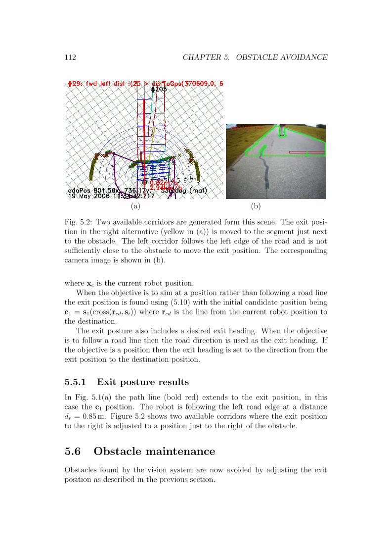
112 CHAPTER 5. OBSTACLE AVOIDANCE
(a) (b)
Fig. 5.2: Two available corridors are generated form this scene. The exit posi-tion in the right alternative (yellow in (a)) is moved to the segment just nextto the obstacle. The left corridor follows the left edge of the road and is notsufficiently close to the obstacle to move the exit position. The correspondingcamera image is shown in (b).
where xc is the current robot position.When the objective is to aim at a position rather than following a road line
the exit position is found using (5.10) with the initial candidate position beingc1 = s1(cross(rcd, si)) where rcd is the line from the current robot position tothe destination.
The exit posture also includes a desired exit heading. When the objectiveis to follow a road line then the road direction is used as the exit heading. Ifthe objective is a position then the exit heading is set to the direction from theexit position to the destination position.
5.5.1 Exit posture results
In Fig. 5.1(a) the path line (bold red) extends to the exit position, in thiscase the c1 position. The robot is following the left road edge at a distancedr = 0.85 m. Figure 5.2 shows two available corridors where the exit positionto the right is adjusted to a position just to the right of the obstacle.
5.6 Obstacle maintenance
Obstacles found by the vision system are now avoided by adjusting the exitposition as described in the previous section.
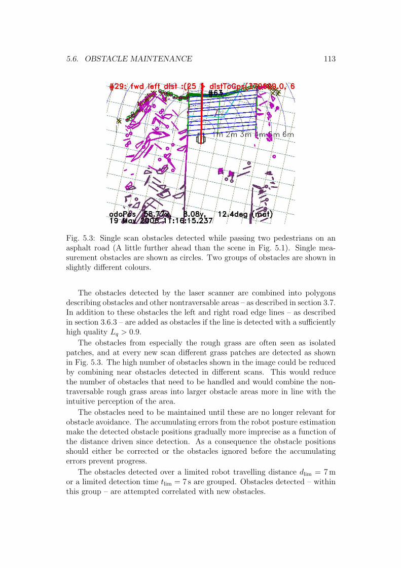
5.6. OBSTACLE MAINTENANCE 113
Fig. 5.3: Single scan obstacles detected while passing two pedestrians on anasphalt road (A little further ahead than the scene in Fig. 5.1). Single mea-surement obstacles are shown as circles. Two groups of obstacles are shown inslightly different colours.
The obstacles detected by the laser scanner are combined into polygonsdescribing obstacles and other nontraversable areas – as described in section 3.7.In addition to these obstacles the left and right road edge lines – as describedin section 3.6.3 – are added as obstacles if the line is detected with a sufficientlyhigh quality Lq > 0.9.
The obstacles from especially the rough grass are often seen as isolatedpatches, and at every new scan different grass patches are detected as shownin Fig. 5.3. The high number of obstacles shown in the image could be reducedby combining near obstacles detected in different scans. This would reducethe number of obstacles that need to be handled and would combine the non-traversable rough grass areas into larger obstacle areas more in line with theintuitive perception of the area.
The obstacles need to be maintained until these are no longer relevant forobstacle avoidance. The accumulating errors from the robot posture estimationmake the detected obstacle positions gradually more imprecise as a function ofthe distance driven since detection. As a consequence the obstacle positionsshould either be corrected or the obstacles ignored before the accumulatingerrors prevent progress.
The obstacles detected over a limited robot travelling distance dlim = 7mor a limited detection time tlim = 7 s are grouped. Obstacles detected – withinthis group – are attempted correlated with new obstacles.

114 CHAPTER 5. OBSTACLE AVOIDANCE
A new obstacle polygon D is tested for correlation with an establishedobstacle polygon E using a proximity function F(D,E) as shown in (5.11).This function evaluates the distance from the closest vertex in D to any edgein E. The distance is signed so that a positive value is evaluated if the nearestvertex in D is outside the polygon E. The polygons are all convex and verticesare ordered counter-clockwise
F(W,G) =j∈[1,m]
min
[i∈[1,n]max (Aiwj,x + Biwj,y + Ci)
]
where
W = w1,w2, . . . ,wn; wi = [wi,x, wi,y]T
G = g1,g2, . . . ,gm; gi = [gi,x, gi,y]T
L = l1, l2, . . . , lm
li = [Ai, Bi, Ci]
∣∣∣∣∣∣∣∣
Aix + Biy + Ci = 0d = [dx, dy]
T = gi − gi−1; g0 = gm
Ai = −dy
|d| ; Bi = dx
|d| ; Ci =dy∗gi,x−dx∗gi,y
|d|i ∈ [1,m]
.
(5.11)
A correlation is said to exist if dlimit > min[F(D,E),F(E, D)]. The roughroad edges are predominantly flat, and in many cases obstacles representingthe same rough area do not overlap. The distance between obstacle detectionin such areas depends on the distance between scans. If the area was a homo-geneous area of single (nontraversable) straws the distance between obstaclesin successive scans would be equal to the robot movement (of this position)between the scans. To allow for correlation between scans the parameter dlimit
could be set to the maximum movement, but as the movement is known a dif-ferent approach is taken. A point is added to the new polygon, at a positionwhere this obstacle would have been detected in the last scan had the obsta-cle been a homogeneous nontraversable rough area. The back-most point inthe candidate polygon (in robot local coordinates) is therefore added at theposition it would have had if detected in the previous scan (the extra point isremoved after the correlation process).
In addition to this extra point the limit dlimit = 0.3m is found experimen-tally to get a reasonable reduction in obstacle count while keeping other typesof distinct obstacle separate.
The resulting set of obstacles after correlation is shown in Fig. 5.4 for thescene in Fig. 5.3.
Similar results are obtained on a gravelled road as shown in Fig. 5.5. Thescene is a gravelled road with rough edges just before it opens for a side roadto the left. The road edge lines are mostly of poor quality. The obstacles areagain combined to almost solid areas on both roadsides.

5.6. OBSTACLE MAINTENANCE 115
Fig. 5.4: The correlated and merged obstacles shown represent the same obsta-cles as shown in Fig. 5.3. Two obstacle groups are shown (in slightly differentcolours).
(a) (b)
Fig. 5.5: The scene is a gravelled road with rough road edges. The raw obstaclesin (a) are combined into nontraversable obstacle areas in (b).
The decision to use convex polygons to describe obstacles was to ease thecomputation, the drawback is that the obstacle may be concave by nature andthe area in this concavity may be needed for navigation. An example could bethat the obstacle extends alongside the robot and an obstacle at the roadsidein front of the robot is detected, this obstacle is merged with the one at the sideof the robot to one convex obstacle, now including the robot position. Thissituation would trigger unnecessary abrupt robot manoeuvres to get the robotout of the obstacle.
There is presently no provision for removal of obstacles nor to reduce theobstacle size, this would be needed if the obstacles were to be retained fora revisit of the area. Moving obstacles – like humans – are not tracked andmay thus produce a series of obstacles. Such obstacles could block the robot
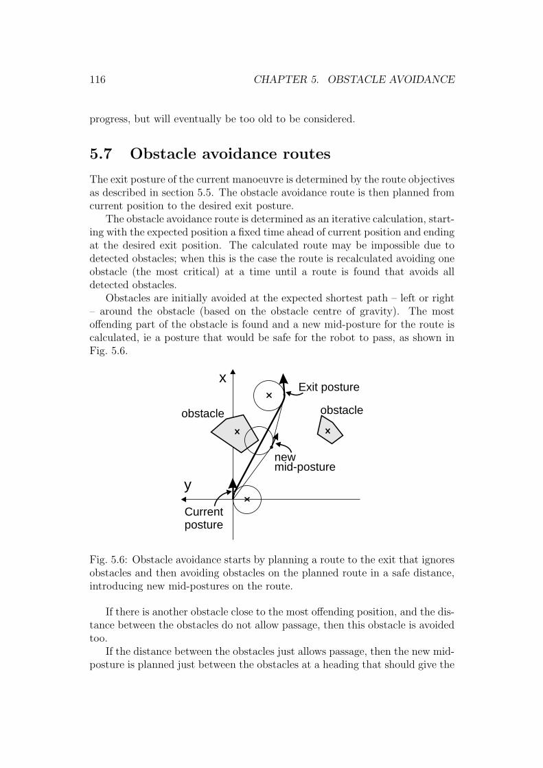
116 CHAPTER 5. OBSTACLE AVOIDANCE
progress, but will eventually be too old to be considered.
5.7 Obstacle avoidance routes
The exit posture of the current manoeuvre is determined by the route objectivesas described in section 5.5. The obstacle avoidance route is then planned fromcurrent position to the desired exit posture.
The obstacle avoidance route is determined as an iterative calculation, start-ing with the expected position a fixed time ahead of current position and endingat the desired exit position. The calculated route may be impossible due todetected obstacles; when this is the case the route is recalculated avoiding oneobstacle (the most critical) at a time until a route is found that avoids alldetected obstacles.
Obstacles are initially avoided at the expected shortest path – left or right– around the obstacle (based on the obstacle centre of gravity). The mostoffending part of the obstacle is found and a new mid-posture for the route iscalculated, ie a posture that would be safe for the robot to pass, as shown inFig. 5.6.
x
y
cgobstacle
newmid-posture
obstacle
Exit posture
Currentposture
Fig. 5.6: Obstacle avoidance starts by planning a route to the exit that ignoresobstacles and then avoiding obstacles on the planned route in a safe distance,introducing new mid-postures on the route.
If there is another obstacle close to the most offending position, and the dis-tance between the obstacles do not allow passage, then this obstacle is avoidedtoo.
If the distance between the obstacles just allows passage, then the new mid-posture is planned just between the obstacles at a heading that should give the

5.7. OBSTACLE AVOIDANCE ROUTES 117
floor
door
ferniture
Fig. 5.7: Obstacle avoidance path planning in an indoor scene. The pathplanner has found a path out of an open doorway avoiding the known obstaclesat the time. The door is erroneously classified as traversable.
safest passage, ie the new mid-posture is the centre of a line connecting theobstacles, and the heading is in the direction of the mid-normal.
The less obvious side of the obstacle is evaluated too, as this may be thebest overall guess.
The new mid-posture splits the path from the robot to the desired exitposture in two. Each of these are then recursively tested for free passage andrecalculated as needed.
An example of path planning is shown in Fig. 5.7. The robot has planneda route through a door opening in an indoor scene. The outdoor obstacleavoidance routes are usually less complicated. The setup is not intended forindoor use, but the indoor scene is handled reasonably well after introduction oftwo minor exceptions: obstacles are not generated for ditches and the obstaclecorrelation distance dlimit is reduced to 0.03 m to reduce the likelihood of twowalls in a corner are correlated into one convex obstacle, as this potentiallycould limit the free area for the robot significantly.
A number of exceptions are introduced to maintain a smooth path and a fastcalculation. The number of alternative paths (the other way around obstacles)is limited (to 6). The number of iterations finding new mid-postures is limitedtoo (to 6). This means that a path may be rejected if the calculation is toocomplicated (but a path may exist). When a new mid-posture is generated close

118 CHAPTER 5. OBSTACLE AVOIDANCE
to an existing one, the old mid-posture is probably not optimal for passage andis replaced by the new.
5.8 Posture to posture manoeuvre
Obstacle avoidance manoeuvres are planned using a combination of straightand curved paths. The manoeuvres from one posture to another will alwaysbe planned using a combination of an arc, a straight part and a final arc. Thearcs can either form a left or a right turn. The arc radius is – when possible –planned to limit the centripetal acceleration.
Both the centripetal and the lateral acceleration are limited in order to getsmooth manoeuvring.
The basic calculation of a posture to posture manoeuvre can be evaluatedas one of two cases: both arcs are in the same direction or the arcs are indifferent directions. That is, right-straight-right or right-straight-left. Thesame manoeuvres starting with a left turn are calculated as a mirror image ofthe corresponding manoeuvre starting with a right turn. The manoeuvres arecalculated in a reference coordinate system aligned with the start posture. Theend posture is then (x2, y2, θ2) as shown in Fig. 5.8 and Fig. 5.9.
The turn radius r is selected not to exceed a desired centripetal accelerationac, for normal manoeuvring as shown in (5.12) for the actual robot velocity v
r =v2
ac
. (5.12)
The arcs φ1, φ2 and the line d are found as described below.
5.8.1 Right, straight and then right
The manoeuvre consists of an arc φ1 with a turn radius of r1, a straight part dand a second turn (to the right) of φ2 at a turn radius r2, as shown in Fig. 5.8(a).
The solution is found by shifting the line d a distance r2 (into d′ in Fig. 5.8),so that it starts at the circle centre C2 and ends at the tangent point to a circlewith centre at C1 and radius r1 − r2. The right angled triangle with this line
(d′) and the radius r1 − r2 as the two smaller sides and the line−−−→C2C1 between
the circle centres C1 and C2 as the longer side is solved, and from that finding

5.8. POSTURE TO POSTURE MANOEUVRE 119
x
y
r2
r1
r -r1 2
d
θ2x ,y2 2
φ2
φ1
C2
C1
d’
T1
T2
x
y
r2
θ2
x ,y2 2
φ1
C2
C1
T1
r1
T2
a b
Fig. 5.8: Calculation of right-straight-right manoeuvre (a) and the same ma-noeuvre with the largest possible entry turn radius (b). The manoeuvres startat (0, 0) heading 0. The exit point is at (x2, y2) heading θ2. The first arc stopsat T1, then straight until T2 where the second arc starts.
the arc sizes φ1 and φ2 as shown in (5.13)
∠(−−→C1T1 = ∠(
−−−→C2C1)− sin−1 r1 − r2
|−−−→C2C1|− π
2
φ1 =π
2− ∠(
−−→C1T1)
∠(−−→C2T2 = ∠(
−−→C1T1
φ2 = ∠(−−→C2T2)− (θ2 +
π
2).
(5.13)
The limitations for this manoeuvre are twofold: The first limitation is aconstruction limitation: the turn radius must be so small that the exit positionis not within the first circle and vice versa. The second limitation is morepractical, the exit angle θ2 should be smaller than the tangent angle ∠(
−−→C2T2),
otherwise the second arc could be up to a full circle. In such cases another
manoeuvre should be selected. At the same time the tangent angle ∠(−−→C1T1)
should be smaller than π2
to avoid too large arcs at the start of the manoeuvre.The last limitation corresponds to the situation where the second circle
crosses the x-axis.
5.8.2 Right, straight and then left
The calculation of the manoeuvre starting with a right turn followed by astraight part ending in a left turn is very similar to the right-straight-right

120 CHAPTER 5. OBSTACLE AVOIDANCE
x
y
r2
r1
r +r1 2
d
θ2
x ,y2 2φ2
φ1
d’C2
C1
T2T1
T’1
Fig. 5.9: Calculation of right-straight-left manoeuvre. The manoeuvre startsat (0, 0) at heading 0, and ends at position (x, y) heading θ2. The maximumturn radius is when the two circles with radii r1 and r2 meet.
manoeuvre, except that the support line d′ is now shifted away from the C1
centre.
The revised calculations are shown in (5.14)
∠(−−→C1T
′1 = ∠(
−−−→C2C1)− sin−1 r1 + r2
|−−−→C2C1|− π
2
φ1 =π
2− ∠(
−−→C1T
′1)
∠(−−→C2T2 = ∠(
−−→C1T
′1 − π
φ2 = θ2 − π
2− (∠(
−−→C2T2)).
(5.14)
The manoeuvre turning radius r1 and r2 must not be so large that the twocircles overlap.
The calculated posture to posture manoeuvre can now be used for calcula-tion of proximity to obstacles as described in the previous section.
5.9 Route selection
The obstacle avoidance planner may provide a number of possible obstacleavoidance routes, as there may be more alternative corridors and thus morethan one possible exit posture. Each exit posture may further result in a num-ber of different obstacle avoidance routes. The available routes are therefore

5.9. ROUTE SELECTION 121
rated using a quality Rw calculated as
Rw =
∑Ni=1 wiqi∑Ni=1 wi
, (5.15)
where qi ∈ Qr and Qr = qσ, qϕ1, q1–5, qe, qw, qd, qm is the set of road qualifiersand wi is the corresponding weight factor for qi. Each value is described below.
Corridor roughness is used as a qualifier qσ to prefer smoother corridors.The value is based on the average of the minimum of the roughness valuesRn found in each of the laser scanner based traversable segments Bj inthe corridor
qσ =
(1 +
sσ
N
N∑j=1
(min(Rn ∈ Bj))
)−1
; wσ1 = 3 , (5.16)
where sσ = 20 to scale the roughness for a reasonable quality interval.
The start manoeuvre is preferred as straight as possible; the angle to thefirst manoeuvre mid-posture (Φ1) is used as a source for the start ma-noeuvre quality
qϕ1 = (1 + Φ1 − ϕd)−1; wϕ1 = 1 , (5.17)
where ϕd is an offset used to prefer some directions. If the robot is tofollow left or right side of the road the offset is set to ϕd = +10 orϕd = −10, correspondingly. If the exit posture is behind the robot theoffset is set to prefer ϕd+70 or ϕd−70 in the most appropriate direction.
The historic heading is calculated from the general direction ϕh travelled 1–5m back from the current position. The ϕh is calculated as the directionof the best fit line for the robot positions recorded for this interval andthe qualifier as
q1–5 = (1 + Φe − ϕh)−1; w1–5 = 2 , (5.18)
where Φe is the direction from the robot to the exit posture.
The road edge quality is used when the robot is following a road edge andis based on the relevant road edge quality LQ (from section 3.6.3) as
qe =
LQ,left when following left road lineLQ,right when following right road lineLQ,top when following road centre line1 otherwise
; we = 1.5 . (5.19)

122 CHAPTER 5. OBSTACLE AVOIDANCE
The corridor width is used as a qualifier based on the road width Rw fromthe laser scanner based corridor. It is used to prefer wider corridors (upto 5 m) and calculated as
qw = (6−min(5, Rw))−1; ww = 0.3 . (5.20)
The path distance is used as a qualifier to prefer routes with a distance equalto the direct distance to the expected target position dd using
qd =
(1 + dm − dd)
−1 for dm = dd
(1 + dm − dd)−2 for dm < dd
; wd = 1 , (5.21)
where dm is the path distance. The desired distance dd is the distanceto the exit posture, except if no vision solution is available and the ma-noeuvre is not for a direct destination. In these cases the exit posture ison a laser scanner traversable segment, and the preferred distance is thedistance at which the laser scanner is expected to see the road (typically2.6m). A shorter distance is thus possible, but this is disfavoured as it –as an example – may be the lower part of a newly detected wall.
The manoeuvre deviation σm from the straight line to the destination isused to calculate the manoeuvre qualifier
qm =
1 +
√√√√ 1
K
K∑i=1
M2i
−1
; wm = 1 , (5.22)
where Mi is the distance from the mid-posture i to the straight linefrom the robot to the exit posture. This qualifier favours straight pathsolutions.
The route having the highest quality is selected. In Fig. 5.10 four routesare generated to three exit postures. The short route (in red) is selected.
5.10 Drive commands
The drive scheduler takes a sequence of drive commands and transforms theseinto wheel speed commands in real time. The best of the paths created bythe obstacle avoidance planner therefore needs to be translated into the set ofcommands used by the drive scheduler.
The first metre of the planned route is transferred to the drive scheduler(or less if the route is shorter). At a maximum speed of 1.5ms−1 and a pathcalculation rate of 2Hz the robot will travel 0.75m at maximum before a newroute is available.
Two types of drive commands are used to control the robot:

5.10. DRIVE COMMANDS 123
road
exit postures
cycle track sidewalk
alternativeroutes
Fig. 5.10: The robot is driving on a cycle path with no vision support. Eachof the road types (road, cycle path and sidewalk) generates an exit positionrelative to the objectives (a waypoint some 25m (almost) straight ahead). Fourroutes are generated towards these points and the shortest (in red) is selectedas the best.
Turn with a given radius is used directly as planned if the turn radius is lessthan 3m (turnr r a, where r is the radius and a is the angle to turn).
Following a target line, where the robot aims at following a provided line(drive x y th, where x and y is a position on the line and th is thedirection of the line).
Turns with a turn radius larger than 3m is divided into a sequence ofline follow commands. Each command may include options for speed andacceleration. A stop criterion that – when fulfilled – makes the drive schedulercontinue to the next command are used to limit the distance for each drivecommand.
The drive sequencer can execute a sequence of these (and other) commands,and supports that they are replaced by a new sequence when needed.
The obstacle avoidance route calculation takes a variable amount of time(but less than 0.3 s), and the robot posture used in the route calculation aretherefore predicted 0.3 s along the last ordered path.
Before the path is sent to the drive scheduler the first part of the route (upto the first mid-posture) is recalculated using the most recent robot posture.

124 CHAPTER 5. OBSTACLE AVOIDANCE
(a) (b)
Fig. 5.11: A fork is seen by the vision sensor (a) and included in the roadoutline shown on the feature map (b). The navigation process provides twomain alternatives and selects the fork to the right.
Fig. 5.12: A pedestrian blocks the vision-based road outline and an exit-posturenext to the pedestrian triggers an early obstacle avoidance manoeuvre.
5.11 Summary
In junctions and transitions from open areas to a narrower road the vision willoften be able to see the exit road or the road alternatives. This can assist thenavigation system in planning a route towards the right road at an early stage.In Fig. 5.11 the vision-based road outline clearly show the road alternatives.
When the road outline is limited by obstacles as in the situation shown inFig. 5.12, the route possibilities will be limited correspondingly, and the resultis an obstacle avoidance route initiated at an early stage. The pedestrian canfollow the robot intentions as soon as the obstacle avoidance route is initiated,and thus limits potential conflict situations.
The calculation of the obstacle avoidance route turned out to be more de-manding than the simplicity of the approach suggested. The number of alter-

5.11. SUMMARY 125
natives and exceptions make the implementation more difficult to test, and –unfortunately – the last error is not found in that piece of code.
The obstacle management ensures a reasonably low number of obstacles,and the history of obstacles aligns nicely with the road.
In the majority of the tested situations the obstacle generation and theobstacle avoidance route planning behave sensibly and produce the optimalresult from the available data.

126 CHAPTER 5. OBSTACLE AVOIDANCE

Chapter 6
Mission planning and execution
6.1 Introduction
This chapter deals with the mission preparation and navigation scheduling.In the previous chapters the sensors are described extracting obstacles andtraversable areas, and how these obstacles and areas are used to generate aroute that avoids the obstacles in search of a higher level goal. All that ismissing is a scheduler that can break a long navigation mission into a sequenceof short term navigation goals needed by the obstacle avoidance function.
A language is needed both when assigning a mission to a robot and whenthis mission is decomposed into a navigation sequence.
A language to implement missions using a language with a high abstractionlevel is described in Simmons & Apfelbaum (1998). This language supportsjob sequencing supports as well as parallel jobs. The parallel jobs are used forexample when driving and speaking simultaneously, or for event monitoring.This and a number of other languages like Brooks (1990) has been definedover the years, but these are primarily used to implement a desired completebehaviour of the robot, ie the mission is compiled and loaded to the robot inexecutable form.
A language for the overall task allocation is described in Mizoguchi et al.(1999) where multiple robot agents in an office environment exchange and ne-gotiate missions or tasks – the described case is handling and distribution ofprintouts from the office printer.
The language described in this chapter is somewhere in between, it is in-tended to control a navigation task for the current part of a mission. Thecurrent mission part may then be replaced by a new script, where the newscript may be modified based on new planning information.
This chapter first discusses the situations that need to be handled and thencontinues describing the selected solution.
The selected solution is a navigation script language that can handle the
127

128 CHAPTER 6. MISSION PLANNING AND EXECUTION
situations foreseen in the test area utilising drive system and the informationprovided by the sensors.
6.2 Mission
A mission is a task, a job, something you can send someone to do. It soundssimple, but there may be a number of subtasks that is implied by the mission.If the mission is to fetch some coffee, then the subtasks could be ’find coffeemachine’, ’find jug’, ’pour coffee’, ’return coffee’, but it could also imply ’makecoffee’, if the machine is empty or ’buy more coffee beans’ if need be.
Such tasks could be handled sequentially with a number if ’if’ statementslike ’if coffee machine is empty: make coffee’ and ’if out of coffee beans: goget some’. But something may occur during execution of some subtasks, theroute may be blocked, the battery condition may require a recharge or anothermission may be assigned with higher priority.
The mission controller is assumed to be able to handle the overall divisionof the mission into tasks and to handle events that may change the missionpriority. The tasks may be for different parts of the robot where for examplenavigation (motion) may be handled as one task, and separate from a ma-nipulation task or a voice and voice recognition task – if such systems wereavailable.
The navigation part of a mission – getting from A to B – may in the sameway be divided into subtasks and be able to handle isolated event types relatedto navigation. Such events could be: the wheels is getting stuck, the robot istrapped in a dead end situation or a change in weather condition affecting thenavigation abilities. Some of these may be handled by the navigation functionand some may be reported to the mission level for possible re-evaluation of themission.
This chapter deals with the navigation part of a mission and the preparationof navigation missions.
6.3 Navigation scheduler
The implemented navigation scheduler takes a navigation script with a com-bination of drive commands and other commands. The drive commands aremostly fed to the obstacle avoidance function, but may – if needed – be feddirectly to the drive scheduler if the obstacle avoidance function needs to bebypassed. The other commands may be a setting change, a calculation, a statuschecking or a conditional jump in the script.
The navigation scheduler maintains a set of global parameters that all partsof the behaviour server may use (and maintain). These parameters include
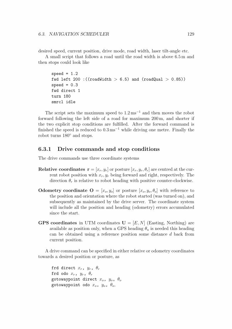
6.3. NAVIGATION SCHEDULER 129
desired speed, current position, drive mode, road width, laser tilt-angle etc.A small script that follows a road until the road width is above 6.5m and
then stops could look like
speed = 1.2
fwd left 200 :((roadWidth > 6.5) and (roadQual > 0.85))
speed = 0.3
fwd direct 1
turn 180
smrcl idle
The script sets the maximum speed to 1.2ms−1 and then moves the robotforward following the left side of a road for maximum 200 m, and shorter ifthe two explicit stop conditions are fulfilled. After the forward command isfinished the speed is reduced to 0.3ms−1 while driving one metre. Finally therobot turns 180 and stops.
6.3.1 Drive commands and stop conditions
The drive commands use three coordinate systems
Relative coordinates r = [xr, yr] or posture [xr, yr, θr] are centred at the cur-rent robot position with xr, yr being forward and right, respectively. Thedirection θr is relative to robot heading with positive counter-clockwise.
Odometry coordinate O = [xo, yo] or posture [xo, yo, θo] with reference tothe position and orientation where the robot started (was turned on), andsubsequently as maintained by the drive server. The coordinate systemwill include all the position and heading (odometry) errors accumulatedsince the start.
GPS coordinates in UTM coordinates U = [E, N ] (Easting, Northing) areavailable as position only, when a GPS heading θu is needed this headingcan be obtained using a reference position some distance d back fromcurrent position.
A drive command can be specified in either relative or odometry coordinatestowards a desired position or posture, as
frd direct xr, yr, θr
frd odo xr, yr, θr
gotowaypoint direct xo, yo, θo
gotowaypoint odo xo, yo, θo,

130 CHAPTER 6. MISSION PLANNING AND EXECUTION
(a) (b)
Fig. 6.1: The forward relative command fwd direct plans a route that avoidsobstacles but ignores the generated corridor (a). The gotowaypoint odo usesodometry coordinates and is in this case not direct and therefore followsthe best available corridor (b). The red circle with a heading vector is thedestination posture.
where fwd uses relative coordinates and gotowaypoint uses odometry coordi-nates. The direct qualifier is used primarily for close navigation, where thecurrent corridor is ignored and the target posture is used directly as exit pos-ture. An example is shown in Fig. 6.1(a). The vision support is not used withthe direct qualifier. The odo qualifier forces the use of a corridor and finds anexit posture within the best suited corridor rather than aiming for the pointdirectly (as in Fig. 6.1(b)), this is primarily used when the target position issome distance away and it is thus relevant to use the vision system to assistpath planning.
The main command for topological navigation is to drive relative to one ofthe road lines. Three commands are available for this purpose
frd left dfrd right dfrd top d,
where d is the maximum distance to follow the road edge. The distance fromthe road edge is determined by a system variable controllable by the script.
The top qualifier makes the robot follow the centre of the road; the top isthe detected highest point of the road. An example is shown in Fig. 6.2.
A number of drive commands are available that bypasses the obstacle avoid-ance path planning, as
idle t
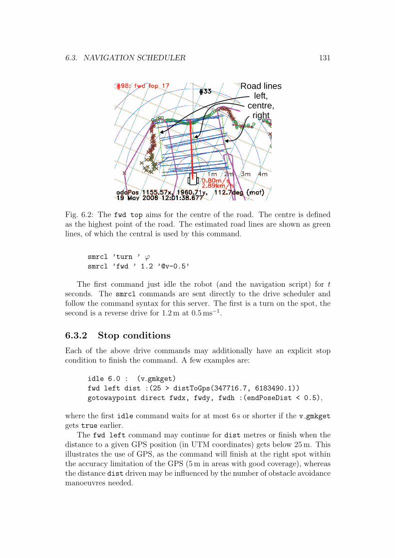
6.3. NAVIGATION SCHEDULER 131
Road linesleft,
centre,right
Fig. 6.2: The fwd top aims for the centre of the road. The centre is definedas the highest point of the road. The estimated road lines are shown as greenlines, of which the central is used by this command.
smrcl ’turn ’ ϕsmrcl ’fwd ’ 1.2 ’@v-0.5’
The first command just idle the robot (and the navigation script) for tseconds. The smrcl commands are sent directly to the drive scheduler andfollow the command syntax for this server. The first is a turn on the spot, thesecond is a reverse drive for 1.2m at 0.5ms−1.
6.3.2 Stop conditions
Each of the above drive commands may additionally have an explicit stopcondition to finish the command. A few examples are:
idle 6.0 : (v gmkget)
fwd left dist :(25 > distToGps(347716.7, 6183490.1))
gotowaypoint direct fwdx, fwdy, fwdh :(endPoseDist < 0.5),
where the first idle command waits for at most 6 s or shorter if the v gmkget
gets true earlier.The fwd left command may continue for dist metres or finish when the
distance to a given GPS position (in UTM coordinates) gets below 25m. Thisillustrates the use of GPS, as the command will finish at the right spot withinthe accuracy limitation of the GPS (5m in areas with good coverage), whereasthe distance dist driven may be influenced by the number of obstacle avoidancemanoeuvres needed.

132 CHAPTER 6. MISSION PLANNING AND EXECUTION
The gotowaypoint direct command will drive for the given position, butas the robot may not move exactly as ordered and may pass the desired pointat a distance, which further could trigger some undesired tight manoeuvres inan attempt to correct the (small) error. To avoid this situation it is often betterto stop slightly – in this case 0.5m – before the destination is reached.
The expression to the right of the ’:’ is evaluated as either true or falseand will finish the command when evaluated to true. A number of variablesand support functions are available when creating stop conditions.
The stop conditions (implicit or explicit) are evaluated at a 5Hz rate.
6.3.3 Sensor control
The sensors – and here especially the vision sensor – may be controlled insidethe script, using a server token in front of the command as
vision ’gmkget gmkref=true extra=false device=’ dev
vision ’camget device=’ dev ’ pos rot focalLength’,
where the command for the vision server is the remainder of the line after thevision keyword. The characters in apostrophes are sent directly to the visionserver, whereas expressions outside the apostrophes are evaluated and replacedby a value.
The first command gmkget requests a guidemark analyses from the cameradevice dev. The second command camget requests the position (pos), rotation(rot) and focal length (focalLength) of the same camera device.
The commands do not wait for a reply – some image analysis may take moreseconds – but when a reply is available a variable that includes the commandname will be set eg v gmkget = true when a gmkget reply is received. Thereturned values are in the same way available as variables; the reply to thecamget command may thus generate and assign the following values:
v camget = 1.0
v camget posX = 0.44
v camget posY = 0.0
v camget posZ = 0.86
v camget rotOmega = 0.0
v camget rotPhi = 0.392
v camget posKappa = 0.0
v camget focalLength = 297.5 ,
where v camget = 1.0 indicates that the reply is received; the value 1.0 isequivalent with true. All variable values are floating point numbers.

6.3. NAVIGATION SCHEDULER 133
6.3.4 Control decisions
A control sequence alternative may be needed if the values obtained on theroute may influence the actions needed. The following example uses the visionserver to analyse for a guidemark, and dependent on the received code takes adifferent approach
try_gmk_again:
v_gmkget = false
t = time
dev = 0
vision ’gmkget gmkref=true extra=false device=’ dev
//# wait for reply
idle 6.0 :(v_gmkget)
if (gmkNewCnt(t) < 1) goto got_no_gmk
if (gmkNewID(t, 13)) goto got_gmk13
if (gmkNewID(t, 11)) goto got_gmk11
got_no_gmk:
n = n + 1
if (n > 6) goto the_end
goto try_gmk_again
//
got_gmk11:
//# got gmk by right door -- enter
calcMapToPose(-2.0, 1.0, -3.14, gmkx, gmky, gmkk)
fwd direct calcx calcy calch :(endposedist < 0.3)
goto try_gmk_again
//
got_gmk13:
...
the_end:
print "Terminated"
The first lines request a guidemark analysis from the vision server, andthen a bit down the command if (gmkNewID(t, 11)) goto got gmk11 an ifstatement that fetches the guidemark 11 from the guidemark database, if thisis newer than the time t. If the guidemark is available then the next line toexecute is after the label got gmk11: found further down. There the guidemarkposition is used to calculate a position relative to the guidemark – in this caseused to enter a door. After the next drive command a goto try gmk again
sends the execution back to the beginning (to look for guidemark 13, that willdo something else and terminate the script).
134 CHAPTER 6. MISSION PLANNING AND EXECUTION
6.3.5 Watch functions
There may be a need to evaluate a condition that requires some calculationbefore a stop condition can be evaluated. One such condition could be tomonitor the progress of the robot, and if it persistently gets further and furtheraway from the target (eg while following a road edge) it may have taken awrong turn and thus it could be time for a recovery action, or to inform themission controller.
To enable such situation monitoring a watch function is implemented. Thefollowing example demonstrates the watch function to monitor for open doorswhile driving down a corridor. The intension is to make a pause at every opendoor.
speed = 1
door = true
doorNow = false
// define watch function
function look_for_door(direc)
ld = laserRange(direc)
doorNow = (ld > 2.5)
if (not door and doorNow and (distSoFar > 1))
skipcall doWait(5)
if (door != doorNow) print "laser dist " ld
door = doorNow
return door
//
function doWait(waitTime)
dd = dd + distSoFar
idle waitTime
return
// start watch for doors to the right
watch doors look_for_door(-90)
//
dist = 25
dd = 0
fwd left dist :((dd + distSoFar) > dist)
unwatch doors
print "Terminated"
A function is defined by the lines from a function to a return. The firstfunction look for door(direc) tests a laser scanner range in the direction ofthe doors (−90) and determines that there is an open door (or rather a lackof wall) if the measured distance is above 2.5 m. If a (new) door is detected

6.3. NAVIGATION SCHEDULER 135
then the if (. . .) skipcall doWait(5) executes a skipcall. The skipcall
terminates the current drive command temporarily and executes the specifiedfunction (in this case a doWait(5)) this function is defined just below and waitsfor 5 s.
The watch function is started by a watch doors look for door(-90) spec-ifying the function to watch and gives the watch a name doors.
The drive command fwd left dist :((dd + distSoFar) > dist) is fo-und near the end of the script. This drive command may be interrupted by theskipcall, and as the variables in the stop criteria distSoFar (distance drivenwithin this drive command) are not maintained between the calls the variabledd holds the distance driven from before the last interruption.
Before the end the watch is closed by the unwatch doors command.This functionality should enable some error recovery, like backing off if the
robot is stuck in obstacles. A number of the tests have been run with a simplespeed monitor, that – if speed is zero for 6 seconds – would try a reverse driveto a position visited a few metres back. The function did not succeed in thefew cases where it was activated for two reasons: when the robot is stuck in thehigh grass the laser scanner detects the grass as near obstacles and shuts offthe drive control (a security measure). In other situations the robot simply wasstuck (unable to move by own power). In both situations a manual assistancewas needed.
Another possibility is progress monitoring to allow a change in strategyif the primary fails. Such behaviour is not tested and the used scripts havetherefore been of the type: succeed or die.
6.3.6 Support functions
A number of support functions are available in the script language. Theseinclude many of the normal math functions like sin(a), atan2(y,x), min(a,b)and sqrt(v) and a number of functions that relates to robot navigation. Manyof these support functions just reduce the number of lines in the script whileothers provide access to more complex data structures. A few of the supportfunctions related to robot navigation are described below (the full set of supportfunctions is listed in appendix B.
Tail rope
The odometry position for the last about 100m are stored as a sort of tailrope. It marks positions that (once) were traversable and describes the routetaken. This tail rope is already used to maintain a system variable histH forthe ’historic’ heading of the last 5m excluding the most current 1m. Thisheading is used when evaluating alternative routes in the obstacle avoidance

136 CHAPTER 6. MISSION PLANNING AND EXECUTION
planning.A more general set of functions are available to use these historic data as
listed below
calcPoseAtTime(time)
calcPoseAtDist(near)
calcPoseFitAtDist(near, far),
where calcPoseAtTime(time) returns the historic posture a specific numberof seconds ago, the returned posture is – as for all functions starting with calc
– stored in the variables calcX, calcY and calcH, respectively. The functionitself returns true if such a posture is available.
The calcPoseAtDist(near) returns the tail rope posture at this (direct)distance from the current position.
The calcPoseFitAtDist(near, far) uses all the historic positions fromnear to far from the current robot position. These positions are fitted toa straight line. The closest position on this line to the posture at the near
distance is returned in the three posture variables. The function itself returnsthe residual variance from the line fitting.
One of the uses of this functionality is when the robot reaches a side roador a junction and needs a position and direction where the road ends beforethe junction. This position and direction may be needed when calculating adirection out of the junction.
An example of this use is shown below
...
// get general direction of road now
calcPoseFitAtDist(0, 25)
// follow left side into junction
fwd left 75 :(7.0 < abs(
distToPoseLineSigned(poseX, poseY, calcX, calcY, calcH)))
// get reference close to end of road
calcPoseFitAtDist(20, 40)
// add a vector in the right direction
calcAddRel(75.0, 150.0)
...,
an example of this manoeuvre is shown in Fig. 6.3.While on the road and at some (less than 75m) distance before the junction
a call to calcPoseFitAtDist (0, 25) is made (at (1)) to mark a line in theroad direction. The next drive command using the stop condition (7.0 <
abs(distToPoseLineSigned(...))) takes the robot into the junction anduntil 7m from the road direction line (at (2)). This is a rather fixated position

6.3. NAVIGATION SCHEDULER 137
7m
robot
2
31
Fig. 6.3: Determination of where a road ends and a junction starts may be abit tricky. At (1) the road direction line is stored. The left road edge is thenfollowed until the robot is 7m away from the stored road line (at (2)), this isa known position a short distance into the junction, and a road end posture isthen estimated from odometry history 20 m back as an on-road reference point(at (3)). From this a relative position is calculated towards the exit road.
relative to the junction, and from here a position and direction of the road justbefore the junction is calculated by calcPoseFitAtDist(20, 40), Then thisposition 20m back (at (3)) is used to calculate a direction towards the rightexit road in the junction.
GPS heading
The position accuracy of the GPS is about 5 m at the best, so a historic positionabout 20m from current position may be usable to get a reasonable GPS head-ing. A distance of up to more than 50m may be usable if the odometry errorscan be assumed to be small. The heading is calculates from UTM coordinatesas
θu = ∠(U−Ud) + θo − ∠(O−Od), (6.1)
where U = [E, N ]T is the current UTM coordinate and Ud is the UTM coordi-nate at an appropriate distance d. Similarly O = [x, y]T is the current odometryposition and Od the odometry position at distance d. θo is the current headingin odometry coordinates.
The angle θu is oriented with East as zero and positive angles counter-

138 CHAPTER 6. MISSION PLANNING AND EXECUTION
clockwise. This angle may be transformed to a compass angle (in radians)by
θcompass =π
2− θu. (6.2)
6.4 Mission assignment - operator interface
Conceptually an operator interface is needed to provide the robot with a mis-sion, and depending on the mission there may be a need for a more complexdialog between the operator (or user) and the robot. In a real world situationwith one or more robots deployed, a mission monitoring function would beneeded to monitor the robot progress for efficient allocation of new missions.
For the end user and especially for the more technical fault finding and de-bugging purposes an operator interface and monitoring ability is needed for allparts of the robot. Especially for research experiments an operator interface isneeded to allow easy change of parameters and intensive monitoring of perfor-mance. A comprehensive operator interface is therefore available that supportsinterface to all servers developed for this project. The interfaces are all text(XML) based especially to ease test and debugging.
The mission assignment to the navigation scheduler is an online operatorfunction, replacing the mission decision functionality.
A mission is normally loaded as a full script file using an online commandlike
<planSet load="scripr.mmr"/>
where planSet is the command identifier to make changes in the navigationsequencer, and scripr.mmr is the filename of the file with the mission script.
The mission can alternatively be added line by line using the operator in-terface command
<planSet add="command"/>
where command is the command line to be added.The robot can thus be controlled by adding one line at a time. A separate
function allows the newly added line to be executed immediately, like
<planSet goto="command"/>
that adds the command, skips the current command and proceeds with theadded command.
The shown user interface commands are packed in XML brackets, as theydescribe the command message format to the behaviour server.

6.5. MISSION PLANNING 139
start
Hunting lodge
end
5-roadjunction
Fig. 6.4: The primary test route. The start position is on a rather longasphalt road. The total route is about 3 km. The map background is fromGoogle Earth.
6.5 Mission planning
The mission planning is primarily prepared from a topological map of the areain which to navigate, supplemented by a more metric-based crossing of thejunctions. The primary test route is shown in Fig. 6.4. It starts on a ratherlong asphalt road with almost no side roads. After this, in front of the huntinglodge, the asphalt road ends and the robot has to cross a gravelled area, andsubsequently a number of forks and junctions need to be passed before the endposition is reached.
The navigation mission planning is first to select which roads can be handledby following one side of the road. Then the detection of junctions may beneeded, and finally a method must be found to get from one road to the nextacross the junction.
The major part of the script can be prepared from this map, as
fwd left 1740 (asphalt road towards hunting lodge),detect road end,cross open square,fwd left 300 (Keep left while passing two sideroads to the right),fwd right 280 (keep right until the 5-road junction),detect junction,cross junction,fwd left 280 (to get to the final destination).
All the roads are assumed to be handled by following one of the road lines.The two junctions that can not be crossed by following a road edge left or rightneed further planning.
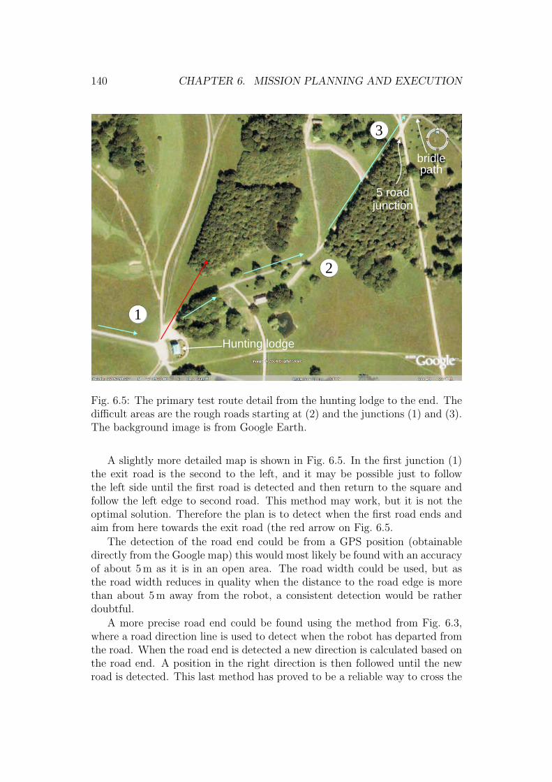
140 CHAPTER 6. MISSION PLANNING AND EXECUTION
Hunting lodge
5 roadjunction
bridlepath
1
2
3
Fig. 6.5: The primary test route detail from the hunting lodge to the end. Thedifficult areas are the rough roads starting at (2) and the junctions (1) and (3).The background image is from Google Earth.
A slightly more detailed map is shown in Fig. 6.5. In the first junction (1)the exit road is the second to the left, and it may be possible just to followthe left side until the first road is detected and then return to the square andfollow the left edge to second road. This method may work, but it is not theoptimal solution. Therefore the plan is to detect when the first road ends andaim from here towards the exit road (the red arrow on Fig. 6.5.
The detection of the road end could be from a GPS position (obtainabledirectly from the Google map) this would most likely be found with an accuracyof about 5m as it is in an open area. The road width could be used, but asthe road width reduces in quality when the distance to the road edge is morethan about 5 m away from the robot, a consistent detection would be ratherdoubtful.
A more precise road end could be found using the method from Fig. 6.3,where a road direction line is used to detect when the robot has departed fromthe road. When the road end is detected a new direction is calculated based onthe road end. A position in the right direction is then followed until the newroad is detected. This last method has proved to be a reliable way to cross the
6.5. MISSION PLANNING 141
junction.
At the second junction (3) it may be possible to follow the direction of theroad before the junction and cross both the junction and the following bridlepath. A GPS point is set to trigger a road direction line generation using acalcPoseFitAtDist(0, 20) from position history 20m back. A further 100malong this line a position is found, and the robot is set to aim for this point.The road sensing should ensure that the robot follows the road, even if theaiming point is a bit off the road. After crossing the junction (and the bridlepath) a road edge can be followed all the way to the goal point.
The potential script could then be prepared as
fwd left 1740 :(25 > distToGps(347716.7, 6183490.1),calcPoseFitAtDist(0, 25) (to get direction line of road),fwd left 75 :(7.0 < abs(distToPoseLineSigned(
poseX, poseY, calcX, calcY, calcH))),calcPoseFitAtDist(12, 25) (gets better road direction line),calcAddRel(75.0, 150.0) (in direction of exit road),gotowaypoint odo calcx calcy :((roadLeftQual > 0.78) and
(roadLeftDist < 2.7) and
(distsofar > 10)) (until road edge is detected),fwd left 300 (Keep left passing two sideroads to the right),fwd right 280 :(25 > distToGps(348223.0, 6183901.0)),calcPoseFitAtDist(0, 20),calcAddRel(100, 0), (across the second junction)gotowaypoint odo calcx calcy :(endPoseDist < 45),fwd left 350 : (30 > distToGps(348485.0, 6184198.0)
The script fails at two points, as the map did not tell the full story. Themost severe error was the five road junction (at (3) in Fig. 6.5), where thecrossing road is at a higher level than the followed road. While climbing ontothe crossing road the laser scanner detects parts of the road at a very smallangle, as a consequence parts of the road are seen as obstacles resulting ina failure to find the road (the entry is partially blocked by the erroneouslydetected obstacles). It turns out that following the road to the left onto thecrossing road, followed by a turn in the direction of the other road producesless false obstacles and the road is crossed more successfully.
The rough, gravelled road starting at (2) in Fig. 6.5 has rough edges, thatproduces low quality road edges. The vision sensor improves the situation, butthe driving is very irregular, and the mission fails occasionally when followingthe left or right road edges. However the gravelled road has a road profile thatis detected with high quality by the centre road line, and the route is traversedmore smoothly when following this line.

142 CHAPTER 6. MISSION PLANNING AND EXECUTION
Additionally the drive speed and other values need to be initialized in thescript. The full script used for the route can be seen at the end of appendix B.
The result is that a navigation script is not likely to succeed unrehearsed.After a first rehearsal the difficult parts of the road may need an adjustednavigation script to succeed.
6.6 Summary
In many situations the mission planning will not allow unrehearsed scriptingfor a navigation path. Especially at rough roads and junctions, that at placesmay challenge the capabilities of the robot, may need careful scripting.
The set of command provided is capable of implementing the needed com-mand script.
The implemented watch functionality has the potential of detecting morecomplicated situations, these could include detection of side roads and missionthreatening situations. Mission threatening situations could be: getting stuckin the rough grass or taking a wrong turn. A detection of such a situation couldthen trigger a skip to a recovery manoeuvre. The usefulness of this functionalityhas not yet been proved.
The navigation script functionality has been tested comprehensively and isable to implement navigation missions successfully.

Chapter 7
Software architecture
7.1 Introduction
The amount of software needed for a functional autonomous robot is significant,at least if the robot should be capable of working at a level, where experimentswith navigation and mission management are relevant subjects.
Software reuse is an obvious solution and when looking at the internet alarge number of open software solutions are available for e.g. motor control,stereo vision, GPS interface and extended Kalman filter. Some of the solutionsmay include reusable parts, but the work needed to understand and adapt thesolutions may be almost as extensive as a recreation from theory.
When reusing software efficiently it should neither be required to under-stand the programming structure nor the coding details, the functionality andthe interface requirements should be sufficient. For this to work a commonstructure or infrastructure is needed.
The software structure needed for navigating mobile robots is the subjectof this chapter. The chapter discusses the available solutions and proposes yetanother. The purposed software architecture fits the requirements of a researchplatform, which allows easy incorporation of new solutions, as well as separatemaintenance of the individual components.
7.2 Related work
The three best known component-based mobile robot oriented solutions are thePlayer by Vaughan et al. (27-31 Oct. 2003), Carnegie Melon Robot Naviga-tion Toolkit (CARMEN) by Montemerlo et al. (2003), and Orca by Brooks etal. (2005). All are based on open source and is available for download from’http://sourceforge.net’.
The component structure in Orca implements clients and servers and lets
143

144 CHAPTER 7. SOFTWARE ARCHITECTURE
these communicate in modes like client pull and server push. The communi-cation subject on each connection is well defined. The implementation buildson software reuse, partially by using a series of available libraries and partiallyby allowing reuse of the produced components. It is not widely used and thenumber of components is small.
The Player solution is not strictly component based as all sensors and con-trols are integrated into one server, this server then allows plugins and commu-nication with external components. Much of the bulk and real-time demandingcommunication is thus embedded in the server and shared to the plugins, in-creasing the performance of these issues.
The CARMEN toolkit is component-based and communicates using anIPC1 (Simmons (2005)) centralised communication that supports the appli-cable communication modes between components. Separate components areavailable for a number of existing robot platforms and sensors (including laserscanner and webcam). The sensor components are typically hardware abstrac-tion components that adapt the sensor data flow to the IPC communicationframework.
7.3 Software architecture requirements
University research projects are often divided into individual projects or pro-jects in small groups. Each project has a limited, and often very short, timeframe in which results have to be produced. Especially in robotics projects amaintained software base is needed if projects are to be undertaken at morethan the lowest levels (like sensor data extraction and drive controlled directlyfrom one sensor). Testing a complicated sensor, an alternative behaviour algo-rithm, a SLAM2 solution or other advanced functionality requires either a largeproject – where most of the resources are spent on the basic functionality – oran established high-level infrastructure on which the new functionality can bebuilt.
The new functionalities built in university projects are mostly discardedafter the reports have been evaluated, some of them for good reasons, but othersshould have been added to the available infrastructure for new projects. Tomake this possible – without a major software maintenance effort – the softwarearchitecture must support such an incremental development. Preferably thesoftware should be sharable among universities and other interested parties, forincreased functionality and reliability (the more people that use the softwarethe more reliable it gets).
The main requirements to robot software architecture are thus:
1IPC: Inter Process Communication2SLAM: Simultaneous Mapping and Localization
7.4. DESIGN DECISIONS 145
• Maintainable in separate units. It should be possible to develop andmaintain a unit of the robot software independent of other software units.The development and maintenance of a unit should not require more thana functional knowledge of the other units to which it is to be connected.
• The communication between units must be open, simple and extensible.Open to allow others to continue maintenance when needed. Simple tosimplify development and debugging as most software developed for re-search are prototypes and thus makes ease of debugging a vital theme.Extensible to allow addition of new features without affecting communi-cation partners that do not need the extension.
• Each component that fulfils an exclusive function on the robot should beexpandable. An exclusive component occupies a vital resource or func-tion in the system; this could be a sensor (eg laser scanner or camera),a manipulator or actuator, a behaviour server or a mapping function.When a new extension is to be tested for such a component it should bepossible to do so without a need of a total replacement of the compo-nent and without overtaking the maintenance responsibility of the basiccomponent.
• Data communication with high bandwidth devices (like cameras or laserscanners) should be considered. Data analyses of data from such devicesshould be possible close to the data source.
7.4 Design decisions
The component structure in Orca was investigated but was not adopted, pri-marily for three reasons. The communication structure seemed too complicated(too much overhead for high data rate connections and too limited in data con-tent for each connection – resulting in too many connections). The extensivelibrary dependency gave implementation difficulties in our Linux distribution.The available components were not sufficiently attractive to overcome the otherlimitations.
The Player structure was too monolithic and the work involved to adapt toour platform seemed discouraging.
The CARMEN robot toolkit has the benefit and the disadvantage of thecentralised communication structure. The communication with high bandwidthdevices has to pass this communication system, and there is no possibility(within the toolkit limits) to reduce the data rate at the source by attachingthe data analysis to the data source. Faster hardware is a solution, but thefaster hardware may be better spent on increased functionality.

146 CHAPTER 7. SOFTWARE ARCHITECTURE
The decision was therefore to design yet another robot framework, the ben-efits being that the available software for our robot platform could be incorpo-rated as is. The available software includes a robot hardware abstraction layerand a drive scheduler. The software architecture could be shaped to the needsas envisaged in the above requirements.
The proposed software architecture is illustrated in Fig. 7.1.
Camera(s)
GPS
Cameraserver
Laserscanner
Laserserver
GyroOdometry
Drivesystem
Driveserver
Missionassignment
Telnet
Missionserver
Operatorinterface
Operatorinterface
GPSserver
Behaviourserver
Fig. 7.1: The software architecture is based on a number of server functionsthat allows connection from clients at points marked with a circle. The messageformat is text (XML) based and allows thus simple monitoring and control ofall servers from tools like eg TELNET
The architecture is based on a number of servers where client connectionscan be attached. This architecture, as well as the basic communication meth-ods – server-push and client-pull – is taken from the Orca terminology. Thecommunication media is selected to be socket-based TCP/IP without a centralcommunication manager. A server occupies one port number only and all theservices provided by the server are communicated through this port. The servermay be attached to other servers through client connections.
The communication data formatting is selected to follow a subset of theXML (Extensible Markup Language) defined in the World Wide Web Consor-dium (2004) recommendation. The interface standard between a client anda server is therefore primarily based on an agreement between a client and aserver on the used tags and attributes in the XML formatted communication.XML is selected as it is well defined, and it remains compatible even if ex-tended, it is text based allowing for interface debugging by use of simple tools– like TELNET. Additionally a number of parsers and coders exist in differentprogramming languages.
Transfer of large data structures (eg a camera image) over a socket con-nection is relatively slow – XML coded or not – compared to data transferinternally in one application or by using shared memory. An internal datatransfer rate may be up to 4 bytes for each CPU clock cycle (on a 32 bit pro-

7.5. COMMUNICATION 147
cessor). Transfer of the same data on a socket connection is often at least 10–40times slower.
A server handling large data structures – like a camera server or a laserscanner server – should therefore include as much data reduction processing aspossible before delivering data to a client. That is, the server should hold thedata analysis functionality so that only the result is transferred to the client.Much of the new data analysis functionality should therefore preferably be builtinto the server directly. To do this without sacrificing separate maintenance ofreused code and new functionality, the new functionality should be added tothe server on a plugin basis.
The software architecture is therefore, to some degree, a mixture of thethree candidate software architectures discussed above: a component structurelike in CARMEN, a plugin capability like in Player and a direct communicationstructure like in Orca.
7.5 Communication
The data transfer is illustrated in Fig. 7.2, where posture data in the driveserver is to be transferred to the behaviour server. The data structure is coded
Behaviourserver
Driveserver
structdouble x, y;double th;double vel;
<pose x=”34.22” y=”0.33” h=”-0.571” vel=”1.03”/>
structdouble x, y;double th;
Fig. 7.2: A data structure is converted to XML-based text format on the com-munication line and converted back at the client end.
as an XML tag pose with the data values as attributes. In the behaviour serverthe posture is transferred back to a similar data structure. The extra velocityfield vel may be an extension to the data structure in the drive server, butthe behaviour server may not need to be modified to understand this extendeddata structure.
The data flow is always controlled from the client. A client can request datafrom a server as a one time service, a client pull data transfer like
<gmkGet device="1" width="0.025"/>,
148 CHAPTER 7. SOFTWARE ARCHITECTURE
which is a request to the camera server to analyse an image from camera deviceone for standard guidemarks with a block width of 2.5 cm. The reply from thecamera server could be
<gmkGet gmkCnt="1">
<gmk code="0007533" cam="left" device="1">
<timeofday tod="1154682383.782351"/>
<pos3d name="gmkPosition" x="2.0302" y="0.5201" z="-0.1500"/>
<rot3d name="gmkRotation" Omega="1.56235" Phi="-0.22109"
Kappa="-2.92682"/>
</gmk>
</gmkGet>.
An alternative communication method is server push, where the client re-quests the server to repeatedly send a data series, like
<push t=0.5 cmd=’gmkGet device="1" width="0.025"’/>,
which when sent to the camera server will trigger a guidemark analysis every0.5 s from camera device 1, and the data found is returned in the same formatas before.
An alternative server push method is to transfer data every time an eventhappens, eg every time there is a new image from a camera, then perform someoperation and return the result, eg
<camPush i=3 cmd=’gmkGet device="1" width="0.025"’/>,
where every third image (i=3) is analysed and the data returned to the clientas before.
The servers may return data to an operator interface and may even be usedas a stand-alone application for some interface, and operated from a text-basedinterface to the server socket.
7.6 Component structure
All components basically have the same structure, a server port, some resourcesand a set of function adding modules. The modules may include connectionsto devices or to other servers.
The server itself holds the basic server functionality. The basic functionalityincludes a server port and the ability to load modules. The server port handlesclient connections and a few commands like name and time. The module loaderis used to add the specific functionality to the server. One or more of thesemodules provide the basic resource needed for the specific functionality of the

7.6. COMPONENT STRUCTURE 149
Cameraserver
Image pool
Resourcemodules
Cameradevices
Device poolImage
Road outlineGuidemark
Functionmodules
Fig. 7.3: A camera server with a number of attached modules. One modulehandles the interface to camera devices in a device pool, additionally an imagepool module with reusable image buffers is available; both are made availableto other modules in the server as server resources. The additional functionmodules then utilise these resources.
server. These resources are then provided as server resources available to allother modules.
The basic construction is illustrated in Fig. 7.3 for the camera server. Eachmodule adds some functionality and makes its services available for the clients,and the resource modules further makes the resource functionality availabledirectly to other modules. The functionality is accessed through a uniquekeyword or a set of keywords. The server directs an XML tag with a matchingkeyword to the module handling that keyword, and provides information aboutthe client requesting the function.
The modules can be added as permanent modules linked into the servercode or be added as plugin modules. Resource modules are added as perma-nent modules to provide common resources of the server. Plugin modules canpresently be added when starting the server application only, but should beextended with online module load and unload functionality, in order to allowtesting without restarting the server component.
As the components are applications in their own right and controllable froma text-based interface, an online help system is made available. The server canprovide a list of modules and the keywords handled by each module. The listin table 7.1 is a list of modules and the handled keywords, which is returnedby the camera server using the function <sysGet functions/>
Table 7.1: An example of modules and function keywords loaded by the cameraserver.Module Function keywords (name and version)server push q sysGet name time help (camera server-1.25)
camera pool camGet camSet camPush camsGet (camControl-1.22)
image imageGet (image-1.22)
image pool poolGet poolList poolSet poolPush (imagePool-1.2)
road outline pathGet (imagePathFinder-1.25) andguidemark gmkGet gmkSet (imageGuidemarkFinder-1.25),
150 CHAPTER 7. SOFTWARE ARCHITECTURE
The first line in table 7.1 (including sysGet) is the function keywords han-dled by the server directly, the rest of the lines are the loaded modules includingthe technical name of the module and its version number.
The available parameters for each function may be listed using an onlinehelp function, like <gmkget help/>.
7.6.1 Client connections
A server module may include a client connection to some other server compo-nent. Client modules are available for the most common data structures. Eachclient module receives and unpacks one or more XML formatted data struc-tures into a C++ structure usable by the server module. The client moduleincludes trigger functions that are called when a full data structure is received.
7.6.2 Mission monitoring
The operator interface component is the only non-server component. The pur-pose is to be able to monitor the activity in each of the server components andpresent the information in an appropriate form.
The most simple operator interface is the text-based network tool calledTELNET, from this tool it is possible to query any of the servers for function-ality, but the reply may be too voluminous to be meaningful. A camera imageprovided in text form will in most cases be difficult to interpret.
An operator interface that provides a graphical interpretation of most ofthe more complex data structures is therefore needed. The purpose is both tomonitor the progress of the primary functionality and to make adjustments tothe available parameters, eg to load a mission for the robot.
Many of the illustrations used in this thesis are directly produced by theoperator interface.
Each server is a stand-alone application with communication to the relevantother servers and resources, there is thus no central function that provides anoverview of the entire network, nor the amount of inter-component communi-cation. Each server must be monitored separately.
7.7 Simulation
Simulation is an important function for any robot research project. In theavailable set of components simulation is handled by creating a simulated deviceor interface in the appropriate server. This simulated device then gets its datafrom a common simulator system. At present a simulator is available whichmay simulate the robot in a 2D environment and from this provide data formost of the robot sensors, including odometry and laser scanner.

7.8. FULL COMPONENT STRUCTURE 151
Cameraserver
Cameradevices
Road outlineGuidemark
Laserserver
Laserscanner
TraversableObstacle detect
EmergencyStop
Odometry posture
Emergency stop
UTMserver
GPS
World pose
Driveserver
Gyro, odom.Drive system
Drivescheduler
Drive mode
Navigationscheduler
Mapserver
Scheduler
SLAM
Odo calibrate
Obstacle mapPose historydrive control
Trav. corridor
Missiondecision
Event detectMission
Navigate DB
Fig. 7.4: A complete component based robot software structure based on thetask breakdown in Fig. 2.2. The servers are the rounded squares. The squaresbelow are server modules. Client connections are attached to a server at thesmall circles.
For this navigation project the simulation is primarily performed by replayusing log-files from real experiments, replacing the drive scheduler server, thelaser scanner server and the camera sensor. The camera server supports sim-ulated camera devices where the images are loaded as if the source was thesimulated device.
7.8 Full component structure
The work breakdown presented in chapter 2 and shown in Fig. 2.2 could beimplemented in the presented software structure as shown in Fig. 7.4.
The main information flow between the components is described in thefollowing.
The drive scheduler server produces an odometry-based posture, which isused by the UTM server to produce a world posture in combination with theGPS.
In the map server the global map is maintained based on traversable corridorand possibly obstacles from the navigation scheduler server.
The navigation database in the map server is used by the mission decisionserver to select the appropriate navigation path for the top priority mission.The selected navigation path sequence is sent to the navigation scheduler.

152 CHAPTER 7. SOFTWARE ARCHITECTURE
Cameraserver
Cameradevices
Road outlineGuidemark
Laserserver
Laserscanner
UTMserver
GPS
Driveserver
Gyro, odom.Drive system
Drivescheduler
NavigationschedulerScheduler
Obstacle mapPose historydrive control
Trav. corridor
Mission
Fig. 7.5: The implemented structure does not follow the described softwarearchitecture for all components – compare with the desired structure in Fig. 7.4.The camera server and the navigation scheduler use the component structureonly.
The navigation scheduler plans a desired short term exit posture based on atraversable corridor. The traversable corridor is obtained from a sensor fusionof road outline from the camera server and the traversable segments from thelaser scanner server. The navigation scheduler then plans a path to the desiredshort term destination and transfers a sequence of drive commands to the drivescheduler.
The drive scheduler server executes the desired drive commands by control-ling the drive system.
This component structure is only partially implemented as described in thenext section.
7.9 Results
The component structure of the implemented and tested system is not expandedto the level shown in Fig. 7.4 for a number of reasons. The actually implementedstructure is as shown in Fig. 7.5. The drive server and the drive scheduler areexisting components, they are well-proved socked-based servers, but they donot comply with the described architecture.
A laser scanner component is available but is not yet implemented in thetested system; the laser scanner functionality is therefore transferred to thenavigation scheduler.
The camera server is implemented following the described architecture. Thenavigation scheduler is partially implemented as described, except for the mod-

7.10. SUMMARY 153
ule structure where the module separation into resource modules and functionmodules is missing.
The GPS server is not component based as described and has no worldposture functionality.
The map server and the mission decision components are not implemented.The concept of having an established infrastructure that is divided into
functional components is a concept that divides the complex functionality intomanageable entities. Adding the text-based interface makes the componentseasy to grasp, and with the functional plugin modules makes the effort requiredfor functional extensions relatively simple to implement.
The implementation of resource modules are not sufficiently standardisedfor easy implementation.
The separated maintenance concept works for the components, as the useof XML makes new and old components compatible over many extensions.The same is not true for the plugin modules. A few updates to a sharedresource may have fatal consequences when attempting to load a module witha different expectation of the shared resource. This is a foreseeable shortcomingand imposes a stronger requirement of the stability of shared resources.
7.10 Summary
A software architecture is proposed that emphasises software reuse and theability to introduce new functionality with only a short introduction to thearchitecture and components. The built components – especially the cameraand laser scanner components – have proved these design objectives in a numberof projects.
The implemented communication protocol based on XML is flexible, exten-sible and easy to understand and allows components to be written in manyprogramming languages and on different platforms. The interface protocol re-laxes the need for strict version dependency across components.
The component structure is not fully implemented and especially the re-source sharing plugin modules have not yet found their final form. It is believedhowever that the architecture is well suited for the task, it suggests a flexiblebut strict structure, and is sufficiently pragmatic and flexible to allow interfaceto components that do not follow the same structure.

154 CHAPTER 7. SOFTWARE ARCHITECTURE
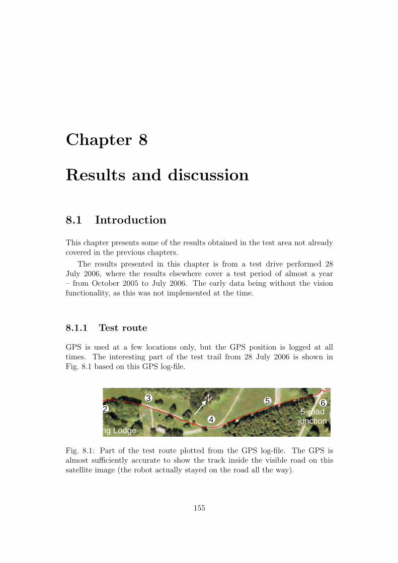
Chapter 8
Results and discussion
8.1 Introduction
This chapter presents some of the results obtained in the test area not alreadycovered in the previous chapters.
The results presented in this chapter is from a test drive performed 28July 2006, where the results elsewhere cover a test period of almost a year– from October 2005 to July 2006. The early data being without the visionfunctionality, as this was not implemented at the time.
8.1.1 Test route
GPS is used at a few locations only, but the GPS position is logged at alltimes. The interesting part of the test trail from 28 July 2006 is shown inFig. 8.1 based on this GPS log-file.
N12
Hunting Lodge
5-roadjunction
3 5 6
4
Fig. 8.1: Part of the test route plotted from the GPS log-file. The GPS isalmost sufficiently accurate to show the track inside the visible road on thissatellite image (the robot actually stayed on the road all the way).
155

156 CHAPTER 8. RESULTS AND DISCUSSION
8.2 Road line quality
The road edge line quality is shown in Fig. 8.2 for a part of the route shown inFig. 8.1.
0 100 200 300 400 500 600 7000.60.8
1
0 100 200 300 400 500 600 7000.60.8
1
0 100 200 300 400 500 600 7000.60.8
1
0 100 200 300 400 500 600 700
51015
(d)
(c)
(b)
(a)
Width
Centre
Right
Left
Fig. 8.2: The curves show the estimation quality for the left (a), right (b) andcentre (c) road line, respectively. The estimated road width is shown in (d).The x-axis is the travelled distance in metre and the road edge quality is in therange [0,1]. The distance is – with reference to Fig. 8.1 – from just before thehunting lodge (1) to just past the fork at (5).
The first 45m is on the main asphalt road where the robot drives at theleft side of the road, the left road quality is high (almost 1.0 – top graph), theright road line quality is lower (about 0.9 – graph (b)) as it is further away, theroad centre line quality (graph (c)) is well defined on the asphalt road with ahigh quality.
After the 45 m the robot enters the open area in front of the hunting lodge.The quality drops for all three lines. When the road width is estimated atits widest (about 15m) the road line quality is rather high (about 0.85). Thequality is the residual from the line fitting, and as the road width estimateconstantly is as wide as the laser scanner range permits, the residual from theline fitting is low. The road edge line quality can thus not alone be taken as anevidence of a road line being detected; the road line quality must be combinedwith the detection distance from the robot.
At 100 m the estimated road width is narrowing as the robot regains contactwith the road edges. The road edge quality stays low until about 150m. Thearea (at (2) in Fig. 8.1) is very flat and the roadside is difficult to classify by

8.3. EXCESSIVE ROLL 157
the laser scanner.At about 150 m the road changes to asphalt and especially the centre of the
road is now tracked with a high quality. At 275m (at (3) in Fig. 8.1) the sideroad to the right makes the right and centre road qualities drop, but the leftroad edge quality level is maintained.
After another 200m at about 350m the road type changes back to gravel.The road profile stays rather convex and the road centre line quality remainshigh for the rest of the route – until the last junction (5) at 650m.
8.3 Excessive roll
Excessive roll makes the road detection in one side of the robot much closer.Occasionally such close detections may violate the obstacle detection assump-tions. Figure 8.3 shows a situation where the robot enters a small pit resultingin a roll to the right. The laser scanner detection from the road is thus muchcloser on the right side.
(b)
(a)
Fig. 8.3: When entering the open area in front of the hunting lodge at (1) inFig. 8.1 there is a pit filled with water on the route as shown in (b). Whenthe robot enters this pit the robot makes a roll (about 8) to the right, andthus the laser scanner detects the right side of the road at a shorter range – asshown in (a). The traversable laser scanner measurements are in green whereasthe nontraversable are in a darker brown.
Where the detections are closer than 1.2m in the x-direction the hsup crite-rion in the raw height feature extraction in section 3.5.4 is triggered, assumingthat the detected object is 0.2m or more above ground level.

158 CHAPTER 8. RESULTS AND DISCUSSION
As a consequence this part of the road is classified as nontraversable andincluded as an obstacle as shown in Figure 8.3(a).
The erroneous classification of the road does not affect the classificationahead, and thus the continued drive is unaffected. This generation of erroneousobstacles may be a problem if they are to be used for mapping purposes.
The situation may have been be resolved correctly if the robot were equippedwith a roll sensor. Alternatively the height criterion could be enhanced to allowsome degree of roll, eg to allow 10 roll as is more than the 8 experienced inFig. 8.3.
8.4 Excessive tilt
When the robot enters a pit this may result in an excessive roll as described inthe previous section, when the robot is leaving the pit an excessive tilt may bethe result. This situation is illustrated in Fig. 8.4(a).
(a) (b)
Fig. 8.4: When entering and leaving a pit the robot tilt may influence themeasurements excessively. In this image – a few scans after the situation inFig. 8.3(a) – the tilt is so high that the laser scanner does not detect the roadbefore maximum range, and hence no measurements are classified as traversable(a). In (b) the robot has stopped as no navigation corridor is available.
The figure shows that the laser scanner does not detect the road surface atall; all measurements – apart from the obstacles to the left – are at maximumrange (8m). The tilt of the robot must therefore be more than 5.5 whenleaving the pit.
The situation produces no traversable road segments, and thus a navigationcorridor is not established. The robot continues to follow the remaining partof the last planned route, ie less than 1m, after this distance the robot stopsat the position shown in Fig. 8.4(b). After a few seconds the scans with no

8.5. OPEN AREAS 159
traversable segments are timed out (as of section 3.6.2 Tfade = 4.5 s) and therobot continues.
The vision road outline shows (as expected) a free path, but this is nottrusted if no corridor is generated based on laser scanner data. The situation isnot critical unless the robot stops in a situation where no traversable segmentis found (robot tilt above 5.5), in such cases the robot is stuck. A situationwhere the robot reaches a cliff edge or a steep downhill edge would show similardetections. A tilt sensor could have been used to resolve this situation.
8.5 Open areas
When driving in open traversable areas the road edge lines are estimated closeto the maximum range of the laser scanner as shown in Fig. 8.5.
Obstacle fromroad line
Estimatedroad lines
(b)
(a)
Fig. 8.5: The open gravelled area in front of the hunting lodge. The fulldetection range of the laser scanner is classified as traversable (green dots andcircles in (a)). The camera view can be seen in (b).
The estimated road edges left and right, are both at maximum range of thelaser scanner. The residual error from the line fit of the left and right roadlines is small and hence the detection quality is high. The quality of the rightedge line is sufficiently high (Lq > 0.9 as from section 5.6) to be added as anobstacle. Both the high quality and the obstacles are undesirable and couldbe avoided if road edges close to the maximum range of the laser scanner wereprohibited from being used in the road edge calculation.

160 CHAPTER 8. RESULTS AND DISCUSSION
8.6 Flat roadsides
The road leaving the open area at the hunting lodge (at point (2) in Fig. 8.1)constitutes a problem for the laser scanner classifier as illustrated in Fig. 8.6.
Approximatelyreal road edge
Vision basedroad outline Corridor
segments
(b)
(a)
Fig. 8.6: Data from the area marked (2) in Fig. 8.1. The blue lines in front ofthe robot are the traversable segments in the used corridor. The closest partof the vision-based road outline is shown at the top of the image. The visionsource image is shown in (b) with the estimated road outline.
At areas where the roadsides are flat and almost in the same plane asthe road, the laser scanner classifier tends to include parts of the roadsideas traversable road. In Fig. 8.6 the traversable segments (the blue lines) areextended up to 1m into the left roadside, compared with the vision-based roadoutline.
The ragged edge detection gives a poor edge line quality, and when the endpoints of the traversable segments are fitted to a straight line, this line may beestimated at some distance into the roadside.
The right road edge is in Fig. 8.6(a) often detected as traversable with onlya few measurements marked as nontraversable. The traversable segments inthe corridor are mostly terminated at the road edge, but many (about 40%)extend into the right roadside in this area.
In this area the vision-based road outline is superior to the laser scannerbased corridor.
Many of the roadside areas along the gravelled roads suffer from this effectresulting in a low quality of the corresponding road edge line. Compare inFig. 8.2 the left and right road edge line qualities at the shown situation –

8.7. SIDE ROADS 161
about 120 m – with the road edge line quality of the gravelled road area fromabout 400m and onwards.
8.7 Side roads
Detection of presence of side roads while passing may be a useful functional-ity for confirmation of own position or when searching for unexplored routealternatives. A situation with a side road is shown in Fig. 8.7.
(a)
(b)
Fig. 8.7: The side road to the right is visible in the road outline, as seen fromthe robot camera in (a) and projected into planar view in (b).
The road outline shows a widening of the road, but this can be taken as aweak evidence only of the presence of a side road, the vision-based road outlinemay in other situations falsely detect a wider road – eg as in Fig. 4.7(h), wherethe right road edge is seen as road. When the side road gets closer it will beout of sight of the camera.
The laser scanner will detect parts of the side road while passing as shownin Fig. 8.8(a). The side road is visible as an opening in the line of obstacles,wide enough for the robot to pass; in this case an opening of about 5m is found.
When going back in history to explore yet undiscovered territory such anopening would be adequate. To make a flag available for the navigation sched-uler may be possible, but this could be sensitive to false detections during robotmanoeuvring.
The road edge detection is a part of the laser scanner road edge detectionand the combination of distance to the edge and the edge line quality may beusable as side road detection. The road lines for this side road are shown inFig. 3.11(a).

162 CHAPTER 8. RESULTS AND DISCUSSION
Robotpath
Vision basedroad outline
Laser basednon-traversable
traversable
Side road
Side road
Road sideobstacles
(a) (b)
Fig. 8.8: The side road in (a) to the right as detected by the laser scanner.This leaves an open area to the right with no obstacles. The side road to theleft in (b) is equally well detected.
The side road to the right, marked (5) in Fig. 8.1, is detected by the laserscanner as shown in Fig. 8.8(b). The edge lines for this side road are shown inFig. 3.11(b).
These two side roads are detectable from the data, but this is not alwaysthe case. At Fig. 8.1 the side roads just before and after the position marked(4) are not detected. The one to the left is no longer in use and is overgrownwith grass. The other to the right is in use, but the surface of the side road isgravel whereas the main road is surfaced with asphalt. The result is that theroad edge line follows the change in surface type as does the vision-based roadoutline.
8.8 Convex obstacles
Obstacles are stored as convex polygon areas with a size limitation. The as-sumption is that the error introduced using a convex polygon description issmall compared to the calculation benefits obtained. Figure 8.9 shows a situa-tion where parts of the area classified as traversable are included in an obstaclepolygon.
In the situation in Fig. 8.9(a) the robot follows a rough left edge at somedistance (1 m) and the obstacles generated cover the rough area on both sidesof the road leaving about 3m obstacle free road width; this is close to theoptimal situation.
In Fig. 8.9(b) – four scans later – parts of the road have been classifiedas nontraversable. The obstacles on both sides are expanded to include thenewly detected nontraversable areas. The expansion makes the convex-shaped

8.9. ROAD RIDGE 163
Vision basedroad outline
Convexobstaclepolygon
Traversablearea inside
obstacleConvexobstaclepolygons
Planned path
(a) (b)
Fig. 8.9: The situation in (a) produces obstacles to the left and to the rightthat cover the nontraversable area reasonably well. The situation in (b) istaken four scans later where part of the road is classified as nontraversable andthe obstacles are expanded to include the newly detected obstacles.
obstacles include parts of the road, previously classified as traversable. Therobot could potentially have been partially within one of these areas, which inturn could trigger unnecessary manoeuvres.
This situation is not critical in this case, but could be if narrower andmore curved roads were to be passed. The solution could be to make theobstacle polygons smaller or to allow concave polygons, at the expense of thecomputational complexity.
8.9 Road ridge
At roads with a very high profile, where the laser scanner cannot see the otherside of the road, the results may be undesired as shown in Fig. 8.10.
The robot is entering from a side road on to a crossing gravelled road (at(6) in Fig. 8.1). The crossing road has a higher level than the side road, and acombination of the road profile and the difference in level make the right sideof the road surface beyond the horizon when seen from the laser scanner. Atthe ’ridge’ the visible road edge may produce a road edge line with sufficienthigh quality to be used as an obstacle as shown in the figure.
At about this time the robot is supposed to cross the road to enter theside road on the other side. The road edge obstacles make the transition moredifficult than intended (and in this case the robot had great difficulties in gettingacross).
The situation could question the benefit of using road side lines as obstacles,or indicate that the laser scanner height is insufficient for this type of road

164 CHAPTER 8. RESULTS AND DISCUSSION
Approximateposition ofroad edges
‘Invisible’road area
Edge lineobstacles
Fig. 8.10: The robot is entering from a side road to a higher crossing road.While climbing to the crossing road the full extent of the road is not visible tothe laser scanner, and might at time produce road edge obstacles at the ’ridge’.
crossing (or both).
8.10 Odometry navigation
The open area in front of the hunting lodge is crossed using odometry basednavigation. The area has a gravel surface and some accumulating odometryerrors are expected. Figure 8.11 shows the odometry based robot path overlaida satellite image of the area.
The overlaid image is aligned with the entry road and the distance from theentry road to the exit road is approximately 50m. The misalignment of thedetection of the exit road is small and presents no problem for the navigationscript.
8.11 Discussion
The results are primarily obtained within the selected test area, but the desiredabilities of the robot should be to be able to cope with more general real worldsituations. The focus on the test area is therefore to be seen as a subset ofthe desired navigation abilities. The ability to navigate within the test areashould therefore not prohibit the ability to cope with other types of outdoorenvironments. The focus has thus been on the general abilities – detectiontraversable areas – and the ability to recognise topological features to assistnavigation, eg along roads and in junctions.

8.11. DISCUSSION 165
Fig. 8.11: Crossing of the hunting lodge area. The satellite image is overlaidwith the odometry path of the robot. The distance across the open area isapproximately 50m.
The detection of road lines is valuable as it allows the robot to follow one ofthese lines. Most of the route is traversed following a road line. At the asphaltroad leading to the hunting lodge (about 1.8 km) the left edge is followed allthe way. The quality of the detection of the road lines is dependent on thedistance to the line. Where the road profile has a clear peak at the centre ofthe road – and this is especially the case for the gravelled roads – the centreroad line is easy to follow, and on most of the gravelled roads the robot followsthis line.
The road lines are implemented as a calculation based on the most recentset of traversable segments; but it is not a continuous calculation. It is expectedthat a continuous calculation of the road lines – eg using a Kalman filter – couldproduce superior results in most situations.
The used robot is not equipped with tilt and roll sensors, and this makesit difficult to interpret measurements in situations with excessive tilt or roll.On this test route – while traversing pits or climbing to a higher level – a fewsituations produced an undesired behaviour in some of the tests. An alternativeto a tilt sensor could be a closed loop servo that adapts the laser scanner tiltto a desired road detection distance; such a solution is expected to be able tosolve some of the tilt related issues.
In open areas the navigation relies primarily on the ability to navigate onodometry. The only open area on the test route requires odometry navigationover a distance of about 50m to hit an about 5m wide exit road; this is not

166 CHAPTER 8. RESULTS AND DISCUSSION
problematic for the used robot.The ability to classify the traversable road is adequate for the creation of
traversable corridors that keep the robot on the road in almost all cases. In thefew cases where the laser scanner based data would allow the robot to enterthe roadside the vision-based road outline will limit the available route to theroad.
The obstacles produced from the nontraversable measurements of the laserscanner mark the road edges and other obstacles satisfactory.
In some situations the produced obstacles are too restrictive. This is thecase where road edge lines with high quality are used to form obstacles. Theuse of road edge lines as obstacles seem to create more problems than theysolve. At the situations when they represent true road lines the obstacles aregenerated adequately without the use of road lines.
Chapter 9
Conclusion
Navigation of an autonomous robot is concerned with the ability of the robotto direct itself from the current position to a desired destination.
The thesis has successfully demonstrated a set of functionalities for mobilerobot navigation. The combined system is primarily tested in an outdoor testarea with a mixture of different road types and junctions. The robot hasautonomously completed a 3 km test route in this environment.
The research has been concentrated on three areas: perception of the en-vironment, transformation of the perceived information into behaviour andconstruction of a modular architecture.
9.1 Perception
Two main sensor types have been investigated for this environment: a laserscanner based road classifier and a vision-based road outline detector. Thecombined perception of these sensors has been demonstrated to be sufficient todirect the robot along the roads and across the junction in the test area.
9.1.1 Laser scanner perception
The used laser scanner is oriented towards the road at an angle of 9 fromhorizontal. This orientation is found to be about optimal for simultaneousdetection of road and obstacles. The road is detected at a distance of about2.6m in front of the robot.
Road corridor
The measured range data from the laser scanner is classified into traversableand nontraversable measurements using a set of seven features extracted from
167

168 CHAPTER 9. CONCLUSION
the data: raw height, roughness, step size, curvature, slope, width, and invaliddata.
The traversable measurements of one laser scan are further grouped intotraversable segments. Traversable segments from a number of scans are usedto generate traversable corridors. The corridors describe traversable areas inwhich the robot should be able to navigate. The generated corridors are madeavailable for the behaviour generation.
More than one corridor may be generated, eg: a corridor following the leftand right side of an obstacle, road alternatives exist or one corridor for a cyclepath and one for the main road. Sometimes a traversable part of the roadsidegenerates an alternative corridor. Which corridor to follow is determined bythe behaviour generation.
The corridor is used to extract further information from the traversed road.
Road lines
Road edge lines are estimated for the left and right limitations of the traversedroad. A further road line is estimated for the road centre representing thehighest point of the road. The road lines are used as reference lines in thebehaviour generation.
The road lines include an estimation quality, and when this quality is highand the road edge is inside the laser scanner range, the road line representsaccurately the true road edge.
Road type
The road type is estimated based on the corridor roughness. The road type isevaluated into the two types found in the test area: asphalt and gravel. Theestimated road type is used to increase the edge detection sensitivity on smoothasphalt roads and is made available for the behaviour generation.
In most cases the road type is estimated correctly, but in a few cases asmooth gravelled road is estimated as asphalt. During the performed tests theroad type has not been used to determine transition from one road segment tothe next in the navigation script.
Obstacles
The nontraversable measurements are filtered into areas to be treated as ob-stacles. These obstacle areas are combined into convex shaped polygon areas.These areas represent roadsides which are nontraversable as well as other obsta-cle types – like pedestrians. The obstacles are made available for the behaviourgeneration.

9.1. PERCEPTION 169
The obstacles generated have reliably been used to avoid stationary obsta-cles.
9.1.2 Vision-based perception
The robot camera is viewing the area in front of the robot – from about 1mto the horizon. Two data types are extracted from the camera images: roadoutline and artificial guidemark positions.
Road outline
The camera image is segmented into road and not road based on a seed areathat is known to be road. A balanced combination of chromaticity and edgedetection is used to determine the transition from road to non-road. The resultis a road outline polygon encapsulating the seed area. The image chromaticityis compensated (based on pixel intensity) to reduce the effect of shadows. Theroad outline is made available for the behaviour generation.
In most cases the road outline represents the true road limitations, but isless reliable in a number of situations: when the seed area partially includes aroadside area and when the colour of obstacles or roadsides is too close to theroad colour. Hard shadows and road paintings are further often estimated asobstacles.
The estimated road outline is able to detect an obstacle that crosses theroad outline only. Obstacles encircled by the road outline are not detected andtypically remain undetected until inside coverage of the laser scanner.
The road outline is projected to robot coordinates under the assumptionthat the road is in the plane of the robot base, when this assumption is violated,eg during robot roll and tilt, the accuracy of the road outline is reduced. Theroad outline covers the area beyond the laser scanner range.
Artificial guidemark
A guidemark sensor function is investigated; this function allows identificationof guidemarks and estimates the position and orientation of the guidemark in3D.
The guidemark is a flat checkerboard type frame with a coded identificationpattern at the centre. The frame is square and is well suited for positionestimation. The code in the centre can be used to make uniquely identifiableguidemarks.
The frame consists of alternating black and white squares. Each square mustbe covered by at least about 4 pixels in the camera image to allow detectionand position estimation. The 3D position and orientation of the guidemark can
170 CHAPTER 9. CONCLUSION
be estimated with an absolute accuracy better than 5 cm and 5, respectively(at the conditions described in chapter 4).
The guidemark ID and the 3D guidemark posture is made available forbehaviour generation.
9.2 Behaviour generation
The behaviour generation utilises the perceived sensor information to avoidobstacles and to make progress in the mission.
The cognitive skills are limited to the utilisation of the perceived data forobstacle avoidance. The remaining high level cognitive skills – determining howthe robot should position itself on the road and how to cross junctions – areleft to a navigation script.
Navigation script
The navigation script describes how the robot is to behave when following aroad, how to detect junctions and how to cross the junction to the next road.The navigation script interpreter has a number of drive modes available, eachdrive mode has a number of options affecting the behaviour. The drive modesinclude: following a road edge line at a given distance and aiming for a position(in robot or odometry coordinates).
The script further allows calculation and branching based on the availabledata. The available data includes – in addition to the perceived sensor informa-tion – the historic posture and the robot status. A watch function is available,and this could – as an example – be used to monitor the current heading todetect when the robot has entered into a side road or a junction.
Sensor fusion
The vision-based road outline is fused with the laser scanner based corridorsto a corridor based on both sensors.
If the vision-based road outline fails for some reason, the navigation con-tinues based on the laser scanner data only.
The combined corridor allows steady road following, both in the situationswhere the laser scanner has difficulties in separation of the road from the road-side, and in situations where the road outline fails (when both fails simultane-ously the performance is degraded). The vision-based road outline allows therobot to start an obstacle avoidance manoeuvre at an early stage. When a per-son is avoided in this way, the intensions of the robot will be visible sufficientlyearly to limit potential conflicts.

9.3. ARCHITECTURE 171
Obstacle avoidance
The obstacle avoidance behaviour is the planning of a short-term route fromcurrent position to a destination position – also called the exit posture – insidethe coverage of the sensors.
The exit posture is typically selected inside an available corridor, and theexit posture is selected for the best possible fulfilment of the current objectivesin the navigation script.
A route is planned from the current posture to the exit posture using avisible graph method. The method starts by testing the direct route fromcurrent position to the exit position, if an obstacle is too close, an avoidanceroute is created, as well as the most likely alternatives. The curvature of theroute is limited to impose restrictions on the dynamic behaviour of the robot.The path is constructed using a combination of straight and curved elements,where the turning radius in the curved part is selected to limit the centripetalacceleration.
More than one obstacle avoidance route may be possible and the mostoptimal of the available routes are selected based on a set of criteria including:route roughness, required manoeuvres and distance.
The path calculation method is fast when there is few obstacles only, butthe processing time increases exponentially with the number of obstacles foundon the path. In the test area the obstacle count is small and thus no realchallenge to the selected method.
Moving obstacles are not considered.
9.3 Architecture
A new software architecture is proposed as the available open source architec-tures were found to be too restrictive.
The proposed architecture is selected to allow the functionality to be im-plemented in components. The components communicate in a client serverarchitecture using XML formatted messages. Each of the components furtherallows plugins to facilitate enhanced or supplementary functionality withoutreplacement of a full component.
Three components are built using this architecture: a laser scanner server,a camera server and a behaviour server.
The laser scanner and vision sensors have high bandwidth requirements.This high bandwidth data is usually reduced significantly during the featureextraction from the sensor data. This sensor processing is therefore best per-formed as a plugin function in the server component for the sensor. The per-ceived data can then be transferred to other components as needed.
172 CHAPTER 9. CONCLUSION
The plugin and the component structures encourage a division of complexfunctionality into manageable sizes. The system knowledge needed to be able tocreate a plugin or use a server component is small, and thus new functionalitiescan be coded and tested within a short time frame. This is especially significantin a university environment, where students at a single course can create andtest advanced functionalities. The architecture is believed to be advantageouswhere distributed development and maintenance are essential.
The maintenance of the components and – to some extent – the plugins areindependent. The use of XML formatted communication enables extension ofthe data structure from one server without the need for clients to be updatedconcurrently (if they do not need the extended information).
The architecture is not fully developed, but the camera server and the laserscanner server have already proved their value in a number of projects.
9.4 Results
Test results have been obtained over a period of almost one year and in anumber of weather conditions including sunshine, overcast and wet weather,but excluding snow and heavy rain.
The road following is mostly unproblematic; especially asphalt roads wherethe roughness difference between the road surface and the roadsides is con-stantly high. On gravelled roads the difference in roughness of the road andparts of the roadside is sometimes small. The corridor edges are here moreragged than on asphalt, the consequence is a lower estimation quality for theleft and right road lines. The road centre line is usually estimated with highquality on the gravelled roads and is easy to follow.
Fork junctions are mostly passed by following the left or right road linesinto the desired road. More complicated junctions are detected when enteringinto the junction and from here the behaviour script directs the robot towardsthe desired exit road.
The navigation script is manually prepared using a map of the area and sub-sequently adjusted after tests in the area. It has not been possible to completean unrehearsed test mission successfully; especially the crossing of junctionsneeds script adjustments.
There are season and weather variations in the performance of the robot.In sunshine the hard shadows from obstacles (eg pedestrians) are taken asobstacles by the vision-based road outline sensor. The slightly more scatteredshadows from trees are less of a problem. During the winter and early spring thevegetation on the roadsides may be more flat and having a more greyish colour,this is slightly more problematic for both the laser scanner and vision-basedsensors – resulting in less smooth road following. Wet weather and partially

9.5. FUTURE WORK 173
wet roads are handled reasonably well. Snow and heavy rain conditions arenot tested, and the sensors are not expected to produce usable results in thesecases.
The required update rates for laser scanner, vision and obstacle avoidanceare speed dependent and is selected to be as low as possible. The laser scannerupdate rate is about 6 Hz at a robot speed of 1ms−1 to allow detection ofobstacles larger than 5 cm. The vision-based road outline is detected at aslower 1Hz rate, as this is the long range road detection (from about 2.6m).The obstacle avoidance path planning was running at a 2Hz rate, as this shouldbe sufficient for obstacle avoidance manoeuvring in the available speed range(up to 1.5 ms−1).
9.5 Future work
For the presented solutions there are a number of enhancements that is expectedto improve the obtained results. These include the following subjects.
• Improvements of the calculation of road lines. The calculation couldprobably be improved by using a continuous calculation, eg a Kalmanfilter. The road lines should neither use measurements close to the laserscanner maximum range nor measurements close to a visible horizon.
• A permanent watch function should be included to detect if the robot hasentered a side road or the road has made a sharp turn. Such a functioncould be based on deviation from a previously stable course. This is theused method to detect junctions and would simplify the navigation script.
• The vision-based road outline could be searched for encircled obstacles.This is a rather simple enhancement and would remove an undesiredfeature from the presented solution, where obstacles with a height up tothe height of the camera may remain undetected.
• A roll and tilt sensor could improve the coordinate conversion of mea-surements, resulting in improved performance in a number of situations.
• An improved GPS handling could allow a drive mode aiming at a GPSposition directly. Such a solution would not improve the results directly,but could potentially simplify the navigation script in some situations.
• In the implemented software architecture the resource-providing plug-ins do not use a standardised method. Such a standardised method forresource sharing should be provided to facilitate a more decentralisedmaintenance structure.

174 CHAPTER 9. CONCLUSION
For the long perspective of navigation autonomy, the following list of subjetsshows the areas, which would have been investigated had time been available:
• Vision-based perception with classification of the seen objects in classeslike: trees, signposts, cars, pedestrians and buildings. This is envisagedas a combination of image segmentation and 3D reconstruction using egthe ’structure from motion’ method. This is a complicated perceptionsensor, of wich the road outline sensor described in this thesis is seen asa small initial step.
• A mapping function where the road outline and other identified objectscreate and update a map while moving. The map elements are assumedto be positioned primarily based on GPS positions, with an allowancefor correction of errors using one of the methods seen in the SLAM com-munity, eg the ’consistent pose estimation’ method described in Konolige(2005) for example or Folkesson et al. (2005).
• With a map in place with some experienced navigation information, thecognitive abilities may be enhanced to increase the autonomy, eg whilefollowing roads or crossing junctions, where experience could determinethe drive mode rather than an operator produced script.
The research is not expected to lead to autonomous robots capable of cop-ing with public traffic during the rush hour initially. The robot autonomy willprobably develop in isolated areas where the rules of behaviour are less de-manding, like in private houses, on agricultural farmland or on the militarybattlefields.

Bibliography
Albus, J. S. (1992), A reference model architecture for intelligent systems de-sign, in P. J. Antsaklis & K. M. Passino, eds, ‘An Introduction to Intelli-gent and Autonomous Control’, Kluwer Academic Publishers, Boston, MA,pp. 57–64.
Albus, J. S., Lumia, R. & McCain, H. G. (1986), Nasa/nbs standard referencemodel for telerobot control systems architecture, Technical Report NBS Tec-nical note #1235 or NASA document SS-GSFC-0027, National Bureau ofStandards (USA).
Andersen, J. C., Andersen, N. & Ravn, O. (2004), Trinocular stereo vision forintelligent robot navigation, in ‘5th IFAC/EURON Symposium on IntelligentAutonomous Vehicles’, Lisboa, Portugal.
Andersen, J. C., Blas, M. R., Andersen, N., Ravn, O. & Blanke, M. (2006),‘Traversable terrain classification for outdoor autonomous robots using single2D laser scans’, Integrated Computer-Aided Engineering.
Aufrere, R., Gowdy, J., Mertz, C., Thorpe, C., Wang, C.-C. & Yata, T. (2003),‘Perception for collision avoidance and autonomous driving’, MechatronicsVol. 13 Issue. 10, 1149–1161.
Babuska, R. (1998), Fuzzy Modeling for Control, Kluwer Academic Publishers.
Barontini, G., Segurini, G., Breemen, A. v., Brodtman, T., Buckingham, R.,Christensen, H. I., Ikonomopoulos, S., Gelin, R., Fournier, R., Gu, C.-Y.,Guettier, C., Hgele, M., Isasi, L., Koeppe, R., Bischoff, R., Patin, B. &Pegman, G. (2005), ‘Building europ, the european robotics platform, thehigh level view’, http://www.robotics-platform.eu.com.
Behringer, R., Travis, W., Daily, R., Bevly, D., Kubinger, W., Herzner, W. &Fehlberg, V. (2005), Rascal - an autonomous ground vehicle for desert drivingin the darpa grand challenge 2005, in ‘Intelligent Transportation Systems,2005. Proceedings. 2005 IEEE’, IEEE, pp. 644–649.
175

176 BIBLIOGRAPHY
Bertozzi, M. & Broggi, A. (1997), ‘Vision-based vehicle guidance’, ComputerVol. 30 Issue. 7, 49–55.
Blanke, M., Kinnaert, M., Lunze, J. & Staroswiecki, M. (2003), Diagnosis andFault-tolerant Control, Springer Verlag.
Blas, M. R., Riisgaard, S., Ravn, O., Andersen, N., Blanke, M. & Andersen,J. C. (2005), Terrain classification for outdoor autonomous robots using 2Dlaser scans., in ‘2nd int. Conf. on Informatics in Control, Automation andRobotics, ICINCO-2005.’, Barcelona, 14-17 September, pp. 347–351.
Brooks, A., Kaupp, T., Makarenko, A., Williams, S. & Oreback, A. (2005), To-wards component-based robotics, in ‘Intelligent Robots and Systems, 2005.(IROS 2005).’, IEEE/RSJ, pp. 163–168.
Brooks, R. A., ed. (1990), The Behavior Language; User’s Guide, MIT Press.
Carstensen, J. M., ed. (2001), Image analysis, vision, and computer graphics,Informatics and Mathematical Modelling, Technical University of Denmark,DTU.
Douglas, D. & Peucker, T. (1973), ‘Algorithms for the reduction of the numberof points required to represent a digitized line or its caricature’, CanadianCartographer pp. 112–122.
Fergus, R., Perona, P. & Zisserman, A. (2003), Object class recognition byunsupervised scale-invariant learning, in ‘Proceedings. 2003 IEEE ComputerSociety Conference on Computer Vision and Pattern Recognition’, IEEEComput. Soc, pp. II–264.
Folkesson, J., Jensfelt, P. & Christensen, H. (2005), Graphical slam using visionand the measurement subspace, in ‘Proceedings of International Conferenceon Intelligent Robots and Systems 2005’, IEEE, pp. 325–330.
Guivant, J. E., Masson, F. R. & Nebot, E. M. (2001), ‘Optimization of thesimultaneous localization and map-building algorithm for real-time imple-mentation’, IEEE Transaction on Robotics and Automation 17(3), 242–257.The University of Sidney, Australia.
Henriksen, L. & Krotkov, E. (1997), Natural terrain hazard detection with alaser rangefinder, in ‘IEEE International Conference on Robotics and Au-tomation’, Vol. 2, pp. 968–973.
Horswill, I. (1994), Visual collision avoidance by segmentation, in ‘Proceedingsof the IEEE/RSJ/GI International Conference on Intelligent Robots andSystems ’94. ’Advanced Robotic Systems and the Real World’, IROS ’94.’,IEEE, pp. 902–909.
BIBLIOGRAPHY 177
Jochem, T., Pomereau, D. & Thorpe, C. (1993), Maniac: a next generation neu-rally based autonomous road follower, in F. Groen, S. Hirose & C. Thorpe,eds, ‘Intelligent Autonomous Systems. IAS-3. Proceedings of the Interna-tional Conference’, IOS Press, pp. 592–601.
Jochem, T., Pomerleau, D. & Thorpe, C. (1995), Vision-based neural net-work road and intersection detection and traversal, in ‘Intelligent Robotsand Systems 95. ’Human Robot Interaction and Cooperative Robots”, IEEEComput. Soc. Press, pp. 344–349 vol.3.
Kadir, T. & Brady, M. (2001), ‘Saliency, scale and image description’, Inter-national Journal of Computer Vision Vol. 45 Issue. 2, 83–105.
Kim, D. & Nevatia, R. (1999), ‘Symbolic navigation with a generic map’, Au-tonomous Robota Vol. 6, 69–88. Soongsil University, Korea and Universityof Southern California, USA.
Kloor, P. L., Lundquist, P., Ohlsson, P., Nygards, J. & Wernersson, A. (1993),Change detection in natural scenes using laser range measurements from amobile robot, in ‘Proceedings of 1st IFAC International Workshop on Intel-ligent Autonomous Vehicles’, IFAC, University of Southampton, pp. 71–76.
Konolige, K. (2005), Slam via variable reduction from constraint maps, in‘Proceedings of the International Conference on Robotics and Automation,2005’, IEEE, pp. 667–672.
Kragic, D.; Christensen, H. (2005), ‘Advances in robot vision’, Robotics andAutonomous Systems Vol. 52 Issue. 1, 1–3.
Liatsis, P., Goulermas, J. & Katsande, P. (2003), A novel lane support frame-work for vision-based vehicle guidance, in ‘Proceedings of the Industrial Tech-nology, 2003 IEEE International Conference’, IEEE, pp. 936–941 Vol.2.
Loaıza, H., Triboulet, J., Lelandais, S. & Barat, C. (2001), ‘Matching segmentsin stereoscopic vision’, IEEE Instrumentation and Measurement Magazinepp. 37–42.
Loaıza, H., Triboulet, J., Lelandais, S., Chavand, F. & Artigue, F. (1999),A multi-configuration stereoscopic vision system for domistic mobile robotlocalization, in ‘Robot Motion and Control, 1999. RoMoCo ’99. Proceedingsof the First Workshop on’, IEEE, pp. 207–212.
Macedo, J., Matthies, L. & Manduchi, R. (2000), Ladar-based discrimination ofgrass from obstacles for autonomous navigation, in ‘Experimental RoboticsVII, Proceedings ISER 2000, Waikiki, Hawaii’, Springer, pp. 111–120.

178 BIBLIOGRAPHY
Mejnertsen, A. & Reske-Nielsen, A. (2006), Control of autonomous tractor,Master’s thesis, Ørsted•DTU, Technical University of Denmark, DK-2800Kgs. Lyngby.
Mizoguchi, F., Nishiyama, H., Ohwada, H. & Hiraishi, H. (1999), ‘Smart officerobot collaboration based on multi-agent programming’, Artificial Intelli-gence Vol. 114 Issue. 1–2, 57–94.
Montemerlo, M. & Thrun, S. (2004), A multi-resolution pyramid for outdoorrobot terrain perception, in ‘Proceedings - Nineteenth National Conferenceon Artificial Intelligence (AAAI-04)’, compendex, pp. 464–469.
Montemerlo, M., Roy, N. & Thrun, S. (2003), Perspectives on standardiza-tion in mobile robot programming: the carnegie mellon navigation (carmen)toolkit, in ‘Proceedings. 2003 IEEE/RSJ International Conference on Intel-ligent Robots and Systems, 2003. (IROS 2003)’, IEEE, pp. 2436–2441 vol.3.
Murray, D. & Little, J. J. (2000), Using real time stereo vision for mobilerobot navigation, in ‘Autonomous Robots’, Kluwer Academic Publishers,The Netherlands, University of British Columbia, Canada, pp. 161–171.
Nielsen, A. & Breiting, M. (2004), Design and implementation of outdoor mo-bile robot, Master’s thesis, Technical University of Denmark, Ørsted•DTU,Automation.
Ponweiser, W., Vincze, M. & Zillich, M. (2005), ‘A software framework to inte-grate vision and reasoning components for cognitive vision systems’, Roboticsand Autonomous Systems Vol. 52 Issue. 1, 101–114.
Riisgaard, S. & Blas, M. R. (2005), Navigation for outdoor mobile robot, Mas-ter’s thesis, Ørsted•DTU, Technical University of Denmark, DK-2800 Kgs.Lyngby.
Robowatch (2006), ‘Ofro surveillance robot by robowatch technologies gmbh’,http://www.robowatch.de.
Se, S., Lowe, D. & Little, J. (2001), Vision-based mobile robot localization andmapping using scale-invariant features, in ‘IEEE International Conferenceon Robotics and Automation, Seoul, Korea’, IEEE, pp. 2051–2058.
Shah, S. & Aggarwal, J. K. (1997), ‘Mobile robot navigation and scene mod-elling using stereo fish-eye lens system’, Machine Vision and Application10, 159–173.
Siegwart, R. & Nourbakhsh, I. R., eds (2004), Introduction to AutonomousMobile Robots, MIT Press.
BIBLIOGRAPHY 179
Simmons, R. (2005), ‘Inter process communication (ipc)’, http://www.cs.cmu.edu/afs/cs/project/TCA/www/ipc/index.html.
Simmons, R. & Apfelbaum, D. (1998), A task description language for robotcontrol, in ‘Proceedings Conference on Intelligent Robotics and Systems’.
Thorpe, C., Jochem, T. & Pomerleau, D. (1997), The 1997 automated high-way free agent demonstration, in ‘Proceedings of Conference on IntelligentTransportation Systems, 1997. ITSC ’97.’, IEEE, pp. 496–501.
Thrun, S., Montemerlo, M., Dahlkamp, H., Stavens, D., Aron, A., Diebel,J., Fong, P., Gale, J., Halpenny, M., Hoffmann, G., Lau, K., Oakley, C.,Palatucci, M., Pratt, V. & Pascal, S. (2006), ‘Stanley: The robot that wonthe darpa grand challenge’, http://cs.stanford.edu/group/roadrunner/.
Trepagnier, P. G., Kinney, P. M., Nagel, J. E., Doner, M. T. & Pearce, J. S.(2005), Team gray techical paper, Technical report, Gray & Company Inc.
Urmson, C., Anhalt, J., Clark, M., Galatali, T., Gonzalez, J. P., J., G., Gutier-rez, A., Harbaugh, S., Johnson-Roberson, M., Kato, H., Koon, P. L., Pe-terson, K., Smith, B. K., Spiker, S., Tryzelaar, E. & Whittaker, W. R. L.(2004), High speed navigation of unrehearsed terrain: Red team technologyfor grand challenge 2004, Technical Report CMU-RI-TR-04-37, Robotics In-stitute, Carnegie Mellon University, Pittsburgh, PA.
Vandapel, N., Huber, D., Kapuria, A. & Hebert, M. (2004), Natural ter-rain classification using 3-d ladar data, in ‘Robotics and Automation, 2004.Proceedings. ICRA ’04. 2004 IEEE International Conference on’, IEEE,pp. 5117–5122.
Vaughan, R., Gerkey, B. & Howard, A. (27-31 Oct. 2003), On device abstrac-tions for portable, reusable robot code, in ‘Proceedings. 2003 IEEE/RSJInternational Conference on Intelligent Robots and Systems, 2003. (IROS2003)’, IEEE, pp. 2421–2427 vol.3.
Wallace, R., Matsuzaki, K., Goto, Y., Crisman, J., Webb, J. & Kanade, T.(1986), Progress in robot road-following, in ‘Proceedings 1986 IEEE Inter-national Conference on Robotics and Automation (Cat. No.86CH2282-2)’,IEEE Comput. Soc. Press, pp. 1615–21 vol 3.
Wijesoma, W., Kodagoda, K. & Balasuriya, A. (2004), ‘Road-boundary de-tection and tracking using ladar sensing’, Robotics and Automation, IEEETransactions on pp. 456–464.

180 BIBLIOGRAPHY
World Wide Web Consordium, . (2004), Extensible markup language (xml) 1.1,Technical Report http://www.w3.org/TR/xml11/, W3C.World Robotics
World Robotics (2005), United Nations Economic Commission for Europe(UNECE) and International Federation of Robotics (IFR).
Xiang, Z. & Ozguner, U. (2005), Environmental perception and multi-sensordata fusion for off-road autonomous vehicles, in ‘Intelligent TransportationSystems, 2005. Proceedings. 2005 IEEE’, IEEE, pp. 584–589.

Appendix A
Trinocular stereovision
This article was presented at 5th IFAC/EURON Symposium on IntelligentAutonomous Vehicles (Andersen et al. (2004)).
Abstract
This paper describes a vision sensor that extracts visible features of objectsusing a set of on-board robot cameras. The purpose of the sensor is to be ableto classify the seen objects into abstract object types like tables, chairs, wallsand doors using these features. The results show that the vision sensor is ableto extract a filtered set of features suitable for the purpose. The method used isstereoscopic scanning followed by a filtering process in 3D space. The methodis insensitive to the shape of the objects and the structure of the background.
A.1 Introduction
The research project behind this paper is focused on autonomous robot nav-igation in an indoor human environment, where the robot is able to find andrecognize some basic types of objects. The robot sensors include camera visionas the primary sensor for this task.
Mobile robot navigation is the discipline of locating own position and tofind a path to the destination. Finding a path involves in this case recognitionand classification of observed objects, so that the destination can be describedin terms of the classified objects, e.g. as ”go to the third table in the first roomto the left”.
The stereoscopic vision sensor provides the majority of the data needed forobject classification. The extracted data should allow for classification intoclasses like chair, table, wall, door or human, without prior knowledge of whereto expect what type of objects.
181

182 APPENDIX A. TRINOCULAR STEREOVISION
Stereoscopic vision systems have been described in a number of papers overthe resent years. Most of these systems extract linear features in the imagesfrom single cameras and then correlate these to get the 3D information like inLoaıza et al. (2001), Loaıza et al. (1999), Kim & Nevatia (1999) and Shah &Aggarwal (1997). In Se et al. (2001), the images are searched for scale invariantfeatures — e.g. line ends — before correlation and 3D calculation.
Most of the stereoscopic camera solutions use three cameras achieve betterimmunity to false correlations. Image processing for stereo calculation is pro-cessing power intensive and only a few papers document image processing timesof less than one second. For obstacle mapping Murray & Little (2000) expect3 updates per second, and, for robot position estimating Se et al. (2001), twoestimates per second were obtained from the camera images using a 700 MHzPC. Faster is better, but processing-times in excess of one second is acceptablewhen the resulting data is to be used for route planning and not directly in themotion control loop.
This paper describes a method where images are scanned for 3D points firstand the filtering is done subsequently in 3D space.
A.2 Objectives and Overview
When looking at an image as in Figure A.1 it is easy to see that it shows a chair,a golf-ball on the floor, and some closets in the background. If a robot is toget to the same conclusion, there is a fair bit of processing is to be performed,some of which is described in the following.
To find out that the nearest object is a chair, a number of tasks must beperformed. The object must be separated from the rest of the image, and itmust be analyzed for properties that indicate it is a chair. The properties couldbe that it has a surface, the seat, of an appropriate size (e.g. 40x40 cm) at anappropriate height (approximately 50 cm), and that it has an open structurebelow the surface to support it. These properties would make it distinguishablefrom other objects like a box or a table.
From one images set the visible features can be extracted. The visiblefeatures of a chair could be the front edge of the seat, the chair bag or partsof the support structure. The idea is that a set of such features is sufficient toperform the needed object classification.
This paper describes a vision sensor and the processing behind the featureextraction.
The sensor has three major parts, the feature filtering, the stereo scanningand the camera calibration. Each of these parts are described below.

A.3. FEATURE FILTERING 183
Top image
Fig. A.1: An image like this is easily decoded by a human, but requires explicitprocessing for a robot.
A.3 Feature filtering
The data from the stereo correlation is 3D positions reconstructed from corre-sponding points in a set of stereoscopic images. About 1000 3D positions areproduced in a full stereoscopic image scanning. These positions are groupedinto spatially separated clusters.
The feature filtering function must ensure that clusters represent one objectonly. As different objects often is seen close together — e.g. a table and a wall— they may not be separable on distance alone.
To separate these clusters into features from just one object, two primarymethods are used. The first is to extract horizontal and vertically orientedfeatures, and the second is to split combined features based on similar positionaland color properties.
In an indoor environment, horizontal and vertical features are often foundin especially empty rooms. These features are extracted first based a densityhistogram along the vertical axis for the horizontal lines. This will typicallyproduce a peak in the histogram when the cluster contains a major feature

184 APPENDIX A. TRINOCULAR STEREOVISION
Axis split
3D cluster
Splitgroups
Split Split
Outlier and size filter
(< 4 points)
Dump
Fuzzysplit
Vm > limit
Not Not Rest
Split
Feature
Fig. A.2: The input clusters are groups of isolated 3D detections, these getsdivided into features of just one object by splitting.
perpendicular to the vertical axis. The peak is then isolated to a new cluster.The same method is used across the image, and this isolates primarily verticallines.
Fig. A.3: The images show the features extracted from the scene in Figure A.1.The left image is top view, and the right image is side view. The three camerapositions are shown as triangles. Each feature is represented with a coloredgroup of 3D detections.
A fuzzy c-means classifier from Babuska (1998) is able to separate 3D po-sitions in a cluster of into two or more sub-clusters. The ellipsoid shape of thesub-clusters may differ, e.g. a cluster representing a chair seat in combinationwith one of its legs, may be divided into a narrow ellipsoid formed cluster fromthe leg and a more ball formed for the seat. The fuzzy c-means method needs toknow the number of sub-clusters, and the computation afford increases rapidlywith the number of clusters. A computational affordable method is to splitclusters into two subclusters until the cluster statistics are reasonable, or the
A.4. STEREOSCOPIC SCANNING 185
clusters are too small to split. This is the method used, and it produces slightlymore clusters than is strictly necessary, as the only drawback.
The cluster statistics is calculated based on the best-fit 3D line. The 3Dline is the major axis of the ellipsoid that best describes the cluster, i.e. wherethe sum of the squared distance from the line to the 3D positions is minimum.The line is found by finding the best fit line in two dimensions twice. First inthe horizontal plane and then in the 2D plane spanned by the vertical axis andone of the horizontal axes. The used axis combinations are selected so thatsingularities are best avoided.
A number of statistics are calculated along this 3D line with the endpointsE1 and E2. One of them is the mass distribution or inertial moment Vm for aunified line length, as shown in Equation A.1.
Vm =1n
∑nj=1
(t(Xj)− t(Xg)
)2
|E2 − E1|2(A.1)
Where Xg is the center of gravity and t(Xj) is the position on the lineclosest to the 3D point Xj, all 3D points are given equal weight. For a uniformdistribution along the 3D line, this value Vm would be 1/12. Clusters are split ifthe mass distribution is above a value comparable with the uniform distribution.
Clusters are furthermore tested for outliers and for splits. Splits are clustersthat are no longer continuous, i.e. there is an opening along the major clusteraxis. Split clusters are divided into continuous subclusters.
The full feature extraction process is shown in Figure A.2, and an exampleof the extracted features is shown in Figure A.3.
The resulting clusters are assumed object features and are shown on top ofone of the images in Figure A.4.
A.4 Stereoscopic scanning
The use of cameras to aid robot navigation has been described in a number ofpapers using a number of different approaches. A two camera solutions withfish-eye lenses is used for navigation in Shah & Aggarwal (1997) by findingsignificant lines ending in the geometric vanishing points, and from these andvertical lines build a model of the traversed corridor. Another project Loaızaet al. (1999) and Loaıza et al. (2001) uses two cameras mounted on top of eachother and does stereoscopic calculation on contrast straight lines found in theimages, the Loaıza et al. (2001) project puts emphasis in color on each side ofthe extracted lines to improve matching. The project Se et al. (2001) uses threecameras in a right angle triangular configuration to remove false correlations.The project also pre-extracts a number of (scale invariant) features before stereo

186 APPENDIX A. TRINOCULAR STEREOVISION
Right image
Fig. A.4: The resulting clusters after filtering is shown on top of one of theoriginal images. In total 848 3D detections are shown in 36 clusters.
calculation, and then stores these points (about 3000 for one room) for theongoing navigation.
These projects all put a great deal of effort into extracting data from thetwo-dimensional images prior to the stereo calculation. This will reduce thestereo calculation effort, but objects are limited to the extracted types, typicallylinear features only. The method selected here does not extract features inthe two-dimensional images but only edges. This ensures that no object getsdiscarded based on its shape.
The camera configuration is as shown in Figure A.5. The cameras arestandard web cameras connected to the robot motherboard using a UniversalSerial Bus (USB) interface. The robot main processor is using a Linux operatingsystem (Redhat standard distribution).
The stereo scanning is performed using two camera images at a time. Thereference image is divided into a number of scanning lines and for each of thesethe corresponding epipolar line is found in the other image. Both images arethen resampled along these lines in 3 pixel wide bands. Contrast edges arefound in the resampled reference image, and for each of these, a match is found

A.4. STEREOSCOPIC SCANNING 187
Fig. A.5: The robot platform used for the experiments with the trinocularcamera mount on top. The distance between any two cameras are 15 cm.
in the other image. The cross-correlation coefficient ρ in range [−1, 1] is foundover a small mask area. The size of this correlation mask area depends of theresolution, and is 3x17 pixels at a 120x160 image resolution and 3x31 pixels fora 240x320 image resolution. The image is scanned in the part of the image thatwould result in a 3D distances from 0.5meter to 20meter from the cameras.To reduce processing the correlation is calculated for every pixel position is thelast correlation was a close match — i.e. a ρ value above 0.2. For ρ below thisvalue, from 1 to 6 pixels gets skipped before another correlation is attempted.
Figure A.6 shows an example on a top and bottom-right image set. One ofthe edges on the floor line in the left image is found in the search area in theright image. The correlation coefficient is shown in the box in the right image,
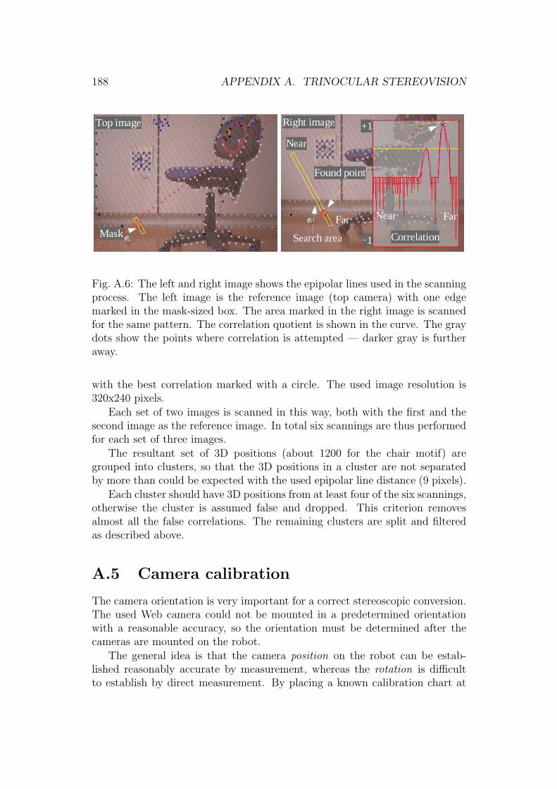
188 APPENDIX A. TRINOCULAR STEREOVISION
Mask
Top image
Search area
Near
Far
Correlation
Near Far
+1
−1
Found point
Right image
Fig. A.6: The left and right image shows the epipolar lines used in the scanningprocess. The left image is the reference image (top camera) with one edgemarked in the mask-sized box. The area marked in the right image is scannedfor the same pattern. The correlation quotient is shown in the curve. The graydots show the points where correlation is attempted — darker gray is furtheraway.
with the best correlation marked with a circle. The used image resolution is320x240 pixels.
Each set of two images is scanned in this way, both with the first and thesecond image as the reference image. In total six scannings are thus performedfor each set of three images.
The resultant set of 3D positions (about 1200 for the chair motif) aregrouped into clusters, so that the 3D positions in a cluster are not separatedby more than could be expected with the used epipolar line distance (9 pixels).
Each cluster should have 3D positions from at least four of the six scannings,otherwise the cluster is assumed false and dropped. This criterion removesalmost all the false correlations. The remaining clusters are split and filteredas described above.
A.5 Camera calibration
The camera orientation is very important for a correct stereoscopic conversion.The used Web camera could not be mounted in a predetermined orientationwith a reasonable accuracy, so the orientation must be determined after thecameras are mounted on the robot.
The general idea is that the camera position on the robot can be estab-lished reasonably accurate by measurement, whereas the rotation is difficultto establish by direct measurement. By placing a known calibration chart at

A.6. RESULTS 189
some distance directly in front of the robot at a known height, it is possible tocalculate a sufficient exact rotation around all three axes for each camera onthe camera mount.
The calibration chart consists of a number of black squares on a white back-ground, arranged as a checkerboard as shown behind the robot in Figure A.5.The corner where two black squares touch is scale invariant and easily detected.Two of the black squares in the calibration chart are omitted and the positionof these are used to determine the center of the calibration chart and from thatthe pixel position of all corners.
The pixel position Xp [xp, yp] corresponding to each corner position Xc
[xc, yc, 0] on the flat calibration chart can be calculated as a function of chart po-sition relative to the camera [xt, yt, zt] and the camera rotation [Ω, Φ, κ] aroundthe three axis. The pixel position Xp and the corresponding point Xc on thecalibration chart are known for up to 100 positions. The camera position androtation form this equation is then estimated using a least-square parameteradjustment method.
This method can determine the orientation of the cameras to about 0.01
for both the left-right orientation Φ and the up-down orientation Ω, and toabout 0.03 for the rotation κ around the camera optical axis.
When using identical cameras with USB interfaces there is no guaranteethat the cameras will be detected in the same order as last time they wereplugged into the robot. The calibration method described can estimate thecamera position to within 1–2 cm, which is sufficiently accurate to determinewhich camera device is at top, left and right position.
The used camera (Philips PCVC 740K) has a focus length of about 1055 pix-els with an image resolution of 640x480 pixels. The radial distortion is esti-mated to about 1.4 ·10−7 proportional to r3 and 8.5 ·10−13 proportional with r5,where r is radius from image center in pixels. These internal camera parametersare estimated off-line using a series of images of the calibration chart.
One image pixel corresponds to an angle of about 0.1 at a 320x240 resolu-tion (The camera opening horizontally is 33.5). A one-pixel error correspondsto about a 10 cm range error at 2 meter distance from the camera with theused camera configuration. Practical results shows an about 5 cm (standarddeviation) distance error from the stereo calculation using a 320x240 imageresolution.
A.6 Results
The processing time from image capture to extracted features is shown in Ta-ble A.1 for the three available camera resolutions.
The long capture time for 640x480 resolution is due to an interface limita-

190 APPENDIX A. TRINOCULAR STEREOVISION
Top image
Fig. A.7: The same chair and golf ball as in Figure A.3, but with more complexbackground. The chair and ball is still extracted. Center image is top viewand right image is side view.
Right Image
1 m−1 m
1 m 2 m 3 m
Toy jeep
Roundtable
Closets 1 m 2 m 3 m
Floor level
Table
Toy jeep1 m
2 m
Fig. A.8: The same method now used on a toy jeep and a round table. Theobjects are extracted to a level where the table should be recognizable as atable.
160x120 320x240 640x480Image delay 0.24 0.24 0.24 secImage capture 0.01 0.06 5.8 secEpipolar dist. 6 9 12 pixStereo scan. 0.53 1.71 4.35 sec3D detections 487 744 1145Feature filt. 0.15 0.11 0.29 secFeatures 19 21 26Total time 0.94 2.03 10.68 sec
Table A.1: Vision sensor timing.
tion, where cameras have to be closed between images. All timings are from a700 MHz PC and for a slightly simpler scene than in Figure A.3.
The main processing time is used for the stereoscopic scanning as would beexpected. At the 160x120 resolution, the epipolar distance is six pixels, and asthe scanning mask is three pixels wide there is an almost full usage of all pixels

A.7. CONCLUSION 191
in the image. The result is available after about one second. The 320x240resolution produces slightly better data, but takes 2 seconds to complete.
In most scenes, the sensor produce from 15 to 40 clusters, where each clusterrepresents a visible feature from one of the objects in the scene.
The delay in camera and interface limits the accuracy of image time stamp-ing, and thereby the accuracy of the position and orientation of the camera,especially if the images was taken during a maneuver. This, in turn, limits theaccuracy of the stereo extraction.
The method is rather insensitive to background structure, as can be seenin Figure A.7, where the closed doors have been opened. The method extractsreadily more complex shaped objects as the toy Jeep in Figure A.8.
Isolation of features from reasonably sized objects — e.g. the table and thechair — seems adequate for a reasonably safe classification. The 3D extensionof objects may be used to get further data from the source images, e.g. addi-tional color or texture information, which can be used to further distinguishobjects and object classes. The additional color and texture extraction is notimplemented yet; neither is the object classification.
A.7 Conclusion
The vision sensor described in this paper combines stereo vision methods usedin e.g. land mapping from aerial photographs, and 3D filtering methods thatin total ensures a robust extraction of all — reasonably sized — objects withinsight of the robot. The processing time for the purposed method is not pro-hibitive, and will be even less so in the future.
The extracted objects seem to be adequate for classification of objects inclasses like chairs, tables, walls and doors.
The process is designed for an in-door environment, but should also beapplicable for out-door use, as there is no dependence on the shape of the seenfeatures.
A.7.1 Next step
The next step is expected to be grouping of detected clusters to isolate non-transparent surfaces, e.g. walls, chair and table surfaces. The image color andtexture of these surfaces can then be determined within the surface, to enhancethe correlation and classification process.

192 APPENDIX A. TRINOCULAR STEREOVISION

Appendix B
Navigation script definition
B.1 Introduction
This is a (syntax) description of the implemented control language of the nav-igation sequencer.
The functionality is controlled by a sequence of statements as defined below:
statements ::= statement [← statement]*
statement ::= (assignment statement | execute statement |function definition | flow control | label | watch call | print | remark |preprocessor statement)
← ::= ’\n’ (newline)
assignment statement ::= variable name ’=’ expression
expression ::= value [ operator value]
value ::= (expression | ’(’expression’)’ | numeric constant | variable value |function)
operator ::= (’+’ | ’-’ | ’*’ | ’/’ | ’>’ | ’<’ | ’==’ | ’!=’ | ’>=’ | ’<=’ | ’&’ | ’|’ |’and’ | ’or’ | ’not’ | ’&&’ | ’||’ | ’<<’ | ’>>’)
variable value ::= [unary operator] variable name
unary operator ::= (’not’ | ’!’ | ’-’ | ’+’)
variable name ::= alpha [(alphanum | ’ ’)]* maximum length 32 characters
function ::= function name ’(’ function params ’)’
193
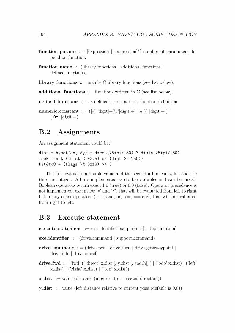
194 APPENDIX B. NAVIGATION SCRIPT DEFINITION
function params ::= [expression [, expression]*] number of parameters de-pend on function.
function name ::=(library functions | additional functions |defined functions)
library functions ::= mainly C library functions (see list below).
additional functions ::= functions written in C (see list below).
defined functions ::= as defined in script ? see function definition
numeric constant ::= ([-] [digit]+[’.’[digit]+] [’e’[-] [digit]+]) |(’0x’ [digit]+)
B.2 Assignments
An assignment statement could be:
dist = hypot(dx, dy) + d*cos(25*pi/180) ? d*sin(25*pi/180)
isok = not ((dist < -2.5) or (dist >= 250))
bit4to8 = (flags \& 0xf8) >> 3
The first evaluates a double value and the second a boolean value and thethird an integer. All are implemented as double variables and can be mixed.Boolean operators return exact 1.0 (true) or 0.0 (false). Operator precedence isnot implemented, except for ’*’ and ’/’, that will be evaluated from left to rightbefore any other operators (+, -, and, or, >=, == etc), that will be evaluatedfrom right to left.
B.3 Execute statement
execute statement ::= exe identifier exe params [: stopcondition]
exe identifier ::= (drive command | support command)
drive command ::= (drive fwd | drive turn | drive gotowaypoint |drive idle | drive smrcl)
drive fwd ::= ’fwd’ ((’direct’ x dist [, y dist [, end h]] ) | (’odo’ x dist) | (’left’x dist) | (’right’ x dist) | (’top’ x dist))
x dist ::= value (distance (in current or selected direction))
y dist ::= value (left distance relative to current pose (default is 0.0))

B.3. EXECUTE STATEMENT 195
end h ::= value (end pose heading (default is 0.0))
drive turn ::= ’turn’ angle (angle (value) to turn ? same as ’smrcl turn angle’)
drive gotowaypoint ::= ’gotowaypoint’ x pos y pos
x pos ::= value (x coordinate in selected coordinate system).
y pos ::= value (y coordinate in selected coordinate system).
drive idle ::= ’idle’ idle time (idle time (value) is a value in seconds)
drive smrcl ::= ’smrcl’ smrcl command
smrcl command ::= (as defined for smrdemo, implicit stop criteria is whensmrdemo reports command completed).
support command ::= (vision | arm | talk | listen | ...) (vision is implementedonly)
exe params ::= depend on exe identifier.
stopcondition ::= (boolean) expression. (execution continues to next line,when expression is true).
B.3.1 Drive command FWD
The fwd orders the robot to drive forward in one of four methods: left, right,top or direct, e.g.:
fwd left 20
Follow left side of road (in wpfEdgeDist distance) for 20 m.
fwd right 30
Follow right side of road (in wpfEdgeDist distance) for 30 m.
fwd top 50
Follow top (centre) of road for 50 m. The variable wpfTopDist determinesthe position of the robot relative to the centre line.If wpfTopDist > 0.0, then drive this distance to the left of the centreline. If wpfTopDist is negative, then to the right.
fwd direct 3.5, -1, 1.57
Drive to the relative position 3.5 m in front of robot, 1 m to the right,and stop in a posture 1.57 (90 deg) counter clockwise relative to currentheading. NB! Use comma separated parameters if space separated valuescould be evaluated (ie ’3 -1’ is 2 and one parameter only, but ’3, -1’ istwo parameters). Y and H parameters may be omitted, default is 0.0.
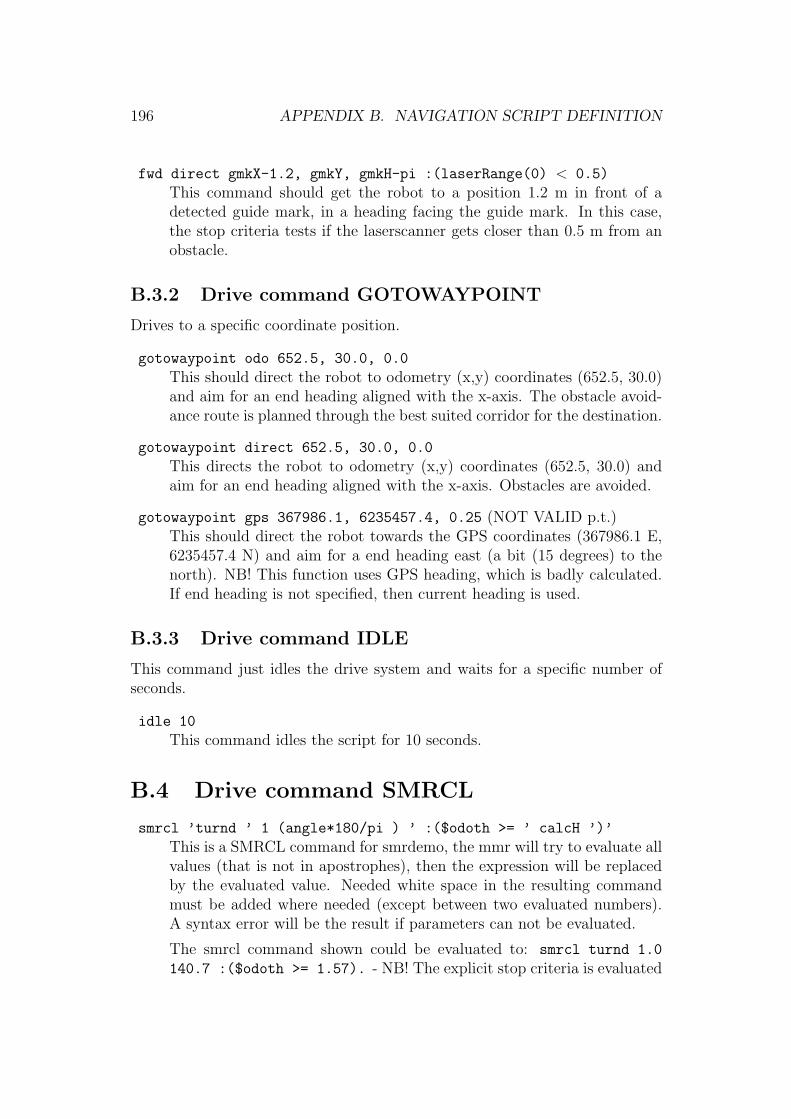
196 APPENDIX B. NAVIGATION SCRIPT DEFINITION
fwd direct gmkX-1.2, gmkY, gmkH-pi :(laserRange(0) < 0.5)
This command should get the robot to a position 1.2 m in front of adetected guide mark, in a heading facing the guide mark. In this case,the stop criteria tests if the laserscanner gets closer than 0.5 m from anobstacle.
B.3.2 Drive command GOTOWAYPOINT
Drives to a specific coordinate position.
gotowaypoint odo 652.5, 30.0, 0.0
This should direct the robot to odometry (x,y) coordinates (652.5, 30.0)and aim for an end heading aligned with the x-axis. The obstacle avoid-ance route is planned through the best suited corridor for the destination.
gotowaypoint direct 652.5, 30.0, 0.0
This directs the robot to odometry (x,y) coordinates (652.5, 30.0) andaim for an end heading aligned with the x-axis. Obstacles are avoided.
gotowaypoint gps 367986.1, 6235457.4, 0.25 (NOT VALID p.t.)This should direct the robot towards the GPS coordinates (367986.1 E,6235457.4 N) and aim for a end heading east (a bit (15 degrees) to thenorth). NB! This function uses GPS heading, which is badly calculated.If end heading is not specified, then current heading is used.
B.3.3 Drive command IDLE
This command just idles the drive system and waits for a specific number ofseconds.
idle 10
This command idles the script for 10 seconds.
B.4 Drive command SMRCL
smrcl ’turnd ’ 1 (angle*180/pi ) ’ :($odoth >= ’ calcH ’)’
This is a SMRCL command for smrdemo, the mmr will try to evaluate allvalues (that is not in apostrophes), then the expression will be replacedby the evaluated value. Needed white space in the resulting commandmust be added where needed (except between two evaluated numbers).A syntax error will be the result if parameters can not be evaluated.
The smrcl command shown could be evaluated to: smrcl turnd 1.0
140.7 :($odoth >= 1.57). - NB! The explicit stop criteria is evaluated

B.5. FUNCTION DEFINITION 197
by smrdemo and not by the mmr, so - the values (here $odoth) must beknown by smrdemo.
B.5 Function definition
function definition ::= ’function’ function identifier ’(’ function params ’)’[statements] ’return’ [expression]
function identifier ::= variable name
label ::= label identifier ’:’
label identifier ::= variable name
function params ::= [variable name [ ’,’ variable name]* ]
B.6 Flow control
flow control ::= (if expr | goto expr | call expr | skip drive)
goto expr ::= ’goto’ label identifier
call expr ::= [’call’] defined function
defined function ::= function identifier ’(’ [expression [’,’ expression]*] ’)’if expr ::= ’if’ ’(’ (boolean) expression ’)’ then expr
then expr ::= flow control | assignment statement
Flow control statements could be:
if (not defined(doorNum)) doorNum = 0
if (doorNum < 7) goto end\_label
call waitAWhile(10)
An if statement has one conditional statement only, so a ’goto’ or ’call’construction must be used if more statements are to be conditional.

198 APPENDIX B. NAVIGATION SCRIPT DEFINITION
B.7 Skip statement
A skip statement is an extended stop-condition for an executable statement.Skip statements can therefore only be used in watch-functions. It will interruptthe main program flow, as either a jump or a function call. The watch functionflow continues unaffected.
skip drive ::= (skip to label | skip function call)
skip to label ::= ’skip’ [label identifier] (if no label, then skip to next line)
skip to function ::= ’skipcall’ defined function
In a watch function a skip line could be:if (doorNum > 25) skip to end
watch call ::= ’watch’ watch name [’every’ value] (call expr |assignment statement | print) ’unwatch’ watch name
Watch statements starts evaluation of a watch function (or statement)at regular intervals (as defined by the ’every’ art) or at sample rate (p.t.3Hz), until an ’unwatch’ statement is executed. Examples could be:watch max speed maxSpeed = max(speed, maxSpeed)
watch look4door()
The first executes an assignment statement at every sample time, thesecond calls a ’look4door()’ function, and uses the short form, wherethe watch name is the same as the function call.
print ::=’print’ [print text | expression]+
print text ::= ’’’ text ’’’ | ’"’ text ’"’
Print statements are simple statements, that sends a string and a valueto the client. The expression evaluates to a double. An example couldbe:print ’Found door number ’ doorNum ’ but expected ’ doorCnt
print ’Finished’
this text and the evaluated values will be send to all connected clients asan XML tag, eg:<help info="Found door number 6 but expected 5"/>\n>.
B.8 Remarks
Remark ::= (’%’ | ’//’ | ’;’) [any non control character]*
The rest of the line is disregarded in the statement evaluation.
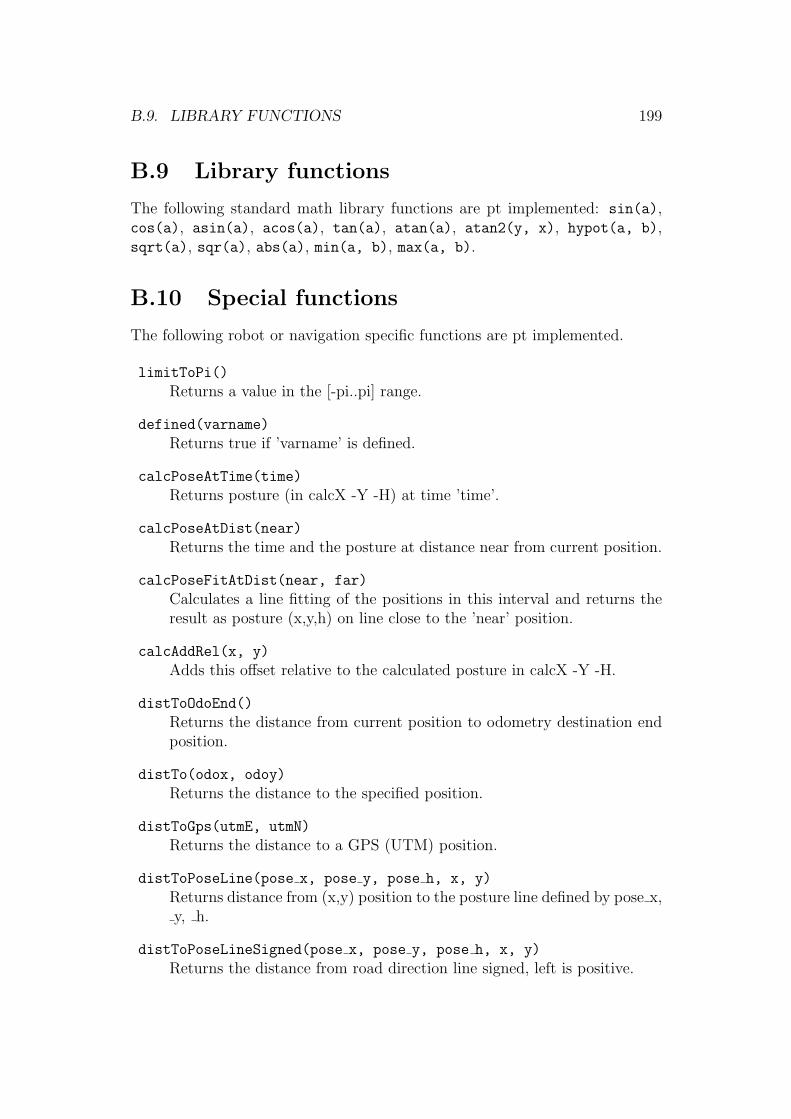
B.9. LIBRARY FUNCTIONS 199
B.9 Library functions
The following standard math library functions are pt implemented: sin(a),cos(a), asin(a), acos(a), tan(a), atan(a), atan2(y, x), hypot(a, b),sqrt(a), sqr(a), abs(a), min(a, b), max(a, b).
B.10 Special functions
The following robot or navigation specific functions are pt implemented.
limitToPi()
Returns a value in the [-pi..pi] range.
defined(varname)
Returns true if ’varname’ is defined.
calcPoseAtTime(time)
Returns posture (in calcX -Y -H) at time ’time’.
calcPoseAtDist(near)
Returns the time and the posture at distance near from current position.
calcPoseFitAtDist(near, far)
Calculates a line fitting of the positions in this interval and returns theresult as posture (x,y,h) on line close to the ’near’ position.
calcAddRel(x, y)
Adds this offset relative to the calculated posture in calcX -Y -H.
distToOdoEnd()
Returns the distance from current position to odometry destination endposition.
distTo(odox, odoy)
Returns the distance to the specified position.
distToGps(utmE, utmN)
Returns the distance to a GPS (UTM) position.
distToPoseLine(pose x, pose y, pose h, x, y)
Returns distance from (x,y) position to the posture line defined by pose x,y, h.
distToPoseLineSigned(pose x, pose y, pose h, x, y)
Returns the distance from road direction line signed, left is positive.
200 APPENDIX B. NAVIGATION SCRIPT DEFINITION
headingGps(dist)
Returns current heading ’u’ (radians) based on odometry and GPS(UTM)position now and at ’dist’ back from current position. (East is zero CCV,to get compas radians use: (pi/2 - u).
laserRange(angle)
Returns laser range measurement closest to this angle (angle 0.0 deg isfont).
B.10.1 Guidemark functions
Guidemark functions work on data returned by camera server following a’gmkget’ command to the camera server, e.g. by statement: ’vision gmkget
extra=true’.
The functions are:
gmkCnt() returns count of guidemark positions available.
gmkNewCnt(t) returns number of stored guidemarks since ’t’. The ’time’ isstored and is used by the ’gmkNewNum(N)’ call.
gmkNewNum(t, N) returns index to guidemark N of the new guidemarks
gmkNum(idx) returns true if guidemark with index idx is found, and setsthe guidemark values (from ’cam getgmk’) in variables: gmkX, gmkY,gmkZ, x, y and z position gmkO, gmkP, gmkK, rotation on x,y and zaxis gmkTime, gmkID detection time and guidemark ID code.
gmkNewID(t, ID) returns true if a guide mark newer than t is available withthis ID, the guidemark values are set as for the ’gmkNum(idx)’ call.
gmkID(ID) returns true if a guide mark is stored with this ID, and the guide-mark values are set as for the ’gmkNum(idx)’ call.
B.11 System defined variables
The following variables are available in the system. The values shown aremostly just examples. The values can be queried or changed from a script orfrom a client.
The values are formatted under the following headings:(index) value ’variable name’ remark.

B.11. SYSTEM DEFINED VARIABLES 201
Constants
#000 0.0000 ’false’.#001 1.0000 ’true’
#002 3.1416 ’pi’.
Road data
#003 0.0000 ’roadValid’ is road (width) data valid.#004 0.7812 ’roadWidth’ estimated road width [m].#005 0.0000 ’roadQual’ road width quality [0..1].#006 1.0000 ’roadTypeLaser’ estimated road type.#007 0.0044 ’roadRoughness’ current road roughness.#008 0.0000 ’roadLeftValid’ left side of road valid.#009 100.0000 ’roadLeftDist’ from robot to left side [m].#010 0.0000 ’roadLeftQual’ road side quality [0..1].#011 0.0000 ’roadRightValid’ right side of road valid.#012 100.0000 ’roadRightDist’ from robot to right side [m].#013 0.0000 ’roadRightQual’ road side quality [0..1].#014 0.0000 ’roadTopValid’ top of road valid.#015 100.0000 ’roadTopDist’ to top-line from robot left is pos.#016 0.0000 ’roadTopQual’ road top quality [0..1].#017 2.3416 ’roadCenterX’ road centre (top) odometry X [m].#018 -0.7940 ’roadCenterY’ road centre (top) odometry Y [m].#019 0.0863 ’roadCenterZ’ road centre (top) odometry Z [m].
Current pose
#020 0.0000 ’posex’ odometry pose X [m].#021 0.0000 ’posey’ odometry pose Y [m].#022 0.0000 ’poseh’ odometry pose Z [m].#023 0.0000 ’odoSpeed’ current robot velocity [m/s].#024 1141403388.6506 ’time’ odometry pose update time [sec].#025 0.0000 ’distOdo’ total odometry based distance driven.
GPS position (in UTM for current zone)
#026 0.0000 ’ekfE’ Easting.#027 0.0000 ’ekfN’ Northing.#028 0.0000 ’ekfh’ Heading, p.t. not reliable (East = 0.0, rad).#029 1141403388.6506 ’ekftime’ latest GPS update time [sec].
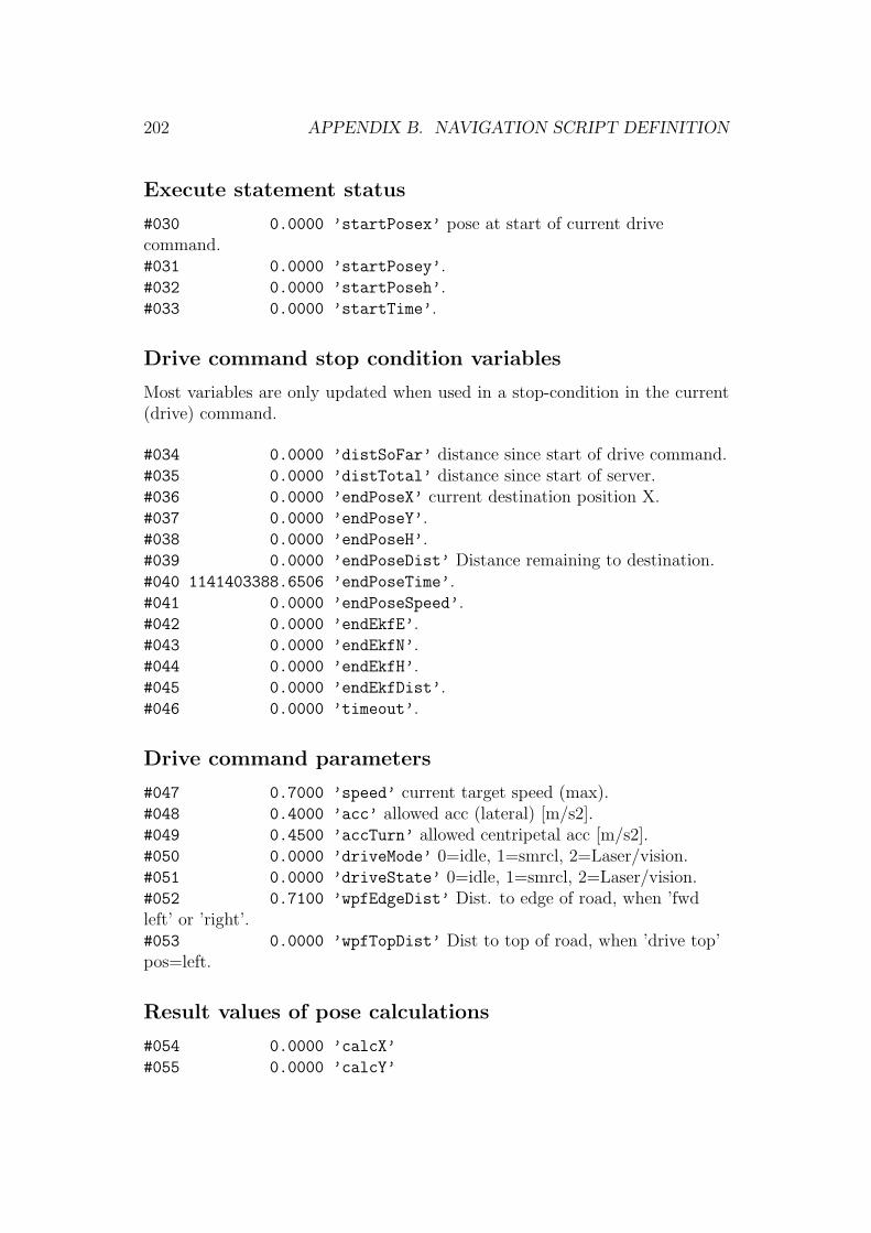
202 APPENDIX B. NAVIGATION SCRIPT DEFINITION
Execute statement status
#030 0.0000 ’startPosex’ pose at start of current drivecommand.#031 0.0000 ’startPosey’.#032 0.0000 ’startPoseh’.#033 0.0000 ’startTime’.
Drive command stop condition variables
Most variables are only updated when used in a stop-condition in the current(drive) command.
#034 0.0000 ’distSoFar’ distance since start of drive command.#035 0.0000 ’distTotal’ distance since start of server.#036 0.0000 ’endPoseX’ current destination position X.#037 0.0000 ’endPoseY’.#038 0.0000 ’endPoseH’.#039 0.0000 ’endPoseDist’ Distance remaining to destination.#040 1141403388.6506 ’endPoseTime’.#041 0.0000 ’endPoseSpeed’.#042 0.0000 ’endEkfE’.#043 0.0000 ’endEkfN’.#044 0.0000 ’endEkfH’.#045 0.0000 ’endEkfDist’.#046 0.0000 ’timeout’.
Drive command parameters
#047 0.7000 ’speed’ current target speed (max).#048 0.4000 ’acc’ allowed acc (lateral) [m/s2].#049 0.4500 ’accTurn’ allowed centripetal acc [m/s2].#050 0.0000 ’driveMode’ 0=idle, 1=smrcl, 2=Laser/vision.#051 0.0000 ’driveState’ 0=idle, 1=smrcl, 2=Laser/vision.#052 0.7100 ’wpfEdgeDist’ Dist. to edge of road, when ’fwdleft’ or ’right’.#053 0.0000 ’wpfTopDist’ Dist to top of road, when ’drive top’pos=left.
Result values of pose calculations
#054 0.0000 ’calcX’
#055 0.0000 ’calcY’

B.11. SYSTEM DEFINED VARIABLES 203
#056 0.0000 ’calcH’
Historic heading
Historic heading based on the last 5 m, excluding the last 1m.
#057 0.0000 ’histH’ [radians]#058 3600.0000 ’histHAge’ age of estimate (3600 is invalid) [sec]#059 1.0000 ’histW’ Weight of hist heading, when selection bestroute
Used angle of laser scanner relative to horizontal
#060 -0.1683 ’laserTilt’ positive is UP [radians]
Parameters for laser scanner based road detection
These variables are mostly for debugging and parameter experiments.
#061 0.1000 ’wpfDevLimit’
#062 0.0075 ’wpfConvex’
#063 0.0250 ’wpfDevOffset’
#064 4.5000 ’wpfEndDev’
#065 1.0000 ’wpfSmooth’
#066 1.0000 ’wpfSmoothAuto’ uses roadTypeLaser#067 0.0000 ’wpfMode’
#068 0.0000 ’wpfIgnoreObstacles’ debug flag#069 1.0000 ’wpfUseIntervalCombiner’
#070 1.0000 ’wpfOutdoorObstacles’
Obstacle maintenance and use
#071 2.0000 ’obstUseCnt’ obstacle groups in obstacle avoid.#072 7.0000 ’obstGrpDist’ obstacle grouping max distance.#073 7.0000 ’obstGrpTime’ obstacle grouping max time.
Guide mark data for selected guide mark
#074 0.0000 ’gmkX’
#075 0.0000 ’gmkY’
#076 0.0000 ’gmkZ’
#077 0.0000 ’gmkO’ - rotation on x-axis (roll) positive clockwise#078 0.0000 ’gmkP’ - rotation on y-axis (pitch) down is positive

204 APPENDIX B. NAVIGATION SCRIPT DEFINITION
#079 0.0000 ’gmkK’ - rotation on z-axis (yaw) left is positive, zerois front#080 0.0000 ’gmkTime’ - guide mark update time#081 0.0000 ’gmkId’ - ID code in guide mark (decimal)
Vision items
#082 1.0000 ’visPathUse’
#083 0.4300 ’visPathBal’
#084 0.6500 ’visPathLim’
#085 1.0000 ’visPathInterval’
#086 0.0000 ’visCamTiltErr’
#087 0.0030 ’visCamTiltGain’
Simulation
Simulation flag and time, used during replay of logdata.#088 0.0000 ’simulated’
#089 1141403388.6689 ’simTime’
B.12 Examples
B.12.1 A 4m square
A 4m square script.
// function for one leg ? drive to position and turn
function drive\_and\_turn(x, y, ang)
gotowaypoint odo, x, y
smrcl turn ang
return
//
// drive on odometry (not gyro) (optional)
odo = 0
gyro = 1
smrcl ’set odocontrol’ odo
// set drive speed to be used
speed = 0.6
// set angle and distance variables
angle = 90
d = 4
if (angle < 0) y = -d

B.12. EXAMPLES 205
drive\_and\_turn(d, 0, angle)
drive\_and\_turn(d, d, angle)
drive\_and\_turn(0, d, angle)
drive\_and\_turn(0, 0, angle)
// stop
smrcl idle
B.12.2 Up and down the hallway
A script that follows the walls up and down a corridor.
// follow left wall and stop where started
speed = 0.5
// drive distance
dist = 25
fwd left dist
// turn right to avoid wall
smrcl turn -175
// go back
fwd right dist
smrcl turn 179
// stop
smrcl idle
B.12.3 Up and down the hallway with stops
The same as the previous script, but extended to check for open doors andmakes a pause at every open door to the right
//# use watch function to look for doors
//# use gyro for heading
smrcl ’set "odocontrol" 1’
smrcl ’set "$gyro1off" 0.32’
speed=1
door = true
doorNow = false
function look_for_door(direc)
ld = laserRange(direc)
doorNow = (ld > 2.5)
if (not door and doorNow and (distSoFar > 1))
skipcall doWait(5)
if (door != doorNow) print "laser distance " ld
door = doorNow

206 APPENDIX B. NAVIGATION SCRIPT DEFINITION
# print "At open door number " door
return door
//#
function doWait(waitTime)
dd = dd + distSoFar
print "Dist so far is now " dd " m"
smrcl ’fwd ’ 0.3 ’ @a 0.3’
smrcl ’idle’
idle waitTime
return
//#
//# make variables for left and right direction
left = 90
right = -90
//# start watch for doors to the right
watch doors look_for_door(right)
//#
//# start drive
dist = 25
dd = 0
fwd left dist :((dd + distSoFar) > dist)
//# stop watch before turning
unwatch doors
//# turn right to avoid wall
smrcl ’turn -175’
//# go back
dd = 0
watch doors look_for_door(left)
fwd right dist :((dd + distSoFar) > dist)
unwatch doors
smrcl ’turn 179’
//# stop
smrcl ’idle’

B.12. EXAMPLES 207
B.12.4 Test area navigation script
//# Dyrehaven full route
//# run on gyro (1), (odo is 0)
smrcl ’set "odocontrol" 1’
//# gyro offset 0.445 19 aug, 0.32 24 aug,
//# 0.19 12 sep, 0.25 17 okt 2005
smrcl ’set "$gyro1off" 0.25’
//#
//# shortcut jump if about 50 m before 5-vej
// goto lbl5Vej
// goto bagslot
///////////////// Hjortekaervej /////////////////////////
//# get going from anywhere on hjortekaervej - if GPS works
acc = 0.4
accturn=0.9
vispathlim=0.65
vispathbal=0.43
vispathuse=true
//# start slow
wpfedgedist = 0.85
speed = 0.7
fwd left 5
//# high speed to just before castle (should be ~1660 m)
//# stop ~20m before end of road
print "To cruse speed"
speed = 1.4
dist = 1740
fwd left dist :(25 > distToGps(347716.7, 6183490.1))
//
/////////// Royal hunting lodge square ////////////////
print "Close to Royal hunting lodge"
//# change to gyro heading for crossing
// of gravelled square (and rest of the way)
smrcl ’set "odocontrol" 1’
//# reduce speed - close to open area
speed = 0.9
//# calculate direction of hjortekrvej
calcPoseFitAtDist(0, 25)
//# add to a waypoint inside castle square
speed = 0.85
//# follow left side into square -

208 APPENDIX B. NAVIGATION SCRIPT DEFINITION
//# until fair distance to hjortekrvej line
fwd left 75 :(7.0 < abs(distToPoseLineSigned(
poseX, poseY, calcX, calcY, calcH)))
//# get better reference close to end of hjrtekrvej
calcPoseFitAtDist(12, 25)
//# add to a point far away in Ndr. Eremitagevej direction
//# - relative to hjortekrvej ref point (GPS-based)
calcAddRel(75.0, 150.0)
//# go towards that point - first just avoid obstacles
//# gotowaypoint odo calcx calcy :(distsofar > 10)
//# then look for road edge
gotowaypoint odo calcx calcy :((roadLeftQual > 0.78) and
(roadLeftDist < 2.7) and (distsofar > 10))
//
///////////////// Behind lodge ///////////////////////////
//# assume left edge is found - continue close to left edge
wpfEdgeDist = 0.85
fwd left 40
//# now we are on asphalt, so get closer to edge and speed up
wpfEdgeDist = 0.65
speed = 1.3
bagslot:
//# continue until just before end of asphalt
fwd left 290 :(30 > distToGps(348053.0, 6183676.0))
print "close to end of asphalt - going top step 1 (for 5m)"
//# switch to top of road (in 2 steps to be smooth)
td = roadTopDist / 2
wpfTopDist = td
fwd top 5
print "close to end of asphalt - going top step 2 (280m)"
//# drive on road centerline - until (25) before junction
lbl5Vej:
wpfTopDist = 0
speed = 1.0
fwd top 280 :(25 > distToGps(348223.0, 6183901.0))
//
///////////////////// 5 vej /////////////////////////////
//# reduce speed
speed = 0.8
calcPoseFitAtDist(0, 20);
//# Follow road to the left, up Chausseen (north)
wpfEdgeDist = 1.1
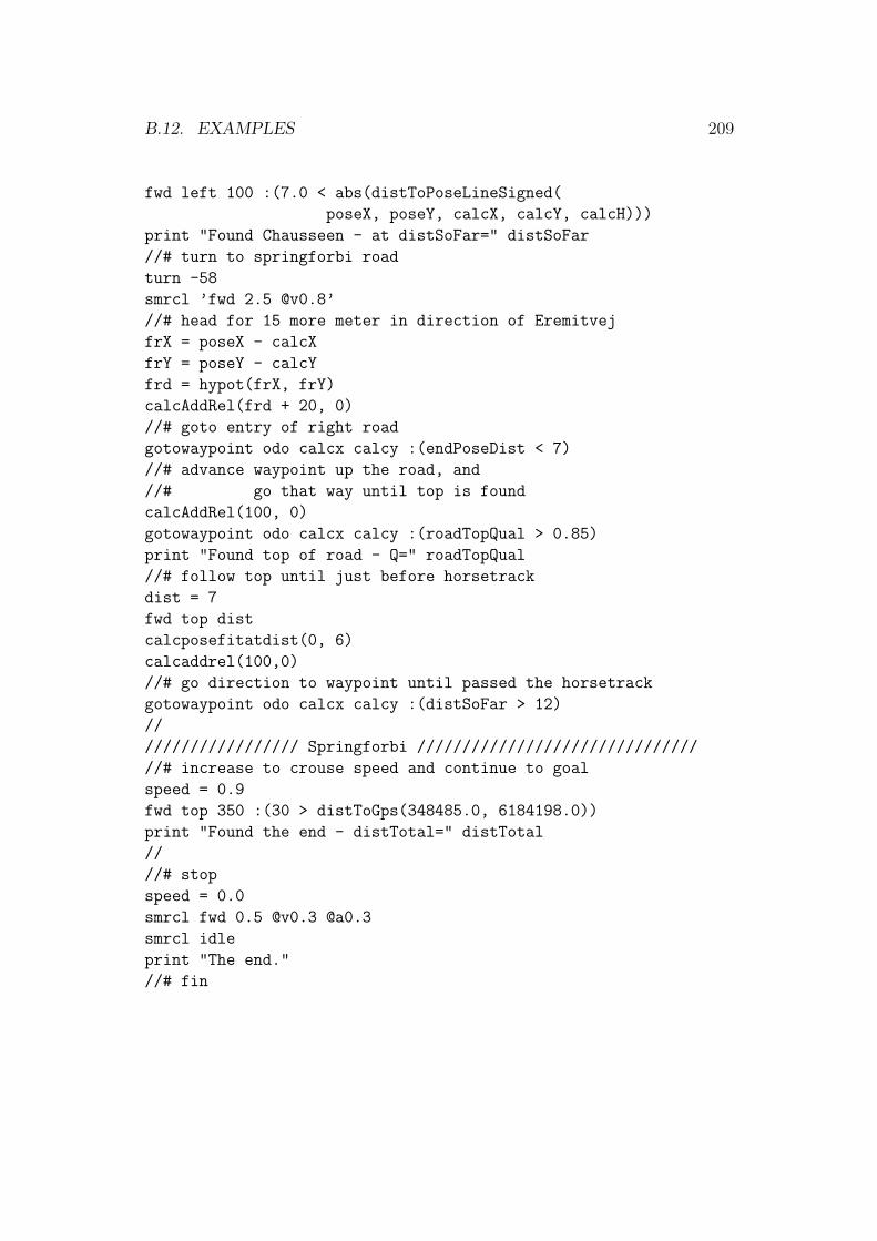
B.12. EXAMPLES 209
fwd left 100 :(7.0 < abs(distToPoseLineSigned(
poseX, poseY, calcX, calcY, calcH)))
print "Found Chausseen - at distSoFar=" distSoFar
//# turn to springforbi road
turn -58
smrcl ’fwd 2.5 @v0.8’
//# head for 15 more meter in direction of Eremitvej
frX = poseX - calcX
frY = poseY - calcY
frd = hypot(frX, frY)
calcAddRel(frd + 20, 0)
//# goto entry of right road
gotowaypoint odo calcx calcy :(endPoseDist < 7)
//# advance waypoint up the road, and
//# go that way until top is found
calcAddRel(100, 0)
gotowaypoint odo calcx calcy :(roadTopQual > 0.85)
print "Found top of road - Q=" roadTopQual
//# follow top until just before horsetrack
dist = 7
fwd top dist
calcposefitatdist(0, 6)
calcaddrel(100,0)
//# go direction to waypoint until passed the horsetrack
gotowaypoint odo calcx calcy :(distSoFar > 12)
//
///////////////// Springforbi ///////////////////////////////
//# increase to crouse speed and continue to goal
speed = 0.9
fwd top 350 :(30 > distToGps(348485.0, 6184198.0))
print "Found the end - distTotal=" distTotal
//
//# stop
speed = 0.0
smrcl fwd 0.5 @v0.3 @a0.3
smrcl idle
print "The end."
//# fin

210 APPENDIX B. NAVIGATION SCRIPT DEFINITION

.

www.oersted.dtu.dk
Ørsted•DTUAutomationTechnical University of DenmarkBuilding 348DK-2800 Kgs. LyngbyDenmarkTel: (+45) 45 25 38 00Fax: (+45) 45 93 16 34E-mail: [email protected]
ISBN 87-91184-64-9