ISSN 1392-2114 ULTRAGARSAS, Nr.4(61). 2006

Investigation of time-reversal approach for detection and characterization of ultrasonic defects in dispersive plates

G. Butėnas, R. Kažys

Prof. K. Baršauskas Ultrasound Institute, Kaunas University of Technology Studentų str. 50, Kaunas, Lithuania, tel. (+370 699 23373) E-mail: gintas_butenas@yahoo.com Abstract

In this paper we investigated the application of time-reversal method for inspecting of defects in plates where Lamb waves suffer dispersion. Theoretical implementation of the time reversal method was carried out by the commercially available finite element analysis software Abaqus Explicit™. It has been demonstrated that the input wave form sent by a transmitting transducer was reconstructed. In the plate with a defect the reconstructed signal differs from the input signal in shape. That difference correlates with geometrical parameters of the defect. Key words: Time reversal mirrors, time reversal acoustics, defect estimation and Lamb waves. Introduction

The guided waves, such as Lamb waves, are widespread tool in non-destructive testing and inspecting of layered plates. The analysis and interpretation of measurement results can be complicated due dispersive and multimodal properties of those waves. These effects are distinct and undesirable in a long-range and high-frequency inspection [1].

In modern acoustic it has been suggested a few methods for dispersion minimization based on signal processing techniques [2] and a priori knowledge about dispersion behavior in that media where Lamb waves are propagating [1]. A different and novel approach using time reversal mirrors for dispersion elimination was presented by [3, 7, 8 and 11].

At the beginning the time reversal mirrors were introduced as a solution to selective focusing in multiple-target media [9,10] and later applied for minimization of the dispersion effects of Lamb waves in dispersive plates [11] and also in defect inspection [7,8]. In the pulse-echo time-reversal method Lamb waves are generated by an ultrasonic transducer and associated responses are recorded by an array of sensors, called a time reversal mirror [5], surrounding the plate boundary. If there is any defect along the wave propagation paths, echoes are produced by defect and recorded by the time reversal mirror. The recorded echoes are then reversed in the time domain and reemitted by the same time reversal mirror. As the reemitted signals converge on the defect location, the amplified echo signals will be produced by the defect.

In this study we investigate spatial configuration of the time reversal mirrors and applicability of the time reversal concept in order to improve the detectability of local defects in planar structures. It is also analyzed how minimal configuration of the time reversal mirror elements affects the reconstructed signal. For low-frequency and long-range wave propagation modeling we use the commercially available finite element analysis software Abaqus/Explicit™ which has a powerful multiprocessing task solver implemented in a personal computer environment.

Application of time reversal Lamb waves to detection of defect in a plate

Has been shown that cracks and delamination with low-aspect-ratio geometry are scattering sources creating elastic waves, which arise from reciprocity in the wave pressure-deformation relation [8]. Wave scattering can be also caused by either horizontal or vertical mode conversion due to which energy of the incident Lamb waves at a specified driving frequency is redistributed into neighboring Lamb wave modes, because defects change the internal geometric boundary condition in plate. Diffraction and reflection of the waves can also produce wave scattering when incident Lamb waves pass through defect.

The time reversibility of waves is fundamentally based on the linear reciprocity of the system [4]. The linear reciprocity and the time reversibility breaks down if there exist any source of wave distortion due to wave scattering along the wave path. Therefore, by comparing the differences between the original input signal and the reconstructed signal, damages such cracks, delamination and fiber breakage should be detected.

In applicable damage detection methods, crack or delamination is interfered by comparing newly obtained data sets with the main data previously measured at the initial condition of the system. Because there might be numerous variations since the principal data were collected, it would be difficult to find a structural damage for all changes in the measured signals. For instance, there may be operational and environmental variations of the system once the baseline data have been collected.

Numerical simulation of time reversal process

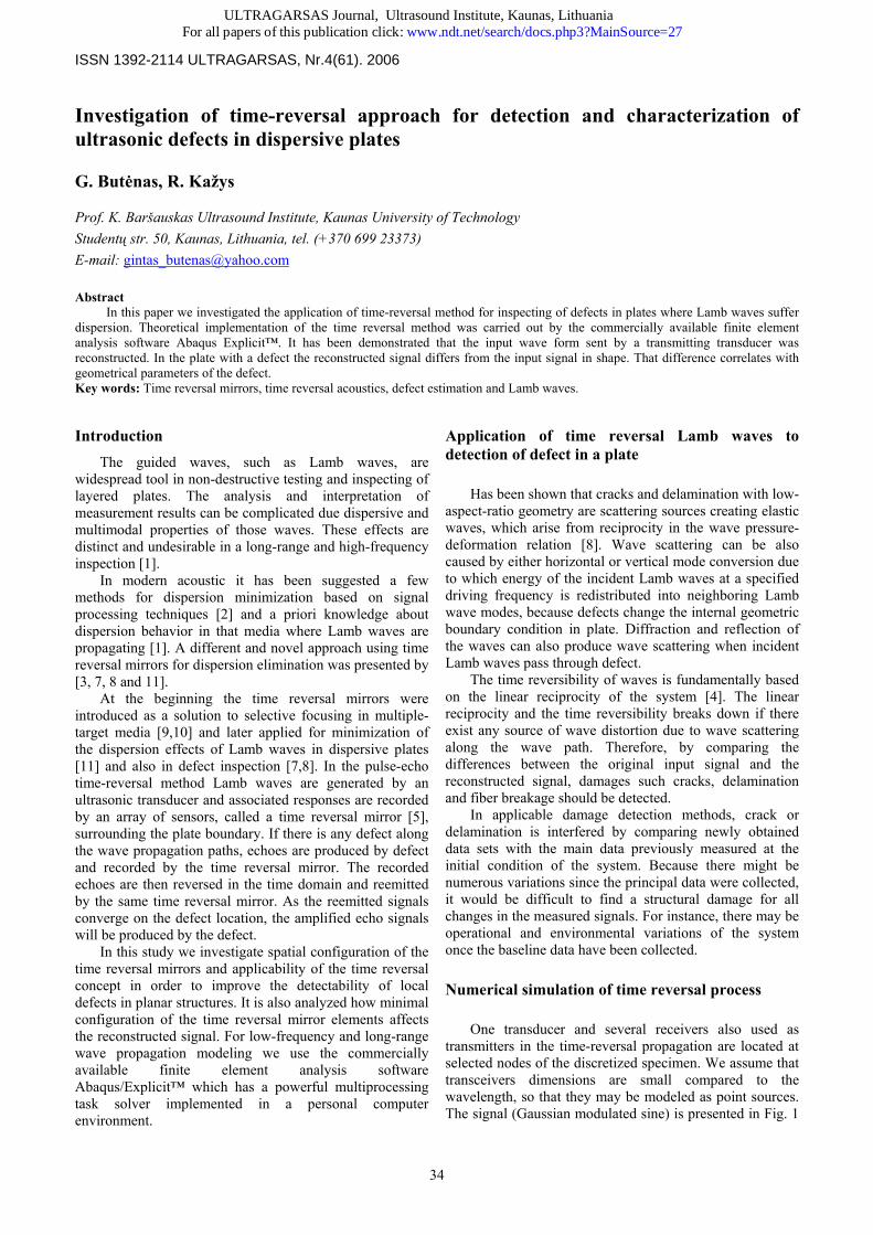
One transducer and several receivers also used as transmitters in the time-reversal propagation are located at selected nodes of the discretized specimen. We assume that transceivers dimensions are small compared to the wavelength, so that they may be modeled as point sources. The signal (Gaussian modulated sine) is presented in Fig. 1

34

ULTRAGARSAS Journal, Ultrasound Institute, Kaunas, LithuaniaFor all papers of this publication click: www.ndt.net/search/docs.php3?MainSource=27

ISSN 1392-2114 ULTRAGARSAS, Nr.4(61). 2006.

and generated in the form of an acoustic pressure at the corresponding node sets.

Fig.1. The waveform of excitation Gaussian modulated sine wave with

frequency 50 kHz

Being the temporal signal, then the signal (j = 1,… N) is received by the N receivers. The

signal in the time window ( ) is amplified, recorded in a PC memory, time-reversed and transmitted back from all receivers simultaneously. The time is reset to 0 at the end of the transmission of the time-reversed signal, which, therefore, is given by:

)(tp forv

)(tprecvj

10 ttt <<

)()( 011 tttApttp recvj

trj −+=− , , (1) 10 ttt <<

where A denotes the constant gain factor for the all receivers.

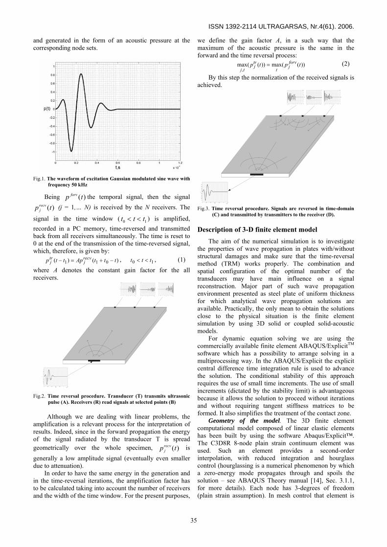
Fig.2. Time reversal procedure. Transducer (T) transmits ultrasonic pulse (A). Receivers (R) read signals at selected points (B)

Although we are dealing with linear problems, the amplification is a relevant process for the interpretation of results. Indeed, since in the forward propagation the energy of the signal radiated by the transducer T is spread geometrically over the whole specimen, is generally a low amplitude signal (eventually even smaller due to attenuation).

)(tprecvj

In order to have the same energy in the generation and in the time-reversal iterations, the amplification factor has to be calculated taking into account the number of receivers and the width of the time window. For the present purposes,

we define the gain factor A, in a such way that the maximum of the acoustic pressure is the same in the forward and the time reversal process:

(2) ))((max))((max,

tptp forvjt

trj

tj=

By this step the normalization of the received signals is achieved.

Fig.3. Time reversal procedure. Signals are reversed in time-domain

(C) and transmitted by transmitters to the receiver (D).

Description of 3-D finite element model The aim of the numerical simulation is to investigate

the properties of wave propagation in plates with/without structural damages and make sure that the time-reversal method (TRM) works properly. The combination and spatial configuration of the optimal number of the transducers may have main influence on a signal reconstruction. Major part of such wave propagation environment presented as steel plate of uniform thickness for which analytical wave propagation solutions are available. Practically, the only mean to obtain the solutions close to the physical situation is the finite element simulation by using 3D solid or coupled solid-acoustic models.

For dynamic equation solving we are using the commercially available finite element ABAQUS/ExplicitTM software which has a possibility to arrange solving in a multiprocessing way. In the ABAQUS/Explicit the explicit central difference time integration rule is used to advance the solution. The conditional stability of this approach requires the use of small time increments. The use of small increments (dictated by the stability limit) is advantageous because it allows the solution to proceed without iterations and without requiring tangent stiffness matrices to be formed. It also simplifies the treatment of the contact zone.

Geometry of the model. The 3D finite element computational model composed of linear elastic elements has been built by using the software Abaqus/Explicit™. The C3D8R 8-node plain strain continuum element was used. Such an element provides a second-order interpolation, with reduced integration and hourglass control (hourglassing is a numerical phenomenon by which a zero-energy mode propagates through and spoils the solution – see ABAQUS Theory manual [14], Sec. 3.1.1, for more details). Each node has 3-degrees of freedom (plain strain assumption). In mesh control that element is

35

ISSN 1392-2114 ULTRAGARSAS, Nr.4(61). 2006

The stresses caused by the piezoelectric effect can be conveniently presented as:

used when average strain is calculated, without second-order accuracy and distortion control. The purpose of the element is to achieve a faster computation procedure. This is implemented by imposing strict limitations on the range of applicability, thereby simplifying the calculation:

J iK KJ i iJ iT d c E e E= = , (4)

where - the piezoelectric coefficient, iJe iJ iK KJe d c= ,

KJc - the stiffness tensor determined under a constant value of the electric field.

• Elements must be cuboids; all edges parallel to the global x, y , z axes;

• Small displacement, small strain and negligible rigid body rotation; Material model. The whole assembly is assumed to be

a homogeneous elastic steel structure and is modeled using the following parameters: • Elastic material only.

With the C3D8R element the performance of the model is similar to the fully integrated solid; however the performance is even better than of a traditional constant strain element. Single element bending and torsion modes are included, so meshing guidelines are as for fully integrated solids – e.g., thin structures can be modeled with a single solid element through the thickness if required.

Density: ρ = 7800 kg/m3; Young modulus: E = 205,33 GPa; Poisson’s ratio: P = 0,29.

Forcing law. In a reality the ultrasonic wave is excited by means of a piezoelectric transducer (PT). Because of the inverse piezoelectric effect phenomenon the PT deforms under the influence of the applied external electric field. The simplest approximation of this phenomenon may be presented by means of the equivalent force diagram. The deformation excited by the PT is defined as:

, (3) iiJJ EdS =

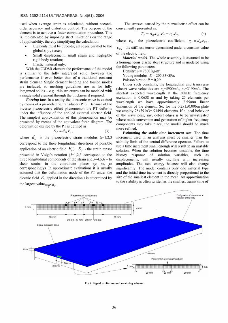
Under such constants, the longitudinal and transverse (shear) wave velocities are cL=5900m/s, cT=3190m/s. The shortest expected wavelength at the 50kHz frequency excitation is 0.0638 m and by taking 25 elements per wavelength we have approximately 2.55mm linear dimension of the element. So, for the 0.2x1x0.006m plate we employ 78x391x3= 91494 elements. If a local behavior of the wave near, say, defect edges is to be investigated where mode conversion and generation of higher frequency components may take place, the model should be much more refined.

Estimating the stable time increment size. The time increment used in an analysis must be smaller than the stability limit of the central-difference operator. Failure to use a time increment small enough will result in an unstable solution. When the solution becomes unstable, the time history response of solution variables, such as displacements, will usually oscillate with increasing amplitudes. The total energy balance will also change significantly. The model contains only one material type and the initial time increment is directly proportional to the size of the smallest element in the mesh. An approximation to the stability is often written as the smallest transit time of

where is the piezoelectric strain modulus (i=1,2,3 correspond to the three longitudinal directions of possible application of an electric field ),

iJd

iE JS - the strain tensor presented in Voigt’s notation (J=1,2,3 correspond to the three longitudinal components of the strain and J=4,5,6 – to shear strains in the coordinate planes xy, xz, yz correspondingly). In approximate evaluations it is usually assumed that the deformation mode of the PT under the electric field applied in the direction i is determined by the largest value .

iEmax iJJ

d

Fig.4. Signal excitation and receiving scheme

36

ISSN 1392-2114 ULTRAGARSAS, Nr.4(61). 2006.

a dilatational wave across any of elements in the mesh.

dcLt min≈Δ , (5)

where - the smallest element dimension in the mesh

and is the dilatational wave speed. Actually this

estimate for is only approximate and in most cases is not a conservative estimate. In general, the actual stable time increment we choose is less than this estimate by the factor

minL

dctΔ

3/1 as recommended in the Abaqus/Explicit manual (see section 6.3.3, Explicit dynamic analysis) [14].

Simulation results We calculated the signal response at the five selected

points A, B, C, D and E, as showed in Fig.4, under assumption that they are point receivers and transmitters; therefore the geometry of transducers is not taken into account.

Fig.5. Signal received by A and E transducers

Fig.6. Signal received by B and D transducers

Fig.7. Signal received by transducer C

The time of recording depends on that, how many modes we should to take in account without disturbance of the reflected waves. Actually, we are interested in propagation of A0 mode which is strongly dispersive.

The signal form in Fig.5 and Fig.6 represents two identical waveforms recorded respectively at the points A and E, and B and D. As the generating transducer is in the middle of the plate and also the receiving transducers are distributed symmetrically from the middle point C, therefore the results obtained at the points A, E and B, D are similar.

After the procedure, which was described in the previous paragraphs, the received signals are reverted in the time domain and retransmitted simultaneously. We have investigated two types of the time reversal wave propagation – in the plate with and without defect. The size of the defect is comparable to the wave length of the generated pulse. The geometry of the defect is shown in Fig. 9. The transducers are positioned in the same place as in the test without defect.

Fig.8. Position and placement of a regular geometry defect in steel plate

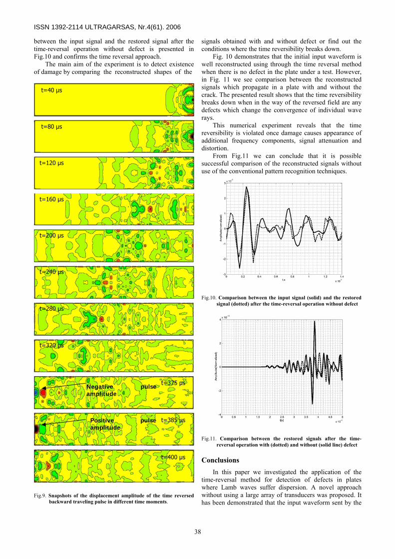
In the first numerical experiment we carried out calculation of the time-reversed wavefield. The propagation of the pulse presented in snapshots of the reversed field at different time moments is presented in Fig. 9. At the beginning we observe the various ‘rays’ for an individual transceiver and later the convergence with others. From the beginning of the wave propagation we see the process of the field front curvature change in the opposite direction. The wave front turns over to the opposite side after 120μs (in the middle of the plate) and, as expected, in the time instants 375μs and 385μs we see the significant grow of the signal amplitude and we can select the negative and positive amplitudes of our initial pulse. The comparison

37

ISSN 1392-2114 ULTRAGARSAS, Nr.4(61). 2006

between the input signal and the restored signal after the time-reversal operation without defect is presented in Fig.10 and confirms the time reversal approach.

The main aim of the experiment is to detect existence of damage by comparing the reconstructed shapes of the

Fig.9. Snapshots of the displacement amplitude of the time reversed backward traveling pulse in different time moments.

signals obtained with and without defect or find out the conditions where the time reversibility breaks down.

Fig. 10 demonstrates that the initial input waveform is well reconstructed using through the time reversal method when there is no defect in the plate under a test. However, in Fig. 11 we see comparison between the reconstructed signals which propagate in a plate with and without the crack. The presented result shows that the time reversibility breaks down when in the way of the reversed field are any defects which change the convergence of individual wave rays.

t=40 μs

This numerical experiment reveals that the time reversibility is violated once damage causes appearance of additional frequency components, signal attenuation and distortion.

t=80 μs

From Fig.11 we can conclude that it is possible successful comparison of the reconstructed signals without use of the conventional pattern recognition techniques.

t=120 μs

t=160 μs

t=200 μs

t=240 μs

Fig.10. Comparison between the input signal (solid) and the restored signal (dotted) after the time-reversal operation without defect

t=280 μs

t=320 μs

t=375 μsNegative pulse amplitude

t=385 μsPositive pulse amplitude

Fig.11. Comparison between the restored signals after the time-reversal operation with (dotted) and without (solid line) defect

t=400 μs Conclusions In this paper we investigated the application of the

time-reversal method for detection of defects in plates where Lamb waves suffer dispersion. A novel approach without using a large array of transducers was proposed. It has been demonstrated that the input waveform sent by the

38

ISSN 1392-2114 ULTRAGARSAS, Nr.4(61). 2006.

actuating transducer may be reconstructed. In the plate with the vertical crack the reconstructed signal significantly differs from the input signal. Further research is concentrated on an optimal design of the scanning system, e.g., selection of spacing between the transducers, the frequency of an ultrasonic wave and power requirements.

References

1. Wilcox P., Lowe M. and Cawley P. The effect of dispersion on long-range inspection using ultrasonic guided waves. NDT & E International. 2001. Vol.34. P.1-9.

2. Wilcox P., Lowe M. and Cawley P. A signal processing technique to remove the effects of dispersion from guided wave signals. In “Review of progress in QNDE”. 2001. Vol. 20. P.555-562.

3. Ing R.K., Fink M. Time-reversed Lamb waves. IEEE Transactions on Ultrasonics, Ferroelectrics and Frequency control. 1998. Vol. 45. P. 1032-1043

4. Fink M. Time-reversed acoustic. Scientific American. November 1999. Vol. 281. P. 91-97.

5. Fink M. Acoustic Time-Reversal Mirrors. Springer-Verlag, Berlin Heidelberg. 2002.

6. Delsanto P., Johnson P., Scalerandi M. and TenCate J. LISA simulations of time-reversed acoustic and elastic wave experiments. Journal of Physics D: Applied Physics. 2002. Vol.35. P.3145-3152.

7. Wang Ch., Rose J., Chang F. A. Computerized time-reversal method for structural health monitoring. Proceedings of SPIE Conference on Smart Structures and NDE, San Diego, CA, USA. 2003.

8. Park H., Sohn H., Law K., Farrar Ch. Time reversal active sensing for health monitoring of a composite plate. Journal of Sound and Vibration. 2004.

9. Prada C., Lartillot N., Fink M. Selective focusing in multiple-targed media: The transfer matrix method. Ultrasonic Symposium.1993. P.1139-1142.

10. Prada C., Fink M. Eigenmodes of the time reversal operator: A solution to selective focusing in multiple target media. Wave motion. 1994. P.151-163.

11. Nunes I., Negreira C. Efficiency parameters in time reversal acoustic: Application to dispersive media and multimode wave propagation. J. Acous. Soc. Am. 2005. Vol. 117(3). P.1202-1209.

12. Barauskas R., Daniulaitis V. Simulation of ultrasonic pulse propagation in solids. CMM-2003 – Computer Methods in Mechanics, Gliwice, Poland. 2003.

13. Predoi M., Sorohan S., Constantin N., Gavan M., Constantinescu D. Analysis of Lamb wave propagation in steel plate. 22nd Danubia-Adria symposium on Experimental Methods in Solid Mechanics, Monticelli Terme/Parma, Italy. 2005.

14. Abaqus/Explicit™. v6.3 Theory Manual, sec. 3.1.1. 2005

G. Butėnas, R. Kažys

Ultragarsinis laiko apgrąžos metodas defektams dispersinių savybių turinčiose plokštėse surasti ir apibūdinti

Reziumė

Aptariamas laiko apgrąžos (time-reversal) metodo taikymas defektų parametrams matuoti plokštėse, kuriose Lembo bangos patiria dispersiją. Teoriniai laiko apgrąžos tyrimai atlikti pasitelkiant baigtinių elementų programinį paketą Abaqus Explicit™. Tyrimų rezultatai rodo, kad iš keitiklio išsiųsto impulso forma atkuriama pritaikius laiko apgrąžos metodą. Plokštėse, kuriose yra defektų, atkurto signalo amplitudė priklausomai nuo defekto dydžio skiriasi. Šis skirtumas tiesiogiai koreliuoja su geometriniais defekto parametrais.

Pateikta spaudai 2006 11 14

39