introduction to random processes · prerequisites (i) probability theory i random (stochastic)...

Introduction to Random Processes

Gonzalo MateosDept. of ECE and Goergen Institute for Data Science

University of [email protected]

http://www.ece.rochester.edu/~gmateosb/

August 30, 2018

Introduction to Random Processes Introduction 1

mailto:[email protected]

http://www.ece.rochester.edu/~gmateosb/

Introductions

Introductions

Class description and contents

Gambling


Who we are, where to find me, lecture times

I Gonzalo Mateos

I Assistant Professor, Dept. of Electrical and Computer Engineering

I Hopeman 413, [email protected]

I http://www.ece.rochester.edu/~gmateosb

I Where? We meet in Gavett Hall 206

I When? Mondays and Wednesdays 4:50 pm to 6:05 pm

I My office hours, Tuesdays at 10 amI Anytime, as long as you have something interesting to tell me

I Class website

http://www.ece.rochester.edu/~gmateosb/ECE440.html



http://www.ece.rochester.edu/~gmateosb

http://www.ece.rochester.edu/~gmateosb/ECE440.html

Teaching assistants

I Four great TAs to help you with your homework

I Chang Ye


I His office hours, Mondays at 1 pm

I Rasoul Shafipour


I His office hours, Wednesdays at 1 pm




Teaching assistants

I Four great TAs to help you with your homework

I April Wang


I Her office hours, Thursdays at 3 pm

I Yang Li


I His office hours, Fridays at 1 pm




Prerequisites

(I) Probability theory

I Random (Stochastic) processes are collections of random variables

I Basic knowledge expected. Will review in the first five lectures

(II) Calculus and linear algebra

I Integrals, limits, infinite series, differential equations

I Vector/matrix notation, systems of linear equations, eigenvalues

(III) Programming in Matlab

I Needed for homework

I If you know programming you can learn Matlab in one afternoon

⇒ But it has to be this afternoon


Homework and grading

(I) Homework sets (10 in 15 weeks) worth 28 points

I Important and demanding part of this class

I Collaboration accepted, welcomed, and encouraged

(II) Midterm examination on Monday October 29 worth 36 points

(III) Final take-home examination on December 16-19 worth 36 points

I Work independently. This time no collaboration, no discussion

I ECE 271 students get 10 free points

I At least 60 points are required for passing (C grade)

I B requires at least 75 points. A at least 92. No curve

⇒ Goal is for everyone to earn an A


Textbooks

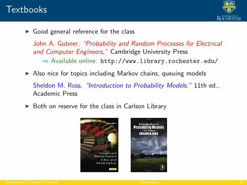
I Good general reference for the class

John A. Gubner, “Probability and Random Processes for Electricaland Computer Engineers,” Cambridge University Press

⇒ Available online: http://www.library.rochester.edu/

I Also nice for topics including Markov chains, queuing models

Sheldon M. Ross, “Introduction to Probability Models,” 11th ed.,Academic Press

I Both on reserve for the class in Carlson Library


http://www.library.rochester.edu/

Be nice

I I work hard for this course, expect you to do the same

X Come to class, be on time, pay attention, ask

X Do all of your homework

× Do not hand in as yours the solution of others (or mine)

× Do not collaborate in the take-home final

I A little bit of (conditional) probability ...

I Probability of getting an E in this class is 0.04

I Probability of getting an E given you skip 4 homework sets is 0.7

⇒ I’ll give you three notices, afterwards, I’ll give up on you

I Come and learn. Useful down the road


Class contents

Introductions


Gambling


Stochastic systems

I Stochastic system: Anything random that evolves in time

⇒ Time can be discrete n = 0, 1, 2 . . ., or continuous t ∈ [0,∞)

I More formally, random processes assign a function to a random event

I Compare with “random variable assigns a value to a random event”

I Can interpret a random process as a collection of random variables

⇒ Generalizes concept of random vector to functions

⇒ Or generalizes the concept of function to random settings


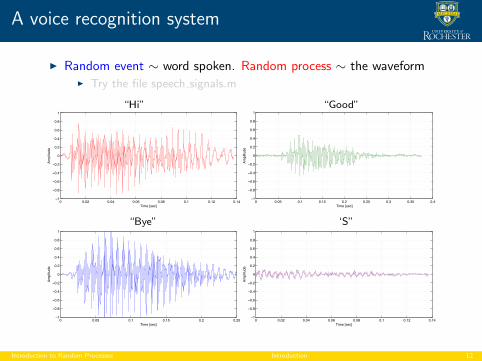
A voice recognition system

I Random event ∼ word spoken. Random process ∼ the waveformI Try the file speech signals.m

“Hi” “Good”

0 0.02 0.04 0.06 0.08 0.1 0.12 0.14−1

−0.8

−0.6

−0.4

−0.2

0

0.2

0.4

0.6

0.8

1

Time [sec]

Ampl

itude

0 0.05 0.1 0.15 0.2 0.25 0.3 0.35 0.4−1

−0.8

−0.6

−0.4

−0.2

0

0.2

0.4

0.6

0.8

1

Time [sec]

Ampl

itude

“Bye” ‘S”

0 0.05 0.1 0.15 0.2 0.25−1

−0.8

−0.6

−0.4

−0.2

0

0.2

0.4

0.6

0.8

1

Time [sec]

Ampl

itude

0 0.02 0.04 0.06 0.08 0.1 0.12 0.14−1

−0.8

−0.6

−0.4

−0.2

0

0.2

0.4

0.6

0.8

1

Time [sec]

Ampl

itude


Four thematic blocks

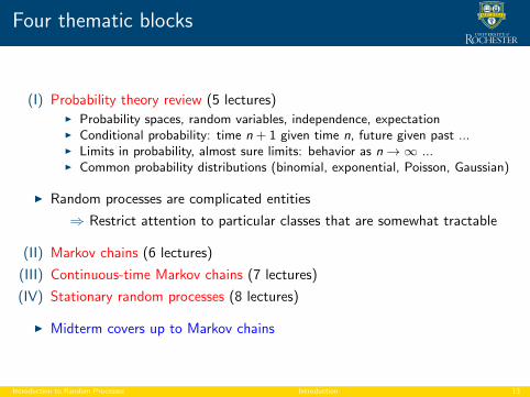
(I) Probability theory review (5 lectures)I Probability spaces, random variables, independence, expectationI Conditional probability: time n + 1 given time n, future given past ...I Limits in probability, almost sure limits: behavior as n → ∞ ...I Common probability distributions (binomial, exponential, Poisson, Gaussian)

I Random processes are complicated entities

⇒ Restrict attention to particular classes that are somewhat tractable

(II) Markov chains (6 lectures)

(III) Continuous-time Markov chains (7 lectures)

(IV) Stationary random processes (8 lectures)

I Midterm covers up to Markov chains


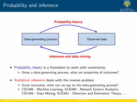
Probability and inference

Data-generating process

Observed data

Probability theory

Inference and data mining

I Probability theory is a formalism to work with uncertaintyI Given a data-generating process, what are properties of outcomes?

I Statistical inference deals with the inverse problemI Given outcomes, what can we say on the data-generating process?I CSC446 - Machine Learning, ECE440 - Network Science Analytics,

CSC440 - Data Mining, ECE441 - Detection and Estimation Theory, . . .


Markov chains

I Countable set of states 1, 2, . . .. At discrete time n, state is Xn

I Memoryless (Markov) property

⇒ Probability of next state Xn+1 depends on current state Xn

⇒ But not on past states Xn−1, Xn−2, . . .

I Can be happy (Xn = 0) or sad (Xn = 1)

I Tomorrow’s mood only affected bytoday’s mood

I Whether happy or sad today, likely tobe happy tomorrow

I But when sad, a little less likely so

H S

0.8

0.2

0.3

0.7

I Of interest: classification of states, ergodicity, limiting distributions

I Applications: Google’s PageRank, epidemic modeling, queues, ...


Continuous-time Markov chains

I Countable set of states 1, 2, . . .. Continuous-time index t, state X (t)

⇒ Transition between states can happen at any time

⇒ Markov: Future independent of the past given the present

I Probability of changing state inan infinitesimal time dt

H S

0.2dt

0.7dt

I Of interest: Poisson processes, exponential distributions, transitionprobabilities, Kolmogorov equations, limit distributions

I Applications: Chemical reactions, queues, communication networks,weather forecasting, ...


Stationary random processes

I Continuous time t, continuous state X (t), not necessarily Markov

I Prob. distribution of X (t) constant or becomes constant as t grows

⇒ System has a steady state in a random sense

I Of interest: Brownian motion, white noise, Gaussian processes,autocorrelation, power spectral density

I Applications: Black Scholes model for option pricing, radar, facerecognition, noise in electric circuits, filtering and equalization, ...


Gambling

Introductions


Gambling


An interesting betting game

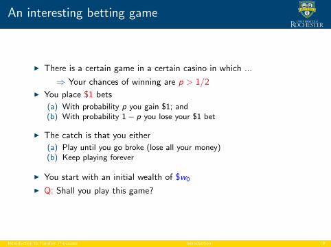
I There is a certain game in a certain casino in which ...

⇒ Your chances of winning are p > 1/2

I You place $1 bets

(a) With probability p you gain $1; and(b) With probability 1− p you lose your $1 bet

I The catch is that you either

(a) Play until you go broke (lose all your money)(b) Keep playing forever

I You start with an initial wealth of $w0

I Q: Shall you play this game?


Modeling

I Let t be a time index (number of bets placed)

I Denote as X (t) the outcome of the bet at time t

⇒ X (t) = 1 if bet is won (w.p. p)

⇒ X (t) = 0 if bet is lost (w.p. 1− p)

I X (t) is called a Bernoulli random variable with parameter p

I Denote as W (t) the player’s wealth at time t. Initialize W (0) = w0

I At times t > 0 wealth W (t) depends on past wins and losses

⇒ When bet is won W (t + 1) = W (t)+1

⇒ When bet is lost W (t + 1) = W (t)−1

I More compactly can write W (t + 1) = W (t) + (2X (t)− 1)

⇒ Only holds so long as W (t) > 0


Coding

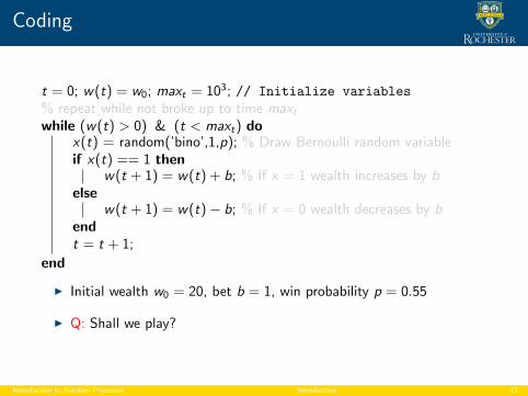
t = 0; w(t) = w0; maxt = 103; // Initialize variables

% repeat while not broke up to time maxtwhile (w(t) > 0) & (t < maxt) do

x(t) = random(’bino’,1,p); % Draw Bernoulli random variableif x(t) == 1 then

w(t + 1) = w(t) + b; % If x = 1 wealth increases by belse

w(t + 1) = w(t)− b; % If x = 0 wealth decreases by bendt = t + 1;

end

I Initial wealth w0 = 20, bet b = 1, win probability p = 0.55

I Q: Shall we play?


One lucky player

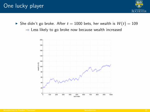
I She didn’t go broke. After t = 1000 bets, her wealth is W (t) = 109

⇒ Less likely to go broke now because wealth increased

0 100 200 300 400 500 600 700 800 900 10000

20

40

60

80

100

120

140

160

180

200

bet index

weal

th (i

n $)


Two lucky players

I After t = 1000 bets, wealths are W1(t) = 109 and W2(t) = 139

⇒ Increasing wealth seems to be a pattern

0 100 200 300 400 500 600 700 800 900 10000

20

40

60

80

100

120

140

160

180

200

bet index

weal

th (i

n $)


Ten lucky players

I Wealths Wj(t) after t = 1000 bets between 78 and 139

⇒ Increasing wealth is definitely a pattern

0 100 200 300 400 500 600 700 800 900 10000

20

40

60

80

100

120

140

160

180

200

bet index

weal

th (i

n $)


One unlucky player

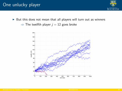
I But this does not mean that all players will turn out as winners

⇒ The twelfth player j = 12 goes broke

0 100 200 300 400 500 600 700 800 900 10000

20

40

60

80

100

120

140

160

180

200

bet index

weal

th (i

n $)


One unlucky player

I But this does not mean that all players will turn out as winners

⇒ The twelfth player j = 12 goes broke

0 50 100 150 200 2500

5

10

15

20

25

30

35

40

bet index

weal

th (i

n $)


One hundred players

I All players (except for j = 12) end up with substantially more money

0 100 200 300 400 500 600 700 800 900 10000

20

40

60

80

100

120

140

160

180

200

bet index

weal

th (i

n $)


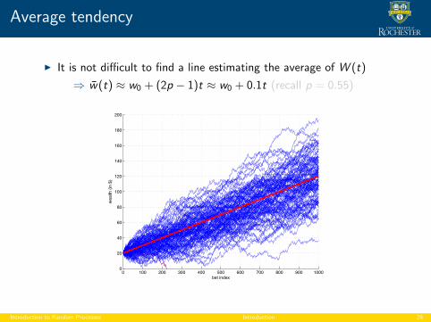
Average tendency

I It is not difficult to find a line estimating the average of W (t)

⇒ w̄(t) ≈ w0 + (2p − 1)t ≈ w0 + 0.1t (recall p = 0.55)

0 100 200 300 400 500 600 700 800 900 10000

20

40

60

80

100

120

140

160

180

200

bet index

weal

th (i

n $)


Where does the average tendency come from?

I Assuming we do not go broke, we can write

W (t + 1) = W (t) +(2X (t)− 1

), t = 0, 1, 2, . . .

I The assumption is incorrect as we saw, but suffices for simplicity

I Taking expectations on both sides and using linearity of expectation

E [W (t + 1)] = E [W (t)] +(2E [X (t)]− 1

)I The expected value of Bernoulli X (t) is

E [X (t)] = 1× P (X (t) = 1) + 0× P (X (t) = 0) = p

I Which yields ⇒ E [W (t + 1)] = E [W (t)] + (2p − 1)

I Applying recursively ⇒ E [W (t + 1)] = w0 + (2p − 1)(t + 1)


Gambling as LTI system with stochastic input

I Recall the evolution of wealth W (t + 1) = W (t) +(2X (t)− 1

)

1

t -1

2x(t)-1

+

Delay

w(t+1) 2x(t)-1

w(t)

Accumulator

t

w(t+1)

I View W (t+1) as output of LTI system with random input 2X (t)−1

I Recognize accumulator ⇒ W (t + 1) = w0 +t∑

τ=0

(2X (τ)− 1

)I Useful, a lot we can say about sums of random variables

I Filtering random processes in signal processing, communications, . . .


Numerical analysis of simulation outcomes

I For a more accurate approximation analyze simulation outcomes

I Consider J experiments. Each yields a wealth history Wj(t)

I Can estimate the average outcome via the sample average W̄J(t)

W̄J(t) :=1

J

J∑j=1

Wj(t)

I Do not confuse W̄J(t) with E [W (t)]I W̄J(t) is computed from experiments, it is a random quantity in itselfI E [W (t)] is a property of the random variable W (t)I We will see later that for large J, W̄J(t) → E [W (t)]


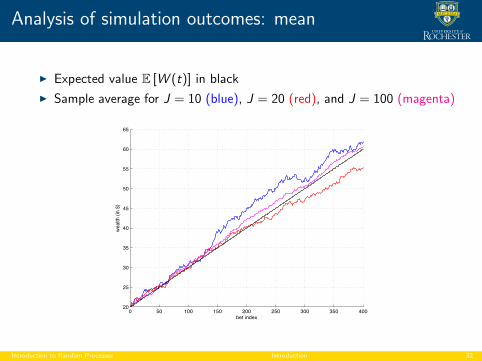
Analysis of simulation outcomes: mean

I Expected value E [W (t)] in black

I Sample average for J = 10 (blue), J = 20 (red), and J = 100 (magenta)

0 50 100 150 200 250 300 350 40020

25

30

35

40

45

50

55

60

65

bet index

weal

th (i

n $)


Analysis of simulation outcomes: distribution

I There is more information in the simulation’s output

I Estimate the probability distribution function (pdf) ⇒ Histogram

I Consider a set of points w (0), . . . ,w (M)

I Indicator function of the event w (m) ≤ Wj(t) < w (m+1)

I{w (m) ≤ Wj(t) < w (m+1)

}=

{1, if w (m) ≤ Wj(t) < w (m+1)

0, otherwise

I Histogram is then defined as

H[t;w (m),w (m+1)

]=

1

J

J∑j=1

I{w (m) ≤ Wj(t) < w (m+1)

}I Fraction of experiments with wealth Wj(t) between w (m) and w (m+1)


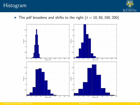
Histogram

I The pdf broadens and shifts to the right (t = 10, 50, 100, 200)

0 10 20 30 40 50 60 70 80 900

0.05

0.1

0.15

0.2

0.25

wealth (in $)

frequ

ency

0 10 20 30 40 50 60 70 80 900

0.05

0.1

0.15

0.2

0.25

wealth (in $)

frequ

ency

0 10 20 30 40 50 60 70 80 900

0.05

0.1

0.15

0.2

0.25

wealth (in $)

frequ

ency

0 10 20 30 40 50 60 70 80 900

0.05

0.1

0.15

0.2

0.25

wealth (in $)

frequ

ency


What is this class about?

I Analysis and simulation of stochastic systems

⇒ A system that evolves in time with some randomness

I They are usually quite complex ⇒ Simulations

I We will learn how to model stochastic systems, e.g.,I X (t) Bernoulli with parameter pI W (t + 1) = W (t) + 1, when X (t) = 1I W (t + 1) = W (t)− 1, when X (t) = 0

I ... how to analyze their properties, e.g., E [W (t)] = w0 + (2p − 1)t

I ... and how to interpret simulations and experiments, e.g.,I Average tendency through sample averageI Estimate probability distributions via histograms


introduction to random processes · prerequisites (i) probability theory i random (stochastic)...

Documents