introduction to programming using python - lncc · introduction to programming using python...
TRANSCRIPT
Introduction to Programming usingPython
Programming Course for Biologists at thePasteur Institute
by Katja Schuerer, Corinne Maufrais, Catherine Letondal, Eric Deveaud, andMarie-Agnes Petit
Introduction to Programming using Python [http://www.python.org/]:Programming Course for Biologists at the Pasteur Instituteby Katja Schuerer, Corinne Maufrais, Catherine Letondal, Eric Deveaud, and Marie-Agnes Petit
Published February, 1 2005Copyright © 2005 Pasteur Institute [http://www.pasteur.fr/]
The objective of this course is to teach programming concepts to biologists. It is thus aimed at people who arenot professional computer scientists, but who need a better control of computers for their own research. This pro-gramming course is part of a course in informatics for biology [http://www.pasteur.fr/formation/infobio/infobio-en.html]. If you are already a programmer, and if you are just looking for an introduction to Python, you can goto this Python course [http://www.pasteur.fr/recherche/unites/sis/formation/python/] (in Bioinformatics).
PDF version of this course [support.pdf]
This course is still under construction. Comments are welcome.
Handouts for practical sessions (still under construction) will be available on request.
Contact: [email protected]
Table of Contents
1. Introduction . . . . . . . . . . . . . . . . . . . . . . . . . . . . . . . . . . . . . . . . . . . . . . . . . . . . . . . . . . . . . . . . . . . . . . . . . . . . . . . . 11.1. First session. . . . . . . . . . . . . . . . . . . . . . . . . . . . . . . . . . . . . . . . . . . . . . . . . . . . . . . . . . . . . . . . . . . . . . . . . 11.2. Documentation. . . . . . . . . . . . . . . . . . . . . . . . . . . . . . . . . . . . . . . . . . . . . . . . . . . . . . . . . . . . . . . . . . . . . . 61.3. Why Python . . . . . . . . . . . . . . . . . . . . . . . . . . . . . . . . . . . . . . . . . . . . . . . . . . . . . . . . . . . . . . . . . . . . . . . . 61.4. Programming Languages. . . . . . . . . . . . . . . . . . . . . . . . . . . . . . . . . . . . . . . . . . . . . . . . . . . . . . . . . . . . . 6
2. Variables . . . . . . . . . . . . . . . . . . . . . . . . . . . . . . . . . . . . . . . . . . . . . . . . . . . . . . . . . . . . . . . . . . . . . . . . . . . . . . . . . . 92.1. Data, values and types of values. . . . . . . . . . . . . . . . . . . . . . . . . . . . . . . . . . . . . . . . . . . . . . . . . . . . . . . 92.2. Variables or naming values. . . . . . . . . . . . . . . . . . . . . . . . . . . . . . . . . . . . . . . . . . . . . . . . . . . . . . . . . . . 92.3. Variable and keywords, variable syntax. . . . . . . . . . . . . . . . . . . . . . . . . . . . . . . . . . . . . . . . . . . . . . . 102.4. Namespaces or representing variables. . . . . . . . . . . . . . . . . . . . . . . . . . . . . . . . . . . . . . . . . . . . . . . . . 112.5. Reassignment of variables. . . . . . . . . . . . . . . . . . . . . . . . . . . . . . . . . . . . . . . . . . . . . . . . . . . . . . . . . . . 12
3. Statements, expressions and functions. . . . . . . . . . . . . . . . . . . . . . . . . . . . . . . . . . . . . . . . . . . . . . . . . . . . . . . 153.1. Statements. . . . . . . . . . . . . . . . . . . . . . . . . . . . . . . . . . . . . . . . . . . . . . . . . . . . . . . . . . . . . . . . . . . . . . . . . 153.2. Sequences or chaining statements. . . . . . . . . . . . . . . . . . . . . . . . . . . . . . . . . . . . . . . . . . . . . . . . . . . . 153.3. Functions. . . . . . . . . . . . . . . . . . . . . . . . . . . . . . . . . . . . . . . . . . . . . . . . . . . . . . . . . . . . . . . . . . . . . . . . . . 153.4. Operations. . . . . . . . . . . . . . . . . . . . . . . . . . . . . . . . . . . . . . . . . . . . . . . . . . . . . . . . . . . . . . . . . . . . . . . . . 163.5. Composition and Evaluation of Expressions. . . . . . . . . . . . . . . . . . . . . . . . . . . . . . . . . . . . . . . . . . . 16
4. Communication with outside. . . . . . . . . . . . . . . . . . . . . . . . . . . . . . . . . . . . . . . . . . . . . . . . . . . . . . . . . . . . . . . . 194.1. Output . . . . . . . . . . . . . . . . . . . . . . . . . . . . . . . . . . . . . . . . . . . . . . . . . . . . . . . . . . . . . . . . . . . . . . . . . . . . 194.2. Formatting strings. . . . . . . . . . . . . . . . . . . . . . . . . . . . . . . . . . . . . . . . . . . . . . . . . . . . . . . . . . . . . . . . . . 194.3. Input . . . . . . . . . . . . . . . . . . . . . . . . . . . . . . . . . . . . . . . . . . . . . . . . . . . . . . . . . . . . . . . . . . . . . . . . . . . . . . 22
5. Program execution. . . . . . . . . . . . . . . . . . . . . . . . . . . . . . . . . . . . . . . . . . . . . . . . . . . . . . . . . . . . . . . . . . . . . . . . . 255.1. Executing code from a file. . . . . . . . . . . . . . . . . . . . . . . . . . . . . . . . . . . . . . . . . . . . . . . . . . . . . . . . . . . 255.2. Interpreter and Compiler. . . . . . . . . . . . . . . . . . . . . . . . . . . . . . . . . . . . . . . . . . . . . . . . . . . . . . . . . . . . 27
6. Strings . . . . . . . . . . . . . . . . . . . . . . . . . . . . . . . . . . . . . . . . . . . . . . . . . . . . . . . . . . . . . . . . . . . . . . . . . . . . . . . . . . . 316.1. Values as objects. . . . . . . . . . . . . . . . . . . . . . . . . . . . . . . . . . . . . . . . . . . . . . . . . . . . . . . . . . . . . . . . . . . 316.2. Working with strings. . . . . . . . . . . . . . . . . . . . . . . . . . . . . . . . . . . . . . . . . . . . . . . . . . . . . . . . . . . . . . . . 32
7. Branching and Decisions. . . . . . . . . . . . . . . . . . . . . . . . . . . . . . . . . . . . . . . . . . . . . . . . . . . . . . . . . . . . . . . . . . . 377.1. Conditional execution. . . . . . . . . . . . . . . . . . . . . . . . . . . . . . . . . . . . . . . . . . . . . . . . . . . . . . . . . . . . . . . 377.2. Conditions and Boolean expressions. . . . . . . . . . . . . . . . . . . . . . . . . . . . . . . . . . . . . . . . . . . . . . . . . . 387.3. Logical operators. . . . . . . . . . . . . . . . . . . . . . . . . . . . . . . . . . . . . . . . . . . . . . . . . . . . . . . . . . . . . . . . . . . 397.4. Alternative execution. . . . . . . . . . . . . . . . . . . . . . . . . . . . . . . . . . . . . . . . . . . . . . . . . . . . . . . . . . . . . . . 407.5. Chained conditional execution. . . . . . . . . . . . . . . . . . . . . . . . . . . . . . . . . . . . . . . . . . . . . . . . . . . . . . . 417.6. Nested conditions. . . . . . . . . . . . . . . . . . . . . . . . . . . . . . . . . . . . . . . . . . . . . . . . . . . . . . . . . . . . . . . . . . 427.7. Solutions . . . . . . . . . . . . . . . . . . . . . . . . . . . . . . . . . . . . . . . . . . . . . . . . . . . . . . . . . . . . . . . . . . . . . . . . . . 44
8. Defining Functions . . . . . . . . . . . . . . . . . . . . . . . . . . . . . . . . . . . . . . . . . . . . . . . . . . . . . . . . . . . . . . . . . . . . . . . . 458.1. Defining Functions. . . . . . . . . . . . . . . . . . . . . . . . . . . . . . . . . . . . . . . . . . . . . . . . . . . . . . . . . . . . . . . . . 458.2. Parameters and Arguments or the difference between a function definition and a function call 478.3. Functions and namespaces. . . . . . . . . . . . . . . . . . . . . . . . . . . . . . . . . . . . . . . . . . . . . . . . . . . . . . . . . . . 498.4. Boolean functions. . . . . . . . . . . . . . . . . . . . . . . . . . . . . . . . . . . . . . . . . . . . . . . . . . . . . . . . . . . . . . . . . . 51
9. Collections . . . . . . . . . . . . . . . . . . . . . . . . . . . . . . . . . . . . . . . . . . . . . . . . . . . . . . . . . . . . . . . . . . . . . . . . . . . . . . . 539.1. Datatypes for collections. . . . . . . . . . . . . . . . . . . . . . . . . . . . . . . . . . . . . . . . . . . . . . . . . . . . . . . . . . . . 539.2. Methods, Operators and Functions on Lists. . . . . . . . . . . . . . . . . . . . . . . . . . . . . . . . . . . . . . . . . . . . 55

9.3. Methods, Operators and Functions on Dictionaries. . . . . . . . . . . . . . . . . . . . . . . . . . . . . . . . . . . . . 579.4. What data type for which collection. . . . . . . . . . . . . . . . . . . . . . . . . . . . . . . . . . . . . . . . . . . . . . . . . . 58
10. Repetitions . . . . . . . . . . . . . . . . . . . . . . . . . . . . . . . . . . . . . . . . . . . . . . . . . . . . . . . . . . . . . . . . . . . . . . . . . . . . . . 5910.1. Repetitions. . . . . . . . . . . . . . . . . . . . . . . . . . . . . . . . . . . . . . . . . . . . . . . . . . . . . . . . . . . . . . . . . . . . . . . 5910.2. The for loop . . . . . . . . . . . . . . . . . . . . . . . . . . . . . . . . . . . . . . . . . . . . . . . . . . . . . . . . . . . . . . . . . . . . . . 5910.3. The while loop . . . . . . . . . . . . . . . . . . . . . . . . . . . . . . . . . . . . . . . . . . . . . . . . . . . . . . . . . . . . . . . . . . . . 6410.4. Comparison of for and while loops. . . . . . . . . . . . . . . . . . . . . . . . . . . . . . . . . . . . . . . . . . . . . . . . . . 6710.5. Range and Xrange objects. . . . . . . . . . . . . . . . . . . . . . . . . . . . . . . . . . . . . . . . . . . . . . . . . . . . . . . . . . 6810.6. The map function. . . . . . . . . . . . . . . . . . . . . . . . . . . . . . . . . . . . . . . . . . . . . . . . . . . . . . . . . . . . . . . . . 6810.7. Solutions . . . . . . . . . . . . . . . . . . . . . . . . . . . . . . . . . . . . . . . . . . . . . . . . . . . . . . . . . . . . . . . . . . . . . . . . . 70
11. Nested data structures. . . . . . . . . . . . . . . . . . . . . . . . . . . . . . . . . . . . . . . . . . . . . . . . . . . . . . . . . . . . . . . . . . . . . 7111.1. Nested data structures. . . . . . . . . . . . . . . . . . . . . . . . . . . . . . . . . . . . . . . . . . . . . . . . . . . . . . . . . . . . . . 7111.2. Identity of objects. . . . . . . . . . . . . . . . . . . . . . . . . . . . . . . . . . . . . . . . . . . . . . . . . . . . . . . . . . . . . . . . . 7311.3. Copying complex data structures. . . . . . . . . . . . . . . . . . . . . . . . . . . . . . . . . . . . . . . . . . . . . . . . . . . . 7511.4. Modifying nested structures. . . . . . . . . . . . . . . . . . . . . . . . . . . . . . . . . . . . . . . . . . . . . . . . . . . . . . . . 76
12. Files . . . . . . . . . . . . . . . . . . . . . . . . . . . . . . . . . . . . . . . . . . . . . . . . . . . . . . . . . . . . . . . . . . . . . . . . . . . . . . . . . . . . 8112.1. Handle files in programs. . . . . . . . . . . . . . . . . . . . . . . . . . . . . . . . . . . . . . . . . . . . . . . . . . . . . . . . . . . 8112.2. Reading data from files. . . . . . . . . . . . . . . . . . . . . . . . . . . . . . . . . . . . . . . . . . . . . . . . . . . . . . . . . . . . 8312.3. Writing in files . . . . . . . . . . . . . . . . . . . . . . . . . . . . . . . . . . . . . . . . . . . . . . . . . . . . . . . . . . . . . . . . . . . . 8412.4. Design problems. . . . . . . . . . . . . . . . . . . . . . . . . . . . . . . . . . . . . . . . . . . . . . . . . . . . . . . . . . . . . . . . . . 8712.5. Documentation strings. . . . . . . . . . . . . . . . . . . . . . . . . . . . . . . . . . . . . . . . . . . . . . . . . . . . . . . . . . . . . 91
13. Recursive functions. . . . . . . . . . . . . . . . . . . . . . . . . . . . . . . . . . . . . . . . . . . . . . . . . . . . . . . . . . . . . . . . . . . . . . . 9713.1. Recursive functions definitions. . . . . . . . . . . . . . . . . . . . . . . . . . . . . . . . . . . . . . . . . . . . . . . . . . . . . . 9713.2. Flow of execution of recursive functions. . . . . . . . . . . . . . . . . . . . . . . . . . . . . . . . . . . . . . . . . . . . . 9913.3. Recursive data structures. . . . . . . . . . . . . . . . . . . . . . . . . . . . . . . . . . . . . . . . . . . . . . . . . . . . . . . . . . 101
14. Exceptions . . . . . . . . . . . . . . . . . . . . . . . . . . . . . . . . . . . . . . . . . . . . . . . . . . . . . . . . . . . . . . . . . . . . . . . . . . . . . 10714.1. General Mechanism. . . . . . . . . . . . . . . . . . . . . . . . . . . . . . . . . . . . . . . . . . . . . . . . . . . . . . . . . . . . . . 10714.2. Python built-in exceptions. . . . . . . . . . . . . . . . . . . . . . . . . . . . . . . . . . . . . . . . . . . . . . . . . . . . . . . . . 10714.3. Raising exceptions. . . . . . . . . . . . . . . . . . . . . . . . . . . . . . . . . . . . . . . . . . . . . . . . . . . . . . . . . . . . . . . 10814.4. Defining exceptions. . . . . . . . . . . . . . . . . . . . . . . . . . . . . . . . . . . . . . . . . . . . . . . . . . . . . . . . . . . . . . 109
15. Modules and packages in Python. . . . . . . . . . . . . . . . . . . . . . . . . . . . . . . . . . . . . . . . . . . . . . . . . . . . . . . . . . 11115.1. Modules . . . . . . . . . . . . . . . . . . . . . . . . . . . . . . . . . . . . . . . . . . . . . . . . . . . . . . . . . . . . . . . . . . . . . . . . 111
15.1.1. Using modules. . . . . . . . . . . . . . . . . . . . . . . . . . . . . . . . . . . . . . . . . . . . . . . . . . . . . . . . . . . . 11115.1.2. Building modules. . . . . . . . . . . . . . . . . . . . . . . . . . . . . . . . . . . . . . . . . . . . . . . . . . . . . . . . . 11115.1.3. Where are the modules?. . . . . . . . . . . . . . . . . . . . . . . . . . . . . . . . . . . . . . . . . . . . . . . . . . . 11215.1.4. How does it work?. . . . . . . . . . . . . . . . . . . . . . . . . . . . . . . . . . . . . . . . . . . . . . . . . . . . . . . . 11315.1.5. Running a module from the command line. . . . . . . . . . . . . . . . . . . . . . . . . . . . . . . . . . . 115
15.2. Packages. . . . . . . . . . . . . . . . . . . . . . . . . . . . . . . . . . . . . . . . . . . . . . . . . . . . . . . . . . . . . . . . . . . . . . . . 11515.2.1. Loading . . . . . . . . . . . . . . . . . . . . . . . . . . . . . . . . . . . . . . . . . . . . . . . . . . . . . . . . . . . . . . . . . . 116
15.3. Getting information on available modules and packages. . . . . . . . . . . . . . . . . . . . . . . . . . . . . . 11816. Scripting . . . . . . . . . . . . . . . . . . . . . . . . . . . . . . . . . . . . . . . . . . . . . . . . . . . . . . . . . . . . . . . . . . . . . . . . . . . . . . . 119
16.1. Using the system environment: os and sys modules. . . . . . . . . . . . . . . . . . . . . . . . . . . . . . . . . . 11916.2. Running Programs. . . . . . . . . . . . . . . . . . . . . . . . . . . . . . . . . . . . . . . . . . . . . . . . . . . . . . . . . . . . . . . 12016.3. Parsing command line options with getopt. . . . . . . . . . . . . . . . . . . . . . . . . . . . . . . . . . . . . . . . . . 12316.4. Parsing. . . . . . . . . . . . . . . . . . . . . . . . . . . . . . . . . . . . . . . . . . . . . . . . . . . . . . . . . . . . . . . . . . . . . . . . . . 12516.5. Searching for patterns.. . . . . . . . . . . . . . . . . . . . . . . . . . . . . . . . . . . . . . . . . . . . . . . . . . . . . . . . . . . . 128

16.5.1. Introduction to regular expressions. . . . . . . . . . . . . . . . . . . . . . . . . . . . . . . . . . . . . . . . . . 12816.5.2. Regular expressions in Python. . . . . . . . . . . . . . . . . . . . . . . . . . . . . . . . . . . . . . . . . . . . . . 12916.5.3. Prosite. . . . . . . . . . . . . . . . . . . . . . . . . . . . . . . . . . . . . . . . . . . . . . . . . . . . . . . . . . . . . . . . . . . 13316.5.4. Searching for patterns and parsing. . . . . . . . . . . . . . . . . . . . . . . . . . . . . . . . . . . . . . . . . . 134
17. Object-oriented programming. . . . . . . . . . . . . . . . . . . . . . . . . . . . . . . . . . . . . . . . . . . . . . . . . . . . . . . . . . . . . 13517.1. Introduction . . . . . . . . . . . . . . . . . . . . . . . . . . . . . . . . . . . . . . . . . . . . . . . . . . . . . . . . . . . . . . . . . . . . . 13517.2. What is a class? An example. . . . . . . . . . . . . . . . . . . . . . . . . . . . . . . . . . . . . . . . . . . . . . . . . . . . . . 135
17.2.1. Objects description. . . . . . . . . . . . . . . . . . . . . . . . . . . . . . . . . . . . . . . . . . . . . . . . . . . . . . . . 13517.2.2. Methods . . . . . . . . . . . . . . . . . . . . . . . . . . . . . . . . . . . . . . . . . . . . . . . . . . . . . . . . . . . . . . . . . 13517.2.3. Class definition. . . . . . . . . . . . . . . . . . . . . . . . . . . . . . . . . . . . . . . . . . . . . . . . . . . . . . . . . . . 136
17.3. Using classes in Python. . . . . . . . . . . . . . . . . . . . . . . . . . . . . . . . . . . . . . . . . . . . . . . . . . . . . . . . . . . 13817.3.1. Creating instances. . . . . . . . . . . . . . . . . . . . . . . . . . . . . . . . . . . . . . . . . . . . . . . . . . . . . . . . . 138
17.4. Combining objects. . . . . . . . . . . . . . . . . . . . . . . . . . . . . . . . . . . . . . . . . . . . . . . . . . . . . . . . . . . . . . . 14017.5. Classes and objects in Python: technical aspects. . . . . . . . . . . . . . . . . . . . . . . . . . . . . . . . . . . . . 144
17.5.1. Namespaces. . . . . . . . . . . . . . . . . . . . . . . . . . . . . . . . . . . . . . . . . . . . . . . . . . . . . . . . . . . . . . 14417.5.2. Objects lifespan. . . . . . . . . . . . . . . . . . . . . . . . . . . . . . . . . . . . . . . . . . . . . . . . . . . . . . . . . . . 14817.5.3. Objects equality. . . . . . . . . . . . . . . . . . . . . . . . . . . . . . . . . . . . . . . . . . . . . . . . . . . . . . . . . . . 14917.5.4. Classes and types. . . . . . . . . . . . . . . . . . . . . . . . . . . . . . . . . . . . . . . . . . . . . . . . . . . . . . . . . 15017.5.5. Getting information on classes and instances. . . . . . . . . . . . . . . . . . . . . . . . . . . . . . . . . 150
18. Object-oriented design. . . . . . . . . . . . . . . . . . . . . . . . . . . . . . . . . . . . . . . . . . . . . . . . . . . . . . . . . . . . . . . . . . . 15318.1. Introduction . . . . . . . . . . . . . . . . . . . . . . . . . . . . . . . . . . . . . . . . . . . . . . . . . . . . . . . . . . . . . . . . . . . . . 15318.2. Components. . . . . . . . . . . . . . . . . . . . . . . . . . . . . . . . . . . . . . . . . . . . . . . . . . . . . . . . . . . . . . . . . . . . . 153
18.2.1. Software quality factors. . . . . . . . . . . . . . . . . . . . . . . . . . . . . . . . . . . . . . . . . . . . . . . . . . . . 15318.2.2. Large scale programming. . . . . . . . . . . . . . . . . . . . . . . . . . . . . . . . . . . . . . . . . . . . . . . . . . 15318.2.3. Modularity . . . . . . . . . . . . . . . . . . . . . . . . . . . . . . . . . . . . . . . . . . . . . . . . . . . . . . . . . . . . . . . 15418.2.4. Methodology. . . . . . . . . . . . . . . . . . . . . . . . . . . . . . . . . . . . . . . . . . . . . . . . . . . . . . . . . . . . . 15618.2.5. Reusability. . . . . . . . . . . . . . . . . . . . . . . . . . . . . . . . . . . . . . . . . . . . . . . . . . . . . . . . . . . . . . . 156
18.3. Abstract Data Types. . . . . . . . . . . . . . . . . . . . . . . . . . . . . . . . . . . . . . . . . . . . . . . . . . . . . . . . . . . . . . 15718.3.1. Definition . . . . . . . . . . . . . . . . . . . . . . . . . . . . . . . . . . . . . . . . . . . . . . . . . . . . . . . . . . . . . . . . 15718.3.2. Information hiding . . . . . . . . . . . . . . . . . . . . . . . . . . . . . . . . . . . . . . . . . . . . . . . . . . . . . . . . 16018.3.3. Using special methods within classes. . . . . . . . . . . . . . . . . . . . . . . . . . . . . . . . . . . . . . . . 163
18.4. Inheritance: sharing code among classes. . . . . . . . . . . . . . . . . . . . . . . . . . . . . . . . . . . . . . . . . . . . 16318.4.1. Introduction . . . . . . . . . . . . . . . . . . . . . . . . . . . . . . . . . . . . . . . . . . . . . . . . . . . . . . . . . . . . . . 16318.4.2. Discussion. . . . . . . . . . . . . . . . . . . . . . . . . . . . . . . . . . . . . . . . . . . . . . . . . . . . . . . . . . . . . . . 169
18.5. Flexibility . . . . . . . . . . . . . . . . . . . . . . . . . . . . . . . . . . . . . . . . . . . . . . . . . . . . . . . . . . . . . . . . . . . . . . . 17318.5.1. Summary of mechanisms for flexibility in Python. . . . . . . . . . . . . . . . . . . . . . . . . . . . . 17318.5.2. Manual overloading. . . . . . . . . . . . . . . . . . . . . . . . . . . . . . . . . . . . . . . . . . . . . . . . . . . . . . . 174
18.6. Object-oriented design patterns. . . . . . . . . . . . . . . . . . . . . . . . . . . . . . . . . . . . . . . . . . . . . . . . . . . . 176Bibliography . . . . . . . . . . . . . . . . . . . . . . . . . . . . . . . . . . . . . . . . . . . . . . . . . . . . . . . . . . . . . . . . . . . . . . . . . . . . . . . 187


List of Figures
1.1. History of programming languages(Source). . . . . . . . . . . . . . . . . . . . . . . . . . . . . . . . . . . . . . . . . . . . . . . . . . 72.1. Namespace. . . . . . . . . . . . . . . . . . . . . . . . . . . . . . . . . . . . . . . . . . . . . . . . . . . . . . . . . . . . . . . . . . . . . . . . . . . . . . 112.2. Reassigning values to variables. . . . . . . . . . . . . . . . . . . . . . . . . . . . . . . . . . . . . . . . . . . . . . . . . . . . . . . . . . . . 124.1. Interpretation of formatting templates. . . . . . . . . . . . . . . . . . . . . . . . . . . . . . . . . . . . . . . . . . . . . . . . . . . . . . 205.1. Comparison of compiled and interpreted code. . . . . . . . . . . . . . . . . . . . . . . . . . . . . . . . . . . . . . . . . . . . . . . 285.2. Execution of byte compiled code. . . . . . . . . . . . . . . . . . . . . . . . . . . . . . . . . . . . . . . . . . . . . . . . . . . . . . . . . . 286.1. String indices. . . . . . . . . . . . . . . . . . . . . . . . . . . . . . . . . . . . . . . . . . . . . . . . . . . . . . . . . . . . . . . . . . . . . . . . . . . . 337.1. Flow of execution of a simple condition. . . . . . . . . . . . . . . . . . . . . . . . . . . . . . . . . . . . . . . . . . . . . . . . . . . . 377.2. If statement . . . . . . . . . . . . . . . . . . . . . . . . . . . . . . . . . . . . . . . . . . . . . . . . . . . . . . . . . . . . . . . . . . . . . . . . . . . . . 377.3. Block structure of the if statement. . . . . . . . . . . . . . . . . . . . . . . . . . . . . . . . . . . . . . . . . . . . . . . . . . . . . . . . . 387.4. Flow of execution of an alternative condition. . . . . . . . . . . . . . . . . . . . . . . . . . . . . . . . . . . . . . . . . . . . . . . . 407.5. Multiple alternatives or Chained conditions. . . . . . . . . . . . . . . . . . . . . . . . . . . . . . . . . . . . . . . . . . . . . . . . . 417.6. Nested conditions. . . . . . . . . . . . . . . . . . . . . . . . . . . . . . . . . . . . . . . . . . . . . . . . . . . . . . . . . . . . . . . . . . . . . . . . 437.7. Multiple alternatives without elif. . . . . . . . . . . . . . . . . . . . . . . . . . . . . . . . . . . . . . . . . . . . . . . . . . . . . . . . . . 448.1. Function definitions. . . . . . . . . . . . . . . . . . . . . . . . . . . . . . . . . . . . . . . . . . . . . . . . . . . . . . . . . . . . . . . . . . . . . . 458.2. Blocks and indentation. . . . . . . . . . . . . . . . . . . . . . . . . . . . . . . . . . . . . . . . . . . . . . . . . . . . . . . . . . . . . . . . . . . 478.3. Stack diagram of function calls. . . . . . . . . . . . . . . . . . . . . . . . . . . . . . . . . . . . . . . . . . . . . . . . . . . . . . . . . . . . 489.1. Comparison some collection datatypes. . . . . . . . . . . . . . . . . . . . . . . . . . . . . . . . . . . . . . . . . . . . . . . . . . . . . 5510.1. The for loop . . . . . . . . . . . . . . . . . . . . . . . . . . . . . . . . . . . . . . . . . . . . . . . . . . . . . . . . . . . . . . . . . . . . . . . . . . . . 6010.2. Flow of execution of a while statement. . . . . . . . . . . . . . . . . . . . . . . . . . . . . . . . . . . . . . . . . . . . . . . . . . . . 6410.3. Structure of the while statement. . . . . . . . . . . . . . . . . . . . . . . . . . . . . . . . . . . . . . . . . . . . . . . . . . . . . . . . . . 6610.4. Passing functions as arguments. . . . . . . . . . . . . . . . . . . . . . . . . . . . . . . . . . . . . . . . . . . . . . . . . . . . . . . . . . . 6911.1. Representation of nested lists. . . . . . . . . . . . . . . . . . . . . . . . . . . . . . . . . . . . . . . . . . . . . . . . . . . . . . . . . . . . 7111.2. Accessing elements in nested lists. . . . . . . . . . . . . . . . . . . . . . . . . . . . . . . . . . . . . . . . . . . . . . . . . . . . . . . . 7211.3. Representation of a nested dictionary. . . . . . . . . . . . . . . . . . . . . . . . . . . . . . . . . . . . . . . . . . . . . . . . . . . . . 7311.4. List comparison. . . . . . . . . . . . . . . . . . . . . . . . . . . . . . . . . . . . . . . . . . . . . . . . . . . . . . . . . . . . . . . . . . . . . . . . 7411.5. Copying nested structures. . . . . . . . . . . . . . . . . . . . . . . . . . . . . . . . . . . . . . . . . . . . . . . . . . . . . . . . . . . . . . . . 7611.6. Modifying compound objects. . . . . . . . . . . . . . . . . . . . . . . . . . . . . . . . . . . . . . . . . . . . . . . . . . . . . . . . . . . . 7712.1. ReBase file format. . . . . . . . . . . . . . . . . . . . . . . . . . . . . . . . . . . . . . . . . . . . . . . . . . . . . . . . . . . . . . . . . . . . . . 8312.2. Flowchart of the processing of the sequence. . . . . . . . . . . . . . . . . . . . . . . . . . . . . . . . . . . . . . . . . . . . . . . 9013.1. Stack diagram of recursive function calls. . . . . . . . . . . . . . . . . . . . . . . . . . . . . . . . . . . . . . . . . . . . . . . . . . 9913.2. A phylogenetic tree topology. . . . . . . . . . . . . . . . . . . . . . . . . . . . . . . . . . . . . . . . . . . . . . . . . . . . . . . . . . . 10113.3. Tree representation using a recursive list structure. . . . . . . . . . . . . . . . . . . . . . . . . . . . . . . . . . . . . . . . . 10114.1. Exceptions class hierarchy. . . . . . . . . . . . . . . . . . . . . . . . . . . . . . . . . . . . . . . . . . . . . . . . . . . . . . . . . . . . . . 10715.1. Module namespace. . . . . . . . . . . . . . . . . . . . . . . . . . . . . . . . . . . . . . . . . . . . . . . . . . . . . . . . . . . . . . . . . . . . 11315.2. Loading specific components. . . . . . . . . . . . . . . . . . . . . . . . . . . . . . . . . . . . . . . . . . . . . . . . . . . . . . . . . . . 11416.1. Manual parsing. . . . . . . . . . . . . . . . . . . . . . . . . . . . . . . . . . . . . . . . . . . . . . . . . . . . . . . . . . . . . . . . . . . . . . . . 12516.2. Event-based parsing. . . . . . . . . . . . . . . . . . . . . . . . . . . . . . . . . . . . . . . . . . . . . . . . . . . . . . . . . . . . . . . . . . . 12516.3. Parsing: decorated grammar. . . . . . . . . . . . . . . . . . . . . . . . . . . . . . . . . . . . . . . . . . . . . . . . . . . . . . . . . . . . 12616.4. Parsing result as a hierarchical document. . . . . . . . . . . . . . . . . . . . . . . . . . . . . . . . . . . . . . . . . . . . . . . . . 12716.5. Pattern searching. . . . . . . . . . . . . . . . . . . . . . . . . . . . . . . . . . . . . . . . . . . . . . . . . . . . . . . . . . . . . . . . . . . . . . 12916.6. Python regular expressions. . . . . . . . . . . . . . . . . . . . . . . . . . . . . . . . . . . . . . . . . . . . . . . . . . . . . . . . . . . . . 13016.7. Python regular expressions: classes and methods summary. . . . . . . . . . . . . . . . . . . . . . . . . . . . . . . . . 133

17.1. Motif object . . . . . . . . . . . . . . . . . . . . . . . . . . . . . . . . . . . . . . . . . . . . . . . . . . . . . . . . . . . . . . . . . . . . . . . . . . . 13517.2. Representation showing object’s methods as counters. . . . . . . . . . . . . . . . . . . . . . . . . . . . . . . . . . . . . . 13617.3. A Match object o1 with embedded Motif m1 and Protein p1 (not feasible in Python). . . . . . . . . . 14117.4. Two match objects and a pattern.. . . . . . . . . . . . . . . . . . . . . . . . . . . . . . . . . . . . . . . . . . . . . . . . . . . . . . . . 14117.5. UML diagram for the Motif, Match and Protein classes.. . . . . . . . . . . . . . . . . . . . . . . . . . . . . . . . . . . 14217.6. Classes and instances dictionaries.. . . . . . . . . . . . . . . . . . . . . . . . . . . . . . . . . . . . . . . . . . . . . . . . . . . . . . 14417.7. Class attributes in class dictionary. . . . . . . . . . . . . . . . . . . . . . . . . . . . . . . . . . . . . . . . . . . . . . . . . . . . . . . 14617.8. Classes methods and bound methods. . . . . . . . . . . . . . . . . . . . . . . . . . . . . . . . . . . . . . . . . . . . . . . . . . . . . 14717.9. Types of classes and objects.. . . . . . . . . . . . . . . . . . . . . . . . . . . . . . . . . . . . . . . . . . . . . . . . . . . . . . . . . . . 15018.1. Components as a language. . . . . . . . . . . . . . . . . . . . . . . . . . . . . . . . . . . . . . . . . . . . . . . . . . . . . . . . . . . . . . 15418.2. Three implementations of stacks. . . . . . . . . . . . . . . . . . . . . . . . . . . . . . . . . . . . . . . . . . . . . . . . . . . . . . . . 15818.3. Post office representation of the ADT stack. . . . . . . . . . . . . . . . . . . . . . . . . . . . . . . . . . . . . . . . . . . . . . . 16118.4. Dynamic binding (1). . . . . . . . . . . . . . . . . . . . . . . . . . . . . . . . . . . . . . . . . . . . . . . . . . . . . . . . . . . . . . . . . . . 16718.5. Dynamic binding (2). . . . . . . . . . . . . . . . . . . . . . . . . . . . . . . . . . . . . . . . . . . . . . . . . . . . . . . . . . . . . . . . . . . 16718.6. UML diagram for inheritance. . . . . . . . . . . . . . . . . . . . . . . . . . . . . . . . . . . . . . . . . . . . . . . . . . . . . . . . . . . 16818.7. Multiple Inheritance . . . . . . . . . . . . . . . . . . . . . . . . . . . . . . . . . . . . . . . . . . . . . . . . . . . . . . . . . . . . . . . . . . . 16918.8. Alignment inheritance classes hierarchy. . . . . . . . . . . . . . . . . . . . . . . . . . . . . . . . . . . . . . . . . . . . . . . . . . 17018.9. Alignment classes with more composition. . . . . . . . . . . . . . . . . . . . . . . . . . . . . . . . . . . . . . . . . . . . . . . . 17218.10. Delegation. . . . . . . . . . . . . . . . . . . . . . . . . . . . . . . . . . . . . . . . . . . . . . . . . . . . . . . . . . . . . . . . . . . . . . . . . . . 17818.11. A composite tree. . . . . . . . . . . . . . . . . . . . . . . . . . . . . . . . . . . . . . . . . . . . . . . . . . . . . . . . . . . . . . . . . . . . . 182

List of Tables
3.1. Order of operator evaluation (highest to lowest). . . . . . . . . . . . . . . . . . . . . . . . . . . . . . . . . . . . . . . . . . . . . 174.1. String formatting: Conversion characters. . . . . . . . . . . . . . . . . . . . . . . . . . . . . . . . . . . . . . . . . . . . . . . . . . . 214.2. String formatting: Modifiers. . . . . . . . . . . . . . . . . . . . . . . . . . . . . . . . . . . . . . . . . . . . . . . . . . . . . . . . . . . . . . 224.3. Type conversion functions. . . . . . . . . . . . . . . . . . . . . . . . . . . . . . . . . . . . . . . . . . . . . . . . . . . . . . . . . . . . . . . . 236.1. String methods, operators and builtin functions. . . . . . . . . . . . . . . . . . . . . . . . . . . . . . . . . . . . . . . . . . . . . . 346.2. Boolean methods and operators on strings. . . . . . . . . . . . . . . . . . . . . . . . . . . . . . . . . . . . . . . . . . . . . . . . . . 357.1. Boolean operators. . . . . . . . . . . . . . . . . . . . . . . . . . . . . . . . . . . . . . . . . . . . . . . . . . . . . . . . . . . . . . . . . . . . . . . . 399.1. Sequence types: Operators and Functions. . . . . . . . . . . . . . . . . . . . . . . . . . . . . . . . . . . . . . . . . . . . . . . . . . . 569.2. List methods . . . . . . . . . . . . . . . . . . . . . . . . . . . . . . . . . . . . . . . . . . . . . . . . . . . . . . . . . . . . . . . . . . . . . . . . . . . . 569.3. Dictionary methods and operations. . . . . . . . . . . . . . . . . . . . . . . . . . . . . . . . . . . . . . . . . . . . . . . . . . . . . . . . 5712.1. File methods. . . . . . . . . . . . . . . . . . . . . . . . . . . . . . . . . . . . . . . . . . . . . . . . . . . . . . . . . . . . . . . . . . . . . . . . . . . 8212.2. File modes. . . . . . . . . . . . . . . . . . . . . . . . . . . . . . . . . . . . . . . . . . . . . . . . . . . . . . . . . . . . . . . . . . . . . . . . . . . . . 8218.1. Stack class interface. . . . . . . . . . . . . . . . . . . . . . . . . . . . . . . . . . . . . . . . . . . . . . . . . . . . . . . . . . . . . . . . . . . 15818.2. Some of the special methods to redefine Python operators. . . . . . . . . . . . . . . . . . . . . . . . . . . . . . . . . . 163

List of Examples
5.1. Executing code from a file. . . . . . . . . . . . . . . . . . . . . . . . . . . . . . . . . . . . . . . . . . . . . . . . . . . . . . . . . . . . . . . . 258.1. More complex function definition. . . . . . . . . . . . . . . . . . . . . . . . . . . . . . . . . . . . . . . . . . . . . . . . . . . . . . . . . . 478.2. Function to check whether a character is a valid amino acid. . . . . . . . . . . . . . . . . . . . . . . . . . . . . . . . . . . 5210.1. Translate a cds sequence into its corresponding protein sequence. . . . . . . . . . . . . . . . . . . . . . . . . . . . . 6310.2. First example of a while loop. . . . . . . . . . . . . . . . . . . . . . . . . . . . . . . . . . . . . . . . . . . . . . . . . . . . . . . . . . . . 6510.3. Translation of a cds sequence using the while statement. . . . . . . . . . . . . . . . . . . . . . . . . . . . . . . . . . . . . 6511.1. A mixed nested datastructure. . . . . . . . . . . . . . . . . . . . . . . . . . . . . . . . . . . . . . . . . . . . . . . . . . . . . . . . . . . . . 7312.1. Reading from files. . . . . . . . . . . . . . . . . . . . . . . . . . . . . . . . . . . . . . . . . . . . . . . . . . . . . . . . . . . . . . . . . . . . . . 8112.2. Restriction of a DNA sequence. . . . . . . . . . . . . . . . . . . . . . . . . . . . . . . . . . . . . . . . . . . . . . . . . . . . . . . . . . . 8914.1. Filename error. . . . . . . . . . . . . . . . . . . . . . . . . . . . . . . . . . . . . . . . . . . . . . . . . . . . . . . . . . . . . . . . . . . . . . . . 10714.2. Raising an exception in case of a wrong DNA character. . . . . . . . . . . . . . . . . . . . . . . . . . . . . . . . . . . . 10914.3. Raising your own exception in case of a wrong DNA character. . . . . . . . . . . . . . . . . . . . . . . . . . . . . 10914.4. Exceptions defined in Biopython. . . . . . . . . . . . . . . . . . . . . . . . . . . . . . . . . . . . . . . . . . . . . . . . . . . . . . . . 11015.1. A module . . . . . . . . . . . . . . . . . . . . . . . . . . . . . . . . . . . . . . . . . . . . . . . . . . . . . . . . . . . . . . . . . . . . . . . . . . . . . 11215.2. Using the Bio.Fasta package. . . . . . . . . . . . . . . . . . . . . . . . . . . . . . . . . . . . . . . . . . . . . . . . . . . . . . . . . . . . 11616.1. Walking subdirectories. . . . . . . . . . . . . . . . . . . . . . . . . . . . . . . . . . . . . . . . . . . . . . . . . . . . . . . . . . . . . . . . . 11916.2. Running a program (1). . . . . . . . . . . . . . . . . . . . . . . . . . . . . . . . . . . . . . . . . . . . . . . . . . . . . . . . . . . . . . . . . 12016.3. Running a program (2). . . . . . . . . . . . . . . . . . . . . . . . . . . . . . . . . . . . . . . . . . . . . . . . . . . . . . . . . . . . . . . . . 12116.4. Running a program (3). . . . . . . . . . . . . . . . . . . . . . . . . . . . . . . . . . . . . . . . . . . . . . . . . . . . . . . . . . . . . . . . . 12216.5. Getopt example. . . . . . . . . . . . . . . . . . . . . . . . . . . . . . . . . . . . . . . . . . . . . . . . . . . . . . . . . . . . . . . . . . . . . . . 12316.6. Searching for the occurrence of PS00079 and PS00080 Prosite patterns in the Human Ferroxidaseprotein . . . . . . . . . . . . . . . . . . . . . . . . . . . . . . . . . . . . . . . . . . . . . . . . . . . . . . . . . . . . . . . . . . . . . . . . . . . . . . . . . . . . . 13117.1. Motif, a class for protein motifs. . . . . . . . . . . . . . . . . . . . . . . . . . . . . . . . . . . . . . . . . . . . . . . . . . . . . . . . . 13718.1. A Stack . . . . . . . . . . . . . . . . . . . . . . . . . . . . . . . . . . . . . . . . . . . . . . . . . . . . . . . . . . . . . . . . . . . . . . . . . . . . . . . 15718.2. Stack class using an array-up implementation. . . . . . . . . . . . . . . . . . . . . . . . . . . . . . . . . . . . . . . . . . . . 16118.3. Defining a Stack special method. . . . . . . . . . . . . . . . . . . . . . . . . . . . . . . . . . . . . . . . . . . . . . . . . . . . . . . . 16318.4. Inheritance example (1): sequences. . . . . . . . . . . . . . . . . . . . . . . . . . . . . . . . . . . . . . . . . . . . . . . . . . . . . . 16418.5. Inheritance example (2): alignment scoring. . . . . . . . . . . . . . . . . . . . . . . . . . . . . . . . . . . . . . . . . . . . . . . 16418.6. Critique of inheritance: alignment classes. . . . . . . . . . . . . . . . . . . . . . . . . . . . . . . . . . . . . . . . . . . . . . . . 17018.7. Curve class: manual overloading. . . . . . . . . . . . . . . . . . . . . . . . . . . . . . . . . . . . . . . . . . . . . . . . . . . . . . . . 17418.8. An uppercase sequence class. . . . . . . . . . . . . . . . . . . . . . . . . . . . . . . . . . . . . . . . . . . . . . . . . . . . . . . . . . . . 17918.9. A composite tree. . . . . . . . . . . . . . . . . . . . . . . . . . . . . . . . . . . . . . . . . . . . . . . . . . . . . . . . . . . . . . . . . . . . . . 182

List of Exercises
3.1. Composition . . . . . . . . . . . . . . . . . . . . . . . . . . . . . . . . . . . . . . . . . . . . . . . . . . . . . . . . . . . . . . . . . . . . . . . . . . . . 175.1. Execute code from a file. . . . . . . . . . . . . . . . . . . . . . . . . . . . . . . . . . . . . . . . . . . . . . . . . . . . . . . . . . . . . . . . . . 267.1. Chained conditions. . . . . . . . . . . . . . . . . . . . . . . . . . . . . . . . . . . . . . . . . . . . . . . . . . . . . . . . . . . . . . . . . . . . . . . 427.2. Nested condition. . . . . . . . . . . . . . . . . . . . . . . . . . . . . . . . . . . . . . . . . . . . . . . . . . . . . . . . . . . . . . . . . . . . . . . . . 4210.1. Repetitions. . . . . . . . . . . . . . . . . . . . . . . . . . . . . . . . . . . . . . . . . . . . . . . . . . . . . . . . . . . . . . . . . . . . . . . . . . . . . 5910.2. Write the complete codon usage function. . . . . . . . . . . . . . . . . . . . . . . . . . . . . . . . . . . . . . . . . . . . . . . . . . 6410.3. Rewrite for as while. . . . . . . . . . . . . . . . . . . . . . . . . . . . . . . . . . . . . . . . . . . . . . . . . . . . . . . . . . . . . . . . . . . . . 6711.1. Representing complex structures. . . . . . . . . . . . . . . . . . . . . . . . . . . . . . . . . . . . . . . . . . . . . . . . . . . . . . . . . 7312.1. Multiple sequences for all enzymes. . . . . . . . . . . . . . . . . . . . . . . . . . . . . . . . . . . . . . . . . . . . . . . . . . . . . . . 9115.1. Locating modules. . . . . . . . . . . . . . . . . . . . . . . . . . . . . . . . . . . . . . . . . . . . . . . . . . . . . . . . . . . . . . . . . . . . . . 11315.2. Bio.SwissProt package. . . . . . . . . . . . . . . . . . . . . . . . . . . . . . . . . . . . . . . . . . . . . . . . . . . . . . . . . . . . . . . . . 11715.3. Using a class from a module. . . . . . . . . . . . . . . . . . . . . . . . . . . . . . . . . . . . . . . . . . . . . . . . . . . . . . . . . . . . 11715.4. Import from Bio.Clustalw . . . . . . . . . . . . . . . . . . . . . . . . . . . . . . . . . . . . . . . . . . . . . . . . . . . . . . . . . . . . . . 11716.1. Basename of the current working directory. . . . . . . . . . . . . . . . . . . . . . . . . . . . . . . . . . . . . . . . . . . . . . . 11916.2. Finding files in directories. . . . . . . . . . . . . . . . . . . . . . . . . . . . . . . . . . . . . . . . . . . . . . . . . . . . . . . . . . . . . . 12017.1. A Dictionary class. . . . . . . . . . . . . . . . . . . . . . . . . . . . . . . . . . . . . . . . . . . . . . . . . . . . . . . . . . . . . . . . . . . . . 14518.1. Alternative implementation of the Stack class. . . . . . . . . . . . . . . . . . . . . . . . . . . . . . . . . . . . . . . . . . . . . 16318.2. Example of an abstract framework: Enzyme parser. . . . . . . . . . . . . . . . . . . . . . . . . . . . . . . . . . . . . . . . 17318.3. An analyzed sequence class. . . . . . . . . . . . . . . . . . . . . . . . . . . . . . . . . . . . . . . . . . . . . . . . . . . . . . . . . . . . . 18018.4. A partially editable sequence. . . . . . . . . . . . . . . . . . . . . . . . . . . . . . . . . . . . . . . . . . . . . . . . . . . . . . . . . . . . 180

Chapter 1. Introduction
Chapter 1. Introduction
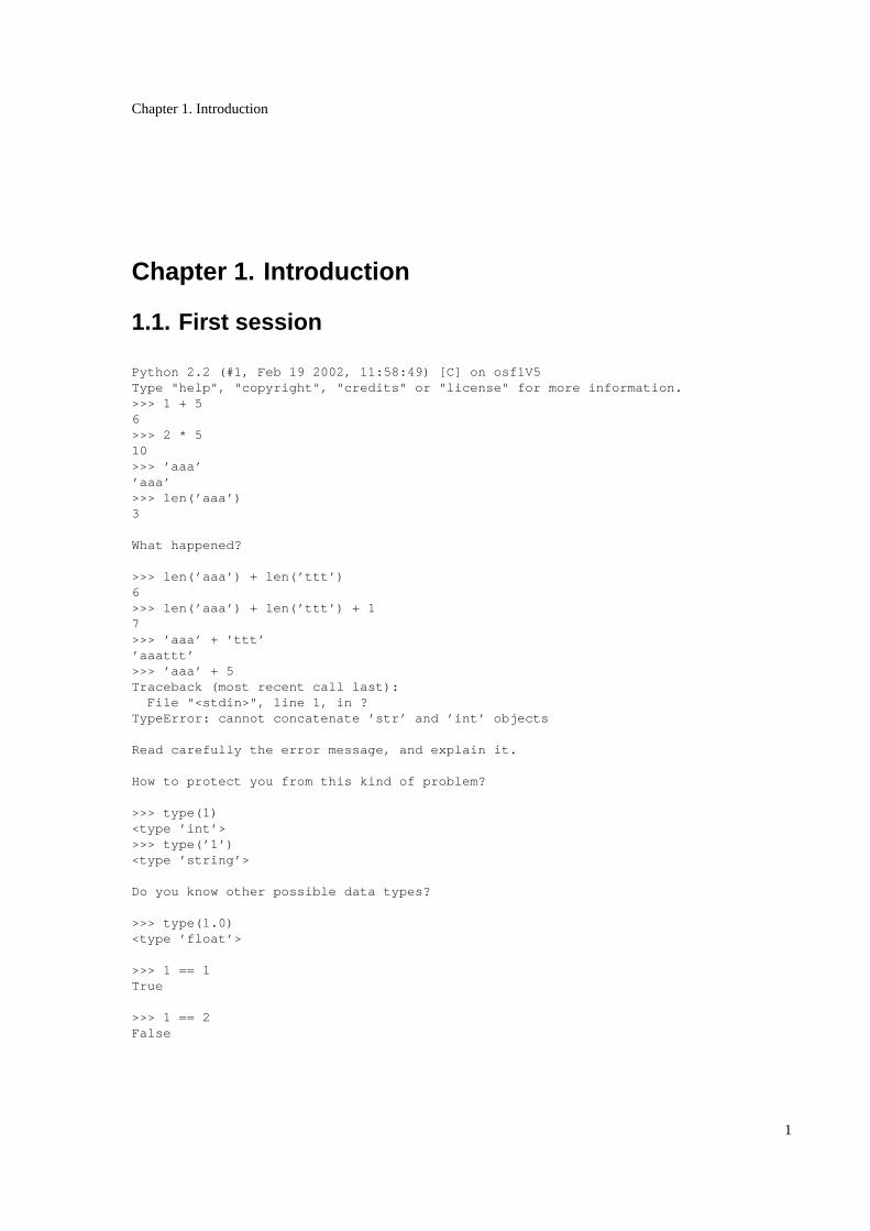
1.1. First session
Python 2.2 (#1, Feb 19 2002, 11:58:49) [C] on osf1V5Type "help", "copyright", "credits" or "license" for more information.>>> 1 + 56>>> 2 * 510>>> ’aaa’’aaa’>>> len(’aaa’)3
What happened?
>>> len(’aaa’) + len(’ttt’)6>>> len(’aaa’) + len(’ttt’) + 17>>> ’aaa’ + ’ttt’’aaattt’>>> ’aaa’ + 5Traceback (most recent call last):
File "<stdin>", line 1, in ?TypeError: cannot concatenate ’str’ and ’int’ objects
Read carefully the error message, and explain it.
How to protect you from this kind of problem?
>>> type(1)<type ’int’>>>> type(’1’)<type ’string’>
Do you know other possible data types?
>>> type(1.0)<type ’float’>
>>> 1 == 1True
>>> 1 == 2False
1

Chapter 1. Introduction
You can associate a name to a value:
>>> a = 3>>> a3
The interpreter displays 3 instead of a.
>>> a = 2>>> a2>>> a * 510>>> b = a * 5>>> b10>>> a = 1>>> b10
Why hasn’t b changed?
What is the difference between:>>> b = a * 5and:>>> b = 5?
>>> a = 1 in this case a is a number>>> a + 23>>> a = ’1’ in this case a is a string>>> a + 1
Traceback (most recent call last):File "<stdin>", line 1, in ?
TypeError: cannot add type "int" to string
What do you conclude about the type of a variable?
Some magical stuff, that will be explained later:
>>> from string import *
We can also perform calculus on strings:
>>> codon=’atg’>>> codon * 3’atgatgatg’>>> seq1 = ’agcgccttgaattcggcaccaggcaaatctcaaggagaagttccggggagaaggtgaaga’>>> seq2 = ’cggggagtggggagttgagtcgcaagatgagcgagcggatgtccactatgagcgataata’
2
Chapter 1. Introduction
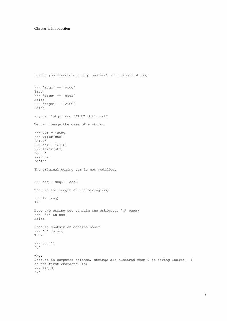
How do you concatenate seq1 and seq2 in a single string?
>>> ’atgc’ == ’atgc’True>>> ’atgc’ == ’gcta’False>>> ’atgc’ == ’ATGC’False
why are ’atgc’ and ’ATGC’ different?
We can change the case of a string:
>>> str = ’atgc’>>> upper(str)’ATGC’>>> str = ’GATC’>>> lower(str)’gatc’>>> str’GATC’
The original string str is not modified.
>>> seq = seq1 + seq2
What is the length of the string seq?
>>> len(seq)120
Does the string seq contain the ambiguous ’n’ base?>>> ’n’ in seqFalse
Does it contain an adenine base?>>> ’a’ in seqTrue
>>> seq[1]’g’
Why?Because in computer science, strings are numbered from 0 to string length - 1so the first character is:>>> seq[0]’a’
3
Chapter 1. Introduction
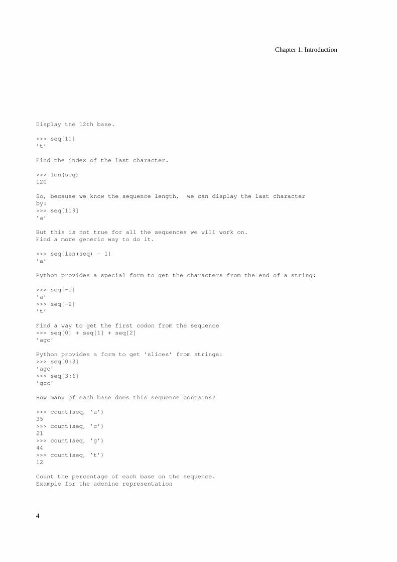
Display the 12th base.
>>> seq[11]’t’
Find the index of the last character.
>>> len(seq)120
So, because we know the sequence length, we can display the last characterby:>>> seq[119]’a’
But this is not true for all the sequences we will work on.Find a more generic way to do it.
>>> seq[len(seq) - 1]’a’
Python provides a special form to get the characters from the end of a string:
>>> seq[-1]’a’>>> seq[-2]’t’
Find a way to get the first codon from the sequence>>> seq[0] + seq[1] + seq[2]’agc’
Python provides a form to get ’slices’ from strings:>>> seq[0:3]’agc’>>> seq[3:6]’gcc’
How many of each base does this sequence contains?
>>> count(seq, ’a’)35>>> count(seq, ’c’)21>>> count(seq, ’g’)44>>> count(seq, ’t’)12
Count the percentage of each base on the sequence.Example for the adenine representation
4
Chapter 1. Introduction
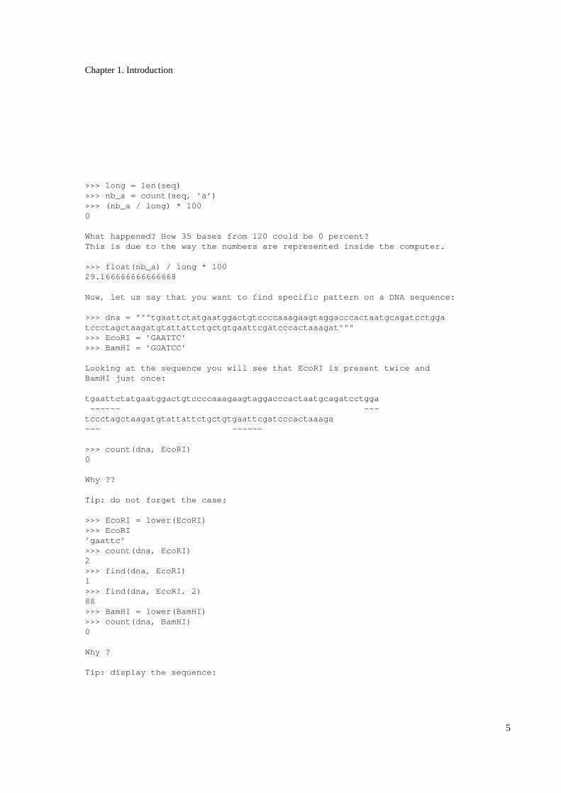
>>> long = len(seq)>>> nb_a = count(seq, ’a’)>>> (nb_a / long) * 1000
What happened? How 35 bases from 120 could be 0 percent?This is due to the way the numbers are represented inside the computer.
>>> float(nb_a) / long * 10029.166666666666668
Now, let us say that you want to find specific pattern on a DNA sequence:
>>> dna = """tgaattctatgaatggactgtccccaaagaagtaggacccactaatgcagatcctggatccctagctaagatgtattattctgctgtgaattcgatcccactaaagat""">>> EcoRI = ’GAATTC’>>> BamHI = ’GGATCC’
Looking at the sequence you will see that EcoRI is present twice andBamHI just once:
tgaattctatgaatggactgtccccaaagaagtaggacccactaatgcagatcctgga~~~~~~ ~~~
tccctagctaagatgtattattctgctgtgaattcgatcccactaaaga~~~ ~~~~~~
>>> count(dna, EcoRI)0
Why ??
Tip: do not forget the case:
>>> EcoRI = lower(EcoRI)>>> EcoRI’gaattc’>>> count(dna, EcoRI)2>>> find(dna, EcoRI)1>>> find(dna, EcoRI, 2)88>>> BamHI = lower(BamHI)>>> count(dna, BamHI)0
Why ?
Tip: display the sequence:
5
Chapter 1. Introduction
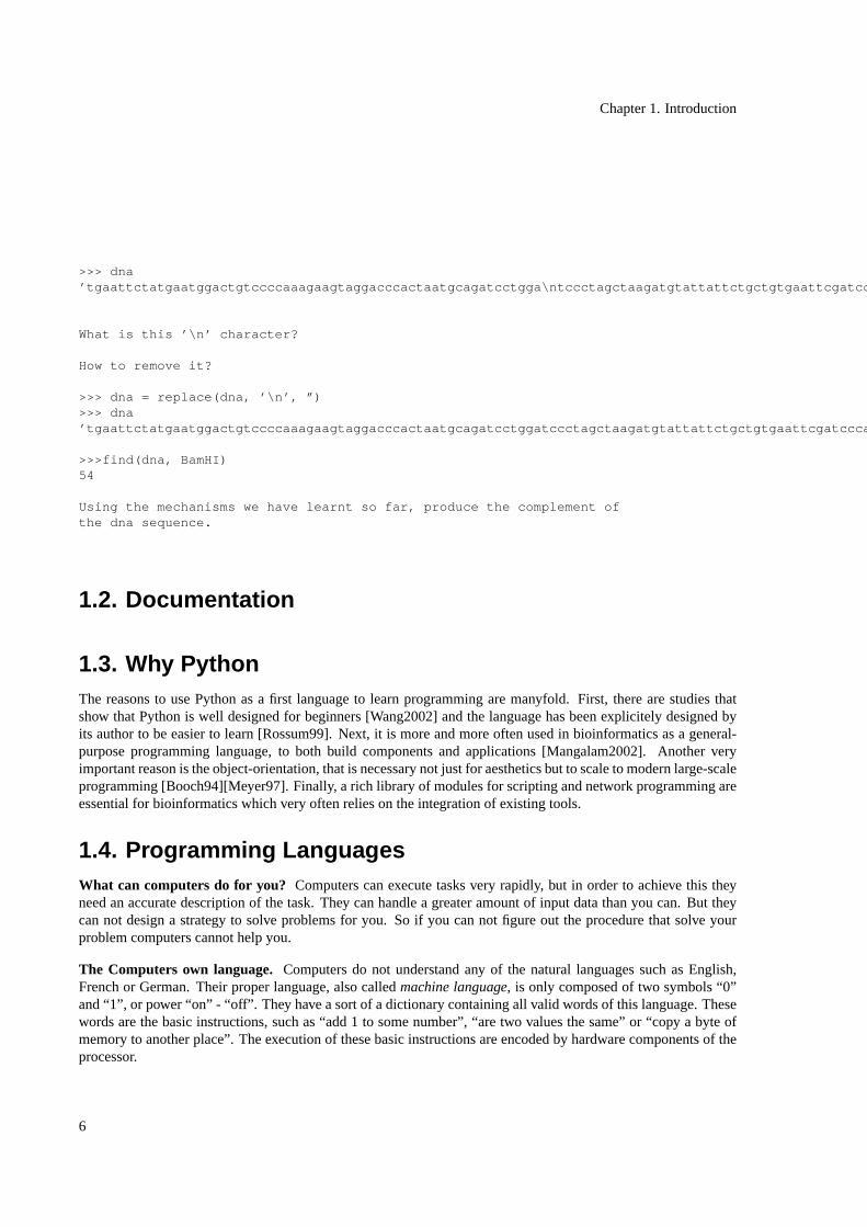
>>> dna’tgaattctatgaatggactgtccccaaagaagtaggacccactaatgcagatcctgga\ntccctagctaagatgtattattctgctgtgaattcgatcccactaaagat’
What is this ’\n’ character?
How to remove it?
>>> dna = replace(dna, ’\n’, ”)>>> dna’tgaattctatgaatggactgtccccaaagaagtaggacccactaatgcagatcctggatccctagctaagatgtattattctgctgtgaattcgatcccactaaagat’
>>>find(dna, BamHI)54
Using the mechanisms we have learnt so far, produce the complement ofthe dna sequence.
1.2. Documentation
1.3. Why PythonThe reasons to use Python as a first language to learn programming are manyfold. First, there are studies thatshow that Python is well designed for beginners [Wang2002] and the language has been explicitely designed byits author to be easier to learn [Rossum99]. Next, it is more and more often used in bioinformatics as a general-purpose programming language, to both build components and applications [Mangalam2002]. Another veryimportant reason is the object-orientation, that is necessary not just for aesthetics but to scale to modern large-scaleprogramming [Booch94][Meyer97]. Finally, a rich library of modules for scripting and network programming areessential for bioinformatics which very often relies on the integration of existing tools.
1.4. Programming LanguagesWhat can computers do for you? Computers can execute tasks very rapidly, but in order to achieve this theyneed an accurate description of the task. They can handle a greater amount of input data than you can. But theycan not design a strategy to solve problems for you. So if you can not figure out the procedure that solve yourproblem computers cannot help you.
The Computers own language. Computers do not understand any of the natural languages such as English,French or German. Their proper language, also calledmachine language, is only composed of two symbols “0”and “1”, or power “on” - “off”. They have a sort of a dictionary containing all valid words of this language. Thesewords are the basic instructions, such as “add 1 to some number”, “are two values the same” or “copy a byte ofmemory to another place”. The execution of these basic instructions are encoded by hardware components of theprocessor.
6

Chapter 1. Introduction
Programming languages. Programming languages belongs to the group offormal languages. Some otherexamples offormal languagesare the system of mathematical expressions or the languages chemists use todescribe molecules. They have been invented as intermediate abstraction level between humans and computers.
Why do not use natural languages as programming languages?Programming languagesare design to preventproblems occurring withnatural language.
Ambiguity Natural languages are full of ambiguities and we need the context of a word in order tochoose the appropriate meaning. “minute” for example is used as a unit of time as a noun,but means tiny as adjective: only the context would distinguish the meaning.
Redundancy Natural languages are full of redundancy helping to solve ambiguity problems and tominimize misunderstandings. When you say “We are playing tennis at the moment.”, “atthe moment” is not really necessary but underlines that it is happening now.
Literacy Natural languages are full of idioms and metaphors. The most popular in English isprobably “It rains cats and dogs.”. Besides, this can be very complicated even if you speaka foreign language very well.
Programming languagesare foreign languages for computers. Therefore you need a program that translates yoursource codeinto themachine language. Programming languagesare voluntarily unambiguous, nearly contextfree and non-redundant, in order to prevent errors in the translation process.
History of programming languages. It is instructive to try to communicate with a computer in its own language.This let you learn a lot about how processors work. However, in order to do this, you will have to manipulate only0’s and 1’s. You will need a good memory, but probably you would never try to write a program solving real worldproblems at this basic level ofmachine code.
Because humans have difficulties to understand, analyze and extract informations of sequences of zeros and ones,they have written a language calledAssemblerthat maps the instruction words to synonyms that give an idea ofwhat the instruction does, so for instance0001becameadd. Assemblerincreased the legibility of the code, butthe instruction set remained basic and depended on the hardware of the computer.
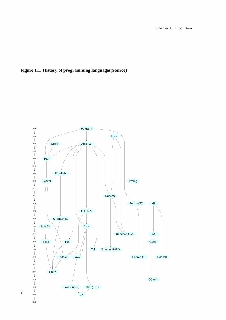
In order to write algorithms for solving more complex problems, there was a need for machine independenthigherlevel programming languageswith a more elaborated instruction set than thelow levelAssembler. The first oneswereFortran andC and a lot more have been invented right now. A short history of a subset of programminglanguages is shown in Figure 1.1.
7
Chapter 1. Introduction
Figure 1.1. History of programming languages(Source)
1956
1958
1960
1962
1964
1966
1968
1970
1972
1974
1976
1978
1980
1982
1984
1986
1988
1990
1992
1994
1996
1998
2000
2002
Smalltalk 80
Ruby
SML
Caml
OCaml
Perl
Fortran I
PL/I
Algol 60
Fortran 77
Scheme
Scheme R4RS
Common Lisp
Pascal
HaskellFortran 90
Prolog
Cobol
Smalltalk
C (K&R)
Tcl
C++
Java
Java 2 (v1.2)
Python
C#
Lisp
Ada 83
Eiffel
C++ (ISO)
ML
8

Chapter 2. Variables
Chapter 2. Variables
2.1. Data, values and types of valuesIn the first session we have explored some basic issues about a DNA sequence. The specific DNA sequence’atcgat’ was one of our data. For computer scientists this is also avalue. During the program executionvaluesare represented in the memory of the computer. In order to interpret these representations correctlyvalueshave atype.
Type
Typesaresetsof data orvaluessharing some specific properties and their associated operations.
We have modeled the DNA sequence, out of habit, as astring. 1 Strings are one of the basic types that Python canhandle. In the gc calculation we have seen two other ones:integersandfloats. If you are not sure what sort of datayou are working with, you can ask Python about it.
>>> type(’atcgat’)<type ’str’>>>> type(1)<type ’int’>>>> type(’1’)<type ’str’>
2.2. Variables or naming valuesIf you need avaluemore than once or you need the result of a calculation later, you have to give it a name toremember it. Computer scientists also saybinding a value to a nameor assign a value to a variable.
Binding
Binding is the process ofnamingavalue.
Variable
Variablesarenamesbound tovalues. You can also say that avariable is anamethat refers to avalue.
>>> EcoRI = ’GAATTC’
For Python the model is important because it knows nothing about DNA but it knows a lot about strings.
9
Chapter 2. Variables
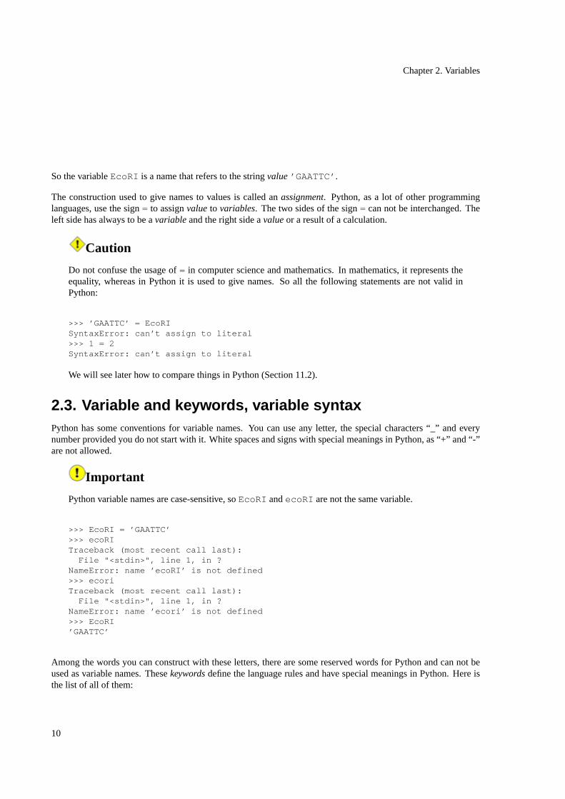
So the variableEcoRI is a name that refers to the stringvalue’GAATTC’ .
The construction used to give names to values is called anassignment. Python, as a lot of other programminglanguages, use the sign= to assignvalueto variables. The two sides of the sign= can not be interchanged. Theleft side has always to be avariableand the right side avalueor a result of a calculation.
Caution
Do not confuse the usage of= in computer science and mathematics. In mathematics, it represents theequality, whereas in Python it is used to give names. So all the following statements are not valid inPython:
>>> ’GAATTC’ = EcoRISyntaxError: can’t assign to literal>>> 1 = 2SyntaxError: can’t assign to literal
We will see later how to compare things in Python (Section 11.2).
2.3. Variable and keywords, variable syntaxPython has some conventions for variable names. You can use any letter, the special characters “_” and everynumber provided you do not start with it. White spaces and signs with special meanings in Python, as “+” and “-”are not allowed.
Important
Python variable names are case-sensitive, soEcoRI andecoRI are not the same variable.
>>> EcoRI = ’GAATTC’>>> ecoRITraceback (most recent call last):
File "<stdin>", line 1, in ?NameError: name ’ecoRI’ is not defined>>> ecoriTraceback (most recent call last):
File "<stdin>", line 1, in ?NameError: name ’ecori’ is not defined>>> EcoRI’GAATTC’
Among the words you can construct with these letters, there are some reserved words for Python and can not beused as variable names. Thesekeywordsdefine the language rules and have special meanings in Python. Here isthe list of all of them:
10

Chapter 2. Variables
and assert break class continue def del elifelse except exec finally for from global ifimport in is lambda not or pass printraise return try while yield
2.4. Namespaces or representing variablesHow does Python find the value referenced by a variable? Python storesbindingsin aNamespace.
Namespace
A namespaceis a mapping of variable names to their values.
You can also think about anamespaceas a sort ofdictionary containing all defined variable names and thecorresponding reference to their values.
Reference
A referenceis a sort of pointer to a location in memory.
Therefore you do not have to know where exactly your value can be found in memory, Python handles this for youvia variables.
Figure 2.1. Namespace
EcoRI
gc
’GAATTC’
0.546
Memory space
105
Namespace
Figure 2.1 shows a representation of some namespace.Valueswhich have not been referenced by avariable, arenot accessible to you, because you can not access the memory space directly. So if a result of a calculation isreturned, you can use it directly and forget about it after that. Or you can create a variable holding this value andthen access this value via the variable as often as you want.
>>> from string import *
11
Chapter 2. Variables
>>> cds = """atgagtgaacgtctgagcattaccccgctggggccgtatatcggcgcacaaatttcgggtgccgacctgacgcgcccgttaagcgataatcagtttgaacagctttaccatgcggtgctgcgccatcaggtggtgtttctacgcgatcaagctattacgccgcagcagcaacgcgcgctggcccagcgttttggcgaattgcatattcaccctgtttacccgcatgccgaaggggttgacgagatcatcgtgctggatacccataacgataatccgccagataacgacaactggcataccgatgtgacatttattgaaacgccacccgcaggggcgattctggcagctaaagagttaccttcgaccggcggtgatacgctctggaccagcggtattgcggcctatgaggcgctctctgttcccttccgccagctgctgagtgggctgcgtgcggagcatgatttccgtaaatcgttcccggaatacaaataccgcaaaaccgaggaggaacatcaacgctggcgcgaggcggtcgcgaaaaacccgccgttgctacatccggtggtgcgaacgcatccggtgagcggtaaacaggcgctgtttgtgaatgaaggctttactacgcgaattgttgatgtgagcgagaaagagagcgaagccttgttaagttttttgtttgcccatatcaccaaaccggagtttcaggtgcgctggcgctggcaaccaaatgatattgcgatttgggataaccgcgtgacccagcactatgccaatgccgattacctgccacagcgacggataatgcatcgggcgacgatccttggggataaaccgttttatcgggcggggtaa""".replace("\n","")
>>> float(count(cds, ’G’) + count(cds, ’C’))/ len(cds)0.54460093896713613
Here the result of the gc-calculation is lost.
>>> gc = float(count(cds, ’G’) + count(cds, ’C’))/ len(cds)>>> gc0.54460093896713613
In this example you can remember the result of the gc calculation, because it is stored in the variablegc .
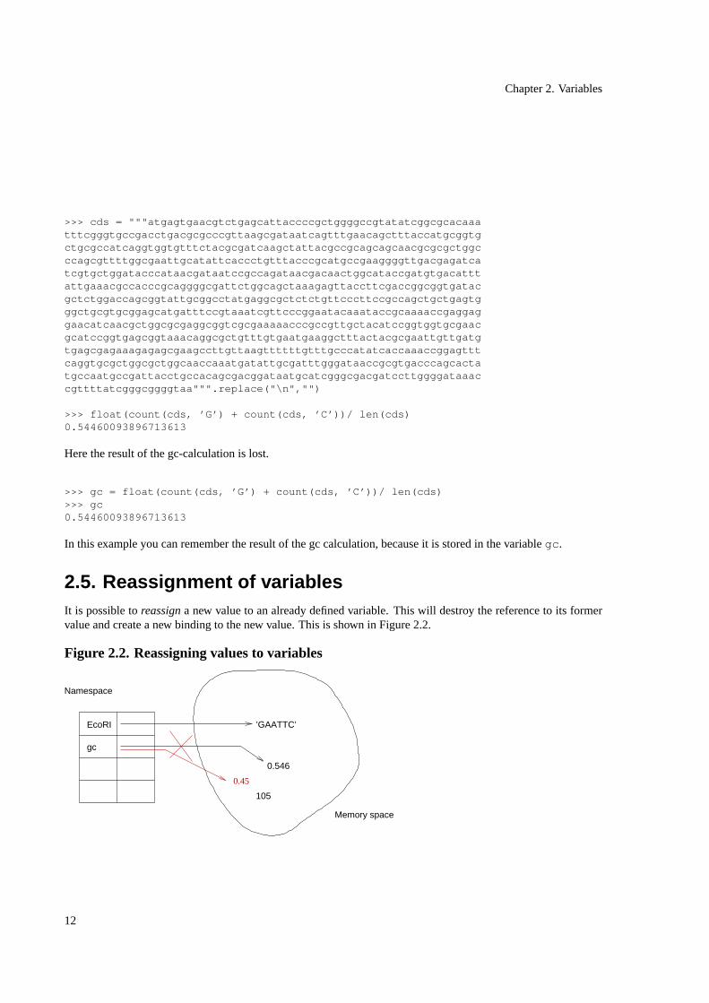
2.5. Reassignment of variablesIt is possible toreassigna new value to an already defined variable. This will destroy the reference to its formervalue and create a new binding to the new value. This is shown in Figure 2.2.
Figure 2.2. Reassigning values to variables
EcoRI
gc
’GAATTC’
0.546
Memory space
105
0.45
Namespace
12
Chapter 2. Variables
Note
In Python, it is possible to reassign a new value with a different type to a variable. This is calleddynamictyping, because the type of the variable is assigned dynamically. Note that this is not the case in allprogramming languages. Sometimes, as inC, the type of variables is assigned statically and has to bedeclared before use. This is some way more secure because types of variables can be checked only byexamining the source code, whereas that is not possible if variables are dynamically typed.
13

Chapter 2. Variables
14
Chapter 3. Statements, expressions and functions
Chapter 3. Statements, expressions and functions
3.1. StatementsIn our first practical lesson, the first thing we did, was the invocation of the Python interpreter. During the firstsession we enteredstatementsthat were read, analyzed and executed by the interpreter.
Statement
Statementsare instructionsor commands that the Python interpreter can execute. Each statement is read by theinterpreter, analyzed and then executed.
3.2. Sequences or chaining statements
Program
A programis asequenceof statements that can by executed by the Python interpreter.
Sequence
Sequencingis a simpleprogramming featurethat allows to chain instructions that will be executed one by onefrom top to bottom.
Later we are going to learn more complicated ways to control the flow of a program, such asbranchingandrepetition.
3.3. Functions
Function
Functionsarenamed sequencesof statements that execute some task.
We have already used functions, such as:
>>> type(’GAATTC’)<type ’str’>>>> len(cds)852
For examplelen is a function that calculates the length of things and we asked here for the length of our DNAsequencecds .
15

Chapter 3. Statements, expressions and functions
Function call
Function callsare statements that execute orcall a function. The Python syntax offunction callsis thefunctionnamefollowed by a comma separated list ofargumentsinclosed into parentheses. Even if a function does not takeany argument the parentheses are necessary.
Differences between function calls and variables.As variable names, function namesare stored in a namespacewith a reference to their corresponding sequence of statements. When they are called, their name is searched in thenamespace and the reference to their sequence of statements is returned. The procedure is the same as for variablenames. But unlike them, the following parentheses indicate that the returned value is a sequence of statements thathas to be executed. That’s why they are even necessary for functions which are called without arguments.
Arguments of functions
Argumentsarevaluesprovided to a function when the function is called. We will see more about them soon.
3.4. Operations
Operations and Operators
Operationsare “basic”functionswith their own syntax.
They have a specialOperator(a sign or a word) that is the same as a function name.Unary Operators, operationswhich take one argument, are followed by their argument, andsecondary operatorsare surrounded by their twoarguments.
Here are some examples:
>>> ’GTnnAC’ + ’GAATTC’’GTnnACGAATTC’>>> ’GAATTC’ * 3’GAATTCGAATTCGAATTC’>>> ’n’ in ’GTnnAC’1
This is only a simpler way of writing these functions provided by Python, because humans are in general morefamiliar with this syntax closely related to the mathematical formal language.
3.5. Composition and Evaluation of Expressions
Composition and Expression
Compositionis a way to combine functions. The combination is also called anExpression.
16

Chapter 3. Statements, expressions and functions
We have already used it. Here is the most complex example we have seen so far:
>>> float(count(cds, ’G’) + count(cds, ’C’)) / len(cds)0.54460093896713613
What is happening when thisexpressionis executed? The first thing to say is that it is a mixed expressionof operations and function calls. Let’s start with the function calls. If a function is called with an argumentrepresenting a composed expression, this one is executed first and the result value is passed to the calling function.So thecds variable is evaluated, which returns the value that it refers to. This value is passed to thelen functionwhich returns the length of this value. The same happens for thefloat function. The operationcount(cds,’G’) + count(cds, ’C’) is evaluated first, and the result is passed as argument tofloat .
Let’s continue with the operations. There is a precedence list, shown in Table 3.1, for all operators, whichdetermines what to execute first if there are no parentheses, otherwise it is the same as for function calls. So,for the operationcount(cds, ’G’) + count(cds, ’C’) the twocount functions are executed first onthe value of thecds variable and “G” and “C” respectively. And the two counts are added. The result value ofthe addition is then passed as argument to thefloat function followed by the division of the results of the twofunctionsfloat andlen .
Table 3.1. Order of operator evaluation (highest to lowest)
Operator Name+x, -x, ~x Unary operatorsx ** y Power (right associative)x * y, x / y,x % y Multiplication, division, modulox + y, x - y Addition, subtractionx << y, x >> y Bit shiftingx & y Bitwise andx | y Bitwise orx < y, x <= y, x > y, x >= y, x == y,x != y, x <> y, x is y, x is not y, xin s, x not in s<
Comparison, identity, sequence membership tests
not x Logical negationx and y Logical andlambda args: expr Anonymous function
So, as in mathematics, the innermost function or operation is evaluated first and the result is passed as argumentto the enclosing function or operation. It is important to notice thatvariablesare evaluated and only theirvaluesare passed as argument to the function. We will have a closer look at this when we talk about function definitionsin Section 8.1.
Exercise 3.1. Composition
Have a look at this example. Can you explain what happens? If you can’t please read this section once again.
17

Chapter 3. Statements, expressions and functions
>>> from string import *>>> replace(replace(replace(cds, ’A’, ’a’), ’T’, ’A’), ’a’, ’T’)
18

Chapter 4. Communication with outside
Chapter 4. Communication with outside
4.1. OutputWe saw in the previous chapter how to export information outside of the program using theprint statement.Let’s give a little bit more details of its use here.
The print statements can be followed by a variable number of values separated by commas. Without a valueprint puts only a newline character on thestandard output, generally the screen. If values are provided, theyare transformed into strings, and then are written in the given order, separated by a space character. The line isterminated by a newline character. You can suppress the final newline character by adding a comma at the end ofthe list. The following example illustrates all these possibilities:
#! /usr/local/bin/python
from string import *
dna = "ATGCAGTGCATAAGTTGAGATTAGAGACCCGACAGTA"
gc = float(count(dna, ’G’) + count(dna, ’C’))/ len(dna)
print gc
print "the gc percentage of dna:", dna, "is:", gcprintprint "the gc percentage of dna:", dnaprint " is:", gcprintprint "the gc percentage of dna:", dna,print "is:", gc
producing the following output:
caroline:~> python print_gc.2.py0.432432432432the gc percentage of dna: ATGCAGTGCATAAGTTGAGATTAGAGACCCGACAGTA is: 0.432432432432
the gc percentage of dna: ATGCAGTGCATAAGTTGAGATTAGAGACCCGACAGTAis: 0.432432432432
the gc percentage of dna: ATGCAGTGCATAAGTTGAGATTAGAGACCCGACAGTA is: 0.432432432432caroline:~>
4.2. Formatting strings
19

Chapter 4. Communication with outside
Important
All data printed on the screen have to be character data. But values can have different types. Thereforethey have to be transformed into strings beforehand. This transformation is handled by theprintstatement.
It is possible to control this transformation when a specific format is needed. In the examples above, the floatvalue of the gc calculation is written with lots of digits following the dot which are not very significant. The nextexample shows a more reasonable output:
>>> print "%.3f" % gc0.432>>> print "%3.1f %%" % (gc*100)43.2 %>>> print "the gc percentage of dna: %10s... is: %4.1f %%." % (dna, gc*100)the gc percentage of dna: ATGCAGTGCA... is: 43.2 %
Figure 4.1 shows how to interpret the example above. The%(modulo) operator can be used to format strings. Itis preceded by the formatting template and followed by a comma separated list of values enclosed in parentheses.These values replace the formatting place holders in the template string. A place holder starts with a % followedby some modifiers and a character indicating the type of the value. There has to be the same number of values andplace holders.
20

Chapter 4. Communication with outside
Figure 4.1. Interpretation of formatting templates
(gc*100)
indicates thata format follows
f. 13%
the type of theletter indicating
value to formatnumber of digitsfollowing the
dotof digitstotal number
print "%3.1f %%" %>>>
43.2 %
formatting stringvalues that will replace the placholders
followed by a tuple offormating string andpreceeded by thepercent operator
by parenthesesby commas and enclosed they have to be separated if there are more than oneformat placeholdervalues replacing the
Table 4.1 provides the characters that you can use in the formatting template and Table 4.2 gives the modifiers ofthe formatting character.
Important
Remember that the type of a formatting result is a string and no more the type of the input value.
>>> "%.1f" % (gc*100)’43.2’>>> res = "%.1f" % (gc*100)>>> at = 100 - resTraceback (most recent call last):
File "<stdin>", line 1, in ?TypeError: unsupported operand type(s) for -: ’int’ and ’str’>>> res’43.2’
Table 4.1. String formatting: Conversion characters
Formatting character Output Example Result
21

Chapter 4. Communication with outside
d,i decimal or long integer "%d" % 10 ’10’o,x octal/hexadecimal integer"%o" % 10 ’12’f,e,E normal, ’E’ notation of
floating point numbers"%e" % 10.0 ’1.000000e+01’
s strings or any object thathas astr() method
"%s" % [1, 2, 3] ’[1, 2, 3]’
r string, use therepr()function of the object
"%r" % [1, 2, 3] ’[1, 2, 3]’
% literal %
Table 4.2. String formatting: Modifiers
Modifier Action Example Resultname in parentheses selects the key name in a
mapping object"%(num)d %(str)s"% { ’num’:1,’str’:’dna’}
’1 dna’
-,+ left, right alignment "%-10s" % "dna" ’dna_______’0 zero filled string "%04i" % 10 ’0010’number minimum field width "%10s" % "dna" ’_______dna’. number precision "%4.2f" % 10.1 ’10.10’
4.3. InputAs you can print results on the screen, you can read data from the keyboard which is the standard input device.Python provides theraw_input function for that, which is used as follows:
>>> nb = raw_input("Enter a number, please:")Enter a number, please:12
The prompt argument is optional and the input has to be terminated by a return.
Important
raw_input always returns a string, even if you entered a number. Therefore you have to convertthe string input by yourself into whatever you need. Table 4.3 gives an overview of all possible typeconversion function.
>>> nb’12’>>> type(nb)<type ’str’>>>> nb = int(nb)
22
Chapter 4. Communication with outside
>>> nb12>>> type(nb)<type ’int’>
Notice that a user can enter whatever he wants. So, the input is probably not what you want, and the typeconversion can therefore fail. It is careful to test before converting input strings.
>>> nb = raw_input("Please enter a number:")Please enter a number:toto>>> nb’toto’>>> int(nb)Traceback (most recent call last):
File "<stdin>", line 1, in ?ValueError: invalid literal for int(): toto
The following function controls the input:
def read_number():while 1:
nb = raw_input("Please enter a number:")try:
nbconv = int(nb)except:
print nb, "is not a number."continue
else:break
return nb
and produces the following output:
>>> read_number()Please enter a number:totototo is not a number.Please enter a number:12’12’
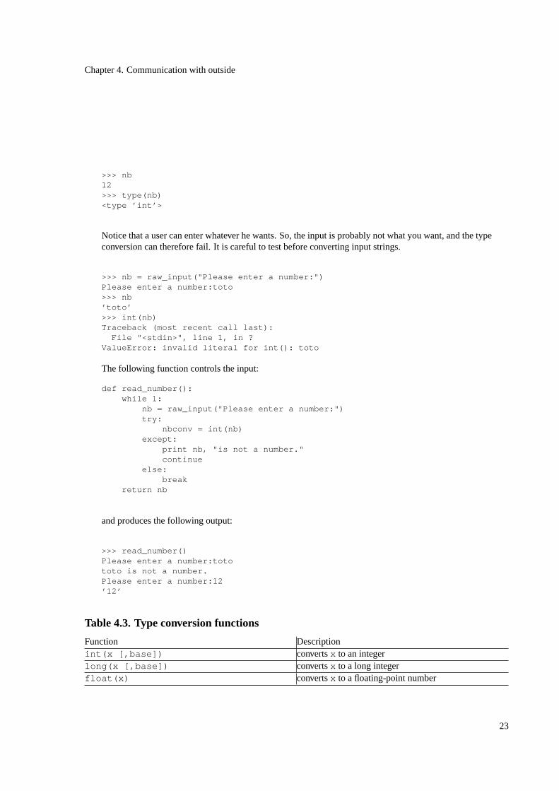
Table 4.3. Type conversion functions
Function Descriptionint(x [,base]) convertsx to an integerlong(x [,base]) convertsx to a long integerfloat(x) convertsx to a floating-point number
23

Chapter 4. Communication with outside
complex(real [,imag]) creates a complex numberstr(x) convertsx to a string representationrepr(x) convertsx to an expression stringeval(str) evaluatesstr and returns an objecttuple(s) converts a sequence object to a tuplelist(s) converts a sequence object to a listchr(x) converts an integer to a characterunichr(x) converts an integer to a Unicode characterord(c) converts a character to its integer valuehex(x) converts an integer to a hexadecimal stringoct(x) converts an integer to an octal string
24
Chapter 5. Program execution
Chapter 5. Program execution
5.1. Executing code from a fileUntil now we have only workedinteractivelyduring aninterpreter session. But each time we leave our session alldefinitions made are lost, and we have to re-enter them again in the next session of the interpreter whenever weneed them. This is not very convenient. To avoid that, you can put your code in a file and then pass the file to thePython interpreter. Here is an example:
Example 5.1. Executing code from a file
Take the code for the cds translation as example and put it in a file namedgc.py :
from string import *
cds = """atgagtgaacgtctgagcattaccccgctggggccgtatatcggcgcacaaatttcgggtgccgacctgacgcgcccgttaagcgataatcagtttgaacagctttaccatgcggtgctgcgccatcaggtggtgtttctacgcgatcaagctattacgccgcagcagcaacgcgcgctggcccagcgttttggcgaattgcatattcaccctgtttacccgcatgccgaaggggttgacgagatcatcgtgctggatacccataacgataatccgccagataacgacaactggcataccgatgtgacatttattgaaacgccacccgcaggggcgattctggcagctaaagagttaccttcgaccggcggtgatacgctctggaccagcggtattgcggcctatgaggcgctctctgttcccttccgccagctgctgagtgggctgcgtgcggagcatgatttccgtaaatcgttcccggaatacaaataccgcaaaaccgaggaggaacatcaacgctggcgcgaggcggtcgcgaaaaacccgccgttgctacatccggtggtgcgaacgcatccggtgagcggtaaacaggcgctgtttgtgaatgaaggctttactacgcgaattgttgatgtgagcgagaaagagagcgaagccttgttaagttttttgtttgcccatatcaccaaaccggagtttcaggtgcgctggcgctggcaaccaaatgatattgcgatttgggataaccgcgtgacccagcactatgccaatgccgattacctgccacagcgacggataatgcatcgggcgacgatccttggggataaaccgttttatcgggcggggtaa""".replace("\n","")
gc = float(count(cds, ’g’) + count(cds, ’c’))/ len(cds)
print gc
and now pass this file to the interpreter:
caroline:~/python_cours> python gc.py0.54460093896713613
❶ Theprint statement is used to write a message on the screen. We will have a closer look at this statementlater (Section 4.1).
25
Chapter 5. Program execution
Tip
You can name your file as you like. However, there is a convention for files containing python code tohave apy extension.
You can also make your file executable if you put the following line at the beginning of your file, indicating thatthis file has to be executed with thePython interpreter:
#! /usr/local/bin/python
(Don’t forget to set thex execution bit under UNIX system.) Now you can execute your file:
caroline:~/python_cours> ./gc.py0.54460093896713613
This will automatically call thePython interpreter and execute all the code in your file.
You can also load the code of a file in a interactive interpreter session with the-i option:
caroline:~/python_cours> python -i gc.py0.54460093896713613>>>
This will start the interpreter, execute all the code in your file and than give you aPython prompt to continue:
>>> cds’atgagtgaacgtctgagcattaccccgctggggccgtatatcggcgcacaaatttcgggtgccgacctgacgcgcccgttaagcgataatcagtttgaacagctttaccatgcggtgctgcgccatcaggtggtgtttctacgcgatcaagctattacgccgcagcagcaacgcgcgctggcccagcgttttggcgaattgcatattcaccctgtttacccgcatgccgaaggggttgacgagatcatcgtgctggatacccataacgataatccgccagataacgacaactggcataccgatgtgacatttattgaaacgccacccgcaggggcgattctggcagctaaagagttaccttcgaccggcggtgatacgctctggaccagcggtattgcggcctatgaggcgctctctgttcccttccgccagctgctgagtgggctgcgtgcggagcatgatttccgtaaatcgttcccggaatacaaataccgcaaaaccgaggaggaacatcaacgctggcgcgaggcggtcgcgaaaaacccgccgttgctacatccggtggtgcgaacgcatccggtgagcggtaaacaggcgctgtttgtgaatgaaggctttactacgcgaattgttgatgtgagcgagaaagagagcgaagccttgttaagttttttgtttgcccatatcaccaaaccggagtttcaggtgcgctggcgctggcaaccaaatgatattgcgatttgggataaccgcgtgacccagcactatgccaatgccgattacctgccacagcgacggataatgcatcgggcgacgatccttggggataaaccgttttatcgggcggggtaa’
>>>cds="atgagtgaacgtctgagcattaccccgctggggccgtatatcggcgcacaaatttcgggtgccgacctgacgcgcccgtt"
>>>cds’atgagtgaacgtctgagcattaccccgctggggccgtatatcggcgcacaaatttcgggtgccgacctgacgcgcccgtt’>>>gc0.54460093896713613
Important
It is important to remember that thePython interpreter executes codefrom top to bottom, this is also truefor code in a file. So, pay attention todefinethings before youusethem.
26
Chapter 5. Program execution
Exercise 5.1. Execute code from a file
Take all expressions that we have written so far and put them in a file.
Important
Notice that you have to ask explicitly for printing a result when you execute some code from a file, whilean interactiveinterpreter session the result of the execution of a statement is printed automatically. So toview the result of thetranslate function in the code above, theprint statement is necessary in thefile version, whereas during aninteractiveinterpreter session we have never written it.
5.2. Interpreter and CompilerLet’s introduce at this point some concepts ofexecutionof programs written inhigh level programming languages.As we have already seen, the only language that a computer can understand is the so calledmachine language.These languages are composed of a set of basic operations whose execution is implemented in the hardware ofthe processor. We have also seen that high level programming languages provide a machine-independent levelof abstraction that is higher than the machine language. Therefore, they are more adapted to a human-machineinteraction. But this also implies that there is a sort of translator between the high level programming languageand the machine languages. There exists two sorts oftranslators:
Interpreter
An Interpreter is aprogramthat implements or simulates avirtual machineusing the base set of instructions ofaprogramming languageas itsmachine language.
You can also think of anInterpreter as aprogramthat implements a library containing the implementation of thebasic instruction set of aprogramming languagein machine language.
An Interpreter reads the statements of a program, analyzes them and then executes them on the virtual machineor calls the corresponding instructions of the library.
Interactive interpreter session
During aninteractiveinterpreter session the statements are not only read, analyzed and executed but the result oftheevaluation of an expressionis alsoprinted. This is also called aREAD - EVAL - PRINT loop.
Important
Pay attention, theREAD - EVAL - PRINTloop is only entered in aninteractivesession. If you ask theinterpreterto execute code in a file, results of expression evaluationsare notprinted. You have to do thisby yourself.
27

Chapter 5. Program execution
Compiler
A Compiler is a program that translates code of aprogramming languagein machine code, also calledobjectcode. The object code can be executed directly on the machine where it was compiled.
Figure 5.1 compares the usage of interpreters and compilers.
Figure 5.1. Comparison of compiled and interpreted code
Compiler
Interpreter
processorsource code
virtual machine
So using acompilerseparatestranslationandexecutionof a program. In contrast of aninterpretedprogram thesource codeis translated only once.
The object codeis machine-dependentmeaning that thecompiledprogram can only be executed on a machinefor which it has been compiled, whereas aninterpretedprogram is notmachine-dependentbecause themachine-dependentpart is in the interpreter itself.
Figure 5.2 illustrates another concept of program execution that tries to combine the advantage of more effectiveexecution of compiled code and the advantage of machine-independence of interpreted code. This concept is usedby theJAVA programming language for example and in a more subtle way byPython.
28
Chapter 5. Program execution
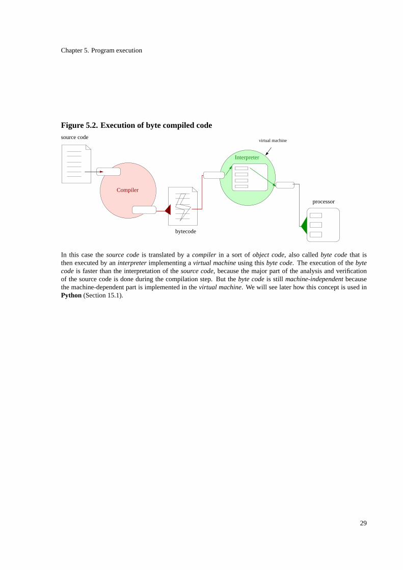
Figure 5.2. Execution of byte compiled codesource code
Compiler
bytecode
Interpreter
virtual machine
processor
In this case thesource codeis translated by acompiler in a sort ofobject code, also calledbyte codethat isthen executed by aninterpreter implementing avirtual machineusing thisbyte code. The execution of thebytecodeis faster than the interpretation of thesource code, because the major part of the analysis and verificationof the source code is done during the compilation step. But thebyte codeis still machine-independentbecausethe machine-dependent part is implemented in thevirtual machine. We will see later how this concept is used inPython (Section 15.1).
29

Chapter 5. Program execution
30
Chapter 6. Strings
Chapter 6. StringsSo far we have seen a lot about strings. Before giving a summary about this data type, let us introduce a newsyntax feature.
6.1. Values as objectsWe have seen thatstringshave avalue. But Pythonvaluesare more than that. They areobjects.
Object
Objectsare things that know more than theirvalues. In particular, you can ask them to perform specialized tasksthat only they can do.
Up to now we have used some special functions handling string data available to us by the up to nowmagicstatementfrom string import * . But stringsthemselves know how to execute all of them and even more.Look at this:
>>> motif = "gaattc">>> motif.upper()’GAATTC’>>> motif’gaattc’>>> motif.isalpha()1>>> motif.count(’n’)0
>>> motif = ’GAATTC_’>>> motif + motif’GAATTC_GAATTC_’>>> motif * 3’GAATTC_GAATTC_GAATTC_’
At the first glance this looks a little bit strange, but you can read the. (dot) operator as: “ask objectmotif to dosomething” as: transformmotif in an uppercase string (upper ), ask whether it contains only letters (isalpha )or count the number of “n” characters.
Objects as namespaces.How does it work? All objects have their own namespace containing all variable andfunction names that are defined for that object. As already describeb in Section 2.4 you can see all names definedfor an object by using thedir function:
>>> dir(motif)[’__add__’, ’__class__’, ’__contains__’, ’__delattr__’, ’__eq__’, ’__ge__’,’__getattribute__’, ’__getitem__’, ’__getslice__’, ’__gt__’, ’__hash__’,’__init__’, ’__le__’, ’__len__’, ’__lt__’, ’__mul__’, ’__ne__’, ’__new__’,
31
Chapter 6. Strings
’__reduce__’, ’__repr__’, ’__rmul__’, ’__setattr__’, ’__str__’, ’capitalize’,’center’, ’count’, ’decode’, ’encode’, ’endswith’, ’expandtabs’, ’find’,
’index’, ’isalnum’, ’isalpha’, ’isdigit’, ’islower’, ’isspace’, ’istitle’,’isupper’, ’join’, ’ljust’, ’lower’, ’lstrip’, ’replace’, ’rfind’, ’rindex’,’rjust’, ’rstrip’, ’split’, ’splitlines’, ’startswith’, ’strip’, ’swapcase’,’title’, ’translate’, ’upper’]
The dot operator is used to access this namespace. It will look up in the namespace of the object for the namefollowing the dot operator.
>>> motif.__class__<type ’str’>>>> motif.replace(’a’, ’A’)’gAAttc’
Variables and functions defined in object namespaces are calledattributesandmethodsof the object.
Attribute
An attribute is avariabledefined in a namespace of an object, which can only be accessed via the object himself.
Method
Methodsarefunctionsdefined in a namespace of anobject.
This is just a little introduction to objects making it possible to use theobject syntaxfor the basic types in Python.We will give further explanation intoobject-oriented programmingin Chapter 17.
6.2. Working with strings
Strings
Stringsare sequences orordered collectionsof characters.
You can write them in Python using quotes, double quotes, triple quotes or triple double quotes. The triple quotenotation permits to write strings spanning multiple lines with keeping any line feed.
>>> ’ATGCA’’ATGCA’>>> "ATGCA"’ATGCA’>>> """ATGATA... AGAGA"""
32

Chapter 6. Strings
’ATGATA\nAGAGA’
The first thing that we would sum up is how to extract characters or substrings . Characters are accessible usingtheir position in the string which has to be enclosed into brackets following the string. The position number canbe positive or negative, which means starting at the beginning or the end of the string. Substrings are extracted byproviding an interval of the start and end position separated by a colon. Both positions are optional which meanseither to start at the beginning of the string or to extract the substring until the end. When accessing characters, itis forbidden to access position that does not exist, whereas during substring extraction, the longest possible stringis extracted.
>>> motif = ’GAATTC’>>> motif[0]’G’>>> motif[-1]’C’
>>> motif[0:3]’GAA’>>> motif[1:3]’AA’>>> motif[:3]’GAA’>>> motif[3:]’TTC’>>> motif[3:6]’TTC’>>> motif[3:-1]’TT’>>> motif[-3:-1]’TT’>>> motif[:]’GAATTC’
>>> motif[100]Traceback (most recent call last):
File "<stdin>", line 1, in ?IndexError: string index out of range>>> motif[3:100]’TTC’>>> motif[3:2]”
Caution
Figure 6.1 compares positive and negative indices. Be careful, forward string indices starts always with0, whereas backward string indices starts with -1.
33

Chapter 6. Strings
Figure 6.1. String indices
EcoRI[1:4] == EcoRI[−5:−2]
G A A T T C0 1 2 3 4 5
−6 −5 −4 −3 −2 −1
motif =
Caution
It is also important to notice that the character at the end position during a substring extraction is neverincluded in the extracted substring.
Warning
Strings are immutable in Python. This means you can neither change characters or substrings. You havealways to create a new copy of the string.
>>> motif[1] = ’n’Traceback (most recent call last):
File "<stdin>", line 1, in ?TypeError: object doesn’t support item assignment
>>> motif[:1] + ’n’ + motif[2:]’GnATTC’
A list of all other methods, function and operators and their action on string objects are summarized in Table 6.1and Table 6.2).
Table 6.1. String methods, operators and builtin functions
Method, Operator, Function Descriptions + t Concatenations * 3 Repetitionlen(s) Returns the length of smin(s), max(s) Returns the “smallest”, “largest” character of s, depend-
ing on their position in the ASCII code
34
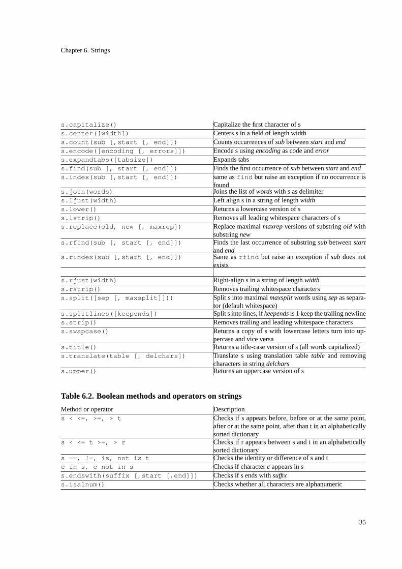
Chapter 6. Strings
s.capitalize() Capitalize the first character of ss.center([width]) Centers s in a field of length widths.count(sub [,start [, end]]) Counts occurrences ofsubbetweenstart andends.encode([encoding [, errors]]) Encode s usingencodingas code anderrors.expandtabs([tabsize]) Expands tabss.find(sub [, start [, end]]) Finds the first occurrence ofsubbetweenstart andends.index(sub [,start [, end]]) same asfind but raise an exception if no occurrence is
founds.join(words) Joins the list ofwordswith s as delimiters.ljust(width) Left align s in a string of lengthwidths.lower() Returns a lowercase version of ss.lstrip() Removes all leading whitespace characters of ss.replace(old, new [, maxrep]) Replace maximalmaxrepversions of substringold with
substringnews.rfind(sub [, start [, end]]) Finds the last occurrence of substringsubbetweenstart
andends.rindex(sub [,start [, end]]) Same asrfind but raise an exception ifsubdoes not
exists
s.rjust(width) Right-align s in a string of lengthwidths.rstrip() Removes trailing whitespace characterss.split([sep [, maxsplit]])) Split s into maximalmaxsplitwords usingsepas separa-
tor (default whitespace)s.splitlines([keepends]) Split s into lines, ifkeependsis 1 keep the trailing newlines.strip() Removes trailing and leading whitespace characterss.swapcase() Returns a copy of s with lowercase letters turn into up-
percase and vice versas.title() Returns a title-case version of s (all words capitalized)s.translate(table [, delchars]) Translate s using translation tabletable and removing
characters in stringdelcharss.upper() Returns an uppercase version of s
Table 6.2. Boolean methods and operators on strings
Method or operator Descriptions < <=, >=, > t Checks if s appears before, before or at the same point,
after or at the same point, after than t in an alphabeticallysorted dictionary
s < <= t >=, > r Checks if r appears between s and t in an alphabeticallysorted dictionary
s ==, !=, is, not is t Checks the identity or difference of s and tc in s, c not in s Checks if characterc appears in ss.endswith(suffix [,start [,end]]) Checks if s ends withsuffixs.isalnum() Checks whether all characters are alphanumeric
35

Chapter 6. Strings
s.isalpha() Checks whether all characters are alphabetics.isdigit() Checks whether all characters are digitss.islower() Checks whether all characters are lowercases.isspace() Checks whether all characters are whitespaces.istitle() Checks whether s is title-case meaning all words are
capitalizeds.isupper()s.startswith(prefix [, start [,end]]))
Checks whether s starts withprefixbetweenstartandend
36
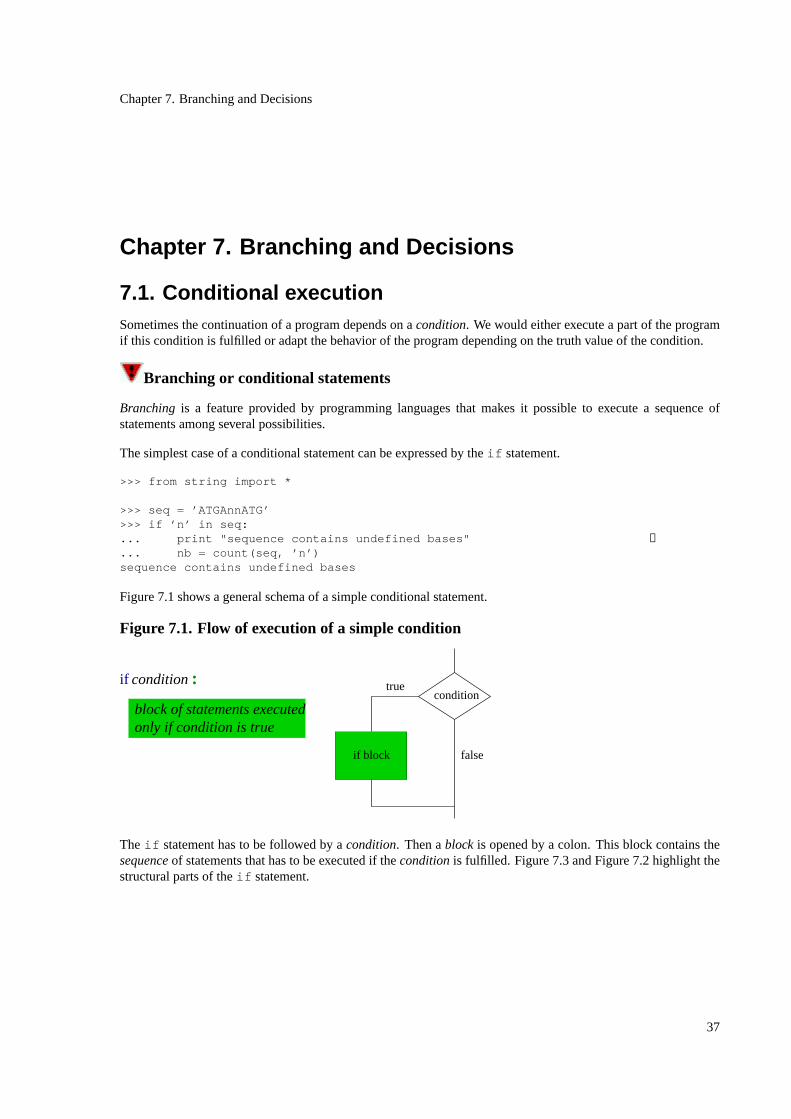
Chapter 7. Branching and Decisions
Chapter 7. Branching and Decisions
7.1. Conditional executionSometimes the continuation of a program depends on acondition. We would either execute a part of the programif this condition is fulfilled or adapt the behavior of the program depending on the truth value of the condition.
Branching or conditional statements
Branching is a feature provided by programming languages that makes it possible to execute a sequence ofstatements among several possibilities.
The simplest case of a conditional statement can be expressed by theif statement.
>>> from string import *
>>> seq = ’ATGAnnATG’>>> if ’n’ in seq:... print "sequence contains undefined bases" ❶... nb = count(seq, ’n’)sequence contains undefined bases
Figure 7.1 shows a general schema of a simple conditional statement.
Figure 7.1. Flow of execution of a simple condition
condition
if block
only if condition is trueblock of statements executed
true
false
condition :if
The if statement has to be followed by acondition. Then ablock is opened by a colon. This block contains thesequenceof statements that has to be executed if theconditionis fulfilled. Figure 7.3 and Figure 7.2 highlight thestructural parts of theif statement.
37

Chapter 7. Branching and Decisions
Figure 7.2. If statement
>>>. . .
. . . nb = count(seq, ’n’)
’n’ in seqif print "sequence contains undefined bases"
sequence contains undefined bases
sequence of instructionsONLY executed if the condition is true
body of the if statement
:
condition
Figure 7.3. Block structure of the if statement
:>>>. . .
. . .
if ’n’ in seq
nb = count(seq, ’n’) print "sequence contains undefined bases"
sequence contains undefined bases
header line
block inititiation
body of the if statement
block of codesame indentation to
indicate a block
7.2. Conditions and Boolean expressionsTheconditionin the if statement has to be aboolean expression.
Conditions or Boolean expressions
Conditional or boolean expressionsareexpressionsthat are eithertrueor false.
Here are some examples of simpleboolean expressionsor conditions:
>>> 1 < 0False>>> 1 > 0True>>> 1 == 0False>>> ’n’ in ’ATGCGTAnAGTA’True>>> ’A’ > ’C’False>>> ’AG’ < ’AA’
38
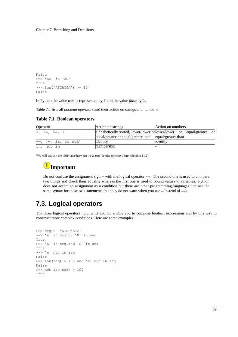
Chapter 7. Branching and Decisions
False>>> ’AG’ != ’AC’True>>> len(’ATGACGA’) >= 10False
In Python the valuetrue is represented by1 and the valuefalseby 0.
Table 7.1 lists allboolean operatorsand their action on strings and numbers.
Table 7.1. Boolean operators
Operator Action on strings Action on numbers<, <=, >=, > alphabetically sorted, lower/lower or
equal/greater or equal/greater thanlower/lower or equal/greater orequal/greater than
==, !=, is, is not a identity identityin, not in membership -
aWe will explain the difference between these two identity operators later (Section 11.2).
Important
Do not confuse the assignment sign= with the logical operator==. The second one is used to comparetwo things and check their equality whereas the first one is used to bound values to variables. Pythondoes not accept an assignment as a condition but there are other programming languages that use thesame syntax for these two statements, but they do not warn when you use= instead of==.
7.3. Logical operatorsThe three logical operatorsnot , and andor enable you to compose boolean expressions and by this way toconstruct more complex conditions. Here are some examples:
>>> seq = ’ATGCnATG’>>> ’n’ in seq or ’N’ in seqTrue>>> ’A’ in seq and ’C’ in seqTrue>>> ’n’ not in seqFalse>>> len(seq) > 100 and ’n’ not in seqFalse>>> not len(seq) > 100True
39
Chapter 7. Branching and Decisions
Caution
Theor operation is not anexclusiveor as it is sometimes used in the current languages. Anor expressionis also true if both subexpressions are true.
>>> seq = ’ATGCnATG’>>> ’A’ in seq or ’C’ in seqTrue
7.4. Alternative executionIf the condition of aif statement is not fulfilled no statement is executed.
>>> seq = ’ATGACGATAG’>>> if ’n’ in seq:
print "sequence contains undefined characters">>>
An alternativesequence of statements, that will be executed if theconditionis not fulfilled, can be specified withtheelse statement.
>>> seq = ’ATGACGATAG’>>> if ’n’ in seq:... print "sequence contains undefined bases"... else:
print "sequence contains only defined bases"sequence contains only defined bases
Here theif andelse are followed by ablockcontaining the statements to execute depending on the truth valueof thecondition. In this case exactly one of them is executed, which is illustrated in Figure 7.4
40
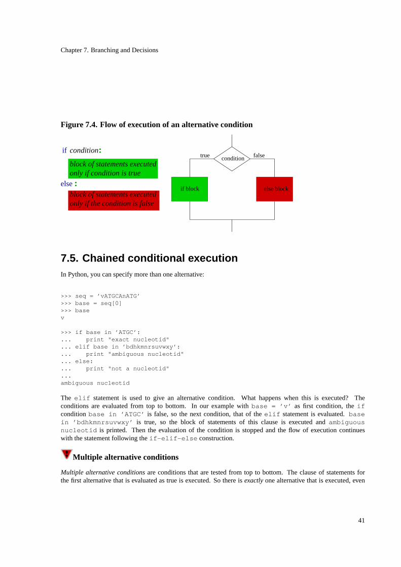
Chapter 7. Branching and Decisions
Figure 7.4. Flow of execution of an alternative condition
condition
else block
true falseif condition:
if block
only if the condition is falseblock of statements executed
else :only if condition is trueblock of statements executed
7.5. Chained conditional executionIn Python, you can specify more than one alternative:
>>> seq = ’vATGCAnATG’>>> base = seq[0]>>> basev
>>> if base in ’ATGC’:... print "exact nucleotid"... elif base in ’bdhkmnrsuvwxy’:... print "ambiguous nucleotid"... else:... print "not a nucleotid"...ambiguous nucleotid
The elif statement is used to give an alternative condition. What happens when this is executed? Theconditions are evaluated from top to bottom. In our example withbase = ’v’ as first condition, theifconditionbase in ’ATGC’ is false, so the next condition, that of theelif statement is evaluated.basein ’bdhkmnrsuvwxy’ is true, so the block of statements of this clause is executed andambiguousnucleotid is printed. Then the evaluation of the condition is stopped and the flow of execution continueswith the statement following theif-elif-else construction.
Multiple alternative conditions
Multiple alternative conditionsare conditions that are tested from top to bottom. The clause of statements forthe first alternative that is evaluated as true is executed. So there isexactlyone alternative that is executed, even
41
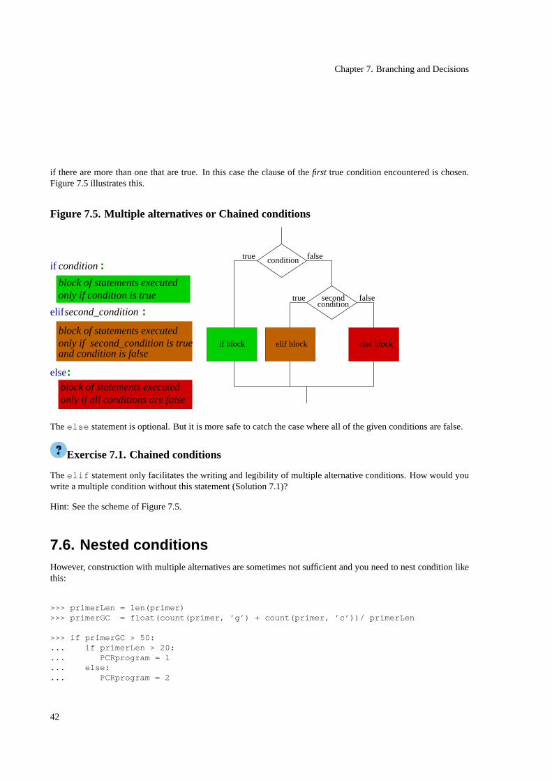
Chapter 7. Branching and Decisions
if there are more than one that are true. In this case the clause of thefirst true condition encountered is chosen.Figure 7.5 illustrates this.
Figure 7.5. Multiple alternatives or Chained conditions
else:block of statements executedonly if all conditions are false
if block else blockelif block
condition falsetrue
secondcondition
falsetrue
only if second_condition is trueand condition is false
block of statements executed
elifsecond_condition :only if condition is trueblock of statements executed
if :condition
Theelse statement is optional. But it is more safe to catch the case where all of the given conditions are false.
Exercise 7.1. Chained conditions
Theelif statement only facilitates the writing and legibility of multiple alternative conditions. How would youwrite a multiple condition without this statement (Solution 7.1)?
Hint: See the scheme of Figure 7.5.
7.6. Nested conditionsHowever, construction with multiple alternatives are sometimes not sufficient and you need to nest condition likethis:
>>> primerLen = len(primer)>>> primerGC = float(count(primer, ’g’) + count(primer, ’c’))/ primerLen
>>> if primerGC > 50:... if primerLen > 20:... PCRprogram = 1... else:... PCRprogram = 2
42
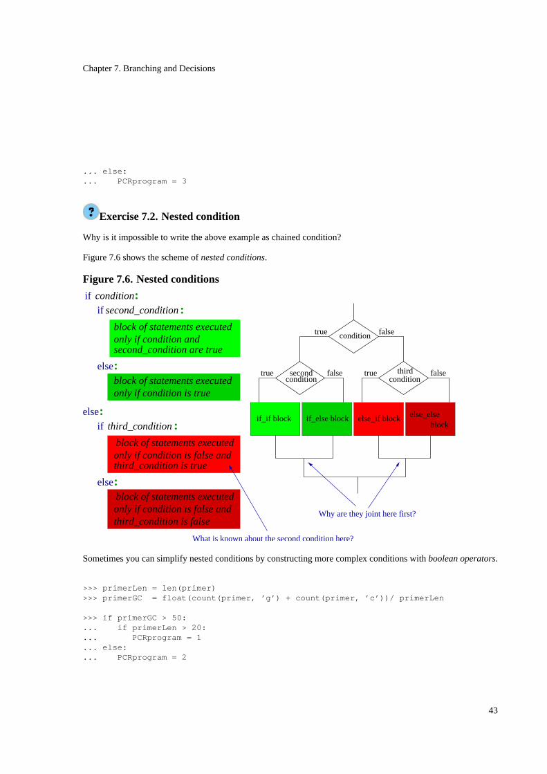
Chapter 7. Branching and Decisions
... else:
... PCRprogram = 3
Exercise 7.2. Nested condition
Why is it impossible to write the above example as chained condition?
Figure 7.6 shows the scheme ofnested conditions.
Figure 7.6. Nested conditions
if condition:
else:
else:
else:
if second_condition
if third_condition :
block of statements executedonly if condition andsecond_condition are true
block of statements executedonly if condition is true
block of statements executedonly if condition is false andthird_condition is true
block of statements executedonly if condition is false andthird_condition is false
:
Why are they joint here first?
if_if block
secondcondition
falsetrue
condition falsetrue
falsetrue
else_if blockif_else block
conditionthird
else_else block
What is known about the second condition here?
Sometimes you can simplify nested conditions by constructing more complex conditions withboolean operators.
>>> primerLen = len(primer)>>> primerGC = float(count(primer, ’g’) + count(primer, ’c’))/ primerLen
>>> if primerGC > 50:... if primerLen > 20:... PCRprogram = 1... else:... PCRprogram = 2
43

Chapter 7. Branching and Decisions
can be expressed as:
>>> if primerGC > 50 and primerLen > 20:... PCRprogram = 1... else:... PCRprogram = 2
Caution
Even if the second version is easier to read, be careful and always check whether the complex conditionyou have written, is what you really want. Such errors are called semantic error. They can not be detectedby the interpreter because the syntax of the program is correct, even if it is not necessarily what you wantto compute.
7.7. Solutions
Solution 7.1. Chained conditions
Exercise 7.1
Figure 7.7. Multiple alternatives without elif
if condition:block of statements executedonly if condition is true
block of statements executed
elifsecond_condition :
block of statements executed
else:
only if the second conditionis true
only if all conditions are false
if condition:block of statements executedonly if condition is true
else:if second_condition:
block of statements executedonly if all conditions are false
else:
block of statements executedonly if the second conditionis true
44
Chapter 8. Defining Functions
Chapter 8. Defining Functions
8.1. Defining FunctionsIn Section 3.3 we have learnt how to apply or call functions. So let’s remember the example calculating theGC-percentage of a DNA sequence.
>>> float(count(cds, ’G’) + count(cds, ’C’)) / len(cds)
This calculates the gc percentage of the specific DNA sequencecds , but we can use the same formula to calculatethe gc percentage of other DNA sequences. The only thing to do is to replacecds by the new DNA sequence inthe formula. But it is not very convenient to remember the formula and retype it all the time. It would be mucheasier to type the following instead.
>>> gc(’ATGCAT’)0.33333333333333331>>> gc(cds)0.54460093896713613
The only thing we have to remember is the name of the newfunctionand its use.
Abstraction
The possibility to define such newfunction executing tasks specified by yourself, is anabstraction feature,provided by all high level programming languages.
Important
It is also important to notice that functions have to be defined before they are called. You can not usesomething that is not defined.
Here is the syntax of such a new definition in Python:
>>> from string import *
>>> def gc(seq):... return float(count(seq, ’G’) + count(seq, ’C’)) / len(seq)
Let’s have a closer look at this definition. Figure 8.1 illustrates the structure of a function definition.
45

Chapter 8. Defining Functions
Figure 8.1. Function definitions
during a function call the parameter
statement indicating a new function
that has to be followed by the function nameand a comma separated list of parameters
and a colon indication the start of a new block
statement used to return back a result indentationdefining ablock
of a calculation
definition in Python
:>>> def gc(seq). . . return float(count(seq, ’G’) + count(seq, ’C’)) / len(seq)
secondpromptindicatinga newblock
its argument value(a sort of place holder) is replaced by
def andreturn arebasic instructions.
Basic instruction
Basic instructionsare statements that define the language rules and the semantic of Python. They constitute thebasic set of instructions of Python. Eachbasic instructionhas its own syntax that you have to learn in order tomaster the programming language.
The return basic instruction is used to return the result of a function back, in our example the value of the GCpercentage of the specified DNA sequence.
Thedef basic instruction indicates to Python that a function definition follows. It has to be followed by the newfunction name and a comma separated list of parameter names enclosed into parentheses.
Parameter
Parametersarevariable names. When the function is called they are bound in the same order to the argumentsgiven.
The body of a function contains the piece of code needed to execute the subtask of the function. In the exampleabove, the body contains only thereturn statement. Here is a more complex example that excludes ambiguousbases from the GC percentage calculation.
>>> from string import *
>>> def gc(seq):... nbases = count(seq, ’N’)... gcpercent = float(count(seq, ’G’) + count(seq, ’C’)) / (len(seq) - nbases)... return gcpercent
In this example the body of the function contains three instructions (2 assignments and the return statement). Thebody of a function follows the definition line and is written as an indentedblock initiated by a colon.
46
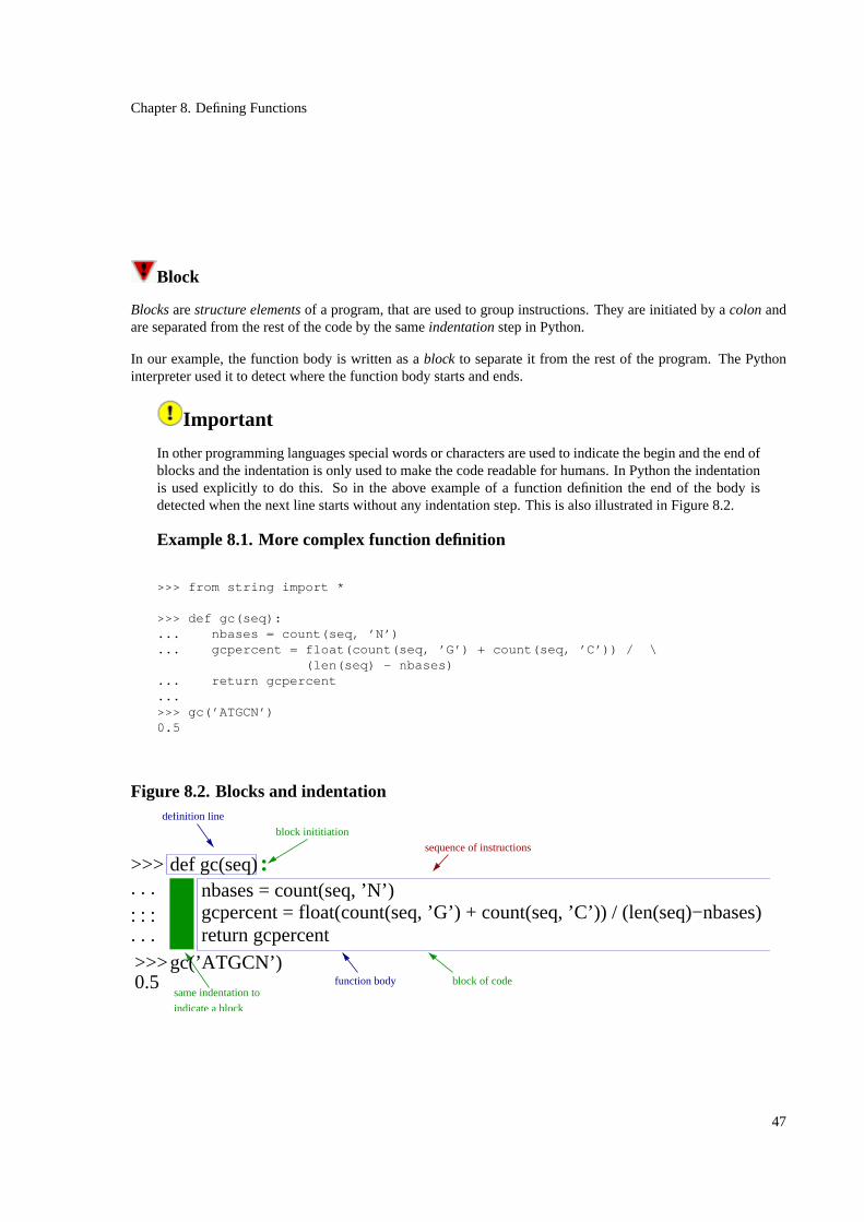
Chapter 8. Defining Functions
Block
Blocksarestructure elementsof a program, that are used to group instructions. They are initiated by acolonandare separated from the rest of the code by the sameindentationstep in Python.
In our example, the function body is written as ablock to separate it from the rest of the program. The Pythoninterpreter used it to detect where the function body starts and ends.
Important
In other programming languages special words or characters are used to indicate the begin and the end ofblocks and the indentation is only used to make the code readable for humans. In Python the indentationis used explicitly to do this. So in the above example of a function definition the end of the body isdetected when the next line starts without any indentation step. This is also illustrated in Figure 8.2.
Example 8.1. More complex function definition
>>> from string import *
>>> def gc(seq):... nbases = count(seq, ’N’)... gcpercent = float(count(seq, ’G’) + count(seq, ’C’)) / \
(len(seq) - nbases)... return gcpercent...>>> gc(’ATGCN’)0.5
Figure 8.2. Blocks and indentation
nbases = count(seq, ’N’)
return gcpercent
gc(’ATGCN’)
def gc(seq)>>>
>>>
. . .
. . .
. . .
. . .
0.5
definition line
block inititiation
sequence of instructions
block of codefunction bodysame indentation to
indicate a block
:
gcpercent = float(count(seq, ’G’) + count(seq, ’C’)) / (len(seq)−nbases)
47
Chapter 8. Defining Functions
8.2. Parameters and Arguments or the difference between afunction definition and a function call
As we have already said, functions are named sequences of statements that execute a specific task. Afunctiondefinitionis the construction that gives a name to this special sequence of statements. Whereas afunction callisthe execution of this sequence of statements. We have also seen that the execution can be parameterized. Thismeans, that there are special variables, theparameters, in the function which are bound to values, thearguments,during the function call.
Flow of execution. Some precision about theflow of execution. If you call a function the statements of thefunction body are executed. The execution of the current sequence of statements areis interrupted and theflow ofexecutionjumps to the sequence of statements named by the function. The function statements are executed andthen theflow of executioncontinues with the sequence from where the function was called.
Caution
The statements in the function body are only executed at a function call, so all errors in this piece of codeare only reported at the execution.
Now if we remember that within a function you can call other functions, the above scheme becomes rapidlydisturbing, but Python keeps a track from where a function is called and there is only one statement at a time thatis executed. You can visualize this using astack diagramof the function calls.
Stack
A stackis an ordered set of things which can be accessed in two ways. You can put things on the top of the stack,and only take back the thing on the top of the stack. A common example is a stack of plates (it is hard to get aplate from within the stack). A stack is sometimes called aLIFO an abbreviation oflast-in-first-out.
So what Python does is to handle a stack of function calls. If a function is called, Python puts the position fromwhere it is called on the stack, executes the function and when the function execution is finished Python gets theposition to continue back from the stack. Figure 8.3 shows the stack diagram of the execution of thegc function(Example 8.1).
48

Chapter 8. Defining Functions
Figure 8.3. Stack diagram of function calls
gc
/
gc
nbases’ATGCNNATGC’seq
gcpercent
xy
4.0
’ATGCNNATGC’
2
seqnbases
gcpercent
’ATGCNNATGC’
2
seqnbases
gcpercent
’ATGCNNATGC’
2
seqnbases
gcpercent
’ATGCNNATGC’ssub ’N’
’ATGCNNATGC’seqnbases
gcpercent
s ’ATGCNNATGC’
xy 2
’ATGCNNATGC’
2
seqnbases
gcpercent
’ATGCNNATGC’
2
seqnbases
gcpercent
4.0xy
xy 2
9
’ATGCNNATGC’
2
seqnbases
gcpercent
xy
x
xy
2
’ATGCNNATGC’ssub ’G’
xy
x
’ATGCNNATGC’ssub ’C’
xy
2
2
4.0xy
x
xy
2
2xy
’ATGCNNATGC’
2
seqnbases
gcpercent
’ATGCNNATGC’
2
seqnbases
gcpercent
xy
4x
’ATGCNNATGC’seq
gcpercent2nbases0.5714285
gc
len
/
count
gc gc
/
− −
count
+
float
/
gc
gc(’ATGCNNATGC’) count
gc
gc
/
float
+
/
+
float
/
gc gc
float
/
gc
7
4.0xy
4.0
8.3. Functions and namespacesEven if it is confusing at the beginning, thedna variable in the function call is not the same as thedna parameterof thegc function. During the function call the global variable is evaluated and its value’ATGACT’ is assignedto the parameterdna of thegc function.
How does Python distinguish the two variables? It can do so, because they are not in the same namespace.All functions have two associated namespaces, alocal and aglobal namespace. Theglobal namespace is thenamespace where the function is defined and thelocal namespace is a namespace created at the function definitionwhere parameters are defined. The local namespace contains also alllocal variables. Local variablesare variablesthat are bound to value in the function body. When a function is defined, its source code is analyzed and all usednames are sorted in the two namespaces.
If a variable name is searched during a function execution, Python looks in the local namespace for local variablesand in the global namespace for global variables. If a global variable is not found there, the builtin namespace issearched. If it is not found there, an error is produced.
builtin namespace
Thebuiltin namespaceis anamespacethat contains all predefined function of Python.
You can ask Python which names are defined in the global and the local namespace using the functionsglobals() andlocals() .
>>> from string import *>>> def gc(seq):... nbases = count(seq, ’N’)... gcpercent = float(count(seq, ’G’) + count(seq, ’C’)) / (len(seq) - nbases)
49
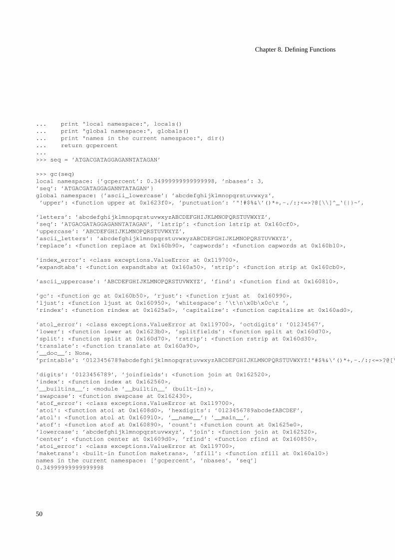
Chapter 8. Defining Functions
... print "local namespace:", locals()
... print "global namespace:", globals()
... print "names in the current namespace:", dir()
... return gcpercent
...>>> seq = ’ATGACGATAGGAGANNTATAGAN’
>>> gc(seq)local namespace: {’gcpercent’: 0.34999999999999998, ’nbases’: 3,’seq’: ’ATGACGATAGGAGANNTATAGAN’}global namespace: {’ascii_lowercase’: ’abcdefghijklmnopqrstuvwxyz’,
’upper’: <function upper at 0x1623f0>, ’punctuation’: ’"!#$%&\’()*+,-./:;<=>?@[\\]^_‘{|}~’,
’letters’: ’abcdefghijklmnopqrstuvwxyzABCDEFGHIJKLMNOPQRSTUVWXYZ’,’seq’: ’ATGACGATAGGAGANNTATAGAN’, ’lstrip’: <function lstrip at 0x160cf0>,’uppercase’: ’ABCDEFGHIJKLMNOPQRSTUVWXYZ’,’ascii_letters’: ’abcdefghijklmnopqrstuvwxyzABCDEFGHIJKLMNOPQRSTUVWXYZ’,’replace’: <function replace at 0x160b90>, ’capwords’: <function capwords at 0x160b10>,
’index_error’: <class exceptions.ValueError at 0x119700>,’expandtabs’: <function expandtabs at 0x160a50>, ’strip’: <function strip at 0x160cb0>,
’ascii_uppercase’: ’ABCDEFGHIJKLMNOPQRSTUVWXYZ’, ’find’: <function find at 0x160810>,
’gc’: <function gc at 0x160b50>, ’rjust’: <function rjust at 0x160990>,’ljust’: <function ljust at 0x160950>, ’whitespace’: ’\t\n\x0b\x0c\r ’,’rindex’: <function rindex at 0x1625a0>, ’capitalize’: <function capitalize at 0x160ad0>,
’atol_error’: <class exceptions.ValueError at 0x119700>, ’octdigits’: ’01234567’,’lower’: <function lower at 0x1623b0>, ’splitfields’: <function split at 0x160d70>,’split’: <function split at 0x160d70>, ’rstrip’: <function rstrip at 0x160d30>,’translate’: <function translate at 0x160a90>,’__doc__’: None,’printable’: ’0123456789abcdefghijklmnopqrstuvwxyzABCDEFGHIJKLMNOPQRSTUVWXYZ!"#$%&\’()*+,-./:;<=>?@[\\]^_‘{|}~ \t\n\r\x0b\x0c’,
’digits’: ’0123456789’, ’joinfields’: <function join at 0x162520>,’index’: <function index at 0x162560>,’__builtins__’: <module ’__builtin__’ (built-in)>,’swapcase’: <function swapcase at 0x162430>,’atof_error’: <class exceptions.ValueError at 0x119700>,’atoi’: <function atoi at 0x1608d0>, ’hexdigits’: ’0123456789abcdefABCDEF’,’atol’: <function atol at 0x160910>, ’__name__’: ’__main__’,’atof’: <function atof at 0x160890>, ’count’: <function count at 0x1625e0>,’lowercase’: ’abcdefghijklmnopqrstuvwxyz’, ’join’: <function join at 0x162520>,’center’: <function center at 0x1609d0>, ’rfind’: <function rfind at 0x160850>,’atoi_error’: <class exceptions.ValueError at 0x119700>,’maketrans’: <built-in function maketrans>, ’zfill’: <function zfill at 0x160a10>}names in the current namespace: [’gcpercent’, ’nbases’, ’seq’]0.34999999999999998
50
Chapter 8. Defining Functions
Thedir function shows all the names defined in the current namespace.
>>> from string import *
>>> dir()[’__builtins__’, ’__doc__’, ’__name__’, ’ascii_letters’, ’ascii_lowercase’,’ascii_uppercase’, ’atof’, ’atof_error’, ’atoi’, ’atoi_error’, ’atol’,’atol_error’, ’capitalize’, ’capwords’, ’center’, ’count’, ’digits’,’expandtabs’, ’find’, ’gc’, ’hexdigits’, ’index’, ’index_error’, ’join’,’joinfields’, ’letters’, ’ljust’, ’lower’, ’lowercase’, ’lstrip’, ’maketrans’,’octdigits’, ’printable’, ’punctuation’, ’replace’, ’rfind’, ’rindex’, ’rjust’,’rstrip’, ’seq’, ’split’, ’splitfields’, ’strip’, ’swapcase’, ’translate’,’upper’, ’uppercase’, ’whitespace’, ’zfill’]
8.4. Boolean functionsWhenever a condition is too complex, you can write aboolean function.
Boolean function
Boolean functionsarefunctionthat return truth values (in Python either0 or 1).
It is good style to give them a name that indicates its nature, often the function name starts withis .
Here is an example that tests if a character is a valid amino acid:
>>> from string import *
>>> def isAminoAcid(aa):... AA = upper(aa)... if AA < ’A’ or AA > ’Z’:... return 0... if AA in ’JOU’:... return 0... return 1
you can also write it as follow:
>>> from string import *
>>> def isAminoAcid(aa):... AA = upper(aa)... if AA < ’A’:... ok = 0... elif AA > ’Z’:... ok = 0
51
Chapter 8. Defining Functions
... elif AA in ’JOU’:
... ok = 0
... else:
... ok = 1
... return ok
or using boolean operators:
Example 8.2. Function to check whether a character is a valid amino acid
>>> def isAminoAcid(aa):... return (’A’ <= aa <= ’Z’ or ’a’ <= aa <= ’z’) and aa not in ’jouJOU’
Using this function makes your code easier to understand because the function name expresses what you want totest:
>>> prot = ’ATGAFDWDWDAWDAQW’>>> oneaa = prot[0]
>>> if isAminoAcid(oneaa):... print ’ok’... else:
print ’not a valid amino acid’ok
52
Chapter 9. Collections
Chapter 9. Collections
9.1. Datatypes for collectionsIn the proceeding chapter we have seen thatstringscan be interpreted ascollections of characters.But they area very restricted sort of collection, you can only put characters in a string and a string is always ordered. But weneed often to handle collections of all sorts of objects and sometimes these collections are not even homogeneous,meaning that they may contain objects of different types. Python provides several predefineddata types thatcan manage such collections. The two most used structures are calledLists andDictionaries. Both can handlecollections of different sorts of objects, but what are their differences?
List
Listsaremutable ordered collectionsof objects of different sorts. The objects are accessible using their positionin theordered collection.
Dictionary
Dictionariesaremutable unordered collectionswhich may contain objects of different sorts. The objects can beaccessed using akey.
Here are some examples comparing a list version of a collection of enzyme’s pattern and a dictionary version ofthe same collection. Lists are created using a comma separated list of all elements enclosed into brackets, whereasdictionaries are enclosed into braces and contain a comma separated list of key-value pairs, each separated by acolon.
>>> patternList = [ ’gaattc’, ’ggatcc’, ’aagctt’ ]>>> patternList[’gaattc’, ’ggatcc’, ’aagctt’]
>>> patternDict = { ’EcoRI’ : ’gaattc’, ’BamHI’ : ’ggatcc’, ’HindIII’ : ’aagctt’ }>>> patternDict{ ’EcoRI’ : ’gaattc’, ’BamHI’ : ’ggatcc’, ’HindIII’ : ’aagctt’ }
To access the elements we use the position in the list and the key for the dictionary.
Important
List indices have the same properties as string indices, in particular they start with 0 (remember Figure6.1).
>>> patternList[0]’gaattc’>>> patternDict[’EcoRI’]
53

Chapter 9. Collections
’gaattc’
As for strings you can get the number of elements in the collection, as well as the smallest and the greatest element.
>>> len(patternList)3>>> len(patternDict)3
Lists can be sliced but dictionaries cannot. Remember that dictionaries are unordered collections, so getting aslice does not make any sense.
>>> digest = patternList[:1]>>> digest[’gaattc’]
You can ask whether an element is in the collection. Dictionaries have two possibilities to perform this.
>>> ’gaattc’ in patternList1>>> patternDict.has_key(’HindIII’)1>>> ’HindIII’ in patternDict1
Unlike strings both collections are mutable. This means that you can remove, add or even change their elements.
>>> del patternList[0]>>> patternList[’ggatcc’, ’aagctt’]>>> patternList[0] = ’gaattc’>>> patternList[’gaattc’, ’aagctt’]>>> patternList.append(’ggattc’)>>> patternList[’gaattc’, ’aagctt’, ’ggattc’]>>> del patternList[:2]>>> patternList[’ggattc’]
>>> del patternDict[’EcoRI’]>>> patternDict{’BamHI’: ’ggatcc’, ’HindIII’: ’aagctt’}>>> patternDict[’EcoRI’] = ’gaattc’>>> patternDict{’BamHI’: ’ggatcc’, ’EcoRI’: ’gaattc’, ’HindIII’: ’aagctt’}>>> patternDict[’BamHI’] =”
54
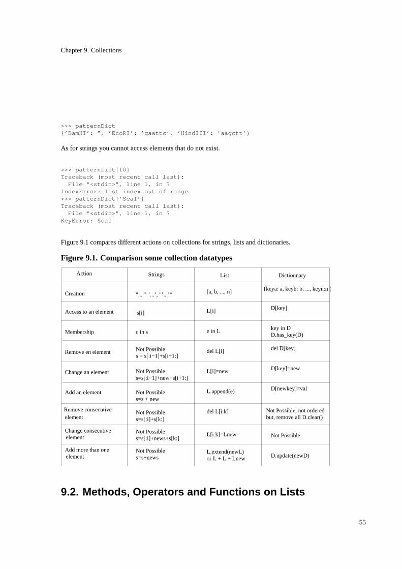
Chapter 9. Collections
>>> patternDict{’BamHI’: ”, ’EcoRI’: ’gaattc’, ’HindIII’: ’aagctt’}
As for strings you cannot access elements that do not exist.
>>> patternList[10]Traceback (most recent call last):
File "<stdin>", line 1, in ?IndexError: list index out of range>>> patternDict[’ScaI’]Traceback (most recent call last):
File "<stdin>", line 1, in ?KeyError: ScaI
Figure 9.1 compares different actions on collections for strings, lists and dictionaries.
Figure 9.1. Comparison some collection datatypes
Remove consecutiveelement
elementChange consecutive
Add more than oneelement
L.extend(newL)or L + L + Lnew
Not Possibles = s[:i−1]+s[i+1:]
Not Possibles=s[:i−1]+new+s[i+1:]
Not Possibles=s[:i]+s[k:]
Not Possibles=s[:i]+news+s[k:]
Not Possibles=s + new
Not Possibles=s+news
D[key]
key in DD.has_key(D)
del D[key]
D[key]=new
D[newkey]=val
Not Possible
D.update(newD)
Action DictionnaryList Strings
Membership
Remove en element
Change an element
Add an element
Access to an element
Creation
L[i]
e in L
del L[i]
L[i]=new
L.append(e)
del L[i:k]
L[i:k]=Lnew
[a, b, ..., n]
s[i]
c in s
"..."’ ’...’, "’...’"{keya: a, keyb: b, ..., keyn:n }
Not Possible, not orderedbut, remove all D.clear()
9.2. Methods, Operators and Functions on Lists
55
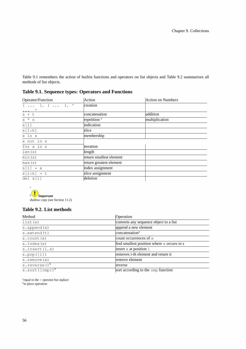
Chapter 9. Collections
Table 9.1 remembers the action of builtin functions and operators on list objects and Table 9.2 summarizes allmethods of list objects.
Table 9.1. Sequence types: Operators and Functions
Operator/Function Action Action on Numbers[ ... ], ( ... ), "... "
creation
s + t concatenation additions * n repetitiona multiplications[i] indications[i:k] slicex in s membershipx not in sfor a in s iterationlen(s) lengthmin(s) return smallest elementmax(s) return greatest elements[i] = x index assignments[i:k] = t slice assignmentdel s[i] deletion
a
a Importantshallow copy (see Section 11.2)
Table 9.2. List methodsMethod Operationlist(s) converts any sequence object to a lists.append(x) append a new elements.extend(t) concatenationa
s.count(x) count occurrences ofxs.index(x) find smallest position wherex occurs in ss.insert(i,x) insertx at positionis.pop([i]) removes i-th element and return its.remove(x) remove elements.reverse() b reverses.sort([cmp]) b sort according to thecmp function
aequal to the+ operator but inplacebin place operation
56
Chapter 9. Collections
Important
It is important to know whether a function or method, that is applied to amutableobjects, modifies thisobject internally or whether it returns a new object containing these modifications. Look at the followingexample that shows two possibilities to concatenate lists. The+ operator creates a new list whereas themethodextend adds one list to the other:
>>> l1 = [ ’EcoRI’, ’BamHI’ ]>>> l2 = [ ’HindIII’ ]>>> l1[’EcoRI’, ’BamHI’]>>> l2[’HindIII’]>>> l1 + l2[’EcoRI’, ’BamHI’, ’HindIII’]>>> l1[’EcoRI’, ’BamHI’]>>> l2[’HindIII’]>>> l1.extend(l2)>>> l1[’EcoRI’, ’BamHI’, ’HindIII’]>>> l2[’HindIII’]
9.3. Methods, Operators and Functions on DictionariesContrary to strings and lists the ordering of the elements in dictionaries does not matter. Elements are accessed bya unique key rather than by an index number.
Important
It is important to notice thatdictionary keyshave to beuniqueandimmutable.
Table 9.3 gives an overview of the methods and operations on dictionaries.
Table 9.3. Dictionary methods and operations
Method or Operation Actiond[key] get the value of the entry with keykey in dd[key] = val set the value of entry with keykey to valdel d[key] delete entry with keykeyd.clear() removes all entrieslen(d) number of items
57
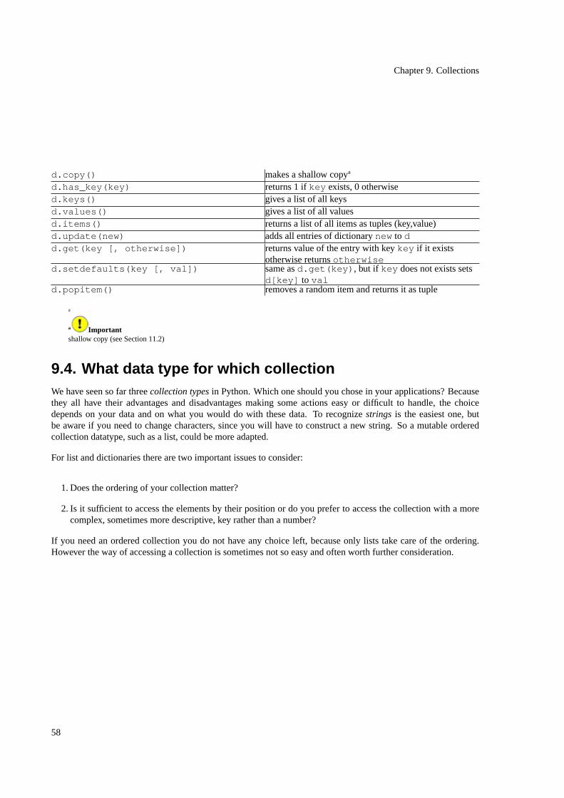
Chapter 9. Collections
d.copy() makes a shallow copya
d.has_key(key) returns 1 ifkey exists, 0 otherwised.keys() gives a list of all keysd.values() gives a list of all valuesd.items() returns a list of all items as tuples (key,value)d.update(new) adds all entries of dictionarynew to dd.get(key [, otherwise]) returns value of the entry with keykey if it exists
otherwise returnsotherwised.setdefaults(key [, val]) same asd.get(key) , but if key does not exists sets
d[key] to vald.popitem() removes a random item and returns it as tuple
a
a Importantshallow copy (see Section 11.2)
9.4. What data type for which collectionWe have seen so far threecollection typesin Python. Which one should you chose in your applications? Becausethey all have their advantages and disadvantages making some actions easy or difficult to handle, the choicedepends on your data and on what you would do with these data. To recognizestrings is the easiest one, butbe aware if you need to change characters, since you will have to construct a new string. So a mutable orderedcollection datatype, such as a list, could be more adapted.
For list and dictionaries there are two important issues to consider:
1.Does the ordering of your collection matter?
2. Is it sufficient to access the elements by their position or do you prefer to access the collection with a morecomplex, sometimes more descriptive, key rather than a number?
If you need an ordered collection you do not have any choice left, because only lists take care of the ordering.However the way of accessing a collection is sometimes not so easy and often worth further consideration.
58

Chapter 10. Repetitions
Chapter 10. Repetitions
10.1. RepetitionsSometimes you need to do the same thing several times with different data. Whereas humans make often errorsduring a repetitive procedure, computers execute repetitive tasks very well.
One possibility to write repetitions is to repeat the code as often as needed, but this is neither elegant nor readable,and above all you cannot do this if the number of repetition times is not constant or is not known beforehand.
Just as now, we have seen all that we need to do repetitive tasks.
Exercise 10.1. Repetitions
Try to find out how to perform a repetitive task, only with the statements seen so far. It is not very easy if you havenot seen this and we will discuss this later (Chapter 13).
Because repetitions are common programming tasks, high level programming languages provide special structuresand statements for this purpose. Python has two of them:for andwhile . Let us see thefor statement first.
10.2. The for loopVerify protein sequences.Let us start with an example that checks whether all characters of a protein sequenceare valid amino acid characters. How could we do this by hand? One possibility is to start at the beginning of theprotein sequence and check each character one by one. Here is a more formal description of the algorithm:
1. for eachcharacter of the protein sequence
a. if the current character is not an amino acid
• print the invalid character
b. end if
2. end for
In Python this can be performed with thefor statement.
59

Chapter 10. Repetitions
The for loop
Thefor loop enables to iterate on an ordered collection of objects and to execute the same sequence of statementsfor each element.
This sort of iteration is also known as atraversal, because the collection istraversedfrom left to right and aparticular task is applied to each element.
So in our example, the collection of elements is a string which we traverse with thefor loop. We also have tospecify what a valid amino acid is, because computers do not know about it. Nevertheless we have already writtena function doing this (Example 8.2).
>>> protein = "SERLSITPLGPYIGAQIJSGADLTRPLSDNQFEQLYHAVLRHQVVFLRDQAITPQQQRALA"
>>> for aa in protein:... if not isAminoAcid(aa):... print "protein contains unknown amino acid: ", aa...protein contains unknown amino acid: J
As def andif , thefor statement is also a statement containing ablock. Theheader linegives the two essentialinformation for the traversal. It starts withfor followed by avariable nameto which each element of thecollection is assigned during the execution of theblockof statements. The second half of theheaderindicates thecollectionin which the elements can be found. As in all functions, operations and expressions, the collection canbe specified by avalue, avariableor even acomposed expression.
Figure 10.1. The for loop
for aa in protein :
if isAminoAcid(aa):
iteration variable collection to traverse use of the iteration variablein the body
to repeat for each elementsequence of statements
print "protein contains unknown amino acid: ", aa
Getting the position of invalid amino acids. As written above we cannot show the position of the invalidamino acid in the protein sequence, because only the amino acid character is known in the body of thefor loop.Therefore, we have to iterate over the indices of the sequence. Here is the algorithm:
1. for each position in the protein sequence
a. if the character at this position is not an amino acid
• print the position and the invalid character
60

Chapter 10. Repetitions
b. end if
2. end for
What are the possible values of the positions? Remember the string indices, they start at 0 and end at one beforethe length of the string. Python has a function that gives the possibility to create a list of numbers that is calledrange . Using this function, we can translate the algorithms above into Python:
>>> for i in range(len(protein)):... if not isAminoAcid(protein[i]):... print "protein contains unknown amino acid " , protein[i] , \... " at position ", i
Note
There is a convention in most programming languages to usei, k, l as variable names for theiteration variable.
Translate cds sequences.Let’s take another example. Say that we have a cds sequence and that we would like toknow such things as the corresponding amino acid sequence or the codon usage. How could we achieve this? Forsure, it looks like a traversal of the cds sequence, but the things we are looking for do not correspond anymore toone nucleotide of the cds sequence but to a codon which is a three letter substring. If we could access the codonsone by one, the translation into the amino acid sequence would look like this:
• for each codon in the cds sequence:
• add the amino acid corresponding to the current codon to the protein sequence
In the body of the loop we need to establish the correspondence between a codon sequence and the amino acid.We know how to do this by hand, by looking up a codon in the codon translation table. A dictionary is the datatype that gives us such sort of access to the collection of codons.
>>> code = { ’ttt’: ’F’, ’tct’: ’S’, ’tat’: ’Y’, ’tgt’: ’C’,... ’ttc’: ’F’, ’tcc’: ’S’, ’tac’: ’Y’, ’tgc’: ’C’,... ’tta’: ’L’, ’tca’: ’S’, ’taa’: ’*’, ’tga’: ’*’,... ’ttg’: ’L’, ’tcg’: ’S’, ’tag’: ’*’, ’tgg’: ’W’,... ’ctt’: ’L’, ’cct’: ’P’, ’cat’: ’H’, ’cgt’: ’R’,... ’ctc’: ’L’, ’ccc’: ’P’, ’cac’: ’H’, ’cgc’: ’R’,... ’cta’: ’L’, ’cca’: ’P’, ’caa’: ’Q’, ’cga’: ’R’,... ’ctg’: ’L’, ’ccg’: ’P’, ’cag’: ’Q’, ’cgg’: ’R’,... ’att’: ’I’, ’act’: ’T’, ’aat’: ’N’, ’agt’: ’S’,... ’atc’: ’I’, ’acc’: ’T’, ’aac’: ’N’, ’agc’: ’S’,... ’ata’: ’I’, ’aca’: ’T’, ’aaa’: ’K’, ’aga’: ’R’,... ’atg’: ’M’, ’acg’: ’T’, ’aag’: ’K’, ’agg’: ’R’,... ’gtt’: ’V’, ’gct’: ’A’, ’gat’: ’D’, ’ggt’: ’G’,
61
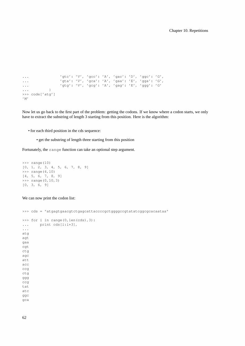
Chapter 10. Repetitions
... ’gtc’: ’V’, ’gcc’: ’A’, ’gac’: ’D’, ’ggc’: ’G’,
... ’gta’: ’V’, ’gca’: ’A’, ’gaa’: ’E’, ’gga’: ’G’,
... ’gtg’: ’V’, ’gcg’: ’A’, ’gag’: ’E’, ’ggg’: ’G’
... }>>> code[’atg’]’M’
Now let us go back to the first part of the problem: getting the codons. If we know where a codon starts, we onlyhave to extract the substring of length 3 starting from this position. Here is the algorithm:
• for each third position in the cds sequence:
• get the substring of length three starting from this position
Fortunately, therange function can take an optional step argument.
>>> range(10)[0, 1, 2, 3, 4, 5, 6, 7, 8, 9]>>> range(4,10)[4, 5, 6, 7, 8, 9]>>> range(0,10,3)[0, 3, 6, 9]
We can now print the codon list:
>>> cds = "atgagtgaacgtctgagcattaccccgctggggccgtatatcggcgcacaataa"
>>> for i in range(0,len(cds),3):... print cds[i:i+3],...atgagtgaacgtctgagcattaccccgctggggccgtatatcggcgca
62
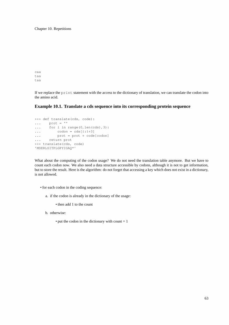
Chapter 10. Repetitions
caataataa
If we replace theprint statement with the access to the dictionary of translation, we can translate the codon intothe amino acid.
Example 10.1. Translate a cds sequence into its corresponding protein sequence
>>> def translate(cds, code):... prot = ""... for i in range(0,len(cds),3):... codon = cds[i:i+3]... prot = prot + code[codon]... return prot>>> translate(cds, code)’MSERLSITPLGPYIGAQ*’
What about the computing of the codon usage? We do not need the translation table anymore. But we have tocount each codon now. We also need a data structure accessible by codons, although it is not to get information,but to store the result. Here is the algorithm: do not forget that accessing a key which does not exist in a dictionary,is not allowed.
• for each codon in the coding sequence:
a. if the codon is already in the dictionary of the usage:
• then add 1 to the count
b. otherwise:
• put the codon in the dictionary with count = 1
63
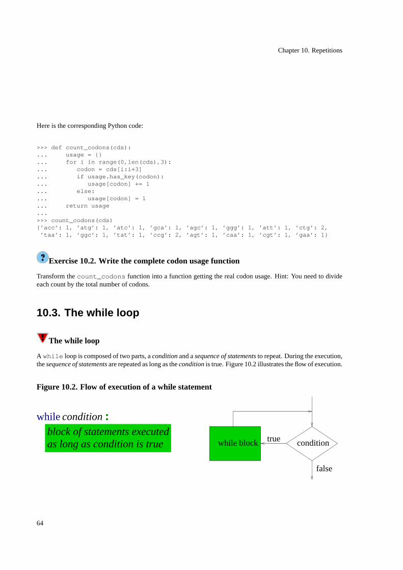
Chapter 10. Repetitions
Here is the corresponding Python code:
>>> def count_codons(cds):... usage = {}... for i in range(0,len(cds),3):... codon = cds[i:i+3]... if usage.has_key(codon):... usage[codon] += 1... else:... usage[codon] = 1... return usage...>>> count_codons(cds){’acc’: 1, ’atg’: 1, ’atc’: 1, ’gca’: 1, ’agc’: 1, ’ggg’: 1, ’att’: 1, ’ctg’: 2,
’taa’: 1, ’ggc’: 1, ’tat’: 1, ’ccg’: 2, ’agt’: 1, ’caa’: 1, ’cgt’: 1, ’gaa’: 1}
Exercise 10.2. Write the complete codon usage function
Transform thecount_codons function into a function getting the real codon usage. Hint: You need to divideeach count by the total number of codons.
10.3. The while loop
The while loop
A while loop is composed of two parts, aconditionand asequence of statementsto repeat. During the execution,thesequence of statementsare repeated as long as theconditionis true. Figure 10.2 illustrates the flow of execution.
Figure 10.2. Flow of execution of a while statement
conditionwhile block true
false
block of statements executed
while condition :
as long as condition is true
64

Chapter 10. Repetitions
Before saying more, let us illustrate that with an example. We have already shown how to use thefind method ofstrings to find pattern (Section 1.1). Let’s try now to find all occurrences of a specific pattern in a DNA sequence.Here is one possible way to proceed:
Procedure 10.6. Find all occurrences of a pattern in a sequence
INPUT: a DNA sequenceseqand a patternpat
OUTPUT: a list of positionsmatchescontaining all start positions ofpat in seq
1. matches<- empty list2. current_match<- position of the first occurrence of patternpat in sequenceseqor -1 if there is not anyone3. as long ascurrent_matchis not -1:
a. matches<- matches+ current_matchesb. current_match<- position of the next occurrence of patternpat in sequenceseqaftercurrent_matchor
-1 if there is not anyone
4. return matches
Example 10.2. First example of a while loop
And here is the implementation inPython:
def findpos(seq, pat):matches = []current_match = seq.find(pat)while current_match != -1:
matches.append(current_match)current_match =seq.find(pat, current_match+1)
return matches
Let’s follow with a second example that rewrites thetranslate function (Example 10.1) using awhile loopinstead of thefor traversal.
Example 10.3. Translation of a cds sequence using the while statement
This version follows the same procedure as the implementation with thefor statement.
code = {’ttt’: ’F’, ’tct’: ’S’, ’tat’: ’Y’, ’tgt’: ’C’,’ttc’: ’F’, ’tcc’: ’S’, ’tac’: ’Y’, ’tgc’: ’C’,’tta’: ’L’, ’tca’: ’S’, ’taa’: ’*’, ’tga’: ’*’,’ttg’: ’L’, ’tcg’: ’S’, ’tag’: ’*’, ’tgg’: ’W’,’ctt’: ’L’, ’cct’: ’P’, ’cat’: ’H’, ’cgt’: ’R’,’ctc’: ’L’, ’ccc’: ’P’, ’cac’: ’H’, ’cgc’: ’R’,
65
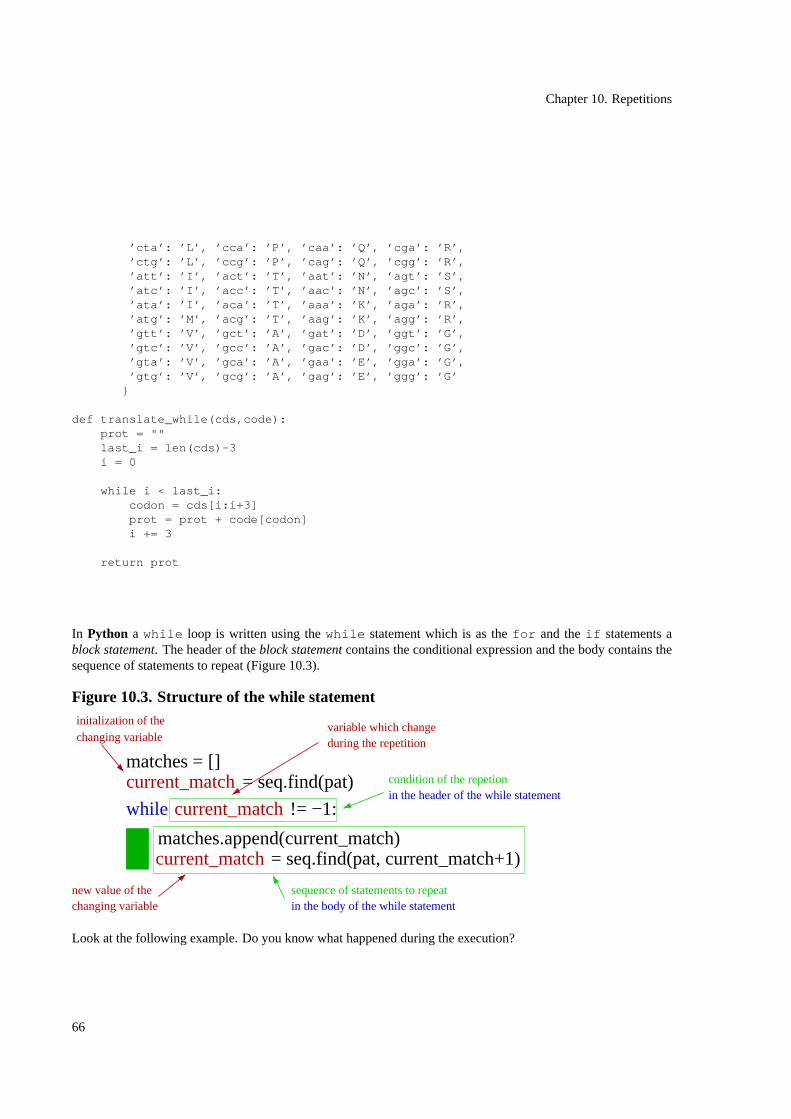
Chapter 10. Repetitions
’cta’: ’L’, ’cca’: ’P’, ’caa’: ’Q’, ’cga’: ’R’,’ctg’: ’L’, ’ccg’: ’P’, ’cag’: ’Q’, ’cgg’: ’R’,’att’: ’I’, ’act’: ’T’, ’aat’: ’N’, ’agt’: ’S’,’atc’: ’I’, ’acc’: ’T’, ’aac’: ’N’, ’agc’: ’S’,’ata’: ’I’, ’aca’: ’T’, ’aaa’: ’K’, ’aga’: ’R’,’atg’: ’M’, ’acg’: ’T’, ’aag’: ’K’, ’agg’: ’R’,’gtt’: ’V’, ’gct’: ’A’, ’gat’: ’D’, ’ggt’: ’G’,’gtc’: ’V’, ’gcc’: ’A’, ’gac’: ’D’, ’ggc’: ’G’,’gta’: ’V’, ’gca’: ’A’, ’gaa’: ’E’, ’gga’: ’G’,’gtg’: ’V’, ’gcg’: ’A’, ’gag’: ’E’, ’ggg’: ’G’
}
def translate_while(cds,code):prot = ""last_i = len(cds)-3i = 0
while i < last_i:codon = cds[i:i+3]prot = prot + code[codon]i += 3
return prot
In Python a while loop is written using thewhile statement which is as thefor and theif statements ablock statement. The header of theblock statementcontains the conditional expression and the body contains thesequence of statements to repeat (Figure 10.3).
Figure 10.3. Structure of the while statementinitalization of thechanging variable
variable which change during the repetition
condition of the repetionin the header of the while statement
in the body of the while statementsequence of statements to repeat
changing variablenew value of the
current_match = seq.find(pat, current_match+1)matches.append(current_match)
current_matchwhile != −1:
current_match = seq.find(pat)matches = []
Look at the following example. Do you know what happened during the execution?
66
Chapter 10. Repetitions
while 1:print "hello"
It simply never stops, because 1 is always true and therefore it is neither an algorithm nor a program. But itillustrates an important feature of awhile loop. The conditional expression has to contain at least one variablewhose value changes during the execution of the sequence of statements.
This variable is often a simple iterator, which is increased or decreased until it reaches a limit. One example ofsuch aniterator is the variablei in Example 10.3. The behavior of thecurrent_match variable in Example10.2 is more complicated, because it represents two situations. Its value is the start position of a pattern occurrenceor it is -1 if there are no more occurrences. In this example the second argument of thefind function ensuresthat thenextoccurrence is found but no occurrence missed.
Because the iteration variable is used in the condition and the condition is evaluated first when awhile loopis entered, it has to be defined before entering the loop. This means there are two different affectations of thisvariable. A first affectation orinitialization before the loop is entered and a second affectation statement in therepeated sequence of statements that gives it the next value. In general, this is the last statement of the sequence.Even if it is not always the case, and sometimes not necessary, it is a convention to put it at the end if possiblebecause it is easy to find if it has been forgotten.
Warning
Conditions ofwhile loops are frequent error sources. They are sometimes difficult to detect becausethey are semantic errors that produce wrong results on all or sometimes only special input data sets. Youhave to ensure that the iteration variable changes and that the end condition is always reached.
10.4. Comparison of for and while loopsWhat are the differences betweenwhile andfor ? And in which cases it is more appropriated to use one or theother? There are many cases where it is only a question of feeling.
But the while loop is the more general one because its loop condition is more flexible and can be morecomplicated than that of afor loop. The condition of afor loop is always the same and implicit in theconstruction. Afor loop stops if there are no more elements in the collection to treat. For simple traversalsor iterations over index ranges it is a good advice to use thefor statement because it handles the iteration variablefor you, so it is more secure thanwhile where you have to handle the end of the iteration and the change of theiteration variable by yourself.
The while loop can take every boolean expression as condition and permits therefore more complex endconditions. It is also the better choice if the iteration variable does not change evently by the same step or ifthere are more than one iteration variable. Even if you can handle more than one iteration variable in aforstatement, the collections from which to choose the values must have the same number of elements.
67
Chapter 10. Repetitions
Exercise 10.3. Rewrite for as while
Imagine that there is nofor statement in the Python language. How can you rewrite it aswhile statement? Takethe following pseudocode as example:
for var in collection:do something with var
Thefor loop is a special case of the
10.5. Range and Xrange objectsWe have already introduced therange function which generates a list of integers from a start to an end value(the last is not included) with a regular interval. This function is very useful while writingfor loops because itgives the possibility to iterate rather over the indices of a collection than over their elements. So you have not onlyaccess to the value of the element but also its position in the collection.
Sometimes you need to iterate over a great interval of integers. In this case the list generated by therangefunction would be long and therefore take a lot of memory space and time to be constructed. In such cases it ismore appropriated to use thexrange function which is used in the same way as therange function. But ratherthan to create the list of integers physically in memory, it creates an object that calculates the new value if it isasked for the next element in the list.
10.6. The map functionWe will finish this chapter with the introduction of the functionmap which allows to apply a function to allarguments of an ordered collection. The result is always a list even if the ordered collection is a string. If thefunction takes more than one argument, as many collections as arguments have to be specified as arguments.maptakes the first argument from the first collection, the second one from the second collection and so on.
>>> map(isAminoAcid, "atgahryuox")[1, 1, 1, 1, 1, 1, 1, 0, 0, 1]
>>> def add10(n):... return n+10...>>> map(add10, [0,1,2,3,4,5])[10, 11, 12, 13, 14, 15]>>> def add(a,b):
return a+b>>> map(add, [1,2,3], [1,2,3])[2,4,6]
68

Chapter 10. Repetitions
Passing functions as arguments.This is the first example where we pass a function as an argument. Even if thislooks strange at the beginning,function namesare references asvariable nameswhich are bound to the sequencesof statements defined in the body of thefunction definition. The sequence of statements can be viewed as an objectwhich has the particularity that it can be called with arguments. Figure 10.4 shows what happens when passing afunction as argument. This illustrates that there is no difference between variables and functions as arguments.
Figure 10.4. Passing functions as arguments
sequence of statements
that checks if a character
is an amino acid
global namespace
’athncfxuoa’
local namespace: map(isAminAcid, prot)
isAminoAcid
prot
function
sequence
Another example that handles function names as references is renaming a function as follows:
>>> isAA = isAminoAcid>>> isAA(’a’)1
The only difference between function and variable names is that function names are bound to objects that can becalled using the function call syntax.
>>> isAminoAcid<function isAminoAcid at 0x111ad0>>>> isAminoAcid(’a’)1
Without the parenthesis the object bound to the nameisAminoAcid is shown by the interpreter, whereas addingthe parentheses will call the function object bound toisAminoAcid .
69
Chapter 10. Repetitions
Rewriting mapwith for . mapwith a function that takes only one argument, can be rewritten as follows..
Rewritemap(func, collection)
1. res< empty list2. for eachelementin collection:
• res < res appended withfunc(element)
3. return res
10.7. Solutions
Solution 10.1. Rewrite for as while
Exercise 10.3
while collection:var = collection[0]do something with varcollection = collection[1:]
or using an index
i = 0while i < len(collection):
var = collection[i]do something with vari += 1
70
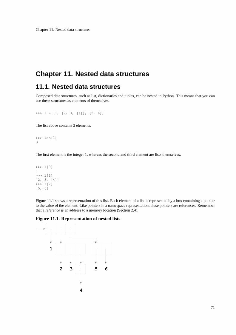
Chapter 11. Nested data structures
Chapter 11. Nested data structures
11.1. Nested data structuresComposed data structures, such as list, dictionaries and tuples, can be nested in Python. This means that you canuse these structures as elements of themselves.
>>> l = [1, [2, 3, [4]], [5, 6]]
The list above contains 3 elements.
>>> len(l)3
The first element is the integer 1, whereas the second and third element are lists themselves.
>>> l[0]1>>> l[1][2, 3, [4]]>>> l[2][5, 6]
Figure 11.1 shows a representation of this list. Each element of a list is represented by a box containing a pointerto the value of the element. Like pointers in a namespace representation, these pointers are references. Rememberthat areferenceis an address to a memory location (Section 2.4).
Figure 11.1. Representation of nested lists
2
4
1
3 65
71
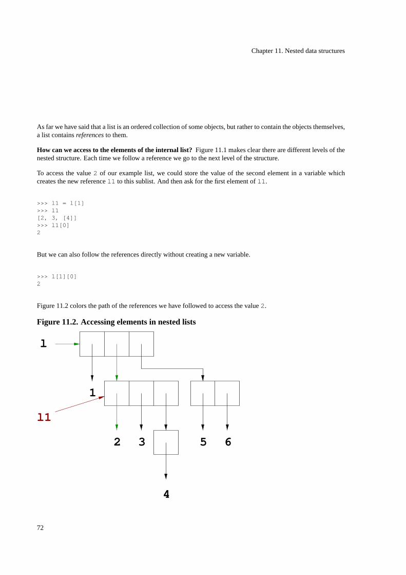
Chapter 11. Nested data structures
As far we have said that a list is an ordered collection of some objects, but rather to contain the objects themselves,a list containsreferencesto them.
How can we access to the elements of the internal list?Figure 11.1 makes clear there are different levels of thenested structure. Each time we follow a reference we go to the next level of the structure.
To access the value2 of our example list, we could store the value of the second element in a variable whichcreates the new referencel1 to this sublist. And then ask for the first element ofl1 .
>>> l1 = l[1]>>> l1[2, 3, [4]]>>> l1[0]2
But we can also follow the references directly without creating a new variable.
>>> l[1][0]2
Figure 11.2 colors the path of the references we have followed to access the value2.
Figure 11.2. Accessing elements in nested lists
l1
l
2
4
1
3 65
72

Chapter 11. Nested data structures
Nested dictionaries. Dictionaries can be nested in the same way as lists. Here is an example of a dictionary thatstores restriction enzyme data.
>>> enzdict = { ’EcoRI’: {’pattern’: ’GAATTC’, ’cut_position’: ’1’},’BamHI’: {’pattern’: ’GGATCC’, ’cut_position’: ’1’}}
>>> enzdict{ ’EcoRI’: {’pattern’: ’GAATTC’, ’cut_position’: ’1’},
’BamHI’: {’pattern’: ’GGATCC’, ’cut_position’: ’1’}}
>>> enzdict[’EcoRI’][’pattern’]’GAATTC’
Figure 11.3 shows a representation ofenzdict .
Figure 11.3. Representation of a nested dictionary
cut_position
pattern
cut_position
pattern
EcoRI
BamHI
GAATTC
1
GGATCC
1
Mixed structures. In the same way as above you can construct mixed structures. Here is an example of arestriction enzyme dictionary that stores, in addition to the pattern, all occurrences of the pattern in a sequence.
Example 11.1. A mixed nested datastructure
>>> enzdict = { ’EcoRI’: {’pattern’: ’GAATTC’, ’occ’: [0, 109, 601]},’BamHI’: {’pattern’: ’GGATCC’, ’occ’: [31, 59]}
Exercise 11.1. Representing complex structures
Try to draw a representation of the the mixed structure in Example 11.1.
11.2. Identity of objects
73

Chapter 11. Nested data structures
In ??? we have said that there exists the two operators== and is for comparing objects in Python withoutexplaining their differences.
Both operators compare the identity of objects or values, but theis operator looks if their memory locations arethe same, whereas the== operator rather does a content based comparison. Therefore for simple objects, such asintegers, and immutable objects, such as strings, the operators return the same result, but their behavior is differentfor composed objects as lists and dictionaries. The following listing shows some examples:
>>> 10.0 == 101>>> 10.0 is 100>>> 10 is 101>>> 10.0 is 10.01
>>> "atg" == "atg"1>>> "atg" is "atg"1>>> start = "atg">>> end = start>>> start == end1
>>> L1 = [1, 2, 3]>>> L1 == [1, 2, 3]1>>> L1 is [1, 2, 3]0>>> L2 = L1>>> L1 is L21>>> L3 = L1[:]>>> L1 is L30
>>> [1, [2, 3]] == [1, 2, 3]0>>> [1, [2, 3]] == [1, [2, 3]]1
Figure 11.4 shows a representation to illustrate the examples of list comparisons done above.
74
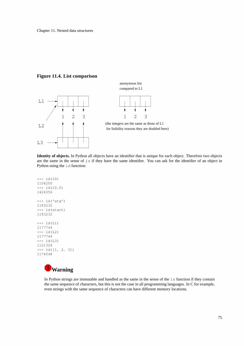
Chapter 11. Nested data structures
Figure 11.4. List comparison
1 2 3
L1
L2
L3
1 2 3
(the integers are the same as those of L1
for lisibility reasons they are doubled here)
anonymous list
compared to L1
Identity of objects. In Python all objects have an identifier that is unique for each object. Therefore two objectsare the same in the sense ofis if they have the same identifier. You can ask for the identifier of an object inPython using theid function:
>>> id(10)1104200>>> id(10.0)1424356
>>> id("atg")1183232>>> id(start)1183232
>>> id(L1)1177744>>> id(L2)1177744>>> id(L3)1121328>>> id([1, 2, 3])1174048
Warning
In Python strings are immutable and handled as the same in the sense of theis function if they containthe same sequence of characters, but this is not the case in all programming languages. In C for example,even strings with the same sequence of characters can have different memory locations.
75
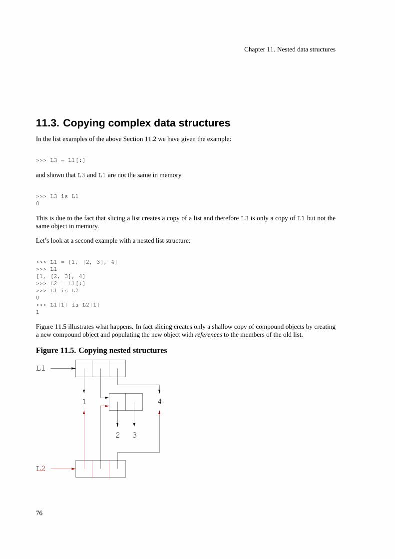
Chapter 11. Nested data structures
11.3. Copying complex data structuresIn the list examples of the above Section 11.2 we have given the example:
>>> L3 = L1[:]
and shown thatL3 andL1 are not the same in memory
>>> L3 is L10
This is due to the fact that slicing a list creates a copy of a list and thereforeL3 is only a copy ofL1 but not thesame object in memory.
Let’s look at a second example with a nested list structure:
>>> L1 = [1, [2, 3], 4]>>> L1[1, [2, 3], 4]>>> L2 = L1[:]>>> L1 is L20>>> L1[1] is L2[1]1
Figure 11.5 illustrates what happens. In fact slicing creates only a shallow copy of compound objects by creatinga new compound object and populating the new object withreferencesto the members of the old list.
Figure 11.5. Copying nested structures
L1
L2
4
2 3
1
76
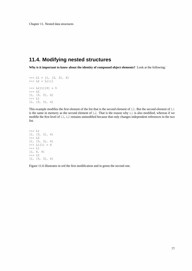
Chapter 11. Nested data structures
11.4. Modifying nested structuresWhy is it important to know about the identity of compound object elements? Look at the following:
>>> L1 = [1, [2, 3], 4]>>> L2 = L1[:]
>>> L2[1][0] = 5>>> L2[1, [5, 3], 4]>>> L1[1, [5, 3], 4]
This example modifies the first element of the list that is the second element ofL2 . But the second element ofL1is the same in memory as the second element ofL2 . That is the reason whyL1 is also modified, whereas if wemodifie the first level ofL1 , L2 remains unmodified because that only changes independent references in the twolist.
>>> L1[1, [5, 3], 4]>>> L2[1, [5, 3], 4]>>> L1[1] = 6>>> L1[1, 6, 4]>>> L2[1, [5, 3], 4]
Figure 11.6 illustrates in red the first modification and in green the second one.
77

Chapter 11. Nested data structures
Figure 11.6. Modifying compound objects
L1
L2
4
3
1
5 2
6
Copying references occurs also when you use variables.
>>> a = [1, 2]>>> b = a>>> a is b1>>> c = [a, 3]>>> c[[1, 2], 3]>>> c[0] is a1>>> a[1] = 0>>> c[[1, 0], 3]>>> a[1, 0]>>> b[1, 0]
>>> c[0] = 0>>> c[0, 3]>>> a[1, 0]
Independent copies.It is possible to get an independent copy via thedeepcopy function defined in thecopymodule.
78
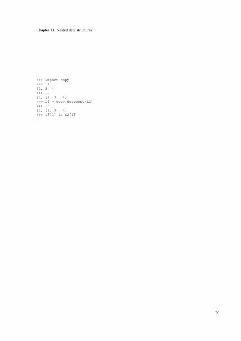
Chapter 11. Nested data structures
>>> import copy>>> L1[1, 2, 4]>>> L2[1, [1, 3], 4]>>> L3 = copy.deepcopy(L2)>>> L3[1, [1, 3], 4]>>> L3[1] is L2[1]0
79

Chapter 11. Nested data structures
80
Chapter 12. Files
Chapter 12. FilesDuring a program execution data are stored in memory. But if the program ends the data are cleared from memory.In this chapter we will explain how programs can communicate data permanently.
In the above sections we have seen how we can communicateinteractivelywith programs during their execution.However, if we need to store data permanently, we have to store them infiles.
Files
Filesare entities containing character data which are stored on external devices, such as disks or CD-ROMs.
12.1. Handle files in programsFiles are likebooks. You openthem to start working, thenreador write in them and youclosethem when youhave finished your work. However, you have always to know where you are in the book. As children use theirfingers when they start to learn reading, you manipulate afile pointerwhich indicates your current position in thefile.
File data are ordered collections, such as lists. But you have to traverse all elements to get to a position, whereaslists can by accessed directly using an index.
Opening. When you open a file in Python using the built-in functionopen , you have to indicate, in addition toits name, whether you want to read from it or write in it. The default is reading.
Working. Thefile objectcreated by the open function has methods to read from the file, to write in it and to movethefile pointerto another position.
Although Python can handle files containing binary data as well as text data,file objectshave special functions towork with text files, such as reading line per line.
At this point we like to show two possibilities to handle text file data line per line. The first one uses the loopwhile :
infile="<some-file-name">infh=open(infile)
line=infh.readline()while line:
#do something with the lineline=infh.readline()
infh.close()
81

Chapter 12. Files
And the second one the loopfor .
Example 12.1. Reading from files
infile="<some-file-name>"infh=open(infile)
for line in infh.xreadlines()#do something with the line
infh.close()
There exists two file methods,readlines andxreadlines , with the same properties asrange andxrange .The first one reads all the lines of a file and puts them in a list, whereas the second one allows to iterate over alllines without creating the list. The first one is appropriated for small files, but if you are not sure about the numberof lines in your file, the second one prevents to overload the memory.
Table 12.1 gives a list of all common used file methods and Table 12.2 explains all possiblemodesto work withfiles.
Table 12.1. File methodsMethod Actionread([n]) reads at mostn bytes; if non is specified, reads the
entire filereadline([n]) reads a line of input, ifn is specified reads at mostn
bytesreadlines() reads all lines and returns them in a listxreadlines() reads all lines but handles them as aXRangeType a
write(s) writes stringsswritelines(l) writes all strings in listl as linesclose() closes the fileseek(offset [, mode]) changes to a new fileposition=start + offset .
start is specified by the mode argument:mode=0(default),start = start of the file,mode=1, start =current file position andmode=2, start = end of thefile
aSee Section 10.5 for more informations
Table 12.2. File modesMode Descriptionr readw writea append
82
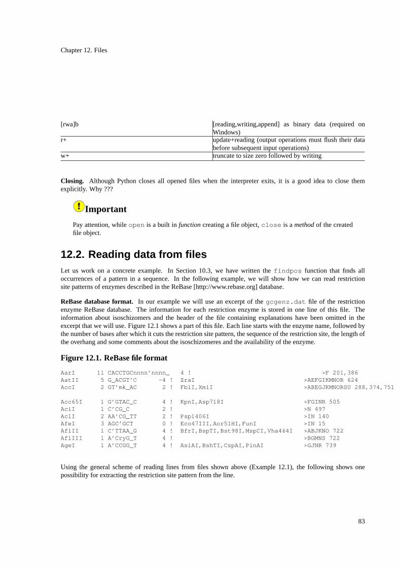
Chapter 12. Files
[rwa]b [reading,writing,append] as binary data (required onWindows)
r+ update+reading (output operations must flush their databefore subsequent input operations)
w+ truncate to size zero followed by writing
Closing. Although Python closes all opened files when the interpreter exits, it is a good idea to close themexplicitly. Why ???
Important
Pay attention, whileopen is a built in functioncreating a file object,close is amethodof the createdfile object.
12.2. Reading data from filesLet us work on a concrete example. In Section 10.3, we have written thefindpos function that finds alloccurrences of a pattern in a sequence. In the following example, we will show how we can read restrictionsite patterns of enzymes described in the ReBase [http://www.rebase.org] database.
ReBase database format.In our example we will use an excerpt of thegcgenz.dat file of the restrictionenzyme ReBase database. The information for each restriction enzyme is stored in one line of this file. Theinformation about isoschizomers and the header of the file containing explanations have been omitted in theexcerpt that we will use. Figure 12.1 shows a part of this file. Each line starts with the enzyme name, followed bythe number of bases after which it cuts the restriction site pattern, the sequence of the restriction site, the length ofthe overhang and some comments about the isoschizomeres and the availability of the enzyme.
Figure 12.1. ReBase file format
AarI 11 CACCTGCnnnn’nnnn_ 4 ! >F 201,386AatII 5 G_ACGT’C -4 ! ZraI >AEFGIKMNOR 624AccI 2 GT’mk_AC 2 ! FblI,XmiI >ABEGJKMNORSU 288,374,751
Acc65I 1 G’GTAC_C 4 ! KpnI,Asp718I >FGINR 505AciI 1 C’CG_C 2 ! >N 497AclI 2 AA’CG_TT 2 ! Psp1406I >IN 140AfeI 3 AGC’GCT 0 ! Eco47III,Aor51HI,FunI >IN 15AflII 1 C’TTAA_G 4 ! BfrI,BspTI,Bst98I,MspCI,Vha464I >ABJKNO 722AflIII 1 A’CryG_T 4 ! >BGMNS 722AgeI 1 A’CCGG_T 4 ! AsiAI,BshTI,CspAI,PinAI >GJNR 739
Using the general scheme of reading lines from files shown above (Example 12.1), the following shows onepossibility for extracting the restriction site pattern from the line.
83
Chapter 12. Files
Procedure 12.1. read_rebase
INPUT: afile in rebase format
OUTPUT: a dictionaryenz_dictcontaining all restriction patterns indexed by their name
1. enz_dict<- empty dictionary2. infh <- openfile for reading3. for each line read frominfh:
a. split line in its fieldsb. name<- first fieldc. pat<- third fieldd. clean patto get a string containing only the sequence recognized by the restriction enzymee. add the cleanedpat to enz_dictwith nameas key
4. closeinfh5. return enz_dict
here is one possibility how to translate this procedure into Python:
def get_site_only(pat):newpat = ""for c in pat:
if c.isalpha():newpat +=c
return newpat
def read_rebase(filename):enz_dict={}infh= open(filename)for line in infh.xreadlines():
fields = line.split()name = fields[0]pat = fields[2]enz_dict[name] = get_site_only(pat)
infh.close()return enz_dict
print read_rebase("../data/rebase.dat")
12.3. Writing in filesLet us continue our restriction site example. Because we have got the enzyme pattern from the ReBase database,we can now process our sequence with all these patterns using thefindpos function (Example 10.2). There isonly one restriction: at the moment thefindpos function can only findexactrestriction patterns, so we have toexclude all patterns containing ambiguous bases.
84

Chapter 12. Files
INPUT: a dictionaryenz_dictcontaining all restriction site patterns accessible by enzyme name, a sequenceseqto search for
OUTPUT: list of start position of every occurrence for each pattern in the dictionary.
• for eachkeyenznamein enz_dict:
a. pat<- pattern ofenznamein enz_dictb. if pat is anexactpattern
i. occs<- findpos(seq,pat)ii. print all occs
Theprint_matches in the following listing of functions prints the results of the analysis on the screen.
seq = ""
def isexact(pat):for c in pat.upper():
if c not in ’ATGC’:return 0
return 1
def findpos(seq, pat):matches = []current_match = seq.find(pat)while current_match != -1:
matches.append(current_match)current_match =seq.find(pat, current_match+1)
return matches
def print_matches(enz, matches):if matches:
print "Enzyme %s matches at:" % enz,for m in matches:
print m,print
else:print "No match found for enzyme %s." % enz
for enzname in enz_dict.keys():pat = enz_dict[enzname]if isexact(pat):
print_matches(enzname, findpos(seq, pat))
85

Chapter 12. Files
In order to store the results permanently, we will see now how we can write the information in a file. As forreading, we have to open a file although now in a writing mode, write our results in the file and then close it.
def print_matches(enz, matches):ofh = open("rebase.res", "w")if matches:
print >>ofh, "Enzyme %s matches at:" % enz,for m in matches:
print >>ofh, m,print >>ofh
else:print >>ofh, "No match found for enzyme %s." % enz
ofh.close()
The problem with thisprint_matches function is that it prints only the result oflast enzyme. Because if weclose the file after writing the information, the next time we will open the file for writing the next result, we willoverwrite the old result. We have two possibilities to solve this. First, we can open the file toappendat the endof the file. Or second, we can open the file for writing in the main stream of the program and then pass the fileobject as argument toprint_matches , and close the file only when all results have been written. We preferthe second solution.
seq = ""
def isexact(pat):for c in pat.upper():
if c not in ’ATGC’:return 0
return 1
def findpos(seq, pat):matches = []current_match = seq.find(pat)while current_match != -1:
matches.append(current_match)current_match =seq.find(pat, current_match+1)
return matches
def print_matches(ofh, enz, matches):if matches:
print >>ofh, "Enzyme %s matches at:" % enz,for m in matches:
print >>ofh, m,print >>ofh
else:print >>ofh, "No match found for enzyme %s." % enz
ofh = open("rebase.res", "w")for enzname in enz_dict.keys():
pat = enz_dict[enzname]
86
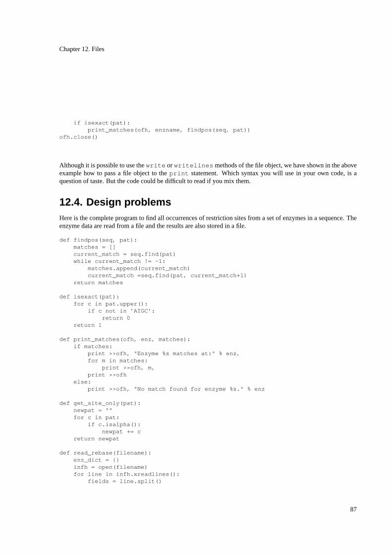
Chapter 12. Files
if isexact(pat):print_matches(ofh, enzname, findpos(seq, pat))
ofh.close()
Although it is possible to use thewrite or writelines methods of the file object, we have shown in the aboveexample how to pass a file object to theprint statement. Which syntax you will use in your own code, is aquestion of taste. But the code could be difficult to read if you mix them.
12.4. Design problemsHere is the complete program to find all occurrences of restriction sites from a set of enzymes in a sequence. Theenzyme data are read from a file and the results are also stored in a file.
def findpos(seq, pat):matches = []current_match = seq.find(pat)while current_match != -1:
matches.append(current_match)current_match =seq.find(pat, current_match+1)
return matches
def isexact(pat):for c in pat.upper():
if c not in ’ATGC’:return 0
return 1
def print_matches(ofh, enz, matches):if matches:
print >>ofh, "Enzyme %s matches at:" % enz,for m in matches:
print >>ofh, m,print >>ofh
else:print >>ofh, "No match found for enzyme %s." % enz
def get_site_only(pat):newpat = ""for c in pat:
if c.isalpha():newpat += c
return newpat
def read_rebase(filename):enz_dict = {}infh = open(filename)for line in infh.xreadlines():
fields = line.split()
87

Chapter 12. Files
name = fields[0]pat = fields[2]enz_dict[name] = get_site_only(pat)
infh.close()return enz_dict
def findpos(seq, pat):matches = []current_match = seq.find(pat)while current_match != -1:
matches.append(current_match)current_match =seq.find(pat, current_match+1)
return matches
seq = """atgagtgaacgtctgagcattaccccgctggggccgtatatcggcgcacaaatttcgggtgccgacctgacgcgcccgttaagcgataatcagtttgaacagctttaccatgcggtgctgcgccatcaggtggtgtttctacgcgatcaagctattacgccgcagcagcaacgcgcgctggcccagcgttttggcgaattgcatattcaccctgtttacccgcatgccgaaggggttgacgagatcatcgtgctggatacccataacgataatccgccagataacgacaactggcataccgatgtgacatttattgaaacgccacccgcaggggcgattctggcagctaaagagttaccttcgaccggcggtgatacgctctggaccagcggtattgcggcctatgaggcgctctctgttcccttccgccagctgctgagtgggctgcgtgcggagcatgatttccgtaaatcgttcccggaatacaaataccgcaaaaccgaggaggaacatcaacgctggcgcgaggcggtcgcgaaaaacccgccgttgctacatccggtggtgcgaacgcatccggtgagcggtaaacaggcgctgtttgtgaatgaaggctttactacgcgaattgttgatgtgagcgagaaagagagcgaagccttgttaagttttttgtttgcccatatcaccaaaccggagtttcaggtgcgctggcgctggcaaccaaatgatattgcgatttgggataaccgcgtgacccagcactatgccaatgccgattacctgccacagcgacggataatgcatcgggcgacgatccttggggataaaccgttttatcgggcggggtaa""".replace("\n","").upper()
enzdict = read_rebase("../data/rebase.dat")
ofh = open("rebase.res", "w")for enzname in enzdict.keys():
pat = enzdict[enzname]if isexact(pat):
print_matches(ofh, enzname, findpos(seq, pat))ofh.close()
We have written this program step by step by broadening the problem at each step, but we have never looked atthe global design of the program. Therefore we have used two strategies while reading and writing. In the readingstep all data are read at once, whereas the results are written each time we got them.
In biological problems it is often necessary to handle lots of data and this can lead to problems if you try to handleall of them in memory, as we have done with the enzyme data. Sometimes we need all the data to solve a problem,
88
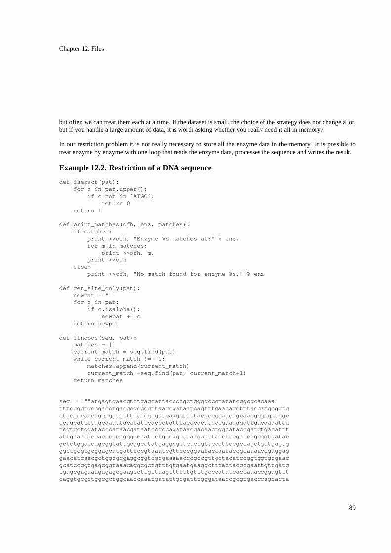
Chapter 12. Files
but often we can treat them each at a time. If the dataset is small, the choice of the strategy does not change a lot,but if you handle a large amount of data, it is worth asking whether you really need it all in memory?
In our restriction problem it is not really necessary to store all the enzyme data in the memory. It is possible totreat enzyme by enzyme with one loop that reads the enzyme data, processes the sequence and writes the result.
Example 12.2. Restriction of a DNA sequence
def isexact(pat):for c in pat.upper():
if c not in ’ATGC’:return 0
return 1
def print_matches(ofh, enz, matches):if matches:
print >>ofh, "Enzyme %s matches at:" % enz,for m in matches:
print >>ofh, m,print >>ofh
else:print >>ofh, "No match found for enzyme %s." % enz
def get_site_only(pat):newpat = ""for c in pat:
if c.isalpha():newpat += c
return newpat
def findpos(seq, pat):matches = []current_match = seq.find(pat)while current_match != -1:
matches.append(current_match)current_match =seq.find(pat, current_match+1)
return matches
seq = """atgagtgaacgtctgagcattaccccgctggggccgtatatcggcgcacaaatttcgggtgccgacctgacgcgcccgttaagcgataatcagtttgaacagctttaccatgcggtgctgcgccatcaggtggtgtttctacgcgatcaagctattacgccgcagcagcaacgcgcgctggcccagcgttttggcgaattgcatattcaccctgtttacccgcatgccgaaggggttgacgagatcatcgtgctggatacccataacgataatccgccagataacgacaactggcataccgatgtgacatttattgaaacgccacccgcaggggcgattctggcagctaaagagttaccttcgaccggcggtgatacgctctggaccagcggtattgcggcctatgaggcgctctctgttcccttccgccagctgctgagtgggctgcgtgcggagcatgatttccgtaaatcgttcccggaatacaaataccgcaaaaccgaggaggaacatcaacgctggcgcgaggcggtcgcgaaaaacccgccgttgctacatccggtggtgcgaacgcatccggtgagcggtaaacaggcgctgtttgtgaatgaaggctttactacgcgaattgttgatgtgagcgagaaagagagcgaagccttgttaagttttttgtttgcccatatcaccaaaccggagtttcaggtgcgctggcgctggcaaccaaatgatattgcgatttgggataaccgcgtgacccagcacta
89
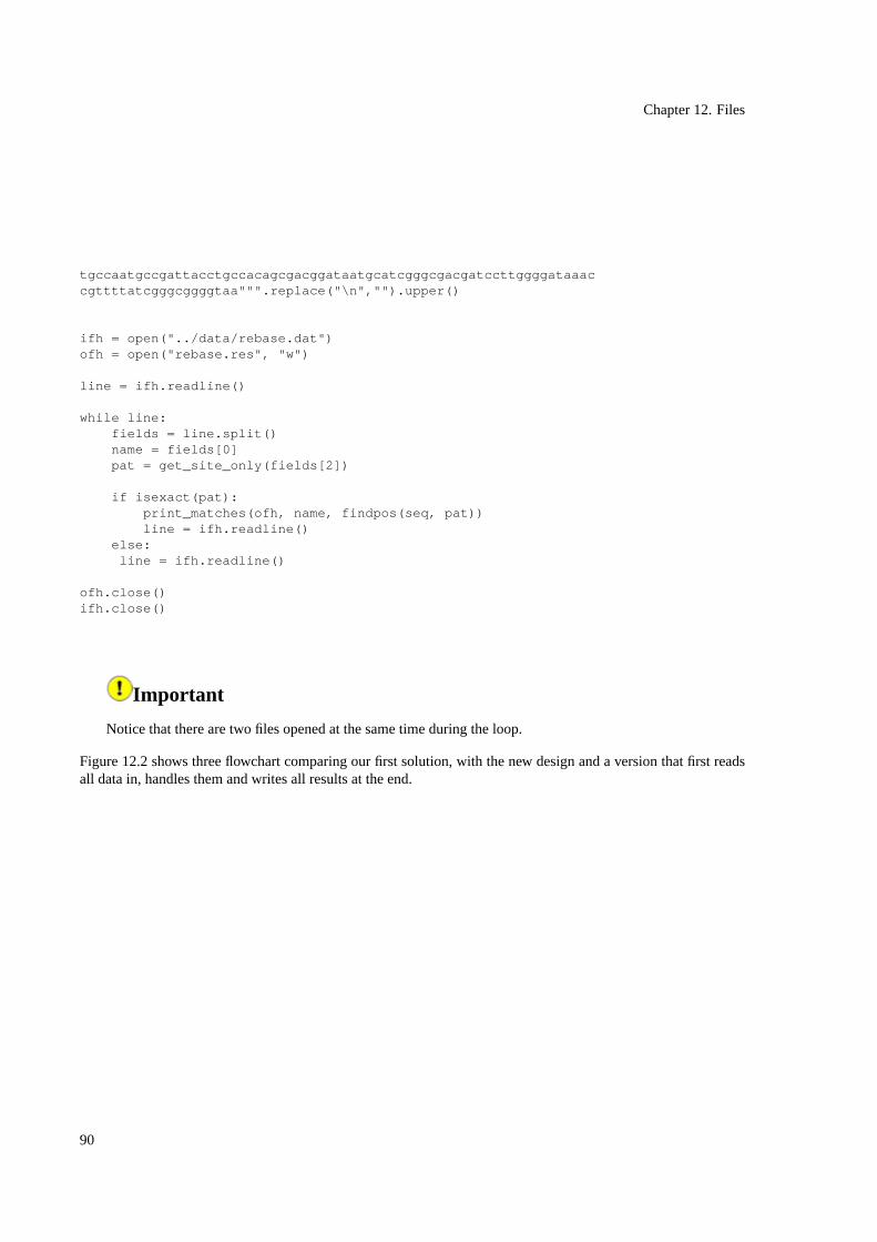
Chapter 12. Files
tgccaatgccgattacctgccacagcgacggataatgcatcgggcgacgatccttggggataaaccgttttatcgggcggggtaa""".replace("\n","").upper()
ifh = open("../data/rebase.dat")ofh = open("rebase.res", "w")
line = ifh.readline()
while line:fields = line.split()name = fields[0]pat = get_site_only(fields[2])
if isexact(pat):print_matches(ofh, name, findpos(seq, pat))line = ifh.readline()
else:line = ifh.readline()
ofh.close()ifh.close()
Important
Notice that there are two files opened at the same time during the loop.
Figure 12.2 shows three flowchart comparing our first solution, with the new design and a version that first readsall data in, handles them and writes all results at the end.
90

Chapter 12. Files
Figure 12.2. Flowchart of the processing of the sequence
open the input file
open output file
close the output file
open the input file
open output file
close the output file
open the input file
open output file
close the output file
close the input file
close the input file
close the input file
Exercise 12.1. Multiple sequences for all enzymes
Think about alternative solutions, their advantages and problems if you need to process more than one sequencefor all restriction enzymes.
12.5. Documentation stringsThe code of the program written in this section (Example 12.2) fills about one page. If you put it away for a whileand look on it a week later, it might be difficult to remember all the choices made during the development and itmight take a lot of time to understand it. This fact underlines the importance todocument programs.
91
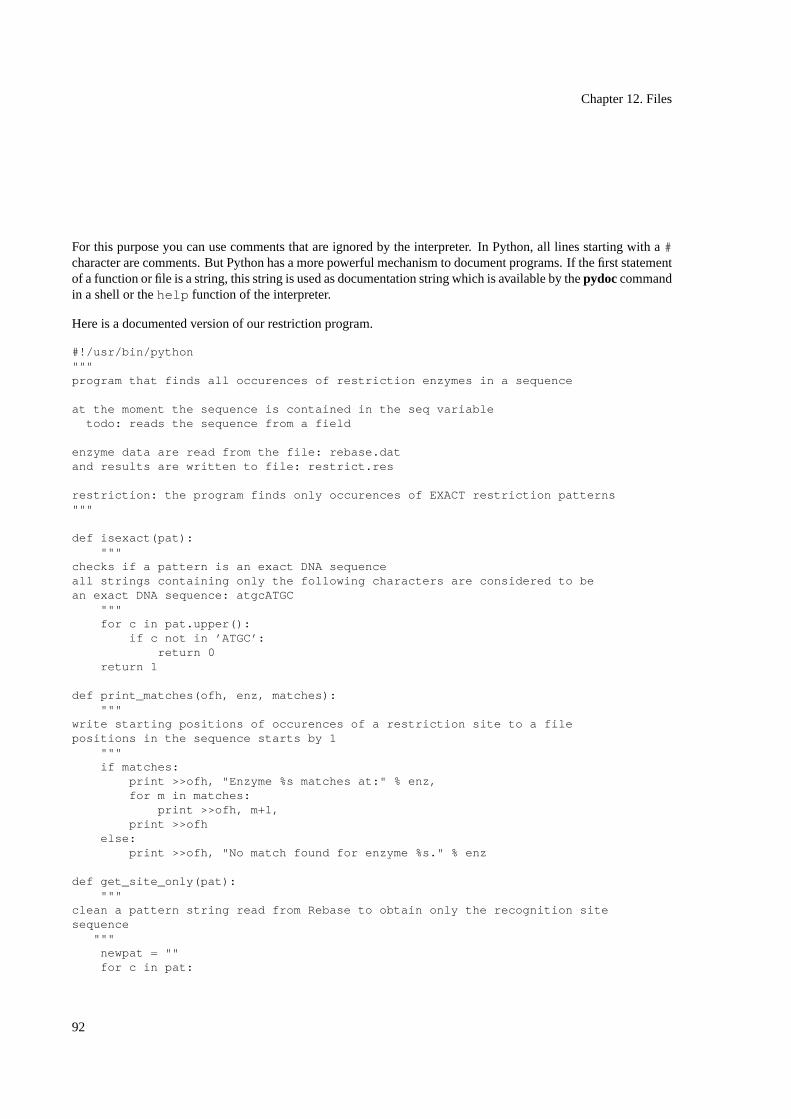
Chapter 12. Files
For this purpose you can use comments that are ignored by the interpreter. In Python, all lines starting with a#character are comments. But Python has a more powerful mechanism to document programs. If the first statementof a function or file is a string, this string is used as documentation string which is available by thepydoccommandin a shell or thehelp function of the interpreter.
Here is a documented version of our restriction program.
#!/usr/bin/python"""program that finds all occurences of restriction enzymes in a sequence
at the moment the sequence is contained in the seq variabletodo: reads the sequence from a field
enzyme data are read from the file: rebase.datand results are written to file: restrict.res
restriction: the program finds only occurences of EXACT restriction patterns"""
def isexact(pat):"""
checks if a pattern is an exact DNA sequenceall strings containing only the following characters are considered to bean exact DNA sequence: atgcATGC
"""for c in pat.upper():
if c not in ’ATGC’:return 0
return 1
def print_matches(ofh, enz, matches):"""
write starting positions of occurences of a restriction site to a filepositions in the sequence starts by 1
"""if matches:
print >>ofh, "Enzyme %s matches at:" % enz,for m in matches:
print >>ofh, m+1,print >>ofh
else:print >>ofh, "No match found for enzyme %s." % enz
def get_site_only(pat):"""
clean a pattern string read from Rebase to obtain only the recognition sitesequence
"""newpat = ""for c in pat:
92
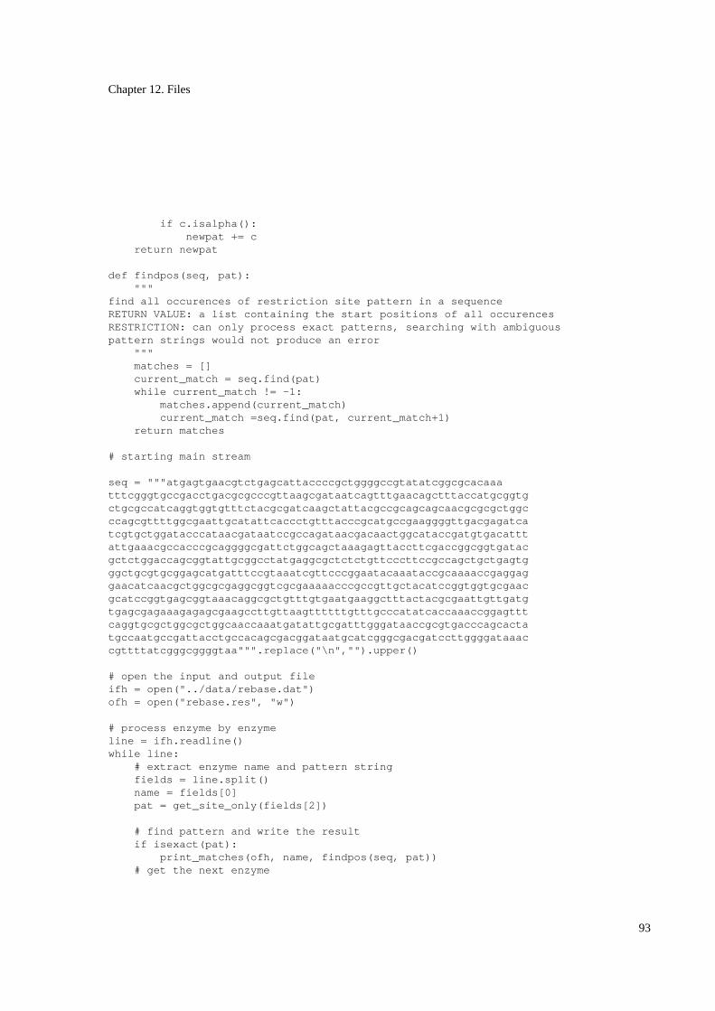
Chapter 12. Files
if c.isalpha():newpat += c
return newpat
def findpos(seq, pat):"""
find all occurences of restriction site pattern in a sequenceRETURN VALUE: a list containing the start positions of all occurencesRESTRICTION: can only process exact patterns, searching with ambiguouspattern strings would not produce an error
"""matches = []current_match = seq.find(pat)while current_match != -1:
matches.append(current_match)current_match =seq.find(pat, current_match+1)
return matches
# starting main stream
seq = """atgagtgaacgtctgagcattaccccgctggggccgtatatcggcgcacaaatttcgggtgccgacctgacgcgcccgttaagcgataatcagtttgaacagctttaccatgcggtgctgcgccatcaggtggtgtttctacgcgatcaagctattacgccgcagcagcaacgcgcgctggcccagcgttttggcgaattgcatattcaccctgtttacccgcatgccgaaggggttgacgagatcatcgtgctggatacccataacgataatccgccagataacgacaactggcataccgatgtgacatttattgaaacgccacccgcaggggcgattctggcagctaaagagttaccttcgaccggcggtgatacgctctggaccagcggtattgcggcctatgaggcgctctctgttcccttccgccagctgctgagtgggctgcgtgcggagcatgatttccgtaaatcgttcccggaatacaaataccgcaaaaccgaggaggaacatcaacgctggcgcgaggcggtcgcgaaaaacccgccgttgctacatccggtggtgcgaacgcatccggtgagcggtaaacaggcgctgtttgtgaatgaaggctttactacgcgaattgttgatgtgagcgagaaagagagcgaagccttgttaagttttttgtttgcccatatcaccaaaccggagtttcaggtgcgctggcgctggcaaccaaatgatattgcgatttgggataaccgcgtgacccagcactatgccaatgccgattacctgccacagcgacggataatgcatcgggcgacgatccttggggataaaccgttttatcgggcggggtaa""".replace("\n","").upper()
# open the input and output fileifh = open("../data/rebase.dat")ofh = open("rebase.res", "w")
# process enzyme by enzymeline = ifh.readline()while line:
# extract enzyme name and pattern stringfields = line.split()name = fields[0]pat = get_site_only(fields[2])
# find pattern and write the resultif isexact(pat):
print_matches(ofh, name, findpos(seq, pat))# get the next enzyme
93
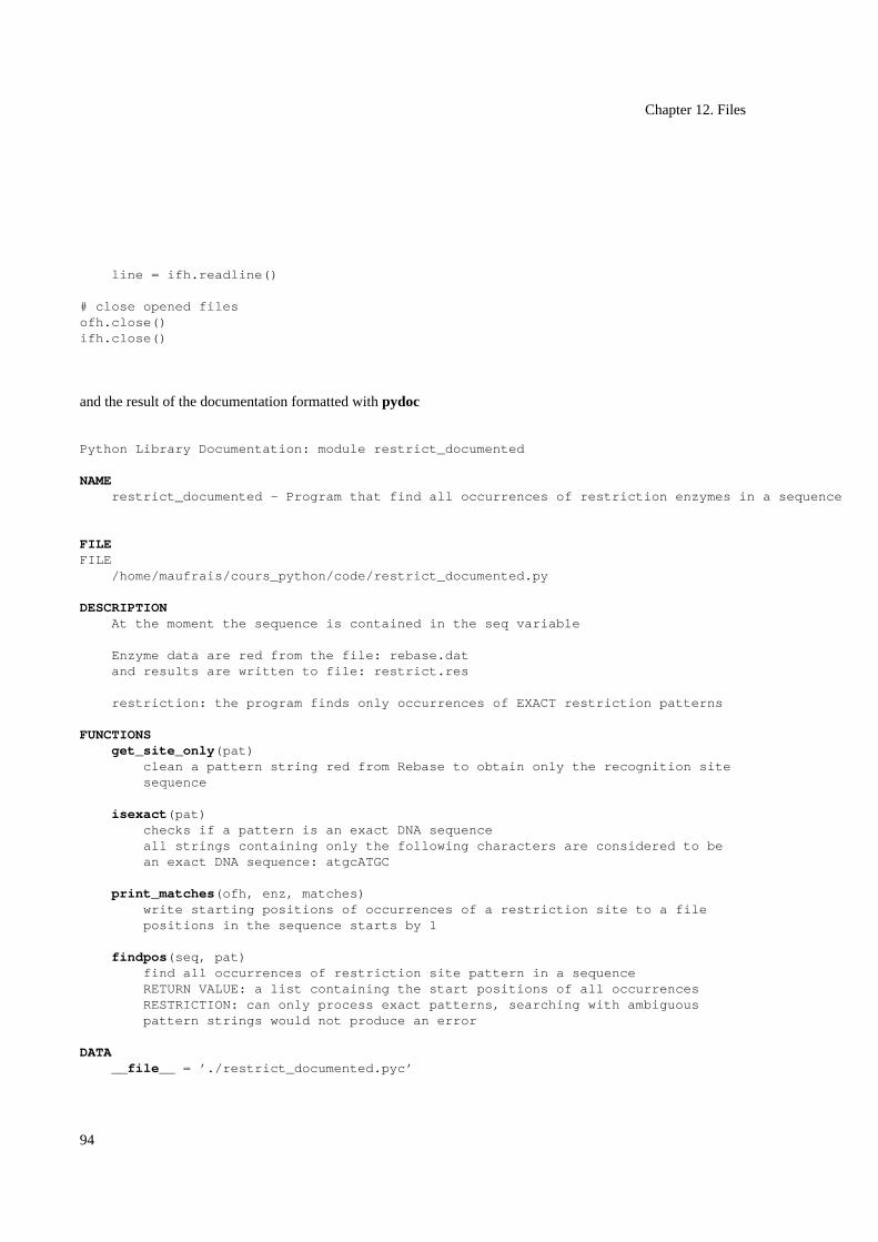
Chapter 12. Files
line = ifh.readline()
# close opened filesofh.close()ifh.close()
and the result of the documentation formatted withpydoc
Python Library Documentation: module restrict_documented
NAMErestrict_documented - Program that find all occurrences of restriction enzymes in a sequence
FILEFILE
/home/maufrais/cours_python/code/restrict_documented.py
DESCRIPTIONAt the moment the sequence is contained in the seq variable
Enzyme data are red from the file: rebase.datand results are written to file: restrict.res
restriction: the program finds only occurrences of EXACT restriction patterns
FUNCTIONSget_site_only (pat)
clean a pattern string red from Rebase to obtain only the recognition sitesequence
isexact (pat)checks if a pattern is an exact DNA sequenceall strings containing only the following characters are considered to bean exact DNA sequence: atgcATGC
print_matches (ofh, enz, matches)write starting positions of occurrences of a restriction site to a filepositions in the sequence starts by 1
findpos (seq, pat)find all occurrences of restriction site pattern in a sequenceRETURN VALUE: a list containing the start positions of all occurrencesRESTRICTION: can only process exact patterns, searching with ambiguouspattern strings would not produce an error
DATA__file__ = ’./restrict_documented.pyc’
94
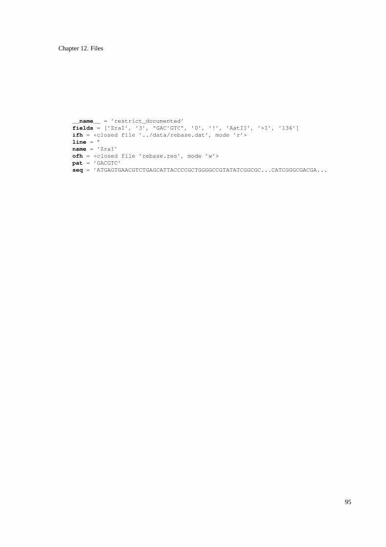
Chapter 12. Files
__name__ = ’restrict_documented’fields = [’ZraI’, ’3’, "GAC’GTC", ’0’, ’!’, ’AatII’, ’>I’, ’136’]ifh = <closed file ’../data/rebase.dat’, mode ’r’>line = ”name = ’ZraI’ofh = <closed file ’rebase.res’, mode ’w’>pat = ’GACGTC’seq = ’ATGAGTGAACGTCTGAGCATTACCCCGCTGGGGCCGTATATCGGCGC...CATCGGGCGACGA...
95

Chapter 12. Files
96
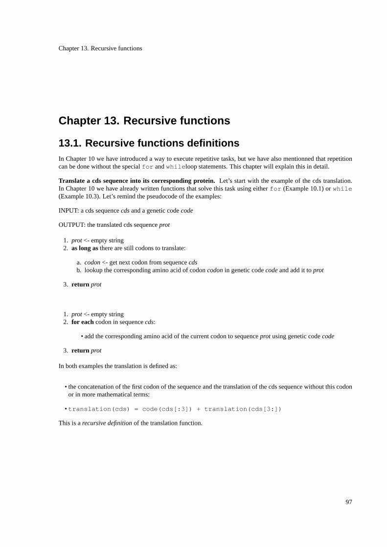
Chapter 13. Recursive functions
Chapter 13. Recursive functions
13.1. Recursive functions definitionsIn Chapter 10 we have introduced a way to execute repetitive tasks, but we have also mentionned that repetitioncan be done without the specialfor andwhile loop statements. This chapter will explain this in detail.
Translate a cds sequence into its corresponding protein.Let’s start with the example of the cds translation.In Chapter 10 we have already written functions that solve this task using eitherfor (Example 10.1) orwhile(Example 10.3). Let’s remind the pseudocode of the examples:
INPUT: a cds sequencecdsand a genetic codecode
OUTPUT: the translated cds sequenceprot
1. prot <- empty string2. as long asthere are still codons to translate:
a. codon<- get next codon from sequencecdsb. lookup the corresponding amino acid of codoncodonin genetic codecodeand add it toprot
3. return prot
1. prot <- empty string2. for eachcodon in sequencecds:
• add the corresponding amino acid of the current codon to sequenceprot using genetic codecode
3. return prot
In both examples the translation is defined as:
• the concatenation of the first codon of the sequence and the translation of the cds sequence without this codonor in more mathematical terms:
• translation(cds) = code(cds[:3]) + translation(cds[3:])
This is arecursive definitionof the translation function.
97

Chapter 13. Recursive functions
Recursive functions
A recursive functionis afunctionthat use itself during the calculation procedure.
Recursive definition
A recursive definitionof a function is a definition that uses the function itself in the definition.
It is important to notice that we need aterminal condition otherwise the recursion would never stop. In our casethe recursion stops if there are no more codons to translate:
• the protein sequence of the an empty cds sequence is empty
• or in more mathematical terms:translation("") = ""
Therefore the pseudocode can be written as follow without using loop structures:
INPUT: a cds sequencecdsand a genetic codecode
OUTPUT: the translated sequenceprot
1. if cdsis empty:
a. *** This is the terminal condition ***b. return empty string
2. otherwise:
a. *** This is the recursion ***b. codon<- first codon of sequencecdsc. return the concatenation of the corresponding amino acid of the first codon of sequencecdsin genetic
codecodeand the translation of the rest of thecdssequence
98
Chapter 13. Recursive functions
and implemented in Python like that:
code = {’ttt’: ’F’, ’tct’: ’S’, ’tat’: ’Y’, ’tgt’: ’C’,’ttc’: ’F’, ’tcc’: ’S’, ’tac’: ’Y’, ’tgc’: ’C’,’tta’: ’L’, ’tca’: ’S’, ’taa’: ’*’, ’tga’: ’*’,’ttg’: ’L’, ’tcg’: ’S’, ’tag’: ’*’, ’tgg’: ’W’,’ctt’: ’L’, ’cct’: ’P’, ’cat’: ’H’, ’cgt’: ’R’,’ctc’: ’L’, ’ccc’: ’P’, ’cac’: ’H’, ’cgc’: ’R’,’cta’: ’L’, ’cca’: ’P’, ’caa’: ’Q’, ’cga’: ’R’,’ctg’: ’L’, ’ccg’: ’P’, ’cag’: ’Q’, ’cgg’: ’R’,’att’: ’I’, ’act’: ’T’, ’aat’: ’N’, ’agt’: ’S’,’atc’: ’I’, ’acc’: ’T’, ’aac’: ’N’, ’agc’: ’S’,’ata’: ’I’, ’aca’: ’T’, ’aaa’: ’K’, ’aga’: ’R’,’atg’: ’M’, ’acg’: ’T’, ’aag’: ’K’, ’agg’: ’R’,’gtt’: ’V’, ’gct’: ’A’, ’gat’: ’D’, ’ggt’: ’G’,’gtc’: ’V’, ’gcc’: ’A’, ’gac’: ’D’, ’ggc’: ’G’,’gta’: ’V’, ’gca’: ’A’, ’gaa’: ’E’, ’gga’: ’G’,’gtg’: ’V’, ’gcg’: ’A’, ’gag’: ’E’, ’ggg’: ’G’
}
def rectranslate(cds, code):if cds == "":
return ""else:
codon = cds[:3]return code[codon] + rectranslate(cds[3:], code)
print rectranslate("atgattgctggt", code)
13.2. Flow of execution of recursive functionsAt first glance recursive functions look a little bit strange because it seems that we use something that we have notdefined. But remember that the statements in the body of a function are only executed when the function is called.At the definition step, the function is just added in the current namespace. Therefore it will be defined when wecall it in the body.
Writing recursive functions is sometimes difficult, because we doubt that we have defined a function executing thespecific task, when we call the it . Therefore it is useful to remember this fact during the development of recursivefunctions.
Stack diagram of recursive functions. Let’s have a deeper look at the flow of execution of recursive functions.Figure 13.1 shows the stack diagram of function calls.
99

Chapter 13. Recursive functions
Figure 13.1. Stack diagram of recursive function calls
return
return
return
return
return
code
cds
code
cds
code
cds
"gctggt"
code
cds
code
cds
"atgattgctggt"
""
"ggt"
"attgctggt"
{ ’ttt’: ’F’ , ..., ’ggg’: ’G’ }
""
"G"
"AG"
"IAG"
"MIAG"
rectranslate("atgattgctggt", code)
rectranslate
rectranslate
rectranslate
rectranslate
rectranslate
Figure 13.1 shows that thetranslate function is called with a cds sequence of decreasing length and the localfunction namespaces are piled up until the terminal condition is reached.
=> rectranslate("atgattgctggt", code)===> rectranslate("attgctggt", code)=====> rectranslate("gctggt", code)=======> rectranslate("ggt", code)=========> rectranslate("", code)=========> return ""=======> return "G"=====> return "AG"===> return "IAG"=> return "MIAG"
100
Chapter 13. Recursive functions
Important
Recursive function calls can take a lot of memory space because for each recursive call the localnamespace for the given function call has to be stored. It is important to pay attention on this factbecause memory space is a limited resource on a computer.
13.3. Recursive data structuresIn the Chapter 11, we have worked with examples using nested list. If we examine them a little bit more, we willsee that a nested list can be defined recursively.
Nested list
A nested list is an ordered collection of elements that are:
• either items
• or nested lists
The items define the content, whereas the lists define the structure of the collection.
How can we use this?Let’s use phylogenetic trees as examples for such a recursive list structure. Figure 13.2shows an example of a phylogenetic tree topology that can be implemented in Python as follows:
>>> tree = [[[[’human’, ’chimpanzee’], ’gorilla’], ’orang-utan’], ’gibbon’]
Figure 13.2 shows the representation oftree .
101

Chapter 13. Recursive functions
Figure 13.2. A phylogenetic tree topology
human chimpanzee gorilla orang−utan gibbon
Figure 13.3. Tree representation using a recursive list structure
chimpanzeehuman gorilla orang−utan gibbon
tree
Working with recursive structures. Assume that we would do something for each branching point in the abovetree. A simple traversal usingfor or while is no more possible, because both loop structures handle only onelevel of the list. But with recursive functions that we have introduced in Chapter 13, we can do such things withthe following strategy:
Procedure 13.4. tree_traversal(tree)
INPUT: a treetree
1. do what you have to do when you enter the branching point2. if tree is a list:
a. *** recursion step ***b. for eachelementof tree:
102
Chapter 13. Recursive functions
• tree_traversal(element)
3. otherwise:
• *** end condition of the recursion, here the leaves of the tree ***
4. do what you have to do when you leave the branching point
Doing something when you enter the branching point, is also known aspreorder traversalof a tree, whereas doingsomething when leaving a branching point is also calledpostorder traversalof a tree.
We will give two example applications of this strategy for our tree. The first one prints all species of the trees:
tree = [[[[’human’, ’chimpanzee’], ’gorilla’], ’orang-utan’], ’gibbon’]
import types
def print_species(tree):if type(tree) is types.ListType:
for child in tree:print_species(child)
else:print tree
>>> print_species(tree)humanchimpanzeegorillaorang-utangibbon
and the second one that prints for a tree or a binary tree2 the two populations that are split at this point.
tree = [[[[’human’, ’chimpanzee’], ’gorilla’], ’orang-utan’], ’gibbon’]
import types
def splits(tree):if type(tree) is types.ListType:
all_leaves = []for child in tree:
child_leaves = splits(child)print child_leaves,all_leaves += child_leaves
A binary tree is a tree with maximal two subtrees for each branching point.
103
Chapter 13. Recursive functions
printreturn all_leaves
else:return [ tree ]
def binary_splits(tree):if type(tree) is types.ListType:
left = binary_splits(tree[0])right = binary_splits(tree[1])print left, rightreturn left + right
else:return [ tree ]
>>> splits(tree)[’human’] [’chimpanzee’][’human’, ’chimpanzee’] [’gorilla’][’human’, ’chimpanzee’, ’gorilla’] [’orang-utan’][’human’, ’chimpanzee’, ’gorilla’, ’orang-utan’] [’gibbon’][’human’, ’chimpanzee’, ’gorilla’, ’orang-utan’, ’gibbon’]
Finally, we will show the code that separates the work to do from the tree traversal itself by functions. Thetraversal functiontree_traversal do not change for the task. The user has only to redefine the functionsdo_prework , do_postwork anddo_leafwork .
import types
def do_prework(node):print "prework:", node
def do_postwork(node):print "postwork:", node
def is_leaf(node):return type(node) is not types.ListType
def do_leafwork(leaf):print "that is a leaf:", leaf
def tree_traversal (node):do_prework(node)
if not is_leaf(node):for child in node:
tree_traversal(child)
104

Chapter 13. Recursive functions
else:do_leafwork(node)
do_postwork(node)
>>> tree=[[[[’human’, ’chimpanzee’], ’gorilla’], ’orang-utan’], ’gibbon’]>>> tree_traversal(tree)prework: [[[[’human’, ’chimpanzee’], ’gorilla’], ’orang-utan’], ’gibbon’]prework: [[[’human’, ’chimpanzee’], ’gorilla’], ’orang-utan’]prework: [[’human’, ’chimpanzee’], ’gorilla’]prework: [’human’, ’chimpanzee’]prework: humanthat is a leaf: humanpostwork: humanprework: chimpanzeethat is a leaf: chimpanzeepostwork: chimpanzeepostwork: [’human’, ’chimpanzee’]prework: gorillathat is a leaf: gorillapostwork: gorillapostwork: [[’human’, ’chimpanzee’], ’gorilla’]prework: orang-utanthat is a leaf: orang-utanpostwork: orang-utanpostwork: [[[’human’, ’chimpanzee’], ’gorilla’], ’orang-utan’]prework: gibbonthat is a leaf: gibbonpostwork: gibbonpostwork: [[[[’human’, ’chimpanzee’], ’gorilla’], ’orang-utan’], ’gibbon’]
105

Chapter 13. Recursive functions
106

Chapter 14. Exceptions
Chapter 14. Exceptions
14.1. General MechanismExceptions are a mechanism to handle errors during the execution of a program. An exception israisedwheneveran error occurs:
Example 14.1. Filename error
>>> f = open(’my_fil’)Traceback (most recent call last):
File "<stdin>", line 1, in ?IOError: [Errno 2] No such file or directory: ’my_fil’
An exception can becaughtby the code where the error occurred:
try:f = open(’my_fil’)
except IOError, e:print e
Variablee contains the cause of the error:
[Errno 2] No such file or directory: ’my_fil’
14.2. Python built-in exceptions
107
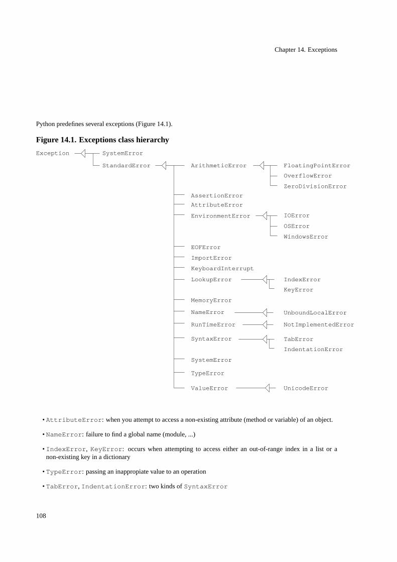
Chapter 14. Exceptions
Python predefines several exceptions (Figure 14.1).
Figure 14.1. Exceptions class hierarchy
ZeroDivisionError
ArithmeticError FloatingPointError
OverflowError
EnvironmentError IOError
WindowsError
OSError
RunTimeError NotImplementedError
NameError UnboundLocalError
SyntaxError TabError
IndentationError
UnicodeErrorValueError
Exception SystemError
StandardError
AttributeError
AssertionError
EOFError
ImportError
KeyboardInterrupt
MemoryError
LookupError IndexError
KeyError
TypeError
SystemError
• AttributeError : when you attempt to access a non-existing attribute (method or variable) of an object.
• NameError : failure to find a global name (module, ...)
• IndexError , KeyError : occurs when attempting to access either an out-of-range index in a list or anon-existing key in a dictionary
• TypeError : passing an inappropiate value to an operation
• TabError , IndentationError : two kinds ofSyntaxError
108
Chapter 14. Exceptions
14.3. Raising exceptionsYou can alsoraisean exception in your code, if you consider that the program should be interrupted:
if something_wrong:raise Exception
You can associate a message to theraise statement:
if something_wrong:raise Exception, " something went wrong"
Example 14.2. Raising an exception in case of a wrong DNA character
def check_dna(dna, alphabet=’atgc’):""" using exceptions """
for base in dna:if base not in alphabet:
raise ValueError, "%s not in %s" % (base, alphabet)
return 1
14.4. Defining exceptionsPython provides a set of pre-defined exception classes that you can specialize by sub-classing to define specificexceptions for your application (Figure 14.1).
Go to
Since exceptions are defined as classes and by inheritance, you will need some knowledge about classesin order to fully understand this section (see Chapter 17).
Example 14.3. Raising your own exception in case of a wrong DNA character
In the following code, you define an exceptionAlphabetError that can be used when the sequence passed tothe function does not correspond to thealphabet .
class AlphabetError(ValueError): ❶pass
def check_dna(dna, alphabet=’atgc’):
109
Chapter 14. Exceptions
""" using exceptions """
for base in dna:if base not in alphabet:
raise AlphabetError, "%s not in %s" % (base, alphabet)
return 1
❶ Definition of a new exception in categoryValueError : AlphabetError is a class, that is a sub-class of classValueError . The only statement present in classAlphabetError is pass sinceAlphabetError does not define any new behaviour: it is just a new class name.
Example 14.4. Exceptions defined in Biopython
Some Biopython modules define their own exceptions, such as:
• ParserFailureError (GenBank package)
• BadMatrix (SubsMat package)
110

Chapter 15. Modules and packages in Python
Chapter 15. Modules and packages in Python
15.1. ModulesA module is a component providing Python definitions of functions, variables or classes... all corresponding to agiven specific thema. All these definitions are contained in a single Python file. Thanks to modules, you can reuseready-to-use definitions in your own programs. Python also encourages you to build your own modules in a rathersimple way.
15.1.1. Using modules
In order to use a module, just use theimport statement. Let us take an example. Python comes with numerousmodules, and a very useful one is thesys module (sys stands for "system"): it provides information on the contextof the run and the environment of the Python interpreter. For instance, consider the following code:
#!/local/bin/pythonimport sys
print "arguments: ", sys.argv
Say that you stored in a modexa.py file, and that you run it like this:
./modexa.py 1 a seq.fasta
This will produces the following output:
arguments: [’./modexa.py’, ’1’, ’a’, ’seq.fasta’]
Explanation: By using theargv variable defined in thesys module, you can thus access to the values providedon the command line when launching the program. As shown in this example, the access to this information ismade possible by:
• importing the module through theimport statement, which provides access to the module’s definitions
• using theargv variable defined in the module by a qualified name:sys.argv .
111

Chapter 15. Modules and packages in Python
You may also select specific components from the module:
from sys import argvprint "arguments: ", argv
In this case, you only import one definition (theargv variable) from thesys module. The other definitions arenot loaded.
15.1.2. Building modules
You build your own module by creating a Python file. For instance, if the fileValSeq.py contains the followingcode (adapted from the BiopythonValSeq module):
Example 15.1. A module
# file Valseq.py
valid_sequence_dict = { "P1": "complete protein", \"F1": "protein fragment", "DL": "linear DNA", "DC": "circular DNA", \"RL": "linear RNA", "RC":"circular RNA", "N3": "transfer RNA", \"N1": "other" }
def find_valid_key(e):for key,value in valid_sequence_dict.items():
if value == e:return key
you can use it by loading it:
import ValSeq
whereValSeq is the module name. You can then access to its definitions, which may be variables, functions,classes, etc...:
>>> print ValSeq.valid_sequence_dict[’RL’]linear RNA>>> ValSeq.find_valid_key("linear RNA")
RL
15.1.3. Where are the modules?
Modules are mainly stored in files that are searched:
112

Chapter 15. Modules and packages in Python
• in your current working directory,
• in PYTHONHOME, where Python has been installed,
• in a path, i.e a colon (’:’) separated list of file paths, stored in the environment variablePYTHONPATH. Youcan check this path through thesys.path variable.
Files may be:
• Python files, suffixed by.py (when loaded for the first time, compiled version of the file is stored in thecorresponding.pyc file),
• defined as C extensions,
• built-in modules linked to the Python interpreter.
Exercise 15.1. Locating modules
Sometimes, it is not enough to usepydoc or help . Looking at the source code can bring a better understanding,even if you should of course never use undocumented features.
Browse the directory treePYTHONHOME/site-packages/Bio/.
15.1.4. How does it work?
When importing a module, the interpreter creates a new namespace, in which the Python code of the module’s fileis run. The interpreter also defines a variable (such assys , ValSeq , ...) that refers to this new namespace, bywhich the namespace becomes available to your program (Figure 15.2).
Figure 15.1. Module namespace
argv
path
sys
import sys
current namespace
...
...
113
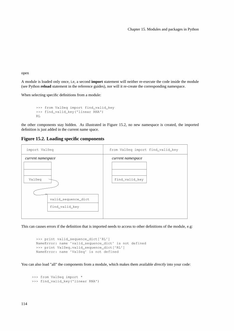
Chapter 15. Modules and packages in Python
open
A module is loaded only once, i.e, a secondimport statement will neither re-execute the code inside the module(see Pythonreload statement in the reference guides), nor will it re-create the corresponding namespace.
When selecting specific definitions from a module:
>>> from ValSeq import find_valid_key>>> find_valid_key("linear RNA")RL
the other components stay hidden. As illustrated in Figure 15.2, no new namespace is created, the importeddefinition is just added in the current name space.
Figure 15.2. Loading specific components
ValSeq
valid_sequence_dict
find_valid_key
find_valid_key
import ValSeq from ValSeq import find_valid_key
current namespace current namespace
This can causes errors if the definition that is imported needs to access to other definitions of the module, e.g:
>>> print valid_sequence_dict[’RL’]NameError: name ’valid_sequence_dict’ is not defined>>> print ValSeq.valid_sequence_dict[’RL’]NameError: name ’ValSeq’ is not defined
You can also load "all" the components from a module, which makes them availabledirectly into your code:
>>> from ValSeq import *>>> find_valid_key("linear RNA")
114

Chapter 15. Modules and packages in Python
You probably did this many times in order to use thestring module’s definitions, right? The result of:
>>> from string import *
is that all the definitions of the module are copied in your current namespace.
Caution
Be aware of potential names collision: for instance, if you current namespace contains a definition of avariable called, say:count , it will be destroyed and overloaded by thestring module’s definition ofthecount function.
Caution
You can restrict the components being imported by animport * statement. The__all__ variable,also used for packages (Section 15.2), can explicitly list the components that should be directly accessible(see Exercise 15.4).
15.1.5. Running a module from the command line
When the file of a module is run from the command line (instead for being imported):
% python ValSeq.py
the module does not behaves like a module anymore. It is, instead, run within the default__main__ module (i.enot theValSeq module):
% python -i ValSeq.py>>> ValSeq.find_valid_key("linear RNA")NameError: name ’ValSeq’ is not defined>>> find_valid_key("linear RNA")’DL’
For this reason, the code executed when the module is loaded (e.g: either with import or from the command line)can be made dependent of its current name by testing this name. The current module’s name is stored in a specialpurpose variable__name__:
if __name__ == ’__main__’:# statements that you want to be executed only when the# module is executed from the command line# (not when importing the code by an import statement)
print find_valid_key("linear RNA")
115

Chapter 15. Modules and packages in Python
15.2. PackagesA package is a set of modules or sub-packages. A package is actually a directory containing either.py files orsub-directories defining other packages.
The dot (.) operator is used to describe a hierarchy of packages and modules. For instance, the moduleBio.WWW.ExPASy is located in the filePYTHONHOME/site-packages/Bio/WWW/ExPASy.py . Thismodule belongs to the Bio.WWW package located into thePYTHONHOME/site-packages/Bio/WWW/directory.
15.2.1. Loading
When loading a package, the__init__.py file is executed. If the__init__.py defines classes, functions,etc... they become available at once, as shown in the following example:
Example 15.2. Using the Bio.Fasta package
>>> import Bio.Fasta>>> handle = open("data/ceru_human.fasta")>>> it = Bio.Fasta.Iterator(pin, Bio.Fasta.SequenceParser())>>> seq = it.next()>>> print seq.seq>>> it.close()
However, loading a package does not automatically load the inner modules. For instance, even though theBio.Fasta package directory contains the following files:
% ls Bio/FastaFastaAlign.py FastaAlign.pyc __init__.py __init__.pyc
this does not imply that importing theBio.Fasta package loads theBio.Fasta.FastaAlign module:
>>> import Bio.Fasta>>> Bio.Fasta.FastaAlign.parse_file("data/ceru_human.fasta")AttributeError: ’module’ object has no attribute ’FastaAlign’
Issuing:
>>> from Bio.Fasta import *
will however load theBio.Fasta.FastaAlign , because this module is mentioned in the__all__ attributein theBio/Fasta/__init__.py file:
116
Chapter 15. Modules and packages in Python
__all__ = [’FastaAlign’,
]
Other attributes of interest for packages and modules:
• __name__
• __path__
• __file__
Exercise 15.2. Bio.SwissProt package
Which import statements are necessary to make the following code work?
expasy = ExPASy.get_sprot_raw(’CERU_HUMAN’)sp = SProt.Iterator(expasy, SProt.RecordParser())record = sp.next()print record.keywords
???
Exercise 15.3. Using a class from a module
Why does the following code issue an error?
from Bio.SubsMat import FreqTabledict = ... # whateverf = FreqTable(dict, ’COUNT’)TypeError: ’module’ object is not callable
???
Exercise 15.4. Import from Bio.Clustalw
Why does the following code not work?
from Bio.Clustalw import *
117
Chapter 15. Modules and packages in Python
a=ClustalAlignment()NameError: name ’ClustalAlignment’ is not defined
???
15.3. Getting information on available modules and pack-ages
You can use thehelp to get the list of available modules:
>>> help("modules")
Please wait a moment while I gather a list of all available modules...
To search through the documentation of modules for a specific word, for instance "SProt", also use thehelpcommand like this:
>>> help("modules SProt")
Here is a list of matching modules. Enter any module name to get more help.
Bio.SwissProt.KeyWList - KeyWList.pyBio.SwissProt.SProt - SProt.pyBio.SwissProt (package)
Thesys also contains the dictionary of loaded modules.
118
Chapter 16. Scripting
Chapter 16. Scripting
16.1. Using the system environment: os and sys modulesThere are modules in the Python library that help you to interact with the system.
The sys module. The sys module provides an interface with the Python interpreter: you can retrieve theversion , the strings displayed as prompt (by default: ’>>>’ and ’...’), etc... You can find the arguments thatwere provided on the command line:
% python -i prog.py myseq.fasta>>> import sys>>> sys.argv[’prog.py’, ’myseq.fasta’]
The file handle for the standard input, output and error are accessible from thesys module:
>>> sys.stdout.write("a string\n")a string>>> sys.stdin.read()a lineanother line’a line\nanother line\n’ ❶
❶ You have to enter a Ctl-D here to end the input.
The os module. This module is very helpful to handle files and directories, processus, and also to get environmentvariables (seeenviron dictionary). One of the most useful component is theos.path module, that you use toget informations on files:
>>> import os.path>>> os.path.exists(’myseq.fasta’)1>>> os.path.isfile(’myseq.fasta’)1>>> os.path.isdir(’myseq.fasta’)0>>> os.path.basename(’/local/bin/perl’)’perl’
119
Chapter 16. Scripting
Exercise 16.1. Basename of the current working directory
Write the statements to display thebasename of the current working directory.
Theos.path module provides a method:walk that enables to walk in all the directories from a starting directoryand to call a given function on each.
Example 16.1. Walking subdirectories
The following code displays for each directory its name and how many files it contains:
>>> def f(arg, dirname, fnames):... print dirname, ": ", len(fnames)
>>> os.path.walk(’.’, f, None)
The arguments of functionf must be:<variable>dirname</variable>, which is the name of the directory, and<variable>fnames</variable>which is a list containing the names of the files and subdirectories in<variable>dirname</variable>.<variable>arg</variable>is a free parameter, that is passed towalk (here: None).
Exercise 16.2. Finding files in directories
Find a file of a given name and bigger than a given size in a directory and its sub-directories. Only consider files,not directories.
16.2. Running ProgramsYou can run external programs from a Python program. There are three major tasks to perform in order to runprograms from a script:
• Building the command line.
• Testing for success and checking for potential errors.
• Getting results.
120

Chapter 16. Scripting
Example 16.2. Running a program (1)
The simplest way to run a program is by using thesystem of theos module. The result of the program will beprinted on the standard output, which is normally the screen. The return value reports about the success or failureof the execution.
import oscmd="golden swissprot:malk_ecoli"status = os.system(cmd)print "Status: ", status
Another Python module,commands, enables to store the result of the execution in a string:
import commandscmd="golden swissprot:malk_ecoli"output = commands.getoutput(cmd)print "Output: ", output
To get both result and status:
import commandscmd="golden swissprot:malk_ecoli"status, output = commands.getstatusoutput(cmd)print "Output: ", outputprint "Status: ", status
Example 16.3. Running a program (2)
A more elaborate but lower level interface to run commands is provided by thepopen function from theosmodule. The following script runs a program that fetches a Swissprot entry given its entry name, and prints it onthe screen.
import osimport stringcmd="golden swissprot:malk_ecoli" ❶handle = os.popen(cmd, ’r’) ❷print string.join(handle.readlines()) ❸handle.close()
❶ Builds the command line with a program name and the arguments.❷ Runs the command and stores a handle in thehandle variable. A handle for a command is the same kind
of objects as a file handle: you open it (with thepopen command, read from it, and close it.❸ Reads all the lines from the handle, and prints the joint result.
121
Chapter 16. Scripting
If the program takes time and if you wish to read the result step by step as long as results show up, you can do likethis:
import osimport sys
cmd="blastall -i " + sys.argv[1] + " -p blastp -d swissprot"handle = os.popen(cmd, ’r’, 1)for line in handle:
print line,handle.close()
What if the entry name does not have a corresponding entry in the database? Let us try the following code:
import osimport sysimport stringcmd="golden swissprot:" + sys.argv[1] ❶handle = os.popen(cmd, ’r’)print string.join(handle.readlines())status = handle.close()if status is not None:
print "An error occured: ", status ❷
❶ Takes the entry name from the Python command line arguments, by using thesys moduleargv variable.❷ If the provided entry name is invalid, the program returns a non zero value, that is returned by theclose
function.
If you wish to get the complete error message from the program, use thepopen3 function:
import osimport syscmd="golden swissprot:" + sys.argv[1]tochild, fromchild, childerror = os.popen3(cmd, ’r’)err = childerror.readlines()if len(err) > 0:
print errelse:
print fromchild.readlines()
In this script, the call returns three objects: one to get results:fromchild (standard output), one to write to theprogram - on itsstandard input- (for instance when the program is prompting for a value (see Example 16.4):tochild , and one to access to thestandard errorfile descriptor of the program.
122
Chapter 16. Scripting
Example 16.4. Running a program (3)
The next example shows how to run aninteractiveprogram, both reading the output and writing on the standardinput to answer program’s questions. The Phylipdnapars program, once having read the input file containing analignment, that is always calledinfile , waits for the user to enter ’y’ and ’Return’ to proceed. The followingscript runs dnapars after some file cleaning.
import popen2import os.path
cmd = "dnapars"
if os.path.exists(’treefile’): ❶os.unlink(’treefile’)
if os.path.exists(’outfile’):os.unlink(’outfile’)
child = popen2.Popen3(cmd) ❷print "PID: ", child.pidchild.tochild.write("y\n") ❸child.tochild.close()child.wait() ❹print "".join(child.fromchild.readlines()) ❺status = child.fromchild.close()if status is not None:
print "status: ", status
❶ Removes olddnaparsoutput files.❷ Use of the classPopen3 that stores the information about the run program. The return value:child , is
an object representing the "child" processus, that has attributes to get the channels to communicate with theprocessus: a handle to write to the standard input of the processus (child.tochild ), and a handle to readits output (child.fromchild ). See Chapter 17 for more informations on classes.
❸ Answers to program prompt.❹ This statements helps in cleaning the processus after completion.❸ Reads results.
16.3. Parsing command line options with getoptThegetopt module helps script to parse a complex command line options. Example 16.5 shows an example.
Example 16.5. Getopt example
This example shows a piece of code for handling options in a program called, say,filteralig , taking an alignmentand filtering some sites according to specific criteria. Options are of the form: ’-o1 value1 -o2 value2’ where ’o1’and ’o2’ are the names of the options and value1, value2 are their argument, which might be optional for some ofthe parameters. You can use this script this way, for instance:
123

Chapter 16. Scripting
filteralig -t0.7 -f2,3 align_file
import sysimport getopt
def usage(prog="filtersites"): ❶print """
filteralig : filter sites in alignments
filteralig [-ch] [-t <threshold>] [-f <frames>] [-i <cols>] <alignment>
-h print this message
-c print colum numbers of the original alignment
-t <threshold> filter all colums with a conservation above <threshold>-f <frames> filter all codonpositions of frames
possible values 1, 2, 3for more than one use syntaxe: ’1,2’
-i <cols> filter this columnssyntaxe: give a string with the column numbers separated by
’,’
<alignment> the file has to be in clustalw format
"""
o, a = getopt.getopt(sys.argv[1:], ’ct:f:i:h’) ❷opts = {}for k,v in o: ❸
opts[k] = vif opts.has_key(’-h’): ❹
usage(); sys.exit(0)if len(a) < 1: ❺
usage(); sys.exit("alignment file missing")
❶ A usage function is very useful to help the user in case of an error on the command line.
❷ The first parameter for thegetopt function should be a string containing the actual arguments the scripthas been called with, not including the script name, available insys.argv[0] .
The second parameter is a string describing the expected options. The options string which is passed togetopt is here: ’ct:f:i:h’. This means that the following options are available: c, t, f, i and h. When a ’:’ isadded just after, this means that the option expects a value. For instance, the ’-t’ option requires a thresholdvalue. See theusage !
124
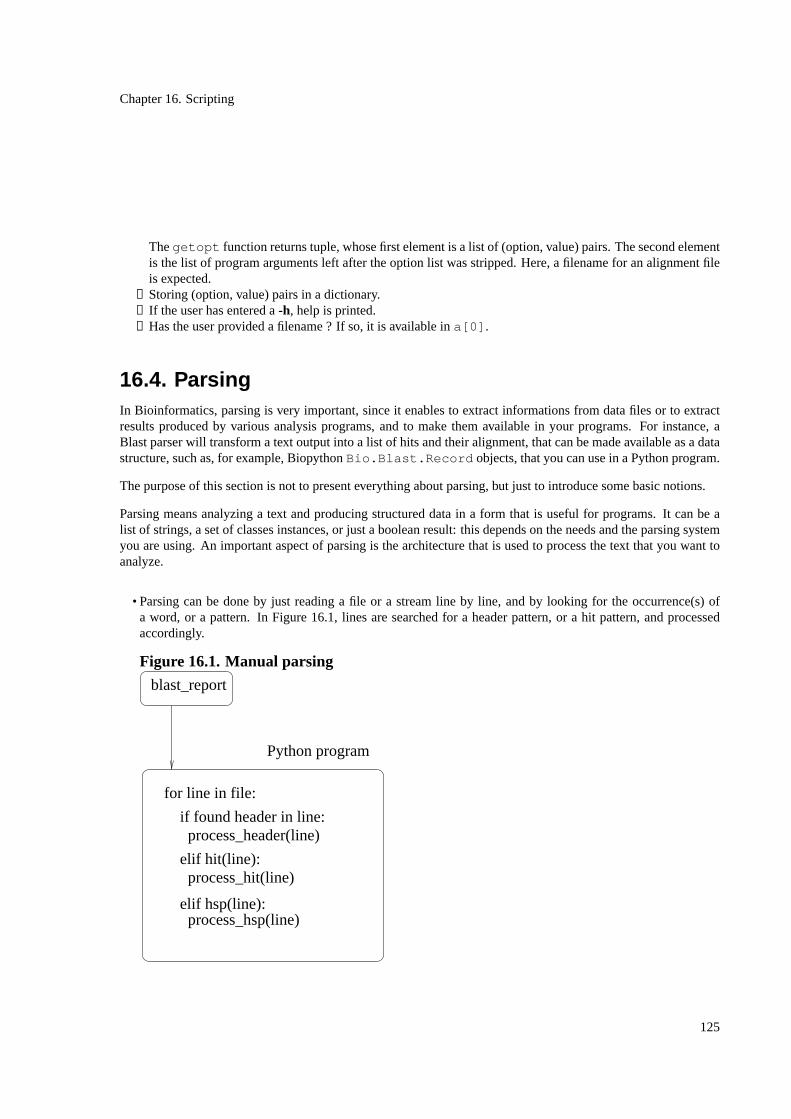
Chapter 16. Scripting
Thegetopt function returns tuple, whose first element is a list of (option, value) pairs. The second elementis the list of program arguments left after the option list was stripped. Here, a filename for an alignment fileis expected.
❸ Storing (option, value) pairs in a dictionary.❹ If the user has entered a-h, help is printed.❺ Has the user provided a filename ? If so, it is available ina[0] .
16.4. ParsingIn Bioinformatics, parsing is very important, since it enables to extract informations from data files or to extractresults produced by various analysis programs, and to make them available in your programs. For instance, aBlast parser will transform a text output into a list of hits and their alignment, that can be made available as a datastructure, such as, for example, BiopythonBio.Blast.Record objects, that you can use in a Python program.
The purpose of this section is not to present everything about parsing, but just to introduce some basic notions.
Parsing means analyzing a text and producing structured data in a form that is useful for programs. It can be alist of strings, a set of classes instances, or just a boolean result: this depends on the needs and the parsing systemyou are using. An important aspect of parsing is the architecture that is used to process the text that you want toanalyze.
• Parsing can be done by just reading a file or a stream line by line, and by looking for the occurrence(s) ofa word, or a pattern. In Figure 16.1, lines are searched for a header pattern, or a hit pattern, and processedaccordingly.
Figure 16.1. Manual parsing
blast_report
Python program
process_header(line)
elif hit(line): process_hit(line)
process_hsp(line) elif hsp(line):
for line in file:
if found header in line:
125
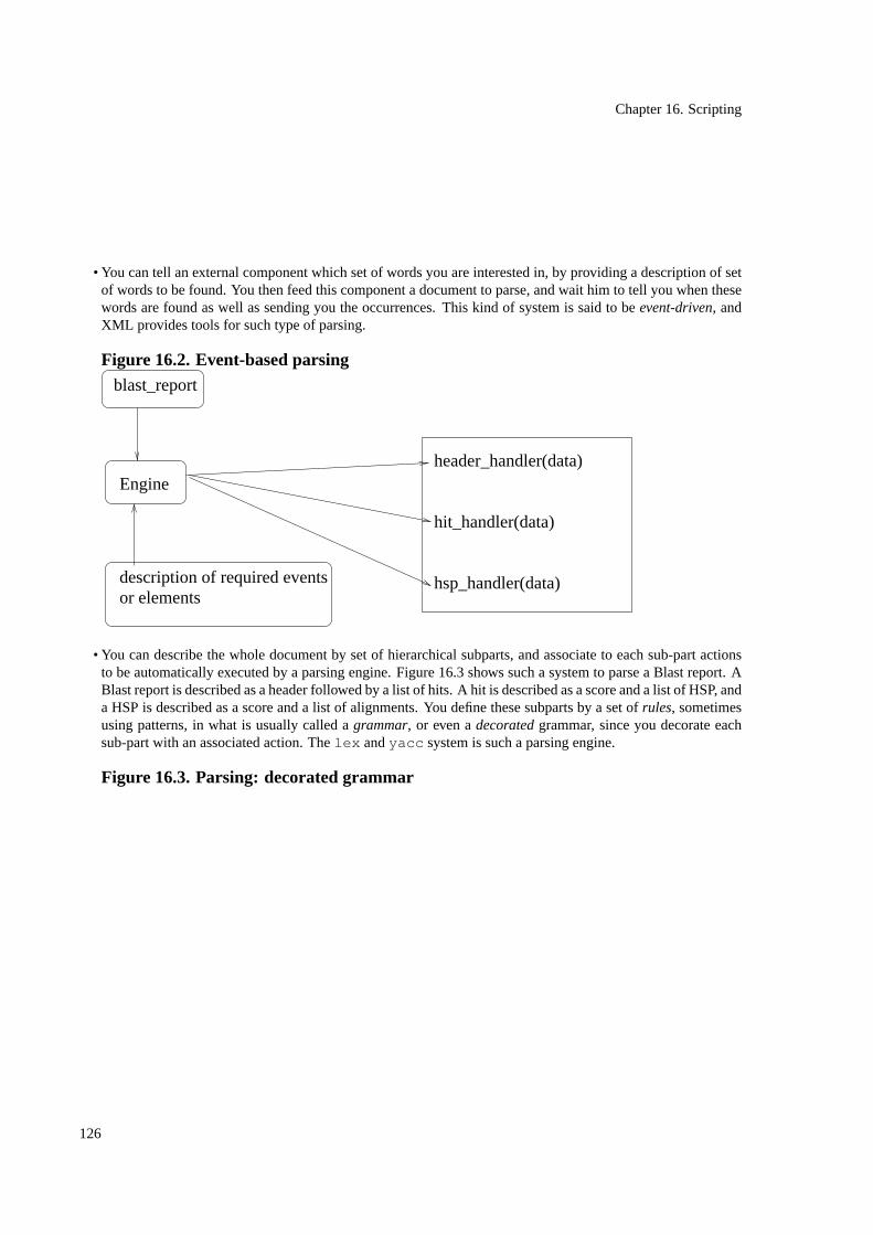
Chapter 16. Scripting
• You can tell an external component which set of words you are interested in, by providing a description of setof words to be found. You then feed this component a document to parse, and wait him to tell you when thesewords are found as well as sending you the occurrences. This kind of system is said to beevent-driven, andXML provides tools for such type of parsing.
Figure 16.2. Event-based parsing
header_handler(data)
hit_handler(data)
hsp_handler(data)
blast_report
description of required eventsor elements
Engine
• You can describe the whole document by set of hierarchical subparts, and associate to each sub-part actionsto be automatically executed by a parsing engine. Figure 16.3 shows such a system to parse a Blast report. ABlast report is described as a header followed by a list of hits. A hit is described as a score and a list of HSP, anda HSP is described as a score and a list of alignments. You define these subparts by a set ofrules, sometimesusing patterns, in what is usually called agrammar, or even adecoratedgrammar, since you decorate eachsub-part with an associated action. Thelex andyacc system is such a parsing engine.
Figure 16.3. Parsing: decorated grammar
126
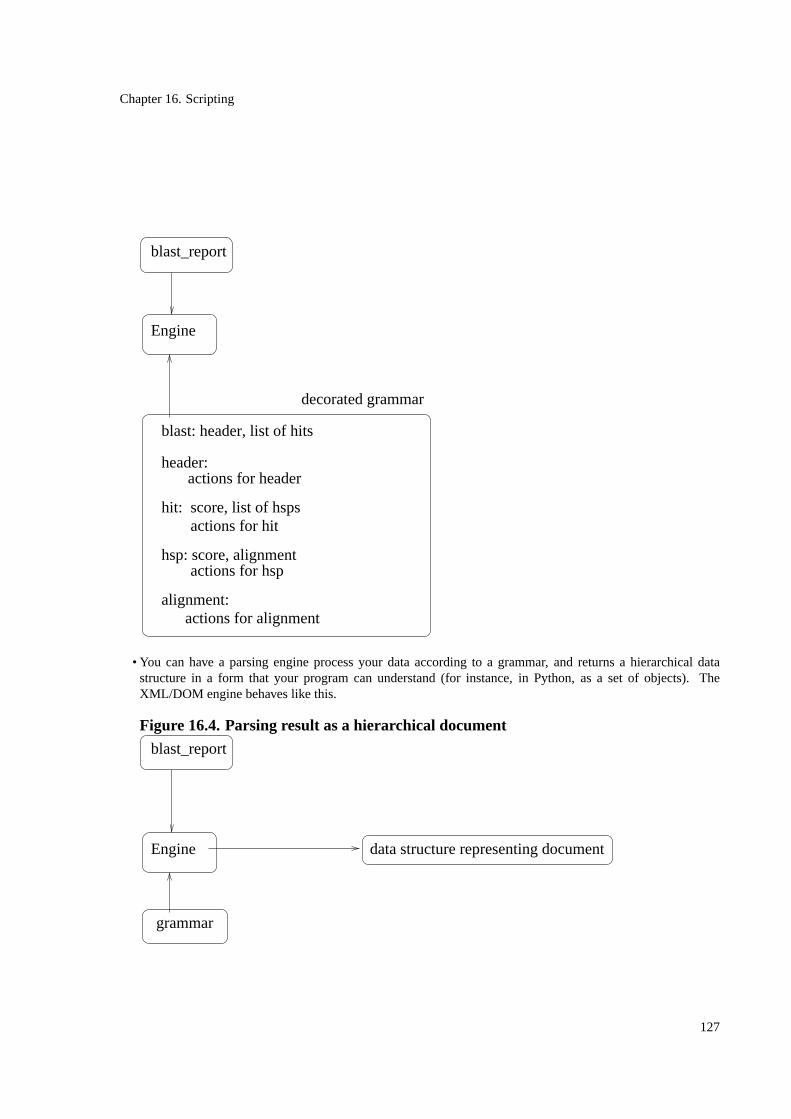
Chapter 16. Scripting
Engine
blast_report
actions for alignmentalignment:
blast: header, list of hits
actions for hsphsp: score, alignment
actions for hithit: score, list of hsps
actions for headerheader:
decorated grammar
• You can have a parsing engine process your data according to a grammar, and returns a hierarchical datastructure in a form that your program can understand (for instance, in Python, as a set of objects). TheXML/DOM engine behaves like this.
Figure 16.4. Parsing result as a hierarchical document
blast_report
Engine
grammar
data structure representing document
127

Chapter 16. Scripting
So, in all the cases, there is an engine driving the whole process, be it a simple loop or a specialized component.In this chapter, we will just do some "manual" parsing with patterns that are introduced in Section 16.5, as well assome event-driven parsing will be done as a practical work on abstract frameworks (see Exercise 18.2), and duringthe Web/XML course.
16.5. Searching for patterns.
16.5.1. Introduction to regular expressions
Regular expressionis a term used in computer science to refer to the language that is used to describe patterns tobe searched for in a text. The term comes from the computing languages theory where regular expressions areused to denote regular languages. In turn, regular languages are defined as the languages that can be recognizedby a finite-state automaton (a topic that will be introduced in the algorithmic course).
The aim of a pattern is to define not only one word to be searched for, but a set of words. This definition isprovided in a given language, depending on the system you are working with; the set of corresponding words alsodepends on the system.
In the Unix shell, for instance:
ls s*
means list all the files beginning by ’s’, and potentially followed by anything. The command:
ls s[ie]n*
means list all the files beginning by ’s’, followed by either ’i’ or ’e’, and followed by anything, including nothing.So, in the context of thels function within a Unix shell, the set of words is defined as the files existing on thefilesytem (as opposed, for instance, to the files stored on another computer, not being made available through adistributed filesystem).
In the Prosite database, patterns describing protein domains are described, such as:
H-C-H-x(3)-H-x(3)-[AG]-[LM]
which represent the following set of amino-acid sequences: sequences begining by ’HCH’, followed by 3 positionscontaining any amino-acid letter, followed by ’H’, followed again by 3 free positions, followed by either ’A’ or’G’, followed by either ’L’ or ’M’. As you can notice, the language to define patterns is different from the Unixshell, as well as the set of corresponding words. Here, they are just sequences of amino-acids letters.
In thegrep Unix command, a command to search for patterns in files, although similar to the shell pattern syntax,there is a slight difference. Say that a file contains:
128
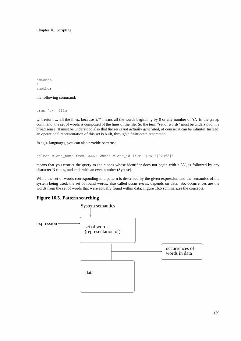
Chapter 16. Scripting
sciencesanother
the following command:
grep ’s*’ file
will return ... all the lines, because ’s*’ means all the words beginning by 0 or any number of ’s’. In thegrepcommand, the set of words is composed of the lines of the file. So the term "set of words" must be understood in abroad sense. It must be understood also thatthe set is not actually generated, of course: it can be infinite! Instead,an operational representation of this set is built, through a finite-state automaton.
In SQLlanguages, you can also provide patterns:
select clone_name from CLONE where clone_id like ’[^A]%[02468]’
means that you restrict the query to the clones whose identifier does not begin with a ’A’, is followed by anycharacter N times, and ends with an even number (Sybase).
While the set of words corresponding to a pattern is described by the given expression and the semantics of thesystem being used, the set of found words, also calledoccurrences, depends on data. So, occurrences are thewords from the set of words that were actually found within data. Figure 16.5 summarizes the concepts.
Figure 16.5. Pattern searching
expression
System semantics
set of words
data
occurrences ofwords in data
(representation of)
129

Chapter 16. Scripting
16.5.2. Regular expressions in Python
A detailed presentation of Python regular expressions is available here: Regular Expression HOWTO [http://py-howto.sourceforge.net/regex/regex.html]. To get information about there module, see pydoc, but also thesremodule (Support for regular expressions), for whichre is a wrapper.
In Python, regular expressions are handled by a module:re :
>>> import re
Before searching for a pattern, you must firstcompileit (this builds the "set of words", or rather the representationof this set):
>>> expression = ’[AP]{1,2}D’>>> pattern = re.compile(expression)
pattern is apattern object. You then issue asearch, for instance in the small sequenceseq , by a request to thepattern object:
>>> seq = "RPAD">>> match = pattern.search(seq)
This establishes thematching, or correspondances, between the set of possible words and data.match is calleda match object. To get the occurrences, you can ask the match object for the start and end of the match in thesearched text:
>>> print match.start(), match.end(), seq[match.start():match.end()]1 4 PAD
or thegroup :
>>> match.group(0)’PAD’
130

Chapter 16. Scripting
Figure 16.6 summarizes this system.
Figure 16.6. Python regular expressions
expressionpattern object
pattern.search()
match object
match.start()match.end()match.group(0)
data
pattern.match()
re.compile
Example 16.6. Searching for the occurrence of PS00079 and PS00080 Prosite patterns inthe Human Ferroxidase protein
import sysimport refrom Bio.SwissProt import SProt
sp = open(sys.argv[1])iterator = SProt.Iterator(sp, SProt.SequenceParser())seq = iterator.next().seqsp.close()
PS00079 = ’G.[FYW].[LIVMFYW].[CST].{8,8}G[LM]...[LIVMFYW]’ ❶pattern = re.compile(PS00079) ❷match = pattern.search(seq.tostring()) ❸print PS00079print match.start(), match.end(), seq[match.start():match.end()] ❹
❶ The regular expression is stored in a string.❷ The regular expression is compiled in a pattern.❸ The compiled pattern is searched in the sequence.❹ The result of the search is printed.
131
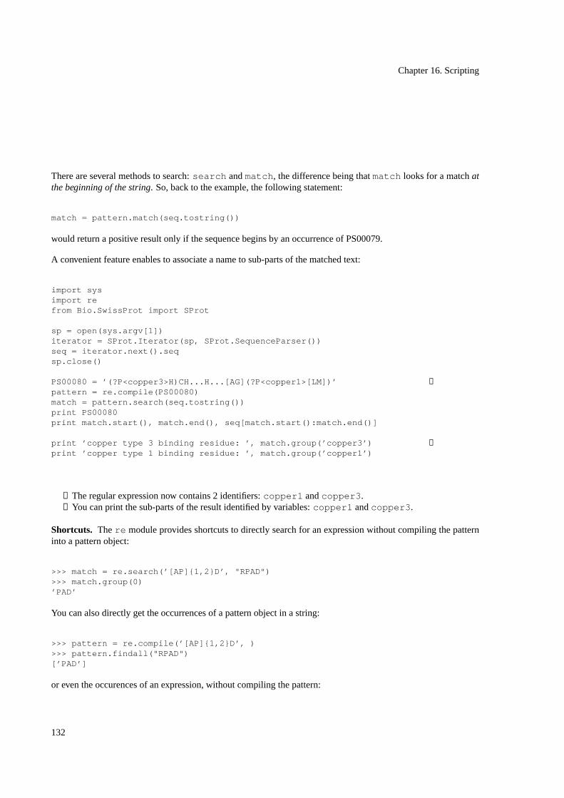
Chapter 16. Scripting
There are several methods to search:search andmatch , the difference being thatmatch looks for a matchatthe beginning of the string. So, back to the example, the following statement:
match = pattern.match(seq.tostring())
would return a positive result only if the sequence begins by an occurrence of PS00079.
A convenient feature enables to associate a name to sub-parts of the matched text:
import sysimport refrom Bio.SwissProt import SProt
sp = open(sys.argv[1])iterator = SProt.Iterator(sp, SProt.SequenceParser())seq = iterator.next().seqsp.close()
PS00080 = ’(?P<copper3>H)CH...H...[AG](?P<copper1>[LM])’ ❶pattern = re.compile(PS00080)match = pattern.search(seq.tostring())print PS00080print match.start(), match.end(), seq[match.start():match.end()]
print ’copper type 3 binding residue: ’, match.group(’copper3’) ❷print ’copper type 1 binding residue: ’, match.group(’copper1’)
❶ The regular expression now contains 2 identifiers:copper1 andcopper3 .❷ You can print the sub-parts of the result identified by variables:copper1 andcopper3 .
Shortcuts. There module provides shortcuts to directly search for an expression without compiling the patterninto a pattern object:
>>> match = re.search(’[AP]{1,2}D’, "RPAD")>>> match.group(0)’PAD’
You can also directly get the occurrences of a pattern object in a string:
>>> pattern = re.compile(’[AP]{1,2}D’, )>>> pattern.findall("RPAD")[’PAD’]
or even the occurences of an expression, without compiling the pattern:
132
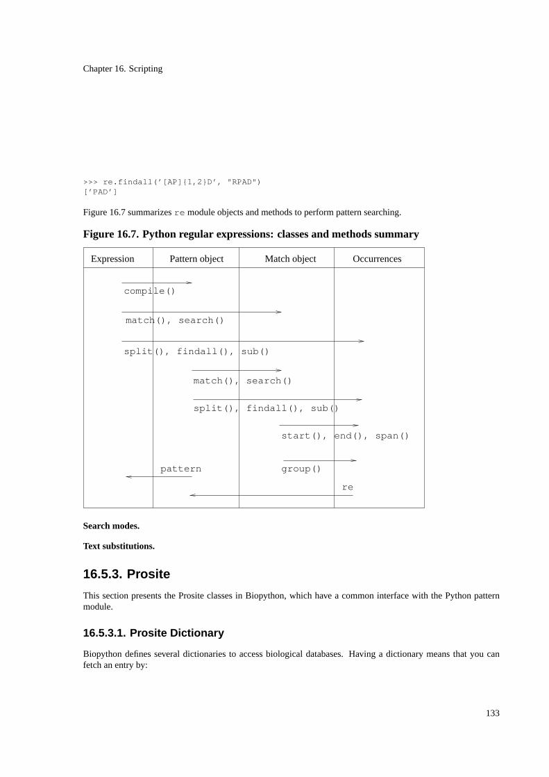
Chapter 16. Scripting
>>> re.findall(’[AP]{1,2}D’, "RPAD")[’PAD’]
Figure 16.7 summarizesre module objects and methods to perform pattern searching.
Figure 16.7. Python regular expressions: classes and methods summary
Expression Pattern object Match object Occurrences
compile()
split(), findall(), sub()
match(), search()
split(), findall(), sub()
match(), search()
start(), end(), span()
group()pattern
re
Search modes.
Text substitutions.
16.5.3. Prosite
This section presents the Prosite classes in Biopython, which have a common interface with the Python patternmodule.
16.5.3.1. Prosite Dictionary
Biopython defines several dictionaries to access biological databases. Having a dictionary means that you canfetch an entry by:
133
Chapter 16. Scripting
entry = prosite[’PS00079’]
For this to work, you first need to create the dictionary:
prosite = Bio.Prosite.ExPASyDictionary()
As you can guess by the name of the module, you actually fetch the Prosite entry on the Web. You could also fetchthe Prosite entry from a local database with the golden program (see ???). The entry fetched above is actually astring. In order to have the dictionary return a record, you must rather create it like this:
prosite = Bio.Prosite.ExPASyDictionary(parser=Bio.Prosite.RecordParser())
16.5.3.2. Prosite patterns
The Bio.Prosite package defines aPattern class that enables to create patterns which may be searchedfor in sequences objects, as in there Python module for regular expressions. The result of a search is aPrositeMatch , that behaves in a way similar to a regular expression match.
16.5.4. Searching for patterns and parsing
As a conclusion, let us summarize how pattern searching and parsing interact when analyzing text. Basic textanalysis is performed by searching for patterns, that are extracted (or scanned) from a text. Then patternsoccurrences may be analyzed (or parsed) as a more general structure. In more complex parsing architectures,as the ones that have been introduced in Section 16.4, it is theparserengine which drives the process, by asking ascannerto feed him with basic token found in the text. In such systems, regular expressions are defined and usedin the scanner.
134
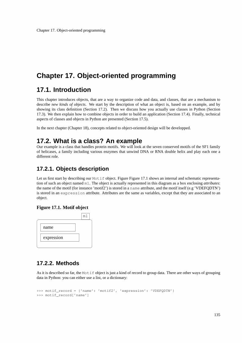
Chapter 17. Object-oriented programming
Chapter 17. Object-oriented programming
17.1. IntroductionThis chapter introduces objects, that are a way to organize code and data, and classes, that are a mechanism todescribenew kinds of objects. We start by the description of what an object is, based on an example, and byshowing its class definition (Section 17.2). Then we discuss how you actually use classes in Python (Section17.3). We then explain how to combine objects in order to build an application (Section 17.4). Finally, technicalaspects of classes and objects in Python are presented (Section 17.5).
In the next chapter (Chapter 18), concepts related to object-oriented design will be developped.
17.2. What is a class? An exampleOur example is a class that handles protein motifs. We will look at the seven conserved motifs of the SF1 familyof helicases, a family including various enzymes that unwind DNA or RNA double helix and play each one adifferent role.
17.2.1. Objects description
Let us first start by describing ourMotif object. Figure Figure 17.1 shows an internal and schematic representa-tion of such an object namedm1. The object is actually represented in this diagram as a box enclosingattributes:the name of the motif (for instance ’motif2’) is stored in anameattribute, and the motif itself (e.g ’VDEFQDTN’)is stored in anexpression attribute. Attributes are the same as variables, except that they are associated to anobject.
Figure 17.1. Motif object
expression
name
m1
17.2.2. Methods
As it is described so far, theMotif object is just a kind of record to group data. There are other ways of groupingdata in Python: you can either use a list, or a dictionary:
>>> motif_record = {’name’: ’motif2’, ’expression’: ’VDEFQDTN’}>>> motif_record[’name’]
135

Chapter 17. Object-oriented programming
’motif2’
but an object is actually more than just that. As shown in Figure 17.2 (and as stated in Section 6.1), an objectis indeed more than just a value or a record of values: it "knows" what it can do, or, in other words, it has anassociated behaviour. This behaviour is described by functions that are associated to it, and these functions arecalledmethods. For instance, ourMotif object can perform one operation: it can look whether a protein containsthis motif, and return its position by calling thefind() function:
>>> m1.find(prot)360
So, available operations are an important aspect of objects, that we need to add in our representation. In Figure17.2, methods are represented as "counters", as at the post office.
Figure 17.2. Representation showing object’s methods as counters
name
m1
expressionfind
So, with objects, not only do we have a convenient way to group data that are related, but we also have a way togroup dataand their related operationsin the same place.
Object
An object is a construction to group values and operations on these values.
17.2.3. Class definition
Now, how do you define objects, such as ourMotif object, with their attributes and methods?
In object-oriented programming, you define objects by defining a class for them.
Class
A class is anobject maker: it contains all the statements needed to create an object, its attributes, as well as thestatements to describe the operations that the object will be able to perform.
The termclasscan be somewhat misleading, for it also refers to something belonging to aclassification. In object-oriented programming, a class can indeed also be a member of a set of classes organized in a hierarchy. This aspect
136
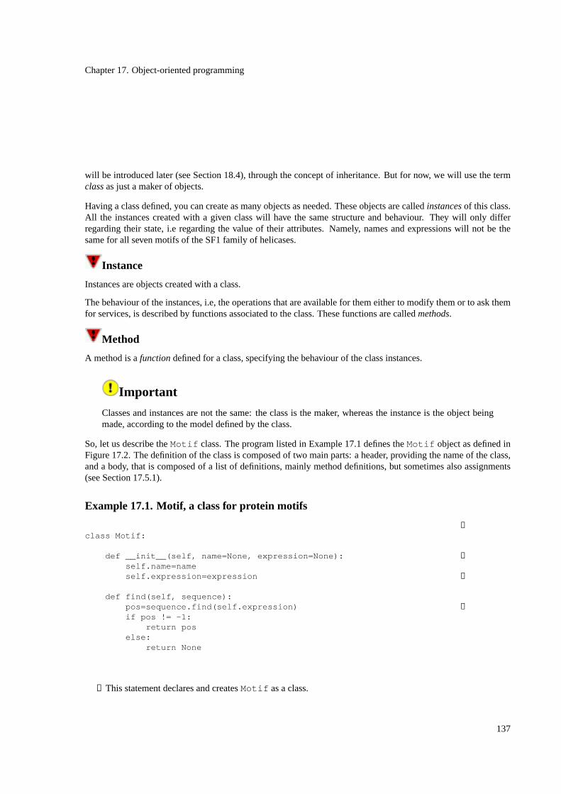
Chapter 17. Object-oriented programming
will be introduced later (see Section 18.4), through the concept of inheritance. But for now, we will use the termclassas just a maker of objects.
Having a class defined, you can create as many objects as needed. These objects are calledinstancesof this class.All the instances created with a given class will have the same structure and behaviour. They will only differregarding their state, i.e regarding the value of their attributes. Namely, names and expressions will not be thesame for all seven motifs of the SF1 family of helicases.
Instance
Instances are objects created with a class.
The behaviour of the instances, i.e, the operations that are available for them either to modify them or to ask themfor services, is described by functions associated to the class. These functions are calledmethods.
Method
A method is afunctiondefined for a class, specifying the behaviour of the class instances.
Important
Classes and instances are not the same: the class is the maker, whereas the instance is the object beingmade, according to the model defined by the class.
So, let us describe theMotif class. The program listed in Example 17.1 defines theMotif object as defined inFigure 17.2. The definition of the class is composed of two main parts: a header, providing the name of the class,and a body, that is composed of a list of definitions, mainly method definitions, but sometimes also assignments(see Section 17.5.1).
Example 17.1. Motif, a class for protein motifs
❶class Motif:
def __init__(self, name=None, expression=None): ❷self.name=nameself.expression=expression ❸
def find(self, sequence):pos=sequence.find(self.expression) ❹if pos != -1:
return poselse:
return None
❶ This statement declares and createsMotif as a class.
137

Chapter 17. Object-oriented programming
❷ The__init__ method is automatically called at instance creation (see below).❸ Initialization of instances attributes (name andexpression ).❹ This method defines how to compute the position of a motif in a sequence.
Theself parameter represents the object itself. You could of course use any other word likecarrot or ego , butthis would not help the reading of your code by others... Soself is present in the Class and methods definitionseach time the reference to the object instance is needed.
The __init__ method is used in a class when you want all instances to be automatically processed from thebegining. Here in ourMotif class, when an instance is created, it receives values for two attributesself.nameandself.expression , which are arguments of the__init__ method.It is also good practice to place in the__init__ all other attributes that belong to class instances, with empty values. They are not given as argumentsbecause their values will only appear later, as methods output for example. Of course, classes run perfectly wellwithout any__init__ method, but it is again good practice to have one, placed at the begining of the class.
Let us look at one of these methods definitions, thefind method, which computes the position of a motif in asequence:
def find(self, sequence):m=sequence.find(self.expression)if m != -1:
return mreturn None
Method definitions follow exactly the same pattern as standard function definitions,except for their first parameter,self. An instance identificator, actually a reference to the instance, is required in order for the statements withinmethods to access to the current instance attributes: here, the access to theexpression attribute is needed inorder perform the search. In fact, Pythonautomatically passes the instance reference as the first argument of amethod. Hence, it is associated to the first parameter which is theself parameter.
17.3. Using classes in Python
17.3.1. Creating instances
How are we going to use thisMotif class? The first thing that we need to do is to create some real protein motifswith it.
You have actually already used classes and created instances of classes throughout this course: strings, lists, etc...However, most of the time the objects you have manipulated were not directly created by your own code, butrather by other components: for instance the “[]” operator creates a list, the “""” operator creates a string, theopen function creates a file handle, etc...
But the actual direct syntax toinstantiatea class, i.e to create an instance of class, is by calling a function with thesame name as the class. So, in order to create an instance of theMotif class we have just defined, i.e an objectwhich handles protein motifs, you do:
138
Chapter 17. Object-oriented programming
>>> m1 = Motif()
After theMotif() function is called, the instance of the classMotif is referred to by them1variable. The classinstantiation by aMotif() call actually calls the__init__ method defined in theMotif class. The m1 objectwas given no argument at instance creation, so by default its attributes are set to None. If no default value is givenin the__init__ method, arguments have to be present at instantiation. In the case of theMotif class, if wewant to provide initial values for thenameandexpression attributes, we do :
>>> m2 = Motif(’motif2’, ’VDEFQDTN’)
This time, the newMotif instance has been created with values fornameandexpression attributes. You canalso use keyword arguments (especially if you are no longer sure in what order they should be entered) :
>>> m2 = Motif(name=’motif2’, expression= ”VDEFQDTN’)
So, this creates the object and makes it available from them2variable. You can now use this object to callMotifclass methods, by using the dot operator:
>>> m2.find(prot)56
You don’t need to specify the argument for the reference to the instance (remember: methods always receive theinstance reference as the first argument). This is automatically done by Python. In fact, calling:
>>> m2.find(prot)56
is equivalent to:
>>> Motif.find(m2, prot)56
The interpretor can find which classm2belongs to, and handles the passing of the instance reference argumentautomatically.
There are also automatic ways for instantiating objects, rather than manually entering attribute values, by readinga file for example. If file "SF1motifs" contains the motifs you want to work with, you can proceed this way :
def load_motifs(filename):SF1list=[]ifh=open(filename)
139

Chapter 17. Object-oriented programming
line=ifh.readline()while line!=”:
(name, expression)=line.split()motif=Motif(name,expression)listeSF1.append(motif)line=ifh.readline()
ifh.close()return SF1list
SF1list=load_motifs ("SF1motifs")
Following is a complete example of how the classMotif can be used, supposing that this class, together with theload_motifs function, are placed in a module "helicase" :
import helicaseprot = """MDVSYLLDSLNDKQREAVAAPRSNLLVLAGAGSGKTRVLVHRIAWLMSVENCSPYSIMAVTFTNKAAAEMRHRIGQLMGTSQGGMWVGTFHGLAHRLLRAHHMDANLPQDFQILDSEDQLRLLKRLIKAMNLDEKQWPPRQAMWYINSQKDEGLRPHHIQSYGNPVEQTWQKVYQAYQEACDRAGLVDFAELLLRAHELWLNKPHILQHYRERFTNILVDEFQDTNNIQYAWIRLLAGDTGKVMIVGDDDQSIYGWRGAQVENIQRFLNDFPGAETIRLEQNYRSTSNILSAANALIENNNGRLGKKLWTDGADGEPISLYCAFNELDEARFVVNRIKTWQDNGGALAECAILYRSNAQSRVLEEALLQASMPYRIYGGMRFFERQEIKDALSYLRLIANRNDDAAFERVVNTPTRGIGDRTLDVVRQTSRDRQLTLWQACRELLQEKALAGRAASALQRFMELIDALAQETADMPLHVQTDRVIKDSGLRTMYEQEKGEKGQTRIENLEELVTATRQFSYNEEDEDLMPLQAFLSHAALEAGEGQADTWQDAVQLMTLHSAKGLEFPQVFIVGMEEGMFPSQMSLDEGGRLEEERRLAYVGVTRAMQKLTLTYAETRRLYGKEVYHRPSRFIGELPEECVEEVRLRATVSRPVSHQRMGTPMVENDSGYKLGQRVRHAKFGEGTIVNMEGSGEHSRLQVAFQGQGIKWLVAAYARLESV""".replace("\n","")
SF1list = helicase.load_motifs("SF1motifs")
for motif in SF1list:print "Motif %s (%s) " % (motif.expression, motif.name)position=motif.find(prot)if position:
print "matches at:", positionelse:
print "is absent"print
where motifs are loaded from a file "SF1motifs" through theload_motifs function defined above.
17.4. Combining objects
140

Chapter 17. Object-oriented programming
A program is generally not built on a single object, but rather on a combination of several objects that interacttogether. In theMotif example, we can have two other kinds of objects: a motifmatchobject, that stores thepositions of the motif in a particular protein, found with thefind method, as well as the the original pattern andsequence. Such an object could provide methods such astostring , to print the result, andshow to return theslice of the protein sequence that matches the expression. These objects will be instances of the classMatch . Thesecond kind of object is going to embed the protein sequence, it will store the name and sequence, and a methodto annotate protein,annotate . These objects will be instances of the classProtein .
So, we need to associate the originalMotif object to theMatch object, as well as to theProtein object wherethe matches are found. A way to represent this is to say that theMatch objecthas aaMotif and aProtein . Infigure Figure 17.3, you can see the internal representation of aMatch objectcontainingMotif andProteinobjects.
Figure 17.3. A Match object o1 with embedded Motif m1 and Protein p1 (not feasible inPython)
positions
name
expression
m1 (a Motif object)
name
sequence
p1 (a Protein object)
o1
tostring
show
find
annotate
However, there is another much more efficient way of associating our objects. First, there is no way in Python toembed one objectinsideanother object: objects are independant entities. Second, what if we decide to associatethe same Motif to anotherMatch (a match in another protein, for instance)? So, we rather have independant
141

Chapter 17. Object-oriented programming
Motif andProtein objects. And the attribute for this object within theMatch object thus has to be areference.This is illustrated in Figure 17.4 by arrows from the matches objects (o1 ando2) to theMotif objectm1.
Figure 17.4. Two match objects and a pattern.
positions
positions
name
o2 (another Match object)
o1 (a Match object)
m1
p1
m1 (a Motif object)
m2 (another Motif object)
sequence
name
name
name
expression
expression
m2
p1
p1 (a Protein object)
tostring
find
find
tostring
show
show
annotate
142
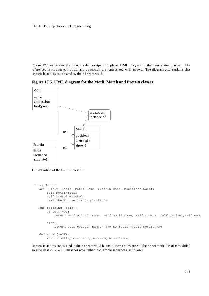
Chapter 17. Object-oriented programming
Figure 17.5 represents the objects relationships through an UML diagram of their respective classes. Thereferences inMatch to Motif and Protein are represented with arrows. The diagram also explains thatMatch instances are created by thefind method.
Figure 17.5. UML diagram for the Motif, Match and Protein classes.
creates aninstance of
name
Motif
expression
Match
namesequence
p1Protein
positionstostring()
m1
show()
annotate()
find(prot)
The definition of theMatch class is:
class Match:def __init__(self, motif=None, protein=None, positions=None):
self.motif=motifself.protein=protein(self.begin, self.end)=positions
def tostring (self):if self.pos:
return self.protein.name, self.motif.name, self.show(), self.begin+1,self.end
else:return self.protein.name." has no motif ".self.motif.name
def show (self):return self.protein.seq[self.begin:self.end]
Match instances are created in thefind method bound toMotif instances. Thefind method is also modifiedso as to dealProtein instances now, rather than simple sequences, as follows:
143

Chapter 17. Object-oriented programming
def find(self, protein):begin=protein.sequence.find(self.expression)end=begin+len(self.expression)+1positions=(begin, end)if positions:
return Match(self, protein, positions)else:
return Match(self, protein, None)
TheMatch class can be used as follows:
SF1list = helicase.load_motifs("SF1motifs")for motif in SF1list:
match = motif.find(prot)print match.tostring()
17.5. Classes and objects in Python: technical aspectsThe aim of this section is to clarify technical aspects of classes and objects in Python.
17.5.1. Namespaces
Classes and instances have their own namespaces, that is accessible with the dot (’.’) operator. As illustrated byFigure 17.6, these namespaces are implemented by dictionaries, one for each instance, and one for the class (seealso [Martelli2002]).
Figure 17.6. Classes and instances dictionaries.
__dict__
__class____class__
__dict__
__dict__name name
Motif
m1
expression
m2
expression
find
144

Chapter 17. Object-oriented programming
Instances attributes. As we have learnt, a class may define attributes for its instances. For example, attributes ofm1, such as thename, are directly available through the dot operator:
>>> m1.name’motif2’
The dictionary for the instance attributes is also accessible by its__dict__ variable, or thevars() function:
>>> m1.__dict__{’expression’: ’VDEFQDTN’, ’name’: ’motif2’}>>> vars(p1){’expression’: ’VDEFQDTN’, ’name’: ’motif2’}
Thedir() command lists more attributes:
>>> dir(m1)[’__doc__’, ’__init__’, ’__module__’, ’find’, ’name’, ’expression’]
because it is not limited to the dictionary of the instance. It actually also displays its class attributes, and recursivelythe attributes of its class base classes (see Section 18.4).
You can add attributes to an instance that were not defined by the class, such as theother_var in the following:
>>> m1.other_var = 10>>> m1.__dict__{’expression’: ’VDEFQDTN’, ’name’: ’motif2’, ’other_var’: 10}
Adding attributes on-the-fly is not something that is available in many object-oriented programming languages !Be aware that this type of programming should be used carefully, since by doing this, you start to have instancesthat have different behaviour, at least if you consider that the list of attributes defines a behaviour. This is not thesame as having a differentstateby having different values for the same attribute. But this matter is probably atopic of discussion.
Exercise 17.1. A Dictionary class
What is the difference between:
>>> class Dict:pass
>>> d = Dict()>>> d.x = 10>>> d.y = 0.5>>> d.__dict__{’y’: 0.5, ’x’: 10}>>> vars(d)
145
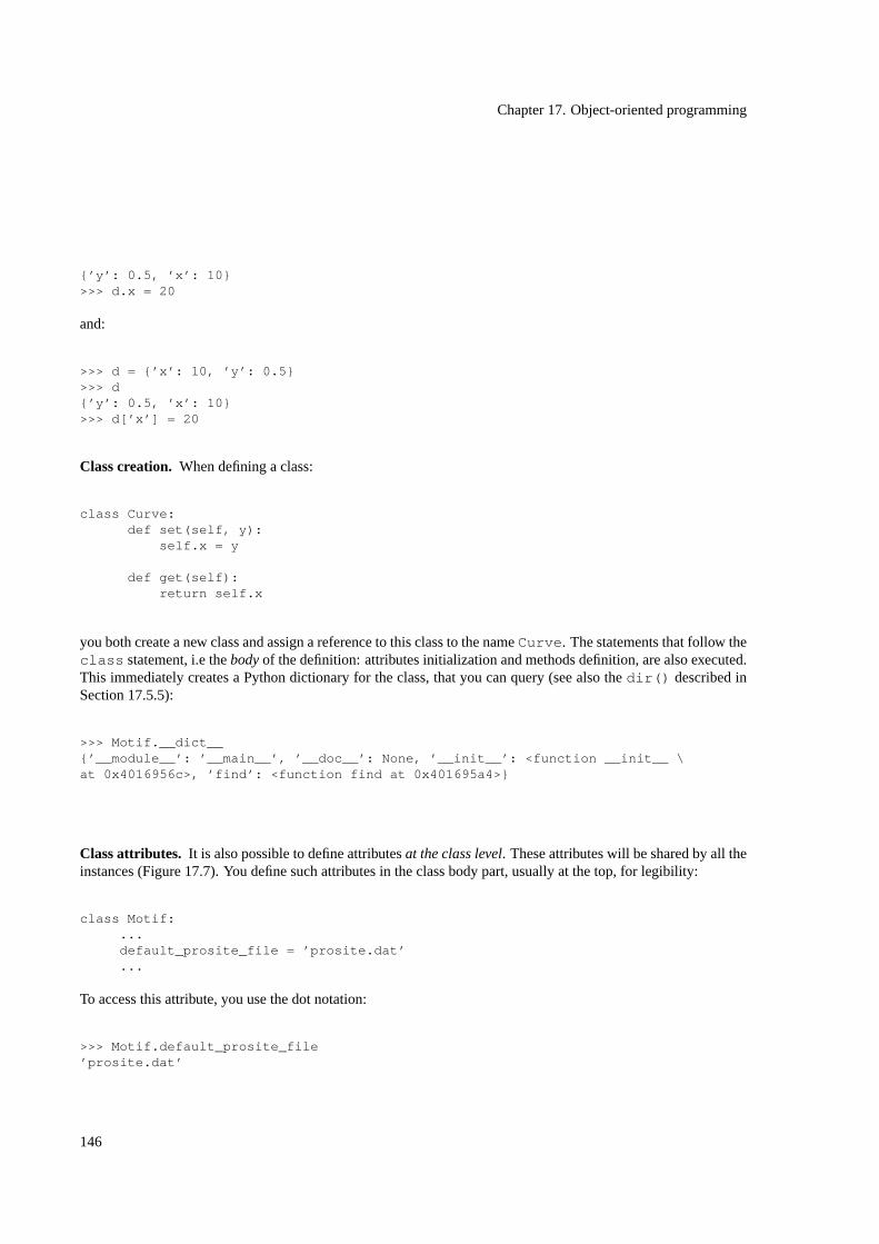
Chapter 17. Object-oriented programming
{’y’: 0.5, ’x’: 10}>>> d.x = 20
and:
>>> d = {’x’: 10, ’y’: 0.5}>>> d{’y’: 0.5, ’x’: 10}>>> d[’x’] = 20
Class creation. When defining a class:
class Curve:def set(self, y):
self.x = y
def get(self):return self.x
you both create a new class and assign a reference to this class to the nameCurve . The statements that follow theclass statement, i.e thebodyof the definition: attributes initialization and methods definition, are also executed.This immediately creates a Python dictionary for the class, that you can query (see also thedir() described inSection 17.5.5):
>>> Motif.__dict__{’__module__’: ’__main__’, ’__doc__’: None, ’__init__’: <function __init__ \at 0x4016956c>, ’find’: <function find at 0x401695a4>}
Class attributes. It is also possible to define attributesat the class level. These attributes will be shared by all theinstances (Figure 17.7). You define such attributes in the class body part, usually at the top, for legibility:
class Motif:...default_prosite_file = ’prosite.dat’...
To access this attribute, you use the dot notation:
>>> Motif.default_prosite_file’prosite.dat’
146
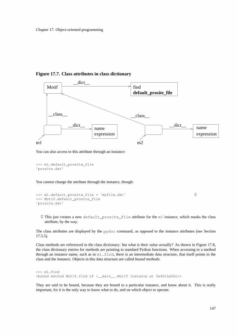
Chapter 17. Object-oriented programming
Figure 17.7. Class attributes in class dictionary
__dict__
__class____class__
__dict__
__dict__name name
Motif
m1
expression
m2
expression
default_prosite_filefind
You can also access to this attribute through an instance:
>>> m1.default_prosite_file’prosite.dat’
You cannotchange the attribute through the instance, though:
>>> m1.default_prosite_file = ’myfile.dat’ ❶>>> Motif.default_prosite_file’prosite.dat’
❶ This just creates a newdefault_prosite_file attribute for them1 instance, which masks the classattribute, by the way.
The class attributes are displayed by thepydoc command, as opposed to the instance attributes (see Section17.5.5).
Class methods are referenced in the class dictionary: but what is theirvalueactually? As shown in Figure 17.8,the class dictionary entries for methods are pointing to standard Python functions. When accessing to a methodthrough an instance name, such as inm1.find , there is an intermediate data structure, that itself points to theclass and the instance. Objects in this data structure are calledbound methods:
>>> m1.find<bound method Motif.find of <__main__.Motif instance at 0x4016a56c>>
They are said to be bound, because they are bound to a particular instance, and know about it. This is reallyimportant, for it is the only way to know what to do, and on which object to operate.
147
Chapter 17. Object-oriented programming
Figure 17.8. Classes methods and bound methods
__class__
__dict__Motif
m1 expressionname
__dict__bound method
find
find
m1.find
17.5.2. Objects lifespan
Once it is created, an object’s lifespan depends on the fact that there are references on it. Namely, as opposed tovariable following lexical scope, an object can still exist after exiting the function or method where it has beencreated, as long as there is a valid reference to it, as shown in the following example:
class C1: pass
class C2:def show(self):
print "I am an instance of class ", self.__class__
def create_C2_ref_in(p):p.c2 = C2() ❶
c1 = C1()create_C2_ref_in(c1) ❷c1.c2.show() ❸
❶ This function creates an instance of classC2 and stores its reference in an attribute ofp, an instance of classC1.
❷ Creation of theC2 instance by callingcreate_C2_ref_in❸ This statement displays: "I am an instance of class __main__.C2"
148

Chapter 17. Object-oriented programming
As you can observe, theC2 instance exists after exiting thecreate_C2_ref_in function. It will exist as longas its reference remains in thec1.c2 attribute. If you issue:
c1.c2 = None
There will be no reference left to ourC2 instance, and it will be automatically deleted. The same would happen ifyou would issue an additional call to thecreate_C2_ref_in function:
create_C2_ref_in(c1)
it would overwrite the preceeding reference to the formerC2 instance, and delete it. You can check this by askingthec1.c2 reference for its identity:
id(c1.c2)
Of course, another way to delete an object is to use thedel function:
del c1.c2
17.5.3. Objects equality
Instances equality cannot be tested by the== operator.If we come back to our Curve class:
>>> c = Curve()>>> c.set(5)>>> c.__dict__{’x’: 5}>>> d = Curve()>>> d.set(5)>>> d.__dict__{’x’: 5}>>> c == dFalse
This means that the equality operator must be defined by the programmer. See the__eq__ special method inSection 18.3.3.
Instances identity means that two objects are in factthe sameobject, or more exactly, that two variables refer tothe same object.
>>> c1 = Curve()>>> c2 = c1>>> c2 is c1
149
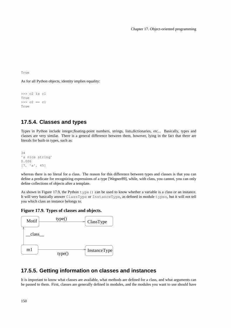
Chapter 17. Object-oriented programming
True
As for all Python objects, identity implies equality:
>>> c2 is c1True>>> c2 == c1True
17.5.4. Classes and types
Types in Python include integer,floating-point numbers, strings, lists,dictionaries, etc... Basically, types andclasses are very similar. There is a general difference between them, however, lying in the fact that there areliterals for built-in types, such as:
34’a nice string’0.006[7, ’a’, 45]
whereas there is no literal for a class. The reason for this difference between types and classes is that you candefine a predicate for recognizing expressions of a type [Wegner89], while, with class, you cannot, you can onlydefine collections of objects after a template.
As shown in Figure 17.9, the Pythontype() can be used to know whether a variable is a class or an instance.It will very basically answerClassType or InstanceType , as defined in moduletypes , but it will not tellyou which class an instance belongs to.
Figure 17.9. Types of classes and objects.
ClassTypeMotif type()
InstanceTypem1type()
__class__
17.5.5. Getting information on classes and instances
It is important to know what classes are available, what methods are defined for a class, and what arguments canbe passed to them. First, classes are generally defined in modules, and the modules you want to use should have
150

Chapter 17. Object-oriented programming
some documentation to explain how to use them. Then, you have thepydoccommand that lists the methods of theclass, and describes their parameters. The following command displays information on theMotif class, providedit is in thehelicase.py file:
pydoc helicase.Motif
See also the embedding module, which might bring additional documentation about related components. Thismay be important when several classes work together, as is described in Section 17.4.
When you consult the documentation of a class with thepydoccommand, you get most of the time a strange list ofmethod names, such as__str__ or __getitem__ . These methods are special methods to redefine operators,and will be explained in the next chapter on object-oriented design (Section 18.3.3).
Caution: the defined instances attributes will not be listed by pydoc, since they belong to the instances rather thanto the class. That is why they should be described in the documentation string of the class. If they are not, whichsometimes happens..., run the Python interpretor and create an instance, then ask for its dictionary or use thedir()command:
>>> m1 = Motif()>>> dir(m1)[’__doc__’, ’__init__’, ’__module__’, ’find’, ’name’, ’expression’]
Information on instances. There are some mechanisms to know about the class of a given instance. You can usethe special attribute__class__ :
>>> m1 = Motif()>>> m1.__class__class __main__.Motif at 0x81d1d64>
You can even use this information to create other instances:
>>> m2=m1.__class__()>>> m2__main__.Motif instance at 0x8194ca4>
This can be useful if you need to create an object of the same class of another source object, without knowing theclass of the source object. You can also ask whether an object belongs to a given class:
>>> isinstance(m1,Motif)True
As mentionned above, the Pythontype() will not provide the class of an instance, but just:InstanceType(see Figure 17.9).
151
Chapter 17. Object-oriented programming
152
Chapter 18. Object-oriented design
Chapter 18. Object-oriented design
18.1. IntroductionWe first describe general software engineering guidelines to design components (Section 18.2.5). We next moveon to the general question about why and how to design classes, and more specifically, how to design newabstractdata types(Section 18.3). We will then re-discuss the issue of flexibility (Section 18.5) and describe inheritance(Section 18.4). Last, we will introduce the design patterns catalog (Section 18.6), which are well-known designsolutions to standard problems in object-oriented programming.
18.2. Components
18.2.1. Software quality factors
The topics introduced in this section address some of the issues of software quality, and how Python can help onthis matter.
Before entering into details, let us just summarize some important concepts (you can find a good and moreexhaustive description in [Meyer97]). There is no absolute quality in software: depending on the context, scale,scope and goals of the program being developped, you might very well either write on-the-fly short pieces of codeto solve a temporary problem, or spend a significant effort to have your application follow an industrial designprocess. So, rather than only a global so-called standard that should be applied for each program you write, thereare a fewquality factorsto be evaluated according to the actual needs of the project. Among these factors, oneusually distinguish between internal and external factors.Externalquality factors are the ones that corresponds tovisible requirements, directly important for the user of the software, such asvalidity , robustnessor efficiency.Internal quality factors are properties of the code itself, such as legibility or modularity. In fact, internal factorsoften indirectly help to get external quality. Some factors, such asreusability, extensibility andcompatibility ,that we will study more thoroughly here, belong to external quality factors in the sense that they can be requiredby the users of a software library or the programmers of a shared source code; they are also important internalquality factors in the sense that they make the internal quality of the source code better. The aim of this chapter ismainly to describe these factors, as well as internal quality factors.
18.2.2. Large scale programming
Theoretically, in order to get a program that performs a given task and solves the problem you have specified, abasic set of instructions such as: branching, repetitions, expressions and data structures can be sufficient. Now,the programs that you produce can become a problem by themselves, for several reasons:
• They can become very large, resulting in thousand lines of code where it is becoming difficult to make even aslight change (extensibilityproblem).
153
Chapter 18. Object-oriented design
• When an application is developped within a team, it is important for different people to be able to share thecode and combine parts developped by different people (compatibility) ; having big and complex source filescan become a problem.
• During your programmer’s life, or within a team, you will very often have to re-use the same kind ofinstructions set: searching for an item in a collection, organizing a hierarchical data structure, converting dataformats, ...; moreover, such typical blocks of code have certainly already been done elsewhere (reusability).Generally, source code not well designed for re-use can thus be a problem.
So, depending on the context of the project, there are some issues which are just related to themanagement ofsource codeby humans, as opposed to the specification of the task to perform. And if you think about it, youprobably tend to use variable names that are relevant to your data and problem, aren’t you? So, why? This isprobably not for the computer, but, of course, rather for the human reader. So, in order to handle source structureand management issues, several conceptual and technical solutions have been designed in modern programminglanguages. This is the topic of this chapter.
Let us say that we have to develop source code for a big application and that we want this source code to be spreadand shared among several team members, to be easy to maintain and evolve (extensible), and to be useful outsideof the project for other people (reusable). What are the properties a source code should have for these purpose?
• it should be divided in small manageable chunks
• these chunks should be logically divided
• they should be easy to understand and use
• they should be as independant as possible: you should not have to use chunk A each time you need to usechunk B
• they should have a clearinterfacedefining what they can do
The most important concept to obtain these properties is calledmodularity, or how to build modular softwarecomponents. The general idea related to software components is that an application program can be built bycombining small logical building blocks. In this approach, as shown in figure Figure 18.1, building blocks form akind of high-level language.
154
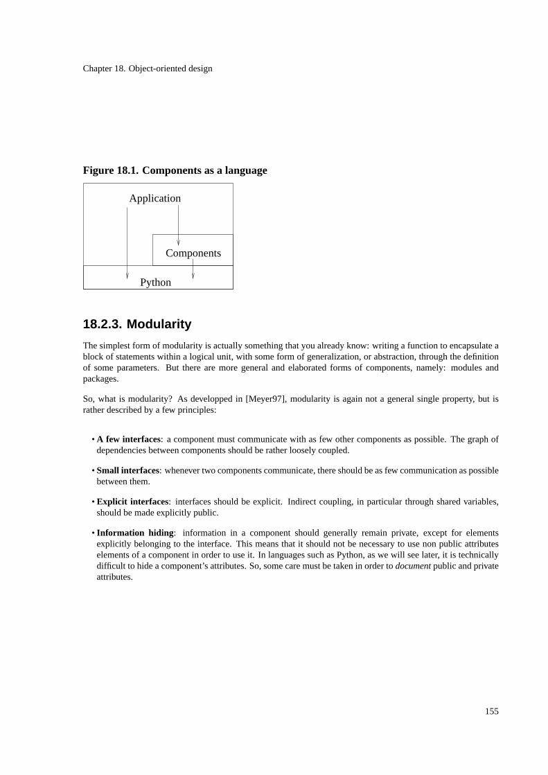
Chapter 18. Object-oriented design
Figure 18.1. Components as a language
Application
Python
Components
18.2.3. Modularity
The simplest form of modularity is actually something that you already know: writing a function to encapsulate ablock of statements within a logical unit, with some form of generalization, or abstraction, through the definitionof some parameters. But there are more general and elaborated forms of components, namely: modules andpackages.
So, what is modularity? As developped in [Meyer97], modularity is again not a general single property, but israther described by a few principles:
• A few interfaces: a component must communicate with as few other components as possible. The graph ofdependencies between components should be rather loosely coupled.
• Small interfaces: whenever two components communicate, there should be as few communication as possiblebetween them.
• Explicit interfaces: interfaces should be explicit. Indirect coupling, in particular through shared variables,should be made explicitly public.
• Information hiding : information in a component should generally remain private, except for elementsexplicitly belonging to the interface. This means that it should not be necessary to use non public attributeselements of a component in order to use it. In languages such as Python, as we will see later, it is technicallydifficult to hide a component’s attributes. So, some care must be taken in order todocumentpublic and privateattributes.
155
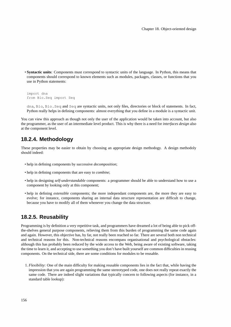
Chapter 18. Object-oriented design
• Syntactic units: Components must correspond to syntactic units of the language. In Python, this means thatcomponents should correspond to known elements such as modules, packages, classes, or functions that youuse in Python statements:
import dnafrom Bio.Seq import Seq
dna , Bio , Bio.Seq andSeq are syntactic units, not only files, directories or block of statements. In fact,Python really helps in defining components: almost everything that you define in a module is a syntactic unit.
You can view this approach as though not only the user of the application would be taken into account, but alsothe programmer, as the user of an intermediate level product. This is why there is a need forinterfaces designalsoat the component level.
18.2.4. Methodology
These properties may be easier to obtain by choosing an appropriate design methodogy. A design methodolyshould indeed:
• help in defining components by successivedecomposition;
• help in defining components that are easy tocombine;
• help in designingself-understandablecomponents: a programmer should be able to understand how to use acomponent by looking only at this component;
• help in definingextensiblecomponents; the more independant components are, the more they are easy toevolve; for instance, components sharing an internal data structure representation are difficult to change,because you have to modify all of them whenever you change the data structure.
18.2.5. Reusability
Programming is by definition a very repetitive task, and programmers have dreamed a lot of being able to pick off-the-shelves general purpose components, relieving them from this burden of programming the same code againand again. However, this objective has, by far, not really been reached so far. There are several both non technicaland technical reasons for this. Non-technical reasons encompass organisational and psychological obstacles:although this has probably been reduced by the wide access to the Web, being aware of existing software, takingthe time to learn it, and accepting to use something you don’t have built yourself are common difficulties in reusingcomponents. On the technical side, there are some conditions for modules to be reusable.
1.Flexibility: One of the main difficulty for making reusable components lies in the fact that, while having theimpression that you are again programming the same stereotyped code, one does not really repeat exactly thesame code. There are indeed slight variations that typically concern to following aspects (for instance, in astandard table lookup):
156

Chapter 18. Object-oriented design
• types: the exact data type being used may vary: the table might contain integers, strings, ...
• data structures and algorithms may vary: the table might be implemented with an array, a dictionary, abinary search tree, ... ; the comparison function in the sort procedure may also vary according to the typeof the items.
So, as you can understand from these remarks, the moreflexible the component is, the more reusable it is.Flexibility can be partly obtained by modularity, as long as modules are well designed. However, in order toget real flexibility, other techniques are required, such as genericity, polymorphism, or inheritance, that aredescribed in Section 18.5.
2. Independancy towards the internal representation: by providing a interface that does not imply any specificinternal data structure, the module can be used more safely. The client program will be able to use the sameinterface, even if the internal representation is modified.
3.Group of related objects: it is easier to use components when all objects that should be used together (thedata structures, data and algorithms) are actually grouped in the same component.
4.Common features: common features or similar templates among different modules should be made shareable,thus making the whole set of modules more consistent.
18.3. Abstract Data Types
18.3.1. DefinitionWhat is an abstract data type? Well, a data type is what we have just presented in chapter Chapter 17: inPython, as in many object-oriented language, it is a class. So, whyabstract? One of the main objectives incomponent building, as we have seen in section Section 18.2, is to provide components that a programmer (you,your colleagues, or any programmer downloading your code) can be confident in. In order to get this programmer,who is aclient of your code, confident into your class, you have to make it as stable as possible, and the bestmethod to get a stable class is to define it at a level whereno implementation decision is visible. In other words,defining a class should consist in defining a data type providing some abstractservices, whoseinterfaceare clearlydefined in term of parameters and return value and potential side effects. The advantages of this approach are thefollowing:
• The implementor of the class can change the implementation for maintenance, bug fixes or optimizationreasons, without disturbing the client code.
• The data type is defined as a set of high-level services with asemantic contractdefining both the output thatis provided and the input that is required from the client. This actually correspond to the general definition ofa type in programming: a type is defined as a set of possible values and aset of operationsavailable on thesevalues.
Among the methods defined in the interface of a data type, there are methods that build or change the state of thecorresponding object, which are calledconstructorsandmodificators, and there are methods to access the object,which are calledaccessors.
157
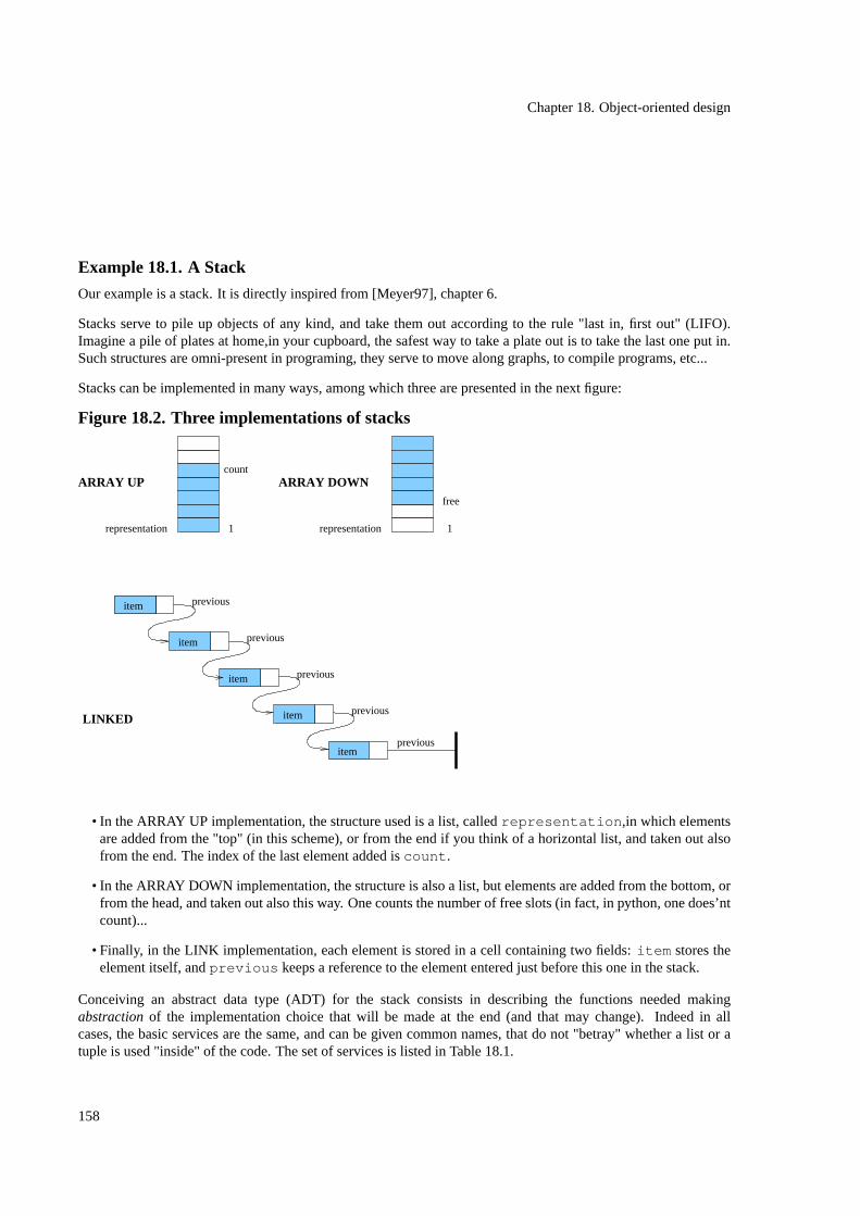
Chapter 18. Object-oriented design
Example 18.1. A Stack
Our example is a stack. It is directly inspired from [Meyer97], chapter 6.
Stacks serve to pile up objects of any kind, and take them out according to the rule "last in, first out" (LIFO).Imagine a pile of plates at home,in your cupboard, the safest way to take a plate out is to take the last one put in.Such structures are omni-present in programing, they serve to move along graphs, to compile programs, etc...
Stacks can be implemented in many ways, among which three are presented in the next figure:
Figure 18.2. Three implementations of stacks
1
count
representation
ARRAY DOWN
representation 1
free
item
item
item
item
item
previous
previous
previous
previous
previous
ARRAY UP
LINKED
• In the ARRAY UP implementation, the structure used is a list, calledrepresentation ,in which elementsare added from the "top" (in this scheme), or from the end if you think of a horizontal list, and taken out alsofrom the end. The index of the last element added iscount .
• In the ARRAY DOWN implementation, the structure is also a list, but elements are added from the bottom, orfrom the head, and taken out also this way. One counts the number of free slots (in fact, in python, one does’ntcount)...
• Finally, in the LINK implementation, each element is stored in a cell containing two fields:item stores theelement itself, andprevious keeps a reference to the element entered just before this one in the stack.
Conceiving an abstract data type (ADT) for the stack consists in describing the functions needed makingabstractionof the implementation choice that will be made at the end (and that may change). Indeed in allcases, the basic services are the same, and can be given common names, that do not "betray" whether a list or atuple is used "inside" of the code. The set of services is listed in Table 18.1.
158
Chapter 18. Object-oriented design
Table 18.1. Stack class interface
159
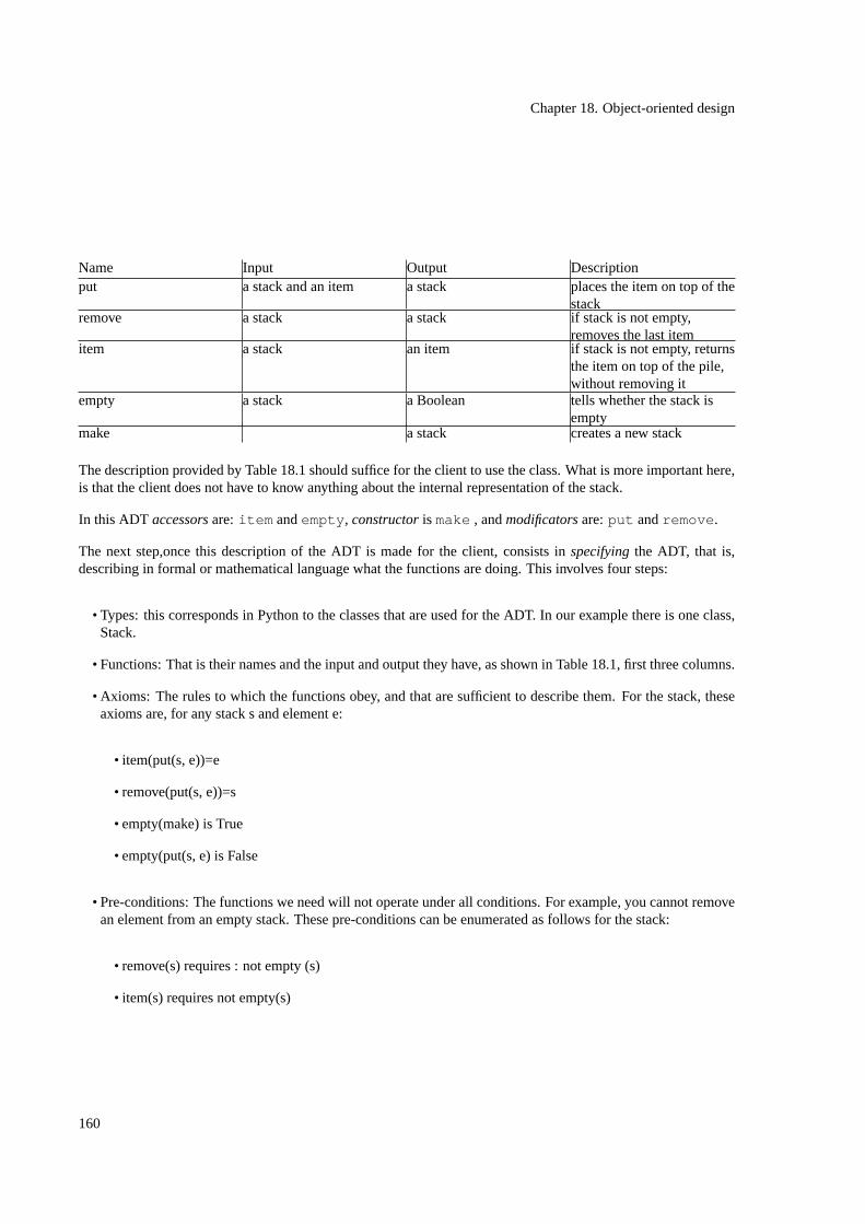
Chapter 18. Object-oriented design
Name Input Output Descriptionput a stack and an item a stack places the item on top of the
stackremove a stack a stack if stack is not empty,
removes the last itemitem a stack an item if stack is not empty, returns
the item on top of the pile,without removing it
empty a stack a Boolean tells whether the stack isempty
make a stack creates a new stack
The description provided by Table 18.1 should suffice for the client to use the class. What is more important here,is that the client does not have to know anything about the internal representation of the stack.
In this ADT accessorsare: item andempty , constructoris make , andmodificatorsare:put andremove .
The next step,once this description of the ADT is made for the client, consists inspecifyingthe ADT, that is,describing in formal or mathematical language what the functions are doing. This involves four steps:
• Types: this corresponds in Python to the classes that are used for the ADT. In our example there is one class,Stack.
• Functions: That is their names and the input and output they have, as shown in Table 18.1, first three columns.
• Axioms: The rules to which the functions obey, and that are sufficient to describe them. For the stack, theseaxioms are, for any stack s and element e:
• item(put(s, e))=e
• remove(put(s, e))=s
• empty(make) is True
• empty(put(s, e) is False
• Pre-conditions: The functions we need will not operate under all conditions. For example, you cannot removean element from an empty stack. These pre-conditions can be enumerated as follows for the stack:
• remove(s) requires : not empty (s)
• item(s) requires not empty(s)
160

Chapter 18. Object-oriented design
Axioms and pre-conditions formulate more precisely what is said inthe fourth column of Table 18.1
18.3.2. Information hiding
It is a good design practice to protect an instance local data. Why is that? The first reason is that it makes theinterface of the class more easy to grasp. The client just knows what needs to be known in order for the componentto be used properly. A second reason is that class data should rather be handled by the class methods: there mightbe some coherence to be maintained among different attributes, that a method can check. Another importantreason is to avoid the risk of collisions, that could happen between the class and the potential base classes, as wewill explain in Section 18.4, devoted to inheritance.
The problem is that there is no real mechanism in Python to prevent a client code from accessing to an instanceattributes, as there are in other languages (such as Java or C++), where you can declareprivate and publicattributes. Python provides just the following: if you name a variable with a ’__’ prefix and no ’_’ suffix, such as:
__list = []
within a class named, e.g:Stack , Python automatically changes it to:_Stack__list . You can still access it,but you are aware that you are probably doing something odd, and it can help to avoid name collisions.
Another way to distinguishpublicandprivateattributes and methods is to prefix the private ones with a single ’_’character. This does not provoke any automatic addition by Python, but it is warning the reader that this part of thecode is private. Another style matter is the naming of classes, where it is a good idea to capitalize the first letter ofclass names, to distinguish them from variable or function names. Be aware finally that some methods in Pythonare framed by double ’__’ on both side, they are calledspecial methodsand described in the next p aragraph.
The lesson to be learnt is that attributes you want to be accessible should be mentionned explicitely, anddocumented as such.
So, coming back to our ADT Stack, what has been said so far allows us to draw the following ’post-office’ likerepresentation: outside stand the public methods that the client can access, and inside stand the private attribute :_list in the case of ’array up’ or ’array down’ implementations, _pair in the case of ’link’ implementation.
Figure 18.3. Post office representation of the ADT stack
_list _pair
put
item
empty
remove
put
item
empty
remove
161

Chapter 18. Object-oriented design
Now that the ADT is specified, that we know which attributes and methods are public or private, We can turn tothe implementation part of our example. Because we will use Python language, the implementation with a list andarray up is probably the more intuitive, this is the one shown in Example 18.2.
Example 18.2. Stack class using an array-up implementation
#! /usr/local/public/bin/python
class Stack:"""A class to handle stacks"""
def __init__(self):"""initializes a stack"""self.__list=[]
def put(self, elem):"""places an item on top of the stack"""self.__list.append(elem)
def remove(self):"""if not empty, removes the last item placed on the stackelse does not do anything"""if self.__list:
last=self.__list[-1]self.__list.remove(last)
def item(self):"""if not empty, returns the item on top of the stackwithout removing itelse does not do anything"""if self.__list:
return self.__list[-1]
def empty(self):"""tells if the stack is empty"""if len(self.__list)==0:
return Truereturn False
162

Chapter 18. Object-oriented design
Exercise 18.1. Alternative implementation of the Stack class
Implement a stack according to the ’link’ principle.
18.3.3. Using special methods within classes
The usual Python operators, such as ’+’, the ’[ ]’ operator to access an item or a slice, the assignment ’=’ operator,the equality ’==’ operator, but also ’print’ etc..., are defined withspecial methodsthat have different definitions fordifferent types. Indeed adding two integers is not the same as adding two strings. It is very convenient to redefinethese special methods inside the classes created with Python. The very basicspecial methodsencountered in mostclasses is the one allowing to use ’print’.
Suchspecial methodshave obligate names, and are framed by ’__’, such as __str__ for ’print’. A set a veryprecious pages in the book ’Python. Essential reference’ concerns all the tables (3.7 to 3.10) listing these obligatenames. Here below in Table 18.2, we will list a small number of examples.
Table 18.2. Some of the special methods to redefine Python operators
Operator Special method Description[] __getitem__ access to an item== __eq__ test for equality. __getattr__ access to anon existingattribute. and = __setattr__ modification of an attributelen() __len__ length computationprint __str__ string form for instance valuedel __del__ deletion of an instance
In Example 18.3, we extend the classStack using the __str__ special method.
Example 18.3. Defining a Stack special method
def __str__(self):return self.__list
18.4. Inheritance: sharing code among classes
18.4.1. Introduction
163

Chapter 18. Object-oriented design
What we have seen so far,object-basedprogramming, consists in designing programs with objects, that are builtwith classes. In most object-oriented programming languages, you also have a mechanism that enables classes toshare code. The idea is very simple: whenever there are some commonalities between classes, why having themrepeat the same code, thus leading to maintenance complexity and potential inconsistency? So the principle ofthis mechanism is to define some classes as being the same as other ones, with some differences.
Example 18.4. Inheritance example (1): sequences
We would like to design different classes for different types of sequences: indeed, having all the methods definedonly for protein sequences also available for DNA sequences can be considered a problem. At the same time,some functionalities are common to both types of sequences: cleaning the sequence, producing a Fasta formatto name a few. So we will have two classes to deal with DNA and protein sequences (DNAsequence andProteinsequence ), together with a common class to deal with general sequence functions (Sequence ). Inorder to specify that aDNAsequence (or aProteinsequence ) is aSequence in Python is:
class DNAsequence(Sequence):
The DNAsequence class is called asubclass, and theSequence is called asuperclassor a base class.Following theclass statement, there areonly the definitions specific to theDNAsequence class: you donot need to re-specify the other ones.
class DNAsequence(Sequence):
def gc(self):"""GC percent"""...
def revcomp(self):"""reverse complement"""...
def translate(self):"""translation into a protein"""...
Example 18.5. Inheritance example (2): alignment scoring
In Python, you can pass a function (such asscore_gap )as a parameter to another function (such asalign ) :
def score_gap(gap=-1):return gap
def align(seq1, seq2, compare, score_gap):
164
Chapter 18. Object-oriented design
"""statements to align seq1 with seq2,using compare and score_gap function as a parameters
"""
But what if you need to change the default value forscore_gap gap parameter? This is not possible: for thispurpose, you need a class.
So, say you have aScoring class that provides methods to compare characters and score gaps in alignmentaccording to standard scoring functions in alignments. You can use it as an argument to analign :
>>> scoring = Scoring()>>> align(’ATGATGAT’, ’CTGATC’, scoring=scoring)(’ATGATGAT-’, ’---CTGATC’)
Within the align function, there is a call to thescore_gap method (and alsocompare ) of the Scoringinstance:
scores = [ matrice[row-1, col-1].score +scoring.compare(matrice.rowlabel[row], matrice.collabel[col]),matrice[row, col-1].score + scoring.score_gap(),matrice[row-1, col].score + scoring.score_gap() ]
If you need to customize the scoring parameters, namely: thegap score value, you can just instantiate theScoring class with appropriate arguments, as defined in its__init__ method:
>>> scoring = Scoring(gap=-10)
and pass it to thealign function:
>>> align(’ATGATGAT’, ’CTGATC’, scoring=scoring)
or even shorter:
>>> align(’ATGATGAT’, ’CTGATC’, scoring=Scoring(gap=-10))
But now, say you would like not only to change this parameter, but also change thestructureof the scoring scheme,in particular to have a gap cost that depends on the size of the gap (affine gap cost). So instead of just:
def score_gap(gap=-1):return gap
you want:
165
Chapter 18. Object-oriented design
def score_gap(gapinit=-10, gapextend=-1, length=0):return gapinit + (gapextend * length)
For this, you need to have your own scoring class, that you can callScoringAffine , and use it in your dynamicalignment program:
>>> scoring = ScoringAffine()>>> align(’MLELLPTAVEGVSQAQITGRPEWIWLALGTALMGLGTLYFLVKGMGVSDPDA’,
’MLQSGMSTYVPGGESIFLWVGTAGMFLGMLYFIARGWSVSDQRR’,scoring=scoring)
(’MLELLPTAVEGVSQAQITGRPEWIWLALGTALMGLGTLYFLVKGMGVSDPDA’,’------MLQSGMSTYVPGGESIFLW--VGTAGMFLGMLYFIARGWSVSDQRR’)
To get this, you will need to define aScoringAffine class, right? But the only difference with theScoringclass is thescore_gap method. Theinheritancemechanism allows you to define theScoringAffine classas being aScoring class, with aspecialisation. Following theclass statement, there areonly the definitionsspecific to theScoringAffine class: you do not need to re-specify the other ones.
class ScoringAffine(Scoring):
def score_gap(self, gapinit=-10, gapextend=-1, length=0):return gapinit + (gapextend * length)
18.4.1.1. Overloading
When a method is redefined (oroverriden) in the subclass, which is the case of thescore_gap method that wasalready defined in theScoring class, it is said that the method isoverloaded. This means that, according tothe actual class of a scoring instance, which can be eitherScoring or ScoringAffine , the method actuallycalled is not always the same. In other words, the namescore_gap has several meanings, depending on thecontext of the call.
Overloading
Overloading a method is to have several definitions of the same method in different places, that will be usedaccording to the context of the call.
The term overloading is also used about operators. The ’+’ operator, for instance, is overloaded in the sense thatit refers to different operations when used with strings and integers.
18.4.1.2. How does it work? Dynamic binding.
As we said above, by declaringScoringAffine as a subclass ofScoring , you do not need to re-specify inScoringAffine the methods that are already defined inScoring . The way it works is that Python looks
166

Chapter 18. Object-oriented design
up methods starting from the actual class of the object (e.g for ourscoring variable, it isScoringAffine ),and, if not found, by looking up further inScoringAffine base classes (Scoring ) for the needed methodor attribute. So, when looking up for thescore_gap method (Figure 18.4), Python finds it in the current class.When looking up for other methods, such as thecompare method, which is not defined in theScoringAffineclass, Python follows the graph of base classes (Figure 18.5). Here, we only have one:Scoring , wherecompare is defined.
Figure 18.4. Dynamic binding (1)
ScoringAffine __dict__
__bases__
Scoring comparescore_gap
__dict__
score_gap
__class__
mon_scoremon_score.score_gap()
167
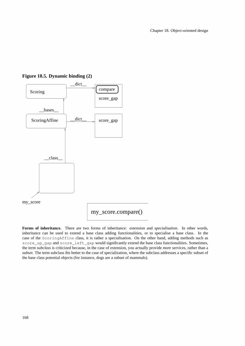
Chapter 18. Object-oriented design
Figure 18.5. Dynamic binding (2)
ScoringAffine __dict__
Scoringscore_gap
__dict__compare
score_gap
__class__
__bases__
my_score
my_score.compare()
Forms of inheritance. There are two forms of inheritance:extensionand specialisation. In other words,inheritance can be used to extend a base class adding functionalities, or to specialise a base class. In thecase of theScoringAffine class, it is rather a specialisation. On the other hand, adding methods such asscore_up_gap andscore_left_gap would significantly extend the base class functionalities. Sometimes,the termsubclassis criticized because, in the case of extension, you actually providemoreservices, rather than asubset. The term subclass fits better to the case of specialization, where the subclass addresses a specific subset ofthe base class potential objects (for instance, dogs are a subset of mammals).
168

Chapter 18. Object-oriented design
UML diagrams. Classes relationships (as well as instances relationships, not represented here) can be representedby so-called UML diagrams, as illustrated in Figure 18.6.
Figure 18.6. UML diagram for inheritance
ScoringAffine
Scoring
18.4.1.3. Multiple inheritance
In Python, as in several programming language, you can have a class inherit from several base classes. Normally,this happens when you need to mix very different functionalities. For instance, you want to wrap your class witha class that provides tools for testing (Figure 18.7, or services for persistence. Inheriting from classes that comefrom the same hierarchy can be tricky, in particular if methods are defined everywhere: you will have to know howthe interpretor choose a path in the classes graph. But this case is more like a theoretical limit case, that shouldnot happen in a well designed program.
Figure 18.7. Multiple Inheritance
Testing A
B
18.4.2. Discussion
169
Chapter 18. Object-oriented design
Benefits of inheritance.
• Regardingflexibility, the inheritance mechanism provides a convenient way to define variants at the methodlevel: with inheritance indeed, themethods become parameters, since you can redefine any of them. So youget more than just the possibility of changing a parameter value.
• Regardingreusability, inheritance is very efficient, since the objective is to reuse a code which is alreadydefined. Components designed with the idea of reuse in mind very often have a clean inheritance hierarchy inorder to provide a way for programmers to adapt the component to their own need.
• Inheritance also provides an elegantextensibilitymechanism, by definition. It lets you extend a class withoutchanging the code of this class, or the code of the module containing the class.
Combining class or combining objects?Using inheritance is not mandatory. The main risk of using it too muchis to get a complex set of classes having a lot of dependencies and that are difficult to understand. There aregenerally two possibilities to get things done in object-oriented programming:
• Inheritance:you combine classes in order to get a "rich" class providing a set of services coming from eachcombined class.
• Composition:you combine objects from different classes.
Example 18.6. Critique of inheritance: alignment classes
You can describe alignment algorithms by dynamic programming as a collection of related algorithms that youcan classify according to some criteria:
• global / local
• stripped / not stripped
• gap cost: constant / linear / affine
It is thus tempting to build a hierarchy of all the variants, a classification, with an abstract alignment class on topof all the others, as shown in Figure 18.8. With the criteria described above, you get 2 * 2 * 3 sub-classes in all.Since there is no local stripped alignment, we only have 9 concrete sub-classes.
170

Chapter 18. Object-oriented design
Figure 18.8. Alignment inheritance classes hierarchy
NWAlignment StripNWAlignment SWAlignment
StripNWAlignmentLinearGap
StripNWAlignmentAffineGap
SWAlignmentLinearGap
SWAlignmentAffineGap
AbstractAlignment
NWAlignmentLinearGap
NWAlignmentAffineGap
The problem of this design is that you have too many classes. Moreover, the next time you will want to addanother criterium, you will have to multiply again the number of combinations by the number of variants for thiscriterium. There is a way to avoid this: instead of combining classes, it is often possible to combine objects.For instance, we can dissociate the criteria and have them specified in different classes and combine the objectsinstead of the classes. As shown in Figure 18.9, we need classes to handle different forms of gap calculation :classScoring ; we need a class to handle local or global alignment : classPath do the job since it computesthe final alignment(s) according to the global or local pathes that have been just computed. We finally need anAligner set of classes to decide which parts of the matrix to compute, in the case of a stripped alignment, youget differentbegin andend methods. We should then get only 3 + 2 + 2 sub-classes. We have actually less,since the base class can sometimes be used directly. When doing the alignment, we need to instantiate one of eachof these three categories of classes. So for instance, when doing a Needleman and Wunsch alignment with lineargap scoring, we do:
>>> path = NWPath()>>> aligner = Aligner(scoring=ScoringLinear())>>> matrix = aligner.align(seq1,seq2)
171

Chapter 18. Object-oriented design
>>> print path.backtrack(matrix)
For a Smith and Waterman alignment with simple scoring, we have:
>>> path = SWPath()>>> aligner = Aligner(scoring=Scoring())>>> matrix = aligner.align(seq1,seq2)>>> print path.backtrack(matrix)
Figure 18.9. Alignment classes with more composition
Scoring
StripAligner
Path
SWPath
Aligner
ScoringAffine
ScoringLinear
The use of composition instead of inheritance is also illustrated by the design patterns from [Gamma95], that areintroduced in Section 18.6.
Problem with inheritance for extension. When using inheritance to extend a base class, you might want to havea method in the subclass not just overloading the method in the base class, but as a complement. In this case,one usually first calls the base class, and then performs the complementary stuff. In Python, you have to knowexplicitely the name of the superclass to perform this call:
class ScoringAffine(Scoring):
def score_gap(gapextend=-1, length=0):return Scoring.score_gap() + (gapextend * length)
Be aware, that this can become rather tricky sometimes, for you have to design a real protocol describing thesequence of calls that have to be done among classes, when not only one method is involved.
172

Chapter 18. Object-oriented design
When using inheritance or composition: summary. The question of choosing between inheritance andcomposition to combine objects A and B results in deciding whether Ais-aB or whether Ahas-aB. Unfortunately,it is not always possible to decide about this, only on the basis of the nature of A and B. There a few guidelines,though (see [Harrison97], chapter 2).
• The main advantage of inheritance over composition is that method binding, e.g lookup and actual methodcall, is done automatically: you do not have to perform the method lookup and call, whereas, when combiningobjects, you have to know which one has the appropriate method. For instance, aCurve instancehas aplot,that is requested for performing graphical tasks (see Section 17.2). The curve has indeed no direct method toget things displayed, it has to behave as awrapperfor thePlot redraw . In a different design, you could havetheCurve and thePlot classes combined in aGraphicalCurve class inheriting from the two others.
• Use composition when you catch yourself making exceptions to theis-a rule and redefining several inheritedmethods or willing to protect access to the base class attributes and/or methods. In such a case, the advantagedescribed in the previous item of having automatic attribute and method access becomes a problem.
• Use composition when the relationships between objects are dynamic: say for instance that the graphicaldisplay you want for theCurve is not aPlot based on Pmw.Blt [http://pmw.sourceforge.net/doc/Blt.html]anymore, but another widget. Or, similarly, that thePlot objects should rather be connected to another classof internal curve.
• Use composition when a single object must have more than one part of a given type: in thePlot exampleagain, we wanted to have more than oneCurve displayed.
• Use composition to avoid deep inheritance hierarchies (see Example 18.6 with alignment classes).
• If you can’t decide between inheritance and composition, take composition.
• Do not use inheritance when you get too many combined method calls between base class and sub-classes,which can happen when using inheritance for extension.
• Use inheritance when you want to build an abstract framework, which purpose is to be specialized for varioususes (see Exercise 18.2). A good example is the parsing framework in Biopython, that lets you create as manynew parsers as needed. Inheritance also provides a good mechanism to design several layers of abstraction,that define interfaces that programmers must follow when developping their components. Bioperl modules,although not developped in a true object-oriented language, are a good example of this.
173
Chapter 18. Object-oriented design
Exercise 18.2. Example of an abstract framework: Enzyme parser
Design a parser for the Enzyme database, using Biopython parsing framework. See ??? for more details.
18.5. Flexibility
18.5.1. Summary of mechanisms for flexibility in Python
Earlier, in Section 18.2.5, we have seen that one of the powerful properties a software piece can have is to bereusable. We also concluded that the more flexible it is, the more general and thus reusable it will be. Let us nowsummarize some mechanisms in object-oriented programming that help in achieving more flexibility.
• Genericity: genericity (as available in the ADA programming language), is a technique to define parametersfor a module, exactly as you define parameters for a function, thus making the module more general. Forinstance, you can define the type of an element of a Table module, or the function to move to the next item, asbeing generic. There is no specific syntax in Python to define generic components, but in a way, it is not reallynecessary because Python is dynamically typed, and can handle functions as parameters for other functions.
• Inheritance: as we have just seen in Section 18.4 this describes the ability, in object-oriented programming, toderive a class from another, either to extend it or to specialize it.
• Overloading, which refers to the possibility for an operator or a function to behave differently accordingto the actual data types of their operands or arguments. This feature does not directly address the problemof flexibility: it is rather an elegant syntactic mean not to have different operators or names to performsimilar tasks on different objects or sets of objects. In this sense, it is actually a form of polymorphism.In object-oriented programming, overloading moreover exactly means being able to redefine a method in aderived class, thus enabling polymorphism of instances: given an instance, it is possible that you do not knowexactly to which class in a hierarchy it belongs (e.gScoring or ScoringAffine ). In other programminglanguages, such as Java, there is another kind of overloading: it is possible,within the same class, to haveseveral definitions of the same method, but with differentsignatures, i.e a different set of parameters. Thisdoes not exist in Python, and as described below (see ), you have to handle it manually.
• Polymorphism: refers to the possibility for something to be of several forms, e.g, for an object to be of anytype. In Python, for instance, lists are polymorphic, since you can put items of any type in a list. Overloadingis one aspect of polymorphism, polymorphism of methods. Polymorphism brings a lot of flexibility, just onlybecause you do not have to define as many classes as potential data type for it, as you would have to do instatically typed languages. In this sense, Python helps in designing more simple classes frameworks.
174
Chapter 18. Object-oriented design
Some of these techniques, mainly inheritance, are available in Python, other, such as genericity and overloading,are not, or in a restricted way.
18.5.2. Manual overloading
If you want a method to behave differently according to the parameters, you must either create subclasses or writethe code to analyze the parameters yourself. In Example 18.7, there is an example a method dealing with differenttypes of parameters, that are manually handled.
Example 18.7. Curve class: manual overloading
def __getitem__(self, key):"""Extended access to the curve.c[3]c[’toto’]c[’x<100’]c[’x==y’]"""_x = []_y = []_result = Noneif type(key) is ListType: ❶
_x = key_x.sort()_y = self.y(_x)_result = Curve(zip(_x, _y))
elif type(key) is SliceType: ❷_x = self._range_x(key.start, key.stop)_y = apply(self.y, _x)if _x and _y:
_result = Curve(zip(_x, _y))elif self._curve.has_key(key): ❸
_result = self._curve[key]elif type(key) is StringType: ❹
_x = self._tag_x(key)if len(_x) > 0: ❺
_x.sort()_y = self.y(_x)_result = Curve(zip(_x, _y))
else: ❻_result = self._getexpr(key)
if _result is not None:return _result
❶ Recognizes the argument as a list.
175

Chapter 18. Object-oriented design
❷ Recognizes the argument as a slice.❸ Recognizes the argument as an index.❹ Recognizes the argument as a string, that is going to be further analyzed as a tag name or an expression.❺ Recognizes the argument as a tag name.❻ Recognizes the argument as an expression, such as ’x< y’ or ’y>10’.
Python is not able to do this analysis automatically, because it is dynamically typed. You do not have any meanto specify thetypeof the parameter. In a language providing static typing and full method overloading, i.e alsowithin the same class, you could have several__getitem__ definitions that would look like:
def __getitem__(self, key: List):...
def __getitem__(self, key: Slice):...
def __getitem__(self, key: String):...
As you can notice, this is of course not valid Python code, since there is no possibility to define the type of aparameter in Python.
18.6. Object-oriented design patternsPresenting Python classes and various related mechanisms without any description of their common uses wouldbe like defining thefor andwhile statements without any description of the typical uses of these constructions,and how they adapt to various programming needs. It is the purpose of this section to present common usesof classes and objects, the so-calleddesign patterns, that have been used for a long time by programmers sinceobject-oriented programming was born.
Computer science is full of design patterns, and there is no exception for object-oriented programming. A catalogof object-oriented has been published by [Gamma95], and [Christopher2002] has a chapter dedicated to a fewof them, with examples implemented in Python. Design patterns are not programs: they are widely useddesignchoices to build programs. As such, they form a kind of conceptual catalog that you are encouraged toreusetobuild your application. Not only are they useful in order not to reinvent the wheel and to save your time, but alsobecause they provide acomprehension frameworkfor programmers who intend to reuse your code and who needto understand it. This part does not aim at an exhaustive presentation of object-oriented design patterns, which arevery well described elsewhere. Its main purpose is to give a taste of it, with examples in bioinformatics, and tointroduce the main related ideas.
There are three categories of object-oriented patterns:
• Creationalpatterns: patterns that can be used tocreateobjects.
• Structuralpatterns: patterns that can be used tocombineobjects and classes in order to build structured objects.
• Behavioralpatterns: patterns that can be used to build a computation and to control data flows.
176
Chapter 18. Object-oriented design
Creational patterns. There are two main categories of creational patterns: those for creating objects withouthaving to know the class name, that you could call "abstract object makers" (abstract factoryandfactory method),and those to ensure a certain property regarding object creation, such as prohibiting more than one instance fora class (singleton), building a set of instances from different classes in a consistent way (builder), or creating aninstance with a specific state (prototype).
• Abstract factory:an abstract factory is an object maker, where, instead of specifying a class name, you specifythe kind of object you want. For instance, say that you want to create an agent to run analysis programs, youcan ask a factory to do it for you:
clustalw = AnalysisFactory.program(’clustalw’)result = clustalw.run(seqfile = ’myseqs’)print result.alig
Theclustalw object is an instance of, say, theAnalysisAgent.Clustalw class, but you do not haveto know about it at creation time. The only thing you know is the name of the program you want (’clustalw’),and the factory will do the rest for you.
• Factory method:a factory method is very similar to an abstract factory: just, instead of being a class, it is amethod.
• For instance, you can create a sequence object (Bio.Seq.Seq in Biopython) by asking theget_seq_by_num method of an alignment object (Bio.Align.Generic.Alignment ):
first_seq = align.get_seq_by_num(0)
The method which creates this instance ofBio.Seq.Seq is a factory method. The difference with afactory class is also that the factory method is often more than an object maker: it sometimes incorporatesmuch more knowledge about the way to create the object than a factory would.
• A more simple factory method would be anew method defined in a class to create new instances of thesame class:
my_scoring = scoring.new()
In this case, notice that in order to createmy_scoring , you really do not have to know the actual classof scoring : the only thing you know is that you will getthe same one, even if there is a whole hierarchyof different classes of scoring.
177
Chapter 18. Object-oriented design
• Another example could be a factory method in thePlot class:
p = Plot()p.new_curve([...])
that would create an instance of theCurve class and draw it as soon as created.
• Singleton:ensures that you cannot create more than one instance. For example, if you can define a class tocontain operations and data for genetic code: you need only one instance of this class to perform the task.Actually, this pattern would not be implemented with a class in Python, but rather with a module, at least ifyou can define it statically (a dynamic singleton could not be a module, for a module has to be a file):
>>> import genetic_code>>> genetic_code.aa(’TTT’)F
• Prototype: this pattern also lets you create a new object without knowing its class, but here, the new targetobject is created with the same state as the source object:
another_seq = seq.copy()
The interest is that you do not get an "empty" object here, but an object identical toseq . You can thus playwith another_seq , change its attributes, etc... without breaking the original object.
• Builder: you sometimes need to create a complex object composed of several parts. This is the role of thebuilder.
• For instance, a builder is needed to build the whole set of nodes and leafs of a tree.
• Or you could design a builder to create bothCurve andPlot instances in a coherent way as parts of aGraphicalCurves complex object:
gc = GraphicalCurves(file=’my_curves’)
For instance,my_curves might contain description of set of curves to display in the same plot or indifferent plots.
• The Blast parser in Biopython simultaneously instantiates several classes that are all component parts ofof hit: Description , Alignment andHeader .
178

Chapter 18. Object-oriented design
Structural patterns. Structural patterns address issues regarding how to combine and structure objects. Forthis reason, several structural patterns provide alternative solutions to design problems that would else involveinheritance relationships between classes.
• Decorator, proxy, adapter:these patterns all enable to combine two (or more) components, as shown in Figure18.10. There is one component, A, "in front" of another one, B. A is the visible object a client will see. The roleof A is either to extend or restrict B, or help in using B. So, this pattern is similar to subclassing, except that,where a sub-classinheritsa method from a base class, the decoratordelegatesto its decoratee when it does nothave the required method. The advantage is flexibility (see Section 18.4.2): you can combine several of thesecomponents in any order at run time without having to create a big and complex hierarchy of subclasses.
Figure 18.10. DelegationA
B
Generally, the Python code of theA class looks like:
class A:def __init__(self, b):
"""storing of the decoratee b (b is an instance of class B)"""self.b = b
def __getattr__(self, name):"""
methods/attributes A does not know about are delegatedto b
"""return getattr(self.b, name)
At use time, an instance of classA is created by providing ab instance.
b = B()a = A(b)print a.f()
Everything that classA cannot perform is forwarded tob (providing that classB knows about it).
• Thedecoratorenables to add functionalities to another object. Example 18.8 shows a very simple decoratorthat prints a sequence in uppercase.
179

Chapter 18. Object-oriented design
Example 18.8. An uppercase sequence class
import string
class UpSeq:
def __init__(self, seq):self.seq = seq
def __str__(self):return string.upper(self.seq)
def __getattr__(self,name):return getattr(self.seq,name)
The way to use it is for instance:
>>> s=UpSeq(’atcgctgtc’)>>> print sATCGCTGTC>>> s[0:3]’atc’>>> len(s)9
Exercise 18.3. An analyzed sequence class
How would you design sequence classes where all sequence analyses of typef would be available as:
seq.f()
without actually defining all the possiblef methods within the sequence class?
• Theproxyrather handles the access to an object. There are several kinds of proxy:
• protection proxy: to protect the access to an object.
180
Chapter 18. Object-oriented design
Exercise 18.4. A partially editable sequence
How would you design a sequence class where the only allowed editions would be:
del seq[i]
on a gap character, and:
seq[i] = ’A’
on a ’N’ character?
• virtual proxy: to physically fetch data only when needed. Database dictionaries in Biopython work thisway:
prosite = Bio.Prosite.ExPASyDictionary()entry = prosite[’PS00079’]
Data are fetched only when an access to an entry is actually requested.
• remote proxy: to simulate a local access for a remotely activated procedure.
• Theadapter(or wrapper) helps in connecting two components that have been developped independantlyand that have a different interface. For instance, thePise package transforms Unix programs interfacesin standardized interfaces, either Web interfaces, or API. For instance, thegoldenUnix command has thefollowing interface:
bash> golden embl:MMVASP
But thePise wrapper enables to run it and get the result by a Python program, having an interface definedin the Python language:
factory = PiseFactory()golden = factory.program("golden",db="embl",query="MMVASP")job = golden.run()print job->content()
181

Chapter 18. Object-oriented design
• Composite: this pattern is often used to handle complex composite recursive structures. Example 18.9 showsa set of classes for a tree structure, illustrated in Figure 18.11. The main idea of the composite design patternis to provide anuniform interfaceto instances from different classes in the same hierarchy, where instancesare all components of the same composite complex object. In Example 18.9, you have two types of nodes:Node andLeaf , but you want a similar interface for them, that is at least defined by a common base class,AbstractNode , with two operations:print subtree . These operations should be callable on any nodeinstance, without knowing its actual sub-class.
>>> t1 = Node ( Leaf ( ’A’, 0.71399),Node ( Node ( Leaf(’B’, -0.00804),
Leaf(’C’, 0.07470),0.15685),Leaf (’D’, -0.04732)
))
>>> print t1(A: 0.71399, ((B: -0.00804, C: 0.0747), D: -0.04732))>>> t2 = t1.right.subtree()>>> print t2((B: -0.00804, C: 0.0747), D: -0.04732)>>> t3 = t1.left.subtree()>>> print t3’A’: 0.71399
Figure 18.11. A composite treeAbstractNode__str__subtree
Leaf__str__
Node
subtreeright
left
__str__subtree
Example 18.9. A composite tree
❶class AbstractNode:
def __str__(self):pass
182

Chapter 18. Object-oriented design
def subtree(self):pass
❷class Node(AbstractNode):
def __init__(self, left=None, right=None, length=None):self.left=leftself.right=rightself.length=length
def __str__(self):return "(" + self.left.__str__() + ", " + self.right.__str__() + ")"
def subtree(self):return Node(self.left, self.right)
class Leaf(AbstractNode): ❸def __init__(self, name, length=None):
self.name = nameself.length=lengthself.left = Noneself.right = None
def __str__(self):return self.name + ": " + str(self.length)
def subtree(self):return Leaf(self.name, self.length)
❶ Abstract classAbstractNode , base class for bothNode andLeaf❷ Internal nodes are instances ofNode class.❸ Leafs are instances ofLeaf class.
Behavioral patterns. Patterns of this category are very useful in sequence analysis, where you often have tocombine algorithms and to analyze complex data structure in a flexible way.
• Template: this pattern consists in separating the invariant part of an algorithm from the variant part. In a sortingprocedure, you can generally separate the function which compares items from the main body of the algorithm.The template method, in this case, is thesort() method, whereas thecompare() can be defined by eachsubclass depending on its implementation or data types. In the dynamic programming align function, thetemplate methods can be thebegin end andinner methods. TheScoring method may vary dependingon the preferred scoring scheme, as defined in subclasses of theScoring class.
183
Chapter 18. Object-oriented design
• Strategy: it is the object-oriented equivalent of passing a function as an argument. TheScoring is a strategy.Variations on methods. So, you don’t necessarily need inheritance to have a function be a parameter. Forinstance, the following function enables you to provide your own functions forscore_gap andcompare :
def align(matrice, begin, inner, end, score_gap, compare):...
So, do we need a subclass for this or even to have aScoring class at all? The answer is that with class andinheritance, your methods are all pooled together in a "packet", but there is some additional burden on yourside, since you have to define a subclass and instantiate it. On the other hand, passing a function as a parameterhas a limit: you can’t change the default values for parameters, such as the default value for a gap initiation orextension in our example.
• Iterator: an iterator is an object that let you browse a sequence of items from the beginning to the end.Generally, it provides:
• a method to start iteration
• a method to get the next item
• a method to test for the end of the iteration
Usually, one distinguishesinternal versusexternaliterators. An external iterator is an iterator which enablesto do afor or awhile loop on a range of values that are returned by the iterator:
for e in l.elements():f(e)
or:
i = l.iterator()e = i.next()while e:
f(e)e = i.next()
In the above examples, you control the loop. On the other hand, an internal iterator just lets you define afunction or a method (say,f ) to apply to all elements:
l.iterate(f)
In the Biopython package, files and databases are generally available through an iterator.
handle = open(...) ❶
184
Chapter 18. Object-oriented design
iter = Bio.Fasta.Iterator(handle) ❷seq = iter.next() ❸while seq:
print seq.nameprint seq.seq ❹seq = iter.next()
handle.close()
❶ Starting the iterator.❷ Getting the next element.❸ Testing for the end of the iteration.❹ Getting the next element.
• Visitor: this pattern is useful to specify a function that will be applied on each item of a collection. The Pythonmap function provides a way to use visitors, such as thef function, which visits each item of thel list in turn:
>>> def f(x):return x + 1
>>> l=[0,1,2]>>> map(f,l)[1, 2, 3]
Themap is an example of an internal iterator (with thef function as a visitor).
• ObserverTheobserverpattern provides a framework to maintain a consistent distributed state between looselycoupled components. One agent, the observer, is in charge of maintaining a list ofsubscribers, e.g componentsthat have subscribed to be informed about changes in a given state. Whenever a change occurs in a state, theobserver has to inform each subscriber about it.A well-known example is the Model-View-Controller [Krasner88] framework. The view components, the oneswho actually display data, subscribe to "edit events" in order to be able to refresh and redisplay them whenevera change occurs.
185
Chapter 18. Object-oriented design
186
Chapter 18. Object-oriented design
BibliographyPython Books[Beazley2001]Python. Essential Reference. 2. David M. Beazley. 0-7357-1091-0. New Riders. 2001.
[Christopher2002]Python Programming Patterns. Thomas W Christopher. 0-13-040956-1. Prentice Hall. 2002.
[Deitel2002]Python. How to program. H. M. Deitel, P. J. Deitel, J. P. Liperi, and B. A. Wiederman. 0-13-092361-3. Prentice Hall. 2002.
[Downey2002]How to Think Like a Computer Scientist. Learining with Python. Allen Downey, JeffreyElkner, and Chris Meyers. 0-97167775-0-6. Green Tea Press. 2002. www.thinkpython.com[http://www.thinkpython.com].
[Grayson2000]Python and Tkinter Programming. John E. Grayson. 1-884777-81-3. Manning Publications Co..2000.
[LutzAscher2001]Learning Python. Mark Lutz and David Ascher. 1-56592-464-9. O’Reilly. 2001.
[Lutz2001]Programming Python. Mark Lutz. 0-596-00085-5. O’Reilly. 2001.
[Martelli2002]Python Cookbook. Alex Martelli and David Ascher. 0-596-00167-3. O’Reilly. 2002.
Other Books[Meyer97]Object Oriented software Construction. Bertrand Meyer. 0-13-629155-4. Prentice Hall Professional
Technical Reference. 1997.
[Booch94] Object-Oriented Analysis and Design with Applications. Grady Booch. Addison-Wesley ObjectTechnology Series. 1994.
[Gamma95]Design Patterns, Elements of Reusable Object-Oriented Software. Erich Gamma, Richard Helm,Ralph Johnson, and John Vlissides. Addison Wesley. 1995.
[Harrison97]Tcl/Tk Tools. Mark Harrison. O’Reilly. 1997.
Articles[Wegner89]BYTE Magazine. “Learning the language”. Peter Wegner. 245-253. march, 1989.
[Mangalam2002]The Bio* toolkits - a brief overview. “Briefings in Bioinformatics”. Mangalam Harry. 296-302.2002.
[Rossum99]Computer Programming for Everybody. Guido van Rossum. 1999.
[Wang2000] A Qualitative Analysis of the Usability of Perl, Python, and Tcl. Proceedings of The TenthInternational Python Conference. Lingyun Wang and Phil Pfeiffer. 2002.
[Krasner88]Journal of Object-Oriented Programming (JOOP). 1. 3. “A Cookbook for Using the Model-View-Controller User Interface Paradigm in Smalltalk-80”. G Krasner and S Pope. 26-49. 1988.
187

Chapter 18. Object-oriented design
188