forecasting using - rob j hyndman 1exponential smoothing methods so far 2holt-winters’ seasonal...
TRANSCRIPT

Forecasting using
6. ETS models
OTexts.com/fpp/7/
Forecasting using R 1
Rob J Hyndman
Outline
1 Exponential smoothing methods so far
2 Holt-Winters’ seasonal method
3 Taxonomy of exponential smoothingmethods
4 Exponential smoothing state space models
Forecasting using R Exponential smoothing methods so far 2
Exponential smoothing methods
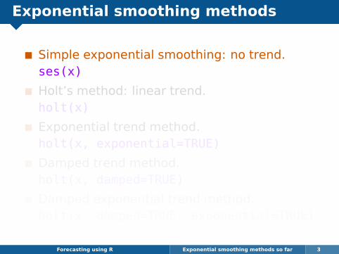
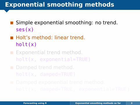
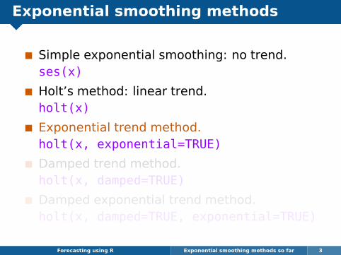
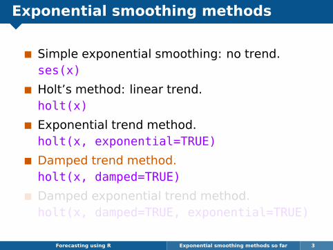
Simple exponential smoothing: no trend.ses(x)
Holt’s method: linear trend.holt(x)
Exponential trend method.holt(x, exponential=TRUE)
Damped trend method.holt(x, damped=TRUE)
Damped exponential trend method.holt(x, damped=TRUE, exponential=TRUE)
Forecasting using R Exponential smoothing methods so far 3
Exponential smoothing methods
Simple exponential smoothing: no trend.ses(x)
Holt’s method: linear trend.holt(x)
Exponential trend method.holt(x, exponential=TRUE)
Damped trend method.holt(x, damped=TRUE)
Damped exponential trend method.holt(x, damped=TRUE, exponential=TRUE)
Forecasting using R Exponential smoothing methods so far 3

Outline
1 Exponential smoothing methods so far
2 Holt-Winters’ seasonal method
3 Taxonomy of exponential smoothingmethods
4 Exponential smoothing state space models
Forecasting using R Holt-Winters’ seasonal method 4
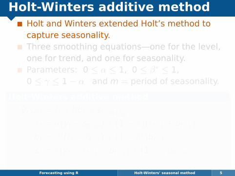
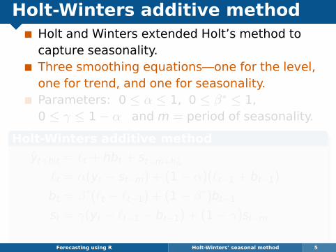
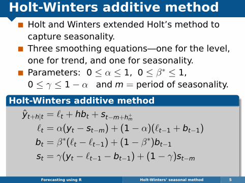
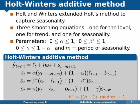
Holt-Winters additive methodHolt and Winters extended Holt’s method tocapture seasonality.Three smoothing equations—one for the level,one for trend, and one for seasonality.Parameters: 0 ≤ α ≤ 1, 0 ≤ β∗ ≤ 1,0 ≤ γ ≤ 1− α and m = period of seasonality.
Holt-Winters additive method
yt+h|t = `t + hbt + st−m+h+m
`t = α(yt − st−m) + (1− α)(`t−1 + bt−1)
bt = β∗(`t − `t−1) + (1− β∗)bt−1
st = γ(yt − `t−1 − bt−1) + (1− γ)st−m
Forecasting using R Holt-Winters’ seasonal method 5
Holt-Winters additive methodHolt and Winters extended Holt’s method tocapture seasonality.Three smoothing equations—one for the level,one for trend, and one for seasonality.Parameters: 0 ≤ α ≤ 1, 0 ≤ β∗ ≤ 1,0 ≤ γ ≤ 1− α and m = period of seasonality.
Holt-Winters additive method
yt+h|t = `t + hbt + st−m+h+m
`t = α(yt − st−m) + (1− α)(`t−1 + bt−1)
bt = β∗(`t − `t−1) + (1− β∗)bt−1
st = γ(yt − `t−1 − bt−1) + (1− γ)st−mh+m = b(h− 1) mod mc+ 1
Forecasting using R Holt-Winters’ seasonal method 5
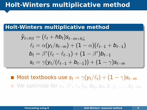
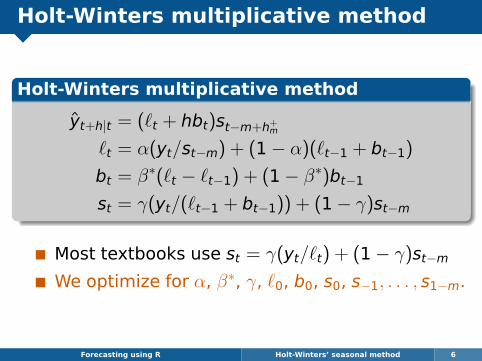
Holt-Winters multiplicative method
Holt-Winters multiplicative method
yt+h|t = (`t + hbt)st−m+h+m
`t = α(yt/st−m) + (1− α)(`t−1 + bt−1)
bt = β∗(`t − `t−1) + (1− β∗)bt−1
st = γ(yt/(`t−1 + bt−1)) + (1− γ)st−m
Most textbooks use st = γ(yt/`t) + (1− γ)st−mWe optimize for α, β∗, γ, `0, b0, s0, s−1, . . . , s1−m.
Forecasting using R Holt-Winters’ seasonal method 6
Holt-Winters multiplicative method
Holt-Winters multiplicative method
yt+h|t = (`t + hbt)st−m+h+m
`t = α(yt/st−m) + (1− α)(`t−1 + bt−1)
bt = β∗(`t − `t−1) + (1− β∗)bt−1
st = γ(yt/(`t−1 + bt−1)) + (1− γ)st−m
Most textbooks use st = γ(yt/`t) + (1− γ)st−mWe optimize for α, β∗, γ, `0, b0, s0, s−1, . . . , s1−m.
Forecasting using R Holt-Winters’ seasonal method 6

Damped Holt-Winters method
Damped Holt-Winters multiplicative method
yt+h|t = [`t + (1 + φ+ φ2 + · · ·+ φh−1)bt]st−m+h+m
`t = α(yt/st−m) + (1− α)(`t−1 + φbt−1)
bt = β∗(`t − `t−1) + (1− β∗)φbt−1
st = γ[yt/(`t−1 + φbt−1)] + (1− γ)st−m
This is often the single most accurateforecasting method for seasonal data.
Forecasting using R Holt-Winters’ seasonal method 7

A confusing array of methods?
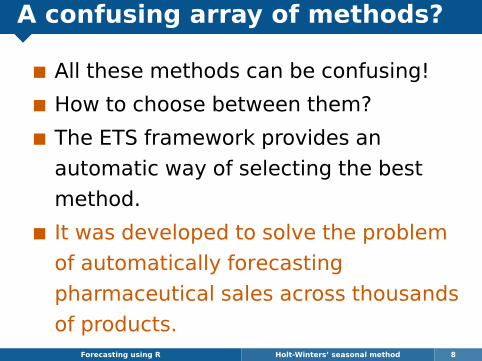
All these methods can be confusing!
How to choose between them?
The ETS framework provides an
automatic way of selecting the best
method.
It was developed to solve the problem
of automatically forecasting
pharmaceutical sales across thousands
of products.Forecasting using R Holt-Winters’ seasonal method 8
A confusing array of methods?
All these methods can be confusing!
How to choose between them?
The ETS framework provides an
automatic way of selecting the best
method.
It was developed to solve the problem
of automatically forecasting
pharmaceutical sales across thousands
of products.Forecasting using R Holt-Winters’ seasonal method 8
Outline
1 Exponential smoothing methods so far
2 Holt-Winters’ seasonal method
3 Taxonomy of exponential smoothingmethods
4 Exponential smoothing state space models
Forecasting using R Taxonomy of exponential smoothing methods 9

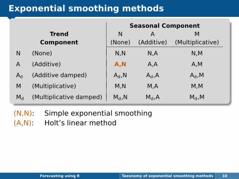
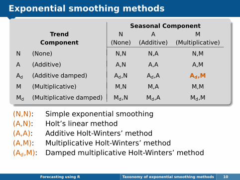
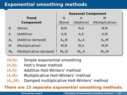
Exponential smoothing methods
Seasonal ComponentTrend N A M
Component (None) (Additive) (Multiplicative)
N (None) N,N N,A N,M
A (Additive) A,N A,A A,M
Ad (Additive damped) Ad,N Ad,A Ad,M
M (Multiplicative) M,N M,A M,M
Md (Multiplicative damped) Md,N Md,A Md,M
Forecasting using R Taxonomy of exponential smoothing methods 10

Exponential smoothing methods
Seasonal ComponentTrend N A M
Component (None) (Additive) (Multiplicative)
N (None) N,N N,A N,M
A (Additive) A,N A,A A,M
Ad (Additive damped) Ad,N Ad,A Ad,M
M (Multiplicative) M,N M,A M,M
Md (Multiplicative damped) Md,N Md,A Md,M
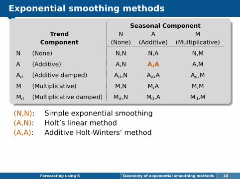
(N,N): Simple exponential smoothing
Forecasting using R Taxonomy of exponential smoothing methods 10
Exponential smoothing methods
Seasonal ComponentTrend N A M
Component (None) (Additive) (Multiplicative)
N (None) N,N N,A N,M
A (Additive) A,N A,A A,M
Ad (Additive damped) Ad,N Ad,A Ad,M
M (Multiplicative) M,N M,A M,M
Md (Multiplicative damped) Md,N Md,A Md,M
(N,N): Simple exponential smoothing(A,N): Holt’s linear method
Forecasting using R Taxonomy of exponential smoothing methods 10
Exponential smoothing methods
Seasonal ComponentTrend N A M
Component (None) (Additive) (Multiplicative)
N (None) N,N N,A N,M
A (Additive) A,N A,A A,M
Ad (Additive damped) Ad,N Ad,A Ad,M
M (Multiplicative) M,N M,A M,M
Md (Multiplicative damped) Md,N Md,A Md,M
(N,N): Simple exponential smoothing(A,N): Holt’s linear method(A,A): Additive Holt-Winters’ method
Forecasting using R Taxonomy of exponential smoothing methods 10

Exponential smoothing methods
Seasonal ComponentTrend N A M
Component (None) (Additive) (Multiplicative)
N (None) N,N N,A N,M
A (Additive) A,N A,A A,M
Ad (Additive damped) Ad,N Ad,A Ad,M
M (Multiplicative) M,N M,A M,M
Md (Multiplicative damped) Md,N Md,A Md,M
(N,N): Simple exponential smoothing(A,N): Holt’s linear method(A,A): Additive Holt-Winters’ method(A,M): Multiplicative Holt-Winters’ method
Forecasting using R Taxonomy of exponential smoothing methods 10
Exponential smoothing methods
Seasonal ComponentTrend N A M
Component (None) (Additive) (Multiplicative)
N (None) N,N N,A N,M
A (Additive) A,N A,A A,M
Ad (Additive damped) Ad,N Ad,A Ad,M
M (Multiplicative) M,N M,A M,M
Md (Multiplicative damped) Md,N Md,A Md,M
(N,N): Simple exponential smoothing(A,N): Holt’s linear method(A,A): Additive Holt-Winters’ method(A,M): Multiplicative Holt-Winters’ method(Ad,M): Damped multiplicative Holt-Winters’ method
There are 15 separate exponential smoothing methods.Forecasting using R Taxonomy of exponential smoothing methods 10
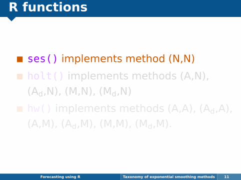
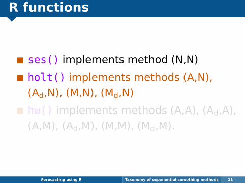
R functions
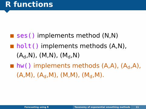
ses() implements method (N,N)
holt() implements methods (A,N),
(Ad,N), (M,N), (Md,N)
hw() implements methods (A,A), (Ad,A),
(A,M), (Ad,M), (M,M), (Md,M).
Forecasting using R Taxonomy of exponential smoothing methods 11
R functions
ses() implements method (N,N)
holt() implements methods (A,N),
(Ad,N), (M,N), (Md,N)
hw() implements methods (A,A), (Ad,A),
(A,M), (Ad,M), (M,M), (Md,M).
Forecasting using R Taxonomy of exponential smoothing methods 11
R functions
ses() implements method (N,N)
holt() implements methods (A,N),
(Ad,N), (M,N), (Md,N)
hw() implements methods (A,A), (Ad,A),
(A,M), (Ad,M), (M,M), (Md,M).
Forecasting using R Taxonomy of exponential smoothing methods 11
Outline
1 Exponential smoothing methods so far
2 Holt-Winters’ seasonal method
3 Taxonomy of exponential smoothingmethods
4 Exponential smoothing state space models
Forecasting using R Exponential smoothing state space models 12
Exponential smoothing
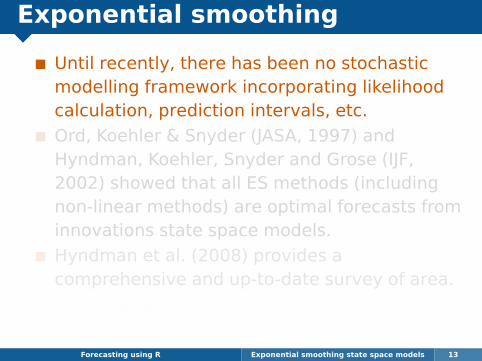
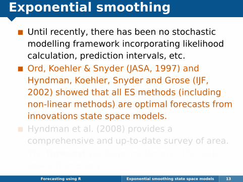
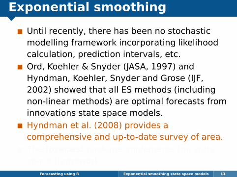
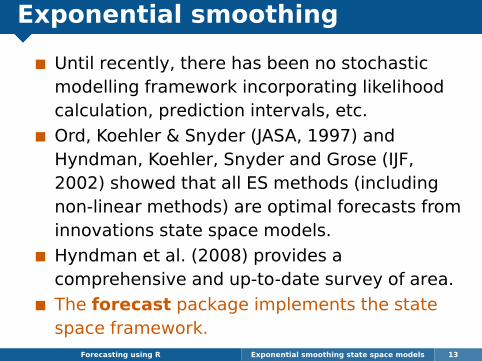
Until recently, there has been no stochasticmodelling framework incorporating likelihoodcalculation, prediction intervals, etc.
Ord, Koehler & Snyder (JASA, 1997) andHyndman, Koehler, Snyder and Grose (IJF,2002) showed that all ES methods (includingnon-linear methods) are optimal forecasts frominnovations state space models.
Hyndman et al. (2008) provides acomprehensive and up-to-date survey of area.
The forecast package implements the statespace framework.
Forecasting using R Exponential smoothing state space models 13
Exponential smoothing
Until recently, there has been no stochasticmodelling framework incorporating likelihoodcalculation, prediction intervals, etc.
Ord, Koehler & Snyder (JASA, 1997) andHyndman, Koehler, Snyder and Grose (IJF,2002) showed that all ES methods (includingnon-linear methods) are optimal forecasts frominnovations state space models.
Hyndman et al. (2008) provides acomprehensive and up-to-date survey of area.
The forecast package implements the statespace framework.
Forecasting using R Exponential smoothing state space models 13

Exponential smoothing
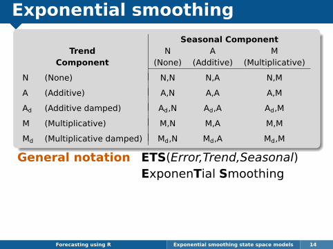
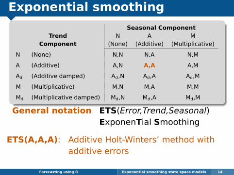
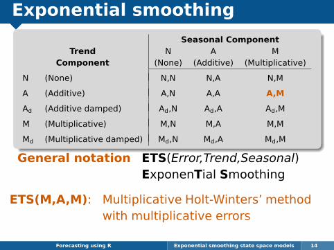
Seasonal ComponentTrend N A M
Component (None) (Additive) (Multiplicative)
N (None) N,N N,A N,M
A (Additive) A,N A,A A,M
Ad (Additive damped) Ad,N Ad,A Ad,M
M (Multiplicative) M,N M,A M,M
Md (Multiplicative damped) Md,N Md,A Md,M
General notation ETS(Error,Trend,Seasonal)
Forecasting using R Exponential smoothing state space models 14

Exponential smoothing
Seasonal ComponentTrend N A M
Component (None) (Additive) (Multiplicative)
N (None) N,N N,A N,M
A (Additive) A,N A,A A,M
Ad (Additive damped) Ad,N Ad,A Ad,M
M (Multiplicative) M,N M,A M,M
Md (Multiplicative damped) Md,N Md,A Md,M
General notation ETS(Error,Trend,Seasonal)
Forecasting using R Exponential smoothing state space models 14
Exponential smoothing
Seasonal ComponentTrend N A M
Component (None) (Additive) (Multiplicative)
N (None) N,N N,A N,M
A (Additive) A,N A,A A,M
Ad (Additive damped) Ad,N Ad,A Ad,M
M (Multiplicative) M,N M,A M,M
Md (Multiplicative damped) Md,N Md,A Md,M
General notation ETS(Error,Trend,Seasonal)ExponenTial Smoothing
Forecasting using R Exponential smoothing state space models 14

Exponential smoothing
Seasonal ComponentTrend N A M
Component (None) (Additive) (Multiplicative)
N (None) N,N N,A N,M
A (Additive) A,N A,A A,M
Ad (Additive damped) Ad,N Ad,A Ad,M
M (Multiplicative) M,N M,A M,M
Md (Multiplicative damped) Md,N Md,A Md,M
General notation ETS(Error,Trend,Seasonal)ExponenTial Smoothing
ETS(A,N,N): Simple exponential smoothing withadditive errors
Forecasting using R Exponential smoothing state space models 14

Exponential smoothing
Seasonal ComponentTrend N A M
Component (None) (Additive) (Multiplicative)
N (None) N,N N,A N,M
A (Additive) A,N A,A A,M
Ad (Additive damped) Ad,N Ad,A Ad,M
M (Multiplicative) M,N M,A M,M
Md (Multiplicative damped) Md,N Md,A Md,M
General notation ETS(Error,Trend,Seasonal)ExponenTial Smoothing
ETS(A,A,N): Holt’s linear method with additiveerrors
Forecasting using R Exponential smoothing state space models 14
Exponential smoothing
Seasonal ComponentTrend N A M
Component (None) (Additive) (Multiplicative)
N (None) N,N N,A N,M
A (Additive) A,N A,A A,M
Ad (Additive damped) Ad,N Ad,A Ad,M
M (Multiplicative) M,N M,A M,M
Md (Multiplicative damped) Md,N Md,A Md,M
General notation ETS(Error,Trend,Seasonal)ExponenTial Smoothing
ETS(A,A,A): Additive Holt-Winters’ method withadditive errors
Forecasting using R Exponential smoothing state space models 14
Exponential smoothing
Seasonal ComponentTrend N A M
Component (None) (Additive) (Multiplicative)
N (None) N,N N,A N,M
A (Additive) A,N A,A A,M
Ad (Additive damped) Ad,N Ad,A Ad,M
M (Multiplicative) M,N M,A M,M
Md (Multiplicative damped) Md,N Md,A Md,M
General notation ETS(Error,Trend,Seasonal)ExponenTial Smoothing
ETS(M,A,M): Multiplicative Holt-Winters’ methodwith multiplicative errors
Forecasting using R Exponential smoothing state space models 14

Exponential smoothing
Seasonal ComponentTrend N A M
Component (None) (Additive) (Multiplicative)
N (None) N,N N,A N,M
A (Additive) A,N A,A A,M
Ad (Additive damped) Ad,N Ad,A Ad,M
M (Multiplicative) M,N M,A M,M
Md (Multiplicative damped) Md,N Md,A Md,M
General notation ETS(Error,Trend,Seasonal)ExponenTial Smoothing
ETS(A,Ad,N): Damped trend method with addi-tive errors
Forecasting using R Exponential smoothing state space models 14

Exponential smoothing
Seasonal ComponentTrend N A M
Component (None) (Additive) (Multiplicative)
N (None) N,N N,A N,M
A (Additive) A,N A,A A,M
Ad (Additive damped) Ad,N Ad,A Ad,M
M (Multiplicative) M,N M,A M,M
Md (Multiplicative damped) Md,N Md,A Md,M
General notation ETS(Error,Trend,Seasonal)ExponenTial Smoothing
There are 30 separate models in the ETSframework
Forecasting using R Exponential smoothing state space models 14
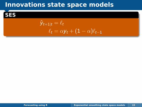
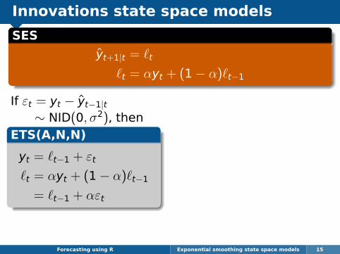
Innovations state space models
SES
yt+1|t = `t
`t = αyt + (1− α)`t−1
Forecasting using R Exponential smoothing state space models 15
Innovations state space models
SES
yt+1|t = `t
`t = αyt + (1− α)`t−1
Forecasting using R Exponential smoothing state space models 15
If εt = yt − yt−1|t∼ NID(0, σ2), then
ETS(A,N,N)
yt = `t−1 + εt
`t = αyt + (1− α)`t−1
= `t−1 + αεt

Innovations state space models
SES
yt+1|t = `t
`t = αyt + (1− α)`t−1
Forecasting using R Exponential smoothing state space models 15
If εt = yt − yt−1|t∼ NID(0, σ2), then
ETS(A,N,N)
yt = `t−1 + εt
`t = αyt + (1− α)`t−1
= `t−1 + αεt
If εt = (yt − yt−1|t)/yt−1|t∼ NID(0, σ2), then
ETS(M,N,N)
yt = `t−1(1 + εt)
`t = αyt + (1− α)`t−1
= `t−1(1 + αεt)

Innovations state space models
SES
yt+1|t = `t
`t = αyt + (1− α)`t−1
All exponential smoothing methods can be writtenusing analogous state space equations.
Forecasting using R Exponential smoothing state space models 15
If εt = yt − yt−1|t∼ NID(0, σ2), then
ETS(A,N,N)
yt = `t−1 + εt
`t = αyt + (1− α)`t−1
= `t−1 + αεt
If εt = (yt − yt−1|t)/yt−1|t∼ NID(0, σ2), then
ETS(M,N,N)
yt = `t−1(1 + εt)
`t = αyt + (1− α)`t−1
= `t−1(1 + αεt)

Innovations state space models
Example: Holt-Winters’ multiplicativeseasonal method
ETS(M,A,M)
yt = (`t−1 + bt−1)st−m(1 + εt)
`t = (`t−1 + bt−1)(1 + αεt)
bt = bt−1 + β(`t−1 + bt−1)εt
st = st−m(1 + γεt)
where β = αβ∗.
Forecasting using R Exponential smoothing state space models 16

Innovations state space models
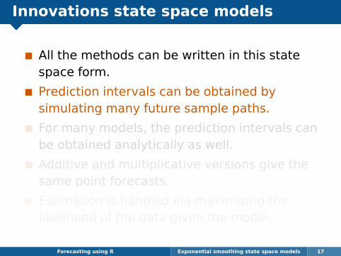
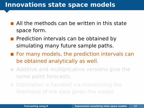
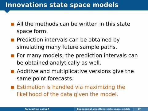
All the methods can be written in this statespace form.
Prediction intervals can be obtained bysimulating many future sample paths.
For many models, the prediction intervals canbe obtained analytically as well.
Additive and multiplicative versions give thesame point forecasts.
Estimation is handled via maximizing thelikelihood of the data given the model.
Forecasting using R Exponential smoothing state space models 17
Innovations state space models
All the methods can be written in this statespace form.
Prediction intervals can be obtained bysimulating many future sample paths.
For many models, the prediction intervals canbe obtained analytically as well.
Additive and multiplicative versions give thesame point forecasts.
Estimation is handled via maximizing thelikelihood of the data given the model.
Forecasting using R Exponential smoothing state space models 17

Akaike’s Information Criterion
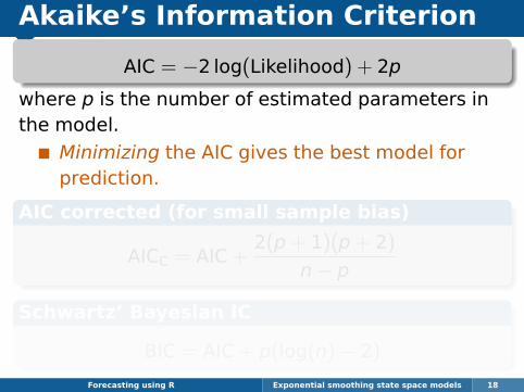
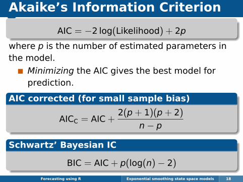
AIC = −2 log(Likelihood) + 2p
where p is the number of estimated parameters inthe model.
Minimizing the AIC gives the best model forprediction.
AIC corrected (for small sample bias)
AICC = AIC +2(p+ 1)(p+ 2)
n− p
Schwartz’ Bayesian IC
BIC = AIC + p(log(n)− 2)
Forecasting using R Exponential smoothing state space models 18
Akaike’s Information Criterion
AIC = −2 log(Likelihood) + 2p
where p is the number of estimated parameters inthe model.
Minimizing the AIC gives the best model forprediction.
AIC corrected (for small sample bias)
AICC = AIC +2(p+ 1)(p+ 2)
n− p
Schwartz’ Bayesian IC
BIC = AIC + p(log(n)− 2)
Forecasting using R Exponential smoothing state space models 18
Akaike’s Information Criterion
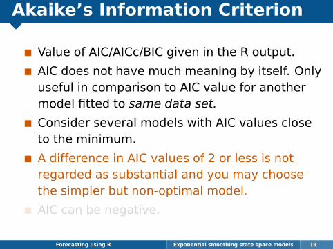
Value of AIC/AICc/BIC given in the R output.
AIC does not have much meaning by itself. Onlyuseful in comparison to AIC value for anothermodel fitted to same data set.
Consider several models with AIC values closeto the minimum.
A difference in AIC values of 2 or less is notregarded as substantial and you may choosethe simpler but non-optimal model.
AIC can be negative.
Forecasting using R Exponential smoothing state space models 19

Akaike’s Information Criterion
Value of AIC/AICc/BIC given in the R output.
AIC does not have much meaning by itself. Onlyuseful in comparison to AIC value for anothermodel fitted to same data set.
Consider several models with AIC values closeto the minimum.
A difference in AIC values of 2 or less is notregarded as substantial and you may choosethe simpler but non-optimal model.
AIC can be negative.
Forecasting using R Exponential smoothing state space models 19
Exponential smoothing
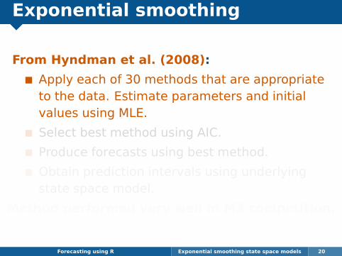
From Hyndman et al. (2008):
Apply each of 30 methods that are appropriateto the data. Estimate parameters and initialvalues using MLE.
Select best method using AIC.
Produce forecasts using best method.
Obtain prediction intervals using underlyingstate space model.
Method performed very well in M3 competition.
Forecasting using R Exponential smoothing state space models 20
Exponential smoothing
From Hyndman et al. (2008):
Apply each of 30 methods that are appropriateto the data. Estimate parameters and initialvalues using MLE.
Select best method using AIC.
Produce forecasts using best method.
Obtain prediction intervals using underlyingstate space model.
Method performed very well in M3 competition.
Forecasting using R Exponential smoothing state space models 20

Exponential smoothing
fit <- ets(ausbeer)fit2 <- ets(ausbeer,model="AAA",damped=FALSE)fcast1 <- forecast(fit, h=20)fcast2 <- forecast(fit2, h=20)
ets(y, model="ZZZ", damped=NULL, alpha=NULL,beta=NULL, gamma=NULL, phi=NULL,additive.only=FALSE,lower=c(rep(0.0001,3),0.80),upper=c(rep(0.9999,3),0.98),opt.crit=c("lik","amse","mse","sigma"), nmse=3,bounds=c("both","usual","admissible"),ic=c("aic","aicc","bic"), restrict=TRUE)
Forecasting using R Exponential smoothing state space models 21
Exponential smoothing
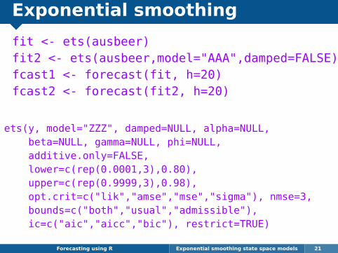
fit <- ets(ausbeer)fit2 <- ets(ausbeer,model="AAA",damped=FALSE)fcast1 <- forecast(fit, h=20)fcast2 <- forecast(fit2, h=20)
ets(y, model="ZZZ", damped=NULL, alpha=NULL,beta=NULL, gamma=NULL, phi=NULL,additive.only=FALSE,lower=c(rep(0.0001,3),0.80),upper=c(rep(0.9999,3),0.98),opt.crit=c("lik","amse","mse","sigma"), nmse=3,bounds=c("both","usual","admissible"),ic=c("aic","aicc","bic"), restrict=TRUE)
Forecasting using R Exponential smoothing state space models 21
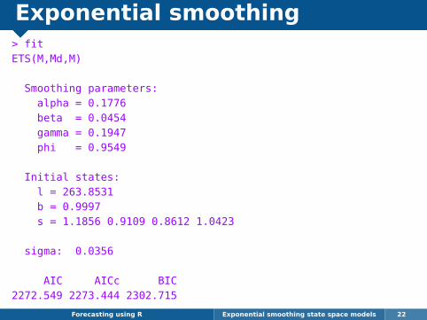
Exponential smoothing> fitETS(M,Md,M)
Smoothing parameters:alpha = 0.1776beta = 0.0454gamma = 0.1947phi = 0.9549
Initial states:l = 263.8531b = 0.9997s = 1.1856 0.9109 0.8612 1.0423
sigma: 0.0356
AIC AICc BIC2272.549 2273.444 2302.715
Forecasting using R Exponential smoothing state space models 22
Exponential smoothing
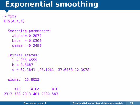
> fit2ETS(A,A,A)
Smoothing parameters:alpha = 0.2079beta = 0.0304gamma = 0.2483
Initial states:l = 255.6559b = 0.5687s = 52.3841 -27.1061 -37.6758 12.3978
sigma: 15.9053
AIC AICc BIC2312.768 2313.481 2339.583
Forecasting using R Exponential smoothing state space models 23

Exponential smoothing
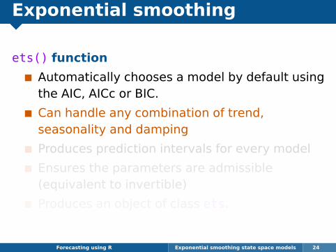
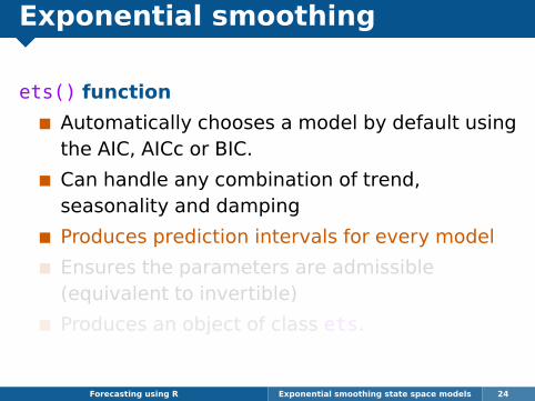
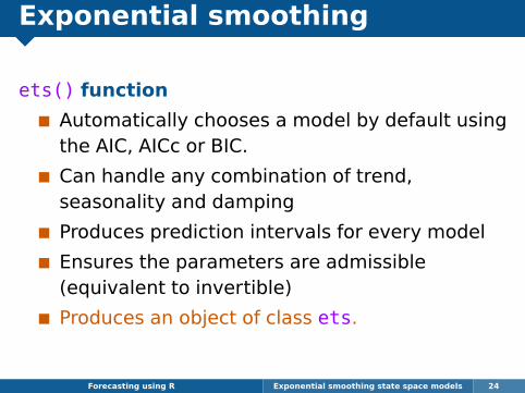
ets() function
Automatically chooses a model by default usingthe AIC, AICc or BIC.
Can handle any combination of trend,seasonality and damping
Produces prediction intervals for every model
Ensures the parameters are admissible(equivalent to invertible)
Produces an object of class ets.
Forecasting using R Exponential smoothing state space models 24
Exponential smoothing
ets() function
Automatically chooses a model by default usingthe AIC, AICc or BIC.
Can handle any combination of trend,seasonality and damping
Produces prediction intervals for every model
Ensures the parameters are admissible(equivalent to invertible)
Produces an object of class ets.
Forecasting using R Exponential smoothing state space models 24

Exponential smoothing
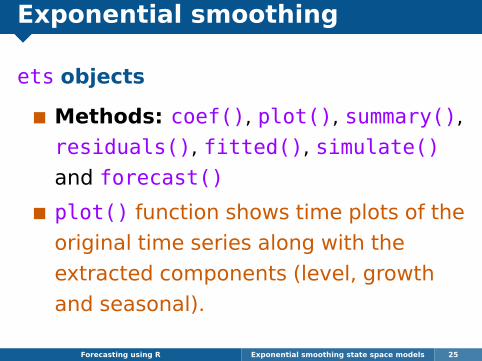
ets objects
Methods: coef(), plot(), summary(),
residuals(), fitted(), simulate()
and forecast()
plot() function shows time plots of the
original time series along with the
extracted components (level, growth
and seasonal).
Forecasting using R Exponential smoothing state space models 25
Exponential smoothing
ets objects
Methods: coef(), plot(), summary(),
residuals(), fitted(), simulate()
and forecast()
plot() function shows time plots of the
original time series along with the
extracted components (level, growth
and seasonal).
Forecasting using R Exponential smoothing state space models 25

Exponential smoothing
Forecasting using R Exponential smoothing state space models 26
200
400
600
obse
rved
250
350
450
leve
l
0.99
01.
005
slop
e
0.9
1.1
1960 1970 1980 1990 2000 2010
seas
on
Time
Decomposition by ETS(M,Md,M) methodplot(fit)

Goodness-of-fit
> accuracy(fit)ME RMSE MAE MPE MAPE MASE
0.17847 15.48781 11.77800 0.07204 2.81921 0.20705
> accuracy(fit2)ME RMSE MAE MPE MAPE MASE
-0.11711 15.90526 12.18930 -0.03765 2.91255 0.21428
Forecasting using R Exponential smoothing state space models 27
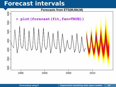
Forecast intervals
Forecasting using R Exponential smoothing state space models 28
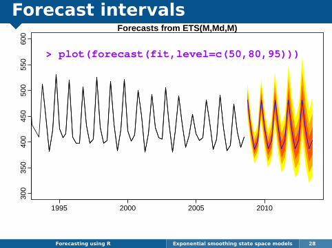
Forecasts from ETS(M,Md,M)
1995 2000 2005 2010
300
350
400
450
500
550
600
> plot(forecast(fit,level=c(50,80,95)))
Forecast intervals
Forecasting using R Exponential smoothing state space models 28
Forecasts from ETS(M,Md,M)
1995 2000 2005 2010
300
350
400
450
500
550
600
> plot(forecast(fit,fan=TRUE))
Exponential smoothing
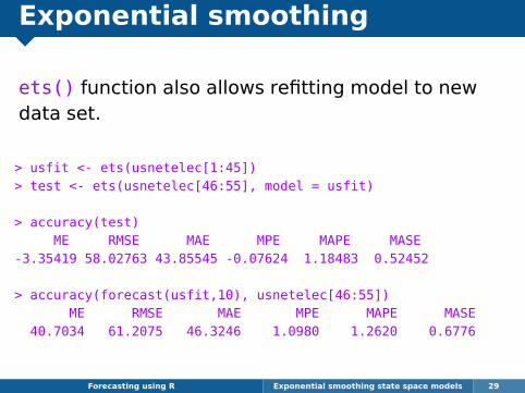
ets() function also allows refitting model to newdata set.
> usfit <- ets(usnetelec[1:45])> test <- ets(usnetelec[46:55], model = usfit)
> accuracy(test)ME RMSE MAE MPE MAPE MASE
-3.35419 58.02763 43.85545 -0.07624 1.18483 0.52452
> accuracy(forecast(usfit,10), usnetelec[46:55])ME RMSE MAE MPE MAPE MASE
40.7034 61.2075 46.3246 1.0980 1.2620 0.6776
Forecasting using R Exponential smoothing state space models 29

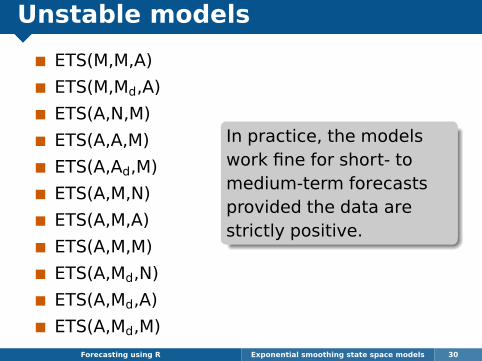
Unstable models
ETS(M,M,A)
ETS(M,Md,A)
ETS(A,N,M)
ETS(A,A,M)
ETS(A,Ad,M)
ETS(A,M,N)
ETS(A,M,A)
ETS(A,M,M)
ETS(A,Md,N)
ETS(A,Md,A)
ETS(A,Md,M)Forecasting using R Exponential smoothing state space models 30
Unstable models
ETS(M,M,A)
ETS(M,Md,A)
ETS(A,N,M)
ETS(A,A,M)
ETS(A,Ad,M)
ETS(A,M,N)
ETS(A,M,A)
ETS(A,M,M)
ETS(A,Md,N)
ETS(A,Md,A)
ETS(A,Md,M)Forecasting using R Exponential smoothing state space models 30
In practice, the modelswork fine for short- tomedium-term forecastsprovided the data arestrictly positive.
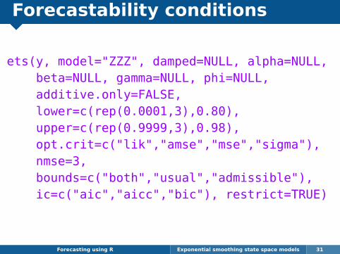
Forecastability conditions
ets(y, model="ZZZ", damped=NULL, alpha=NULL,beta=NULL, gamma=NULL, phi=NULL,additive.only=FALSE,lower=c(rep(0.0001,3),0.80),upper=c(rep(0.9999,3),0.98),opt.crit=c("lik","amse","mse","sigma"),nmse=3,bounds=c("both","usual","admissible"),ic=c("aic","aicc","bic"), restrict=TRUE)
Forecasting using R Exponential smoothing state space models 31

The magic forecast() function
forecast returns forecasts when applied to anets object (or the output from many other timeseries models).
If you use forecast directly on data, it willselect an ETS model automatically and thenreturn forecasts.
Forecasting using R Exponential smoothing state space models 32