forecasting exchange rates using feedforward and recurrent

Forecasting Exchange Rates Using Feedforward and Recurrent Neural NetworksAuthor(s): Chung-Ming Kuan and Tung LiuReviewed work(s):Source: Journal of Applied Econometrics, Vol. 10, No. 4 (Oct. - Dec., 1995), pp. 347-364Published by: John Wiley & SonsStable URL: http://www.jstor.org/stable/2285052 .Accessed: 18/12/2011 23:47

Your use of the JSTOR archive indicates your acceptance of the Terms & Conditions of Use, available at .http://www.jstor.org/page/info/about/policies/terms.jsp

JSTOR is a not-for-profit service that helps scholars, researchers, and students discover, use, and build upon a wide range ofcontent in a trusted digital archive. We use information technology and tools to increase productivity and facilitate new formsof scholarship. For more information about JSTOR, please contact [email protected].

John Wiley & Sons is collaborating with JSTOR to digitize, preserve and extend access to Journal of AppliedEconometrics.

http://www.jstor.org

http://www.jstor.org/action/showPublisher?publisherCode=jwiley

http://www.jstor.org/stable/2285052?origin=JSTOR-pdf

http://www.jstor.org/page/info/about/policies/terms.jsp

JOURNAL OF APPLIED ECONOMETRICS, VOL. 10, 347-364 (1995)

FORECASTING EXCHANGE RATES USING FEEDFORWARD AND RECURRENT NEURAL NETWORKS

CHUNG-MING KUAN Department of Economics, 21 Hsu-chow Road, National Taiwan University, Taipei 10020, Taiwan

AND

TUNG LIU Department of Economics, Ball State University, Muncie, IN 47306, USA

SUMMARY

In this paper we investigate the out-of-sample forecasting ability of feedforward and recurrent neural networks based on empirical foreign exchange rate data. A two-step procedure is proposed to construct suitable networks, in which networks are selected based on the predictive stochastic complexity (PSC) criterion, and the selected networks are estimated using both recursive Newton algorithms and the method of nonlinear least squares. Our results show that PSC is a sensible criterion for selecting networks and for certain exchange rate series, some selected network models have significant market timing ability and/or significantly lower out-of-sample mean squared prediction error relative to the random walk model.

1. INTRODUCTION

Neural networks provide a general class of nonlinear models which has been successfully applied in many different fields. Numerous empirical and computational applications can be found in the Proceedings of the International Joint Conference on Neural Networks and Conference of Neural Information Processing Systems. In spite of its success in various fields, there are only a few applications of neural networks in economics. Neural networks are novel in econometric applications in the following two respects. First, the class of multilayer neural networks can well approximate a large class of functions (Hornik et al., 1989; and Cybenko, 1989), whereas most of the commonly used nonlinear time-series models do not have this property. Second, as shown in Barron (1991), neural networks are more parsimonious models than linear subspace methods such as polynomial, spline, and trigonometric series expansions in approximating unknown functions. Thus, if the behaviour of economic variables exhibits nonlinearity, a suitably constructed neural network can serve as a useful tool to capture such regularity.

In this paper we investigate possible nonlinear patterns in foreign exchange data using feedforward, and recurrent networks. It has been widely accepted that foreign exchange rates are I(1) (integrated of order one) processes and that changes of exchange rates are uncorrelated over time. Hence, changes in exchange rates are not linearly predictable in general. For a

comprehensive review of these issues, see Baillie and McMahon (1989). Since the empirical studies supporting these conclusions rely mainly on linear time series techniques, it is not unreasonable to conjecture that the linear unpredictability of exchange rates may be due to limitations of linear models. Hsieh (1989) finds that changes of exchange rates may be nonlinearly dependent, even though they are linearly uncorrelated. Some researchers also

CCC 0883-7252/95/040347-18 Received May 1992 ( 1995 by John Wiley & Sons, Ltd. Revised September 1994

C.-M. KUAN AND T. LIU

provide evidence in favor of nonlinear forecasts (e.g. Taylor, 1980, 1982; Engel and Hamilton, 1990; Engel, 1991; Chinn, 1991). On the other hand, Diebold and Nason (1990) find that nonlinearities of exchange rates, if any, cannot be exploited to improve forecasting. Therefore, we treat neural networks as alternative nonlinear models and focus on whether neural networks can provide superior out-of-sample forecasts.

This paper has two objectives. First, we introduce different neural network modeling techniques and propose a two-step procedure to construct suitable neural networks. In the first step of the proposed procedure, we apply the recursive Newton algorithms of Kuan and White (1994a) and Kuan (1994) to estimate a family of networks and compute the so-called 'predictive stochastic complexity' (Rissanen, 1987), from which we can easily select suitable network structures. In the second step, statistically more efficient estimates for networks selected from the first step are obtained by the method of nonlinear least squares using recursive estimates as initial values. Our procedure differs from previous applications of feedforward networks in economics (e.g. White, 1988; Kuan and White, 1990) in that networks are selected objectively. Also, the application of recurrent networks is new in applied econometrics; hence its performance would also be of interest to researchers.

Second, we investigate the forecasting performance of networks selected from the proposed procedure. In particular, model performance is evaluated using various statistical tests, rather than crude comparison. Financial economists are usually interested in sign predictions (i.e. forecasts of the direction of future price changes) which yield important information for financial decisions such as market timing (see e.g. Levich, 1981; Merton, 1981). We apply the market timing test of Henriksson and Merton (1981) to justify whether the forecasts from network models are of economic value in practice; a nonparametric test for sign predictions proposed by Pesaran and Timmermann (1992) is also conducted. Other than sign predictions, we, as many other econometricians, are also interested in out-of-sample MSPE (mean squared prediction errors) performance. We use the Mizrach (1992) test to evaluate the MSPE performance of networks relative to the random walk model. Our results show that network models perform differently for different exchange rate series and that predictive stochastic complexity is a sensible criterion for selecting networks. For certain exchange rates, some network models perform reasonably well; for example, for the Japanese yen and British pound some selected networks have significant market timing ability and/or significantly lower out-of- sample MSPE relative to the random walk model in different testing periods; for the Canadian dollar and deutsche mark, however, selected networks exhibit only mediocre performance.

This paper proceeds as follows. We review feedforward and recurrent networks in Section 2. The network building procedure, including the estimation methods, complexity regularization criteria, and a two-step procedure, are described in Section 3. Empirical results are analysed in Section 4. Section 5 concludes the paper. Details of the recursive Newton algorithms are summarized in the Appendix.

2. FEEDFORWARD AND RECURRENT NETWORKS

In this section we briefly describe the functional forms of feedforward and recurrent networks and their properties; for more details see Kuan and White (1994a).

A neural network may be interpreted as a nonlinear regression function characterizing the relationship between the dependent variable (target) y and an n-vector of explanatory variables (inputs) x. Instead of postulating a specific nonlinear function, a neural network model is constructed by combining many 'basic' nonlinear functions via a multilayer structure. In a feedforward network, the explanatory variables first simultaneously activate q hidden units in

348

FORECASTING WITH NEURAL NETWORKS

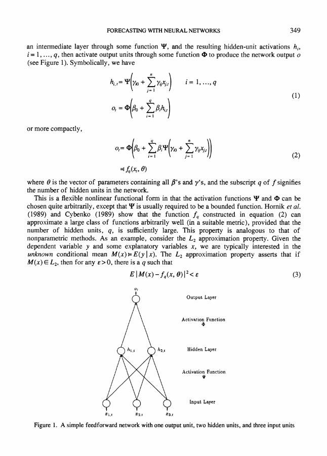
an intermediate layer through some function I, and the resulting hidden-unit activations hi, i= 1, ..., q, then activate output units through some function i to produce the network output o (see Figure 1). Symbolically, we have

f n n

hi,,= Ty Yio + Ey,i . i =

1

... . q j=1

* q , (1) o, = PO + ,Ahi,,

i=!

or more compactly, P 4 t n !

o,= a PO + E, Ai' Yo + YX,, i i=1 j= I (2)

=f,(x,, 0) where 0 is the vector of parameters containing all 4's and y's, and the subscript q of f signifies the number of hidden units in the network.

This is a flexible nonlinear functional form in that the activation functions v and b can be chosen quite arbitrarily, except that v is usually required to be a bounded function. Hornik et al. (1989) and Cybenko (1989) show that the function fq constructed in equation (2) can approximate a large class of functions arbitrarily well (in a suitable metric), provided that the number of hidden units, q, is sufficiently large. This property is analogous to that of nonparametric methods. As an example, consider the L2 approximation property. Given the dependent variable y and some explanatory variables x, we are typically interested in the unknown conditional mean M(x) - E(y Ix). The L2 approximation property asserts that if M(x) E L2, then for any e > O, there is a q such that

EI M(x) - fq(x, O) 12< (3)

Ot

Output Layer

Activation Function

h) , h2,t Hidden Layer

Activation Function

Input Layer

Figure 1. A simple feedforward network with one output unit, two hidden units, and three input units

349


Barron (1991) also shows that a feedforward network can achieve an approximation rate O(l/q) by using a number of parameters O(qn) that grows linearly in q, whereas traditional polynomial, spline, and trigonometric expansions require exponentially O(qe) terms to achieve the same approximation rate. Thus, neural networks are (asymptotically) relatively more parsimonious than these series expansions in approximating unknown functions. These two properties make feedforward networks an attractive econometric tool in (nonparametric) applications.

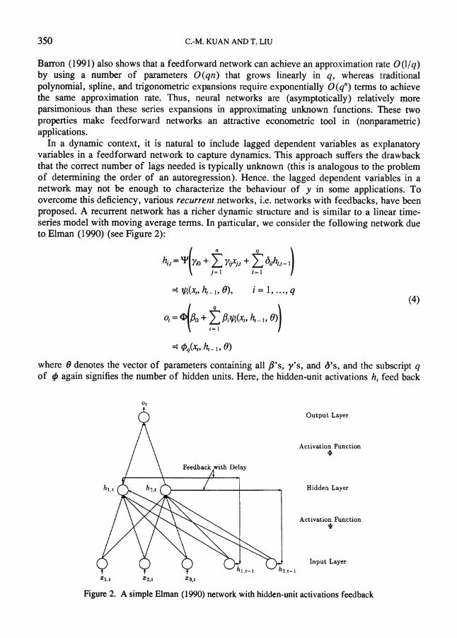
In a dynamic context, it is natural to include lagged dependent variables as explanatory variables in a feedforward network to capture dynamics. This approach suffers the drawback that the correct number of lags needed is typically unknown (this is analogous to the problem of determining the order of an autoregression). Hence. the lagged dependent variables in a network may not be enough to characterize the behaviour of y in some applications. To overcome this deficiency, various recurrent networks, i.e. networks with feedbacks, have been proposed. A recurrent network has a richer dynamic structure and is similar to a linear time- series model with moving average terms. In particular, we consider the following network due to Elman (1990) (see Figure 2):

n q

hi,t = yio + E lYiji, + E A1ih.,- j=l 1=1

(x,, h, , 0), i= 1, ..., q (4)

o, = ( + Afi,(x,, h, , 0)) i '=1 /

pq(t,, h,_ 1, 0)

where 0 denotes the vector of parameters containing all /'s, y's, and 6's, and the subscript q of 0 again signifies the number of hidden units. Here, the hidden-unit activations hi feed back

ot

Output Layer

Activation Function

Feedback with Delay

hi,t ( . h2,t / Hidden Layer

Activation Function

lt 1 ,_ I Input Layer IT iT IT ^"^i.i~~~hl~-i ' 2,-

Figure 2. A simple Elman (1990) network with hidden-unit activations feedback

350


to the input layer with delay and serve to 'memorize' the past information (cf. equation (1)). From equation (4) we can write, by recursive substitution,

hi,,= ip(x,,ip(x,_, h,2, ..., 0), 0)= =.=:ri(x', 0) i=1,..., q (5)

where x' = (x,,x, x,...,xi), and ip is vector-valued with ipi as its ith element. Hence, hj, depends on x, and its entire history. It follows that

o, = (q(X,, h,_1, 0)- gq(X, 0) (6)

is also a function of x, and its history (cf. equation (2)). In view of equation (6), a recurrent network may capture more dynamic characteristics of y, than does a feedforward network. In the L2 context, a recurrent network may be interpreted as an approximation of E(y, Ix'). To ensure proper behaviour of the Elman (1990) network, Kuan and White (1994b) show that, aside from some regularity conditions on the data y and x and some smoothness conditions (such as continuous differentiability) on m and Y, the hidden unit activation function v must also be a contraction mapping in h, _; otherwise, hi, will approach its upper or lower bound very quickly when t is a bounded function or will explod whhen v is an unbounded function. Kuan et al. (1994) show that a sufficient condition assuring the contraction mapping property is 6i, <4/q, for all i, 1.

3. BUILDING EMPIRICAL NETWORKS

In practice, there are basically two tasks in building neural networks: (i) unknown network parameters must be estimated, and (ii) a suitable network structure fq or 0 must be determined. We will discuss these two tasks in turn and propose a two-step procedure for constructing empirical neural networks.

3.1. Estimation methods

In view of equation (3), for a feedforward network fq it is quite natural to estimate the parameters of interest 0Q which minimize mean squared approximation error, i.e.

= argmin E I E(y x) - f(x, 0)12

Observe that

E I y -f,(x, 0)12 = E I y -E(y Ix) 12 + E I E(y I x) - f(x, 0) 12 (7)

As E(y Ix) is the best L2 predictor of y given x, the first term on the right-hand side of equation (7) cannot be minimized in L2; hence 0* is an MSE (mean squared error) minimizer:

q0 =argmin E|y- f4(x, 0)12

where the function on the right-hand side is just the well-known least-squares criterion function. Practically, estimates of 0 can be obtained using nonrecursive (off-line) or recursive (on-line) estimation methods. Econometricians are familiar with various nonrecursive, nonlinear least squares (NLS) optimization techniques. It is well known that NLS estimates are consistent for 0 and asymptotically normally distributed under very general conditions. Recursive estimation methods include, e.g. the back-propagation (BP) algorithm of Rumelhart et al (1986) and the Newton algorithm of Kuan and White (1994a). Kuan and White (1994a) show that both the BP and Newton algorithms are root-t consistent for 06 where t denotes the recursive step, but the Newton algorithm is statistically more efficient than the BP algorithm and is asymptotically

351


equivalent to the NLS method. Although recursive estimates are not as efficient as NLS estimates in finite samples, they are useful when on-line information processing is important. Moreover, recursive methods can facilitate network selection, as discussed in the subsection below. White (1989) also suggests that one can perform recursive estimation up to certain time point and then apply a NLS technique to improve efficiency of estimates.

Similarly, the parameters of interest in a recurrent network q5 are

0 = argmin lim E y, - 0,(x,, h,_ , 0)12 t ->00

where limit is taken to accommodate the effects of network feedbacks h,_l (Kuan and White, 1994b). The estimates of 0* can also be obtained using nonrecursive or recursive methods. In view of equation (5) and (6), h, and o, depend on 0 directly and also indirectly through the presence of lagged hidden-unit activations h,_l. Thus, in calculating the derivatives of S q with respect to 0, parameter dependence of h,_l must be taken into account to ensure proper search direction. Owing to this parameter-dependent structure and the constraints required for 6's (discussed in Section 2), NLS optimization techniques involving analytic derivatives are difficult to implement. Our experience shows that NLS estimation using numerical derivatives usually suffers the problem of a singular information matrix. Alternatively, one could use a recursive estimation method such as the 'recurrent Newton algorithm' of Kuan (1994), which is analogous to that of Kuan and White (1994a) for feedforward networks. This algorithm is also root-t consistent for Oq (see e.g. Benveniste et al., 1990). Kuan (1994) also shows that it is more efficient than the recurrent BP algorithm of Kuan et al. (1994). The recursive Newton algorithms for feedforward and recurrent networks used in our applications are described in the Appendix.

3.2. Complexity regularization criteria

The second task in practice is to determine a suitable network structure so that the unknown conditional mean function can be well approximated. As network functions D and Y can be chosen quite arbitrarily, this task amounts to determining network complexity, i.e. the number of explanatory variables and the number of hidden units. A very simple network may not be able to approximate the unknown conditional mean function well; an excessively complex network may over fit the data with little improvement in approximation accuracy. There is, however, no definite conclusion regarding how the complexity should be regularized. As neural network models are, by construction, some approximating functions, it is our opinion that the determination of network complexity is a model-selection problem. Thus, one possible criterion is the Schwarz (1978) Information Criterion (SIC). Note that selecting networks based on SIC is computationally demanding because NLS is required for estimating every possible network.

An alternative criterion to regularize network complexity is the 'Predictive Stochastic Complexity' (PSC) criterion due to Rissanen (1986a,b); see also Rissanen (1987). Given a function m(x, 0), where 0 is a k-dimensional parameter vector, and a sample of T observations, PSC is computed as the average of squared, 'honest' prediction errors:

T

T- E ( - m(x,, ))2 (8) k t=k+l

where 0, is the predicted parameter obtained from the data up to time t- 1. The prediction error Y - m(x,, 0,) is 'honest' in the sense that no information at time t or beyond is used to calculate 0,; in particular, the well-known recursive residual is a special case of honest prediction error. A

352


model is selected if it has the smallest PSC within a class of models. If two models have the same PSC, the simpler one is selected. Clearly, the PSC criterion is based on forward validation, which is important in forecasting. Rissanen also shows that for encoding a sequence of numbers, the PSC criterion can determine the code with the shortest code length asymptotically. For a thorough discussion of the notion of stochastic complexity we refer to Rissanen (1989). Obviously, calculation of PSC is also computationally demanding if NLS is

required to obtain 0, for each t. Following the idea of Gerencser and Rissanen (1992), we can

compute 0, using recursive estimation methods, which are more tractable computationally. Thus, recursive estimation methods are also useful for selecting appropriate network structures based on PSC.

3.3. Two-step procedure

In this paper we employ a two-step procedure to construct our empirical neural networks. We first choose the activation functions Y as the logistic function and D as the identity function in the networks equations (1) and (4). These choices are quite standard in the neural network literature. The dependent variables y are changes of log exchange rates, and for each exchange rate, networks explanatory variables x are own lagged dependent variables. The resulting networks are therefore nonlinear AR models. One could, of course, include other explanatory variables in networks to create nonlinear ARX models.

Specifically, our feedforward networks are of the form:

qI1 I f,(x,, )= A + - 1

'=l 1+ exp -(i + E YiiYt-i i _ \ j=l _-

and recurrent networks are:

q)= + S - , 1 I 4q(Xt 0) = Po + A n 9

i \ v yj=l /=1

1 hi, + exp -o + ,h,,

1 + exp - 0 + Z y-j + Z <h/.t-1 j=l /=1

The following two-step procedure is then used to determine the network structures and estimate their unknown parameters:

(1) Recursive estimation. A family of feedforward or recurrent networks with different n and q (the numbers of lagged dependent variables and hidden units) is estimated using the Newton algorithms (Al) or (A2) in the Appendix. For each network, (a) Ten sets of initial parameters are generated randomly from N(0,1), and the one that results in the lowest MSE is used as the initial values for recursive algorithms. (b) We then let the Newton algorithms run through the data set once and compute the

resulting PSC values. Note that network structures are fixed during recursive estimation. After recursive estimation is complete, we select the three networks with the lowest PSC values and

proceed to the second step.

353


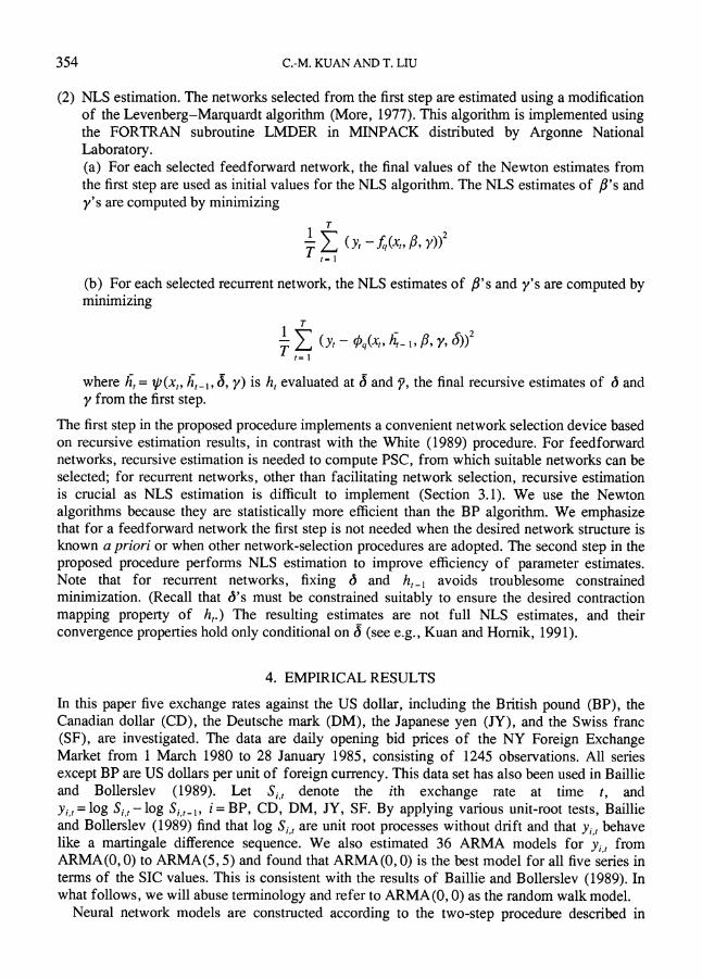
(2) NLS estimation. The networks selected from the first step are estimated using a modification of the Levenberg-Marquardt algorithm (More, 1977). This algorithm is implemented using the FORTRAN subroutine LMDER in MINPACK distributed by Argonne National Laboratory. (a) For each selected feedforward network, the final values of the Newton estimates from the first step are used as initial values for the NLS algorithm. The NLS estimates of /'s and y's are computed by minimizing

T

T E (Y- f(X,,, ))2 t= 1

(b) For each selected recurrent network, the NLS estimates of /'s and y's are computed by minimizing

1 E (y- 0(x,,-, , /,y ))2 t=1

where h, = ,(x,, h/,, , y) is h, evaluated at B and y, the final recursive estimates of 6 and y from the first step.

The first step in the proposed procedure implements a convenient network selection device based on recursive estimation results, in contrast with the White (1989) procedure. For feedforward networks, recursive estimation is needed to compute PSC, from which suitable networks can be selected; for recurrent networks, other than facilitating network selection, recursive estimation is crucial as NLS estimation is difficult to implement (Section 3.1). We use the Newton algorithms because they are statistically more efficient than the BP algorithm. We emphasize that for a feedforward network the first step is not needed when the desired network structure is known a priori or when other network-selection procedures are adopted. The second step in the proposed procedure performs NLS estimation to improve efficiency of parameter estimates. Note that for recurrent networks, fixing 6 and h,_I avoids troublesome constrained minimization. (Recall that 6's must be constrained suitably to ensure the desired contraction mapping property of h,.) The resulting estimates are not full NLS estimates, and their convergence properties hold only conditional on 6 (see e.g., Kuan and Homik, 1991).

4. EMPIRICAL RESULTS

In this paper five exchange rates against the US dollar, including the British pound (BP), the Canadian dollar (CD), the Deutsche mark (DM), the Japanese yen (JY), and the Swiss franc (SF), are investigated. The data are daily opening bid prices of the NY Foreign Exchange Market from 1 March 1980 to 28 January 1985, consisting of 1245 observations. All series except BP are US dollars per unit of foreign currency. This data set has also been used in Baillie and Bollerslev (1989). Let S,, denote the ith exchange rate at time t, and yi, = log S,, - log S,,_, i = BP, CD, DM, JY, SF. By applying various unit-root tests, Baillie and Bollerslev (1989) find that log S,, are unit root processes without drift and that y,, behave like a martingale difference sequence. We also estimated 36 ARMA models for y,, from ARMA (0,0) to ARMA(5, 5) and found that ARMA(0, 0) is the best model for all five series in terms of the SIC values. This is consistent with the results of Baillie and Bollerslev (1989). In what follows, we will abuse terminology and refer to ARMA(0,0) as the random walk model.

Neural network models are constructed according to the two-step procedure described in

354


Section 3. For each series, the network explanatory variables are lagged dependent variables; all variables are multiplied by 100 to reduce round-off errors. We have also constructed networks for each y,, using lagged yjt,, j* i, as additional explanatory variables, but the results are not particularly exciting. We therefore confine ourselves to networks of the present form which, as we have mentioned, are simply nonlinear AR models. In the first step, 30 feedforward and recurrent networks (with 1-6 lagged yi,, and 2-6 hidden units) are estimated using the recursive Newton algorithms, and the three networks with the best PSC values are selected.1 In the second step, the selected networks are further 'smoothed' using the method of NLS. (We omit- networks with one hidden unit because they are not practically interesting.) Ideally, we can construct a multiple-output network for all five series, analogous to a multivariate nonlinear regression model. A program implementing multiple-output networks is currently under development.

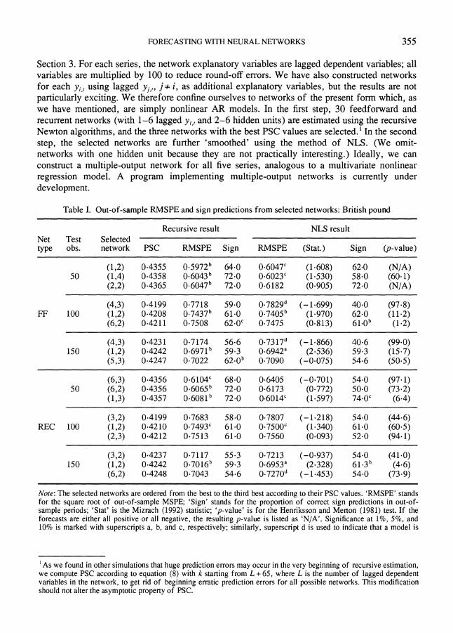
Table I. Out-of-sample RMSPE and sign predictions from selected networks: British pound

Recursive result NLS result Net Test Selected type obs. network PSC RMSPE Sign RMSPE (Stat.) Sign (p-value)

(1,2) 0.4355 0.5972b 64.0 0.6047c (1-608) 62.0 (N/A) 50 (1,4) 0.4358 0.6043b 72.0 0.6023c (1-530) 58.0 (60-1)

(2,2) 0.4365 0.6047b 72.0 0.6182 (0.905) 72.0 (N/A)

(4,3) 0.4199 0.7718 59.0 0.7829d (-1.699) 40.0 (97.8) FF 100 (1,2) 0.4208 0.7437b 61.0 0.7405b (1.970) 62.0 (11.2)

(6,2) 0.4211 0.7508 620Oc 0.7475 (0.813) 61.0b (1.2)

(4,3) 0.4231 0.7174 56.6 0.7317d (-1.866) 40.6 (99.0) 150 (1,2) 0.4242 0.6971b 59.3 0.6942a (2.536) 59.3 (15.7)

(5,3) 0.4247 0.7022 62.0b 0.7090 (-0.075) 54.6 (50.5)

(6,3) 0.4356 0.6104c 68.0 0.6405 (-0.701) 54.0 (97.1) 50 (6,2) 0.4356 0.6065b 72.0 0.6173 (0.772) 50.0 (73.2)

(1,3) 0.4357 0.6081b 72.0 0.6014c (1.597) 74.0' (6.4)

(3,2) 0.4199 0.7683 58.0 0.7807 (-1.218) 54.0 (44.6) REC 100 (1,2) 0.4210 0.7493c 61.0 0.7500c (1.340) 61.0 (60.5)

(2,3) 0.4212 0.7513 61.0 0.7560 (0.093) 52.0 (94.1)

(3,2) 0.4237 0.7117 55.3 0.7213 (-0.937) 54.0 (41.0) 150 (1,2) 0.4242 0.7016b 59.3 0.6953a (2.328) 61.3b (4.6)

(6,2) 0.4248 0.7043 54.6 0.7270" (-1.453) 54.0 (73.9)

Note: The selected networks are ordered from the best to the third best according to their PSC values. 'RMSPE' stands for the square root of out-of-sample MSPE; 'Sign' stands for the proportion of correct sign predictions in out-of- sample periods; 'Stat' is the Mizrach (1992) statistic; 'p-value' is for the Henriksson and Merton (1981) test. If the forecasts are either all positive or all negative, the resulting p-value is listed as 'N/A'. Significance at 1%, 5%, and 10% is marked with superscripts a, b, and c, respectively; similarly, superscript d is used to indicate that a model is

'As we found in other simulations that huge prediction errors may occur in the very beginning of recursive estimation, we compute PSC according to equation (8) with k starting from L + 65, where L is the number of lagged dependent variables in the network, to get rid of beginning erratic prediction errors for all possible networks. This modification should not alter the asymptotic property of PSC.

355


To evaluate the forecasting performance of different models of yj,, we reserve the last 50, 100, and 150 observations as out-of-sample testing periods and estimate models using 1194, 1144, and 1094 observations, respectively. These choices are arbitrary. The out-of- sample performances of network models are evaluated using two criteria: one based on sign predictions (i.e. forecasts of the direction of future price changes) and the other based on one-step-ahead MSPE. As sign predictions yield important information for financial decisions such as market timing, it is important to test whether they are of economic value in practice (see e.g., Levich, 1981; Merton, 1981; Henriksson and Merton, 1981). For this purpose, we apply the market timing test of Henriksson and Merton (1981), which is the uniformly most powerful test for market timing ability under their conditions. In this test, the number of correct forecasts has a hypergeometric distribution under the null of no market timing ability, and we use the IMSL subroutine HYPDF to compute the resulting p- values. We also apply a test proposed by Pesaran and Timmermann (1992) which is a Hausman-type of test designed to assess the performance of sign predictions. As the limiting distribution of this test is N(0, 1), its one-sided critical values at 1%, 5%, and 10% levels are 2.33, 1.645, and 1.282, respectively. (We thank referees and the editor for these suggestions.) It is also typical in econometric applications to compare out-of-sample MSPE performance of a model relative to the random walk model. We therefore apply the MSPE- comparison test of Mizrach (1992) to evaluate statistical significance of network forecasts (cf. Diebold and Mariano, 1991). The limiting distribution of this test is also N(0, 1); in our

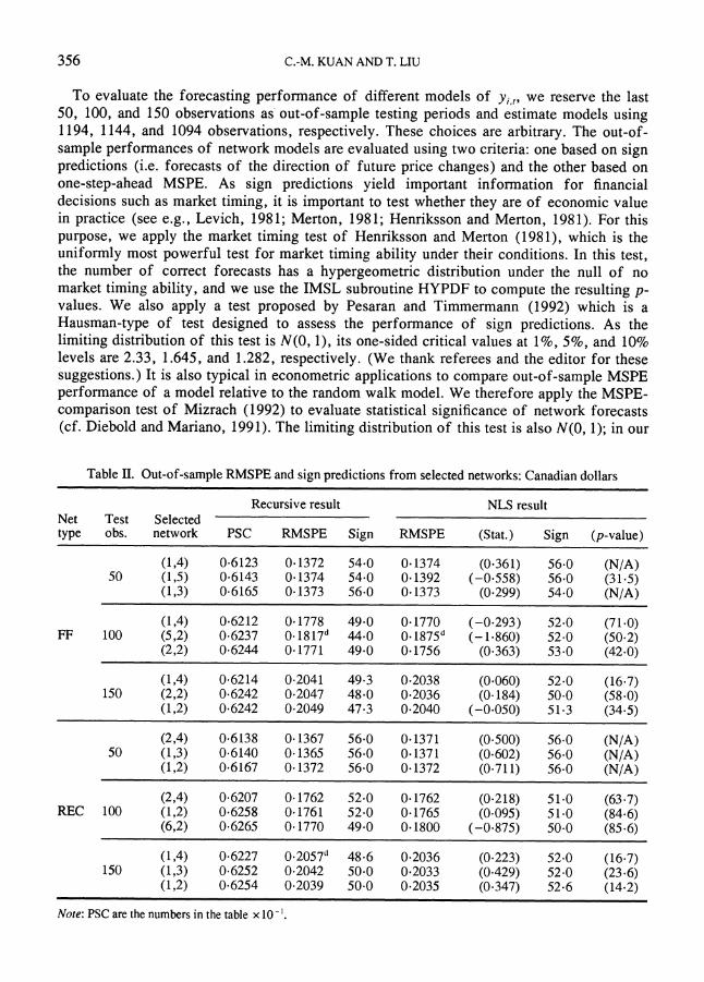
Table II. Out-of-sample RMSPE and sign predictions from selected networks: Canadian dollars

Recursive result NLS result Net Test Selected type obs. network PSC RMSPE Sign RMSPE (Stat. ) Sign (p-value)

(1,4) 0.6123 0.1372 54.0 0.1374 (0-361) 56.0 (N/A) 50 (1,5) 0.6143 0.1374 54.0 0.1392 (-0.558) 56.0 (31-5)

(1,3) 0.6165 0.1373 56.0 0.1373 (0-299) 54.0 (N/A)

(1,4) 0.6212 0.1778 49-0 0.1770 (-0-293) 52-0 (71.0) FF 100 (5,2) 0.6237 0.1817d 44.0 0.1875d (-1-860) 52.0 (50-2)

(2,2) 0.6244 0.1771 49.0 0.1756 (0-363) 53.0 (42-0)

(1,4) 0.6214 0-2041 49.3 0-2038 (0-060) 52.0 (16-7) 150 (2,2) 0.6242 0.2047 48-0 0-2036 (0-184) 50-0 (58-0)

(1,2) 0.6242 0.2049 47.3 0-2040 (-0-050) 51.3 (34.5)

(2,4) 0.6138 0.1367 56.0 0-1371 (0-500) 56.0 (N/A) 50 (1,3) 0.6140 0.1365 56.0 0-1371 (0-602) 56-0 (N/A)

(1,2) 0.6167 0.1372 56.0 0.1372 (0-711) 56.0 (N/A)

(2,4) 0.6207 0.1762 52.0 0-1762 (0-218) 51.0 (63-7) REC 100 (1,2) 0.6258 0.1761 52.0 0-1765 (0-095) 51.0 (84-6)

(6,2) 0-6265 0.1770 49.0 0-1800 (-0.875) 50-0 (85-6)

(1,4) 0.6227 0.2057" 48.6 0-2036 (0-223) 52.0 (16-7) 150 (1,3) 0.6252 0.2042 50-0 0.2033 (0-429) 52.0 (23-6)

(1,2) 0.6254 0.2039 50.0 0.2035 (0-347) 52.6 (14-2)

Note: PSC are the numbers in the table x 10- .

356


computation, models with out-of-sample MSPE smaller than the random walk model have positive statistics. Out-of-sample forecasting results from recursive and NLS estimation are summarized in Tables I-V, where we use FF and REC to denote feedforward and recurrent networks and write a network with L lagged dependent variables and H hidden units as (L, H). We report only the Mizrach statistics and p-values for NLS results; complete tables including statistics and p-values for recursive results are available upon request. Note also that the Mizrach test is based on MSPE comparison, but our tables report the square root of MSPE (RMSPE).

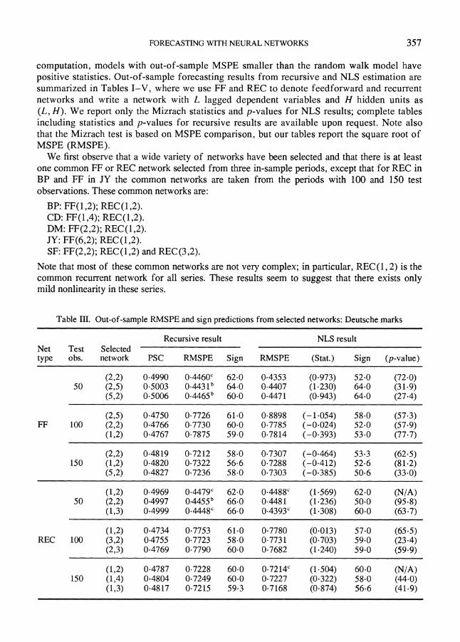
We first observe that a wide variety of networks have been selected and that there is at least one common FF or REC network selected from three in-sample periods, except that for REC in BP and FF in JY the common networks are taken from the periods with 100 and 150 test observations. These common networks are:

BP: FF(1,2); REC(1,2). CD: FF(1,4); REC(1,2). DM: FF(2,2); REC(1,2). JY: FF(6,2); REC(1,2). SF: FF(2,2); REC(1,2) and REC(3,2).

Note that most of these common networks are not very complex; common recurrent network for all series. These results seem to mild nonlinearity in these series.

in particular, REC(1, 2) is the suggest that there exists only

Table III. Out-of-sample RMSPE and sign predictions from selected networks: Deutsche marks


(2,2) 0.4990 0.4460c 62.0 0.4353 (0-973) 52.0 (72-0) 50 (2,5) 0.5003 0.4431 64.0 0.4407 (1-230) 64.0 (31-9)

(5,2) 0.5006 0.4465b 60.0 04471 (0-943) 64.0 (27-4)

(2,5) 0.4750 0.7726 61.0 0.8898 (-1.054) 58.0 (57-3) FF 100 (2,2) 0.4766 0.7730 60.0 0.7785 (-0.024) 52.0 (57-9)

(1,2) 0.4767 0.7875 59.0 0.7814 (-0.393) 53.0 (77-7)

(2,2) 0.4819 07212 58.0 0.7307 (-0.464) 53.3 (62-5) 150 (1,2) 0.4820 0.7322 56.6 0.7288 (-0.412) 52.6 (81-2)

(5,2) 04827 0.7236 58.0 0.7303 (-0.385) 50.6 (33-0)

(1,2) 0.4969 0.4479c 62.0 0.4488c (1-569) 62.0 (N/A) 50 (2,2) 0.4997 0.4455b 66.0 0.4481 (1-236) 50.0 (95-8)

(1,3) 0.4999 0.4448 66.0 0.4393c (1-308) 60.0 (63-7)

(1,2) 04734 0.7753 61.0 0.7780 (0-013) 57.0 (65-5) REC 100 (3,2) 0-4755 0.7723 58.0 0.7731 (0-703) 59.0 (23-4)

(2,3) 04769 0.7790 60.0 07682 (1-240) 59.0 (59-9)

(1,2) 0.4787 0.7228 60.0 0.7214c (1-504) 60.0 (N/A) 150 (1,4) 0.4804 0.7249 60.0 0.7227 (0-322) 58.0 (44.0)

(1,3) 0.4817 0.7215 59.3 0-7168 (0-874) 56.6 (41.9)

357


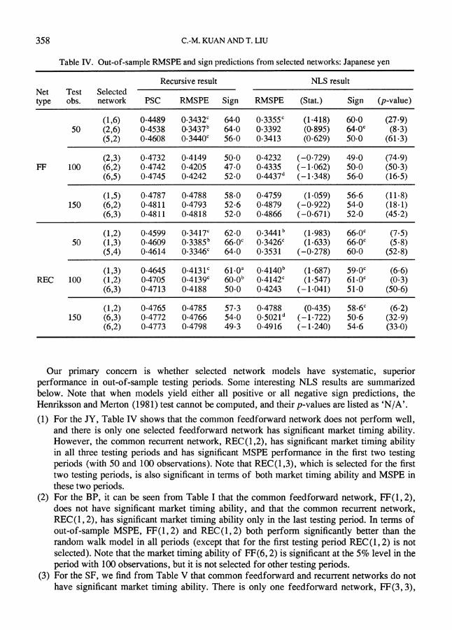
Table IV. Out-of-sample RMSPE and sign predictions from selected networks: Japanese yen


(1,6) 0.4489 0.3432c 64.0 0.3355c (1-418) 60.0 (27-9) 50 (2,6) 0.4538 0.3437b 64-0 0.3392 (0-895) 64.0c (8-3)

(5,2) 0.4608 0.3440c 56.0 0.3413 (0-629) 50.0 (61-3)

(2,3) 0.4732 0.4149 50.0 0.4232 (-0.729) 49.0 (74.9) FF 100 (6,2) 0.4742 0.4205 47.0 0.4335 (-1.062) 50.0 (50-3)

(6,5) 0.4745 0.4242 52.0 0.4437d (-1.348) 56.0 (16.5)

(1,5) 0.4787 0.4788 58.0 0.4759 (1.059) 56.6 (11.8) 150 (6,2) 0.4811 0.4793 52.6 0.4879 (-0.922) 54.0 (18.1)

(6,3) 0.4811 0.4818 52.0 0.4866 (-0.671) 52.0 (45.2)

(1,2) 0.4599 0.3417c 62.0 0.3441b (1.983) 66.0c (7.5) 50 (1,3) 0.4609 0.3385b 66-0c 0.3426c (1.633) 66.0c (5.8)

(5,4) 0.4614 0.3346c 64.0 0.3531 (-0.278) 60.0 (52.8)

(1,3) 0.4645 0.4131c 61.0a 0.4140b (1.687) 59.0C (6.6) REC 100 (1,2) 0.4705 0.4139c 60*0b 0.4142C (1.547) 61.0C (0.3)

(6,3) 0.4713 0.4188 50.0 0.4243 (-1.041) 51.0 (50.6)

(1,2) 0.4765 0.4785 57.3 0.4788 (0-435) 58.6c (6-2) 150 (6,3) 0.4772 0.4766 54.0 0.5021d (-1.722) 50.6 (32.9)

(6,2) 0.4773 0.4798 49.3 0.4916 (-1.240) 54.6 (33.0)

Our primary concern is whether selected network models have systematic, superior performance in out-of-sample testing periods. Some interesting NLS results are summarized below. Note that when models yield either all positive or all negative sign predictions, the Henriksson and Merton (1981) test cannot be computed, and their p-values are listed as 'N/A'.

(1) For the JY, Table IV shows that the common feedforward network does not perform well, and there is only one selected feedforward network has significant market timing ability. However, the common recurrent network, REC(1,2), has significant market timing ability in all three testing periods and has significant MSPE performance in the first two testing periods (with 50 and 100 observations). Note that REC(1,3), which is selected for the first two testing periods, is also significant in terms of both market timing ability and MSPE in these two periods.

(2) For the BP, it can be seen from Table I that the common feedforward network, FF(1, 2), does not have significant market timing ability, and that the common recurrent network, REC(1,2), has significant market timing ability only in the last testing period. In terms of out-of-sample MSPE, FF(1,2) and REC(1,2) both perform significantly better than the random walk model in all periods (except that for the first testing period REC(1,2) is not selected). Note that the market timing ability of FF(6, 2) is significant at the 5% level in the period with 100 observations, but it is not selected for other testing periods.

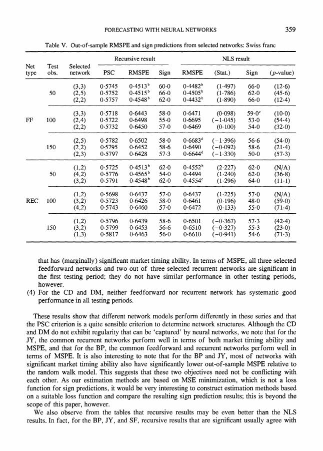
(3) For the SF, we w find from Table V that common feedforward and recurrent networks do not have significant market timing ability. There is only one feedforward network, FF(3, 3),

358


Table V. Out-of-sample RMSPE and sign predictions from selected networks: Swiss franc


(3,3) 0.5745 0.4513b 60-0 0.4482b (1-497) 66.0 (12.6) 50 (2,5) 0.5752 0.4515b 66.0 0.4505b (1-786) 62.0 (45-6)

(2,2) 0.5757 0.4548b 62.0 0.4432b (1-890) 66.0 (12-4)

(3,3) 05718 0.6443 58.0 0.6471 (0-098) 59.0c (10-0) FF 100 (2,4) 0.5722 0-6498 55.0 0.6695 (- 1045) 53.0 (54-4)

(2,2) 0.5732 0.6450 57.0 0.6469 (0-100) 54.0 (32.0)

(2,5) 0.5782 0.6502 58.0 0.6683d (-1.396) 56.6 (54.0) 150 (2,2) 0.5795 0.6452 58.6 0.6490 (-0.092) 58.6 (21.4)

(2,3) 0.5797 0.6428 57.3 0.6644d (-1-330) 50.0 (57-3)

(1,2) 0.5725 0.4513b 62.0 0.4552b (2-227) 62.0 (N/A) 50 (4,2) 0.5776 0.4565b 54.0 0.4494 (1.240) 62.0 (36.8)

(3,2) 0.5791 0.4548b 62.0 0.4554c (1-296) 64.0 (11-1)

(1,2) 0.5698 0-6437 57.0 0.6437 (1-225) 57.0 (N/A) REC 100 (3,2) 0.5723 0.6426 58.0 0.6461 (0-196) 48.0 (59-0)

(4,2) 0.5743 0.6460 57.0 0.6472 (0-133) 55.0 (71.4)

(1,2) 0.5796 0-6439 58.6 0.6501 (-0.367) 57.3 (42.4) 150 (3,2) 0.5799 0.6453 56.6 0.6510 (-0.327) 55.3 (23.0)

(1,3) 0.5817 0.6463 56.0 0.6610 (-0.941) 54.6 (71.3) _ ~~~ ~ ~~~~~~~~~~~~~~~~~~, .m

that has (marginally) significant market timing ability. In terms of MSPE, all three selected feedforward networks and two out of three selected recurrent networks are significant in the first testing period; they do not have similar performance in other testing periods, however.

(4) For the CD and DM, neither feedforward nor recurrent network has systematic good performance in all testing periods.

These results show that different network models perform differently in these series and that the PSC criterion is a quite sensible criterion to determine network structures. Although the CD and DM do not exhibit regularity that can be 'captured' by neural networks, we note that for the JY, the common recurrent networks perform well in terms of both market timing ability and MSPE, and that for the BP, the common feedforward and recurrent networks perform well in terms of MSPE. It is also interesting to note that for the BP and JY, most of networks with

significant market timing ability also have significantly lower out-of-sample MSPE relative to the random walk model. This suggests that these two objectives need not be conflicting with each other. As our estimation methods are based on MSE minimization, which is not a loss function for sign predictions, it would be very interesting to construct estimation methods based on a suitable loss function and compare the resulting sign prediction results; this is beyond the

scope of this paper, however. We also observe from the tables that recursive results may be even better than the NLS

results. In fact, for the BP, JY, and SF, recursive results that are significant usually agree with

359


the NLS results. This indicates that the Newton algorithms for a sample of more than 1000 observations have quite satisfactory performance; some simulation results of the Newton algorithm can be found in Kuan (1994).

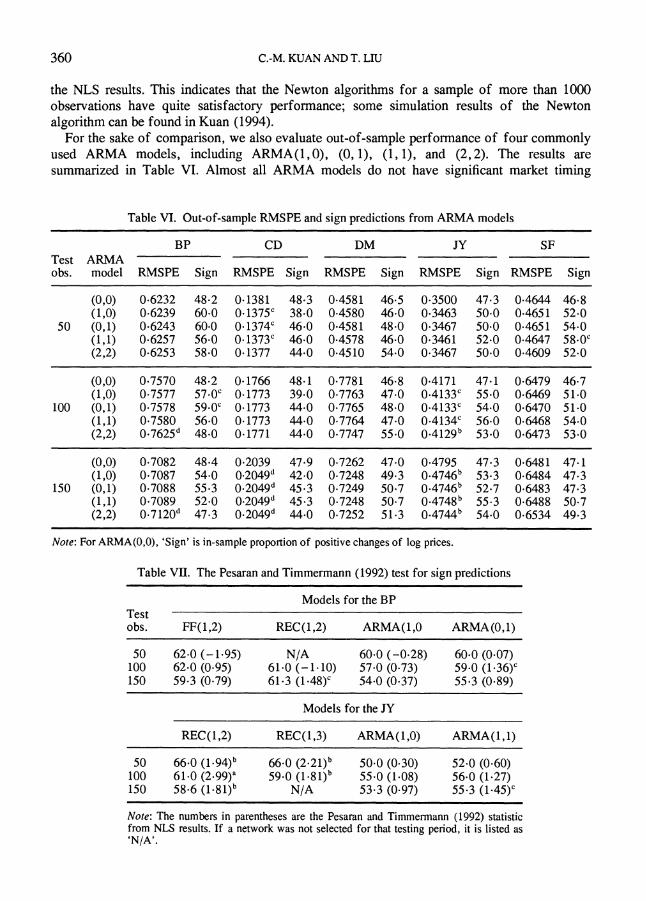
For the sake of comparison, we also evaluate out-of-sample performance of four commonly used ARMA models, including ARMA(1,0), (0,1), (1,1), and (2,2). The results are summarized in Table VI. Almost all ARMA models do not have significant market timing

Table VI. Out-of-sample RMSPE and sign predictions from ARMA models

BP CD DM JY SF Test ARMA obs. model RMSPE Sign RMSPE Sign RMSPE Sign RMSPE Sign RMSPE Sign

(0,0) 0.6232 48.2 0.1381 48-3 0.4581 46-5 0.3500 47-3 0.4644 46-8 (1,0) 0.6239 60-0 0-1375c 38-0 0.4580 46.0 0-3463 50-0 0-4651 52-0

50 (0,1) 0.6243 60-0 0-1374c 46-0 0.4581 48.0 0-3467 50.0 0-4651 54-0 (1,1) 0.6257 56-0 0-1373C 46-0 0-4578 46.0 0-3461 52-0 0-4647 58-.0 (2,2) 0-6253 58.0 0-1377 44.0 0-4510 54-0 0.3467 50-0 0-4609 52-0

(0,0) 0-7570 48.2 0-1766 48-1 0.7781 46.8 0.4171 47-1 0.6479 46-7 (1,0) 0.7577 57.0c 0-1773 39-0 0-7763 47.0 0.4133c 55-0 0-6469 51-0

100 (0,1) 0.7578 59.0c 0.1773 44-0 0-7765 48.0 0.4133C 54.0 0.6470 51.0 (1,1) 0.7580 56-0 0-1773 44.0 0.7764 47-0 0.4134c 56-0 0-6468 54-0 (2,2) 0*7625d 48.0 0-1771 44-0 0.7747 55.0 0-4129b 53.0 0-6473 53-0

(0,0) 0.7082 48.4 0-2039 47.9 0.7262 47-0 0.4795 47.3 0.6481 47-1 (1,0) 0.7087 54.0 0.2049d 42-0 0-7248 49-3 0.4746b 53.3 0-6484 47.3

150 (0,1) 0.7088 55.3 0-2049d 45.3 0.7249 50-7 0.4746b 52.7 0-6483 47-3 (1,1) 0.7089 52.0 0-2049d 45.3 0.7248 50.7 0-4748b 55-3 0.6488 50-7 (2,2) 0.7120d 47.3 0-2049d 44-0 0-7252 51.3 0-4744b 54-0 0-6534 49-3

Note: For ARMA(0,0), 'Sign' is in-sample proportion of positive changes of log prices.

Table VII. The Pesaran and Timmermann (1992) test for sign predictions

Models for the BP Test obs. FF(1,2) REC(1,2) ARMA(1,0 ARMA(0,1)

50 62.0 (-1-95) N/A 60.0 (-0-28) 60-0 (0-07) 100 62.0 (0-95) 61.0 (-1.10) 57.0 (0-73) 59-0 (1.36)c 150 59-3 (0-79) 61-3 (1.48)c 54.0 (0-37) 55-3 (0-89)

Models for the JY

REC(1,2) REC(1,3) ARMA(1,0) ARMA(1,1)

50 66-0 (1.94)b 66-0 (2*21)b 50.0 (0-30) 52-0 (0-60) 100 61.0 (2.99)a 59-0 (1-81)b 55.0 (1-08) 56-0 (1-27) 150 58.6 (1.81)b N/A 53.3 (0-97) 55.3 (1.45)c

Note: The numbers in parentheses are the Pesaran and Timmermann (1992) statistic from NLS results. If a network was not selected for that testing period, it is listed as 'N/A'.

360


ability in these testing periods, except that ARMA(1,0) and ARMA(0,1) for the BP are significant in the period with 100 observations and ARMA(1, 1) for the SF is significant in the period with 50 observations. In terms of MSPE, all ARMA models for the JY have significant out-of-sample MSPE in testing periods with 100 and 150 observations, and three ARMA models for the CD have significant out-of-sample MSPE in the first testing period. Note that these significant ARMA models have almost identical MSPE.

We also apply the Pesaran and Timmermann (1992) test to evaluate sign predictions. To conserve space, we do not report all statistics here, but we summarize the results for some 'good' models discussed above in Table VII. For the BP, the test results for network models agree with those of the market timing test, but significance level is different. Note, however, that ARMA(1, 0) becomes insignificant in the second testing period under this test. For the JY, both REC(1,2) and REC(1,3) are still significant at the 5% level in all periods, whereas ARMA(1, 1) becomes significant at the 10% level in the last testing period. All the results we obtained suggest that REC(1, 2) and REC(1, 3) have systematic good performance for the JY series.

5. CONCLUSIONS

In this paper we propose a two-step procedure to estimate and select feedforward and recurrent networks and carefully evaluate the forecasting performance of selected networks in different out-of-sample periods. The forecasting results are mixed. We find networks with significant market timing ability (sign predictions) and/or significantly lower out-of-sample MSPE (relative to the random walk model) in only two out of the five series we evaluated. For other series, network models do not exhibit superior forecasting performance. Nevertheless, our results suggest that PSC is quite sensible in selecting networks and that the proposed two-step procedure may be used as a standard network construction procedure in other applications. Our results show that nonlinearity in exchange rates may be exploited to improve both point and sign forecasts, in contrast with the conclusion of Diebold and Nason (1990). Although some of the results reported here are quite encouraging, they provide only limited evidence supporting the usefulness of neural network models. We hope this paper will provoke more research in this direction in the future.

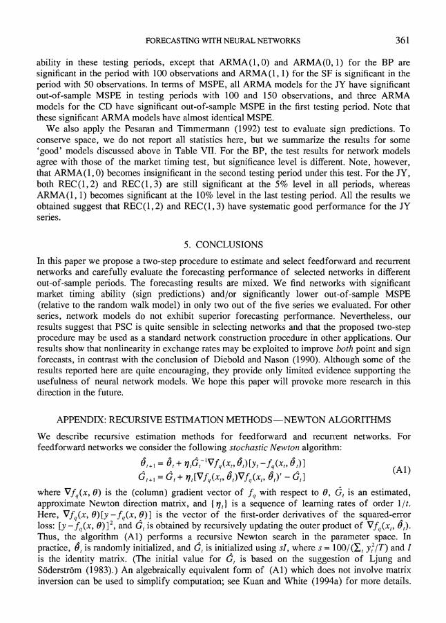
APPENDIX: RECURSIVE ESTIMATION METHODS-NEWTON ALGORITHMS

We describe recursive estimation methods for feedforward and recurrent networks. For feedforward networks we consider the following stochastic Newton algorithm:

0t+^= ,+ )ritG VfQ(X ,)[y, (-fq(x,, O,)]

G, +l = G,+ rlt[Vf,(x,, Ot)Vfq(xt, Y,) - (,A where Vfq(x, 0) is the (column) gradient vector of f, with respect to 0, G, is an estimated, approximate Newton direction matrix, and {?l,) is a sequence of learning rates of order 1/t. Here, Vfq(x, 0)[y -f,(x, 0)] is the vector of the first-order derivatives of the squared-error loss: [y -fq(x, 0)]2, and G, is obtained by recursively updating the outer product of Vfq(xt, 0,). Thus, the algorithm (Al) performs a recursive Newton search in the parameter space. In

practice, 0, is randomly initialized, and G, is initialized using sI, where s = 100/(I, y2/T) and I is the identity matrix. (The initial value for G, is based on the suggestion of Ljung and S6derstr6m (1983).) An algebraically equivalent form of (Al) which does not involve matrix inversion can be used to simplify computation; see Kuan and White (1994a) for more details.

361


We also note that if f is a linear function, the algorithm (Al) reduces to the well-known recursive least square algorithm.

A recurrent Newton algorithm analogous to (Al) is

l= 0,-j,G lV^ e,e, (A2) e,t, = x,- r/,h,-'vt,I, ,+ = G, + (VVe - ,)

where , and h, are column vectors of the first-order derivatives of b with respect to 0 and h, respectively. Note that we have omitted the subscript q of 0 for notational simplicity. In this algorithm, 0, and G, are initialized as above, the ith (i = l,..., q) hidden-unit activation is updated according to

hs, = (yo,, + ^ ivj + Z .1 = (x,, ,) (A3)

A with initial value 1/2, and the jth (j = 1, ..., q) column of A,+l is updated according to

Aj,+ = ijp.(x,,/ h,- , 0,) + At,jth(x,, h,_., 0,) (A4)

with initial values 0, where tij , and Ij.h are column vectors of the first-order derivatives of the

jth hidden unit tj with respect to 0 and h, respectively. As v is the logistic function in our application, it is bounded between 0 and 1. Setting the initial value of h, at 1/2 is equivalent to assuming no knowledge of hidden units in the beginning. This algorithm is implemented with a truncation device to ensure 6,i <4/q for all i, 1. More details of equation (A2) used in this study can be found in the Appendix of Kuan (1994).

Note that a recurrent network not depending on h,l_ is a feedforward network. In this case, the I h term is zero so that the updating equations of A, are not needed, and (A2) simply reduces to the standard Newton algorithm (Al).

ACKNOWLEDGEMENTS

We would like to thank Roger Koenker, Bill Maloney, Paul Newbold, four anonymous referees, and the editor for their invaluable suggestions and comments. We are most grateful to Richard Baillie for providing us with the data set and to Bruce Mizrach and Hal White for permitting us to access their programs. C.-M. Kuan also thanks the Research Board of the University of Illinois for research support. All remaining errorisare ours. An early version of this paper (based on a different data set) was presented at the 1992 North American Winter Meeting of the Econometric Society in New Orleans, Louisiana.

REFERENCES

Baillie, R. T. and T. Bollerslev (1989), 'Common stochastic trends in a system of exchange rates', Journal of Finlance, 44, 167-181.

Baillie, R. T. and P. C. McMahon (1989), The Foreign Exchange Market: Theory anzd Econometric Evidence, Cambridge University Press, New York.

Barron, A. R. (1991), 'Universal approximation bounds for superpositions of a sigmoidal function', Technical Report No. 58, Department of Statistics, University of Illinois, Urbana- Champaign.

362


Benveniste, A., Metivier, M. and P. Priouret (1990), Adaptive Algorithms and Stochastic Approximations, Springer-Verlag, Berlin.

Chinn, M. D. (1991), 'Some linear and nonlinear thoughts on exchange rates', Journal of International Money and Finance, 10, 214-230.

Cybenko, G. (1989), 'Approximations by superpositions of a sigmoidal function', Mathematics of Control, Signals and Systems, 2, 303-314.

Diebold, F. X. and R. S. Mariano (1991), 'Comparing predictive accuracy I: An asymptotic test', Discussion Paper 52, Institute for Empirical Macroeconomics, Federal Reserve Bank of Minneapolis.

Diebold, F. X. and J. A. Nason (1990), 'Nonparametric exchange rate prediction?', Journal of International Economics, 28, 315-332.

Elman, J. L. (1990), 'Finding structure in time', Cognitive Science, 14, 179-211. Engel, C. (1991), 'Can the Markov switching model forecast exchange rates?' Working Paper, University

of Washington. Engel, C. and J. Hamilton (1990), 'Long swings in the exchange rates: Are they in the data and do markets

know it?' American Economic Review, 80, 689-713. Gerencser, L. and J. Rissanen (1992), 'Asymptotics of predictive stochastic complexity', in D. Brillinger,

P. Caines, J. Geweke, E. Parzen, M. Rosenblatt, and M. Taqqu (eds), New Directions in Time Series Analysis, Part 2, Springer-Verlag, New York.

Henriksson, R. D. and R. C. Merton (1981), 'On market timing and investment performance II: Statistical procedures for evaluating forecasting skills', Journal of Business, 54, 513-533.

Hornik, K., Stinchcombe, M. and H. White (1989), 'Multi-layer feedforward networks are universal approximators', Neural Networks, 2, 359-366.

Hsieh, D. A. (1989), 'Testing for nonlinear dependence in daily foreign exchange rates', Journal of Business, 62, 329-368.

Kuan, C.-M. (1994), 'A recurrent Newton algorithm and its convergence property', IEEE Transactions on Neural Networks, forthcoming.

Kuan, C.-M. and K. Hornik (1991), 'Learning in a partially hard-wired recurrent network', Neural Network World, 1, 39-45.

Kuan, C.-M., Hornik, K. and H. White (1994), 'A convergence result for learning in recurrent neural networks', Neural Computation, 6, 620-640.

Kuan, C.-M. and H. White (1990), 'Predicting appliance ownership using logit, neural network, and regression tree models', BEBR Working Paper 90-1647, College of Commerce, University of Illinois, Urbana-Champaign.

Kuan, C.-M. and H. White (1994a), 'Artificial neural networks: An econometric perspective', Econometric Reviews, 13, 1-91.

Kuan, C.-M. and H. White (1994b), 'Adaptive learning with nonlinear dynamics driven by dependent processes', Econoinetrica, forthcoming.

Levich, R. (1981), 'How to compare chance with forecasting expertise', Euromoney, August, 61-78. Ljung, L. and T. Sdderstrom (1983), Theory and Practice of Recursive Identification, MIT Press,

Cambridge, MA. Merton, R. C. (1981), 'On market timing and investment performance, I: An equilibrium theory of value

for market forecasts', Journal of Business, 54, 363-406. Mizrach, B. (1992), 'Forecast comparison in L2', Working paper, University of Pennsylvania. More, J. (1977), 'The Levenberg-Marquardt algorithm, implementation and theory', in G. A. Watson

(ed.), Numerical Analysis, Springer-Verlag, New York. Pesaran, M. H. and A. Timmermann (1992), 'A simple nonparametric test of predictive performance',

Journal of Business and Economic Statistics, 10, 461-465. Rissanen, J. (1986a), 'A predictive least-squares principle', IMA Journal of Mathematical Control &

Information, 3, 211-222. Rissanen, J. (1986b), 'Stochastic complexity and modeling', Annals of Statistics, 14, 1080-1100. Rissanen, J. (1987), 'Stochastic complexity (with discussions)', Journal of the Royal Statistical Society,

B, 49, 223-239 and 252-265. Rissanen, J. (1989), Stochastic Complexity in Statistical Inquiry, World Science Publishing Co.,

Singapore. Rumelhart, D. E., Hinton, D. E. and R. J. Williams (1986), 'Learning internal representation by error

propagation', in D. E. Rumelhart and J. L. McClelland (eds), Parallel Distributed Processing: Exploration in the Microstructure of Cognition, Vol. 1, 318-362, MIT Press, Cambridge, MA.

363

364 C.-M. KUAN AND T. LIU

Schwarz, G. (1978), 'Estimating the dimension of a model', Annals of Statistics, 6, 461-464. Taylor, S. J. (1980), 'Conjectured models for trends in financial prices, tests and forecasts', Journal of

the Royal Statistical Society, A, 143, 338-362. Taylor, S. J. (1982), 'Tests of the random walk hypothesis against a price trend hypothesis', Journal of

Financial and Quantitative Analysis, 17, 37-61. White, H. (1988), 'Economic prediction using neural networks: The case of IBM Stock Prices', in

Proceedings of the IEEE Second International Conference on Neural Networks, II, pp. 451-458, SOS Printing, San Diego.

White, H. (1989), 'Some asymptotic results for learning in single hidden-layer feedforward network models', Journal of the Americatn Statistical Association, 84, 1003-1013.

forecasting exchange rates using feedforward and recurrent

Documents