Ecotoxicological applications of Dynamic Energy1

Budget theory ∗2

S.A.L.M. Kooijman†, J. Baas, D. Bontje, M. Broerse,

C. A. M. van Gestel, and T. Jager

Faculty Earth & Life Sciences

Vrije Universiteit, de Boelelaan 1085, 1081 HV Amsterdam, NL3

∗subm J. Devillers (ed) Ecotoxicological Modelling, Springer

†corresponding author: bas@bio.vu.nl. File-name: kinetics.tex

1

Abstract4

The Dynamic Energy Budget (DEB) theory for metabolic organisation specifies quantitatively5

the processes of uptake of substrate by organisms and its use for the purpose of maintenance,6

growth, maturation and reproduction. It applies to all organisms. Animals are special because7

they typically feed on other organisms. This couples the uptake of the different required sub-8

strates, and their energetics can, therefore, be captured realistically with a single reserve and9

a single structure compartment in biomass. Effects of chemical compounds (e.g. toxicants) are10

included by linking parameter values to internal concentrations. This involves a toxico-kinetic11

module that is linked to the DEB, in terms of uptake, elimination and (metabolic) transforma-12

tion of the compounds. The core of the kinetic module is the simple one-compartment model,13

but extensions and modifications are required to link it to DEBs. We discuss how these exten-14

sions relate to each other and how they can be organised in a coherent framework that deals15

with effects of compounds with varying concentrations and with mixtures of chemicals. For the16

one-compartment model and its extensions, as well as for the standard DEB model for indi-17

vidual organisms, theory is available for the co-variation of parameter values among different18

applications, which facilitates model applications and extrapolations.19

Keywords: Dynamic Energy Budgets, effects on processes, kinetics, metabolism, transfor-20

mation21

2

1 Introduction22

The societal interest in ecotoxicology is in the effects of chemical compounds on organisms,23

especially at the population and ecosystem level. Sometimes these effects are intentional,24

but more typically they concern adverse side-effects of other (industrial) activities. The25

scientific interest in effects of chemical compounds is in perturbating the metabolic system,26

which can reveal its organisation. This approach supplements ideas originating from molec-27

ular biology, but now applied at the individual level; the sheer complexity of biochemical28

organisation hampers reliable predictions of the performance of individuals. Understanding29

the metabolic organisation from basic physical and chemical principles is the target of Dy-30

namic Energy Budget (DEB) theory [1, 2]. In reverse, this theory can be used to quantify31

effects of chemical compounds, i.e. changes of the metabolic performance of individuals.32

This chapter describes how DEB theory quantifies toxicity as a process.33

The effects can usually be linked to the concentration of compounds inside the organism34

or inside certain tissues or organs of an organism. This makes that toxicokinetics is basic35

to effect studies. The physiological state of an organism, such as its size, its lipid content,36

and the importance of the various uptake and elimination routes (feeding, reproduction,37

excretion) interacts actively with toxicokinetics, so a more elaborate analysis of toxicoki-38

3

netics should be linked to the metabolic organisation of the organism [3]. In the section39

on toxicokinetics, we start with familiar classic models that hardly include the physiology40

of the organism, and stepwise include modules that do make this link in terms of logical41

extensions of the classic models.42

Three ranges of concentrations of any compound in an organism can be delineated: too-43

little, enough and too-much. The definition of the enough-range is that variations of44

concentrations within this range do not translate into variations of the physiological perfor-45

mance of the individual. Some of the ranges can have size zero; such as the too-little-range46

for cadmium. Effects are quantified in the context of DEB theory as changes of (metabolic)47

parameters as linked to changes in internal concentrations. These parameters can be the48

hazard rate (for lethal effects), the specific food uptake rate, the specific maintenance49

costs, etc. Changes in a single parameter can have many physiological consequences for50

the individual. DEB theory is used not only to specify the possible modes of action of a51

chemical compound, but also how the various physiological processes interact. An increase52

in the maintenance costs by some compound, for instance, reduces growth, and since food53

uptake is linked to body size, it indirectly reduces food uptake, and so affects reproduc-54

tion (and development). The existence of the ranges too-little, enough and too-much of55

concentrations of any compound directly follows from a consistency argument, where no56

4

classification of compounds is accepted (e.g. toxic and non-toxic compounds), and many57

compounds (namely those that make up reserve) exist that do change in concentration58

in the organism, without affecting parameter values. An important consequence is the59

existence of an internal No Effect Concentration (NEC), as will be discussed below.60

Effects at the population level are evaluated from those at the individual level, by consid-61

ering populations as a set of interacting individuals [4-8]. Although DEB-based population62

dynamics can be complex, particular aspects of population performance, such as the pop-63

ulation growth rate at constant environmental conditions, are not very complex. Moreover64

particular simplifying approximations are possible. The focus of toxicology is typically at65

time scales that are short relative to the life span of the individual. That of ecotoxicology,66

however, are much longer, involving the whole life history of organisms; effects on feeding,67

growth, reproduction and survival are essential and typically outside the scope of toxicol-68

ogy. This has strong implications for the best design of models. While pharmacokinetics69

models frequently have many variables and parameters, such complex models are of little70

use for applications at the population level, where a strong need is felt for relatively sim-71

ple models, but then applied to many species and in complex situations. DEB theory is72

especially designed for this task.73

5

Chemical transformations are basic to metabolism, and transformations of toxicants are74

no exception. Compounds that dissociate in water should be considered as a mixture of75

ionic and molecular forms, and the pH affects that mixture. This makes that the effect of76

a single pure compound is of rather academic interest; we have to think in terms of the77

dynamic mixtures of compounds. Because of its strong links with chemical and physical78

principles, DEB theory has straightforward ways to deal with effects of mixtures. Some79

of this theory rests on the covariation of parameter values across species of organism and80

across chemical compounds. Theory on this covariation is implied by DEB theory, and is81

one of its most powerful aspects.82

We first introduce some notions of DEB theory, and then discuss toxicokinetics and effects83

in the context of DEB theory.84

2 The standard DEB model in a nutshell85

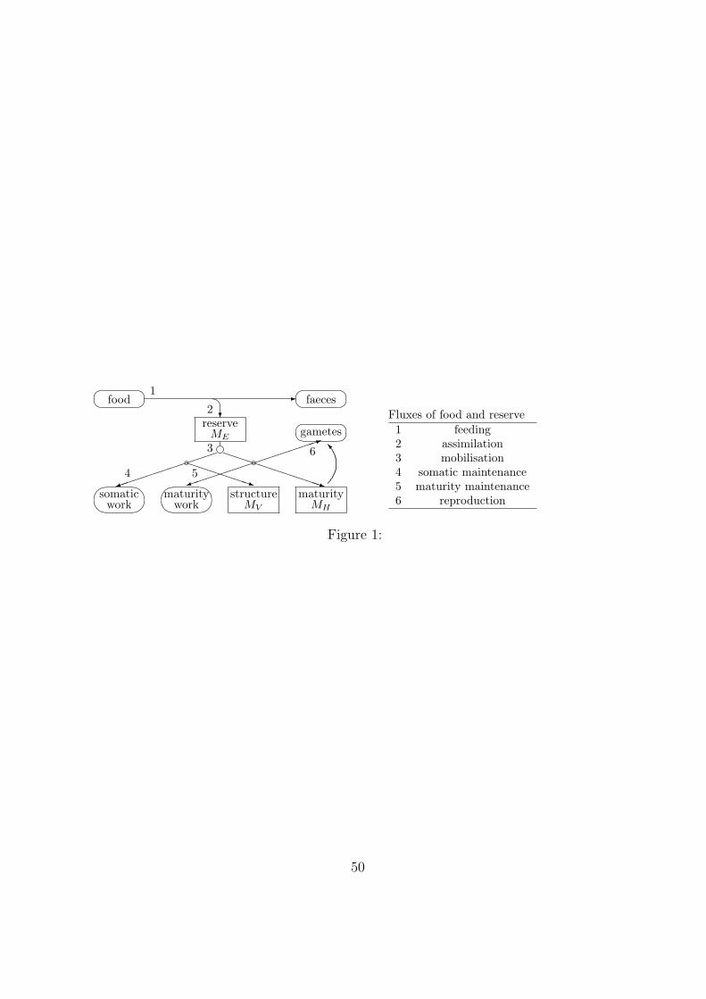
[Figure 1 about here.]86

The standard DEB model concerns an isomorph. i.e. an organism that does not change87

in shape during growth, that feeds on a single food source (of constant chemical composi-88

tion), and has a single reserve a single structure and three life stages: embryo (which does89

not feed), juvenile (which does not allocate to reproduction) and adult (which allocates90

6

to reproduction, but not to maturation). This is in some respects the simplest model in91

the context of DEB theory, which is thought to be appropriate for most animals. Food92

is converted to reserve, and reserve to structure. Reserve does not require maintenance,93

but structure does, mainly to fuel its turnover, see Figure 1. Reserve can have active94

metabolic functions and serves the role of representing metabolic memory. Reserve and95

structure do not change in chemical composition (strong homeostasis). At constant food96

availability, reserve and structure increase in harmony, i.e. the ratio of their amounts, the97

reserve density, remains constant (weak homeostasis).98

The shape (and so the change of shape) is important because food uptake is proportional99

to surface area, and maintenance mostly to (structural) volume. The handling time of100

food (including digestion and metabolic processing) is proportional to the mass of food101

“particles”, during which food acquisition is ceased. The mobilisation rate of reserve to102

fuel the metabolic needs follows from the weak and strong homeostasis assumptions [9]; a103

mechanism is presented by Kooijman and Troost [10]. Allocation to growth and somatic104

maintenance (so to the soma) comprises a fixed fraction of mobilised reserve, the remaining105

fraction is allocated to maturation (or reproduction) and maturity maintenance.106

The transition from the embryo to the juvenile stage (i.e. birth) occurs by initiating107

assimilation when the maturity exceeds a threshold value, and from the juvenile to the108

7

adult stage (i.e. puberty) by initiating allocation to reproduction and ceasing of alloca-109

tion to maturation at another threshold value for maturity. Reserve that is allocated to110

reproduction is first collected in a buffer, that is subjected to buffer handling rules (such111

as spawning once per season, or convert the buffer content into an egg as soon as there is112

enough).113

Biomass consists of reserve and structure, and can, therefore, change in chemical com-114

position (e.g. lipid content) in response to the nutritional condition; maturity has the status115

of information, not that of mass or energy. Apart from some minor details, the presented116

set of simple rules fully specify the dynamics of the individual, including all mass and117

energy fluxes, such as the uptake of dioxygen, the production of carbon dioxide, nitrogen118

waste and heat. It takes some time to see exactly how; Sousa et al. [9] gives a nice evalu-119

ation. Aging is considered to result from a side effect of Reactive Oxygen Species (ROS),120

and is so linked to the uptake of dioxygen [11]. A high food uptake results in a large amount121

of reserve, so a high use of reserve, a high uptake of dioxygen, an acceleration of aging122

and a reduction of life span. The induction of tumours is also linked to the occurrence of123

ROS, and other reactive molecules, such as mutagenic compounds. This gives a natural124

link between aging and tumour induction.125

8

The standard DEB model has been extended into many directions for the various pur-126

poses. The allocation rule to the soma, for instance, can be refined to allocation to various127

body parts (e.g. organs), where growth of each body part is proportional to the allocated128

reserve flux minus what is required for maintenance of that part. Rather than using fixed129

fractions of the mobilised reserve, the fractions can be linked to the relative workload of130

the body part. This allows a dynamic adaptation of the body parts in interaction with131

their use. Tumours can be considered as body parts, and the “workload” of the tumour132

is the consumption of maintenance. This formulation produced realistic predictions of the133

effects of caloric restriction on tumour growth, and of the growth of tumours in young134

versus old hosts [12]. This approach can be extended to various types of tumours, where135

tumour growth is not linked to that of the whole body, but that of a particular body part.136

Many tumours result from destruction of local cell-to-cell communication, rather than from137

genotoxic effects, but these different routes have similar dynamics.138

Other types of extensions of the standard DEB model concern the inclusion of variations139

in chemical composition of food (with consequences for the transformation of food into re-140

serve) and size-dependent selection of different food items. For example many herbivores141

are carnivores when young. Animals are special because they feed on other organisms.142

Most other organisms take the food-compounds (energy source, carbon source, nitrate,143

9

phosphate) that they need independently from the environment, which necessitates the144

inclusion of more than one reserve; see Kooijman and Troost [10] for the evolutionary145

perspectives. Most micro-organisms grow and divide, and don’t have the three life stages146

delineated by the standard model. This makes that their change in shape hardly mat-147

ters and that surface areas can be taken proportional to volumes, which simplifies matters148

considerably. The partial differential equations that are required to described the phys-149

iologically structured population dynamics of isomorphs then collapse to a small set of150

ordinary differential equations. Plants, on the other hand, require at least two types of151

structure (roots and shoots) and have a complex adaptive morphology (i.e. surface area-152

volume relationships); their budgets are most complex to quantify.153

3 Family of toxicokinetic models154

Originally (before the 1950’s) the focus of toxicology, i.e. the field that gave rise to ecotox-155

icology, was on medical applications of compounds in a pharmacological context. Subjects156

where given a particular dose, and the interest is in the redistribution inside the body, and157

in transformation and elimination. The aim is to reach the target organ and to achieve a158

particular effect that restores the health or well-being of the subject. A closely related inter-159

est that developed simultaneously was health protection (disinfection and food protection160

10

products), with the purpose of killing certain species of pathogenic organism (especially161

microorganisms), or to reduce their impact.162

After the 1950’s ecotoxicology began to flourish and gradually became more independent163

of toxicology, where the initial focus was in positive and (later) negative effects of biocides.164

This came with extensions of the interest in the various uptake and elimination routes165

that are of ecological relevance, and the environmental physical-chemistry of transport166

and transformation. The aim is to kill particular species of pest organism locally (insects,167

weeds), and to avoid effects on other, non-target, species (crop and beneficial species).168

After the 1970’s the interest further generalised to an environmental concern of avoiding169

effects of pollutants on organisms, with an increasing attention for (bio)degradation of170

compounds that are released into the environment, coupled to human activity [13].171

This historic development and branching of the interest in toxico-kinetics came with a172

narrowing of the focus on a particular aspect of toxico-kinetics in the various applications173

that, we feel, is counter-productive from a scientific point of view. The purpose of this174

section is an attempt to restore the coherence in the field, by emphasising the general175

eco-physiological context and the relationship of the various models with the core model176

for toxico-kinetics: the one-compartment model. The more subtle models account for the177

interaction with the metabolism of the organism, which involves its metabolic organisation.178

11

We here focus on the logical coherence of toxico-kinetics, bio-availability and metabolism,179

including effects (= changes in metabolism). It is not meant to be a review. For recent180

reviews on toxico-kinetic models, see o.a. Barber [14] and Mackay and Fraser [15]. See181

Table 1 for a list of frequently used symbols.182

[Table 1 about here.]183

3.1 One-compartment model184

[Figure 2 about here.]185

The core model in toxico-kinetics is the one-compartment model, see Fig. 2. It states186

that the uptake rate is proportional to the environmental concentration c, and the elimi-187

nation rate is proportional to the internal concentration Q:188

d

dtQ = ke (P0dc(t) − Q) (1)

Q(t) = Q(0) exp(−tke) + keP0d

∫ t

0

c(s) exp((s − t)ke) ds (2)

= Q(0) exp(−tke) + P0dc (1 − exp(−tke)) for c is constant (3)

where P0d = Q(∞)/c is the BioConcentration Factor (BCF) and ke the elimination rate.189

The product keP0d is known as the uptake rate, and is frequently indicated with ku, which190

12

is misleading because its units are d−1 m3 C-mol−1. Even if we would work with kg rather191

than C-mol, and the specific density of the organism equals 1 kg dm−3, the BCF is not192

dimensionless [1]. It is typically more convenient to work with molalities in soils (mol kg−1),193

and with molarities (mol l−1) in water. Molalities give the uptake rate the units d−1 g C-194

mol−1. Many workers use gram rather than mole to quantify the compound, but this choice195

is less practical to compare the toxicity of different compounds. The elimination rate ke196

has dimension ‘per time’ and is indepenendent of how the compound is quantified; contrary197

to the uptake rate, the elimination rate can be extracted from effect data and determines198

how fast effects build up in time, relative to the long-term effect level.199

The concentrations c and Q must obviously exist, meaning that the environment and200

the organism are taken to be homogeneous. This condition can be relaxed without making201

the model more complex by allowing a spatial structure (such as organs), and an exchange202

between the parts that is fast relative to the exchange between the organism and the envi-203

ronment. Other implicit assumptions of the one-compartment model are that the organism204

does not change in size or in chemical composition, so changes in food availability must205

be negligible. The (bio)availability of the compound remains constant. So transformations206

can be excluded, and the environment is large relative to the organism and well-mixed.207

Sometimes, e.g. in the case of a large fish in a small aquarium, this is not true and the208

13

dynamics of the concentration in the organism and the environment should be considered209

simultaneously: the 1-1 compartment model [16]. These restrictions will be removed below.210

Since rates generally depend on temperature, and temperature typically changes in211

time, the elimination rate ke can change in time as well [17]. In the sequel we will dis-212

cuss rates of metabolism, and like all rates, these also depend on temperature, frequently213

according to the Arrhenius relationship [1].214

3.2 Multi-compartment models215

If transport inside the organism is not fast, relative to the exchange with the environment,216

multiple-compartment models should be considered [18, 19]. If exchange with the environ-217

ment is only via compartment number 0, the change in the concentrations in the nested218

compartments number 0 and 1 is219

d

dtQ0 = ke (P0dc − Q0) + k10Q1 − k01Q0;

d

dtQ1 = k01Q0 − k10Q1 (4)

where k01 and k10 are the exchange rates between the compartments, see Fig. 2. The220

partition coefficient between the compartments equals P10 ≡ Q1(∞)/Q0(∞) = k01/k10,221

while P0d ≡ Q0(∞)/c remains unchanged. In many cases whole body measurements are222

used. If M0 and M1 denote the masses of compartment 0 and 1, the whole body partition223

coefficient with the environment amounts to P+d = (M0 + M1P10)P0d/M+, with M+ =224

14

M0+M1 is the whole body mass. This rather complex behaviour of the whole body partition225

coefficient can be a source of problems in fitting models to data. In many practical cases226

it is not possible to identify the compartments and to measure the concentrations in these227

compartments directly. The use of multi-compartment models cannot be recommended in228

such cases.229

This extension still classifies as a transport model, so in a clean environment (c = 0), the230

organism will loose all its load (Q0(∞) = Q1(∞) = 0). Quite a few data sets on the231

kinetics of (“heavy”) metals in organisms show that once loaded, an organism never fully232

looses its load [20-22]. Such behaviour cannot be captured by multi-compartment models233

because this involves an extension to transformation of compounds (technically speaking,234

sequestered compounds belong to a different chemical species).235

If k01, k10 ≫ ke, we can assume that Q1(t) ≃ P10 Q0(t), and the kinetics Eq 4 reduces to236

Eq 1, with Q replaced by Q0. This situation is called time-scale separation.237

The interpretation of the compartments can be a special tissue or organ, or, more abstract,238

reserve (compartment 1) and structure (compartment 0). The latter makes sense in the239

context of DEB theory, where both compartments are assumed to have a constant, but240

different, chemical composition, while reserve is relatively rich in lipids in many animal241

taxa. While Eq 4 assumes that the size of all compartments does not change, we will relax242

15

on this below, when we allow more interactions with metabolism and energetics.243

We can obviously include more compartments, and more complex interactions with the244

environment, but the number of parameters rapidly increases this way. In practice multi-245

compartments are used if the one-compartment model fits data badly. The introduction246

of more parameters generally improves the fit, but not necessarily for the right reasons.247

As a rule of thumb it is only advisable to use more compartment models if data on the248

concentrations inside the compartments are available. If lack of fit of the one-compartment249

model is the only motivation, alternatives should be considered that are discussed below.250

3.3 Film models251

Film models are conceptually related to multi-compartment models because both are ex-252

tensions of the one-compartment model that include more detail in transport (so in physical253

factors), though in different but complementary ways. Film models are especially popular254

in environmental chemistry for following the transport of compounds from one environ-255

mental compartment (such as water) to another (such as air). Both compartments are256

assumed to be well-mixed, except for a narrow film at the interface of both compartments,257

where transport is by diffusion.258

16

To follow the dynamics for the densities of the compound n (mol/m), we need to define a259

spatial axis perpendicular to the interface and choose the origin at the boundary between260

the bulk and the film (on each side of the interface). Let Li be the depth of the film, di261

the diffusivity of the compound in the film, and vij the exchange velocity of the compound262

between the two media. As discussed in Kooijman et al. [16], the dynamics of the densities263

is given by partial differential equations (pde’s) for medium i = 1 − j and j = 0 or 1264

0 =∂

∂tni(L, t) − di

∂2

∂L2ni(L, t) for L ∈ (0, Li) (5)

with boundary conditions at L = 0 (i.e. the boundary between the film and the well-mixed265

medium) for vi = di/Li266

0 =∂

∂tni(0, t) − vi

∂

∂Lni(0, t) (6)

and boundary conditions at L = Li (i.e. the interface between the media where the two267

films meet)268

0 = vjinj(Lj, t) − vijni(Li, t) + di∂

∂Lni(Li, t) (7)

The boundary condition at L = 0, and the diffusion process in the film is rather standard,269

but we believe that the boundary condition at L = Li is presented for the first time in270

Kooijman et al. [16]. Users of the popular film models typically skip the formulation of the271

pde and directly focus at steady state situations; they typically use the concentration jump272

17

across the interface that belongs to the situation when there is no net transport across the273

interface. As long as there is transport, however, the concentration jump differs from this274

equilibrium value.275

The depth of the films is typically assumed to be small and the transport in the films in276

steady state, which makes that the density profiles in the films are linear. This leads to277

the 1-1-compartment kinetics for the bulk densities278

d

dtni(0) = kij(Pijnj(0) − ni(0)); kij =

vi/Li

1 + Pijvi/vj − vi/vij

(8)

where Li is the depth of the medium. This approximation only applies if vivj < vijvj +vjivi279

and the transport in the film is rate limiting. The 1-1-compartment kinetics also results,280

however, if the film depths reduce to zero and if the diffusivities are high. The rate from281

i to j then reduces to kij = viL−1

i (1 − vi/vij)−1. In these two situations, transport in the282

film is no longer rate limiting.283

The applicability of film models to toxico-kinetics in organisms is still an open question.284

It can be argued that a stagnant water film sticks to aquatic or soil organisms (and air to285

a terrestrial organism), and that the skin (or cuticula) is not well served by the internal286

redistribution system (blood) of the organism. If toxico-kinetics is fully limited by transport287

in the film, and if it is not limited by the film, one-compartment kinetics results; only in the288

intermediary situation we can expect some deviations. Yet the discussion is not completely289

18

academic, since these details matter for how the elimination rate depends on the partition290

coefficient [16, 23].291

3.4 Uptake and elimination routes292

We now consider extensions of the one-compartment model due to biological factors by293

accounting for various uptake and elimination routes. These routes depend on the type of294

organism, its habitat and properties of the compound. Animals that live in (wet) soil are in295

intense contact with the water film around soil particles, and their situation has similarities296

with that of aquatic animals. Direct transport through the skin can be important, which297

involves the surface area of an organism. Some parts of the skin are more permeable,298

especially that used by the respiratory system for dioxygen uptake and carbon dioxide299

excretion. The uptake rate might be linked to the respiratory rate, which depends on300

the energetics of the organism. Generally, the respiration rate scales with a weighted sum301

of surface area and volume, but the proportionality constants depend on the nutritional302

conditions of the organism [1]. For terrestrial animals, uptake via the lungs from air and303

via skin contact with the soil must be considered. Sometimes uptake is via drinking; the304

DEB theory quantifies drinking via the water balance for the individual and involves a.o.305

metabolism and transpiration. The details can be found in Kooijman [1].306

19

A second important uptake route is via food and the gut epithelium. The feeding rate307

depends on food availability, food quality, and the surface area of the organism [1].308

The elimination can follow the same routes as uptake, but there are several additional309

routes to consider, namely via products of organisms. The first possibility is the route310

that excreted nitrogen waste follows (urination). Reproductive products (mostly eggs311

and sperm) can also be an important elimination route. Moulting (e.g. ecdysozoans,312

including the rejection of gut epithelium, e.g. collembolans) or the production of mucus313

(e.g. lophotrochozoans) or milk (e.g. female mammals) are other possible excretion routes.314

The DEB theory quantifies reproductive and other products as functions of the amounts315

of reserve and structure of the individual. In the standard DEB model they work out to be316

cubic polynomials in body length, but the coefficients depend on the nutritional conditions317

(amount of reserves per structure) [1].318

3.5 Changes in body size and composition319

The body size of an organism matters in the context of toxico-kinetics for several rea-320

sons [24]. As exchange is via surface area, and is proportional to concentration, surface321

area-volume interactions are involved. This problem also applies to compartment and film322

models, but gets a new dimension if we consider changes in body size, which are linked to323

20

the nutritional condition of organisms (lipid content), and so to (changes in) body com-324

position. Small changes in size can have a substantial effect on the shape of accumulation325

curves.326

If an organism does not change in shape during growth (so it remains isomorphic), surface327

area is proportional to volume2/3, or to squared length. Moreover, dilution by growth328

should be taken into account, even at low growth rates. This modifies Eq 1 to329

d

dtQ = (P0dc(t) − Q) ve/L − Qr with r =

d

dtln L3 (9)

where L is the length, and ve = Lmke is the elimination velocity for maximum length Lm.330

The last term, Qr, represents the dilution by growth. If it equals zero, we can replace331

ve/L by the constant elimination rate k′

e, but its meaning still matters if we compare the332

kinetics in two organisms of different size. DEB theory specifies how the change in (cubed)333

length depends on the amount of reserve and structure of the organism, and how the334

change in reserve depends on these state variables and food availability. Food intake and335

maintenance play an important role in growth and together they control the maximum size336

an organism can reach, since food intake is proportional to a surface area and maintenance337

to structural volume. Wallace had this insight in 1865 already [25].338

The DEB theory allows for particular changes in body composition, because reserve and339

structure can change in relative amounts and both have a constant composition. Food340

21

(substrate) is first transformed into reserve, and reserve is used for metabolic purposes,341

such as somatic and maturity maintenance, growth, maturation and reproduction. The342

change in reserve density for metabolic use is proportional to the reserve density per length,343

which makes that high growth rates come with high reserve densities, i.e. the ratio of the344

amounts of reserve and structure.345

Reserves are in many animal taxa relatively enriched in lipids, which might have a strong346

influence on the kinetics of hydrophobic compounds. The body burden of eel in a ditch that347

is polluted with mercury or PCB might greatly exceed that of other fish partly because eel348

is relative rich in lipids. This illustrates the importance of lipid dynamics. Freshly laid eggs349

consist almost exclusively of reserve, which makes egg production a potentially important350

elimination route for lipophyllic compounds. The reserve allocation to reproduction is via351

a buffer that comes with species-specific buffer handling rules. Many aquatic species spawn352

once a year only (e.g. most bivalves and fish), which implies that the buffer size gradually353

increases between two spawning events and makes a sharp jump down at spawning. The354

body burden can also make a jump at spawning (up or down, depending on the properties355

of the compound).356

The difference in lipid content between reserve and structure invites for the application of a357

nested two-compartment model, where the exchange with the environment is via structure.358

22

This links up nicely with food uptake, because reserve does not play a role in it, and food359

uptake is also proportional to squared structural length. An important difference with the360

nested two-compartment model is, however, that the size of the compartments typically361

changes in time, especially the reserve. When redistribution of the compound between the362

compartments reserve and structure is relatively fast, and the nested two-compartment363

model for the compound reduces to a one-compartment one, reserve dynamics still affects364

toxico-kinetics, because the lipid content is changing in time. The resulting dynamics for365

active uptake from food amounts to366

d

dtQ = (PV dcd + PV XfcX)

ve

L− Q(PV W

ve

L+ r) with PV W = 1 + PEV (mE + mER) (10)

where cd and cX are the concentrations of the compound in the environment and in food,367

f is the scaled functional response, PV d and PV X are the partition coefficients of the368

compound in structure and environment or food. The reserve density mE and the repro-369

duction buffer density mER now modify the partition coefficient between structure and370

biomass (i.e. reserve plus structure), via the partition coefficient between reserve and371

structure PEV . DEB theory specifies how structural length L, the reserve density mE and372

the reproduction buffer density mER change in time.373

The reproduction buffer is not of importance in all species, and not always in males. If374

food density is constant, the reserve density mE becomes constant. In those situations375

23

the structure-biomass partition coefficient PV W is constant as well. If also the dilution376

by growth can be neglected, i.e. r = 0 and L is constant, Eq 10 still reduces to the one-377

compartment model Eq 1.378

Many accumulation-elimination experiments are done under starvation conditions; e.g. it is379

hardly feasible to feed mussels adequately in the laboratory. The reserve density decreases380

during the experiment, so the chemical composition is changing, which can affect the381

toxico-kinetics [26].382

Some situations require more advanced modelling of the uptake and eliminations route,383

where e.g. gut contents exchanges with the body in more complex ways, and defecation384

might be an elimination route.385

3.6 Metabolism and transformation386

Both uptake and elimination can depend on the metabolic activity [27]. Respiration is387

frequently used as a quantifier for metabolic activity. This explains the popularity of body388

size scaling relationships for respiration [28], and the many attempts to relate many other389

quantities to respiration. In the context of DEB theory, however, and that of indirect390

calorimetry, respiration is a rather ambiguous term, because it can stand for the use of391

dioxygen, or the production of carbon dioxide or heat. These are not all proportional392

24

to each other, however. Moreover all these three fluxes have contributions from various393

processes, such as assimilation, maintenance, growth etc. Since the use of reserves fuels394

all non-assimilatory activities, this is an obvious quantifier to link to the rate at which395

compounds are transformed or taken up. For uptake of compounds via the respiratory396

system, the use of dioxygen might be a better quantity to link to uptake under aerobic397

conditions.398

Respiration rates turn out to be cubic polynomials in structural length in DEB theory,399

which resemble the popular allometric functions numerically in great detail. The coeffi-400

cients depend on the nutritional conditions in particular ways. Since elimination rates are401

inversely proportional to length because of surface area-volume interactions, as has been402

discussed, and the specific metabolic rate is very close to this relationship, it is by no means403

easy to evaluate the role of metabolism in direct uptake and elimination in undisturbed404

subjects.405

The role of metabolism is easier to access for elimination via products and if the elimination406

rate is not proportional to the internal concentration, but has a maximum capacity. The407

classic example is the elimination of alcohol in human blood [29]. This type of kinetics can408

be described as409

d

dtQ = keP0dc − keQ/(KQ + Q) (11)

25

where K is a half saturation constant for the elimination process. It reduces to the one-410

compartment model Eq 1 for small internal concentrations, relative to the half saturation411

constant, KQ ≫ Q. The elimination rate can now be linked to metabolic activity, and so412

to body size. If particular organs are involved, such as the liver in the case of alcohol, the413

DEB theory can be used to study adaptation processes to particular metabolic functions.414

In the case of alcohol, the uptake term should obviously be replaced by a more appropriate415

one that applies to the particular subject.416

Many toxicants are metabolically modified. This especially applies to lipophyllic com-417

pounds, which are typically transformed into more hydrophyllic ones, which are more eas-418

ily excreted but also metabolically more active. The rate of transformation can be linked419

to the metabolic rate, and so depends on body size and nutritional conditions. These420

metabolic products can be more toxic than the original lipophyllic compound.421

4 Bio-availability422

Compounds are not only transformed in the organism, but also in the environment which423

affects their availability. Many have an ionic and a molecular form, which are taken up424

at different rates; the ionic species requiring counter ions, which complicates their uptake.425

Speciation depends on the concentration of compound and environmental properties, such426

26

as the pH. It can vary in time and also occurs inside the organism, but the internal pH427

usually varies within a narrow band only. Models for mixtures of chemicals can be used in428

this case (see section on effects). Internal concentration gradients could develop if transport429

inside the organism is slow; film models should be used in this case. A nice example of a case430

where concentration gradients result from transformation in combination with transport is431

the fluke Fasciola which has an aerobic metabolism near its surface with the micro-aerobic432

environment inside its host, but an anaerobic metabolism in the core of its body [30].433

Another problem, which occurs especially in soils, is that the transport through the medium434

can be slow enough for concentration gradients to develop around the organism. Film435

models should then be used again.436

A major problem in the translation of laboratory toxicity tests to field situations is the437

formation of ligands with (mainly) organic compound that are typically abundant in the438

field, but not in the bioassay. Ligands reduce the availability substantially, and typically has439

a rather complex dynamics. Moreover compounds can be transformed by (photo)chemical440

transformation and by actions of (micro)organisms. This implies that the concentration441

of available compounds changes in time, and our methodology to assess effects of chemical442

compounds should be able to take this into account.443

27

These processes of transformation require compound-specific modelling and this short sec-444

tion demonstrates that bio-availability issues interact with toxico-kinetics and effects of445

chemical compounds in dynamic ways, which calls for a dynamic approach to effects of446

chemicals [3, 31].447

5 Effects at the individual level448

Compound affect individuals via changes of parameter values as functions of the internal449

concentration [32, 33]. The parameter values are independent of the internal concentration450

in the “enough”-range of the compound. This implies the existence of an internal No Effect451

Concentrations (NECs) at either end of the “enough”-range; the upper end is typically of452

interest for ecotoxicological applications. Outside the “enough”- range the value of the453

target parameter is approximately a linear function of the internal concentration as long454

as the changes in parameter value are small; the inverse slope is called the tolerance con-455

centration (a large value means that the compound is not very toxic). Small changes in456

parameter values do not necessarily translate into small changes of some end-point, such457

as the cumulative number of offspring [34] or the body size [35] at the end of some stan-458

dardised exposure period. DEB theory specifies how exactly changes in parameter values459

translate into the performance of the individual. Typical target parameters are the specific460

28

maintenance costs, or the yield of structure on reserve, or the maximum specific assimila-461

tion rate or the yield of reserve on food or the yield of offspring on reserve. For effects on462

survival, the hazard rate serves the role of target parameter, and the inverse “tolerance con-463

centration” for the hazard rate is called the killing rate. Mutagenic compounds can induce464

tumours [36], but also accelerate ageing by enhancing the effects of ROS. The partitioning465

fraction for mobilised reserve can be the target parameter for endocrine disruptors.466

Using sound theory for how effects depend on internal concentrations, DEB-based theory467

can handle varying concentrations of toxicant [37-40], even pulse exposures [41]. DEB468

theory applies to all organisms, including bacteria that decompose organic pollutants.469

A proper description of this process should account for adaptation [42], co-metabolism470

[43] and the fact most bacteria occur in flocculated form in nature [44], which affect the471

availability of the compound.472

The model of linear effects of internal concentrations on parameter values has been ex-473

tended into several directions, such as adaptation to the compound, inclusion of the recent474

exposure history via receptor dynamics [45] and attempts to include particular molecular475

mechanisms [46].476

29

5.1 Mixtures and NECs477

Mixtures of compounds affect parameters values via addition of the effects of single com-478

pounds, plus an interaction term which is proportional to the products of the internal479

concentrations of the compound [47]. This interaction term can be positive or negative;480

a construct that is the core of the analysis of variance (ANOVA) model and rests on a481

simple Taylor series approximation of a general non-linear multivariate function, which482

only applies for small changes of parameter values; the non-linearities of the effects should483

be taken into account for larger changes. These non-linearities might well be specific for484

the compound and the species and, therefore, lack generality. Notice that linear effects485

on parameter values translate into non-linear effects of the performance of the individual486

because the DEB models are non-linear. Also notice that each DEB parameter has a NEC487

value for any compound; the lowest value among all parameters might be considered as the488

NEC of a compound for the organism, but its estimation requires to study effects on all 13489

parameters of the standard DEB model, in principle. Since this study can be demanding,490

it is in practice essential to talk about the NEC of a compound for an organism for a491

particular DEB parameter.492

The NEC reflects the ability of the individual to avoid changes of performance. From a493

statistical point of view, this robust parameter has very nice properties [48-50]. The NEC494

30

is not meant to imply that some molecules of a compound don’t have an effect, while other495

molecules do. The removal of a kidney in a healthy person can illustrate the NEC concept:496

the removal implies an effect at the sub-organismic level, but this effect generally does not497

translate into an effect at the individual level. The NEC, therefore, depends on the level498

of observation. We can delineate three cases of how compounds in the mixture combine499

for the NEC500

• the presence of other compounds is of no relevance to the NEC of any particular501

compound502

• the various compounds add, like they do for effects, and at the moment effects show503

up, the amounts of the compounds that show no effects remain constant504

• the various compounds add, like they do for effects, and the amounts of the com-505

pounds that show no effects continue changing with the internal concentration of the506

compounds; if a compound continues accumulation more than other compounds, its507

NEC increases while that of the other compounds in the mixture decreases508

The third case is possibly most realistic, but also computationally the most complex. In509

many practical situations the results are very similar to the second case, which can be510

used as an approximation. If compounds in a mixture are equally toxic, and so all have511

31

the same NEC, the second case is formally identical to this special case [51]. This way512

of described effects of mixtures turns out to fit well with experimental data [47] and each513

pair of compounds have a single interaction parameter, which does not change in time. If514

there are k compounds in a mixture, there are k(k − 1)/2 interaction parameters, just like515

in ANOVA.516

A further reflection on the NEC might clarify the concept. Any compound affects (in517

principle) all DEB parameters (including the hazard rate), but the NEC for the various518

parameters differ. This makes that, if the internal concentration increases, the parameter519

with the lowest NEC first starts to change, but other parameters follow later. In a mixture520

of compounds, this can readely lead to a rather complex situation where in a narrow range521

of (internal) concentrations of compounds in a mixture several parameters start changing522

[51]. Even in absence of the above-mentioned chemical interactions of compounds on a523

single parameter, interactions via the energy budget occur, which are hard to distinguish524

from the chemical interactions on a single parameter. Chemical interactions are typically525

rare, but interactions via the budget always occur.526

32

5.2 Hormesis527

Hormesis, the phenomenon that low concentrations of a toxicant seem to have a stimu-528

lating rather than an inhibiting effect on some endpoint, can result from interactions of529

the compound with a secondary stress, such as resulting from very high levels of food530

availability. If a compound decreases the yield of structure on reserve, it reduces growth531

and delays birth (if an embryo is exposed) and puberty (in the case of juveniles), but also532

reduces the size at birth. A reduction of growth indirectly reduces reproduction, because533

food uptake is linked to size. Since it also reduces size at birth, the overall effect can be534

a hormesis effect on reproduction (in terms of number of offspring per time) [52]. Indirect535

effects on reproduction differ from direct effects by not only reducing, but also delaying536

reproduction. This has important population dynamical consequences.537

5.3 Co-variation of parameter values538

A very powerful property of the standard DEB model and the one-compartment model539

is that they imply rules for how parameter values co-vary among species and compounds540

[53, 23, 9]; this variation directly translates into how expected effects vary. These expec-541

tations can be used to fill gaps in knowledge about parameter values, but cannot replace542

the need for this knowledge. Evolutionary adaptations and differences in mode of ac-543

33

tion of compounds can cause deviation from expected parameter values for species, and544

compounds, respectively.545

The reasoning behind the scaling relationships for the standard model rests on the as-546

sumption that parameters that relate to the local biochemical environment in an organism547

are independent of the maximum body size of a species, but parameters that relate to548

the physical design of an organism depends on the maximum size. Strange enough, this549

simple assumption fully species the covariation of parameter values. The application is550

best illustrated with the maximum length Lm an endotherm can reach in the standard551

DEB model. This length is a simple function of three parameters, Lm = κ{pAm}/[pM ],552

where κ is the fraction of mobilised reserve that is allocated to the soma, {pAm} is the553

surface-area specific maximum assimilation energy flux and [pM ] is the volume-specific so-554

matic maintenance cost. Since κ and [pM ] depend on the local biochemical environment,555

they are independent of maximum length, which implies that {pAm} must be proportional556

to maximum length. All other parameters can be converted in simple ways to quantities557

that depend on the local biochemical environment; these transformations then defined how558

they depend on maximum length. When we divide the maturity at birth and puberty by559

the cubed maximum length, we arrive at a maturity-density, which reflects the local bio-560

chemical environment and should not depend on maximum length. So the maturity at561

34

birth and puberty are proportional to the cubed maximum length. Many quantities, such562

as the use of dioxygen by an individual, can be written as functions of parameter values563

and amounts of reserve and structure. So the maximum respiration rate of a species is a564

function of parameter values, while we know of each parameter how it depends on maxi-565

mum length. It can be show that maximum respiration rate scales between a squared and566

a cubed maximum length, and the weight-specific respiration with weight to the power567

−1/4, a well-known result since Kleiber [54].568

The reasoning behind the scaling relationships for the one-compartment model rests on the569

assumption that transport to and from the compartment is skewly symmetric [16]. The570

ratio of the concentrations in the compartment and the environment at equilibrium is a571

ratio of uptake and the elimination rates, just like the maximum length of the individual in572

the standard DEB model. This implies, see [16], that the uptake rate is proportional to the573

square root of the partition coefficient, and the elimination rate is inversely proportional574

to the square root of the partition coefficient. Film models are extensions of the one-575

compartment model, that behave at the interface between the environments basically in576

the same way as an one-compartment model; only around this interface they differ because577

film models account for concentration gradients. This deviation can be taken into account578

with the result that elimination rates are (almost) independent of the partition coefficient579

35

for low values of the partition coefficient and inversely proportional to it at high values.580

Effects parameters can be included into the scaling reasoning is similar ways, with the581

result that the NEC is inversely proportional to the partition coefficient, and the tolerance582

concentration or the killing rate is proportional to the partition coefficient.583

The octanol-water partition coefficient is frequently taken as a substitute for the body-584

water partition coefficient, with the advantage that reliable computational methods exist to585

evaluate this partition coefficient from the chemical structure of the molecule. In practice,586

however, octanol is not an ideal chemical model for organisms which change the chemical587

composition of their bodies. This makes that the co-variation of NECs, elimination and588

killing rates show less scatter and can be expected on the basis of the variation between589

each of these three parameters and the octanol-water partition coefficient [23].590

We are unaware of any descriptive model for toxico-kinetics and/or metabolic organisation591

for which theory on the co-variation of parameter values is available, and we doubt that it592

even possible to derive such theory for descriptive models. Co-variation theory is not avail-593

able for the so-called net-production models [55], for instance, where maintenance needs594

are first subtracted from assimilation before allocation to storage, growth or reproduction.595

The fact that the predicted relationships of now over thirty eco-physiological quantities,596

such as length of the embryonic and juvenile periods, maximum reproduction rate, maxi-597

36

mum growth rate, maximum population growth rate, vary with the maximum body size of598

species in ways that match empirical patterns provides strong support of the DEB theory.599

The one-compartment and standard DEB models share the property that the independent600

variable (the partition coefficient in the case of toxicokinetics and the maximum length in601

the case of budgets) can be written as a ratio of an incoming flux (of toxicant and food,602

respectively) and an outgoing flux (excretion and maintenance, respectively). This shared603

property seems to be crucial for the core theory.604

One of the many possible applications of the scaling relationships is in the effects of mix-605

tures of compounds with similar modes of action, such as the poly-chlorinated hydro-606

carbons. Suppose we know the concentrations and the partition coefficients of the com-607

pounds in the mixture. We then link the elimination rates, the NECs and the tolerance608

concentrations to the partition coefficients in the way described, and estimate the three609

proportionality constants for the results of a bioassays with the mixture.610

The sound theoretical basis for effects of toxicants in combination with rules for the co-611

variation of parameter values offers the possibility for extrapolation, from one individual612

to another, from one species of organism to another, and, sometimes, from one type of613

compound to another [23]. These crosslinks partly reduce the need for a huge experimental614

effort that should be invested in more advanced forms of environmental risk assessment,615

37

such as discussed in Brack et al. [13]. Moreover, the theory simplifies to parameter poor616

models under particular conditions. It has been demonstrated that many popular empirical617

models turn out to be special cases of the general theory [1]. This might help in particular618

applications.619

6 Effects at the population and ecosystem level620

At high food levels, organisms grow and reproduce fast and the maintenance costs com-621

prise only a tiny fraction of the budget of the individuals. If a compound increases the622

maintenance cost for individuals, say by a factor two, these effects are hardly felt by a623

fast-growing population. Fast growth never lasts long in nature, due to the depletion of624

food resources. At carrying capacity, where the generation of food resources just matches625

the maintenance needs of a population (this is the maintenance needs of the collection of626

individuals plus a low reproductive output that cancels the mortality), maintenance costs627

comprise the dominant factor of the budget of individuals. If a toxic compounds now in-628

creases the maintenance cost by a factor two, it in fact reduces the carrying capacity by629

a factor two. This simple argument shows that the effects of toxicants on populations is630

dynamic, even if the concentration of the compound would be constant [56]. It also shows631

that no single quantifier for toxicity can exist at the population level.632

38

If a toxic compound increases the cost of growth or reproduction, the effects hardly depend633

on the growth rate of the population, so on the food level, which shows that the mode of634

action is important for how effects on individuals translate to those on populations. It635

might be difficult to tell the various modes of action apart on the basis of the results from636

a standardised toxicity bioassay. The reason why the mode of action is still important is637

in the biological significance of the observed effect, which must be found at the population638

level. Details in the reproduction strategy of populations turn out to be important for how639

effects on reproduction translate to the population level [57].640

Although bioassays with meso-cosms have the charm of being close to the actual interest641

of effects of toxicants to be avoided, the experimental control is extremely weak which642

results in a huge scatter of trajectories of experimental meso-cosms. The result is that the643

effects have to be huge to recognise them as effects [58]. Moreover the expected long term644

behaviour of chemically perturbated ecosystems is very complex, as shown by bifurcation645

analysis [59].646

The specific population growth rate integrates the various performances of individuals647

naturally, and can rather easily be evaluated [60]. A delay of the onset of reproduction can648

be at least as important as a reduction of the reproduction for the fate of the population.649

39

7 Concluding remarks650

We argued that models for effects of chemical compounds should have three modules:651

• dynamic energy budgets for how organisms generally deal with resource uptake and652

allocation653

• toxico-kinetics for how organisms acquire the compounds654

• chances of budget parameters as function of the internal concentrations655

We discussed the basics for each of these modules: the standard DEB model, the one-656

compartment model and the linear change in target parameters. We also indicated were657

and how these models can be extended, from simple to more complex, to include partic-658

ular phenomena. We discussed how budgets affect both the kinetics and the effects and,659

therefore, have a central role in effects models. Practice teaches that the restriction of660

realistic modelling is not in the model formulation as such, but in the useful application of661

these models to data. More complex models have more parameters and many of these pa-662

rameters are by no means easy to extract from available experimental data. They require663

knowledge of physiological and ecological processes that are typically outside the scope664

of typical (eco)toxicological research. Kooijman et al. [61] discusses why any particular665

application of DEB theory requires only a limited set of parameter values, and how these666

40

values can be obtained from simple observation on growth and reproduction at several667

levels of food availability.668

The practical need to fill in gaps in knowledge about parameter values is the reason why669

due attention has been given to theory for the co-variation of parameter values; this theory670

naturally follows from the logical structure of the one-compartment model and the standard671

DEB model. Extensions of both models can modify the co-variation of parameters, as has672

been discussed.673

Contrary to descriptive models, models with strong links with underlying processes can674

be used for a variety of extrapolation purposes, from acute to chronic exposure, from one675

species to another, from one compound to another, from individuals to populations, from676

laboratory to field situations [31]. Such extrapolations are typically required in environ-677

mental risk assesment, where NECs should play a key role [62]. The use of models to predict678

exposure in the environment is frequent, but to predict effects is still rare. The complexity679

of the response of organisms to changes in their chemical environment doubtlessly con-680

tributed to this. Yet we think that thirty years of applications of DEB theory to quantify681

effects of compounds on organisms have demonstrated that the theory is both effective and682

realistic. Many of the computations behind the models in this chapter can be done with the683

freely downloadable software package DEBtool: http://www.bio.vu.nl/thb/deb/deblab/684

41

8 Acknowledgements685

This research has been supported financially by the European Union (European Commis-686

sion, FP6 Contract No. 003956 and No 511237-GOCE).687

References688

[1] Kooijman SALM (2000) Dynamic Energy and Mass Budgets in Biological Systems. Cambridge689

University Pres690

[2] Kooijman SALM (2001) Quantitative aspects of metabolic organization; a discussion of concepts.691

Phil Trans R Soc B, 356:331–349692

[3] Kooijman SALM (1997) Process-oriented descriptions of toxic effects. In: Schuurmann G, Markert693

B (eds) Ecotoxicology, pages 483–519. Spektrum Akademischer Verlag694

[4] Kooijman SALM , Andersen T, Kooi BW (2004) Dynamic energy budget representations of stoichio-695

metric constraints to population models. Ecol 85:1230–1243696

[5] Kooijman SALM, Grasman J, Kooi BW (2007) A new class of non-linear stochastic population models697

with mass conservation. Math Biosci 210:378–394698

[6] Kooi BW, Kelpin FDL (2003) Structured population dynamics, a modeling perspective. Comm theor699

Biol 8:125–168700

[7] Kooijman SALM, Kooi BW, Hallam TG (1999) The application of mass and energy conservation laws701

in physiologically structured population models of heterotrophic organisms. J theor Biol 197:371–392702

42

[8] Nisbet RM, Muller EB, Brooks AJ, Hosseini P (1997). Models relating individual and population703

response to contaminants. Environ Mod Assess 2:7–12704

[9] Sousa T, Domingos T, Kooijman SALM (2008) From empirical patterns to theory: A formal metabolic705

theory of life. Phil Trans R Soc B, to appear706

[10] Kooijman SALM, Troost TA (2007) Quantitative steps in the evolution of metabolic organisation as707

specified by the dynamic energy budget theory. Biol Rev 82:1–30708

[11] Leeuwen IMM van, Kelpin FDL, Kooijman SALM (2002) A mathematical model that accounts for709

the effects of caloric restriction on body weight and longevity. Biogerontol 3:373–381710

[12] Leeuwen IMM van, Zonneveld C, Kooijman SALM (2003) The embedded tumor: host physiology is711

important for the interpretation of tumor growth. Brit J Cancer 89:2254–2263712

[13] Brack W, Bakker J, Deerenberg C, Deckere E de, Gils J van, Hein M, Jurajda P, Kooijman S, Lamoree713

M, Lek S, Lopez de Alda MJ, Marcomini A, Munoz I, Rattei S, Segner H, Thomas K, Ohe P van der,714

Westrich B, Zwart D de, Schmitt-Jansen M (2005) Models for assessing and forecasting the impact715

of environmental key pollutants on freshwater and marine ecosystems and biodiversity. Environ Sci716

Pollut Res 12:252–256717

[14] Barber MC (2003) A review and comparison of models for predicting dynamic chemical bioconcen-718

tration in fish. Environ Toxicol Chem 22(9):1963–1992719

[15] Mackay D, Fraser A (2000) Bioaccumulation of persistent organic chemicals: mechanisms and models.720

Environ Pollut 110:375–391721

[16] Kooijman SALM, Jager T, Kooi BW (2004) The relationship between elimination rates and partition722

coefficients of chemical compounds. Chemosphere 57:745–753723

43

[17] Janssen MPM, Bergema WF (1991) The effect of temperature on cadmium kinetics and oxygen724

consumption in soil arthropods. Environ Toxicol Chem 10:1493–1501725

[18] Godfrey K (1983) Compartmental models and their application. Academic Press, London726

[19] Jacquez JA (1972) Compartmental analysis in biology and medicine. Elsevier Publ Comp, Amsterdam727

[20] Spurgeon DJ, Hopkin SP (1999) Comparisons of metal accumulation and excretion kinetics in earth-728

worms (Eisenia fetida) exposed to contaminated field and laboratory soils. Appl Soil Ecol 11:227–243729

[21] Sheppard SC, Evenden WG, Cronwell TC(1997) Depuration and uptake kinetics of I, Cs, Mn, Zn730

and Cd by the earthworm (lumbricus terrestris) in radiotracerspiked litter. Environ Toxicol Chem731

16:2106–2112732

[22] Vijver MG, Vink JPM, Jager T, Wolterbeek HT, Straalen NM van, Gestel CAM van (2005) Elimina-733

tion and uptake kinetics of Zn and Cd in the earthworm Lumbricus rubellus exposed to contaminated734

floodplain soil. Soil Biol Biochem 10:1843–1851735

[23] Kooijman SALM, Baas J, Bontje D, Broerse M, Jager T, Gestel CAM van, Hattum B van (2007)736

Scaling relationships based on partition coefficients and body sizes have similarities and interactions.737

SAR and QSAR in Environ Res 18:315–330738

[24] Kooijman SALM, Haren RJF van (1990) Animal energy budgets affect the kinetics of xenobiotics.739

Chemosphere 21:681–693740

[25] Finch CE (1994) Longevity, senescence, and the genome. University of Chicago Press741

[26] Haren RJF van, Schepers HE, Kooijman SALM (1994) Dynamic energy budgets affect kinetics of742

xenobiotics in the marine mussel Mytilus edulis. Chemosphere 29:163–189743

44

[27] Molen GW van der, Kooijman SALM, Wittsiepe J, Schrey P, Flesch-Janys D, Slob W (2000) Estima-744

tion of dioxin and furan elimination rates from cross-sectional data using a pharmacokinetic model.745

J Exp Anal Environ Epidemiol 10:579–585746

[28] Peters RH (1983) The ecological implications of body size. Cambridge University Press747

[29] Wagner JG (1958) The kinetics of alcohol elimination in man. Acta Pharmacol Toxicol 14:265–289748

[30] Tielens AGM (1982) The energy metabolism of the juvenile liver fluke, Fasciola hepatica, during its749

development in the vertebrate host. PhD thesis, Utrecht University750

[31] Jager T, Heugens EHW, Kooijman SALM (2006) Making sense of ecotoxicological test results: to-751

wards process-based models. Ecotoxicol 15:305–314752

[32] Jager T, Crommentuijn T, Gestel CAM van, Kooijman SALM (2004) Simultaneous modelling of753

multiple endpoints in life-cycle toxicity tests. Environ Sci Technol 38:2894–2900754

[33] Pery ARR, Flammarion P, Vollat B, Bedaux JJM, Kooijman S A L M, Garric J (2002) Using a755

biology-based model (debtox) to analyse bioassays in ecotoxicology: Opportunities & recommenda-756

tions. Environ Toxicol Chem 21:459–465757

[34] Kooijman SALM, Bedaux JJM (1996) Analysis of toxicity tests on Daphnia survival and reproduction.758

Water Res 30:1711–1723759

[35] Kooijman SALM, Bedaux JJM (1996) Analysis of toxicity tests on fish growth. Water Res 30:1633–760

1644761

[36] Leeuwen IMM van, Zonneveld C (2001) From exposure to effect: a comparison of modeling approaches762

to chemical carcinogenesis. Mut Res 489:17–45763

45

[37] Pery ARR, Bedaux JJM, Zonneveld C, Kooijman SALM (2001) Analysis of bioassays with time-764

varying concentrations. Water Res 35:3825–3832765

[38] Alda Alvarez O, Jager T, Nunez Colao B, Kammenga JE (2006) Temporal dynamics of effect con-766

centrations. Environ Sci Technol pages 2478–2484767

[39] Klepper O, Bedaux JJM (1997) A robust method for nonlinear parameter estimation illustrated on768

a toxicological model. Nonlin Anal 30:1677–1686769

[40] Klepper O, Bedaux JJM (1997) Nonlinear parameter estimation for toxicological threshold models.770

Ecol Modell 102:315–324771

[41] Pieters BJ, Jager T, Kraak MHS, Admiraal W (2006) Modeling responses of Daphnia magna to pes-772

ticide pulse exposure under varying food conditions: intrinsic versus apparent sensitivity. Ecotoxicol773

15:601–608774

[42] Brandt BW, Kelpin FDL, Leeuwen IMM van, Kooijman SALM (2004) Modelling microbial adaptation775

to changing availability of substrates. Water Res 38:1003–1013776

[43] Brandt BW, Leeuwen IMM van, Kooijman SALM (2003). A general model for multiple substrate777

biodegradation. application to co-metabolism of non structurally analogous compounds. Water Res778

37:4843–4854779

[44] Brandt BW, Kooijman SALM (2000) Two parameters account for the flocculated growth of microbes780

in biodegradation assays. Biotech Bioeng 70:677–684781

[45] Jager T, Kooijman SALM (2005) Modeling receptor kinetics in the analysis of survival data for782

organophosphorus pesticides. Environ Sci Technol 39:8307–8314783

46

[46] Muller EB, Nisbet RM (1997) Modeling the effect of toxicants on the parameters of dynamic energy784

budget models. In: Dwyer F J, Doane T R, Hinman M L (eds) Environmental Toxicology and Risk785

Assessment: Modeling and Risk Assessment, vol 6. American Society for Testing and Materials786

[47] Baas J, Houte BPP van, Gestel CAM van, Kooijman SALM (2007) Modelling the effects of binary787

mixtures on survival in time. Environ Toxicol Chem 26:1320–1327788

[48] Andersen JS, Bedaux JJM, Kooijman SALM, Holst H (2000) The influence of design parameters on789

statistical inference in non-linear estimation; a simulation study based on survival data and hazard790

modelling. J Agri Biol Environ Stat 5:323–341791

[49] Baas J, Jager T, Kooijman SALM (2008) The statistical properties of nec estimates if values scatter792

among individuals. Water Res, subm793

[50] Kooijman SALM, Bedaux JJM (1996) Some statistical properties of estimates of no-effects concen-794

trations. Water Res 30:1724–1728795

[51] Jager T, Baas J, Kooijman SALM (2008) An ecotoxicodynamic reference model for sub-lethal effect796

of mixtures. Environ Sci Technol, subm797

[52] Kooijman SALM (2008) What the egg can tell about its hen: embryo development on the basis of798

dynamic energy budgets. J Math Biol, subm799

[53] Kooijman SALM (1986) Energy budgets can explain body size relations. J theor Biol 121:269–282800

[54] Kleiber M (1932) Body size and metabolism. Hilgardia 6:315–353801

[55] Lika K, Kooijman SALM (2003) Life history implications of allocation to growth versus reproduction802

in dynamic energy budgets. Bull Math Biol 65:809–834803

47

[56] Kooijman SALM (1985) Toxicity at population level. In: Cairns J (ed) Multispecies toxicity testing.,804

pages 143–164. Pergamon Press, New York805

[57] Alda Alvarez O, Jager T, Kooijman SALM, Kammenga J (2005) Responses to stress of Caenorhabditis806

elegans populations with different reproductive strategies. Func Ecol 19:656–664807

[58] Kooijman SALM (1988) Strategies in ecotoxicological research. Environ Aspects Appl Biol 17(1):11–808

17809

[59] Kooi BW, Bontje D, Voorn GAK van, Kooijman SALM (2008) Sublethal contaminants effects in a810

simple aquatic food chain. Ecol Modell 112:304–318811

[60] Kooijman SALM, Hanstveit AO, Nyholm N (1996) No-effect concentrations in alga growth inhibition812

tests. Water Res 30:1625–1632813

[61] Kooijman SALM, Sousa T, Pecqueri L, Meer J van der, Jager T(2008) From food-dependent statistics814

to metabolic parameters, a practical guide to the use of dynamic energy budget theory. Biol Rev,815

subm816

[62] Kooijman SALM, Bedaux JJM, Slob W (1996) No-effect concentration as a basis for ecological risk817

assessment. Risk Anal 16:445–447818

48

List of Figures819

1 The standard DEB model with fluxes (moles per time) and pools (moles).820

Assimilation is zero during the embryo stage and becomes positive at the821

transition to the juvenile stage (birth) if food is available. Age is zero at the822

start of the embryo stage. Reproduction is zero during the juvenile stage823

and becomes positive at the transition to the adult stage (puberty), when824

further investment into maturation is ceased. . . . . . . . . . . . . . . . . . 50825

2 The scheme of the one- and two-compartment models. The factor P0d con-826

verts an external concentration into an internal one; all rates labelled k have827

dimension ‘per time’. In the two-compartment model P0d does not have the828

interpretation of the bioconcentration factor. . . . . . . . . . . . . . . . . . 51829

49

�

�food -

�

�faeces�

?reserve

MEe���������)�

���

somaticwork

PPPPPPq

b

structureMV

PPPPPPPPPqmaturity

MH

��

��

maturitywork

������)

������1

b

�

�gametes

1

2

3

4 5

6 I

Fluxes of food and reserve

1 feeding2 assimilation3 mobilisation4 somatic maintenance5 maturity maintenance6 reproduction

Figure 1:

50

- Qc�

keP0d

ke

- Q0c�

keP0d

ke

- Q1

�

k01

k10

Figure 2:

51

List of Tables830

1 List of frequently used symbols, with units and interpretation. The unit831

C-mol represents the number of C-atoms in a organism as multiple of the832

number of Avogadro. . . . . . . . . . . . . . . . . . . . . . . . . . . . . . . 53833

52

Table 1:symbol units interpretation

t d timec M concentration of compound in the environmentni mol m−1 density of compoundQ mol C-mol−1 concentration of compound in an organismr d−1 specific growth rate of structureke d−1 elimination ratek01, k10 d−1 exchange rates between compartmentsP0d mol C-mol−1 M−1 BioConcentration Factor (BCF)vij , ve m d−1 velocity, elimination -di m2 d−1 diffusivitymE , mER C-mol C-mol−1 reserve density, reproduction buffer density

53