adm1-based robust interval observer for anaerobic digestion processes

Jose Luis Montiel-Escobar

Vıctor Alcaraz-Gonzalez

Hugo Oscar Mendez-Acosta

Victor Gonzalez-Alvarez

Universidad de Guadalajara, CUCEI,

Guadalajara, Jalisco, Mexico

Research Article

ADM1-Based Robust Interval Observer forAnaerobic Digestion Processes

A robust state estimation scheme is proposed for anaerobic digestion (AD) processes to

estimate key variables under the most uncertain scenarios (namely, uncertainties on

the process inputs and unknown reaction and specific growth rates). This scheme

combines the use of the IWA Anaerobic Digestion Model No. 1 (ADM1), the interval

observer theory and a minimum number of measurements to reconstruct the unmea-

sured process variables within guaranteed lower and upper bounds in which they

evolve. The performance of this robust estimation scheme is evaluated via numerical

simulations that are carried out under actual operating conditions. It is shown that

under some structural and operational conditions, the proposed robust interval

observer (RIO) has the property of remaining stable in the face of uncertain process

inputs, badly known kinetics and load disturbances. It is also shown that the RIO is

indeed a powerful tool for the estimation of biomass (composed of seven different

species) from a minimum number of measurements in a system with a total of 32

variables from which 24 correspond to state variables.

Keywords: Biochemical process; Biomass estimation; Nonlinear systems; State estimation

Received: December 22, 2011; revised: April 12, 2012; accepted: May 4, 2012

DOI: 10.1002/clen.201100718

1 Introduction

Major problems exist in the anaerobic digestion (AD) processes

(paralleled in the chemical and food-processing industries) con-

cerned with the on-line estimation of parameters and variables that

determine the process behaviour. The fundamental problem is that

the key variables cannot be measured at a rate that enables their

efficient regulation. Often a variable of interest must be determined

indirectly from other measurable properties and even if a variable is

easily measured, its valuemay be corrupted by the presence of noise.

Furthermore, time delays which may accompany certain measure-

ments also pose serious control problems which can lead to insta-

bility of the controlled process. Besides the measurement problems,

the process itself may be subject to random, un-modelled upsets

which must be considered and dealt with in order to achieve satis-

factory control of AD processes [1]. A method particularly suited for

this purpose is the proposal of on-line estimation schemes also

known as software sensors.

The idea behind state estimation is to optimally determine (in

some sense) the values of the process states based upon themeasured

variables and a dynamic model of the process which is used to infer

un-measurable states and to predict the process states between

measurements. Thus, the success of state estimators depends

strongly on the accuracy of the model. For biochemical processes,

manymathematicalmodels at the cell level have been developed and

used to predict substrate consumption, cell growth and cell compo-

sition, product formation, etc. [2–5]. The progress in understanding

of cellular metabolic processes and the regulation system structure

for specific pathways have made it possible to establish mechanistic,

structured models including many of the fundamental processes

involved in cellular metabolism of complex biochemical processes.

In the particular case of AD, the International Water Association

(IWA) has created a task group for mathematical modelling of

anaerobic process [6], with the goal to construct a common platform

for AD processes modelling and benchmarking and to increase model

application in research, development and optimization of such a

process. The resulting model was the IWA Anaerobic Digestion

Model No. 1 (ADM1), which comprises the several stages in bio-

chemical and physico-chemical processes occurring in AD [7].

Biochemical processes include substrate disintegration, hydrolysis,

acidogenesis, acetogenesis and methanogenesis carried out by seven

bacterial groups, whereas physico-chemical processes take into

account ion association–dissociation and gas–liquid transfer aspects.

On the other hand, there has been an increasing interest in recent

years to develop new state and parameter estimation schemes to

reduce the deficiencies of classical state estimators (namely, Kalman

filters and Luenberger observers) encountered in areas like process

control. New state estimators, called asymptotic observers (AO) and

the adjustable asymptotic observers (AAO) have been designed and

implemented in several wastewater treatment processes in the state

estimation of key variables that are further applied in efficient

control schemes. However, their success have been limited since

these observers require the full knowledge of all the input variables

of the plant that otherwise, may lead to a non-observable and even

undetectable system. In order to overcome this problem, a class of

Correspondence: V. Alcaraz-Gonzalez, Departamento de Ing. Quımica,Universidad de Guadalajara – CUCEI, Blvd. Marcelino Garcıa Barragan1451, 44430 Guadalajara, Jalisco, MexicoE-mail: [email protected]

Abbreviations: AD, anaerobic digestion; AAO, adjustable asymptoticobservers; AO, asymptotic observers; IO, interval observers; ODE,ordinary differential equations; RIO, robust interval observer; WWTP,wastewater treatment process

Clean – Soil, Air, Water 2012, 40 (9), 933–940 933

� 2012 WILEY-VCH Verlag GmbH & Co. KGaA, Weinheim www.clean-journal.com

observers, named interval observers (IO), have been recently pro-

posed to deal with the estimation problem in lumped AD processes

described by ordinary differential equations (ODE) [8, 9] and

extended to distributed parameter systems [10]. The main charac-

teristics of the IO’s is that they are able to give guaranteed interval

estimations of the state variables rather than the exact estimation of

them, if an upper and a lower bound (i.e., an interval) for each one of

the unmeasured process inputs are given.

In this contribution, we devise a robust interval observer (RIO)

based on the ADM1 model to reconstruct 14 state variables of the

ADM1 model using only 10 measured state variables. This robust

observer is capable of coping simultaneously with the problems

posed by both the uncertainties in the process inputs and the lack

of knowledge of the nonlinearities. We show that, under some

structural and operational conditions, the RIO has the property of

remaining stable under the influence of time varying parameters,

system failures, load disturbances, unknown kinetics and inputs.

Based upon the work of [8, 11, 12], existence conditions of this

observer are derived by assuming that only guaranteed lower and

upper limits on both process inputs and initial conditions are avail-

able. In Section 2, a generalized model is firstly presented in order to

be used as a basis of construction of the RIO under a mathematical

point of view. Thus, some hypotheses as well as some structural and

operational conditions are stated and then the general form of

the AO-based RIO is shown. In Section 3, the RIO is adapted and

implemented by numerical simulations to the ADM1 model, whose

results are also depicted and discussed in this section. Finally, some

conclusions and perspectives are made.

2 Materials and methods

2.1 A generalized model

The following general nonlinear time-varying lumped model is

introduced

_xðtÞ ¼ C fðxðtÞ; tÞ þ AðtÞxðtÞ þ bðtÞ (1)

where x(t)2Rn is the state vector, C2R

n�r represents a matrix of

constant coefficients (e.g., stoichiometric or yield coefficients) while

f(x(t),t)2Rr denotes the vector of nonlinearities corresponding to

process kinetics. The state matrix is represented by the time varying

matrix A(t)2Rn�n and finally, b(t)2R

n groups process inputs (e.g.,

mass feeding rate) and/or other possibly time varying functions (e.g.,

gaseous outflow rate).

The partial knowledge and the uncertainties of the system are

expressed in the following hypotheses:

Hypotheses H1 [9, 13, 14]:

(a) A(t) is known and bounded 8t� 0; i.e., there exist two constant

matrices A– and Aþ such as A� � AðtÞ � Aþ

(b) C is known and constant. Additionally, it is considered that rank

C2¼ rank C in Eq. (2)

(c) Initial conditions of the state vector are unknown but guaran-

teed bounds are given as: x�ð0Þ � xð0Þ � xþð0Þ(d) The input vector b(t) is unknown but guaranteed bounds,

possibly time varying, are given as: b�ðtÞ � bðtÞ � bþðtÞ(e) m states that variables are measured on-line.

Note: Inequalities in hypotheses ‘‘H1 a–d’’ should be understood as

element-by-element.

From hypothesis H1e, Eq. (1) can be split in the following

form:

_x1ðtÞ ¼ C1 fðxðtÞ; tÞ þ A11ðtÞx1ðtÞ þ A12ðtÞx2ðtÞ þ b1ðtÞ

_x2ðtÞ ¼ C2 fðxðtÞ; tÞ þ A21ðtÞx1ðtÞ þ A22ðtÞx2ðtÞ þ b2ðtÞ(2)

where x12Rs, (with s¼ n�m) represents the vector of variables to

be estimated while x22Rm represents the m state variables that

are measured. Matrices A11(t)2Rs�s, A12(t)2R

s�m, A21(t)2Rm�s,

A22(t)2Rm�m, C12R

s�r, C22Rm�r, b12R

s and b22Rm are the

corresponding partitions of A(t), C and b(t), respectively.

2.2 The robust interval observer

The main requirements for the application of the proposed

observer scheme are [9, 13, 14]: (i) the existence of a known-input

observer (in the present case, an AO was chosen because of

its robustness against the badly known process kinetics [11]);

(ii) an interval in which initial conditions as well as the

non-measured inputs of the process evolve (these requirements

are fulfilled with the accomplishment of hypotheses H1a–d

[9, 13, 14]); (iii) a system property called cooperativity must hold

[15]. This last property consists basically in that all the elements

of the state matrix of a system are all negative/zero or all positive/

zero. The direct consequence of this property in the proposed

estimation approach is that the RIO estimates guaranteed

intervals of the unmeasured states instead of their exact values.

Needless to say, the actual values are inside the estimated

intervals.

Now, rather than providing the lengthy derivation of the RIO, the

key assumptions and requirements for its application are discussed

in this section. For this purpose an IO is devised by assuming that

nonlinearities f(x(t),t) are fully unknown and that both, the input

disturbances and the initial conditions, are also unknown, but

bounded. Thus, under hypotheses H1, the following set-valued RIO

[9, 13, 14]:

For the upper bound:

_wþðtÞ ¼ WðtÞwþðtÞ þ XðtÞx2ðtÞ þMvþðtÞ

wð0Þþ ¼ N xð0Þþ

xþ1 ðtÞ ¼ N�11 ðwþðtÞ � N2x2ðtÞÞ

For the lower bound:

_w�ðtÞ ¼ WðtÞw�ðtÞ þ XðtÞx2ðtÞ þMv�ðtÞ

wð0Þ� ¼ N xð0Þ�

x�1 ðtÞ ¼ N�11 ðw�ðtÞ � N2x2ðtÞÞ

8>>>>>>>>>>>>>>>>>>>>>><>>>>>>>>>>>>>>>>>>>>>>:

(3)

with

M ¼ ½N1...N2

..

.~N2�; ~N2 ¼ ½jN2;ijj�;

vþðtÞ ¼ bþ1 ðtÞ

1

2ðbþ

2 ðtÞ þ b�2 ðtÞÞ

1

2ðbþ

2 ðtÞ � b�2 ðtÞÞ

� �T

v�ðtÞ ¼ b�1 ðtÞ

1

2ðbþ

2 ðtÞ þ b�2 ðtÞÞ �1

2ðbþ

2 ðtÞ � b�2 ðtÞÞ

� �T

XðtÞ ¼ N1A12ðtÞ þ N2A22ðtÞ �WðtÞN2

934 J. L. Montiel-Escobar et al. Clean – Soil, Air, Water 2012, 40 (9), 933–940


where N12Rs�s is an arbitrary invertible matrix, N2 ¼ �N1C1C

12

with N22Rs�r, C1

2 is the generalized pseudo-inverse of C2,

N ¼ ½N1...N2� and WðtÞ ¼ N1A11ðtÞ þ N2A21ðtÞð ÞN�1

1 is cooperative

[15]; guarantees that x�1 tð Þ � x1 tð Þ � xþ1 tð Þ; 8t � 0. Further details

about the design and construction of this observer can be found

in [9, 13, 14].

3 Results and discussion

3.1 Application to an anaerobic digestion process

The AD system considered in this paper consists of a liquid-phase

continuous stirred tank reactor (CSTR) type bioreactor, with a single

input and a single output stream. Thus, according with ADM1, this

_j1

..

.

_j13

..

.

_j22

_j23

_j24

2666666666666666664

3777777777777777775

¼C1

� � �C2

264

375

r5

r6

r7

..

.

r11

r12

26666666666664

37777777777775

þA11

..

.A12

. . . : . . .

A21...

A22

266664

377775

j1

..

.

j13

..

.

j22

j23

j24

266666666666666664

377777777777777775

þ

Dji1

..

.

Dji13 þ kLaðSHCO3 þ KHCO2Pgas;CO2Þ

..

.

Dji22 þ 16kLa� KH;H2Pgas;H2

Dji23 þ 64kLa� KH;CH4Pgas;CH4

Dji24

2666666666666666664

3777777777777777775

(4)

or simply _jðtÞ ¼ CrðjðtÞ; tÞ þ AðtÞjðtÞ þ bðtÞ which matches exactly Eq. (1) with xðtÞ ¼ jðtÞ.

jðtÞ ¼ ½x1...x2�T

with x1ðtÞ ¼ XC XCH Xpr Xli Xsu Xaa Xfa XC4 Xpro Xac XH2 XI SIC SIN� �T

x2ðtÞ ¼ Ssu Saa Sfa Sva Sbu Spro Sac SH2 SCH4 SI� �T

The partitions of matrices A(t) and C are, respectively, given by:

A11 ¼ �

Dþ kdis 0 0 0 �kdec;Xsu�kdec;Xaa

�kdec;Xfa�kdec;XC4

�kdec;Xpro�kdec;Xac

�kdec;XH20 0 0

�fch;xckdis Dþ khyd;CH 0 0 0 0 0 0 0 0 0 0 0 0

�fpr;xckdis 0 Dþ khyd;pr 0 0 0 0 0 0 0 0 0 0 0

�fli;xckdis 0 0 Dþ khyd;li 0 0 0 0 0 0 0 0 0 0

0 0 0 0 Dþ kdec;Xsu0 0 0 0 0 0 0 0 0

0 0 0 0 0 Dþ kdec;Xaa0 0 0 0 0 0 0 0

0 0 0 0 0 0 Dþ kdec;Xfa0 0 0 0 0 0 0

0 0 0 0 0 0 0 Dþ kdec;XC40 0 0 0 0 0

0 0 0 0 0 0 0 0 Dþ kdec;Xpro0 0 0 0 0

0 0 0 0 0 0 0 0 0 Dþ kdec;Xac0 0 0 0

0 0 0 0 0 0 0 0 0 0 Dþ kdec;XH20 0 0

�fxI;xckdis 0 0 0 0 0 0 0 0 0 0 D 0 0

s1kdis s2khyd;CH s3khyd;pr s4khyd;li s13kdec;Xsus13kdec;Xaa

s13kdec;Xfas13kdec;XC4

s13kdec;Xpros13kdec;Xac

s13kdec;XH20 Dþ kLa 0

�ankdis 0 0 0 bnkdec;Xsubnkdec;Xaa

bnkdec;Xfabnkdec;XC4

bnkdec;Xprobnkdec;Xac

bnkdec;XH20 0 D

26666666666666666666666666666666666664

37777777777777777777777777777777777775

A12 ¼ 0½ �

A21 ¼

0 khyd;CH 0 ð1� ffa;liÞkhyd;li 0 0 0 0 0 0 0 0 0

0 0 khyd;pr 0 0 0 0 0 0 0 0 0 0

0 0 0 ffa;likhyd;li 0 0 0 0 0 0 0 0 0

0 0 0 0 0 0 0 0 0 0 0 0 0 0

0 0 0 0 0 0 0 0 0 0 0 0 0 0

0 0 0 0 0 0 0 0 0 0 0 0 0 0

0 0 0 0 0 0 0 0 0 0 0 0 0 0

0 0 0 0 0 0 0 0 0 0 0 0 0 0

0 0 0 0 0 0 0 0 0 0 0 0 0 0

fsI;xckdis 0 0 0 0 0 0 0 0 0 0 0 0 0

26666666666666666666664

37777777777777777777775

Clean – Soil, Air, Water 2012, 40 (9), 933–940 ADM1-Based Robust Interval Observer 935


system can be represented in the following matrix form:

with

an ¼ Nx � fxI;xcNI � fsI;xcNI � fpr;xcNaa

bn ¼ �ðNbac � NxcÞA122R

14�10

In this model, Xj and Sj denote the concentrations of the differ-

ent bacterial populations and all the other chemical and biological

species that are present in the system, respectively. The units

for all state variables are given in kg COD/m3 except those of SINand SIC whose units are, respectively, kmol N/m3 and kmol C/m3.

In all cases, the upper index i or in, indicates ‘‘influent concen-

tration’’. Pgas,k denotes the partial pressure of the kth gas while

D¼D(t)¼ qin/Vliq� 0 is the dilution rate (d�1). Vector rðjðtÞ; tÞ 2R8

includes all the highly nonlinear functions that describe the bio-

chemical reactions in the system, including specific biomass

growth rates. We have to point out that the elements of r are

r5 to r12 as they appear in the original ADM1model description (we

prefer to keep this description to facilitate the easier reading and

interpretation of this contribution among readers familiarized

with ADM1 model). Thus, the matrix product Cr of Eq. (4) is

consistent. Detailed definitions of the different functions and their

values, as well as equations for the gas phase and ionic balance can

be found in the technical report of the ADM1 [6] and in [16]. The

complete list of ADM1 state variables considered in this contri-

bution is shown in Tab. 1.

Table 1. State variables in ADM1

Description Statesymbol

Stoichiometricunit

Soluble inerts Si kg COD/m3

Monosaccharides Ssu kg COD/m3

Amino acids Saa kg COD/m3

Long chain fatty acids (LCFA) Sfa kg COD/m3

Total valerate Sva kg COD/m3

Total butyrate Sbu kgCOD/m3

Total propionate Spro kg COD/m3

Total acetate Sac kg COD/m3

Dissolved hydrogen SH2 kgCOD/m3

Dissolved methane SCH4 kgCOD/m3

Particulate inerts Xi kg COD/m3

Composites XC kgCOD/m3

Carbohydrates XCH kgCOD/m3

Proteins Xpr kg COD/m3

Lipids Xli kg COD/m3

Sugar degraders Xsu kg COD/m3

Amino acid degraders Xaa kg COD/m3

LCFA degraders Xfa kg COD/m3

Valerate and butyrate degraders XC4 kg COD/m3

Propionate degraders Xpro kg COD/m3

Acetate degraders Xac kg COD/m3

Hydrogen degraders XH2 kgCOD/m3

Inorganic nitrogen SIN kmolN/m3

Inorganic carbon SIC kmol C/m3

A22 ¼

�D 0 0 0 0 0 0 0 0 00 �D 0 0 0 0 0 0 0 00 0 �D 0 0 0 0 0 0 00 0 0 �D 0 0 0 0 0 00 0 0 0 �D 0 0 0 0 00 0 0 0 0 �D 0 0 0 00 0 0 0 0 0 �D 0 0 00 0 0 0 0 0 0 �ðDþ kLaÞ 0 00 0 0 0 0 0 0 0 �ðDþ kLaÞ 00 0 0 0 0 0 0 0 0 �D

2666666666666664

3777777777777775

C1 ¼

0 0 0 0 0 0 0 0

0 0 0 0 0 0 0 0

0 0 0 0 0 0 0 0

0 0 0 0 0 0 0 0

Ysu 0 0 0 0 0 0 0

0 Yaa 0 0 0 0 0 0

0 0 Yfa 0 0 0 0 0

0 0 0 YC4 YC4 0 0 0

0 0 0 0 0 Ypro 0 0

0 0 0 0 0 0 Yac 0

0 0 0 0 0 0 0 YH2

0 0 0 0 0 0 0 0

�s5 �s6 �s7 �s8 �s9 �s10 �s11 �s12�YsuNbacNaa �YaaNbac �YfaNbac �YC4Nbac �YC4Nbac �YproNbac �YacNbac �YH2Nbac

266666666666666666666666664

377777777777777777777777775

C2 ¼

�1 0 0 0 0 0 0 0

0 �1 0 0 0 0 0 0

0 0 �1 0 0 0 0 0

0 ð1� YaaÞfva;aa 0 �1 0 0 0 0

ð1� YsuÞfbu;su ð1� YaaÞfbu;aa 0 0 �1 0 0 0

ð1� YsuÞfpro;su ð1� YaaÞfpro;aa 0 ð1� YC4 Þ0:54 0 �1 0 0

ð1� YsuÞfac;su ð1� YaaÞfac;aa ð1� YfaÞ0:7 ð1� YC4 Þ0:31 ð1� YC4 Þ0:8 ð1� YproÞ0:57 �1 0

ð1� YsuÞfH2 ;su ð1� YaaÞfH2 ;aa ð1� YfaÞ0:3 ð1� YC4 Þ0:15 ð1� YC4 Þ0:2 ð1� YproÞ0:43 0 �1

0 0 0 0 0 0 1� Yac 1� YH2

0 0 0 0 0 0 0 0

266666666666666664

377777777777777775



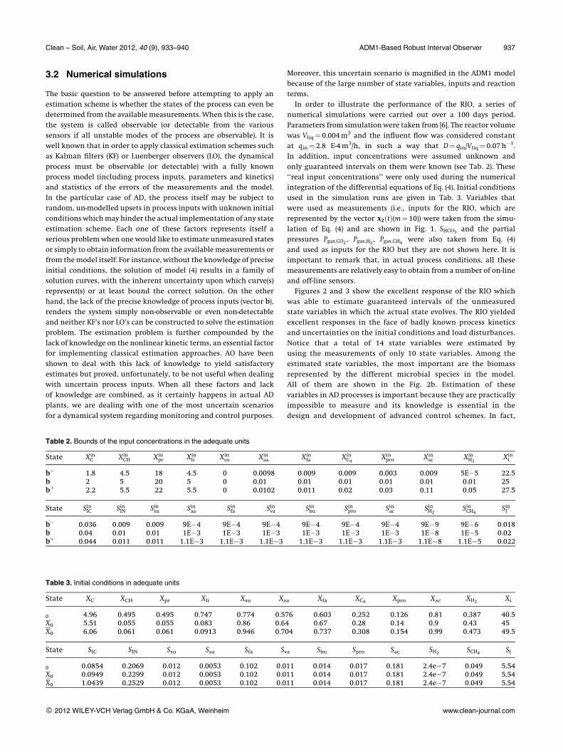
3.2 Numerical simulations

The basic question to be answered before attempting to apply an

estimation scheme is whether the states of the process can even be

determined from the available measurements. When this is the case,

the system is called observable (or detectable from the various

sensors if all unstable modes of the process are observable). It is

well known that in order to apply classical estimation schemes such

as Kalman filters (KF) or Luenberger observers (LO), the dynamical

process must be observable (or detectable) with a fully known

process model (including process inputs, parameters and kinetics)

and statistics of the errors of the measurements and the model.

In the particular case of AD, the process itself may be subject to

random, un-modelled upsets in process inputs with unknown initial

conditionswhichmay hinder the actual implementation of any state

estimation scheme. Each one of these factors represents itself a

serious problemwhen one would like to estimate unmeasured states

or simply to obtain information from the availablemeasurements or

from themodel itself. For instance, without the knowledge of precise

initial conditions, the solution of model (4) results in a family of

solution curves, with the inherent uncertainty upon which curve(s)

represent(s) or at least bound the correct solution. On the other

hand, the lack of the precise knowledge of process inputs (vector b),

renders the system simply non-observable or even non-detectable

and neither KF’s nor LO’s can be constructed to solve the estimation

problem. The estimation problem is further compounded by the

lack of knowledge on the nonlinear kinetic terms, an essential factor

for implementing classical estimation approaches. AO have been

shown to deal with this lack of knowledge to yield satisfactory

estimates but proved, unfortunately, to be not useful when dealing

with uncertain process inputs. When all these factors and lack

of knowledge are combined, as it certainly happens in actual AD

plants, we are dealing with one of the most uncertain scenarios

for a dynamical system regarding monitoring and control purposes.

Moreover, this uncertain scenario is magnified in the ADM1 model

because of the large number of state variables, inputs and reaction

terms.

In order to illustrate the performance of the RIO, a series of

numerical simulations were carried out over a 100 days period.

Parameters from simulationwere taken from [6]. The reactor volume

was Vliq¼ 0.004m3 and the influent flow was considered constant

at qin¼ 2.8 E-4m3/h, in such a way that D¼ qin/Vliq¼ 0.07h�1.

In addition, input concentrations were assumed unknown and

only guaranteed intervals on them were known (see Tab. 2). These

‘‘real input concentrations’’ were only used during the numerical

integration of the differential equations of Eq. (4). Initial conditions

used in the simulation runs are given in Tab. 3. Variables that

were used as measurements (i.e., inputs for the RIO, which are

represented by the vector x2ðtÞ(m¼ 10)) were taken from the simu-

lation of Eq. (4) and are shown in Fig. 1. SHCO3 and the partial

pressures Pgas;CO2, Pgas;H2

, Pgas;CH4were also taken from Eq. (4)

and used as inputs for the RIO but they are not shown here. It is

important to remark that, in actual process conditions, all these

measurements are relatively easy to obtain from a number of on-line

and off-line sensors.

Figures 2 and 3 show the excellent response of the RIO which

was able to estimate guaranteed intervals of the unmeasured

state variables in which the actual state evolves. The RIO yielded

excellent responses in the face of badly known process kinetics

and uncertainties on the initial conditions and load disturbances.

Notice that a total of 14 state variables were estimated by

using the measurements of only 10 state variables. Among the

estimated state variables, the most important are the biomass

represented by the different microbial species in the model.

All of them are shown in the Fig. 2b. Estimation of these

variables in AD processes is important because they are practically

impossible to measure and its knowledge is essential in the

design and development of advanced control schemes. In fact,

Table 3. Initial conditions in adequate units

State XC XCH Xpr Xli Xsu Xaa Xfa XC4 Xpro Xac XH2 Xi

0 4.96 0.495 0.495 0.747 0.774 0.576 0.603 0.252 0.126 0.81 0.387 40.5X0 5.51 0.055 0.055 0.083 0.86 0.64 0.67 0.28 0.14 0.9 0.43 45X0 6.06 0.061 0.061 0.0913 0.946 0.704 0.737 0.308 0.154 0.99 0.473 49.5

State SIC SIN Ssu Saa Sfa Sva Sbu Spro Sac SH2 SCH4 SI

0 0.0854 0.2069 0.012 0.0053 0.102 0.011 0.014 0.017 0.181 2.4e�7 0.049 5.54X0 0.0949 0.2299 0.012 0.0053 0.102 0.011 0.014 0.017 0.181 2.4e�7 0.049 5.54X0 1.0439 0.2529 0.012 0.0053 0.102 0.011 0.014 0.017 0.181 2.4e�7 0.049 5.54

Table 2. Bounds of the input concentrations in the adequate units

State XinC Xin

CH Xinpr Xin

li Xinsu Xin

aa Xinfa Xin

C4Xinpro Xin

ac XinH2

Xini

b� 1.8 4.5 18 4.5 0 0.0098 0.009 0.009 0.003 0.009 5E�5 22.5b 2 5 20 5 0 0.01 0.01 0.01 0.01 0.01 0.01 25bþ 2.2 5.5 22 5.5 0 0.0102 0.011 0.02 0.03 0.11 0.05 27.5

State SinIC SinIN Sinsu Sinaa Sinfa Sinva Sinbu Sinpro Sinac SinH2SinCH4

SinI

b� 0.036 0.009 0.009 9E�4 9E�4 9E�4 9E�4 9E�4 9E�4 9E�9 9E�6 0.018b 0.04 0.01 0.01 1E�3 1E�3 1E�3 1E�3 1E�3 1E�3 1E�8 1E�5 0.02bþ 0.044 0.011 0.011 1.1E�3 1.1E�3 1.1E�3 1.1E�3 1.1E�3 1.1E�3 1.1E�8 1.1E�5 0.022



only volatile suspended solids readings are related to the total

concentration of biomass with no identification of a particular

bacterial species. Recent improvements in the techniques for

the on-line monitoring of fermentation processes (such as

molecular biology) are beginning to overcome these problems

but unfortunately for AD process, these are still time consuming

and expensive.

Figure 3a and b depict the estimation results for XC and SIC,

respectively. It is clear in these figures that the SIC and XC bounds

were closer to their respective model prediction values than

other states and practically there were no significant differences

between the estimated states and the actual values. On one

hand, this is an effect of the selection of bounds on both, the

initial conditions and process inputs. Certainly, as the selected

bounds are reduced, so are the estimated interval. However, even

when the robustness and stability of the RIO is independent of

these factors, as it has been rigorously proved in [8, 9, 11–14],

the respective values shown in Tabs. 2 and 3 were chosen to show

in practice these features. In all the cases, the uncertainty interval

was chosen as �10% of the central value, except for Xinaa, X

inC4, Xin

pro,

Xinac and Xin

H2. In the case of Xin

aa the RIO showed to be very sensitive

to uncertainties on process inputs and thus, the uncertainty

interval was reduced to �2% of the central value. Nevertheless,

in the case of XinC4, Xin

pro, Xinac and Xin

H2the percentage �10% of the

central was not enough for showing a significant difference in

the estimated interval and thus, this allowed us to increase

considerably the uncertainty range of process input as it is

shown in Tab. 1. Nevertheless, the accuracy on the estimation

provided by the RIO is also a function of the stoichiometric/yield

coefficients [13, 14], and then potential users should take

Figure 1. Measured states (from model).

Figure 2. Actual (dash-dot) state variables (from model) as well as lowerand upper estimated bounds (solid) given by the RIO: (a) Concentration ofproteins, lipids and carbohydrates. (b) Concentration of microorganismspecies.



precautions before attempting to implement the proposed RIO

scheme in actual AD processes. It is also important to mention

that the convergence properties of RIO presented in this paper

cannot be modified by the user as they depend on the hydro-

dynamic properties of the system which are represented in the

matrix A by the dilution rate D [1, 13, 14]. However, since the basic

structure of the RIO is the AO, one could derive an AAO as in [17]

in order to improve its convergence properties. Finally, notice

that the robustness against uncertainties on initial conditions is

especially relevant because they are far away of the final steady

state. This means that the RIO was able to provide estimates of the

unmeasured variables even in the transitory state, which add an

extra robustness feature to the application of the RIO in WWTP

in general and in AD processes in particular, where the steady

state is rarely achieved.

3.3 Concluding remarks

In this contribution, a RIO was proposed for an anaerobic process

described by ADM1, whose behaviour is described by a highly non-

linear and high dimension dynamic system. This observer was satis-

factorily tested via numerical simulations. Such simulations were

carried out with typical but highly uncertain operational conditions

close to those used in a real AD plant. The RIO exhibited excellent

convergence and stability properties, and predicted correctly

the dynamical intervals where the unmeasured states actually

evolve under unknown input concentrations, uncertainties on

initial conditions and a full ignorance of the kinetic terms.

Acknowledgments

This publication is one of the results of the Regional Network Latin

America of the global collaborative project ‘‘EXCEED – Excellence

Center for Development Cooperation – Sustainable Water

Management in Developing Countries’’ consisting of 35 universities

and research centres from 18 countries on 4 continents. The authors

highly acknowledge the support of German Academic Exchange

Service DAAD for taking part in this EXCEED project.

The authors have declared no conflicts of interest.

References

[1] D. Dochain, P. A. Vanrolleghem, Dynamical Modelling and Estimation inWastewater Treatment Processes, IWA Publishing, London, UK 2001.

[2] G. Olsson, M. K. Nielsen, Z. Yuan, A. Lynggaard-Jensen, J. P. Steyer,Instrumentation, Control and Automation in Wastewater Systems, IWAScientific Technical Report, No 15, IWA Publishing, London, UK2005.

[3] J. P. Steyer, O. Bernard, D. Batstone, I. Angelidaki, Lessons Learntfrom 15 Years of ICA in Anaerobic Digesters,Water Sci. Technol. 2006,53 (4), 25–33.

[4] R. Antonelli, J. Harmand, J. P. Steyer, A. Astolfi, Set-Point Regulationof an Anaerobic Digestion, Process with Bounded Output Feedback,IEEE Trans. Control Syst. Technol. 2003, 11 (4), 495–504.

[5] O. Bernard, Z. Hadj-Sadok, D. Dochain, A. Genovesi, J. P. Steyer,Dynamical Model Development and Parameter Identification forAnaerobicWastewater Treatment Process, Biotechnol. Bioeng. 2001, 75(4), 424–438.

[6] D. J. Batstone, J. Keller, I. Angelidaki, S. Kalyuzhnui, S. G.Pavlostathis, A. Rozzi, W. Sanders, et al., Anaerobic Digestion ModelNo.1 (ADM1), Scientific and Technical Report No. 13, IWA Publishing,London, UK 2002.

[7] D. J. Batstone, J. Keller, I. Angelidaki, S. Kalyuzhnui, S. G.Pavlostathis, A. Rozzi, W. Sanders, et al., The IWA AnaerobicDigestion Model No.1 (ADM1), Water Sci. Technol. 2002, 45, 65–73.

[8] J. L. Gouze, A. Rapaport, M. Z. Hadj-Sadok, Interval Observersfor Uncertain Biological Systems, Ecol. Model. 2000, 133 (1–2),45–56.

[9] V. Alcaraz-Gonzalez, J. Harmand, A. Rapaport, J. P. Steyer, V.Gonzalez-Alvarez, C. Pelayo-Ortiz, Software Sensors for UncertainWastewater Treatment Processes: A New Approach Based onInterval Observers, Water Res. 2002, 36 (10), 2515–2524.

[10] E. Aguilar-Garnica, D. Dochain, V. Alcaraz-Gonzalez, V. Gonzalez-Alvarez, A Multivariable Control Scheme in a Two-Stage AnaerobicDigestion System Described by Partial Differential Equations,J. Process Control 2009, 19, 1324–1332.

[11] A. Rapaport, J. Harmand, Robust Regulation of a Bioreactor ina Highly Uncertain Environment, in IFAC-International Workshopon Decision and Control in Waste Bio-Processing, Narbonne, France1998.

[12] A. Rapaport, J. Harmand, Robust Regulation of a Class of PartiallyObserved Nonlinear Continuous Bioreactors, J. Process Control 1999,12 (2), 291–302.

[13] V. Alcaraz-Gonzalez, V. Gonzalez-Alvarez, Robust nonlinear observ-ers for bioprocesses: Application to wastewater treatment, inSelected Topics in Dynamics and Control of Chemical and BiologicalProcesses (Eds: H. O. Mendez-Acosta, R. Femat, V. Gonzalez-Alvarez),Springer, Berlin 2007, pp. 125–172.

Figure 3. Actual (dash-dot) state variables (from model) as well as lowerand upper estimated bounds (solid) given by the RIO: (a) Particulates. (b)Inorganic carbon and soluble nitrogen.



[14] V. Alcaraz-Gonzalez, J. Harmand, A. Rapaport, J. P. Steyer, V.Gonzalez-Alvarez, C. Pelayo-Ortiz, Application of a RobustInterval Observer to an Anaerobic Digestion Process, Dev. Chem.Eng. Miner. Process. 2005, 13 (3–4), 267–278.

[15] H. L. Smith,Monotone Dynamical Systems. An introduction to the Theory ofCompetitive and Cooperative Systems (AMS Mathematical Surveys andMonographs), American Mathematical Society, Providence, RI 1995,Chapter 1, pp. 1–13.

[16] C. Rosen, U. Jeppsson, Description of the ADM1 for BenchmarkSimulations, Technical Report, Department of Industrial ElectricalEngineering and Automation (IEA), Lund University, Lund, Sweden2006.

[17] V. Alcaraz-Gonzalez, R. Salazar-Pena, V. Gonzalez-Alvarez, J. L.Gouze, J. P. Steyer, A Tunable Multivariable Non-Linear RobustObserver for Biological Systems, C. R. Biol. 2005, 328 (4), 317–325.



adm1-based robust interval observer for anaerobic digestion processes

Documents