Electrical Engineering 42/100 Department of Electrical Engineering and Computer SciencesSummer 2012 University of California, Berkeley

First-Order RC and RL Transient Circuits

When we studied resistive circuits, we never really explored the concept of transients, or circuit responses tosudden changes in a circuit. That is not to say we couldn’t have done so; rather, it was not very interesting, aspurely resistive circuits have no concept of time. That is, if we consider an arbitrary switch action in a resistivecircuit, we would simply apply our circuit analysis techniques to the circuit before and after the switch action.The new values will likely be different from the old ones, but there is no notion of how we got to the new valuesfrom the old ones. We simply assume an instantaneous, discontinuous jump.

Not so with circuits containing capacitors and inductors. These devices have i-v characteristics which containexplicit dependencies on time. The voltage or current of one of these devices depends not only on some otherquantity at this moment, but also on a quantity in the past. Such dependencies are captured through thederivative and integral operators. Hence we cannot have instantaneous changes in certain quantities.

iC(t) = CdvC(t)

dt(1)

vL(t) = LdiL(t)

dt(2)

The Canonical Charging and Discharging RC Circuits

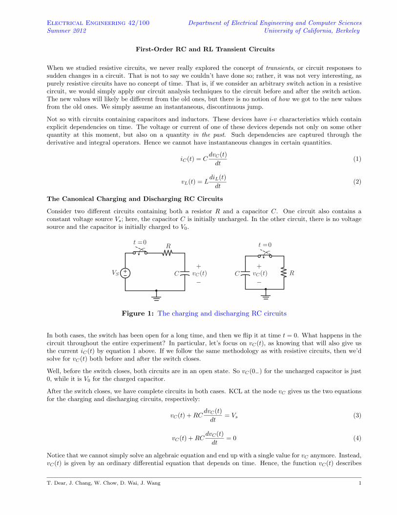
Consider two different circuits containing both a resistor R and a capacitor C. One circuit also contains aconstant voltage source Vs; here, the capacitor C is initially uncharged. In the other circuit, there is no voltagesource and the capacitor is initially charged to V0.

+

R

CVS vC ( t)+

−C vC ( t)

+

−R

t = 0 t = 0

Figure 1: The charging and discharging RC circuits

In both cases, the switch has been open for a long time, and then we flip it at time t = 0. What happens in thecircuit throughout the entire experiment? In particular, let’s focus on vC(t), as knowing that will also give usthe current iC(t) by equation 1 above. If we follow the same methodology as with resistive circuits, then we’dsolve for vC(t) both before and after the switch closes.

Well, before the switch closes, both circuits are in an open state. So vC(0−) for the uncharged capacitor is just0, while it is V0 for the charged capacitor.

After the switch closes, we have complete circuits in both cases. KCL at the node vC gives us the two equationsfor the charging and discharging circuits, respectively:

vC(t) +RCdvC(t)

dt= Vs (3)

vC(t) +RCdvC(t)

dt= 0 (4)

Notice that we cannot simply solve an algebraic equation and end up with a single value for vC anymore. Instead,vC(t) is given by an ordinary differential equation that depends on time. Hence, the function vC(t) describes

T. Dear, J. Chang, W. Chow, D. Wai, J. Wang 1

the transient response after the switch closes; it is not instantaneous. The other observation you should make isthat the equations for both cases are strikingly similar. The task that is now left to us is to solve these ODEs.

Solving First-Order Ordinary Differential Equations

The general form of the first-order ODE that we are interested in is the following:

x(t) + τdx(t)

dt= f(t) (5)

Here, the time constant τ and the forcing function f(t) are given, and we are solving for x(t). ODE theory tellsus that there are two separate solutions to the above equation, and the general solution is the superposition ofthe two. First we consider the homogeneous equation:

x(t) + τdx(t)

dt= 0 (6)

Notice that the only difference from the original equation 5 is that the RHS is 0. The solution to this can befound by substitution or direct integration. This is known as the complementary solution, or the natural responseof the circuit in the absence of any active sources:

xc(t) = Ke−t/τ (7)

Clearly, the natural response of a circuit is to decay to 0. Hence, without any sources present, any capacitor(inductor) will eventually discharge until it has no voltage (current) left across it.

The other solution of the ODE is the particular solution or forced response xp(t), due to the forcing function.Unlike the complementary solution, we have no general formula for finding this. The only headway we have isthat xp(t) takes the same form as that of f(t). This must hold as xp(t) appears on the LHS of the ODE, alongwith its derivative, and their linear combination must equal f(t). Thus, one would assume a solution xp(t) ofthe form of f(t) plus its derivative.

Some examples of particular solutions are shown below. Notice that we always assign arbitrary constants toeach term to preserve generality.

• If f(t) is constant, e.g. f(t) = 1, assume xp(t) = A

• If f(t) is linear, e.g. f(t) = 3t, assume xp(t) = At+B

• If f(t) is quadratic, e.g. f(t) = −2t2 + 5t, assume xp(t) = At2 +Bt+ C

• If f(t) is exponential, e.g. f(t) = 5e−ωt, assume xp(t) = Ae−ωt

• If f(t) is sinusoidal, e.g. f(t) = 7 cosωt, assume xp(t) = A sinωt+B cosωt

The list goes on and on. The majority of the circuits you will see here, however, only involve DC sources, whichmeans f(t) will almost always be constant. The final step is to add both the complementary and particularsolutions together for the complete solution to the original ODE.

x(t) = xc(t) + xp(t) (8)

Because we know that xc(t) worked due to it evaluating the LHS of the ODE to 0, we can add this to xp(t),and the subsequent function x(t) should stil satisfy the ODE. What we gained here was an even more generalsolution for the ODE. Finally, we still have a whole bunch of constants floating around. These we can solve forby using the initial and final conditions of the circuit and plugging them into the function x(t).

Note that you will not always have the opportunity to use final conditions, as you do not always necessarily knowwhat they are. For DC sources, it is correct to apply DC steady-state analysis if you are simply solving for x(∞).However, we would not be able to infer the final condition of a circuit with a non-DC source. In addition, whenusing initial conditions you must take care that your assumptions make physical sense. For example, voltagecannot change instantaneously across a capacitor, but no such restriction exists for the current.

An alternative way to solve for the constants is to plug the solution x(t) back into the original ODE. This wouldyield another equation to use in solving for the constants.

T. Dear, J. Chang, W. Chow, D. Wai, J. Wang 2

Back to the RC Circuits

Using our handy guide above, we conclude that the solution (both complementary and particular) to the ODEs3 and 4 looks like this:

vC(t) = Ke−t/RC +A (9)

The charging case gives us boundary conditions vC(0) = 0, as we know the voltage value immediately beforethe switch closes, and vC(∞) = Vs, as the capacitor becomes an open circuit at DC steady-state and causes allof the source voltage to appear across it. Using these two conditions, we obtain the solution for the chargingcapacitor:

vC(t) = Vs(1− e−t/RC) (10)

On the other hand, the discharging capacitor has boundary conditions vC(0) = V0 and vC(∞) = 0, since weexpect the capacitor to have completely discharged after a long time. Plugging these in and solving for constantsthus gives us the discharging solution:

vC(t) = V0e−t/RC (11)

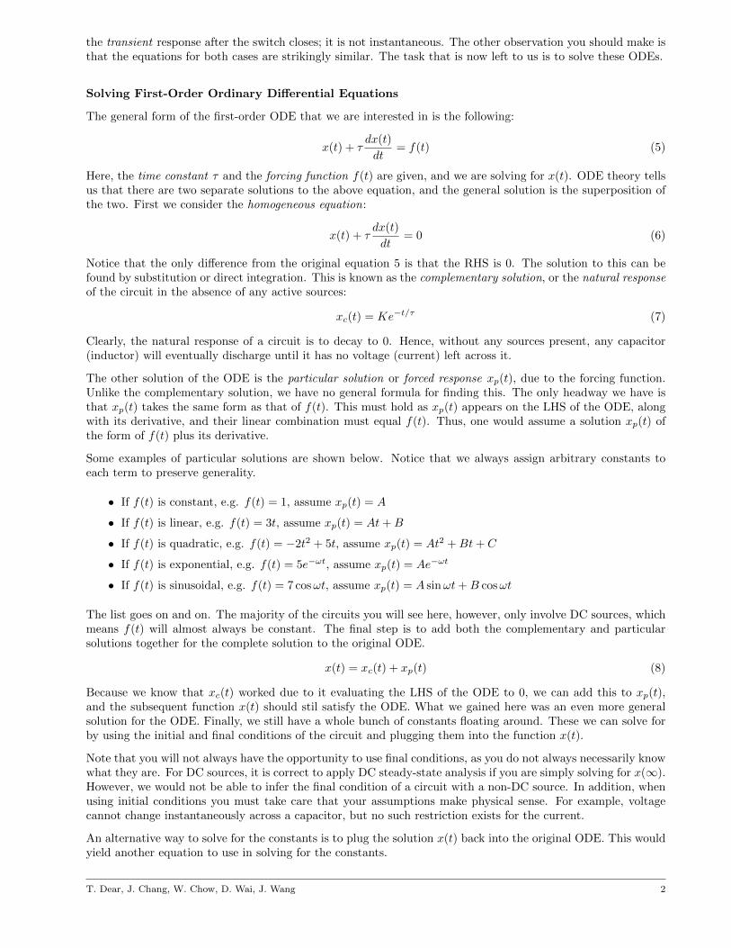
We thus conclude that the first-order transient behavior of RC (and RL, as we’ll see) circuits is governed bydecaying exponential functions. Instead of changing immediately, it takes some time for the charge on a capacitorto move onto or off the plates. This exponential behavior can also be explained physically.

In the charging case, the voltage initially rises quickly because there is little charge on the capacitor to opposethe further piling on of charge onto the plate. As the voltage increases, however, it becomes harder for morecharges to get onto the plates, hence leading to the exponential slowdown toward the final value, which is solelydriven by our voltage source forcing function.

In the discharging case, the voltage initially falls quickly. In the absence of other driving forces, the initialbuildup on the capacitor pushes the charge off at a greater rate. But as the voltage decreases, there is less“force” driving the charges off, hence leading to an exponential slowdown.

t

vC ( t)

τ

V0Vs

0.63Vs

0.37V0

t

vC ( t)

τ

Figure 2: Solutions to the charging and discharging RC circuits

Notice in both cases that the time constant is τ = RC. In other words, how fast or how slow the (dis)chargingoccurs depends on how large the resistance and capacitance are. One time constant gives us e−τ/τ = e−1 ≈ 0.37,which translates to vC(τ) = 0.63Vs and vC(τ) = 0.37V0 in the charging and discharging cases, respectively. Sowe say that the circuit is 63% toward its final value after about one time constant. Although these exponentialsasymptotically approach these final values and never exactly reach it, we can pretty much approximate thatthey do so after about three time constants. At that point, we have vC(3τ) = 0.95Vs and vC(3τ) = 0.05V0 foreach of the two cases.

Lastly, what if we had wanted to find another quantity, like the current iC(t)? Since we have the voltage, it is asimple matter to use equation 1 and differentiate the voltage to obtain it. The other option could have been tosolve for it initially without solving for voltage, for example by writing a KVL loop instead. For the dischargingcase, we would get the following equation:

RiC(t) +1

C

∫iC(t)dt = 0 (12)

T. Dear, J. Chang, W. Chow, D. Wai, J. Wang 3

While this is not an ODE, recall that we can differentiate the equation and rearrange to obtain

iC(t) +RCdiC(t)

dt= 0 (13)

which is exactly identical to the equation for the voltage. So we can assume the solution form iC(t) = Ke−t/τ

and solve for the constant as before. However, note that the initial condition is not 0! The current was obviously0 right before the switch closed, but this tells us nothing about its value immediately afterward. In fact, theinitial current is given by Ohm’s law across the resistor, since the capacitor’s voltage appears across it. Hencethe initial current should be i(0+) = V0/R, which is obviously discontinuous from its previous value.

If we differentiate 11 directly to find iC(t), we have that the solution should be

iC(t) =V0Re−t/RC (14)

which agrees with our observation above.

RL Circuits

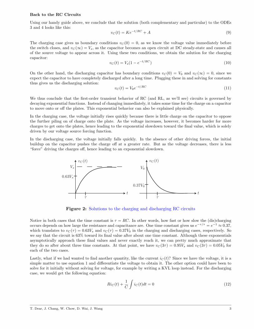
First-order circuits with inductors can be analyzed in much the same way. Consider the “charging” and “dis-charging” RL circuits below.

I S R L i L ( t) I S RL i L ( t)

t = 0t = 0

Figure 3: The “charging” and “discharging” RL circuits

While the notion of charging an inductor doesn’t really make sense, one can think of this in terms of current.In DC steady-state, inductors act as shorts and allow any current to flow through them, but inductors opposeimmediate changes in current and introduce delays between the initial and final currents. Again, these timetransient responses are given by decaying exponentials. First note that we can derive KVL equations as follows:

iL(t) +L

R

diL(t)

dt= IS (15)

iL(t) +L

R

diL(t)

dt= 0 (16)

Aside from the time constant, these equations are exactly the same as those for the voltage in a RC circuit.Furthermore, the boundary conditions are analogous; in the charging case, iL(0) = 0 and iL(∞) = IS , while fordischarging we have iL(0) = IS and iL(∞) = 0. The solutions to the ODEs 15 and 16 are just

iL(t) = IS(1− e−t/τ ) (17)

iL(t) = ISe−t/τ (18)

All of the analyses that we applied to RC circuits can be applied to RL circuits as well, the only differences beingthat we are dealing with current and that the time constant is τ = L

R . Physically, the inductor in the first circuitoriginally had no current flowing through it, but it must eventually end up as a short-circuit in DC steady-state.So it takes some time for the device to “charge up” and allow current to increase to its final value. In the secondcircuit, the inductor originally had IS flowing through it, since is a short after being in DC steady-state for along time. Even though it becomes disconnected from the current source, it tries to keep some current going fora while until it decays to 0.

T. Dear, J. Chang, W. Chow, D. Wai, J. Wang 4

Again, it is important to note that only current is restricted to not changing instantaneously; no such conditionholds for the voltage across an inductor. As with a capacitor, this also turns out to be discontinuous; it is anexercise left to the reader to show that the voltage vL(t) in each case is actually given by

vL(t) = RISe−t/τ (19)

vL(t) = −RISe−t/τ (20)

Circuits with Multiple Resistors, Sources, and Switches

While the examples that we analyzed were simple and cute, RC and RL circuits can quickly get ugly, as withresistive and amplifier circuits. However, the same techniques that we’ve used here can be extended to anyfirst-order circuit.

Look back at the RC and RL circuit diagrams. The ODEs that we obtained only apply to these circuit con-figurations, but do they look familiar? Indeed, the capacitor sees a Thevenin circuit, while the inductor seesa Norton circuit! Since we know that any linear circuit has these equivalent circuits, this gives an alternativemethod for writing down the ODE. Given any circuit with a capacitor or inductor, we can reduce the rest ofthe circuit down to a Thevenin or Norton equivalent. Thus, for any arbitrary RC or RL circuit with a singlecapacitor or inductor, the governing ODEs are

vC(t) +RThCdvC(t)

dt= vTh(t) (21)

iL(t) +L

RN

diL(t)

dt= iN (t) (22)

where the Thevenin and Norton circuits are those as seen by the capacitor or inductor.

Before getting too excited, do note that this technique is rarely employed to its fullest extent, since we neveractually require the entire governing ODE. The only pieces that we need from it are the time constant and theform of the forcing function. We can usually guess the latter by simple inspection of the circuit sources. Inaddition, it is often easier to just use analysis techniques like KCL or KVL to write ODEs for vC(t) and iL(t)directly, from which we can also find the time constant.

The greatest advantage that this technique provides us is the ability to find the time constant without writingdown any ODEs, which then gives us the complementary solution. This is especially useful when the circuitcontains no dependent sources. Recall that in this case RTh = Req with all sources zeroed out. This is often thequicker way to solve for the time constant, as we would just find Req as seen by the capacitor or inductor.

Consider the following example, which exemplifies the title of this section.

+ +10 V

10 kΩ

vx

4vx

1µF

10 kΩ

vC ( t)

+

−

t = 0 t = 0 .1

+ −

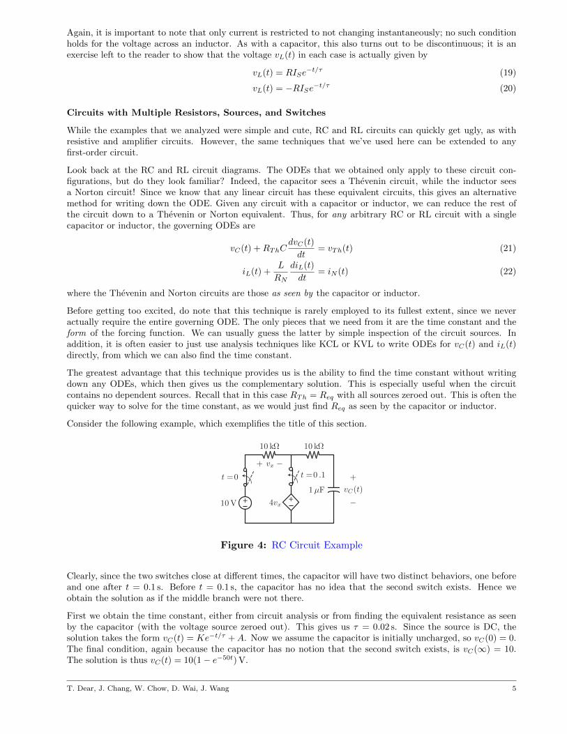
Figure 4: RC Circuit Example

Clearly, since the two switches close at different times, the capacitor will have two distinct behaviors, one beforeand one after t = 0.1 s. Before t = 0.1 s, the capacitor has no idea that the second switch exists. Hence weobtain the solution as if the middle branch were not there.

First we obtain the time constant, either from circuit analysis or from finding the equivalent resistance as seenby the capacitor (with the voltage source zeroed out). This gives us τ = 0.02 s. Since the source is DC, thesolution takes the form vC(t) = Ke−t/τ +A. Now we assume the capacitor is initially uncharged, so vC(0) = 0.The final condition, again because the capacitor has no notion that the second switch exists, is vC(∞) = 10.The solution is thus vC(t) = 10(1− e−50t) V.

T. Dear, J. Chang, W. Chow, D. Wai, J. Wang 5

+10 V

10 kΩ

1µF

10 kΩ

vC ( t)

+

−

t = 0

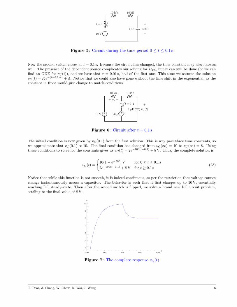
Figure 5: Circuit during the time period 0 ≤ t ≤ 0.1 s

Now the second switch closes at t = 0.1 s. Because the circuit has changed, the time constant may also have aswell. The presence of the dependent source complicates our solving for RTh, but it can still be done (or we canfind an ODE for vC(t)), and we have that τ = 0.01 s, half of the first one. This time we assume the solutionvC(t) = Ke−(t−0.1)/τ +A. Notice that we could also have gone without the time shift in the exponential, as theconstant in front would just change to match conditions.

+ +10 V

10 kΩ

vx

4vx

1µF

10 kΩ

vC ( t)

+

−

t = 0 .1

+ −

Figure 6: Circuit after t = 0.1 s

The initial condition is now given by vC(0.1) from the first solution. This is way past three time constants, sowe approximate that vC(0.1) ≈ 10. The final condition has changed from vC(∞) = 10 to vC(∞) = 8. Usingthese conditions to solve for the constants gives us vC(t) = 2e−100(t−0.1) + 8 V. Thus, the complete solution is

vC(t) =

10(1− e−50t) V for 0 ≤ t ≤ 0.1 s

2e−100(t−0.1) + 8 V for t ≥ 0.1 s(23)

Notice that while this function is not smooth, it is indeed continuous, as per the restriction that voltage cannotchange instantaneously across a capacitor. The behavior is such that it first charges up to 10 V, essentiallyreaching DC steady-state. Then after the second switch is flipped, we solve a brand new RC circuit problem,settling to the final value of 8 V.

0.00 0.05 0.10 0.15 0.20t

4

5

6

7

8

9

10

vC

Figure 7: The complete response vC(t)

T. Dear, J. Chang, W. Chow, D. Wai, J. Wang 6