random variables and probability; normal distribution

Chapter 2Random Variables and Probability;Normal Distribution

2.1 Probability and Random Variables

We say that a phenomenon is random if, on the basis of our best knowledge, we can-not exactly predict its result. What really happens is only one of many possibilities.In every day life we meet random results of lotteries, a non-predictable dispersionof gun shots at a target or a random travel time through a crowded city.

An intuitively understandable idea of random phenomena can be formalized bythe concept of random events and probability. Using formal definitions, we say thatthe random event (a collection of sample points) is a result of some random phe-nomena, and its probability is the chance that this phenomenon will occur, expressedby a number from the interval [0,1].

Example 2.1 (An unbiased coin flipping) During an experiment of a single flip of anunbiased coin, two results are possible: the occurrence of heads and the occurrenceof tails. Both results are random events. The probability of heads and the probabilityof tails are equal and they are 1/2.

In this example we can say that the set of all possible results of the experimenthas two elements (occurrence of heads and occurrence of tails). We interpret theprobabilities of occurrence of these elementary events in the following way: if werepeat flipping the coin a sufficient number of times, then the number of occurrencesof heads (or, equivalently, the number of occurrences of tails) divided by the num-ber of flips will tend to 1/2. This is the so-called frequency interpretation of theprobability.

Example 2.2 (Dice casting) During an experiment of a single cast of an unbiaseddie, six results are possible: the occurrence of a face with n = 1, 2, 3, 4, 5, or 6 spots.Then the set of the results (elementary events, sample points) contains six elements.The probability of each event (the occurrence of a face with n spots) equals 1/6.This means that if the number of casts tends to infinity, then the following ratio:

Z. Kotulski, W. Szczepinski, Error Analysis with Applications in Engineering,Solid Mechanics and Its Applications 169,DOI 10.1007/978-90-481-3570-7_2, © Springer Science+Business Media B.V. 2010

15

http://dx.doi.org/10.1007/978-90-481-3570-7_2

16 2 Random Variables and Probability; Normal Distribution

number of casts, when n spots occurred

total number of casts

tends to 1/6, for n = 1, 2, 3, 4, 5, and 6.

The expected outcome of the experiment described in Example 2.2 may be morecomplicated than the occurrence of a fixed number of spots. For example, we canask: What is the probability that the single cast results in a face with an even numberof spots? What is the probability that we will see a face which has more than 4 spots?Of course, we can easily deduce that in the first case the probability is 1/2 and inthe second one 1/3.

The above examples show that it is conceptually easy to define an event andthe probability of an event if the number of possible outcomes of the experiment(e.g., coin flipping or dice casting) is finite and the outcome of each result is equallyprobable. In such a case, the probability of some event is defined as the frequencyof occurrences of this event when the number of experiments tends to infinity.

In some situations, we can introduce another definition of probability. If the setof results of an experiment is infinite but it is contained in some set on a plane (alter-natively: in 3-dimensional space, on a straight line, etc.), then the probability has ageometrical interpretation. The probability of a certain outcome of an experiment isthe ratio of the area of the subset corresponding to these results, to the area of the setcorresponding to all possible results of the experiment. The geometrical definitionof probability has some limitations: the results of the experiment must be located ina bounded set on the plane and, moreover, they must be evenly distributed over thisset.

The definitions of an event and the probability of an event used today have theirorigin in measure theory. The fundamental object of probability theory is the prob-ability space. A probability space is defined by the triad (Ω,�,P ), where Ω is thesample space containing all elementary events (sample points), � is the σ -algebraof Borel subsets of the sample space Ω containing all possible events (elementaryand compound), and P is a (probability) measure defined on �.

We will now comment on the above definitions. Elementary events ω (beingelements of the sample space Ω) are results of some experiment, mutually exclud-ing each other; this means that only one elementary event can be the result of theexperiment. Generally, (compound) events in an experiment are elements of the σ -algebra �. Occurrence of an event A can be the result of several elementary events;knowing the outcome of an experiment we are able to decide if the event A oc-curred. The probability measure P or, simply, the probability, has the property thatit is equal to 1 for the certain event (the whole sample space Ω , that is, the eventthat the experiment had some outcome). Certainly, the probability of the impossibleevent (the empty set ∅) is zero.

Example 2.3 (An unbiased coin flipping, continuation) The probability space forthe experiment of a single fair coin flip is (Ω,�,P ), where: the sample space Ω isthe following 2-element set:

Ω = ({heads}, {tails});

2.1 Probability and Random Variables 17

the σ -algebra � consists of four elements: the empty set ∅, two 1-element sets, andthe whole sample space Ω :

� = (∅, {heads} , {tails} ,Ω) ;

the probability P is defined as:

P ({heads}) = 1

2, P ({tails}) = 1

2.

Example 2.4 (Dice casting, continuation) In the experiment of a single balanced diecast, the probability space is the following: the sample space Ω has 6 elements:

Ω = ({1 spot} , {2 spots} , {3 spots} , {4 spots} , {5 spots} , {6 spots}) ;

the σ -algebra � consists of the following elements: the empty set ∅, all subsets ofΩ containing 1, 2, 3, 4, and 5 elements and the whole sample space Ω :

� =⎛⎝

∅, 6 one-element subsets, 15 two-element subsets,20 three-element subsets, 15 four-element subsets,

6 five-element subsets, Ω

⎞⎠ ;

the probability P is defined as:

P ({1 spot}) = P ({2 spots}) = P ({3 spots})= P ({4 spots}) = P ({5 spots}) = P ({6 spots}) = 1

6.

The concept of randomness and probability presented here identifies events withsubsets of the sample space Ω, which are elements of the σ -algebra �. Therefore,we are able to perform on these events the operations analogous to the operations ofset theory. For two events A,B ∈ �, we can define the union A ∪ B (A or B hap-pens), intersection A ∩ B (A and B occur simultaneously), difference A\B (A oc-curs but B does not), etc. Probability, as we mentioned, is a measure; it has thefollowing properties:

0 ≤ P (A) ≤ 1, (2.1)

P (∅) = 0, P (Ω) = 1, (2.2)

P (A ∪ B) = P (A) + P (B) − P (A ∩ B) , (2.3)

and for a countable number of disjoint events Aj :

P

(⋃j

Aj

)=

∑j

P (Ai). (2.4)


In probability theory, it is very important to know the relationship betweenevents: their dependence or independence. We say that two events A and B areindependent if their probabilities satisfy the following condition:

P (A ∩ B) = P (A)P (B) , (2.5)

which means that the probability of the simultaneous occurrence of both events isequal to the product of probabilities of their separate occurrence. If condition (2.5)is not satisfied, the events A and B are dependent.

To know to what extent the events A and B are dependent, we can use the condi-tional probability P(A|B), which is defined as

P (A|B) = P (A ∩ B)

P (B). (2.6)

The quantity P(A|B), which is the probability of A conditioned on B , we un-derstand to be the probability of occurrence of A under the condition that B hasoccurred.

Using formula (2.5) in (2.6), we see that if events A and B are independent then

P (A|B) = P (A) . (2.7)

The concept of the conditional probability is strongly related to the definitionof complete probability. If we have some sequence of mutually excluding eventsBj , j = 1,2, . . . , n, Bk ∩Bl = ∅ for k �= l, satisfying additionally

⋃j Bj = Ω, then

the probability of any event A can be represented as

P (A) =∑j

P(A|Bj

)P

(Bj

). (2.8)

The last equation enables us to calculate the probability of some event A if weknow its probability under some additional conditions, that is, if we know that someevent Bj has occurred.

Example 2.5 (Dice casting, continuation) Consider the experiment of the die sin-gle cast and define two events: A, the outcome is a face with an even numberof spots, and B, the face with a number of spots greater than 4. We can verifywhether these two events are independent. Using the elementary events definedin Example 2.4 we find that the events are: A = ({2 spots}, {4 spots}, {6 spots}),B = ({5 spots}, {6 spots}), and their probabilities are: P(A) = 1

2 , P(B) = 13 .

The intersection of the events is: A ∩ B = ({6 spots}), and the probability ofintersection, P(A∩B) = 1

6 . It is seen that the events A and B satisfy condition (2.5),that is, they are independent.

If we replace the event B with a new one: B1—the number of spots is greater than5 (that is, B1 = ({6 spots}) and P(B1) = 1

6 ), then the intersection of the events isA ∩ B1 = ({6 spots}) and it is seen that the events A and B1 are dependent, becauseP(A)P (B1) = 1

12 and P(A ∩ B1) = 16 , so the condition (2.5) is not satisfied.

2.1 Probability and Random Variables 19

The description of results of experiments or observations of random phenomenain terms really existing in these processes is very complicated. To make the mod-eling of the processes more convenient we can introduce the concept of a randomvariable.

The real-valued function X(ω) defined on the sample space Ω of random eventsω is called a random variable if a pre-image1 A of every interval of real numbers ofthe form I = (−∞, x) is a random event (an element of the σ -algebra �).

Probability P describing properties of random events can also describe randomvariables. It is transferred from the σ -algebra of events to the space of real-valuedrandom variables by pre-images of the intervals I :

P (I) = P (ω such that X (ω) < x) . (2.9)

For a given sample space we can consider various random variables. Our choicedepends on the purpose of the modeling.

Example 2.6 (An unbiased coin flipping, continuation)

(a) Consider the experiment of a symmetric coin single flip. Assign number 1 tothe outcome of heads and number −1 to the outcome of tails. Such a randomvariable may be used for description of a random walk on a straight line. Westart from x = 0 and repeat the coin flipping. If the outcome is heads then weadd 1 to x, if tails, we subtract 1. After every trial the value of x is greater by 1 orsmaller by 1 than the value in the previous step. We repeat the trial many timesobtaining the x-coordinate of the walking particle in every step (see, e.g., [11]).

(b) Consider the same experiment. We assign number 1 to heads and number 0 totails. Repeating the trials many times and writing down the obtained numberswe generate random numbers in binary notation.

Analogously to the events, we can define independence of random variables.We will say that two random variables X and Y (defined on the probability space(Ω,�,P )) are independent if for all x1 ≤ x2 and y1 ≤ y2 the events of the form{ω : x1 ≤ X(ω) < x2} and {ω : y1 ≤ Y(ω) < y2} are independent.

The theorem concerning the complete probability (2.8) makes it possible to ap-ply in many technical problems the so-called conditioning technique. This methodis based on the procedure of decomposition of the initial complicated problem intoa number of tasks easy to solve when we assume certain conditions to be satisfiedwith a certain probability. Then the simplified problems are solved and, finally, thegeneral non-conditioned solution is obtained by averaging of the set of solutionswith respect to the assumed probability distribution. Such a technique lets us calcu-late the parameters (e.g., moments) or distributions of random variables in various

1Assume, we have a function X : Ω → R and let A be a subset of the set of real numbers R.The pre-image (or inverse image) A for the function X is a set B ⊂ Ω , containing all the elementsω ∈ Ω such that their image belongs to A, which means X(ω) ∈ A. In such a case we write:B = X−1(A).


engineering problems. The reader can find more about this technique in the papers[12, 13] or the textbook [20].

2.2 The Cumulative Distribution Function; the ProbabilityDensity Function

Most problems of the error calculus arising in technological applications concernthe analysis of random variables with continuous distributions. Random variablesof such a nature may assume any value from a certain range. The cumulative distri-bution function (or: probability distribution function) F(x) of any one-dimensionalrandom variable X is defined by the expression2:

F (x) = P (X < x) , (2.10)

which means that the cumulative distribution function is defined as a function, thevalue of which for a given x is equal to the probability of an event that the randomvariable X is smaller than the number x.

The cumulative distribution function is defined for all real numbers and it is anon-decreasing, continuous on the left, function. Moreover, for x tending to minusinfinity and plus infinity, it satisfies the following conditions:

F (−∞) = 0, F (∞) = 1. (2.11)

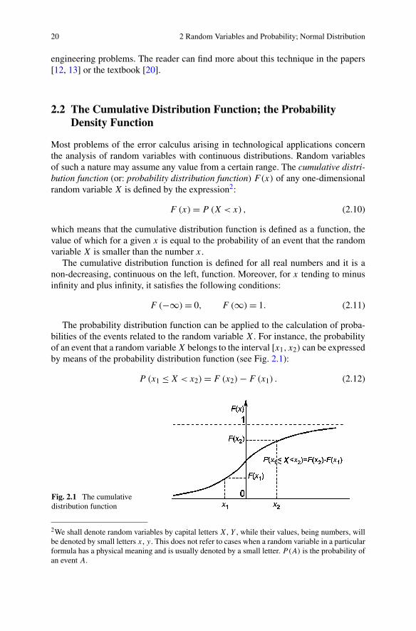
The probability distribution function can be applied to the calculation of proba-bilities of the events related to the random variable X. For instance, the probabilityof an event that a random variable X belongs to the interval [x1, x2) can be expressedby means of the probability distribution function (see Fig. 2.1):

P (x1 ≤ X < x2) = F (x2) − F (x1) . (2.12)

Fig. 2.1 The cumulativedistribution function

2We shall denote random variables by capital letters X, Y , while their values, being numbers, willbe denoted by small letters x, y. This does not refer to cases when a random variable in a particularformula has a physical meaning and is usually denoted by a small letter. P (A) is the probability ofan event A.

2.2 The Cumulative Distribution Function; the Probability Density Function 21

If the random variable X is discrete, that is, if it takes values from a finite (orcountable) set: {xj , j = 1,2, . . . ,N} (or {xj , j = 1,2, . . .}), then the cumulativedistribution function is discontinuous at these points and its jumps are equal to pj .

Moreover, the following equality holds:

P(X = xj ) = pj . (2.13)

Over the intervals of continuity, x ∈ [xj , xj+1), the cumulative distribution function

F(x) of the discrete random variable X is constant and equal to F(x) = ∑j

k=1 pk =Fj . An example of the cumulative distribution function of some discrete randomvariable is presented in Fig. 1.3.

The cumulative distribution function of a random variable with a continuous dis-tribution (the continuous random variable) may be expressed in the form of theintegral

F (x) =∫ x

−∞f (ξ) dξ. (2.14)

Function f (x) in (2.14) is referred to as the probability density function (or sim-ply probability density) of a random variable X. If the cumulative frequency distri-bution F(x) has a derivative at any point x, then such a derivative represents thedensity

f (x) = F ′ (x) . (2.15)

Since the cumulative distribution function describes the normalized probabilitymeasure (the probability of the certain event equals 1, which means that P(−∞ <

X < ∞) = 1) and is a non-decreasing function, the probability density functionf (x) has the following two properties:

A =∫ ∞

−∞f (x)dx = 1 (2.16)

and

f (x) ≥ 0. (2.17)

Thus, the area A between the graph of function f (x) and the horizontal axis x ofthe random variable is equal to unity.

The probability of any event that the variable X lies in the interval [x1, x2), whichis, that it will have the value P(x1 ≤ X < x2), is defined by the following:3

P (x1 ≤ X < x2) =∫ x2

x1

f (x) dx. (2.18)

The relation (2.18) is presented graphically in Fig. 2.2.

3For continuous distributions the probability that a random variable is located in a closed intervalis the same as in an interval closed on one side or as in an open interval. In (2.18) we decided tochoose an option of the interval closed on the left-hand side.


Fig. 2.2 The probabilitydensity function

Fig. 2.3 The quantilefunction, see (2.19)

The cumulative distribution function and the probability density function are notthe only functions characterizing a random variable. In some situations the inversedistribution function G(α), sometimes called the quantile function, is more conve-nient. For a given cumulative distribution function F(x), the quantile function isdefined as a function satisfying the following conditions:

x = G(α) = G(F (x)) ,

P (X ≤ G(α)) = α.(2.19)

This mutual relation between F(x) and G(α) is shown graphically in Fig. 2.3.In some applications of inspection theory and reliability theory, and also in some

problems of mathematical statistics, the survival function S(x) is useful. It is definedas the probability that the random variable X is greater than or equal to x:

S (x) = P (X ≥ x) = 1 − F (x) . (2.20)

2.3 Moments 23

More definitions of functions describing the properties of distributions of randomvariables can be found in handbooks dealing with probability theory or mathemati-cal statistics (see, e.g., [6, 7]).

2.3 Moments

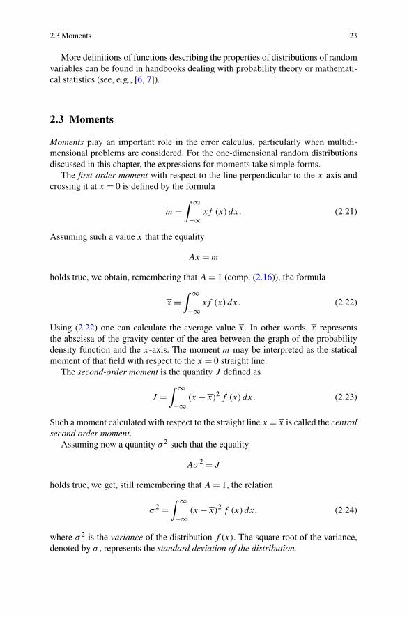
Moments play an important role in the error calculus, particularly when multidi-mensional problems are considered. For the one-dimensional random distributionsdiscussed in this chapter, the expressions for moments take simple forms.

The first-order moment with respect to the line perpendicular to the x-axis andcrossing it at x = 0 is defined by the formula

m =∫ ∞

−∞xf (x)dx. (2.21)

Assuming such a value x that the equality

Ax = m

holds true, we obtain, remembering that A = 1 (comp. (2.16)), the formula

x =∫ ∞

−∞xf (x)dx. (2.22)

Using (2.22) one can calculate the average value x. In other words, x representsthe abscissa of the gravity center of the area between the graph of the probabilitydensity function and the x-axis. The moment m may be interpreted as the staticalmoment of that field with respect to the x = 0 straight line.

The second-order moment is the quantity J defined as

J =∫ ∞

−∞(x − x)2 f (x) dx. (2.23)

Such a moment calculated with respect to the straight line x = x is called the centralsecond order moment.

Assuming now a quantity σ 2 such that the equality

Aσ 2 = J

holds true, we get, still remembering that A = 1, the relation

σ 2 =∫ ∞

−∞(x − x)2 f (x) dx, (2.24)

where σ 2 is the variance of the distribution f (x). The square root of the variance,denoted by σ , represents the standard deviation of the distribution.


Note that the quantity J given by formula (2.23) is, in terms used in engineeringapplications, the central inertia moment of the area between the graph of the func-tion f (x) and the x-axis. Using such an interpretation it is seen that the standarddeviation represents the so-called inertia radius of that field.

Of practical significance is also the average deviation d defined as

d =∫ ∞

−∞|x − x|f (x)dx. (2.25)

The concept of the average value x may be generalized; in this way we obtainmoments of order n, n = 0,1,2,3, . . . (called the ordinary moments of n-th order),defined as:

mn = xn =∫ ∞

−∞xnf (x) dx. (2.26)

In the new notation the average value (or: the mean value) is the moment oforder 1, namely m1.

The generalization of the variance are central moments of order n,n = 2,3,4, . . . , defined as:

μn =∫ ∞

−∞(x − m1)

n f (x) dx. (2.27)

Using definition (2.27) of the central moment we obtain the following relationbetween central moments and ordinary moments:

μn =∫ ∞

−∞(x − m1)

n f (x) dx

=∫ ∞

−∞

(n∑

j=0

(−1)j(

n

j

)xn−jm

j

1

)f (x)dx =

n∑j=0

(−1)j(

n

j

)mn−jm

j

1. (2.28)

In particular, the variance σ 2 can be represented as:

σ 2 = μ2 = m2 − m21. (2.29)

Except for the ordinary and central moments defined above, the absolute mo-ments (ordinary and central), that is, average values of powers of the absolute valueof x, can be defined by the following formulas:

mabsn =

∫ ∞

−∞|x|n f (x) dx, (2.30)

μabsn =

∫ ∞

−∞|x − m1|n f (x) dx. (2.31)

The most often used absolute moment is the average deviation d , defined by (2.25).

2.3 Moments 25

Let us remark that for even values of n, the absolute moments and moments(ordinary and central) are identical.

Existence of moments is strongly connected with integrability of the probabilitydensity function f (x) multiplied by some power of x. The condition of existenceof the moment of a given order n is the convergence of the integral

∫ ∞−∞ xnf (x)dx;

from the existence of the moment for a certain given range n = n0 we obtain themoments of lower orders. Therefore, the greatest n for which the moments exist iscalled the range of the random variable. In applications, the most often requiredassumption is that random variables have finite variances, that is, they are randomvariables of the second order.

Example 2.7 (The Cauchy distribution) The probability distribution with the prob-ability density function

f (x) = 1

πb{[(x − a)/b]2 + 1} (2.32)

and the cumulative distribution function

F (x) = 1

2+ 1

πarctan

(x − a

b

), (2.33)

is called the Cauchy distribution. It is an example of distribution which has no mo-ments (for each n = 1,2, . . . the integral

mn =∫ ∞

−∞xndx

πb{[(x − a)/b]2 + 1}is divergent).

Example 2.8 (The normal distribution) The probability distribution with the proba-bility density function

f (x) = 1√2πσ 2

exp

[−(x − m)2

2σ 2

](2.34)

is called the normal distribution. It is an example of distribution which has momentsof any order (for each n = 1,2, . . . the integral

mn =∫ ∞

−∞xn

√2πσ 2

exp

[−(x − m)2

2σ 2

]dx

is finite).

Remark 2.1 Assume that a certain random variable X has a finite mean value mX

and variance σ 2X . Then we can consider the new random variable X, defined as

X = X − mX


and called the centered random variable. This new random variable X (sometimescalled the fluctuation of X) has zero average (mean) value and a variance equal tothe variance of the original random variable X,

mX = 0, σ 2X

= σ 2X.

Such decompositions of random variables are often applied in error analysis. Inthe above procedure we interpret the random variable X as the result of a mea-surement with some random error, the mean value mX as the nominal value of themeasured quantity, and the fluctuation X as the random measurement error itself.

2.4 The Normal Probability Distribution

The normal distribution, called also the Gaussian distribution, plays a basic rolein error calculus. In most engineering applications random variables, such as smallerrors of measurements, small errors of positioning accuracy of certain mechanisms,e.g., robot manipulators or small deviations of magnitudes of certain parametersof objects in mass production, may be treated as those having normal probabilitydistribution. They are called normal (Gaussian) random variables.

In the normal distribution, the probability density function takes the form [2]:

f (x) = 1

σ√

2πexp

[− (x − x)2

2σ 2

], (2.35)

where x is the average value, comp. (2.22), and σ stands for the standard deviation(comp. (2.24)).

Introducing a new random variable

T = X − x

σ, (2.36)

which is called the normalized random variable corresponding to X (comp. [19]),we get another form of the probability density function,

φ (t) = 1√2π

exp

[− t2

2

]. (2.37)

Between the two forms of the probability density function, there exists the relation

f (x) = 1

σ√

2πexp

[− (x − x)2

2σ 2

]= 1

σφ (t) , t = x − x

σ. (2.38)

The numerical values of the normalized Gaussian distribution φ(t) may be cal-culated with the use of a computer or even a pocket calculator. Moreover, they are

2.4 The Normal Probability Distribution 27

Table 2.1 The probability density function φ(t) of the normalized Gaussian distribution

t 0 2 4 6 8

0.0 0.3989 0.3989 0.3986 0.3982 0.3977

0.1 0.3970 0.3961 0.3951 0.3939 0.3925

0.2 0.3910 0.3894 0.3876 0.3857 0.3836

0.3 0.3814 0.3790 0.3765 0.3739 0.3712

0.4 0.3683 0.3653 0.3621 0.3589 0.3555

0.5 0.3521 0.3485 0.3443 0.3410 0.3372

0.6 0.3332 0.3292 0.3251 0.3209 0.3166

0.7 0.3123 0.3079 0.3034 0.2989 0.2943

0.8 0.2897 0.2850 0.2803 0.2756 0.2709

0.9 0.2661 0.2613 0.2565 0.2516 0.2468

1.0 0.2420 0.2371 0.2323 0.2275 0.2227

1.1 0.2179 0.2131 0.2033 0.2036 0.1989

1.2 0.1942 0.1895 0.1849 0.1804 0.1758

1.3 0.1714 0.1669 0.1626 0.1582 0.1539

1.4 0.1497 0.1456 0.1415 0.1374 0.1334

1.5 0.1295 0.1257 0.1219 0.1182 0.1145

1.6 0.1109 0.1074 0.1040 0.1006 0.0973

1.7 0.0940 0.0909 0.0878 0.0848 0.0818

1.8 0.0790 0.0761 0.0734 0.0707 0.0681

1.9 0.0656 0.0632 0.0608 0.0584 0.0562

2.0 0.0540 0.0519 0.0498 0.0478 0.0459

2.1 0.0440 0.0422 0.0404 0.0387 0.0371

2.2 0.0355 0.0339 0.0325 0.0310 0.0297

2.3 0.0283 0.0270 0.0258 0.0246 0.0235

2.4 0.0224 0.0213 0.0203 0.0194 0.0184

2.5 0.0175 0.0167 0.0158 0.0151 0.0143

2.6 0.0136 0.0129 0.0122 0.0116 0.0110

2.7 0.0104 0.0099 0.0093 0.0089 0.0084

2.8 0.0079 0.0075 0.0071 0.0063 0.0063

2.9 0.0060 0.0056 0.0053 0.0050 0.0047

3.0 0.0044 0.0042 0.0039 0.0037 0.0035

tabulated in numerous books (comp. [9, 10]). To make this book sufficiently self-contained, the values are given in Table 2.1.4 Knowing the function φ(t) and thestandard deviation σ of a particular non-normalized normal distribution, we may

4The numbers 0, 2, 4, 6 and 8 in the heading of the table are values of the second fractional digitof the number t .


Fig. 2.4 The normalized probability density function of the normal (Gaussian) distribution

calculate by means of formula (2.38) the values of f (x) for any value of the inde-pendent variable x. In practical calculations one can use the graph of the functionφ(t) shown in Fig. 2.4. The graph has two inflexion points P, for t = +1 and fort = −1.

In Fig. 2.4 is also shown a simple graphical procedure allowing us to find thegraph of the function f (x) if the graph of the normalized density function φ(t)

is given. The smaller is the standard deviation σ of the normal distribution, thesmaller will be the dispersion of the random variable X around the average value x.This property of normal distribution is illustrated in Fig. 2.5, in which three variousnormal distributions are presented. Their average value is of the same magnitudex = 0, while standard deviations are different having the values σ = 0.5, σ = 1.0,

and σ = 2.0, respectively.The diagrams of normal probability densities are symmetrical with respect to the

average value x, at which they have a maximum. This maximum value of the densityis given by the formula

f (x) = 1

σ√

2π. (2.39)

The relation between the half-width tα of any arbitrarily chosen range (−tα, tα)

and the probability α that the random variable T takes the value located inside thisrange is of great practical significance. Some selected values of the pairs tα, (1 −α)

are collated in Table 2.2 (comp. Fig. 2.6). The quantity (1 −α) is called the residualprobability.

In practice, certain specific ranges are often used, bounded by the multiplicitiesof the standard deviation σ, namely:

(−σ,σ ) , the probability is α = 0.6826,

(−2σ,2σ) , the probability is α = 0.9544,


Fig. 2.5 The probability density function of the normal distribution for several values of the stan-dard deviation

Table 2.2 The residual probabilities of thenormal distribution tα 1 − α

0.0 1.0000

0.5 0.6170

1.0 0.3174

1.5 0.1336

2.0 0.0456

2.5 0.0124

3.0 0.0027

(−3σ,3σ) , the probability is α = 0.9973.

These numbers indicate that the normal distribution of a random variable is con-centrated in the vicinity of the average value x. The probability that the value of arandom variable X with the normal distribution differs from its average value bymore than 3σ equals 0.0027. Such a significant property justifies to a certain degreethe so-called three-sigma rule, that is, often used also in cases when other distribu-tions are involved, not only when the normal distribution is considered. This ruleshould not, however, be used uncritically for any arbitrary probability distribution(comp. [6]).


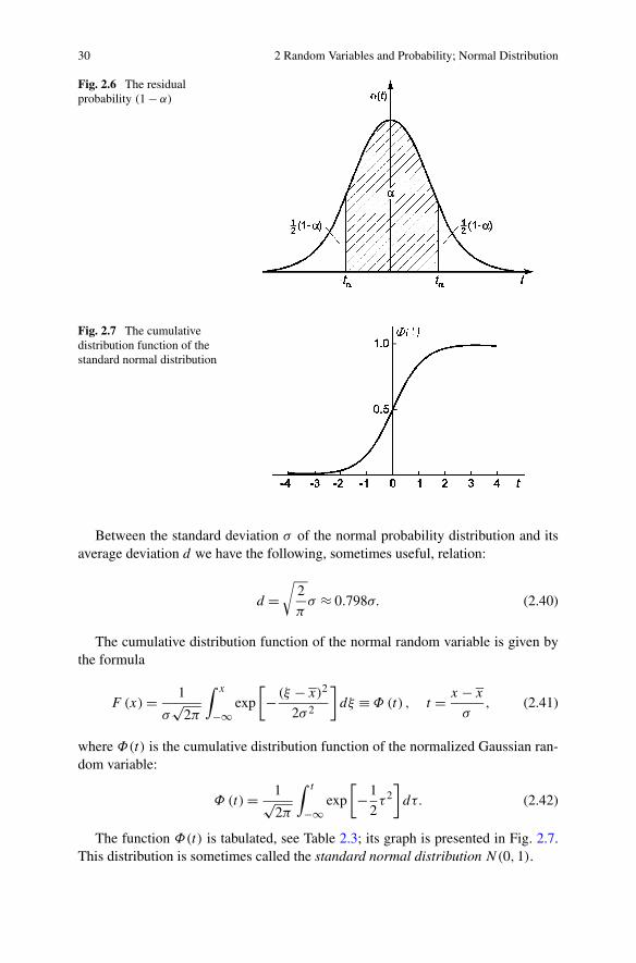
Fig. 2.6 The residualprobability (1 − α)

Fig. 2.7 The cumulativedistribution function of thestandard normal distribution

Between the standard deviation σ of the normal probability distribution and itsaverage deviation d we have the following, sometimes useful, relation:

d =√

2

πσ ≈ 0.798σ. (2.40)

The cumulative distribution function of the normal random variable is given bythe formula

F (x) = 1

σ√

2π

∫ x

−∞exp

[− (ξ − x)2

2σ 2

]dξ ≡ Φ (t) , t = x − x

σ, (2.41)

where Φ(t) is the cumulative distribution function of the normalized Gaussian ran-dom variable:

Φ (t) = 1√2π

∫ t

−∞exp

[−1

2τ 2

]dτ. (2.42)

The function Φ(t) is tabulated, see Table 2.3; its graph is presented in Fig. 2.7.This distribution is sometimes called the standard normal distribution N(0,1).


Table 2.3 The cumulative distribution function of the normalized Gaussian distribution

t Φ(t) t Φ(t) t Φ(t) t Φ(t) t Φ(t)

−3.00 0.0013 −1.75 0.0401 −0.50 0.3085 0.75 0.7734 2.00 0.9773

−2.95 0.0016 −1.70 0.0446 −0.45 0.3264 0.80 0.7881 2.05 0.9798

−2.90 0.0019 −1.65 0.0495 −0.40 0.3446 0.85 0.8023 2.10 0.9821

−2.85 0.0022 −1.60 0.0548 −0.35 0.3632 0.90 0.8159 2.15 0.9842

−2.80 0.0026 −1.55 0.0606 −0.30 0.3821 0.95 0.8289 2.20 0.9861

−2.75 0.0030 −1.50 0.0668 −0.25 0.4013 1.00 0.8413 2.25 0.9878

−2.70 0.0035 −1.45 0.0745 −0.20 0.4207 1.05 0.8531 2.30 0.9893

−2.65 0.0040 −1.40 0.0808 −0.15 0.4404 1.10 0.8643 2.35 0.9906

−2.60 0.0047 −1.35 0.0885 −0.10 0.4602 1.15 0.8749 2.40 0.9918

−2.55 0.0056 −1.30 0.0968 −0.05 0.4801 1.20 0.8849 2.45 0.9929

−2.50 0.0062 −1.25 0.1056 0.00 0.5000 1.25 0.8944 2.50 0.9938

−2.45 0.0071 −1.20 0.1151 0.05 0.5199 1.30 0.9032 2.55 0.9946

−2.40 0.0082 −1.15 0.1251 0.10 0.5398 1.35 0.9115 2.60 0.9953

−2.35 0.0094 −1.10 0.1357 0.15 0.5596 1.40 0.9192 2.65 0.9960

−2.30 0.0107 −1.05 0.1469 0.20 0.5793 1.45 0.9265 2.70 0.9965

−2.25 0.0122 −1.00 0.1587 0.25 0.5987 1.50 0.9332 2.75 0.9979

−2.20 0.0139 −0.95 0.1711 0.30 0.6179 1.55 0.9394 2.80 0.9974

−2.15 0.0158 −0.90 0.1841 0.35 0.6368 1.60 0.9452 2.85 0.9978

−2.10 0.0179 −0.85 0.1977 0.40 0.6554 1.65 0.9505 2.90 0.9981

−2.05 0.0202 −0.80 0.2119 0.45 0.6736 1.70 0.9554 2.95 0.9984

−2.00 0.0227 −0.75 0.2266 0.50 0.6915 1.75 0.9599 3.00 0.9987

−1.95 0.0256 −0.70 0.2420 0.55 0.7088 1.80 0.9641 – –

−1.90 0.0287 −0.65 0.2578 0.60 0.7257 1.85 0.9678 – –

−1.85 0.0322 −0.60 0.2743 0.65 0.7422 1.90 0.9713 – –

−1.80 0.0359 −0.55 0.2912 0.70 0.7580 1.95 0.9744 – –

In practical calculations often the so-called error function,

erf(t) = 1√2π

∫ t

0exp

[−1

2τ 2

]dτ, (2.43)

is used instead of the cumulative distribution function of the normalized Gaussianrandom variable. The error function is tabulated and given in various books (comp.,e.g., [1, 10]). Its values are also given in Table 2.4.

The error function is directly connected with the cumulative distribution functionΦ(t) by the simple formulas:

Φ (t) = 1

2− erf (−t) for t ≤ 0,

Φ (t) = 1

2+ erf (t) for t > 0.

(2.44)


Table 2.4 The error functiont erf(f ) t erf(t) t erf(t)

0.00 0.0000 1.00 0.3413 2.00 0.4773

0.05 0.0199 1.05 0.3531 2.05 0.4798

0.10 0.0398 1.10 0.3643 2.10 0.4821

0.15 0.0596 1.15 0.3749 2.15 0.4842

0.20 0.0793 1.20 0.3849 2.20 0.4861

0.25 0.0987 1.25 0.3944 2.25 0.4878

0.30 0.1179 1.30 0.4032 2.30 0.4893

0.35 0.1368 1.35 0.4115 2.35 0.4906

0.40 0.1554 1.40 0.4192 2.40 0.4918

0.45 0.1736 1.45 0.4265 2.45 0.4929

0.50 0.1915 1.50 0.4332 2.50 0.4938

0.55 0.2088 1.55 0.4394 2.55 0.4946

0.60 0.2257 1.60 0.4452 2.60 0.4953

0.65 0.2422 1.65 0.4505 2.65 0.4960

0.70 0.2580 1.70 0.4554 2.70 0.4965

0.75 0.2734 1.75 0.4599 2.75 0.4979

0.80 0.2881 1.80 0.4641 2.80 0.4974

0.85 0.3023 1.85 0.4678 2.85 0.4978

0.90 0.3159 1.90 0.4713 2.90 0.4981

0.95 0.3289 1.95 0.4744 2.95 0.4984

– – – – 3.00 0.4987

The error function erf(t) is a special function and has no representation in the formof a combination of elementary functions. However, in certain books one can findapproximate expressions allowing one to calculate the values of that function bymeans of elementary functions. Two such practical methods are presented below.They are based on the asymptotic expansions (comp. [1, 7]).

Method 2.1

erf (t) = 1 −(a1z + a2z

2 + a3z3 + a4z

4 + a5z5)

exp[−t2] + ε (t) , (2.45)

where

z = 1

1 + pt, |ε (t)| ≤ 1.5 × 10−7

and

p = 0.3275911, a1 = 0.254829592,

a2 = −0.284496736, a3 = 1.421413741,


Fig. 2.8 Experimental generation of the normal distribution, the Galton box

a4 = −1.453152027, a5 = 1.061405429.

Method 2.2

erf (t) = 1 − 1

(a1t + a2t2 + a3t3 + a4t4 + a5t5 + a6t6)16+ ε(t), (2.46)

where

|ε (t)| ≤ 3 × 10−7

and

a1 = 0.0705230784, a2 = 0.0422820123,

a3 = 0.0092705272, a4 = 0.0001520143,

a5 = 0.0002765672, a6 = 0.0000430638.

The numerical values of the error function calculated according to each of theseapproximate formulas are often more accurate (the accuracy order 10−7 for all x ∈[0,∞)) than those given in the popular textbooks.

For clarity, the generation of the normal distribution can be demonstrated byusing simple devices, such as that shown in Fig. 2.8 (cf. [5]). Small metal balls


Fig. 2.9 The scheme of cells in the Galton box

falling down from a container T and striking numerous metal pins are randomlydirected to the right or to the left. Finally, they fall at random into one of the separatesmall containers at the bottom of the device. The distribution of the number of ballsin consecutive containers is close to the normal distribution. Similar examples maybe found in [21].

Such a result of this educational experiment may be interpreted in two ways.From the mathematical point of view we can say that the normal distribution isformed as the consequence of the so-called central limit theorem, comp. [6]. Eachball falling down is randomly directed to the right or to the left, suffering a unitdisplacement with the same probability. Its final location in a specific containerat the bottom is the sum of such displacements, which is the sum of independentrandom variables.

The fact that the distribution obtained in such an experimental device tends to thenormal distribution may be proved by simple calculus, see [17]. Let us consider anarbitrary set of three cells A, B , C separated from the device in Fig. 2.8, and, more-over, let us assume that the probability distribution in the model may be described bya continuous function P(x, y), if the distances between the pins are tending to zero(a → 0 and b → 0). The configuration of these separated cells is shown in Fig. 2.9.

Let the probabilities that a moving downwards ball falls to the cell B or C are:

P (x − a, y) and P (x + a, y) ,

respectively. Hence, we may express the momentary probabilities of migration ofballs to the cell A located in the lower layer (marked as y + b), using the formula


for the complete probability, see (2.8). We obtain:

P (x, y + b) = 1

2P (x − a, y) + 1

2P (x + a, y) . (2.47)

Then, using Taylor’s expansion of all terms of (2.47) around the point (x, y), wecan write:

P (x, y + b) − P (x, y) = b∂P (x, y)

∂y+ 1

2b2 ∂2P(x, y)

∂y2+ · · ·,

P (x − a, y) − P (x, y) = −a∂P (x, y)

∂x+ 1

2a2 ∂2P(x, y)

∂x2+ · · ·,

P (x + a, y) − P (x, y) = a∂P (x, y)

∂x+ 1

2a2 ∂2P(x, y)

∂x2+ · · ·.

Substituting the above equations in (2.47) and decreasing the dimensions of the cellsto a zero limit in such a way that simultaneously two conditions are satisfied:

a → 0, b → 0, anda2

2b= D = const., (2.48)

we obtain the following partial differential equation for the probability density func-tion P(x, y):

∂P (x, y)

∂y− D

∂2P(x, y)

∂y2= 0. (2.49)

Equation (2.49), obtained in [17], is of the same type as the equation of conduc-tion of heat in solids, cf., e.g., [4]. Its solution can be written in the form

P (x, y) = β√y

exp

[− x2

4Dy

]. (2.50)

To make the solution P(x, y) of (2.50) to be a probability density function we takethe parameter β such that the integral with respect to x of the right-hand of (2.50),for each y = const. is equal to 1,

∫ ∞

−∞P (x, y) dx = 2β

√πD = 1,

from which it follows that

β = 1

2√

πD. (2.51)

Thus, the solution to (2.49) can be written as

P (x, y) = 1

2√

πDyexp

[− x2

4Dy

], (2.52)


Fig. 2.10 Approximation ofa histogram presented inFig. 1.2 by the normalprobability density function

and after substitution

σ = √2Dy (2.53)

as

P (x, y) ≡ f (x) = 1

σ√

2πexp

[− x2

2σ 2

]. (2.54)

Comparing the obtained expression (2.54) with the known probability densityfunction of the normal distribution (2.35) of a zero mean value (x = 0) we obtainan argument that the probability distribution, which is a result of random symmetric(that is with probability 1

2 in every side) reflections of balls on pins of the Galtonbox presented in Fig. 2.8, is really the normal distribution.

This result can be also interpreted more generally: we deal with the normal prob-ability distribution of a random variable when this variable is influenced by numer-ous independent factors. Such an interpretation explains why the normal distributioncorresponds so well to the distribution of errors of measurements, which usuallyarise as a result of numerous unknown external factors.

Let us now consider an example of application of the continuous normal dis-tribution to the description of the quasi-stepwise distribution shown in the form ofthe histogram presented in Fig. 1.2. For the quasi-stepwise distribution, the average


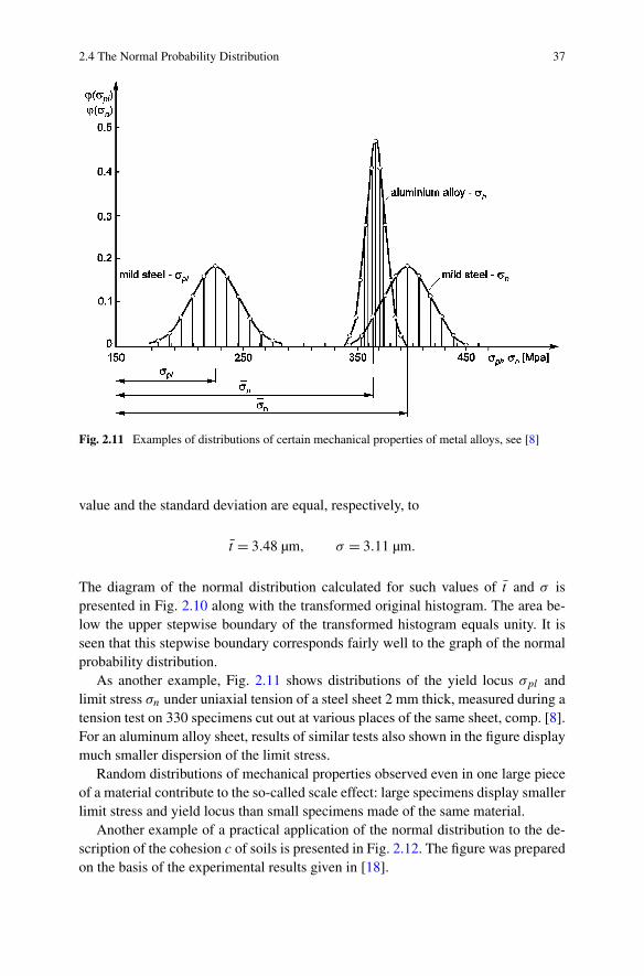
Fig. 2.11 Examples of distributions of certain mechanical properties of metal alloys, see [8]

value and the standard deviation are equal, respectively, to

t = 3.48 µm, σ = 3.11 µm.

The diagram of the normal distribution calculated for such values of t and σ ispresented in Fig. 2.10 along with the transformed original histogram. The area be-low the upper stepwise boundary of the transformed histogram equals unity. It isseen that this stepwise boundary corresponds fairly well to the graph of the normalprobability distribution.

As another example, Fig. 2.11 shows distributions of the yield locus σpl andlimit stress σn under uniaxial tension of a steel sheet 2 mm thick, measured during atension test on 330 specimens cut out at various places of the same sheet, comp. [8].For an aluminum alloy sheet, results of similar tests also shown in the figure displaymuch smaller dispersion of the limit stress.

Random distributions of mechanical properties observed even in one large pieceof a material contribute to the so-called scale effect: large specimens display smallerlimit stress and yield locus than small specimens made of the same material.

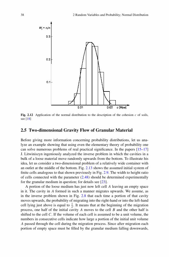
Another example of a practical application of the normal distribution to the de-scription of the cohesion c of soils is presented in Fig. 2.12. The figure was preparedon the basis of the experimental results given in [18].


Fig. 2.12 Application of the normal distribution to the description of the cohesion c of soils,see [18]

2.5 Two-dimensional Gravity Flow of Granular Material

Before giving more information concerning probability distributions, let us ana-lyze an example showing that using even the elementary theory of probability onecan solve numerous problems of real practical significance. In the papers [15–17]J. Litwiniszyn ingeniously analyzed the inverse problem in which the cavities in abulk of a loose material move randomly upwards from the bottom. To illustrate hisidea, let us consider a two-dimensional problem of a relatively wide container withan outlet at the middle of the bottom. Fig. 2.13 shows the assumed initial system offinite cells analogous to that shown previously in Fig. 2.9. The width to height ratioof cells connected with the parameter (2.48) should be determined experimentallyfor the granular medium in question; for details see [23].

A portion of the loose medium has just now left cell A leaving an empty spacein it. The cavity in A formed in such a manner migrates upwards. We assume, asin the inverse problem shown in Fig. 2.8 that each time a portion of that cavitymoves upwards, the probability of migrating into the right-hand or into the left-handcell lying just above is equal to 1

2 . It means that at the beginning of the migrationprocess, one half of the initial cavity A moves to the cell B and the other half isshifted to the cell C. If the volume of each cell is assumed to be a unit volume, thenumbers in consecutive cells indicate how large a portion of the initial unit volumeA passed through the cell during the migration process. Since after migration eachportion of empty space must be filled by the granular medium falling downwards,

2.5 Two-dimensional Gravity Flow of Granular Material 39

Fig. 2.13 Assumed system of cells for the problem of gravity flow from a bin

these numbers correspond to the average vertical displacement of the medium inparticular cells. These vertical displacements are represented in Fig. 2.14. However,each particle of the medium is displaced also horizontally.

Below is presented a simple approximate method of determining total displace-ments [22]. Let us analyze an arbitrary set of three adjacent cells taken from thesystem of cells shown in Fig. 2.13. They are represented in Fig. 2.15a. The num-bers in them correspond to the fraction of the initial volume of the cavity A, whichpassed through the cell during the migration towards the free surface of the bulk ofthe medium. According to the finite cells methodology, only one half of these frac-tions migrates from each cell A and B to the cell C. It is assumed that this migrationtakes place along the respective lines A − C or B − C joining central points of thecells. Directions and magnitudes of these migrating portions of the cavity may berepresented by vectors WBC and WAC as shown in Fig. 2.15b. They may be treatedas components of the resulting vector Wcav representing the direction and the mag-nitude of the averaged momentary flux of the cavity into cell C during the migrationprocess. The opposite vector Wmat may be treated as a representation of the fluxof the mass of granular medium filling the space left by cavities moving upwards.In order to calculate the magnitude of the averaged displacement vector u of theparticles of the medium, it is assumed that its direction coincides with the direction


Fig. 2.14 Vertical displacement of granular material in cells

of the vector Wmat . To make this procedure consistent with that described before,it is assumed that the vertical component of the displacement vector u is equal tothe vertical displacement of the respective sector of the stepwise deformed bound-ary between the rows of cells (cf. Fig. 2.14). Using this approximate procedure, thevectors of displacements have been calculated for the problem shown in Fig. 2.13and Fig. 2.14. Results are shown in Fig. 2.16.

In Fig. 2.17 is presented an analogous solution for prediction of the movementsof a crowd in a relatively narrow exit [14].

Figure 2.18 shows the theoretical field of displacements vectors calculated in themanner described above.

In order to verify experimentally such a theoretical motion pattern, a preliminarysimple experimental simulation model composed of an assembly of coins of threedifferent diameters has been used. The initial configuration of the assembly corre-sponding to the theoretical problem shown in Fig. 2.17 is presented in Fig. 2.19. Thecoins are located on a glass plate in the initial horizontal position. Then the plate isinclined with respect to the horizontal plane and the coins begin to slide downwardsdue to the gravity forces. This movement is disturbed by random mutual contactsbetween neighbors. The final configuration of displaced coins is shown in Fig. 2.20.


Fig. 2.15 Calculation ofdisplacements of the granularmaterial in cells, after [22]

Fig. 2.16 Calculated displacements of granular medium in a bin, after [22]

The experiment was performed in three stages. In each stage one of the blockingstrips at the bottom was removed. For each stage displacements of particular coinswere measured. They are shown in Fig. 2.21. The stochastic nature of the move-ments of coins is visible. Let us notice, however, that their general layout is close tothat shown previously in Fig. 2.18.


Fig. 2.17 Assumed system of finite cells and vertical displacements in a crowd in narrow exits,see [14]

Fig. 2.18 Calculated displacements of a crowd in a narrow exit, see [14]

The next example concerns the problem of terrain subsidence caused by subter-ranean exploitation. The solution is shown in Fig. 2.22 (cf. [24]).

In the lower part of the soil resting on a bedrock, the empty space A−B −C −D

has been left by underground exploitation. In the following process of subsidencethis empty space will be filled by the soil migrating downwards. Let us divide thisempty space into a number of cells, each of them being of unit volume. These unitcavities migrate upwards through the system of cells shown in the figure. It is as-sumed that each time a cavity in the particular cell migrates upwards, the probabilitythat it moves to the left or to the right cell, just above it, is equal to 1/2. Numbersshown in particular cells indicate how large was the portion of a unit cavity which


Fig. 2.19 Initial configuration of coins located on a glass plate, see [14]

Fig. 2.20 Final configuration of coins in an experimental simulation of movements of a crowd,see [14]

has passed through the cell during the migration process. On the basis of these num-bers, the diagram representing a stepwise approximation of the final subsidenceshown in Fig. 2.23 has been prepared. The procedure described above allows us tocalculate the vectors of displacements in the entire deformation zone Fig. 2.24.


Fig. 2.21 Experimentallydetermined displacements ofcoins in the test shown inFigs. 2.19 and 2.20

Fig. 2.22 Assumed systemof finite cells for the analysisof terrain subsidence, see [24]

Fig. 2.23 Verticaldisplacement of granularmedium in cells of theassumed system, see [24]

In Fig. 2.25 is presented a simple experimental simulation of such a subsidenceprocess. The coins of different diameters are located on a glass plate as shown inthe photograph. To simulate the initial configuration corresponding to that shownin Fig. 2.22, two bottom rows on the right side have been left without coins. Then


Fig. 2.24 Calculateddisplacements of a granularmedium in the process ofterrain subsidence shown inFigs. 2.22 and 2.23, after [24]

Fig. 2.25 Initial configuration of coins located on a glass plate, see [24]

the blocking strip at the bottom has been removed and the plate was inclined withrespect to its initial horizontal position. The coins slid downwards due to gravityforce. The final configuration of coins is shown in Fig. 2.26.

The displacements of central points of several coins resulting from this experi-mental simulation are shown in Fig. 2.27.

Let us note that this experimental result is similar to that resulting from theoreti-cal solution shown in Fig. 2.24.

Summarizing the considerations of this subsection we see that the calculationmethods proposed by J. Litwiniszyn were, both, very effective in solving quite in-volved geotechnics problems and very illustrative. They were also an inspirationfor mathematically more advanced models, e.g., description of the random walk ofvoids by means of diffusive Markov processes, cf. [3].


Fig. 2.26 Final configuration of coins in an experimental simulation of terrain subsidence

Fig. 2.27 Experimentally determined displacements of coins in the test shown in Figs. 2.25 and2.26, after [23]

Problem 2.1 Consider a system of four electric elements connected in series. Theprobability of defective operation of these elements after one year of work is, re-spectively, 0.6, 0.5, 0.4, and 0.3, and is independent one from the other. Calculatethe probability of defective operation of the system of elements. Calculate the prob-ability that the system works correctly.

Problem 2.2 A sample of 200 mass-produced elements is tested by random choiceof 10 elements. It is rejected if at least one of the elements is defective. Calculatethe probability of the rejection of the sample of elements if 5% of the elements inthe sample are defective.

Problem 2.3 Calculate the probability that a sample of 100 mass-produced ele-ments will be accepted if it contains 5 defective elements and we test 50 elementsallowing at the most two defective elements among them.

References 47

References

1. Abramowitz, M., Stegun, I.: Handbook of Mathematical Functions with Formulas, Graphs andMathematical Tables. Dover, New York (1965)

2. Bryc, W.: The Normal Distribution. Characterization with Applications. Lecture Notes inStatistics, vol. 100. Springer, New York (1995)

3. Brzakała, W.: Diffusion of voids in the stochastic loose medium. Bull. Acad. Pol. Sci., Sér.Sci. Tech. 30, 487–491 (1982)

4. Carslaw, H.S., Jaeger, J.C.: Conduction of Heat in Solids, 2nd edn. Oxford University Press,London (1986)

5. Cranz, H.: Aussere Ballistik. Springer, Berlin (1926)6. Fisz, M.: Probability Theory and Mathematical Statistics, 3rd edn. Krieger, Melbourne (1980)7. Hastings, N.A.J., Peacock, J.B.: Statistical Distributions, 2nd edn. Wiley–Interscience, New

York (1993)8. Jastrzebski, P.: Strength and carrying capacity of steel and aluminum strips. Scientific Reports

of Warsaw University of Technology, No. 1 (1968) (in Polish)9. Knuth, D.E.: Seminumerical Algorithms, 3rd edn. The Art of Computer Programming, vol. 2.

Addison–Wesley, Reading (1998)10. Korn, G.A., Korn, Th.M.: Mathematical Handbook for Scientists and Engineers, 2nd edn.

Dover, New York (2000)11. Kotulski, Z.: Random walk with finite speed as a model of pollution transport in turbulent

atmosphere. Arch. Mech. 45(5), 537–562 (1993)12. Kotulski, Z.: On efficiency of identification of a stochastic crack propagation model based on

Virkler experimental data. Arch. Mech. 50(5), 829–847 (1998)13. Kotulski, Z., Sobczyk, K.: Effects of parameter uncertainty on the response of vibratory sys-

tems to random excitation. J. Sound Vib. 119(1), 159–171 (1987)14. Kotulski, Z., Szczepinski, W.: On a model for prediction of the movements of a crowd in

narrow exits. Eng. Trans. 53(4), 347–361 (2005)15. Litwiniszyn, J.: Application of the equation of stochastic processes to mechanics of loose

bodies. Arch. Mech. 8, 393–411 (1956)16. Litwiniszyn, J.: An application of the random walk argument to the mechanics of granular

media. In: Proc. IUTAM Symp. on Rheology and Soil Mechanics, Grenoble, April 1964.Springer, Berlin (1966)

17. Litwiniszyn, J.: Stochastic methods in mechanics of granular bodies. In: CISM Course andLectures No. 93. Springer, Udine (1974)

18. Matsuo, M., Kuroda, K.: Probabilistic approach to design of embankments. Soil Found. 14(2),1–17 (1974)

19. Papoulis, A.: Probability, Random Variables, and Stochastic Processes with Errata Sheet,4th edn. McGraw–Hill, New York (2002)

20. Sobczyk, K.: Stochastic Differential Equations with Applications to Physics and Engineering.Kluwer Academic, Dordrecht (1991)

21. Steinhaus, H.: Mathematical Kaleidoscope, 8th edn. Polish Educational Editors, Warsaw(1956) (in Polish)

22. Szczepinski, W.: On the movement of granular materials in bins and hoppers. Part I—Two-dimensional problems. Eng. Trans. 51(4), 419–431 (2003)

23. Szczepinski, W.: On the stochastic approach to the three-dimensional problems of strata me-chanics. Bull. Acad. Pol. Sci., Sér. Sci. Tech. 51(4), 335–345 (2003)

24. Szczepinski, W., Zowczak, W.: The method of finite cells for the analysis of terrain subsidencecaused by tectonic movements or by subterranean exploitation. Arch. Mech. 59(6), 541–557(2007)

http://www.springer.com/978-90-481-3569-1

random variables and probability; normal distribution

Documents