rain bird low-volume landscape irrigation and drip design manual
TRANSCRIPT
®
Low-Volume Landscape Irrigation Design Manual

®
Xerigation ®: Maximizing the effective useof every drop of water
Low-VolumeLandscape Irrigation Design Manual

© Copyright Rain Bird Sales, Inc., Landscape Drip Division 2000
Information contained in this manual is based upon generally accepted formulas, computation and trade practices. If anyproblems, difficulties or injuries should arise from or in connection with the use or application of this information or if there isany error herein, typographical or otherwise, Rain Bird Sales, Inc. and its subsidiaries and affiliates or any agent or employeethereof, shall not be responsible or liable therefor.
Forward
FOREWORD
Over the past four years, “Xerigation® Product, Design and Installation” semi-nars have been conducted across the U.S., in Mexico, Canada and even Europe.Rain Bird has talked to more than 1,000 irrigation professionals about landscapelow-volume irrigation. In the past, the most frequently asked question was,“Why should I use low-volume irrigation?” Today, however, most seminarattendees share the basic understanding that, when properly used, landscapelow-volume irrigation products can save significant amounts of water. Theseproducts can also help keep water off walls, windows, sidewalks and streets. Atthe same time, the use of these products promotes healthier plant growth becausewater is delivered more slowly and at lower pressures at or near plant root zones.
Now, the most frequently asked questions are, “What is the proper way to dodrip design?” “How do you decide when and where to use drip products?”“How can the maintenance factor associated with drip be significantly reducedor eliminated?” These kinds of questions indicate a growing acceptance of low-volume irrigation within the industry, a trend that is helping landscape dripirrigation equipment become fundamental to good water management practice.
This design manual is intended to provide straightforward answers to thesequestions. It is our hope that the reader will realize the benefits of landscape low-volume irrigation by utilizing the design approach explained in this manual. It isan approach that has proven itself in practice over the past several years.
This manual continues to take the same cutting-edge approach to low-volumeirrigation by considering plant root depths and water loss due to percolationbelow the root zone to be essential design parameters.
In this manual, we will introduce the Xerigation product line and discuss thebenefits of its use. We will then discuss the design approach for a low-volumedelivery system and follow up with practical recommendations for installation,ongoing maintenance and troubleshooting.
For more information on the Xerigation product line or Rain Bird’s broad line ofirrigation products, contact your local Rain Bird Distributor, Rain Bird Represen-tative, or call our Technical Services Group at 1-800-247-3782. Or, visit ourwebsite at www.rainbird.com.
The reader should realize that it is not possible in a single publication to cover allconceivable drip design situations that may arise. As such, it is not the intent ofthis design manual to provide all the answers. Rather, this manual is intended tohelp the user understand the fundamentals of low-volume irrigation and toprovide a foundation for a successful experience with drip.
®
Contents Page i
CONTENTS
What is Xerigation®? .......................................................................... 1Low-volume Irrigation ............................................................. 1Benefits of Low-Volume Irrigation ......................................... 2Selecting Low-Volume Irrigation ............................................ 4
Installation Cost ............................................................... 4Size of Area ....................................................................... 4Vandalism ......................................................................... 4Safety ................................................................................. 4Intended Use .................................................................... 4
Xerigation Product Line ........................................................... 4
The Design Process ........................................................................... 5An Innovative Approach ......................................................... 5The Xerigation Design Process ................................................ 6Individual Plants Versus Dense Plantings ............................. 7
Gather Site Data ................................................................................. 9Site Information ............................................................. 10Water source ................................................................... 10Soil Type ...........................................................................11Climate and PET ............................................................ 13Hydrozones .................................................................... 14
Chapter 3 Review .................................................................... 15Sample Property ............................................................ 15Site Data Worksheet ...................................................... 17Answer Key .................................................................... 18
Determine Plant Water Requirements ........................................ 19Calculating Water Requirements .......................................... 21
Site Information ............................................................. 21Calculate Kc .................................................................... 21Water Requirement for Densely Planted Areas ........ 24Water Requirement for Individual Plants .................. 24
Chapter 4 Review .................................................................... 26Answer Key .................................................................... 27
Irrigate Base Plants .......................................................................... 29Identifying the Base Plant ...................................................... 29
Dense Plantings ............................................................. 29Sparse Plantings ............................................................. 29
Emission Devices .................................................................... 30Xerigation Products Application Matrix .................... 32Dense Plantings ............................................................. 32 Landscape Dripline .................................................. 32 Xeri-Sprays ................................................................ 38 Xeri-Pop Series Micro-Spray Pop-Ups .................. 38 Multi-Port Spray Nozzle ......................................... 38
1
23
4
5
®
78
9
10
Page ii Contents
Sparse Plantings ............................................................. 38 Selecting Emitters ..................................................... 39 Calculating the Wetted Area ................................... 40
Chapter Review ....................................................................... 41Answer Key .................................................................... 42
Calculate System Run Time........................................................... 431. Calculate System Run Time ............................................... 44
Dense Plantings ............................................................. 44Sparse Planting .............................................................. 45
2. Determine Maximum Run Time ....................................... 463. Determine Irrigation Interval ............................................ 48Chapter Review ....................................................................... 49
Answer Key .................................................................... 50
Irrigate Non-Base Plants ................................................................ 51Chapter Review ....................................................................... 52
Answer Key .................................................................... 53Dense Hydrozone Design Worksheet .................................. 54
System Layout .................................................................................. 55Using Inline Tubing ................................................................ 57
Placing Supplemental Emitters ................................... 57System Configuration ............................................................. 59Irrigating Slopes ...................................................................... 61Container Plants ...................................................................... 62
System Hydraulics ........................................................................... 63Water Pressure ......................................................................... 63
Static/Dynamic Pressure .............................................. 63Calculating Pressure Loss ...................................................... 64
Flow ................................................................................. 64Determine Maximum Lateral Lengths ....................... 68Pressure Loss Calculation ............................................ 69
High Pressure .......................................................................... 71Hydraulics Worksheet ............................................................ 72
Installation, Maintenance, and Trouble Shooting .................... 73Installation................................................................................ 73Maintenance and Troubleshooting ....................................... 74
Appendices ....................................................................................... 77Formulas For Xerigation Design ........................................... 77PET Data ................................................................................... 81Friction Loss and Performance Data .................................... 85Xerigation Planning Blank Forms ......................................... 87Glossary .................................................................................... 95Xerigation Product Line ......................................................... 99Installation Details ................................................................ 103
Bibliography ................................................................................... 104
Index ................................................................................................. 105
6
®
What is Xerigation? Page 1
WHAT IS XERIGATION®?Xerigation is Rain Bird’s registered trademark term for a system that distributeswater directly to plant root zones using Rain Bird’s low-volume, landscape-specific irrigation products. “Xerigation” is closely related to the wordXeriscape™, which refers to a landscape that conserves water by following the“Seven Principles of Xeriscape Landscaping.” These principles are:
1. Proper planning and design.
2. Soil analysis and improvement.
3. Practical turf areas.
4. Appropriate plant selection.
5. Efficient irrigation.
6. Mulching.
7. Appropriate maintenance.
It is in the interest of efficient irrigation that Rain Bird developed the Xerigationproduct line to meet the evolving needs of today’s landscapes by maximizing theeffective use of every drop of water.
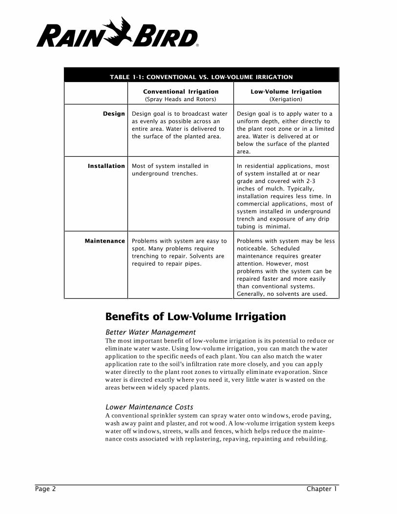
Low-Volume IrrigationLow-volume irrigation is simply a method of distributing water to plants. Likeconventional overhead systems, a low-volume system requires proper design,installation, and ongoing maintenance. Table 1-1 highlights some of the similari-ties and differences between conventional and low-volume irrigation systems.
1®
Benefits of Low-Volume IrrigationBetter Water ManagementThe most important benefit of low-volume irrigation is its potential to reduce oreliminate water waste. Using low-volume irrigation, you can match the waterapplication to the specific needs of each plant. You can also match the waterapplication rate to the soil’s infiltration rate more closely, and you can applywater directly to the plant root zones to virtually eliminate evaporation. Sincewater is directed exactly where you need it, very little water is wasted on theareas between widely spaced plants.
Lower Maintenance CostsA conventional sprinkler system can spray water onto windows, erode paving,wash away paint and plaster, and rot wood. A low-volume irrigation system keepswater off windows, streets, walls and fences, which helps reduce the mainte-nance costs associated with replastering, repaving, repainting and rebuilding.
Page 2 Chapter 1
TABLE 1-1: CONVENTIONAL VS. LOW-VOLUME IRRIGATION
Conventional Irrigation(Spray Heads and Rotors)
Low-Volume Irrigation(Xerigation)
Design Design goal is to broadcast wateras evenly as possible across anentire area. Water is delivered tothe surface of the planted area.
Design goal is to apply water to auniform depth, either directly tothe plant root zone or in a limitedarea. Water is delivered at orbelow the surface of the plantedarea.
Installation Most of system installed inunderground trenches.
In residential applications, mostof system installed at or neargrade and covered with 2-3inches of mulch. Typically,installation requires less time. Incommercial applications, most ofsystem installed in undergroundtrench and exposure of any driptubing is minimal.
Maintenance Problems with system are easy tospot. Many problems requiretrenching to repair. Solvents arerequired to repair pipes.
Problems with system may be lessnoticeable. Scheduledmaintenance requires greaterattention. However, mostproblems with the system can berepaired faster and more easilythan conventional systems.Generally, no solvents are used.
®
What is Xerigation? Page 3
40%25%Water Intake:Root Depth:
30%50%
20%75%
10%100%
Figure 1-1: Soil moisture extraction by plant root zone
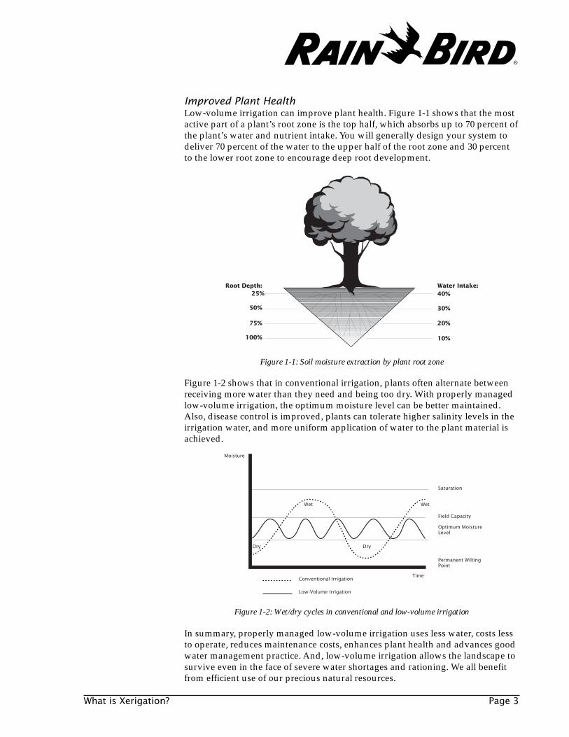
Improved Plant HealthLow-volume irrigation can improve plant health. Figure 1-1 shows that the mostactive part of a plant’s root zone is the top half, which absorbs up to 70 percent ofthe plant’s water and nutrient intake. You will generally design your system todeliver 70 percent of the water to the upper half of the root zone and 30 percentto the lower root zone to encourage deep root development.
Figure 1-2 shows that in conventional irrigation, plants often alternate betweenreceiving more water than they need and being too dry. With properly managedlow-volume irrigation, the optimum moisture level can be better maintained.Also, disease control is improved, plants can tolerate higher salinity levels in theirrigation water, and more uniform application of water to the plant material isachieved.
Figure 1-2: Wet/dry cycles in conventional and low-volume irrigation
Time
Wet
DryDry
Wet
Conventional Irrigation
Low-Volume Irrigation
Saturation
Optimum MoistureLevel
Field Capacity
Permanent WiltingPoint
Moisture
In summary, properly managed low-volume irrigation uses less water, costs lessto operate, reduces maintenance costs, enhances plant health and advances goodwater management practice. And, low-volume irrigation allows the landscape tosurvive even in the face of severe water shortages and rationing. We all benefitfrom efficient use of our precious natural resources.
®
Installation Cost
Size of Area
Vandalism
Safety
Intended Use
Selecting Low-Volume IrrigationA Xerigation design is appropriate in any nongrass planting scheme where low-volume irrigation can reduce water usage and improve plant health. Some of thefactors that might affect your decision include installation cost, size of the areabeing irrigated, protection from vandalism, human safety and the type of mainte-nance that will be provided.
In most cases, the cost of materials will be similar for low-volume and conven-tional irrigation systems. The cost of labor, however, is often less for a low-volume system. Because you can often install low-volume systems at or neargrade, you will usually need less trenching and therefore less time and labor.
Generally, nongrass planting areas of any size can use low-volume irrigation.There are, however, two considerations: plant density and maintenance. A large,densely planted area with a homogeneous plant material, for example, requiresuniform watering over a fairly consistent root depth and is therefore betterirrigated with broadcast methods. Also, a large area may be easier to maintain ifirrigated with a conventional system, which has fewer parts.
In areas where vandalism can be a problem, it is important to design a systemthat can be installed below grade as much as possible, with exposed componentsplaced out of sight. Consider the individual circumstances of the site whendeciding between low-volume and conventional approaches.
Low-volume systems provide greater safety by reducing run-off on walks andpaved areas, and overthrow into the street or pedestrian right-of-way.
Low-volume irrigation may be less appropriate for sites with heavy trafficbecause the exposed tubing can be damaged. Frequent soil cultivation may alsodamage low-volume tubing. In these cases, a low-volume system may still beappropriate if you install it below ground using conventional PVC piping (orhigh-density polyethylene tubing in colder climates) and drip componentsinstalled on 1/2" threaded risers. Although the cost of installing low-volumesystems below grade may be higher, the long-term benefits of this type of irriga-tion make it a very worthwhile alternative. This is, in fact, how most commercialdrip systems are designed and installed today.
Xerigation Product LineRain Bird’s Xerigation product line offers a full range of low-volume irrigationproducts for many landscape applications. These products include a variety ofemission devices, distribution components, valves, filters, pressure regulatorsand risers.
Illustrations and capsule descriptions of many of these Rain Bird Xerigationproducts are included in the appendix of this manual. For complete informationabout the Xerigation product line, see the Xerigation section of Rain Bird’sLandscape Irrigation Products Catalog. To obtain a copy of this catalog, contact theRain Bird Technical Services Group at 1-800-247-3782. Or, visit the Rain Birdwebsite at www.rainbird.com, where you can review Rain Bird’s online catalogand download construction/installation details, written specifications andtechnical information.
Page 4 Chapter 1
®
THE DESIGN PROCESS
An Innovative ApproachOverhead, broadcast methods of irrigation are ideal for turfgrass, which requiresa uniform precipitation rate over its entire planted area. However, the use ofoverhead irrigation in sparsely planted, nongrass areas causes water to fall onunplanted ground and is wasted, or worse yet, promotes weed growth. A con-ventional overhead system also is not the best approach for a mixed plantingwhere some specimens need more water than others. Such a system lacks theflexibility of a drip system to deliver different amounts of water to differentplants in the same planting area. Even many low-volume design approaches failto truly optimize the application of water, when water waste below the plant rootzone is ignored or not considered.
This manual describes a design process that minimizes water waste below theroot zone and that strives to apply the precise amount of water required by eachindividual plant or group of plants in a landscape. This design process is basedon actual cutting-edge research in the field of low-volume irrigation. Landscapeand irrigation designers can use this information to design systems based notonly on the size of a planted area, but on a plant’s root depth, soil type, waterrequirement and density of planting for the greatest efficiency possible.
The Design Process Page 5
2®
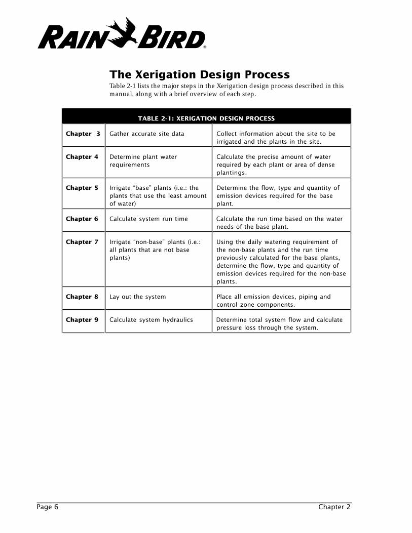
The Xerigation Design ProcessTable 2-1 lists the major steps in the Xerigation design process described in thismanual, along with a brief overview of each step.
Page 6 Chapter 2
TABLE 2-1: XERIGATION DESIGN PROCESS
Chapter 3 Gather accurate site data Collect information about the site to beirrigated and the plants in the site.
Chapter 4 Determine plant waterrequirements
Calculate the precise amount of waterrequired by each plant or area of denseplantings.
Chapter 5 Irrigate “base” plants (i.e.: theplants that use the least amountof water)
Determine the flow, type and quantity ofemission devices required for the baseplant.
Chapter 6 Calculate system run time Calculate the run time based on the waterneeds of the base plant.
Chapter 7 Irrigate “non-base” plants (i.e.:all plants that are not baseplants)
Using the daily watering requirement ofthe non-base plants and the run timepreviously calculated for the base plants,determine the flow, type and quantity ofemission devices required for the non-baseplants.
Chapter 8 Lay out the system Place all emission devices, piping andcontrol zone components.
Chapter 9 Calculate system hydraulics Determine total system flow and calculatepressure loss through the system.
®
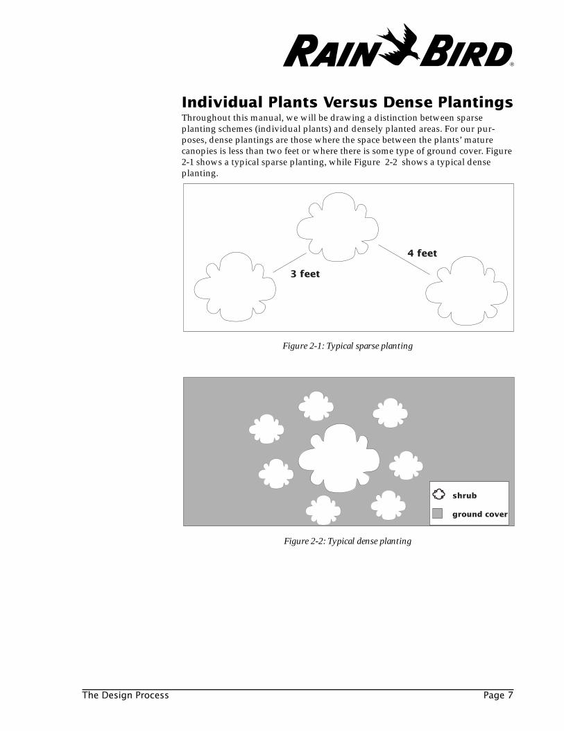
Individual Plants Versus Dense PlantingsThroughout this manual, we will be drawing a distinction between sparseplanting schemes (individual plants) and densely planted areas. For our pur-poses, dense plantings are those where the space between the plants’ maturecanopies is less than two feet or where there is some type of ground cover. Figure2-1 shows a typical sparse planting, while Figure 2-2 shows a typical denseplanting.
Figure 2-1: Typical sparse planting
Figure 2-2: Typical dense planting
The Design Process Page 7
3 feet
4 feet
shrub
ground cover
®

Page 8 Chapter 2
As you will see later in this manual, this distinction between sparse and denseplanting schemes is important because the planting scheme strongly suggestswhich type of low-volume irrigation system design approach to take and whichdrip products to use.
• Individual plants are generally irrigated by individual emission devices thatsupply a precise amount of water directly to the plant’s root zone (see Figure2-3). These devices include single- and multi-outlet emitters, as well asmicro-bubblers.
• Dense plantings require emission devices that supply a precise amount ofwater across the entire area. These devices include inline emitter tubing(shown in Figure 2-4) and micro-sprays.
Figure 2-4: Dense planting irrigated with inline emitter tubing
Figure 2-3: Sparse planting irrigated with multi-outlet emitters
®
Gather Site Data Page 9
GATHER SITE DATA
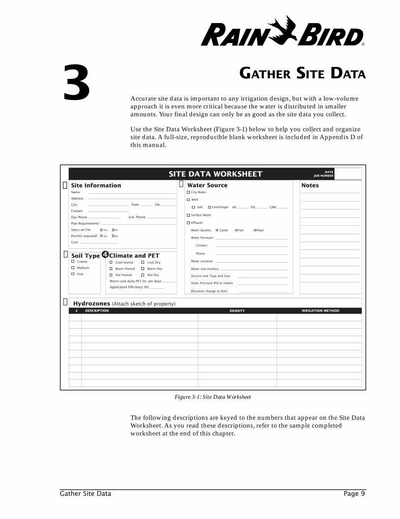
Accurate site data is important to any irrigation design, but with a low-volumeapproach it is even more critical because the water is distributed in smalleramounts. Your final design can only be as good as the site data you collect.
Use the Site Data Worksheet (Figure 3-1) below to help you collect and organizesite data. A full-size, reproducible blank worksheet is included in Appendix D ofthis manual.
The following descriptions are keyed to the numbers that appear on the Site DataWorksheet. As you read these descriptions, refer to the sample completedworksheet at the end of this chapter.
SITE DATA WORKSHEET
Site Information
Eve. Phone
Water Source Notes➋
Yes No
Yes No
Soil TypeCoarse
Medium
Fine
Name
Address
City
Contact
Day Phone
Pipe Requirements
Specs on File
Permits required?
Cost
City Water
Well:
Surface Water
Effluent
Water Purveyor
Contact
Phone
Meter Location
Meter size (inches)
Service Line Type and Size
Static Pressure (PSI at meter)
Elevation change (± feet)
Good Fair PoorWater Quality:
HP PSI GPMSub CentrifugalState Zip
Climate and PETCool Humid
Warm Humid
Hot Humid
Cool Dry
Warm Dry
Hot Dry
Worst case daily PET (in. per day):
Application Efficiency (%):
➎ Hydrozones (Attach sketch of property)DESCRIPTION DENSITY# IRRIGATION METHOD
DATEJOB NUMBER
❶
➌
3
Figure 3-1: Site Data Worksheet
®
Page 10 Chapter 3
This section of the form is for identifying the site, recording information aboutthe owner and making notes about local requirements for permits and systemspecifications.
In this section of the worksheet, check off the type of water source (city water,well, surface water, or effluent). If a pump is used, indicate the type and itsspecifications. For all water sources, indicate the quality of the water based onthe amount of particulate matter present. Fill in the meter size, location, andstatic water pressure (measured at the meter). Then fill in the information aboutthe service line.
“Dirty” water can be a problem for low-volume systems because of the compo-nents’ small orifices. Plan to include filters in your low-volume system to screenout particulates from the water before they become a problem. Table 3-1 showsminimum filtration required for most emitters.
If your water is dirty or contains organic contaminants, consider installing a sandmedia filter in your system. Hard water may need to be chemically treated toprevent mineral buildup that could clog emitters. If clogging is a concern, insteadof emitters use Xeri-Bubblers, which have larger orifices and can be easily takenapart and cleaned. Contact your Rain Bird distributor for more information aboutspecific filtration requirements.
On commercial systems using water that does not contain organic contaminents,it is cost-effective to install a Rain Bird Automatic Filter Kit near the point ofconnection (see Figure 8-7, Chapter 8). The 150 PSI rated kit is available in 1", 1-1/2" and 2" sizes and consists of a Y-Filter, a Rain Bird PESB scrubber valve,which acts as an automatic flush valve, and fittings. Various screen sizes from 30to 200 mesh are available to meet the needs of a variety of applications. Whenthe “scrubber” valve is connected to a multi-program irrigation controller such asthe Rain Bird ESP-LX+ or ESP-MC, a flush cycle can be programmed to virtuallyeliminate the need to routinely clean the filter manually.
It is always best to include the appropriate filter in your drip system design, evenwhen using potable water.
➋ Water Source
➊ Site Information
In many cases, you can call your local water purveyor for information about thewater source. The water purveyor should be able to tell you the meter size (ifthere is one) and the cost of water. The water purveyor may also provide a water-quality report and help you understand it. However, measurements of staticpressure and water quality should be performed on-site whenever possible.
0.5 GPH 1.0 GPH and largerLandscape Dripline 0.6
and 0.9 GPH
TABLE 3-1: MINIMUM FILTRATION REQUIREMENTS
200 mesh75 microns
150 mesh100 microns
120 mesh125 microns
®
Gather Site Data Page 11
Soil absorbs and holds water in much the same way as a sponge. A given typeand volume of soil will hold a given amount of moisture. The ability of soil tohold moisture, and the amount of moisture it can hold, will greatly affect theirrigation design and irrigation schedule.
Soil consists of sand, silt and clay particles and the percentage of each is whatdetermines the soil type. Because the percentage of any one of the three particlescan differ, there is virtually an unlimited number of soil types.
The simplest way to determine the soil type is to place a moistened soil sample inyour hand and squeeze. Take the sample from a representative part of the site andfrom approximately the same depth to which you will be watering. In other words,if you want to water to a depth of six inches, dig down six inches to take yoursoil sample. Table 3-2 lists the general characteristics of the three main soil types.
➌ Soil Type
One of the most significant differences between different soil types is the way inwhich they absorb and hold water. Capillary action is the primary force inspreading water horizontally through soil. Vertical movement of water in the soilis influenced by both gravity and capillary action.
An inline emitter tubing system such as Landscape Dripline relies on the soil toevenly spread water throughout the planting area. The more homogeneous thesoil in the planting area, the more uniform the water distribution. Therefore,compacted soil must be tilled to an 8” to 12" (20 - 30 cm) depth and should beirrigated to field capacity prior to planting. In coarser soils, water is more likelyto be absorbed vertically, but will not spread very far horizontally. The oppositeis true for fine, clay-like soil.
Note: Emitters should be used very carefully in very coarse soils as water willpercolate downward before it can spread very far horizontally. Micro-sprays orconventional irrigation may be more appropriate.
TABLE 3-2: DETERMINING THE SOIL TYPE
SOIL TYPE CHARACTERISTICS
Coarse Soil particles are loose. Squeezed in the hand when dry, itfalls apart when pressure is released. Squeezed when moist,it will form a cast, but will crumble easily when touched.
Medium Has a moderate amount of fine grains of sand and very littleclay. When dry, it can be readily broken. Squeezed whenwet, it will form a cast that can be easily handled.
Fine When dry, may form hard lumps or clods. When wet, the soilis quite plastic and flexible. When squeezed between thethumb and forefinger the soil will form a ribbon that willnot crack.
®
Saturation
FieldCapacity
PermanentWilting Point
Gravitational Water(Rapid drainage)
Capillary Water(Slow drainage)
Available Water(AW)
Hygroscopic Water(Essentially no drainage)
ReadilyAvailable
Water
Figure 3-2: Soil, water, plant relationships
Page 12 Chapter 3
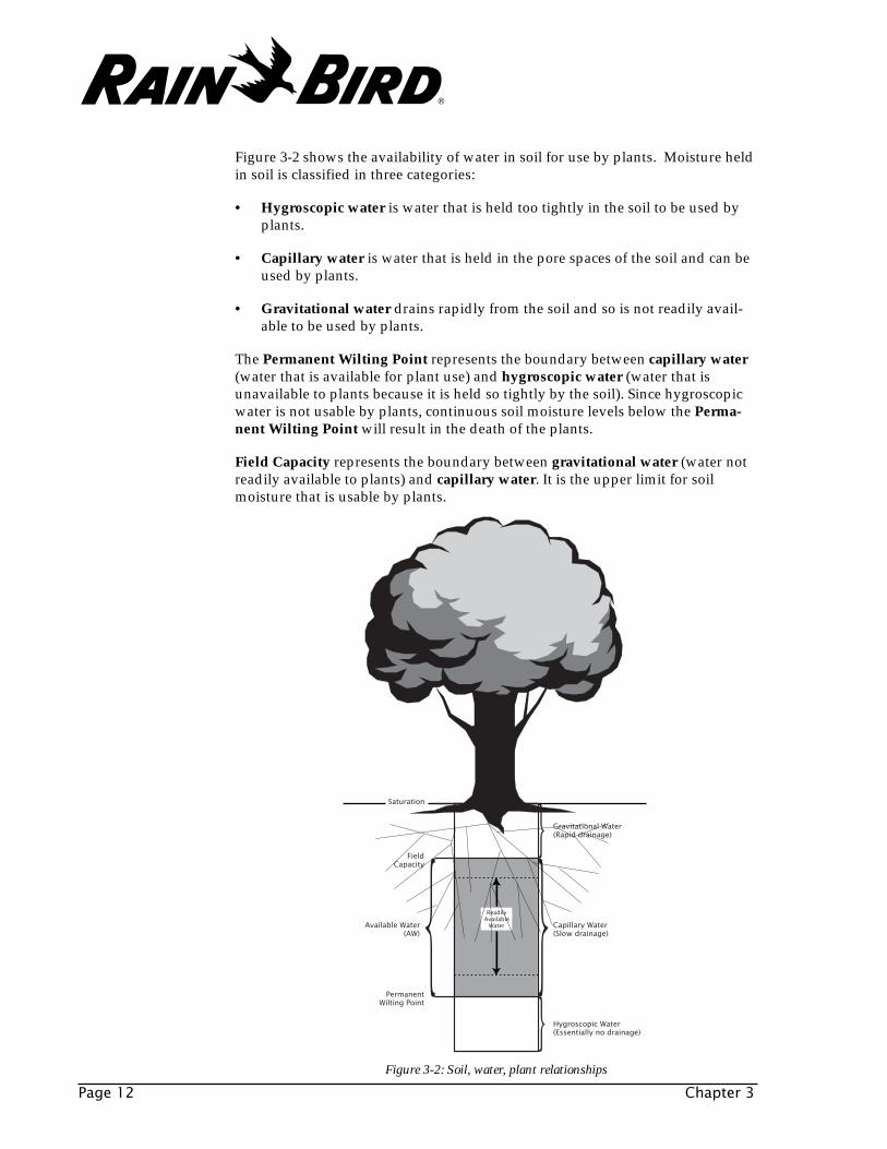
Figure 3-2 shows the availability of water in soil for use by plants. Moisture heldin soil is classified in three categories:
• Hygroscopic water is water that is held too tightly in the soil to be used byplants.
• Capillary water is water that is held in the pore spaces of the soil and can beused by plants.
• Gravitational water drains rapidly from the soil and so is not readily avail-able to be used by plants.
The Permanent Wilting Point represents the boundary between capillary water(water that is available for plant use) and hygroscopic water (water that isunavailable to plants because it is held so tightly by the soil). Since hygroscopicwater is not usable by plants, continuous soil moisture levels below the Perma-nent Wilting Point will result in the death of the plants.
Field Capacity represents the boundary between gravitational water (water notreadily available to plants) and capillary water. It is the upper limit for soilmoisture that is usable by plants.
®
Gather Site Data Page 13
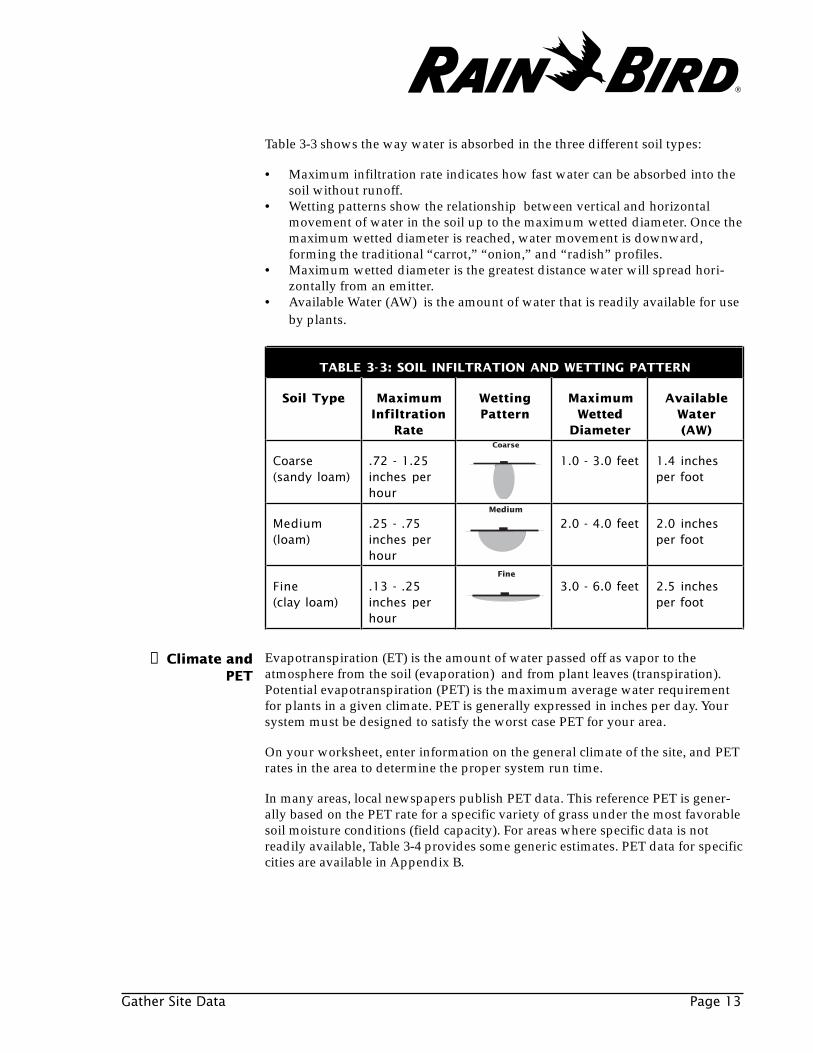
Table 3-3 shows the way water is absorbed in the three different soil types:
• Maximum infiltration rate indicates how fast water can be absorbed into thesoil without runoff.
• Wetting patterns show the relationship between vertical and horizontalmovement of water in the soil up to the maximum wetted diameter. Once themaximum wetted diameter is reached, water movement is downward,forming the traditional “carrot,” “onion,” and “radish” profiles.
• Maximum wetted diameter is the greatest distance water will spread hori-zontally from an emitter.
• Available Water (AW) is the amount of water that is readily available for useby plants.
Evapotranspiration (ET) is the amount of water passed off as vapor to theatmosphere from the soil (evaporation) and from plant leaves (transpiration).Potential evapotranspiration (PET) is the maximum average water requirementfor plants in a given climate. PET is generally expressed in inches per day. Yoursystem must be designed to satisfy the worst case PET for your area.
On your worksheet, enter information on the general climate of the site, and PETrates in the area to determine the proper system run time.
In many areas, local newspapers publish PET data. This reference PET is gener-ally based on the PET rate for a specific variety of grass under the most favorablesoil moisture conditions (field capacity). For areas where specific data is notreadily available, Table 3-4 provides some generic estimates. PET data for specificcities are available in Appendix B.
➍ Climate andPET
TABLE 3-3: SOIL INFILTRATION AND WETTING PATTERN
Soil Type MaximumInfiltration
Rate
WettingPattern
MaximumWetted
Diameter
AvailableWater(AW)
Coarse(sandy loam)
.72 - 1.25inches perhour
1.0 - 3.0 feet 1.4 inchesper foot
Medium(loam)
.25 - .75inches perhour
2.0 - 4.0 feet 2.0 inchesper foot
Fine(clay loam)
.13 - .25inches perhour
3.0 - 6.0 feet 2.5 inchesper foot
Medium
Fine
Coarse
®
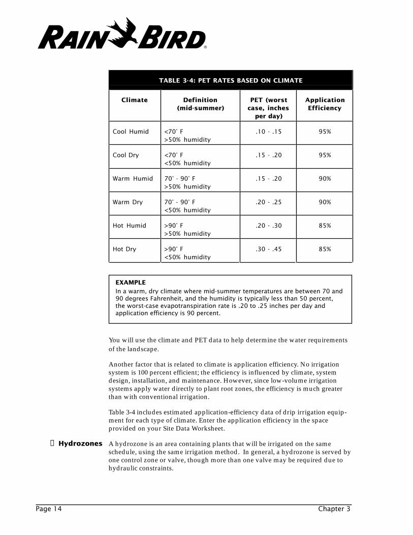
EXAMPLEIn a warm, dry climate where mid-summer temperatures are between 70 and90 degrees Fahrenheit, and the humidity is typically less than 50 percent,the worst-case evapotranspiration rate is .20 to .25 inches per day andapplication efficiency is 90 percent.
You will use the climate and PET data to help determine the water requirementsof the landscape.
Page 14 Chapter 3
Another factor that is related to climate is application efficiency. No irrigationsystem is 100 percent efficient; the efficiency is influenced by climate, systemdesign, installation, and maintenance. However, since low-volume irrigationsystems apply water directly to plant root zones, the efficiency is much greaterthan with conventional irrigation.
Table 3-4 includes estimated application-efficiency data of drip irrigation equip-ment for each type of climate. Enter the application efficiency in the spaceprovided on your Site Data Worksheet.
A hydrozone is an area containing plants that will be irrigated on the sameschedule, using the same irrigation method. In general, a hydrozone is served byone control zone or valve, though more than one valve may be required due tohydraulic constraints.
➎ Hydrozones
TABLE 3-4: PET RATES BASED ON CLIMATE
Climate Definition(mid-summer)
PET (worstcase, inches
per day)
ApplicationEfficiency
Cool Humid <70° F>50% humidity
.10 - .15 95%
Cool Dry <70° F<50% humidity
.15 - .20 95%
Warm Humid 70° - 90° F>50% humidity
.15 - .20 90%
Warm Dry 70° - 90° F<50% humidity
.20 - .25 90%
Hot Humid >90° F>50% humidity
.20 - .30 85%
Hot Dry >90° F<50% humidity
.30 - .45 85%
®
Gather Site Data Page 15
On your Site Data Worksheet, enter a general description of the plants in eachhydrozone, such as “mixed ground cover and shrubs.” In some cases, thisinformation will come from the planting plan; in other cases, you will collect thedata from an actual site survey. Also, describe the planting density in eachhydrozone, this will strongly influence the selection of emission devices.
For each hydrozone, enter the irrigation method to be used. At this point, youmay simply want to distinguish low-volume hydrozones from other areasrequiring conventional turf rotors or spray heads.
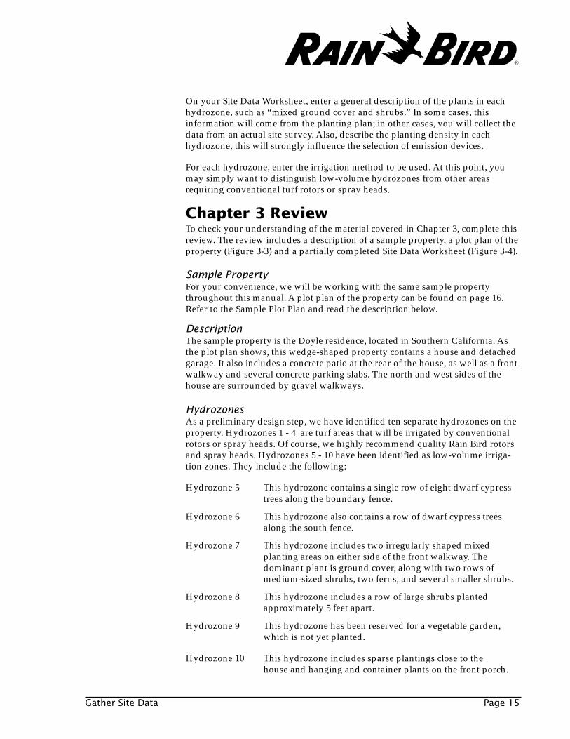
Chapter 3 ReviewTo check your understanding of the material covered in Chapter 3, complete thisreview. The review includes a description of a sample property, a plot plan of theproperty (Figure 3-3) and a partially completed Site Data Worksheet (Figure 3-4).
Sample PropertyFor your convenience, we will be working with the same sample propertythroughout this manual. A plot plan of the property can be found on page 16.Refer to the Sample Plot Plan and read the description below.
DescriptionThe sample property is the Doyle residence, located in Southern California. Asthe plot plan shows, this wedge-shaped property contains a house and detachedgarage. It also includes a concrete patio at the rear of the house, as well as a frontwalkway and several concrete parking slabs. The north and west sides of thehouse are surrounded by gravel walkways.
HydrozonesAs a preliminary design step, we have identified ten separate hydrozones on theproperty. Hydrozones 1 - 4 are turf areas that will be irrigated by conventionalrotors or spray heads. Of course, we highly recommend quality Rain Bird rotorsand spray heads. Hydrozones 5 - 10 have been identified as low-volume irriga-tion zones. They include the following:
Hydrozone 5 This hydrozone contains a single row of eight dwarf cypresstrees along the boundary fence.
Hydrozone 6 This hydrozone also contains a row of dwarf cypress treesalong the south fence.
Hydrozone 7 This hydrozone includes two irregularly shaped mixedplanting areas on either side of the front walkway. Thedominant plant is ground cover, along with two rows ofmedium-sized shrubs, two ferns, and several smaller shrubs.
Hydrozone 8 This hydrozone includes a row of large shrubs plantedapproximately 5 feet apart.
Hydrozone 9 This hydrozone has been reserved for a vegetable garden,which is not yet planted.
Hydrozone 10 This hydrozone includes sparse plantings close to thehouse and hanging and container plants on the front porch.
®

Page 16 Chapter 3
����������������������������������������
GARAGE
HOUSE
SHED
TURF
TURF
TURF VEG.GARDEN
FENCE
PORCH
C O N N O R L A N E
FENCE
TURF
N S
E
W
10
H H H
C C C C
M
Hydrozone
Ground Cover
Gravel Walkways
Concrete
Water Meter
Container Plant
Hanging Plant
Shrub
Tree
����C
M
H
10
Figure 3-3: Sample Plot Plan—Doyle Residence
®
Gather Site Data Page 17
SITE DATA WORKSHEET
Site Information
Eve. Phone
❶ Water Source Notes➋
Yes No
Yes No
Soil TypeCoarse
Medium
Fine
➌
Name
Address
City
Contact
Day Phone
Pipe Requirements
Specs on File
Permits required?
Cost
City Water
Well:
Surface Water
Effluent
Water Purveyor
Contact
Phone
Meter Location
Meter size (inches)
Service Line Type and Size
Static Pressure (PSI at meter)
Elevation change (± feet)
Good Fair PoorWater Quality:
HP PSI GPMSub CentrifugalState Zip
Climate and PETCool Humid
Warm Humid
Hot Humid
Cool Dry
Warm Dry
Hot Dry
Worst case daily PET (in. per day):
Application Efficiency (%):
➎ Hydrozones (Attach sketch of property)DESCRIPTION DENSITY# IRRIGATION METHOD
DATEJOB NUMBER
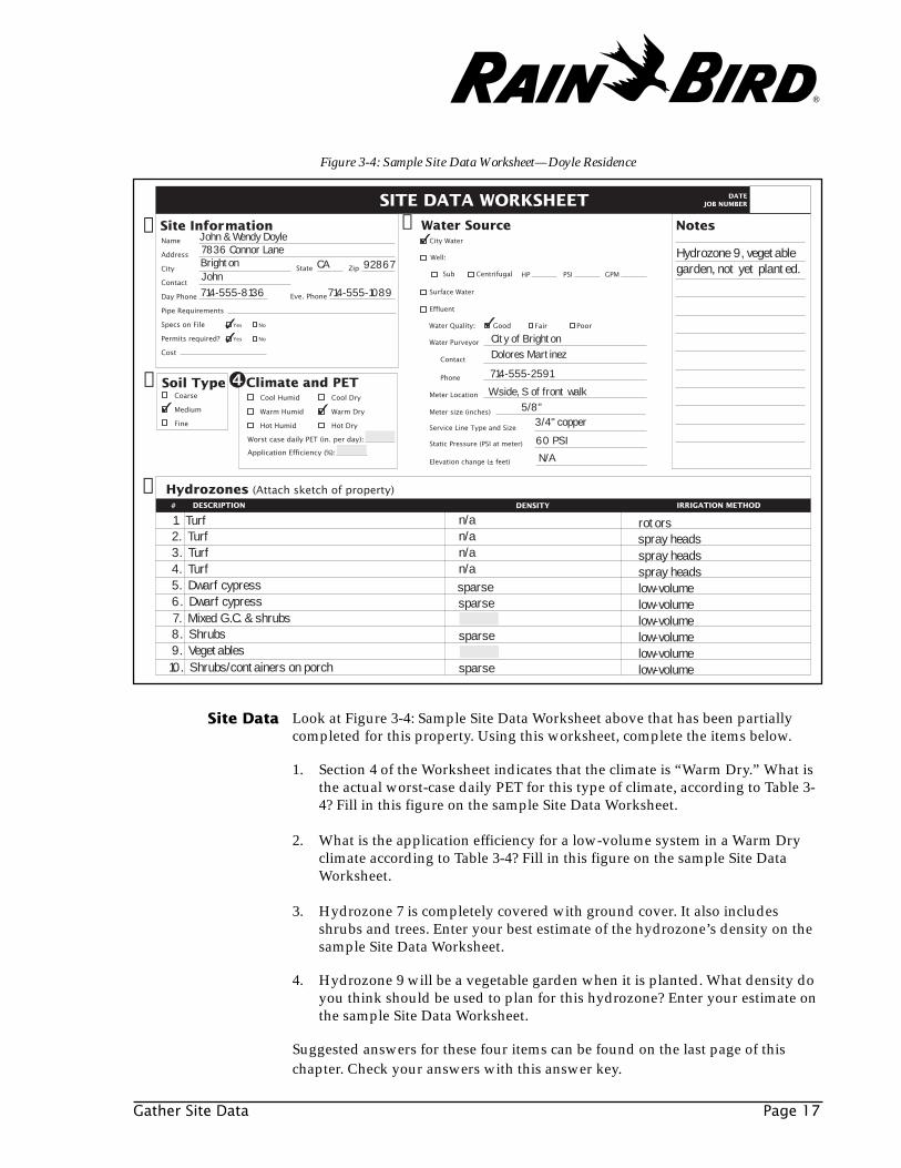
John & Wendy Doyle7836 Connor Lane
JohnBrighton CA 92867
City of BrightonDolores Martinez
714-555-2591
1. Turf2. Turf3. Turf4. Turf5. Dwarf cypress
rotorsspray heads
sparse
n/an/an/an/a
sparse
sparse
sparse
spray headsspray headslow-volumelow-volumelow-volumelow-volumelow-volumelow-volume
6. Dwarf cypress7. Mixed G.C. & shrubs8. Shrubs9. Vegetables10. Shrubs/containers on porch
Hydrozone 9, vegetable garden, not yet planted.
714-555-8136 714-555-1089
W side, S of front walk5/8"
60 PSI
N/A
3/4" copper
Look at Figure 3-4: Sample Site Data Worksheet above that has been partiallycompleted for this property. Using this worksheet, complete the items below.
1. Section 4 of the Worksheet indicates that the climate is “Warm Dry.” What isthe actual worst-case daily PET for this type of climate, according to Table 3-4? Fill in this figure on the sample Site Data Worksheet.
2. What is the application efficiency for a low-volume system in a Warm Dryclimate according to Table 3-4? Fill in this figure on the sample Site DataWorksheet.
3. Hydrozone 7 is completely covered with ground cover. It also includesshrubs and trees. Enter your best estimate of the hydrozone’s density on thesample Site Data Worksheet.
4. Hydrozone 9 will be a vegetable garden when it is planted. What density doyou think should be used to plan for this hydrozone? Enter your estimate onthe sample Site Data Worksheet.
Suggested answers for these four items can be found on the last page of thischapter. Check your answers with this answer key.
Site Data
Figure 3-4: Sample Site Data Worksheet—Doyle Residence
®
Page 18 Chapter 3
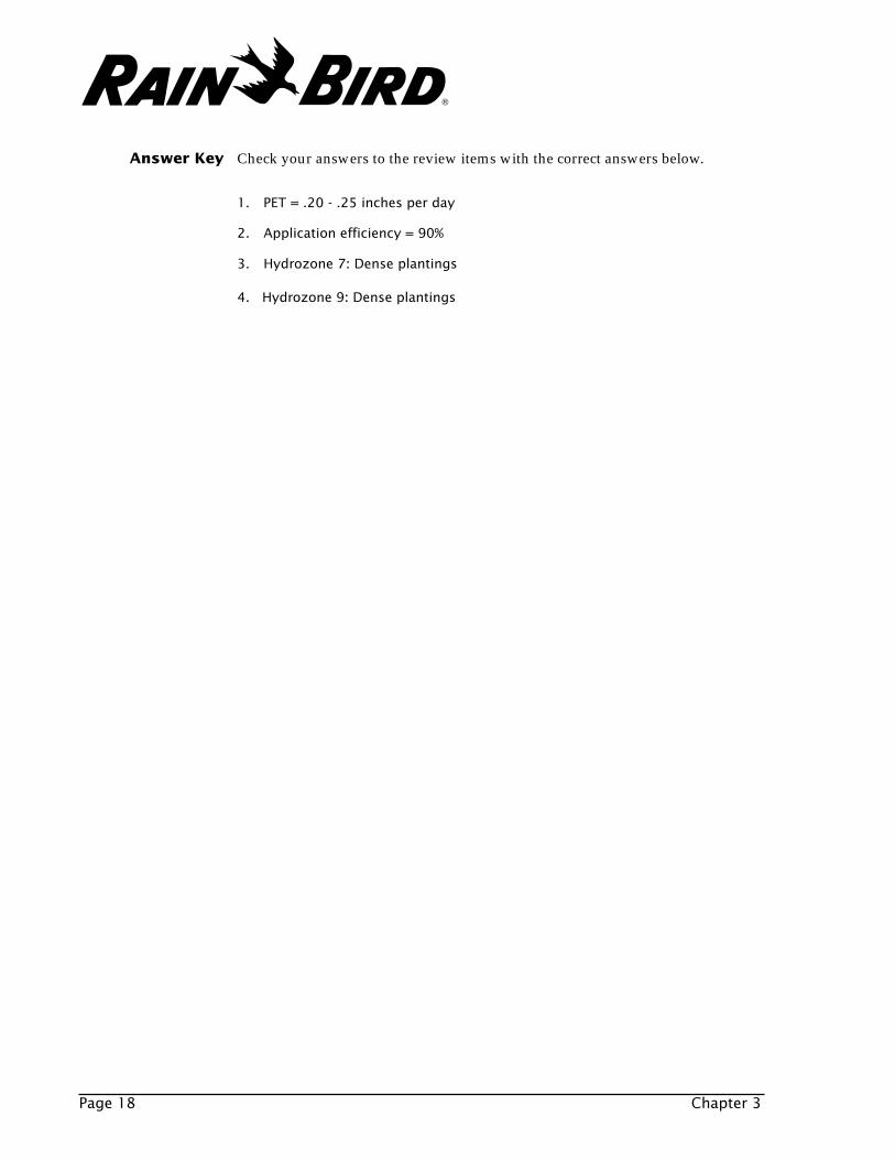
Check your answers to the review items with the correct answers below.
1. PET = .20 - .25 inches per day
2. Application efficiency = 90%
3. Hydrozone 7: Dense plantings
4. Hydrozone 9: Dense plantings
Answer Key
®
Determine Plant Water Requirements Page 19
DETERMINE PLANTWATER REQUIREMENTS
The goal of Xerigation design is to apply water efficiently and effectively to eachplant or group of plants in the landscape. To do this, you will need to estimatethe daily water requirements of the various plant material in your landscape.
Individual, sparsely arranged plants will be irrigated by individual emitters orindividual micro-bubblers. The water requirement for these plants is measured ingallons per day.
Groups of densely arranged plants will be irrigated by micro-sprays, Xeri-PopTM
micro-spray pop-ups or Landscape Dripline inline emitter tubing. These are alldesigned to distribute a precise amount of water over a fixed area. Like conven-tional irrigation, the water requirement for densely arranged plants is measuredin inches per day.
To help you calculate the water requirements and plan the rest of your low-volume installation, we have provided two hydrozone design worksheets: onefor densely planted hydrozones (Figure 4-1) and one for sparsely plantedhydrozones (Figure 4-2). Full-size samples that you can photocopy are includedin Appendix D of this manual.
At the end of Chapter 7, you will find a partially completed sample worksheet.This can serve as a guide as you read the following descriptions.
4®
Page 20 Chapter 4
Figure 4-1:
Dense
Hydrozone
Design
Worksheet
Water Requirement
.623 Area K PET✕ ✕ ✕c
Application Efficiency= Gallons per Day (GPD)
LOW-VOLUME DESIGN WORKSHEET: DENSE HYDROZONE
ADDITIONALPLANT SPECIES
SPECIESFACTOR
DENSITYFACTOR
MICROCLIMATEFACTOR Kc
PLANTDIAMETER
(FT.)
CANOPYAREA
(SQ. FT.)
WATERREQUIREMENT
(GPD)
EMISSION DEVICES
TYPE FLOW QUANTITY SPACING
Base Plant
Non-Base Plants
Water Requirement
K PET = Inches per Dayc ×
Plant Canopy Area
0.7854 Diameter Diameter = Square Feet✕ ✕
BASE PLANTSPECIES
SPECIESFACTOR
DENSITYFACTOR
MICROCLIMATEFACTOR
EMITTERFLOW RATE
ADJUSTEDEDRKc
DATEJOB NUMBER
DESCRIPTION
HYDROZONE
Eve. Phone
Name
Address
City
Contact
Day Phone
Daily PET (inches per day)
Application Efficiency
State Zip
CoarseSoil Type:
Medium
Fine
Site Information1 1
3
3 5
Ground Cover Only
Ground Cover/Trees
Ground Cover /Shrubs
Ground Cover/Shrubs/Trees
Shrubs/Trees
Shrubs Only
Planting Scheme
Base PlantGround Cover
Shrubs
Emitter Spacing
12"
18"
24"
36"
6
SYSTEM RUN TIME
5
2
24
WATERREQUIREMENT
4
Water Requirement
.623 Area K PET✕ ✕ ✕c
Application Efficiency= Gallons per Day (GPD)
LOW-VOLUME DESIGN WORKSHEET: SPARSE HYDROZONE
PLANT SPECIES SPECIESFACTOR
DENSITYFACTOR
MICROCLIMATEFACTOR Kc
PLANTDIAMETER
(FT.)
CANOPYAREA
(SQ. FT.)
WATERREQUIREMENT
(GPD)
EMISSION DEVICES
TYPE FLOW QUANTITY SPACING
Minimum Area To Be Wetted
0.7854 Diameter Diameter 50% = Square Feet✕ ✕ ×
DATEJOB NUMBER
DESCRIPTION
HYDROZONE
Eve. Phone
Name
Address
City
Contact
Day Phone
Daily PET (inches per day)
Application Efficiency
State Zip
CoarseSoil Type:
Medium
Fine
Site Information1 1
3 4 6
SYSTEM RUN TIME5
2
®
Determine Plant Water Requirements Page 21
Calculating Water RequirementsBegin by filling in the identifying information about the site and the hydrozoneat the top of the worksheet. Transfer the Daily PET, Application Efficiency, andSoil Type from the Dense Hydrozone Worksheet (Figure 7-1 at the end of Chapter7) to the appropriate places on the dense and sparse hydrozone worksheets(Figures 4-1 and 4-2, page 20). This information will be very important when youcompute the water requirements of the individual plants in the hydrozone.
Be sure to write the number of the hydrozone in the box at the upper right cornerof the worksheet. You may also want to include a one- or two-word description,such as “front planter.”
∂ Gather SiteInformation
∑ Calculate Kc As described in Chapter 3, the potential evapotranspiration rate (PET) describesthe amount of water used by a specific variety of grass under ideal moistureconditions. To calculate the exact water requirement of an individual plant, youmust adjust PET to account for specific conditions and the needs of the plant. Theadjustment factor is called the plant’s “Kc”. The terms “crop coefficient” and“plant factor” are also sometimes used.
Use the spaces on the worksheets to calculate Kc for each plant in yourhydrozone. Note that for densely planted hydrozones there are separate spacesfor recording information on base plants and non-base plants.
TABLE 4-1: BASE PLANTS IN DENSE HYDROZONES
Planting Scheme Base Plant
Ground cover only Ground cover
Ground cover and trees Ground cover
Ground cover and shrubs Ground cover
Shrubs and trees Shrubs
Shrubs only Shrubs
Ground cover, trees, and shrubs Ground cover
Dense Hydrozones OnlyIn a densely planted hydrozone, you must first identify the “base plant.” Thebase plant is the plant material in the hydrozone that uses the least amount ofwater per day. Often, it is also the plant that covers the majority of the plantedarea—generally either ground cover or shrubs. Use Table 4-1 to help you identifythe base plant for your hydrozone.
Plant SpeciesIt’s very important that you accurately list each of the plants in the hydrozone. Insome cases, this information will come from the planting plan; in other cases, youwill collect the data from an actual site survey.
®

Density FactorThe density factor indicates how densely the plants are placed in the hydrozone.As the density of the plants increases, so does the density factor.
In the top portion of the worksheet’s “density factor” box, indicate the approxi-mate range of the plant’s density factor: low, average, or high. Later, you canassign a value to the density factor, using Table 4-3 as a guideline.
EXAMPLE
Assume that you have a hydrozone planted only with shrubs that require agreat deal of water. If you locate the “Shrubs” row in Table 4-2 and read acrossto the “High” column, you’ll find that the species factor is 0.7. “High” wouldbe entered in the top half of the species factor box on the worksheet and“0.7” would be entered in the bottom half of the species factor box.
Page 22 Chapter 4
Species FactorThe species factor is an adjustment to PET that reflects the amount of water that aparticular species of plant needs relative to turf grass. The range can be from 0.2for plants like cactus and succulents that require little water, up to 0.9 for plantslike ferns that require a great deal of water.
On the dense hydrozone worksheet (Figure 4-1, page 20), indicate the estimatedrange of the plant’s species factor: “low,” “average” or “high” based on Table 4-2below. Note this in the top portion of the “species factor” box. Later, you canassign a numerical value to the species factor, again using Table 4-2 as a guideline.
TABLE 4-2: ESTIMATED SPECIES FACTORS
Plant Type Low Average High
Trees 0.2 0.5 0.9
Shrubs 0.2 0.5 0.7
Ground covers 0.2 0.5 0.7
Mixed trees, shrubs, ground covers 0.2 0.5 0.9
TABLE 4-3: ESTIMATED DENSITY FACTORS
Plant Type Low Average High
Trees 0.5 1.0 1.3
Shrubs 0.5 1.0 1.1
Ground covers 0.5 1.0 1.1
Mixed trees, shrubs, ground cover 0.6 1.1 1.3
®
Determine Plant Water Requirements Page 23
Microclimate FactorA microclimate is a sub-climate. Even small residential sites will have areas withentirely different climatic conditions. For example, areas in direct sunlight versusareas in the shade. The two areas may have identical plantings but the waterrequirements of the plants will be very different. Ideally, each microclimatewould be zoned separately. However, when this is not practical, drip irrigation isflexible enough to meet the needs of these special conditions.
EXAMPLE
Assume that you have a hydrozone that contains only sparsely planted shrubs.Locate the row labeled “Shrubs,” and read across to the “Low” column. You’llfind that the density factor for this plant is 0.5. “Low” would be entered in thetop half of the “density factor” box on your worksheet and “0.5” would beentered in the bottom half of the box.
A less obvious example of different microclimates might be areas close to a houseor a driveway, where reflective heat will change the water requirements com-pared to an area surrounded by turf. In fact, experiments have shown thatplantings surrounded by pavement may have a PET as much as fifty percenthigher than the same types of plants in a park setting.
For each plant in the hydrozone, record on your worksheet an estimate of themicroclimate: low, average, or high, based on the water adjustment the area willrequire. A “low” microclimate will require less water, and a “high” microclimatewill require more water. Record your estimate in the top portion of the “microcli-mate factor” box. Later, you can assign a value to the microclimate factor, usingTable 4-4 as a guideline.
EXAMPLE
Assume that you have a hydrozone planted with shrubs only. This hydrozoneis adjacent to the street, and it is surrounded by cement walkways. Therefore,you estimate the microclimate factor as high. If you locate the “Shrubs” row inTable 4-4 and read across to the “High” column, you’ll find that the microcli-mate factor for this plant is 1.3. “High” would be entered in the top half of the“microclimate factor” box and “1.3” would be entered in the bottom half of thebox on your worksheet.
TABLE 4-4: ESTIMATED MICROCLIMATE FACTORS
Plant Type Low Average High
Trees 0.5 1.0 1.4
Shrubs 0.5 1.0 1.3
Ground covers 0.5 1.0 1.2
Mixed trees, shrubs, ground cover 0.5 1.0 1.4
®
To calculate the Kc values, simply multiply each plant’s species factor, densityfactor, and microclimate factor. Round this number to the nearest tenth, andrecord it in the “Kc” column of the worksheet.
➌ CalculateWater Require-
ment for DensePlantings
➌ Calculate WaterRequirement forIndividual Plants
in a SparseHydrozone
The water requirement for individual plants in a sparse planting scheme ismeasured in gallons per day (GPD). To calculate the water requirement for anindividual plant, you must first calculate the area of the plant’s root zone. Youcan approximate the area of the root zone by using the area of the plant’s canopy.
Plant DiameterFor each plant, enter into the worksheet the diameter of the plant’s maturecanopy. That means that if immature plants are currently in place, you will needto estimate how big they will grow as they mature. For the water requirementcalculation, you should estimate the diameter of the plant’s canopy in feet.
EXAMPLE:
Assume the PET for our site is 0.35 inches per day (an arbitrary numberselected for this example). Previously, we calculated a Kc of 0.5. To deter-mine the water requirement, multiply these two figures together (0.35 x 0.5= 0.175). The water requirement for the base plant under these circum-stances is .175 inches per day.
After rounding to the nearest tenth, you find that the water requirement forthis site is 0.2 inches per day.
The water requirement for the base plant in a densely planted hydrozone ismeasured in inches per day. To calculate the water requirement in inches per day,the formula is:
Water Requirement (inches per day) = Kc × PET
EXAMPLE
You’re designing for a hydrozone that includes only sparsely planted shrubsthat require a great deal of supplemental water. Therefore, the species factoris high (0.7), and the density factor is low (0.5). The hydrozone is adjacent tothe street, and it is surrounded by cement walkways, so you’ve assigned it ahigh microclimate factor (1.3).
To calculate Kc you multiply:
0.7 x 0.5 x 1.3 = 0.455
After rounding to the nearest tenth, you find that the Kc for this shrub is 0.5.Enter this number in the “Kc” box on your worksheet.
Page 24 Chapter 4
KcOnce you have collected all the information about the plants in the hydrozone,and assigned the values for species, density, and microclimate factors, you cancalculate the Kc for each plant. Kc indicates the plant’s need for water as it relatesto the established PET rate in the area.
®
Determine Plant Water Requirements Page 25
Area of Plant CanopyUse the following formula to determine the area of the plant’s canopy.
Canopy Area (sq. ft.) = .7854 x Diameter (ft.) x Diameter (ft.)
Water Requirement (GPD)The water requirement for individual plants is measured in gallons per day. Tocompute the water requirement for an individual plant, you must know the areaof the plant’s root zone, its Kc, the worst case PET rate for the area, and theapplication efficiency of the irrigation system. The formula is:
Gallons per Day per Plant = .623 x Canopy Area (sq. ft.) x Kc x PET Application Efficiency
EXAMPLE
You are calculating the area of the root zone for a large shrub. The maturecanopy of the shrub is 6.5 feet in diameter. To calculate the area, you multiply:
.7854 x 6.5 ft. x 6.5 ft. = 33.18315 sq. ft.
After rounding to the nearest tenth, you find that the area of the root zone is33.2 sq. ft.
Application EfficiencyTo determine the application efficiency (the efficiency with which water isactually made available to plants) refer to the Site Data worksheet on page 11 andidentify the climate type. In the worksheet, the climate was identified as warm,dry. From Table 3-4, a warm, dry climate results in an application efficiency of 90percent. For use in the GPD (gallons per day) formula shown below, convert thepercentage to a decimal, i.e., 0.90.
EXAMPLE
You’re calculating the water requirement for the shrub used in the previousexamples. At this point, you know the following information:
Area of plant canopy = 33.2 sq. ft.Kc = 0.5PET (worst case, mid-summer) = .20 in./dayApplication Efficiency = .90
To determine the plant’s water requirement, you calculate:
.623 33.2 sq. ft. 0.5 .20 in..90
2.298177 GPD× × ×
=
After rounding to the nearest tenth, you find that the water requirement forthis plant is 2.3 gallons per day.
Calculate the water requirement for each plant in the hydrozone, and record yourresults in the spaces provided on the worksheet.
®
Chapter 4 ReviewTo check your understanding of the material covered in Chapter 4, complete thisreview. The review is based on the partially completed hydrozone worksheetwhich is located at the end of Chapter 7.
1. The worksheet indicates that the base plant is a ground cover: Ice Plant.Using the information in the sample worksheet, and Tables 4-2 through 4-4,calculate the Kc for the ice plant.
2. The non-base plants in this hydrozone include two ferns. Calculate the Kc forthe ferns.
3. Calculate the water requirement for the base plant. Remember that for densebase plants, the water requirement is measured in inches per day.
4. Calculate the water requirement for the two ferns (5-foot diameter). Remem-ber that the water requirement for individual plants is calculated in gallonsper day. To calculate the water requirement, you must first calculate the areaof the plant canopy.
Page 26 Chapter 4
®
Determine Plant Water Requirements Page 27
Check your answers to the review items with the correct answers below.
1. Species Factor = 0.2Density Factor = 1.1Microclimate Factor = 1.2
Kc = 0.3
2. Species Factor = 0.7Density Factor = 0.5Microclimate Factor = 1.3
Kc = 0.5
3. Water requirement = 0.06 inches per day
4. Canopy Area = 19.6 square feetWater Requirement = 1.4 gallons per day
Answer Key
®

Page 28 Chapter 4
®
Irrigate Base Plants Page 29
IRRIGATE BASE PLANTS
In this chapter, you will:
1. Identify the hydrozone’s base plant.
2. Select emission devices for the base plant.
This chapter will continue to use the Hydrozone Design Worksheets introducedin the previous chapter. Use the sample worksheet at the end of Chapter 7 as areference while reading this chapter.
Identifying the Base PlantIf you have not already identified the base plant, you must do so now.
In a densely planted hydrozone, the base plant is the plant material with thelowest water requirement in the hydrozone. It is also typically the type of plantthat covers the majority of the planted area—generally either ground cover orshrubs. For dense hydrozones, you identify the base plant as part of calculatingthe water requirement.
In a sparsely planted hydrozone, the base plant is the individual plant with thelowest water requirement. You will run your system just long enough to irrigatethis base plant. You will design your system to deliver the required amount ofwater to all other plants in the time it takes to irrigate the base plant.
Estimate the water requirements of all the individual plants in the hydrozone,and choose the plant with the lowest water requirement as your base plant. Enterthis plant in the “Base Plant” section of your design worksheet for easy reference.
5
Dense Plantings
Sparse Plantings
®
Page 30 Chapter 5
➍ Emission DevicesTo select the best emission device or devices to irrigate the base plant, start byconsidering the following:
• Types of Plants. As we have already seen, the primary factor that affectsyour design is the water requirement of the individual plants or groups ofplants in the landscape.
• Intended Use. Factors such as traffic and the threat of vandalism will affectyour choice of distribution components and emission devices. For example,micro-sprays and micro-bubblers are probably not appropriate in high-trafficareas. These emission devices can also create overspray.
In areas that are prone to vandalism, system components that can be in-stalled below grade are better than above-ground devices. LandscapeDripline and Xeri-Pop micro-spray pop-ups would be good choices becausethey are out of sight when not in operation.
• Size of Planted Area. It may be too labor intensive and costly to installindividual emitters over a very large planted area. In these cases, it might bemore economical to use Landscape Dripline, micro-sprays or Xeri-Pops. Forextremely large areas, consider using conventional sprays or rotary headswith a separate drip zone around the perimeter to eliminate unwantedoverspray onto walkways or streets.
• Soil Type and Infiltration Rate. As shown in Chapter 2, different soil typesabsorb water in different ways. In coarse (sandy) soil, water tends to perco-late downward, while in fine (clay) soil the moisture tends to spread horizon-tally before moving vertically.
When irrigating areas with very coarse soil, consider using higher flow PCModules or micro-bubblers rather than emitters. Conversely, avoid higherflow PC Modules and micro-bubblers when irrigating very fine clay soil,unless you build troughs or wells around each plant being watered. Choos-ing emitters with low flow rates will help avoid runoff.
• Watering Window. The watering window is the amount of time available forirrigation each day. For example, some sites might require that conventionalirrigation take place during the night to avoid problems with overspray orrunoff or to follow municipal regulations. A low-volume system usingemitters may increase the watering window by permitting irrigation to takeplace during the day. Micro-sprays and micro-bubblers may have a morelimited watering window than emitters or Landscape Dripline systemsbecause they discharge water into the air, making them more similar toconventional sprays and rotors.
®
Irrigate Base Plants Page 31
Labor CostConsiderations
• Cost. The equipment cost for low-volume systems is generally lower thanconventional systems. However, in many cases the installation cost will behigher for commercial drip systems and lower for residential low-volumesystems. This is because commercial drip systems tend to be installed oneither buried PVC or high-density polyethyelene tubing. Residential dripsystems typically use poly drip tubing installed at grade, which can beinstalled more quickly (once crews are familiar with low-volume irrigationinstallation techniques).
Among low-volume systems, there will also be labor cost differences. For example,a system requiring many individual emitters may cost more than one that uses asmaller number of micro-sprays or inline emitter tubing. The Xerigation productline includes a variety of emission devices designed for many different applica-tions. Table 5-1 will help you select the most appropriate emission devices foreach plant or group of plants in your landscape. For more information aboutthese products, see the Xerigation section of the Rain Bird Landscape IrrigationProducts Catalog.
®
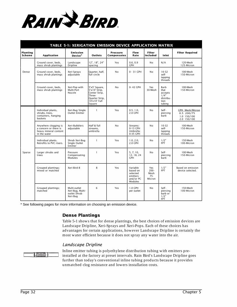
TABLE 5-1: XERIGATION EMISSION DEVICE APPLICATION MATRIX
PlantingScheme Application
EmissionDevice* Outlets
PressureCompensates
FlowRate
FilterIncluded Inlet
Filter Required
Ground cover, beds,mass shrub plantings
LandscapeDripline
12", 18", 24"spacing
Yes 0.6, 0.9GPH
No N/A 120-Mesh 125-Micron
Dense Ground cover, beds,mass shrub plantings
Xeri-Spraysadjustable
Quarter, half,full circle
No 0 - 31 GPH No 10-32self-tappingthreads
100-Mesh 150-Micron
Ground cover, beds,mass shrub plantings
Xeri-Pop withMulti-PortNozzle
5'x5' Square,5'x10' Strip,Center Strip,Three-Quarter Strip,10'x10' FullSquare
No 0- 42 GPH Yes 30-Mesh
Barbthataccepts1/4"distribu -tiontubing
100-Mesh 150-Micron
Individual plants,shrubs, trees,containers, hangingbaskets
Xeri-Bug SingleOutlet Emitter
1 Yes 0.5, 1.0,2.0 GPH
No Self -piercingbarb
GPH Mesh/Micron0.5 .200/75 1.0 150/100 2.0 150/100
Anywhere clogging isa concern or there isheavy mineral contentin the water
Xeri-Bubblersadjustable
Half & fullstreams,umbrella
No Streams: 0-13 GPHUmbrella:0-35 GPH
No 10-32self-tappingthreads
100-Mesh 150-Micron
Individual plants.Retrofits to PVC risers.
Shrub Xeri-BugSingle OutletEmitter
1 Yes 1.0, 2.0,2.0 GPH
No 1/2"FPT
150-Mesh 100-Micron
Sparse Larger shrubs andtrees
PressureCompensatingModules
1 Yes 5, 7, 10,12, 18, 24GPH
No Self -piercingbarb
100-Mesh 150-Micron
Grouped plantings;mixed or matched
Xeri-Bird-8 8 Yes Variablebased onselectedemittersand/or PCModules
Yes 200 -Mesh 75-
Micron
1/2”FPT
Based on emissiondevice selected.
Grouped plantings;matched
Multi-outletXeri-Bug, Multi -outlet ShrubXeri-Bug
6 Yes 1.0 GPHper outlet
No Self -piercingbarb or1/2”FPT
150-Mesh 100-Micron
Dense PlantingsTable 5-1 shows that for dense plantings, the best choices of emission devices areLandscape Dripline, Xeri-Sprays and Xeri-Pops. Each of these choices hasadvantages for certain applications, however Landscape Dripline is certainly themost water efficient because it does not spray any water into the air.
Page 32 Chapter 5
Landscape DriplineInline emitter tubing is polyethylene distribution tubing with emitters pre-installed at the factory at preset intervals. Rain Bird's Landscape Dripline goesfurther than today's conventional inline tubing products because it providesunmatched clog resistance and lowers installation costs.
* See following pages for more information on choosing an emission device.
®
Irrigate Base Plants Page 33
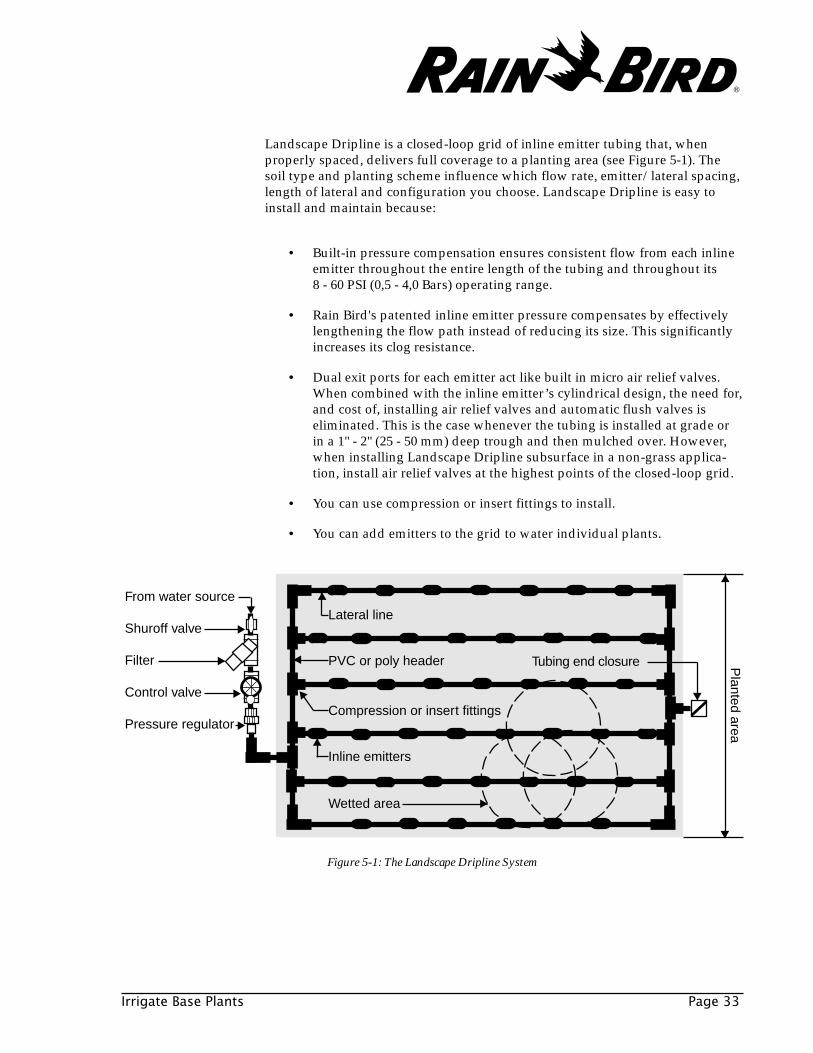
Landscape Dripline is a closed-loop grid of inline emitter tubing that, whenproperly spaced, delivers full coverage to a planting area (see Figure 5-1). Thesoil type and planting scheme influence which flow rate, emitter/lateral spacing,length of lateral and configuration you choose. Landscape Dripline is easy toinstall and maintain because:
• Built-in pressure compensation ensures consistent flow from each inlineemitter throughout the entire length of the tubing and throughout its8 - 60 PSI (0,5 - 4,0 Bars) operating range.
• Rain Bird's patented inline emitter pressure compensates by effectivelylengthening the flow path instead of reducing its size. This significantlyincreases its clog resistance.
• Dual exit ports for each emitter act like built in micro air relief valves.When combined with the inline emitter’s cylindrical design, the need for,and cost of, installing air relief valves and automatic flush valves iseliminated. This is the case whenever the tubing is installed at grade orin a 1" - 2" (25 - 50 mm) deep trough and then mulched over. However,when installing Landscape Dripline subsurface in a non-grass applica-tion, install air relief valves at the highest points of the closed-loop grid.
• You can use compression or insert fittings to install.
• You can add emitters to the grid to water individual plants.
Figure 5-1: The Landscape Dripline System
Planted area
From water source
Shuroff valve
Filter
Control valve
Pressure regulator
Lateral line
PVC or poly header
Compression or insert fittings
Wetted area
Inline emitters
Tubing end closure
▲
▲
▲
▲
▲
▲
▲
▲▲
▲
▲
▲
▲
®
Page 34 Chapter 5
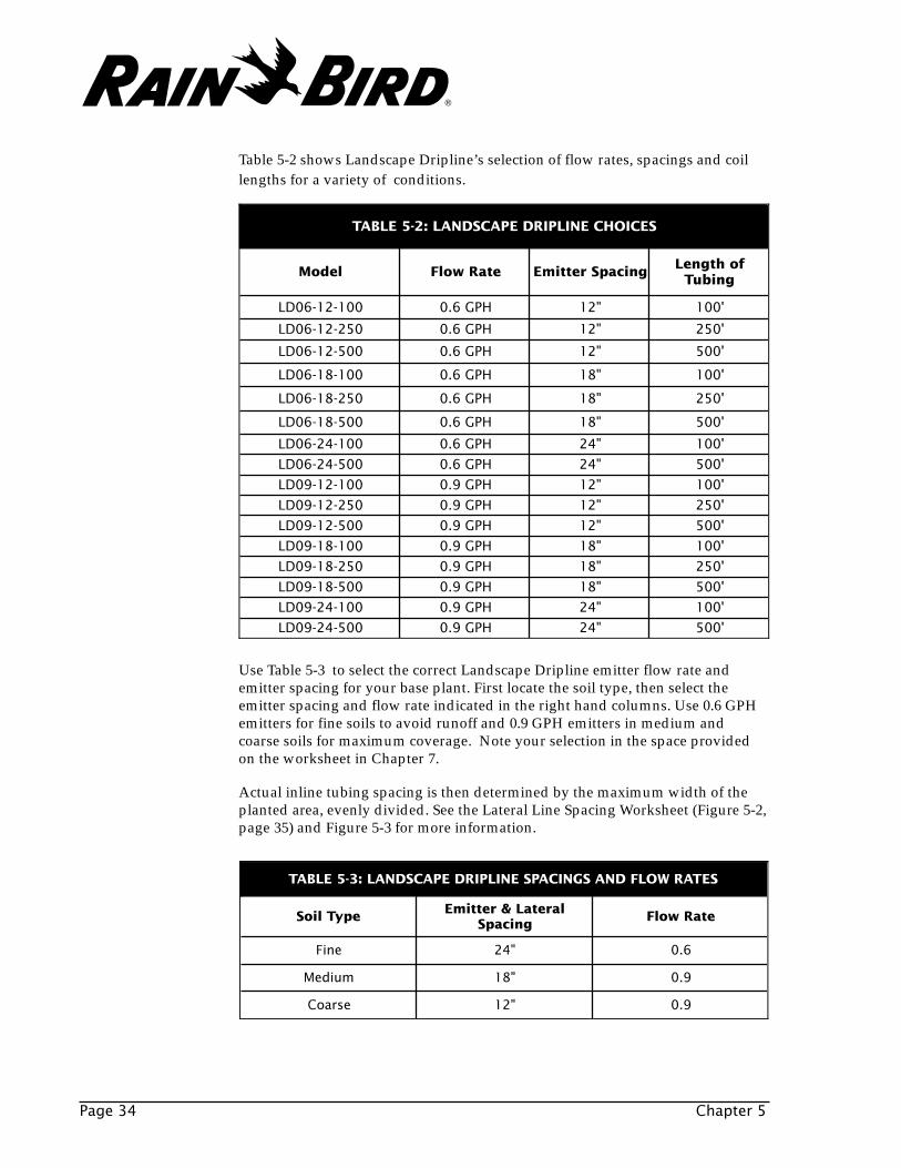
Table 5-2 shows Landscape Dripline’s selection of flow rates, spacings and coillengths for a variety of conditions.
Use Table 5-3 to select the correct Landscape Dripline emitter flow rate andemitter spacing for your base plant. First locate the soil type, then select theemitter spacing and flow rate indicated in the right hand columns. Use 0.6 GPHemitters for fine soils to avoid runoff and 0.9 GPH emitters in medium andcoarse soils for maximum coverage. Note your selection in the space providedon the worksheet in Chapter 7.
Actual inline tubing spacing is then determined by the maximum width of theplanted area, evenly divided. See the Lateral Line Spacing Worksheet (Figure 5-2,page 35) and Figure 5-3 for more information.
TABLE 5-2: LANDSCAPE DRIPLINE CHOICES
Model Flow Rate Emitter Spacing Length ofTubing
LD06-12-100 0.6 GPH 12" 100'
LD06-12-250 0.6 GPH 12" 250'
LD06-12-500 0.6 GPH 12" 500'
LD06-18-100 0.6 GPH 18" 100'
LD06-18-250 0.6 GPH 18" 250'
LD06-18-500 0.6 GPH 18" 500'
LD06-24-100 0.6 GPH 24" 100'
LD06-24-500 0.6 GPH 24" 500'
LD09-12-100 0.9 GPH 12" 100'
LD09-12-250 0.9 GPH 12" 250'
LD09-12-500 0.9 GPH 12" 500'
LD09-18-100 0.9 GPH 18" 100'
LD09-18-250 0.9 GPH 18" 250'
LD09-18-500 0.9 GPH 18" 500'
LD09-24-100 0.9 GPH 24" 100'
LD09-24-500 0.9 GPH 24" 500'
TABLE 5-3: LANDSCAPE DRIPLINE SPACINGS AND FLOW RATES
Soil Type Emitter & LateralSpacing
Flow Rate
Fine 24" 0.6
Medium 18" 0.9
Coarse 12" 0.9
®
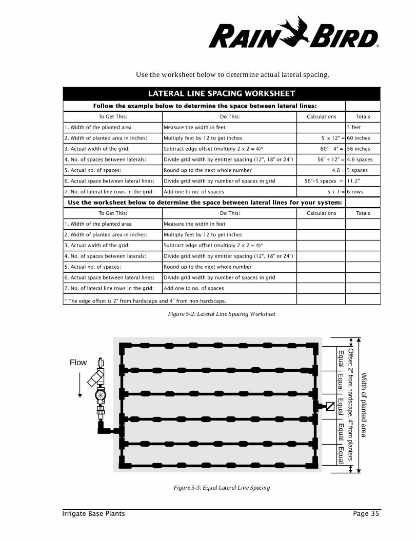
LATERAL LINE SPACING WORKSHEET
Follow the example below to determine the space between lateral lines:
To Get This: Do This: Calculations Totals
1. Width of the planted area Measure the width in feet 5 feet
2. Width of planted area in inches: Multiply feet by 12 to get inches 5' x 12" = 60 inches
3. Actual width of the grid: Subtract edge offset (multiply 2 x 2 = 4)* 60" - 4" = 56 inches
4. No. of spaces between laterals: Divide grid width by emitter spacing (12", 18" or 24") 56" ÷ 12" = 4.6 spaces
5. Actual no. of spaces: Round up to the next whole number 4.6 = 5 spaces
6. Actual space between lateral lines: Divide grid width by number of spaces in grid 56"÷5 spaces = 11.2"
7. No. of lateral line rows in the grid: Add one to no. of spaces 5 + 1 = 6 rows
Use the worksheet below to determine the space between lateral lines for your system:
To Get This: Do This: Calculations Totals
1. Width of the planted area Measure the width in feet
2. Width of planted area in inches: Multiply feet by 12 to get inches
3. Actual width of the grid: Subtract edge offset (multiply 2 x 2 = 4)*
4. No. of spaces between laterals: Divide grid width by emitter spacing (12", 18" or 24")
5. Actual no. of spaces: Round up to the next whole number
6. Actual space between lateral lines: Divide grid width by number of spaces in grid
7. No. of lateral line rows in the grid: Add one to no. of spaces
* The edge offset is 2" from hardscape and 4" from non-hardscape.
Irrigate Base Plants Page 35
Figure 5-3: Equal Lateral Line Spacing
Use the worksheet below to determine actual lateral spacing.
Width of planted area
Offset: 2" from
hardscape, 4” from planters
Equal
Equal
Equal
Equal
Equal
▲
▲
▲
▲
▲
▲
Flow
▲
Figure 5-2: Lateral Line Spacing Worksheet
®
Page 36 Chapter 5
Wateringdepth
( )x
Emitter spacing: x
Coarse soil Medium soil Fine soil
2x 4x
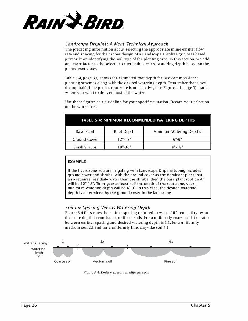
Figure 5-4: Emitter spacing in different soils
Landscape Dripline: A More Technical ApproachThe preceding information about selecting the appropriate inline emitter flowrate and spacing for the proper design of a Landscape Dripline grid was basedprimarily on identifying the soil type of the planting area. In this section, we addone more factor to the selection criteria: the desired watering depth based on theplants’ root zones.
Table 5-4, page 39, shows the estimated root depth for two common denseplanting schemes along with the desired watering depth. Remember that sincethe top half of the plant’s root zone is most active, (see Figure 1-1, page 3) that iswhere you want to deliver most of the water.
Use these figures as a guideline for your specific situation. Record your selectionon the worksheet.
Emitter Spacing Versus Watering DepthFigure 5-4 illustrates the emitter spacing required to water different soil types tothe same depth in consistent, uniform soils. For a uniformly coarse soil, the ratiobetween emitter spacing and desired watering depth is 1:1, for a uniformlymedium soil 2:1 and for a uniformly fine, clay-like soil 4:1.
EXAMPLE
If the hydrozone you are irrigating with Landscape Dripline tubing includesground cover and shrubs, with the ground cover as the dominant plant thatalso requires less daily water than the shrubs, then the base plant root depthwill be 12"-18”. To irrigate at least half the depth of the root zone, yourminimum watering depth will be 6”-9”. In this case, the desired wateringdepth is determined by the ground cover in the landscape.
TABLE 5-4: MINIMUM RECOMMENDED WATERING DEPTHS
Base Plant Root Depth Minimum Watering Depths
Ground Cover 12"-18" 6"-9"
Small Shrubs 18"-36" 9"-18"
®
Irrigate Base Plants Page 37
However, there is a limit to the horizontal spread of water by capillary action inthe soil even when that soil has been well amended and is consistent throughoutthe planting area. As a result, you must be careful not to exceed the maximumallowable spacing of the emitters as shown in Table 5-5. If this maximum spacingis exceeded, dry spots between emitters will result and it is likely that salts willbuild up around the plants’ roots.
Applying The More Technical ApproachUse Table 5-6 to select the correct emitter spacing for your base plant. First locatethe soil type, and then the desired watering depth. Select the emitter spacingindicated in the right hand column.
EXAMPLE
To irrigate to a depth of 9” in medium soil, choose Landscape Dripline tubingwith 0.9 or 0.6 GPH emitters spaced at 18” intervals and lateral spacing thatdoes not exceed 18”.
In many cases, you can choose the flow rate based on your preference for systemrun time; the higher the flow rate, the less time it takes to deliver a given amountof water to the plant. However, you should always use 0.6 GPH emitters for veryfine soils to avoid runoff.
TABLE 5-5: MAXIMUM EMISSION DEVICE SPACING (INCHES)
Emitter Flow Coarse Medium Fine
0.6 GPH 12.0 27.6 39.9
0.9 GPH 20.4 33.7 42.9
2.0 GPH 39.6 51.6 67.2
TABLE 5-6: RECOMMENDED EMITTER SPACING
Soil Type Minimum DesiredWatering Depth
Emitter Spacing
Coarse6"
12"18"
Use Micro-Sprays12"18"
Medium6"9"
12"18"
12"18"24"36"
Fine6"9"
12"
24"36"48"
®
Table 5-1 shows that for sparse plantings, the best choices of emission devices areXeri-Bug emitters, Xeri-Bubblers, Pressure Compensating Modules and the Xeri-Bird-8. You can use 1.0 or 2.0 GPH emitters for most sparse planting schemes,and 0.5 GPH emitters for container plants and very fine soils. For larger shrubsand trees, choose pressure-compensating modules or Xeri-Bubblers to providelarger flows and to reduce the total number of emitters required. To eliminatepossible runoff, consider the use of wells or troughs to capture the higher flow.
Sparse Plantings
Page 38 Chapter 5
Xeri-SpraysRain Bird’s Xeri-Sprays (max. flow 31 GPH at 30 PSI) have higher flow rates thanmost drip emitters, but lower flow rates than conventional sprays (up to 216GPH). They are best suited to irrigating large, densely planted areas such as largeareas of ground cover. Avoid using Xeri-Sprays in windy conditions. Xeri-Spraysshould be placed head-to-head to allow for at least a 50% overlap of the spraypatterns. Xeri-Sprays will provide, on average, approximately one inch per hourof water.
Xeri-Pop Series Micro-spray Pop-UpsRain Bird’s XP Series Xeri-Pop micro-spray pop-ups are much like conventionalpop-up spray heads except that they feature a 1/4" barb inlet instead of thetraditional 1/2" threaded inlet. They accept 5, 8 and 10 Series MPR nozzles withflow rates of 45 GPH (0.75 GPM) or less. Xeri-Pops are available in 2", 4" or 6"pop-up models. They pop up to water and then pop down flush when not inoperation so they are practically invisible and less vulnerable to damage. A 40 or50 PSI pressure regulator is recommended for a Xeri-Pop zone.
Multi-Port Spray Nozzle (available Spring 2000)The Multi-Port spray nozzle is unique in that it provides five patterns in one low-flow micro-spray nozzle. Its patent-pending design is based on four independentflow quadrants that can be opened, much like an emitter hole is punched intodrip tubing. The Multi-Port nozzle is compatible with all 1800 Series, UNI-SpraySeries and Xeri-Pop micro-spray pop-ups. In addition, it is virtually mist-free athigher pressures of up to 70 PSI.
For non-turf applications, Xeri-Pops are ideal for:
• High traffic areas where vandalism, safety or aesthetics are a concern.
• Dense plantings where single-outlet emitters would be cost prohibitive toinstall and conventional spray heads would overspray. Xeri-Pops have awide and adjustable area of coverage from a 5’ x 5’ quadrant up to a 10’ x 10’square.
• Irregularly shaped planters to help avoid overspray.
• Use with PCS screens (0.1, 0.2, 0.3, 0.4 and 0.6 GPM) and 5 B Series bubblernozzles to create a low-volume pop-up micro-bubbler that is easily visiblewhen in operation. Provides water-saving benefits of drip with the lowmaintenance of pop-ups.
®
Irrigate Base Plants Page 39
Selecting Emitters
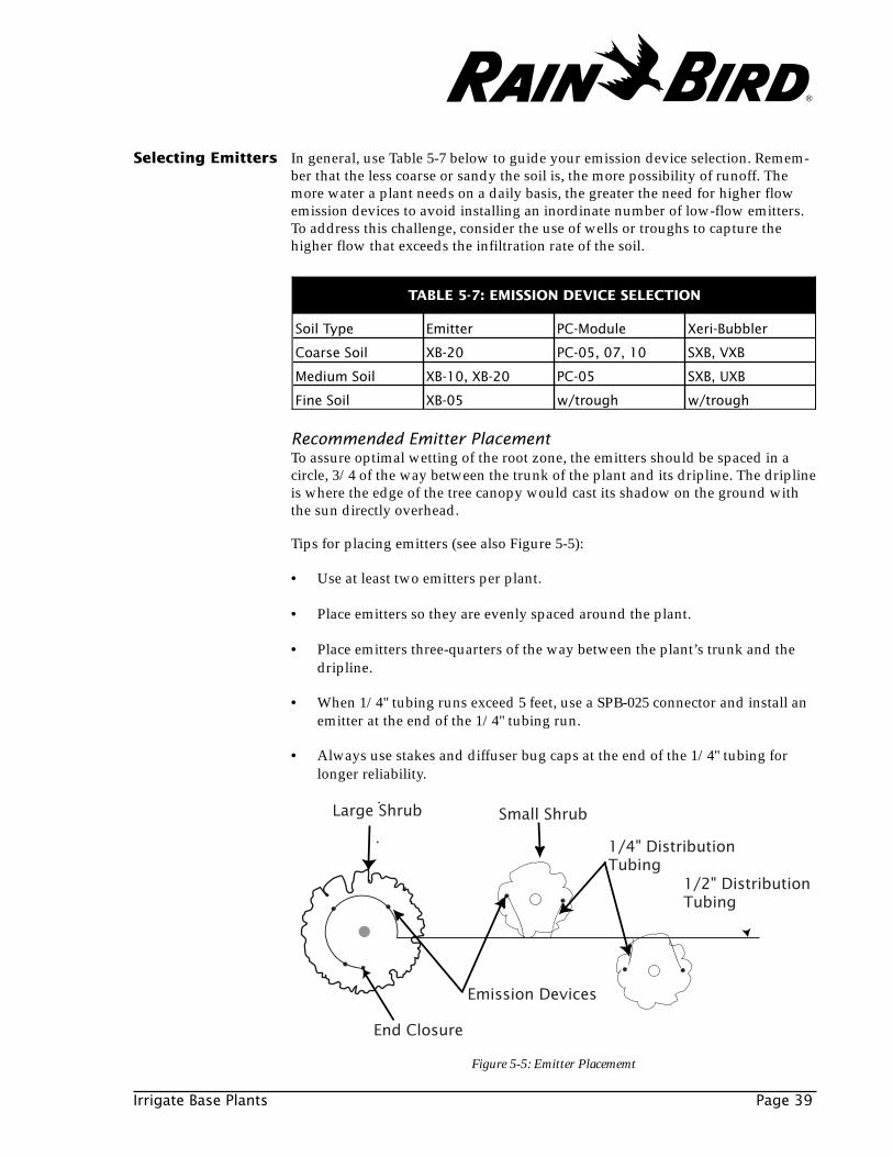
TABLE 5-7: EMISSION DEVICE SELECTION
Soil Type Emitter PC-Module Xeri-Bubbler
Coarse Soil XB-20 PC-05, 07, 10 SXB, VXB
Medium Soil XB-10, XB-20 PC-05 SXB, UXB
Fine Soil XB-05 w/trough w/trough
In general, use Table 5-7 below to guide your emission device selection. Remem-ber that the less coarse or sandy the soil is, the more possibility of runoff. Themore water a plant needs on a daily basis, the greater the need for higher flowemission devices to avoid installing an inordinate number of low-flow emitters.To address this challenge, consider the use of wells or troughs to capture thehigher flow that exceeds the infiltration rate of the soil.
Recommended Emitter PlacementTo assure optimal wetting of the root zone, the emitters should be spaced in acircle, 3/4 of the way between the trunk of the plant and its dripline. The driplineis where the edge of the tree canopy would cast its shadow on the ground withthe sun directly overhead.
Tips for placing emitters (see also Figure 5-5):
• Use at least two emitters per plant.
• Place emitters so they are evenly spaced around the plant.
• Place emitters three-quarters of the way between the plant’s trunk and thedripline.
• When 1/4" tubing runs exceed 5 feet, use a SPB-025 connector and install anemitter at the end of the 1/4" tubing run.
• Always use stakes and diffuser bug caps at the end of the 1/4" tubing forlonger reliability.
Figure 5-5: Emitter Placememt
Small Shrub
End Closure
Large Shrub
Emission Devices
1/4" Distribution Tubing
1/2" Distribution Tubing
®
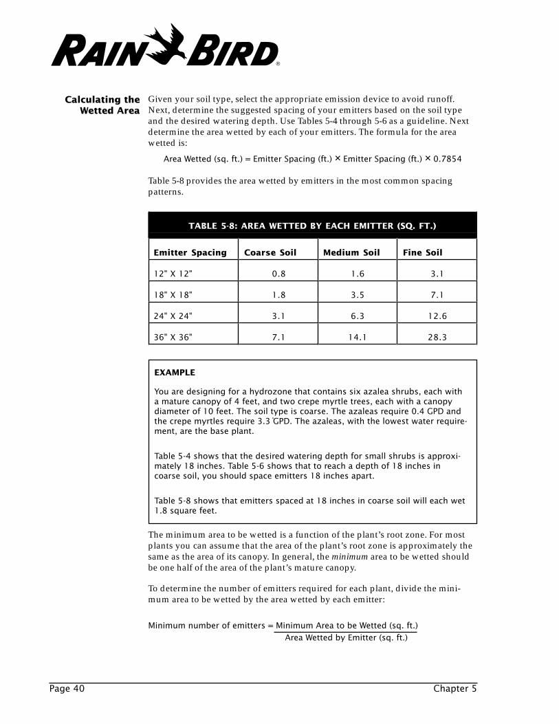
Table 5-8 provides the area wetted by emitters in the most common spacingpatterns.
Area Wetted (sq. ft.) = Emitter Spacing (ft.) × Emitter Spacing (ft.) × 0.7854
Given your soil type, select the appropriate emission device to avoid runoff.Next, determine the suggested spacing of your emitters based on the soil typeand the desired watering depth. Use Tables 5-4 through 5-6 as a guideline. Nextdetermine the area wetted by each of your emitters. The formula for the areawetted is:
Calculating theWetted Area
Page 40 Chapter 5
The minimum area to be wetted is a function of the plant’s root zone. For mostplants you can assume that the area of the plant’s root zone is approximately thesame as the area of its canopy. In general, the minimum area to be wetted shouldbe one half of the area of the plant’s mature canopy.
To determine the number of emitters required for each plant, divide the mini-mum area to be wetted by the area wetted by each emitter:
Minimum number of emitters = Minimum Area to be Wetted (sq. ft.) Area Wetted by Emitter (sq. ft.)
EXAMPLE
You are designing for a hydrozone that contains six azalea shrubs, each witha mature canopy of 4 feet, and two crepe myrtle trees, each with a canopydiameter of 10 feet. The soil type is coarse. The azaleas require 0.4 GPD andthe crepe myrtles require 3.3␣ GPD. The azaleas, with the lowest water require-ment, are the base plant.
Table 5-4 shows that the desired watering depth for small shrubs is approxi-mately 18 inches. Table 5-6 shows that to reach a depth of 18 inches incoarse soil, you should space emitters 18 inches apart.
Table 5-8 shows that emitters spaced at 18 inches in coarse soil will each wet1.8 square feet.
TABLE 5-8: AREA WETTED BY EACH EMITTER (SQ. FT.)
Emitter Spacing Coarse Soil Medium Soil Fine Soil
12" X 12" 0.8 1.6 3.1
18" X 18" 1.8 3.5 7.1
24" X 24" 3.1 6.3 12.6
36" X 36" 7.1 14.1 28.3
®
Irrigate Base Plants Page 41
Chapter ReviewTo check your understanding of the material covered in Chapter 5, complete thisreview. The review is partly based on the partially completed hydrozoneworksheet (Figure 7-1) which is located at the end of Chapter 7.
1. In a densely planted hydrozone, is the base plant the plant materal that hasthe highest or lowest water requirement in the hydrozone?
2. For each emission device, indicate whether it is best suited to water a denseplanting scheme or individual plants in a sparse planting scheme:
a. Xeri-Bug emittersb. Xeri-Bubblersc. Landscape Dripline tubingd. Lower flow PC-Modulese. Xeri-Sprays
3. For each soil type, indicate the suggested Landscape Dripline inline emitterflow rate and lateral spacing.
a. Coarseb. Mediumc. Fine
4. The base plant in our sample hydrozone is ice plant, a dense ground coverplanted in medium soil. We will use Landscape Dripline with 0.9 GPMemitters to irrigate this plant. Use Table 5-3 to determine the emitter andlateral spacing for the ice plant.
5. Determine the number of Landscape Dripline rows and the space betweenrows for a planted area 10’ wide using the Lateral Line Spacing Worksheet onpage 35.
EXAMPLE
The minimum area to be wetted for each 4-foot azalea is 6.3 square feet. Thisis because the area of the root zone is estimated as:
.7854 x diameter x diameter or .7854 x 4 x 4 = 12.6 sq. ft.
The minimum area that should be wetted is 50 percent of the root zone or1/2 x 12.6 = 6.3 sq. ft.
Dividing this by the area wetted by each emitter (1.8 square feet) tells us thatwe will need at least four emitters for each azalea.
®
Page 42 Chapter 5
Check your answers to the review items with the correct answers below.
1. Lowest
2. a. Sparse
b. Sparse
c. Dense
d. Sparse
e. Dense
3. a. 0.9 GPH/12" spacingb. 0.9 GPH/18” spacingc. 0.6 GPH/24” spacing
4. Emitter and lateral spacing = 18 inches
5. Number of rows = 11 rows Spacing between rows = 11.6 inches
Answer Key
®

Calculate System Run Time Page 43
CALCULATE SYSTEMRUN TIME
The system run time is determined by the base plant. Since the base plant is theplant that requires the least amount of water, you will run the system only longenough to supply the correct amount of water to the base plant. In the nextchapter, you will determine the flow rates for the non-base plants as well as thebest-suited emission devices to achieve these flow rates. This will be based ontwo things: the watering schedule for the base plant and the daily wateringrequirements of the non-base plants.
This chapter will use the same hydrozone design worksheets introduced in theprevious chapters. Refer to the sample worksheet (Figure 7-1) located at the endof Chapter 7, as you read this chapter.
The process of calculating the system run time involves several steps:
1. Calculate the run time per day using a general formula.
2. Determine the maximum system run time. Maximum run time is the lengthof time the system can run before you begin to waste water due to deeppercolation loss below the desired watering depth.
3. Determine the irrigation interval—how often you will run your system.
6®
Because both the EDR formula and the data in Table 6-1 are based on 100%application efficiency, you must adjust the EDR figure you use for the applicationefficiency of your system in a particular climate. To do this, multiply the EDRfigure from the table and the application efficiency (percentage) that you re-corded on your Site Data Worksheet. The result is the “adjusted EDR.”
EXAMPLE
If you are using Landscape Dripline with 0.9 GPH emitters spaced at 18” X 18”,the EDR from table 6-1 is 0.64 inches per hour. If the climate is warm humid,the application efficiency will be approximately 90%.
Multiply the EDR (0.64 inches per hour) by the application efficiency expressedas a decimal (0.90). The adjusted EDR is 0.576 or 0.58 inches per hour.
Page 44 Chapter 6
1.Calculate System Run TimeThe general formula for system run time is:
Run Time Per Day = Water Requirement
Flow Rate
However, since the water requirements are measured differently, you will applythis general formula in slightly different ways for dense and sparse plantings.
In Chapter 4, you calculated the water requirement for dense plantings in inchesper day (also see Appendix B). In order to calculate the system run time, youmust also measure the flow in inches per hour. We call this flow measurement“Emitter Discharge Rate,” (EDR). EDR is measured in inches per hour.
The formula for determining EDR is:
EDR (inches per hour) = 231.0 ✻ q s ✻ l
where: q = emitter flow rate (gallons per hour)s = emitter spacing (inches)l = lateral spacing (inches)
Dense Plantings
Table 6-1 shows the EDR for the most common Landscape Dripline spacingschemes. For other emission devices, calculate EDR using the formula.
TABLE 6-1: EMITTER DISCHARGE RATES (EDR) FOR LANDSCAPE DRIPLINEIN INCHES PER HOUR*
Emitter Flow Rate
Emitter Spacing Lateral Spacing 0.6 GPH 0.9 GPH
12” 12” 0.96 in./hr. 1.44 in./hr.
18” 18” 0.43 in./hr. 0.64 in./hr.
24” 24” 0.24 in./hr. 0.36 in./hr.
*At 100% Application Efficiency
®
Calculate System Run Time Page 45
EXAMPLE
You determine that the water requirement for the base plants in yourhydrozone is 0.2 inches per day based on the formula in Chapter 4 andAppendix B. The adjusted EDR is 0.58 inches per hour.
Divide the water requirement by the adjusted EDR to determine the systemrun time. The system run time is 0.34 hours.
Then you multiply the hours by 60 to find the run time in minutes:
0.34 Hours x 60 minutes = 21 minutes per day
To calculate the system run time for densely planted base plants, use the follow-ing variation of the general formula:
Run Time Per Day (hours) = Water Requirement (inches per day) Adjusted EDR (inches per hour)
In Chapter 4, you calculated the water requirement in gallons per day for sparseplantings. To calculate the system run time for sparse plantings, the formula is:
Run Time Per Day (hours) = Water Requirement (GPD) Flow (GPH)
Sparse Planting
Most irrigation controllers are set in minutes, so you must convert to minutes bymultiplying run time (in hours) by 60.
EXAMPLE
Assume you have determined that the water requirement for your base plant is1.4 gallons per day. You have selected two single-outlet 2.0-GPH emitters towater each plant. To calculate the system run time, you first calculate theadjusted flow:
4.0 GPH (2 emitters @ 2.0 GPH) × .90 = 3.6 GPH
Then divide the water requirement (1.4 GPD) by adjusted flow (3.6 GPH) andround to two decimal places:
1.4 GPD ÷ 3.6 GPH = 0.39 Hours
Then you multiply the hours by 60 to find the run time in minutes:
0.39 Hours x 60 minutes = 23 minutes per day
Be sure to total the flows of all emitters used to irrigate a single base plant. Also,since the flow amounts are based on 100% application efficiency, you must adjustthe result for the application efficiency of your system. To do this, multiply thetotal flow and the application efficiency (percentage) that you recorded on yourSite Data Worksheet. The result is the “adjusted flow.” Most irrigation controllersare set in minutes, so you must convert to minutes by multiplying Run Time (inhours) by 60.
®
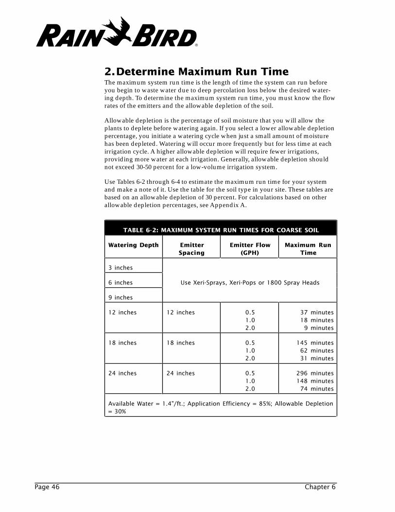
2.Determine Maximum Run TimeThe maximum system run time is the length of time the system can run beforeyou begin to waste water due to deep percolation loss below the desired water-ing depth. To determine the maximum system run time, you must know the flowrates of the emitters and the allowable depletion of the soil.
Allowable depletion is the percentage of soil moisture that you will allow theplants to deplete before watering again. If you select a lower allowable depletionpercentage, you initiate a watering cycle when just a small amount of moisturehas been depleted. Watering will occur more frequently but for less time at eachirrigation cycle. A higher allowable depletion will require fewer irrigations,providing more water at each irrigation. Generally, allowable depletion shouldnot exceed 30-50 percent for a low-volume irrigation system.
Use Tables 6-2 through 6-4 to estimate the maximum run time for your systemand make a note of it. Use the table for the soil type in your site. These tables arebased on an allowable depletion of 30 percent. For calculations based on otherallowable depletion percentages, see Appendix A.
Page 46 Chapter 6
TABLE 6-2: MAXIMUM SYSTEM RUN TIMES FOR COARSE SOIL
Watering Depth EmitterSpacing
Emitter Flow(GPH)
Maximum RunTime
3 inches
6 inches Use Xeri-Sprays, Xeri-Pops or 1800 Spray Heads
9 inches
12 inches 12 inches 0.51.02.0
37 minutes18 minutes
9 minutes
18 inches 18 inches 0.51.02.0
145 minutes62 minutes31 minutes
24 inches 24 inches 0.51.02.0
296 minutes148 minutes
74 minutes
Available Water = 1.4"/ft.; Application Efficiency = 85%; Allowable Depletion= 30%
®

Calculate System Run Time Page 47
TABLE 6-3: MAXIMUM SYSTEM RUN TIME FOR MEDIUM SOIL
Watering Depth EmitterSpacing
Emitter Flow(GPH)
Maximum RunTime
3 inches Use Xeri-Sprays or Xeri-Pops
6 inches 12 inches 0.51.02.0
26 minutes13 minutes
7 minutes
9 inches 18 inches 0.51.02.0
89 minutes45 minutes22 minutes
12 inches 24 inches 0.51.02.0
211 minutes106 minutes
53 minutes
18 inches 36 inches 0.51.02.0
713 minutes357 minutes178 minutes
24 inches 48 inches Use individual emitters based onplant needs.
Available Water = 2.0"/ft.; Application Efficiency = 85%;
Allowable Depletion = 30%
TABLE 6-4: MAXIMUM SYSTEM RUN TIME FOR FINE SOIL
Watering Depth EmitterSpacing
Emitter Flow(GPH)
Maximum RunTime
3 inches 12 inches 0.51.02.0
16 minutes8 minutes4 minutes
6 inches 24 inches 0.51.02.0
132 minutes66 minutes33 minutes
9 inches 36 inches 0.51.02.0
446 minutes223 minutes111 minutes
12 inches 48 inches Use individual emitters based onplant needs.
Available Water = 2.5"/ft.; Application Efficiency = 85%;
Allowable Depletion = 30%
®
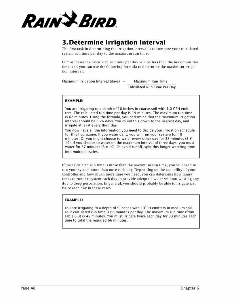
Page 48 Chapter 6
3.Determine Irrigation IntervalThe first task in determining the irrigation interval is to compare your calculatedsystem run time per day to the maximum run time.
In most cases the calculated run time per day will be less than the maximum runtime, and you can use the following formula to determine the maximum irriga-tion interval:
EXAMPLE:
You are irrigating to a depth of 9 inches with 1 GPH emitters in medium soil.Your calculated run time is 66 minutes per day. The maximum run time (fromTable 6-3) is 45 minutes. You must irrigate twice each day for 33 minutes eachtime to total the required 66 minutes.
If the calculated run time is more than the maximum run time, you will need torun your system more than once each day. Depending on the capability of yourcontroller and how much more time you need, you can determine how manytimes to run the system each day to provide adequate water without wasting anydue to deep percolation. In general, you should probably be able to irrigate justtwice each day in these cases.
EXAMPLE:
You are irrigating to a depth of 18 inches in coarse soil with 1.0␣ GPH emit-ters. The calculated run time per day is 19 minutes. The maximum run timeis 62 minutes. Using the formula, you determine that the maximum irrigationinterval should be 3.26 days. You round this down to the nearest day, andirrigate at least every third day.You now have all the information you need to decide your irrigation schedulefor this hydrozone. If you water daily, you will run your system for 19minutes. Or you might choose to water every other day for 38 minutes (2 ¥19). If you choose to water on the maximum interval of three days, you mustwater for 57 minutes (3 x 19). To avoid runoff, split this longer watering timeinto multiple cycles.
Maximum Irrigation Interval (days) = Maximum Run Time
Calculated Run Time Per Day
®
Calculate System Run Time Page 49
Chapter ReviewTo check your understanding of the material covered in Chapter 6, complete thisreview. The review is based on the partially completed hydrozone worksheet(Figure 7-1) which is located at the end of Chapter 7.
1. We have determined that we will use Landscape Dripline with 0.6 GPHemitters spaced at 12" to irrigate the base plant in hydrozone 7. Use Table 6-1to determine the EDR.
2. Calculate the Adjusted EDR by multiplying the EDR by the applicationefficiency.
3. Calculate the system run time in minutes for this hydrozone.
4. Use the tables to determine the maximum run time for this hydrozone.
5. Determine the maximum irrigation interval for this hydrozone.
6. If we choose to irrigate once every two days, how long will each irrigationcycle be?
®
Page 50 Chapter 6
Answer KeyCheck your answers to the review items with the correct answers below.
1. EDR = 0.96
2. Adjusted EDR = 0.888 X .90 = 0.86 inches per day
3. System Run Time = 4.2 minutes per day
4. Maximum Run Time = approximately 26 minutes.
5. Maximum Irrigation Interval = 6 days
6. Irrigation cycle: 8.4 minutes (2 x 15)
®
Irrigate Non-Base Plants Page 51
IRRIGATE NON-BASE PLANTS
In earlier chapters, you determined the base plant for your hydrozone: the plantwith the smallest daily water requirement. You then selected emission devices toirrigate the base plant and calculated the system run time based on the emissiondevices you chose.
In this chapter, you will select emission devices for the non-base plants in thehydrozone. Because you’ve already determined the system run time, you willneed to take this into account in determining the flow, type and quantity ofemission devices to use for each non-base plant.
To calculate the number of emission devices required for each non-base plant,you must determine the minimum flow rate required to irrigate the plant in thetime allotted.
Divide the daily water requirement for each remaining plant by the system runtime you have already calculated (for your base plant). This result tells you theminimum flow rate required for each plant.
7
EXAMPLE
You have determined that the system run time will be 0.2 hour. Yourhydrozone includes a crepe myrtle tree with a daily requirement of 3.3 GPD.You can calculate the minimum flow rate required for the crepe myrtle bydividing:
3.3 GPD ÷ 0.2 hour = 16.5 Gallons per Hour
Next, select emission devices for each plant so that the total flow rate meets orexceeds your calculated flow rate. Avoid using two emission devices withdifferent flow rates for the same plant. Use Table 7-1 as a guide.
®
Chapter ReviewTo check your understanding of the material covered in Chapter 7, complete thisreview. The review is based on the partially completed hydrozone worksheet(Figure 7-1) which is located on the next page.
1. Calculate the total flow needed to irrigate each of the ferns within the systemrun time.
2. We have determined that Xeri-Bubblers set for an umbrella pattern are themost effective way to irrigate the ferns. If we use two Xeri-Bubblers for eachfern, what should the flow for each bubbler be?
Page 52 Chapter 7
EXAMPLEReferring to Table 7-1, you select four 5.0 GPH Pressure-CompensatingModules to water the crepe myrtle. These four devices will provide a com-bined flow of 20.0 GPH, which is somewhat more than the calculated flow of16.5 GPH. The preferred use of four emission devices versus one or two flowdevices will be explained in the next chapter.
It is important to consider the soil type and how best to avoid potential runoff inclay-like soils. It may be best to create some type of reservoir at the base of plantsto capture the water from higher flow emission devices, such as the PC-10, 10GPH Pressure Compensating Module.
Complete this process of calculating flow rates and selecting emission devices foreach non-base plant. Refer to chapter 5 as well as subsequent chapters forinformation about placement of the emission devices.
TABLE 7-1: EMISSION DEVICE FLOW RATES
Emission Device Available Flow Rates
Xeri-Bug Single Outlet Pressure Compensating Emitter 0.5, 1.0, 2.0 GPH
Shrub Xeri-Bug Single Outlet Pressure Compensating Emitter 1.0, 2.0 GPH
Pressure Compensating Modules 5.0, 7.0, 10.0, 12.0,18.0, 24.0 GPH
Multi-Outlet Xeri-Bug; Multi-Outlet Shrub Xeri-Bug 1.0 GPH per outlet (up to 6 outlets)
Xeri-Bubblers Streams: 0-13.0 GPH, Umbrella: 0-35.0 GPH
Xeri-Sprays 0-31.0 GPH
Landscape Dripline 0.6, 0.9 GPH
Xeri-Pops w/ Multi-Port Nozzle 10.5, 21.0, 31.5, 42.0 GPH
Xeri-Pops w/ PCS Screens and choice of MPR Nozzle 0.1, 0.2, 0.3, 0.4, 0.6 GPM
®

Irrigate Non-Base Plants Page 53
Water Requirement
.623 Area K PET× × ×c
Application Efficiency= Gallons per Day (GPD)
LOW-VOLUME DESIGN WORKSHEET: DENSE HYDROZONE
ADDITIONALPLANT SPECIES
SPECIESFACTOR
DENSITYFACTOR
MICROCLIMATEFACTOR Kc
PLANTDIAMETER
(FT.)
CANOPYAREA
(SQ. FT.)
WATERREQUIREMENT
(GPD)
EMISSION DEVICES
TYPE FLOW QUANTITY SPACING
Base Plant
Non-Base Plants
Water Requirement
K PET = Inches per Dayc ×
Plant Canopy Area
0.7854 Diameter Diameter = Square Feet× ×
BASE PLANTSPECIES
SPECIESFACTOR
DENSITYFACTOR
MICROCLIMATEFACTOR
WATERREQUIREMENT
EMITTERFLOW RATE
ADJUSTEDEDRKc
DATEJOB NUMBER
DESCRIPTION
HYDROZONE
Eve. Phone
Name
Address
City
Contact
Day Phone
Daily PET (inches per day)
Application Efficiency
State Zip
CoarseSoil Type:
Medium
Fine
Site Information1 1
3
3 4 5
Ground Cover Only
Ground Cover/Trees
Ground Cover /Shrubs
Ground Cover/Shrubs/Trees
Shrubs/Trees
Shrubs Only
Planting Scheme
Base PlantGround Cover
Shrubs
Watering Depth3"
6"
9"
12"
18"
24"
36"
Emitter Spacing
12"
18"
24"
36"
4
6
SYSTEM RUN TIME
5
2
2
John & Wendy Doyle7836 Connor LaneBrighton CAJohn
714-555-81360.20
90%
Ice Plant
Azaleas (2)
Privet (12)
Hawthorne (6)
Ferns (2)
low
avg.
avg.
avg.
high
0.5
0.5
0.5
0.5
1.0
1.0
1.3
1.3
1.3
0.3 4.0 12.6 0.5 P.C. Mod. 7.0 2 per
2 per
2 per
2 per
10.0
10.0
P.C. Mod.
P.C. Mod.
Xeri-Bubbler
0.7
0.7
7.1
7.1
3.0
3.0
5.0
7
Mixed G. C.& shrubs
0.7
0.7
high
high
high
high
high
high
low
med.
med.
low
714-555-1089
92867
Figure 7-1: Dense Hydrozone Design Worksheet
®
Page 54 Chapter 7
Check your answers to the review items with the correct answers below.
1. Total flow = 20 GPH
2. Emitter flow = 10 GPH
Answer Key
®
System Layout Page 55
SYSTEM LAYOUT
System layout for low-volume hydrozones is relatively easy. Once youhave determined the type, number and spacing of emission devicesrequired for each plant or group of plants, simply determine the mostcost-effective way to connect the various emission devices to the watersource. However, you must also be certain not to exceed the hydraulicconstraints of the system components. (See Chapter 9 for information onhydraulics.)
Figure 8-1 shows a typical hydrozone layout, including the placement ofemission devices around each plant in the hydrozone.
8
Figure 8-1: Correct placement of emitters
Figure 8-2 shows several options for individual plants that require multipleemission devices, including a single loop of tubing, rigid PVC pipe and a multi-outlet emitter with 1/4" distribution tubing.
Figures 8-3 and 8-4 show typical layouts using poly drip tubing (LandscapeDripline) and Rigid PVC tubing.
TreeEnd Closure
Shrub
Control Zone Components
Lateral Tubing
End Closure Inline Emitter Tubing
Emission Devices
®
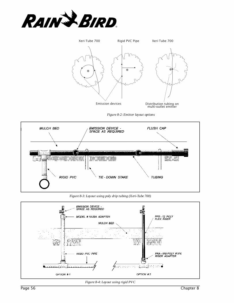
Page 56 Chapter 8
Figure 8-4: Layout using rigid PVC
Figure 8-3: Layout using poly drip tubing (Xeri-Tube 700)
Figure 8-2: Emitter layout options
Xeri-Tube 700
Emission devices Distribution tubing onmulti-outlet emitter
Rigid PVC Pipe Xeri-Tube 700
❘
▼
®
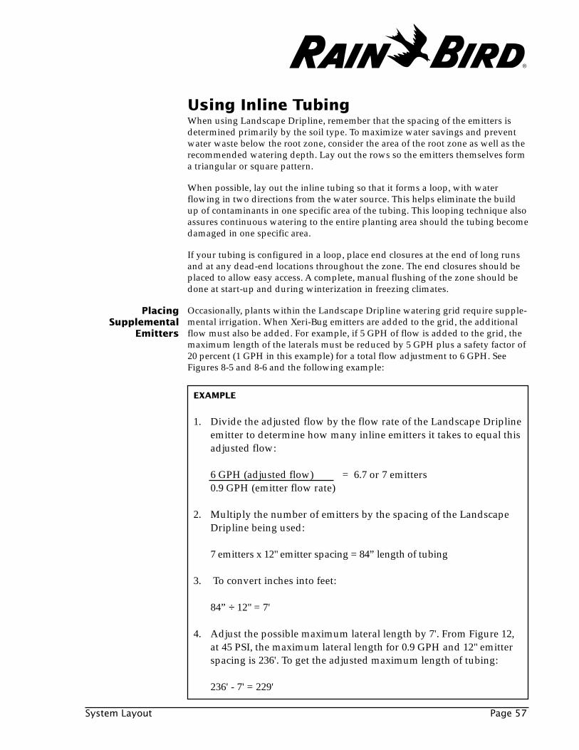
System Layout Page 57
Using Inline TubingWhen using Landscape Dripline, remember that the spacing of the emitters isdetermined primarily by the soil type. To maximize water savings and preventwater waste below the root zone, consider the area of the root zone as well as therecommended watering depth. Lay out the rows so the emitters themselves forma triangular or square pattern.
When possible, lay out the inline tubing so that it forms a loop, with waterflowing in two directions from the water source. This helps eliminate the buildup of contaminants in one specific area of the tubing. This looping technique alsoassures continuous watering to the entire planting area should the tubing becomedamaged in one specific area.
If your tubing is configured in a loop, place end closures at the end of long runsand at any dead-end locations throughout the zone. The end closures should beplaced to allow easy access. A complete, manual flushing of the zone should bedone at start-up and during winterization in freezing climates.
Occasionally, plants within the Landscape Dripline watering grid require supple-mental irrigation. When Xeri-Bug emitters are added to the grid, the additionalflow must also be added. For example, if 5 GPH of flow is added to the grid, themaximum length of the laterals must be reduced by 5 GPH plus a safety factor of20 percent (1 GPH in this example) for a total flow adjustment to 6 GPH. SeeFigures 8-5 and 8-6 and the following example:
PlacingSupplemental
Emitters
EXAMPLE
1. Divide the adjusted flow by the flow rate of the Landscape Driplineemitter to determine how many inline emitters it takes to equal thisadjusted flow:
6 GPH (adjusted flow) = 6.7 or 7 emitters0.9 GPH (emitter flow rate)
2. Multiply the number of emitters by the spacing of the LandscapeDripline being used:
7 emitters x 12" emitter spacing = 84” length of tubing
3. To convert inches into feet:
84” ÷ 12" = 7'
4. Adjust the possible maximum lateral length by 7'. From Figure 12,at 45 PSI, the maximum lateral length for 0.9 GPH and 12" emitterspacing is 236'. To get the adjusted maximum length of tubing:
236' - 7' = 229'
®
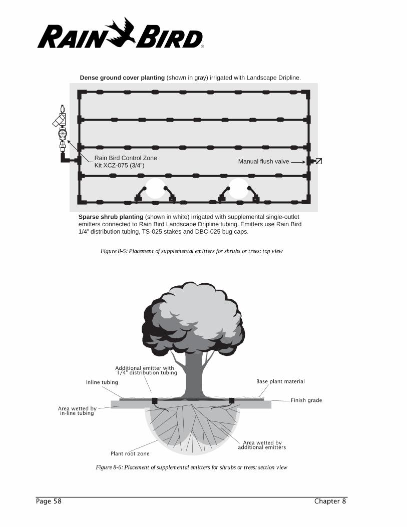
Page 58 Chapter 8
Inline tubing
Area wetted byin-line tubing
Plant root zone
Area wetted byadditional emitters
Additional emitter with1/4" distribution tubing
Finish grade
Base plant material
Figure 8-6: Placement of supplemental emitters for shrubs or trees: section view
Dense ground cover planting (shown in gray) irrigated with Landscape Dripline.
▲Manual flush valve
▲
Rain Bird Control ZoneKit XCZ-075 (3/4”)
Sparse shrub planting (shown in white) irrigated with supplemental single-outletemitters connected to Rain Bird Landscape Dripline tubing. Emitters use Rain Bird1/4” distribution tubing, TS-025 stakes and DBC-025 bug caps.
Figure 8-5: Placement of supplemental emitters for shrubs or trees: top view
®
System Layout Page 59
System ConfigurationWhen a significant distance exists between the system's primary filter and theLandscape Dripline grid, Rain Bird's Control Zone Kit should be installed. TheControl Zone Kit filter acts as a secondary filter to protect the Landscape Driplinegrid against contamination that could be caused by a break in the sub-main. Thekit consists of a ball valve, 200-mesh Y-filter, remote control valve (or anti-siphonvalve), 3/4" pressure regulator and Schedule 80 close nipples.
Landscape Dripline should have an operating pressure of no more than 60 PSI (4Bars). If static pressure is higher than 60 PSI (4 Bars) at the start of the LandscapeDripline run, pressure regulation is required. When this is the case, use compres-sion fittings or make sure to clamp your insert fittings. Pressure regulatorsshould be installed as close to the planting area as possible to assure that thedesired pressure is available to the Landscape Dripline watering zone.
Choose either Rain Bird LD16 Series insert fittings or Rain Bird 600CF Seriescompression fittings when installing and connecting Rain Bird's LandscapeDripline. While insert fittings are designed to be used up to 45 PSI (3 Bars)without clamps, compression fittings can be used up to 60 PSI (4 Bars) withoutthe need for any clamps. They are recommended for hot weather climates toprovide maximum retention strength.
Landscape Dripline requires the use of stakes or staples to install it securely tothe ground. Use Table 8-1 as a guide for staking:
Filtration
PressureRegulation
Use Insert orCompression
Fittings
Stakes andStaples
TABLE 8-1: SPACING OF STAKES AND STAPLES
Soil Type Stake Spacing Additional Stakes
Fine 4'-6' (1,2-1,8 m) Before and after every turn
Medium 3'-5' (0,9-1,5 m) Before and after every turn
Coarse 2'-3' (0,6-0,9 m) Before and after every turn
®
Page 60 Chapter 8
Water Meter
Approved BackflowPreventer
Automatic Filter Kitor Rotary Disk Filter(optional for large systems)
PVC Main Line
Control Zone Kit: Shut-Off Ball Valve 120-Mesh Filter Electric Control Valve Pressure Regulator
Landscape DriplineLaterals
Polyethylene orPVC Header
Manual Flush Valve
Center FeedEnd Feed
Figure 8-7: Landscape Dripline system configuration
Tubing End Closure
Filter
®
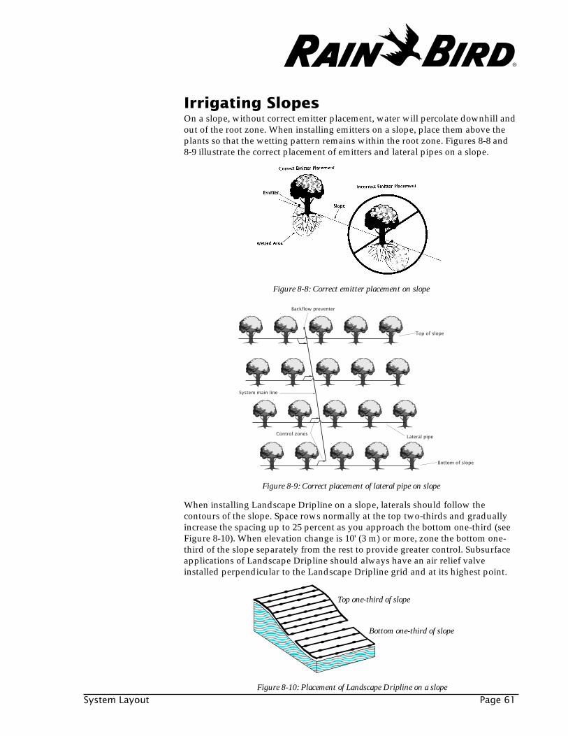
System Layout Page 61
Irrigating SlopesOn a slope, without correct emitter placement, water will percolate downhill andout of the root zone. When installing emitters on a slope, place them above theplants so that the wetting pattern remains within the root zone. Figures 8-8 and8-9 illustrate the correct placement of emitters and lateral pipes on a slope.
Figure 8-8: Correct emitter placement on slope
Top of slope
Bottom of slope
Backflow preventer
System main line
Lateral pipeControl zones
Figure 8-9: Correct placement of lateral pipe on slope
When installing Landscape Dripline on a slope, laterals should follow thecontours of the slope. Space rows normally at the top two-thirds and graduallyincrease the spacing up to 25 percent as you approach the bottom one-third (seeFigure 8-10). When elevation change is 10' (3 m) or more, zone the bottom one-third of the slope separately from the rest to provide greater control. Subsurfaceapplications of Landscape Dripline should always have an air relief valveinstalled perpendicular to the Landscape Dripline grid and at its highest point.
Figure 8-10: Placement of Landscape Dripline on a slope
������
��������������
Top one-third of slope
Bottom one-third of slope
®
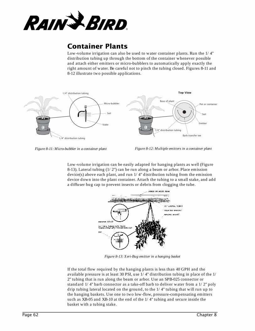
Top View
Pot or containerBase of plant
Soil
Barb transfer tee
1/4" distribution tubing
Emitter
Soil
Micro-bubbler
1/4" distribution tubing
Stake
1/4" distribution tubing
Figure 8-12: Multiple emitters in a container plantFigure 8-11: Micro-bubbler in a container plant
Page 62 Chapter 8
Figure 8-13: Xeri-Bug emitter in a hanging basket
If the total flow required by the hanging plants is less than 40 GPH and theavailable pressure is at least 30 PSI, use 1/4" distribution tubing in place of the 1/2" tubing that is run along the beam or arbor. Use an SPB-025 connector orstandard 1/4" barb connector as a take-off barb to deliver water from a 1/2" polydrip tubing lateral located on the ground, to the 1/4" tubing that will run up tothe hanging baskets. Use one to two low-flow, pressure-compensating emitterssuch as XB-05 and XB-10 at the end of the 1/4" tubing and secure inside thebasket with a tubing stake.
Container PlantsLow-volume irrigation can also be used to water container plants. Run the 1/4"distribution tubing up through the bottom of the container whenever possibleand attach either emitters or micro-bubblers to automatically apply exactly theright amount of water. Be careful not to pinch the tubing closed. Figures 8-11 and8-12 illustrate two possible applications.
Low-volume irrigation can be easily adapted for hanging plants as well (Figure8-13). Lateral tubing (1/2") can be run along a beam or arbor. Place emissiondevice(s) above each plant, and run 1/4" distribution tubing from the emissiondevice down into the plant container. Attach the tubing to a small stake, and adda diffuser bug cap to prevent insects or debris from clogging the tube.
®
System Hydraulics Page 63
SYSTEM HYDRAULICS
Chapter 3 covered gathering site data and Chapters 4 - 8 described how to designand lay out your low-volume irrigation system. This chapter covers systemhydraulics, the final step in the design process.
The main goal of determining system hydraulics is to assure that there is sufficientflow and water pressure available to irrigate all parts of the landscape. The waterpressure at various points in the irrigation system is influenced by changes inelevation and by loss of pressure due to friction between water and the systemcomponents.
This chapter is not intended to be a complete course in irrigation system hydrau-lics. If you need basic training in hydraulics, we recommend that you obtain RainBird’s Landscape Irrigation Design Manual (P/N D38470A). Contact your local RainBird distributor or Rain Bird representative about ordering this training material.
Water PressureWater pressure is defined as the force exerted by water over a given area. Waterpressure is most often measured in pounds (force) per square inch (area), abbre-viated PSI.
Static pressure is the pressure of water in a completely closed system, such as amain line with all of its outlet valves turned off. The static water pressure at thewater source (usually the water meter or pump outlet) is the starting point foryour hydraulic design. It indicates the potential pressure that is available tooperate your irrigation system.
You should determine the static pressure at the water source as you collect sitedata. For more information on collecting site data, see Chapter 3.
Dynamic pressure is the water pressure at any point in the system at a givenflow. Dynamic pressure will vary throughout the system due to friction loss andelevation changes.
Friction LossFriction loss is a pressure loss caused by water flowing through the system. Thisloss occurs in every component of the system through which water flows. Pipes,valves, water meters, backflow preventers and pipe fittings all provide someresistance to the water flowing through them, creating a pressure loss. Theroughness on the inside surfaces of these components creates a drag on the flowingwater causing turbulence, which reduces pressure. The shape of each component,or changes in flow direction (such as within a valve) add to the pressure loss.
Elevation ChangesChanges in elevation also cause changes in water pressure. Each foot of elevationchange means a change in pressure of .433 PSI. That is, it takes .433 PSI to movewater up one foot. And if water flows down one foot, there will be a pressure gainof .433 PSI. Obviously, significant changes in elevation within your irrigation sitecan have a major impact on the pressure in the system.
9
Static Pressure
Dynamic Pressure
®
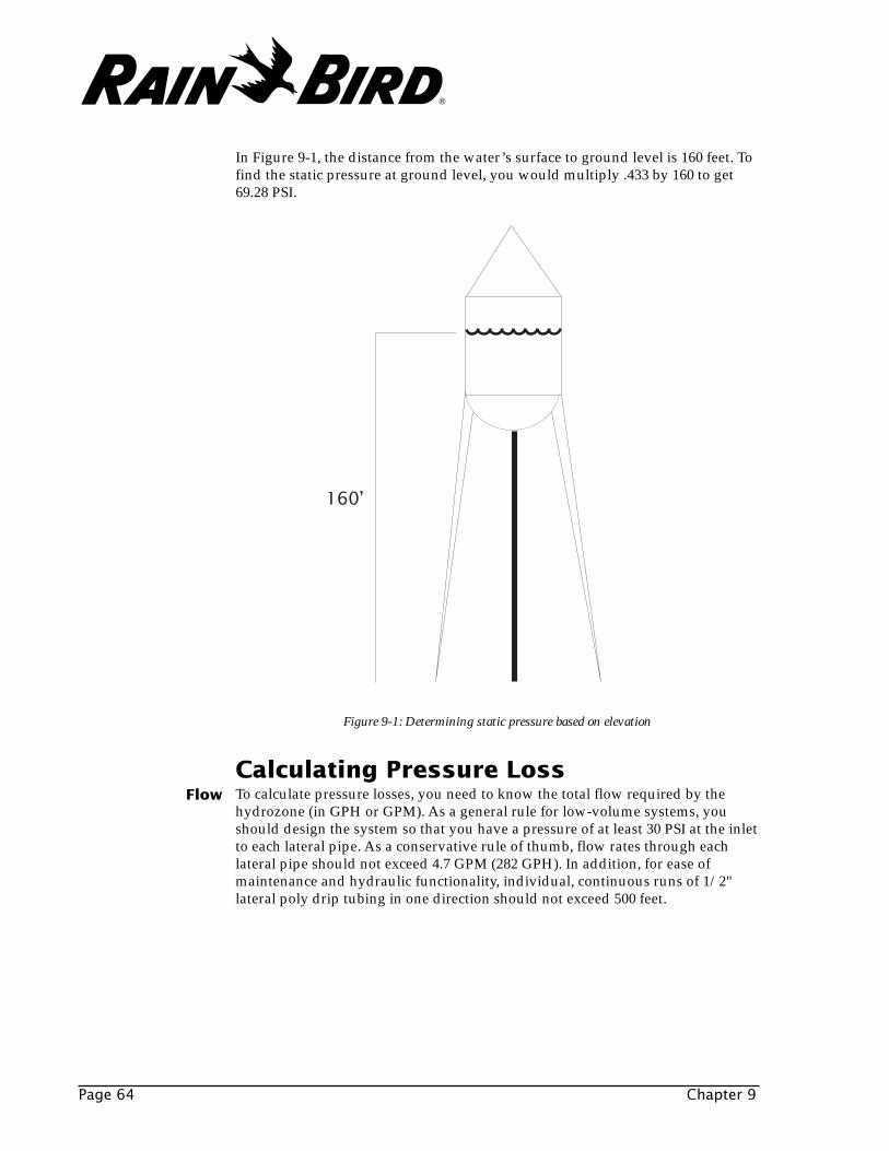
In Figure 9-1, the distance from the water’s surface to ground level is 160 feet. Tofind the static pressure at ground level, you would multiply .433 by 160 to get69.28 PSI.
160’
Figure 9-1: Determining static pressure based on elevation
Flow
Calculating Pressure LossTo calculate pressure losses, you need to know the total flow required by thehydrozone (in GPH or GPM). As a general rule for low-volume systems, youshould design the system so that you have a pressure of at least 30 PSI at the inletto each lateral pipe. As a conservative rule of thumb, flow rates through eachlateral pipe should not exceed 4.7 GPM (282 GPH). In addition, for ease ofmaintenance and hydraulic functionality, individual, continuous runs of 1/2"lateral poly drip tubing in one direction should not exceed 500 feet.
Page 64 Chapter 9
®
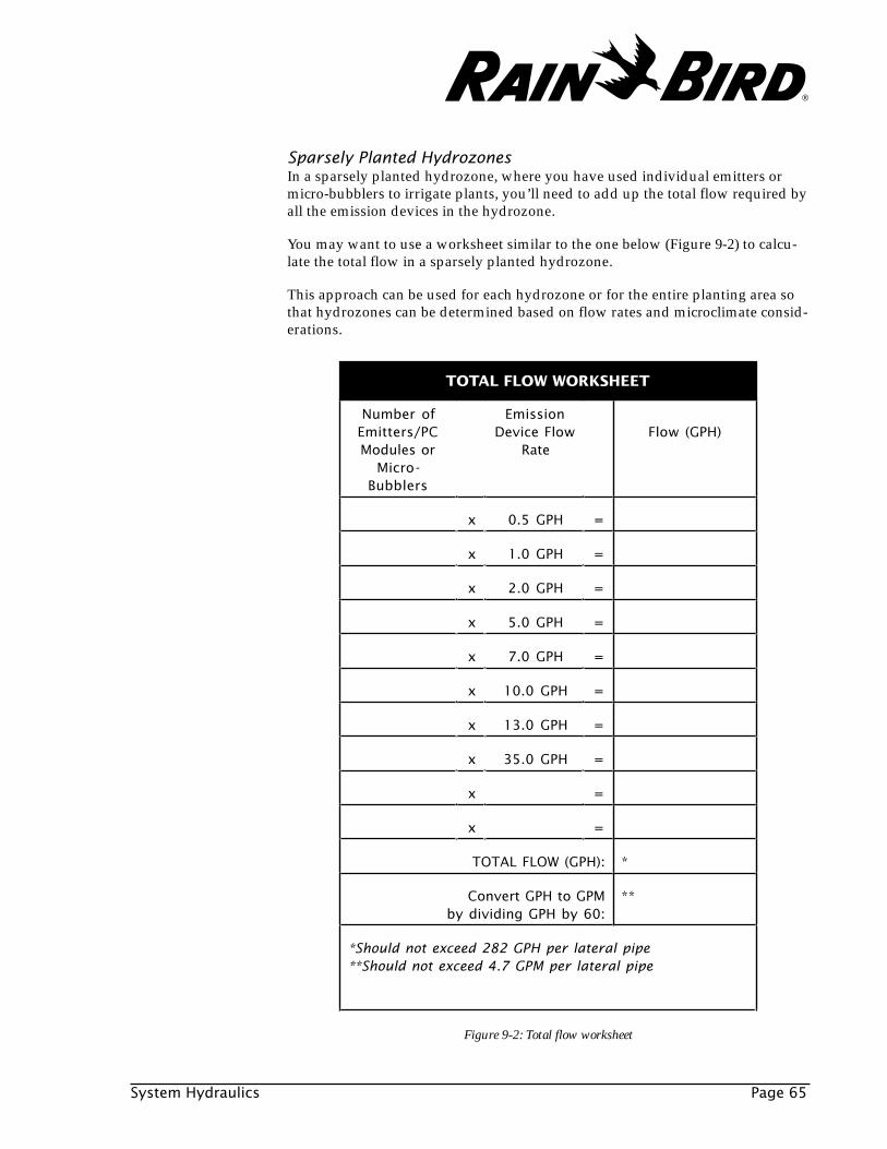
System Hydraulics Page 65
Sparsely Planted HydrozonesIn a sparsely planted hydrozone, where you have used individual emitters ormicro-bubblers to irrigate plants, you’ll need to add up the total flow required byall the emission devices in the hydrozone.
You may want to use a worksheet similar to the one below (Figure 9-2) to calcu-late the total flow in a sparsely planted hydrozone.
This approach can be used for each hydrozone or for the entire planting area sothat hydrozones can be determined based on flow rates and microclimate consid-erations.
Number ofEmitters/PCModules or
Micro-Bubblers
EmissionDevice Flow
RateFlow (GPH)
x 0.5 GPH =
x 1.0 GPH =
x 2.0 GPH =
x 5.0 GPH =
x 7.0 GPH =
x 10.0 GPH =
x 13.0 GPH =
x 35.0 GPH =
x =
x =
TOTAL FLOW (GPH): *
Convert GPH to GPMby dividing GPH by 60:
**
*Should not exceed 282 GPH per lateral pipe**Should not exceed 4.7 GPM per lateral pipe
TOTAL FLOW WORKSHEET
Figure 9-2: Total flow worksheet
®
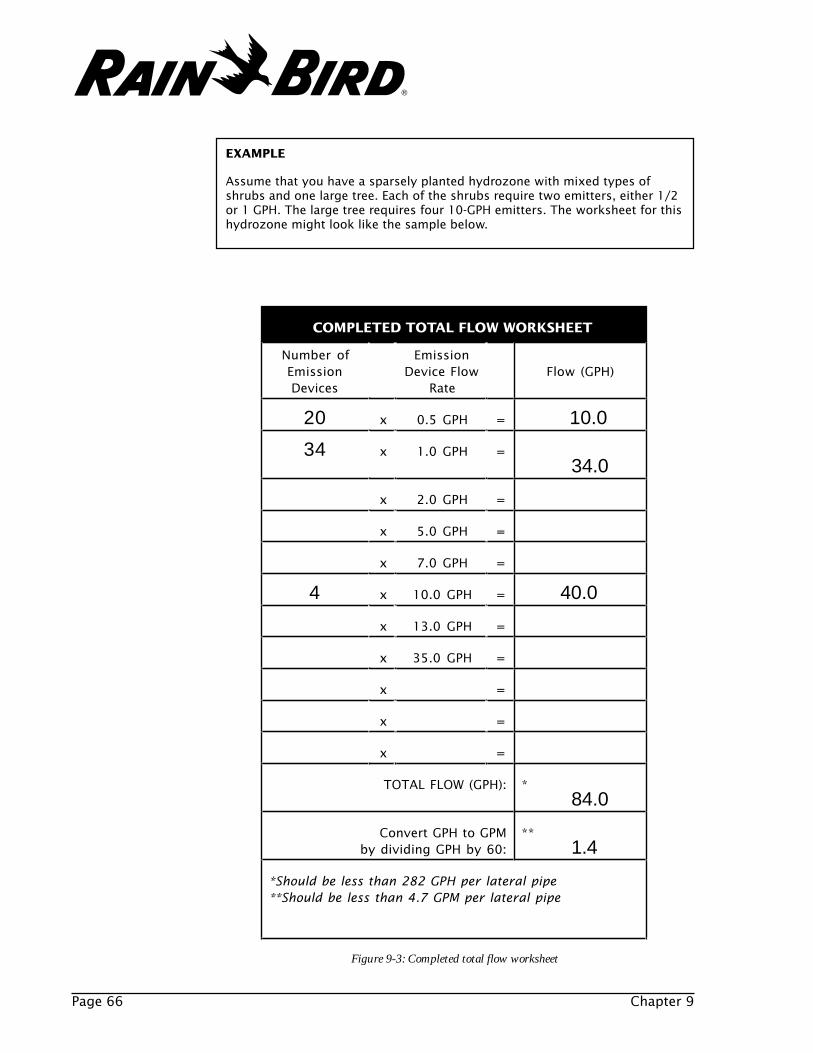
Page 66 Chapter 9
EXAMPLE
Assume that you have a sparsely planted hydrozone with mixed types ofshrubs and one large tree. Each of the shrubs require two emitters, either 1/2or 1 GPH. The large tree requires four 10-GPH emitters. The worksheet for thishydrozone might look like the sample below.
Number ofEmissionDevices
EmissionDevice Flow
RateFlow (GPH)
20 x 0.5 GPH = 10.0
34 x 1.0 GPH =34.0
x 2.0 GPH =
x 5.0 GPH =
x 7.0 GPH =
4 x 10.0 GPH = 40.0
x 13.0 GPH =
x 35.0 GPH =
x =
x =
x =
TOTAL FLOW (GPH): *84.0
Convert GPH to GPMby dividing GPH by 60:
**1.4
*Should be less than 282 GPH per lateral pipe**Should be less than 4.7 GPM per lateral pipe
COMPLETED TOTAL FLOW WORKSHEET
Figure 9-3: Completed total flow worksheet
®
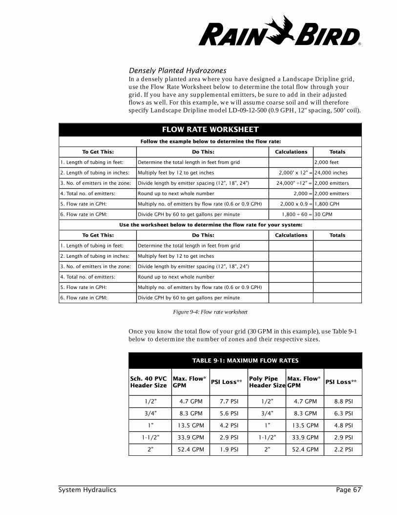
Densely Planted HydrozonesIn a densely planted area where you have designed a Landscape Dripline grid,use the Flow Rate Worksheet below to determine the total flow through yourgrid. If you have any supplemental emitters, be sure to add in their adjustedflows as well. For this example, we will assume coarse soil and will thereforespecify Landscape Dripline model LD-09-12-500 (0.9 GPH, 12" spacing, 500’ coil).
System Hydraulics Page 67
Once you know the total flow of your grid (30 GPM in this example), use Table 9-1below to determine the number of zones and their respective sizes.
FLOW RATE WORKSHEET
Follow the example below to determine the flow rate:
To Get This: Do This: Calculations Totals
1. Length of tubing in feet: Determine the total length in feet from grid 2,000 feet
2. Length of tubing in inches: Multiply feet by 12 to get inches 2,000' x 12" = 24,000 inches
3. No. of emitters in the zone: Divide length by emitter spacing (12", 18", 24") 24,000" ÷12" = 2,000 emitters
4. Total no. of emitters: Round up to next whole number 2,000 = 2,000 emitters
5. Flow rate in GPH: Multiply no. of emitters by flow rate (0.6 or 0.9 GPH) 2,000 x 0.9 = 1,800 GPH
6. Flow rate in GPM: Divide GPH by 60 to get gallons per minute 1,800 ÷ 60 = 30 GPM
Use the worksheet below to determine the flow rate for your system:
To Get This: Do This: Calculations Totals
1. Length of tubing in feet: Determine the total length in feet from grid
2. Length of tubing in inches: Multiply feet by 12 to get inches
3. No. of emitters in the zone: Divide length by emitter spacing (12", 18", 24")
4. Total no. of emitters: Round up to next whole number
5. Flow rate in GPH: Multiply no. of emitters by flow rate (0.6 or 0.9 GPH)
6. Flow rate in GPM: Divide GPH by 60 to get gallons per minute
TABLE 9-1: MAXIMUM FLOW RATES
Sch. 40 PVC Header Size
Max. Flow* GPM
PSI Loss** Poly Pipe Header Size
Max. Flow* GPM
PSI Loss**
1/2" 4.7 GPM 7.7 PSI 1/2" 4.7 GPM 8.8 PSI
3/4" 8.3 GPM 5.6 PSI 3/4" 8.3 GPM 6.3 PSI
1" 13.5 GPM 4.2 PSI 1" 13.5 GPM 4.8 PSI
1-1/2" 33.9 GPM 2.9 PSI 1-1/2" 33.9 GPM 2.9 PSI
2" 52.4 GPM 1.9 PSI 2" 52.4 GPM 2.2 PSI
Figure 9-4: Flow rate worksheet
®
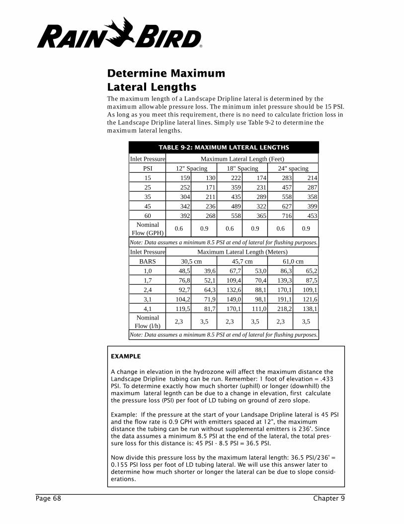
Page 68 Chapter 9
Determine MaximumLateral LengthsThe maximum length of a Landscape Dripline lateral is determined by themaximum allowable pressure loss. The minimum inlet pressure should be 15 PSI.As long as you meet this requirement, there is no need to calculate friction loss inthe Landscape Dripline lateral lines. Simply use Table 9-2 to determine themaximum lateral lengths.
EXAMPLE
A change in elevation in the hydrozone will affect the maximum distance theLandscape Dripline tubing can be run. Remember: 1 foot of elevation = .433PSI. To determine exactly how much shorter (uphill) or longer (downhill) themaximum lateral legnth can be due to a change in elevation, first calculatethe pressure loss (PSI) per foot of LD tubing on ground of zero slope.
Example: If the pressure at the start of your Landsape Dripline lateral is 45 PSIand the flow rate is 0.9 GPH with emitters spaced at 12", the maximumdistance the tubing can be run without supplemental emitters is 236'. Sincethe data assumes a minimum 8.5 PSI at the end of the lateral, the total pres-sure loss for this distance is: 45 PSI - 8.5 PSI = 36.5 PSI.
Now divide this pressure loss by the maximum lateral length: 36.5 PSI/236' =0.155 PSI loss per foot of LD tubing lateral. We will use this answer later todetermine how much shorter or longer the lateral can be due to slope consid-erations.
Inlet Pressure Maximum Lateral Length (Feet)
PSI 12" Spacing 18" Spacing 24" spacing
15 159 130 222 174 283 214
25 252 171 359 231 457 287
35 304 211 435 289 558 358
45 342 236 489 322 627 399
60 392 268 558 365 716 453Nominal
Flow (GPH)0.6 0.9 0.6 0.9 0.6 0.9
Note: Data assumes a minimum 8.5 PSI at end of lateral.
Inlet Pressure Maximum Lateral Length (Meters)
BARS 30,5 cm 45,7 cm 61,0 cm
1,0 48,5 39,6 67,7 53,0 86,3 65,2
1,7 76,8 52,1 109,4 70,4 139,3 87,5
2,4 92,7 64,3 132,6 88,1 170,1 109,1
3,1 104,2 71,9 149,0 98,1 191,1 121,6
4,1 119,5 81,7 170,1 111,0 218,2 138,1Nominal
Flow (l/h)2,3 3,5 2,3 3,5 2,3 3,5
Note: Data assumes a minimum 0,6 bars at end of lateral.
TABLE 9-2: MAXIMUM LATERAL LENGTHS
Note: Data assumes a minimum 8.5 PSI at end of lateral for flushing purposes.
Note: Data assumes a minimum 8.5 PSI at end of lateral for flushing purposes.
®
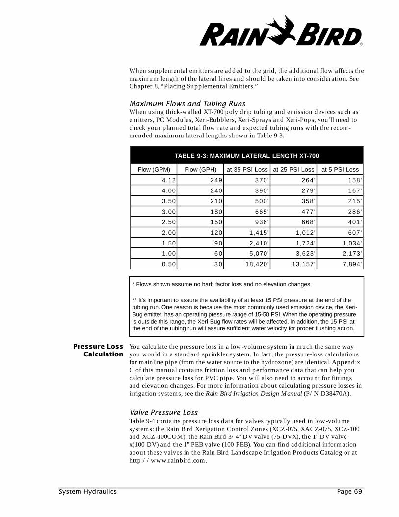
System Hydraulics Page 69
Maximum Flows and Tubing RunsWhen using thick-walled XT-700 poly drip tubing and emission devices such asemitters, PC Modules, Xeri-Bubblers, Xeri-Sprays and Xeri-Pops, you’ll need tocheck your planned total flow rate and expected tubing runs with the recom-mended maximum lateral lengths shown in Table 9-3.
* Flows shown assume no barb factor loss and no elevation changes.
** It’s important to assure the availability of at least 15 PSI pressure at the end of thetubing run. One reason is because the most commonly used emission device, the Xeri-Bug emitter, has an operating pressure range of 15-50 PSI. When the operating pressureis outside this range, the Xeri-Bug flow rates will be affected. In addition, the 15 PSI atthe end of the tubing run will assure sufficient water velocity for proper flushing action.
You calculate the pressure loss in a low-volume system in much the same wayyou would in a standard sprinkler system. In fact, the pressure-loss calculationsfor mainline pipe (from the water source to the hydrozone) are identical. AppendixC of this manual contains friction loss and performance data that can help youcalculate pressure loss for PVC pipe. You will also need to account for fittingsand elevation changes. For more information about calculating pressure losses inirrigation systems, see the Rain Bird Irrigation Design Manual (P/N D38470A).
Pressure LossCalculation
When supplemental emitters are added to the grid, the additional flow affects themaximum length of the lateral lines and should be taken into consideration. SeeChapter 8, “Placing Supplemental Emitters.”
Valve Pressure LossTable 9-4 contains pressure loss data for valves typically used in low-volumesystems: the Rain Bird Xerigation Control Zones (XCZ-075, XACZ-075, XCZ-100and XCZ-100COM), the Rain Bird 3/4" DV valve (75-DVX), the 1" DV valvex(100-DV) and the 1" PEB valve (100-PEB). You can find additional informationabout these valves in the Rain Bird Landscape Irrigation Products Catalog or athttp://www.rainbird.com.
TABLE 9-3: MAXIMUM LATERAL LENGTH XT-700
Flow (GPM) Flow (GPH) at 35 PSI Loss at 25 PSI Loss at 5 PSI Loss
4.12 249 370' 264' 158'
4.00 240 390' 279' 167'
3.50 210 500' 358' 215'
3.00 180 665' 477' 286'
2.50 150 936' 668' 401'
2.00 120 1,415' 1,012' 607'
1.50 9 0 2,410' 1,724' 1,034'
1.00 6 0 5,070' 3,623' 2,173'
0.50 3 0 18,420' 13,157' 7,894'
®
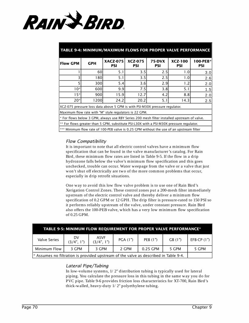
TABLE 9-5: MINIMUM FLOW REQUIREMENT FOR PROPER VALVE PERFORMANCE*
Valve Series DV(3/4", 1")
ASVF(3/4", 1")
PGA (1") PEB (1") GB (1") EFB-CP (1")
Minimum Flow 3 GPM 3 GPM 2 GPM 0.25 GPM 5 GPM 5 GPM
* Assumes no filtration is provided upstream of the valve as described in Table 9-4.
Page 70 Chapter 9
Flow CompatibilityIt is important to note that all electric control valves have a minimum flowspecification that can be found in the valve manufacturer’s catalog. For RainBird, these minimum flow rates are listed in Table 9-5. If the flow in a driphydrozone falls below the valve’s minimum flow specification and this goesunchecked, trouble can occur. Water weepage from the valve or a valve that justwon’t shut off electrically are two of the more common problems that occur,especially in drip retrofit situations.
One way to avoid this low flow valve problem is to use one of Rain Bird’sXerigation Control Zones. These control zones put a 200-mesh filter immediatelyupstream of the electric control valve and thereby deliver a minimum flowspecification of 0.2 GPM or 12 GPH. The drip filter is pressure-rated to 150 PSI soit performs reliably upstream of the valve, under constant pressure. Rain Birdalso offers the 100-PEB valve, which has a very low minimum flow specificationof 0.25 GPM.
*
Lateral Pipe/TubingIn low-volume systems, 1/2" distribution tubing is typically used for lateralpiping. You calculate the pressure loss in this tubing in the same way you do forPVC pipe. Table 9-6 provides friction loss characteristics for XT-700, Rain Bird’sthick-walled, heavy-duty 1/2" polyethylene tubing.
TABLE 9-4: MINIMUM/MAXIMUM FLOWS FOR PROPER VALVE PERFORMANCE
Flow GPM GPH XACZ-075PSI
XCZ-075PSI
75-DVXPSI
XCZ-100PSI
100-PEBPSI
1 60 5.1 3.5 2.5 1.0 3.03 180 5.1 3.5 2.5 1.0 2.65 300 5.4 3.6 2.9 1.2 2.0
10* 600 9.9 7.5 3.8 5.1 1.515* 900 15.9 12.7 4.2 8.8 2.020* 1200 24.2 20.2 5.1 14.3 2.5
XCZ-075 pressure loss data above 5 GPM is with PSI-M30X pressure regulator.
Maximum flow rate with "M" style regulators is 22 GPM.
* For flows below 3 GPM, always use RBY Series 200 mesh filter installed upstream of valve.
** For flows greater than 5 GPM, substitute PSI-L30X with a PSI-M30X pressure regulator.
*** Minimum flow rate of 100-PEB valve is 0.25 GPM without the use of an upstream filter
®
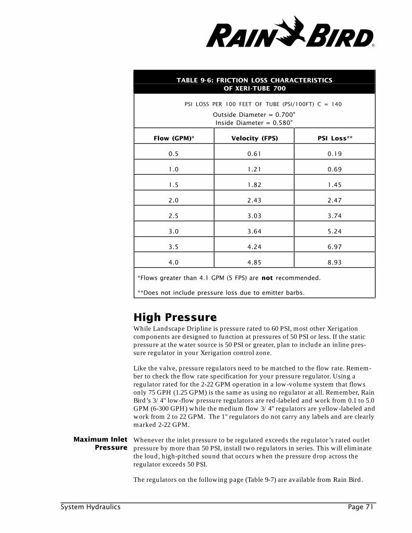
System Hydraulics Page 71
High PressureWhile Landscape Dripline is pressure rated to 60 PSI, most other Xerigationcomponents are designed to function at pressures of 50 PSI or less. If the staticpressure at the water source is 50 PSI or greater, plan to include an inline pres-sure regulator in your Xerigation control zone.
Like the valve, pressure regulators need to be matched to the flow rate. Remem-ber to check the flow rate specification for your pressure regulator. Using aregulator rated for the 2-22 GPM operation in a low-volume system that flowsonly 75 GPH (1.25 GPM) is the same as using no regulator at all. Remember, RainBird’s 3/4" low-flow pressure regulators are red-labeled and work from 0.1 to 5.0GPM (6-300 GPH) while the medium flow 3/4" regulators are yellow-labeled andwork from 2 to 22 GPM. The 1" regulators do not carry any labels and are clearlymarked 2-22 GPM.
Whenever the inlet pressure to be regulated exceeds the regulator’s rated outletpressure by more than 50 PSI, install two regulators in series. This will eliminatethe loud, high-pitched sound that occurs when the pressure drop across theregulator exceeds 50 PSI.
The regulators on the following page (Table 9-7) are available from Rain Bird.
Maximum InletPressure
TABLE 9-6: FRICTION LOSS CHARACTERISTICSOF XERI-TUBE 700
PSI LOSS PER 100 FEET OF TUBE (PSI/100FT) C = 140
Outside Diameter = 0.700"Inside Diameter = 0.580"
Flow (GPM)* Velocity (FPS) PSI Loss**
0.5 0.61 0.19
1.0 1.21 0.69
1.5 1.82 1.45
2.0 2.43 2.47
2.5 3.03 3.74
3.0 3.64 5.24
3.5 4.24 6.97
4.0 4.85 8.93
*Flows greater than 4.1 GPM (5 FPS) are not recommended.
**Does not include pressure loss due to emitter barbs.
®
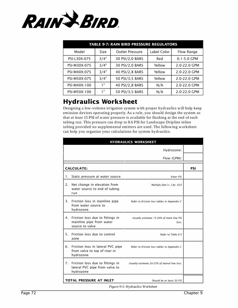
HYDRAULICS WORKSHEET
Hydrozone:
Flow (GPM):
CALCULATE: PSI
1. Static pressure at water source Enter PSI
2. Net change in elevation fromwater source to end of tubingrun
Multiply feet (+,-) by .433
3. Friction loss in mainline pipefrom water source tohydrozone
Refer to friction loss tables in Appendix C
4. Friction loss due to fittings inmainline pipe from watersource to valve
Usually estimate 15-20% of main line PSI
loss.
5. Friction loss due to controlzone
Refer to Table 9-5
6. Friction loss in lateral PVC pipefrom valve to top of riser inhydrozone
Refer to friction loss tables in Appendix C
7. Friction loss due to fittings inlateral PVC pipe from valve tohydrozone
Usually estimate 20-25% of lateral line loss.
TOTAL PRESSURE AT INLET Should be at least 30 PSI
Hydraulics WorksheetDesigning a low-volume irrigation system with proper hydraulics will help keepemission devices operating properly. As a rule, you should design the system sothat at least 15 PSI of water pressure is available for flushing at the end of eachtubing run. This pressure can drop to 8.6 PSI for Landscape Dripline inlinetubing provided no supplemental emitters are used. The following worksheetcan help you organize your calculations for system hydraulics.
Page 72 Chapter 9
TABLE 9-7: RAIN BIRD PRESSURE REGULATORS
Model Size Outlet Pressure Label Color Flow Range
PSI-L30X-075 3/4" 30 PSI/2,0 BARS Red 0.1-5.0 GPM
PSI-M30X-075 3/4" 30 PSI/2,0 BARS Yellow 2.0-22.0 GPM
PSI-M40X-075 3/4" 40 PSI/2,8 BARS Yellow 2.0-22.0 GPM
PSI-M50X-075 3/4" 50 PSI/3,5 BARS Yellow 2.0-22.0 GPM
PSI-M40X-100 1" 40 PSI/2,8 BARS N/A 2.0-22.0 GPM
PSI-M50X-100 1" 50 PSI/3,5 BARS N/A 2.0-22.0 GPM
Figure 9-5: Hydraulics Worksheet
®
Installation, Maintenance and Troubleshooting Page 73
INSTALLATION, MAINTENANCEAND TROUBLESHOOTING
InstallationInstallation of low-volume irrigation components, while slightly different fromconventional-system installation, is a straight forward process. The followingsteps define a typical low-volume installation.
1. Analyze the site. Compare the site to your irrigation plan and note anyobstructions or discrepancies. Modify your plan to reflect actual site conditions.
2. Locate or mark components. Use chalk or flags to mark the locations ofvalves, trenches, etc.
3. Plant large-specimen plant material.
4. Install and set up backflow devices to meet local codes.
5. Trench and lay main line to the control zone.
6. Pressure test the main line.
7. Set valve boxes and install control zone components.
8. Flush the valves.
9. Run lateral PVC pipe or high density polyethylene pipe to riser units. Eachriser unit includes the fittings necessary to connect a 1/2" schedule 80 riser tothe poly drip tubing (typically a compression elbow or tee).
10. Backfill trenches and rough grade.
11. Plant shrubs and trees.
10®

Page 74 Chapter 10
12. Layout XT-700 poly drip tubing or Landscape Dripline using fittings asneeded. Warm the tubing in the sun before installing to make it more flexible.Don’t pull tubing too tight; allow for expansion and contraction due tochanging weather conditions.
13. Flush the line to remove debris.
14. Attach emission devices.
15. Staple XT-700 poly drip tubing or Landscape Dripline to grade.
16. Finish grade.
17. Plant ground cover.
18. Operate system for approximately two weeks, checking for correct operationof all emission devices.
19. Flush system to remove any debris.
20. Mulch to cover system components and conserve water.
Maintenance and TroubleshootingThere is a common misconception that low-volume irrigation systems require farmore maintenance than conventional irrigation systems. In fact, the conventionalsystems also require substantial maintenance to keep them operating optimally.However, conventional systems tend to be more “forgiving” of poor maintenancepractices. Since the entire area is being irrigated, it is more likely that individualplants will be able to survive a poorly adjusted system.
In low-volume irrigation, each plant receives only as much water as it actuallyrequires. As a result, a clogged emitter or similar problem can cause extremestress to the plant that relies on that emitter for its water needs.
While the amount of maintenance for a low-volume system will not differ muchfrom conventional systems, the type of maintenance will. In a conventionalsystem, regular site reviews and system checks can determine problem areasfairly easily, but once a problem is found, it may be quite difficult to repair.
In a low-volume system, maintenance is more detail-oriented. Filters must becleaned on a regular basis, depending on the water source being used. Sitereviews require close scrutiny for signs of plant stress caused by a cloggedemitter. However, once a problem is found, it can generally be fixed on the spot.Table 10-1 outlines the recommended maintenance for low-volume systems.Table 10-2 includes a list of common system problems and their typical causesand solutions.
®
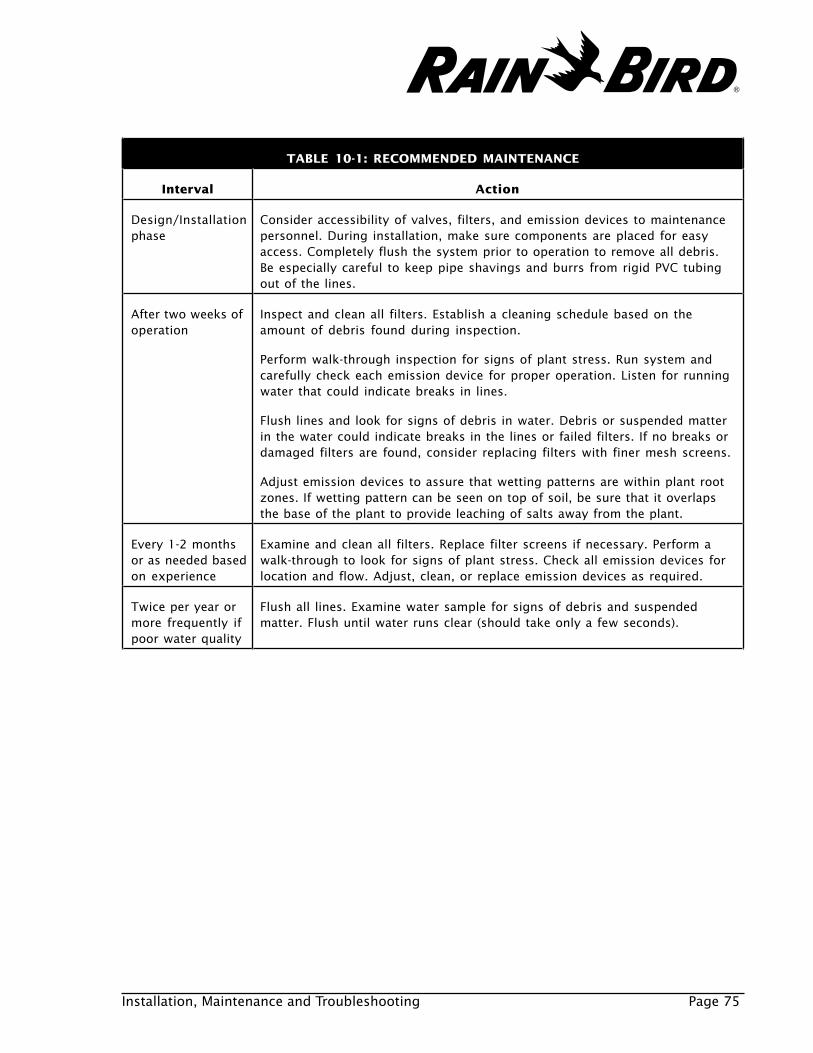
Installation, Maintenance and Troubleshooting Page 75
TABLE 10-1: RECOMMENDED MAINTENANCE
Interval Action
Design/Installationphase
Consider accessibility of valves, filters, and emission devices to maintenancepersonnel. During installation, make sure components are placed for easyaccess. Completely flush the system prior to operation to remove all debris.Be especially careful to keep pipe shavings and burrs from rigid PVC tubingout of the lines.
After two weeks ofoperation
Inspect and clean all filters. Establish a cleaning schedule based on theamount of debris found during inspection.
Perform walk-through inspection for signs of plant stress. Run system andcarefully check each emission device for proper operation. Listen for runningwater that could indicate breaks in lines.
Flush lines and look for signs of debris in water. Debris or suspended matterin the water could indicate breaks in the lines or failed filters. If no breaks ordamaged filters are found, consider replacing filters with finer mesh screens.
Adjust emission devices to assure that wetting patterns are within plant rootzones. If wetting pattern can be seen on top of soil, be sure that it overlapsthe base of the plant to provide leaching of salts away from the plant.
Every 1-2 monthsor as needed basedon experience
Examine and clean all filters. Replace filter screens if necessary. Perform awalk-through to look for signs of plant stress. Check all emission devices forlocation and flow. Adjust, clean, or replace emission devices as required.
Twice per year ormore frequently ifpoor water quality
Flush all lines. Examine water sample for signs of debris and suspendedmatter. Flush until water runs clear (should take only a few seconds).
®
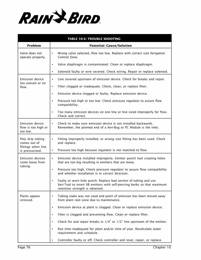
Page 76 Chapter 10
TABLE 10-2: TROUBLE SHOOTING
Problem Potential Cause/Solution
Valve does notoperate properly.
• Wrong valve selected, flow too low. Replace with correct size XerigationControl Zone.
• Valve diaphragm is contaminated. Clean or replace diaphragm.
• Solenoid faulty or wire severed. Check wiring. Repair or replace solenoid.
Emission devicehas uneven or noflow.
• Line severed upstream of emission device. Check for breaks and repair.
• Filter clogged or inadequate. Check, clean, or replace filter.
• Emission device clogged or faulty. Replace emission device.
• Pressure too high or too low. Check pressure regulator to assure flowcompatibility.
• Too many emission devices on one line or line sized improperly for flow.Check and correct.
Emission deviceflow is too high ortoo low.
• Check to make sure emission device is not installed backwards.Remember, the pointed end of a Xeri-Bug or PC Module is the inlet.
Poly drip tubingcomes out offittings when lineis pressurized.
• Fitting improperly installed, or wrong size fitting has been used. Checkand replace.
• Pressure too high because regulator is not matched to flow.
Emission devicescome loose fromtubing.
• Emission device installed improperly. Emitter punch tool creating holesthat are too big resulting in emitters that are loose.
• Pressure too high. Check pressure regulator to assure flow compatibilityand whether installation is in correct direction.
• Faulty or worn hole punch. Replace bad section of tubing and use Xeri-Tool to insert XB emitters with self-piercing barbs so that maximumretention strength is obtained.
Plants appearstressed.
• Tubing stake was not used and point of emission has been moved awayfrom plant root zone due to maintenance.
• Emission device at plant is clogged. Clean or replace emission device.
• Filter is clogged and preventing flow. Clean or replace filter.
• Check for and repair breaks in 1/4” or 1/2” line upstream of the emitter.
• Run time inadequate for plant and/or time of year. Recalculate waterrequirement and schedule.
• Controller faulty or off. Check controller and reset, repair, or replace.
®
Formulas for Xerigation Design Page 77
FORMULAS FORXERIGATION DESIGN
Kc is an adjustment factor to PET that accounts for the needs of a specific plant inspecific growing conditions. It is also known as the “crop coefficient” or the “plantfactor.”
The formula for Kc is:
Kc = Species Factor x Density Factor x Microclimate Factor
The water requirement for a densely planted hydrozone is measured in inchesper day.
The formula for the water requirement of a densely planted area is:
Water Requirement (inches per day) = Kc x PET
Where:Kc = Crop coefficient (plant factor) of the base plantPET = Published daily evapotranspiration rate (inches per day)
In order to determine the water requirement of individual plants you must firstcalculate the area of the plant’s canopy.
The formula for the area of a plant’s canopy is:
Area (square feet) = 0.7854 x Diameter (feet) x Diameter (feet)
A
Water Require-ment For a DensePlanting Scheme
Plant CanopyArea
®
Page 78 Appendix A
The water requirement for an individual plant is measured in gallons per day.
The formula for the water requirement for an individual plant is:
Water Requirement (GPD) = .623 x A x Kc x PET
e
Where:A = Area of the plant’s canopy (square feet)Kc = Crop coefficient (plant factor) of the plantPET = Published daily evapotranspiration rate (inches per day)e = Application efficiency (percentage in decimal form)
Knowing the maximum system run time helps to avoid wasted water due to run-off or deep percolation. Keep in mind that the actual system run time willgenerally be less than the maximum run time.
The formula for maximum system run time1 is:
Maximum Run Time (hours) = 0.000361 x C x AW x D x S2
q x e
Where:C = Allowable water depletion (percentage in decimal form)AW = Available Water (inches per foot)D = Desired watering depth (inches)S = Emitter spacing (inches)q = Flow rate (GPH)e = Efficiency (percentage in decimal form)
1Developed at California Polytechnic University, Pomona by Professor Joseph Y. T. Hung, 1993.
Water Require-ment For a Sparse
Planting Scheme
Maximum SystemRun Time
®

Formulas for Xerigation Design Page 79
Once you calculate the system run time and the maximum run time, you candetermine how often to run the system.
Maximum Irrigation Interval (days) = Maximum Run Time
Calculated Run Time
The general formula for system run time is:
Run Time (hours) = Water Requirement
Flow
However, since the water requirements are measured differently for sparseplantings and dense plantings, you must apply the formula differently.
Dense Planting SchemeThe formula for system run time for dense plants is based on a measurement offlow in inches per day. We call this measurement “Emitter Discharge Rate” orEDR. EDR is measured in inches per hour.
The formula for determining EDR is:
EDR (inches per hour) = 231.0 x q s x l
Where:q = emitter flow rate (gallons per hour)s = emitter spacing (inches)l = lateral spacing (inches)
EDR must be further adjusted by multiplying it by the application efficiency(percentage) to arrive at “Adjusted EDR.”
The formula for system run time for dense plantings is:
Run Time (hours) = Water Requirement (inches per day)
Adjusted EDR (inches per hour)
System Run Time
Irrigation Interval
®
Page 80 Appendix A
The result can be converted from hours to minutes by multiplying it by 60minutes.
Sparse Planting SchemeThe formula for system run time for a sparse planting scheme is shown below.The water requirement of the base plant must be used and is measured in gallonsper day:
Run Time (hours) = Water Requirement (gallon per day)
Total Flow at Base Plant (GPH)
The number of emission devices required for an individual plant will depend onthe following:
• Area of root zone.• Plant water requirement.• Percent of root zone to be wetted.
The formula is:
Number of Emitters = Plant Area (sq. ft.) x Percent to be Wetted Area Wetted by One Emitter (sq.ft.)
Number ofEmitters
®
PET Data Page 81
B PET DATA
Alabama
Birmingham .20
Montgomery .21
Mobile .20
Alaska
Anchorage .16
Fairbanks .20
Arizona
Flagstaff .23
Phoenix .30
Tuscon .27
Arkansas
Fort Smith .20
Little Rock .20
Texarkana .21
California
Bakersfield .25
Eureka .18
Fresno .25
Los Angeles .20
Palm Springs .37
Sacramento .20
San Francisco .15
Colorado
Alamosa .15
Denver .18
Pueblo .20
Connecticut
Hartford .20
New Haven .20
Delaware
Wilmington .20
Florida
Fort Meyers .24
Jacksonville .25
Key West .24
Pensacola .26
Tampa .26
Georgia
Atlanta .23
Augusta .24
Macon .23
Savannah .24
Hawaii
Hilo .17
Honolulu .20
Kahului .20
Lihue .19
Idaho
Boise .24
Lewiston .23
Pocatello .22
Illinois
Chicago .19
Peoria .20
Springfield .21
Indiana
Evansville .21
Fort Wayne .20
Indianapolis .21
South Bend .20
Iowa
Des Moines .21
Sioux City .20
Waterloo .19
Kansas
Dodge City .26
Topeka .25
Wichita .26
Kentucky
Lexington .19
Louisville .20
®
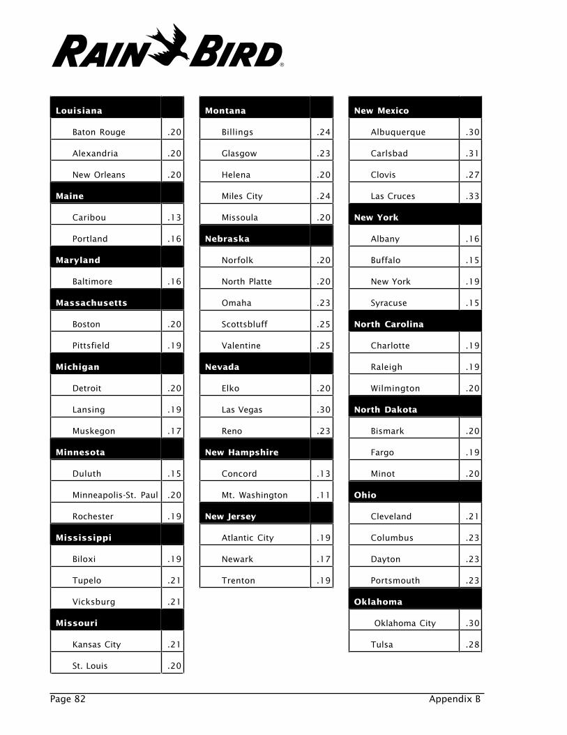
Page 82 Appendix B
Louisiana
Baton Rouge .20
Alexandria .20
New Orleans .20
Maine
Caribou .13
Portland .16
Maryland
Baltimore .16
Massachusetts
Boston .20
Pittsfield .19
Michigan
Detroit .20
Lansing .19
Muskegon .17
Minnesota
Duluth .15
Minneapolis-St. Paul .20
Rochester .19
Mississippi
Biloxi .19
Tupelo .21
Vicksburg .21
Missouri
Kansas City .21
St. Louis .20
Montana
Billings .24
Glasgow .23
Helena .20
Miles City .24
Missoula .20
Nebraska
Norfolk .20
North Platte .20
Omaha .23
Scottsbluff .25
Valentine .25
Nevada
Elko .20
Las Vegas .30
Reno .23
New Hampshire
Concord .13
Mt. Washington .11
New Jersey
Atlantic City .19
Newark .17
Trenton .19
New Mexico
Albuquerque .30
Carlsbad .31
Clovis .27
Las Cruces .33
New York
Albany .16
Buffalo .15
New York .19
Syracuse .15
North Carolina
Charlotte .19
Raleigh .19
Wilmington .20
North Dakota
Bismark .20
Fargo .19
Minot .20
Ohio
Cleveland .21
Columbus .23
Dayton .23
Portsmouth .23
Oklahoma
Oklahoma City .30
Tulsa .28
®
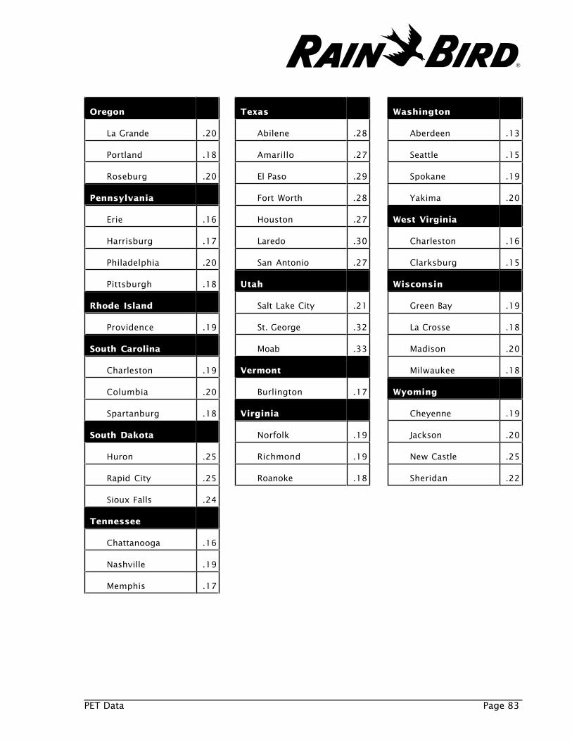
PET Data Page 83
Oregon
La Grande .20
Portland .18
Roseburg .20
Pennsylvania
Erie .16
Harrisburg .17
Philadelphia .20
Pittsburgh .18
Rhode Island
Providence .19
South Carolina
Charleston .19
Columbia .20
Spartanburg .18
South Dakota
Huron .25
Rapid City .25
Sioux Falls .24
Tennessee
Chattanooga .16
Nashville .19
Memphis .17
Texas
Abilene .28
Amarillo .27
El Paso .29
Fort Worth .28
Houston .27
Laredo .30
San Antonio .27
Utah
Salt Lake City .21
St. George .32
Moab .33
Vermont
Burlington .17
Virginia
Norfolk .19
Richmond .19
Roanoke .18
Washington
Aberdeen .13
Seattle .15
Spokane .19
Yakima .20
West Virginia
Charleston .16
Clarksburg .15
Wisconsin
Green Bay .19
La Crosse .18
Madison .20
Milwaukee .18
Wyoming
Cheyenne .19
Jackson .20
New Castle .25
Sheridan .22
®

Page 84 Appendix B
®
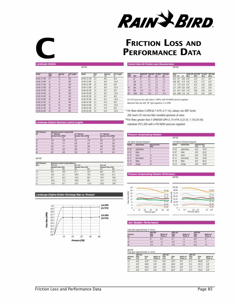
Friction Loss and Performance Data Page 85
FRICTION LOSS ANDPERFORMANCE DATA
Landscape Dripline Emitter Discharge Rate vs. Pressure
METRIC
Inlet Pressure Maximum Lateral Length (Meters)Bars 30,5 cm 45,7 cm 61,0 cm
Nominal Flow (l/h): Nominal Flow (l/h): Nominal Flow (l/h): 2,3 3,5 2,3 3,5 2,3 3,5
1,0 48,5 39,6 67,7 53,0 86,3 65,21,7 76,8 52,1 109,4 70,4 139,3 87,52,4 92,7 64,3 132,6 88,1 170,1 109,13,1 104,2 71,9 149,0 98,1 191,1 121,64,1 119,5 81,7 170,1 111,0 218,2 138,1
Model Flow Spacing Coil LengthGPH in. ft.
LD-06-12-100 .61 12 100LD-06-12-500 .61 12 500LD-09-12-100 .92 12 100LD-09-12-500 .92 12 500LD-06-18-100 .61 18 100LD-06-18-500 .61 18 500LD-09-18-100 .92 18 100LD-09-18-500 .92 18 500LD-06-24-100 .61 24 100LD-06-24-500 .61 24 500LD-09-24-100 .92 24 100LD-09-24-500 .92 24 500
METRIC
Model Flow Spacing Coil Lengthl/h cm m
LD-06-12-100 2,3 30,5 30,5LD-06-12-500 2,3 30,5 152,4LD-09-12-100 3,5 30,5 30,5LD-09-12-500 3,5 30,5 152,4LD-06-18-100 2,3 45,7 30,5LD-06-18-500 2,3 45,7 152,4LD-09-18-100 3,5 45,7 30,5LD-09-18-500 3,5 45,7 152,4LD-06-24-100 2,3 61,0 30,5LD-06-24-500 2,3 61,0 152,4LD-09-24-100 3,5 61,0 30,5LD-09-24-500 3,5 61,0 152,4
Landscape Dripline
Landscape Dripline Maximum Lateral Lengths
Inlet Pressure Maximum Lateral Length (feet)psi 12" Spacing 18" Spacing 24" Spacing
Nominal Flow (GPH): Nominal Flow (GPH): Nominal Flow (GPH): .6 .9 .6 .9 .6 .9
15 159 130 222 174 283 21425 252 171 359 231 457 28735 304 211 435 289 558 35845 342 236 489 322 627 39960 392 268 558 365 716 453
Flow
Rat
e (G
PM)
1.00.90.80.70.60.50.40.30.20.10.0
15 25 35 45 60
Pressure (PSI)
0.6 GPH(2,2 l/h)
0.9 GPH(3,5 l/h)
C
100-Mesh Filtration RequiredModel Outlet/Color Nominal Flow
GPM
PC-05 Light Brown 5PC-07 Violet 7PC-10 Green 10PC-12 Dark Brown 12PC-18 White 18PC-24 Orange 24
METRIC
150-Micron Filtration RequiredModel Outlet/Color Nominal Flow
m3⁄h l/h
PC-05 Light Brown 0,02 18,95PC-07 Violet 0,03 26,53PC-10 Green 0,04 37,90PC-12 Dark Brown 0,05 45,48PC-18 White 0,07 68,22PC-24 Orange 0,09 90,96
Pressure-Compensating Modules
METRICAt 15,2 cm Above Finished Grade5 ° Trajectory ■ ▲
Pressure-Compensating Modules Performance
Flow
Rat
e (G
PH)
2824201612
840
0 10 20 30 40 50 60Pressure (psi)
PC-24
PC-18
PC-12
PC-10
PC-07
PC-05
Flow
Rat
e (l/
h)
105,9890,8475,7060,5645,4230,2815,14
00 1,0 2,0 2,5 3,5 4,0
Pressure (Bars)
PC-24
PC-18
PC-12
PC-10
PC-07
PC-05
Xeri-Bubbler Performance
METRICFully open (approximately 22 clicks)
SXB-360 SXB-180 UXB-360Pressure Flow Flow Radius of Flow Flow Radius of Flow Flow Radius ofBars m3⁄h l/h Throw m m3⁄h l/h Throw m m3⁄h l/h Throw m
1,0 0,03 32,97 0,18 0,03 32,97 0,37 0,11 108,02 0,211,5 0,04 40,82 0,34 0,04 40,82 0,49 0,12 120,13 0,382,0 0,05 48,25 0,45 0,05 48,25 0,60 0,13 131,11 0,552,1 0,05 49,27 0,46 0,05 48,27 0,61 0,13 132,65 0,58
Xeri-Bubbler Performance
Fully open (approximately 22 clicks)SXB-360 SXB-180 UXB-360
Pressure Flow Radius of Flow Radius of Flow Radius ofpsi GPH Throw ft. GPH Throw ft. GPH Throw ft.
15 8.7 0.6 8.7 1.2 28.5 0.720 10.3 1.0 10.3 1.5 31.0 1.130 13.0 1.5 13.0 2.0 35.0 1.9
Flow XACZ-075 XCZ-075 75-DVX XCZ-100GPM GPH psi psi psi psi
1 60 5.1 3.5 2.5 1.03 180 5.1 3.5 2.5 1.05 300 5.4 3.6 2.9 1.210* 600 9.9 7.5 3.8 5.115* 900 15.9 12.7 4.2 8.820* 1200 24.2 20.2 5.1 14.3
METRIC
Flow XACZ-075 XCZ-075 75-DVX XCZ-100m3⁄h l/h l/s Bars Bars Bars Bars
0,23 227 0,06 0,35 0,24 0,17 0,070,68 682 0,19 0,35 0,24 0,17 0,071,14 1137 0,32 0,37 0,25 0,20 0,082,27 2274 0,63 0,68 0,52 0,26 0,353,41 3411 0,95 1,10 0,88 0,29 0,614,54 4548 1,26 1,67 1,39 0,35 0,99
Control Zone Kit Friction Loss Characteristics
XCZ-075 pressure loss data above 5 GPM is with PSI-M30X pressure regulator.
Maximum flow rate with “M” style regulators is 22 GPM.
* For flows below 3 GPM (0,7 m3⁄h; 0,11 l/s), always use RBY Series
200 mesh (75-micron) filter installed upstream of valve.
**For flows greater than 5 GPM/300 GPH (1,14 m3⁄h; 0,32 l/s; 1.135,50 l/h),
substitute PSI-L30X with a PSI-M30X pressure regulator.
®

In-Line WYE Filter
Pressure Loss (psi)Flow Rate 100 150 200GPM mesh mesh mesh
RBY-0755 0 0 0.510 0.5 0.5 1.515 2.4 2.6 2.920 5.2 5.4 5.430 12.0 12.5 13.0RBY-1005 0 0 010 0.5 0.5 0.515 2.1 2.2 2.520 4.7 4.9 4.930 8.6 8.8 8.8
METRIC
Pressure Loss (Bars)Flow 150 100 75m3⁄h l/s micron micron micron
RBY-0751,14 0,32 0,00 0,00 0,032,27 0,63 0,03 0,03 0,103,41 0,95 0,17 0,18 0,204,54 1,26 0,36 0,37 0,376,81 1,89 0,83 0,86 0,90RBY-1001,14 0,32 0,00 0,00 0,002,27 0,63 0,03 0,03 0,033,41 0,95 0,14 0,15 0,174,54 1,26 0,32 0,34 0,346,81 1,89 0,59 0,61 0,61
Replacement Filter Elements
Model Size Filtration Color
RBY-100MX 100-mesh filter RedRBY-150MX 150-mesh filter BlueRBY-200MX 200-mesh filter White
METRIC
Model Size Filtration Color
RBY-100MX 150-micron filter RedRBY-150MX 100-micron filter BlueRBY-200MX 75-micron filter White
Model Inlet/Color Nominal Filtration Flow RequiredGPH mesh
XB-05 Barb/Blue 0.5 200XB-10 Barb/Black 1.0 150XB-20 Barb/Red 2.0 150XBT-10 Thread/Black 1.0 150XBT-20 Thread/Black 2.0 150
METRIC
Model Inlet/Color Nominal Filtration Flow Requiredl/h microns
XB-05 Barb/Blue 1,90 75XB-10 Barb/Black 3,79 100XB-20 Barb/Red 7,58 100XBT-10 Thread/Black 3,79 100XBT-20 Thread/Black 7,58 100
Xeri-Bug Emitter Specifications and Models
METRICXeri-Bug Emitter Performance
2.5
2
1.5
1
0.5
00 10 20 30 40 50
Pressure (psi)
Flow
Rat
e (G
PH) XB-20
XBT-20
XB-10XBT-10
XB-05
9,46
7,57
5,68
3,79
1,89
00 0,7 1,4 2,1 2,8 3,5
Pressure (Bars)
XB-20XBT-20
XB-10XBT-10
XB-05
Flow
Rat
e (l/
h)
METRICMulti-Outlet Xeri-Bug Emitter Performance
1.5
1.2
0.9
0.6
0.3
00 20 40 60
Pressure (psi)
Flow
Rat
e (G
PH)
XB-10-6XBT-10-6
Flush Mode
5,68
4,54
3,41
2,27
1,14
00 1,5 2,0 2,5 3,5 4,0
Pressure (Bars)
XB-10-6XBT-10-6
Flush Mode
Flow
Rat
e (l/
h)
METRIC
O.D. 6 mm I.D. 4 mmFlow Velocity Barsm3⁄h l/h
0,00 3,79 0,08 0,010,01 7,58 0,16 0,040,01 11,37 0,24 0,090,02 15,16 0,32 0,150,02 18,95 0,41 0,220,02 22,74 0,48 0,310,03 26,53 0,57 0,410,03 30,32 0,65 0,530,03 34,11 0,73 0,660,04 37,90 0,81 0,800,04 41,69 0,89 0,950,05 45,48 0,97 1,120,05 49,27 1,05 1,290,05 53,06 1,13 1,480,06 56,85 1,21 1,690,06 60,64 1,30 1,900,06 64,43 1,38 2,130,07 68,22 1,46 2,360,07 72,01 1,54 2,610,08 75,80 1,62 2,870,09 94,75 2,03 4,340,11 113,70 2,43 6,08
1/4" Distribution Tubing Friction Loss Characteristics
O.D. .220" I.D. .160"Flow Velocity psiGPH fps Loss
1 0.27 0.162 0.53 0.593 0.80 1.244 1.06 2.125 1.33 3.206 1.59 4.497 1.86 5.978 2.13 7.649 2.39 9.5010 2.66 11.5411 2.92 13.7912 3.19 16.1713 3.45 18.7514 3.72 21.5015 3.98 24.4316 4.25 27.5317 4.52 30.8018 4.78 34.2319 5.05 37.8320 5.31 41.6025 6.64 62.8630 7.97 88.08
psi Loss Per 100 Feet of tubing; C=150
Bars Loss per 100 Meters of tubing
Note: Use of tubing at flows shown in dark shaded
area is not recommended, as velocities exceed
5 ft./sec. (1,5 m/s).
O.D. .700" I.D. .580"Flow Velocity LossGPM fps psi
0.50 0.61 0.191.00 1.21 0.691.50 1.82 1.452.00 2.43 2.472.50 3.03 3.743.00 3.64 5.243.50 4.24 6.974.00 4.85 8.934.50 5.46 11.105.00 6.06 13.505.50 6.67 16.106.00 7.28 18.92
METRIC
O.D. 18mm I.D. 15mmFlow Flow Velocity Lossm3⁄h l/h m/s Bars
0,11 0,03 0,19 0,010,23 0,06 0,37 0,050,34 0,09 0,56 0,100,45 0,13 0,74 0,170,57 0,16 0,92 0,260,68 0,19 1,11 0,360,79 0,22 1,29 0,480,91 0,25 1,48 0,621,02 0,28 1,67 0,771,14 0,32 1,85 0,931,25 0,35 2,03 1,111,36 0,38 2,22 1,31
Xeri-Tube™ 700 Friction Loss Characteristics
psi Loss per 100 Feet of Pipe (psi/100ft.) C=140
Bars Loss per 100 Meters of Pipe (Bars/100m)
Note: Use of tubing at flows shown in dark shaded area is not recommended,
as velocities exceed 5 ft./sec. (1,5 m/s).
Page 86 Appendix C
0
2.5
2
1.5
1
0.5
10 20 30 400
50Pressure (psi)
Flow
Rate
(G
PH)
0
9,46
7,57
5,68
3,79
1,89
0,7 1,4 2,1 2,80
3,5Pressure (Bars)
Flow
Rate
(l/
h)
XB-20XB-20
XB-10 XB-10
XB-05 XB-05
®

Xerigation Planning Forms Page 87
XERIGATION PLANNING FORMS
Photocopy the planning forms on the following pages and use them to help youplan your Xerigation projects.D
®
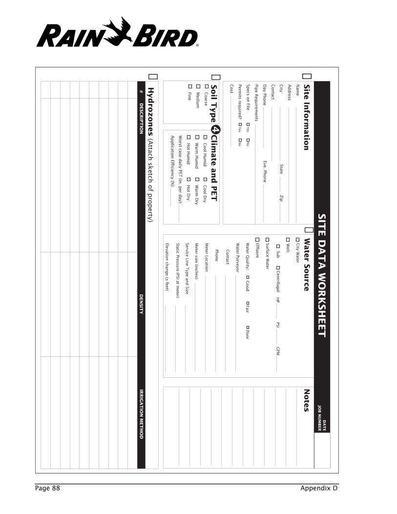
Page 88 Appendix D
SIT
E D
AT
A W
OR
KSH
EET
Site
Info
rmatio
n
Eve. Phone
Wate
r Sou
rceN
ote
s➋
Yes N
o
Yes N
o
Soil T
yp
eC
oarse
Med
ium
Fine
Nam
e
Address
City
Contact
Day Ph
one
Pipe R
equirem
ents
Specs o
n File
Permits req
uired
?
Cost
City W
ater
Well:
Surface W
ater
Effluen
t
Water Pu
rveyor
Contact
Phone
Meter Lo
cation
Meter size (in
ches)
Service Line T
ype an
d Size
Static Pressure (PSI at m
eter)
Elevation ch
ange (±
feet)
Good
FairPo
or
Water Q
uality:
HP
PSIG
PMSu
b C
entrifu
gal
StateZip
Clim
ate
an
d P
ET
Cool H
um
id
Warm
Hum
id
Hot H
um
id
Cool D
ry
Warm
Dry
Hot D
ry
Worst case d
aily PET (in
. per d
ay):
Applicatio
n Efficien
cy (%):
➎H
yd
rozon
es
(Attach
sketch o
f pro
perty)
DESC
RIP
TIO
ND
EN
SIT
Y#
IRR
IGA
TIO
N M
ET
HO
D
DA
TE
JOB N
UM
BER
❶➌
®
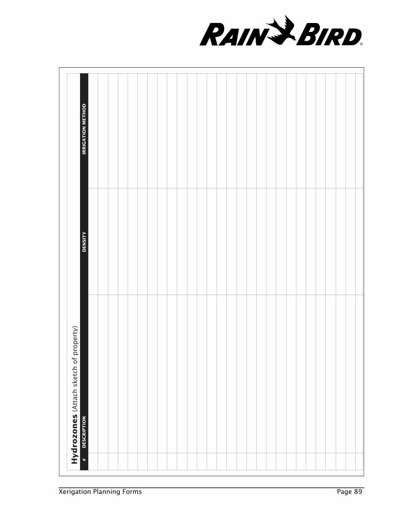
Xerigation Planning Forms Page 89
Hyd
rozon
es
(Att
ach s
ketc
h o
f pro
per
ty)
DESC
RIP
TIO
ND
EN
SIT
Y#
IRR
IGA
TIO
N M
ET
HO
D
®
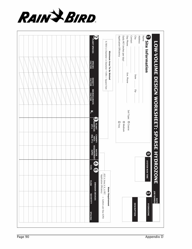
Page 90 Appendix D
Wate
r Req
uire
men
t
.62
3
Area
K
PET✕
✕✕
c
Applicatio
n Efficien
cy=
Gallo
ns p
er Day (G
PD)
LO
W-V
OLU
ME D
ESIG
N W
OR
KSH
EET
: SPA
RSE H
YD
RO
ZO
NE
PLA
NT
SPEC
IES
SPEC
IES
FA
CT
OR
DEN
SIT
YFA
CT
OR
MIC
RO
CLIM
AT
EFA
CT
OR
Kc
PLA
NT
DIA
MET
ER
(FT
.)
CA
NO
PY
AR
EA
(SQ
. FT
.)
WA
TER
REQ
UIR
EM
EN
T(G
PD
)
EM
ISSIO
N D
EV
ICES
TY
PE
FLO
WQ
UA
NT
ITY
SPA
CIN
G
Min
imu
m A
rea T
o B
e W
ette
d
0.7
85
4
Diam
eter D
iameter
50
% =
Square Feet
✕✕
×
DA
TE
JOB N
UM
BERD
ESC
RIP
TIO
N
HY
DR
OZO
NE
Eve. Phone
Nam
e
Address
City
Contact
Day Ph
one
Daily PET
(inch
es per d
ay)
Applicatio
n Efficien
cy
StateZip
Coarse
Soil T
ype:
Med
ium
Fine
Site
Info
rmatio
n1
1
34
6
SY
ST
EM
RU
N T
IME
5
2
®
Xerigation Planning Forms Page 91
AD
DIT
ION
AL
PLA
NT
SPEC
IES
SPEC
IES
FA
CT
OR
DEN
SIT
YFA
CT
OR
MIC
RO
CLIM
AT
EFA
CT
OR
Kc
PLA
NT
DIA
MET
ER
(FT
.)
CA
NO
PY
AR
EA
(SQ
. FT
.)
WA
TER
REQ
UIR
EM
EN
T(G
PD
)
EM
ISSIO
N D
EV
ICES
TY
PE
FLO
WQ
UA
NT
ITY
SPA
CIN
G
®
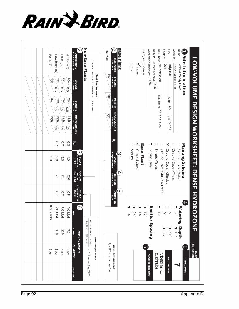
Page 92 Appendix D
Wate
r Req
uire
men
t
.62
3
Area
K
PET×
××c
Applicatio
n Efficien
cy=
Gallo
ns p
er Day (G
PD)
LO
W-V
OLU
ME D
ESIG
N W
OR
KSH
EET
: DEN
SE H
YD
RO
ZO
NE
AD
DIT
ION
AL
PLA
NT
SPEC
IES
SPEC
IES
FA
CT
OR
DEN
SIT
YFA
CT
OR
MIC
RO
CLIM
AT
EFA
CT
OR
Kc
PLA
NT
DIA
MET
ER
(FT
.)
CA
NO
PY
AR
EA
(SQ
. FT
.)
WA
TER
REQ
UIR
EM
EN
T(G
PD
)
EM
ISSIO
N D
EV
ICES
TY
PE
FLO
WQ
UA
NT
ITY
SPA
CIN
G
Base P
lan
t
Non
-Base P
lan
ts
Wate
r Req
uire
men
t
K
PET =
Inch
es per D
ayc ×
Pla
nt C
an
op
y A
rea
0.7
85
4
Diam
eter D
iameter =
Square Feet
××
BA
SE P
LA
NT
SPEC
IES
SPEC
IES
FA
CT
OR
DEN
SIT
YFA
CT
OR
MIC
RO
CLIM
AT
EFA
CT
OR
WA
TER
REQ
UIR
EM
EN
TEM
ITT
ER
FLO
W R
AT
EA
DJU
ST
ED
ED
RK
c
DA
TE
JOB N
UM
BERD
ESC
RIP
TIO
N
HY
DR
OZO
NE
Eve. Phone
Nam
e
Address
City
Contact
Day Ph
one
Daily PET
(inch
es per d
ay)
Applicatio
n Efficien
cy
StateZip
Coarse
Soil T
ype:
Med
ium
Fine
Site
Info
rmatio
n1
1
3 34
5
Gro
und C
over O
nly
Gro
und C
over/T
rees
Gro
und C
over /Sh
rubs
Gro
und C
over/Sh
rubs/T
rees
Shru
bs/T
rees
Shru
bs O
nly
Pla
ntin
g S
chem
e
Base P
lan
tG
round C
over
Shru
bs
Wate
ring
Dep
th3
"
6"
9"
12
"
18
"
24
"
36
"
Em
itter S
pacin
g
12
"
18
"
24
"
36
"
4
6
SY
ST
EM
RU
N T
IME
5
2 2
John & Wendy Doyle
7836
Connor LaneBrighton
CAJohn
714-555-8136
0.20
90%
Ice Plant
Azaleas (2)
Privet (12)
Hawthorne (6
)
Ferns (2)
lowavg.
avg.
avg.
high
0.5
0.5
0.5
0.5
1.01.0
1.31.31.3
0.3
4.012.6
0.5
P.C. Mod.
7.02 per
2 per
2 per
2 per
10.0
10.0
P.C. Mod.
P.C. Mod.
Xeri-Bubbler
0.7
0.7
7.1
7.1
3.0
3.0
5.0
7
Mixed G
. C.& shrubs
0.7
0.7
highhigh
high
high
high
highlow
med.
med.
low
714-555-108
9
9286
7
®

Xerigation Planning Forms Page 93
AD
DIT
ION
AL
PLA
NT
SPEC
IES
SPEC
IES
FA
CT
OR
DEN
SIT
YFA
CT
OR
MIC
RO
CLIM
AT
EFA
CT
OR
Kc
PLA
NT
DIA
MET
ER
(FT
.)
CA
NO
PY
AR
EA
(SQ
. FT
.)
WA
TER
REQ
UIR
EM
EN
T(G
PD
)
EM
ISSIO
N D
EV
ICES
TY
PE
FLO
WQ
UA
NT
ITY
SPA
CIN
G
®
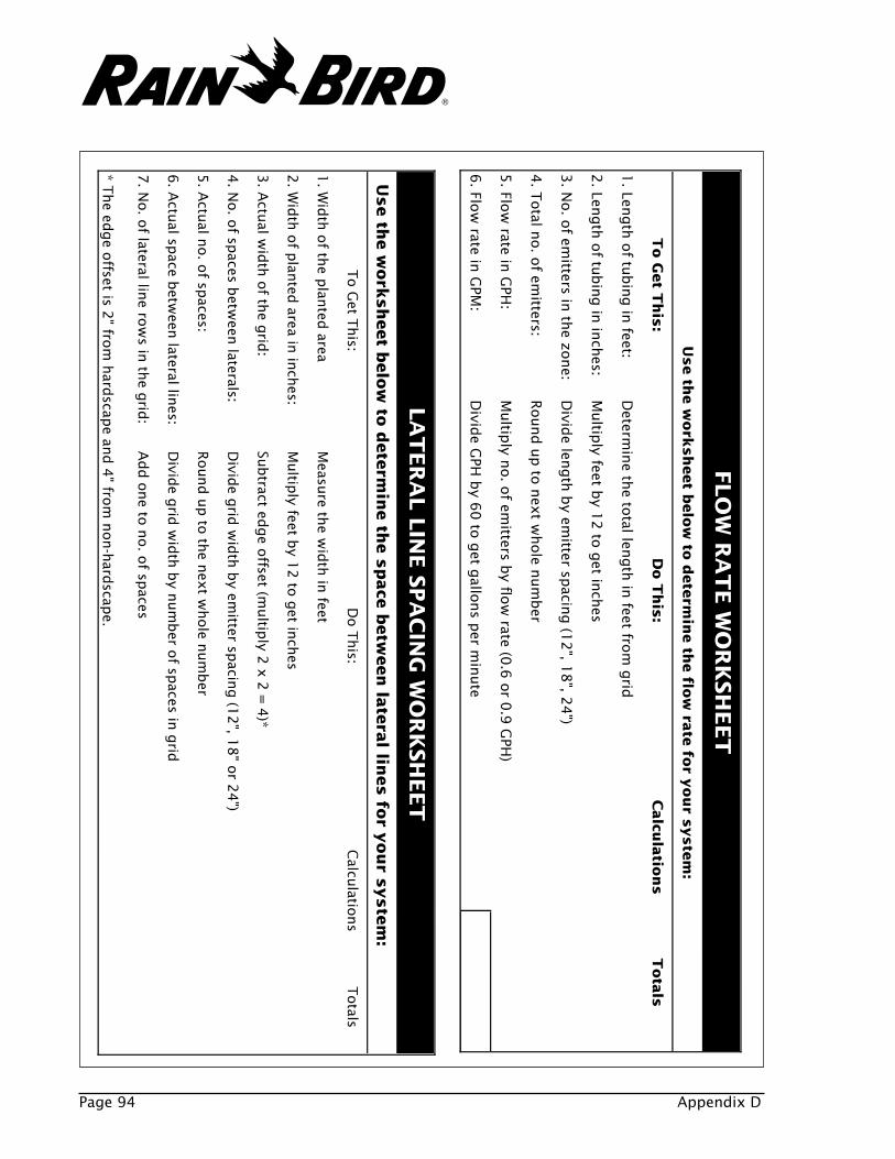
Page 94 Appendix D
FLO
W R
AT
E W
OR
KSH
EET
Use th
e w
ork
sh
eet b
elo
w to
dete
rmin
e th
e flo
w ra
te fo
r you
r syste
m:
To G
et T
his
:D
o T
his
:C
alcu
latio
ns
Tota
ls
1. Len
gth
of tu
bin
g in
feet:D
etermin
e the to
tal length
in feet fro
m g
rid
2. Len
gth
of tu
bin
g in
inch
es:M
ultip
ly feet by 1
2 to
get in
ches
3. N
o. o
f emitters in
the zo
ne:
Divid
e length
by em
itter spacin
g (1
2", 1
8", 2
4")
4. T
otal n
o. o
f emitters:
Round u
p to
nex
t whole n
um
ber
5. Flo
w rate in
GPH
:M
ultip
ly no. o
f emitters b
y flow
rate (0.6
or 0
.9 G
PH)
6. Flo
w rate in
GPM
:D
ivide G
PH b
y 60
to g
et gallo
ns p
er min
ute
LA
TER
AL L
INE S
PA
CIN
G W
OR
KSH
EET
Use th
e w
ork
sh
eet b
elo
w to
dete
rmin
e th
e s
pace
betw
een
late
ral lin
es fo
r you
r syste
m:
To G
et This:
Do T
his:
Calcu
lations
Totals
1. W
idth
of th
e plan
ted area
Measu
re the w
idth
in feet
2. W
idth
of p
lanted
area in in
ches:
Multip
ly feet by 1
2 to
get in
ches
3. A
ctual w
idth
of th
e grid
:Su
btract ed
ge o
ffset (multip
ly 2 x
2 =
4)*
4. N
o. o
f spaces b
etween
laterals:D
ivide g
rid w
idth
by em
itter spacin
g (1
2", 1
8" o
r 24
")
5. A
ctual n
o. o
f spaces:
Round u
p to
the n
ext w
hole n
um
ber
6. A
ctual sp
ace betw
een lateral lin
es:D
ivide g
rid w
idth
by n
um
ber o
f spaces in
grid
7. N
o. o
f lateral line ro
ws in
the g
rid:
Add o
ne to
no. o
f spaces
* The ed
ge o
ffset is 2" fro
m h
ardscap
e and 4
" from
non-h
ardscap
e.
®
GLOSSARYE
Glossary Page 95
1/2" polyethylene
tubing
a low-volume distribution component typically used to bring water from a Schedule 80
riser into a hydrozone.
1/4" distribution
tubing
a low-volume distribution component typically used to bring water directly to plant root
zones; also known as “spaghetti” tubing.
allowable depletion (also known as Management Allowable Depletion) the percent of soil moisture that an
irrigator will allow to be depleted before irrigating again; selection of a low allowable
depletion requires more frequent irrigation of smaller amounts. A higher allowable
depletion will require fewer irrigations of larger amounts. Generally, allowable
depletion should not exceed 30-50 percent for a low-volume irrigation system.
base plant the plant that requires the least amount of water in a given planting scheme, typically
is the predominant plant in a dense planting scheme.
capillary action the primary force in spreading water horizontally through soil.
compression fitting a fitting used to connect 1/2" poly drip tubing in a low-volume system; compression
fittings are attached to the outside of the tube so that the connection becomes tighter as
the pressure increases.
control zone in a low-volume system, a collection of components that controls the flow and pressure of
water to the hydrozone; the control zone includes a ball valve, an in-line WYE filter, a
remote control valve and a pressure regulator.
controller a device that automatically opens and closes the valves in an irrigation system accordin
to a pre-set program.
crop coefficient (also known as the Plant Factor, or Kc)
an adjustment factor used to equate actual plant- water use to referenced PET; a given
plant type may use less water than the referenced ET rate for an area. Multiplying the
plant's crop coefficient by the referenced ET rate adjusts ET to the actual plant water
use. Crop coefficient values are not widely available for landscape plants, but they are
grouped into one of three categories: low, medium or high water usage. See Chapter 4 for
information on calculating crop coefficients.
distribution
component
a low-volume irrigation component that brings water to the individual hydrozones and
plants; distribution components can include 1/2" polyethylene tubing, 1/4" spaghetti
tubing, compression fittings and flex risers.
®
distribution tubing See 1/4" distribution tubing.
drip emitter a low-volume emission device that delivers water at low flow rates, one drip at a time;
drip emitters are used to apply water directly to an individual plant root zone.
emission device a low-volume irrigation component that delivers water directly to the plants; emission
devices can include bubblers, drip emitters, microsprays and inline emitter tubing.
filter a device used in a control zone or multi-outlet emission device to screen dirt and debris
from the water; filters are important in low-volume systems because the small emission
devices can easily become clogged.
flow the amount of water, usually measured in gallons per minute or gallons per hour, that can
pass through an irrigation system.
GPH an abbreviation for gallons per hour, which is a measure of the flow of water through an
irrigation system; GPH is typically used to measure flow in low-volume irrigation
systems.
GPM an abbreviation for gallons per minute, which is a measure of the flow of water through
an irrigation system; GPM is typically used to measure flow in conventional irrigation
systems.
hydrozone a grouping of plants served by one control zone and irrigated by a low-volume system; a
hydrozone typically has a common microclimate and may consist of plants with like
water requirements or with mixed water requirements.
inline emitter tubing a polyethylene tube with emitters pre-installed at a specific distance from each other a
the factory.
infiltration rate the rate at which water applied to the soil enters the soil without causing runoff.
low-volume irrigation a type of watering system in which a precise amount of water is applied directly to the
root zones of plants, typically in gallons per hour.
matched hydrozone a hydrozone in which all of the plants have the same water needs; plants in a matched
hydrozone may each be watered by the same type and number of emitters and typically
will be watered together on the same valve.
maximum system run
time
the longest period of time a low-volume irrigation system can run without water loss to
deep percolation (or water penetration below the plant root zone).
micro-bubbler a low-volume emission device that delivers water at higher flow rates than drip emitte
but at lower flow rates than micro-sprays; micro-bubblers are used to apply water
directly to an individual plant root zone.
Page 96 Appendix E
®
Glossary Page 97
microclimate a small sub-climate within a project site created by adjacent hardscape, a shade tree or
exposure.
micro-spray a low-volume emission device that operates similarly to a conventional sprayhead, but
much lower flow rates; microsprays are used to water an entire hydrozone rather than
individual plant root zones.
mixed hydrozone a hydrozone in which the plants have different water needs. When plants having
different watering needs are grouped together, emission devices will be different for eac
plant. In many cases, the emitters will be matched for the individual plant needs so tha
the plant group may be watered on the same valve.
multi-outlet emission
device
a low-volume emission device that contains several drip emitters connected to
1/4" distribution tubing; the tubing is then run to several different plants.
planting scheme the arrangement of plants within a hydrozone; the planting scheme can refer to a dense o
sparse configuration, or to matching or mixing by watering needs.
polyethylene tubing See 1/2" polyethylene tubing.
potential
evapotranspiration
(PET)
the amount of water that is used by the combination of evaporation from the soil and
transpiration from plants growing in the soil; PET is generally expressed in inches per
day.
retrofit the process of changing an existing conventional irrigation system into a low-volume
system.
soil types types of soil determined by their composition; soil is made up of sand, silt and clay
particles, the percentage of each determines the soil type. Soil type will affect the
irrigation design and watering schedule.
—clay a medium-fine textured soil that usually forms very hard lumps or clods when dry and is
quite plastic and sticky when wet; when the moist soil is pinched between the thumb an
finger, it will form a long, flexible ribbon. Some clays are very high in colloids, are
friable, and may lack plasticity at all conditions of moisture.
—clay loam a moderately fine textured soil that usually breaks into clods or lumps that are hard
when dry. When the moist soil is pinched between the thumb and finger, it will form a
thin ribbon that will break readily, barely sustaining its own weight. The moist soil is
plastic and will form a cast that will bear much handling. When kneaded in the hand,
does not crumble readily, but tends to work into a heavy compact mass.
®
soil types, continued
—loam soil having a mixture of the different grades of sand, silt and clay in such proportion tha
none of the characteristics predominate; it is mellow with a somewhat gritty feel, and
when moist is slightly plastic. Squeezed when dry, it will form a cast that will bear
careful handling; the cast formed by squeezing the moist soil can be handled quite freely
without breaking.
—sand a loose and single-grained soil; the individual grains can easily be seen or felt. Squeezed
in the hand when dry, it will fall apart when pressure is released. Squeezed when mois
it will form a cast but will crumble when touched.
—sandy loam a soil containing much sand, but which has enough silt and clay to make it somewhat
cohesive; the individual sand grains can readily be seen and felt. Squeezed when dry, it
will form a cast that will readily fall apart, but if squeezed when moist, a cast can be
formed that will bear careful handling without breaking.
—silt loam a soil having a moderate amount of the fine grades of sand and only a small amount of
clay, over half of the particles being of the size called "silt." When dry, it may appear
cloddy, but the lumps can be readily broken. When pulverized, it feels smooth, soft, and
floury. When wet, the soil readily runs together. Either dry or moist, it will form casts
that can be freely handled without breaking; however, when moistened and squeezed
between thumb and finger, it will not "ribbon" but will be broken in appearance.
spaghetti tubing See 1/4" distribution tubing.
system efficiency a factor that denotes how efficient the irrigation system is at applying water. When
water is discharged from the system, only a certain percentage will reach the plant root
zone and be available for consumption. The percentage of water that reaches the plant
and is available equals system efficiency. It is impossible to reach a 100% eficiency.
valve a device that opens and closes to allow pressurized water to flow through pipes.
valve box an underground enclosure that protects valves from moisture and other damage.
valve zone a group of sprinklers that are controlled by a single valve (see hydrozone).
water source pressurized water in a city main line or water pumped from a well, lake or pond.
watering window the amount of time available to water in any one period.
wetting pattern the area of the ground that is wet just after irrigation; an ideal wetting pattern covers th
root zone of the plant without leaving a puddle.
Xeriscape a planting scheme that groups plants with the same irrigation requirements together.
Page 98 Appendix E
®
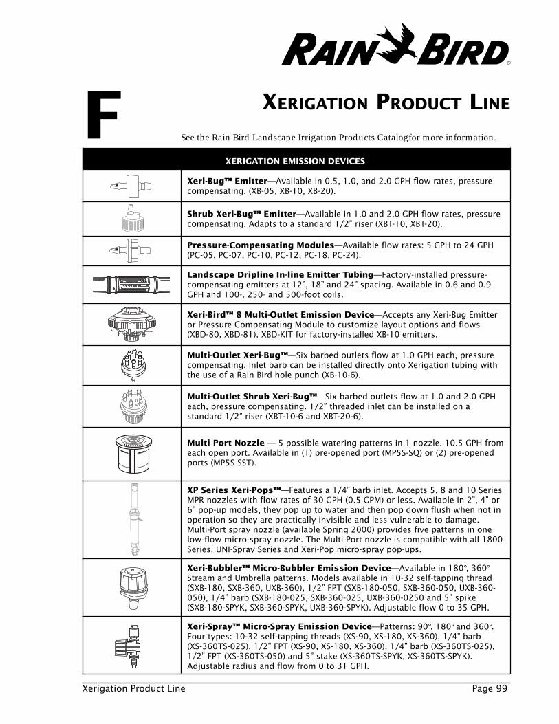
XERIGATION PRODUCT LINE
See the Rain Bird Landscape Irrigation Products Catalogfor more information.
Xerigation Product Line Page 99
FXeri-Bug™ Emitter—Available in 0.5, 1.0, and 2.0 GPH flow rates, pressurecompensating. (XB-05, XB-10, XB-20).
Shrub Xeri-Bug™ Emitter—Available in 1.0 and 2.0 GPH flow rates, pressurecompensating. Adapts to a standard 1/2” riser (XBT-10, XBT-20).
Pressure-Compensating Modules—Available flow rates: 5 GPH to 24 GPH(PC-05, PC-07, PC-10, PC-12, PC-18, PC-24).
Landscape Dripline In-line Emitter Tubing—Factory-installed pressure-compensating emitters at 12”, 18” and 24” spacing. Available in 0.6 and 0.9GPH and 100-, 250- and 500-foot coils.
Xeri-Bird™ 8 Multi-Outlet Emission Device—Accepts any Xeri-Bug Emitteror Pressure Compensating Module to customize layout options and flows(XBD-80, XBD-81). XBD-KIT for factory-installed XB-10 emitters.
Multi-Outlet Xeri-Bug™—Six barbed outlets flow at 1.0 GPH each, pressurecompensating. Inlet barb can be installed directly onto Xerigation tubing withthe use of a Rain Bird hole punch (XB-10-6).
Multi-Outlet Shrub Xeri-Bug™—Six barbed outlets flow at 1.0 and 2.0 GPHeach, pressure compensating. 1/2” threaded inlet can be installed on astandard 1/2” riser (XBT-10-6 and XBT-20-6).
XP Series Xeri-Pops™—Features a 1/4” barb inlet. Accepts 5, 8 and 10 SeriesMPR nozzles with flow rates of 30 GPH (0.5 GPM) or less. Available in 2”, 4” or6” pop-up models, they pop up to water and then pop down flush when not inoperation so they are practically invisible and less vulnerable to damage.Multi-Port spray nozzle (available Spring 2000) provides five patterns in onelow-flow micro-spray nozzle. The Multi-Port nozzle is compatible with all 1800Series, UNI-Spray Series and Xeri-Pop micro-spray pop-ups.
Xeri-Bubbler™ Micro-Bubbler Emission Device—Available in 180°, 360°Stream and Umbrella patterns. Models available in 10-32 self-tapping thread(SXB-180, SXB-360, UXB-360), 1/2” FPT (SXB-180-050, SXB-360-050, UXB-360-050), 1/4” barb (SXB-180-025, SXB-360-025, UXB-360-0250 and 5” spike(SXB-180-SPYK, SXB-360-SPYK, UXB-360-SPYK). Adjustable flow 0 to 35 GPH.
Xeri-Spray™ Micro-Spray Emission Device—Patterns: 90°, 180° and 360°.Four types: 10-32 self-tapping threads (XS-90, XS-180, XS-360), 1/4” barb(XS-360TS-025), 1/2” FPT (XS-90, XS-180, XS-360), 1/4” barb (XS-360TS-025),1/2” FPT (XS-360TS-050) and 5” stake (XS-360TS-SPYK, XS-360TS-SPYK).Adjustable radius and flow from 0 to 31 GPH.
XERIGATION EMISSION DEVICES
Multi Port Nozzle — 5 possible watering patterns in 1 nozzle. 10.5 GPH fromeach open port. Available in (1) pre-opened port (MP5S-SQ) or (2) pre-openedports (MP5S-SST).
®

Page 100 Appendix F
* Toro is a registered trademark of Toro Corporation.
RAIN BIRD
XERI-CAPXC-T-570
RAIN BIRD
XERI-CAPXC-1800
Xerigation Control Zone Kit—Prepackaged kit includes Ball Valve, InlineFilter, Remote Control Valve, Pressure Regulator, and 3/4” Schedule 80 Nipples(XCZ-075, XCZ-100). With anti-syphon valve use model (075-ASVF), Withcommercial PEB valve, use XCZ-100COM.
3/4” DVX Remote Control Valve—(75-DVX). Handles flow from 12 to900 GPH.
In-line WYE Filters—Available in 3/4" (RBY-075-200X) or 1" (RBY-100-200X).Three color coded replacement mesh screen sizes are also available: 100-Mesh(RBY-100MX), 150-Mesh (RBY-150MX), 200-Mesh (RBY-200MX).
In-line Pressure Regulators—Suitable for above- or below-ground installa-tion. (Low flow 0.1-5 GPM: PSI-L30X-075, Medium flow 2-22 GPM: PSI-M30X-075, PSI-M40X-075, PSI-M50X-075, PSI-M40X-100, PSI-M50X-100).
Ball Valve—Ideal for isolation valve applications. (XBV—075).
Automatic Filter Kit—Combines Y-filter and fittings with PESB scrubber valve.When connected to filter’s flush port, PESB valve can be controlled by timer toregularly flush filter. Specify desired mesh: 30, 50, 100, 150 or 200-mesh.Models: 1” (AF100-LSS), 1-1/2” (AF150-LSS), 2” (AF200-LSS).
1800 Xerigation Retrofit Kit—Change any 1804, 1806, or 1812 spraysystem into Xerigation. Includes 200-mesh filtration and 30 PSI regulator.(RETRO-1800).
Retrofit Pressure Regulator—Fits standard 1/2” riser, regulates pressure to30 PSI (PRS-050).
Xeri-Caps™ for Sprayheads—Cap fits over any Rain Bird 1800 (XC-1800) orToro* 570 (XC-T-570) sprayhead for retrofitting.
XERIGATION RETROFIT COMPONENTS
XERIGATION CONTROL ZONE COMPONENTS
®
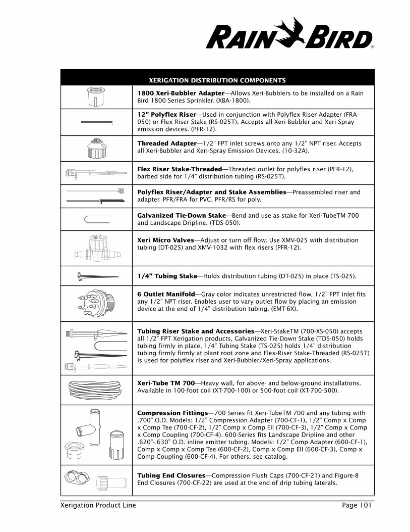
Xerigation Product Line Page 101
1800 Xeri-Bubbler Adapter—Allows Xeri-Bubblers to be installed on a RainBird 1800 Series Sprinkler. (XBA-1800).
12" Polyflex Riser—Used in conjunction with Polyflex Riser Adapter (FRA-050) or Flex Riser Stake (RS-025T). Accepts all Xeri-Bubbler and Xeri-Sprayemission devices. (PFR-12).
Threaded Adapter—1/2” FPT inlet screws onto any 1/2” NPT riser. Acceptsall Xeri-Bubbler and Xeri-Spray Emission Devices. (10-32A).
Flex Riser Stake-Threaded—Threaded outlet for polyflex riser (PFR-12),barbed side for 1/4” distribution tubing (RS-025T).
Polyflex Riser/Adapter and Stake Assemblies—Preassembled riser andadapter. PFR/FRA for PVC, PFR/RS for poly.
Galvanized Tie-Down Stake—Bend and use as stake for Xeri-TubeTM 700and Landscape Dripline. (TDS-050).
Xeri Micro Valves—Adjust or turn off flow. Use XMV-025 with distributiontubing (DT-025) and XMV-1032 with flex risers (PFR-12).
1/4" Tubing Stake—Holds distribution tubing (DT-025) in place (TS-025).
6 Outlet Manifold—Gray color indicates unrestricted flow, 1/2” FPT inlet fitsany 1/2” NPT riser. Enables user to vary outlet flow by placing an emissiondevice at the end of 1/4” distribution tubing. (EMT-6X).
Tubing Riser Stake and Accessories—Xeri-StakeTM (700-XS-050) acceptsall 1/2” FPT Xerigation products, Galvanized Tie-Down Stake (TDS-050) holdstubing firmly in place, 1/4” Tubing Stake (TS-025) holds 1/4” distributiontubing firmly firmly at plant root zone and Flex-Riser Stake-Threaded (RS-025T)is used for polyflex riser and Xeri-Bubbler/Xeri-Spray applications.
Xeri-Tube TM 700—Heavy wall, for above- and below-ground installations.Available in 100-foot coil (XT-700-100) or 500-foot coil (XT-700-500).
Compression Fittings—700 Series fit Xeri-TubeTM 700 and any tubing with.700” O.D. Models: 1/2” Compression Adapter (700-CF-1), 1/2” Comp x Compx Comp Tee (700-CF-2), 1/2” Comp x Comp EII (700-CF-3), 1/2” Comp x Compx Comp Coupling (700-CF-4). 600-Series fits Landscape Dripline and other.620”-.630” O.D. inline emitter tubing. Models: 1/2” Comp Adapter (600-CF-1),Comp x Comp x Comp Tee (600-CF-2), Comp x Comp EII (600-CF-3), Comp xComp Coupling (600-CF-4). For others, see catalog.
XERIGATION DISTRIBUTION COMPONENTS
Tubing End Closures—Compression Flush Caps (700-CF-21) and Figure-8End Closures (700-CF-22) are used at the end of drip tubing laterals.
®
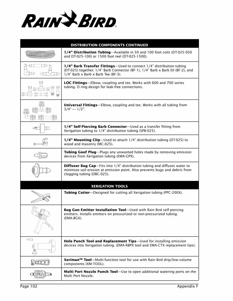
Page 102 Appendix F
EMA BG
DISTRIBUTION COMPONENTS CONTINUED
XERIGATION TOOLS
1/4" Distribution Tubing—Available in 50 and 100 foot coils (DT-025-050and DT-025-100) or 1500 foot reel (DT-025-1500).
1/4" Barb Transfer Fittings—Used to connect 1/4” distribution tubing(DT-025) together. 1/4” Barb Connector (BF-1), 1/4” Barb x Barb EII (BF-2), and1/4” Barb x Barb x Barb Tee (BF-3).
1/4" Self-Piercing Barb Connector—Used as a transfer fitting fromXerigation tubing to 1/4” distribution tubing (SPB-025).
1/4" Mounting Clip—Used to attach 1/4” distribution tubing (DT-025) towood and masonry (MC-025).
Tubing Goof Plug—Plugs any unwanted holes made by removing emissiondevices from Xerigation tubing (EMA-GPX).
Diffuser Bug Cap—Fits into 1/4” distribution tubing and diffuses water tominimize soil erosion at emission point. Also prevents bugs and debris fromclogging tubing (DBC-025).
Tubing Cutter—Designed for cutting all Xerigation tubing (PPC-200X).
Bug Gun Emitter Installation Tool—Used with Rain Bird self-piercingemitters. Installs emitters on pressurized or non-pressurized tubing.(EMA-BGX).
Hole Punch Tool and Replacement Tips—Used for installing emissiondevices into Xerigation tubing. (EMA-RBPX tool and EMA-CTX replacement tips).
Xeriman™ Tool—Multi-function tool for use with Rain Bird drip/low-volumecomponents (XM-TOOL).
LOC Fittings—Elbow, coupling and tee. Works with 600 and 700 seriestubing. O ring design for leak-free connections.
Universal Fittings—Elbow, coupling and tee. Works with all tubing from3/4" — 1/2".
Multi Port Nozzle Punch Tool—Use to open additional watering ports on theMulti Port Nozzle.
®
Installation Details Page 103
INSTALLATION DETAILS
Installation details for Xerigation products can be downloaded from Rain Bird’s website at:
www.rainbird.com.
1. From the Rain Bird home page, click on Landscape Drip.
2. From the Xerigation home page, click on Technical Information.
3. From the Technical Information page, click on Download Files.
4. From the Download Technical Information page, follow the instructions and clickon the appropriate file type (xeri.exe, jxeri.exe, wxeri.exe, dxeri.exe) under theXerigation category.
OR
Go directly to the Download Technical Information page and follow the instructions at:
www.rainbird.com/rbturf/technical/download.htm
From the Download Technical Information page, follow the instructions and clickon the appropriate file type (xeri.exe, jxeri.exe, wxeri.exe, dxeri.exe) under theXerigation category.
®
Page 104 Bibliography
BIBLIOGRAPHY
Drip Irrigation Design for Landscapes, by Joseph Y. T. Hung, Paper Number 88-2066presented at the American Society of Agricultural Engineers, Rapid City, SD,1988.
Determining Drip Emitter Spacing and Watering Time for Maximum Water UseEfficiency, by Joseph Y. T. Hung, Paper presented at the Irrigation Association, SanDiego, CA, 1993.
Estimating Water Requirements of Landscape Plantings: The Landscape CoefficientMethod, Cooperative Extension University of California, Division of Agricultureand Natural Resources, Leaflet 21493.
Water Use Classification of Landscape Species, (WUCOLS Project), CooperativeExtension University of California, February 1992.
Landscape Drip Irrigation Design Manual, by Keith Shepersky, Rain Bird Sales, Inc.,1984.
Irrigation Principles and Practices, Fourth Edition, by Vaughn E. Hansen, Orson W.Israelsen, Glen E. Stringham, 1979.
Rain Bird Trickle Irrigation Design, First Edition, by Jack Keller, Ph. D. and DavidKarmeli, Ph. D., Rain Bird Sprinkler Manufacturing Corp., 1975.
For more information about the Landscape and Irrigation Design program atCalifornia State Polytechnic University, Pomona, California, call 909-869-2220.
®
Index Page 105
—A—Adjusted EDR, 44Allowable depletion, 46Application efficiency, 14, 17, 25, 44Application, emission device, 30Area
canopy, 39mature canopy, 40minimum to be wetted, 40plant canopy, 25root zone, 39wetted per emitter, 40
Available water, 12
—B—Base plant, 29
dense hydrozone, 21irrigating, 29sparse hydrozone, 29, 38
—C—Canopy, mature, 25Capillary action, 11City water, 10Clay, 11Climate, 11Coefficient, crop, 21Container plants, irrigating, 62Control zone, 14, 69Controller, 45Conventional irrigation, 5, 14Cool dry climate, 14Cool humid climate, 14Crop coefficient, 21, 24Cycle, wet/dry, 3
—D—Dense Hydrozone Design Worksheet, 20Dense hydrozone, water requirements, 21Dense plants, 7
emission devices, 32system run time, 44water requirement, 24
Density factor, 22Depletion, allowable, 46Depth
emission device, 30, 39, 55minimum watering, 36root, 36
Design process, 6Design Worksheet
Dense Hydrozone, 20Sparse Hydrozone, 20
Desired watering depthminimum, 36
Diameter, plant, 24Dirty water, 10Discharge rate, emitter, 44DV Valve, 69Dynamic pressure, 63
—E—EDR, 44EDR, adjusted, 45Efficiency, application, 14, 25, 44Effluent, 10Elevation, 63Emission device
depth, 36flow rate, 37non-base plants, 51placement, 55plants, non-base, 51selecting, 30, 51spacing, 33, 36
Emission device, supplemental onLandscape Dripline, 57
Emitter discharge rate, 44Emitters. See Emission devicesEvaporation, 13Evapotranspiration, potential, 13, 21
—F—Factor
density, 22microclimate, 23plant, 22species, 22
Field capacity, 12Filter, 10, 32Filtration, 10, 32Flow, 64
maximum, 67, 69Flow rate, 32, 51
emission device, 37Friction loss, 63
—G—Gravitational water, 12Ground cover, 21
—H—Hanging plants, irrigating, 62Hot dry climate, 14Hot humid climate, 14Hydraulics, 63Hydrozone, 14
dense, water requirements, 21sparse, base plant, 29
Hygroscopic water, 12
—I—Individual plants, 7
system run time, 45water requirement, 24
Infiltration rate, maximum, 13Inlet, 32Inline tubing. See Landscape DriplineInstallation, 73
Installation details, 103
Installation cost, 4, 31Intended use, 30Interval, irrigation, 48Irrigating
base plants, 29large areas, 30slopes, 61
Irrigationconventional. See Conventional irrigationlow-volume. See Low-volume irrigation
Irrigation design, 6Irrigation interval, 48Irrigation method, 15
—K—Kc, 21, 24
calculating, 21, 24
—L—Landscape Dripline, 32, 57
choices and models, 34grid system, 33lateral spacing, 35slopes, installation on, 61staking and stapling, 59supplemental emission devices, 57system configuration, 60
Landscape irrigation design, 6Large areas, irrigating, 30Lateral pipe, pressure loss, 70Layout, 55Length, tubing, 68Low-volume irrigation, 1, 14
benefits, 2design, 5selecting, 4
INDEX
®
—R—Rain Bird, Technical support, 4Rate
emission device flow, 37emitter discharge, 44
Reference PET, 13, 81Root depth, 36Root zone, 2, 5Run time
calculating, 44system, 43system, maximum, 46
—S—Safety, 4, 30Sand, 11Scheduling, 43Screen, 10Selecting emission devices
dense plants, 32sparse plants, 37
Selecting low-volume irrigation, 4Shrub Xeri-Bug Single
Outlet Emitter, 32, 52Silt, 11Site data, 9, 17Slopes, irrigating, 61Soil
coarse, 11fine, 11medium, 11type, 11
Source, water, 10Spacing
emission device, 36maximum, 37
Sparse Hydrozone Design Worksheet, 20Sparse hydrozone, base plant, 29Sparse plants, 7
selecting emission devices, 30, 51system run time, 45water requirement, 24
Speciesfactor, 22plant, 22
Stakes and staples, 59Static pressure, 10, 63Sub-climate. See MicroclimateSurface water, 10System layout, 55, 60System run time, 43
calculating, 44maximum, 46
—T—Technical support, 4Time, system run, 43Traffic, 30Transpiration, 13Trees, 23Troubleshooting, 74
—V—Valve, 14
pressure loss through, 69zone, 14
Valve, DV, 69Vandalism, 4, 30
—W—Warm dry climate, 14Warm humid climate, 14Wasted water, 2, 15Water
available, 12capillary, 12dirty, 10gravitational, 12hygroscopic, 12meter, 10movement
horizontal, 11vertical, 11
pressure, 10, 63quality, 10requirement, 19
calculating, 21dense plants, 24sparse plants, 24
source, 10Water requirement, 19, 21, 51
dense hydrozone, 21dense plants, 24individual plants, 24sparse plants, 24
Wateringdepth, minimum desired, 36window, 30
Well water, 10Wet/dry cycle, 3Wetted diameter, maximum, 13Wetting pattern, 13
emission device, 52maximum, 13
Wilting point, permanent, 12Window, watering, 30Worksheet
Dense Hydrozone Design, 20Site Data, 9Sparse Hydrozone Design, 20
—X—Xeri-Bird-8, 32Xeri-Bubblers, 32, 52Xeri-Bug Single Outlet Emitter, 32, 52
Xeri-Pop Micro-Spray Pop-Ups, 32, 38
Xerigation, 1design, 6products, 32, 99
Xeriscape, 1Xeri-Sprays, 32, 38
Page 106 Index
—M—Maintenance, 74Maximum emission device spacing, 37Maximum infiltration rate, 13Maximum lateral lengths, 68Maximum system run time, 46Maximum wetted diameter, 13Maximum wetting patterns, 13Mesh, 10Meter, water, 10Microclimate, 23Microclimate factor, 23Micro-sprays, 32, 43Minimum area to be wetted, 40Minimum desired watering depth, 36Minimum watering depth, 36Multi-outlet Shrub Xeri-Bug, 32, 52Multi-outlet Xeri-Bug, 32, 52
—N—Non-base plants, irrigating, 51
—O—Outlet, 32
—P—Permanent wilting point, 12PET, 13, 21, 81Plant
base, dense hydrozone, 21canopy, 25diameter, 24dominant, 21factor, 21species, 22water requirement, 19
Planting scheme, 21Plants
dense, 7selecting emission devices, 32water requirement, 24
individual, 7water requirement, 24
sparse, 7selecting emission devices, 37water requirement, 24
Plants, non-baseirrigating, 51
Potential evaportranspiration, 13, 21, 81Pressure
dynamic, 63loss, 63, 85
lateral pipe, 70valve, 70
static, 10, 63water, 63
Pressure Compensating Modules, 32, 52Pressure compensation, 32Products, Xerigation, 32, 99
®

Rain Bird Corporation970 West Sierra Madre Avenue, Azusa, CA 91702Phone: (626) 963-9311 Fax: (626) 812-3411
Specification Hotline1-800-458-3005 (U.S. only)
Rain Bird Technical Services(800) 247-3782 (U.S. only)
www.rainbird.comA Recycled Paper.Rain Bird. Conserving More Than Water
® Registered Trademark of Rain Bird Sprinkler Mfg. Corp.©2000 Rain Bird Sprinkler Mfg. Corp. 2/00D39030D
®
For Technical Assistance,Call Toll Free1-800-247-3782
®
An ancient Indian legend tells of a terrible drought that befell the landhundreds of years ago. Crops withered and the watering holes dried up.For a generation there was no relief. Everyone but the children gave uphope. Then, one day, a great bird overheard the children’s simple, urgentprayers. The bird flew to the heavens and returned with the long-awaited,life-giving rain. The bird-like appearance of the efficient impact sprinkler,which the company founders introduced to the world in 1935, promptedthem to name their new company after the great rain bird of Indianlegend. And so the modern Rain Bird legend was born.Since our dramatic entrance into the market more than 60 years ago,Rain Bird has grown into the largest manufacturer of irrigation systemsin the world. Quality products. Water-saving solutions. Worldwide serviceand support. At every step, our focus has been to manage and conserveour planet’s most valuable, natural resource—water. Rain Bird. Becauseevery drop counts.