Queuing Networks: Burke’s Queuing Networks: Burke’s Theorem, Kleinrock’s Theorem, Kleinrock’s

Approximation, and Jackson’s Approximation, and Jackson’s TheoremTheorem

Wade Trappe

Lecture OverviewLecture Overview

Network of Queues Introduction– Queues in Tandem– Product Form Solutions– Burke’s Theorem– What is reversibility?

Kleinrock’s Approximation Quick Jackson Theorem

In many networking scenarios, a customer or packet must receive service from many servers before its final task is completed.

Hence, departures from a queue might become arrivals at another queue. – All that discussion we did in M/G/1 queues becomes very

important for networks of queues!

Consider two queues in tandem:– Departures from first queue become arrivals at second queue– First queue’s arrival process is Poisson with rate and

service time is exponential with rate – Service time at the second queue is exponential with rate

and independent of first server’s service time

How do we model these two queues together?– What’s the state and state diagram?

Network of Queues: Setup Network of Queues: Setup

2

1

Two Queues in TandemTwo Queues in Tandem

Queue2

We need to keep track of N1(t) and N2(t) to describe the state of the system!

Queue1

Two Queues in Tandem: State DiagramTwo Queues in Tandem: State Diagram

Our state diagram must keep track of both N1(t) and N2(t), and the many transitions that are possible…

n1=0 1 2 3

n2=0

1

2

3

Define (N1(t), N2(t)) to be the state vector for the two queues in tandem

Notice, now, that we have a Markov Process in terms of the state vector

Recall the global balance equations for M/M/1 queues:

What this means is: At steady state, the amount entering a state is equal to the amount leaving the state.

We similarly may find the global balance equations for this two queue system

Global Balance Equations for 2 Queues, pg 1Global Balance Equations for 2 Queues, pg 1

,...2,1j,ppp

pp

1j1jj

10

Global Balance Equations for 2 Queues, pg 2Global Balance Equations for 2 Queues, pg 2

Global Balance Equations: Case 1

Case 2: n>0, m=0

Case 3: m>0, n=0

Case 4: n>0, m>0

1N,0NP0N,0NP 21221

0N,1nNP1N,nNP0N,nNP 21212211

1mN,1NP1mN,0NPmN,0NP 211212212

mN,1nNP

1mN,1nNP

1mN,nNPmN,nNP

21

211

2122121

Steady State PMFs for Two M/M/1 QueuesSteady State PMFs for Two M/M/1 Queues

We may show that the following joint probability mass function satisfies the global balance equations

where i=/i

So, how do we get P(N1=n)?– Easy, its just an M/M/1!

– So P(N1=n) = (1-1)1n for n=0,1,2…

How do we get P(N2=m)?– Answer: It’s a marginal. Integrate out the joint pmf!– Sum over all n to get:

m222 1mNP

m22

n1121 11mN,nNP

CheckThis!

Steady State PMFs for Two Queues, pg 2Steady State PMFs for Two Queues, pg 2

This looks “interesting”

means

Thus, the number of customers at queue 1 and the number at queue 2 at a particular time are independent random variables!

The steady state at queue 2 is the same as for an M/M/1 queue with Poisson arrival rate and exponential service time 2 .

Definition: A network of queues is said to have a product-form solution when the joint pmf of the number of customers at each queue is the product of the marginal pmfs of the number of customers at each queue.

m22

n1121 11mN,nNP

mNPnNPmN,nNP 2121

Burke’s TheoremBurke’s Theorem Burke’s Theorem is the fundamental result describing “product form”

solutions Burke’s Theorem: Consider an M/M/1, M/M/m, M/M/infinity queuing

system at steady state with arrival rate , then– The departure process is Poisson with rate ;– At each time t, the number of customers in the system N(t) is

independent of the sequence of departure times prior to t.

What Burke’s Theorem implies:– Two queue problem follows from Burke’s Thm (arrivals to queue 2 are

Poisson with rate ).– Arrivals to queue 2 prior to time t are departures from queue 1 prior to

time t, thus Burke’s theorem says queue-1’s departures (queue-2’s arrivals) are independent of N1(t).

– N2(t) is determined by the sequence of arrivals from queue-1 prior to time t and independent of service times, then N1(t) and N2(t) are independent as random variables.

– Note: N1(t) and N2(t) are not independent as processes!

Consider the network of queues:

Here Queue 1 is driven by a Poisson process with rate 1, , and the departures are randomly routed to queues 2 and 3.

Queue 3 has an additional, independent Poisson arrival process with rate 2.

Example Application of Burke’s ThmExample Application of Burke’s Thm

1

2

3

1/2

1/2

1

2

Example Application of Burke’s Thm, pg 2Example Application of Burke’s Thm, pg 2 Burke’s Theorem says:

– N1(t) and N2(t) are independent

– N1(t) and N3(t) are independent

Recall that the random split of a Poisson process yields independent Poisson processes– Hence inputs to Queue 2 and Queue 3 are independent

Input to Queue 2 is Poisson with rate 1/2

Input to Queue 3 is Poisson with rate 1/2 + 2

Thus

where 1=/1, 2=/22 , 3=(/3. All queues are assumed to be stable.

n33

m22

k11321 111n)t(N,m)t(N,k)t(NP

Reversible Markov ProcessesReversible Markov Processes

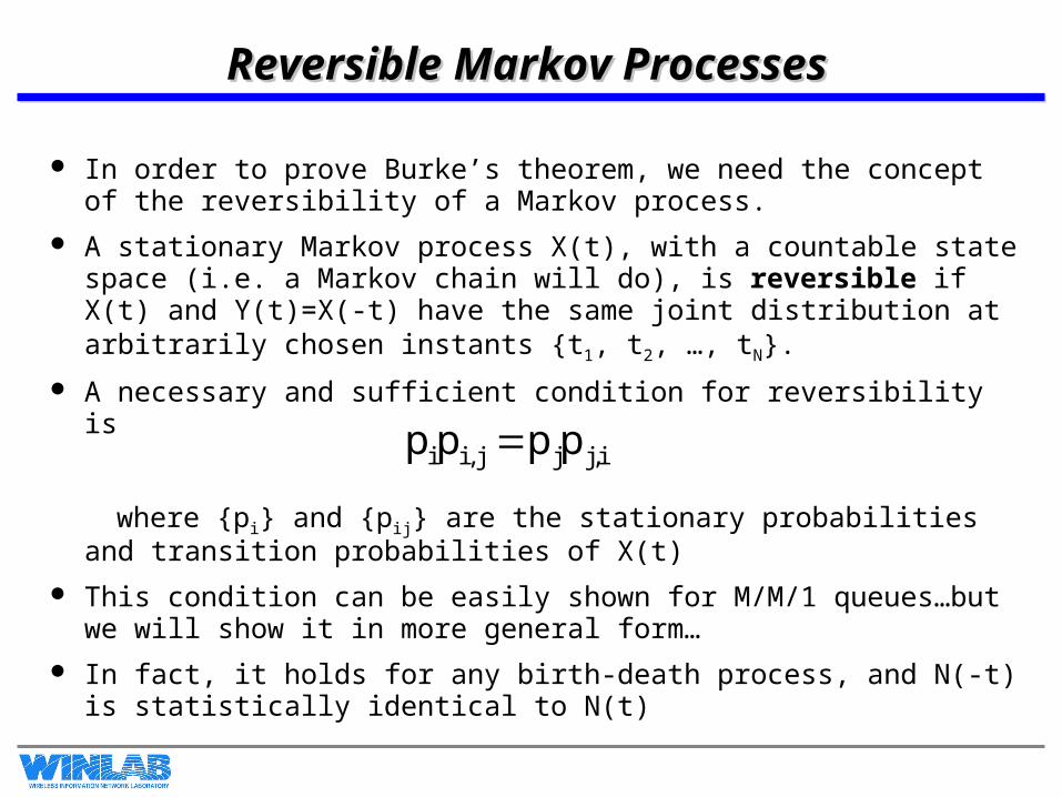
In order to prove Burke’s theorem, we need the concept of the reversibility of a Markov process.

A stationary Markov process X(t), with a countable state space (i.e. a Markov chain will do), is reversible if X(t) and Y(t)=X(-t) have the same joint distribution at arbitrarily chosen instants {t1, t2, …, tN}.

A necessary and sufficient condition for reversibility is

where {pi} and {pij} are the stationary probabilities and transition probabilities of X(t)

This condition can be easily shown for M/M/1 queues…but we will show it in more general form…

In fact, it holds for any birth-death process, and N(-t) is statistically identical to N(t)

i,jjj,ii pppp

Reversible Markov Processes, pg 2Reversible Markov Processes, pg 2

Time-Reversal Theorem: Let {X(t): t>=0} be a stationary Markov process with (infinitesimal) generator P=[pij], and with initial distribution equal to stationary distribution. Then for all T>0, the time-reversed process

is equivalent to a stationary Markov process with (infinitesimal) generator given by:

for all state pairs (i,j)

Tt0:)tT(X

i

jijij p

ppp~

ijP~

Reversible Markov Processes, pg 3Reversible Markov Processes, pg 3

Proof: Let Q(t)=[qij(t)] denote the transition probabilities of X(t),

We need to show X(T-t) is a Markov process with transition probabilities

Then we obtain the necessary and sufficient condition by differentiating this and setting t=0. (Its an infinitesimal generator)

i)0(X|j)t(XP)t(q ij

i

jijij p

)t(qp)t(q~)t(Q

~

Reversible Markov Processes, pg 4Reversible Markov Processes, pg 4

Consider the interval (0,t+s] and divide it into (0,t] and (t,t+s], i.e. set T=t+s.

The joint probability of the three random variables

is

Similarly we have

)0(X)st(X~

)s(X)t(X~

)st(X)0(X~

)t(q)s(qp

i)st(X,i)s(X,i)0(XP

i)st(X~

,i)t(X~

,i)0(X~

P

01122 i,ii,ii

012

210

)t(qp

i)ts(X,i)s(XPi)t(X~

,i)0(X~

P

011 i,ii

0110

Reversible Markov Processes, pg 5Reversible Markov Processes, pg 5

The conditional probability

Hence, we have shown that is a Markov process with generator (after differentiation).P

~

j,i

12

i

i,ii

012

q~i)t(X

~|i)st(X

~P

p

)t(qp

i)0(X~

,i)t(X~

|i)st(X~

P

1

122

tX~

B-D Processes are ReversibleB-D Processes are Reversible It is now easy to show the following Time Reversibility of B-D Processes: The stationary B-D process N(t)

with generator P and steady state probabilities p is a time-reversible Markov process. Thus, the time-reversal of the death process is a birth process.

Burke’s Theorem follows from this:– Interdeparture times of the forward-time system are the interarrival

times of the time-reversed system... Hence we have Poisson with rate coming out of the system.

– Fix a time t, then the departures before time t from the forward system are arrivals after time t in the reverse system.

– Arrivals in reverse system are Poisson, and thus arrivals in reverse system after time t do not depend on N(t)

– Consequently, departures after time t in forward system do not depend on N(t)

What we derived held true because the first queue was M/M/1 and implicitly we assumed it had achieved steady state and independent service times between queues!

The problem is more complicated when we have more general networks of queues.

Again, consider two transmission lines in sequence. – The arrivals to the first are Poisson of rate , but all customers

(packets) have deterministic and equal service times, i.e. we have an M/D/1 queue.

– Average packet delay for first queue is given by Pollaczek-Khinchine formula.

Step back to Network of QueuesStep back to Network of Queues

Queue2Queue1

Network of Queues, M/D/1 first queueNetwork of Queues, M/D/1 first queue

The interarrival times of the second queue must be at least 1/– Why?

Now, each packet arriving at either queue takes 1/ time to process. – The first packet being finished by first queue is immediately

sent to second server

– It takes at least another 1/ amount of time for first queue to get and finish the next packet/customer.

– So, first packet will be finished by second server at or before the next packet arrives to second server.

Result: No queue (waiting) at second system!

Two Queues, correlated service timesTwo Queues, correlated service times

Earlier we considered the service times independent of each other and independent of the arrival times.

Reality: A big packet at the first system is probably still a big packet at the second system!– Interarrival times at the second queue are strongly correlated

with packet lengths!

Long packets at first system will typically find the queue at the second server more empty…

Shorter packets from the first system will typically find the queue at the second server more busy because the second server is processing some prior “big” packet…

It is tough to find an analytical solution for joint pmf under dependence assumptions!

The Kleinrock Independence ApproximationThe Kleinrock Independence Approximation

We have argued that in practice there is dependence upon the interarrival times and service times. – Independence is lost after the first system!

Reality hurt us, but reality provides us one more gift…

Reality: Real networks typically involve more than one stream of packets merging at a node… The combination of multiple streams helps restore independence in many cases!

This observation is due to Kleinrock.

Kleinrock’s Approximation: It is often appropriate to use M/M/1 queues for each communication link when the arrivals at entry points are Poisson, packet lengths are roughly exponentially distributed, network is dense and traffic is heavy.

Quick Look at Jackson’s TheoremQuick Look at Jackson’s Theorem

Many queuing networks, a packet/customer may visit a queue more than once.

Burke’s theorem does not apply! Typical example: Queue with feedback

If the arrival rate is much less than departure rate, then net arrival process has a few, isolated external arrivals followed by a burst of feedback arrivals (dependent on packet length).

p

1-p

Jackson’s Theorem, (Open) pg 1.Jackson’s Theorem, (Open) pg 1. Consider a queuing network consisting of M separate service stations,

each with its own queue. Define the vector process:

In an open queuing network, customers may arrive from an external “source” and eventually may leave the network (as depicted in previous slide).

A closed network has no arrivals or departures from the system (total customers is fixed… just they may move around)

Assumptions:– The rate of the source (birth process) is , and a customer goes to

station i with probability qsi.– Service time at station k is exponential with rate k .– Customers are “routed” according to a Markov chain: Probability

that a customer departing station i goes to station j is qij.

)t(N,),t(N),t(NtN M21

Jackson’s Theorem, (Open) pg 2.Jackson’s Theorem, (Open) pg 2.

Jackson’s Decomposition Theorem: For an open queue as described, the joint distribution of the queue vector n(t) is given by:

where P(Nk=nk) is the steady state pmf of an M/M/1 system with arrival rate k and service rate k, i.e.

Where k describes the “utilization” factor of system k.

KK2211 nNPnNPnNPnP

knkkk 1nNP k