MANAGERIAL ECONOMICS

(Important Questions and suggested model answers)

1. Define Managerial Economics.

Managerial economics is a specialized discipline of management studies which deals with application of economic theory and techniques to business management. Managerial economics is evolved by establishing links on integration between economic theory and decision sciences (tools and methods of analysis) along with business management in theory and practice---for optimal solution to business/managerial decision problems. This means, managerial economics pertains to the overlapping area of economics along with the tools of decision sciences such as mathematical economics, statistics and econometrics as applied to business management problems.

“Managerial economics is a science which studies the economic aspects of behaviour of the firm as an enterprise, and helps to allocate scarce resources to their alternative uses in such a manner as to optimize the firm’s ultimate objective, as an organization and a social institution, under conditions of the imperfect knowledge, risk and uncertainty. It provides principles, method, and techniques of analysis of economic behaviour and at the same time prescribes ways and means to optimize economic efficiency.”

2. Discuss the nature and scope of Managerial Economics. What are the other related disciplines?

Nature and Scope of Managerial Economics:

All managerial decisions are basically economic in nature. The decisions are either directly related to Economics or have economic implications; they might not be based simply on economic calculations, and might involve several non-economic, social, political, legal and technological considerations as well. Managerial economics helps not only to analyse the economic content and implications of the managerial decisions but also to integrate several other aspects leading to sound decisions.

1

Managerial economics incorporates elements of both micro and macroeconomics dealing with managerial problems in arriving at optimal decisions. It uses analytical tools of mathematical economics and econometrics with two main approaches to economic methodology involving ‘descriptive’ as well as ‘prescriptive’ models.

Managerial economics differs from traditional economics in one important respect that it is directly concerned in dealing with real people in real business situations. Managerial economics is concerned more about behaviour on the practical side.

Managerial economics deals with a thorough analysis of key elements involved in the business decision making.

Most managerial decisions are made under conditions of varying degrees of uncertainty about the future. To reduce this element of uncertainty, it is essential to have homework of research/investigation on the problem solving before action is undertaken.

Knowledge of managerial economics is a boon to the manager/businessman/entrepreneur. Modern businessman never believes in luck. He bangs on skilful management and appropriate timely economic decision making. This art is facilitated by the science of managerial economics.

Other related disciplines:

Managerial economics is closely related to and draws heavily upon several areas in economics such as Theory of the Firm, Microeconomics, Macroeconomics, Industrial Economics, and so on. Managerial economics is basically micro in nature in that it deals with the firm’s behaviour in three basic areas viz. Utility analysis, Theory of the Firm and Factor pricing. Managerial Economics draws a few aspects from Macroeconomics such as national income, technology forecasting, which are relevant to sales/demand forecasting. While Industrial Economics analyses the economic problems of the industry as a whole, Managerial Economics deals with the economic aspects of managerial decision making at a micro level irrespective of the sphere of activity.

2

Macro Economics is not only related to but is also an integral part of the functional areas of management such as production, finance, accounting, marketing, operations research and personnel. To illustrate, Capital budgeting might be taught in finance and accounting as well as in Economics. While Economics would analyse the firm’s investment decisions and economic viability of projects, finance would study their financial viability. E.g. The Garland Project linking Himalyan rivers to the southern plateau was considered feasible from the technical point of view, but it was thought to be financially not feasible as it involved investment beyond India’s capacity.

Distinguish between Micro and Macro Economics.

Broadly speaking, microeconomic analysis is individualistic, whereas macroeconomic analysis is aggregative. Microeconomics deals with the part (individual) units while macroeconomics deals with the whole (all units taken together) of the economy.

1. Difference in nature: Microeconomics is the study of the behaviour of the individual units. Macroeconomics is the study of the behaviour of the economy as a whole.

2. Difference in methodology: Microeconomics is individualistic; whereas macroeconomics is aggregative in its approach.

3. Difference in economic variables: Microeconomics is concerned with the behaviour of microvariables or microquantities.. Macroeconomics is concerned with the behaviour of macrovariables and macroquantities. In short, microeconomics deals with the individual incomes and output, whereas macroeconomics deals with the national income and national output.

4. Difference in field of interest: Microeconomics primarily deals with the problems of pricing and income distribution. Macroeconomics pertains to the problems of the size of national income, economic growth and general price level.

3

5. Difference in outlook and scope: The concept of ‘industry’ in microeconomics is an aggregate concept but it refers to all firms producing homogenous goods taken together. Macroeconomics uses aggregates which relate to the entire economy or to a large sector of the economy. Aggregate demand covers all market demands.

6. Demarcation in areas of study: Theories of value and economic welfare are major areas in microeconomics. Theories of Income and employment are core topics in macroeconomics.

Is Managerial Economics a Positive or Normative Science? Discuss.

Positive Economics explains the economic phenomenon as “What is, what was and what it will be. Normative Economics prescribes what it ought to be”. Positive sciences simply describe, while normative sciences simply prescribe.

According to Prof. Robbins, economics is a positive science. Science is, after all, a search for truth and therefore, economics should study the truth as it is and not as it ought to be. This is because when we say that this ought to be like this, we presume that our point of view is correct. In a study of a problem at a given point of time, not only economic considerations but also many other considerations such as ethical, political etc. must be considered. A policy decision is taken after weighing the relative importance of all these factors. There are bound to be differences in respect of policy prescription and it is better to keep away from areas which are controversial and study the facts as they are.

According to economists like Marshall and Pigou, the ultimate object of the study of any science is to contribute to human welfare. Thus economics should be a normative science. It should be able to suggest policy measure to the politicians. It should be able to prescribe guidelines for the conduct of economic activities. Not only economists should build up the economic theory but also at the same time they should provide policy measures.

4

We must strike a balance between these two extreme views. As Keynes put it, “The main function of economics is not to provide a body of settled conclusions immediately applicable to policy. It provides a method or a technique of thinking, which enables its possessor to draw correct conclusions.”

Managerial economics is a blending of pure or positive science with applied or normative science. It is positive when it is confined to statements about causes and effects and to functional relations of economic variables. It is normative when it involves norms and standards, mixing them with cause-effect analysis.

One cannot disregard the normative functions of managerial economics, though the discipline may be treated primarily as a positive science. Normative approach in managerial economics has ethical considerations and involves value judgments based on philosophical, cultural and religious positions of the community.

The value judgments and normative aspect and counselling in managerial economic studies can never be dispensed with altogether.

We may thus conclude, that Managerial Economics is both a Positive and Normative Science.

Briefly discuss the three fundamental concepts of Managerial Economics.

Managerial Economics is confined to the following three major fields:

(1) Pricing (2) Distribution (3) Welfare.

Chart:

5

Pricing: Microeconomics assumes the toal quantity of resources available in an economic society as given and seeks to explain how these shall be allocated to the production of particular goods for the satisfaction of chosen wants. In a free market economy, the allocatioin of resources is based on the relative prices and profitability of different goods. To explain the allocation of resources, microeconomics seeks to explain the pricing phenomenon.

Price theory explains how the price of a particular commodity is determined in the commodity market. For in depth analysis of price determination it contains:

Theory of demand of the analysis of consumer behaviour. Theory of production and cost or the analysis of producer behaviour. Theory of product [pricing or price determination under different

market structures.

Distribution: The theory of distributioin basically deals with factor pricing. It seeks to explain how rewards of the individual factors of production such as land, labour, capital and enterprise are determined for their productive contribution. In other words, it is concerned with rent, wages, interest, profits, as the respective rewards of land, labour, capital and enterprise respectively.

Since demand and supply of each of these factors are different, there are separate theories to these. Thus the field of distribution includes, general theory of distribution and theories of rent, wages, interest and profits.

Welfare: The theory of economic welfare explains how an individual consumer maximizes his satisfaction when production efficiency is achieved by allocation of resources in such a way as to maximize output from a limited set of input.

Along with individual economic welfare, welfare economics is also concerned with social welfare, which is based on overall economic efficiency of the system. When maximum individual wants are satisfied at the best possible optimum level by a production pattern through efficient allocation of resources, overall economic efficiency or ‘Pareto optimality’ condition is reached. Such a situation can raise the standard of living of the population and maximize social welfare.

6

What are the important uses and limitation of microeconomics?Importance and Uses:1. It explains price determination and the allocation of resources.2. It has direct relevance in business decision-making.3. It serves as a guide for business’ production planning.4. It serves as a basis for prediction.5. It teaches the art of economizing.6. It is useful in determination of economic policies of the Government.7. It serves as the basis for welfare economics.8. It explains the phenomena of International Trade.

Limitations:1. Most of the micro-economic theories are abstract.2. Most of the microeconomic theories are static – based on ceteris paribus, i.e. “other things being equal”.3. Microeconomics unrealistically assumes ‘laissez-faire’ policy and pure capitalism.4. Microeconomics studies only parts and not the whole of the economic system. It cannot explain the functioning of the economy at large.5. By assuming independence of wants and production in the system, microeconomics has failed to consider their ‘dependent effect’ on economic welfare.6. Microeconomics misleads when one tries to generalize from the individual behaviour.7. Microeconomics in dealing with macroeconomic system unrealistically assumes full employment.

How does Managerial Economists help the Manager in decision making and forward planning?Managerial Economists act as operations researchers and systems analysts in the management services department of large business firms usually in the private sector. Their job lies in designing the course of operations to maintain and improve the ‘systems’ of the firm in terms of productivity, market share, load factor percentage and so on and prepare reports for helping the decision makers to cope with current as well as anticipated future problems. In modern business, managers constantly face the major problem of choice among alternative ways of producing goods and allied business decisions. Managerial economists assist them in making a rational choice.

7

A Managerial economist is an economic adviser to a firm or businessman. A firm or entrepreneur, in the course of its/his business operations, has to take a number of decisions which are vital to the survival and growth of the business. Such decisions may pertain to the nature of the product to be produced, the quantity, quality, cost, price and its distribution, planning and diversification of business, renewal of worn out equipments and machinery, modernization, etc. The Managerial economist helps the businessman or the manager in arriving at correct decisions.

In short, the business economist while helping in the decision making process, measures a number of micro and macro variables by applying intelligently certain quantitative and qualitative techniques to the practical aspects and problems encountered by a business firm in its business activity. Forecasting is a fundamental activity of the Managerial economist. Indeed a business economist is greatly helpful to the management by virtue of his studies of economic analysis. He is an effective model builder. He deals with the business problems in a sharp manner with a deep probing.A Managerial economist in a business firm may carry on a wide range of duties, such as:

Demand estimation and forecasting. Preparation of business forecasts; to provide forecasts of changes

in costs and business conditions based on market research and policy analysis.

Analysis of the market survey to determine the nature and extent of competition.

Analysing the issues and problems of the concerned industry. Assisting the business planning process of the firm. Discovering new and possible fields of business endeavour and its

cost-benefit analysis as well as feasibility studies. Advising on pricing, investment and capital budgeting policies. Evaluation of capital budgets. Building micro and macro economic models of particular aspects

of the firm’s activities that are useful in solving specific business problems. Most models may be prediction oriented.

Directing economic research activity. Briefing the management on current domestic and global economic

issues and challenges. DEMAND

8

What is Demand?

A demand is the effective desire or want for a commodity, which is backed up by the ability (i.e. money or purchasing power) and willingness to pay for it. The demand for a product refers to the amount of it which will be bought per unit of time at a particular price. The demand can be expressed as actual and potential.Consumer demand has two levels: a) Individual Demand and b) Market Demand. Market demand is the sum total of individual demand. Prices are determined on the basis of market demand. Market demand serves as a guidepost to producers in adjusting their supplies in a market economy.

Factors influencing individual demands are :

Price of the products. Income of the buyer. Tastes, Habits and Preferences. Relative prices of other goods. Relative prices of substitute and complementary products. Consumer’s expectations about future price of the commodity. Advertisement effect.

Factors influencing Market Demand: Price of the product. Distribution of Income and Wealth. Community’s common habits and scale of preferences. General standards of living and spending habits of the people. Number of buyers in the market and the growth of population. Age structure and sex ratio of the population. Future expecations. Level of taxation and Tax structure. Inventions and Innovations. Fashions Climate and weather conditions. Customs Advertisement and Sales propaganda.

Demand Function:

9

At any point in time, the quantity demanded of a given product (goods or services) depends upon a number of key variables or determinants. A demand function in mathematical terms expresses the functional relationship between the demand for the product and its various determining variables.

Dx – Quantity demanded = f(Px) – function of price.

Here all other determining variables are assumed to be constant, keeping only price as variable.

If the demand function is to be stated taking into account all variables, without assuming them as constant, demand function is

Dx = f (Px, + Ps + Pc + Yd +T, A, N, u)

Dx = Demand for X. Px = Price of X, Ps = Price of Substitute of X, Pc = Price of Complementary Goods, Yd = Disposable Income, T = Taste of the buyer or preference, A = Advertising effect, N = Number of buyers u = Unknown other determinants.

Demand function is not the quantity demanded at a given price, but quantity demanded at each level of price.

a = signifies initial demand irrespective of price (constant parameter). b = functional relationship between P – Price and D – Demand (constant parameter) Linear demand function is expressed as D = a – bP.b has minus (-) sign to denote a negative function. Demand is decreasing function of price.b is the slope ( vertical length ÷ horizontal length) of the demand curve, and suggests that it is downward sloping.

10

Dx = 20 – 2Px (Dx is Quantity demanded of X, Px Price of X)

What is law of demand? What are its exceptions? Why does a Demand Curve slope downward?

Law of Demand: Ceteris paribus, the higher the price of a commodity, the smaller is the quantity demanded and lower the price, larger the quantity demanded. Other things remaining unchanged, the demand varies inversely to changes in price. Dx = f(Px). The demand curve is downward sloping indicating an inverse relationship between price and demand.

The price is measured on the Y – axis and Demand on the X- axis. When the price falls, demand increases. The downward slope of demand curve implies that the consumer tends to buy more when the price falls. Thus the demand curve is shown as downward sloping.

What are the assumptions underlying law of demand?

Assumptions underlying the law of demand:

No change in Consumer’s income. No change in consumer’s preferences. No change in the Fashion. No change in the Price of Related Goods. No expectation of Future price changes of shortages. No change in size, age composition, sex ratio of the population. No change in the range of goods available to the consumers. No change in the distribution of income and wealth of the community. No change in government policy. No change in weather conditions.

Exceptions to the Law of Demand:

Sometimes it may be observed, that with a fall in price, demand also falls and with a rise in price, demand also rises. This is apparently contrary to the

11

Dx = 20 – 2Px

Y

5

4

3

2

1

0

law of demand. The demand curve in such cases will be typically unusual and will be upward sloping.

There are few such exceptional cases:- Giffen Goods: In the case of certain Giffen goods, when price falls,

quite often less quantity will be purchased because of the negative income effect and people’s increasing preference for a superior commodity with rise in their real income. E.g. staple foods such as cheap potatoes, cheap bread, pucca rice, vegetable ghee, etc. as against good potatoes, cake, basmati rice and pure ghee.

Articles of Snob appeal (Veblen effect) : Sometimes, certain commodities are demanded just because they happen to be expensive or prestige goods and have a ‘snob appeal’. They satisfy the aristocratic desire to preserve the exclusiveness for unique goods. These goods are purchased by few rich people who use them as status symbol. When prices of articles like diamonds rise, their demand rises. Rolls Royce car is another example.

Speculation: When people are convinced that the price of a particular commodity will rise further, they will not contract their demand; on the contrary they may purchase more for profiteering. In the stock exchange, people tend to buy more and more when prices are rising and unload heavily when prices start falling.

Consumer’s phychological bias or illusion: When the consumer is wrongly biased against the quality of a commodity with reduction in the price such as in the case of a stock clearance sale and does not buy at reduced prices, thinking that these goods on ‘sale’ are of inferior quality.

Reasons for change (increase or decrease) in demand:

Change in income. Changes in taste, habits and preference. Change in fashions and customs Change in distributioin of wealth. Change in substitutes. Change in demand of position of complementary goods. Change in population. Advertisement and publicity persuasion.

12

Change in the value of money. Change in the level of taxation. Expectation of future changes in price.

Explain Veblen effect and draw up the market demand curve for veblen effect product. ((2/2004)

Thorstein Veblen argued that the affluent class in the society has a tendency to demonstrate their superiority of ‘high class’By spending on frivolous goods and services – super luxury items such as diamonds, fivestar hotels, palatial buildings, business or executive class of air travel. Though the market demand for such a commodity tends to rise when its price falls, the individual demand of the snobbish buyer will fall. When a prestige good loses its snob value, its market demand from the snobbish buyers will decrease with fall in its price; and the demand may be added up from the new common buyers.

In certain branded goods such as ‘Ray Ban’ or ‘Levis’ products i.e. exclusive or designer products, there exists an inherent paradox. Initially these goods are meant to serve the Veblen effect. At high prices, there is limited but good demand from the richer sections. But when these goods are produced in larger quantity, their prices fall. It will carry mass appeal to upper middle class. So the demand will expand initially. Further increase in output will lead to further price reduction. But at this price, the product loses its exclusivity or snob effect and the richer sections exclusive demand will fall. The product will now be purchased on account of its functional utility and will be competing in the market with other similar goods.

The demand curve DD has changing slopes at a and b points. At price P1, the demand is Q1. When the price is lowered to P2, demand is Q2. A further reduction of price to P3, leads to a fall in demand as the brand loses exclusivity appeal. After that the product demand is determined just by its functional utility.

How is an indifference curve technique an improvement over Marshallian utility analysis?

The indifference curve approach is considered superior to the Marshallian utility analysis of consumer demand in the following respects:

13

It is more realistic. Marshall assumes cardinal measurement of utility, which is unrealistic. The indifference curve technique makes an ordinal comparison of utility and the level of satisfaction.

It uses the concept of scale of preferences with lesser assumptions than the Marshallian concept of utility. The scale of preference is laid down on the basis of a consumer’s tastes and likings, independent of his income. Unlike Marshall, the Hicksian scale of preference needs no information as to how much satisfaction is gained but it aims only at knowing whether a consumer’s satisfaction level is greater than, less than or equal to, between the various combinations of two goods.

It dispenses with the assumption of constant marginal utility of money. Marshallian analysis assumes that to the consumer the marginal utility of money remains constant. In the indifference curve analysis, such assumption is not needed.

It is wider in scope: Marshallian demand theory deals with a single commodity taken exclusively. Hick’s ordinal approach, considers at least two goods in combination. Thus, the complementarity and substitutability aspects of goods are being explicitly considered in Hicksian analysis.

It uses concept of Marginal Rate of Substitution which is scientific and measurable: The utility approach is based on the law of diminishing marginal utility. On the other hand, the indifference curve approach rests on the principle of diminishing marginal rate of substitution. The concept of marginal rate of substitution is superior to that of marginal utility because it considers two goods together and also because it is a ratio expressed in physical units of two goods and as such, it is practically measurable. The replacement of the law of MU by MRS, is a positive change in a more scientific manner.

It expresses the conditions of consumer equilibrium in a better way: In Marshallian analysis, the consumer equilibrium condition is MUx = MUy . Since utility cannot be measured numerically, this condition is impracticable. Px PyIn Hicksian analysis, the equilibrium condition is expressed as MRSxy = Px/Py which is measurable.

14

It is more comprehensive as it recognizes the fact that equilibrium in purchasing one commodity depends on the price of other goods and their stocks as well.

It analyses the price effect in a better way: The Marshallian demand curve has no means to separate the price effect into income and substitution effects. In the indifference curve analysis, the price consumption curve enables us to have the bifurcation of price effect into income and substitution effects. It examines the Phenomenon of Giffen Paradox. Marshall views the Giffen Paradox as an exception to the law of demand, whereas the case of Giffen goods is incorporated in the price consumption curve to examine the consumer’s typical behaviour caused by negative income effect. Thus the unsolved riddle about Giffen goods in the utility analysis is solved by the indifference curve analysis. It represents the law of demand in a broader and more precise way.

What are the shortcomings of the indifference curve approach?

It does not provide any positive change in the utility analysis.It retains the Marshallian assumption of diminishing marginal utility:It unrealisitically assumes perfect knowledge of utility with the consumer.It is weak in structure.It has limited scope.It is introspective.It is not applicable to indivisible goods.It assumes transitivity condition.

15

ELASTICITY OF DEMAND

Demand usually varies with price. The extent of variation of demand is not uniform. Sometimes the demand is greatly responsive to price changes, while at other times, it may be less responsive. Elasticity is the extent of responsiveness to variation. Two factors are relevant for measuring the elasticity of demand – a) demand b) the detriment of demand. A ratio is made of the two variables for measuring the elasticity coefficient.

Elasticity of demand = % change in quantity demanded % change in detriment of demand

Unless specified, elasticity of demand means price elasticity of demand. Logically, however, the concept of elasticity should measure the responsiveness of demand to changes in variables concerned with demand function. Thus there can be many kinds of elasticities of demand. Most important are

Price elasticity of demandIncome elasticity of demandCross elasticity of demand

Marshallian classification of Price elasticity:

1. Unit elasticity of demand (e = 1)2. Elastic demand - elasticity greater than unity. (e > 1)3. Inelastic demand – elasticity is less than unity (e<1)

Explain with graphs how modern economists have classified price elasticity of demand. What are the managerial uses of price elasticity of demand?

Price elasticity of demand:Ratio Method:The extent of responsiveness of demand for a commodity to a given change in price, other demand determinants remaining constant, is termed as the price elasticity of demand. It is the ratio of relative change in demand variables to price variables.

16

Coeff.of price elasticity e = % change in quantity demanded OR % change in price

proportionate change in quantity demanded = Δ Q ÷ Δ P = Δ Q x P

proportionate change in price.Q P ΔP Q

Q = Original demand, ∆Q = change in demandP = Original Price, ∆P = change in price

The above method is also known as percentage method, when the ratio is expressed as a percentage.

e = % ∆ Q %∆PRevenue Method:

Marshall suggested that the easiest way of ascertaining whether or not the demand is elastic, is to examine the change in total outlay of the consumer or total revenue of the seller corresponding to change in price of the product.

Total Revenue (or Total outlay) = Price x Quantity purchased (or sold)

According to this method, if the total revenue remains unchanged with a change in the price, the demand is unit elastic, as demand changes in the same proportion as price.

With a fall in price, if the total revenue rises, or with a rise in price, the total revenue falls, the elasticity is more than unity.

With a rise in price, the total revenue also rises and with a fall in price, total revenue also falls, the demand is less than unity.

17

Point elasticity method or Geometric Method:

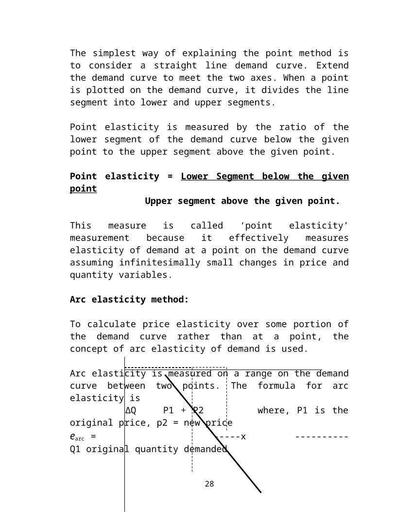
The simplest way of explaining the point method is to consider a straight line demand curve. Extend the demand curve to meet the two axes. When a point is plotted on the demand curve, it divides the line segment into lower and upper segments.

Point elasticity is measured by the ratio of the lower segment of the demand curve below the given point to the upper segment above the given point.

Point elasticity = Lower Segment below the given point Upper segment above the given point.

This measure is called ‘point elasticity’ measurement because it effectively measures elasticity of demand at a point on the demand curve assuming infinitesimally small changes in price and quantity variables.

Arc elasticity method:

To calculate price elasticity over some portion of the demand curve rather than at a point, the concept of arc elasticity of demand is used.

Arc elasticity is measured on a range on the demand curve between two points. The formula for arc elasticity is

∆Q P1 + P2 where, P1 is the original price, p2 = new priceearc = -----x ---------- Q1 original quantity demanded

∆P Q1 + Q2 Q2 new demand ∆ P = P2 – P1, ∆ Q = Q2 – Q1

For practical decision making, it is better to use arc elasticity measure when price changes more than 5%.For all theoretical purposes, point elasticity rather than arc elasticity is commonly used.

18

What are the factors influencing elasticity of demand?

1. Nature of the commodity – according to the nature of satisfaction the goods give. Luxury goods are price elastic.

2. Availability of close substitutes – demand will be elastic.

3. Number of uses the commodity can be put to – Single use goods will have less elastic demand but demand becomes elastic if it can be put to several uses.

4. Consumer’s income – demand from low income group will be elastic while from very rich persons, relatively inelastic.

5. Height of price and range of price change – highly priced goods, demand less elastic with small change in price. But with large changes, demand will be elastic.

6. Proportion of expenditure 7. Durability of the commodity.8. Influence of habit and custom9. Complementary goods. Goods which are jointly demanded are less elastic.10.Time – less elastic during short periods generally.11. Recurrence of demand.12. Possibility of postponement.

Income Elasticity of Demand:

Income elasticity of demand is defined as the ratio of percentage or proportional change in the quantity demanded to the percentage or proportional change in income.

Income elasticity = % change in quantity demanded = em = % ∆ Q % change in income. % ∆M

OR ∆ Q x M or ∆ Q . M Q ∆M ∆ M Q

19

Cross elasticity of demand:

The cross elasticity of demand refers to the degree of responsiveness of demand for a commodity to a given change in the price of some related commodity.The cross elasticity of demand between two goods is measured by dividing the proportionate change in the quantity demanded of X by the proportionate change in the price of Y.

Cross elasticity of demand : Proportionate or percentage change in demand for X

Proportionate or percentage change in the price of Y.

Ec or e xy = ∆ Qx x ∆ Py = ∆ Qx x Px Qx Py ∆Py Qx

Advertising or Promotional elasticity of demand :

eA = Percentage or proportionate change in sales Percentage or proportionate change in ad.expenditure.

Arc Advertising elasticity : ∆ Q x A1 + A2 ∆A Q1 + Q2

What is demand forecasting?

Demand forecasting is not a speculative exercise into the unknown. It is essentially a reasonable judgment of future probabilities of the market events based on scientific background. Demand forecasting is an estimate of the future demand. It cannot be hundred per cent precise. But, it gives a reliable approximation regarding the possible outcome, with a reasonable accuracy. It is based on the statistical data about past behaviour and empirical relationships of the demand determinants. It is based on mathematical laws of probability.

20

What are the criteria of a good forecasting method?

Criteria of a good forecasting method:

Joel Dean lays down the following criteria of a good forecasting method:

Accuracy: Forecast should be accurate as far as possible. Its accuracy must be judged by examining the past forecasts in the light of the present situation.

Plausibility: It implies management’s understanding of the method used for forecasting. It is essential for a correct interpretation of the results.

Simplicity:A simpler method is always more comprehensive than the complicated one.

Economy: It should involve lesser costs as far as possible. Its costs must be compared against the benefits of forecasts.

Quickness: It should yield quick results. A time consuming method may delay the decision making process.

Flexibility: Not only the forecast is to be maintained up to date, there should be possibility of changes to be incorporated in the relationships entailed in forecast procedure, time to time.

Explain the survey methods of demand forecasting.

Market Survey or Opinion Poll:

A market survey is also called an opinion survey or opinion poll. While conducting an opinion poll, the respondents should be chosen correctly after ascertaining whose opinion is valuable in the matter. For example, in order to estimate the demand for newly designed electric meters, the opinion of the engineers in the purchase and service departments of electric companies is important and not that of the ultimate consumers who have no say in the matter.

21

1. Representative sample: For conducting a survey, a sample population is selected from the total population. It can then be classified into different groups, each with its own character. A percentage of each group can be surveyed in order to get varying opinions. The sample population has to be as representative of the total population as possible. The degree of the accuracy of the survey would depend upon the representative character of the sample population.2. A case: A student was asked to find out the image of a big cotton textile mill as her project. The project report including the survey had to be completed within 60 days without any financial commitment on the part of the company under study. A study, under such constraints, would naturally have its own limitations. The student chose the method of stratified sampling, confined to a big city, the headquarters of the company. The population was broadly classified into: (i) employees sub-grouped into different strata, taking a few samples from each. (ii) all wholesalers (iii) a few retailers in the city, selected on the basis of their share in sales (iv) customers visiting retail outlets responded to the questionnaire (v) different strata of general population, which at one time or the other purchased the products of the mill – regrouped according to age, income, education and status, selecting a few samples from each group. Within these constraints a sample of 200 persons was collected. The results were quite encouraging.

Discuss the popular time series analysis techniques used for demand forecasting.Time series analysis:Time series analysis helps to identify: (1) a long-run movement of the variable; (2) seasonal fluctuations which are oscillatory but confined to one year; (3) cyclical movements which are oscillatory and periodic.The values of the movements are repeated between peaks and troughs.

A time series is dis-aggregated into four components or elements (i) Trend (T) (ii) Seasonal component (S) (iii) Cycle (C) and (iv) an irregular or random component. The first three are systematic while the last one is unsystematic. The residue after eliminating the systematic components falls in random component.These components can be written in two forms additive or multiplicative – T+S+C+R OR TSCR. In the additive form it is assumed that there is no interaction among the different components whereas in the multiplicative form there is interaction. The multiplicative form can be written in the additive form by taking the log as “ log y = log T + log S + log C + log R.”

22

A common method of decomposition is to calculate the trend and eliminate it from the original series by dividing throughout as TSCR/T; in the same way other elements can be separated out. In the additive form an element is removed by subtracting it from the series.

Much depends on the purpose. For example, if the growth rate of a variable, say agricultural production, is to be estimated, calculating the trend equation directly may not give the correct results, as agriculture is subject to both seasonal and cyclical fluctuations. Thus, both the fluctuations are to be removed first in order to attain better accuracy.

The decomposition of time series analysis has certain implicit assumptions:

1) the order of removal should be trend, seasonal, and cyclical. If the order is changed, changed values will result.2) effects are independent of each other; and 3) the trend is linear and the cycle is regular.

Criticism of the Method: These assumptions have been questioned. Separation of trend and cycle may be dubious as both may be the result of the same set of factors. Irregular variations may outweigh the others and the phenomenon of the business cycle may not be very relevant in a planned economy. The decomposition of the time series is an artificial attempt imposed by the analyst. As a descriptive device this may be adequate, but as an explanatory device for isolating different facts, th scheme is seriously deficient. It is because, the deterministic hypothesis underlying the systematic part is open to doubt from the point of view of behaviour of economic agents. Because of these shortcomings, in recent years, the emphasis in the study of time series has shifted to analysis of probabilistic processes.

23

MONOPOLISTIC COMPETITION

Q. Monopolistic Competition is a blend of perfect competition and monopoly. Discuss. How is price-output determined under monopolistic competition?

Monopolistic competition as the name suggests entails the attributes of both monopoly and competition.Following are the main features:

Large number of sellers:

There are fairly large number of sellers. They sell closely related but not identical products. The large number of firms in the same line of production leads to competition. Competition is keen but impure because there is no homogeneity of products offered. There are less chances of collusion between them to eliminate competition and rig prices, as the number is quite large.

The quantity supplied by an individual firm is relatively small compared to the total market shared by all the firms. Thus there is very limited degree of control over the market price by any firm.

In determining pricing and output policy, each firm can afford to ignore reaction by rivals. The number of firms being large enough, the impact of such an action by an individual firm, is insignificant.

Product Differentiation:

The firm’s independence under monopolistic competition, is attributed to the degree of product differentiation it adopts. It is essentially competition with differentiated products. The most distinguishing factor of monopolistic competition is that the products are all branded and identified. There is no homogeneity of products though they may be similar. Through such product differentiation, each seller acquires certain degree of monopoly power.

Large number of buyers:

24

There are numerous buyers. But buyers have preference for specific brands. Buyers are literally patrons of a particular seller. Buying here is by choice not by chance.

Free entry:

Entry and exit of buyers is freely possible. There are no barriers. There is unrestricted entry of new firms into the group till it reaches complete equilibrium. This makes the competition stiff because of close substitutes but with different brand names produced by new entrants. This market situation is more similar to perfect competition than monopoly. Owing to unrestricted entry of new firms, abnormal profits are usually competed away in the long run. Firms will seek to realize pure economic profits once again by advertising and innovatioin in products and processes resorting to non-price competition – competition in product variation as well as increase in advertising expenditure.

Selling costs:

Advertising and other forms of sales promotion are an integral part of monopolistic competition. These outlays are termed as selling costs. This kind of heavy expenditure on sales promotion is because products are identified and differentiated by their brand names unlike in perfect competition, where products are homogenous without brand name, needing no advertisement at all and firms experiencing perfectly elastic demand curves.

Selling efforts are required to effect a shift in demand in order to capture a better share of the market. Increase in demand is achieved through advertisement and sales promotional efforts i.e. by increase in selling costs. Success in achieving this increase, depends on how effective is the product differentiation and preference achieved through advertisement.

Two dimensional competition:

There are two aspects in monopolisitic competition: (1) There cannot be too much variation in price and the product has to be competitively prices. Hence price competition. (2) There is non-price competition in terms of product differentiation and spending on selling costs in order to capture a bigger share of the market.

25

The Group:

The firms involved in monopolistic competition are termed as “group” and not “industry”. A group is a cluster of firms producing very related but differentiated products. Monopolistic competition is characterized by product differentiation. Firms produce similar but not identical goods. We cannot conceive of an industry – such as automobile or bicycle industry in an analytical sense – in the monopolistic competition. On account of product differentiation, products of each firm, is identifiable and each firm is an industry in itself, just like a monopoly form.

In reality, major companies control a large number of products over a wide spectrum of the industrial economy. There are a variety of product groups such as , Automobiles, Textiles, Footwear, Soaps and Detergents, Foods and Beverages, Drugs and Chemicals, Cosmetics, Confectionery, Paper, Electronics, Computers, Cement, Metals and Metal Products, Construction etc.

Q. “A firm under monopolistic competition is a price maker”. Explain how price is determined under monopolistic competition.

“A firm under monopolistic competition is a price maker. Unlike perfect competition, there is pricing problem. The firm has to determine a suitable price for its product which yields maximum total profit. Assuminga given variety of products and constant selling outlays, when price is the only variable factory, shortrun analysis of price adjustment, is similar to pure monopoly. The market share of an individual firm in the total market of all the firms in the group, is insignificant to cause any serious effect on the market share of others by any downward price revision by the firm to increase the market share. In the long run, however, a major difference is noticeable in the equilibrium process, due to entry of new firms competing away the abnormal profits. This causes change in demand conditions and other factors associated with the process of group equilibrium.

Price determinatioin in the shortrun:

In the short run, the firm can adopt an independent price policy with least consideration for the varieties produced and the prices charged by other

26

producers. The firm being rational in determining the price, will seek to maximize the total profits.

There is a definite demand schedule as the quality of the product is given. The product is differentiated. So the demand curve or sales curve is downward sloping. The demand curve of a firm in monopolistic competition is more elastic than in pure monopoly.

The degree of elasticity depends on the number of firms in the group and the extent of product differentiation. If the number of firms is large, the demand will be highly elastic, while it will be less elastic if the number is small.

In order to maximize its total profits in the short run, the firm produces that level of output at which marginal cost is equal to marginal revenue (MC = MR). Equilibrium output is determined at the point of intersection of MR and MC.

Figure:

We have assumed the case of a firm with hypothetical cost and revenue data in a monopolistically competitive market. For simplicity sake, it is assumed that demand and cost conditions are identical for all the firms in the group. These are bold assumptions made by Chamberlin. No doubt these assumptions very much simplify the model but they are not altogether unrealistic. In the case of retail shops such as provision stores and chemist shops, standardized products will tend to have more or less identical demand and cost conditions, as their product differentiation is confined to only locational differences.

27

Equilibrium point E is determined where SMC = SMR, OP price, OQ output, ٱ PABC profit.

Price determination in the Long-run:

When firms earn super-normal profits in the short-run, some new firms will be attracted to enter the business, as the group is open. On account of rivals’ entry, the share of the firm in the toal market will be reduced due to competition from an increasing number of close substitutes. Gradually, in the long run, the firm will earn only normal profits.

Monopolistic competition implies severe competition between a large number of firms producing close substitute products. Hence this market situation is more similar to perfect competition than monopoly. Owing to the unrestricted entry of new firms, monopoly profits are usually competed away in the long run. Consequently, firms will resort to non-price competition i.e. competition in product variation as well as by increasing their advertising expenditure (selling costs).

OLIGOPOLY

Oligopoly is a market situation comprising only a few firms in a given line of production. The price and output polisy of oligopolistic firms are interdependent. The oligopoly model fits well into such industries as automobile, manufacure of electrical appliances etc. in our country. In an Oligopolistic market, the firms may be producing either homogenous products or product differentiation in a given line of production.

The following are the distinguishing features of an oligopolistic market:-

Few Sellers : Homogeneous or differentiated products supplied by a few firms.

Interdependence: Firms have a high degree of dependence in their business policies, price and output fixation.

High cross elasticities: Firms under oligopoly have high degree of cross elasticities and are always in fear of retaliation by rivals. Firms consider the possible action and reaction of its competitors while making changes in price or output.

28

Each firm tries to attract customers towards its product by incurring excessive advertisement expenditure. It is only under oligopoly that advertising comes fully into its own.

Constant struggle: Competition in Oligopoly consists of constant struggle of rivals against rivals and is unique.

Lack of uniformity: There is lack of uniformity in the size of different oligopolies.

Lack of certainty: In oligopolistic competition firms hae two conflicting motives – 1) to remain independent in decision making and 2) to maximize profits despite being interdependent. To pursue these ends, they act and react to the price-output variation of one another in an unending atmosphere of uncertainty.

Price rigidity: Each firm sticks to its own price due to constant fear of retaliation from rivals in case of reduction in price. The firm rather resorts to non-price competition by advertising heavily.

Kinked Demand Curve: According to Paul Sweezy, firms in an oligopolistic market, have a kinky demand curve for their products.

KINKED DEMAND HYPOTHESIS OF AN OLIGOPOLY MARKET:

The kinked Demand Curve or the Average Revenue Curve of an Oligopoly Firm, has two segments : 1) the relatively elastic segment and (2) relatively inelastic segment.

29

OUTPUT

Corresponding To the given price OP, there is a kink at point K on the demand curve DD. DK is the elastic segment, while KD is the inelastic segment of the curve. Kink implies an abrupt change in the slope of the demand curve.Demand curve is flatter before the kink and steeper after the kink.

The kink indicates the indeterminateness of the course or demand for the product of the seller concerned. He thinks it worthwhile to follow the prevailing price and not to make any change. In this case, raising of price, would contract sales considerably as demand tends to be more elastic to change in price. Lower of price, on the otherhand, will lead to retaliation from rivals owing to close interdependence of price-output movement in the oligopolistic market. Hence, seller will not expect much rise in sales because of price reduction.

An important point involved in kinked demand curve is that it accounts for the kinked average revenue curve to the oligopoly firm. The kinked average revenue curve in turn, implies a discontinuous marginal revenue curve MA – BR. Thus, the kinky marginal revenue curve explains the phenomenon of price rigidity in the theory of oligopoly prices.

In an oligopolistic market, once a general price level is reached, whether by collusion or by price leadership or through some formal agreement, it tends to remain unchanged over a long period of time. The price rigidity is on account of price interdependence indicated by the kinked demand curve. Discontinuity of the oligopoly firm’s marginal revenue curve at the point of equilibrium price, the price output combinatioin at the kink tends to remain unchanged even though marginal cost may change. The firm’s marginal cost curve can fluctuate between MC1 and MC2 within the range of the gap in the MR curve without disturbing the equilibrium price and output position of

30

the firm. The price remains the same at the level of OP, and output OQ, despite change in the margin costs.

PERFECT COMPETION

What are the features of perfect competition? Explain.

What are ISOquants? What are their properties? What is the difference between ISOquant curve and Indifference curve?

‘ISO’ means ‘equal’. ‘quant’ stands for ‘quantity’. The equal product curve is called Iso-quant or ‘production iso-quant’. It represents all the combinations of two factor inputs which produce a given quantity of product. It signifies a definite measurable quantity of output. Each Iso-quant curve stands for a specific quantity of output. A number of curves can be drawn for different specific quantities of output. All these curves together form the Iso-quant map.

Iso-quant measures a quantum of production resulting from alternative combinatioin of two variable inputs.

Difference between Iso-quant curve and Indifference curve

1. Indifference curve refers to two commodities. Iso-quant curve relates to combination of two factors of production.2. Indifference curve indicates level of satisfaction. Is-quant curve indicates quantity of output.3. No numerical measurement of satisfaction is possible. So it cannot be labelled. Iso-quant curve can be easily labeled as physical units out output are measurable.

31

4. The extent of difference of satisfaction is not quantifiable in the Indifference map. But in Iso-quant map, we can measure the exact difference between quantitites represented by one curve and another.

Properties of Iso-quants:

Isoquants have a negative slope. In order to maintain one level of output, when the amount of one factor is increased, that of the other is decreased. At each point on the iso-quant curve, we get a combination of two factors, which give the same level of output.

Isoquants are convex to the origin. The slope of the isoquant measures the marginal rate of technical substitution of one factor input (say labour) for the other factor inpur (say capital). MRTS measures the rate of reduction in one factor for an additional unit of another factor in combination for producing the same quantity of output. The convexity of the isoquant curve suggests that MRTS is diminishing, meaning, when quantity of one factor is increased, the less of another factor will be given up, keeping the output constant.

Iso-quants do not intersect. Each Isoquant represents a specific quantum of output. If two Isoquants intersect each other, it would lead to a logical contradiction as Isoquant representing a smaller quantity cannot be on a line representing a larger quantity.

Isoquants do not intercept either X or Y axis. If an Isoquant touches any axis, it means that any one factor can be taken as zero. Since it is not possible to produce a product with a single factor, Isoquants do not meet either axis.

Iso-quant is an oval shape curve. If relatively small amount of one factor is combined with relatively large amount of another factor, marginal productivity tends to be negative resulting in decline in total output. In such cases, the end portion of the curves are regarded as uneconomical and the curves are oval shaped.

Tangents of Iso-quants in an Iso-quant map represent the loci of equilibrium when different quantities of output are produced by the firm at minimum costs under the situation of two variable factor-inputs with their fixed price ratio.

32

Solved Problem in Isoquants: Refer to Problems.

33