quantum monte carlo -...
TRANSCRIPT

1
ceperley random walks
Quantum Monte Carlo1. Introduction to Monte Carlo: sampling, random numbers,
Markov chains, estimating errors2. Variational Monte Carlo: sampling and wavefunctions.3. Diffusion Monte Carlo: branching random walks, fermion sign
problem4. Introduction to Path Integrals: formalism, sampling, the
action.5. Boson & Fermion Path Integrals: permutations, exchange
moves, superfluidity and bose condensation.
Goal: to solve quantum many-body systems with computer simulation.
Examples: liquid and solid helium, electron gas, hydrogen,…
I only will cover continuum quantum Monte Carlo, not lattice models!
ceperley random walks
Monte Carlo and Random Walks
Today we start with an introduction to basic Monte Carlo techniques.
• What is Monte Carlo?– Any computational method which uses random numbers
as an essential part of the algorithm– Equivalent to performing integrals by randomly sampling
an integral.– Often a Markov chain, in particular Metropolis MC
• References– Allen & Tildesley “Computer Simulation of Liquids”– Frenkel & Smit “Molecule Simulations”– Thijssen, “Computational Physics”– Kalos & Whitlock, “Monte Carlo Methods” – “Numerical Recipes”

2
ceperley random walks
MC is advantageous for high dimensional integrals
Consider an integral in the unit hypercube:
By conventional deterministic methods:• Lay out a grid with L points in each direction with h=1/L
• Number of points is N=LD ∝ CPU time.HOW DOES ERROR GO WITH CPU TIME and DIMENSIONALITY?• Error in trapizoidal rule goes as ε=f’’(x) h2.
• The CPU time ∝ ε-D/2 .
• By sampling CPU time ∝ ε-2. To get another decimal place takes 100 times longer!
1
1 10
... ( ,.... )D DI dx dx f x x= ∫
ceperley random walks
Other reasons to do Monte Carlo:– Conceptually and practically simple.– Comes with built in error bars.
Many methods of integration have been tried, and will be tried in this world of sin and woe. No one pretends that Monte Carlo is perfect or all-wise. Indeed, it has been said that Monte Carlo is the worst method except all those other methods that have been tried from time to time. Churchill 1947
Good Log(error) Bad
Log(CPU Time)
MC2D
4D 6D 8D
3
ceperley random walks
Central Limit Theorem (Gauss)Sample N values from p(x)dx. (x1, x2, x3,… xN)Estimate mean from What is the pdf of mean?Solve by fourier transforms.If you add together two random variables, you multiply together
their characteristic functions:
Then
Taylor expand:
cumulants
1
1
N
iNi
y x=
= ∑
1 ...
1
( ) ( )
( ) ( ) ( )
( ) ( )
( ) ( / )
( )ln( ( ))
!
N
ikx ikxx
x y x y
Nx x x
Ny x
n
x nn
c k e dxp x e
c k c k c k
c k c k
c k c k N
ikc k
nκ
+
+
∞
=
= =
=
=
=
=
∫
∑
ceperley random walks
What happens to the reduced moments?
Hence the n=1 moment remains invariant.The rest get reduced by higher and higher powers of N.
Given enough averaging almost anything becomes a Gaussian distribution.
1
2
3
4
mean=variance=skewness
cumula
=
kurtosis
n s
=
t n
κκ
κ
κ
κ
µ 1 nn n Nκ κ −=
( )
2 3 21 2 3
2( )12 2
/ 2 / 6 ....
3 4
1 / 22
lim ( )
set ... 0 and fourier transform
( ) / 2N y
ik k N ik NN yc k e
p y N eκ
κ
κ κ κ
κ κ
πκ−
− −→∞
−
=
= = =
=
4
ceperley random walks
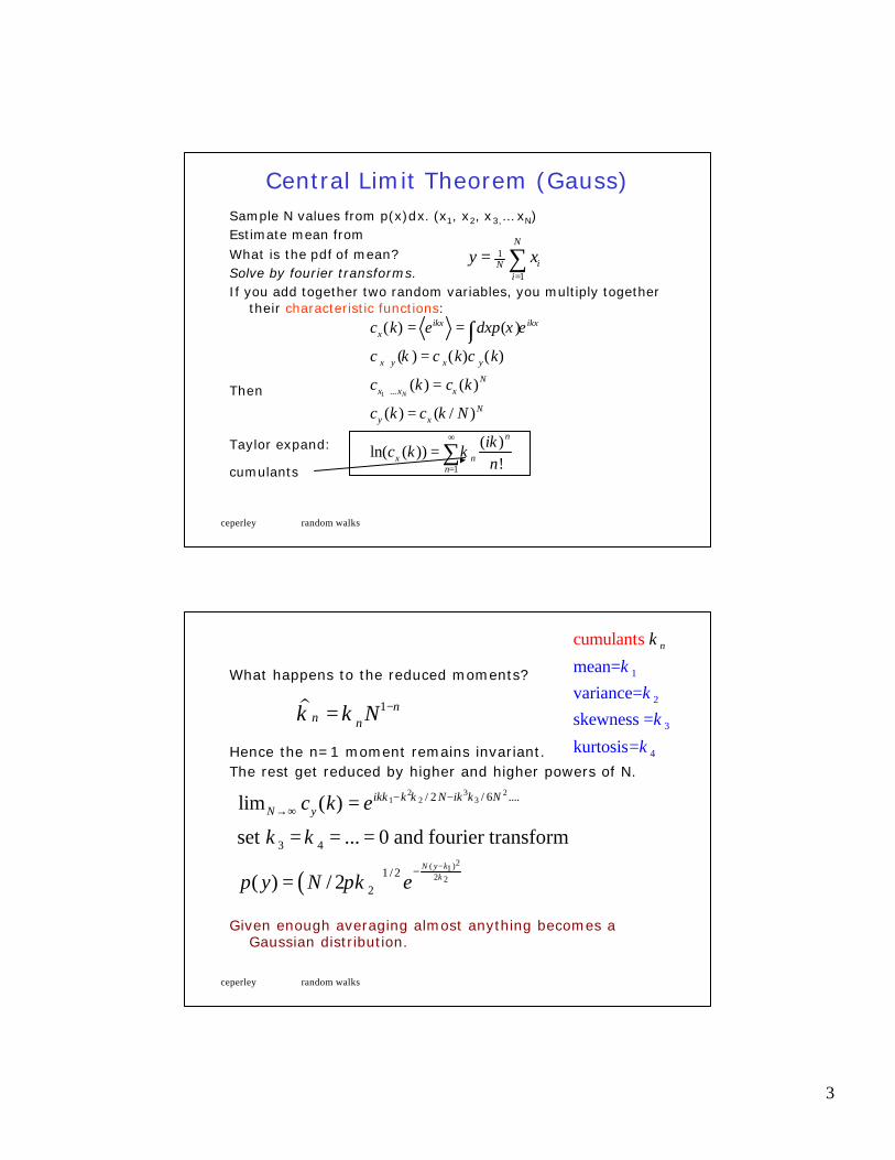
Approach to normality
ceperley random walks
Conditions on Central Limit Theorem
• We need the first three moments to exist.– If I0 is not defined⇒p(x) not a pdf– If I1 does not exist ⇒integral not mathematically
well-posed.– If I2 does not exist ⇒ infinite variance. Important to
know if variance is finite for Monte Carlo.• Divergence could happen because of tails of distribution
• Or because of singular points, e.g. at x=0
( )n nnI x dxp x x= = ∫
22 ( )I dxp x x
∞
−∞
= ∫ 3lim ( ) 0x x p x→±∞ →
30lim ( )→± →x x p x finite
5
ceperley random walks
Random Number GenerationAlso read “Numerical Recipes”.
What is a random number?
– A single number is not random. Only an infinite sequence can be described as random.
– Random means the absence of order (a negative property).
– Can an intelligent gambler make money by betting on the next numbers that will turn up?
– All subsequences are equally distributed. This is the property that MC uses to do integrals.
ceperley random walks
Random numbers on a computer• Truly random--the result of a physical process such as
timing clocks, circuit noise, bad memory
– Too slow (we need 1010/sec)– Too expensive– Low quality– Not reproducible
• Pseudo-random. prng (pseudo means fake)– Deterministic sequence
– But if you don’t know the algorithm, they appear to be random
• Quasi-random (quasi means almost random)– “half way” between random and a uniform grid
6
ceperley random walks
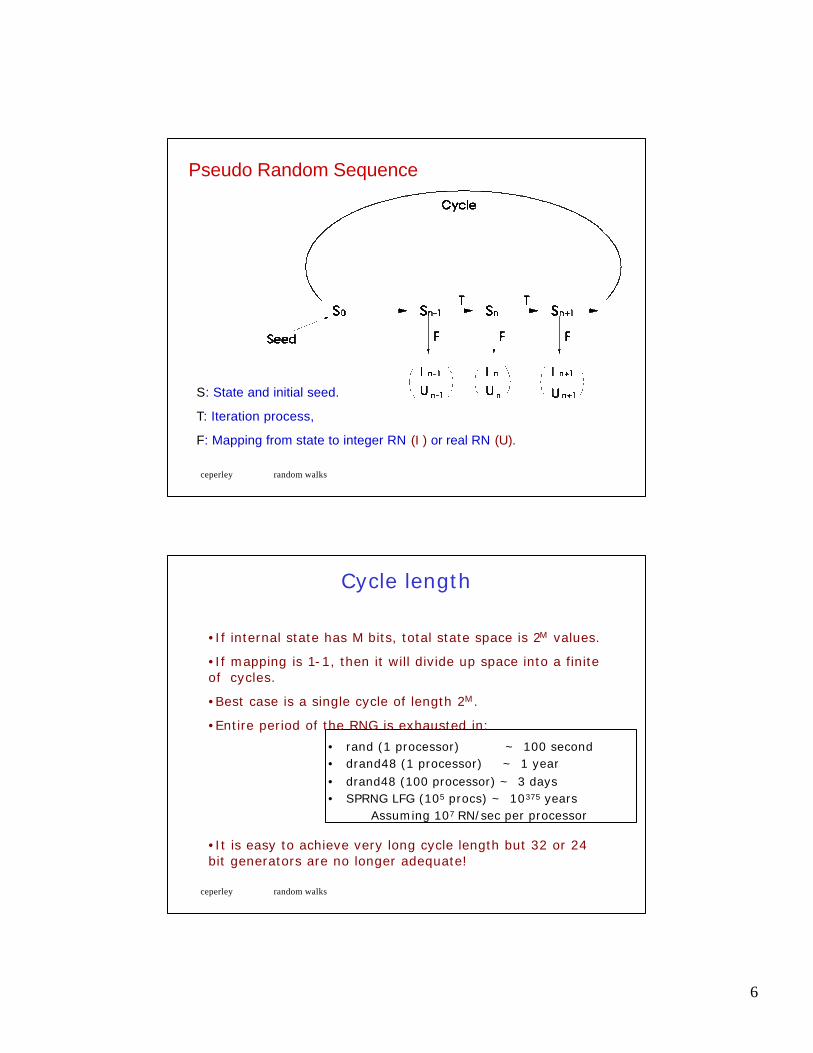
Pseudo Random Sequence
S: State and initial seed.
T: Iteration process,
F: Mapping from state to integer RN (I ) or real RN (U).
ceperley random walks
Cycle length
• rand (1 processor) ~ 100 second• drand48 (1 processor) ~ 1 year • drand48 (100 processor) ~ 3 days• SPRNG LFG (105 procs) ~ 10375 years
Assuming 107 RN/sec per processor
•If internal state has M bits, total state space is 2M values.
•If mapping is 1-1, then it will divide up space into a finite of cycles.
•Best case is a single cycle of length 2M.
•Entire period of the RNG is exhausted in:
•It is easy to achieve very long cycle length but 32 or 24 bit generators are no longer adequate!

7
ceperley random walks
Common PRNG Generators• Multiplicative Lagged
Fibonacci • Modified Lagged
Fibonacci
• Combined Multiple Recursive
• 48 bit LCG• 64 bit LCG• Prime Modulus LCG
zn = zn-k * zn-l
zn = zn-k + zn-l
(modulo 2m )
zn = a*zn-1 + p
(modulo m )
zn = an-1*zn-1 + ...+ an-k*zn-k + LCG
varyinitialization
vary a
vary p
vary LCG
ParallelizationRecurrence
ceperley random walks
Sequential RNG Problems
• Correlations non-uniformity in higher dimensions
Uniform in 1-D but non-uniform in 2-D
This is the important property to guarantee:
MC uses numbers many at a time--they need to be uniform.1 2( ) ( ) ( ) ( )i i i if x g x f x g x+ + =
8
ceperley random walks
Recommendation:for very careful work use several generators!
• For most real-life MC simulations, passing existing statistical tests is necessary but not sufficient.
• Random number generators are still a black art.• Rerun with different generators, since algorithm may be
sensitive to different RNG correlations.• Computational effort is not wasted, since results can be
combined to lower error bars.• In SPRNG, relinking is sufficient to change RNGs
ceperley random walks
Importance SamplingGiven the integral
How should we sample x to maximize the efficiency? Estimator
Transform the integral to:
The variance is:
Optimal sampling:
( )I dxf x= ∫
( ) ( )( )
( ) ( )p
f x f xI dxp x
p x p x
= =
∫2 2
2( ) ( )( ) ( )
0 with constraints ( )
p
f x f xI dx I
p x p x
p x
υ
δυδ
= − = −
=
∫

9
ceperley random walks
Parameterize as:
Solution:
Estimator:
If f(x) is entirely positive or negative, estimator is constant. “zero variance principle.”
We can’t sample p*(x), but its form can guide us.Importance sampling is a general technique: it works in
many dimensions.
2
2
( )( )
( )q x
p xdxq x
=∫
* ( )( )
( )
f xp x
dx f x=
∫* ( ( ))( ) / ( )
( )sign f xf x p x
dx f x=
∫
ceperley random walks
Example of important sampling.2
2
2
1 / 2
( )1
( ) ( )xa
xef xx
p x a eπ
−
−−
=+
=Optimize “a”
Mean value is independent of a. CPU time is not
10
ceperley random walks
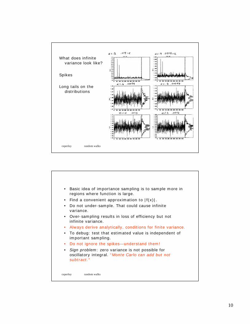
What does infinite variance look like?
Spikes
Long tails on the distributions
ceperley random walks
• Basic idea of importance sampling is to sample more in regions where function is large.
• Find a convenient approximation to |f(x)|.• Do not under-sample. That could cause infinite
variance.• Over-sampling results in loss of efficiency but not
infinite variance.• Always derive analytically, conditions for finite variance.• To debug: test that estimated value is independent of
important sampling.• Do not ignore the spikes—understand them!
• Sign problem: zero variance is not possible for oscillatory integral. “Monte Carlo can add but not subtract.”
11
ceperley random walks
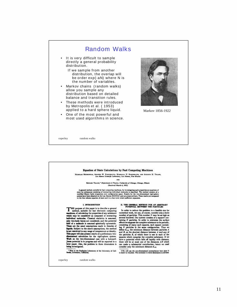
Random Walks• It is very difficult to sample
directly a general probability distribution.If we sample from another
distribution, the overlap will be order exp(-aN) where N is the number of variables.
• Markov chains (random walks) allow you sample any distribution based on detailed balance and transition rules.
• These methods were introduced by Metropolis et al. ( 1953) applied to a hard sphere liquid.
• One of the most powerful and most used algorithms in science.
Markov 1856-1922
ceperley random walks
12
ceperley random walks
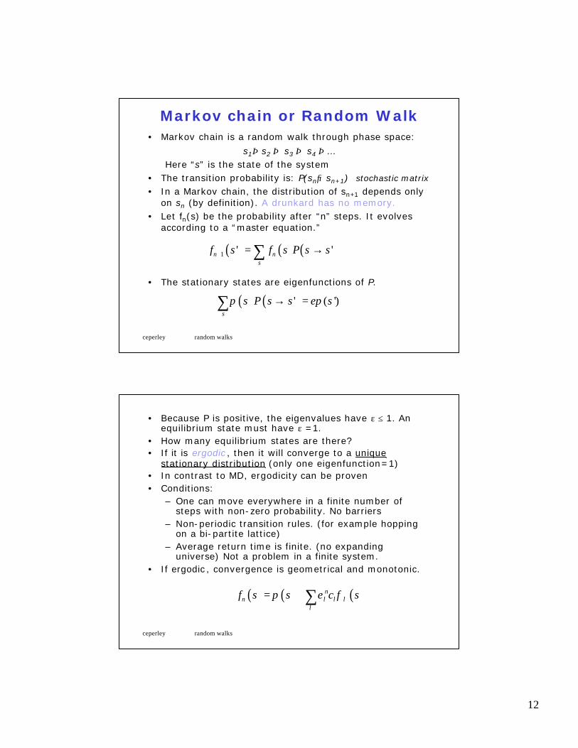
Markov chain or Random Walk• Markov chain is a random walk through phase space:
s1⇒s2 ⇒ s3 ⇒ s4 ⇒…Here “s” is the state of the system
• The transition probability is: P(sn→sn+1) stochastic matrix
• In a Markov chain, the distribution of sn+1 depends only on sn (by definition). A drunkard has no memory.
• Let fn(s) be the probability after “n” steps. It evolves according to a “master equation.”
• The stationary states are eigenfunctions of P.
( ) ( ) ( )1 ' 'n ns
f s f s P s s+ = →∑
( ) ( )' ( ')s
s P s s sπ επ→ =∑
ceperley random walks
• Because P is positive, the eigenvalues have ε ≤ 1. An equilibrium state must have ε =1.
• How many equilibrium states are there?• If it is ergodic , then it will converge to a unique
stationary distribution (only one eigenfunction=1)• In contrast to MD, ergodicity can be proven• Conditions:
– One can move everywhere in a finite number of steps with non-zero probability. No barriers
– Non-periodic transition rules. (for example hopping on a bi-partite lattice)
– Average return time is finite. (no expanding universe) Not a problem in a finite system.
• If ergodic , convergence is geometrical and monotonic.
( ) ( ) ( )nnf s s c sλ λ λ
λ
π ε φ= + ∑

13
ceperley random walks
Metropolis algorithmThree key concepts:
1. Sample by using an ergodic random walk.2. Determine equilibrium state by using detailed
balance3. Achieve detailed balance by using rejections.
Detailed balance: π (s) P(s → s’) = π (s’)P (s’ → s ).Rate balance from s to s’.
Put π (s) into the master equation.
• Hence π(s) is an eigenfunction.
• If P(s ⇒s’) is ergodic then π (s) is the unique steady state solution.
( ) ( ) ( ) ( ) ( ) ( )' ' ' ' ' ( ')s s s
s P s s s P s s s P s s sπ π π π→ = → = → =∑ ∑ ∑
ceperley random walks
Rejection Method
( ) ( ' ) ( ')' min 1,( ') ( )
T s s sA s sT s s s
ππ
→→ = →
Metropolis achieves detailed balance by rejecting moves.
Break up transition probability into sampling and acceptance:
The optimal acceptance probability that gives detailed balance is:
Note that normalization of π(s) is not needed or used!
( ) ( ) ( )( )( )
' ' '
' sampling probability
' acceptance probability
P s s T s s A s s
T s s
A s s
→ = → →
→ =
→ =
14
ceperley random walks
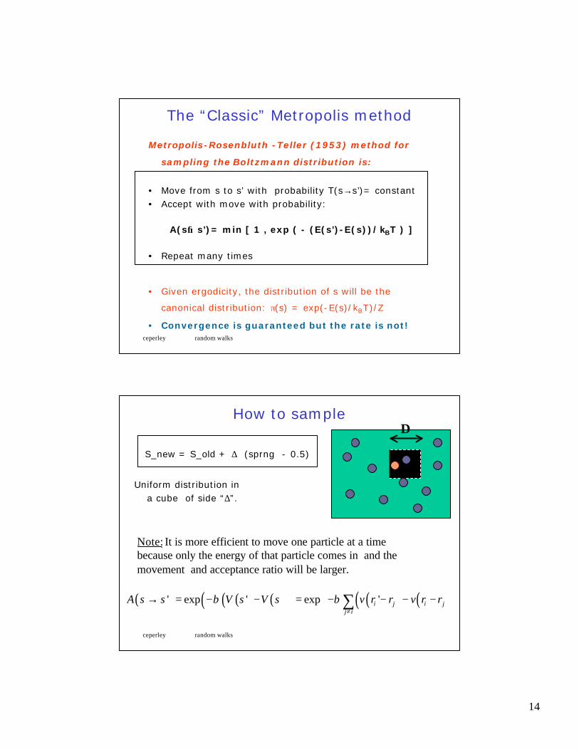
The “Classic” Metropolis method
Metropolis-Rosenbluth -Teller (1953) method for
sampling the Boltzmann distribution is:
• Move from s to s’ with probability T(s→s’)= constant• Accept with move with probability:
A(s→s’)= min [ 1 , exp ( - (E(s’)-E(s))/kBT ) ]
• Repeat many times
• Given ergodicity, the distribution of s will be the
canonical distribution: π(s) = exp(-E(s)/kBT)/Z
• Convergence is guaranteed but the rate is not!
ceperley random walks
How to sample
S_new = S_old + ∆ (sprng - 0.5)
Uniform distribution in a cube of side “∆”.
∆
Note: It is more efficient to move one particle at a time because only the energy of that particle comes in and the movement and acceptance ratio will be larger.
( ) ( ) ( )( )( ) ( ) ( )( )' exp ' exp 'i j i jj i
A s s V s V s v r r v r rβ β≠
→ = − − = − − − −
∑
15
ceperley random walks
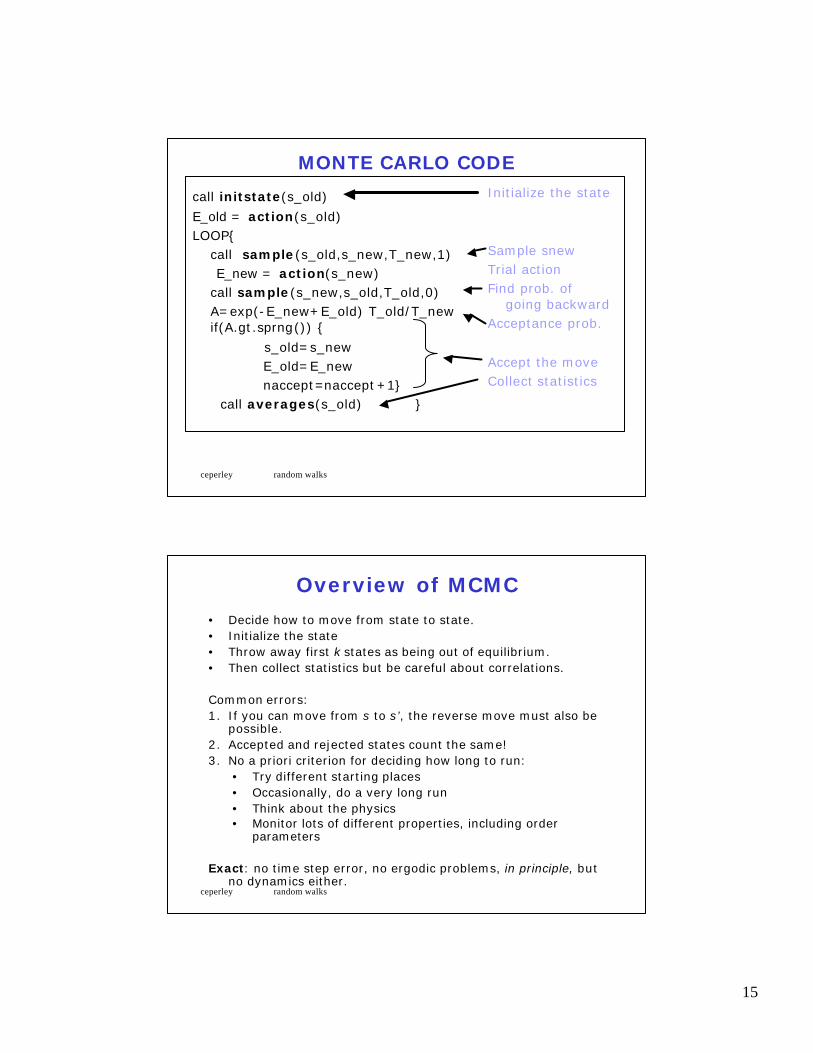
MONTE CARLO CODE
call initstate(s_old)
E_old = action(s_old)LOOP{
call sample(s_old,s_new,T_new,1)E_new = action(s_new)
call sample(s_new,s_old,T_old,0) A=exp(-E_new+E_old) T_old/T_new if(A.gt.sprng()) {
s_old=s_newE_old=E_newnaccept=naccept+1}
call averages(s_old) }
Initialize the state
Sample snewTrial actionFind prob. of
going backward Acceptance prob.
Accept the moveCollect statistics
ceperley random walks
Overview of MCMC
• Decide how to move from state to state.• Initialize the state• Throw away first k states as being out of equilibrium.• Then collect statistics but be careful about correlations.
Common errors:1. If you can move from s to s’, the reverse move must also be
possible.2. Accepted and rejected states count the same!3. No a priori criterion for deciding how long to run:
• Try different starting places• Occasionally, do a very long run • Think about the physics• Monitor lots of different properties, including order
parameters
Exact: no time step error, no ergodic problems, in principle, but no dynamics either.
16
ceperley random walks
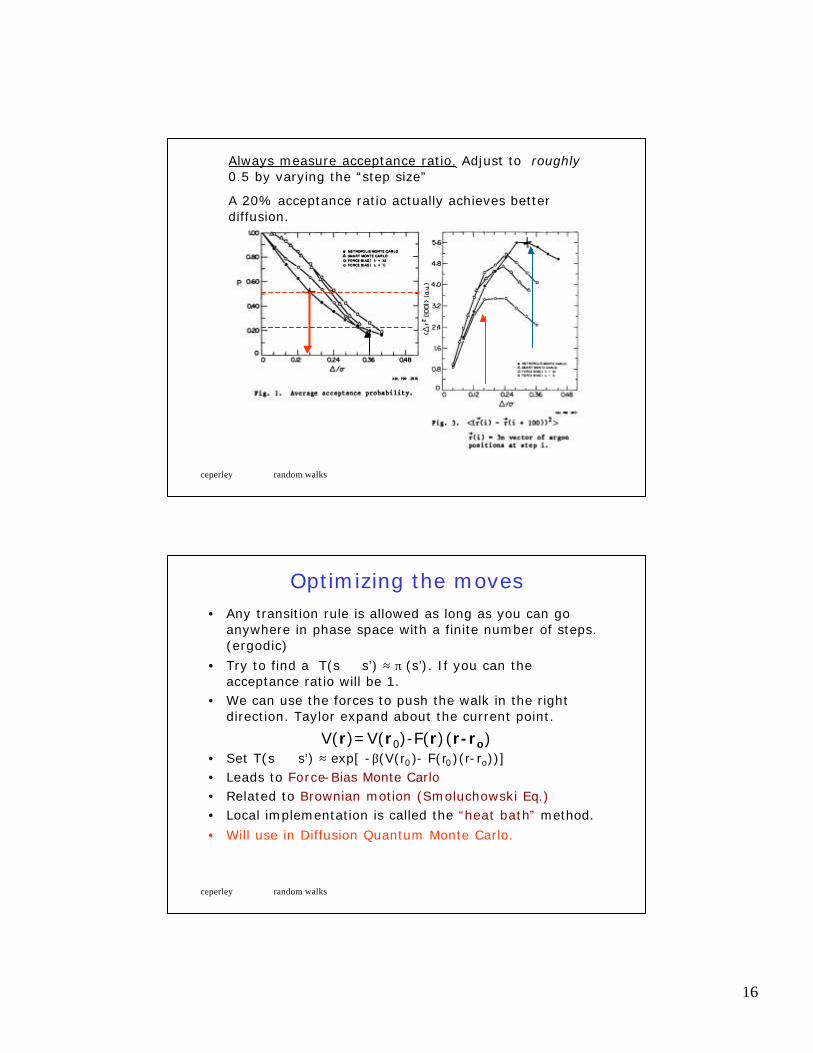
Always measure acceptance ratio. Adjust to roughly 0.5 by varying the “step size”
A 20% acceptance ratio actually achieves better diffusion.
ceperley random walks
Optimizing the moves• Any transition rule is allowed as long as you can go
anywhere in phase space with a finite number of steps. (ergodic)
• Try to find a T(s ⇒ s’) ≈ π (s’). If you can the acceptance ratio will be 1.
• We can use the forces to push the walk in the right direction. Taylor expand about the current point.
V(r)=V(r0)-F(r)(r-ro)• Set T(s ⇒ s’) ≈ exp[ -β(V(r0)- F(r0)(r-ro))]• Leads to Force-Bias Monte Carlo• Related to Brownian motion (Smoluchowski Eq.)• Local implementation is called the “heat bath” method.
• Will use in Diffusion Quantum Monte Carlo.

17
ceperley random walks
Problems with estimating errors
• Any good simulation quotes systematic and statistical errors for anything important.
• The error and mean are simultaneously determined from the same data. HOW?
• Central limit theorem: the distribution of an average approaches a normal distribution (if the variance is finite). One standard deviation means ~2/3 of the time the correct answer is within σ of the sample average.
• Problem in simulation: data is correlated in time . It takes a “correlation” time to be “ergodic .”
• We must throw away the initial transient and get rid of autocorrelation.
• We need ≥20 independent data points to estimate errors.
ceperley random walks
DataSpork
You need to be able to look at the data and estimate the error bars.
Interactive code to perform statistical analysis of data.
Download from Materials Computation Center at U of Illinois.
18
ceperley random walks
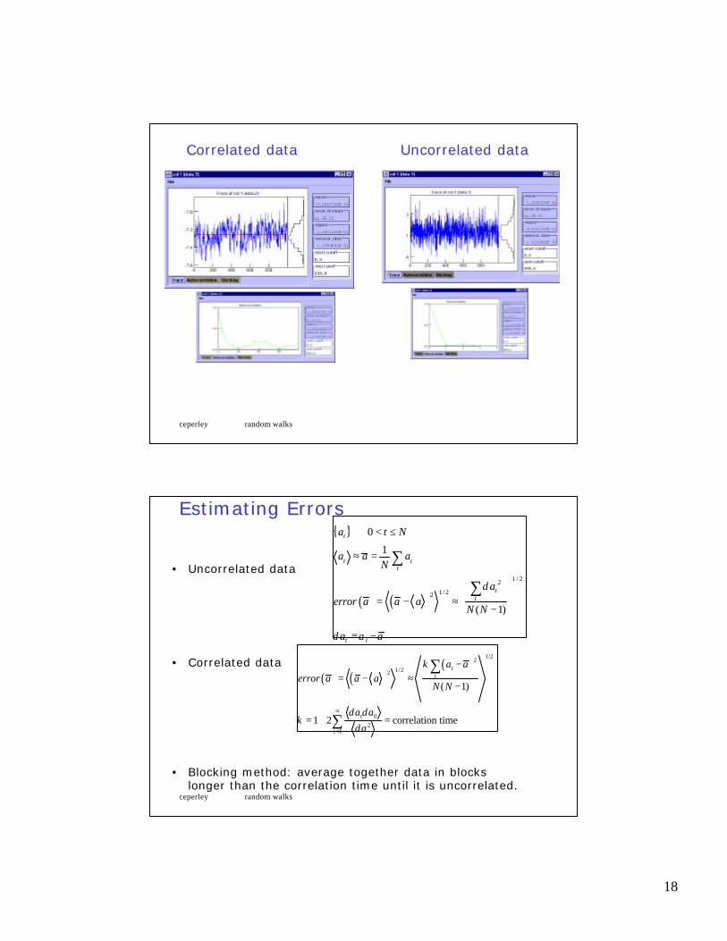
Correlated data Uncorrelated data
ceperley random walks
Estimating Errors
• Uncorrelated data
• Correlated data
• Blocking method: average together data in blocks longer than the correlation time until it is uncorrelated.
{ }
( ) ( )1 / 22
1 / 22
0
1
( 1)
t
t tt
tt
t t
a t N
a a aN
aerror a a a
N N
a a a
δ
δ
< ≤
≈ =
= − ≈ −
≡ −
∑
∑
( ) ( )( )
1/22
1/22
02
1
( 1)
1 2 correlation time
tt
t
t
a aerror a a a
N N
a a
a
κ
δ δκ
δ
∞
=
−= − ≈
−
= + =
∑
∑

19
ceperley random walks
Proof of variance estimate
( ) ( )( )
( )
( )
( )
1/22
1 /22
1 0
'2
2 22 2
' '2 2 2, ' , ' ' 1
( 1)
1 2 correlation time 2 C(t)
( , ') ' =autocorrelation function
1
tt
t
t t
N N N
t t tt tt t t t t t
a aerror a a a
N N
dtC tt
a aC t t C t t
a
a aa a a a C C a
N N N N
κ
κδ
δ δ
δ
δ δ κδ δ δ
∞∞
=
∞
−= =−∞
−= − ≈
−
= + = ≈
≡ = −
− = = < =
∑
∑ ∫
∑ ∑ ∑ ∑
t
t’
κ
1t
t
a aN
= ∑
ceperley random walks
Estimating Errors
• Trace of A(t):
• Equilibration time.
• Histogram of values of A ( P(A) ).
• Mean of A (a).
• Variance of A ( v ).
• estimate of the mean: ΣA(t)/N
• estimate of the variance
• Autocorrelation of A (C(t)).
• Correlation time (κ ).
• The (estimated) error of the (estimated) mean(σ ).
• Efficiency [= 1/(CPU time * error 2)]
20
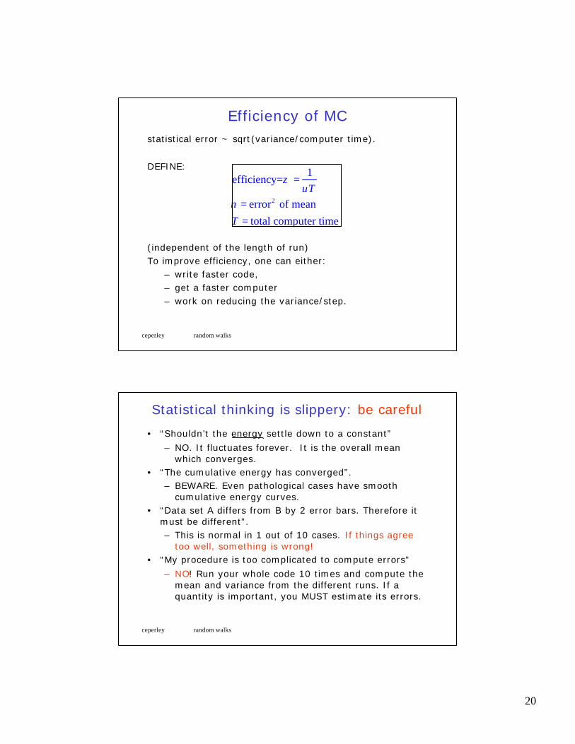
ceperley random walks
Efficiency of MCstatistical error ~ sqrt(variance/computer time).
DEFINE:
(independent of the length of run)To improve efficiency, one can either:
– write faster code, – get a faster computer– work on reducing the variance/step.
2
1efficiency=
error of meantotal computer time
T
T
ζυ
ν
=
==
ceperley random walks
Statistical thinking is slippery: be careful
• “Shouldn’t the energy settle down to a constant”
– NO. It fluctuates forever. It is the overall mean which converges.
• “The cumulative energy has converged”.– BEWARE. Even pathological cases have smooth
cumulative energy curves.• “Data set A differs from B by 2 error bars. Therefore it
must be different”. – This is normal in 1 out of 10 cases. If things agree
too well, something is wrong!• “My procedure is too complicated to compute errors”
– NO! Run your whole code 10 times and compute the mean and variance from the different runs. If a quantity is important, you MUST estimate its errors.