quantum degeneracy and interactions in the rb - k bose ... · quantum degeneracy and interactions...
TRANSCRIPT

Quantum Degeneracy and Interactions in the
87Rb -40K Bose-Fermi Mixture
by
Jonathan Michael Goldwin
B.Sc. Physics and Mathematics,
University of Wisconsin – Madison, 1999
A thesis submitted to the
Faculty of the Graduate School of the
University of Colorado in partial fulfillment
of the requirements for the degree of
Doctor of Philosophy
Department of Physics
2005
This thesis entitled:Quantum Degeneracy and Interactions in the 87Rb -40K Bose-Fermi Mixture
written by Jonathan Michael Goldwinhas been approved for the Department of Physics
Deborah S. Jin
Jun Ye
Date
The final copy of this thesis has been examined by the signatories, and we findthat both the content and the form meet acceptable presentation standards of
scholarly work in the above mentioned discipline.
iii
Goldwin, Jonathan Michael (Ph.D., Physics)
Quantum Degeneracy and Interactions in the 87Rb -40K Bose-Fermi Mixture
Thesis directed by Associate Professor Deborah S. Jin
An apparatus for producing dilute-gas quantum degenerate Bose-Fermi mix-
tures is presented. The experiment uses forced evaporative cooling to obtain a
nearly pure 87Rb Bose-Einstein condensate immersed in a gas of sympathetically
cooled 40K atoms at 0.2 times the Fermi temperature. The design, construction,
and operation of the apparatus are described in detail. The onset of quantum
degeneracy is characterized and contrasted between species, revealing the effects
of quantum statistics on the bulk properties of the gases.
The apparatus is then used to study the interactions between species in
ultracold non-degenerate mixtures. Measurements of rethermalization rates are
used to determine the elastic scattering cross-section between species. From these
measurements the magnitude of the inter-species s-wave scattering length is de-
termined. The scattering length is central to characterizing a variety of static and
dynamic properties of the mixture. The apparatus is additionally used to study for
the first time Feshbach resonances in the collisions between 87Rb and 40K atoms.
These resonances present a means for experimentally tuning the scattering length
between species to any desired value. Prospects for future experiments exploiting
this real-time control over the interactions are discussed.
iv
Dedication
For my parents.
Acknowledgements
I would like to acknowledge the contributions of a number of people to
the work described in this thesis. It is the nature of the JILA quantum gas
collaboration that literally dozens of people will at one time or another contribute
ideas to each experiment.
The first word of thanks must go to Debbie, who took me in with only my
eagerness to work as a credential. She spent many hours in the lab with me when
I started, and gave me considerable freedom later on. I can only hope that her
clear thinking, intense focus, and ability to distill problems to their essence has
rubbed off on me over time. Secondary advisor credits go to Eric Cornell and Carl
Wieman, who have invested considerable time and effort into creating the work
environment that exists here today. Their earnest desire to educate, combined
with vast reserves of experience, imagination, and scientific rigor, has led to a
unique place for graduate students to develop our skills.
Somewhere between our advisors and the other contributors to these exper-
iments must come Shin Inouye. Shin was a post-doc with us from a time when
we were still optimizing our MOTs through our recent observation of Feshbach
resonances. In fact Shin was involved with nearly all of the experiments described
in this thesis, and contributed a considerable amount of technical expertise to
the design of the experiment. More importantly, Shin always encouraged me to
reduce problems in the lab to something like the “spherical cow” approximation,
vi
in order to quickly estimate which things I should worry about and which could
be safely neglected.
The various measurements in this thesis were performed in conjunction with
(in order of appearance) Scott Papp, Michele Olsen, and Jianying Lang. Bonna
Newman also made important early contributions to the design and construction
of the experiment, as did Brett DePaola, who was able to assist us via the JILA
visiting fellows program, and Ashley Carter, who spent a semester with us under
the OSEP program at CU. Chris Ticknor and John Bohn provided invaluable
theoretical support. Other people contributing to our experiment at one time
or another include Brian DeMarco (who showed me, in addition to other things,
how to trigger a ‘scope), Steve Gensemer, Tom Loftus, Cindy Regal and Markus
Greiner. A general word of thanks goes out to the large number of students,
post-docs, and visiting fellows who have worked their way through the quantum
gas collaboration during my time. I would also like to acknowledge stimulating
discussions on the joys and tribulations of 87Rb -40K mixtures with Giacomo
Roati of the LENS group, as well as with Christian Ospelkaus of the University
of Hamburg, and Thilo Stoferle of the ETH in Zurich.
Much electronics expertise was provided by James Fung-A-Fat and Terry
Brown. Mechanical engineering (and beyond) was provided by Hans Green, Blaine
Horner, Todd Asnicar, and Tom Foote. Computing expertise from Joel Frahm,
James McKown, and Pete Ruprecht has been crucial, as has the hard work of
Pam Leland, Ed and Randall Holliness, Brian Lynch, and Maryly Dole.
Finally on a personal note I would like to thank my parents for their undying
support over all these years. And I am especially grateful to Mary Ellen Flynn
for her love and support, which have weathered the Sturm und Drang of this work
with much grace and understanding.

Contents
Chapter
1 Introduction 1
1.1 I See Fermions . . . . . . . . . . . . . . . . . . . . . . . . . . . . . 2
1.2 Fermions And Bosons Unite! . . . . . . . . . . . . . . . . . . . . . 5
1.3 Overview of this Thesis . . . . . . . . . . . . . . . . . . . . . . . . 7
2 The Machine 11
2.1 Vacuum System . . . . . . . . . . . . . . . . . . . . . . . . . . . . 12
2.2 Computer Control . . . . . . . . . . . . . . . . . . . . . . . . . . 17
2.2.1 Logic Control . . . . . . . . . . . . . . . . . . . . . . . . . 17
2.2.2 GPIB Control . . . . . . . . . . . . . . . . . . . . . . . . . 19
2.2.3 Digital-to-Analog Converters . . . . . . . . . . . . . . . . . 22
2.3 Transport Coils . . . . . . . . . . . . . . . . . . . . . . . . . . . . 23
2.3.1 Coil Design and Control Circuitry . . . . . . . . . . . . . . 23
2.3.2 Cart Motion . . . . . . . . . . . . . . . . . . . . . . . . . . 29
2.4 Ioffe-Pritchard Trap . . . . . . . . . . . . . . . . . . . . . . . . . . 35
2.4.1 Trap Design . . . . . . . . . . . . . . . . . . . . . . . . . . 35
2.4.2 Trap Frequencies . . . . . . . . . . . . . . . . . . . . . . . 37
2.5 Laser Systems . . . . . . . . . . . . . . . . . . . . . . . . . . . . . 39
2.5.1 Lasers, Lasers, and More Lasers . . . . . . . . . . . . . . . 39

viii
2.5.2 Tapered Amplifier . . . . . . . . . . . . . . . . . . . . . . . 46
2.5.3 Far Off-Resonance Optical Trap . . . . . . . . . . . . . . . 51
3 Cooling to Quantum Degeneracy 58
3.1 Two-Species Magneto-Optical Trap . . . . . . . . . . . . . . . . . 59
3.1.1 Atomic Sources and Vapor Pressures . . . . . . . . . . . . 59
3.1.2 Light-Assisted Collisions and Losses . . . . . . . . . . . . . 66
3.2 Compressing, Cooling, Pumping, and Loading . . . . . . . . . . . 70
3.3 Sympathetic Cooling . . . . . . . . . . . . . . . . . . . . . . . . . 73
3.3.1 Experiment: Evaporation “Trajectories” . . . . . . . . . . 74
3.3.2 Thermodynamics Intermezzo — IP Trap . . . . . . . . . . 78
3.3.3 Theory: Energy-Dependent Collision Cross-Section . . . . 84
3.4 Onset of Quantum Degeneracy . . . . . . . . . . . . . . . . . . . . 86
3.4.1 Bosons . . . . . . . . . . . . . . . . . . . . . . . . . . . . . 87
3.4.2 Fermions . . . . . . . . . . . . . . . . . . . . . . . . . . . . 90
3.5 Limits to Sympathetic Cooling . . . . . . . . . . . . . . . . . . . . 94
4 Cross-Species Interactions 100
4.1 Cross-Dimensional Rethermalization . . . . . . . . . . . . . . . . 102
4.2 Mean-Field Intermezzo — Equilibrium Properties . . . . . . . . . 108
4.2.1 Theory: Phase Separation, Fermions in a Box, and Collapse 111
4.2.2 Experiment: No Collapse Instability Observed at JILA . . 117
4.3 Excitations . . . . . . . . . . . . . . . . . . . . . . . . . . . . . . 124
4.3.1 Quadrupole “Breathe” Mode . . . . . . . . . . . . . . . . . 125
4.3.2 Frequency Domain and High-Order BEC Excitations . . . 130
4.3.3 Theory: Boson-Induced Pairing of Fermions . . . . . . . . 135
4.4 Heteronuclear Feshbach Resonances . . . . . . . . . . . . . . . . . 137
4.4.1 Scattering Resonance Overview . . . . . . . . . . . . . . . 138
ix
4.4.2 Observation of Feshbach Resonances . . . . . . . . . . . . 144
4.4.3 Analysis and Results . . . . . . . . . . . . . . . . . . . . . 158
5 Summary and Outlook 165
Appendix
A Monte Carlo Simulation Details 167
A.1 Choice of Parameters and Failure Modes . . . . . . . . . . . . . . 167
A.2 Transition to Hydrodynamic Behavior . . . . . . . . . . . . . . . . 170
B Cross-dimensional Rethermalization Supplement 175
B.1 Thermal Averages with Different Anisotropies for Each Species . . 175
B.2 Analytic Best Fit to Exponential Decay . . . . . . . . . . . . . . . 177
Bibliography 181

x
Tables
Table
2.1 Vapor pressure constants for Rb and K . . . . . . . . . . . . . . . 15
2.2 Hyperfine constants for 87Rb and the stable isotopes of K . . . . 40
2.3 Transition wavelengths, linewidths, and saturation intensities for
Rb and K . . . . . . . . . . . . . . . . . . . . . . . . . . . . . . . 45
2.4 MOT light detunings and peak intensities . . . . . . . . . . . . . 50
3.1 Lowest values of T/TF reported in 87Rb -40K experiments. . . . . 95
4.1 Compendium of reported values for the 87Rb -40K triplet scattering
length . . . . . . . . . . . . . . . . . . . . . . . . . . . . . . . . . 109
4.2 Upper limits on |aRbK| . . . . . . . . . . . . . . . . . . . . . . . . 124
4.3 Identification of high-order BEC excitations . . . . . . . . . . . . 135
4.4 Hyperfine parameters for the Breit-Rabi equation . . . . . . . . . 148
4.5 Summary of observed 87Rb -40K resonances . . . . . . . . . . . . 158
4.6 Summary of calculated elastic s-wave features . . . . . . . . . . . 164

Figures
Figure
1.1 Applications of work with atomic Fermi gases and Bose-Fermi mix-
tures . . . . . . . . . . . . . . . . . . . . . . . . . . . . . . . . . . 4
1.2 Characteristic Fermi temperatures and operating temperatures of
some quantum degenerate fermion systems . . . . . . . . . . . . . 6
1.3 The incredible journey from room temperature to quantum degen-
eracy . . . . . . . . . . . . . . . . . . . . . . . . . . . . . . . . . . 9
2.1 Schematic of the vacuum assembly . . . . . . . . . . . . . . . . . 13
2.2 Vapor pressures of Rb and K as a function of temperature . . . . 15
2.3 Collection cell heaters . . . . . . . . . . . . . . . . . . . . . . . . 16
2.4 Schematic of computer controls for the experiment . . . . . . . . . 18
2.5 Buffer circuit for digital TTL lines . . . . . . . . . . . . . . . . . . 20
2.6 Measured axial field of transport coils in Helmholtz configuration 26
2.7 Measured axial field of transport coils in anti-Helmholtz configuration 27
2.8 Schematic of the control circuit for the transport coils . . . . . . . 28
2.9 Servo circuit for B-field stabilization . . . . . . . . . . . . . . . . 30
2.10 Multiplexing circuit . . . . . . . . . . . . . . . . . . . . . . . . . . 31
2.11 Switching circuit . . . . . . . . . . . . . . . . . . . . . . . . . . . 32
2.12 Example cart motion during the experiment . . . . . . . . . . . . 34

xii
2.13 Schematic of the Ioffe-Pritchard trap . . . . . . . . . . . . . . . . 36
2.14 Energy level schematics for 87Rb and 40K . . . . . . . . . . . . . 41
2.15 Energy level schematics for the stable K isotopes . . . . . . . . . 42
2.16 87Rb saturated absorption spectroscopy . . . . . . . . . . . . . . 43
2.17 K saturated absorption spectroscopy . . . . . . . . . . . . . . . . 44
2.18 Some AOM configurations used . . . . . . . . . . . . . . . . . . . 47
2.19 AOM driver circuit . . . . . . . . . . . . . . . . . . . . . . . . . . 48
2.20 Spectrum of the injected tapered amplifier . . . . . . . . . . . . . 50
2.21 YAG intensity servo . . . . . . . . . . . . . . . . . . . . . . . . . 53
2.22 FORT optics schematic . . . . . . . . . . . . . . . . . . . . . . . . 54
2.23 FORT beam characterization . . . . . . . . . . . . . . . . . . . . 55
3.1 Schematic of MOT loading rate with increasing alkali-metal vapor
pressure . . . . . . . . . . . . . . . . . . . . . . . . . . . . . . . . 63
3.2 Same, for two-species case . . . . . . . . . . . . . . . . . . . . . . 64
3.3 Response of 87Rb and 40K MOTs to the Rb alkali metal dispenser 65
3.4 Response of 87Rb and 40K MOTs to the K alkali metal dispenser 67
3.5 Observation of light-assisted losses of 40K in the two-species MOT 69
3.6 Effect of Doppler cooling of 40K . . . . . . . . . . . . . . . . . . . 72
3.7 Zeemann sublevels of 87Rb and 40K in a harmonic magnetic potential 75
3.8 Single-species 87Rb evaporation trajectory . . . . . . . . . . . . . 77
3.9 Inelastic losses at the end of evaporation . . . . . . . . . . . . . . 79
3.10 Effect of gravity on the collision rate . . . . . . . . . . . . . . . . 83
3.11 87Rb -40K cross-section as a function of energy . . . . . . . . . . 85
3.12 Observation of the BEC phase transition . . . . . . . . . . . . . . 89
3.13 Calculated peak BEC density as a function of number . . . . . . . 91
3.14 Observation of Fermi degeneracy . . . . . . . . . . . . . . . . . . 93

xiii
3.15 Specific heats of ideal Bose and Fermi gases . . . . . . . . . . . . 96
4.1 Cross-dimensional rethermalization of 40K in the presence of 87Rb 103
4.2 Cross-dimensional relaxation over varying 87Rb density . . . . . . 106
4.3 Comparison of experiments and theory for the 87Rb -40K cross-
section . . . . . . . . . . . . . . . . . . . . . . . . . . . . . . . . . 110
4.4 Mean-field effect of a condensate on the fermions . . . . . . . . . 114
4.5 Theoretical equilibrium profiles . . . . . . . . . . . . . . . . . . . 116
4.6 Fermion chemical potential with interactions . . . . . . . . . . . . 118
4.7 Theoretical dependence of the central densities on mean-field cou-
pling strength . . . . . . . . . . . . . . . . . . . . . . . . . . . . . 119
4.8 Slow decay of 40K atoms with 87Rb BEC . . . . . . . . . . . . . 122
4.9 Stability diagram for attractive interactions . . . . . . . . . . . . 123
4.10 Measurement of the damping of breathe modes . . . . . . . . . . 127
4.11 Dependence of breathe mode damping rates as a function of drive
amplitude . . . . . . . . . . . . . . . . . . . . . . . . . . . . . . . 129
4.12 Example of excitation spectroscopy using parametric heating . . . 131
4.13 Density dependence of collective excitation frequency . . . . . . . 132
4.14 Observation of higher-lying BEC excitations . . . . . . . . . . . . 134
4.15 Feshbach resonance schematic . . . . . . . . . . . . . . . . . . . . 140
4.16 Spherical well scattering resonances . . . . . . . . . . . . . . . . . 145
4.17 Breit-Rabi diagrams for 87Rb . . . . . . . . . . . . . . . . . . . . 148
4.18 Breit-Rabi diagrams for 40K . . . . . . . . . . . . . . . . . . . . . 149
4.19 Schematic search for Feshbach resonances . . . . . . . . . . . . . . 152
4.20 First observation of 87Rb -40K Feshbach resonances . . . . . . . . 154
4.21 Detail of the widest inelastic feature . . . . . . . . . . . . . . . . . 155
4.22 Observed 87Rb-87Rb resonance . . . . . . . . . . . . . . . . . . . 157

xiv
4.23 Most recently observed 87Rb -40K resonance . . . . . . . . . . . . 159
4.24 Measured widths of the inelastic features . . . . . . . . . . . . . . 161
4.25 Scattering length determination from inelastic resonance features . 162
4.26 Theoretical elastic resonance features . . . . . . . . . . . . . . . . 164
A.1 Effect of bad choice of time-step on the MC simulation . . . . . . 169
A.2 Effect of bad choice of critical distance of approach on the MC
simulation . . . . . . . . . . . . . . . . . . . . . . . . . . . . . . . 171
A.3 Nonlinear relaxation rate for CDR due to hydrodynamic effects . 173
A.4 Signature of hydrodynamic effects on relaxation . . . . . . . . . . 174
B.1 Effect of energy anisotropies on thermal averages . . . . . . . . . 178
B.2 Fermion relaxation with double exponential decay . . . . . . . . . 179

Chapter 1
Introduction
That the impossible should be asked of me,good, what else could be asked of me? Butthe absurd! Of me whom they have reducedto reason.
- Samuel Beckett, The Unnamable
This thesis describes some of the first experiments probing and manipu-
lating the cross-species interactions in an ultracold dilute gas mixture of Bosons
and Fermions. To date most systems of this type have been used as practical
tools, bypassing the Pauli exclusion principle in order to cool gases of fermionic
atoms to only a fraction of the Fermi temperature. Bose-Fermi mixtures, how-
ever, additionally allow us to study a variety of many-body quantum mechanical
systems of interest to condensed matter physics, with the degree of control and rel-
ative theoretical simplicity of atomic gases. In our systems interactions between
atoms are typically short-range and two-body in nature, impurities are absent,
and smooth, regular, time-dependent trapping potentials are easily generated in
the lab. Furthermore, through the use of Feshbach resonances, the interactions
may be controlled in real time in the experiments.
2
In this thesis I describe the design, construction, and operation of an exper-
imental apparatus we have built for trapping and cooling to quantum degeneracy
a dilute-gas mixture composed of 87Rb (boson) and 40K (fermion) atoms. It
is shown that such a mixture can be cooled using relatively standard techniques
until a nearly pure Bose-Einstein condensate coexists with a quantum degenerate
gas of fermions at around 20% of the Fermi temperature. I will describe measure-
ments we have made of the s-wave elastic collision cross-section between 87Rb and
40K atoms in the ultracold, but non-degenerate regime. These measurements give
us important information on the interactions between species in quantum degener-
ate mixtures. Finally, I will present our most recent work where we have identified
a number of inter-species Feshbach resonances in the 87Rb -40K system. These
resonances represent, in principle, a means for exerting complete real-time control
over the interactions between species. This kind of control may allow us to study
a significant number of exciting new phenomena in the future.
A more detailed overview of this thesis is given in Section 1.3. Before pro-
ceeding, however, I would like to give some motivation for our interest in quantum
degenerate atomic Fermi gases and Bose-Fermi mixtures.
1.1 I See Fermions
It is a peculiar fact of the quantum mechanical world that all of the con-
stituents of the ordinary matter and light around us fall into one of two categories
— they are either bosons or fermions. Bosons and fermions are distinguished on
the one hand by their quantum mechanical spin, which takes on integer values
for bosons and half-integer values for fermions. On the other hand the differ-
ences between bosons and fermions can become manifest even in the absence of
spin-dependent forces. The bulk properties of ensembles of identical particles can
be strikingly different depending on which family the particles belong to. The
3
behavior of groups of identical fermions underlies the rich variety of elements in
the periodic table, and the concerted efforts of identical bosons have brought us
the laser.
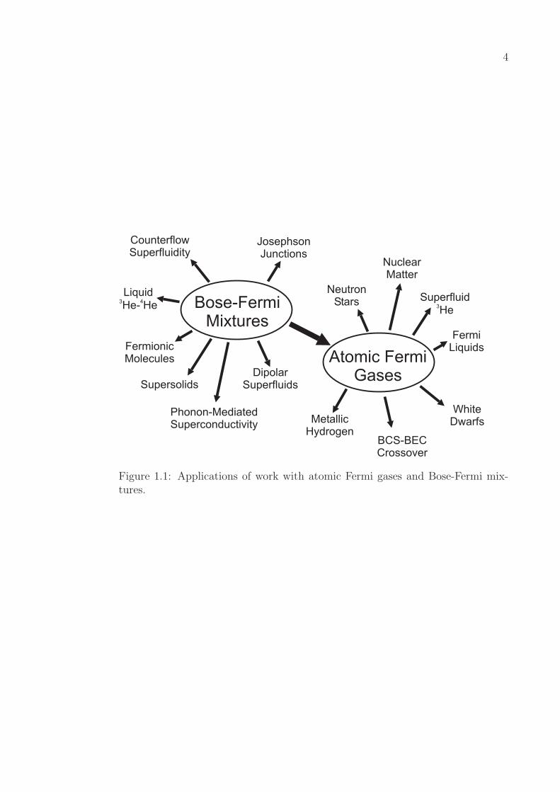
The experiments described in this thesis aim to study and exploit the be-
havior of ensembles of 87Rb atoms (which are composite bosons) and 40K atoms
(composite fermions). In Fig. 1.1 I show schematically some of the fields of re-
search that can benefit from the type of work we are doing. Particular applications
of Bose-Fermi mixtures are discussed in the next section, but these mixtures were
originally conceived as a tool for producing degenerate Fermi gases, and this is
how they have been most commonly used to date. Atomic Fermi gases may be
used to understand such wildly different fermionic systems as normal metals, neu-
tron and white dwarf stars, heavy nuclei, superfluid 3He, and metallic hydrogen.
There is much to be learned about high-Tc superconductivity, for example, from
the study of ultracold gases. And if we make a quantum computer in the process,
then who’s going to complain?
In qualified defense of our friend the fermion, I would like to argue against
the notion that fermions are less “sociable” than bosons [1]. The renowned Pauli
exclusion principle only describes a fermion’s reluctance to share a quantum state
with an identical fermion. A fermion will happily make room for a distinguishable
fermion, or even a boson. In this sense I would argue that fermions are more open
and sociable than the narcissistic bosons — the bosons, who would all crowd into
their ground state with others just like themselves, and never ask what lies above.
For better or worse, Pauli taught us that identical fermions will not share
a quantum state. It is this very behavior that leads to the well known statistical
distribution of fermions at zero temperature, with a single fermion in each available
quantum state, starting at lowest energy and moving up one state at a time until
we run out of particles. The very last fermion occupies a special place in this
4
JosephsonJunctions
MetallicHydrogen
WhiteDwarfs
FermiLiquids
NeutronStars
DipolarSuperfluids
FermionicMolecules
Phonon-MediatedSuperconductivity
BCS-BECCrossover
NuclearMatter
Supersolids
CounterflowSuperfluidity
SuperfluidHe
3
LiquidHe-
3 4He Bose-Fermi
Mixtures
Atomic FermiGases
Figure 1.1: Applications of work with atomic Fermi gases and Bose-Fermi mix-tures.

5
distribution, which defines the Fermi energy EF of the system. Only particles in
states near the Fermi energy can partake in the joys of perturbative excitation
[2]. States far above EF are not occupied, and particles below EF are pinned by
the presence of the fermions around them, with no unoccupied state to scatter
into. The Fermi temperature, defined by TF = EF /kB with kB Boltzmann’s
constant, defines the characteristic temperature that the system must approach
before quantum statistical effects may begin to appear.
The Fermi temperature is directly related to the density of a system, in the
sense that high densities lead to high TF , and low to low. One reason that dilute
atomic gases are so useful to study is our ability to understand their behavior
with relatively simple theories. This in turn is due to the fact that our systems
are dominated by short-range interactions, and have such low densities that we
rarely have to go to more than a two-body picture to get some understanding of
what is happening. As seen in Fig. 1.2, where I outline some typical values of
TF for various quantum degenerate fermion systems, this means we must get our
atoms extremely cold in order to access their quantum statistical properties. This
incredible technical achievement has only been possible in the last decade, and is
at the heart of the work I’ll describe here.
1.2 Fermions And Bosons Unite!
When we began designing the experiment described in this thesis there was
still only one successful Fermi gas experiment [3], using simultaneous evaporative
cooling of two spin states of 40K. The presence of a second spin state helps bypass
the reluctance of fermions to collide during the cooling. The common wisdom
at the time was that a simpler approach might be to sympathetically cool a gas
of fermions in the presence of bosons. Although we can debate the premise that
this is “simpler,” I know of ten quantum degenerate Fermi gas experiments in the

6
1012
1011
102
101
10 –10-6 -7
10 –104 5
TF
[ K ]
10 –10-2 -1
10-6
10-9
10-2–10
-3
10-3
10-2
T T/F
Neutron Stars / White Dwarfs
Copper Metal
High- SuperconductorsTc
Heavy Nuclei
Superfluid He3
Quantum DegenerateAtomic Gases
Figure 1.2: Characteristic Fermi temperatures and operating temperatures ofsome quantum degenerate fermion systems.
7
world, and only two of them use different spin states of a single isotopic species.
The rest are produced by sympathetic cooling. There are at least seven more
sympathetic cooling experiments being built.
It is my belief that the quantum degenerate Bose-Fermi mixture will ulti-
mately be seen as more than just a way to produce degenerate Fermi gases. For
example, although fermions in optical lattice potentials already provide a great
system for simulating Fermi gases in metals [4], the optical lattice cannot play all
the roles of the condensed matter lattice it pretends to be. Specifically, optical
lattices do not exhibit excitations such as phonons, which are crucial to our un-
derstanding of superconductivity in the BCS regime. I think the most exciting
prospect for Bose-Fermi mixtures is the prediction of a boson-mediated pairing of
the fermions [5, 6, 7], where phonons in the condensate give rise to the effective
attractive interactions between fermions needed for Cooper pairing and Fermi su-
perfluidity. Other applications of Bose-Fermi mixtures include the formation of
ultracold fermionic molecules [8], which can only be produced from a combination
of bosons and fermions, and the creation of a supersolid phase [9] or a host of
other exotic phases [10] in optical lattices.
1.3 Overview of this Thesis
As stated at the beginning of this chapter, this thesis describes some of the
first experiments probing and manipulating the cross-species interactions in Bose-
Fermi mixtures. Although many of the theoretical descriptions and experimental
techniques presented here are extensions of work already established in the field,
the Bose-Fermi mixture is more than the sum of its parts and deserves to be
considered a unique and rich system on its own. In this thesis I hope to lay out a
very specific and detailed account of the tools needed to produce such a system,
as well as a more general treatment of the kind of physics one may encounter by

8
studying it. In this final introductory section, I would like to lay out the basic
structure of this thesis, in order to guide the interested reader.
In chapter 2 I give a very detailed technical description of the apparatus we
have built for producing a quantum degenerate 87Rb -40K mixture. This chapter
is intended mainly for the benefit of people in our lab, and for others working with
or developing new ultracold gas experiments. I describe the design and assembly
of the vacuum system, the various elements of computer control, the magnetic
trapping coils and their control circuits, and the many lasers and optics used in
the experiment.
Chapter 3 describes the cooling and trapping techniques needed to achieve
simultaneous quantum degeneracy of bosons and fermions. The process begins
with the capture and cooling of atoms in a two-species magneto-optical trap; the
atoms are subsequently transferred in a three-step process to a Ioffe-Pritchard
type magnetic trap for the final stages of evaporative and sympathetic cooling.
The experimental procedure is described, and the characterization of quantum
degeneracy is outlined in some detail for bosons and fermions. Some possible
limits to the temperature we can achieve with sympathetic cooling are discussed,
along with implications for future experiments. This “incredible journey” the
atoms take from room temperature to a few tens of billionths of a degree above
absolute zero is outlined schematically in Fig. 1.3.
Chapter 4 details the main experimental results we have achieved with the
machine. I first discuss some ways to probe the collisional interactions between
species. The discussion focuses on our extension of cross-dimensional rethermal-
ization techniques to the (non-degenerate) Bose-Fermi mixture. I will describe
why the knowledge gleaned from these measurements, namely the magnitude of
the cross-species scattering length, is so important in understanding a variety of
properties of the mixture. I will then present some measurements of collective ex-

9
102
10-4
10 –10-3 -6
10 –10-7 -8
T [ K ]
10-2
101
10 –101 2
10 –102 3
LT[ nm ]
>1
10-20
10-9–10
-11
10 –10-9 -1
D
Alkali Metal Dispenser
Magneto-optical Trap
Sympathetic Cooling
Quantum Degeneracy
Figure 1.3: The incredible journey from room temperature to quantum degener-acy. The quantities ΛT and D are the thermal de Broglie wavelength and peakphase-space density, respectively. Both are discussed in detail in Sect. 3.4.

10
citations of the mixture, and describe a variety of related measurement techniques,
with an eye towards future experiments.
Also in chapter 4 I describe our search for, and discovery of, several heteronu-
clear Feshbach resonances in the 87Rb -40K system. These resonances represent,
in my view, the crowning achievement of the work described here, due to the large
number of significant and exciting experiments that resonant control of the inter-
actions renders accessible to us. I describe our use of a far off-resonant optical
trap and discuss the preparation and detection of resonant states of the mixture.
Implications for the theoretical understanding of the 87Rb -40K system are laid
out, based on detailed coupled-channel calculations of the collision processes per-
formed by Chris Ticknor and John Bohn. The comparison between theory and
experiment allows us to refine the parameters characterizing the collisions between
87Rb and 40K atoms.
Finally in Chapter 5 I conclude with a summary of the work presented in
this thesis, and describe what I think are the natural next steps for the experi-
ment. I will additionally describe some proposals for some of the more exciting
future experiments that could be performed with our system, including the cov-
eted boson-mediated mechanism for the high-Tc pairing of fermions.
Chapter 2
The Machine
In this chapter I’ll describe the details of the design, construction, and op-
eration of our experimental apparatus. I will focus on aspects of the experiment
that are unique and include some more detailed discussions of the installation
or optimization procedures we use for some of the components. This chapter is
intended to be most useful for people still working in the lab, or others hoping to
build a similar experiment of their own.
The chapter is organized as follows. I begin in Section 2.1 with a description
of the vacuum system we have built, and in Section 2.2 I describe the computer
control elements that we use. In Section 2.3 I present the moving magnetic coil
assembly used in our experiment, and describe how it is used for the MOT, for the
mechanical transport to an ultrahigh vacuum (UHV) cell, and for production of
uniform magnetic fields for accessing inter-species Feshbach resonances. In Section
2.4 I describe the Ioffe-Pritchard trap we have built for evaporative cooling; this
trap is extremely compact, and operates at relatively low power. Finally Sect. 2.5
details the various lasers used for cooling, trapping, pumping, and probing the
atoms. This section also includes a description of a far-off-resonance optical dipole
trap, which we used to access the Feshbach resonances described in Chapter 4.

12
2.1 Vacuum System
In this section I will describe our vacuum system in some detail. The vacuum
assembly is shown schematically in Fig. 2.1. The system consists of two Pyrex cells
separated by a stainless steel tube that allows for differential pumping between
cells. The first cell, which we call the “collection cell,” was made at JILA and
is home to the two-species magneto-optical trap (MOT). The 2′′ × 2′′ × 6′′ cell
contains two arms — one with four Rb dispensers, and one with four K dispensers.
The Rb dispensers are purchased from SAES Getters [11], and the enriched K
dispensers are produced at JILA, as described in Ref. [12]. Enriched K dispensers
are necessary due to the extremely low natural abundance of 40K (0.0117%) [13].
The collection cell is connected with a “T” to a 20 L/s ion pump and a long,
narrow tube, which we call the “transfer tube.” The purpose of the tube is to
allow differential pumping between the collection cell (at relatively high pressure,
in order to collect a lot of atoms), and the second glass cell, or “science cell,”
which is maintained at higher vacuum in order to provide long trapping lifetimes
and efficient evaporation of the 87Rb atoms. For example our 1/e lifetime in
the magnetic trap in the collection cell is about 2 to 4 seconds. In contrast our
lifetimes in the science cell exceed 100 seconds for 87Rb atoms, and 400 seconds
for 40K. Our evaporative cooling sequence lasts about 30 seconds.
The pressure gradient from end-to-end across the transfer tube is inversely
proportional to the conductance of the tube. At the low pressures used in these
experiments, the vacuum is in the so-called “molecular flow” regime. This means
that the conductance is independent of pressure [14]. In this case the conductance
of air through the tube is given by C = 12 d3/l [L/s], where d is the diameter of
the aperture, and l is the length of the component, and both are measured in cm.
Note that conductances add (in series and parallel) like capacitors in an electronic

13
40 L/s
20 L/s
Valve
Ti:subpump Ion
pumpsTOPVIEW
SIDEVIEW
“Sciencecell”
“Collectioncell”
Transfertube
“Transfercoils”
Alkali metaldispensers
Window
Figure 2.1: Schematic of the vacuum assembly. The top view is shown aboveand the side view below. The “collection” and “science” cells are glass, and therest of the components are stainless steel connected by ConFlat components withcopper gaskets. For clarity we have omitted the alkali metal dispensers from thetop view. Additionally a bellows to the left of the “transfer tube,” which correctsfor imperfections in the straightness of some commercial vacuum parts, has beenincorporated into the tube itself in the drawing. The valve was used to rough outthe system before the bake-out. The window on the front of the collection celltransmits light for optical pumping and imaging of the atoms in either cell. Thetotal distance between cell centers is ∼ 81 cm, and the smallest inner diametersare 1 cm. The “transfer coils” are free to move between cells by means of a lineartranslation stage, described in Section 2.3.

14
circuit. As an example, our transfer tube is ∼ 1 cm in diameter, and 9.5 inches
(∼ 24 cm), giving a conductance of only Ctube = 0.5 L/s.1 If for simplicity we
consider just the transfer tube and the 20 L/s pump, then the pressure at the
output end of the transfer tube is related to pressure at the input end by [14]
Pout
Pin
=Ctube/Spump
1 + Ctube/Spump
' 2% , (2.1)
where Spump = 20 L/s is just the pumping speed of the ion pump.
The room-temperature vapor pressure of Potassium is much lower than that
of Rubidium, so that some amount of heating of the collection cell is required to
keep 40K atoms from adsorbing onto the glass. The vapor pressure constants A
and B are shown in Table 2.1. The constants A and B give the vapor pressure as
a function of temperature T (in Kelvin) according to Pvap[Torr] = 760×10A10B/T
[15], as shown in Fig.2.2 for temperatures around 300 K. The Rubidium pressure
is roughly 20 times higher at 300 K; Potassium must be brought to 328 K to
obtain a pressure equal to the Rubidium pressure at 300 K. In order to maintain
a workable 40K pressure in the collection cell, we have built a set of heaters,
shown in Figure 2.3. Parts of the cell not covered by these heaters are wrapped
with Minco flexible foil heaters, allowing us to keep the entire cell above 50 C.
The science cell is made from a commercial fluorometer cell from Starna cells,
and is a 1 cm square cylinder of 4 cm length. The cell was smoothly matched to a
glass-to-metal seal welded onto a standard conflat vacuum flange. The science cell
is pumped by a Titanium sublimation (Ti:sub) pump and a 40 L/s ion pump. The
Ti:sub pump is attached to a homemade nipple that places the pump filaments
in the center of a large (4 12
′′) four-way cross. The large area provides an excellent
1 Note that the total conductance is even lower if we take into account the rest of thedistance between the two cells. The remainder of this distance is comprised mostly of two “T”components, leading to each of the two ion pumps, and a 3′′ long bellows (not shown in Fig. 2.1),with an inner diameter of ∼ 1 cm.

15
Figure 2.2: Vapor pressures Pvap of Rubidium (solid curve) and Potassium(dashed) as a function of temperature T in the vicinity of 300 K.
A B Pvap @ 300 K
Rb 4.857 −4215 5× 10⁻⁷ Torr
K 4.961 −4646 2× 10⁻⁸
Table 2.1: Vapor pressures for Rubidium and Potassium. The constants Aand B are used to calculate the vapor pressure Pvap according to the formulaPvap[Torr] = 760× 10A10B/T , with T the temperature in Kelvin. Values for Aand B were taken from Ref. [15].

16
2.0
0"
1.2
5"
4.50"
Eddycurrentslots
Sideheaters
Top/bottomheaters
Mountinggrooves
Figure 2.3: Heaters for the collection cell. All parts are 1/8-inch thick blackanodized aluminum. Slots are cut to inhibit large-wavelength eddy currents inthe bodies of the Al plates. The large holes allow the MOT beams to enter andexit the cell, and show the beam geometry in the experiment. (Note that theholes are slightly larger than shown here, and actually allow a 1.25′′ beam to passthrough.) The mounting grooves allow the plates to be bound to the collectioncell with insulated wire and a thin layer of thermal grease. Not shown are severaltapped holes for mounting low-profile 1 Ω resistors, driven at constant current toprovide ohmic heating to temperatures > 50 C.

17
surface for the evaporated Titanium, which was crucial in achieving high vacuum
early in the experiment.
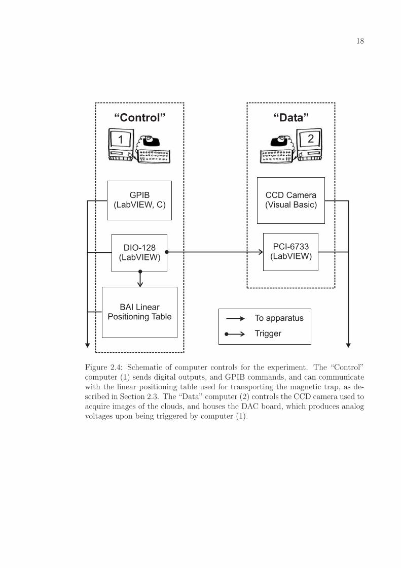
2.2 Computer Control
Computer controls for the experiment can be broken down into three cat-
egories: (i) control over 64 TTL (logic) bits, used for driving various pieces of
electronic equipment; (ii) GPIB control of frequency synthesizers and abitrary
waveform generators; and (iii) control of digital-to-analog converters (DACs), used
in a variety of ramp controls throughout the experiment. I will briefly describe
each type of control. An overview of the computer control for the experiment is
shown schematically in Fig. 2.4. For completeness I have included communication
with the linear positioning table that moves the transport coils (see Sect. 2.3),
and the CCD camera used for imaging the clouds.
2.2.1 Logic Control
To control the TTL’s necessary for the experiment, we use a single fast
timing board, the DIO-128, from Viewpoint Systems. This is the same timing
board used in the experiment described in Ref. [16]. Because of the importance of
this board in the experiment, I’ll discuss its operation in some detail. The DIO-128
board is capable of handling 64 digital lines of input and 64 digital outputs; as we
have only used the outputs, I will limit the discussion here to the board’s output
capabilities. The outputs are organized into four “ports,” consisting of 16 TTL
lines each. The maximum output frequency (defined as half the update rate, since
a high/low sequence is necessary for a square-wave cycle) is spec’d at ∼ 1100 kHz
for a single port, and 500 kHz when operating all four ports. In other words,
one can achieve µs switching with all lines running. Note that the board can be
daisy-chained with additional DIO-128 boards in the event that more lines are
18
“Control” “Data”
1 2
PCI-6733(LabVIEW)
DIO-128(LabVIEW)
GPIB(LabVIEW, C)
BAI LinearPositioning Table
CCD Camera(Visual Basic)
To apparatus
Trigger
Figure 2.4: Schematic of computer controls for the experiment. The “Control”computer (1) sends digital outputs, and GPIB commands, and can communicatewith the linear positioning table used for transporting the magnetic trap, as de-scribed in Section 2.3. The “Data” computer (2) controls the CCD camera used toacquire images of the clouds, and houses the DAC board, which produces analogvoltages upon being triggered by computer (1).

19
needed. In addition to providing more TTL lines, this could allow the production
of home-made digital-to-analog converters.
The maximum current sourced by the board is specified at only 15 mA per
line, meaning any instrument accepting a TTL should have greater than 333 Ω
input impedance. Since this is not the case for all of our instruments, and in order
to isolate electrical noise in the computer from the instruments, we optically isolate
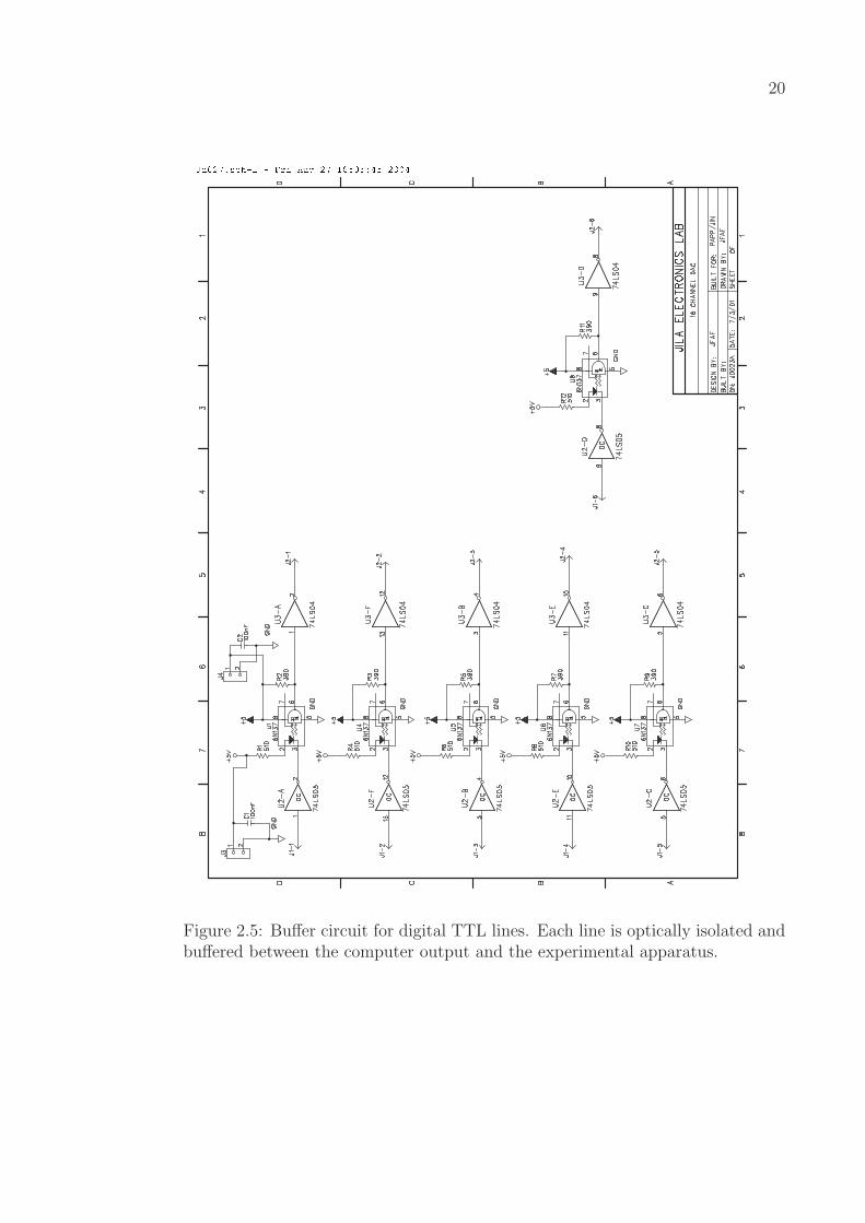
and buffer the outputs. The isolation circuit is shown in Fig.2.5.
The data describing a single experimental time-line are downloaded to the
DIO-128 first-in-first-out (FIFO) buffer. Upon receiving a software trigger (in our
case provided by LabVIEW code), the board begins outputting the experimental
sequence. The board can perform two concurrent types of task — the higher
priority task controls the digital outputs, and the lower priority task communicates
with the computer. Because of this prioritization, communication with the control
computer does not affect the performance of the experiment.
The data loaded to the FIFO buffer consist of six 16-bit words for each time
stamp — two words giving the time-stamp itself, and four words each describing
the state of one port at that time. That is, the state of all 16 lines comprising a
given port are encoded in a single 16-bit number. Only times when a bit is switched
are included in the buffer, so that holding a set of TTLs for an indefinitely long
time has no effect on the length of the buffer. The 32-bit time-stamp allows times
as large as (232 − 1) = 4294967295 in units of the resolution, or more than 72
minutes of µs timing.
2.2.2 GPIB Control
The GPIB control for the experiment has been limited to (i) real-time GPIB
control of the radio-frequency (rf)-synthesizer used for evaporation, and (ii) down-
loading of arbitrary waveforms to function generators for a variety of ramps and
20
Figure 2.5: Buffer circuit for digital TTL lines. Each line is optically isolated andbuffered between the computer output and the experimental apparatus.

21
modulations.
The evaporation is controlled by a dynamic link library (DLL) written in the
C language, and controlled by the same LabVIEW software that controls the DIO-
128 timing board. The evaporation “trajectory” consists of a set of times, powers,
frequencies, exponential decay time constants, and offsets (or “asymptotes”) used
to build a series of exponential frequency sweeps, as described in Ref. [16]. The
DLL waits 50 ms before updating the synthesizer. At 50 ms, the system clock is
polled and the time is used to calculate the correct frequency, and the frequency
and power (if the power is to be switched) commands are sent to the synthesizer.
We originally used the DLL to control the evaporation because the shot-to-shot
variation in timing with LabVIEW was as large as a few hundred milliseconds.
The downside of the DLL in its current form is that it completely takes over
the computer operating system while it runs. Although this doesn’t affect the
TTL timing, as described above, it does prevent real-time control of other GPIB
devices and makes it necessary to wait until completion of a running experiment
before modifying the next experimental timeline. We are currently working on
eliminating the timing problem from the LabVIEW control, which does not appear
to affect other experiments at JILA.
The remaining GPIB control is limited to downloading arbitrary waveforms
to Stanford Research Systems (SRS) DS-345 function generators. These devices
are capable of 16,300-point arbitrary waves, as well as a variety of built-in sweeps
and modulations with frequencies up to 30 MHz. We used these with GPIB
programming primarily for various ramp-and-hold applications before we acquired
a digital-to-analog converter (DAC) board. Since installation of the DAC board,
described in the next section, the DS-345s are used mostly for pulsed modulations,
for example to modulate the trapping potentials in the magnetic or optical traps,
or for the rf- and µ-wave sweeps (by frequency-mixing with the synthesizers) used

22
to transfer atoms into the appropriate magnetic sub-states for experiments with
Feshbach resonances.
2.2.3 Digital-to-Analog Converters
For arbitrary analog voltages, we use the PCI-6733 DAC board from Na-
tional Instruments. The PCI-6733 allows control of eight 16-bit analog voltages,
with up to 1 MS/s update rates for four channels. (As with the DIO-128 board,
there are inputs available that we don’t use, and will therefore be ignored here.)
The default voltage range is ±10 V, corresponding to a minimum voltage step of
∼ 300µV. If finer resolution is desired, an external reference voltage Vref can be
used to give selected channels a range of ±Vref corresponding to a voltage step size
of 2−15 × Vref . There are an additional eight digital I/O lines that can be either
added to the DIO-128 board or processed as homemade DACs, depending on the
needs of the experiment.
The data describing the desired DAC voltages as a function of time are
downloaded to the PCI-6733 buffer, and the board waits for a TTL trigger from
the DIO-128 board. One drawback to the DAC board is that a uniform time-
step is assumed, rather than using individual time-stamps like the DIO-128. This
means that fast timing required in one part of the buffer will enforce fast timing
everywhere, leading to very large buffer sizes. Since the buffer length is limited
to 214 = 16384 samples, this limits the total on-board signal length to less than
2 seconds for a 100 µs time step.2 To help overcome this problem we use
several separate buffers that are triggered serially. One could also use a simple
multiplexing circuit to use fast DAC buffers to generate ramps (for example) and
then switch over to constant voltages for long holds.
2 Actually the board can also be used for much longer waveforms by utilizing the computermemory. We have so far not seen a degradation in performance when running the board thisway.
23
2.3 Transport Coils
In this section I will describe the moving transport coils at the heart of our
experiment. This versatile coil set (i) provides the magnetic gradient potential
used in the MOT, (ii) provides the stronger quadrupole trap used during the
transport, and (iii) produces the nearly uniform B-field used to access magnetic-
field-tunable Feshbach resonances.
First I will describe the coil design and the circuits that control the coils.
These circuits provide stable currents from a few Amps all the way to the power-
supply limited value of 440 A.
I then discuss the actual motion of the coil set between cells. This type
of transfer was introduced at JILA in the lab next door to ours (see Ref. [16])
during the design stage of our experiment. We adopted this technology in our
experiment in order to obviate the need for a capture MOT in the science cell. The
system is simple to setup and essentially never requires readjustment, realignment,
re-optimization, or other forms of re-tweaking. We did, however, encounter a
potentially catastrophic flaw with the proprietary control software that will be
described.
2.3.1 Coil Design and Control Circuitry
The transport coils consist of a simple pair of identical solenoids, each three
layers deep axially, and five deep radially, wrapped from insulated hollow square
copper tubing. The 1/8-inch inner diameter of the tubing allows sufficient water
flow to cool the coils when running up to our highest currents (∼ 400 A, for a
few seconds). The inner diameter of the smallest turns is 7.4 cm, and the inner
distance between coils is 7.6 cm. The coils are mounted on a large anodized
aluminum “cart,” with slots cut through all mounting parts to inhibit large-scale

24
eddy currents.
The coil set operates as a quadrupole trap in anti-Helmholtz configuration
and produces a nearly uniform field in Helmholtz configuration.3 The magnetic
field component along the z-axis produced by a single coil of radius a at z = 0 is
given by [17]
Bz(z) =µ0 I
2
a2
(a2 + z2)3/2, (2.2)
where I is the current, and µ0 = 4π × 10−7 H/m = 1.257 G · cm/A is the per-
meability of free space. In Helmholtz configuration the field is therefore flat to
first order in z. From the requirement ∇ · ~B = 0 in free space, and using the x-y
symmetry of the system, we get a radial gradient in anti-Helmholtz configuration
that is half the strength of the axial gradient and opposite in sign. In other words,
the magnitude of the field near the center of the coils takes the form
| ~B | '
B0 , Helmholtz
β√
ρ2 + 4 z2 , anti-Helmholtz
, (2.3)
where ρ = (x2 + y2)1/2 is the radial distance, and z is measured from the center
of the coils. It is the field magnitude | ~B | which is proportional to the potential
acting on the atoms.
The axial magnetic field measured with a Gauss meter is shown for Helmholtz
(anti-Hemholtz) configuration in Fig. 2.6 (Fig. 2.7). The points are the measured
fields, and the solid lines are fits to a model assuming two sets of ideal coils (thirty
coils total). Since the coils are wound from hollow tubing, there is some ambi-
guity in the location of the current in the idealized coils. To accommodate this I
3 Throughout this thesis I will use “Helmholtz” (“Anti-Helmholtz”) configuration as a short-hand to refer to the case where the fields from the two coils add (subtract) at the centerpoint. This does not imply the B-field along the axial direction has a zero second derivative in“Helmholtz” configuration. This condition would require that the radius of the coils be equalto the distance between coils, which is not true for either magnetic trap in our system.
25
measured the inner and out radii a(±)i and coil positions z
(±)j , and included fitting
parameters ∆a,z that place the idealized coils within the real coils according to
aideali = a
(−)i + ∆a
[a
(+)i − a
(−)i
], i = 1, 2, 3, 4, 5
zidealj = z
(−)j + ∆z
[z
(+)j − z
(−)j
], j = 1, 2, 3 , (2.4)
with the constraints 0 ≤ ∆a,z ≤ 1 for the fits. The best fit to the Helmholtz
data gave ∆a,z ' 0.5, and the Anti-Helmholtz data gave ∆a ' 0.3 and ∆z ' 0.4.
The systematic uncertainty due to the inexact placement and angle of the flexible
Gauss meter probe was estimated to be an additional 2%, which is much larger
than the fit uncertainties. This gives a final B-field calibration of
B0 = 1.50± 0.03 G/A (Helmholtz)
2 β = 0.490± 0.010 G/cm/A (Anti-Helmholtz)
. (2.5)
We will see later, when we discuss our observation of Feshbach resonances, that
this bias field calibration is in reasonable agreement with calibrations from mi-
crowave and rf-sweeps of the atoms at different fields.
The control circuit for the transport coils is shown schematically in Fig. 2.8.
An H-type configuration of four MOSFETs is used to switch the current direction
of one of the coils (coil “B” in the figure), and another MOSFET acts as the master
switch for the circuit.4 The FETs are mounted onto liquid heat-exchanging plates
for cooling, and copper bus bars are used for connections between FETs, and to
connect to the 4/0 welding cable delivering the current from the power supply.
The power supply is an Agilent 6690A, capable of delivering 15 V and 440 A,
with an interlock set to trip when the flow of cooling water through the coils or
FETs becomes too low. The power supply voltage is controlled by the DAC board
described in Section 2.2.4 Physically, each FET in the schematic consists of a set of three APT10M07JVR (Advanced
Power Technologies) FETs in parallel. This improves the field stability by reducing the powerdissipated by each FET.

26
Figure 2.6: Measured axial field of the transport coils, running 200 A in Helmholtzconfiguration. The points were measured with a Gauss meter, and the line is a fitto a model described in the text.
27
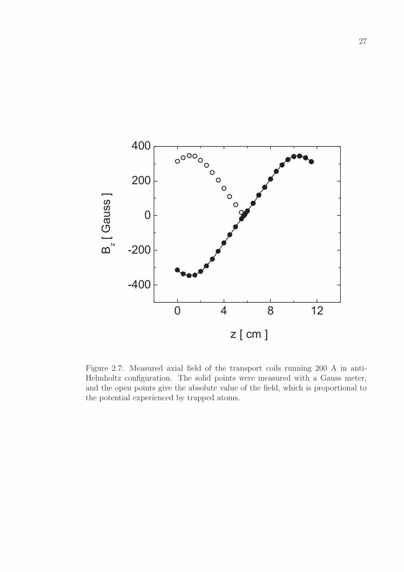
Figure 2.7: Measured axial field of the transport coils running 200 A in anti-Helmholtz configuration. The solid points were measured with a Gauss meter,and the open points give the absolute value of the field, which is proportional tothe potential experienced by trapped atoms.
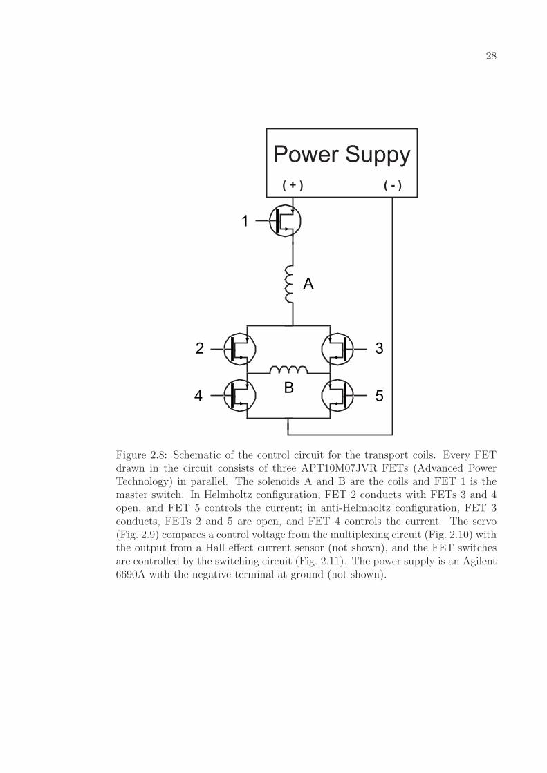
28
Power Suppy( + ) ( - )
1
2 3
4 5
A
B
Figure 2.8: Schematic of the control circuit for the transport coils. Every FETdrawn in the circuit consists of three APT10M07JVR FETs (Advanced PowerTechnology) in parallel. The solenoids A and B are the coils and FET 1 is themaster switch. In Helmholtz configuration, FET 2 conducts with FETs 3 and 4open, and FET 5 controls the current; in anti-Helmholtz configuration, FET 3conducts, FETs 2 and 5 are open, and FET 4 controls the current. The servo(Fig. 2.9) compares a control voltage from the multiplexing circuit (Fig. 2.10) withthe output from a Hall effect current sensor (not shown), and the FET switchesare controlled by the switching circuit (Fig. 2.11). The power supply is an Agilent6690A with the negative terminal at ground (not shown).
29
Active stabilization of the B-field is provided by the servo circuit shown in
Fig. 2.9. The current is monitored using an F. W. Bell CLN-500 Hall effect current
sensor. The multiplexing circuit in Fig. 2.10 allows us to switch the servo control
voltage between various (constant) set points, or a DAC control voltage for ramps
and modulations. The switching between Helmholtz and anti-Helmholtz current
configurations is achieved with the circuit shown in Fig. 2.11.
2.3.2 Cart Motion
The coil set described in the previous section is used to mechanically trans-
port atoms from a relatively high-pressure cell where the atomic sources reside to
a low-pressure cell with long lifetimes for evaporation and experiments [16]. The
total distance traveled by the coils is ∼ 81 cm, in a time of about 6 seconds. This
time is limited by the need to stop and move slowly across an anomalous magnetic
feature in our vacuum system near the science cell. We refer to this feature as the
magnetic “speed bump,” and find that we must move slowly across it in order to
avoid a severe loss of atoms.
We use a Parker-Daedal 406900XR series linear positioning table5 with an
Aerotech BM/BMS series brushless motor. The track is 900 mm long, with a
25 mm lead ballscrew, and is specified to have ±5.0 µm repeatability and to be
capable of traveling the whole stroke in 1.5 seconds. With the Aerotech motor,
the measured step size was 6.32± 0.08 µm. When testing the repeatability of the
positioning without re-zeroing the device between commands, I could observe no
variation in the final cart position using a dial indicator with 0.005 inch (12.7 µm)
markings. When re-zeroing between motion commands I observed better than 1/2
tick-mark (∼ 6 µm) repeatability, moving the cart at speeds of ∼ 6 to 60 cm/s.
5 Full part number: 406900XR-MS-D5H3L3C9M4E1B1R1P1, from which various featuresand specifications may be divined.

30
Figure 2.9: Servo circuit for B-field stabilization. The signal from a Hall effect fieldprobe is compared to a voltage set-point from the multiplex circuit in Fig. 2.10.

31
Figure 2.10: Multiplexing circuit. The circuit uses a three-bit digital input toswitch between eight possible control voltages for the servo circuit in Fig. 2.9.The input at J1 allows a variable voltage input, which is provided by the DACboard described in Section 2.2.3.

32
Figure 2.11: Switching circuit for the transport coils. The switching circuit feedsall of the FETs shown in the schematic in Fig. 2.8. This includes the masterswitch, the directional switches (Helmholtz to anti-Helmholtz), and the controlFETs.

33
We do not typically re-zero the cart unless there has been some failure (such as a
power outage) that leads us to doubt the accuracy of the current position.
The control for the cart motion is provided by a text-based series of com-
mands that are downloaded to the cart controller. The controller then waits for a
TTL input to trigger the motion (the controller allows three bits each of input and
output TTLs). An example of the velocity of the cart as a function of position
is shown in Fig. 2.12. When the cart is not in motion, the motor applies a stall
torque in order to maintain the position. We find that this creates electrical noise
which gets written onto the diode lasers. This is eliminated by “disabling” the
cart when not in motion, which turns off the stall torque. Since the motion of the
cart creates a lot of table vibration and acoustic noise, we further use a sample-
and-hold feature in our laser frequency stabilization servos to temporarily disable
the servo while the cart is in motion.6 Finally to protect against electro-magnetic
fields produced by the motor, we have the track oriented with the motor nearest
the collection cell, where we are much less sensitive to stray fields and radiated rf
than in the science cell.
Before leaving the discussion of the cart, I want to mention a potentially
catastrophic bug we uncovered in the proprietary software. The track has software
limit switches (the code will not let you send a motion command that would
surpass the limit) as well as hardware limit switches (a small magnet attached to
the cart passes over a sensor fixed onto the track). We found that if we tell the
cart to move to the exact location of the software limit, the cart will execute the
motion to the software limit, and then continue at full speed into the physical
end of the track. This represents a serious threat to anything in the path of the
cart.
6 Actually the Rb master laser can hold its lock during the cart motion, but we temporarilyunlock it anyway.

34
Figure 2.12: Example cart motion during the experiment. Data were obtainedby polling the cart controller for the position and velocity during the motion,and arrows indicate the time-order of the travel. The motion here is symmetricbetween cells, although it need not be in the experiment. The trajectory wecurrently use reaches three times the top speed of the data shown here.

35
2.4 Ioffe-Pritchard Trap
A well known limitation of the type of quadrupole magnetic trap described
above is that the magnetic field goes to zero at the center of the trap. This gives
the opportunity for an atom moving through the center to experience a so-called
Majorana spin flip (see, for example [18]), which may result in the atom being
lost from the trap. One solution to this problem is to transfer to a trap with
a non-zero bias field. Although the elegant TOP trap was the first home to an
atomic BEC [19], the celebrated Ioffe-Pritchard trap has been the workhorse of
the majority of BEC experiments throughout the last decade.
Since the magnetic transport allows us to forego the production of a second
two-species MOT in the science cell, we are able to use a very small (1 cm×1 cm)
cell, and correspondingly small Ioffe-Pritchard trap. The ability to place our
trapping coils so close to the atoms allows us to run with a current of only 27 A. In
this section I’ll describe the design and construction of the trap, the magnetic field
it produces, and the corresponding trapping frequencies for 87Rb and 40K atoms.
2.4.1 Trap Design
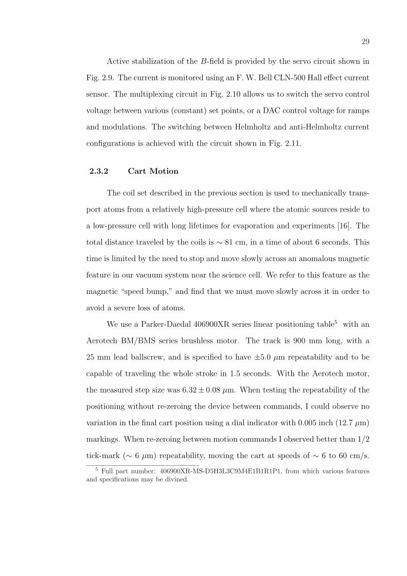
Our basic Ioffe-Pritchard trap design is shown schematically in Fig. 2.13.
The radial gradient field is produced by four identical coils, oriented with axes
along the x- and y-directions of the trap. The direction of flow of the current
is arranged so that the axial (z) component of the fields generated by each pair
cancel, leaving a pure radial gradient field. The axial confinement is produced by
a pair of “pinch” coils that produce the strong field curvature, and a larger pair
of “bias” coils which provide near-cancellation of the offset field at the center of
trap. As we’ll see below, smaller offset fields result in stronger radial confinement.
All coil forms are made from copper with internal channels for cooling wa-
36
Bias
Pinch
Radial
xz
y
8 c
m
6 cm
Figure 2.13: Schematic of the Ioffe-Pritchard trap. Not shown is an additionalpair of radial coils which slide over the glass cell (dark grey, center), perpendicularto the page. Coils are wrapped on water-cooled copper forms (light grey). Allforms are mounted on a phenolic cube (dashed lines). There are 4 + 5 turns oneach pinch coil, 2×8 turns for each bias coil, and 2×17 turns for each radial coil.

37
ter, slits to prevent eddy currents, and holes on axis for optical access. Coils
are wrapped from 19 AWG square magnet wire with Kapton insulation. Ther-
mal grease and vacuum-impregnated epoxy help maintain thermal conductance
between the two coil layers, and a thin copper shim is wrapped around the outer
layer and connected to the form to help cool the outer layer. All forms are mounted
on a phenolic cube. There are 4 + 5 turns on each pinch coil, 2× 8 turns for each
bias coil, and 2× 17 turns for each radial coil.
The current through the coils is actively stabilized with the same basic servo
circuit shown in Fig. 2.9. We additionally provide a “bleed” circuit that includes
a servo to shunt current away from the bias coils. This allows us to raise the
offset field at the center of the trap, which decompresses the trap in the radial
directions.
2.4.2 Trap Frequencies
As described above, a Ioffe-Pritchard trap is generically composed of a radial
gradient field superposed on an axial curvature field. A positive offset, or bias,
field at the center of the trap prevents atom losses from Majorana spin-flips. Here
we will focus on the properties of the magnetic field near the center of the trap,
where the atoms in cold gases typically reside. The interested reader may consult
Pritchard’s original paper [19] or the nice overview in Ref. [20] for more detailed
descriptions of the field.
Near the center of the trap the field is characterized by the bias field B0,
the radial gradient β = ∂xBx = −∂yBy, and the axial curvature γ = ∂2zBz/2.7
The field magnitude is given by [21]
∣∣∣ ~B∣∣∣ =
√[B0 + γ z2 − 1
2γ (x2 + y2)
]2
+ (β − γ z)2 x2 + (β + γ z)2 y2 .
7 Note that there is no consensus in the literature over whether “curvature” should denotethe second derivative of the field, or half as much.

38
The axial field is, to a good approximation, harmonic everywhere. The radial field
is harmonic near the center, and linear farther away. That is,
| ~B | '
B0 +1
2
(β2
B0
− γ
)ρ2 + γ z2 , ρ ¿ R0
β ρ + γ z2 , ρ À R0
, (2.6)
where ρ = (x2 + y2)1/2 is the radial distance from the axis, and R0 = 2 B20/( β2 −
γ B0) sets the length scale for the change.
At low fields the potential UIP an atom feels is given by µ| ~B |, where
µ = gF mF µB is the magnetic moment of an atom whose z-component of total
spin ~F is mF (gF is the Lande g-factor and µB the Bohr magneton). All of
the magnetic trapping discussed in this work involves alkali-metal atoms in their
so-called “stretched” states, which have magnetic moments equal to the Bohr
magneton. In other words UIP will be the same for 87Rb and 40K atoms in their
stretched states. We can then rewrite Eq.(2.6) in terms of the energy,
UIP '
µB0 +1
2m
(ω2
ρρ2 + ω2
zz2)
, kBT ¿ µB0
µβ ρ + 12mω2
z , kBT À µB0
, (2.7)
where the harmonic trapping frequencies for an atom of mass m are given by
ω2ρ =
µ
m
(β2
B0
− γ
)
ω2z = 2
µ
mγ . (2.8)
Note that (i) the axial frequency ωz is determined solely by the curvature
γ, (ii) changing B0 offers a simple way to independently adjust ωr, and (iii) the
product κ = mω2 is the same for each species if µ is the same. This last fact,
together with the properties of Boltzmann gases in harmonic potentials, allowed
us to replace R0 with kBT when we went from Eq.(2.6) to Eq.(2.7).
To measure the trap frequencies, we induce a small-amplitude center-of-
mass “sloshing” motion to very cold 87Rb clouds. The cloud then oscillates at

39
exactly the trap frequency. As an example, the calibration we performed during
our rethermalization measurements gave
ωρ = 2 π × 156.6± 0.4 Hz
ωz = 2 π × 25.01± 0.11 Hz , (2.9)
at an operating current of 27 A. Note that due to the mass difference between
species, the trapping frequencies for 40K are (87/40)1/2 ' 1.5 times higher. As-
suming a bias field of 1.4 Gauss (from measurements of the trap bottom using rf
sweeps), this implies B0 = 52 mG/A, β = 5.6 G/cm/A, and 2 γ = 14 G/cm2/A.
Finally, note that when trapping two species with very different masses it
becomes necessary to provide strong radial trapping in order to preserve overlap
between the two species. If we add gravity (in the y-direction) to Eq.(2.7) we
find the equilibrium vertical position y0 = −g/ω2r (measured from the center of
the IP trap). Since ω2r ∝ m, the different species experience a different vertical
trap center. As the clouds are cooled they become smaller and the spatial overlap
between clouds is reduced. This in turn inhibits the rethermalizing collisions
needed to drive the process of sympathetic cooling of the fermions. This point is
elaborated on in Sect. 3.3.2.
2.5 Laser Systems
2.5.1 Lasers, Lasers, and More Lasers
We use a total of three external-cavity diode lasers (ECDLs), three injected
(“slave”) lasers, and one semiconductor tapered-amplifier (TA) to produce all of
the laser light for the experiment, with the notable exception of the optical dipole
trap described in Sect. 2.5.3. The hyperfine frequency shift for a state with nuclear

40Element I Fg Ag Fe Ae Be
(Jg = 1/2) [MHz] (Je = 3/2) [MHz] [MHz]
87Rb 3/2 1, 2 3417.341 0–3 84.845 12.5239K 3/2 1, 2 230.859 0–3 6.06 2.8340K 4 7/2, 9/2 −285.731 5/2–11/2 −7.59 −3.541K 3/2 1, 2 127.007 0–3 3.40 3.34
Table 2.2: Hyperfine constants for 87Rb and the stable isotopes of K, afterRef. [22]. Subscripts g and e refer to the S1/2 ground and P3/2 excited states,respectively. Note the negative values of A and B for 40K, reflecting the inversionof its hyperfine structure, as shown in Fig. 2.14.
spin I and total electron spin J , is given by [22]8
∆νhf =1
2KAhf +
1
8
3 K(K + 1)− 4 I(I + 1) J(J + 1)
I(2I − 1) J(2J − 1)Bhf , (2.10)
where K ≡ F (F + 1) − I(I + 1) − J(J + 1), and the constants Ahf and Bhf
are determined empirically [23]. Values of Ahf and Bhf for 87Rb and the stable
isotopes of K are shown in Table 2.2. Energy level schematics calculated from
Eq.(2.10) are shown for 87Rb and 40K in Fig. 2.14. The saturated absorption
spectra used for locking the Rb and K lasers are shown in Figs. 2.16 and 2.17,
respectively.
Each species requires two frequencies of light for the MOT, one on a closed
cycling transition (“trap” light) which performs the bulk of the trapping and
cooling,9 and one for “repumping” atoms out of the lower-F ground state (i.e., the
ground state with lower F , not lower energy). Atoms can spontaneously decay into
the lower-F ground state after off-resonant excitation to other excited states by
the trap light. This is especially a problem in 40K MOTs, due to the small excited
state hyperfine splittings. We use the F = 2 → F ′ = 3 (9/2 → 11/2) transition for
8 Note that the corresponding equation (4.2) in Ref. [22] has a typographical error, so thatthe (2J − 1) term in the denominator reads (J − 1).
9 Actually, as discussed in Ref. [13], a 40K MOT can experience a non-negligible trappingforce from the repump light.

41
1286 MHz
102 MHz
767 nm
40
KI = 4
780 nm
2
P3/2
2
S1/2
87
RbI = 3/2
F’ = 3 (194)F’ = 5/2 (54.5)F’ = 7/2 (30.6)F’ = 9/2 (-2.3)F’ = 11/2 (-45.7)
F = 2 (2563)
F = 7/2 (463.1)
F = 9/2 (-822.7)
F = 1 (-4272)
F’ = 2 (-73)
F’ = 1 (-230)
F’ = 0 (-302)
6835 MHz
496 MHz
Figure 2.14: Energy level schematics for 87Rb and 40K. Numbers in parenthesesare the hyperfine frequency shifts in MHz. Here I is the nuclear spin, which isrelatively large in 40K, and aligned anti-parallel to the nuclear magnetic moment,giving rise to the inverted hyperfine structure [13]; F is the total spin. For com-parison the natural atomic linewidth of the D2 (S1/2 → P3/2) transition Γat is2π × 5.98 MHz for Rb and 2π × 6.09 MHz for K.
42
2P3/2
2S1/2
F = 2 (173.1)
F’ = 3 (14.3)F’ = 3 (8.5)
F’ = 5/2 (54.5)
F’ = 2 (-6.7)F’ = 2 (-5.1)
F’ = 7/2 (30.6)
F’ = 1 (-16.0)F’ = 1 (-8.5)
F’ = 9/2 (-2.3)
F’ = 0 (-19.2)F’ = 0 (-8.6)
F’ = 11/2 (-45.7)
F = 7/2 (588.7)
F = 2 (-140.0)
F = 1 (-394.0)
F = 9/2 (-697.1)
125.6 MHz
254.0 MHz
F = 1 (-288.6)
39K, = 3/2 (+)I
41K, = 3/2 (+)I
40K, = 4 (-)I
767 nm
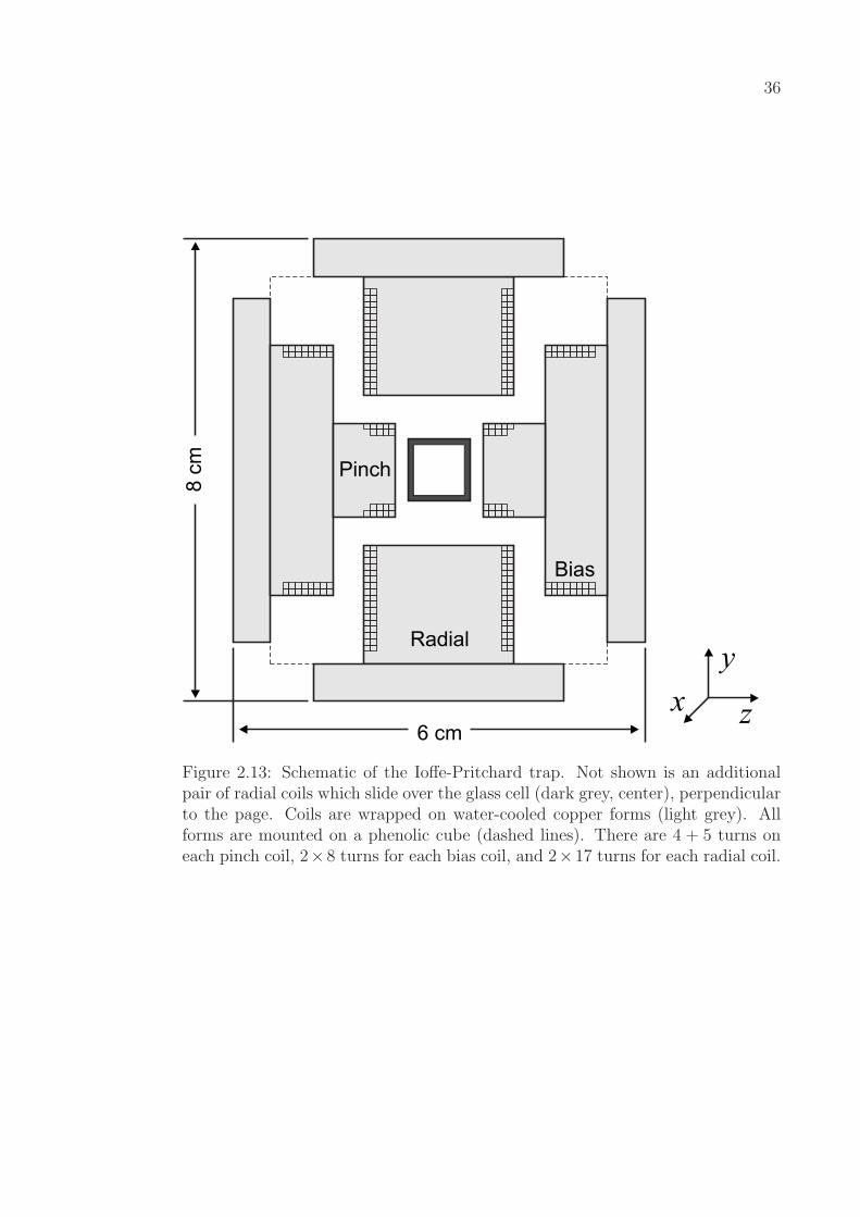
Figure 2.15: Energy level schematics for the stable K isotopes, after Ref. [24].Numbers in parentheses are the frequency shifts in MHz. The + (−) after Idenotes a nuclear spin parallel (anti-parallel) to the nuclear magnetic moment.The ground-state frequencies are referenced to 39K.

43
Figure 2.16: 87Rb saturated absorption spectroscopy. Only the F = 2 → F ′
manifold is shown. The laser is locked to the peak of the F ′ = 2, 3 crossover.
44
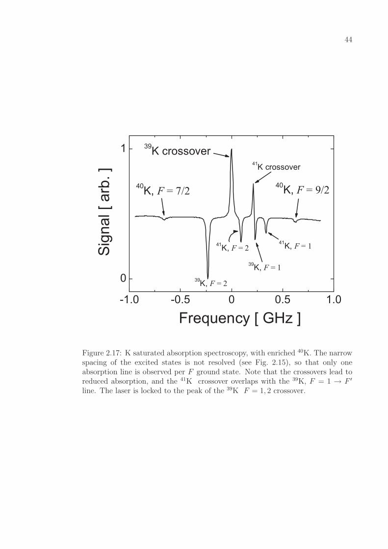
Figure 2.17: K saturated absorption spectroscopy, with enriched 40K. The narrowspacing of the excited states is not resolved (see Fig. 2.15), so that only oneabsorption line is observed per F ground state. Note that the crossovers lead toreduced absorption, and the 41K crossover overlaps with the 39K, F = 1 → F ′
line. The laser is locked to the peak of the 39K F = 1, 2 crossover.
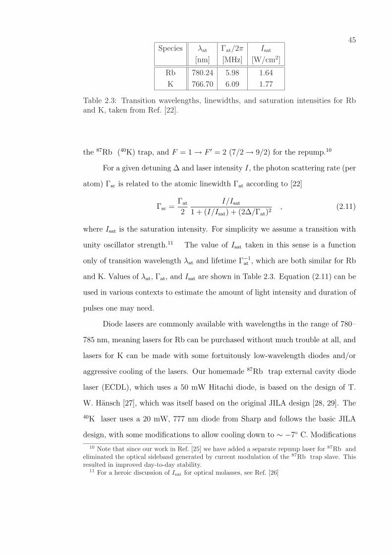
45Species λat Γat/2π Isat
[nm] [MHz] [W/cm2]
Rb 780.24 5.98 1.64
K 766.70 6.09 1.77
Table 2.3: Transition wavelengths, linewidths, and saturation intensities for Rband K, taken from Ref. [22].
the 87Rb (40K) trap, and F = 1 → F ′ = 2 (7/2 → 9/2) for the repump.10
For a given detuning ∆ and laser intensity I, the photon scattering rate (per
atom) Γsc is related to the atomic linewidth Γat according to [22]
Γsc =Γat
2
I/Isat
1 + (I/Isat) + (2∆/Γat)2, (2.11)
where Isat is the saturation intensity. For simplicity we assume a transition with
unity oscillator strength.11 The value of Isat taken in this sense is a function
only of transition wavelength λat and lifetime Γ−1at , which are both similar for Rb
and K. Values of λat, Γat, and Isat are shown in Table 2.3. Equation (2.11) can be
used in various contexts to estimate the amount of light intensity and duration of
pulses one may need.
Diode lasers are commonly available with wavelengths in the range of 780–
785 nm, meaning lasers for Rb can be purchased without much trouble at all, and
lasers for K can be made with some fortuitously low-wavelength diodes and/or
aggressive cooling of the lasers. Our homemade 87Rb trap external cavity diode
laser (ECDL), which uses a 50 mW Hitachi diode, is based on the design of T.
W. Hansch [27], which was itself based on the original JILA design [28, 29]. The
40K laser uses a 20 mW, 777 nm diode from Sharp and follows the basic JILA
design, with some modifications to allow cooling down to ∼ −7 C. Modifications
10 Note that since our work in Ref. [25] we have added a separate repump laser for 87Rb andeliminated the optical sideband generated by current modulation of the 87Rb trap slave. Thisresulted in improved day-to-day stability.
11 For a heroic discussion of Isat for optical molasses, see Ref. [26]

46
include enclosure in a sealed aluminum box to inhibit moisture build-up, the use of
smaller aluminum parts for lower thermal mass, a DC fan which flows air over the
fins on the heat sink, and vacuum-style feed-throughs which allow manipulation
of the collimation lens and grating without opening the laser. The 87Rb repump
ECDL is a Vortex laser from New Focus, which uses an anti-reflection (AR)-coated
diode and the Littman-Metcalf cavity design [30].
We additionally use three injection-locked (“slave”) diode lasers to provide
“pre-amplification” before injecting the tapered amplifier (TA), described below.
The 87Rb trap slave again uses a 50 mW Hitachi diode, as does the 40K trap
slave, which is cooled to −40 C with a combination of two thermo-electric coolers
(TECs) and a copper liquid heat exchange plate from Melcor. The housing for the
40K trap slave is again hermetically sealed to inhibit condensation on the laser and
collimating lens. The 40K repump slave uses a special diode from a batch of five
diodes purchased from Semiconductor Laser International. The diode operates
(at room temperature) at 768 nm, allowing us to avoid extravagant cooling.
All lasers are driven by JILA current drivers, and the current to each diode
passes through a diode protection circuit connected as close as possible to each
diode [13]. This circuit protects the diodes from reverse voltages and transient
spikes. For completeness some AOM configurations used in the experiment are
shown in Fig. 2.18, and a circuit to drive the voltage-controlled oscillators (VCOs)
and mixers for the AOMs is shown in Fig. 2.19.
2.5.2 Tapered Amplifier
One advantage of the 87Rb-40K system, which we pointed out in Ref. [25], is
the ability to use a single semiconductor tapered amplifier (TA) for all four colors
of light used in the two-species MOT. These devices easily achieve the 13 nm
(7 THz) optical bandwidth required, allowing us to produce a single beam with
47
f f2f 2f
f
AOM
n + dn
AOM
n
AOM
n - dn
n + dn
2dn
n
2n
l/4
mirror
Figure 2.18: Some AOM configurations used in the experiment. The direction ofthe AOM arrow reflects the direction of beam deflection for a positive frequencyshift. In the top “double-passed” configuration, which is the most common in theexperiment, a single AOM shifts the beam by a frequency ν in the first pass. Thebeam is retroreflected and shifted again, for a total frequency shift of 2ν. Althoughthis configuration typically produces less power at the desired frequency than asingle AOM, the output beam exhibits no steering as ν is tuned. In the lowerconfiguration, which is used only by the 87Rb repump ECDL, two AOMs runningat ν + δν and ν − δν are combined using a system of three lenses of focal lengthf in a way that gives a total shift of 2δν. This configuration allows us to quicklycontrol the output power of the laser with only a small frequency shift from thelock point at the peak of the F = 1 → F ′ = 2 transition.

48
1 1
2 2
AA
BB
0.1
u
C8
R2
100k
47u
C7
C8
0.1
u
100k
R7
47u
C10
40.2
kR6
40.2
kR3
1
2
3 4
LM
399
U3
-+
23
7
6
4
U10
LM
C6081
-+
23
7
6
4
LM
C6081
U12
S1
7.5
kR1
100
R8
R9
10k
R10
20k
-+
23
7
6
4LM
C6081
U15
R11
51
+C
6
10u
+
10u
C5
10n
C1
L1
10uH
100n
C2
10k
R15
- +
2 3
7
6
4
OP
27
U18
100k
R16
10k
R17
R12
10k
- +
2 3
7
6
4
OP
27
U7
100k
R13
10k
R14
1 2 3 45678
MA
X319
U17
R18
300
S1
1 2 3 45678
MA
X319
U2
+15V
+15V
+15V
+15V
-15V
+5V
+15V
+12V
+15V
-15V
-15V
+15V
-15V
-15V
+5V
-15V
+15V
+15V
+/-
15V
+/-
15V
Revis
ion:
Tw
o-C
hannel A
OM
Driver
1.0
11
Page
of
22 D
ecem
ber,
2001
J.G
. /
S.I
. /
T.B
.
JIL
A,
Univ
ers
ity o
f C
olo
rado -
- B
ould
er
Page S
ize:
ext. f
req.
in
freq.
out
IN
O
UT
CO
M
LM
7812
VC
O P
ow
er
Po
we
r F
ilte
r
atten.
oute
xt. f
req.
in
TT
L in
Figure 2.19: Circuit used for driving VCOs and mixers for AOMs. An analogswitch (MAX319) selects between two settings for power (“atten.”) and frequency.One pair of settings can further be manually switched between a potentiometeron the front panel and an input control voltage. The ±15 V power is filteredto block rf reflections from getting back onto the power supply. Not shown are0.1 µF capacitors connected to ground on the power to all the devices (see, forexample, the +15 V power on U10 and U12).

49
all of the light needed for the MOT. The spectrum of the injected TA is shown in
Fig.2.20. A detailed description of the use of such a device for multi-color injection
(up to 12 GHz) is given in Ref. [31]. The TA chip is purchased as a stand-alone
product from Toptica Photonics, and is installed in a homemade housing [13] and
driven by a homemade current driver. The device produces optical power up to
500 mW.12
The light injecting the TA must have a particular linear polarization for
amplification [13]. To combine 780 and 767 nm light, we use a combination of
polarizing beam-splitting (PBS) cubes and custom waveplates. The waveplates,
produced by Lens Optics, provide 27 12λ retardation at 780 nm, and 28 λ (i.e.,
none) at 767 nm. This allows us to combine 780 and 767 nm light with the same
polarization without losing power. To do this we combine the two colors using
orthogonal (linear) polarizations on a PBS cube. Then a waveplate after the cube
rotates the polarization of the 780 nm light in order to be the same as the 767 nm
light.
With a single beam output from the TA containing all the necessary fre-
quencies, we build a three-beam (retro-reflected) σ ⊥ σ MOT, where the two
species are simultaneously trapped and cooled. Typical values for the detunings
of the trap light and the intensities of the trap and repump light are shown in
Table 2.4. The beam geometry has one horizontal pair entering the cell transverse
to the axis of the transfer tube, and two pairs each at 45 to the table surface, in
a vertical plane through the axis (recall the collection cell heaters shown in Fig
2.3). We typically trap a few 109 87Rb atoms with 1 to 2× 10⁷ 40K atoms. The
MOTs are overlapped in space, although the physically smaller 40K MOT is not
perfectly centered on the 87Rb MOT.
12 New devices from Eagleyard Photonics appear to perform similarly, but are cheaper, andhave output powers greater than 1.5 W at 767 nm.

50
Figure 2.20: Spectral output of the injected tapered amplifier. These data weretaken on an Ando spectrum analyzer, with a resolution of 0.1 nm. The Rb and Kpeaks at 780 and 767 nm, respectively, are clearly visible, although the separatetrap and repump frequencies are not resolved. The amplified spontaneous emissionis suppressed by almost three orders of magnitude compared to the peaks.
87Rb 40K
−∆trap [MHz] 22 19
Itrap [mW/cm2] 50 26
Irep [mW/cm2] 2 6
Table 2.4: MOT light detunings and total peak intensities. Peak intensities donot account for losses on the collection cell and nearest optics, or the competitionbetween different frequencies in the TA when all colors are injecting it simultane-ously. The intensity at the atoms is estimated to be lower by no more than half.Using these numbers gives a lower limit on the number of atoms in the MOTscalculated from fluorescence of the atoms.

51
Before leaving the discussion of the TA chips, I should say something about
their lifetimes. Our first device, which had much higher amplification (100 to 200×gain) than its successors, lasted about 21 months from installation to death. We
believe the chip died with burn damage on the front facet. Evidence for this
included a comb-like structure in the spectral output, which we interpreted as
showing cavity modes arising from the increased reflection of the front facet due
to the burn. Also, the power in the amplified spontaneous emission (ASE) had
increased greatly, and when we imaged the facet with our CCD camera we could
see a shadow in the center of the output light. The next device survived only
four months after installation. This device worked fine until we went to lunch one
day. When we returned, the output power had dropped considerably and was too
low to make a MOT. Neighboring labs had experienced no electrical disturbances
during our time away from the lab, and Toptica was unable to determine what
happened after studying the device. The replacement device, which is currently
in use, has been running for 16 months. We always keep a backup device in the
lab.
2.5.3 Far Off-Resonance Optical Trap
Last, but not least, is the laser we use to form the far off-resonance optical
trap (FORT). We use a VersaDisk Yb:YAG laser from Elektronik Laser System,
capable of producing as much as 5.7 W of single-frequency light at 1030 nm.
Although we observe mode-hops due to temperature drifts of the laser cavity, the
output power remains stable. Since we do not actually require single-frequency
operation for our trap, we have not upgraded the cavity to a more stable design.
The laser itself resides in a closed box on its own breadboard beneath the
main optics table. The breadboard sits on a homemade steel I-beam table, with
large compressible hemispheres from Berg between the breadboard and table for

52
vibration isolation. The intensity of the YAG light is controlled with an 80 MHz
AOM, using the servo circuit shown in Fig. 2.21. The unshifted light is sent to
a power meter and Fabry-Perot spectrum analyzer for monitoring. The shifted
light is coupled into an optical fiber, using a fiber coupler from Oz Optics. We
typically run the system at powers of 1 W at the atoms (2 W out of the laser)
without any problems.
The fiber delivers the light for the optical trapping beam to the main ex-
perimental table. The optics which generate the trap reside on a small aluminum
breadboard that can be removed from the experiment for setup and testing pur-
poses. The optical setup is shown schematically in Fig. 2.22.
The installation of the FORT was performed as follows. On a breadboard in
a separate lab we set up and tested the optics with 1030 nm light, optimizing the
alignment and tilt of the lenses to minimize any astigmatism or other aberrations
in the beam profile. Measurements of the spot size as a function of position were
made with a CCD beam profiler, as shown in Fig. 2.23. The focal position (x, y,
and z) was then compared to that for resonant (767 or 780 nm) light, and the
difference was recorded. The FORT optics were then installed into the experiment
and aligned by eye onto the Ioffe-Pritchard trap. This alignment was good enough
to observe loss of magnetically trapped atoms when sending resonant laser light
into the science cell. Using resonant light, the optical alignment was then adjusted
for the strongest “kill” of the trapped atoms (using the translating lens and finely
adjustable mirror L3 and M2 in Fig. 2.22). After switching back to the far-detuned
YAG light, and making the previously determined adjustments to the lens and
mirror, we were able to load cold atoms into the FORT. Finally the lens and
mirror were tweaked again to optimize the number and temperature of the atoms
trapped in the FORT.

53
+
-PD sig (neg)
PD ground
Control Voltage
mixer
R7 D1
R5
R4
R2
R1
R3
C3
C2
C1
U1
R6
+
-U2
U = OP-27
U = OP-627
R = 1 k
R = 1.5 k
C = 4.7 nF
C = 470 pF
C = 100 nF
D = IN4148
1
2
1-6
7
1
2
3
1
W
W
YAG Intensity Servo
Design by: SIDrawn by: JG
Figure 2.21: YAG intensity servo. The laser power is observed on a photodiode(PD) after the atoms and stabilized with a mixer and AOM placed before the fiber.The circuit allows the control voltage to be derived from a knob on the front panelor an external input, for example a DAC signal (not shown). Also not shown isa MAX319 analog switch before R7 for switching between control voltages. Thediode D1 ensures the output is always positive. Since the mixer responds onlyto the magnitude of the current, fluctuations around zero when controlling lowpowers could otherwise lead to a 180 phase-shift in the servo loop.

54
FC
L1
M1 M2
L2
L3
FC: Oz Opticsangle-cut= 6.2
L : Melles-Griot
01LAO 037/077= 40, = 18
f
f
1
f
L : ThorLabs
AC508-200B= 50, 200
L : Melles-Griot
06LAI 015/08350, = 190
2
3
f
f =
f =
f
Figure 2.22: FORT optics schematic. The light from the YAG is coupled intothe experiment using an angle-cut fiber (FC). The angle-cut prevents intensityfluctuations from etalon effects. The lenses L1 and L2 form a simple telescope toexpand the beam, and L3 focuses the beam onto the position of the atoms. Theposition of L3 along the propagation direction is adjusted with a translation stagenot shown. The mirrors M1 and M2 use New Focus Ultima mirror mounts, andM2 has micrometer knobs for repeatable optimization and adjustment. All focallengths f and lens diameters φ are given in mm.
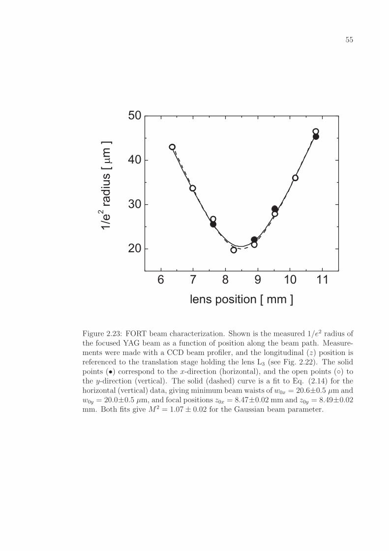
55
Figure 2.23: FORT beam characterization. Shown is the measured 1/e2 radius ofthe focused YAG beam as a function of position along the beam path. Measure-ments were made with a CCD beam profiler, and the longitudinal (z) position isreferenced to the translation stage holding the lens L3 (see Fig. 2.22). The solidpoints (•) correspond to the x-direction (horizontal), and the open points () tothe y-direction (vertical). The solid (dashed) curve is a fit to Eq. (2.14) for thehorizontal (vertical) data, giving minimum beam waists of w0x = 20.6±0.5 µm andw0y = 20.0±0.5 µm, and focal positions z0x = 8.47±0.02 mm and z0y = 8.49±0.02mm. Both fits give M2 = 1.07± 0.02 for the Gaussian beam parameter.

56
The FORT potential is related to the light intensity I(~x) by [32]
UFORT(~x) = −3 π c2
2 ω3at
Γat
(1
ωat − ω+
1
ωat + ω
)I(~x)
' 3 π c2
2 ω3at
Γat
∆I(~x) , (2.12)
where c is the speed of light in vacuum, ωat = 2π c/λat is the atomic resonance
frequency, and ω = 2π c/1030 nm is the FORT laser frequency. The second
equation holds for |∆| ¿ ω, where ∆ = ω − ωat is the detuning of the FORT
laser from the atomic resonance. Note that in our experiment ∆ < 0, so that the
potential is attractive.
Our FORT potential is derived from a single focused beam with a nearly
pure TEM00 mode (see Figs. 2.22 and 2.23). The intensity distribution for such a
beam is given by
I(~x) =P
π w2(z)exp
[−2
ρ2
w2(z)
], (2.13)
where P is the total power in the beam, ρ = (x2 + y2)1/2 is the radial distance
from the optical axis, and z is the distance along direction of propagation of the
beam. The 1/e2 beam radius varies along the beam path according to
w(z) = w0
√1 + M2
(z
zR
)2
, (2.14)
where M2 is the Gaussian beam parameter (M2 = 1 for an ideal Gaussian beam),
and zR = π w20/λFORT is the Rayleigh range for λFORT = 1030 nm. The measured
beam radius as a function of position was shown in Fig. 2.23, along with a fit to
Eq.(2.14) giving M2 = 1.07± 0.02, verifying the nearly ideal nature of the spatial
mode of the beam. The measurements in Fig. 2.23 suggest a waist w0 ∼ 20 µm,
which was the design goal for the optical system in Fig. 2.22.
Although the intensity distribution described by Eq.(2.13) is anharmonic,
we can Taylor expand around the beam focus for sufficiently small (that is, cold)
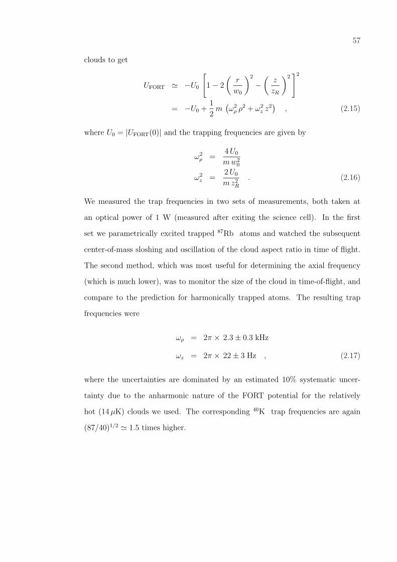
57
clouds to get
UFORT ' −U0
[1− 2
(r
w0
)2
−(
z
zR
)2]2
= −U0 +1
2m
(ω2
ρ ρ2 + ω2z z2
), (2.15)
where U0 = |UFORT(0)| and the trapping frequencies are given by
ω2ρ =
4 U0
mw20
ω2z =
2 U0
mz2R
. (2.16)
We measured the trap frequencies in two sets of measurements, both taken at
an optical power of 1 W (measured after exiting the science cell). In the first
set we parametrically excited trapped 87Rb atoms and watched the subsequent
center-of-mass sloshing and oscillation of the cloud aspect ratio in time of flight.
The second method, which was most useful for determining the axial frequency
(which is much lower), was to monitor the size of the cloud in time-of-flight, and
compare to the prediction for harmonically trapped atoms. The resulting trap
frequencies were
ωρ = 2π × 2.3± 0.3 kHz
ωz = 2π × 22± 3 Hz , (2.17)
where the uncertainties are dominated by an estimated 10% systematic uncer-
tainty due to the anharmonic nature of the FORT potential for the relatively
hot (14 µK) clouds we used. The corresponding 40K trap frequencies are again
(87/40)1/2 ' 1.5 times higher.

Chapter 3
Cooling to Quantum Degeneracy
In this chapter I will describe the various stages of trapping and cooling that
lead from a room temperature vapor of various Rb and K isotopes to a quantum
degenerate 87Rb -40K mixture at only a few tens of nanokelvin (recall Fig. 1.3).
The first stage of collection and cooling is provided by the two-species
magneto-optical trap (MOT). The MOT gets us all the way down to ∼ 150 µK,
which still amazes me, considering the relative simplicity of it all. I’ll describe var-
ious elements of the main challenge we have experienced with the MOT, namely
that our enriched 40K sources do not appear to provide independent control of
the K vapor pressure. Through the work of Kurt Miller and extensions by Josh
Zirbel here at JILA, I’ll describe a simple model of the expected source behavior,
and how to diagnose bad sources.
The MOT also gives rise to the first interactions between 87Rb and 40K in
our experiment. Light-assisted inelastic collisions lead to a depletion of roughly
half of our trapped 40K atoms when 87Rb atoms are introduced into the MOT.
I’ll present our observation of these losses and compare to a previous measurement
performed in another lab using 85Rb and 39K.
From the MOT we transfer the atoms into a purely magnetic quadrupole
potential, which moves on a translation stage to a higher vacuum cell. I will
briefly describe the preparation of atoms before their transfer to the quadrupole
59
trap (compression, cooling, and optical pumping).
Atoms are finally loaded from the quadrupole trap into the Ioffe-Pritchard
trap for the final stage of cooling. I’ll describe how we can directly cool 87Rb atoms
via forced rf evaporation without evaporating the 40K atoms. This allows us to
efficiently cool the 40K atoms sympathetically by virtue of their thermal contact
with the 87Rb gas. In addition to discussing the efficiency of the evaporation, and
our characterization of the quantum degeneracy of the bosons and fermions, I’ll
discuss the temperature dependence of the 87Rb -40K elastic collision cross-section
and some possible limits to the sympathetic cooling process.
3.1 Two-Species Magneto-Optical Trap
In this section I will describe the construction and operation of the two-
species magneto-optical trap (MOT) used in the initial trapping and cooling stage
of the experiment. The MOT is perhaps the only part of a sympathetic cooling
experiment that is any more complex than a comparable single-species experiment.
Specifically, the need for lasers and optics is essentially doubled, which has led in
our lab to an optical table so dense with components that many visitors express
some shock at the apparent complexity of it all. This is in fact why we have
adopted the magnetic transport design developed in Ref. [16], which eliminates
the need for a second MOT and the near-doubling of the numbers of optics and
lasers that would imply.
3.1.1 Atomic Sources and Vapor Pressures
I would like to first discuss the use of alkali metal dispensers for the two-
species MOT. In particular I will address the competition between the 87Rb and
40K vapor pressures and the consequences for the numbers of atoms that are
loaded into the MOT. The discussion here is derived (to my knowledge) from a
60
conceptual picture developed by Kurt Miller [33], and adapted to the two-species
case by Josh Zirbel. Because of the problems we have had in our experiment, I
consider this discussion important to those wishing to build similar apparatuses.
We first consider the behavior of a single-species 87Rb MOT. For simplicity
we ignore the effects of density-dependent losses. In this case loading of atoms
into the MOT obeys [34]
d
dtN(t) = L− Γ N(t) , (3.1)
where N is the number of trapped atoms, L is the loading rate of atoms into the
MOT, and Γ is the loss rate of atoms from the MOT. The MOT loading rate is
proportional to the pressure PRb of 87Rb atoms. The MOT loss rate Γ is given
by [35]
Γ = ΓRb + Γbg , (3.2)
where ΓRb is the loss rate due to collisions with 87Rb atoms, and Γbg is due
to collisions with “background” atoms (i.e., everything else). It is important to
note that, like L, ΓRb is proportional to PRb. Likewise Γbg is proportional to the
background pressure Pbg.
It is useful to make the dependence on pressures explicit. To that end we
define the reduced quantities l = L/PRb, γRb = ΓRb/PRb, and γbg = Γbg/Pbg.
Then Eq.(3.1) becomes
d
dtN = l PRb − (γRb PRb + γbg Pbg) N , (3.3)
which yields the solution
N(t) = N0
(1− e−Γ t
), (3.4)
where the MOT loss rate Γ is written in reduced form
Γ = γRb PRb + γbg Pbg , (3.5)

61
and the equilibrium MOT number N0 is given by
N0 =L
ΓRb + Γbg
=l PRb
γRb PRb + γbg Pbg
. (3.6)
In the limit PRb À Pbg, the steady-state MOT number is independent of the
87Rb vapor pressure. This number represents the maximum number of atoms
that could conceivably be trapped in the MOT, given by
Nmax =l
γRb
. (3.7)
The limit Nmax is generally a function of parameters like beam size and intensity,
detunings, and the B-field gradient, as well as the 87Rb-87Rb scattering cross-
section and the natural abundance of 87Rb. According to Eq.(3.6), N0 is equal to
half of Nmax when PRb = (γbg/γRb) Pbg. This condition represents the boundary
between background- and 87Rb-dominated operation of the MOT.
Kurt’s main contribution to our understanding of the MOT behavior begins
with considering a plot of N0 Γ as a function of Γ. Such a plot is shown schemat-
ically in Fig. 3.1. The values of N0 and Γ are determined experimentally from
fitting the time-dependence of the MOT fluorescence to Eq.(3.4) during a filling
sequence. At first it may seem that a plot of N0 Γ versus Γ just yields a line
through zero with slope N0, but it is important to remember that we are varying
Γ here only by increasing PRb and keeping Pbg fixed. Because there is still some
background pressure in the absence of Rb, the MOT number N0 extrapolates to
zero where Γ = Γbg 6= 0. The y-intercept can therefore be used to determine the
point PRb = Pbg where the 87Rb vapor pressure is exactly equal to the background
pressure. Similarly the slope of the curve is given by
d
d Γ(N0 Γ) =
(d Γ
dPRb
)−1d
dPRb
(N0 Γ)
=l
γRb
. (3.8)
62
The slope therefore gives the maximum number of atoms that could be trapped
by the MOT Nmax, given by Eq.(3.7). This simple plot contains some important
information on the vacuum system and MOT performance.
We now extend our discussion to the two-species case. The goal is to know
how many 87Rb or 40K atoms could be trapped in a single-species MOT with
both species present in the vacuum system. When considering the behavior of
one MOT, the other species can be considered a part of the background gas Pbg.
For concreteness let’s consider the loading rate and equilibrium number of atoms
for a 40K MOT with 87Rb also present in the vacuum chamber. If there is
independent control of the 40K pressure PK, then changing PK just reproduces
the results for the single-species MOT in Fig. 3.1. However if we increase PRb
(keeping PK constant), we expect to move out horizontally from the y-axis. The
expected behavior is shown schematically in Fig. 3.2.
We now turn to some data from our experiment. In Fig. 3.3, we see the
response of the single-species MOTs to the Rb dispenser. The parameters Γ and
N0 are obtained from fitting a series of MOT fills to Eq.(3.4). The 87Rb data give
NRbmax = 5.08 ± 0.11 × 10⁹, where the uncertainty is from the fit only. Referring
back to Fig. 3.2, we see that the positive slope for the 40K data reflects the lack
of independent control of PRb and PK in our system. To be exact, the data here
give NKmax = 1.44 ± 0.03 × 10⁷, while only firing the Rb dispenser! Although
this is ∼ 300 times smaller than NRbmax, it corresponds roughly to the number of
40K atoms we actually do capture in the MOT. We interpret this as being due to
the presence of 40K atoms adsorbed onto the Rb dispenser or the nearby glass.
Firing the dispenser heats the area, releasing 40K back into the system.
In Fig. 3.4, we perform a similar series of measurements, this time firing the
K dispenser. The first thing to note is that the value obtained for NKmax is about the
same as in Fig. 3.3. This again suggests that our K dispensers are malfunctioning,

63
Figure 3.1: Schematic of MOT loading rate with increasing alkali-metal vaporpressure for a single-species 87Rb MOT, after Ref. [33]. The solid line showsthe expected behavior of N0Γ as a function of Γ as the 87Rb vapor pressure isincreased. The line extrapolates to N0Γ = 0 when the 87Rb pressure goes tozero, leaving only the vacuum background pressure Pbg. The slope of the linegives the maximum number that could be trapped in the MOT Nmax, definedin Eq.(3.7). The boundary between background pressure dominated operationand vapor pressure dominated is defined by the condition ΓRb = Γbg, and can bedetermined from the y-intercept.

64
Figure 3.2: MOT loading rate with increasing 40K vapor pressure for a single-species 40K MOT in the presence of 87Rb. The solid grey dot represents theinitial condition, at time t = 0. If only the 40K pressure PK is increased, thenthe behavior from Fig. 3.1 is reproduced. If on the other hand PK is kept fixedand PRb is increased, then the system moves horizontally on this plot. A lack ofindependent control over the pressures results in a line with reduced slope. Thiscan be identified in the experiment if the y-intercept becomes positive.
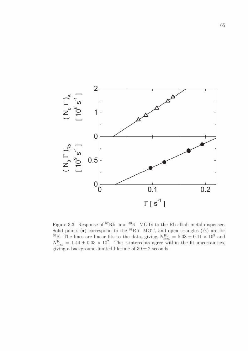
65
Figure 3.3: Response of 87Rb and 40K MOTs to the Rb alkali metal dispenser.Solid points (•) correspond to the 87Rb MOT, and open triangles (4) are for40K. The lines are linear fits to the data, giving NRb
max = 5.08 ± 0.11 × 10⁹ andNK
max = 1.44 ± 0.03 × 10⁷. The x-intercepts agree within the fit uncertainties,giving a background-limited lifetime of 39± 2 seconds.

66
since they provide no more trapped 40K than the Rb dispenser. Furthermore,
the value of NRbmax obtained here is almost 80% of the previous, suggesting that
the K dispenser is releasing significant amounts of 87Rb into the system. Since
performing the experiments described in this thesis, we have opened the vacuum
system and replaced the alkali sources. Future work will include characterizing the
new sources as described here and developing some workable level of independent
control over the 87Rb and 40K vapor pressures.
3.1.2 Light-Assisted Collisions and Losses
In the previous section we considered the behavior of the single-species
MOTs with respect to the atomic sources we use. In this section I would like
to briefly turn our attention to the operation of the two-species MOT. In partic-
ular I will discuss our observation of light-assisted loss processes that reduce the
number of atoms that can be trapped. This loss represents the first instance of
cross-species interactions in our experiment, and is intimately related to the vari-
ety of 87Rb -40K molecular states that can contribute to cold collisions between
species.
The effects of inelastic collisions between species are shown in Fig. 3.5. The
number of 40K atoms as a function of time is determined through fluorescence
imaging in the collection cell, using a narrow-band interference filter from CVI.
This filter has a transmission of ∼ 0.5 at 767 nm, with an optical depth of 4
(i.e., transmission of e−4) outside of its 3 nm bandwidth. We take a sequence
of images by strobing the camera during the MOT fill, beginning with a single-
species 40K MOT, and then introducing 87Rb. As the 87Rb MOT fills, there is
a corresponding depletion of the 40K MOT number to about 55% of the single-
species value, due to light-assisted collisions. For these data, the single-species
40K loading rate N0 Γ = 4 × 10⁶ sec−1, and the depletion rate is about half as
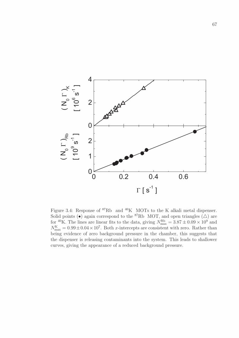
67
Figure 3.4: Response of 87Rb and 40K MOTs to the K alkali metal dispenser.Solid points (•) again correspond to the 87Rb MOT, and open triangles (4) arefor 40K. The lines are linear fits to the data, giving NRb
max = 3.87± 0.09× 10⁹ andNK
max = 0.99±0.04×10⁷. Both x-intercepts are consistent with zero. Rather thanbeing evidence of zero background pressure in the chamber, this suggests thatthe dispenser is releasing contaminants into the system. This leads to shallowercurves, giving the appearance of a reduced background pressure.
68
much.
Gallagher and Pritchard [36] first realized that the low temperatures ob-
tained in MOTs made it necessary to consider slow, long-range collisions, in the
sense that hyperfine interactions and spontaneous decay from excited molecular
states can occur during the time the atoms interact. Although their original work
considered a single-species MOT, the same basic physical principles apply for het-
eronuclear collisions. In fact a whole literature of two-species experimental results
has been obtained by the group of V. S. Bagnato in Sao Paulo, Brazil, in addition
to work at the Universities of Connecticut and Wisconsin. An excellent summary
of both the theoretical and experimental work on this subject is given in Ref. [37].
Returning to our discussion in the previous section, we should modify Eq.(3.1)
to include such loss processes in our expression for the MOT fill. Since our number
of trapped 40K atoms is relatively small, we can neglect 40K-40K losses and focus
on the loss induced by 87Rb atoms. Following the Brazilian group’s work with a
85Rb -39K MOT [38], we write
d
dtNK = L− Γ NK − β′
∫d3xnK(~x) nRb(~x) , (3.9)
where L and Γ should be interpreted as the loading and loss rates for a single-
species 40K MOT, n(~x) is the density of each species, and β′ is the loss-rate
coefficient. The data in Fig. 3.5 suggest a loss-rate coefficient of
β′ = 6± 3× 10⁻¹¹ cm3/s , (3.10)
where the uncertainty is dominated by the uncertainty in the atom numbers. This
value is similar to the 85Rb -39K value reported in Ref. [38] for similar beam inten-
sities. In principle the relative importance of various competing loss mechanisms
can be determined by varying the laser intensities and detunings. We decided
early in the experiment, however, that the loss of half of our 40K atoms from the

69
Figure 3.5: Observation of light-assisted losses of 40K in the two-species MOT, aspresented in Ref. [25]. The MOT number is determined from fluorescence imagesof the cloud, with a narrow-band filter providing an optical depth of ∼ 4 for Rblight. Each point is the average of nine consecutive runs of the experiment, andthe error bar is the standard error. The solid line is a fit to exponential fill or decayin each region (II-IV). In region I (t ≤ 0) the 87Rb light is locked off-resonance,and the B-field is turned off, in order to allow a calibration of the light levels forthe fluorescence; in region II (0 ≤ t < 25 sec) the 87Rb light remains off-resonanceand the B-field is turned on, allowing a fill of the single-species 40K MOT; inregion III (25 ≤ t < 35 sec) the 87Rb MOT is allowed to fill, and the subsequentcollisional losses deplete the number of 40K atoms; region IV (35 ≤ t < 50 sec)sees a return to the single-species MOT, and in region V (t ≥ 50 sec) the B-fieldis off and the 87Rb light is again off-resonance.
70
two-species MOT is acceptable. As we will see later in this chapter, sympathetic
cooling places less stringent requirements on the number of 40K atoms we load
into the magnetic trap than if the atoms were being evaporated directly.
3.2 Compressing, Cooling, Pumping, and Loading
After collection and cooling in the two-species MOT, atoms are loaded into
a strong quadrupole magnetic trap, generated by a coil pair mounted on a moving
translation stage, as described in Section 2.3. In this section I’ll describe the
transfer into the quadrupole trap, which involves compressing the 87Rb cloud,
cooling the 40K cloud, and optically pumping both clouds. With atoms loaded into
the quadrupole transfer trap we will then be in a position to begin sympathetically
cooling our fermions towards quantum degeneracy.
The first challenge in the transfer sequence is to load a spatially large
87Rb MOT into the quadrupole transport trap (“QT trap”). If the cloud is
too large the atoms will pick up excess potential energy in the tightly confining
QT trap, and that energy will result in an increased temperature after rethermal-
ization. The 87Rb MOT is large due to the strong radiation trapping [39]. Ways
to address this problem include transiently increasing the magnetic field gradient,
adjusting the intensity and detuning of the trapping and repumping light, or any
combination of the above [40]. Another solution is the so-called dark-spot MOT
[41], where the repumping light is blocked from the center of the cloud so that
atoms trapped there stop absorbing and emitting photons. In our case we use
what may be the simplest possible compression scheme — we reduce the repump-
ing light intensity for 50 ms before releasing from the MOT. The time scale, to
which the compression is not very sensitive, is long enough to let the atoms go
“dark” to the trap light and short enough to avoid any significant losses from the
MOT. We refer to this compressed MOT stage as the CMOT, and I stress that

71
we perform the CMOT only for the 87Rb atoms, by reducing the power of the
87Rb repump light injecting the tapered amplifier.
The 40K MOT, which has ∼ 100 times fewer atoms, is already roughly
the size of the 87Rb CMOT. We can still try to reduce the temperature of the
40K cloud in the QT trap by optically cooling the atoms before loading. If we
quickly jump the 40K trap light frequency towards resonance before releasing from
the MOT, we observe a pronounced (∼ 3×) increase in the number of 40K atoms.
We show in Fig. 3.6 an example of the dependence of the 40K number at the
end of the sympathetic cooling cycle on the detuning of the cooling light.1 Since
the MOT number is roughly unchanged by the jump (and the steady-state MOT
number is reduced at the jump frequency), we attribute this increase in number
to begin due to improved Doppler cooling of the 40K atoms. This reduces losses
associated with adsorption of atoms onto the walls of the transfer tube and science
cell. As with the CMOT, the cooling is not very sensitive to the duration of the
cooling stage as long as it’s greater than ∼ 10 ms (we use 50 ms, as with the
CMOT).
With our 87Rb atoms compressed, and our 40K atoms cooled, there is still
some optical pumping to be done before loading into the QT trap. Our goal is to
load the 87Rb |F = 2,mF = 2 〉 and 40K | 9/2, 9/2 〉 states into the Ioffe-Pritchard
trap for evaporative cooling. These states have the strongest confinement in the
magnetic trap, and their combination is immune to spin-exchange collisions. The
CMOT, by design, puts 87Rb atoms into some uncontrolled mixture of the F = 1
ground states; it is not known what states the 40K atoms populate after the cooling
stage. To optically pump the atoms, we release them from the CMOT/cooling
stage and apply a few-Gauss bias field to provide a quantization axis. We then
1 Due to the relatively low atom numbers, our 40K clouds are too dilute to image withabsorption imaging until nearly the end of the evaporation sequence.

72
Figure 3.6: Effect of Doppler cooling of 40K atoms before loading the QT trap.The number of 40K atoms at the end of the evaporation sequence is shown as afunction of the trap AOM frequency during the cooling stage. The AOM shiftsthe frequency towards the blue in a single pass. The arrow at 259 MHz indicatesthe MOT detuning. The resonance frequency (at zero field) corresponds to 278MHz.
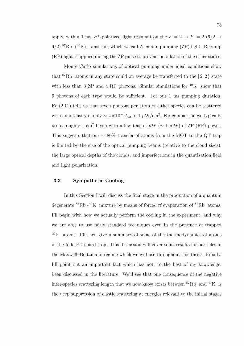
73
apply, within 1 ms, σ+-polarized light resonant on the F = 2 → F ′ = 2 (9/2 →9/2) 87Rb (40K) transition, which we call Zeemann pumping (ZP) light. Repump
(RP) light is applied during the ZP pulse to prevent population of the other states.
Monte Carlo simulations of optical pumping under ideal conditions show
that 87Rb atoms in any state could on average be transferred to the | 2, 2 〉 state
with less than 3 ZP and 4 RP photons. Similar simulations for 40K show that
6 photons of each type would be sufficient. For our 1 ms pumping duration,
Eq.(2.11) tells us that seven photons per atom of either species can be scattered
with an intensity of only ∼ 4×10⁻⁴Isat < 1 µW/cm2. For comparison we typically
use a roughly 1 cm2 beam with a few tens of µW (∼ 1 mW) of ZP (RP) power.
This suggests that our ∼ 80% transfer of atoms from the MOT to the QT trap
is limited by the size of the optical pumping beams (relative to the cloud sizes),
the large optical depths of the clouds, and imperfections in the quantization field
and light polarization.
3.3 Sympathetic Cooling
In this Section I will discuss the final stage in the production of a quantum
degenerate 87Rb -40K mixture by means of forced rf evaporation of 87Rb atoms.
I’ll begin with how we actually perform the cooling in the experiment, and why
we are able to use fairly standard techniques even in the presence of trapped
40K atoms. I’ll then give a summary of some of the thermodynamics of atoms
in the Ioffe-Pritchard trap. This discussion will cover some results for particles in
the Maxwell–Boltzmann regime which we will use throughout this thesis. Finally,
I’ll point out an important fact which has not, to the best of my knowledge,
been discussed in the literature. We’ll see that one consequence of the negative
inter-species scattering length that we now know exists between 87Rb and 40K is
the deep suppression of elastic scattering at energies relevant to the initial stages

74
of our evaporation. This may have important ramifications for the design and
construction of new 87Rb -40K experiments.
3.3.1 Experiment: Evaporation “Trajectories”
To evaporatively cool the 87Rb gas, we selectively remove high-energy
atoms from the cloud, thereby lowering the mean energy per particle. Subse-
quent collisions rethermalize the gas to a lower temperature, and in the presence
of 87Rb -40K collisions the 40K atoms are cooled as well. The term “selectively”
must be taken here to mean (i) selecting specifically high-energy atoms, as well
as (ii) evaporating only 87Rb atoms, and leaving high-energy 40K atoms alone.
The criterion (i) is satisfied by exploiting resonant spin-flipping transi-
tions to anti-trapped states in the spatially-dependent magnetic field of the Ioffe-
Pritchard (IP) trap. Atoms with higher energies are more likely to reach locations
of higher potential (proportional to | ~BIP(~x)|), and can be selectively removed with
resonant spin-flips at the higher field.
Due to the relatively large nuclear spin for 40K (I = 4) there are more total
spin states than for 87Rb (I = 3/2). This is shown schematically in Fig. 3.7 for
the experimentally relevant F = 2 states of 87Rb and F = 9/2 states of 40K. We
can now see a way to satisfy criterion (ii) during the cooling. Since the energy
splittings are different for 87Rb and 40K (the 40K splittings are 4/9 the size of the
87Rb splittings), the 87Rb |F = 2,mF = 2 〉 and 40K | 9/2, 9/2 〉 states will satisfy
the resonance condition for spin-flips at very different fields. Equivalently, for a
given spin-flip frequency a 40K atom must have 9/4 the energy of a 87Rb atom
in order to be transferred out of the trap.
Our primary diagnostic in evaluating the performance of the evaporation is

75
mF
+ 2
+ 1
0
- 1
- 2
+ 9/2
.
.
.
- 9/2
UIP
x
UIP
x
Figure 3.7: Zeemann sublevels of 87Rb (left) and 40K (right) in a harmonicmagnetic potential. Clouds in the stretched states (|F = 2, mF = 2〉 for 87Rb and|9/2, 9/2〉 for 40K) are shown schematically as the dark solid regions, which havethe same energies for Boltzmann distributions in thermal equilibrium. The arrows(l) designate the rf photon, which drives a Zeemann transition in 87Rb, and leavesthe 40K cloud unaffected.

76
the evaporation efficiency parameter α defined by [42]
αev =d ln T
d ln N, (3.11)
where N is the number of 87Rb atoms, T is the temperature of the gas in Kelvin,
and we assume the distribution is never far from equilibrium. An example of the
dependence of N on T is shown for 87Rb evaporation in the absence of 40K atoms
in Fig. 3.8.
The goal in the experiment is to achieve runaway evaporation, where the
mean rate of rethermalizing elastic collisions rapidly increases as the temperature
decreases. In other words,
d ln Γcoll
d ln T< 0 , (3.12)
where Γcoll is the mean rate of elastic collisions in Hz. We will see later that Γcoll
is proportional to N/T in a harmonic trap. Then using T ∝ Nαev we have the
critical value of αevap for runaway evaporation
αcrit = 1 . (3.13)
Note that we have neglected losses due to collisions with background atoms and
inelastic density-dependent losses, which make αcrit slightly greater than 1 in the
experiment. Our good evaporation conditions correspond to αev ∼ 1.2 to 1.4.
A full diagnostic of the two-species evaporation is not available to us due to
the low optical density of 40K atoms during the early stages of evaporation. The
highest temperature 40K cloud we have imaged out of the IP trap is only ∼ 10 µK,
which is well over an order of magnitude colder than our initial 87Rb load. Looking
at the 87Rb cloud over the whole range of evaporation we can see no significant
change in the evaporation with 40K atoms present until at or near the Bose-
Einstein condensate phase transition. This is consistent with the sympathetic

77
Figure 3.8: Single-species 87Rb evaporation trajectory. The solid points show thenumber of atoms at each temperature during the evaporation, and the solid line isa fit to Eq.(3.11), giving αev = 1.218±0.013 (more recent results give an improvedαev = 1.35± 0.06). The dashed line is the expected BEC transition temperaturefor an ideal gas (data with BEC are not shown). The 87Rb trapping frequencieswere ωρ = 2π × 112 Hz and ωz = 2π × 27 Hz.

78
cooling model in Ref. [43], considering our relatively low 40K number. Near
the BEC transition there is some enhanced loss of both species, probably due
to ordinary 2- and 3-body inelastic losses accompanying the sharp increase in
87Rb density. An example of the 87Rb and 40K numbers during the last stage
of evaporation is shown in Fig. 3.9. The apparent delay between the onset of the
40K loss and the formation of the condensate is believed to be due to the 100-
200 ms hold before the image, allowing a small condensate to form at relatively
high density and then “melt” before imaging. This would be consistent with
the calculated BEC transition temperature for 3× 10⁶ atoms of Tc ' 500 nK, as
shown in the figure. By assuming either purely 2- or 3-body losses we can estimate
upper limits for the corresponding inelastic rate constants. Using the 1/e decay
time for 40K of 2.4± 0.5 s from the data we obtain KRbK = 4× 10⁻¹⁵ cm3/s and
KRbRbK = 3 × 10⁻²⁹ cm6/s. These numbers are in rough agreement with other
measurements we have performed of 40K loss rates.2
3.3.2 Thermodynamics Intermezzo — IP Trap
In this subsection I will summarize some basic thermodynamic results for
non-degenerate atoms in the Ioffe-Pritchard (IP) trap. I will focus on the collision
rate, which is important to our rethermalization measurements described in the
next chapter. We will also consider the phase-space-density, which characterizes
the importance of quantum statistical effects on the thermodynamics of the gases.
For Maxwell-Boltzmann (MB) statistics, the statistical distribution function
fMB(~x, ~p) is proportional to exp[−(UIP + p2/2m)/kBT ], where m is the mass and
p the momentum. For simplicity we will work in the harmonic approximation
for the potential UIP(~x). Recall that this approximation becomes better as the
2 During two separate measurements of 40K losses in the presence of condensates, we obtainedupper limits of KRbK = 2and 3× 10⁻¹⁵ cm3/s and KRbRbK = 1× 10⁻²⁹ cm6/s.
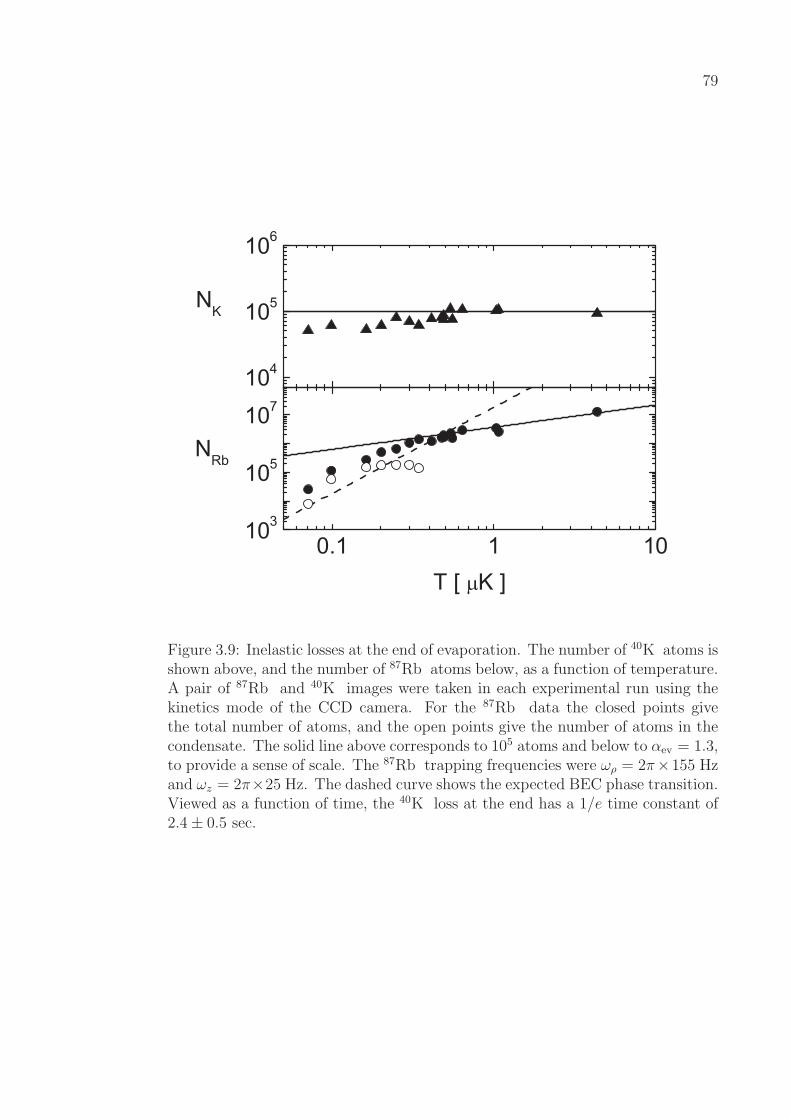
79
Figure 3.9: Inelastic losses at the end of evaporation. The number of 40K atoms isshown above, and the number of 87Rb atoms below, as a function of temperature.A pair of 87Rb and 40K images were taken in each experimental run using thekinetics mode of the CCD camera. For the 87Rb data the closed points givethe total number of atoms, and the open points give the number of atoms in thecondensate. The solid line above corresponds to 105 atoms and below to αev = 1.3,to provide a sense of scale. The 87Rb trapping frequencies were ωρ = 2π×155 Hzand ωz = 2π×25 Hz. The dashed curve shows the expected BEC phase transition.Viewed as a function of time, the 40K loss at the end has a 1/e time constant of2.4± 0.5 sec.

80
clouds become colder. The peak density is fixed by the normalization condition∫
d3xn(~x) = N giving
n(~x) = N
(κ
2π kBT
)3/2
exp
(−κ2
ρ ρ2 + κ2z z2
2 kBT
), (3.14)
where κρ = mω2ρ and κz = mω2
z are the radial and axial trap spring con-
stants (which are the same for 87Rb and 40K atoms in the stretched states),
κ = (κ2ρ κz)
1/3 is the geometric mean spring constant, and ρ = (x2 + y2)1/2 as be-
fore. Using the thermal de Broglie wavelength ΛT = (2π~2/mkBT )1/2, this im-
mediately gives the peak phase-space density
D = n(0) ΛT
= N
(~ω
kBT
)3
, (3.15)
where ω = (ω2ρ ωz)
1/3 is the geometric mean trap frequency. The phase-space
density (PSD) relates the spatial extent of a quantum mechanical wave-packet in
the gas to the distance between atoms. The onset of quantum degeneracy occurs
when D ∼ 1.
One important quantity for both evaporative and sympathetic cooling is the
mean rate of elastic collisions per particle. To calculate collision rates, we need to
consider two systems of particles, labeled i and j ; we can take i = j to calculate
single-species averages (for example, the mean rate of 87Rb-87Rb collisions). The
mean rate per 1-type atom of collisions with 2-type atoms is defined by
Γ12 = 〈n2 σ12 v12 〉1= 〈n2 〉1 σ12 〈 v12 〉1 , (3.16)
where n2 is the density of type-2 atoms, σ12 is the elastic collision cross section,3
and v12 = |~v1 − ~v2| is the relative collision speed. The subscript on the brackets
3 Note that for distinguishable particles the s-wave cross section is related to the scatteringlength a by σ = 4π a2, and for identical bosons we have σ = 8π a2. The cross section betweenidentical fermions is zero according to the Pauli exclusion principle.

81
reflects the fact that we are averaging n2 and v12 over the distribution of 1-type
atoms. To separate σ12 and the averages 〈n2 〉1 and 〈 v12 〉1 we have assumed
isotropic, energy-independent collisions, appropriate in the limit of s-wave scat-
tering. We will return to the question of how good an assumption this is for the
87Rb -40K system in the next section.
The density overlap 〈n2 〉1 is defined by
〈n2 〉1 =1
N1
∫d3x1 n1(~x1) n2(~x1) .
According to Eq. (3.14), the densities n1(~x) and n2(~x) differ only by the factor of
Ni,j out front. Then for Gaussian density profiles we get
〈n2 〉1 = N2
(κ
4π kBT
)3/2
. (3.17)
To get 〈 v12 〉 we transform to center-of-mass (CM) and relative coordinates
~VCM =m1 ~v1 + m2 ~v2
m1 + m2
~vrel = ~v1 − ~v2 . (3.18)
This allows us to rewrite the total kinetic energy
p21
2 m1
+p2
2
2 m2
=P 2
CM
2 M+
p2rel
2 µ,
where PCM = M VCM, prel = µ vrel, and M = m1 + m2 is the total mass, and
µ = m1 m2/(m1 + m2) the reduced mass, of the colliding atoms. Now v12 is just
another name for vrel. Then the average collision speed between 1- and 2-type
particles is
〈 v12 〉 =
(µ
2π kBT
)3/2 ∫ ∞
0
4π v2rel dvrel exp
(−1
2
µ v2rel
kBT
)vrel
=
√8 kBT
π µ. (3.19)

82
Combining Eqs.(3.16),(3.17), and (3.19), we finally have
Γ12 =σ12
23/2π2
κ3/2
õ
N2
kBT. (3.20)
There are two things I’d like to point out about this result. First note that
the collision rate goes like N/T . This fact was used in our previous discussion of
the evaporation efficiency. In contrast a uniform (i.e., untrapped) sample has a
collision rate proportional T 1/2, so that runaway evaporation can not occur.
Second let me discuss the effect of gravity, which we have so far neglected.
We used n1(~x)/N1 = n2(~x)/N2 in our derivation of the collision rate, which is
not exactly true under the influence of gravity. Although to lowest order the
shapes and sizes of the clouds are not affected, the equilibrium vertical position
becomes y0 = −g/ω2ρ (measured from the trap center), where g is the gravitational
acceleration. This leads to different y0 for 87Rb and 40K atoms in the trap. For
Gaussian density profiles this results in a reduction in overlap between species
given by
〈n2 〉1 = fsag 〈n2 〉2 , (3.21)
where
fsag = exp
[−1
4(m1 −m2)
2 g2
κρ kBT
]. (3.22)
For a 87Rb -40K mixture with a 87Rb radial trap frequency of ωρ = 2π × 160 Hz,
fsag = 1/e at a temperature of 73 nK. For comparison if the trap frequency is
reduced by half, then fsag = 1/e at 290 nK. The effect of gravity on the collision
rate at 1 µK for varying trap frequency is shown in Fig. 3.10. The differential sag
in the trap sets an additional design constraint for two-species experiments.
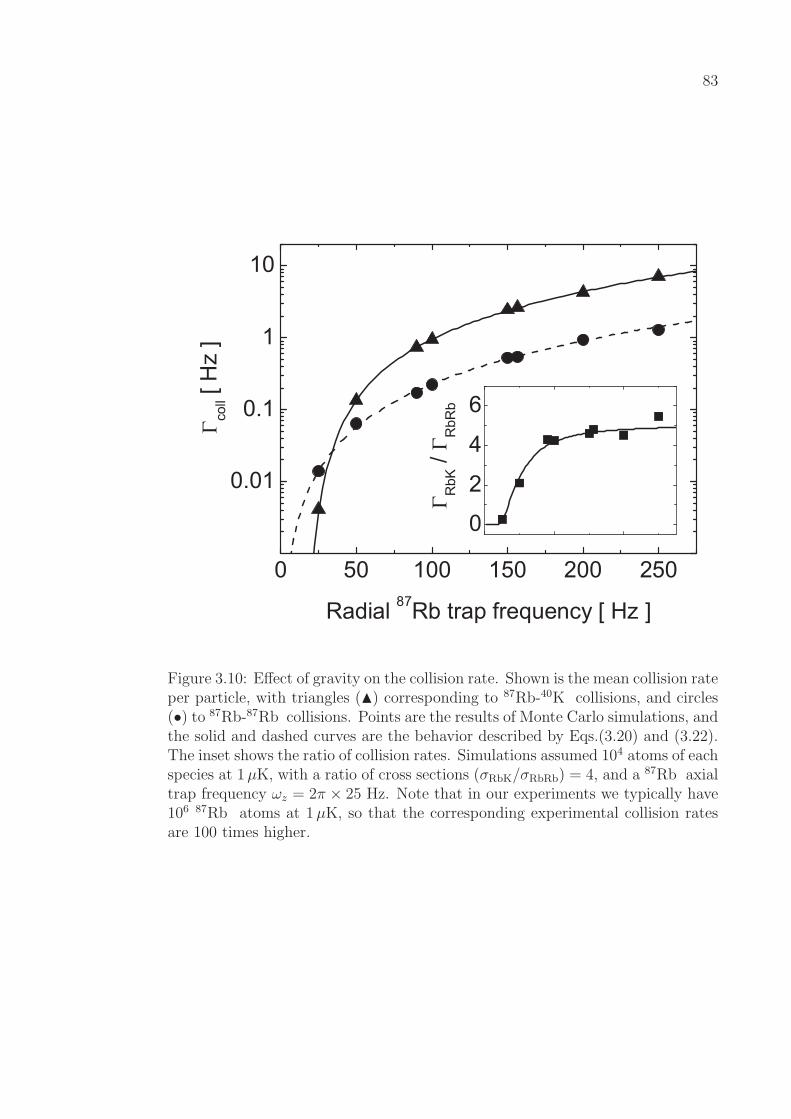
83
Figure 3.10: Effect of gravity on the collision rate. Shown is the mean collision rateper particle, with triangles (N) corresponding to 87Rb-40K collisions, and circles(•) to 87Rb-87Rb collisions. Points are the results of Monte Carlo simulations, andthe solid and dashed curves are the behavior described by Eqs.(3.20) and (3.22).The inset shows the ratio of collision rates. Simulations assumed 104 atoms of eachspecies at 1 µK, with a ratio of cross sections (σRbK/σRbRb) = 4, and a 87Rb axialtrap frequency ωz = 2π × 25 Hz. Note that in our experiments we typically have106 87Rb atoms at 1 µK, so that the corresponding experimental collision ratesare 100 times higher.
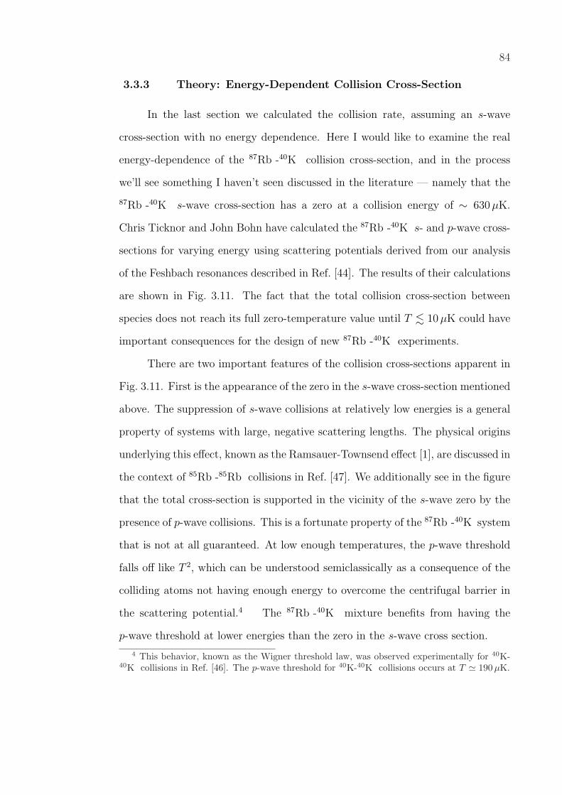
84
3.3.3 Theory: Energy-Dependent Collision Cross-Section
In the last section we calculated the collision rate, assuming an s-wave
cross-section with no energy dependence. Here I would like to examine the real
energy-dependence of the 87Rb -40K collision cross-section, and in the process
we’ll see something I haven’t seen discussed in the literature — namely that the
87Rb -40K s-wave cross-section has a zero at a collision energy of ∼ 630 µK.
Chris Ticknor and John Bohn have calculated the 87Rb -40K s- and p-wave cross-
sections for varying energy using scattering potentials derived from our analysis
of the Feshbach resonances described in Ref. [44]. The results of their calculations
are shown in Fig. 3.11. The fact that the total collision cross-section between
species does not reach its full zero-temperature value until T . 10 µK could have
important consequences for the design of new 87Rb -40K experiments.
There are two important features of the collision cross-sections apparent in
Fig. 3.11. First is the appearance of the zero in the s-wave cross-section mentioned
above. The suppression of s-wave collisions at relatively low energies is a general
property of systems with large, negative scattering lengths. The physical origins
underlying this effect, known as the Ramsauer-Townsend effect [1], are discussed in
the context of 85Rb -85Rb collisions in Ref. [47]. We additionally see in the figure
that the total cross-section is supported in the vicinity of the s-wave zero by the
presence of p-wave collisions. This is a fortunate property of the 87Rb -40K system
that is not at all guaranteed. At low enough temperatures, the p-wave threshold
falls off like T 2, which can be understood semiclassically as a consequence of the
colliding atoms not having enough energy to overcome the centrifugal barrier in
the scattering potential.4 The 87Rb -40K mixture benefits from having the
p-wave threshold at lower energies than the zero in the s-wave cross section.
4 This behavior, known as the Wigner threshold law, was observed experimentally for 40K-40K collisions in Ref. [46]. The p-wave threshold for 40K-40K collisions occurs at T ' 190 µK.

85
Figure 3.11: Theoretical energy dependence of the 87Rb -40K elastic collisioncross-section. The dashed (dotted) curve is the s-wave (p-wave) cross-section asa function of collision energy (but not thermally averaged), and the solid curveis the total cross-section. Calculations were performed by Chris Ticknor andJohn Bohn and assume a triplet scattering length |aRbK| = 280 a0 [44]. Forreference we have marked the T = 0 limits for |F = 2,mF = 2 〉Rb ⊗ | 2, 2 〉Rb and| 9/2, 9/2 〉K ⊗ | 9/2, 7/2 〉K collisions, from Refs. [45] and [46], respectively. (Thesymbol ⊗ here denotes the direct or Cartesian product [1]).
86
To estimate the 87Rb -40K p-wave threshold we consider the long-range
form of the collision potential,
URbK(R) ' ~2 l(l + 1)
2 µR2− C6
R6, (3.23)
where R is the internuclear separation, l = 1 is the angular momentum quantum
number for p-wave collisions, µ = mRb mK/(mRb + mK) is the reduced mass, and
C6 = 4274 a.u. is the van der Waals coefficient [48]. Setting the collision energy
Ecoll equal to the maximum of URbK, and using Ecoll = 3kBT/2 gives a p-wave
threshold of ∼ 110 µK (or 170 µK collision energy). This energy is marked in
Fig. 3.11, and is in good agreement with the behavior described by the full coupled-
channel calculation. The fact that the p-wave threshold is at lower energy than
the s-wave zero means that collisions between species are never fully suppressed.
Note, however, that the cross-section in the vicinity of the s-wave zero is only
about 1% of the zero temperature value.
Finally we note that the T 2 dependence of the p-wave cross-section at
low temperatures is just a specific example of a more general threshold behav-
ior. Specifically the cross-section corresponding to the lth partial wave obeys
σl ∝ T 2 l at low energies [1]. For example the calculated threshold temperature
for 87Rb -40K d-wave collisions is 577 µK, and below this temperature the d-wave
cross-section will fall off like T 4. This means that the total cross-section in the
vicinity of the s-wave zero may be larger than what is shown in Fig. 3.11.
3.4 Onset of Quantum Degeneracy
We now turn our attention to the onset of quantum degeneracy in the ex-
periment. The quantum statistics of bosons and fermions will each be considered
in turn. We will see how quantum degeneracy is manifest in the experiment, and
set the ground work for our discussions of interactions between species in the next

87
chapter. More detailed derivations of these results can be found in Refs. [49, 21]
for the bosons and Refs. [50, 13] for the fermions.
3.4.1 Bosons
For Bose-Einstein distributions the density profile corresponding to Eq.(3.14)
is modified by quantum statistics to give
nBE(~x) = g3/2(exp[(µ− UIP)/kBT ]) Λ−3T , (3.24)
where gν(α) =∑∞
i=1 αi/iν is the Bose function (sometimes called the polylog-
arithm and denoted Liν(α)), ΛT = (2π~2/mkBT )1/2 is the thermal de Broglie
wavelength, and we have suppressed the spatial dependence of UIP(~x) for simplic-
ity. Note that for α ¿ 1 the Bose function obeys g3/2(α) ' α, so that a Gaussian
distribution is recovered in the classical limit, or in the “wings” of the gas, where
higher-energy atoms are more likely to be found. In contrast the profile of the
cloud is more sharply peaked at the center than the classical Gaussian profile.
This reflects the proclivity of bosons in a single spin-state to aggregate into the
lower-energy states of the trapping potential.
In the thermodynamic limit an ideal gas of harmonically trapped bosons
undergoes a phase transition to BEC at a critical temperature
kBT (0)c = ~ω
[N
ζ(3)
]1/3
, (3.25)
where ζ(3) = 1.20206... is the Riemann zeta function. At this point a macroscopic
number of atoms N0 begins to occupy the ground state of the system. For fitting
images of expanded clouds, we consider the total density of bosons to be the sum
of a “thermal” component and a condensed component [21].
The number of atoms in the condensate is related to the total number of
88
atoms Ntot by
N0
Ntot
= 1−[
T
T(0)c
]3
, (3.26)
showing a steep initial population of the condensate after cooling below T(0)c .
Results from the experiment are shown in Fig. 3.12.
Corrections to the calculated condensate fraction due to the finite number
of atoms and repulsive boson-boson interactions are discussed in Refs. [49, 51].
The main result of these corrections is a softening of the transition and a shift
towards lower transition temperature, as seen in the data. When including these
effects the agreement between theory and experiment is excellent. Although these
data were taken in the presence of ∼ 104 40K atoms, the fermions are expected to
have a negligible effect on the bosons here. As we’ll discuss in more detail later,
this is due to the fact that the density of 104 fermions under these conditions is
much less than the condensate density.
The ground-state condensate wave-function, or order parameter Ψ0, obeys
the time-independent Gross-Pitaevskii (GP) equation [49]
[− ~2
2 m∇2 + UIP(~x) + g N0 |Ψ0(~x)|2
]Ψ0(~x) = µ Ψ0(~x) , (3.27)
where g = 4π~2a/m is the coupling constant for bosons with scattering length
a, and N0 is the number of atoms in the condensate.5 With our choice of
normalization∫
d3x |Ψ0|2 = 1, the density of condensed atoms is related to the
condensate wave function by nc = N0 |Ψ0|2. Note that the chemical potential µ is
typically on the order ∼ 1.5 kHz (75 nK) in our experiments.
In the limit of small gN0, the solution to Eq.(3.27) is just nc = N0|ψ0|2, with
ψ0 the single-particle Gaussian oscillator ground state. For sufficiently large and
positive gN0, the mean-field term in Eq.(3.27) dominates and the kinetic energy
5 As pointed out in Ref. [52], we replace N0 by N0 − 1 if the particle number is fixed.
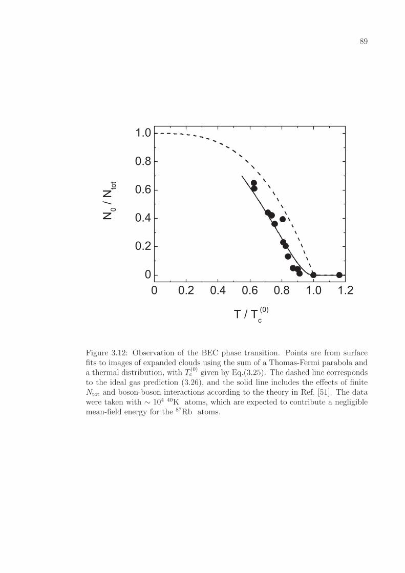
89
Figure 3.12: Observation of the BEC phase transition. Points are from surfacefits to images of expanded clouds using the sum of a Thomas-Fermi parabola anda thermal distribution, with T
(0)c given by Eq.(3.25). The dashed line corresponds
to the ideal gas prediction (3.26), and the solid line includes the effects of finiteNtot and boson-boson interactions according to the theory in Ref. [51]. The datawere taken with ∼ 104 40K atoms, which are expected to contribute a negligiblemean-field energy for the 87Rb atoms.
90
can be neglected. This yields an algebraic equation for the Thomas-Fermi (TF)
density profile of the condensate
nc(~x)TF−→ 1
g[ µTF − UIP(~x) ] Θ[ µTF − UIP(~x) ] , (3.28)
where Θ(·) is the unit step function. The condensate density is therefore zero
outside the TF radius in the ith direction, given by m ω2i X2
TFi/2 = µTF. The
chemical potential is determined by the normalization condition on nc, yielding
µTF =~ω
2
(15N0
a
aHO
)2/5
, (3.29)
where aHO = (~ /mω)1/2 is the geometric mean oscillator length for the bosons,
which is typically ∼ 1 µm for our experiments, compared to a ' 5 nm [45].
To determine when the TF approximation is valid, I solved the GP equation
for the peak condensate density nc(0) as a function of N0. The results are shown
in Fig. 3.13 and compared to the weakly- and strongly-interacting limits. The
calculations assumed 87Rb atoms in a 2π × 100 Hz spherical trap. For these
parameters there is a clear transition from non-interacting behavior to the TF
approximation at N0 ∼ 100. Since we are not even able to measure so few atoms
with our imaging system, we feel free to use the TF approximation for fitting our
images.
3.4.2 Fermions
Things are somewhat more subtle for fermions, since there is no phase transi-
tion in our system.6 Thermodynamic properties of the Fermi gas can be attained
through the chemical potential, but practically speaking we focus on the fugacity
Z = exp(µ/kBT ), which can be obtained by solution to the equation [13]
−g3(−Z) =1
6
(T
TF
)−3
, (3.30)
6 Note that we love them all the same, however.
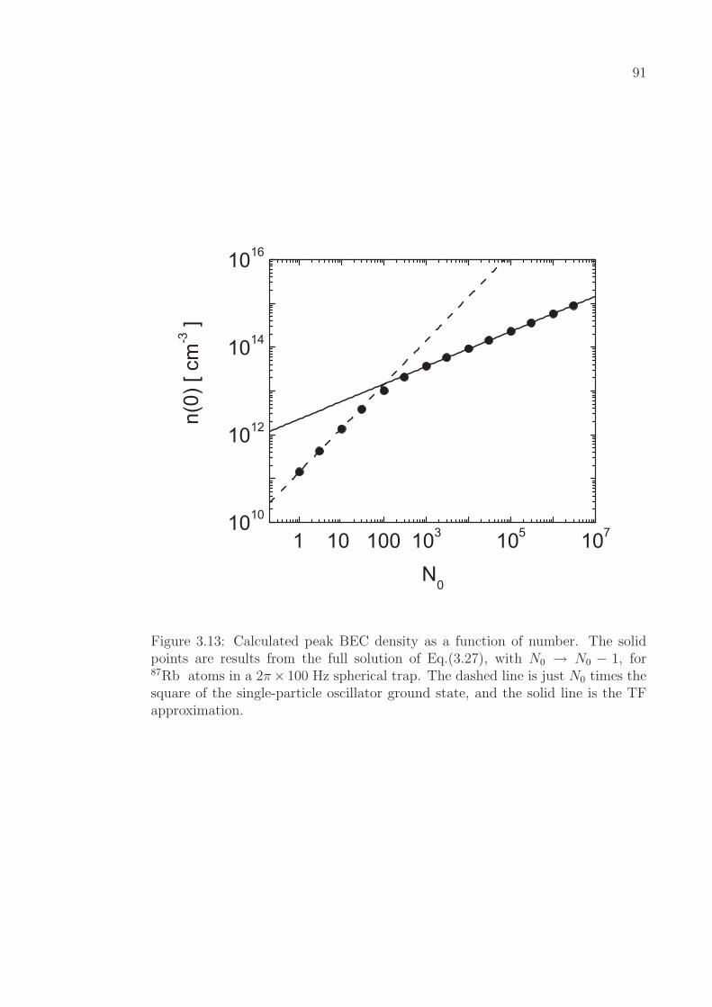
91
Figure 3.13: Calculated peak BEC density as a function of number. The solidpoints are results from the full solution of Eq.(3.27), with N0 → N0 − 1, for87Rb atoms in a 2π× 100 Hz spherical trap. The dashed line is just N0 times thesquare of the single-particle oscillator ground state, and the solid line is the TFapproximation.
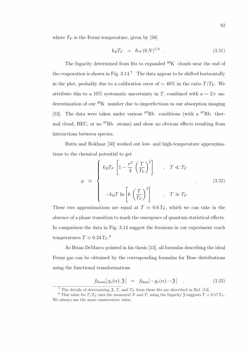
92
where TF is the Fermi temperature, given by [50]
kBTF = ~ω (6 N)1/3 . (3.31)
The fugacity determined from fits to expanded 40K clouds near the end of
the evaporation is shown in Fig. 3.14.7 The data appear to be shifted horizontally
in the plot, probably due to a calibration error of ∼ 40% in the ratio T/TF . We
attribute this to a 10% systematic uncertainty in T , combined with a ∼ 2× un-
derestimation of our 40K number due to imperfections in our absorption imaging
[53]. The data were taken under various 87Rb conditions (with a 87Rb ther-
mal cloud, BEC, or no 87Rb atoms) and show no obvious effects resulting from
interactions between species.
Butts and Rokhsar [50] worked out low- and high-temperature approxima-
tions to the chemical potential to get
µ '
kBTF
[1− π2
3
(T
TF
)2]
, T ¿ TF
−kBT ln
[6
(T
TF
)3]
, T À TF
. (3.32)
These two approximations are equal at T ' 0.6 TF , which we can take in the
absence of a phase transition to mark the emergence of quantum statistical effects.
In comparison the data in Fig. 3.14 suggest the fermions in our experiment reach
temperatures T ' 0.24 TF .8
As Brian DeMarco pointed in his thesis [13], all formulas describing the ideal
Fermi gas can be obtained by the corresponding formulas for Bose distributions
using the functional transformations
fFermi[ gν(α); Z ] = fBose[−gν(α);−Z ] . (3.33)
7 The details of determining Z, T , and TF from these fits are described in Ref. [13].8 This value for T/TF uses the measured N and T ; using the fugacity Z suggests T = 0.17 TF .
We always use the more conservative value.

93
Figure 3.14: Observation of Fermi degeneracy. The points show the fugacity asa function of T/TF , determined from surface fits as described in Ref. [13]. Thetriangles (N) are in the presence of thermal 87Rb atoms, solid circles (•) arein the presence of BEC, and open circles () have had 87Rb atoms removed byevaporating through the trap bottom. The solid line is the ideal gas predictionfrom Eq.(3.30), and the dashed line is the same prediction with a 1.4× correctionto T/TF .

94
The density profile of the fermions corresponding to Eq.(3.24) is now more rounded
than the classical Gaussian profile at the center of the cloud. This reflects the
effect of the Pauli pressure for the fermions.
In the limit T → 0 there is a Thomas-Fermi (TF) approximation for the
density of the fermions. The chemical potential µ = kBTF ≡ EF in this limit, and
the density distribution becomes
nFD(~x)TF−→
√2
3 π2
mf
~3
2/3
[ EF − UIP(~x) ]3/2 Θ[ EF − UIP(~x) ] . (3.34)
Note that the TF approximation here yields a profile with no atoms outside a
distance determined by µ = UIP(~x), as with the condensate in the previous section.
Due to the Pauli pressure, however, µTF is typically much larger for the fermions
than for the bosons. For example consider 105 atoms of either species in a spherical
trap with 87Rb frequency 2π× 100 Hz. Under these conditions the Fermi energy
EF ' 500 nK, whereas the BEC chemical potential is only ' 80 nK. In other
words, the Pauli pressure results in a fermi gas roughly 3 times larger than the
condensate and about 13 times larger than the single-particle Guassian ground
state for 40K.
3.5 Limits to Sympathetic Cooling
One important question deserving our attention here is what limits the
lowest T/TF we can achieve by sympathetic cooling? Here I will just summarize
some mechanisms that have been proposed, and what they each predict for the
87Rb -40K system. At this point more experimental work is needed to understand
what technical issues, if any, may be limiting the lowest T/TF in the experiments.
We can, however, see in Table 3.1 that the four existing 87Rb -40K experiments
have all reported similar results.9
9 Note that all of the experiments have similar trapping potentials except the ETH experi-ment, which has a weaker radial confinement leading to a geometric mean trapping frequency

95Expt. T/TF NK Ref.
LENS 0.2 5× 10⁴ [54]
JILA 0.2 1× 10⁵ [53]
ETH 0.3 6× 10⁵ [4]
Hamburg 0.2 1× 10⁶ [55]
Table 3.1: Lowest values of T/TF reported in 87Rb -40K experiments.
The first sympathetically cooled degenerate Fermi gas was produced by the
Rice group using 6Li and 7Li [56]. To the best of my knowledge, that work
represents the introduction of the assertion that the sympathetic cooling “bot-
toms out” when the heat capacity Cf of the fermions exceeds the heat capacity
Cb of the bosons. This occurs because the total number of bosons Nb is decreasing
while the number of fermions Nf is held roughly constant, and because the heat
capacity of the bosons drops precipitously after crossing the BEC transition. The
heat capacities for ideal Bose and Fermi gases are shown as a function of T in
Fig. 3.15, assuming equal numbers of 87Rb and 40K atoms in their respective
stretched states. Note that due to the different masses, Eqs.(3.25) and (3.31) show
that under these conditions Bose-Einstein condensation occurs at a temperature
0.35 TF . Since the BEC phase transition is accompanied by a discontinuous jump
in Cb, and the low-temperature behaviors obey Cf ∝ T and Cb ∝ T 3, this sug-
gests the existence of a point where Cb = Cf . This point is given by 0.18 TF in
this example, which is actually quite close to what we observe in the experiment.
This agreement is almost certainly fortuitous, however, since we have so far ne-
glected the important effects of gravitational sag (which is minimal in the 6Li-7Li
experiment), and the finite heating rates in the experiments.
of ωRb = 2π × 70 Hz, compared to ωRb ∼ 2π × 90 Hz for the other experiments. Note alsothat in the ETH experiment, the 87Rb atoms are removed after sympathetic cooling, and atwo-component 40K mixture is evaporatively cooled to 0.2 TF with 5× 10⁴ atoms in each spinstate.

96
Figure 3.15: Specific heats of ideal Bose and Fermi gases. The heat capacityper particle is given in units of kB as a function of T/TF for equal numbers ofnon-interacting 87Rb and 40K atoms in the thermodynamic limit. The solid lineis for the bosons, showing the transition to BEC at ∼ 0.35 TF , and the dashedline is for the fermions. The dotted line shows the Maxwell-Boltzmann behavior,C = 3NkB.
97
Recently, Brown-Hayes and Onofrio [57] have elaborated on the simple
heat capacity model. They consider Bose and Fermi gases in their respective
TF regimes, and assume that the sympathetic cooling actually continues until
Cb/Cf ' 0.1. Using low temperature approximations for Cb and Cf , they predict
a minimum achievable temperature of 0.06 TF for equal numbers of atoms in a
87Rb -40K mixture. Although this is significantly lower than what we observe,
they go on to include the effects of gravitational sag and mean-field interactions.
As we saw in Sect. 3.3.2 gravity reduces the spatial overlap of the clouds, but we
will see later that the attractive 87Rb -40K interactions act to recover some of the
overlap. The result is a net increase in minimum temperature (proportional to
the square of the reduction in overlap) of about 8 times to 0.5 TF , which is incom-
patible with our results. Although their model seems insufficient to quantitatively
predict the minimum temperature, I have pointed it out here because the authors
additionally suggest some ways to improve sympathetic cooling by optimizing the
choice of species (for masses and magnetic confinement) and trap frequencies, in-
cluding the application of bichromatic optical dipole traps to selectively change
the confinement of each species.
The heat capacity model of the limit to sympathetic cooling is based on
an intuitive model of the cooling process where two gases initially at different
temperatures are brought into thermal contact. The idea is that both species
are initially in thermal equilibrium, and some evaporation of the bosons leads to
a lower-energy Bose gas. The fermions are then cooled as both gases reach an
intermediate temperature, and a new evaporation step proceeds. Carr and Castin
have shown [58] that in some sense it is ideal to have Cf À Cb, in order to minimize
the number of bosons one must evaporate in order to reach zero temperature.
Although their work casts some important doubts on the simple heat capacity
argument for the limit of the cooling process, their model always achieves T = 0

98
fermions, and is therefore not useful in our search here to understand what actually
does limit the process in experiments.
Another possible limit that Carr and Castin examined (in conjunction with
Bourdel [59]) is based on a heating mechanism originally suggested by Timmer-
mans [60], where particle losses in the Fermi sea lead to an increase in T/TF .
They predict minimum attainable temperatures below 0.1 TF for a ratio of loss
rate to collision rate of 10−2. Without performing detailed calculations for our
masses, atom numbers, and heating and collision rates, it is hard to make a bet-
ter quantitative prediction. Note also that their theory neglects the gravitational
sag, and boson-boson and boson-fermion interactions. The interesting thing about
their work is rather the suggestion that even in the absence of other limits to the
cooling, the hole-heating will ultimately limit experiments to the ∼ 0.01 TF level,
which is not significantly lower than the best degenerate Fermi gas experiments
to date (which include some direct evaporation of the fermions). This mechanism
additionally effects any degenerate Fermi gas, regardless of whether sympathetic
cooling is employed.
The last mechanism I’d like to consider was proposed by Timmermans and
Cote in Ref. [61]. They pointed out that the superfluidity of the BEC will inhibit
collisions with fermions traveling slower than the Landau critical velocity in the
gas. This velocity c is given by the Bogoliubov speed of sound
mb c2 = µb ,
where mb and µb are the boson mass and chemical potential, respectively. Using
the local density approximation (LDA) this gives a spatially dependent critical
speed
c(~x) =
√g
mb
nc(~x) , (3.35)
99
where g = 4π~2a/mb is the coupling constant for bosons with scattering length
a and nc is the condensate density. The authors used the quantum Boltzmann
equation to show that a homogenous Maxwell-Boltzmann distribution originally
with a thermal speed vT = 3 c would cool to a distribution with peak speed slightly
lower than c. To translate this to our harmonically trapped samples we take the
average speed of sound 〈 c 〉 = N−10
∫d3xnc(~x) c(~x). For our typical conditions
we then get 〈 c 〉 = 1.9 mm/s. Setting vT = 〈 c 〉 and using mf v2T /2 = 3 kBT/2
with mf the mass of a 40K atom, we get a limiting temperature of ' 6 nK, or
T/TF ' 0.01, which is again much better than what we achieve in the experiment.
This, together with the fact that the real fermion distribution is weighted towards
higher speeds than a Maxwell-Boltzmann distribution, suggests that superfluidity
is not yet limiting the cooling process in our experiment.10 As with the hole-
heating, however, we see what may be a fundamental limit to the cooling of our
fermions to about 1% of the Fermi temperature.
10 With the caveat that we have ignored the fact that fermions will always be able to scatteroff of the low-density edge of the condensate. A more detailed calculation is needed to addressthis effect.

Chapter 4
Cross-Species Interactions
In this chapter I will present our main experimental results investigating
ways to probe and manipulate the cross-species interactions characterized by the
s-wave scattering length abf . The parameter abf is crucial in understanding a
variety of the static and dynamic properties of quantum degenerate Bose-Fermi
mixtures.
I’ll begin in Sect. 4.1 with a discussion of how we can make relatively precise
measurements of the magnitude of abf by measuring rethermalization rates in
non-degenerate clouds. This type of measurement was originally developed at
JILA for a single-species Bose gas in Ref. [62]. Subsequent studies have extended
the technique to Fermi-Fermi mixtures [46], single-species resonant collisions [63],
and Bose-Bose mixtures [64]. The quantum statistical suppression of fermion-
fermion collisions makes this type of measurement especially robust for Bose-Fermi
mixtures.
In Sect. 4.2 I will elaborate on the importance of the Bose-Bose and Bose-
Fermi scattering lengths with respect to the equilibrium state of the mixture. We
will discuss some possible mechanical instabilities and how they relate to the size
and sign of the scattering lengths, and the numbers of atoms of each species in
the mixture.
In Sect. 4.3 I’ll describe some measurements of the excitations of the mixture.
101
We first examine the quadrupole “breathe” mode for non-degenerate fermions in
the presence of bosons. The damping rate gives us the magnitude of the scat-
tering length and the excitation frequency, in principle, gives information on the
importance of hydrodynamic effects. This will lead to our observation of some-
what higher-lying excitations of a 87Rb BEC in the presence of a thermal cloud
of 87Rb atoms. Besides being, to my knowledge, the first verification of some
longstanding theoretical calculations of the excitation spectra of BECs in elon-
gated traps, this measurement serves as an example of how parametric excitation
of the atoms can be extremely useful for systems with many available excitation
modes. Finally, as one possible excitation for future study, I will discuss the the-
oretical proposal for a Boson-induced pairing of the fermions. This calculation
suggests the observation of pairing may be within reach of current experiments
using Feshbach resonances between species.
Finally, in Sect. 4.4 I will describe our hunt for, and observation of, heteronu-
clear Feshbach resonances in the collisions between 87Rb and 40K atoms. The
discovery of these resonances represents the “crown jewel” of the work described
in this thesis. It is these resonances that in principle grant the experimenter
real-time control over abf in the mixture. In addition to providing access to phe-
nomena such as phase-separation and mechanical collapse, this control may allow
production for the first time of quantum degenerate fermionic molecules, as well
as observation of boson-mediated pairing of the fermions. Finally we use the ob-
servations of the resonance locations to refine our knowledge of the non-resonant
scattering properties we measured in Sects. 4.1 and 4.3.1. The knowledge gleaned
from the locations of the resonances gives us the first insight in our experiment
into the singlet scattering properties between 87Rb and 40K atoms. This knowl-
edge could in turn be used to refine the predictions of various 87Rb -40K Feshbach
resonances presented in Ref. [65].
102
4.1 Cross-Dimensional Rethermalization
In this section I will describe our cross-dimensional rethermalization (CDR)
measurements on non-degenerate 87Rb -40K mixtures. These measurements pro-
vide a relatively simple and robust way to determine the value of |abf | in the
system, which is crucial to characterizing a variety of equilibrium and dynamic
properties of the mixture. Our CDR measurements were reported in Ref. [53] and
our theoretical work was presented in Ref. [66].
The essence of cross-dimensional rethermalization is as follows. If one pre-
pares a gas with different mean energies in the different Cartesian directions, the
gas will subsequently relax into thermal equilibrium. An example from the exper-
iment is shown in Fig. 4.1. In a purely harmonic trap the only way for the gas
to spatially redistribute its energy is through collisions between atoms, since the
potential energy is perfectly separable in the three directions. In an elastic s-wave
collision, where the total energy and momenta are conserved, the relative motion
of colliding particles is completely randomized. That is, the isotropic nature of the
scattering amplitude leads to a uniform redistribution of kinetic energy between
directions. The potential energy in each direction can be thought of as being on
average equal to the corresponding kinetic energy immediately following the col-
lision. This assumption is valid in the so-called “collisionless” regime, where the
collision rate is small compared to the trapping frequencies. This is the regime
where we perform the measurements described in this section.
A detailed analysis of single-species CDR reveals that the relaxation has the
form of an exponential decay, with a 1/e time-constant proportional to the mean
time between collisions in the gas [67]. The Bose-Fermi case is more difficult
to handle analytically, but we make the following important observation. The
fermions in our mixture are spin-polarized, so that if they are well below the p-

103
Figure 4.1: Cross-dimensional rethermalization of 40K in the presence of 87Rb.Shown is the square of the cloud aspect ratio (radial/axial) in time-of-flight, as afunction of hold time after introducing an energy anisotropy between the radialand axial directions. The square of the aspect ratio is proportional to the ratio ofenergies in the radial and axial directions. The 40K atoms rethermalize by meansof collisions with the 87Rb atoms. The solid line is a fit to the ratio of exponentiallydecaying curves. The error bar shows the typical statistical uncertainty.

104
wave threshold (∼ 190 µK for 40K [46]) fermion-fermion collisions are suppressed;
s-wave collisions between identical fermions are forbidden by the Pauli exclusion
principle. The fermions therefore collide only with the bosons. Then the discussion
above regarding the spatial redistribution of kinetic energy holds for the fermions.
We again expect their rethermalization to look like exponential decay with a time
constant proportional to the mean time per fermion between collisions.
In the experiment the non-equilibrium state of the mixture is prepared in the
following way. We first produce a mixture of 1×10⁵ 40K and 4×10⁵ 87Rb atoms
at ∼ 1 µK as described in the previous chapter. The radial trap strength is
reduced for the entire cooling stage by applying an extra ∼ 3 G bias field to the
IP trap. The 87Rb radial trap frequency is ωρ = 2π× 95 Hz in the decompressed
trap (the axial frequency is always 2π × 25 Hz). We then optionally apply a
sequence of 1 ms rf sweeps to reduce the 87Rb number by as much as a factor of 4
using spin-flips in the magnetic trap. The 87Rb radial trapping frequency is then
ramped to 2π × 160 Hz over a time scale that is slow compared to the radial trap
period and fast with respect to the rethermalization rates in the gas. Immediately
after the compression there is therefore an excess of energy in the radial directions.
Neglecting any rethermalization that may occur during the compression, the mean
energies (kinetic plus potential) in the radial and axial directions are related by
(Ex,y/Ez) = (160/95) for either species of atoms.1 The fact that both species
begin at the same temperature, experience the same initial energy anisotropy,
and then equilibrate together means that there is never any net transfer of energy
from one gas to the other during the rethermalization. This is instrumental in
removing effects due to the systematic uncertainty in determining atom numbers.
1 Note that in Ref. [53] we state that the trap frequency (νρ = ωρ/2π) goes from 90 to160 Hz during the compression. I think the 90 Hz is a typo. During the CDR measurementswe measured νρ = 95.23 ± 0.13 Hz before the compression and 156.6 ± 0.4 Hz after, using87Rb dipole oscillations. This calibration was used for the data analysis as well as the MonteCarlo simulations, so that our results remain unchanged.

105
With an excess of energy in the x and y directions, we simply vary the hold
time in the compressed trap, and then measure the rms Gaussian sizes (σρ,z) of
the clouds after time-of-flight expansion. The aspect ratio (σz/σρ) is used for the
analysis instead of the radial and axial sizes in order to reduce the effects of shot-
to-shot variations in the starting temperature of the mixture. The square of the
aspect ratio, which is proportional to Ez/Ex,y, is fit to the ratio of exponentially
decaying curves, whose 1/e time constant determines the relaxation time constant
τ . Such a fit is shown as the solid curve in Fig. 4.1.
We measured τK over a variety of different 87Rb densities. The results
are shown in Fig. 4.2, where we plot the relaxation rate versus the product of
87Rb density and T 1/2 (proportional to the mean collision speed). We also show
a set of “control” experiments where we measure τRb in the absence of 40K atoms.
Note that both relaxation rates vary linearly with the product 〈nRb 〉T 1/2. We’ll
see below that the slopes of linear fits through the origin are proportional to
the collision cross-sections, and therefore the square of the scattering lengths.
This linear behavior additionally demonstrates that we remain in the collisionless
regime for these measurements. Hydrodynamic behavior leads to a nonlinear
density dependence, since energy is “stored” in the potential energy of particles
pinned in place by collisions. For examples of this kind of behavior, see the
experiment in Ref. [68] and the discussion in Appendix A.
For these measurements we extract the magnitude of the 87Rb -40K scat-
tering length as follows. The linear behavior in Fig. 4.2 allows us to write the
relaxation rates [62, 53]
ΓK ≡ τ−1K =
1
β〈ΓRbRb 〉
ΓRb ≡ τ−1Rb =
1
α〈ΓRbK 〉 , (4.1)
where ΓRbRb (ΓRbK) is the Rb-Rb (Rb-K) collision rate, and the average 〈ΓRbK 〉

106
Figure 4.2: Cross-dimensional relaxation over varying 87Rb density. Open points() are for 40K relaxation in the presence of 87Rb, and solid points (•) are forthe single-species 87Rb control experiment. Lines are fits through the origin; theslopes are proportional to the corresponding collision cross-sections. Vertical errorbars are from the fit uncertainties, and horizontal error bars include shot-to-shotfluctuations in 87Rb number and temperature, and a 10% systematic uncertaintyin T [53]; the systematic uncertainty in 87Rb number is removed in the analysisby taking the ratio of the two slopes and using Eq.(4.2).

107
is taken over the distribution of 40K atoms (see Eqs.(3.20) and (3.22)). The
constants of proportionality α and β reflect the mean number of collisions per
particle needed for rethermalization.
If we compare the observed single-species 87Rb relaxation rate to the relax-
ation rate of 40K atoms in the presence of 87Rb, we find
τRb
τK
=1
23/2
α
β
√1 +
mRb
mK
(aRbK
aRbRb
)2
, (4.2)
where we have suppressed the appearance of fsag(T ) in the 87Rb -40K collision
rate for simplicity.2 This important relation is at the heart of why the CDR
technique is so robust for Bose-Fermi mixtures. The 87Rb density has fallen
out of the analysis, taking with it the large systematic uncertainty that typically
accompanies it and limits the precision of such measurements. In conjunction
with the facts that (i) there is no energy transferred between gases (which would
give rise to an additional number dependence) and (ii) the 87Rb-87Rb scattering
length aRbRb = 98.98± 0.04 a0 is extremely well known from a variety of high-
precision experiments with 85Rb and 87Rb [45, 69], Eq.(4.2) allows a relatively
precise determination of |aRbK| with a simple collisional measurement.
The constants α and β were determined for our experimental conditions
using classical Monte Carlo simulations, as described in Refs. [53, 66]. The result
is
α = 2.67± 0.13
β = 2.1± 0.2 . (4.3)
Note that a number of analytic and numerical studies have found α to lie between
2.5 and 2.7 [62, 70, 71, 46, 72, 67], in good agreement with our results. I am not
aware of any previous theoretical results for β in the literature.
2 For the experiments considered here, fsag represents a 3–5% correction to the density, andis included in the analysis.

108
With these values of α and β, our measurements of relaxation rates in
Fig. 4.2, and the accepted value of aRbRb, we obtain a value for |aRbK| of
|aRbK| = 250± 30 a0 , (4.4)
where we have used σRbRb = 8π a2RbRb and σRbK = 4π a2
RbK. For comparison I
have compiled in Table 4.1 values of |aRbK| from a variety of different works.3 I
have additionally included the result of measurements we have performed using
quadrupole “breathe” oscillations. These experiments are described in detail in
Sect. 4.3.1 below.
Finally, we compare in Fig. 4.3 our experimental measurements of the col-
lision cross-section with the results of detailed coupled-channel calculations per-
formed by Chris Ticknor and John Bohn. The calculations assume the value of
aRbK determined we obtained in Ref. [44] from our observation of inter-species
Feshbach resonances (described in Sect. 4.4 below). The agreement between ex-
periment and theory is excellent.
4.2 Mean-Field Intermezzo — Equilibrium Properties
So far our theoretical descriptions of the degenerate Bose and Fermi gases
have neglected the interactions between species. In this section I’ll detail some
of the more important aspects of the zero-temperature mean-field theory of Bose-
Fermi mixtures, using the Thomas-Fermi (TF) approximations for each species.
This model was introduced in the seminal paper by Mølmer [77], and has been
expanded on in numerous works since.4
Here I’ll focus on the mean-field energies for each species in the mixture,
as well as the equilibrium density profiles for different signs and strengths of the
3 I feel obliged to point out here a pre-print I have recently discovered, wherein the scatteringlengths for various isotopic Rb-K mixtures are calculated. Ozturk and Ozcelik obtain −200 a0
for the 87Rb -40K mixture. See arXiv:physics/0403073.4 The interested reader is urged to look up papers citing Ref. [77].

109
|aRbK| Ref. Method
95+98−33 [73] Heat-transfer∗
261+159−170 [74] Heat-transfer + dipole oscillation∗
330+160−100 [75] Heat-transfer
410+90−80 [76] Dipole oscillation
395± 15 [54] Mean-field theory + experiment
250± 30 [53] CDR
260± 50± 70 § 4.3.1 Quadrupole oscillation
281± 15 [44] Feshbach resonances
275+7−8 § 4.4.3 Feshbach resonances
Table 4.1: Compendium of reported values for the 87Rb -40K triplet scatteringlength. All values are in units of a0, the Bohr radius. An asterisk (∗) denotesa result employing a mass-scaling to 87Rb -40K from a measurement on a 87Rb-41K mixture. Heat-transfer experiments selectively heat the Rb atoms, and thenmonitor the transfer of energy to K atoms. Results below the double bar are fromour experiment. The uncertainty on our quadrupole oscillation measurement isstated in the form ± statistical ± systematic, where the systematic uncertaintyarises from the systematic uncertainty in atom numbers.
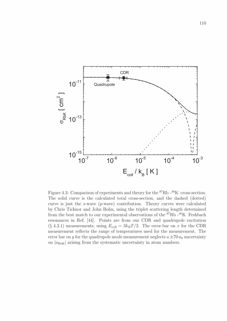
110
Figure 4.3: Comparison of experiments and theory for the 87Rb -40K cross-section.The solid curve is the calculated total cross-section, and the dashed (dotted)curve is just the s-wave (p-wave) contribution. Theory curves were calculatedby Chris Ticknor and John Bohn, using the triplet scattering length determinedfrom the best match to our experimental observations of the 87Rb -40K Feshbachresonances in Ref. [44]. Points are from our CDR and quadrupole excitation(§ 4.3.1) measurements, using Ecoll = 3kBT/2. The error-bar on x for the CDRmeasurement reflects the range of temperatures used for the measurement. Theerror bar on y for the quadrupole mode measurement neglects a ±70 a0 uncertaintyon |aRbK| arising from the systematic uncertainty in atom numbers.

111
coupling parameter (proportional to the interspecies scattering length). In addi-
tion I’ll discuss some null results from our experiment which appear to contradict
some observations from the LENS group. Resolution of this conflict is important
for understanding the equilibrium properties of 87Rb -40K mixtures with different
numbers of atoms and in different confining potentials.
4.2.1 Theory: Phase Separation, Fermions in a Box, and Collapse
Our description of Bose-Fermi mixtures is centered on the concept of mean-
field potentials, proportional for one species to the density of atoms of the other
species. Specifically we write the total boson and fermion potential energies
Ub(~x) = Uext(~x) + gbf nf (~x)
Uf (~x) = Uext(~x) + gbf nb(~x) , (4.5)
where Uext is the external trapping potential, nσ is the density of species σ =
(b, f), and the coupling constant gbf = 2π~2abf/µbf , with abf the scattering length
between bosons and fermions, and µbf the reduced mass between bosons of mass
mb and fermions of mass mf . We assume that Uext is a spherically symmetric
harmonic potential with trapping frequencies ωb and ωf = (mb/mf )1/2ωb for the
bosons and fermions, respectively.
Roth and Feldmeier gave the energy density functional for the system [78, 79]
ε(~x) =2π~2abb
mb
n2b +
3 (6π2)2/3~2
10mf
n5/3f +
4π~2abf
mbf
nb nf + Uext (nb + nf ) , (4.6)
where abb is the boson-boson scattering length, and we have suppressed the spatial
dependence for simplicity. The chemical potentials µσ are obtained from the
relations µσ = ∂ε/∂nσ, giving
µb = Ub(~x) + gbb nb(~x)
µf = Uf (~x) +~2 [6π2nf (~x)]
2mf
2/3
, (4.7)
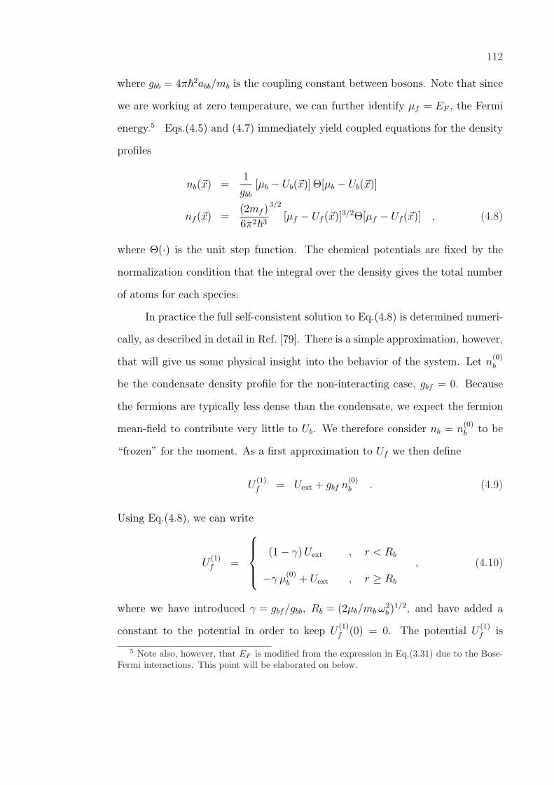
112
where gbb = 4π~2abb/mb is the coupling constant between bosons. Note that since
we are working at zero temperature, we can further identify µf = EF , the Fermi
energy.5 Eqs.(4.5) and (4.7) immediately yield coupled equations for the density
profiles
nb(~x) =1
gbb
[µb − Ub(~x)] Θ[µb − Ub(~x)]
nf (~x) =(2mf )
6π2~3
3/2
[µf − Uf (~x)]3/2Θ[µf − Uf (~x)] , (4.8)
where Θ(·) is the unit step function. The chemical potentials are fixed by the
normalization condition that the integral over the density gives the total number
of atoms for each species.
In practice the full self-consistent solution to Eq.(4.8) is determined numeri-
cally, as described in detail in Ref. [79]. There is a simple approximation, however,
that will give us some physical insight into the behavior of the system. Let n(0)b
be the condensate density profile for the non-interacting case, gbf = 0. Because
the fermions are typically less dense than the condensate, we expect the fermion
mean-field to contribute very little to Ub. We therefore consider nb = n(0)b to be
“frozen” for the moment. As a first approximation to Uf we then define
U(1)f = Uext + gbf n
(0)b . (4.9)
Using Eq.(4.8), we can write
U(1)f =
(1− γ) Uext , r < Rb
−γ µ(0)b + Uext , r ≥ Rb
, (4.10)
where we have introduced γ = gbf/gbb, Rb = (2µb/mb ω2b )
1/2, and have added a
constant to the potential in order to keep U(1)f (0) = 0. The potential U
(1)f is
5 Note also, however, that EF is modified from the expression in Eq.(3.31) due to the Bose-Fermi interactions. This point will be elaborated on below.

113
shown schematically in Fig. 4.4 for various values of γ (neglecting the shift of
γ µ(0)b for clarity). Our analysis of the positions of the 87Rb -40K Feshbach reso-
nances in Ref. [44] suggests a value of γ = −4.5 ± 0.2 for a mixture in the state
|F = 2,mF = 2 〉Rb ⊗ | 9/2, 9/2 〉K, which is the mixture we magnetically trap and
sympathetically cool. This sets a sense of scale for γ. Note also that the reso-
nances themselves give us access in principle to any value of γ desired. For this
reason we will consider all values of γ in our discussion.
Equation (4.10) and Fig. 4.4 show that fermions within the condensate ra-
dius Rb experience a harmonic potential with an effective trapping frequency
ω′f = ωf (1 − γ)1/2 for γ < 1. For the “magic” value γ = 1, the condensate
mean-field cancels the external potential for the fermions, giving rise to a uniform
sample of fermions at the trap center, or “fermions in a box.” Fermions in a box
are predicted to occur for abf = 2 abb mf/(mb + mf ) ' 62 a0 for the 87Rb -40K sys-
tem.6 For γ > 1, the fermions feel a repulsive bump in the center of the trap,
and for sufficiently strong interactions, the fermions will be expelled from the
trap center. This phenomenon is referred to as phase separation. In this limit
the fermions are expected to form a dilute shell around the BEC core.7 In
the limit of strong attractive interactions between species (large, negative γ), the
presence of the bosons gives rise to a region of exceedingly strong confinement for
the fermions at the center of the trap. For strong enough attractive interactions,
the peak fermion density can become large enough to appreciably modify Ub in
such a way that the boson density then begins to increase. The positive feedback
between nb and nf can lead to a runaway “collapse” of the system, where the
6 Production of BEC in a box has just been observed in the group of Mark Raizen at theUniversity of Texas, using specially tailored optical potentials. See arXiv:cond-mat/0503590.
7 In our discussion of phase separation, we are assuming a moderate boson-boson repulsion,and that there are not more fermions than bosons, as in the experiments. Under differentconditions it is also possible to have a condensate shell around a Fermi gas core. For a detaileddiscussion of this, along with the only description I’ve seen of spontaneous symmetry-breakingfor Bose-Fermi mixtures in elongated traps, see Ref. [80].
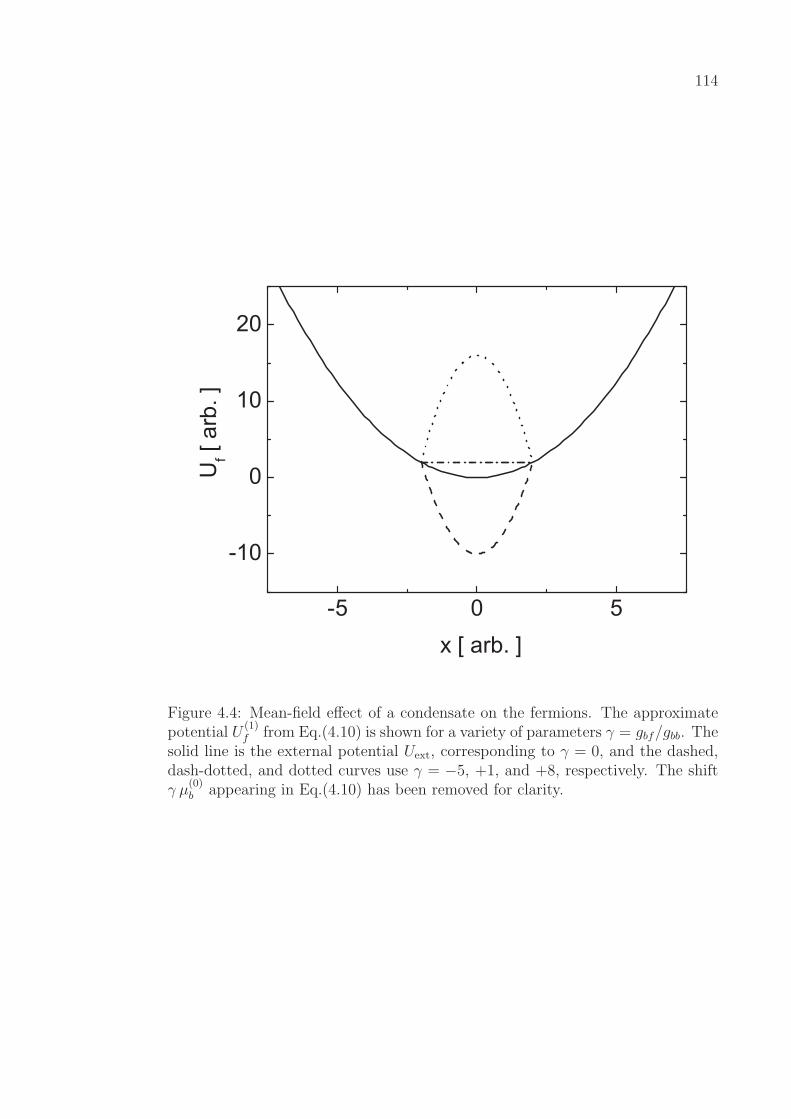
114
Figure 4.4: Mean-field effect of a condensate on the fermions. The approximatepotential U
(1)f from Eq.(4.10) is shown for a variety of parameters γ = gbf/gbb. The
solid line is the external potential Uext, corresponding to γ = 0, and the dashed,dash-dotted, and dotted curves use γ = −5, +1, and +8, respectively. The shiftγ µ
(0)b appearing in Eq.(4.10) has been removed for clarity.

115
densities become essentially singular at the trap center. We will have more to say
about this scenario later. Self-consistent equilibrium density profiles calculated
from Eq.(4.8) are shown in Fig. 4.5 for various values of the interaction strength.
In analogy with the discussion leading to Eq.(4.10) we can estimate the
fermion chemical potential by
µ(1)f = µ
(0)f − γ µ
(0)b . (4.11)
This in turn leads us to some approximations for the central density of the mixture.
For positive γ, we get an estimate for the critical parameter for phase separation
γsep by simply defining
n(1)f (0) =
(2 mf )
6 π2~3
3/2 [µ
(0)f − γ µ
(0)b
]3/2
. (4.12)
The phase separation is then expected when n(1)f (0) = 0 in Eq.(4.12), so that we
predict γ(1)sep = µ
(0)f /µ
(0)b .
For sufficiently strong attractive interactions our method of approximation
is expected to fail, as we have assumed n(1)b ' n
(0)b , which will no longer be accurate
as the collapse is approached. We may, however, write Eq.(4.7) in matrix form
G · ~n = ~µ, with ~n = (nb(0), nf (0))T and ~µ = (µb, µf )T (superscript T ’s denote a
transpose), and coupling matrix
G =
gbb gbf
gbf 3 π2 ~2/mf kF
, (4.13)
with kF = [6 π2nf (0)]1/3 = (2 mfµf )1/2/~ the Fermi wavenumber. The condition
that G · ~n = ~µ has a non-trivial solution for the densities is then equivalent to
setting the determinant of G equal to zero. Solution of the resulting equation
gives a critical value of γ for collapse of
γcol =
√3 π2~2
mf kF gbb
. (4.14)

116
Figure 4.5: Theoretical equilibrium profiles in the TF approximation. The cal-culations assumed 105 atoms each of 87Rb and 40K, in a spherical trap withωRb = 2π × 100 Hz. The values of γ are the same as in Fig. 4.4.
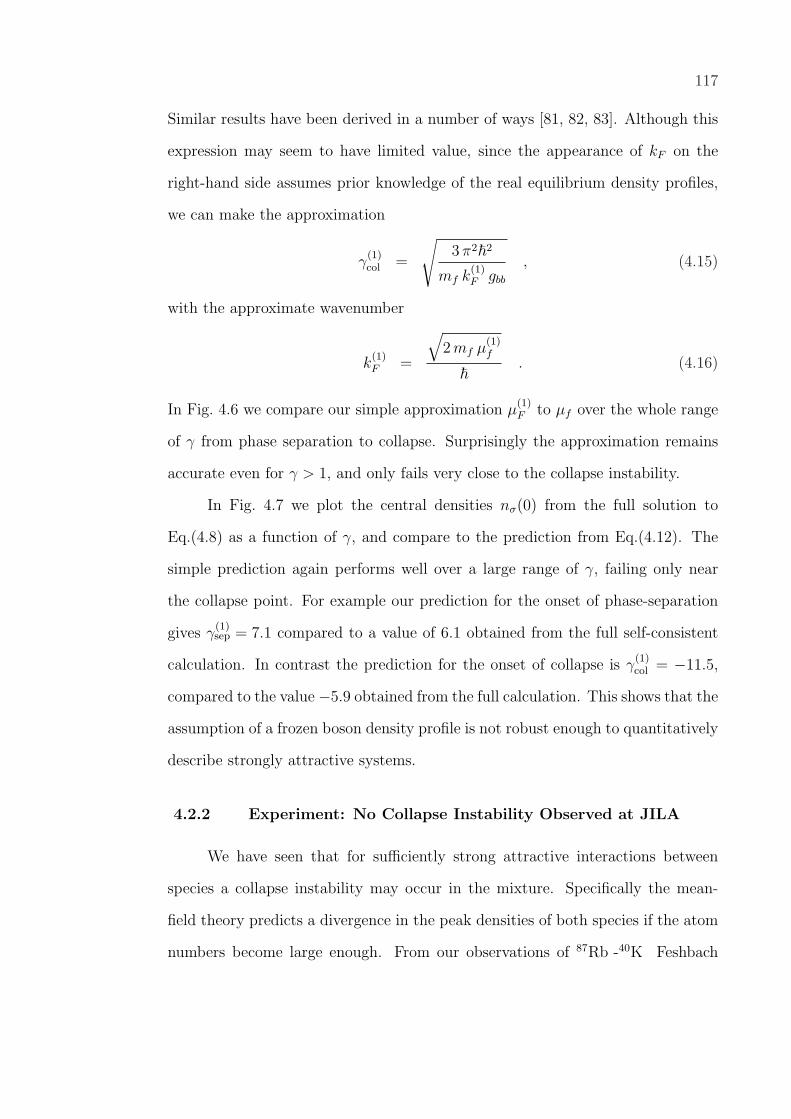
117
Similar results have been derived in a number of ways [81, 82, 83]. Although this
expression may seem to have limited value, since the appearance of kF on the
right-hand side assumes prior knowledge of the real equilibrium density profiles,
we can make the approximation
γ(1)col =
√3 π2~2
mf k(1)F gbb
, (4.15)
with the approximate wavenumber
k(1)F =
√2 mf µ
(1)f
~. (4.16)
In Fig. 4.6 we compare our simple approximation µ(1)F to µf over the whole range
of γ from phase separation to collapse. Surprisingly the approximation remains
accurate even for γ > 1, and only fails very close to the collapse instability.
In Fig. 4.7 we plot the central densities nσ(0) from the full solution to
Eq.(4.8) as a function of γ, and compare to the prediction from Eq.(4.12). The
simple prediction again performs well over a large range of γ, failing only near
the collapse point. For example our prediction for the onset of phase-separation
gives γ(1)sep = 7.1 compared to a value of 6.1 obtained from the full self-consistent
calculation. In contrast the prediction for the onset of collapse is γ(1)col = −11.5,
compared to the value−5.9 obtained from the full calculation. This shows that the
assumption of a frozen boson density profile is not robust enough to quantitatively
describe strongly attractive systems.
4.2.2 Experiment: No Collapse Instability Observed at JILA
We have seen that for sufficiently strong attractive interactions between
species a collapse instability may occur in the mixture. Specifically the mean-
field theory predicts a divergence in the peak densities of both species if the atom
numbers become large enough. From our observations of 87Rb -40K Feshbach

118
Figure 4.6: Fermion chemical potential with interactions. The points are thecalculated chemical potential for a 87Rb -40K mixture with 105 atoms of eachspecies in a spherical trap with ωRb = 2π × 100 Hz. The solid line shows theprediction of a slope −γ µ
(0)b through the non-interacting value (dashed line). The
vertical dotted lines show the locations of the collapse (left) and phase separation(right), as shown in Fig. 4.7.

119
Figure 4.7: Theoretical dependence of the central densities on mean-field cou-pling strength. Circles give the condensate density, and triangles correspond tothe fermions, for the same conditions as in Fig. 4.6. In each case the open pointsuse the TF approximation for the bosons, and the filled points use the GP equa-tion. The solid curve is the prediction from Eq.(4.12), and the dashed line is thenoninteracting value for the bosons. The vertical dotted lines mark the collapse(left) and phase-separation (right) instabilities.
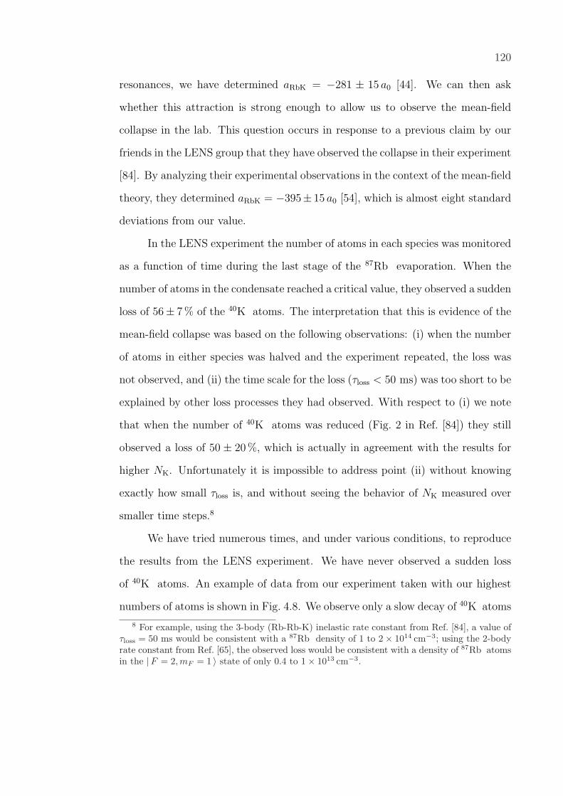
120
resonances, we have determined aRbK = −281 ± 15 a0 [44]. We can then ask
whether this attraction is strong enough to allow us to observe the mean-field
collapse in the lab. This question occurs in response to a previous claim by our
friends in the LENS group that they have observed the collapse in their experiment
[84]. By analyzing their experimental observations in the context of the mean-field
theory, they determined aRbK = −395± 15 a0 [54], which is almost eight standard
deviations from our value.
In the LENS experiment the number of atoms in each species was monitored
as a function of time during the last stage of the 87Rb evaporation. When the
number of atoms in the condensate reached a critical value, they observed a sudden
loss of 56± 7 % of the 40K atoms. The interpretation that this is evidence of the
mean-field collapse was based on the following observations: (i) when the number
of atoms in either species was halved and the experiment repeated, the loss was
not observed, and (ii) the time scale for the loss (τloss < 50 ms) was too short to be
explained by other loss processes they had observed. With respect to (i) we note
that when the number of 40K atoms was reduced (Fig. 2 in Ref. [84]) they still
observed a loss of 50 ± 20 %, which is actually in agreement with the results for
higher NK. Unfortunately it is impossible to address point (ii) without knowing
exactly how small τloss is, and without seeing the behavior of NK measured over
smaller time steps.8
We have tried numerous times, and under various conditions, to reproduce
the results from the LENS experiment. We have never observed a sudden loss
of 40K atoms. An example of data from our experiment taken with our highest
numbers of atoms is shown in Fig. 4.8. We observe only a slow decay of 40K atoms
8 For example, using the 3-body (Rb-Rb-K) inelastic rate constant from Ref. [84], a value ofτloss = 50 ms would be consistent with a 87Rb density of 1 to 2× 1014 cm−3; using the 2-bodyrate constant from Ref. [65], the observed loss would be consistent with a density of 87Rb atomsin the |F = 2,mF = 1 〉 state of only 0.4 to 1× 1013 cm−3.

121
when the 87Rb condensate is formed. Additional measurements using faster
evaporation rates, as in the LENS experiment, showed similar results.
In Fig. 4.9 we show the theoretical stability diagram for the 87Rb -40K mix-
ture for attractive interactions of varying strengths. All calculations assume a
spherical trap with ωRb = 2π × 90 Hz, which is similar to the geometric mean
trap strengths of both our experiment and the LENS experiment. The theoretical
calculations are compared to the experimental observations, and we have included
a recent result from a new 87Rb -40K experiment in the group of Klaus Sengstock
at the University of Hamburg.9 The results of the LENS experiment are clearly
incompatible with the other experiments and the value aRbK = −281 ± 15 a0.
Since our calculations have neglected the stabilizing effects of finite temperature
[85, 86, 87], gravitational sag,10 and a repulsive second-order contribution to the
interaction [88],11 the discrepancy is actually worse than what we have shown
here.
Finally in Table 4.2 we show the upper limits on |aRbK| imposed by the
mean-field theory as a result of the various experimental findings. Note that
the gravitational sag is neglected in these calculations, which leads to a value of
|aRbK| that is 3% lower than what was given in Ref. [54]. From our work we must
conclude that there is either some aspect of the mean-field theory which has been
neglected or violated, or the sudden loss of fermions reported in Ref. [84] must find
a new interpretation, for example enhanced inelastic losses due to the presence
9 Christian Ospelkaus, in a seminar presented at JILA [55], has reported a stable mixturewith 1.5×10⁶ 87Rb atoms and 7.0×10⁵ 40K atoms in a trap with ωRb = 2π×(2552 ·11.3)1/3 Hz.
10 The LENS trap has stronger radial confinement than ours, which reduces their vertical sagand helps to preserve the density overlap. However, they have a weaker axial confinement anda significant tilt to their trap, resulting in a large axial displacement between equilibrium cloudpositions [54]. In any event the reduction in overlap always suppresses the collapse instabilityto some degree. Note also that the Hamburg experiment has the tightest radial confinement ofthe three experiments.
11 Quoted from the LENS group in Ref. [54]: “[T]he inclusion of [the second-order] termstabilizes the system in the range of atom numbers considered here for any value of the scatteringlength, thus forbidding the collapse, in contrast with the experimental findings.”

122
Figure 4.8: Slow decay of 40K atoms with 87Rb BEC. Circles give the numberof atoms in the BEC and triangles give the number of 40K atoms, as a functionof time during the final stage of 87Rb evaporation (t = 0 marks the start of theevaporation). The solid curve is a fit to a flat region followed by exponential decay,with a 1/e time constant of about 2 seconds. This curve and the dashed curve areintended as guides to the eye. These are the same data as in Fig. 3.9, where wediscussed the fact that the apparent delay between the loss of 40K atoms and theformation of the condensate is an artifact of a short hold time between the end ofevaporation and the time-of-flight. Similar data taken without this delay (usingan rf switch on the evaporation knife) also showed a slow decay of 40K number, asdid data taken with different evaporation rates. We have never observed evidenceof the collapse instability in our experiment.
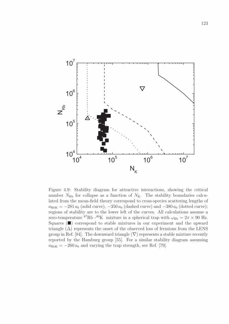
123
Figure 4.9: Stability diagram for attractive interactions, showing the criticalnumber NRb for collapse as a function of NK. The stability boundaries calcu-lated from the mean-field theory correspond to cross-species scattering lengths ofaRbK = −281 a0 (solid curve), −350 a0 (dashed curve) and −380 a0 (dotted curve);regions of stability are to the lower left of the curves. All calculations assume azero-temperature 87Rb -40K mixture in a spherical trap with ωRb = 2π × 90 Hz.Squares (¥) correspond to stable mixtures in our experiment and the upwardtriangle (∆) represents the onset of the observed loss of fermions from the LENSgroup in Ref. [84]. The downward triangle (∇) represents a stable mixture recentlyreported by the Hamburg group [55]. For a similar stability diagram assumingaRbK = −260 a0 and varying the trap strength, see Ref. [79].

124Expt. Nf Nb |aRbK|max
LENS [84, 54] 2.0× 10⁴ 1.5× 10⁵ 384 a0
JILA 6.5 2.6 366
Hamburg [55] 70 15 308
Table 4.2: Upper limits on |aRbK|. The maximum numbers of atoms observed instable, quantum degenerate mixtures in each experiment are used to determineupper limits on |aRbK| according to the mean-field theory.
of trapped atoms in undesired spin states. The 87Rb -40K Feshbach resonances
which we observed in Ref. [44], and which are discussed in detail in Sects. 4.4.2
and 4.4.3, should allow us to study the collapse in a more controlled manner in
the future.
4.3 Excitations
So far we have been concerned with the equilibrium properties of Bose-
Fermi mixtures. In this section I will turn to some measurements of excitations
in our system. The spectra of excitations are generally enriched by the coupling
between purely bosonic and fermionic modes, and can reveal information about
the interactions not easily obtained by other means. For example Capuzzi and co-
workers showed in Ref. [89] that the modification to the frequencies of low-lying
collective excitations can herald the onset of the collapse and phase-separation
instabilities.
Here I’ll begin with an experiment we have performed where we measured
the damping rate of fermions undergoing a quadrupolar “breathe” mode after
selective excitation in the presence of thermal bosons. The rate of damping of
the excitation reveals information on the strength of the interactions through the
magnitude of the scattering length |abf |. The measurement we have performed is
in the collisionless regime, where the frequency of the excitation is just equal to

125
twice the bare trap frequency. As the bosons condense or the mean-field coupling
between species increases, the frequencies of the modes are expected to change,
and therefore reveal additional information, including even the sign of the scat-
tering length [89].
I’ll then discuss how we can map out the excitation spectra in the fourier
domain by varying the frequency at which we parametrically excite the gas and
measuring the response. This discussion will focus on a measurement we have
performed with a partially condensed sample of 87Rb in the absence of 40K atoms.
In this measurement we were able to use the coupling between thermal atoms and
the condensate to observe higher-lying condensate excitations. The frequencies of
these modes were mapped out by observing the “melting” of the condensate due
to the dissipative coupling.
Finally I’ll discuss the prospects for observing p-wave pairing of the fermions
induced by interactions with the condensate [5, 6, 7]. I will show how the use of
inter-species Feshbach resonances may make it feasible to observe the pairing in
experiments without reaching the phase-separation or collapse instabilities.
4.3.1 Quadrupole “Breathe” Mode
Consider a single particle in a harmonic trapping potential with radial and
axial frequencies ωρ and ωz, respectively. If the radial trap frequency is modulated
with strength ε at a frequency ω the total potential energy is given by
U(~x, t) =1
2m
[ω2
ρ (1 + ε sin ωt) ρ2 + ω2z z2
], (4.17)
which leads to the Mathieu equation for the total energy. In a gas of atoms the
presence of collisions generally leads to damping, so that the work done on the
particles goes into heating the gas. This kind of parametric heating is considered
in Refs. [90, 91]. If, however, the modulating drive is short compared to rether-

126
malization times, the heating can be initially avoided and a collective excitation
can be generated. Data from the experiment showing the damping of this kind of
excitation are shown in Fig. 4.10. This mode, which is often called the “breathe”
mode, has quadrupolar symmetry with m = 0 and was studied theoretically for
a single-species thermal gas in Refs. [71, 92], and experimentally across the BEC
phase transition for a 87Rb gas in [93]. In the collisionless regime, the energy
oscillates between kinetic and potential energies at twice the trap frequency, until
collisions convert the excess energy into heat and the gas relaxes into thermal
equilibrium.
One interesting aspect of the breathe mode is that the constant of propor-
tionality α = τdamp/τcoll which we discussed with respect to the 87Rb-87Rb CDR
experiment is now quite different. We found for the CDR measurement that
αCDR ' 2.5 to 2.7, but the theoretical prediction for the quadrupole breathe
mode is αQB = 15, higher by a factor of six. Furthermore the non-interacting
modes for 87Rb and 40K are well separated as a result of the different masses be-
tween species. This allows us to selectively excite a breathe mode in 40K without
affecting the 87Rb atoms. We will see that the constant of proportionality βQB
for the 40K atoms is much smaller than αQB under these conditions.
The constants αQB and βQB are again determined from classical Monte Carlo
simulations. To save computation time, we neglect the possibility of collisions
during the trap modulation. This, together with the fact the simulation assumes
a perfectly harmonic potential whose frequency is known exactly, means that
the response of the simulated particles to the excitation is larger than in the
experiments. We can, however, vary the amplitude of the drive in the simulations,
and observe the behavior of αQB and βQB. The results are shown in Fig. 4.11. The
87Rb single-species simulations show that αQB → 14.7±0.4 as ε → 0, in agreement
with the prediction αQB = 15 from Refs. [71, 92]. To the best of my knowledge,

127
Figure 4.10: Measurement of the damping of breathe modes. Shown is the squareof the aspect ratio in time-of-flight expansion as a function of evolution time inthe trap after the initial excitation. Dots (•, above) and triangles (N, below) arefor 87Rb atoms alone and 40K atoms in the presence of 87Rb, respectively. Thecurves are fits to damped oscillations, giving damping times of τRbRb = 200± 30ms and τRbK = 31 ± 4 ms. Note that the 87Rb data extend to 1000 ms. The87Rb trap frequencies were ωρ = 2π×91.0 Hz and ωz = 2π×25.6 Hz. The relevantexperimental parameters were NRb = 7.0 ± 0.8 × 10⁵, T = 510 ± 50 nK for theupper data and NK = 1.9±0.2×10⁵, NRb = 3.5±0.2×10⁵, and T = 470±50 nKbelow, where the uncertainties on number reflect statistical uncertainties only.
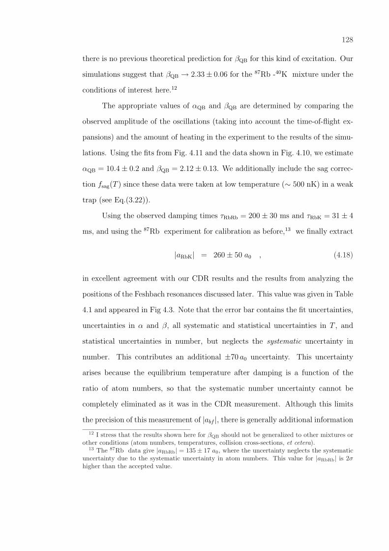
128
there is no previous theoretical prediction for βQB for this kind of excitation. Our
simulations suggest that βQB → 2.33± 0.06 for the 87Rb -40K mixture under the
conditions of interest here.12
The appropriate values of αQB and βQB are determined by comparing the
observed amplitude of the oscillations (taking into account the time-of-flight ex-
pansions) and the amount of heating in the experiment to the results of the simu-
lations. Using the fits from Fig. 4.11 and the data shown in Fig. 4.10, we estimate
αQB = 10.4± 0.2 and βQB = 2.12± 0.13. We additionally include the sag correc-
tion fsag(T ) since these data were taken at low temperature (∼ 500 nK) in a weak
trap (see Eq.(3.22)).
Using the observed damping times τRbRb = 200± 30 ms and τRbK = 31± 4
ms, and using the 87Rb experiment for calibration as before,13 we finally extract
|aRbK| = 260± 50 a0 , (4.18)
in excellent agreement with our CDR results and the results from analyzing the
positions of the Feshbach resonances discussed later. This value was given in Table
4.1 and appeared in Fig 4.3. Note that the error bar contains the fit uncertainties,
uncertainties in α and β, all systematic and statistical uncertainties in T , and
statistical uncertainties in number, but neglects the systematic uncertainty in
number. This contributes an additional ±70 a0 uncertainty. This uncertainty
arises because the equilibrium temperature after damping is a function of the
ratio of atom numbers, so that the systematic number uncertainty cannot be
completely eliminated as it was in the CDR measurement. Although this limits
the precision of this measurement of |abf |, there is generally additional information
12 I stress that the results shown here for βQB should not be generalized to other mixtures orother conditions (atom numbers, temperatures, collision cross-sections, et cetera).
13 The 87Rb data give |aRbRb| = 135± 17 a0, where the uncertainty neglects the systematicuncertainty due to the systematic uncertainty in atom numbers. This value for |aRbRb| is 2σhigher than the accepted value.
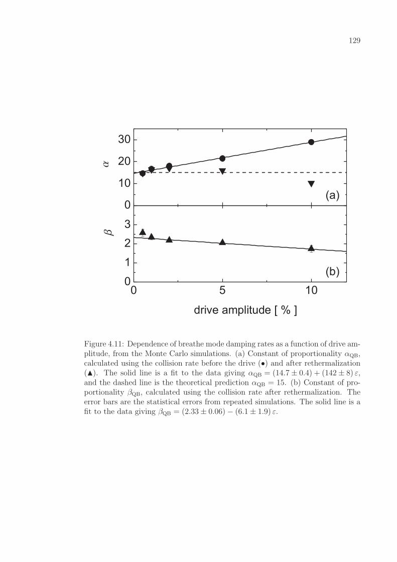
129
Figure 4.11: Dependence of breathe mode damping rates as a function of drive am-plitude, from the Monte Carlo simulations. (a) Constant of proportionality αQB,calculated using the collision rate before the drive (•) and after rethermalization(N). The solid line is a fit to the data giving αQB = (14.7± 0.4) + (142± 8) ε,and the dashed line is the theoretical prediction αQB = 15. (b) Constant of pro-portionality βQB, calculated using the collision rate after rethermalization. Theerror bars are the statistical errors from repeated simulations. The solid line is afit to the data giving βQB = (2.33± 0.06)− (6.1± 1.9) ε.

130
in the frequency of the mode. This could make this type of measurement preferable
when the interactions between species become strong.
4.3.2 Frequency Domain and High-Order BEC Excitations
In Fig. 4.10 we observed the damped oscillation of (σz/σρ)2 as a function
of time after the excitation. We could also have studied the breathe mode by
varying the frequency of the drive, and measuring the response. For example, if
we wait long enough after exciting the mode to let it completely damp out, then
the excitation energy is converted into heat and the increased temperature of the
gas reveals the underlying excitation. Data from this type of measurement are
shown in Fig. 4.12, where we have driven an axial quadrupole mode in a single-
species gas of thermal 87Rb atoms. This type of collective excitation spectroscopy
has a few important advantages when one is interested in the mode frequency.
One practical advantage of the frequency-domain method is that relatively
few data points are needed to precisely determine the mode frequency. In Fig. 4.12
we took 10 data points and achieved a relative fit uncertainty of only 1.5× 10⁻³
on the resonance frequency. Additionally, the width of the resonance is only 420
mHz, which is limited by the fourier width of the modulation pulse we applied to
drive the excitation. This allowed us to observe that the frequency of the mode
we excited did not equal 2 ωz, as we expected. We interpret this as evidence of
beginning to approach the hydrodynamic regime. To verify this we compare this
measurement to a similar measurement taken with lower atom number in Fig. 4.13.
We have additionally included the theoretical prediction from Ref. [92], which
interpolates between the value 2 ωz in the collisionless regime to (12/5)1/2 ωz '1.55 ωz in the hydrodynamic regime.
Another potential advantage of the frequency-domain measurement becomes
evident in systems where many modes exist at nearby frequencies. As an example
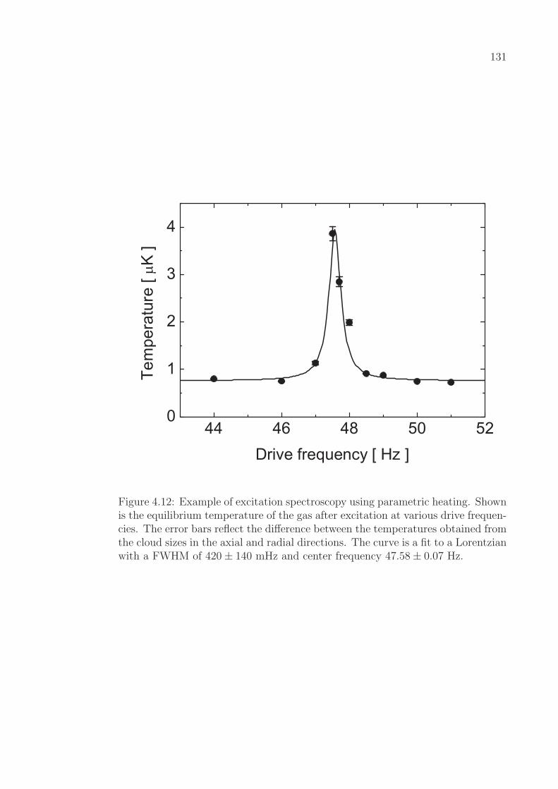
131
Figure 4.12: Example of excitation spectroscopy using parametric heating. Shownis the equilibrium temperature of the gas after excitation at various drive frequen-cies. The error bars reflect the difference between the temperatures obtained fromthe cloud sizes in the axial and radial directions. The curve is a fit to a Lorentzianwith a FWHM of 420± 140 mHz and center frequency 47.58± 0.07 Hz.
132
Figure 4.13: Density dependence of collective excitation frequency. Points showthe axial quadrupole resonance frequency measured through parametric heatingas a function of the ratio of trap frequency and collision rate. Error bars reflectstatistical errors on N and T only. The curve is the interpolating formula Eq.(19)from Ref. [92] with no free parameters.

133
we show in Fig. 4.14 our observation of a series of nearly uniformly-spaced reso-
nances of a 87Rb condensate. The condensate is excited with a modulation of the
axial trap strength, and the condensate fraction is monitored as a function of drive
frequency. Dissipative interactions with thermal 87Rb atoms lead to heating and
subsequent melting of the condensate at the resonances. It is believed that the
coupling between the BEC and thermal atoms, whose modes occur at different
frequencies, also assists in the excitation process. Although these data were taken
without 40K atoms, I see no reason why 40K atoms couldn’t serve the purpose of
the thermal 87Rb atoms here in future experiments using interacting mixtures.
Stringari calculated the spectrum of azimuthally-symmetric axial excitations
for elongated BECs and found [94]
ωl = ωz
√l (l + 3)
4, l = 1, 2, 3... (4.19)
for mode number l. Note that the lowest mode (l = 1) is identified with the
dipole or “slosh” mode and the l = 2 mode corresponds to the quadrupole mode,
analogous to the breathe mode of thermal atoms we discussed in Sect. 4.3.1.
The mode frequencies are determined experimentally from Gaussian fits to
the observed resonances. The positions of the peaks are then fit to Eq.(4.19)
assuming consecutive modes, and letting ωz vary. The best fit corresponds to
ωz = 2π × 24.89± 0.07 Hz, compared to the value 2π × 24.78± 0.05 Hz obtained
from slosh measurements of 87Rb clouds. In Table 4.3 we compare the predictions
with the resonance positions observed in the experiment. These results suggest
that the features in Fig. 4.14 correspond to modes l = 12 to 15.
Finally note that the calculation leading to Eq.(4.19) assumes ωz ¿ ωρ,
compared to the experimental value here of (ωz/ωρ) = 0.16. Corrections to the
calculated spectrum due to the finite ratio of trap frequencies are dealt with in
Refs. [94, 95], and beyond-mean-field corrections are discussed in Refs. [94, 96],
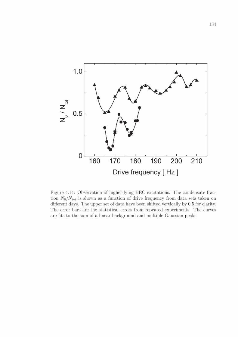
134
Figure 4.14: Observation of higher-lying BEC excitations. The condensate frac-tion N0/Ntot is shown as a function of drive frequency from data sets taken ondifferent days. The upper set of data have been shifted vertically by 0.5 for clarity.The error bars are the statistical errors from repeated experiments. The curvesare fits to the sum of a linear background and multiple Gaussian peaks.
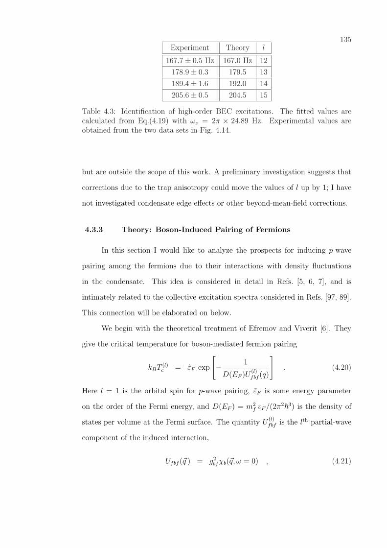
135Experiment Theory l
167.7± 0.5 Hz 167.0 Hz 12
178.9± 0.3 179.5 13
189.4± 1.6 192.0 14
205.6± 0.5 204.5 15
Table 4.3: Identification of high-order BEC excitations. The fitted values arecalculated from Eq.(4.19) with ωz = 2π × 24.89 Hz. Experimental values areobtained from the two data sets in Fig. 4.14.
but are outside the scope of this work. A preliminary investigation suggests that
corrections due to the trap anisotropy could move the values of l up by 1; I have
not investigated condensate edge effects or other beyond-mean-field corrections.
4.3.3 Theory: Boson-Induced Pairing of Fermions
In this section I would like to analyze the prospects for inducing p-wave
pairing among the fermions due to their interactions with density fluctuations
in the condensate. This idea is considered in detail in Refs. [5, 6, 7], and is
intimately related to the collective excitation spectra considered in Refs. [97, 89].
This connection will be elaborated on below.
We begin with the theoretical treatment of Efremov and Viverit [6]. They
give the critical temperature for boson-mediated fermion pairing
kBT (l)c = εF exp
[− 1
D(EF )U(l)fbf (q)
]. (4.20)
Here l = 1 is the orbital spin for p-wave pairing, εF is some energy parameter
on the order of the Fermi energy, and D(EF ) = m2f vF /(2π2~3) is the density of
states per volume at the Fermi surface. The quantity U(l)fbf is the lth partial-wave
component of the induced interaction,
Ufbf (~q ) = g2bfχb(~q, ω = 0) , (4.21)

136
where we have introduced the boson density-density response function χb. The
function χb(~q, ω) describes the response of the condensate density to perturbations
with wave number ~q and frequency ω.
For simplicity, Efremov and Viverit neglected the effect of the fermions on
the condensate response function. We note, however, that Yip has shown that the
effect of the interactions between species is to modify χb according to [97]
χb
gbf−→ χb
1− g2bf χb χf
. (4.22)
The non-interacting response functions are given in the local density approxima-
tion by
χb(~q, ω) = − 1
gbb
[c2b q2
ω2 − c2b q2 − (q2/2mb)2
]
χf (~q, ω) = D(EF )
[1− ω
2 vF qln
(ω + vF q
ω − vF q
)], (4.23)
where cb = (nb/gbb mb)1/2 is the Bogoliubov sound speed for the condensate, and
vF = (2EF /mf )1/2 is the Fermi speed. We have assumed q ¿ mf vF /~ in our
expression for χf .14
Returning to Eq.(4.21) we can write
Ufbf (~q) =g2
bf
gbb
1
Λbf + (q/2mbcb)2, (4.24)
where we have introduced Λbf = 1− g2bfD(EF )/gbb for simplicity. The lth compo-
nent of Ufbf is found by projecting onto the Legendre polynomial Pl(cos θ), where
q = 2kF sin(θ/2). This gives
U(1)fbf (κbf ) =
g2bf
gbb
2
κ2bf
[(1
2+
Λbf
κ2bf
)ln
(1 +
κ2bf
Λbf
)− 1
], (4.25)
where κbf = mf vF /mb cb. Note that in the limit of weak interactions Λbf → 1,
and we recover the result from Ref. [6].
14 Actually for fermion pairing we will be interested in q on the order of mf vF , but in thelimit ω → 0. In this limit, the terms we are neglecting are equal to zero, so that our expressionstill holds.

137
Equations (4.20) and (4.25) can now be used to calculate the critical temper-
ature for pairing. Without resonantly enhanced interactions the critical temper-
ature for pairing under typical conditions in our magnetic trap is ∼ 10−11 TF ,
which is absurdly far outside the reach of current experiments. Assuming a
87Rb -40K Feshbach resonance is used to bring the system near the collapse or
phase separation instabilities, however, the theory predicts T(1)c ∼ 0.17 TF for
reasonable experimental conditions. It should be noted that once U(1)fbf becomes
sufficiently large, the assumptions underlying the theory begin to break down.
In this case a more sophisticated calculation along the lines of that in Ref. [98]
should be developed for Bose-Fermi mixtures. However the fact that we can ap-
proach this condition without hitting the collapse or phase separation instabilities
is already a moral victory and extremely encouraging for future experiments.
4.4 Heteronuclear Feshbach Resonances
Throughout this thesis I have emphasized the importance of the inter-species
s-wave scattering length aRbK in characterizing the Bose-Fermi interactions in
the mixture. From the need for large collision cross-sections during sympathetic
cooling to the structure and stability of the equilibrium ground state of the mixture
and its spectra of excitations, the parameter aRbK is central to describing and
understanding the properties of the system. In this section I will discuss our
observation of 87Rb -40K Feshbach resonances. These resonances provide for the
first time a means for experimentally varying aRbK from −∞ to +∞ in a relatively
straightforward way.
I’ll begin this section with a brief description of the type of Feshbach reso-
nances described in this thesis. We will cover a review of basic scattering theory,
focusing more on results and applications than on detailed derivations. I will de-
fine what we mean by resonant scattering, and consider the example of scattering

138
from a spherical well potential. Although this simple example does not contain
all of the ingredients of a real Feshbach resonance (which must have two or more
coupled collision channels), the spherical well illustrates in a clear way the con-
nection between bound states of a potential and the divergence of the scattering
length.
I will then describe our experimental search for, and observation of, several
magnetically-tunable Feshbach resonances between 87Rb and 40K atoms. First
I’ll explain how and why we load the atoms into a purely optical trapping po-
tential and transfer the atoms to a particular set of states. Then I’ll show how
the strongly enhanced inelastic scattering at the position of the resonances al-
lowed us to locate three resonances in an initial search covering a large range of
magnetic fields. Subsequent comparison of the observed resonance positions with
full coupled-channel calculations performed by Chris Ticknor and John Bohn sug-
gested that one of these resonances could be p-wave in nature. This was verified
experimentally through the observation of a predicted third s-wave resonance,
which we had missed in the initial search. In the process of looking for the third
s-wave resonance, we additionally observed a 87Rb-87Rb resonance, which I’ll also
discuss. Finally our observation of the third 87Rb -40K s-wave resonance is used
to refine our values for the triplet and singlet scattering lengths between species.
4.4.1 Scattering Resonance Overview
4.4.1.1 Magnetically Tunable Feshbach Resonances
Scattering potentials between colliding alkali-metal atoms are shown schemat-
ically in Fig. 4.15. What the real 87Rb -40K potentials have in common with these
cartoons is a long-range van der Waals attraction which gives way to a short-range
139
hard-core repulsion.15 The net effect is an attractive potential well. Although
the cartoons do not show it, these wells are typically on the order of 103 to 104
K deep, which is astronomically larger than any other energy scale in the prob-
lem. At very large inter-nuclear separations the potentials are flat, and we can
think of the atoms as being independent. The asymptotic energies of the open
(incoming and outgoing) and closed (excited state) channels are then separated by
something like the hyperfine splitting, which may be 10 to 100 mK. This energy
scale, although much smaller than the well depth, is still much higher than the
temperature of the gas. The fact that exiting the collision in the excited state
is energetically forbidden is the origin of the term “closed” for the upper state.
However, because of the depth of the upper well it remains possible for a bound
state of the well to be resonant with the low collision energy (typically 100 nK to
10 µK from the open channel threshold). If the two potentials enjoy some coupling
γ, then a Feshbach resonance may arise. For example the hyperfine interaction
between atoms can result in a temporary flip of one atom’s spin. We’ll see that
virtual transitions of this type can have a dramatic effect on the collisions in the
mixture.
In the experiments we exploit the fact that the different potentials generally
have different magnetic moments. This allows us to tune the threshold energies
of the open and closed channels relative to one another by means of the Zeeman
effect. This is the nature of the Feshbach resonances described in this thesis.
4.4.1.2 Resonant Scattering and Bound States
I will now briefly review some basic results for quantum mechanical scatter-
ing. We will assume low-energy scattering, and focus primarily on the scattering
length a. More detailed discussions of scattering and resonances can be found, for
15 The real 87Rb -40K potentials are described in detail in Ref. [99].
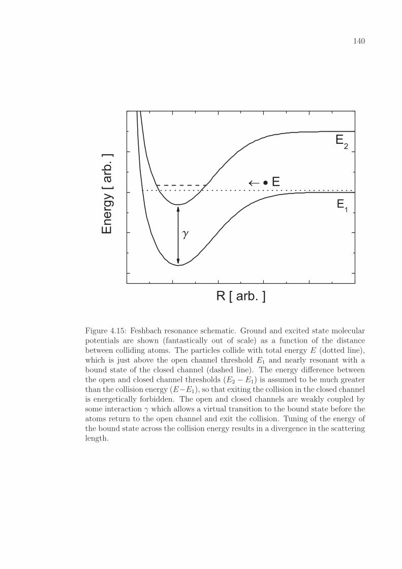
140
Figure 4.15: Feshbach resonance schematic. Ground and excited state molecularpotentials are shown (fantastically out of scale) as a function of the distancebetween colliding atoms. The particles collide with total energy E (dotted line),which is just above the open channel threshold E1 and nearly resonant with abound state of the closed channel (dashed line). The energy difference betweenthe open and closed channel thresholds (E2 −E1) is assumed to be much greaterthan the collision energy (E−E1), so that exiting the collision in the closed channelis energetically forbidden. The open and closed channels are weakly coupled bysome interaction γ which allows a virtual transition to the bound state before theatoms return to the open channel and exit the collision. Tuning of the energy ofthe bound state across the collision energy results in a divergence in the scatteringlength.

141
example, in Refs. [1, 100, 101].
The Schrodinger equation for two colliding atoms is given by
[− ~2
2 µ R∇2
R + V (R)
]ψ(R) = E ψ(R) , (4.26)
where µ is the reduced mass, V (R) is the interaction potential, and R is the
internuclear separation. In writing Eq.(4.26) we have neglected the center-of-
mass (CM) degrees of freedom, which lead to a plane-wave solution if no potential
acts on the CM position. For low-energy scattering it is convenient to rewrite
Eq.(4.26) as
(d2
dR2+ k2
)ul(R) =
[U(R) +
l (l + 1)
R2
]ul(R) , (4.27)
where k2 = 2µE/~2, U(R) = 2µV (R)/~2, and l is the angular momentum quan-
tum number. The function ul(R) is the lth partial-wave component of the reduced
wave function. We will restrict our discussion to s-wave (l = 0) collisions, and
drop the l labels for simplicity. As we have seen our gases are typically cold enough
that atoms cannot (classically) overcome the centrifugal barrier for collisions with
l > 0. Although this may not be true under resonant conditions, this assumption
will simplify our discussion.
As in Fig. 4.15 the scattering potential V (R) is assumed to be flat at exceed-
ingly large separations. This is the region of interest to experimentally observable
quantities. At large separations the solution to Eq.(4.27) therefore takes the form
of a linear combination of kR j0(kR) and kR n0(kR) with j0 and n0 the spherical
Bessel and Neumann functions of the first kinds, respectively. In the limit R →∞this corresponds to the sum of sin kR and cos kR. In other words, the only affect
of the scattering potential on the outgoing wave function ψ(+)(R) = exp(ikR)/R
142
is encoded in a phase shift δ, defined by
limR→∞
ψ(R) =e−ikR
R− e2iδ eikR
R
= ψ(−)(R)− S ψ(+)(R) , (4.28)
where ψ(R) is the total wave function, ψ(−) (ψ(+)) is an incoming (outgoing) wave,
and we have introduced the S- or scattering matrix, S = exp(2iδ).16
The effect of the scattering potential has been reduced to the single para-
meter δ, but the phase-shift is not the most convenient quantity for describing
experiments. On the other hand, I have stressed throughout this thesis that the
scattering length a makes a wonderful choice. The connection between δ and a is
given by
a = limk→0
(−tan δ
k
). (4.29)
We will see that the scattering potential can lead to a divergence in a under the
right conditions. This is what is meant in this thesis by a scattering resonance.
Let’s now consider a simple scattering calculation that will illustrate what a
scattering resonance looks like, and how it relates to the presence of bound states
of the scattering potential. For this discussion we will consider only a single open
channel. As a crude model of the lower potential in Fig. 4.15 we introduce the
absurdly-named spherical square well potential
V (R) = −V0 Θ(R−R0) , (4.30)
where Θ(·) is the unit step function.
Since the potential V (R) is piece-wise constant, the reduced wave function
16 Despite its name, S will be a scalar throughout our discussion. Note also that since we areinterested in elastic collisions, the phase shift δ is purely real.
143
u(R) takes the form
u(R) =
α sin k′R , R ≤ R0
exp(−ikR)− S exp(ikR) , R > R0
, (4.31)
where ~ k = (2µE)1/2, ~ k′ = [2µ(E + V0)]1/2, and α is just a normalization
constant.
To get α and S we match u(R) and its derivative at R = R0, giving
S = exp(−2ikR0)
(k′R0 cot k′R0 + ikR0
k′R0 cot k′R0 − ikR0
). (4.32)
The S-matrix gives (i) the phase shift δ, and therefore the scattering length a, as
well as (ii) the bound states of the potential V (R) at the poles of S [1]. We begin
with the scattering length.
Using Eq.(4.28), and taking the logarithm of Eq.(4.32) gives the phase shift
δ = tan−1
(k
k′tan k′R0
)− kR0 , (4.33)
and the scattering length is
a = R0
(1− tan k′R0
k′R0
). (4.34)
We can now identify the well radius R0 with the off-resonant scattering length.
Note that a diverges whenever k′R0 equals an odd-integer multiple of π/2. This
is an example of a potential that gives rise to multiple scattering resonances.
In Fig. 4.16 we show the scattering length and cross-section as a function of
the well depth V0 for zero-energy (k = 0) collisions. The cross-section σ = 4π a2
for distinguishable scatterers. In the case of non-zero k, the collision cross-section
is unitarity-limited according to [1]
σ =4π a2
1 + k2a2. (4.35)

144
For fixed k then, the resonant cross-section is limited to σmax = 4π/k2. Alter-
natively for any given value of a, Eq.(4.35) allows us to determine the energy at
which σ is reduced to σmax/2. As an example, for a 87Rb -40K mixture with
aRbK = −280 a0 we have k2a2 = 1 for a collision energy Ecoll ' 40 µK. This
may be important for sympathetic cooling, which relies on large cross-sections for
efficient rethermalization.17
Note that the scattering resonances in Fig. 4.16 occur whenever the scat-
tering potential becomes deep enough to accommodate another bound state just
below the open channel threshold. This connection between the appearance of a
bound state and a scattering resonance is an example of Levinson’s theorem [47].
4.4.2 Observation of Feshbach Resonances
Since the first observations of magnetically-tunable Feshbach resonances
[102, 103, 104], control over the scattering length has led to a variety of im-
portant and exciting experiments in the field of ultracold atomic gases. Obser-
vations of Feshbach resonances have exploited the divergent nature of the elastic
and inelastic scattering properties to perform very high-precision spectroscopy
of the molecular potentials describing the collisions [105, 45, 69, 106, 107]. The
ability to experimentally tune a has led to the production and controlled col-
lapse of a 85Rb Bose-Einstein condensate [108, 109], as well as the production of
long-lived bright matter-wave solitons in 7Li BECs [110, 111]. Ultracold mole-
cules have been produced using time-dependent fields near Feshbach resonances
[112, 113, 114, 115, 116, 117, 118, 119, 107]. BECs of molecules have been created
from Bose gases [112, 120, 121], and the matter-wave coherence of the molecular
BECs has been demonstrated [112, 121]. Molecular condensates have also been
17 For more on the energy dependence of the 87Rb -40K elastic collision cross-section see thediscussion in Sect. 3.3.3.

145
Figure 4.16: Spherical well scattering resonances. Shown is the scattering lengtha (above) and cross-section σ = 4π a2 (below) as a function of V0, with k = 0.The vertical dotted lines in the lower plot locate [(2n + 1)π/2]2 for integer n ≥ 0,corresponding to the appearance of additional bound states of the potential.
146
produced from quantum degenerate Fermi gases [122, 123, 124], and more re-
cent experiments with Fermi gases have accessed the BCS-BEC crossover regime
[125, 126, 127, 128].
In this section I’ll describe how we search for and induce Feshbach resonances
in the collisions between atoms of chemically distinct species. For every one of the
experiments described above, some analogous phenomenon has been predicted to
occur in Bose-Fermi mixtures. These experiments are expected to greatly enrich
our studies of Bose-Fermi mixtures in innumerable exciting ways.
4.4.2.1 Transfer to Resonant States
In our preceding discussion we noted that the Zeeman effect can be used
to tune the separation between the threshold energies of molecular potentials
with different magnetic moments. This in turn may lead to Feshbach resonances
under favorable conditions. In Chapter 3 we said that our magnetic trapping is
performed with the 87Rb |F = 2,mF = 2 〉 and 40K | 9/2, 9/2 〉 states (labeled
by the low-field quantum numbers F and mF ). These states have the strongest
magnetic confinement in the Ioffe-Pritchard trap and are immune to inelastic spin-
changing collisions. However it is the nature of this combination of states that
the molecular potentials corresponding to the cartoons in Fig. 4.15 both have the
same magnetic moment. The relative energies of the open and closed channels
are thus not tunable in a magnetic field. We must therefore transfer our atoms to
other spin states to observe Feshbach resonances between species.
The ground-state energies of 87Rb (40K) atoms are shown as a function of
magnetic field in Fig. 4.17 (4.18). Note the inverted hyperfine structure of 40K,
which has the larger-F manifold at lower energy. For the experiments described
in this thesis we transfer the atoms to the lowest energy states, which are | 1, 1 〉for 87Rb and | 9/2,−9/2 〉 for 40K. Mixtures of these states are stable against two-

147
body decay mechanisms such as dipolar loss, which can depend on magnetic field.
Because these states are strong-field seeking, and because we will be applying
external magnetic fields strong enough to overwhelm our Ioffe-Pritchard trap, we
load the atoms into a far-off-resonance optical trap (FORT), formed at the focus
of a Yb:YAG laser beam. This laser and the optical setup and drive electronics
used to generate the trap were described in Sect. 2.5.3.
The energy of ground state | J = 1/2; F,mF 〉 as a function of magnetic field
is determined by the Breit-Rabi formula [129],
EFmF
(B) = − ∆Ehf
2(2I + 1)+ gI µB mF B
±∆Ehf
2
√1 +
4mF
2I + 1x + x2 , (4.36)
where the splitting ∆Ehf is related to the hyperfine constant Ahf according to
∆Ehf = Ahf(I + 1/2), and x = (gJ − gI) µB B/∆Ehf is a dimensionless variable
related to the electronic and nuclear Lande g-factors. The ± in Eq.(4.36) cor-
responds to states with mF = mI ± 1/2. Note that a sign ambiguity arises in
evaluating Eq.(4.36) for states with mF = ±(I + 1/2). For these states it is
convenient to use [26]
EFmF
(B) =I
2I + 1∆Ehf ± 1
2(gJ + 2I gI) µB B . (4.37)
The relevant constants and parameters for 87Rb and 40K are given in Table 4.4,
and the Bohr magneton µB = h× 1.399 624 624(56) MHz/G [130] with h Planck’s
constant.
The transfer to the resonant states is performed as follows. We halt the
sympathetic cooling cycle just before the onset of quantum degeneracy, in order
to limit density-dependent inelastic losses in the FORT. The optical trap is then
ramped on linearly to 1 W in 500 ms, and the IP trap is shut off. During the IP
trap shut-off a ∼ 3 G bias field remains in order to maintain the spin-polarization

148
Figure 4.17: Breit-Rabi diagrams for 87Rb. States are labeled according to the low-field quantum numbers |F, mF 〉. The state | 2, 2 〉 is used for magnetic trappingand evaporative cooling, and | 1, 1 〉 is used for accessing Feshbach resonances.
87Rb 40K
I 3/2 4
Ahf [ MHz ] 3417.341 306 42(15) −285.730 8(24)
gI −0.000 995 141 4(10) 0.000 176 490(34)
gJ 2.002 331 13(20) 2.002 294 21(24)
Table 4.4: Hyperfine parameters for the Breit-Rabi equation. All values are takenfrom Ref. [23].
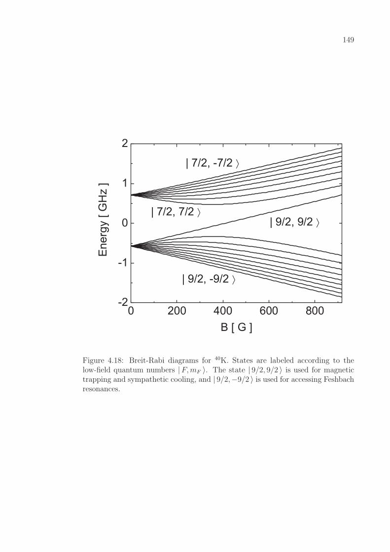
149
Figure 4.18: Breit-Rabi diagrams for 40K. States are labeled according to thelow-field quantum numbers |F, mF 〉. The state | 9/2, 9/2 〉 is used for magnetictrapping and sympathetic cooling, and | 9/2,−9/2 〉 is used for accessing Feshbachresonances.
150
of the atoms. At this point we have a non-degenerate | 2, 2 〉Rb ⊗ | 9/2, 9/2 〉Kmixture at ∼ 14 µK. To transfer 87Rb atoms from the | 2, 2 〉 to the | 1, 1 〉 state,
we apply a frequency-swept µ-wave pulse at low field. The transfer efficiency is
greater than 90%, and any atoms remaining in the | 2, 2 〉 state are removed with
a 5 ms resonant pulse of probe light. The B-field is then increased to ∼ 17 G in
100 ms, and the 40K atoms are transferred to the | 9/2,−9/2 〉 state via adiabatic
rapid passage induced by an rf field that is frequency swept across all ten magnetic
sublevels [131]. The 40K transfer is reversible to within our number measurement
fluctuations (∼ 10%).
For imaging we transfer 87Rb atoms back to the | 2, 2 〉 state and image at
low field. Imaging of 40K atoms can either be performed using the | 9/2,−9/2 〉state, by reversing the direction of the probe quantization field, or by returning the
atoms to the | 9/2, 9/2 〉 state. For our first measurements we imaged 40K atoms
in the optical trap, since the optical density was too low to image in time-of-flight
expansion. Subsequent improvements to the experiment allowed us to increase
our number of atoms and image 40K in expansion and verify, among other things,
that the temperature was the same for each species.
In order to calibrate the magnetic field we performed a variety of rf and
µ-wave transfers of 87Rb (| 2, 2 〉 → | 2,−2 〉 and | 1, 1 〉) and rf transfers of
40K (| 9/2, 9/2 〉 → | 9/2,−9/2 〉) with varying currents to the magnetic coils.
The corresponding B-field values were determined using Eq.(4.36), yielding a cal-
ibration of
B = (2.5± 0.3) G + (145.11± 0.10) G/VDAC , (4.38)
where VDAC is the DAC voltage used to control the magnetic coils, as described in
Chapter 2. The 2.5 G offset is due to the field from the additional bias coil. The
uncertainty here, which I’ll refer to as the “calibration uncertainty,” reflects only
151
the fit uncertainties in the calibration. Note that since the conversion from VDAC
to the current in the coils is given by 100 A/VDAC, the calibration in Eq.(4.38)
is in reasonable agreement with the calibration in Eq.(2.5), which was obtained
with a Gaussmeter over a large spatial range.
4.4.2.2 The Initial Search — “Happy Family”
We initially searched for 87Rb -40K Feshbach resonances over our entire
range of B-fields (up to 640 G). This was because the predicted locations of the
resonances in Ref. [65] had large uncertainties compared to the predicted widths,
and because the predictions were based on values of the 87Rb -40K triplet scatter-
ing length which we believed to be inaccurate based upon our own measurements.
In our search we exploited the technique used for the first observations of Feshbach
resonances in 23Na [102]. The MIT group’s method involved sweeping the mag-
netic field over some relatively large range in order to locate positions of strong
inelastic losses. A typical experimental timeline for the search is shown schemat-
ically in Fig. 4.19. Subsequent sweeps were narrowed until individual features
could be discriminated.
Our initial search used 30 G, 1080 ms sweeps, and uncovered a broad region
of loss at higher fields. By reducing the sweeps to 15 G we could see two clear
features, and a third feature that was the subject of some initial controversy. We
were also able to observe these features when we reversed the direction of the
sweeps (sweeping from high to low fields). We subsequently held the mixture at
fixed B for the full 1080 ms. The resulting loss features are shown in Fig. 4.20.
For these measurements we had 3× 10⁵ 87Rb atoms and only 3× 10⁴ 40K atoms,
so we could not observe loss of 87Rb atoms at the resonances. We could however
observe that no 40K atoms were lost when 87Rb atoms had been removed prior to
loading the FORT. All of the known 87Rb | 1, 1 〉 ⊗ | 1, 1 〉 resonances in this field
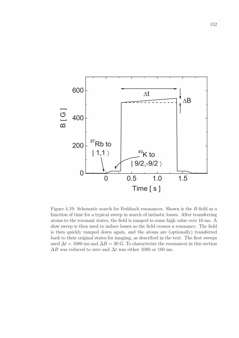
152
Figure 4.19: Schematic search for Feshbach resonances. Shown is the B-field as afunction of time for a typical sweep in search of inelastic losses. After transferringatoms to the resonant states, the field is ramped to some high value over 10 ms. Aslow sweep is then used to induce losses as the field crosses a resonance. The fieldis then quickly ramped down again, and the atoms are (optionally) transferredback to their original states for imaging, as described in the text. The first sweepsused ∆t = 1080 ms and ∆B = 30 G. To characterize the resonances in this section∆B was reduced to zero and ∆t was either 1080 or 180 ms.
153
range have been mapped out theoretically and experimentally by Marte et al. [69].
This allowed us to conclude that we had observed the first heteronuclear Feshbach
resonances between 87Rb and 40K. A detail of the widest of the inelastic features
(resonance “S”) is shown in Fig. 4.21. Comparison with theoretical calculations
suggests that this resonance also has the widest elastic feature, being about 10 G
from peak to zero.
There is currently no theory directly connecting the elastic and inelastic scat-
tering features for Bose-Fermi Feshbach resonances. We have used both Gaussian
and Lorentzian fits to determine the center locations and widths of the observed
inelastic features. These positions are compared to detailed coupled-channel cal-
culations of 87Rb -40K scattering performed by Chris Ticknor and John Bohn [44].
For these calculations, the 87Rb -40K triplet and singlet scattering lengths as and
at are tweaked by modifying the repulsive inner walls of the 87Rb -40K molecular
potentials. For each pair of values of as and at, a calculation of a(B) is performed,
and the theoretical positions of the elastic Feshbach resonances can be compared
to the experimentally observed loss features.
From the original predictions in Ref. [65], we expected a trio of resonances
appearing somewhere roughly between 500 and 600 G. When we tried to make
sense of the data in Fig. 4.20, however, we were unable to get reasonable agreement
between theory and the experiment. Something was evidently still missing. We
had an idea, but it seemed like a long shot.
4.4.2.3 The Missing Link
To reconcile the discrepancy between our observations and the theory, we
proposed that the low-field (“M”) resonance might be the p-wave resonance origi-
nally predicted to exist in Ref. [132]. When p-wave scattering was included in the
calculations, we saw that it was possible that we had observed a p-wave resonance

154
Figure 4.20: First observation of 87Rb -40K Feshbach resonances. The number of40K atoms is shown after holding at fixed B for 1080 ms. The solid points (•)are with 87Rb atoms present, and the open points () have had 87Rb removedprior to loading the optical trap. For the two lowest points no 40K atoms couldbe observed and we show our estimate for the smallest number we could measure,based on the noise level of the images. For the record the labels are not quantumnumbers, but correspond to the names “Michele,” “Jon,” and “Shin,” who eachadopted one resonance. According to Gaussian fits to the loss features, and usingthe calibration from Eq.(4.38), the features occur at 493.6 ± 0.5, 513.5 ± 0.5,and 544.9 ± 0.6 G, where the uncertainty reflects only the fit and calibrationuncertainties.
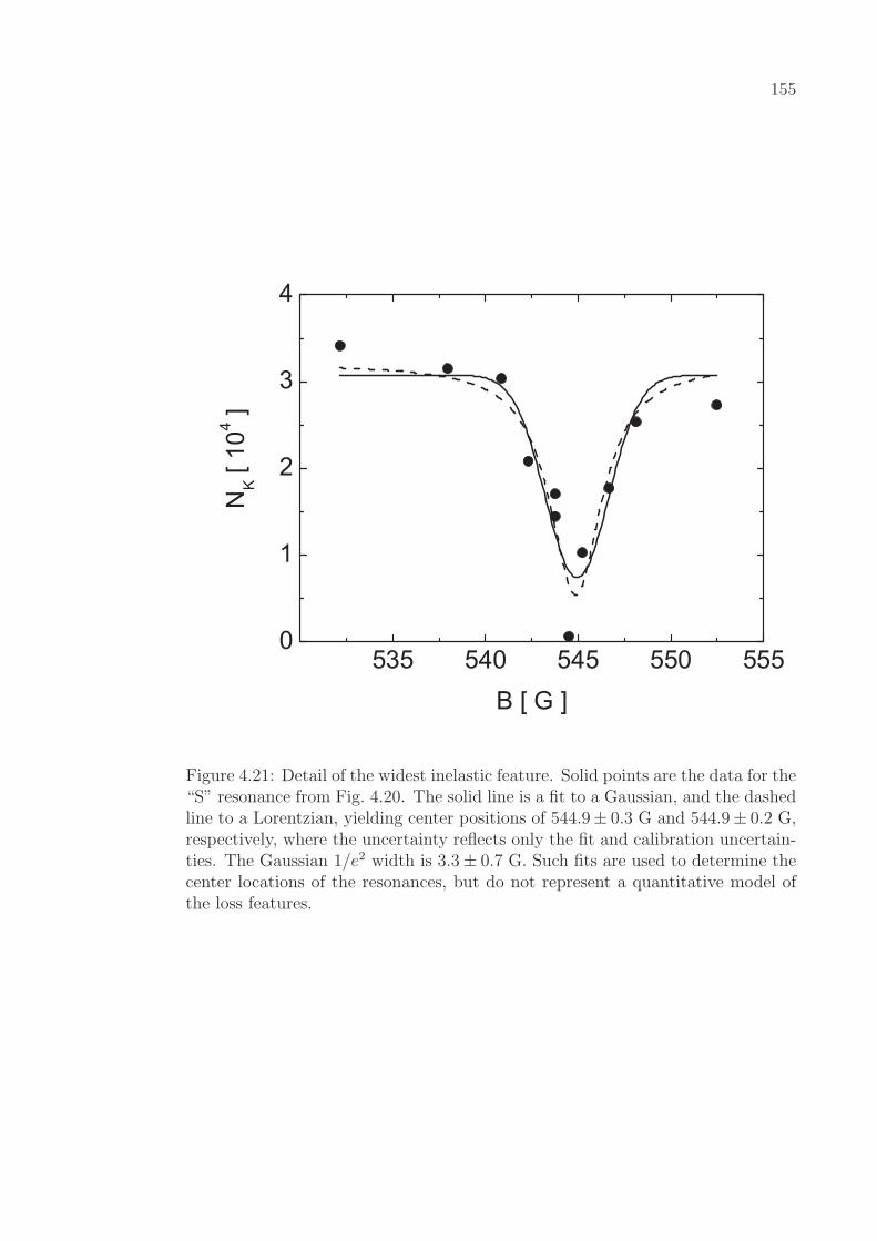
155
Figure 4.21: Detail of the widest inelastic feature. Solid points are the data for the“S” resonance from Fig. 4.20. The solid line is a fit to a Gaussian, and the dashedline to a Lorentzian, yielding center positions of 544.9± 0.3 G and 544.9± 0.2 G,respectively, where the uncertainty reflects only the fit and calibration uncertain-ties. The Gaussian 1/e2 width is 3.3± 0.7 G. Such fits are used to determine thecenter locations of the resonances, but do not represent a quantitative model ofthe loss features.
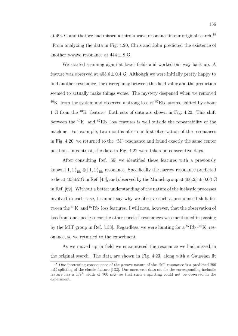
156
at 494 G and that we had missed a third s-wave resonance in our original search.18
From analyzing the data in Fig. 4.20, Chris and John predicted the existence of
another s-wave resonance at 444± 8 G.
We started scanning again at lower fields and worked our way back up. A
feature was observed at 403.6± 0.4 G. Although we were initially pretty happy to
find another resonance, the discrepancy between this field value and the prediction
seemed to actually make things worse. The mystery deepened when we removed
40K from the system and observed a strong loss of 87Rb atoms, shifted by about
1 G from the 40K feature. Both sets of data are shown in Fig. 4.22. This shift
between the 40K and 87Rb loss features is well outside the repeatability of the
machine. For example, two months after our first observation of the resonances
in Fig. 4.20, we returned to the “M” resonance and found exactly the same center
position. In contrast, the data in Fig. 4.22 were taken on consecutive days.
After consulting Ref. [69] we identified these features with a previously
known | 1, 1 〉Rb ⊗ | 1, 1 〉Rb resonance. Specifically the narrow resonance predicted
to lie at 403±2 G in Ref. [45], and observed by the Munich group at 406.23± 0.03 G
in Ref. [69]. Without a better understanding of the nature of the inelastic processes
involved in each case, I cannot say why we observe such a pronounced shift be-
tween the 40K and 87Rb loss features. I will note, however, that the observation of
loss from one species near the other species’ resonances was mentioned in passing
by the MIT group in Ref. [133]. Regardless, we were hunting for a 87Rb -40K res-
onance, so we returned to the experiment.
As we moved up in field we encountered the resonance we had missed in
the original search. The data are shown in Fig. 4.23, along with a Gaussian fit
18 One interesting consequence of the p-wave nature of the “M” resonance is a predicted 290mG splitting of the elastic feature [132]. Our narrowest data set for the corresponding inelasticfeature has a 1/e2 width of 700 mG, so that such a splitting could not be observed in theexperiment.
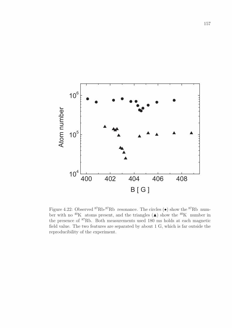
157
Figure 4.22: Observed 87Rb-87Rb resonance. The circles (•) show the 87Rb num-ber with no 40K atoms present, and the triangles (N) show the 40K number inthe presence of 87Rb. Both measurements used 180 ms holds at each magneticfield value. The two features are separated by about 1 G, which is far outside thereproducibility of the experiment.
158Resonance B [G] ∆t [ms]
S 544.9± 0.6 1080
J 513.5± 0.5 1080
M 493.6± 0.5 1080
493.8± 0.5 180
Jy 454.6± 0.5 180
Table 4.5: Summary of observed 87Rb -40K resonances. Shown are the centerpositions of the inelastic features obtained from Gaussian fits, and using the B-field calibration in Eq.(4.38). Error bars reflect only the fit and field calibrationuncertainties. The hold time ∆t is also shown in order to highlight a possible shiftin the position of the “M” resonance.
with center position 454.6 ± 0.5 G, in good agreement with Chris’ and John’s
prediction. These data used a 180 ms hold, and were measured in time-of-flight
by imaging the 40K atoms directly in the | 9/2,−9/2 〉 state with a reversed probe
quantization field. Our search for and preliminary identification of the Feshbach
resonances was now complete.
4.4.3 Analysis and Results
In this section we analyze our experimental observations and compare the
results to the theoretical description of the resonances. We show in Table 4.5 the
positions of the four 87Rb -40K resonances we have so far observed. I have included
two measurements of the “M” resonance taken with different hold times (1080 and
180 ms). These data show a 170 ± 90 mG shift between centers. This may be a
real effect related to the B-field stability over the longer hold time, or the shot-
to-shot repeatability of the experiment. In the future the calibration uncertainty
can be reduced by calibrating the field with single-species measurements at each
resonance position [69]. This is superfluous for our purposes here, since we still
lack a theory to connect the inelastic and elastic features.

159
Figure 4.23: Most recently observed 87Rb -40K resonance. Points show the num-ber of 40K atoms remaining after 180 ms hold with 87Rb at each field value. Theerror bars reflect the statistical error from repeated measurements. The curve isa Gaussian fit with center position 454.6± 0.5 G. This resonance is labeled “Jy”(“Jianying”) throughout this thesis, in keeping with the labels in Fig. 4.20.
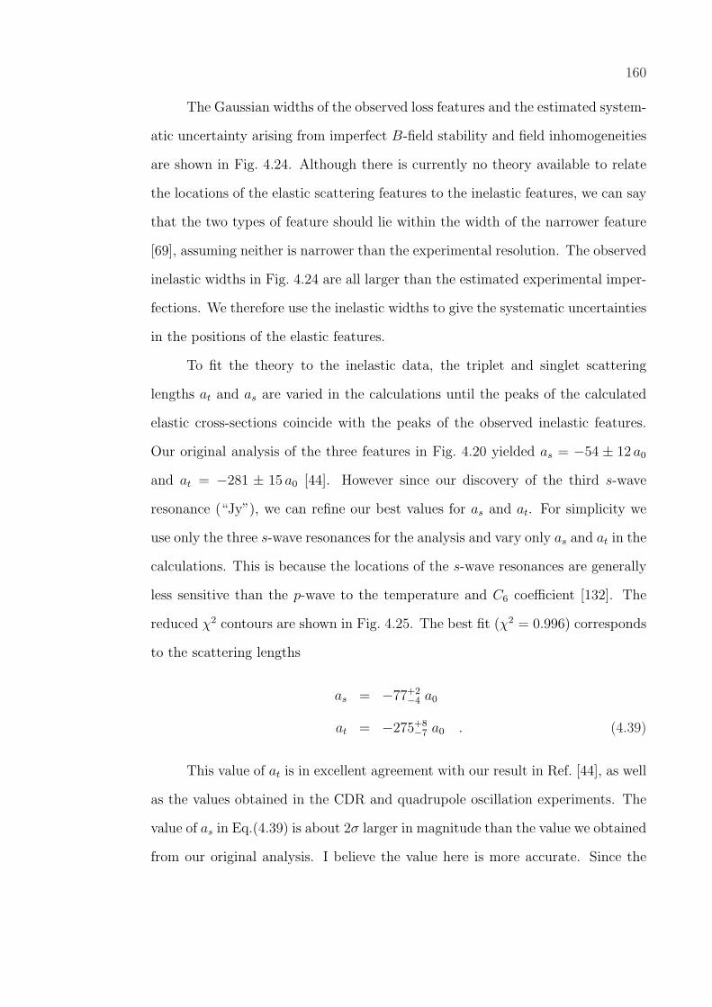
160
The Gaussian widths of the observed loss features and the estimated system-
atic uncertainty arising from imperfect B-field stability and field inhomogeneities
are shown in Fig. 4.24. Although there is currently no theory available to relate
the locations of the elastic scattering features to the inelastic features, we can say
that the two types of feature should lie within the width of the narrower feature
[69], assuming neither is narrower than the experimental resolution. The observed
inelastic widths in Fig. 4.24 are all larger than the estimated experimental imper-
fections. We therefore use the inelastic widths to give the systematic uncertainties
in the positions of the elastic features.
To fit the theory to the inelastic data, the triplet and singlet scattering
lengths at and as are varied in the calculations until the peaks of the calculated
elastic cross-sections coincide with the peaks of the observed inelastic features.
Our original analysis of the three features in Fig. 4.20 yielded as = −54 ± 12 a0
and at = −281 ± 15 a0 [44]. However since our discovery of the third s-wave
resonance (“Jy”), we can refine our best values for as and at. For simplicity we
use only the three s-wave resonances for the analysis and vary only as and at in the
calculations. This is because the locations of the s-wave resonances are generally
less sensitive than the p-wave to the temperature and C6 coefficient [132]. The
reduced χ2 contours are shown in Fig. 4.25. The best fit (χ2 = 0.996) corresponds
to the scattering lengths
as = −77+2−4 a0
at = −275+8−7 a0 . (4.39)
This value of at is in excellent agreement with our result in Ref. [44], as well
as the values obtained in the CDR and quadrupole oscillation experiments. The
value of as in Eq.(4.39) is about 2σ larger in magnitude than the value we obtained
from our original analysis. I believe the value here is more accurate. Since the

161
Figure 4.24: Measured widths of the inelastic features. Points show the 1/e2
widths of gaussian fits to the loss features. Squares (¥) use 1080 ms hold times andcircles (•) use 180 ms; error bars denote only the fit and calibration uncertainties.The dashed line is the total estimated width arising from systematic errors, scaledby 2× to convert rms values to 1/e2 values.

162
Figure 4.25: Scattering length determination from inelastic resonance features.Shown are reduced χ2 contours in the singlet-triplet scattering length plane, fromfits to the locations of the three s-wave resonances. The best fit gives χ2 = 0.996for (at = −275 a0, as = −77 a0), indicated by the star. The dashed contour showswhere χ2 has increased by 1, and the solid contour by 2.3 [134]. The solid contourdetermines the error bars shown in Eq.(4.39).

163
locations of the “S” and “J” resonances are predominantly sensitive to at, the
original value of as was determined almost exclusively by the p-wave resonance.
In contrast the position of the s-wave “Jy” resonance is more sensitive to as than
to at, allowing us to obtain a more robust fit. We can re-analyze the p-wave
resonance in the future after we have more detailed experimental and theoretical
results. Newly acquired spectroscopic data [135, 136, 137] may help to fine-tune
the calculations by improving the 87Rb -40K potentials.
Finally from the best fits we obtain a detailed picture of the predicted elas-
tic scattering length as a function of magnetic field. In Fig. 4.26 we show the
results of the coupled-channel calculation for the nominal singlet and triplet scat-
tering lengths given in Eq.(4.39). By fitting the coupled-channel calculation to
the formula
a(B) = abg
(1−
3∑i=1
∆i
B −B0i
), (4.40)
we obtain the parameters characterizing the s-wave elastic resonance features.
The results are shown in Table 4.6. According to the calculation the background
scattering length abg = −225 a0 for | 1, 1 〉Rb ⊗ | 9/2,−9/2 〉K collisions. The pre-
dicted 10 G width of the “S” resonance makes it suitable for a variety experiments
we would like to perform.
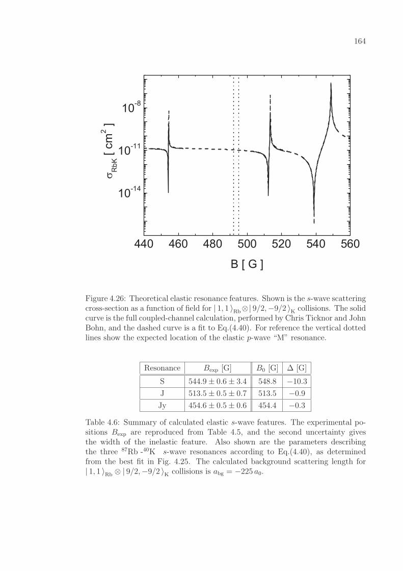
164
Figure 4.26: Theoretical elastic resonance features. Shown is the s-wave scatteringcross-section as a function of field for | 1, 1 〉Rb⊗| 9/2,−9/2 〉K collisions. The solidcurve is the full coupled-channel calculation, performed by Chris Ticknor and JohnBohn, and the dashed curve is a fit to Eq.(4.40). For reference the vertical dottedlines show the expected location of the elastic p-wave “M” resonance.
Resonance Bexp [G] B0 [G] ∆ [G]
S 544.9± 0.6± 3.4 548.8 −10.3
J 513.5± 0.5± 0.7 513.5 −0.9
Jy 454.6± 0.5± 0.6 454.4 −0.3
Table 4.6: Summary of calculated elastic s-wave features. The experimental po-sitions Bexp are reproduced from Table 4.5, and the second uncertainty givesthe width of the inelastic feature. Also shown are the parameters describingthe three 87Rb -40K s-wave resonances according to Eq.(4.40), as determinedfrom the best fit in Fig. 4.25. The calculated background scattering length for| 1, 1 〉Rb ⊗ | 9/2,−9/2 〉K collisions is abg = −225 a0.

Chapter 5
Summary and Outlook
I have described in this thesis the design, construction, and operation of an
experimental apparatus we have built for producing and studying quantum degen-
erate 87Rb -40K Bose-Fermi mixtures. By evaporatively cooling the bosons and
sympathetically cooling the fermions, we can produce a nearly pure Bose-Einstein
condensate of 87Rb atoms coexisting with a Fermi gas of 40K atoms at about
0.2 times the Fermi temperature. The appearance of quantum degeneracy in the
experiments has been characterized for each species and compared to theoretical
predictions.
I have additionally presented measurements of the magnitude of the s-wave
scattering length |aRbK| between species. The scattering length is important in
characterizing a variety of the equilibrium and dynamic properties of the mixture.
I have discussed techniques for studying some elementary excitations of the sys-
tem, and have analyzed the prospect for exploiting interactions with phonons in
the condensate to create fermion pairs. It has been shown that current theory
places this prospect within reach of current experiments.
Finally I have discussed our observation of Feshbach resonances between
87Rb and 40K atoms in non-degenerate mixtures. These important experiments
open up the possibility of tuning aRbK to any desired value in the experiment.
Our experimental observations have been compared to theoretical calculations

166
and used to refine parameters describing the collisions between species.
The future of this experiment lies in exploiting these resonances in a variety
of useful and exciting ways. After first measuring the elastic properties of the
resonances, we can begin to utilize the resonant control of the interactions between
species in a number of experiments. Possible studies include the controlled collapse
of the mixture, the production of polar fermionic molecules, the generation of a
boson-induced sound mode among spin-polarized fermions, generation of bright
Bose-Fermi matter wave solitons, and the boson-induced pairing of fermions.
Relevant Publications
• J. Goldwin, S. B. Papp, B. DeMarco, and D. S. Jin, Two-species magneto-
optical trap with 40K and 87Rb, Phys. Rev. A 65 021402 (2002)
• J. Goldwin, S. Inouye, M. L. Olsen, B. Newman, B. D. DePaola, and D.
S. Jin, Measurement of the interaction strength in a Bose-Fermi mixture
with 87Rb and 40K, Phys. Rev. A 70, 021601 (2004)
• S. Inouye, J. Goldwin, M. L. Olsen, C. Ticknor, J. L. Bohn, and D. S.
Jin, Observation of Heteronuclear Feshbach Resonances in a Mixture of
Bosons and Fermions, Phys. Rev. Lett. 93, 183201 (2004)
• J. Goldwin, S. Inouye, M. L. Olsen, and D. S. Jin, Cross-dimensional
relaxation in Bose-Fermi mixtures, Phys. Rev. A 71, 043408 (2005)

Appendix A
Monte Carlo Simulation Details
These appendices refer to the Monte Carlo simulations and ana-lytic theory which we presented in detail in Ref. [66]. Familiaritywith that reference is assumed throughout this discussion.
In this first Appendix, let me describe some aspects of the Monte Carlo (MC)
simulations that lurk behind the scenes, and are not often presented in the light
of day. These notes are intended for people wishing to develop MC simulations of
their own, or even hoping to debunk our hard-earned and rigorously established
results.
A.1 Choice of Parameters and Failure Modes
The Monte Carlo (MC) simulations are extremely useful for simulating var-
ious experiments, but they can also be very dangerous if the user puts his/her
blind faith in their results. We have found that the best approach to the simu-
lations is to treat them like the experiments themselves, and to subject them to
intense scrutiny and modeling in order to understand (and, only then, believe)
the results. Here I will talk about some failure modes of the simulations that we
have studied.
In Ref. [66] we described the simulation in some detail. In that discussion
we talked about the probability for two particles, labeled k and l to collide. This

168
probability was said to be given by
pcoll =σkl |~vk − ~vl|∆ t
Vc
. (A.1)
Although we said it, and you believed it, this is only true assuming pcoll is very
small. To see why, note that the equilibrium distribution of relative speeds is
Gaussian. This means that for any fixed values of cross-section, time-step, and
collision volume Vc, there is still some finite probability that the relative collision
speed will be large enough to make pcoll greater than one. We conclude that pcoll
does not represent a probability in the conventional sense. The real distribution
of times between collisions is given by a Poisson distribution [138], so that the
collision probability is
Pcoll = 1− exp(−pcoll) (A.2)
' pcoll .
This is the basis for our statement that 〈 pcoll 〉 should be kept well below ∼ 10%
for accurate results. Note that Eq.(A.2) is still only approximate, as it ignores
any possibility for 3-body collisions, or multiple 2-body collisions within a single
time-step, but we will see that it is still very good until exceedingly bad choices
of the parameters ∆t and rc are made.
In Fig. A.1 we show the number of collisions per calculated collision time
τcoll = 〈Γcoll 〉−1 as a function of 〈 pcoll 〉 for a single-species simulation of particles
in equilibrium. When 〈 pcoll 〉 becomes too large, we observe too few collisions,
since we look for them only once per time-step. The results in Fig. A.1 suggest
that the approximation in Eq.(A.2) is still good for 〈 pcoll 〉 ∼ 1. Our simulations,
which typically use 〈 pcoll 〉 in the range of 10−3 to 10−2, are therefore expected to
be accurate in this respect.
The other input parameter we use is the critical distance rc between atoms.
Particles in the simulation must come within rc of each other for a collision to be

169
Figure A.1: Effect of bad choice of time-step on the MC simulation. Shown isthe number of collisions per calculated collision time as a function of 〈 pcoll 〉 fora single-species gas in equilibrium. Filled points (•) use pcoll and open points ()use 1 − exp(−pcoll) to calculate the collision probability in the simulations. Thesolid line is just the expected behavior for a Poisson distribution. All simulationsused 103 particles with an average of 10−2 particles per volume Vc.

170
considered. Although in Ref. [66] we referred to the probability of a cell of volume
Vc = 4πr3c/3 being occupied, this is again not a probability in the conventional
sense, as nothing forbids a choice of parameters where the average number of
particles per cell volume Vc is greater than 1. Results from the MC simulations
are shown in Fig. A.2. If Vc is large enough, any given particle will see all N − 1
of the other particles within the volume. The number of collisions per particle
in one collision time will then saturate at (N − 1) 〈 pcoll 〉, since the calculated
collision probability is independent of the positions of the particles. Since we are
considering dilute gases, one may expect that in the limit Vc → 0 there will be no
chance for collisions in the simulations, but this is not the case. If the quantity pcoll
is kept constant, then the time-step ∆t ∝ Vc. This means that for every decrease
in Vc, there must be a corresponding increase in the number of times collisions
are searched for. This ensures that a constant rate of collisions is maintained.
We again conclude that our insistence on keeping 〈n 〉 Vc around 10−3 to 10−2 is
extremely conservative, and should lead to accurate simulations.
A.2 Transition to Hydrodynamic Behavior
In this section I will use the MC simulations to consider the onset of hydro-
dynamic behavior in cross-dimensional relaxation (CDR) experiments. Hydrody-
namic behavior is generally characterized by a density (or cross-section) so high
that a particle undergoes many collisions within a time equal to the trap period.
If this happens, the kinetic energy is continuously being re-randomized and the
atoms no longer undergo simple harmonic motion in the trap. If one imagines
that we begin the CDR experiment with anisotropic energy Ω = Ex,y/Ez, then
collisions will randomize the relative kinetic energies of colliding atoms before they
have had a chance to move very far. The gas will then have isotropic kinetic en-
ergy, but the potential (and center-of-mass kinetic) energies will still maintain the
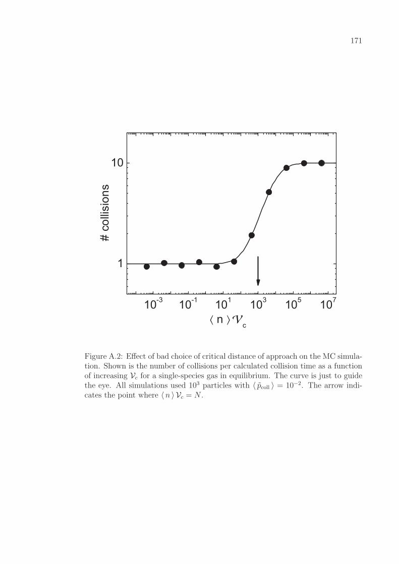
171
Figure A.2: Effect of bad choice of critical distance of approach on the MC simula-tion. Shown is the number of collisions per calculated collision time as a functionof increasing Vc for a single-species gas in equilibrium. The curve is just to guidethe eye. All simulations used 103 particles with 〈 pcoll 〉 = 10−2. The arrow indi-cates the point where 〈n 〉 Vc = N .
172
initial anisotropy Ω. The observed relaxation rate will therefore be slower than in
a system with the same collision rate but much higher trapping frequencies.
Our MC simulations typically use atom numbers ∼ 104 to save computation
time. These numbers, however, are expected to leave our simulations in the col-
lisionless regime. To determine when a system like ours enters the hydrodynamic
regime I ran a series of simulations of 87Rb -40K relaxation with the trapping fre-
quencies fixed to our experimental conditions. The collision rates were varied by
either increasing the number of particles, decreasing the temperature (the simula-
tions always use Maxwell-Boltzmann statistics), or increasing the collision cross-
sections (with the ratio σbb/σbf fixed). Results are shown in Fig. A.3. For these
simulations, hydrodynamic behavior was observed to begin for 〈Γcoll 〉 ∼ ωz,K.
The inset to Fig. A.3 describes the oscillatory behavior which is observed for
simulations of CDR in the hydrodynamic regime. An example of the relaxation in
this regime is shown in Fig. A.4. Note the 180 phase-shift between oscillations of
the axial and radial energies, which means the cloud aspect ratio also oscillates. As
the gas goes more deeply into the hydrodynamic regime, the oscillation frequency
appears to approach twice the 87Rb axial frequency. The 87Rb axial frequency is
the lowest trap frequency in the system, and twice this frequency is the frequency
at which kinetic and potential energy are exchanged in the absence of collisions.
This oscillatory behavior and the nonlinear dependence of the damping rate on
the boson density may be used as a guide in experiments. One should be able
to clearly identify whether measurements are performed in the collisionless or
hydrodynamic regime.

173
Figure A.3: Nonlinear relaxation rate for CDR due to hydrodynamic effects.Points are from the MC simulations with dots (•) varying the number of atoms,up-triangles (N) varying the cross-section (with |abf/abb| = 3 fixed), and down-triangles (H) varying the temperature. All points used NRb = 4 NK. The solidline is the collisionless prediction assuming β = 2.0 for x ≤ 1, and the dashedline shows a x−2/3 decay for x > 1, to guide the eye. The dotted line showsthe 87Rb axial trap frequency (in rad/s), which is the lowest trap frequency inthe system. Relaxation curves corresponding to the open points (∆,∇) showedhydrodynamic behavior (see Fig. A.4). Damping rates for these simulations weredetermined from fits to Ez(t) using damped sines, and neglecting early times.The inset shows the frequency of the hydrodynamic oscillations. For comparison,the dashed curve interpolates between twice the 87Rb and 40K axial frequencies(2× 25 Hz and 2× 37 Hz, respectively).
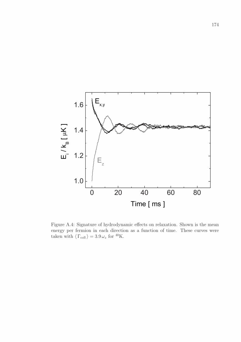
174
Figure A.4: Signature of hydrodynamic effects on relaxation. Shown is the meanenergy per fermion in each direction as a function of time. These curves weretaken with 〈Γcoll 〉 = 3.9 ωz for 40K.
Appendix B
Cross-dimensional Rethermalization Supplement
Wherein the author leaves a record of various details and equationswhose complexity renders them a distraction elsewhere.
B.1 Thermal Averages with Different Anisotropies for Each Species
Although our theory described in Ref. [66] assumes separable Gaussian dis-
tributions for each species in each direction, the center-of-mass (CM) and relative
velocities are generally correlated if the energy anisotropy is not the same between
species. To see this, note that
1
2
(m1 v2
1i
E1i
+m1 v2
2i
E2i
)=
1
2
(M V 2
CMi
εCMi
+µ v2
reli
εreli
)− µ δi VCMi vreli , (B.1)
where Eσi is the mean energy for species σ in the ith direction, and we have defined
εCMi = (m1 + m2)E1i E2i
m2 E1i + m1 E2i
εreli =m2 E1i + m1 E2i
m1 + m2
δi =E1i − E2i
E1i E2i
. (B.2)
Although the energy anisotropy is the same for each species at the beginning
and end of the experiment (Ω and 1, respectively), the fact that α and β are
generally different means that the two species will have different anisotropies at
intermediate times.

176
With the definitions above, and using the distribution function exp(−H/kBT ),
one can calculate the following averages:
〈 vrel 〉 =
√2 Erelz
π µ[1 + Ωrel Q(Ωrel) ]
〈 v2reli 〉 =
E1i
m1
+E2i
m2
〈VCMi vreli 〉 =(E1i − E2i) Ereli
m2 E1i + m1 E2i
〈 vrel v2relx 〉 =
1√2π
(Erelz
µ
)3/2Ωrel
Ωrel − 1[ 3 Ωrel − 2 + (3 Ωrel − 4) Ωrel Q(Ωrel) ]
〈 vrel v2relz 〉 =
√2
π
(Erelz
µ
)3/21
Ωrel − 1
[Ωrel − 2 + Ω2
rel Q(Ωrel)]
〈 vrel VCMi vreli 〉 =
(m1 m2
m1 + m2
)E1i − E2i
m2 E1i + m1 E2i
〈 vrel v2reli 〉 , (B.3)
where we have introduced the definitions
Ereli =m2 E1i + m1 E2i
m1 + m2
Ωrel =Erelx
Erelz
Q(x) =
tanh−1√
1− x√1− x
, x < 1
1 , x = 1
tan−1√
1− x√1− x
, x > 1
. (B.4)
We are now in a position to consider ratios of the type
〈 vrel v2relx 〉
〈 vrel 〉 〈 v2relx 〉
, (B.5)
which we claimed in Ref. [66] are roughly equal to 4/3 for reasonable anisotropies.
As an example of a “reasonable” anisotropy, we take Ω = 1.64, which we used
in the CDR measurements and many of the MC simulations. Figure B.1 shows
the ratio in Eq.(B.5) as a function of m1/m2 for varying anisotropies Ω1 and
Ω2. In the “worst-case” scenario, where one species maintains Ω = 1.64 and the

177
other is isotropic, this ratio lies between 1.333 and 1.375 for any choice of masses,
corresponding to only a 3% variation. In fact one can show more generally that
this ratio is always between 1 and 3/2.
Although it is not immediately evident from Eq.(B.3), one can additionally
show that the averages of interest to our theoretical treatment (see Eq.(6) and
following in Ref. [66]) are related by
〈 vrel v2reli 〉
〈 vrel 〉 〈 v2reli 〉
=〈 vrel VCMi vreli 〉〈 vrel 〉 〈VCMi vreli 〉
〈 vrel v2relx 〉
〈 vrel 〉 〈 v2relx 〉
− 4
3=
4
3− 〈 vrel v
2relz 〉
〈 vrel 〉 〈 v2relz 〉
. (B.6)
B.2 Analytic Best Fit to Exponential Decay
In Ref. [66] we determined an upper limit βu for the constant of propor-
tionality β. We saw that the fermion relaxation, described by Eq.(8) in that
work, does not generally correspond to pure exponential decay. In Fig. B.2 we
compare solutions for the relaxation for light and heavy fermions, neglecting the
effects of boson-boson collisions (i.e., assuming γ = 0 in the language of Ref. [66]).
The light fermions begin to relax quickly, and then are held up by the residual
anisotropy of the bosons. In contrast the heavy fermions relax slowly at first, and
then somewhat more quickly as the energy of the bosons becomes more isotropic.
In other words, for heavy fermions the small-τ behavior gives an estimate for βu
that reliably bounds β from above, but for light fermions something more robust
is needed.
To determine the best approximation to pure exponential decay, we analyt-
ically minimize the integrated squared error
err2 =
∫ ∞
0
dτ
[χ1(τ)− exp
(− τ
βu
)]2
(B.7)
with respect to the parameter β. Minimization of the error requires ∂/∂βu = 0,

178
Figure B.1: Effect of energy anisotropies on thermal averages. Shown is the ratiogiven in Eq.(B.5) as a function of mass ratio m1/m2 for different anisotropies.Points are from Monte Carlo integrations, and the solid line is from Eq.(B.3), forthe case of Ω1 = 1.64 and Ω2 = 1. The dashed and dotted lines are for differentanisotropies, as labeled.

179
Figure B.2: Fermion relaxation with double exponential decay. Shown is the en-ergy anisotropy of the fermions as a function of time (in units of the mean timeτ between collisions). The upper (lower) solid curve is the solution to Enskog’sequation from Ref. [66], with masses corresponding to a 40K-7Li (6Li-133Cs) mix-ture, and with γ = 0. In each case the dashed line is the exponential decayextrapolated from the small-τ behavior.
180
so that we need to solve
0 =
∫ ∞
0
dτ[χ1(τ)− e−τ/βu
]τ e−τ/βu . (B.8)
Now if we take γ = 0 in Eq.(8) of Ref. [66], then
χ1(τ) =(1− η)(1− 2 η) e−
23
τ + η e−43
η (1−η) τ
1− 2 η (1− η). (B.9)
Carrying out the integral leads to the condition
(1− η)(1− 2 η)
(3 + 2 βu)2+
η
[ 3 + 4 η βu (1− η) ]2=
1
36[ 1− 2 η (1− η) ] (B.10)
The above polynomial equation is solved numerically with a root finder [134],
beginning with an initial guess value of βl in order to obtain the physical solution.

Bibliography
[1] J. J. Sakurai, Modern Quantum Mechanics (Addison-Wesley, New York,1994).
[2] M. P. Marder, Condensed Matter Physics (John Wiley & Sons, New York,2000).
[3] B. DeMarco and D. S. Jin, Onset of Fermi Degeneracy in a Trapped AtomicGas, Science 285, 1703 (1999).
[4] M. Kohl, H. Moritz, T. Stoferle, K. Gunter, and T. Esslinger, FermionicAtoms in a Three Dimensional Optical Lattice: Observing Fermi Surfaces,Dynamics, and Interactions, Phys. Rev. Lett. 94, 080403 (2005).
[5] M. J. Bijlsma, B. A. Heringa and H. T. C. Stoof, Phonon exchange in diluteFermi-Bose mixtures: Tailoring the Fermi-Fermi interaction, Phys. Rev. A61, 053601 (2000).
[6] D. V. Efremov and L. Viverit, p-wave Cooper pairing of fermions in mixturesof dilute Fermi and Bose gases, Phys. Rev. B 65, 134519 (2002).
[7] F. Matera, Fermion pairing in Bose-Fermi mixtures, Phys. Rev. A 68,043624 (2003).
[8] M. A. Baranov, M. S. Mar’enko, Val. S. Rychkov, and G. V. Shlyapnikov,Superfluid pairing in a polarized dipolar Fermi gas, Phys. Rev. A. 66 013606(2002).
[9] H. P. Buchler and G. Blatter, Supersolid versus Phase Separation in AtomicBose-Fermi Mixtures, Phys. Rev. Lett. 91, 130404 (2003).
[10] M. Lewenstein, L. Santos, M. A. Baranov, and H. Fehrmann, Atomic Bose-Fermi Mixtures in an Optical Lattice, Phys. Rev. Lett. 92 050401 (2004).
[11] Throughout this thesis trade names are used for identification purposes only,and do not constitute an endorsement by the author or his institution.

182
[12] B. DeMarco, H. Rohner, and D. S. Jin, An enriched 40K source for fermionicatom studies, Rev. Sci. Inst. 70, 1967 (1999).
[13] B. DeMarco, Quantum Behavior of an Atomic Fermi Gas, Ph.D. thesis,University of Colorado – Boulder (2001).
[14] J. Moore, C. C. Davis, and M. A. Coplan, Building Scientific Apparatus:a Practical Guide to Design and Construction (Perseus, Cambridge, MA,1991).
[15] David R. Lide (Ed.), CRC Handbook of Chemistry and Physics (CRC Press,Boca Raton, 1993).
[16] H. Lewandowski, Coherences and correlations in an ultracold Bose gas,Ph.D. thesis, University of Colorado – Boulder (2002).
[17] D. J. Griffiths, Introduction to Electrodynamics (Prentice Hall, Upper SaddleRiver, New Jersey, 1989).
[18] W. Petrich, M. H. Anderson, J. R. Ensher, and E. A. Cornell, Stable, TightlyConfining Magnetic Trap for Evaporative Cooling of Neutral Atoms, Phys.Rev. Lett. 74, 3352 (1995).
[19] D. E. Pritchard, Cooling Neutral Atoms in a Magnetic Trap for PrecisionSpectroscopy, Phys. Rev. Lett. 51, 1336 (1983).
[20] T. Bergeman, G. Erez and H. J. Metcalf, Magnetostatic trapping fields forneutral atoms, Phys. Rev. A 35, 1535 (1987).
[21] Dan M. Stamper-Kurn, Peeking and poking at a new quantum fluid: Studiesof gaseous Bose-Einstein condensates in magnetic and optical traps, Ph.D.Thesis, Massuchesetts Institute of Technology (2000).
[22] H. J. Metcalf and P. van der Straten, Laser Cooling and Trapping (Springer,New York, 1999).
[23] E. Arimondo, M. Inguscio, and P. Violino, Experimental determinations ofthe hyperfine structure in the alkali atoms, Rev. Mod. Phys. 49, 31 (1977).
[24] R. Williamson, Magneto-optical trapping of short-lived radioactive isotopes,Ph.D. thesis, University of Wisconsin – Madison (1997).
[25] J. Goldwin, S. B. Papp, B. DeMarco, and D. S. Jin, Two-species magneto-optical trap with 40K and 87Rb, Phys. Rev. A 65 021402 (2002).
[26] D. Steck, Quantum Chaos, Transport, and Decoherence in Atom Optics,Ph.D. thesis, University of Texas – Austin (2001).

183
[27] L. Ricci, M. Weidemuller, T. Esslinger, A. Hemmerich, C. Zimmermann, V.Vuletic, W. Konig, and T. W. Hansch, A Compact Grating-Stabilized DiodeLaser System for Atomic Physics, Opt. Commun. 117, 541 (1995).
[28] C. Wieman and L. Hollberg, Using diode lasers for atomic physics, Rev. Sci.Inst. 62, 1 (1991).
[29] K. B. MacAdam, A. Steinbach, and C. Wieman, A narrow-band tunablediode laser system with grating feedback, and a saturated absorption spec-trometer for Cs and Rb, Am. J. Phys. 60, 1098 (1992).
[30] M. G. Littman and H. J. Metcalf, Spectrally narrow pulsed dye laser withoutbeam expander, Appl. Opt. 17, 2224 (1978).
[31] G. Ferrari, M.-O. Mewes, F. Schreck, and C. Salomon, High-power multiple-frequency narrow-linewidth laser source based on a semiconductor taperedamplifier, Opt. Lett. 24, 151 (1999).
[32] R. Grimm, M. Weidemuller, and Y. B. Ovchinnikov, Optical dipole trapsfor neutral atoms, Adv. Atom. Mol. Opt. Phys. 42, 95 (2000); pre-printavailable at arXiv:physics/9902072.
[33] K. Miller, Trapping and cooling Rubidium in far-off-resonant optical dipoletraps, Ph.D. thesis, University of Colorado – Boulder (2004).
[34] C. Monroe, W. Swann, H. Robinson, and C. Wieman, Very cold trappedatoms in a vapor cell, Phys. Rev. Lett. 65, 1571 (1990).
[35] B. P. Anderson and M. A. Kasevich, Loading a vapor-cell magneto-optic trapusing light-induced atom desorption, Phys. Rev. A 63, 023404 (2001).
[36] A. Gallagher and D. E. Pritchard, Exoergic collisions of cold Na∗-Na, Phys.Rev. Lett. 63, 957 (1989).
[37] J. Weiner, V. S. Bagnato, S. Zilio, and P. S. Julienne, Experiments andtheory in cold and ultracold collisions, Rev. Mod. Phys. 71, 1 (1999).
[38] L. G. Marcassa, G. D. Telles, S. R. Muniz, and V. S. Bagnato, Collisionallosses in a K-Rb cold mixture, Phys. Rev. A 63, 013413 (2000).
[39] T. Walker, D. Sesko, and C. Wieman, Collective behavior of optically trappedneutral atoms, Phys. Rev. Lett. 64, 408 (1989).
[40] W. Petrich, M. H. Anderson, J. R. Ensher, and E. A. Cornell, Behavior ofatoms in a compressed magneto-optical trap, J. Opt. Soc. Am. B 11, 1332(1994).
184
[41] W. Ketterle, K. B. Davis, M. A. Joffe, A. Martin, and D. E. Pritchard, Highdensities of cold atoms in a dark spontaneous-force optical trap, Phys. Rev.Lett. 70, 2253 (1993).
[42] K. Dieckmann, Bose-Einstein Condensation with High Atom Number in aDeep Magnetic Trap, Ph.D. thesis, University of Amsterdam – Netherlands(2001).
[43] G. Delannoy, S. G. Murdoch, V. Boyer, V. Josse, P. Bouyer, and A. Aspect,Understanding the production of dual Bose-Einstein condensation with sym-pathetic cooling, Phys. Rev. A 63, 051602 (2001).
[44] S. Inouye, J. Goldwin, M. L. Olsen, C. Ticknor, J. L. Bohn, and D. S. Jin,Observation of Heteronuclear Feshbach Resonances in a Mixture of Bosonsand Fermions, Phys. Rev. Lett. 93, 183201 (2004).
[45] E. G. M. van Kempen, S. J. J. M. F. Kokkelmans, D. J. Heinzen, and B.J. Verhaar, Interisotope Determination of Ultracold Rubidium Interactionsfrom Three High-Precision Experiments, Phys. Rev. Lett. 88, 093201 (2002).
[46] B. DeMarco, J. L. Bohn, J. P. Burke, Jr., M. Holland, and D. S. Jin, Mea-surement of p-Wave Threshold Law Using Evaporatively Cooled FermionicAtoms, Phys. Rev. Lett. 82, 4208 (1999).
[47] J. P. Burke, Jr., Theoretical Investigation of Cold Alkali Atom Collisions,Ph. D. thesis, University of Colorado – Boulder (1999).
[48] A. Derevianko, J. F. Babb, and A. Dalgarno, High-precision calculations ofvan der Waals coefficients for heteronuclear alkali-metal dimers, Phys. Rev.A 63, 052704 (2001).
[49] F. Dafolvo, S. Giorgini, L. P. Pitaevskii, and S. Stringari, Theory of Bose-Einstein condensation in trapped gases, Rev. Mod. Phys. 71, 463 (1999).
[50] D. A. Butts and D. S. Rokhsar, Trapped Fermi gases, Phys. Rev. A 55, 4346(1997).
[51] M. Naraschewski and D. M. Stamper-Kurn, Analytical description of atrapped semi-ideal Bose gas at finite temperature, Phys. Rev. A 58, 2423(1998).
[52] J. E. Williams, The Preparation of Topological Modes in a Strongly-CoupledTwo-Component Bose-Einstein Condensate, Ph.D. thesis, University of Col-orado – Boulder (1994).
[53] J. Goldwin, S. Inouye, M. L. Olsen, B. Newman, B. D. DePaola, and D. S.Jin, Measurement of the interaction strength in a Bose-Fermi mixture with87Rb and 40K, Phys. Rev. A 70, 021601 (2004).

185
[54] M. Modugno, F. Ferlaino, F. Riboli, G. Roati, G. Modugno, and M. Inguscio,Mean-field analysis of the stability of a K-Rb Fermi-Bose mixture, Phys.Rev. A 68, 043626 (2003).
[55] C. Ospelkaus, Quantum degenerate Fermi-Bose mixture with 40K and 87Rb,seminar presented at JILA, 22 February, 2005.
[56] A. G. Truscott, K. E. Strecker, W. I. McAlexander, G. B. Partridge, andR. G. Hulet, Observation of Fermi Pressure in a Gas of Trapped Atoms,Science 291, 2570 (2001).
[57] M. Brown-Hayes and R. Onofrio, Optimal cooling strategies for magneticallytrapped atomic Fermi-Bose mixtures, Phys. Rev. A 70, 063614 (2004).
[58] L. D. Carr and Y. Castin, Limits of sympathetic cooling of fermions: Therole of heat capacity of the coolant, Phys. Rev. A 69, 043611 (2004).
[59] L. D. Carr, T. Bourdel and Y. Castin, Limits of sympathetic cooling offermions by zero-temperature bosons due to particle losses, Phys. Rev. A69, 033603 (2004).
[60] E. Timmermans, Degenerate Fermion Gas Heating by Hole Creation, Phys.Rev. Lett. 87, 240403 (2001).
[61] E. Timmermans and R. Cote, Superfluidity in Sympathetic Cooling withAtomic Bose-Einstein Condensates, Phys. Rev. Lett. 80, 3419 (1998).
[62] C. Monroe, E. A. Cornell, C. A. Sackett, C. J. Myatt, and C. E. Wieman,Measurement of Cs-Cs elastic scattering at T = 30 µK, Phys. Rev. Lett. 70,414 (1993).
[63] M. Arndt, M. Ben Dahan, D. Guery-Odelin, M. W. Reynolds, and J. Dal-ibard, Observation of a Zero-Energy Resonance in Cs-Cs Collisions, Phys.Rev. Lett. 79, 625 (1997).
[64] I. Bloch, M. Greiner, O. Mandel, T. W. Hansch, and T. Esslinger, Sympa-thetic cooling of 85Rb and 87Rb, Phys. Rev. A 64 021402 (2001).
[65] A. Simoni, F. Ferlaino, G. Roati, G. Modugno, and M. Inguscio, MagneticControl of the Interaction in Ultracold K-Rb Mixtures, Phys. Rev. Lett. 90,163202 (2003).
[66] J. Goldwin, S. Inouye, M. L. Olsen, and D. S. Jin, Cross-dimensional relax-ation in Bose-Fermi mixtures, Phys. Rev. A 71, 043408 (2005).
[67] J. L. Roberts, Bose-Einstein Condensates with Tunable Atom-atom Inter-actions: The First Experiments with 85Rb BECs, Ph.D. thesis, University ofColorado — Boulder, 2001.

186
[68] S. D. Gensemer and D. S. Jin, Transition from Collisionless to Hydrody-namic Behavior in an Ultracold Fermi Gas, Phys. Rev. Lett. 87, 173201(2001).
[69] A. Marte, T. Volz, J. Schuster, S. Durr, G. Rempe, E. G. M. van Kem-pen, and B. J. Verhaar, Feshbach Resonances in Rubidium 87: PrecisionMeasurement and Analysis, Phys. Rev. Lett. 89, 283202 (2002).
[70] H. Wu and C. J. Foot, Direct simulation of evaporative cooling, J. Phys. B29, L321 (1996).
[71] G. M. Kavoulakis, C. J. Pethick, and H. Smith, Relaxation Processes inClouds of Trapped Bosons above the Bose-Einstein Condensation Tempera-ture, Phys. Rev. Lett. 81, 4036 (1998).
[72] G. M. Kavoulakis, C. J. Pethick, and H. Smith, Collisional relaxation indiffuse clouds of trapped bosons, Phys. Rev. A 61, 053603 (2000).
[73] G. Modugno, G. Ferrari, G. Roati, R. J. Brecha, A. Simoni, and M. Inguscio,Bose-Einstein Condensation of Potassium Atoms by Sympathetic Cooling,Science 294, 1320 (2001).
[74] G. Ferrari, M. Inguscio, W. Jastrzebski, G. Modugno, G. Roati, and A.Simoni, Collisional Properties of Ultracold K-Rb Mixtures, Phys. Rev. Lett.89, 053202 (2002).
[75] G. Roati, F. Riboli, G. Modugno, and M. Inguscio, Fermi-Bose QuantumDegenerate 40K-87Rb Mixture with Attractive Interaction, Phys. Rev. Lett.89 150403 (2002).
[76] F. Ferlaino, R. J. Brecha, P. Hannaford, F. Riboli, G. Roati, G. Modugno,and M. Inguscio, Dipolar oscillations in a quantum degenerate Fermi-Boseatomic mixture, J. Opt. B: Quantum Semiclass. Opt. 5, S3 (2003).
[77] K. Mølmer, Bose Condensates and Fermi Gases at Zero Temperature, Phys.Rev. Lett. 80, 1804 (1998).
[78] R. Roth and H. Feldmeier, Mean-field instability of trapped dilute boson-fermion mixtures, Phys. Rev. A 65, 021603 (2002).
[79] R. Roth, Structure and stability of trapped atomic boson-fermion mixtures,Phys. Rev. A 66, 013614 (2002).
[80] N. Nygaard and K. Mølmer, Component separation in harmonically trappedboson-fermion mixtures, Phys. Rev. A 59, 2974 (1999).
[81] T. Miyakawa, T. Suzuki, and H. Yabu, Induced instability for boson-fermionmixed condensates of alkali-metal atoms due to the attractive boson-fermioninteraction, Phys. Rev. A 64, 033611 (2001).
187
[82] H. Pu, W. Zhang, M. Wilkens, and P. Meystre, Phonon Spectrum andDynamical Stability of a Dilute Quantum Degenerate Bose-Fermi Mixture,Phys. Rev. Lett. 88, 070408 (2002).
[83] C. P. Search, H. Pu, W. Zhang, and P. Meystre, Quasiparticle spectrumand dynamical stability of an atomic Bose-Einstein condensate coupled to adegenerate Fermi gas, Phys. Rev. A 65, 063615 (2002).
[84] G. Modugno, G. Roati, F. Riboli, F. Ferlaino, R. J. Brecha, and M. Inguscio,Collapse of a Degenerate Fermi Gas, Science 297, 2240 (2002).
[85] X.-J. Liu, M. Modugno, and H. Hu, Finite-temperature effects on the col-lapse of trapped Bose-Fermi mixtures, Phys. Rev. A 68, 053605 (2003).
[86] S. T. Chui and V. N. Ryzhov, Collapse transition in mixtures of bosons andfermions, Phys. Rev. A 69, 043607 (2004).
[87] S. T. Chui, V. N. Ryzhov, and E. E. Tareyeva, Stability of the Bose Systemin Bose-Fermi Mixture with Attraction between Bosons and Fermions, JETPLett. 80, 274 (2004).
[88] A. P. Albus, F. Illuminati, and M. Wilkens, Ground-state properties oftrapped Bose-Fermi mixtures: Role of exchange correlation, Phys. Rev. A67, 063606 (2003).
[89] P. Capuzzi, A. Minguzzi, and P. Tosi, Collective excitations in trapped boson-fermion mixtures: From demixing to collapse, Phys. Rev. A 68, 033605(2003).
[90] M. E. Gehm, K. M. O’Hara, T. A. Savard, and J. E. Thomas, Dynamics ofnoise-induced heating in atom traps, Phys. Rev. A 58, 3914 (1998).
[91] R. Jauregui, Nonperturbative and perturbative treatments of parametric heat-ing in atom traps, Phys. Rev. A 64, 053408 (2001).
[92] D. Guery-Odelin, F. Zamelli, J. Dalibard, and S. Stringari, Collective oscil-lations of a classical gas confined in harmonic traps, Phys. Rev. A 60, 4851(1999).
[93] D. S. Jin, M. R. Matthews, J. R. Ensher, C. E. Wieman, and E. A. Cor-nell, Temperature-Dependent Damping and Frequency Shifts in CollectiveExcitations of a Dilute Bose-Einstein Condensate, Phys. Rev. Lett. 78, 764(1997).
[94] S. Stringari, Dynamics of Bose-Einstein condensed gases in highly deformedtraps, Phys. Rev. A 58, 2385 (1998).
188
[95] Y.-l. Ma and S.-T. Chui, Analytical expressions for the hydrodynamic ex-citation spectrum of Bose-Einstein condensates in axially anisotropic traps,Phys. Rev. A 65, 053610 (2002).
[96] E. Braaten and J. Pearson, Semiclassical Corrections to the Oscillation Fre-quencies of a Trapped Bose-Einstein Condensate, Phys. Rev. Lett. 82 255,(1999).
[97] S. K. Yip, Collective modes in a dilute Bose-Fermi mixture, Phys. Rev. A,64, 023609 (2001).
[98] M. Holland, S. J. J. M. F. Kokkelmans, M. L. Chiofalo, and R. Walser,Resonance Superfluidity in a Quantum Degenerate Fermi Gas, Phys. Rev.Lett. 87, 120406 (2001).
[99] S. Rousseau, A. R. Allouche, and M. Aubert-Frecon, Theoretical Study of theElectronic Structure of the KRb Molecule, J. Mol. Spect. 203, 235 (2000).
[100] R. Landau, Quantum Mechanics II: A Second Course in Quantum Theory(John Wiley & Sons, New York, 1996).
[101] H. Friedrich, Theoretical Atomic Physics (Springer, Berlin, 1998).
[102] S. Inouye, M. R. Andrews, J. Stenger, H.-J. Miesner, D. M. Stamper-Kurn,and W. Ketterle, Observation of Feshbach resonances in a Bose-Einsteincondensate, Nature (London) 392, 151 (1998).
[103] Ph. Courteille, R. S. Freeland, D. J. Heinzen, F. A. van Abeelen and B.J. Verhaar, Observation of a Feshbach Resonance in Cold Atom Scattering,Phys. Rev. Lett. 81, 69 (1998).
[104] J. L. Roberts, N. R. Claussen, J. P. Burke, Jr., C. H. Greene, E. A. Cornell,and C. E. Wieman, Resonant Magnetic Field Control of Elastic Scatteringin Cold 85Rb, Phys. Rev. Lett. 81, 5109 (1998).
[105] C. Chin, V. Vuletic, A. J. Kerman, and S. Chu, High Resolution FeshbachSpectroscopy of Cesium, Phys. Rev. Lett. 85, 2717 (2000).
[106] N. Claussen, S. J. J. M. F. Kokkelmans, S. T. Thompson, E. A. Donley,E. Hodby, and C. E. Wieman, Very-high-precision bound-state spectroscopynear a 85Rb Feshbach resonance, Phys. Rev. A 67, 060701 (2003).
[107] C. Chin, V. Vuletic, A. J. Kerman, S. Chu, E. Tiesinga, P. J. Leo, and C.J. Williams, Precision Feshbach spectroscopy of ultracold Cs2, Phys. Rev. A70, 032701 (2004).
[108] S. L. Cornish, N. R. Claussen, J. L. Roberts, E. A. Cornell, and C. E.Wieman, Stable 85Rb Bose-Einstein Condensates with Widely Tunable In-teractions, Phys. Rev. Lett. 85, 1795 (2000).

189
[109] E. A. Donley, N. Claussen, S. L. Cornish, J. L. Roberts, E. A. Cornell,and C. E. Wieman, Dynamics of collapsing and exploding Bose-Einsteincondensates, Nature 412, 295 (2001).
[110] K. E. Strecker, G. B. Partridge, A. G. Truscott, and R. G. Hulet, Formationand propagation of matter-wave soliton trains, Nature 417, 150 (2002).
[111] L. Khaykovich, F. Schreck, G. Ferrari, T. Bourdel, J. Cubizolles, L. D. Carr,Y. Castin, and C. Salomon, Formation of a Matter-Wave Bright Soliton,Science 296, 1290 (2002).
[112] E. A. Donley, N. R. Claussen, S. T. Thompson, and C. E. Wieman, Atom-molecule coherence in a Bose-Einstein condensate, Nature 417, 529 (2002).
[113] C. A. Regal, C. Ticknor, J. L. Bohn, and D. S. Jin, Creation of ultracoldmolecules from a Fermi gas of atoms, Nature 424, 47 (2003).
[114] C. Chin, A. J. Kerman, V. Vuletic, and S. Chu, Sensitive Detection of ColdCesium Molecules Formed on Feshbach Resonances, Phys. Rev. Lett. 90,033201 (2003).
[115] K. E. Strecker, G. B. Partridge, and R. G. Hulet, Conversion of an AtomicFermi Gas to a Long-Lived Molecular Bose Gas, Phys. Rev. Lett. 91, 080406(2003).
[116] K. Xu, T. Mukaiyama, J. R. Abo-Shaeer, J. K. Chin, D. E. Miller, and W.Ketterle, Formation of Quantum-Degenerate Sodium Molecules, Phys. Rev.Lett. 91, 210402 (2003).
[117] J. Cubizolles, T. Bourdel, S. J. J. M. F. Kokkelmans, G. V. Shlyapnikov,and C. Salomon, Production of Long-Lived Ultracold Li2 Molecules from aFermi Gas, Phys. Rev. Lett. 91, 240401 (2003).
[118] S. Jochim, M. Bartenstein, A. Altmeyer, G. Hendl, C. Chin, J. HeckerDenschlag, and R. Grimm, Pure Gas of Optically Trapped Molecules Createdfrom Fermionic Atoms, Phys. Rev. Lett. 91, 240402 (2003).
[119] S. Durr, T. Volz, A. Marte, and G. Rempe, Observation of Molecules Pro-duced from a Bose-Einstein Condensate, Phys. Rev. Lett. 92, 020406 (2004).
[120] J. Herbig, T. Kraemer, M. Mark, T. Weber, C. Chin, H.-C. Nagerl, and R.Grimm, Preparation of a Pure Molecular Quantum Gas, Science 301, 1510(2003).
[121] J. R. Abo-Shaeer, D. E. Miller, J. K. Chin, K. Xu, T. Mukaiyama, and W.Ketterle, Coherent Molecular Optics Using Ultracold Sodium Dimers, Phys.Rev. Lett. 94, 040405 (2005).

190
[122] M. Greiner, C. A. Regal, and D. S. Jin, Emergence of a molecular Bose-Einstein condensate from a Fermi gas, Nature 426, 537 (2003).
[123] S. Jochim, M. Bartenstein, A. Altmeyer, G. Hendl, S. Riedl, C. Chin, J.Hecker Denschlag, and R. Grimm, Bose-Einstein Condensation of Mole-cules, Science 302, 2101 (2003).
[124] M. W. Zwierlein, C. A. Stan, C. H. Schunck, S. M. F. Raupach, S. Gupta, Z.Hadzibabic, and W. Ketterle, Observation of Bose-Einstein Condensationof Molecules, Phys. Rev. Lett. 91, 250401 (2003).
[125] C. A. Regal, M. Greiner, and D. S. Jin, Observation of Resonance Conden-sation of Fermionic Atom Pairs, Phys. Rev. Lett. 92, 040403 (2004).
[126] M. W. Zwierlein, C. A. Stan, C. H. Schunck, S. M. F. Raupach, A. J.Kerman, and W. Ketterle, Condensation of Pairs of Fermionic Atoms neara Feshbach Resonance, Phys. Rev. Lett. 92, 120403 (2004).
[127] T. Bourdel, L. Khaykovich, J. Cubizolles, J. Zhang, F. Chevy, M. Teich-mann, L. Tarruell, S. J. J. M. F. Kokkelmans, and C. Salomon, Experimen-tal Study of the BEC-BCS Crossover Region in Lithium 6, Phys. Rev. Lett.93, 050401 (2004).
[128] C. Chin, M. Bartenstein, A. Altmeyer, S. Riedl, S. Jochim, J. Hecker Den-schlag, and R. Grimm, Observation of the Pairing Gap in a Strongly Inter-acting Fermi Gas, Science 305, 1128 (2004).
[129] G. Breit and I. I. Rabi, Measurement of Nuclear Spin, Phys. Rev. 38, 2082(1931).
[130] P. J. Mohr and B. N. Taylor, CODATA recommended values of the funda-mental physical constants: 1998, Rev. Mod. Phys. 72, 351 (2000).
[131] T. Loftus, C. A. Regal, C. Ticknor, J. L. Bohn, and D. S. Jin, Resonantcontrol of elastic collisions in an optically trapped Fermi gas of atoms, Phys.Rev. Lett. 88, 173201 (2002).
[132] C. Ticknor, C. A. Regal, D. S. Jin, and J. L. Bohn, Multiplet structureof Feshbach resonances in nonzero partial waves, Phys. Rev. A 69, 042712(2004).
[133] C. A. Stan, M. W. Zwierlein, C. H. Schunck, S. M. F. Raupach, and W. Ket-terle, Observation of Feshbach Resonances between Two Different AtomicSpecies, Phys. Rev. Lett. 93, 143001 (2004).
[134] W. H. Press, S. A. Teukolsky, W. T. Vetterling, and B. P. Flannery, Nu-merical Recipes in C (Cambridge, UK, 1999).

191
[135] D. Wang, J. Qi, M. F. Stone, O. Nikolayeva, H. Wang, B. Hattaway, S. D.Gensemer, P. L. Gould, E. E. Eyler, and W. C. Stwalley, PhotoassociativeProduction and Trapping of Ultracold KRb Molecules, Phys. Rev. Lett. 93,243005 (2004).
[136] D. Wang, J. Qi, M. F. Stone, O. Nikolayeva, B. Hattaway, S. D. Gensemer,H. Wang, W. T. Zemke, P. L. Gould, E. E. Eyler and W. C. Stwalley,The photoassociative spectroscopy, photoassociative molecule formation, andtrapping of ultracold 39K 85Rb, Eur. Phys. J. D 31, 165 (2004).
[137] W. C. Stwalley, Improved dissociation energy of the 39K 85Rb molecule, J.Chem. Phys. 122, 084319 (2005).
[138] R. V. Hogg and A. T. Craig, Introduction to Mathematical Statistics (Pren-tice Hall, Englewood Cliffs, New Jersey 1995).