quantitative imaging of ischemic stroke through thinned ... · quantitative imaging of ischemic...

Quantitative imaging of ischemic strokethrough thinned skull in mice with Multi

Exposure Speckle Imaging

Ashwin B. Parthasarathy, S. M. Shams Kazmi and Andrew K. DunnDepartment of Biomedical Engineering, The University of Texas at Austin, Austin, TX 78712

[email protected]

Abstract: Laser Speckle Contrast Imaging (LSCI) has become a widelyused technique to image cerebral blood flow in vivo. However, the quan-titative accuracy of blood flow changes measured through the thin skullhas not been investigated thoroughly. We recently developed a new MultiExposure Speckle Imaging (MESI) technique to image blood flow whileaccounting for the effect of scattering from static tissue elements. In thispaper we present the first in vivo demonstration of the MESI technique.The MESI technique was used to image the blood flow changes in a mousecortex following photothrombotic occlusion of the middle cerebral artery.The Multi Exposure Speckle Imaging technique was found to accuratelyestimate flow changes due to ischemia in mice brains in vivo. Theseestimates of these flow changes were found to be unaffected by scatteringfrom thinned skull.

© 2010 Optical Society of America

OCIS codes: (120.6150) Speckle imaging, (170.3890) Medical optics instrumentation,(170.0110) Imaging systems, (170.3880) Medical and biological imaging

References and links1. A. Fercher and J. Briers, “Flow visualization by means of single-exposure speckle photography,” Optics Com-

munications 37(5), 326–330 (1981).2. A. Dunn, H. Bolay, M. Moskowitz, and D. Boas, “Dynamic Imaging of Cerebral Blood Flow Using Laser

Speckle,” Journal of Cerebral Blood Flow & Metabolism 21, 195–201 (2001).3. B. Weber, C. Burger, M. Wyss, G. von Schulthess, F. Scheffold, and A. Buck, “Optical imaging of the spatiotem-

poral dynamics of cerebral blood flow and oxidative metabolism in the rat barrel cortex,” European Journal ofNeuroscience 20(10), 2664–2670 (2004).

4. T. Durduran, M. Burnett, G. Yu, C. Zhou, D. Furuya, A. Yodh, J. Detre, and J. Greenberg, “SpatiotemporalQuantification of Cerebral Blood Flow During Functional Activation in Rat Somatosensory Cortex Using Laser-Speckle Flowmetry,” Journal of Cerebral Blood Flow & Metabolism 24, 518–525 (2004).

5. D. Atochin, J. Murciano, Y. Gursoy-Ozdemir, T. Krasik, F. Noda, C. Ayata, A. Dunn, M. Moskowitz, P. Huang,and V. Muzykantov, “Mouse Model of Microembolic Stroke and Reperfusion,” Stroke 35(9), 2177–2182 (2004).

6. B. Ruth, “Measuring the steady-state value and the dynamics of the skin blood flow using the non-contact laserspeckle method.” Medical Engineering and Physics 16(2), 105–11 (1994).

7. B. Choi, N. Kang, and J. Nelson, “Laser speckle imaging for monitoring blood flow dynamics in the in vivorodent dorsal skin fold model,” Microvascular Research 68, 143–146 (2004).

8. K. Yaoeda, M. Shirakashi, S. Funaki, H. Funaki, T. Nakatsue, A. Fukushima, and H. Abe, “Measurement ofmicrocirculation in optic nerve head by laser speckle flowgraphy in normal volunteers,” American Journal ofOpthalmology 130(5), 606–610 (2000).

9. J. Briers, “Laser Doppler, speckle and related techniques for blood perfusion mapping and imaging,” Physiolog-ical Measurement 22, R35–R66 (2001).

10. D. Boas and A. Dunn, “Laser speckle contrast imaging in biomedical optics,” Journal of Biomedical Optics 15,011,109 (2010).

#127521 - $15.00 USD Received 26 Apr 2010; revised 28 Jun 2010; accepted 1 Jul 2010; published 16 Jul 2010(C) 2010 OSA 2 August 2010 / Vol. 1, No. 1 / BIOMEDICAL OPTICS EXPRESS 246

11. R. Bandyopadhyay, A. Gittings, S. Suh, P. Dixon, and D. Durian, “Speckle-visibility spectroscopy: A tool tostudy time-varying dynamics,” Review of Scientific Instruments 76, 093,110 (2005).

12. A. Parthasarathy, W. Tom, A. Gopal, X. Zhang, and A. Dunn, “Robust flow measurement with multi-exposurespeckle imaging,” Optics Express 16(3), 1975–1989 (2008).

13. R. Bonner and R. Nossal, “Model for laser Doppler measurements of blood flow in tissue,” Applied Optics20(12), 2097–2107 (1981).

14. C. Ayata, A. Dunn, Y. Gursoy-Ozdemir, Z. Huang, D. Boas, and M. Moskowitz, “Laser speckle flowmetry forthe study of cerebrovascular physiology in normal and ischemic mouse cortex,” Journal of Cerebral Blood Flow& Metabolism 24(7), 744–755 (2004).

15. H. Shin, A. Dunn, P. Jones, D. Boas, M. Moskowitz, and C. Ayata, “Vasoconstrictive neurovascular couplingduring focal ischemic depolarizations,” Journal of Cerebral Blood Flow & Metabolism 26, 1018–1030 (2006).

16. H. Shin, P. Jones, M. Garcia-Alloza, L. Borrelli, S. Greenberg, B. Bacskai, M. Frosch, B. Hyman, M. Moskowitz,and C. Ayata, “Age-dependent cerebrovascular dysfunction in a transgenic mouse model of cerebral amyloidangiopathy,” Brain 130(9), 2310 (2007).

17. S. Yuan, A. Devor, D. Boas, and A. Dunn, “Determination of optimal exposure time for imaging of blood flowchanges with laser speckle contrast imaging,” Applied Optics 44(10), 1823–1830 (2005).

18. S. J. Kirkpatrick, D. D. Duncan, and E. M. Wells-Gray, “Detrimental effects of speckle-pixel size matching inlaser speckle contrast imaging,” Optics Letters 33(24), 2886–2888 (2008).

19. D. D. Duncan and S. J. Kirkpatrick, “Can laser speckle flowmetry be made a quantitative tool?” J. Opt. Soc. Am.A 25(8), 2088–2094 (2008).

20. P. Li, S. Ni, L. Zhang, S. Zeng, and Q. Luo, “Imaging cerebral blood flow through the intact rat skull withtemporal laser speckle imaging,” Optics Letters 31(12), 1824–1826 (2006).

21. P. Zakharov, A. Volker, A. Buck, B. Weber, and F. Scheffold, “Quantitative modeling of laser speckle imaging,”Opt. Lett. 31(23), 3465–3467 (2006).

22. P. Zakharov, A. V”olker, M. Wyss, F. Haiss, N. Calcinaghi, C. Zunzunegui, A. Buck, F. Scheffold, and B. Weber, “Dynamic laserspeckle imaging of cerebral blood flow,” Opt. Express 17, 13,904–13,917 (2009).

23. W. Tom, A. Ponticorvo, and A. Dunn, “Efficient Processing of Laser Speckle Contrast Images,” IEEE Transac-tions on Medical Imaging 27(12), 1728–1738 (2008).

24. P. Lemieux and D. Durian, “Investigating non-Gaussian scattering processes by using n th-order intensity corre-lation functions,” Journal of Optical Society of America A 16(7), 1651–1664 (1999).

25. D. Boas and A. Yodh, “Spatially varying dynamical properties of turbid media probed with diffusing temporallight correlation,” Journal of Optical Society of America A 14(1), 192–215 (1997).

26. B. Watson, W. Dietrich, R. Busto, M. Wachtel, and M. Ginsberg, “Induction of reproducible brain infarction byphotochemically initiated thrombosis,” Annals of neurology 17(5), 497–504 (1985).

27. J. Lee, M. Park, Y. Kim, K. Moon, S. Joo, T. Kim, J. Kim, and S. Kim, “Photochemically induced cerebralischemia in a mouse model,” Surgical neurology 67(6), 620–625 (2007).

28. C. Cheung, J. Culver, K. Takahashi, J. Greenberg, and A. Yodh, “In vivo cerebrovascular NIRS measurement,”Physics in Medicine and Biology 46, 2053–2065 (2001).

29. T. Durduran, C. Zhou, B. Edlow, G. Yu, R. Choe, M. Kim, B. Cucchiara, M. Putt, Q. Shah, S. Kasner, et al.,“Transcranial optical monitoring of cerebrovascular hemodynamics in acute stroke patients,” Opt. Express 17,3884–3902 (2009).

1. Introduction

Laser Speckle Contrast Imaging (LSCI) is a minimally invasive optical technique to imageblood flow in vivo. The primary advantage of LSCI is that blood flow measurements canbe obtained at high spatial and temporal resolutions using inexpensive and relatively sim-ple instrumentation. For these reasons, since being first implemented for biological applica-tions by Fercher and Briers[1], LSCI has been used extensively to image blood flow in thebrain [2, 3, 4, 5], skin [6, 7] and retina [8]. A few recent reviews [9, 10] have outlined the basicprinciples of laser speckle and some of its most popular applications.

Briefly, speckle is caused by the coherent addition of randomly scattered laser light. Thescattered photons travel slightly different paths and interfere at the detector, which in the caseof LSCI is a camera sensor, to produce a grainy pattern. When the photons scatter off movingparticles, they cause temporal fluctuations in the speckle pattern [1, 10]. These fluctuations canbe easily converted to spatial contrast, by computing the ratio of the standard deviation to themean intensity in a local region [2]. This speckle contrast is then related to the exposure duration


of the camera (T ) and the correlation time (τc) using mathematical models [1, 11, 12]. Moreaccurately, τc is the characteristic decay time of the backscattered speckle electric field [12,1, 11]. The final measure of blood flow with LSCI is hence the correlation time (τc), whichfollows an inverse relationship to blood flow [13]. While the absolute value of blood flow interms of m/sec is very difficult to determine, correlation time measures and relative correlationtime measures are acceptable measures of blood flow[14].

The basic LSCI technique has been largely unchanged from its original form [1, 9]. Con-sequently, many of its limitations still remain. For example, the LSCI technique is good atmeasuring relative changes in blood flow, but cannot produce baseline measures. Additionally,LSCI may underestimate large decreases in flow, particularly in the presence of static scatter-ers [12]. It is important to correct this underestimation in large flow changes for applicationssuch as mapping the effects of stroke in the brain, where tissue viability is often estimated fromthe spatial extent of reduction in blood flow [2, 15, 14]. Another limitation has been the inabil-ity of LSCI to account for scattering from static tissue elements, such as the skull. While thislimitation can be overcome by performing a full craniotomy, it is preferable to retain at least athinned skull for chronic and long term studies [16]. Furthermore, in other areas of applicationsuch as blood flow measurement in the skin, it is not always feasible to physically remove thestatic scattering components.

There has been some recent progress in improving the theory and instrumentation of LSCI.Yuan et. al. [17] described some basic instrumentation details which help increase sensitivity ofLSCI to flow changes, while recently Kirkpatrick et. al. [18] described practical conditions thatwould help reduce errors in computing speckle contrast. Bandyopadhyay et. al. [11] correctedwhat had been a persistent mathematical error in the model describing speckle contrast. Duncanet. al. [19] presented some arguments on the proper statistical model to be used in describingspeckle contrast. Some progress has been made in accounting for the presence of static tissueelements. Li et. al. [20] showed that blood flow measurements can be made through the skullusing a temporal processing scheme. Zakharov et. al. [21] presented a mathematical modelto account for the presence of static particles and later [22] presented a refined processingtechnique to obtain cerebral blood flow measurements through the thin skull.

Recently, we presented an improved speckle imaging technique called Multi ExposureSpeckle Imaging (MESI) that takes advantage of the dependence of the speckle contrast oncamera exposure duration and addresses some of the limitations mentioned here [12]. We de-veloped a new mathematical model to account for the presence of static tissue elements, anda new instrument to utilize this model and produce accurate and consistent measures of bloodflow changes in the presence of static scatterers using flow phantoms. In this paper, we showthat the MESI technique works well in vivo, by imaging blood flow changes induced by occlud-ing the middle cerebral artery (MCA) in a mouse brain. We show that our technique accuratelypredicts an almost 100% reduction in blood flow due to the stroke. Also, using a partial cran-iotomy model, we demonstrate that MESI estimates of blood flow changes are not affected bythe presence of a thin skull.

2. Materials and Methods

2.1. The Multi Exposure Speckle Imaging technique

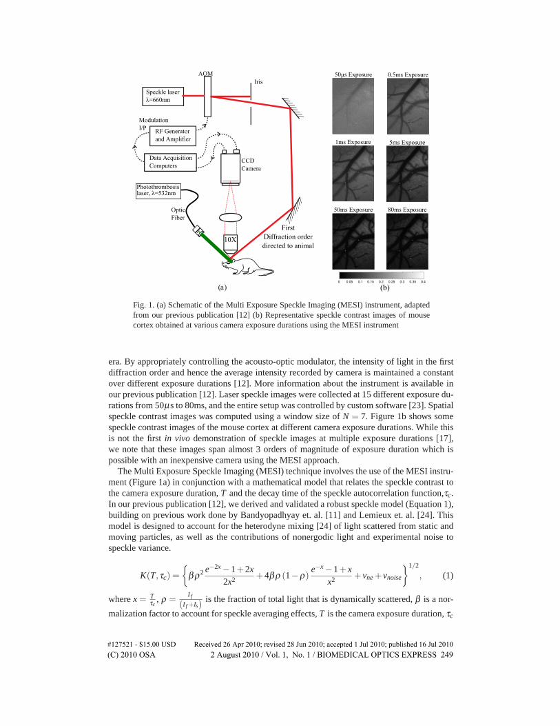
The Multi Exposure Speckle Imaging (MESI) instrument is shown in Figure 1a. Speckle imagesat different camera exposure durations are acquired by triggering a camera (Basler 602f, BaslerVision Technologies, Germany) and simultaneously gating a laser diode (λ = 660nm, 95mW,Micro laser Systems Inc., Garden Grove, CA, USA) with an acousto optic modulator to equal-ize the energy of each laser pulse. The first diffraction order is directed towards the animal, andthe backscattered light is collected by a microscope objective (10X) and imaged onto the cam-


(a)

AOMIris

RF Generator and Amplifier

Data AcquisitionComputers

CCDCamera

ModulationI/P

First Diffraction orderdirected to animal

(b)

Speckle laserλ=660nm

Photothrombosis laser, λ=532nm

10X

OpticFiber

50μs Exposure 0.5ms Exposure

1ms Exposure

50ms Exposure 80ms Exposure

5ms Exposure

Fig. 1. (a) Schematic of the Multi Exposure Speckle Imaging (MESI) instrument, adaptedfrom our previous publication [12] (b) Representative speckle contrast images of mousecortex obtained at various camera exposure durations using the MESI instrument

era. By appropriately controlling the acousto-optic modulator, the intensity of light in the firstdiffraction order and hence the average intensity recorded by camera is maintained a constantover different exposure durations [12]. More information about the instrument is available inour previous publication [12]. Laser speckle images were collected at 15 different exposure du-rations from 50μs to 80ms, and the entire setup was controlled by custom software [23]. Spatialspeckle contrast images was computed using a window size of N = 7. Figure 1b shows somespeckle contrast images of the mouse cortex at different camera exposure durations. While thisis not the first in vivo demonstration of speckle images at multiple exposure durations [17],we note that these images span almost 3 orders of magnitude of exposure duration which ispossible with an inexpensive camera using the MESI approach.

The Multi Exposure Speckle Imaging (MESI) technique involves the use of the MESI instru-ment (Figure 1a) in conjunction with a mathematical model that relates the speckle contrast tothe camera exposure duration, T and the decay time of the speckle autocorrelation function,τc.In our previous publication [12], we derived and validated a robust speckle model (Equation 1),building on previous work done by Bandyopadhyay et. al. [11] and Lemieux et. al. [24]. Thismodel is designed to account for the heterodyne mixing [24] of light scattered from static andmoving particles, as well as the contributions of nonergodic light and experimental noise tospeckle variance.

K(T,τc) ={

βρ2 e−2x −1+2x2x2 +4βρ (1−ρ)

e−x −1+ xx2 + vne + vnoise

}1/2

, (1)

where x = Tτc

, ρ = I f

(I f +Is) is the fraction of total light that is dynamically scattered, β is a nor-

malization factor to account for speckle averaging effects, T is the camera exposure duration, τc


(b) (c)(a)

Thin Skull

Craniotomy

1

23

4

5

6

Fig. 2. (a) Speckle contrast image (5ms exposure duration) illustrating the partial cran-iotomy model. The regions within the closed loops (Regions 1, 3 and 5) are in the cran-iotomy. Regions outside the closed loops (Regions 2, 4 and 6) are in the thin skull region.Speckle Contrast images of a branch of the MCA, illustrating ischemic stroke induced us-ing photo thrombosis (b) Before stroke (c) After stroke

the correlation time is the characteristic decay time of the speckle electric field autocorrelationfunction, vnoise is the constant variance due to experimental noise and vne is the constant vari-ance due to nonergodic light. For our experiments, we lump vnoise and vne into a single spatialvariance vs = vne +vnoise. vne in Equation 1 is a constant that is used to link spatial speckle anal-ysis with temporal statistics. The exact value of the constant and its mathematical expressiondoes not affect the flow estimates. However it can be derived using Equation 16 from Boas et.al. [25]. The MESI data, which consists of speckle contrast measurements obtained at multi-ple exposure durations using the instrument (Figure 1a) can now be fit to Equation 1 to findunknown constants β , ρ , vs, and τc which is a measure of flow. The ability to experimentallymeasure speckle variance as a function of exposure duration of the camera, enables better andmore consistent estimates of τc and hence blood flow.

2.2. Animal preparation

The MESI technique was used to image cerebral blood flow changes that occur during ischemicstroke in mice. Mice (CD-1; male, 25−30 g, n = 5) were used for these experiments. All ex-perimental procedures were approved by the Animal Care and Use Committee at the Universityof Texas at Austin. The animals were anesthetized by inhalation of 2−3% isoflurane in oxygenthrough a nose cone. Body temperature was maintained at 37oC using a feedback controlledheating plate (ATC100, World Percision Instruments, Sarasota, FL, USA) during the experi-ment. The animals were fixed in a stereotaxic frame (Kopf Instruments, Tujunga, CA, USA)and an ∼ 3mm×3mm portion of the skull was exposed by thinning it down using a dental burr(IdealTM Micro-Drill, Fine Science tools, Foster City, CA, USA). Further, part of this thinnedskull was removed to create a partial craniotomy (shown in Figure 2a). Care was taken to en-sure that the boundary between the thin skull and the craniotomy was over a vessel and that theboundary was away from major branches. This ensured that one can expect the same blood flowchanges across the boundary. The partial craniotomy was completed by building a well aroundthe region using dental cement and filling it with mineral oil. The surgery was supplementedwith subcutaneous injections of Atropine (0.04mg/kg) every hour to prevent respiratory diffi-culties and intraparetonial injections of dextrose-saline (2ml/kg/h of 5%w/v) for hydration.


Region 2

Region 1

Region 3

Region 4

(a) (b)

10−5 10−4 10−3 10−2 10−10

0.005

0.01

0.015

0.02

0.025

0.03

0.035

Exposure Duration (seconds)Sp

eckl

e va

rianc

e (a

.u.)

Region1Region2Region3Region4

Fig. 3. (a) Speckle contrast image (5ms exposure) illustrating regions of different flow (b)Time integrated speckle variance curves with decay rates corresponding to flow rates. Thedata points have been fit to Equation 1

2.3. Ischemic stroke using photothrombosis

To induce an ischemic stroke, the middle cerebral artery (MCA) was occluded using pho-tothrombosis [26, 27]. During animal preparation, the temporalis muscle in the same hemi-sphere of the craniotomy was carefully resected from the temporal bone. The temporal bonewas then thinned using the dental burr till it was transparent and the MCA was visible. A laserbeam (λ = 532nm, Spectra Physics, Santa Clara, CA, USA) was directed towards the MCAthrough an optical fiber. Typical laser power delivered to the animal during the experimentwas ∼ 0.5− 0.75W. During the experiment, a 1ml bolus intraparetonial injection of a photosensitive thrombotic agent Rose Bengal (15mg/kg) was administered to the animal. The laserlight interacts with the Rose Bengal to cause thrombosis in the MCA resulting in occlusion.Figures 2b & c show LSCI images (at 5ms exposure) before and after the stroke was induced.Occluding the MCA created a severe stroke and reduced blood flow by almost 100% in thecortical regions downstream.

2.4. Imaging paradigm

The experimental setup shown in Figure 1 was used to acquire multi exposure speckle imagesbefore, during and after the stroke. Laser speckle images at 15 exposure durations rangingfrom 50μs to 80ms were used to compile one MESI frame. Typically, 3000 MESI frames werecollected for each experiment. Each MESI frame took ∼ 1.5 seconds to acquire. The field ofview of the cortex as measured by the MESI instrument was ∼ 800×500μm. Specific regionsof interest as shown in Figure 3a were identified, and the average speckle contrast in theseregions were computed for all MESI frames to produce the time integrated speckle contrastcurves shown in Figure 3b. Each curve was then fit to Equation 1 to estimate blood flow (τc).


3. Results

3.1. Estimating blood flow using the MESI technique

Figure 3 illustrates the first step in obtaining blood flow estimates using the MESI technique.In this example, the MESI instrument (Figure 1a) was used to obtain raw speckle images atmultiple exposure durations of a mouse brain whose cortex had been exposed by performing afull craniotomy. After converting these raw images to speckle contrast images, specific regionsof interest were identified (Figure 3a), and the average speckle contrast in these regions werecomputed and plotted as a function of camera exposure duration (Figure 3b). These experimen-tally measured time integrated speckle variance, K(T,τc)2 curves were then fit to Equation 1using the Trust-Region algorithm to obtain estimates for blood flow (through τc, the decaytime of the speckle autocorrelation function [12, 14]). The curves correspond to different re-gions shown in Figure 3a. From these curves, it can be observed that the variance decays witha lower τc value (and hence higher blood flow) in region 1 which is in the middle of a majorvessel (a vein), when compared to region 4 which is in the parenchyma.

3.2. Imaging blood flow changes due to ischemic stroke

For stroke experiments, the partial craniotomy procedure was followed during animal prepara-tion. A representative image of this model is shown in Figure 4a. Regions 1, 3, and 5 are in thecraniotomy, while regions 2, 4 and 6 are under the thin skull. MESI images were obtained andthe blood flow was estimated using the procedures described in the previous section. Figure 4bshows how the time integrated speckle variance curves are different for two regions across thethin skull boundary. The primary points of difference between the curves obtained from regionsacross the boundary are (a) an apparent change in the shape of the time integrated speckle vari-

Region 1Region 2Region 3Region 4

Thin Skull

Craniotomy

1

23

46

5

(a) (b)

Spec

kle

Var

ianc

e (a

.u.)

0

0.005

0.01

0.015

0.02

0.025

0.03

0.035

0.04

10−5 10−4 10−3 10−2 10−1Exposure Duration (seconds)

ρ=0.95

ρ=0.52

ρ=0.87

ρ=0.80

Fig. 4. (a) Illustration of partial craniotomy model. The regions enclosed by the closedloops (regions 1,3 & 5) are located in the craniotomy. Regions outside of the closed loops(regions 2,4 & 6) are located in the thinned (but intact) skull. (b) Time integrated specklevariance curves illustrating the influence of static scattering due to the presence of thethinned skull. A decrease in the value of ρ indicates an increase in the amount of staticscattering. Regions 2 and 4 show distinct offset at large exposure durations. This offset itdue to increased vs over the thinned skull


ance curve over the thin skull due to variation in ρ (the fraction of light that is dynamicallyscattered [12]), and (b) an increase in the variance at the longer exposure durations due to anincrease in vs (the constant spatial variance that accounts for nonergodicity and experimentalnoise [12]). This difference is more apparent in the regions on the vessel (regions 1 and 2) thanit is in regions in the parenchyma (regions 3 and 4). With LSCI at a single exposure, regions1 and 2 measure vastly different speckle contrast values even though the actual blood flowis likely identical. Under baseline conditions, the ratio of the correlation time in region 1 tothe correlation time in region 2 was found to be 0.6238± 0.0238 using the MESI technique,while this ratio was estimated to be 0.3771±0.0215 using the LSCI technique. While the idealvalue for these ratios should be 1, these estimates suggest that the MESI technique predictsτc values that are more consistent across the thin skull boundary. The ratio of the correlationtime in region 3 to the correlation time in region 4 was found to be 0.883± 0.055 using theMESI technique, while this ratio was estimated to be 0.889±0.019 using the LSCI technique.The MESI and LSCI estimates of these ratios are similar over the parenchyma regions becausethe thickness of the thinned skull is nonuniform and was found to be thinner, as evidenced byhigher values of ρ in region 4 compared to region 2.

Each stroke experiment was performed after waiting for about 30 minutes after surgicalpreparation. The first 10 minutes of the data was used as baseline measures to compute therelative blood flow change. The thrombosis inducing laser was kept on during the entire courseof the experiment. Rose Bengal was injected 10 minutes after start of the experiment and datacollection was continued for about an hour. Data acquisition was not stopped while the dyewas being injected. Immediately after the completion of data acquisition, the animal (n = 2)was sacrificed and 30 MESI frames (1 MESI frame consists of 15 exposure durations) werecollected as a zero flow reference.

Since β is an experimental constant, its in vivo determination is important to obtain accurateflow measures [12]. In addition to β , ρ and vs also have to be determined in vivo. However,we contend that changes in the physiology can change ρ and vs, and hence these parameterswere not held fixed during the fitting process. First, β was estimated under baseline conditionsfor the regions in the craniotomy (regions 1, 3 and 5 shown in figure 4a), by using equation 1and holding ρ = 1. A statistical average of the estimated values of β were found for eachregion and this average value was used for the corresponding pair. For example, the value of βestimated from region 1, would be used for regions 1 and 2. The MESI curves from entire dataset was then fit to Equation 1 using the estimated value of β , and holding it constant. Unknownparameters ρ , vs and the flow measure τc were estimated from this fitting process.

Figure 5a shows the relative blood flow change as measured using the MESI technique inregion 1, in the same animal as in Figure 4. Since τc can be assumed to be inversely related toblood flow [13], relative blood flow may be defined as the ratio of τbaseline to τmeasured . Here,τbaseline is the statistical average of the correlation time estimates during the first 10 minutes.From time t = 10 min to t = 30 min, the blood flow is seen to fluctuate. These fluctuations aredue to the increase and decrease of blood flow while the clot is being formed in the MCA.For the MCA to be completely occluded, the photo thrombosis process has to create enoughthrombus to occlude the vessel and its downstream branches. Since the MCA is a major artery,partially formed thrombus can be washed down by blood pressure. The partially formed clotsbreak down and produce blood flow fluctuations. These fluctuations were observed in all ani-mals before the stroke was formed. Once the thrombosis process is complete, the blood flowsettles to a stable value. Figure 5a shows that the relative blood flow drops to almost 0 after theclot is fully formed. The average percentage reduction in blood flow in the blood vessel, due tothe ischemic stroke in all animals was estimated to be 97.3±2.09% using the MESI techniqueand 87.67±7.04% using the LSCI technique. The estimates of average percentage reduction in


Time (minutes)(b)(a)

10 20 30 40 50 60 70 800

0.2

0.4

0.6

0.8

1

1.2

1.4

τ base

line/τ

Exposure Duration (seconds)

Spec

kle

Var

ianc

e (a

.u.)

10−5 10−4 10−3 10−2 10−10

0.005

0.01

0.015

0.02

0.025

0.03

0.035

0.04

0.045

0.05 Pre StrokePost StrokePost Mortem

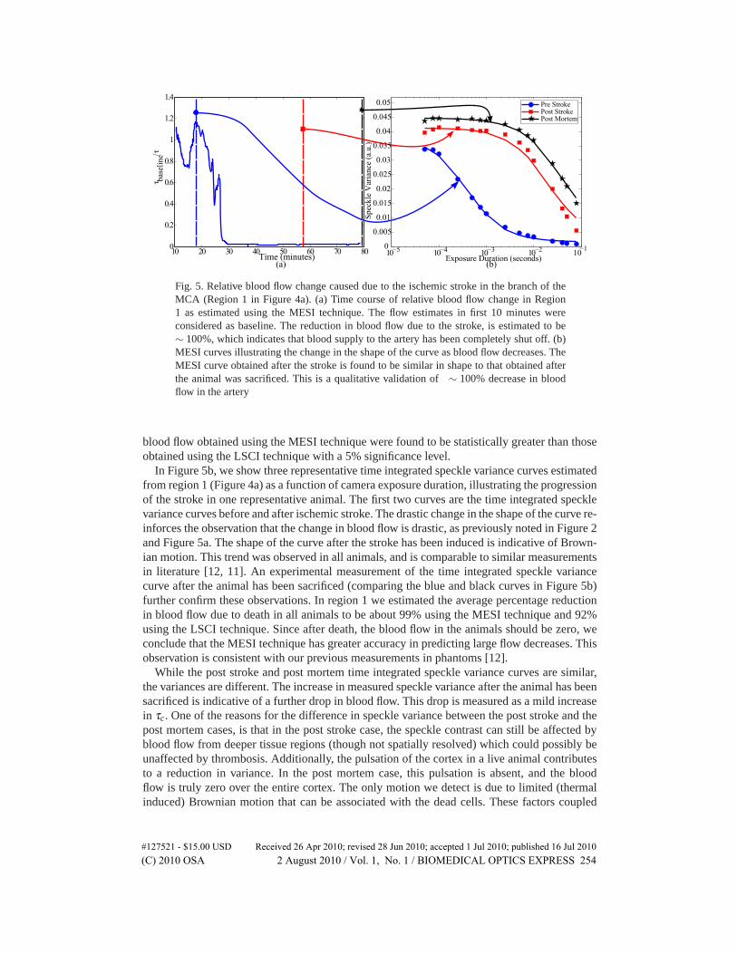
Fig. 5. Relative blood flow change caused due to the ischemic stroke in the branch of theMCA (Region 1 in Figure 4a). (a) Time course of relative blood flow change in Region1 as estimated using the MESI technique. The flow estimates in first 10 minutes wereconsidered as baseline. The reduction in blood flow due to the stroke, is estimated to be∼ 100%, which indicates that blood supply to the artery has been completely shut off. (b)MESI curves illustrating the change in the shape of the curve as blood flow decreases. TheMESI curve obtained after the stroke is found to be similar in shape to that obtained afterthe animal was sacrificed. This is a qualitative validation of ∼ 100% decrease in bloodflow in the artery

blood flow obtained using the MESI technique were found to be statistically greater than thoseobtained using the LSCI technique with a 5% significance level.

In Figure 5b, we show three representative time integrated speckle variance curves estimatedfrom region 1 (Figure 4a) as a function of camera exposure duration, illustrating the progressionof the stroke in one representative animal. The first two curves are the time integrated specklevariance curves before and after ischemic stroke. The drastic change in the shape of the curve re-inforces the observation that the change in blood flow is drastic, as previously noted in Figure 2and Figure 5a. The shape of the curve after the stroke has been induced is indicative of Brown-ian motion. This trend was observed in all animals, and is comparable to similar measurementsin literature [12, 11]. An experimental measurement of the time integrated speckle variancecurve after the animal has been sacrificed (comparing the blue and black curves in Figure 5b)further confirm these observations. In region 1 we estimated the average percentage reductionin blood flow due to death in all animals to be about 99% using the MESI technique and 92%using the LSCI technique. Since after death, the blood flow in the animals should be zero, weconclude that the MESI technique has greater accuracy in predicting large flow decreases. Thisobservation is consistent with our previous measurements in phantoms [12].

While the post stroke and post mortem time integrated speckle variance curves are similar,the variances are different. The increase in measured speckle variance after the animal has beensacrificed is indicative of a further drop in blood flow. This drop is measured as a mild increasein τc. One of the reasons for the difference in speckle variance between the post stroke and thepost mortem cases, is that in the post stroke case, the speckle contrast can still be affected byblood flow from deeper tissue regions (though not spatially resolved) which could possibly beunaffected by thrombosis. Additionally, the pulsation of the cortex in a live animal contributesto a reduction in variance. In the post mortem case, this pulsation is absent, and the bloodflow is truly zero over the entire cortex. The only motion we detect is due to limited (thermalinduced) Brownian motion that can be associated with the dead cells. These factors coupled


10 20 30 40 50 60 70 800

0.5

1

1.5

Time (minutes)

τ base

line/τ

Region 1Region 2Region 3Region 4Region 5Region 6

10 20 30 40 50 60 70 800

0.5

1

1.5

Time (minutes)

τ base

line/τ

Region 1Region 2Region 3Region 4Region 5Region 6

(a) (b)

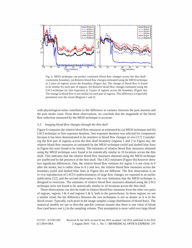
Fig. 6. MESI technique can predict consistent blood flow changes across the thin skull -craniotomy boundary. (a) Relative blood flow changes estimated using the MESI techniquein 3 pairs of regions across the boundary (Figure 4a). The change in blood flow is foundto be similar for each pair of regions. (b) Relative blood flow changes estimated using theLSCI technique (at 5ms exposure) in 3 pairs of regions across the boundary (Figure 4a).The change in blood flow is not similar for each pair of regions. This difference is especiallyprominent over the vessel (Regions 1 and 2)

with physiological noise contribute to the difference in variance between the post mortem andthe post stroke cases. From these observations, we conclude that the magnitude of the bloodflow reduction measured by the MESI technique is accurate.

3.3. Imaging blood flow changes through the thin skull

Figure 6 compares the relative blood flow measures as estimated by (a) MESI technique and (b)LSCI technique at 5ms exposure duration. 5ms exposure duration was selected for comparisonbecause it has been demonstrated to be sensitive to blood flow changes in vivo [17]. Consider-ing the first pair of regions across the thin skull boundary (regions 1 and 2 in Figure 4a), therelative blood flow measures as estimated by the MESI technique (solid and dashed blue linesin Figure 6a) were found to be similar. The estimates of relative blood flow measures obtainedusing the MESI technique were found to be statistically similar in 10 locations across the thinskull. This indicates that the relative blood flow measures obtained using the MESI techniqueare unaffected by the presence of the thin skull. The LSCI estimates (Figure 6b) however showtwo significant differences. One, the relative blood flow estimate for region 1 is not close to 0after the stroke, but is rather close to 0.2 and two, the relative blood flow measures across theboundary (solid and dashed blue lines in Figure 6b) are different. The first observation is anin vivo reproduction of LSCI’s underestimation of large flow changes we reported in an earlierpublication [12], and the second observation is the very limitation that the MESI technique isdesigned to overcome. The estimates of relative blood flow measures obtained using the LSCItechnique were not found to be statistically similar in 10 locations across the thin skull.

These observations can also be made in relative blood flow measures from the other two pairsof regions, regions 3 & 4 and regions 5 & 6, both in the parenchyma. In these regions we seea similar trend, but the difference between the two techniques is not as drastic as it is in theblood vessel. Typically, each pixel in the image samples a large distribution of blood flows. Thestatistical models we use to describe speckle contrast assume that there is one value of bloodflow (and hence one τc) in the sampling volume. This assumption is more valid over large blood


10.90.80.70.60.50.40.30.20.10

(a) (b)

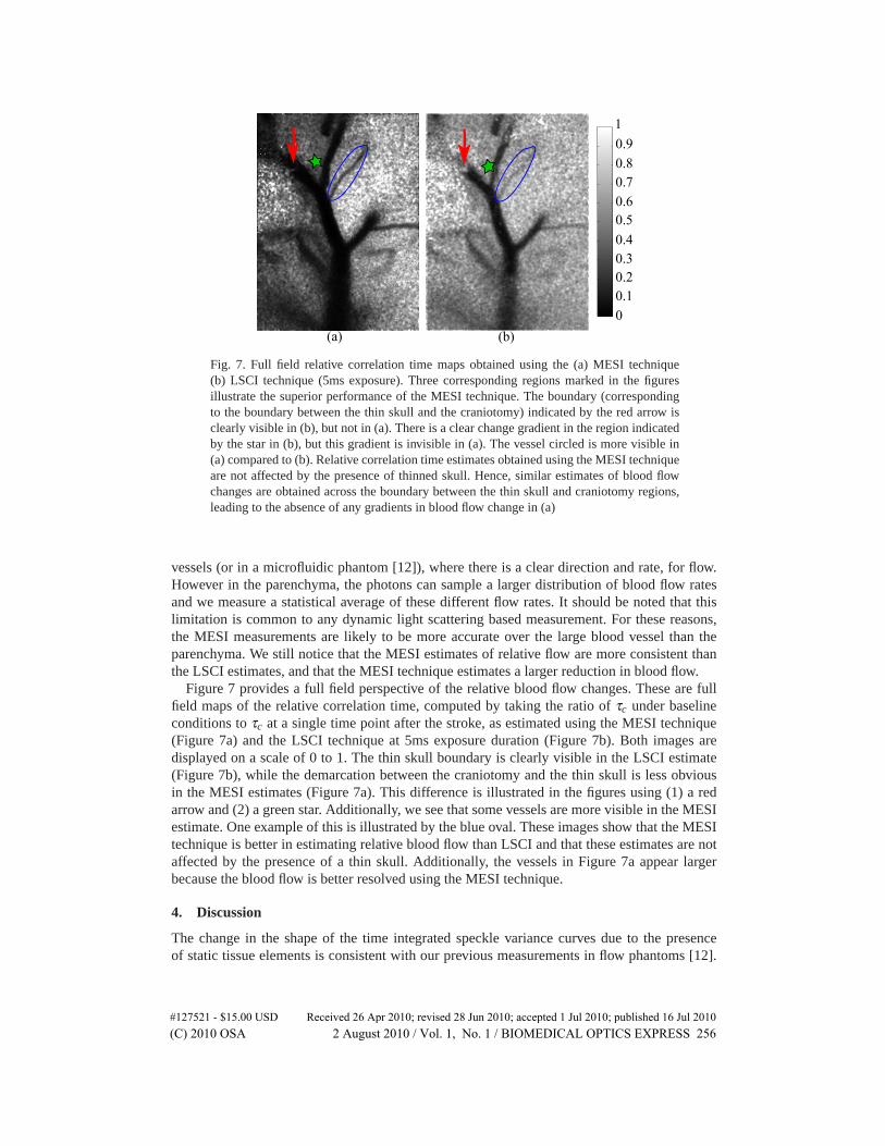
Fig. 7. Full field relative correlation time maps obtained using the (a) MESI technique(b) LSCI technique (5ms exposure). Three corresponding regions marked in the figuresillustrate the superior performance of the MESI technique. The boundary (correspondingto the boundary between the thin skull and the craniotomy) indicated by the red arrow isclearly visible in (b), but not in (a). There is a clear change gradient in the region indicatedby the star in (b), but this gradient is invisible in (a). The vessel circled is more visible in(a) compared to (b). Relative correlation time estimates obtained using the MESI techniqueare not affected by the presence of thinned skull. Hence, similar estimates of blood flowchanges are obtained across the boundary between the thin skull and craniotomy regions,leading to the absence of any gradients in blood flow change in (a)

vessels (or in a microfluidic phantom [12]), where there is a clear direction and rate, for flow.However in the parenchyma, the photons can sample a larger distribution of blood flow ratesand we measure a statistical average of these different flow rates. It should be noted that thislimitation is common to any dynamic light scattering based measurement. For these reasons,the MESI measurements are likely to be more accurate over the large blood vessel than theparenchyma. We still notice that the MESI estimates of relative flow are more consistent thanthe LSCI estimates, and that the MESI technique estimates a larger reduction in blood flow.

Figure 7 provides a full field perspective of the relative blood flow changes. These are fullfield maps of the relative correlation time, computed by taking the ratio of τc under baselineconditions to τc at a single time point after the stroke, as estimated using the MESI technique(Figure 7a) and the LSCI technique at 5ms exposure duration (Figure 7b). Both images aredisplayed on a scale of 0 to 1. The thin skull boundary is clearly visible in the LSCI estimate(Figure 7b), while the demarcation between the craniotomy and the thin skull is less obviousin the MESI estimates (Figure 7a). This difference is illustrated in the figures using (1) a redarrow and (2) a green star. Additionally, we see that some vessels are more visible in the MESIestimate. One example of this is illustrated by the blue oval. These images show that the MESItechnique is better in estimating relative blood flow than LSCI and that these estimates are notaffected by the presence of a thin skull. Additionally, the vessels in Figure 7a appear largerbecause the blood flow is better resolved using the MESI technique.

4. Discussion

The change in the shape of the time integrated speckle variance curves due to the presenceof static tissue elements is consistent with our previous measurements in flow phantoms [12].


While in the case of the tissue phantoms, the change in the shape was affected in equal parts dueto the influence of ρ and vs, in the in vivo measures, we find that the static speckle variance vs isthe more dominant factor. In the microfluidic device we used earlier, the flow channel was theonly part of the device containing dynamic scatterers. We believe that in the microfluidic device,the influence of ρ was greater due to the opportunity for a photon to interact with static particleson the sides of the channel and below the channel. This is clearly not the case in vivo, becausethe only place where a photon can interact from a static particle is from the thin skull. This couldexplain a comparatively reduced role that ρ plays in the in vivo measurements. Nevertheless,there is no way of accurately determining the value of ρ or vs without using Equation 1 and theMESI instrument. Hence, the MESI technique is better suited to obtain consistent and accuratemeasurements of blood flow changes in the presence of a thin skull. Our technique is similar tothe methods used by Zakharov et. al. [22], who presented an alternate method to estimate bloodflow accurately in the presence a thinned skull. While their dynamic Laser Speckle Imagingtechnique aims at separating the dynamic speckle fluctuations from the static component, ourMESI technique is aimed at interpreting and modeling the recorded intensity as a mixture oftemporal and static back scattered intensities.

Recently, Duncan et. al. [19] pointed out that a Gaussian function (g1(τ) = e−τ2/τ2c ) is a

better statistical model to describe the dynamics of ordered flow in a vessel as opposed to thetraditionally used negative exponential model [1] (g1(τ) = e−τ/τc). The former correspondsto a Gaussian distribution of velocities, while the negative exponential model corresponds to aLorentzian distribution of velocities in the sample volume. In order to test this hypothesis, weproceeded to derive a new MESI expression using the Gaussian function to describe speckle dy-namics, and account for scattering from static tissue elements. We substituted g1(τ) = e−τ2/τ2

c

in Equation 9 in our previous publication [12] and evaluated the integral to arrive at the newexpression.

K(T,τc) ={

βρ2 e−2x2 −1+√

2πxerf(√

2x)2x2

+2βρ (1−ρ)e−x2 −1+

√πxerf(x)

x2 + vne + vnoise

}1/2

, (2)

We estimated the relative blood flow changes in regions 1 and 2 (Figure 4a) using Equation 2and the MESI technique. We compared these estimates to those we already obtained usingEquation 1 and to the corresponding LSCI estimates at a few exposure durations other than5ms. These results are plotted in Figure 8.

From Figure 8 we observe that using the Gaussian statistical model and Equation 2 do notchange our estimates of relative flow changes significantly. By incorporating the principlesof heterodyne mixing into Equation 2 and by using the MESI technique, we are still able toobtain consistent flow measures across the boundary of the thin skull. Duncan et. al [19] alsopointed out that the differences between the Lorentzian and the Gaussian models are moreprominent at the lower exposure durations. By sampling a range of exposure durations, we areminimizing the difference between the two models. Also as we explained earlier, each specklesamples a wide range of flow rates. The differences between the two models are not significantenough to overcome the statistical variability in value of τc. In addition, physiological noise andvariability are bigger sources of uncertainty in the fitting process than a small change affectedby using a different model. Our observations are in agreement with Cheung et. al [28] andDurduran et. al. [29] who showed that the Lorentzian model is a better fit for in vivo bloodflow measurements using noninvasive diffuse correlation spectroscopy measurements, due tothe complex fluid dynamics of blood flow in vessels.


%R

educ

tion

in B

lood

Flo

w

100

90

80

70

60

50

40

30

20

10

0

CraniotomyThin Skull

MESILorentzian Gaussian 0.25ms 1ms 5ms 10ms 50ms

LSCI

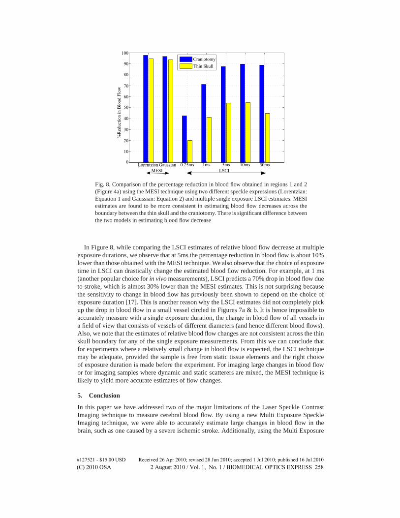
Fig. 8. Comparison of the percentage reduction in blood flow obtained in regions 1 and 2(Figure 4a) using the MESI technique using two different speckle expressions (Lorentzian:Equation 1 and Gaussian: Equation 2) and multiple single exposure LSCI estimates. MESIestimates are found to be more consistent in estimating blood flow decreases across theboundary between the thin skull and the craniotomy. There is significant difference betweenthe two models in estimating blood flow decrease

In Figure 8, while comparing the LSCI estimates of relative blood flow decrease at multipleexposure durations, we observe that at 5ms the percentage reduction in blood flow is about 10%lower than those obtained with the MESI technique. We also observe that the choice of exposuretime in LSCI can drastically change the estimated blood flow reduction. For example, at 1 ms(another popular choice for in vivo measurements), LSCI predicts a 70% drop in blood flow dueto stroke, which is almost 30% lower than the MESI estimates. This is not surprising becausethe sensitivity to change in blood flow has previously been shown to depend on the choice ofexposure duration [17]. This is another reason why the LSCI estimates did not completely pickup the drop in blood flow in a small vessel circled in Figures 7a & b. It is hence impossible toaccurately measure with a single exposure duration, the change in blood flow of all vessels ina field of view that consists of vessels of different diameters (and hence different blood flows).Also, we note that the estimates of relative blood flow changes are not consistent across the thinskull boundary for any of the single exposure measurements. From this we can conclude thatfor experiments where a relatively small change in blood flow is expected, the LSCI techniquemay be adequate, provided the sample is free from static tissue elements and the right choiceof exposure duration is made before the experiment. For imaging large changes in blood flowor for imaging samples where dynamic and static scatterers are mixed, the MESI technique islikely to yield more accurate estimates of flow changes.

5. Conclusion

In this paper we have addressed two of the major limitations of the Laser Speckle ContrastImaging technique to measure cerebral blood flow. By using a new Multi Exposure SpeckleImaging technique, we were able to accurately estimate large changes in blood flow in thebrain, such as one caused by a severe ischemic stroke. Additionally, using the Multi Exposure


Speckle Imaging technique, we were able to image through a thinned yet intact skull, andobtain consistent and accurate measures of changes in cerebral blood flow. These developmentsshould improve the quantitative accuracy of cerebral blood flow images. Also, the ability toquantitatively image through the skull will give researchers more freedom to design chronicand long term studies of ischemic strokes.

Acknowledgments

This work was funded by grants from the American Heart Association (0735136N), the Na-tional Science Foundation (CBET/0737731), the Coulter Foundation and the Dana Foundation.


quantitative imaging of ischemic stroke through thinned ... · quantitative imaging of ischemic...

Documents