python text processing with - github pages · natural language processing. you want to employ...

Python Text Processing with NLTK 2.0 Cookbook

Over 80 practical recipes for using Python's NLTK suite of libraries to maximize your Natural Language Processing capabilities.

Jacob Perkins

BIRMINGHAM - MUMBAI

Python Text Processing with NLTK 2.0 Cookbook

Copyright © 2010 Packt Publishing

All rights reserved. No part of this book may be reproduced, stored in a retrieval system, or transmitted in any form or by any means, without the prior written permission of the publisher, except in the case of brief quotations embedded in critical articles or reviews.

Every effort has been made in the preparation of this book to ensure the accuracy of the information presented. However, the information contained in this book is sold without warranty, either express or implied. Neither the author, nor Packt Publishing, and its dealers and distributors will be held liable for any damages caused or alleged to be caused directly or indirectly by this book.

Packt Publishing has endeavored to provide trademark information about all of the companies and products mentioned in this book by the appropriate use of capitals. However, Packt Publishing cannot guarantee the accuracy of this information.

First published: November 2010

Production Reference: 1031110

Published by Packt Publishing Ltd. 32 Lincoln Road Olton Birmingham, B27 6PA, UK.

ISBN 978-1-849513-60-9

www.packtpub.com

Cover Image by Sujay Gawand ([email protected])

Credits

AuthorJacob Perkins

ReviewersPatrick Chan

Herjend Teny

Acquisition EditorSteven Wilding

Development EditorMaitreya Bhakal

Technical EditorsBianca Sequeira

Aditi Suvarna

Copy EditorLaxmi Subramanian

IndexerTejal Daruwale

Editorial Team LeaderAditya Belpathak

Project Team LeaderPriya Mukherji

Project CoordinatorShubhanjan Chatterjee

ProofreaderJoanna McMahon

GraphicsNilesh Mohite

Production Coordinator Adline Swetha Jesuthas

Cover WorkAdline Swetha Jesuthas

About the Author

Jacob Perkins has been an avid user of open source software since high school, when he first built his own computer and didn't want to pay for Windows. At one point he had five operating systems installed, including Red Hat Linux, OpenBSD, and BeOS.

While at Washington University in St. Louis, Jacob took classes in Spanish and poetry writing, and worked on an independent study project that eventually became his Master's project: WUGLE—a GUI for manipulating logical expressions. In his free time, he wrote the Gnome2 version of Seahorse (a GUI for encryption and key management), which has since been translated into over a dozen languages and is included in the default Gnome distribution.

After receiving his MS in Computer Science, Jacob tried to start a web development studio with some friends, but since no one knew anything about web development, it didn't work out as planned. Once he'd actually learned about web development, he went off and co-founded another company called Weotta, which sparked his interest in Machine Learning and Natural Language Processing.

Jacob is currently the CTO/Chief Hacker for Weotta and blogs about what he's learned along the way at http://streamhacker.com/. He is also applying this knowledge to produce text processing APIs and demos at http://text-processing.com/. This book is a synthesis of his knowledge on processing text using Python, NLTK, and more.

Thanks to my parents for all their support, even when they don't understand what I'm doing; Grant for sparking my interest in Natural Language Processing; Les for inspiring me to program when I had no desire to; Arnie for all the algorithm discussions; and the whole Wernick family for feeding me such good food whenever I come over.

About the Reviewers

Patrick Chan is an engineer/programmer in the telecommunications industry. He is an avid fan of Linux and Python. His less geekier pursuits include Toastmasters, music, and running.

Herjend Teny graduated from the University of Melbourne. He has worked mainly in the education sector and as a part of research teams. The topics that he has worked on mainly involve embedded programming, signal processing, simulation, and some stochastic modeling. His current interests now lie in many aspects of web programming, using Django. One of the books that he has worked on is the Python Testing: Beginner's Guide.

I'd like to thank Patrick Chan for his help in many aspects, and his crazy and odd ideas. Also to Hattie, for her tolerance in letting me do this review until late at night. Thank you!!

Table of ContentsPreface 1Chapter 1: Tokenizing Text and WordNet Basics 7

Introduction 7Tokenizing text into sentences 8Tokenizing sentences into words 9Tokenizing sentences using regular expressions 11Filtering stopwords in a tokenized sentence 13Looking up synsets for a word in WordNet 14Looking up lemmas and synonyms in WordNet 17Calculating WordNet synset similarity 19Discovering word collocations 21

Chapter 2: Replacing and Correcting Words 25Introduction 25Stemming words 25Lemmatizing words with WordNet 28Translating text with Babelfish 30Replacing words matching regular expressions 32Removing repeating characters 34Spelling correction with Enchant 36Replacing synonyms 39Replacing negations with antonyms 41

Chapter 3: Creating Custom Corpora 45Introduction 45Setting up a custom corpus 46Creating a word list corpus 48Creating a part-of-speech tagged word corpus 50

ii

Table of Contents

Creating a chunked phrase corpus 54Creating a categorized text corpus 58Creating a categorized chunk corpus reader 61Lazy corpus loading 68Creating a custom corpus view 70Creating a MongoDB backed corpus reader 74Corpus editing with file locking 77

Chapter 4: Part-of-Speech Tagging 81Introduction 82Default tagging 82Training a unigram part-of-speech tagger 85Combining taggers with backoff tagging 88Training and combining Ngram taggers 89Creating a model of likely word tags 92Tagging with regular expressions 94Affix tagging 96Training a Brill tagger 98Training the TnT tagger 100Using WordNet for tagging 103Tagging proper names 105Classifier based tagging 106

Chapter 5: Extracting Chunks 111Introduction 111Chunking and chinking with regular expressions 112Merging and splitting chunks with regular expressions 117Expanding and removing chunks with regular expressions 121Partial parsing with regular expressions 123Training a tagger-based chunker 126Classification-based chunking 129Extracting named entities 133Extracting proper noun chunks 135Extracting location chunks 137Training a named entity chunker 140

Chapter 6: Transforming Chunks and Trees 143Introduction 143Filtering insignificant words 144Correcting verb forms 146Swapping verb phrases 149Swapping noun cardinals 150Swapping infinitive phrases 151

iii

Table of Contents

Singularizing plural nouns 153Chaining chunk transformations 154Converting a chunk tree to text 155Flattening a deep tree 157Creating a shallow tree 161Converting tree nodes 163

Chapter 7: Text Classification 167Introduction 167Bag of Words feature extraction 168Training a naive Bayes classifier 170Training a decision tree classifier 177Training a maximum entropy classifier 180Measuring precision and recall of a classifier 183Calculating high information words 187Combining classifiers with voting 191Classifying with multiple binary classifiers 193

Chapter 8: Distributed Processing and Handling Large Datasets 201Introduction 202Distributed tagging with execnet 202Distributed chunking with execnet 206Parallel list processing with execnet 209Storing a frequency distribution in Redis 211Storing a conditional frequency distribution in Redis 215Storing an ordered dictionary in Redis 218Distributed word scoring with Redis and execnet 221

Chapter 9: Parsing Specific Data 227Introduction 227Parsing dates and times with Dateutil 228Time zone lookup and conversion 230Tagging temporal expressions with Timex 233Extracting URLs from HTML with lxml 234Cleaning and stripping HTML 236Converting HTML entities with BeautifulSoup 238Detecting and converting character encodings 240

Appendix: Penn Treebank Part-of-Speech Tags 243Index 247

PrefaceNatural Language Processing is used everywhere—in search engines, spell checkers, mobile phones, computer games, and even in your washing machine. Python's Natural Language Toolkit (NLTK) suite of libraries has rapidly emerged as one of the most efficient tools for Natural Language Processing. You want to employ nothing less than the best techniques in Natural Language Processing—and this book is your answer.

Python Text Processing with NLTK 2.0 Cookbook is your handy and illustrative guide, which will walk you through all the Natural Language Processing techniques in a step-by-step manner. It will demystify the advanced features of text analysis and text mining using the comprehensive NLTK suite.

This book cuts short the preamble and lets you dive right into the science of text processing with a practical hands-on approach.

Get started off with learning tokenization of text. Receive an overview of WordNet and how to use it. Learn the basics as well as advanced features of stemming and lemmatization. Discover various ways to replace words with simpler and more common (read: more searched) variants. Create your own corpora and learn to create custom corpus readers for data stored in MongoDB. Use and manipulate POS taggers. Transform and normalize parsed chunks to produce a canonical form without changing their meaning. Dig into feature extraction and text classification. Learn how to easily handle huge amounts of data without any loss in efficiency or speed.

This book will teach you all that and beyond, in a hands-on learn-by-doing manner. Make yourself an expert in using the NLTK for Natural Language Processing with this handy companion.

Preface

2

What this book coversChapter 1, Tokenizing Text and WordNet Basics, covers the basics of tokenizing text and using WordNet.

Chapter 2, Replacing and Correcting Words, discusses various word replacement and correction techniques. The recipes cover the gamut of linguistic compression, spelling correction, and text normalization.

Chapter 3, Creating Custom Corpora, covers how to use corpus readers and create custom corpora. At the same time, it explains how to use the existing corpus data that comes with NLTK.

Chapter 4, Part-of-Speech Tagging, explains the process of converting a sentence, in the form of a list of words, into a list of tuples. It also explains taggers, which are trainable.

Chapter 5, Extracting Chunks, explains the process of extracting short phrases from a part-of-speech tagged sentence. It uses Penn Treebank corpus for basic training and testing chunk extraction, and the CoNLL 2000 corpus as it has a simpler and more flexible format that supports multiple chunk types.

Chapter 6, Transforming Chunks and Trees, shows you how to do various transforms on both chunks and trees. The functions detailed in these recipes modify data, as opposed to learning from it.

Chapter 7, Text Classification, describes a way to categorize documents or pieces of text and, by examining the word usage in a piece of text, classifiers decide what class label should be assigned to it.

Chapter 8, Distributed Processing and Handling Large Datasets, discusses how to use execnet to do parallel and distributed processing with NLTK. It also explains how to use the Redis data structure server/database to store frequency distributions.

Chapter 9, Parsing Specific Data, covers parsing specific kinds of data, focusing primarily on dates, times, and HTML.

Appendix, Penn Treebank Part-of-Speech Tags, lists a table of all the part-of-speech tags that occur in the treebank corpus distributed with NLTK.

Preface

3

What you need for this bookIn the course of this book, you will need the following software utilities to try out various code examples listed:

• NLTK

• MongoDB

• PyMongo

• Redis

• redis-py

• execnet

• Enchant

• PyEnchant

• PyYAML

• dateutil

• chardet

• BeautifulSoup

• lxml

• SimpleParse

• mxBase

• lockfile

Who this book is forThis book is for Python programmers who want to quickly get to grips with using the NLTK for Natural Language Processing. Familiarity with basic text processing concepts is required. Programmers experienced in the NLTK will find it useful. Students of linguistics will find it invaluable.

ConventionsIn this book, you will find a number of styles of text that distinguish between different kinds of information. Here are some examples of these styles, and an explanation of their meaning.

Code words in text are shown as follows: "Now we want to split para into sentences. First we need to import the sentence tokenization function, and then we can call it with the paragraph as an argument."

Preface

4

A block of code is set as follows:

>>> para = "Hello World. It's good to see you. Thanks for buying this book." >>> from nltk.tokenize import sent_tokenize >>> sent_tokenize(para)

New terms and important words are shown in bold.

Warnings or important notes appear in a box like this.

Tips and tricks appear like this.

Reader feedbackFeedback from our readers is always welcome. Let us know what you think about this book—what you liked or may have disliked. Reader feedback is important for us to develop titles that you really get the most out of.

To send us general feedback, simply send an e-mail to [email protected], and mention the book title via the subject of your message.

If there is a book that you need and would like to see us publish, please send us a note in the SUGGEST A TITLE form on www.packtpub.com or e-mail [email protected].

If there is a topic that you have expertise in and you are interested in either writing or contributing to a book, see our author guide on www.packtpub.com/authors.

Customer supportNow that you are the proud owner of a Packt book, we have a number of things to help you to get the most from your purchase.

Downloading the example code for this bookYou can download the example code files for all Packt books you have purchased from your account at http://www.PacktPub.com. If you purchased this book elsewhere, you can visit http://www.PacktPub.com/support and register to have the files e-mailed directly to you.

Preface

5

ErrataAlthough we have taken every care to ensure the accuracy of our content, mistakes do happen. If you find a mistake in one of our books—maybe a mistake in the text or the code—we would be grateful if you would report this to us. By doing so, you can save other readers from frustration and help us improve subsequent versions of this book. If you find any errata, please report them by visiting http://www.packtpub.com/support, selecting your book, clicking on the errata submission form link, and entering the details of your errata. Once your errata are verified, your submission will be accepted and the errata will be uploaded on our website, or added to any list of existing errata, under the Errata section of that title. Any existing errata can be viewed by selecting your title from http://www.packtpub.com/support.

PiracyPiracy of copyright material on the Internet is an ongoing problem across all media. At Packt, we take the protection of our copyright and licenses very seriously. If you come across any illegal copies of our works, in any form, on the Internet, please provide us with the location address or website name immediately so that we can pursue a remedy.

Please contact us at [email protected] with a link to the suspected pirated material.

We appreciate your help in protecting our authors, and our ability to bring you valuable content.

QuestionsYou can contact us at [email protected] if you are having a problem with any aspect of the book, and we will do our best to address it.

1Tokenizing Text and

WordNet Basics

In this chapter, we will cover:

f Tokenizing text into sentences

f Tokenizing sentences into words

f Tokenizing sentences using regular expressions

f Filtering stopwords in a tokenized sentence

f Looking up synsets for a word in WordNet

f Looking up lemmas and synonyms in WordNet

f Calculating WordNet synset similarity

f Discovering word collocations

IntroductionNLTK is the Natural Language Toolkit, a comprehensive Python library for natural language processing and text analytics. Originally designed for teaching, it has been adopted in the industry for research and development due to its usefulness and breadth of coverage.

This chapter will cover the basics of tokenizing text and using WordNet. Tokenization is a method of breaking up a piece of text into many pieces, and is an essential first step for recipes in later chapters.

Tokenizing Text and WordNet Basics

8

WordNet is a dictionary designed for programmatic access by natural language processing systems. NLTK includes a WordNet corpus reader, which we will use to access and explore WordNet. We'll be using WordNet again in later chapters, so it's important to familiarize yourself with the basics first.

Tokenizing text into sentencesTokenization is the process of splitting a string into a list of pieces, or tokens. We'll start by splitting a paragraph into a list of sentences.

Getting readyInstallation instructions for NLTK are available at http://www.nltk.org/download and the latest version as of this writing is 2.0b9. NLTK requires Python 2.4 or higher, but is not compatible with Python 3.0. The recommended Python version is 2.6.

Once you've installed NLTK, you'll also need to install the data by following the instructions at http://www.nltk.org/data. We recommend installing everything, as we'll be using a number of corpora and pickled objects. The data is installed in a data directory, which on Mac and Linux/Unix is usually /usr/share/nltk_data, or on Windows is C:\nltk_data. Make sure that tokenizers/punkt.zip is in the data directory and has been unpacked so that there's a file at tokenizers/punkt/english.pickle.

Finally, to run the code examples, you'll need to start a Python console. Instructions on how to do so are available at http://www.nltk.org/getting-started. For Mac with Linux/Unix users, you can open a terminal and type python.

How to do it...Once NLTK is installed and you have a Python console running, we can start by creating a paragraph of text:

>>> para = "Hello World. It's good to see you. Thanks for buying this book."

Now we want to split para into sentences. First we need to import the sentence tokenization function, and then we can call it with the paragraph as an argument.

>>> from nltk.tokenize import sent_tokenize>>> sent_tokenize(para)['Hello World.', "It's good to see you.", 'Thanks for buying this book.']

So now we have a list of sentences that we can use for further processing.

Chapter 1

9

How it works...sent_tokenize uses an instance of PunktSentenceTokenizer from the nltk.tokenize.punkt module. This instance has already been trained on and works well for many European languages. So it knows what punctuation and characters mark the end of a sentence and the beginning of a new sentence.

There's more...The instance used in sent_tokenize() is actually loaded on demand from a pickle file. So if you're going to be tokenizing a lot of sentences, it's more efficient to load the PunktSentenceTokenizer once, and call its tokenize() method instead.

>>> import nltk.data>>> tokenizer = nltk.data.load('tokenizers/punkt/english.pickle')>>> tokenizer.tokenize(para)['Hello World.', "It's good to see you.", 'Thanks for buying this book.']

Other languagesIf you want to tokenize sentences in languages other than English, you can load one of the other pickle files in tokenizers/punkt and use it just like the English sentence tokenizer. Here's an example for Spanish:

>>> spanish_tokenizer = nltk.data.load('tokenizers/punkt/spanish.pickle')>>> spanish_tokenizer.tokenize('Hola amigo. Estoy bien.')

See alsoIn the next recipe, we'll learn how to split sentences into individual words. After that, we'll cover how to use regular expressions for tokenizing text.

Tokenizing sentences into wordsIn this recipe, we'll split a sentence into individual words. The simple task of creating a list of words from a string is an essential part of all text processing.


10

How to do it...Basic word tokenization is very simple: use the word_tokenize() function:

>>> from nltk.tokenize import word_tokenize>>> word_tokenize('Hello World.')['Hello', 'World', '.']

How it works...word_tokenize() is a wrapper function that calls tokenize() on an instance of the TreebankWordTokenizer. It's equivalent to the following:

>>> from nltk.tokenize import TreebankWordTokenizer>>> tokenizer = TreebankWordTokenizer()>>> tokenizer.tokenize('Hello World.')['Hello', 'World', '.']

It works by separating words using spaces and punctuation. And as you can see, it does not discard the punctuation, allowing you to decide what to do with it.

There's more...Ignoring the obviously named WhitespaceTokenizer and SpaceTokenizer, there are two other word tokenizers worth looking at: PunktWordTokenizer and WordPunctTokenizer. These differ from the TreebankWordTokenizer by how they handle punctuation and contractions, but they all inherit from TokenizerI. The inheritance tree looks like this:

Chapter 1

11

ContractionsTreebankWordTokenizer uses conventions found in the Penn Treebank corpus, which we'll be using for training in Chapter 4, Part-of-Speech Tagging and Chapter 5, Extracting Chunks. One of these conventions is to separate contractions. For example:

>>> word_tokenize("can't")['ca', "n't"]

If you find this convention unacceptable, then read on for alternatives, and see the next recipe for tokenizing with regular expressions.

PunktWordTokenizerAn alternative word tokenizer is the PunktWordTokenizer. It splits on punctuation, but keeps it with the word instead of creating separate tokens.

>>> from nltk.tokenize import PunktWordTokenizer>>> tokenizer = PunktWordTokenizer()>>> tokenizer.tokenize("Can't is a contraction.")['Can', "'t", 'is', 'a', 'contraction.']

WordPunctTokenizerAnother alternative word tokenizer is WordPunctTokenizer. It splits all punctuations into separate tokens.

>>> from nltk.tokenize import WordPunctTokenizer>>> tokenizer = WordPunctTokenizer()>>> tokenizer.tokenize("Can't is a contraction.")['Can', "'", 't', 'is', 'a', 'contraction', '.']

See alsoFor more control over word tokenization, you'll want to read the next recipe to learn how to use regular expressions and the RegexpTokenizer for tokenization.

Tokenizing sentences using regular expressions

Regular expression can be used if you want complete control over how to tokenize text. As regular expressions can get complicated very quickly, we only recommend using them if the word tokenizers covered in the previous recipe are unacceptable.


12

Getting readyFirst you need to decide how you want to tokenize a piece of text, as this will determine how you construct your regular expression. The choices are:

f Match on the tokens

f Match on the separators, or gaps

We'll start with an example of the first, matching alphanumeric tokens plus single quotes so that we don't split up contractions.

How to do it...We'll create an instance of the RegexpTokenizer, giving it a regular expression string to use for matching tokens.

>>> from nltk.tokenize import RegexpTokenizer>>> tokenizer = RegexpTokenizer("[\w']+")>>> tokenizer.tokenize("Can't is a contraction.")["Can't", 'is', 'a', 'contraction']

There's also a simple helper function you can use in case you don't want to instantiate the class.

>>> from nltk.tokenize import regexp_tokenize>>> regexp_tokenize("Can't is a contraction.", "[\w']+")["Can't", 'is', 'a', 'contraction']

Now we finally have something that can treat contractions as whole words, instead of splitting them into tokens.

How it works...The RegexpTokenizer works by compiling your pattern, then calling re.findall() on your text. You could do all this yourself using the re module, but the RegexpTokenizer implements the TokenizerI interface, just like all the word tokenizers from the previous recipe. This means it can be used by other parts of the NLTK package, such as corpus readers, which we'll cover in detail in Chapter 3, Creating Custom Corpora. Many corpus readers need a way to tokenize the text they're reading, and can take optional keyword arguments specifying an instance of a TokenizerI subclass. This way, you have the ability to provide your own tokenizer instance if the default tokenizer is unsuitable.

Chapter 1

13

There's more...RegexpTokenizer can also work by matching the gaps, instead of the tokens. Instead of using re.findall(), the RegexpTokenizer will use re.split(). This is how the BlanklineTokenizer in nltk.tokenize is implemented.

Simple whitespace tokenizerHere's a simple example of using the RegexpTokenizer to tokenize on whitespace:

>>> tokenizer = RegexpTokenizer('\s+', gaps=True)>>> tokenizer.tokenize("Can't is a contraction.") ["Can't", 'is', 'a', 'contraction.']

Notice that punctuation still remains in the tokens.

See alsoFor simpler word tokenization, see the previous recipe.

Filtering stopwords in a tokenized sentenceStopwords are common words that generally do not contribute to the meaning of a sentence, at least for the purposes of information retrieval and natural language processing. Most search engines will filter stopwords out of search queries and documents in order to save space in their index.

Getting readyNLTK comes with a stopwords corpus that contains word lists for many languages. Be sure to unzip the datafile so NLTK can find these word lists in nltk_data/corpora/stopwords/.

How to do it...We're going to create a set of all English stopwords, then use it to filter stopwords from a sentence.

>>> from nltk.corpus import stopwords>>> english_stops = set(stopwords.words('english'))>>> words = ["Can't", 'is', 'a', 'contraction']>>> [word for word in words if word not in english_stops]["Can't", 'contraction']


14

How it works...The stopwords corpus is an instance of nltk.corpus.reader.WordListCorpusReader. As such, it has a words() method that can take a single argument for the file ID, which in this case is 'english', referring to a file containing a list of English stopwords. You could also call stopwords.words() with no argument to get a list of all stopwords in every language available.

There's more...You can see the list of all English stopwords using stopwords.words('english') or by examining the word list file at nltk_data/corpora/stopwords/english. There are also stopword lists for many other languages. You can see the complete list of languages using the fileids() method:

>>> stopwords.fileids()['danish', 'dutch', 'english', 'finnish', 'french', 'german', 'hungarian', 'italian', 'norwegian', 'portuguese', 'russian', 'spanish', 'swedish', 'turkish']

Any of these fileids can be used as an argument to the words() method to get a list of stopwords for that language.

See alsoIf you'd like to create your own stopwords corpus, see the Creating a word list corpus recipe in Chapter 3, Creating Custom Corpora, to learn how to use the WordListCorpusReader. We'll also be using stopwords in the Discovering word collocations recipe, later in this chapter.

Looking up synsets for a word in WordNetWordNet is a lexical database for the English language. In other words, it's a dictionary designed specifically for natural language processing.

NLTK comes with a simple interface for looking up words in WordNet. What you get is a list of synset instances, which are groupings of synonymous words that express the same concept. Many words have only one synset, but some have several. We'll now explore a single synset, and in the next recipe, we'll look at several in more detail.

Chapter 1

15

Getting readyBe sure you've unzipped the wordnet corpus in nltk_data/corpora/wordnet. This will allow the WordNetCorpusReader to access it.

How to do it...Now we're going to lookup the synset for cookbook, and explore some of the properties and methods of a synset.

>>> from nltk.corpus import wordnet>>> syn = wordnet.synsets('cookbook')[0]>>> syn.name'cookbook.n.01'>>> syn.definition'a book of recipes and cooking directions'

How it works...You can look up any word in WordNet using wordnet.synsets(word) to get a list of synsets. The list may be empty if the word is not found. The list may also have quite a few elements, as some words can have many possible meanings and therefore many synsets.

There's more...Each synset in the list has a number of attributes you can use to learn more about it. The name attribute will give you a unique name for the synset, which you can use to get the synset directly.

>>> wordnet.synset('cookbook.n.01')Synset('cookbook.n.01')

The definition attribute should be self-explanatory. Some synsets also have an examples attribute, which contains a list of phrases that use the word in context.

>>> wordnet.synsets('cooking')[0].examples['cooking can be a great art', 'people are needed who have experience in cookery', 'he left the preparation of meals to his wife']

HypernymsSynsets are organized in a kind of inheritance tree. More abstract terms are known as hypernyms and more specific terms are hyponyms. This tree can be traced all the way up to a root hypernym.


16

Hypernyms provide a way to categorize and group words based on their similarity to each other. The synset similarity recipe details the functions used to calculate similarity based on the distance between two words in the hypernym tree.

>>> syn.hypernyms()[Synset('reference_book.n.01')]>>> syn.hypernyms()[0].hyponyms()[Synset('encyclopedia.n.01'), Synset('directory.n.01'), Synset('source_book.n.01'), Synset('handbook.n.01'), Synset('instruction_book.n.01'), Synset('cookbook.n.01'), Synset('annual.n.02'), Synset('atlas.n.02'), Synset('wordbook.n.01')]>>> syn.root_hypernyms()[Synset('entity.n.01')]

As you can see, reference book is a hypernym of cookbook, but cookbook is only one of many hyponyms of reference book. All these types of books have the same root hypernym, entity, one of the most abstract terms in the English language. You can trace the entire path from entity down to cookbook using the hypernym_paths() method.

>>> syn.hypernym_paths()[[Synset('entity.n.01'), Synset('physical_entity.n.01'), Synset('object.n.01'), Synset('whole.n.02'), Synset('artifact.n.01'), Synset('creation.n.02'), Synset('product.n.02'), Synset('work.n.02'), Synset('publication.n.01'), Synset('book.n.01'), Synset('reference_book.n.01'), Synset('cookbook.n.01')]]

This method returns a list of lists, where each list starts at the root hypernym and ends with the original Synset. Most of the time you'll only get one nested list of synsets.

Part-of-speech (POS)You can also look up a simplified part-of-speech tag.

>>> syn.pos'n'

There are four common POS found in WordNet.

Part-of-speech TagNoun nAdjective aAdverb rVerb v

These POS tags can be used for looking up specific synsets for a word. For example, the word great can be used as a noun or an adjective. In WordNet, great has one noun synset and six adjective synsets.

Chapter 1

17

>>> len(wordnet.synsets('great'))7>>> len(wordnet.synsets('great', pos='n'))1>>> len(wordnet.synsets('great', pos='a'))6

These POS tags will be referenced more in the Using WordNet for Tagging recipe of Chapter 4, Part-of-Speech Tagging.

See alsoIn the next two recipes, we'll explore lemmas and how to calculate synset similarity. In Chapter 2, Replacing and Correcting Words, we'll use WordNet for lemmatization, synonym replacement, and then explore the use of antonyms.

Looking up lemmas and synonyms in WordNet

Building on the previous recipe, we can also look up lemmas in WordNet to find synonyms of a word. A lemma (in linguistics) is the canonical form, or morphological form, of a word.

How to do it...In the following block of code, we'll find that there are two lemmas for the cookbook synset by using the lemmas attribute:

>>> from nltk.corpus import wordnet>>> syn = wordnet.synsets('cookbook')[0]>>> lemmas = syn.lemmas>>> len(lemmas)2>>> lemmas[0].name'cookbook'>>> lemmas[1].name'cookery_book'>>> lemmas[0].synset == lemmas[1].synsetTrue


18

How it works...As you can see, cookery_book and cookbook are two distinct lemmas in the same synset. In fact, a lemma can only belong to a single synset. In this way, a synset represents a group of lemmas that all have the same meaning, while a lemma represents a distinct word form.

There's more...Since lemmas in a synset all have the same meaning, they can be treated as synonyms. So if you wanted to get all synonyms for a synset, you could do:

>>> [lemma.name for lemma in syn.lemmas]['cookbook', 'cookery_book']

All possible synonymsAs mentioned before, many words have multiple synsets because the word can have different meanings depending on the context. But let's say you didn't care about the context, and wanted to get all possible synonyms for a word.

>>> synonyms = []>>> for syn in wordnet.synsets('book'):... for lemma in syn.lemmas:... synonyms.append(lemma.name)>>> len(synonyms)38

As you can see, there appears to be 38 possible synonyms for the word book. But in fact, some are verb forms, and many are just different usages of book. Instead, if we take the set of synonyms, there are fewer unique words.

>>> len(set(synonyms))25

AntonymsSome lemmas also have antonyms. The word good, for example, has 27 synsets, five of which have lemmas with antonyms.

>>> gn2 = wordnet.synset('good.n.02')>>> gn2.definition'moral excellence or admirableness'>>> evil = gn2.lemmas[0].antonyms()[0]>>> evil.name'evil'>>> evil.synset.definition

Chapter 1

19

'the quality of being morally wrong in principle or practice'>>> ga1 = wordnet.synset('good.a.01')>>> ga1.definition'having desirable or positive qualities especially those suitable for a thing specified'>>> bad = ga1.lemmas[0].antonyms()[0]>>> bad.name'bad'>>> bad.synset.definition'having undesirable or negative qualities'

The antonyms() method returns a list of lemmas. In the first case here, we see that the second synset for good as a noun is defined as moral excellence, and its first antonym is evil, defined as morally wrong. In the second case, when good is used as an adjective to describe positive qualities, the first antonym is bad, which describes negative qualities.

See also

In the next recipe, we'll learn how to calculate synset similarity. Then in Chapter 2, Replacing and Correcting Words, we'll revisit lemmas for lemmatization, synonym replacement, and antonym replacement.

Calculating WordNet synset similaritySynsets are organized in a hypernym tree. This tree can be used for reasoning about the similarity between the synsets it contains. Two synsets are more similar, the closer they are in the tree.

How to do it...If you were to look at all the hyponyms of reference book (which is the hypernym of cookbook) you'd see that one of them is instruction_book. These seem intuitively very similar to cookbook, so let's see what WordNet similarity has to say about it.

>>> from nltk.corpus import wordnet>>> cb = wordnet.synset('cookbook.n.01')>>> ib = wordnet.synset('instruction_book.n.01')>>> cb.wup_similarity(ib)0.91666666666666663

So they are over 91% similar!


20

How it works...wup_similarity is short for Wu-Palmer Similarity, which is a scoring method based on how similar the word senses are and where the synsets occur relative to each other in the hypernym tree. One of the core metrics used to calculate similarity is the shortest path distance between the two synsets and their common hypernym.

>>> ref = cb.hypernyms()[0]>>> cb.shortest_path_distance(ref)1>>> ib.shortest_path_distance(ref)1>>> cb.shortest_path_distance(ib)2

So cookbook and instruction book must be very similar, because they are only one step away from the same hypernym, reference book, and therefore only two steps away from each other.

There's more...Let's look at two dissimilar words to see what kind of score we get. We'll compare dog with cookbook, two seemingly very different words.

>>> dog = wordnet.synsets('dog')[0]>>> dog.wup_similarity(cb)0.38095238095238093

Wow, dog and cookbook are apparently 38% similar! This is because they share common hypernyms farther up the tree.

>>> dog.common_hypernyms(cb)[Synset('object.n.01'), Synset('whole.n.02'), Synset('physical_entity.n.01'), Synset('entity.n.01')]

Comparing verbsThe previous comparisons were all between nouns, but the same can be done for verbs as well.

>>> cook = wordnet.synset('cook.v.01')>>> bake = wordnet.synset('bake.v.02')>>> cook.wup_similarity(bake)0.75

Chapter 1

21

The previous synsets were obviously handpicked for demonstration, and the reason is that the hypernym tree for verbs has a lot more breadth and a lot less depth. While most nouns can be traced up to object, thereby providing a basis for similarity, many verbs do not share common hypernyms, making WordNet unable to calculate similarity. For example, if you were to use the synset for bake.v.01 here, instead of bake.v.02, the return value would be None. This is because the root hypernyms of the two synsets are different, with no overlapping paths. For this reason, you also cannot calculate similarity between words with different parts of speech.

Path and LCH similarityTwo other similarity comparisons are the path similarity and Leacock Chodorow (LCH) similarity.

>>> cb.path_similarity(ib)0.33333333333333331>>> cb.path_similarity(dog)0.071428571428571425>>> cb.lch_similarity(ib)2.5389738710582761>>> cb.lch_similarity(dog)0.99852883011112725

As you can see, the number ranges are very different for these scoring methods, which is why we prefer the wup_similarity() method.

See alsoThe recipe on Looking up synsets for a word in WordNet, discussed earlier in this chapter, has more details about hypernyms and the hypernym tree.

Discovering word collocationsCollocations are two or more words that tend to appear frequently together, such as "United States". Of course, there are many other words that can come after "United", for example "United Kingdom", "United Airlines", and so on. As with many aspects of natural language processing, context is very important, and for collocations, context is everything!

In the case of collocations, the context will be a document in the form of a list of words. Discovering collocations in this list of words means that we'll find common phrases that occur frequently throughout the text. For fun, we'll start with the script for Monty Python and the Holy Grail.


22

Getting readyThe script for Monty Python and the Holy Grail is found in the webtext corpus, so be sure that it's unzipped in nltk_data/corpora/webtext/.

How to do it...We're going to create a list of all lowercased words in the text, and then produce a BigramCollocationFinder, which we can use to find bigrams, which are pairs of words. These bigrams are found using association measurement functions found in the nltk.metrics package.

>>> from nltk.corpus import webtext>>> from nltk.collocations import BigramCollocationFinder>>> from nltk.metrics import BigramAssocMeasures>>> words = [w.lower() for w in webtext.words('grail.txt')]>>> bcf = BigramCollocationFinder.from_words(words)>>> bcf.nbest(BigramAssocMeasures.likelihood_ratio, 4)[("'", 's'), ('arthur', ':'), ('#', '1'), ("'", 't')]

Well that's not very useful! Let's refine it a bit by adding a word filter to remove punctuation and stopwords.

>>> from nltk.corpus import stopwords>>> stopset = set(stopwords.words('english'))>>> filter_stops = lambda w: len(w) < 3 or w in stopset>>> bcf.apply_word_filter(filter_stops)>>> bcf.nbest(BigramAssocMeasures.likelihood_ratio, 4)[('black', 'knight'), ('clop', 'clop'), ('head', 'knight'), ('mumble', 'mumble')]

Much better—we can clearly see four of the most common bigrams in Monty Python and the Holy Grail. If you'd like to see more than four, simply increase the number to whatever you want, and the collocation finder will do its best.

How it works...The BigramCollocationFinder constructs two frequency distributions: one for each word, and another for bigrams. A frequency distribution, or FreqDist in NLTK, is basically an enhanced dictionary where the keys are what's being counted, and the values are the counts. Any filtering functions that are applied, reduce the size of these two FreqDists by eliminating any words that don't pass the filter. By using a filtering function to eliminate all words that are one or two characters, and all English stopwords, we can get a much cleaner result. After filtering, the collocation finder is ready to accept a generic scoring function for finding collocations. Additional scoring functions are covered in the Scoring functions section further in this chapter.

Chapter 1

23

There's more...In addition to BigramCollocationFinder, there's also TrigramCollocationFinder, for finding triples instead of pairs. This time, we'll look for trigrams in Australian singles ads.

>>> from nltk.collocations import TrigramCollocationFinder>>> from nltk.metrics import TrigramAssocMeasures>>> words = [w.lower() for w in webtext.words('singles.txt')]>>> tcf = TrigramCollocationFinder.from_words(words)>>> tcf.apply_word_filter(filter_stops)>>> tcf.apply_freq_filter(3)>>> tcf.nbest(TrigramAssocMeasures.likelihood_ratio, 4)[('long', 'term', 'relationship')]

Now, we don't know whether people are looking for a long-term relationship or not, but clearly it's an important topic. In addition to the stopword filter, we also applied a frequency filter which removed any trigrams that occurred less than three times. This is why only one result was returned when we asked for four—because there was only one result that occurred more than twice.

Scoring functionsThere are many more scoring functions available besides likelihood_ratio(). But other than raw_freq(), you may need a bit of a statistics background to understand how they work. Consult the NLTK API documentation for NgramAssocMeasures in the nltk.metrics package, to see all the possible scoring functions.

Scoring ngramsIn addition to the nbest() method, there are two other ways to get ngrams (a generic term for describing bigrams and trigrams) from a collocation finder.

1. above_score(score_fn, min_score) can be used to get all ngrams with scores that are at least min_score. The min_score that you choose will depend heavily on the score_fn you use.

2. score_ngrams(score_fn) will return a list with tuple pairs of (ngram, score). This can be used to inform your choice for min_score in the previous step.

See also

The nltk.metrics module will be used again in Chapter 7, Text Classification.

2Replacing and

Correcting Words


f Stemming words f Lemmatizing words with WordNet f Translating text with Babelfish f Replacing words matching regular expressions f Removing repeating characters f Spelling correction with Enchant f Replacing synonyms f Replacing negations with antonyms

IntroductionIn this chapter, we will go over various word replacement and correction techniques. The recipes cover the gamut of linguistic compression, spelling correction, and text normalization. All of these methods can be very useful for pre-processing text before search indexing, document classification, and text analysis.

Stemming wordsStemming is a technique for removing affixes from a word, ending up with the stem. For example, the stem of "cooking" is "cook", and a good stemming algorithm knows that the "ing" suffix can be removed. Stemming is most commonly used by search engines for indexing words. Instead of storing all forms of a word, a search engine can store only the stems, greatly reducing the size of index while increasing retrieval accuracy.

Replacing and Correcting Words

26

One of the most common stemming algorithms is the Porter Stemming Algorithm, by Martin Porter. It is designed to remove and replace well known suffixes of English words, and its usage in NLTK will be covered next.

The resulting stem is not always a valid word. For example, the stem of "cookery" is "cookeri". This is a feature, not a bug.

How to do it...NLTK comes with an implementation of the Porter Stemming Algorithm, which is very easy to use. Simply instantiate the PorterStemmer class and call the stem() method with the word you want to stem.

>>> from nltk.stem import PorterStemmer>>> stemmer = PorterStemmer()>>> stemmer.stem('cooking')'cook'>>> stemmer.stem('cookery')'cookeri'

How it works...The PorterStemmer knows a number of regular word forms and suffixes, and uses that knowledge to transform your input word to a final stem through a series of steps. The resulting stem is often a shorter word, or at least a common form of the word, that has the same root meaning.

There's more...There are other stemming algorithms out there besides the Porter Stemming Algorithm, such as the Lancaster Stemming Algorithm, developed at Lancaster University. NLTK includes it as the LancasterStemmer class. At the time of writing, there is no definitive research demonstrating the superiority of one algorithm over the other. However, Porter Stemming is generally the default choice.

Chapter 2

27

All the stemmers covered next inherit from the StemmerI interface, which defines the stem() method. The following is an inheritance diagram showing this:

LancasterStemmerThe LancasterStemmer functions just like the PorterStemmer, but can produce slightly different results. It is known to be slightly more aggressive than the PorterStemmer.

>>> from nltk.stem import LancasterStemmer>>> stemmer = LancasterStemmer()>>> stemmer.stem('cooking')'cook'>>> stemmer.stem('cookery')'cookery'

RegexpStemmerYou can also construct your own stemmer using the RegexpStemmer. It takes a single regular expression (either compiled or as a string) and will remove any prefix or suffix that matches.

>>> from nltk.stem import RegexpStemmer>>> stemmer = RegexpStemmer('ing')>>> stemmer.stem('cooking')'cook'>>> stemmer.stem('cookery')'cookery'>>> stemmer.stem('ingleside')'leside'

A RegexpStemmer should only be used in very specific cases that are not covered by the PorterStemmer or LancasterStemmer.


28

SnowballStemmerNew in NLTK 2.0b9 is the SnowballStemmer, which supports 13 non-English languages. To use it, you create an instance with the name of the language you are using, and then call the stem() method. Here is a list of all the supported languages, and an example using the Spanish SnowballStemmer:

>>> from nltk.stem import SnowballStemmer>>> SnowballStemmer.languages('danish', 'dutch', 'finnish', 'french', 'german', 'hungarian', 'italian', 'norwegian', 'portuguese', 'romanian', 'russian', 'spanish', 'swedish')>>> spanish_stemmer = SnowballStemmer('spanish')>>> spanish_stemmer.stem('hola')u'hol'

See alsoIn the next recipe, we will cover lemmatization, which is quite similar to stemming, but subtly different.

Lemmatizing words with WordNetLemmatization is very similar to stemming, but is more akin to synonym replacement. A lemma is a root word, as opposed to the root stem. So unlike stemming, you are always left with a valid word which means the same thing. But the word you end up with can be completely different. A few examples will explain lemmatization...

Getting readyBe sure you have unzipped the wordnet corpus in nltk_data/corpora/wordnet. This will allow the WordNetLemmatizer to access WordNet. You should also be somewhat familiar with the part-of-speech tags covered in the Looking up synsets for a word in WordNet recipe of Chapter 1, Tokenizing Text and WordNet Basics.

How to do it...We will use the WordNetLemmatizer to find lemmas:

>>> from nltk.stem import WordNetLemmatizer>>> lemmatizer = WordNetLemmatizer()>>> lemmatizer.lemmatize('cooking')'cooking'

Chapter 2

29

>>> lemmatizer.lemmatize('cooking', pos='v')'cook'>>> lemmatizer.lemmatize('cookbooks')'cookbook'

How it works...The WordNetLemmatizer is a thin wrapper around the WordNet corpus, and uses the morphy() function of the WordNetCorpusReader to find a lemma. If no lemma is found, the word is returned as it is. Unlike with stemming, knowing the part of speech of the word is important. As demonstrated previously, "cooking" does not have a lemma unless you specify that the part of speech (pos) is a verb. This is because the default part of speech is a noun, and since "cooking" is not a noun, no lemma is found. "Cookbooks", on the other hand, is a noun, and its lemma is the singular form, "cookbook".

There's more...Here's an example that illustrates one of the major differences between stemming and lemmatization:

>>> from nltk.stem import PorterStemmer>>> stemmer = PorterStemmer()>>> stemmer.stem('believes')'believ'>>> lemmatizer.lemmatize('believes')'belief'

Instead of just chopping off the "es" like the PorterStemmer, the WordNetLemmatizer finds a valid root word. Where a stemmer only looks at the form of the word, the lemmatizer looks at the meaning of the word. And by returning a lemma, you will always get a valid word.

Combining stemming with lemmatizationStemming and lemmatization can be combined to compress words more than either process can by itself. These cases are somewhat rare, but they do exist:

>>> stemmer.stem('buses')'buse'>>> lemmatizer.lemmatize('buses')'bus'>>> stemmer.stem('bus')'bu'


30

In this example, stemming saves one character, lemmatizing saves two characters, and stemming the lemma saves a total of three characters out of five characters. That is nearly a 60% compression rate! This level of word compression over many thousands of words, while unlikely to always produce such high gains, can still make a huge difference.

See alsoIn the previous recipe, we covered stemming basics and WordNet was introduced in the Looking up synsets for a word in WordNet and Looking up lemmas and synonyms in WordNet recipes of Chapter 1, Tokenizing Text and WordNet Basics. Looking forward, we will cover the Using WordNet for Tagging recipe in Chapter 4, Part-of-Speech Tagging.

Translating text with BabelfishBabelfish is an online language translation API provided by Yahoo. With it, you can translate text in a source language to a target language. NLTK comes with a simple interface for using it.

Getting readyBe sure you are connected to the internet first. The babelfish.translate() function requires access to Yahoo's online API in order to work.

How to do it...To translate your text, you first need to know two things:

1. The language of your text or source language.

2. The language you want to translate to or target language.

Language detection is outside the scope of this recipe, so we will assume you already know the source and target languages.

>>> from nltk.misc import babelfish>>> babelfish.translate('cookbook', 'english', 'spanish')'libro de cocina'>>> babelfish.translate('libro de cocina', 'spanish', 'english')'kitchen book'>>> babelfish.translate('cookbook', 'english', 'german')'Kochbuch'>>> babelfish.translate('kochbuch', 'german', 'english')'cook book'

Chapter 2

31

You cannot translate using the same language for both source and target. Attempting to do so will raise a BabelfishChangedError.

How it works...The translate() function is a small function that sends a urllib request to http://babelfish.yahoo.com/translate_txt, and then searches the response for the translated text.

If Yahoo, for whatever reason, had changed their HTML response to the point that translate() cannot identify the translated text, a BabelfishChangedError will be raised. This is unlikely to happen, but if it does, you may need to upgrade to a newer version of NLTK and/or report the error.

There's more...There is also a fun function called babelize() that translates back and forth between the source and target language until there are no more changes.

>>> for text in babelfish.babelize('cookbook', 'english', 'spanish'):... print textcookbooklibro de cocinakitchen booklibro de la cocinabook of the kitchen

Available languagesYou can see all the languages available for translation by examining the available_languages attribute.

>>> babelfish.available_languages['Portuguese', 'Chinese', 'German', 'Japanese', 'French', 'Spanish', 'Russian', 'Greek', 'English', 'Korean', 'Italian']

The lowercased version of each of these languages can be used as a source or target language for translation.


32

Replacing words matching regular expressions

Now we are going to get into the process of replacing words. Where stemming and lemmatization are a kind of linguistic compression, and word replacement can be thought of as error correction, or text normalization.

For this recipe, we will be replacing words based on regular expressions, with a focus on expanding contractions. Remember when we were tokenizing words in Chapter 1, Tokenizing Text and WordNet Basics and it was clear that most tokenizers had trouble with contractions? This recipe aims to fix that by replacing contractions with their expanded forms, such as by replacing "can't" with "cannot", or "would've" with "would have".

Getting readyUnderstanding how this recipe works will require a basic knowledge of regular expressions and the re module. The key things to know are matching patterns and the re.subn() function.

How to do it...First, we need to define a number of replacement patterns. This will be a list of tuple pairs, where the first element is the pattern to match on, and the second element is the replacement.

Next, we will create a RegexpReplacer class that will compile the patterns, and provide a replace() method to substitute all found patterns with their replacements.

The following code can be found in the replacers.py module and is meant to be imported, not typed into the console:

import re

replacement_patterns = [ (r'won\'t', 'will not'), (r'can\'t', 'cannot'), (r'i\'m', 'i am'), (r'ain\'t', 'is not'), (r'(\w+)\'ll', '\g<1> will'), (r'(\w+)n\'t', '\g<1> not'), (r'(\w+)\'ve', '\g<1> have'), (r'(\w+)\'s', '\g<1> is'), (r'(\w+)\'re', '\g<1> are'), (r'(\w+)\'d', '\g<1> would')

]class RegexpReplacer(object):

Chapter 2

33

def __init__(self, patterns=replacement_patterns): self.patterns = [(re.compile(regex), repl) for (regex, repl) in patterns]

def replace(self, text): s = text for (pattern, repl) in self.patterns: (s, count) = re.subn(pattern, repl, s) return s

How it works...Here is a simple usage example:

>>> from replacers import RegexpReplacer>>> replacer = RegexpReplacer()>>> replacer.replace("can't is a contraction")'cannot is a contraction'>>> replacer.replace("I should've done that thing I didn't do")'I should have done that thing I did not do'

RegexpReplacer.replace() works by replacing every instance of a replacement pattern with its corresponding substitution pattern. In replacement_patterns, we have defined tuples such as (r'(\w+)\'ve', '\g<1> have'). The first element matches a group of ASCII characters followed by 've. By grouping the characters before the 've in parenthesis, a match group is found and can be used in the substitution pattern with the \g<1> reference. So we keep everything before 've, then replace 've with the word have. This is how "should've" can become "should have".

There's more...This replacement technique can work with any kind of regular expression, not just contractions. So you could replace any occurrence of "&" with "and", or eliminate all occurrences of "-" by replacing it with the empty string. The RegexpReplacer can take any list of replacement patterns for whatever purpose.

Replacement before tokenizationLet us try using the RegexpReplacer as a preliminary step before tokenization:

>>> from nltk.tokenize import word_tokenize>>> from replacers import RegexpReplacer>>> replacer = RegexpReplacer()>>> word_tokenize("can't is a contraction")['ca', "n't", 'is', 'a', 'contraction']>>> word_tokenize(replacer.replace("can't is a contraction"))['can', 'not', 'is', 'a', 'contraction']


34

Much better! By eliminating the contractions in the first place, the tokenizer will produce cleaner results. Cleaning up text before processing is a common pattern in natural language processing.

See also

For more information on tokenization, see the first three recipes in Chapter 1, Tokenizing Text and WordNet Basics. For more replacement techniques, continue reading the rest of this chapter.

Removing repeating charactersIn everyday language, people are often not strictly grammatical. They will write things like "I looooooove it" in order to emphasize the word "love". But computers don't know that "looooooove" is a variation of "love" unless they are told. This recipe presents a method for removing those annoying repeating characters in order to end up with a "proper" English word.

Getting readyAs in the previous recipe, we will be making use of the re module, and more specifically, backreferences. A backreference is a way to refer to a previously matched group in a regular expression. This is what will allow us to match and remove repeating characters.

How to do it...We will create a class that has the same form as the RegexpReplacer from the previous recipe. It will have a replace() method that takes a single word and returns a more correct version of that word, with dubious repeating characters removed. The following code can be found in replacers.py and is meant to be imported:

import re

class RepeatReplacer(object): def __init__(self): self.repeat_regexp = re.compile(r'(\w*)(\w)\2(\w*)') self.repl = r'\1\2\3'

def replace(self, word): repl_word = self.repeat_regexp.sub(self.repl, word) if repl_word != word: return self.replace(repl_word)

else: return repl_word

Chapter 2

35

And now some example use cases:>>> from replacers import RepeatReplacer>>> replacer = RepeatReplacer()>>> replacer.replace('looooove')'love'>>> replacer.replace('oooooh')'oh'>>> replacer.replace('goose')'gose'

How it works...RepeatReplacer starts by compiling a regular expression for matching and defining a replacement string with backreferences. The repeat_regexp matches three groups:

1. Zero or more starting characters (\w*).2. A single character (\w), followed by another instance of that character \2.3. Zero or more ending characters (\w*).

The replacement string is then used to keep all the matched groups, while discarding the backreference to the second group. So the word "looooove" gets split into (l)(o)o(ooove) and then recombined as "loooove", discarding the second "o". This continues until only one "o" remains, when repeat_regexp no longer matches the string, and no more characters are removed.

There's more...In the preceding examples, you can see that the RepeatReplacer is a bit too greedy and ends up changing "goose" into "gose". To correct this issue, we can augment the replace() function with a WordNet lookup. If WordNet recognizes the word, then we can stop replacing characters. Here is the WordNet augmented version:

import refrom nltk.corpus import wordnet

class RepeatReplacer(object): def __init__(self): self.repeat_regexp = re.compile(r'(\w*)(\w)\2(\w*)') self.repl = r'\1\2\3'

def replace(self, word): if wordnet.synsets(word): return word repl_word = self.repeat_regexp.sub(self.repl, word)

if repl_word != word: return self.replace(repl_word) else: return repl_word


36

Now, "goose" will be found in WordNet, and no character replacement will take place. And "oooooh" will become "ooh" instead of "oh", because "ooh" is actually a word in WordNet, defined as an expression of admiration or pleasure.

See alsoRead the next recipe to learn how to correct misspellings. And for more on WordNet, refer to the WordNet recipes in Chapter 1, Tokenizing Text and WordNet Basics. We will also be using WordNet for antonym replacement later in this chapter.

Spelling correction with EnchantReplacing repeating characters is actually an extreme form of spelling correction. In this recipe, we will take on the less extreme case of correcting minor spelling issues using Enchant—a spelling correction API.

Getting readyYou will need to install Enchant, and a dictionary for it to use. Enchant is an offshoot of the "Abiword" open source word processor, and more information can be found at http://www.abisource.com/projects/enchant/.

For dictionaries, aspell is a good open source spellchecker and dictionary that can be found at http://aspell.net/.

Finally, you will need the pyenchant library, which can be found at http://www.rfk.id.au/software/pyenchant/. You should be able to install it with the easy_install command that comes with python-setuptools, such as by doing sudo easy_install pyenchant on Linux or Unix.

How to do it...We will create a new class called SpellingReplacer in replacers.py, and this time the replace() method will check Enchant to see whether the word is valid or not. If not, we will look up suggested alternatives and return the best match using nltk.metrics.edit_distance():

import enchantfrom nltk.metrics import edit_distance

class SpellingReplacer(object): def __init__(self, dict_name='en', max_dist=2): self.spell_dict = enchant.Dict(dict_name) self.max_dist = 2

Chapter 2

37

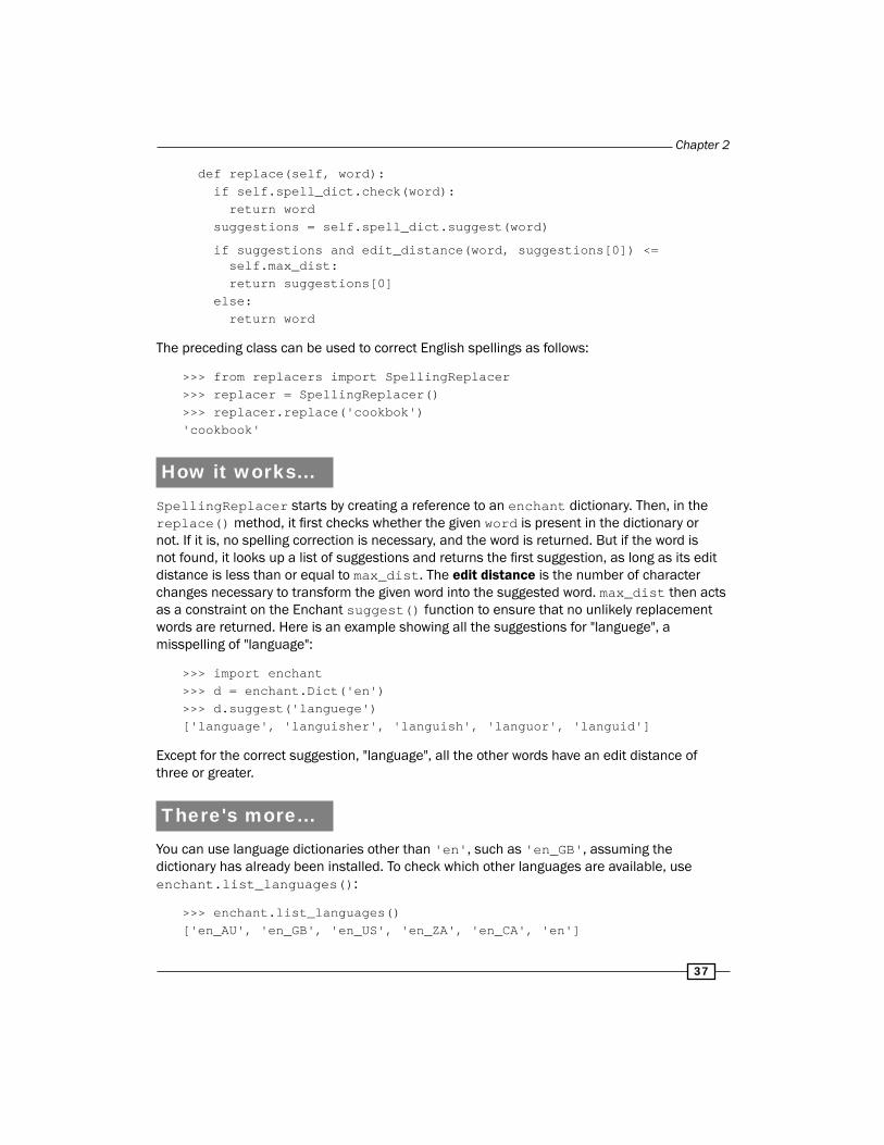
def replace(self, word): if self.spell_dict.check(word): return word suggestions = self.spell_dict.suggest(word)

if suggestions and edit_distance(word, suggestions[0]) <= self.max_dist: return suggestions[0] else: return word

The preceding class can be used to correct English spellings as follows:

>>> from replacers import SpellingReplacer>>> replacer = SpellingReplacer()>>> replacer.replace('cookbok')'cookbook'

How it works...SpellingReplacer starts by creating a reference to an enchant dictionary. Then, in the replace() method, it first checks whether the given word is present in the dictionary or not. If it is, no spelling correction is necessary, and the word is returned. But if the word is not found, it looks up a list of suggestions and returns the first suggestion, as long as its edit distance is less than or equal to max_dist. The edit distance is the number of character changes necessary to transform the given word into the suggested word. max_dist then acts as a constraint on the Enchant suggest() function to ensure that no unlikely replacement words are returned. Here is an example showing all the suggestions for "languege", a misspelling of "language":

>>> import enchant>>> d = enchant.Dict('en')>>> d.suggest('languege')['language', 'languisher', 'languish', 'languor', 'languid']

Except for the correct suggestion, "language", all the other words have an edit distance of three or greater.

There's more...You can use language dictionaries other than 'en', such as 'en_GB', assuming the dictionary has already been installed. To check which other languages are available, use enchant.list_languages():

>>> enchant.list_languages()['en_AU', 'en_GB', 'en_US', 'en_ZA', 'en_CA', 'en']


38

If you try to use a dictionary that doesn't exist, you will get enchant.DictNotFoundError. You can first check whether the dictionary exists using enchant.dict_exists(), which will return True if the named dictionary exists, or False otherwise.

en_GB dictionaryAlways be sure to use the correct dictionary for whichever language you are doing spelling correction on. 'en_US' can give you different results than 'en_GB', such as for the word "theater". "Theater" is the American English spelling, whereas the British English spelling is "Theatre":

>>> import enchant>>> dUS = enchant.Dict('en_US')>>> dUS.check('theater')True>>> dGB = enchant.Dict('en_GB')>>> dGB.check('theater')False>>> from replacers import SpellingReplacer>>> us_replacer = SpellingReplacer('en_US')>>> us_replacer.replace('theater')'theater'>>> gb_replacer = SpellingReplacer('en_GB')>>> gb_replacer.replace('theater')'theatre'

Personal word listsEnchant also supports personal word lists. These can be combined with an existing dictionary, allowing you to augment the dictionary with your own words. So let us say you had a file named mywords.txt that had nltk on one line. You could then create a dictionary augmented with your personal word list as follows:

>>> d = enchant.Dict('en_US')>>> d.check('nltk')False>>> d = enchant.DictWithPWL('en_US', 'mywords.txt')>>> d.check('nltk')True

Chapter 2

39

To use an augmented dictionary with our SpellingReplacer, we can create a subclass in replacers.py that takes an existing spelling dictionary.

class CustomSpellingReplacer(SpellingReplacer): def __init__(self, spell_dict, max_dist=2): self.spell_dict = spell_dict self.max_dist = max_dist

This CustomSpellingReplacer will not replace any words that you put into mywords.txt.

>>> from replacers import CustomSpellingReplacer>>> d = enchant.DictWithPWL('en_US', 'mywords.txt')>>> replacer = CustomSpellingReplacer(d)>>> replacer.replace('nltk')'nltk'

See alsoThe previous recipe covered an extreme form of spelling correction by replacing repeating characters. You could also do spelling correction by simple word replacement as discussed in the next recipe.

Replacing synonymsIt is often useful to reduce the vocabulary of a text by replacing words with common synonyms. By compressing the vocabulary without losing meaning, you can save memory in cases such as frequency analysis and text indexing. Vocabulary reduction can also increase the occurrence of significant collocations, which was covered in the Discovering word collocations recipe of Chapter 1, Tokenizing Text and WordNet Basics.

Getting readyYou will need to have a defined mapping of a word to its synonym. This is a simple controlled vocabulary. We will start by hardcoding the synonyms as a Python dictionary, then explore other options for storing synonym maps.

How to do it...We'll first create a WordReplacer class in replacers.py that takes a word replacement mapping:

class WordReplacer(object): def __init__(self, word_map): self.word_map = word_map def replace(self, word): return self.word_map.get(word, word)


40

Then we can demonstrate its usage for simple word replacement:

>>> from replacers import wordReplacer>>> replacer = WordReplacer({'bday': 'birthday'})>>> replacer.replace('bday')'birthday'>>> replacer.replace('happy')'happy'

How it works...WordReplacer is simply a class wrapper around a Python dictionary. The replace() method looks up the given word in its word_map and returns the replacement synonym if it exists. Otherwise, the given word is returned as is.

If you were only using the word_map dictionary, you would have no need for the WordReplacer class, and could instead call word_map.get() directly. But WordReplacer can act as a base class for other classes that construct the word_map from various file formats. Read on for more information.

There's more...Hardcoding synonyms as a Python dictionary is not a good long-term solution. Two better alternatives are to store the synonyms in a CSV file or in a YAML file. Choose whichever format is easiest for whoever will be maintaining your synonym vocabulary. Both of the classes outlined in the following section inherit the replace() method from WordReplacer.

CSV synonym replacementThe CsvWordReplacer class extends WordReplacer in replacers.py in order to construct the word_map from a CSV file:

import csv

class CsvWordReplacer(WordReplacer): def __init__(self, fname): word_map = {} for line in csv.reader(open(fname)): word, syn = line word_map[word] = syn super(CsvWordReplacer, self).__init__(word_map)

Chapter 2

41

Your CSV file should be two columns, where the first column is the word, and the second column is the synonym meant to replace it. If this file is called synonyms.csv and the first line is bday, birthday, then you can do:

>>> from replacers import CsvWordReplacer>>> replacer = CsvWordReplacer('synonyms.csv')>>> replacer.replace('bday')'birthday'>>> replacer.replace('happy')'happy'

YAML synonym replacementIf you have PyYAML installed, you can create a YamlWordReplacer in replacers.py. Download and installation instructions for PyYAML are located at http://pyyaml.org/wiki/PyYAML.

import yaml

class YamlWordReplacer(WordReplacer): def __init__(self, fname): word_map = yaml.load(open(fname)) super(YamlWordReplacer, self).__init__(word_map)

Your YAML file should be a simple mapping of "word: synonym", such as bday: birthday. Note that the YAML syntax is very particular, and the space after the colon is required. If the file is named synonyms.yaml, you can do:

>>> from replacers import YamlWordReplacer>>> replacer = YamlWordReplacer('synonyms.yaml')>>> replacer.replace('bday')'birthday'>>> replacer.replace('happy')'happy'

See alsoYou can use the WordReplacer to do any kind of word replacement, even spelling correction for more complicated words that can't be automatically corrected, as we did in the previous recipe. In the next recipe, we will cover antonym replacement.

Replacing negations with antonymsThe opposite of synonym replacement is antonym replacement. An antonym is the opposite meaning of a word. This time, instead of creating custom word mappings, we can use WordNet to replace words with unambiguous antonyms. Refer to the Looking up lemmas and synonyms in WordNet recipe in Chapter 1, Tokenizing Text and WordNet Basics for more details on antonym lookups.


42

How to do it...Let us say you have a sentence such as "let's not uglify our code". With antonym replacement, you can replace "not uglify" with "beautify", resulting in the sentence "let's beautify our code". To do this, we will need to create an AntonymReplacer in replacers.py as follows:

from nltk.corpus import wordnetclass AntonymReplacer(object): def replace(self, word, pos=None): antonyms = set() for syn in wordnet.synsets(word, pos=pos): for lemma in syn.lemmas: for antonym in lemma.antonyms(): antonyms.add(antonym.name) if len(antonyms) == 1: return antonyms.pop() else: return None

def replace_negations(self, sent): i, l = 0, len(sent) words = [] while i < l: word = sent[i] if word == 'not' and i+1 < l: ant = self.replace(sent[i+1]) if ant: words.append(ant) i += 2 continue words.append(word) i += 1 return words

Now we can tokenize the original sentence into ["let's", 'not', 'uglify', 'our', 'code'], and pass this to the replace_negations() function. Here are some examples:

>>> from replacers import AntonymReplacer>>> replacer = AntonymReplacer()>>> replacer.replace('good')>>> replacer.replace('uglify')'beautify'>>> sent = ["let's", 'not', 'uglify', 'our', 'code']>>> replacer.replace_negations(sent)["let's", 'beautify', 'our', 'code']

Chapter 2

43

How it works...The AntonymReplacer has two methods: replace() and replace_negations(). The replace() method takes a single word and an optional part of speech tag, then looks up the synsets for the word in WordNet. Going through all the synsets and every lemma of each synset, it creates a set of all antonyms found. If only one antonym is found, then it is an unambiguous replacement. If there is more than one antonym found, which can happen quite often, then we don't know for sure which antonym is correct. In the case of multiple antonyms (or no antonyms), replace() returns None since it cannot make a decision.

In replace_negations(), we look through a tokenized sentence for the word "not". If "not" is found, then we try to find an antonym for the next word using replace(). If we find an antonym, then it is appended to the list of words, replacing "not" and the original word. All other words are appended as it is, resulting in a tokenized sentence with unambiguous negations replaced by their antonyms.

There's more...Since unambiguous antonyms aren't very common in WordNet, you may want to create a custom antonym mapping the same way we did for synonyms. This AntonymWordReplacer could be constructed by inheriting from both WordReplacer and AntonymReplacer:

class AntonymWordReplacer(WordReplacer, AntonymReplacer): pass

The order of inheritance is very important, as we want the initialization and replace() function of WordReplacer combined with the replace_negations() function from AntonymReplacer. The result is a replacer that can do the following:

>>> from replacers import AntonymWordReplacer>>> replacer = AntonymWordReplacer({'evil': 'good'})>>> replacer.replace_negations(['good', 'is', 'not', 'evil'])['good', 'is', 'good']

Of course, you could also inherit from CsvWordReplacer or YamlWordReplacer instead of WordReplacer if you want to load the antonym word mappings from a file.

See alsoThe previous recipe covers the WordReplacer from the perspective of synonym replacement. And in Chapter 1, Tokenizing Text and WordNet Basics Wordnet usage is covered in detail in the Looking up synsets for a word in Wordnet and Looking up lemmas and synonyms in Wordnet recipes.

3Creating Custom

Corpora


f Setting up a custom corpus

f Creating a word list corpus

f Creating a part-of-speech tagged word corpus

f Creating a chunked phrase corpus

f Creating a categorized text corpus

f Creating a categorized chunk corpus reader

f Lazy corpus loading

f Creating a custom corpus view

f Creating a MongoDB backed corpus reader

f Corpus editing with file locking

IntroductionIn this chapter, we'll cover how to use corpus readers and create custom corpora. At the same time, you'll learn how to use the existing corpus data that comes with NLTK. This information is essential for future chapters when we'll need to access the corpora as training data. We'll also cover creating custom corpus readers, which can be used when your corpus is not in a file format that NLTK already recognizes, or if your corpus is not in files at all, but instead is located in a database such as MongoDB.

Creating Custom Corpora

46

Setting up a custom corpusA corpus is a collection of text documents, and corpora is the plural of corpus. So a custom corpus is really just a bunch of text files in a directory, often alongside many other directories of text files.

Getting readyYou should already have the NLTK data package installed, following the instructions at http://www.nltk.org/data. We'll assume that the data is installed to C:\nltk_data on Windows, and /usr/share/nltk_data on Linux, Unix, or Mac OS X.

How to do it...NLTK defines a list of data directories, or paths, in nltk.data.path. Our custom corpora must be within one of these paths so it can be found by NLTK. So as not to conflict with the official data package, we'll create a custom nltk_data directory in our home directory. Here's some Python code to create this directory and verify that it is in the list of known paths specified by nltk.data.path:

>>> import os, os.path>>> path = os.path.expanduser('~/nltk_data')>>> if not os.path.exists(path):... os.mkdir(path)>>> os.path.exists(path)True>>> import nltk.data>>> path in nltk.data.pathTrue

If the last line, path in nltk.data.path, is True, then you should now have a nltk_data directory in your home directory. The path should be %UserProfile%\nltk_data on Windows, or ~/nltk_data on Unix, Linux, or Mac OS X. For simplicity, I'll refer to the directory as ~/nltk_data.

If the last line does not return True, try creating the nltk_data directory manually in your home directory, then verify that the absolute path is in nltk.data.path. It's essential to ensure that this directory exists and is in nltk.data.path before continuing. Once you have your nltk_data directory, the convention is that corpora reside in a corpora subdirectory. Create this corpora directory within the nltk_data directory, so that the path is ~/nltk_data/corpora. Finally, we'll create a subdirectory in corpora to hold our custom corpus. Let's call it cookbook, giving us the full path of ~/nltk_data/corpora/cookbook.

Chapter 3

47

Now we can create a simple word list file and make sure it loads. In Chapter 2, Replacing and Correcting Words, Spelling correction with Enchant recipe, we created a word list file called mywords.txt. Put this file into ~/nltk_data/corpora/cookbook/. Now we can use nltk.data.load() to load the file.

>>> import nltk.data>>> nltk.data.load('corpora/cookbook/mywords.txt', format='raw')'nltk\n'

We need to specify format='raw' since nltk.data.load() doesn't know how to interpret .txt files. As we'll see, it does know how to interpret a number of other file formats.

How it works...The nltk.data.load() function recognizes a number of formats, such as 'raw', 'pickle', and 'yaml'. If no format is specified, then it tries to guess the format based on the file's extension. In the previous case, we have a .txt file, which is not a recognized extension, so we have to specify the 'raw' format. But if we used a file that ended in .yaml, then we would not need to specify the format.

Filenames passed in to nltk.data.load() can be absolute or relative paths. Relative paths must be relative to one of the paths specified in nltk.data.path. The file is found using nltk.data.find(path), which searches all known paths combined with the relative path. Absolute paths do not require a search, and are used as is.

There's more...For most corpora access, you won't actually need to use nltk.data.load, as that will be handled by the CorpusReader classes covered in the following recipes. But it's a good function to be familiar with for loading .pickle files and .yaml files, plus it introduces the idea of putting all of your data files into a path known by NLTK.

Loading a YAML fileIf you put the synonyms.yaml file from the Chapter 2, Replacing and Correcting Words, Replacing synonyms recipe, into ~/nltk_data/corpora/cookbook (next to mywords.txt), you can use nltk.data.load() to load it without specifying a format.

>>> import nltk.data>>> nltk.data.load('corpora/cookbook/synonyms.yaml'){'bday': 'birthday'}

This assumes that PyYAML is installed. If not, you can find download and installation instructions at http://pyyaml.org/wiki/PyYAML.


48

See alsoIn the next recipes, we'll cover various corpus readers, and then in the Lazy corpus loading recipe, we'll use the LazyCorpusLoader, which expects corpus data to be in a corpora subdirectory of one of the paths specified by nltk.data.path.

Creating a word list corpusThe WordListCorpusReader is one of the simplest CorpusReader classes. It provides access to a file containing a list of words, one word per line. In fact, you've already used it when we used the stopwords corpus in the Filtering stopwords in a tokenized sentence and Discovering word collocations recipes in Chapter 1, Tokenizing Text and WordNet Basics.

Getting readyWe need to start by creating a word list file. This could be a single column CSV file, or just a normal text file with one word per line. Let's create a file named wordlist that looks like this:

nltkcorpuscorporawordnet

How to do it...Now we can instantiate a WordListCorpusReader that will produce a list of words from our file. It takes two arguments: the directory path containing the files, and a list of filenames. If you open the Python console in the same directory as the files, then '.' can be used as the directory path. Otherwise, you must use a directory path such as: 'nltk_data/corpora/cookbook'.

>>> from nltk.corpus.reader import WordListCorpusReader>>> reader = WordListCorpusReader('.', ['wordlist'])>>> reader.words()['nltk', 'corpus', 'corpora', 'wordnet']>>> reader.fileids()['wordlist']

Chapter 3

49

How it works...WordListCorpusReader inherits from CorpusReader, which is a common base class for all corpus readers. CorpusReader does all the work of identifying which files to read, while WordListCorpus reads the files and tokenizes each line to produce a list of words. Here's an inheritance diagram:

When you call the words() function, it calls nltk.tokenize.line_tokenize() on the raw file data, which you can access using the raw() function.

>>> reader.raw()'nltk\ncorpus\ncorpora\nwordnet\n'>>> from nltk.tokenize import line_tokenize>>> line_tokenize(reader.raw())['nltk', 'corpus', 'corpora', 'wordnet']

There's more...The stopwords corpus is a good example of a multi-file WordListCorpusReader. In Chapter 1, Tokenizing Text and WordNet Basics, in the Filtering stopwords in a tokenized sentence recipe, we saw that it had one word list file for each language, and you could access the words for that language by calling stopwords.words(fileid). If you want to create your own multi-file word list corpus, this is a great example to follow.

Names corpusAnother word list corpus that comes with NLTK is the names corpus. It contains two files: female.txt and male.txt, each containing a list of a few thousand common first names organized by gender.

>>> from nltk.corpus import names>>> names.fileids()['female.txt', 'male.txt']>>> len(names.words('female.txt'))5001


50

>>> len(names.words('male.txt'))2943

English wordsNLTK also comes with a large list of English words. There's one file with 850 basic words, and another list with over 200,000 known English words.

>>> from nltk.corpus import words>>> words.fileids()['en', 'en-basic']>>> len(words.words('en-basic'))850>>> len(words.words('en'))234936

See also

In Chapter 1, Tokenizing Text and WordNet Basics, the Filtering stopwords in a tokenized sentence recipe, has more details on using the stopwords corpus. In the following recipes, we'll cover more advanced corpus file formats and corpus reader classes.

Creating a part-of-speech tagged word corpus

Part-of-speech tagging is the process of identifying the part-of-speech tag for a word. Most of the time, a tagger must first be trained on a training corpus. How to train and use a tagger is covered in detail in Chapter 4, Part-of-Speech Tagging, but first we must know how to create and use a training corpus of part-of-speech tagged words.

Getting readyThe simplest format for a tagged corpus is of the form "word/tag". Following is an excerpt from the brown corpus:

The/at-tl expense/nn and/cc time/nn involved/vbn are/ber astronomical/jj ./.

Each word has a tag denoting its part-of-speech. For example, nn refers to a noun, while a tag that starts with vb is a verb.

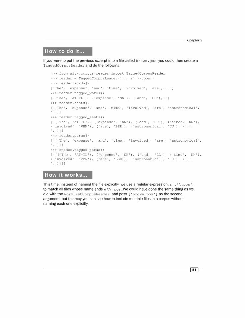
Chapter 3

51

How to do it...If you were to put the previous excerpt into a file called brown.pos, you could then create a TaggedCorpusReader and do the following:

>>> from nltk.corpus.reader import TaggedCorpusReader>>> reader = TaggedCorpusReader('.', r'.*\.pos')>>> reader.words()['The', 'expense', 'and', 'time', 'involved', 'are', ...]>>> reader.tagged_words()[('The', 'AT-TL'), ('expense', 'NN'), ('and', 'CC'), …]>>> reader.sents()[['The', 'expense', 'and', 'time', 'involved', 'are', 'astronomical', '.']]>>> reader.tagged_sents()[[('The', 'AT-TL'), ('expense', 'NN'), ('and', 'CC'), ('time', 'NN'), ('involved', 'VBN'), ('are', 'BER'), ('astronomical', 'JJ'), ('.', '.')]]>>> reader.paras()[[['The', 'expense', 'and', 'time', 'involved', 'are', 'astronomical', '.']]]>>> reader.tagged_paras()[[[('The', 'AT-TL'), ('expense', 'NN'), ('and', 'CC'), ('time', 'NN'), ('involved', 'VBN'), ('are', 'BER'), ('astronomical', 'JJ'), ('.', '.')]]]

How it works...This time, instead of naming the file explicitly, we use a regular expression, r'.*\.pos', to match all files whose name ends with .pos. We could have done the same thing as we did with the WordListCorpusReader, and pass ['brown.pos'] as the second argument, but this way you can see how to include multiple files in a corpus without naming each one explicitly.


52

TaggedCorpusReader provides a number of methods for extracting text from a corpus. First, you can get a list of all words, or a list of tagged tokens. A tagged token is simply a tuple of (word, tag). Next, you can get a list of every sentence, and also every tagged sentence, where the sentence is itself a list of words or tagged tokens. Finally, you can get a list of paragraphs, where each paragraph is a list of sentences, and each sentence is a list of words or tagged tokens. Here's an inheritance diagram listing all the major methods:

There's more...The functions demonstrated in the previous diagram all depend on tokenizers for splitting the text. TaggedCorpusReader tries to have good defaults, but you can customize them by passing in your own tokenizers at initialization time.

Customizing the word tokenizerThe default word tokenizer is an instance of nltk.tokenize.WhitespaceTokenizer. If you want to use a different tokenizer, you can pass that in as word_tokenizer.

>>> from nltk.tokenize import SpaceTokenizer>>> reader = TaggedCorpusReader('.', r'.*\.pos', word_tokenizer=SpaceTokenizer())>>> reader.words()['The', 'expense', 'and', 'time', 'involved', 'are', ...]

Chapter 3

53

Customizing the sentence tokenizerThe default sentence tokenizer is an instance of nltk.tokenize.RegexpTokenize with '\n' to identify the gaps. It assumes that each sentence is on a line all by itself, and individual sentences do not have line breaks. To customize this, you can pass in your own tokenizer as sent_tokenizer.

>>> from nltk.tokenize import LineTokenizer>>> reader = TaggedCorpusReader('.', r'.*\.pos', sent_tokenizer=LineTokenizer())>>> reader.sents()[['The', 'expense', 'and', 'time', 'involved', 'are', 'astronomical', '.']]

Customizing the paragraph block readerParagraphs are assumed to be split by blank lines. This is done with the default para_block_reader, which is nltk.corpus.reader.util.read_blankline_block. There are a number of other block reader functions in nltk.corpus.reader.util, whose purpose is to read blocks of text from a stream. Their usage will be covered in more detail in the later recipe, Creating a custom corpus view, where we'll create a custom corpus reader.

Customizing the tag separatorIf you don't want to use '/' as the word/tag separator, you can pass an alternative string to TaggedCorpusReader for sep. The default is sep='/', but if you want to split words and tags with '|', such as 'word|tag', then you should pass in sep='|'.

Simplifying tags with a tag mapping functionIf you'd like to somehow transform the part-of-speech tags, you can pass in a tag_mapping_function at initialization, then call one of the tagged_* functions with simplify_tags=True. Here's an example where we lowercase each tag:

>>> reader = TaggedCorpusReader('.', r'.*\.pos', tag_mapping_function=lambda t: t.lower())>>> reader.tagged_words(simplify_tags=True)[('The', 'at-tl'), ('expense', 'nn'), ('and', 'cc'), …]

Calling tagged_words() without simplify_tags=True would produce the same result as if you did not pass in a tag_mapping_function.

There are also a number of tag simplification functions defined in nltk.tag.simplify. These can be useful for reducing the number of different part-of-speech tags.

>>> from nltk.tag import simplify>>> reader = TaggedCorpusReader('.', r'.*\.pos', tag_mapping_function=simplify.simplify_brown_tag)>>> reader.tagged_words(simplify_tags=True)


54

[('The', 'DET'), ('expense', 'N'), ('and', 'CNJ'), ...]>>> reader = TaggedCorpusReader('.', r'.*\.pos', tag_mapping_function=simplify.simplify_tag)>>> reader.tagged_words(simplify_tags=True)[('The', 'A'), ('expense', 'N'), ('and', 'C'), ...]

See also

Chapter 4, Part-of-Speech Tagging will cover part-of-speech tags and tagging in much more detail. And for more on tokenizers, see the first three recipes of Chapter 1, Tokenizing Text and WordNet Basics.

In the next recipe, we'll create a chunked phrase corpus, where each phrase is also part-of-speech tagged.

Creating a chunked phrase corpusA chunk is a short phrase within a sentence. If you remember sentence diagrams from grade school, they were a tree-like representation of phrases within a sentence. This is exactly what chunks are: sub-trees within a sentence tree, and they will be covered in much more detail in Chapter 5, Extracting Chunks. Following is a sample sentence tree with three noun phrase (NP) chunks shown as sub-trees.

This recipe will cover how to create a corpus with sentences that contain chunks.

Getting readyHere is an excerpt from the tagged treebank corpus. It has part-of-speech tags, as in the previous recipe, but it also has square brackets for denoting chunks. This is the same sentence as in the previous tree diagram, but in text form:

[Earlier/JJR staff-reduction/NN moves/NNS] have/VBP trimmed/VBN about/IN [300/CD jobs/NNS] ,/, [the/DT spokesman/NN] said/VBD ./.

In this format, every chunk is a noun phrase. Words that are not within brackets are part of the sentence tree, but are not part of any noun phrase sub-tree.

Chapter 3

55

How to do it...Put this excerpt into a file called treebank.chunk, and then do the following:

>>> from nltk.corpus.reader import ChunkedCorpusReader>>> reader = ChunkedCorpusReader('.', r'.*\.chunk')>>> reader.chunked_words()[Tree('NP', [('Earlier', 'JJR'), ('staff-reduction', 'NN'), ('moves', 'NNS')]), ('have', 'VBP'), ...]>>> reader.chunked_sents()[Tree('S', [Tree('NP', [('Earlier', 'JJR'), ('staff-reduction', 'NN'), ('moves', 'NNS')]), ('have', 'VBP'), ('trimmed', 'VBN'), ('about', 'IN'), Tree('NP', [('300', 'CD'), ('jobs', 'NNS')]), (',', ','), Tree('NP', [('the', 'DT'), ('spokesman', 'NN')]), ('said', 'VBD'), ('.', '.')])]>>> reader.chunked_paras()[[Tree('S', [Tree('NP', [('Earlier', 'JJR'), ('staff-reduction', 'NN'), ('moves', 'NNS')]), ('have', 'VBP'), ('trimmed', 'VBN'), ('about', 'IN'), Tree('NP', [('300', 'CD'), ('jobs', 'NNS')]), (',', ','), Tree('NP', [('the', 'DT'), ('spokesman', 'NN')]), ('said', 'VBD'), ('.', '.')])]]

The ChunkedCorpusReader provides the same methods as the TaggedCorpusReader for getting tagged tokens, along with three new methods for getting chunks. Each chunk is represented as an instance of nltk.tree.Tree. Sentence level trees look like Tree('S', [...]) while noun phrase trees look like Tree('NP', [...]). In chunked_sents(), you get a list of sentence trees, with each noun-phrase as a sub-tree of the sentence. In chunked_words(), you get a list of noun phrase trees alongside tagged tokens of words that were not in a chunk. Here's an inheritance diagram listing the major methods:


56

You can draw a Tree by calling the draw() method. Using the corpus reader defined earlier, you could do reader.chunked_sents()[0].draw() to get the same sentence tree diagram shown at the beginning of this recipe.

How it works...ChunkedCorpusReader is similar to the TaggedCorpusReader from the last recipe. It has the same default sent_tokenizer and para_block_reader, but instead of a word_tokenizer, it uses a str2chunktree() function. The default is nltk.chunk.util.tagstr2tree(), which parses a sentence string containing bracketed chunks into a sentence tree, with each chunk as a noun phrase sub-tree. Words are split by whitespace, and the default word/tag separator is '/'. If you want to customize the chunk parsing, then you can pass in your own function for str2chunktree().

There's more...An alternative format for denoting chunks is called IOB tags. IOB tags are similar to part-of-speech tags, but provide a way to denote the inside, outside, and beginning of a chunk. They also have the benefit of allowing multiple different chunk phrase types, not just noun phrases. Here is an excerpt from the conll2000 corpus. Each word is on its own line with a part-of-speech tag followed by an IOB tag.

Mr. NNP B-NPMeador NNP I-NPhad VBD B-VPbeen VBN I-VPexecutive JJ B-NPvice NN I-NPpresident NN I-NPof IN B-PPBalcor NNP B-NP. . O

B-NP denotes the beginning of a noun phrase, while I-NP denotes that the word is inside of the current noun phrase. B-VP and I-VP denote the beginning and inside of a verb phrase. O ends the sentence.

To read a corpus using the IOB format, you must use the ConllChunkCorpusReader. Each sentence is separated by a blank line, but there is no separation for paragraphs. This means that the para_* methods are not available. If you put the previous IOB example text into a file named conll.iob, you can create and use a ConllChunkCorpusReader with the code we are about to see. The third argument to ConllChunkCorpusReader should be a tuple or list specifying the types of chunks in the file, which in this case is ('NP', 'VP', 'PP').

Chapter 3

57

>>> from nltk.corpus.reader import ConllChunkCorpusReader>>> conllreader = ConllChunkCorpusReader('.', r'.*\.iob', ('NP', 'VP', 'PP'))>>> conllreader.chunked_words()[Tree('NP', [('Mr.', 'NNP'), ('Meador', 'NNP')]), Tree('VP', [('had', 'VBD'), ('been', 'VBN')]), ...]>>> conllreader.chunked_sents()[Tree('S', [Tree('NP', [('Mr.', 'NNP'), ('Meador', 'NNP')]), Tree('VP', [('had', 'VBD'), ('been', 'VBN')]), Tree('NP', [('executive', 'JJ'), ('vice', 'NN'), ('president', 'NN')]), Tree('PP', [('of', 'IN')]), Tree('NP', [('Balcor', 'NNP')]), ('.', '.')])]>>> conllreader.iob_words()[('Mr.', 'NNP', 'B-NP'), ('Meador', 'NNP', 'I-NP'), ...]>>> conllreader.iob_sents()[[('Mr.', 'NNP', 'B-NP'), ('Meador', 'NNP', 'I-NP'), ('had', 'VBD', 'B-VP'), ('been', 'VBN', 'I-VP'), ('executive', 'JJ', 'B-NP'), ('vice', 'NN', 'I-NP'), ('president', 'NN', 'I-NP'), ('of', 'IN', 'B-PP'), ('Balcor', 'NNP', 'B-NP'), ('.', '.', 'O')]]

The previous code also shows the iob_words() and iob_sents() methods, which return lists of three tuples of (word, pos, iob). The inheritance diagram for ConllChunkCorpusReader looks like the following, with most of the methods implemented by its superclass, ConllCorpusReader:


58

Tree leavesWhen it comes to chunk trees, the leaves of a tree are the tagged tokens. So if you want to get a list of all the tagged tokens in a tree, call the leaves() method.

>>> reader.chunked_words()[0].leaves()[('Earlier', 'JJR'), ('staff-reduction', 'NN'), ('moves', 'NNS')]>>> reader.chunked_sents()[0].leaves()[('Earlier', 'JJR'), ('staff-reduction', 'NN'), ('moves', 'NNS'), ('have', 'VBP'), ('trimmed', 'VBN'), ('about', 'IN'), ('300', 'CD'), ('jobs', 'NNS'), (',', ','), ('the', 'DT'), ('spokesman', 'NN'), ('said', 'VBD'), ('.', '.')]>>> reader.chunked_paras()[0][0].leaves()[('Earlier', 'JJR'), ('staff-reduction', 'NN'), ('moves', 'NNS'), ('have', 'VBP'), ('trimmed', 'VBN'), ('about', 'IN'), ('300', 'CD'), ('jobs', 'NNS'), (',', ','), ('the', 'DT'), ('spokesman', 'NN'), ('said', 'VBD'), ('.', '.')]

Treebank chunk corpusThe nltk.corpus.treebank_chunk corpus uses ChunkedCorpusReader to provide part-of-speech tagged words and noun phrase chunks of Wall Street Journal headlines. NLTK comes with a 5% sample from the Penn Treebank Project. You can find out more at http://www.cis.upenn.edu/~treebank/home.html.

CoNLL2000 corpusCoNLL stands for the Conference on Computational Natural Language Learning. For the year 2000 conference, a shared task was undertaken to produce a corpus of chunks based on the Wall Street Journal corpus. In addition to noun phrases (NP), it also contains verb phrases (VP) and prepositional phrases (PP). This chunked corpus is available as nltk.corpus.conll2000, which is an instance of ConllChunkCorpusReader. You can read more at http://www.cnts.ua.ac.be/conll2000/chunking/.

See also

Chapter 5, Extracting Chunks will cover chunk extraction in detail. Also see the previous recipe for details on getting tagged tokens from a corpus reader.

Creating a categorized text corpusIf you have a large corpus of text, you may want to categorize it into separate sections. The brown corpus, for example, has a number of different categories.

>>> from nltk.corpus import brown>>> brown.categories()

Chapter 3

59

['adventure', 'belles_lettres', 'editorial', 'fiction', 'government', 'hobbies', 'humor', 'learned', 'lore', 'mystery', 'news', 'religion', 'reviews', 'romance', 'science_fiction']

In this recipe, we'll learn how to create our own categorized text corpus.

Getting readyThe easiest way to categorize a corpus is to have one file for each category. Following are two excerpts from the movie_reviews corpus:

movie_pos.txt

the thin red line is flawed but it provokes .

movie_neg.txt

a big-budget and glossy production can not make up for a lack of spontaneity that permeates their tv show .

With these two files, we'll have two categories: pos and neg.

How to do it...We'll use the CategorizedPlaintextCorpusReader, which inherits from both PlaintextCorpusReader and CategorizedCorpusReader. These two superclasses require three arguments: the root directory, the fileids, and a category specification.

>>> from nltk.corpus.reader import CategorizedPlaintextCorpusReader>>> reader = CategorizedPlaintextCorpusReader('.', r'movie_.*\.txt', cat_pattern=r'movie_(\w+)\.txt')>>> reader.categories()['neg', 'pos']>>> reader.fileids(categories=['neg'])['movie_neg.txt']>>> reader.fileids(categories=['pos'])['movie_pos.txt']


60

How it works...The first two arguments to CategorizedPlaintextCorpusReader are the root directory and fileids, which are passed on to the PlaintextCorpusReader to read in the files. The cat_pattern keyword argument is a regular expression for extracting the category names from the fileids. In our case, the category is the part of the fileid after movie_ and before .txt. The category must be surrounded by grouping parenthesis.

cat_pattern is passed to CategorizedCorpusReader, which overrides the common corpus reader functions such as fileids(), words(), sents(), and paras() to accept a categories keyword argument. This way, you could get all the pos sentences by calling reader.sents(categories=['pos']). CategorizedCorpusReader also provides the categories() function, which returns a list of all known categories in the corpus.

CategorizedPlaintextCorpusReader is an example of using multiple-inheritance to join methods from multiple superclasses, as shown in the following diagram:

There's more...Instead of cat_pattern, you could pass in a cat_map, which is a dictionary mapping a fileid to a list of category labels.

>>> reader = CategorizedPlaintextCorpusReader('.', r'movie_.*\.txt', cat_map={'movie_pos.txt': ['pos'], 'movie_neg.txt': ['neg']})>>> reader.categories()['neg', 'pos']

Chapter 3

61

Category fileA third way of specifying categories is to use the cat_file keyword argument to specify a filename containing a mapping of fileid to category. For example, the brown corpus has a file called cats.txt that looks like this:

ca44 newscb01 editorial

The reuters corpus has files in multiple categories, and its cats.txt looks like this:

test/14840 rubber coffee lumber palm-oil veg-oiltest/14841 wheat grain

Categorized tagged corpus readerThe brown corpus reader is actually an instance of CategorizedTaggedCorpusReader, which inherits from CategorizedCorpusReader and TaggedCorpusReader. Just like in CategorizedPlaintextCorpusReader, it overrides all the methods of TaggedCorpusReader to allow a categories argument, so you can call brown.tagged_sents(categories=['news']) to get all the tagged sentences from the news category. You can use the CategorizedTaggedCorpusReader just like CategorizedPlaintextCorpusReader for your own categorized and tagged text corpora.

Categorized corporaThe movie_reviews corpus reader is an instance of CategorizedPlaintextCorpusReader, as is the reuters corpus reader. But where the movie_reviews corpus only has two categories (neg and pos), reuters has 90 categories. These corpora are often used for training and evaluating classifiers, which will be covered in Chapter 7, Text Classification.

See alsoIn the next recipe, we'll create a subclass of CategorizedCorpusReader and ChunkedCorpusReader for reading a categorized chunk corpus. Also see Chapter 7, Text Classification in which we use categorized text for classification.

Creating a categorized chunk corpus readerNLTK provides a CategorizedPlaintextCorpusReader and CategorizedTaggedCorpusReader, but there's no categorized corpus reader for chunked corpora. So in this recipe, we're going to make one.


62

Getting readyRefer to the earlier recipe, Creating a chunked phrase corpus, for an explanation of ChunkedCorpusReader, and to the previous recipe for details on CategorizedPlaintextCorpusReader and CategorizedTaggedCorpusReader, both of which inherit from CategorizedCorpusReader.

How to do it...We'll create a class called CategorizedChunkedCorpusReader that inherits from both CategorizedCorpusReader and ChunkedCorpusReader. It is heavily based on the CategorizedTaggedCorpusReader, and also provides three additional methods for getting categorized chunks. The following code is found in catchunked.py:

from nltk.corpus.reader import CategorizedCorpusReader, ChunkedCorpusReader

class CategorizedChunkedCorpusReader(CategorizedCorpusReader, ChunkedCorpusReader): def __init__(self, *args, **kwargs): CategorizedCorpusReader.__init__(self, kwargs) ChunkedCorpusReader.__init__(self, *args, **kwargs)

def _resolve(self, fileids, categories): if fileids is not None and categories is not None: raise ValueError('Specify fileids or categories, not both') if categories is not None: return self.fileids(categories) else: return fileids

All of the following methods call the corresponding function in ChunkedCorpusReader with the value returned from _resolve(). We'll start with the plain text methods.

def raw(self, fileids=None, categories=None): return ChunkedCorpusReader.raw(self, self._resolve(fileids, categories))

def words(self, fileids=None, categories=None): return ChunkedCorpusReader.words(self, self._resolve(fileids, categories))

def sents(self, fileids=None, categories=None): return ChunkedCorpusReader.sents(self, self._resolve(fileids, categories))

def paras(self, fileids=None, categories=None):

Chapter 3

63

return ChunkedCorpusReader.paras(self, self._resolve(fileids, categories))

Next comes the tagged text methods.

def tagged_words(self, fileids=None, categories=None, simplify_tags=False): return ChunkedCorpusReader.tagged_words( self, self._resolve(fileids, categories), simplify_tags) def tagged_sents(self, fileids=None, categories=None, simplify_tags=False): return ChunkedCorpusReader.tagged_sents( self, self._resolve(fileids, categories), simplify_tags) def tagged_paras(self, fileids=None, categories=None, simplify_tags=False): return ChunkedCorpusReader.tagged_paras( self, self._resolve(fileids, categories), simplify_tags)

And finally, the chunked methods, which is what we've really been after.

def chunked_words(self, fileids=None, categories=None): return ChunkedCorpusReader.chunked_words( self, self._resolve(fileids, categories)) def chunked_sents(self, fileids=None, categories=None): return ChunkedCorpusReader.chunked_sents( self, self._resolve(fileids, categories)) def chunked_paras(self, fileids=None, categories=None): return ChunkedCorpusReader.chunked_paras( self, self._resolve(fileids, categories))

All these methods together give us a complete CategorizedChunkedCorpusReader.


64

How it works...CategorizedChunkedCorpusReader overrides all the ChunkedCorpusReader methods to take a categories argument for locating fileids. These fileids are found with the internal _resolve() function. This _resolve() function makes use of CategorizedCorpusReader.fileids() to return fileids for a given list of categories. If no categories are given, _resolve() just returns the given fileids, which could be None, in which case all files are read. The initialization of both CategorizedCorpusReader and ChunkedCorpusReader is what makes this all possible. If you look at the code for CategorizedTaggedCorpusReader, you'll see it's very similar. The inheritance diagram looks like this:

Here's some example code for using the treebank corpus. All we're doing is making categories out of the fileids, but the point is that you could use the same techniques to create your own categorized chunk corpus.

>>> import nltk.data>>> from catchunked import CategorizedChunkedCorpusReader>>> path = nltk.data.find('corpora/treebank/tagged')>>> reader = CategorizedChunkedCorpusReader(path, r'wsj_.*\.pos', cat_pattern=r'wsj_(.*)\.pos')>>> len(reader.categories()) == len(reader.fileids())True>>> len(reader.chunked_sents(categories=['0001']))16

Chapter 3

65

We use nltk.data.find() to search the data directories to get a FileSystemPathPointer to the treebank corpus. All the treebank tagged files start with wsj_ followed by a number, and end with .pos. The previous code turns that file number into a category.

There's more...As covered in the Creating a chunked phrase corpus recipe, there's an alternative format and reader for a chunk corpus using IOB tags. To have a categorized corpus of IOB chunks, we have to make a new corpus reader.

Categorized Conll chunk corpus readerHere's a subclass of CategorizedCorpusReader and ConllChunkReader called CategorizedConllChunkCorpusReader. It overrides all methods of ConllCorpusReader that take a fileids argument, so the methods can also take a categories argument. The ConllChunkCorpusReader is just a small subclass of ConllCorpusReader that handles initialization; most of the work is done in ConllCorpusReader. This code can also be found in catchunked.py.

from nltk.corpus.reader import CategorizedCorpusReader, ConllCorpusReader, ConllChunkCorpusReader

class CategorizedConllChunkCorpusReader(CategorizedCorpusReader, ConllChunkCorpusReader): def __init__(self, *args, **kwargs): CategorizedCorpusReader.__init__(self, kwargs) ConllChunkCorpusReader.__init__(self, *args, **kwargs) def _resolve(self, fileids, categories): if fileids is not None and categories is not None: raise ValueError('Specify fileids or categories, not both') if categories is not None: return self.fileids(categories) else: return fileids

All the following methods call the corresponding method of ConllCorpusReader with the value returned from _resolve(). We'll start with the plain text methods.

def raw(self, fileids=None, categories=None): return ConllCorpusReader.raw(self, self._resolve(fileids, categories)) def words(self, fileids=None, categories=None):


66

return ConllCorpusReader.words(self, self._resolve(fileids, categories)) def sents(self, fileids=None, categories=None): return ConllCorpusReader.sents(self, self._resolve(fileids, categories))

The ConllCorpusReader does not recognize paragraphs, so there are no *_paras() methods. Next are the tagged and chunked methods.

def tagged_words(self, fileids=None, categories=None): return ConllCorpusReader.tagged_words(self, self._resolve(fileids, categories)) def tagged_sents(self, fileids=None, categories=None): return ConllCorpusReader.tagged_sents(self, self._resolve(fileids, categories)) def chunked_words(self, fileids=None, categories=None, chunk_types=None): return ConllCorpusReader.chunked_words( self, self._resolve(fileids, categories), chunk_types) def chunked_sents(self, fileids=None, categories=None, chunk_types=None): return ConllCorpusReader.chunked_sents( self, self._resolve(fileids, categories), chunk_types)

For completeness, we must override the following methods of the ConllCorpusReader:

def parsed_sents(self, fileids=None, categories=None, pos_in_tree=None): return ConllCorpusReader.parsed_sents( self, self._resolve(fileids, categories), pos_in_tree) def srl_spans(self, fileids=None, categories=None): return ConllCorpusReader.srl_spans(self, self._resolve(fileids, categories)) def srl_instances(self, fileids=None, categories=None, pos_in_tree=None, flatten=True): return ConllCorpusReader.srl_instances( self, self._resolve(fileids, categories), pos_in_tree, flatten)

Chapter 3

67

def iob_words(self, fileids=None, categories=None): return ConllCorpusReader.iob_words(self, self._resolve(fileids, categories)) def iob_sents(self, fileids=None, categories=None): return ConllCorpusReader.iob_sents(self, self._resolve(fileids, categories))

The inheritance diagram for this class is as follows:

Following is some example code using the conll2000 corpus. Like with treebank, we're using the fileids for categories. The ConllChunkCorpusReader requires a third argument to specify the chunk_types. These chunk_types are used to parse the IOB tags. As you learned in the Creating a chunked phrase corpus recipe, the conll2000 corpus recognizes three chunk types:

f NP for noun phrases

f VP for verb phrases

f PP for prepositional phrases

>>> import nltk.data>>> from catchunked import CategorizedConllChunkCorpusReader


68

>>> path = nltk.data.find('corpora/conll2000')>>> reader = CategorizedConllChunkCorpusReader(path, r'.*\.txt', ('NP','VP','PP'), cat_pattern=r'(.*)\.txt')>>> reader.categories()['test', 'train']>>> reader.fileids()['test.txt', 'train.txt']>>> len(reader.chunked_sents(categories=['test']))2012

See alsoIn the Creating a chunked phrase corpus recipe in this chapter, we covered both the ChunkedCorpusReader and ConllChunkCorpusReader. And in the previous recipe, we covered CategorizedPlaintextCorpusReader and CategorizedTaggedCorpusReader, which share the same superclass used by CategorizedChunkedCorpusReader and CategorizedConllChunkReader—CategorizedCorpusReader.

Lazy corpus loadingLoading a corpus reader can be an expensive operation due to the number of files, file sizes, and various initialization tasks. And while you'll often want to specify a corpus reader in a common module, you don't always need to access it right away. To speed up module import time when a corpus reader is defined, NLTK provides a LazyCorpusLoader class that can transform itself into your actual corpus reader as soon as you need it. This way, you can define a corpus reader in a common module without it slowing down module loading.

How to do it...LazyCorpusLoader requires two arguments: the name of the corpus and the corpus reader class, plus any other arguments needed to initialize the corpus reader class.

The name argument specifies the root directory name of the corpus, which must be within a corpora subdirectory of one of the paths in nltk.data.path. See the first recipe of this chapter, Setting up a custom corpus, for more details on nltk.data.path.

For example, if you have a custom corpora named cookbook in your local nltk_data directory, its path would be ~/nltk_data/corpora/cookbook. You'd then pass 'cookbook' to LazyCorpusLoader as the name, and LazyCorpusLoader will look in ~/nltk_data/corpora for a directory named 'cookbook'.

Chapter 3

69

The second argument to LazyCorpusLoader is reader_cls, which should be the name of a subclass of CorpusReader, such as WordListCorpusReader. You will also need to pass in any other arguments required by the reader_cls for initialization. This will be demonstrated as follows, using the same wordlist file we created in the earlier recipe, Creating a word list corpus. The third argument to LazyCorpusLoader is the list of filenames and fileids that will be passed in to WordListCorpusReader at initialization.

>>> from nltk.corpus.util import LazyCorpusLoader>>> from nltk.corpus.reader import WordListCorpusReader>>> reader = LazyCorpusLoader('cookbook', WordListCorpusReader, ['wordlist'])>>> isinstance(reader, LazyCorpusLoader)True>>> reader.fileids()['wordlist']>>> isinstance(reader, LazyCorpusLoader)False>>> isinstance(reader, WordListCorpusReader)True

How it works...LazyCorpusLoader stores all the arguments given, but otherwise does nothing until you try to access an attribute or method. This way initialization is very fast, eliminating the overhead of loading the corpus reader immediately. As soon as you do access an attribute or method, it does the following:

1. Calls nltk.data.find('corpora/%s' % name) to find the corpus data root directory.

2. Instantiate the corpus reader class with the root directory and any other arguments.

3. Transforms itself into the corpus reader class.

So in the previous example code, before we call reader.fileids(), reader is an instance of LazyCorpusLoader, but after the call, reader is an instance of WordListCorpusReader.

There's more...All of the corpora included with NLTK and defined in nltk.corpus are initially an instance of LazyCorpusLoader. Here's some code from nltk.corpus defining the treebank corpora.

treebank = LazyCorpusLoader(

'treebank/combined', BracketParseCorpusReader, r'wsj_.*\.mrg',


70

tag_mapping_function=simplify_wsj_tag)

treebank_chunk = LazyCorpusLoader(

'treebank/tagged', ChunkedCorpusReader, r'wsj_.*\.pos',

sent_tokenizer=RegexpTokenizer(r'(?<=/\.)\s*(?![^\[]*\])', gaps=True),

para_block_reader=tagged_treebank_para_block_reader)

treebank_raw = LazyCorpusLoader(

'treebank/raw', PlaintextCorpusReader, r'wsj_.*')

As you can see, any number of additional arguments can be passed through by LazyCorpusLoader to its reader_cls.

Creating a custom corpus viewA corpus view is a class wrapper around a corpus file that reads in blocks of tokens as needed. Its purpose is to provide a view into a file without reading the whole file at once (since corpus files can often be quite large). If the corpus readers included by NLTK already meet all your needs, then you do not have to know anything about corpus views. But, if you have a custom file format that needs special handling, this recipe will show you how to create and use a custom corpus view. The main corpus view class is StreamBackedCorpusView, which opens a single file as a stream, and maintains an internal cache of blocks it has read.

Blocks of tokens are read in with a block reader function. A block can be any piece of text, such as a paragraph or a line, and tokens are parts of a block, such as individual words. In the Creating a part-of-speech tagged word corpus recipe, we discussed the default para_block_reader function of the TaggedCorpusReader, which reads lines from a file until it finds a blank line, then returns those lines as a single paragraph token. The actual block reader function is: nltk.corpus.reader.util.read_blankline_block. TaggedCorpusReader passes this block reader function into a TaggedCorpusView whenever it needs to read blocks from a file. TaggedCorpusView is a subclass of StreamBackedCorpusView that knows to split paragraphs of "word/tag" into (word, tag) tuples.

How to do it...We'll start with the simple case of a plain text file with a heading that should be ignored by the corpus reader. Let's make a file called heading_text.txt that looks like this:

A simple heading

Here is the actual text for the corpus.

Paragraphs are split by blanklines.

This is the 3rd paragraph.

Chapter 3

71

Normally we'd use the PlaintextCorpusReader but, by default, it will treat A simple heading as the first paragraph. To ignore this heading, we need to subclass the PlaintextCorpusReader so we can override its CorpusView class variable with our own StreamBackedCorpusView subclass. This code is found in corpus.py.

from nltk.corpus.reader import PlaintextCorpusReaderfrom nltk.corpus.reader.util import StreamBackedCorpusView

class IgnoreHeadingCorpusView(StreamBackedCorpusView): def __init__(self, *args, **kwargs): StreamBackedCorpusView.__init__(self, *args, **kwargs) # open self._stream self._open() # skip the heading block self.read_block(self._stream) # reset the start position to the current position in the stream self._filepos = [self._stream.tell()]

class IgnoreHeadingCorpusReader(PlaintextCorpusReader): CorpusView = IgnoreHeadingCorpusView

To demonstrate that this works as expected, here's the code showing that the default PlaintextCorpusReader finds four paragraphs, while our IgnoreHeadingCorpusReader only has three paragraphs.

>>> from nltk.corpus.reader import PlaintextCorpusReader>>> plain = PlaintextCorpusReader('.', ['heading_text.txt'])>>> len(plain.paras())4>>> from corpus import IgnoreHeadingCorpusReader>>> reader = IgnoreHeadingCorpusReader('.', ['heading_text.txt'])>>> len(reader.paras())3

How it works...The PlaintextCorpusReader by design has a CorpusView class variable that can be overridden by subclasses. So we do just that, and make our IgnoreHeadingCorpusView the CorpusView.


72

Most corpus readers do not have a CorpusView class variable because they require very specific corpus views.

The IgnoreHeadingCorpusView is a subclass of StreamBackedCorpusView that does the following on initialization:

1. Open the file using self._open(). This function is defined by StreamBackedCorpusView, and sets the internal instance variable self._stream to the opened file.

2. Read one block with read_blankline_block(), which will read the heading as a paragraph, and move the stream's file position forward to the next block.

3. Reset the start file position to the current position of self._stream. self._filepos is an internal index of where each block is in the file.

Here's a diagram illustrating the relationships between the classes:

There's more...Corpus views can get a lot fancier and more complicated, but the core concept is the same: read blocks from a stream to return a list of tokens. There are a number of block readers provided in nltk.corpus.reader.util, but you can always create your own. If you do want to define your own block reader function, then you have two choices on how to implement it:

1. Define it as a separate function and pass it in to StreamBackedCorpusView as block_reader. This is a good option if your block reader is fairly simple, reusable, and doesn't require any outside variables or configuration.

Chapter 3

73

2. Subclass StreamBackedCorpusView and override the read_block() method. This is what many custom corpus views do because the block reading is highly specialized and requires additional functions and configuration, usually provided by the corpus reader when the corpus view is initialized.

Block reader functionsFollowing is a survey of most of the included block readers in nltk.corpus.reader.util. Unless otherwise noted, each block reader function takes a single argument: the stream to read from.

f read_whitespace_block() will read 20 lines from the stream, splitting each line into tokens by whitespace.

f read_wordpunct_block() reads 20 lines from the stream, splitting each line using nltk.tokenize.wordpunct_tokenize().

f read_line_block() reads 20 lines from the stream and returns them as a list, with each line as a token.

f read_blankline_block() will read lines from the stream until it finds a blank line. It will then return a single token of all lines found combined into a single string.

f read_regexp_block() takes two additional arguments, which must be regular expressions that can be passed to re.match(): a start_re and end_re. start_re matches the starting line of a block, and end_re matches the ending line of the block. end_re defaults to None, in which case the block will end as soon as a new start_re match is found. The return value is a single token of all lines in the block joined into a single string.

Pickle corpus viewIf you want to have a corpus of pickled objects, you can use the PickleCorpusView, a subclass of StreamBackedCorpusView found in nltk.corpus.reader.util. A file consists of blocks of pickled objects, and can be created with the PickleCorpusView.write() class method, which takes a sequence of objects and an output file, then pickles each object using pickle.dump() and writes it to the file. It overrides the read_block() method to return a list of unpickled objects from the stream, using pickle.load().


74

Concatenated corpus viewAlso found in nltk.corpus.reader.util is the ConcatenatedCorpusView. This class is useful if you have multiple files that you want a corpus reader to treat as a single file. A ConcatenatedCorpusView is created by giving it a list of corpus_views, which are then iterated over as if they were a single view.

See alsoThe concept of block readers was introduced in the Creating a part-of-speech tagged word corpus recipe in this chapter.

Creating a MongoDB backed corpus readerAll the corpus readers we've dealt with so far have been file-based. That is in part due to the design of the CorpusReader base class, and also the assumption that most corpus data will be in text files. But sometimes you'll have a bunch of data stored in a database that you want to access and use just like a text file corpus. In this recipe, we'll cover the case where you have documents in MongoDB, and you want to use a particular field of each document as your block of text.

Getting readyMongoDB is a document-oriented database that has become a popular alternative to relational databases such as MySQL. The installation and setup of MongoDB is outside the scope of this book, but you can find instructions at http://www.mongodb.org/display/DOCS/Quickstart.

You'll also need to install PyMongo, a Python driver for MongoDB. You should be able to do this with either easy_install or pip, by doing sudo easy_install pymongo or sudo pip install pymongo.

The code in the How to do it... section assumes that your database is on localhost port 27017, which is the MongoDB default configuration, and that you'll be using the test database with a collection named corpus that contains documents with a text field. Explanations for these arguments are available in the PyMongo documentation at http://api.mongodb.org/python/.

Chapter 3

75

How to do it...Since the CorpusReader class assumes you have a file-based corpus, we can't directly subclass it. Instead, we're going to emulate both the StreamBackedCorpusView and PlaintextCorpusReader. StreamBackedCorpusView is a subclass of nltk.util.AbstractLazySequence, so we'll subclass AbstractLazySequence to create a MongoDB view, and then create a new class that will use the view to provide functionality similar to the PlaintextCorpusReader. This code is found in mongoreader.py.

import pymongofrom nltk.data import LazyLoaderfrom nltk.tokenize import TreebankWordTokenizerfrom nltk.util import AbstractLazySequence, LazyMap, LazyConcatenation

class MongoDBLazySequence(AbstractLazySequence): def __init__(self, host='localhost', port=27017, db='test', collection='corpus', field='text'): self.conn = pymongo.Connection(host, port) self.collection = self.conn[db][collection] self.field = field

def __len__(self): return self.collection.count()

def iterate_from(self, start): f = lambda d: d.get(self.field, '') return iter(LazyMap(f, self.collection.find(fields=[self.field], skip=start)))

class MongoDBCorpusReader(object): def __init__(self, word_tokenizer=TreebankWordTokenizer(), sent_tokenizer=LazyLoader('tokenizers/punkt/english.pickle'), **kwargs): self._seq = MongoDBLazySequence(**kwargs) self._word_tokenize = word_tokenizer.tokenize self._sent_tokenize = sent_tokenizer.tokenize

def text(self): return self._seq

def words(self): return LazyConcatenation(LazyMap(self._word_tokenize, self.text()))

def sents(self): return LazyConcatenation(LazyMap(self._sent_tokenize, self.text()))


76

How it works...AbstractLazySequence is an abstract class that provides read-only, on-demand iteration. Subclasses must implement the __len__() and iterate_from(start) methods, while it provides the rest of the list and iterator emulation methods. By creating the MongoDBLazySequence subclass as our view, we can iterate over documents in the MongoDB collection on-demand, without keeping all the documents in memory. LazyMap is a lazy version of Python's built-in map() function, and is used in iterate_from() to transform the document into the specific field that we're interested in. It's also a subclass of AbstractLazySequence.

The MongoDBCorpusReader creates an internal instance of MongoDBLazySequence for iteration, then defines the word and sentence tokenization methods. The text() method simply returns the instance of MongoDBLazySequence, which results in a lazily evaluated list of each text field. The words() method uses LazyMap and LazyConcatenation to return a lazily evaluated list of all words, while the sents() method does the same for sentences. The sent_tokenizer is loaded on demand with LazyLoader, which is a wrapper around nltk.data.load(), analogous to LazyCorpusLoader. LazyConcatentation is a subclass of AbstractLazySequence too, and produces a flat list from a given list of lists (each list may also be lazy). In our case, we're concatenating the results of LazyMap to ensure we don't return nested lists.

There's more...All of the parameters are configurable. For example, if you had a db named website, with a collection named comments, whose documents had a field called comment, you could create a MongoDBCorpusReader as follows:

>>> reader = MongoDBCorpusReader(db='website', collection='comments', field='comment')

You can also pass in custom instances for word_tokenizer and sent_tokenizer, as long as the objects implement the nltk.tokenize.TokenizerI interface by providing a tokenize(text) method.

See also

Corpus views were covered in the previous recipe, and tokenization was covered in Chapter 1, Tokenizing Text and WordNet Basics.

Chapter 3

77

Corpus editing with file lockingCorpus readers and views are all read-only, but there may be times when you want to add to or edit the corpus files. However, modifying a corpus file while other processes are using it, such as through a corpus reader, can lead to dangerous undefined behavior. This is where file locking comes in handy.

Getting readyYou must install the lockfile library using sudo easy_install lockfile or sudo pip install lockfile. This library provides cross-platform file locking, and so will work on Windows, Unix/Linux, Mac OX, and more. You can find detailed documentation on lockfile at http://packages.python.org/lockfile/.

For the following code to work, you must also have Python 2.6. Versions 2.4 and earlier do not support the with keyword.

How to do it...Here are two file editing functions: append_line() and remove_line(). Both try to acquire an exclusive lock on the file before updating it. An exclusive lock means that these functions will wait until no other process is reading from or writing to the file. Once the lock is acquired, any other process that tries to access the file will have to wait until the lock is released. This way, modifying the file will be safe and not cause any undefined behavior in other processes. These functions can be found in corpus.py.

import lockfile, tempfile, shutil

def append_line(fname, line): with lockfile.FileLock(fname): fp = open(fname, 'a+') fp.write(line) fp.write('\n') fp.close()

def remove_line(fname, line):

with lockfile.FileLock(fname): tmp = tempfile.TemporaryFile() fp = open(fname, 'r+') # write all lines from orig file, except if matches given line for l in fp: if l.strip() != line: tmp.write(l)


78

# reset file pointers so entire files are copied fp.seek(0) tmp.seek(0) # copy tmp into fp, then truncate to remove trailing line(s) shutil.copyfileobj(tmp, fp) fp.truncate() fp.close() tmp.close()

The lock acquiring and releasing happens transparently when you do with lockfile.FileLock(fname).

Instead of using with lockfile.FileLock(fname), you can also get a lock by calling lock = lockfile.FileLock(fname), then call lock.acquire() to acquire the lock, and lock.release() to release the lock. This alternative usage is compatible with Python 2.4.

How it works...You can use these functions as follows:

>>> from corpus import append_line, remove_line>>> append_line('test.txt', 'foo')>>> remove_line('test.txt', 'foo')

In append_line(), a lock is acquired, the file is opened in append mode, the text is written along with an end-of-line character, and then the file is closed, releasing the lock.

A lock acquired by lockfile only protects the file from other processes that also use lockfile. In other words, just because your Python process has a lock with lockfile, doesn't mean a non-Python process can't modify the file. For this reason, it's best to only use lockfile with files that will not be edited by any non-Python processes, or Python processes that do not use lockfile.

Chapter 3

79

The remove_line() function is a bit more complicated. Because we're removing a line and not a specific section of the file, we need to iterate over the file to find each instance of the line to remove. The easiest way to do this while writing the changes back to the file, is to use a TemporaryFile to hold the changes, then copy that file back into the original file using shutil.copyfileobj().

These functions are best suited for a word list corpus, or some other corpus type with presumably unique lines, that may be edited by multiple people at about the same time, such as through a web interface. Using these functions with a more document-oriented corpus such as brown, treebank, or conll2000, is probably a bad idea.

4Part-of-Speech

Tagging


f Default tagging

f Training a unigram part-of-speech tagger

f Combining taggers with backoff tagging

f Training and combining Ngram taggers

f Creating a model of likely word tags

f Tagging with regular expressions

f Affix tagging

f Training a Brill tagger

f Training the TnT tagger

f Using WordNet for tagging

f Tagging proper names

f Classifier-based tagging

Part-of-Speech Tagging

82

IntroductionPart-of-speech tagging is the process of converting a sentence, in the form of a list of words, into a list of tuples, where each tuple is of the form (word, tag). The tag is a part-of-speech tag and signifies whether the word is a noun, adjective, verb, and so on.

Most of the taggers we will cover are trainable. They use a list of tagged sentences as their training data, such as what you get from the tagged_sents() function of a TaggedCorpusReader (see the Creating a part-of-speech tagged word corpus recipe in Chapter 3, Creating Custom Corpora for more details). With these training sentences, the tagger generates an internal model that will tell them how to tag a word. Other taggers use external data sources or match word patterns to choose a tag for a word.

All taggers in NLTK are in the nltk.tag package and inherit from the TaggerI base class. TaggerI requires all subclasses to implement a tag() method, which takes a list of words as input, and returns a list of tagged words as output. TaggerI also provides an evaluate() method for evaluating the accuracy of the tagger (covered at the end of the Default tagging recipe). Many taggers can also be combined into a backoff chain, so that if one tagger cannot tag a word, the next tagger is used, and so on.

Part-of-speech tagging is a necessary step before chunking, which is covered in Chapter 5, Extracting Chunks. Without the part-of-speech tags, a chunker cannot know how to extract phrases from a sentence. But with part-of-speech tags, you can tell a chunker how to identify phrases based on tag patterns.

Default taggingDefault tagging provides a baseline for part-of-speech tagging. It simply assigns the same part-of-speech tag to every token. We do this using the DefaultTagger.

Getting readyWe are going to use the treebank corpus for most of this chapter because it's a common standard and is quick to load and test. But everything we do should apply equally well to brown, conll2000, and any other part-of-speech tagged corpus.

How to do it...The DefaultTagger takes a single argument—the tag you want to apply. We will give it 'NN', which is the tag for a singular noun.

>>> from nltk.tag import DefaultTagger>>> tagger = DefaultTagger('NN')

Chapter 4

83

>>> tagger.tag(['Hello', 'World'])[('Hello', 'NN'), ('World', 'NN')]

Every tagger has a tag() method that takes a list of tokens, where each token is a single word. This list of tokens is usually a list of words produced by a word tokenizer (see Chapter 1, Tokenizing Text and WordNet Basics for more on tokenization). As you can see, tag() returns a list of tagged tokens, where a tagged token is a tuple of (word, tag).

How it works...DefaultTagger is a subclass of SequentialBackoffTagger. Every subclass of SequentialBackoffTagger must implement the choose_tag() method, which takes three arguments:

1. The list of tokens.

2. The index of the current token whose tag we want to choose.

3. The history, which is a list of the previous tags.

SequentialBackoffTagger implements the tag() method, which calls the choose_tag() of the subclass for each index in the tokens list, while accumulating a history of the previously tagged tokens. This history is the reason for the Sequential in SequentialBackoffTagger. We will get to the Backoff portion of the name in the Combining taggers with backoff tagging recipe. The following is a diagram showing the inheritance tree:

The choose_tag() method of DefaultTagger is very simple—it returns the tag we gave it at initialization time. It does not care about the current token or the history.


84

There's more...There are a lot of different tags you could give to the DefaultTagger. You can find a complete list of possible tags for the treebank corpus at http://www.ling.upenn.edu/courses/Fall_2003/ling001/penn_treebank_pos.html. These tags are also documented in Appendix, Penn Treebank Part-of-Speech Tags.

Evaluating accuracyTo know how accurate a tagger is, you can use the evaluate() method, which takes a list of tagged tokens as a gold standard to evaluate the tagger. Using our default tagger created earlier, we can evaluate it against a subset of the treebank corpus tagged sentences.

>>> from nltk.corpus import treebank>>> test_sents = treebank.tagged_sents()[3000:]>>> tagger.evaluate(test_sents)0.14331966328512843

So by just choosing 'NN' for every tag, we can achieve 14% accuracy testing on ¼th of the treebank corpus. We will be reusing these same test_sents for evaluating more taggers in upcoming recipes.

Batch tagging sentencesTaggerI also implements a batch_tag() method that can be used to tag a list of sentences, instead of a single sentence. Here's an example of tagging two simple sentences:

>>> tagger.batch_tag([['Hello', 'world', '.'], ['How', 'are', 'you', '?']])[[('Hello', 'NN'), ('world', 'NN'), ('.', 'NN')], [('How', 'NN'), ('are', 'NN'), ('you', 'NN'), ('?', 'NN')]]

The result is a list of two tagged sentences, and of course every tag is NN because we are using the DefaultTagger. The batch_tag() method can be quite useful if you have many sentences you wish to tag all at once.

Untagging a tagged sentenceTagged sentences can be untagged using nltk.tag.untag(). Calling this function with a tagged sentence will return a list of words without the tags.

>>> from nltk.tag import untag>>> untag([('Hello', 'NN'), ('World', 'NN')])['Hello', 'World']

Chapter 4

85

See also

For more on tokenization, see Chapter 1, Tokenizing Text and WordNet Basics. And to learn more about tagged sentences, see the Creating a part-of-speech tagged word corpus recipe in Chapter 3, Creating Custom Corpora. For a complete list of part-of-speech tags found in the treebank corpus, see Appendix, Penn Treebank Part-of-Speech Tags.

Training a unigram part-of-speech taggerA unigram generally refers to a single token. Therefore, a unigram tagger only uses a single word as its context for determining the part-of-speech tag.

The UnigramTagger inherits from NgramTagger, which is a subclass of ContextTagger, which inherits from SequentialBackoffTagger. In other words, the UnigramTagger is a context-based tagger whose context is a single word, or unigram.

How to do it...UnigramTagger can be trained by giving it a list of tagged sentences at initialization.

>>> from nltk.tag import UnigramTagger>>> from nltk.corpus import treebank>>> train_sents = treebank.tagged_sents()[:3000]>>> tagger = UnigramTagger(train_sents)>>> treebank.sents()[0]['Pierre', 'Vinken', ',', '61', 'years', 'old', ',', 'will', 'join', 'the', 'board', 'as', 'a', 'nonexecutive', 'director', 'Nov.', '29', '.']>>> tagger.tag(treebank.sents()[0])[('Pierre', 'NNP'), ('Vinken', 'NNP'), (',', ','), ('61', 'CD'), ('years', 'NNS'), ('old', 'JJ'), (',', ','), ('will', 'MD'), ('join', 'VB'), ('the', 'DT'), ('board', 'NN'), ('as', 'IN'), ('a', 'DT'), ('nonexecutive', 'JJ'), ('director', 'NN'), ('Nov.', 'NNP'), ('29', 'CD'), ('.', '.')]

We use the first 3,000 tagged sentences of the treebank corpus as the training set to initialize the UnigramTagger. Then we see the first sentence as a list of words, and can see how it is transformed by the tag() function into a list of tagged tokens.


86

How it works...The UnigramTagger builds a context model from the list of tagged sentences. Because UnigramTagger inherits from ContextTagger, instead of providing a choose_tag() method, it must implement a context() method, which takes the same three arguments as choose_tag(). The result of context() is, in this case, the word token. The context token is used to create the model, and also to look up the best tag once the model is created. Here's an inheritance diagram showing each class, starting at SequentialBackoffTagger:

Let's see how accurate the UnigramTagger is on the test sentences (see the previous recipe for how test_sents is created).

>>> tagger.evaluate(test_sents)0.85763004532700193

It has almost 86% accuracy for a tagger that only uses single word lookup to determine the part-of-speech tag. All accuracy gains from here on will be much smaller.

There's more...The model building is actually implemented in ContextTagger. Given the list of tagged sentences, it calculates the frequency that a tag has occurred for each context. The tag with the highest frequency for a context is stored in the model.

Chapter 4

87

Overriding the context modelAll taggers that inherit from ContextTagger can take a pre-built model instead of training their own. This model is simply a Python dict mapping a context key to a tag. The context keys will depend on what the ContextTagger subclass returns from its context() method. For UnigramTagger, context keys are individual words. But for other NgramTagger subclasses, the context keys will be tuples.

Here's an example where we pass a very simple model to the UnigramTagger instead of a training set:

>>> tagger = UnigramTagger(model={'Pierre': 'NN'})>>> tagger.tag(treebank.sents()[0])[('Pierre', 'NN'), ('Vinken', None), (',', None), ('61', None), ('years', None), ('old', None), (',', None), ('will', None), ('join', None), ('the', None), ('board', None), ('as', None), ('a', None), ('nonexecutive', None),('director', None), ('Nov.', None), ('29', None), ('.', None)]

Since the model only contained the context key, 'Pierre', only the first word got a tag. Every other word got None as the tag since the context word was not in the model. So unless you know exactly what you are doing, let the tagger train its own model instead of passing in your own.

One good case for passing a self-created model to the UnigramTagger is for when you have a dictionary of words and tags, and you know that every word should always map to its tag. Then, you can put this UnigramTagger as your first backoff tagger (covered in the next recipe), to look up tags for unambiguous words.

Minimum frequency cutoffThe ContextTagger uses frequency of occurrence to decide which tag is most likely for a given context. By default, it will do this even if the context word and tag occurs only once. If you would like to set a minimum frequency threshold, then you can pass a cutoff value to the UnigramTagger.

>>> tagger = UnigramTagger(train_sents, cutoff=3)>>> tagger.evaluate(test_sents)0.775350744657889

In this case, using cutoff=3 has decreased accuracy, but there may be times when a cutoff is a good idea.


88

See alsoIn the next recipe, we will cover backoff tagging to combine taggers. And in the Creating a model of likely word tags recipe, we will learn how to statistically determine tags for very common words.

Combining taggers with backoff taggingBackoff tagging is one of the core features of SequentialBackoffTagger. It allows you to chain taggers together so that if one tagger doesn't know how to tag a word, it can pass the word on to the next backoff tagger. If that one can't do it, it can pass the word on to the next backoff tagger, and so on until there are no backoff taggers left to check.

How to do it...Every subclass of SequentialBackoffTagger can take a backoff keyword argument whose value is another instance of a SequentialBackoffTagger. So we will use the DefaultTagger from the Default tagging recipe as the backoff to the UnigramTagger from the Training a unigram part-of-speech tagger recipe. Refer to both recipes for details on train_sents and test_sents.

>>> tagger1 = DefaultTagger('NN')>>> tagger2 = UnigramTagger(train_sents, backoff=tagger1)>>> tagger2.evaluate(test_sents)0.87459529462551266

By using a default tag of NN whenever the UnigramTagger is unable to tag a word, we have increased the accuracy by almost 2%!

How it works...When a SequentialBackoffTagger is initialized, it creates an internal list of backoff taggers with itself as the first element. If a backoff tagger is given, then the backoff tagger's internal list of taggers is appended. Here's some code to illustrate this:

>>> tagger1._taggers == [tagger1]True>>> tagger2._taggers == [tagger2, tagger1]True

Chapter 4

89

The _taggers is the internal list of backoff taggers that the SequentialBackoffTagger uses when the tag() method is called. It goes through its list of taggers, calling choose_tag() on each one. As soon as a tag is found, it stops and returns that tag. This means that if the primary tagger can tag the word, then that's the tag that will be returned. But if it returns None, then the next tagger is tried, and so on until a tag is found, or else None is returned. Of course, None will never be returned if your final backoff tagger is a DefaultTagger.

There's more...While most of the taggers included in NLTK are subclasses of SequentialBackoffTagger, not all of them are. There's a few taggers that we will cover in later recipes that cannot be used as part of a backoff tagging chain, such as the BrillTagger. However, these taggers generally take another tagger to use as a baseline, and a SequentialBackoffTagger is often a good choice for that baseline.

Pickling and unpickling a trained taggerSince training a tagger can take a while, and you generally only need to do the training once, pickling a trained tagger is a useful way to save it for later usage. If your trained tagger is called tagger, then here's how to dump and load it with pickle:

>>> import pickle>>> f = open('tagger.pickle', 'w')>>> pickle.dump(tagger, f)>>> f.close()>>> f = open('tagger.pickle', 'r')>>> tagger = pickle.load(f)

If your tagger pickle file is located in a NLTK data directory, you could also use nltk.data.load('tagger.pickle') to load the tagger.

See alsoIn the next recipe, we will combine more taggers with backoff tagging. Also see the previous two recipes for details on the DefaultTagger and UnigramTagger.

Training and combining Ngram taggersIn addition to UnigramTagger, there are two more NgramTagger subclasses: BigramTagger and TrigramTagger. BigramTagger uses the previous tag as part of its context, while TrigramTagger uses the previous two tags. An ngram is a subsequence of n items, so the BigramTagger looks at two items (the previous tag and word), and the TrigramTagger looks at three items.


90

These two taggers are good at handling words whose part-of-speech tag is context dependent. Many words have a different part-of-speech depending on how they are used. For example, we have been talking about taggers that "tag" words. In this case, "tag" is used as a verb. But the result of tagging is a part-of-speech tag, so "tag" can also be a noun. The idea with the NgramTagger subclasses is that by looking at the previous words and part-of-speech tags, we can better guess the part-of-speech tag for the current word.

Getting readyRefer to the first two recipes of this chapter for details on constructing train_sents and test_sents.

How to do it...By themselves, BigramTagger and TrigramTagger perform quite poorly. This is partly because they cannot learn context from the first word(s) in a sentence.

>>> from nltk.tag import BigramTagger, TrigramTagger>>> bitagger = BigramTagger(train_sents)>>> bitagger.evaluate(test_sents)0.11336067342974315>>> tritagger = TrigramTagger(train_sents)>>> tritagger.evaluate(test_sents)0.0688107058061731

Where they can make a contribution is when we combine them with backoff tagging. This time, instead of creating each tagger individually, we will create a function that will take train_sents, a list of SequentialBackoffTagger classes, and an optional final backoff tagger, and then train each tagger with the previous tagger as a backoff. Here's code from tag_util.py:

def backoff_tagger(train_sents, tagger_classes, backoff=None): for cls in tagger_classes: backoff = cls(train_sents, backoff=backoff) return backoff

And to use it, we can do the following:

>>> from tag_util import backoff_tagger>>> backoff = DefaultTagger('NN')>>> tagger = backoff_tagger(train_sents, [UnigramTagger, BigramTagger, TrigramTagger], backoff=backoff)>>> tagger.evaluate(test_sents)0.88163177206993304

Chapter 4

91

So we have gained almost 1% accuracy by including the BigramTagger and TrigramTagger in the backoff chain. For corpora other than treebank, the accuracy gain may be more significant.

How it works...The backoff_tagger function creates an instance of each tagger class in the list, giving it the train_sents and the previous tagger as a backoff. The order of the list of tagger classes is quite important—the first class in the list will be trained first, and be given the initial backoff tagger. This tagger will then become the backoff tagger for the next tagger class in the list. The final tagger returned will be an instance of the last tagger class in the list. Here's some code to clarify this chain:

>>> tagger._taggers[-1] == backoffTrue>>> isinstance(tagger._taggers[0], TrigramTagger)True>>> isinstance(tagger._taggers[1], BigramTagger)True

So we end up with a TrigramTagger, whose first backoff is a BigramTagger. Then the next backoff will be a UnigramTagger, whose backoff is the DefaultTagger.

There's more...The backoff_tagger function doesn't just work with NgramTagger classes. It can be used for constructing a chain containing any subclasses of SequentialBackoffTagger.

BigramTagger and TrigramTagger, because they are subclasses of NgramTagger and ContextTagger, can also take a model and cutoff argument, just like the UnigramTagger. But unlike for UnigramTagger, the context keys of the model must be 2-tuples, where the first element is a section of the history, and the second element is the current token. For the BigramTagger, an appropriate context key looks like ((prevtag,), word), and for TrigramTagger it looks like ((prevtag1, prevtag2), word).

Quadgram TaggerThe NgramTagger class can be used by itself to create a tagger that uses Ngrams longer than three for its context key.

>>> from nltk.tag import NgramTagger>>> quadtagger = NgramTagger(4, train_sents)>>> quadtagger.evaluate(test_sents)0.058191236779624435


92

It's even worse than the TrigramTagger! Here's an alternative implementation of a QuadgramTagger that we can include in a list to backoff_tagger. This code can be found in taggers.py:

from nltk.tag import NgramTagger

class QuadgramTagger(NgramTagger): def __init__(self, *args, **kwargs): NgramTagger.__init__(self, 4, *args, **kwargs)

This is essentially how BigramTagger and TrigramTagger are implemented; simple subclasses of NgramTagger that pass in the number of ngrams to look at in the history argument of the context() method.

Now let's see how it does as part of a backoff chain:

>>> from taggers import QuadgramTagger>>> quadtagger = backoff_tagger(train_sents, [UnigramTagger, BigramTagger, TrigramTagger, QuadgramTagger], backoff=backoff)>>> quadtagger.evaluate(test_sents)0.88111374919058927

It's actually slightly worse than before when we stopped with the TrigramTagger. So the lesson is that too much context can have a negative effect on accuracy.

See alsoThe previous two recipes cover the UnigramTagger and backoff tagging.

Creating a model of likely word tagsAs mentioned earlier in this chapter in the Training a unigram part-of-speech tagger recipe, using a custom model with a UnigramTagger should only be done if you know exactly what you are doing. In this recipe, we are going to create a model for the most common words, most of which always have the same tag no matter what.

Chapter 4

93

How to do it...To find the most common words, we can use nltk.probability.FreqDist to count word frequencies in the treebank corpus. Then, we can create a ConditionalFreqDist for tagged words, where we count the frequency of every tag for every word. Using these counts, we can construct a model of the 200 most frequent words as keys, with the most frequent tag for each word as a value. Here's the model creation function defined in tag_util.py:

from nltk.probability import FreqDist, ConditionalFreqDist

def word_tag_model(words, tagged_words, limit=200): fd = FreqDist(words) most_freq = fd.keys()[:limit] cfd = ConditionalFreqDist(tagged_words) return dict((word, cfd[word].max()) for word in most_freq)

And to use it with a UnigramTagger, we can do the following:

>>> from tag_util import word_tag_model>>> from nltk.corpus import treebank>>> model = word_tag_model(treebank.words(), treebank.tagged_words())>>> tagger = UnigramTagger(model=model)>>> tagger.evaluate(test_sents)0.55972372113101665

An accuracy of almost 56% is ok, but nowhere near as good as the trained UnigramTagger. Let's try adding it to our backoff chain:

>>> default_tagger = DefaultTagger('NN')>>> likely_tagger = UnigramTagger(model=model, backoff=default_tagger)>>> tagger = backoff_tagger(train_sents, [UnigramTagger, BigramTagger, TrigramTagger], backoff=likely_tagger)>>> tagger.evaluate(test_sents)0.88163177206993304

The final accuracy is exactly the same as without the likely_tagger. This is because the frequency calculations we did to create the model are almost exactly what happens when we train a UnigramTagger.


94

How it works...The word_tag_model() function takes a list of all words, a list of all tagged words, and the maximum number of words we want to use for our model. We give the list of words to a FreqDist, which counts the frequency of each word. Then we get the top 200 words from the FreqDist by calling fd.keys(), which returns all words ordered by highest frequency to lowest. We give the list of tagged words to a ConditionalFreqDist, which creates a FreqDist of tags for each word, with the word as the condition. Finally, we return a dict of the top 200 words mapped to their most likely tag.

There's more...It may seem useless to include this tagger as it does not change the accuracy. But the point of this recipe is to demonstrate how to construct a useful model for a UnigramTagger. Custom model construction is a way to create a manual override of trained taggers that are otherwise black boxes. And by putting the likely tagger in the front of the chain, we can actually improve accuracy a little bit:

>>> tagger = backoff_tagger(train_sents, [UnigramTagger, BigramTagger, TrigramTagger], backoff=default_tagger)>>> likely_tagger = UnigramTagger(model=model, backoff=tagger)>>> likely_tagger.evaluate(test_sents)0.88245197496222749

Putting custom model taggers at the front of the backoff chain gives you complete control over how specific words are tagged, while letting the trained taggers handle everything else.

See alsoThe Training a unigram part-of-speech tagger recipe has details on the UnigramTagger and a simple custom model example. See the earlier recipes Combining taggers with backoff tagging and Training and combining Ngram taggers for details on backoff tagging.

Tagging with regular expressionsYou can use regular expression matching to tag words. For example, you can match numbers with \d to assign the tag CD (which refers to a Cardinal number). Or you could match on known word patterns, such as the suffix "ing". There's lot of flexibility here, but be careful of over-specifying since language is naturally inexact, and there are always exceptions to the rule.

Chapter 4

95

Getting readyFor this recipe to make sense, you should be familiar with regular expression syntax and Python's re module.

How to do it...The RegexpTagger expects a list of 2-tuples, where the first element in the tuple is a regular expression, and the second element is the tag. The following patterns can be found in tag_util.py:

patterns = [ (r'^\d+$', 'CD'), (r'.*ing$', 'VBG'), # gerunds, i.e. wondering (r'.*ment$', 'NN'), # i.e. wonderment (r'.*ful$', 'JJ') # i.e. wonderful]

Once you have constructed this list of patterns, you can pass it into RegexpTagger.

>>> from tag_util import patterns>>> from nltk.tag import RegexpTagger>>> tagger = RegexpTagger(patterns)>>> tagger.evaluate(test_sents)0.037470321605870924

So it's not too great with just a few patterns, but since RegexpTagger is a subclass of SequentialBackoffTagger, it can be useful as part of a backoff chain, especially if you are able to come up with more word patterns.

How it works...The RegexpTagger saves the patterns given at initialization, then on each call to choose_tag(), it iterates over the patterns and returns the tag for the first expression that matches the current word using re.match(). This means that if you have two expressions that could match, the tag of the first one will always be returned, and the second expression won't even be tried.

There's more...The RegexpTagger can replace the DefaultTagger if you give it a pattern such as (r'.*', 'NN'). This pattern should, of course, be last in the list of patterns, otherwise no other patterns will match.


96

See alsoIn the next recipe, we will cover the AffixTagger, which learns how to tag based on prefixes and suffixes of words. And see the Default tagging recipe for details on the DefaultTagger.

Affix taggingThe AffixTagger is another ContextTagger subclass, but this time the context is either the prefix or the suffix of a word. This means the AffixTagger is able to learn tags based on fixed-length substrings of the beginning or ending of a word.

How to do it...The default arguments for an AffixTagger specify three-character suffixes, and that words must be at least five characters long. If a word is less than five characters long, then None is returned as the tag.

>>> from nltk.tag import AffixTagger>>> tagger = AffixTagger(train_sents)>>> tagger.evaluate(test_sents)0.27528599179797109

So it does ok by itself with the default arguments. Let's try it by specifying three-character prefixes:

>>> prefix_tagger = AffixTagger(train_sents, affix_length=3)>>> prefix_tagger.evaluate(test_sents)0.23682279300669112

To learn on two-character suffixes, the code looks like this:

>>> suffix_tagger = AffixTagger(train_sents, affix_length=-2)>>> suffix_tagger.evaluate(test_sents)0.31953377940859057

How it works...A positive value for affix_length means that the AffixTagger will learn word prefixes, essentially word[:affix_length]. If the affix_length is negative, then suffixes are learned using word[affix_length:].

Chapter 4

97

There's more...You can combine multiple affix taggers in a backoff chain if you want to learn about multiple character length affixes. Here's an example of four AffixTagger classes learning about two and three-character prefixes and suffixes:

>>> pre3_tagger = AffixTagger(train_sents, affix_length=3)>>> pre3_tagger.evaluate(test_sents)0.23682279300669112>>> pre2_tagger = AffixTagger(train_sents, affix_length=2, backoff=pre3_tagger)>>> pre2_tagger.evaluate(test_sents)0.29816533563565722>>> suf2_tagger = AffixTagger(train_sents, affix_length=-2, backoff=pre2_tagger)>>> suf2_tagger.evaluate(test_sents)0.32523203108137277>>> suf3_tagger = AffixTagger(train_sents, affix_length=-3, backoff=suf2_tagger)>>> suf3_tagger.evaluate(test_sents)0.35924886682495144

As you can see, the accuracy goes up each time.

The preceding ordering is not the best, nor is it the worst. I will leave it to you to explore the possibilities and discover the best backoff chain of AffixTagger and affix_length values.

Min stem lengthAffixTagger also takes a min_stem_length keyword argument with a default value of 2. If the word length is less than min_stem_length plus the absolute value of affix_length, then None is returned by the context() method. Increasing min_stem_length forces the AffixTagger to only learn on longer words, while decreasing min_stem_length will allow it to learn on shorter words. Of course, for shorter words, the affix_length could be equal to or greater than the word length, and AffixTagger would essentially be acting like a UnigramTagger.

See alsoYou can manually specify prefixes and suffixes using regular expressions, as shown in the previous recipe. The Training a unigram part-of-speech tagger and Training and combining Ngram taggers recipes have details on NgramTagger subclasses, which are also subclasses of ContextTagger.


98

Training a Brill taggerThe BrillTagger is a transformation-based tagger. It is the first tagger that is not a subclass of SequentialBackoffTagger. Instead, the BrillTagger uses a series of rules to correct the results of an initial tagger. These rules are scored based on how many errors they correct minus the number of new errors they produce.

How to do it...Here's a function from tag_util.py that trains a BrillTagger using FastBrillTaggerTrainer. It requires an initial_tagger and train_sents.

from nltk.tag import brill

def train_brill_tagger(initial_tagger, train_sents, **kwargs): sym_bounds = [(1,1), (2,2), (1,2), (1,3)] asym_bounds = [(-1,-1), (1,1)] templates = [ brill.SymmetricProximateTokensTemplate(brill.ProximateTagsRule, *sym_bounds), brill.SymmetricProximateTokensTemplate(brill.ProximateWordsRule, *sym_bounds), brill.ProximateTokensTemplate(brill.ProximateTagsRule, *asym_bounds), brill.ProximateTokensTemplate(brill.ProximateWordsRule, *asym_bounds) ] trainer = brill.FastBrillTaggerTrainer(initial_tagger, templates, deterministic=True) return trainer.train(train_sents, **kwargs)

To use it, we can create our initial_tagger from a backoff chain of NgramTagger classes, then pass that into the train_brill_tagger() function to get a BrillTagger back.

>>> default_tagger = DefaultTagger('NN')>>> initial_tagger = backoff_tagger(train_sents, [UnigramTagger, BigramTagger, TrigramTagger], backoff=default_tagger)>>> initial_tagger.evaluate(test_sents)0.88163177206993304>>> from tag_util import train_brill_tagger>>> brill_tagger = train_brill_tagger(initial_tagger, train_sents)>>> brill_tagger.evaluate(test_sents)0.88327217785452194

Chapter 4

99

So the BrillTagger has slightly increased accuracy over the initial_tagger.

How it works...The FastBrillTaggerTrainer takes an initial_tagger and a list of templates. These templates must implement the BrillTemplateI interface. The two template implementations included with NLTK are ProximateTokensTemplate and SymmetricProximateTokensTemplate. Each template is used to generate a list of BrillRule subclasses. The actual class of the rules produced is passed in to the template at initialization. The basic workflow looks like this:

The two BrillRule subclasses used are ProximateTagsRule and ProximateWordsRule, which are both subclasses of ProximateTokensRule. ProximateTagsRule looks at surrounding tags to do error correction, and ProximateWordsRule looks at the surrounding words.

The bounds that we pass in to each template are lists of (start, end) tuples that get passed in to each rule as conditions. The conditions tell the rule which tokens it can look at. For example, if the condition is (1, 1), then the rule will only look at the next token. But if the condition is (1, 2), then the rule will look at both the next token and the token after it. For (-1, -1) the rule will look only at the previous token.

ProximateTokensTemplate produces ProximateTokensRule that look at each token for its given conditions to do error correction. Positive and negative conditions must be explicitly specified. SymmetricProximateTokensTemplate, on the other hand, produces pairs of ProximateTokensRule, where one rule uses the given conditions, and the other rule uses the negative of the conditions. So when we pass a list of positive (start, end) tuples to a SymmetricProximateTokensTemplate, it will also produce a ProximateTokensRule that uses (-start, -end). This is why it's symmetric—it produces rules that look on both sides of the token.

Unlike with ProximateTokensTemplate, you should not give negative bounds to SymmetricProximateTokensTemplate, since it will produce those itself. Only use positive number bounds with SymmetricProximateTokensTemplate.


100

There's more...You can control the number of rules generated using the max_rules keyword argument to the FastBrillTaggerTrainer.train() method. The default value is 200. You can also control the quality of rules used with the min_score keyword argument. The default value is 2, though 3 can be a good choice as well.

Increasing max_rules or min_score will greatly increase training time, without necessarily increasing accuracy. Change these values with care.

TracingYou can watch the FastBrillTaggerTrainer do its work by passing trace=1 into the constructor. This can give you output such as:

Training Brill tagger on 3000 sentences...

Finding initial useful rules...

Found 10709 useful rules.

Selecting rules...

This means it found 10709 rules with a score of at least min_score, and then it selects the best rules, keeping no more than max_rules.

The default is trace=0, which means the trainer will work silently without printing its status.

See alsoThe Training and combining Ngram taggers recipe details the construction of the initial_tagger used previously, and the Default tagging recipe explains the default_tagger.

Training the TnT taggerTnT stands for Trigrams'n'Tags. It is a statistical tagger based on second order Markov models. You can read the original paper that lead to the implementation at http://acl.ldc.upenn.edu/A/A00/A00-1031.pdf.

How to do it...The TnT tagger has a slightly different API than previous taggers we have encountered. You must explicitly call the train() method after you have created it. Here's a basic example:

>>> from nltk.tag import tnt>>> tnt_tagger = tnt.TnT()

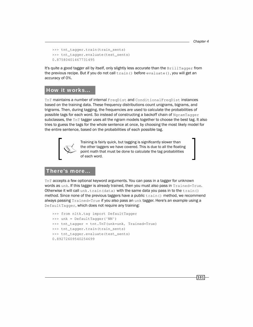
Chapter 4

101

>>> tnt_tagger.train(train_sents)>>> tnt_tagger.evaluate(test_sents)0.87580401467731495

It's quite a good tagger all by itself, only slightly less accurate than the BrillTagger from the previous recipe. But if you do not call train() before evaluate(), you will get an accuracy of 0%.

How it works...TnT maintains a number of internal FreqDist and ConditionalFreqDist instances based on the training data. These frequency distributions count unigrams, bigrams, and trigrams. Then, during tagging, the frequencies are used to calculate the probabilities of possible tags for each word. So instead of constructing a backoff chain of NgramTagger subclasses, the TnT tagger uses all the ngram models together to choose the best tag. It also tries to guess the tags for the whole sentence at once, by choosing the most likely model for the entire sentence, based on the probabilities of each possible tag.

Training is fairly quick, but tagging is significantly slower than the other taggers we have covered. This is due to all the floating point math that must be done to calculate the tag probabilities of each word.

There's more...TnT accepts a few optional keyword arguments. You can pass in a tagger for unknown words as unk. If this tagger is already trained, then you must also pass in Trained=True. Otherwise it will call unk.train(data) with the same data you pass in to the train() method. Since none of the previous taggers have a public train() method, we recommend always passing Trained=True if you also pass an unk tagger. Here's an example using a DefaultTagger, which does not require any training:

>>> from nltk.tag import DefaultTagger>>> unk = DefaultTagger('NN')>>> tnt_tagger = tnt.TnT(unk=unk, Trained=True)>>> tnt_tagger.train(train_sents)>>> tnt_tagger.evaluate(test_sents)0.89272609540254699


102

So we got an almost 2% increase in accuracy! You must use a tagger that can tag a single word without having seen that word before. This is because the unknown tagger's tag() method is only called with a single word sentence. Other good candidates for an unknown tagger are RegexpTagger or AffixTagger. Passing in a UnigramTagger that's been trained on the same data is pretty much useless, as it will have seen the exact same words, and therefore have the same unknown word blind spots.

Controlling the beam searchAnother parameter you can modify for TnT is N, which controls the number of possible solutions the tagger maintains while trying to guess the tags for a sentence. N defaults to 1,000. Increasing it will greatly increase the amount of memory used during tagging, without necessarily increasing accuracy. Decreasing N will decrease memory usage, but could also decrease accuracy. Here's what happens when you set N=100:

>>> tnt_tagger = tnt.TnT(N=100)>>> tnt_tagger.train(train_sents)>>> tnt_tagger.evaluate(test_sents)0.87580401467731495

So the accuracy is exactly the same, but we use significantly less memory to achieve it. However, don't assume that accuracy will not change if you decrease N; experiment with your own data to be sure.

Capitalization significanceYou can pass C=True if you want capitalization of words to be significant. The default is C=False, which means all words are lowercased. The documentation on C says that treating capitalization as significant probably will not increase accuracy. In my own testing, there was a very slight (< 0.01%) increase in accuracy with C=True, probably because case-sensitivity can help identify proper nouns.

See alsoWe covered the DefaultTagger in the Default tagging recipe, backoff tagging in the Combining taggers with backoff tagging recipe, NgramTagger subclasses in the Training a unigram part-of-speech tagger and Training combining Ngram taggers recipes, RegexpTagger in the Tagging with regular expressions recipe, and the AffixTagger in the Affix tagging recipe.

Chapter 4

103

Using WordNet for taggingIf you remember from the Looking up synsets for a word in Wordnet recipe in Chapter 1, Tokenizing Text and WordNet Basics, WordNet synsets specify a part-of-speech tag. It's a very restricted set of possible tags, and many words have multiple synsets with different part-of-speech tags, but this information can be useful for tagging unknown words. WordNet is essentially a giant dictionary, and it's likely to contain many words that are not in your training data.

Getting readyFirst, we need to decide how to map WordNet part-of-speech tags to the Penn Treebank part-of-speech tags we have been using. The following is a table mapping one to the other. See the Looking up synsets for a word in Wordnet recipe in Chapter 1, Tokenizing Text and WordNet Basics for more details. The "s", which was not shown before, is just another kind of adjective, at least for tagging purposes.

WordNet Tag Treebank Tagn NNa JJs JJr RBv VB

How to do it...Now we can create a class that will look up words in WordNet, then chose the most common tag from the synsets it finds. The WordNetTagger defined next can be found in taggers.py:

from nltk.tag import SequentialBackoffTaggerfrom nltk.corpus import wordnetfrom nltk.probability import FreqDist

class WordNetTagger(SequentialBackoffTagger): ''' >>> wt = WordNetTagger() >>> wt.tag(['food', 'is', 'great']) [('food', 'NN'), ('is', 'VB'), ('great', 'JJ')] ''' def __init__(self, *args, **kwargs): SequentialBackoffTagger.__init__(self, *args, **kwargs) self.wordnet_tag_map = {


104

'n': 'NN', 's': 'JJ', 'a': 'JJ', 'r': 'RB', 'v': 'VB' } def choose_tag(self, tokens, index, history): word = tokens[index] fd = FreqDist() for synset in wordnet.synsets(word): fd.inc(synset.pos) return self.wordnet_tag_map.get(fd.max())

How it works...The WordNetTagger simply counts the number of each part-of-speech tag found in the synsets for a word. The most common tag is then mapped to a treebank tag using an internal mapping. Here's some sample usage code:

>>> from taggers import WordNetTagger>>> wn_tagger = WordNetTagger()>>> wn_tagger.evaluate(train_sents)0.18451574615215904

So it's not too accurate, but that's to be expected. We only have enough information to produce four different kinds of tags, while there are 36 possible tags in treebank. And many words can have different part-of-speech tags depending on their context. But if we put the WordNetTagger at the end of an NgramTagger backoff chain, then we can improve accuracy over the DefaultTagger.

>>> from tag_util import backoff_tagger>>> from nltk.tag import UnigramTagger, BigramTagger, TrigramTagger>>> tagger = backoff_tagger(train_sents, [UnigramTagger, BigramTagger, TrigramTagger], backoff=wn_tagger)>>> tagger.evaluate(test_sents)0.88564644938484782

See also

The Looking up synsets for a word in Wordnet recipe in Chapter 1, Tokenizing Text and WordNet Basics details how to use the wordnet corpus and what kinds of part-of-speech tags it knows about. And in the Combining taggers with backoff tagging and Training and combining Ngram taggers recipes, we went over backoff tagging with ngram taggers.

Chapter 4

105

Tagging proper namesUsing the included names corpus, we can create a simple tagger for tagging names as proper nouns.

How to do it...The NamesTagger is a subclass of SequentialBackoffTagger as it's probably only useful near the end of a backoff chain. At initialization, we create a set of all names in the names corpus, lowercasing each name to make lookup easier. Then we implement the choose_tag() method, which simply checks if the current word is in the names_set. If it is, we return the tag NNP (which is the tag for proper nouns). If it isn't, we return None so the next tagger in the chain can tag the word. The following code can be found in taggers.py:

from nltk.tag import SequentialBackoffTaggerfrom nltk.corpus import names

class NamesTagger(SequentialBackoffTagger): def __init__(self, *args, **kwargs): SequentialBackoffTagger.__init__(self, *args, **kwargs) self.name_set = set([n.lower() for n in names.words()]) def choose_tag(self, tokens, index, history): word = tokens[index] if word.lower() in self.name_set: return 'NNP' else: return None

How it works...NamesTagger should be pretty self-explanatory. Its usage is also simple:

>>> from taggers import NamesTagger>>> nt = NamesTagger()>>> nt.tag(['Jacob'])[('Jacob', 'NNP')]

It's probably best to use the NamesTagger right before a DefaultTagger, so it's at the end of a backoff chain. But it could probably go anywhere in the chain since it's unlikely to mistag a word.


106

See alsoThe Combining taggers with backoff tagging recipe goes over the details of using SequentialBackoffTagger subclasses.

Classifier based taggingThe ClassifierBasedPOSTagger uses classification to do part-of-speech tagging. Features are extracted from words, then passed to an internal classifier. The classifier classifies the features and returns a label; in this case, a part-of-speech tag. Classification will be covered in detail in Chapter 7, Text Classification.

ClassifierBasedPOSTagger is a subclass of ClassifierBasedTagger that implements a feature detector that combines many of the techniques of previous taggers into a single feature set. The feature detector finds multiple length suffixes, does some regular expression matching, and looks at the unigram, bigram, and trigram history to produce a fairly complete set of features for each word. The feature sets it produces are used to train the internal classifier, and are used for classifying words into part-of-speech tags.

How to do it...Basic usage of the ClassifierBasedPOSTagger is much like any other SequentialBackoffTaggger. You pass in training sentences, it trains an internal classifier, and you get a very accurate tagger.

>>> from nltk.tag.sequential import ClassifierBasedPOSTagger>>> tagger = ClassifierBasedPOSTagger(train=train_sents)>>> tagger.evaluate(test_sents)0.93097345132743359

Notice a slight modification to initialization—train_sents must be passed in as the train keyword argument.

How it works...ClassifierBasedPOSTagger inherits from ClassifierBasedTagger and only implements a feature_detector() method. All the training and tagging is done in ClassifierBasedTagger. It defaults to training a NaiveBayesClassifier with the given training data. Once this classifier is trained, it is used to classify word features produced by the feature_detector() method.

Chapter 4

107

The ClassifierBasedTagger is often the most accurate tagger, but it's also one of the slowest taggers. If speed is an issue, you should stick with a BrillTagger based on a backoff chain of NgramTagger subclasses and other simple taggers.

The ClassifierBasedTagger also inherits from FeatursetTaggerI (which is just an empty class), creating an inheritance tree that looks like this:

There's more...You can use a different classifier instead of NaiveBayesClassifier by passing in your own classifier_builder function. For example, to use a MaxentClassifier, you would do the following:

>>> from nltk.classify import MaxentClassifier>>> me_tagger = ClassifierBasedPOSTagger(train=train_sents, classifier_builder=MaxentClassifier.train)>>> me_tagger.evaluate(test_sents)0.93093028275415501

The MaxentClassifier takes even longer to train than NaiveBayesClassifier. If you have scipy and numpy installed, training will be faster than normal, but still slower than NaiveBayesClassifier.


108

Custom feature detectorIf you want to do your own feature detection, there are two ways to do it.

1. Subclass ClassifierBasedTagger and implement a feature_detector() method.

2. Pass a method as the feature_detector keyword argument into ClassifierBasedTagger at initialization.

Either way, you need a feature detection method that can take the same arguments as choose_tag(): tokens, index, and history. But instead of returning a tag, you return a dict of key-value features, where the key is the feature name, and the value is the feature value. A very simple example would be a unigram feature detector (found in tag_util.py).

def unigram_feature_detector(tokens, index, history): return {'word': tokens[index]}

Then using the second method, you would pass the following into ClassifierBasedTagger as feature_detector:

>>> from nltk.tag.sequential import ClassifierBasedTagger>>> from tag_util import unigram_feature_detector>>> tagger = ClassifierBasedTagger(train=train_sents, feature_detector=unigram_feature_detector)>>> tagger.evaluate(test_sents)0.87338657457371038

Cutoff probabilityBecause a classifier will always return the best result it can, passing in a backoff tagger is useless unless you also pass in a cutoff_prob to specify the probability threshold for classification. Then, if the probability of the chosen tag is less than cutoff_prob, the backoff tagger will be used. Here's an example using the DefaultTagger as the backoff, and setting cutoff_prob to 0.3:

>>> default = DefaultTagger('NN')>>> tagger = ClassifierBasedPOSTagger(train=train_sents, backoff=default, cutoff_prob=0.3)>>> tagger.evaluate(test_sents)0.93110295704726964

So we get a slight increase in accuracy if the ClassifierBasedPOSTagger uses the DefaultTagger whenever its tag probability is less than 30%.

Chapter 4

109

Pre-trained classifierIf you want to use a classifier that's already been trained, then you can pass that in to ClassifierBasedTagger or ClassifierBasedPOSTagger as classifier. In this case, the classifier_builder argument is ignored and no training takes place. However, you must ensure that the classifier has been trained on and can classify feature sets produced by whatever feature_detector() method you use.

See also

Chapter 7, Text Classification will cover classification in depth.

5Extracting Chunks


f Chunking and chinking with regular expressions

f Merging and splitting chunks with regular expressions

f Expanding and removing chunks with regular expressions

f Partial parsing with regular expressions

f Training a tagger-based chunker

f Classification-based chunking

f Extracting named entities

f Extracting proper noun chunks

f Extracting location chunks

f Training a named entity chunker

IntroductionChunk extraction or partial parsing is the process of extracting short phrases from a part-of-speech tagged sentence. This is different than full parsing, in that we are interested in standalone chunks or phrases instead of full parse trees. The idea is that meaningful phrases can be extracted from a sentence by simply looking for particular patterns of part-of-speech tags.

As in Chapter 4, Part-of-Speech Tagging, we will be using the Penn Treebank corpus for basic training and testing chunk extraction. We will also be using the CoNLL 2000 corpus as it has a simpler and more flexible format that supports multiple chunk types (refer to the Creating a chunked phrase corpus recipe in Chapter 3, Creating Custom Corpora for more details on the conll2000 corpus and IOB tags).

Extracting Chunks

112

Chunking and chinking with regular expressions

Using modified regular expressions, we can define chunk patterns. These are patterns of part-of-speech tags that define what kinds of words make up a chunk. We can also define patterns for what kinds of words should not be in a chunk. These unchunked words are known as chinks.

A ChunkRule specifies what to include in a chunk, while a ChinkRule specifies what to exclude from a chunk. In other words, chunking creates chunks, while chinking breaks up those chunks.

Getting readyWe first need to know how to define chunk patterns. These are modified regular expressions designed to match sequences of part-of-speech tags. An individual tag is specified by surrounding angle brackets, such as <NN> to match a noun tag. Multiple tags can then be combined, as in <DT><NN> to match a determiner followed by a noun. Regular expression syntax can be used within the angle brackets to match individual tag patterns, so you can do <NN.*> to match all nouns including NN and NNS. You can also use regular expression syntax outside of the angle brackets to match patterns of tags. <DT>?<NN.*>+ will match an optional determiner followed by one or more nouns. The chunk patterns are converted internally to regular expressions using the tag_pattern2re_pattern() function:

>>> from nltk.chunk import tag_pattern2re_pattern>>> tag_pattern2re_pattern('<DT>?<NN.*>+')'(<(DT)>)?(<(NN[^\\{\\}<>]*)>)+'

You don't have to use this function to do chunking, but it might be useful or interesting to see how your chunk patterns convert to regular expressions.

How to do it...The pattern for specifying a chunk is to use surrounding curly braces, such as {<DT><NN>}. To specify a chink, you flip the braces, as in }<VB>{. These rules can be combined into a grammar for a particular phrase type. Here's a grammar for noun-phrases that combines both a chunk and a chink pattern, along with the result of parsing the sentence "The book has many chapters":

>>> from nltk.chunk import RegexpParser>>> chunker = RegexpParser(r'''... NP:... {<DT><NN.*><.*>*<NN.*>}... }<VB.*>{

Chapter 5

113

... ''')>>> chunker.parse([('the', 'DT'), ('book', 'NN'), ('has', 'VBZ'), ('many', 'JJ'), ('chapters', 'NNS')])Tree('S', [Tree('NP', [('the', 'DT'), ('book', 'NN')]), ('has', 'VBZ'), Tree('NP', [('many', 'JJ'), ('chapters', 'NNS')])])

The grammar tells the RegexpParser that there are two rules for parsing NP chunks. The first chunk pattern says that a chunk starts with a determiner followed by any kind of noun. Then any number of other words is allowed, until a final noun is found. The second pattern says that verbs should be chinked, thus separating any large chunks that contain a verb. The result is a tree with two noun-phrase chunks: "the book" and "many chapters".

Tagged sentences are always parsed into a Tree (found in the nltk.tree module). The top node of the Tree is 'S', which stands for sentence. Any chunks found will be subtrees whose nodes will refer to the chunk type. In this case, the chunk type is 'NP' for noun-phrase. Trees can be drawn calling the draw() method, as in t.draw().

How it works...Here's what happens, step-by-step:

1. The sentence is converted into a flat Tree, as shown in the following figure:

2. The Tree is used to create a ChunkString.

3. RegexpParser parses the grammar to create a NP RegexpChunkParser with the given rules.

4. A ChunkRule is created and applied to the ChunkString, which matches the entire sentence into a chunk, as shown in the following figure:

Extracting Chunks

114

5. A ChinkRule is created and applied to the same ChunkString, which splits the big chunk into two smaller chunks with a verb between them, as shown in the following figure:

6. The ChunkString is converted back to a Tree, now with two NP chunk subtrees, as shown in the following figure:

You can do this yourself using the classes in nltk.chunk.regexp. ChunkRule and ChinkRule are both subclasses of RegexpChunkRule and require two arguments: the pattern, and a description of the rule. ChunkString is an object that starts with a flat tree, which is then modified by each rule when it is passed in to the rule's apply() method. A ChunkString is converted back to a Tree with the to_chunkstruct() method. Here's the code to demonstrate it:

>>> from nltk.chunk.regexp import ChunkString, ChunkRule, ChinkRule>>> from nltk.tree import Tree>>> t = Tree('S', [('the', 'DT'), ('book', 'NN'), ('has', 'VBZ'), ('many', 'JJ'), ('chapters', 'NNS')])>>> cs = ChunkString(t)>>> cs<ChunkString: '<DT><NN><VBZ><JJ><NNS>'>>>> ur = ChunkRule('<DT><NN.*><.*>*<NN.*>', 'chunk determiners and nouns')>>> ur.apply(cs)>>> cs<ChunkString: '{<DT><NN><VBZ><JJ><NNS>}'>>>> ir = ChinkRule('<VB.*>', 'chink verbs')>>> ir.apply(cs)>>> cs<ChunkString: '{<DT><NN>}<VBZ>{<JJ><NNS>}'>>>> cs.to_chunkstruct()Tree('S', [Tree('CHUNK', [('the', 'DT'), ('book', 'NN')]), ('has', 'VBZ'), Tree('CHUNK', [('many', 'JJ'), ('chapters', 'NNS')])])

The preceding tree diagrams can be drawn at each step by calling cs.to_chunkstruct().draw().

Chapter 5

115

There's more...You will notice that the subtrees from the ChunkString are tagged as 'CHUNK' and not 'NP'. That's because the previous rules are phrase agnostic; they create chunks without needing to know what kind of chunks they are.

Internally, the RegexpParser creates a RegexpChunkParser for each chunk phrase type. So if you are only chunking NP phrases, there will only be one RegexpChunkParser. The RegexpChunkParser gets all the rules for the specific chunk type, and handles applying the rules in order and converting the 'CHUNK' trees to the specific chunk type, such as 'NP'.

Here's some code to illustrate the usage of RegexpChunkParser. We pass the previous two rules into the RegexpChunkParser, and then parse the same sentence tree we created before. The resulting tree is just like what we got from applying both rules in order, except 'CHUNK' has been replaced with 'NP' in the two subtrees. This is because RegexpChunkParser defaults to chunk_node='NP'.

>>> from nltk.chunk import RegexpChunkParser>>> chunker = RegexpChunkParser([ur, ir])>>> chunker.parse(t)Tree('S', [Tree('NP', [('the', 'DT'), ('book', 'NN')]), ('has', 'VBZ'), Tree('NP', [('many', 'JJ'), ('chapters', 'NNS')])])

Different chunk typesIf you wanted to parse a different chunk type, then you could pass that in as chunk_node to RegexpChunkParser. Here's the same code we have just seen, but instead of 'NP' subtrees, we will call them 'CP' for custom phrase.

>>> from nltk.chunk import RegexpChunkParser>>> chunker = RegexpChunkParser([ur, ir], chunk_node='CP')>>> chunker.parse(t)Tree('S', [Tree('CP', [('the', 'DT'), ('book', 'NN')]), ('has', 'VBZ'), Tree('CP', [('many', 'JJ'), ('chapters', 'NNS')])])

RegexpParser does this internally when you specify multiple phrase types. This will be covered in Partial parsing with regular expressions.

Alternative patternsThe same parsing results can be obtained by using two chunk patterns in the grammar, and discarding the chink pattern:

>>> chunker = RegexpParser(r'''... NP:... {<DT><NN.*>}... {<JJ><NN.*>}

Extracting Chunks

116

... ''')>>> chunker.parse(t)Tree('S', [Tree('NP', [('the', 'DT'), ('book', 'NN')]), ('has', 'VBZ'), Tree('NP', [('many', 'JJ'), ('chapters', 'NNS')])])

In fact, you could reduce the two chunk patterns into a single pattern.

>>> chunker = RegexpParser(r'''... NP:... {(<DT>|<JJ>)<NN.*>}... ''')>>> chunker.parse(t)Tree('S', [Tree('NP', [('the', 'DT'), ('book', 'NN')]), ('has', 'VBZ'), Tree('NP', [('many', 'JJ'), ('chapters', 'NNS')])])

How you create and combine patterns is really up to you. Pattern creation is a process of trial and error, and entirely depends on what your data looks like and which patterns are easiest to express.

Chunk rule with contextYou can also create chunk rules with a surrounding tag context. For example, if your pattern is <DT>{<NN>}, which will be parsed into a ChunkRuleWithContext. Any time there's a tag on either side of the curly braces, you will get a ChunkRuleWithContext instead of a ChunkRule. This can allow you to be more specific about when to parse particular kinds of chunks.

Here's an example of using ChunkWithContext directly. It takes four arguments: the left context, the pattern to chunk, the right context, and a description:

>>> from nltk.chunk.regexp import ChunkRuleWithContext>>> ctx = ChunkRuleWithContext('<DT>', '<NN.*>', '<.*>', 'chunk nouns only after determiners')>>> cs = ChunkString(t)>>> cs<ChunkString: '<DT><NN><VBZ><JJ><NNS>'>>>> ctx.apply(cs)>>> cs<ChunkString: '<DT>{<NN>}<VBZ><JJ><NNS>'>>>> cs.to_chunkstruct()Tree('S', [('the', 'DT'), Tree('CHUNK', [('book', 'NN')]), ('has', 'VBZ'), ('many', 'JJ'), ('chapters', 'NNS')])

Chapter 5

117

This example only chunks nouns that follow a determiner, therefore ignoring the noun that follows an adjective. Here's how it would look using the RegexpParser:

>>> chunker = RegexpParser(r'''... NP:... <DT>{<NN.*>}... ''')>>> chunker.parse(t)Tree('S', [('the', 'DT'), Tree('NP', [('book', 'NN')]), ('has', 'VBZ'), ('many', 'JJ'), ('chapters', 'NNS')])

See alsoIn the next recipe, we will cover merging and splitting chunks.

Merging and splitting chunks with regular expressions

In this recipe, we will cover two more rules for chunking. A MergeRule can merge two chunks together based on the end of the first chunk and the beginning of the second chunk. A SplitRule will split a chunk into two based on the specified split pattern.

How to do it...A SplitRule is specified with two opposing curly braces surrounded by a pattern on either side. To split a chunk after a noun, you would do <NN.*>}{<.*>. A MergeRule is specified by flipping the curly braces, and will join chunks where the end of the first chunk matches the left pattern, and the beginning of the next chunk matches the right pattern. To merge two chunks where the first ends with a noun and the second begins with a noun, you would use <NN.*>{}<NN.*>.

The order of rules is very important and re-ordering can affect the results. The RegexpParser applies the rules one at a time from top to bottom, so each rule will be applied to the ChunkString resulting from the previous rule.

Extracting Chunks

118

Here's an example of splitting and merging, starting with the sentence tree as shown next:

1. The whole sentence is chunked, as shown in the following diagram:

2. The chunk is split into multiple chunks after every noun, as shown in the following tree:

3. Each chunk with a determiner is split into separate chunks, creating four chunks where there were three:

4. Chunks ending with a noun are merged with the next chunk if it begins with a noun, reducing the four chunks back down to three, as shown in the following diagram:

Using the RegexpParser, the code looks like this:

>>> chunker = RegexpParser(r'''... NP:... {<DT><.*>*<NN.*>}... <NN.*>}{<.*>

Chapter 5

119

... <.*>}{<DT>

... <NN.*>{}<NN.*>

... ''')>>> sent = [('the', 'DT'), ('sushi', 'NN'), ('roll', 'NN'), ('was', 'VBD'), ('filled', 'VBN'), ('with', 'IN'), ('the', 'DT'), ('fish', 'NN')]>>> chunker.parse(sent)Tree('S', [Tree('NP', [('the', 'DT'), ('sushi', 'NN'), ('roll', 'NN')]), Tree('NP', [('was', 'VBD'), ('filled', 'VBN'), ('with', 'IN')]), Tree('NP', [('the', 'DT'), ('fish', 'NN')])])

And the final tree of NP chunks is shown in the following diagram:

How it works...The MergeRule and SplitRule classes take three arguments: the left pattern, right pattern, and a description. The RegexpParser takes care of splitting the original patterns on the curly braces to get the left and right sides, but you can also create these manually. Here's a step-by-step walkthrough of how the original sentence is modified by applying each rule:

>>> from nltk.chunk.regexp import MergeRule, SplitRule>>> cs = ChunkString(Tree('S', sent))>>> cs<ChunkString: '<DT><NN><NN><VBD><VBN><IN><DT><NN>'>>>> ur = ChunkRule('<DT><.*>*<NN.*>', 'chunk determiner to noun')>>> ur.apply(cs)>>> cs<ChunkString: '{<DT><NN><NN><VBD><VBN><IN><DT><NN>}'>>>> sr1 = SplitRule('<NN.*>', '<.*>', 'split after noun')>>> sr1.apply(cs)>>> cs<ChunkString: '{<DT><NN>}{<NN>}{<VBD><VBN><IN><DT><NN>}'>>>> sr2 = SplitRule('<.*>', '<DT>', 'split before determiner')>>> sr2.apply(cs)>>> cs<ChunkString: '{<DT><NN>}{<NN>}{<VBD><VBN><IN>}{<DT><NN>}'>>>> mr = MergeRule('<NN.*>', '<NN.*>', 'merge nouns')>>> mr.apply(cs)

Extracting Chunks

120

>>> cs<ChunkString: '{<DT><NN><NN>}{<VBD><VBN><IN>}{<DT><NN>}'>>>> cs.to_chunkstruct()Tree('S', [Tree('CHUNK', [('the', 'DT'), ('sushi', 'NN'), ('roll', 'NN')]), Tree('CHUNK', [('was', 'VBD'), ('filled', 'VBN'), ('with', 'IN')]), Tree('CHUNK', [('the', 'DT'), ('fish', 'NN')])])

There's more...The parsing of the rules and splitting of left and right patterns is done in the static parse() method of the RegexpChunkRule superclass. This is called by the RegexpParser to get the list of rules to pass in to the RegexpChunkParser. Here are some examples of parsing the patterns used before:

>>> from nltk.chunk.regexp import RegexpChunkRule>>> RegexpChunkRule.parse('{<DT><.*>*<NN.*>}')<ChunkRule: '<DT><.*>*<NN.*>'>>>> RegexpChunkRule.parse('<.*>}{<DT>')<SplitRule: '<.*>', '<DT>'>>>> RegexpChunkRule.parse('<NN.*>{}<NN.*>')<MergeRule: '<NN.*>', '<NN.*>'>

Rule descriptionsDescriptions for each rule can be specified with a comment string after the rule (a comment string must start with #). If no comment string is found, the rule's description will be empty. Here's an example:

>>> RegexpChunkRule.parse('{<DT><.*>*<NN.*>} # chunk everything').descr()'chunk everything'>>> RegexpChunkRule.parse('{<DT><.*>*<NN.*>}').descr()''

Comment string descriptions can also be used within grammar strings that are passed to RegexpParser.

See alsoThe previous recipe goes over how to use ChunkRule and how rules are passed in to RegexpChunkParser.

Chapter 5

121

Expanding and removing chunks with regular expressions

There are three RegexpChunkRule subclasses that are not supported by RegexpChunkRule.parse() and therefore must be created manually if you want to use them. These rules are:

1. ExpandLeftRule: Adds unchunked (chink) words to the left of a chunk to the chunk.

2. ExpandRightRule: Adds unchunked (chink) words to the right of a chunk to the chunk.

3. UnChunkRule: Unchunk any matching chunk.

How to do it...ExpandLeftRule and ExpandRightRule both take two patterns along with a description as arguments. For ExpandLeftRule, the first pattern is the chink we want to add to the beginning of the chunk, while the right pattern will match the beginning of the chunk we want to expand. With ExpandRightRule, the left pattern should match the end of the chunk we want to expand, and the right pattern matches the chink we want to add to the end of the chunk. The idea is similar to the MergeRule, but in this case we are merging chink words instead of other chunks.

UnChunkRule is the opposite of ChunkRule. Any chunk that exactly matches the UnChunkRule pattern will be unchunked, and become a chink. Here's some code demonstrating usage with the RegexpChunkParser:

>>> from nltk.chunk.regexp import ChunkRule, ExpandLeftRule, ExpandRightRule, UnChunkRule>>> from nltk.chunk import RegexpChunkParser>>> ur = ChunkRule('<NN>', 'single noun')>>> el = ExpandLeftRule('<DT>', '<NN>', 'get left determiner')>>> er = ExpandRightRule('<NN>', '<NNS>', 'get right plural noun')>>> un = UnChunkRule('<DT><NN.*>*', 'unchunk everything')>>> chunker = RegexpChunkParser([ur, el, er, un])>>> sent = [('the', 'DT'), ('sushi', 'NN'), ('rolls', 'NNS')]>>> chunker.parse(sent)Tree('S', [('the', 'DT'), ('sushi', 'NN'), ('rolls', 'NNS')])

You will notice the end result is a flat sentence, which is exactly what we started with. That's because the final UnChunkRule undid the chunk created by the previous rules. Read on to see the step-by-step procedure of what happened.

Extracting Chunks

122

How it works...The preceding rules were applied in the following order, starting with the sentence tree shown below:

1. Make single nouns into a chunk, as shown in the following diagram:

2. Expand left determiners into chunks that begin with a noun, as shown in the following diagram:

3. Expand right plural nouns into chunks that end with a noun, chunking the whole sentence as shown in the following diagram:

4. Unchunk every chunk that is a determiner + noun + plural noun, resulting in the original sentence tree, as shown in the following diagram:

Chapter 5

123

Here's the code showing each step:

>>> from nltk.chunk.regexp import ChunkString>>> from nltk.tree import Tree>>> cs = ChunkString(Tree('S', sent))>>> cs<ChunkString: '<DT><NN><NNS>'>>>> ur.apply(cs)>>> cs<ChunkString: '<DT>{<NN>}<NNS>'>>>> el.apply(cs)>>> cs<ChunkString: '{<DT><NN>}<NNS>'>>>> er.apply(cs)>>> cs<ChunkString: '{<DT><NN><NNS>}'>>>> un.apply(cs)>>> cs<ChunkString: '<DT><NN><NNS>'>

There's more...In practice, you can probably get away with only using the previous four rules: ChunkRule, ChinkRule, MergeRule, and SplitRule. But if you do need very fine-grained control over chunk parsing and removing, now you know how to do it with the expansion and unchunk rules.

See alsoThe previous two recipes covered the more common chunk rules that are supported by RegexpChunkRule.parse() and RegexpParser.

Partial parsing with regular expressionsSo far, we have only been parsing noun-phrases. But RegexpParser supports grammar with multiple phrase types, such as verb-phrases and prepositional-phrases. We can put the rules we have learned to use and define a grammar that can be evaluated against the conll2000 corpus, which has NP, VP, and PP phrases.

Extracting Chunks

124

How to do it...We will define a grammar to parse three phrase types. For noun-phrases, we have a ChunkRule that looks for an optional determiner followed by one or more nouns. We then have a MergeRule for adding an adjective to the front of a noun chunk. For prepositional-phrases, we simply chunk any IN word, such as "in" or "on". For verb-phrases, we chunk an optional modal word (such as "should") followed by a verb.

Each grammar rule is followed by a # comment. This comment is passed in to each rule as the description. Comments are optional, but they can be helpful notes for understanding what the rule does, and will be included in trace output.

>>> chunker = RegexpParser(r'''... NP:... {<DT>?<NN.*>+} # chunk optional determiner with nouns... <JJ>{}<NN.*> # merge adjective with noun chunk... PP:... {<IN>} # chunk preposition... VP:... {<MD>?<VB.*>} # chunk optional modal with verb... ''')>>> from nltk.corpus import conll2000>>> score = chunker.evaluate(conll2000.chunked_sents())>>> score.accuracy()0.61485735457576884

When we call evaluate() on the chunker, we give it a list of chunked sentences and get back a ChunkScore object, which can give us the accuracy of the chunker, along with a number of other metrics.

How it works...The RegexpParser parses the grammar string into sets of rules, one set of rules for each phrase type. These rules are used to create a RegexpChunkParser. The rules are parsed using RegexpChunkRule.parse(), which returns one of the five subclasses: ChunkRule, ChinkRule, MergeRule, SplitRule, or ChunkRuleWithContext.

Now that the grammar has been translated into sets of rules, these rules are used to parse a tagged sentence into a Tree structure. RegexpParser inherits from ChunkParserI, which provides a parse() method to parse the tagged words. Whenever a part of the tagged tokens match a chunk rule, a subtree is constructed so that the tagged tokens become the leaves of a Tree whose node string is the chunk tag. ChunkParserI also provides the evaluate() method, which compares the given chunked sentences to the output of the parse() method to construct and return a ChunkScore object.

Chapter 5

125

There's more...You can also evaluate this chunker on the treebank_chunk corpus.

>>> from nltk.corpus import treebank_chunk>>> treebank_score = chunker.evaluate(treebank_chunk.chunked_sents())>>> treebank_score.accuracy()0.49033970276008493

The treebank_chunk corpus is a special version of the treebank corpus that provides a chunked_sents() method. The regular treebank corpus cannot provide that method due to its file format.

ChunkScore metricsChunkScore provides a few other metrics besides accuracy. Of the chunks the chunker was able to guess, precision tells you how many were correct. Recall tells you how well the chunker did at finding correct chunks, compared to how many total chunks there were.

>>> score.precision()0.60201948127375005>>> score.recall()0.60607250250584699

You can also get lists of chunks that were missed by the chunker, chunks that were incorrectly found, correct chunks, and guessed chunks. These can be useful to figure out how to improve your chunk grammar.

>>> len(score.missed())47161>>> len(score.incorrect())47967>>> len(score.correct())119720>>> len(score.guessed())120526

As you can see by the number of incorrect chunks, and by comparing guessed() and correct(), our chunker guessed that there were more chunks that actually existed. And it also missed a good number of correct chunks.

Looping and tracingIf you want to apply the chunk rules in your grammar more than once, you pass loop=2 into RegexpParser at initialization. The default is loop=1.

Extracting Chunks

126

To watch an internal trace of the chunking process, pass trace=1 into RegexpParser. To get even more output, pass in trace=2. This will give you a printout of what the chunker is doing as it is doing it. Rule comments/descriptions will be included in the trace output, giving you a good idea of which rule is applied when.

See alsoIf coming up with regular expression chunk patterns seems like too much work, then read the next recipes where we will cover how to train a chunker based on a corpus of chunked sentences.

Training a tagger-based chunkerTraining a chunker can be a great alternative to manually specifying regular expression chunk patterns. Instead of a painstaking process of trial and error to get the exact right patterns, we can use existing corpus data to train chunkers much like we did in Chapter 4, Part-of-Speech Tagging.

How to do it...As with the part-of-speech tagging, we will use the treebank corpus data for training. But this time we will use the treebank_chunk corpus, which is specifically formatted to produce chunked sentences in the form of trees. These chunked_sents() will be used by a TagChunker class to train a tagger-based chunker. The TagChunker uses a helper function conll_tag_chunks() to extract a list of (pos, iob) tuples from a list of Tree. These (pos, iob) tuples are then used to train a tagger in the same way (word, pos) tuples were used in Chapter 4, Part-of-Speech Tagging to train part-of-speech taggers. But instead of learning part-of-speech tags for words, we are learning IOB tags for part-of-speech tags. Here's the code from chunkers.py:

import nltk.chunk, itertoolsfrom nltk.tag import UnigramTagger, BigramTaggerfrom tag_util import backoff_tagger

def conll_tag_chunks(chunk_sents): tagged_sents = [nltk.chunk.tree2conlltags(tree) for tree in chunk_sents] return [[(t, c) for (w, t, c) in sent] for sent in tagged_sents]

class TagChunker(nltk.chunk.ChunkParserI): def __init__(self, train_chunks, tagger_classes=[UnigramTagger, BigramTagger]): train_sents = conll_tag_chunks(train_chunks) self.tagger = backoff_tagger(train_sents, tagger_classes)

Chapter 5

127

def parse(self, tagged_sent): if not tagged_sent: return None (words, tags) = zip(*tagged_sent) chunks = self.tagger.tag(tags) wtc = itertools.izip(words, chunks) return nltk.chunk.conlltags2tree([(w,t,c) for (w,(t,c)) in wtc])

Once we have our trained TagChunker, we can then evaluate the ChunkScore the same way we did for the RegexpParser in the previous recipes.

>>> from chunkers import TagChunker>>> from nltk.corpus import treebank_chunk>>> train_chunks = treebank_chunk.chunked_sents()[:3000]>>> test_chunks = treebank_chunk.chunked_sents()[3000:]>>> chunker = TagChunker(train_chunks)>>> score = chunker.evaluate(test_chunks)>>> score.accuracy()0.97320393352514278>>> score.precision()0.91665343705350055>>> score.recall()0.9465573770491803

Pretty darn accurate! Training a chunker is clearly a great alternative to manually specified grammars and regular expressions.

How it works...

Recall from the Creating a chunked phrase corpus recipe in Chapter 3, Creating Custom Corpora that the conll2000 corpus defines chunks using IOB tags, which specify the type of chunk and where it begins and ends. We can train a part-of-speech tagger on these IOB tag patterns, and then use that to power a ChunkerI subclass. But first we need to transform a Tree that you would get from the chunked_sents() method of a corpus into a format usable by a part-of-speech tagger. This is what conll_tag_chunks() does. It uses nltk.chunk.tree2conlltags() to convert a sentence Tree into a list of 3-tuples of the form (word, pos, iob) where pos is the part-of-speech tag and iob is an IOB tag, such as B-NP to mark the beginning of a noun-phrase, or I-NP to mark that the word is inside the noun-phrase. The reverse of this method is nltk.chunk.conlltags2tree(). Here's some code to demonstrate these nltk.chunk functions:

>>> import nltk.chunk>>> from nltk.tree import Tree>>> t = Tree('S', [Tree('NP', [('the', 'DT'), ('book', 'NN')])])>>> nltk.chunk.tree2conlltags(t)[('the', 'DT', 'B-NP'), ('book', 'NN', 'I-NP')]>>> nltk.chunk.conlltags2tree([('the', 'DT', 'B-NP'), ('book', 'NN', 'I-NP')])Tree('S', [Tree('NP', [('the', 'DT'), ('book', 'NN')])])

Extracting Chunks

128

The next step is to convert these 3-tuples into 2-tuples that the tagger can recognize. Because the RegexpParser uses part-of-speech tags for chunk patterns, we will do that here too and use part-of-speech tags as if they were words to tag. By simply dropping the word from 3-tuple (word, pos, iob), the conll_tag_chunks() function returns a list of 2-tuples of the form (pos, iob). When given the preceding example Tree in a list, the results are in a format we can feed to a tagger.

>>> conll_tag_chunks([t])[[('DT', 'B-NP'), ('NN', 'I-NP')]]

The final step is a subclass of ChunkParserI called TagChunker. It trains on a list of chunk trees using an internal tagger. This internal tagger is composed of a UnigramTagger and a BigramTagger in a backoff chain, using the backoff_tagger() method created in the Training and combining Ngram taggers recipe in Chapter 4, Part-of-Speech Tagging.

Finally, ChunkerI subclasses must implement a parse() method that expects a part-of-speech tagged sentence. We unzip that sentence into a list of words and part-of-speech tags. The tags are then tagged by the tagger to get IOB tags, which are then re-combined with the words and part-of-speech tags to create 3-tuples we can pass to nltk.chunk.conlltags2tree() to return a final Tree.

There's more...Since we have been talking about the conll IOB tags, let us see how the TagChunker does on the conll2000 corpus:

>>> from nltk.corpus import conll2000>>> conll_train = conll2000.chunked_sents('train.txt')>>> conll_test = conll2000.chunked_sents('test.txt')>>> chunker = TagChunker(conll_train)>>> score = chunker.evaluate(conll_test)>>> score.accuracy()0.89505456234037617>>> score.precision()0.81148419743556754>>> score.recall()0.86441916769448635

Not quite as good as on treebank_chunk, but conll2000 is a much larger corpus, so it's not too surprising.

Chapter 5

129

Using different taggersIf you want to use different tagger classes with the TagChunker, you can pass them in as tagger_classes. For example, here's the TagChunker using just a UnigramTagger:

>>> from nltk.tag import UnigramTagger>>> uni_chunker = TagChunker(train_chunks, tagger_classes=[UnigramTagger])>>> score = uni_chunker.evaluate(test_chunks)>>> score.accuracy()0.96749259243354657

The tagger_classes will be passed directly into the backoff_tagger() function, which means they must be subclasses of SequentialBackoffTagger. In testing, the default of tagger_classes=[UnigramTagger, BigramTagger] produces the best results.

See also

The Training and combining Ngram taggers recipe in Chapter 4, Part-of-Speech Tagging covers backoff tagging with a UnigramTagger and BigramTagger. ChunkScore metrics returned by the evaluate() method of a chunker were explained in the previous recipe.

Classification-based chunkingUnlike most part-of-speech taggers, the ClassifierBasedTagger learns from features. That means we can create a ClassifierChunker that can learn from both the words and part-of-speech tags, instead of only the part-of-speech tags as the TagChunker does.

How to do it...For the ClassifierChunker, we don't want to discard the words from the training sentences, as we did in the previous recipe. Instead, to remain compatible with the 2-tuple (word, pos) format required for training a ClassiferBasedTagger, we convert the (word, pos, iob) 3-tuples from nltk.chunk.tree2conlltags() into ((word, pos), iob) 2-tuples using the chunk_trees2train_chunks() function. This code can be found in chunkers.py:

import nltk.chunkfrom nltk.tag import ClassifierBasedTagger

def chunk_trees2train_chunks(chunk_sents): tag_sents = [nltk.chunk.tree2conlltags(sent) for sent in chunk_sents] return [[((w,t),c) for (w,t,c) in sent] for sent in tag_sents]

Extracting Chunks

130

Next, we need a feature detector function to pass into ClassifierBasedTagger. Our default feature detector function, prev_next_pos_iob(), knows that the list of tokens is really a list of (word, pos) tuples, and can use that to return a feature set suitable for a classifier. To give the classifier as much information as we can, this feature set contains the current, previous and next word, and part-of-speech tag, along with the previous IOB tag.

def prev_next_pos_iob(tokens, index, history): word, pos = tokens[index]

if index == 0: prevword, prevpos, previob = ('<START>',)*3 else: prevword, prevpos = tokens[index-1] previob = history[index-1]

if index == len(tokens) - 1: nextword, nextpos = ('<END>',)*2 else: nextword, nextpos = tokens[index+1]

feats = { 'word': word, 'pos': pos, 'nextword': nextword, 'nextpos': nextpos, 'prevword': prevword, 'prevpos': prevpos, 'previob': previob } return feats

Now we can define the ClassifierChunker, which uses an internal ClassifierBasedTagger with features extracted using prev_next_pos_iob(), and training sentences from chunk_trees2train_chunks(). As a subclass of ChunkerParserI, it implements the parse() method, which converts the ((w, t), c) tuples produced by the internal tagger into a Tree using nltk.chunk.conlltags2tree().

class ClassifierChunker(nltk.chunk.ChunkParserI): def __init__(self, train_sents, feature_detector=prev_next_pos_iob, **kwargs): if not feature_detector: feature_detector = self.feature_detector

train_chunks = chunk_trees2train_chunks(train_sents) self.tagger = ClassifierBasedTagger(train=train_chunks, feature_detector=feature_detector, **kwargs)

Chapter 5

131

def parse(self, tagged_sent): if not tagged_sent: return None chunks = self.tagger.tag(tagged_sent) return nltk.chunk.conlltags2tree([(w,t,c) for ((w,t),c) in chunks])

Using the same train_chunks and test_chunks from the treebank_chunk corpus in the previous recipe, we can evaluate this code from chunkers.py:

>>> from chunkers import ClassifierChunker>>> chunker = ClassifierChunker(train_chunks)>>> score = chunker.evaluate(test_chunks)>>> score.accuracy()0.97217331558380216>>> score.precision()0.92588387933830685>>> score.recall()0.93590163934426229

Compared to the TagChunker, all the scores have gone up a bit. Let us see how it does on conll2000:

>>> chunker = ClassifierChunker(conll_train)>>> score = chunker.evaluate(conll_test)>>> score.accuracy()0.92646220740021534>>> score.precision()0.87379243109102189>>> score.recall()0.90073546206203459

This is much improved over the TagChunker.

How it works...Like the TagChunker in the previous recipe, we are training a part-of-speech tagger for IOB tagging. But in this case, we want to include the word as a feature to power a classifier. By creating nested 2-tuples of the form ((word, pos), iob), we can pass the word through the tagger into our feature detector function. chunk_trees2train_chunks() produces these nested 2-tuples, and prev_next_pos_iob() is aware of them and uses each element as a feature. The following features are extracted:

f The current word and part-of-speech tag

f The previous word, part-of-speech tag, and IOB tag

f The next word and part-of-speech tag

Extracting Chunks

132

The arguments to prev_next_pos_iob() look the same as the feature_detector() method of the ClassifierBasedTagger: tokens, index, and history. But this time, tokens will be a list of (word, pos) 2-tuples, and history will be a list of IOB tags. The special feature values '<START>' and '<END>' are used if there are no previous or next tokens.

The ClassifierChunker uses an internal ClassifierBasedTagger and prev_next_pos_iob() as its default feature_detector. The results from the tagger, which are in the same nested 2-tuple form, are then reformatted into 3-tuples to return a final Tree using nltk.chunk.conlltags2tree().

There's more...You can use your own feature detector function by passing it in to the ClassifierChunker as feature_detector. The tokens will contain a list of (word, tag) tuples, and history will be a list of the previous IOB tags found.

Using a different classifier builderThe ClassifierBasedTagger defaults to using NaiveBayesClassifier.train as its classifier_builder. But you can use any classifier you want by overriding the classifier_builder keyword argument. Here's an example using MaxentClassifier.train:

>>> from nltk.classify import MaxentClassifier>>> builder = lambda toks: MaxentClassifier.train(toks, trace=0, max_iter=10, min_lldelta=0.01)>>> me_chunker = ClassifierChunker(train_chunks, classifier_builder=builder)>>> score = me_chunker.evaluate(test_chunks)>>> score.accuracy()0.9748357452655988>>> score.precision()0.93794355504208615>>> score.recall()0.93163934426229511

Instead of using MaxentClassifier.train directly, it has been wrapped in a lambda so that its output is quiet (trace=0) and it finishes in a reasonable amount of time. As you can see, the scores are slightly different compared to using the NaiveBayesClassifier.

Chapter 5

133

See alsoThe previous recipe, Training a tagger-based chunker, introduced the idea of using a part-of-speech tagger for training a chunker. The Classifier-based tagging recipe in Chapter 4, Part-of-Speech Tagging describes ClassifierBasedPOSTagger, which is a subclass of ClassifierBasedTagger. In Chapter 7, Text Classification, we will cover classification in detail.

Extracting named entitiesNamed entity recognition is a specific kind of chunk extraction that uses entity tags instead of, or in addition to, chunk tags. Common entity tags include PERSON, ORGANIZATION, and LOCATION. Part-of-speech tagged sentences are parsed into chunk trees as with normal chunking, but the nodes of the trees can be entity tags instead of chunk phrase tags.

How to do it...NLTK comes with a pre-trained named entity chunker. This chunker has been trained on data from the ACE program, a NIST (National Institute of Standards and Technology) sponsored program for Automatic Content Extraction, which you can read more about here: http://www.itl.nist.gov/iad/894.01/tests/ace/. Unfortunately, this data is not included in the NLTK corpora, but the trained chunker is. This chunker can be used through the ne_chunk() method in the nltk.chunk module. ne_chunk() will chunk a single sentence into a Tree. The following is an example using ne_chunk() on the first tagged sentence of the treebank_chunk corpus:

>>> from nltk.chunk import ne_chunk>>> ne_chunk(treebank_chunk.tagged_sents()[0])Tree('S', [Tree('PERSON', [('Pierre', 'NNP')]), Tree('ORGANIZATION', [('Vinken', 'NNP')]), (',', ','), ('61', 'CD'), ('years', 'NNS'), ('old', 'JJ'), (',', ','), ('will', 'MD'), ('join', 'VB'), ('the', 'DT'), ('board', 'NN'), ('as', 'IN'), ('a', 'DT'), ('nonexecutive', 'JJ'), ('director', 'NN'), ('Nov.', 'NNP'), ('29', 'CD'), ('.', '.')])

You can see two entity tags are found: PERSON and ORGANIZATION. Each of these subtrees contain a list of the words that are recognized as a PERSON or ORGANIZATION. To extract these named entities, we can write a simple helper method that will get the leaves of all the subtrees we are interested in.

def sub_leaves(tree, node): return [t.leaves() for t in tree.subtrees (lambda s: s.node == node)]

Extracting Chunks

134

Then we can call this method to get all the PERSON or ORGANIZATION leaves from a tree.

>>> tree = ne_chunk(treebank_chunk.tagged_sents()[0])>>> from chunkers import sub_leaves>>> sub_leaves(tree, 'PERSON')[[('Pierre', 'NNP')]]>>> sub_leaves(tree, 'ORGANIZATION')[[('Vinken', 'NNP')]]

You may notice that the chunker has mistakenly separated "Vinken" into its own ORGANIZATION Tree instead of including it with the PERSON Tree containing "Pierre". Such is the case with statistical natural language processing—you can't always expect perfection.

How it works...The pre-trained named entity chunker is much like any other chunker, and in fact uses a MaxentClassifier powered ClassifierBasedTagger to determine IOB tags. But instead of B-NP and I-NP IOB tags, it uses B-PERSON, I-PERSON, B-ORGANIZATION, I-ORGANIZATION, and more. It also uses the O tag to mark words that are not part of a named entity (and thus outside the named entity subtrees).

There's more...To process multiple sentences at a time, you can use batch_ne_chunk(). Here's an example where we process the first 10 sentences from treebank_chunk.tagged_sents() and get the ORGANIZATION sub_leaves():

>>> from nltk.chunk import batch_ne_chunk>>> trees = batch_ne_chunk(treebank_chunk.tagged_sents()[:10])>>> [sub_leaves(t, 'ORGANIZATION') for t in trees][[[('Vinken', 'NNP')]], [[('Elsevier', 'NNP')]], [[('Consolidated', 'NNP'), ('Gold', 'NNP'), ('Fields', 'NNP')]], [], [], [[('Inc.', 'NNP')], [('Micronite', 'NN')]], [[('New', 'NNP'), ('England', 'NNP'), ('Journal', 'NNP')]], [[('Lorillard', 'NNP')]], [], []]

You can see there are a couple of multi-word ORGANIZATION chunks, such as "New England Journal". There are also a few sentences that have no ORGANIZATION chunks, as indicated by the empty lists [].

Chapter 5

135

Binary named entity extractionIf you don't care about the particular kind of named entity to extract, you can pass binary=True into ne_chunk() or batch_ne_chunk(). Now, all named entities will be tagged with NE:

>>> ne_chunk(treebank_chunk.tagged_sents()[0], binary=True)Tree('S', [Tree('NE', [('Pierre', 'NNP'), ('Vinken', 'NNP')]), (',', ','), ('61', 'CD'), ('years', 'NNS'), ('old', 'JJ'), (',', ','), ('will', 'MD'), ('join', 'VB'), ('the', 'DT'), ('board', 'NN'), ('as', 'IN'), ('a', 'DT'), ('nonexecutive', 'JJ'), ('director', 'NN'), ('Nov.', 'NNP'), ('29', 'CD'), ('.', '.')])

If we get the sub_leaves(), we can see that "Pierre Vinken" is correctly combined into a single named entity.

>>> sub_leaves(ne_chunk(treebank_chunk.tagged_sents()[0], binary=True), 'NE')[[('Pierre', 'NNP'), ('Vinken', 'NNP')]]

See alsoIn the next recipe, we will create our own simple named entity chunker.

Extracting proper noun chunksA simple way to do named entity extraction is to chunk all proper nouns (tagged with NNP). We can tag these chunks as NAME, since the definition of a proper noun is the name of a person, place, or thing.

How to do it...Using the RegexpParser, we can create a very simple grammar that combines all proper nouns into a NAME chunk. Then we can test this on the first tagged sentence of treebank_chunk to compare the results to the previous recipe.

>>> chunker = RegexpParser(r'''... NAME:... {<NNP>+}... ''')>>> sub_leaves(chunker.parse(treebank_chunk.tagged_sents()[0]), 'NAME')[[('Pierre', 'NNP'), ('Vinken', 'NNP')], [('Nov.', 'NNP')]]

Although we get "Nov." as a NAME chunk, this isn't a wrong result, as "Nov." is the name of a month.

Extracting Chunks

136

How it works...The NAME chunker is a simple usage of the RegexpParser, covered in Chunking and chinking with regular expressions, Merging and splitting chunks with regular expressions, and Partial parsing with regular expressions recipes of this chapter. All sequences of NNP tagged words are combined into NAME chunks.

There's more...If we wanted to be sure to only chunk the names of people, then we can build a PersonChunker that uses the names corpus for chunking. This class can be found in chunkers.py:

import nltk.chunkfrom nltk.corpus import names

class PersonChunker(nltk.chunk.ChunkParserI): def __init__(self): self.name_set = set(names.words())

def parse(self, tagged_sent): iobs = [] in_person = False

for word, tag in tagged_sent: if word in self.name_set and in_person: iobs.append((word, tag, 'I-PERSON')) elif word in self.name_set: iobs.append((word, tag, 'B-PERSON')) in_person = True else: iobs.append((word, tag, 'O')) in_person = False

return nltk.chunk.conlltags2tree(iobs)

The PersonChunker iterates over the tagged sentence, checking if each word is in its names_set (constructed from the names corpus). If the current word is in the names_set, then it uses either the B-PERSON or I-PERSON IOB tags, depending on whether the previous word was also in the names_set. Any word that's not in the names_set gets the O IOB tag. When complete, the list of IOB tags is converted to a Tree using nltk.chunk.conlltags2tree(). Using it on the same tagged sentence as before, we get the following result:

>>> from chunkers import PersonChunker>>> chunker = PersonChunker()>>> sub_leaves(chunker.parse(treebank_chunk.tagged_sents()[0]), 'PERSON')[[('Pierre', 'NNP')]]

Chapter 5

137

We no longer get "Nov.", but we have also lost "Vinken", as it is not found in the names corpus. This recipe highlights some of the difficulties of chunk extraction and natural language processing in general:

f If you use general patterns, you will get general results

f If you are looking for specific results, you must use specific data

f If your specific data is incomplete, your results will be incomplete too

See alsoThe previous recipe defines the sub_leaves() method used to show the found chunks. In the next recipe, we will cover how to find LOCATION chunks based on the gazetteers corpus.

Extracting location chunksTo identify location chunks, we can make a different kind of ChunkParserI subclass that uses the gazetteers corpus to identify location words. gazetteers is a WordListCorpusReader that contains the following location words:

f Country names

f U.S. states and abbreviations

f Major U.S. cities

f Canadian provinces

f Mexican states

How to do it...The LocationChunker, found in chunkers.py, iterates over a tagged sentence looking for words that are found in the gazetteers corpus. When it finds one or more location words, it creates a LOCATION chunk using IOB tags. The helper method iob_locations() is where the IOB LOCATION tags are produced, and the parse() method converts these IOB tags to a Tree.

import nltk.chunkfrom nltk.corpus import gazetteers

class LocationChunker(nltk.chunk.ChunkParserI): def __init__(self): self.locations = set(gazetteers.words()) self.lookahead = 0

Extracting Chunks

138

for loc in self.locations: nwords = loc.count(' ')

if nwords > self.lookahead: self.lookahead = nwords

def iob_locations(self, tagged_sent): i = 0 l = len(tagged_sent) inside = False

while i < l: word, tag = tagged_sent[i] j = i + 1 k = j + self.lookahead nextwords, nexttags = [], [] loc = False

while j < k: if ' '.join([word] + nextwords) in self.locations: if inside: yield word, tag, 'I-LOCATION' else: yield word, tag, 'B-LOCATION'

for nword, ntag in zip(nextwords, nexttags): yield nword, ntag, 'I-LOCATION'

loc, inside = True, True i = j break

if j < l: nextword, nexttag = tagged_sent[j] nextwords.append(nextword) nexttags.append(nexttag) j += 1 else: break

if not loc: inside = False i += 1 yield word, tag, 'O'

Chapter 5

139

def parse(self, tagged_sent): iobs = self.iob_locations(tagged_sent) return nltk.chunk.conlltags2tree(iobs)

We can use the LocationChunker to parse the following sentence into two locations, "San Francisco, CA is cold compared to San Jose, CA":

>>> from chunkers import LocationChunker>>> t = loc.parse([('San', 'NNP'), ('Francisco', 'NNP'), ('CA', 'NNP'), ('is', 'BE'), ('cold', 'JJ'), ('compared', 'VBD'), ('to', 'TO'), ('San', 'NNP'), ('Jose', 'NNP'), ('CA', 'NNP')])>>> sub_leaves(t, 'LOCATION')[[('San', 'NNP'), ('Francisco', 'NNP'), ('CA', 'NNP')], [('San', 'NNP'), ('Jose', 'NNP'), ('CA', 'NNP')]]

And the result is that we get two LOCATION chunks, just as expected.

How it works...The LocationChunker starts by constructing a set of all locations in the gazetteers corpus. Then it finds the maximum number of words in a single location string, so it knows how many words it must look ahead when parsing a tagged sentence.

The parse() method calls a helper method iob_locations(), which generates 3-tuples of the form (word, pos, iob) where iob is either O if the word is not a location, or B-LOCATION or I-LOCATION for LOCATION chunks. iob_locations() finds location chunks by looking at the current word and the next words to check if the combined word is in the locations set. Multiple location words that are next to each other are then put into the same LOCATION chunk, such as in the preceding example with "San Francisco" and "CA".

Like in the previous recipe, it's simpler and more convenient to construct a list of (word, pos, iob) tuples to pass in to nltk.chunk.conlltags2tree() to return a Tree. The alternative is to construct a Tree manually, but that requires keeping track of children, subtrees, and where you currently are in the Tree.

There's more...One of the nice aspects of this LocationChunker is that it doesn't care about the part-of-speech tags. As long as the location words are found in the locations set, any part-of-speech tag will do.

Extracting Chunks

140

See alsoIn the next recipe, we will cover how to train a named entity chunker using the ieer corpus.

Training a named entity chunkerYou can train your own named entity chunker using the ieer corpus, which stands for Information Extraction—Entity Recognition (ieer). It takes a bit of extra work though, because the ieer corpus has chunk trees, but no part-of-speech tags for words.

How to do it...Using the ieertree2conlltags() and ieer_chunked_sents() functions in chunkers.py, we can create named entity chunk trees from the ieer corpus to train the ClassifierChunker created in Classification-based chunking recipe of this chapter.

import nltk.tag, nltk.chunk, itertoolsfrom nltk.corpus import ieer

def ieertree2conlltags(tree, tag=nltk.tag.pos_tag): words, ents = zip(*tree.pos()) iobs = [] prev = None

for ent in ents: if ent == tree.node: iobs.append('O') prev = None elif prev == ent: iobs.append('I-%s' % ent) else: iobs.append('B-%s' % ent) prev = ent

words, tags = zip(*tag(words)) return itertools.izip(words, tags, iobs)

def ieer_chunked_sents(tag=nltk.tag.pos_tag): for doc in ieer.parsed_docs(): tagged = ieertree2conlltags(doc.text, tag) yield nltk.chunk.conlltags2tree(tagged)

Chapter 5

141

We will use 80 out of 94 sentences for training, and the rest for testing. Then we can see how it does on the first sentence of the treebank_chunk corpus.

>>> from chunkers import ieer_chunked_sents, ClassifierChunker>>> from nltk.corpus import treebank_chunk>>> ieer_chunks = list(ieer_chunked_sents())>>> len(ieer_chunks)94>>> chunker = ClassifierChunker(ieer_chunks[:80])>>> chunker.parse(treebank_chunk.tagged_sents()[0])Tree('S', [Tree('LOCATION', [('Pierre', 'NNP'), ('Vinken', 'NNP')]), (',', ','), Tree('DURATION', [('61', 'CD'), ('years', 'NNS')]), Tree('MEASURE', [('old', 'JJ')]), (',', ','), ('will', 'MD'), ('join', 'VB'), ('the', 'DT'), ('board', 'NN'), ('as', 'IN'), ('a', 'DT'), ('nonexecutive', 'JJ'), ('director', 'NN'), Tree('DATE', [('Nov.', 'NNP'), ('29', 'CD')]), ('.', '.')])

So it found a correct DURATION and DATE, but tagged "Pierre Vinken" as a LOCATION. Let us see how it scores against the rest of ieer chunk trees:

>>> score = chunker.evaluate(ieer_chunks[80:])>>> score.accuracy()0.88290183880706252>>> score.precision()0.40887174541947929>>> score.recall()0.50536352800953521

Accuracy is pretty good, but precision and recall are very low. That means lots of false negatives and false positives.

How it works...The truth is, we are not working with ideal training data. The ieer trees generated by ieer_chunked_sents() are not entirely accurate. First, there are no explicit sentence breaks, so each document is a single tree. Second, the words are not explicitly tagged, so we have to guess using nltk.tag.pos_tag().

The ieer corpus provides a parsed_docs() method that returns a list of documents with a text attribute. This text attribute is a document Tree that is converted to a list of 3-tuples of the form (word, pos, iob). To get these final 3-tuples, we must first flatten the Tree using tree.pos(), which returns a list of 2-tuples of the form (word, entity), where entity is either the entity tag or the top tag of the tree. Any words whose entity is the top tag are outside the named entity chunks and get the IOB tag O. All words that have unique entity tags are either the beginning of or inside a named entity chunk. Once we have all the IOB tags, then we can get the part-of-speech tags of all the words and join the words, part-of-speech tags, and IOB tags into 3-tuples using itertools.izip().

Extracting Chunks

142

There's more...Despite the non-ideal training data, the ieer corpus provides a good place to start for training a named entity chunker. The data comes from the New York Times and AP Newswire reports. Each doc from ieer.parsed_docs() also contains a headline attribute that is a Tree.

>>> from nltk.corpus import ieer>>> ieer.parsed_docs()[0].headlineTree('DOCUMENT', ['Kenyans', 'protest', 'tax', 'hikes'])

See alsoThe Extracting named entities recipe in this chapter, covers the pre-trained named entity chunker that comes included with NLTK.

6Transforming Chunks

and Trees


f Filtering insignificant words

f Correcting verb forms

f Swapping verb phrases

f Swapping noun cardinals

f Swapping infinitive phrases

f Singularizing plural nouns

f Chaining chunk transformations

f Converting a chunk tree to text

f Flattening a deep tree

f Creating a shallow tree

f Converting tree nodes

IntroductionNow that you know how to get chunks/phrases from a sentence, what do you do with them? This chapter will show you how to do various transforms on both chunks and trees. The chunk transforms are for grammatical correction and rearranging phrases without loss of meaning. The tree transforms give you ways to modify and flatten deep parse trees.

Transforming Chunks and Trees

144

The functions detailed in these recipes modify data, as opposed to learning from it. That means it's not safe to apply them indiscriminately. A thorough knowledge of the data you want to transform, along with a few experiments, should help you decide which functions to apply and when.

Whenever the term chunk is used in this chapter, it could refer to an actual chunk extracted by a chunker, or it could simply refer to a short phrase or sentence in the form of a list of tagged words. What's important in this chapter is what you can do with a chunk, not where it came from.

Filtering insignificant wordsMany of the most commonly used words are insignificant when it comes to discerning the meaning of a phrase. For example, in the phrase "the movie was terrible", the most significant words are "movie" and "terrible", while "the" and "was" are almost useless. You could get the same meaning if you took them out, such as "movie terrible" or "terrible movie". Either way, the sentiment is the same. In this recipe, we'll learn how to remove the insignificant words, and keep the significant ones, by looking at their part-of-speech tags.

Getting readyFirst, we need to decide which part-of-speech tags are significant and which are not. Looking through the treebank corpus for stopwords yields the following table of insignificant words and tags:

Word Taga DTall PDTan DTand CCor CCthat WDTthe DT

Other than CC, all the tags end with DT. This means we can filter out insignificant words by looking at the tag's suffix.

Chapter 6

145

How to do it...In transforms.py there is a function called filter_insignificant(). It takes a single chunk, which should be a list of tagged words, and returns a new chunk without any insignificant tagged words. It defaults to filtering out any tags that end with DT or CC.

def filter_insignificant(chunk, tag_suffixes=['DT', 'CC']): good = [] for word, tag in chunk: ok = True for suffix in tag_suffixes: if tag.endswith(suffix): ok = False break if ok: good.append((word, tag)) return good

Now we can use it on the part-of-speech tagged version of "the terrible movie".

>>> from transforms import filter_insignificant>>> filter_insignificant([('the', 'DT'), ('terrible', 'JJ'), ('movie', 'NN')])[('terrible', 'JJ'), ('movie', 'NN')]

As you can see, the word "the" is eliminated from the chunk.

How it works...filter_insignificant() iterates over the tagged words in the chunk. For each tag, it checks if that tag ends with any of the tag_suffixes. If it does, then the tagged word is skipped. However if the tag is ok, then the tagged word is appended to a new good chunk that is returned.

There's more...The way filter_insignificant() is defined, you can pass in your own tag suffixes if DT and CC are not enough, or are incorrect for your case. For example, you might decide that possessive words and pronouns such as "you", "your", "their", and "theirs" are no good but DT and CC words are ok. The tag suffixes would then be PRP and PRP$. Following is an example of this function:


146

>>> filter_insignificant([('your', 'PRP$'), ('book', 'NN'), ('is', 'VBZ'), ('great', 'JJ')], tag_suffixes=['PRP', 'PRP$'])[('book', 'NN'), ('is', 'VBZ'), ('great', 'JJ')]

Filtering insignificant words can be a good complement to stopword filtering for purposes such as search engine indexing, querying, and text classification.

See alsoThis recipe is analogous to the Filtering stopwords in a tokenized sentence recipe in Chapter 1, Tokenizing Text and WordNet Basics.

Correcting verb formsIt's fairly common to find incorrect verb forms in real-world language. For example, the correct form of "is our children learning?" is "are our children learning?". The verb "is" should only be used with singular nouns, while "are" is for plural nouns, such as "children". We can correct these mistakes by creating verb correction mappings that are used depending on whether there's a plural or singular noun in the chunk.

Getting readyWe first need to define the verb correction mappings in transforms.py. We'll create two mappings, one for plural to singular, and another for singular to plural.

plural_verb_forms = { ('is', 'VBZ'): ('are', 'VBP'), ('was', 'VBD'): ('were', 'VBD')}

singular_verb_forms = { ('are', 'VBP'): ('is', 'VBZ'), ('were', 'VBD'): ('was', 'VBD')}

Each mapping has a tagged verb that maps to another tagged verb. These initial mappings cover the basics of mapping, is to are, was to were, and vice versa.

Chapter 6

147

How to do it...In transforms.py there is a function called correct_verbs(). Pass it a chunk with incorrect verb forms, and you'll get a corrected chunk back. It uses a helper function first_chunk_index() to search the chunk for the position of the first tagged word where pred returns True.

def first_chunk_index(chunk, pred, start=0, step=1): l = len(chunk) end = l if step > 0 else -1 for i in range(start, end, step): if pred(chunk[i]): return i return None

def correct_verbs(chunk): vbidx = first_chunk_index(chunk, lambda (word, tag): tag.startswith('VB')) # if no verb found, do nothing if vbidx is None: return chunk verb, vbtag = chunk[vbidx] nnpred = lambda (word, tag): tag.startswith('NN') # find nearest noun to the right of verb nnidx = first_chunk_index(chunk, nnpred, start=vbidx+1) # if no noun found to right, look to the left if nnidx is None: nnidx = first_chunk_index(chunk, nnpred, start=vbidx-1, step=-1) # if no noun found, do nothing if nnidx is None: return chunk noun, nntag = chunk[nnidx] # get correct verb form and insert into chunk if nntag.endswith('S'): chunk[vbidx] = plural_verb_forms.get((verb, vbtag), (verb, vbtag)) else: chunk[vbidx] = singular_verb_forms.get((verb, vbtag), (verb, vbtag)) return chunk


148

When we call it on a part-of-speech tagged "is our children learning" chunk, we get back the correct form, "are our children learning".

>>> from transforms import correct_verbs>>> correct_verbs([('is', 'VBZ'), ('our', 'PRP$'), ('children', 'NNS'), ('learning', 'VBG')])[('are', 'VBP'), ('our', 'PRP$'), ('children', 'NNS'), ('learning', 'VBG')]

We can also try this with a singular noun and an incorrect plural verb.

>>> correct_verbs([('our', 'PRP$'), ('child', 'NN'), ('were', 'VBD'), ('learning', 'VBG')])[('our', 'PRP$'), ('child', 'NN'), ('was', 'VBD'), ('learning', 'VBG')]

In this case, "were" becomes "was" because "child" is a singular noun.

How it works...The correct_verbs() function starts by looking for a verb in the chunk. If no verb is found, the chunk is returned with no changes. Once a verb is found, we keep the verb, its tag, and its index in the chunk. Then we look on either side of the verb to find the nearest noun, starting on the right, and only looking to the left if no noun is found on the right. If no noun is found at all, the chunk is returned as is. But if a noun is found, then we lookup the correct verb form depending on whether or not the noun is plural.

Recall from Chapter 4, Part-of-Speech Tagging, that plural nouns are tagged with NNS, while singular nouns are tagged with NN. This means we can check the plurality of a noun by seeing if its tag ends with S. Once we get the corrected verb form, it is inserted into the chunk to replace the original verb form.

To make searching through the chunk easier, we define a function called first_chunk_index(). It takes a chunk, a lambda predicate, the starting index, and a step increment. The predicate function is called with each tagged word until it returns True. If it never returns True, then None is returned. The starting index defaults to zero and the step increment to one. As you'll see in upcoming recipes, we can search backwards by overriding start and setting step to -1. This small utility function will be a key part of subsequent transform functions.

See alsoThe next four recipes all make use of first_chunk_index() to perform chunk transformations.

Chapter 6

149

Swapping verb phrasesSwapping the words around a verb can eliminate the passive voice from particular phrases. For example, "the book was great" can be transformed into "the great book".

How to do it...In transforms.py there is a function called swap_verb_phrase(). It swaps the right-hand side of the chunk with the left-hand side, using the verb as the pivot point. It uses the first_chunk_index() function defined in the previous recipe to find the verb to pivot around.

def swap_verb_phrase(chunk): # find location of verb vbpred = lambda (word, tag): tag != 'VBG' and tag.startswith('VB') and len(tag) > 2 vbidx = first_chunk_index(chunk, vbpred) if vbidx is None: return chunk return chunk[vbidx+1:] + chunk[:vbidx]

Now we can see how it works on the part-of-speech tagged phrase "the book was great".

>>> from transforms import swap_verb_phrase>>> swap_verb_phrase([('the', 'DT'), ('book', 'NN'), ('was', 'VBD'), ('great', 'JJ')])[('great', 'JJ'), ('the', 'DT'), ('book', 'NN')]

The result is "great the book". This phrase clearly isn't grammatically correct, so read on to learn how to fix it.

How it works...Using first_chunk_index() from the previous recipe, we start by finding the first matching verb that is not a gerund (a word that ends in "ing") tagged with VBG. Once we've found the verb, we return the chunk with the right side before the left, and remove the verb.

The reason we don't want to pivot around a gerund is that gerunds are commonly used to describe nouns, and pivoting around one would remove that description. Here's an example where you can see how not pivoting around a gerund is a good thing:

>>> swap_verb_phrase([('this', 'DT'), ('gripping', 'VBG'), ('book', 'NN'), ('is', 'VBZ'), ('fantastic', 'JJ')])


150

[('fantastic', 'JJ'), ('this', 'DT'), ('gripping', 'VBG'), ('book', 'NN')]

If we had pivoted around the gerund, the result would be "book is fantastic this", and we'd lose the gerund "gripping".

There's more...Filtering insignificant words makes the final result more readable. By filtering either before or after swap_verb_phrase(), we get "fantastic gripping book" instead of "fantastic this gripping book".

>>> from transforms import swap_verb_phrase, filter_insignificant>>> swap_verb_phrase(filter_insignificant([('this', 'DT'), ('gripping', 'VBG'), ('book', 'NN'), ('is', 'VBZ'), ('fantastic', 'JJ')]))[('fantastic', 'JJ'), ('gripping', 'VBG'), ('book', 'NN')]>>> filter_insignificant(swap_verb_phrase([('this', 'DT'), ('gripping', 'VBG'), ('book', 'NN'), ('is', 'VBZ'), ('fantastic', 'JJ')]))[('fantastic', 'JJ'), ('gripping', 'VBG'), ('book', 'NN')]

Either way, we get a shorter grammatical chunk with no loss of meaning.

See alsoThe previous recipe defines first_chunk_index(), which is used to find the verb in the chunk.

Swapping noun cardinalsIn a chunk, a cardinal word—tagged as CD—refers to a number, such as "10". These cardinals often occur before or after a noun. For normalization purposes, it can be useful to always put the cardinal before the noun.

How to do it...The function swap_noun_cardinal() is defined in transforms.py. It swaps any cardinal that occurs immediately after a noun with the noun, so that the cardinal occurs immediately before the noun.

def swap_noun_cardinal(chunk): cdidx = first_chunk_index(chunk, lambda (word, tag): tag == 'CD') # cdidx must be > 0 and there must be a noun immediately before it if not cdidx or not chunk[cdidx-1][1].startswith('NN'):

Chapter 6

151

return chunk noun, nntag = chunk[cdidx-1] chunk[cdidx-1] = chunk[cdidx] chunk[cdidx] = noun, nntag return chunk

Let's try it on a date, such as "Dec 10", and another common phrase "the top 10".

>>> from transforms import swap_noun_cardinal>>> swap_noun_cardinal([('Dec.', 'NNP'), ('10', 'CD')])[('10', 'CD'), ('Dec.', 'NNP')]>>> swap_noun_cardinal([('the', 'DT'), ('top', 'NN'), ('10', 'CD')])[('the', 'DT'), ('10', 'CD'), ('top', 'NN')]

The result is that the numbers are now in front of the noun, creating "10 Dec" and "the 10 top".

How it works...We start by looking for a CD tag in the chunk. If no CD is found, or if the CD is at the beginning of the chunk, then the chunk is returned as is. There must also be a noun immediately before the CD. If we do find a CD with a noun preceding it, then we swap the noun and cardinal in place.

See alsoThe Correcting verb forms recipe defines the first_chunk_index() function, used to find tagged words in a chunk.

Swapping infinitive phrasesAn infinitive phrase has the form "A of B", such as "book of recipes". These can often be transformed into a new form while retaining the same meaning, such as "recipes book".

How to do it...An infinitive phrase can be found by looking for a word tagged with IN. The function swap_infinitive_phrase(), defined in transforms.py, will return a chunk that swaps the portion of the phrase after the IN word with the portion before the IN word.

def swap_infinitive_phrase(chunk): inpred = lambda (word, tag): tag == 'IN' and word != 'like' inidx = first_chunk_index(chunk, inpred)


152

if inidx is None: return chunk nnpred = lambda (word, tag): tag.startswith('NN') nnidx = first_chunk_index(chunk, nnpred, start=inidx, step=-1) or 0 return chunk[:nnidx] + chunk[inidx+1:] + chunk[nnidx:inidx]

The function can now be used to transform "book of recipes" into "recipes book".

>>> from transforms import swap_infinitive_phrase>>> swap_infinitive_phrase([('book', 'NN'), ('of', 'IN'), ('recipes', 'NNS')])[('recipes', 'NNS'), ('book', 'NN')]

How it works...This function is similar to the swap_verb_phrase() function described in the Swapping verb phrases recipe. The inpred lambda is passed to first_chunk_index() to look for a word whose tag is IN. Next, nnpred is used to find the first noun that occurs before the IN word, so we can insert the portion of the chunk after the IN word between the noun and the beginning of the chunk. A more complicated example should demonstrate this:

>>> swap_infinitive_phrase([('delicious', 'JJ'), ('book', 'NN'), ('of', 'IN'), ('recipes', 'NNS')])[('delicious', 'JJ'), ('recipes', 'NNS'), ('book', 'NN')]

We don't want the result to be "recipes delicious book". Instead, we want to insert "recipes" before the noun "book", but after the adjective "delicious". Hence, the need to find the nnidx occurring before the inidx.

There's more...You'll notice that the inpred lambda checks to make sure the word is not "like". That's because "like" phrases must be treated differently, as transforming them the same way will result in an ungrammatical phrase. For example, "tastes like chicken" should not be transformed into "chicken tastes":

>>> swap_infinitive_phrase([('tastes', 'VBZ'), ('like', 'IN'), ('chicken', 'NN')])[('tastes', 'VBZ'), ('like', 'IN'), ('chicken', 'NN')]

Chapter 6

153

See alsoIn the next recipe, we'll learn how to transform "recipes book" into the more normal form "recipe book".

Singularizing plural nounsAs we saw in the previous recipe, the transformation process can result in phrases such as "recipes book". This is a NNS followed by an NN, when a more proper version of the phrase would be "recipe book", which is an NN followed by another NN. We can do another transform to correct these improper plural nouns.

How to do it...transforms.py defines a function called singularize_plural_noun(), which will de-pluralize a plural noun (tagged with NNS) that is followed by another noun.

def singularize_plural_noun(chunk): nnspred = lambda (word, tag): tag == 'NNS' nnsidx = first_chunk_index(chunk, nnspred) if nnsidx is not None and nnsidx+1 < len(chunk) and chunk[nnsidx+1][1][:2] == 'NN': noun, nnstag = chunk[nnsidx] chunk[nnsidx] = (noun.rstrip('s'), nnstag.rstrip('S')) return chunk

Using it on "recipes book", we get the more correct form, "recipe book".

>>> from transforms import singularize_plural_noun>>> singularize_plural_noun([('recipes', 'NNS'), ('book', 'NN')])[('recipe', 'NN'), ('book', 'NN')]

How it works...We start by looking for a plural noun with the tag NNS. If found, and if the next word is a noun (determined by making sure the tag starts with NN), then we de-pluralize the plural noun by removing an "s" from the right side of both the tag and the word.

The tag is assumed to be capitalized, so an uppercase "S" is removed from the right side of the tag, while a lowercase "s" is removed from the right side of the word.


154

See alsoThe previous recipe shows how a transformation can result in a plural noun followed by a singular noun, though this could also occur naturally in real-world text.

Chaining chunk transformationsThe transform functions defined in the previous recipes can be chained together to normalize chunks. The resulting chunks are often shorter with no loss of meaning.

How to do it...In transforms.py is the function transform_chunk(). It takes a single chunk and an optional list of transform functions. It calls each transform function on the chunk, one at a time, and returns the final chunk.

def transform_chunk(chunk, chain=[filter_insignificant, swap_verb_phrase, swap_infinitive_phrase, singularize_plural_noun], trace=0): for f in chain: chunk = f(chunk) if trace: print f.__name__, ':', chunk return chunk

Using it on the phrase "the book of recipes is delicious", we get "delicious recipe book":

>>> from transforms import transform_chunk>>> transform_chunk([('the', 'DT'), ('book', 'NN'), ('of', 'IN'), ('recipes', 'NNS'), ('is', 'VBZ'), ('delicious', 'JJ')])[('delicious', 'JJ'), ('recipe', 'NN'), ('book', 'NN')]

How it works...The transform_chunk() function defaults to chaining the following functions in order:

f filter_insignificant()

f swap_verb_phrase()

f swap_infinitive_phrase()

f singularize_plural_noun()

Each function transforms the chunk that results from the previous function, starting with the original chunk.

Chapter 6

155

The order in which you apply transform functions can be significant. Experiment with your own data to determine which transforms are best, and in which order they should be applied.

There's more...You can pass trace=1 into transform_chunk() to get an output at each step.

>>> from transforms import transform_chunk>>> transform_chunk([('the', 'DT'), ('book', 'NN'), ('of', 'IN'), ('recipes', 'NNS'), ('is', 'VBZ'), ('delicious', 'JJ')], trace=1)filter_insignificant : [('book', 'NN'), ('of', 'IN'), ('recipes', 'NNS'), ('is', 'VBZ'), ('delicious', 'JJ')]swap_verb_phrase : [('delicious', 'JJ'), ('book', 'NN'), ('of', 'IN'), ('recipes', 'NNS')]swap_infinitive_phrase : [('delicious', 'JJ'), ('recipes', 'NNS'), ('book', 'NN')]singularize_plural_noun : [('delicious', 'JJ'), ('recipe', 'NN'), ('book', 'NN')][('delicious', 'JJ'), ('recipe', 'NN'), ('book', 'NN')]

This shows you the result of each transform function, which is then passed in to the next transform function until a final chunk is returned.

See alsoThe transform functions used were defined in the previous recipes of this chapter.

Converting a chunk tree to textAt some point, you may want to convert a Tree or sub-tree back to a sentence or chunk string. This is mostly straightforward, except when it comes to properly outputting punctuation.

How to do it...We'll use the first Tree of the treebank_chunk as our example. The obvious first step is to join all the words in the tree with a space.

>>> from nltk.corpus import treebank_chunk>>> tree = treebank_chunk.chunked_sents()[0]>>> ' '.join([w for w, t in tree.leaves()])'Pierre Vinken , 61 years old , will join the board as a nonexecutive director Nov. 29 .'


156

As you can see, the punctuation isn't quite right. The commas and period are treated as individual words, and so get the surrounding spaces as well. We can fix this using regular expression substitution. This is implemented in the chunk_tree_to_sent() function found in transforms.py.

import repunct_re = re.compile(r'\s([,\.;\?])')

def chunk_tree_to_sent(tree, concat=' '): s = concat.join([w for w, t in tree.leaves()]) return re.sub(punct_re, r'\g<1>', s)

Using this function results in a much cleaner sentence, with no space before each punctuation mark:

>>> from transforms import chunk_tree_to_sent>>> chunk_tree_to_sent(tree)'Pierre Vinken, 61 years old, will join the board as a nonexecutive director Nov. 29.'

How it works...To correct the extra spaces in front of the punctuation, we create a regular expression punct_re that will match a space followed by any of the known punctuation characters. We have to escape both '.' and '?' with a '\' since they are special characters. The punctuation is surrounded by parenthesis so we can use the matched group for substitution.

Once we have our regular expression, we define chunk_tree_to_sent(), whose first step is to join the words by a concatenation character that defaults to a space. Then we can call re.sub() to replace all the punctuation matches with just the punctuation group. This eliminates the space in front of the punctuation characters, resulting in a more correct string.

There's more...We can simplify this function a little by using nltk.tag.untag() to get words from the tree's leaves, instead of using our own list comprehension.

import nltk.tag, repunct_re = re.compile(r'\s([,\.;\?])')

def chunk_tree_to_sent(tree, concat=' '): s = concat.join(nltk.tag.untag(tree.leaves())) return re.sub(punct_re, r'\g<1>', s)

Chapter 6

157

See alsoThe nltk.tag.untag() function was covered at the end of the Default tagging recipe in Chapter 4, Part-of-Speech Tagging.

Flattening a deep treeSome of the included corpora contain parsed sentences, which are often deep trees of nested phrases. Unfortunately, these trees are too deep to use for training a chunker, since IOB tag parsing is not designed for nested chunks. To make these trees usable for chunker training, we must flatten them.

Getting readyWe're going to use the first parsed sentence of the treebank corpus as our example. Here's a diagram showing how deeply nested this tree is:

You may notice that the part-of-speech tags are part of the tree structure, instead of being included with the word. This will be handled next using the Tree.pos() method, which was designed specifically for combining words with pre-terminal Tree nodes such as part-of-speech tags.

How to do it...In transforms.py there is a function named flatten_deeptree(). It takes a single Tree and will return a new Tree that keeps only the lowest level trees. It uses a helper function flatten_childtrees() to do most of the work.

from nltk.tree import Tree

def flatten_childtrees(trees): children = []


158

for t in trees: if t.height() < 3: children.extend(t.pos()) elif t.height() == 3: children.append(Tree(t.node, t.pos())) else: children.extend(flatten_childtrees([c for c in t])) return children

def flatten_deeptree(tree): return Tree(tree.node, flatten_childtrees([c for c in tree]))

We can use it on the first parsed sentence of the treebank corpus to get a flatter tree:

>>> from nltk.corpus import treebank>>> from transforms import flatten_deeptree>>> flatten_deeptree(treebank.parsed_sents()[0])Tree('S', [Tree('NP', [('Pierre', 'NNP'), ('Vinken', 'NNP')]), (',', ','), Tree('NP', [('61', 'CD'), ('years', 'NNS')]), ('old', 'JJ'), (',', ','), ('will', 'MD'), ('join', 'VB'), Tree('NP', [('the', 'DT'), ('board', 'NN')]), ('as', 'IN'), Tree('NP', [('a', 'DT'), ('nonexecutive', 'JJ'), ('director', 'NN')]), Tree('NP-TMP', [('Nov.', 'NNP'), ('29', 'CD')]), ('.', '.')])

The result is a much flatter Tree that only includes NP phrases. Words that are not part of a NP phrase are separated. This flatter tree is shown as follows:

This Tree is quite similar to the first chunk Tree from the treebank_chunk corpus. The main difference is that the rightmost NP Tree is separated into two sub-trees in the previous diagram, one of them named NP-TMP.

The first tree from treebank_chunk is shown as follows for comparison:

Chapter 6

159

How it works...The solution is composed of two functions: flatten_deeptree() returns a new Tree from the given tree by calling flatten_childtrees() on each of the given tree's children.

flatten_childtrees() is a recursive function that drills down into the Tree until it finds child trees whose height() is equal to or less than three. A Tree whose height() is less than three looks like this:

>>> from nltk.tree import Tree>>> Tree('NNP', ['Pierre']).height()2

These short trees are converted into lists of tuples using the pos() function.

>>> Tree('NNP', ['Pierre']).pos()[('Pierre', 'NNP')]

Trees whose height() is equal to three are the lowest level trees that we're interested in keeping. These trees look like this:

>>> Tree('NP', [Tree('NNP', ['Pierre']), Tree('NNP', ['Vinken'])]).height()3

When we call pos() on that tree, we get:

>>> Tree('NP', [Tree('NNP', ['Pierre']), Tree('NNP', ['Vinken'])]).pos()[('Pierre', 'NNP'), ('Vinken', 'NNP')]

The recursive nature of flatten_childtrees() eliminates all trees whose height is greater than three.


160

There's more...Flattening a deep Tree allows us to call nltk.chunk.util.tree2conlltags() on the flattened Tree, a necessary step to train a chunker. If you try to call this function before flattening the Tree, you get a ValueError exception.

>>> from nltk.chunk.util import tree2conlltags>>> tree2conlltags(treebank.parsed_sents()[0])Traceback (most recent call last): File "<stdin>", line 1, in <module> File "/usr/local/lib/python2.6/dist-packages/nltk/chunk/util.py", line 417, in tree2conlltags raise ValueError, "Tree is too deeply nested to be printed in CoNLL format"ValueError: Tree is too deeply nested to be printed in CoNLL format

However, after flattening there's no problem:

>>> tree2conlltags(flatten_deeptree(treebank.parsed_sents()[0]))[('Pierre', 'NNP', 'B-NP'), ('Vinken', 'NNP', 'I-NP'), (',', ',', 'O'), ('61', 'CD', 'B-NP'), ('years', 'NNS', 'I-NP'), ('old', 'JJ', 'O'), (',', ',', 'O'), ('will', 'MD', 'O'), ('join', 'VB', 'O'), ('the', 'DT', 'B-NP'), ('board', 'NN', 'I-NP'), ('as', 'IN', 'O'), ('a', 'DT', 'B-NP'), ('nonexecutive', 'JJ', 'I-NP'), ('director', 'NN', 'I-NP'), ('Nov.', 'NNP', 'B-NP-TMP'), ('29', 'CD', 'I-NP-TMP'), ('.', '.', 'O')]

Being able to flatten trees, opens up the possibility of training a chunker on corpora consisting of deep parse trees.

CESS-ESP and CESS-CAT treebankThe cess_esp and cess_cat corpora have parsed sentences, but no chunked sentences. In other words, they have deep trees that must be flattened in order to train a chunker. In fact, the trees are so deep that a diagram can't be shown, but the flattening can be demonstrated by showing the height() of the tree before and after flattening.

>>> from nltk.corpus import cess_esp>>> cess_esp.parsed_sents()[0].height()22>>> flatten_deeptree(cess_esp.parsed_sents()[0]).height()3

Chapter 6

161

See also

The Training a tagger-based chunker recipe in Chapter 5, Extracting Chunks covers training a chunker using IOB tags.

Creating a shallow treeIn the previous recipe, we flattened a deep Tree by only keeping the lowest level sub-trees. In this recipe, we'll keep only the highest level sub-trees instead.

How to do it...We'll be using the first parsed sentence from the treebank corpus as our example. Recall from the previous recipe that the sentence Tree looks like this:

The shallow_tree() function defined in transforms.py eliminates all the nested sub-trees, keeping only the top tree nodes.


def shallow_tree(tree): children = [] for t in tree: if t.height() < 3: children.extend(t.pos()) else: children.append(Tree(t.node, t.pos())) return Tree(tree.node, children)


162

Using it on the first parsed sentence in treebank results in a Tree with only two sub-trees.

>>> from transforms import shallow_tree>>> shallow_tree(treebank.parsed_sents()[0])Tree('S', [Tree('NP-SBJ', [('Pierre', 'NNP'), ('Vinken', 'NNP'), (',', ','), ('61', 'CD'), ('years', 'NNS'), ('old', 'JJ'), (',', ',')]), Tree('VP', [('will', 'MD'), ('join', 'VB'), ('the', 'DT'), ('board', 'NN'), ('as', 'IN'), ('a', 'DT'), ('nonexecutive', 'JJ'), ('director', 'NN'), ('Nov.', 'NNP'), ('29', 'CD')]), ('.', '.')])

We can visually and programmatically see the difference, as shown in the following diagram and code:

>>> treebank.parsed_sents()[0].height()7>>> shallow_tree(treebank.parsed_sents()[0]).height()3

As in the previous recipe, the height of the new tree is three so it can be used for training a chunker.

How it works...The shallow_tree() function iterates over each of the top-level sub-trees in order to create new child trees. If the height() of a sub-tree is less than three, then that sub-tree is replaced by a list of its part-of-speech tagged children. All other sub-trees are replaced by a new Tree whose children are the part-of-speech tagged leaves. This eliminates all nested sub-trees while retaining the top-level sub-trees.

This function is an alternative to flatten_deeptree() from the previous recipe, for when you want to keep the higher level tree nodes and ignore the lower level nodes.

See alsoThe previous recipe covers how to flatten a Tree and keep the lowest level sub-trees, as opposed to keeping the highest level sub-trees.

Chapter 6

163

Converting tree nodesAs you've seen in previous recipes, parse trees often have a variety of Tree node types that are not present in chunk trees. If you want to use the parse trees to train a chunker, then you'll probably want to reduce this variety by converting some of these tree nodes to more common node types.

Getting readyFirst, we have to decide what Tree nodes need to be converted. Let's take a look at that first Tree again:

Immediately you can see that there are two alternative NP sub-trees: NP-SBJ and NP-TMP. Let's convert both of those to NP. The mapping will be as follows:

Original Node New NodeNP-SBJ NPNP-TMP NP

How to do it...In transforms.py there is a function convert_tree_nodes(). It takes two arguments: the Tree to convert, and a node conversion mapping. It returns a new Tree with all matching nodes replaced based on the values in the mapping.


def convert_tree_nodes(tree, mapping): children = [] for t in tree: if isinstance(t, Tree):


164

children.append(convert_tree_nodes(t, mapping)) else: children.append(t) node = mapping.get(tree.node, tree.node) return Tree(node, children)

Using the mapping table shown earlier, we can pass it in as a dict to convert_tree_nodes() and convert the first parsed sentence from treebank.

>>> from transforms import convert_tree_nodes>>> mapping = {'NP-SBJ': 'NP', 'NP-TMP': 'NP'}>>> convert_tree_nodes(treebank.parsed_sents()[0], mapping)Tree('S', [Tree('NP', [Tree('NP', [Tree('NNP', ['Pierre']), Tree('NNP', ['Vinken'])]), Tree(',', [',']), Tree('ADJP', [Tree('NP', [Tree('CD', ['61']), Tree('NNS', ['years'])]), Tree('JJ', ['old'])]), Tree(',', [','])]), Tree('VP', [Tree('MD', ['will']), Tree('VP', [Tree('VB', ['join']), Tree('NP', [Tree('DT', ['the']), Tree('NN', ['board'])]), Tree('PP-CLR', [Tree('IN', ['as']), Tree('NP', [Tree('DT', ['a']), Tree('JJ', ['nonexecutive']), Tree('NN', ['director'])])]), Tree('NP', [Tree('NNP', ['Nov.']), Tree('CD', ['29'])])])]), Tree('.', ['.'])])

In the following diagram, you can see that the NP-* sub-trees have been replaced with NP sub-trees:

How it works...convert_tree_nodes() recursively converts every child sub-tree using the mapping. The Tree is then rebuilt with the converted nodes and children until the entire Tree has been converted.

The result is a brand new Tree instance with new sub-trees whose nodes have been converted.

Chapter 6

165

See alsoThe previous two recipes cover different methods of flattening a parse Tree, both of which can produce sub-trees that may require mapping before using them to train a chunker. Chunker training is covered in the Training a tagger-based chunker recipe in Chapter 5, Extracting Chunks.

7Text Classification


f Bag of Words feature extraction

f Training a naive Bayes classifier

f Training a decision tree classifier

f Training a maximum entropy classifier

f Measuring precision and recall of a classifier

f Calculating high information words

f Combining classifiers with voting

f Classifying with multiple binary classifiers

IntroductionText classification is a way to categorize documents or pieces of text. By examining the word usage in a piece of text, classifiers can decide what class label to assign to it. A binary classifier decides between two labels, such as positive or negative. The text can either be one label or the other, but not both, whereas a multi-label classifier can assign one or more labels to a piece of text.

Classification works by learning from labeled feature sets, or training data, to later classify an unlabeled feature set. A feature set is basically a key-value mapping of feature names to feature values. In the case of text classification, the feature names are usually words, and the values are all True. As the documents may have unknown words, and the number of possible words may be very large, words that don't occur in the text are omitted, instead of including them in a feature set with the value False.

Text Classification

168

An instance is a single feature set. It represents a single occurrence of a combination of features. We will use instance and feature set interchangeably. A labeled feature set is an instance with a known class label that we can use for training or evaluation.

Bag of Words feature extractionText feature extraction is the process of transforming what is essentially a list of words into a feature set that is usable by a classifier. The NLTK classifiers expect dict style feature sets, so we must therefore transform our text into a dict. The Bag of Words model is the simplest method; it constructs a word presence feature set from all the words of an instance.

How to do it...The idea is to convert a list of words into a dict, where each word becomes a key with the value True. The bag_of_words() function in featx.py looks like this:

def bag_of_words(words): return dict([(word, True) for word in words])

We can use it with a list of words, in this case the tokenized sentence "the quick brown fox":

>>> from featx import bag_of_words>>> bag_of_words(['the', 'quick', 'brown', 'fox']){'quick': True, 'brown': True, 'the': True, 'fox': True}

The resulting dict is known as a bag of words because the words are not in order, and it doesn't matter where in the list of words they occurred, or how many times they occurred. All that matters is that the word is found at least once.

How it works...The bag_of_words() function is a very simple list comprehension that constructs a dict from the given words, where every word gets the value True.

Since we have to assign a value to each word in order to create a dict, True is a logical choice for the value to indicate word presence. If we knew the universe of all possible words, we could assign the value False to all the words that are not in the given list of words. But most of the time, we don't know all possible words beforehand. Plus, the dict that would result from assigning False to every possible word would be very large (assuming all words in the English language are possible). So instead, to keep feature extraction simple and use less memory, we stick with assigning the value True to all words that occur at least once. We don't assign the value False to any words since we don't know what the set of possible words are; we only know about the words we are given.

Chapter 7

169

There's more...In the default Bag of Words model, all words are treated equally. But that's not always a good idea. As we already know, some words are so common that they are practically meaningless. If you have a set of words that you want to exclude, you can use the bag_of_words_not_in_set() function in featx.py.

def bag_of_words_not_in_set(words, badwords): return bag_of_words(set(words) - set(badwords))

This function can be used, among other things, to filter stopwords. Here's an example where we filter the word "the" from "the quick brown fox":

>>> from featx import bag_of_words_not_in_set>>> bag_of_words_not_in_set(['the', 'quick', 'brown', 'fox'], ['the']){'quick': True, 'brown': True, 'fox': True}

As expected, the resulting dict has "quick", "brown", and "fox", but not "the".

Filtering stopwordsHere's an example of using the bag_of_words_not_in_set() function to filter all English stopwords:

from nltk.corpus import stopwords

def bag_of_non_stopwords(words, stopfile='english'): badwords = stopwords.words(stopfile) return bag_of_words_not_in_set(words, badwords)

You can pass a different language filename as the stopfile keyword argument if you are using a language other than English. Using this function produces the same result as the previous example:

>>> from featx import bag_of_non_stopwords>>> bag_of_non_stopwords(['the', 'quick', 'brown', 'fox']){'quick': True, 'brown': True, 'fox': True}

Here, "the" is a stopword, so it is not present in the returned dict.

Text Classification

170

Including significant bigramsIn addition to single words, it often helps to include significant bigrams. As significant bigrams are less common than most individual words, including them in the Bag of Words can help the classifier make better decisions. We can use the BigramCollocationFinder covered in the Discovering word collocations recipe of Chapter 1, Tokenizing Text and WordNet Basics, to find significant bigrams. bag_of_bigrams_words() found in featx.py will return a dict of all words along with the 200 most significant bigrams.

from nltk.collocations import BigramCollocationFinderfrom nltk.metrics import BigramAssocMeasures

def bag_of_bigrams_words(words, score_fn=BigramAssocMeasures.chi_sq, n=200): bigram_finder = BigramCollocationFinder.from_words(words) bigrams = bigram_finder.nbest(score_fn, n) return bag_of_words(words + bigrams)

The bigrams will be present in the returned dict as (word1, word2) and will have the value as True. Using the same example words as before, we get all words plus every bigram:

>>> from featx import bag_of_bigrams_words>>> bag_of_bigrams_words(['the', 'quick', 'brown', 'fox']){'brown': True, ('brown', 'fox'): True, ('the', 'quick'): True, 'fox': True, ('quick', 'brown'): True, 'quick': True, 'the': True}

You can change the maximum number of bigrams found by altering the keyword argument n.

See also

The Discovering word collocations recipe of Chapter 1, Tokenizing Text and WordNet Basics covers the BigramCollocationFinder in more detail. In the next recipe, we will train a NaiveBayesClassifier using feature sets created with the Bag of Words model.

Training a naive Bayes classifierNow that we can extract features from text, we can train a classifier. The easiest classifier to get started with is the NaiveBayesClassifier. It uses Bayes Theorem to predict the probability that a given feature set belongs to a particular label. The formula is:

P(label | features) = P(label) * P(features | label) / P(features)

Chapter 7

171

f P(label) is the prior probability of the label occurring, which is the same as the likelihood that a random feature set will have the label. This is based on the number of training instances with the label compared to the total number of training instances. For example, if 60/100 training instances have the label, the prior probability of the label is 60 percent.

f P(features | label) is the prior probability of a given feature set being classified as that label. This is based on which features have occurred with each label in the training data.

f P(features) is the prior probability of a given feature set occurring. This is the likelihood of a random feature set being the same as the given feature set, and is based on the observed feature sets in the training data. For example, if the given feature set occurs twice in 100 training instances, the prior probability is 2 percent.

f P(label | features) tells us the probability that the given features should have that label. If this value is high, then we can be reasonably confident that the label is correct for the given features.

Getting readyWe are going to be using the movie_reviews corpus for our initial classification examples. This corpus contains two categories of text: pos and neg. These categories are exclusive, which makes a classifier trained on them a binary classifier. Binary classifiers have only two classification labels, and will always choose one or the other.

Each file in the movie_reviews corpus is composed of either positive or negative movie reviews. We will be using each file as a single instance for both training and testing the classifier. Because of the nature of the text and its categories, the classification we will be doing is a form of sentiment analysis. If the classifier returns pos, then the text expresses positive sentiment, whereas if we get neg, then the text expresses negative sentiment.

How to do it...For training, we need to first create a list of labeled feature sets. This list should be of the form [(featureset, label)] where the featureset is a dict, and label is the known class label for the featureset. The label_feats_from_corpus() function in featx.py takes a corpus, such as movie_reviews, and a feature_detector function, which defaults to bag_of_words. It then constructs and returns a mapping of the form {label: [featureset]}. We can use this mapping to create a list of labeled training instances and testing instances. The reason to do it this way is because we can get a fair sample from each label.

import collectionsdef label_feats_from_corpus(corp, feature_detector=bag_of_words): label_feats = collections.defaultdict(list) for label in corp.categories():

Text Classification

172

for fileid in corp.fileids(categories=[label]): feats = feature_detector(corp.words(fileids=[fileid])) label_feats[label].append(feats) return label_feats

Once we can get a mapping of label : feature sets, we want to construct a list of labeled training instances and testing instances. The function split_label_feats() in featx.py takes a mapping returned from label_feats_from_corpus() and splits each list of feature sets into labeled training and testing instances.

def split_label_feats(lfeats, split=0.75): train_feats = [] test_feats = [] for label, feats in lfeats.iteritems(): cutoff = int(len(feats) * split) train_feats.extend([(feat, label) for feat in feats[:cutoff]]) test_feats.extend([(feat, label) for feat in feats[cutoff:]]) return train_feats, test_feats

Using these functions with the movie_reviews corpus gives us the lists of labeled feature sets we need to train and test a classifier.

>>> from nltk.corpus import movie_reviews>>> from featx import label_feats_from_corpus, split_label_feats>>> movie_reviews.categories()['neg', 'pos']>>> lfeats = label_feats_from_corpus(movie_reviews)>>> lfeats.keys()['neg', 'pos']>>> train_feats, test_feats = split_label_feats(lfeats)>>> len(train_feats)1500>>> len(test_feats)500

So there are 1,000 pos files, 1,000 neg files, and we end up with 1,500 labeled training instances and 500 labeled testing instances, each composed of equal parts pos and neg. Now we can train a NaiveBayesClassifier using its train() class method,

>>> from nltk.classify import NaiveBayesClassifier>>> nb_classifier = NaiveBayesClassifier.train(train_feats)>>> nb_classifier.labels()['neg', 'pos']

Chapter 7

173

Let's test the classifier on a couple of made up reviews. The classify() method takes a single argument, which should be a feature set. We can use the same bag_of_words() feature detector on a made up list of words to get our feature set.

>>> from featx import bag_of_words>>> negfeat = bag_of_words(['the', 'plot', 'was', 'ludicrous'])>>> nb_classifier.classify(negfeat)'neg'>>> posfeat = bag_of_words(['kate', 'winslet', 'is', 'accessible'])>>> nb_classifier.classify(posfeat)'pos'

How it works...The label_feats_from_corpus() assumes that the corpus is categorized, and that a single file represents a single instance for feature extraction. It iterates over each category label, and extracts features from each file in that category using the feature_detector() function, which defaults to bag_of_words(). It returns a dict whose keys are the category labels, and the values are lists of instances for that category.

If we had the label_feats_from_corpus() function, return a list of labeled feature sets, instead of a dict, it would be much harder to get the balanced training data. The list would be ordered by label, and if you took a slice of it, you would almost certainly be getting far more of one label than another. By returning a dict, you can take slices from the feature sets of each label.

Now we need to split the labeled feature sets into training and testing instances using split_label_feats(). This function allows us to take a fair sample of labeled feature sets from each label, using the split keyword argument to determine the size of the sample. split defaults to 0.75, which means the first three-fourths of the labeled feature sets for each label will be used for training, and the remaining one-fourth will be used for testing.

Once we have split up our training and testing feats, we train a classifier using the NaiveBayesClassifier.train() method. This class method builds two probability distributions for calculating prior probabilities. These are passed in to the NaiveBayesClassifier constructor. The label_probdist contains P(label), the prior probability for each label. The feature_probdist contains P(feature name = feature value | label). In our case, it will store P(word=True | label). Both are calculated based on the frequency of occurrence of each label, and each feature name and value in the training data.

Text Classification

174

The NaiveBayesClassifier inherits from ClassifierI, which requires subclasses to provide a labels() method, and at least one of the classify() and prob_classify() methods. The following diagram shows these and other methods, which will be covered shortly:

There's more...We can test the accuracy of the classifier using nltk.classify.util.accuracy() and the test_feats created previously.

>>> from nltk.classify.util import accuracy>>> accuracy(nb_classifier, test_feats)0.72799999999999998

This tells us that the classifier correctly guessed the label of nearly 73 percent of the testing feature sets.

Classification probabilityWhile the classify() method returns only a single label, you can use the prob_classify() method to get the classification probability of each label. This can be useful if you want to use probability thresholds greater than 50 percent for classification.

>>> probs = nb_classifier.prob_classify(test_feats[0][0])>>> probs.samples()['neg', 'pos']>>> probs.max()'pos'>>> probs.prob('pos')0.99999996464309127>>> probs.prob('neg')3.5356889692409258e-08

Chapter 7

175

In this case, the classifier says that the first testing instance is nearly 100 percent likely to be pos.

Most informative featuresThe NaiveBayesClassifier has two methods that are quite useful for learning about your data. Both methods take a keyword argument n to control how many results to show. The most_informative_features() method returns a list of the form [(feature name, feature value)] ordered by most informative to least informative. In our case, the feature value will always be True.

>>> nb_classifier.most_informative_features(n=5)[('magnificent', True), ('outstanding', True), ('insulting', True), ('vulnerable', True), ('ludicrous', True)]

The show_most_informative_features() method will print out the results from most_informative_features() and will also include the probability of a feature pair belonging to each label.

>>> nb_classifier.show_most_informative_features(n=5)Most Informative Features

magnificent = True pos : neg = 15.0 : 1.0

outstanding = True pos : neg = 13.6 : 1.0

insulting = True neg : pos = 13.0 : 1.0

vulnerable = True pos : neg = 12.3 : 1.0

ludicrous = True neg : pos = 11.8 : 1.0

The informativeness, or information gain, of each feature pair is based on the prior probability of the feature pair occurring for each label. More informative features are those that occur primarily in one label and not the other. Less informative features are those that occur frequently in both labels.

Training estimatorDuring training, the NaiveBayesClassifier constructs its probability distributions using an estimator parameter, which defaults to nltk.probability.ELEProbDist. But you can use any estimator you want, and there are quite a few to choose from. The only constraints are that it must inherit from nltk.probability.ProbDistI and its constructor must take a bins keyword argument. Here's an example using the LaplaceProdDist:

>>> from nltk.probability import LaplaceProbDist>>> nb_classifier = NaiveBayesClassifier.train(train_feats, estimator=LaplaceProbDist)>>> accuracy(nb_classifier, test_feats)0.71599999999999997

Text Classification

176

As you can see, accuracy is slightly lower, so choose your estimator carefully.

You cannot use nltk.probability.MLEProbDist as the estimator, or any ProbDistI subclass that does not take the bins keyword argument. Training will fail with TypeError: __init__() got an unexpected keyword argument 'bins'.

Manual trainingYou don't have to use the train() class method to construct a NaiveBayesClassifier. You can instead create the label_probdist and feature_probdist manually. label_probdist should be an instance of ProbDistI, and should contain the prior probabilities for each label. feature_probdist should be a dict whose keys are tuples of the form (label, feature name) and whose values are instances of ProbDistI that have the probabilities for each feature value. In our case, each ProbDistI should have only one value, True=1. Here's a very simple example using manually constructed DictionaryProbDist:

>>> from nltk.probability import DictionaryProbDist>>> label_probdist = DictionaryProbDist({'pos': 0.5, 'neg': 0.5})>>> true_probdist = DictionaryProbDist({True: 1})>>> feature_probdist = {('pos', 'yes'): true_probdist, ('neg', 'no'): true_probdist}>>> classifier = NaiveBayesClassifier(label_probdist, feature_probdist)>>> classifier.classify({'yes': True})'pos'>>> classifier.classify({'no': True})'neg'

See alsoIn the next recipes, we will train two more classifiers, the DecisionTreeClassifier, and the MaxentClassifier. In the Measuring precision and recall of a classifier recipe in this chapter, we will use precision and recall instead of accuracy to evaluate the classifiers. And then in the Calculating high information words recipe, we will see how using only the most informative features can improve classifier performance.

The movie_reviews corpus is an instance of CategorizedPlaintextCorpusReader, which is covered in the Creating a categorized text corpus recipe in Chapter 3, Creating Custom Corpora.

Chapter 7

177

Training a decision tree classifierThe DecisionTreeClassifier works by creating a tree structure, where each node corresponds to a feature name, and the branches correspond to the feature values. Tracing down the branches, you get to the leaves of the tree, which are the classification labels.

Getting readyFor the DecisionTreeClassifier to work for text classification, you must use NLTK 2.0b9 or later. This is because earlier versions are unable to deal with unknown features. If the DecisionTreeClassifier encountered a word/feature that it hadn't seen before, then it raised an exception. This bug has now been fixed by yours truly, and is included in all NLTK versions since 2.0b9.

How to do it...Using the same train_feats and test_feats we created from the movie_reviews corpus in the previous recipe, we can call the DecisionTreeClassifier.train() class method to get a trained classifier. We pass binary=True because all of our features are binary: either the word is present or it's not. For other classification use cases where you have multi-valued features, you will want to stick to the default binary=False.

In this context, binary refers to feature values, and is not to be confused with a binary classifier. Our word features are binary because the value is either True, or the word is not present. If our features could take more than two values, we would have to use binary=False. A binary classifier, on the other hand, is a classifier that only chooses between two labels. In our case, we are training a binary DecisionTreeClassifier on binary features. But it's also possible to have a binary classifier with non-binary features, or a non-binary classifier with binary features.

Following is the code for training and evaluating the accuracy of a DecisionTreeClassifier:

>>> from nltk.classify import DecisionTreeClassifier>>> dt_classifier = DecisionTreeClassifier.train(train_feats, binary=True, entropy_cutoff=0.8, depth_cutoff=5, support_cutoff=30)>>> accuracy(dt_classifier, test_feats)0.68799999999999994

Text Classification

178

The DecisionTreeClassifier can take much longer to train than the NaiveBayesClassifier. For that reason, the default parameters have been overridden so it trains faster. These parameters will be explained later.

How it works...The DecisionTreeClassifier, like the NaiveBayesClassifier, is also an instance of ClassifierI. During training, the DecisionTreeClassifier creates a tree where the child nodes are also instances of DecisionTreeClassifier. The leaf nodes contain only a single label, while the intermediate child nodes contain decision mappings for each feature. These decisions map each feature value to another DecisionTreeClassifier, which itself may contain decisions for another feature, or it may be a final leaf node with a classification label. The train() class method builds this tree from the ground up, starting with the leaf nodes. It then refines itself to minimize the number of decisions needed to get to a label by putting the most informative features at the top.

To classify, the DecisionTreeClassifier looks at the given feature set and traces down the tree, using known feature names and values to make decisions. Because we are creating a binary tree, each DecisionTreeClassifier instance also has a default decision tree, which it uses when a known feature is not present in the feature set being classified. This is a common occurrence in text-based feature sets, and indicates that a known word was not in the text being classified. This also contributes information towards a classification decision.

There's more...The parameters passed in to DecisionTreeClassifier.train() can be tweaked to improve accuracy or decrease training time. Generally, if you want to improve accuracy, you must accept a longer training time and if you want to decrease the training time, the accuracy will most likely decrease as well.

Entropy cutoffThe entropy_cutoff is used during the tree refinement process. If the entropy of the probability distribution of label choices in the tree is greater than the entropy_cutoff, then the tree is refined further. But if the entropy is lower than the entropy_cutoff, then tree refinement is halted.

Entropy is the uncertainty of the outcome. As entropy approaches 1.0, uncertainty increases and, conversely, as entropy approaches 0.0, uncertainty decreases. In other words, when you have similar probabilities, the entropy will be high as each probability has a similar likelihood (or uncertainty of occurrence). But the more the probabilities differ, the lower the entropy will be.

Chapter 7

179

Entropy is calculated by giving nltk.probability.entropy() a MLEProbDist created from a FreqDist of label counts. Here's an example showing the entropy of various FreqDist values:

>>> from nltk.probability import FreqDist, MLEProbDist, entropy>>> fd = FreqDist({'pos': 30, 'neg': 10})>>> entropy(MLEProbDist(fd))0.81127812445913283>>> fd['neg'] = 25>>> entropy(MLEProbDist(fd))0.99403021147695647>>> fd['neg'] = 30>>> entropy(MLEProbDist(fd))1.0>>> fd['neg'] = 1>>> entropy(MLEProbDist(fd))0.20559250818508304

What this all means is that if the label occurrence is very skewed one way or the other, the tree doesn't need to be refined because entropy/uncertainty is low. But when the entropy is greater than entropy_cutoff then the tree must be refined with further decisions to reduce the uncertainty. Higher values of entropy_cutoff will decrease both accuracy and training time.

Depth cutoffThe depth_cutoff is also used during refinement to control the depth of the tree. The final decision tree will never be deeper than the depth_cutoff. The default value is 100, which means that classification may require up to 100 decisions before reaching a leaf node. Decreasing the depth_cutoff will decrease the training time and most likely decrease the accuracy as well.

Support cutoffThe support_cutoff controls how many labeled feature sets are required to refine the tree. As the DecisionTreeClassifier refines itself, labeled feature sets are eliminated once they no longer provide value to the training process. When the number of labeled feature sets is less than or equal to support_cutoff, refinement stops, at least for that section of the tree.

Another way to look at it is that support_cutoff specifies the minimum number of instances that are required to make a decision about a feature. If support_cutoff is 20, and you have less than 20 labeled feature sets with a given feature, then you don't have enough instances to make a good decision, and refinement around that feature must come to a stop.

Text Classification

180

See alsoThe previous recipe covered the creation of training and test feature sets from the movie_reviews corpus. In the next recipe, we will cover training a MaxentClassifier, and in the Measuring precision and recall of a classifier recipe in this chapter, we will use precision and recall to evaluate all the classifiers.

Training a maximum entropy classifierThe third classifier which we will cover is the MaxentClassifier, also known as a conditional exponential classifier. The maximum entropy classifier converts labeled feature sets to vectors using encoding. This encoded vector is then used to calculate weights for each feature that can then be combined to determine the most likely label for a feature set.

Getting readyThe MaxentClassifier requires the numpy package, and optionally the scipy package. This is because the feature encodings use numpy arrays. Having scipy installed also means you will be able to use faster algorithms that consume less memory. You can find installation for both at http://www.scipy.org/Installing_SciPy.

Many of the algorithms can be quite memory hungry, so you may want to quit all your other programs while training a MaxentClassifier, just to be safe.

How to do it...We will use the same train_feats and test_feats from the movie_reviews corpus that we constructed before, and call the MaxentClassifier.train() class method. Like the DecisionTreeClassifier, MaxentClassifier.train() has its own specific parameters that have been tweaked to speed up training. These parameters will be explained in more detail later.

>>> from nltk.classify import MaxentClassifier>>> me_classifier = MaxentClassifier.train(train_feats, algorithm='iis', trace=0, max_iter=1, min_lldelta=0.5)>>> accuracy(me_classifier, test_feats)0.5

The reason this classifier has such a low accuracy is because the parameters have been set such that it is unable to learn a more accurate model. This is due to the time required to train a suitable model using the iis algorithm. Higher accuracy models can be learned much faster using the scipy algorithms.

Chapter 7

181

If training is taking a long time, you can usually cut it off manually by hitting Ctrl + C. This should stop the current iteration and still return a classifier based on whatever state the model is in.

How it works...Like the previous classifiers, MaxentClassifier inherits from ClassifierI. Depending on the algorithm, MaxentClassifier.train() calls one of the training functions in the nltk.classify.maxent module. If scipy is not installed, the default algorithm is iis, and the function used is train_maxent_classifier_with_iis(). The other algorithm that doesn't require scipy is gis, which uses the train_maxent_classifier_with_gis() function. gis stands for General Iterative Scaling, while iis stands for Improved Iterative Scaling. If scipy is installed, the train_maxent_classifier_with_scipy() function is used, and the default algorithm is cg. If megam is installed and you specify the megam algorithm, then train_maxent_classifier_with_megam() is used.

The basic idea behind the maximum entropy model is to build some probability distributions that fit the observed data, then choose whichever probability distribution has the highest entropy. The gis and iis algorithms do so by iteratively improving the weights used to classify features. This is where the max_iter and min_lldelta parameters come into play.

The max_iter specifies the maximum number of iterations to go through and update the weights. More iterations will generally improve accuracy, but only up to a point. Eventually, the changes from one iteration to the next will hit a plateau and further iterations are useless.

The min_lldelta specifies the minimum change in the log likelihood required to continue iteratively improving the weights. Before beginning training iterations, an instance of the nltk.classify.util.CutoffChecker is created. When its check() method is called, it uses functions such as nltk.classify.util.log_likelihood() to decide whether the cutoff limits have been reached. The log likelihood is the log (using math.log()) of the average label probability of the training data (which is the log of the average likelihood of a label). As the log likelihood increases, the model improves. But it too will reach a plateau where further increases are so small that there is no point in continuing. Specifying the min_lldelta allows you to control how much each iteration must increase the log likelihood before stopping iterations.

Text Classification

182

There's more...Like the NaiveBayesClassifier, you can see the most informative features by calling the show_most_informative_features() method.

>>> me_classifier.show_most_informative_features(n=4)-0.740 worst==True and label is 'pos'

0.740 worst==True and label is 'neg'

0.715 bad==True and label is 'neg'

-0.715 bad==True and label is 'pos'

The numbers shown are the weights for each feature. This tells us that the word worst is negatively weighted towards the pos label, and positively weighted towards the neg label. In other words, if the word worst is found in the feature set, then there's a strong possibility that the text should be classified neg.

Scipy algorithmsThe algorithms available when scipy is installed are:

f CG (Conjugate gradient algorithm)—the default scipy algorithm

f BFGS (Broyden-Fletcher-Goldfarb-Shanno algorithm)—very memory hungry

f Powell

f LBFGSB (limited memory version of BFGS)

f Nelder-Mead

Here's what happens when you use the CG algorithm:

>>> me_classifier = MaxentClassifier.train(train_feats, algorithm='cg', trace=0, max_iter=10)>>> accuracy(me_classifier, test_feats)0.85599999999999998

This is the most accurate classifier so far.

Chapter 7

183

Megam algorithmIf you have installed the megam package, then you can use the megam algorithm. It's a bit faster than the scipy algorithms and about as accurate. Installation instructions and information can be found at http://www.cs.utah.edu/~hal/megam/. The function nltk.classify.megam.config_megam() can be used to specify where the megam executable is found. Or, if megam can be found in the standard executable paths, NLTK will configure it automatically.

>>> me_classifier = MaxentClassifier.train(train_feats, algorithm='megam', trace=0, max_iter=10)[Found megam: /usr/local/bin/megam]>>> accuracy(me_classifier, test_feats)0.86799999999999999

The megam algorithm is highly recommended for its accuracy and speed of training.

See alsoThe Bag of Words feature extraction and the Training a naive Bayes classifier recipes in this chapter show how to construct the training and testing features from the movie_reviews corpus. In the next recipe, we will cover how and why to evaluate a classifier using precision and recall instead of accuracy.

Measuring precision and recall of a classifier

In addition to accuracy, there are a number of other metrics used to evaluate classifiers. Two of the most common are precision and recall. To understand these two metrics, we must first understand false positives and false negatives. False positives happen when a classifier classifies a feature set with a label it shouldn't have. False negatives happen when a classifier doesn't assign a label to a feature set that should have it. In a binary classifier, these errors happen at the same time.

Here's an example: the classifier classifies a movie review as pos, when it should have been neg. This counts as a false positive for the pos label, and a false negative for the neg label. If the classifier had correctly guessed neg, then it would count as a true positive for the neg label, and a true negative for the pos label.

How does this apply to precision and recall? Precision is the lack of false positives, and recall is the lack of false negatives. As you will see, these two metrics are often in competition: the more precise a classifier is, the lower the recall, and vice versa.

Text Classification

184

How to do it...Let's calculate the precision and recall of the NaiveBayesClassifier we trained in the Training a naive Bayes classifier recipe. The precision_recall() function in classification.py looks like this:

import collectionsfrom nltk import metrics

def precision_recall(classifier, testfeats): refsets = collections.defaultdict(set) testsets = collections.defaultdict(set)

for i, (feats, label) in enumerate(testfeats): refsets[label].add(i) observed = classifier.classify(feats) testsets[observed].add(i)

precisions = {} recalls = {}

for label in classifier.labels(): precisions[label] = metrics.precision(refsets[label], testsets[label]) recalls[label] = metrics.recall(refsets[label], testsets[label])

return precisions, recalls

This function takes two arguments:

1. The trained classifier.

2. Labeled test features, also known as a gold standard.

These are the same arguments you pass to the accuracy() function. The precision_recall() returns two dictionaries; the first holds the precision for each label, and the second holds the recall for each label. Here's an example usage with the nb_classifier and the test_feats we created in the Training a naive Bayes classifier recipe earlier:

>>> from classification import precision_recall>>> nb_precisions, nb_recalls = precision_recall(nb_classifier, test_feats)>>> nb_precisions['pos']0.6413612565445026>>> nb_precisions['neg']0.9576271186440678>>> nb_recalls['pos']0.97999999999999998>>> nb_recalls['neg']0.45200000000000001

Chapter 7

185

This tells us that while the NaiveBayesClassifier can correctly identify most of the pos feature sets (high recall), it also classifies many of the neg feature sets as pos (low precision). This behavior contributes to the high precision but low recall for the neg label—as the neg label isn't given often (low recall), and when it is, it's very likely to be correct (high precision). The conclusion could be that there are certain common words that are biased towards the pos label, but occur frequently enough in the neg feature sets to cause mis-classifications. To correct this behavior, we will use only the most informative words in the next recipe, Calculating high information words.

How it works...To calculate precision and recall, we must build two sets for each label. The first set is known as the reference set, and contains all the correct values. The second set is called the test set, and contains the values guessed by the classifier. These two sets are compared to calculate the precision or recall for each label.

Precision is defined as the size of the intersection of both sets divided by the size of the test set. In other words, the percentage of the test set that was guessed correctly. In Python, the code is float(len(reference.intersection(test))) / len(test).

Recall is the size of the intersection of both sets divided by the size of the reference set, or the percentage of the reference set that was guessed correctly. The Python code is float(len(reference.intersection(test))) / len(reference).

The precision_recall() function in classification.py iterates over the labeled test features and classifies each one. We store the numeric index of the feature set (starting with 0) in the reference set for the known training label, and also store the index in the test set for the guessed label. If the classifier guesses pos but the training label is neg, then the index is stored in the reference set for neg and the test set for pos.

We use the numeric index because the feature sets aren't hashable, and we need a unique value for each feature set.

The nltk.metrics package contains functions for calculating both precision and recall, so all we really have to do is build the sets, then call the appropriate function.

Text Classification

186

There's more...Let's try it with the MaxentClassifier we trained in the previous recipe:

>>> me_precisions, me_recalls = precision_recall(me_classifier, test_feats)>>> me_precisions['pos']0.8801652892561983>>> me_precisions['neg']0.85658914728682167>>> me_recalls['pos']0.85199999999999998>>> me_recalls['neg']0.88400000000000001

This classifier is much more well-rounded than the NaiveBayesClassifier. In this case, the label bias is much less significant, and the reason is that the MaxentClassifier weighs its features according to its own internal model. Words that are more significant are those that occur primarily in a single label, and will get higher weights in the model. Words that are common to both labels will get lower weights, as they are less significant.

F-measureThe F-measure is defined as the weighted harmonic mean of precision and recall. If p is the precision, and r is the recall, the formula is:

1/(alpha/p + (1-alpha)/r)

where alpha is a weighing constant that defaults to 0.5. You can use nltk.metrics.f_measure() to get the F-measure. It takes the same arguments as for the precision() and recall() functions: a reference set and a test set. It's often used instead of accuracy to measure a classifier. However, precision and recall are found to be much more useful metrics, as the F-measure can hide the kinds of imbalances we saw with the NaiveBayesClassifier.

See alsoIn the Training a naive Bayes classifier recipe, we collected training and testing feature sets, and trained the NaiveBayesClassifier. The MaxentClassifier was trained in the Training a maximum entropy classifier recipe. In the next recipe, we will explore eliminating the less significant words, and use only the high information words to create our feature sets.

Chapter 7

187

Calculating high information wordsA high information word is a word that is strongly biased towards a single classification label. These are the kinds of words we saw when we called the show_most_informative_features() method on both the NaiveBayesClassifier and the MaxentClassifier. Somewhat surprisingly, the top words are different for both classifiers. This discrepancy is due to how each classifier calculates the significance of each feature, and it's actually beneficial to have these different methods as they can be combined to improve accuracy, as we will see in the next recipe, Combining classifiers with voting.

The low information words are words that are common to all labels. It may be counter-intuitive, but eliminating these words from the training data can actually improve accuracy, precision, and recall. The reason this works is that using only high information words reduces the noise and confusion of a classifier's internal model. If all the words/features are highly biased one way or the other, it's much easier for the classifier to make a correct guess.

How to do it...First, we need to calculate the high information words in the movie_review corpus. We can do this using the high_information_words() function in featx.py:

from nltk.metrics import BigramAssocMeasuresfrom nltk.probability import FreqDist, ConditionalFreqDist

def high_information_words(labelled_words, score_fn=BigramAssocMeasures.chi_sq, min_score=5): word_fd = FreqDist() label_word_fd = ConditionalFreqDist()

for label, words in labelled_words: for word in words: word_fd.inc(word) label_word_fd[label].inc(word)

n_xx = label_word_fd.N() high_info_words = set()

for label in label_word_fd.conditions(): n_xi = label_word_fd[label].N() word_scores = collections.defaultdict(int)

for word, n_ii in label_word_fd[label].iteritems(): n_ix = word_fd[word] score = score_fn(n_ii, (n_ix, n_xi), n_xx) word_scores[word] = score

bestwords = [word for word, score in word_scores.iteritems() if score >= min_score]

Text Classification

188

high_info_words |= set(bestwords)

return high_info_words

It takes one argument , which is a list of 2-tuples of the form [(label, words)] where label is the classification label, and words is a list of words that occur under that label. It returns a list of the high information words, sorted from most informative to least informative.

Once we have the high information words, we use the feature detector function bag_of_words_in_set(), also found in featx.py, which will let us filter out all low information words.

def bag_of_words_in_set(words, goodwords): return bag_of_words(set(words) & set(goodwords))

With this new feature detector, we can call label_feats_from_corpus() and get a new train_feats and test_feats using split_label_feats(). These two functions were covered in the Training a naive Bayes classifier recipe in this chapter.

>>> from featx import high_information_words, bag_of_words_in_set>>> labels = movie_reviews.categories()>>> labeled_words = [(l, movie_reviews.words(categories=[l])) for l in labels]>>> high_info_words = set(high_information_words(labeled_words))>>> feat_det = lambda words: bag_of_words_in_set(words, high_info_words)>>> lfeats = label_feats_from_corpus(movie_reviews, feature_detector=feat_det)>>> train_feats, test_feats = split_label_feats(lfeats)

Now that we have new training and testing feature sets, let's train and evaluate a NaiveBayesClassifier:

>>> nb_classifier = NaiveBayesClassifier.train(train_feats)>>> accuracy(nb_classifier, test_feats)0.91000000000000003>>> nb_precisions, nb_recalls = precision_recall(nb_classifier, test_feats)>>> nb_precisions['pos']0.89883268482490275>>> nb_precisions['neg']0.92181069958847739>>> nb_recalls['pos']0.92400000000000004>>> nb_recalls['neg']0.89600000000000002

Chapter 7

189

While the neg precision and pos recall have both decreased somewhat, neg recall and pos precision have increased drastically. Accuracy is now a little higher than the MaxentClassifier.

How it works...The high_information_words() function starts by counting the frequency of every word, as well as the conditional frequency for each word within each label. This is why we need the words to be labelled, so we know how often each word occurs in each label.

Once we have this FreqDist and ConditionalFreqDist, we can score each word on a per-label basis. The default score_fn is nltk.metrics.BigramAssocMeasures.chi_sq(), which calculates the chi-square score for each word using the following parameters:

1. n_ii: The frequency of the word in the label.

2. n_ix: The total frequency of the word across all labels.

3. n_xi: The total frequency of all words that occurred in the label.

4. n_xx: The total frequency for all words in all labels.

The simplest way to think about these numbers is that the closer n_ii is to n_ix, the higher the score. Or, the more often a word occurs in a label, relative to its overall occurrence, the higher the score.

Once we have the scores for each word in each label, we can filter out all words whose score is below the min_score threshold. We keep the words that meet or exceed the threshold, and return all high scoring words in each label.

It is recommended to experiment with different values of min_score to see what happens. In some cases, less words may improve the metrics even more, while in other cases more words is better.

There's more...There are a number of other scoring functions available in the BigramAssocMeasures class, such as phi_sq() for phi-square, pmi() for pointwise mutual information, and jaccard() for using the Jaccard index. They all take the same arguments, and so can be used interchangeably with chi_sq().

Text Classification

190

MaxentClassifier with high information wordsLet's evaluate the MaxentClassifier using the high information words feature sets:

>>> me_classifier = MaxentClassifier.train(train_feats, algorithm='megam', trace=0, max_iter=10)>>> accuracy(me_classifier, test_feats)0.88200000000000001>>> me_precisions, me_recalls = precision_recall(me_classifier, test_feats)>>> me_precisions['pos']0.88663967611336036>>> me_precisions['neg']0.87747035573122534>>> me_recalls['pos']0.876>>> me_recalls['neg']0.88800000000000001

As you can see, the improvements are much more modest than with the NaiveBayesClassifier due to the fact that the MaxentClassifier already weights all features by significance. But using only the high information words still makes a positive difference compared to when we used all the words. And the precisions and recalls for each label are closer to each other, giving the MaxentClassifier even more well-rounded performance.

DecisionTreeClassifier with high information wordsNow, let's evaluate the DecisionTreeClassifier:

>>> dt_classifier = DecisionTreeClassifier.train(train_feats, binary=True, depth_cutoff=20, support_cutoff=20, entropy_cutoff=0.01)>>> accuracy(dt_classifier, test_feats)0.68600000000000005>>> dt_precisions, dt_recalls = precision_recall(dt_classifier, test_feats)>>> dt_precisions['pos']0.6741573033707865>>> dt_precisions['neg']0.69957081545064381>>> dt_recalls['pos']0.71999999999999997>>> dt_recalls['neg']0.65200000000000002

Chapter 7

191

The accuracy is about the same, even with a larger depth_cutoff, and smaller support_cutoff and entropy_cutoff. The results show that the DecisionTreeClassifier was already putting the high information features at the top of the tree, and it will only improve if we increase the depth significantly. But that could make training time prohibitively long.

See alsoWe started this chapter with the Bag of Words feature extraction recipe. The NaiveBayesClassifier was originally trained in the Training a naive Bayes classifier recipe, and the MaxentClassifier was trained in the Training a maximum entropy classifier recipe. Details on precision and recall can be found in the Measuring precision and recall of a classifier recipe. We will be using only high information words in the next two recipes, where we combine classifiers.

Combining classifiers with votingOne way to improve classification performance is to combine classifiers. The simplest way to combine multiple classifiers is to use voting, and choose whichever label gets the most votes. For this style of voting, it's best to have an odd number of classifiers so that there are no ties. This means combining at least three classifiers together. The individual classifiers should also use different algorithms; the idea is that multiple algorithms are better than one, and the combination of many can compensate for individual bias.

Getting readyAs we need to have at least three trained classifiers to combine, we are going to use a NaiveBayesClassifier, a DecisionTreeClassifier, and a MaxentClassifier, all trained on the highest information words of the movie_reviews corpus. These were all trained in the previous recipe, so we will combine these three classifiers with voting.

How to do it...In the classification.py module, there is a MaxVoteClassifier class.

import itertoolsfrom nltk.classify import ClassifierIfrom nltk.probability import FreqDist

class MaxVoteClassifier(ClassifierI): def __init__(self, *classifiers): self._classifiers = classifiers

Text Classification

192

self._labels = sorted(set(itertools.chain(*[c.labels() for c in classifiers])))

def labels(self): return self._labels

def classify(self, feats): counts = FreqDist()

for classifier in self._classifiers: counts.inc(classifier.classify(feats))

return counts.max()

To create it, you pass in a list of classifiers that you want to combine. Once created, it works just like any other classifier. Though it may take about three times longer to classify, it should generally be at least as accurate as any individual classifier.

>>> from classification import MaxVoteClassifier>>> mv_classifier = MaxVoteClassifier(nb_classifier, dt_classifier, me_classifier)>>> mv_classifier.labels()['neg', 'pos']>>> accuracy(mv_classifier, test_feats)0.89600000000000002>>> mv_precisions, mv_recalls = precision_recall(mv_classifier, test_feats)>>> mv_precisions['pos']0.8928571428571429>>> mv_precisions['neg']0.89919354838709675>>> mv_recalls['pos']0.90000000000000002>>> mv_recalls['neg']0.89200000000000002

These metrics are about on par with the MaxentClassifier and NaiveBayesClassifier. Some numbers are slightly better, some worse. It's likely that a significant improvement to the DecisionTreeClassifier could produce some better numbers.

Chapter 7

193

How it works...The MaxVoteClassifier extends the nltk.classify.ClassifierI interface, which requires implementing at least two methods:

f The labels() function must return a list of possible labels. This will be the union of the labels() of each classifier passed in at initialization.

f The classify() function takes a single feature set and returns a label. The MaxVoteClassifier iterates over its classifiers and calls classify() on each of them, recording their label as a vote in a FreqDist. The label with the most votes is returned using FreqDist.max().

While it doesn't check for this, the MaxVoteClassifier assumes that all the classifiers passed in at initialization use the same labels. Breaking this assumption may lead to odd behavior.

See alsoIn the previous recipe, we trained a NaiveBayesClassifier, a MaxentClassifier, and a DecisionTreeClassifier using only the highest information words. In the next recipe, we will use the reuters corpus and combine many binary classifiers in order to create a multi-label classifier.

Classifying with multiple binary classifiersSo far we have focused on binary classifiers, which classify with one of two possible labels. The same techniques for training a binary classifier can also be used to create a multi-class classifier, which is a classifier that can classify with one of many possible labels. But there are also cases where you need to be able to classify with multiple labels. A classifier that can return more than one label is a multi-label classifier.

A common technique for creating a multi-label classifier is to combine many binary classifiers, one for each label. You train each binary classifier so that it either returns a known label, or returns something else to signal that the label does not apply. Then you can run all the binary classifiers on your feature set to collect all the applicable labels.

Text Classification

194

Getting readyThe reuters corpus contains multi-labeled text that we can use for training and evaluation.

>>> from nltk.corpus import reuters>>> len(reuters.categories())90

We will train one binary classifier per label, which means we will end up with 90 binary classifiers.

How to do it...First, we should calculate the high information words in the reuters corpus. This is done with the reuters_high_info_words() function in featx.py.

from nltk.corpus import reuters

def reuters_high_info_words(score_fn=BigramAssocMeasures.chi_sq): labeled_words = []

for label in reuters.categories(): labeled_words.append((label, reuters.words(categories=[label])))

return high_information_words(labeled_words, score_fn=score_fn)

Then we need to get training and test feature sets based on those high information words. This is done with the reuters_train_test_feats(), also found in featx.py. It defaults to using bag_of_words() as its feature_detector, but we will be overriding this using bag_of_words_in_set() to use only the high information words.

def reuters_train_test_feats(feature_detector=bag_of_words): train_feats = [] test_feats = []

for fileid in reuters.fileids(): if fileid.startswith('training'): featlist = train_feats else: # fileid.startswith('test') featlist = test_feats

feats = feature_detector(reuters.words(fileid)) labels = reuters.categories(fileid) featlist.append((feats, labels))

return train_feats, test_feats

Chapter 7

195

We can use these two functions to get a list of multi-labeled training and testing feature sets.

>>> from featx import reuters_high_info_words, reuters_train_test_feats>>> rwords = reuters_high_info_words()>>> featdet = lambda words: bag_of_words_in_set(words, rwords)>>> multi_train_feats, multi_test_feats = reuters_train_test_feats(featdet)

The multi_train_feats and multi_test_feats are multi-labeled feature sets. That means they have a list of labels, instead of a single label, and they look like the [(featureset, [label])], as each feature set can have one or more labels. With this training data, we can train multiple binary classifiers. The train_binary_classifiers() function in the classification.py takes a training function, a list of multi-label feature sets, and a set of possible labels to return a dict of the label : binary classifier.

def train_binary_classifiers(trainf, labelled_feats, labelset): pos_feats = collections.defaultdict(list) neg_feats = collections.defaultdict(list) classifiers = {}

for feat, labels in labelled_feats: for label in labels: pos_feats[label].append(feat)

for label in labelset - set(labels): neg_feats[label].append(feat)

for label in labelset: postrain = [(feat, label) for feat in pos_feats[label]] negtrain = [(feat, '!%s' % label) for feat in neg_feats[label]] classifiers[label] = trainf(postrain + negtrain)

return classifiers

To use this function, we need to provide a training function that takes a single argument, which is the training data. This will be a simple lambda wrapper around the MaxentClassifier.train(), so we can specify extra keyword arguments.

>>> from classification import train_binary_classifiers>>> trainf = lambda train_feats: MaxentClassifier.train(train_feats, algorithm='megam', trace=0, max_iter=10)>>> labelset = set(reuters.categories())>>> classifiers = train_binary_classifiers(trainf, multi_train_feats, labelset)>>> len(classifiers)90

Text Classification

196

Now we can define a MultiBinaryClassifier, which takes a list of labeled classifiers of the form [(label, classifier)] where the classifier is assumed to be a binary classifier that either returns the label, or something else if the label doesn't apply.

from nltk.classify import MultiClassifierI

class MultiBinaryClassifier(MultiClassifierI): def __init__(self, *label_classifiers): self._label_classifiers = dict(label_classifiers) self._labels = sorted(self._label_classifiers.keys())

def labels(self): return self._labels

def classify(self, feats): lbls = set()

for label, classifier in self._label_classifiers.iteritems(): if classifier.classify(feats) == label: lbls.add(label)

return lbls

We can construct this class using the binary classifiers we just created.

>>> from classification import MultiBinaryClassifier>>> multi_classifier = MultiBinaryClassifier(*classifiers.items())

To evaluate this classifier, we can use precision and recall, but not accuracy. That's because the accuracy function assumes single values, and doesn't take into account partial matches. For example, if the multi-classifier returns three labels for a feature set, and two of them are correct but the third is not, then the accuracy() would mark that as incorrect. So instead of using accuracy, we will use the masi distance, which measures partial overlap between two sets. The lower the masi distance, the better the match. A lower average masi distance, therefore, means more accurate partial matches. The multi_metrics() function in the classification.py calculates the precision and recall of each label, along with the average masi distance.

import collectionsfrom nltk import metrics

def multi_metrics(multi_classifier, test_feats): mds = [] refsets = collections.defaultdict(set) testsets = collections.defaultdict(set)

for i, (feat, labels) in enumerate(test_feats): for label in labels: refsets[label].add(i)

guessed = multi_classifier.classify(feat)

Chapter 7

197

for label in guessed: testsets[label].add(i)

mds.append(metrics.masi_distance(set(labels), guessed))

avg_md = sum(mds) / float(len(mds)) precisions = {} recalls = {}

for label in multi_classifier.labels(): precisions[label] = metrics.precision(refsets[label], testsets[label]) recalls[label] = metrics.recall(refsets[label], testsets[label])

return precisions, recalls, avg_md

Using this with the multi_classifier we just created, gives us the following results:

>>> from classification import multi_metrics>>> multi_precisions, multi_recalls, avg_md = multi_metrics(multi_classifier, multi_test_feats)>>> avg_md0.18191264129488705

So our average masi distance is fairly low, which means our multi-label classifier is usually mostly accurate. Let's take a look at a few precisions and recalls:

>>> multi_precisions['zinc']1.0>>> multi_recalls['zinc']0.84615384615384615>>> len(reuters.fileids(categories=['zinc']))34>>> multi_precisions['sunseed']0.5>>> multi_recalls['sunseed']0.20000000000000001>>> len(reuters.fileids(categories=['sunseed']))16>>> multi_precisions['rand']None>>> multi_recalls['rand']0.0>>> len(reuters.fileids(categories=['rand']))3

Text Classification

198

As you can see, there's quite a range of values. But, in general, the labels that have more feature sets will have higher precision and recall, and those with less feature sets will have lower performance. When there's not a lot of feature sets for a classifier to learn from, you can't expect it to perform well.

How it works...The reuters_high_info_words() function is fairly simple; it constructs a list of [(label, words)] for each category of the reuters corpus, then passes it in to the high_information_words() function to return a list of the most informative words in the reuters corpus.

With the resulting set of words, we create a feature detector function using the bag_of_words_in_set(). This is then passed in to the reuters_train_test_feats(), which returns two lists, the first containing [(feats, labels)] for all the training files, and the second list has the same for all the test files.

Next, we train a binary classifier for each label using train_binary_classifiers(). This function constructs two lists for each label, one containing positive training feature sets, the other containing negative training feature sets. The Positive feature sets are those feature sets that classify for the label. The Negative feature sets for a label comes from the positive feature sets for all other labels. For example, a feature set that is positive for zinc and sunseed is a negative example for all the other 88 labels. Once we have positive and negative feature sets for each label, we can train a binary classifier for each label using the given training function.

With the resulting dictionary of binary classifiers, we create an instance of the MultiBinaryClassifier. This class extends the nltk.classify.MultiClassifierI interface, which requires at least two functions:

1. The labels() function must return a list of possible labels.

2. The classify() function takes a single feature set and returns a set of labels. To create this set, we iterate over the binary classifiers, and any time a call to the classify() returns its label, we add it to the set. If it returns something else, we continue.

Chapter 7

199

Finally, we evaluate the multi-label classifier using the multi_metrics() function. It is similar to the precision_recall() function from the Measuring precision and recall of a classifier recipe, but in this case we know the classifier is an instance of the MultiClassifierI and it can therefore return multiple labels. It also keeps track of the masi distance for each set of classification labels using the nltk.metrics.masi_distance(). The multi_metrics() function returns three values:

1. A dictionary of precisions for each label.

2. A dictionary of recalls for each label.

3. The average masi distance for each feature set.

There's more...The nature of the reuters corpus introduces the class-imbalance problem. This problem occurs when some labels have very few feature sets, and other labels have many. The binary classifiers that have few positive instances to train on end up with far more negative instances, and are therefore strongly biased towards the negative label. There's nothing inherently wrong about this, as the bias reflects the data, but the negative instances can overwhelm the classifier to the point where it's nearly impossible to get a positive result. There are a number of advanced techniques for overcoming this problem, but they are out of the scope of this book.

See alsoThe MaxentClassifier is covered in the Training a maximum entropy classifier recipe in this chapter. The Measuring precision and recall of a classifier recipe shows how to evaluate a classifier, while the Calculating high information words recipe describes how to use only the best features.

8Distributed

Processing and Handling Large

Datasets


f Distributed tagging with execnet

f Distributed chunking with execnet

f Parallel list processing with execnet

f Storing a frequency distribution in Redis

f Storing a conditional frequency distribution in Redis

f Storing an ordered dictionary in Redis

f Distributed word scoring with Redis and execnet

Distributed Processing and Handling Large Datasets

202

IntroductionNLTK is great for in-memory single-processor natural language processing. However, there are times when you have a lot of data to process and want to take advantage of multiple CPUs, multi-core CPUs, and even multiple computers. Or perhaps you want to store frequencies and probabilities in a persistent, shared database so multiple processes can access it simultaneously. For the first case, we'll be using execnet to do parallel and distributed processing with NLTK. For the second case, you'll learn how to use the Redis data structure server/database to store frequency distributions and more.

Distributed tagging with execnetExecnet is a distributed execution library for python. It allows you to create gateways and channels for remote code execution. A gateway is a connection from the calling process to a remote environment. The remote environment can be a local subprocess or an SSH connection to a remote node. A channel is created from a gateway and handles communication between the channel creator and the remote code.

Since many NLTK processes require 100 percent CPU utilization during computation, execnet is an ideal way to distribute that computation for maximum resource usage. You can create one gateway per CPU core, and it doesn't matter whether the cores are in your local computer or spread across remote machines. In many situations, you only need to have the trained objects and data on a single machine, and can send the objects and data to the remote nodes as needed.

Getting readyYou'll need to install execnet for this to work. It should be as simple as sudo pip install execnet or sudo easy_install execnet. The current version of execnet, as of this writing, is 1.0.8. The execnet homepage, which has API documentation and examples, is at http://codespeak.net/execnet/.

How to do it...We start by importing the required modules, as well as an additional module remote_tag.py that will be explained in the next section. We also need to import pickle so we can serialize the tagger. Execnet does not natively know how to deal with complex objects such as a part-of-speech tagger, so we must dump the tagger to a string using pickle.dumps(). We'll use the default tagger that's used by the nltk.tag.pos_tag() function, but you could load and dump any pre-trained part-of-speech tagger as long as it implements the TaggerI interface.

Chapter 8

203

Once we have a serialized tagger, we start execnet by making a gateway with execnet.makegateway(). The default gateway creates a Python subprocess, and we can call the remote_exec() method with the remote_tag module to create a channel. With an open channel, we send over the serialized tagger and then the first tokenized sentence of the treebank corpus.

You don't have to do any special serialization of simple types such as lists and tuples, since execnet already knows how to handle serializing the built-in types.

Now if we call channel.receive(), we get back a tagged sentence that is equivalent to the first tagged sentence in the treebank corpus, so we know the tagging worked. We end by exiting the gateway, which closes the channel and kills the subprocess.

>>> import execnet, remote_tag, nltk.tag, nltk.data>>> from nltk.corpus import treebank>>> import cPickle as pickle>>> tagger = pickle.dumps(nltk.data.load(nltk.tag._POS_TAGGER))>>> gw = execnet.makegateway()>>> channel = gw.remote_exec(remote_tag)>>> channel.send(tagger)>>> channel.send(treebank.sents()[0])>>> tagged_sentence = channel.receive()>>> tagged_sentence == treebank.tagged_sents()[0]True>>> gw.exit()

Visually, the communication process looks like this:


204

How it works...The gateway's remote_exec() method takes a single argument that can be one of the following three types:

1. A string of code to execute remotely.

2. The name of a pure function that will be serialized and executed remotely.

3. The name of a pure module whose source will be executed remotely.

We use the third option with the remote_tag.py module, which is defined as follows:

import cPickle as pickle if __name__ == '__channelexec__': tagger = pickle.loads(channel.receive()) for sentence in channel: channel.send(tagger.tag(sentence))

A pure module is a module that is self-contained. It can only access Python modules that are available where it executes, and does not have access to any variables or states that exist wherever the gateway is initially created. To detect that the module is being executed by execnet, you can look at the __name__ variable. If it's equal to '__channelexec__', then it is being used to create a remote channel. This is similar to doing if __name__ == '__main__' to check if a module is being executed on the command line.

The first thing we do is call channel.receive() to get the serialized tagger, which we load using pickle.loads(). You may notice that channel is not imported anywhere—that's because it is included in the global namespace of the module. Any module that execnet executes remotely has access to the channel variable in order to communicate with the channel creator.

Once we have the tagger, we iteratively tag() each tokenized sentence that we receive from the channel. This allows us to tag as many sentences as the sender wants to send, as iteration will not stop until the channel is closed. What we've essentially created is a compute node for part-of-speech tagging that dedicates 100 percent of its resources to tagging whatever sentences it receives. As long as the channel remains open, the node is available for processing.

Chapter 8

205

There's more...This is a simple example that opens a single gateway and channel. But execnet can do a lot more, such as opening multiple channels to increase parallel processing, as well as opening gateways to remote hosts over SSH to do distributed processing.

Multiple channelsWe can create multiple channels, one per gateway, to make the processing more parallel. Each gateway creates a new subprocess (or remote interpreter if using an SSH gateway) and we use one channel per gateway for communication. Once we've created two channels, we can combine them using the MultiChannel class, which allows us to iterate over the channels, and make a receive queue to receive messages from each channel.

After creating each channel and sending the tagger, we cycle through the channels to send an even number of sentences to each channel for tagging. Then we collect all the responses from the queue. A call to queue.get() will return a 2-tuple of (channel, message) in case you need to know which channel the message came from.

If you don't want to wait forever, you can also pass a timeout keyword argument with the maximum number of seconds you want to wait, as in queue.get(timeout=4). This can be a good way to handle network errors.

Once all the tagged sentences have been collected, we can exit the gateways. Here's the code:

>>> import itertools>>> gw1 = execnet.makegateway()>>> gw2 = execnet.makegateway()>>> ch1 = gw1.remote_exec(remote_tag)>>> ch1.send(tagger)>>> ch2 = gw2.remote_exec(remote_tag)>>> ch2.send(tagger)>>> mch = execnet.MultiChannel([ch1, ch2])>>> queue = mch.make_receive_queue()>>> channels = itertools.cycle(mch)>>> for sentence in treebank.sents()[:4]:... channel = channels.next()... channel.send(sentence)>>> tagged_sentences = []>>> for i in range(4):... channel, tagged_sentence = queue.get()... tagged_sentences.append(tagged_sentence)>>> len(tagged_sentences)


206

4>>> gw1.exit()>>> gw2.exit()

Local versus remote gatewaysThe default gateway spec is popen, which creates a Python subprocess on the local machine. This means execnet.makegateway() is equivalent to execnet.makegateway('popen'). If you have passwordless SSH access to a remote machine, then you can create a remote gateway using execnet.makegateway('ssh=remotehost') where remotehost should be the hostname of the machine. A SSH gateway spawns a new Python interpreter for executing the code remotely. As long as the code you're using for remote execution is pure, you only need a Python interpreter on the remote machine.

Channels work exactly the same no matter what kind of gateway is used; the only difference will be communication time. This means you can mix and match local subprocesses with remote interpreters to distribute your computations across many machines in a network. There are many more details on gateways in the API documentation at http://codespeak.net/execnet/basics.html.

See also

Part-of-speech tagging and taggers are covered in detail in Chapter 4, Part-of-Speech Tagging. In the next recipe, we'll use execnet to do distributed chunk extraction.

Distributed chunking with execnetIn this recipe, we'll do chunking and tagging over an execnet gateway. This will be very similar to the tagging in the previous recipe, but we'll be sending two objects instead of one, and we will be receiving a Tree instead of a list, which requires pickling and unpickling for serialization.

Getting readyAs in the previous recipe, you must have execnet installed.

Chapter 8

207

How to do it...The setup code is very similar to the last recipe, and we'll use the same pickled tagger as well. First we'll pickle the default chunker used by nltk.chunk.ne_chunk(), though any chunker would do. Next, we make a gateway for the remote_chunk module, get a channel, and send the pickled tagger and chunker over. Then we receive back a pickled Tree, which we can unpickle and inspect to see the result. Finally, we exit the gateway.

>>> import execnet, remote_chunk>>> import nltk.data, nltk.tag, nltk.chunk>>> import cPickle as pickle>>> from nltk.corpus import treebank_chunk>>> tagger = pickle.dumps(nltk.data.load(nltk.tag._POS_TAGGER))>>> chunker = pickle.dumps(nltk.data.load(nltk.chunk._MULTICLASS_NE_CHUNKER))>>> gw = execnet.makegateway()>>> channel = gw.remote_exec(remote_chunk)>>> channel.send(tagger)>>> channel.send(chunker)>>> channel.send(treebank_chunk.sents()[0])>>> chunk_tree = pickle.loads(channel.receive())>>> chunk_treeTree('S', [Tree('PERSON', [('Pierre', 'NNP')]), Tree('ORGANIZATION', [('Vinken', 'NNP')]), (',', ','), ('61', 'CD'), ('years', 'NNS'), ('old', 'JJ'), (',', ','), ('will', 'MD'), ('join', 'VB'), ('the', 'DT'), ('board', 'NN'), ('as', 'IN'), ('a', 'DT'), ('nonexecutive', 'JJ'), ('director', 'NN'), ('Nov.', 'NNP'), ('29', 'CD'), ('.', '.')])>>> gw.exit()

The communication this time is slightly different.


208

How it works...The remote_chunk.py module is just a little bit more complicated than the remote_tag.py module from the previous recipe. In addition to receiving a pickled tagger, it also expects to receive a pickled chunker that implements the ChunkerI interface. Once it has both a tagger and a chunker, it expects to receive any number of tokenized sentences, which it tags and parses into a Tree. This tree is then pickled and sent back over the channel.

import cPickle as pickle

if __name__ == '__channelexec__': tagger = pickle.loads(channel.receive()) chunker = pickle.loads(channel.receive())

for sent in channel: tree = chunker.parse(tagger.tag(sent)) channel.send(pickle.dumps(tree))

The Tree must be pickled because it is not a simple built-in type.

There's more...Note that the remote_chunk module is pure. Its only external dependency is the pickle (or cPickle) module, which is part of the Python standard library. It doesn't need to import any NLTK modules in order to use the tagger or chunker, because all the necessary data is pickled and sent over the channel. As long as you structure your remote code like this, with no external dependencies, you only need NLTK to be installed on a single machine—the one that starts the gateway and sends the objects over the channel.

Python subprocessesIf you look at your task/system monitor (or top in *nix) while running the execnet code, you may notice a few extra python Processes. Every gateway spawns a new, self-contained, shared-nothing Python interpreter process, which is killed when you call the exit() method. Unlike with threads, there is no shared memory to worry about, and no global interpreter lock to slow things down. All you have are separate communicating processes. This is true whether the processes are local or remote. Instead of locking and synchronization, all you have to worry about is the order in which the messages are sent and received.

See alsoThe previous recipe explains execnet gateways and channels in detail. In the next recipe, we'll use execnet to process a list in parallel.

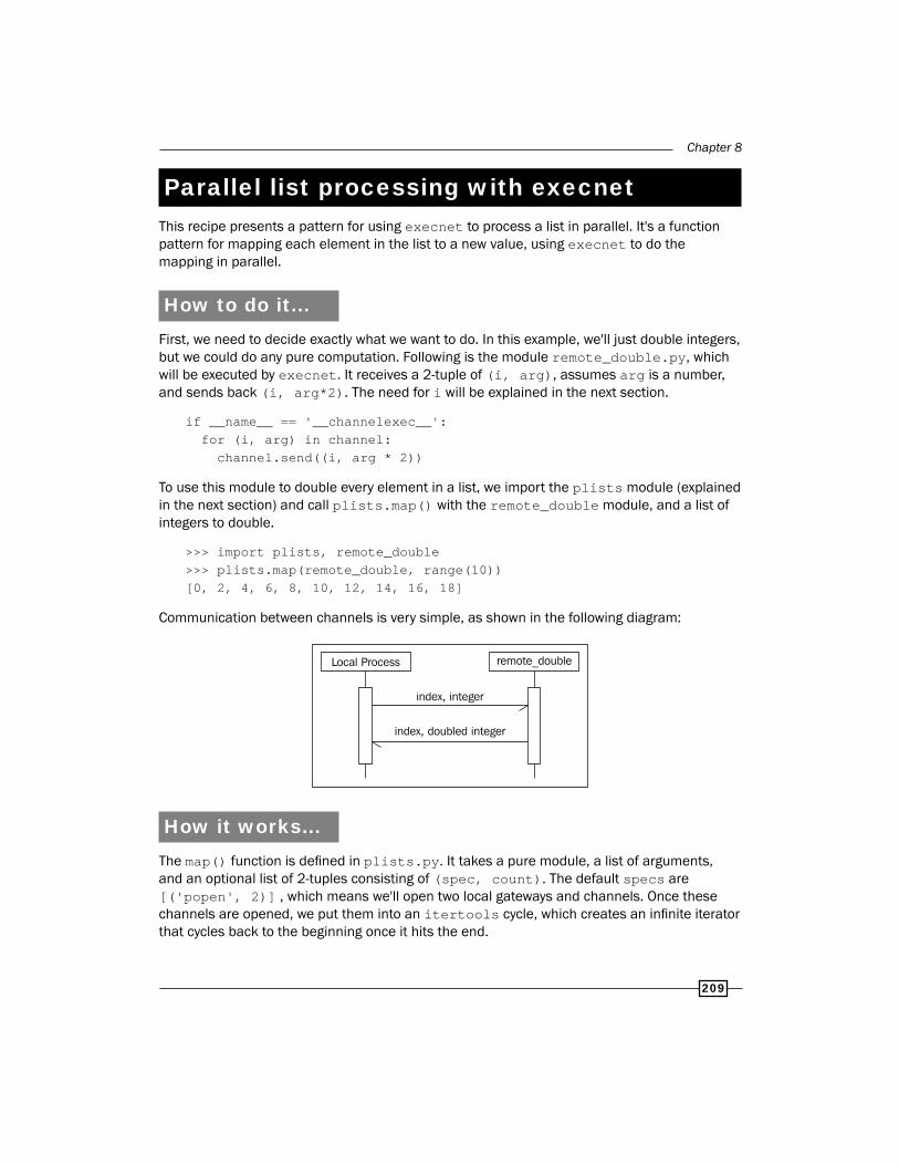
Chapter 8

209

Parallel list processing with execnetThis recipe presents a pattern for using execnet to process a list in parallel. It's a function pattern for mapping each element in the list to a new value, using execnet to do the mapping in parallel.

How to do it...First, we need to decide exactly what we want to do. In this example, we'll just double integers, but we could do any pure computation. Following is the module remote_double.py, which will be executed by execnet. It receives a 2-tuple of (i, arg), assumes arg is a number, and sends back (i, arg*2). The need for i will be explained in the next section.

if __name__ == '__channelexec__': for (i, arg) in channel: channel.send((i, arg * 2))

To use this module to double every element in a list, we import the plists module (explained in the next section) and call plists.map() with the remote_double module, and a list of integers to double.

>>> import plists, remote_double>>> plists.map(remote_double, range(10))[0, 2, 4, 6, 8, 10, 12, 14, 16, 18]

Communication between channels is very simple, as shown in the following diagram:

How it works...The map() function is defined in plists.py. It takes a pure module, a list of arguments, and an optional list of 2-tuples consisting of (spec, count). The default specs are [('popen', 2)] , which means we'll open two local gateways and channels. Once these channels are opened, we put them into an itertools cycle, which creates an infinite iterator that cycles back to the beginning once it hits the end.


210

Now we can send each argument in args to a channel for processing, and since the channels are cycled, each channel gets an almost even distribution of arguments. This is where i comes in—we don't know in what order we'll get the results back, so i, as the index of each arg in the list, is passed to the channel and back so we can combine the results in the original order. We then wait for results with a MultiChannel receive queue and insert them into a pre-filled list that's the same length as the original args. Once we have all the expected results, we can exit the gateways and return the results.

import itertools, execnet

def map(mod, args, specs=[('popen', 2)]): gateways = [] channels = []

for spec, count in specs: for i in range(count): gw = execnet.makegateway(spec) gateways.append(gw) channels.append(gw.remote_exec(mod))

cyc = itertools.cycle(channels)

for i, arg in enumerate(args): channel = cyc.next() channel.send((i, arg))

mch = execnet.MultiChannel(channels) queue = mch.make_receive_queue() l = len(args) results = [None] * l

for j in range(l): channel, (i, result) = queue.get() results[i] = result

for gw in gateways: gw.exit()

return results

There's more...You can increase the parallelization by modifying the specs, as follows:

>>> plists.map(remote_double, range(10), [('popen', 4)])[0, 2, 4, 6, 8, 10, 12, 14, 16, 18]

However, more parallelization does not necessarily mean faster processing. It depends on the available resources, and the more gateways and channels you have open, the more overhead is required. Ideally there should be one gateway and channel per CPU core.

Chapter 8

211

You can use plists.map() with any pure module as long as it receives and sends back 2-tuples where i is the first element. This pattern is most useful when you have a bunch of numbers to crunch, and want to process them as quickly as possible.

See alsoThe previous recipes cover execnet features in greater detail.

Storing a frequency distribution in RedisThe nltk.probability.FreqDist class is used in many classes throughout NLTK for storing and managing frequency distributions. It's quite useful, but it's all in-memory, and doesn't provide a way to persist the data. A single FreqDist is also not accessible to multiple processes. We can change all that by building a FreqDist on top of Redis.

Redis is a data structure server that is one of the more popular NoSQL databases. Among other things, it provides a network accessible database for storing dictionaries (also known as hash maps). Building a FreqDist interface to a Redis hash map will allow us to create a persistent FreqDist that is accessible to multiple local and remote processes at the same time.

Most Redis operations are atomic, so it's even possible to have multiple processes write to the FreqDist concurrently.

Getting readyFor this and subsequent recipes, we need to install both Redis and redis-py. A quick start install guide for Redis is available at http://code.google.com/p/redis/wiki/QuickStart. To use hash maps, you should install at least version 2.0.0 (the latest version as of this writing).

The Redis Python driver redis-py can be installed using pip install redis or easy_install redis. Ensure you install at least version 2.0.0 to use hash maps. The redis-py homepage is at http://github.com/andymccurdy/redis-py/.

Once both are installed and a redis-server process is running, you're ready to go. Let's assume redis-server is running on localhost on port 6379 (the default host and port).


212

How to do it...The FreqDist class extends the built-in dict class, which makes a FreqDist an enhanced dictionary. The FreqDist class provides two additional key methods: inc() and N(). The inc() method takes a single sample argument for the key, along with an optional count keyword argument that defaults to 1, and increments the value at sample by count. N() returns the number of sample outcomes, which is the sum of all the values in the frequency distribution.

We can create an API-compatible class on top of Redis by extending a RedisHashMap (that will be explained in the next section), then implementing the inc() and N() methods. Since the FreqDist only stores integers, we also override a few other methods to ensure values are always integers. This RedisHashFreqDist (defined in redisprob.py) uses the hincrby command for the inc() method to increment the sample value by count, and sums all the values in the hash map for the N() method.

from rediscollections import RedisHashMap

class RedisHashFreqDist(RedisHashMap): def inc(self, sample, count=1): self._r.hincrby(self._name, sample, count)

def N(self): return int(sum(self.values()))

def __getitem__(self, key): return int(RedisHashMap.__getitem__(self, key) or 0)

def values(self): return [int(v) for v in RedisHashMap.values(self)]

def items(self): return [(k, int(v)) for (k, v) in RedisHashMap.items(self)]

We can use this class just like a FreqDist. To instantiate it, we must pass a Redis connection and the name of our hash map. The name should be a unique reference to this particular FreqDist so that it doesn't clash with any other keys in Redis.

>>> from redis import Redis>>> from redisprob import RedisHashFreqDist>>> r = Redis()>>> rhfd = RedisHashFreqDist(r, 'test')>>> len(rhfd)0>>> rhfd.inc('foo')>>> rhfd['foo']1>>> rhfd.items()>>> len(rhfd)1

Chapter 8

213

The name of the hash map and the sample keys will be encoded to replace whitespace and & characters with _. This is because the Redis protocol uses these characters for communication. It's best if the name and keys don't include whitespace to begin with.

How it works...Most of the work is done in the RedisHashMap class, found in rediscollections.py, which extends collections.MutableMapping, then overrides all methods that require Redis-specific commands. Here's an outline of each method that uses a specific Redis command:

f __len__(): Uses the hlen command to get the number of elements in the hash map

f __contains__(): Uses the hexists command to check if an element exists in the hash map

f __getitem__(): Uses the hget command to get a value from the hash map

f __setitem__(): Uses the hset command to set a value in the hash map

f __delitem__(): Uses the hdel command to remove a value from the hash map

f keys(): Uses the hkeys command to get all the keys in the hash map

f values(): Uses the hvals command to get all the values in the hash map

f items(): Uses the hgetall command to get a dictionary containing all the keys and values in the hash map

f clear(): Uses the delete command to remove the entire hash map from Redis

Extending collections.MutableMapping provides a number of other dict compatible methods based on the previous methods, such as update() and setdefault(), so we don't have to implement them ourselves.

The initialization used for the RedisHashFreqDist is actually implemented here, and requires a Redis connection and a name for the hash map. The connection and name are both stored internally to use with all the subsequent commands. As mentioned before, whitespace is replaced by underscore in the name and all keys, for compatibility with the Redis network protocol.

import collections, re

white = r'[\s&]+'

def encode_key(key):


214

return re.sub(white, '_', key.strip())

class RedisHashMap(collections.MutableMapping): def __init__(self, r, name): self._r = r self._name = encode_key(name)

def __iter__(self): return iter(self.items())

def __len__(self): return self._r.hlen(self._name)

def __contains__(self, key): return self._r.hexists(self._name, encode_key(key))

def __getitem__(self, key): return self._r.hget(self._name, encode_key(key))

def __setitem__(self, key, val): self._r.hset(self._name, encode_key(key), val)

def __delitem__(self, key): self._r.hdel(self._name, encode_key(key))

def keys(self): return self._r.hkeys(self._name)

def values(self): return self._r.hvals(self._name)

def items(self): return self._r.hgetall(self._name).items()

def get(self, key, default=0): return self[key] or default

def iteritems(self): return iter(self)

def clear(self): self._r.delete(self._name)

There's more...The RedisHashMap can be used by itself as a persistent key-value dictionary. However, while the hash map can support a large number of keys and arbitrary string values, its storage structure is more optimal for integer values and smaller numbers of keys. However, don't let that stop you from taking full advantage of Redis. It's very fast (for a network server) and does its best to efficiently encode whatever data you throw at it.

Chapter 8

215

While Redis is quite fast for a network database, it will be significantly slower than the in-memory FreqDist. There's no way around this, but while you sacrifice speed, you gain persistence and the ability to do concurrent processing.

See alsoIn the next recipe, we'll create a conditional frequency distribution based on the Redis frequency distribution created here.

Storing a conditional frequency distribution in Redis

The nltk.probability.ConditionalFreqDist class is a container for FreqDist instances, with one FreqDist per condition. It is used to count frequencies that are dependent on another condition, such as another word or a class label. We used this class in the Calculating high information words recipe in Chapter 7, Text Classification. Here, we'll create an API-compatible class on top of Redis using the RedisHashFreqDist from the previous recipe.

Getting readyAs in the previous recipe, you'll need to have Redis and redis-py installed with an instance of redis-server running.

How to do it...We define a RedisConditionalHashFreqDist class in redisprob.py that extends nltk.probability.ConditionalFreqDist and overrides the __contains__() and __getitem__() methods. We then override __getitem__() so we can create an instance of RedisHashFreqDist instead of a FreqDist, and override __contains__() so we can call encode_key() from the rediscollections module before checking if the RedisHashFreqDist exists.

from nltk.probability import ConditionalFreqDistfrom rediscollections import encode_key

class RedisConditionalHashFreqDist(ConditionalFreqDist): def __init__(self, r, name, cond_samples=None): self._r = r self._name = name ConditionalFreqDist.__init__(self, cond_samples)


216

# initialize self._fdists for all matching keys for key in self._r.keys(encode_key('%s:*' % name)): condition = key.split(':')[1] self[condition] # calls self.__getitem__(condition)

def __contains__(self, condition): return encode_key(condition) in self._fdists

def __getitem__(self, condition): if condition not in self._fdists: key = '%s:%s' % (self._name, condition) self._fdists[condition] = RedisHashFreqDist(self._r, key)

return self._fdists[condition]

def clear(self): for fdist in self._fdists.values(): fdist.clear()

An instance of this class can be created by passing in a Redis connection and a base name. After that, it works just like a ConditionalFreqDist.

>>> from redis import Redis>>> from redisprob import RedisConditionalHashFreqDist>>> r = Redis()>>> rchfd = RedisConditionalHashFreqDist(r, 'condhash')>>> rchfd.N()0>>> rchfd.conditions()[]>>> rchfd['cond1'].inc('foo')>>> rchfd.N()1>>> rchfd['cond1']['foo']1>>> rchfd.conditions()['cond1']>>> rchfd.clear()

Chapter 8

217

How it works...The RedisConditionalHashFreqDist uses name prefixes to reference RedisHashFreqDist instances. The name passed in to the RedisConditionalHashFreqDist is a base name that is combined with each condition to create a unique name for each RedisHashFreqDist. For example, if the base name of the RedisConditionalHashFreqDist is 'condhash', and the condition is 'cond1', then the final name for the RedisHashFreqDist is 'condhash:cond1'. This naming pattern is used at initialization to find all the existing hash maps using the keys command. By searching for all keys matching 'condhash:*', we can identify all the existing conditions and create an instance of RedisHashFreqDist for each.

Combining strings with colons is a common naming convention for Redis keys as a way to define namespaces. In our case, each RedisConditionalHashFreqDist instance defines a single namespace of hash maps.

The ConditionalFreqDist class stores an internal dictionary at self._fdists that is a mapping of condition to FreqDist. The RedisConditionalHashFreqDist class still uses self._fdists, but the values are instances of RedisHashFreqDist instead of FreqDist. self._fdists is created when we call ConditionalFreqDist.__init__(), and values are initialized as necessary in the __getitem__() method.

There's more...RedisConditionalHashFreqDist also defines a clear() method. This is a helper method that calls clear() on all the internal RedisHashFreqDist instances. The clear() method is not defined in ConditionalFreqDist.

See alsoThe previous recipe covers the RedisHashFreqDist in detail. Also see the Calculating high information words recipe in Chapter 7, Text Classification, for example usage of a ConditionalFreqDist.


218

Storing an ordered dictionary in RedisAn ordered dictionary is like a normal dict, but the keys are ordered by an ordering function. In the case of Redis, it supports ordered dictionaries whose keys are strings and whose values are floating point scores. This structure can come in handy for cases such as calculating information gain (covered in the Calculating high information words recipe in Chapter 7, Text Classification) when you want to store all the words and scores for later use.

Getting readyAgain, you'll need Redis and redis-py installed, with an instance of redis-server running.

How to do it...The RedisOrderedDict class in rediscollections.py extends collections.MutableMapping to get a number of dict compatible methods for free. Then it implements all the key methods that require Redis ordered set (also known as Zset) commands.

class RedisOrderedDict(collections.MutableMapping): def __init__(self, r, name): self._r = r self._name = encode_key(name)

def __iter__(self): return iter(self.items())

def __len__(self): return self._r.zcard(self._name)

def __getitem__(self, key): val = self._r.zscore(self._name, encode_key(key))

if val is None: raise KeyError else: return val

def __setitem__(self, key, score): self._r.zadd(self._name, encode_key(key), score)

def __delitem__(self, key):by brain feels dead

self._r.zrem(self._name, encode_key(key))

def keys(self, start=0, end=-1): # we use zrevrange to get keys sorted by high value instead of by lowest

Chapter 8

219

return self._r.zrevrange(self._name, start, end)

def values(self, start=0, end=-1): return [v for (k, v) in self.items(start=start, end=end)]

def items(self, start=0, end=-1): return self._r.zrevrange(self._name, start, end, withscores=True)

def get(self, key, default=0): return self[key] or default

def iteritems(self):

return iter(self)

def clear(self): self._r.delete(self._name)

You can create an instance of RedisOrderedDict by passing in a Redis connection and a unique name.

>>> from redis import Redis>>> from rediscollections import RedisOrderedDict>>> r = Redis()>>> rod = RedisOrderedDict(r, 'test.txt')>>> rod.get('bar')>>> len(rod)0>>> rod['bar'] = 5.2>>> rod['bar']5.2000000000000002>>> len(rod)1>>> rod.items()[('bar', 5.2000000000000002)]>>> rod.clear()

How it works...Much of the code may look similar to the RedisHashMap, which is to be expected since they both extend collections.MutableMapping. The main difference here is that RedisOrderedSet orders keys by floating point values, and so is not suited for arbitrary key-value storage like the RedisHashMap. Here's an outline explaining each key method and how it works with Redis:

f __len__(): Uses the zcard command to get the number of elements in the ordered set.


220

f __getitem__(): Uses the zscore command to get the score of a key, and returns 0 if the key does not exist.

f __setitem__(): Uses the zadd command to add a key to the ordered set with the given score, or updates the score if the key already exists.

f __delitem__(): Uses the zrem command to remove a key from the ordered set.

f keys(): Uses the zrevrange command to get all the keys in the ordered set, sorted by highest score. It takes two optional keyword arguments start and end to more efficiently get a slice of the ordered keys.

f values(): Extracts all the scores from the items() method.

f items(): Uses the zrevrange command to get the scores of each key in order to return a list of 2-tuples ordered by highest score. Like keys(), it takes start and end keyword arguments to efficiently get a slice.

f clear(): Uses the delete command to remove the entire ordered set from Redis.

The default ordering of items in a Redis ordered set is low-to-high, so that the key with the lowest score comes first. This is the same as Python's default list ordering when you call sort() or sorted(), but it's not what we want when it comes to scoring. For storing scores, we expect items to be sorted from high-to-low, which is why keys() and items() use zrevrange instead of zrange.

There's more...As mentioned previously, the keys() and items() methods take optional start and end keyword arguments to get a slice of the results. This makes the RedisOrderedDict optimal for storing scores, then getting the top N keys. Here's a simple example where we assign three word scores, then get the top two:

>>> from redis import Redis>>> from rediscollections import RedisOrderedDict>>> r = Redis()>>> rod = RedisOrderedDict(r, 'scores')>>> rod['best'] = 10>>> rod['worst'] = 0.1>>> rod['middle'] = 5>>> rod.keys()['best', 'middle', 'worst']>>> rod.keys(start=0, end=1)['best', 'middle']>>> rod.clear()

Chapter 8

221

See also

Calculating high information words recipe in Chapter 7, Text Classification, describes how to calculate information gain, which is a good case for storing word scores in a RedisOrderedDict. The Storing a frequency distribution in Redis recipe introduces Redis and the RedisHashMap.

Distributed word scoring with Redis and execnet

We can use Redis and execnet together to do distributed word scoring. In the Calculating high information words recipe in Chapter 7, Text Classification, we calculated the information gain of each word in the movie_reviews corpus using a FreqDist and ConditionalFreqDist. Now that we have Redis, we can do the same thing using a RedisHashFreqDist and a RedisConditionalHashFreqDist, then store the scores in a RedisOrderedDict. We can use execnet to distribute the counting in order to get better performance out of Redis.

Getting readyRedis, redis-py, and execnet must be installed, and an instance of redis-server must be running on localhost.

How to do it...We start by getting a list of (label, words) tuples for each label in the movie_reviews corpus (which only has pos and neg labels). Then we get the word_scores using score_words() from the dist_featx module. word_scores is an instance of RedisOrderedDict, and we can see that the total number of words is 39,764. Using the keys() method, we can then get the top 1000 words, and inspect the top five just to see what they are. Once we have all we want from word_scores, we can delete the keys in Redis as we no longer need the data.

>>> from dist_featx import score_words>>> from nltk.corpus import movie_reviews>>> labels = movie_reviews.categories()>>> labelled_words = [(l, movie_reviews.words(categories=[l])) for l in labels]>>> word_scores = score_words(labelled_words)>>> len(word_scores)39764>>> topn_words = word_scores.keys(end=1000)


222

>>> topn_words[0:5]['_', 'bad', '?', 'movie', 't']>>> from redis import Redis>>> r = Redis()>>> [r.delete(key) for key in ['word_fd', 'label_word_fd:neg', 'label_word_fd:pos', 'word_scores']][True, True, True, True]

The score_words() function in dist_featx can take a while to complete, so expect to wait a couple of minutes. The overhead of using execnet and Redis means it will take significantly longer than a non-distributed in-memory version of the function.

How it works...The dist_featx.py module contains the score_words() function, which does the following:

1. Opens gateways and channels, sending initialization data to each.

2. Sends each (label, words) tuple over a channel for counting.

3. Sends a done message to each channel, waits for a done reply back, then closes the channels and gateways.

4. Calculates the score of each word based on the counts and stores in a RedisOrderedDict.

In our case of counting words in the movie_reviews corpus, calling score_words() opens two gateways and channels, one for counting the pos words, and the other for counting the neg words. The communication is as follows:

Chapter 8

223

Once the counting is finished, we can score all the words and store the results. The code itself is as follows:

import itertools, execnet, remote_word_countfrom nltk.metrics import BigramAssocMeasuresfrom redis import Redisfrom redisprob import RedisHashFreqDist, RedisConditionalHashFreqDistfrom rediscollections import RedisOrderedDict

def score_words(labelled_words, score_fn=BigramAssocMeasures.chi_sq, host='localhost', specs=[('popen', 2)]): gateways = [] channels = []

for spec, count in specs: for i in range(count): gw = execnet.makegateway(spec) gateways.append(gw) channel = gw.remote_exec(remote_word_count) channel.send((host, 'word_fd', 'label_word_fd')) channels.append(channel)

cyc = itertools.cycle(channels)

for label, words in labelled_words: channel = cyc.next() channel.send((label, list(words)))

for channel in channels: channel.send('done') assert 'done' == channel.receive() channel.waitclose(5)

for gateway in gateways: gateway.exit()

r = Redis(host) fd = RedisHashFreqDist(r, 'word_fd') cfd = RedisConditionalHashFreqDist(r, 'label_word_fd') word_scores = RedisOrderedDict(r, 'word_scores') n_xx = cfd.N()

for label in cfd.conditions(): n_xi = cfd[label].N()

for word, n_ii in cfd[label].iteritems(): n_ix = fd[word]

if n_ii and n_ix and n_xi and n_xx: score = score_fn(n_ii, (n_ix, n_xi), n_xx) word_scores[word] = score

return word_scores

Note that this scoring method will only be accurate when there are two labels. If there are more than two labels, then word scores for each label should be stored in separate RedisOrderedDict instances, one per label.


224

The remote_word_count.py module looks as follows:

from redis import Redisfrom redisprob import RedisHashFreqDist, RedisConditionalHashFreqDist

if __name__ == '__channelexec__': host, fd_name, cfd_name = channel.receive() r = Redis(host) fd = RedisHashFreqDist(r, fd_name) cfd = RedisConditionalHashFreqDist(r, cfd_name)

for data in channel: if data == 'done': channel.send('done') break

label, words = data

for word in words: fd.inc(word) cfd[label].inc(word)

You'll notice this is not a pure module as it requires being able to import both redis and redisprob. The reason is that instances of RedisHashFreqDist and RedisConditionalHashFreqDist cannot be pickled and sent over the channel. Instead, we send the host name and key names over the channel so we can create the instances in the remote module. Once we have the instances, there are two kinds of data we can receive over the channel:

1. A done message, which signals that there is no more data coming in over the channel. We reply back with another done message, then exit the loop to close the channel.

2. A 2-tuple of (label, words), which we then iterate over to increment counts in both the RedisHashFreqDist and RedisConditionalHashFreqDist.

There's more...In this particular case, it would be faster to compute the scores without using Redis or execnet. However, by using Redis, we can store the scores persistently for later examination and usage. Being able to inspect all the word counts and scores manually is a great way to learn about your data. We can also tweak feature extraction without having to re-compute the scores. For example, you could use featx.bag_of_words_in_set() (found in Chapter 7, Text Classification) with the top N words from the RedisOrderedDict, where N could be 1,000, 2,000, or whatever number you want. If our data size is much greater, the benefits of execnet will be much more apparent. Horizontal scalability using execnet or some other method to distribute computations across many nodes becomes more valuable, as the size of the data you need to process increases.

Chapter 8

225

See also

The Calculating high information words recipe in Chapter 7, Text Classification introduces information gain scoring of words for feature extraction and classification. The first three recipes of this chapter show how to use execnet, while the next three recipes describe RedisHashFreqDist, RedisConditionalHashFreqDist, and RedisOrderedDict respectively.

9Parsing Specific Data


f Parsing dates and times with Dateutil

f Time zone lookup and conversion

f Tagging temporal expressions with Timex

f Extracting URLs from HTML with lxml

f Cleaning and stripping HTML

f Converting HTML entities with BeautifulSoup

f Detecting and converting character encodings

IntroductionThis chapter covers parsing specific kinds of data, focusing primarily on dates, times, and HTML. Luckily, there are a number of useful libraries for accomplishing this, so we don't have to delve into tricky and overly complicated regular expressions. These libraries can be great complements to the NLTK:

f dateutil: Provides date/time parsing and time zone conversion

f timex: Can identify time words in text

f lxml and BeautifulSoup: Can parse, clean, and convert HTML

f chardet: Detects the character encoding of text

The libraries can be useful for pre-processing text before passing it to an NLTK object, or post-processing text that has been processed and extracted using NLTK. Here's an example that ties many of these tools together.

Parsing Specific Data

228

Let's say you need to parse a blog article about a restaurant. You can use lxml or BeautifulSoup to extract the article text, outbound links, and the date and time when the article was written. The date and time can then be parsed to a Python datetime object with dateutil. Once you have the article text, you can use chardet to ensure it's UTF-8 before cleaning out the HTML and running it through NLTK-based part-of-speech tagging, chunk extraction, and/or text classification, to create additional metadata about the article. If there's an event happening at the restaurant, you may be able to discover that by looking at the time words identified by timex. The point of this example is that real-world text processing often requires more than just NLTK-based natural language processing, and the functionality covered in this chapter can help with those additional requirements.

Parsing dates and times with DateutilIf you need to parse dates and times in Python, there is no better library than dateutil. The parser module can parse datetime strings in many more formats than can be shown here, while the tz module provides everything you need for looking up time zones. Combined, these modules make it quite easy to parse strings into time zone aware datetime objects.

Getting readyYou can install dateutil using pip or easy_install, that is sudo pip install dateutil or sudo easy_install dateutil. Complete documentation can be found at http://labix.org/python-dateutil.

How to do it...Let's dive into a few parsing examples:

>>> from dateutil import parser>>> parser.parse('Thu Sep 25 10:36:28 2010')datetime.datetime(2010, 9, 25, 10, 36, 28)>>> parser.parse('Thursday, 25. September 2010 10:36AM')datetime.datetime(2010, 9, 25, 10, 36)>>> parser.parse('9/25/2010 10:36:28')datetime.datetime(2010, 9, 25, 10, 36, 28)>>> parser.parse('9/25/2010')datetime.datetime(2010, 9, 25, 0, 0)>>> parser.parse('2010-09-25T10:36:28Z')datetime.datetime(2010, 9, 25, 10, 36, 28, tzinfo=tzutc())

As you can see, all it takes is importing the parser module and calling the parse() function with a datetime string. The parser will do its best to return a sensible datetime object, but if it cannot parse the string, it will raise a ValueError.

Chapter 9

229

How it works...The parser does not use regular expressions. Instead, it looks for recognizable tokens and does its best to guess what those tokens refer to. The order of these tokens matters, for example, some cultures use a date format that looks like Month/Day/Year (the default order) while others use a Day/Month/Year format. To deal with this, the parse() function takes an optional keyword argument dayfirst, which defaults to False. If you set it to True, it can correctly parse dates in the latter format.

>>> parser.parse('25/9/2010', dayfirst=True)datetime.datetime(2010, 9, 25, 0, 0)

Another ordering issue can occur with two-digit years. For example, '10-9-25' is ambiguous. Since dateutil defaults to the Month-Day-Year format, '10-9-25' is parsed to the year 2025. But if you pass yearfirst=True into parse(), it will be parsed to the year 2010.

>>> parser.parse('10-9-25')datetime.datetime(2025, 10, 9, 0, 0)>>> parser.parse('10-9-25', yearfirst=True)datetime.datetime(2010, 9, 25, 0, 0)

There's more...The dateutil parser can also do fuzzy parsing, which allows it to ignore extraneous characters in a datetime string. With the default value of False, parse() will raise a ValueError when it encounters unknown tokens. But if fuzzy=True, then a datetime object can usually be returned.

>>> try:... parser.parse('9/25/2010 at about 10:36AM')... except ValueError:... 'cannot parse''cannot parse'>>> parser.parse('9/25/2010 at about 10:36AM', fuzzy=True)datetime.datetime(2010, 9, 25, 10, 36)

See alsoIn the next recipe, we'll use the tz module from dateutil to do time zone lookup and conversion.


230

Time zone lookup and conversionMost datetime objects returned from the dateutil parser are naive, meaning they don't have an explicit tzinfo, which specifies the time zone and UTC offset. In the previous recipe, only one of the examples had a tzinfo, and that's because it's in the standard ISO format for UTC date and time strings. UTC is the coordinated universal time, and is the same as GMT. ISO is the International Standards Organization, which among other things, specifies standard date and time formatting.

Python datetime objects can either be naive or aware. If a datetime object has a tzinfo, then it is aware. Otherwise the datetime is naive. To make a naive datetime object time zone aware, you must give it an explicit tzinfo. However, the Python datetime library only defines an abstract base class for tzinfo, and leaves it up to the others to actually implement tzinfo creation. This is where the tz module of dateutil comes in—it provides everything you need to lookup time zones from your OS time zone data.

Getting readydateutil should be installed using pip or easy_install. You should also make sure your operating system has time zone data. On Linux, this is usually found in /usr/share/zoneinfo, and the Ubuntu package is called tzdata. If you have a number of files and directories in /usr/share/zoneinfo, such as America/, Europe/, and so on, then you should be ready to proceed. The following examples show directory paths for Ubuntu Linux.

How to do it...Let's start by getting a UTC tzinfo object. This can be done by calling tz.tzutc(), and you can check that the offset is 0 by calling the utcoffset() method with a UTC datetime object.

>>> from dateutil import tz>>> tz.tzutc()tzutc()>>> import datetime>>> tz.tzutc().utcoffset(datetime.datetime.utcnow())datetime.timedelta(0)

To get tzinfo objects for other time zones, you can pass in a time zone file path to the gettz() function.

>>> tz.gettz('US/Pacific')tzfile('/usr/share/zoneinfo/US/Pacific')>>> tz.gettz('US/Pacific').utcoffset(datetime.datetime.utcnow())datetime.timedelta(-1, 61200)

Chapter 9

231

>>> tz.gettz('Europe/Paris')tzfile('/usr/share/zoneinfo/Europe/Paris')>>> tz.gettz('Europe/Paris').utcoffset(datetime.datetime.utcnow())datetime.timedelta(0, 7200)

You can see the UTC offsets are timedelta objects, where the first number is days, and the second number is seconds.

If you're storing datetimes in a database, it's a good idea to store them all in UTC to eliminate any time zone ambiguity. Even if the database can recognize time zones, it's still a good practice.

To convert a non-UTC datetime object to UTC, it must be made time zone aware. If you try to convert a naive datetime to UTC, you'll get a ValueError exception. To make a naive datetime time zone aware, you simply call the replace() method with the correct tzinfo. Once a datetime object has a tzinfo, then UTC conversion can be performed by calling the astimezone() method with tz.tzutc().

>>> pst = tz.gettz('US/Pacific')>>> dt = datetime.datetime(2010, 9, 25, 10, 36)>>> dt.tzinfo>>> dt.astimezone(tz.tzutc())Traceback (most recent call last): File "/usr/lib/python2.6/doctest.py", line 1248, in __run compileflags, 1) in test.globs File "<doctest __main__[22]>", line 1, in <module> dt.astimezone(tz.tzutc())ValueError: astimezone() cannot be applied to a naive datetime>>> dt.replace(tzinfo=pst)datetime.datetime(2010, 9, 25, 10, 36, tzinfo=tzfile('/usr/share/zoneinfo/US/Pacific'))>>> dt.replace(tzinfo=pst).astimezone(tz.tzutc())datetime.datetime(2010, 9, 25, 17, 36, tzinfo=tzutc())

How it works...The tzutc and tzfile objects are both subclasses of tzinfo. As such, they know the correct UTC offset for time zone conversion (which is 0 for tzutc). A tzfile object knows how to read your operating system's zoneinfo files to get the necessary offset data. The replace() method of a datetime object does what its name implies—it replaces attributes. Once a datetime has a tzinfo, the astimezone() method will be able to convert the time using the UTC offsets, and then replace the current tzinfo with the new tzinfo.


232

Note that both replace() and astimezone() return new datetime objects. They do not modify the current object.

There's more...You can pass a tzinfos keyword argument into the dateutil parser to detect otherwise unrecognized time zones.

>>> parser.parse('Wednesday, Aug 4, 2010 at 6:30 p.m. (CDT)', fuzzy=True)datetime.datetime(2010, 8, 4, 18, 30)>>> tzinfos = {'CDT': tz.gettz('US/Central')}>>> parser.parse('Wednesday, Aug 4, 2010 at 6:30 p.m. (CDT)', fuzzy=True, tzinfos=tzinfos)datetime.datetime(2010, 8, 4, 18, 30, tzinfo=tzfile('/usr/share/zoneinfo/US/Central'))

In the first instance, we get a naive datetime since the time zone is not recognized. However, when we pass in the tzinfos mapping, we get a time zone aware datetime.

Local time zoneIf you want to lookup your local time zone, you can call tz.tzlocal(), which will use whatever your operating system thinks is the local time zone. In Ubuntu Linux, this is usually specified in the /etc/timezone file.

Custom offsetsYou can create your own tzinfo object with a custom UTC offset using the tzoffset object. A custom offset of one hour can be created as follows:

>>> tz.tzoffset('custom', 3600)tzoffset('custom', 3600)

You must provide a name as the first argument, and the offset time in seconds as the second argument.

See alsoThe previous recipe covers parsing datetime strings with dateutil.parser.

Chapter 9

233

Tagging temporal expressions with TimexThe NLTK project has a little known contrib repository that contains, among other things, a module called timex.py that can tag temporal expressions. A temporal expression is just one or more time words, such as "this week", or "next month". These are ambiguous expressions that are relative to some other point in time, like when the text was written. The timex module provides a way to annotate text so these expressions can be extracted for further analysis. More on TIMEX can be found at http://timex2.mitre.org/.

Getting readyThe timex.py module is part of the nltk_contrib package, which is separate from the current version of NLTK. This means you need to install it yourself, or use the timex.py module that is included with the book's code download. You can also download timex.py directly from http://code.google.com/p/nltk/source/browse/trunk/nltk_contrib/nltk_contrib/timex.py.

If you want to install the entire nltk_contrib package, you can check out the source at http://nltk.googlecode.com/svn/trunk/ and do sudo python setup.py install from within the nltk_contrib folder. If you do this, you'll need to do from nltk_contrib import timex instead of just import timex as done in the following How to do it... section.

For this recipe, you have to download the timex.py module into the same folder as the rest of the code, so that import timex does not cause an ImportError.

You'll also need to get the egenix-mx-base package installed. This is a C extension library for Python, so if you have all the correct Python development headers installed, you should be able to do sudo pip install egenix-mx-base or sudo easy_install egenix-mx-base. If you're running Ubuntu Linux, you can instead do sudo apt-get install python-egenix-mxdatetime. If none of those work, you can go to http://www.egenix.com/products/python/mxBase/ to download the package and find installation instructions.

How to do it...Using timex is very simple: pass a string into the timex.tag() function and get back an annotated string. The annotations will be XML TIMEX tags surrounding each temporal expression.

>>> import timex>>> timex.tag("Let's go sometime this week")"Let's go sometime <TIMEX2>this week</TIMEX2>">>> timex.tag("Tomorrow I'm going to the park.")"<TIMEX2>Tomorrow</TIMEX2> I'm going to the park."


234

How it works...The implementation of timex.py is essentially over 300 lines of conditional regular expression matches. When one of the known expressions match, it creates a RelativeDateTime object (from the mx.DateTime module). This RelativeDateTime is then converted back to a string with surrounding TIMEX tags and replaces the original matched string in the text.

There's more...timex is smart enough not to tag expressions that have already been tagged, so it's ok to pass TIMEX tagged text into the tag() function.

>>> timex.tag("Let's go sometime <TIMEX2>this week</TIMEX2>")"Let's go sometime <TIMEX2>this week</TIMEX2>"

See alsoIn the next recipe, we'll be extracting URLs from HTML, but the same modules and techniques can be used to extract the TIMEX tagged expressions for further processing.

Extracting URLs from HTML with lxmlA common task when parsing HTML is extracting links. This is one of the core functions of every general web crawler. There are a number of Python libraries for parsing HTML, and lxml is one of the best. As you'll see, it comes with some great helper functions geared specifically towards link extraction.

Getting readylxml is a Python binding for the C libraries libxml2 and libxslt. This makes it a very fast XML and HTML parsing library, while still being pythonic. However, that also means you need to install the C libraries for it to work. Installation instructions are at http://codespeak.net/lxml/installation.html. However, if you're running Ubuntu Linux, installation is as easy as sudo apt-get install python-lxml.

Chapter 9

235

How to do it...lxml comes with an html module designed specifically for parsing HTML. Using the fromstring() function, we can parse an HTML string, then get a list of all the links. The iterlinks() method generates four-tuples of the form (element, attr, link, pos):

f element: This is the parsed node of the anchor tag from which the link is extracted. If you're just interested in the link, you can ignore this.

f attr: This is the attribute the link came from, which is usually href. f link: This is the actual URL extracted from the anchor tag. f pos: This is the numeric index of the anchor tag in the document. The first tag has a

pos of 0, the second has a pos of 1, and so on.

Following is some code to demonstrate:>>> from lxml import html>>> doc = html.fromstring('Hello <a href="/world">world</a>')>>> links = list(doc.iterlinks())>>> len(links)1>>> (el, attr, link, pos) = links[0]>>> attr'href'>>> link'/world'>>> pos0

How it works...lxml parses the HTML into an ElementTree. This is a tree structure of parent nodes and child nodes, where each node represents an HTML tag, and contains all the corresponding attributes of that tag. Once the tree is created, it can be iterated on to find elements, such as the a or anchor tag. The core tree handling code is in the lxml.etree module, while the lxml.html module contains only HTML-specific functions for creating and iterating a tree. For complete documentation, see the lxml tutorial: http://codespeak.net/lxml/tutorial.html.

There's more...You'll notice in the previous code that the link is relative, meaning it's not an absolute URL. We can make it absolute by calling the make_links_absolute() method with a base URL before extracting the links.

>>> doc.make_links_absolute('http://hello')>>> abslinks = list(doc.iterlinks())


236

>>> (el, attr, link, pos) = abslinks[0]>>> link'http://hello/world'

Extracting links directlyIf you don't want to do anything other than extract links, you can call the iterlinks() function with an HTML string.

>>> links = list(html.iterlinks('Hello <a href="/world">world</a>'))>>> links[0][2]'/world'

Parsing HTML from URLs or filesInstead of parsing an HTML string using the fromstring() function, you can call the parse() function with a URL or file name. For example, html.parse("http://my/url") or html.parse("/path/to/file"). The result will be the same as if you loaded the URL or file into a string yourself, then called fromstring().

Extracting links with XPathsInstead of using the iterlinks() method, you can also get links using the xpath() method, which is a general way to extract whatever you want from HTML or XML parse trees.

>>> doc.xpath('//a/@href')[0]'http://hello/world'

For more on XPath syntax, see http://www.w3schools.com/XPath/xpath_syntax.asp.

See alsoIn the next recipe, we'll cover cleaning and stripping HTML.

Cleaning and stripping HTMLCleaning up text is one of the unfortunate but entirely necessary aspects of text processing. When it comes to parsing HTML, you probably don't want to deal with any embedded JavaScript or CSS, and are only interested in the tags and text. Or you may want to remove the HTML entirely, and process only the text. This recipe covers how to do both of these pre-processing actions.

Chapter 9

237

Getting readyYou'll need to install lxml. See the previous recipe or http://codespeak.net/lxml/installation.html for installation instructions. You'll also need NLTK installed for stripping HTML.

How to do it...We can use the clean_html() function in the lxml.html.clean module to remove unnecessary HTML tags and embedded JavaScript from an HTML string.

>>> import lxml.html.clean>>> lxml.html.clean.clean_html('<html><head></head><body onload=loadfunc()>my text</body></html>')'<div><body>my text</body></div>'

The result is much cleaner and easier to deal with. The full module path to the clean_html() function is used because there's also has a clean_html() function in the nltk.util module, but its purpose is different. The nltk.util.clean_html() function removes all HTML tags when you just want the text.

>>> import nltk.util>>> nltk.util.clean_html('<div><body>my text</body></div>')'my text'

How it works...The lxml.html.clean_html() function parses the HTML string into a tree, then iterates over and removes all nodes that should be removed. It also cleans nodes of unnecessary attributes (such as embedded JavaScript) using regular expression matching and substitution.

The nltk.util.clean_html() function performs a bunch of regular expression substitutions to remove HTML tags. To be safe, it's best to strip the HTML after cleaning it to ensure the regular expressions will match.

There's more...The lxml.html.clean module defines a default Cleaner class that's used when you call clean_html(). You can customize the behavior of this class by creating your own instance and calling its clean_html() method. For more details on this class, see http://codespeak.net/lxml/lxmlhtml.html.


238

See alsoThe lxml.html module was introduced in the previous recipe for parsing HTML and extracting links. In the next recipe, we'll cover un-escaping HTML entities.

Converting HTML entities with BeautifulSoup

HTML entities are strings such as & or <. These are encodings of normal ASCII characters that have special uses in HTML. For example, < is the entity for <. You can't just have < within HTML tags because it is the beginning character for an HTML tag, hence the need to escape it and define the < entity. The entity code for & is & which, as we've just seen, is the beginning character for an entity code. If you need to process the text within an HTML document, then you'll want to convert these entities back to their normal characters so you can recognize them and handle them appropriately.

Getting readyYou'll need to install BeautifulSoup, which you should be able to do with sudo pip install BeautifulSoup or sudo easy_install BeautifulSoup. You can read more about BeautifulSoup at http://www.crummy.com/software/BeautifulSoup/.

How to do it...BeautifulSoup is an HTML parser library that also contains an XML parser called BeautifulStoneSoup. This is what we can use for entity conversion. It's quite simple: create an instance of BeautifulStoneSoup given a string containing HTML entities and specify the keyword argument convertEntities='html'. Convert this instance to a string, and you'll get the ASCII representation of the HTML entities.

>>> from BeautifulSoup import BeautifulStoneSoup>>> unicode(BeautifulStoneSoup('<', convertEntities='html'))u'<'>>> unicode(BeautifulStoneSoup('&', convertEntities='html'))u'&'

It's ok to run the string through multiple times, as long as the ASCII characters are not by themselves. If your string is just a single ASCII character for an HTML entity, that character will be lost.

>>> unicode(BeautifulStoneSoup('<', convertEntities='html'))u''

Chapter 9

239

>>> unicode(BeautifulStoneSoup('< ', convertEntities='html'))u'< '

To make sure the character isn't lost, all that's required is to have another character in the string that is not part of an entity code.

How it works...To convert the HTML entities, BeautifulStoneSoup looks for tokens that look like an entity and replaces them with their corresponding value in the htmlentitydefs.name2codepoint dictionary from the Python standard library. It can do this if the entity token is within an HTML tag, or when it's in a normal string.

There's more...BeautifulSoup is an excellent HTML and XML parser in its own right, and can be a great alternative to lxml. It's particularly good at handling malformed HTML. You can read more about how to use it at http://www.crummy.com/software/BeautifulSoup/documentation.html.

Extracting URLs with BeautifulSoupHere's an example of using BeautifulSoup to extract URLs, like we did in the Extracting URLs from HTML with lxml recipe. You first create the soup with an HTML string, call the findAll() method with 'a' to get all anchor tags, and pull out the 'href' attribute to get the URLs.

>>> from BeautifulSoup import BeautifulSoup>>> soup = BeautifulSoup('Hello <a href="/world">world</a>')>>> [a['href'] for a in soup.findAll('a')][u'/world']

See alsoIn the Extracting URLs from HTML with lxml recipe, we covered how to use lxml to extract URLs from an HTML string, and we covered Cleaning and stripping HTML after that recipe.


240

Detecting and converting character encodings

A common occurrence with text processing is finding text that has a non-standard character encoding. Ideally, all text would be ASCII or UTF-8, but that's just not the reality. In cases when you have non-ASCII or non-UTF-8 text and you don't know what the character encoding is, you'll need to detect it and convert the text to a standard encoding before further processing it.

Getting readyYou'll need to install the chardet module, using sudo pip install chardet or sudo easy_install chardet. You can learn more about chardet at http://chardet.feedparser.org/.

How to do it...Encoding detection and conversion functions are provided in encoding.py. These are simple wrapper functions around the chardet module. To detect the encoding of a string, call encoding.detect(). You'll get back a dict containing two attributes: confidence and encoding. confidence is a probability of how confident chardet is that the value for encoding is correct.

# -*- coding: utf-8 -*-import chardet

def detect(s): try: return chardet.detect(s) except UnicodeDecodeError: return chardet.detect(s.encode('utf-8'))

def convert(s): encoding = detect(s)['encoding'] if encoding == 'utf-8': return unicode(s) else: return unicode(s, encoding)

Here's some example code using detect() to determine character encoding:

>>> import encoding>>> encoding.detect('ascii'){'confidence': 1.0, 'encoding': 'ascii'}

Chapter 9

241

>>> encoding.detect(u'abcdé'){'confidence': 0.75249999999999995, 'encoding': 'utf-8'}>>> encoding.detect('\222\222\223\225'){'confidence': 0.5, 'encoding': 'windows-1252'}

To convert a string to a standard unicode encoding, call encoding.convert(). This will decode the string from its original encoding, then re-encode it as UTF-8.

>>> encoding.convert('ascii')u'ascii' >>> encoding.convert(u'abcdé')u'abcd\\xc3\\xa9'>>> encoding.convert('\222\222\223\225')u'\u2019\u2019\u201c\u2022'

How it works...The detect() function is a wrapper around chardet.detect() which can handle UnicodeDecodeError exceptions. In these cases, the string is encoded in UTF-8 before trying to detect the encoding.

The convert() function first calls detect() to get the encoding, then returns a unicode string with the encoding as the second argument. By passing the encoding into unicode(), the string is decoded from the original encoding, allowing it to be re-encoded into a standard encoding.

There's more...The comment at the top of the module, # -*- coding: utf-8 -*-, is a hint to the Python interpreter, telling it which encoding to use for the strings in the code. This is helpful for when you have non-ASCII strings in your source code, and is documented in detail at http://www.python.org/dev/peps/pep-0263/.

Converting to ASCIIIf you want pure ASCII text, with non-ASCII characters converted to ASCII equivalents, or dropped if there is no equivalent character, then you can use the unicodedata.normalize() function.

>>> import unicodedata>>> unicodedata.normalize('NFKD', u'abcd\xe9').encode('ascii', 'ignore')'abcde'


242

Specifying 'NFKD' as the first argument ensures the non-ASCII characters are replaced with their equivalent ASCII versions, and the final call to encode() with 'ignore' as the second argument will remove any extraneous unicode characters.

See alsoEncoding detection and conversion is a recommended first step before doing HTML processing with lxml or BeautifulSoup, covered in the Extracting URLs from HTML with lxml and Converting HTML entities with BeautifulSoup recipes.

Penn Treebank Part-of-Speech Tags

Following is a table of all the part-of-speech tags that occur in the treebank corpus distributed with NLTK. The tags and counts shown here were acquired using the following code:

>>> from nltk.probability import FreqDist>>> from nltk.corpus import treebank>>> fd = FreqDist()>>> for word, tag in treebank.tagged_words():... fd.inc(tag)>>> fd.items()

The FreqDist fd contains all the counts shown here for every tag in the treebank corpus. You can inspect each tag count individually by doing fd[tag], as in fd['DT']. Punctuation tags are also shown, along with special tags such as -NONE-, which signifies that the part-of-speech tag is unknown. Descriptions of most of the tags can be found at http://www.ling.upenn.edu/courses/Fall_2003/ling001/penn_treebank_pos.html.

Penn Treebank Part-of-Speech Tags

244

Part-of-speech tag Frequency of occurrence

# 16

$ 724

'' 694

, 4,886

-LRB- 120

-NONE- 6,592

-RRB- 126

. 384

: 563

`` 712

CC 2,265

CD 3,546

DT 8,165

EX 88

FW 4

IN 9,857

JJ 5,834

JJR 381

JJS 182

LS 13

MD 927

NN 13,166

NNP 9,410

NNPS 244

NNS 6,047

PDT 27

POS 824

PRP 1,716

Appendix

245

Part-of-speech tag Frequency of occurrence

PRP$ 766

RB 2,822

RBR 136

RBS 35

RP 216

SYM 1

TO 2,179

UH 3

VB 2,554

VBD 3,043

VBG 1,460

VBN 2,134

VBP 1,321

VBZ 2,125

WDT 445

WP 241

WP$ 14

IndexSymbols__contains__() method 213__delitem__() method 213, 220__getitem__() method 213, 220__len__() method 213, 219__setitem__() method 213, 220

AAbstractLazySequence class

working 76accuracy() function 184ACE 133AffixTagger

about 96min_stem_length keyword argument 97working 96

anchor tag 235AntonymReplacer class 43antonyms

about 18, 41negations, replacing 41, 43

antonyms() method 19append_line() function 78aspell 36Automatic Content Extraction. See ACEavailable_languages attribute 31

BBabelfish

about 30text, translating 30, 31

babelfish.translate() function 30babelize() function 31backoff_tagger function 91

backoff taggingabout 88taggers, combining 88

backreference 34bag_of_bigrams_words() function 170bag_of_words() function

format 168working 168

Bag of Words model 168bag_of_words_not_in_set() function

about 169example 169

batch_tag() method 84Bayes Theorem

using 170BeautifulSoup library

about 227, 238, 239HTML entities, converting 238URLs, extracting 239

BigramCollocationFinder constructsbigrams, finding 22

BigramTaggerabout 90working 90, 91

binary classifier 167, 171binary named entity

extracting 135block 70block reader functions

read_blankline_block() 73read_line_block() 73read_regexp_block() 73read_whitespace_block() 73read_wordpunct_block() 73

BrillTaggerabout 98

248

training 98, 99working 99

Ccapitalization

need for 102cardinal word 150categorized chunk corpus reader

creating 61-64categorized text corpus

creating 58, 59category file 61cess_cat corpora

and cess_esp corpora 160cess_esp corpora

and cess_cat corpora 160channel

about 202multiple channels, creating 205

character encodingsconverting 240, 241detecting 240, 241

chardet.detect() function 241chardet library 227chinking

about 112with, regular expressions 112-114

ChinkRule class 112chinks 112choose_tag() method

about 83arguments 83

ChunkedCorpusReaderabout 55working 56

chunked phrase corpuscreating 54

chunk extraction 111chunking

about 112classification-based 129-132looping 125tracing 126with, regular expressions 112-114

chunk patternsabout 112

working 113, 114chunk rule

with, context 116, 117ChunkRule class 112chunks

about 54, 111, 144expanding, with regular expressions 121-123merging, with regular expressions 117-119removing, with regular expressions 121-123splitting, with regular expressions 117-119types 115

ChunkScoremetrics 125

chunk transformationschaining 154

chunk treeconverting, to text 155, 156

chunk_tree_to_sent() functionabout 156working 156

ChunkWithContext classexample 116

classification probabilitygetting 174, 175

ClassifierBasedPOSTaggerabout 106working 106

ClassifierBasedTagger class 129-132ClassifierChunker class 129-132classifiers

combining, with voting 191, 192classify() method 174, 175class-imbalance problem 199clean_html() function 237clear() method 213, 220collocations 21conditional exponential classifier. See

MaxentClassifierconditional frequency distribution

storing, in Redis 215, 217Conference on Computational Natural

Language Learning. See CoNLLCoNLL 58Conll chunk corpus reader

categorizing 65, 66context model

overriding 87

249

convert() function 241convert_tree_nodes() function

about 163tree nodes, converting 163, 164working 164

corporaabout 46categorizing 61

corpus 46corpus editing

and file locking 77, 78corpus view 70correct_verbs() function

about 147verb forms, correcting 146, 148working 148

CSV synonym replacement 40CsvWordReplacer class 40custom corpus

setting up 46, 47custom corpus view

creating 70

Ddates

parsing, with dateutil library 228, 229dateutil library

about 227dates, parsing 228, 229installing 230times, parsing 228, 229

decision tree classifiertraining 177, 178

DecisionTreeClassifierabout 177depth cutoff 179entropy cutoff 178, 179evaluating 190, 191support cutoff 179working 178

deep treeflattening 157-160

DefaultTaggerworking 83

default tagging 82depth_cutoff 179

detect() function 241dict style feature sets 168distributed chunking

execnet, used 206, 208distributed tagging

execnet, used 202, 204

Eedit distance 37Enchant

about 36personal word list 38

en_GB Dictionary 38entity tags 133entropy

about 178calculating 179

entropy_cutoff 178, 179estimator

training 175, 176evaluate() method 82, 84exclusive lock 77execnet

about 202distributed chunking 206, 208distributed tagging 202, 204distributed word scoring 221-223parallel list processing 209, 210

execnet.makegateway() function 203ExpandLeftRule rule 121ExpandRightRule rule 121

Ffalse negatives 183false positives 183feature detector 106feature_detector() function 173features 106feature set 106, 167filter_insignificant() function

about 145insignificant words, filtering 144, 145working 145

first_chunk_index() functionabout 147, 148using 149

250

flatten_childtrees() functionabout 157deep tree, flattening 159working 159

flatten_deeptree() functionabout 157, 162deep tree, flattening 158, 159working 159

F-measure 186frequency distribution

about 22storing, in Redis 211-214

full parsing 111fuzzy parsing 229

Ggateways

about 202local, comparing with remote 206

General Iterative Scaling. See gisgis 181grammar 112

Hheight() function 160high information word

about 187measuring 188, 189

high_information_words() functionworking 189

HTML entitiesabout 238converting, with BeautifulSoup library 238

hypernyms 15hyponyms 15

Iieer_chunked_sents() function

about 141using 140

ieer corpus 140ieertree2conlltags() function

using 140iis 181

Improved Iterative Scaling. See iisinfinitive phrase

about 151swapping 151

Information Extraction—Entity Recognition. See ieer corpus

information gain 175inpred lambda 152installation, NLTK 8instance 168International Standards Organization. See ISOIOB tags 56ISO 230items() method 213, 220iterlinks() function 235, 236

Jjaccard() function 189Jaccard index 189

Kkeys() method 213, 220

Llabel_feats_from_corpus() function 171, 173labelled feature sets 167LancasterStemmer class 26, 27Lancaster Stemming Algorithm 26LazyCorpusLoader class

about 68arguments 68working 69

Leacock Chodorow (LCH) similarity 21leaves() method 58lemma

about 17, 28finding, in WordNet 17, 18

lemmatizationabout 28combining, with stemming 29, 30

linksextracting 236

local gatewaysversus remote gateways 206

251

LocationChunker classworking 139

location chunksextracting 137, 139

log likelihood 181low information words 187lxml.html.clean_html() function 237lxml library

about 227, 234URLs, extracting from HTML 234working 235

Mmap() function 209masi distance

using 196MaxentClassifier

about 180evaluating 190requisites 180using 107working 181

maximum entropy classifiertraining 180, 181

MaxVoteClassifierworking 193

megam algorithmabout 183working 183

MergeRule classabout 117working 119

MongoDBabout 74working 76

morphy() function 29multi-label classifier 167

about 193classifying with 195, 196

multiple binary classifierscreating 193, 194

multiple channelscreating 205

Nnaive Bayes classifier

training 170-174NaiveBayesClassifier

about 170manual training 176working 173, 174

NaiveBayesClassifier classifier, methodsmost_informative_features() 175show_most_informative_features() 175

NaiveBayesClassifier.train() method 173NAME chunker 136, 139named entities

extracting 133, 134named entity chunker

training 140, 141named entity recognition 133, 134names corpus 49NamesTagger

about 105working 105

National Institute of Standards and Technology. See NIST

Natural Language Toolkit. See NLTKnegations

replacing, with antonyms 41, 43negative feature sets 198ngram 89NgramTagger 90NIST 133NLTK

about 7, 14, 202installing 8URL 8

nltk.data.find() functiondata directories, searching 65

nltk.data.load() function 47NLTK data package

installing 46nltk.metrics package 23nltk.tag package 82nltk.tag.pos_tag() function 202nltk.tag.untag() function 84nltk.tokenize.punkt module 9nltk.util.clean_html() function 237

252

non-UTC datetime objectconverting, to UTC datetime object 231

noun cardinalsswapping 150

Oordered dictionary

about 218, 219storing, in Redis 218, 219

Pparagraph block reader

customizing 53parallel list processing

execnet, used 209, 210parse() method 120, 139partial parsing

about 111with, regular expressions 123, 124

part-of-speech tagged word corpuscreating 50, 51

part-of-speech taggingabout 50, 82need for 82

part-of-speech tags 244`` 244, 244. 244’’ 244# 244$ 244about 82CC 244CD 244DT 244EX 244FW 244IN 244JJ 244JJR 244JJS 244-LRB- 244LS 244MD 244NN 244

NNP 244NNPS 244NNS 244-NONE- 244PDT 244POS 244PRP 244PRP$ 245RB 245RBR 245RBS 245RP 245-RRB- 244SYM 245TO 245UH 245VB 245VBD 245VBG 245VBN 245VBP 245VBZ 245WDT 245WP 245WP$ 245

path similarity 21Penn Treebank corpus 111P(features | label) probability 171P(features) probability 171phrases 111PickleCorpusView 73P(label | features) probability 171P(label) probability 171plural nouns

singularizing 153PorterStemmer class 26, 27Porter Stemming Algorithm 26positive feature sets 198POS tag

about 16example 16

precisionabout 183, 185measuring 183, 184

precision_recall() function 184, 185prob_classify() method 174

253

proper namestagging 105, 106

proper noun chunksextracting 135

PunktSentenceTokenizer 9PunktWordTokenizer 11pyenchant library 36Python subprocesses 208

QQuadgramTagger

about 91working 92

Rread_blankline_block() function 73read_line_block() function 73read_regexp_block() function 73read_whitespace_block() function 73read_wordpunct_block() function 73recall 183, 185Redis

about 211conditional frequency distribution, storing

215, 217distributed word scoring 221-223frequency distribution, storing 211-214ordered dictionary, storing 218, 219

reference set 185re.findall() method 12RegexpReplacer.replace() 33RegexpStemmer class 27RegexpTagger

about 95working 95

RegexpTokenizertokenizing, on whitespace 13working 12

regular expressionschinking 112-114chunking 112-114partial parsing 123, 124sentences, tokenizing 11, 12used, in tagging 94, 95

remote_exec() methodabout 203arguments, types 204

remote gatewaysversus local gateways 206

remove_line() function 78repeatitive characters

removing 34, 35RepeatReplacer class 35replace() method 32, 43replace_negations() method 43re.subn() function 32reuters corpus 194reuters_high_info_words() function 194

working 198

Sscoring functions 23scoring ngrams 23sentences

tagged sentence, untagging 84tagging 84tokenizing, into words 9, 10tokenizing, regular expressions used 11, 12

sentence tokenizercustomizing 53

SequentialBackoffTaggerabout 88working 88

shallow treecreating 161, 162

shallow_tree() functionabout 161shallow tree, creating 161, 162working 162

show_most_informative_features() method 182, 187

significant bigramsabout 170including 170

singularize_plural_noun() functionabout 153plural nouns, singularizing 153working 153

SnowballStemmer class 28SpaceTokenizer 10

254

SpellingReplacer class 37spellings

correcting, with Enchant 36, 37spicy algorithms

about 182Broyden-Fletcher-Goldfarb-Shanno algorithm

(BFGS) 182Conjugate gradient (CG) algorithm 182LBFGSB (limited memory version of BFGS)

182Nelder-Mead 182Powell 182

split_label_feats() function 173SplitRule class

about 117working 119

StemmerI interface 27stem() method 27, 28stemming

about 25combining, with lemmatization 29, 30

stopfile keyword 169stopwords

about 13, 144filtering 169filtering, in tokenized sentence 13

support_cutoff 179swap_infinitive_phrase() function

about 151infinitive phrases, swapping 152working 152

swap_noun_cardinal() functionabout 150noun cardinals, swapping 151working 151

swap_verb_phrase() functionabout 149verb phrases, swapping 149

synonymsreplacing 39, 40finding, in WordNet 17, 18

synsetsabout 15finding, for word in WordNet 14, 15

Ttag 82tagged corpus reader

categorizing 61TaggedCorpusReader

creating 51working 52

tagged sentenceuntagging 84

tagged_sents() function 82tagged token 52, 83tagger-based chunker

training 126-128taggers

about 82AffixTagger 96BigramTagger 89-91BrillTagger 98, 99ClassifierBasedPOSTagger 106, 107combining, with backoff tagging 88ContextTagger 85DefaultTagger 82, 83NamesTagger 105NgramTagger 85-91Quadgram 91, 92RegexpTagger 95SequentialBackoffTagger 83, 88TnT tagger 100, 101TrigramTagger 89UnigramTagger 85, 86, 93WordNetTagger 104

taggingregular expressions, used 94, 95WordNet, used 103, 104

tag mapping functiontags, simplifying 53

tag() method 82tag_pattern2re_pattern() function 112tag separator

customizing 53t.draw() method 113temporal expression

about 233tagging, with timex library 233

test set 185

255

texttokenizing, into sentences 8, 9translating, with Bablefish 30, 31

text classification 167text feature extraction 168time

parsing, with dateutil library 228, 229timex library

about 227temporal expressions, tagging 233using 233

TnT taggerabout 100working 101

tokenization 7, 8tokenized sentence

stopwords, filtering 13tokens 70trained tagger

preserving 89unpreserving 89

transform_chunk() functionabout 154chunk transformations, chaining 154working 154

treebank_chunk corpus 125treebank corpus 144, 243TreebankWordTokenizer 10, 11tree nodes

converting 163, 164Tree.pos() method 157TrigramCollocationFinder 23Trigrams’n’Tags. See TnT taggerTrigramTagger

about 89working 90, 91

true negative 183true positive 183tzfile object 231tzinfo object

getting 230tz.tzlocal() function 232

UUnChunkRule rule 121unicodedata.normalize() function 241

unigram 85UnigramTagger

about 85, 93training 85working 86

unlabelled feature set 167urllib request 31UTC 230

Vvalues() method 213, 220verb forms

correcting 146, 148verb phrases

swapping 149verbs

comparing 21voting

classifiers, combining with 191, 192

WWhitespaceTokenizer 10word list corpus

creating 48, 49WordListCorpusReader

about 48working 49

WordNetabout 8, 14lemma, finding 17, 18POS tag 16synonyms, finding 17, 18synset similarity, comparing 19, 20used, for tagging 103, 104words, lemmatising 28

WordNetCorpusReader class 29WordNetLemmatizer class 29WordNetTagger

working 104WordPunctTokenizer 11WordReplacer class 40words

lemmatising, with WordNet 28replacing, based on regular expressions

32, 33stemming 25, 26

256

insignificant words, filtering 144, 145word_tag_model() function 94word_tokenize() function

about 10working 10

word tokenizercustomizing 52

Wu-Palmer Similarity method. See wup_similarity() method

wup_similarity() method 20, 21

Xxpath() method

links, extracting 236

YYAML file

loading 47YAML synonym replacement 41

Thank you for buying Python Text Processing with

NLTK 2.0 Cookbook

About Packt PublishingPackt, pronounced 'packed', published its first book "Mastering phpMyAdmin for Effective MySQL Management" in April 2004 and subsequently continued to specialize in publishing highly focused books on specific technologies and solutions.

Our books and publications share the experiences of your fellow IT professionals in adapting and customizing today's systems, applications, and frameworks. Our solution based books give you the knowledge and power to customize the software and technologies you're using to get the job done. Packt books are more specific and less general than the IT books you have seen in the past. Our unique business model allows us to bring you more focused information, giving you more of what you need to know, and less of what you don't.

Packt is a modern, yet unique publishing company, which focuses on producing quality, cutting-edge books for communities of developers, administrators, and newbies alike. For more information, please visit our website: www.packtpub.com.

About Packt Open SourceIn 2010, Packt launched two new brands, Packt Open Source and Packt Enterprise, in order to continue its focus on specialization. This book is part of the Packt Open Source brand, home to books published on software built around Open Source licences, and offering information to anybody from advanced developers to budding web designers. The Open Source brand also runs Packt's Open Source Royalty Scheme, by which Packt gives a royalty to each Open Source project about whose software a book is sold.

Writing for PacktWe welcome all inquiries from people who are interested in authoring. Book proposals should be sent to [email protected]. If your book idea is still at an early stage and you would like to discuss it first before writing a formal book proposal, contact us; one of our commissioning editors will get in touch with you.

We're not just looking for published authors; if you have strong technical skills but no writing experience, our experienced editors can help you develop a writing career, or simply get some additional reward for your expertise.

Expert Python ProgrammingISBN: 978-1-847194-94-7 Paperback: 372 pages

Best practices for designing, coding, and distributing your Python software

1. Learn Python development best practices from an expert, with detailed coverage of naming and coding conventions

2. Apply object-oriented principles, design patterns, and advanced syntax tricks

3. Manage your code with distributed version control

4. Profile and optimize your code

MySQL for PythonISBN: 978-1-849510-18-9 Paperback: 440 pages

Integrate the flexibility of Python and the power of MySQL to boost the productivity of your Python applications

1. Implement the outstanding features of Python's MySQL library to their full potential

2. See how to make MySQL take the processing burden from your programs

3. Learn how to employ Python with MySQL to power your websites and desktop applications

4. Apply your knowledge of MySQL and Python to real-world problems instead of hypothetical scenarios

Please check www.PacktPub.com for information on our titles

Python 3 Object Oriented ProgrammingISBN: 978-1-849511-26-1 Paperback: 404 pages

Harness the power of Python 3 objects

1. Learn how to do Object Oriented Programming in Python using this step-by-step tutorial

2. Design public interfaces using abstraction, encapsulation, and information hiding

3. Turn your designs into working software by studying the Python syntax

4. Raise, handle, define, and manipulate exceptions using special error objects

Python Testing: Beginner's GuideISBN: 978-1-847198-84-6 Paperback: 256 pages

An easy and convenient approach to testing your powerful Python projects

1. Covers everything you need to test your code in Python

2. Easiest and enjoyable approach to learn Python testing

3. Write, execute, and understand the result of tests in the unit test framework


Spring Python 1.1ISBN: 978-1-849510-66-0 Paperback: 264 pages

Create powerful and versatile Spring Python applications using pragmatic libraries and useful abstractions

1. Maximize the use of Spring features in Python and develop impressive Spring Python applications

2. Explore the versatility of Spring Python by integrating it with frameworks, libraries, and tools

3. Discover the non-intrusive Spring way of wiring together Python components

4. Packed with hands-on-examples, case studies, and clear explanations for better understanding

Python MultimediaISBN: 978-1-849510-16-5 Paperback: 292 pages

Learn how to develop Multimedia applications using Python with this practical step-by-step guide

1. Use Python Imaging Library for digital image processing.

2. Create exciting 2D cartoon characters using Pyglet multimedia framework

3. Create GUI-based audio and video players using QT Phonon framework.

4. Get to grips with the primer on GStreamer multimedia framework and use this API for audio and video processing.


Matplotlib for Python DevelopersISBN: 978-1-847197-90-0 Paperback: 308 pages

Build remarkable publication-quality plots the easy way

1. Create high quality 2D plots by using Matplotlib productively

2. Incremental introduction to Matplotlib, from the ground up to advanced levels

3. Embed Matplotlib in GTK+, Qt, and wxWidgets applications as well as web sites to utilize them in Python applications

4. Deploy Matplotlib in web applications and expose it on the Web using popular web frameworks such as Pylons and Django


python text processing with - github pages · natural language processing. you want to employ...

Documents