pump jet mixing and pipeline transfer assessment for high-activity radioactive … ·...
TRANSCRIPT
PNNL-13275
Pump Jet Mixing and Pipeline TransferAssessment for High-ActivityRadioactive Wastes in HanfordTank 241 -AZ-1 02
Y. OnishiK. P. RecknagleB. E. Wells
July 2000
Prepared forthe U.S. Department of Energyunder Contract DE-AC06-76RL0 1830
Pacific Northwest National LaboratoryRichland, Washington 99352

DISCLAIMER
This report was+prepared as an account of work sponsoredby an agency of the United States Government. Neitherthe United States Government nor any agency thereof, norany of their empioyees, make any warranty, express orimplied, or assumes any legal liability or responsibility forthe accuracy, completeness, or usefulness of anyinformation, apparatus, product, or process disciosed~ orrepresents that its use would not infringe privately ownedrights. Reference herein to any specific commercialproduct, process, or service by trade name, trademark,manufacturer, or otherwise does not necessarily constituteor imply its endorsement, recommendation, or favoring bythe United States Government or any agency thereof. Theviews and opinions of authors expressed herein do notnecessarily state or reflect those of the United StatesGovernment or any agency thereof.
/,

DISCLAIMER
Portions of this document may be illegiblein electronic image products. Images areproduced from the best available originaldocument.
Summary
We evaluated how well two 300-hp mixer pumps would mix solid and liquid radioactivewastes stored in Hanford double-shell Tank 241-AZ-102 (AZ-102) and confirmed the adequacyof a three-inch (7.6-cm) pipeline system to transfer the resulting mixed waste slurry to the APTank Farm and a planned waste treatment (vitrification) plant on the Hanford Site. Tank AZ-102contains 854,000 gzdlons (3,230 m3) of supernatant liquid and 95,000 gallons (360 m3) of sludgemade up of aging waste (or neutralized current acid waste).
The study comprises three assessments: waste chemistry, pump jet mixing, and pipelinetransfer. Our waste chemical modeling assessment indicates that the sludge, consisting of thesolids and interstitial solution, and the supernatant liquid are basically in an equilibriumcondition. Thus, pump jet mixing would not cause much solids precipitation and dissolution,only 1.5% or less of the total AZ-102 sludge.
Our pump jet mixing modeling indicates that two 300-hp mixer pumps would mobilize up toabout 23 ft (7.0 m) of the sludge nearest the pump but would not erode the waste within seveninches (O.18 m) of the tank bottom. This results in about half of the sludge being uniformlymixed in the tank and the other half being unmixed (not eroded) at the tank bottom.
We evaluated sludge mobilization and mixing for cases where a diluent (a mixture of water,ferric nitrate, sodium nitrite, and sodium hydroxide) was added to the tank at a volume ratio of6:1 (diluent to sludge). We assumed that half of the AZ-102 sludge was dissolved and that theyield strength of the washed AZ-102 sludge was reduced from 1,540 Pa to 1.2 Pa for thisassessment. These pump jet mixing simulations indicated that, under these assumptions, the two300-hp mixer pumps would totally mobilize and uniformly mix the sludge in Tank AZ-102within two hours.
The waste pipeline transfer assessments indicate that the critical velocity for the AZ-102slurry is 1.5 ft/sec (0.46 m/s) or less, which is much less than the expected 6-ft./see (1.8-m/s)operating pipeline velocity. At the 1.2-ft./see (0.37 nis) critical velocity predicted by the Waspmethod, the associated pressure drops from the AZ Farm to the AP Farm and to the treatmentplant are expected to be 7.3 ft (2.2 m) and 14 ft (4.2 m), respectively, corresponding to only 1.6%and 3.0% of the available 450-ft (137-m) pump head. At 6-ft/sec (1.8 mh) operating velocity,the expected pressure drops between AZ- 102 and the AP Tank Farm and treatment plant are153 ft (47 m) and 285 ft (87 m), respectively, 34% and 63% of the available pump head. If thesolids concentration were 36 VOIYO,the pressure drop from the AZ Tank Farm to the treatmentplant would be 450 ft (137 m) at 6-ft/sec (1.8-m/s) velocity, which is more than 2. l-ft/sec(0.64 rds) critical velocity at this solids concentration. Even if the mixer pumps were tomobilize the entire inventory of AZ-102 solids, the average suspended solids concentrationwould be 3.1 VOIYU,which is less than 10% of the 36 vol%. Thus, the pipeline transfer pump hasenough capacity to transfer the AZ-102 slurry under expected conditions to the AP Tank Farmand treatment plant without depositing solids in the pipelines.
...m

Contents
summary...
...................................................................................................................................111
1.0 Introduction ......................................................................................................................... 1
2.0 Tank Waste Chmcteristics ..................................................................................................3
3.0 Waste Chemistry Assessment ...............................................................................................5
3.1 Chemical Modeling Approach ..........................................................................................5
3.2 Step 1: Selection of Aqueous Species of Interstitial Solution ...........................................6
3.3 Step 2: Determination of Dissolvable Solids in AZ-102 Sludge ....................................... 6
3.3.1 Step 2.1: Identification of Dissolvable Solids ............................................................ 8
3.3.2 Step 2.2: Conflation of Dissolvable Solids .......................................................... 10
3.4 Step 3: Mixture of AZ-102 Sludge and Supernatant Liquid ........................................... 11
3.5 Step 4: Determination of Changes on Waste Properties and Solid AmountDue to Cheticd Reactions ............................................................................................ 14
4.0 Pump Jet Waste Mixing Evaluation .................................................................................... 15
4.1 Pump Jet Mixing in Current AZ-102 Tank Conditions ................................................... 15
4.1.1 Sludge Mobiltiation ................................................................................................ 15
4.1.2 Jet Velocity Distribution .......................................................................................... 26
4.2 Alternative Pump Jet Mixing Approaches ......................................................................3l
5.0
6.0
7.0
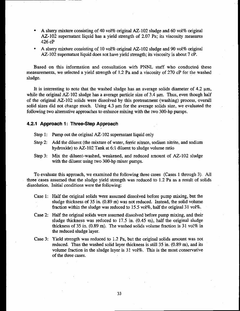
4.2.1 Approach 1: Three-Step Approach ..........................................................................33
4.2.2 Approach 2: Four-Step Approach 34...........................................................................
4.2.3 Alternative Approach Evaluation Results ................................................................34
AZ-102 Waste Pipeline Trmsfer ........................................................................................47
Summary and Conclusions .................................................................................................5l
Approach 1: Three-step approach .................................................................................52
Approach 2: Four-step approach ...................................................................................52
References .........................................................................................................................55
v
2.1
3.1
3.2
3.3
3.4
4.1
4.2
4.3
4.4
4.5
4.6
4.7
4.8
4.9
Figures
AZ-102 Tank Waste Volume-Based Particle Size Distibution ............................................4
Predicted Aqueous Species Concentrations of the AZ-102Interstitial Solution with Measured Data ........................................................................... 10
Predicted AZ-102 Solid Concentrations with Measured Data ............................................ 11
Predicted Aqueous Species Concentrations Resulting from MixingTank AZ-102 Sludge and Supematant Liquid, and Measured Values of theOriginal Supematant Liquid Primto Mx~g . .................................................................... 13.
Predicted Solids Concentrations Resulting from Mixing AZ-102 Sludge ‘and Supematant Liquid and Expected Solid Concentrations .............................................. 13
Initial Conditions of Sludge and Supernatant Liquid on Vertical Plane 2 ........................... 17
Predicted Distributions of Velocity and Solids Concentration onVertical Plane 2 at Two Skulation Hours ......................................................................... 19
Predicted Distributions of Velocity and Solids Concentration onVertical Plane 7 at Two Simulation Hours .........................................................................20
Predicted Distributions of Velocity and Solids Concentration on.
Vertical Plane 10 at Two Skulation Hous .......................................................................2l
Predicted Distributions of Velocity and Solids Concentration onVertical Plane 13 at Two Simulation Hours ....................................................................... 22
Predicted Distributions of Velocity and Solids Concentration onVertical Plane 14 at Two Simulation Hours .......................................................................23
Predicted Distributions of Velocity and Solids Concentration onVertical Plane 15 at Two SirnuIation Hom .......................................................................24
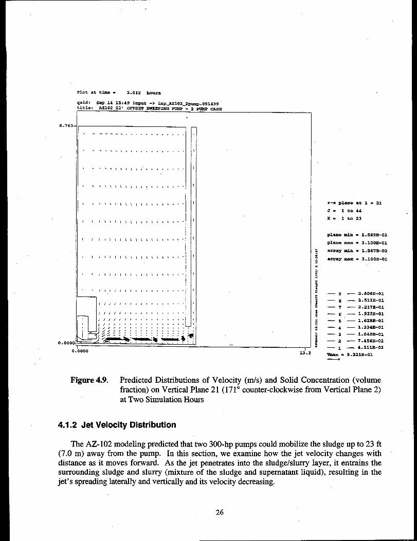
Predicted Distributions of Velocity and Solids Concentration onVertical Plane 21 at Two Simulation Hours .......................................................................25
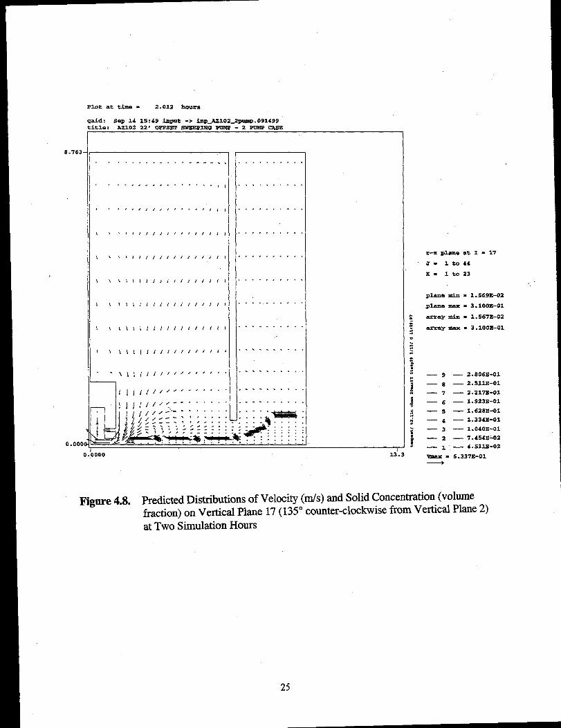
Predicted Distributions of Velocity and Solids Concent@ion onVertical Plane 17 at Two Simulation Hours .......................................................................26
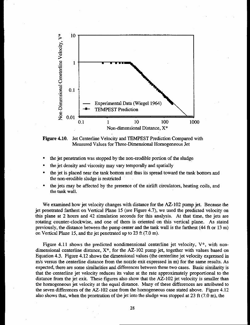
4.10 Jet Centerline Velocity and TEMPEST Prediction Compared withMeasured Values for Three-Dimensional Homogeneous Jet ..............................................28
4.11 Predicted Nondimensional Jet Centerline Velocity of the AZ-102 Pump Jetwith the Homogeneous Jet Velocity Distribution ...............................................................29
4.12 Predicted Jet Centerline Velocity with Centerline Distance of the AZ-102Pump Jet with Homogeneous Jet Velocity Distribution .....................................................29
4.13 Predicted Lateral Distribution of Nondimensional Longitudinal Velocityfor AZ-102 Pump Jet with Homogeneous Jet Velocity Distribution ...................................3O
4.14 Predicted Lateral Distribution of Longitudinal Velocity with LateralDistance for AZ-102 Pump Jet with Homogeneous Jet Velocity Distribution ....................31
4.15 Predicted Distributions of Velocity and Solids Concentration onVertical Plane 14 at Two Simulation Hours for Case 1......................................................35
4.16 Predicted Distributions of Velocity and Solids Concentration onVertical Plane 15 at Two Simulation Hours for Case 1 36......................................................
vi
4.17 Predicted Distributions of Velocity and Solids Concentration onVertical Plane 17 at Two SimulationHours for Case 1......................................................37
4.18 Predicted Distributions of Velocity and Solids Concentration onVertical Plane 14 at Two Simulation Hours for Case 2 ...................................................... 38
4.19 Predicted Distributions of Velocity and Solids Concentration onVertical Plane 15 at Two Simulation Hours for Case 2 ...................................................... 39
4.20 Predicted Distributions of Velocity and Solids Concentration onVertical Plane 17 at Two Simulation Hours for Case 2 ......................................................40
4.21 Predicted Distributions of Velocity and Solids Concentration onVertical Plane 14 at Two Simulation Hours for Case 3 ......................................................4l
4.22 Predicted Distributions of Velocity and Solids Concentration onVertical Plane 15 at Two Simulation Hours for Case 3 ......................................................42
4.23 Predicted Distributions of Velocity and Solids Concentration onVertical Plane 17 at Two 3Simulation Hours for Case 3 ....................................................43
4.24 Predicted Distributions of Velocity and Solids Concentration onVertical Plane 14 at Two Simulation Hours for Case 4 ......................................................44
-4.25 Predicted Distributions of Velocity and Solids Concentration onVertical Plane 15 at Two Simulation Hours for Case 4 ......................................................45
4.26 Predicted Distributions of Velocity and Solids Concentration on
5.1
5.2
3.1
3.2
3.3
3.4
5.1
5.2
5.3
Vertical Plane 17at Two Simulation Hours for Case 4 ......................................................46
Calculated Pipeline Pressure Drop Versus Pipeline Velocity for theAZ-102 Slurry with 1.6 vol% Solids ..................................................................................49
Calculated Pipeline Pressure Drop Versus Solids Concentration for theAZ-102 Slurry at 6 ft/sec (1.8 mh) ...................................................................................50
Tables
Chemical Compositions and Their Measured or Estimated Concentrationsfor Interstitial Solution of AZ-102 Sludge ...........................................................................7
Solids and Their Measured or Estimated Concentrations in AZ-102 Sludge ........................7
Summary of Solid Testing by GMIN ................................................................................. 10
Chemical Compositions and Measured or Estimated Concentrationsof the AZ-102 Supematant Liquid ..................................................................................... 12
Pipeline Transfer Assessment Parameters ..........................................................................47
AZ-102 Slurry Transfer Conditions at Critical Velocity of 1.2 ft/sec (0.37 rrh) ................48
&-102 Slurry Transfer Conditions at Pipeline Velocity of 6 Wsec (1.8 inks)....................48
vii
1.0 Introduction
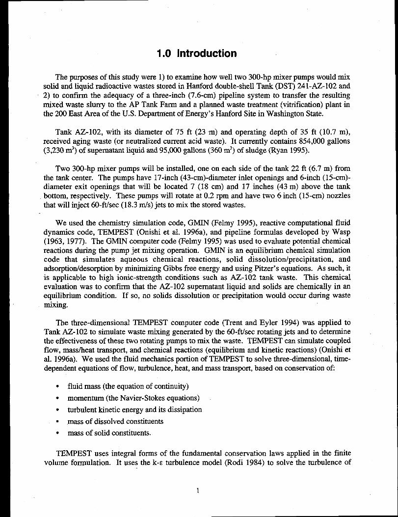
The purposes of this study were 1) to examine how well two 300-hp mixer pumps would mixsolid and liquid radioactive wastes stored in Hanford double-shell Tank (DST) 241-AZ-102 and2) to confirm the adequacy of a three-inch (7.6-cm) pipeline system to transfer the resultingmixed waste slurry to the AP Tank Farm and a planned waste treatment (vitrification) plant inthe 200 East Area of the U.S. Department of Energy’s Hanford Site in Washington State.
Tank AZ-102, with its diameter of 75 ft (23 m) and operating depth of 35 ft (10.7 m),received aging waste (or neutralized current acid waste). It currently contains 854,000 gallons(3,230 m’) of supematant liquid and 95,000 gallons (360 m’) of sludge (Ryan 1995).
Two 300-hp mixer pumps will be installed, one on each side of the tank 22 ft (6.7 m) fromthe tank center. The pumps have 17-inch (43-cm)-diameter inlet openings and 6-inch (15-cm)-diameter exit openings that will be located 7 (18 cm) and 17 inches (43 m) above the tankbottom, respectively. These pumps will rotate at 0.2 rpm and have two 6 inch (15-cm) nozzlesthat will inject 60-ft/sec (18.3 m/s) jets to mix the stored wastes.
We used the chemistry simulation code, GMIN (Felmy 1995), reactive computational fluiddynamics code, TEMPEST (Onishi et al. 1996a), and pipeline formulas developed by Wasp(1963, 1977). The GMIN computer code (Felmy 1995) was used to evaluate potential chemicalreactions during the pump jet mixing operation. GMIN is an equilibrium chemical simulationcode that simulates aqueous chemical reactions, solid dissolution/precipitation, andadsorption/desorption by minimizing Gibbs free energy and using Pitzer’s equations. As such, itis applicable to high ionic-strength conditions such as AZ-102 tank waste. This chemiciilevaluation was to confm that the AZ-102 supematant liquid and solids are chemically in anequilibrium condition. If so, no solids dissolution or precipitation would occur during wastemixing.
The three-dimensional TEMPEST computer code (Trent and Eyler 1994) was applied toTank AZ- 102 to simulate waste mixing generated by the 60-ft./sec rotating jets and to determinethe effectiveness of these two rotating pumps to mix the waste. TEMPEST can simulate coupledflow, mass/heat transport, and chemical reactions (equilibrium and kinetic reactions) (Onishi etal. 1996a). We used the fluid mechanics portion of TEMPEST to solve three-dimensional, time-dependent equations of flow, turbulence, heat, and mass transport, based on conservation ofi
● fluid mass (the equation of continuity)
● momentum (the Navier-Stokes equations)
“ turbulent kinetic energy and its dissipation● mass of dissolved constituents● mass of solid constituents.
TEMPEST uses integral forms of the fundamentalvolume formulation. It uses the k-s turbulence model
conservation laws applied in the finite(Rodi 1984) to solve the turbulence of
1
kinetic energy and its dissipation. TEMPEST can accommodatenon-Newtonian fluids as well asfluids whose rheology depends upon solid concentrations (Mahoney and Trent 1995; Onishi andTrent 1998).
We used the empirical Wasp formulas (Wasp 1963, 1977) to estimate the pipe flow’s criticalvelocity, below which solids could deposit in the pipe, and the pipeline pressure drop to evaluatetransfer of the mixed AZ-102 slurry to the AP Tank Farm and to the treatment plant through the3-inch (7.6-cm) pipeline. We also used the Oroskar-Turian (1980) and Zandi-Govatos (1967)methods to evaluate the critical velocity.
Section 2 describes the AZ-102 waste conditions. Section 3 describes chemical modeling byGMIN, and Section 4 reports pump jet mixing modeling results with TEMPEST. AZ-102 wastepipeline transfer assessments using the WASP, Oroskar-Turian, and Zandi-Govatos methods arepresented in Section 5. The summary and conclusions are presented in Section 6, and citedreferences are listed in Section 7.
2
2.0 Tank Waste Characteristics
Tank AZ-102 has a diameter and an operating depth of 75 ft (23 m) and 35 ft (10.7 m),respectively; its operational storage capacity is 1,160,000 gallons (4,390 m3). The tank containstwenty 30-inch- (76-cm-) diameter airlift circulators and 33-inch- (84-cm-)-diameter steamheating coils, which are no longer used. It currently contains 854,000 gallons (3,230 m3) ofsupematant liquid and 95,000 gallons (360 m3)of sludge-type radioactive waste (Ryan 1995).
Tank AZ- 102 received high-level aging waste from the PUREX Plant, high strontium wastefrom B Plant, and complex concentrated waste from 242-A evaporator beginning in 1976. In1986, most of this waste was removed. After 1986, it received aging waste (or neutralizedcurrent acid waste) from the PUREX Plant and waste water. Although it still remains in activeservice, the tank last received an aging waste in 1990 (Ryan 1995).
Current waste make-up is 90 vol% supematant liquid and 10 vol% sludge. The supematantliquid and sludge occupy 310 inches (7.87 m) and 35 inches (0.89 m), respectively, of the totaltank waste level of 345 inches (8.76 m). The average temperature of the supematant liquid is131°F (55”c), and the maximum sludge temperature is 182°F (83°C).
The density and viscosity of the supematant liquid are 1,100 kg/m3 and 1 cP, respectively(Ryan 1995). The dissolved solids constitute 15.9 wt% of the supematant liquid, and 84.1 wt%is water. The bulk sludge density is 1,490 kg/m3 (Ryan 1995).. The sludge has a yield strengthof 1,540 Pa; within a few centimeters of the bottom the yield strength is 2,650 Pa. Once thesludge is disturbed, the yield strength maybe reduced to about 60 Pay) roughly a 25- to 44-foldreduction. When the sludge was mixed with 1.5 times its volume of supematant liquid, the yieldstrength of the mixture was reduced to 2 Pajb) a 770- to 1,300-fold reduction from the undilutedcondition. When the sludge was diluted by 10 times its volume of supematant liquid, the mixedslurry totally lost its yield strength. ”Thus, diluting the sludge with liquid significantly reduces itsability to resist mobilization.
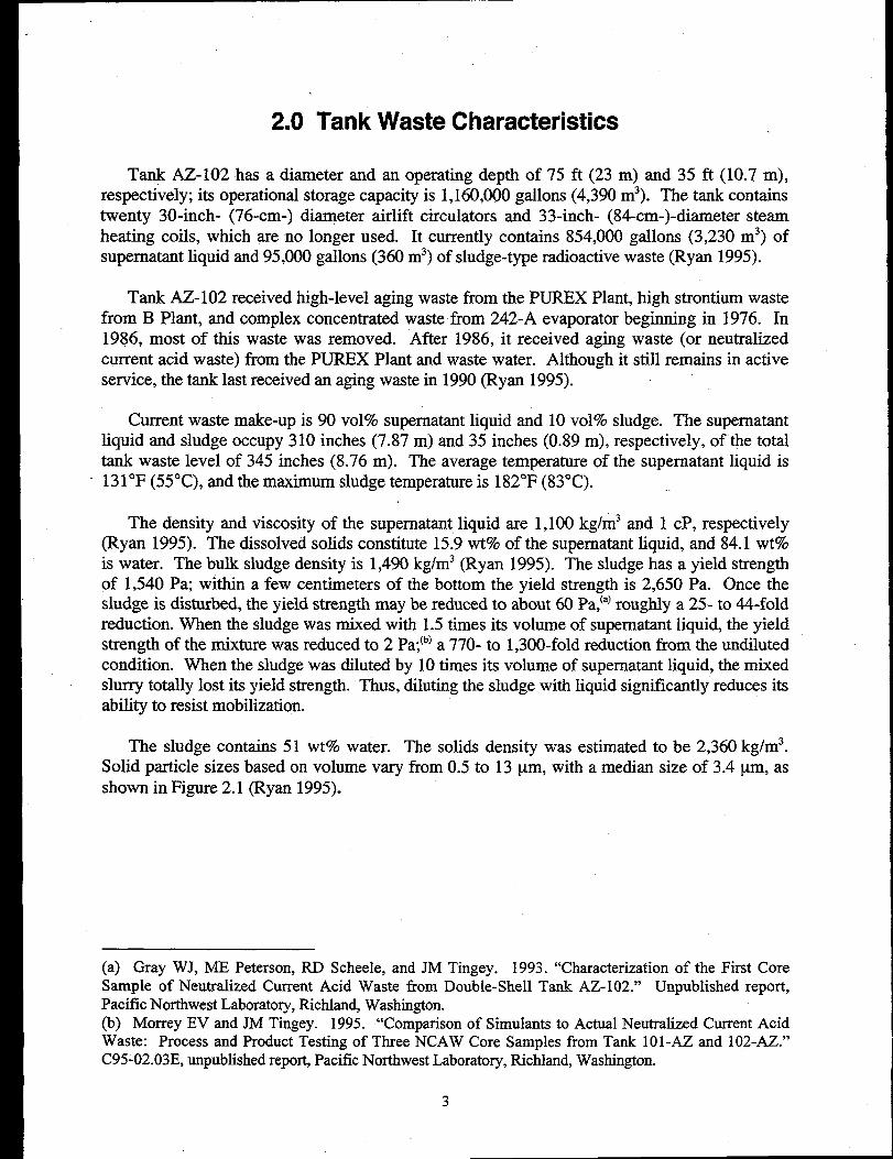
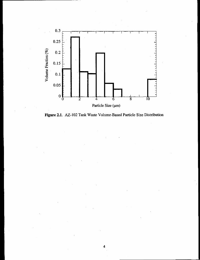
The sludge contains 51 wt% water. The solids density was estimated to be 2,360 kg/m3.Solid particle sizes based on volume vary from 0.5 to 13 ~m, with a median size of 3.4 pm, asshown in Figure 2.1 (Ryan 1995).
(a) Gray WJ, ME Peterson, RD Scheele, and JM Tingey. 1993. “Characterization of the First CoreSample of Neutralized Current Acid Waste from Double-Shell Tank AZ-102.” Unpublished report,Pacific Northwest Laboratory, Richland, Washington.(b) Morrey EV and JM Tingey. 1995. “Comparison of Simulants to Actual Neutralized Current AcidWaste: Process and Product Testing of Three NCAW Core Samples from Tank 101-AZ and 102-AZ.”C95-02.03E, unpublished report, Pacific Northwest Laboratory, Richland, Washington.
3
0.3
0.25
0.2
0.15
0.1
I I I I I I I I I I -1
—
I I
6 8 10
0.05
0
Particle Size (pm)
Figure 2.1. AZ- 102 Tank Waste Volbme-Based Particle Size Distribution
4
3.0 Waste Chemistry Assessment
3.1 Chemical Modeling Approach
As stated in Sections 1 and 2, the waste in Tank AZ-102 is high-activity level aging waste (orneutralized current acid waste). There are 854,000 gallons (3,230 m3) of supematant liquid and95,000 gallons (360 m3) of sludge (Ryan 1995). The average temperature of the supematantliquid is 131°F (55°C); the maximum sludge temperature is reported to be 182°F (83°C) (Ryan1995).
We investigated whether the AZ-102 supematant liquid and solids are in an equilibriumcondition. Because the present waste has been in AZ-102 since 1986 and the sludge thickness isonly 35 inches (0.88 m), the sludge and supematant liquid are expected to be in equilibriumcondition. If they are not in equilibrium, AZ-102 waste properties (e.g., density and viscosity ofsupematant liquid and sludge, and sludge yield strength) and the amount of solids in the sludgemay change due to solids dissolution and precipitation induced by the pump jet mixing. Thesepossible changes, in turn, would affect how and how much AZ-102 sludge would be mobilizedby the two 300-hp mixer pumps. Thus we performed a chemical evaluation of the waste beforeassessing the effectiveness of the mixer pumps.
We used the chemical code GMIN to simulate chemical reactions and phase equilibrium todetermine whether
“ AZ-102 solids are in equilibrium condition with the interstitial solution within theAZ-102 sludge
● AZ-102 sludge (consisting of the solids and the interstitial solution) would be in anequilibrium condhion with AZ-102 supematant liquid if the mixer pumps fully mixthe sludge and supematant liquid.
The following steps were taken to conduct this assessment
STEP 1. Assign cations, anions, and neutral aqueous species with the correct chargebalance for the interstitial solution of the sludge by using the measuredanalytical chemistry data.
STEP 2. Dete~ine dissolvable solids in the sludge that are saturated with theinterstitial solution
Substep 2.1, Simulate chemical reactions between the interstitial solution and onesolid at a time to determine whether the solid is saturated with themeasured interstitial solution without much change in solutionchemistry.
5
Substep 2.2. Simulate chemical reactions of the interstitial solution aqueous
STEP 3.
STEP 4.
We chose
species and all dissolvable solids selected under Substep 2.1together to confii that these solids axe saturated with the interstitialsolution without much change in solution conditions.
Simulate chemical reactions of the full mixture of sludge (both interstitialsolution and solids as selected under Step 2) and the supernatant liquid todetermine whether solids precipitation and dissolution will occur due topump jet mixing.
Determine possible changes in waste properties and solid amounts due tochemical reactions identiled under Step 3.
131“F (55”C) as the waste temperature for all the AZ-102 chemistry assessments.
3.2 Step 1: Selection of Aqueous Species of Interstitial Solution
Tank AZ-102 sludge (solid and interstitial solution) mostIy contains Al, Cd, Cr, Fe, Na, Ni,Si, U, Zr, inorganic carbon, and organic carbon (likely acetate), with the main anions of F, OH-,NO;, N02-, and SOA2-(Ryan 1995) .(’b) Water accounts for 51% of the sludge. Based on thecharacterization report by Ryan (1995), we selected the following species for the interstitialsolution to perform the chemical reaction modeling: Na+, Al(OH)l-, Cr(OH)q-, COJ2-,H#i012-,NO;, NO;, SOq2-,F OH, NaNO~(aq), and NaN02(aq). For interstitial solution in the AZ-102sludge layer, aqueous species selected in this study and their measured or estimated modalitiesare presented in Table 3.1. These molality values were input into GMIN for the sludgechemistry assessment. Note that NO~-and N02- in this table include their anion forms as well asapart of neutral aqueous species of NaNO~(aq) and NaNOz(aq), respectively.
3.3 Step 2: Determination of Dissolvable Solids in AZ-102 Sludge
Based on the characterization report by Ryan (1995) and chemical analysis performed byGray et al.(’) we selected the following as possible dissolvable solids in the AZ-102 sludge:Al(OH)~(s), amorphous Cr(OH)~, NaNO,(s), NaN02(s), thermonatrite (N%CO~”H20(s)),thenardite (Na#OJ(s)), NaF(s), and amorphous SiOz. Solids-bearing Cd, Fe, La, Ni, U, Zr, andorganic carbon (likely acetate) were treated here as insolvable solids with interstitial solution andsupernatant liquid of AZ-102 tank waste. Thus were not considered for possible dissolution orprecipitation due to pump jet mixing. These solids have very low volubility limits, as evidencedby very low or below detection levels of aqueous concentrations of species bearing these solidsin the interstitial solution. Thus this assumption was judged to be reasonable and conservative
(a) Gray WJ, ME Peterson, RD Scheele, and JM Tingey. 1993. “Characterization of the First CoreSample of Neutralized Current Acid Waste from Double-Shell Tank AZ-102.” Unpublished report,Pacific Northwest Laborato~, Richland, Washington.(b) Morrey EV and JM Tingey. 1995. “Comparison of Simulants to Actual Neutralized Current AcidWaste: Process and Product Testing of Three NCAW Core Samples from Tank 101-AZ and 102-AZ.”C95-02.03E, unpublished repoti~ Pacific Northwest Laboratory, Richland, Washington.
6
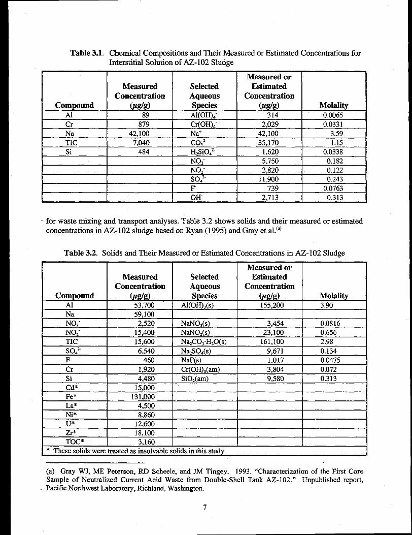
Table 3.1. Chemical Compositions and Their Measured or Estimated Concentrations forInterstitial Solution of AZ-102 Sludge
Measured orMeasured Selected Estimated
Concentration Aqueous ConcentrationCompound (Wk) Species Q%@ Molality
Al 89 Al(OH): 314 0.0065Cr 879 Cr(OH)i 2,029 0.0331Na 42,100 Na+ 42,100 3.59TIc 7,040 co32- 35,170 1.15Si 484 H#iOh2- 1,620 0.0338
NO; 5,750 0.182NO; 2,820 0.122S03 11,900 0.243F 739 0.0763OH- 2,713 0.313
for waste mixing and transport analyses. Table 3.2 shows solids and their measured or estimatedconcentrations in AZ-102 sludge based on Ryan (1995) and Gray et al.(’)
Table 3.2. Solids and Their Measured or Estimated Concentrations in AZ-102 Sludge
Measured orMeasured Selected Estimated
Concentration Aqueous ConcentrationCompound (wk ) Species (l@@) Molality
Al 53,700 Al(OH)~(s) 155,200 3.90Na 59,100NO~ 2,520 NaNO~(s) 3,454 0.0816NO; 15,400 NaN02(s) 23,100 0.656TIc 15,600 Na2CO~”H20(s) 161,100 2.98so42- 6$10 Na2SOg(s) 9,671 0.134F 460 NaF(s) 1.017 0.0475Cr 1.920 fi ,-... / \u[ um.( am) I 3.804 I 0.072
I 4.480 I SiO,(am) I 9.580 I 0.313I Cd* I 15.000 I I I
Fe* 131.000 I I II 4.500 I I II 8.860 I I I
fi* 18,100TOC* 3,160
* These solids were treated as insolvable solids in this study.
(a) Gray WJ, ME Peterson, RD Scheele, and JM Tingey. 1993. “Characterization of the First CoreSample of Neutralized Current Acid Waste from Double-Shell Tank AZ-102.” Unpublished report,Pacific Northwest Laborato~, fichland, Washington.
7
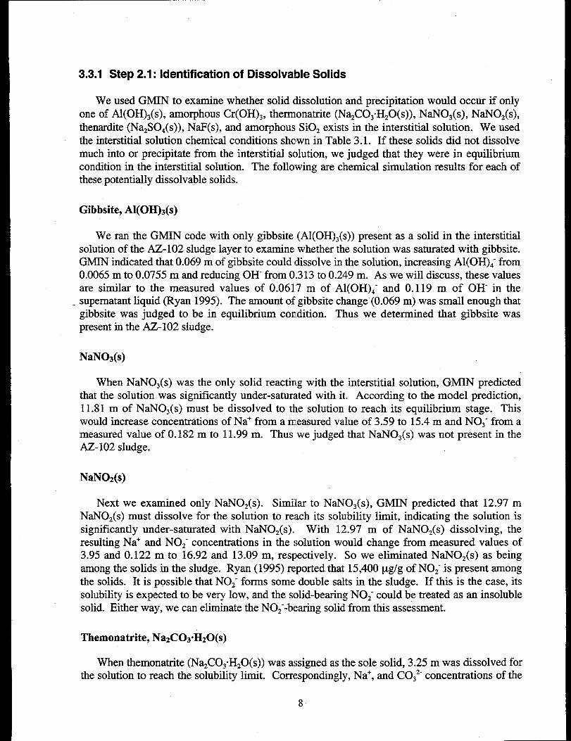
3.3.1 Step 2.1: Identification of Dissolvable Solids
We used GMIN to examine whether solid dissolution and precipitation would occur if onlyone of Al(OH)~(s), amorphous Cr(OH)~, thermonatrite (N~CO~.H20(s)), NaNO~(s), NaNOz(s),thenardite (NazSOg(s)), NaF(s), and amorphous Si02 exists in the interstitial solution. We usedthe interstitial solution chemical conditions shown in Table 3.1. If these solids did not dissolvemuch into or precipitate from the interstitial solution, we judged that they were in equilibriumcondition in the interstitial solution. The following are chemical simulation results for each ofthese potentially dissolvable solids.
Gibbsite, A1(OH)S(S)
We ran the GMIN code with only gibbsite (Al(OH)~(s)) present as a solid in the interstitialsolution of the AZ-102 sludge layer to examine whether the solution was saturated with gibbsite.GMIN indicated that 0.069 m of gibbsite could dissolve in the solution, increasing Al(OH)~ from0.0065 m to 0.0755 m and reducing OH”from 0.313 to 0.249 m. As we will discuss, these valuesare similar to the measured values of 0.0617 m of Al(OH)J- and 0.119 m of OH- in the
- supematant liquid (Ryan 1995). The amount of gibbsite change (0.069 m) was small enough thatgibbsite was judged to be in equilibrium condition. Thus we determined that gibbsite waspresent in the AZ-102 sludge.
NaN03(s)
When NaNO~(s) was the only solid reacting with the interstitial solution, GMIN predictedthat the solution was significantly under-saturated with it. According to the model prediction,11.81 m of NaNO~(s) must be dissolved to the solution to reach its equilibrium stage. Thiswould increase concentrations of Na+ from a measured value of 3.59 to 15.4 m and NO~-from ameasured value of 0.182 m to 11.99 m. Thus we judged that NaNO~(s) was not present in theAZ-102 sludge.
NaNOz(s)
Next we examined only NaNOz(s). Similar to NaNO~(s), GMIN predicted that 12.97 mNaNOz(s) must dissolve for the solution to reach its volubility limit, indicating the solution issignificantly under-saturated with NaN02(s). With 12.97 m of NaNOz(s) dissolving, theresulting Na+ and NOZ-concentrations in the solution would change from measured values of3.95 and 0.122 m to 16.92 and 13.09 m, respectively. So we eliminated NaN02(s) as beingamong the solids in the sludge. Ryan (1995) reported that 15,400 ~g/g of NOZ-is present amongthe solids. It is possible that NO; forms some double salts in the sludge. If this is the case, itsvolubility is expected to be very low, and the solid-bearing N02- could be treated as an insolublesolid. Either way, we can eliminate the N02--bearing solid from this assessment.
Themonatrite, NazCOs*H20(s)
When themonatrite (N~CO~”HzO(s)) was assigned as the sole solid, 3.25 m was dissolved forthe solution to reach the sohibility limit. Correspondingly, Na+, and COJ2-concentrations of the
8
interstitial solution changed from measured values of 3.59 and 1.15 m to 6.84 and 4.40 m,respectively. The molality of hydroxide also changed from 0.313 m to 3.56 m. Thus the GMINresults indicate that themonatrite is not among the solids, and we eliminated it from the list ofsolids present in the sludge. Although it is unlikely, it is possible that at about 25 to 40”C,N~COjC10HZO(S)and N~CO~”7HzO(s) could be present instead of NazCO~-H20(s). It is alsopossible that CO~maybe a part of some double or triple salts having very low volubility limits.Because we did not have their thermodynamic data into our GMIN database, we could not checkout these possibilities. However, because the waste has been in the tank for about 14 years,liquid, especially the interstitial solution within the sludge layer, is most likely in equilibriumcondition with the CO~-bearing solids and not under-saturated with them. If we did not accountfor these CO~-bearing solids being dissolved, our mixing assessment would be conservative.
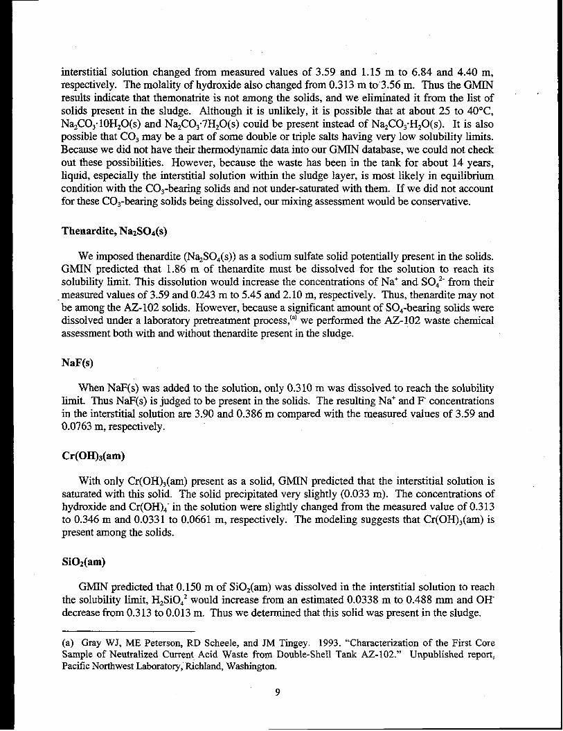
Thenardlte, Na2S04(s)
We imposed thenardite (Na#OA(s)) as a sodium sulfate solid potentially present in the solids.GMIN predicted that 1.86 m of thenardite must be dissolved for the solution to reach itsvolubility limit. This dissolution would increase the concentrations of Na+ and SOa2-from their
. measured values of 3.59 and 0.243 m to 5.45 and 2.10 m, respectively. Thus, thenardite may notbe among the AZ-102 solids. However, because a significant amount of SOJ-bearing solids weredissolved under a laboratory pretreatment process, “) we performed the AZ-102 waste chemicalassessment both with and without thenardite present in the sludge.
NaF(s)
When NaF(s) was added to the solution, only 0.310 m was dissolved to reach the volubilitylimit. Thus NaF(s) is judged to be present in the solids. The resulting Na+ and F concentrationsin the interstitial solution are 3.90 and 0.386 m compared with the measured values of 3.59 and0.0763 m, respectively.
Cars
With only Cr(OH)~(am) present as a solid, GMIN predicted that the interstitial solution issaturated with this solid. The solid precipitated very slightly (0.033 m). The concentrations ofhydroxide and Cr(OH)~ in the solution were slightly changed from the measured value of 0.313to 0.346 m and 0.0331 to 0.0661 m, respectively. The modeling suggests that Cry ispresent among the solids.
SiOz(am)
GMIN predicted that 0.150 m of Si02(am) was dissolved in the interstitial solution to reachthe volubility limit, H2Si012would increase from an estimated 0.0338 m to 0.488 mm and OH-decrease from 0.313 to 0.013 m. Thus we determined that this solid was present in the sludge.
(a) Gray WJ, ME Peterson, RD Scheele, and JM Tingey. 1993. “Characterization of the First CoreSample of Neutralized Current Acid Waste from Double-Shell Tank AZ-102.” Unpublished report,Pacific Northwest Laboratory, Richland, Washington.
9
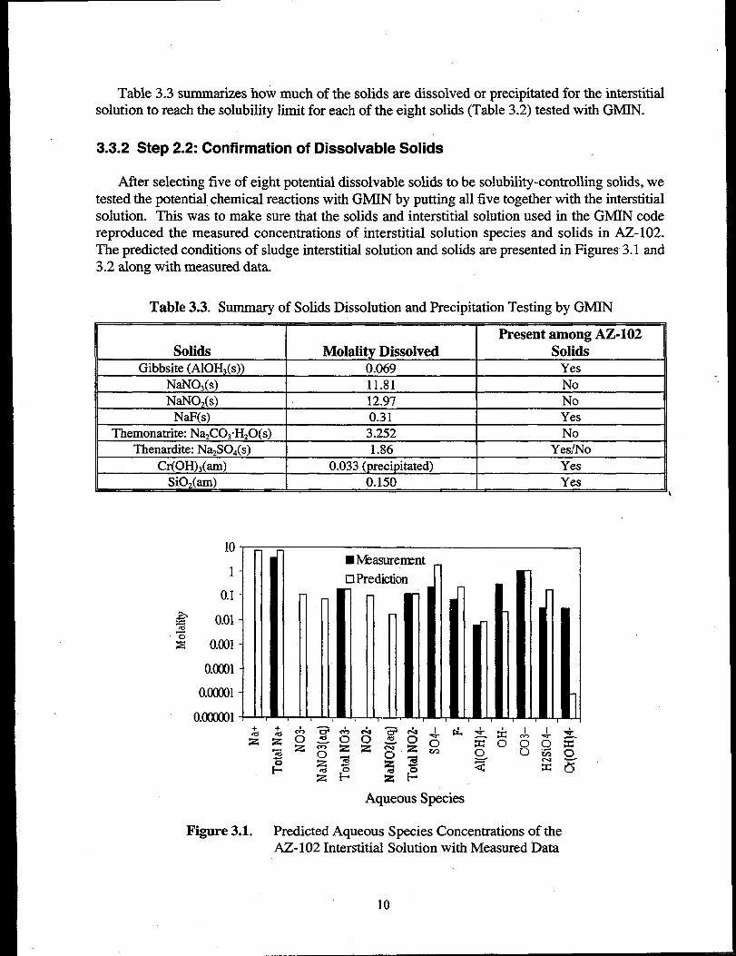
Table 3.3 summarizes how much of the solids are dissolved or precipitated for the interstitialsolution to reach the volubility limit for each of the eight solids (Table 3.2) tested with GMIN.
3.3.2 Step 2.2: Confirmation of Dissolvable Solids
After selecting five of eight potential dissolvable solids to be volubility-controlling solids, wetested the potential chemical reactions with GMIN by putting all five together with the interstitialsolution. This was to make sure that the solids and interstitial solution used in the GMIN codereproduced the measured concentrations of interstitial solution species and solids in AZ-102.The predicted conditions of sludge interstitial solution and solids are presented in Figures 3.1 and3.2 along with measured data.
Table 3.3. Summary of Solids Dissolution and Precipitation Testing by GMIN
Present among AZ-102Molality Dissolved Solids
Gibbsite (AIOHj(s)) 0.069 Yes11.81 No
No0.31 Yes
Themonatrite: NazCO~.HzO(s) 3.252 NoThenardite: Na$OA(s) 1.86 Yes/No
Car, 0.033 (precipitated) YesYes
t
10
1
0.1
0.0001
0.00001
0.00ooo1
■ MwuremmtEIPredfion
— II... SF’ 26
Aqueous Species
Figure 3.1. Predicted Aqueous Species Concentrations of theAZ-102 Interstitial Solution with Measured Data
10

These figures show that our AZ-102 waste chemistry predictions are reasonable based on theconditions we imposed (e.g., measured interstitial solution aqueous species concentrations wereour starting points without fust knowing specitlc solids present in the sludge). With thenarditepresent, the predicted Na+concentration was 7.00 m compared with a measured value of 3.59 m.Without thenardite, the predicted Na+ concentration of 3.85 m is much closer to measured value.For sodium, nitrate, and nitrite, the measurements only included the total amounts.
Through these modeling analyses, we concluded that the solids present in Tank AZ-102 areAl(OH)~(s), amorphous Cr(OH)~, NaF(s), amorphous SiOz, and possibly thenardite (N@O,(s)).The AZ- 102 interstitial solution in the sludge layer consists of H20 and aqueous chemicalspecies of Na+, Al(OH)g-,Cr(OH)d-, CO~2-,H2SiOJ2-,NO~-,NOZ-,SOd2-,F- OH-, NaNO~(aq), andNaN02(aq). We then mixed the sludge having these chemical characteristics with the AZ-102supematant liquid to determine whether any chemical and associated physical property changeswould OCCUr.
10
0.01
■ hhsuremmtQPred*n
,
solids
Figure 3.2. Predicted AZ-102 Solid Concentrations with Measured Data
3.4 Step 3: IVlixture of AZ-102 Sludge and Supernatant Liquid
Tank AZ-102 contains nine times as much supematant liquid as AZ-102 sludge by volume(Ryan 1995). The supematant liquid contains 84.1 wt% water. Its temperature averages about131°F (55”C). Table 3.4 shows its measured or estimated aqueous species concentrations (Ryan1995).(a)
(a) Gray WJ, ME Peterson, RD Scheele, and JM Tingey. 1993. “Characterization of the First CoreSample of Neutralized Current Acid Waste from Double-Shell Tank AZ-102.” Unpublished report,PacificNorthwestLaboratory,Richland,Washington.
11
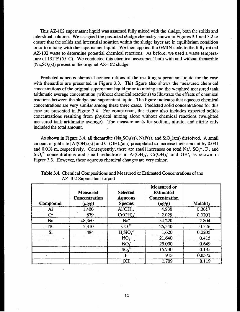
This AZ-102 supematant liquid was assumed fully mixed with the sludge, both the solids andinterstitial solution. We assigned the predicted sludge chemistry shown in Figures 3.1 and 3.2 toensure that the solids and interstitial solution within the sludge layer are in equilibrium conditionprior to mixing with the supematant liquid. We then applied the GMIN code to the fully mixedAZ-102 waste to determine potential chemical reactions. As before, we used a waste tempera-ture of 131‘F (55”C). We conducted this chemical assessment both with and without thenardite(Na$30.(s)) present in the original AZ-102 sludge.
Predicted aqueous chemical concentrations of the resulting supematant liquid for the casewith thenardite are presented in Figure 3.3. This figure also shows the measured chemicalconcentrations of the original supematant liquid prior to mixing and the weighted measured tankarithmetic average concentration (without cherrnicalreactions) to illustrate the effects of chemicalreactions between the sludge and supematant liquid. The figure indicates that aqueous chemicalconcentrations are very similar among these three cases. Predicted solid concentrations for thiscase are presented in Figure 3.4. For comparison, this figure also includes expected solidsconcentrations resulting from physical mixing alone without chemical reactions (weightedmeasured tank arithrnatic average). The measurements for sodium, nitrate, and nitrite onlyincluded the total amount.
As shown in Figure 3.4, all thenardite (N@lOd(s)), NaF(s), and Si02(am) dissolved. A smallamount of gibbsite [Al(OH)~(s)] ‘&d Cr(OH)~(am) precipitated to increase their amount by 0.031and 0.018 m, respectively. Consequently, there are small increases on total Na+, SOQ2-,F, andSiOq2-concentrations and small reductions in Al(OH)~, Cr(OH)~ and OH-, as shown inFigure 3.3. However, these aqueous chemical changes are very minor.
Table 3.4. Chemical Compositions and Measured or Estimated Concentrations of theAZ-102 Supematant Liquid
Measured orMeasured Selected Estimated
Concentration Aqueous ConcentrationCompound @k) Species (@g) Molality
Al 1,400 Al(OH)~ 4,930 0.0617Cr 879 Cr(OH)~ 2,029 0.0201Na 48,360 Na+ 54,220 2.804
TIc 5,310 co 2- 26,540 0.526Si 484 H$iOA2- 1,620 0.0205
NO; 21,640 0.415NO; 25,090 0.649so;- 15,730 0.195F 913 0.0572OH” 1,709 0.119
12
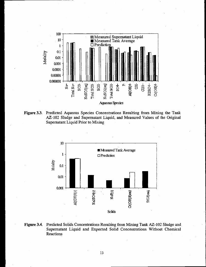
Figure 3.3.
Figure 3.4.
1(XI
10
1& 0.1.-z 0.01s 0.001
0.0001
O.ml
O.ml
ElMeasured Supematant Liquid■ Measured Ta.& Average -❑ Predict.i
Predicted Aqueous Species Concentrations Resulting from Mixing the TankAZ-102 Sludge and Supernatant Liquid, and Measured Values of the OriginalSupernatant Liquid Prior to Mixing
10
0.01
O.(x)l
■ Masured Tank Average
•l Prediction
I
Gsolids
Predicted Solids Concentrations Resulting from Mixing Tank AZ-102 Sludge andSupernatant Liquid and Expected Solid Concentrations Without ChemicalReactions
13
3.5 Step 4: Determination of Changes on Waste Properties and SolidAmount due to Chemical Reactions
The dissolution of thenardite (Na#Og(s)), NaF(s), and SiOz(am) attributes to a reduction ofsolids weight by 5,180, 550, 510 kg, respectively, for a total solid weight loss of 6,240 kg. Onthe other hand, precipitation of gibbsite (Al(OH)~(s)) and Cr(OH)~(am) contributes a solid weightgain of 6,540 and 510 kg, totaling 7,050 kg. Thus mixing the AZ-102 sludge and supematantliquid would result in the solids gaining 810 kg. Because the total AZ-102 sludge weighsapproximately 536,400 kg (Ryan 1995), the solid weight gain of810 kg corresponds to O.15% ofthe original sludge weight.
When we did not include thenardite among the AZ-102 solids, all NaF(s), and Si02(am) weredissolved, and a small amount of gibbsite [Al(OH)~(s)] and Cr(OH)~(am) precipitated, increasingits amount by 0.031 and 0.018 m, respectively. This corresponded to solid weight losses of 550and 510 kg for NaF(s) and SiOz(am) and weight gains of 6,540 and 510 kg. The net result is thesolid weight gain of 5,990 kg, corresponding to 1.1 wt% gain by the total AZ-102 sludge.
The chemical assessment discussed in this section indicates that mixing the sludge andsupernatant liquid of Tank AZ-102 would not change the waste properties and solids amount inany discemable manner due to chemical reactions resulting from the pump jet mixing. Thus, wedid not include the effects of chemistry on pump jet mixing when we assessed the effectivenessof the two 300-hp mixer pumps to mix the sludge and supematant liquid.
14

4.0 Pump Jet Waste Mixing Evaluation
4.1 Pump Jet Mixing in Current AZ-102 Tank Conditions
4.1.1 Sludge Mobilization
We evaluated how much” AZ-102 waste would be mixed by the 300-hp mixer pumps insimulations with the TEMPEST computer code (Onishi and Trent 1999). Because the chemicalassessment discussed in Section 3 indicated that the pump jet mixing would change the AZ-102waste properties and total solids volume very little, we used the values reported in the AZ-102Tank Characterization Report (Ryan 1995) and 1993 PNNL measurements.(a) Based on thesereports, we assigned the supernatant liquid density and viscosity to be 1,100 kg/m3 and 1 cP,respectively, in the model. The solids density and sludge yield strength were assigned to be2,360 kg/m3 and 1,540 Pa, respectively. With the assigned solid volume concentrationof31 % inthe sludge layer, the bulk sludge density corresponded to the measured value of 1,490 kg/m3.
The viscosity of the slurry changes spatially and temporally during mixing operations as aresult of the mixing of supematant liquid and solids. Based on viscosity measurements reportedby Gray et al.,(’)we prograrrimed the slurry viscosity in the AZ-102 model to vary with the solidsvolume concentration during the simulation as
wherec, =c Vmax=P’~L =
% =
/-%—
~L
solid volume fraction of
c“
c Vmax(4.1)
le slurrymaximum solid volume fkaction (0.33 in this study)viscosity of slurry at solid concentration of Cvviscosity of supematant liquid (1.0 CPin this study)viscosity of sludge layer (426 CPwhen the sludge moves at strain rate of 5 s-l).
As shown in Figure 2.1, the AZ-102 solid size distribution varied from 1 to 11 p, averaging3.4 pm. Corresponding settling velocities are small, 7.4 x 10-7,8.6 x 10-6,and 9.0 x 10⁻⁵rids,respectively. As previous pump jet mixing studies indicate (Onishi et al. 1996b; Onishi andRecknagle 1997, 1998; Whyatt et al. 1996), these settling velocities are much smaller than anexpected slurry velocity induced by pump jets in the tank, and resulting distributions of 1- to 11-~m solid particles are expected to be very similar to each other. Thus we assigned the diametersof all the solids to be 3.4 ~m for the AZ-102 pump jet mixing modeling. Because the actualsolids settling velocities will decrease with solid concentrations expected to occur in the tank, we
(a) Gray WJ, ME Peterson, RD Scheele, and Jh4 Tingey. 1993. “Characterization of the First CoreSample of Neutralized Current Acid Waste from Doubie-Shell Tank AZ-102.” Unpublished report,Pacific Northwest Laboratory, Richland, Washington.
15
assigned the hindering settling velocity changing with the solid concentration during thesimulation as
v, =V,o(ll- -%ac Vnlax
(4.2)
where= constant (4.7 in this study based on the Stokes Law)
;, = hindered setting velocity at solid volume fraction of CvV,. = unhindered settling velocity (settling velocity in a clear liquid containing no solids).
As stated above, the AZ-102 model contains twenty 30-inch (76-cm) -diameter airliftcirculators and 33-inch (84-cm)-diameter steam heating coils. These airlift circulators andheating coils are suspended approximately 30 in. (0.76 m) above the tank bottom. Because theyact as potential obstacles to the jets in mixing the waste, we included them in the model.
Each of the pumps has a 17-inch (43-cm)-diameter withdrawal inlet and two 6-inch (O.15-m)-diameter nozzles to inject 60-f/sec (l&3 rnh) jets. Because the pumps are on opposite sides ofthe tank, 22 ft (6.7 m) from the center, and they were assumed to rotate at 0.2 rpm in asynchronized mode, we only needed to simulate one half (the right side) of AZ-102 based onsymmetry.
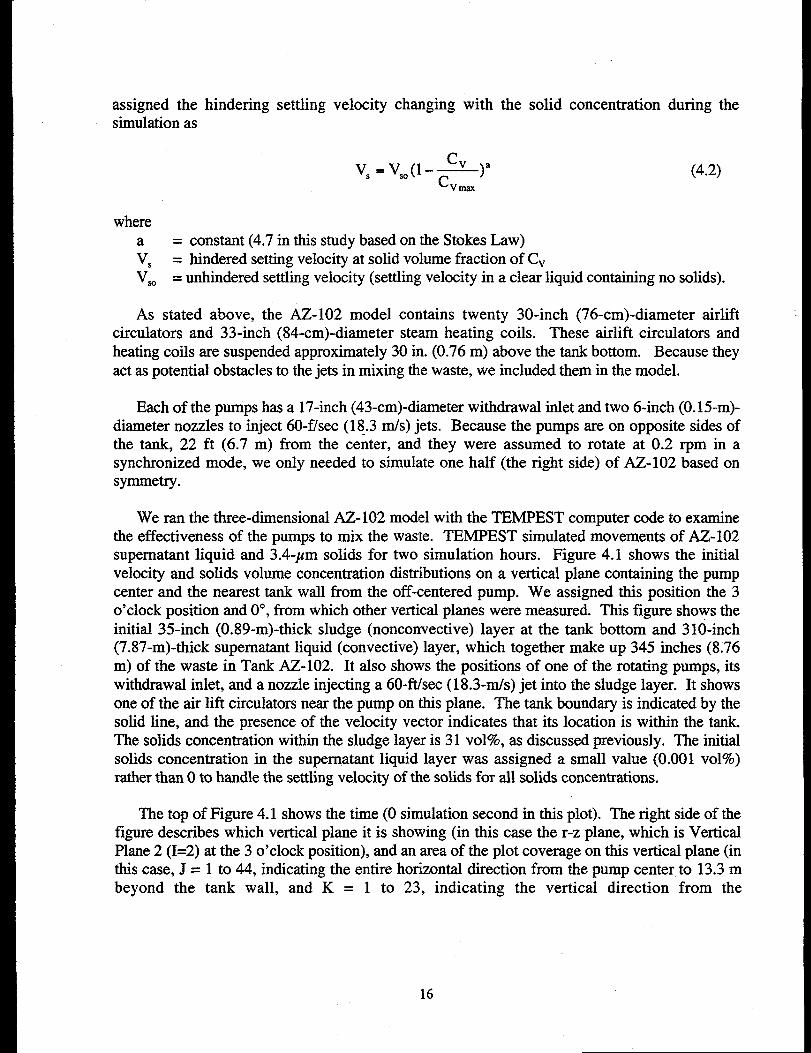
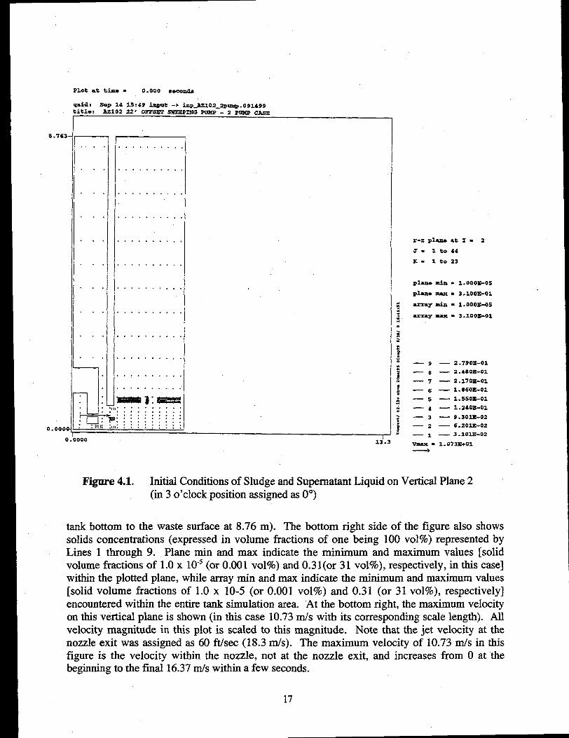
We ran the three-dimensional AZ-102 model with the TEMPEST computer code to examinethe effectiveness of the pumps to mix the waste. TEMPEST simulated movements of AZ-102supernatant liquid and 3.4-pm solids for two simulation hours. Figure 4.1 shows the initialvelocity and solids volume concentration distributions on a vertical plane containing the pumpcenter and the nearest tank wall from the off-centered pump. We assigned this position the 3o’clock position and 0°, from which other vertical planes were measured. This figure shows theinitial 35-inch (0.89-m)-thick sludge (nonconnective) layer at the tank bottom and 310-inch(7.87-m)-thick supematant liquid (convective) layer, which together makeup 345 inches (8.76m) of the waste in Tank AZ-102. It also shows the positions of one of the rotating pumps, itswithdrawal inlet, and a nozzle injecting a 60-ft/sec (18.3-m/s) jet into the sludge layer. It showsone of the airlift circulators near the pump on this plane. The tank boundary is indicated by thesolid line, and the presence of the velocity vector indicates that its location is within the tank.The solids concentration within the sludge layer is31 vol%, as discussed previously. The initialsolids concentration in the supematant liquid layer was assigned a small value (0.001 vol%)rather than Oto handle the settling velocity of the solids for all solids concentrations.
The top of Figure 4.1 shows the time (Osimulation second in this plot). The right side of thefigure describes which vertical plane it is showing (in this case the r-z plane, which is VerticalPlane 2 (1=2) at the 3 o’clock position), and an area of the plot coverage on this vertical plane (inthis case, J = 1 to 44, indicating the entire horizontal direction from the pump center to 13.3 mbeyond the tank wall, and K = 1 to 23, indicating the vertical direction from the
16
Plot at time = 0.000 sweads
8.763
0.0006
0
~ia: &p M 15:49 input -> *-3J31OL2IWW .091499itle: A2102 22 ‘ oFPs3m swEEPnw PUMP - 2 PUMP CAss
. . .
. . .
. . .
. . .
. . .
. . .
. . .
. . .
. . .
. . .
~
. .
. .. .,
: q,,; a)00
. . .
. . . . . . . . . .
. . . . . . . .
. . . . . . . . . .
. . . . . . . . . .
. . . . . . . . . .
,. ... . . . . .
. . . . . . . . .
. . . . . . . . .
. . . . .
. . . . . . . . .
. . . . . . . . .
L_JE!ss!#il:#=maa. . . . . . . . .. . . . . . . .,:::::: ::::::”:; ::. . . . . . .
r-zpl.aneat I=2
a- zt044
x- lt023
plan. & = 1.000s-05
plaw max = 3.1OOZ-OI
array mill = 1.000s-05
array max = 3.1008-01
—9
—8
—7
‘6
—5
—4
—3
—2
—z
— 2.79073-01
— 2.480B-01
— 2 .170E-01
— 1.860K-01
— 1.550E-01
— Z.2402!-01
— 9 .30~-02
— 6.202E-02
— 3 .102s-02
13.3 Vmax - 1.073E+01~
Figure 4.1. Initial Conditions of Sludge and Supematant Liquid on Vertical Plane 2(in 3 o’clock position assigned as 0°)
tank bottom to the waste surface at 8.76 m). The bottom right side of the figure also showssolids concentrations (expressed in volume fractions of one being 100 vol%) represented byLines 1 through 9. Plane min and max indicate the minimum and maximum values [solidvolume fractions of 1.0 x 10⁻⁵(or 0.001 vol%) and 0.3 l(or 31 vol%), respectively, in this case]within the plotted plane, while array min and max indicate the minimum and maximum values[solid volume fractions of 1.0 x 10⁻⁵ (or 0.001 vol%) and 0.31 (or 31 vol%), respectively]encountered within the entire tank simulation area. At the bottom right, the maximum velocityon this vertical plane is shown (in this case 10.73 nds with its corresponding scale length). Allvelocity magnitude in this plot is scaled to this magnitude. Note that the jet velocity at thenozzle exit was assigned as 60 ftisec (18.3 m/s). The maximum velocity of 10.73 rrds in thisfigure is the velocity within the nozzle, not at the nozzle exit, and increases from O at thebeginning to the final 16.37 IU/Swithin a few seconds.
17
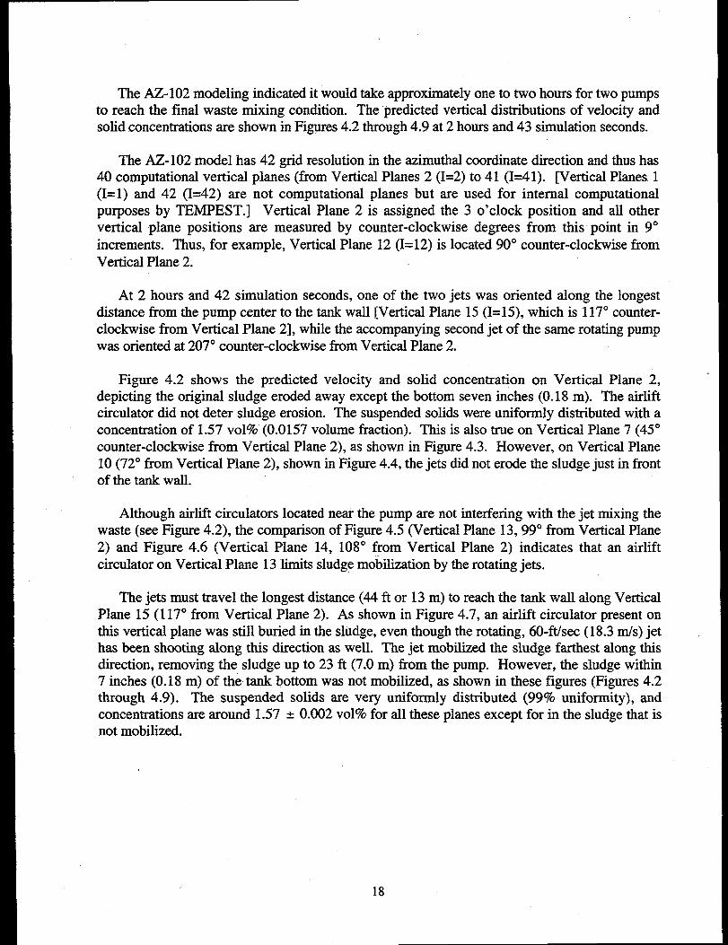
The AZ-102 modeling indicated it would take approximately one to two hours for two pumpsto reach the final waste mixing condition. The predicted vertical distributions of velocity andsolid concentrations are shown in Figures 4.2 through 4.9 at 2 hours and 43 simulation seconds.
The AZ- 102 model has 42 grid resolution in the azimuthal coordinate direction and thus has40 computational vertical planes (from Vertical Planes 2 (1=2) to 41 (1=41). [Vertical Planes 1(1=1) and 42 (1=42) are not computational planes but are used for internal computationalpurposes by TEMPEST.] Vertical Plane 2 is assigned the 3 o’clock position and all othervertical plane positions are measured by counter-clockwise degrees from this point in 9°increments. Thus, for example, Vertical Plane 12 (I= 12) is located 90° counter-clockwise fromVertical Plane 2.
At 2 hours and 42 simulation seconds, one of the two jets was oriented along the longestdistance from the pump center to the tank wall [Vertical Plane 15 (1=15), which is 117° counter-clockwise from Vertical Plane 2], while the accompanying second jet of the same rotating pumpwas oriented at 207° counter-clockwise from Vertical Plane 2.
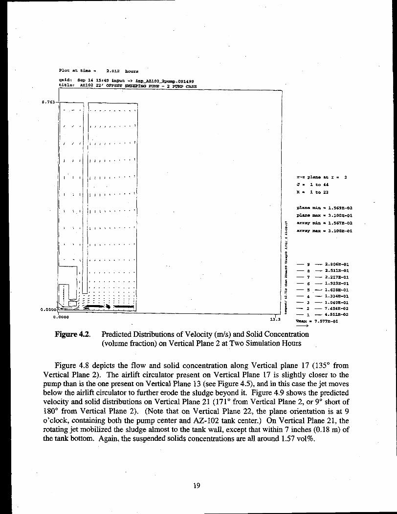
Figure 4.2 shows the predicted velocity and solid concentration on Vertical Plane 2, “depicting the original sludge eroded away except the bottom seven inches (O.18 m). The airliftcirculator did not deter sludge erosion. The suspended solids were uniformly distributed with aconcentration of 1.57 vol% (0.0157 volume fraction). This is also true on Vertical Plane 7 (45°counter-clockwise from Vertical Plane 2), as shown in Figure 4.3. However, on Vertical Plane10 (72° from Vertical Plane 2), shown in Figure 4.4, the jets did not erode the sludge just in frontof the tank wall.
Although airlift circulators located near the pump are not interfering with the jet mixing thewaste (see Figure 4.2), the comparison of Figure 4.5 (Vertical Plane 13, 99° from Vertical Plane2) and Figure 4.6 (Vertical Plane 14, 108° from Vertical Plane 2) indicates that an airliftcirculator on Vertical Plane 13 limits sludge mobilization by the rotating jets.
The jets must travel the longest distance (44 ft or 13 m) to reach the tank wall along VerticalPlane 15 (1 17° from Vertical Plane 2). As shown in Figure 4.7, an airlift circulator present onthis vertical plane was still buried in the sludge, even though the rotating, 60-ft/sec (18.3 rnk) jethas been shooting along this direction as well. The jet mobilized the sludge farthest along thisdirection, removing the sludge up to 23 ft (7.0 m) horn the pump. However, the sludge within7 inches (O.18 m) of the tank bottom was not mobilized, as shown in these figures (Figures 4.2through 4.9). The suspended solids are very uniformly distributed (99Y0 uniformity), andconcentrations are aroundnot mobilized.
0.002 vol% for all
18
these planes except for in the sludge that is
Plot at time . 2.012 hours
qaid: Sep 14 15:49 input -> iap_Az102_2w .091499ith: A2102 22r OFFSET SWEEPING PUMP - 2 PUMP CASE
8.763.
0.000(
c
. . ..- ----
,,> (..-.,
11114’..’>
,,, ,’ ...,1
,,, ;,, ..,1
,,, ,,. ..!1
,,, ,. . ...1
111~..-..’
,8, ,. . ...1
,, . . . . . . .,
,,, . . . . . .,
. . . . . . . . .
piu,,........,....................._q’:&=::~+~:i [—. . . . . . .)00 I---
r-z Plane at I = 2
3= lt044
K= lt023
Dh53 * = 1.569E-02
plane w = 3.10074-01
; -Uy min = 1.567E-02
R= -W = = 3.1OOE-O1
—9
‘8
—7
‘6
—5
—4
—3
—2
—1
— 2 .806E-01
— 2.S12E-01
— 2.217E-01
— 1.923E-01
— 1.628E-01
— 1.334E-01
— 1.040s-01
— 7.454E-02
— 4.512B-02
7.S77E-01
F~e 4.2. Predicted Distributions of Velocity (m/s) and Solid Concentration(volume fraction) on Vertical Plane 2 at Two Simulation Hours
Figure 4.8 depicts the flow and solid concentration along Vertical plane 17 (135° fromVertical Plane 2). The airlift circulator present on Vertical Plane 17 is slightly closer to thepump than is the one present on Vertical Plane 13 (see Figure 4.5), and in this case the jet movesbelow the airlift circulator to further erode the sludge beyond it. Figure 4.9 shows the predictedvelocity and solid distributions on Vertical Plane 21 (1710 from Vertical Plane 2, or 9° short of180° from Vertical Plane 2). (Note that on Vertical Plane 22, the plane orientation is at 9o’clock, containing both the pump center and AZ-102 tank center.) On Vertical Plane 21, therotating jet mobilized the sludge almost to the tank wall, except that within 7 inches (O.18 m) ofthe tank bottom. Aimin. the susmended solids concentrations are all around 1.57 vol%.“.-–-,–––--.=
19
8.763-
0.0000
0
Plot at time. 2.012 hours
lid: Sep 14 1S :49 input -> ~P.~m2_2QunQ .091499.tle: ~102 22* OFFSET SWSSP2F?G PUMP - 2 PUMP CA8E
---- ______ _____ . . .
---- ----- ----- .,,
/ ------ . . . . . . . . . 1!
1 .,------ ..$..-,~fr
11,,....’”’” ‘“11
\\ \\....- ------*1 I
\\ \\ \\\\.. -----,1;
. \\ \\\\.. .----. J1
. \\ \\\\.. .-----, /
I,i \\\....-----, ,
@
.,, ,,, . . . .. ---.$
4,, ,,, . . . -------
?., .,... ---------
,, . . . . ------ -.
;: .:.: ::: :::::
2Z7~ili%b!<i:++:1
zYzplaneat I.7.
SS= lt044
K= 1 to 23
plane mia . 1.570E-02
Plane w = 3 .1OOE-O1
. ~BY & = 3..567E-O2:f
array max = 3 .1OOE-O12e
—9
‘8
—7
‘6
—5
—4
—3
—2
—1
— 2.806E.01
— 2.512s-01
— 2.217E-01
— 1.92333-01
— 1.628E-01
— 1.334E-01
— 1.040E-01
- 7.45433-02
— 4.51233-02>00 13’.3 Wmax = 8.043E-01
F-e 4.3. Predicted Distributions of Velocity (m/s) and Solid Concentration (volumefraction) on Vertical Plane 7 (45° counter-clockwise from Vertical Plane 2) atTwo Simulation Hours
If the rotating jets had mobilized all the sludge and unifonrdy distributed the solids within theentire tank, the resulting solids concentration would be 3.1 vol%. Note that the solids constitute31 vol% of the original sludge, which in turn corresponds to 10 vol% of the waste. Thesuspended solids concentration predicted by the AZ-102 model is 1.57 vol%, which is 50% of3.1 vol%. Thus, the rotating jet pumps mobilized 50% of the sludge.
20
Plot at time = 2.012 hours
8.763
0.0001
(
lid: Sep 14 15:49 input .> inP-=lo2_2RumR .091499;tle: 2.!410222* OFFSET SWESSXNG ~ - 2 PUMP CASE
--—- —-—- ---- ----- . . . . . .
-------- __ -s.... ,,, ,,, ~
---h----c. . ..\\\\\\\ \
. . . . . --~-s ~.. .\\\ \\\\l
. . . . . . ------ . . . . 111111
,!. s...... ------- 1)///1
\\ . . . . . . . ......,f ?Ilti
\\ \\\.... . . . . . . . ,/ 1111
\ \\\\\\... . . . . . . ,/ //)1
\ \ \ \\\\..... ..---~j~jl
Doo 13’.3
r-z plene at I = 10
J= lto&4
K= lt023
plane m.ia . 1.S70%-02
Plum ma% = 3 .1OOE-O1
array mill = 1.567E-02
array XMX . 3.1OOE-O1
—9 — 2.S06E-01
‘8 — 2.511s-ol
—7 — 2.217E-01
‘6 — 1.923E-01
—5 — 1.628E-01
—4 — 1.334s,-01
—3 — 1.040E-01
—2 — 7 .4S4S-02
—1 — 4.511E-02
WIEw = 7 .905)3-01—
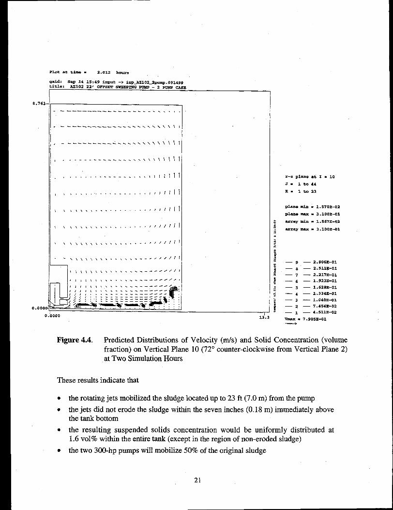
Fi~re 4.4. Predicted Distributions of Velocity (m/s) and Solid Concentrationfraction) on Vertical Planeat Two Simulation Hours
These results indicate that
10 (72° counter-clockwise from Vertical(volumePlane 2)
●
●
●
●
the rotating jets mobilized the sludge located up to 23 ft (7.0 m) from the pump
the jets did not erode the sludge within the seven inches (O.18 m) immediately abovethe tank bottom
the resulting suspended solids concentration would be uniformly distributed at1.6 vol% within the entire tank (except in the region of non-eroded sludge)
the two 300-hp pumps will mobilize 50% of the original sludge
21
Plot at time = 2.012 hours
8.763
O.ooc
id: Sep 14 15:49 input ->tle:
hP-A3102_2m=m .091499U102 22’ 0F3WST SWEEP2NG PUMP - 2 PuMP CASE
---- ----- . . . . . . . . . .
---- ----- . . . . . . . . . .
---- ------ .%-. ----- -..
1 ---------- ------ =-.
i,$,~------- -------’
\\ \\i\lllil]JIJ Jl$ ,1
1
\\lllJIJlll\\i-/
lilillll i\\\\\-/
0.’0000
. . ..- ----- .
. . . . . . . . . . . . . .
. . . . . . . . . . . . . .
. . . . . . . . . . . . . .
. . . . . . . . . . . . . .
... .\\., . . . . . .
- ..\\\.... . . . .
.. \\\\\.. . . . .
. \\\\\\*.. . . .
,Itll $,,,. . . .
,,r f,,,.... . . .
,, !....--. . . . .
-T=+= j :Z5%45=::,.. . . . . . . . . .. . .. . . . . . . . . . . . .:.:: :;::: ::::: .:,.. . . . . . . . . .::::: ::::: ::::
13!3
r-z plane at I . 13
a= lt044
K= lt023
Dke min = 1.569E-02
DhRe max = 3.100s-01
-ay & = 1.567Z-02
array zuuc = 3.100S.-01
—9 — 2.806E-01
‘8 — 2 .511E-01
—7 — 2.217z-01
—6 — 1.923E-01
—5 — 1.628E-01
—4 — 1.334SF01
—3 — 1.040E-01
—2 — 7.454%02
—1 — 4.5UE-02
man% = 6.996E-01
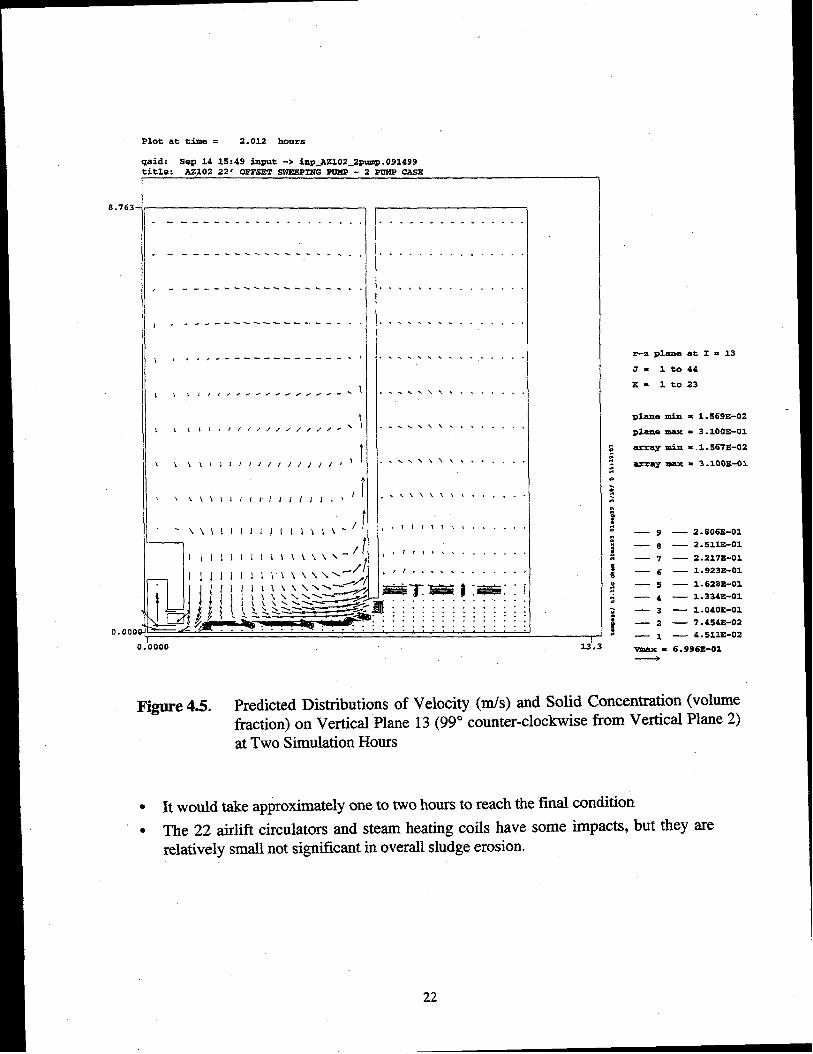
Figure 4.5. Predicted Distributions of Velocity (m/s) and Solid Concentration (volumefraction) on Vertical Plane 13 (99° counter-clockwise from Vertical Plane 2)at Two Simulation Hours
● It would take approximately one to two hours to reach the final condition● The 22 airlift circulators and steam heating coils have some impacts, but they are
relatively small not significant in overall sludge erosion.
22
Plot at time= 2.012 hours
8.763
0.00(
id: Sen 14 15:49 input .> ia3).A2102_2pulsg).091499tle : A2102 22* 03TSET SWEEPING l?O’MF- 2 PUBS?CASE
. . . . . . . . . . . . . . . . . . . . . . . . . . . . .
---- ---- . . . . . . . . . . . . . . . . . . . . .
---- ---- ----- . . . . . . . . . . . . . . . . .
. ---- ----- ----- ----- ----- . . .
. . . . . ----- . . . . . ----- ----- ----
,,, ,,, . . . . . . ------ ------ .
,,, ,,, , <,, . . ..- ------ -- . . . .‘.. .
.,, !,,?. ./ ------ ----.~~~ $~$..
,,, ,., ,, ., /,---- --- ,1111 !,,..
. . . . . . . . .
. . . . . . . . .
. . . . . . . . .
. . . . . . . . .
. .
. . . . . . . . .
. . . . . . . . .
. . . . . . . .
1’
,,, ,,, ,,J, ,,a. . ,1/1///// ,,.
illllt 4&t,\ ,..- / ///-’///// . . .
. . . . . . . .
. . . . . . . .
. . . . . . . .
. . .=4==?==$:~. . . . . . . .. . . . . . . .. .:: :.: :::. . . . . . .
1-000 13.3
r-z plane at I . 14
$7= lt044
3C. lt023
Plaiiemin = 1.56SE-02
plane max = 3.1OOE-O1
array u+ = 1.567E.-O2
array max . 3.100)3-01
— 9 — 2.806E-01
‘8 — 2.s1233-01
—7 — 2.217E-01
‘6 — 1.923E-01
—5 — 1.628x-01
—4 — 1.3343+01
—3 — 1.040E-01
—2 — 7.45433-02
— 1 — 4.511E-02
v+% = 1.315Etoo
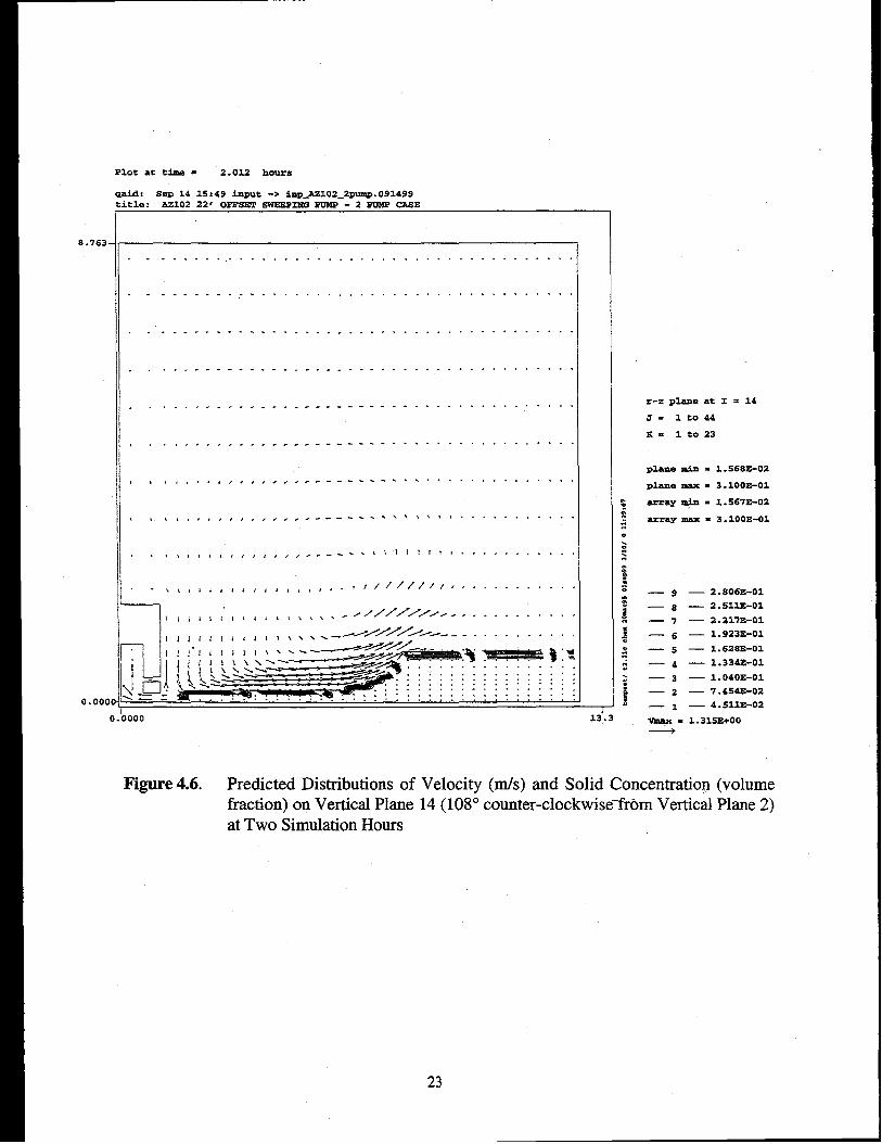
Figure 4.6. Predicted Distributions of Velocity (M./s) and Solid Concentration (volumefraction) on Vertical Plane 14 (108° counter-clockwise-from Vertical Plane 2)at Two Simulation Hours
23
Plot at time- 2.012 hours
8.763.
0.0001
(
tid: Sep 14 15:49 input -> iap_As102_2puaIp.091499Ltle: A2102 22~ OFPSET SW&EP2NQ PUMP - 2 PUMP CASE
. . . . . . . . . . . . . . . . . .
. . . . . . . . . . . . . . . . . . . . . . . . . .
. . . . . . . . . . . . . . . . . . . . ..,, , .
. . . . . . . . . . . . . . . . . . . . . ..
. . . . . . . . . . . . . . . . . . . . . . . . . .
. . . . . . . . . . . . . . . . . . . . . . . . . .
. . . . . . . . .. . . . . . . . . . . . ,.. , .,
. . . . . . . . . . . . . . . . . . . . . . . . . .
. . . . ... . . . . . . . . . . . . . ... , .,
. .. . . . . . . . . . . .-, . . . . . . . . . . . .
1 .........................
. . . . . . . . . . .
. . . . . . . . . . . .
... ,.. . . . . . .
. . . . . . . . . . . .
. . . . . . . .. . . . .
. . . . . . . . . . . .
. . ...! . . . . . . .
. . . . . . . . . . . .
. . . . . . ------
. . . . . ----- . .
. . . . . . . . . . .-
. . . . . . . . . . . .
. . . . . . . . . . . .Tl_l..........................,.......................@@?:...........-.............----------------
~==z =Z=zzz::z: ::n:&s&:~&::;::*fi~:::; :=;;::;!::.. ..... .. ., ....,000
r-z pl.me at I = 15
ir. lt044
K= lto23
plane min = 1.567E-02
Plainma% = 3 .1OOE-O1
=ay An = 1.567s-02
array ma% = 3.1OOE-O1
—9
‘8
—7
‘6
—5
—4
—3
—2
—1
— 2.806=-01
— 2.513.E-01
— 2 .217E-01
— 1.923E-01
— 1.628S-01
— 1.334’s-01
— 1.040s-01
— 7.454E-02
— 4.512B-02
~ = 1.637=+01
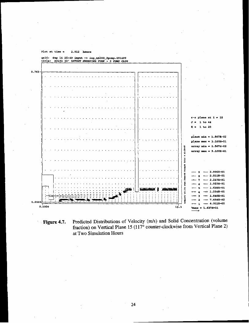
Figure 4.7. Predicted Distributions of Velocity (rnls) and Solid Concentration (volumefraction) on Vertical Plane15(117° counter-clockwise from Vertical Plane 2)at Two Simulation Hours
24
8.763
0.000
Plot at time = 2.012 hours
id: Sep 14 15:49 input -> ins)_As102_2wIm.091499tle: 3A3102 22 ~ OPYSST SWEEP2NQ Slm? - 2 PuMs CASE
. . . . . . . . . . . ---- . . .
. . . ... , ,,. . . . . . .,,
/11,////-”””””,
>00
. . . . . .
. . . . . . . .
., .,7.,
. . . . . . . .
., ..,. ,.
. . . . . . . .
..-. .,
----- . . .
. .. ----
. . . . . .
. . . . . . . .
. . . . . . . .
,;::~?
,&. . . . . . ..: ::: :. . . . . .. . . . . . . . .,. ... . . . .
A. 3
r-z plane at I = 17
a= lt044
x= lt023
plane min = 1.569E-02
plane ma% = 3 .1OOE-O1
array min = 1.567E-02
array max = 3 .1OOI3-O1
—9 — 2.806E-01
‘8 — 2.Sllz-ol
—7 — 2.217E-01
—6 — 1.923E-01
—5 — 1.628P.-O1
—4 — 1.334s-01
—3 — 1.040E-01
—2 — 7 .454E-02
—1 — 4.511s-02
wax . 6.337E-01
Figure 4.8. Predicted Distributions of Velocity (rnls) and Solid Concentration (volumefraction) on Vertical Plane 17 (135° counter-clockwise from Vertical Plane 2)at Two Simulation Hours
25
8.763
0.000(
c
Plot at time . 2.012 hours
lid: seP 14 1s:49 iU&t ‘> iIIp_A!4102_2pump.091499.tle: ~2102 221 OP.FSZT SWEZP2NG PUMP - 2 POMP CASE
---- -- ... ----- ~.,.
---- ,,, , ,,, , ,,, . . .
,. .\\\ l\),,, ,’, ,s. .
Ii \\, \,, L,,, 11 ,1$..
11 I\ll\\ L\,, ,,, ,,. .
II Illli l\\,, ,,, ,,. .
1, ll!llll\l\ l!L*L..
,, 1111 !lll, , ,l\h b.-
. . \llll) l,,, ,,s. s..
Jl)tlt24’ #as . . . . .nil,,..,..:::::::::~/,,/,8*
1
1
1
I
1
I
1
!
MU;;:::’;:::::;;:::..lJ=-7Jjg: :: :;~
. . . . . . . . . . ... :: :)00
—
13’.3 Vmax
Figure 4.9. Predicted Distributions of Velocity (m/s) and Solid Concentrate—fraction) on Vertical Plane 21 (171° counter-clockwise fkom Vertiat Two Simulation Hours
4.1.2 Jet Velocity Distribution
The AZ-102 modeling predicted that two 300-hp pumps could mobilize the sludg(7.0 m) away from the pump. In this section, we examine how the jet velocity cdistance as it moves forward. As the jet penetrates into the sludgelslurry layer, itsumounding sludge and slurry (mixture of the sludge and supematant liquid), resljet’s spreading laterally and vertically and its velocity decreasing.
26
There have been many experimental studies todetermine how jet velocity changes withlongitudinal and lateral distances for a homogeneous jet penetrating into a still fluid in irhitespace (e.g., water jet injected into still water, and air jet injected into still air). These studiesindicate that the velocity along the jet centerline may decrease linearly with the downstreamdistance, as expressed by the following nondimensional form (Wiegel 1966):
.V”=1 for X* S 6.2
6.2v*=— for
X*X* z 6.2
where
Vc,v“=—V.
xand X*=—
DO
DO = nozzle diameterVc, = jet centerline velocityV. = jet exit velocity at a nozziex = downstream distance along the jet centerline
The lateral velocity distribution may be expressed by the following normal (or Gaussian)distribution (Wiegel 1966):
V= V,,e-n(i)’ = VC,e-77(>)2 (4.4)
where
R*=LDO
and r = the lateral distance from the jet centerline.
The TEMPEST code reproduced the velocity distribution of the homogeneous jet well (Trentand Michener 1993), as shown in Figure 4.10, which compares the predicted jet centerlinevelocities with the velocity distribution expressed by Equation 4.3. However, these homo-geneous jet conditions are quite different from the Tank AZ-102 pump jet condhion. Forexample, unlike the homogeneous jet case, in AZ-102
● the jet rotates at 2 rpm
● the jet density and viscosity maybe different from those of surrounding sludge/slunyand supernatant liquids, at least until the waste is fully mixed
“ the sludge is non-Newtonian and has yield strength
27
(4.3)
10
1
0.1
0.01
— Experimental Data (Wiegel 1964)+ TEMJ?EST Prediction
\
0.1 1 10 100 1000Non-dimensional Distance, X*
Figure 4.10. Jet Centerline Velocity and TEMPEST Prediction Compared withMeasured Values for Three-Dimensional Homogeneous Jet
● the jet penetration was stopped by the non-erodible portion of the sludge
“ the jet density and viscosity may vary temporally and spatially
“ the jet is placed near the tank bottom and thus its spread toward the tank bottom andthe non-erodible sludge is restricted
“ the jets maybe affected by the presence of the airlift circulators, heating coils, andthe tank wall.
We examined how jet velocity changes with distance for the AZ-102 pump jet. Because thejet penetrated farthest on Vertical Plane 15 (see Figure 4.7), we used the predicted velocity onthis plane at 2 hours and 42 simulation seconds for this analysis. At that time, the jets arerotating counter-clockwise, and one of them is oriented on this vertical plane. As statedpreviously, the distance between the pump center and the tank wall is the farthest (44 ft or 13 m)on Vertical Plane 15, and the jet penetrated up to 23 ft (7.0 m).
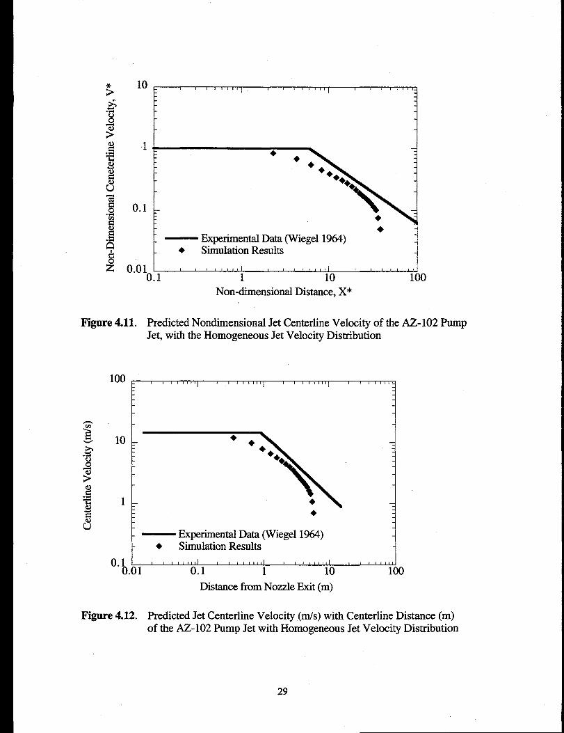
Figure 4.11 shows the predicted nondimensional centerline jet velocity, V*, with non-dimensional centerline distance, X*, for the AZ- 102 pump jet, together with values based onEquation 4.3. Figure 4.12 shows the dimensional values (the centerline jet velocity expressed inm/s versus the centerline distance from the nozzle exit expressed in m) for the same results. Asexpected, there are some similarities and differences between these two cases. Basic similarity isthat the centerline jet velocity reduces its value at the rate approximately proportional to thedistance from the jet exit. These figures also show that the AZ-102 jet velocity is smaller thanthe homogeneous jet velocity at the equal distance. Many of these differences are attributed tothe seven differences of the AZ-102 case from the homogeneous case stated above. Figure 4.12also shows that, when the penetration of the jet into the sludge was stopped at 23 ft (7.0 m), the
28
10 ~ ! I , f I 1 I 8 ! , I I I I 1 I I ) , 1, , , 0
0.1 .
+— Experimental Data (Wiegel 1964)
* Simulation Results
0.01 1 , ! 1 t I 1!I , , ! 1 , , , 1I I I 1 ! 11t 10.1 1 10 100
Non-dimensional Distance, X*
Figure 4.11. Predicted Nondimensional Jet Centerline Velocity of the AZ-102 PumpJet, with the Homogeneous Jet Velocity Distribution
100, 1 I I 1 [ 1 1 1, t 1 # 1 I I { , I 1 , 1 1 1 1 1 1 I I 1 1 1 ! L.
10 ~ ++
●4
1 ~ ●
+
- — Experimental Data (Wiegel 1964)~ + Simulation Results 4
0.1 I 1 1 1 ! , , , , , 1 i 1 1 I + t , 1 , , r 1 t , ! , t ! 1 I I I
0.01 0.1 1 10 100
Distance from Nozzle Exit (m)
Figure 4.12. Predicted Jet Centerline Velocity (m/s) with Centerline Distance (m)of the AZ-102 Pump Jet with Homogeneous Jet Velocity Distribution
29
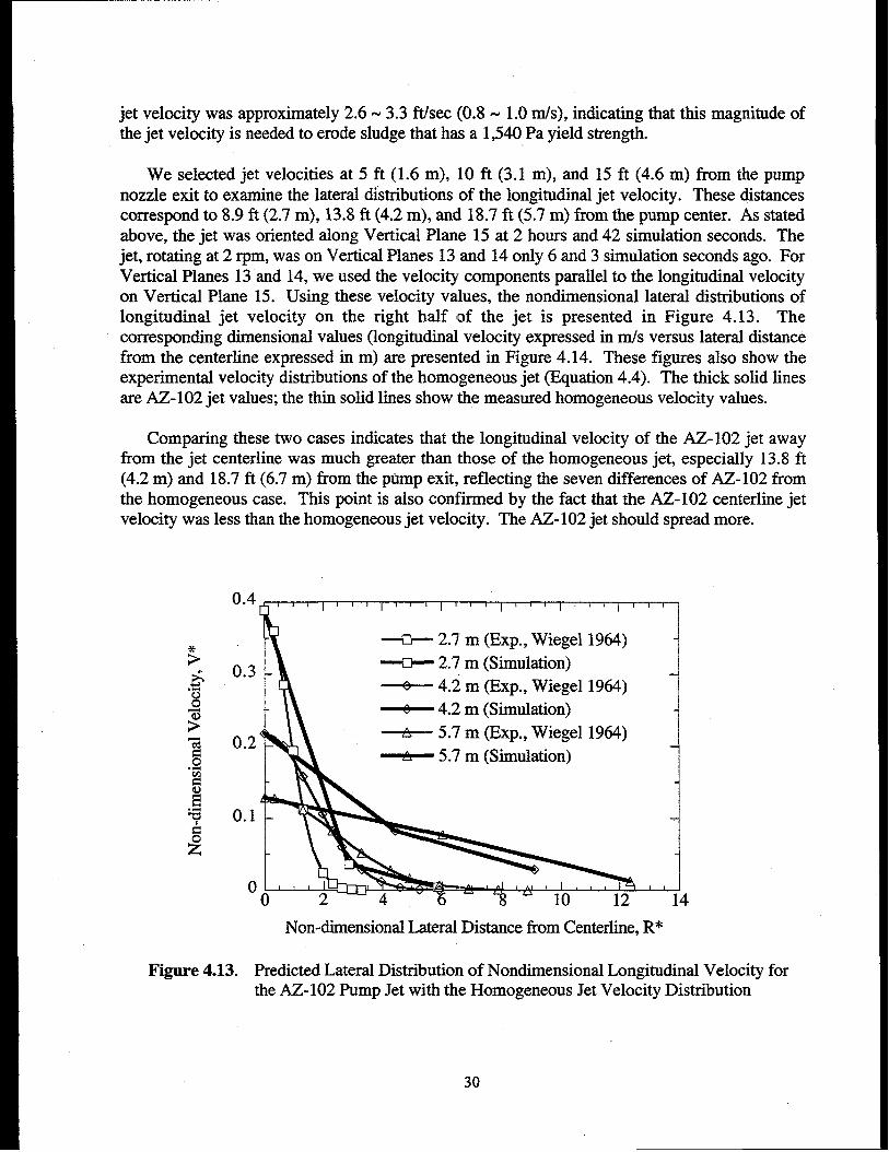
jet velocity was approximately 2.6 N 3.3 ft.lsec (0.8 -1.0 m/s), indicating that this magnitude ofthe jet velocity is needed to erode sludge that has a 1,540 Pa yield strength.
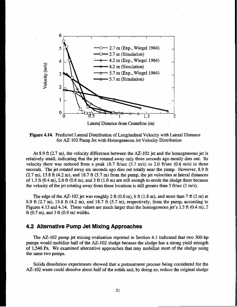
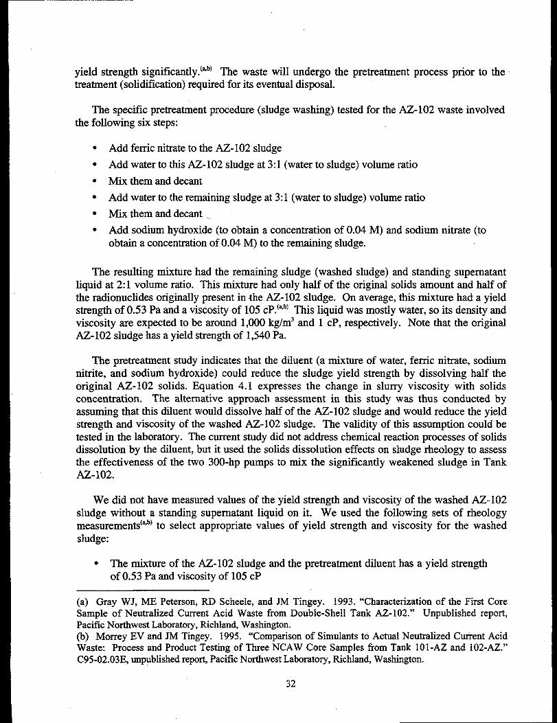
We selected jet velocities at 5 ft (1.6 m), 10 ft (3.1 m), and 15 ft (4.6 m) from the pumpnozzle exit to examine the lateral distributions of the longitudinal jet velocity. These distancescorrespond to 8.9 ft (2.7 m), 13.8 ft (4.2 m), and 18.7 ft (5.7 m) from the pump center. As statedabove, the jet was oriented along Vertical Plane 15 at 2 hours and 42 simulation seconds. Thejet, rotating at 2 rpm, was on Vertical Planes 13 and 14 only 6 and 3 simulation seconds ago. ForVertical Planes 13 and 14, we used the velocity components parallel to the longitudinal velocityon Vertical Plane 15. Using these velocity values, the nondimensional lateral distributions oflongitudinal jet velocity on the right half of the jet is presented in Figure 4.13. Thecorresponding dimensional values (longitudinal velocity expressed in mls versus lateral distancefrom the centerline expressed in m) are presented in Figure 4.14. These figures also show theexperimental velocity distributions of the homogeneous jet (Equation 4.4). The thick solid linesare AZ- 102 jet values; the thin solid lines show the measured homogeneous velocity values.
Comparing these two cases indicates that the longitudinal velocity of the AZ-102 jet awayfrom the jet centerline was much greater than those of the homogeneous jet, especially 13.8 ft(4.2 m) and 18.7 ft (6.7 m) from the pump exit, reflecting the seven differences of AZ-102 fromthe homogeneous case. This point is also confined by the fact that the AZ-102 centerline jetvelocity was less than the homogeneous jet velocity. The AZ- 102 jet should spread more.
0.3
0.2
0.1
0
Ii~ 2.7 m (Simulation)~ 4.2 m (Exp., Wiegel 1964)~ 4.2 m (Simulation) i
Non-dimensional Lateral Distance horn Centerline, R*
Figure 4.13. Predicted Lateral Distribution of Nondimensional Longitudinal Velocity forthe AZ-102 Pump Jet with the Homogeneous Jet Velocity Distribution
30
5 ~ 2.7 m (Exp., Wiegel 1964)2.7 m (Simulation)
4 - ~ 4.2 m (Exp., Wiegel 1964)
~’4.2 m (Simulation)
34 ~ 5.7 m (Exp., Wiegel 1964)
~ 5.7 m (Simulation)
2 -
1 -
0 10 2
Lateral Distance from Centerline (m)
Figure 4.14. Predicted Lateral Distribution of Longitudinal Velocity with Lateral Distancefor AZ-102 Pump Jet with Homogeneous Jet Velocity Distribution
At 8.9 ft (2.7 m), the velocity difference between the AZ-102 jet and the homogeneous jet isrelatively small, indicating that the jet rotated away only three seconds ago mostly dies out. Itsvelocity there was reduced from a peak 18.7 ftisec (5.7 m/s) to 2.0 ft/sec (0.6 m/s) in threeseconds. The jet rotated away six seconds ago dies out totally near the pump. However, 8.9 ft(2.7 m), 13.8 ft (4.2 m), and 18.7 ft (5.7 m) from the pump, the jet velocities at lateral distancesof 1.3 ft (0.4 m), 2.6 ft (0.8 m), and 3 ft (1.0 m) are still enough to erode the sludge there becausethe velocity of the jet rotating away from these locations is still greater than 3 ft/sec (1 m/s).
The edge of the AZ-102 jet was roughly 2 ft (0.6 m), 6 ft (1.8 m), and more than 7 ft (2 m) at8.9 fi (2.7 m), 13.8 ft (4.2 m), and 18.7 ft (5.7 m), respectively, from the pump, according toFigures 4.13 and 4.14. These values are much larger than the homogeneous jet’s 1.3 ft (0.4 m), 213(0.7 m), and 3 ft (0.9 m) widths.
4.2 Alternative Pump Jet Mixing Approaches
The AZ-102 pump jet mixing evaluation reported in Section 4.1 indicated that two 300-hppumps would mobilize half of the AZ-102 sludge because the sludge has a strong yield strengthof 1,540 Pa. We examined alternative approaches that may mobilize most of the sludge usingthe same two pumps.
Solids dissolution experiments showed that a pretreatment process being considered for theAZ-102 waste could dissolve about half of the solids and, by doing so, reduce the original sludge
31
yield strength significantly. ‘%b)The waste will undergo the pretreatment process prior to thetreatment (solidification) required for its eventual disposal.
The spec~lc pretreatment procedure (sludge washing) tested for the AZ-102 waste involvedthe following six steps:
● Add ferric nitrate to the AZ-102 sludge
● Add water to this AZ-102 sludge at 3:1 (water to sludge) volume ratio
● Mix them and decant
c Add water to the remaining sludge at 3:1 (water to sludge) volume ratio
● Mix them and decant,.
“ Add sodium hydroxide (to obtain a concentration of 0.04 M) and sodium nitrate (toobtain a concentration of 0.04 M) to the remaining sludge.
The resulting mixture had the remaining sludge (washed sludge) and standing supernatantliquid at 2:1 volume ratio. This mixture had only half of the original solids amount and half ofthe radionuclides originally present in the AZ-102 sludge. On average, this mixture had a yieldstrength of 0.53 Pa and a viscosity of 105 cP.(ah)This liquid was mostly water, so its density andviscosity are expected to be around 1,000 kg/m3 and 1 cP, respectively. Note that the originalAZ-102 sludge has a yield strength of 1,540 Pa.
The pretreatment study indicates that the diluent (a mixture of water, ferric nitrate, sodiumnitrite, and sodium hydroxide) could reduce the sludge yield strength by dissolving half theoriginal AZ- 102 solids. Equation 4.1 expresses the change in slurry viscosity with solidsconcentration. The alternative approach assessment in this study was thus conducted byassuming that this diluent would dissolve half of the AZ-102 sludge and would reduce the yieldstrength and viscosity of the washed AZ-102 sludge. The validity of this assumption could betested in the laboratory. The current study did not address chemical reaction processes of solidsdissolution by the diluent, but it used the solids dissolution effects on sludge rheology to assessthe effectiveness of the two 300-hp pumps to mix the significantly weakened sludge in TankAZ-102.
We did not have measured values of the yield strength and viscosity of the washed AZ-102sludge without a standing supematant liquid on it. We used the following sets of rheologymeasurements to select appropriate values of yield strength and viscosity for the washedsludge:
s The mixture of the AZ-102 sludge and the pretreatment diluent has a yield strengthof 0.53 Pa and viscosity of 105 CP
(a) Gray WJ, ME Peterson, RD Scheele, and JM Tingey. 1993. “Characterization of the First CoreSample of Neutralized Current Acid Waste from Double-Shell Tank AZ-102.” Unpublished report,Pacific Northwest Laboratory, Richland, Washington.(b) Morrey EV and JM Tingey. 1995. “Comparisonof Simukmtsto Actual Neutralized Cu.frentAcidWaste: Process and Product Testing of Three NCAW Core Samples from Tank 101-AZ and 102-AZ.”C95-02.03E,unpublishedreport,PacificNorthwestLaboratory,Richland,Washington.
32
● A slurry mixture consisting of 40 vol% origin@ AZ-102 sludge and 60 VOI%originalAZ-102 supernatant liquid has a yield strength of 2.07 P~ its viscosity measures426 cp
“ A slurry mixture consisting of 10 vol% original AZ-102 sludge and 90 vol% originalAZ-102 supernatant liquid does not have yield strength; its viscosity is about 7 cP.
Based on this information and consultation with PNNL staff who conducted thesemeasurements, we selected a”yield strength of 1.2 Pa and a viscosity of 270 CP for the washedsludge.
It is interesting to note that the washed sludge has an average solids diameter of 4.2 ~m,while the original AZ- 102 sludge has a average particle size of 3.4 ~m. Thus, even though halfof the original AZ-102 solids were dissolved by this pretreatment (washing) process, overallsolid sizes did not change much. Using 4.3 pm for the average solids size, we evaluated thefollowing two alternative approaches to enhance mixing with the two 300-hp pumps.
4.2.1 Approach 1: Three-Step Approach
Step 1: Pump out the original AZ-102 supematant liquid only
Step 2: Add the diluent (the mixture of water, ferric nitrate, sodium nitrite, and sodiumhydroxide) to AZ-102 Tankat61 diluent to sludge volume ratio
Step 3: Mix the diluent-washed, weakened, and reduced amount of AZ-102 sludgewith the diluent using two 300-hp mixer pumps.
To evaluate this approach, we examined the following three cases (Cases 1 through 3). Allthree cases assumed that the sludge yield strength was reduced to 1.2 Pa as a result of solidsdissolution.
Case 1:
Case 2:
Case 3:
Initial conditions were the following:
Half the original solids were assumed dissolved before pump mixing, but thesludge thickness of 35 in. (0.89 m) was not reduced. Instead, the solid volumefraction within the sludge was reduced to 15.5 vol%, half the original31 vol%.
Half the original solids were assumed dissolved before pump mixing, and theirsludge thickness was reduced to 17.5 in. (0.45 m), half the oiiginal sludgethickness of 35 in. (0.89 m). The washed solids volume fraction is 31 vol% inthe reduced sludge layer.
Yield strength was reduced to 1.2 Pa, but the original solids amount was notreduced. Thus the washed solid layer thickness is still 35 in. (0.89 m), and itsvolume fraction in the sludge layer is 31 vol%. This is the most conservativeof the three cases.
33
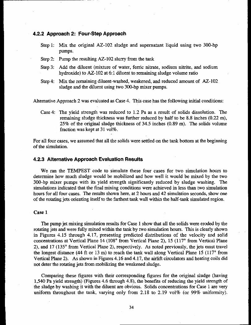
4.2.2 Approach 2:
Step 1: Mix thepumps.
Four-Step Approach
original AZ- 102 sludge and supernatant liquid using two 300-hp
Step 2: Pump the resulting AZ-102 slurry from the tank
Step 3: Add the diluent (mixture of water, ferric nitrate, sodium nitrite, and sodiumhydroxide) to AZ-102 at 6:1 diluent to remaining sludge volume ratio
Step 4: Mix the remaining diluent-washed, weakened, and reduced amount of AZ-102sludge and the diluent using two 300-hp mixer pumps.
Alternative Approach 2 was evaluated as Case 4., This case has the following initial conditions:
Case 4: The yield strength was reduced to 1.2 Pa as a result of solids dissolution. Theremaining sludge thickness was further reduced by half to be 8.8 inches (0.22 m),25% of the original sludge thickness of 34.5 inches (0.89 m). The solids volumefraction was kept at31 VOI%.
For all four cases, we assumed that all the solids were settled on the tank bottom at the beginningof the simulation.
4.2.3 Alternative Approach Evaluation Results
We ran the TEMPEST code to simulate these four cases for two simulation hours todetermine how much sludge would be mobilized and how well it would be mixed by the two300-hp mixer pumps with its yield strength significantly reduced by sludge washing. Thesimulations indicated that the final mixing conditions were achieved in less than two simulationhours for all four cases. The results shown here, at 2 hours and 42 simulation seconds, show oneof the rotating jets orienting itself to the farthest tank wall within the half-tank simulated region.
Case 1
The pump jet mixing simulation results for Case 1 show that all the solids were eroded by therotating jets and were fully mixed within the tank by two simulation hours. This is clearly shownin Figures 4.15 through 4.17, presenting predicted distributions of the velocity and solidconcentrations at Vertical Plane 14 (108° from Vertical Pkme 2), 15 (1 17° from Vertical Plane2), and 17 (135° from Vertical Plane 2), respectively. As noted previously, the jets must travelthe longest distance (44 ft or 13 m) to reach the tank wall along Vertical Plane 15 (117° fromVertical Plane 2). As shown in Figures 4.16 and 4.17, the airlift circulators and heating coils didnot deter the rotating jets from mobilizing the weakened sludge.
Comparing these figures with their corresponding figures for the original sludge (having1,540 Pa yield strength) (Figures 4.6 through 4.8), the benefits of reducing the yield strength ofthe sludge by washing it with the diluent are obvious. Solids concentrations for Case 1 are veryuniform throughout the tank, varying only from 2.18 to 2.19 vol% (or 99~0 uniformity).
34
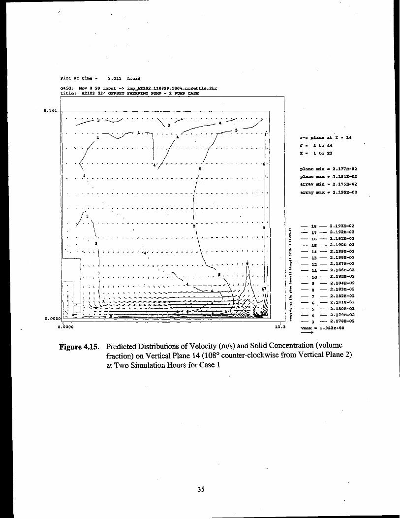
Plot at time . 2.012 hours
6.144 -
0.000(
(
,id: NOV 8 99 input -> inP_AZ102_l10899 .100%.nosettle .2hrtle: AS102 22~ OFPSET SV?EEP2NG POW - 2 PUMP CASE
—
4
-[
. . . . . . . . . . . . . . . . ---- ---- ---- . . . . . . . . ..
. . . . . . . . . . . . ---- ---- ~--- ---- -.. . . . . . . !
. . . . . . . . . . ----- ----- ---- ----- . .. . . . 0. 4
[
3
)
. . . . . . . . . . . . . . ----- ----- ----- . . . . . ..!5
\ 6
—
\
[
. . . . . . . . ...> . .. s-- -~-..~ ------ .* $.,. ~
3
\
... ,,, ., .,., , .~..-dd-.-..d .--- . . ..$ I.. .
!,, . . . . ,., .,
\\ A i
.< ------ .-- .--’ \’l l’”’
3$ 8,1088,,< ,84
I
‘:; x”--- ”~’””””
11111411, . .. \\\\--- -& <.__... II I!,..
000 13’.3
r-z plane at I = 14
J= lto44
K= 1 to 23
Plane mia = 2.177s-02
PIS=FJ ma% = 2.194E-02
array min = 2.17533-02
array ma% = 2.195E-02
— 18 — 2 .193E-02
- 17 — 2.192E-02
— 16 — 2.19333-02
— 15 — 2.190E-02
— 14 — 2 .1S9E-02
— 13 — 2 .188=-02
— 12 — 2.187E-02
— II — 2.186E-02
— 10 — 2.18!23-02
—9 — 2.184E-02
‘8 — 2.183E-02
—7 — 2 .182E+02
‘6 — 2.182E-02
—5 — 2 .1803+02
—4 — 2.179E-02
—3 — 2.178E-02
VMS% = 1.922E+O0—
II Fkure 4.15. predicted Distributions of Velocity (m/s) and Solid Concentration (volume
fraction) on Vertical Plane 14 (108° counter-clockwise from Vertical Plane 2)at Two Simulation Hours for Case 1
35
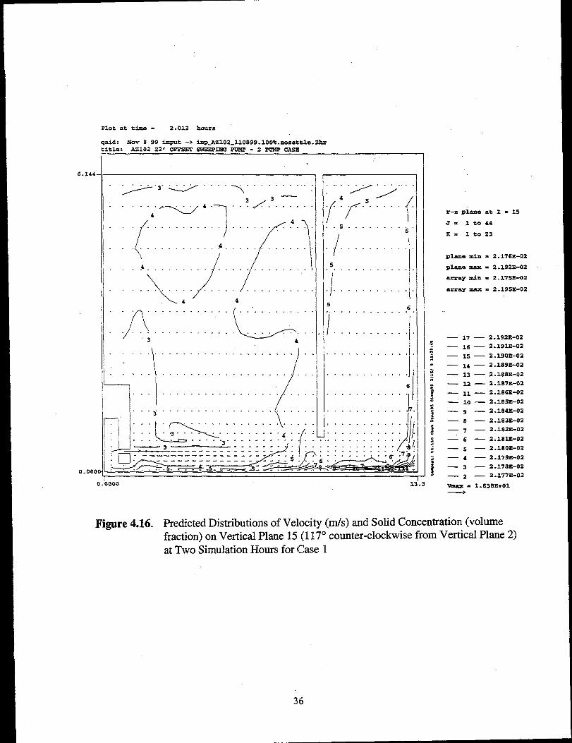
Plot at time . 2.012 hours
6.144.
0.000
id: NW S 99 input -> inp.AZ102_l10899. 100’%.nosettle. 2hrtie: Az102 22* OFFSET SWEEP2NG PUMP - 2 PUMP CA8E
.Y.,. v . . .. y . . . . . . . . . . ;
. . . .
1“4”-U 4-”
{. . . . . . . . . . . . 4
//)
. . . . . . . . . . . . .
(
4. . . . . . . . . . . . . . . . . . . . . . . . . .
4. . . . . . . . . . . . . . . . . . . . . . . .
\). . . . . . . . . . . . . . . . . . . . . . . .
4
F... .............. .............
3
“-\
. . . . . . . . . . . . . . . .
. . . . . . . . . . . . . .
1
. . . . . . . . . . . .
. . .3“’””’”””’
—
:“”-”””””””””L-~ -
4
/
. . . . . . . . . . .
. . . . . . . . . . . .
. . . . . . . . . . ,.
. . . . . . . . . . . .
. . . . . . . . . . . .
. . . . . . .4-(”
..-. ---- . .
5.. . . . . . . . . .
6. .
I............. . . . . . . . . . . . ,
. . . . . . . . . . . .
6
1. . . . . . . . . . . . .
I. . . . . . . . . . . .
. .
000 13!3
r-z plane at I = 15
3= 1 co 44
x= lt023
plane min = 2.176E-02
Plane ma% = 2.192E-02
llX?2W fin = 2.17SE-02
array nusx . 2.195E-02
— 17 — 2.192E-02
— 16 — 2 .191E-02
— 15 — 2 .190E-02
— 14 — 2.189E-02
— 13 — 2.L88E-122
— 12 — 2.187E-02
— 11 — 2.186E-02
- 10 — 2 .185E-02
—9 — 2.1842-02
—8 — 2.183?6-02
—7 — 2.182E-02
‘6 — 2 .1s3s3-02
—5 — 2.180E-02
—4 — 2.1798+02
—3 — 2.17 SE-02
— 2 — 2.177E-02
Vma% - 1.638E+OI—
Figure 4.16. Predicted Distributions of Velocity (m/s) and Solid Concentration (volumefraction) on Vertical Plane 15 (117° counter-clockwise from Vertical Plane 2)at Two Simulation Hours for Case 1
36
J
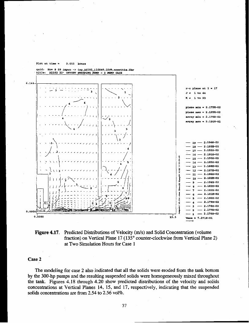
Plot at time - 2.012 hours
6.144
0.000
!
Lid: Nov 8 99 input -> bPJZ102_l10899. 100% .nosettle .2hr,tle: AZ102 22* OFPSZT SWESPING POMP - 2 POMP CASE
. . . . . . . . . . . ---- --.-- 3 - . . . . ...-3
\. . . . . . . . . . . .-.- .,,
“----’f”<)”],...-----.....4 ‘all
\/f’-----------. ./J/J
4
,, .. . ..- . . . . . ,,, ,, ,
,. ‘)>3, ------ . ., /,,,
.1
,, ,3 <<.. ... //,,,/
1\
71I
\JJ/// .--l- <b. J
Hip ----”-’.””11 /0----.-”.” ..
. . . .
“\,.. ,
1
. . . . . 2 . . . .
“v,., ,,, . .,
33
,,, ,,, / / ‘}4
/
,,, ,, ,,, ,
,.. . . . . .‘4,
5’
000 13’.3
r-z plane at I . 17
3. lt044
K= lt023
ZIlaae mixi = 2.175E-02
plane max = 2.195E-02
array min = 2.175E-02
array ma% = 2.195E-02
,-
— 19 — 2.194E-02
— 18 — 2.193E-02
— 17 — 2.192E-02
- 16 — 2 .191?4-02
— 15 — 2 .190E-02
— 14 — 2.189E-02
— 13 — 2 .188E-02
— 12 — 2.187E-02
— 11 — 2.186E-02
— 10 — 2.18=+02
—9 — 2.184E-02
—8 — 2 .183E-02
—7 — 2.1827+02
‘6 — 2.181E-02
—5 — 2.180E-02
—4 — 2.179E-02
—3 - 2.1783!-02
—2 — 2.177E-02
—1 — 2 .176E-02
VIM% = 7.2733+01—
Figure 4.17. Predicted Distributions of Velocity (m/s) and Solid Concentration (volumefraction) on Vertical Plane 17 (135° counter-clockwise from Vertical Plane 2)at Two Simulation Hours for Case 1
Case 2
The modeling for case 2 also indicated that all the solids were eroded from the tank bottomby the 300-hp pumps and the resulting suspended solids were homogeneously mixed throughoutthe tank. Figures 4.18 through 4.20 show predicted distributions of the velocity and solidsconcentrations at Vertical Planes 14, 15, and 17, respectively, indicating that the suspendedsolids concentrations are ilom 2.54 to 2.56 VOI%.
37
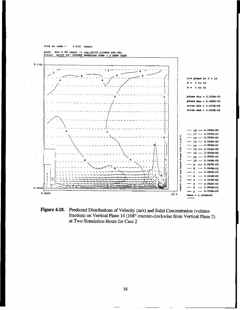
Plot at time= 2.012 hours
5.715
0.000(
(
qaid: Now? 6 99 input -> inP_Az102_l10699 .50%.23XX.tle: AZ102 22, OFFSET 8WEEP2NG PUMP - 2 PUNP CASE
. . .. . . . . .. . . . . . . . . .3
~ 3 -*--’ ------4 “
~’~.”-F:-:7-5-”-”(
. . . . . . . . . . . . . . . ---
4
./
v. . . . . . . . . . . . . . . ----. . . . . . . . . . . . . . . . . .
. . . . . . . . . . . -+. . --- --
/
------ -
----- -5
/
------ -
n I. . ............------------/.,
. .
.
—
/ /-
. . . . . . . . . . . . --e- ---- ----
. . . . . . . . . . ----- ----- ----4 5
---- . . . . . . . . .
---- . . . . . . . . .6
----- . . . . . .,,
------ . . . . . . . .
----- . . . . . . . .
---- . . . . ,!. < ,
---- . . . . ,,, , 6
----- ..\ \,6. .$
II----.\\,11, , ,
\
,,, ,,, ,4, ,,, ,
1111, ,,,4 ‘“:+a!:-=i’i!(/111! 188’8%
300 13’.3
r-z ptie at I = 14
a= lt044
x= 1 to 23
Plane m,i.n= 2.539E-02
Plaummax= 2.558E-02
array b - 2.537E-02
array max = 2.560z-02
— 18 — 2 .558s-02
—. 17 — 2.55773-02
— 16 — 2.5’6E-02
— 15 — 2.554E-02
— 14 — 2.553E-02
— 13 — 2.552E-02
— 12 — 2 .553PF02
— xl — 2.550E-02
— 10 — 2.549E-02
—9 — 2.547E-02
—8 — 2 .S46E-02
—7 — 2.54S.E-02
‘6 — 2 .544E-02
—5 — 2 .543E-02
—4 — 2 .542E-02
—3 — 2.54013-02
—2 — 2.539s-02
- = 1.940E+O0—
Figure 4.18. Predicted Distributions of VeIocity (m/s) and Solid Concentration (volumefraction) on Vertical Plane 14 (108° counter-clockwise from Vertical Plane 2)at Two Simulation Hours for Case 2
38
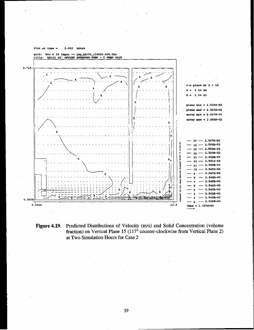
5.715.
0.000
Plot at tiaua = 2.012 hours
qaid: NOV 6 99 inrmt -> inz-AZ102_l10699 .50%.2hr.tle: A2102 22* OmSET SmsXtw mm - 2 mm+ am
. . . .3.
. .4
//
. . . .
. .
. . . . . . .
~4. . . . . . . .
. . . . . . . .
. . . . . . . . . . . . .
%
L 3~
. . . . . . . . . . .
{
4 -,
4. . . . . . . . . . . . . . .
L
4. . . . . . . . . . . . . .
. . . . . . . . . . . . . . . . ,.
. . . . . . . . .,
n. .......................4
\
. . . . . . . . . . . . . . . . . . . . . . . . . . .
.,. . . . . . . . . . . . . . . . . . . . . . . . .
. . . . . . . . . . . . . . . . . . . . . . . . . . .
74
L.
. . . . . . . . . . . . . . . . . . . . . . . .
. . . . . . . . . . . . . . . . . . . . . . . .
. 4./......
( ./.’. ‘<5 6
/
. . . . . . . . . .
. . . . . . . . . .
5
/
. .
. . .
. . .
,.. . .
. . . . ,.
. . . . . .
. . . . . .
. . . . . . . .
II4
_) ,0
. . . . . . . . . . . . . . . . . . . . . . . . .‘.. . . . . . . . . . .[’II...............-----..... ...........[..---------------------...............
;•~2i:i::i;:;i~:;~~W.-s. -. -s_____- -~-:. . .. ...” “. . . .
000 13’.3
r-z plane at I = 15
J* lt044
K= lt023
plane m.in . 2 .539E-02
plane mex = 2.S57=-02
anmy An = 2.S37=-02
array me% = 2 .560E-02
— 17 — 2.557E-02
— 16 — 2.5563?, -02
— 15 — 2.554E-02
— 14 — 2.5533?-02
— 13 — 2.552E-02
— 12 — 2.!351E-02
— 11 — 2.550E-02
— 10 — 2.549E-02
— 9 — 2.547E-02
—8 — 2 .546E-02
—7 — 2.545E-02
‘6 - 2.544E-02
—5 — 2.543E-02
—4 — 2.542E-02
—3 — 2.540E-02
—2 — 2.539E-02
VJWC . 1.637E+01—
Figure 4.19. Predicted Distributions of Velocity (m/s) and Solid Concentration (volume—fraction) on Vertical Plane 15 (117° counter-clockwise from Vertical Plane 2)at Two Simulation Hours for Case 2
39
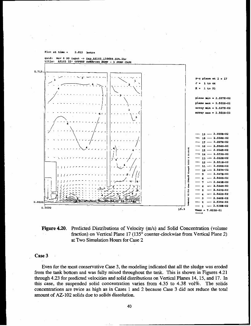
Plot at time= 2.012 hours
qaid: NOV 6 99 input -> bp_Azlo2_l10699. 50%.2hrtitle: AZ102 22* OFl?Sm mmmrs — - ? — m>cow
5.715
0.000(+
. . ./.. ..\. ~--. . . . .. . . .3
/
\. .,.1..
. . ,~4
1’
. ---- -., ,4
/
.K...?<
. . . . . . . . .+. . ...,,3’ $... . .
. . . ---- -.. , .,+ ., 1 \,,4, .,,. . .
3---- ---- . . .
-,141J li(4a .4,.
L
/,
‘w
3
,, --- ------ .,4 ,. //[ lldda 84a..
\
,., ,. . . . . . . . .* .,,, ,,, ,,, ,,, ,,
,., ,,. .e --
/
-/, ,,, , ,,, ,,, ,,. ,
. . 4 4
\
,,, ,, ---- ,,, /,, ,,, .,. ’,4. ,
1/”-\ilJ,.--~ -.s 4,,’ --------
4
i
~/1111 . ~ ----- ...,, .-- ?----
J / /, / < ---- . . . . . . .-----5-Q I
] / / / / ----------- --- ‘6- ‘8;/ ] /:::: ::;----- _.5--.-----7. ,
i
J .=
- ‘~y:::d~
J: .~j!j ~ ~ i } ~~s$~-~> -.-- -.
nn,-1 I .-... 13.a
r-z Qbne at I . 17
J= lto44
K= lto23
$Ilatm d.n = 2 .537E-Q2
plane max . 2.560E-02
may nib = 2.537E-02
a~ay niax = 2.560&02
— 19 — 2.ss9B-02
— 18 — 2 .5S8E-02
— 3.7— 2.557E-02
— 16 — 2.556E-02
— 3.5— 2.554E-02
— 14 — 2.553E-02
— 13 — 2.552E-02
— 12 — 2.551E-02
— 11 — 2.550=-02
— 10 — 2.549E-02
—9 — 2.547E-02
‘8 — 2.546E-02
—7 — 2.545E-02
‘6 — 2.544E-02
—5 — 2.543E-02
—4 — 2.5422-02
—3 — 2.540E-02
—2 — 2 .5393+02
—1 — 2.538E-02
Vmax = 7 .821E-01
F@we 4.20. Predicted Distributions of Velocity (m/s) and Solid Concentration (volumefraction) on Vertical Plane 17 (135° counter-clockwise from Vertical Plane 2)at Two Simulation Hours for Case 2
Case 3
Even for the most conservative Case 3, the modeling indicated that all the sludge was erodedfrom the tank bottom and was fully mixed throughout the tank. This is shown in Figures 4.21through 4.23 for predicted velocities and solid distributions on Vertical Planes 14, 15, and 17. Inthis case, the suspended solid concentration varies from 4.35 to 4.38 vol?lo, The solidsconcentrations are twice as high as in Cases 1 and 2 because Case 3 did not reduce the totalamount of AZ-102 solids due to solids dissolution.
40
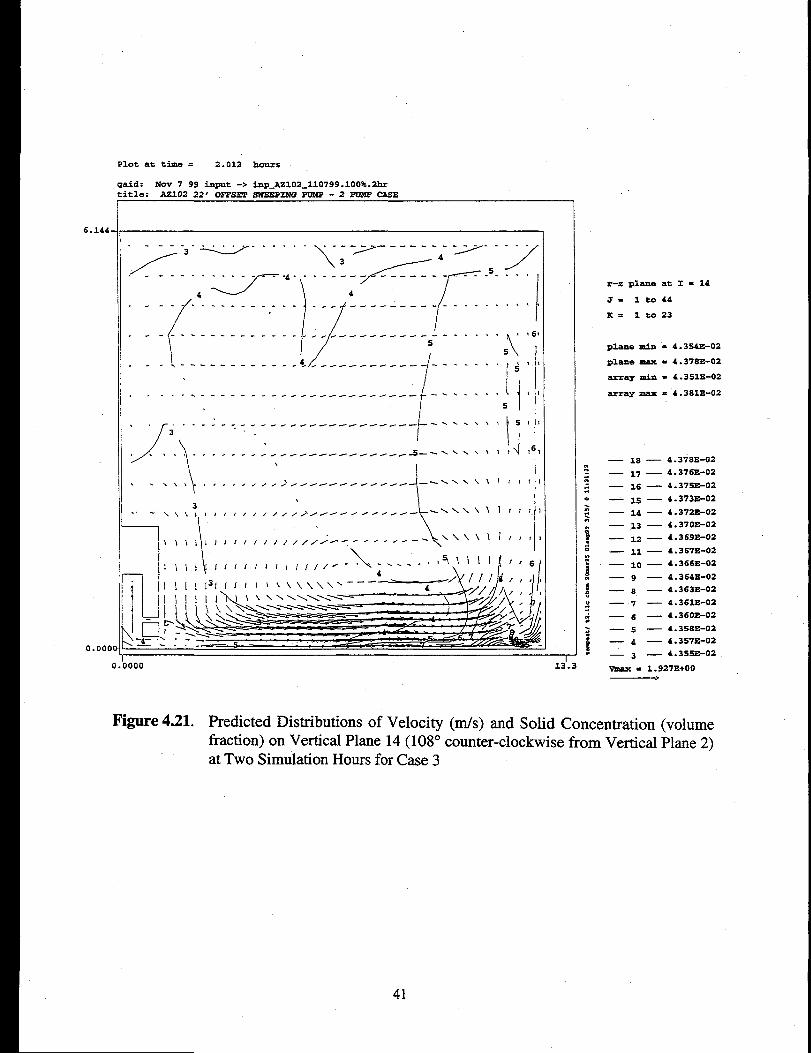
Plot at eh . 2.012 hours
6.144.
0.000
id: NOV 7 99 ~t -> inP_3Az102_l10799.100%.2hrtie: AS102 22a 0FFSS3’ SWEEP2NQ SUMP - 2 PVMP CASE
---- . . . . . -.
----- ------ -.. .
/
II,---- ------ ------ ~---- ----- ---- -...$~ 1 ~
5
. . If3-:--” ~-.-”-------------->’ ““ :’ ‘
Jp
n\-4_ ,..—-
\ 1.\\ill Jo/////////- <--------\\\\ \l/lf
Ill \““s11/ JJJll l///~- .-----’
t%\\ll
ll1131111!t\\\\\\’- --—
___. .
c 000 13’.3
r-z plane at I = 14
J= lt044
K. lt023
plane xain = 4.354E-02
plane ma% = 4.378E-02
-ay tin = 4.351E-02
array m = 4.381E-02
— 18 — 4.3;8E-02
— L7 — 4.376E-02
— 16 — 4.375E-02
— 15 — 4.373E-02
— 14 — 4.372E-02
— 13 — 4.370E-02
— 12 — 4.369E-02
— 11 — 4.367E-02— 10 — 4.366E-02
—9 — 4.364E-02
‘8 — 4.363E-02
—7 — 4.362s-02
‘6 — 4.360E-02
—5 — 4.356E-02
—4 — 4.357E-02
— 3 — 4.355E-02
Vmax = 1.927E+O0
Figure 4.21. Predicted Distributions of Velocity (m/s) and Solid Concentration (volumefraction) on Vertical Plane 14 (108: counter-clockwise from Vertical Plane 2)at Two Simulation Hours for Case 3
41
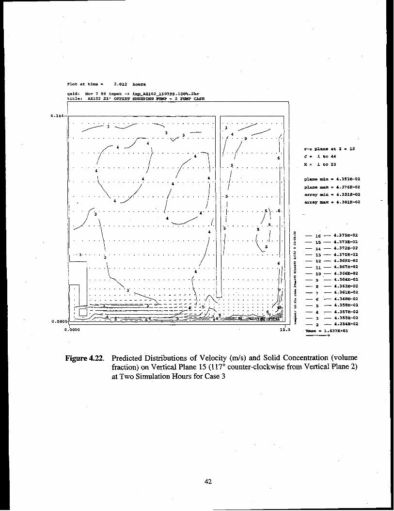
Plot at time . 2.012 hours
id: NOV 7 99 input -> inp_A2102_l10799 .100%.2hr.... ..... .. . .-”.. -—. -.. —- ,,—... ....
6.144
0.000
. . . . . . . . .. . . .~3y-y3---,3 /
. . . . . . . . . . ./J-;’”w3’””-”’ fj=. . ......................---. ...-.‘,/
[/. . . . . . . . . . . .4
/ . . . .. f4..\ :.~..::::::!6 :
\ 4 4.(, . . . . . . . ./ . . . . . . 4 . . . . . . .. .. .. .. . . .
“.””””~4”/””””““”””’ “ ;“””””-””’”[
./ II
.. .................................3
~j. .6.
\ 4 /“’ ‘‘/ “
\
. . . . . . . . . . . . . . . . . /... .4
I
. .
5
I. . k . . . . . . . . . . . . . . . . . -. ./.11.1.
.. 3-..\3 . .
/
I.... ..
/J\. ...! .5. .5
(
I. . . . . . . . ,
5
. . . . . . . .
6. . . . . . . .
\
. . . . . . . . . . . . . . . . . . . . . . . . . . . . .4
\l
. . . . . . . . . . . . . . . . . . . . . . . . . . . . . . . . . . . . .
. . . . . . . . . . . . . . . . . . . . . . . . . . . ..-. . . . . . . ./1
-’-%’’’’’””~ ““’
. . . . . . . . . .
., . ..- -
—-——–’’–-=2zz_z I:zz; : :< y. : “
%/
J,. . . . . . . . . .
J
. . . . . . . . . . .
. . . . . . .A . . . . . . . . . . . .
.@&&5___ 54 ‘--~#>&’8
———— -- —.- . .
__ ---- . .
fboo
r-z plane at S = 15
a. lt044
K. lt023
pl~e tin = 4.353E-02
plane ma% . 4.376E-02
array min = 4.351E-02
array ma% = 4.38133-02
— 16 — 4.375E-02
— 1S — 4.373E-02
— 14 — 4.37233-02
— 13 — 4.370!3-02
— 12 — 4-369E-02— 11 — 4.367E-02
— 10 — 4.36633-02
— 9 “— 4.364E-02
—8 — 4.363E-02
—7 — 4.363s3-02
—6 — 4.360E-02
—5 — 4 .358E-02
— 4 - 4.357E-02
—3 — 4.355E-02
—2 — 4.354E-02
VmaX = 1.637E+01
Figure 4.22. Predicted Distributions of Velocity (m/s) and Solid Concentration (volumefmction) on Vertical Plane 15(1 17° counter-clockwise from Vertical Plane 2)at Two Simulation Hours for Case 3
42
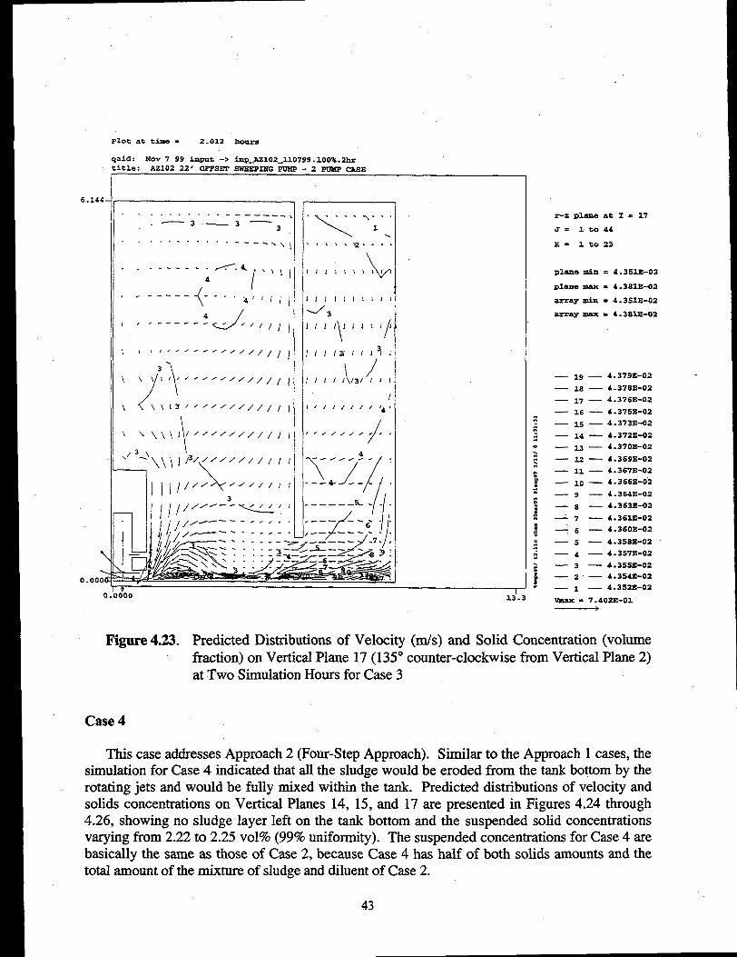
Plot at tima = 2.012 hours
6.144
\
.
0.000
id: Nov 7 99 input -> inp_A2102-110799 .1OO%.2IU1-1.. ..*I-I997. ,----- —n,. .— . —. “..-..=. -.”. “. “. .- “.. .“—-.” .ucAr - 4 .“- a.
. . . . . . . . . . -. --— -., . . . -.x- . ..—~ —3—
3\
1.
. . . . . . . . . . . ----’\\ “’’’’2’”””
)00 13.3
r-z plane at I . 17
.7= lt044
x= lt023
Diane tin = 4 .351E-02
plane zuax . 4.381E-02
array min = 4.351E-02
array max . 4.3823+02
— 19 — 4.379E-02
— 18 — 4.378E-02
— 17 — 4.376E-02
— 16 — 4 .375E-02
- 15 — 4.373E-02
— 14 — 4.372E-02
— 13 — 4 .370E-02
— 12 — 4.369E-02
— 11 — 4.367E-02
— 10 — 4.366E-02
—9
‘8
-7
‘6
—5
—4
—3
—2
—1
— 4.364E-02
— 4.363E-02
— 4.361E-02
— 4 .360E-02
— 4.358)3-02
— 4.3573+02
— 4.355E-02
— 4.354E-02
— 4.3S2E-02
muax = 7.4023+01>
Figure 4.23. Predicted Distributions of Velocity (m/s) and Solid Concentration (volumefraction) on Vertical Plane 17 (135° counter-clockwise from Vertical Plane 2)at Two Simulation Hours for Case 3
Case 4
This case addresses Approach 2 (Four-Step Approach). Similar to the Approach 1 cases, thesimulation for Case 4 indicated that all the sludge would be eroded from the tank bottom by therotating jets and would be fully mixed within the tank. Predicted distributions of velocity andsolids concentrations on Vertical Planes 14, 15, and 17 are presented in Figures 4.24 through4.26, showing no sludge layer left on the tank bottom and the suspended solid concentrationsvarying from 2.22 to 2.25 V0190(99’ZOuniformity). The suspended concentrations for Case 4 arebasically the same as those of Case 2, because Case 4 has half of both solids amounts and thetotal amount of the mixture of sludge and diluent of Case 2.
43
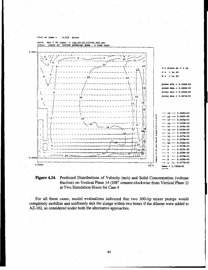
Plot at time . 2.012 hours
2.858
0.000
(
lid: IsOv 7 99 input-> inR_A2102_110799 .25%.2bx.tIe: ~102 22. o~m SWEESIMG ~ _ 2 _ ~
. . . . ___ .----- —- .—-
y:!%+’: k+=$=z. . .,- 9 ------------- ---
/ II f -(
----- ---- . . . . . .12
. . . . ---- ----- ---- ----- _,_ -—_ ---- . .8 w
. 8.,-,.,-. ----- ---- xl ----- ~..--_ ---
~1 /
+> . 1 . .
,. .,, ,. ..- ----- --
{
------~ ~-.-- _____ .
i
.\ . .
. .
\.
.9 .
.\
11I!-
., ,1, ---------
1------~s-~,- _____ ----
P\\,.
9., .,.. ------ -
I
------ -=~e~ ----- -.. !
10 Ii ‘
II,,,-.-------------z . . . . ______ \
,1\
11... ...,. ----- -------- .-. . . ..- --- \\\\
4 . . . . . . . -/-. ,/, ---- /- ..,. . . . . .
1
\\\l
? g /.////-,.“id’’’--’’..’----”” “
L2
,, ,
,, \
I
00013”.3
z-z plane at x - 14
.3- lt044
Pi= lt023
91ane mi.n = 2 .226E-02
Plana XMX . 2.246E-02
array tin . 2 .222E-02
a~ay m = 2.247E-02
— 19 — 2 .24SE-02
— 18 — 2 .244=02
— 17 — 2 .243E-02
— 16 — 2 .242E-02
— 15 — 2 .240E-02
— 14 — 2 .239E-02
— 13 — 2 .238E-02
— X? — 2.237E-02
— M — z-23sE-02
— 10 — 2 .234E-02
—9 — 2.233E-02
—8 — 2.232E-02
—7 - 2.230E-02
‘6 — 2 .229E-02
—5 — 2 .228E-02
—4 — 2.227E-02
W = 1.782E+O0—
predicted Distributions of Velocity (m/s) and Solid Concentration (volumefraction) on Vertical Plane 14 (108° counter-clockwise from Vertical Plane ~)at Two Simulation Hours for Case 4
For all these cases, model evaluations indicated that two 300-hp mixer pumps wouldcompletely mobilize and uniformly mix the sludge within two hours if the diluent were added toAZ-102, as considered under both the alternative approaches.
44
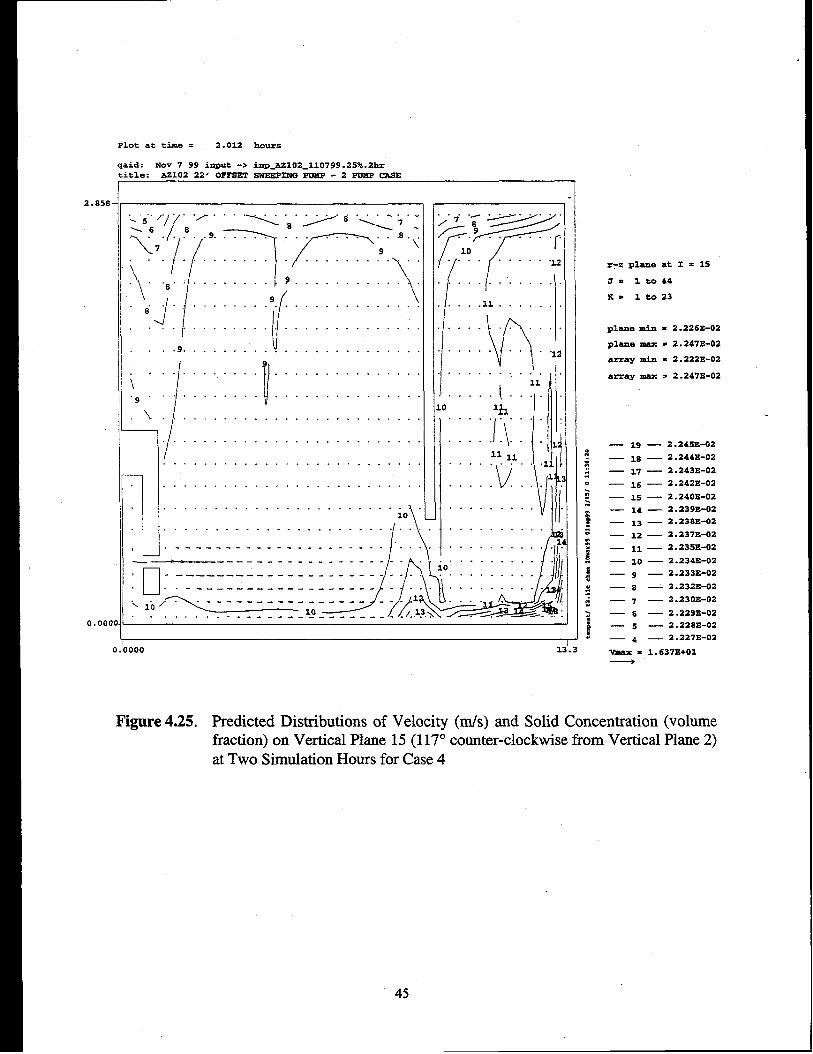
Plot at time . 2.012 hours
2.858
0.000
id: Nov 7 99 input -> inP_A=02_110799 .26%.21utle: A2102 22* OFPSET SWZEPJ2W PUMP - 2 PUMP CASE
. .. . . . .
[
/.
%’”8““’”/
/
. . . . . . .\. .
“S” -”..
..l8“”.”.””
. . . . . . . .
. . ..9 . . . .
/
i“””’”””. . . . . . . .9
““”Y
T................
.8. /8.<7.
B.,
/9
\
. . . . . . . . . .
9 . . . . . . . . . . .
{
\9
. . . . . . . . . . . . . . . . . . .
. . . . . . . . . . . . . . . . . . .
. . . . . . . . . . . . . . . . . . .
1.... .................. .............,\, . . . . . . . . . . . . . . . . . . . . . . . .
. . . . . . . . . . . . . . . . . .
. . . . . . . . . . . . . . . . . . . . . . . .
. . . . . .
. . . . .
. . . . . . . . . . . . . . . . . . .
. . . . . . . . . . . . . . . . . .101
. . . . . . . . . . . . . . . . -1 ~
1--------------------.. ..—---—---------------P‘rl --------------------i+.1 1------------------ ---A-4-
U
-G-.-j~. . . . . ---- ---- ____---- ---
H=-;10
(’ (’........- -12
. . . . . . . . . .
. . . .11 . . . . . . .
v)
. . . . . . . . . .
. . . . . . .. .12
. . . . . . . . . . . .
. . . . . 1-:.lb
~
. . . . . . . . . . .
l\. . . . . . . .“1
11 ~~. . . . . . . . ,,
v
1 i
1. . . . . . . . . .
/
. . . . . . . . ,,
‘J..........
1. . . . . . . . . . .,. . . . . . . . . .. . . . . . . . . II.........._.+l
. . . .—/- .. :
000 13’.3
r-z plane at I . 1S
s= lt044
K= lt023
plane min = 2 .226E-02
Plium= - 2 .247E-02
array min = 2.222E-02
array ma% s 2 .247E-02
— 19 — 2.245?4-02
— 18 — 2.244E-02
— 3.7— 2.243E-02
— 16 — 2.242E-02
— 15 — 2 .240E-02
— 14 — 2.239E-02
— 13 — 2.238E-02
— 12 — 2 .237E-02
— 11 — 2 .235E-02
— 10 — 2.2342-02
—9 — 2.233E-02
—8 - 2.23233-02
—7 — 2 .230E-02
—6 — 2 .229E-02
—5 — 2.228E-02
— 4 — 2 .227s3-02
~ = 1.637E+01
Figure 4.25. Predicted Distributions of Velocity (m/s) and Solid Concentration (volume—fraction) on Vertical Plane 15 (1178 counter-clockwise from Vertical Plane 2)at Two Simulation Hours for Case 4
45
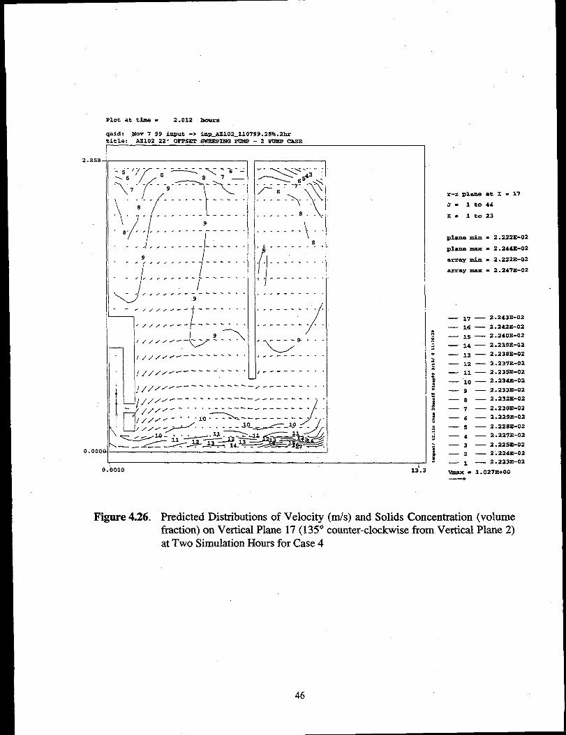
Plot at time= 2.012 hours
2.858
0.000
Lid: Nov 7 99 input -> tiP-AZ102_l10799 .25%.2br.tle: A2102 22 v 0FP8ET 8W2EP3.NG ~ - 2 PUMP CAEE
\s6’~- ‘~ --*K; “?“-
f\( 7“\...--------------
7 9
\
.-. . ----- ------
8. . . . . . . . . ---- -..
/{
9
‘ 8” < ’ >’”------ ‘--”
. . . ,,, . ---- ---- -.
9.-, ,,, , ---- ---- . .
J/
.-, ,,, , ..-- ---s . .
-. /,,,. ------- -,-.9
-. ////A-- +-------
L,///.’ ~---- -----
,//.’ /~---- 2.x///// ~~-----’ ‘.”
,,,, /,/----------
. ---- B . .\.
\------ -
/_-. ~.-
,------ -.
I------ -------------
/
------- ---
------- ---
~....
----- -..
------- ---
//,,/,4-- .----..-,.- --------
,,//// ----- --+--- ,---- ----i“~.
1,,/,,--...------_<----.......-..---. -----.--.,.=&’. “ “ “ -‘“
:.?42 e
I
1000 13’.3
Z-Z D%cUI- at I = 17
J= lto44
X= lto23
plane mi.n = 2.222E-02
plane m = 2.244E-02
array lain - 2.222E-02
may max. = 2.247s-02
Figure 4.26. Predicted Distributions of Velocity (m/s) and Solids Concentration (volume
— 17 — 2.243E-02
— 16 — 2.242S-02
— 15 — 2.2408+02
— 1.4— 2.239X-02
— 13 — 2 .2383+02
— 12 — 2 .237E-02
— 11 — 2.23!N3-02
— 10 — 2.234E-02
—9 — 2 .233E-02
‘8 — 2.232E-02
—7 — 2.230?3-02
‘6 — 2.229E-02
—5 — 2 .2283+02
—4 — 2 .227E-02
—3 — 2.225E-02
—2 — 2 .224E-02
— I — z-2z3E-02
‘imax = 1.027E+O0—
fraction) on Vertical Phme 17 (135° counter-clockwise from Vertical Plane 2)at Two Simulation Hours for Case 4
46
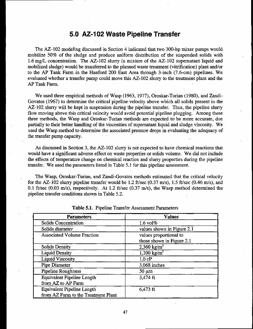
5.0 AZ-1 02 Waste Pipeline Transfer
The AZ-102 modeling discussed in Section 4 indicated that two 300-hp mixer pumps wouldmobilize 50% of the sludge and produce uniform distribution of the suspended solids with1.6 mg/L concentration. The AZ-102 slurry (a mixture of the AZ-102 supernatant liquid andmobilized sludge) would be transferred to the planned waste treatment (vitrification) plant adorto the AP Tank Farm in the Hanford 200 East Area through 3-inch (7.6-cm) pipelines. Weevaluated whether a transfer pump could move this AZ-102 slurry to the treatment plant and theAP Tank Farm.
We used three empirical methods of Wasp (1963, 1977), Oroskar-Turian (1980), and Zandi-Govatos (1967) to determine the critical pipeline velocity above which all solids present in theAZ- 102 slurry will be kept in suspension during the pipeline transfer. Thus, the pipeline slurryflow moving above this critical velocity would avoid potential pipeline plugging. Among thesethree methods, the Wasp and Oroskar-Turian methods are expected to be more accurate, duepartially to their better handling of the viscosities of supematant liquid and sludge viscosity. Weused the Wasp method to determine the associated pressure drops in evaluating the adequacy ofthe transfer pump capacity. .
As discussed in Section 3, the AZ-102 slurry is not expected to have chemical reactions thatwould have a sigtilcant adverse effect on waste properties or solids volume. We did not includethe effects of temperature change on chemical reaction and slurry properties during the pipelinetransfer. We used the parameters listed in Table 5.1 for this pipeline assessment.
The Wasp, Oroskar-Turian, and Zandi-Govatos methods estimated that the critical velocityfor the AZ-102 slurry pipeline transfer would be 1.2 ft/sec (0.37 m/s), 1.5 ft/sec (0.46 mls), and0.1 Il./see (0.03 nis), respectively. At 1.2 ft/sec (0.37 m/s), the Wasp method determined thepipeline transfer conditions shown in Table 5.2.
Table 5.1. Pipeline Transfer Assessment Parameters
1 Parameters I ValuesSolids Concentration 1.6 vol%Solids diameter values shown in Figure 2.1
I Associated Volume Fraction values proportional tothose shown in Fimre 2.1
Solids Density 2,360 kg/m3Liquid Density 1,100 kg/m3Liquid Viscosity 1.0 CPPipe Diameter 3.068 inchesPipeline Roughness 50 ~mEquivalent Pipeline Length 3,474 ftfrom AZ to AP Farm
I Equivalent Pipeline Length 6,473 ftfrom AZ Farm to the Treatment Plant 1
47
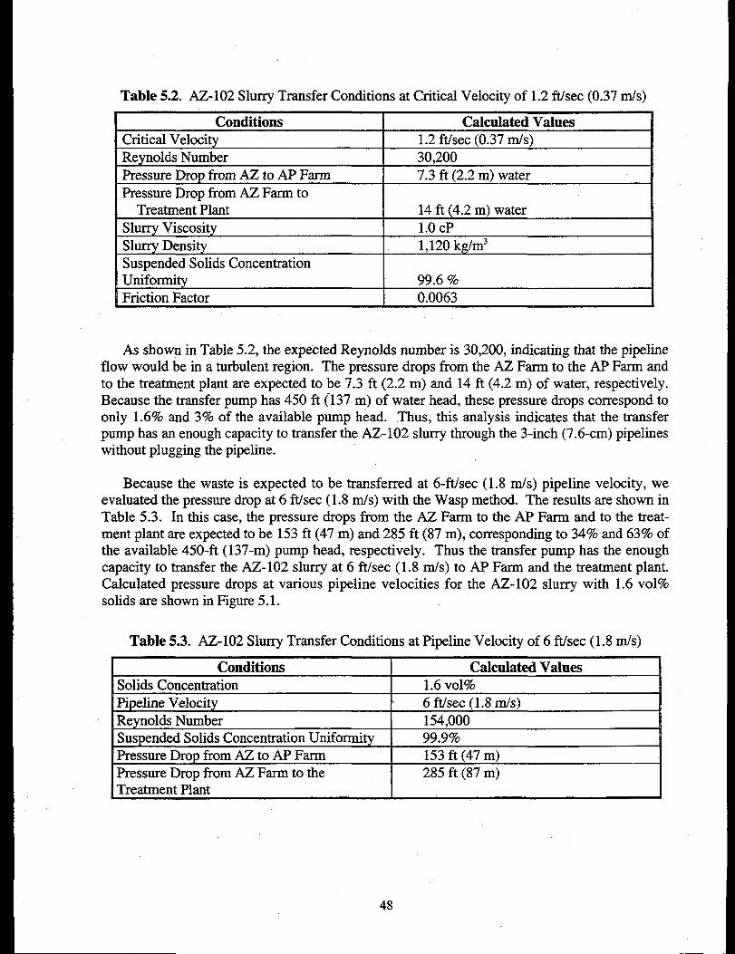
Table 5.2. AZ-102 Slurry Transfer Conditions at Critical Velocity of 1.2 ft/sec (0.37 m/s)
Conditions I Calculated ValuesCritical Velocity 1.2 ftisec (0.37 mls)Reynolds Number 30,200Pressure Drop from AZ to AP Farm 7.3 ft (2.2 m) waterPressure Drop from AZ Farm to
Treatment Plant 14 ft (4.2 m) waterSlurry Viscosity 1.OCP ‘Slurry Density 1,120 kg/m3Suspended Solids ConcentrationUniformity 99.6 %Friction Factor 0.0063
As shown in Table 5.2, the expected Reynolds number is 30,200, indicating that the pipelineflow would be in a turbulent region. The pressure drops from the AZ Farm to the AP Farm andto the treatment plant are expected to be 7.3 ft (2.2 m) and 14 ft (4.2 m) of water, respectively.Because the transfer pump has 450 ft (137 m) of water head, these pressure drops correspond toonly 1.6~0 and 3’ZOof the available pump head. Thus, this analysis indicates that the transferpump has an enough capacity to transfer the AZ-102 slurry through the 3-inch (7.6-cm) pipelineswithout plugging the pipeline.
Because the waste is expected to be transferred at 6-ft/sec (1.8 n-ds) pipeline velocity, weevaluated the pressure drop at 6 ftkec (1.8 m/s) with the Wasp method. The results are shown inTable 5.3. In this case, the pressure drops from the AZ Farm to the AP Farm and to the treat-ment plant are expected to be 153 ft (47 m) and 28$ ft (87 m), corresponding to 34f10and 63% ofthe available 450-ft (137-m) pump head, respectively. Thus the transfer pump has the enoughcapacity to transfer the AZ-102 slurry at 6 Wsec (1.8 m/s) to AP Farm and the treatment plant.Calculated pressure drops at various pipeline velocities for the AZ-102 slurry with 1.6 vol%solids are shown in Figure 5.1.
Table 5.3. AZ-102 SlurryTransfer Conditions at Pipeline Velocity of 6 ft/sec (1.8 rnh)
Conditions Calculated ValuesSolids Concentration 1.6 vol%Pi~eline Velocitv 6 ftisec (1.8 rrds)Reynolds Number 154,000Suspended Solids Concentration Uniformity 99.9%Pressure Drop from AZ to AP Farm 153 ft (47 m)Pressure Drop from AZ Farm to the 285 ft (87 m)
ITreatment Plant I 1
48
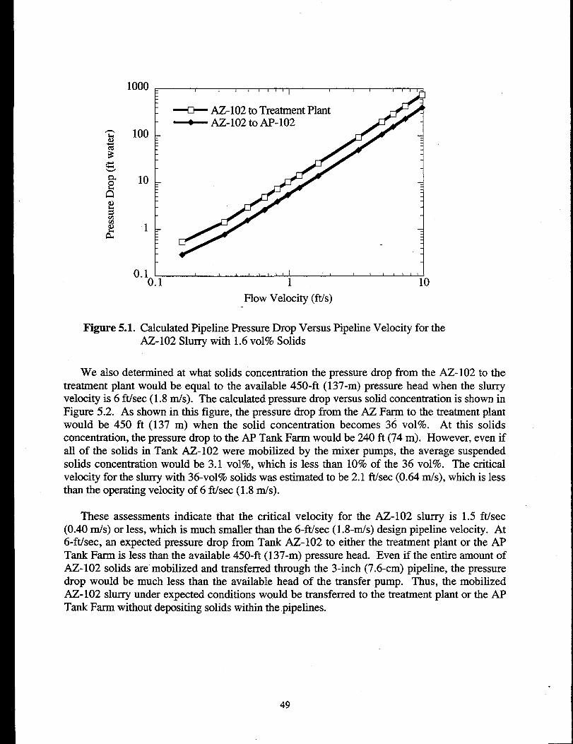
1000 ~ 1 1 t t 1 1 I 1 I ! 1 , 1 1 r i !~
‘2aJ
$$j
100 .
10 :
1 .
~ AZ-102 to Treatment Plant~ AZ-102 to AP-102
q
0., ~0.1 1 10
Flow Velocity (ft/s)
Figure 5.1. Calculated Pipeline Pressure Drop Versus Pipeline Velocity for theAZ-102 Slurry with 1.6 vol% Solids
We also determined at what solids concentration the pressure drop from the AZ-102 to thetreatment plant would be equal to the available 450-ft (137-m) pressure head when the slurryvelocity is 6 ftlsec (1.8 m/s). The calculated pressure drop versus solid concentration is shown inFigure 5.2. As shown in this figure, the pressure drop from the AZ Farm to the treatment plantwould be 450 ft (137 m) when the solid concentration becomes 36 VO1%. At this solidsconcentration, the pressure drop to the AP Tank Farm would be 240 ft (74 m). However, even ifall of the solids in Tank AZ-102 were mobilized by the mixer pumps, the average suspendedsolids concentration would be 3.1 VOIYO,which is less than 10?Ioof the 36 vol~o. The criticalvelocity for the slurry with 36-vo19i0solids was estimated to be 2.1 ftkec (0.64 m/s), which is lessthan the operating velocity of617./sec (1.8 m/s).
These assessments indicate that the critical velocity for the AZ- 102 slurry is 1.5 ft/sec(0.40 mh) or less, which is much smaller than the 6-ft/sec (1.8-m/s) design pipeline velocity. At6-ft/see, an expected pressure drop from Tank AZ-102 to either the treatment plant or the APTank Farm is less than the available 450-ft (137-m) pressure head. Even if the entire amount ofAZ-102 solids are mobilized and transferred through the 3-inch (7.6-cm) pipeline, the pressuredrop would be much less than the available head of the transfer pump. Thus, the mobilizedAZ-102 slurry under expected conditions would be transferred to the treatment plant or the APTank Farm without depositing solids within the pipelines.
49
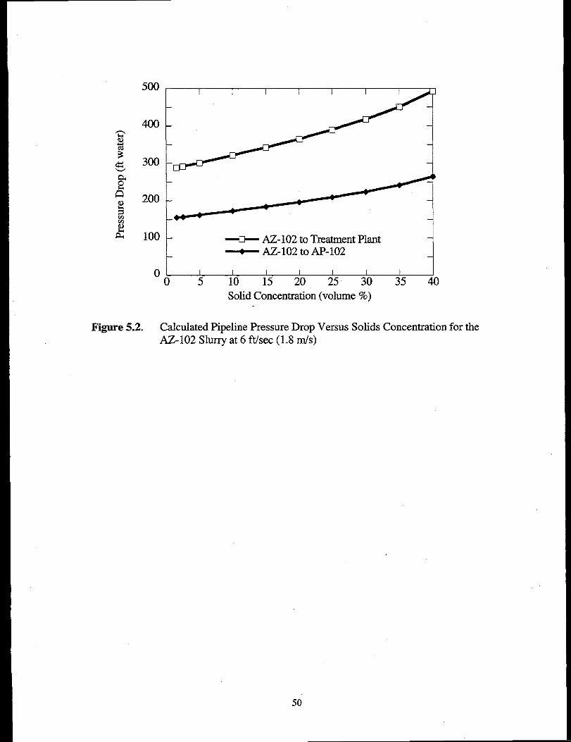
500
400
300
100
1
~ AZ-102 to Treatment Plant~ AZ-102 to AP-102
i01 I I 1 I I I [ 1
0 5 10 15 20 25 30 35 40SolidConcentration (volume%)
Figure 5.2. Calculated Pipeline Pressure Drop Versus Solids Concentration for theAZ-102 Slurry at 6 ft.kec (1.8 m/s)
50
6.0 Summary and Conclusions
We examined how well two 300-hp mixer pumps would mix the solid and liquid radioactivewastes stored in Hanford Tank AZ-102 and confirmed the adequacy of a 3-inch (7.6-cm)pipeline system to transfer the resulting mixed waste slurry to the AP Tank Farm and the plannedwaste treatment (vitrification) plant within the 200 East Area of the Hanford Site.
Our waste chemical modeling assessment using the GMIN chemical code indicates that thesludge, consisting of the solids and interstitial solutions, and the supematant liquid are basicallyin an equilibrium condition, so the pump jet mixing of the sludge and supematant liquid ofAZ-102 waste would not change the waste properties and the solids amount in any discemablemanner due to chemical reactions. Some of the chemical assessment results are stated below:
●
●
●
●
Most of the solids present in the sludge are non-dissolvable with AZ-102 interstitialsolution and supematant liquid.
Expected dissolvable solids with these solutions are Al(OH)~(s), NaF(s),Cry, SiO,(am), and possibly thenardite (Na$O,(s)).
Mixing of the supematant liquid and sludge would dissolve NaF(s), SiOz(am), andNz$Oa(s), while small amounts of Cr(OH)2(arn) and Al(OH)~(s) would precipitate.
Resulting changes on solid amounts due to precipitation and dissolution areinsignificant to the total amount of the AZ-102 waste (1.5 % or less).
We then evaluated how much AZ-102 waste the two 300-hp mixer pumps would mix bysimulating pump jet mixing with the TEMPEST computer code. Because the chemicalassessment indicated that the pump jet mixing would not change the AZ- 102 waste propertiesand total solids volume very much, we did not simulate the potential chemical reactions duringthe pump jet mixing modeling. The mixing assessment indicates that the two 300-hp mixerpumps would mobilize half of the sludge, which has a yield strength of 1,540 Pa. Some of themain results are described below.
The two 300-hp pumps will mobilize 50% of the original sludge
The rotating pump jets would mobilize the sludge up to 23 ft (7.0 m) from the pump
Jets would not erode the sludge within 7 in. (O.18 m) of the tank bottom
The resulting suspended solids concentration would be 1.6 vol% and uniformlydistributed in the entire tank (except the region of noneroded sludge)
It will take one to two hours to reach the final fully mixed condition
Twenty-two airlift circulators and steam heating coils have some relatively smallimpacts, but they are not significant in the overall sludge erosion
The centerline jet velocity reduces its value at a rate approximately proportional tothe distance from the jet exit. However, the AZ-102 jet velocity is smaller than thatof the classical homogeneous jet experiment at equal distance because thenonhomogeneous, rotating, non-Newtonian, AZ-102 jets are located near the tankbottom and are confined by the sludge bank and tank wall.
51
Because pump jet mixing would mobilize only half of the AZ-102 sludge, we explored apossible way to improve the effectiveness of the pumps to mobilize the AZ-102 waste. Theprevious AZ- 102 pre-treatment experimental study indicates that the diluent (a mixture of water,ferric nitrate, sodium nitrite, and sodium hydroxide) could significantly reduce the sludge yieldstrength by dissolving half the original AZ-102 solids. Thus, we developed the concept of twoalternative approaches and assessed them by assuming that this diluent would dissolve half of theAZ-102 solids and reduce the yield strength from 1,540 Pa to 1.2 Pa. The validity of thisassumption could be tested in laboratory studies. The alternative approaches considered here are
Approach 1: Three-step approach
Step 1: Pump out the original AZ-102 supematant liquid only
Step 2: Add the diluent (the mixture of water, ferric nitrate, sodium nitrite, and sodiumhydroxide) to Tank AZ-102 at a 6:1 (diluent to sludge) volume ratio
Step 3: Mix the diluent-washed, weakened, and reduced amount of AZ-102 sludge withthe diluent using two 300-hp mixer pumps.
Approach 2: Four-step approach -
Step 1: Mix the original AZ-102 sludge and supematant liquid using two 300-hp pumps
Step 2: Pump the resulting AZ-102 slurry from the tank
Step 3: Add the diluent (mixture of water, ferric nitrate, sodium nitrite, and sodiumhydroxide) to AZ-102 tank at 6:1 (diluent to remaining sludge) volume ratio
Step 4: Mix the remaining diluent-washed, weakened, and reduced amount of AZ-102sludge and the diluent by two 300-hp mixer pumps.
We applied the TEMPEST code to four cases representing these two alternative approaches.These pump jet mixing simulations indicated that for both alternative approaches, two 300-hpmixer pumps would totally mobilize and uniformly mix the sludge within two hours if thisdiluent were added to Tank AZ-102.
We used the three empirical methods of Wasp, Oroskar-Turian, and Zandi-Govatos todetermine whether a transfer pump could move the AZ-102 slurry (a mixture of the AZ-102supematant liquid and mobilized sludge) to the AP Tank Farm and to the planned wastetreatment (vitrification) plant through three-inclh (7.6-cm) pipelines. Because the AZ-102 slurryis basically in equilibrium condition, we did not include the effects of chemical reactions in thepipeline assessment.
The assessments indicate that the critical velocity for the AZ- 102 slurry is 1.5 ftisec(0.46 m/s) or less, which is much less than the expected 6-ft/sec (1.8-m/s) operating pipelinevelocity. At the 1.2-ft/sec (0.37 m/s) critical velocity (with corresponding Reynolds number of30,200) predicted by the Wasp method, the associated pressure drops from the AZ Farm to theAP Farm and the treatment plant are expected to be .7.3 ft (2.2 m) and 14 ft (4.2 m) of water,
52
respectively. Because the transfer pump has 450 ft (137 m) of water head, these pressure dropscorrespond to only 1.6% and 3% of the available pump head.
At a 6-ft/sec (1.8 m/s) operating velocity, the expected pressure drop from Tank AZ-102 tothe AP Tank Farm or the treatment plant is 153 ft (47 m) and 285 ft (87 m), respectively,corresponding to 3470 and 63% of the available 450-fl (137-m) pump head.
We determined that the pressure drop from the AZ Tank Farm to the treatment plant wouldbe 450 ft (137 m) at 6 ft/sec ( 1.8 rnks)velocity if the solids concentration becomes 36 vol%. Atthis solids concentration, the pressure drop to the AP Tank Farm would be 240 ft (74 m).However, even if the entire amount of solids in Tank AZ-102 were mobilized by the mixerpumps, the average suspended solid concentrations would be 3.1 vol%, which is less than 10% ofthe 36 vol%. Thus, even if the entire volume of solids in Tank AZ-106 were mobilized andtransferred through the 3-in. (7.6-cm) pipelines, the pressure drop would be much less than theavailable head of the transfer pump. The estimated critical velocity for the slurry with 36-vo1’ZOsolids is 2.1 ftisec (0.64 rids), which is less than the operating velocity of 6 ft/sec (1.8 n-ds).Thus, the pipeline transfer pump has the enough capacity to transfer the AZ-102 slurry underexpected conditions to AP Tank Farm and the treatment plant without depositing solids withinthe pipelines.
53

54

7.0 References
Felmy AR. 1995. “GMIN: A Computerized Chemical Equilibrium Program Using aConstrained Minimization of the Gibbs Free Energy.” Chemical Equilibrium and ReactionModels. SSSA Special Publication 42, pp. 37-407.
Mahoney LA and DS Trent. 1995. “Correlation Models for Waste Tank Sludge and Slurries.”PNL-10695, Pacific Northwest National Laboratory, Richland, Washington.
Onishi Y and KP Recknagle. 1997, “Tank AZ-101 Criticality Assessment Resulting born PumpJet Mixing: Sludge Mixing Simulations.” PNNL- 11486, Pacific Northwest National Laboratory,Richland, Washington.
Onishi Y and KP Recknagle. 1998. Performance Evaluation of Rotating Pump Jet Mixing ofRadioactive Wastes in Hanford Tanks 24I-AP-102 and -104. PNNL- 11920, Pacific NorthwestNational Laboratory, Richland, Washington.
Onishi Y and DS Trent. March 1999. “Mobilization Modeling of Erosion-Resisting RadioactiveTank Waste.” Proceedings of the Rheology in the Mineral Indust~ II, Kahuku, pp. 45-56.United Engineering Foundation, New York.
Onishi Y, HC Reid, DS Trent, and JD Hudson. 1996a. “Tank Waste Modeling with CoupledChemistry and Hydrothermal Dynamics.” Proceedings of 1996 National Heat TransferConference, Vol. 9, pp. 262-269. The American Nuclear Society, Houston.
Onishi Y, R Shekarriz, KP Recknagle, PA Smith, J Liu, YL Chen, DR Rector, and JD Hudson.1996b. “Tank SY-102 Waste Retrieval Assessment: Theological Measurements and Pump JetMixing Simulation.” PNNL- 11352, Pacific Northwest National Laboratory, Richland,Washington.
Oroskar AR and RM Turian. 1980. “The critical velocity in pipeline flow of slurries.” AZChE J.,26, pp. 550-558.
Rodi W. 1984. “Turbulence Models and Their Application in Hydraulics— a State of the ArtReview.” Institut fir Hydromechanik, University of Karlsruhe, Germany.
Ryan GW. 1995. Tank Characterization Report for Double Shell Tank 241-AZ102. WHC-SD-WM-ER-411 Rev. O,Westinghouse Hanford Company, Richland, Washington.
Schreiber RD. 1995. Tank Characterization Report for Double Shell Tank 241-AZ-102. WHC-SD-WM-ER-411 Rev. O-A,Westinghouse Hanford Company, Richland, Washington.
Trent DS and TE Michener. 1993. Numerical Simulation of Jet Mixing Concepts in Tank 241-SY-101. PNL-8559, PacYlc Northwest Laboratory, Richland, Washington.
55
Trent DS and LL Eyler. 1994. “TEMPEST: A Computer Program for Three-Dimensional TimeDependent Computational Fluid Dynamics.” PNL-8857 Vol. 1, Version T, Mod 2, PacificNorthwest National Laboratory, Richland, Washington.
Wasp EJ. 1963, “Cross Country Coal Pipe Line Hydraulics.” Pipeline News, p. 20.
Wasp EJ, JP Kenny, and RL Gandhi. 1977. “Solid-Liquid Slurry Pipeline Transportation.”Trans. Tech. Publ.
Whyatt GA, RJ Serne, SV Mattigold, Y Onishi, MR Powell, JH Westik Jr, LM Liljegren,GR Golcar, KP Recknagle, PM Doctor, VG Zhirnov, and J Dixon. 1996. Potential forCriticaliQ in Hanford Tanks Resulting j70m Retrieval of Tank Waste. PNNL- 11304, PacificNorthwest National Laboratory, Richland, Washington.
Wiegel RL. 1964. Oceanographical Engineering. Prentice-Hall, Inc., New Jersey, pp. 424-427.
Zandi I and G Govatos. 1967. “Heterogeneous Flow of Solids in Pipelines.” Y. Hydr. Div.,AXE, 93:HY3, Proc. Paper 5244, pp. 145-159.
56
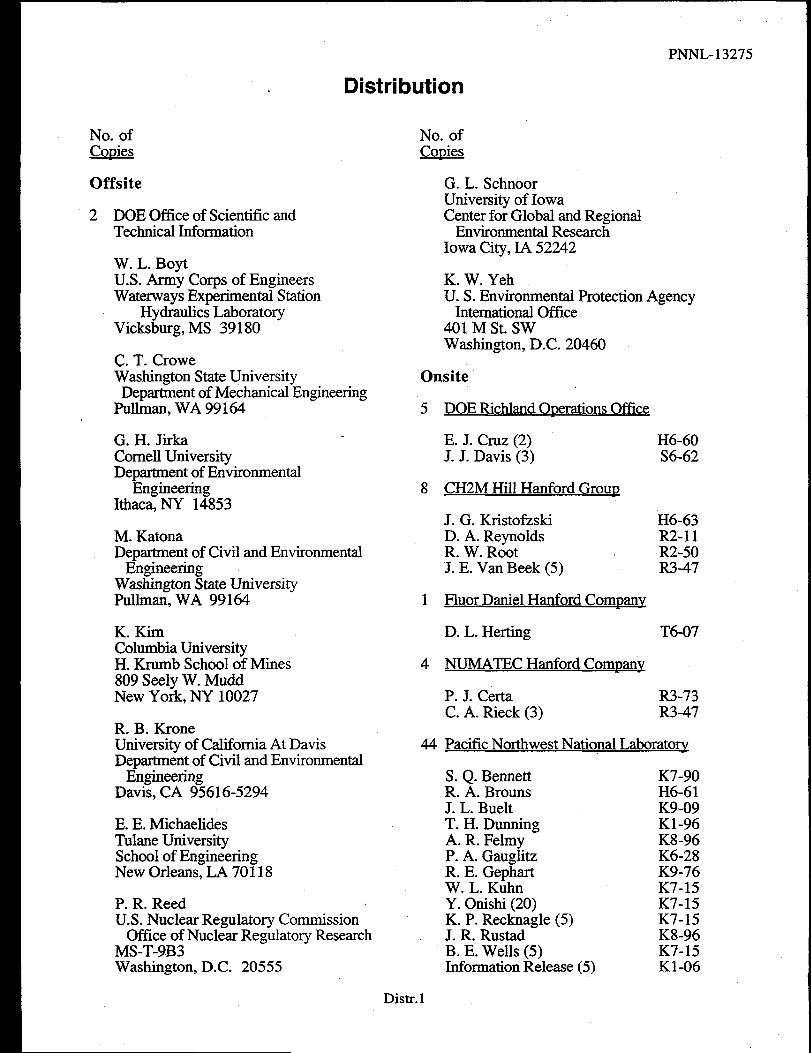
PNNL-13275
Distribution
No. of-
Offsite
2 DOE Office of Scientitlc andTechnical Information
W. L. BoytU.S. Army Corps of EngineersWaterways Experimental Station
Hydraulics LaboratoryVicksburg, MS 39180
C. T. CroweWashington State UniversityDepartment of Mechanical Engineering
Pullman, WA 99164
G. H. JirkaCornell UniversityDepartment of Environmental
EngineetigIthac% NY 14853
M. KatonaDepartment of Civil and Environmental
EngineeringWashington State UniversityPullman, WA 99164
K. KimColumbia UniversityH. Krumb School of Mines809 Seely W. MuddNew York, NY 10027
R. B. KroneUniversity of California At DavisDepartment of Civil and Environmental
EngineeringDavis, CA 95616-5294
E. E. MichaelidesTulane UniversitySchool of EngineeringNew Orleans, LA 70118
P. R. ReedU.S. Nuclear Regulatory Commission
Office of Nuclear Regulatory ResearchMS-T-9.B3Washington, D.C. 20555
No. ofQ212i=
G. L. SchnoorUniversity of IowaCenter for Global and Regional
Environmental ResearchIowa City, IA 52242
K. W. YehU.S. Environmental Protection Agency
International Oi%ce401 M St. SWWashington, D.C. 20460
Onsite
5
8
1
4
DOE Richland Ownztions Office
E. J. Cruz (2) H6-60J. J. Davis (3) S6-62
CH2M Hill Hanford GI-OUD
J. G. Kristofzski H6-63D.A. Reynolds R2-11R. W. Root R2-50J. E. Van Beek (5) R3-47
Fluor Daniel Hanford Commmy
D. L. Herting T6-07
NUMATEC Hanford Commmy
P. J. Certa R3-73C. A. Rieck (3) R3-47
44 Pacific Northwest National Laboratory
S. Q. Bennett K7-90R. A. Brouns H6-61J. L. Buelt K9-09T. H. Dunning K1-96A. R. Fehny K8-96P. A. Gauglitz K6-28R. E. Gephart K9-76W. L. Kuhn K7-15Y. Onishi (20) K7-15K. P. Recknagle (5) K7-15J. R. Rustad K8-96B. E. Wells (5.) K7-15Information Release (5) K1-06
Distr.1