Pulsed Nuclear Magnetic Resonance

1 Background

What we call “nuclear magnetic resonance” (NMR) was developed simultaneously but indepen-dently by Edward Purcell and Felix Bloch in 1946. The experimental method and theoreticalinterpretation they developed is now called “continuous-wave NMR” (CWNMR). A differentexperimental technique, called “pulsed NMR” (PNMR), was introduced in 1950 by Erwin Hahn.Pulsed NMR is used in magnetic resonance imaging (MRI). Purcell and Bloch won the NobelPrize in Physics in 1952 for NMR; more recently NMR was the subject of Nobel Prizes in Chem-istry in 1991 and 2002. We have both NMR setups in the advanced labs: one is a variation ofthe CWNMR method, and the other is a pulsed NMR system.

The physics underlying NMR is the same for both the continuous and pulsed methods, butthe information obtained may be different. Certainly, the words used to describe what is beingdone in the experiments are different: in the continuous-wave case one tunes a radio-frequencyoscillator to “beat” against the resonance of a nuclear magnetic moment in a magnetic field;in the pulsed case, one applies a sequence of RF pulses called π-pulses (180 degree pulses) orπ/2-pulses (90 degree pulses) and looks for “free induction decay” and “spin echoes”.

Below, we give a very simplified introduction, based on classical ideas, to the physics of NMR.More thorough discussions, focusing on the CWNMR technique, may be found in in the booksby Preston and Dietz [1] and Melissinos [2] (see references). In particular, the chapter in Prestonand Dietz gives a nice description of the connection between quantum-mechanical and semi-classical approaches to NMR physics. For a comprehensive treatment of NMR, see the book bySlichter [3].

1.1 Semiclassical ideas

To observe NMR, one needs nuclei with a non-zero angular momentum ~I and magnetic moment~µ. The relationship between these two quantities is

~µ = γ~I , (1)

where γ is the gyromagnetic ratio.

A simple classical calculation would give γ = q/2M , where q is the charge of the nucleus and Mis its mass. But quantum mechanics requires this dimensionally correct result to be modified.In practice, we specify γ in units of the nuclear magneton µn ≡ eh̄/2mp times a dimensionlessfactor g called the “spectroscopic splitting factor” (often just “g factor”):

γ =gµnh̄

=ge

2mp, (2)

where e is the elementary charge and mp is the mass of one proton. The g factor is on the orderof unity. It is positive for some nuclei, and negative for others. For the proton, g = +5.586; atable of various g factors may be found in Preston and Dietz.

When a nucleus of moment ~µ is placed in a magnetic field ~B0 it will experience a torque causing

1

a change in the angular momentum following Newton’s second law:

~τ = ~µ× ~B0 =d~I

dt=

1

γ

d~µ

dt. (3)

Figure 1 shows some of the vectors defined with ~B0 lying along the z axis (which is horizontalin most lab setups, including ours). The rate of change of ~µ is, by Eq. (3), both perpendicular

Figure 1: (a) Vectors defined in semiclassical picture of NMR. (b) Tip of angular momentumvector ~I, viewed opposite to ~B0.

to ~B0 and ~µ itself; hence ~µ precesses about the direction of ~B0. From Fig. 1 it is easy to derivefrom geometry and Eq. (3) that the magnitudes of the vectors ~µ× ~B and d~I/dt obey

µB0 sin θ =µ

γsin θ

(dφ

dt

); (4)

thus

ω0 ≡dφ

dt= γB0 , (5)

which is the Larmor angular frequency.

When we deal with nuclei of spin I = 1/2 (e.g., protons), quantum mechanics tells us that in amagnetic field ~B0 the ground state splits into two sublevels, as shown in Fig. 2. The energies

Figure 2: Splitting of nuclear energy levels due to applied magnetic field.

U of the two sublevels are given by

U = −~µ · ~B0 = −µzB0 = −γh̄mIB0 , (6)

where mI is the angular momentum projection of I along the z direction defined by ~B0, mI =±1/2. The difference in energy between the two sublevels is thus

∆U = U− − U+ = γh̄B0 , (7)

2

where U± is the energy of the state corresponding to mI = ±1/2. Transitions between the twoenergy sublevels may be induced by photons carrying one unit of angular momentum (h̄) andenergy h̄ω0 such that

h̄ω0 = γh̄B0 , (8)

or ω0 = γB0, which is the same as the Larmor frequency, Eq. (5).

For free protons, the gyromagnetic ratio is

γ = 2.675× 108 radians/(seconds-tesla) ,

so for fields in the 0.1–1 tesla range the frequencies will be in the megahertz range. Theseare radio frequencies (RF), and both of our setups—pulsed and continuous—work in this MHzrange. (Historical note: There was an advantage to having NMR work in the RF range,as existing radio equipment and techniques were used for detection and modulation of NMRsignals.) Given that magnetic fields in these experiments are frequently measured in kilogauss,a useful relationship to remember for protons is,

f0 (MHz) = 4.2577×B0 (kilogauss) , (9)

where f0 = ω0/2π.

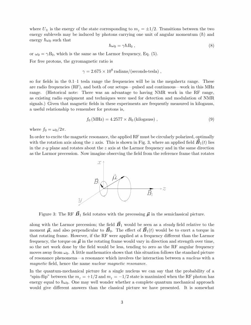
In order to excite the magnetic resonance, the applied RF must be circularly polarized, optimallywith the rotation axis along the z axis. This is shown in Fig. 3, where an applied field ~B1(t) liesin the x-y plane and rotates about the z axis at the Larmor frequency and in the same directionas the Larmor precession. Now imagine observing the field from the reference frame that rotates

Figure 3: The RF ~B1 field rotates with the precessing ~µ in the semiclassical picture.

along with the Larmor precession; the field ~B1 would be seen as a steady field relative to themoment ~µ, and also perpendicular to ~B0. The effect of ~B1(t) would be to exert a torque inthat rotating frame. However, if the RF were applied at a frequency different than the Larmorfrequency, the torque on ~µ in the rotating frame would vary in direction and strength over time,so the net work done by the field would be less, tending to zero as the RF angular frequencymoves away from ω0. A little mathematics shows that this situation follows the standard pictureof resonance phenomena—a resonance which involves the interaction between a nucleus with amagnetic field, hence the name nuclear magnetic resonance.

In the quantum-mechanical picture for a single nucleus we can say that the probability of a“spin-flip” between the mI = +1/2 and mI = −1/2 state is maximized when the RF photon hasenergy equal to h̄ω0. One may well wonder whether a complete quantum mechanical approachwould give different answers than the classical picture we have presented. It is somewhat

3

surprising to learn that Bloch showed that the classical equations governing NMR can be derivedfrom quantum mechanics. See the text by Slichter for a readable and thorough presentation ofthis result [3].

1.2 Net magnetization and relaxation

Clearly, any physical sample will consist of many atoms and the NMR signal measured by anexperiment will be due to the combined effect of the magnetic field on them all. As an example,consider an assembly of N protons, say, in water, glycerin, mineral oil, or animal tissue. Thenet magnetization ~M of the sample is the vector sum of all of the individual moments ~µi. Forthe example of spin- 1

2protons, the net magnetization along the z-axis, Mz would be given by

Mz =∑

i

γh̄mI i =1

2γh̄ (N+ −N−) , (10)

where mI i denotes the state of the ith proton, and N+, N− are the numbers of protons in the+ 1

2and − 1

2state, respectively. When an RF field ~B1(t) is applied, some protons have their

spin flip to align against ~B0; these absorb energy from the RF field. Other protons experiencea spin-flip to align with ~B0; these give energy back to the RF field. Thus, if the populations ofthe two sublevels were equal, Mz = 0 and no net energy would be absorbed from the RF field.

At room temperature with no RF field but with the steady ~B0 field there will be a smalldifference between the number of protons with spins aligned in the direction of ~B0 and thenumber aligned opposite to it; the magnetic sublevel with mI = + 1

2will have a slightly larger

population N+ than the population N− in sublevel mI = − 12. The ratio of the populations

is proportional to the ratio of the associated Boltzmann factors, according to the principles ofstatistical mechanics:

N+

N−=

exp(−U+/kT )

exp(−U−/kT )=

exp (+ 12γh̄B0/kT )

exp (− 12γh̄B0/kT )

= eγh̄B0/kT . (11)

If one applies the RF ~B1(t) to this equilibrium population, energy goes into the system, sincethere is an imbalance in the number of up (+ 1

2) spins versus down (− 1

2) spins. In a fairly short

time, however, this imbalance will vanish, because the continuous transfer of energy involvingeach moment will cause the populations N+ and N− to become equal. At this point, the netenergy absorbed by the system drops to zero, Mz = 0 and the sample is said to be saturated.

There is still a tendency for the system to recover its equilibrium configuration, even while it issubject to the oscillating field. The collection of protons could continue to absorb energy froman oscillating magnetic field ~B1(t) if the equilibrium populations would be restored quicklyfollowing a previous absorption event. The decay of Mz to its its equilibrium (nonzero) value isdue to energy exchanges between the proton magnetic moments and their local environments.

Let us consider the magnetization a bit more generally. The net magnetization ~M is a vector,and thus can be broken into components. The component along the direction of the staticfield Mz is called the longitudinal magnetization, and the components along two orthogonaldirections perpendicular to ~B0 are called the transverse magnetizations Mx and My. Clearly,each of these components is the sum of the individual component moments µz, µx and µy,respectively, e.g., Mx =

∑i µxi. Now look again at Fig. 3 which depicts a single moment

precessing about ~B0. It should be obvious that for a collection of magnetic moments at a

4

particular time, each precessing independently about ~B0, one could have a nonzero Mz but a(possibly) zero Mx or My.

The equilibrium nonzero Mz exists because the moments aligned parallel to ~B0 are at a lowerenergy than those aligned antiparallel. In order to return to equilibrium following absorptionfrom the ~B1(t) field, the moments would need to give energy to their surroundings, convention-ally called the “lattice” (even if we are dealing with liquid or gaseous materials). The relaxationof Mz to its equilibrium value is called the “longitudinal” or “spin-lattice” relaxation, and isassociated with a characteristic time called T1. In liquids, T1 is typically very short but in solidsT1 may be quite long. For example, T1 is a few milliseconds in water but thousands of secondsin ice. This is one reason why we use liquid samples in the continuous NMR setup, as the shortT1 allows for a continuous input of energy from the oscillator coil.

A nonzero Mx or My is harder to obtain because there is no reason for individual moments toprefer a particular transverse direction. At best Mx and My can oscillate between positive andnegative values at the Larmor frequency, if one can first contrive to force the moments to have anet projection onto, say, the x-axis (and indeed one can—we’ll see how). However, the resultingoscillating Mx decays because variations in the local magnetic field cause different moments toprecess at different rates. This is called “spin-spin dephasing”, and the characteristic time forthis process is called T2, the “spin-spin” or “transverse” relaxation time.

With these two relaxation processes in mind, consider how one would detect the signal of theseprecessing and relaxing moments. Since they are magnetic, an obvious choice would be to usea pickup coil. The coil also needs to be oriented transverse to the static field in order to sensethe precession, since in an orientation parallel to ~B0, the coil would only be sensitive to a slightchange in flux from a non-oscillatory Mz; whereas the transverse component Mx or My willoscillate between positive and negative values at the Larmor frequency ω0.

This arrangement is depicted schematically in Fig. 4, which is taken from the article by Hahn[4]. The top of the figure shows that at t = 0, all of the moments are aligned along the +xdirection and the pickup coil has its axis along the y-axis. The static field ~B0 points out of thepage toward the viewer, thus the moments will precess in the clockwise direction (following thesense of ~M × ~B0). The right side of the figure depicts the voltage measured across the pickupcoil. Faraday’s law requires that this voltage be proportional to the rate of change of the fluxthrough the coil, and it is a simple matter to prove that the maximum signal from the coil willoccur at t = 0 in this setup. (Try it: let the field in the coil be µ0

~M which is rotating aboutthe z-axis at ω0, and calculate the rate of change of the flux, dΦ/dt from this.)

As the moments precess, the induced voltage oscillates at the Larmor frequency (νLARMOR

inthe figure), and also decays. The decay is due to both the spin-spin dephasing, shown as aspreading of the moments away from the principal rotating x-axis—the T2 process—and to therelaxation of the moments towards the z-axis—the T1 process.

While the overall decay of the signal from the pickup coil comes from a combination of spin-spin and spin-lattice relaxation, experimentally, a third effect often predominates: spin-spindephasing due to inhomogeneities in the external field ~B0 over the volume of the sample.Taken together, the three effects lead to a combined relaxation time T ∗2 defined as

1

T ∗2=

1

T1+

1

T2+ γ∆B0 , (12)

where ∆B0 is the variation in B0. In effect, γ∆B0 is equal to a spread in Larmor frequencies∆ω0 which, all else being equal, would cause spin-spin dephasing in a characteristic time of

5

Figure 4: Induction signal measured by a pickup coil in the transverse plane following orientationof moments along the x-axis. Taken from the article by Hahn [4].

1/∆ω0. Similarly, one can assign an effective resonance width ∆ωeff ∼ 1/T ∗2 .

In summary, two processes are involved in the relaxation of the magnetization to the equilibriumvalue: 1) spin-lattice relaxation, which involves energy exchange with the environment, and ischaracterized by the time constant T1; 2) spin-spin relaxation, characterized by a time constantT2, which is caused by loss of the phase relationships among the various moments and is due tothe fact that each spin experiences a slightly different local magnetic field. In a practical setup,the measured signal comes from the oscillating transverse magnetization, characterized by atime constant T ∗2 that is related to T1 and T2, but is typically dominated by inhomogeneities inthe static field ~B0. It is important to note that the recovery to equilibrium following saturationfollows T1, but the decay of the detected signal follows T ∗2 . As required by Eq. (12), T ∗2 < T1,and in practice T ∗2 � T1.

1.3 The two experimental methods

In the continuous NMR method, the RF excitation producing the rotating ~B1 field is appliedall of the time. The resonance is created by having the ~B0 field swept slowly through the valuewhich satisfies Eq. (5). A pickup coil surrounding the sample detects the resonance, and thissignal is mixed with the fixed RF signal to create “beats” (the term for the modulation oftwo signals which have nearly the same frequency). The effect of the beats can be seen on anoscilloscope. Once the resonant signal is found, the relationship between the magnetic field andthe resonant frequency is fixed, and depending on the givens, the information can be used toextract B0 itself, γ, or related quantities. One can also crudely measure T ∗2 by looking at thedecay of the beat signal.

6

In the pulsed NMR method, the RF excitation is applied to the sample in a series of shortbursts, or pulses. The application of the RF field for a short time (the “pulse width”) allowsthe applied torque to rotate the net magnetization ~M by a specific amount. For example, onecan apply a pulse of RF field to rotate all moments by 90◦. If this pulse is applied to a sampleinitially at equilibrium with a net magnetization ~M = Mzk̂, then ~M will become Mz ı̂ (i.e.,the same magnitude of magnetization now pointing in an orthogonal direction), which will thenprecess about the z-axis. The pickup coil will see a signal like that shown in Fig. 4 as themagnetization decays back to its equilibrium state. A pulse which accomplishes this trick iscalled a “π/2 pulse”, and the signal seen as a consequence is called the “free induction decay”.A pulse of a longer duration can flip the net magnetization completely: Mzk̂ → −Mzk̂; thistype of pulse is called a “π pulse”. Interestingly, the free induction decay signal immediatelyfollowing a π pulse is zero since there is no net transverse component of the magnetizationavailable to induce such a signal.

The real utility of the pulse method comes from using a sequence of pulses. By such sequences,one can measure accurately and independently T1 and T2, and also compensate for the effectsof field inhomogeneity. The discussion of pulse sequences and their effects are taken up in moredetail in the next sections.

7

2 The pulsed NMR experiment

This experiment is performed with the TeachSpin PS1-A pulsed nuclear magnetic resonance(PNMR) spectrometer. This instrument was designed for use in a teaching laboratory. Itsmodular design separates the basic functions (oscillator and RF amplifier, RF receiver/detectorand pulse programmer) of a PNMR system, allowing the experimenter to investigate and under-stand the function of each module, and how and why the interconnections between the modulesare made.

The pulsed NMR technique involves a number of subtle and somewhat complex ideas andmethods. One way to learn it is to read through the theory, as laid out here or in the PS1-Amanual, and then use the instrument to quickly make the measurements. Another way, perhapsmore instructive, is to learn the theory and technique at the same time. In what follows, wewill assume that you will proceed along the second way. If, however, you have already read thetheory, and would prefer to move directly to the measurement tasks, you can turn to Section 3(p. 25) for a summary of those.

The instruction manual for the PS1-A gives complete details on the instrument and its opera-tion. Our instructions will focus on the particular operations needed to make the measurements.We will refer to relevant passages in the manual by means of a marginal note. Copies of the Like this.

manual are available in the lab and online at the course website.

2.1 Pulses and Free Induction Decay

We begin by stating a curious result. Recall that the magnetic moments in our system precessunder the influence of the torque from a magnetic field, Eq. 3. This precession occurs with aprecession angular frequency ω0 = γB0. If we were to transform our coordinate system to onewhich rotated along with this precession, i.e., we translate coordinates x, y and z, as measuredin the fixed lab reference frame to x′, y′ and z′ in the rotating frame, where

x′ = x cosω0t− y sinω0t ,

y′ = x sinω0t+ y cosω0t ,

z′ = z ,

we would find that the magnetic field B0 vanishes! This must be true, since in this rotatingframe (at exactly ω0), there is no precession. PS1-A

pp. 5-7Now consider what would happen if we apply a time-dependent magnetic field ~B1(t) whichrotates at exactly the frequency ω0 and lies in the x-y plane, e.g.,

~B1(t) = (B1 cosω0t) ı̂− (B1 sinω0t) ̂ .

In the rotating frame, ~B1(t) would appear to be a constant. The net effect, as seen from therotating frame, would be a precession of the moment about an axis lying in the x′-y′ plane ata frequency ω1 equal to γB1.

Assume, for an illustration, that we have a moment ~µ initially pointing along the +z ′ (also the+z) axis, collinear with ~B0, and that we turn on ~B1(t) at exactly t = 0. In the rotating frame,~B1(t) = B1ı̂

′, where ı̂′ is the unit vector along the rotating +x′ axis. Thus, we would see ~µ

rotate about the +x′ axis, initially tilting toward the +y′ axis (according to µk̂′ × B1ı̂

′). Now

8

imagine that we turn off ~B1(t) right at the point where ~µ lies along the +y′ axis. In the labframe, the motion of the tip of the vector corresponding to ~µ would look like a spiral endingwith the moment lying in the x-y plane precessing about the z axis. This motion is shown inFig. 5 which is taken from the article by Hahn [4].

Figure 5: The classical motion of a moment ~µ under the influence of a static ~B0 and rotating~B1(t) field. From Hahn [4].

Now assume that the same time-dependent field (static ~B0 + rotating ~B1(t) for a short time)is applied to a whole collection of moments initially at equilibrium in the static ~B0 field. Thesame motion followed by our single moment ~µ will now be executed by the net magnetization~M , because at equilibrium, ~M = M k̂. The result? ~M is tilted into the x-y plane and precesses

about the z-axis; a pickup coil lying in this plane would detect the induced voltage, followingthe discussion in Section 1.2. This is the “free induction decay” (FID) signal.

The rotation of ~M is accomplished by turning the rotating field on and off: a pulse. Since ~Mis rotated by 90◦, we call such a pulse a “π/2 pulse”. The duration of a π/2 pulse is equal tothe period of precession t1 due to ~B1 divided by 4. From the relation ω1 = γB1, and becauseω1 = 2πf1 = 2π/t1, we obtain the time for the π/2 pulse:

tπ/2 =1

4t1 =

π

2γB1(13)

To create a π/2 pulse and to see the resulting signal from a pickup coil, we need the followingapparatus:

• A steady magnetic field ~B0, here supplied by a permanent magnet.

• A pickup coil, with its axis perpendicular to the direction of ~B0, along with electronicsto sense the RF signal created by the coil: a receiver and detector circuit.

• An excitation coil to create the rotating ~B1(t) field, with its axis also perpendicularto ~B0, along with electronics to create an alternating RF current of sufficient strength:an RF oscillator and amplifier. (Note: the excitation coil in our (and most) apparatusactually produces a linear oscillating magnetic field. Such a field is equivalent to twocounter-rotating fields. The field that rotates in the “wrong” direction only causes a

9

Figure 6: Block diagram of the PS1-A Pulsed NMR apparatus.

negligibly small perturbation to the measured angular rotation frequency—the “Bloch-Siegert shift”.)

• Electronics which can allow one to tune the oscillator to the resonant frequency f0: a“mixer” circuit which produces a signal showing the difference between the oscillator andreceiver signals.

• Electronics which can act as a switch to turn the RF current on and off in a carefullycontrolled manner: a “pulse programmer”.

• And, finally, a sample containing moments: the protons (hydrogen nuclei) in water andhydrocarbons.

This apparatus is supplied by the PS1-A system, whose block diagram is shown in Fig. 6. PS1-Ap. 15

2.1.1 Operation of the pulse programmer

We will start with learning to operate the pulse programmer module of the apparatus. Thepulse programmer creates logic-level pulses (0-4V) which are used by the other electronics tocontrol the application of the RF pulse and detection of the NMR signal.

The front panel of the pulse programmer is shown in Fig. 7. The programmer creates two typesof pulses, called A and B. To observe free induction decay, you need only use A pulses, but wewill use the B pulses later on, so this exercise will look at both types.

Details of the controls are given in the PS1-A manual, here we give a brief overview of the PS1-App. 17-20pulse programmer function.

• Type A pulses are controlled by the A-WIDTH knob—to set the pulse duration—and theREPETITION TIME controls—to set how often the pulses occur. The REPETITION TIMEcontrols are operational only when the MODE switch is set to INT (internal). The othersettings of the MODE switch allow a pulse to be initiated by an external signal (into EXTSTART) or by the press of a button (MAN START).

10

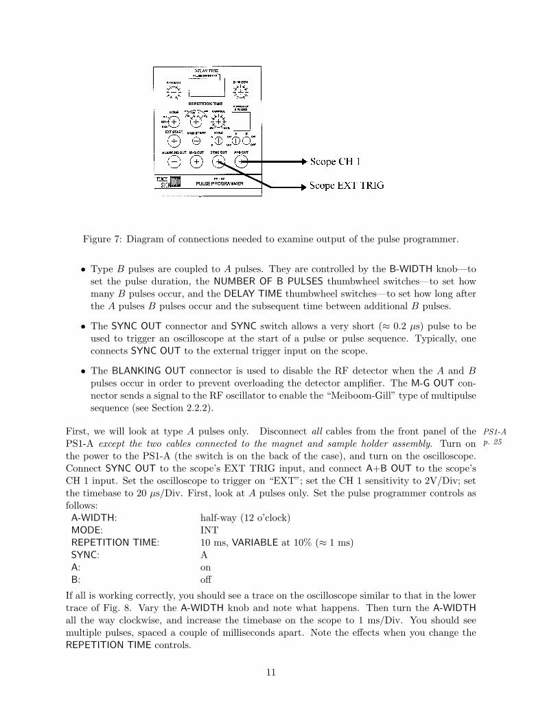
Figure 7: Diagram of connections needed to examine output of the pulse programmer.

• Type B pulses are coupled to A pulses. They are controlled by the B-WIDTH knob—toset the pulse duration, the NUMBER OF B PULSES thumbwheel switches—to set howmany B pulses occur, and the DELAY TIME thumbwheel switches—to set how long afterthe A pulses B pulses occur and the subsequent time between additional B pulses.

• The SYNC OUT connector and SYNC switch allows a very short (≈ 0.2 µs) pulse to beused to trigger an oscilloscope at the start of a pulse or pulse sequence. Typically, oneconnects SYNC OUT to the external trigger input on the scope.

• The BLANKING OUT connector is used to disable the RF detector when the A and Bpulses occur in order to prevent overloading the detector amplifier. The M-G OUT con-nector sends a signal to the RF oscillator to enable the “Meiboom-Gill” type of multipulsesequence (see Section 2.2.2).

First, we will look at type A pulses only. Disconnect all cables from the front panel of the PS1-Ap. 25PS1-A except the two cables connected to the magnet and sample holder assembly. Turn on

the power to the PS1-A (the switch is on the back of the case), and turn on the oscilloscope.Connect SYNC OUT to the scope’s EXT TRIG input, and connect A+B OUT to the scope’sCH 1 input. Set the oscilloscope to trigger on “EXT”; set the CH 1 sensitivity to 2V/Div; setthe timebase to 20 µs/Div. First, look at A pulses only. Set the pulse programmer controls asfollows:

A-WIDTH: half-way (12 o’clock)MODE: INTREPETITION TIME: 10 ms, VARIABLE at 10% (≈ 1 ms)SYNC: AA: onB: off

If all is working correctly, you should see a trace on the oscilloscope similar to that in the lowertrace of Fig. 8. Vary the A-WIDTH knob and note what happens. Then turn the A-WIDTHall the way clockwise, and increase the timebase on the scope to 1 ms/Div. You should seemultiple pulses, spaced a couple of milliseconds apart. Note the effects when you change theREPETITION TIME controls.

11

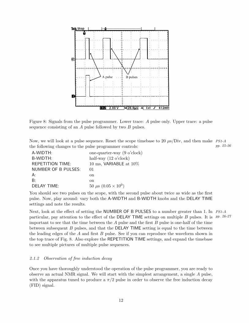
Figure 8: Signals from the pulse programmer. Lower trace: A pulse only. Upper trace: a pulsesequence consisting of an A pulse followed by two B pulses.

Now, we will look at a pulse sequence. Reset the scope timebase to 20 µs/Div, and then make PS1-App. 25-26the following changes to the pulse programmer controls:

A-WIDTH: one-quarter-way (9 o’clock)B-WIDTH: half-way (12 o’clock)REPETITION TIME: 10 ms, VARIABLE at 10%NUMBER OF B PULSES: 01A: onB: onDELAY TIME: 50 µs (0.05× 100)

You should see two pulses on the scope, with the second pulse about twice as wide as the firstpulse. Now, play around: vary both the A-WIDTH and B-WIDTH knobs and the DELAY TIMEsettings and note the results.

Next, look at the effect of setting the NUMBER OF B PULSES to a number greater than 1. In PS1-App. 26-27particular, pay attention to the effect of the DELAY TIME settings on multiple B pulses. It is

important to see that the time between the A pulse and the first B pulse is one-half of the timebetween subsequent B pulses, and that the DELAY TIME setting is equal to the time betweenthe leading edges of the A and first B pulse. See if you can reproduce the waveform shown inthe top trace of Fig. 8. Also explore the REPETITION TIME settings, and expand the timebaseto see multiple pictures of multiple pulse sequences.

2.1.2 Observation of free induction decay

Once you have thoroughly understood the operation of the pulse programmer, you are ready toobserve an actual NMR signal. We will start with the simplest arrangement, a single A pulse,with the apparatus tuned to produce a π/2 pulse in order to observe the free induction decay(FID) signal.

12

The modules on the spectrometer are described here. Set the controls as indicated.

15 MHz Receiver This module senses the RF signal produced by the sample-probe coil, PS1-A,pp. 22-24amplifies it and rectifies it. The rectified signal is sent to the oscilloscope. The unrectified

RF signal is sent to the mixer in order to optimize the oscillator frequency.

GAIN: about 30%BLANKING: onTIME CONST: .01 msTUNING: 12 o’clock

Pulse Programmer You want to set the controls to make only A type pulses. First, calculatethe time needed for a π/2 pulse from Eq. (13), given γ = 2.765× 104 rad/s-gauss and themagnetic field B1 ≈ 12 gauss, according to the manufacturer. Then set the programmer PS1-A

p. 20controls:A-WIDTH: Set to calculated tπ/2 (use scope)

B-WIDTH: Fully CCWNUMBER OF B PULSES: 00REPETITION TIME: 100 ms, VARIABLE at 100% (≈ 100 ms)SYNC: AA: onB: off

15 MHz OSC/AMP/MIXER This module has three separate circuits in one box. The15 MHz oscillator is controlled by the FREQUENCY ADJUST knob and the COARSE/FINEswitch which changes the significant digit incremented by the knob. The oscillator signalis fed internally to the input of the power amp which is turned on (or “gated”) by thesignal going into A+B IN. The output of the power amp, RF OUT is connected to thesample probe excitation coil and delivers an RF power of 150 watts peak power. The M-G PS1-A

p. 20IN and M-G switch are used to synchronize the phase of the RF signal with the gatingin order to implement the “Meiboom-Gill” type of multipulse sequence, as described inSection 2.2.2. Set the controls as follows:

FREQUENCY: 15.00000CW-RF: onM-G: on

Now connect the modules together and to the oscilloscope following the diagram shown inFig. 9. Use the short cables to connect one module to another, and use the long cables tomake connections to the oscilloscope. Connect the DETECTOR OUT to CH 1 of the digitaloscilloscope, and the MIXER OUT to CH 2. Set the oscilloscope to trigger on “EXT”; set theCH 1 sensitivity to 2V/Div; set the CH 2 sensitivity to 5V/Div; set the timebase to 40 µs/Div.

Make sure that the O-ring on the sample vial is 1.5 inches from the bottom and carefully lowerthe mineral oil sample into the sample holder inside the magnet assembly.

After some adjustment of the oscilloscope, you should observe traces that bear some resemblanceto those in Fig. 10. If you don’t get anything like Fig. 10 (or anything at all), check theconnections on the PS1-A and the switch and knob settings. The CH 1 signal (lower trace)is the free induction decay (FID). This signal is half of the envelope of the RF oscillationsgenerated by the precession of the net magnetization in the x-y plane. It is the envelope (which

13

Figure 9: Diagram of connections on the PS1-A spectrometer to make pulsed NMR measure-ments.

Figure 10: Signals of free induction decay. Upper trace: mixer output showing beats indicatingthe frequency difference between the resonance frequency and the oscillator frequency. Lowertrace: detector output showing the FID signal, which is the positive amplitude envelope of theRF signal obtained from the pick-up coil.

14

represents the magnitude of the net magnetization) and not the individual oscillations that isof interest here. (A rough picture of the RF oscillations can be seen in Fig. 9.2 in the PS1-Amanual.) The signal on CH 2 (upper trace) is the mixer output. The oscillations on this signal, PS1-A

pp. 22-23also known as “beats”, are at the difference frequency between the detected signal (due to theprecession of the net magnetization in the x-y plane) and the frequency of the RF oscillator.

Adjust the frequency on the oscillator to reduce the frequency of the beats on the mixer outputto a minimum. Figure 11 shows a collection of mixer output signals for different oscillatorfrequencies. The goal of your adjustment is to make the number of oscillations, or zero-crossings,go to zero; the initial bump in the signal is not important. When the beats are at a minimum,you can adjust the TUNING knob to maximize the amplitude of the FID signal.

Finally, pull the sample out of the holder and slide the O-ring down a few millimeters. Thenslowly lower it back into the sample holder, pressing down so as to scoot the O-ring along thesample vial, while watching the FID signal on the scope. The signal will be strongest when thesample material is centered in the magnetic field. You should try to adjust the position of theO-ring to maximize the FID signal.

Figure 11: Signals from the mixer output for different oscillator frequencies near resonance.Traces from the bottom, moving up: 9 kHz low (R1), 2 kHz low (R2), on resonance (2), 2 kHzhigh (R3).

Now tune the A pulse width to maximize the FID signal in the following manner: turn theA-WIDTH knob completely counterclockwise (the FID signal will diminish), and then slowlyturn it clockwise until the FID signal is largest. Measure the A pulse width (you will need tomove some connections around) and compare it to the width you calculated earlier.

The pulse width you have just measured is the pulse width needed for a π/2 rotation of the netmagnetization ~M . The decay of the FID signal depends on T ∗2 , as noted in the introduction,but is also dependent on the time constant of the detector. You may wish to see what differentsettings of the TIME CONST switch do to the FID signal. You may also notice that the FIDsignal does not decay exactly following an exponential curve; this is because the signals from thedifferent precession frequencies mix together, and the resulting signal is more complex than a

15

simple dying-off of the transverse magnetization. As you will see, T ∗2 is much shorter than eitherT2 or T1, indicating that magnetic field inhomogeneity is fairly significant in this apparatus.

Now explore what happens if you increase the A pulse width beyond tπ/2. You should first seethe FID signal decrease, nearly to zero, and then increase again. Measure the pulse widths forthe pulse that gives a minimum FID signal and the pulse that gives the following maximum.How are these pulses related to tπ/2? Discuss the relationship between these pulses, the rotation

of ~M , and the resulting FID signal.

Technical note: If the field of the permanent magnet changes in time (due to changes in thetemperature of the magnet) the resonant frequency will change, and beats will reappear on PS1-A

p. 16the mixer output signal. If this happens during the course of your measurements, the oscillatorfrequency should be re-adjusted to minimize the beats.

2.2 Pulse sequences and measurements of T1 and T2

Now we will see the real power of the pulsed NMR method in its ability to measure the longitu-dinal (spin-lattice) relaxation time constant T1 and the transverse (spin-spin) relaxation timeT2 even when the static magnetic field ~B0 is not very uniform.

2.2.1 Measuring T1: 2 pulse sequence

The amplitude of the FID signal induced by a π/2 pulse is proportional to the initial longitudinalmagnetization Mz. Immediately following a π/2 pulse, Mz ≈ 0, which you could confirm byapplying another π/2 pulse at that time and noting that the FID signal was zero. (Indeed, youwill have done this already if you think of what a pulse of 2 × tπ/2 does!) It takes a while forMz to recover its equilibrium value, and if you hit the sample with another π/2 pulse beforeequilibrium has been reestablished, then this second FID signal will be weaker than the firstone.

The longitudinal magnetization relaxes according to an exponential function:

Mz(t) = M0 − (M0 −Mi) e−t/T1 , (14)

where M0 is the equilibrium value of Mz and Mi is equal to Mz at t = 0. One way of estimating PS1-Ap. 4T1 suggested by Eq. (14) is to decrease the time between successive π/2 pulses until you see

the FID signal drop by about 1/3 (i.e., 1/e) of its “equilibrium” value. You can see this byletting Mi = 0 (what you get after a π/2 pulse) in Eq. (14) and calculating Mz(t = T1). Trythis: reduce the REPETITION TIME and see how the FID signal behaves. Can you make anestimate of T1 by this method? (You may find that you cannot make the FID signal reduce by1/3 if T1 is too short. Don’t sweat it; this method is merely qualitative.)

A more elegant measurement of T1 may be accomplished by a two pulse sequence. If one appliesa longer pulse—a π pulse—the net magnetization ~M can be inverted: M0 → −M0. The decayof Mz can be tracked by applying subsequent π/2 pulses at varying intervals after the π pulse,since the FID signal is proportional to Mz at any time. Of particular interest is the point atwhich Mz momentarily vanishes, or “crosses zero” in its decay from a net negative value to theequilibrium positive value.

This pulse sequence is illustrated in Fig. 12, which is taken from reference [5]. In the figure,we see that a π pulse initially inverts the magnetization, and that a π/2 pulse interrogates the

16

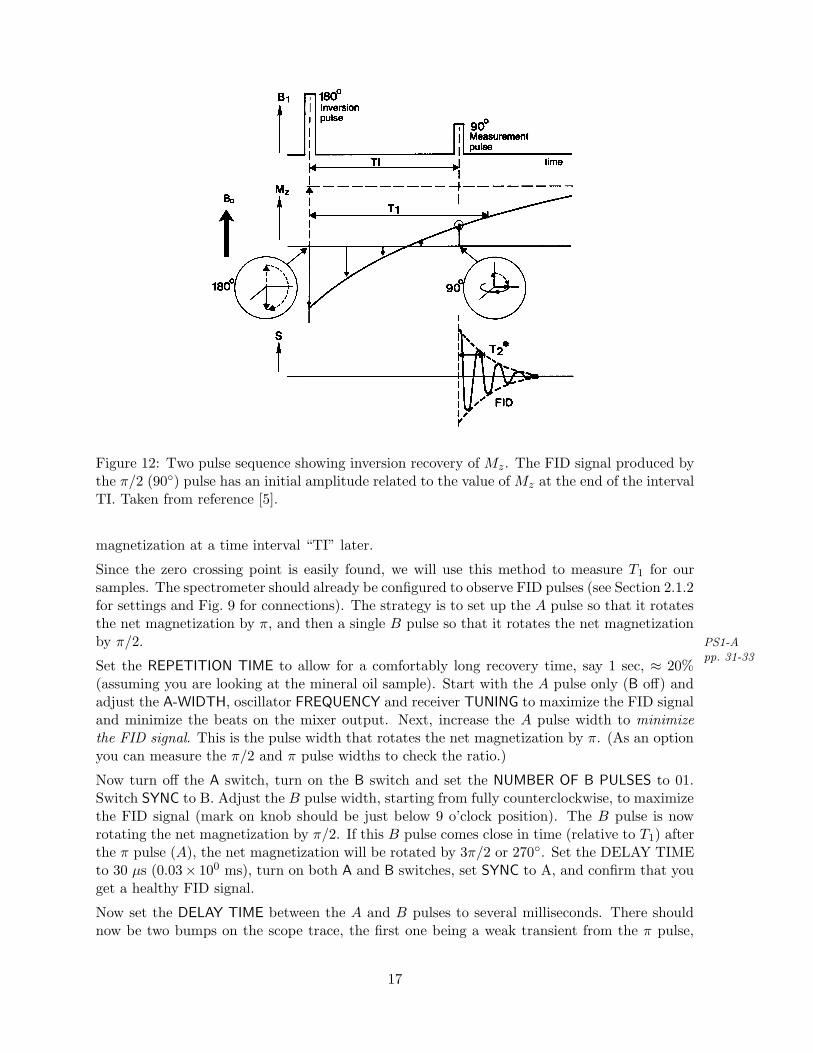
Figure 12: Two pulse sequence showing inversion recovery of Mz. The FID signal produced bythe π/2 (90◦) pulse has an initial amplitude related to the value of Mz at the end of the intervalTI. Taken from reference [5].

magnetization at a time interval “TI” later.

Since the zero crossing point is easily found, we will use this method to measure T1 for oursamples. The spectrometer should already be configured to observe FID pulses (see Section 2.1.2for settings and Fig. 9 for connections). The strategy is to set up the A pulse so that it rotatesthe net magnetization by π, and then a single B pulse so that it rotates the net magnetizationby π/2. PS1-A

pp. 31-33Set the REPETITION TIME to allow for a comfortably long recovery time, say 1 sec, ≈ 20%(assuming you are looking at the mineral oil sample). Start with the A pulse only (B off) andadjust the A-WIDTH, oscillator FREQUENCY and receiver TUNING to maximize the FID signaland minimize the beats on the mixer output. Next, increase the A pulse width to minimizethe FID signal. This is the pulse width that rotates the net magnetization by π. (As an optionyou can measure the π/2 and π pulse widths to check the ratio.)

Now turn off the A switch, turn on the B switch and set the NUMBER OF B PULSES to 01.Switch SYNC to B. Adjust the B pulse width, starting from fully counterclockwise, to maximizethe FID signal (mark on knob should be just below 9 o’clock position). The B pulse is nowrotating the net magnetization by π/2. If this B pulse comes close in time (relative to T1) afterthe π pulse (A), the net magnetization will be rotated by 3π/2 or 270◦. Set the DELAY TIMEto 30 µs (0.03× 100 ms), turn on both A and B switches, set SYNC to A, and confirm that youget a healthy FID signal.

Now set the DELAY TIME between the A and B pulses to several milliseconds. There shouldnow be two bumps on the scope trace, the first one being a weak transient from the π pulse,

17

the second one being the stronger FID signal. As the delay time is increased (millisecondintervals are handy) the amplitude of the FID signal should decrease until at some delay time,it goes away (almost) completely, as shown in Fig. 13. At this point in time, there is no netmagnetization, hence no FID signal; in the language of Eq. (10), N+ = N− for a brief moment.You will notice that if you keep increasing the delay time, the FID signal reappears, indicatingthat Mz has gone from net negative value to a net positive value, as indicated in Fig. 12.

Figure 13: Oscilloscope traces showing zero-crossing method of determining T1. The π pulseoccurs at the trigger point (T), and the FID signal from the π/2 pulse first diminishes asthe delay time increases (traces R1 and R2), nearly vanishing at the delay time in the thirdtrace from the top (R3), and then recovers at a later delay time (R4). Sample: H2O+CuSO4;T1 ≈ 2.6 ms.

The delay time for Mz to decay to 0, may be used to calculate T1. Since Mz = 0 is halfwaybetween Mz = −M0 and Mz = +M0, the zero-crossing time interval is equal to the “half-life”of the exponential decay. You can use this fact to calculate T1. If you want to work it out, letMi = −M0 and Mz(t) = 0 in Eq. (14) and find T1 in terms of t.

Big instrumentation hint: For samples of long T1 you will find that in order to see both the Aand B pulse responses you will need to increase the Time/Div setting on the oscilloscope somuch that it becomes hard to see the pulses because they become proportionately narrower.But since you are only looking for the DELAY TIME setting which minimizes the FID signalfrom the B pulse you can simply switch the SYNC to B, allowing you to view only the FIDsignal with a comfortable Time/Div setting.

Incidentally, you may want to see the reduction in T1 when the pulse-sequence repetition timeis much shorter. Why is this so?

2.2.2 Measuring T2: spin echoes & multipulse sequence

You may have noticed, while adjusting the controls to set up the π–π/2 pulse sequence in theprevious exercise, that you saw an additional bump in the scope trace at twice the delay time.

18

This curious artifact was also noticed by Erwin Hahn in 1949 (when he was still a graduatestudent). Hahn realized that the signal must be due to a “rephasing” of the transverse compo-nents of the magnetic moments in the sample, leading to a nonzero transverse magnetizationand subsequent FID signal. He called this process a “spin echo” [6]. In this exercise you willlearn how to create a spin echo and how to use it to make a good measurement of the spin-spinrelaxation time constant T2.

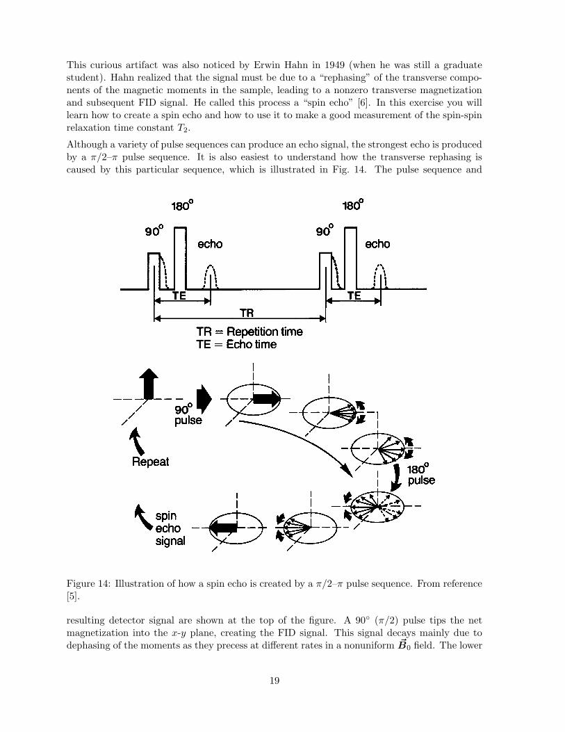
Although a variety of pulse sequences can produce an echo signal, the strongest echo is producedby a π/2–π pulse sequence. It is also easiest to understand how the transverse rephasing iscaused by this particular sequence, which is illustrated in Fig. 14. The pulse sequence and

Figure 14: Illustration of how a spin echo is created by a π/2–π pulse sequence. From reference[5].

resulting detector signal are shown at the top of the figure. A 90◦ (π/2) pulse tips the netmagnetization into the x-y plane, creating the FID signal. This signal decays mainly due todephasing of the moments as they precess at different rates in a nonuniform ~B0 field. The lower

19

part of the figure shows this dephasing from the point of view of the rotating reference frame.In this frame we see that some moments lag behind the group, while others lead. A 180◦ (π)pulse is applied at time τ after the π/2 pulse. This pulse effectively “flips the pancake” of thecollection of dephased magnetic moments about an axis in the x-y plane. The overall precessionof the group continues in the same direction, but now those moments which had lagged thegroup now lead the group, and vice versa. At time 2τ (TE in the figure) all of the momentscome back into phase, and we see a recovery of the FID signal.

Hahn nicely illustrates the formation of the echo by means of an analogy [4, p. 8]:

Let a team of runners with different but constant running speeds start off ata time t = 0 as they would do at a track meet. . . At some time T these runnerswould be distributed around the race track in apparently random positions. Thereferee fires his gun at a time t = τ > T , and by previous arrangement the racersquickly turn about-face and run in the opposite direction with their original speeds.Obviously, at a time t = 2τ , the runners will return together precisely at the startingline.

Before worrying about T2 and its relationship to spin echoes, first set up the spectrometer sothat you can see an echo. The spectrometer should already be configured to observe FID pulses(see Section 2.1.2 for settings and Fig. 9 for connections).

Now you want to set the A pulse so that it rotates the net magnetization by π/2 and thenmake a single B pulse so that it rotates the net magnetization by π. Start with just the A PS1-A

pp. 33pulse (B pulses turned off) and adjust the electronics (A-WIDTH, TUNING and FREQUENCY)to maximize the FID signal. Set the repetition time to 1 sec, 30% (again, assuming mineraloil as a sample; with other samples you may need a longer time for full recovery of Mz) andmake sure that the M-G switch is on. Next, turn on the B pulses and set the NUMBER OF BPULSES to 01 and the DELAY TIME to 2.5 ms. Finally, adjust the B-WIDTH (starting fromfully counterclockwise) to maximize spin echo which occurs at twice the delay time. You shouldget a scope display similar to that in Fig. 15.

Now note what happens when you increase the delay time. The reduction in the magnitude ofthe echo signal is due to a loss of “phase memory” among the magnetic moments. This in turnis due to variations in the local magnetic field of each moment over time; it does not dependon the static variation in the applied ~B0 field that is responsible for the comparatively shortFID decay time. In other words, the reduction in the spin echo amplitude follows T2, not T ∗2 .Hahn explains [4, p. 9]:

The decay of the echo may be understood in terms of the race track analogy ifit is assumed now that the runners become fatigued after the start of the race. Forthis reason they may change their speeds erratically or even drop out of the racecompletely. Consequently, following the second gun shot (the second pulse) some ofthe racers may return together at the starting line, but not all of them.

In terms of the analogy, T ∗2 depends on the inherent differences in base speeds among therunners; in terms of our collection of moments this is like the different precession speeds of thespins in different parts of the sample. However, T2 depends on the changing of each runner’sspeed over time; similarly, each moment will change its precession speed as it feels the fluctuatingeffects of neighboring moments, diffusing molecules, etc.

20

Figure 15: Oscilloscope trace showing one spin echo. The small transient between the initial FIDsignal and the echo is from the π pulse. Note that the initial FID signal is larger in magnitudethan the echo, indicating loss of phase memory among the spins. Sample: H2O+CuSO4.

So, a way to measure T2 is to track the peak height of the spin echo as a function of the delaytime. For example, you could look for the change in delay time which reduces the echo by 1/2,and thus obtain the “half life” of the spin echo.

Unfortunately, this method is still beset by the effects of a non-homogeneous ~B0 field. If themolecules in the sample (typically a liquid) can diffuse easily to other parts, then the precessionspeeds of the moments in those molecules will change as they move into regions of differentstatic field. The dephasing of the moments will occur more quickly than it would if the fieldwere uniform.

Hahn was aware of the effects of diffusion in a nonuniform field, and developed a theoreticalexpression for the amplitude of a spin echo which depended on T2 as well as the diffusionconstant and magnetic field gradient. Later, Carr and Purcell discovered that the effects ofdiffusion could be minimized if one used a multipulse sequence, wherein many successive πpulses followed after the initial π/2 pulse [7]. The result of such a sequence is a single scopetrace showing many spin echoes. In effect, each echo is like a “start pulse” for the later π pulsethat creates a subsequent echo. The decay of the echo amplitudes follows an exponential curve,of time constant T2 as long as the echo spacing is sufficiently close together relative to thediffusion time. A diagram showing the method of the multipulse sequence is given in Fig. 16and an example of the scope trace with multiple echoes is shown in Fig. 17.

Use the multipulse sequence method to measure T2 for the samples. The instrument should PS1-App. 33-34already be set up to look at a single spin echo. All you need to do is increase the NUMBER OF

B PULSES. Note the effect; you should get a picture like Fig. 17. With more B pulses it maynow be easier to optimize the echo signals by fine tuning the A and B pulse widths; do this,and strive for maximum echo amplitudes and minimum between-echo “glitches” (short pulses).

As the NUMBER OF B PULSES is increased, the sweep speed of the scope (time per division)must be reduced to display all the echoes. But as the sweep speed is reduced, so is the sampling

21

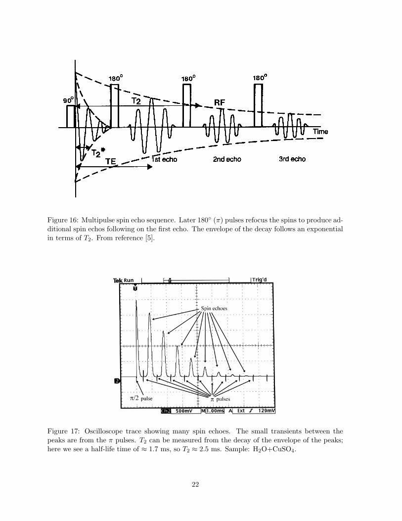
Figure 16: Multipulse spin echo sequence. Later 180◦ (π) pulses refocus the spins to produce ad-ditional spin echos following on the first echo. The envelope of the decay follows an exponentialin terms of T2. From reference [5].

Figure 17: Oscilloscope trace showing many spin echoes. The small transients between thepeaks are from the π pulses. T2 can be measured from the decay of the envelope of the peaks;here we see a half-life time of ≈ 1.7 ms, so T2 ≈ 2.5 ms. Sample: H2O+CuSO4.

22

rate (indicated at the top of the scope screen). If the sampling rate is too low, the echo signalswill not be captured accurately. Check this out on the scope with 3 or 4 echoes and the DELAYTIME set to several milliseconds. Reduce the sweep speed of the scope to 25 ms/Div or slowerand observe how the amplitude of the echoes is no longer accurately captured. You can workaround this limitation by using the scope’s “Peak Detect” feature. With this feature, only themost extreme voltage at each pixel time is recorded. The Peak Detect mode is available underthe scope’s “Acquire” menu.

Also, you may need to increase the repetition time to allow the system to come to equilibriumbetween pulse sequences. As pointed out in the PS1-A manual, “. . . each pulse sequence mustwait at least 3 T1 (preferably 6–10 T1’s) before repeating the pulse train.” If the repetition PS1-A

p. 29time is too short, the FID and echo signals will be reduced. Once you have selected the numberof B pulses for your T2 measurement, adjust the repetition time so that a slight variation inthis time does not affect the amplitude of the echoes. For samples with a very long T1, youmay get better results by using manual triggering of the pulse sequence. You can do this bysetting the MODE switch to MAN, and then firing the sequence with the MAN START button.The scope will hold the most recent waveform indefinitely.

Once a satisfactory spin echo sequence has been acquired, time and voltage measurementsneed to be taken of the maxima of the echoes to map out the envelope. This is most easilyaccomplished using the paired cursors on the scope (activate the “Cursor” menu for this option)which allow for both time and voltage measurements. It is useful to record the ∆V and ∆tmeasurements as well as the absolute values at each echo maximum.

2.3 Student Exercises

Now that you know how to operate the spectrometer and measure T1 and T2 accurately, youneed to carry out some investigations. Here are some possibilities. You are required to do atleast two of these, but you may do as many as you like.

Exercise1: Characteristics of different materials

Measure T1 and T2 for a few of the following materials: mineral oil, Vaseline, glycerine, water,ethyl alcohol. Note: some have very long time constants, so you will need to keep a watchon the pulse repetition time and, in the case of T2, the number of pulses and associated delaytime. If your multipulse envelope does not follow an exponential curve, you have work to do.(Reduce the delay time and increase the number of B pulses.)

Exercise 2: Effect of phase transition on NMR signals

Attempt to get a signal from the paraffin (wax) sample. It is weak, isn’t it? Now warm thesample tube with a candle flame until the wax melts (no hotter!!!) and quickly insert the tubeinto the magnet assembly so you can see the much stronger signal from the liquid paraffin. Ifyou work quickly, you may be able to track T2 as it cools. (Following T1 is harder.)

23

Exercise 3: Effect of doping with paramagnetic ions

If you have done the continuous NMR experiment, you will be familiar with the idea behind thisexperiment. There is a jar with a saturated CuSO4 solution available, as well as sample vialsand deionized water. Use a syringe to put one drop of the CuSO4 solution into a clean vial, andthen add 9 drops of pure water. Measure T1 and T2 for the sample. Then make another samplewith 1 drop of your mixture, and 9 drops of pure water, and repeat the measurement. Continuein this manner until you have covered several decades of dilution, and then plot your results.(Log-log scales are handy.) If you look up solubility data in a handbook, you can calculatethe absolute concentration of the Cu++ ions. Compare your results to those given by Hahn [6,p. 586].

Exercise 4: Effect of diffusion on spin echo signal

As discussed above, diffusion of spins in a magnetic field gradient will affect the spin-echoamplitude. Hahn [6], and later, Carr and Purcell [7], derived an expression for the decayenvelope which included the diffusion effects. It has this form:

Mpeak(t) = Mi exp(−t/T2) exp(−Kt3/n2) , (15)

where Mpeak(t) is the amplitude of the echo peak at time t, Mi is the amplitude of the initialπ/2-pulse response, K is a function of the diffusion constant and field gradient, and n is thenumber of intervening π pulses between the time of the initial π/2 pulse and the echo at timet. As shown by Carr and Purcell

K =γ2(∂B0∂z

)2D

12, (16)

where γ is as defined in Eq. 1, ∂B0/∂z is the gradient of the static field along the field direction,and D is the diffusion constant of the sample material. As is evident from Eq. (15), if T 3

2 � Kand n = 1, the decay of the echo envelope should follow a form proportional to e−Kt

3. But if we

increase the number of π pulses while making the time between them shorter, that is increasen, we can reduce the effect of the e−Kt

3factor.

In this exercise you want to test Eq. (15). Choose a sample with a long T2—pure water is good.Set the instrument to make spin echoes; you will want a long repeat time, since T1 is also long.Then study how the spin echo envelope evolves as you increase the NUMBER OF B PULSESwhile decreasing the DELAY TIME.

If you use the newer TDS 3012 (color screen) oscilloscope (not the older TDS 320, 340 or 360monochrome scopes), you can obtain a picture of the pulse-height envelope that shows thee−Kt

3form to best effect. Use the manual trigger mode (MODE set to MAN, use MAN START

to trigger), and the infinite persistence feature of the scope (available under the “Display”menu button)—this feature holds all previous waveforms indefinitely. Set the NUMBER OF BPULSES to 1, and then make a succession of traces by advancing the DELAY TIME and firingthe sequence with the MAN START switch. The scope will simply add all of the signal tracesto the display, and you can print out the final picture. If you do not have access to the TDS3012, you can still do the experiment by measuring the pulse height of the echo for each valueof the DELAY TIME, and then plotting the results.

24

Exercise 5: The Meiboom-Gill multipulse sequence

The Carr-Purcell multipulse method of obtaining T2 suffers from a systematic experimentalerror: if the width and field strength of the π pulses are not exactly right, then the phase errorfrom each pulse will accumulate, leading to a decay of the echo envelope that is too rapid.To wit: if the π pulses produce, say, a rotation of 186◦ per pulse (rather than the expected180◦), then after, say, ten such pulses, the effective rotation would accumulate to a tilting of themoments by 60◦ out of the x-y plane, and the FID signal would be about half what it shouldbe (∝ cos 60◦).

Meiboom and Gill discovered a way to correct for this accumulated error by a simple trick.They found that by shifting the phase of the RF signal by 90◦ for the first π/2 pulse relative tothe phase of the RF signal for the subsequent π pulses, that the phase error of two successiveπ pulses could be made to cancel, and thus, over many pulses, there would be no accumulatederror. In effect, the 90◦ phase shift causes the first π/2 rotation of ~M to be about the y′ axis(in the rotating frame of reference), but the following π rotations will be about the x′ axis [8].

As noted, the PS1-A has a provision for implementing (or not) the Meiboom-Gill phase shifton the first pulse. You can study the effect of this by setting up a long multipulse sequence andthen noting how the spin echo envelope depends on the setting of the M-G switch and the B-WIDTH position. In particular, you can see a very interesting modulation of the echo envelopewith the M-G switch off and the B-WIDTH set notably low. In your notebook discussion, see ifyou can explain the modulation in terms of the effect of accumulated phase errors. Mineral oilworks well as a sample.

3 A Summary of Tasks for the Prepared Student

If you have read through the write-up and feel that you know the theoretical underpinningswell enough, you may want to follow the list below as you do the lab.

1. Learn how to use the pulse programmer. You should know how to set up single pulse se-quences, double pulse sequences, and multipulse sequences, with various repetition times,delay times, and A and B pulse widths.

2. Set up the instrument to observe free induction decay (FID) by means of a π/2 pulseapplied to a mineral oil sample. Study the effect of varying the A pulse width.

3. Study the effect of shortening the pulse repetition time on the FID signal. Use this effectto estimate the longitudinal relaxation time T1.

4. Set up a π–π/2 pulse sequence to make an accurate measurement of T1 by means of thezero-crossing method. Measure T1 for mineral oil.

5. Set up the instrument to observe spin echoes using the π/2–π pulse sequence. Then usethe multipulse sequence with many more π pulses to display the envelope of the echoamplitudes. Use this to obtain an accurate measurement of T2 for mineral oil.

6. Carry out at least two of the exercises in Section 2.3. Make sure you obtain representativeprintouts of the oscilloscope displays along with your hand-written data.

25

References

[1] Preston, D. W., and E. R. Dietz, The Art of Experimental Physics, John Wiley & Sons,New York, 1991, pages 264–285.

[2] Melissinos, A. C., Experiments in Modern Physics, Academic Press, San Diego, 1966, pages340–374.

[3] Slichter, C. P., Principles of magnetic resonance, 2nd Ed., Springer-Verlag, Berlin, 1978.

[4] Hahn, E. L., “Free nuclear induction”, Physics Today, November 1953, pp. 4-9.

[5] Philips Medical Systems, “Principles of MR Imaging”, published by Philips Medical Sys-tems, The Netherlands (1984). Copies are available in the lab.

[6] Hahn, E. L., “Spin echoes”, Phys. Rev. 80, 580–594 (1950).

[7] Carr, H. Y., and E. M. Purcell, “Effects of diffusion on free precession in nuclear magneticresonance experiments”, Phys. Rev. 94, 630–638 (1954).

[8] Meiboom, S., and D. Gill, “Modified spin-echo method for measuring nuclear relaxationtimes”, Rev. Sci. Inst., 29, 688–691 (1958).

Prepared by J. Stoltenberg, D. Pengra, R. Van Dyck and O. Vilchespulsed_NMR.tex -- Updated 24 February 2006

26