psychology 205: research methods in psychology paper 1: · pdf filermdata entry descriptive...

RM Data entry Descriptive Statistics Inferential Statistics by condition Conclusions

Psychology 205: Research Methods in PsychologyPaper 1: A study in False Memories

William Revelle

Department of PsychologyNorthwestern UniversityEvanston, Illinois USA

October, 2016

1 / 39


Outline

Roediger and McDermott study

Data entry

Descriptive StatisticsRecallRecognition

Inferential Statistics by conditionFalse Recognition

Conclusions

2 / 39


Roediger and McDermott

Meta-theoretical question

1. memory as photograph versus memory as reconstruction(memory as photo vs. photoshop)

2. “recovered” childhood memories of trauma versus ?false?memories

3. legal testimony of accuracy of memory

3 / 39


Roediger and McDermott- background

Prior work

1. memory distortions over time – Bartlett

2. reconstructive memory – Loftus

3. low error rates in recognition memory – Underwood

4. intrusions in free recall – Deese

4 / 39


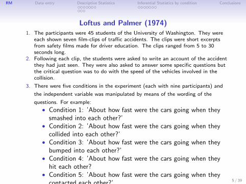
Loftus and Palmer (1974)1. The participants were 45 students of the University of Washington. They were

each shown seven film-clips of traffic accidents. The clips were short excerptsfrom safety films made for driver education. The clips ranged from 5 to 30seconds long.

2. Following each clip, the students were asked to write an account of the accidentthey had just seen. They were also asked to answer some specific questions butthe critical question was to do with the speed of the vehicles involved in thecollision.

3. There were five conditions in the experiment (each with nine participants) and

the independent variable was manipulated by means of the wording of the

questions. For example:

• Condition 1: ’About how fast were the cars going when theysmashed into each other?’

• Condition 2: ’About how fast were the cars going when theycollided into each other?’

• Condition 3: ’About how fast were the cars going when theybumped into each other?’

• Condition 4: ’About how fast were the cars going when theyhit each other?

• Condition 5: ’About how fast were the cars going when theycontacted each other?’

4. The basic question was therefore ’About how fast were the cars going when they***** each other?’. In each condition, a different word or phrase was used to fillin the blank. These words were; smashed, collided, bumped, hit, contacted.

From http://www.holah.co.uk/study/loftus/

5 / 39


Loftus and Palmer (1974)

• Condition 1: ’About how fast were the cars going when they smashed into eachother?’

• Condition 2: ’About how fast were the cars going when they collided into eachother?’

• Condition 3: ’About how fast were the cars going when they bumped into eachother?’

• Condition 4: ’About how fast were the cars going when they hit each other?

• Condition 5: ’About how fast were the cars going when they contacted eachother?’

The basic question was therefore ’About how fast were the cars going when they***** each other?’. In each condition, a different word or phrase was used to fill inthe blank. These words were; smashed, collided, bumped, hit, contacted.

From http://www.holah.co.uk/study/loftus/

6 / 39


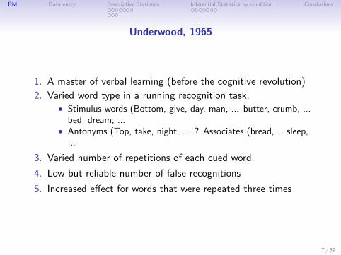
Underwood, 1965

1. A master of verbal learning (before the cognitive revolution)

2. Varied word type in a running recognition task.• Stimulus words (Bottom, give, day, man, ... butter, crumb, ...

bed, dream, ...• Antonyms (Top, take, night, ... ? Associates (bread, .. sleep,

...

3. Varied number of repetitions of each cued word.

4. Low but reliable number of false recognitions

5. Increased effect for words that were repeated three times

7 / 39


Deese, 1959

1. Another verbal learning master

2. Lists consisting of 12 words each were presented to 50 Ss for atest of immediate recall. In the recall of these lists, particularwords occurred as intrusions which varied in frequency from0% for one list to 44% for another.

3. Data gathered on word- association frequencies clearly showedthat the probability of a particular word occurring in recall asan intrusion was determined by the average frequency withwhich that word occurs as an association to words on the list.

8 / 39


Roediger and McDermott

1. Alternative explanations for memory effects• (1) connection strength models of memory• (2) network models of association

2. Theoretical statement• not testing theory but rather testing phenomenon• need to get a robust measure of false memory in order to study

it

9 / 39


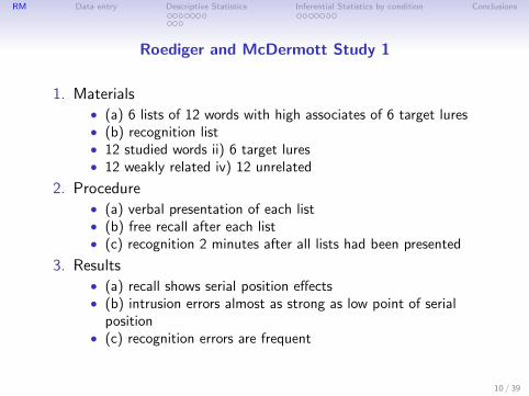
Roediger and McDermott Study 1

1. Materials• (a) 6 lists of 12 words with high associates of 6 target lures• (b) recognition list• 12 studied words ii) 6 target lures• 12 weakly related iv) 12 unrelated

2. Procedure• (a) verbal presentation of each list• (b) free recall after each list• (c) recognition 2 minutes after all lists had been presented

3. Results• (a) recall shows serial position effects• (b) intrusion errors almost as strong as low point of serial

position• (c) recognition errors are frequent

10 / 39


Roediger and McDermott Study 2

1. Materials• (a) 16 lists

2. procedure

3. results

11 / 39


Our replication and extension

1. A conceptual replication of R & M

2. Same basic paradigm, same word lists, slight differences intiming

3. But added the variable of seeing versus hearing

4. Two primary Independent Variables:• Mode of presentation (Oral versus Visual) ?• Recall vs. math

5. Based upon prior work in 205, observed lower rates ofsubsequent false recognition than R & M. Was this due tomodality of presentation

6. Within subject study (why?)

12 / 39


The basic design

1. Independent Variables• Mode of presentation• Recall vs. math

2. Dependent variables• Recall per list (examine order effects)• Recognition of

• real words (varying by position)• false words• control words

3. Design mixed within (mode and recall) with order (between)

13 / 39


Within subject threats to validity

1. Order effects• Learning• Fatigue• Materials

2. Confounding of Independent variables• We want to have no correlation between independent variables

14 / 39


Getting the data

The data are stored on a web server and may be accessed fromthere using the read.file function.After reading the data, it useful to check the dimensions of thedata and then to get basic descriptive statistics.Before doing any analysis that requires the psych package, it isnecessary to make it available by using the library command.This needs to be done once per session.After reading in the data, we ask for the dimensions of the data aswell as the names of the columns.R code

library(psych) #make psych activefile.url <- "http://personality-project.org/revelle/syllabi/205/memory.txt"memory <- read.file(file=file.url) #read the data from the remote sitedim(memory) #show the dimensions of the data framecolnames(memory) #what are the variables?

dim(memory)[1] 22 539colnames(memory)

[1] "List" "L1P1" "L1P2" "L1P3" "L1P4" "L1P5" "L1P6" "L1P7" "L1P8" "L1P9"[11] "L1P10" "L1P11" "L1P12" "L1P13" "L1P14" "L1P15" "L1Tot" "L2P1" "L2P2" "L2P3"...

15 / 39


Find Recall by list – do they differ?R code

recall.tots <- memory[c(16,32,48,64,80,96,112,128,144,160,176,192,208,224,240,256)+1]

dim(recall.tots) #just to make suredescribe(recall.tots) #the descriptive statistics

recall.tots <- my.data[c(16,32,48,64,80,96,112,128,144,160,176,192,208,224,240,256)]

1] 22 16describe(recall.tots) #the descriptive statistics

vars n mean sd median trimmed mad min max range skew kurtosis seL1Tot 1 10 10.90 1.66 10.5 10.88 1.48 8 14 6 0.14 -0.78 0.53L2Tot 2 11 10.55 1.92 10.0 10.67 2.97 7 13 6 -0.33 -1.10 0.58L3Tot 3 11 10.82 1.94 10.0 10.67 1.48 9 14 5 0.53 -1.37 0.58L4Tot 4 10 10.90 1.37 11.0 11.00 1.48 8 13 5 -0.54 -0.32 0.43L5Tot 5 10 10.80 1.87 10.5 10.62 2.22 9 14 5 0.35 -1.58 0.59L6Tot 6 11 11.64 1.63 12.0 11.78 1.48 9 13 4 -0.60 -1.44 0.49L7Tot 7 11 11.82 1.60 12.0 11.78 1.48 9 15 6 0.13 -0.49 0.48L8Tot 8 10 12.10 2.13 12.0 12.12 2.22 9 15 6 -0.05 -1.35 0.67L9Tot 9 11 11.73 1.42 12.0 11.67 1.48 10 14 4 0.06 -1.62 0.43L10Tot 10 10 11.40 1.65 11.5 11.25 0.74 9 15 6 0.63 -0.15 0.52L11Tot 11 10 12.10 0.88 12.0 12.12 1.48 11 13 2 -0.16 -1.81 0.28L12Tot 12 11 10.73 1.95 10.0 10.67 1.48 8 14 6 0.49 -1.09 0.59L13Tot 13 11 12.00 1.84 11.0 11.89 1.48 10 15 5 0.26 -1.69 0.56L14Tot 14 10 10.80 2.78 11.0 11.12 2.97 5 14 9 -0.74 -0.69 0.88L15Tot 15 10 11.20 2.15 11.5 11.50 0.74 6 14 8 -1.14 0.77 0.68L16Tot 16 11 11.36 2.25 12.0 11.44 2.97 8 14 6 -0.37 -1.57 0.68

16 / 39


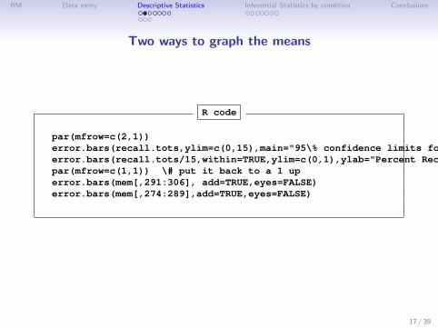
Two ways to graph the means

R code

par(mfrow=c(2,1))error.bars(recall.tots,ylim=c(0,15),main="95\% confidence limits for independent trials") \#independent trialserror.bars(recall.tots/15,within=TRUE,ylim=c(0,1),ylab="Percent Recall",xlab="List",main="95\% confidence limits for correlated trials") \#correlated trialspar(mfrow=c(1,1)) \# put it back to a 1 uperror.bars(mem[,291:306], add=TRUE,eyes=FALSE)error.bars(mem[,274:289],add=TRUE,eyes=FALSE)

17 / 39


Two ways t draw error bars

95% confidence limits for independent trials

Independent Variable

Dep

ende

nt V

aria

ble

L1Tot L3Tot L5Tot L7Tot L9Tot L11Tot L13Tot L15Tot

05

1015

95% confidence limits for correlated trials

Independent Variable

Dep

ende

nt V

aria

ble


05

1015

18 / 39


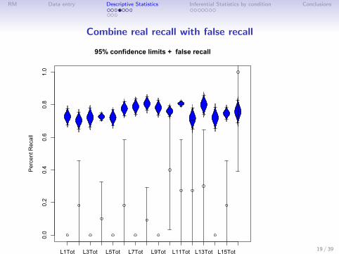
Combine real recall with false recall

95% confidence limits + false recall

List

Per

cent

Rec

all


0.0

0.2

0.4

0.6

0.8

1.0

19 / 39


What about serial position effects

1. Why do we care about serial position?

2. If subjects were following directions, then the first and lastwords should have been remembered better than theintermediate words.

3. Earlier theories of serial position suggested that the recencyportion was a measure of short term memory, the lower partof the middle of the curve was longer term storage.

4. But it was then found that serial position happens for manysequential phenomena (e.g. football games).

20 / 39


Scoring for serial positions

We need to combine across lists for position 1, then across lists forposition 2, etc.

R code

mem <- memory[-1] #get rid of the first columnnsub <- 21lists <- 16words <- 16word.position <- seq(1,256,16)Position <- matrix(0,nrow=nsub,ncol=words) #create a matrix to keep the datafor(i in 1:nsub) {

for(k in 1:words) {Position[i,k] <- sum(mem[i,word.position+k-1],na.rm=TRUE)}}

colnames(Position) <- paste0("Pos",1:16)rownames(Position) <- paste0("Subj",1:21)error.bars(Position[,1:15]/8,ylim=c(0,1),

ylab="Percent Recalled",xlab="Serial Position",main="Recall by Serial Position (False in Red)")

21 / 39


Serial Position effects including False Memory (Red)

Recall by Serial Position (False in Red)

Serial Position

Per

cent

Rec

alle

d

Pos1 Pos3 Pos5 Pos7 Pos9 Pos11 Pos13 Pos15

0.0

0.2

0.4

0.6

0.8

1.0

22 / 39


Summarize the Types of Recognition by Recall

R code

First, find the sums for each typetots <- seq(323,442,17)describe(mem[tots])error.bars(mem[tots[1:4]]/24,ylab="Percent recognized",

xlab="Recall/Recognition type",main="Percent Recognition as function of Prior Recall",

ylim=c(0,1))

vars n mean sd median trimmed mad min max range skew kurtosis sePrsRRTot 1 21 19.33 5.55 18 18.71 4.45 11 36 25 1.14 1.50 1.21PrsRnRTot 2 21 1.76 3.03 1 1.00 1.48 0 13 13 2.60 6.46 0.66PrsnRRTot 3 21 16.24 9.71 21 16.88 2.97 0 27 27 -0.83 -0.98 2.12PrsnRnRTot 4 21 8.05 6.34 5 7.35 4.45 2 20 18 0.74 -0.98 1.38PrmRRTot 5 21 1.95 3.29 1 1.18 1.48 0 14 14 2.42 5.85 0.72PrmRnRTot 6 21 0.67 1.35 0 0.35 0.00 0 4 4 1.62 1.01 0.30PrmnRRTot 7 21 5.00 3.49 5 4.76 2.97 0 13 13 0.39 -0.47 0.76PrmnRnRTot 8 21 7.33 3.57 8 7.41 4.45 1 13 12 -0.12 -1.14 0.78

23 / 39


Does prior recall affect subsequent recognition?

Percent Recognition as function of Prior Recall

Recall/Recognition type

Per

cent

reco

gniz

ed

PrsRRTot PrsRnRTot PrsnRRTot PrsnRnRTot

0.0

0.2

0.4

0.6

0.8

1.0

24 / 39


Does prior recall affect subsequent False recognition?

Percent FalseRecognition as function of Prior Recall

Recall/Recognition type

Per

cent

Fal

se re

cogn

ition

PrmRRTot PrmRnRTot PrmnRRTot PrmnRnRTot

0.0

0.2

0.4

0.6

0.8

1.0

25 / 39


Still to come

1. Does Recall depend upon modality of presentation?

2. Does Correct Recognition depend upon modality ofpresentation and opportunity to recall?

3. Does False Recognition depend upon modality of presentationand opportunity to recall?

26 / 39


Find the Recognition by condition meansR code

mem <-mem[-22,] #remove extra line

Visual <- c(1,2,7,8,11,12,13,14)Oral <- c(3,4,5,6,9,10,15,16)RecallA <- c(1,4,5,8,10,11,14,15)RecallB <- c(2,3,6,7,9,12,13,16)Recog.cond <- c("PrsRR1" , "PrsRR2", "PrsRR3" ,"PrsRR4" , "PrsRR5" , "PrsRR6" , "PrsRR7" , "PrsRR8" , "PrsRR9" , "PrsRR10" , "PrsRR11" , "PrsRR12", "PrsRR13" ,

"PrsRR14" , "PrsRR15", "PrsRR16" , "PrsRnR1", "PrsRnR2", "PrsRnR3", "PrsRnR4", "PrsRnR5", "PrsRnR6" ,"PrsRnR7" , "PrsRnR8" , "PrsRnR9" , "PrsRnR10" , "PrsRnR11" , "PrsRnR12" , "PrsRnR13" , "PrsRnR14" , "PrsRnR15", "PrsRnR16" )

nrecall.cond <- c("PrsnRR1", "PrsnRR2" , "PrsnRR3", "PrsnRR4", "PrsnRR5" , "PrsnRR6", "PrsnRR7", "PrsnRR8" , "PrsnRR9" , "PrsnRR10" ,"PrsnRR11" , "PrsnRR12", "PrsnRR13" , "PrsnRR14" , "PrsnRR15" , "PrsnRR16" , "PrsnRnR1" , "PrsnRnR2" , "PrsnRnR3" ,"PrsnRnR4" , "PrsnRnR5" , "PrsnRnR6" , "PrsnRnR7", "PrsnRnR8" , "PrsnRnR9" , "PrsnRnR10" ,"PrsnRnR11", "PrsnRnR12", "PrsnRnR13" ,"PrsnRnR14" ,"PrsnRnR15", "PrsnRnR16")recog <- mem[Recog.cond]VisArr<- rowSums(recog[RecallA[RecallA %in% Visual]],na.rm=TRUE)VisBrr <- rowSums(recog[RecallB[RecallB %in% Visual]],na.rm=TRUE)OralArr<- rowSums(recog[ RecallA[RecallA %in% Oral]],na.rm=TRUE)OralBrr <- rowSums(recog[RecallB[RecallB %in% Oral]],na.rm=TRUE)

recall.rec.df <-data.frame(VisAr,VisBr,OralAr,OralBr)

nrecog <- mem[nrecall.cond]

recog.df <- data.frame(VisAr,VisBr,OralAr,OralBr)VisAr <- rowSums(recog[RecallA[RecallA %in% Visual]],na.rm=TRUE) + rowSums(recog[RecallA[RecallA %in% Visual]+16],na.rm=TRUE)VisBr <- rowSums(recog[RecallB[RecallB %in% Visual]],na.rm=TRUE) + rowSums(recog[RecallB[RecallB %in% Visual]+16],na.rm=TRUE)OralAr<- rowSums(recog[ RecallA[RecallA %in% Oral]],na.rm=TRUE) + rowSums(recog[RecallA[RecallA %in% Visual]+16],na.rm=TRUE)OralBr <- rowSums(recog[RecallB[RecallB %in% Oral]],na.rm=TRUE) + rowSums(recog[RecallB[RecallB %in% Visual]+16],na.rm=TRUE)recog.df <- data.frame(VisAr,VisBr,OralAr,OralBr)

VisAnr <- rowSums(nrecog[RecallA[RecallA %in% Visual]],na.rm=TRUE)VisBnr<- rowSums(nrecog[RecallB[RecallB %in% Visual]],na.rm=TRUE)OralAnr <- rowSums(nrecog[ RecallA[RecallA %in% Oral]],na.rm=TRUE)OralBnr <- rowSums(nrecog[RecallB[RecallB %in% Oral]],na.rm=TRUE)

recog.df <- data.frame(VisArr,VisBrr,OralArr,OralBrr,VisAnr,VisBnr,OralAnr,OralBnr)recog.df <- data.frame(recog.df,total=rowSums(recog.df))

27 / 39


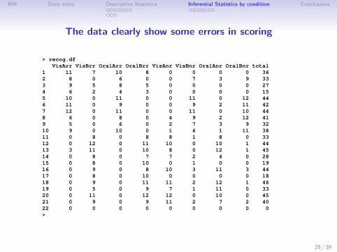
The data clearly show some errors in scoring

> recog.dfVisArr VisBrr OralArr OralBrr VisAnr VisBnr OralAnr OralBnr total

1 11 7 10 8 0 0 0 0 362 8 0 6 0 0 7 3 9 333 9 5 8 5 0 0 0 0 274 6 2 4 3 0 0 0 0 155 10 0 11 0 0 11 0 12 446 11 0 9 0 0 9 2 11 427 12 0 11 0 0 11 0 10 448 6 0 8 0 4 9 2 12 419 5 0 6 0 2 7 3 9 3210 9 0 10 0 1 6 1 11 3811 0 8 0 8 8 1 8 0 3312 0 12 0 11 10 0 10 1 4413 3 11 0 10 8 0 12 1 4514 0 8 0 7 7 2 4 0 2815 0 8 0 10 0 1 0 0 1916 0 9 0 8 10 3 11 3 4417 0 8 0 10 0 0 0 0 1818 0 9 0 11 11 2 12 1 4619 0 5 0 9 7 1 11 0 3320 0 11 0 12 12 0 10 0 4521 0 9 0 9 11 2 7 2 4022 0 0 0 0 0 0 0 0 0>

28 / 39


Fixed data

fixed <- edit(recog.df)fixed<- fixed[-22,] #get rid of the non-existent subjectfixed

VisArr VisBrr OralArr OralBrr VisAnr VisBnr OralAnr OralBnr total1 11 0 10 0 0 7 0 8 362 8 0 6 0 0 7 3 9 333 9 0 8 0 0 5 0 5 274 6 0 4 0 0 2 0 3 155 10 0 11 0 0 11 0 12 446 11 0 9 0 0 9 2 11 427 12 0 11 0 0 11 0 10 448 6 0 8 0 4 9 2 12 419 5 0 6 0 2 7 3 9 3210 9 0 10 0 1 6 1 11 3811 0 8 0 8 8 1 8 0 3312 0 12 0 11 10 0 10 1 4413 0 11 0 10 8 0 12 1 4514 0 8 0 7 7 2 4 0 2815 0 8 0 10 0 1 0 0 1916 0 9 0 8 10 3 11 3 4417 0 8 0 10 0 0 0 0 1818 0 9 0 11 11 2 12 1 4619 0 5 0 9 7 1 11 0 3320 0 11 0 12 12 0 10 0 4521 0 9 0 9 11 2 7 2 40

29 / 39


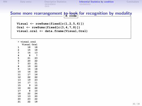
Some more rearrangement to look for recognition by modalityR code

Visual <- rowSums(fixed[c(1,2,5,6)])Oral <- rowSums(fixed[c(3,4,7,8)])visual.oral <- data.frame(Visual,Oral)

> visual.oralVisual Oral

1 18 182 15 183 14 134 8 75 21 236 20 227 23 218 19 229 14 1810 16 2211 17 1612 22 2213 19 2314 17 1115 9 1016 22 2217 8 1018 22 2419 13 2020 23 2221 22 18

30 / 39


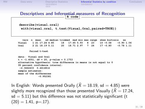
Descriptives and Inferential measures of RecognitionR code

describe(visual.oral)with(visual.oral, t.test(Visual,Oral,paired=TRUE))

vars n mean sd median trimmed mad min max range skew kurtosis seVisual 1 21 17.24 4.85 18 17.65 5.93 8 23 15 -0.58 -0.90 1.06Oral 2 21 18.19 5.11 20 18.71 2.97 7 24 17 -0.80 -0.78 1.11

Paired t-test

data: Visual and Oralt = -1.4051, df = 20, p-value = 0.1753alternative hypothesis: true difference in means is not equal to 095 percent confidence interval:-2.3662433 0.4614814

sample estimates:mean of the differences

-0.952381

In English: Words presented Orally (X̄ = 18.19, sd = 4.85) wereslightly more recognized than those presented Visually (X̄ = 17.24,sd = 5.11) but this difference was not statistically significant (t(20) = 1.41, p=.17).

31 / 39


Total False RecognitionR code

FalseMem.names <- colnames(mem)[375:442]total.false <- rowSums( mem[1:21,FalseMem.names[c(17,34,51)]])recognition <- data.frame(visual.oral/24,false=total.false/16)real.vs.false <- data.frame(real = (Visual + Oral)/48,false =total.false/16)describe(real.vs.false)with(real.vs.false,t.test(real,false,paired=TRUE))

describe(real.vs.false)vars n mean sd median trimmed mad min max range skew kurtosis se

real 1 21 0.74 0.2 0.79 0.76 0.19 0.31 0.96 0.65 -0.78 -0.65 0.04false 2 21 0.48 0.2 0.50 0.46 0.19 0.19 0.94 0.75 0.56 -0.54 0.04

Paired t-testdata: real and falset = 4.0448, df = 20, p-value = 0.0006335alternative hypothesis: true difference in means is not equal to 095 percent confidence interval:0.1268372 0.3969723


0.2619048

In English: Real words were recognized more (X̄ = .74, sd = .2)than were cued but not presented words (X̄ = .48, sd = .2),( t(20) = 4.05, p =.0006). 32 / 39


Two ways of showing the results (with and without cats eyes

Veridical and False Recognition

Condition

Recognition

Visual Oral false

0.0

0.2

0.4

0.6

0.8

1.0

33 / 39


Two ways of showing the results (Cats eyes show the confidenceintervals more clearly)

Veridical and False Recognition

Condition

Recognition

Visual Oral false

0.0

0.2

0.4

0.6

0.8

1.0

34 / 39


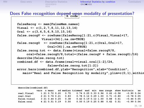
Does False recognition depend upon modality of presentation?R code

falseRecog <- mem[FalseMem.names]Visual <- c(1,2,7,8,11,12,13,14)Oral <- c(3,4,5,6,9,10,15,16)false.recogV <- rowSums(falseRecog[1:21,c(Visual,Visual+17,

Visual+34)],na.rm=TRUE)false.recogO <- rowSums(falseRecog[1:21,c(Oral,Oral+17,

Oral+34)],na.rm=TRUE)false.recog.tot <- data.frame(visual=false.recogV/8,

oral=false.recogO/8,total=(false.recogV + false.recogO)/16)describe(false.recog.tot)combined.df <- data.frame(real=visual.oral[1:2]/24,

false=false.recog.tot[1:2])error.bars(combined.df,ylab="Recognition",xlab="Condition",

main="Real and False Recognition by modality",ylim=c(0,1),within=TRUE)

describe(combined.df)vars n mean sd median trimmed mad min max range skew kurtosis se

real.Visual 1 21 0.72 0.20 0.75 0.74 0.25 0.33 0.96 0.62 -0.58 -0.90 0.04real.Oral 2 21 0.76 0.21 0.83 0.78 0.12 0.29 1.00 0.71 -0.80 -0.78 0.05false.visual 3 21 0.44 0.25 0.38 0.42 0.19 0.12 1.00 0.88 0.61 -0.46 0.05false.oral 4 21 0.51 0.19 0.50 0.50 0.19 0.25 0.88 0.62 0.51 -0.99 0.04

35 / 39


Real versus False Recognition varies by Modality

Real and False Recognition by modality

Condition

Recognition

real.Visual real.Oral false.visual false.oral

0.0

0.2

0.4

0.6

0.8

1.0

36 / 39


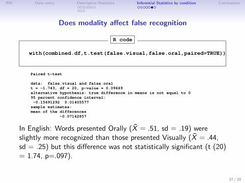
Does modality affect false recognition

R code

with(combined.df,t.test(false.visual,false.oral,paired=TRUE))

Paired t-test

data: false.visual and false.oralt = -1.743, df = 20, p-value = 0.09669alternative hypothesis: true difference in means is not equal to 095 percent confidence interval:-0.15691292 0.01405577


-0.07142857

In English: Words presented Orally (X̄ = .51, sd = .19) wereslightly more recognized than those presented Visually (X̄ = .44,sd = .25) but this difference was not statistically significant (t (20)= 1.74, p=.097).

37 / 39


Memory as an ability, False memory as a different ability (or bias?)

real.Visual

0.3 0.4 0.5 0.6 0.7 0.8 0.9 1.0

0.81 -0.140.3 0.4 0.5 0.6 0.7 0.8 0.9

0.4

0.6

0.8

-0.06

0.3

0.5

0.7

0.9 real.Oral

-0.20 0.00false.visual

0.2

0.6

1.0

0.65

0.4 0.5 0.6 0.7 0.8 0.9

0.3

0.5

0.7

0.9

0.2 0.4 0.6 0.8 1.0

false.oral

38 / 39


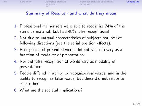
Summary of Results - and what do they mean

1. Professional memorizers were able to recognize 74% of thestimulus material, but had 48% false recognitions!

2. Not due to unusual characteristics of subjects nor lack offollowing directions (see the serial position effects).

3. Recognition of presented words did not seem to vary as afunction of modality of presentation.

4. Nor did false recognition of words vary as modality ofpresentation.

5. People differed in ability to recognize real words, and in theability to recognize false words, but these did not relate toeach other.

6. What are the societal implications?

39 / 39

psychology 205: research methods in psychology paper 1: · pdf filermdata entry descriptive...

Documents