http://pss.sagepub.com/Psychological Science

http://pss.sagepub.com/content/early/2013/11/07/0956797613504966The online version of this article can be found at:

 DOI: 10.1177/0956797613504966

published online 12 November 2013Psychological ScienceGeoff Cumming

The New Statistics: Why and How  

Published by:

http://www.sagepublications.com

On behalf of: 

  Association for Psychological Science

can be found at:Psychological ScienceAdditional services and information for    

  http://pss.sagepub.com/cgi/alertsEmail Alerts:

 

http://pss.sagepub.com/subscriptionsSubscriptions:  

http://www.sagepub.com/journalsReprints.navReprints:  

http://www.sagepub.com/journalsPermissions.navPermissions:  

What is This? 

- Nov 12, 2013OnlineFirst Version of Record >>

at WAKE FOREST UNIV on November 16, 2013pss.sagepub.comDownloaded from at WAKE FOREST UNIV on November 16, 2013pss.sagepub.comDownloaded from

Psychological ScienceXX(X) 1 –23© The Author(s) 2013Reprints and permissions: sagepub.com/journalsPermissions.navDOI: 10.1177/0956797613504966pss.sagepub.com

General Article

There is increasing concern that most current published research findings are false. (Ioannidis, 2005, abstract)

It is time for researchers to avail themselves of the full arsenal of quantitative and qualitative statistical tools. . . . The current practice of focusing exclusively on a dichotomous reject-nonreject decision strategy of null hypothesis testing can actually impede scientific progress. . . . The focus of research should be on . . . what data tell us about the magnitude of effects, the practical significance of effects, and the steady accumulation of knowledge. (Kirk, 2003, p. 100)

We need to make substantial changes to how we usually carry out research. My aim here is to explain why the changes are necessary and to suggest how, practically, we should proceed. I use the new statistics as a broad label for what is required: The strategies and techniques are not themselves new, but for many researchers, adopt-ing them would be new, as well as a great step forward.

Ioannidis (2005) and other scholars have explained that our published research is biased and in many cases not to be trusted. In response, we need to declare in advance our detailed research plans whenever possible, avoid bias in our data analysis, make our full results pub-licly available whatever the outcome, and appreciate the importance of replication. I discuss these issues in the Research Integrity section. Then, in sections on estima-tion, I discuss a further response to Ioannidis, which is to accept Kirk’s advice that we should switch from null-hypothesis significance testing (NHST) to using effect sizes (ESs), estimation, and cumulation of evidence. Along the way, I propose 25 guidelines for improving the way we conduct research (see Table 1).

These are not mere tweaks to business as usual, but substantial changes that will require effort, as well as changes in attitudes and established practices. We need revised textbooks, software, and other resources, but

504966 PSSXXX10.1177/0956797613504966CummingThe New Statistics: Why and Howresearch-article2013

Corresponding Author:Geoff Cumming, Statistical Cognition Laboratory, School of Psychological Science, La Trobe University, Victoria 3086, Australia E-mail: g.cumming@latrobe.edu.au

The New Statistics: Why and How

Geoff CummingLa Trobe University

AbstractWe need to make substantial changes to how we conduct research. First, in response to heightened concern that our published research literature is incomplete and untrustworthy, we need new requirements to ensure research integrity. These include prespecification of studies whenever possible, avoidance of selection and other inappropriate data-analytic practices, complete reporting, and encouragement of replication. Second, in response to renewed recognition of the severe flaws of null-hypothesis significance testing (NHST), we need to shift from reliance on NHST to estimation and other preferred techniques. The new statistics refers to recommended practices, including estimation based on effect sizes, confidence intervals, and meta-analysis. The techniques are not new, but adopting them widely would be new for many researchers, as well as highly beneficial. This article explains why the new statistics are important and offers guidance for their use. It describes an eight-step new-statistics strategy for research with integrity, which starts with formulation of research questions in estimation terms, has no place for NHST, and is aimed at building a cumulative quantitative discipline.

Keywordsresearch integrity, the new statistics, estimation, meta-analysis, replication, statistical analysis, research methods

Received 7/8/13; Revision accepted 8/20/13

Psychological Science OnlineFirst, published on November 12, 2013 as doi:10.1177/0956797613504966

at WAKE FOREST UNIV on November 16, 2013pss.sagepub.comDownloaded from

2 Cumming

sufficient guidance is available for us to make the changes now, even as we develop further new-statistics practices. The changes will prove highly worthwhile: Our publicly available literature will become more trustworthy, our discipline more quantitative, and our research progress more rapid.

Research Integrity

Researchers in psychological science and other disci-plines are currently discussing a set of severe problems with how we conduct, analyze, and report our research. Three problems are central:

•• Published research is a biased selection of all research;

•• data analysis and reporting are often selective and biased; and

•• in many research fields, studies are rarely repli-cated, so false conclusions persist.

Ioannidis (2005) invoked all three problems as he famously explained “why most published research find-ings are false.” He identified as an underlying cause our reliance on NHST, and in particular, the imperative to achieve statistical significance, which is the key to publi-cation, career advancement, research funding, and—especially for drug companies—profits. This imperative explains selective publication, motivates data selection and tweaking until the p value is sufficiently small, and deludes us into thinking that any finding that meets the criterion of statistical significance is true and does not require replication.

Simmons, Nelson, and Simonsohn (2011) made a key contribution in arguing that “undisclosed flexibility in data collection and analysis allows presenting anything

Table 1.• Twenty-Five Guidelines for Improving Psychological Research

1. Promote research integrity: (a) a public research literature that is complete and trustworthy and (b) ethical practice, including full and accurate reporting of research.

2. Understand, discuss, and help other researchers appreciate the challenges of (a) complete reporting, (b) avoiding selection and bias in data analysis, and (c) replicating studies.

3. Make sure that any study worth doing properly is reported, with full details. 4. Make clear the status of any result—whether it deserves the confidence that arises from a fully prespecified

study or is to some extent speculative. 5. Carry out replication studies that can improve precision and test robustness, and studies that provide

converging perspectives and investigate alternative explanations. 6. Build a cumulative quantitative discipline. 7. Whenever possible, adopt estimation thinking and avoid dichotomous thinking. 8. Remember that obtained results are one possibility from an infinite sequence. 9. Do not trust any p value.10. Whenever possible, avoid using statistical significance or p values; simply omit any mention of null-

hypothesis significance testing (NHST).11. Move beyond NHST and use the most appropriate methods, whether estimation or other approaches.12. Use knowledgeable judgment in context to interpret observed effect sizes (ESs).13. Interpret your single confidence interval (CI), but bear in mind the dance. Your 95% CI just might be one

of the 5% that miss. As Figure 1 illustrates, it might be red!14. Prefer 95% CIs to SE bars. Routinely report 95% CIs, and use error bars to depict them in figures.15. If your ES of interest is a difference, use the CI on that difference for interpretation. Only in the case of

independence can the separate CIs inform interpretation.16. Consider interpreting ESs and CIs for preselected comparisons as an effective way to analyze results from

randomized control trials and other multiway designs.17. When appropriate, use the CIs on correlations and proportions, and their differences, for interpretation18. Use small- or large-scale meta-analysis whenever that helps build a cumulative discipline.19. Use a random-effects model for meta-analysis and, when possible, investigate potential moderators.20. Publish results so as to facilitate their inclusion in future meta-analyses.21. Make every effort to increase the informativeness of planned research.22. If using NHST, consider and perhaps calculate power to guide planning.23. Beware of any power statement that does not state an ES; do not use post hoc power.24. Use a precision-for-planning analysis whenever that may be helpful.25. Adopt an estimation perspective when considering issues of research integrity.

at WAKE FOREST UNIV on November 16, 2013pss.sagepub.comDownloaded from

The New Statistics: Why and How 3

as significant.” Researchers can very easily test a few extra participants, drop or add dependent variables, select which comparisons to analyze, drop some results as aberrant, try a few different analysis strategies, and then finally select which of all these things to report. There are sufficient degrees of freedom for statistically significant results to be proclaimed, whatever the original data. Simmons et al. emphasized the second of the three central problems I noted, but also discussed the first and third.

Important sets of articles discussing research-integrity issues appeared in Perspectives on Psychological Science in 2012 and 2013 (volume 7, issue 6; volume 8, issue 4). The former issue included introductions by Pashler and Wagenmakers (2012) and by Spellman (2012). Debate continues, as does work on tools and policies to address the problems. Here, I discuss how we should respond.

Two meanings of research integrity

First, consider the broad label research integrity. I use this term with two meanings. The first refers to the integ-rity of the publicly available research literature, in the sense of being complete, coherent, and trustworthy. To ensure integrity of the literature, we must report all research conducted to a reasonable standard, and report-ing must be full and accurate. The second meaning refers to the values and behavior of researchers, who must con-duct, analyze, and report their research with integrity. We must be honest and ethical, in particular by reporting in full and accurate detail. (See Guideline 1 in Table 1.)

Addressing the three problems

In considering how to address our three central prob-lems, and thus work toward research integrity, we need to recognize that psychological science uses a wonder-fully broad range of approaches to research. We conduct experiments, and also use surveys, interviews, and other qualitative techniques; we study people’s reactions to one-off historical events, mine existing databases, ana-lyze video recordings, run longitudinal studies for decades, use computer simulations to explore possibili-ties, and analyze data from brain scans and DNA sequenc-ing. We collaborate with disciplines that have their own measures, methods, and statistical tools—to the extent that we help develop new disciplines, with names like neuroeconomics and psychoinformatics. We therefore cannot expect that any simple set of new requirements will suffice; in addition, we need to understand the prob-lems sufficiently well to devise the best responses for any particular research situation, and to guide development of new policies, textbooks, software, and other resources. Guideline 2 (Table 1) summarizes the three problems, to which I now turn.

Complete publication

Meta-analysis is a set of techniques for integrating the results from a number of studies on the same or similar issues. If a meta-analysis cannot include all relevant stud-ies, its result is likely to be biased—the file-drawer effect. Therefore, any research conducted to at least a reason-able standard must be fully reported. Such reporting may be in a journal, an online research repository, or some other enduring, publicly accessible form. Future meta-analysts must be able to find the research easily; only then can meta-analysis yield results free of bias.

Achieving such complete reporting—and thus a research literature with integrity—is challenging, given pressure on journal space, editors’ desire to publish what is new and striking, the career imperative to achieve vis-ibility in the most selective journals, and a concern for basic quality control. Solutions will include fuller use of online supplementary material for journal articles, new online journals, and open-access databases. We can expect top journals to continue to seek importance, nov-elty, and high quality in the research they choose to pub-lish, but we need to develop a range of other outlets so that complete and detailed reporting is possible for any research of at least reasonable quality, especially if it was fully prespecified (see the next section). Note that whether research meets the standard of “at least reason-able quality” must be assessed independently of the results, to avoid bias in which results are reported. Full reporting means that all results must be reported, whether ESs are small or large, seemingly important or not, and that sufficient information must be provided so that inclu-sion in future meta-analyses will be easy and other researchers will be able to replicate the study. The Journal Article Reporting Standards listed in the American Psychological Association’s (APA’s) Publication Manual (APA, 2010, pp. 247–250; see also Cooper, 2011) will help.

One key requirement is that a decision to report research—in the sense of making it publicly available, somehow—must be independent of the results. (See Guideline 3 in Table 1.) The best way to ensure this is to make a commitment to report research in advance of conducting it (Wagenmakers, Wetzels, Borsboom, van der Maas, & Kievit, 2012). Ethics review boards should require a commitment to report research fully within a stated number of months—or strong reasons why report-ing is not warranted—as a condition for granting approval for proposed research.

Data selection

Psychologists have long recognized the distinction between planned and post hoc analyses, and the dangers of cherry-picking, or capitalizing on chance. Simmons et

at WAKE FOREST UNIV on November 16, 2013pss.sagepub.comDownloaded from

4 Cumming

al. (2011) explained how insidious and multifaceted the selection problem is. We need a much more comprehen-sive response than mere statistical adjustment for multi-ple post hoc tests. The best way to avoid all of the biases Simmons et al. identified is to specify and commit to full details of a study in advance. Research falls on a spec-trum, from such fully prespecified studies, which provide the most convincing results and must be reported, to free exploration of data, results of which might be intriguing but must—if reported at all—be identified as speculation, possibly cherry-picked.

Confirmatory and exploratory are terms that are widely used to refer to research at the ends of this spec-trum. Confirmatory, however, might imply that a dichot-omous yes/no answer is expected and suggest, wrongly, that a fully planned study cannot simply ask a question (e.g., How effective is the new procedure?). I therefore prefer the terms prespecified and exploratory. An alterna-tive is question answering and question formulating.

Prespecified research.• Full details of a study need to be specified in advance of seeing any results. The procedure, selection of participants, sample sizes, measures, and sta-tistical analyses all must be described in detail and, prefer-ably, registered independently of the researchers (e.g., at Open Science Framework, openscienceframework.org). Such preregistration might or might not be public. Any departures from the prespecified plan must be docu-mented and explained, and may compromise the confi-dence we can have in the results. After the research has been conducted, a full account must be reported, and this should include all the information needed for inclusion of the results in future meta-analyses.

Sample sizes, in particular, need to be declared in advance—unless the researcher will use a sequential or Bayesian statistical procedure that takes account of vari-able N. I explain later that a precision-for-planning analy-sis (or a power analysis if one is using NHST) may usefully guide the choice of N, but such an analysis is not mandatory: Long confidence intervals (CIs) will soon let us know if our experiment is weak and can give only imprecise estimates. The crucial point is that N must be specified independently of any results of the study.

Exploratory research.• Tukey (1977) advocated explora-tion of data and provided numerous techniques and examples. Serendipity must be given a chance: If we do not explore, we might miss valuable insights that could suggest new research directions. We should routinely fol-low planned analyses with exploration. Occasionally the results might be sufficiently interesting to warrant mention in a report, but then they must be clearly identified as speculative, quite possibly the result of cherry-picking.

Exploration has a second meaning: Running pilot tests to explore ideas, refine procedures and tasks, and guide where precious research effort is best directed is often one of the most rewarding stages of research. No matter how intriguing, however, the results of such pilot work rarely deserve even a brief mention in a report. The aim of such work is to discover how to prespecify in detail a study that is likely to find answers to our research questions, and that must be reported. Any researcher needs to choose the moment to switch from not-for-reporting pilot testing to prespecified, must-be-reported research.

Between prespecified and exploratory.• Considering the diversity of our research, full prespecification may sometimes not be feasible, in which case we need to do the best we can, keeping in mind the argument of Sim-mons et al. (2011). Any selection—in particular, any selection after seeing the data—is worrisome. Reporting of all we did, including all data-analytic steps and explo-ration, must be complete. Acting with research integrity requires that we be fully informative about prespecifica-tion, selection, and the status of any result—whether it deserves the confidence that arises from a fully prespeci-fied study or is to some extent speculative. (See Guide-line 4 in Table 1.)

Replication

A single study is rarely, if ever, definitive; additional related evidence is required. Such evidence may come from a close replication, which, with meta-analysis, should give more precise estimates than the original study. A more general replication may increase precision and also provide evidence of generality or robustness of the original finding. We need increased recognition of the value of both close and more general replications, and greater opportunities to report them.

A study that keeps some features of the original and varies others can give a converging perspective, ideally both increasing confidence in the original finding and starting to explore variables that influence it. Converging lines of evidence that are at least largely independent typically provide much stronger support for a finding than any single line of evidence. Some disciplines, includ-ing archaeology, astronomy, and paleontology, are theory based and also successfully cumulative, despite often having little scope for close replication. Researchers in these fields find ingenious ways to explore converging perspectives, triangulate into tests of theoretical predic-tions, and evaluate alternative explanations (Fiedler, Kutner, & Krueger, 2012); we can do this too. (See Guideline 5 in Table 1.)

at WAKE FOREST UNIV on November 16, 2013pss.sagepub.comDownloaded from

The New Statistics: Why and How 5

Research integrity: conclusion

For the research literature to be trustworthy, we need to have confidence that it is complete and that all studies of at least reasonable quality have been reported in full detail, with any departures from prespecified procedures, sample sizes, or analysis methods being documented in full. We therefore need to be confident that all research-ers have conducted and reported their work honestly and completely. These are demanding but essential require-ments, and achieving them will require new resources, rules, and procedures, as well as persistent, diligent efforts.

Further discussion is needed of research integrity, as well as of the most effective practical strategies for achiev-ing the two types of research integrity I have identified. The discussion needs to be enriched by more explicit consideration of ethics in relation to research practices and statistical analysis (Panter & Sterba, 2011) and, more broadly, by consideration of the values that inform the choices researchers need to make at every stage of plan-ning, conducting, analyzing, interpreting, and reporting research (Douglas, 2007).

As I mentioned, Ioannidis (2005) identified reliance on NHST as a major cause of many of the problems with research integrity, so shifting from NHST would be a big help. There are additional strong reasons to make this change: For more than half a century, distinguished schol-ars have published damning critiques of NHST and have described the damage it does. They have advocated a shift from NHST to better techniques, with many nominating estimation—meaning ESs, CIs, and meta-analysis—as their approach of choice. Most of the remainder of this article is concerned with explaining why such a shift is so impor-tant and how we can achieve it in practice. Our reward will be not only improved research integrity, but also a more quantitative, successful discipline.

Estimation: Why

Suppose you read in the news that “support for Proposition X is 53%, in a poll with an error margin of 2%.” Most readers immediately understand that the 53% came from a sample and, assuming that the poll was competent, conclude that 53% is a fair estimate of sup-port in the population. The 2% suggests the largest likely error. Reporting a result in such a way, or as 53 ±•2%, or as 53% with a 95% CI of [51, 55], is natural and informa-tive. It is more informative than stating that support is “statistically significantly greater than 50%, p < .01.” The 53% is our point estimate, and the CI our interval esti-mate, whose length indicates precision of estimation. Such a focus on estimation is the natural choice in many branches of science and accords well with a core aim of

psychological science, which is to build a cumulative quantitative discipline. (See Guideline 6 in Table 1.)

Rodgers (2010) argued that psychological science is, increasingly, developing quantitative models. That is excellent news, and supports this core aim. I am advocat-ing estimation as usually the most informative approach and also urging avoidance of NHST whenever possible. I summarize a few reasons why we should make the change and then discuss how to use estimation and meta-analysis in practice.

In a book on the new statistics (Cumming, 2012), I discussed most of the issues mentioned in the remainder of this article. I do not refer to that book in every section below, but it extends the discussion here and includes many relevant examples. It is accompanied by Exploratory Software for Confidence Intervals, or ESCI (“ESS-key”), which runs under Microsoft Excel and can be freely downloaded from the Internet, at www.thenewstatistics .com (Cumming, 2013). ESCI includes simulations illus-trating many new-statistics ideas, as well as tools for cal-culating and picturing CIs and meta-analysis.

NHST is fatally flawed

Kline (2004, chap. 3; also available at tiny.cc/klinechap3) provided an excellent summary of the deep flaws in NHST and how we use it. He identified mistaken beliefs, damaging practices, and ways in which NHST retards research progress. Anderson (1997) has made a set of pithy statements about the problems of NHST available on the Internet. Very few defenses of NHST have been attempted; it simply persists, and is deeply embedded in our thinking. Kirk (2003), quoted at the outset of this article, identified one central problem: NHST prompts us to see the world as black or white, and to formulate our research aims and make our conclusions in dichotomous terms—an effect is statistically significant or it is not; it exists or it does not. Moving from such dichotomous thinking to estimation thinking is a major challenge, but an essential step. (See Guideline 7 in Table 1.)

Why is NHST so deeply entrenched? I suspect the seductive appeal—the apparent but illusory certainty—of declaring an effect “statistically significant” is a large part of the problem. Dawkins (2004) identified “the tyranny of the discontinuous mind” (p. 252) as an inherent human tendency to seek the reassurance of an either-or classifi-cation, and van Deemter (2010) labeled as “false clarity” (p. 6) our preference for black or white over nuance. In contrast to a seemingly definitive dichotomous decision, a CI is often discouragingly long, although its quantifica-tion of uncertainty is accurate, and a message we need to come to terms with.

Despite warnings in statistics textbooks, the word sig-nificant is part of the seductive appeal: A “statistically

at WAKE FOREST UNIV on November 16, 2013pss.sagepub.comDownloaded from

6 Cumming

significant” effect in the results section becomes “signifi-cant” in the discussion or abstract, and “significant” shouts “important.” Kline (2004) recommended that if we use NHST, we should refer to “a statistical difference,” omit-ting “significant.” That is a good policy; the safest plan is never to use the word significant. The best policy is, whenever possible, not to use NHST at all.

Replication, p values, and CIs

I describe here a major problem of NHST that is too little recognized. If p reveals truth, and we replicate the exper-iment—doing everything the same except with a new random sample—then replication p, the p value in the

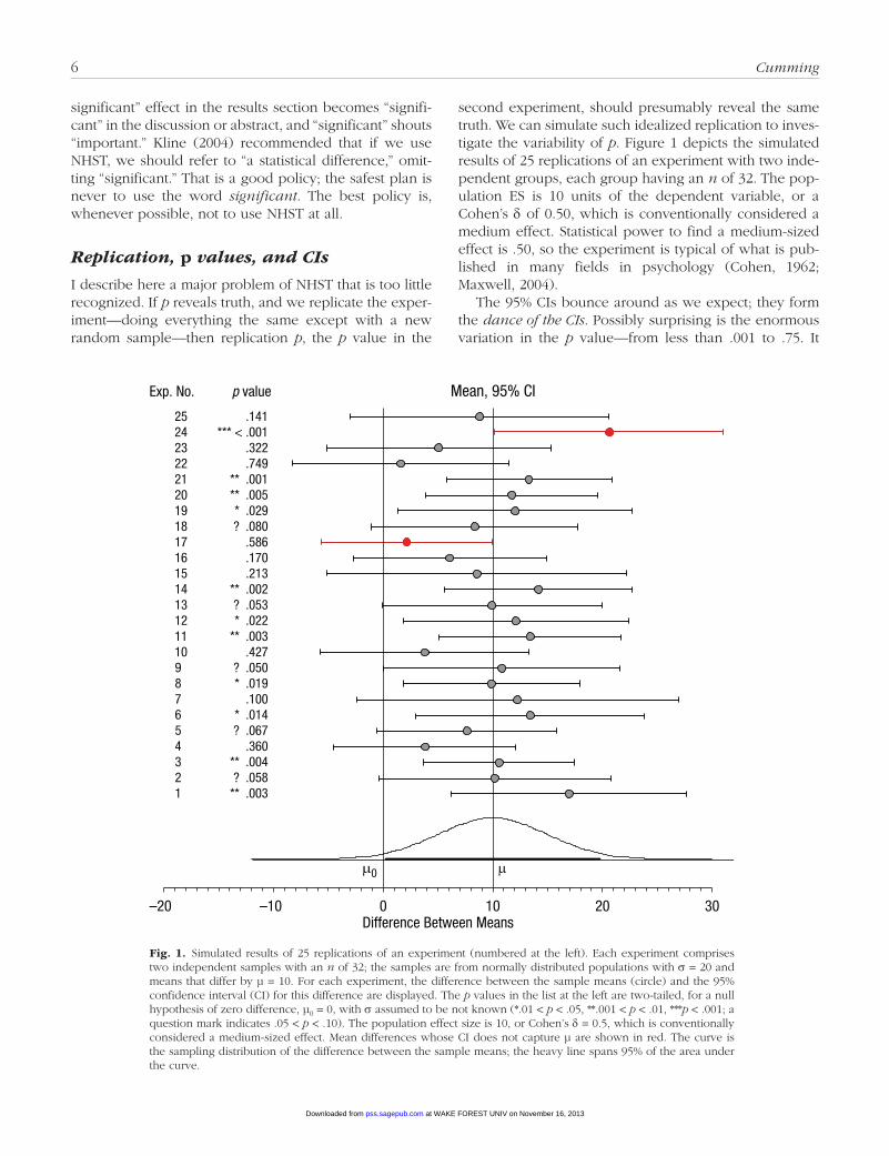
second experiment, should presumably reveal the same truth. We can simulate such idealized replication to inves-tigate the variability of p. Figure 1 depicts the simulated results of 25 replications of an experiment with two inde-pendent groups, each group having an n of 32. The pop-ulation ES is 10 units of the dependent variable, or a Cohen’s δ of 0.50, which is conventionally considered a medium effect. Statistical power to find a medium-sized effect is .50, so the experiment is typical of what is pub-lished in many fields in psychology (Cohen, 1962; Maxwell, 2004).

The 95% CIs bounce around as we expect; they form the dance of the CIs. Possibly surprising is the enormous variation in the p value—from less than .001 to .75. It

** .005* .029? .080

.586

.170

.213** .002? .053* .022

** .003.427

? .050* .019

.100* .014? .067

.360

µ0

.14125*** < .00124

.32223

.74922** .00121

2019181716151413121110987654

** .0043? .0582

** .0031

p value Mean, 95% CI

µ

Exp. No.

–20 –10 0 10 20 30Difference Between Means

Fig. 1.• Simulated results of 25 replications of an experiment (numbered at the left). Each experiment comprises two independent samples with an n of 32; the samples are from normally distributed populations with σ = 20 and means that differ by µ = 10. For each experiment, the difference between the sample means (circle) and the 95% confidence interval (CI) for this difference are displayed. The p values in the list at the left are two-tailed, for a null hypothesis of zero difference, µ0 = 0, with σ assumed to be not known (*.01 < p < .05, **.001 < p < .01, ***p < .001; a question mark indicates .05 < p < .10). The population effect size is 10, or Cohen’s δ = 0.5, which is conventionally considered a medium-sized effect. Mean differences whose CI does not capture µ are shown in red. The curve is the sampling distribution of the difference between the sample means; the heavy line spans 95% of the area under the curve.

at WAKE FOREST UNIV on November 16, 2013pss.sagepub.comDownloaded from

The New Statistics: Why and How 7

seems that p can take almost any value! This dance of the p values is astonishingly wide! You can see more about the dance at tiny.cc/dancepvals and download ESCI (Cumming, 2013) to run the simulation. Vary the popula-tion ES and n, and you will find that even when power is high—in fact, in virtually every situation—p varies dra-matically (Cumming, 2008).

CIs and p values are based on the same statistical the-ory, and with practice, it is easy to translate from a CI to the p value by noting where the interval falls in relation to the null value, µ0 = 0. It is also possible to translate in the other direction and use knowledge of the sample ES (the difference between the group means) and the p value to picture the CI; this may be the best way to interpret a p value. These translations do not mean that p and the CI are equally useful: The CI is much more informative because it indicates the extent of uncertainty, in addition to provid-ing the best point estimate of what we want to know.

Running a single experiment amounts to choosing randomly from an infinite sequence of replications like those in Figure 1. A single CI is informative about the infinite sequence, because its length indicates approxi-mately the extent of bouncing around in the dance. In stark contrast, a single p value gives virtually no informa-tion about the infinite sequence of p values. (See Guideline 8 in Table 1.)

What does an experiment tell us about the likely result if we repeat that experiment? For each experiment in Figure 1, note whether the CI includes the mean of the next experiment. In 20 of the 24 cases, the 95% CI includes the mean next above it in the figure. That is 83.3% of the experiments, which happens to be very close to the long-run average of 83.4% (Cumming & Maillardet, 2006; Cumming, Williams, & Fidler, 2004). So a 95% CI is an 83% prediction interval for the ES estimate of a replication experiment. In other words, a CI is usefully informative about what is likely to happen next time.

Now consider NHST. A replication has traditionally been regarded as “successful” if its statistical-significance status matches that of the original experiment—both ps < .05 or both ps ≥ .05. In Figure 1, just 9 of the 24 (38%) replications match the significance status of the experi-ment immediately below, and are thus successful by this criterion. With power of .50, as here, in the long run we can expect 50% to be successful. Even with power of .80, only 68% of replications will be successful. This example illustrates that NHST gives only poor information about the likely result of a replication.

Considering exact p values gives an even more dra-matic contrast with CIs. If an experiment gives a two-tailed p of .05, an 80% prediction interval for one-tailed p in a replication study is (.00008, .44), which means there is an 80% chance that p will fall in that interval, a 10% chance that p will be less than .00008, and a 10% chance that p will be greater than .44. Perhaps remarkably, that

prediction interval for p is independent of N, because the calculation of p takes account of sample size. Whatever the N, a p value gives only extremely vague information about replication (Cumming, 2008). Any calculated value of p could easily have been very different had we merely taken a different sample, and therefore we should not trust any p value. (See Guideline 9 in Table 1.)

Evidence that CIs are better than NHST

My colleagues and I (Coulson, Healey, Fidler, & Cumming, 2010) presented evidence that, at least in some common situations, researchers who see results presented as CIs are much more likely to make a correct interpretation if they think in terms of estimation than if they consider NHST. This finding suggests that it is best to interpret CIs as intervals, without invoking NHST, and, further, that it is better to report CIs and make no mention of NHST or p values. Fidler and Loftus (2009) reported further evi-dence that CIs are likely to prompt better interpretation than is a report based on NHST. Such evidence comes from the research field of statistical cognition, which investigates how researchers and other individuals under-stand, or misunderstand, various statistical concepts, and how results can best be analyzed and presented for cor-rect comprehension by readers. If our statistical practices are to be evidence based, we must be guided by such empirical results. In this case, the evidence suggests that we should use estimation and avoid NHST.

Defenses of NHST

Schmidt and Hunter (1997) noted eight prominent attempted justifications of NHST. These justifications claimed, for example, that significance testing is needed

•• to identify which results are real and which are due to chance,

•• to determine whether or not an effect exists,•• to ensure that data analysis is objective, and•• to allow us to make clear decisions, as in practice

we need to do.

Schmidt and Hunter made a detailed response to each statement. They concluded that each is false, that we should cease to use NHST, and that estimation provides a much better way to analyze results, draw conclusions, and make decisions—even when the researcher may pri-marily care only about whether some effect is nonzero.

Shifting from NHST: additional considerations

I am advocating shifting as much as possible from NHST to estimation. This is no mere fad or personal preference:

at WAKE FOREST UNIV on November 16, 2013pss.sagepub.comDownloaded from

8 Cumming

The damage done by NHST is substantial and well docu-mented (e.g., Fidler, 2005, chap. 3); the improved research progress offered by estimation is also substantial, and a key step toward achieving the core aim expressed in Guideline 6. Identification of NHST as a main cause of problems with research integrity (Ioannidis, 2005) rein-forces the need to shift, and the urgency of doing so.

I recognize how difficult it may be to move from the seductive but illusory certainty of “statistically significant,” but we need to abandon that security blanket, overcome that addiction. I suggest that, once freed from the require-ment to report p values, we may appreciate how simple, natural, and informative it is to report that “support for Proposition X is 53%, with a 95% CI of [51, 55],” and then interpret those point and interval estimates in practical terms. The introductory statistics course need no longer turn promising students away from our discipline, having terminally discouraged them with the weird arbitrariness of NHST. Finally, APA’s Publication Manual (APA, 2010, p. 34) makes an unequivocal statement that interpreta-tion of results should whenever possible be based on ES estimates and CIs. (That and other statistical recommen-dations of the 2010 edition of the manual were discussed by Cumming, Fidler, Kalinowski, & Lai, 2012.) It is time to move on from NHST. Whenever possible, avoid using statistical significance or p values; simply omit any men-tion of NHST. (See Guideline 10 in Table 1.)

Estimation: How

In this section, I start with an eight-step new-statistics strategy, discuss some preliminaries, and then consider ESs, CIs, the interpretation of both of these, and meta- analysis.

An eight-step new-statistics strategy for research with integrity

The following eight steps highlight aspects of the research process that are especially relevant for achieving the changes discussed in this article.

1. Formulate research questions in estimation terms. To use estimation thinking, ask “How large is the effect?” or “To what extent . . . ?” Avoid dichotomous expressions such as “test the hypoth-esis of no difference” or “Is this treatment better?”

2. Identify the ESs that will best answer the research questions. If, for example, the ques-tion asks about the difference between two means, then that difference is the required ES, as illus-trated in Figure 1. If the question asks how well a model describes some data, then the ES is a mea-sure of goodness of fit.

3. Declare full details of the intended proce-dure and data analysis. Prespecify as many aspects of your intended study as you can, includ-ing sample sizes. A fully prespecified study is best.

4. After running the study, calculate point esti-mates and CIs for the chosen ESs. For Experiment 1 in Figure 1, the estimated difference between the means is 16.9, 95% CI [6.1, 27.7]. (That is the APA format. From here on, I omit “95% CI,” so square brackets signal a 95% CI.)

5. Make one or more figures, including CIs. As in Figure 1, use error bars to depict 95% CIs.

6. Interpret the ESs and CIs. In writing up results, discuss the ES estimates, which are the main research outcome, and the CI lengths, which indi-cate precision. Consider theoretical and practical implications, in accord with the research aims.

7. Use meta-analytic thinking throughout. Think of any single study as building on past stud-ies and leading to future studies. Present results to facilitate their inclusion in future meta-analyses. Use meta-analysis to integrate findings whenever appropriate.

8. Report. Make a full description of the research, preferably including the raw data, available to other researchers. This may be done via journal publication or posting to some enduring publicly available online repository (e.g., figshare, figshare.com; Open Science Framework, openscience framework.org; Psych FileDrawer, psychfile drawer.org). Be fully transparent about every step, including data analysis—and especially about any exploration or selection, which requires the cor-responding results to be identified as speculative.

All these steps differ from past common practice. Step 1 may require a big change in thinking, but may be the key to adopting the new statistics, because asking “how much” naturally prompts a quantitative answer—an ES. Step 6 calls for informed judgment, rather than a mechan-ical statement of statistical significance. Steps 3 and 8 are necessary for research integrity.

The new statistics in context

The eight-step strategy is, of course, far from a complete recipe for good research. There is no mention, for exam-ple, of selecting a good design or finding measures with good reliability and validity. Consider, in addition, the excellent advice of the APA Task Force on Statistical Inference (Wilkinson & Task Force on Statistical Inference, 1999; also available at tiny.cc/tfsi1999), including the advice to keep things simple, when appropriate: “Simpler classical approaches [to designs and analytic methods]

at WAKE FOREST UNIV on November 16, 2013pss.sagepub.comDownloaded from

The New Statistics: Why and How 9

often can provide elegant and sufficient answers to important questions” (p. 598, italics in the original). The task force also advised researchers, “As soon as you have collected your data, . . . look at your data” (p. 597, italics in the original).

I see the first essential stage of statistical reform as being a shift from NHST. I focus on estimation as an achievable step forward, but other approaches also deserve wider use. Never again will any technique—CIs or anything else—be as widely used as p values have been. (See Guideline 11 in Table 1.)

I mention next four examples of further valuable approaches:

•• Data exploration: John Tukey’s (1977) book Exploratory Data Analysis legitimated data explo-ration and also provides a wealth of practical guid-ance. There is great scope to bring Tukey’s approach into the era of powerful interactive soft-ware for data mining and representation.

•• Bayesian methods: These are becoming commonly used in some disciplines, for example, ecology (McCarthy, 2007). Bayesian approaches to estima-tion based on credible intervals, to model assess-ment and selection, and to meta-analysis are highly valuable (Kruschke, 2010). I would be wary, how-ever, of Bayesian hypothesis testing, if it does not escape the limitations of dichotomous thinking.

•• Robust methods: The common assumption of nor-mally distributed populations is often unrealistic, and conventional methods are not as robust to typical departures from normality as is often assumed. Robust methods largely sidestep such problems and deserve to be more widely used (Erceg-Hurn & Mirosevich, 2008; Wilcox, 2011).

•• Resampling and bootstrapping methods: These are attractive in many situations. They often require few assumptions and can be used to estimate CIs (Kirby & Gerlanc, 2013).

Note that considering options for data analysis does not license choosing among them after running the experiment: Selecting the analysis strategy was one of the degrees of freedom described by Simmons et al. (2011); that strategy should be prespecified along with other details of the intended study.

ESs

An ES is simply an amount of anything of interest (Cumming & Fidler, 2009). Means, differences between means, frequencies, correlations, and many other familiar quantities are ESs. A p value, however, is not an ES. A sample ES, calculated from data, is typically our point

estimate of the population ES. ESs can be reported in original units (e.g., milliseconds or score units) or in some standardized or units-free measure (e.g., Cohen’s d, β, η

p2, or a proportion of variance). ESs in original units

may often be more readily interpreted, but a standard-ized ES can assist comparison over studies and is usually necessary for meta-analysis. Reporting both kinds of ESs is often useful.

Cohen’s d.• Cohen’s d deserves discussion because it is widely useful but has pitfalls. It is a standardized ES that is calculated by taking an original-units ES, usually the difference between two means, and expressing this as a number of standard deviations. The original-units ES is divided by a standardizer that we choose as a suitable unit of measurement:

( )= E C– / ,d M M s (1)

where ME and MC are experimental (E) and control (C) means, and s is the standardizer. Cohen’s d is thus a kind of z score. First we choose a population standard deviation that makes sense as the unit for d, and then we choose our best estimate of that standard deviation to use as s in the denominator of d. For two indepen-dent groups, if we assume homogeneity of variance, the pooled standard deviation within groups, sp, is our stan-dardizer, just as we use for the independent-groups t test. If we suspect the treatment notably affects variabil-ity, we might prefer the control population’s standard deviation, estimated by sC (the control group’s standard deviation), as the standardizer. If we have several com-parable control groups, pooling over these may give a more precise estimate to use as the standardizer. These choices obviously lead to different values for d, so whenever we see a value of d, we need to know how it was calculated before we can interpret it. When report-ing values of d, make sure to describe how they were calculated.

Now consider a repeated measure design, in which each participant experiences both E and C treatments. We would probably regard the C population as the refer-ence and choose its standard deviation, estimated by sC, as the standardizer. However, the CI on the difference in this repeated measure design (and also the paired t test) is calculated using sdiff, the standard deviation of the paired differences, rather than sC. As noted earlier, with two independent groups, sp serves as the standardizer for d and also for the independent-groups t test. By contrast, the repeated measure design emphasizes that the stan-dard deviation we choose as the standardizer may be quite different from the standard deviation we use for inference, whether based on a CI or a t test.

at WAKE FOREST UNIV on November 16, 2013pss.sagepub.comDownloaded from

10 Cumming

Equation 1 emphasizes that d is the ratio of two quan-tities, each estimated from data (Cumming & Finch, 2001). If we replicate the experiment, both numerator and denominator—the original-units ES and the standard-izer—will be different. Cohen’s d is thus measured on a “rubber ruler,” whose unit, the standardizer, stretches in or out if we repeat the experiment. We therefore must be very careful when interpreting d, especially when we compare d values given by different conditions or experi-ments. Do the original-units ESs differ, does the standard-izer differ, or do both differ? This difficulty has led some scholars, especially in medicine (Greenland, Schlesselman, & Criqui, 1986), to argue that standardized ES measures should never be used. In psychology, however, we have little option but to use a standardized ES when we wish to meta-analyze results from studies that used different original-units measures—different measures of anxiety, for example.

I have three final remarks about d. Because d is the ratio of two estimated quantities, its distribution is com-plex, and it is not straightforward to calculate CIs for d. ESCI can provide CIs on d in a number of basic situa-tions, or you can use good approximations (Cumming & Fidler, 2009). (See Grissom & Kim, 2012, chap. 3, for more about CIs for d.) Second, symbols and terms refer-ring to the standardized difference between means, cal-culated in various ways, are used inconsistently in the literature. “Hedges’s g,” for example, is used with at least two different meanings. I recommend following common practice and using Cohen’s d as the generic term, but be sure to explain how d was calculated. Third, the simple calculations of d I have discussed give values that are biased estimates of δ, the population ES; d is somewhat too large, especially when N is small. A simple adjust-ment (Grissom & Kim, 2012, p. 70, or use ESCI) is required to give dunb, the unbiased version of Cohen’s d; we should usually prefer dunb. (For more on Cohen’s d, see Cumming, 2012, chap. 11.)

Interpretation of ESs.• Interpretation of ESs requires informed judgment in context. We need to trust our expertise and report our assessment of the size, impor-tance, and theoretical or practical value of an ES, taking full account of the research situation. Cohen (1988) sug-gested 0.2, 0.5, and 0.8 as small, medium, and large val-ues of d, but emphasized that making a judgment in context should be preferred to these fallback bench-marks. Interpretation should include consideration, when appropriate, of the manipulation or treatment, the partici-pants, and the research aims. When interpreting an ES, give reasons.

Published reference points can sometimes guide inter-pretation: For the Beck Depression Inventory-II (Beck, Steer, Ball, & Ranieri, 1996), for example, scores of 0

through 13, 14 through 19, 20 through 28, and 29 through 63 are labeled as indicating, respectively, minimal, mild, moderate, and severe levels of depression. In pain research, a change in rating of 10 mm on the 100-mm visual analog scale is often regarded as the smallest change of clinical importance—although no doubt differ-ent interpretations may be appropriate in different situa-tions. A neuropsychology colleague tells me that, as a rough guideline, he uses a decrease of 15% in a client’s memory score as the smallest change possibly of clinical interest. Comparison with ESs found in past research can be useful. I hope increasing attention to ES interpretation will prompt emergence of additional formal or informal conventions to help guide interpretation of various sizes of effect. However, no guideline will be universally appli-cable, and researchers must take responsibility for their ES interpretations. (See Guideline 12 in Table 1.)

Interpretation of CIs

CIs indicate the precision of our ES estimates, so interpre-tation of ESs must be accompanied by interpretation of CIs. I offer six approaches, one or more of which may be useful in any particular case. The discussion here refers to a 95% CI for a population mean, µ, but generally applies to any CI. (For an introduction to CIs and their use, see Cumming & Finch, 2005; also available at tiny .cc/inferencebyeye.)

One from an infinite sequence.• The CI calculated from our data is one from the dance, as Figure 1 illus-trates. In the long run, 95% of CIs will include µ, and an unidentified 5% will miss. Most likely our CI includes µ, but it might not—it might be red, as in Figure 1.

Thinking of our CI as coming from an infinite sequence is the correct interpretation, but in practice we need to interpret what we have—our single interval. That is rea-sonable, providing our CI is typical of the dance. It usu-ally is, with two exceptions. First, in Figure 1, the CIs vary somewhat in length, because each is based on the sam-ple’s standard deviation. Each CI length is an estimate of the length of the heavy line at the bottom of the figure, which indicates an interval including 95% of the area under the curve, which would be the CI length if we knew the population standard deviation. With two groups of n = 32, CI length varies noticeably from experiment to experiment. A smaller n gives greater variation, and if n is less than, say, 10, the variation is so large that the length of a single CI may be a very poor estimate of pre-cision. A CI is of little practical use when samples are very small.

A second exception occurs when our CI is not chosen randomly. If we run several experiments but report only the largest ES, or the shortest CI, that result is not typical

at WAKE FOREST UNIV on November 16, 2013pss.sagepub.comDownloaded from

The New Statistics: Why and How 11

of the dance, and the CI is practically uninterpretable. Simmons et al. (2011) explained how such selection is problematic. Barring a tiny sample or data selection, it is generally reasonable to interpret our single CI, and the following five approaches all do that. We should, how-ever, always remember the dance: Our CI just might be red! (See Guideline 13 in Table 1.)

Focus on our interval.• Our CI defines a set of plausi-ble, or likely, values for µ, and values outside the interval are relatively implausible. We can be 95% confident that our interval includes µ and can think of the lower and upper limits as likely lower and upper bounds for µ. Interpret the point estimate—the sample mean (M) at the center of the interval—and also the two limits of the CI. If an interval is sufficiently short and close to zero that you regard every value in the interval as negligible, you can conclude that the true value of µ is, for practical pur-poses, zero or very close to zero. That is the best way to think about what, in the NHST world, is acceptance of a null hypothesis.

Prediction.• As I discussed earlier, our CI is an 83% pre-diction interval for the ES that would be given by a repli-cation experiment (Cumming & Maillardet, 2006). Our CI defines a range within which the mean of a repeat exper-iment most likely will fall (on average, a 5-in-6 chance).

Precision.• The margin of error (MOE—pronounced “mow-ee”) is the length of one arm of a CI and indicates precision. Our estimation error is the difference between the sample and population means (M – µ). We can be 95% confident that this error is no greater than the MOE in absolute value. A large MOE indicates low precision and an uninformative experiment; a small MOE is gold. A major purpose of meta-analysis is to integrate evidence to increase precision. Later, I discuss another use of pre-cision—to assist research planning.

The cat’s-eye picture of a CI.• The curve in Figure 1 shows the sampling distribution of M, the difference between the two sample means: As the dance also illus-trates, most values of M fall close to µ, and progressively fewer fall at greater distances. The curve is also the distri-bution of estimation errors: Errors are most likely close to zero, and larger errors are progressively less likely, which implies that our interval has most likely fallen so that M is close to µ. Therefore, values close to our M are the best bet for µ, and values closer to the limits of our CI are suc-cessively less good bets.

The curve, if centered around M rather than µ, indi-cates the relative plausibility, or likelihood, of values being the true value of µ. The center graphics of Figure 2

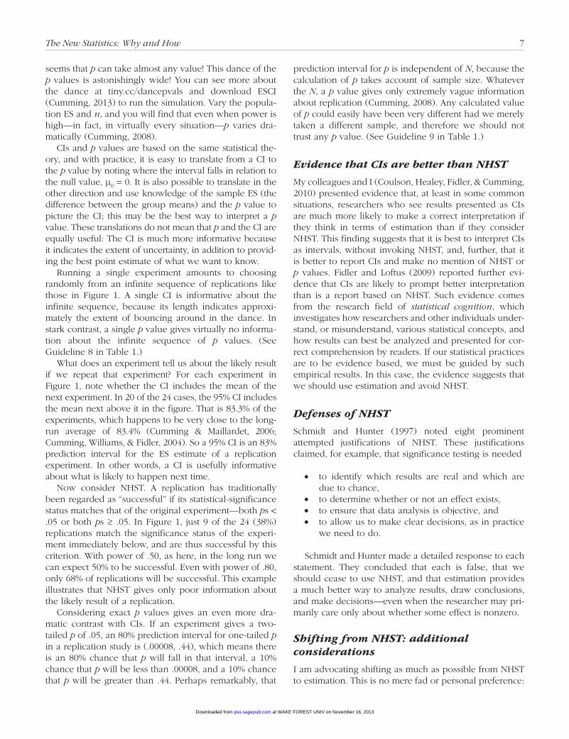
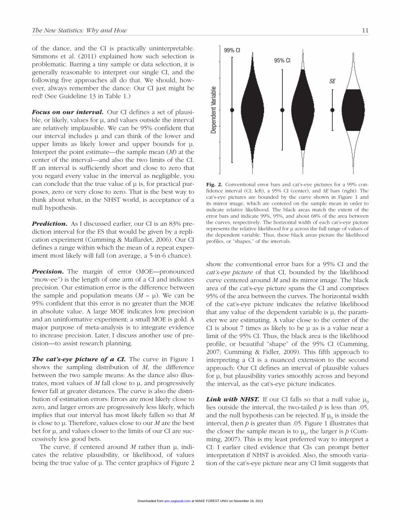
show the conventional error bars for a 95% CI and the cat’s-eye picture of that CI, bounded by the likelihood curve centered around M and its mirror image. The black area of the cat’s-eye picture spans the CI and comprises 95% of the area between the curves. The horizontal width of the cat’s-eye picture indicates the relative likelihood that any value of the dependent variable is µ, the param-eter we are estimating. A value close to the center of the CI is about 7 times as likely to be µ as is a value near a limit of the 95% CI. Thus, the black area is the likelihood profile, or beautiful “shape” of the 95% CI (Cumming, 2007; Cumming & Fidler, 2009). This fifth approach to interpreting a CI is a nuanced extension to the second approach: Our CI defines an interval of plausible values for µ, but plausibility varies smoothly across and beyond the interval, as the cat’s-eye picture indicates.

Link with NHST.• If our CI falls so that a null value µ0 lies outside the interval, the two-tailed p is less than .05, and the null hypothesis can be rejected. If µ0 is inside the interval, then p is greater than .05. Figure 1 illustrates that the closer the sample mean is to µ0, the larger is p (Cum-ming, 2007). This is my least preferred way to interpret a CI: I earlier cited evidence that CIs can prompt better interpretation if NHST is avoided. Also, the smooth varia-tion of the cat’s-eye picture near any CI limit suggests that

SE

95% CI

99% CI

Depe

nden

t Var

iabl

e

Fig. 2.• Conventional error bars and cat’s-eye pictures for a 99% con-fidence interval (CI; left), a 95% CI (center), and SE bars (right). The cat’s-eye pictures are bounded by the curve shown in Figure 1 and its mirror image, which are centered on the sample mean in order to indicate relative likelihood. The black areas match the extent of the error bars and indicate 99%, 95%, and about 68% of the area between the curves, respectively. The horizontal width of each cat’s-eye picture represents the relative likelihood for µ across the full range of values of the dependent variable. Thus, these black areas picture the likelihood profiles, or “shapes,” of the intervals.

at WAKE FOREST UNIV on November 16, 2013pss.sagepub.comDownloaded from

12 Cumming

we should not lapse back into dichotomous thinking by attaching any particular importance to whether a value of interest lies just inside or just outside our CI.

Error bars: prefer 95% CIs

It is extremely unfortunate that the familiar error-bar graphic can mean so many different things. Figure 2 uses it to depict a 99% CI and SE bars (i.e., mean ±1 SE), as well as a 95% CI; the same graphic may also represent standard deviations, CIs with other levels of confidence, or various other quantities. Every figure with error bars must state clearly what the bars represent. (An introduc-tory discussion of error bars was provided by Cumming, Fidler, & Vaux, 2007.)

Numerous articles in Psychological Science have included figures with SE bars, although these have rarely been used to guide interpretation. The best way to think of SE bars on a mean is usually to double the whole length—so the bars extend 2 SE above and 2 SE below the mean—and interpret them as being, approximately, the 95% CI, as Figure 2 illustrates (Cumming & Finch, 2005). The right-hand cat’s-eye picture in Figure 2 illus-trates that relative likelihood changes little across SE bars, which span only about two thirds of the area between the two curves. SE bars are usually approximately equiva-lent to 68% CIs and are 52% prediction intervals (Cumming & Maillardet, 2006): There is about a coin-toss chance that a repeat of the experiment will give a sample ES within the original SE bars.

It may be discouraging to display 95% CIs rather than the much shorter SE bars, but there are strong reasons for preferring CIs. First, they are designed for inference. Second, for means, although there is usually a simple relation between SE bars and the 95% CI, that relation breaks down if N is small; for other measures, including correlations, there is no simple relation between the CI and any standard error. Therefore, SE bars cannot be relied on to provide inferential information, which is what we want. Since the 1980s, medical researchers have routinely reported CIs, not SE bars. We should do the same. (See Guideline 14 in Table 1.)

Figure 2 shows that 99% CIs simply extend further than 95% CIs, to span 99% rather than 95% of the area between the two likelihood curves. They are about one third longer than 95% CIs. Further approximate bench-marks are that 90% CIs are about five sixths as long as 95% CIs, and 50% CIs are about one third as long. Noting benchmarks like these (Cumming, 2007) allows you to convert easily among CIs with various levels of confi-dence. In matters of life and death, it might seem better to use 99% CIs, or even 99.9% CIs (about two thirds lon-ger than 95% CIs), but I suggest that it is virtually always best to use 95% CIs. We should build our intuitions

(bearing in mind the cat’s-eye picture) for 95% CIs—the most common CIs—and use benchmarks if necessary to interpret other CIs.

Examples of ES and CI interpretation

As I have discussed, interpretation of ESs and CIs relies on knowledgeable judgment in context, and should be nuanced and meaningful. This approach will lack the seductive but illusory certainty of a p-value cutoff. If that seems a step too far, recall the dance of the p values and reflect on how unreliable p is, and how inappropriate it is as an arbiter of research quality or publishability. We happily rely on informed judgment for evaluation of research questions, research designs, and numerous aspects of how research is conducted and analyzed; we need to extend that reliance to assessment of results and interpretations. With full reporting, informed debate about interpretation is possible and appropriate, just as it is about any other aspect of research. I offer five brief examples of reporting and discussing ESs and CIs.

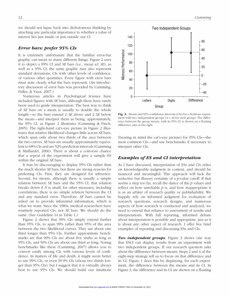
Two independent groups.• Figure 3 shows one way that ESCI can display results from an experiment with two independent groups. If our research question asks about the difference between means, Steps 2 and 4 of the eight-step strategy tell us to focus on that difference and its CI. Figure 1 does this by displaying, for each experi-ment, the difference between the means and its CI. In Figure 3, the difference and its CI are shown on a floating

80

60

40

20

0

–20

–400

20

40

60

80

100

120

140

Letters Digits Difference

Mem

ory

Perfo

rman

ce

Two Independent Groups

Group

Fig. 3.• Means and 95% confidence intervals (CIs) for a fictitious experi-ment with two independent groups (n = 40 for each group). The differ-ence between the group means, with its 95% CI, is shown on a floating difference axis at the right.

at WAKE FOREST UNIV on November 16, 2013pss.sagepub.comDownloaded from

The New Statistics: Why and How 13

difference axis, but the group means and CIs are also displayed. The common practice of displaying group means gives a general picture, but interpretation of any difference should be informed by the appropriate CI—the CI on that difference. In Figure 3 the difference is 54.0 [7.2, 100.8], which suggests that our experiment has low precision and is perhaps of little value—although it might still make a useful contribution to a meta-analysis. That is a much better approach than declaring the result “statisti-cally significant, p = .024.”

For independent groups, the CI on the difference is usually, as in Figure 3, about 1.4 times the average of the lengths of the CIs on the two means. The two separate CIs can be used to assess the difference. Finch and I (Cumming & Finch, 2005; see also Cumming, 2009) described rules of eye for doing this. If the two groups’ CIs just touch or do not overlap, there is reasonable evi-dence of a population difference, and, approximately, p is less than .01. If the two groups’ CIs overlap by only a moderate amount (no more than half the average MOE, as approximately in Fig. 3), there is some evidence of a difference, and, approximately, p is less than .05. I have stated here the approximate p values, but there is no need to invoke p values: Simply interpret the two inter-vals, but note well that the means must be independent for these rules of eye to be valid.

By contrast, in a paired or repeated measure design, the CI on the difference is typically shorter than the CIs on the separate measures, because the two measures

(e.g., pretest and posttest) are usually positively corre-lated. The shortness of that CI reflects the sensitivity of the design: The higher the correlation, the more sensitive the design and the shorter the CI. With a repeated mea-sure, overlap of the separate CIs is totally irrelevant, no rule of eye is possible, and we must have the CI on the difference if we are to interpret the difference. (See Guideline 15 in Table 1.)

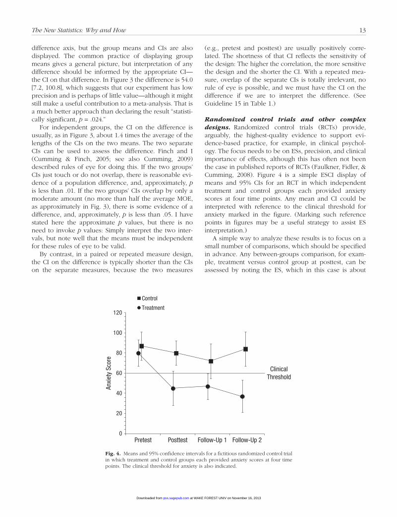
Randomized control trials and other complex designs.• Randomized control trials (RCTs) provide, arguably, the highest-quality evidence to support evi-dence-based practice, for example, in clinical psychol-ogy. The focus needs to be on ESs, precision, and clinical importance of effects, although this has often not been the case in published reports of RCTs (Faulkner, Fidler, & Cumming, 2008). Figure 4 is a simple ESCI display of means and 95% CIs for an RCT in which independent treatment and control groups each provided anxiety scores at four time points. Any mean and CI could be interpreted with reference to the clinical threshold for anxiety marked in the figure. (Marking such reference points in figures may be a useful strategy to assist ES interpretation.)

A simple way to analyze these results is to focus on a small number of comparisons, which should be specified in advance. Any between-groups comparison, for exam-ple, treatment versus control group at posttest, can be assessed by noting the ES, which in this case is about

ClinicalThreshold

0

20

40

60

80

100

120

Pretest Posttest Follow-Up 1 Follow-Up 2

Anxi

ety

Scor

e

Control

Treatment

Fig. 4.• Means and 95% confidence intervals for a fictitious randomized control trial in which treatment and control groups each provided anxiety scores at four time points. The clinical threshold for anxiety is also indicated.

at WAKE FOREST UNIV on November 16, 2013pss.sagepub.comDownloaded from

14 Cumming

−35, and considering the two CIs. You could use the 1.4 rule from the previous section to estimate that the CI on the ES (the difference) has a MOE of about 20, and then make a clinical judgment about this anxiety reduction of −35 [−55, −15].

The situation is different, however, for a within-group comparison. For example, if we want to compare Follow-Up 1 and Follow-Up 2 for the treatment group, we can note the ES, which is about 10, but cannot make any judgment about the precision of that estimated change, because the comparison involves a repeated measure. The two separate CIs are irrelevant. To assess any repeated measure comparison, we need to have the CI on the change in question reported explicitly, either numerically in the text or in a figure that displays within-group changes. An attractive alternative is to use the techniques of Masson and Loftus (2003) and Blouin and Riopelle (2005) to calculate CIs for repeated measure effects and display these in a figure showing means. We need further development of graphical conventions for displaying CIs on contrasts in complex designs. (See Fidler, Faulkner, & Cumming, 2008, for further discussion of an estimation-based approach to reporting and inter-preting RCTs.)

When inspecting any figure with CIs, be careful to note the type—independent or repeated measure—of any comparison of interest. CIs on individual means are relevant only for assessing independent comparisons. It is therefore essential that any figure clearly indicate for each independent variable whether that variable has independent-groups or repeated measure status. In Figure 4, the lines joining the means within a group hint at a repeated measure variable, and including such lines is a convention worth supporting, but the convention is not used with sufficient consistency to be a dependable guide.

More generally, choosing in advance the comparisons or contrasts most relevant for answering research ques-tions, rather than, for example, starting with an overall analysis of variance, can be an effective and easily-under-stood strategy. Rosenthal, Rosnow, and Rubin (2000) described this approach, and Steiger (2004) explained how to calculate and use CIs for contrasts in a range of multiway designs. (See Guideline 16 in Table 1.)

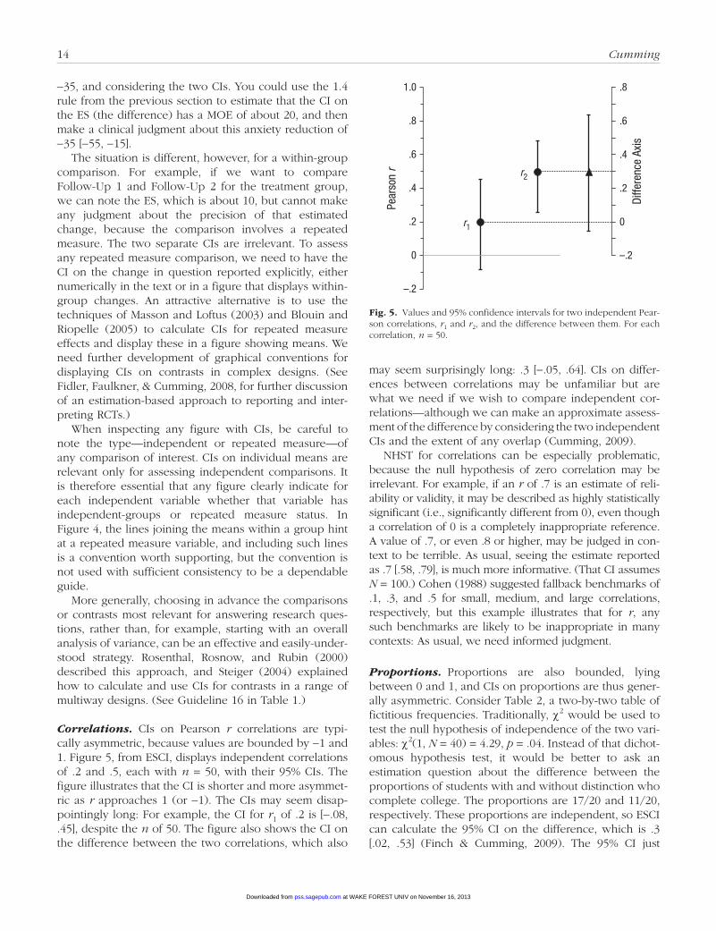
Correlations.• CIs on Pearson r correlations are typi-cally asymmetric, because values are bounded by −1 and 1. Figure 5, from ESCI, displays independent correlations of .2 and .5, each with n = 50, with their 95% CIs. The figure illustrates that the CI is shorter and more asymmet-ric as r approaches 1 (or −1). The CIs may seem disap-pointingly long: For example, the CI for r1 of .2 is [−.08, .45], despite the n of 50. The figure also shows the CI on the difference between the two correlations, which also

may seem surprisingly long: .3 [−.05, .64]. CIs on differ-ences between correlations may be unfamiliar but are what we need if we wish to compare independent cor-relations—although we can make an approximate assess-ment of the difference by considering the two independent CIs and the extent of any overlap (Cumming, 2009).

NHST for correlations can be especially problematic, because the null hypothesis of zero correlation may be irrelevant. For example, if an r of .7 is an estimate of reli-ability or validity, it may be described as highly statistically significant (i.e., significantly different from 0), even though a correlation of 0 is a completely inappropriate reference. A value of .7, or even .8 or higher, may be judged in con-text to be terrible. As usual, seeing the estimate reported as .7 [.58, .79], is much more informative. (That CI assumes N = 100.) Cohen (1988) suggested fallback benchmarks of .1, .3, and .5 for small, medium, and large correlations, respectively, but this example illustrates that for r, any such benchmarks are likely to be inappropriate in many contexts: As usual, we need informed judgment.

Proportions.• Proportions are also bounded, lying between 0 and 1, and CIs on proportions are thus gener-ally asymmetric. Consider Table 2, a two-by-two table of fictitious frequencies. Traditionally, χ2 would be used to test the null hypothesis of independence of the two vari-ables: χ2(1, N = 40) = 4.29, p = .04. Instead of that dichot-omous hypothesis test, it would be better to ask an estimation question about the difference between the proportions of students with and without distinction who complete college. The proportions are 17/20 and 11/20, respectively. These proportions are independent, so ESCI can calculate the 95% CI on the difference, which is .3 [.02, .53] (Finch & Cumming, 2009). The 95% CI just

r1

r2

.8

.6

.4

.2

0

–.2

Diffe

renc

e Ax

is

–.2

0

.2

.4

.6

.8

1.0

Pear

son r

Fig. 5.• Values and 95% confidence intervals for two independent Pear-son correlations, r1 and r2, and the difference between them. For each correlation, n = 50.

at WAKE FOREST UNIV on November 16, 2013pss.sagepub.comDownloaded from

The New Statistics: Why and How 15

misses zero, which is consistent with the p value of .04 in the χ2 analysis. The estimation approach is, as usual, more informative, because it gives a point estimate (.3) in answer to our question and a CI to indicate the precision. With such small frequencies, it is not surprising that our CI is so long. (See Guideline 17 in Table 1.)

Assessment of model fit.• Consider a somewhat differ-ent example of CI use. Velicer et al. (2008) used a num-ber of previous data sets and expert judgment to generate quantitative predictions for 15 variables from the trans-theoretical model of behavior change. They then took an entirely independent data set and estimated the 15 vari-ables. Because the test data set was large (N of approxi-mately 4,000), the CIs were short. Velicer et al. found that the CIs included the predicted values for 11 of the 15 variables, a result they interpreted as strong support for most aspects of the model. Examination of 2 variables for which the predictions were rather inaccurate suggested

lines for further theoretical and empirical investigation. Such assessment of quantitative models accords well with Guideline 6 and the argument of Rodgers (2010) that psychology should become more quantitative.

Meta-analysis

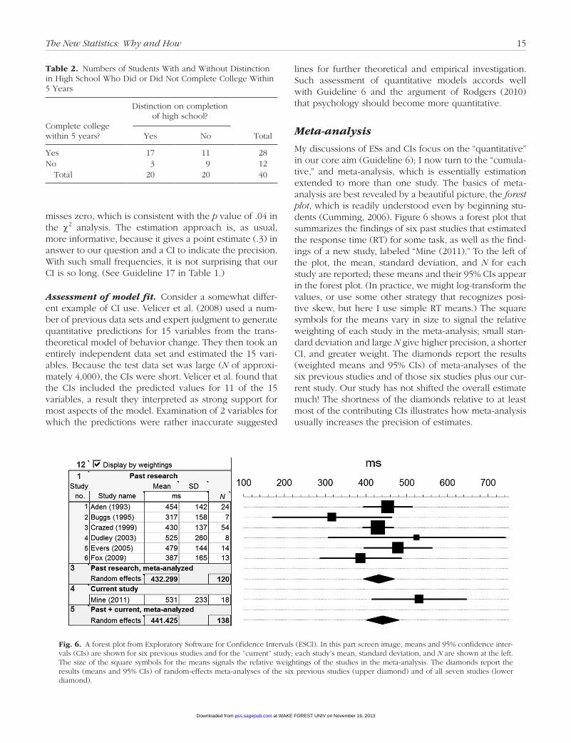
My discussions of ESs and CIs focus on the “quantitative” in our core aim (Guideline 6); I now turn to the “cumula-tive,” and meta-analysis, which is essentially estimation extended to more than one study. The basics of meta-analysis are best revealed by a beautiful picture, the forest plot, which is readily understood even by beginning stu-dents (Cumming, 2006). Figure 6 shows a forest plot that summarizes the findings of six past studies that estimated the response time (RT) for some task, as well as the find-ings of a new study, labeled “Mine (2011).” To the left of the plot, the mean, standard deviation, and N for each study are reported; these means and their 95% CIs appear in the forest plot. (In practice, we might log-transform the values, or use some other strategy that recognizes posi-tive skew, but here I use simple RT means.) The square symbols for the means vary in size to signal the relative weighting of each study in the meta-analysis; small stan-dard deviation and large N give higher precision, a shorter CI, and greater weight. The diamonds report the results (weighted means and 95% CIs) of meta-analyses of the six previous studies and of those six studies plus our cur-rent study. Our study has not shifted the overall estimate much! The shortness of the diamonds relative to at least most of the contributing CIs illustrates how meta-analysis usually increases the precision of estimates.

Table 2.• Numbers of Students With and Without Distinction in High School Who Did or Did Not Complete College Within 5 Years

Distinction on completion of high school?

Complete college within 5 years? Yes No Total

Yes 17 11 28No 3 9 12• Total 20 20 40

Fig. 6.• A forest plot from Exploratory Software for Confidence Intervals (ESCI). In this part screen image, means and 95% confidence inter-vals (CIs) are shown for six previous studies and for the “current” study; each study’s mean, standard deviation, and N are shown at the left. The size of the square symbols for the means signals the relative weightings of the studies in the meta-analysis. The diamonds report the results (means and 95% CIs) of random-effects meta-analyses of the six previous studies (upper diamond) and of all seven studies (lower diamond).

at WAKE FOREST UNIV on November 16, 2013pss.sagepub.comDownloaded from

16 Cumming

Figure 6 illustrates a meta-analysis in which every study used the same original measure, RT in millisec-onds. In psychological science, however, different studies usually use different original measures, and for meta-analysis we need a standardized, or units-free, ES mea-sure, most commonly Cohen’s d or Pearson’s r. The original-units ESs need to be transformed into ds or rs for meta-analysis.

Many published meta-analyses report substantial proj-ects, integrating results from dozens or even hundreds of studies. Cooper provided detailed guidance for the seven steps involved in a large meta-analysis (Cooper, 2010), as well as advice on reporting a meta-analysis in accord with the Meta-Analysis Reporting Standards (MARS) spec-ified in APA’s (2010, pp. 251–252) Publication Manual (Cooper, 2011). Borenstein, Hedges, Higgins, and Rothstein (2009) discussed many aspects of meta-analy-sis, especially data analysis, and the widely used CMA software (available from Biostat, www.Meta-Analysis .com).

It is vital to appreciate that meta-analysis is no mere mechanical procedure, and that conducting a large meta-analysis requires domain expertise and informed judg-ment at every step: defining questions, finding and selecting relevant literature, choosing variables and mea-sures, extracting and then analyzing data, assessing pos-sible moderating variables, and more. Even so, conducting at least a small-scale meta-analysis should be practically achievable without extended specialized training.

Large meta-analyses may be most visible, but meta-analysis can often be very useful on a smaller scale as well. A minimum of two results may suffice for a meta-analysis. Consider meta-analysis to combine results from several of your studies, or from your current study plus even only one or two previous studies. You need not even notice whether any individual study would give sta-tistical significance—we care only about the CIs, and especially the result of the meta-analysis, which may be a pleasingly short CI. (See Guideline 18 in Table 1.)

Heterogeneity.• Imagine that all the studies in Figure 6 had the same N and were so similar that we can assume they all estimate the same population mean, µ. In that case, the study-to-study variation in means should be similar to that in the dance in Figure 1. In other words, the bouncing around in the forest plot should match what we expect simply because of sampling variability. If there is notably more variability than this, we can say the set of studies is heterogeneous, and there may be one or more moderating variables that affect the ES. Meta-anal-ysis offers us more precise estimates, but also the highly valuable possibility of identifying such moderators.

Suppose that some of the studies in Figure 6 hap-pened to use only female participants (F studies), and others only males (M studies). We can meta-analyze the

sets of F and M studies separately and assess the two results, using, of course, the two CIs. If we find the over-all F mean to be, for example, notably smaller than the M mean, gender is a likely moderator of RT. We cannot be sure, because our moderator analysis is correlational rather than experimental—there was no random alloca-tion of studies to gender. Some variable or variables other than gender may be the cause of the observed difference. But moderator analysis can identify a variable as possibly important even when no single study has manipulated that variable! That is a highly valuable feature of meta-analysis. Moderator analysis can extend to continuous variables if we use meta-regression: The ES from each study is regressed against the value of some variable (e.g., participants’ mean age) that varies over studies. An important part of meta-analysis is choosing in advance a small number of potential moderating variables for inves-tigation, and coding the value of those variables for each study, for use in the moderator analysis.

Models for meta-analysis.• If we assume that every study estimates the same µ, we are using the fixed-effect model. More realistic, and what we should routinely pre-fer (Schmidt, Oh, & Hayes, 2009), is the random-effects model, which assumes that the population means esti-mated by the different studies are randomly chosen from a superpopulation with standard deviation of τ. There-fore, τ is an index of heterogeneity. In the meta-analysis of all seven studies in Figure 6, the estimate of τ is 33.7 ms [0, 68.4]—a long CI because we have only a small number of studies. The data are compatible with τ being as small as zero (no heterogeneity; i.e., the fixed-effect model applies) or as large as 68 ms (considerable hetero-geneity). With more studies, a substantial estimated τ, and a shorter CI, we may have clear evidence of hetero-geneity, which would encourage us to seek one or more moderators. The random-effects model may be our choice, but its assumptions are also possibly unrealistic; better models would be welcome. The varying-coeffi-cient model of Bonett (2009) is attractive, although it has not yet achieved widespread recognition. (See Guideline 19 in Table 1.)

Meta-analysis and NHST.• Meta-analysis need make no use of NHST. Indeed, NHST has caused some of its worst damage by distorting the results of meta-analysis, which can give valid results only if an unbiased set of studies is included, which usually means we should try to find and include all relevant studies. As I mentioned ear-lier when discussing research integrity, selective publica-tion biases meta-analysis. Imagine meta-analyzing only the replications in Figure 1 for which p is less than .05: The combined ES would be much too large. Two strate-gies have been developed in response to this problem. First, great effort is needed to find all relevant studies,

at WAKE FOREST UNIV on November 16, 2013pss.sagepub.comDownloaded from

The New Statistics: Why and How 17

whether or not published. We need to seek conference papers, theses, and technical reports, and make direct inquiries to all relevant researchers we can reach. Sec-ond, we can use a number of ways to estimate the extent to which a set of studies we are meta-analyzing might be biased because relevant studies are missing (Borenstein et al., 2009, chap. 30). Both these approaches offer only partial solutions to publication bias, which can be fully solved only when all relevant research is made available publicly—when we have achieved research integrity.

The argument (Simmons et al., 2011) that any pub-lished result may be distorted to an unknown extent by selection and other inappropriate data-analytic practices is worrying. Suddenly, everything seems to be, to some unknown extent, in doubt—and this will remain the case until we have full research integrity. Of course, we cannot expect meta-analysis to produce valid results from invalid input. Meta-analysts have little option but to include all studies that meet their selection criteria; however, they need to be alert to the possibility that any study, or any set of studies from a single laboratory, may be biased. If, for example, a set of studies is distinctly too homoge-neous—it shows distinctly less bouncing around than we would expect from sampling variability, as illustrated in Figure 1—we can suspect selection or distortion of some kind. Further discussion of this serious problem for meta-analysis is needed.

Even so, meta-analysis can give the best estimates jus-tified by research to date, as well as the best guidance for practitioners. By also identifying important variables, it can bring order to a messy literature, give theoretical insight, and suggest directions for future research. These are all important aspects of a cumulative discipline. Beyond meta-analysis of ESs and CIs is the even more enticing prospect of meta-analysis of the full data from previous studies (Cooper & Patall, 2009), which should become possible more often as researchers post their raw data on the Internet.

Meta-analytic thinking.• Any one study is most likely contributing rather than determining; it needs to be con-sidered alongside any comparable past studies and with the assumption that future studies will build on its contri-bution. That is meta-analytic thinking (Cumming & Finch, 2001), an important aspect of the new statistics, and Step 7 in our strategy. It also implies appreciation of replica-tion, and of our result as one from an infinite dance, as Figure 1 suggests. Meta-analytic thinking emphasizes that we must report our results in sufficient detail, with appro-priate ESs and CIs, to facilitate inclusion in future meta-analyses. (See Guideline 20 in Table 1.)

Research planning

One of the most challenging and creative parts of empiri-cal research is devising ingenious studies likely to

provide precise answers to our research questions. I refer to such studies as informative. The challenge of research design and planning is to increase informativeness, and it is worth much time and effort to do this: We should refine tasks, seek measures likely to have better reliability and validity, consider participant selection and training, use repeated measures when appropriate, consider statis-tical control, limit design complexity so informativeness is increased for the remaining questions, use large sam-ple sizes, and consider measuring more than once and then averaging; in general, we should reduce error vari-ability in any way we can, and call on the full range of advice in handbooks of design and analysis. High infor-mativeness is gold. (See Guideline 21 in Table 1.)

Statistical power.• Statistical power is the probability that if the population ES is equal to δ, a target we specify, our planned experiment will achieve statistical signifi-cance at a stated value of α. I am ambivalent about statis-tical power for two reasons. First, it is defined in terms of NHST, so it has meaning or relevance only if we are using NHST, and has no place when we are using the new sta-tistics. However, anyone who uses NHST needs to con-sider power. (See Guideline 22 in Table 1.)

Second, the term power is often used ambiguously, perhaps referring to the narrow technical concept of sta-tistical power, but often referring more broadly to the size, sensitivity, quality, or informativeness of an experi-ment. For clarity, I suggest using informativeness, as I did earlier, for this second, broader concept.

For a given experimental design, statistical power is a function of sample size, α, and the target δ. Increasing sample size increases informativeness as well as power, but we can also increase power merely by choosing α of .10 rather than .05, or by increasing the target δ—neither of which increases informativeness. Therefore, high power does not necessarily imply an informative or high-quality experiment.

Funding bodies and ethical review boards often require justification for proposed experiments, especially proposed sample sizes. It is particularly important to jus-tify sample sizes when human participants may be sub-jected to inconvenience or risk. Power calculations have traditionally been expected, but these can be fudged: For example, power is especially sensitive to δ, so a small change to the target δ may lead to a substantial change in power. For a two-independent-groups design with n of 32 in each group, choosing δ of 0.50 gives power of .50, as in Figure 1, but δ of 0.60 or 0.70 gives power of .67 or .79, respectively. Power of .80 is, following Cohen (1988), often regarded as acceptable, even though 20% of such experiments would fail to achieve statistical significance if the population ES were equal to the stated target δ. For several simple designs, ESCI provides power curves and calculations. Beyond that, I recommend the excellent free software G*Power 3 (available at tiny.cc/gpower3).

at WAKE FOREST UNIV on November 16, 2013pss.sagepub.comDownloaded from

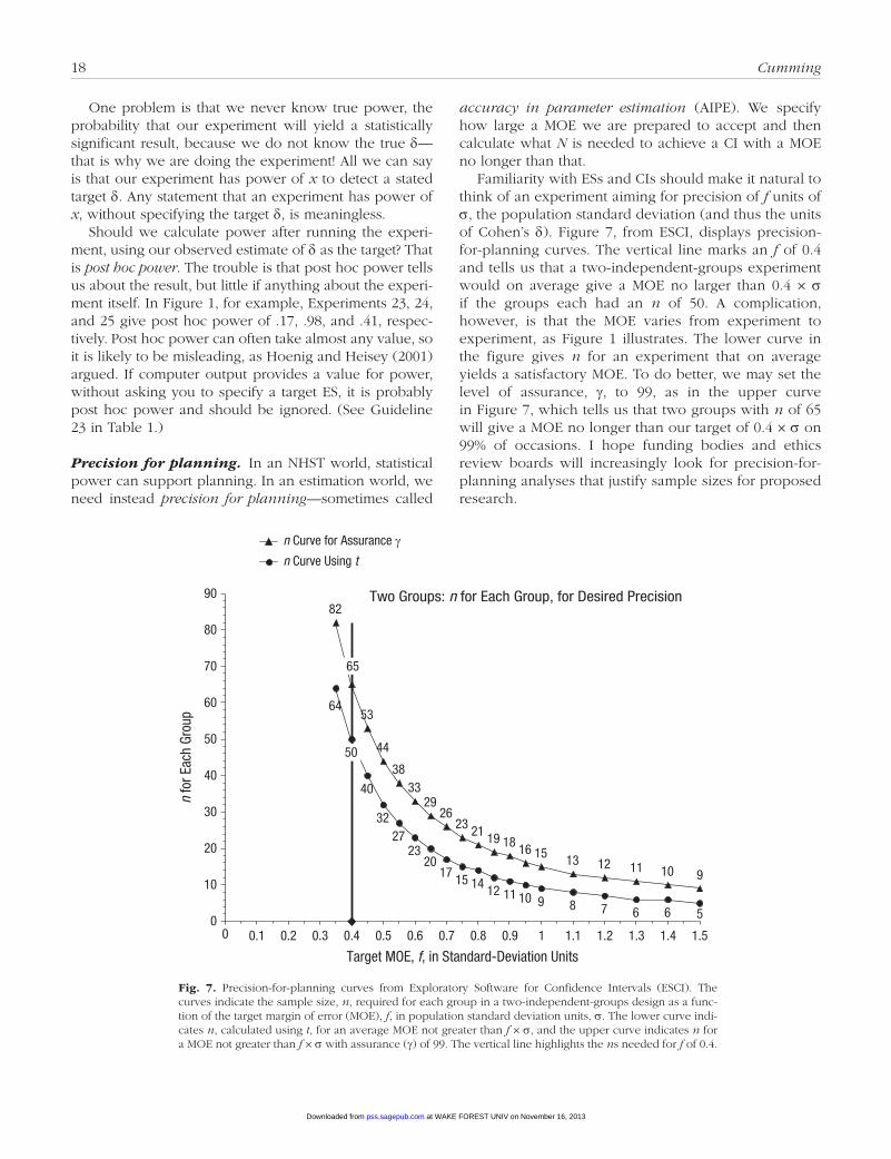
18 Cumming

One problem is that we never know true power, the probability that our experiment will yield a statistically significant result, because we do not know the true δ—that is why we are doing the experiment! All we can say is that our experiment has power of x to detect a stated target δ. Any statement that an experiment has power of x, without specifying the target δ, is meaningless.

Should we calculate power after running the experi-ment, using our observed estimate of δ as the target? That is post hoc power. The trouble is that post hoc power tells us about the result, but little if anything about the experi-ment itself. In Figure 1, for example, Experiments 23, 24, and 25 give post hoc power of .17, .98, and .41, respec-tively. Post hoc power can often take almost any value, so it is likely to be misleading, as Hoenig and Heisey (2001) argued. If computer output provides a value for power, without asking you to specify a target ES, it is probably post hoc power and should be ignored. (See Guideline 23 in Table 1.)

Precision for planning.• In an NHST world, statistical power can support planning. In an estimation world, we need instead precision for planning—sometimes called

accuracy in parameter estimation (AIPE). We specify how large a MOE we are prepared to accept and then calculate what N is needed to achieve a CI with a MOE no longer than that.

Familiarity with ESs and CIs should make it natural to think of an experiment aiming for precision of f units of σ, the population standard deviation (and thus the units of Cohen’s δ). Figure 7, from ESCI, displays precision-for-planning curves. The vertical line marks an f of 0.4 and tells us that a two-independent-groups experiment would on average give a MOE no larger than 0.4 × σ if the groups each had an n of 50. A complication, however, is that the MOE varies from experiment to experiment, as Figure 1 illustrates. The lower curve in the figure gives n for an experiment that on average yields a satisfactory MOE. To do better, we may set the level of assurance, γ, to 99, as in the upper curve in Figure 7, which tells us that two groups with n of 65 will give a MOE no longer than our target of 0.4 × σ on 99% of occasions. I hope funding bodies and ethics review boards will increasingly look for precision-for-planning analyses that justify sample sizes for proposed research.

64

50

40

3227

2320

17 15 14 12 11 10 9 8 7 6 6 5

82

53

44

3833

2926

23 21 19 18 16 15 13 12 11 10 9

65

50

0

10

20

30

40

50

60

70

80

90

0 0.1 0.2 0.3 0.4 0.5 0.6 0.7 0.8 0.9 1 1.1 1.2 1.3 1.4 1.5

n fo

r Eac

h Gr

oup

Target MOE, f, in Standard-Deviation Units

Two Groups: n for Each Group, for Desired Precision

n Curve Using t

n Curve for Assurance γ

Fig. 7.• Precision-for-planning curves from Exploratory Software for Confidence Intervals (ESCI). The curves indicate the sample size, n, required for each group in a two-independent-groups design as a func-tion of the target margin of error (MOE), f, in population standard deviation units, σ. The lower curve indi-cates n, calculated using t, for an average MOE not greater than f × σ, and the upper curve indicates n for a MOE not greater than f × σ with assurance (γ) of 99. The vertical line highlights the ns needed for f of 0.4.

at WAKE FOREST UNIV on November 16, 2013pss.sagepub.comDownloaded from

The New Statistics: Why and How 19

Figure 7 shows that small changes to f can indicate the need for large changes to n. The corresponding figure for a repeated measure experiment indicates that much smaller Ns will suffice if we have a reasonably large cor-relation between the measures. Such figures should give us practical guidance in choosing experimental designs and sample sizes likely to make an experiment suffi-ciently informative to be worth running. After we con-duct an experiment, the MOE calculated from the data tells us, of course, what precision we achieved. Previously (Cumming, 2012, chap. 13), I have discussed precision for planning, and ESCI provides calculations for several simple situations. Precision-for-planning techniques are being developed for an increasing range of ES measures and designs (Maxwell, Kelley, & Rausch, 2008). (See Guideline 24 in Table 1.)

New-statistics resources

A wide range of new-statistics resources has become available in recent years. As mentioned earlier, exten-sions of most of the discussions in this estimation section, and information about ESCI, are available elsewhere (Cumming, 2012, 2013). Fidler and I (Fidler & Cumming, 2013) also discussed many of the topics of this article. Kline (2013b) discussed many new-statistics issues and provided guidance for deriving and presenting ESs and CIs in a wide range of situations, including meta-analysis. Kline’s book goes further than mine in several ways, including consideration of measurement error as well as sampling variability, more complex designs, and boot-strapping and Bayesian techniques. Ellis (2010) provided an accessible introduction to a range of ES measures. Fritz, Morris, and Richler (2012) discussed a range of ES measures, especially in the context of multiway designs, with an emphasis on practical use and interpretation. Grissom and Kim (2012) discussed a very wide range of ES measures and described in most cases how to calcu-late the CIs on those measures. They considered ESs and CIs for an extensive range of designs, including multivari-ate ones. Smithson (2003) explained how to calculate CIs on R2 and a range of other ES measures, and has pro-vided very useful scripts (Smithson, n.d.) to assist in these calculations. Altman, Machin, Bryant, and Gardner (2000) provided simple guidance for using CIs with many basic ES measures used in medicine, including risk ratios and odds ratios.

Statistics textbooks are increasingly including coverage of ESs and CIs, as well as at least brief mention of meta-analysis, even if they have not yet relegated NHST to a secondary topic, required only to assist understanding of past published research. An early mover was Tabachnick and Fidell’s (2007) book, which includes guidance for cal-culating CIs in many multivariate situations. Baguley’s

(2012) advanced textbook includes extensive guidance on estimation techniques.

A wide range of software that is helpful for under-standing and calculating ESs and CIs is freely available on the Internet. In many cases, a Web site is linked to a book or journal article, but provides software or links that are of use independently of the book or article. I have already mentioned ESCI (Cumming, 2013). Ellis’s (2010) book is accompanied by a Web site (Ellis, n.d.) that provides extensive discussion of ESs and a link to a calculator for Cohen’s d. Kline’s (2013b) book is accompanied by a Web site (Kline, 2013a) that provides a very useful set of links to software and calculators for a variety of ESs and CIs, arranged to correspond with successive chapters in the book. Becker (1999) has provided a simple calculator for d and r in a few common situations, and Soper (2006–2013) has provided a wide range of statistical calculators, including calculators for many ES measures and CIs. Another extensive collection of ES calculators, with CIs provided also in many cases, is available from Wilson (n.d.), although this Web site does not yet provide full details of the formulas used. More specialized software, in the R language, for calculating ESs and CIs on ESs includes MBESS (Kelley, 2007; Kelley, n.d.) and bootES (Kirby & Gerlanc, 2013; Gerlanc & Kirby, 2013). As always, when using statistical software, especially online calculators, it is important to be sure that the formulas are appropriate for your situation. Calculation of d needs particular care, as I discussed earlier in the section on Cohen’s d.

Research integrity from an estimation perspective

To conclude this discussion of estimation, I want to revisit research integrity. Many contributors to discussions of research integrity, including Ioannidis (2005), have iden-tified use of statistical significance as a crucial part of the problem. Even so, most contributions have been framed in terms of NHST. For example, discussion of replication is usually in terms of whether a replication experiment is “successful,” with statistical significance used as the crite-rion for success. It would be valuable to put such dichot-omous thinking aside and to revisit all contributions to the discussion from an estimation perspective. If we made no reference to NHST, and routinely used estima-tion and meta-analysis, how would the arguments change? Replication attempts would not be labeled dichotomously as successes or failures, but would usu-ally yield, via meta-analysis, more precise estimates. Not using NHST would remove the pressure to find ways to tweak p to get past the sharp criterion for statistical sig-nificance (Masicampo & Lalande, 2012). CIs would indi-cate the extent of uncertainty, weaken the delusion that a single result is definitive, and make it more natural to

at WAKE FOREST UNIV on November 16, 2013pss.sagepub.comDownloaded from

20 Cumming

seek further evidence or conduct another study. Meta-analytic thinking also prompts replication.

In these ways, shifting from NHST to the new statistics should ease the problems, but serious challenges remain. After this shift, it will be just as important that variables and analyses not be selected to give desired results, and that research be fully prespecified and then reported in full detail. (See Guideline 25 in Table 1.)

Toward a Cumulative Quantitative Discipline

The statistical-reform context

As I mentioned, for more than half a century, scholars have been publishing cogent critiques of NHST, documenting the damage it does, and urging change. There have been very few replies, but also little reduction in reliance on NHST. Two reform attempts are worth noting. In the 1970s and 1980s, Ken Rothman published many articles in medi-cal journals advocating use of CIs and avoidance of NHST. His efforts and those of other researchers led the International Committee of Medical Journal Editors (1988) to issue guidelines specifying that CIs should be reported whenever possible. In 1990, Rothman became the found-ing editor of Epidemiology, declaring that the journal would not publish p values. For the 10 years of his editor-ship, the journal flourished while publishing almost no NHST (Fidler, Thomason, Cumming, Finch, & Leeman, 2004), demonstrating again that good science does not require p values. More broadly across medicine, for more than two decades, most empirical articles have reported CIs. However, NHST is almost always reported as well, the CIs are only sometimes interpreted, and conclusions are usually based on p values. Reliance on NHST continues, to the extent that Ioannidis (2005) identified it as a major underlying cause of the problems he discussed.

In psychology, Geoff Loftus in 1993 took editorship of Memory & Cognition primarily to try to improve its statis-tical practices. He strongly encouraged use of figures with error bars and avoidance of p values. Over the 4 years of his editorship, use of figures with error bars increased, but NHST remained close to universal; after he left the journal, fewer figures with error bars appeared (Finch et al., 2004). More generally, the fascinating his-tory of the spread of NHST in a number of disciplines, the numerous devastating critiques, and the generally disappointing efforts at reform have been described in scholarly detail by Fidler (2005).

Reform efforts by the Association for Psychological Science

Why should the current reform efforts of Psychological Science and the Association for Psychological Science

(APS) be more successful? There are at least four reasons. First, heightened recognition of research-integrity issues demands change, and the central causal role of NHST demands that it be scrutinized anew. Second, the push for change comes not only from one insightful and enter-prising editor, but also from other APS leaders. Third, over the past decade, additional helpful resources, as cited earlier, have become available to support the practi-cal use of estimation, including meta-analysis. Fourth, other important players are also supporting change: For example, as mentioned earlier, APA’s (2010) Publication Manual included unequivocal statements that interpreta-tion should be based on estimation. The Psychonomic Society’s (2012) statistical guidelines highlight problems with NHST and recommend use of better techniques, notably estimation. In addition, the Task Force on Publication and Research Practices of the Society for Personality and Social Psychology (SPSP Task Force on Publication and Research Practices, in press) made simi-lar recommendations and considered the implications for research training.

Simply do not use NHST

I want to be clear about what I am not advocating. I am not suggesting that we simply report CIs alongside NHST. That would most likely lead to the situation currently found in medicine—CIs are reported but not routinely interpreted, and conclusions are largely based on p val-ues. Nor am I suggesting that we report CIs, but not NHST, and then base interpretation primarily on whether or not CIs include zero. That would merely be NHST by stealth. These two approaches would amount to NHST business as usual, perpetuation of all the old problems, and no extra impetus toward research integrity and a cumulative quantitative discipline.

Instead, I recommend following as much as possible all the steps in the eight-step strategy. I include “when-ever possible” in my recommendations that we avoid NHST, to cover any cases in which it is not possible to calculate a relevant CI; I expect such cases to be rare, and to become rarer. I strongly suggest that the best plan is simply to go cold turkey, omit any mention of NHST, and focus on finding words to give a meaningful interpreta-tion of the ES estimates and CIs that give the best answers to your research questions. To be clear, I conclude from the arguments and evidence I have reviewed that best research practice is not to use NHST at all; we should strive to adopt best practice, and therefore should simply avoid NHST and use better techniques.

Yes, your studies are likely to be more complex than the simple examples I have discussed, but I have described five approaches to interpreting CIs—not count-ing the interpretation based on NHST—hoping that one or more will be helpful in any particular situation. If it is

at WAKE FOREST UNIV on November 16, 2013pss.sagepub.comDownloaded from

The New Statistics: Why and How 21

relevant, you can note that a CI is far, or very far, from zero, and therefore zero is a correspondingly implausible true value for the parameter being estimated; you can do this without invoking p values and while still focusing on the positive information the CI gives about likely values of the parameter.

Enjoy the benefits

I suggest that we note and appreciate whenever using a new-statistics approach gives insight: Perhaps a small meta-analysis gives a pleasingly precise estimate that is helpful to a clinical colleague, or a fully prespecified study provides results we can rely on while considering a tricky issue, or formulating our research questions in estimation terms prompts us to develop a small quantita-tive model. Savor such moments: They signal progress and should become the norm.

The key idea is meta-analytic thinking: Appreciate any study as part of a future meta-analysis. With good under-standing of meta-analysis, we know how essential it is that our research literature be complete and trustworthy, and that all studies be reported in full and accurate detail. Of course, replication is required and contributes to bet-ter estimates and research progress. NHST is irrelevant, so we can stop worrying about it and just not mention it—a sure way to avoid the damage it does. There is no need for polemics about whether we are formally ban-ning NHST. It can simply fall by the wayside, and after a while we will scarcely notice it has gone, because we are focused on the exciting work of building a cumulative quantitative discipline with integrity.

Author Contributions

G. Cumming is the sole author of this article and is responsible for its content.

Acknowledgments

I thank Kathryn Bock, Pierre Dragicevic, Fiona Fidler, Lewis Halsey, Lisa Harvey, Kris Kirby, Daniël Lakens, Matthew Page, Hal Pashler, Steven Raaijmakers, Neil Thomason, and a number of Senior and Associate Editors of Psychological Science for valuable comments on drafts of this manuscript.

Declaration of Conflicting Interests

The author declared that he earns royalties on his book (Cumming, 2012) that is referred to in this article.

Funding

This research was supported by the Australian Research Council.

References

Altman, D. G., Machin, D., Bryant, T. N., & Gardner, M. J. (2000). Statistics with confidence: Confidence intervals and statisti-cal guidelines (2nd ed.). London, England: BMJ Books.

American Psychological Association. (2010). Publication man-ual of the American Psychological Association (6th ed.). Washington, DC: Author.

Anderson, D. (1997). A few quotes regarding hypothesis testing. Retrieved from tiny.cc/nhstquotes

Baguley, T. (2012). Serious stats: A guide to advanced statistics for the behavioral sciences. Houndmills, England: Palgrave Macmillan.

Beck, A. T., Steer, R. A., Ball, R., & Ranieri, W. F. (1996). Comparison of Beck Depression Inventories -IA and -II in psychiatric outpatients. Journal of Personality Assessment, 67, 588–597. doi:10.1207/s15327752jpa6703_13

Becker, L. A. (1999). Effect size calculators. Retrieved from tiny .cc/beckerescalc

Blouin, D. C., & Riopelle, A. J. (2005). On confidence inter-vals for within-subjects designs. Psychological Methods, 10, 397–412. doi:10.1037/1082-989X.10.4.397

Bonett, D. G. (2009). Meta-analytic interval estimation for standardized and unstandardized mean differences. Psychological Methods, 14, 225–238. doi:10.1037/a0016619

Borenstein, M., Hedges, L. V., Higgins, J. P. T., & Rothstein, H. R. (2009). Introduction to meta-analysis. Chichester, England: Wiley.

Cohen, J. (1962). The statistical power of abnormal social psy-chological research: A review. Journal of Abnormal and Social Psychology, 65, 145–153. doi:10.1037/h0045186

Cohen, J. (1988). Statistical power analysis for the behavioral sciences (2nd ed.). Hillsdale, NJ: Erlbaum.

Cooper, H., & Patall, E. A. (2009). The relative benefits of meta-analysis conducted with individual participant data ver-sus aggregated data. Psychological Methods, 14, 165–176. doi:10.1037/a0015565

Cooper, H. M. (2010). Research synthesis and meta-analysis: A step-by-step approach (4th ed.). Thousand Oaks, CA: Sage.

Cooper, H. M. (2011). Reporting research in psychology: How to meet journal article reporting standards. Washington, DC: American Psychological Association.

Coulson, M., Healey, M., Fidler, F., & Cumming, G. (2010). Confidence intervals permit, but don’t guarantee, bet-ter inference than statistical significance testing. Frontiers in Quantitative Psychology and Measurement, 1, 26. Retrieved from http://www.frontiersin.org/Journal/10.3389/ fpsyg.2010.00026/full

Cumming, G. (2006). Meta-analysis: Pictures that explain how experimental findings can be integrated. Retrieved from https://www.stat.auckland.ac.nz/~iase/publications/17/C105.pdf

Cumming, G. (2007). Inference by eye: Pictures of confidence intervals and thinking about levels of confidence. Teaching Statistics, 29, 89–93. doi:10.1111/j.1467-9639.2007.00267.x

Cumming, G. (2008). Replication and p intervals: p values pre-dict the future only vaguely, but confidence intervals do much better. Perspectives on Psychological Science, 3, 286–300. doi:10.1111/j.1745-6924.2008.00079.x

Cumming, G. (2009). Inference by eye: Reading the overlap of independent confidence intervals. Statistics in Medicine, 28, 205–220. doi:10.1002/sim.3471

Cumming, G. (2012). Understanding the new statistics: Effect sizes, confidence intervals, and meta-analysis. New York, NY: Routledge.

at WAKE FOREST UNIV on November 16, 2013pss.sagepub.comDownloaded from

22 Cumming

Cumming, G. (2013). The new statistics: Estimation for better research. Retrieved from www.thenewstatistics.com

Cumming, G., & Fidler, F. (2009). Confidence intervals: Better answers to better questions. Zeitschrift für Psychologie/Journal of Psychology, 217, 15–26. doi:10.1027/0044-3409.217.1.15

Cumming, G., Fidler, F., Kalinowski, P., & Lai, J. (2012). The statistical recommendations of the American Psychological Association Publication Manual: Effect sizes, confidence intervals, and meta-analysis. Australian Journal of Psychology, 64, 138–146. doi:10.1111/j.1742-9536.2011.00037.x

Cumming, G., Fidler, F., & Vaux, D. L. (2007). Error bars in experimental biology. Journal of Cell Biology, 177, 7–11. doi:10.1083/jcb.200611141

Cumming, G., & Finch, S. (2001). A primer on the understand-ing, use and calculation of confidence intervals that are based on central and noncentral distributions. Educational and Psychological Measurement, 61, 532–574. doi:10.1177/ 0013164401614002

Cumming, G., & Finch, S. (2005). Inference by eye: Confidence intervals, and how to read pictures of data. American Psychologist, 60, 170–180. doi:10.1037/0003-066X.60.2.170

Cumming, G., & Maillardet, R. (2006). Confidence intervals and replication: Where will the next mean fall? Psychological Methods, 11, 217–227. doi:10.1037/1082-989X.11.3.217

Cumming, G., Williams, J., & Fidler, F. (2004). Replication, and researchers’ understanding of confidence intervals and standard error bars. Understanding Statistics, 3, 299–311. doi:10.1207/s15328031us0304_5

Dawkins, R. (2004). The ancestor’s tale: A pilgrimage to the dawn of life. London, England: Weidenfeld & Nicolson.

Douglas, H. (2007). Rejecting the ideal of value-free science. In H. Kincaid, J. Dupre, & A. Wylie (Eds.), Value-free sci-ence? Ideals and illusions (pp. 120–139). Oxford, England: Oxford University Press.

Ellis, P. D. (2010). The essential guide to effect sizes: Statistical power, meta-analysis, and the interpretation of research results. Cambridge, England: Cambridge University Press.

Ellis, P. D. (n.d.). Effect size FAQs: Research that matters, results that make sense. Retrieved from tiny.cc/ellissite

Erceg-Hurn, D. M., & Mirosevich, V. M. (2008). Modern robust statistical methods: An easy way to maximize the accuracy and power of your research. American Psychologist, 63, 591–601. doi:10.1037/0003-066X.63.7.591

Faulkner, C., Fidler, F., & Cumming, G. (2008). The value of RCT evidence depends on the quality of statistical anal-ysis. Behaviour Research and Therapy, 46, 270–281. doi:10.1016/j.brat.2007.12.001

Fidler, F. (2005). From statistical significance to effect estima-tion: Statistical reform in psychology, medicine and ecology (Doctoral dissertation). Retrieved from tiny.cc/fionasphd

Fidler, F., & Cumming, G. (2013). Effect size estimation and confidence intervals. In J. A. Schinka & W. F. Velicer (Eds.), Handbook of psychology: Vol. 2. Research methods in psy-chology (2nd ed., pp. 142–163). Hoboken, NJ: Wiley.

Fidler, F., Faulkner, S., & Cumming, G. (2008). Analyzing and presenting outcomes: Focus on effect size estimates and

confidence intervals. In A. M. Nezu & C. M. Nezu (Eds.), Evidence-based outcome research: A practical guide to con-ducting randomized controlled trials for psychosocial inter-ventions (pp. 315–334). New York, NY: Oxford University Press.

Fidler, F., & Loftus, G. (2009). Why figures with error bars should replace p values: Some conceptual arguments and empirical demonstrations. Zeitschrift für Psychologie/Journal of Psychology, 217, 27–37. doi:10.1027/0044-3409.217.1.27

Fidler, F., Thomason, N., Cumming, G., Finch, S., & Leeman, J. (2004). Editors can lead researchers to confidence intervals, but can’t make them think: Statistical reform lessons from medicine. Psychological Science, 15, 119–126. doi:10.1111/j.0963-7214.2004.01502008.x

Fiedler, K., Kutner, F., & Krueger, J. I. (2012). The long way from α-error control to validity proper: Problems with a short-sighted false-positive debate. Perspectives on Psychological Science, 7, 661–669. doi:10.1177/1745691612462587

Finch, S., & Cumming, G. (2009). Putting research in context: Understanding confidence intervals from one or more studies. Journal of Pediatric Psychology, 34, 903–916. doi:10.1093/jpepsy/jsn118

Finch, S., Cumming, G., Williams, J., Palmer, L., Griffith, E., Alders, C., . . . Goodman, O. (2004). Reform of statistical inference in psychology: The case of Memory & Cognition. Behavior Research Methods, Instruments, & Computers, 36, 312–324. doi: 10.3758/BF03195577

Fritz, C. O., Morris, P. E., & Richler, J. J. (2012). Effect size estimates: Current use, calculations, and interpretation. Journal of Experimental Psychology: General, 141, 2–18. doi:10.1037/a0024338

Gerlanc, D., & Kirby, K. (2013). bootES: Bootstrap effect sizes. Retrieved from tiny.cc/bootes

Greenland, S., Schlesselman, J. J., & Criqui, M. H. (1986). The fallacy of employing standardized regression coefficients and correlations as measures of effect. American Journal of Epidemiology, 123, 203–208.

Grissom, R. J., & Kim, J. J. (2012). Effect sizes for research: Univariate and multivariate applications (2nd ed.). New York, NY: Routledge.

Hoenig, J. M., & Heisey, D. M. (2001). The abuse of power: The pervasive fallacy of power calculations for data analysis. The American Statistician, 55, 19–24. doi:10.1198/000313001300339897

International Committee of Medical Journal Editors. (1988). Uniform requirements for manuscripts submitted to bio-medical journals. Annals of Internal Medicine, 108, 258–265. doi:10.7326/0003-4819-108-2-258

Ioannidis, J. P. A. (2005). Why most published research findings are false. PLoS Medicine, 2, e124. Retrieved from http://www.plosmedicine.org/article/info:doi/10.1371/journal .pmed.0020124

Kelley, K. (2007). Methods for the behavioral, educational, and social sciences: An R package. Behavior Research Methods, 39, 979–984. doi:10.3758/BF03192993

Kelley, K. (n.d.). MBESS: An R package. Retrieved from tiny .cc/mbess

at WAKE FOREST UNIV on November 16, 2013pss.sagepub.comDownloaded from

The New Statistics: Why and How 23

Kirby, K. N., & Gerlanc, D. (2013). BootES: An R package for bootstrap confidence intervals on effect sizes. Behavior Research Methods. Advance online publication. doi:10.3758/s13428-013-0330-5

Kirk, R. E. (2003). The importance of effect magnitude. In S. F. Davis (Ed.), Handbook of research methods in experimental psychology (pp. 83–105). Malden, MA: Blackwell.

Kline, R. B. (2004). Beyond significance testing: Reforming data analysis methods in behavioral research. Washington, DC: APA Books.

Kline, R. B. (2013a). Beyond significance testing (2nd edition): Reader and instructor resource guide. Retrieved from tiny .cc/rklinesite

Kline, R. B. (2013b). Beyond significance testing: Statistics reform in the behavioral sciences (2nd ed.). Washington, DC: APA Books.

Kruschke, J. K. (2010). Doing Bayesian data analysis: A tutorial with R and BUGS. New York, NY: Academic Press.

Masicampo, E. J., & Lalande, D. R. (2012). A peculiar preva-lence of p values just below .05. The Quarterly Journal of Experimental Psychology, 65, 2271–2279. doi:10.1080/174 70218.2012.711335

Masson, M. E. J., & Loftus, G. R. (2003). Using confidence inter-vals for graphically based data interpretation. Canadian Journal of Experimental Psychology/Revue Canadienne de Psychologie Expérimentale, 57, 203–220. doi:10.1037/h0087426

Maxwell, S. E. (2004). The persistence of underpowered studies in psychological research: Causes, consequences, and rem-edies. Psychological Methods, 9, 147–163. doi:10.1037/1082-989X.9.2.147

Maxwell, S. E., Kelley, K., & Rausch, J. R. (2008). Sample-size planning for statistical power and accuracy in parameter estimation. Annual Review of Psychology, 59, 537–563. doi:10.1146/annurev.psych.59.103006.093735

McCarthy, M. A. (2007). Bayesian methods for ecology. Cambridge, England: Cambridge University Press.

Panter, A. T., & Sterba, S. K. (2011). Handbook of ethics in quantitative methodology. New York, NY: Routledge.

Pashler, H., & Wagenmakers, E. J. (2012). Editors’ introduction to the special section on replicability in psychological sci-ence: A crisis of confidence? Perspectives on Psychological Science, 7, 528–530. doi:10.1177/1745691612465253

Psychonomic Society. (2012). 2012 Psychonomic Society guidelines on statistical issues. Retrieved from tiny.cc/ psychonomicstats

Rodgers, J. L. (2010). The epistemology of mathematical and statistical modeling: A quiet methodological revolution. American Psychologist, 65, 1–12. doi:10.1037/a0018326

Rosenthal, R., Rosnow, R. L., & Rubin, D. B. (2000). Contrasts and effect sizes in behavioral research: A correlational approach. Cambridge, England: Cambridge University Press.

Schmidt, F. L., & Hunter, J. E. (1997). Eight common but false objections to the discontinuation of significance testing in the analysis of research data. In L. L. Harlow, S. A. Mulaik,

& J. H. Steiger (Eds.), What if there were no significance tests? (pp. 37–64). Mahwah, NJ: Erlbaum.

Schmidt, F. L., Oh, I.-S., & Hayes, T. L. (2009). Fixed- versus random-effects models in meta-analysis: Model proper-ties and an empirical comparison of differences in results. British Journal of Mathematical and Statistical Psychology, 62, 97–128. doi:10.1348/000711007X255327

Simmons, J. P., Nelson, L. D., & Simonsohn, U. (2011). False-positive psychology: Undisclosed flexibility in data collection and analysis allows presenting anything as significant. Psychological Science, 22, 1359–1366. doi:10.1177/0956797611417632

Smithson, M. (2003). Confidence intervals. Thousand Oaks, CA: Sage.

Smithson, M. (n.d.). Scripts and software for noncentral confi-dence interval and power calculations. Retrieved from tiny .cc/mikecis

Soper, D. (2006–2013). Statistics calculators Version 3.0. Retrieved from tiny.cc/sopercalc

Spellman, B. A. (2012). Introduction to the special section on research practices. Perspectives on Psychological Science, 7, 655–656. doi:10.1177/1745691612465075

SPSP Task Force on Publication and Research Practices. (in press). Improving the dependability of research in person-ality and social psychology: Recommendations for research and educational practice. Personality and Social Psychology Review.

Steiger, J. H. (2004). Beyond the F test: Effect size confidence intervals and tests of close fit in the analysis of variance and contrast analysis. Psychological Methods, 9, 164–182. doi:10.1037/1082-989X.9.2.164

Tabachnick, B. G., & Fidell, L. S. (2007). Using multivariate statistics (5th ed.). Boston, MA: Pearson.

Tukey, J. W. (1977). Exploratory data analysis. Reading, MA: Addison-Wesley.

van Deemter, K. (2010). Not exactly: In praise of vagueness. Oxford, England: Oxford University Press.

Velicer, W. F., Cumming, G., Fava, J. L., Rossi, J. S., Prochaska, J. O., & Johnson, J. (2008). Theory testing using quanti-tative predictions of effect size. Applied Psychology: An International Review, 57, 589–608. doi:10.1111/j.1464-0597.2008.00348.x

Wagenmakers, E. J., Wetzels, R., Borsboom, D., van der Maas, H. J. L., & Kievit, R. A. (2012). An agenda for purely con-firmatory research. Perspectives on Psychological Science, 7, 632–638. doi:10.1177/1745691612463078

Wilcox, R. (2011). Modern statistics for the social and behav-ioral sciences: A practical introduction. Boca Raton, FL: CRC Press.

Wilkinson, L., & Task Force on Statistical Inference. (1999). Statistical methods in psychology journals: Guidelines and explanations. American Psychologist, 54, 594–604. doi:10.1037/0003-066X.54.8.594

Wilson, D. B. (n.d.). Practical meta-analysis effect size calcula-tor. Retrieved from tiny.cc/campbellcalc

at WAKE FOREST UNIV on November 16, 2013pss.sagepub.comDownloaded from