©20

11 N

atu

re A

mer

ica,

Inc.

All

rig

hts

res

erve

d.

protocol

1290 | VOL.6 NO.9 | 2011 | nature protocols

IntroDuctIonCOBRA methods have been successfully used in the field of micro-bial metabolic engineering1–3 and are being extended to modeling transcriptional4–8 and signaling9–11 networks and in the field of public health12. Specifically, COBRA methods have been used to guide metabolic pathway engineering, to model pathogens13 and host-pathogen interactions14, and to assess the impact of disease states on human metabolism15. A wide variety of COBRA methods have been developed over the years16,17. COBRA methods have been used in hundreds of research articles over the past decade, which characterize genome-scale properties of metabolic networks and their phenotypic states18–20.

The COBRA approach focuses on using physicochemical, data-driven and biological constraints to enumerate the set of feasible phenotypic states of a reconstructed biological network in a given condition (Fig. 1a). These constraints include compartmentaliza-tion, mass conservation, molecular crowding21 and thermodynamic directionality22–24. More recently, transcriptome data have been used to reduce the size of the set of computed feasible states14,25,26. Although COBRA methods may not provide a unique solution, they provide a reduced set of solutions that may be used to guide biological hypothesis development27. The COBRA Toolbox pro-vides researchers with a high-level interface to a variety of COBRA methods. Detailed descriptions of COBRA methods can be found in a variety of reviews3,16,28,29.

The biological network models that are analyzed with COBRA methods are constructed in a bottom-up fashion from bibliomic and experimental data, and thus represent biochemically, geneti-cally and genomically (BiGG) consistent knowledgebases30,31. BiGG knowledgebases are manually curated 2D genome annotations32 that relate biological functions, such as metabolic reactions, to the genome through the use of the gene-protein-reaction formalism33 (Fig. 1b). Application of the BiGG formalism to metabolism has been particularly successful, and metabolic reconstructions are

available for many organisms34–42. A detailed protocol describing the construction of high-quality BiGG knowledgebases for metabolism—and their transformation into mathematical models—has been recently published43.

The first release of the COBRA Toolbox in 2007 provided access to a variety of methods, including flux balance analy-sis, gene essentiality analysis and minimization of metabolic adjustment analysis (Table 1). Since the release of the first ver-sion of the COBRA Toolbox, many additional COBRA-related methods have been published44–48. In version 2.0 of the COBRA Toolbox, we have extended the capabilities to include geometric flux-balance analysis (FBA)44, loop law49, creation of context-specific subnetwork models using omics data14,25, Monte Carlo sampling15,50–52, 13C fluxomics, gap filling45,53, metabolic engineer-ing46–48 and visualization of computational models of metabolism (Table 1 and Fig. 2).

In addition, methods5,24,54 and resources55 have been developed by community members, which can serve as add-ons to the core COBRA Toolbox or provide models or other input. Specifically, Chandrasekaran and Price54 have developed a method—probabilistic regulation of metabolism—that incorporates regulatory information from transcriptome, ChIP-chip or literature data into a metabolic network model. Fleming and Thiele24 developed an extension to thermodynamically constrain reaction directionality, and Henry et al.55 have developed a web-based resource (http://www.theseed.org/models/) that provides access to draft metabolic network reconstructions for a variety of organisms—these models may be imported into the COBRA Toolbox for further refinement and analysis.

This protocol aims to provide researchers with the ability to use the in silico methods included in the toolbox with only high-level knowledge of the algorithms. Because of the wide range of creative uses for COBRA methods, not all of the capa-bilities of the COBRA Toolbox are described in this protocol;

Quantitative prediction of cellular metabolism with constraint-based models: the COBRA Toolbox v2.0Jan Schellenberger1, Richard Que2, Ronan M T Fleming3, Ines Thiele4, Jeffrey D Orth2, Adam M Feist2, Daniel C Zielinski2, Aarash Bordbar2, Nathan E Lewis2, Sorena Rahmanian2, Joseph Kang2, Daniel R Hyduke2 & Bernhard Ø Palsson2

1Bioinformatics Program, University of California San Diego, La Jolla, California, USA. 2Bioengineering Department, University of California San Diego, La Jolla, California, USA. 3Science Institute & Center for Systems Biology, University of Iceland, Reykjavik, Iceland. 4Faculty of Industrial Engineering, Mechanical Engineering & Computer Science & Center for Systems Biology, University of Iceland, Reykjavik, Iceland. Correspondence should be addressed to B.Ø.P. (palsson@ucsd.edu) or D.R.H. (hyduke@ucsd.edu).

Published online 4 August 2011; doi:10.1038/nprot.2011.308

over the past decade, a growing community of researchers has emerged around the use of constraint-based reconstruction and analysis (coBra) methods to simulate, analyze and predict a variety of metabolic phenotypes using genome-scale models. the coBra toolbox, a MatlaB package for implementing coBra methods, was presented earlier. Here we present a substantial update of this in silico toolbox. Version 2.0 of the coBra toolbox expands the scope of computations by including in silico analysis methods developed since its original release. new functions include (i) network gap filling, (ii) 13c analysis, (iii) metabolic engineering, (iv) omics-guided analysis and (v) visualization. as with the first version, the coBra toolbox reads and writes systems biology markup language–formatted models. In version 2.0, we improved performance, usability and the level of documentation. a suite of test scripts can now be used to learn the core functionality of the toolbox and validate results. this toolbox lowers the barrier of entry to use powerful coBra methods.

©20

11 N

atu

re A

mer

ica,

Inc.

All

rig

hts

res

erve

d.

protocol

nature protocols | VOL.6 NO.9 | 2011 | 1291

additional functionalities are described in the Documentation.

The COBRA Toolbox supports mod-els in the systems biology markup lan-guage (SBML) format56. Importing the models into MATLAB is dependent on libSBML57 and the SBMLToolbox58. Because SBML does not yet provide complete support for a few key COBRA parameters, we provide an explicit description of the COBRA extensions to SBML below and in Supplementary Discussion. The COBRA Toolbox is available for download from http://www.cobratoolbox.org. Detailed docu-mentation in HTML format is available in the ‘docs’ folder of the COBRA Toolbox.

Toolbox installationThere are two options for installing the COBRA Toolbox: ‘à la carte’ or bundled. The à la carte version only contains the COBRA Toolbox. The bundled version includes the COBRA Toolbox, libSBML, the SBMLToolbox, GNU linear programming kit (GLPK) and glpkmex. The bundled version has been tested on Mac OS X 10.6 Snow Leopard (64-bit), Ubuntu GNU/Linux Lucid (64-bit), Windows XP (32-bit) and Windows 7 (64-bit). Separate installation instructions are provided in Equipment Setup.

COBRA-compliant SBML fileDocumentation on the SBML standard is available on the SBML web-site (http://sbml.org), and a description of a COBRA-compliant SBML file is provided in the Supplementary Discussion. Sample models in COBRA-compliant SBML may be downloaded from the BiGG knowl-edgebase (http://bigg.ucsd.edu)31, or draft models may be downloaded from the Model SEED (http://www.theseed.org/models)55. The model files must include the following information for all calculations: stoi-chiometry of each reaction, upper and lower bounds of each reaction and objective function coefficients for each reaction.

Several functions within the COBRA Toolbox47,48 require infor-mation that is not yet in the SBML standard or is scheduled for removal in SBML 3 and beyond. The gene-reaction associations are essential for relating the metabolic reactions to the genome, and the subsystem is useful for ontological classification. Metabolite formu-las and charges are necessary to ensure that the model is physically consistent (no generation of mass or energy). Additional annotation parameters, such as KEGG or CAS IDs, should be specified in the notes field.

< reaction > … < notes > < html xmlns = ‘http://www.w3.org/1999/xhtml’ > < p > GENE_ASSOCIATION: ((gene1) and (gene2)) or

(gene3) < /p > < p > SUBSYSTEM: Transport Inner Membrane < /p > < p > KEGGID: … < /p > … < /html > < /notes > < /reaction > < metabolite > …

Abbreviation Glycolytic reactions

HEX1 [c]GLC + ATP G6P + ADP+ H

PGI [c]G6P F6P

PFK [c]ATP + F6P ADP + FDP + H

FBA [c]FDP DHAP + G3P

TPI [c]DHAP G3P

GAPD [c]G3P + NAD + PI 13DPG + H + NADH

PGK [c]13DPG + ADP 3PG + ATP

PGM [c]3PG 2PG

ENO [c]2PG H2O + PEP

PYK [c]ADP + H + PEP ATP + PYR

GAPD

ENO

PYK

HEX1

TPI

PGI

PFK

FBA

PGK

PGM

HEX1 PGI PFK FBA TPI GAPD PGK PGM ENO PYK

ATP –1 0 –1 0 0 0 1 0 0 1GLC –1 0 0 0 0 0 0 0 0 0ADP 1 0 1 0 0 0 –1 0 0 –1G6P 1 –1 0 0 0 0 0 0 0 0H 1 0 1 0 0 1 0 0 0 –1F6P 0 1 –1 0 0 0 0 0 0 0FDP 0 0 1 –1 0 0 0 0 0 0DHAP 0 0 0 1 –1 0 0 0 0 0G3P 0 0 0 1 1 –1 0 0 0 0NAD 0 0 0 0 0 –1 0 0 0 0PI 0 0 0 0 0 –1 0 0 0 013DPG 0 0 0 0 0 1 –1 0 0 0NADH 0 0 0 0 0 1 0 0 0 03PG 0 0 0 0 0 0 1 –1 0 02PG 0 0 0 0 0 0 0 1 –1 0PEP 0 0 0 0 0 0 0 0 1 –1H2O 0 0 0 0 0 0 0 0 1 0PYR 0 0 0 0 0 0 0 0 0 1

Reactions

Met

abol

ites

BiGG knowledgebase

GapA

GAPD

b1416

gapC2

b1779

gapA

and

GapC

b1417

gapC1

or

Gene

Peptide

Protein

Reaction

b

a Networkreconstruction

Reconstructednetwork

Application ofconstraints

Space of allowednetwork states

Mass conservationThermodynamics

Maximum reaction ratesRegulation

Experimental measurements

GenomicsGenetics

BiochemistryPhysiology

Other ‘-omics’ data

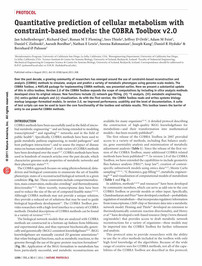
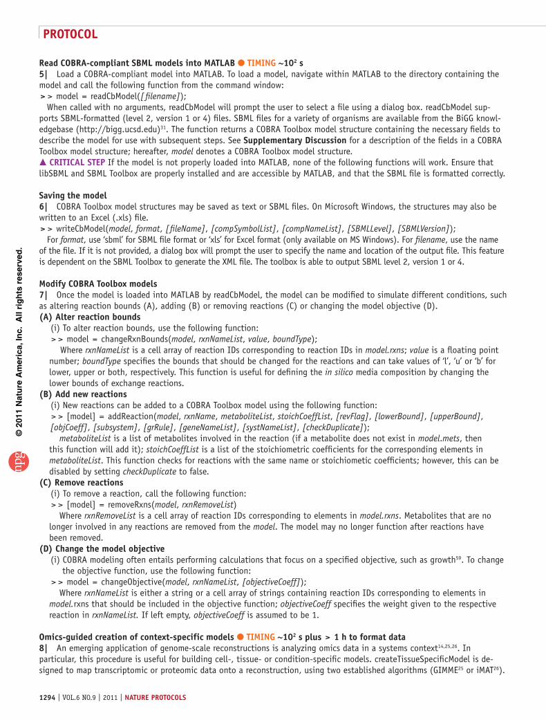
Figure 1 | The philosophy of COBRA. (a) COBRA of biological networks involves the creation of network models from a variety of biological data sources. The capabilities of the model are then assessed in the context of physical, chemical, regulatory and omics constraints (reproduced from Becker et al.17 with permission). (b) COBRA models are often derived from BiGG knowledgebases, which are essentially 2D annotations of the genome that relate metabolic activity to genomic loci. (Left inset) In E.coli, the GAPD activity can be provided by two isozymes (GapA or GapC); GapC is a heteromeric protein that requires genes from two genomic loci. The contents of a BiGG knowledgebase can be converted to a map (right) to facilitate visual interpretation, or to a mathematical modeling formalism to develop and explore hypotheses, such as a stoichiometric matrix (bottom) that can be used to explore mass flow through the network (reproduced with permission from Reed et al.33, with modifications).

©20

11 N

atu

re A

mer

ica,

Inc.

All

rig

hts

res

erve

d.

protocol

1292 | VOL.6 NO.9 | 2011 | nature protocols

< notes > < html xmlns = ‘http://www.w3.org/1999/xhtml’ > < p > FORMULA: C6H12O6 < /p > < p > CHARGE: 0 < /p > < p > CAS: … < /p > … < /html > < /notes > < /metabolite >

Metabolic map filesThe visualization tools require text files of the coordinates for placing metabolites and reactions on a map. Map coordinate files for many metabolic pathways are avail-able from the BiGG knowledgebase. The COBRA Toolbox relates COBRA SBML

models to the map coordinate files through the reaction and metab-olite IDs. A map file for glycolysis may be used with various SBML models as long as the identifiers match. The format for a map file is described in Supplementary Discussion.

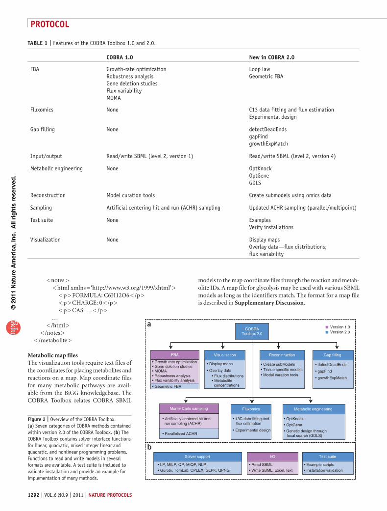
taBle 1 | Features of the COBRA Toolbox 1.0 and 2.0.

coBra 1.0 new in coBra 2.0

FBA Growth-rate optimization Robustness analysis Gene deletion studies Flux variability MOMA

Loop law Geometric FBA

Fluxomics None C13 data fitting and flux estimation Experimental design

Gap filling None detectDeadEnds gapFind growthExpMatch

Input/output Read/write SBML (level 2, version 1) Read/write SBML (level 2, version 4)

Metabolic engineering None OptKnock OptGene GDLS

Reconstruction Model curation tools Create submodels using omics data

Sampling Artificial centering hit and run (ACHR) sampling Updated ACHR sampling (parallel/multipoint)

Test suite None Examples Verify installations

Visualization None Display maps Overlay data—flux distributions; flux variability

Solver support

COBRAToolbox 2.0

FBA Gap filling

I/O Test suite

Visualization Reconstruction

Metabolic engineering FluxomicsMonte Carlo sampling

• LP, MILP, QP, MIQP, NLP

• Gurobi, TomLab, CPLEX, GLPK, QPNG

• Geometric FBA

• Growth rate optimization• Gene deletion studies• MOMA

• Flux variability analysis• Robustness analysis

• detectDeadEnds

• gapFind

• growthExpMatch

• Read SBML

• Write SBML, Excel, text

• Example scripts

• Installation validation

• Display maps

• Overlay data• Flux distributions• Metabolite concentrations

• Create subModels • Tissue specific models• Model curation tools

a

b

• OptKnock

• OptGene

• Genetic design through local search (GDLS)

• 13C data fitting and flux estimation

• Experimental design

• Artificially centered hit and run sampling (ACHR)

• Parallelized ACHR

Version 1.0Version 2.0

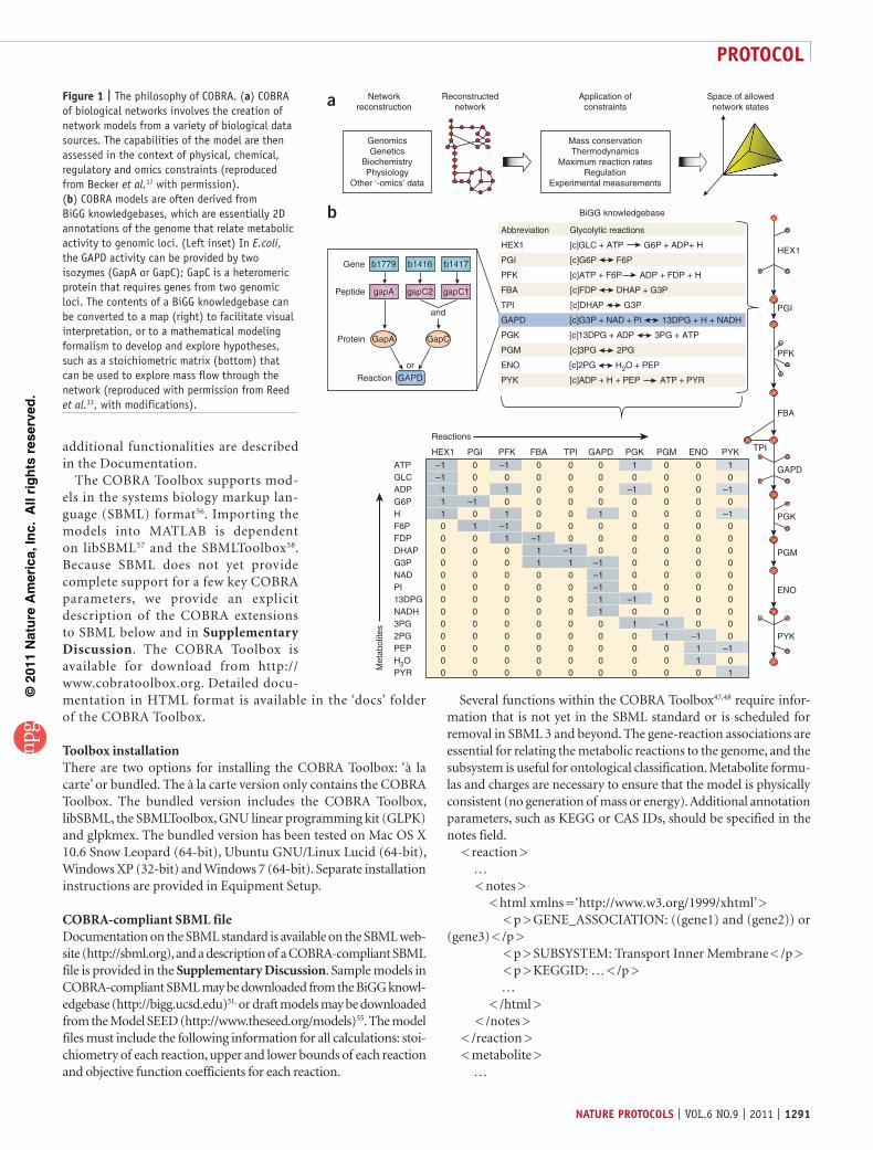
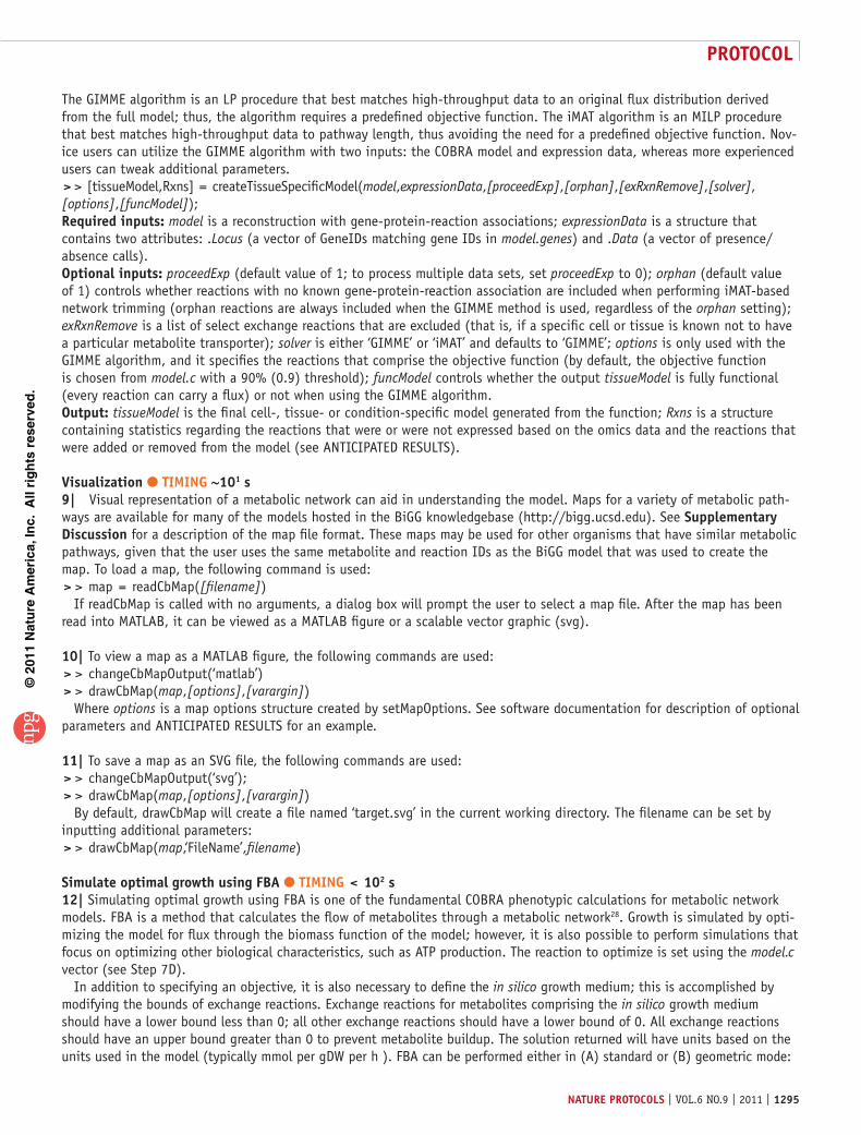
Figure 2 | Overview of the COBRA Toolbox. (a) Seven categories of COBRA methods contained within version 2.0 of the COBRA Toolbox. (b) The COBRA Toolbox contains solver interface functions for linear, quadratic, mixed integer linear and quadratic, and nonlinear programming problems. Functions to read and write models in several formats are available. A test suite is included to validate installation and provide an example for implementation of many methods.

©20

11 N

atu

re A

mer

ica,

Inc.

All

rig

hts

res

erve

d.

protocol

nature protocols | VOL.6 NO.9 | 2011 | 1293

MaterIalsEQUIPMENT

The COBRA Toolbox version 2.0 or above (http://www.cobratoolbox.org)A computer capable of running MATLABVersion 7.0 or above of MATLAB (MathWorks) numerical computation and visualization software (http://www.mathworks.com)libSBML programming library 4.0.1 or above (http://www.sbml.org)SBMLToolbox version 3.1.1 or above for MATLAB to allow reading and writing models in SBML format (http://www.sbml.org)A linear programming (LP) solver. Currently, the COBRA Toolbox supports the following:Gurobi (Gurobi Optimization, http://www.gurobi.com) through Gurobi Mex (http://www.convexoptimization.com/wikimization/index.php/Gurobi_mex)CPLEX (ILOG) through Tomlab (Tomlab Optimization, http://tomopt.com)GLPK (http://www.gnu.org/software/glpk) through glpkmex (http://glpkmex.sourceforge.net). Please note that GLPK does not provide accurate solutions for OptKnock or Genetic Design Local Search (GDLS) calculations as implemented in the Toolbox ! cautIon Other solvers (such as Mosek, http://www.mosek.com; LINDO, http://www.lindo.com; and PDCO, http://www.stanford.edu/group/SOL/soft-ware/pdco.html) may work with the COBRA Toolbox but they have not been validated. crItIcal For best performance, it may be necessary to adjust parameters of the installed solver.A quadratic programming (QP) solver (optional). Currently, the COBRA toolbox supports the following:CPLEX (ILOG) through Tomlab

•••

••

•

•

••

•

•

QPNG (part of GLPK)—please note that QPNG does not provide accurate solutions for MOMA as implemented in the Toolbox ! cautIon Other solvers (such as Mosek and PDCO) may work with the COBRA Toolbox but they have not been validated. crItIcal For best performance, it may be necessary to adjust parameters of the installed solver.A nonlinear programming (NLP) solver (optional). Currently, the COBRA toolbox supports:SNOPT through Tomlab crItIcal For best performance, it may be necessary to adjust parameters of the installed solver.

EQUIPMENT SETUPÀ la carte installation of COBRA Toolbox

Install MATLABInstall libSBML, the SBML Toolbox and selected solvers according to their specific instructions.Unpack the COBRA 2.0 archive

Bundled installation of COBRA ToolboxInstall MATLABUnpack the COBRA 2.0 archive. Cobra_Install_Path is the path to the top-level directory for the COBRA ToolboxUpdate Shared Library Path (Mac OS X and GNU/Linux only). For Mac OS DYLD_LIBRARY_PATH = Cobra_Install_Path/external/toolboxes/SBMLToolbox_3.1.2/toolbox/. For GNU/Linux LD_LI-BRARY_PATH = Cobra_Install_Path/external/toolboxes/SBMLToolbox_3.1.2/toolbox.

•

•

•

••

•

••

•

proceDureInitializing the coBra toolbox crItIcal Italics denotes a parameter that is supplied to a function. A bracketed [parameter] is optional. The symbol > > denotes the MATLAB command line; anything directly following > > is meant to be entered on the command line. All time estimates for the functions are predicated on a model using ~1,200 genes, 2,300 reactions, 1,800 metabolites and a compu-ter with a 2.4-GHz Intel Core 2 Duo processor. When substantial preprocessing efforts are required, we provide time estimates based on personal experience.

1| Navigate to the directory where you installed the COBRA Toolbox: > > initCobraToolbox()

2| Save the paths added if desired: > > savepath()

changing coBra solvers3| Set the solvers used by the COBRA Toolbox using the following function: > > changeCobraSolver(solverName, [solverType]);

Variables are defined as follows: solverName specifies the solver package to be used; the COBRA Toolbox currently supports ‘gurobi’, ‘tomlab_cplex’, ‘glpk’ and ‘qpng’. solverType (default ‘LP’) specifies the type of problems (‘LP’, ‘MILP’, ‘QP’, ‘MIQP’, ‘NLP’) to solve with the solver specified by solverName. When changeCobraSolver is called without any arguments, it will return the names of the current settings of the solvers.

run coBra toolbox test suite ● tIMInG ~103 s4| The test suite contains scripts that test the functionality of scripts within the COBRA Toolbox. The scripts in the testing directory provide useful examples of many of the functions of the toolbox. > > testAll()

testAll sequentially navigates the test suite directory (testing) and runs each test. Upon completion, it displays those tests that were completed successfully and those that failed. ! cautIon For solver suites other than Gurobi or Tomlab, the user may encounter failures that require tuning of solver parameters.? trouBlesHootInG

©20

11 N

atu

re A

mer

ica,

Inc.

All

rig

hts

res

erve

d.

protocol

1294 | VOL.6 NO.9 | 2011 | nature protocols

read coBra-compliant sBMl models into MatlaB ● tIMInG ~102 s5| Load a COBRA-compliant model into MATLAB. To load a model, navigate within MATLAB to the directory containing the model and call the following function from the command window: > > model = readCbModel([filename]);

When called with no arguments, readCbModel will prompt the user to select a file using a dialog box. readCbModel sup-ports SBML-formatted (level 2, version 1 or 4) files. SBML files for a variety of organisms are available from the BiGG knowl-edgebase (http://bigg.ucsd.edu)31. The function returns a COBRA Toolbox model structure containing the necessary fields to describe the model for use with subsequent steps. See supplementary Discussion for a description of the fields in a COBRA Toolbox model structure; hereafter, model denotes a COBRA Toolbox model structure. crItIcal step If the model is not properly loaded into MATLAB, none of the following functions will work. Ensure that libSBML and SBML Toolbox are properly installed and are accessible by MATLAB, and that the SBML file is formatted correctly.

saving the model6| COBRA Toolbox model structures may be saved as text or SBML files. On Microsoft Windows, the structures may also be written to an Excel (.xls) file. > > writeCbModel(model, format, [fileName], [compSymbolList], [compNameList], [SBMLLevel], [SBMLVersion]);

For format, use ‘sbml’ for SBML file format or ‘xls’ for Excel format (only available on MS Windows). For filename, use the name of the file. If it is not provided, a dialog box will prompt the user to specify the name and location of the output file. This feature is dependent on the SBML Toolbox to generate the XML file. The toolbox is able to output SBML level 2, version 1 or 4.

Modify coBra toolbox models7| Once the model is loaded into MATLAB by readCbModel, the model can be modified to simulate different conditions, such as altering reaction bounds (A), adding (B) or removing reactions (C) or changing the model objective (D).(a) alter reaction bounds (i) To alter reaction bounds, use the following function: > > model = changeRxnBounds(model, rxnNameList, value, boundType);

Where rxnNameList is a cell array of reaction IDs corresponding to reaction IDs in model.rxns; value is a floating point number; boundType specifies the bounds that should be changed for the reactions and can take values of ‘l’, ‘u’ or ‘b’ for lower, upper or both, respectively. This function is useful for defining the in silico media composition by changing the lower bounds of exchange reactions.

(B) add new reactions (i) New reactions can be added to a COBRA Toolbox model using the following function: > > [model] = addReaction(model, rxnName, metaboliteList, stoichCoeffList, [revFlag], [lowerBound], [upperBound],

[objCoeff], [subsystem], [grRule], [geneNameList], [systNameList], [checkDuplicate]); metaboliteList is a list of metabolites involved in the reaction (if a metabolite does not exist in model.mets, then this function will add it); stoichCoeffList is a list of the stoichiometric coefficients for the corresponding elements in metaboliteList. This function checks for reactions with the same name or stoichiometic coefficients; however, this can be disabled by setting checkDuplicate to false.

(c) remove reactions (i) To remove a reaction, call the following function: > > [model] = removeRxns(model, rxnRemoveList)

Where rxnRemoveList is a cell array of reaction IDs corresponding to elements in model.rxns. Metabolites that are no longer involved in any reactions are removed from the model. The model may no longer function after reactions have been removed.

(D) change the model objective (i) COBRA modeling often entails performing calculations that focus on a specified objective, such as growth59. To change

the objective function, use the following function: > > model = changeObjective(model, rxnNameList, [objectiveCoeff]);

Where rxnNameList is either a string or a cell array of strings containing reaction IDs corresponding to elements in model.rxns that should be included in the objective function; objectiveCoeff specifies the weight given to the respective reaction in rxnNameList. If left empty, objectiveCoeff is assumed to be 1.

omics-guided creation of context-specific models ● tIMInG ~102 s plus > 1 h to format data8| An emerging application of genome-scale reconstructions is analyzing omics data in a systems context14,25,26. In particular, this procedure is useful for building cell-, tissue- or condition-specific models. createTissueSpecificModel is de-signed to map transcriptomic or proteomic data onto a reconstruction, using two established algorithms (GIMME25 or iMAT26).

©20

11 N

atu

re A

mer

ica,

Inc.

All

rig

hts

res

erve

d.

protocol

nature protocols | VOL.6 NO.9 | 2011 | 1295

The GIMME algorithm is an LP procedure that best matches high-throughput data to an original flux distribution derived from the full model; thus, the algorithm requires a predefined objective function. The iMAT algorithm is an MILP procedure that best matches high-throughput data to pathway length, thus avoiding the need for a predefined objective function. Nov-ice users can utilize the GIMME algorithm with two inputs: the COBRA model and expression data, whereas more experienced users can tweak additional parameters. > > [tissueModel,Rxns] = createTissueSpecificModel(model,expressionData,[proceedExp],[orphan],[exRxnRemove],[solver], [options],[funcModel]);required inputs: model is a reconstruction with gene-protein-reaction associations; expressionData is a structure that contains two attributes: .Locus (a vector of GeneIDs matching gene IDs in model.genes) and .Data (a vector of presence/absence calls).optional inputs: proceedExp (default value of 1; to process multiple data sets, set proceedExp to 0); orphan (default value of 1) controls whether reactions with no known gene-protein-reaction association are included when performing iMAT-based network trimming (orphan reactions are always included when the GIMME method is used, regardless of the orphan setting); exRxnRemove is a list of select exchange reactions that are excluded (that is, if a specific cell or tissue is known not to have a particular metabolite transporter); solver is either ‘GIMME’ or ‘iMAT’ and defaults to ‘GIMME’; options is only used with the GIMME algorithm, and it specifies the reactions that comprise the objective function (by default, the objective function is chosen from model.c with a 90% (0.9) threshold); funcModel controls whether the output tissueModel is fully functional (every reaction can carry a flux) or not when using the GIMME algorithm.output: tissueModel is the final cell-, tissue- or condition-specific model generated from the function; Rxns is a structure containing statistics regarding the reactions that were or were not expressed based on the omics data and the reactions that were added or removed from the model (see ANTICIPATED RESULTS).

Visualization ● tIMInG ~101 s9| Visual representation of a metabolic network can aid in understanding the model. Maps for a variety of metabolic path-ways are available for many of the models hosted in the BiGG knowledgebase (http://bigg.ucsd.edu). See supplementary Discussion for a description of the map file format. These maps may be used for other organisms that have similar metabolic pathways, given that the user uses the same metabolite and reaction IDs as the BiGG model that was used to create the map. To load a map, the following command is used: > > map = readCbMap([filename])

If readCbMap is called with no arguments, a dialog box will prompt the user to select a map file. After the map has been read into MATLAB, it can be viewed as a MATLAB figure or a scalable vector graphic (svg).

10| To view a map as a MATLAB figure, the following commands are used: > > changeCbMapOutput(‘matlab’) > > drawCbMap(map,[options],[varargin])

Where options is a map options structure created by setMapOptions. See software documentation for description of optional parameters and ANTICIPATED RESULTS for an example.

11| To save a map as an SVG file, the following commands are used: > > changeCbMapOutput(‘svg’); > > drawCbMap(map,[options],[varargin])

By default, drawCbMap will create a file named ‘target.svg’ in the current working directory. The filename can be set by inputting additional parameters: > > drawCbMap(map,‘FileName’,filename)

simulate optimal growth using FBa ● tIMInG < 102 s12| Simulating optimal growth using FBA is one of the fundamental COBRA phenotypic calculations for metabolic network models. FBA is a method that calculates the flow of metabolites through a metabolic network28. Growth is simulated by opti-mizing the model for flux through the biomass function of the model; however, it is also possible to perform simulations that focus on optimizing other biological characteristics, such as ATP production. The reaction to optimize is set using the model.c vector (see Step 7D).

In addition to specifying an objective, it is also necessary to define the in silico growth medium; this is accomplished by modifying the bounds of exchange reactions. Exchange reactions for metabolites comprising the in silico growth medium should have a lower bound less than 0; all other exchange reactions should have a lower bound of 0. All exchange reactions should have an upper bound greater than 0 to prevent metabolite buildup. The solution returned will have units based on the units used in the model (typically mmol per gDW per h ). FBA can be performed either in (A) standard or (B) geometric mode:

©20

11 N

atu

re A

mer

ica,

Inc.

All

rig

hts

res

erve

d.

protocol

1296 | VOL.6 NO.9 | 2011 | nature protocols

(a) standard mode (i) Standard FBA is performed as follows: > > [solution] = optimizeCbModel(model, [osenseStr], [minNorm], [allowLoops])

Where osenseStr is either ‘max’ or ‘min’ to maximize or minimize the value of the objective, respectively; minNorm (default 0, if non-zero, attempt to find a solution that minimizes the presence of loops); allowLoops (default true; if set to false, use the loop law algorithm49 to remove loops—this procedure can be time-consuming). optimizeCbModel will return a solution structure containing the objective value ‘f ’, the primal solution ‘x’, the dual solution ‘y’, the reduced cost ‘w’, a universal status flag ‘stat’, a solver-specific status flag ‘origStat’ and the time to compute the solution ‘time’. The primal solution, ‘x’, represents the flux carried by each reaction within the model. The dual solution, ‘y’, represents the shadow prices for each metabolite and indicates the extent to which the addition of the corresponding metabolite will increase or decrease the objective value28,60. The reduced cost, ‘w’, indicates the extent to which each reaction affects the objective. A solver status of 1 indicates that an optimal solution was found.

(B) Geometric mode (i) Geometric FBA44 is an alternative to standard FBA. Geometric FBA attempts to return the minimal flux distribution

central to the bounds of the solution space while still maintaining optimal growth rate. The flux distribution returned should then be reproducible regardless of the solver used.

> > flux = geometricFBA(model,[varargin]) The function returns the vector ‘flux’, which contains the centered optimal flux distribution.

13| To visualize an optimal flux distribution, the optimal flux distribution obtained using optimizeCbModel or geometricFBA can be overlaid onto an existing map of the model using the following function: > > drawFlux(map, model, flux, [options], [varargin])

Where map is a map object created with readCbMap (see Visualization, Step 9); model is the COBRA model structure that was used for performing FBA or Geometric FBA; options is a drawCbMap options structure.

14| To classify model genes on the basis of an optimal FBA solution, parsimonious FBA (pFBA) is an FBA approach that incorporates flux parsimony as a constraint to categorize the solution space61. The concept of flux parsimony, in the context of a metabolic network, refers to minimizing the total material flow required to achieve an objective.

In this method, genes are classified into six categories: (i) essential genes (i.e., metabolic genes necessary for in silico growth in the given media); (ii) pFBA-optima genes (i.e., non-essential genes contributing to the optimal growth rate and minimum gene-associated flux); (iii) enzymatically less-efficient genes, which require more flux through enzymatic steps than through alternative pathways that meet the same predicted growth rate; (iv) metabolically less-efficient genes requiring a growth rate reduction if used; (v) pFBA no-flux genes that are unable to carry flux in the experimental conditions; and (vi) blocked genes, which are only associated with the reactions that cannot carry a flux under any condition (‘blocked’ reactions).

To categorize the genes and reactions within a model and return a model with flux minimization constraints, execute the following: > > [GeneClasses, RxnClasses, modelIrrevFM] = pFBA(model, [varargin])

Where GeneClasses contains a list of all genes that are within the categories above; RxnClasses contains a list of all reac-tions that are within the categories above; and modelIrrevFM is a model that contains the flux minimization constraints. If a map is available for the model, the results from this function can be visualized by using the ‘map’ and ‘mapoutname’ flags in the varargin input. A test case may be found in the ANTICIPATED RESULTS section. Additional options are described in the software documentation directory. crItIcal step The subsequent steps in this protocol rely on the functionality of optimizeCbModel. If optimizeCbModel fails to return a feasible flux distribution for the examples within this protocol, the problem may be due to the installation of the LP solver. It is not necessary that geometricFBA return a solution for the subsequent steps.

solving coBra problem structures (advanced user) ● tIMInG > 100 s15| The COBRA toolbox has five function calls used for solving different optimization problems. Basic users will not need to call these low-level functions directly, as higher-level functions encapsulate these calls. These functions act as a common interface for different LP, MILP, QP, MIQP and NLP solvers, thus ensuring that laboratories can share code even when using different installed solvers.

The five solver functions use a similar input argument structure: problem structure followed by optional argument/value pairs. The required fields in the problem structure vary for each function to supply the required information to solve the type of problem. For example, the mixed integer problem structures require a field that specifies variable type (continuous, integer, binary). A description of the format of COBRA problem structures can be found in supplementary Discussion. The COBRA solution structure also provides a common output format regardless of the solver used.

©20

11 N

atu

re A

mer

ica,

Inc.

All

rig

hts

res

erve

d.

protocol

nature protocols | VOL.6 NO.9 | 2011 | 1297

> > [solution] = solveCobraLP(LPproblem, [varargin]) > > [solution] = solveCobraMILP(MILPproblem, [varargin]) > > [solution] = solveCobraQP(QPproblem, [varargin]) > > [solution] = solveCobraMIQP(MIQPproblem, [varargin]) > > [solution] = solveCobraNLP(NLPproblem, [varargin])

simulating deletion studies ● tIMInG ~102–104 s16| Deletion studies can be easily simulated with in silico models. Gene deletion methods within the COBRA Toolbox are de-pendent on the proper setup of the gene-reaction matrix, as well as on the rules defining the Boolean relationship between genes and reactions. Reactions that are affected by a gene deletion have their upper and lower flux bounds set to zero, and are therefore not functional. The set of reactions on which a gene deletion has an effect is calculated using the gene reac-tion association and rules.

It is possible to study either (A) single essential gene deletions or (B) pairs of synthetic lethal genes. The possible results from deletion studies are unchanged maximal growth, reduced maximal growth or no growth (lethal). Deletion studies can be used to predict gene/reaction essentiality.(a) essential gene study (i) Apply the following code: > > [grRatio, grRateKO, grRateWT, hasEffect, delRxns, fluxSolution] = singleGeneDeletion(model, method, [geneList])

Where method can be either ‘FBA’ (default), ‘MOMA’62 or linear MOMA (‘lMOMA’); geneList is a cell array of genes cor-responding to model.genes (if not provided, deletion simulations are performed for all genes in the model); grRatio is the growth rate of the knockout/growth rate of wild type (WT); grRateKO is the growth rate of the knockouts; grRateWT is the WT growth rate; hasEffect is a Boolean list indicating whether deletion of the corresponding gene alters the growth rate; delRxns contains a list of the reactions, the bounds of which are set to 0 for each gene deletion; and fluxSolution is the flux solution for each deletion.

(B) synthetic lethal study (i) Apply the following code: > > [grRatioDble, grRateKO, grRateWT] = doubleGeneDeletion(model, method, [geneList1], [geneList2])

Where method can be either ‘FBA’ (default), ‘MOMA’62 or linear MOMA (‘lMOMA’); geneList1 is a cell array of genes corresponding to model.genes (if not provided, the function assumes all genes in model.genes are to be interrogated); geneList2 is a cell array of genes that correspond to the second set of genes in the synthetic lethal pair (if not pro-vided, the function assumes that all genes in model.genes are to be interrogated); grRatioDble is the growth rate of the knockout/growth rate of WT; grRateKO is the growth rate of the knockouts; and grRateWT is the WT growth rate.

Flux variability analysis (FVa) ● tIMInG ~102 s17| Flux balance analysis only returns a single flux distribution that corresponds to maximal growth under given growth con-ditions. However, alternate optimal solutions may exist, which correspond to maximal growth. FVA calculates the full range of numerical values for each reaction flux within the network63.

To determine the minimum and maximum flux values that the reactions within the model can carry, while obtaining a spe-cific percentage of optimal growth rate, the following function is used: > > [minFlux, maxFlux] = fluxVariability(model, optPercentage, [rxnNameList], [verbFlag], [allowLoops])

Where optPercentage (default 100) specifies the percentage of optimal that an alternate flux distribution must realize in order to be considered an acceptable alternative flux distribution.

Visualization of FVa results18| To visualize the results from this function, a flux variability map can be generated from an existing reaction map, thereby color-coding reactions based on flux directionality. > > drawFluxVariability(map, model, minFlux, maxFlux, [options])

Where map is the map structure corresponding to the model read in using readCbMap; model is the COBRA model structure used in the fluxVariability function; minFlux and maxFlux are vectors generated by the fluxVariability function described above; and options is a structure containing optional parameters such as edge and node color and size: bidirectional reversible reactions are colored green, unidirectional reversible reactions that carry flux in the forward direction are colored magenta, unidirectional reversible reactions that carry flux only in the reverse direction are colored cyan and irreversible fluxes are colored blue.

©20

11 N

atu

re A

mer

ica,

Inc.

All

rig

hts

res

erve

d.

protocol

1298 | VOL.6 NO.9 | 2011 | nature protocols

sampling the solution space (advanced user) ● tIMInG > 102 s19| FBA only returns a single optimal point and thus yields little information about the entire solution space. An alternative approach is to characterize the solution space using sampling27. The generalized parallel sampler samples can be assigned to any arbitrary linearly constrained space by moving a fixed number of points in parallel. > > [sampleStructOut, mixedFrac] = gpSampler(sampleStruct, [nPoints], [bias], [maxTime], [maxSteps])

Where sampleStruct is the COBRA Toolbox problem structure for LP problems (see supplementary Discussion); nPoints is the number of sampling points; maxTime is the maximum sampling time; bias is a structure that imposes marginal distri-butions on reactions; sampleStructOut is sampleStruct with the addition of the ‘points’ field containing the solutions; and mixedFrac gives an estimate of the extent to which the sampling solution is mixed relative to the warm-up points—a mixedFrac value of 0.5 indicates complete mixing.

Fluxomics (advanced user) ● tIMInG > 102 s20| Carbon-13 (C13) tracing experiments provide the ability to measure internal flux rates in a metabolic network64. To use this data, additional information regarding carbon tracking must be added to the COBRA model. This is stored in the .isotopomer field as described in supplementary Discussion (Section S.4.). To use the C13 solver, the functions must be generated: > > [experiment] = generateIsotopomerSolver(model, inputMet, [experiment], [FVAflag])

Where model is the COBRA model with an .isotopomer field; inputMet is a string corresponding to the C13-labeled input; experiment is a list of metabolites that must be measured; and FVAflag removes reactions that cannot carry a flux.

21| Two solvers are generated, one based on the cumomer method65 and one on the faster elementary metabolite unit method66. The solvers are called internally during the scoreC13Fit function below. A given flux distribution can be scored against a set of C13 data: > > output = scoreC13Fit(ν0,expdata,model)

Where ν0 is the initial guess for fitting, and expdata is one or more sets of experimental data described in supplementary Discussion Section S.3.

22| Next, the most optimal flux distribution can be found with a nonlinear optimization: > > [vout] = fitC13Data(ν0,expdata,model, [majorIterationLimit])

This function will return the flux with the lowest experimental score found by the NLP solver. Very often it is useful to compute the confidence intervals of reactions, which are consistent with C13 data. > > [vs, output, v0] = C13ConfidenceInterval(ν0, expdata, model, max_score, [directions], [majorIterationLimit]) (~102 s)

Where ν0 is the initial guess; expdata is the experimental data that must be fit; max_score is the highest acceptable score; and directions is the list of reactions and reaction ratios that will be maximized and minimized (by default all reactions).

Gap filling ● tIMInG ~103 s23| Because of incomplete knowledge, a metabolic model may possess gaps. A gap is defined as missing biochemical information that can explain discrepancies between model predictions and experimental data. Gaps are typically the reac-tions that facilitate the conversion of an available metabolite in the model to one that is necessary to achieve an objective. Identifying gaps in metabolic models can be attempted using either (A) detectDeadEnds or (B) gapFind.(a) Detect dead ends in a model (i) Apply the following code: > > outputMets = detectDeadEnds(model, [removeExternalMets])

The detectDeadEnds function searches the model.S matrix for metabolites that participate in only one reaction (can either be produced or consumed) and returns the corresponding indices for the metabolites in the model.mets field. Setting removeExternalMets to true removes external metabolites from the results. Not all gaps can be identified by simply inspecting the model.S matrix.

(B) Find all gaps in a model (i) The GapFind algorithm45 allows one to find all gaps in a model and all metabolites that are downstream from a

model gap: > > [allGaps, rootGaps, downstreamGaps] = gapFind(model, findNCgaps, verbFlag)

Where allGaps is a list of the metabolite indices for a metabolite at a gap; rootGaps is a list of metabolites that cannot be produced; and downstreamGaps is a list of metabolites that are produced in a reaction that requires a metabolite that cannot be produced. This function is run in an interactive and iterative manner to guarantee that all gaps are identified. Set the lower bound of all exchange reactions within model to − 1, the upper bound of all reactions to a relatively large positive number

©20

11 N

atu

re A

mer

ica,

Inc.

All

rig

hts

res

erve

d.

protocol

nature protocols | VOL.6 NO.9 | 2011 | 1299

(for example 105) and the lower bound of all reversible reactions to a relatively large negative number (for example − 105) within model. The appropriate bound magnitude required varies from model to model. If the bound magnitudes are too small, the algorithm will incorrectly identify many metabolites as gaps; if this occurs, increase the bound magnitudes by tenfold. Repeat this process as necessary until the algorithm does not identify all metabolites as gaps.

24| In addition to these two gap identification functions, the COBRA Toolbox includes an optimization-based algorithm (growthExpMatch) that identifies candidate reactions to fill gaps in the model53. growthExpMatch identifies the minimum number of reactions from a universal reaction database that are required for a metabolic model to grow on a specified substrate. > > [solution] = growthExpMatch(model, KEGGFilename, compartment, iterations, dictionary, logFile, threshold)

Where KEGGFilename is the name of the reaction .lst file downloaded from KEGG (http://www.genome.jp/kegg)67,68; compartment is a string denoting for which compartment to generate exchange reactions; iterations controls the number of iterations to run the function; dictionary is an n x 2 cell array that maps metabolites to KEGG IDs; logFile is the name of the .mat file to save the solution to; and threshold is the minimum value that the biomass function can take for the model to be considered growing.

25| Display the growthExpMatch solution by printing the log file using the following function: > > printSolutionGEM(matrixSUX, solution)

Where matrixSUX is generated with the generateSUXMatrix function, and where solution is the solution generated in Step 24.

Metabolic engineering ● tIMInG 102–103 s26| The COBRA Toolbox version 2.0 provides three methods for in silico metabolic engineering: (A) OptKnock46, (B) OptGene47 and (C) GDLS48.(a) optKnock (i) OptKnock runs the OptKnock algorithm46 to determine reaction sets to knock out for the overproduction of a specific

product when the model is optimized for internal cellular objectives. > > [OptKnockSol, biLevelMILPproblem] = OptKnock(model, selectedRxnList, [options], [constrOpt], [prevSolutions],

[verbFlag]) Where OptKnockSol contains the best knockout set, and biLevelMILPproblem is the MILP problem generated by the algorithm and subsequently solved. See ANTICIPATED RESULTS for an example setup of options and constrOpt structures. There are several points to take note of when calling the OptKnock function. First, the function does not use the upper and lower bounds set within the model that is passed in. The model is first converted into irreversible format, splitting reactions with a lower bound < 0 and upper bound > 0. The resulting set of reactions has its lower bounds set to 0 and upper bounds set to options.νMax. Use the constrOpt structure to apply constraints on reactions, such as a minimal flux through the biomass function or ATP maintenance. Failure to set the proper constraints may lead to incorrect predictions generated by the function.

(B) optGene (i) OptGene is an evolutionary programming-based method to determine gene knockout strategies for overproduction of a

specific product47. It can handle nonlinear objective functions such as product flux multiplied by biomass. > > [x, population, scores, optGeneSol] = OptGene(model, targetRxn, substrateRxn, generxnList, maxKOs, [population])

Where targetRxn specifies the reaction to optimize; substrateRxn specifies the exchange reaction for the growth; generxnList is a cell array of strings that specifies the genes or reactions that are allowed to be deleted; and maxKOs sets the maximum number of knockouts; x is the best scoring set as determined by the functions optGeneFitness or optGeneFitnessTilt; population is the binary matrix representing the knockout sets; and optGeneSol is the structure summarizing the results. If resuming a previous simulation, the binary matrix (population) can be specified.

(c) Genetic design local search (i) The GDLS algorithm48 may be used to identify what to knock out in order to increase in silico production of desired metabolites > > [gdlsSolution, biLevelMILPproblem, gdlsSolutionStructs] = GDLS(model, targetRxns, [vargin])

Where targetRxns is a specific list of genes, gene sets or reactions to delete; gdlsSolution is the knockout solution; biLevelMILPproblem is the bilevel MILP problem for the solution; and gdlsSolutionStructs contains the intermediate solutions. This approach typically runs faster than the global search performed by OptKnock; however, it is not guaranteed to identify the global optima.

? trouBlesHootInG

©20

11 N

atu

re A

mer

ica,

Inc.

All

rig

hts

res

erve

d.

protocol

1300 | VOL.6 NO.9 | 2011 | nature protocols

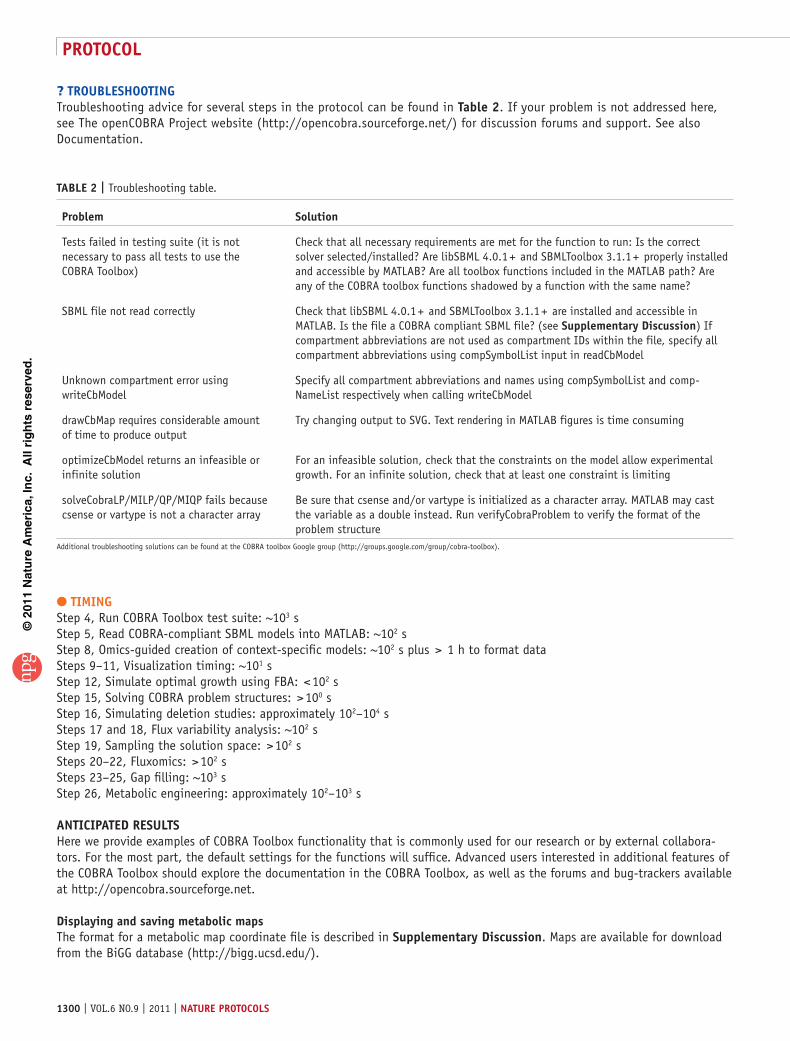
? trouBlesHootInGTroubleshooting advice for several steps in the protocol can be found in table 2. If your problem is not addressed here, see The openCOBRA Project website (http://opencobra.sourceforge.net/) for discussion forums and support. See also Documentation.

● tIMInGStep 4, Run COBRA Toolbox test suite: ~103 sStep 5, Read COBRA-compliant SBML models into MATLAB: ~102 sStep 8, Omics-guided creation of context-specific models: ~102 s plus > 1 h to format dataSteps 9–11, Visualization timing: ~101 sStep 12, Simulate optimal growth using FBA: < 102 sStep 15, Solving COBRA problem structures: > 100 sStep 16, Simulating deletion studies: approximately 102–104 sSteps 17 and 18, Flux variability analysis: ~102 sStep 19, Sampling the solution space: > 102 sSteps 20–22, Fluxomics: > 102 sSteps 23–25, Gap filling: ~103 sStep 26, Metabolic engineering: approximately 102–103 s

antIcIpateD resultsHere we provide examples of COBRA Toolbox functionality that is commonly used for our research or by external collabora-tors. For the most part, the default settings for the functions will suffice. Advanced users interested in additional features of the COBRA Toolbox should explore the documentation in the COBRA Toolbox, as well as the forums and bug-trackers available at http://opencobra.sourceforge.net.

Displaying and saving metabolic mapsThe format for a metabolic map coordinate file is described in supplementary Discussion. Maps are available for download from the BiGG database (http://bigg.ucsd.edu/).

taBle 2 | Troubleshooting table.

problem solution

Tests failed in testing suite (it is not necessary to pass all tests to use the COBRA Toolbox)

Check that all necessary requirements are met for the function to run: Is the correct solver selected/installed? Are libSBML 4.0.1 + and SBMLToolbox 3.1.1 + properly installed and accessible by MATLAB? Are all toolbox functions included in the MATLAB path? Are any of the COBRA toolbox functions shadowed by a function with the same name?

SBML file not read correctly Check that libSBML 4.0.1 + and SBMLToolbox 3.1.1 + are installed and accessible in MATLAB. Is the file a COBRA compliant SBML file? (see supplementary Discussion) If compartment abbreviations are not used as compartment IDs within the file, specify all compartment abbreviations using compSymbolList input in readCbModel

Unknown compartment error using writeCbModel

Specify all compartment abbreviations and names using compSymbolList and comp-NameList respectively when calling writeCbModel

drawCbMap requires considerable amount of time to produce output

Try changing output to SVG. Text rendering in MATLAB figures is time consuming

optimizeCbModel returns an infeasible or infinite solution

For an infeasible solution, check that the constraints on the model allow experimental growth. For an infinite solution, check that at least one constraint is limiting

solveCobraLP/MILP/QP/MIQP fails because csense or vartype is not a character array

Be sure that csense and/or vartype is initialized as a character array. MATLAB may cast the variable as a double instead. Run verifyCobraProblem to verify the format of the problem structure

Additional troubleshooting solutions can be found at the COBRA toolbox Google group (http://groups.google.com/group/cobra-toolbox).

©20

11 N

atu

re A

mer

ica,

Inc.

All

rig

hts

res

erve

d.

protocol

nature protocols | VOL.6 NO.9 | 2011 | 1301

load a map coordinate file. Navigate to the directory (testing/testMaps) containing the map file ‘ecoli_core_map.txt’ and then execute the following command:

> > map = readCbMap(‘ecoli_core_map.txt’);

Display a metabolic map. > > changeCbMapOutput(‘matlab’); > > drawCbMap(map);The following example illustrates one of the many ways to change the appearance of a map. Colors are based on the RGB

style. To change all of the nodes to black and the edges to red, first create an n × 3 matrix, where n is the number of nodes in the map and each row is the RGB for black ([0,0,0]).

> > node_colors = repmat([0,0,0],size(map.molName,1),1);Next, create an n × 3 matrix, where n is the number of edges in the map and each row is the RGB for red ([1,0,0]). > > edge_colors = repmat([1,0,0],size(map.connectionName,1),1);Next, create a map options structure. The first argument is either an empty matrix or a previously created map options

structure. > > options = setMapOptions([], map, ‘nodeColor’, node_colors, ‘edgeColor’, edge_colors); > > drawCbMap(map, options);

save a metabolic map. > > changeCbMapOutput(‘svg’) > > drawCbMap(map);The file ‘target.svg’ will be saved in the working directory.

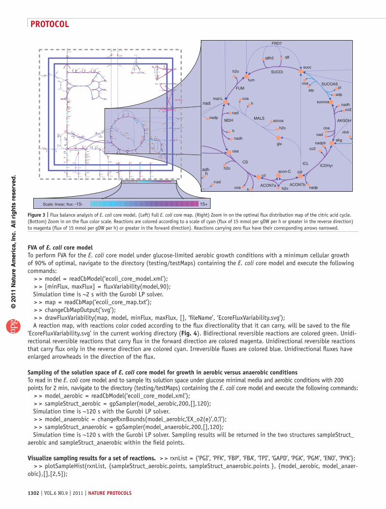
optimal flux distributions and growth rates for E. coli core modelTo read in the Escherichia coli (E. coli) core model and predict a flux distribution for optimal growth, navigate to the direc-tory (testing/testMaps) containing the E. coli core model and map file, and then execute the following functions:

> > model = readCbModel(‘ecoli_core_model.xml’); > > map = readCbMap(‘ecoli_core_map.txt’); > > changeCbMapOutput(‘svg’); > > solution = optimizeCbModel(model);The expected optimal biomass flux (solution.f) is ~0.87. > > drawFlux(map, model, solution.x, [], ‘FileName’, ‘EcoreOptFlux1.svg’);The drawFlux function call generates an .svg file named EcoreOptFlux1.svg in the working directory. The reactions are

color coded using a linear scale from cyan (corresponding to a flux of − 29.17) to magenta (corresponding to a flux of 45.51).

To more easily extract data from the map, change the width of the reaction arrows corresponding to reactions carrying zero flux to 1 point. In addition, set the lower and upper bounds to − 15 and 15, respectively.

> > drawFlux(map, model, solution.x, [], ‘ZeroFluxWidth’, 1, ‘lb’, − 15, ‘ub’, 15, ‘FileName’, ‘EcoreOptFlux2.svg’);An .svg file named EcoreOptFlux2.svg should be saved in the working directory, with reactions color coded from cyan (flux

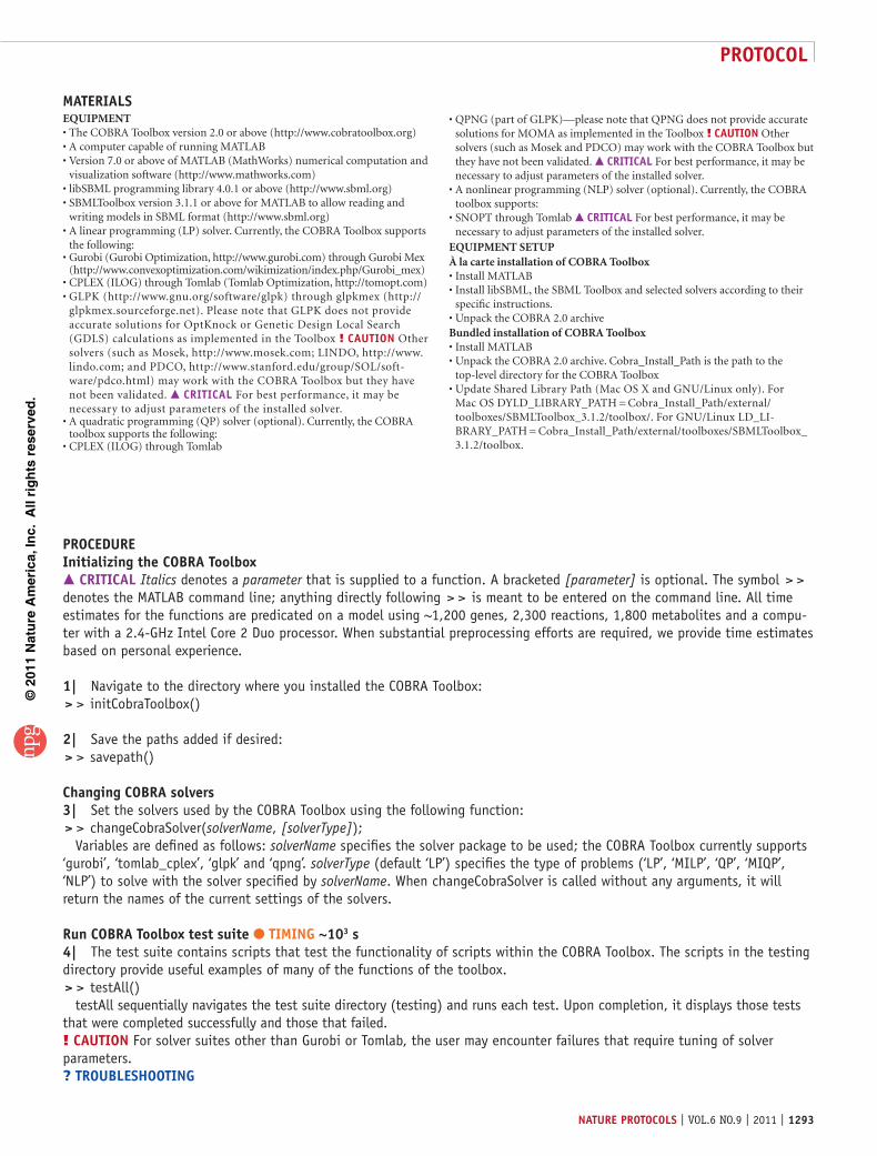
of − 15 or less) to magenta (flux of 15 or greater); reactions carrying zero flux have their corresponding arrows narrowed (Fig. 3).

parsimonious FBa categorization of genes for E. coli growth on acetateTo perform pFBA on the E. coli core model growing in an acetate minimal medium and to plot the results, navigate to the directory (testing/testMaps) containing the E. coli core model and execute the following commands:

> > map = readCbMap(‘ecoli_core_map.txt’); > > model = readCbModel(‘ecoli_core_model.xml’);Remove glucose from the minimal medium. > > model = changeRxnBounds(model,’EX_glc(e)’,0,’l’);Add acetate to the minimal medium. > > model = changeRxnBounds(model,’EX_ac(e)’,-10,’l’); > > [pFBAGeneClasses pFBARxn] = pFBA(model, ‘map’, map, ‘mapOutName’, ‘Ecore_pFBA_ac.svg’);A reaction map, with reactions color coded according to the reaction class, will be saved as ‘Ecore_pFBA_ac.svg’ in the

working directory. Inspecting the map will show that pyruvate kinase (PYK) is classified by pFBA as enzymatically less ef-ficient. This is because its use does not reduce the computed growth rate, but it increases the amount of flux through the network. Interestingly, it has been reported that this enzyme is downregulated in wild-type E. coli when grown on acetate minimal medium69. Simulation time is ~20 s with the Gurobi LP solver.

©20

11 N

atu

re A

mer

ica,

Inc.

All

rig

hts

res

erve

d.

protocol

1302 | VOL.6 NO.9 | 2011 | nature protocols

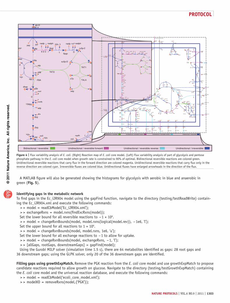
FVa of E. coli core modelTo perform FVA for the E. coli core model under glucose-limited aerobic growth conditions with a minimum cellular growth of 90% of optimal, navigate to the directory (testing/testMaps) containing the E. coli core model and execute the following commands:

> > model = readCbModel(‘ecoli_core_model.xml’); > > [minFlux, maxFlux] = fluxVariability(model,90);Simulation time is ~2 s with the Gurobi LP solver. > > map = readCbMap(‘ecoli_core_map.txt’); > > changeCbMapOutput(‘svg’); > > drawFluxVariability(map, model, minFlux, maxFlux, [], ‘fileName’, ‘EcoreFluxVariability.svg’);A reaction map, with reactions color coded according to the flux directionality that it can carry, will be saved to the file

‘EcoreFluxVariability.svg’ in the current working directory (Fig. 4). Bidirectional reversible reactions are colored green. Unidi-rectional reversible reactions that carry flux in the forward direction are colored magenta. Unidirectional reversible reactions that carry flux only in the reverse direction are colored cyan. Irreversible fluxes are colored blue. Unidirectional fluxes have enlarged arrowheads in the direction of the flux.

sampling of the solution space of E. coli core model for growth in aerobic versus anaerobic conditionsTo read in the E. coli core model and to sample its solution space under glucose minimal media and aerobic conditions with 200 points for 2 min, navigate to the directory (testing/testMaps) containing the E. coli core model and execute the following commands:

> > model_aerobic = readCbModel(‘ecoli_core_model.xml’); > > sampleStruct_aerobic = gpSampler(model_aerobic,200,[],120);Simulation time is ~120 s with the Gurobi LP solver. > > model_anaerobic = changeRxnBounds(model_aerobic,‘EX_o2(e)’,0,‘l’); > > sampleStruct_anaerobic = gpSampler(model_anaerobic,200,[],120);Simulation time is ~120 s with the Gurobi LP solver. Sampling results will be returned in the two structures sampleStruct_

aerobic and sampleStruct_anaerobic within the field points.

Visualize sampling results for a set of reactions. > > rxnList = {‘PGI’, ‘PFK’, ‘FBP’, ‘FBA’, ‘TPI’, ‘GAPD’, ‘PGK’, ‘PGM’, ‘ENO’, ‘PYK’}; > > plotSampleHist(rxnList, {sampleStruct_aerobic.points, sampleStruct_anaerobic.points }, {model_aerobic, model_anaer-

obic},[],[2,5]);

h2o

fum

mal-L

icit

nadp

nadphco2

akg

oaa

glx

succ

coa

atppi

succoa

adp

coa

nad

co2nadh

accoa

h2o

hcoa

nad

nad

nadh

h nh4

h2o

cit

coa h

nadp

h

q8

acon-C

nad

h2o

adh

q8h2

FUM

ICDHyrICL

SUCOAS

AKGDHMALSMDH

CS

ACONTa ACONTb

ALCD2

FRD7

SUCDi

Scale: linear; flux: -15- 15+

15+

22

2

22

2

4

2

3

2

2

0.5

2

2

2

4

atp

3pg

13dpg

adp

nadp

6pgc

co2 nadph

ru5p-D

o2o2o2oo

nadpn

nadh

h

hh

nadphn

nadn

h2oh2fummumum

mal-Laal-lal-mal-

icitt

nadp

nadphnad

co2co2

akggakg

nadnad

pyryppyr

coacoa

co2

coaacoaaacc

nadh

h2opep

co2

hpi

oaa

2pg

h2oooh2o

g6p

f6p

nh4

nh4

h2ooh2o

fdffdp

pipi

succucs

ggglx

cccs ccsucc

atpampamp

adpadp

gln-Lngl

q8q8

q8h28h

co2

g3pgs7ps7

e4ppe4 f6pf6

hh

adppad

atpppatp

glu-Lg

hh

glu-Lg

hh

lac-Dac-D

pyrpy

xu5p-Dxxxu

hh

coac

atpa pi

succoasucc

adp

atp

adpdp

hh

g3p

atp

nh4

gln-Lgln-Ln Lngln-gl

adp

h

pi

hh

hh

lac-D

coaacoa

naddnad

co2

nadh

coacfoor

atp

adpaco2c

pi

hhh

hhpi

akga

hhhh

apppppddhap

hhh hh

h2o

r5pr5

accoa

h2o

h

coa

pi

actpcoa

aatpah2oohpip adpahh

nad

co22co2

nadhnad

nadp nadphh

6pgl

acac

h2o2oh

nh44hn

h2o

pipi

h

naddnad

nadhhdnad

hh

nad

nadh

h

h2o

h2o co2

atppatp

h2ooh2o

hh

amppmpam

pipi

glc-D

h

etoh

h

atp

ac

adp

nadphphdphnad

hh

nadppdpnad

fumfum

hh

hh

h

h

peppe pyrp

h

hh

for

h2o h

nad

pi

nadh

h

hhhh

h2onadpnadphnh444h4

hh

pipip

hhhh

h2o

h2o2oh2o

citcititc

coacoacohhhh

hh hh

nadp

co2nadph

hh

nadaddnad

hh

hh

nadhhnana h

h

q8q8q8

acald

mal-L

acaldacon-C

pepp

hhh

pyr

nad

h2oh2oh

nadhdad

coa

frufru

nadhnad

nad

etoh

q8h2

hh

h

h

PGKPP

GNDGGNGNDGND

O2tt

THD2THD2

FUM

ICDHyr

PDH

PPC

ENOENEN

PGIPGPG

NH4tNHHNH4

FBPFB

EX_succ(e)X_su

ICL

ADK1DD

EX gln-L(e)EX_gln-L(e)X_gln

EX_co2(e)EXEX

TALATT

PYK

GLUt2rrGLU 2

EX_lac-D(e)XX

EX_pyr(e)

RPE

EX h(e)_ ( )

SUCOAS

EX_glu-L(e)glu

TKT2TKT2T

GLNS

D-LACt2-LL

NADTRHDNADN DDTRHD

AKGDH

PFLPFL

EX_o2(e)EX 2(e)

PPCKPPCKKK

PIt2rPIt2r

AKGt22r

FBAFBF

TPI

CYTBDC

RPI

MALS

PPPPPTArTT

GLNa�cGLNa�c

ME1

G�PDH2rGG�PDG�PG�PDH2r

EX_ac(e)

GLUNGL

ATPM

LDH_DLD

MDH

H2OtH22H2O

EX_h2o(e)

TKT1

CO2tCOCO2

EX_a� g(e)

PPSPP

EX_glc(e)

EETTOHt2rTT

PGMP

EX_etoh(e)

ACKrACACACAC

EX_nh4(e)EXEX

GLUSyGGLUSy

EX_p�(e)E

FUMt2_2

ACt2rACt2rA

GLCptsGLCptsLCGLCp

SUCCCt�SUCCt�t�t�

PGLPPGLPGL

GAPDGAGA

EX_�u� (e)

SUCCt2_2Ct2_SUCCt2 2S 22

GLUDyyGLGLLUDGL

ATPS4r44

CSCSCS

PYRt22rPYR 2

ME2M

EX_�or(e)EE

ACALDCALDACACALCA

ACALDtACALDtAAA

EX_acal� (e)

ACONNTTTaaaaaTTTT ACONT�

ALCD2�CD2

FORt2OO FORt�

FRD�

RUpts2FR

EX_�ru(e)

MALt2_2MALt2

EX_�al-L(e )E

NADH1�N

SUCD�CD�SUCSUCD

Scale: Linear; Flux: -15-

PFKFF

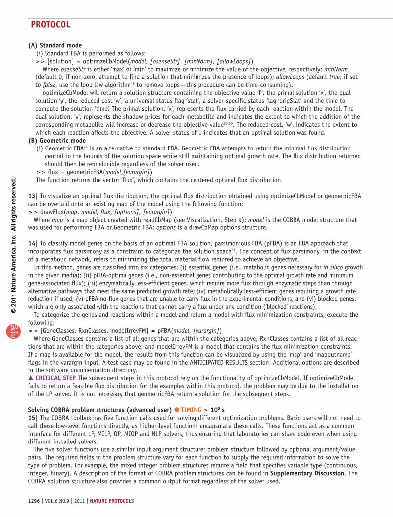
Figure 3 | Flux balance analysis of E. coli core model. (Left) Full E. coli core map. (Right) Zoom in on the optimal flux distribution map of the citric acid cycle. (Bottom) Zoom in on the flux color scale. Reactions are colored according to a scale of cyan (flux of 15 mmol per gDW per h or greater in the reverse direction) to magenta (flux of 15 mmol per gDW per h) or greater in the forward direction). Reactions carrying zero flux have their corresponding arrows narrowed.

©20

11 N

atu

re A

mer

ica,

Inc.

All

rig

hts

res

erve

d.

protocol

nature protocols | VOL.6 NO.9 | 2011 | 1303

A MATLAB figure will also be generated showing the histograms for glycolysis with aerobic in blue and anaerobic in green (Fig. 5).

Identifying gaps in the metabolic networkTo find gaps in the Ec_iJR904 model using the gapFind function, navigate to the directory (testing/testReadWrite) contain-ing the Ec_iJR904.xml and execute the following commands:

> > model = readCbModel(‘Ec_iJR904.xml’); > > exchangeRxns = model.rxns(findExcRxns(model));Set the lower bound for all reversible reactions to − 1 × 106. > > model = changeRxnBounds(model, model.rxns(logical(model.rev)), − 1e6, ‘l’);Set the upper bound for all reactions to 1 × 106. > > model = changeRxnBounds(model, model.rxns, 1e6, ‘u’);Set the lower bound for all exchange reactions to − 1 to allow for uptake. > > model = changeRxnBounds(model, exchangeRxns, − 1, ‘l’); > > [allGaps, rootGaps, downstreamGaps] = gapFind(model);Using the Gurobi MILP solver (simulation time 1.5 s), there are 64 metabolites identified as gaps: 28 root gaps and

36 downstream gaps; using the GLPK solver, only 20 of the 36 downstream gaps are identified.

Filling gaps using growthexpMatch. Remove the PGK reaction from the E. coli core model and use growthExpMatch to propose candidate reactions required to allow growth on glucose. Navigate to the directory (testing/testGrowthExpMatch) containing the E. coli core model and the universal reaction database, and execute the following commands:

> > model = readCbModel(‘ecoli_core_model.xml’); > > modelKO = removeRxns(model,{‘PGK’});

Bidirectional / reversible: Unidirectional / reversible forward: Unidirectional / reversible reverse: Unidirectional / irreversible:

2

2

2

2

4

2

3

2

2

0.5

2

2

2

4

atp

3pg

13dpg

adp

nadp

6pgc

co2 nadph

ru5p-D

o2o2

nadp

nadh

h

h

nadph

nad

h2o fum

mal-L

icit

nadp

nadphco2

akg

nad

pyr

coa

co2

accoa

nadh

h2opepco2

hpi

oaa

2pg

h2o

g6p

f6p

nh4

nh4

h2o

fdp

pi

succ

glx

succ

atpamp

adp

gln-L

q8

q8h2

co2

g3ps7p

e4ppe4 f6pf6

h

adp

atp

glu-L

h

glu-L

h

lac-D

pyr

xu5p-D

h

coa

atp pi

succoa

adp

atp

adph

g3p

atp

nh4

gln-L

adphpi

h

h

lac-D

coanad

co2nadh

coafor

atpadp

co2

pih

hpi

akg

hh

dhap

h h

h2o

r5p

accoa

h2o

hcoa

pi

actpcoa

atph2opi adph

nad

co2nadh

nadp nadphh

6pgl

ac

h2o

nh4

h2o

pi

h

nad

nadhh

nad

nadh

h

h2o

h2o co2

atph2o

hh

amp

pi

glc-D

h

etoh

h

atpac

adp

nadph

h

nadp

fumh

h

h

h

pep pyr

h

h

for

h2o h

nadpi

nadhh

hh

nadph2onadphnh4

h

pi

h

h2o

h2o

cit

coah

h h

nadp

co2nadph

h

nad

h

h

nadh

h

q8

acald

mal-L

acaldacon-C

pep

h

pyr

nad

h2o

nadh

coa

fru

nadh

nad

etoh

q8h2

h

h

h

PGK

GND

O2t

THD2

FUM

ICDHyr

PDH

PPC

ENO

PGI

NH4t

FBP

EX_succ(e)

ICL

ADK1

EX_gln-L(e)

EX_co2(e)

TALA

PYK

GLUt2r

EX_lac-D(e)

EX_pyr(e)

RPE

EX_h(e)

SUCOAS

PFK

EX_glu-L(e)

TKT2

GLNS

D-LACt2

NADTRHD

AKGDH

PFL

EX_o2(e)

PPCK

PIt2r

AKGt2r

FBA

TPI

CYTBD

RPI

MALS

PTArGLNabc

ME1

G6PDH2r

EX_ac(e)

GLUN

ATPM

LDH_D

MDH

H2Ot

EX_h2o(e)

TKT1

CO2t

EX_akg(e)

PPS

EX_glc(e)

ETOHt2r

PGM

EX_etoh(e)

ACKr

EX_nh4(e)

GLUSy

EX_pi(e)

FUMt2_2

ACt2r

GLCpts

SUCCt3

PGL

GAPD

EX_fum(e)

SUCCt2_2

GLUDy

ATPS4r

CS

PYRt2r

ME2

EX_for(e)

ACALD

ACALDt

EX_acald(e)

ACONTa ACONTb

ALCD2x

FORt2 FORti

FRD7

FRUpts2

EX_fru(e)

MALt2_2

EX_mal-L(e)

NADH16

SUCDi

3pg

13dpg

adp

nadp

6pgc

co2 nadph

ru5p-D

h2opepco2

h

2pg

h2o

g6pgg

f6p

h2ofdp

pi

g333g

f666f6

xu5p-D

atp

adpadphh

g3pdhap

r555r5

naddd

co2

nadh

nadp nadphh

6pglpg

hhpiipi

glc-D

pep pyr h2o h

nadpi

nadhh

nnn

pepp

pyr

�� �

� �D

��C��C��C

�� �

�����

�B��

���

�� �

� � �

� ��

��1 11

� 6�D�2 r

�� �

�LCpt spL�LC

� � L

� �� D

��2

Bidirectional / reversible: Unidirectional / reversible forward: Unidirectional / reversible reverse: Unidirectional / irreversible:

TKT2

TKT1

TALAFBAs7p

e4p

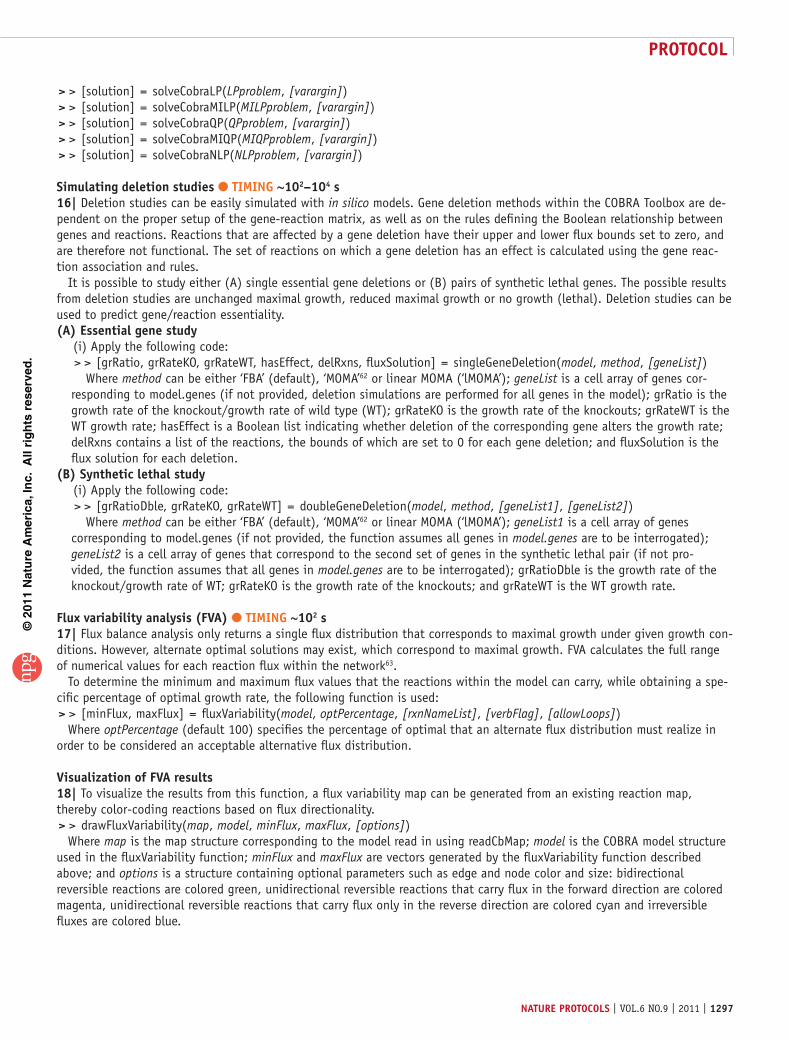
Figure 4 | Flux variability analysis of E. coli. (Right) Reaction map of E. coli core model. (Left) Flux variability analysis of part of glycolysis and pentose phosphate pathway in the E. coli core model when growth rate is constrained to 90% of optimal. Bidirectional reversible reactions are colored green. Unidirectional reversible reactions that carry flux in the forward direction are colored magenta. Unidirectional reversible reactions that carry flux only in the reverse direction are colored cyan. Irreversible fluxes are colored blue. Unidirectional fluxes have enlarged arrowheads in the direction of the flux.

©20

11 N

atu

re A

mer

ica,

Inc.

All

rig

hts

res

erve

d.

protocol

1304 | VOL.6 NO.9 | 2011 | nature protocols

> > KEGGFilename = ‘2010_07_30_KEGG_reaction.lst’;

> > load(‘Dictionary.mat’); > > growthExpMatch(modelKO, KEGG-

Filename, ‘[c]’, 5, dictionary,’GEMLog.txt’);The PGK reaction is removed from

the E. coli core model, thus removing the ability of the model to produce biomass from glucose. Updated versions of the KEGG reaction list should be downloaded from the KEGG website (http://www.genome.jp/kegg)67,68. The resulting GEMLog file should contain five solutions (table 3); please note that if no solutions are found, then the log file will not be generated. The first solu-tion R01512 corresponds to the PGK reaction that was removed previously. The remaining four solutions are alternate reaction sets that, when added, allow the model to grow on glucose. With the Gurobi MILP solver, simulation time is ~2 × 103 s.

optimize product secretion using the E. coli core modelset up model for strain design. Navigate to the directory (testing/testMaps) containing the E. coli core model and execute the following commands.

> > model = readCbModel(‘ecoli_core_model.xml’);Adjust the minimal medium composition to be anaerobic and contain a supply of glucose (20 mmol per gDW per h). > > model = changeRxnBounds(model, {‘EX_o2(e)’, ‘EX_glc(e)’}, [0, –20], ‘l’);Build a list of candidate reactions for deletion to optimize product formation. It is wise to exclude exchange and transport

reactions, and biomass and ATP maintenance requirements. > > selectedRxns = {model.rxns{ [1, 3:5, 7:8, 10, 12, 15:16, 18, 40:41, 44, 46, 48:49, 51, 53:55, 57, 59:62, 64:68,

71:77, 79:83, 85:86, 89:95]}};

optKnock analysis of model. To optimize for lactate secretion with five deletions or less using the OptKnock method: > > options.targetRxn = ‘EX_lac-D(e)’; > > options.vMax = 1000; > > options.numDel = 5; > > options.numDelSense = ‘L’;

–15–10–5 0 50

0.2

0.4

0.6PGI

10 20 30 40 500

0.1

0.2

0.3

0.4

PFK

10 20 30 400

0.2

0.4

0.6FBP

2 4 6 80

0.1

0.2

0.3

0.4

0.5FBA

2 4 6 80

0.1

0.2

0.3

0.4

0.5TPI

12 14 16 180

0.1

0.2

0.3GAPD

–18–16–14–120

0.1

0.2

0.3PGK

–18–16–14–120

0.1

0.2

0.3PGM

12 14 16 180

0.1

0.2

0.3ENO

10 20 300

0.1

0.2

0.3

0.4PYK

Pro

babi

lity

dens

ity

Flux through reaction (mmol per gDW per h)

Figure 5 | Sampling histogram of glycolysis, using the E. coli core model under aerobic and anaerobic glucose minimal medium conditions. For growth in aerobic (blue) versus anaerobic (green) medium, there is a large shift in the probable flux through many of the reactions. In general, the range of flux probabilities for each reaction became more constrained. Phosphoglucose isomerase (PGI) switched from being able to carry flux in either direction with aerobic conditions to only carrying flux in the forward direction with anaerobic conditions.

taBle 3 | GrowthExpMatch gap-filling solutions.

# KeGG ID reaction name reaction formula

1 ‘R01512_b’ Phosphoglycerate kinase ATP + 3-phospho-D-glycerate ADP + 3-phospho-D-glyceroyl phosphate

2 ‘R02188_f’ 3-Phospho-D-glyceroyl-phosphate:polyphosphate phosphotransferase

3-Phospho-D-glyceroyl phosphate + (phosphate)n 3-phospho-D- glycerate + (phosphate)n

3 ‘R01515_f’ Acylphosphatase 3-Phospho-D-glyceroyl phosphate + H2O 3-phospho-D-glycerate + orthophosphate

4 ‘R00761_f’ Fructose-6-phosphate phosphoketolase D-Fructose 6-phosphate + orthophosphate acetyl phosphate + D- erythrose 4-phosphate + H2O

5 ‘R00024_f’ ‘R01523_f’

Ribulose-bisphosphate carboxylase Phosphoribulokinase

D-Ribulose 1,5-bisphosphate + CO2 + H2O 2,3-Phospho-D-glycerate ATP + D-ribulose 5-phosphate ADP + D-ribulose 1,5-bisphosphate

Solutions from five iterations of growthExpMatch on a PGK knockout growing on glucose using the E. coli core model. The first solution returned is the knocked-out reaction. Solutions from iterations 2, 3 and 5 are reactions to use 3-phospho-D-glycerol phosphate while the solution from iteration 4 bypasses the gap by converting D-fructose 6-phosphate to D-erythrose 4-phosphate and acetyl phosphate.

©20

11 N

atu

re A

mer

ica,

Inc.

All

rig

hts

res

erve

d.

protocol

nature protocols | VOL.6 NO.9 | 2011 | 1305

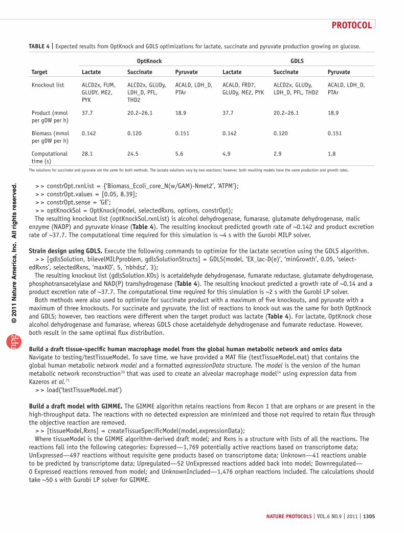
> > constrOpt.rxnList = {‘Biomass_Ecoli_core_N(w/GAM)-Nmet2’, ‘ATPM’}; > > constrOpt.values = [0.05, 8.39]; > > constrOpt.sense = ‘GE’; > > optKnockSol = OptKnock(model, selectedRxns, options, constrOpt);The resulting knockout list (optKnockSol.rxnList) is alcohol dehydrogenase, fumarase, glutamate dehydrogenase, malic

enzyme (NADP) and pyruvate kinase (table 4). The resulting knockout predicted growth rate of ~0.142 and product excretion rate of ~37.7. The computational time required for this simulation is ~4 s with the Gurobi MILP solver.

strain design using GDls. Execute the following commands to optimize for the lactate secretion using the GDLS algorithm. > > [gdlsSolution, bilevelMILPproblem, gdlsSolutionStructs] = GDLS(model, ‘EX_lac-D(e)’, ‘minGrowth’, 0.05, ‘select-

edRxns’, selectedRxns, ‘maxKO’, 5, ‘nbhdsz’, 3);The resulting knockout list (gdlsSolution.KOs) is acetaldehyde dehydrogenase, fumarate reductase, glutamate dehydrogenase,

phosphotransacetylase and NAD(P) transhydrogenase (table 4). The resulting knockout predicted a growth rate of ~0.14 and a product excretion rate of ~37.7. The computational time required for this simulation is ~2 s with the Gurobi LP solver.

Both methods were also used to optimize for succinate product with a maximum of five knockouts, and pyruvate with a maximum of three knockouts. For succinate and pyruvate, the list of reactions to knock out was the same for both OptKnock and GDLS; however, two reactions were different when the target product was lactate (table 4). For lactate, OptKnock chose alcohol dehydrogenase and fumarase, whereas GDLS chose acetaldehyde dehydrogenase and fumarate reductase. However, both result in the same optimal flux distribution.

Build a draft tissue-specific human macrophage model from the global human metabolic network and omics dataNavigate to testing/testTissueModel. To save time, we have provided a MAT file (testTissueModel.mat) that contains the global human metabolic network model and a formatted expressionData structure. The model is the version of the human metabolic network reconstruction70 that was used to create an alveolar macrophage model14 using expression data from Kazeros et al.71

> > load(‘testTissueModel.mat’)

Build a draft model with GIMMe. The GIMME algorithm retains reactions from Recon 1 that are orphans or are present in the high-throughput data. The reactions with no detected expression are minimized and those not required to retain flux through the objective reaction are removed.

> > [tissueModel,Rxns] = createTissueSpecificModel(model,expressionData);Where tissueModel is the GIMME algorithm-derived draft model; and Rxns is a structure with lists of all the reactions. The

reactions fall into the following categories: Expressed—1,769 potentially active reactions based on transcriptome data; UnExpressed—497 reactions without requisite gene products based on transcriptome data; Unknown—41 reactions unable to be predicted by transcriptome data; Upregulated—52 UnExpressed reactions added back into model; Downregulated— 0 Expressed reactions removed from model; and UnknownIncluded—1,476 orphan reactions included. The calculations should take ~50 s with Gurobi LP solver for GIMME.

taBle 4 | Expected results from OptKnock and GDLS optimizations for lactate, succinate and pyruvate production growing on glucose.

optKnock GDls

target lactate succinate pyruvate lactate succinate pyruvate

Knockout list ALCD2x, FUM, GLUDY, ME2, PYK

ALCD2x, GLUDy, LDH_D, PFL, THD2

ACALD, LDH_D, PTAr

ACALD, FRD7, GLUDy, ME2, PYK

ALCD2x, GLUDy, LDH_D, PFL, THD2

ACALD, LDH_D, PTAr

Product (mmol per gDW per h)

37.7 20.2–26.1 18.9 37.7 20.2–26.1 18.9

Biomass (mmol per gDW per h)

0.142 0.120 0.151 0.142 0.120 0.151

Computational time (s)

28.1 24.5 5.6 4.9 2.9 1.8

The solutions for succinate and pyruvate are the same for both methods. The lactate solutions vary by two reactions; however, both resulting models have the same production and growth rates.

©20

11 N

atu

re A

mer

ica,

Inc.

All

rig

hts

res

erve

d.

protocol

1306 | VOL.6 NO.9 | 2011 | nature protocols

Note: Supplementary information is available in the HTML version of this article.

acKnowleDGMents We thank individuals who have contributed to or tested COBRA 2.0: S. Gudmundsson, T. Conrad, N. Jamshidi, R. Notebaart and J. Feala. Funding was provided in part by the National Institute of Allergy and Infectious Diseases NIH/DHHS through interagency agreement Y1-AI-8401-01, NIH grants GM68837-05A1, DE-PS02-08ER08-01, GM057089-12 and GM057089-11S1, and the CalIT2 Summer scholars program. R.F. and I.T. were funded by U.S. Department of Energy, Offices of Advanced Scientific Computing Research and the Biological and Environmental Research as part of the Scientific Discovery Through Advanced Computing program, grant DE-SC0002009. N.L. was funded through a National Science Foundation Integrative Graduate Education and Research Traineeship (IGERT) Program Plant Systems Biology training grant (# DGE-0504645).

autHor contrIButIons J.S., R.Q., R.M.T.F., I.T., J.D.O., A.M.F., D.C.Z., A.B., N.E.L., S.R., J.K. and D.R.H. contributed modules to the COBRA Toolbox v2.0. D.R.H., J.S., R.Q., A.B., J.D.O., N.E.L. and B.Ø.P. wrote the manuscript.

coMpetInG FInancIal Interests The authors declare competing financial interests: details accompany the full-text HTML version of the paper at http://www.natureprotocols.com/.

Published online at http://www.natureprotocols.com/. Reprints and permissions information is available online at http://www.nature.com/reprints/index.html.

1. Feist, A.M. et al. Model-driven evaluation of the production potential for growth-coupled products of Escherichia coli. Metab. Eng. 12, 173–186 (2010).

2. Feist, A.M. & Palsson, B.O. The growing scope of applications of genome-scale metabolic reconstructions using Escherichia coli. Nat. Biotechnol. 26, 659–667 (2008).

3. Oberhardt, M.A., Palsson, B.O. & Papin, J.A. Applications of genome-scale metabolic reconstructions. Mol. Syst. Biol. 5, 320 (2009).

4. Covert, M.W., Knight, E.M., Reed, J.L., Herrgard, M.J. & Palsson, B.O. Integrating high-throughput and computational data elucidates bacterial networks. Nature 429, 92–96 (2004).

5. Gianchandani, E.P., Joyce, A.R., Palsson, B.O. & Papin, J.A. Functional states of the genome-scale Escherichia coli transcriptional regulatory system. PLoS Comput. Biol. 5, e1000403 (2009).

6. Brynildsen, M.P., Wong, W.W. & Liao, J.C. Transcriptional regulation and metabolism. Biochem. Soc. Trans. 33, 1423–1426 (2005).

7. Thiele, I., Fleming, R.M., Bordbar, A., Schellenberger, J. & Palsson, B.O. Functional characterization of alternate optimal solutions of Escherichia coli’s transcriptional and translational machinery. Biophys. J. 98, 2072–2081 (2010).

8. Thiele, I., Jamshidi, N., Fleming, R.M. & Palsson, B.O. Genome-scale reconstruction of Escherichia coli’s transcriptional and translational machinery: a knowledge base, its mathematical formulation, and its functional characterization. PLoS Comput. Biol. 5, e1000312 (2009).

9. Papin, J.A., Hunter, T., Palsson, B.O. & Subramaniam, S. Reconstruction of cellular signalling networks and analysis of their properties. Nat. Rev. Mol. Cell Biol. 6, 99–111 (2005).

10. Li, F., Thiele, I., Jamshidi, N. & Palsson, B.O. Identification of potential pathway mediation targets in Toll-like receptor signaling. PLoS Comput. Biol. 5, e1000292 (2009).

11. Hyduke, D.R. & Palsson, B.Ø. Towards genome-scale signalling-network reconstructions. Nat. Rev. Genet. 11, 297–307 (2010).

12. Raman, K., Vashisht, R. & Chandra, N. Strategies for efficient disruption of metabolism in Mycobacterium tuberculosis from network analysis. Mol. Biosyst. 5, 1740–1751 (2009).

13. Becker, S.A. & Palsson, B.O. Genome-scale reconstruction of the metabolic network in Staphylococcus aureus N315: an initial draft to the two-dimensional annotation. BMC Microbiol. 5, 8 (2005).

14. Bordbar, A., Lewis, N.E., Schellenberger, J., Palsson, B.O. & Jamshidi, N. Insight into human alveolar macrophage and M. tuberculosis interactions via metabolic reconstructions. Mol. Syst. Biol. 6, 422 (2010).

15. Thiele, I., Price, N.D., Vo, T.D. & Palsson, B.O. Candidate metabolic network states in human mitochondria. Impact of diabetes, ischemia, and diet. J. Biol. Chem. 280, 11683–11695 (2005).

16. Price, N.D., Reed, J.L. & Palsson, B.O. Genome-scale models of microbial cells: evaluating the consequences of constraints. Nat. Rev. Micro. 2, 886–897 (2004).

17. Becker, S.A. et al. Quantitative prediction of cellular metabolism with constraint-based models: the COBRA Toolbox. Nat. Protoc. 2, 727–738 (2007).

18. Notebaart, R.A., Teusink, B., Siezen, R.J. & Papp, B. Co-regulation of metabolic genes is better explained by flux coupling than by network distance. PLoS Comput. Biol. 4, e26 (2008).

19. Durot, M., Bourguignon, P.Y. & Schachter, V. Genome-scale models of bacterial metabolism: reconstruction and applications. FEMS Microbiol. Rev. 33, 164–190 (2009).

20. Raman, K., Yeturu, K. & Chandra, N. targetTB: a target identification pipeline for Mycobacterium tuberculosis through an interactome, reactome and genome-scale structural analysis. BMC Syst. Biol. 2, 109 (2008).

21. Vazquez, A. et al. Impact of the solvent capacity constraint on E. coli metabolism. BMC Syst. Biol. 2, 7 (2008).

22. Henry, C.S., Jankowski, M.D., Broadbelt, L.J. & Hatzimanikatis, V. Genome-scale thermodynamic analysis of Escherichia coli metabolism. Biophys. J. 90, 1453–1461 (2006).

23. Fleming, R.M., Thiele, I. & Nasheuer, H.P. Quantitative assignment of reaction directionality in constraint-based models of metabolism: application to Escherichia coli. Biophys. Chem. 145, 47–56 (2009).

24. Fleming, R.M. & Thiele, I. von Bertalanffy 1.0: a COBRA toolbox extension to thermodynamically constrain metabolic models. Bioinfomatics 27, 142–143 (2010).

25. Becker, S.A. & Palsson, B.O. Context-specific metabolic networks are consistent with experiments. PLoS Comput. Biol. 4, e1000082 (2008).

26. Shlomi, T., Cabili, M.N., Herrgard, M.J., Palsson, B.O. & Ruppin, E. Network-based prediction of human tissue-specific metabolism. Nat. Biotech. 26, 1003–1010 (2008).

27. Schellenberger, J. & Palsson, B.O. Use of randomized sampling for analysis of metabolic networks. J. Biol. Chem. 284, 5457–5461 (2009).

28. Orth, J.D., Thiele, I. & Palsson, B.O. What is flux balance analysis? Nat. Biotech. 28, 245–248 (2010).

29. Orth, J.D. & Palsson, B.Ø. Systematizing the generation of missing metabolic knowledge. Biotechnol. Bioeng. 107, 403–412 (2010).

30. Palsson, B. Metabolic systems biology. FEBS Lett. 583, 3900–3904 (2009).31. Schellenberger, J., Park, J., Conrad, T. & Palsson, B. BiGG: a biochemical

genetic and genomic knowledgebase of large scale metabolic reconstructions. BMC Bioinformatics 11, 213 (2010).

32. Palsson, B.O. Two-dimensional annotation of genomes. Nat. Biotechnol. 22, 1218–1219 (2004).

33. Reed, J.L., Famili, I., Thiele, I. & Palsson, B.O. Towards multidimensional genome annotation. Nat. Rev. Genet. 7, 130–141 (2006).

34. Feist, A.M. et al. A genome-scale metabolic reconstruction for Escherichia coli K-12 MG1655 that accounts for 1260 ORFs and thermodynamic information. Mol. Syst. Biol. 3 (2007).

35. Hong, S.H. et al. The genome sequence of the capnophilic rumen bacterium Mannheimia succiniciproducens. Nat. Biotech. 22, 1275–1281 (2004).

36. Mo, M., Palsson, B. & Herrgard, M. Connecting extracellular metabolomic measurements to intracellular flux states in yeast. BMC Syst. Biol. 3, 37 (2009).

37. Nogales, J., Palsson, B. & Thiele, I. A genome-scale metabolic reconstruction of Pseudomonas putida KT2440: iJN746 as a cell factory. BMC Syst. Biol. 2, 79 (2008).

38. Raghunathan, A., Reed, J., Shin, S., Palsson, B. & Daefler, S. Constraint-based analysis of metabolic capacity of Salmonella typhimurium during host-pathogen interaction. BMC Syst. Biol. 3, 38 (2009).

39. Nookaew, I. et al. The genome-scale metabolic model iIN800 of Saccharomyces cerevisiae and its validation: a scaffold to query lipid metabolism. BMC Syst. Biol. 2, 71 (2008).

40. Kuepfer, L., Sauer, U. & Blank, L.M. Metabolic functions of duplicate genes in Saccharomyces cerevisiae. Genome Res. 15, 1421–1430 (2005).

41. Gonzalez, O. et al. Reconstruction, modeling & analysis of Halobacterium salinarum R-1 metabolism. Mol. Biosyst. 4, 148–159 (2008).

42. Heinemann, M., Kummel, A., Ruinatscha, R. & Panke, S. In silico genome-scale reconstruction and validation of the Staphylococcus aureus metabolic network. Biotechnol. Bioeng. 92, 850–864 (2005).

43. Thiele, I. & Palsson, B.O. A protocol for generating a high-quality genome-scale metabolic reconstruction. Nat. Protocols 5, 93–121 (2010).

44. Smallbone, K. & Simeonidis, E. Flux balance analysis: a geometric perspective. J. Theor. Biol. 258, 311–315 (2009).

45. Satish Kumar, V., Dasika, M. & Maranas, C. Optimization based automated curation of metabolic reconstructions. BMC Bioinformatics 8, 212 (2007).

©20

11 N

atu

re A

mer

ica,

Inc.

All

rig

hts

res

erve

d.

protocol

nature protocols | VOL.6 NO.9 | 2011 | 1307

46. Burgard, A.P., Pharkya, P. & Maranas, C.D. Optknock: a bilevel programming framework for identifying gene knockout strategies for microbial strain optimization. Biotechnol. Bioeng. 84, 647–657 (2003).

47. Patil, K., Rocha, I., Forster, J. & Nielsen, J. Evolutionary programming as a platform for in silico metabolic engineering. BMC Bioinformatics 6, 308 (2005).

48. Lun, D.S. et al. Large-scale identification of genetic design strategies using local search. Mol. Syst. Biol. 5, 296 (2009).

49. Schellenberger, J., Lewis, N.E. & Palsson, B.Ø. Elimination of thermodynamically infeasible loops in steady-state metabolic models. Biophysical. J. 200, 544–553 (2011).

50. Price, N.D., Schellenberger, J. & Palsson, B.O. Uniform sampling of steady-state flux spaces: means to design experiments and to interpret enzymopathies. Biophys. J. 87, 2172–2186 (2004).

51. Wiback, S.J., Famili, I., Greenberg, H.J. & Palsson, B.O. Monte Carlo sampling can be used to determine the size and shape of the steady-state flux space. J. Theor. Biol. 228, 437–447 (2004).

52. Almaas, E., Kovacs, B., Vicsek, T., Oltvai, Z.N. & Barabasi, A.L. Global organization of metabolic fluxes in the bacterium Escherichia coli. Nature 427, 839–843 (2004).

53. Reed, J.L. et al. Systems approach to refining genome annotation. Proc. Natl. Acad. Sci. USA 103, 17480–17484 (2006).

54. Chandrasekaran, S. & Price, N.D. Probabilistic integrative modeling of genome-scale metabolic and regulatory networks in Escherichia coli and Mycobacterium tuberculosis. Proc. Natl. Acad. Sci. USA 107, 17845–17850 (2010).

55. Henry, C.S. et al. High-throughput generation, optimization and analysis of genome-scale metabolic models. Nat. Biotechnol. 28, 977–982 (2010).

56. Hucka, M. et al. The systems biology markup language (SBML): a medium for representation and exchange of biochemical network models. Bioinformatics 19, 524–531 (2003).

57. Bornstein, B.J., Keating, S.M., Jouraku, A. & Hucka, M. LibSBML: an API Library for SBML. Bioinformatics 24, 880–881 (2008).

58. Keating, S.M., Bornstein, B.J., Finney, A. & Hucka, M. SBMLToolbox: an SBML toolbox for MATLAB users. Bioinformatics 22, 1275–1277 (2006).

59. Feist, A.M. & Palsson, B.O. The biomass objective function. Curr. Opin. Microbiol. 13, 344–349 (2010).

60. Varma, A. & Palsson, B.O. Metabolic capabilities of Escherichia coli: I. Synthesis of biosynthetic precursors and cofactors. J. Theor. Biol. 165, 477–502 (1993).

61. Lewis, N.E. et al. Omic data from evolved E. coli are consistent with computed optimal growth from genome-scale models. Mol. Syst. Biol. 6, 390 (2010).

62. Segrè, D., Vitkup, D. & Church, G.M. Analysis of optimality in natural and perturbed metabolic networks. Proc. Natl. Acad. Sci. USA 99, 15112–15117 (2002).

63. Mahadevan, R. & Schilling, C.H. The effects of alternate optimal solutions in constraint-based genome-scale metabolic models. Metabol. Engin. 5, 264–276 (2003).

64. Fischer, E., Zamboni, N. & Sauer, U. High-throughput metabolic flux analysis based on gas chromatography-mass spectrometry derived 13C constraints. Anal. Biochem. 325, 308–316 (2004).

65. Wiechert, W., Möllney, M., Isermann, N., Wurzel, M. & de Graaf, A.A. Bidirectional reaction steps in metabolic networks: III. Explicit solution and analysis of isotopomer labeling systems. Biotechnol. Bioeng. 66, 69–85 (1999).

66. Antoniewicz, M.R., Kelleher, J.K. & Stephanopoulos, G. Elementary metabolite units (EMU): a novel framework for modeling isotopic distributions. Metabol. Engin. 9, 68–86 (2007).

67. Kanehisa, M. & Goto, S. KEGG: kyoto encyclopedia of genes and genomes. Nucleic Acids. Res. 28, 27–30 (2000).

68. Kanehisa, M., Goto, S., Kawashima, S., Okuno, Y. & Hattori, M. The KEGG resource for deciphering the genome. Nucleic Acids. Res. 32, D277–D280 (2004).

69. Waygood, E.B. & Sanwal, B.D. The control of pyruvate kinases of Escherichia coli. I. Physicochemical and regulatory properties of the enzyme activated by fructose 1,6-diphosphate. J. Biol. Chem. 249, 265–274 (1974).

70. Duarte, N.C. et al. Global reconstruction of the human metabolic network based on genomic and bibliomic data. Proc. Natl. Acad. Sci. USA 104, 1777–1782 (2007).

71. Kazeros, A. et al. Overexpression of apoptotic cell removal receptor MERTK in alveolar macrophages of cigarette smokers. Am. J. Respir. Cell Mol. Biol. 39, 747–757 (2008).