property-liability insurance loss reserve ranges based on ... · interest rate and inflation...

Property-Liability Insurance LossReserve Ranges Based on Economic

Valueby Stephen P. D’Arcy, Alfred Au, and Liang Zhang

ABSTRACT

Anumber ofmethods tomeasure thevariability of property-liability loss reserves have been developed to meet the re-quirements of regulators, rating agencies, and management.These methods focus on nominal, undiscounted reserves, inline with statutory reserve requirements. Recently, though,there has been a trend to consider the fair value, or eco-nomic value, of loss reserves. Insurance regulators world-wide are starting to consider the economic value of lossreserves, which reflects how much needs to be set asidetoday to settle these claims, instead of focusing on nomi-nal values. If insurers switch to economic values for lossreserves, then reserve variability would need to be calcu-lated on this basis as well. This approach will add consid-erable complexity to reserve variability calculations. Thispaper combines loss reserve variability and economic val-uation. Loss reserve ranges are calculated on a nominaland economic basis for a simplified insurer to illustrate thekey variables that impact loss reserve variability. Nominalinterest rate and inflation volatility, interest rate-inflationcorrelation, and the relationship between claim cost andgeneral inflation are key factors that affect economic lossreserve variability. Actuaries will need to focus on mea-suring these values accurately if insurers adopt economicvaluation of loss reserves.

KEYWORDS

Loss reserve ranges, economic value, stochastic simulation

42 CASUALTY ACTUARIAL SOCIETY VOLUME 3/ISSUE 1

Property-Liability Insurance Loss Reserve Ranges Based on Economic Value

1. IntroductionTraditional loss reserving approaches in the

property-casualty field produced a single pointestimate value. Although no one truly expectslosses to develop at exactly the stated value, thefocus was on a single value for reserves thatdid not reflect the uncertainty inherent in theprocess. As the use of stochastic models in theinsurance industry grew, for dynamic financialanalysis (DFA), for asset liability management(ALM) and other advanced financial techniques,loss reserve variability became an important is-sue. McClenahan (2003) describes the historyof interest in reserve variability and loss reserveranges. Hettinger (2006) surveys the different ap-proaches used to establish reserve ranges. TheCAS Working Party on Quantifying Variabilityin Reserve Estimates (2005) provides a detaileddescription of the issue of reserve variability, in-cluding an extensive bibliography and set of is-sues that still need to be addressed. The conclu-sions of this Working Party are that despite ex-tensive research on this area to date there is noclear consensus within the actuarial professionas to the appropriate approach for measuring thisuncertainty, and that much additional work needsto be done in this area. All of the approachesdescribed in this report, and suggestions for fu-ture research, focus on measuring uncertainty instatutory loss reserves. Given recent attention tofair value insurance accounting, future researchshould also focus on more accurate economic re-serve ranges.The use of nominal values for loss reserves is

sometimes justified as providing a safety load,or risk margin, over the true (economic) value ofthe reserves. However, risk margins determinedin this way would fluctuate with interest ratesand vary by loss payout patterns. A more ap-propriate approach, which is beyond the scopeof this research, would be to establish risk mar-gins based on the risks inherent in the reserveestimation process, such as determining the risk

margin based on the difference between the ex-pected economic value and a level such as the75th percentile value.The Financial Accounting Standards Board

(FASB) and the International Accounting Stan-dards Board (IASB) have proposed an alterna-tive approach to valuing insurance liabilities, in-cluding loss reserves. This approach, termed fairvalue, proposes that loss reserves in financial re-ports be set at a level that reflects the value thatwould exist if these liabilities were sold to an-other party in an arms length transaction. Therelative infrequency with which these exchangesactually take place, and the confidentiality sur-rounding most trades that do occur, make thisapproach to valuation more of a theoretical ex-ercise than a practical one, at least in the cur-rent environment. However, fair value would re-flect the time value of money, so the trend wouldbe to set loss reserves at their economic ratherthan nominal values if these proposals are imple-mented. The issues involved, and financial im-plications, in fair value accounting are coveredextensively in the Casualty Actuarial Society re-port, Fair Value of P&C Liabilities: Practical Im-plications (2004). However, despite the compre-hensive nature of the papers included in this re-port, little attention is paid to the impact the useof fair value accounting would have on loss re-serve ranges. If reserves are to be calculated on afair value basis, then reserve ranges should alsobe based on this approach as well.A final impetus for this project is the recent

criticism of the casualty actuarial profession overinaccurate loss reserves, and the profession’s re-sponse to these attacks. A Standard & Poor’sreport (2003) blamed the reserve shortfalls theindustry reported in 2002 and 2003 on actuar-ial “naiveté or knavery.” The actuarial profes-sion responded strongly to this criticism, bothwith information and with investigation (Miller2004). The Casualty Actuarial Society formed atask force to address the issues of actuarial cred-

VOLUME 3/ISSUE 1 CASUALTY ACTUARIAL SOCIETY 43

Variance Advancing the Science of Risk

ibility. The report of the Task Force on ActuarialCredibility (2005) included the recommendationthat actuarial valuations include ranges to indi-cate the level of uncertainty in the reserving pro-cess, and that additional work be done to clarifywhat the ranges indicate. Once again, the focuswas on statutory loss reserve indications, ratherthan the economic value.The critical problem with setting reserve

ranges based on nominal values is the impactof inflation on loss development. Based on rela-tively recent history (the 1970s) and current eco-nomic conditions (increasing international de-mand for raw materials, vulnerable oil supplies,the U.S. Federal Reserve’s response to the sub-prime credit crisis), increasing inflation has tobe accorded some probability of occurring in thefuture by any actuary calculating loss reserveranges. As inflation will affect all lines of busi-ness simultaneously, the impact of sustained highinflation would be to cause significant adverseloss reserve development for property-liabilityinsurers. Loss reserve ranges based on nominalvalues would therefore include the high valuesthat would be caused by a significant rise in in-flation. However, inflation and interest rates areclosely related, as first observed by Irving Fisher(1930) and confirmed by economists consistentlysince. The loss reserves impacted by high infla-tion would most likely be accompanied by highinterest rates, so the economic value of those re-serves would not be that much higher than theeconomic value of the point estimate for reserves.Using economic values to determine reserveranges could also lead to narrower ranges andprovide a clearer estimate of the true financialimpact of reserve uncertainty.This project utilizes realistic stochastic models

for interest rates, inflation, and loss developmentto determine loss reserve distributions and rangeson both a nominal and economic basis, drawsa comparison between the two approaches, andexplains why the appropriate measure of uncer-

tainty is based on the economic value. This workbuilds on prior work by Ahlgrim, D’Arcy, andGorvett (2005) developing a financial scenariogenerator for the CAS and SOA as well as re-search on the interest sensitivity of loss reservesby D’Arcy and Gorvett (2000) and Ahlgrim,D’Arcy, and Gorvett (2004).This study measures the uncertainty in loss

reserving that is based on process risk, the in-herent variability of a known stochastic process.In this analysis, both the distribution of lossesand the parameters of the distributions are given.Thus, unlike actual loss reserving applications,there is no model risk or parameter risk. Settingloss reserves in practice involves more degrees ofuncertainty, and would therefore lead to greatervariability in the underlying distributions of ulti-mate losses and larger reserve ranges. This studyis meant to illustrate the difference between nom-inal and economic ranges, and starting with spec-ified loss distributions more clearly demonstratesthis effect.

2. Review of loss reservingmethodsA primary responsibility of insurers is to en-

sure they have adequate capital to pay outstand-ing losses. Much research has been done onmethods to evaluate and set these loss reserves.Berquist and Sherman (1977) and Wiser, Cock-ley, and Gardner (2001) provide excellent de-scriptions of the standard approaches used to ob-tain a point estimate for loss reserves. Loss re-serve ranges became an issue in the past twodecades, and has also been addressed in numer-ous papers. For example, Mack (1993) presentedthe chain-ladder estimates and ways to calculatethe variance of the estimate. Murphy (1994) of-fered other variations of the chain-ladder methodin a regression setting. Venter (2007) worked onimproving the accuracy of these estimates andreducing the variances of the ranges. Other con-tributors to loss reserve estimates and discus-



sions on the strengths and weaknesses of vari-ous evaluation models include Zehnwirth (1994),Narayan and Warthen (1997), Barnett and Zehn-wirth (1998), Patel and Raws (1998), and Kirsch-ner, Kerley, and Isaacs (2002). These works typ-ically deal with nominal undiscounted value ofloss reserves in line with statutory reserve re-quirements. Shapland (2003) explores the mean-ing of “reasonable” loss reserves, emphasizingthe need for models to take into account the var-ious risks involved along with “reasonable” as-sumptions. His paper points out that reasonable-ness is subject to many aspects, such as culture,guidelines, availability of information, and theaudience; as such the paper concludes that morespecific input is needed on what should be con-sidered “reasonable” in the actuarial profession.Traditional methods use imbedded historical

inflation to produce the nominal reserves. Out-standing losses will be exposed to the impact ofinflation until they are finally paid. If the infla-tion rate during the experience period has beenhigh, loss severity will be projected to be highgenerating large loss reserves. Similarly, after pe-riods of low inflation, loss severity will be pro-jected to increase more slowly, leading to lowerloss reserves. Because inflation and interest ratesare correlated, an insurer with an effective AssetLiability Management (ALM) strategy for deal-ing with interest rate risk can alleviate some ofthe impact of changing inflation.There have been reserving techniques that at-

tempt to isolate the inflationary component fromthe other effects, such as those proposed by But-sic (1981), Richards (1981), and Taylor (1977).Butsic investigated the effect of inflation uponincurred losses and loss reserves, as well as theinflation effect on investment income. For bothincreases and decreases in inflation, these com-ponents are found to vary proportionally. Ac-cording to Butsic, as competitive pricing is de-pendent on a combination of both claim costsand investment income, insurers are to a large

extent unaffected by unanticipated changes in in-flation. Richards provides a simplified techniqueto evaluate the impact of inflation on loss re-serves by factoring out inflation from historicalloss data. Assumptions of future inflation canthen be factored in to project possible valuesof future loss reserves. Under the Taylor sepa-ration method, loss development is divided intotwo components, inflation and superimposed in-flation. This method assumes the inflation com-ponent affects all loss payments made in a givenyear to the same degree, regardless of the orig-inal accident year. Essentially, unpaid losses arenot considered to be fixed in value over time butrather are fully sensitive to inflation. An alterna-tive to this assumption is proposed by D’Arcyand Gorvett (2000), which allows loss reservesto gradually become “fixed” in value from thetime of the loss to the time of settlement. In-flation would only affect the unpaid losses thathave not yet become fixed in value. These twomethods will be described in detail in the modelsection.

3. Asset liability management

Asset liability management (ALM) is a processin which organizations manage risk by consider-ing the impact that an event would have on boththeir assets and their liabilities; risk is managedby using the offsetting effects to reduce aggre-gate risk to an acceptable level. For example, thefall of the dollar against the euro might increasethe cost of claims an insurer would have to payon business written in Europe. If the insurer heldassets denominated in euros, then thesewould increase in value as the dollar fell, off-setting some, or all, of the increased claim costs.Although ALM can be used to deal with any typeof financial risk, in practice most insurers focuson interest rate risk. In this context, if both as-sets and liabilities change by the same amountwhen interest rates rise or fall, there will be nointerest rate risk for the firm. However, if they



respond differently, the firm will be exposed tointerest rate risk. Prior to the 1970s, mismatchesbetween assets and liabilities were not a signif-icant concern. Interest rates in the United Statesexperienced only minor fluctuations, making anylosses due to asset-liability mismatch insignifi-cant. However the late 1970s and early 1980swere a period of high and volatile interest rates,making ALM a necessity for any viable financialinstitution. If interest rates increase, fixed incomebonds decrease in value and the economic value(the discounted value of future loss payments)of the loss reserves decreases. The opposite oc-curs for both the assets and liabilities when inter-est rates decrease. Ahlgrim, D’Arcy, and Gorvett(2004) provide a detailed analysis of the effectiveduration and convexity of liabilities for property-liability insurers under stochastic interest ratesthat shows how assets can be invested to reducethe impact of interest rate risk.Insurers can employ an ALM program to re-

duce the impact of inflation on loss reserves andmaintain their surplus with changing interestrates. This requires insurers with short effectiveduration liabilities to hold short-term assets.Some insurers invest in longer duration assetsthat offer higher yields. During periods of sta-ble or declining interest rates, this approach willprovide a higher return. However, when inter-est rates rise this strategy can be costly.1 Theeffect of duration mismatching on loss reservesgiven expectations of future inflation volatility isa complicated issue, and is outside the scope ofthis paper. As will be shown later, the higher thecorrelation between nominal interest rates and in-flation, such as in the 1970s, the more importantand significant ALM’s impact will be.

1In late 2007 and early 2008, many banks suffered significant lossesby following a similar mismatched strategy. They used off balancesheet structured investment vehicles (SIV) that invested in long-term bonds, often tied to subprime mortgages, but financed theinvestments with short-term debt. When the value of the assets felland the credit markets froze up increasing short-term borrowingcosts, the banks incurred significant losses which, in some cases,cost the CEOs their jobs (Hilsenrath 2008).

4. Economic value of lossreservesRecent developments by the Financial Ac-

counting Standards Board (FASB) and the Inter-national Accounting Standards Committee(IASC) have advocated fair value accountingmeasures. The American Academy of Actuariesestablished the Fair Value Task Force to addressthis issue. The fair value of a financial asset or li-ability is its market value, or the market value ofa similar asset or liability plus some adjustments.If a market does not exist, the asset or liabilityshould be discounted to its present value at anappropriate capitalization rate depending on therisk components it encompasses. The Fair Valuereport by AAA (2002) provides details on thevaluation principles. The promotion of fair valueaccounting, which considers both risk and thetime value of money, indicates a new trend to-wards economic valuation.The trend towards economic or market value

based measurement of the balance sheet replac-ing existing accounting measures is also seen inthe European Union, where solvency regulationis currently under reform. The European insur-ance and reinsurance federation, CEA (2007),describes how the new Solvency II project takesan integrated risk approach which will better ac-count for the risks an insurer is exposed to thanthe current fixed standards under Solvency I. Sol-vency II introduces the use of a market-consistentvaluation of assets and liabilities and market con-sistent reserve valuation, much like those pro-posed under fair value accounting in the UnitedStates.Australian regulations have required ranges

based on economic value since 1999. The valueof the insurer’s liabilities is generally assumedto be independent of the insurer’s underlying as-sets. The Australian Prudential Regulation Au-thority’s “Audit and Actuarial Reporting and Val-uation” (2006) and Institute of Actuaries of Aus-tralia Professional Standard 300 (2007) requireloss reserves to be discounted by current observ-



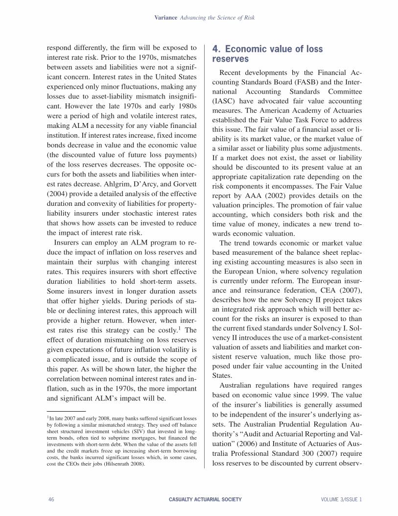
Figure 1. Annual observed inflation since 1930

able market-based rates. These rates are based oncharacteristics of the future obligations, or de-rived from a yield of a replicating portfolio oflow-risk securities. The study mentions that ap-propriate allowance can be made for future claimescalation from inflation and superimposed in-flation (e.g. social or legal costs), but no clearmethodology is provided as to how inflationshould be taken into account.Although there has been much discussion on

the meaning of fair or economic value, both with-in and outside the United States, little attentionhas been given so far to the impact of economicvalue on loss reserve ranges. This paper ties to-gether the loss reserve ranges with the economicvalues to show the relationship between loss re-serve ranges on a nominal and economic basisand to illustrate some of the issues involved incalculating reserve ranges on economic values.The economic value of an insurer’s liabilities

is determined by discounting expected futurecash flows emanating from the liabilities by theirappropriate discount rate. Butsic (1988) andD’Arcy (1987) explore discounting reserves us-ing a risk-adjusted interest rate which reflectsthe risk inherent in the outstanding reserve.

Girard (2002) evaluates this using the company’scost of capital. Actuarial Standard of Practice No.20 (Actuarial Standards Board 1992) addressesissues actuaries should consider in determiningdiscounted loss reserves. This standard suggeststhat possible discount factors could be the risk-free interest rate or the discount rate used in assetvaluation.

5. Trends in inflation level andvolatility

Inflation as measured by the 12-month changein the Consumer Price Index (CPI) has variedwidely, from ¡11% to +20% over the period1922 through 2007 (Figure 1). Since the adop-tion of Keynesian economic policies in devel-oped countries following World War II, the gen-eral trend has been to avoid deflation at the costof persistent inflation.2 Rapid increases in oilprices in the 1970s and the early 21st century

2There is some disagreement over how much of an impact Keyne-sian economic policies have had on inflation patterns. The impactof open market bond purchases by the Federal Reserve, particularlyduring full employment periods, could have a more significant im-pact on inflation. Regardless, the United States has not experiencedsignificant deflation since the 1950s, so that is the period used todetermine the parameters calculated for the models in this work.



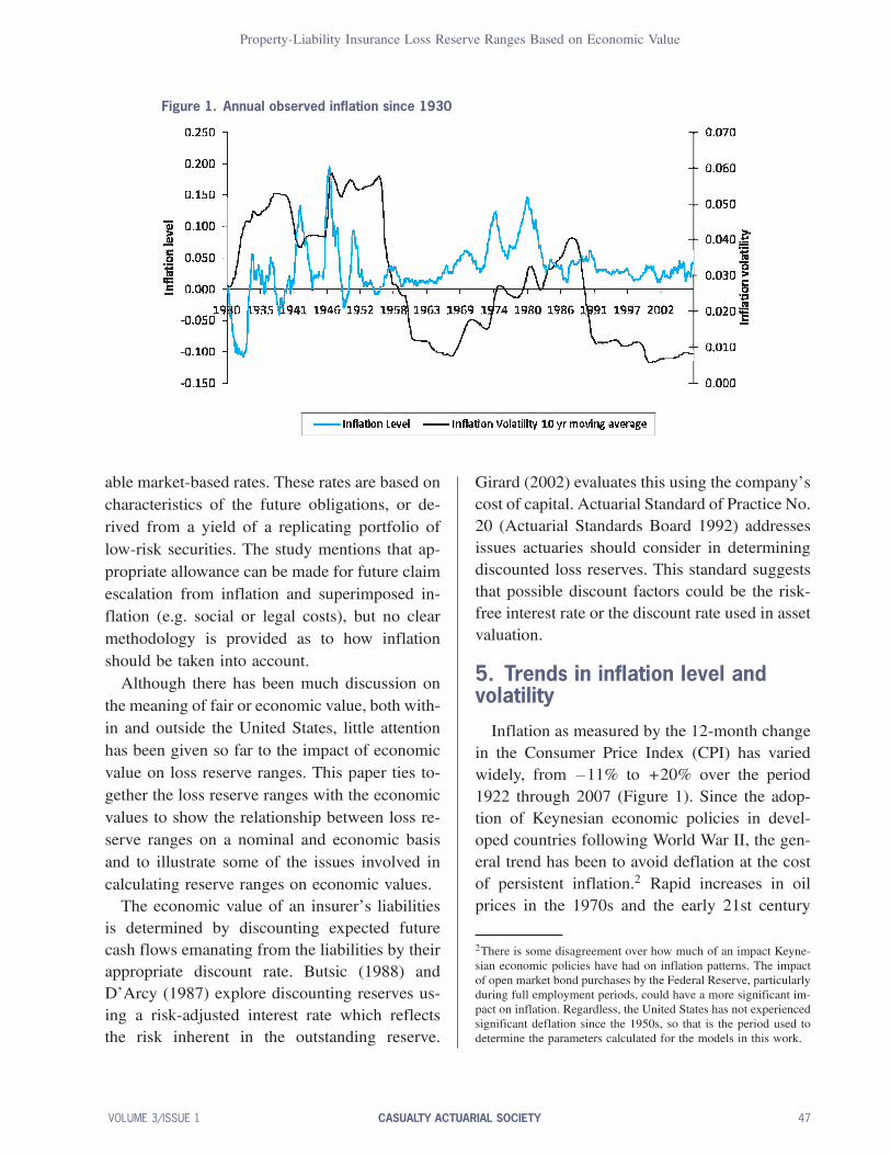
Figure 2. Annualized monthly observed inflation since 1999

have increased inflation rates. The steady depre-ciation of the dollar in recent years has also putadditional inflationary pressures on the U.S.economy. Recently, concern over the financialconsequences of the subprime mortgage crisisand credit crunch has led the U.S. Federal Re-serve to lower the discount rate to shield theeconomy from a housing slump and stabilize tur-bulence in the financial markets. Lowering inter-est rates is likely to lead to an increase in futureinflation. Oil prices have risen sharply, the dollarhas dropped to historical lows against the euroand gold prices have soared. Falling prices oflong-term government debt after the recent ratedrop suggests investors concern over inflation.Thus, the potential for inflation to increase mustbe incorporated into any financial forecast.Figure 1 shows the inflation level and the in-

flation volatility (based on a ten-year moving av-erage) since 1930. Inflation volatility, similar tointerest rate volatility in interest rate models, isthe standard deviation of the inflation rate overa one-year period. The ten-year moving averageinflation volatility is calculated based on infla-tion rates over the last 120 months. The inflationrate is determined by the CPI at the end of each

month compared to the CPI one year prior. Notethe periods of deflation that occurred during theDepression and right after World War II, and theinflation spikes of the 1940s, 1950s, 1970s, and1980s. Inflation volatility has also experiencedseveral spikes, most recently in the 1980s. Forthe last decade, volatility has been at historiclows. Figure 2 shows the same data from thepast 10 years, where there appears to be a risein both inflation and inflation volatility. On thisgraph, inflation volatility is shown on a year-by-year basis (using only the last 12 months of data)to show the recent volatility more clearly. Withthe current upward trend in inflation volatility,it is necessary to consider the possibility infla-tion volatility returning to the levels of the 1950sor the 1980s. Inflation volatility determines howaccurately we are able to predict future infla-tion trends; the greater the volatility, the lowerthe ability to forecast future inflation, and thusthe greater uncertainty on its impact on loss re-serves.

6. The modelsThe loss reserving model used in this research

invokes: a loss generation model for loss sever-ity, a loss decay model for loss payout patterns,



a two-factor Hull-White model for nominal in-terest rates, a Ornstein-Uhlenbeck model for in-flation, adjustment for correlation between thenominal interest rate and inflation, adjustment forclaims cost inflation, and a fixed claims modelfor the impact of inflation on unpaid claimsmodel. A sensitivity analysis worksheet is alsobuilt in to test the sensitivity of the parameters.

6.1. Loss generation model

The loss generation model generates aggregateclaims based on the user’s input of the num-ber of claims, choice of distribution of the claimseverity, and the mean and standard deviation ofseverity. The number of claims is assumed to beknown. The severity of claims can follow a Nor-mal, Log-normal or Pareto distribution.

6.2. Loss decay model

These losses can be settled either at a fixedtime or at a rate based on a decay model over anumber of years. If the claims are to be settled ona decaying basis, the decay model calculates theproportion of losses to be settled each year givena decay factor. For simplicity, loss severity is as-sumed to be independent of time to settlement.The decay model is of the following form:

Xt+1 = (1¡®) ¤ Xt (6.1)

where Xi is the number of claims settled in yeari, and ® is the decay factor or the proportion ofclaims settled each year.

6.3. Nominal interest rate model

A two-factor Hull-White model is used to gen-erate nominal interest rate paths. The Hull-Whitemodel uses a mean-reverting process with theshort-term real interest rate reverting to a long-term real interest rate, which is itself stochasticand reverting to a long-term average level.

drt = ·r(lt¡ rt)dt+¾rdzrdlt = ·l(¹¡ lt)dt+¾ldzl

(6.2)

where t is the time, r is the short-term rate, l isthe long-term rate, · is the mean reversion speed,¹ is the average mean reversion level, dt is thetime step, ¾ is the volatility and dz is a Wienerprocess. This model allows for negative values,which is not theoretically possible for nominalinterest rates. We impose a minimum short-termand long-term rate of 0% to adjust for this.

6.4. Inflation model

A one-factor Ornstein-Uhlenbeck model isused to generate inflation paths. The Ornstein-Uhlenbeck model uses a mean-reverting processwith the current short-term inflation reverting tothe long-term mean.

drt = ·r(¹r¡ rt)dt+¾rdzr, (6.3)

where t is the time, r is the current inflation, · isthe mean reversion speed, ¹ is the long-term in-flation mean, dt is the time step, ¾ is the volatilityand dz is a Wiener process.

6.5. Correlated nominal and realinterest rates

The short-term nominal interest rate and in-flation rates are correlated through their randomshock components. The random dz component isadjusted for a weighted average between a com-mon correlated random component and an indi-vidual random component.

dzr,nominal = ½dzcorrelated +q1¡ ½2dznominal

(6.4)

dzr,inflation = ½dzcorrelated +q1¡ ½2dzinflation

where ½ is the correlation factor between theshort-term interest rate and inflation rate, and dzare Wiener processes.

6.6. Masterson Claims Cost Index

Claim costs do not simply grow at the rate ofinflation. The Masterson Claim Cost Index mea-sures the rate at which claims costs are inflated



over time by decomposing the costs into its var-ious components and inflating each part sepa-rately (Masterson 1981; Masterson 1987; VanArk 1996; Pecora 2005). For this research, theMasterson Claim Cost Index is simplified to alinear projection of the inflation rate.

6.7. Fixed claim model

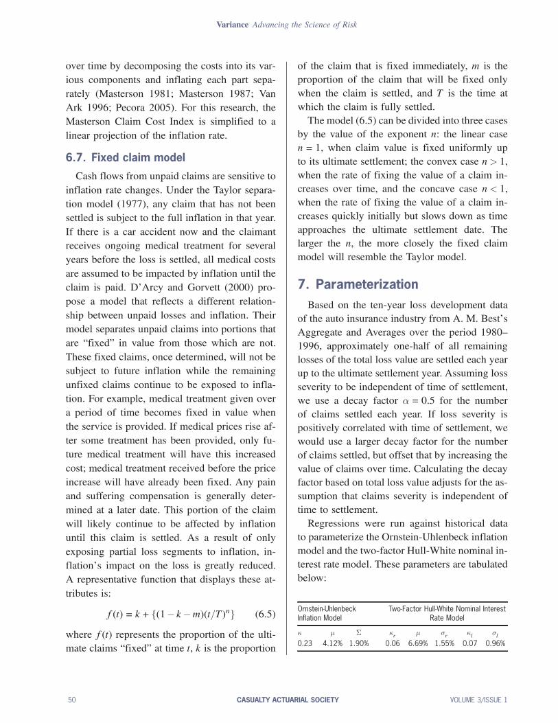
Cash flows from unpaid claims are sensitive toinflation rate changes. Under the Taylor separa-tion model (1977), any claim that has not beensettled is subject to the full inflation in that year.If there is a car accident now and the claimantreceives ongoing medical treatment for severalyears before the loss is settled, all medical costsare assumed to be impacted by inflation until theclaim is paid. D’Arcy and Gorvett (2000) pro-pose a model that reflects a different relation-ship between unpaid losses and inflation. Theirmodel separates unpaid claims into portions thatare “fixed” in value from those which are not.These fixed claims, once determined, will not besubject to future inflation while the remainingunfixed claims continue to be exposed to infla-tion. For example, medical treatment given overa period of time becomes fixed in value whenthe service is provided. If medical prices rise af-ter some treatment has been provided, only fu-ture medical treatment will have this increasedcost; medical treatment received before the priceincrease will have already been fixed. Any painand suffering compensation is generally deter-mined at a later date. This portion of the claimwill likely continue to be affected by inflationuntil this claim is settled. As a result of onlyexposing partial loss segments to inflation, in-flation’s impact on the loss is greatly reduced.A representative function that displays these at-tributes is:

f(t) = k+ f(1¡ k¡m)(t=T)ng (6.5)

where f(t) represents the proportion of the ulti-mate claims “fixed” at time t, k is the proportion

of the claim that is fixed immediately, m is theproportion of the claim that will be fixed onlywhen the claim is settled, and T is the time atwhich the claim is fully settled.The model (6.5) can be divided into three cases

by the value of the exponent n: the linear casen= 1, when claim value is fixed uniformly upto its ultimate settlement; the convex case n > 1,when the rate of fixing the value of a claim in-creases over time, and the concave case n < 1,when the rate of fixing the value of a claim in-creases quickly initially but slows down as timeapproaches the ultimate settlement date. Thelarger the n, the more closely the fixed claimmodel will resemble the Taylor model.

7. ParameterizationBased on the ten-year loss development data

of the auto insurance industry from A. M. Best’sAggregate and Averages over the period 1980—1996, approximately one-half of all remaininglosses of the total loss value are settled each yearup to the ultimate settlement year. Assuming lossseverity to be independent of time of settlement,we use a decay factor ®= 0:5 for the numberof claims settled each year. If loss severity ispositively correlated with time of settlement, wewould use a larger decay factor for the numberof claims settled, but offset that by increasing thevalue of claims over time. Calculating the decayfactor based on total loss value adjusts for the as-sumption that claims severity is independent oftime to settlement.Regressions were run against historical data

to parameterize the Ornstein-Uhlenbeck inflationmodel and the two-factor Hull-White nominal in-terest rate model. These parameters are tabulatedbelow:

Ornstein-UhlenbeckInflation Model

Two-Factor Hull-White Nominal InterestRate Model

· ¹ § ·r ¹ ¾r ·l ¾l0.23 4.12% 1.90% 0.06 6.69% 1.55% 0.07 0.96%



The Fisher formula is an equilibrium statementthat, on average, nominal rates and inflation arelinked. Sarte (1998) has found that in an envi-ronment with stochastic inflation, the Fisher for-mula is still a reasonable approximation to itsmore complete counterpart in a dynamic endow-ment environment. It is also worthy to note thatinflation is a matter of government policy ratherthan just a fact of nature; and the model shouldbe adjusted to match the current economic situ-ation.The correlation between the three-month U.S.

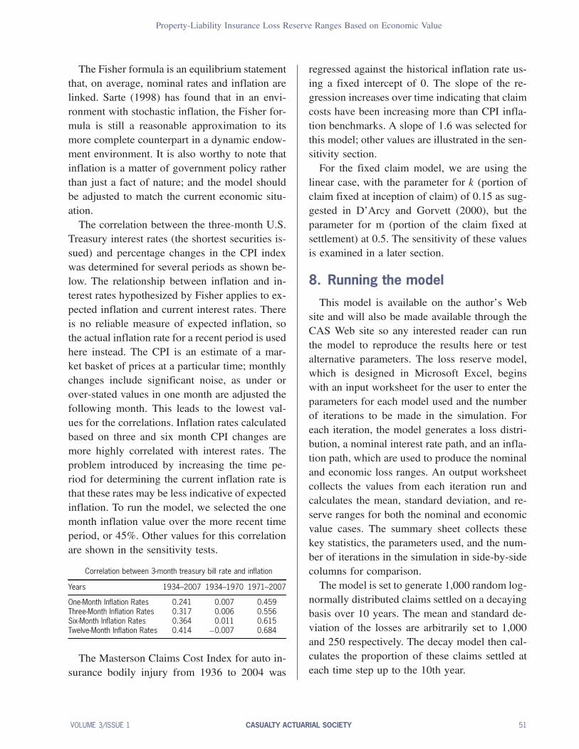
Treasury interest rates (the shortest securities is-sued) and percentage changes in the CPI indexwas determined for several periods as shown be-low. The relationship between inflation and in-terest rates hypothesized by Fisher applies to ex-pected inflation and current interest rates. Thereis no reliable measure of expected inflation, sothe actual inflation rate for a recent period is usedhere instead. The CPI is an estimate of a mar-ket basket of prices at a particular time; monthlychanges include significant noise, as under orover-stated values in one month are adjusted thefollowing month. This leads to the lowest val-ues for the correlations. Inflation rates calculatedbased on three and six month CPI changes aremore highly correlated with interest rates. Theproblem introduced by increasing the time pe-riod for determining the current inflation rate isthat these rates may be less indicative of expectedinflation. To run the model, we selected the onemonth inflation value over the more recent timeperiod, or 45%. Other values for this correlationare shown in the sensitivity tests.

Correlation between 3-month treasury bill rate and inflation

Years 1934–2007 1934–1970 1971–2007

One-Month Inflation Rates 0.241 0.007 0.459Three-Month Inflation Rates 0.317 0.006 0.556Six-Month Inflation Rates 0.364 0.011 0.615Twelve-Month Inflation Rates 0.414 ¡0:007 0.684

The Masterson Claims Cost Index for auto in-surance bodily injury from 1936 to 2004 was

regressed against the historical inflation rate us-ing a fixed intercept of 0. The slope of the re-gression increases over time indicating that claimcosts have been increasing more than CPI infla-tion benchmarks. A slope of 1.6 was selected forthis model; other values are illustrated in the sen-sitivity section.For the fixed claim model, we are using the

linear case, with the parameter for k (portion ofclaim fixed at inception of claim) of 0.15 as sug-gested in D’Arcy and Gorvett (2000), but theparameter for m (portion of the claim fixed atsettlement) at 0.5. The sensitivity of these valuesis examined in a later section.

8. Running the modelThis model is available on the author’s Web

site and will also be made available through theCAS Web site so any interested reader can runthe model to reproduce the results here or testalternative parameters. The loss reserve model,which is designed in Microsoft Excel, beginswith an input worksheet for the user to enter theparameters for each model used and the numberof iterations to be made in the simulation. Foreach iteration, the model generates a loss distri-bution, a nominal interest rate path, and an infla-tion path, which are used to produce the nominaland economic loss ranges. An output worksheetcollects the values from each iteration run andcalculates the mean, standard deviation, and re-serve ranges for both the nominal and economicvalue cases. The summary sheet collects thesekey statistics, the parameters used, and the num-ber of iterations in the simulation in side-by-sidecolumns for comparison.The model is set to generate 1,000 random log-

normally distributed claims settled on a decayingbasis over 10 years. The mean and standard de-viation of the losses are arbitrarily set to 1,000and 250 respectively. The decay model then cal-culates the proportion of these claims settled ateach time step up to the 10th year.



The generated losses are compounded at theinflation rate up to their time of settlement. Thisis the nominal, undiscounted value of losses thatinsurers are statutorily required to have as a re-serve. The interest rate model generates cumu-lative interest rate paths corresponding to eachtime period up to settlement. The nominal val-ues are then discounted back by this cumulativeinterest rate factor to obtain the economic valueof losses.For a simplified example, assume a single

claim of $1,000 (based on the price level in effectwhen the loss occurred) is settled at the end offive years, and the annual nominal interest rateis 5%. Also assume that the inflation is equal toone half of the nominal rate throughout the fiveyears, i.e., (1+5%)0:5¡ 1 = 0:0247. The nomi-nal value of the loss reserve would be $1,000 ¤(1+2:47%)5 = $1129:73. This nominal value isdiscounted back by the interest rate over the fiveyears to get the economic value $1129:73 ¤(1+5%)¡5 = $885:17. In economic terms, theamount that should be reserved for handling thisloss in today’s dollars is $885.17. Now considerwhat would happen if interest rates changedby 200 basis points up or down. If thenominal rate is 7%, inflation will be (1+7%)0:5

¡1 = 3:44%, and the nominal value and econ-omic value will be $1,184.30 and $844.39, re-spectively. If the nominal rate is 3%, inflationwill be (1+3%)0:5¡ 1 = 1:49%, and the nominalvalue and economic value will be $1,076.70 and$928.77, respectively. Thus, the nominal valuerange will be $1,129:73¡ $1,076:70 = $53:03,and the economic value range will be $928:77¡$885:17 = $43:60. The economic value range isonly 82% of the nominal value range. This is asimplified example illustrating three possible val-ues of one claim, assuming inflation is propor-tional to the nominal rate. Under circumstanceslike this, the reserve range based on economicvalues will be smaller than reserve ranges basedon nominal values.

Now consider a book of 1,000 such claims andallow inflation to vary independently of nominalrates. The average nominal and economic val-ues of these 1,000 claims are determined basedon the interest rate and inflation paths generatedfor that simulation. This claims generation pro-cess is repeated for 10,000 simulations, with eachsimulation generating a different interest rate andinflation path for the 1,000 claims of that itera-tion, and a distribution of nominal and economicloss reserves are generated. The mean, standarddeviation, minimum, maximum, as well as the5, 25, 75, and 95 percentile for both the nomi-nal and economic loss ranges are determined andcompared. A confidence interval ratio is com-puted by dividing the economic range confidenceinterval by the nominal range confidence inter-val for both a 50 percent (ranging from the 25thpercentile to the 75th percentile) and 90 percent(ranging from the 5th percentile to the 95th per-centile) confidence interval. These ratios will beused as an indicator of the difference in volatilitybetween the economic loss ranges and nominalloss ranges.

9. Results

To examine the effects of how the confidenceinterval is affected by changes in the assump-tions, 10,000 simulations were run for each ofthe following cases. As the 50 percent and 90percent confidence interval ratios turn out to befairly close, only the 90 percent confidence inter-val ratios are shown here. The complete resultsare available from the authors. A monthly timestep was chosen to provide a close approxima-tion to continuous interest rate models, as infla-tion data are only available monthly.

9.1. Taylor Model versus Fixed ClaimModel

The first example is based on running themodel with the following assumptions: 1) month-ly time step, 2) a correlation factor of 45% be-



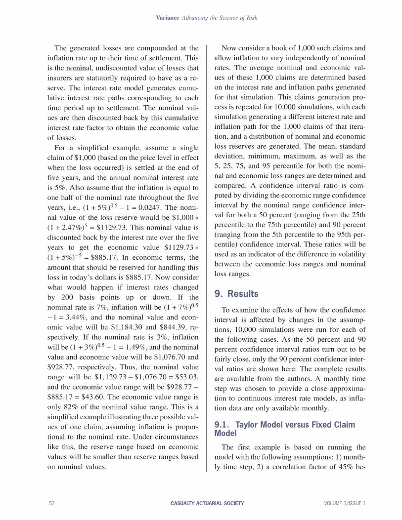
Figure 3. Taylor (blue) vs. fixed claim (base case, black)

Table 1. Summary values for Taylor model (A) and fixed claum model (B)

Standard Percentiles 90% Confidence ConfidenceCase Mean Deviation 5th 95th Interval Interval Ratio

A—nominal 1097016.132 40241.05642 1033427.88 1165584.07 132156.19 94.15%A—economic 1052020.311 37895.67459 991242.95 1115669.17 124426.22B—nominal 1063890.967 28761.53405 1018485.77 1112663.88 94178.11 101.78%B—economic 1021643.248 29192.93832 974956.77 1070811.09 95854.32

tween the nominal interest rate and inflation,3) claims inflation rate of 1.6 times the generalinflation rate, 4) the Taylor separation model.This is Case A. Figure 3 shows the distribu-tions for both the nominal and economic values;as would be expected, the economic values arelower than the nominal values, but the economicreserve range turns out to be approximately 94%of the nominal loss reserve range. Discountingdoes not reduce the ranges much. The second ex-ample, Case B, incorporate the fixed loss modelsuggested by D’Arcy and Gorvett (2000). In thiscase there is a significant decrease in the standarddeviation of the nominal and economic reservesbecause losses are only partially exposed to in-flation throughout its time to settlement. (Fixedclaims are no longer affected by future inflation.)In this case the confidence interval ratio (the eco-nomic range divided by the nominal range) is

102%. Discounting reserves reduces the level ofthe reserves, but not the range. We will treatCase B as the base case and examine additionalchanges in relationship to this case. The meanvalues, standard deviations, 5th and 95th per-centiles and the 90% confidence intervals are forboth nominal and economic values for Case Aand Case B are shown on Table 1.

9.2. High claims cost inflation

The relationship between claims inflation andthe general inflation rate has varied widely overthe period 1936 through 2004, but claims infla-tion is consistently higher than overall inflation.One reason for this is that medical costs are a ma-jor component of auto insurance claims and thesehave consistently outpaced general inflation. Thethird-party payer relationship also reduces resis-tance to cost increases, leading to higher infla-



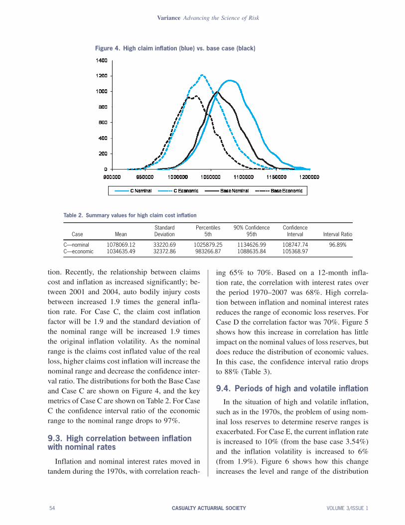
Figure 4. High claim inflation (blue) vs. base case (black)

Table 2. Summary values for high claim cost inflation


C—nominal 1078069.12 33220.69 1025879.25 1134626.99 108747.74 96.89%C—economic 1034635.49 32372.86 983266.87 1088635.84 105368.97

tion. Recently, the relationship between claimscost and inflation as increased significantly; be-tween 2001 and 2004, auto bodily injury costsbetween increased 1.9 times the general infla-tion rate. For Case C, the claim cost inflationfactor will be 1.9 and the standard deviation ofthe nominal range will be increased 1.9 timesthe original inflation volatility. As the nominalrange is the claims cost inflated value of the realloss, higher claims cost inflation will increase thenominal range and decrease the confidence inter-val ratio. The distributions for both the Base Caseand Case C are shown on Figure 4, and the keymetrics of Case C are shown on Table 2. For CaseC the confidence interval ratio of the economicrange to the nominal range drops to 97%.

9.3. High correlation between inflationwith nominal rates

Inflation and nominal interest rates moved intandem during the 1970s, with correlation reach-

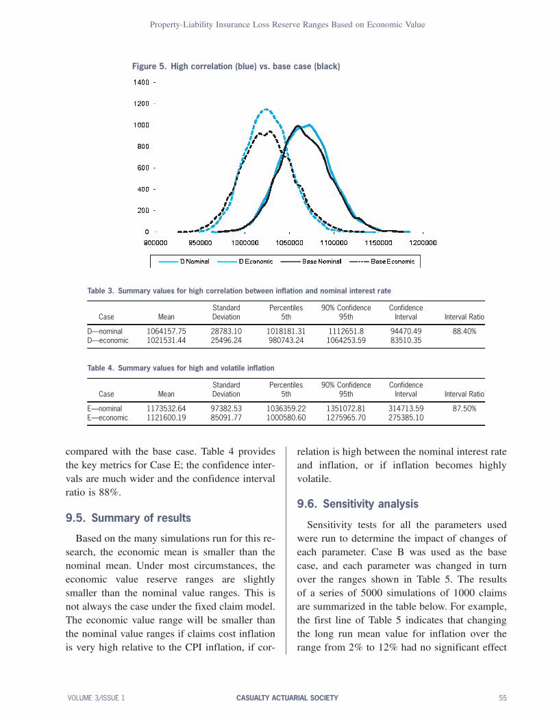
ing 65% to 70%. Based on a 12-month infla-tion rate, the correlation with interest rates overthe period 1970—2007 was 68%. High correla-tion between inflation and nominal interest ratesreduces the range of economic loss reserves. ForCase D the correlation factor was 70%. Figure 5shows how this increase in correlation has littleimpact on the nominal values of loss reserves, butdoes reduce the distribution of economic values.In this case, the confidence interval ratio dropsto 88% (Table 3).

9.4. Periods of high and volatile inflation

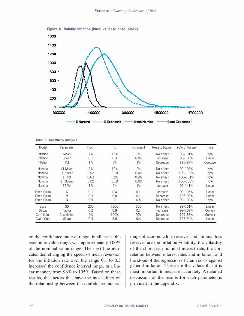
In the situation of high and volatile inflation,such as in the 1970s, the problem of using nom-inal loss reserves to determine reserve ranges isexacerbated. For Case E, the current inflation rateis increased to 10% (from the base case 3.54%)and the inflation volatility is increased to 6%(from 1.9%). Figure 6 shows how this changeincreases the level and range of the distribution



Figure 5. High correlation (blue) vs. base case (black)

Table 3. Summary values for high correlation between inflation and nominal interest rate


D—nominal 1064157.75 28783.10 1018181.31 1112651.8 94470.49 88.40%D—economic 1021531.44 25496.24 980743.24 1064253.59 83510.35

Table 4. Summary values for high and volatile inflation


E—nominal 1173532.64 97382.53 1036359.22 1351072.81 314713.59 87.50%E—economic 1121600.19 85091.77 1000580.60 1275965.70 275385.10

compared with the base case. Table 4 providesthe key metrics for Case E; the confidence inter-vals are much wider and the confidence intervalratio is 88%.

9.5. Summary of results

Based on the many simulations run for this re-search, the economic mean is smaller than thenominal mean. Under most circumstances, theeconomic value reserve ranges are slightlysmaller than the nominal value ranges. This isnot always the case under the fixed claim model.The economic value range will be smaller thanthe nominal value ranges if claims cost inflationis very high relative to the CPI inflation, if cor-

relation is high between the nominal interest rateand inflation, or if inflation becomes highlyvolatile.

9.6. Sensitivity analysis

Sensitivity tests for all the parameters usedwere run to determine the impact of changes ofeach parameter. Case B was used as the basecase, and each parameter was changed in turnover the ranges shown in Table 5. The resultsof a series of 5000 simulations of 1000 claimsare summarized in the table below. For example,the first line of Table 5 indicates that changingthe long run mean value for inflation over therange from 2% to 12% had no significant effect



Figure 6. Volatile inflation (blue) vs. base case (black)

Table 5. Sensitivity analysis

Model Parameter From To Increment Results (ratios) 90% CI Range Type

Inflation Mean 2% 12% 2% No effect 98–101% N/AInflation Speed 0.1 0.3 0.05 Increase 96–105% LinearInflation Vol 1% 8% 1% Decrease 115–87% Concave

Nominal LT Mean 2% 10% 2% No effect 99–103% N/ANominal LT Speed 0.02 0.10 0.02 No effect 100–102% N/ANominal LT Vol 0.6% 1.2% 0.2% No effect 100–101% N/ANominal ST Speed 0.02 0.10 0.02 No effect 100–103% N/ANominal ST Vol 1% 5% 1% Increase 96–141% Linear

Fixed Claim K 0.1 0.4 0.1 Increase 99–105% LinearFixed Claim M 0.3 0.8 0.1 Decrease 106–98% LinearFixed Claim N 0.5 2 0.5 No effect 99–102% N/A

Loss SD 200 1000 200 No effect 98–101% LinearDecay Factor 0.2 0.8 0.1 Increase 92–102% Convex

Correlation Correlation 0% 100% 20% Decrease 109–58% ConvexClaim Cost Slope 0.4 2.0 0.4 Decrease 127–94% Linear

on the confidence interval range; in all cases, theeconomic value range was approximately 100%of the nominal value range. The next line indi-cates that changing the speed of mean reversionfor the inflation rate over the range 0.1 to 0.3increased the confidence interval range, in a lin-ear manner, from 96% to 105%. Based on theseresults, the factors that have the most effect onthe relationship between the confidence interval

range of economic loss reserves and nominal lossreserves are the inflation volatility, the volatilityof the short-term nominal interest rate, the cor-relation between interest rates and inflation, andthe slope of the regression of claim costs againstgeneral inflation. These are the values that it ismost important to measure accurately. A detaileddiscussion of the results for each parameter isprovided in the appendix.



10. Conclusion

Property-liability insurance companies havetraditionally valued their loss reserves on a nomi-nal basis due to statutory requirements. These re-quirements do not reflect the economic value ofthe future payments and distort insurance com-pany financial statements. Nominal loss reservesoverstate the impact of inflation on reserves,though only slightly under the current economicenvironment, as they ignore the relationship be-tween inflation and nominal interest rates. Theeconomic impact on loss reserves of a change ininflation is commonly offset by a similar shift inthe nominal interest rate and by the high claimscost inflation. Loss reserve ranges based on nom-inal values accentuate this problem. Recent pro-posals advocate the use of fair value account-ing for loss reserves, which would replace nomi-nal values with economic values. In this studya loss reserve model was developed to quan-tify the uncertainty introduced by stochastic in-terest rates and inflation rates and to comparereserve ranges based on nominal and economicvalues. The results demonstrate a variety of sce-narios under which the reserve ranges based oneconomic values can be either smaller or largerthan the nominal value ranges. However, use ofeconomic values for loss reserves would betterserve the insurance industry and its regulators.The key reason for encouraging the use of eco-nomic value ranges is that they properly reflectthe true measure of the uncertainty involved inloss reserving. An additional benefit is that theranges are smaller in many circumstances, andthe current economic environment seems to bemoving toward those situations. Claim cost in-flation and the level and volatility of inflationappear to have an upward trend. Economic valuereserves would provide more credible values ofthe cost and uncertainty of future loss payments,and in the cases mentioned before, would have asmaller confidence interval range.

Acknowledgment

The authors wish to thank the Actuarial Foun-dation and the Casualty Actuarial Society for fi-nancial support for this research.

ReferencesActuarial Standards Board, Actuarial Standard of PracticeNo. 20, “Discounting of Property and Casualty Loss andLoss Adjustment Expense Reserves,” April 1992, http://www.actuarialstandardsboard.org/pdf/asops/asop020037.pdf.

Ahlgrim, Kevin, Stephen P. D’Arcy, and RichardW. Gorvett,“The Effective Duration and Convexity of Liabilities forProperty-Liability Insurers Under Stochastic InterestRates,” Geneva Papers on Risk and Insurance Theory 29:1,2004, pp. 75—108.

Ahlgrim, Kevin, Stephen P. D’Arcy, and RichardW. Gorvett,“Modeling Financial Scenarios: A Framework for the Ac-tuarial Profession,” Proceedings of the Casualty ActuarialSociety 92, 2005, pp. 60—98.

American Academy of Actuaries, “Fair Valuation of Insur-ance Liabilities: Principles and Methods,” 2002, http://www.actuary.org/pdf/finreport/fairval sept02.pdf.

Australian Prudential Regulation Authority, GPS 310, “Au-dit and Actuarial Reporting and Valuation,” February2006, http://www.apra.gov.au/General/upload/GPS-310-Audit-and-Actuarial-Valuation.pdf.

Barnett, Glen, and Ben Zehnwirth, “Best Estimates for Re-serves,” Casualty Actuarial Society Forum, Fall 1998, pp.1—54.

Berquist, James R., and Richard E. Sherman, “Loss Re-serve Adequacy. Testing: A Comprehensive, SystematicApproach,” Proceedings of the Casualty Actuarial Society64, 1977, pp. 123—184.

Best’s Aggregates and Averages, Property-Casualty, A. M.Best, selected years.

Butsic, Robert P., “The Effect of Inflation on Losses andPremiums for Property-Liability Insurers,” Casualty Ac-tuarial Society Discussion Paper Program, 1981, pp. 58—102.

Butsic, Robert P., “Determining the Proper Interest Rate forLoss Reserve Discounting: An Economic Approach,” Ca-sualty Actuarial Society Discussion Paper Program, Fall1988, pp. 147—186.

Casualty Actuarial Society, “Fair Value of P&C Liabili-ties: Practical Implications,” 2004, http://www.casact.org/pubs/fairvalue/FairValueBook.pdf.

Casualty Actuarial Society, “Task Force on Actuarial Credi-bility,” 2005, http://www.casact.org/about/reports/tfacrpt.pdf.

CAS Working Party on Quantifying Variability in ReserveEstimates, Casualty Actuarial Forum, Fall 2005, pp. 29—146.



CEA Information Papers, “Solvency II: Understanding theprocess,” 2007, http://www.cea.assur.org/cea/download/publ/article257.pdf.

D’Arcy, Stephen P., “Revisions in Loss Reserving Tech-niques Necessary to Discount Property-Liability Loss Re-serves” Proceedings of the Casualty Actuarial Society 74,1987, pp. 75—100.

D’Arcy, Stephen and Richard W. Gorvett, “Measuring theInterest Rate Sensitivity of Loss Reserves,” Proceedingsof the Casualty Actuarial Society 87, 2000, pp. 365—400,http://www.casact.org/pubs/proceed/proceed00/00365.pdf.

Fisher, Irving, The Theory of Interest, New York: Macmillan,1930, Ch. 19.

Girard, Luke N., “An Approach to Fair Valuation of Insur-ance Liabilities Using the Firm’s Cost of Capital,” NorthAmerican Actuarial Journal 6:2, 2002, pp. 18—46.

Hettinger, Thomas, “What Reserve Ranges Makes YouComfortable,” Midwestern Actuarial Forum Fall Meet-ing, 2006, http://www.casact.org/affiliates/maf/0906/hettinger.pdf.

Hilsenrath, Jon, “WhenNervesGet Short, CreditGets Tight,”Wall Street Journal, February 19, 2008, p. C 1.

Institute of Actuaries of Australia, Professional Standard300, “Valuations of General Insurance Claims,” August2007, http://www.actuaries.asn.au/NR/rdonlyres/0A2FF56A-1489-404F-BBF3-CB7D916B269E/2908/PS300ApprovedbyCouncil28August2008.pdf.

Kirschner, Gerald S., Colin Kerley, and Belinda Isaacs,“Two Approaches to Calculating Correlated Reserve In-dications Across Multiple Lines of Business,” CasualtyActuarial Society Forum, Fall 2002, pp. 211—246.

Mack, Thomas, “Distribution-free Calculation of the Stan-dard Error of Chain Ladder Reserve Estimates,” ASTINBulletin 23, 1993, pp. 213—225.

Masterson, Norton E., “Property-Casualty Insurance Infla-tion Indexes: Communicating with the Public,” CasualtyActuarial Society Discussion Paper Program, 1981, pp.344—370.

Masterson, Norton E., “Economic Factors in Property/Casu-alty Insurance Claims Costs,” Best’s Review, June 1987,pp. 50—52.

McClenahan, Charles L., “Estimation and Application ofRanges of Reasonable Estimates,” Casualty Actuarial So-ciety Forum, Fall, 2003, pp. 213—230.

Miller, Mary Frances, “Are You Part of the Solution,”Actuarial Review 31:2, February 2004, http://www.casact.org/pubs/actrev/feb04/pres.htm.

Murphy, Daniel M., “Unbiased Loss Development Factors,”Proceedings of the Casualty Actuarial Society 81, 1994,pp. 154—222.

Narayan, Prakash, and Thomas V. Warthen, “A Compara-tive Study of the Performance of Loss Reserving Meth-ods Through Simulation,” Casualty Actuarial SocietyForum, Summer 1997, pp. 175—196.

Patel, Chandu C., and Alfred Raws, III, “Statistical Mod-eling Techniques for Reserve Ranges: A Simulation Ap-proach,” Casualty Actuarial Society Forum, Fall 1998,pp. 229—255.

Pecora, Jeremy P., “Setting the Pace,” Best’s Review, Jan-uary 2005, pp. 87—88.

Richards, William F., “Evaluating the Impact of Inflation onLoss Reserves,” Casualty Actuarial Society DiscussionPaper Program, Fall 1981, pp. 384—400.

Sarte, Pierre-Daniel G., “Fisher’s Equation and the Infla-tion Risk Premium in a Simple Endowment Economy,”Economic Quarterly 84, Fall 1998, pp. 53—72.

Shapland, Mark R., “Loss Reserve Estimates: A StatisticalApproach for Determining ‘Reasonableness’,” CasualtyActuarial Society Forum, Fall 2003, pp. 321—360.

Standard & Poor’s, “Insurance Actuaries: A Crisis of Cred-ibility,” 2003.

Taylor, Greg C., “Separation of Inflation and Other Effectsfrom the Distribution of Non-Life Insurance Claim De-lays,” ASTIN Bulletin 9, 1977, pp. 219—230.

Van Ark, William R., “Gap in Claims Cost Trends Contin-ues to Narrow,” Best’s Review, March 1996, pp. 22—23.

Venter, Gary G., “Refining Reserve Runoff Ranges,” ASTINColloquium, Orlando, FL, 2007.

Wiser, Ronald F., Jo Ellen Cockley, and Andrea Gardner,“Loss Reserving” Foundations of Casualty Actuarial Sci-ence, Casualty Actuarial Society, 2001, Ch. 5, pp. 197—285.

Zehnwirth, Ben, “Probabilistic Development Factor Modelswith Applications to Loss Reserve Variability, PredictionIntervals, and Risk Based Capital,” Casualty ActuarialSociety Forum, Spring 1994, pp. 447—606.

Appendix—Sensitivity Analysis

For any stochastic model, the number simula-tions run in a study is an important determinantof the consistency and accuracy of the results.Running too few simulations can lead to widelyvarying results and erroneous conclusions. Toomany simulations, on the other hand, waste timeand computer resources. For simple models, sta-tistical analysis can be used to determine the ap-propriate number of simulations to run. However,in this project, which consists of five separatestochastic models, that approach is not feasible.



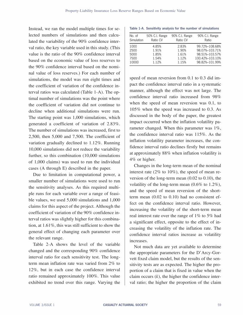
Instead, we ran the model multiple times for se-

lected numbers of simulations and then calcu-

lated the variability of the 90% confidence inter-

val ratio, the key variable used in this study. (Thisvalue is the ratio of the 90% confidence interval

based on the economic value of loss reserves to

the 90% confidence interval based on the nomi-nal value of loss reserves.) For each number of

simulations, the model was run eight times and

the coefficient of variation of the confidence in-terval ratios was calculated (Table 1-A). The op-

timal number of simulations was the point where

the coefficient of variation did not continue todecline when additional simulations were run.

The starting point was 1,000 simulations, which

generated a coefficient of variation of 2.83%.

The number of simulations was increased, first to2,500, then 5,000 and 7,500. The coefficient of

variation gradually declined to 1.12%. Running

10,000 simulations did not reduce the variabilityfurther, so this combination (10,000 simulations

of 1,000 claims) was used to run the individual

cases (A through E) described in the paper.Due to limitation in computational power, a

smaller number of simulations were used to run

the sensitivity analyses. As this required multi-

ple runs for each variable over a range of feasi-ble values, we used 5,000 simulations and 1,000

claims for this aspect of the project. Although the

coefficient of variation of the 90% confidence in-terval ratios was slightly higher for this combina-

tion, at 1.61%, this was still sufficient to show the

general effect of changing each parameter overthe relevant range.

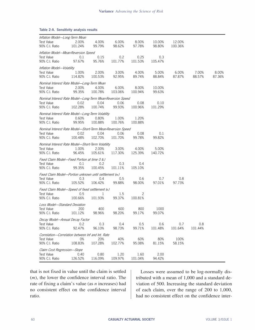
Table 2-A shows the level of the variable

changed and the corresponding 90% confidenceinterval ratio for each sensitivity test. The long-

term mean inflation rate was varied from 2% to

12%, but in each case the confidence interval

ratio remained approximately 100%. This valueexhibited no trend over this range. Varying the

Table 1-A. Sensitivity analysis for the number of simulations

No. of 50% C.I. Range 90% C.I. Range 90% C.I. RangeSimulation Ratio CV Ratio CV Ratio

1000 4.85% 2.83% 99.72%–108.68%2500 1.91% 1.90% 98.07%–103.71%5000 1.85% 1.61% 98.51%–103.57%7500 1.54% 1.12% 100.42%–103.10%10000 1.12% 1.15% 98.82%–101.99%

speed of mean reversion from 0.1 to 0.3 did im-pact the confidence interval ratio in a systematicmanner, although the effect was not large. Theconfidence interval ratio increased from 98%when the speed of mean reversion was 0.1, to105% when the speed was increased to 0.3. Asdiscussed in the body of the paper, the greatestimpact occurred when the inflation volatility pa-rameter changed. When this parameter was 1%,the confidence interval ratio was 115%. As theinflation volatility parameter increases, the con-fidence interval ratio declines firstly but remainsat approximately 88% when inflation volatility is4% or higher.Changes in the long-term mean of the nominal

interest rate (2% to 10%), the speed of mean re-version of the long-term mean (0.02 to 0.10), thevolatility of the long-term mean (0.6% to 1.2%),and the speed of mean reversion of the short-term mean (0.02 to 0.10) had no consistent ef-fect on the confidence interval ratio. However,increasing the volatility of the short-term meanreal interest rate over the range of 1% to 5% hada significant effect, opposite to the effect of in-creasing the volatility of the inflation rate. Theconfidence interval ratios increase as volatilityincreases.Not much data are yet available to determine

the appropriate parameters for the D’Arcy-Gor-vett fixed claim model, but the results of the sen-sitivity tests are as expected. The higher the pro-portion of a claim that is fixed in value when theclaim occurs (k), the higher the confidence inter-val ratio; the higher the proportion of the claim



Table 2-A. Sensitivity analysis results

Inflation Model—Long-Term MeanTest Value 2.00% 4.00% 6.00% 8.00% 10.00% 12.00%90% C.I. Ratio 101.24% 99.79% 98.62% 97.78% 98.80% 100.36%

Inflation Model—Mean-Reversion SpeedTest Value 0.1 0.15 0.2 0.25 0.390% C.I. Ratio 97.67% 95.76% 101.77% 101.53% 105.47%

Inflation Model—VolatilityTest Value 1.00% 2.00% 3.00% 4.00% 5.00% 6.00% 7.00% 8.00%90% C.I. Ratio 114.82% 100.53% 92.95% 89.74% 88.84% 87.87% 88.57% 87.36%

Nominal Interest Rate Model—Long-Term MeanTest Value 2.00% 4.00% 6.00% 8.00% 10.00%90% C.I. Ratio 99.35% 100.78% 103.06% 100.94% 99.63%

Nominal Interest Rate Model—Long-Term Mean-Reversion SpeedTest Value 0.02 0.04 0.06 0.08 0.1090% C.I. Ratio 102.28% 100.74% 99.93% 100.96% 101.29%

Nominal Interest Rate Model—Long-Term VolatilityTest Value 0.60% 0.80% 1.00% 1.20%90% C.I. Ratio 99.95% 100.88% 100.76% 100.88%

Nominal Interest Rate Model—Short-Term Mean-Reversion SpeedTest Value 0.02 0.04 0.06 0.08 0.190% C.I. Ratio 100.48% 102.70% 101.70% 99.78% 99.82%

Nominal Interest Rate Model—Short-Term VolatilityTest Value 1.00% 2.00% 3.00% 4.00% 5.00%90% C.I. Ratio 96.45% 105.61% 117.30% 125.39% 140.72%

Fixed Claim Model—Fixed Portion at time 0 (k)Test Value 0.1 0.2 0.3 0.490% C.I. Ratio 99.35% 100.45% 101.11% 105.10%

Fixed Claim Model—Portion unknown until settlement (m)Test Value 0.3 0.4 0.5 0.6 0.7 0.890% C.I. Ratio 105.52% 106.42% 99.88% 98.00% 97.01% 97.73%

Fixed Claim Model—Speed of fixed settlement (n)Test Value 0.5 1 1.5 290% C.I. Ratio 100.66% 101.93% 99.37% 100.81%

Loss Model—Standard DeviationTest Value 200 400 600 800 100090% C.I. Ratio 101.12% 98.96% 98.20% 99.17% 99.07%

Decay Model—Annual Decay FactorTest Value 0.2 0.3 0.4 0.5 0.6 0.7 0.890% C.I. Ratio 92.47% 96.10% 98.73% 99.71% 101.48% 101.64% 101.44%

Correlation—Correlation between Inf and Int. RateTest Value 0% 20% 40% 60% 80% 100%90% C.I. Ratio 108.83% 107.28% 102.77% 95.08% 81.15% 58.15%

Claim Cost Regression—SlopeTest Value 0.40 0.80 1.20 1.60 2.0090% C.I. Ratio 126.52% 116.09% 109.97% 101.04% 94.42%

that is not fixed in value until the claim is settled(m), the lower the confidence interval ratio. Therate of fixing a claim’s value (as n increases) hadno consistent effect on the confidence intervalratio.

Losses were assumed to be log-normally dis-tributed with a mean of 1,000 and a standard de-viation of 500. Increasing the standard deviationof each claim, over the range of 200 to 1,000,had no consistent effect on the confidence inter-



val ratio. Changing the decay factor represent-ing what portion of unsettled claims were set-tled each year had a slight impact on the confi-dence interval range; a higher decay factor ledto a higher confidence interval range. Changingthe correlation between the inflation rate and thenominal interest rate from 0% to 100% had a sig-nificant impact on the confidence interval ratio.The higher the correlation, the lower the confi-dence interval ratio. Increasing the slope in theclaim cost regression formula over the range of0.4 to 2.0 also decreased the confidence intervalratio.

The purpose of the sensitivity analysis is to in-dicate which of the many parameters used in thismodel have the greatest impact on the results andthe conclusions of this paper. In almost all cases,the conclusion that the use of economic valuesto determine loss reserves would lead to smallerreserve ranges is supported. Attention should befocused on measuring the parameters with thegreatest impact on determining loss reserves andtheir ranges under either nominal or economicvalues. Thus, measures of interest rate and in-flation volatility and the fixed claim parametersshould be studied closely.


property-liability insurance loss reserve ranges based on ... · interest rate and inflation...

Documents