propeller scour analysis - canada.ca · this means that ship and tug propeller sediment scour...

Appendix G.16 Hatch Report – Pacific NorthWest LNG LNG Jetty Propeller Scour Analysis

Pacific Northwest LNG - LNG Jetty Propeller Scour Analysis - December 11, 2014

H345670-0000-12-124-0009, Rev. 1 Page i

© Hatch 2014 All rights reserved, including all rights relating to the use of this document or its contents.

Pacific Northwest LNG LNG Jetty

Propeller Scour Analysis

2014-12-11 1 Approved for

Use L. Absalonsen O. Sayao O. Sayao

Date Rev. Status Prepared By Checked By Approved By Approved By

Client


H345670-0000-12-124-0009, Rev. 1 Page ii


Table of Contents

1. Introduction .................................................................................................................................... 1

2. Simulations ..................................................................................................................................... 1

3. PNW LNG Design Vessels ............................................................................................................. 2

4. Input Data for Modelling Study ..................................................................................................... 4

4.1 Bathymetry .......................................................................................................................... 4

4.2 Tides and Water Levels ...................................................................................................... 4

4.3 Sediments ........................................................................................................................... 5

4.4 Model Input Parameters ...................................................................................................... 7

4.5 LNG Vessel Manoeuvres and Paths ................................................................................... 8 4.5.1 Case 1: Berthing with Bows North ......................................................................... 8 4.5.2 Case 2: Berthing with Bows South....................................................................... 10

5. Velocity Plumes and Scour ......................................................................................................... 11

5.1 LNG Propeller Wash Plume .............................................................................................. 11

5.2 VSP Tugs Propeller Wash Plume ..................................................................................... 12

6. Hydrodynamic Modelling ............................................................................................................ 14

6.1 Model Description ............................................................................................................. 14

6.2 Storm Simulation ............................................................................................................... 14

7. Sedimentation Fate Modelling .................................................................................................... 17

7.1 Model Description ............................................................................................................. 17

7.2 Sensitivity of the Eroded Volumes .................................................................................... 17

7.3 Volumes Eroded during the Manoeuvres ......................................................................... 17

7.4 Trap locations and Total Suspended Solids Measurements ............................................ 18

7.5 TSS Threshold .................................................................................................................. 19

8. Propeller Scour Results .............................................................................................................. 19

8.1 Case 1: Berthing with Bows North .................................................................................... 20

8.2 Case 2: Berthing with Bows South .................................................................................... 22

9. Conclusions .................................................................................................................................. 26

List of Tables

Table 4-1: Hydrographic Tide and Chart Datum at Port Edward, BC ........................................................... 4 Table 4-2: Hydrographic tide and Chart Datum at Prince Rupert, BC .......................................................... 4 Table 4-3: Model input parameters ............................................................................................................... 8 Table 7-1: Sediment eroded during the simulation periods ........................................................................ 17


H345670-0000-12-124-0009, Rev. 1 Page iii


List of Figures Figure 1-1: Location of the proposed PNW LNG terminal ............................................................................ 1 Figure 2-1: Numerical grid for the CMS Flow and PTM models ................................................................... 2 Figure 3-1: Typical views of an VS Tug (source: Østensjø and Voith Schneider) ........................................ 3 Figure 4-1: Water level probability of exceedance; Prince Rupert station, Jan 1909 to Mar 2014 ............... 5 Figure 4-2: Particle size distribution MEG 001 sample (614887-1000-41ER-0001-Appendix B) ................. 6 Figure 4-3: Grain size scales and soil classification systems (source: USACE, 1984) ................................ 7 Figure 4-4: Arrival path for LNGC berthing with bow North .......................................................................... 9 Figure 4-5: Departure path for LNGC berthing with bow North (red LNGC indicates the location where LNG propulsion via Dead Slow ahead starts on depths greater than 30 m) .............................................. 10 Figure 5-1: Bed shear stress induced by LNGC as a function of propeller axis distance .......................... 11 Figure 5-2: Calculated velocity plume at the propeller depth for a typical LNGC ....................................... 12 Figure 5-3: Calculated velocity plume at the seabed (-30 m CD) for a typical LNGC ................................ 12 Figure 5-4: VSP velocity profile at the centerline after 60 s of simulation (modified from Robert Allan Ltd.) .................................................................................................................................................................... 12 Figure 5-5: VSP velocity 0.5 m above the bottom after 60 s of simulation (modified from Robert Allan Ltd.) .................................................................................................................................................................... 13 Figure 6-1: Hydrodynamic conditions in the first 6 hours after a spring tide ............................................... 15 Figure 6-2: Hydrodynamic conditions from 8 hours to 14 hours after a spring tide .................................... 16 Figure 7-1: Tidal elevations assumed to calculate the volume scoured by the vessels arriving and departing the terminal. Tides measured at Prince Rupert station .............................................................. 18 Figure 7-2: Location of the virtual traps measuring TSS concentration on Flora Bank .............................. 19 Figure 8-1: TSS concentration above background levels for Traps 25 and 26 (Case 1) ........................... 20 Figure 8-2: Sediment deposition pattern (mm) after 1 month of simulation (Case 1) ................................. 21 Figure 8-3: TSS concentrations above background level after one LNGC manoeuvre (4 hours; Case 1). 22 Figure 8-4: TSS concentration above background levels for Traps 25 and 26 (Case 2) ........................... 23 Figure 8-5: Sediment deposition pattern (mm) after 1 month of simulation (Case 2) ................................. 24 Figure 8-6: TSS concentrations above background level after one LNGC manoeuvre (4 hours; Case 2). 25

H345670-0000-12-124-0009, Rev. 1 Page 1


1. Introduction

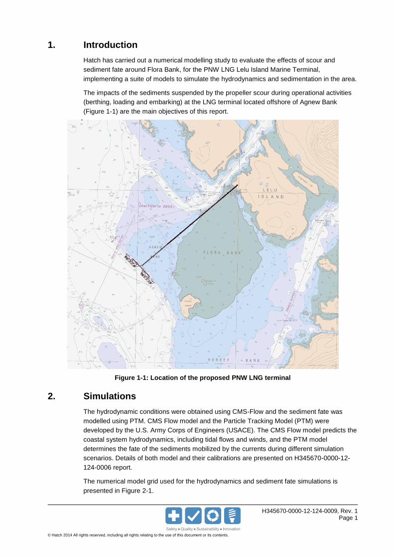
Hatch has carried out a numerical modelling study to evaluate the effects of scour and

sediment fate around Flora Bank, for the PNW LNG Lelu Island Marine Terminal,

implementing a suite of models to simulate the hydrodynamics and sedimentation in the area.

The impacts of the sediments suspended by the propeller scour during operational activities

(berthing, loading and embarking) at the LNG terminal located offshore of Agnew Bank

(Figure 1-1) are the main objectives of this report.

Figure 1-1: Location of the proposed PNW LNG terminal

2. Simulations

The hydrodynamic conditions were obtained using CMS-Flow and the sediment fate was

modelled using PTM. CMS Flow model and the Particle Tracking Model (PTM) were

developed by the U.S. Army Corps of Engineers (USACE). The CMS Flow model predicts the

coastal system hydrodynamics, including tidal flows and winds, and the PTM model

determines the fate of the sediments mobilized by the currents during different simulation

scenarios. Details of both model and their calibrations are presented on H345670-0000-12-

124-0006 report.

The numerical model grid used for the hydrodynamics and sediment fate simulations is

presented in Figure 2-1.

H345670-0000-12-124-0009, Rev. 1 Page 2


Figure 2-1: Numerical grid for the CMS Flow and PTM models

3. PNW LNG Design Vessels

The full range of design Liquefied Natural Gas Carriers (LNGC) is presented in Hatch’s Basis

of Design report (H345670-0000-12-109-0001, Rev. C). For the purpose of this study, the

Moss type LNGC is considered because it has the most windage of all design LNG carriers

that might call at the PNW terminal, and hence presents the most significant manoeuvrability

challenges. This means that ship and tug propeller sediment scour volumes will reflect the

most conservative case. Details of the Moss type LNGC are presented below:

Moss Type 150,000m³ LNGC

Length Overall: 290 m

Beam: 48.9 m

Moulded Depth: 23.35 m

Summer Draft: 12.5 m

Design Draft: 11.5 m

Single Propeller Diameter: 7.8 m

The LNGCs will be escorted by four tugs when arriving the terminal. In order to achieve the

least possible scour volumes from tug propeller actions, the project has decided to use tugs

of the Voith Schneider Propeller (VSP).

H345670-0000-12-124-0009, Rev. 1 Page 3


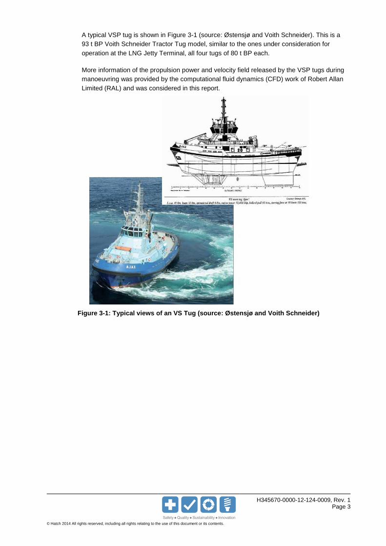
A typical VSP tug is shown in Figure 3-1 (source: Østensjø and Voith Schneider). This is a

93 t BP Voith Schneider Tractor Tug model, similar to the ones under consideration for

operation at the LNG Jetty Terminal, all four tugs of 80 t BP each.

More information of the propulsion power and velocity field released by the VSP tugs during

manoeuvring was provided by the computational fluid dynamics (CFD) work of Robert Allan

Limited (RAL) and was considered in this report.

Figure 3-1: Typical views of an VS Tug (source: Østensjø and Voith Schneider)

H345670-0000-12-124-0009, Rev. 1 Page 4


4. Input Data for Modelling Study

4.1 Bathymetry

Bathymetric data is available from several sources, including survey data collected by

McElhanney Consulting Services Ltd (Contracted by KBR LLC) and data from the Canadian

Hydrographic Survey (nautical charts, data sheets and multi beam data). More details about

the bathymetric data is provided on H345670-0000-12-220-0019.

4.2 Tides and Water Levels

Tide levels near Lelu Island are provided from local Hydrographic Tide and Chart at Port

Edward, BC, as published in the Canadian Tide and Current Tables, Volume 7 (Table 4-1).

The tidal variation in this region is significant with over 7 m changes in water elevation.

Table 4-1: Hydrographic Tide and Chart Datum at Port Edward, BC

Tide Level Elevation (m) (Chart Datum)

Higher High Water Level (Large Tide) 7.4

Higher High Water Level (Mean Tide) 6.1

Mean Sea Level 3.8

Lower Low Water Level (Large Tide) 1.2

Lowest Normal Tide (Chart Datum) 0.0


CHS provides predicted tide levels for the Prince Edward station based on historical

measurements. Current water level measurements as well as tidal predictions are available

for the Prince Rupert station, which is located north of the project site. The tide levels

published by CHS for Prince Rupert are listed in Table 4-2.

Table 4-2: Hydrographic tide and Chart Datum at Prince Rupert, BC

Tide Level Elevation (m) (Chart Datum)

Higher High Water Level (Large Tide) 7.5

Higher High Water Level (Mean Tide) 6.1

Mean Sea Level 3.8


Lowest Normal Tide (Chart Datum) 0.0

Lower Low Water Level (Large Tide) -0.2

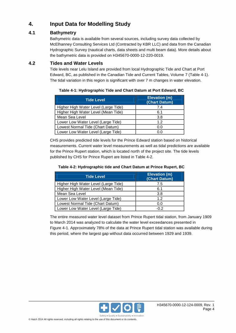
The entire measured water level dataset from Prince Rupert tidal station, from January 1909

to March 2014 was analyzed to calculate the water level exceedances presented in

Figure 4-1. Approximately 78% of the data at Prince Rupert tidal station was available during

this period, where the largest gap without data occurred between 1929 and 1939.

H345670-0000-12-124-0009, Rev. 1 Page 5


Figure 4-1: Water level probability of exceedance; Prince Rupert station, Jan 1909 to Mar 2014

4.3 Sediments

The study was developed considering the following sources:

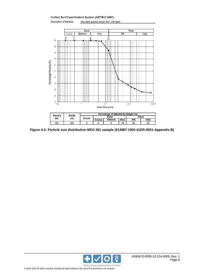
Sediment sample 001 as analysed by MEG (614887-1000-41ER-0001-Appendix B) and

shown in Figure 4-2, and

Results of three boreholes located near the LNG terminal (boreholes #35, 36 and 37),

FUGRO 2014 geotechnical investigations (04.10130058).

Note that in Figure 4-2, the grain size distribution curve for sample MEG 001, the USC

system is used to define the sediment fractions, where the median diameter D50 = 0.038 mm

(D50 is the size for which 50% by weight of the sediment sample is finer). This sample also

shows that the sediment consists of 16% fine sand, 64% silt and 20% clay. In Hatch reports

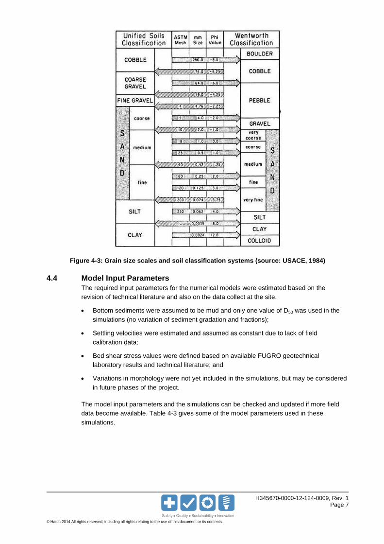
the Unified Soil Classification (USC) system of Figure 4-3 is used for all sediment

characterizations.

Borehole #36 (FUGRO) is the closest one to Berth 2, which was considered on the LNG

propeller scour analysis, since the sediments suspended by the propellers on this berth are

more likely to move towards Flora Bank when compared with Berth 1. The results from

borehole #36 (FUGRO) showed that the surface sediments (D50 = 0.033 mm) are similar to

the MEG 001 sample, therefore MEG 001 sample was used for the PTM simulations.

H345670-0000-12-124-0009, Rev. 1 Page 6


Figure 4-2: Particle size distribution MEG 001 sample (614887-1000-41ER-0001-Appendix B)

H345670-0000-12-124-0009, Rev. 1 Page 7


Figure 4-3: Grain size scales and soil classification systems (source: USACE, 1984)

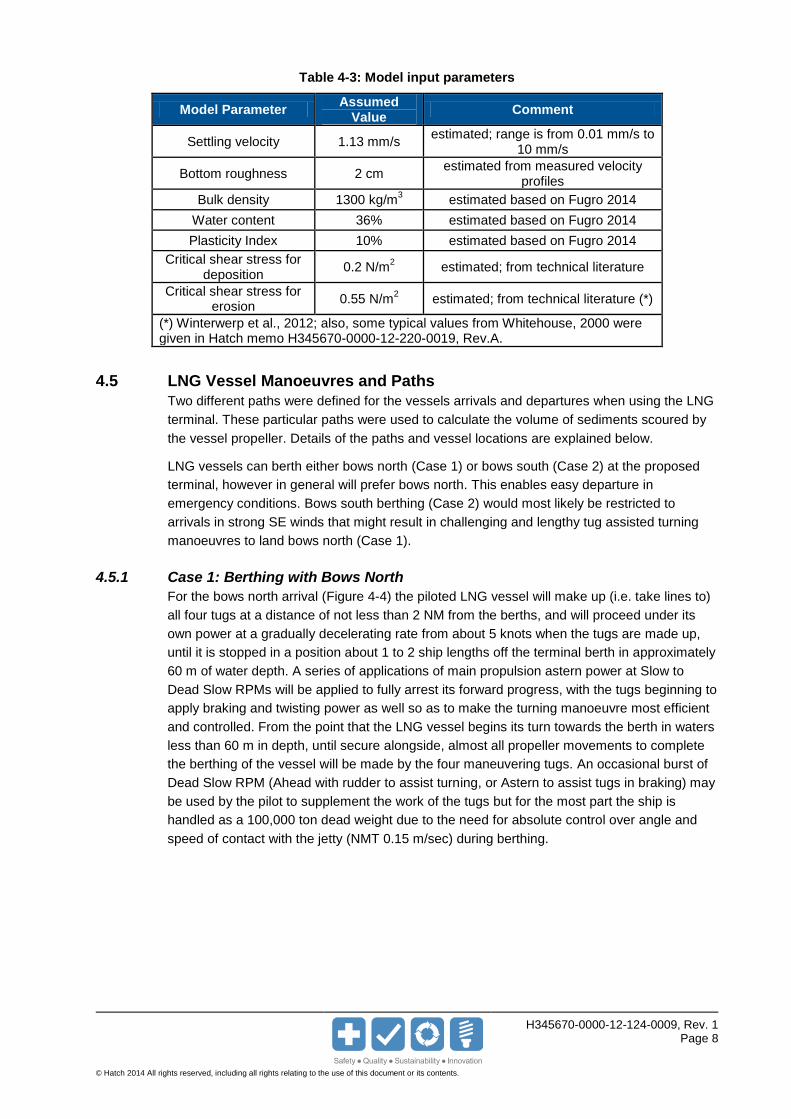
4.4 Model Input Parameters

The required input parameters for the numerical models were estimated based on the

revision of technical literature and also on the data collect at the site.

Bottom sediments were assumed to be mud and only one value of D50 was used in the

simulations (no variation of sediment gradation and fractions);

Settling velocities were estimated and assumed as constant due to lack of field

calibration data;

Bed shear stress values were defined based on available FUGRO geotechnical

laboratory results and technical literature; and

Variations in morphology were not yet included in the simulations, but may be considered

in future phases of the project.

The model input parameters and the simulations can be checked and updated if more field

data become available. Table 4-3 gives some of the model parameters used in these

simulations.

H345670-0000-12-124-0009, Rev. 1 Page 8


Table 4-3: Model input parameters

Model Parameter Assumed

Value Comment

Settling velocity 1.13 mm/s estimated; range is from 0.01 mm/s to

10 mm/s

Bottom roughness 2 cm estimated from measured velocity

profiles

Bulk density 1300 kg/m3 estimated based on Fugro 2014

Water content 36% estimated based on Fugro 2014

Plasticity Index 10% estimated based on Fugro 2014

Critical shear stress for deposition

0.2 N/m2 estimated; from technical literature

Critical shear stress for erosion

0.55 N/m2 estimated; from technical literature (*)

(*) Winterwerp et al., 2012; also, some typical values from Whitehouse, 2000 were given in Hatch memo H345670-0000-12-220-0019, Rev.A.

4.5 LNG Vessel Manoeuvres and Paths

Two different paths were defined for the vessels arrivals and departures when using the LNG

terminal. These particular paths were used to calculate the volume of sediments scoured by

the vessel propeller. Details of the paths and vessel locations are explained below.

LNG vessels can berth either bows north (Case 1) or bows south (Case 2) at the proposed

terminal, however in general will prefer bows north. This enables easy departure in

emergency conditions. Bows south berthing (Case 2) would most likely be restricted to

arrivals in strong SE winds that might result in challenging and lengthy tug assisted turning

manoeuvres to land bows north (Case 1).

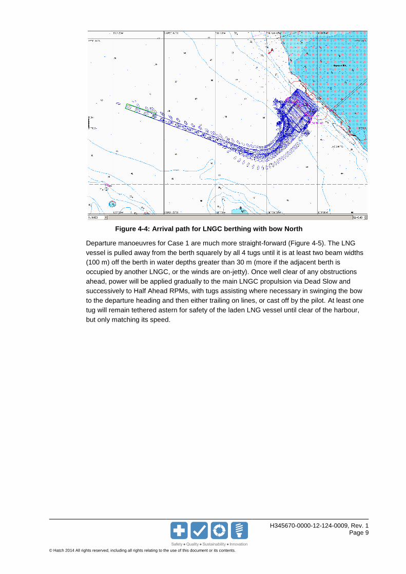
4.5.1 Case 1: Berthing with Bows North

For the bows north arrival (Figure 4-4) the piloted LNG vessel will make up (i.e. take lines to)

all four tugs at a distance of not less than 2 NM from the berths, and will proceed under its

own power at a gradually decelerating rate from about 5 knots when the tugs are made up,

until it is stopped in a position about 1 to 2 ship lengths off the terminal berth in approximately

60 m of water depth. A series of applications of main propulsion astern power at Slow to

Dead Slow RPMs will be applied to fully arrest its forward progress, with the tugs beginning to

apply braking and twisting power as well so as to make the turning manoeuvre most efficient

and controlled. From the point that the LNG vessel begins its turn towards the berth in waters

less than 60 m in depth, until secure alongside, almost all propeller movements to complete

the berthing of the vessel will be made by the four maneuvering tugs. An occasional burst of

Dead Slow RPM (Ahead with rudder to assist turning, or Astern to assist tugs in braking) may

be used by the pilot to supplement the work of the tugs but for the most part the ship is

handled as a 100,000 ton dead weight due to the need for absolute control over angle and

speed of contact with the jetty (NMT 0.15 m/sec) during berthing.

H345670-0000-12-124-0009, Rev. 1 Page 9


Figure 4-4: Arrival path for LNGC berthing with bow North

Departure manoeuvres for Case 1 are much more straight-forward (Figure 4-5). The LNG

vessel is pulled away from the berth squarely by all 4 tugs until it is at least two beam widths

(100 m) off the berth in water depths greater than 30 m (more if the adjacent berth is

occupied by another LNGC, or the winds are on-jetty). Once well clear of any obstructions

ahead, power will be applied gradually to the main LNGC propulsion via Dead Slow and

successively to Half Ahead RPMs, with tugs assisting where necessary in swinging the bow

to the departure heading and then either trailing on lines, or cast off by the pilot. At least one

tug will remain tethered astern for safety of the laden LNG vessel until clear of the harbour,

but only matching its speed.

H345670-0000-12-124-0009, Rev. 1 Page 10


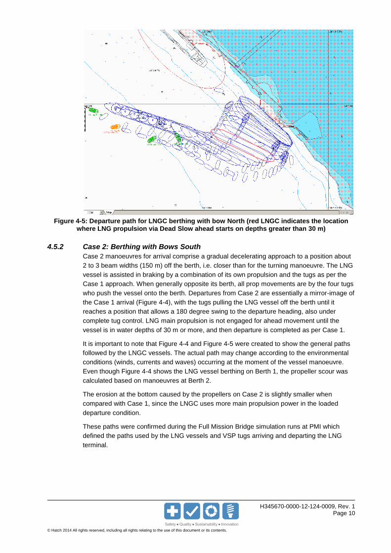
Figure 4-5: Departure path for LNGC berthing with bow North (red LNGC indicates the location where LNG propulsion via Dead Slow ahead starts on depths greater than 30 m)

4.5.2 Case 2: Berthing with Bows South

Case 2 manoeuvres for arrival comprise a gradual decelerating approach to a position about

2 to 3 beam widths (150 m) off the berth, i.e. closer than for the turning manoeuvre. The LNG

vessel is assisted in braking by a combination of its own propulsion and the tugs as per the

Case 1 approach. When generally opposite its berth, all prop movements are by the four tugs

who push the vessel onto the berth. Departures from Case 2 are essentially a mirror-image of

the Case 1 arrival (Figure 4-4), with the tugs pulling the LNG vessel off the berth until it

reaches a position that allows a 180 degree swing to the departure heading, also under

complete tug control. LNG main propulsion is not engaged for ahead movement until the

vessel is in water depths of 30 m or more, and then departure is completed as per Case 1.

It is important to note that Figure 4-4 and Figure 4-5 were created to show the general paths

followed by the LNGC vessels. The actual path may change according to the environmental

conditions (winds, currents and waves) occurring at the moment of the vessel manoeuvre.

Even though Figure 4-4 shows the LNG vessel berthing on Berth 1, the propeller scour was

calculated based on manoeuvres at Berth 2.

The erosion at the bottom caused by the propellers on Case 2 is slightly smaller when

compared with Case 1, since the LNGC uses more main propulsion power in the loaded

departure condition.

These paths were confirmed during the Full Mission Bridge simulation runs at PMI which

defined the paths used by the LNG vessels and VSP tugs arriving and departing the LNG

terminal.

H345670-0000-12-124-0009, Rev. 1 Page 11


5. Velocity Plumes and Scour

5.1 LNG Propeller Wash Plume

The design vessel characteristics were obtained from Hatch’s Basis of Design, H345670-

0000-12-109-0001, Rev. C (Section 3). The parameters and data for LNGC vessels and tugs,

such as number of propellers, propeller diameter and geometry below the keel, as well as

rated power, were provided by PNW LNG and MITAGS-PMI, as well as by Master Mariner

Capt. John Swann.

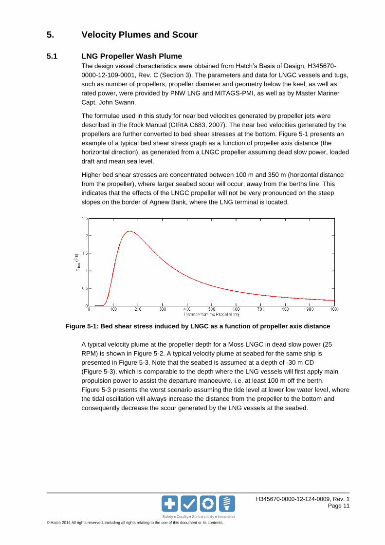
The formulae used in this study for near bed velocities generated by propeller jets were

described in the Rock Manual (CIRIA C683, 2007). The near bed velocities generated by the

propellers are further converted to bed shear stresses at the bottom. Figure 5-1 presents an

example of a typical bed shear stress graph as a function of propeller axis distance (the

horizontal direction), as generated from a LNGC propeller assuming dead slow power, loaded

draft and mean sea level.

Higher bed shear stresses are concentrated between 100 m and 350 m (horizontal distance

from the propeller), where larger seabed scour will occur, away from the berths line. This

indicates that the effects of the LNGC propeller will not be very pronounced on the steep

slopes on the border of Agnew Bank, where the LNG terminal is located.

Figure 5-1: Bed shear stress induced by LNGC as a function of propeller axis distance

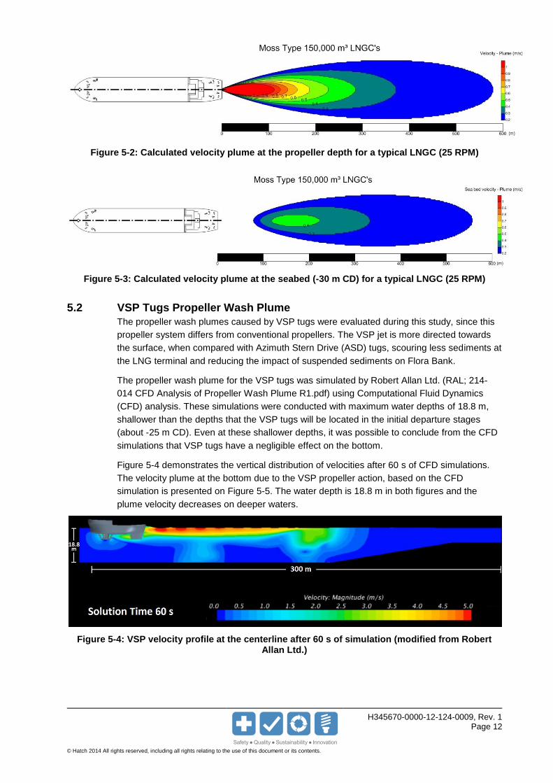
A typical velocity plume at the propeller depth for a Moss LNGC in dead slow power (25

RPM) is shown in Figure 5-2. A typical velocity plume at seabed for the same ship is

presented in Figure 5-3. Note that the seabed is assumed at a depth of -30 m CD

(Figure 5-3), which is comparable to the depth where the LNG vessels will first apply main

propulsion power to assist the departure manoeuvre, i.e. at least 100 m off the berth.

Figure 5-3 presents the worst scenario assuming the tide level at lower low water level, where

the tidal oscillation will always increase the distance from the propeller to the bottom and

consequently decrease the scour generated by the LNG vessels at the seabed.

H345670-0000-12-124-0009, Rev. 1 Page 12


Figure 5-2: Calculated velocity plume at the propeller depth for a typical LNGC (25 RPM)

Figure 5-3: Calculated velocity plume at the seabed (-30 m CD) for a typical LNGC (25 RPM)

5.2 VSP Tugs Propeller Wash Plume

The propeller wash plumes caused by VSP tugs were evaluated during this study, since this

propeller system differs from conventional propellers. The VSP jet is more directed towards

the surface, when compared with Azimuth Stern Drive (ASD) tugs, scouring less sediments at

the LNG terminal and reducing the impact of suspended sediments on Flora Bank.

The propeller wash plume for the VSP tugs was simulated by Robert Allan Ltd. (RAL; 214-

014 CFD Analysis of Propeller Wash Plume R1.pdf) using Computational Fluid Dynamics

(CFD) analysis. These simulations were conducted with maximum water depths of 18.8 m,

shallower than the depths that the VSP tugs will be located in the initial departure stages

(about -25 m CD). Even at these shallower depths, it was possible to conclude from the CFD

simulations that VSP tugs have a negligible effect on the bottom.

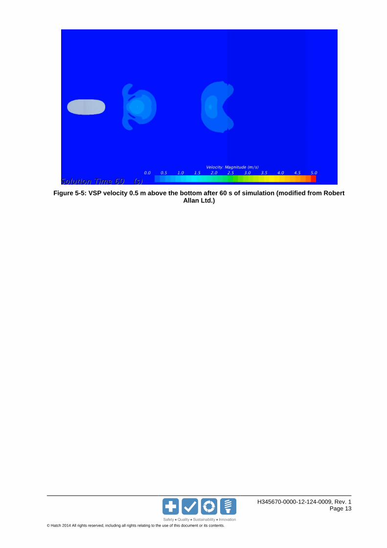
Figure 5-4 demonstrates the vertical distribution of velocities after 60 s of CFD simulations.

The velocity plume at the bottom due to the VSP propeller action, based on the CFD

simulation is presented on Figure 5-5. The water depth is 18.8 m in both figures and the

plume velocity decreases on deeper waters.

Figure 5-4: VSP velocity profile at the centerline after 60 s of simulation (modified from Robert Allan Ltd.)

H345670-0000-12-124-0009, Rev. 1 Page 13


Figure 5-5: VSP velocity 0.5 m above the bottom after 60 s of simulation (modified from Robert Allan Ltd.)

H345670-0000-12-124-0009, Rev. 1 Page 14


6. Hydrodynamic Modelling

6.1 Model Description

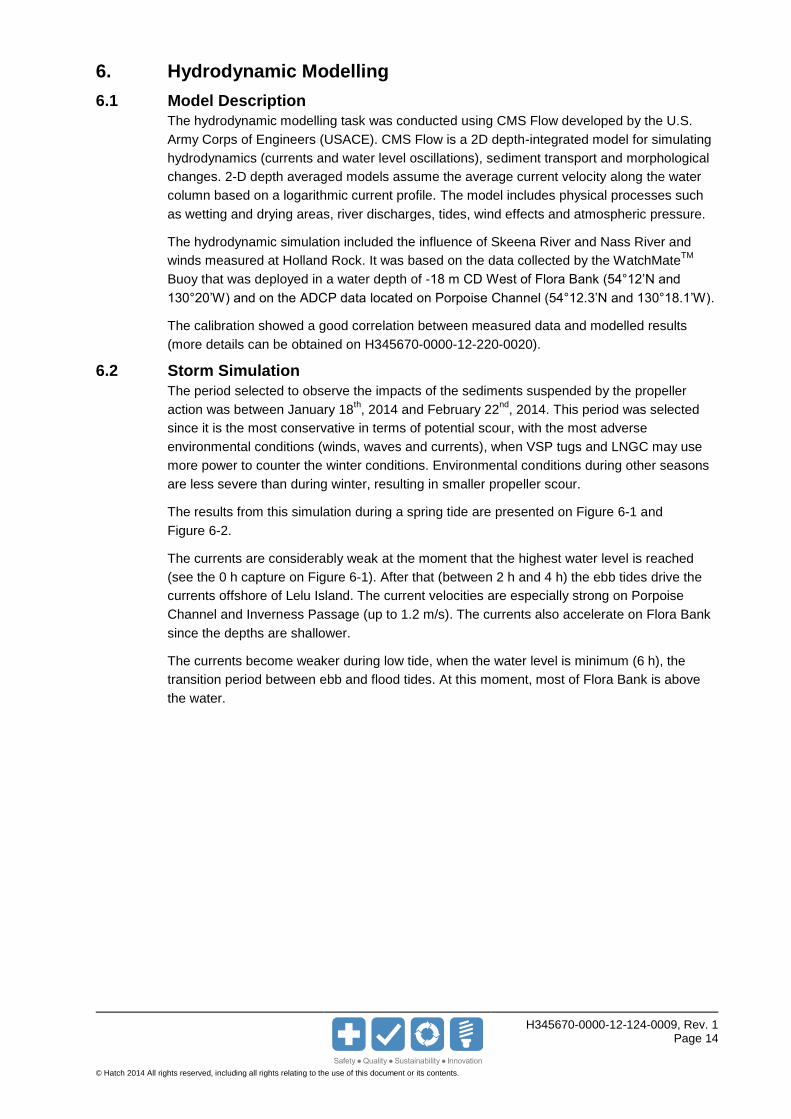
The hydrodynamic modelling task was conducted using CMS Flow developed by the U.S.

Army Corps of Engineers (USACE). CMS Flow is a 2D depth-integrated model for simulating

hydrodynamics (currents and water level oscillations), sediment transport and morphological

changes. 2-D depth averaged models assume the average current velocity along the water

column based on a logarithmic current profile. The model includes physical processes such

as wetting and drying areas, river discharges, tides, wind effects and atmospheric pressure.

The hydrodynamic simulation included the influence of Skeena River and Nass River and

winds measured at Holland Rock. It was based on the data collected by the WatchMateTM

Buoy that was deployed in a water depth of -18 m CD West of Flora Bank (54°12’N and

130°20’W) and on the ADCP data located on Porpoise Channel (54°12.3’N and 130°18.1’W).

The calibration showed a good correlation between measured data and modelled results

(more details can be obtained on H345670-0000-12-220-0020).

6.2 Storm Simulation

The period selected to observe the impacts of the sediments suspended by the propeller

action was between January 18th, 2014 and February 22

nd, 2014. This period was selected

since it is the most conservative in terms of potential scour, with the most adverse

environmental conditions (winds, waves and currents), when VSP tugs and LNGC may use

more power to counter the winter conditions. Environmental conditions during other seasons

are less severe than during winter, resulting in smaller propeller scour.

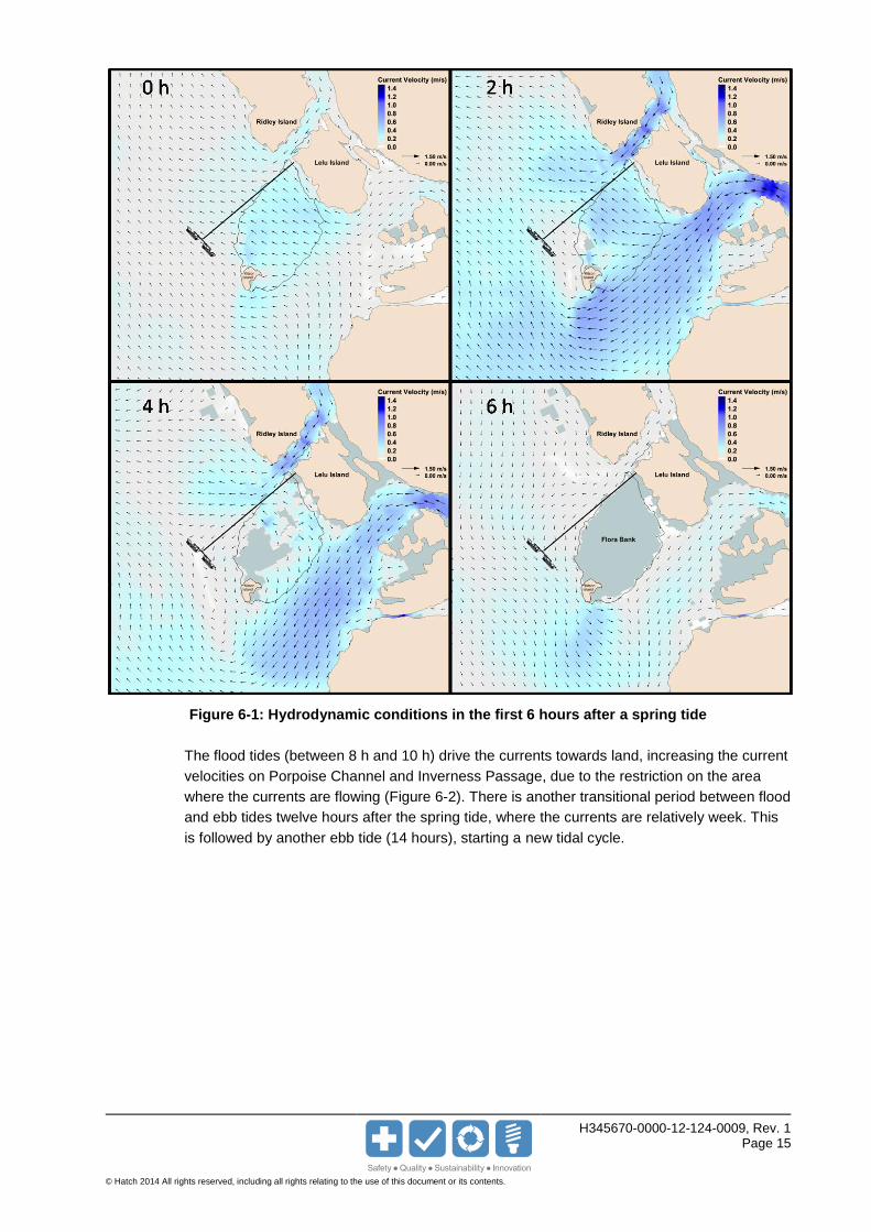
The results from this simulation during a spring tide are presented on Figure 6-1 and

Figure 6-2.

The currents are considerably weak at the moment that the highest water level is reached

(see the 0 h capture on Figure 6-1). After that (between 2 h and 4 h) the ebb tides drive the

currents offshore of Lelu Island. The current velocities are especially strong on Porpoise

Channel and Inverness Passage (up to 1.2 m/s). The currents also accelerate on Flora Bank

since the depths are shallower.

The currents become weaker during low tide, when the water level is minimum (6 h), the

transition period between ebb and flood tides. At this moment, most of Flora Bank is above

the water.

H345670-0000-12-124-0009, Rev. 1 Page 15


Figure 6-1: Hydrodynamic conditions in the first 6 hours after a spring tide

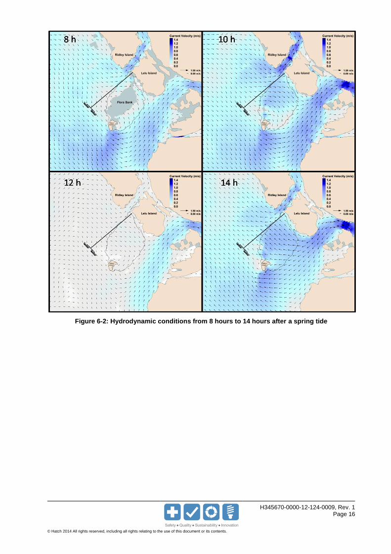
The flood tides (between 8 h and 10 h) drive the currents towards land, increasing the current

velocities on Porpoise Channel and Inverness Passage, due to the restriction on the area

where the currents are flowing (Figure 6-2). There is another transitional period between flood

and ebb tides twelve hours after the spring tide, where the currents are relatively week. This

is followed by another ebb tide (14 hours), starting a new tidal cycle.

H345670-0000-12-124-0009, Rev. 1 Page 16


Figure 6-2: Hydrodynamic conditions from 8 hours to 14 hours after a spring tide

H345670-0000-12-124-0009, Rev. 1 Page 17


7. Sedimentation Fate Modelling

A sedimentation study was conducted using the Particle Tracking Model (PTM), developed by

the USACE. PTM investigates the sediment pathways and fate after sediments are eroded

and suspended by the LNGC and the tugs propellers. After the sediments are suspended, the

particles are transported by the local hydrodynamic conditions as predicted with CMS Flow

hydrodynamic simulations, which are input conditions for the PTM.

7.1 Model Description

The fate of the sediments eroded during LNGC arrivals and departures at the LNG terminal

(Figure 1-1) was simulated using PTM. The sediment scoured by the LNG vessel and tugs

were used as input conditions for the simulations described in this section, based on the

arrival and departure paths presented on Section 4.5.

The simulations assumed a Moss LNGC assisted by four VSP tugs. The LNGC are not

restricted to tidal levels, being able to arrival and depart the terminal at any tidal stage.

For the PTM simulations, it was assumed one LNG vessel arrival and one departure per day

for one month. The first particle release of the PTM simulation (simulating the first arrival) was

2 days after the beginning of the hydrodynamic circulation, excluding the ramp-up period. The

last release (simulating the last departure) was 2 days before the end of the hydrodynamic

circulation, allowing the necessary time for the particles scoured by the propeller to be

transported by the local currents and to deposit.

Also, it was assumed 29 arrivals and 29 departures during the PTM simulations, considering

two days of downtime during storm conditions (H345670-0000-12-124-0005), periods that the

LNGC wouldn't be able to use the terminal.

7.2 Sensitivity of the Eroded Volumes

Vessel manoeuvres will not be limited by any tidal level, accessing the terminal at different

tidal stages. The volume of sediments suspended during each arrival and departure is

associated with the tidal stage, since the tide level can change more than 7 m. Therefore the

total volume eroded during one month will change with the water level oscillation.

A sensitivity study was conducted to identify the total volume that would be representative of

the environmental conditions around Flora Bank. In this sensitivity test, the total volume

during one month was calculated 40 times assuming a random distribution of water levels for

arrival and departures. The average volume obtained during the sensitivity test was used as

input condition for the PTM simulations.

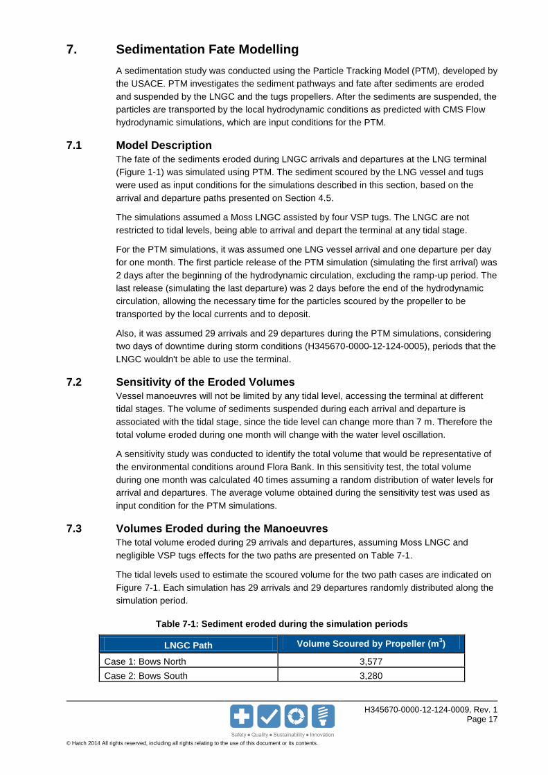
7.3 Volumes Eroded during the Manoeuvres

The total volume eroded during 29 arrivals and departures, assuming Moss LNGC and

negligible VSP tugs effects for the two paths are presented on Table 7-1.

The tidal levels used to estimate the scoured volume for the two path cases are indicated on

Figure 7-1. Each simulation has 29 arrivals and 29 departures randomly distributed along the

simulation period.

Table 7-1: Sediment eroded during the simulation periods

LNGC Path Volume Scoured by Propeller (m3)

Case 1: Bows North 3,577

Case 2: Bows South 3,280

H345670-0000-12-124-0009, Rev. 1 Page 18


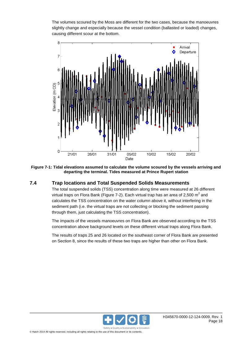
The volumes scoured by the Moss are different for the two cases, because the manoeuvres

slightly change and especially because the vessel condition (ballasted or loaded) changes,

causing different scour at the bottom.

Figure 7-1: Tidal elevations assumed to calculate the volume scoured by the vessels arriving and departing the terminal. Tides measured at Prince Rupert station

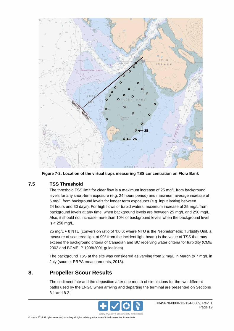
7.4 Trap locations and Total Suspended Solids Measurements

The total suspended solids (TSS) concentration along time were measured at 26 different

virtual traps on Flora Bank (Figure 7-2). Each virtual trap has an area of 2,500 m2 and

calculates the TSS concentration on the water column above it, without interfering in the

sediment path (i.e. the virtual traps are not collecting or blocking the sediment passing

through them, just calculating the TSS concentration).

The impacts of the vessels manoeuvres on Flora Bank are observed according to the TSS

concentration above background levels on these different virtual traps along Flora Bank.

The results of traps 25 and 26 located on the southeast corner of Flora Bank are presented

on Section 8, since the results of these two traps are higher than other on Flora Bank.

H345670-0000-12-124-0009, Rev. 1 Page 19


Figure 7-2: Location of the virtual traps measuring TSS concentration on Flora Bank

7.5 TSS Threshold

The threshold TSS limit for clear flow is a maximum increase of 25 mg/L from background

levels for any short-term exposure (e.g. 24 hours period) and maximum average increase of

5 mg/L from background levels for longer term exposures (e.g. input lasting between

24 hours and 30 days). For high flows or turbid waters, maximum increase of 25 mg/L from

background levels at any time, when background levels are between 25 mg/L and 250 mg/L.

Also, it should not increase more than 10% of background levels when the background level

is ≥ 250 mg/L.

25 mg/L ≈ 8 NTU (conversion ratio of 1:0.3; where NTU is the Nephelometric Turbidity Unit, a

measure of scattered light at 90° from the incident light beam) is the value of TSS that may

exceed the background criteria of Canadian and BC receiving water criteria for turbidity (CME

2002 and BCMELP 1998/2001 guidelines).

The background TSS at the site was considered as varying from 2 mg/L in March to 7 mg/L in

July (source: PRPA measurements, 2013).

8. Propeller Scour Results

The sediment fate and the deposition after one month of simulations for the two different

paths used by the LNGC when arriving and departing the terminal are presented on Sections

8.1 and 8.2.

H345670-0000-12-124-0009, Rev. 1 Page 20


The four hour period when the highest TSS concentration was calculated by the model for

each case is also presented, indicating the sediment plume pattern and the plume path

during those situations.

TSS concentrations above background levels were calculated on 26 traps located along Flora

Bank (Figure 7-2). Only the results on Trap 25 and Trap 26 are presented, since the

concentrations observed on the other traps are almost negligible.

8.1 Case 1: Berthing with Bows North

During this simulation, the vessels were assumed to be berthing with bow towards North. The

vessels will be steered by the VSP tugs, when arriving at the terminal, using almost no LNG

engine power during this manoeuvre. For the departure manoeuvre, the tugs will pull the LNG

vessel to a minimum distance of approximately two beam widths (100 m) from the berth, and

the LNGC will then get underway with its engine at Dead Slow Ahead power.

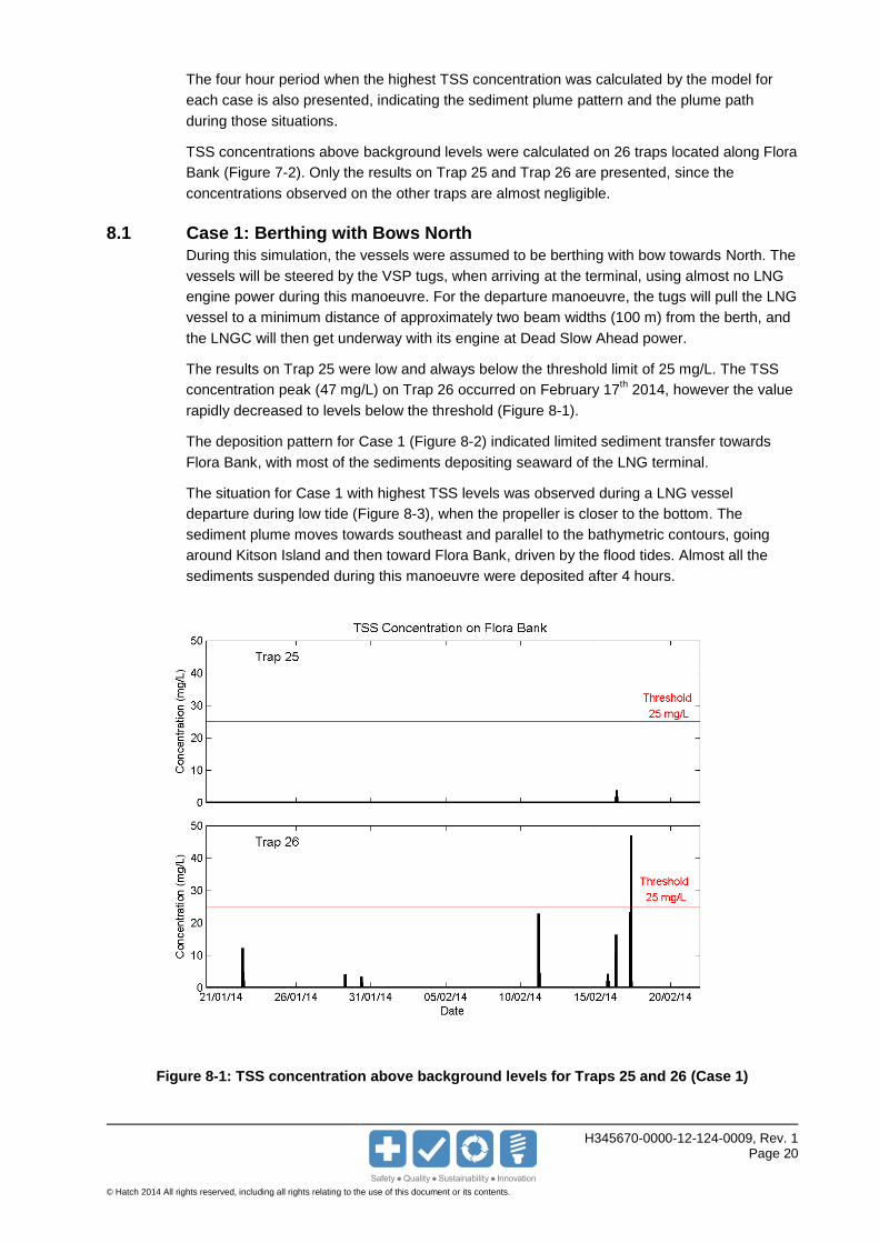
The results on Trap 25 were low and always below the threshold limit of 25 mg/L. The TSS

concentration peak (47 mg/L) on Trap 26 occurred on February 17th 2014, however the value

rapidly decreased to levels below the threshold (Figure 8-1).

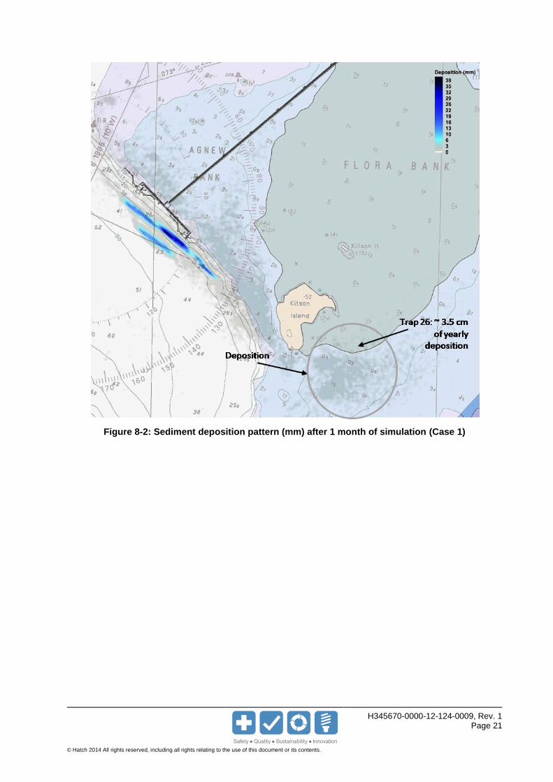
The deposition pattern for Case 1 (Figure 8-2) indicated limited sediment transfer towards

Flora Bank, with most of the sediments depositing seaward of the LNG terminal.

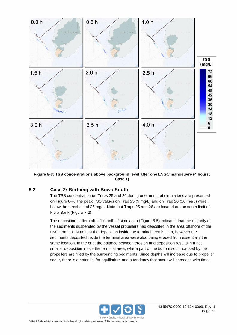
The situation for Case 1 with highest TSS levels was observed during a LNG vessel

departure during low tide (Figure 8-3), when the propeller is closer to the bottom. The

sediment plume moves towards southeast and parallel to the bathymetric contours, going

around Kitson Island and then toward Flora Bank, driven by the flood tides. Almost all the

sediments suspended during this manoeuvre were deposited after 4 hours.

Figure 8-1: TSS concentration above background levels for Traps 25 and 26 (Case 1)

H345670-0000-12-124-0009, Rev. 1 Page 21


Figure 8-2: Sediment deposition pattern (mm) after 1 month of simulation (Case 1)

H345670-0000-12-124-0009, Rev. 1 Page 22


Figure 8-3: TSS concentrations above background level after one LNGC manoeuvre (4 hours; Case 1)

8.2 Case 2: Berthing with Bows South

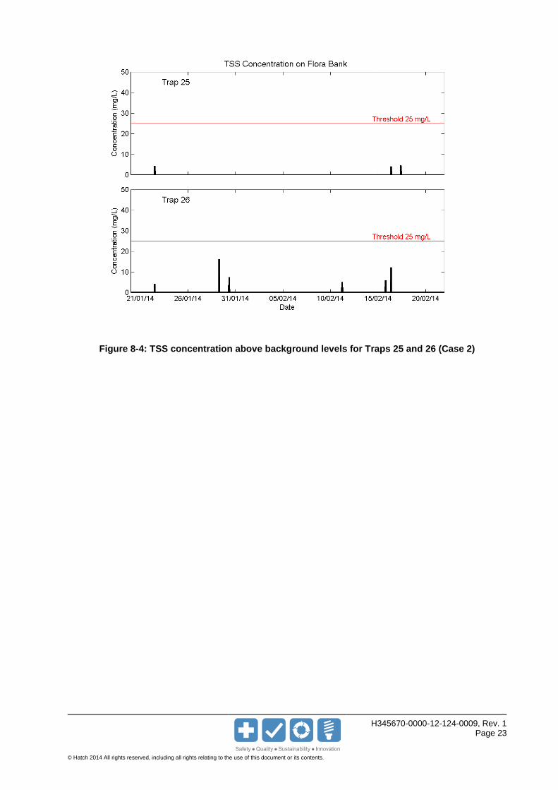
The TSS concentration on Traps 25 and 26 during one month of simulations are presented

on Figure 8-4. The peak TSS values on Trap 25 (5 mg/L) and on Trap 26 (16 mg/L) were

below the threshold of 25 mg/L. Note that Traps 25 and 26 are located on the south limit of

Flora Bank (Figure 7-2).

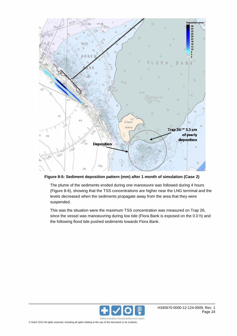
The deposition pattern after 1 month of simulation (Figure 8-5) indicates that the majority of

the sediments suspended by the vessel propellers had deposited in the area offshore of the

LNG terminal. Note that the deposition inside the terminal area is high, however the

sediments deposited inside the terminal area were also being eroded from essentially the

same location. In the end, the balance between erosion and deposition results in a net

smaller deposition inside the terminal area, where part of the bottom scour caused by the

propellers are filled by the surrounding sediments. Since depths will increase due to propeller

scour, there is a potential for equilibrium and a tendency that scour will decrease with time.

H345670-0000-12-124-0009, Rev. 1 Page 23


Figure 8-4: TSS concentration above background levels for Traps 25 and 26 (Case 2)

H345670-0000-12-124-0009, Rev. 1 Page 24


Figure 8-5: Sediment deposition pattern (mm) after 1 month of simulation (Case 2)

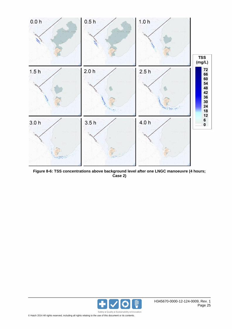
The plume of the sediments eroded during one manoeuvre was followed during 4 hours

(Figure 8-6), showing that the TSS concentrations are higher near the LNG terminal and the

levels decreased when the sediments propagate away from the area that they were

suspended.

This was the situation were the maximum TSS concentration was measured on Trap 26,

since the vessel was manoeuvring during low tide (Flora Bank is exposed on the 0.0 h) and

the following flood tide pushed sediments towards Flora Bank.

H345670-0000-12-124-0009, Rev. 1 Page 25


Figure 8-6: TSS concentrations above background level after one LNGC manoeuvre (4 hours; Case 2)

H345670-0000-12-124-0009, Rev. 1 Page 26


9. Conclusions

A hydrodynamic and sedimentation study was conducted to predict sediment pathways and

fate after the sediments were scoured and suspended by the LNG vessel propeller

manoeuvring at the PNW LNG terminal.

The numerical model study was developed using CMS Flow to predict local hydrodynamic

conditions and PTM to investigate the sediment fate, including deposition areas and levels of

total suspended solids (TSS) above background. This study was conducted assuming 29

LNGC arrivals and 29 departures during one month that represents the most conservative

conditions for generation of scoured sediment volumes.

The PTM simulation results yield a general idea about the sediment fate during one month of

simulation, assuming two different paths used by the LNG vessels.

When the LNG vessels are berthing with bow towards North (Case 1), the TSS threshold

value is exceeded, however only during a short amount of time (less than 1 hour for each

peak) and only on the southern edge of Flora Bank. The TSS concentrations were below the

threshold value (25 mg/L) when the LNGCs are berthing with the bow towards South

(Case 2). All other traps, spread over Flora Bank, measured negligible TSS concentrations

during the simulation period.

The deposition patterns indicate that most of the sediments are deposited seaward of the

LNG terminal, independently of the path used by the LNGC and only a minimum fraction of

the sediments are depositing on the southern edge of Flora Bank.

propeller scour analysis - canada.ca · this means that ship and tug propeller sediment scour...

Documents