projecting global land-use change and its effect on ecosystem

Projecting Global Land-Use Change and Its Effect onEcosystem Service Provision and Biodiversity withSimple ModelsErik Nelson1*, Heather Sander2¤, Peter Hawthorne3, Marc Conte1, Driss Ennaanay1, Stacie Wolny1,

Steven Manson4, Stephen Polasky2,5

1 The Natural Capital Project, Woods Institute for the Environment, Stanford University, Stanford, California, United States of America, 2 Conservation Biology Graduate

Program, University of Minnesota, St. Paul, Minnesota, United States of America, 3 Department of Ecology, Evolution, and Behavior, University of Minnesota, St. Paul,

Minnesota, United States of America, 4 Department of Geography, University of Minnesota, Minneapolis, Minnesota, United States of America, 5 Department of Applied

Economics, University of Minnesota, St. Paul, Minnesota, United States of America

Abstract

Background: As the global human population grows and its consumption patterns change, additional land will be neededfor living space and agricultural production. A critical question facing global society is how to meet growing humandemands for living space, food, fuel, and other materials while sustaining ecosystem services and biodiversity [1].

Methodology/Principal Findings: We spatially allocate two scenarios of 2000 to 2015 global areal change in urban land andcropland at the grid cell-level and measure the impact of this change on the provision of ecosystem services andbiodiversity. The models and techniques used to spatially allocate land-use/land-cover (LULC) change and evaluate itsimpact on ecosystems are relatively simple and transparent [2]. The difference in the magnitude and pattern of croplandexpansion across the two scenarios engenders different tradeoffs among crop production, provision of species habitat, andother important ecosystem services such as biomass carbon storage. For example, in one scenario, 5.2 grams of carbonstored in biomass is released for every additional calorie of crop produced across the globe; under the other scenario thistradeoff rate is 13.7. By comparing scenarios and their impacts we can begin to identify the global pattern of cropland andirrigation development that is significant enough to meet future food needs but has less of an impact on ecosystem serviceand habitat provision.

Conclusions/Significance: Urban area and croplands will expand in the future to meet human needs for living space,livelihoods, and food. In order to jointly provide desired levels of urban land, food production, and ecosystem service andspecies habitat provision the global society will have to become much more strategic in its allocation of intensivelymanaged land uses. Here we illustrate a method for quickly and transparently evaluating the performance of potentialglobal futures.

Citation: Nelson E, Sander H, Hawthorne P, Conte M, Ennaanay D, et al. (2010) Projecting Global Land-Use Change and Its Effect on Ecosystem Service Provisionand Biodiversity with Simple Models. PLoS ONE 5(12): e14327. doi:10.1371/journal.pone.0014327

Editor: Adina Maya Merenlender, University of California, United States of America

Received April 10, 2010; Accepted November 8, 2010; Published December 15, 2010

This is an open-access article distributed under the terms of the Creative Commons Public Domain declaration which stipulates that, once placed in the publicdomain, this work may be freely reproduced, distributed, transmitted, modified, built upon, or otherwise used by anyone for any lawful purpose.

Funding: We are grateful for support from P and H Bing, V and R Sant, the MacArthur and Winslow foundations, and the Institute on the Environment at theUniversity of Minnesota. The funders had no role in study design, data collection and analysis, decision to publish, or preparation of the manuscript.

Competing Interests: The authors have declared that no competing interests exist.

* E-mail: [email protected]

¤ Current address: National Exposure Research Laboratory, Ecological Exposure Research Division, U.S. Environmental Protection Agency, Cincinnati, Ohio, UnitedStates of America

Introduction

The earth’s capacity to provide enough living space, food, andclean water to meet human needs as well as the habitat needs ofother species is being severely tested [3–5]. A growing globalhuman population and the associated increase in demand forliving space, food, water, fuel, and other materials and servicesmakes ecosystem service and biodiversity sustenance a difficultchallenge. Having a clear understanding of how ecosystem serviceand habitat provision might change over time due to global urbanand cropland development is a prerequisite for charting a globalfuture that can meet these interconnected challenges [1]. In this

paper, we develop methods for allocating expected areal changesin global land use/land cover (LULC) and for analyzing the likelyconsequences of these changes on the provision of severalecosystem services and species habitat.

Our approach provides a relatively simple and transparentmethod for creating spatially-explicit projections of global LULCchange at the grid cell-level. Our spatial allocation of expectedurban and cropland areal development is guided by rules thatincorporate basic demographic, economic development, andbiophysical principles. This method allows for the relatively quickcreation of spatially-explicit projections of business-as-usualfutures or alternative futures that might emerge if decision-

PLoS ONE | www.plosone.org 1 December 2010 | Volume 5 | Issue 12 | e14327

making on urban and cropland development across the worldchanges, either due to shifts in consumption preferences or land-use policies.

We couple global LULC conversion scenarios with models thatpredict the consequences of these changes on the provision ofcrop, water availability, carbon storage in biomass (a climateregulation service), and habitat for species. Changes in ecosystemservice provision are modeled using the Integrated Valuation ofEcosystem Services and Tradeoffs (InVEST) software system.InVEST is a suite of geographic information science models andalgorithms that converts changes in LULC patterns into changesin terrestrial carbon storage, water availability, crop production,habitat for species, and other ecosystem service outputs (not allservices modeled by InVEST are included in this illustration).Combining maps of alternative LULC futures with InVEST, wecan estimate the range of potential changes in ecosystem serviceprovision and tradeoffs among various services at differentgeographical and socioeconomic scales. These predictions canhelp frame the discussion of preferred global change outcomes andpolicy mechanisms needed to obtain them.

To illustrate our approach, we create two plausible scenarios ofspatially-explicit LULC change for the period 2000 to 2015. Tocreate a scenario we estimate global areal change in urban landand cropland from 2000 to 2015 and then spatially allocate thechange at the grid cell-level. Cropland areal growth across theglobe under the country scenario is given by extrapolating country-level 1985 to 2000 cropland growth trends to the 2000 to 2015period [6]. Cropland areal growth across the globe under theregional scenario is based on estimates of regional growth incropland area as given by the OECD-FAO’s Agricultural Outlooktrade model [7] where a region can be comprised of one country(e.g., the U.S.) or many countries (e.g., sub-Saharan Africa). Bothscenarios assume the same level and pattern of urbanization [8].Therefore, differences across the two scenarios are completelyexplained by divergent cropland development patterns. In thisillustration, the area of grid cells classified as urban increases23.6% across the globe between 2000 and 2015, a gain of 0.76million sq. km2. The area of grid cells classified as croplandincreases by 1.48 million sq. km2 (a 5.8% increase compared to2000) under the country scenario and by 1.88 million sq. km2 (a7.4% increase compared to 2000) under the regional scenario. Thecountry scenario is distinguished by significant cropland expansionin China and Indonesia while the regional scenario is highlighted bysignificant cropland expansion in Brazil with net croplandabandonment in China.

We translate LULC changes under each scenario into changesin crop production, water availability, carbon storage in biomass,and species habitat using InVEST. The expansion of urban andcropland area leads to global declines in species habitat andbiomass carbon storage. However, as measured by impact onglobal ecosystem services and habitat loss, the country scenario issuperior to the regional scenario. First, the country scenario generatesa greater increase in the caloric value of crop production. Second,under the country scenario the gain in caloric production is donemore efficiently as measured by the tradeoffs between biomasscarbon storage and species habitat provision. Specifically, underthe country scenario 5.2 grams of biomass carbon is released due toLULC conversion for every additional calorie of crop produced.Under the regional scenario this tradeoff rate is 13.7. Further, underthe country scenario 0.0016 square meters of species habitat is lostfor every additional calorie of crop produced. Under the regionalscenario this tradeoff rate is 0.0021.

The superiority of the country scenario is due primarily to twoglobal development patterns. First, under the country scenario, large

sources of biomass carbon storage are not converted to croplandwhen compared to the regional scenario. For example, significantcropland development in Brazil under the regional scenario, animportant source of global biomass carbon stock, largely explainsthat scenario’s relatively poor performance on the crop – carbonemissions tradeoff ratio. Second, under the country scenario there isgreater cropland expansion in areas with greater agriculturaltechnological and irrigation capacities, both important factors insustaining continued increases in crop production efficiencies. Forexample, under the country scenario 62.3% of the net gain incropland grid cell area is projected to be irrigated to some degreewhereas under the regional scenario only 33.1% of net gain incropland grid cell area is projected to be irrigated to some degree.These results highlight the general principle that the likelihood ofmeeting the joint challenge of sufficiently increasing foodproduction while maintaining ecosystem service and specieshabitat provision will increase if we allocate cropland to areas ofhigh or increasing agricultural productivity that do not alsoprovide high levels of ecosystem services or important habitat.Developed countries currently have the highest agriculturalproductivity capacities and contain some of the least importantsources of several ecosystem services and species habitat due topast development [9]. Therefore, if higher agricultural productiv-ity capacities cannot effectively be transferred to the developingworld then best hope for a sustainable future may be a reverse inthe recent trend of minimal to no cropland growth in thedeveloped world [6,7].

Besides describing potential futures and their ramifications onecosystem service and habitat provision, projections of LULCchange can be used to inform policy [10]. We illustrate how ourapproach can be used to guide a policy that provides incentives tomaintain carbon stocks in forest at risk for development (reducingcarbon emissions from deforestation and forest degradation orREDD program [11]). Assuming that the scenarios described hereare two examples of business-as-usual global developmentprojections and using a plausible REDD policy framework, weestimate 0.1 billion metric tons of avoided carbon emission creditswould have been generated across the globe from 2000 to 2015under modest offset prices if the country scenario had been chosenas the baseline and 13 billion metric tons of avoided carbonemission credits would have been generated across the globe if theregional scenario formed the baseline. The stark differences in creditcreation across the two scenarios illustrates how contentious theselection of a business-as-usual emission trajectory for any actualdeforestation avoidance program may be [12,13].

Literature review: modeling global or regional LULCchange at the grid cell-level

Spatially-explicit regional and global LULC change modelinghas been the focus of several prominent research efforts. Forexample, the Millennium Ecosystem Assessment (MA) researchteam has developed four plausible projections of the earth’s future.Each projection or scenario is defined by regional population,economic, and technological growth estimates as well asprojections for food and energy demands to the year 2100 [14–16]. Using a set of climate, agricultural [17], water supply and use[18,19], and LULC change models [20,21], the MA teamtranslated these expected regional change and demand trajectoriesinto global grid cell-level LULC maps for the years 2050 and 2100[22].

Instead of modeling change with such general equilibriummodels, extent and pattern of LULC change can be generated bysimulating the decision making of actors on the landscape. Inagent-based modeling ‘‘agents’’ (e.g., households, firms, govern-

Modeling Global Change


ment agencies, etc.) make LULC decisions over time such thattheir preferences are maximized given land-use policy constraintsand their neighbors’ decisions [23,24]. Alternatively, instead ofsimulating the behavior of agents through time, previous LULCchange behavior on the landscape can be extrapolated into thefuture using one of several statistical techniques [25,26], includingcellular automata [27–29]. In agent-based modeling the challengeis getting the rules that guide agent behavior correct. Thechallenge with the statistical approach is 1) isolating andcontrolling for policy, biophysical, or economic conditions thatshaped past decisions but will not exist in the future and 2)appropriately controlling for conditions that could affect futureLULC decision making but were not present on the landscape inthe past [30].

In other global and regional change research, the spatialallocation of LULC change is guided by a set of rules based onfundamental socioeconomic and biophysical principles. Forexample, McDonald et al. spatially allocate a United Nation’sprojection of country-level urban population growth across a gridusing the notion that cities grow concentrically [31]. TheCalifornia Urban Futures Model [32] allocates expected regionalresidential development such that undeveloped parcels modeled tohave the highest profitability in residential land use are convertedfirst. Alternatively, focus groups of appropriate experts anddecision-makers have been used to codify the socio-economic,policy, and biophysical forces that drive LULC change across aregion [33–35]. The model UPlan opens such rule-making abilityto anyone [36]. In this GIS model users specify future populationlevels, demographic characteristics, and land-use density param-eters. Given these inputs, area needed for each land-use isdetermined and then is spatially allocated according to user-defined or default land-use suitability maps. All of theseapproaches that use rules to spatially allocate LULC change tendto be simpler and more transparent than the general equilibriumscenario analysis as exemplified by the MA, agent-based modeling,or statistical analyses. However, these approaches do not verifythat the resulting spatial patterns of LULC change are compatiblewith projected global or regional demands for food, energy, andother services or that the projected spatial patterns of change areconsistent with past behavior.

Literature review: estimating the impact of grid cell-levelLULC change at global scales on environment, ecosystemservices, and human well-being

Many analyses that estimate the environmental or humanwelfare impact of expected global LULC change work with mapswhere change is summarized at the country- or regional-level.Such analyses have been used to predict changes in globalagriculture production, disease risk, energy use, species persis-tence, and water availability [3,37–40]. However, such broadassessments ignore the heterogeneity in land uses and biophysicaland economic conditions within regions.

To correct for such biases researchers are increasingly using gridcell-level assessments of global LULC change to project changes inthe environment, ecosystem services, and human well-being. Suchan approach is capable of capturing local-scale heterogeneity thatis often important for determining the supply, demand, and valueof ecosystem services. The MA project is a prominent example ofthis. The MA used already-published economic, biophysical, andecosystem service models [41] to estimate the impact of their four2100 grid cell-level LULC maps on the environment, ecosystemservice production, biodiversity, and human well-being [22,42].The LULC change model used by the MA has been used inconjunction with other biophysical and climate models to generate

global maps of predicted net primary productivity and climatemodulation [43], land-use carbon emissions and other carboncycle dynamics [44–47], trends in biodiversity [48,49], foodproduction [50–52], inorganic nitrogen export to coastal waters[53], and of various environmental conditions [54]. McDonald etal. estimate the impact of their future global urban area map onspecies persistence and protected areas in each terrestrialecoregion on the globe [31]. Other ecosystem service models thatcan be used with global grid cell-level LULC maps aresummarized in [55].

In this paper we spatially allocate already published country- orregional-level estimates of urban and cropland area change to thegrid cell-level using a rules-based approach. The inclusion ofcropland areal change and the use of land-use suitability matricesto guide LULC change extend this work beyond McDonald et al.’s work. Further, unlike, McDonald et al., we consider more thanbiodiversity impacts of LULC change around the globe. Weproduce some of the same output as the MA and other globalecosystem service analyses but without using some of the morecomplicated demographic, economic, and technological growthand biophysical models. In fact, the models we use from InVESTto model the impact of global change are open-source, freelyavailable, and readily accessible (http://invest.ecoinformatics.org/).The simpler and more transparent approach lowers the barriers toparticipation in scenario building and ecosystem service provisionmodeling and allows for the quick and transparent assessment offuture scenarios of change. We hope that a demonstration of ourtransparent and flexible method for modeling the potentialramifications of global change leads to wider use of our or similarmodeling approaches by policy-makers throughout the world[56,57].

Our method for estimating the impact of grid cell-levelLULC change at global scales on environment, ecosystemservices, and human well-being

We spatially allocate projected country- or regional-level 2000to 2015 net change in urban and cropland area to the grid cell-level (5 km resolution at the equator). Country-level urbanizationprojections for 2015 are based on urban population expansionestimates from the United Nations [8]. We spatially allocate twodifferent projections of cropland areal change. The first projectionof change is generated by extrapolating the rate of country-levelcropland area change from 1985 to 2000 to the 2000 to 2015 timeperiod (the country scenario). In the other cropland change scenario(the regional scenario), we use the OECD-FAO’s AgriculturalOutlook trade model [7] to estimate 2015 cropland area targets atthe regional-level. The spatial extent and pattern of croplandchange varies across the two scenarios because of differences inexpectations for areal change and the geographic unit of analysis.For example, in the regional scenario cropland growth is greater indeveloping countries than it is under the country scenario.

Spatial allocation of expected urban and cropland change isdone using a cellular modeling technique [58,59]. Under thistechnique, urban expansion between 2000 and 2015 tends tooccur in cells that are near urban land as of 2000 and that havehigher urban suitability scores. A cell’s urban suitability score 1)increases in its projected 2015 population density [60] and 2)decreases in its slope [61]. Urban expansion into protected areas isnot allowed [62].

Then we use the cellular modeling technique and a croplandsuitability map to spatially allocate a scenario’s expected country-level or regional-level net growth in cropland area (or abandon-ment if appropriate) to the grid cell-level. Cropland expansion onlyoccurs on land that is arable, is not in protected areas, and has not



been allocated to urban expansion (i.e., we assume that urban landexpansion will outbid cropland expansion on land highly suitablefor both [4]). The cropland suitability map has higher scores ingrid cells where 1) cereal yield potential under intensivemanagement, including irrigation if applicable, is higher [63]and 2) slopes are gentler [61]. Potential cereal yield tends to behigher in areas with fecund soil, that has sufficient water (eitherdue to rainfall, irrigation, or both), and have temperate climaticconditions. In the end we generate two gridded maps of LULC asof 2015 where urban grid cell extent and pattern is the same acrossboth maps but cropland grid cell extent and pattern differ.

Even though we believe our suitability maps have captured thebasic principles that drive urban and cropland change (in theurban case, we are adopting the basic principles of changeassumed by [60]), we acknowledge that our suitability maps ignoremany dynamics that guide LULC change. For example,infrastructure development plays a key role in both urban andcropland conversion [64]; our suitability maps do not explicitlycapture existing and potential infrastructure development, invest-ments that could increase suitability (e.g., reclaiming land throughdrainage or other means), and other forces of change. In theDiscussion section below we note how our cropland suitabilitylayer could be improved to capture the various forces of changethat we have not included. For now we view our methodology forallocating estimated global LULC change at the grid cell-level as afirst generation model that can be improved over time.

We estimate how the projected global change in LULC extentand pattern from 2000 to 2015 will affect the global provision ofcrops, water availability, carbon storage in biomass, and habitatfor species with the appropriate InVEST models. To calculatechange in global cropland production we first need to calculatechange in annual harvested hectares in each country between2000 and 2015 (we complete this and all subsequent methodo-logical tasks for both scenarios). This calculation is a function offallow land practices and the intensity at which the land is croppedin a country in 2000 and 2015. Next, we convert a country’spattern of change in harvested area into a change in the country’scrop production (measured in both mass and caloric terms) usingthe InVEST agriculture model. In addition to change in harvestarea, country-level change in crop production is a function of therelative change in the potential productivity of land used in thecountry for crop production, expected technological and infra-structure growth in the country’s agricultural sector, and the mixof crops grown in the country [7,65]. The overall productivity ofthe land used for cropland in a country as of 2015 will changecompared to 2000’s overall productivity if cropland expansionoccurs on land with different yield potentials than that of croplandas of 2000. In general, if 1) the country’s spatial allocation ofcropland in 2015 is located on land with greater yield potentialthan its 2000 allocation (which can be aided by the expansion ofirrigation) and/or 2) the country is expected to benefit to fromyield growth in crops that dominate its 2015 crop mix, thengrowth in its crop production will outpace its growth in harvestedarea. We summarize change in crop production by country underboth scenarios.

Predictions of cropland and crop production change, both inmagnitude and spatial pattern, are uncertain for many reasons andwe highlight a few of them here (see the Materials and Methodssection for a complete discussion on sources of uncertainty). Cropyield potential is limited by water availability. Our croplandsuitability layer and the base yields (observed year 2000 yields)used in the crop production model are based on water availabilitytrends of the late 20th century (and irrigation patterns when itcomes to base yields). Climate change and LULC change may

result in shifts in water yield (precipitation less evapotranspiration),thereby making the cropland suitability layer and base yieldestimates imperfect predictors of 2015 patterns in croplandproductivity and base yields. One way we can begin to assesshow crop production may deviate from modeled expectations dueto climate change and LULC-driven changes in evapotranspira-tion is to predict average annual water yield (average annualrainfall less annual evapotranspiration in mm km22) on eachcropland grid cell in 2015. Specifically, we model average annualwater yield in 2000 and 2015 on each cropland grid cell in 2015with use HadCM3 climate model [66] and the InVEST wateryield model [67–72] (we model 2000 yield instead of using actualdata to keep comparisons between 2000 and 2015 consistent). Ifaverage annual water yield on a grid cell decreases over time thenthe cell’s expected productivity as given by late 20th centuryclimate patterns may be too high, especially if the cell primarilycontains rainfed cropland. Further, a decrease in a cell’s yieldreduces the runoff that can be used for irrigation by other croplandgrid cells downstream. With this map of annual water yield, wecan identify the portions of the world where estimated cropproductivity estimates, especially rainfed productivity, may beparticularly vulnerable to climate change as of 2015 and beyond.

Cereal yield potential on a grid cell is partly explained byirrigation; in general, potential yield in a cell is higher if we assumea significant portion of cropland in the cell is irrigated instead ofrainfed. Therefore, in this illustration, areas more likely to beirrigated in the future are more likely to be selected for croplandexpansion (recall that the suitability score of a grid cell is largelydetermined by its relative potential for cereal production). Weassign an arable cell in a country its irrigated yield potentialinstead of its rainfed potential on the cropland suitability layer if ithas a yield potential profile that closely matches the yield potentialprofile of cells with significant irrigation in the country as of 2000[73]. This modeling process creates a yield potential map wheremost cells that were significantly irrigated in 2000 are assignedtheir irrigated yield potential (we model the 2000 irrigationpatterns instead of using the observed pattern to keep comparisonsbetween 2000 and 2015 consistent). In addition, some arable cellsin each country not in cropland as of 2000 but that closelyresemble their country’s irrigated cells as of 2000 are given theirirrigated rather than rainfed yield potential. How similar thesearable cells have to be to those that were significantly irrigated in2000 to receive their irrigated yield potential is determined foreach country by the modeler (SI Text 1). The less strict theresemblance required, the greater the number of arable cells in acountry that are assigned their irrigated yield potential. In the end,if irrigation infrastructure and technology is not implemented inthe pattern assumed by our cropland suitability layer then thespatial allocation of cropland expansion and modeled relativechange in cropland productivity will be inaccurate, especially inthose countries expected to rely heavily on irrigation to fuel theircrop production growth (see Table S1 for country-by-countryestimates of growth in cropland grid cell area that will benefit tosome degree by irrigation under both scenarios).

While we assume that cropland output in a cell is solely afunction of its productive potential and access to water, there aremany other factors that affect the productivity of cropped areas,including infrastructure designed to support agriculture. Forexample, Vera-Diaz et al. show that soybean yields are higher,all else equal, if the farmer has access to markets via roads [74].They surmise that farmers invest more of their time and capital incropping operations if they can easily market their product.Presumably such infrastructure has been established in areaswhere cropland has existed for sometime. Newly established



croplands, however, may not have the infrastructure necessary tosupport maximum production effort. Therefore, the InVESTagriculture production model includes a term that adjustsproduction on newer croplands according to infrastructurecapacity and other factors (e.g., experimentation with fertilizationrates to find the most cost-effective application) that might preventmaximum production capacity immediately. However, we do notuse this term it in this illustrative example due to a lack of globaldata on the relationship between agriculture infrastructure andyields.

It is also possible that arable area around the globe could beexpanded in the future. For example, draining low-lying areas(e.g., polders in the Netherlands) can increase the base of arableland. Conversion of existing agricultural to urban land andincreased demand for food from a growing population willincrease the incentive to make such investments. However, welacked systematic data on which to base an assessment of anexpansion of arable land base through investment and so did notinclude this dynamic in our analysis.

We use the carbon sequestration InVEST model to measure thechange in biomass carbon storage (carbon sequestration) in eachgrid cell due to LULC change. First, we find average biomasscarbon storage levels for each LULC type for each country usingmapped Intergovernmental Panel on Climate Change storage dataand the 2000 LULC map. Second, we apply these average storagevalues to the maps of LULC in 2000 and 2015. The difference ineach grid cell’s storage value between 2000 and 2015 gives agridded map of change in storage. (Because it can take decades fora LULC type to reach its average biomass carbon storage level wedo not technically measure actual biomass carbon sequestrationover the 2000 to 2015 period; instead we measure the eventualchange in biomass carbon storage if the 2015 global LULC mapwere maintained indefinitely.) Our application of the InVESTsequestration model does not account for biomass carbon flux ingrid cells that do not experience a LULC change, it does notaccount for carbon flux due to land management, and we do notattempt to adjust storage capacities and sequestration rates due toexpected climate change. We summarize biomass carbonsequestration results by country under both scenarios.

We also measure the conversion of undeveloped land byecoregion [75,76]. In our analysis we make the simplifyingassumption that undeveloped land – all LULC types other thanurban and cropland – is more likely to provide habitat for speciesthan urban and cropland area. Therefore, changes in undevelopedland area are correlated with change in species habitat. (Ourinability to translate mapped land covers into habitat types and alack of a comprehensive, global dataset on species-land coversuitabilities makes it impossible for us to model changes in globalhabitat; see the Discussion section for more details.) To identifywhich scenario is more detrimental to species persistence wesummarize loss of undeveloped land area at the ecoregion leveland then cross-walk these losses against measures of ecoregionhabitat availability, habitat connectivity, and numbers of endan-gered and threatened species.

We combine projections in LULC change and carbon storagemaps to make a contribution to the recent policy discussions onREDD. Under REDD or some similar avoided emissions policy,countries that reduce deforestation or forest degradation belowsome business-as-usual rate would generate avoided carbonemission credits that could be sold to entities looking to reducetheir carbon emission liabilities. LULC change scenarios that donot assume a REDD policy, like those presented here, could beused by policy makers to predict business-as-usual country-leveldeforestation and associated emissions rates. To simulate a

representative avoided deforestation global policy illustrate thisprocess, we estimate the area of forest in each country that iscleared under a scenario but, given a sufficient avoideddeforestation payment, would have generated more in economicreturns by accepting the avoided deforestation payment thanconverting to the projected land use (subject to a country cap onavoided emission credits that is a function of historic deforestationrates [77]). Because we assume the economic value of urbanexpansion will always be greater than the value of any avoidedemission credit, avoided deforestation and credit generation onlyoccurs in grid cells where cropland is predicted to emerge fromforest between 2000 and 2015 but the value of the credit is greaterthan the expected value of the new cropland. We summarizeavoided emission results by country under both scenarios.(Obviously, if the avoided deforestation policy was implementedas given and occurred as modeled then changes in cropproduction, water yield, biomass carbon emissions, and loss inundeveloped land from 2000 to 2015 would be different thangiven here.)

We order country-level results according to a measure of humandevelopment, the 2006 Human Development Index (HDI; [78]).We do this to identify the spatial correlations between patterns ofglobal change and current human well-being [5,79]. HDI, whichranges from 0 to 1 where higher scores indicate greater overallhuman well-being in a country, is a composite measure of acountry’s life expectancy, educational attainment, and per capitaGDP. HDI scores are often ranked in descending order where thecountry with the highest HDI has a ranking of 1.

Results

Urbanization and cropland grid cell area changeWe plot cumulative country-level net change in urban and

cropland grid cell area between 2000 and 2015 from lowest tohighest HDI score (Figure 1). The area of grid cells classified asurban expands by 0.76 million km2, roughly the size of Turkey(expansion in urban grid cell area does not equal expansion inurban area as many grid cells that are primarily urban will includesome other land covers as well). Depending on the scenario, globalcropland grid cell area is expected to expand by 1.48 to 1.88million km2 over this time period, roughly the size of Iran andLibya, respectively (again, expansion in cropland grid cell areadoes not equal expansion in croplands as many grid cells that areprimarily cropland will include some other land covers as well).This graph understates the amount of new cropland grid cell areathat will emerge across the globe as additional cropland will beneeded to compensate for the cropland that existed as of 2000 butconverts to urban area as of 2015. Most of the growth in croplandis located in the least-developed countries (Brazil and Libya underthe regional scenario are the exceptions).

Crop production servicesChange in harvested area strongly mirrors change in cropland

grid cell area; however, it is not a perfect predictor of change inharvested hectares due to differences across the globe in croppingintensity, fallow practices, and the matrix of land used for otherpurposes in grid cells designated as cropland (see the Methods andMaterials section for information on how we converted change incropland grid cell area to change in harvested hectares). Like thechange in cropland grid cell area, net growth in harvested hectaresin countries with low HDI scores is stronger under both scenarios(panel A of Figure 2). These results are consistent withexpectations that developing countries will produce an increasingshare of the world’s crops in the future [7]. As with the graph of



the net change in cropland grid cell area, this graph understatesthe amount of new harvested area that will emerge across theglobe as additional harvested area will be needed to compensatefor the harvested area that existed as of 2000 but is converted tourban area by 2015.

While growth in harvested area can be a significant driver ofeconomic growth in an area [80], change in crop production mostdirectly impacts human well-being. All else equal, a net increase inarea devoted to crop production in a country will increase itsoutput over time (whether measured in mass or calories). Inaddition, a country’s production will get a boost over time if itgrows crops that are expected to experience yield increases due toimprovements in agricultural methods and technology. Productionlevels in a country can also be positively affected by certainpatterns of cropland change; namely, if a country’s 2015 pattern ofcropped area covers grid cells that, on average, have greater yieldpotential than the cropped area in 2000 then, all else equal,production will increase. A change in a country’s crop mixbetween 2000 and 2015 also affects production (by crop mix wemean the relative amount of harvested hectares devoted to eachcrop type, e.g., rice, wheat, oil crops, etc., in a country). If acountry switches to more dense crops, either in terms of mass orcalories, then, all else equal, its production (as measured by massor calories) will increase. If a country switches towards crops whoseyields are improving due to technology managerial improvementsthen, all else equal, its production (as measured by mass orcalories) will increase.

In panel B of Figure 2 we present modeled change in the massof crop production by country, once under the assumption that the2015 crop mix in a country mimics its 2000 mix (labeled ‘‘2000Crop Mix’’) and another time under the assumption that country-level crop mixes as of 2015 are more in line with forecasts from [7]

(labeled ‘‘Projected 2015 Crop Mix’’). In Table 1 we present moredetailed information on the modeled changes in the mass ofproduction at the country-level under the assumption that the2015 crop mix in a country mimics its 2000 mix. In this case theincrease in the mass of crop production in countries with low HDI(0 to 0.5) is primarily due to the increase in cropped area (and anyimprovements due to a potentially more productive pattern ofcropland) while the increase in the mass of crop production incountries with medium and high HDI (0.5 to 0.8 and 0.8 to 1,respectively) is increasingly explained by improved yields, eitherdue to technological improvement, increased irrigation capacity,the use of more productive land, or all three. Change in the massof production in low and medium HDI countries is more efficientunder the regional scenario (as measured by the ratio of change innet output to net change in harvested area). This result reflects thefact that the cellular modeling technique generally has morefreedom to choose the most suitable cropland grid cells under theregional scenario than it does under the country scenario (i.e., thecellular model is allocating over a region rather than a country).However, because abandonment of cropland area in the highestHDI countries (nations with better access to technologicalimprovements in the agricultural sector) is much smaller underthe country scenario, the difference in crop production growthbetween the scenarios is small despite the regional scenario’sadditional 0.19 million harvested km2 (by 2015 the mass of cropproduction under the country scenario is 10.3% greater than 2000modeled production whereas the gain is 11.2% under the regionalscenario). In Table 2 we present information on the ratio ofchange in net output to net change in harvested area when we use2015 country-level crop mixes that are more in line with forecastsfrom [7]. While the trends across HDI groups that we observed inTable 1 are similar, the global change in the mass of cropproduction under the country and regional scenarios are significantlylower, 1.5% and 1.7%, respectively. In other words, future cropmixes are forecasted to be much lighter from a mass perspectivethan the mixes found in 2000.

While measuring crop production by mass is appropriate foreconomic analyses of production, measuring production in caloriesis a better indicator of the value that crop production provides tohuman well-being [81]. If we convert crop production from massunits to calories [82] global production under the projected 2015crop mix [7] outperforms the 2000 mix in both scenarios (panel Cof Figure 2 and Table 3; we exclude oil and fiber crops from theanalysis). The superiority of the projected crop mix in caloricterms again suggests that lighter but more energy dense grains areexpected to become more and more dominant in global foodproduction. Further, the country scenario now outperforms theregional scenario on the global crop production metric. Thissuggests that the expansion of global harvested area under thecountry scenario tends to occur in countries expected to experiencemore significant yield growth in grains.

Whether the projected increase in calorie production isadequate to meet expanding human demand, both as foodconsumed directly and as feed for livestock, is uncertain. Globalpopulation is projected to increase by 19.1% from 2000 to 2015[8] while caloric production in crops is expected to increase from16.0% to 23.8% (the regional scenario with the 2000 crop mix andthe country scenario with the projected 2015 crop mix; caloriegrowth does not include the growth in the production of meat,eggs, and milk from livestock supported by pasture and rangelandvegetation). However, even if global caloric output is sufficient tokeep pace with population, pockets of malnourishment are likely topersist due to uneven distribution of crop production acrossregions [83].

Figure 1. Projected net change in global urban and croplandgrid cell area from 2000 to 2015. Country-level contribution toprojected global net change in urban and cropland grid cell area issorted by 2006 Human Development Index (HDI) rank. There is oneprojection of urban grid cell area change and two projections ofcropland grid cell area change (the country and regional scenarios). Thegraph also indicates urban grid cell area that was established between2000 and 2015 on cropland grid cells. The portions of the cropland gridcell area curves that decline indicate countries expected to experience anet decline in cropland grid cell area. This graphic does not include the0.007 million km2 gain in urban grid cell area in unclassified HDIcountries. This graphic does not include the 0.03 and 0.07 million km2

net gain in cropland grid cell area in unclassified HDI countries underthe country and regional scenarios, respectively.doi:10.1371/journal.pone.0014327.g001



Annual water yield on rainfed croplandWhether there will be sufficient water to support all modeled

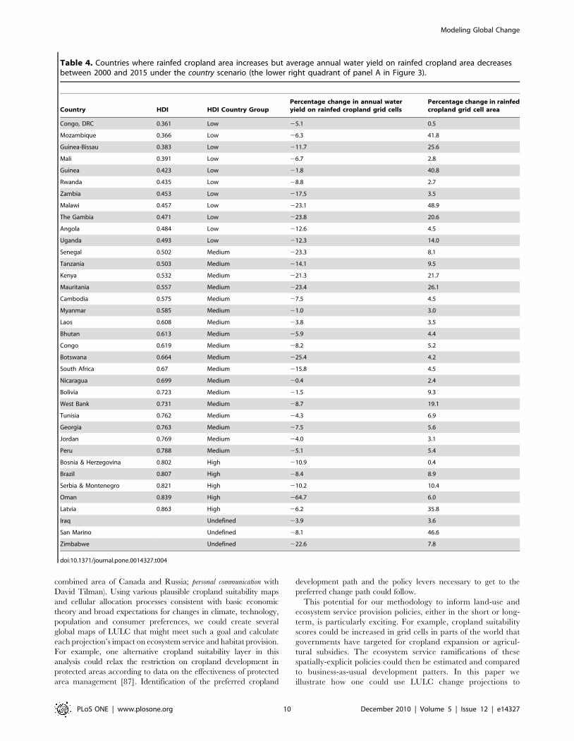
growth in crop production is a major concern. To begin to explorethis issue we plot country-level changes in rainfed cropland gridcell area (cropland in cells assigned the potential rainfed yield onthe cropland suitability layer) versus the projected change inaverage annual water yield on rainfed cropland grid cells (Figure 3).Production on rainfed cropland is limited by water produceddirectly on the cropland and cannot be maintained by irrigation.Therefore, our projections for crop production growth may be toohigh in countries that are projected to expand rainfed croplandarea but experience, on average, a decline in annual wateravailability (the lower right quadrant of the graphs in Figure 3indicates countries with such a tradeoff). There are five morecountries in the lower right quadrant under the regional scenario(panel B) than in the country scenario (panel A). Further, projectedrainfed cropland expansion is quite dramatic in several of these at-risk countries under the regional scenario (see Tables 4 and 5 for alist of all countries in the lower right quadrants of the graphs inFigure 3).

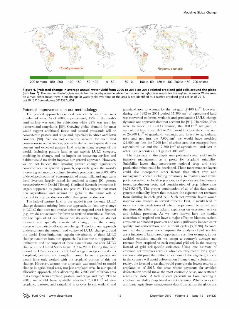
Despite having more countries where, on average, water yieldon rainfed cropland grid cells is decreasing while the area ofrainfed cropland grid cells is increasing, from a global perspectivethe expansion in rainfed cropland under the regional scenario isslightly better aligned with expected changes in annual water yieldpatterns than the country scenario. In 2000, average annual wateryield on all rainfed cropland grid cells across the globe wasestimated to be 636 mm km22. In 2015, the average yield isprojected to be 645 mm km22 under the regional scenario and632 mm km22 under the country scenario. Maps of expectedchanges in water availability on rainfed cropland around the globeand for two regions of the world across the two scenarios areshown in Figures 4 and 5.

Biomass carbon emissions due to land conversionCumulative country-level changes in biomass carbon storage

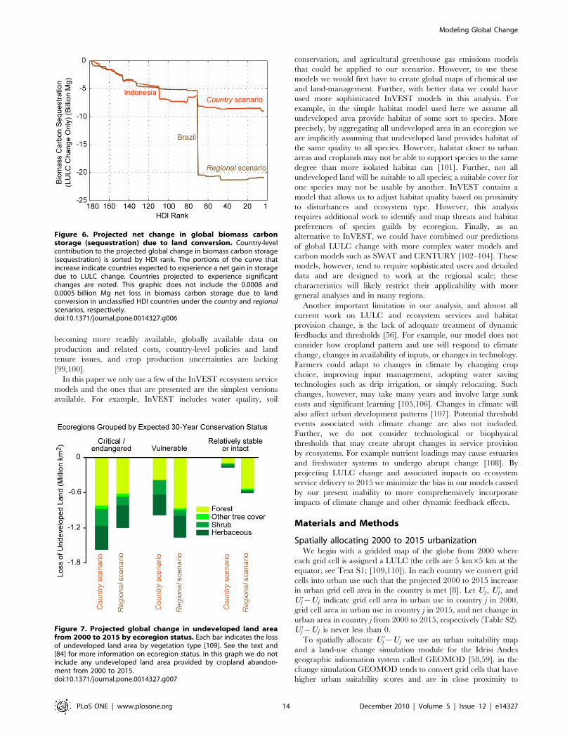
due to land conversion is sorted by HDI rank (Figure 6). Most ofthe difference between the two scenarios is explained by theprojected loss of broadleaved forest area in Brazil (Figure S1).Under the regional scenario, 0.84 million km2 of additionalbroadleaved forest are lost between 2000 and 2015 in Brazilwhen compared to country scenario. Other than Brazil, most of thenet loss in biomass carbon occurs in countries with HDI ranks ofless than 100 (the least-developed countries). Some countries withhigh HDI show a net gain in biomass carbon storage because theircropland abandonment rates are close to or even outpace theirurban growth rates.

Loss in undeveloped land and species persistenceGlobal cropland and urban area expansion reduces the global

supply of undeveloped land (non-urban and non-cropland covers),a land type that is more likely to provide species habitat than otherland uses. In Figure 7 we summarize the gross conversion of globalundeveloped grid cell area by ecoregion conservation status andscenario (by gross we mean that we do not include cropland that isabandoned to less intensive uses). An ecoregion’s conservationstatus indicates the degree of habitat alternation and spatial

Figure 2. Projected net change in global harvested area andcrop production from 2000 to 2015. Country-level contribution toprojected global net change in harvested area (panel A) and cropproduction measured in mass (panel B) and calories (panel C) is sortedby 2006 HDI rank for both scenarios. Countries projected to experiencesignificant changes are noted. For panels B and C scenario results aregiven once assuming each country’s 2000 crop mix remains as of 2015(‘‘The 2000 Crop Mix’’) and once assuming 2015 crop mixes mimicforecasted trends in crop mix (‘‘Projected 2015 Crop Mix’’). By crop mixwe mean the relative amount of harvested area devoted to each croptype (e.g., rice, wheat, oil crops, etc.) in a country. Panel C does notinclude a country’s production of crops in the categories fiber crops, oil

seeds, and other oil crops. The portions of the curves that declineindicate countries expected to experience a net decline in cropproduction on the given metric. This graphic does not include the netgain in harvested area and crop production in unclassified HDIcountries.doi:10.1371/journal.pone.0014327.g002



pattern of remaining habitat in an ecoregion at the end of the 20th

century [84]. Critical and endangered ecoregions retain littlenatural habitat and the habitat that remains is highly fragmentedand the continued persistence of many species is highly uncertain.Vulnerable and relatively stable ecoregions are less disturbed.While the regional scenario converts more undeveloped grid cellarea over the 15 year period (3.2 versus 2.7 million km2), thecountry scenario converts more undeveloped grid cell area in themost endangered ecoregions (1.6 versus 1.2 million km2 in critical/endangered ecoregions).

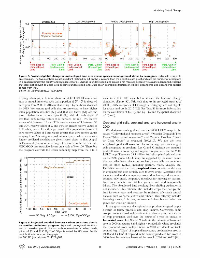
We also plot each ecoregion’s net relative change inundeveloped grid cell area versus the percentage of the ecoregion’sspecies that are critically endangered/endangered according to theIUCN Red List by HDI category [75,85] (Figure 8). An ecoregioncan experience a net grid cell area increase in undeveloped land ifits growth in abandoned cropland grid cell area (not including thecropland abandoned to urban use) is greater than its loss ofundeveloped land to urban and cropland grid cell area [86]. Whileall ecoregions in low development countries show net loses inundeveloped land across both scenarios, none of these ecoregionsare particularly rich in critically endangered/endangered specieswhen compared to some ecoregions in the middle and highdevelopment countries. Finally, Figure 8 indicates that many moreecoregions in middle and high development countries areprojected to experience a net loss in undeveloped grid cell areaunder the country scenario than under the regional scenario.However, particularly large losses of undeveloped land in theMadeira-Tapajos moist forests (Amazon Basin), Southwest Ama-zon moist forests, Uatuma-Trombetas moist forests (AmazonBasin), and Kazakh steppe ecoregions under the regional scenarioaccount for that scenario’s greater conversion of undeveloped landaround the world as indicated by Figure 7.

Avoided emissions analysisIn Figure 9 we summarize avoided emissions assuming a

REDD-like program existed as of 2000 and that our scenarioswere used by program administrators to determine business-as-usual deforestation and associated carbon emissions rates. Wedetermine avoided emissions for two avoided deforestation creditprices, $5 and $150 Mg21 per emissions of CO2e (carbon dioxide-equivalent) avoided. The regional scenario, which had more thantwice the loss of stored biomass carbon than the country scenario,generates far more avoided emission credits. In this illustration,avoided emissions supply is barely affected by offset price; $5offsets generate almost as much avoided emissions as do $150offsets. This result occurs because the net returns to agricultureare, on average, very low in Brazil, the source of most creditsunder both scenarios. This suggests that, assuming transaction andother program costs are kept low, modestly priced carbon offsetscould prevent an aggressive acceleration in agricultural develop-ment in Brazil.

TradeoffsTo summarize, we observe a tradeoff among LULC change and

ecosystem service and species habitat provision from 2000 to 2015.The tradeoff is less severe under the country scenario. Specifically,the grams of carbon released due to LULC conversion peradditional calorie of crop produced is 62% less and the loss ofundeveloped area (our proxy for species habitat) per additionalcalorie of crop produced is 24% less under the country scenariowhen compared to the regional scenario. The country scenario’smore efficient production of calories relies heavily on a 1) fairlydramatic expansion in irrigation capacity, 2) greater croplandexpansion in countries with greater access to technologicalimprovements in agriculture, and 3) avoidance of large-scale land

Table 2. Change in the mass of crop production between 2000 and 2015 using 2015 projected country-level crop mixes in 2015.

Country scenario Regional scenario

HDI CountryGroup

Change in production(million Mg)

Change in prod. /change inharvested km2 (Mg/km2)

Change in production(million Mg)

Change in prod./change in harvested km2 (Mg/km2)

Low 23 91 40 141

Medium 96 294 226 NA

High 230 NA 81 316

Note: Countries that do not have a 2006 HDI are not included in this table.doi:10.1371/journal.pone.0014327.t002

Table 1. Change in the mass of crop production between 2000 and 2015 assuming country-level crop mixes in 2015 mimic thoseobserved in 2000.


HDICountryGroup

No. ofcountries

Net changein millionharvestedkm2

Change inproduction(million Mg)

Change inprod. /change inharvestedkm2

(Mg/km2)

% of countrieswhere newcropland is,on average,more pro-ductive than2000 cropland

Net changein millionharvestedkm2

Change inproduction(million Mg)

Change inprod. /change inharvestedkm2 (Mg/km2)

% of countrieswhere newcropland is, onaverage, moreproductive than2000 cropland

Low 26 0.25 49 194 0.16 0.28 68 243 0.38

Medium 78 0.33 359 1,102 0.33 0.15 228 1,520 0.68

High 73 20.05 215 NA 0.39 0.26 368 1,443 0.59




conversion in important biomass carbon storage areas. The regionalscenario outperforms the country scenario on only one modeledmetric: rainfed cropland under the country scenario is expected toreceive less water than it is under the regional scenario. Therefore, if1) the relatively heavy expansion in irrigation capacity thatunderpins the country scenario’s results does not occur as modeledand 2) the greater water shortages on rainfed cropland under thecountry scenario significantly impairs rainfed cropland productivitythen the tradeoff gap between the two scenarios would shrink.

Discussion

In this paper we demonstrate a straightforward method forallocating expected LULC change given at a spatially coarse levelto a grid cell-level and predicting the impacts of such mappedchange on the provision of several ecosystem services and habitat(see Text S1 for a comparison of projected changes to actualchanges that have occurred since 2000). Our spatial allocationmethod is a cellular process that is guided by maps that describehow well-suited each grid cell is to a particular land use. We thenuse the InVEST methodology to translate LULC changes intochanges in the provision of various ecosystem services and

undeveloped land (our proxy for species habitat). This approachis transparent and well suited to cases where data and technicalexpertise are limited.

In our illustration of this approach we are temporally modest. Weonly project to 2015 for several reasons. First, there are globalprojections for regional agricultural land use and grid cell-levelpopulation density out to 2015. Further, extrapolating country-leveltrends in cropland over a 20-year period (the mid 1990s to the mid2010s) seems reasonable. Second, by only projecting to 2015 weminimize the bias in our models caused by our present inability tomore comprehensively incorporate impacts of climate change andother dynamic feedback effects (see below). However, we feel ourapproach is also well-suited for the exploration of the global impactsof much more distant future scenarios. In such analyses,expectations for country- or regional-level land-use change wouldnot be based on well-calibrated models’ projections for the nearfuture but on plausible global change trajectories. For example,what would the pattern and magnitude of environmental impact beacross the globe if the developing world adopted the current dietpreferences of the developed world by 2060? It has been estimatedthat such a future would require an additional 26 million km2 ofcropland compared to year 2000 levels (approximately the

Figure 3. Projected relative change in rainfed cropland grid cell area versus relative change in average annual water yield onrainfed cropland grid cells. Panel A gives results for the country scenario. Panel B gives results for the regional scenario. Each point represents acountry. A high development country (‘‘High Dev.’’) has a 2006 HDI greater than or equal to 0.8, a middle development country (‘‘Middle Dev.’’) has a2006 HDI greater than or equal to 0.5 but less than 0.8, a low development country (‘‘Low Dev.’’) has a 2006 HDI less then 0.5, and a unclassifiedcountry has no HDI score. We indicate the number of countries (N) and the average HDI score (HD) of those countries in each quadrant in each graph.doi:10.1371/journal.pone.0014327.g003

Table 3. Change in the caloric value of crop production between 2000 and 2015.


2000 Country-LevelCrop Mixes

Projected 2015 Country-LevelCrop Mixes 2000 Country-Level Crop Mixes

Projected 2015 Country-LevelCrop Mixes

HDICountryGroup

Change inproduction(trillioncalories)

Change inproduction/changein harvested km2

(millioncalories/km2)








Change inproduction/change inharvested km2

(million calories/km2)

Low 87 346 109 436 103 368 124 442

Medium 895 2,744 1,141 3,499 658 4,388 886 5,909

High 555 NA 752 NA 569 2,230 734 2,877




combined area of Canada and Russia; personal communication withDavid Tilman). Using various plausible cropland suitability mapsand cellular allocation processes consistent with basic economictheory and broad expectations for changes in climate, technology,population and consumer preferences, we could create severalglobal maps of LULC that might meet such a goal and calculateeach projection’s impact on ecosystem service and habitat provision.For example, one alternative cropland suitability layer in thisanalysis could relax the restriction on cropland development inprotected areas according to data on the effectiveness of protectedarea management [87]. Identification of the preferred cropland

development path and the policy levers necessary to get to thepreferred change path could follow.

This potential for our methodology to inform land-use andecosystem service provision policies, either in the short or long-term, is particularly exciting. For example, cropland suitabilityscores could be increased in grid cells in parts of the world thatgovernments have targeted for cropland expansion or agricul-tural subsidies. The ecosystem service ramifications of thesespatially-explicit policies could then be estimated and comparedto business-as-usual development patters. In this paper weillustrate how one could use LULC change projections to

Table 4. Countries where rainfed cropland area increases but average annual water yield on rainfed cropland area decreasesbetween 2000 and 2015 under the country scenario (the lower right quadrant of panel A in Figure 3).

Country HDI HDI Country GroupPercentage change in annual wateryield on rainfed cropland grid cells

Percentage change in rainfedcropland grid cell area

Congo, DRC 0.361 Low 25.1 0.5

Mozambique 0.366 Low 26.3 41.8

Guinea-Bissau 0.383 Low 211.7 25.6

Mali 0.391 Low 26.7 2.8

Guinea 0.423 Low 21.8 40.8

Rwanda 0.435 Low 28.8 2.7

Zambia 0.453 Low 217.5 3.5

Malawi 0.457 Low 223.1 48.9

The Gambia 0.471 Low 223.8 20.6

Angola 0.484 Low 212.6 4.5

Uganda 0.493 Low 212.3 14.0

Senegal 0.502 Medium 223.3 8.1

Tanzania 0.503 Medium 214.1 9.5

Kenya 0.532 Medium 221.3 21.7

Mauritania 0.557 Medium 223.4 26.1

Cambodia 0.575 Medium 27.5 4.5

Myanmar 0.585 Medium 21.0 3.0

Laos 0.608 Medium 23.8 3.5

Bhutan 0.613 Medium 25.9 4.4

Congo 0.619 Medium 28.2 5.2

Botswana 0.664 Medium 225.4 4.2

South Africa 0.67 Medium 215.8 4.5

Nicaragua 0.699 Medium 20.4 2.4

Bolivia 0.723 Medium 21.5 9.3

West Bank 0.731 Medium 28.7 19.1

Tunisia 0.762 Medium 24.3 6.9

Georgia 0.763 Medium 27.5 5.6

Jordan 0.769 Medium 24.0 3.1

Peru 0.788 Medium 25.1 5.4

Bosnia & Herzegovina 0.802 High 210.9 0.4

Brazil 0.807 High 28.4 8.9

Serbia & Montenegro 0.821 High 210.2 10.4

Oman 0.839 High 264.7 6.0

Latvia 0.863 High 26.2 35.8

Iraq Undefined 23.9 3.6

San Marino Undefined 28.1 46.6

Zimbabwe Undefined 222.6 7.8

doi:10.1371/journal.pone.0014327.t004



establish a baseline of deforestation to set eligibility and caprequirements in a global REDD-like program instead of relyingon historic deforestation rates [88]. Using projected LULC mapsinstead of historic deforestation rates to guide a global REDD-like program avoids the perverse result of rewarding countries

that aggressively deforested in the immediate past. Finally, asnoted above, policy makers could use this tool to begin adiscussion on the more distant future and the impact that another50 or 100 years of development might have on the earth’senvironment.

Table 5. Countries where rainfed cropland area increases but average annual water yield on rainfed cropland area decreasesunder the regional scenario (the lower right quadrant of panel B in Figure 3).

HDI HDI CategoryPercentage change in annual wateryield on rainfed cropland grid cells

Percentage change in rainfedcropland grid cell area

Congo, DRC 0.361 Low 27.2 176.2

Mozambique 0.366 Low 27.9 32.2

Niger 0.37 Low 22.3 45.7

Guinea-Bissau 0.383 Low 215.0 205.7

Mali 0.391 Low 25.4 11.1

Guinea 0.423 Low 25.0 54.7

Malawi 0.457 Low 219.3 18.1

Angola 0.484 Low 23.1 17.4

Senegal 0.502 Medium 224.9 1.9

Tanzania 0.503 Medium 215.9 0.9

Kenya 0.532 Medium 228.3 30.8

Madagascar 0.533 Medium 221.5 25.4

Mauritania 0.557 Medium 228.9 41.8

Cambodia 0.575 Medium 210.5 50.8

Myanmar 0.585 Medium 21.8 5.4

Laos 0.608 Medium 23.9 3.7

Bhutan 0.613 Medium 25.9 4.4

Congo 0.619 Medium 20.1 371.5

Namibia 0.634 Medium 218.0 94.7

Botswana 0.664 Medium 218.0 57.4

Uzbekistan 0.701 Medium 26.1 31.3

Moldova 0.719 Medium 212.8 1.7

Guyana 0.725 Medium 221.4 1775.2

Gabon 0.729 Medium 210.8 319.2

West Bank 0.731 Medium 28.8 28.9

Paraguay 0.752 Medium 213.0 13.7

Azerbaijan 0.758 Medium 224.3 52.1

Tunisia 0.762 Medium 24.3 6.9

Georgia 0.763 Medium 29.4 66.5

Jordan 0.769 Medium 24.0 3.1

Suriname 0.77 Medium 217.3 435.0

Armenia 0.777 Medium 210.9 0.9

Ukraine 0.786 Medium 214.0 9.0

Bosnia & Herzegovina 0.802 High 210.7 1.0

Kazakhstan 0.807 High 25.8 0.4

Belarus 0.817 High 211.5 1.4

Oman 0.839 High 270.4 26.0

Libya 0.84 High 287.8 1099.0

Uruguay 0.859 High 24.2 17.6

Brunei 0.919 High 20.8 45.1

Somalia Undefined 215.7 7.6

Zimbabwe Undefined 222.3 4.9

doi:10.1371/journal.pone.0014327.t005



Potential improvements in our methodologyThe general approach described here can be improved in a

number of ways. As of 2000, approximately 12% of the earth’sland surface was used for cultivation while 22% was used forpastures and rangelands [89]. Growing global demand for meatwould suggest additional forest and natural grasslands will beconverted to pasture and rangeland, especially in Africa and LatinAmerica [90]. We do not currently account for such landconversion in our scenarios, primarily due to inadequate data oncurrent and expected pasture land area in many regions of theworld. Including pasture land as an explicit LULC category,modeling its change, and its impact on ecosystem services andhabitat would no doubt improve our general approach. However,we do not believe that ignoring pasture change significantlycompromises our general approach, especially given the world’sincreasing reliance on confined livestock production (in 2003, 70%of developed countries’ consumption of meat, milk, and eggs camefrom livestock largely raised in confined settings) [90, personalcommunication with David Tilman]. Confined livestock production islargely supported by grains, not pasture. This suggests that mostnew agricultural land around the globe in the future will bedevoted to crop production rather than grass production.

The lack of pasture land in our model is not the only LULCchange dynamic missing from our approach. In fact, any changein LULC that does not involve urban or cropland area is ignored(e.g., we do not account for forest to wetland transitions). Further,for the types of LULC change we do account for, we do notmeasure and spatially allocate all change, just the changenecessary to spatially allocate net change. Therefore, our approachunderestimates the amount and variety of LULC change aroundthe world. Data limitations explain the absence of these LULCchange dynamics from our approach. To illustrate our approach’slimitations and the impact of these assumptions consider LULCchange in the United States from 1992 to 2001. During that timeperiod the US experienced a 400 km2 net gain in agricultural area(cropland, pasture, and rangeland area). In our approach wewould have only worked with the cropland portion of this netchange. However, assume our approach was modified to modelchange in agricultural area, not just cropland area. In our spatialallocation approach, after allocating the 7,200 km2 of urban areathat emerged from cropland, pasture, and rangeland from 1992 to2001, we would have spatially allocated 7,600 km2 of newcropland, pasture, and rangeland area over forest, wetland and

grassland area to account for the net gain of 400 km2. However,during this 1992 to 2001 period 17,300 km2 of agricultural landwas converted to forests, wetlands and grasslands; a LULC changedynamic our approach does not account for [91]. Therefore, if wewere to model all LULC change, the 400 km2 net gain inagricultural land from 1992 to 2001 would include the conversionof 24,900 km2 of grassland, wetlands, and forests to agriculturaluses and not just the 7,600 km2 we would have modeled(24,900 km2 less the 7,200 km2 of urban area that emerged fromagricultural use and the 17,300 km2 of agricultural lands lost toother uses generates a net gain of 400 km2).

The approach in this paper uses potential cereal yield underintensive management as a proxy for cropland suitability.Suitability layers that incorporate regional crop and cropproduction mixes could be developed. These more nuanced layerscould also incorporate other factors that affect crop andmanagement choice including proximity to markets and trans-portation networks, local crop prices, local policies and land tenureissues, production costs, and consideration of crop failure risks[4,74,92–97]. The proper combination of all of this data wouldgenerate suitability layers that measure the expected net revenuesfrom farming in each grid cell. Such net revenue layers wouldimprove our analysis in several respects. First, it would lead tomore accurate predictions of where crops would be grown andtherefore, the effect of cropland expansion on ecosystem serviceand habitat provision. As we have shown here the spatialallocation of cropland can have a major effect on biomass carbonemissions and habitat provision and also significantly impact waterquality, soil conservation, and nutrient cycles [5,93,98]. Second,such suitability layers would improve the analyses of policies thatare a function of land-based opportunity cost. For example, in ouravoided emission analysis we assign a country’s average netrevenue from cropland to each cropland grid cell in the countryinstead of grid cell-specific estimates. Using one estimate ofcropland net revenues across a whole country means for a givencarbon credit price that either all or none of the eligible grid cellsin the country will avoid deforestation (‘‘bang-bang’’ solutions). Inreality, the forested areas that would generate the lowest returns incropland as of 2015, the areas where payments for avoideddeforestation would make the most economic sense, are scatteredacross the globe. A lack of data prevents us from creating acropland suitability map based on net revenues. While crop yieldand basic agriculture management data from across the globe are

Figure 4. Projected change in average annual water yield from 2000 to 2015 on 2015 rainfed cropland grid cells around the globe(mm km22). The map on the left gives results for the country scenario while the map on the right gives results for the regional scenario. White areason a map either mean there is no change in water yield over time or the area is not identified as a rainfed cropland grid cell as of 2015.doi:10.1371/journal.pone.0014327.g004



Figure 5. Projected change in average annual water yield from 2000 to 2015 on 2015 rainfed cropland grid cells for two regions(mm km22). The maps on the left give results for the country scenario while the maps on the right give results for the regional scenario. White areason a map either mean there is no change in water yield over time or the area is not identified as a rainfed cropland grid cell as of 2015.doi:10.1371/journal.pone.0014327.g005



becoming more readily available, globally available data onproduction and related costs, country-level policies and landtenure issues, and crop production uncertainties are lacking[99,100].

In this paper we only use a few of the InVEST ecosystem servicemodels and the ones that are presented are the simplest versionsavailable. For example, InVEST includes water quality, soil

conservation, and agricultural greenhouse gas emissions modelsthat could be applied to our scenarios. However, to use thesemodels we would first have to create global maps of chemical useand land-management. Further, with better data we could haveused more sophisticated InVEST models in this analysis. Forexample, in the simple habitat model used here we assume allundeveloped area provide habitat of some sort to species. Moreprecisely, by aggregating all undeveloped area in an ecoregion weare implicitly assuming that undeveloped land provides habitat ofthe same quality to all species. However, habitat closer to urbanareas and croplands may not be able to support species to the samedegree than more isolated habitat can [101]. Further, not allundeveloped land will be suitable to all species; a suitable cover forone species may not be usable by another. InVEST contains amodel that allows us to adjust habitat quality based on proximityto disturbances and ecosystem type. However, this analysisrequires additional work to identify and map threats and habitatpreferences of species guilds by ecoregion. Finally, as analternative to InVEST, we could have combined our predictionsof global LULC change with more complex water models andcarbon models such as SWAT and CENTURY [102–104]. Thesemodels, however, tend to require sophisticated users and detaileddata and are designed to work at the regional scale; thesecharacteristics will likely restrict their applicability with moregeneral analyses and in many regions.

Another important limitation in our analysis, and almost allcurrent work on LULC and ecosystem services and habitatprovision change, is the lack of adequate treatment of dynamicfeedbacks and thresholds [56]. For example, our model does notconsider how cropland pattern and use will respond to climatechange, changes in availability of inputs, or changes in technology.Farmers could adapt to changes in climate by changing cropchoice, improving input management, adopting water savingtechnologies such as drip irrigation, or simply relocating. Suchchanges, however, may take many years and involve large sunkcosts and significant learning [105,106]. Changes in climate willalso affect urban development patterns [107]. Potential thresholdevents associated with climate change are also not included.Further, we do not consider technological or biophysicalthresholds that may create abrupt changes in service provisionby ecosystems. For example nutrient loadings may cause estuariesand freshwater systems to undergo abrupt change [108]. Byprojecting LULC change and associated impacts on ecosystemservice delivery to 2015 we minimize the bias in our models causedby our present inability to more comprehensively incorporateimpacts of climate change and other dynamic feedback effects.

Materials and Methods

Spatially allocating 2000 to 2015 urbanizationWe begin with a gridded map of the globe from 2000 where

each grid cell is assigned a LULC (the cells are 5 km65 km at theequator, see Text S1; [109,110]). In each country we convert gridcells into urban use such that the projected 2000 to 2015 increasein urban grid cell area in the country is met [8]. Let Uj , U ’j , andU ’j{Uj indicate grid cell area in urban use in country j in 2000,grid cell area in urban use in country j in 2015, and net change inurban area in country j from 2000 to 2015, respectively (Table S2).U ’j{Uj is never less than 0.

To spatially allocate U ’j{Uj we use an urban suitability mapand a land-use change simulation module for the Idrisi Andesgeographic information system called GEOMOD [58,59]. in thechange simulation GEOMOD tends to convert grid cells that havehigher urban suitability scores and are in close proximity to

Figure 6. Projected net change in global biomass carbonstorage (sequestration) due to land conversion. Country-levelcontribution to the projected global change in biomass carbon storage(sequestration) is sorted by HDI rank. The portions of the curve thatincrease indicate countries expected to experience a net gain in storagedue to LULC change. Countries projected to experience significantchanges are noted. This graphic does not include the 0.0008 and0.0005 billion Mg net loss in biomass carbon storage due to landconversion in unclassified HDI countries under the country and regionalscenarios, respectively.doi:10.1371/journal.pone.0014327.g006

Figure 7. Projected global change in undeveloped land areafrom 2000 to 2015 by ecoregion status. Each bar indicates the lossof undeveloped land area by vegetation type [109]. See the text and[84] for more information on ecoregion status. In this graph we do notinclude any undeveloped land area provided by cropland abandon-ment from 2000 to 2015.doi:10.1371/journal.pone.0014327.g007



existing urban grid cells into urban use. A GEOMOD simulationruns in annual time steps such that a portion of U ’j{Uj is allocatedeach year from 2000 to 2015 until all of U ’j{Uj has been allocatedby 2015. We assume grid cells that are projected to have higher2015 population densities [60] and that are flatter [61] are themost suitable for urban use. Specifically, grid cells with slopes ofless than 12% receive values of 5, between 12 and 18% receivevalues of 4, between 18 and 30% receive values of 3, between 30and 50% receive values of 2, and 50% or greater receive values of1. Further, grid cells with a predicted 2015 population density ofzero receive values of 1 and values greater than zero receive valuesranging from 2–5 using an equal interval system where areas withhigher predicted densities are given scores closer to five. A gridcell’s suitability score is the average of its scores on the two metrics.GEOMOD uses suitability layers on a scale of 0 to 100. Thereforethe program converts the urban suitability map from the 1 to 5

scale to a 0 to 100 scale before it runs the land-use changesimulation (Figure S2). Grid cells that are in protected areas as of2000 (IUCN categories of I through VI category) are not eligiblefor urban land use in 2015 [62]. See Text S1 for more informationon the calculation of Uj , U ’j , and U ’j{Uj and the spatial allocationof U ’j{Uj .

Cropland grid cells, cropland area, and harvested area in2000

We designate each grid cell on the 2000 LULC map in thecovers ‘‘Cultivated and managed areas’’, ‘‘Mosaic: Cropland/TreeCover/Other natural vegetation’’, and ‘‘Mosaic: Cropland/Shrubor Grass Cover’’ as cropland [109,110]. We use the termcropland grid cell area to refer to the aggregate area of gridcells designated as cropland. Let Cj and Cr indicate the croplandgrid cell area in country j and region r, respectively, on the 2000LULC map. There are 25.4 million km2 of cropland grid cell areaon the 2000 global LULC map. As suggested by the cover namesthat we collectively refer to as cropland, these cells can contain amix of other LULC, including pasture, roads, villages, etc.Hereafter we use the term cropland area to refer to the areain cropland grid cells actually used to grow crops. (Cropland areaincludes land under temporary crops (double-cropped areas arecounted only once), temporary meadows for mowing or pasture,land under market and kitchen gardens and land temporarilyfallow. The abandoned land resulting from shifting cultivation isnot included. This estimate also includes crops that occupy theland for some years and need not be replanted after each annualharvest, such as cocoa, coffee and rubber. This category includesflowering shrubs, fruit trees, nut trees and vines, but excludes treesgrown for wood or timber.)

In any given year not all cropland area produces cropped outputbecause of fallow practices and crop failures. Conversely, somecropped areas are used multiple times in a calendar year. Let the areaof crop production used over the course of a year be known asharvested area. Let Hj and Hr indicate the estimate of harvestedarea in 2000 in country j and region r, respectively where croplandsthat produced crops multiple times in 2000 are double or triplecounted (e.g., if X km2 of cropland in a country produced one crop in2000 and if Y km2 of cropland in the country produced two crops in2000 then the country’s harvested hectares in 2000 are X+2Y) [6].

Figure 8. Projected global change in undeveloped land area versus species endangerment status by ecoregion. Each circle representsan ecoregion. The two numbers in each quadrant (defined by 0.1 on the y-axis and 0 on the x-axis) in each graph indicate the number of ecoregionsin a quadrant under the country and regional scenarios. Change in undeveloped land area is a net measure because we assume abandoned croplandthat does not convert to urban area becomes undeveloped land. Data on an ecoregion’s fraction of critically endangered and endangered speciescomes from [75].doi:10.1371/journal.pone.0014327.g008

Figure 9. Projected avoided biomass carbon emissions due toan avoided emissions program. Expected country-level contribu-tion to avoided global biomass carbon emissions at offset creditprices of $5 and $150 Mg21 of CO2-e is sorted by HDI rank. Brazil’scontribution is noted on the graph.doi:10.1371/journal.pone.0014327.g009



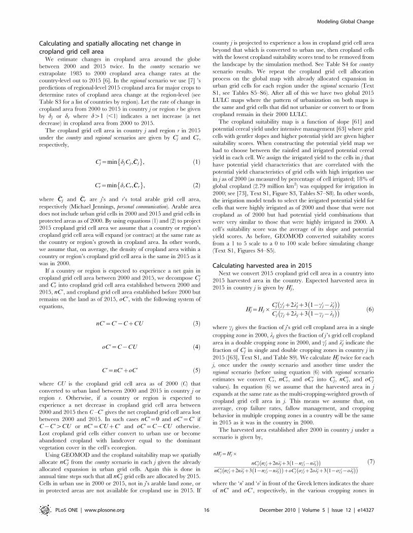
Calculating and spatially allocating net change incropland grid cell area

We estimate changes in cropland area around the globebetween 2000 and 2015 twice. In the country scenario weextrapolate 1985 to 2000 cropland area change rates at thecountry-level out to 2015 [6]. In the regional scenario we use [7] ’spredictions of regional-level 2015 cropland area for major crops todetermine rates of cropland area change at the region-level (seeTable S3 for a list of countries by region). Let the rate of change incropland area from 2000 to 2015 in country j or region r be givenby dj or dr where dw1 (,1) indicates a net increase (a netdecrease) in cropland area from 2000 to 2015.

The cropland grid cell area in country j and region r in 2015under the country and regional scenarios are given by C’j and C’r,respectively,

C’j~min djCj , !CCj

! ", !1"

C’r~min drCr, !CCr

! ", !2"

where !CCj and !CCr are j’s and r’s total arable grid cell area,respectively (Michael Jennings, personal communication). Arable areadoes not include urban grid cells in 2000 and 2015 and grid cells inprotected areas as of 2000. By using equations (1) and (2) to project2015 cropland grid cell area we assume that a country or region’scropland grid cell area will expand (or contract) at the same rate asthe country or region’s growth in cropland area. In other words,we assume that, on average, the density of cropland area within acountry or region’s cropland grid cell area is the same in 2015 as itwas in 2000.

If a country or region is expected to experience a net gain incropland grid cell area between 2000 and 2015, we decompose C’jand C’r into cropland grid cell area established between 2000 and2015, nC’, and cropland grid cell area established before 2000 butremains on the land as of 2015, oC’, with the following system ofequations,

nC’~C’{CzCU !3"

oC’~C{CU !4"

C’~nC’zoC’ !5"

where CU is the cropland grid cell area as of 2000 (C) thatconverted to urban land between 2000 and 2015 in country j orregion r. Otherwise, if a country or region is expected toexperience a net decrease in cropland grid cell area between2000 and 2015 then C –C’ gives the net cropland grid cell area lostbetween 2000 and 2015. In such cases nC’~0 and oC’~C’ ifC{C’wCU or nC’~CUzC’ and oC’~C{CU otherwise.Lost cropland grid cells either convert to urban use or becomeabandoned cropland with landcover equal to the dominantvegetation cover in the cell’s ecoregion.

Using GEOMOD and the cropland suitability map we spatiallyallocate nC’j from the country scenario in each j given the alreadyallocated expansion in urban grid cells. Again this is done inannual time steps such that all nC’j grid cells are allocated by 2015.Cells in urban use in 2000 or 2015, not in j’s arable land zone, orin protected areas are not available for cropland use in 2015. If

county j is projected to experience a loss in cropland grid cell areabeyond that which is converted to urban use, then cropland cellswith the lowest cropland suitability scores tend to be removed fromthe landscape by the simulation method. See Table S4 for countryscenario results. We repeat the cropland grid cell allocationprocess on the global map with already allocated expansion inurban grid cells for each region under the regional scenario (TextS1, see Tables S5–S6). After all of this we have two global 2015LULC maps where the pattern of urbanization on both maps isthe same and grid cells that did not urbanize or convert to or fromcropland remain in their 2000 LULC.

The cropland suitability map is a function of slope [61] andpotential cereal yield under intensive management [63] where gridcells with gentler slopes and higher potential yield are given highersuitability scores. When constructing the potential yield map wehad to choose between the rainfed and irrigated potential cerealyield in each cell. We assign the irrigated yield to the cells in j thathave potential yield characteristics that are correlated with thepotential yield characteristics of grid cells with high irrigation usein j as of 2000 (as measured by percentage of cell irrigated; 18% ofglobal cropland (2.79 million km2) was equipped for irrigation in2000; see [73], Text S1, Figure S3, Tables S7–S8). In other words,the irrigation model tends to select the irrigated potential yield forcells that were highly irrigated as of 2000 and those that were notcropland as of 2000 but had potential yield combinations thatwere very similar to those that were highly irrigated in 2000. Acell’s suitability score was the average of its slope and potentialyield scores. As before, GEOMOD converted suitability scoresfrom a 1 to 5 scale to a 0 to 100 scale before simulating change(Text S1, Figures S4–S5).

Calculating harvested area in 2015Next we convert 2015 cropland grid cell area in a country into

2015 harvested area in the country. Expected harvested area in2015 in country j is given by H ’j ,

H ’j~Hj|C’j c’jz2l’jz3 1{c’j{l’j

# $# $

Cj cjz2ljz3 1{cj{lj

# $# $ !6"

where cj gives the fraction of j’s grid cell cropland area in a single

cropping zone in 2000, lj gives the fraction of j ’s grid cell cropland

area in a double cropping zone in 2000, and c’j and l’j indicate the

fraction of C’j in single and double cropping zones in country j in

2015 ([63], Text S1, and Table S9). We calculate H ’j twice for each

j, once under the country scenario and another time under theregional scenario (before using equation (6) with regional scenarioestimates we convert C’r, nC’r, and oC’r into C’j , nC’j , and oC’jvalues). In equation (6) we assume that the harvested area in jexpands at the same rate as the multi-cropping-weighted growth ofcropland grid cell area in j. This means we assume that, onaverage, crop failure rates, fallow management, and croppingbehavior in multiple cropping zones in a country will be the samein 2015 as it was in the country in 2000.

The harvested area established after 2000 in country j under ascenario is given by,

nH ’j~H ’j|

nC’j nc’jz2nl’jz3 1{nc’j{nl’j# $# $

nC’j nc’jz2nl’jz3 1{nc’j{nl’j# $# $

zoC’j oc’jz2ol’jz3 1{oc’j{ol’j# $# $

!7"

where the ‘n’ and ‘o’ in front of the Greek letters indicates the shareof nC’ and oC’, respectively, in the various cropping zones in

!7"



2015. Finally, harvested area in country j established prior to 2000is given by,

oH ’j~H ’j{nH ’j !8"

We calculate nH ’j and oH ’j twice for each j, once under thecountry scenario and another time under the regional scenario.

Measuring change in crop production between 2000 and2015

To determine 2015 crop production in country j we first calculateeach crop or crop types average yield in country j in 2000, given by Yji

and measured in in Mg ha21, where i = 1, 2, …, I includes individualcrop types (e.g., rice) or crop groups (e.g., treenuts; [6], Text S1, andTable S10). For example, in 2000 96,000 hectares of maize and124,000 hectares of barley were grown in Afghanistan; both cropsbelong to the coarse grains category (so do sorghum and oats, however,neither were produced in Afghanistan in 2000 according to [6]).Respective production was 114,998 Mg of maize and 73,991Mg of barley. Therefore, coarse grain yield in Afghanistan in2000 was 0.859 Mg ha21 (i.e., 114,998 Mg + 73,991 Mg/96,000 ha +124,000 ha).

We determine the caloric production of crop type i in j in 2015with,

P’ji~ajiYjiRi fn nbj

# $nH ’jsjiyjizfo obj

# $oH ’jvji

% &!9"

where aji§1 is country j’s expected 2000 to 2015 growth in i’syield due to technological change ([7,65], Text S1, and TableS11); Ri is the average caloric content Mg21 of crop or crop groupi ([82], Text S1, and Table S12); nbj and obj indicate the relative

difference in the cropland productivity of the new and oldcropland grid cells in 2015, respectively, versus the cropland gridcells in j as of 2000, the functions fn and fo convert nbj and obj into

yield inflators; sji indicates the fraction of ‘‘new’’ harvestedhectares in j in crop or crop group i in 2015, yji[ [0,1] indicates

the degree to which new harvested hectares used for crop or cropgroup i in j meets its projected productive capacity by 2015 wherea 1 indicates it has reached its projected productive capacity; vji

indicates the fraction of ‘‘old’’ harvested hectares in j that is in cropor crop group i in 2015; and

Pi sji~

Pi vji~1. The first term in

equation (9), Pji~ajiYjiRji, is an estimate of year 2000 ha21

caloric production of crop or crop group i in country j and thesecond term converts this to 2015 levels given technology growth,changes in overall productivity of the grid cells used for crops, andcrop mix changes. Relative changes in productivity, nbj and obj ,

are given by relative changes in the suitability of cropland grid cellarea in j. Specifically, the relative difference in the productivity ofcropland grid cell area in 2015 versus 2000 in country j is found bydividing the 2015 average suitability score for new or old croplandgrid cell area in j by the average suitability score for j’s croplandcell area in 2000 (Text S1 and Table S13). For example, if theaverage cropland suitability score for new cropland grid cells incountry j is 55 and the average agriculture suitability score forcropland grid cells in country j on the 2000 map is 49 then

nbj = 55/49 = 1.12. For illustrative purposes we set fn nbj

# $~

fo obj

# $~X 0:5 for all j under both scenarios. The value of yji will

depend on the crop or crop group, the land used for i in j, thetechnology applied to production for i in j, and agricultural-relatedinfrastructure that can be accessed by the newly convertedcropland in country j. Some lands will produce expected yields

within a year or two of establishment while others may take adecade or more. Due to a lack of data we set yji~1 in our model

for all combinations of j and i. If we drop Ri from equation (9) thenP’ji gives 2015 country-level production of crop or crop group i inmetric tons. The change in the production of crop type i in j from2000 to 2015 is given by DPji~P’ji{Pji and the change in allcrop production in country j is given by DPj~

Pi DPji.

We create 5 allocations of sji across all combinations of j and i.Let sq indicate the qth matrix of sji values. One realization of sindicates the relative mix of crop types in each j as observed in2000 (q = Year 2000 crop mix; [6], Text S1, and Table S14). Inanother projection we assume that the areal share of crop typesother than rice, wheat, coarse grains, and oil seeds in each countrywill fall steeply by 2015 when compared to 2000 levels (q = 2; TextS1 and Table S15). In another we assume that the areal share ofcrop types other than rice, wheat, coarse grains, and oil seeds ineach country will fall moderately by 2015 when compared to 2000levels (q = 3; Text S1 and Table S16). In another we assume thatthe areal share of all crop types in each country will remain closeto 2000 levels (q = 4; Text S1 and Table S17). In the last projectionwe set crop share values across countries such that the global areadevoted to rice, wheat, coarse grains, and oil seeds matches thatpredicted by the agricultural trade model in [7] (q = Projected2015 crop mix; [7], Text S1, and Table S18). In this illustration weset vqequal to sq; there is no particular reason, however, whythese must be equal.

Every input into equation (9) can be described with uncertainty.For example, for crop groups i we only use average yields and donot consider the observed distribution’s other moments. More-over, we do not consider how Yji of crop groups i will change overtime due to changes in the areal mix of crops within the group.Nor do we consider how Yji might change as the climate changes,etc. Further, we assume that the effect of nbj and obj on yields aregiven by the functional formX 0:5; other functional forms are notexperimented with. In addition, the values of nbj and obj will besensitive to variables other than the relative change in croplandsuitability, including the specific allocation of crop types across jand water availability. The expected paths of agriculturaltechnology development aji are also highly uncertain. Weexperiment a bit with alternative crop choice allocations, althoughthe matrices sq and vq could be perturbed even more.

Annual water yieldAnnual water yield, measured in mm km22, is equal to the

precipitation that falls during the course of a year less the waterthat evaporates or transpires (actual evapotranspiration) [2,67–72].

Annual water yield in grid cell x In LULC j in 2000 is given byWxj and in 2015 by W ’xj . Hereafter we describe how to calculateWxj. The variable W ’xj is calculated in the same manner but with2015 data, including LULC cover in grid cell x and precipitationin grid cell x. Let,

Wxj~ 1{AETxj

Px

' (Px !10"

where AETxj is the annual actual evapotranspiration on grid cell xwith LULC j in 2000 (measured in mm km22) and Px is the year2000 precipitation on grid cell x (measured in mm km22).Therefore, Wxj represents the amount of water available to thesurface and groundwater systems in x’s watershed over the courseof 2000.

The portion of equation (10) that represents evapotranspiration,AETx/Px, is an approximation of the Budyko curve,



AETxj

Px~

1zmxRxj

1zmxRxjz 1)

Rxj

# $ !11"

where mx is the dimensionless ratio of plant accessible waterstorage to expected precipitation during the year and Rxj is thedimensionless Budyko Dryness index on grid cell x in 2000 and isdefined as the ratio of potential evapotranspiration to precipitation[68,70].

As defined by [70], mx is a non-physical parameter thatcharacterizes the natural climatic-soil properties in grid cell x[69,71,72],

mx~ZxAWCxj

Px!12"

where AWCxj is the volumetric (mm) plant available water contenton grid cell x in LULC j [111], a soil property generally estimatedas the difference in water content (mm) between field capacity andwilting point (i.e., the amount of water that can be held andreleased in the soil for use by a plant), and Zx is a constant that iscalibrated for climatically homogeneous basins (i.e., Z is the samefor all grid cells in a climatically homogeneous basins). The soiltexture and effective soil depth in grid cell x defines AWCx. Theconstant Z adjusts the water balance to account for timingdifferences of monthly intra-annual rainfall and energy distribu-tion patterns, and rainfall intensities. Variation in m across alandscape reflects variation in available water content and rainfallacross the landscape. Although we recognize that the relationshipbetween w and AWC/P is technically non-linear, we assume alinear relationship to simplify modeling.

We define the Budyko dryness index as follows,

Rxj~kxjETox

Px~

PETxj

Px!13"

where ETox is the reference evapotranspiration on grid cell x[112,113] and kxj is the plant evapotranspiration coefficientassociated with the LULC j on grid cell x. ETo is an index ofclimatic demand while kxj is largely determined by j’s vegetativecharacteristics [114]. Budyko dryness index values that are greaterthan one denote grid cells that are potentially arid [68].

We use the HadCM3 climate model with the Intergovernmen-tal Panel on Climate Change A2 greenhouse-gas emissionsscenario to map global annual precipitation [66]. Because globalmaps of precipitation under HadCM3 with the A2 emissionsscenario are not available for 2000 and 2015 we use a modeledprecipitation map from 1990 with the 2000 LULC map and amodeled precipitation map from 2025 with the 2015 LULC maps.Therefore, depending on the pace of climate change, our grid cell-level changes in annual water yield will deviate slightly fromestimates we would have generated if we had been able to use2000 and 2015 precipitation maps with the 2000 and 2015 LULCmaps.

See Table S19 for data on average country-level water yield onrainfed cropland grid cells in 2000 and 2015 under both scenarios.

In our analysis we imply that a decline in average annual wateryield in an area means that rainfed cropland yields in the area maynot increase at the rate of technological growth, all else beingequal (in addition, less runoff will be available for irrigation use).However, this may not be the case in a given area for severalreasons. First, if an annual reduction in water yield in an area isprimarily due to reductions during the non-growing season then

rainfed crop production may not be affected by a decrease inannual water yield (unless the changes in the off-season affectwater storage and soil productivity in the growing seasons).Second, even if water availability decreases during the growingseason farmers can adapt by changing planting patterns ormanagement such that productivity does not decline [115].(Others have argued, however, because farmer adaptation toclimate change may take many years and involve large sunk costs[106], a change in water yield on rainfed cropland will have, atleast in the short run, a negative affect on productivity.)

Change in aboveground biomass carbon storageLet Zj indicate the total mass of aboveground and belowground

biomass carbon stored as of 2000 in country j’s grid cells thatconvert to urban or cropland use by 2015 [116]. Let wj , Qj , and mj

indicate the average Mg ha21 of biomass carbon stored in j’surban, cropland, and less-intensely managed grid cells as of 2000,respectively, where less-intensely managed grid cells are any non-cropland and non-urban grid cells ([116] and Text S1). Thechange in biomass carbon in country j from 2000 to 2015,measured in metric tons, due to land conversion only, is given by,

DBCj~ U ’j{Uj

* +|wj

# $z nC’j|Qj

% &{Zjz

max Cj{C’j{CUj

* +# $,0

! "| mj{Qj

h i% & !14"

The first term of equation (14) gives the expected biomasscarbon storage as of 2015 in cells that convert to urban use incountry j (assuming that new urban areas have attained theaverage storage values of urban areas that existed as of 2000). Thesecond term gives the expected aggregate biomass carbon storagein cells that convert to cropland use in country j (assuming thatnew urban areas have attained the average storage values of urbanareas that existed as of 2000) The last term gives the expectedaggregate biomass carbon storage in abandoned cropland gridcells (that do not convert to urban use) less the biomass carbonstored in the land when it was in cropland in 2000 (assuming thatabandoned cropland areas have attained the average storagevalues of less-intensely managed areas that existed as of 2000).Recall that we do assign a particular vegetation cover toabandoned cropland. However, we do not use the specific biomasscarbon storage values associated with these covers in equation (14);instead we use a country-wide average storage value associatedwith all less-intensely managed types. We do this because resultingvegetative cover on abandoned cropland is highly speculative onour part and using the average value across all less-intenselymanaged types is more conservative.

The metric DBCj does not account for 1) carbon accumulationin grid cells that do not experience a LULC change (e.g., thesequestration from 2000 to 2015 in forests that mature over thatperiod); 2) land management activities that may affect sequestra-tion rates on converted land; and 3) the affect of climate change onstorage capacities and sequestration rates (ha21 storage estimatesare from circa 2000). See Figure S6 for maps of DBCj .

Avoided emissions analysisThe first step in this analysis is to identify which nations would

have been eligible to generate avoided emission credits from 2000to 2015. Avoided emission credits will only be given to developingnations that are predicted to experience deforestation rates greaterthan historic rates. Let Dj represent the predicted annualizeddeforestation rate from 2000 to 2015 in country j where,



Dj~Fj{F ’j15Fj

, !15"

Fj is the forested area in country j in 2000, and F ’j is a scenario’sforested area in j in 2015. Let Djb indicate the observed per annum1990 to 2000 deforestation rate in country j [77]. A developingcountry would have been eligible to begin generating avoidedemissions credits beginning in 2000 if Dj.Djb.

We assume the value of urban land is always larger than anypotential value of an offset. Therefore, an eligible country wouldhave only generated avoided emission credits through avoidedconversion of forest to cropland. The maximum number of creditsthat a country can generate from avoiding forest conversion tocropland is equal to the predicted biomass carbon emissionsbetween 2000 and 2015 due to deforestation for cropland that isabove and beyond the historic deforestation baseline rate, or,

avoidj~Dj{Djb

Dj

XK

k~1AjkCO2jk !16"

where Ajk are the hectares of forest type k in country j in 2000 thatare projected to be in cropland by 2015 under a scenario,

Aj =PK

k~1 Ajk, CO2jk is the average CO2-equivalent (CO2e) ofcarbon stored in biomass ha21 of forest type k in j in 2000 ([116],Text S1, and Table S20). The first term in equation (16) gives j’sshare of emissions due to expected deforestation from 2000 to2015 in j that are eligible for credits. The second term gives thetotal forest biomass CO2e in forest area expected to be lost in jfrom 2000 to 2015 due to cropland conversion. The credit limitavoidj could be higher if the credit limit formula included theemissions from forest expected to be cleared for urban use. Weassume that an avoided emission credit would be in force up to2020. However, because we assume that none of these emissionscan be realistically avoided, avoidj is only equal to the cropland

sector’s share ofDj{Djb

Dj. See column A in Table S21 for a list of

countries where Dj.Djb under each scenario and column B foravoidj values under each scenario.

To determine what portion of avoidj that j would sell we needinformation on 1) the net price of a biomass CO2e credit for theperiod 2000 to 2020 and 2) the opportunity cost of keepingforested parcels forested instead of cleared for agriculture. Let p – cbe the net price of a biomass CO2e credit for the period 2000 to2020 where c includes all program costs associated with a creditthat are incurred by the landowner. In a research environmentwithout data limitations we would determine two unique values foreach cell forested as of 2000: 1) the net revenues associated withkeeping the grid cell in forest up to 2020, including the net value ofthe avoided deforestation credit and 2) the net returns associatedwith clearing the grid cell at some point between 2000 and 2015for crop production up to the year 2020. Then, assuming each gridcell manager is a net revenue maximizer, we would assign avoidedemission credits to each grid cell where avoided deforestationbehavior maximized the manager’s net revenues (subject to thecredit cap).

Due to data limitations, however, we only generate a country-level estimate of net returns to agriculture and therefore cannotmake a parcel-by-parcel comparison of net returns to maintainingforest cover versus net returns to clearing and cropland use(although we could have used the cropland suitability layer in anattempt to diffuse average net returns across a country) Instead, we

calculate the expected net present value (NPV) of all projecteddeforestation for cropland use in j according to a scenario bymultiplying Aj by Vj, the average per hectare expected NPV ofconverting forested area in j to cropland use in 2010 for use up to2020 ([7,117,118], Text S1, and column D of Table S21). Weassume that Vj is equal to 15% of the present value of agriculturalrevenues in country j [118]. If,

p{c! "avoidjwVjAj !17"

or

p{cw VjAj

)avoidj

# $!18"

then the country would, on average, earn more from forestallingall deforestation that produces avoidj until 2020. In other words, weassume that all cropland that emerges on forested land as of 2000in j under a scenario is avoided if inequality (18) is met. Seecolumn G in Table S21 for the right hand side of inequality (18)for each eligible country j under each scenario. We model p – cvalues of $5 and $150 per Mg of CO2e.

Supporting Information

Text S1

Found at: doi:10.1371/journal.pone.0014327.s001 (0.37 MBDOC)

Figure S1 Biomass carbon content on land converted to urbanor cropland use between 2000 and 2015.Found at: doi:10.1371/journal.pone.0014327.s002 (0.21 MB JPG)

Figure S2 Urban suitability map.Found at: doi:10.1371/journal.pone.0014327.s003 (0.24 MB JPG)

Figure S3 Areas where significant irrigation use is assumed if thegrid cell is in cropland use.Found at: doi:10.1371/journal.pone.0014327.s004 (0.37 MB JPG)

Figure S4 Cropland suitability map for the country scenario.Scores have been normalized within a country so cross countrycomparisons are not appropriate.Found at: doi:10.1371/journal.pone.0014327.s005 (0.45 MB JPG)

Figure S5 Cropland suitability map for the regional scenario.Scores have been normalized within a region so cross regioncomparisons are not appropriate.Found at: doi:10.1371/journal.pone.0014327.s006 (0.49 MB JPG)

Figure S6 Net loss of biomass carbon between 2000 and 2015due to LULC change. Results are summarized at the country-leveland presented in Mg ha21 units.Found at: doi:10.1371/journal.pone.0014327.s007 (0.36 MB JPG)

Table S1 Irrigated and rainfed cropland grid cell area in 2000and 2015 under both scenarios.Found at: doi:10.1371/journal.pone.0014327.s008 (0.09 MBXLS)

Table S2 Urban grid cell area in 2000 and 2015 under bothscenarios.Found at: doi:10.1371/journal.pone.0014327.s009 (0.07 MBXLS)

Table S3 Regions and their member countries in the regionalscenario.Found at: doi:10.1371/journal.pone.0014327.s010 (0.03 MBXLS)



Table S4 Change in cropland grid cell area under the countryscenario.Found at: doi:10.1371/journal.pone.0014327.s011 (0.07 MBXLS)

Table S5 Crop grid cell area growth rate for each region underthe regional scenario.Found at: doi:10.1371/journal.pone.0014327.s012 (0.03 MBXLS)

Table S6 Change in cropland grid cell area under the regionalscenario.Found at: doi:10.1371/journal.pone.0014327.s013 (0.04 MBXLS)

Table S7 Estimates of equation (10) in Text S1.Found at: doi:10.1371/journal.pone.0014327.s014 (0.04 MBXLS)

Table S8 Observed irrigation intensity in grid cells assignedirrigated cereal yield by country.Found at: doi:10.1371/journal.pone.0014327.s015 (0.06 MBXLS)

Table S9 The fraction of cropland grid cell area in eachcropping zones under both scenarios.Found at: doi:10.1371/journal.pone.0014327.s016 (0.07 MBXLS)

Table S10 The average yield of each crop or crop group in 2000by country (Mg ha21).Found at: doi:10.1371/journal.pone.0014327.s017 (0.07 MBXLS)

Table S11 Expected growth in yields by crop or crop group andcountry.Found at: doi:10.1371/journal.pone.0014327.s018 (0.06 MBXLS)

Table S12 Calories per crop or crop type.Found at: doi:10.1371/journal.pone.0014327.s019 (0.05 MBXLS)

Table S13 The relative difference in cropland suitability in 2015versus 2000 by country.Found at: doi:10.1371/journal.pone.0014327.s020 (0.06 MBXLS)

Table S14 The relative mix of crops or crop groups produced ineach country in 2000: q = year 2000 crop mix.

Found at: doi:10.1371/journal.pone.0014327.s021 (0.07 MBXLS)

Table S15 Alternative 2015 crop mix by country: q = 2 (‘‘Low’’2015 harvested hectare mix).Found at: doi:10.1371/journal.pone.0014327.s022 (0.07 MBXLS)

Table S16 Alternative 2015 crop mix by country: q = 3 (‘‘Mean’’2015 Harvested Hectare Mix).Found at: doi:10.1371/journal.pone.0014327.s023 (0.07 MBXLS)

Table S17 Alternative 2015 crop mix by country: q = 4 (‘‘Mean’’2015 harvested hectare mix).Found at: doi:10.1371/journal.pone.0014327.s024 (0.07 MBXLS)

Table S18 Alternative 2015 crop mix by country: q = projected2015 crop mix.Found at: doi:10.1371/journal.pone.0014327.s025 (0.07 MBXLS)

Table S19 Average water yield on rainfed cropland in 2000 andunder both scenarios by country.Found at: doi:10.1371/journal.pone.0014327.s026 (0.05 MBXLS)

Table S20 Average biomass carbon storage by forest type bycountry in 2000 (Mg of carbon equivalent ha21).Found at: doi:10.1371/journal.pone.0014327.s027 (0.05 MBXLS)

Table S21 Avoided emissions analysis.Found at: doi:10.1371/journal.pone.0014327.s028 (0.03 MBXLS)

Acknowledgments

The authors wish to thank Taylor Ricketts for providing valuable editorialcomments.

Author Contributions

Conceived and designed the experiments: EJN HS PH MC DE SW SM.Performed the experiments: EJN HS PH MC DE SW. Analyzed the data:EJN HS PH MC SP. Wrote the paper: EJN HS MC SP.

References

1. Millennium Ecosystem Assessment (2005) Ecosystems and human well-being:Synthesis. Washington, DC: Island Press. 155 p.

2. Tallis HT, Ricketts T, Nelson E, Ennaanay D, Wolny S, et al. (2010) InVEST1.004 beta User’s Guide. Palo Alto: The Natural Capital Project, Stanford.Available: http://invest.ecoinformatics.org/. Accessed 2010 Mar 1.

3. Lambin EF, Turner BL, Geist HJ, Agbola SB, Angelsen A, et al. (2001) Thecauses of land-use and land-cover change: Moving beyond the myths. GlobEnviron Change-Human Policy Dimens 11: 261–269.

4. Kareiva P, Watts S, McDonald R, Boucher T (2007) Domesticated nature:Shaping landscapes and ecosystems for human welfare. Science 316:1866–1869.

5. Sala OE, Chapin FS, Armesto JJ, Berlow E, Bloomfield J, et al. (2000)Biodiversity - global biodiversity scenarios for the year 2100. Science 287:1770–1774.

6. The Food and Agriculture Organization of the United Nations (FAO) (2008)FAOSTAT - production database. Available: http://faostat.fao.org/site/339/default.aspx. Accessed 2008 Aug 14.

7. Organisation for Economic Co-operation and Development - The Food andAgriculture Organization of the United Nations (2008) OECD-FAOagricultural outlook 1970-2017. Available: http://www.agri-outlook.org/doc-ument/32/0,3343,en_36774715_36775671_40444896_1_1_1_1,00.html. Ac-cessed 2008 Aug 14.

8. United Nations (2009) United Nations common database. Available: http://unstats.un.org/unsd/cdb_discontinued/cdb_discontinued.asp. Accessed 2008May 14.

9. Ramankutty N, Foley JA, Olejniczak NJ (2002) People on the Land: Changesin Global Population and Croplands during the 20th Century. Ambio 31:251–257.

10. Verburg PH, Schot PP, Dijst MJ, Veldkamp A (2004) Land use changemodelling: Current practice and research priorities. GeoJournal 61: 309–324.

11. Ebeling J, Yasue M (2008) Generating carbon finance through avoideddeforestation and its potential to create climatic, conservation and humandevelopment benefits. Proc R Soc Lond [Biol] 363: 1917–1924.

12. Tacconi L (2009) Compensated successful efforts for avoided deforestation vscompensated reductions. Ecol Econ 68: 2469–2472.

13. Pirard R, Combes J-L, Combes Motel P (2009) A response to the commentaryon ‘‘Compensated successful efforts’’. Ecol Econ 68: 2179–2181.

14. Alcamo J, Vuuren Dv, Cramer W, Alder J, Bennett E, et al. (2005) Changes inecosystem goods and services and their drivers across the scenarios. In:Carpenter S, Pingali P, Bennett E, Zurek M, eds. Ecosystems and HumanWell-being: Scenarios, Volume 2. Washington, DC: Island Press. pp 297–373.

15. Alcamo J, Vuuren Dv, Ringler C, Alder J, Bennett E, et al. (2005) Methodologyfor developing the MA scenarios. In: Carpenter S, Pingali P, Bennett E,



Zurek M, eds. Ecosystems and Human Well-being: Scenarios, Volume 2.Washington, DC: Island Press. pp 145–172.

16. Alcamo J, van Vuuren D, Ringler C, Cramer W, Masui T, et al. (2005)Changes in nature’s balance sheet: Model-based estimates of future worldwideecosystem services. Ecol Soc 10. Available: http://www.ecologyandsociety.org/vol10/iss2/art19/. Accessed 2008 Sep 26.

17. Rosegrant MW, Cai X, Cline S (2002) World water and food to 2025: Dealingwith scarcity. Washington, DC: International Food Policy Research Institute.322 p.

18. Alcamo J, Doll P, Henrichs T, Kaspar F, Lehner B, et al. (2003) Globalestimates of water withdrawals and availability under current and future‘‘business-as-usual’’ conditions. Hydrol Sci J -J Sci Hydrol 48: 339–348.

19. Alcamo J, Doll P, Henrichs T, Kaspar F, Lehner B, et al. (2003) Developmentand testing of the WaterGAP 2 global model of water use and availability.Hydrol Sci J -J Sci Hydrol 48: 317–337.

20. Alcamo J, Leemans R, Kreileman E, eds (1998) Global change scenarios of the21st century: Results from the IMAGE 2.1 model. Oxford: Pergamon. 308 p.

21. IMAGE-team (2001) The IMAGE 2.2 implementation of the SRES scenarios:A comprehensive analysis of emissions, climate change and impacts in the 21st

century. Bilthoven, The Netherlands: National Institute of Public Health andthe Environment.

22. Carpenter S, Pingali P, Bennett E, Zurek M, eds (2005) Ecosystems andHuman Well-being: Scenarios, Volume 2. Washington, DC: Island Press.515 p.

23. Guzy MR, Smith CL, Bolte JP, Hulse DW, Gregory SV (2008) Policy researchusing agent-based modeling to assess future impacts of urban expansion intofarmlands and forests. Ecol Soc 13. Available: http://www.ecologyandsociety.org/vol13/iss1/art37/. Accessed 2009 May 21.

24. Hulse D, Branscomb A, Enright C, Bolte J (2009) Anticipating floodplaintrajectories: A comparison of two alternative futures approaches. LandscapeEcol 24: 1067–1090.

25. Nelson GC, Geoghegan J (2002) Deforestation and land use change: Sparsedata environments. Agric Econ 27: 201–216.

26. Nelson E, Polasky S, Lewis DJ, Plantinga AJ, Lonsdorf E, et al. (2008)Efficiency of incentives to jointly increase carbon sequestration and speciesconservation on a landscape. Proc Natl Acad Sci U S A 105: 9471–9476.

27. Kamusoko C, Aniya M, Adi B, Manjoro M (2009) Rural sustainability underthreat in Zimbabwe – simulation of future land use/cover changes in theBindura district based on the Markov-cellular automata model. Appl Geogr 29:435–447.

28. Landis J, Zhang M (1998) The second generation of the California UrbanFutures model. Part 1: Model logic and theory. Environ Plann B 25: 657–666.Part 2: Specification and calibration results of the land-use change submodel.Environ Plann B 25: 795–824.

29. Clarke KC, Hoppen S (1997) A self-modifying cellular automaton model ofhistorical urbanization in the San Francisco Bay Area. Environ Plann B 24:247–261.

30. Manson SM, Geoghegan J, Turner II BL (2006) State of the art in describingfuture changes in ecosystem services: Forecasting changes in land use and landcover. In: Carpenter S, Pingali P, Bennett E, Zurek M, eds. Ecosystems andHuman Well-being: Scenarios, Volume 2. Washington, DC: Island Press. pp74–76.

31. McDonald RI, Kareiva P, Formana RTT (2008) The implications of currentand future urbanization for global protected areas and biodiversity conserva-tion. Biol Conserv 141: 1695–1703.

32. Landis JD (1994) The California Urban Futures model: a new generation ofmetropolitan simulation models. Environ Plann B 21: 399–420.

33. Baker JP, Hulse DW, Gregory SV, White D, Van Sickle J, et al. (2004)Alternative futures for the Willamette River Basin, Oregon. Ecol Appl 14:313–324.

34. Swetnam RD, Fisher B, Mbilinyi BP, Munishi PKT, Willcock S, et al. (2010)Mapping socio-economic scenarios of land cover change: A GIS method toenable ecosystem service modelling. J Environ Manage, In press.

35. Goldstein JH, Caldarone G, Colvin C, Duarte TK, Ennaanay D, et al. (2010)Integrating ecosystem services into land-use planning in Hawai’I, TEEB D2Case Study. Palo Alto: The Natural Capital Project, Stanford.

36. Johnston RA, Shabazian DR, Gao S (2004) UPlan: a versatile urban growthmodel for transportation planning. Transport Res Rec 1831: 202–209.

37. Patz JA, Martens WJM, Focks DA, Jetten TH (1998) Dengue fever epidemicpotential as projected by general circulation models of global climate change.Environ Health Perspect 106: 147–153.

38. Tilman D, Fargione J, Wolff B, D’Antonio C, Dobson A, et al. (2001)Forecasting agriculturally driven global environmental change. Science 292:281–284.

39. Arnell NW (2004) Climate change and global water resources: SRES emissionsand socio-economic scenarios. Glob Environ Change-Human Policy Dimens14: 31–52.

40. Nelson GC, Rosegrant MW, Koo J, Robertson R, Sulser T, et al. (2009)Climate change. Impact on agriculture and costs of adaptation. Washington,DC: International Food Policy Research Institute. 30 p.

41. Rosegrant MW, Ringler C, Msangi S, Sulser TB, Zhu T, et al. (2008)International Model for Policy Analysis of Agricultural Commodities andTrade (IMPACT): Model Description. Washington, DC: International FoodPolicy Research Institute. 42 p.

42. Netherlands Environmental Assessment Agency (2006) Integrated modelling ofglobal environmental change. An overview of IMAGE 2.4. Bilthoven, TheNetherlands: Netherlands Environmental Assessment Agency. 228 p.

43. DeFries R, Bounoua L (2004) Consequences of land use change for ecosystemservices: A future unlike the past. GeoJournal 61: 345–351.

44. Strengers B, Leemans R, Eickhout B, de Vries B, Bouwman L (2004) The land-use projections and resulting emissions in the IPCC SRES scenarios scenariosas simulated by the IMAGE 2.2 model. GeoJournal 61: 381–393.

45. Van Minnen JG, Strengers B, Eickhout B (2006) Simulating carbon exchangebetween the terrestrial biosphere and the atmosphere. In: Bouwman AF,Kram T, Goldewijk KK, eds. Integrated modelling of global environmentalchange. An overview of IMAGE 2.4. Bilthoven, The Netherlands: NetherlandsEnvironmental Assessment Agency. pp 113–130.

46. Mueller C, Eickhout B, Zaehle S, Bondeau A, Cramer W, et al. (2007) Effectsof changes in CO2, climate, and land use on the carbon balance of the landbiosphere during the 21st century. J Geophys Res 112: G02032.

47. Feddema JJ, Oleson KW, Bonan GB, Mearns LO, Buja LE, et al. (2005) Theimportance of land-cover change in simulating future climates. Science 310:1674–1678.

48. Sala OE, van Vuuren D, Pereira HM, Lodge D, Alder J, et al. (2005)Biodiversity across scenarios. In: Carpenter S, Pingali P, Bennett E, Zurek M,eds. Ecosystems and Human Well-being: Scenarios, Volume 2. Washington,DC: Island Press. pp 375–408.

49. Alkemade R, Bakkenes M, Bobbink R, Miles L, Nellemann C, et al. (2006)GLOBIO 3: Framework for the assessment of global terrestrial biodiversity. In:Bouwman AF, Kram T, Goldewijk KK, eds. Integrated modelling of globalenvironmental change. An overview of IMAGE 2.4. Bilthoven, The Nether-lands: Netherlands Environmental Assessment Agency. pp 171–186.

50. Bouwman AF, Van Der Hoek KW, Van Drecht G (2006) Modelling livestock-crop-land use interactions in global agricultural production systems. In:Bouwman AF, Kram T, Goldewijk KK, eds. Integrated modelling of globalenvironmental change. An overview of IMAGE 2.4. Bilthoven, The Nether-lands: Netherlands Environmental Assessment Agency. pp 77–92.

51. Eickhout B, van Meijl H, Tabeau A (2006) Modelling agricultural trade andfood production under different trade policies. In: Bouwman AF, Kram T,Goldewijk KK, eds. Integrated modeling of global environmental change. Anoverview of IMAGE 2.4. Bilthoven, The Netherlands: Netherlands Environ-mental Assessment Agency. pp 61–76.

52. Nellemann C, MacDevette M, Manders T, Eickhout B, Svihus B, et al. (2009)The environmental food crisis: Environments role in averting future food crises.Birkeland, Norway: United Nations Environment Programme. 101 p.

53. Seitzinger SP, Mayorga E, Bouwman L, Kroeze C, Beusen AHW, et al. (2010)Global river nutrient export: A scenario analysis of past and future trends.Global Biogeochem. Cycles. In press.

54. United Nations Environment Program (2007) Global environment outlook:Environment for development – 4. Valletta, Malta: Progress Press Ltd. 572 p.

55. Nelson EJ, Daily GC (2010) Modelling ecosystem services in terrestrial systems.F1000 Biology Reports 2: 53. doi: 10.3410/B2-53.

56. Tallis HM, Kareiva P (2006) Shaping global environmental decisions usingsocio-ecological models. Trends Ecol Evol 21: 562–568.

57. Reid W (2006) Millennium ecosystem assessment survey of initial impacts.Available: http://www.millenniumassessment.org/documents/Document.798.aspx.pdf. Accessed 2008 Jun 17.

58. Hall CAS, Tian H, Qi Y, Pontius RG, Cornell J (1995) Modelling spatial andtemporal patterns of tropical land use change. J Biogeogr 22: 753–757.

59. Pontius RG, Cornell JD, Hall CAS (2001) Modeling the spatial pattern of land-use change with GEOMOD2: Application and validation for Costa Rica. AgricEcosyst Environ 85: 191–203.

60. Center for International Earth Science Information Network-ColumbiaUniversity, Centro Internacional de Agricultura Tropical (2005) Griddedpopulation of the world version 3 (GPWv3): Population density grids.Available: http://sedac.ciesin.columbia.edu/gpw/global.jsp. Accessed 2008Sep 12.

61. Earth Resources Observation and Science Center (EROS) (1996) GTOPO30.Available: http://eros.usgs.gov/#/Find_Data/Products_and_Data_Available/gtopo30_info. Accessed 2008 Oct 23.

62. United Nations Environment Program-World Conservation MonitoringCentre (2007) World database on protected areas (WDPA) annual release2007. Available: http://www.wdpa.org/AnnualRelease.aspx. Accessed 2008Aug 10.

63. The Food and Agriculture Organization of the United Nations-The Institutefor Applied Systems Analysis (2000) Global agro-ecological zones. Available:http://www.iiasa.ac.at/Research/LUC/GAEZ/index.htm. Accessed 2008 Jul14.

64. Lambin EF, Geist HJ (2006) Land-use and land-cover change: local processesand global impacts. Berlin: Springer-Verlag 222.

65. Rosegrant MW, Paisner MS, Meijer S, Witcover J (2001) Global foodprojections to 2020. Emerging trends and alternative futures. Washington, DC:International Food Policy Research Institute.

66. Solomon S, Qin D, Manning M, Chen Z, Marquis M, et al. (2007)Contribution of working group I to the fourth assessment report of theIntergovernmental Panel on Climate Change, 2007. Cambridge: CambridgeUniversity Press. 1056 p.



67. Budyko MI, Zubenok LI (1961) The determination of evaporation from theland surface. Izv. Ak. Nauk. SSR Se. Geog 6: 6–17.

68. Budyko MI (1974) Climate and life. San Diego: Academic Press. 508 p.69. Milly PCD (1994) Climate, soil water storage, and the average annual water

balance. Water Resour Res 3: 2143–2156.70. Zhang L, Dawes WR, Walker GR (2001) Response of mean annual

evapotranspiration to vegetation changes at catchment scale. Water ResourRes 37: 701–708.

71. Potter NJ, Zhang L, Milly PCD, McMahon TA, Jakeman AJ (2005) Effects ofrainfall seasonality and soil moisture capacity on mean annual water balancefor Australian catchments. Water Resour Res 41: W06007. doi:10.1029/2004WR003697.

72. Donohue RJ, Roderick ML, McVicar TR (2007) On the importance ofincluding vegetation dynamics in Budyko’s hydrological model. Hydrol EarthSyst Sc 11: 983–995.

73. Siebert S, Doll P, Feick S, Hoogeveen J, Frenken K (2007) Global map ofirrigated areas version 4.0.1. Available: http://www.fao.org/nr/water/aquastat/irrigationmap/index10.stm. Accessed 2008 Jul 7.

74. Vera-Diaz MdC, Kaufmann RK, Nepstad DC, Schlesinger P (2008) Aninterdisciplinary model of soybean yield in the Amazon Basin: The climatic,edaphic, and economic determinants. Ecol Econ 65: 420–431.

75. Olson DM, Dinerstein E, Wikramanayake ED, Burgess ND, Powell GVN,et al. (2001) Terrestrial ecoregions of the worlds: A new map of life on earth.Bioscience 51: 933–938.

76. World Wildlife Fund (2006) WildFinder: Online database of speciesdistributions. Available: http://gis.wwfus.org/wildfinder/. Accessed 2008Aug 13.

77. The Food and Agriculture Organization of the United Nations (2009) State ofthe world’s forests 2009. Rome: The Food and Agriculture Organization of theUnited Nations. 168 p.

78. United Nations Development Programme (2008) Human development indices.A statistical update 2008. Available: http://hdr.undp.org/en/media/HDI_2008_EN_Content.pdf. Accessed 2008 Aug 13.

79. Rodriguez JP, Beard TD, Jr., Bennett EM, Cumming GS, Cork SJ, et al. (2006)Trade-offs across space, time, and ecosystem services. Ecol Soc 11. Available:http://www.ecologyandsociety.org/vol11/iss1/art28/. Accessed 2009 May 21.

80. Byerlee D, de Janvry A, Sadoulet E (2009) Agriculture for development:Toward a new paradigm. Annu Rev Resour Econ 1: 15–35.

81. Myers SS, Patz JA (2009) Emerging threats to human health from globalenvironmental change. Annu Rev Resour Econ 34: 223–252.

82. Chatfield C (1953) Food composition tables for international use. Rome: TheFood and Agriculture Organization of the United Nations.

83. Thurow R, Kilman S (2009) Enough: Why the world’s poorest starve in an ageof plenty. New York: PublicAffairs. 416 p.

84. Wikramanayake ED, Dinerstein E, Loucks CJ (2002) Terrestrial ecoregions ofthe Indo-Pacific: A conservation assessment. Washington, DC: Island Press.824 p.

85. IUCN (2001) IUCN red list categories and criteria: Version 3.1. Available:http://www.iucnredlist.org/. Accessed 2008 12 Sep.

86. Rudel TK, Coomes OT, Moran E, Achard F, Angelsen A, et al. (2005) Foresttransitions: Towards a global understanding of land use change. GlobalEnviron Change Part A 15: 23–31.

87. Nagendra H (2008) Do parks work? Impact of protected areas on land coverclearing. Ambio 37: 330–337.

88. Plantinga AJ, Richards KR (2008) International forest carbon sequestration ina post-Kyoto agreement. Discussion Paper 2008-11. Cambridge, MA: HarvardProject on International Climate Agreements.

89. Leff B, Ramankutty N, Foley JA (2004) Geographic distribution of major cropsacross the world. Global Biogeochem Cycles 18: GB1009.

90. Steinfeld H, Gerber P, Wassenaar T, Castel V, Rosales M, et al. (2006)Livestock’s long shadow - environmental issues and options. Rome: The Foodand Agriculture Organization of the United Nations. 390 p.

91. Fry JA, Coan MJ, Homer CG, Meyer DK, Wickham JD (2009) Completion ofthe national land cover database (NLCD) 1992–2001 land cover change retrofitproduct. Open-File Report 2008–1379. Denver: U.S. Geological Survey. 18 p.

92. Veldkamp A, Lambin EF (2001) Predicting land-use change. Agric EcosystEnviron 85: 1–6.

93. Lambin EF, Geist HJ, Lepers E (2003) Dynamics of land-use and land-coverchange in tropical regions. Annu Rev of Env and Resour 28: 205–241.

94. Keys E, McConnell WJ (2005) Global change and the intensification ofagriculture in the tropics. Global Environ Chang 15: 320–337.

95. You L, Wood S, Wood-Sichra U (2009) Generating plausible crop distributionmaps for sub-Saharan Africa using a spatially disaggregated data fusion andoptimization approach. Agricult Sys 99: 126–140.

96. Riebsame WE, Parton WJ, Galvin KA, Burke IC, Bohren L, et al. (1994)Integrated modeling of land-use and cover change. Bioscience 44: 350–356.

97. Irwin EG, Geoghegan J (2001) Theory, data, methods: Developing spatiallyexplicit economic models of land use change. Agric Ecosyst Environ 85: 7–23.

98. Lambin EF, Rounsevell MDA, Geist HJ (2000) Are agricultural land-usemodels able to predict changes in land-use intensity? Agric Ecosyst Environ 82:321–331.

99. Naidoo R, Wamura T (2007) Global-scale mapping of economic benefits fromagricultural lands: Implications for conservation priorities. Biol Cons 140:40–49.

100. Monfreda C, Ramankutty N, Foley, JA (2010) Mapping farming systems of theworld: towards a detailed description of global agricultural land use. Submittedto Front Ecol Environ.

101. Mcdonald RI, Forman RTT, Kareiva P, Neugarten R, Salzer D, et al. (2009)Urban effects, distance, and protected areas in an urbanizing world. LandscapeUrban Plann 93: 63–75.

102. Parton WJ, Stewart JWB, Cole CV (1988) Dynamics of C, N, P and S ingrassland soils - a model. Biogeochemistry 5: 109–131.

103. Bachelet D, Neilson RP, Hickler T, Drapek RJ, Lenihan JM, et al. (2003)Simulating past and future dynamics of natural ecosystems in the United States.Global Biogeochem Cycles 17: 1045.

104. Santhi C, Srinivasan R, Arnold JG, Williams JR (2006) A modeling approachto evaluate the impacts of water quality management plans implemented in awatershed in Texas. Environ Modell Softw 21: 1141–1157.

105. Luedeling E, Zhang M, Girvetz EH (2009) Climatic changes lead to decliningwinter chill for fruit and nut trees in California during 1950–2099. PLoS One4: e6166.

106. Schlenker W, Hanemann WM, Fisher AC (2005) Will US agriculture reallybenefit from global warming? Accounting for irrigation in the hedonicapproach. Am Econ Rev 95: 395–406.

107. Kahn ME (2009) Urban growth and climate change. Ann Rev of Resour Econ1: 333–349.

108. Rockstrom J, Steffen W, Noone K, Persson A, Chapin FS, et al. (2009) A safeoperating space for humanity. Nature 461: 472–475.

109. European Commission, Joint Research Centre (2003) Global land cover 2000database. Available: http://ies.jrc.ec.europa.eu/global-land-cover-2000. Ac-cessed 2008 Jul 7.

110. Hoekstra JM, Boucher TM, Ricketts TH, Roberts C (2005) Confronting abiome crisis: Global disparities of habitat loss and protection. Ecol Lett 8:23–29.

111. Bouwman AF, Fung I, Matthews E, John J (1993) Global analysis of thepotential for nitrous oxide (N2O) production in natural soils. GlobalBiogeochem Cycles 7: 557–597.

112. Hamon WR (1961) Estimating potential evapotranspiration. J Hydraul DivProc Am Soc Civil Eng 87: 107–120.

113. Wolock DM, McCabe GJ (1999) Effects of potential climatic change on annualrunoff in the conterminous United States. J Am Water Resour As 35:1341–1350.

114. Allen RG, Pereira LS, Raes D, Smith M (1998) Crop evapotranspiration -Guidelines for computing crop water requirements - FAO Irrigation anddrainage paper 56. Rome: The Food and Agriculture Organization of theUnited Nations.

115. Mendelsohn R, Nordhaus WD, Shaw D (1994) The Impact of global warmingon agriculture: a Ricardian analysis. Amer Econ Rev 84: 753–71.

116. Ruesch A, Gibbs HK (2008) New IPCC tier-1 global biomass carbon map forthe year 2000. Available: http://cdiac.ornl.gov/epubs/ndp/global_carbon/carbon_documentation.html. Accessed 2008 Jul 7.

117. Organisation for Economic Co-operation and Development - The Food andAgriculture Organization of the United Nations (2009) OECD-FAOagricultural outlook 1970-2018. Available: http://www.agri-outlook.org/pag-es/0,2987,en_36774715_36775671_1_1_1_1_1,00.html. Accessed 2008 Jul 7.

118. Stern N (2007) The Economics of Climate Change. The Stern Review.Cambridge: Cambridge University Press. 712 p.



projecting global land-use change and its effect on ecosystem

Documents