Project Planning and Project Estimation Techniques

Naveen Aggarwal

Responsibilities of a software project manager

• The job responsibility of a project manager ranges from invisible activities like building up team morale to highly visible customer presentations.

• Most managers take responsibility for project proposal writing, project cost estimation, scheduling, project staffing, software process tailoring, project monitoring and control, software configuration management, risk management, interfacing with clients, managerial report writing and presentations etc.

Project Planning Activities

• Estimating the following attributes of the project: – Project size: What will be problem complexity in terms of the effort

and time required to develop the product? – Cost: How much is it going to cost to develop the project? – Duration: How long is it going to take to complete development? – Effort: How much effort would be required?

• The effectiveness of the subsequent planning activities is based on the accuracy of these estimations. – Scheduling manpower and other resources – Staff organization and staffing plans – Risk identification, analysis, and abatement planning – Miscellaneous plans such as quality assurance plan, configuration

management plan, etc.

Precedence ordering among project planning activities

Sliding Window Planning

• Planning a project over a number of stages protects managers from making big commitments too early.

• This technique of staggered planning is known as Sliding Window Planning.

• In the sliding window technique, starting with an initial plan, the project is planned more accurately in successive development stages.

• At the start of a project, project managers have incomplete knowledge about the details of the project. Their information base gradually improves as the project progresses through different phases.

• After the completion of every phase, the project managers can plan each subsequent phase more accurately and with increasing levels of confidence.

Software Project Management Plan (SPMP)

1.Introduction (a) Objectives (b) Major Functions (c) Performance Issues (d) Management and Technical Constraints 2. Project Estimates (a) Historical Data (b) Estimation Techniques (c) Effort, Resource, Cost, and Project Duration Estimates 3. Schedule (a) WBS (b) Network Representation (c) Gantt Chart Representation (d) PERT Chart 4. Project Resources (a) People b) Hardware and Software (c) Special Resources 5. Staff Organization (a) Team Structure (b) Management Reporting 6. Risk Management Plan (a) Risk Analysis (b) Risk Identification (c) Risk Estimation (d) Risk Abatement Procedures 7. Project Tracking and Control Plan 8. Miscellaneous Plans (a) Process Tailoring (b) Quality Assurance Plan (c) Configuration Management Plan

Metrics for software project size estimation

• Currently two metrics are popularly being used widely to estimate size: lines of code (LOC) and function point (FP). The usage of each of these metrics in project size estimation has its own advantages and disadvantages. – LOC

– Function Point Metric • Object Point Metric

• Use Case Points Metrics

Lines of Code (LOC)

• LOC is the simplest among all metrics available to estimate project size.

• This metric is very popular because it is the simplest to use. Using this metric, the project size is estimated by counting the number of source instructions in the developed program.

• Obviously, while counting the number of source instructions, lines used for commenting the code and the header lines should be ignored.

• In order to estimate the LOC count at the beginning of a project, project managers usually divide the problem into modules, and each module into submodules and so on, until the sizes of the different leaf-level modules can be approximately predicted.

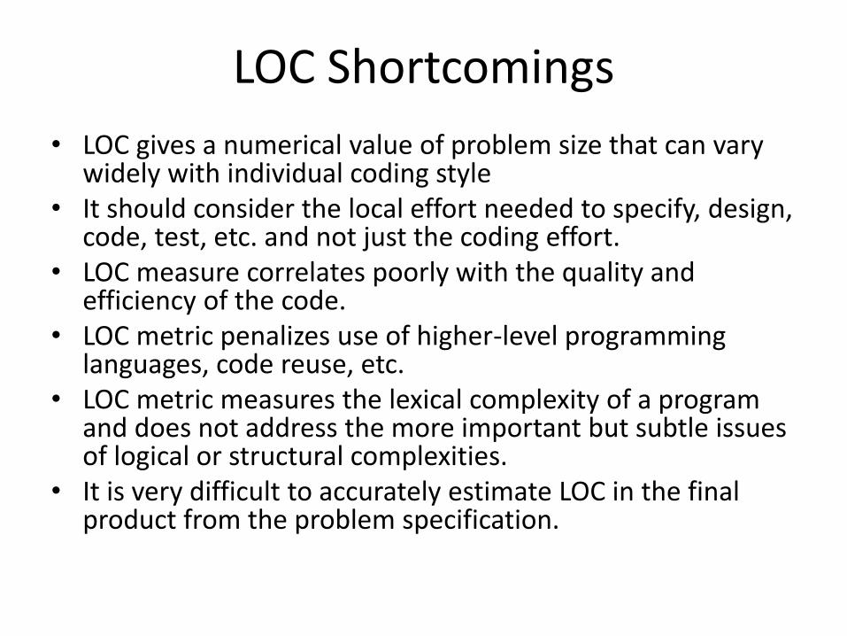
LOC Shortcomings

• LOC gives a numerical value of problem size that can vary widely with individual coding style

• It should consider the local effort needed to specify, design, code, test, etc. and not just the coding effort.

• LOC measure correlates poorly with the quality and efficiency of the code.

• LOC metric penalizes use of higher-level programming languages, code reuse, etc.

• LOC metric measures the lexical complexity of a program and does not address the more important but subtle issues of logical or structural complexities.

• It is very difficult to accurately estimate LOC in the final product from the problem specification.

Function point (FP)

• Function point metric was proposed by Albrecht [1983]. • The conceptual idea behind the function point metric is that

the size of a software product is directly dependent on the number of different functions or features it supports.

• Each function when invoked reads some input data and transforms it to the corresponding output data.

• The computation of the number of input and the output data values to a system gives some indication of the number of functions supported by the system.

• Albrecht postulated that in addition to the number of basic functions that a software performs, the size is also dependent on the number of files and the number of interfaces.

FP Contd …

• Besides using the number of input and output data values, function point metric computes the size of a software product (in units of functions points or FPs) using three other characteristics of the product as shown in the following expression.

• The size of a product in function points (FP) can be expressed as the weighted sum of these five problem characteristics.

• The weights associated with the five characteristics were proposed empirically and validated by the observations over many projects. Function point is computed in two steps. The first step is to compute the unadjusted function point (UFP).

UFP = (Number of inputs)*4 + (Number of outputs)*5 + (Number of inquiries)*4 + (Number of files)*10 + (Number of interfaces)*10

FP Contd …

• Number of inputs – Each data item input by the user is counted. Data inputs should be

distinguished from user inquiries. Inquiries are user commands such as print-account-balance. A group of related inputs are considered as a single input.

• Number of outputs – The outputs considered refer to reports printed, screen outputs, error

messages produced, etc.

• Number of inquiries – It is the number of distinct interactive queries which can be made by the

users.

• Number of files – Each logical file is counted. A logical file means groups of logically related

data.

• Number of interfaces – Here the interfaces considered are the interfaces used to exchange

information with other systems.

FP Adjustment

FP Adjustments

Example

Example

Final FP

Feature point metric

• Feature point metric incorporates an extra parameter algorithm complexity.

• This parameter ensures that the computed size using the feature point metric reflects the fact that the more is the complexity of a function, the greater is the effort required to develop it and therefore its size should be larger compared to simpler functions.

Project Estimation techniques

• Estimation of various project parameters is a basic project planning activity. The important project parameters that are estimated include: project size, effort required to develop the software, project duration, and cost. These estimates not only help in quoting the project cost to the customer, but are also useful in resource planning and scheduling. There are three broad categories of estimation techniques: – Empirical estimation techniques

– Heuristic techniques

– Analytical estimation techniques

Empirical Estimation Techniques

• Empirical estimation techniques are based on making an educated guess of the project parameters.

• Although empirical estimation techniques are based on common sense, different activities involved in estimation have been formalized over the years. Two popular empirical estimation techniques are – Expert judgment technique and

– Delphi cost estimation.

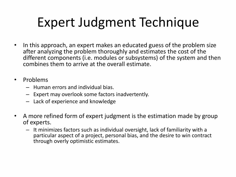
Expert Judgment Technique

• In this approach, an expert makes an educated guess of the problem size after analyzing the problem thoroughly and estimates the cost of the different components (i.e. modules or subsystems) of the system and then combines them to arrive at the overall estimate.

• Problems – Human errors and individual bias. – Expert may overlook some factors inadvertently. – Lack of experience and knowledge

• A more refined form of expert judgment is the estimation made by group of experts. – It minimizes factors such as individual oversight, lack of familiarity with a

particular aspect of a project, personal bias, and the desire to win contract through overly optimistic estimates.

Delphi cost estimation

• Delphi estimation is carried out by a team of experts and a coordinator.

• In this approach, the coordinator provides each estimator with a copy of SRS document to make initial estimate.

• In their estimates, the estimators mention any unusual characteristic of the product which has influenced his estimation.

• The coordinator prepares and distributes the summary of the responses of all the estimators, and includes any unusual rationale noted by any of the estimators and asks the estimators re-estimate.

• This process is iterated for several rounds.

• However, no discussion among the estimators is allowed during the entire estimation process to avoid any biasing.

• After the completion of several iterations of estimations, the coordinator takes the responsibility of compiling the results and preparing the final estimate.

Heuristic Techniques

• Heuristic techniques assume that the relationships among the different project parameters can be modeled using suitable mathematical expressions. Once the basic (independent) parameters are known, the other (dependent) parameters can be easily determined by substituting the value of the basic parameters

• Different heuristic estimation models can be divided into the following two classes: – single variable model and

– the multi variable model.

Single Variable Model

• Single variable estimation models provide a means to estimate the desired characteristics of a problem, using some previously estimated basic (independent) characteristic of the software product such as its size.

• A single variable estimation model takes the following form: Estimated Parameter = c1 * ed1

• In the above expression, e is the characteristic of the software which has

already been estimated (independent variable). • Estimated Parameter is the dependent parameter to be estimated which

could be effort, project duration, staff size, etc. c1 and d1 are constants.

• The values of the constants c1 and d1 are usually determined using data collected from past projects (historical data). The basic COCOMO model is an example of single variable cost estimation model.

Multivariable cost estimation model

Estimated Resource = c1*e1d1 + c2*e2d2 + ...

• Where e1, e2, … are the basic (independent) characteristics of the software already estimated, and c1, c2, d1, d2, … are constants.

• Multivariable estimation models are expected to give more accurate estimates compared to the single variable models,

• The independent parameters influence the dependent parameter to different extents. This is modeled by the constants c1, c2, d1, d2, … .

• Values of these constants are usually determined from historical data.

• The intermediate COCOMO model can be considered to be an example of a multivariable estimation model.

Analytical Estimation Techniques

• Analytical estimation techniques derive the required results starting with basic assumptions regarding the project.

• Thus, unlike empirical and heuristic techniques, analytical techniques do have scientific basis.

• Halstead’s software science is an example of an analytical technique. – It can be used to derive some interesting results starting

with a few simple assumptions. – Halstead’s software science is especially useful for

estimating software maintenance efforts. In fact, it outperforms both empirical and heuristic techniques when used for predicting software maintenance efforts.

Halstead’s Software Science – An Analytical Technique

• Halstead’s software science is an analytical technique to measure size, development effort, and development cost of software products.

• Halstead used a few primitive program parameters to develop the expressions for over all program length, potential minimum value, actual volume, effort, and development time.

• For a given program, let: – η1

be the number of unique operators used in the program, – η2

be the number of unique operands used in the program, – N1

be the total number of operators used in the program, – N2

be the total number of operands used in the program.

Different Parameters

• Length and Vocabulary – The length of a program is total usage of all operators

and operands in the program. Thus, length N = N1 +N2.

– program vocabulary is the number of unique operators and operands used in the program. Thus, program vocabulary η = η1

+ η2.

• Program Volume – V = Nlog2η

– Here the program volume V is the minimum number of bits needed to encode the program.

Different Parameters

• Potential Minimum Volume – The potential minimum volume V* is defined as the volume of most

succinct program in which a problem can be coded. – The minimum volume is obtained when the program can be expressed

using a single source code instruction., say a function call like foo( ) ;. – In other words, the volume is bound from below due to the fact that a

program would have at least two operators and no less than the requisite number of operands.

– Thus, if an algorithm operates on input and output data d1, d2, … dn, the most succinct program would be f(d1, d2, … dn); for which η1

= 2, η2

= n. Therefore, V* = (2 + η2)log2(2 + η2).

• The program level L is given by L = V*/V. – The concept of program level L is introduced in an attempt to measure

the level of abstraction provided by the programming language. – The above result implies that the higher the level of a language, the

less effort it takes to develop a program using that language.

Different Parameters

• Effort and Time – The effort required to develop a program can be obtained

by dividing the program volume with the level of the programming language used to develop the code.

– Thus, effort E = V/L, – Thus, the programming effort E = V²/V* (since L = V*/V)

varies as the square of the volume.

• The programmer’s time T = E/S, where S the speed of mental discriminations. The value of S has been empirically developed from psychological reasoning, and its recommended value for programming applications is 18.

Length of Program

• In terms of unique operators and operands – it can be assumed that any program of length N consists of N/ η unique strings of length η. – Now, it is standard combinatorial result that for any given alphabet of size K, there are exactly Kr different

strings of length r.

• Thus.

– N/η ≤ ηη Or, N ≤ ηη+1

• Since operators and operands usually alternate in a program, the upper bound can be further

refined into N ≤ η η1η1 η2

η2. Also, N must include not only the ordered set of n elements, but it should also include all possible subsets of that ordered sets, i.e. the power set of N strings

Therefore, 2N = η η1

η1 η2η2 Or, taking logarithm on both sides,

N = log 2η +log 2(η1

η1 η2η2 )

So we get, N = log 2 (η1

η1 η2η2 ) approx

N= η1log 2η1

+ η2log 2η2

CoCoMo

• Organic, Semidetached and Embedded software projects – Organic:

• if the project deals with developing a well understood application program, the size of the development team is reasonably small, and the team members are experienced in developing similar types of projects.

– Semidetached: • if the development consists of a mixture of experienced and

inexperienced staff. Team members may have limited experience on related systems but may be unfamiliar with some aspects of the system being developed.

– Embedded: • if the software being developed is strongly coupled to complex

hardware, or if the stringent regulations on the operational procedures exist.

Basic COCOMO Model

• The basic COCOMO model gives an approximate estimate of the project parameters. The basic COCOMO estimation model is given by the following expressions:

Effort = a1

х (KLOC)a2

PM Tdev = b1

x (Effort)b2

Months Where

– KLOC is the estimated size of the software product expressed in Kilo Lines of Code,

– a1, a2, b1, b2

are constants for each category of software products,

– Tdev is the estimated time to develop the software, expressed in months,

– Effort is the total effort required to develop the software product, expressed in person months

(PMs).

Estimation of development effort For the three classes of software products, the formulas for estimating the effort based on the code size are shown below: • Organic : Effort = 2.4(KLOC)1.05 PM

• Semi-detached : Effort = 3.0(KLOC)1.12 PM

• Embedded : Effort = 3.6(KLOC)1.20 PM

Estimation of development time

• Organic : Tdev = 2.5(Effort)0.38 Months

• Semi-detached : Tdev = 2.5(Effort)0.35 Months

• Embedded : Tdev = 2.5(Effort)0.32 Months

Effort Vs Size

Staff Size & Productivity

Example

Intermediate Model

Multipliers of Cost Drivers

Multipliers of Cost Drivers

Complete CoCoMo

Stages of COCOMO-II

Steps

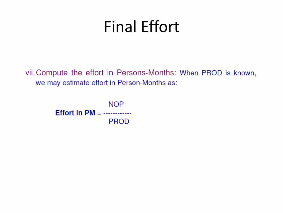
Final Effort

Staffing level estimation

• Norden’s Work – Staffing pattern can be

approximated by the Rayleigh distribution Curve

• Where – E: Effort required at time t.

– K is the area under the curve, and

– td is the time at which the curve attains its maximum value.

Staffing level estimation

• Putnam’s Work • Putnam studied the problem of

staffing of software projects and found that number of delivered lines of code to the effort and the time required to develop the project.

• K is the total effort expended (in PM) in the product development and L is the product size in KLOC.

• td corresponds to the time of system and integration testing. Therefore, td can be approximately considered as the time required to develop the software.

Ck is the state of technology constant and reflects constraints that impede the progress of the programmer. Typical values of Ck = 2 for poor development environment (Ck = 8 for good software development environment Ck = 11 for an excellent environment

Effect of schedule change on cost

From the above expression, it can be easily observed that when the schedule of a project is compressed, the required development effort as well as project development cost increases in proportion to the fourth power of the degree of compression. It means that a relatively small compression in delivery schedule can result in substantial penalty of human effort as well as development cost. For example, if the estimated development time is 1 year, then in order to develop the product in 6 months, the total effort required to develop the product (and hence the project cost) increases 16 times.