problematic topics in ideas to...

Joe Khachan – School of Physics, University of Sydney, 2010

Problematic topics in Ideas to Implementation by Joe Khachan

Some of the topics that have proved to be problematic in the current HSC physics syllabus are the discharge tube, Hertz’s experiments and superconductors. Below are some notes about these topics with extra insights. Some of the questions that these topics address are as follows: What causes a discharge tube to start? What causes the striations in a discharge tube? What causes the dark spaces? How do the luminous and dark regions respond to changing pressure and voltage? Why? How does the electric field behave in a discharge tube? How did Hertz measure the speed of radio waves? Can this experiment be carried out using any spark generator? What did Hertz’s transmitters and detectors look like and how did they work? How easy was it for Hertz to carry out his experiments? How did Hertz measure the polarization of the electromagnetic waves? What is the Meissner effect in superconductors and how does it differ from the behaviour of a perfect conductor? What is the difference between type I and II superconductors? Why is a levitated magnet stable? What is the BCS theory of superconductors? How are Cooper pairs formed and why do they result in zero resistance of the superconductor? Do high temperature superconductors follow the BSC theory? Why? The list of questions can be greatly extended. The ideas to implementation part of the syllabus lends itself to many questions that have so far not been addressed in any satisfactory way because the topics are usually quite advanced and would at least require 4 years of a physics major to be able to start to address them. No doubt there are many other questions about the syllabus. For this reason the author of these notes (Joe Khachan) has created a University of Sydney Physics Teachers Forum website where you can post questions and obtain answers related to the syllabus. The website is as follows:

http://blogs.usyd.edu.au/ptf/


The Discharge Tube Discharge tubes are evacuated glass vessels filled with gas at approximately 1% of atmospheric pressure and two electrodes at opposite ends of the tube. A large potential difference between these electrodes partially ionizes the gas and causes an electrical current to flow through the gas resulting in colours that depend on the type of gas and its pressure. The physical principles of the discharge tube are used in modern day applications such as fluorescent lighting, neon signs and plasma TV sets.

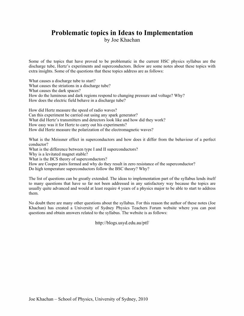
Figure 1. The dark spaces and luminous regions of a discharge tube.

The operating discharge tube, shown in Figure 1, shows the characteristic luminous regions and dark spaces. The negative electrode (cathode) is on the left hand side of the tube, and the positive electrode (anode) is on the right. The Aston dark space is adjacent to the cathode, followed by the first luminous region called the cathode glow. Next are the Crookes dark space, the negative glow, and the Faraday dark space, which is the largest of all the dark spaces. The largest luminous region, known as the positive column, follows and is the most prominent feature of the discharge. The positive column may display periodic regions of bright and dark spaces known as striations. Finally, there are the anode dark space and anode glow adjacent to the anode. An operating discharge tube consists of a mixture of ions, electrons and neutral gas atoms. The discharge starts because energetic particles (such as electrons and protons) continually stream from outside the Earth and strike the surface and atmosphere. This so called “cosmic radiation” can strike gas atoms and produce free ions and electrons in the discharge tube. An electric field causes the free electrons to gain sufficient energy to ionise gas atoms and produce further free ions and electrons, which in turn will accelerate to produce further ionisation. This avalanche of ionisation is the way an electrical discharge is started and maintained.

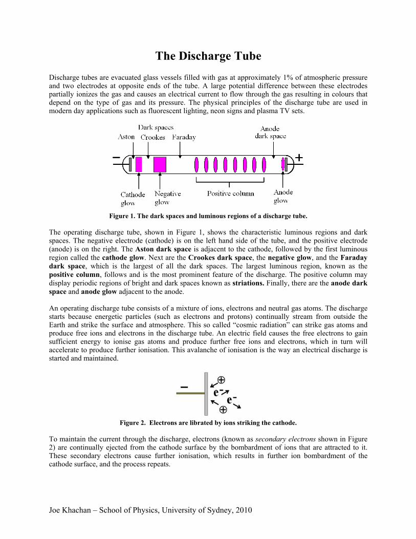
Figure 2. Electrons are librated by ions striking the cathode.

To maintain the current through the discharge, electrons (known as secondary electrons shown in Figure 2) are continually ejected from the cathode surface by the bombardment of ions that are attracted to it. These secondary electrons cause further ionisation, which results in further ion bombardment of the cathode surface, and the process repeats.


Luminous regions in the discharge are areas where the electrons have reached a sufficient energy to ionise the gas. Some of the ions recombine with electrons, which results in the emission of light. Not all atoms will be ionised. Some will simply have their electrons gain energy while remaining bound to the atom or molecule, known as excitation. All excited electrons will fall back to their previous energy state and, in doing so, they give out light. A minimum energy is required to excite or ionise an atom. Many discharge characteristics are related to the average distance electrons travel between collisions with the gas atoms. An increase in gas pressure leads to an increase in the density of gas particles, thus resulting in an electron travelling a shorter distance between collisions, and vice versa. At low pressure, electrons have sufficient distance to accelerate and reach the required ionisation energy. A minimum number of ionisations are required to sustain the avalanche of electrons that maintain the discharge. Below a minimum pressure, it becomes difficult to start an electrical discharge along the tube. At higher pressures there is a large density of gas particles so there is a high probability that electrons will strike them. However, too high a pressure results in very frequent electron collisions such that they do not reach sufficient energy to ionise gas particles. Thus the electric field strength must be increased for them to reach this energy. There is an optimum pressure for starting a discharge at a relatively low electric field.

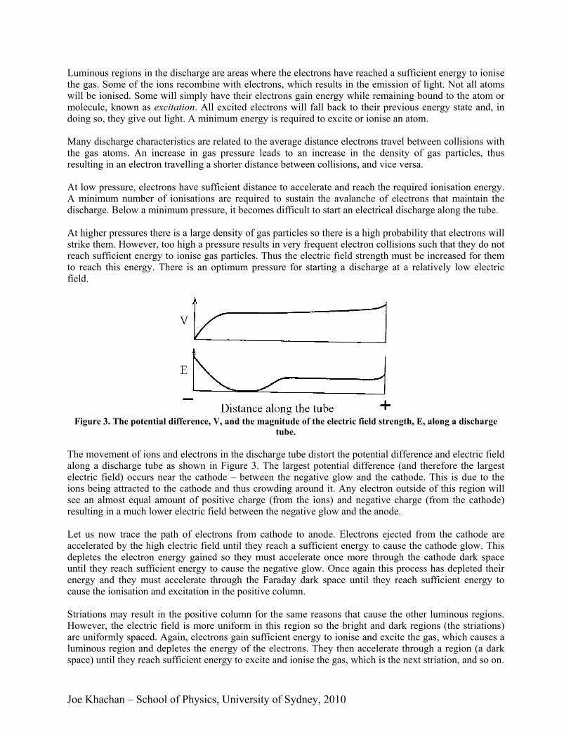
Figure 3. The potential difference, V, and the magnitude of the electric field strength, E, along a discharge

tube. The movement of ions and electrons in the discharge tube distort the potential difference and electric field along a discharge tube as shown in Figure 3. The largest potential difference (and therefore the largest electric field) occurs near the cathode – between the negative glow and the cathode. This is due to the ions being attracted to the cathode and thus crowding around it. Any electron outside of this region will see an almost equal amount of positive charge (from the ions) and negative charge (from the cathode) resulting in a much lower electric field between the negative glow and the anode. Let us now trace the path of electrons from cathode to anode. Electrons ejected from the cathode are accelerated by the high electric field until they reach a sufficient energy to cause the cathode glow. This depletes the electron energy gained so they must accelerate once more through the cathode dark space until they reach sufficient energy to cause the negative glow. Once again this process has depleted their energy and they must accelerate through the Faraday dark space until they reach sufficient energy to cause the ionisation and excitation in the positive column. Striations may result in the positive column for the same reasons that cause the other luminous regions. However, the electric field is more uniform in this region so the bright and dark regions (the striations) are uniformly spaced. Again, electrons gain sufficient energy to ionise and excite the gas, which causes a luminous region and depletes the energy of the electrons. They then accelerate through a region (a dark space) until they reach sufficient energy to excite and ionise the gas, which is the next striation, and so on.


Clear luminous and dark region will be produced if electrons that leave the cathode remain in step. This is not possible in practice. Some electrons will strike gas particles before others and have their energy depleted sooner. This results in a spread of energies as electrons move along the tube. Thus, the luminous regions are diffuse and do not have well defined boundaries. If electrons become too out-of-step with each other, then striations will start to merge into each other and will not be distinguishable from the dark spaces between them, which may happen at too high a pressure. As the pressure is lowered, striations become more widely spaced because there is a lower gas particle density and the electrons will travel longer, on average, before striking a gas particle. The converse happens at higher pressures. Electrons strike gas particles more frequently, so the striations will be more closely spaced. Finally, electrons are accelerated through the anode dark space and strike the anode. These electrons excite or ionise the gas next to the anode causing the anode glow. The colour of the light emitted from the positive column depends on type of gas because it depends on the energy level electrons occupy around the atom, which is different for different elements for example For example, Helium results in a reddish-purple positive column.


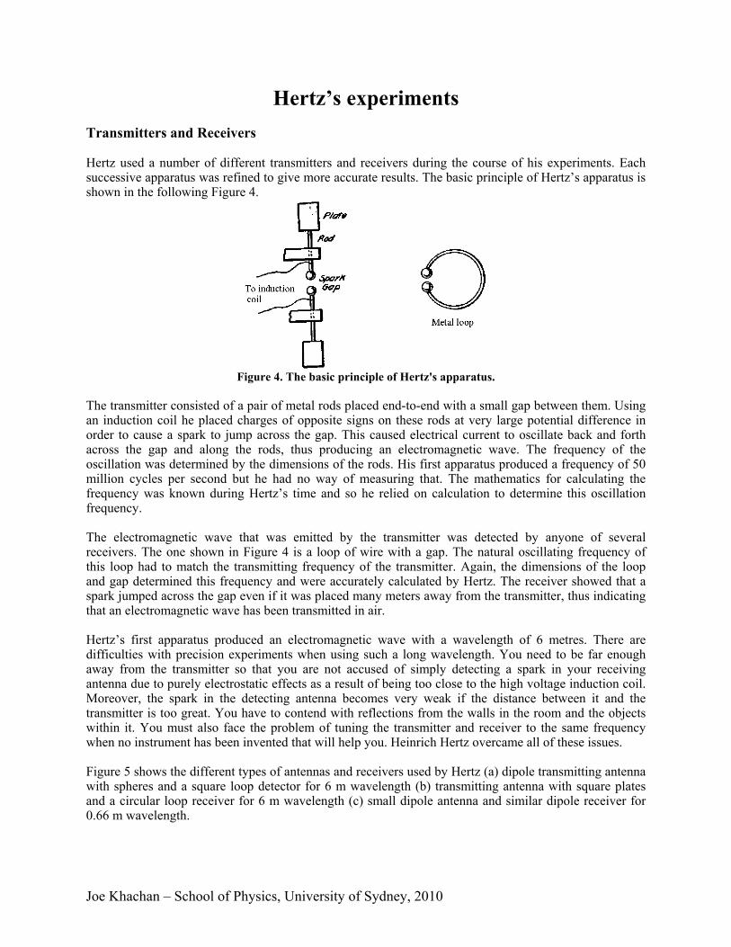
Hertz’s experiments Transmitters and Receivers Hertz used a number of different transmitters and receivers during the course of his experiments. Each successive apparatus was refined to give more accurate results. The basic principle of Hertz’s apparatus is shown in the following Figure 4.

Figure 4. The basic principle of Hertz's apparatus.

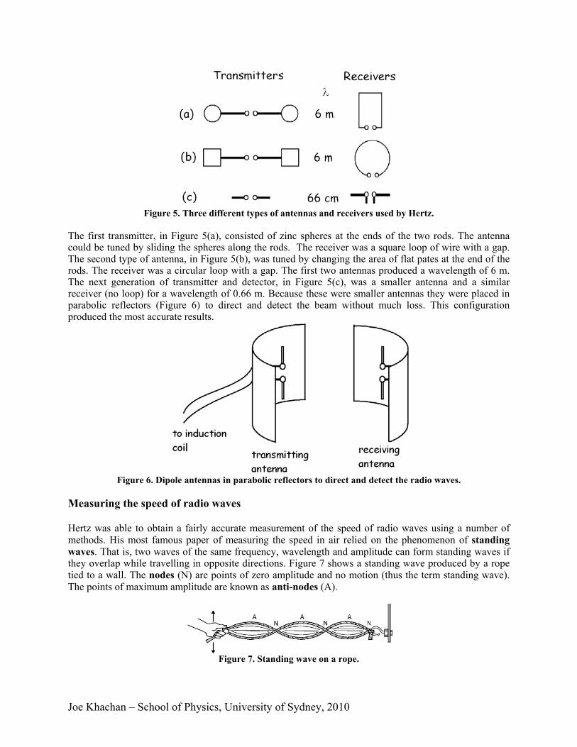
The transmitter consisted of a pair of metal rods placed end-to-end with a small gap between them. Using an induction coil he placed charges of opposite signs on these rods at very large potential difference in order to cause a spark to jump across the gap. This caused electrical current to oscillate back and forth across the gap and along the rods, thus producing an electromagnetic wave. The frequency of the oscillation was determined by the dimensions of the rods. His first apparatus produced a frequency of 50 million cycles per second but he had no way of measuring that. The mathematics for calculating the frequency was known during Hertz’s time and so he relied on calculation to determine this oscillation frequency. The electromagnetic wave that was emitted by the transmitter was detected by anyone of several receivers. The one shown in Figure 4 is a loop of wire with a gap. The natural oscillating frequency of this loop had to match the transmitting frequency of the transmitter. Again, the dimensions of the loop and gap determined this frequency and were accurately calculated by Hertz. The receiver showed that a spark jumped across the gap even if it was placed many meters away from the transmitter, thus indicating that an electromagnetic wave has been transmitted in air. Hertz’s first apparatus produced an electromagnetic wave with a wavelength of 6 metres. There are difficulties with precision experiments when using such a long wavelength. You need to be far enough away from the transmitter so that you are not accused of simply detecting a spark in your receiving antenna due to purely electrostatic effects as a result of being too close to the high voltage induction coil. Moreover, the spark in the detecting antenna becomes very weak if the distance between it and the transmitter is too great. You have to contend with reflections from the walls in the room and the objects within it. You must also face the problem of tuning the transmitter and receiver to the same frequency when no instrument has been invented that will help you. Heinrich Hertz overcame all of these issues. Figure 5 shows the different types of antennas and receivers used by Hertz (a) dipole transmitting antenna with spheres and a square loop detector for 6 m wavelength (b) transmitting antenna with square plates and a circular loop receiver for 6 m wavelength (c) small dipole antenna and similar dipole receiver for 0.66 m wavelength.


Figure 5. Three different types of antennas and receivers used by Hertz.

The first transmitter, in Figure 5(a), consisted of zinc spheres at the ends of the two rods. The antenna could be tuned by sliding the spheres along the rods. The receiver was a square loop of wire with a gap. The second type of antenna, in Figure 5(b), was tuned by changing the area of flat pates at the end of the rods. The receiver was a circular loop with a gap. The first two antennas produced a wavelength of 6 m. The next generation of transmitter and detector, in Figure 5(c), was a smaller antenna and a similar receiver (no loop) for a wavelength of 0.66 m. Because these were smaller antennas they were placed in parabolic reflectors (Figure 6) to direct and detect the beam without much loss. This configuration produced the most accurate results.

Figure 6. Dipole antennas in parabolic reflectors to direct and detect the radio waves.

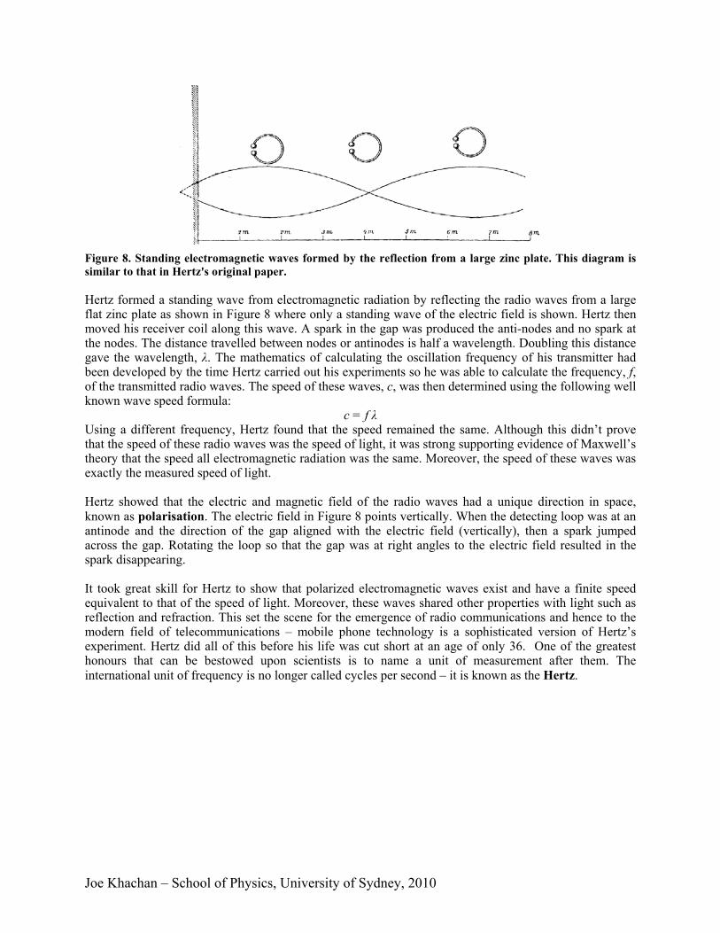
Measuring the speed of radio waves Hertz was able to obtain a fairly accurate measurement of the speed of radio waves using a number of methods. His most famous paper of measuring the speed in air relied on the phenomenon of standing waves. That is, two waves of the same frequency, wavelength and amplitude can form standing waves if they overlap while travelling in opposite directions. Figure 7 shows a standing wave produced by a rope tied to a wall. The nodes (N) are points of zero amplitude and no motion (thus the term standing wave). The points of maximum amplitude are known as anti-nodes (A).

Figure 7. Standing wave on a rope.


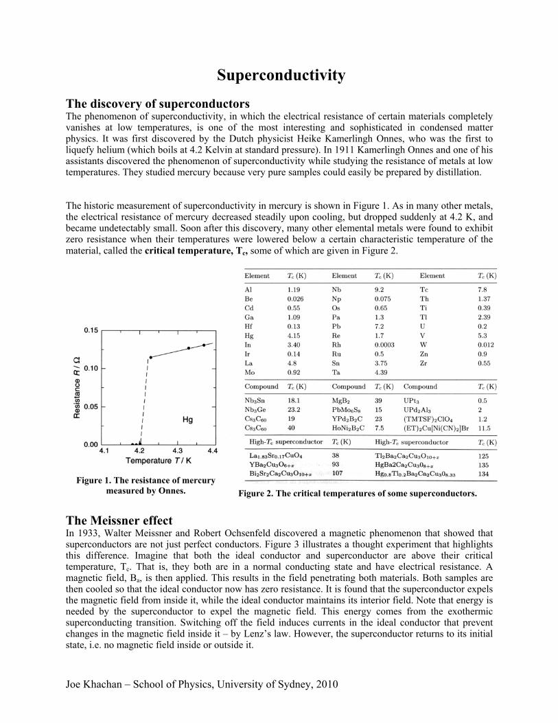
Figure 8. Standing electromagnetic waves formed by the reflection from a large zinc plate. This diagram is similar to that in Hertz's original paper. Hertz formed a standing wave from electromagnetic radiation by reflecting the radio waves from a large flat zinc plate as shown in Figure 8 where only a standing wave of the electric field is shown. Hertz then moved his receiver coil along this wave. A spark in the gap was produced the anti-nodes and no spark at the nodes. The distance travelled between nodes or antinodes is half a wavelength. Doubling this distance gave the wavelength, λ. The mathematics of calculating the oscillation frequency of his transmitter had been developed by the time Hertz carried out his experiments so he was able to calculate the frequency, f, of the transmitted radio waves. The speed of these waves, c, was then determined using the following well known wave speed formula:

c = f λ Using a different frequency, Hertz found that the speed remained the same. Although this didn’t prove that the speed of these radio waves was the speed of light, it was strong supporting evidence of Maxwell’s theory that the speed all electromagnetic radiation was the same. Moreover, the speed of these waves was exactly the measured speed of light. Hertz showed that the electric and magnetic field of the radio waves had a unique direction in space, known as polarisation. The electric field in Figure 8 points vertically. When the detecting loop was at an antinode and the direction of the gap aligned with the electric field (vertically), then a spark jumped across the gap. Rotating the loop so that the gap was at right angles to the electric field resulted in the spark disappearing. It took great skill for Hertz to show that polarized electromagnetic waves exist and have a finite speed equivalent to that of the speed of light. Moreover, these waves shared other properties with light such as reflection and refraction. This set the scene for the emergence of radio communications and hence to the modern field of telecommunications – mobile phone technology is a sophisticated version of Hertz’s experiment. Hertz did all of this before his life was cut short at an age of only 36. One of the greatest honours that can be bestowed upon scientists is to name a unit of measurement after them. The international unit of frequency is no longer called cycles per second – it is known as the Hertz.


Figure 1. The resistance of mercury measured by Onnes.

Superconductivity The discovery of superconductors The phenomenon of superconductivity, in which the electrical resistance of certain materials completely vanishes at low temperatures, is one of the most interesting and sophisticated in condensed matter physics. It was first discovered by the Dutch physicist Heike Kamerlingh Onnes, who was the first to liquefy helium (which boils at 4.2 Kelvin at standard pressure). In 1911 Kamerlingh Onnes and one of his assistants discovered the phenomenon of superconductivity while studying the resistance of metals at low temperatures. They studied mercury because very pure samples could easily be prepared by distillation. The historic measurement of superconductivity in mercury is shown in Figure 1. As in many other metals, the electrical resistance of mercury decreased steadily upon cooling, but dropped suddenly at 4.2 K, and became undetectably small. Soon after this discovery, many other elemental metals were found to exhibit zero resistance when their temperatures were lowered below a certain characteristic temperature of the material, called the critical temperature, Tc, some of which are given in Figure 2.

The Meissner effect In 1933, Walter Meissner and Robert Ochsenfeld discovered a magnetic phenomenon that showed that superconductors are not just perfect conductors. Figure 3 illustrates a thought experiment that highlights this difference. Imagine that both the ideal conductor and superconductor are above their critical temperature, Tc. That is, they both are in a normal conducting state and have electrical resistance. A magnetic field, Ba, is then applied. This results in the field penetrating both materials. Both samples are then cooled so that the ideal conductor now has zero resistance. It is found that the superconductor expels the magnetic field from inside it, while the ideal conductor maintains its interior field. Note that energy is needed by the superconductor to expel the magnetic field. This energy comes from the exothermic superconducting transition. Switching off the field induces currents in the ideal conductor that prevent changes in the magnetic field inside it – by Lenz’s law. However, the superconductor returns to its initial state, i.e. no magnetic field inside or outside it.

Figure 2. The critical temperatures of some superconductors.


Type I and II superconductors High magnetic fields destroy superconductivity and restore the normal conducting state. Depending on the character of this transition, we may distinguish between type I and II superconductors. The graph shown in Figure 4 illustrates the internal magnetic field strength, Bi, with increasing applied magnetic field. It is found that the internal field is zero (as expected from the Meissner effect) until a critical magnetic field, Bc, is reached where a sudden transition to the normal state occurs. This results in the penetration of the applied field into the interior. Superconductors that undergo this abrupt transition to the normal state above a critical magnetic field are known as type I superconductors. Most of the pure elements in Figure 2 tend to be type I superconductors. Type II superconductors, on the other hand, respond differently to an applied magnetic field, as shown in Figure 5. An increasing field from zero results in two critical fields, Bc1 and Bc2. At Bc1 the applied field begins to partially penetrate the interior of the superconductor. However, the superconductivity is maintained at this point. The superconductivity vanishes above the second, much higher, critical field, Bc2. For applied fields between Bc1 and Bc2, the applied field is able to partially penetrate the superconductor, so the Meissner effect is incomplete, allowing the superconductor to tolerate very high magnetic fields.

Type II superconductors are the most technologically useful because the second critical field can be quite high, enabling high field electromagnets to be made out of superconducting wire. Most compounds

Figure 3. The Meissner effect.

Figure 4. Type-I superconductor behaviour.

Figure 5. Type-II superconductor behaviour.


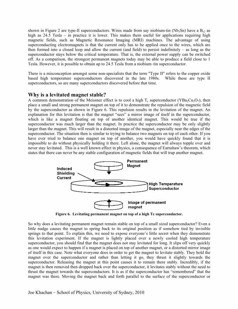
shown in Figure 2 are type-II superconductors. Wires made from say niobium-tin (Nb3Sn) have a Bc2 as high as 24.5 Tesla – in practice it is lower. This makes them useful for applications requiring high magnetic fields, such as Magnetic Resonance Imaging (MRI) machines. The advantage of using superconducting electromagnets is that the current only has to be applied once to the wires, which are then formed into a closed loop and allow the current (and field) to persist indefinitely – as long as the superconductor stays below the critical temperature. That is, the external power supply can be switched off. As a comparison, the strongest permanent magnets today may be able to produce a field close to 1 Tesla. However, it is possible to obtain up to 24.5 Tesla from a niobium–tin superconductor. There is a misconception amongst some non-specialists that the term "Type II" refers to the copper oxide based high temperature superconductors discovered in the late 1980s. While these are type II superconductors, so are many superconductors discovered before that time. Why is a levitated magnet stable? A common demonstration of the Meissner effect is to cool a high Tc superconductor (YBa2Cu3O7), then place a small and strong permanent magnet on top of it to demonstrate the repulsion of the magnetic field by the superconductor as shown in Figure 6. This repulsion results in the levitation of the magnet. An explanation for this levitation is that the magnet “sees” a mirror image of itself in the superconductor, which is like a magnet floating on top of another identical magnet. This would be true if the superconductor was much larger than the magnet. In practice the superconductor may be only slightly larger than the magnet. This will result in a distorted image of the magnet, especially near the edges of the superconductor. The situation then is similar to trying to balance two magnets on top of each other. If you have ever tried to balance one magnet on top of another, you would have quickly found that it is impossible to do without physically holding it there. Left alone, the magnet will always topple over and never stay levitated. This is a well known effect in physics, a consequence of Earnshaw’s theorem, which states that there can never be any stable configuration of magnetic fields that will trap another magnet.

Figure 6. Levitating permanent magnet on top of a high Tc superconductor.

So why does a levitating permanent magnet remain stable on top of a small sized superconductor? Even a little nudge causes the magnet to spring back to its original position as if somehow tied by invisible springs to that point. To explain this, we need to expose everyone’s little secret when they demonstrate this levitation experiment. If the magnet is lightly placed over a newly cooled high temperature superconductor, you should find that the magnet does not stay levitated for long. It slips off very quickly as one would expect to happen if a magnet is placed on top of another magnet, or a distorted mirror image of itself in this case. Note what everyone does in order to get the magnet to levitate stably. They hold the magnet over the superconductor and rather than letting it go, they thrust it slightly towards the superconductor. Releasing the magnet at this point causes it to remain there stably. Incredibly, if the magnet is then removed then dropped back over the superconductor, it levitates stably without the need to thrust the magnet towards the superconductors. It is as if the superconductor has “remembered” that the magnet was there. Moving the magnet back and forth parallel to the surface of the superconductor or


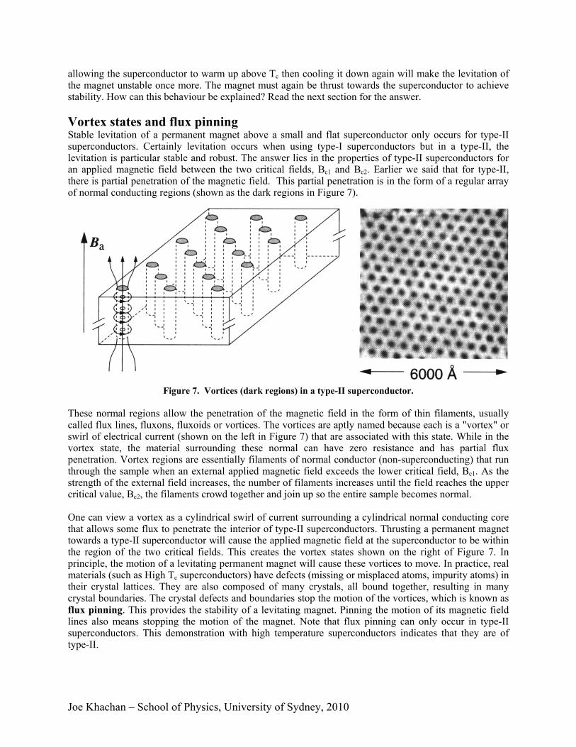
allowing the superconductor to warm up above Tc then cooling it down again will make the levitation of the magnet unstable once more. The magnet must again be thrust towards the superconductor to achieve stability. How can this behaviour be explained? Read the next section for the answer. Vortex states and flux pinning Stable levitation of a permanent magnet above a small and flat superconductor only occurs for type-II superconductors. Certainly levitation occurs when using type-I superconductors but in a type-II, the levitation is particular stable and robust. The answer lies in the properties of type-II superconductors for an applied magnetic field between the two critical fields, Bc1 and Bc2. Earlier we said that for type-II, there is partial penetration of the magnetic field. This partial penetration is in the form of a regular array of normal conducting regions (shown as the dark regions in Figure 7).

Figure 7. Vortices (dark regions) in a type-II superconductor.

These normal regions allow the penetration of the magnetic field in the form of thin filaments, usually called flux lines, fluxons, fluxoids or vortices. The vortices are aptly named because each is a "vortex" or swirl of electrical current (shown on the left in Figure 7) that are associated with this state. While in the vortex state, the material surrounding these normal can have zero resistance and has partial flux penetration. Vortex regions are essentially filaments of normal conductor (non-superconducting) that run through the sample when an external applied magnetic field exceeds the lower critical field, Bc1. As the strength of the external field increases, the number of filaments increases until the field reaches the upper critical value, Bc2, the filaments crowd together and join up so the entire sample becomes normal. One can view a vortex as a cylindrical swirl of current surrounding a cylindrical normal conducting core that allows some flux to penetrate the interior of type-II superconductors. Thrusting a permanent magnet towards a type-II superconductor will cause the applied magnetic field at the superconductor to be within the region of the two critical fields. This creates the vortex states shown on the right of Figure 7. In principle, the motion of a levitating permanent magnet will cause these vortices to move. In practice, real materials (such as High Tc superconductors) have defects (missing or misplaced atoms, impurity atoms) in their crystal lattices. They are also composed of many crystals, all bound together, resulting in many crystal boundaries. The crystal defects and boundaries stop the motion of the vortices, which is known as flux pinning. This provides the stability of a levitating magnet. Pinning the motion of its magnetic field lines also means stopping the motion of the magnet. Note that flux pinning can only occur in type-II superconductors. This demonstration with high temperature superconductors indicates that they are of type-II.


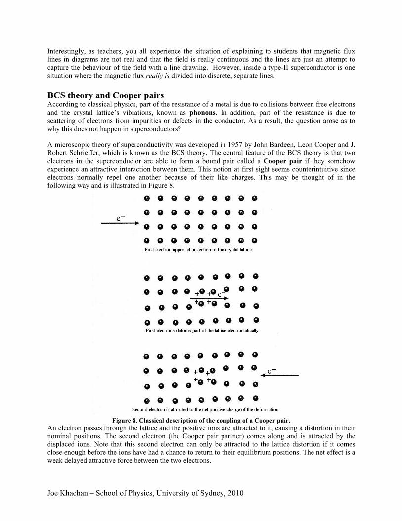
Interestingly, as teachers, you all experience the situation of explaining to students that magnetic flux lines in diagrams are not real and that the field is really continuous and the lines are just an attempt to capture the behaviour of the field with a line drawing. However, inside a type-II superconductor is one situation where the magnetic flux really is divided into discrete, separate lines. BCS theory and Cooper pairs According to classical physics, part of the resistance of a metal is due to collisions between free electrons and the crystal lattice’s vibrations, known as phonons. In addition, part of the resistance is due to scattering of electrons from impurities or defects in the conductor. As a result, the question arose as to why this does not happen in superconductors? A microscopic theory of superconductivity was developed in 1957 by John Bardeen, Leon Cooper and J. Robert Schrieffer, which is known as the BCS theory. The central feature of the BCS theory is that two electrons in the superconductor are able to form a bound pair called a Cooper pair if they somehow experience an attractive interaction between them. This notion at first sight seems counterintuitive since electrons normally repel one another because of their like charges. This may be thought of in the following way and is illustrated in Figure 8.

Figure 8. Classical description of the coupling of a Cooper pair.

An electron passes through the lattice and the positive ions are attracted to it, causing a distortion in their nominal positions. The second electron (the Cooper pair partner) comes along and is attracted by the displaced ions. Note that this second electron can only be attracted to the lattice distortion if it comes close enough before the ions have had a chance to return to their equilibrium positions. The net effect is a weak delayed attractive force between the two electrons.


This short lived distortion of the lattice is sometimes called a virtual phonon because its lifetime is too short to propagate through the lattice like a wave as a normal phonon would. From the BCS theory, the total linear momentum of a Cooper pair must be zero. This means that they travel in opposite directions as shown in Figure 8. In addition, the nominal separation between the Cooper pair (called the coherence length) ranges from hundreds to thousands of ions separating them! This is quite a large distance and has been represented incorrectly in many textbooks on this subject. If electrons in a Cooper pair were too close, such as a couple of atomic spacings apart; the electrostatic (coulomb) repulsion will be much larger than the attraction from the lattice deformation and so they will repel each other. Thus there will be no superconductivity. A current flowing in the superconductor just shifts the total moment slightly from zero so that, on average, one electron in a cooper pair has a slightly larger momentum magnitude that its pair. They do, however, still travel in opposite directions. The interaction between a Cooper pair is transient. Each electron in the pair goes on to form a Cooper pair with other electrons, and this process continues with the newly formed Cooper pair so that each electron goes on to form a Cooper pair with other electrons. The end result is that each electron in the solid is attracted to every other electron forming a large network of interactions. Causing just one of these electrons to collide and scatter from atoms in the lattice means the whole network of electrons must be made to collide into the lattice, which is energetically too costly. The collective behaviour of all the electrons in the solid prevents any further collisions with the lattice. Nature prefers situations that spend a minimum of energy. In this case, the minimum energy situation is to have no collisions with the lattice. A small amount of energy is needed to destroy the superconducting state and make it normal. This energy is called the energy gap. Although a classical description of Cooper pairs has been given here, the formal treatment from the BCS theory is quantum mechanical. The electrons have wave-like behaviour and are described by a wave function that extends throughout the solid and overlaps with other electron wave functions. As a result, the whole network of electrons behaves line one wave function so that their collective motion is coherent. In addition to having a linear momentum, each electron behaves as if it is spinning. This property, surprisingly, is called spin. This does not mean that the electron is actually spinning, but behaves as though it is spinning. The requirement from the BCS theory is that spins of a Cooper pair be in opposite directions. Note that the explanation and pictorial representation of a Cooper pair presented here comes directly from BCS theory. However, current HSC textbooks tend to distort this picture with unphysical situations such as the Cooper pair being within one or two atomic spacings and traveling in the same direction – each of these situations is false. High – Tc superconductors It has long been a dream of scientists working in the field of superconductivity to find a material that becomes a superconductor at room temperature. A discovery of this type will revolutionize every aspect of modern day technology such as power transmission and storage, communication, transport and even the type of computers we make. All of these advances will be faster, cheaper and more energy efficient. This has not been achieved to date. However, in 1986 a class of materials was discovered by Bednorz and Müller that led to superconductors that we use today on a bench-top with liquid nitrogen to cool them. Not surprisingly, Bednorz and Müller received the Nobel Prize in 1987 (the fastest-ever recognition by the Nobel committee). The material we mostly use on bench-tops is Yttrium – Barium – Copper Oxide, or YBa2Cu3O7, otherwise known as the 1-2-3 superconductor, and are classified as high temperature (Tc) superconductors.


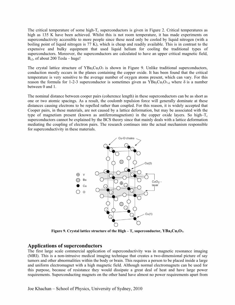
The critical temperature of some high-Tc superconductors is given in Figure 2. Critical temperatures as high as 135 K have been achieved. Whilst this is not room temperature, it has made experiments on superconductivity accessible to more people since these need only be cooled by liquid nitrogen (with a boiling point of liquid nitrogen is 77 K), which is cheap and readily available. This is in contrast to the expensive and bulky equipment that used liquid helium for cooling the traditional types of superconductors. Moreover, the superconductors are calculated to have an upper critical magnetic field, Bc2, of about 200 Tesla – huge! The crystal lattice structure of YBa2Cu3O7 is shown in Figure 9. Unlike traditional superconductors, conduction mostly occurs in the planes containing the copper oxide. It has been found that the critical temperature is very sensitive to the average number of oxygen atoms present, which can vary. For this reason the formula for 1-2-3 superconductor is sometimes given as YBa2Cu3O7-δ where δ is a number between 0 and 1. The nominal distance between cooper pairs (coherence length) in these superconductors can be as short as one or two atomic spacings. As a result, the coulomb repulsion force will generally dominate at these distances causing electrons to be repelled rather than coupled. For this reason, it is widely accepted that Cooper pairs, in these materials, are not caused by a lattice deformation, but may be associated with the type of magnetism present (known as antiferromagnetism) in the copper oxide layers. So high–Tc superconductors cannot be explained by the BCS theory since that mainly deals with a lattice deformation mediating the coupling of electron pairs. The research continues into the actual mechanism responsible for superconductivity in these materials.

Figure 9. Crystal lattice structure of the High – Tc superconductor, YBa2Cu3O7.

Applications of superconductors The first large scale commercial application of superconductivity was in magnetic resonance imaging (MRI). This is a non-intrusive medical imaging technique that creates a two-dimensional picture of say tumors and other abnormalities within the body or brain. This requires a person to be placed inside a large and uniform electromagnet with a high magnetic field. Although normal electromagnets can be used for this purpose, because of resistance they would dissipate a great deal of heat and have large power requirements. Superconducting magnets on the other hand have almost no power requirements apart from


operating the cooling. Once electrical current flows in the superconducting wire, the power supply can be switched off because the wires can be formed into a loop and the current will persist indefinitely as long as the temperature is kept below the transition temperature of the superconductor. Superconductors can also be used to make a device known as a superconducting quantum interference device (SQUID). This is incredibly sensitive to small magnetic fields so that it can detect the magnetic fields from the heart (10-10 Tesla) and even the brain (10-13 Tesla). For comparison, the Earth’s magnetic field is about 10-4 Tesla. As a result, SQUIDs are used in non-intrusive medical diagnostics on the brain. The traditional use of superconductors has been in scientific research where high magnetic field electromagnets are required. The cost of keeping the superconductor cool are much smaller than the cost of operating normal electromagnets, which dissipate heat and have high power requirements. One such application of powerful electromagnets is in high energy physics where beams of protons and other particles are accelerated to almost light speeds and collided with each other so that more fundamental particles are produced. It is expected that this research will answer fundamental questions such as those about the origin of the mass of particles that make up the Universe. Levitating trains have been built that use powerful electromagnets made from superconductors. The superconducting electromagnets are mounted on the train. Normal electromagnets, on a guideway beneath the train, repel (or attract) the superconducting electromagnets to levitate the train while pulling it forwards. A use of large and powerful superconducting electromagnets is in a possible future energy source known as nuclear fusion. When two light nuclei combine to form a heavier nucleus, the process is called nuclear fusion. This results in the release of large amounts of energy without any harmful waste. Two isotopes of hydrogen, deuterium and tritium, will fuse to release energy and helium. Deuterium is available in ordinary water and tritium can be made during the nuclear fusion reactions from another abundantly available element – lithium. For this reason it is called clean nuclear energy. For this reaction to occur, the deuterium and tritium gases must be heated to millions of degrees so that they become fully ionized. As a result, they must be confined in space so that they do not escape while being heated. Powerful and large electromagnets made from superconductors are capable of confining these energetic ions. An international fusion energy project, known as the International Thermonuclear Experimental Reactor (ITER) is currently being built in the south of France that will use large superconducting magnets and is due for completion in 2017. It is expected that this will demonstrate energy production using nuclear fusion.

problematic topics in ideas to...

Documents