problem difficulty for tabu search in job-shop scheduling
TRANSCRIPT

Artificial Intelligence 143 (2003) 189–217
www.elsevier.com/locate/artint
Problem difficulty for tabu search injob-shop scheduling ✩
Jean-Paul Watson a,∗,1, J. Christopher Beck b,2, Adele E. Howe a,1,L. Darrell Whitley a,1
a Department of Computer Science, Colorado State University, Fort Collins, CO 80523-1873, USAb Cork Constraint Computation Centre, University College Cork, Cork, Ireland
Received 12 February 2002
Abstract
Tabu search algorithms are among the most effective approaches for solving the job-shopscheduling problem (JSP). Yet, we have little understanding of why these algorithms work so well,and under what conditions. We develop a model of problem difficulty for tabu search in the JSP,borrowing from similar models developed for SAT and other NP-complete problems. We show thatthe mean distance between random local optima and the nearest optimal solution is highly correlatedwith the cost of locating optimal solutions to typical, random JSPs. Additionally, this model accountsfor the cost of locating sub-optimal solutions, and provides an explanation for differences in therelative difficulty of square versus rectangular JSPs. We also identify two important limitations ofour model. First, model accuracy is inversely correlated with problem difficulty, and is exceptionallypoor for rare, very high-cost problem instances. Second, the model is significantly less accurate forstructured, non-random JSPs. Our results are also likely to be useful in future research on difficultymodels of local search in SAT, as local search cost in both SAT and the JSP is largely dictated bythe same search space features. Similarly, our research represents the first attempt to quantitativelymodel the cost of tabu search for any NP-complete problem, and may possibly be leveraged in aneffort to understand tabu search in problems other than job-shop scheduling. 2002 Elsevier Science B.V. All rights reserved.
✩ This is an extended version of the paper presented at the 6th European Conference on Planning, Toledo,Spain, 2001.
* Corresponding author.E-mail address: [email protected] (J.-P. Watson).
1 The authors from Colorado State University were sponsored by the Air Force Office of Scientific Research,Air Force Materiel Command, USAF, under grant number F49620-00-1-0144. The US Government is authorizedto reproduce and distribute reprints for Governmental purposes notwithstanding any copyright notation thereon.
2 This work was performed while the second author was employed at ILOG, SA.
0004-3702/02/$ – see front matter 2002 Elsevier Science B.V. All rights reserved.PII: S0004-3702(02) 00 36 3- 6

190 J.-P. Watson et al. / Artificial Intelligence 143 (2003) 189–217
Keywords: Problem difficulty; Job-shop scheduling; Local search; Tabu search
1. Introduction
The job-shop scheduling problem (JSP) is widely acknowledged as one of themost difficult NP-complete problems encountered in practice. Nearly all well-knownoptimization and approximation techniques have been applied to the JSP, includinglinear programming, Lagrangian relaxation, branch-and-bound, constraint satisfaction,local search, and even neural networks and expert systems [19]. Most recent comparativestudies of techniques for solving the JSP conclude that local search algorithms providethe best overall performance on the set of widely-available benchmark problems; forexample, see the recent surveys by Blazewicz et al. [6] or Jain and Meeran [19]. Withinthe class of local search algorithms, the strongest performers are typically derivatives oftabu search [6,19,34], the sole exception being the guided local search algorithm of Balasand Vazacopoulos [2]. The power of tabu search for the JSP is perhaps best illustrated byconsidering the computational effort required to locate optimal solutions to a notoriouslydifficult benchmark problem, Fisher and Thompson’s infamous 10 × 10 instance [12]:Nowicki and Smutnicki’s algorithm [22] requires only 30 seconds on a now-dated personalcomputer, while Chambers and Barnes’ algorithm [9] requires less than 4 seconds on amoderately powerful workstation. In contrast, a number of algorithms for the JSP stillhave significant difficulty in finding optimal solutions to this problem instance.
Despite the relative simplicity and excellent performance of tabu search algorithmsfor the JSP, very little is known about why these algorithms work so well, and underwhat conditions. For example, we currently have no answers to fundamental, relatedquestions such as “Why is one problem instance more difficult than another?” and “Whatfeatures of the search space influence search cost?”. No published research has presentedproblem difficulty models of tabu search algorithms for the JSP. Further, only one groupof researchers, Mattfeld et al. [20], have analyzed the link between problem difficulty andlocal search for the JSP in general.
In contrast to the JSP, problem difficulty models do exist for several other well-knownNP-complete problems, such as the Traveling Salesman Problem (TSP) and the BooleanSatisfiability Problem (SAT). Models of local search cost in SAT have received significantrecent attention, and are able to account for much of the variability in problem difficultyobserved for a particular class of random problem instances commonly known as Random3-SAT [10,24,27]. The SAT models relate individual features of the search space to searchcost, and model accuracy is generally quantified as the r2 value of the corresponding linearregression model. We refer to such models as static cost models of local search; the goal ofsuch models is to account for a significant proportion (ideally all) of the variability in localsearch cost observed for a set of problem instances. The ‘static’ modifier derives from thefact these models are largely independent of particular algorithm dynamics, relying insteadon static features of the search space.
Static cost models of local search in SAT are based on three search space features: thenumber of optimal solutions, the backbone size, and the mean distance between random
J.-P. Watson et al. / Artificial Intelligence 143 (2003) 189–217 191
near-optimal solutions (i.e., those with only a few unsatisfied clauses) and the nearestoptimal solution. Clark et al. [10] introduced the first static cost model for SAT, anddemonstrated that the logarithm of the number of optimal (i.e., satisfying) solutions ishighly and negatively correlated with the logarithm of search cost. In SAT, the backboneof a problem instance is the set of Boolean variables that have the same truth value in alloptimal solutions. Both Parkes [24] and Singer et al. [27] demonstrated that the size ofthe problem backbone is inversely proportional to search cost. Most recently, Singer et al.[27] demonstrated a very strong positive correlation between the logarithm of local searchcost and the mean distance between random near-optimal solutions and the nearest optimalsolution.
Static cost models for problems other than SAT have received relatively little attention,the sole exception being the related and more general Constraint Satisfaction Problem(CSP) [10]. However, the factors underlying the SAT models are very intuitive, suggestingthe potential for their applicability to other NP-complete problems, including the JSP;for example, most researchers would be surprised if the number of optimal solutions didnot influence the cost of local search. However, the search spaces of the JSP and SATare thought to be qualitatively dissimilar, and local search algorithms for SAT differ inmany ways from tabu search algorithms for the JSP: e.g., local search algorithms for SAThave a strong stochastic component, while tabu search algorithms for the JSP are largelydeterministic. Consequently, it is unclear a priori whether the SAT models can be leveragedin an effort to understand problem difficulty for tabu search in the JSP.
In this paper, we develop a static cost model of tabu search in the JSP, drawing heavilyfrom existing static cost models of local search in SAT. The resulting model accounts for asignificant proportion of the variability in the cost of finding optimal solutions to randomJSPs with tabu search. We then use the model to provide explanations for two well-knownbut poorly-understood qualitative observations regarding problem difficulty in the JSP, andidentify two important limitations of the model. More specifically, our research makes thefollowing contributions:
(1) We show that analogs of those search space features known to influence local searchcost in SAT, specifically the number of optimal solutions (|optsols|) and the meandistance between random local optima and the nearest optimal solution (dlopt-opt),also influence the cost of locating optimal solutions using tabu search in the JSP.Further, the strength of the influence of these two features is nearly identical in bothproblems. As in SAT, we find that dlopt-opt has a much stronger influence on search costthan |optsols|, and ultimately accounts for a significant proportion of the variabilityin the cost of finding optimal solutions to random JSPs. This result was somewhatunexpected given differences in the search spaces and local search algorithms for theJSP and SAT.
(2) Our experiments indicate that for random JSPs with moderate to large backbones, thecorrelation between backbone size and the number of optimal solutions is extremelyhigh. As a direct consequence, for these problems, backbone size provides no moreinformation than the number of optimal solutions, and vice versa: one of the twofeatures is necessarily redundant. Given the recent surge of interest in the link between
192 J.-P. Watson et al. / Artificial Intelligence 143 (2003) 189–217
backbone size and problem difficulty, the nearly one-to-one correspondence betweenthese two features was completely unanticipated.
(3) In contrast to Singer et al. [27], we find no interaction effect between the backbone sizeand dlopt-opt. Further, we find that more complex static cost models based on multiplesearch space features, or those that consider interaction effects between search spacefeatures, are no more accurate than the simple model based solely on dlopt-opt.
(4) A simple extension of the dlopt-opt model accounts for most of the variability in thecost of finding sub-optimal solutions to the JSP. This extension is the first quantitativemodel of the cost of locating sub-optimal solutions to any NP-complete problem, andprovides an explanation for the existence of ‘cliffs’ in the cost of finding sub-optimalsolutions of varying quality (e.g., see [31]).
(5) For some time, researchers have observed that ‘square’ JSPs are generally moredifficult than ‘rectangular’ JSPs. We show that this phenomenon is likely due todifferences in the distribution of dlopt-opt for the two problem types. For square JSPs,the proportion of problem instances with large values of dlopt-opt is substantial, whilemost rectangular JSPs have very small values of dlopt-opt.
(6) We identify two important limitations of the dlopt-opt model. First, we show that modelaccuracy is inversely proportional to problem difficulty, and is exceptionally poor forvery high-cost problem instances. Second, we demonstrate that the dlopt-opt model issignificantly less accurate when we consider more structured JSPs, specifically thosewith workflow partitions of the job routing orders.
Because local search cost in both the JSP and SAT is influenced by the same searchspace features, our results also identify likely deficiencies in the static cost models oflocal search in SAT. Specifically, we conjecture that the following also hold in SAT: (1)the high correlation between backbone size and the number of optimal solutions, (2) theextreme inaccuracies of the dlopt-opt model on very high-cost problem instances, and (3)the degradation in the accuracy of the dlopt-opt model for structured problem instances.
Although tabu search algorithms have been successfully applied to a number of NP-complete problems, very little is known in general about which search space featuresinfluence problem difficulty, and to what degree. Our research provides a preliminaryanswer to this question for one particular problem, the JSP, and only for a relatively simpleform of tabu search. Consequently, our results may be useful to researchers developingproblem difficulty models of tabu search in NP-complete problems other than the JSP, orfor models of more advanced tabu search algorithms for the JSP.
In the following section, we briefly review prior research on models of problemdifficulty and identify the subset of models that form the basis of our analysis. In Section 3,we define the job-shop scheduling problem and introduce the tabu search algorithm usedin our experiments; the section then concludes with a discussion of prior work on problemdifficulty for local search in the JSP. In Section 4, we develop our static cost model of tabusearch in the JSP. Section 5 details two important applications of the resulting model:accounting for the cost of locating sub-optimal solutions to the JSP, and providing anexplanation for differences in the relative difficulty of square versus rectangular JSPs. InSection 6, we expose two important limitations of the model, both of which suggest new
J.-P. Watson et al. / Artificial Intelligence 143 (2003) 189–217 193
directions in research on problem difficulty models. Finally, we conclude by discussing theimplications of our results in Section 7.
2. Models of problem difficulty
One key lesson from the research into models of problem difficulty is the often‘universal’ nature of these models, in that they typically apply to a wide range of NP-complete problems. For example, phase transitions have been observed in problemsranging SAT to Graph K-colorability [17]. Similarly, the distribution of local optimain many problems exhibits a ‘Big-Valley’ structure, for example in both the TravelingSalesman and Graph Bi-Partitioning Problems [8]. Given the apparent pervasiveness ofthese phenomena, the obvious first step in our research is to determine whether existingmodels can be extended to the JSP. However, before investigating individual models, wefirst consider the following questions:
• What type of information should our model provide?• What existing models provide this type of information?• What are our success criteria?
Our immediate goal is to develop an understanding of existing tabu search algorithmsfor the JSP; subsequently, we intend to leverage such knowledge to improve theperformance of existing algorithms. A detailed understanding of how an algorithm interactswith the search space is clearly required to propose enhancements in a principled manner.Consequently, our goal is to produce quantitative models that relate search space featuresto search cost. We refer to such models as static cost models; the ‘static’ modifier derivesfrom the fact that algorithm dynamics are not explicitly considered. An accurate static costmodel should account for a significant proportion of the variability in difficulty observedfor a set of problem instances.
Much of the research on models of problem difficulty does not share our goal ofrelating search space features to search cost, and as a consequence such models generallyfail to account for much, if any, of the variability in problem difficulty. Within the AIcommunity, phase transitions [17] are the dominant model of problem difficulty. Phasetransition models partition the ‘universe’ of problem instances into a large number ofsubclasses, and are able to account for mean differences in subclass difficulty. However, thevariability within a subclass remains unaccounted for, and is typically largest in the mostdifficult subclasses (i.e., those near the transition region). For example, the cost of solvinginstances in the most difficult subclass of 100-variable Random 3-SAT instances variesover 5 orders of magnitude [10]. Outside of AI, the most widely studied problem difficultymodels are correlation length and the Big-Valley local optima distribution. A correlationlength model measures the ‘smoothness’ of a search space by analyzing the autocorrelationof a time-series of solution quality generated by a random walk. However, the correlationlength for a large number of problems is strictly a function of the problem size (e.g.,the number of cities in the Traveling Salesman Problem) [25]. Consequently, correlationlength models fail to account for any of the often large variance in problem difficulty
194 J.-P. Watson et al. / Artificial Intelligence 143 (2003) 189–217
observed for an ensemble of fixed-size problem instances. Similarly, Big-Valley localoptima distributions are found in both easy and hard problems; the model generally fails toaccount for differences in relative difficulty for individual problem instances.
To date, researchers have only produced static cost models of local search for SATand the closely related Constraint Satisfaction Problem. Static cost models of local searchin SAT are based on three search space features: the number of optimal solutions, thebackbone size, and the mean distance between random near-optimal solutions and thenearest optimal solution. In Section 4, we define each of these features, discuss theproperties of existing static cost models that are based on these features, and analyze theapplicability of these features to static cost models of tabu search in the JSP.
As we discuss in Section 4, the accuracy of a static cost model can be quantifiedby the r2 value of the corresponding linear or multiple regression model. We can alsoquantify worst-case model accuracy by analyzing the magnitude of the residuals under theregression model. Ultimately, our goal is to produce a static cost model with (1) r2 � 0.8and (2) the actual search cost varying no more than 1/2 an order of magnitude from thepredicted search cost. Although somewhat arbitrary, any static cost model satisfying thesetwo criteria would conclusively identify those search space features that largely dictate thecost of tabu search in the JSP. Further, more stringent criteria are likely to leave insufficientroom for measurement and/or sampling error. Finally, as we observe in Section 4, thetask of producing static cost models satisfying the two proposed criteria is sufficientlychallenging.
3. The job-shop scheduling problem, tabu search, and problem difficulty
We now introduce the job-shop scheduling problem and detail the specific tabu searchalgorithm that forms the basis of our analysis. We then briefly review prior research onproblem difficulty and job-shop scheduling.
3.1. The job-shop scheduling problem
We consider the well-known n × m static job-shop scheduling problem (JSP), in whichn jobs must be processed exactly once on each of m machines. Each job i (1 � i � n) isrouted through each of the m machines in some pre-defined order πi , where πi(j) denotesthe j th machine (1 � j � m) in the routing order. The processing of a job on a machineis called an operation, and the processing of job i on machine πi(j) is denoted by oij . Anoperation oij must be processed on machine πi(j) for an integral duration of τij > 0. Onceprocessing is initiated, an operation cannot be pre-empted, and concurrency is not allowed.Finally, for 2 � j � m, oij cannot begin processing until oij−1 has completed processing.
A solution s to an instance of the n × m JSP specifies a processing order forall of the jobs on each machine, and implicitly specifies an earliest start time est(x)
and earliest completion time ect(x) for each operation x [33]. Although a numberof objective functions have been defined for the JSP, most research addresses theproblem of makespan minimization [6]. The makespan Cmax(s) of a solution s isthe maximum earliest completion time of the last operation of any job: Cmax(s) =

J.-P. Watson et al. / Artificial Intelligence 143 (2003) 189–217 195
max(ect(o1,m), ect(o2,m), . . . , ect(on,m)). We denote the optimal (minimal) makespan ofa problem instance by C∗
max. The decision problem of finding a solution to the JSP with amakespan less than or equal to some constant L is known to be NP-complete for m � 2 andn � 3 [14]. Further, the JSP is widely regarded as one of the most difficult NP-completeproblems encountered in practice [6] [19].
As we discuss in Section 3.3, extraction and manipulation of the critical paths of asolution s is a key component of tabu search algorithms for the makespan minimizationform of the JSP. A critical path of a solution s consists of a sequence of operationso1, o2, . . . , ol such that (1) est(o1) = 0, (2) ect(ol) = Cmax(s), and (3) est(oi) = ect(oi−1)
for 1 � i � l, where ect(o0) = 0 by convention. The operations oi are known as criticaloperations. A critical block consists of a contiguous sub-sequence of operations on acritical path that are processed on the same machine. A solution s may possess more thanone critical path. If multiple critical paths exist, they may share common sub-sequences ofcritical operations.
3.2. Generating problem instances
An instance of the n × m JSP is uniquely defined by the set of nm operation durationsτij and the n job routing orders πi (1 � i � n and 1 � j � m). Typically, the τij areindependently and uniformly sampled from a fixed-width interval, such as [1,99] (e.g.,see Taillard [32]). Most often, the job routing orders πi are produced by generatingindependent random permutations of the integers [1 . . .m]. We refer to problem instancesin which both the τij and πi are independently and uniformly sampled as general JSPs.
Well-known specializations of the JSP impose non-random structure on the job routingorders. One common specialization organizes the job routing orders into workflowpartitions: the set of machines is divided into two equal-sized partitions containingmachines 1 through m/2 and m/2 + 1 through m, respectively, and every job must beprocessed on all machines in the first partition before any machine in the second partition.Within the partitions, the job routing orders are produced by generating independentrandom permutations of the integers [1 . . .m/2] and [m/2+1 . . .m], respectively. We referto problem instances resulting from this process as workflow JSPs, which we analyze inSection 6.2.
3.3. Algorithm description
The analyses presented in Sections 4–6 are based on a tabu search algorithm for theJSP introduced by Taillard [33], which we denote TSTaillard. We note that TSTaillard is notthe best available tabu search algorithm for the JSP; the tabu search algorithms of Nowickiand Smutnicki [22] and Barnes and Chambers [3,9] provide stronger overall performance.Rather, we have selected TSTaillard for three reasons. First, TSTaillard provides reasonableperformance on the set of widely-used benchmark problems, and out-performs manyother local and constructive search algorithms for the JSP. Second, state-of-the-art tabusearch algorithms for the JSP are somewhat more complex than TSTaillard, complicatinganalysis; the salient differences are in choice of move operator, the use of re-intensificationmechanisms around high-quality solutions, and the method for constructing the initial
196 J.-P. Watson et al. / Artificial Intelligence 143 (2003) 189–217
solution. Instead of tackling the most complex algorithms first, our goal is to develop astatic cost model for a straightforward implementation of tabu search in the JSP, and thento systematically assess the influence of more complex algorithmic features on the staticcost model of the basic algorithm. Third, as we now discuss, certain features of TSTaillard
make it particularly amenable to analysis, especially in comparison to some of the moreadvanced tabu search algorithms for the JSP.
At the core of any local search algorithm is a move operator, which defines the setof solutions that can be reached in a single step from the current solution; elements ofthis set are called neighbors of the current solution. In the JSP, neighbors are generallyproduced by re-ordering the sequence of operations on a critical path; only through suchre-ordering is it possible to produce a neighbor with a makespan better than that of thecurrent solution. The first successful move operator for the JSP was introduced by vanLaarhoven et al. [35], and is often denoted by N1. The neighborhood of a solution s
under the N1 move operator consists of the set of solutions obtained by swapping theorder of a single pair of adjacent operations on the same critical block in s. An importantproperty of N1 is that it induces search spaces that are provably connected, in that it isalways possible to move from an arbitrary solution to a global optimum. Consequently, itis possible to construct a local search algorithm based on N1 that will eventually locatean optimal solution, given sufficiently large run-times. Hoos [18] refers to algorithms withthis property as being probabilistically approximately complete, or PAC: the probabilityof the algorithm locating an optimal solution approaches 1 as the run-time approaches∞. A primary reason we consider TSTaillard in our analysis is that it is based on the N1operator. Further, TSTaillard is, at least empirically, PAC: in generating the results presentedin Sections 4–6, no trial of TSTaillard failed to locate an optimal solution. In contrast, someother tabu search algorithms for the JSP employ move operators that induce disconnectedsearch spaces, and are consequently not PAC: e.g., Nowicki and Smutnicki’s tabu searchalgorithm. Our primary goal is to model the cost of locating optimal solutions to the JSP,and as we discuss later in this section, the measurement of this cost is straightforward onlyif an algorithm is PAC.
The static cost models we develop in Section 4 are based in part on search space featuresthat involve distances between pairs of solutions: e.g., the average distance betweenlocal optima or the mean distance between random local optima and the nearest optimalsolution. Ideally, the distance between two solutions is defined as the minimum numberof applications of a particular move operator that are required to transform one solutioninto the other. Unfortunately, computation of this measure is generally intractable, andoperator-independent measures are typically substituted. The most widely used operator-independent distance measure in the JSP is defined as follows [20]. Let precedesijk(s) bea Boolean-valued function indicating whether job i is processed before job j on machinek in a solution s. The distance D(s1, s2) between two solutions s1 and s2 to an n × m JSPinstance is then given by:
m∑
i=1
n−1∑
j=1
n∑
k=j+1
precedesijk(s1) ⊕ precedesijk(s2) (1)

J.-P. Watson et al. / Artificial Intelligence 143 (2003) 189–217 197
where the symbol ⊕ denotes the Boolean XOR operator. We denote the normalizeddistance 2D(s1, s2)/mn(n−1) by �D(s1, s2); clearly, 0 � �D(s1, s2) � 1. Another importantproperty of the N1 operator is the fact that Eq. (1) provides a relatively tight lower boundon the number of applications of the N1 move operator to transform solution s1 intosolution s2.
TSTaillard is a relatively ‘vanilla’ implementation of tabu search [16]. As with most tabusearch algorithms for the JSP, recently swapped pairs of jobs are prevented from being re-established for a particular duration, called the tabu tenure. In each iteration of TSTaillard,all N1 neighbors are generated. The neighbors are then classified as tabu (the pair of jobswas recently swapped) or non-tabu, and the best non-tabu move is taken; ties are brokenrandomly. All runs are initiated from randomly generated local optima, produced using astandard steepest-descent algorithm initiated from a random ‘semi-active’ solution [33].The only long-term memory mechanism is a simple aspiration criterion, which over-ridesthe tabu status of any move that results in a solution that is better than any previouslyencountered during the current run. As Taillard indicates [33, p. 100], long-term memoryis only necessary for problems that require a very large (> 1 million) number of iterations,which is not the case for the test problems we consider. The only parameters of TSTaillard
involve computation of the tabu tenure, which is uniformly sampled from the interval[6,14] every 15 iterations. Empirically, TSTaillard fails to be PAC without such a dynamictabu tenure, or if the tabu tenure is sampled from a smaller interval (e.g., [5,10]).
The cost required to solve a given problem instance using TSTaillard, or any PAC algo-rithm, is naturally defined as the number of iterations required to locate an optimal solution.However, the number of iterations is stochastic (with an approximately exponential distri-bution [33]), due to both the randomly generated initial solution and random tie-breakingwhen more than one ‘best’ non-tabu move is available. Consequently, we define the localsearch cost for a problem instance as the median number of iterations required to locate anoptimal solution over 5000 independent runs, which we denote costmed . With 5000 inde-pendent trials, the estimate of costmed is relatively stable.
3.4. Prior research on problem difficulty in the JSP
A number of qualitative observations regarding the relative difficulty of various typesof JSPs have emerged over time [19]:
(1) For both general and workflow JSPs, ‘square’ (n/m ≈ 1) problems are generally moredifficult than ‘rectangular’ (n/m � 1) problems.
(2) Given fixed n and m, workflow JSPs are generally more difficult than general JSPs.(3) The relative difficulty of particular problem instances is largely algorithm independent.
Clearly, any model of problem difficulty for the JSP needs at least to be consistent with,and should ultimately provide explanations for, each of these three observations.
Large differences in the difficulty of square versus rectangular JSPs are easily illustratedby considering the status of the problem instances in Taillard’s JSP benchmark suite,which is available from the OR-Library [4]. Specifically, the optimal makespans of allthe relatively small 20 ×20 and 30 ×20 instances are currently unknown, while optimality

198 J.-P. Watson et al. / Artificial Intelligence 143 (2003) 189–217
has been established for all but two of the larger 50×20 and 100×20 instances, despite theastronomical difference in the sizes of the search spaces. Taillard [33] studied the impactof changes in the ratio of n/m on search cost for TSTaillard. His experiments demonstratedthat for n/m � 6, the growth in the cost of locating optimal solutions grows polynomiallywith increases in n and m, despite an exponential growth in the size of the searchspaces. In contrast, for problems with n/m ≈ 1, the search cost grows exponentially withincreases in n and m, as expected given the proportionate growth in the size of the searchspace. Although intuitive explanations have been proposed for why the growth in problemdifficulty changes with increases in n/m, a complete understanding of this phenomenonremains elusive. No research has analyzed the changes in search space features as n/m isvaried, which is of particular interest when developing static cost models of local search.
The second observation stems in part from computational experiments on two setsof 50 × 10 general and workflow JSPs introduced by Storer et al. [30]: for a numberof algorithms, it is significantly more difficult to find high-quality solutions to theworkflow instances. Further, the optimal makespans of all the general instances are known,while optimality has only been established for one of the workflow instances. The solequantitative study of problem difficulty in the JSP is due to Mattfeld et al. [20], and islargely devoted to providing an explanation for the differences in relative difficulty ofgeneral and workflow JSPs. Mattfeld et al.’s study also provides a possible explanationfor why genetic algorithms generally perform poorly on the JSP. Mattfeld et al. identifiedsignificant differences between the search spaces of Storer et al.’s general and workflowinstances, specifically by demonstrating that the extension of the search space (as measuredby the average distance between random local optima) is larger in workflow JSPs than ingeneral JSPs. These differences suggest a cause for the relative differences in problemdifficulty. Similar differences were observed for two other quantitative search spacemeasures: entropy and correlation length.
Finally, the third observation results from the fact that easy (difficult) benchmarkproblem instances are generally easy (difficult) for all search algorithms, including thosebased on branch-and-bound, constraint programming, and local search. A causal basis forthis phenomenon is lacking, although we hypothesize an explanation for the class of localsearch algorithms in Section 4.5.
4. Modeling the cost of locating optimal solutions
We now introduce and analyze several static models of the cost required by TSTaillard
to find optimal solutions to general JSPs. Each model is based on an individual feature ofthe search space: the number of optimal solutions, the backbone size, the average distancebetween local optima, or the mean distance between random local optima and the nearestoptimal solution. Similar static cost models have been developed for other NP-completeproblems, primarily SAT, and we analyze the applicability of these models to tabu searchin the JSP. We then consider models based on aggregations of these features, specificallyanalyzing the impact of additive and interaction effects.
For a number of reasons, the extension of static cost models of local search in SAT totabu search in the JSP is unclear a priori. For example, the SAT search space is dominated
J.-P. Watson et al. / Artificial Intelligence 143 (2003) 189–217 199
by plateaus of equally-fit ‘quasi-solutions’, each containing an identical, small numberof unsatisfied clauses. The main challenge for local search is to either find an exit froma plateau to an improving quasi-solution, or to escape the plateau by accepting a shortsequence of dis-improving moves [13]. In contrast, the JSP search space is dominatedby local optima with variable-sized and variable-depth attractor basins, which local searchalgorithms must either escape or avoid. Further, local search algorithms for SAT are largelystochastic, while tabu search algorithms such as TSTaillard are largely deterministic. On theother hand, the features underlying the SAT models are very intuitive, and would appear toinfluence the difficulty of local search in a wide range of NP-complete problems.
In this section, we demonstrate that despite significant differences in both search spacetopologies and local search algorithms, a straightforward adaptation of a static cost modelfor SAT yields a surprisingly accurate model of the cost required by TST aillard to locateoptimal solutions to general JSPs. Specifically, we show that (1) the mean distance betweenrandom local optima and the nearest optimal solution accounts for a substantial proportionof the variability in local search cost, (2) backbone size, the number of optimal solutions,and the average distance between local optima account for far less of the variability insearch cost, (3) simultaneous consideration of multiple search space features, throughthe inclusion of either additive or interaction terms, does not result in substantially moreaccurate models, and (4) the correlation between the number of optimal solutions and thebackbone size is extremely high, with one feature providing no more information than theother.
The material presented in this section is a significant extension of an analysis wepreviously reported [36]. In our prior work, we directly replicated the methodologyintroduced by Singer et al. [27], and demonstrated that the static cost models for SATalso apply to TSTaillard for the general JSP. In this section, instead of controlling for varioussearch space features a priori, we adopt a different methodology. Instead, we explicitlyfocus on model accuracy for ‘typical’ instances of the general JSP. The new methodologyalso enables our new insights concerning the existence of interactions between the varioussearch space features.
Finally, as discussed in Section 2, we quantify the accuracy of each static cost modelusing linear or multiple regression techniques. Unless otherwise noted, the assumptionsconcerning model errors (e.g., the errors are normally distributed and homogeneous)are approximately satisfied, and the F -statistics are significant at p < 0.0001. Whenthe regression assumptions are not satisfied, we additionally report the non-parametricSpearman’s rank correlation coefficient.
4.1. Test problems
For a number of reasons, problem difficulty models are typically generated by analyzingrelatively small problem instances. We develop our static cost models using 6×4 and 6×6general JSPs; we selected these two groups because they represent rectangular and squareJSPs, respectively (see Section 3.4). For both groups, we generated 1000 instances usingthe procedures discussed in Section 3.2. Three of the four static cost models we analyzerequire computation of all optimal solutions to a problem instance, which can number inthe tens of millions even for 6×4 and 6×6 general JSPs. Further, costmed for each problem

200 J.-P. Watson et al. / Artificial Intelligence 143 (2003) 189–217
instance is defined as the median search cost over 5000 independent runs of TSTaillard,which requires considerable CPU time for even small JSPs. Consequently, extensiveanalysis of static cost models for larger general JSPs (e.g., 10×10) is currently impractical.For each of the 2000 problem instances, we used an independent implementation of Beckand Fox’s [5] constraint-directed scheduling algorithm to compute the optimal makespanand to enumerate the set of optimal solutions. Finally, we note that the distribution oflog10(costmed) is approximately normal for both problem groups, with any deviation dueto the presence of a few very high-cost problem instances.
4.2. The number of optimal solutions
The first static cost model we consider is based on the number of optimal solutionsto a problem instance, which we denote |optsols|. Intuitively, a decrease in the number ofoptimal solutions should yield an increase in local search cost. This observation formed thebasis of the first static cost model of local search in both SAT and the CSP, first introducedby Clark et al. [10] (and later refined by Singer et al. [27]). Clark et al. demonstrated arelatively strong negative log10–log10 correlation between the number of optimal solutionsand search cost for three local search algorithms, with r-values ranging anywhere from−0.77 to −0.91. However, the model failed to account for the large cost variance observedfor problems with small numbers of optimal solutions, where model residuals varied overthree or more orders of magnitude. We have also observed very similar behavior forTSTaillard in the general JSP [36].
We show scatter-plots of log10(|optsols|) versus log10(costmed) for 6 × 4 and 6 × 6general JSPs in Fig. 1. The r2 values for the corresponding regression models are 0.5365and 0.2223, respectively. Although the model residuals are clearly heterogeneous [10,36],the results are consistent with the computed rank correlation coefficients (−0.7277 and−0.4661, respectively). In comparing the results for the 6 × 4 and 6 × 6 general JSPs,it is important to note the large difference in size of the search spaces: 260 versus 290,respectively. Consequently, although the range of log10(|optsols|) is nearly identical in
Fig. 1. Scatter-plots of log10(|optsols|) versus log10(costmed) for 6×4 (left figure) and 6×6 (right figure) generalJSPs; the least-squares fit lines are super-imposed. The r2 values for the corresponding regression models are0.5307 and 0.2231, respectively.
J.-P. Watson et al. / Artificial Intelligence 143 (2003) 189–217 201
both cases, the relative number of optimal solutions is, on average, much smaller for the6 × 6 general JSP. Given that the accuracy of the |optsols| model is poor for instances withsmall numbers of optimal solutions, the discrepancy between the r2 values of the 6 × 4and 6 × 6 general JSPs can be explained by noting that the frequency of instances withrelatively small numbers of optimal solutions is larger in square general JSPs [36].
The results presented in Fig. 1 indicate that for typical general JSPs, a static cost modelbased on |optsols| is relatively inaccurate, accounting for roughly 50% of the variance insearch cost in the best case. In the general JSP, as n/m → ∞, the frequency of probleminstances with a large number of optimal solutions increases. By extrapolation, we wouldthen expect the accuracy of the |optsols| model to increase as n/m → ∞. In contrast, theaccuracy of the model appears worst for the most difficult class of general JSP (i.e., thosewith n/m ≈ 1.0), with model residuals varying over 2 to 3 orders of magnitude.
4.3. Backbone size
Recently, researchers have introduced several problem difficulty models based on theconcept of a backbone. Informally, the backbone of a problem instance is the set of solutionattributes that have identical values in all optimal solutions to the instance. For example, inSAT the backbone is the set of Boolean variables whose value is identical in all satisfyingassignments; in the TSP, the backbone consists of the set of edges common to all optimaltours. The recent interest in backbones stems largely from the discovery that backbonesize (as measured by the fraction of solution attributes appearing in the backbone) iscorrelated with search cost in SAT (e.g., see Monasson et al. [21]). Specifically, Parkes[24] showed that large-backboned SAT instances begin to appear in large quantities inthe critical region of the phase transition (for a more detailed investigation into therelationship between backbone size and the SAT phase transition, see Singer et al. [27]or Singer [26]). Similarly, Achlioptas et al. [1] demonstrated a rapid transition fromsmall to large-backboned instances in the phase transition region. While researchers havedemonstrated a correlation between backbone size and problem difficulty in SAT, thedegree to which backbone size accounts for the variability in problem difficulty remainslargely unknown.
Only Slaney and Walsh [28] have studied the influence of backbone size on search costin problems other than SAT. Focusing on constructive search algorithms, they analyzedthe cost of both finding optimal solutions and proving optimality for a number of NP-complete problems, including the TSP and the number partitioning problem. For thesetwo problems, Slaney and Walsh report a weak-to-moderate correlation between backbonesize and the cost of finding an optimal solution (0.138 to 0.388). No studies to date havedirectly quantified the correlation between backbone size and problem difficulty for localsearch algorithms.
The definition of a backbone clearly depends on how solutions are represented.The most common solution encoding employed by local search algorithms for the JSP,including TSTaillard, is the disjunctive graph [7]. In the disjunctive graph representation,there are
(n2
)Boolean ‘order’ variables for each of the m machines, where the variables
represent precedence relations between distinct pairs of jobs on the same machine.Consequently, we define the backbone of a JSP as the set of Boolean ordering variables
202 J.-P. Watson et al. / Artificial Intelligence 143 (2003) 189–217
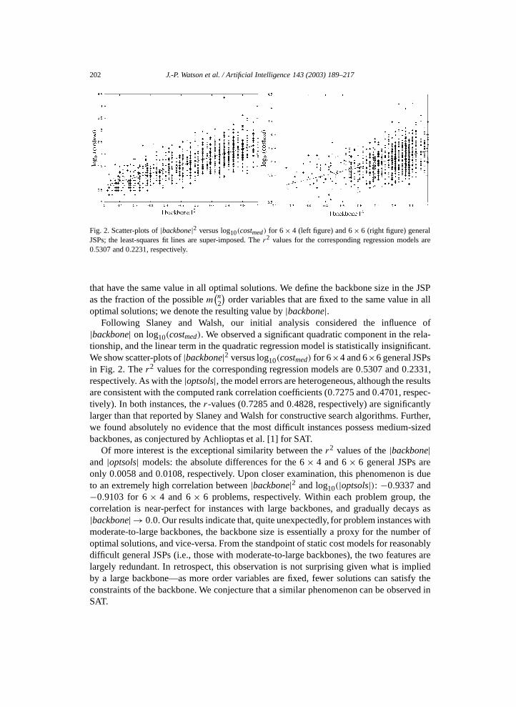
Fig. 2. Scatter-plots of |backbone|2 versus log10(costmed) for 6 × 4 (left figure) and 6 × 6 (right figure) generalJSPs; the least-squares fit lines are super-imposed. The r2 values for the corresponding regression models are0.5307 and 0.2231, respectively.
that have the same value in all optimal solutions. We define the backbone size in the JSPas the fraction of the possible m
(n2
)order variables that are fixed to the same value in all
optimal solutions; we denote the resulting value by |backbone|.Following Slaney and Walsh, our initial analysis considered the influence of
|backbone| on log10(costmed). We observed a significant quadratic component in the rela-tionship, and the linear term in the quadratic regression model is statistically insignificant.We show scatter-plots of |backbone|2 versus log10(costmed) for 6×4 and 6×6 general JSPsin Fig. 2. The r2 values for the corresponding regression models are 0.5307 and 0.2331,respectively. As with the |optsols|, the model errors are heterogeneous, although the resultsare consistent with the computed rank correlation coefficients (0.7275 and 0.4701, respec-tively). In both instances, the r-values (0.7285 and 0.4828, respectively) are significantlylarger than that reported by Slaney and Walsh for constructive search algorithms. Further,we found absolutely no evidence that the most difficult instances possess medium-sizedbackbones, as conjectured by Achlioptas et al. [1] for SAT.
Of more interest is the exceptional similarity between the r2 values of the |backbone|and |optsols| models: the absolute differences for the 6 × 4 and 6 × 6 general JSPs areonly 0.0058 and 0.0108, respectively. Upon closer examination, this phenomenon is dueto an extremely high correlation between |backbone|2 and log10(|optsols|): −0.9337 and−0.9103 for 6 × 4 and 6 × 6 problems, respectively. Within each problem group, thecorrelation is near-perfect for instances with large backbones, and gradually decays as|backbone| → 0.0. Our results indicate that, quite unexpectedly, for problem instances withmoderate-to-large backbones, the backbone size is essentially a proxy for the number ofoptimal solutions, and vice-versa. From the standpoint of static cost models for reasonablydifficult general JSPs (i.e., those with moderate-to-large backbones), the two features arelargely redundant. In retrospect, this observation is not surprising given what is impliedby a large backbone—as more order variables are fixed, fewer solutions can satisfy theconstraints of the backbone. We conjecture that a similar phenomenon can be observed inSAT.
J.-P. Watson et al. / Artificial Intelligence 143 (2003) 189–217 203
4.4. The average distance between random local optima
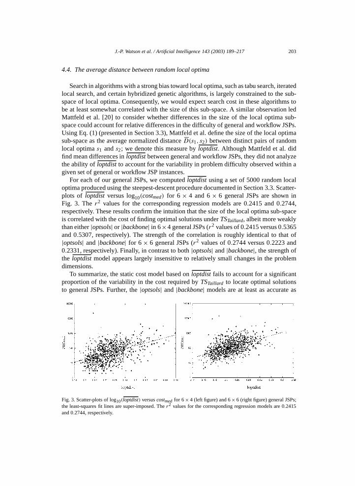
Search in algorithms with a strong bias toward local optima, such as tabu search, iteratedlocal search, and certain hybridized genetic algorithms, is largely constrained to the sub-space of local optima. Consequently, we would expect search cost in these algorithms tobe at least somewhat correlated with the size of this sub-space. A similar observation ledMattfeld et al. [20] to consider whether differences in the size of the local optima sub-space could account for relative differences in the difficulty of general and workflow JSPs.Using Eq. (1) (presented in Section 3.3), Mattfeld et al. define the size of the local optimasub-space as the average normalized distance �D(s1, s2) between distinct pairs of randomlocal optima s1 and s2; we denote this measure by loptdist. Although Mattfeld et al. didfind mean differences in loptdist between general and workflow JSPs, they did not analyzethe ability of loptdist to account for the variability in problem difficulty observed within agiven set of general or workflow JSP instances.
For each of our general JSPs, we computed loptdist using a set of 5000 random localoptima produced using the steepest-descent procedure documented in Section 3.3. Scatter-plots of loptdist versus log10(costmed) for 6 × 4 and 6 × 6 general JSPs are shown inFig. 3. The r2 values for the corresponding regression models are 0.2415 and 0.2744,respectively. These results confirm the intuition that the size of the local optima sub-spaceis correlated with the cost of finding optimal solutions under TSTaillard, albeit more weaklythan either |optsols| or |backbone| in 6×4 general JSPs (r2 values of 0.2415 versus 0.5365and 0.5307, respectively). The strength of the correlation is roughly identical to that of|optsols| and |backbone| for 6 × 6 general JSPs (r2 values of 0.2744 versus 0.2223 and0.2331, respectively). Finally, in contrast to both |optsols| and |backbone|, the strength ofthe loptdist model appears largely insensitive to relatively small changes in the problemdimensions.
To summarize, the static cost model based on loptdist fails to account for a significantproportion of the variability in the cost required by TSTaillard to locate optimal solutionsto general JSPs. Further, the |optsols| and |backbone| models are at least as accurate as
Fig. 3. Scatter-plots of log10(loptdist) versus costmed for 6 × 4 (left figure) and 6 × 6 (right figure) general JSPs;the least-squares fit lines are super-imposed. The r2 values for the corresponding regression models are 0.2415and 0.2744, respectively.
204 J.-P. Watson et al. / Artificial Intelligence 143 (2003) 189–217
the loptdist model. Later in Section 6.2, we re-visit and ultimately refute Mattfeld et al.’soriginal claim regarding the ability of differences in loptdist to account for differences inthe difficulty of general and workflow JSPs.
4.5. The distance between random local optima and the nearest optimal solution
In both the JSP and SAT, the accuracy of the |optsols| model decreases as the numberof optimal solutions approaches 0. Analogously, the |backbone| model is more accurate onproblem instances with small backbones. Singer et al. [27] recently introduced a static costmodel for SAT that largely corrects for these deficiencies. Local search algorithms for SAT,such as GSAT or Walk-SAT [18], quickly locate sub-optimal ‘quasi-solutions’, in whichrelatively few clauses are unsatisfied. These quasi-solutions form a sub-space that containsall optimal solutions, and is largely interconnected; once a solution in this sub-space isidentified, local search is typically restricted to this sub-space. This observation led Singeret al. to hypothesize that the distance between the first quasi-solution encountered and thenearest optimal solution, which we denote dquasi-opt, largely dictates the cost of local searchin SAT.
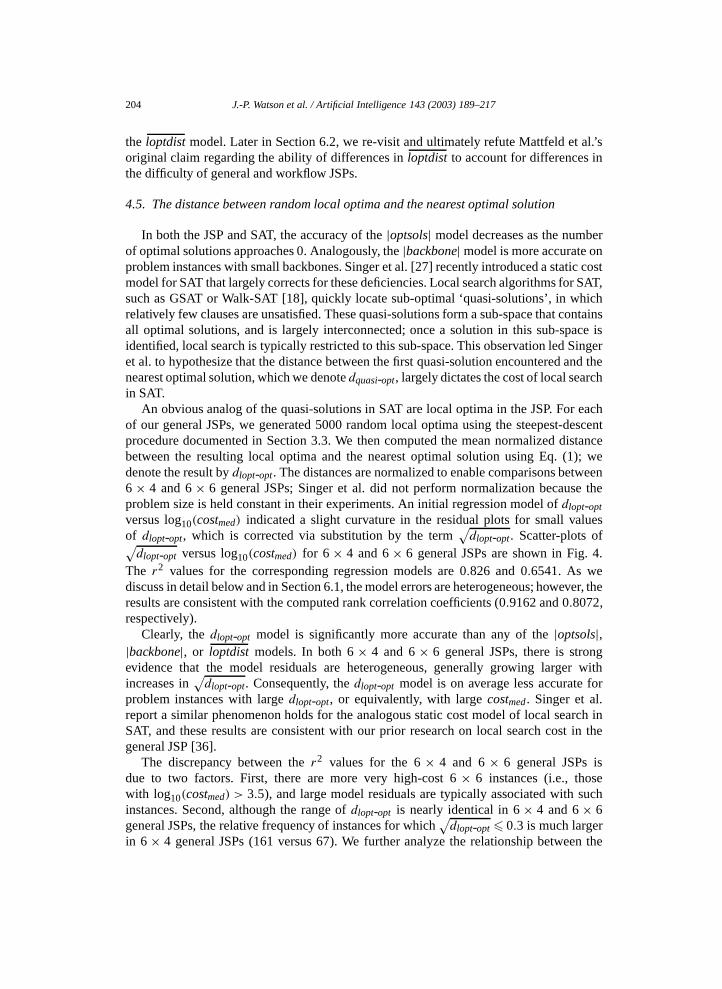
An obvious analog of the quasi-solutions in SAT are local optima in the JSP. For eachof our general JSPs, we generated 5000 random local optima using the steepest-descentprocedure documented in Section 3.3. We then computed the mean normalized distancebetween the resulting local optima and the nearest optimal solution using Eq. (1); wedenote the result by dlopt-opt. The distances are normalized to enable comparisons between6 × 4 and 6 × 6 general JSPs; Singer et al. did not perform normalization because theproblem size is held constant in their experiments. An initial regression model of dlopt-opt
versus log10(costmed) indicated a slight curvature in the residual plots for small valuesof dlopt-opt, which is corrected via substitution by the term
√dlopt-opt. Scatter-plots of√
dlopt-opt versus log10(costmed) for 6 × 4 and 6 × 6 general JSPs are shown in Fig. 4.The r2 values for the corresponding regression models are 0.826 and 0.6541. As wediscuss in detail below and in Section 6.1, the model errors are heterogeneous; however, theresults are consistent with the computed rank correlation coefficients (0.9162 and 0.8072,respectively).
Clearly, the dlopt-opt model is significantly more accurate than any of the |optsols|,|backbone|, or loptdist models. In both 6 × 4 and 6 × 6 general JSPs, there is strongevidence that the model residuals are heterogeneous, generally growing larger withincreases in
√dlopt-opt. Consequently, the dlopt-opt model is on average less accurate for
problem instances with large dlopt-opt, or equivalently, with large costmed . Singer et al.report a similar phenomenon holds for the analogous static cost model of local search inSAT, and these results are consistent with our prior research on local search cost in thegeneral JSP [36].
The discrepancy between the r2 values for the 6 × 4 and 6 × 6 general JSPs isdue to two factors. First, there are more very high-cost 6 × 6 instances (i.e., thosewith log10(costmed) > 3.5), and large model residuals are typically associated with suchinstances. Second, although the range of dlopt-opt is nearly identical in 6 × 4 and 6 × 6general JSPs, the relative frequency of instances for which
√dlopt-opt � 0.3 is much larger
in 6 × 4 general JSPs (161 versus 67). We further analyze the relationship between the
J.-P. Watson et al. / Artificial Intelligence 143 (2003) 189–217 205
Fig. 4. Scatter-plots of√
dlopt-opt versus log10(costmed) for 6 × 4 (left figure) and 6 × 6 (right figure) general
JSPs; the least-squares fit lines are super-imposed. The r2 values for the corresponding regression models are0.826 and 0.6541, respectively.
dlopt-opt model and very high-cost general JSPs in Section 6.1, and consider the influenceof the ratio of jobs to machines (n/m) on the accuracy of the dlopt-opt model in Section 5.2.
To summarize, the static cost model based on dlopt-opt accounts for a substantialproportion of the variance in the cost required by TSTaillard to locate optimal solutionsto ‘typical’ general JSPs. With few exceptions, the model residuals vary over roughly 1 to1.5 orders of magnitude in the 6 × 4 and 6 × 6 problems, respectively; the improvementis substantial in comparison to the residuals for the models based on either |optsols|,|backbone|, or loptdist. Finally, we observe that the dlopt-opt model is also consistent withthe observation that hard (easy) problem instances tend to be hard (easy) for all local searchalgorithms, as discussed in Section 3.4. Intuitively, if the distance between random localoptima and the nearest optimal solution for a particular problem instance is very large, wewould expect the instance to be difficult for any algorithm based on local search, as searchin such algorithms clearly progresses in small increments.
4.6. Models based on multiple search space features
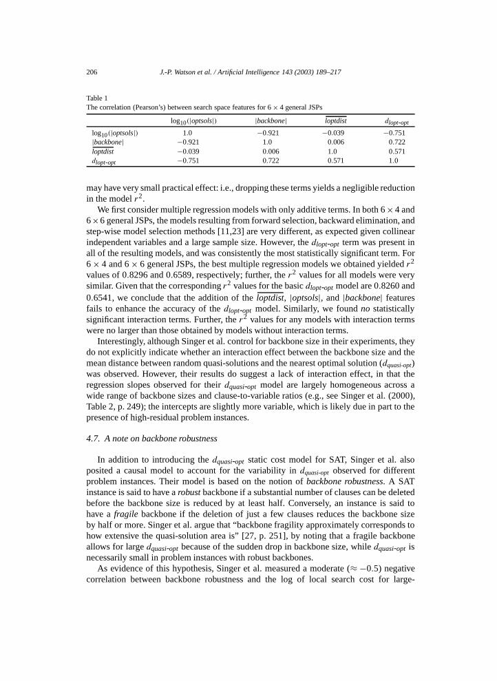
We now consider whether we can improve the accuracy of the dlopt-opt model bysimultaneously considering dlopt-opt in conjunction with the three other search spacefeatures considered earlier in this section. We proceed via well-known multiple regressionmethods. Ideally, the independent variables in a multiple regression model are highlycorrelated with the dependent variable, but not with each other; if the independentvariables are highly correlated, they are said to be collinear. Collinearity is known tocause difficulties for multiple regression model selection techniques, in part because theregression coefficients are not unique, making interpretation very difficult [23]. In Table 1,we show the pair-wise correlation (for 6 × 4 general JSPs) between the four search spacefeatures that serve as the independent variables in our multiple regression model. Similarcorrelations hold for 6 × 6 general JSPs, indicating a high degree of collinearity existsamong the four search space features we have considered. Finally, we note that when thesample size is large, terms may be statistically significant due to high power, but in reality
206 J.-P. Watson et al. / Artificial Intelligence 143 (2003) 189–217
Table 1The correlation (Pearson’s) between search space features for 6 × 4 general JSPs
log10(|optsols|) |backbone| loptdist dlopt-opt
log10(|optsols|) 1.0 −0.921 −0.039 −0.751|backbone| −0.921 1.0 0.006 0.722loptdist −0.039 0.006 1.0 0.571dlopt-opt −0.751 0.722 0.571 1.0
may have very small practical effect: i.e., dropping these terms yields a negligible reductionin the model r2.
We first consider multiple regression models with only additive terms. In both 6 ×4 and6×6 general JSPs, the models resulting from forward selection, backward elimination, andstep-wise model selection methods [11,23] are very different, as expected given collinearindependent variables and a large sample size. However, the dlopt-opt term was present inall of the resulting models, and was consistently the most statistically significant term. For6 × 4 and 6 × 6 general JSPs, the best multiple regression models we obtained yielded r2
values of 0.8296 and 0.6589, respectively; further, the r2 values for all models were verysimilar. Given that the corresponding r2 values for the basic dlopt-opt model are 0.8260 and0.6541, we conclude that the addition of the loptdist, |optsols|, and |backbone| featuresfails to enhance the accuracy of the dlopt-opt model. Similarly, we found no statisticallysignificant interaction terms. Further, the r2 values for any models with interaction termswere no larger than those obtained by models without interaction terms.
Interestingly, although Singer et al. control for backbone size in their experiments, theydo not explicitly indicate whether an interaction effect between the backbone size and themean distance between random quasi-solutions and the nearest optimal solution (dquasi-opt)was observed. However, their results do suggest a lack of interaction effect, in that theregression slopes observed for their dquasi-opt model are largely homogeneous across awide range of backbone sizes and clause-to-variable ratios (e.g., see Singer et al. (2000),Table 2, p. 249); the intercepts are slightly more variable, which is likely due in part to thepresence of high-residual problem instances.
4.7. A note on backbone robustness
In addition to introducing the dquasi-opt static cost model for SAT, Singer et al. alsoposited a causal model to account for the variability in dquasi-opt observed for differentproblem instances. Their model is based on the notion of backbone robustness. A SATinstance is said to have a robust backbone if a substantial number of clauses can be deletedbefore the backbone size is reduced by at least half. Conversely, an instance is said tohave a fragile backbone if the deletion of just a few clauses reduces the backbone sizeby half or more. Singer et al. argue that “backbone fragility approximately corresponds tohow extensive the quasi-solution area is” [27, p. 251], by noting that a fragile backboneallows for large dquasi-opt because of the sudden drop in backbone size, while dquasi-opt isnecessarily small in problem instances with robust backbones.
As evidence of this hypothesis, Singer et al. measured a moderate (≈ −0.5) negativecorrelation between backbone robustness and the log of local search cost for large-
J.-P. Watson et al. / Artificial Intelligence 143 (2003) 189–217 207
backboned SAT instances. Surprisingly, this correlation degraded as the backbone size wasdecreased, leading to the conjecture that “finding the backbone is less of an issue and sobackbone fragility, which hinders this, has less of an effect” [27, p. 254]; this conjecturewas never explicitly tested. We have previously reported very similar results for generalJSPs [36]. As indicated in Section 4.5 and more fully in Section 6, we have since discoveredrelatively serious deficiencies in the dlopt-opt model (and by analogy, likely deficiencies inthe dquasi-opt), and feel it is somewhat premature to posit causal hypotheses before thesource of these deficiencies is completely understood. As a consequence, we have notpursued further analyses of backbone robustness in the JSP.
5. Applications of the dlopt-opt model
The analyses presented in Section 4 demonstrate that the dlopt-opt static cost modelaccounts for a substantial proportion of the variance in the cost of finding optimal solutionsto typical general JSPs using TSTaillard. Further, more complex models that considerdlopt-opt in conjunction with backbone size, the number of optimal solutions, and the sizeof the local optima sub-space fail to yield even marginal improvements in accuracy. In thissection, we additionally show that the dlopt-opt model accounts for both (1) a substantialproportion of the variance in the cost of finding sub-optimal solutions to typical generalJSPs using TSTaillard and (2) differences in the relative difficulty of general JSPs withdifferent job-to-machine ratios.
5.1. Modeling the cost of locating sub-optimal solutions
Because they are incomplete, local search algorithms are only used to find solutionsto satisfiable SAT instances, where the evaluation of the global optima is known, and isequal to the total number of clauses m. Such a priori knowledge leads to the obvioustermination criterion: keep searching until a global optimum is located. Consequently,analyses of problem difficulty for local search in SAT only consider the cost required tolocate globally optimal solutions. For most NP-complete problems, however, the evaluationof the global optimum is not known a priori. Armed only with the knowledge that largerrun-times generally lead to higher-quality solutions, local search practitioners generallyuse the following termination criterion: allocate as much CPU time as possible, and returnthe best solution found.
Although larger run-times generally yield higher-quality solutions, the relationship istypically discontinuous, non-linear, or both. Often, small or moderate increases in run-timefail, on average, to improve solution quality; for example, Stützle [31, p. 47], notes that inthe Traveling Salesman Problem “. . . instances appear to have ‘hard cliffs’ for the localsearch algorithm, corresponding to deep local minima, which are difficult to pass”. Similarobservations have been reported for a variety of NP-complete problems, including theJSP. Another manifestation of this phenomenon has been observed by several researchers,including ourselves. Here, multiple independent trials of a particular local search algorithmtypically yield sub-optimal solutions that can be partitioned into a very small number ofsubsets (often 1), with each subset containing solutions with identical evaluations.
208 J.-P. Watson et al. / Artificial Intelligence 143 (2003) 189–217
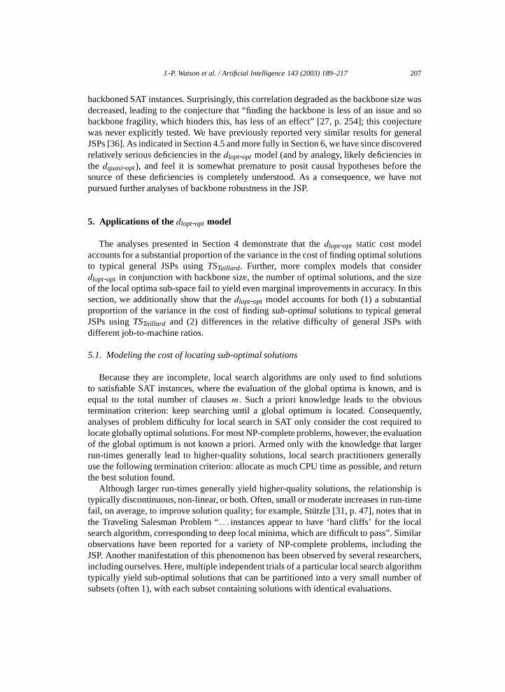
Fig. 5. The offset x from the optimal makespan C∗max, 0 � x � 25, versus the cost costmed(x) required to locate
a solution with Cmax � C∗max + x for two 6 × 6 general JSPs. The numeric annotations indicate either dlopt-T (x)
for a specific x, or the range of dlopt-T (x) over a contiguous sub-interval of x.
One simple way to visualize this phenomenon is to plot the cost required to achieve asolution with an evaluation of at least C∗
max + x over a wide range of x � 0. In Fig. 5, weprovide examples of such plots for two moderately difficult 6 × 6 general JSPs. In bothplots, the offset from the optimal makespan x is varied from 0 to 25, and the median cost(over 5000 independent runs of TSTaillard) required to find a solution with an evaluation ofat least C∗
max +x is computed for each x , which we denote by costmed(x). In the left side ofFig. 5, we see a typical example of a problem instance with discrete jumps in search cost atspecific sub-optimal makespans, with plateaus in search cost in between the jump points.In the right side of Fig. 5, we show a problem instance for which the decay in search costis generally more gradual; a large, discontinuous jump in search cost occurs only betweenx = 0 and x = 1.
As shown in Section 4, the dlopt-opt static cost model accounts for a significantproportion of the variance in the cost of finding optimal solutions to general JSPs usingTSTaillard. Intuitively, this cost is large if TSTaillard is, on average, initiated from solutionsthat are very distant from the nearest optimal solution. We conjecture that this intuitionextends to any subset of solutions, including sub-optimal solutions; we would expectlocal search cost to be proportional to the distance between the initial solutions and thenearest target solution. As evidence of this conjecture, we consider a set T (x) containingall solutions with a makespan between C∗
max and C∗max + x , x � 0, and denote the mean
distance between random local optima and the nearest solution in the set T (x) by dlopt-T (x);as with the computation of dlopt-opt, the statistics are taken over 5000 independent samples.We have annotated the plots in Fig. 5 with the computed dlopt-T (x), 0 � x � 25. In bothinstances, (1) large jumps in search cost clearly coincide with large jumps in dlopt-T (x),(2) intervals of roughly constant search cost correspond to contiguous sub-intervals of x
with nearly identical values of dlopt-T (x), and (3) gradual drops in search cost coincidewith gradual drops in dlopt-T (x). Consequently, we hypothesize that dlopt-T (x) accounts fora significant proportion of the variance in the cost of finding both optimal and sub-optimalsolutions to typical general JSPs using TSTaillard.
To test this hypothesis, we computed costmed(x) and dlopt-T (x) for both our 6 × 4 and6 × 6 general JSPs, varying x from 1 to 25. Finding solutions to 6 × 4 and 6 × 6 general
J.-P. Watson et al. / Artificial Intelligence 143 (2003) 189–217 209
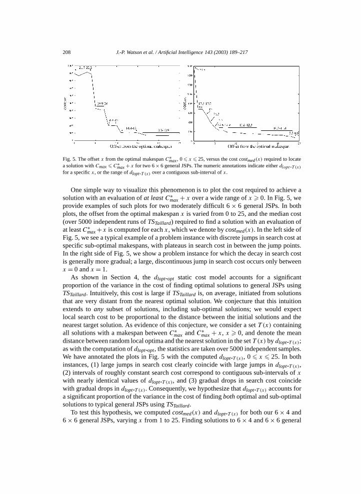
Fig. 6. Scatter-plots of√
dlopt-opt versus log10(costmed) for the sub-optimal 6 × 4 (left figure) and 6 × 6 (right
figure) general JSP problem groups; the regression lines are super-imposed. The r2 values for the correspondingregression models are 0.8866 and 0.8252, respectively.
JSPs with Cmax > C∗max + 25 is generally quite easy for TSTaillard, with costmed(25) � 100
in all but a few cases. Under this methodology, we are effectively creating 25 derivatives ofeach problem instance (one for each value of x), which results in new ‘sub-optimal’ 6 × 4and 6×6 problem groups, each with 25 000 instances. For many of the derivative instances,especially those produced using large x , costmed(x) = 0, or equivalently dlopt-T (x) ≈ 0.0.We observed 1293 6 × 4 zero-cost instances, and 60 6 × 6 zero-cost instances; in bothcases, the zero-cost instances are excluded in the following analysis.
In Fig. 6, we show scatter-plots of√
dlopt-opt versus log10(costmed) for the sub-optimal6 × 4 and 6 × 6 problem groups; the r2 values for the corresponding regression modelsare 0.8866 and 0.8252, respectively. Clearly, the dlopt-opt model accounts for most of thevariance in the cost of finding sub-optimal solutions to typical general JSPs using TSTaillard.We observed larger r2 values in the sub-optimal 6×4 and 6×6 problem groups than for thecorresponding problem groups analyzed in Section 4.5: 0.8866 versus 0.8260 for the 6 × 4problems and 0.8252 versus 0.6541 for the 6×6 problems. We explain the greater accuracyof the dlopt-opt model on the sub-optimal problem groups by noting that the proportion ofinstances with small values of dlopt-opt is larger in the sub-optimal problem groups, whichcorresponds to the region where the dlopt-opt model is most accurate.
We conclude by noting that the dlopt-opt model provides the first quantitative explanationfor ‘cliffs’ in local search cost observed at particular sub-optimal evaluations: abruptchanges in local search cost occur where there are abrupt changes in dlopt-opt. Similarly,the plateaus observed in Fig. 5 occur because solutions on the plateau are equi-distantfrom random local optima; TSTaillard is equally likely to encounter any of the solutions onthe plateau, given a fixed run-time. Similarly, gradual increases in search cost occur whenslightly better solutions are only marginally farther from random local optima.
5.2. Explaining differences in the relative difficulty of square versus rectangular JSPs
Given the accuracy of the dlopt-opt model for both 6 × 4 and 6 × 6 general JSPs, it isnatural to consider whether or not differences in the distribution of dlopt-opt for problems
210 J.-P. Watson et al. / Artificial Intelligence 143 (2003) 189–217
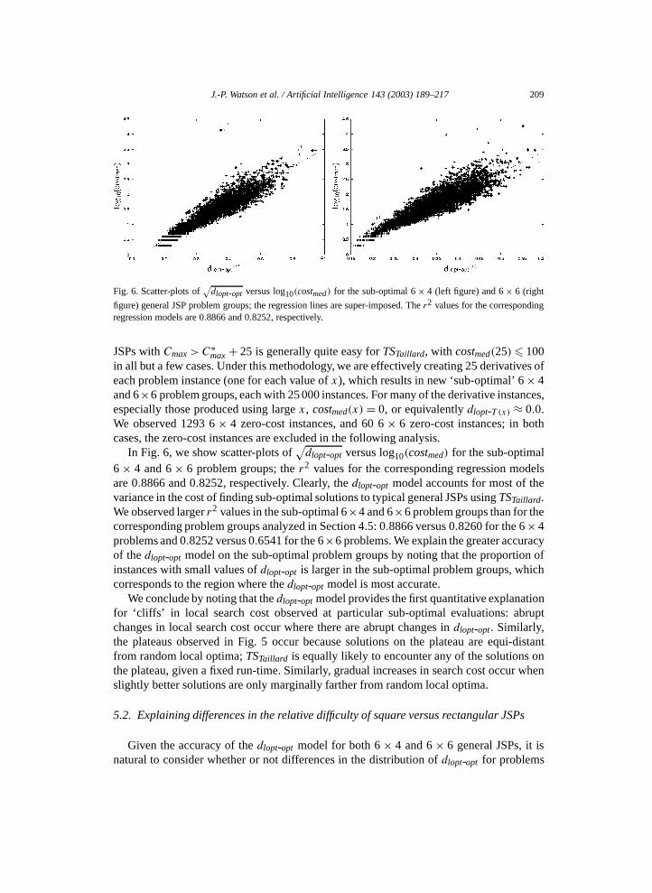
Fig. 7. Histograms of dlopt-opt for 10 000 4 × 3 (left figure) and 7 × 3 (right figure) general JSPs.
with different ratios of n/m can account for the empirical observation that square JSPs aregenerally more difficult than rectangular JSPs.
Fixing m = 3, we generated 10 000 general JSPs for n = 4 through n = 7; although weinitially considered larger values of n, the huge number of optimal solutions (> 1 billionin many cases) prevented us from efficiently computing dlopt-opt. We show histograms ofdlopt-opt for 4×3 and 7×3 general JSPs in Fig. 7. In 4×3 general JSPs, the right-tail massof the distribution is substantial (e.g., for dlopt-opt � 0.3), especially in comparison to thedistribution for 7 × 3 general JSPs, where instances with dlopt-opt � 0.3 are relatively rare.We have also generated histograms for general JSPs with n/m < 1, observing a continuedshift of the distribution mass toward 0.5.
Although not entirely conclusive, our results provide strong evidence that the right-tail mass of the dlopt-opt distribution vanishes as n/m → ∞, suggesting a cause for theempirical observation that square JSPs are generally more difficult than rectangular JSPs.Further, we hypothesize that the shift from exponential to polynomial growth in searchcost at n/m ≈ 6 [33] is due to the disappearance of any significant mass in the right tail ofthe dlopt-opt distribution. However, due to the huge number of optimal solutions in probleminstances with n/m � 4, we are currently unable to empirically test this hypothesis. Finally,we note that the accuracy of the dlopt-opt model should further improve as n/m → ∞, dueto the increasing frequency of instances with small values of dlopt-opt. Consequently, fromthe standpoint of static cost models, only general JSPs with n/m ≈ 1.0 warrant significantattention in the future.
In a previous paper [36], we argued that a shift in the distribution of |backbone|, andnot dlopt-opt, was responsible for differences in the relative difficulty of square versusrectangular JSPs. While our original observation still holds (i.e., the proportion of instanceswith small backbones grows as n/m → ∞), we have chosen to re-cast our original resultsin terms of the more accurate static cost model based on dlopt-opt.
6. Limitations of the dlopt-opt model
Although the dlopt-opt static cost model largely accounts for the cost of finding bothoptimal and sub-optimal solutions to typical general JSPs using TSTaillard, and provides

J.-P. Watson et al. / Artificial Intelligence 143 (2003) 189–217 211
an explanation for the differences in the relative difficulty of general JSPs with differentjob-to-machine ratios, the model is by no means perfect. As discussed in Section 4.5, thedlopt-opt model is less accurate for problem instances with large values of dlopt-opt (or,equivalently, large costmed), and consequently fails to account for roughly 35% of the costvariance in our 6 × 6 general JSPs.
In this section, we identify two additional limitations of the dlopt-opt model. First, weconclusively demonstrate that the accuracy of the dlopt-opt model is exceptionally poor forvery high-cost general JSPs (we provided some preliminary evidence for this conclusion inSection 4.5). Second, we show that the dlopt-opt model is unable to account for a significantproportion of the variance in the cost of finding optimal solutions to more structured JSPs:e.g., workflow JSPs. Although both of the results presented in this section are clearly‘negative’, we feel it is important to identify and report such deficiencies, as research intowhy the dlopt-opt model fails in these circumstances is likely to lead to more general andaccurate static cost models in the future.
6.1. Modeling search cost in exceptionally hard general JSPs
In Section 4.5, we provided evidence that the dlopt-opt model is less accurate for probleminstances with large values of dlopt-opt, or equivalently, large costmed. Of particular concernare the rare, very high-cost (costmed � 10000) instances appearing in both sides of Fig. 4;in all but one case, these instances possess the largest residuals under the correspondingregression model. To determine whether large model residuals are typically associated withvery high-cost general JSPs, we created groups of 6 × 4 and 6 × 6 general JSPs with equalproportions of problem instances over the range of costmed . Specifically, we sub-dividedthe range of possible costmed values into the following four contiguous intervals: [1,49],[50,499], [500,4999], and [5000,∞]. These intervals qualitatively correspond to easy,moderate, difficult, and very difficult problem instances, respectively. For both 6 × 4 and6 × 6 general JSPs, we then produced 500 instances belonging to each interval using agenerate-and-test procedure.
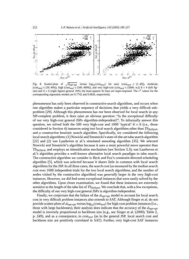
We provide scatter-plots of√
dlopt-opt versus log10(costmed) for the two resultingproblem groups in Fig. 8. The r2 values for the corresponding regression model are0.7742 and 0.6820, respectively. First, we note that because the high-cost and very high-cost instances reside in the right-tail of the log10(costmed) distribution, the large relativefrequencies of problem instances with costmed near the lower bounds of the correspondingintervals was expected. In both problem groups, we observe a substantial reduction in theaccuracy of the dlopt-opt model for high-cost (500 � costmed � 4999) instances. For veryhigh-cost instances (costmed � 5000), the degradation in accuracy is far more extreme,such that
√dlopt-opt provides almost no information about costmed . These results clearly
reinforce the deficiencies of the dlopt-opt model discussed in Section 4.5: accuracy isinversely proportional to both dlopt-opt and costmed. As a direct consequence, although weare now able to account for much of the variability in search cost for ‘typical’ general JSPs,an understanding of the search space properties that make certain problems exceptionallydifficult for TSTaillard remains elusive.
Several researchers have reported situations in which problems that are exceptionallydifficult for one algorithm are much easier for other algorithms [15,29]. To date, this
212 J.-P. Watson et al. / Artificial Intelligence 143 (2003) 189–217
Fig. 8. Scatter-plots of√
dlopt-opt versus log10(costmed) for easy (costmed ∈ [1,49]), moderate(costmed ∈ [50,499]), high (costmed ∈ [500,4999]), and very high-cost (costmed ∈ [5000,∞]) 6 × 4 (left fig-ure) and 6 × 6 (right figure) general JSPs; the least-squares fit lines are super-imposed. The r2 values for thecorresponding regression models are 0.7742 and 0.6820, respectively.
phenomenon has only been observed in constructive search algorithms, and occurs whenone algorithm makes a particular sequence of decisions that yields a very difficult sub-problem [29]. Although this phenomenon has not been observed for local search in anyNP-complete problem, it does raise an obvious question: “Is the exceptional difficultyof our very high-cost general JSPs algorithm-independent?”. To informally answer thisquestion, we solved both the 500 very high-cost and 1000 ‘typical’ 6 × 6 (i.e., thoseconsidered in Section 4) instances using two local search algorithms other than TSTaillard,and a constructive heuristic search algorithm. Specifically, we considered the followinglocal search algorithms: (1) Nowicki and Smutnicki’s state-of-the-art tabu search algorithm[22] and (2) van Laarhoven et al.’s simulated annealing algorithm [35]. We selectedNowicki and Smutnicki’s algorithm because it uses a more powerful move operator thanTSTaillard, and employs an intensification mechanism (see Section 3.3); van Laarhoven etal.’s algorithm provides a well-known alternative local search paradigm to tabu search.The constructive algorithm we consider is Beck and Fox’s constraint-directed schedulingalgorithm [5], which was selected because it shares little in common with local searchalgorithms for the JSP. In all three cases, the search cost (as measured by the median searchcost over 1000 independent trials for the two local search algorithms, and the number ofnodes visited by the constructive algorithm) was generally larger in the very high-costinstances. However, we did find some exceptional instances that were easily solved by theother algorithms. Upon closer examination, we found that these instances are extremelysensitive to the length of the tabu list of TSTaillard. We conclude that, with a few exceptions,the difficulty of our very high-cost general JSPs is algorithm-independent.
Finally, we conjecture that the failure of the dlopt-opt model to account for local searchcost in very difficult problem instances also extends to SAT. Although Singer et al. do notprovide scatter-plots of dlopt-opt versus log10(costmed) for high-cost problem instances (i.e.,those with large backbones), their analysis does indicate that the accuracy of the dlopt-opt
model is inversely proportional to backbone size (e.g., see Singer et al. (2000), Table 2,p. 249), and as a consequence, to costmed (as in the general JSP, local search cost andbackbone size are positively correlated in SAT). Further, very high-cost SAT instances
J.-P. Watson et al. / Artificial Intelligence 143 (2003) 189–217 213
possess the largest residuals under Singer et al.’s model of backbone robustness (e.g., seeSinger et al. (2000), Fig. 11, p. 255), which in turn is correlated with dlopt-opt.
6.2. Modeling search cost in JSPs with workflow
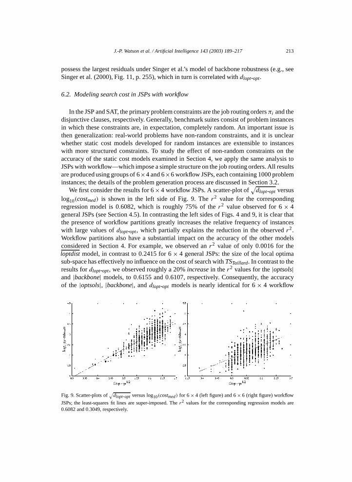
In the JSP and SAT, the primary problem constraints are the job routing orders πi and thedisjunctive clauses, respectively. Generally, benchmark suites consist of problem instancesin which these constraints are, in expectation, completely random. An important issue isthen generalization: real-world problems have non-random constraints, and it is unclearwhether static cost models developed for random instances are extensible to instanceswith more structured constraints. To study the effect of non-random constraints on theaccuracy of the static cost models examined in Section 4, we apply the same analysis toJSPs with workflow—which impose a simple structure on the job routing orders. All resultsare produced using groups of 6×4 and 6×6 workflow JSPs, each containing 1000 probleminstances; the details of the problem generation process are discussed in Section 3.2.
We first consider the results for 6 × 4 workflow JSPs. A scatter-plot of√
dlopt-opt versuslog10(costmed) is shown in the left side of Fig. 9. The r2 value for the correspondingregression model is 0.6082, which is roughly 75% of the r2 value observed for 6 × 4general JSPs (see Section 4.5). In contrasting the left sides of Figs. 4 and 9, it is clear thatthe presence of workflow partitions greatly increases the relative frequency of instanceswith large values of dlopt-opt, which partially explains the reduction in the observed r2.Workflow partitions also have a substantial impact on the accuracy of the other modelsconsidered in Section 4. For example, we observed an r2 value of only 0.0016 for theloptdist model, in contrast to 0.2415 for 6 × 4 general JSPs: the size of the local optimasub-space has effectively no influence on the cost of search with TSTaillard. In contrast to theresults for dlopt-opt, we observed roughly a 20% increase in the r2 values for the |optsols|and |backbone| models, to 0.6155 and 0.6107, respectively. Consequently, the accuracyof the |optsols|, |backbone|, and dlopt-opt models is nearly identical for 6 × 4 workflow
Fig. 9. Scatter-plots of√
dlopt-opt versus log10(costmed) for 6 × 4 (left figure) and 6 × 6 (right figure) workflow
JSPs; the least-squares fit lines are super-imposed. The r2 values for the corresponding regression models are0.6082 and 0.3049, respectively.
214 J.-P. Watson et al. / Artificial Intelligence 143 (2003) 189–217
JSPs. Finally, we note that strong correlation between log10(|optsols|) and |backbone|2 ismaintained (r = −0.8936).
Next, we consider the results for 6×6 workflow JSPs; a scatter-plot of√
dlopt-opt versuslog10(costmed) is shown in the right side of Fig. 9. Here, we see a further reduction inthe accuracy of the dlopt-opt model: the r2 value is over 50% less than that observed for6 × 6 general JSPs, dropping from 0.6541 to 0.3049. As with 6 × 4 workflow JSPs, thereduction in accuracy is partially due to dramatic increases in the relative frequency ofproblem instances with very large values of dlopt-opt. Similarly, the correlation betweenloptdist and log10(costmed) is insignificant (r2 = 0.002983), and we observed an increasein the accuracy of the |optsols| and |backbone| models (to r2 values of 0.3345 and 0.2974,respectively); the relatively strong correlation between log10(|optsols|) and |backbone|2was again maintained (r = −0.8346).
Our results cast serious doubt on Mattfeld et al.’s assertion that differences in therelative difficulty of general and workflow JSPs are due to differences in loptdist. Whilewe observed statistically significant differences between the mean loptdist of generaland workflow JSPs (e.g., 0.2080 versus 0.3465 in 6 × 6 general and workflow JSPs,respectively), we also computed a relatively weak correlation between loptdist andlog10(costmed) for general JSPs – for workflow JSPs, the correlation between these samevariables is effectively 0. Statistically significant mean differences between general andworkflow JSPs also exist for |optsols|, |backbone|2, and
√dlopt-opt. Further, each of these
models is at least as accurate as the loptdist model for both general and workflow JSPs.Consequently, we believe that any of the |optsols|, |backbone|, and dlopt-opt models provideat least an equally likely explanation as the loptdist model for the differences in relativedifficulty between general and workflow JSPs.
Finally, we note that our results provide the first solid evidence that the static costmodels for random and structured problem instances may in fact be quite different. Noresearch to date has considered the impact of problem structure on the static cost modelsfor SAT. Given the strong similarities between the models for the JSP and SAT, weconjecture that existing static cost models for SAT, because they are based on randomproblem instances, are likely to be significantly less accurate when applied to structuredSAT instances.
7. Conclusion
Drawing from research on problem difficulty in SAT, we demonstrated that the dlopt-opt
static cost model accounts for much of the variability in the cost of finding optimalsolutions to general JSPs using a straightforward tabu search algorithm, TSTaillard. Thisresult was somewhat unexpected, given the differences in both the search space topologiesand local search algorithms for the general JSP and SAT. Further, the accuracy of the modelis nearly identical in both problems. In the course of our analyses, we also encounteredseveral other important, unanticipated results:
(1) backbone size and the number of optimal solutions are largely redundant search spacefeatures,
J.-P. Watson et al. / Artificial Intelligence 143 (2003) 189–217 215
(2) there is no significant interaction effect between dlopt-opt and any of the other searchspace features we considered,
(3) multiple-factor models do not significantly improve upon the accuracy of the dlopt-opt
model.
We then used the dlopt-opt model to provide explanations for two qualitative observationsregarding problem difficulty in the JSP. First, we showed that the dlopt-opt model accountsfor much of the variability in the cost of locating sub-optimal solutions to general JSPsusing TSTaillard. The resulting extension provides an explanation for the discontinuousjumps in search cost observed at particular offsets from the optimal makespan. Second,we demonstrated that strong differences in the distributions of dlopt-opt provide a possibleexplanation for differences in the relative difficulty of square versus rectangular JSPs:problem instances with large values of dlopt-opt are common in square JSPs, but arerelatively rare in rectangular JSPs.
Finally, we showed that the dlopt-opt model has some limitations. First, our analysesindicated that the accuracy of the model is inversely proportional to the magnitude ofdlopt-opt, or equivalently, the difficulty of the problem instance. We also found that theaccuracy is exceptionally poor on relatively rare, very high-cost problem instances. Second,we demonstrated that the accuracy of the dlopt-opt model is significantly worse for aparticular class of structured JSPs—those with workflow partitions.
We selected TSTaillard precisely because it serves as a baseline for more advanced tabusearch algorithms, such as the state-of-the-art algorithm of Nowicki and Smutnicki, whichemploy more advanced move operators and make more extensive use of long-term memoryand intensification mechanisms. With a relatively accurate static cost model of Taillard’salgorithm, we can begin to systematically assess the influence of these more advancedfeatures on the model. One inherent limitation of our analysis is that it is only directlyapplicable to tabu-like search algorithms for the JSP. Because static cost models are tied tospecific algorithms, it seems likely that other factors may be responsible for local searchcost in algorithms such as iterated local search or genetic algorithms, which are based onprinciples quite different from tabu search. At the same time, it seems likely that variationson the basic dlopt-opt model may account for the cost of tabu search in other NP-completeproblems.
Because the static cost models for SAT and the JSP are very similar, it also seemslikely that our results will be useful to researchers working on models of local searchcost in SAT. For example, our analyses indicate that the backbone size and the numberof optimal solutions are largely redundant, that simultaneous consideration of numberof optimal solutions, backbone size, the average distance between local optima fail toimprove the accuracy of the basic dlopt-opt model, and that the accuracy of the dlopt-opt
model is exceptionally poor on very high-cost problem instances. We conjecture similarobservations hold in SAT. Similarly, we showed that the static cost models for randomand structured problem instances can be very different. If similar results hold in SAT, theywould provide some evidence that the best algorithms for solving random instances maybe based on different principles than the best algorithms for solving structured instances.

216 J.-P. Watson et al. / Artificial Intelligence 143 (2003) 189–217
References
[1] D. Achlioptas, C. Gomes, H. Kautz, B. Selman, Generating satisfiable problem instances, in: K. Ford (Ed.),Proc. AAAI-2000, Austin, TX, AAAI/MIT Press, Cambridge, MA, 2000, pp. 256–261.
[2] E. Balas, A. Vazacopoulos, Guided local search with shifting bottleneck for job-shop scheduling,Management Sci. 44 (2) (1998) 262–275.
[3] J.W. Barnes, J.B. Chambers, Solving the job shop scheduling problem with tabu search, IIE Trans. 27 (1995)257–263.
[4] J.E. Beasley, OR-library: Distributing test problems by electronic mail, J. Oper. Res. Soc. 41 (11) (1990)1069–1072.
[5] J.C. Beck, M.S. Fox, Dynamic problem structure analysis as a basis for constraint-directed schedulingheuristics, Artificial Intelligence 117 (2) (2000) 31–81.
[6] J. Blazewicz, W. Domschke, E. Pesch, The job shop scheduling problem: Conventional and new solutiontechniques, European J. Oper. Res. 93 (1996) 1–33.
[7] J. Blazewicz, E. Pesch, M. Sterna, The disjunctive graph machine representation of the job shop schedulingproblem, European J. Oper. Res. 127 (2000) 317–331.
[8] K.D. Boese, A.B. Kahng, S. Muddu, A new adaptive multi-start technique for combinatorial optimization,Oper. Res. Lett. 16 (1994) 101–113.
[9] J.B. Chambers, J.W. Barnes, New tabu search results for the job shop scheduling problem, Technical ReportORP96-10, Graduate Program in Operations Research and Industrial Engineering, The University of Texasat Austin, 1996.
[10] D.A. Clark, J. Frank, I.P. Gent, E. MacIntyre, N. Tomov, T. Walsh, Local search and the number ofsolutions, in: Proceedings of the Second International Conference on Principles and Practices of ConstraintProgramming (CP-96), Cambridge, MA, 1996, pp. 119–133.
[11] P.R. Cohen, Empirical Methods for Artificial Intelligence, MIT Press, Cambridge, MA, 1995.[12] H. Fisher, G.L. Thompson, Probabilistic Learning Combinations of Local Job-Shop Scheduling Rules,
Prentice-Hall, Englewood Cliffs, NJ, 1963, Chapter 15, pp. 225–251.[13] J. Frank, P. Cheeseman, J. Stutz, When gravity fails: Local search topology, J. Artificial Intelligence Res. 7
(1997) 249–281.[14] M.R. Garey, D.S. Johnson, R. Sethi, The complexity of flowshop and jobshop scheduling, Math. Oper.
Res. 1 (2) (1976) 117–129.[15] I.P. Gent, T. Walsh, Easy problems are sometimes hard, Artificial Intelligence 70 (1–2) (1994) 335–345.[16] F. Glover, M. Laguna, Tabu Search, Kluwer Academic, Boston, MA, 1997.[17] T. Hogg, B.A. Huberman, C.P. Williams, Phase transitions and the search problem, Artificial Intelli-
gence 81 (1–2) (1996) 1–15.[18] H.H. Hoos, Stochastic local search—Methods, models, applications, PhD Thesis, Darmstadt University of
Technology, 1998.[19] A.S. Jain, S. Meeran, Deterministic job-shop scheduling: Past, present and future, European J. Oper. Res. 113
(1999) 390–434.[20] D.C. Mattfeld, C. Bierwirth, H. Kopfer, A search space analysis of the job shop scheduling problem, Ann.
Oper. Res. 86 (1999) 441–453.[21] R. Monasson, R. Zecchina, S. Kirkpatrick, B. Selman, L. Troyansky, Determining computational complexity
for characteristic ‘phase transitions’, Nature 400 (1998) 133–137.[22] E. Nowicki, C. Smutnicki, A fast taboo search algorithm for the job shop problem, Management Sci. 42 (6)
(1996) 797–813.[23] R. Lyman Ott, An Introduction to Statistical Methods and Data Analysis, Duxbury Press, Belmont, CA,
1993.[24] A.J. Parkes, Clustering at the phase transition, in: Proc. AAAI-97, Providence, RI, 1997, pp. 340–345.[25] C.M. Riedys, P.F. Stadler, Combinatorial landscapes, Technical Report 01-03-014, The Santa Fe Institute,
2001.[26] J. Singer, Why solutions can be hard to find: A featural theory of cost for a local search algorithm on random
satisfiability, PhD Thesis, University of Edinburgh, 2000.[27] J. Singer, I.P. Gent, A. Smaill, Backbone fragility and the local search cost peak, J. Artificial Intelligence
Res. 12 (2000) 235–270.

J.-P. Watson et al. / Artificial Intelligence 143 (2003) 189–217 217
[28] J. Slaney, T. Walsh, Backbones in optimization and approximation, in: B. Nebel (Ed.), Proc. IJCAI-01,Seattle, WA, Morgan Kaufmann, San Mateo, CA, 2001, pp. 254–259.
[29] B. Smith, S. Grant, Sparse constraint graphs and exceptionally hard problems, in: C. Mellish (Ed.), Proc.IJCAI-95, Montreal, Quebec, 1995.
[30] R.H. Storer, S.D. Wu, R. Vaccari, New search spaces for sequencing problems with application to job shopscheduling, Management Sci. 38 (1992) 1495–1509.
[31] T. Stützle, Local search algorithms for combinatorial problems—Analysis, improvements, and newapplications, PhD Thesis, Darmstadt University of Technology, 1999.
[32] E.D. Taillard, Benchmarks for basic scheduling problems, European J. Oper. Res. 64 (1993) 278–285.[33] E.D. Taillard, Parallel taboo search techniques for the job shop scheduling problem, ORSA J. Comput. 6 (2)
(1994) 108–117.[34] R.J.M. Vaessens, E.H.L. Aarts, J.K. Lenstra, Job shop scheduling by local search, INFORMS J.
Comput. 8 (3) (1996) 302–317.[35] P.J.M van Laarhoven, E.H.L. Aarts, J.K. Lenstra, Job shop scheduling by simulated annealing, Oper. Res. 40
(1992) 113–125.[36] J.-P. Watson, J.C. Beck, A.E. Howe, L.D. Whitley, Toward an understanding of local search cost in job-shop
scheduling, in: A. Cesta (Ed.), Proceedings of the Sixth European Conference on Planning, Springer, Berlin,2001.