probability and random variables; and classical estimation...
TRANSCRIPT
- p. 1/85
TH
E
UN I V E
RS
IT
Y
OF
ED
I N BU
R
GH
Probability and Random Variables; and ClassicalEstimation Theory
UDRC Summer School, 20th July 2015
Dr James R. Hopgood
Room 2.05
Alexander Graham Bell Building
The King’s Buildings
Institute for Digital Communications
School of Engineering
College of Science and Engineering
University of Edinburgh

Aims and Objectives
Probability Theory
Scalar Random Variables
Multiple Random Variables
Estimation Theory
MonteCarlo
- p. 2/85
TH
E
UN I V E
RS
IT
Y
OF
ED
I N BU
R
GH
Blank Page
This slide is intentionally left blank.
- p. 3/85
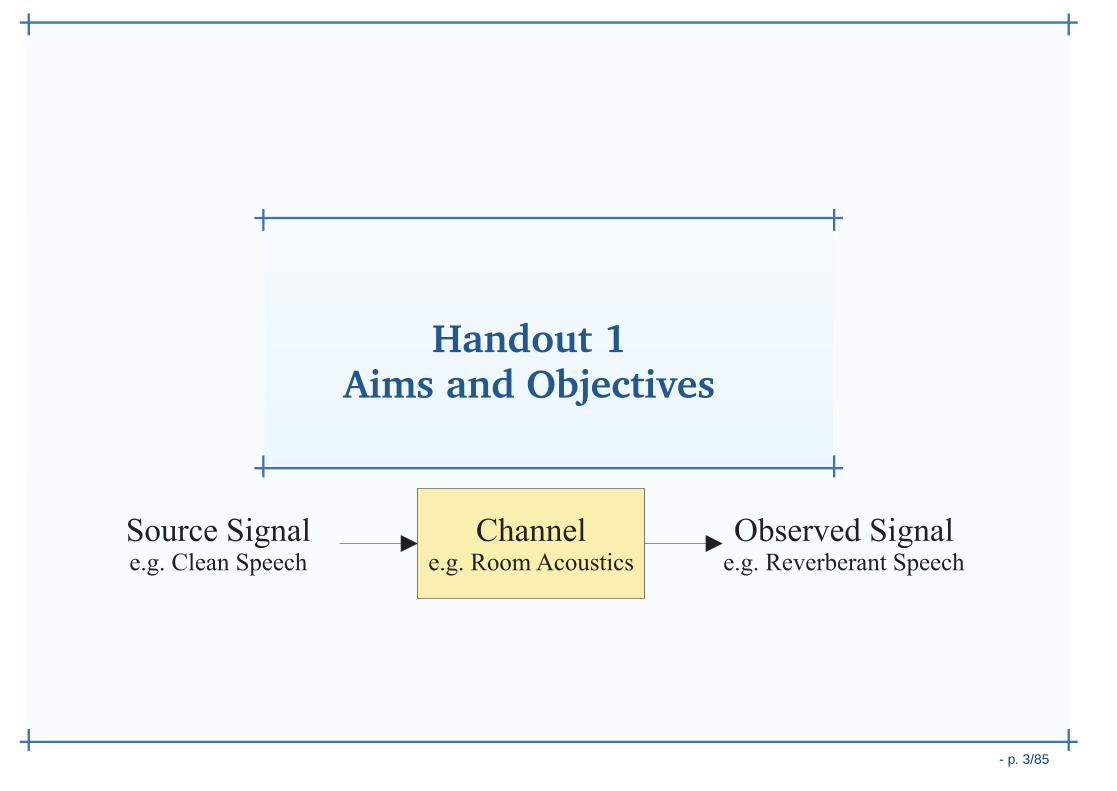
Handout 1Aims and Objectives
Aims and Objectives
•Module Abstract
• Introduction and Overview
•Description and Learning
Outcomes•Structure of the Module
Probability Theory
Scalar Random Variables
Multiple Random Variables
Estimation Theory
MonteCarlo
- p. 4/85
TH
E
UN I V E
RS
IT
Y
OF
ED
I N BU
R
GH
Obtaining the Latest Version of these Hand-outs
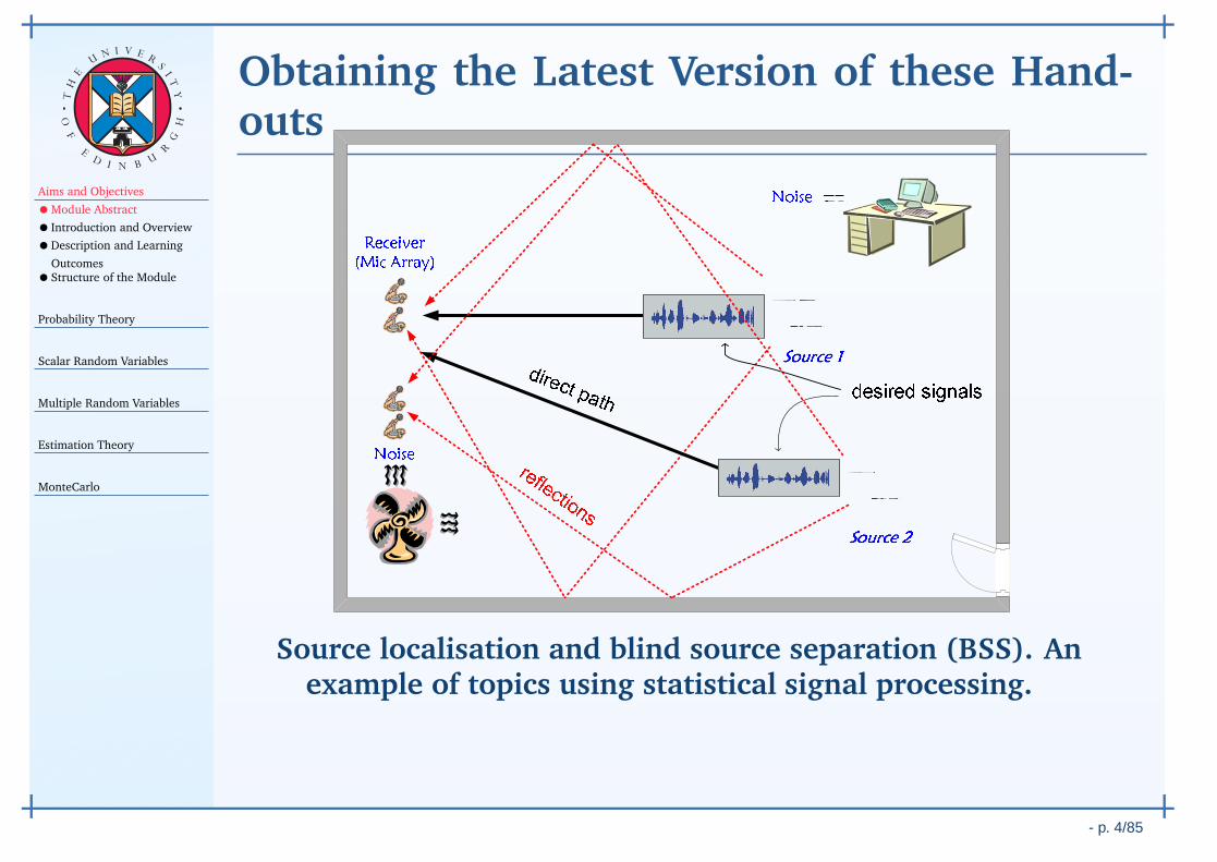
Source localisation and blind source separation (BSS). Anexample of topics using statistical signal processing.
Aims and Objectives
•Module Abstract
• Introduction and Overview
•Description and Learning
Outcomes•Structure of the Module
Probability Theory
Scalar Random Variables
Multiple Random Variables
Estimation Theory
MonteCarlo
- p. 4/85
TH
E
UN I V E
RS
IT
Y
OF
ED
I N BU
R
GH
Obtaining the Latest Version of these Hand-outs
Direct
paths Indirect
paths
Observer
Walls
and other
obstacles
Sound
Source 1
Sound
Source 2
Sound
Source 3
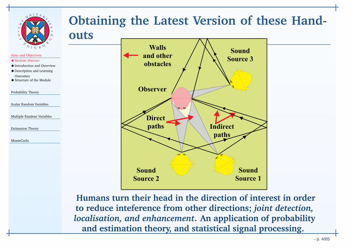
Humans turn their head in the direction of interest in orderto reduce inteference from other directions; joint detection,localisation, and enhancement. An application of probability
and estimation theory, and statistical signal processing.

Aims and Objectives
•Module Abstract
• Introduction and Overview
•Description and Learning
Outcomes•Structure of the Module
Probability Theory
Scalar Random Variables
Multiple Random Variables
Estimation Theory
MonteCarlo
- p. 4/85
TH
E
UN I V E
RS
IT
Y
OF
ED
I N BU
R
GH
Obtaining the Latest Version of these Hand-outs
This research tutorial is intended to cover a wide range ofaspects which cover the fundamentals of statistical signalprocessing.
This tutorial is being continually updated, and feedback iswelcomed. The documents published on the USB stick maydiffer to the slides presented on the day.
The latest version of this document can be found online anddownloaded at:
http://www.mod-udrc.org/events/2015-summer-school
Extended thanks are given to the many MSc students over thepast 11 years who have helped proof-read and improve thesedocuments.
Aims and Objectives
•Module Abstract
• Introduction and Overview
•Description and Learning
Outcomes•Structure of the Module
Probability Theory
Scalar Random Variables
Multiple Random Variables
Estimation Theory
MonteCarlo
- p. 5/85
TH
E
UN I V E
RS
IT
Y
OF
ED
I N BU
R
GH
Module Abstract
This topic is covered in two related lecture modules:
1. Probability, Random Variables, and Estimation Theory, and
2. Statistical Signal Processing,
Random signals are extensively used in algorithms, and are:
constructively used to model real-world processes;
described using probability and statistics.
Their properties are estimated by assumming:
an infinite number of observations or data points;
time-invariant statistics.
In practice, these statistics must be estimated fromfinite-length data signals in noise.
Module investigates relevant statistical properties, how they
Aims and Objectives
•Module Abstract
• Introduction and Overview
•Description and Learning
Outcomes•Structure of the Module
Probability Theory
Scalar Random Variables
Multiple Random Variables
Estimation Theory
MonteCarlo
- p. 6/85
TH
E
UN I V E
RS
IT
Y
OF
ED
I N BU
R
GH
Introduction and Overview
0 50 100 150 200 250 300 350 400 450 500−4
−3
−2
−1
0
1
2
3
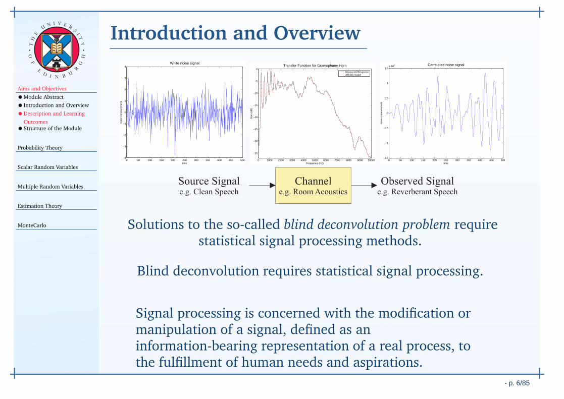
4White noise signal
time
nois
e m
easu
rem
ent
0 1000 2000 3000 4000 5000 6000 7000 8000 9000 10000
−35
−30
−25
−20
−15
−10
−5
0Transfer Function for Gramophone Horn
Frequency (Hz)
Gai
n (d
B)
Measured ResponseAR(68) model
0 50 100 150 200 250 300 350 400 450 500−1.5
−1
−0.5
0
0.5
1
1.5x 10
4 Correlated noise signal
time
nois
e m
easu
rem
ent
Solutions to the so-called blind deconvolution problem requirestatistical signal processing methods.
Blind deconvolution requires statistical signal processing.
Signal processing is concerned with the modification ormanipulation of a signal, defined as aninformation-bearing representation of a real process, tothe fulfillment of human needs and aspirations.

Aims and Objectives
•Module Abstract
• Introduction and Overview
•Description and Learning
Outcomes•Structure of the Module
Probability Theory
Scalar Random Variables
Multiple Random Variables
Estimation Theory
MonteCarlo
- p. 7/85
TH
E
UN I V E
RS
IT
Y
OF
ED
I N BU
R
GH
Description and Learning Outcomes
Module Aims to provide a unified introduction to the theory,implementation, and applications of statistical signalprocessing.
Module Objectives At the end of these modules, a student shouldbe able to:
1. acquired sufficient expertise in this area to understand andimplement spectral estimation, signal modelling,parameter estimation, and adaptive filtering techniques;
2. developed an understanding of the basic concepts andmethodologies in statistical signal processing that providesthe foundation for further study, research, and applicationto new problems.
Aims and Objectives
•Module Abstract
• Introduction and Overview
•Description and Learning
Outcomes•Structure of the Module
Probability Theory
Scalar Random Variables
Multiple Random Variables
Estimation Theory
MonteCarlo
- p. 8/85
TH
E
UN I V E
RS
IT
Y
OF
ED
I N BU
R
GH
Structure of the Module
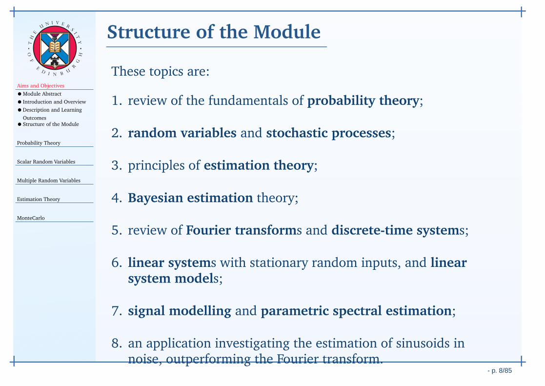
These topics are:
1. review of the fundamentals of probability theory;

Aims and Objectives
•Module Abstract
• Introduction and Overview
•Description and Learning
Outcomes•Structure of the Module
Probability Theory
Scalar Random Variables
Multiple Random Variables
Estimation Theory
MonteCarlo
- p. 8/85
TH
E
UN I V E
RS
IT
Y
OF
ED
I N BU
R
GH
Structure of the Module
These topics are:
1. review of the fundamentals of probability theory;
2. random variables and stochastic processes;
3. principles of estimation theory;
4. Bayesian estimation theory;
5. review of Fourier transforms and discrete-time systems;
6. linear systems with stationary random inputs, and linearsystem models;
7. signal modelling and parametric spectral estimation;
8. an application investigating the estimation of sinusoids innoise, outperforming the Fourier transform.
- p. 9/85
Handout 2Probability Theory
Aims and Objectives
Probability Theory
• Introduction
•Classical Definition of
Probability
•Bertrand’s Paradox
•Using the Classical
Definition•Difficulties with the
Classical Definition•Axiomatic Definition
•Set Theory
•Properties of Axiomatic
Probability
•Countable Spaces
•The Real Line
•Conditional Probability
Scalar Random Variables
Multiple Random Variables
Estimation Theory
MonteCarlo
- p. 10/85
TH
E
UN I V E
RS
IT
Y
OF
ED
I N BU
R
GH
Introduction
The theory of probability deals with averages of massphenomena occurring sequentially or simultaneously;
this might include radar detection, signal detection,anomaly detection, parameter estimation, ...
It is observed that certain averages approach a constant valueas the number of observations increases, and this valueremains the same if the averages are evaluated over anysubsequence specified before the experiment is performed.
Aims and Objectives
Probability Theory
• Introduction
•Classical Definition of
Probability
•Bertrand’s Paradox
•Using the Classical
Definition•Difficulties with the
Classical Definition•Axiomatic Definition
•Set Theory
•Properties of Axiomatic
Probability
•Countable Spaces
•The Real Line
•Conditional Probability
Scalar Random Variables
Multiple Random Variables
Estimation Theory
MonteCarlo
- p. 10/85
TH
E
UN I V E
RS
IT
Y
OF
ED
I N BU
R
GH
Introduction
If an experiment is performed n times, and the event Aoccurs nA times, then with a high degree of certainty, therelative frequency nA/n is close to Pr (A), such that:
Pr (A) ≈ nA
n
provided that n is sufficiently large.
Note that this interpretation and the language used is all veryimprecise.

Aims and Objectives
Probability Theory
• Introduction
•Classical Definition of
Probability
•Bertrand’s Paradox
•Using the Classical
Definition•Difficulties with the
Classical Definition•Axiomatic Definition
•Set Theory
•Properties of Axiomatic
Probability
•Countable Spaces
•The Real Line
•Conditional Probability
Scalar Random Variables
Multiple Random Variables
Estimation Theory
MonteCarlo
- p. 11/85
TH
E
UN I V E
RS
IT
Y
OF
ED
I N BU
R
GH
Classical Definition of Probability
For several centuries, the theory of probability was based on theclassical definition, which states that the probability Pr (A) of anevent A is determine a priori without actual experimentation. Itis given by the ratio:
Pr (A) =NA
N
where:
N is the total number of outcomes,
and NA is the total number of outcomes that are favourable tothe event A, provided that all outcomes are equally probable.
Aims and Objectives
Probability Theory
• Introduction
•Classical Definition of
Probability
•Bertrand’s Paradox
•Using the Classical
Definition•Difficulties with the
Classical Definition•Axiomatic Definition
•Set Theory
•Properties of Axiomatic
Probability
•Countable Spaces
•The Real Line
•Conditional Probability
Scalar Random Variables
Multiple Random Variables
Estimation Theory
MonteCarlo
- p. 12/85
TH
E
UN I V E
RS
IT
Y
OF
ED
I N BU
R
GH
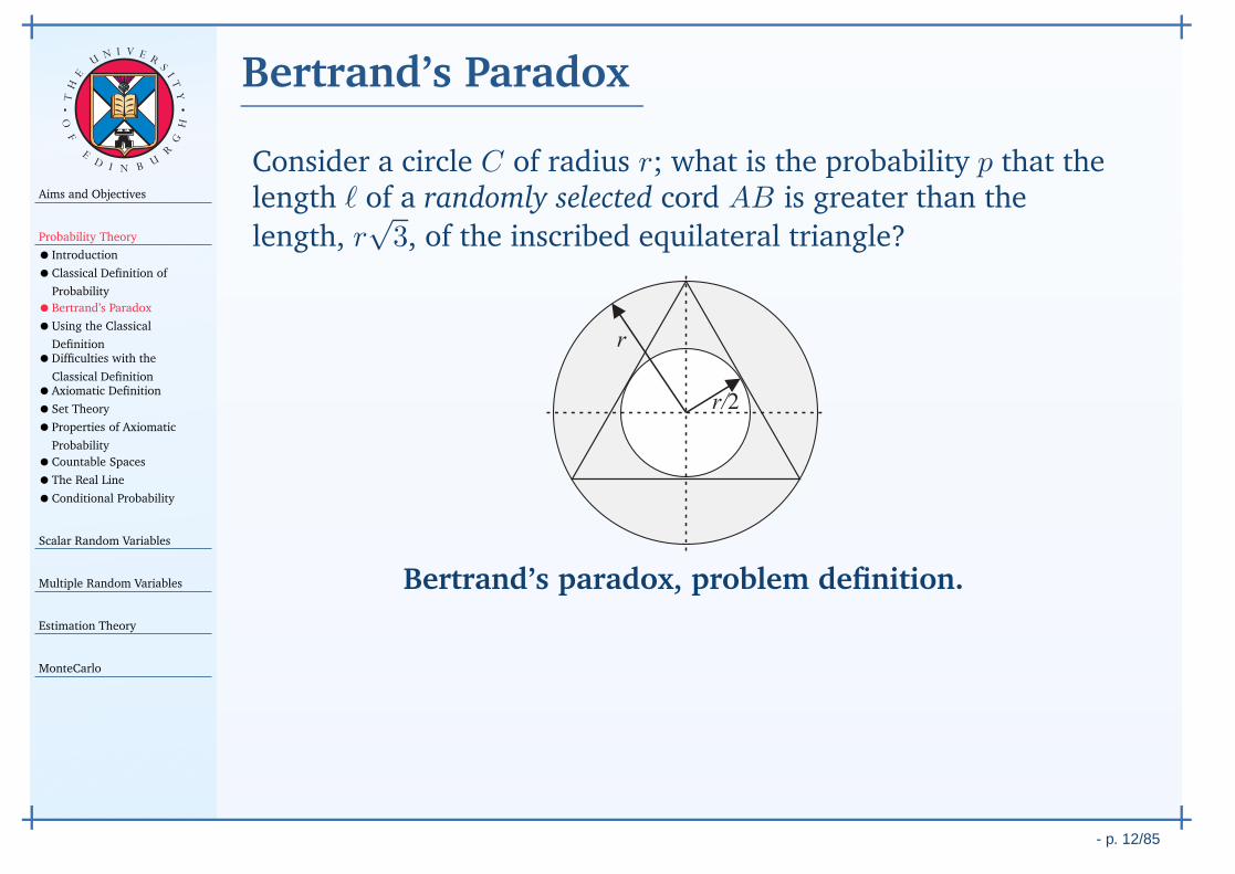
Bertrand’s Paradox
Consider a circle C of radius r; what is the probability p that thelength ℓ of a randomly selected cord AB is greater than the
length, r√3, of the inscribed equilateral triangle?
r/2
r
Bertrand’s paradox, problem definition.
Aims and Objectives
Probability Theory
• Introduction
•Classical Definition of
Probability
•Bertrand’s Paradox
•Using the Classical
Definition•Difficulties with the
Classical Definition•Axiomatic Definition
•Set Theory
•Properties of Axiomatic
Probability
•Countable Spaces
•The Real Line
•Conditional Probability
Scalar Random Variables
Multiple Random Variables
Estimation Theory
MonteCarlo
- p. 12/85
TH
E
UN I V E
RS
IT
Y
OF
ED
I N BU
R
GH
Bertrand’s Paradox
A
B
M
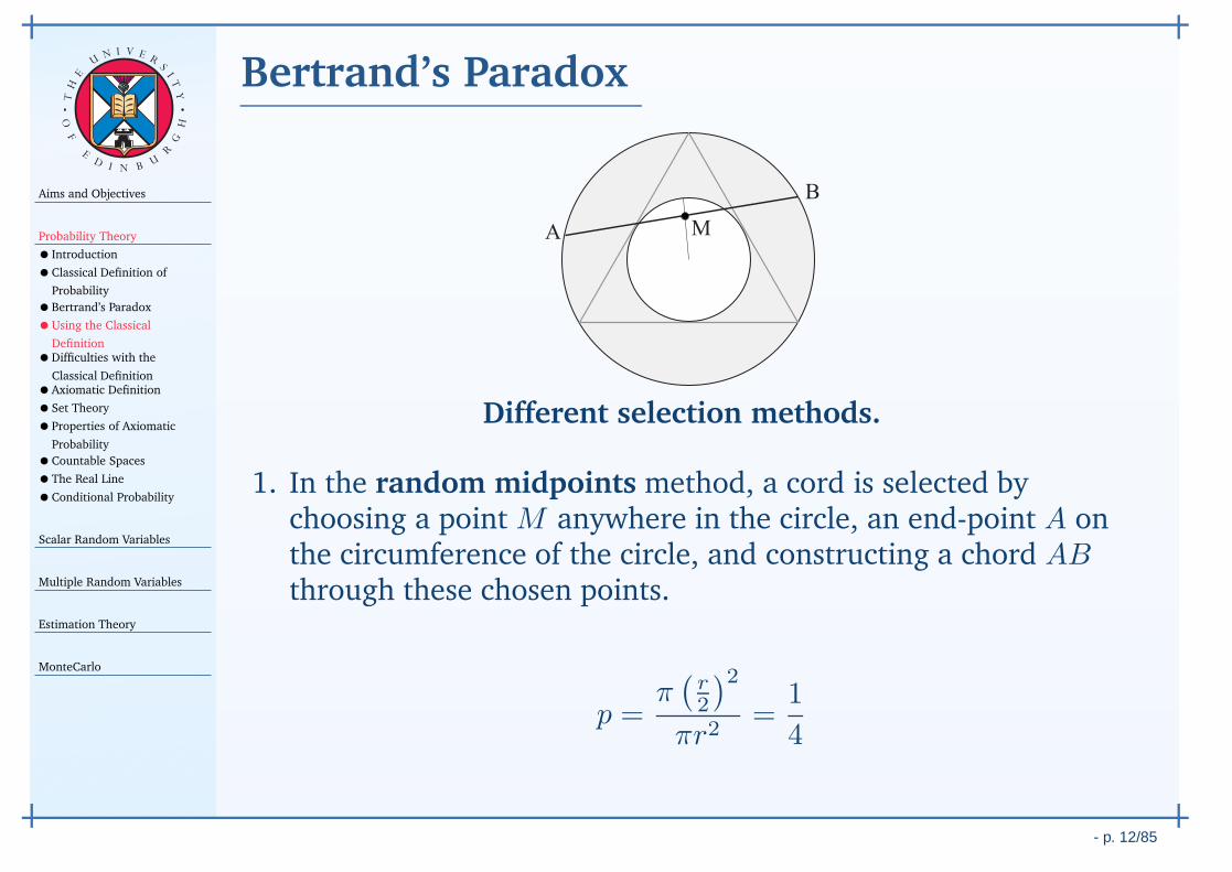
Different selection methods.
1. In the random midpoints method, a cord is selected bychoosing a point M anywhere in the circle, an end-point A onthe circumference of the circle, and constructing a chord ABthrough these chosen points.
p =π(r2
)2
πr2=
1
4
Aims and Objectives
Probability Theory
• Introduction
•Classical Definition of
Probability
•Bertrand’s Paradox
•Using the Classical
Definition•Difficulties with the
Classical Definition•Axiomatic Definition
•Set Theory
•Properties of Axiomatic
Probability
•Countable Spaces
•The Real Line
•Conditional Probability
Scalar Random Variables
Multiple Random Variables
Estimation Theory
MonteCarlo
- p. 12/85
TH
E
UN I V E
RS
IT
Y
OF
ED
I N BU
R
GH
Bertrand’s Paradox
A
B
M
A
BD
E
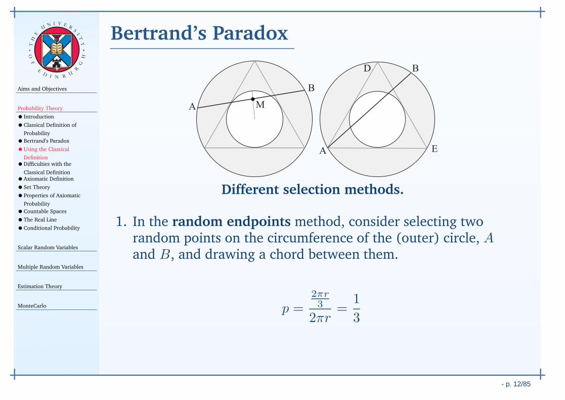
Different selection methods.
1. In the random endpoints method, consider selecting tworandom points on the circumference of the (outer) circle, Aand B, and drawing a chord between them.
p =2πr3
2πr=
1
3
Aims and Objectives
Probability Theory
• Introduction
•Classical Definition of
Probability
•Bertrand’s Paradox
•Using the Classical
Definition•Difficulties with the
Classical Definition•Axiomatic Definition
•Set Theory
•Properties of Axiomatic
Probability
•Countable Spaces
•The Real Line
•Conditional Probability
Scalar Random Variables
Multiple Random Variables
Estimation Theory
MonteCarlo
- p. 12/85
TH
E
UN I V E
RS
IT
Y
OF
ED
I N BU
R
GH
Bertrand’s Paradox
A
B
M
A
BD
E
A BR
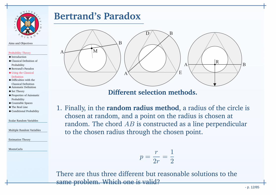
Different selection methods.
1. Finally, in the random radius method, a radius of the circle ischosen at random, and a point on the radius is chosen atrandom. The chord AB is constructed as a line perpendicularto the chosen radius through the chosen point.
p =r
2r=
1
2
There are thus three different but reasonable solutions to thesame problem. Which one is valid?
Aims and Objectives
Probability Theory
• Introduction
•Classical Definition of
Probability
•Bertrand’s Paradox
•Using the Classical
Definition•Difficulties with the
Classical Definition•Axiomatic Definition
•Set Theory
•Properties of Axiomatic
Probability
•Countable Spaces
•The Real Line
•Conditional Probability
Scalar Random Variables
Multiple Random Variables
Estimation Theory
MonteCarlo
- p. 13/85
TH
E
UN I V E
RS
IT
Y
OF
ED
I N BU
R
GH
Using the Classical Definition
The difficulty with the classical definition, as seen in Bertrand’sParadox, is in determining N and NA.
Example (Rolling two dice). Two dice are rolled; find theprobability, p, that the sum of the numbers shown equals 7.
Consider three possibilities:
1. The possible outcomes total 11 which are the sums2, 3, . . . , 12. Of these, only one (the sum 7) is favourable.
Hence, p = 111 .
2. Therefore, to count all possible outcomes which are equallyprobable, it is necessary to could all pairs of numbersdistinguishing between the first and second die. This will givethe correct probability.
Aims and Objectives
Probability Theory
• Introduction
•Classical Definition of
Probability
•Bertrand’s Paradox
•Using the Classical
Definition•Difficulties with the
Classical Definition•Axiomatic Definition
•Set Theory
•Properties of Axiomatic
Probability
•Countable Spaces
•The Real Line
•Conditional Probability
Scalar Random Variables
Multiple Random Variables
Estimation Theory
MonteCarlo
- p. 14/85
TH
E
UN I V E
RS
IT
Y
OF
ED
I N BU
R
GH
Difficulties with the Classical Definition
1. The term equally probable in the definition of probability ismaking use of a concept still to be defined!
2. The definition can only be applied to a limited class ofproblems.
In the die experiment, for example, it is applicable only if thesix faces have the same probability. If the die is loaded and theprobability of a “4” equals 0.2, say, then this cannot bedetermined from the classical ratio.
3. If the number of possible outcomes is infinite, then some othermeasure of infinity for determining the classical probabilityration is needed, such as length, or area. This leads todifficulties, as discussed in Bertrand’s paradox.
Aims and Objectives
Probability Theory
• Introduction
•Classical Definition of
Probability
•Bertrand’s Paradox
•Using the Classical
Definition•Difficulties with the
Classical Definition•Axiomatic Definition
•Set Theory
•Properties of Axiomatic
Probability
•Countable Spaces
•The Real Line
•Conditional Probability
Scalar Random Variables
Multiple Random Variables
Estimation Theory
MonteCarlo
- p. 15/85
TH
E
UN I V E
RS
IT
Y
OF
ED
I N BU
R
GH
Axiomatic Definition
The axiomatic approach to probability is based on the followingthree postulates and on nothing else:
1. The probability Pr (A) of an event A is a non-negative numberassigned to this event:
Pr (A) ≥ 0
2. Defining the certain event, S, as the event that occurs inevery trial, then the probability of the certain event equals 1,such that:
Pr (S) = 1
3. If the events A and B are mutually exclusive, then theprobability of one event or the other occurring separately is:
Pr (A ∪B) = Pr (A) + Pr (B)
Aims and Objectives
Probability Theory
• Introduction
•Classical Definition of
Probability
•Bertrand’s Paradox
•Using the Classical
Definition•Difficulties with the
Classical Definition•Axiomatic Definition
•Set Theory
•Properties of Axiomatic
Probability
•Countable Spaces
•The Real Line
•Conditional Probability
Scalar Random Variables
Multiple Random Variables
Estimation Theory
MonteCarlo
- p. 16/85
TH
E
UN I V E
RS
IT
Y
OF
ED
I N BU
R
GH
Set Theory
Unions and Intersections Unions and intersections arecommutative, associative, and distributive, such that:
A ∪B = B ∪A, (A ∪B) ∪ C = A ∪ (B ∪ C)
AB = BA, (AB)C = A(BC), A(B ∪ C) = AB ∪AC
Complements The complement A of a set A ⊂ S is the setconsisting of all elements of S that are not in A. Note that:
A ∪A = S and A ∩A ≡ AA = ∅
Partitions A partition U of a set S is a collection of mutuallyexclusive subsets Ai of S whose union equations S:
∞⋃
i=1
Ai = S, Ai ∩Aj = ∅, i 6= j ⇒ U = [A1, . . . , An]
Aims and Objectives
Probability Theory
• Introduction
•Classical Definition of
Probability
•Bertrand’s Paradox
•Using the Classical
Definition•Difficulties with the
Classical Definition•Axiomatic Definition
•Set Theory
•Properties of Axiomatic
Probability
•Countable Spaces
•The Real Line
•Conditional Probability
Scalar Random Variables
Multiple Random Variables
Estimation Theory
MonteCarlo
- p. 16/85
TH
E
UN I V E
RS
IT
Y
OF
ED
I N BU
R
GH
Set Theory
De Morgan’s Law Using Venn diagrams, it is relativelystraightforward to show
A ∪ B = A ∩B ≡ AB and A ∩B ≡ AB = A ∪B
Aims and Objectives
Probability Theory
• Introduction
•Classical Definition of
Probability
•Bertrand’s Paradox
•Using the Classical
Definition•Difficulties with the
Classical Definition•Axiomatic Definition
•Set Theory
•Properties of Axiomatic
Probability
•Countable Spaces
•The Real Line
•Conditional Probability
Scalar Random Variables
Multiple Random Variables
Estimation Theory
MonteCarlo
- p. 16/85
TH
E
UN I V E
RS
IT
Y
OF
ED
I N BU
R
GH
Set Theory
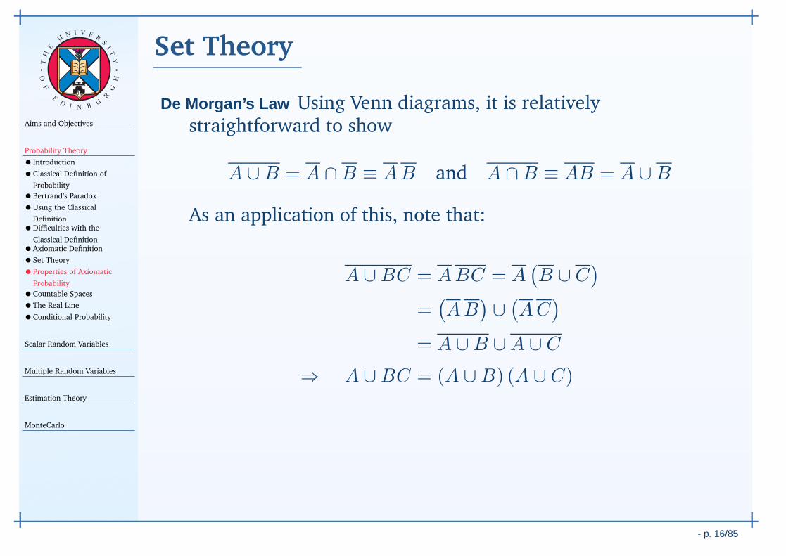
De Morgan’s Law Using Venn diagrams, it is relativelystraightforward to show
A ∪ B = A ∩B ≡ AB and A ∩B ≡ AB = A ∪B
As an application of this, note that:
A ∪BC = ABC = A(B ∪ C
)
=(AB
)∪(AC
)
= A ∪B ∪A ∪ C
⇒ A ∪BC = (A ∪B) (A ∪ C)
Aims and Objectives
Probability Theory
• Introduction
•Classical Definition of
Probability
•Bertrand’s Paradox
•Using the Classical
Definition•Difficulties with the
Classical Definition•Axiomatic Definition
•Set Theory
•Properties of Axiomatic
Probability
•Countable Spaces
•The Real Line
•Conditional Probability
Scalar Random Variables
Multiple Random Variables
Estimation Theory
MonteCarlo
- p. 17/85
TH
E
UN I V E
RS
IT
Y
OF
ED
I N BU
R
GH
Properties of Axiomatic Probability
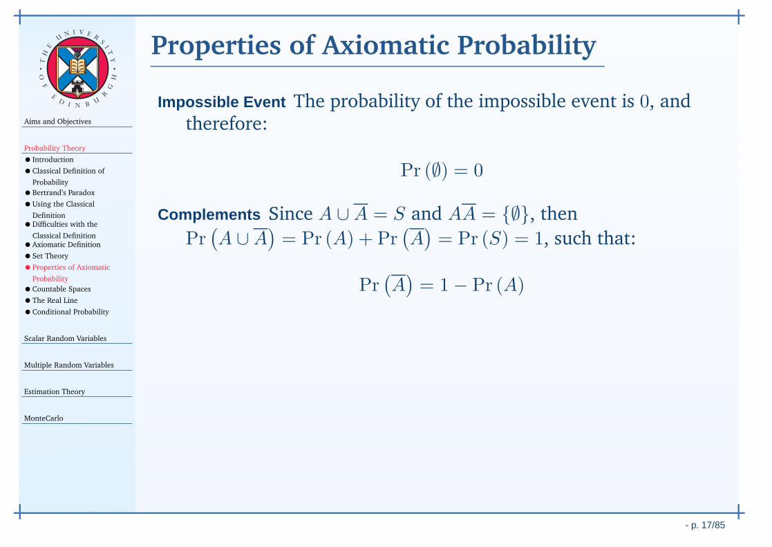
Impossible Event The probability of the impossible event is 0, andtherefore:
Pr (∅) = 0
Aims and Objectives
Probability Theory
• Introduction
•Classical Definition of
Probability
•Bertrand’s Paradox
•Using the Classical
Definition•Difficulties with the
Classical Definition•Axiomatic Definition
•Set Theory
•Properties of Axiomatic
Probability
•Countable Spaces
•The Real Line
•Conditional Probability
Scalar Random Variables
Multiple Random Variables
Estimation Theory
MonteCarlo
- p. 17/85
TH
E
UN I V E
RS
IT
Y
OF
ED
I N BU
R
GH
Properties of Axiomatic Probability
Impossible Event The probability of the impossible event is 0, andtherefore:
Pr (∅) = 0
Complements Since A ∪A = S and AA = ∅, then
Pr(A ∪A
)= Pr (A) + Pr
(A)= Pr (S) = 1, such that:
Pr(A)= 1− Pr (A)
Sum Rule The addition law of probability or the sum rule forany two events A and B is given by:
Pr (A ∪B) = Pr (A) + Pr (B)− Pr (A ∩B)

Aims and Objectives
Probability Theory
• Introduction
•Classical Definition of
Probability
•Bertrand’s Paradox
•Using the Classical
Definition•Difficulties with the
Classical Definition•Axiomatic Definition
•Set Theory
•Properties of Axiomatic
Probability
•Countable Spaces
•The Real Line
•Conditional Probability
Scalar Random Variables
Multiple Random Variables
Estimation Theory
MonteCarlo
- p. 17/85
TH
E
UN I V E
RS
IT
Y
OF
ED
I N BU
R
GH
Properties of Axiomatic Probability
Example (Proof of the Sum Rule). SOLUTION. To prove this,separately write A ∪B and B as the union of two mutuallyexclusive events.
First, note that
A ∪(AB
)=
(A ∪A
)(A ∪B) = A ∪B
and that since A(AB
)=
(AA
)B = ∅B = ∅, then A and
AB are mutually exclusive events.
Second, note that:
B =(A ∪A
)B = (AB) ∪
(AB
)
and that (AB) ∩(AB
)= AAB = ∅B = ∅ and are
therefore mutually exclusive events.
Aims and Objectives
Probability Theory
• Introduction
•Classical Definition of
Probability
•Bertrand’s Paradox
•Using the Classical
Definition•Difficulties with the
Classical Definition•Axiomatic Definition
•Set Theory
•Properties of Axiomatic
Probability
•Countable Spaces
•The Real Line
•Conditional Probability
Scalar Random Variables
Multiple Random Variables
Estimation Theory
MonteCarlo
- p. 17/85
TH
E
UN I V E
RS
IT
Y
OF
ED
I N BU
R
GH
Properties of Axiomatic Probability
Example (Proof of the Sum Rule). SOLUTION. Using these twodisjoint unions, then:
Pr (A ∪B) = Pr(A ∪
(AB
))= Pr (A) + Pr
(AB
)
Pr (B) = Pr((AB) ∪
(AB
))= Pr (AB) + Pr
(AB
)
Eliminating Pr(AB
)by subtracting these equations gives the
desired result:
Pr (A ∪B)− Pr (B) = Pr(A ∪
(AB
))= Pr (A)− Pr (AB)
Aims and Objectives
Probability Theory
• Introduction
•Classical Definition of
Probability
•Bertrand’s Paradox
•Using the Classical
Definition•Difficulties with the
Classical Definition•Axiomatic Definition
•Set Theory
•Properties of Axiomatic
Probability
•Countable Spaces
•The Real Line
•Conditional Probability
Scalar Random Variables
Multiple Random Variables
Estimation Theory
MonteCarlo
- p. 17/85
TH
E
UN I V E
RS
IT
Y
OF
ED
I N BU
R
GH
Properties of Axiomatic Probability
Example (Sum Rule). Let A and B be events with probabilitiesPr (A) = 3/4 and Pr (B) = 1/3. Show that 1/12 ≤ Pr (AB) ≤ 1/3.
SOLUTION. Using the sum rule, that:
Pr (AB) = Pr (A)+Pr (B)−Pr (A ∪B) ≥ Pr (A)+Pr (B)−1 =1
12
which is the case when the whole sample space is covered bythe two events. The second bound occurs since A ∩B ⊂ B andsimilarly A ∩B ⊂ A, where ⊂ denotes subset. Therefore, it canbe deduced Pr (AB) ≤ minPr (A) , Pr (B) = 1/3.
Aims and Objectives
Probability Theory
• Introduction
•Classical Definition of
Probability
•Bertrand’s Paradox
•Using the Classical
Definition•Difficulties with the
Classical Definition•Axiomatic Definition
•Set Theory
•Properties of Axiomatic
Probability
•Countable Spaces
•The Real Line
•Conditional Probability
Scalar Random Variables
Multiple Random Variables
Estimation Theory
MonteCarlo
- p. 18/85
TH
E
UN I V E
RS
IT
Y
OF
ED
I N BU
R
GH
Countable Spaces
If the certain event, S, consists of N outcomes, and N is a finitenumber, then the probabilities of all events can be expressed interms of the probabilities Pr (ζi) = pi of the elementary eventsζi.
Example (Cups and Saucers). Six cups and saucers come in pairs:there are two cups and saucers which are red, two which arewhile, and two which are blue. If the cups are placed randomlyonto the saucers (one each), find the probability that no cup isupon a saucer of the same pattern.

Aims and Objectives
Probability Theory
• Introduction
•Classical Definition of
Probability
•Bertrand’s Paradox
•Using the Classical
Definition•Difficulties with the
Classical Definition•Axiomatic Definition
•Set Theory
•Properties of Axiomatic
Probability
•Countable Spaces
•The Real Line
•Conditional Probability
Scalar Random Variables
Multiple Random Variables
Estimation Theory
MonteCarlo
- p. 18/85
TH
E
UN I V E
RS
IT
Y
OF
ED
I N BU
R
GH
Countable Spaces
Example (Cups and Saucers). SOLUTION. Lay the saucers inorder, say as RRWWBB.
The cups may be arranged in 6! ways, but since each pair of agiven colour may be switched without changing theappearance, there are 6!/(2!)3 = 90 distinct arrangements.
Aims and Objectives
Probability Theory
• Introduction
•Classical Definition of
Probability
•Bertrand’s Paradox
•Using the Classical
Definition•Difficulties with the
Classical Definition•Axiomatic Definition
•Set Theory
•Properties of Axiomatic
Probability
•Countable Spaces
•The Real Line
•Conditional Probability
Scalar Random Variables
Multiple Random Variables
Estimation Theory
MonteCarlo
- p. 18/85
TH
E
UN I V E
RS
IT
Y
OF
ED
I N BU
R
GH
Countable Spaces
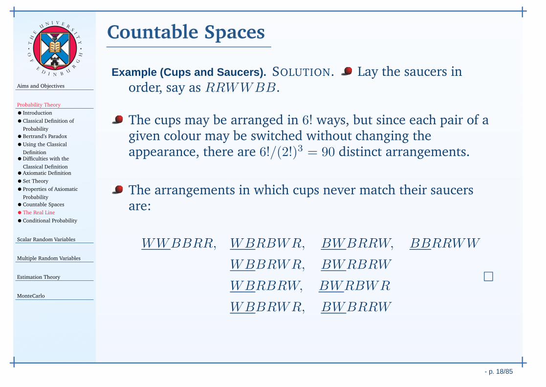
Example (Cups and Saucers). SOLUTION. Lay the saucers inorder, say as RRWWBB.
The cups may be arranged in 6! ways, but since each pair of agiven colour may be switched without changing theappearance, there are 6!/(2!)3 = 90 distinct arrangements.
The arrangements in which cups never match their saucersare:
WWBBRR, WBRBWR, BWBRRW, BBRRWW
WBBRWR, BWRBRW
WBRBRW, BWRBWR
WBBRWR, BWBRRW
Aims and Objectives
Probability Theory
• Introduction
•Classical Definition of
Probability
•Bertrand’s Paradox
•Using the Classical
Definition•Difficulties with the
Classical Definition•Axiomatic Definition
•Set Theory
•Properties of Axiomatic
Probability
•Countable Spaces
•The Real Line
•Conditional Probability
Scalar Random Variables
Multiple Random Variables
Estimation Theory
MonteCarlo
- p. 18/85
TH
E
UN I V E
RS
IT
Y
OF
ED
I N BU
R
GH
Countable Spaces
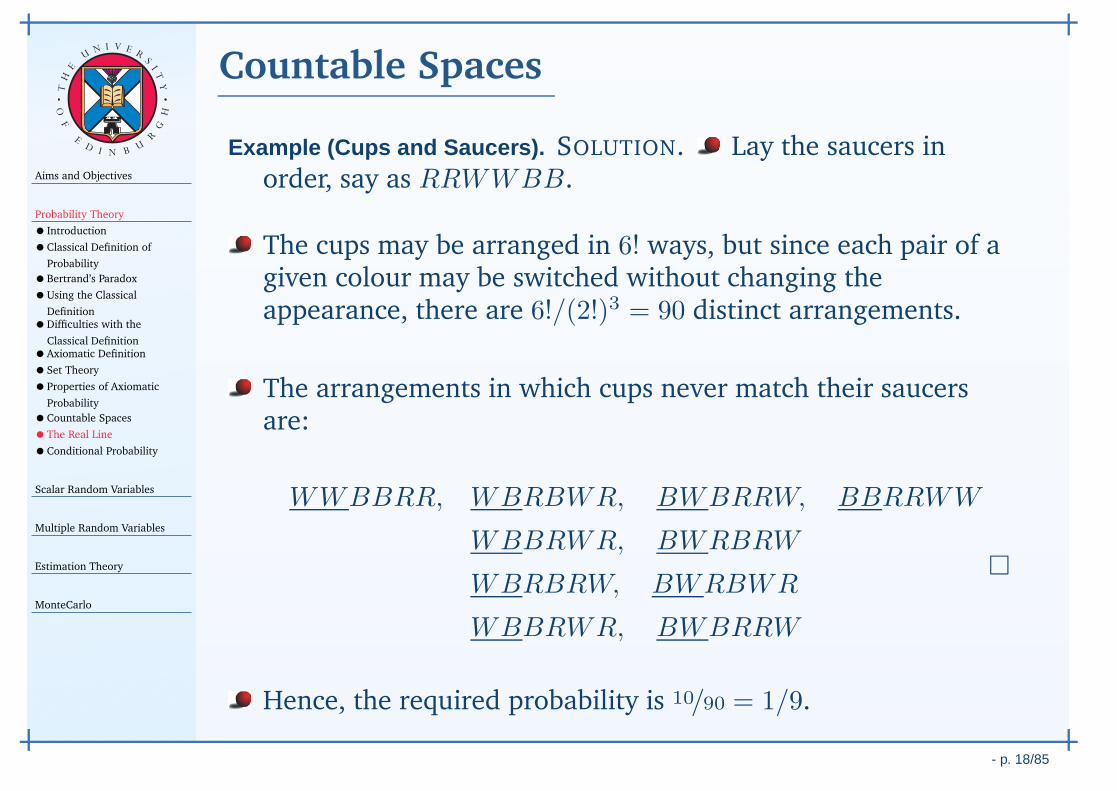
Example (Cups and Saucers). SOLUTION. Lay the saucers inorder, say as RRWWBB.
The cups may be arranged in 6! ways, but since each pair of agiven colour may be switched without changing theappearance, there are 6!/(2!)3 = 90 distinct arrangements.
The arrangements in which cups never match their saucersare:
WWBBRR, WBRBWR, BWBRRW, BBRRWW
WBBRWR, BWRBRW
WBRBRW, BWRBWR
WBBRWR, BWBRRW
Hence, the required probability is 10/90 = 1/9.

Aims and Objectives
Probability Theory
• Introduction
•Classical Definition of
Probability
•Bertrand’s Paradox
•Using the Classical
Definition•Difficulties with the
Classical Definition•Axiomatic Definition
•Set Theory
•Properties of Axiomatic
Probability
•Countable Spaces
•The Real Line
•Conditional Probability
Scalar Random Variables
Multiple Random Variables
Estimation Theory
MonteCarlo
- p. 19/85
TH
E
UN I V E
RS
IT
Y
OF
ED
I N BU
R
GH
The Real Line
If the certain event, S, consists of a non-countable infinity ofelements, then its probabilities cannot be determined in terms ofthe probabilities of elementary events.
Suppose that S is the set of all real numbers. To construct aprobability space on the real line, consider events as intervalsx1 < x ≤ x2, and their countable unions and intersections.
To complete the specification of probabilities for this set, itsuffices to assign probabilities to the events x ≤ xi.
This notion leads to cumulative distribution functions (cdfs)and probability density functions (pdfs) in the next handout.
Aims and Objectives
Probability Theory
• Introduction
•Classical Definition of
Probability
•Bertrand’s Paradox
•Using the Classical
Definition•Difficulties with the
Classical Definition•Axiomatic Definition
•Set Theory
•Properties of Axiomatic
Probability
•Countable Spaces
•The Real Line
•Conditional Probability
Scalar Random Variables
Multiple Random Variables
Estimation Theory
MonteCarlo
- p. 20/85
TH
E
UN I V E
RS
IT
Y
OF
ED
I N BU
R
GH
Conditional Probability
If an experiment is repeated n times, and on each occasion theoccurrences or non-occurrences of two events A and B areobserved. Suppose that only those outcomes for which B occursare considered, and all other experiments are disregarded.
In this smaller collection of trials, the proportion of times that Aoccurs, given that B has occurred, is:
Pr(A∣∣B
)≈ nAB
nB
=nAB/nnB/n
=Pr (AB)
Pr (B)
provided that n is sufficiently large.
It can be shown that this definition satisfies the KolmogorovAxioms.

Aims and Objectives
Probability Theory
• Introduction
•Classical Definition of
Probability
•Bertrand’s Paradox
•Using the Classical
Definition•Difficulties with the
Classical Definition•Axiomatic Definition
•Set Theory
•Properties of Axiomatic
Probability
•Countable Spaces
•The Real Line
•Conditional Probability
Scalar Random Variables
Multiple Random Variables
Estimation Theory
MonteCarlo
- p. 20/85
TH
E
UN I V E
RS
IT
Y
OF
ED
I N BU
R
GH
Conditional Probability
Example (Two Children). A family has two children. What is theprobability that both are boys, given that at least one is a boy?
SOLUTION. The younger and older children may each be male orfemale, and it is assumed that each is equally likely.
Aims and Objectives
Probability Theory
• Introduction
•Classical Definition of
Probability
•Bertrand’s Paradox
•Using the Classical
Definition•Difficulties with the
Classical Definition•Axiomatic Definition
•Set Theory
•Properties of Axiomatic
Probability
•Countable Spaces
•The Real Line
•Conditional Probability
Scalar Random Variables
Multiple Random Variables
Estimation Theory
MonteCarlo
- p. 20/85
TH
E
UN I V E
RS
IT
Y
OF
ED
I N BU
R
GH
Conditional Probability
- p. 21/85
Handout 3Scalar Random Variables
Aims and Objectives
Probability Theory
Scalar Random Variables
•Abstract
•Definition
•Distribution functions
•Density functions
•Properties: Distributions
and Densities•Kolmogorov’s Axioms
•Common Continuous RVs
•Probability transformation
rule•Expectations
•Properties of expectation
operator
•Moments
•Characteristic Functions
•Higher-order statistics
Multiple Random Variables
Estimation Theory
MonteCarlo
- p. 22/85
TH
E
UN I V E
RS
IT
Y
OF
ED
I N BU
R
GH
Abstract
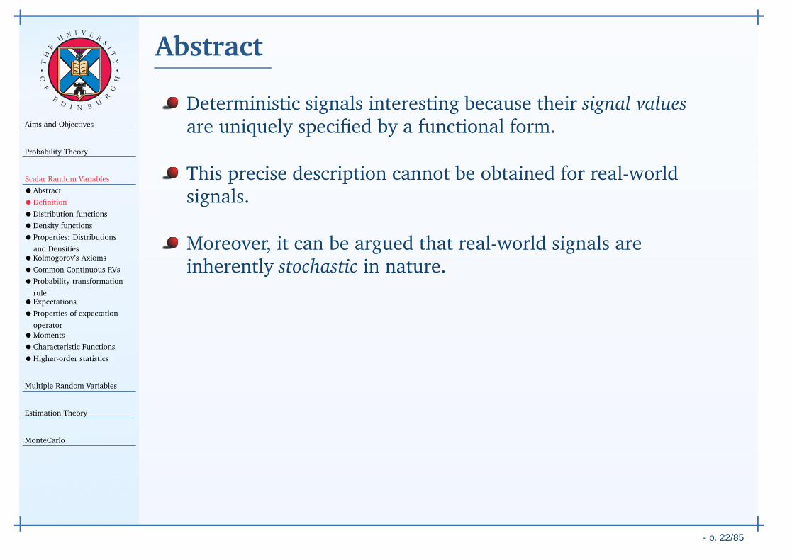
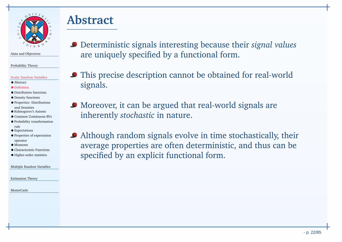
Deterministic signals interesting because their signal valuesare uniquely specified by a functional form.
Aims and Objectives
Probability Theory
Scalar Random Variables
•Abstract
•Definition
•Distribution functions
•Density functions
•Properties: Distributions
and Densities•Kolmogorov’s Axioms
•Common Continuous RVs
•Probability transformation
rule•Expectations
•Properties of expectation
operator
•Moments
•Characteristic Functions
•Higher-order statistics
Multiple Random Variables
Estimation Theory
MonteCarlo
- p. 22/85
TH
E
UN I V E
RS
IT
Y
OF
ED
I N BU
R
GH
Abstract
Deterministic signals interesting because their signal valuesare uniquely specified by a functional form.
This precise description cannot be obtained for real-worldsignals.
Moreover, it can be argued that real-world signals areinherently stochastic in nature.
Although random signals evolve in time stochastically, theiraverage properties are often deterministic, and thus can bespecified by an explicit functional form.
Aims and Objectives
Probability Theory
Scalar Random Variables
•Abstract
•Definition
•Distribution functions
•Density functions
•Properties: Distributions
and Densities•Kolmogorov’s Axioms
•Common Continuous RVs
•Probability transformation
rule•Expectations
•Properties of expectation
operator
•Moments
•Characteristic Functions
•Higher-order statistics
Multiple Random Variables
Estimation Theory
MonteCarlo
- p. 23/85
TH
E
UN I V E
RS
IT
Y
OF
ED
I N BU
R
GH
Definition
R
Abstractsample space, S
X( )z1
X( )z2
X( )z3 R
R
Outcome
z1=“Red”
Outcome
z2=“Green”
Outcome
z3=“Blue”
real number line
PhysicalExperiment
Pr( )z1
Pr( )z2
Pr( )z3
x1=1
x2=2
x3=4
Green
Blue
Red
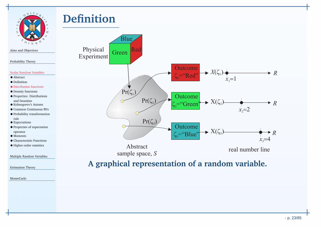
A graphical representation of a random variable.
Aims and Objectives
Probability Theory
Scalar Random Variables
•Abstract
•Definition
•Distribution functions
•Density functions
•Properties: Distributions
and Densities•Kolmogorov’s Axioms
•Common Continuous RVs
•Probability transformation
rule•Expectations
•Properties of expectation
operator
•Moments
•Characteristic Functions
•Higher-order statistics
Multiple Random Variables
Estimation Theory
MonteCarlo
- p. 23/85
TH
E
UN I V E
RS
IT
Y
OF
ED
I N BU
R
GH
Definition
A random variable (RV) X (ζ) is a mapping that assigns a realnumber X ∈ (−∞, ∞) to every outcome ζ from an abstractprobability space.
1. the interval X (ζ) ≤ x is an event in the abstract probabilityspace for every x ∈ R;
2. Pr (X (ζ) = ∞) = 0 and Pr (X (ζ) = −∞) = 0.
Aims and Objectives
Probability Theory
Scalar Random Variables
•Abstract
•Definition
•Distribution functions
•Density functions
•Properties: Distributions
and Densities•Kolmogorov’s Axioms
•Common Continuous RVs
•Probability transformation
rule•Expectations
•Properties of expectation
operator
•Moments
•Characteristic Functions
•Higher-order statistics
Multiple Random Variables
Estimation Theory
MonteCarlo
- p. 23/85
TH
E
UN I V E
RS
IT
Y
OF
ED
I N BU
R
GH
Definition
Example (Rolling die). Consider rolling a die, with six outcomesζi, i ∈ 1, . . . , 6. In this experiment, assign the number 1 toevery even outcome, and the number 0 to every odd outcome.Then the RV X (ζ) is given by:
X (ζ1) = X (ζ3) = X (ζ5) = 0 and X (ζ2) = X (ζ4) = X (ζ6) = 1⋊⋉
Aims and Objectives
Probability Theory
Scalar Random Variables
•Abstract
•Definition
•Distribution functions
•Density functions
•Properties: Distributions
and Densities•Kolmogorov’s Axioms
•Common Continuous RVs
•Probability transformation
rule•Expectations
•Properties of expectation
operator
•Moments
•Characteristic Functions
•Higher-order statistics
Multiple Random Variables
Estimation Theory
MonteCarlo
- p. 24/85
TH
E
UN I V E
RS
IT
Y
OF
ED
I N BU
R
GH
Distribution functions
The probability set function Pr (X (ζ) ≤ x) is a function ofthe set X (ζ) ≤ x, and therefore of the point x ∈ R.
This probability is the cumulative distributionfunction (cdf), FX (x) of a RV X (ζ), and is defined by:
FX (x) , Pr (X (ζ) ≤ x)
Aims and Objectives
Probability Theory
Scalar Random Variables
•Abstract
•Definition
•Distribution functions
•Density functions
•Properties: Distributions
and Densities•Kolmogorov’s Axioms
•Common Continuous RVs
•Probability transformation
rule•Expectations
•Properties of expectation
operator
•Moments
•Characteristic Functions
•Higher-order statistics
Multiple Random Variables
Estimation Theory
MonteCarlo
- p. 25/85
TH
E
UN I V E
RS
IT
Y
OF
ED
I N BU
R
GH
Density functions
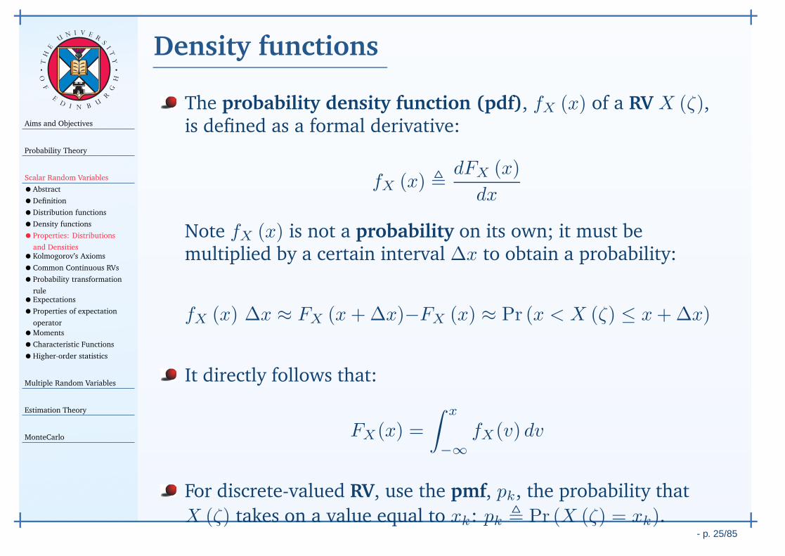
The probability density function (pdf), fX (x) of a RV X (ζ),is defined as a formal derivative:
fX (x) ,dFX (x)
dx
Note fX (x) is not a probability on its own; it must bemultiplied by a certain interval ∆x to obtain a probability:
fX (x) ∆x ≈ FX (x+∆x)−FX (x) ≈ Pr (x < X (ζ) ≤ x+∆x)
Aims and Objectives
Probability Theory
Scalar Random Variables
•Abstract
•Definition
•Distribution functions
•Density functions
•Properties: Distributions
and Densities•Kolmogorov’s Axioms
•Common Continuous RVs
•Probability transformation
rule•Expectations
•Properties of expectation
operator
•Moments
•Characteristic Functions
•Higher-order statistics
Multiple Random Variables
Estimation Theory
MonteCarlo
- p. 25/85
TH
E
UN I V E
RS
IT
Y
OF
ED
I N BU
R
GH
Density functions
The probability density function (pdf), fX (x) of a RV X (ζ),is defined as a formal derivative:
fX (x) ,dFX (x)
dx
Note fX (x) is not a probability on its own; it must bemultiplied by a certain interval ∆x to obtain a probability:
fX (x) ∆x ≈ FX (x+∆x)−FX (x) ≈ Pr (x < X (ζ) ≤ x+∆x)
It directly follows that:
FX(x) =
∫ x
−∞
fX(v) dv
For discrete-valued RV, use the pmf, pk, the probability that
X (ζ) takes on a value equal to xk: pk , Pr (X (ζ) = xk).
Aims and Objectives
Probability Theory
Scalar Random Variables
•Abstract
•Definition
•Distribution functions
•Density functions
•Properties: Distributions
and Densities•Kolmogorov’s Axioms
•Common Continuous RVs
•Probability transformation
rule•Expectations
•Properties of expectation
operator
•Moments
•Characteristic Functions
•Higher-order statistics
Multiple Random Variables
Estimation Theory
MonteCarlo
- p. 26/85
TH
E
UN I V E
RS
IT
Y
OF
ED
I N BU
R
GH
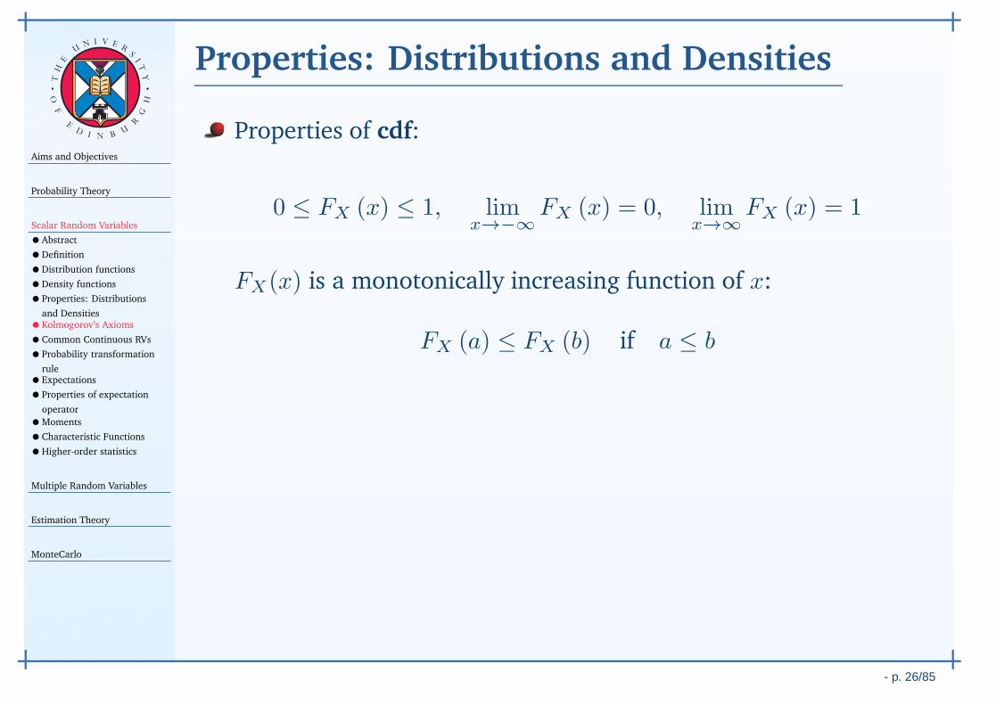
Properties: Distributions and Densities
Properties of cdf:
0 ≤ FX (x) ≤ 1, limx→−∞
FX (x) = 0, limx→∞
FX (x) = 1
FX(x) is a monotonically increasing function of x:
FX (a) ≤ FX (b) if a ≤ b
Aims and Objectives
Probability Theory
Scalar Random Variables
•Abstract
•Definition
•Distribution functions
•Density functions
•Properties: Distributions
and Densities•Kolmogorov’s Axioms
•Common Continuous RVs
•Probability transformation
rule•Expectations
•Properties of expectation
operator
•Moments
•Characteristic Functions
•Higher-order statistics
Multiple Random Variables
Estimation Theory
MonteCarlo
- p. 26/85
TH
E
UN I V E
RS
IT
Y
OF
ED
I N BU
R
GH
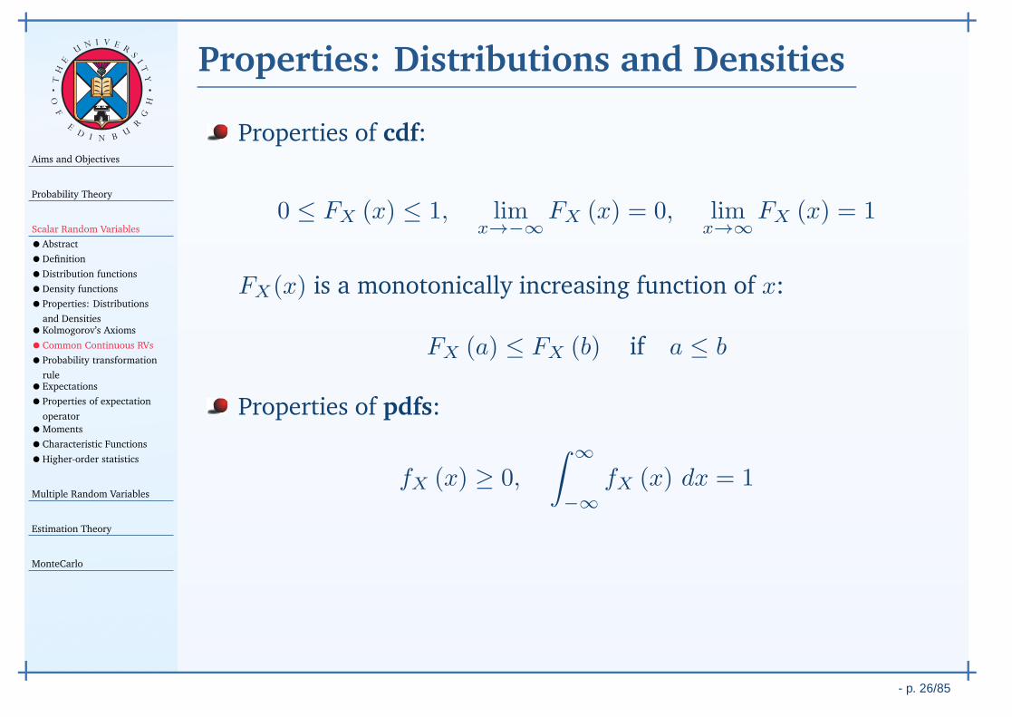
Properties: Distributions and Densities
Properties of cdf:
0 ≤ FX (x) ≤ 1, limx→−∞
FX (x) = 0, limx→∞
FX (x) = 1
FX(x) is a monotonically increasing function of x:
FX (a) ≤ FX (b) if a ≤ b
Properties of pdfs:
fX (x) ≥ 0,
∫ ∞
−∞
fX (x) dx = 1
Aims and Objectives
Probability Theory
Scalar Random Variables
•Abstract
•Definition
•Distribution functions
•Density functions
•Properties: Distributions
and Densities•Kolmogorov’s Axioms
•Common Continuous RVs
•Probability transformation
rule•Expectations
•Properties of expectation
operator
•Moments
•Characteristic Functions
•Higher-order statistics
Multiple Random Variables
Estimation Theory
MonteCarlo
- p. 26/85
TH
E
UN I V E
RS
IT
Y
OF
ED
I N BU
R
GH
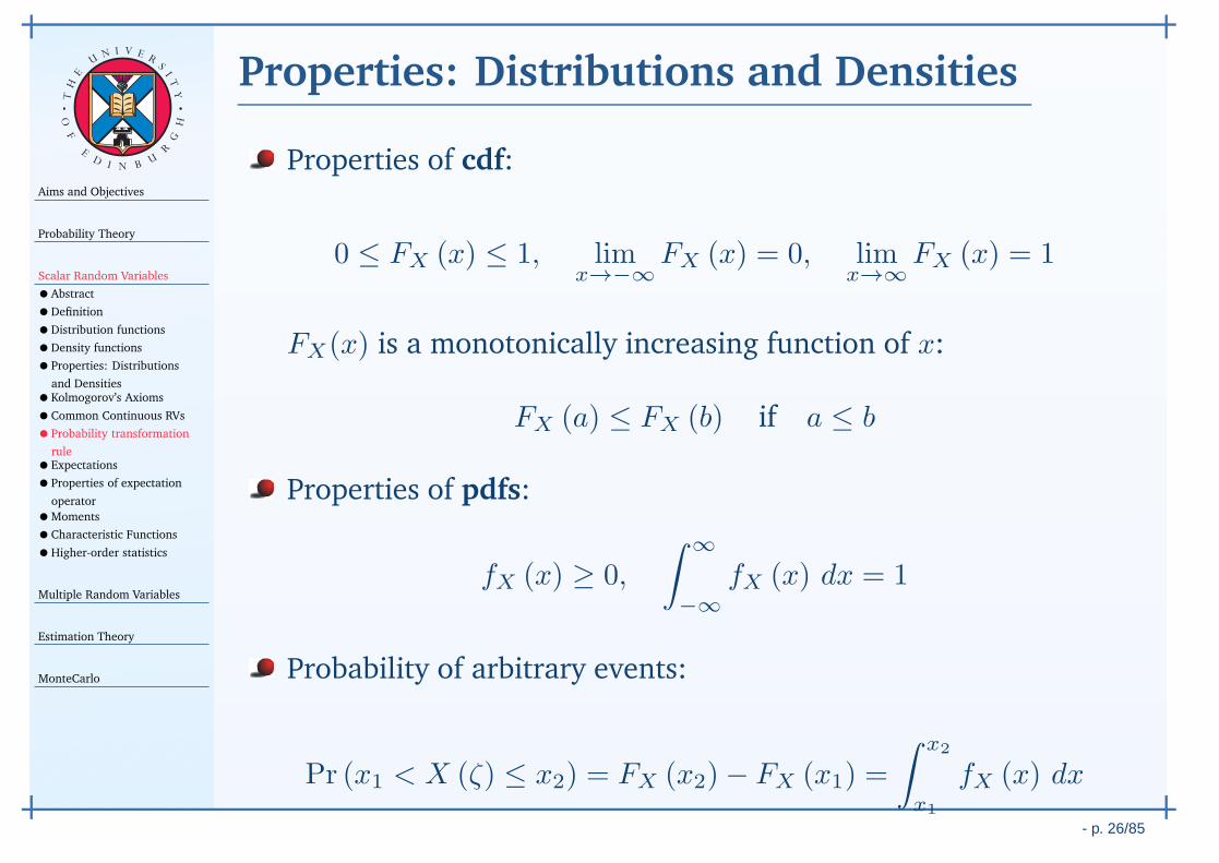
Properties: Distributions and Densities
Properties of cdf:
0 ≤ FX (x) ≤ 1, limx→−∞
FX (x) = 0, limx→∞
FX (x) = 1
FX(x) is a monotonically increasing function of x:
FX (a) ≤ FX (b) if a ≤ b
Properties of pdfs:
fX (x) ≥ 0,
∫ ∞
−∞
fX (x) dx = 1
Probability of arbitrary events:
Pr (x1 < X (ζ) ≤ x2) = FX (x2)− FX (x1) =
∫ x2
x1
fX (x) dx
Aims and Objectives
Probability Theory
Scalar Random Variables
•Abstract
•Definition
•Distribution functions
•Density functions
•Properties: Distributions
and Densities•Kolmogorov’s Axioms
•Common Continuous RVs
•Probability transformation
rule•Expectations
•Properties of expectation
operator
•Moments
•Characteristic Functions
•Higher-order statistics
Multiple Random Variables
Estimation Theory
MonteCarlo
- p. 27/85
TH
E
UN I V E
RS
IT
Y
OF
ED
I N BU
R
GH
Kolmogorov’s Axioms
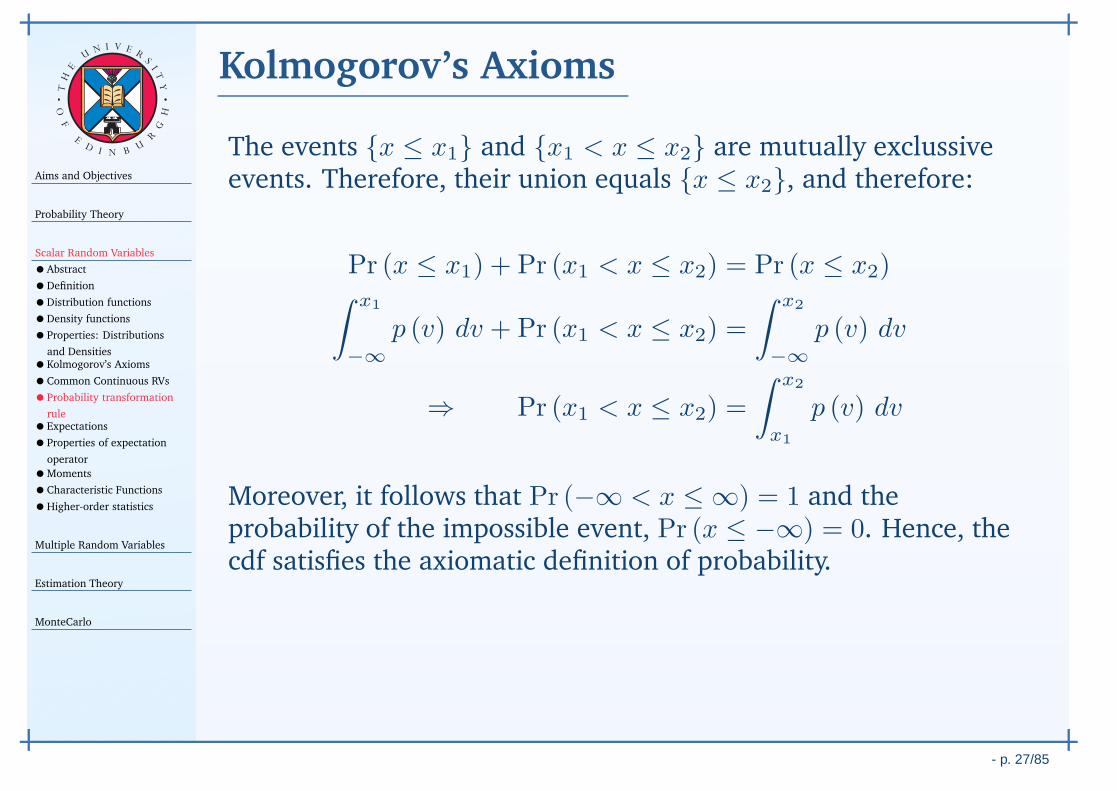
The events x ≤ x1 and x1 < x ≤ x2 are mutually exclussiveevents. Therefore, their union equals x ≤ x2, and therefore:
Pr (x ≤ x1) + Pr (x1 < x ≤ x2) = Pr (x ≤ x2)∫ x1
−∞
p (v) dv + Pr (x1 < x ≤ x2) =
∫ x2
−∞
p (v) dv
⇒ Pr (x1 < x ≤ x2) =
∫ x2
x1
p (v) dv
Moreover, it follows that Pr (−∞ < x ≤ ∞) = 1 and theprobability of the impossible event, Pr (x ≤ −∞) = 0. Hence, thecdf satisfies the axiomatic definition of probability.
Aims and Objectives
Probability Theory
Scalar Random Variables
•Abstract
•Definition
•Distribution functions
•Density functions
•Properties: Distributions
and Densities•Kolmogorov’s Axioms
•Common Continuous RVs
•Probability transformation
rule•Expectations
•Properties of expectation
operator
•Moments
•Characteristic Functions
•Higher-order statistics
Multiple Random Variables
Estimation Theory
MonteCarlo
- p. 28/85
TH
E
UN I V E
RS
IT
Y
OF
ED
I N BU
R
GH
Common Continuous RVs
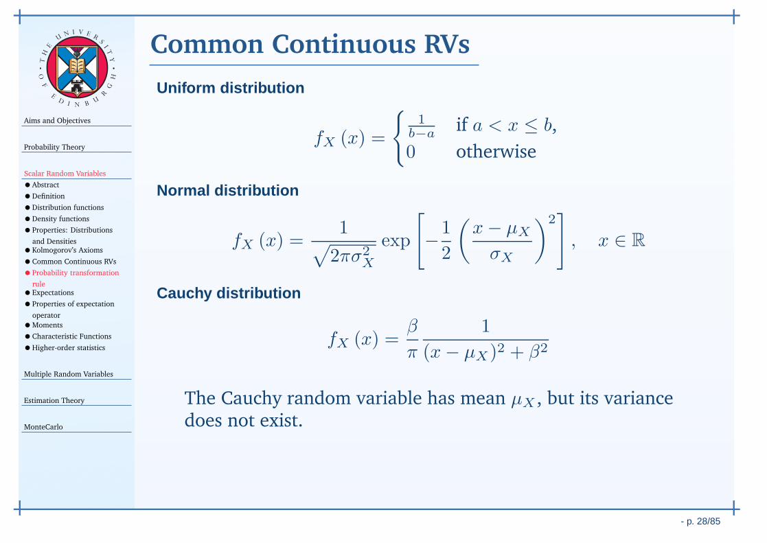
Uniform distribution
fX (x) =
1
b−aif a < x ≤ b,
0 otherwise
Normal distribution
fX (x) =1
√
2πσ2X
exp
[
−1
2
(x− µX
σX
)2]
, x ∈ R
Cauchy distribution
fX (x) =β
π
1
(x− µX)2 + β2
The Cauchy random variable has mean µX , but its variancedoes not exist.
Aims and Objectives
Probability Theory
Scalar Random Variables
•Abstract
•Definition
•Distribution functions
•Density functions
•Properties: Distributions
and Densities•Kolmogorov’s Axioms
•Common Continuous RVs
•Probability transformation
rule•Expectations
•Properties of expectation
operator
•Moments
•Characteristic Functions
•Higher-order statistics
Multiple Random Variables
Estimation Theory
MonteCarlo
- p. 29/85
TH
E
UN I V E
RS
IT
Y
OF
ED
I N BU
R
GH
Probability transformation rule
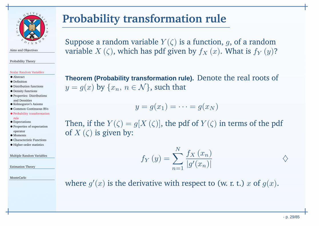
Suppose a random variable Y (ζ) is a function, g, of a randomvariable X (ζ), which has pdf given by fX (x). What is fY (y)?
Aims and Objectives
Probability Theory
Scalar Random Variables
•Abstract
•Definition
•Distribution functions
•Density functions
•Properties: Distributions
and Densities•Kolmogorov’s Axioms
•Common Continuous RVs
•Probability transformation
rule•Expectations
•Properties of expectation
operator
•Moments
•Characteristic Functions
•Higher-order statistics
Multiple Random Variables
Estimation Theory
MonteCarlo
- p. 29/85
TH
E
UN I V E
RS
IT
Y
OF
ED
I N BU
R
GH
Probability transformation rule
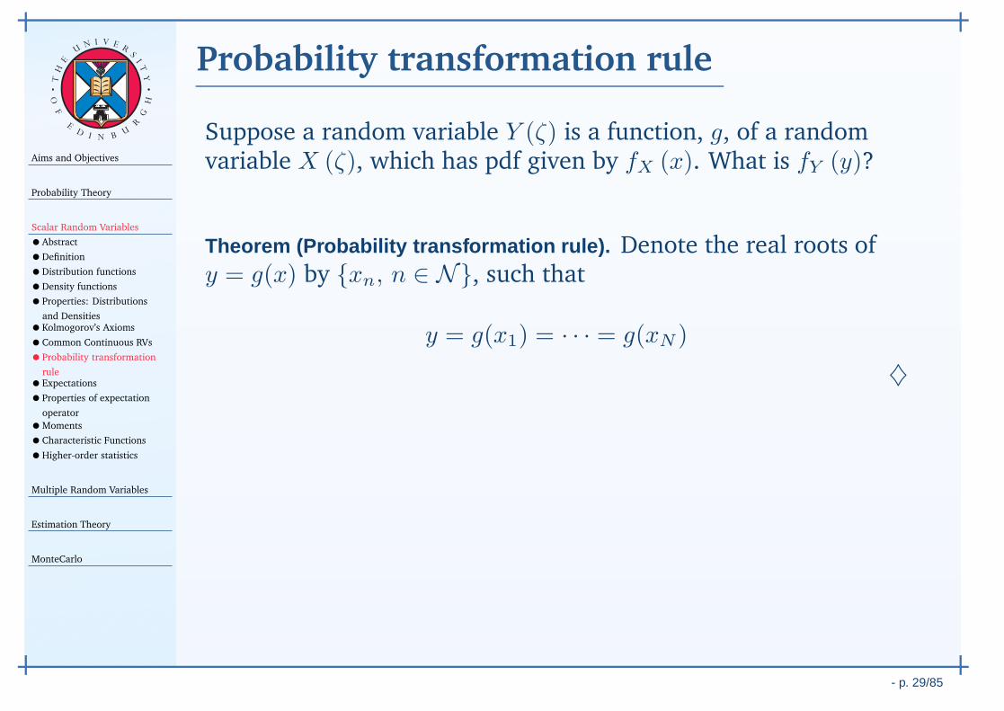
Suppose a random variable Y (ζ) is a function, g, of a randomvariable X (ζ), which has pdf given by fX (x). What is fY (y)?
Theorem (Probability transformation rule). Denote the real roots ofy = g(x) by xn, n ∈ N, such that
y = g(x1) = · · · = g(xN )
♦
Aims and Objectives
Probability Theory
Scalar Random Variables
•Abstract
•Definition
•Distribution functions
•Density functions
•Properties: Distributions
and Densities•Kolmogorov’s Axioms
•Common Continuous RVs
•Probability transformation
rule•Expectations
•Properties of expectation
operator
•Moments
•Characteristic Functions
•Higher-order statistics
Multiple Random Variables
Estimation Theory
MonteCarlo
- p. 29/85
TH
E
UN I V E
RS
IT
Y
OF
ED
I N BU
R
GH
Probability transformation rule
Suppose a random variable Y (ζ) is a function, g, of a randomvariable X (ζ), which has pdf given by fX (x). What is fY (y)?
Theorem (Probability transformation rule). Denote the real roots ofy = g(x) by xn, n ∈ N, such that
y = g(x1) = · · · = g(xN )
Then, if the Y (ζ) = g[X (ζ)], the pdf of Y (ζ) in terms of the pdfof X (ζ) is given by:
fY (y) =N∑
n=1
fX (xn)
|g′(xn)|♦
where g′(x) is the derivative with respect to (w. r. t.) x of g(x).
Aims and Objectives
Probability Theory
Scalar Random Variables
•Abstract
•Definition
•Distribution functions
•Density functions
•Properties: Distributions
and Densities•Kolmogorov’s Axioms
•Common Continuous RVs
•Probability transformation
rule•Expectations
•Properties of expectation
operator
•Moments
•Characteristic Functions
•Higher-order statistics
Multiple Random Variables
Estimation Theory
MonteCarlo
- p. 29/85
TH
E
UN I V E
RS
IT
Y
OF
ED
I N BU
R
GH
Probability transformation rule
Example (Log-normal distribution). Let Y = eX , whereX ∼ N (0, 1). Find the pdf for the RV Y .
SOLUTION. Since X ∼ N (0, 1), then:
fX (x) =1√2π
e−x2
2
Considering the transformation y = g(x) = ex, there is one root,given by x = ln y. Therefore, the derivative of this expression isg′(x) = ex = y.
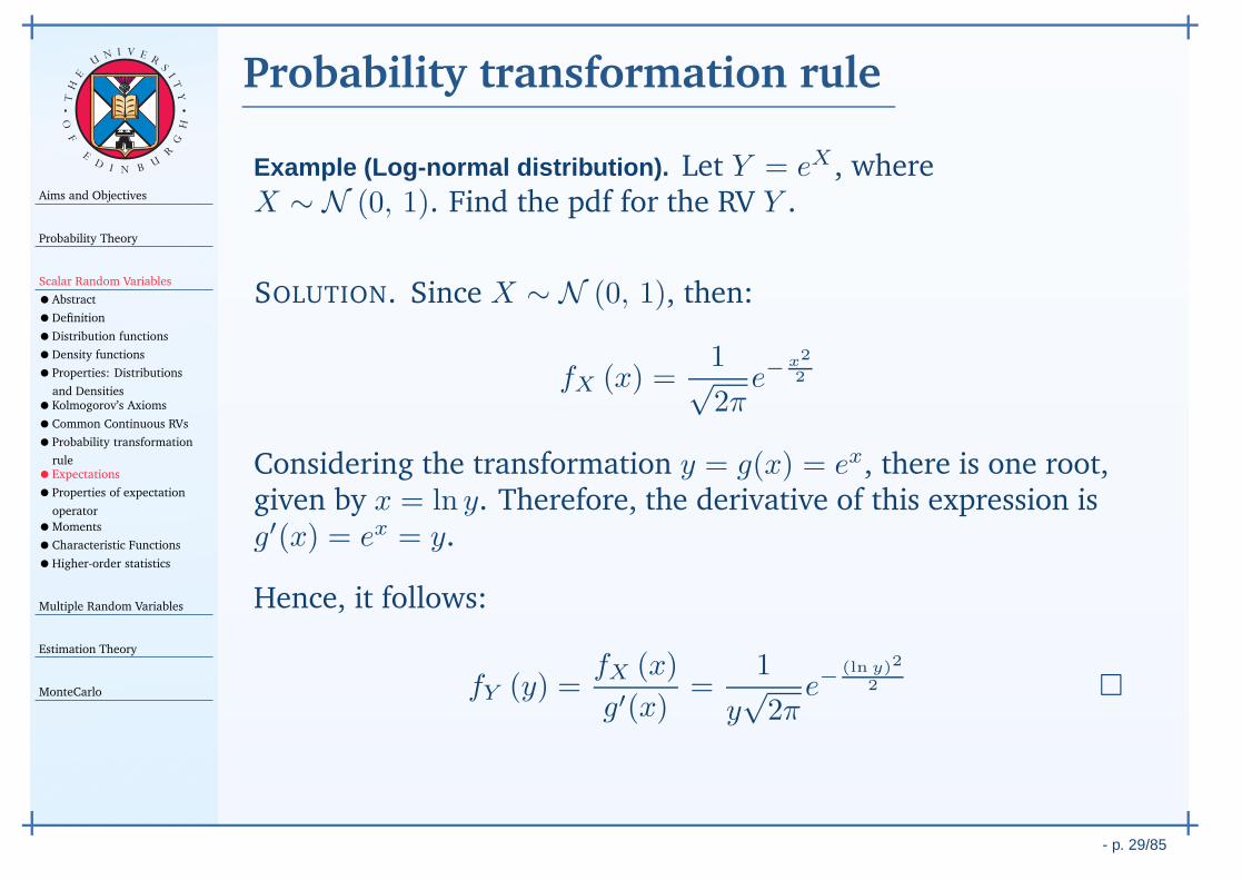
Hence, it follows:
fY (y) =fX (x)
g′(x)=
1
y√2π
e−(ln y)2
2
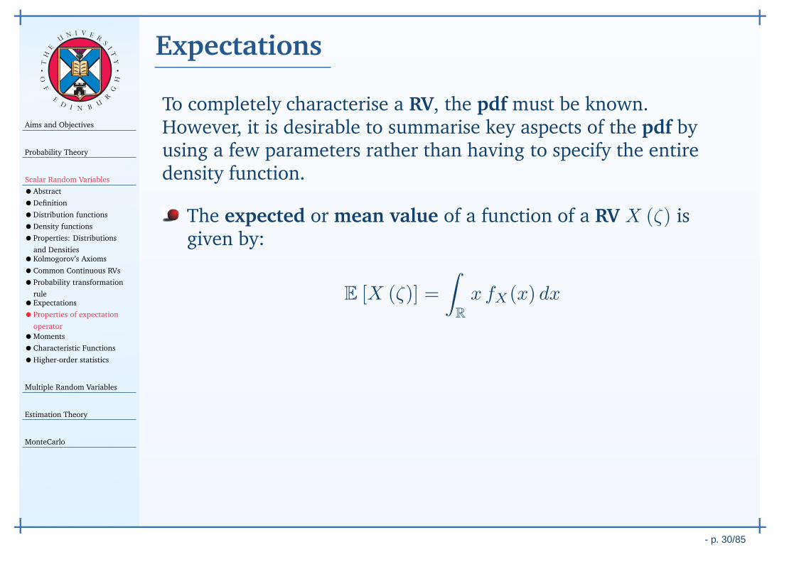
Aims and Objectives
Probability Theory
Scalar Random Variables
•Abstract
•Definition
•Distribution functions
•Density functions
•Properties: Distributions
and Densities•Kolmogorov’s Axioms
•Common Continuous RVs
•Probability transformation
rule•Expectations
•Properties of expectation
operator
•Moments
•Characteristic Functions
•Higher-order statistics
Multiple Random Variables
Estimation Theory
MonteCarlo
- p. 30/85
TH
E
UN I V E
RS
IT
Y
OF
ED
I N BU
R
GH
Expectations
To completely characterise a RV, the pdf must be known.However, it is desirable to summarise key aspects of the pdf byusing a few parameters rather than having to specify the entiredensity function.
The expected or mean value of a function of a RV X (ζ) isgiven by:
E [X (ζ)] =
∫
R
x fX(x) dx
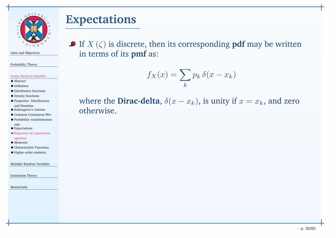
Aims and Objectives
Probability Theory
Scalar Random Variables
•Abstract
•Definition
•Distribution functions
•Density functions
•Properties: Distributions
and Densities•Kolmogorov’s Axioms
•Common Continuous RVs
•Probability transformation
rule•Expectations
•Properties of expectation
operator
•Moments
•Characteristic Functions
•Higher-order statistics
Multiple Random Variables
Estimation Theory
MonteCarlo
- p. 30/85
TH
E
UN I V E
RS
IT
Y
OF
ED
I N BU
R
GH
Expectations
If X (ζ) is discrete, then its corresponding pdf may be writtenin terms of its pmf as:
fX(x) =∑
k
pk δ(x− xk)
where the Dirac-delta, δ(x− xk), is unity if x = xk, and zerootherwise.
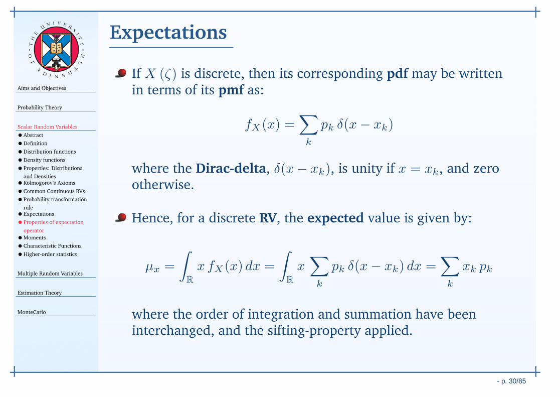
Hence, for a discrete RV, the expected value is given by:
µx =
∫
R
x fX(x) dx =
∫
R
x∑
k
pk δ(x− xk) dx =∑
k
xk pk
where the order of integration and summation have beeninterchanged, and the sifting-property applied.
Aims and Objectives
Probability Theory
Scalar Random Variables
•Abstract
•Definition
•Distribution functions
•Density functions
•Properties: Distributions
and Densities•Kolmogorov’s Axioms
•Common Continuous RVs
•Probability transformation
rule•Expectations
•Properties of expectation
operator
•Moments
•Characteristic Functions
•Higher-order statistics
Multiple Random Variables
Estimation Theory
MonteCarlo
- p. 31/85
TH
E
UN I V E
RS
IT
Y
OF
ED
I N BU
R
GH
Properties of expectation operator
The expectation operator computes a statistical average by usingthe density fX(x) as a weighting function. Hence, the mean µx
can be regarded as the center of gravity of the density.
If fX(x) is an even function, then µX = 0. Note that sincefX(x) ≥ 0, then fX(x) cannot be an odd function.
If fX(x) is symmetrical about x = a, such thatfX(a− x) = fX(x+ a), then µX = a.
The expectation operator is linear:
E [αX (ζ) + β] = αµX + β
If Y (ζ) = gX (ζ) is a RV obtained by transforming X (ζ)through a suitable function, the expectation of Y (ζ) is:
E [Y (ζ)] , E [gX (ζ)] =∫ ∞
−∞
g(x) fX(x) dx
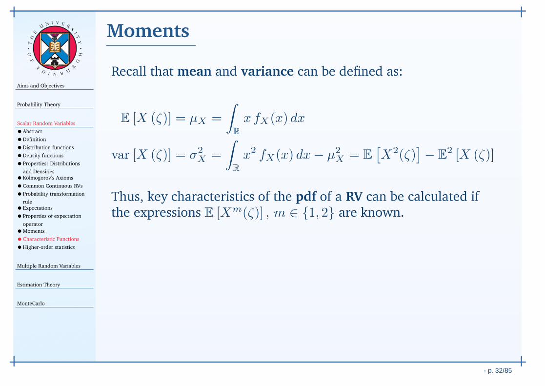
Aims and Objectives
Probability Theory
Scalar Random Variables
•Abstract
•Definition
•Distribution functions
•Density functions
•Properties: Distributions
and Densities•Kolmogorov’s Axioms
•Common Continuous RVs
•Probability transformation
rule•Expectations
•Properties of expectation
operator
•Moments
•Characteristic Functions
•Higher-order statistics
Multiple Random Variables
Estimation Theory
MonteCarlo
- p. 32/85
TH
E
UN I V E
RS
IT
Y
OF
ED
I N BU
R
GH
Moments
Recall that mean and variance can be defined as:
E [X (ζ)] = µX =
∫
R
x fX(x) dx
var [X (ζ)] = σ2X =
∫
R
x2 fX(x) dx− µ2X = E
[X2(ζ)
]− E
2 [X (ζ)]
Thus, key characteristics of the pdf of a RV can be calculated ifthe expressions E [Xm(ζ)] , m ∈ 1, 2 are known.
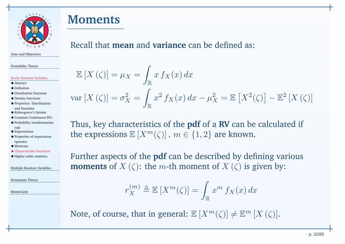
Further aspects of the pdf can be described by defining variousmoments of X (ζ): the m-th moment of X (ζ) is given by:
r(m)X , E [Xm(ζ)] =
∫
R
xm fX(x) dx
Note, of course, that in general: E [Xm(ζ)] 6= Em [X (ζ)].
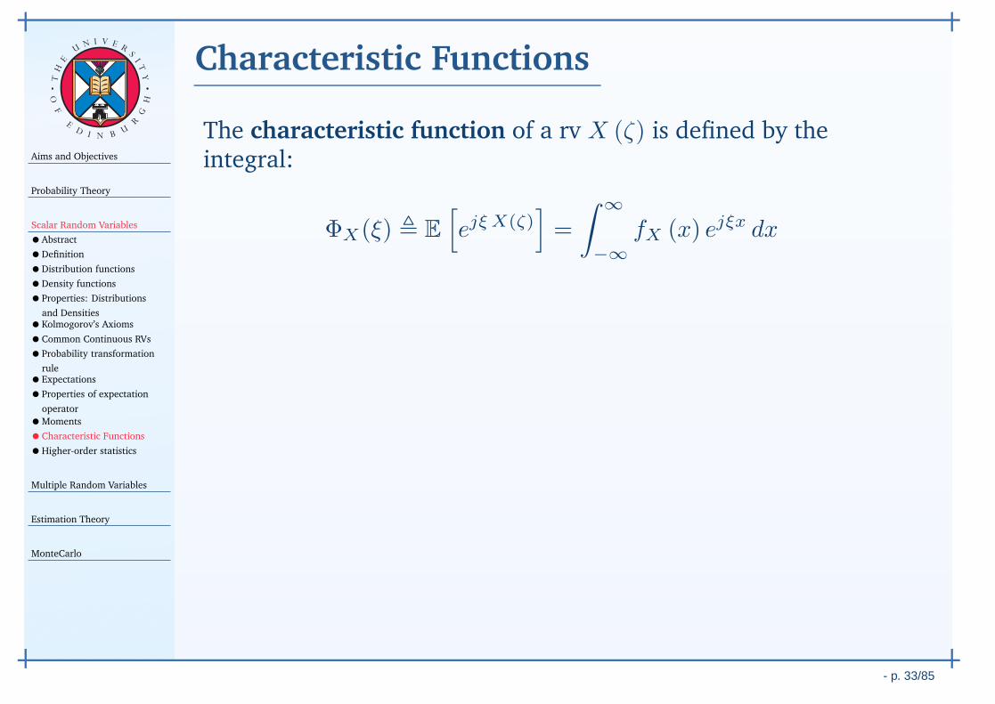
Aims and Objectives
Probability Theory
Scalar Random Variables
•Abstract
•Definition
•Distribution functions
•Density functions
•Properties: Distributions
and Densities•Kolmogorov’s Axioms
•Common Continuous RVs
•Probability transformation
rule•Expectations
•Properties of expectation
operator
•Moments
•Characteristic Functions
•Higher-order statistics
Multiple Random Variables
Estimation Theory
MonteCarlo
- p. 33/85
TH
E
UN I V E
RS
IT
Y
OF
ED
I N BU
R
GH
Characteristic Functions
The characteristic function of a rv X (ζ) is defined by theintegral:
ΦX(ξ) , E
[
ejξ X(ζ)]
=
∫ ∞
−∞
fX (x) ejξx dx
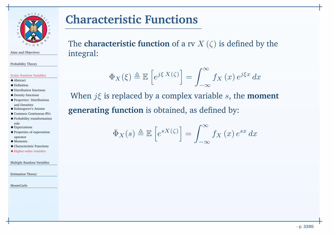
When jξ is replaced by a complex variable s, the moment
generating function is obtained, as defined by:
ΦX(s) , E
[
esX(ζ)]
=
∫ ∞
−∞
fX (x) esx dx
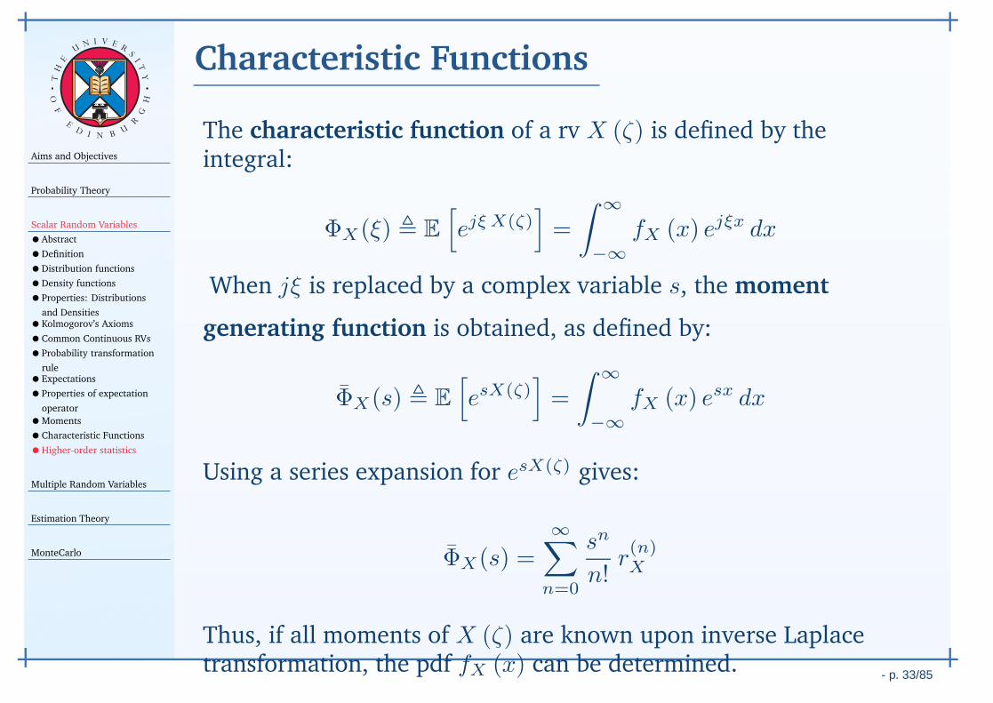
Using a series expansion for esX(ζ) gives:
ΦX(s) =∞∑
n=0
sn
n!r(n)X
Thus, if all moments of X (ζ) are known upon inverse Laplacetransformation, the pdf fX (x) can be determined.
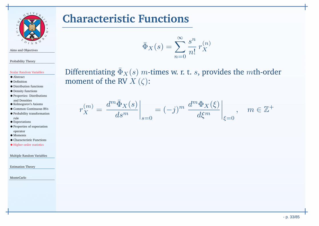
Aims and Objectives
Probability Theory
Scalar Random Variables
•Abstract
•Definition
•Distribution functions
•Density functions
•Properties: Distributions
and Densities•Kolmogorov’s Axioms
•Common Continuous RVs
•Probability transformation
rule•Expectations
•Properties of expectation
operator
•Moments
•Characteristic Functions
•Higher-order statistics
Multiple Random Variables
Estimation Theory
MonteCarlo
- p. 33/85
TH
E
UN I V E
RS
IT
Y
OF
ED
I N BU
R
GH
Characteristic Functions
ΦX(s) =∞∑
n=0
sn
n!r(n)X
Differentiating ΦX(s) m-times w. r. t. s, provides the mth-ordermoment of the RV X (ζ):
r(m)X =
dmΦX(s)
dsm
∣∣∣∣s=0
= (−j)mdmΦX(ξ)
dξm
∣∣∣∣ξ=0
, m ∈ Z+
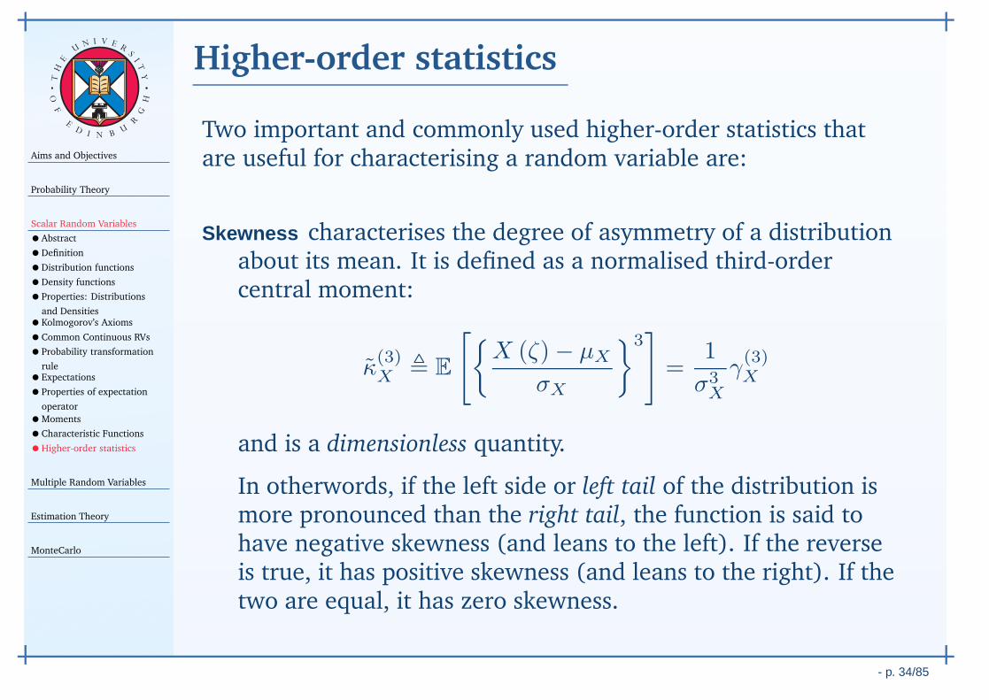
Aims and Objectives
Probability Theory
Scalar Random Variables
•Abstract
•Definition
•Distribution functions
•Density functions
•Properties: Distributions
and Densities•Kolmogorov’s Axioms
•Common Continuous RVs
•Probability transformation
rule•Expectations
•Properties of expectation
operator
•Moments
•Characteristic Functions
•Higher-order statistics
Multiple Random Variables
Estimation Theory
MonteCarlo
- p. 34/85
TH
E
UN I V E
RS
IT
Y
OF
ED
I N BU
R
GH
Higher-order statistics
Two important and commonly used higher-order statistics thatare useful for characterising a random variable are:
Skewness characterises the degree of asymmetry of a distributionabout its mean. It is defined as a normalised third-ordercentral moment:
κ(3)X , E
[X (ζ)− µX
σX
3]
=1
σ3X
γ(3)X
and is a dimensionless quantity.
In otherwords, if the left side or left tail of the distribution ismore pronounced than the right tail, the function is said tohave negative skewness (and leans to the left). If the reverseis true, it has positive skewness (and leans to the right). If thetwo are equal, it has zero skewness.
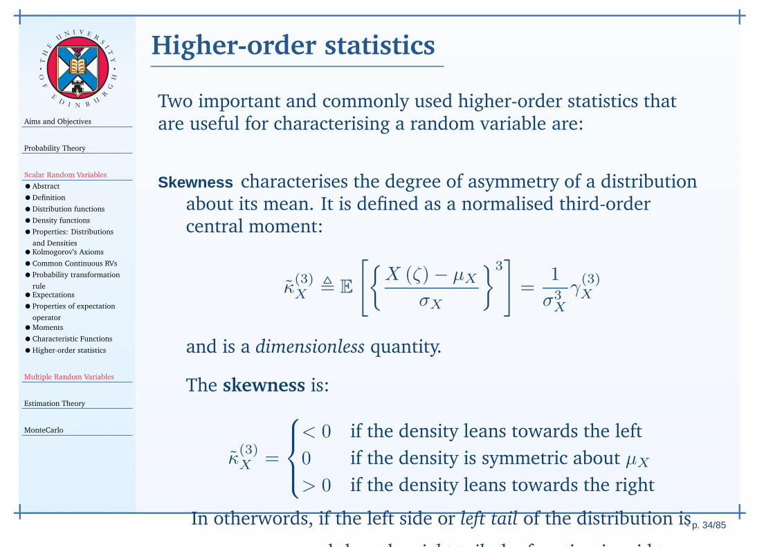
Aims and Objectives
Probability Theory
Scalar Random Variables
•Abstract
•Definition
•Distribution functions
•Density functions
•Properties: Distributions
and Densities•Kolmogorov’s Axioms
•Common Continuous RVs
•Probability transformation
rule•Expectations
•Properties of expectation
operator
•Moments
•Characteristic Functions
•Higher-order statistics
Multiple Random Variables
Estimation Theory
MonteCarlo
- p. 34/85
TH
E
UN I V E
RS
IT
Y
OF
ED
I N BU
R
GH
Higher-order statistics
Two important and commonly used higher-order statistics thatare useful for characterising a random variable are:
Skewness characterises the degree of asymmetry of a distributionabout its mean. It is defined as a normalised third-ordercentral moment:
κ(3)X , E
[X (ζ)− µX
σX
3]
=1
σ3X
γ(3)X
and is a dimensionless quantity.
The skewness is:
κ(3)X =
< 0 if the density leans towards the left
0 if the density is symmetric about µX
> 0 if the density leans towards the right
In otherwords, if the left side or left tail of the distribution is
more pronounced than the right tail, the function is said to
Aims and Objectives
Probability Theory
Scalar Random Variables
•Abstract
•Definition
•Distribution functions
•Density functions
•Properties: Distributions
and Densities•Kolmogorov’s Axioms
•Common Continuous RVs
•Probability transformation
rule•Expectations
•Properties of expectation
operator
•Moments
•Characteristic Functions
•Higher-order statistics
Multiple Random Variables
Estimation Theory
MonteCarlo
- p. 34/85
TH
E
UN I V E
RS
IT
Y
OF
ED
I N BU
R
GH
Higher-order statistics
Kurtosis measures relative flatness or peakedness of a distributionabout its mean value.
This measure is relative with respect to a normal distribution,
which has the property γ(4)X = 3σ4
X , therefore having zerokurtosis.
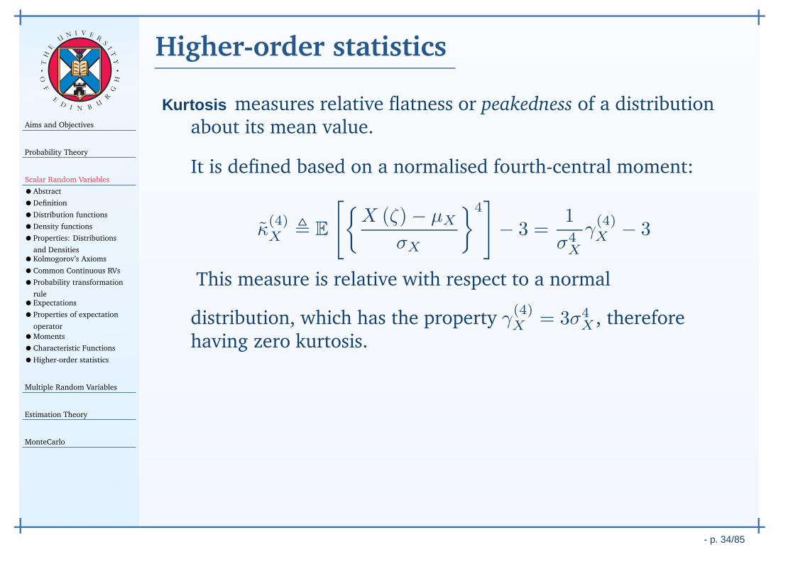
Aims and Objectives
Probability Theory
Scalar Random Variables
•Abstract
•Definition
•Distribution functions
•Density functions
•Properties: Distributions
and Densities•Kolmogorov’s Axioms
•Common Continuous RVs
•Probability transformation
rule•Expectations
•Properties of expectation
operator
•Moments
•Characteristic Functions
•Higher-order statistics
Multiple Random Variables
Estimation Theory
MonteCarlo
- p. 34/85
TH
E
UN I V E
RS
IT
Y
OF
ED
I N BU
R
GH
Higher-order statistics
Kurtosis measures relative flatness or peakedness of a distributionabout its mean value.
It is defined based on a normalised fourth-central moment:
κ(4)X , E
[X (ζ)− µX
σX
4]
− 3 =1
σ4X
γ(4)X − 3
This measure is relative with respect to a normal
distribution, which has the property γ(4)X = 3σ4
X , thereforehaving zero kurtosis.
- p. 35/85
Handout 4Multiple Random Variables
Aims and Objectives
Probability Theory
Scalar Random Variables
Multiple Random Variables
•Abstract
•Definition of Random
Vectors•Distribution and Density
Functions•Marginal Density Function
• Independence
•Conditionals and Bayes’s
•Statistical Description
•Probability Transformation
Rule•Polar Transformation
•Linear Transformations
•Auxiliary Variables
•Multivariate Gaussian
Density Function
•Characteristic Functions
•Sum of Independent
Random Variables•Central limit theorem
Estimation Theory
MonteCarlo
- p. 36/85
TH
E
UN I V E
RS
IT
Y
OF
ED
I N BU
R
GH
Abstract
A group of signal observations can be modelled as a collection ofrandom variables (RVs) that can be grouped to form a randomvector, or vector RV.
This is an extension of the concept of a RV, and generalisesmany of the results presented for scalar RVs.
Note that each element of a random vector is not necessarilygenerated independently from a separate experiment.
Random vectors also lead to the notion of the relationshipbetween the random elements.
This course mainly deals with real-valued random vectors,although the concept can be extended to complex-valuedrandom vectors.
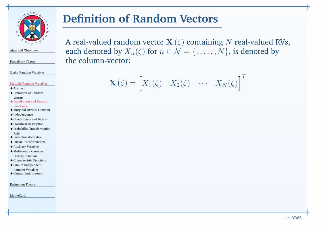
Aims and Objectives
Probability Theory
Scalar Random Variables
Multiple Random Variables
•Abstract
•Definition of Random
Vectors•Distribution and Density
Functions•Marginal Density Function
• Independence
•Conditionals and Bayes’s
•Statistical Description
•Probability Transformation
Rule•Polar Transformation
•Linear Transformations
•Auxiliary Variables
•Multivariate Gaussian
Density Function
•Characteristic Functions
•Sum of Independent
Random Variables•Central limit theorem
Estimation Theory
MonteCarlo
- p. 37/85
TH
E
UN I V E
RS
IT
Y
OF
ED
I N BU
R
GH
Definition of Random Vectors
A real-valued random vector X (ζ) containing N real-valued RVs,each denoted by Xn(ζ) for n ∈ N = 1, . . . , N, is denoted bythe column-vector:
X (ζ) =[
X1(ζ) X2(ζ) · · · XN (ζ)]T
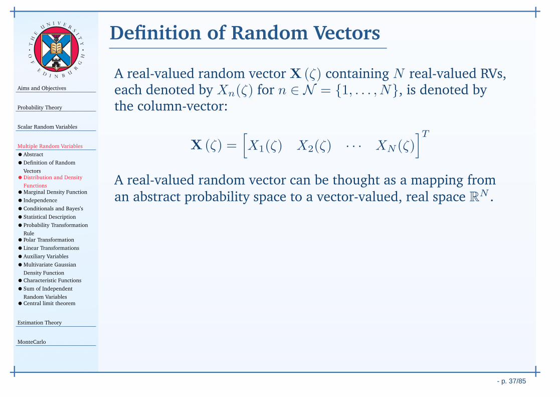
A real-valued random vector can be thought as a mapping from
an abstract probability space to a vector-valued, real space RN .
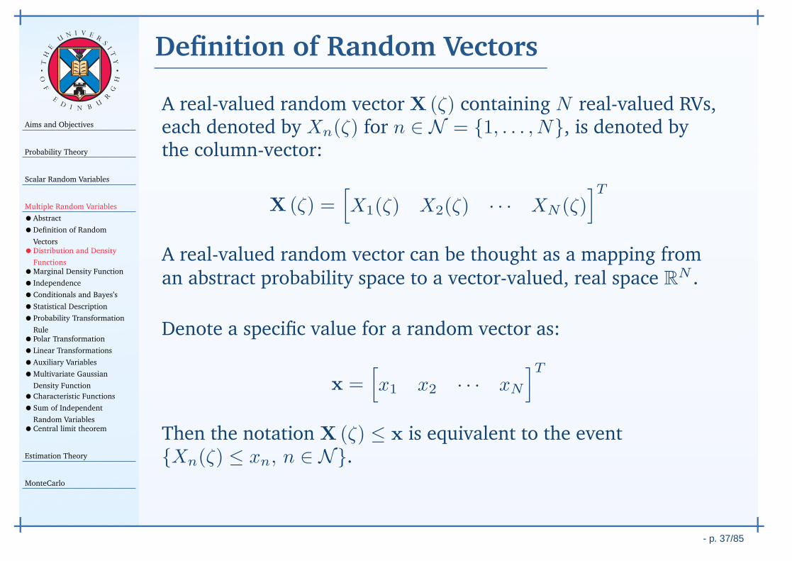
Denote a specific value for a random vector as:
x =[
x1 x2 · · · xN
]T
Then the notation X (ζ) ≤ x is equivalent to the eventXn(ζ) ≤ xn, n ∈ N.
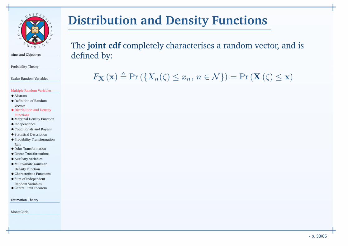
Aims and Objectives
Probability Theory
Scalar Random Variables
Multiple Random Variables
•Abstract
•Definition of Random
Vectors•Distribution and Density
Functions•Marginal Density Function
• Independence
•Conditionals and Bayes’s
•Statistical Description
•Probability Transformation
Rule•Polar Transformation
•Linear Transformations
•Auxiliary Variables
•Multivariate Gaussian
Density Function
•Characteristic Functions
•Sum of Independent
Random Variables•Central limit theorem
Estimation Theory
MonteCarlo
- p. 38/85
TH
E
UN I V E
RS
IT
Y
OF
ED
I N BU
R
GH
Distribution and Density Functions
The joint cdf completely characterises a random vector, and isdefined by:
FX (x) , Pr (Xn(ζ) ≤ xn, n ∈ N) = Pr (X (ζ) ≤ x)
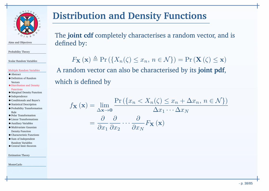
A random vector can also be characterised by its joint pdf,
which is defined by
fX (x) = lim∆x→0
Pr (xn < Xn(ζ) ≤ xn +∆xn, n ∈ N)∆x1 · · ·∆xN
=∂
∂x1
∂
∂x2· · · ∂
∂xN
FX (x)
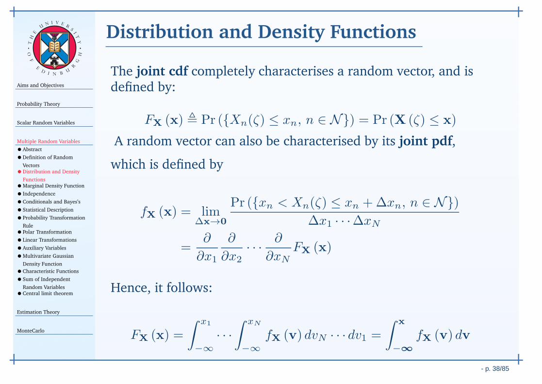
Hence, it follows:
FX (x) =
∫ x1
−∞
· · ·∫ xN
−∞
fX (v) dvN · · · dv1 =
∫ x
−∞
fX (v) dv
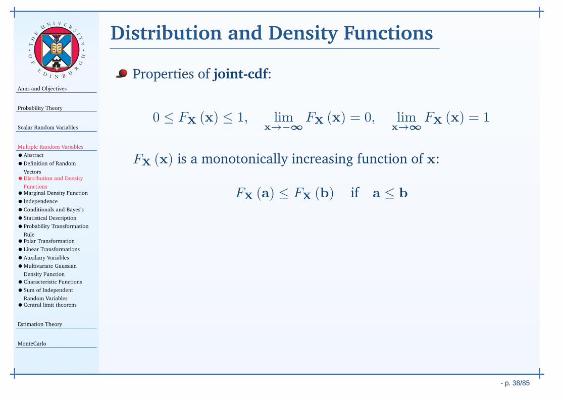
Aims and Objectives
Probability Theory
Scalar Random Variables
Multiple Random Variables
•Abstract
•Definition of Random
Vectors•Distribution and Density
Functions•Marginal Density Function
• Independence
•Conditionals and Bayes’s
•Statistical Description
•Probability Transformation
Rule•Polar Transformation
•Linear Transformations
•Auxiliary Variables
•Multivariate Gaussian
Density Function
•Characteristic Functions
•Sum of Independent
Random Variables•Central limit theorem
Estimation Theory
MonteCarlo
- p. 38/85
TH
E
UN I V E
RS
IT
Y
OF
ED
I N BU
R
GH
Distribution and Density Functions
Properties of joint-cdf:
0 ≤ FX (x) ≤ 1, limx→−∞
FX (x) = 0, limx→∞
FX (x) = 1
FX (x) is a monotonically increasing function of x:
FX (a) ≤ FX (b) if a ≤ b
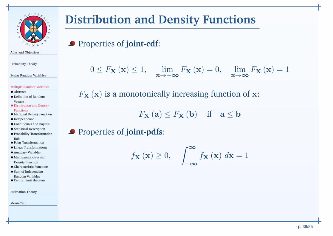
Properties of joint-pdfs:
fX (x) ≥ 0,
∫∞
−∞
fX (x) dx = 1
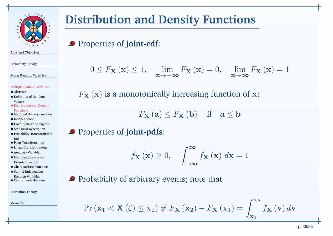
Probability of arbitrary events; note that
Pr (x1 < X (ζ) ≤ x2) 6= FX (x2)− FX (x1) =
∫ x2
x1
fX (v) dv
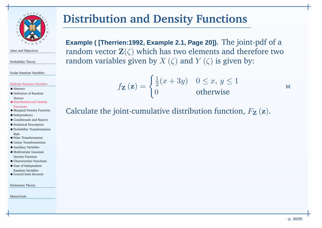
Aims and Objectives
Probability Theory
Scalar Random Variables
Multiple Random Variables
•Abstract
•Definition of Random
Vectors•Distribution and Density
Functions•Marginal Density Function
• Independence
•Conditionals and Bayes’s
•Statistical Description
•Probability Transformation
Rule•Polar Transformation
•Linear Transformations
•Auxiliary Variables
•Multivariate Gaussian
Density Function
•Characteristic Functions
•Sum of Independent
Random Variables•Central limit theorem
Estimation Theory
MonteCarlo
- p. 38/85
TH
E
UN I V E
RS
IT
Y
OF
ED
I N BU
R
GH
Distribution and Density Functions
Example ( [Therrien:1992, Example 2.1, Page 20]). The joint-pdf of arandom vector Z(ζ) which has two elements and therefore tworandom variables given by X (ζ) and Y (ζ) is given by:
fZ (z) =
12 (x+ 3y) 0 ≤ x, y ≤ 1
0 otherwise⋊⋉
Calculate the joint-cumulative distribution function, FZ (z).
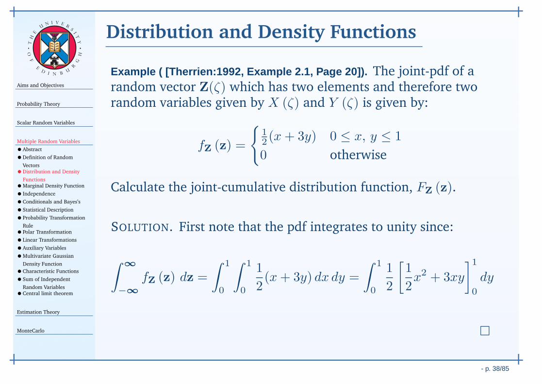
Aims and Objectives
Probability Theory
Scalar Random Variables
Multiple Random Variables
•Abstract
•Definition of Random
Vectors•Distribution and Density
Functions•Marginal Density Function
• Independence
•Conditionals and Bayes’s
•Statistical Description
•Probability Transformation
Rule•Polar Transformation
•Linear Transformations
•Auxiliary Variables
•Multivariate Gaussian
Density Function
•Characteristic Functions
•Sum of Independent
Random Variables•Central limit theorem
Estimation Theory
MonteCarlo
- p. 38/85
TH
E
UN I V E
RS
IT
Y
OF
ED
I N BU
R
GH
Distribution and Density Functions
Example ( [Therrien:1992, Example 2.1, Page 20]). The joint-pdf of arandom vector Z(ζ) which has two elements and therefore tworandom variables given by X (ζ) and Y (ζ) is given by:
fZ (z) =
12 (x+ 3y) 0 ≤ x, y ≤ 1
0 otherwise
Calculate the joint-cumulative distribution function, FZ (z).
SOLUTION. First note that the pdf integrates to unity since:
∫∞
−∞
fZ (z) dz =
∫ 1
0
∫ 1
0
1
2(x+ 3y) dx dy =
∫ 1
0
1
2
[1
2x2 + 3xy
]1
0
dy
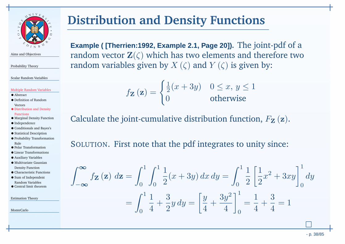
=
∫ 1
0
1
4+
3
2y dy =
[y
4+
3y2
4
]1
0
=1
4+
3
4= 1
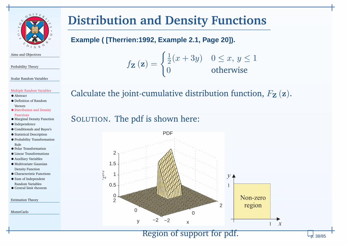
Aims and Objectives
Probability Theory
Scalar Random Variables
Multiple Random Variables
•Abstract
•Definition of Random
Vectors•Distribution and Density
Functions•Marginal Density Function
• Independence
•Conditionals and Bayes’s
•Statistical Description
•Probability Transformation
Rule•Polar Transformation
•Linear Transformations
•Auxiliary Variables
•Multivariate Gaussian
Density Function
•Characteristic Functions
•Sum of Independent
Random Variables•Central limit theorem
Estimation Theory
MonteCarlo
- p. 38/85
TH
E
UN I V E
RS
IT
Y
OF
ED
I N BU
R
GH
Distribution and Density Functions
Example ( [Therrien:1992, Example 2.1, Page 20]).
fZ (z) =
12 (x+ 3y) 0 ≤ x, y ≤ 1
0 otherwise
Calculate the joint-cumulative distribution function, FZ (z).
SOLUTION. The pdf is shown here:
−2
0
2
−2
0
20
0.5
1
1.5
2
x
y
f Z(z
)
Region of support for pdf.
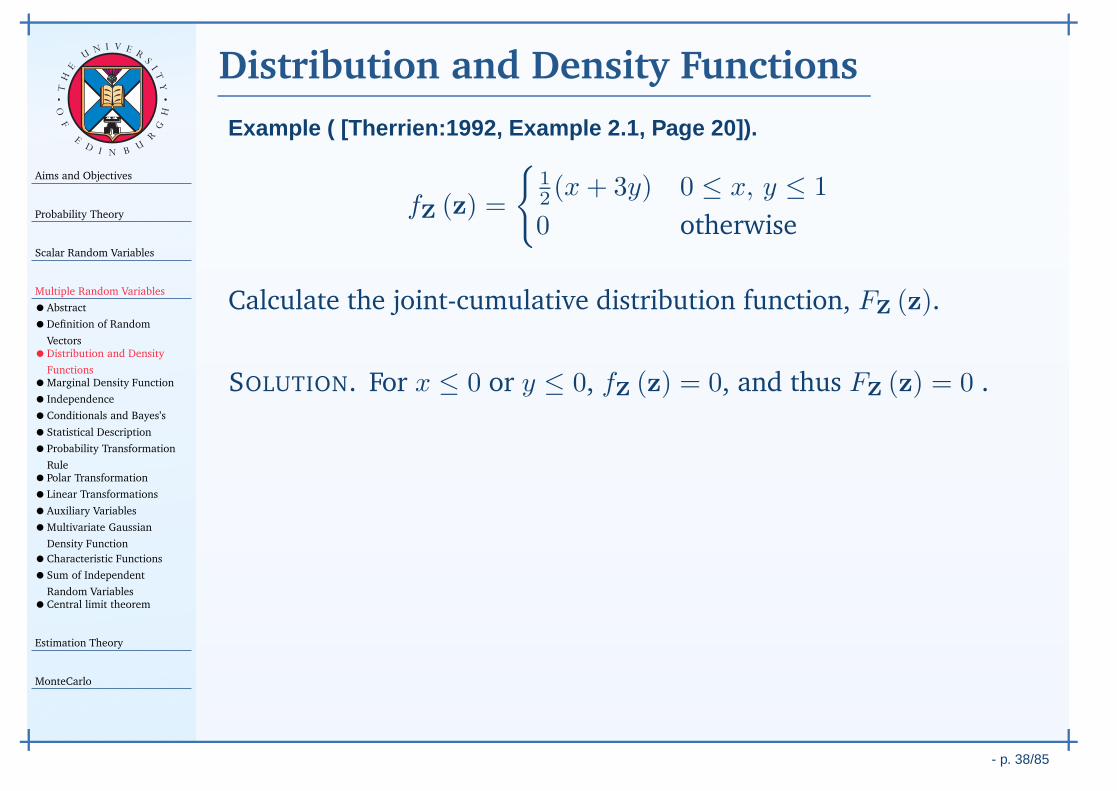
Aims and Objectives
Probability Theory
Scalar Random Variables
Multiple Random Variables
•Abstract
•Definition of Random
Vectors•Distribution and Density
Functions•Marginal Density Function
• Independence
•Conditionals and Bayes’s
•Statistical Description
•Probability Transformation
Rule•Polar Transformation
•Linear Transformations
•Auxiliary Variables
•Multivariate Gaussian
Density Function
•Characteristic Functions
•Sum of Independent
Random Variables•Central limit theorem
Estimation Theory
MonteCarlo
- p. 38/85
TH
E
UN I V E
RS
IT
Y
OF
ED
I N BU
R
GH
Distribution and Density Functions
Example ( [Therrien:1992, Example 2.1, Page 20]).
fZ (z) =
12 (x+ 3y) 0 ≤ x, y ≤ 1
0 otherwise
Calculate the joint-cumulative distribution function, FZ (z).
SOLUTION. For x ≤ 0 or y ≤ 0, fZ (z) = 0, and thus FZ (z) = 0 .
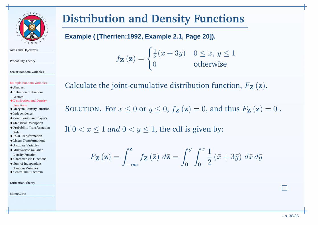
If 0 < x ≤ 1 and 0 < y ≤ 1, the cdf is given by:
FZ (z) =
∫ z
−∞
fZ (z) dz =
∫ y
0
∫ x
0
1
2(x+ 3y) dx dy
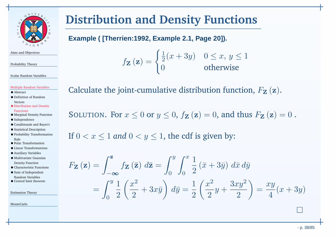
=
∫ y
0
1
2
(x2
2+ 3xy
)
dy =1
2
(x2
2y +
3xy2
2
)
=xy
4(x+ 3y)
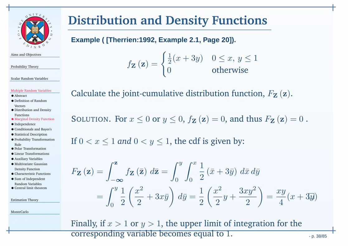
Finally, if x > 1 or y > 1, the upper limit of integration for thecorresponding variable becomes equal to 1.
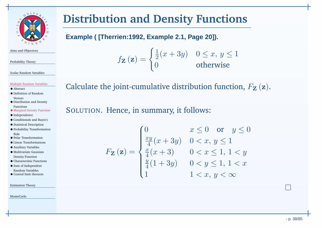
Aims and Objectives
Probability Theory
Scalar Random Variables
Multiple Random Variables
•Abstract
•Definition of Random
Vectors•Distribution and Density
Functions•Marginal Density Function
• Independence
•Conditionals and Bayes’s
•Statistical Description
•Probability Transformation
Rule•Polar Transformation
•Linear Transformations
•Auxiliary Variables
•Multivariate Gaussian
Density Function
•Characteristic Functions
•Sum of Independent
Random Variables•Central limit theorem
Estimation Theory
MonteCarlo
- p. 38/85
TH
E
UN I V E
RS
IT
Y
OF
ED
I N BU
R
GH
Distribution and Density Functions
Example ( [Therrien:1992, Example 2.1, Page 20]).
fZ (z) =
12 (x+ 3y) 0 ≤ x, y ≤ 1
0 otherwise
Calculate the joint-cumulative distribution function, FZ (z).
SOLUTION. Hence, in summary, it follows:
FZ (z) =
0 x ≤ 0 or y ≤ 0xy4 (x+ 3y) 0 < x, y ≤ 1x4 (x+ 3) 0 < x ≤ 1, 1 < yy4 (1 + 3y) 0 < y ≤ 1, 1 < x
1 1 < x, y < ∞
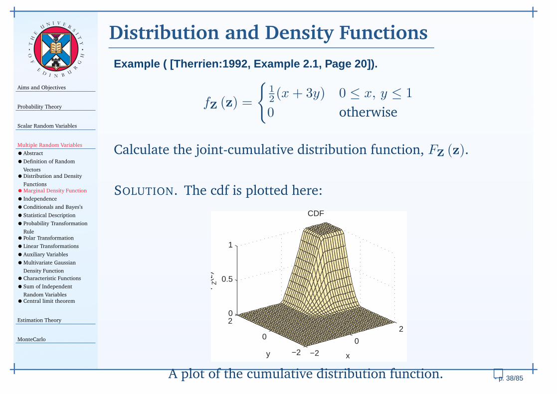
Aims and Objectives
Probability Theory
Scalar Random Variables
Multiple Random Variables
•Abstract
•Definition of Random
Vectors•Distribution and Density
Functions•Marginal Density Function
• Independence
•Conditionals and Bayes’s
•Statistical Description
•Probability Transformation
Rule•Polar Transformation
•Linear Transformations
•Auxiliary Variables
•Multivariate Gaussian
Density Function
•Characteristic Functions
•Sum of Independent
Random Variables•Central limit theorem
Estimation Theory
MonteCarlo
- p. 38/85
TH
E
UN I V E
RS
IT
Y
OF
ED
I N BU
R
GH
Distribution and Density Functions
Example ( [Therrien:1992, Example 2.1, Page 20]).
fZ (z) =
12 (x+ 3y) 0 ≤ x, y ≤ 1
0 otherwise
Calculate the joint-cumulative distribution function, FZ (z).
SOLUTION. The cdf is plotted here:
−2
0
2
−2
0
20
0.5
1
x
CDF
y
FZ(z
)
A plot of the cumulative distribution function.
Aims and Objectives
Probability Theory
Scalar Random Variables
Multiple Random Variables
•Abstract
•Definition of Random
Vectors•Distribution and Density
Functions•Marginal Density Function
• Independence
•Conditionals and Bayes’s
•Statistical Description
•Probability Transformation
Rule•Polar Transformation
•Linear Transformations
•Auxiliary Variables
•Multivariate Gaussian
Density Function
•Characteristic Functions
•Sum of Independent
Random Variables•Central limit theorem
Estimation Theory
MonteCarlo
- p. 39/85
TH
E
UN I V E
RS
IT
Y
OF
ED
I N BU
R
GH
Marginal Density Function
The joint pdf characterises the random vector; the so-calledmarginal pdf describes a subset of RVs from the random vector.
Let k be an M -dimensional vector containing unique indices toelements in the N -dimensional random vector X (ζ),
k =
k1
k2...
kM

Aims and Objectives
Probability Theory
Scalar Random Variables
Multiple Random Variables
•Abstract
•Definition of Random
Vectors•Distribution and Density
Functions•Marginal Density Function
• Independence
•Conditionals and Bayes’s
•Statistical Description
•Probability Transformation
Rule•Polar Transformation
•Linear Transformations
•Auxiliary Variables
•Multivariate Gaussian
Density Function
•Characteristic Functions
•Sum of Independent
Random Variables•Central limit theorem
Estimation Theory
MonteCarlo
- p. 39/85
TH
E
UN I V E
RS
IT
Y
OF
ED
I N BU
R
GH
Marginal Density Function
The joint pdf characterises the random vector; the so-calledmarginal pdf describes a subset of RVs from the random vector.
Let k be an M -dimensional vector containing unique indices toelements in the N -dimensional random vector X (ζ),
Now define a M -dimensional random vector, Xk(ζ), thatcontains the M random variables which are components of X (ζ)and indexed by the elements of k. In other-words, if
k =
k1
k2...
kM
then Xk(ζ) =
Xk1(ζ)
Xk2(ζ)...
XkM(ζ)
Aims and Objectives
Probability Theory
Scalar Random Variables
Multiple Random Variables
•Abstract
•Definition of Random
Vectors•Distribution and Density
Functions•Marginal Density Function
• Independence
•Conditionals and Bayes’s
•Statistical Description
•Probability Transformation
Rule•Polar Transformation
•Linear Transformations
•Auxiliary Variables
•Multivariate Gaussian
Density Function
•Characteristic Functions
•Sum of Independent
Random Variables•Central limit theorem
Estimation Theory
MonteCarlo
- p. 39/85
TH
E
UN I V E
RS
IT
Y
OF
ED
I N BU
R
GH
Marginal Density Function
The marginal pdf is then given by:
fXk(xk) =
∫ ∞
−∞
· · ·∫ ∞
−∞︸ ︷︷ ︸
N − M integrals
fX (x) dx−k
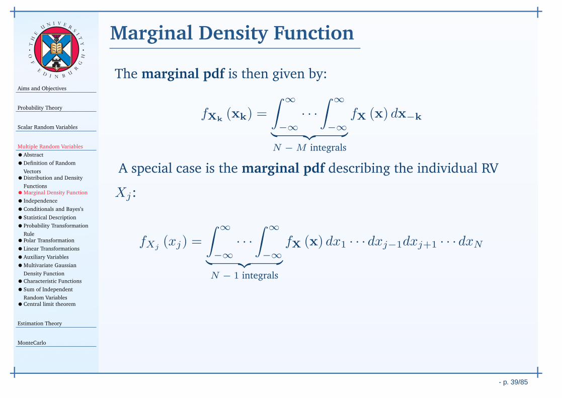
A special case is the marginal pdf describing the individual RV
Xj:
fXj(xj) =
∫ ∞
−∞
· · ·∫ ∞
−∞︸ ︷︷ ︸
N − 1 integrals
fX (x) dx1 · · · dxj−1dxj+1 · · · dxN
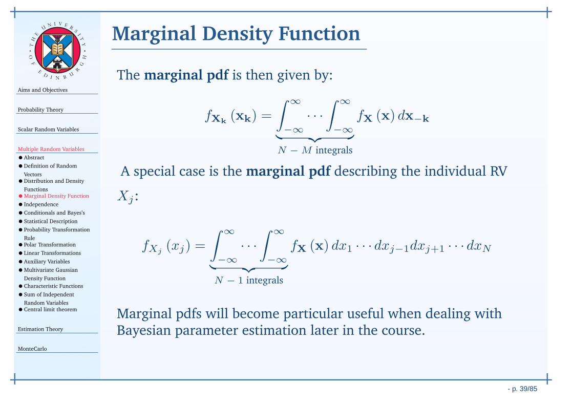
Marginal pdfs will become particular useful when dealing withBayesian parameter estimation later in the course.
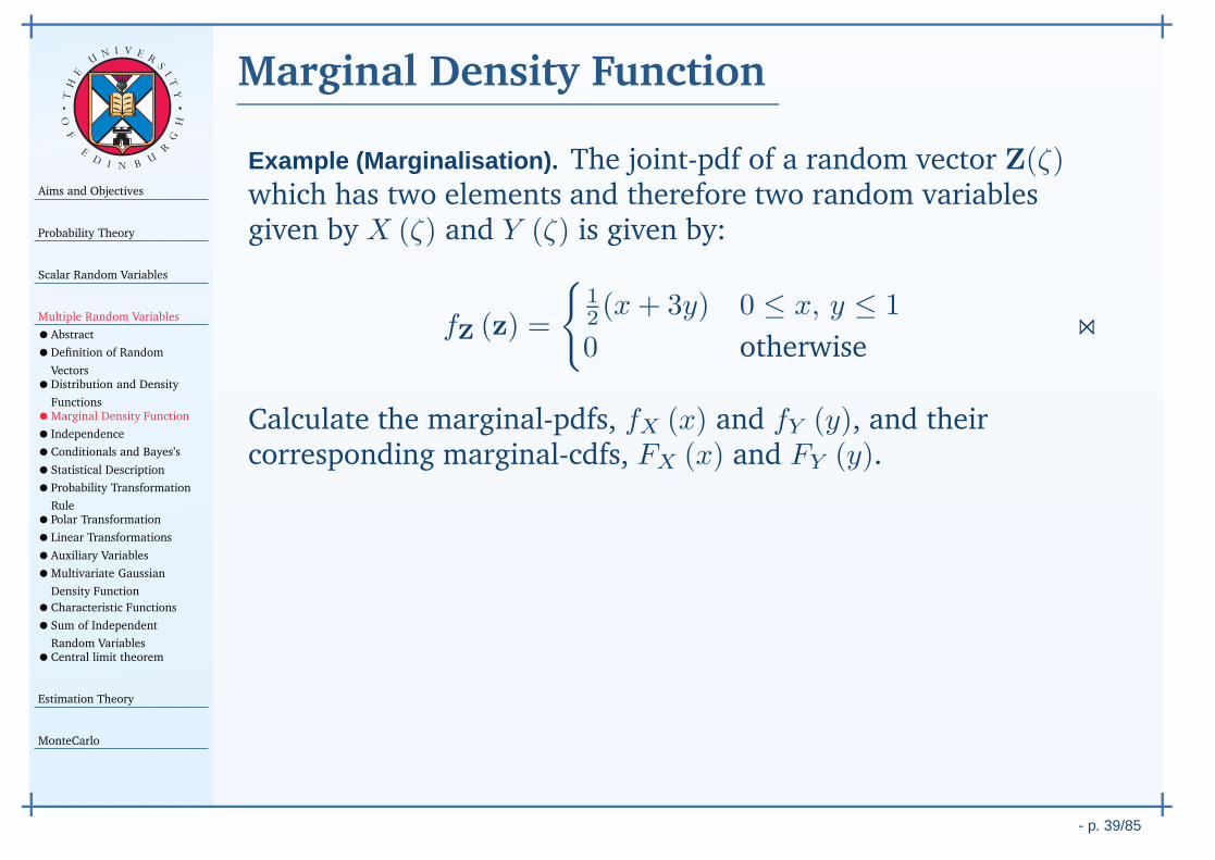
Aims and Objectives
Probability Theory
Scalar Random Variables
Multiple Random Variables
•Abstract
•Definition of Random
Vectors•Distribution and Density
Functions•Marginal Density Function
• Independence
•Conditionals and Bayes’s
•Statistical Description
•Probability Transformation
Rule•Polar Transformation
•Linear Transformations
•Auxiliary Variables
•Multivariate Gaussian
Density Function
•Characteristic Functions
•Sum of Independent
Random Variables•Central limit theorem
Estimation Theory
MonteCarlo
- p. 39/85
TH
E
UN I V E
RS
IT
Y
OF
ED
I N BU
R
GH
Marginal Density Function
Example (Marginalisation). The joint-pdf of a random vector Z(ζ)which has two elements and therefore two random variablesgiven by X (ζ) and Y (ζ) is given by:
fZ (z) =
12 (x+ 3y) 0 ≤ x, y ≤ 1
0 otherwise⋊⋉
Calculate the marginal-pdfs, fX (x) and fY (y), and theircorresponding marginal-cdfs, FX (x) and FY (y).
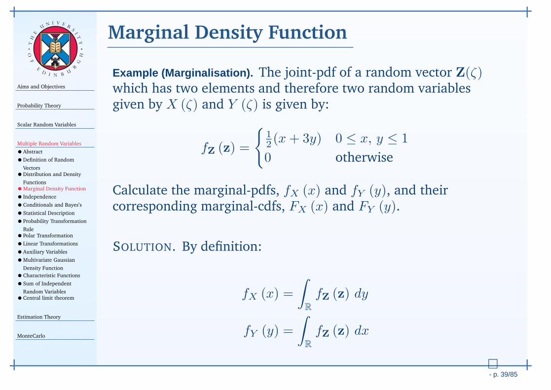
Aims and Objectives
Probability Theory
Scalar Random Variables
Multiple Random Variables
•Abstract
•Definition of Random
Vectors•Distribution and Density
Functions•Marginal Density Function
• Independence
•Conditionals and Bayes’s
•Statistical Description
•Probability Transformation
Rule•Polar Transformation
•Linear Transformations
•Auxiliary Variables
•Multivariate Gaussian
Density Function
•Characteristic Functions
•Sum of Independent
Random Variables•Central limit theorem
Estimation Theory
MonteCarlo
- p. 39/85
TH
E
UN I V E
RS
IT
Y
OF
ED
I N BU
R
GH
Marginal Density Function
Example (Marginalisation). The joint-pdf of a random vector Z(ζ)which has two elements and therefore two random variablesgiven by X (ζ) and Y (ζ) is given by:
fZ (z) =
12 (x+ 3y) 0 ≤ x, y ≤ 1
0 otherwise
Calculate the marginal-pdfs, fX (x) and fY (y), and theircorresponding marginal-cdfs, FX (x) and FY (y).
SOLUTION. By definition:
fX (x) =
∫
R
fZ (z) dy
fY (y) =
∫
R
fZ (z) dx
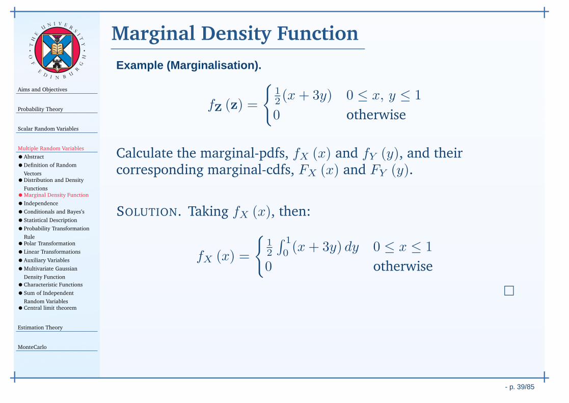
Aims and Objectives
Probability Theory
Scalar Random Variables
Multiple Random Variables
•Abstract
•Definition of Random
Vectors•Distribution and Density
Functions•Marginal Density Function
• Independence
•Conditionals and Bayes’s
•Statistical Description
•Probability Transformation
Rule•Polar Transformation
•Linear Transformations
•Auxiliary Variables
•Multivariate Gaussian
Density Function
•Characteristic Functions
•Sum of Independent
Random Variables•Central limit theorem
Estimation Theory
MonteCarlo
- p. 39/85
TH
E
UN I V E
RS
IT
Y
OF
ED
I N BU
R
GH
Marginal Density Function
Example (Marginalisation).
fZ (z) =
12 (x+ 3y) 0 ≤ x, y ≤ 1
0 otherwise
Calculate the marginal-pdfs, fX (x) and fY (y), and theircorresponding marginal-cdfs, FX (x) and FY (y).
SOLUTION. Taking fX (x), then:
fX (x) =
12
∫ 1
0(x+ 3y) dy 0 ≤ x ≤ 1
0 otherwise
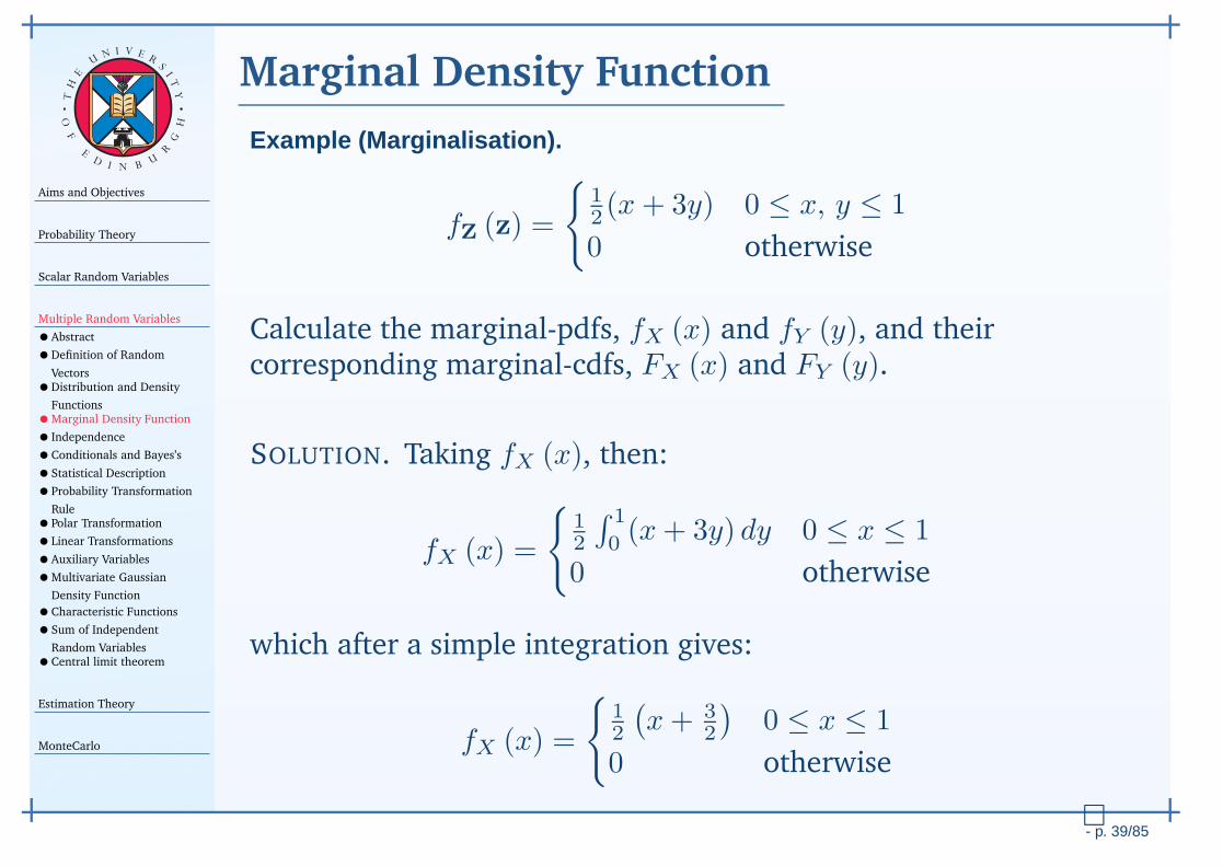
which after a simple integration gives:
fX (x) =
12
(x+ 3
2
)0 ≤ x ≤ 1
0 otherwise
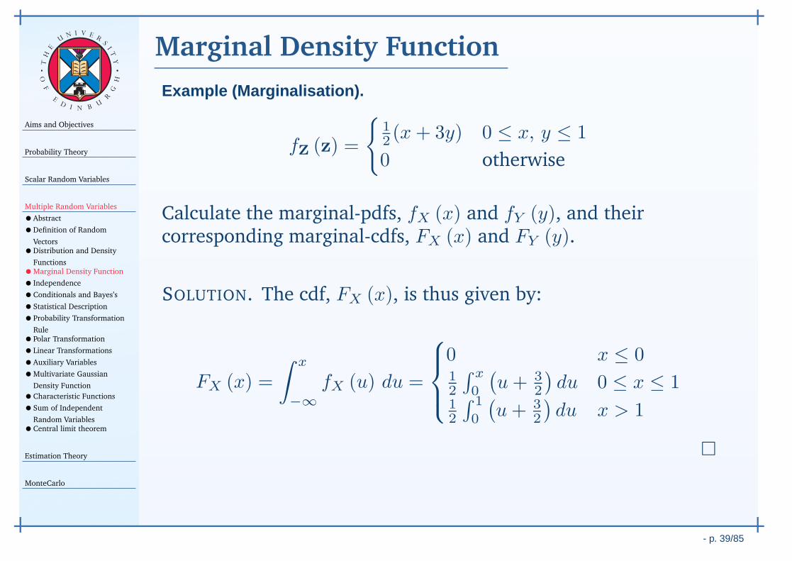
Aims and Objectives
Probability Theory
Scalar Random Variables
Multiple Random Variables
•Abstract
•Definition of Random
Vectors•Distribution and Density
Functions•Marginal Density Function
• Independence
•Conditionals and Bayes’s
•Statistical Description
•Probability Transformation
Rule•Polar Transformation
•Linear Transformations
•Auxiliary Variables
•Multivariate Gaussian
Density Function
•Characteristic Functions
•Sum of Independent
Random Variables•Central limit theorem
Estimation Theory
MonteCarlo
- p. 39/85
TH
E
UN I V E
RS
IT
Y
OF
ED
I N BU
R
GH
Marginal Density Function
Example (Marginalisation).
fZ (z) =
12 (x+ 3y) 0 ≤ x, y ≤ 1
0 otherwise
Calculate the marginal-pdfs, fX (x) and fY (y), and theircorresponding marginal-cdfs, FX (x) and FY (y).
SOLUTION. The cdf, FX (x), is thus given by:
FX (x) =
∫ x
−∞
fX (u) du =
0 x ≤ 012
∫ x
0
(u+ 3
2
)du 0 ≤ x ≤ 1
12
∫ 1
0
(u+ 3
2
)du x > 1
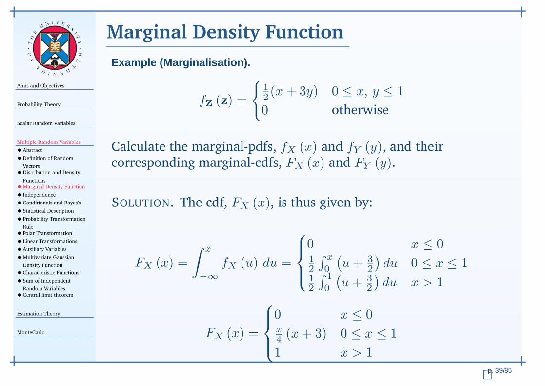
FX (x) =
0 x ≤ 0x4 (x+ 3) 0 ≤ x ≤ 1
1 x > 1

Aims and Objectives
Probability Theory
Scalar Random Variables
Multiple Random Variables
•Abstract
•Definition of Random
Vectors•Distribution and Density
Functions•Marginal Density Function
• Independence
•Conditionals and Bayes’s
•Statistical Description
•Probability Transformation
Rule•Polar Transformation
•Linear Transformations
•Auxiliary Variables
•Multivariate Gaussian
Density Function
•Characteristic Functions
•Sum of Independent
Random Variables•Central limit theorem
Estimation Theory
MonteCarlo
- p. 39/85
TH
E
UN I V E
RS
IT
Y
OF
ED
I N BU
R
GH
Marginal Density Function
Example (Marginalisation).
fZ (z) =
12 (x+ 3y) 0 ≤ x, y ≤ 1
0 otherwise
Calculate the marginal-pdfs, fX (x) and fY (y), and theircorresponding marginal-cdfs, FX (x) and FY (y).
SOLUTION. Similarly, it can be shown that:
fY (y) =
12
(12 + 3y
)0 ≤ y ≤ 1
0 otherwise
and
FY (y) =
0 y ≤ 0y4 (1 + 3y) 0 ≤ y ≤ 1
1 y > 1

Aims and Objectives
Probability Theory
Scalar Random Variables
Multiple Random Variables
•Abstract
•Definition of Random
Vectors•Distribution and Density
Functions•Marginal Density Function
• Independence
•Conditionals and Bayes’s
•Statistical Description
•Probability Transformation
Rule•Polar Transformation
•Linear Transformations
•Auxiliary Variables
•Multivariate Gaussian
Density Function
•Characteristic Functions
•Sum of Independent
Random Variables•Central limit theorem
Estimation Theory
MonteCarlo
- p. 39/85
TH
E
UN I V E
RS
IT
Y
OF
ED
I N BU
R
GH
Marginal Density Function
Example (Marginalisation).
fZ (z) =
12 (x+ 3y) 0 ≤ x, y ≤ 1
0 otherwise
SOLUTION. The marginal-pdfs and cdfs are shown below.
−0.5 0 0.5 1 1.50
0.2
0.4
0.6
0.8
1
1.2
1.4
Marginal PDF, fX(x)
x
f X(x
)
−0.5 0 0.5 1 1.50
0.2
0.4
0.6
0.8
1
Marginal CDF, FX(x)
xF
X(x
)
The marginal-pdf, fX (x), and cdf, FX (x), for the RV, X (ζ).
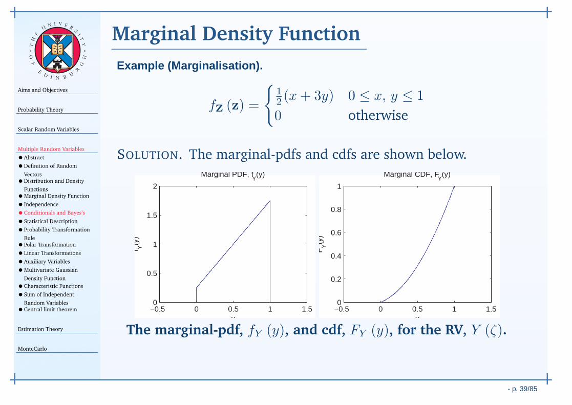
Aims and Objectives
Probability Theory
Scalar Random Variables
Multiple Random Variables
•Abstract
•Definition of Random
Vectors•Distribution and Density
Functions•Marginal Density Function
• Independence
•Conditionals and Bayes’s
•Statistical Description
•Probability Transformation
Rule•Polar Transformation
•Linear Transformations
•Auxiliary Variables
•Multivariate Gaussian
Density Function
•Characteristic Functions
•Sum of Independent
Random Variables•Central limit theorem
Estimation Theory
MonteCarlo
- p. 39/85
TH
E
UN I V E
RS
IT
Y
OF
ED
I N BU
R
GH
Marginal Density Function
Example (Marginalisation).
fZ (z) =
12 (x+ 3y) 0 ≤ x, y ≤ 1
0 otherwise
SOLUTION. The marginal-pdfs and cdfs are shown below.
−0.5 0 0.5 1 1.50
0.5
1
1.5
2
Marginal PDF, fY(y)
y
f Y(y
)
−0.5 0 0.5 1 1.50
0.2
0.4
0.6
0.8
1
Marginal CDF, FY(y)
yF
Y(y
)
The marginal-pdf, fY (y), and cdf, FY (y), for the RV, Y (ζ).
Aims and Objectives
Probability Theory
Scalar Random Variables
Multiple Random Variables
•Abstract
•Definition of Random
Vectors•Distribution and Density
Functions•Marginal Density Function
• Independence
•Conditionals and Bayes’s
•Statistical Description
•Probability Transformation
Rule•Polar Transformation
•Linear Transformations
•Auxiliary Variables
•Multivariate Gaussian
Density Function
•Characteristic Functions
•Sum of Independent
Random Variables•Central limit theorem
Estimation Theory
MonteCarlo
- p. 40/85
TH
E
UN I V E
RS
IT
Y
OF
ED
I N BU
R
GH
Independence
Two random variables, X1(ζ) and X2(ζ) are independent if theevents X1(ζ) ≤ x1 and X2(ζ) ≤ x2 are jointly independent;that is, the events do not influence one another, and
Pr (X1(ζ) ≤ x1, X2(ζ) ≤ x2) = Pr (X1(ζ) ≤ x1) Pr (X2(ζ) ≤ x2)
This then implies that
FX1,X2 (x1, x2) = FX1 (x1)FX2 (x2)
fX1,X2 (x1, x2) = fX1 (x1) fX2 (x2)
Aims and Objectives
Probability Theory
Scalar Random Variables
Multiple Random Variables
•Abstract
•Definition of Random
Vectors•Distribution and Density
Functions•Marginal Density Function
• Independence
•Conditionals and Bayes’s
•Statistical Description
•Probability Transformation
Rule•Polar Transformation
•Linear Transformations
•Auxiliary Variables
•Multivariate Gaussian
Density Function
•Characteristic Functions
•Sum of Independent
Random Variables•Central limit theorem
Estimation Theory
MonteCarlo
- p. 41/85
TH
E
UN I V E
RS
IT
Y
OF
ED
I N BU
R
GH
Conditionals and Bayes’s
The notion of joint probabilities and pdf also leads to the notionof conditional probabilities; what is the probability of a randomvector Y (ζ), given the random vector X (ζ).
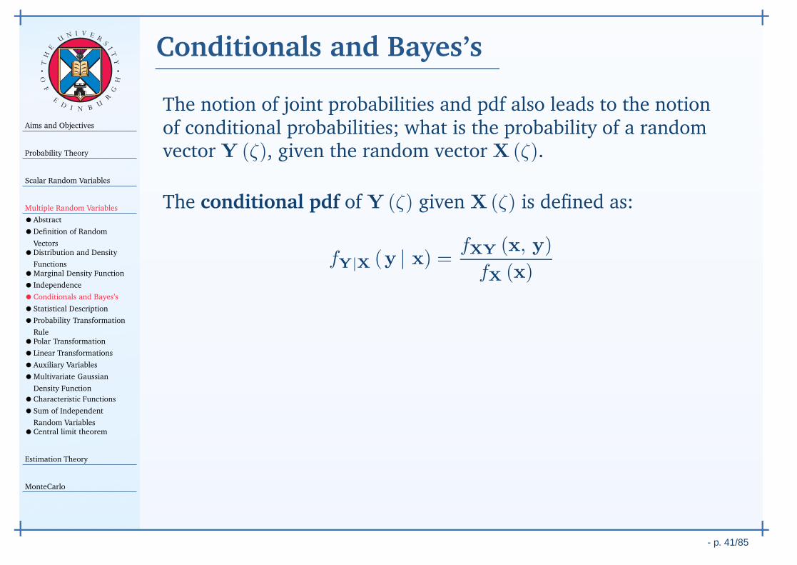
The conditional pdf of Y (ζ) given X (ζ) is defined as:
fY|X (y | x) = fXY (x, y)
fX (x)
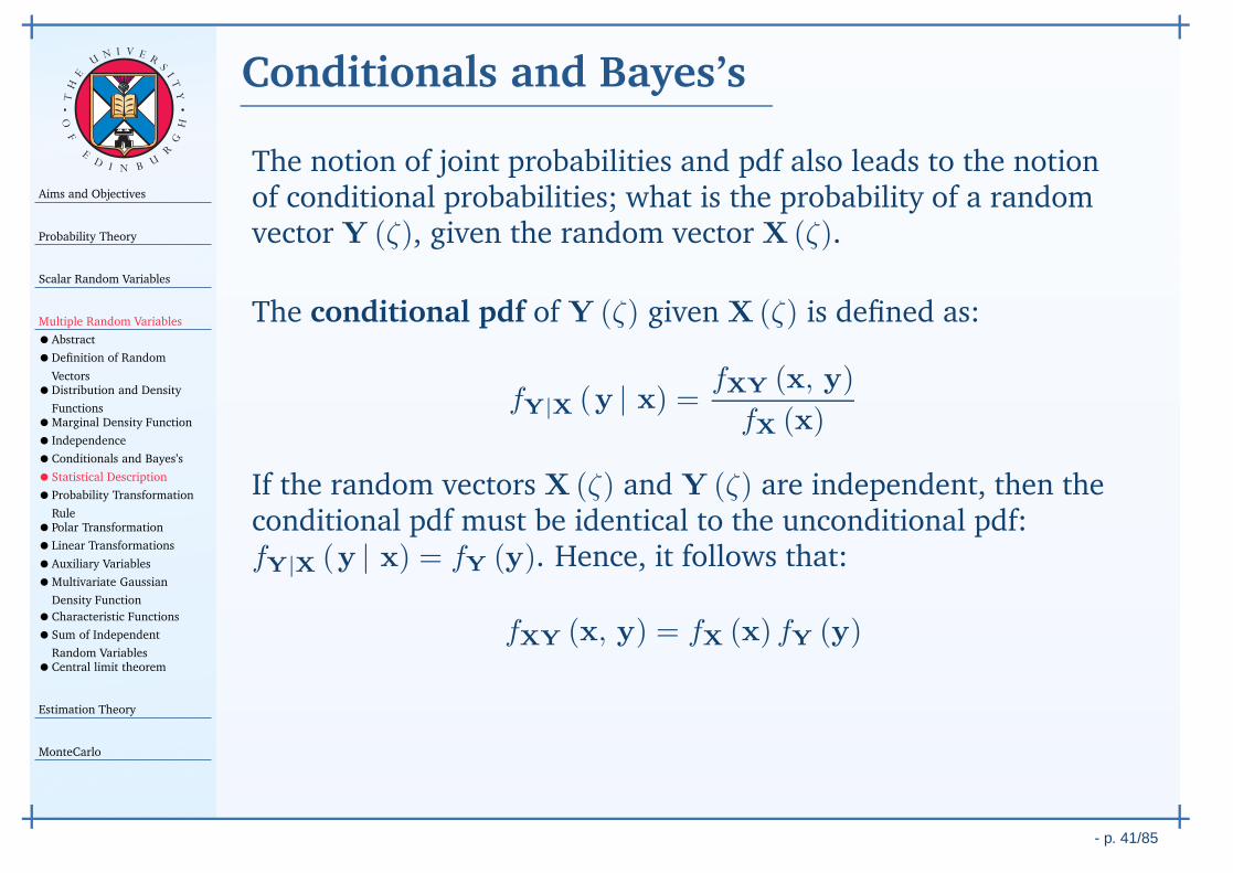
If the random vectors X (ζ) and Y (ζ) are independent, then theconditional pdf must be identical to the unconditional pdf:fY|X (y | x) = fY (y). Hence, it follows that:
fXY (x, y) = fX (x) fY (y)
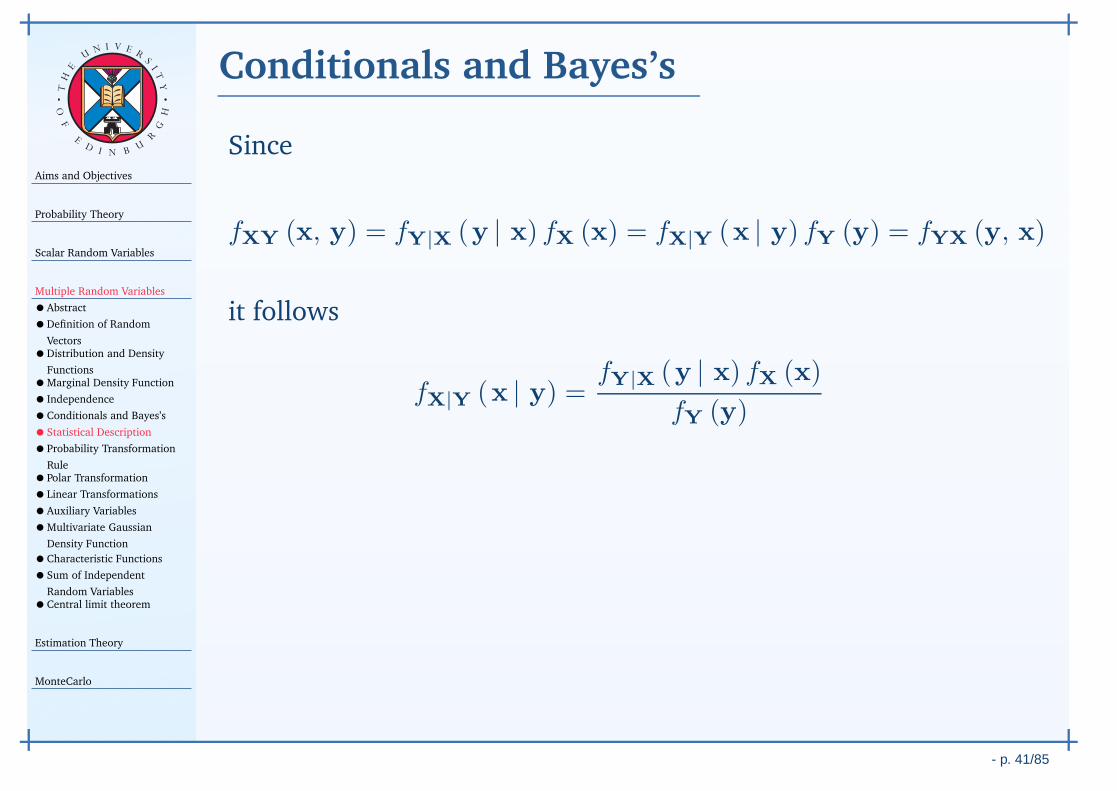
Aims and Objectives
Probability Theory
Scalar Random Variables
Multiple Random Variables
•Abstract
•Definition of Random
Vectors•Distribution and Density
Functions•Marginal Density Function
• Independence
•Conditionals and Bayes’s
•Statistical Description
•Probability Transformation
Rule•Polar Transformation
•Linear Transformations
•Auxiliary Variables
•Multivariate Gaussian
Density Function
•Characteristic Functions
•Sum of Independent
Random Variables•Central limit theorem
Estimation Theory
MonteCarlo
- p. 41/85
TH
E
UN I V E
RS
IT
Y
OF
ED
I N BU
R
GH
Conditionals and Bayes’s
Since
fXY (x, y) = fY|X (y | x) fX (x) = fX|Y (x | y) fY (y) = fYX (y, x)
it follows
fX|Y (x | y) = fY|X (y | x) fX (x)
fY (y)
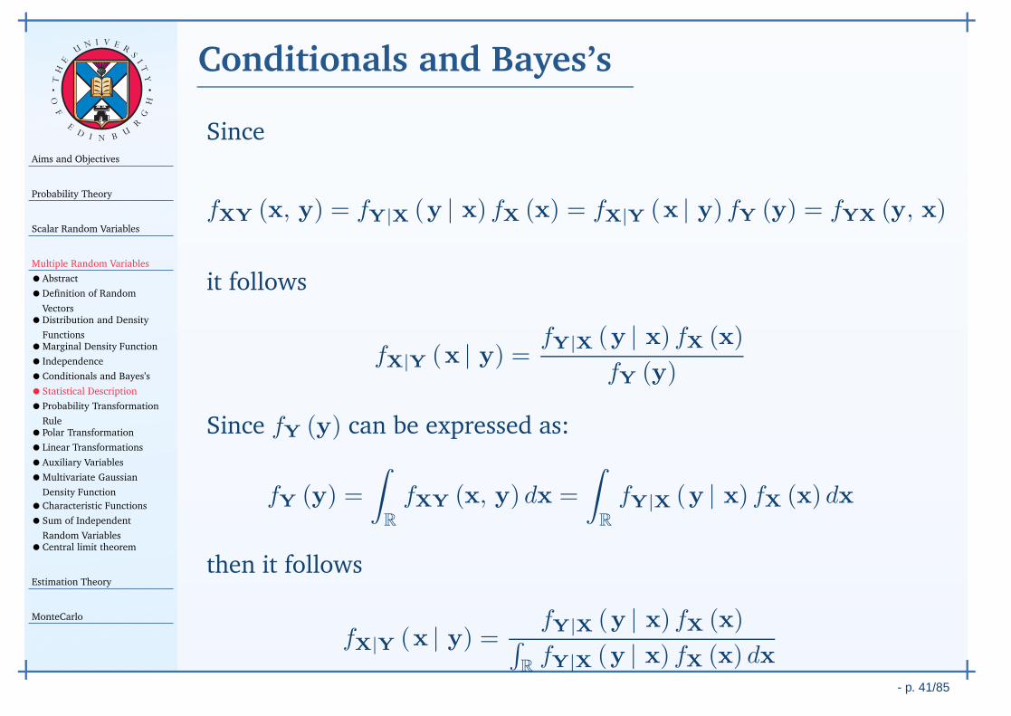
Since fY (y) can be expressed as:
fY (y) =
∫
R
fXY (x, y) dx =
∫
R
fY|X (y | x) fX (x) dx
then it follows
fX|Y (x | y) = fY|X (y | x) fX (x)∫
RfY|X (y | x) fX (x) dx
Aims and Objectives
Probability Theory
Scalar Random Variables
Multiple Random Variables
•Abstract
•Definition of Random
Vectors•Distribution and Density
Functions•Marginal Density Function
• Independence
•Conditionals and Bayes’s
•Statistical Description
•Probability Transformation
Rule•Polar Transformation
•Linear Transformations
•Auxiliary Variables
•Multivariate Gaussian
Density Function
•Characteristic Functions
•Sum of Independent
Random Variables•Central limit theorem
Estimation Theory
MonteCarlo
- p. 42/85
TH
E
UN I V E
RS
IT
Y
OF
ED
I N BU
R
GH
Statistical Description
Statistical averages are more manageable, but less of a completedescription of random vectors.
With care, it is possible to extend many of the statisticaldescriptors for scalar RVs to random vectors.
However, it is important to understand that multiple RVs leads tothe notion of measuring their interaction or dependence. Thisconcept is useful in abstract, but also when dealing withstochastic processes or time-series.
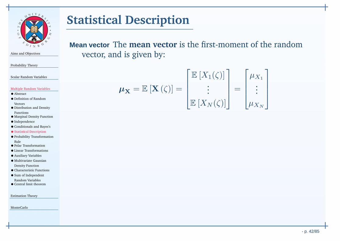
Aims and Objectives
Probability Theory
Scalar Random Variables
Multiple Random Variables
•Abstract
•Definition of Random
Vectors•Distribution and Density
Functions•Marginal Density Function
• Independence
•Conditionals and Bayes’s
•Statistical Description
•Probability Transformation
Rule•Polar Transformation
•Linear Transformations
•Auxiliary Variables
•Multivariate Gaussian
Density Function
•Characteristic Functions
•Sum of Independent
Random Variables•Central limit theorem
Estimation Theory
MonteCarlo
- p. 42/85
TH
E
UN I V E
RS
IT
Y
OF
ED
I N BU
R
GH
Statistical Description
Mean vector The mean vector is the first-moment of the randomvector, and is given by:
µX = E [X (ζ)] =
E [X1(ζ)]...
E [XN (ζ)]
=
µX1
...
µXN
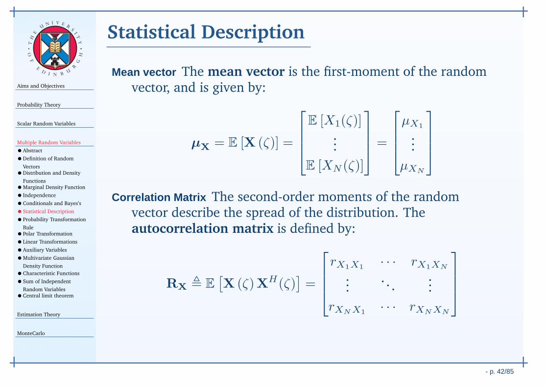
Correlation Matrix The second-order moments of the randomvector describe the spread of the distribution. Theautocorrelation matrix is defined by:
RX , E[X (ζ)XH(ζ)
]=
rX1X1 · · · rX1XN
.... . .
...
rXNX1 · · · rXNXN
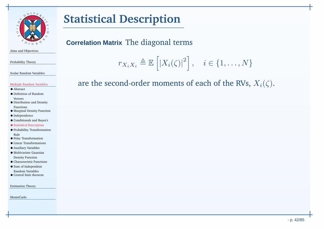
Aims and Objectives
Probability Theory
Scalar Random Variables
Multiple Random Variables
•Abstract
•Definition of Random
Vectors•Distribution and Density
Functions•Marginal Density Function
• Independence
•Conditionals and Bayes’s
•Statistical Description
•Probability Transformation
Rule•Polar Transformation
•Linear Transformations
•Auxiliary Variables
•Multivariate Gaussian
Density Function
•Characteristic Functions
•Sum of Independent
Random Variables•Central limit theorem
Estimation Theory
MonteCarlo
- p. 42/85
TH
E
UN I V E
RS
IT
Y
OF
ED
I N BU
R
GH
Statistical Description
Correlation Matrix The diagonal terms
rXiXi, E
[
|Xi(ζ)|2]
, i ∈ 1, . . . , N
are the second-order moments of each of the RVs, Xi(ζ).
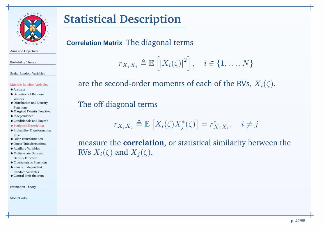
The off-diagonal terms
rXiXj, E
[Xi(ζ)X
∗j (ζ)
]= r∗XjXi
, i 6= j
measure the correlation, or statistical similarity between theRVs Xi(ζ) and Xj(ζ).
If the Xi(ζ) and Xj(ζ) are orthogonal then their correlationis zero:
rXiXj= E
[Xi(ζ)X
∗j (ζ)
]= 0, i 6= j
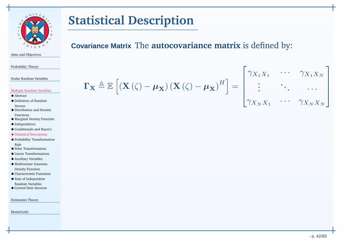
Aims and Objectives
Probability Theory
Scalar Random Variables
Multiple Random Variables
•Abstract
•Definition of Random
Vectors•Distribution and Density
Functions•Marginal Density Function
• Independence
•Conditionals and Bayes’s
•Statistical Description
•Probability Transformation
Rule•Polar Transformation
•Linear Transformations
•Auxiliary Variables
•Multivariate Gaussian
Density Function
•Characteristic Functions
•Sum of Independent
Random Variables•Central limit theorem
Estimation Theory
MonteCarlo
- p. 42/85
TH
E
UN I V E
RS
IT
Y
OF
ED
I N BU
R
GH
Statistical Description
Covariance Matrix The autocovariance matrix is defined by:
ΓX , E
[
(X (ζ)− µX) (X (ζ)− µX)H]
=
γX1X1 · · · γX1XN
.... . . · · ·
γXNX1 · · · γXNXN
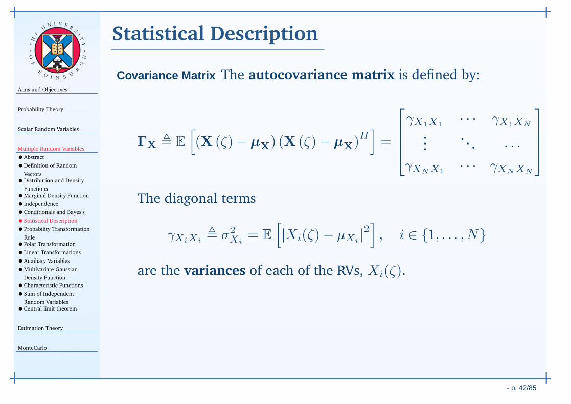
The diagonal terms
γXiXi, σ2
Xi= E
[
|Xi(ζ)− µXi|2]
, i ∈ 1, . . . , N
are the variances of each of the RVs, Xi(ζ).
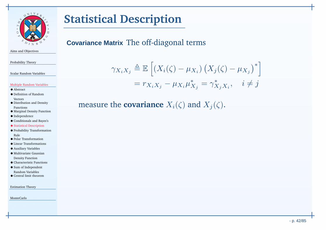
Aims and Objectives
Probability Theory
Scalar Random Variables
Multiple Random Variables
•Abstract
•Definition of Random
Vectors•Distribution and Density
Functions•Marginal Density Function
• Independence
•Conditionals and Bayes’s
•Statistical Description
•Probability Transformation
Rule•Polar Transformation
•Linear Transformations
•Auxiliary Variables
•Multivariate Gaussian
Density Function
•Characteristic Functions
•Sum of Independent
Random Variables•Central limit theorem
Estimation Theory
MonteCarlo
- p. 42/85
TH
E
UN I V E
RS
IT
Y
OF
ED
I N BU
R
GH
Statistical Description
Covariance Matrix The off-diagonal terms
γXiXj, E
[
(Xi(ζ)− µXi)(Xj(ζ)− µXj
)∗]
= rXiXj− µXi
µ∗Xj
= γ∗XjXi
, i 6= j
measure the covariance Xi(ζ) and Xj(ζ).
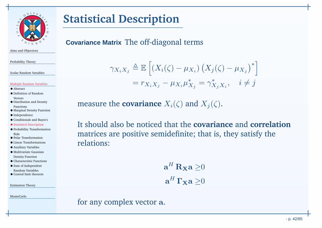
It should also be noticed that the covariance and correlationmatrices are positive semidefinite; that is, they satisfy therelations:
aH RXa ≥0
aH ΓXa ≥0
for any complex vector a.
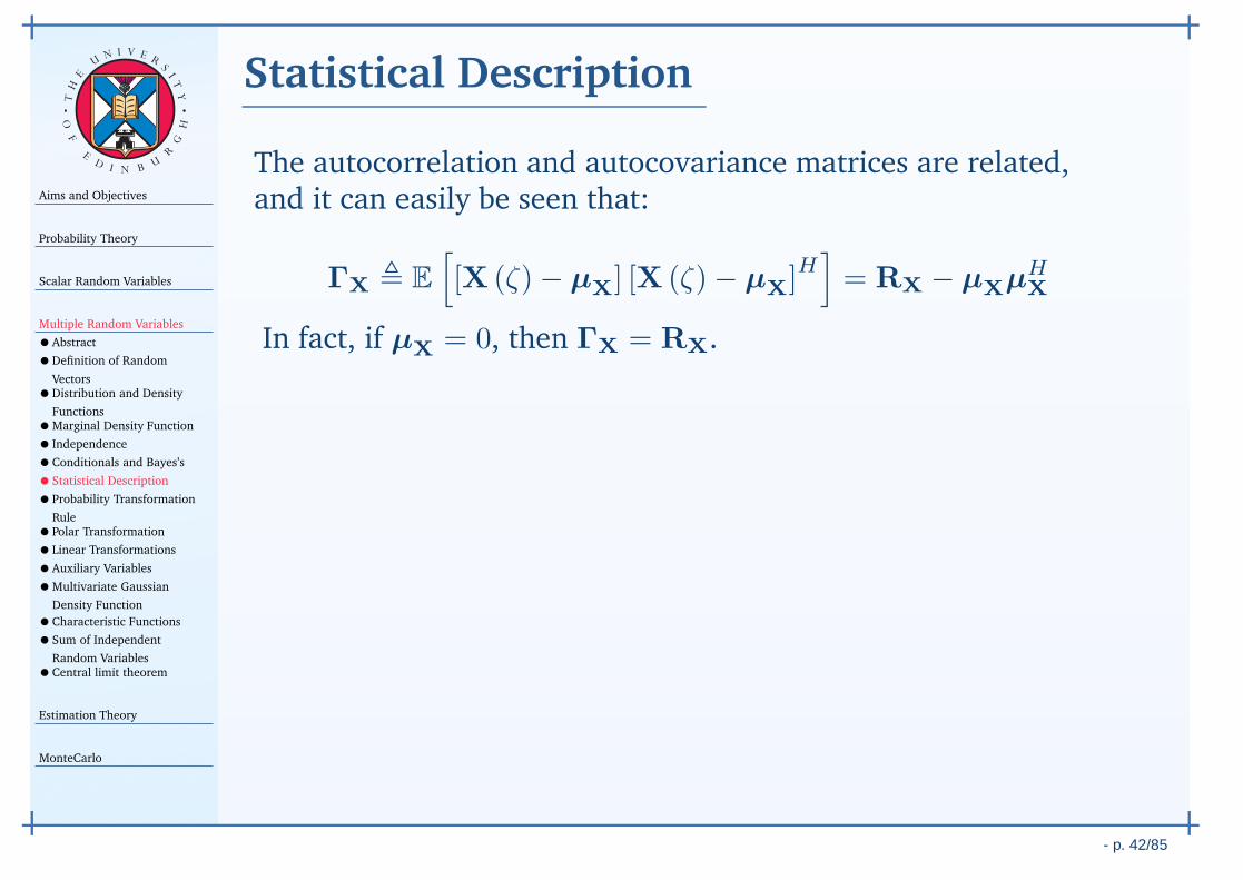
Aims and Objectives
Probability Theory
Scalar Random Variables
Multiple Random Variables
•Abstract
•Definition of Random
Vectors•Distribution and Density
Functions•Marginal Density Function
• Independence
•Conditionals and Bayes’s
•Statistical Description
•Probability Transformation
Rule•Polar Transformation
•Linear Transformations
•Auxiliary Variables
•Multivariate Gaussian
Density Function
•Characteristic Functions
•Sum of Independent
Random Variables•Central limit theorem
Estimation Theory
MonteCarlo
- p. 42/85
TH
E
UN I V E
RS
IT
Y
OF
ED
I N BU
R
GH
Statistical Description
The autocorrelation and autocovariance matrices are related,and it can easily be seen that:
ΓX , E
[
[X (ζ)− µX] [X (ζ)− µX]H]
= RX − µXµHX
In fact, if µX = 0, then ΓX = RX.
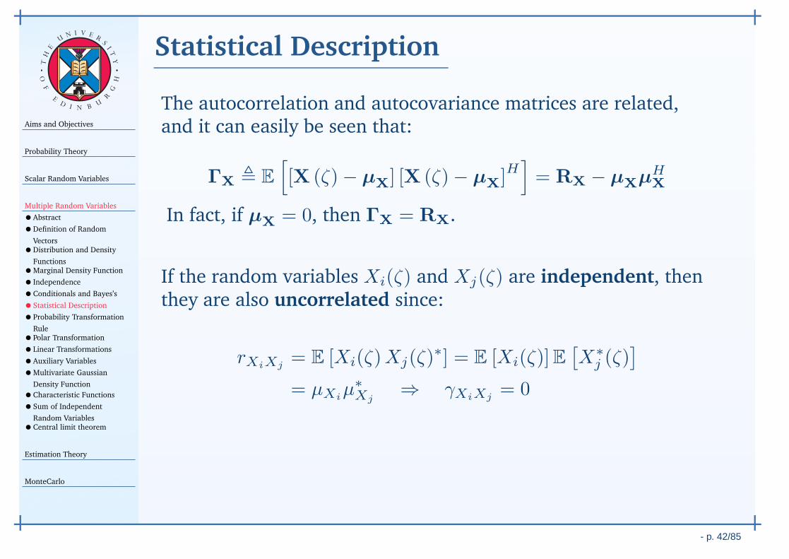
If the random variables Xi(ζ) and Xj(ζ) are independent, thenthey are also uncorrelated since:
rXiXj= E [Xi(ζ)Xj(ζ)
∗] = E [Xi(ζ)]E[X∗
j (ζ)]
= µXiµ∗Xj
⇒ γXiXj= 0
Note, however, that uncorrelatedness does not implyindependence, unless the RVs are jointly-Gaussian.
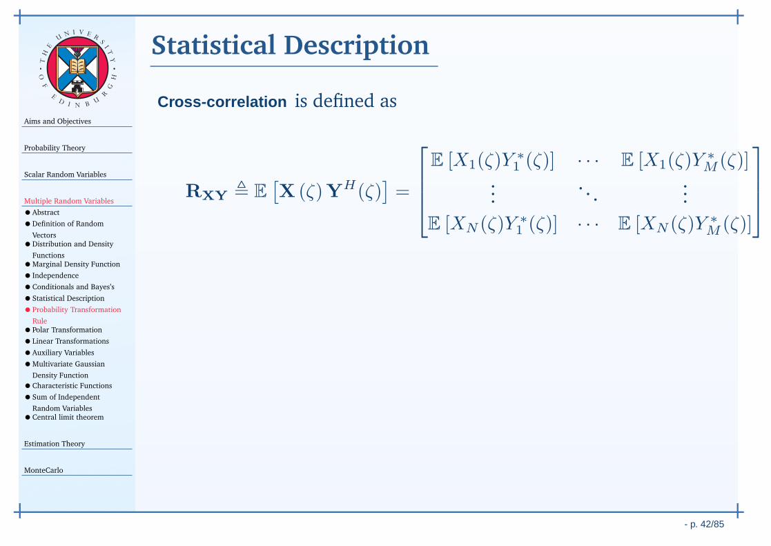
Aims and Objectives
Probability Theory
Scalar Random Variables
Multiple Random Variables
•Abstract
•Definition of Random
Vectors•Distribution and Density
Functions•Marginal Density Function
• Independence
•Conditionals and Bayes’s
•Statistical Description
•Probability Transformation
Rule•Polar Transformation
•Linear Transformations
•Auxiliary Variables
•Multivariate Gaussian
Density Function
•Characteristic Functions
•Sum of Independent
Random Variables•Central limit theorem
Estimation Theory
MonteCarlo
- p. 42/85
TH
E
UN I V E
RS
IT
Y
OF
ED
I N BU
R
GH
Statistical Description
Cross-correlation is defined as
RXY , E[X (ζ)YH(ζ)
]=
E [X1(ζ)Y∗1 (ζ)] · · · E [X1(ζ)Y
∗M (ζ)]
.... . .
...
E [XN (ζ)Y ∗1 (ζ)] · · · E [XN (ζ)Y ∗
M (ζ)]
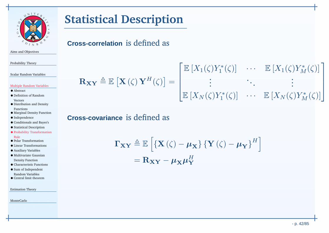
Cross-covariance is defined as
ΓXY , E
[
X (ζ)− µX Y (ζ)− µYH]
= RXY − µXµHY
Uncorrelated if ΓXY = 0 ⇒ RXY = µXµHY.
Orthogonal if RXY = 0.
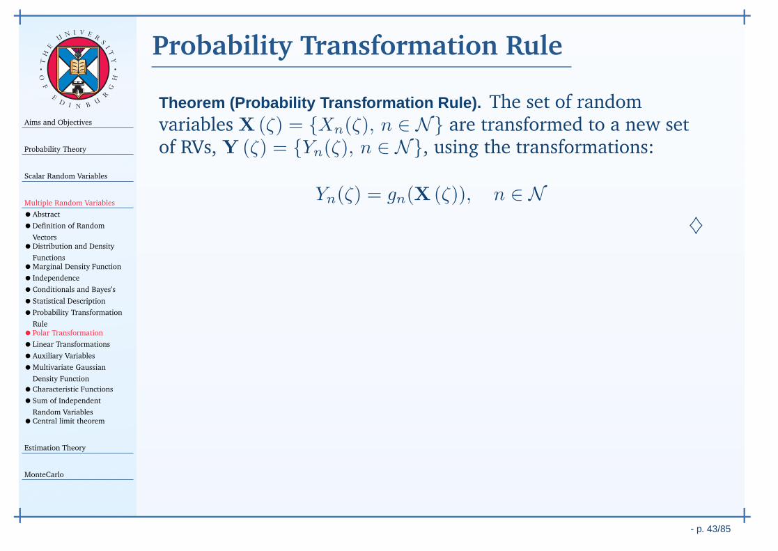
Aims and Objectives
Probability Theory
Scalar Random Variables
Multiple Random Variables
•Abstract
•Definition of Random
Vectors•Distribution and Density
Functions•Marginal Density Function
• Independence
•Conditionals and Bayes’s
•Statistical Description
•Probability Transformation
Rule•Polar Transformation
•Linear Transformations
•Auxiliary Variables
•Multivariate Gaussian
Density Function
•Characteristic Functions
•Sum of Independent
Random Variables•Central limit theorem
Estimation Theory
MonteCarlo
- p. 43/85
TH
E
UN I V E
RS
IT
Y
OF
ED
I N BU
R
GH
Probability Transformation Rule
Theorem (Probability Transformation Rule). The set of randomvariables X (ζ) = Xn(ζ), n ∈ N are transformed to a new setof RVs, Y (ζ) = Yn(ζ), n ∈ N, using the transformations:
Yn(ζ) = gn(X (ζ)), n ∈ N♦
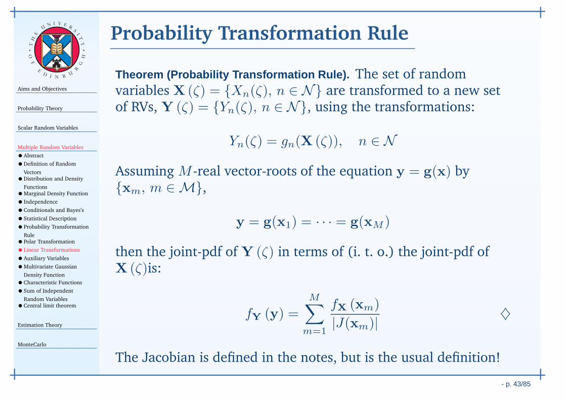
Aims and Objectives
Probability Theory
Scalar Random Variables
Multiple Random Variables
•Abstract
•Definition of Random
Vectors•Distribution and Density
Functions•Marginal Density Function
• Independence
•Conditionals and Bayes’s
•Statistical Description
•Probability Transformation
Rule•Polar Transformation
•Linear Transformations
•Auxiliary Variables
•Multivariate Gaussian
Density Function
•Characteristic Functions
•Sum of Independent
Random Variables•Central limit theorem
Estimation Theory
MonteCarlo
- p. 43/85
TH
E
UN I V E
RS
IT
Y
OF
ED
I N BU
R
GH
Probability Transformation Rule
Theorem (Probability Transformation Rule). The set of randomvariables X (ζ) = Xn(ζ), n ∈ N are transformed to a new setof RVs, Y (ζ) = Yn(ζ), n ∈ N, using the transformations:
Yn(ζ) = gn(X (ζ)), n ∈ N
Assuming M -real vector-roots of the equation y = g(x) byxm, m ∈ M,
y = g(x1) = · · · = g(xM )
then the joint-pdf of Y (ζ) in terms of (i. t. o.) the joint-pdf ofX (ζ)is:
fY (y) =M∑
m=1
fX (xm)
|J(xm)| ♦
The Jacobian is defined in the notes, but is the usual definition!
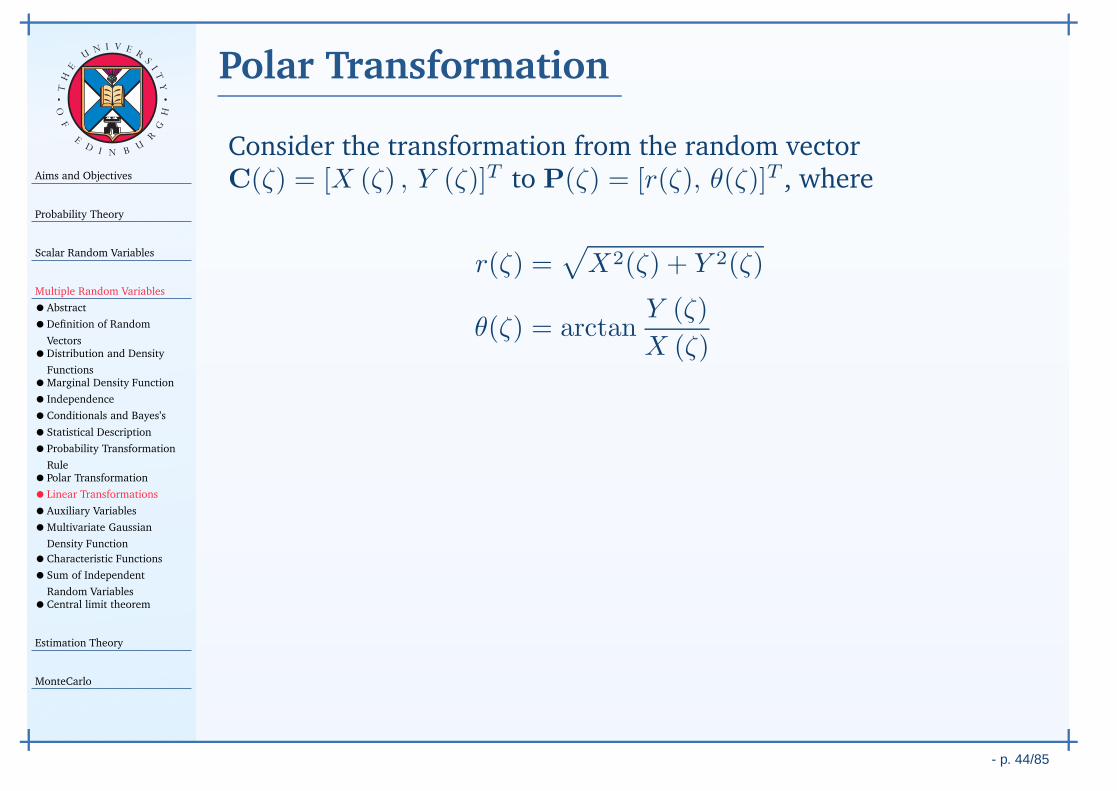
Aims and Objectives
Probability Theory
Scalar Random Variables
Multiple Random Variables
•Abstract
•Definition of Random
Vectors•Distribution and Density
Functions•Marginal Density Function
• Independence
•Conditionals and Bayes’s
•Statistical Description
•Probability Transformation
Rule•Polar Transformation
•Linear Transformations
•Auxiliary Variables
•Multivariate Gaussian
Density Function
•Characteristic Functions
•Sum of Independent
Random Variables•Central limit theorem
Estimation Theory
MonteCarlo
- p. 44/85
TH
E
UN I V E
RS
IT
Y
OF
ED
I N BU
R
GH
Polar Transformation
Consider the transformation from the random vectorC(ζ) = [X (ζ) , Y (ζ)]T to P(ζ) = [r(ζ), θ(ζ)]T , where
r(ζ) =√
X2(ζ) + Y 2(ζ)
θ(ζ) = arctanY (ζ)
X (ζ)
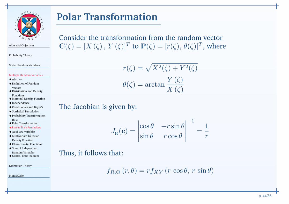
The Jacobian is given by:
Jg(c) =
∣∣∣∣∣
cos θ −r sin θ
sin θ r cos θ
∣∣∣∣∣
−1
=1
r
Thus, it follows that:
fR,Θ (r, θ) = rfXY (r cos θ, r sin θ)
Aims and Objectives
Probability Theory
Scalar Random Variables
Multiple Random Variables
•Abstract
•Definition of Random
Vectors•Distribution and Density
Functions•Marginal Density Function
• Independence
•Conditionals and Bayes’s
•Statistical Description
•Probability Transformation
Rule•Polar Transformation
•Linear Transformations
•Auxiliary Variables
•Multivariate Gaussian
Density Function
•Characteristic Functions
•Sum of Independent
Random Variables•Central limit theorem
Estimation Theory
MonteCarlo
- p. 45/85
TH
E
UN I V E
RS
IT
Y
OF
ED
I N BU
R
GH
Linear Transformations
Since linear systems represent such an important class if signalprocessing systems, it is important to consider lineartransformations of random vectors.
Thus, consider a random vector Y (ζ) defined by a lineartransformation of the random vector X (ζ) through the matrixA:
Y (ζ) = AX (ζ)
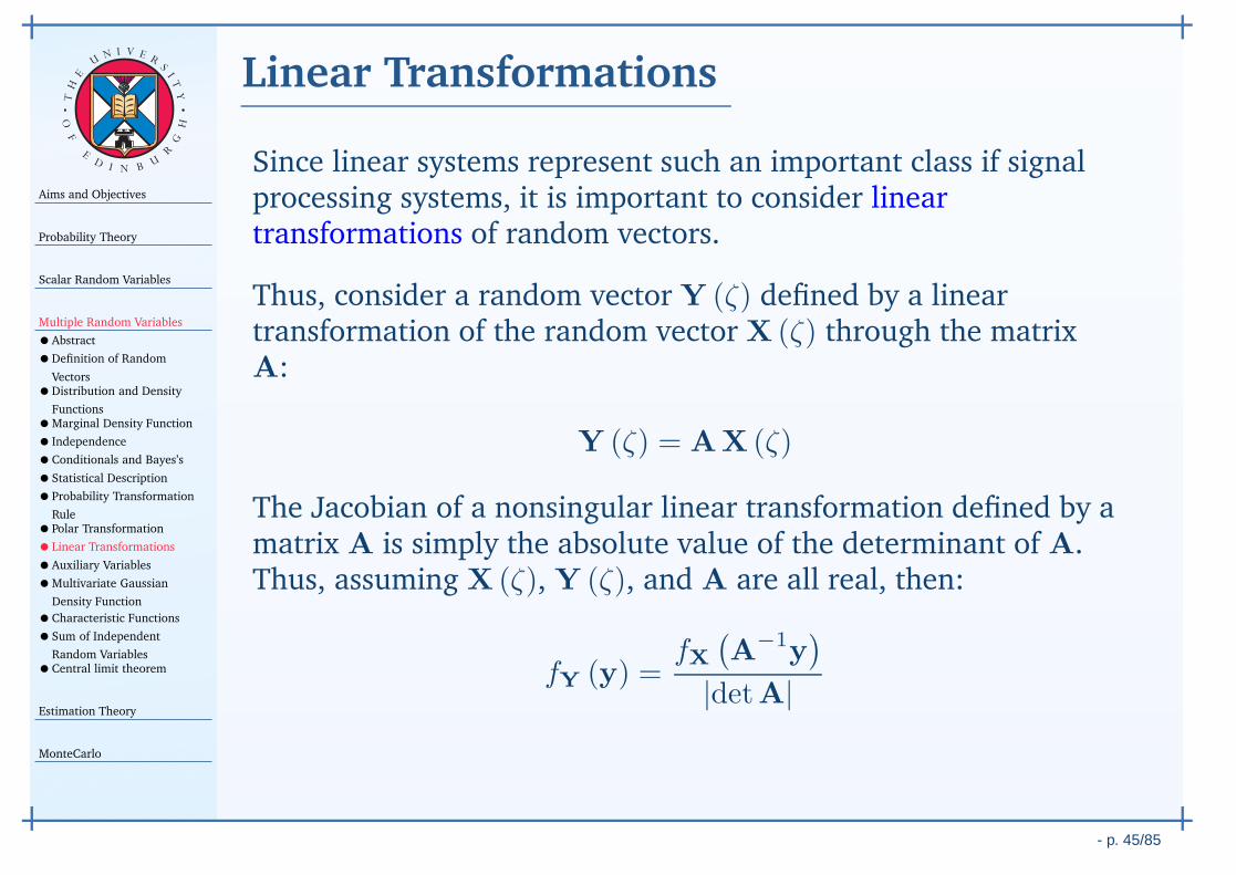
The Jacobian of a nonsingular linear transformation defined by amatrix A is simply the absolute value of the determinant of A.Thus, assuming X (ζ), Y (ζ), and A are all real, then:
fY (y) =fX
(A−1y
)
|detA|
Aims and Objectives
Probability Theory
Scalar Random Variables
Multiple Random Variables
•Abstract
•Definition of Random
Vectors•Distribution and Density
Functions•Marginal Density Function
• Independence
•Conditionals and Bayes’s
•Statistical Description
•Probability Transformation
Rule•Polar Transformation
•Linear Transformations
•Auxiliary Variables
•Multivariate Gaussian
Density Function
•Characteristic Functions
•Sum of Independent
Random Variables•Central limit theorem
Estimation Theory
MonteCarlo
- p. 45/85
TH
E
UN I V E
RS
IT
Y
OF
ED
I N BU
R
GH
Linear Transformations
In general, determining fY (y) is a laborious exercise, except inthe case of Gaussian random vectors.
In practice, however, the knowledge of µY, ΓY, ΓXY or ΓYX issufficient information for many algorithms.
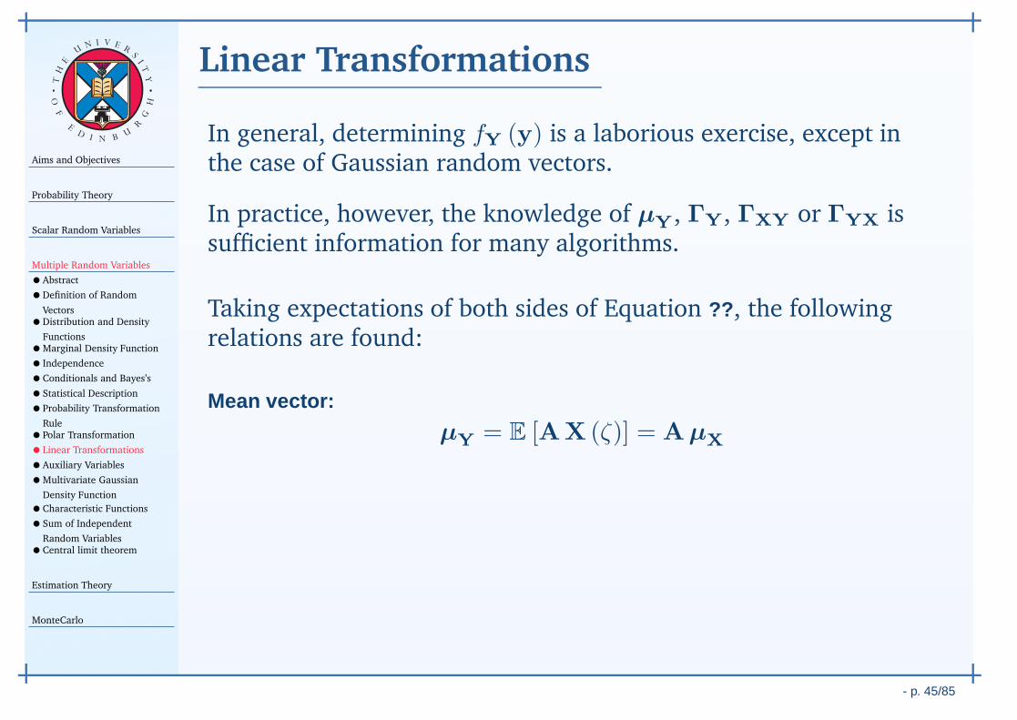
Taking expectations of both sides of Equation ??, the followingrelations are found:
Mean vector:
µY = E [AX (ζ)] = AµX
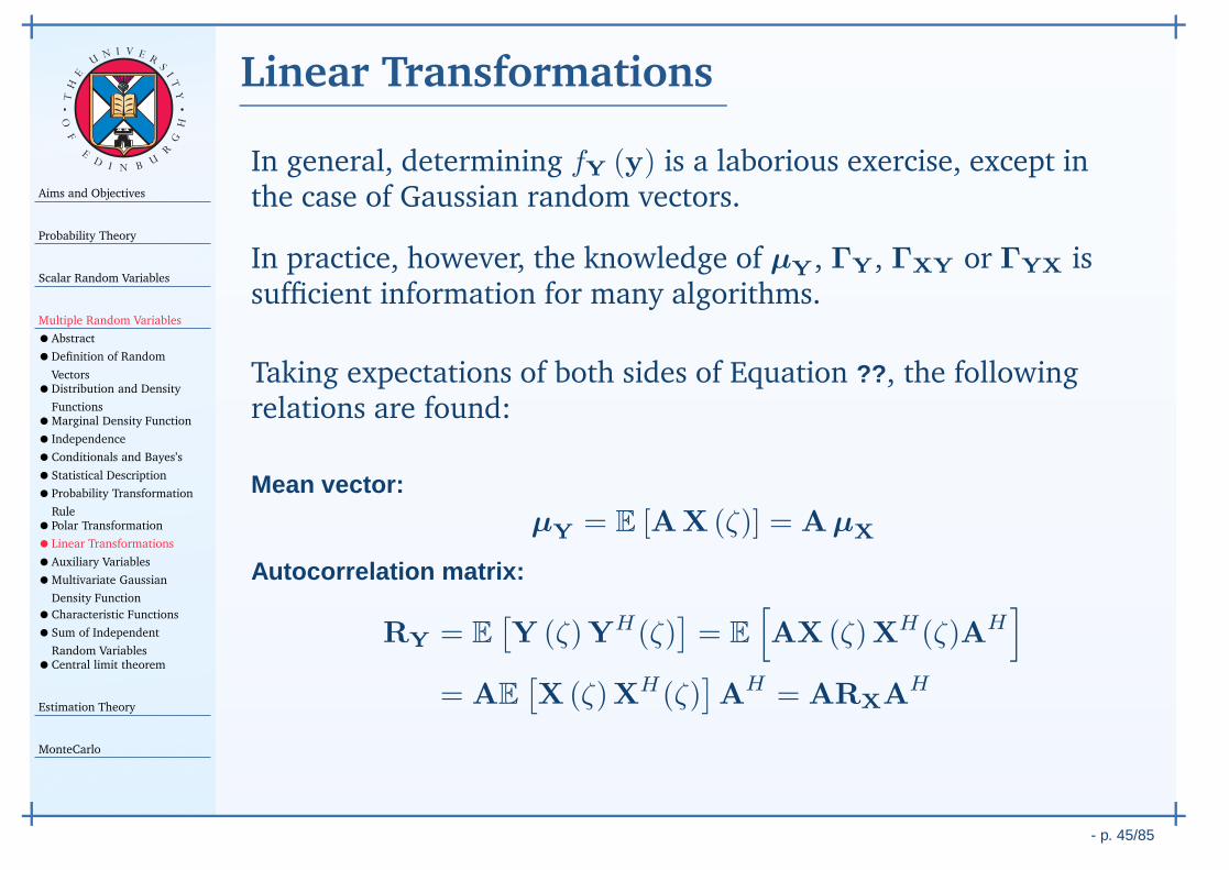
Autocorrelation matrix:
RY = E[Y (ζ)YH(ζ)
]= E
[
AX (ζ)XH(ζ)AH]
= AE[X (ζ)XH(ζ)
]AH = ARXAH
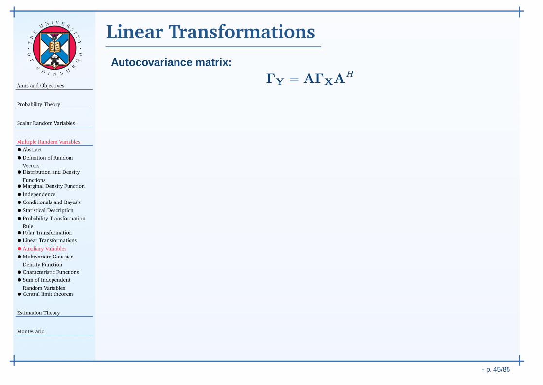
Aims and Objectives
Probability Theory
Scalar Random Variables
Multiple Random Variables
•Abstract
•Definition of Random
Vectors•Distribution and Density
Functions•Marginal Density Function
• Independence
•Conditionals and Bayes’s
•Statistical Description
•Probability Transformation
Rule•Polar Transformation
•Linear Transformations
•Auxiliary Variables
•Multivariate Gaussian
Density Function
•Characteristic Functions
•Sum of Independent
Random Variables•Central limit theorem
Estimation Theory
MonteCarlo
- p. 45/85
TH
E
UN I V E
RS
IT
Y
OF
ED
I N BU
R
GH
Linear Transformations
Autocovariance matrix:
ΓY = AΓXAH
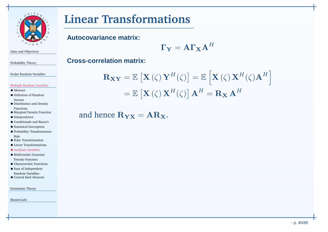
Cross-correlation matrix:
RXY = E[X (ζ)YH(ζ)
]= E
[
X (ζ)XH(ζ)AH]
= E[X (ζ)XH(ζ)
]AH = RX AH
and hence RYX = ARX.
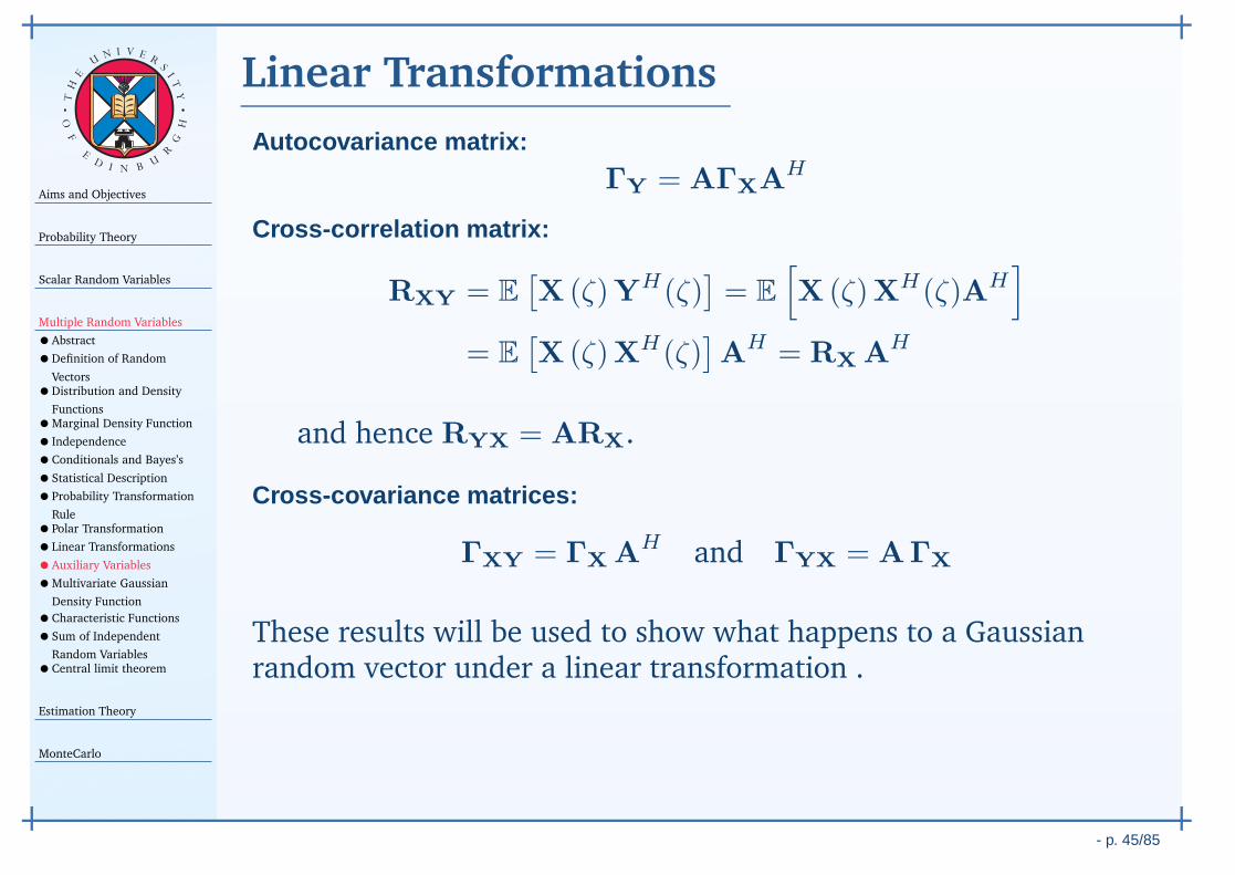
Cross-covariance matrices:
ΓXY = ΓX AH and ΓYX = AΓX
These results will be used to show what happens to a Gaussianrandom vector under a linear transformation .
Aims and Objectives
Probability Theory
Scalar Random Variables
Multiple Random Variables
•Abstract
•Definition of Random
Vectors•Distribution and Density
Functions•Marginal Density Function
• Independence
•Conditionals and Bayes’s
•Statistical Description
•Probability Transformation
Rule•Polar Transformation
•Linear Transformations
•Auxiliary Variables
•Multivariate Gaussian
Density Function
•Characteristic Functions
•Sum of Independent
Random Variables•Central limit theorem
Estimation Theory
MonteCarlo
- p. 46/85
TH
E
UN I V E
RS
IT
Y
OF
ED
I N BU
R
GH
Auxiliary Variables
The density of a RV that is one function Z(ζ) = g(X (ζ) , Y (ζ))of two RVs can be determined by choosing a auxiliary variable.
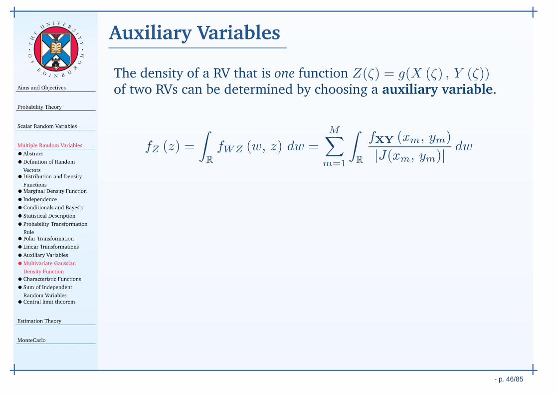
fZ (z) =
∫
R
fWZ (w, z) dw =M∑
m=1
∫
R
fXY (xm, ym)
|J(xm, ym)| dw
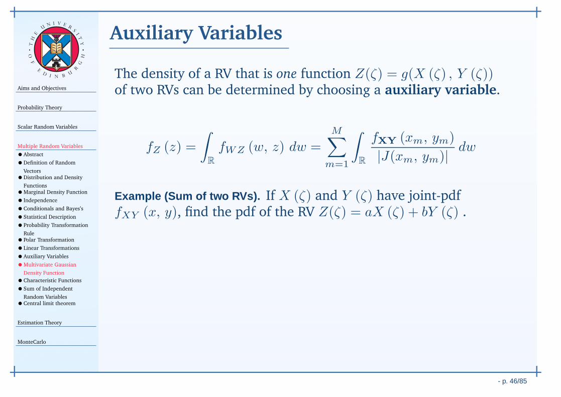
Example (Sum of two RVs). If X (ζ) and Y (ζ) have joint-pdffXY (x, y), find the pdf of the RV Z(ζ) = aX (ζ) + bY (ζ) .
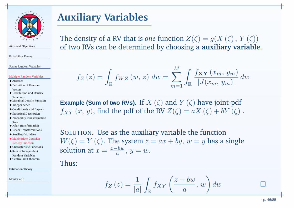
SOLUTION. Use as the auxiliary variable the functionW (ζ) = Y (ζ). The system z = ax+ by, w = y has a single
solution at x = z−bwa
, y = w.
Thus:
fZ (z) =1
|a|
∫
R
fXY
(z − bw
a, w
)
dw
Aims and Objectives
Probability Theory
Scalar Random Variables
Multiple Random Variables
•Abstract
•Definition of Random
Vectors•Distribution and Density
Functions•Marginal Density Function
• Independence
•Conditionals and Bayes’s
•Statistical Description
•Probability Transformation
Rule•Polar Transformation
•Linear Transformations
•Auxiliary Variables
•Multivariate Gaussian
Density Function
•Characteristic Functions
•Sum of Independent
Random Variables•Central limit theorem
Estimation Theory
MonteCarlo
- p. 47/85
TH
E
UN I V E
RS
IT
Y
OF
ED
I N BU
R
GH
Multivariate Gaussian Density Function
Gaussian random vectors play a very important role in the designand analysis of signal processing systems. A Gaussian randomvector is characterised by a multivariate Normal or Gaussiandensity function.
For a real random vector, this density function has the form:
fX (x) =1
(2π)N2 |ΓX| 12
exp
[
−1
2(x− µX)T Γ−1
X (x− µX)
]
where N is the dimension of X (ζ), and X (ζ) has mean µX andcovariance ΓX. It is often denoted as:
fX (x) = N(x∣∣µX, ΓX
)
Aims and Objectives
Probability Theory
Scalar Random Variables
Multiple Random Variables
•Abstract
•Definition of Random
Vectors•Distribution and Density
Functions•Marginal Density Function
• Independence
•Conditionals and Bayes’s
•Statistical Description
•Probability Transformation
Rule•Polar Transformation
•Linear Transformations
•Auxiliary Variables
•Multivariate Gaussian
Density Function
•Characteristic Functions
•Sum of Independent
Random Variables•Central limit theorem
Estimation Theory
MonteCarlo
- p. 47/85
TH
E
UN I V E
RS
IT
Y
OF
ED
I N BU
R
GH
Multivariate Gaussian Density Function
The normal distribution is a useful model of a random vectorbecause of its many important properties.
1. fX (x) = N(x∣∣µX, ΓX
)is completely specified by its mean
µX and covariance ΓX.
2. If the components of X (ζ) are mutually uncorrelated, thenthey are also independent.
3. A linear transformation of a normal random vector is alsonormal.
This is a particularly useful, since the output of a linear systemsubject to a Gaussian input is also Gaussian.
4. If X (ζ) and Y (ζ) are jointly-Gaussian, then so are theirmarginal-distributions, and their conditional-distributions.
Aims and Objectives
Probability Theory
Scalar Random Variables
Multiple Random Variables
•Abstract
•Definition of Random
Vectors•Distribution and Density
Functions•Marginal Density Function
• Independence
•Conditionals and Bayes’s
•Statistical Description
•Probability Transformation
Rule•Polar Transformation
•Linear Transformations
•Auxiliary Variables
•Multivariate Gaussian
Density Function
•Characteristic Functions
•Sum of Independent
Random Variables•Central limit theorem
Estimation Theory
MonteCarlo
- p. 48/85
TH
E
UN I V E
RS
IT
Y
OF
ED
I N BU
R
GH
Characteristic Functions
The characteristic function and moment generating functionfor a scalar random variable can be extended to deal withrandom vectors. Essentially, these are defined as themulti-dimensional Fourier transform of the joint-pdf.
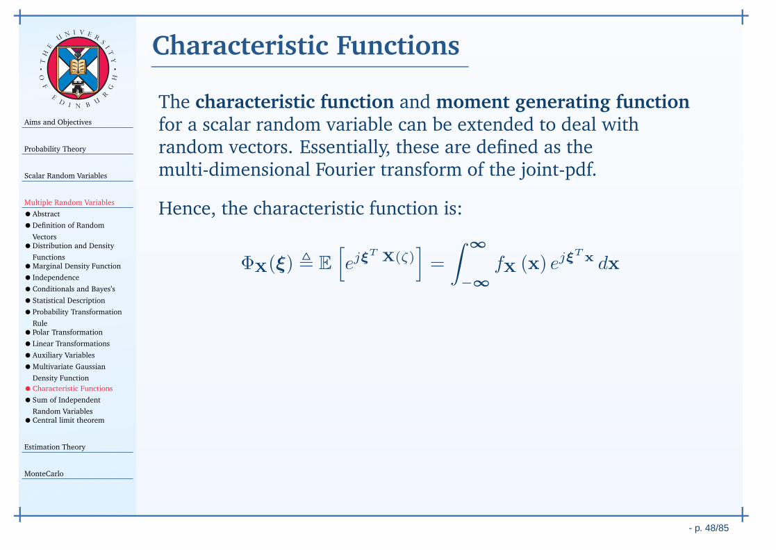
Hence, the characteristic function is:
ΦX(ξ) , E
[
ejξT X(ζ)
]
=
∫∞
−∞
fX (x) ejξTx dx
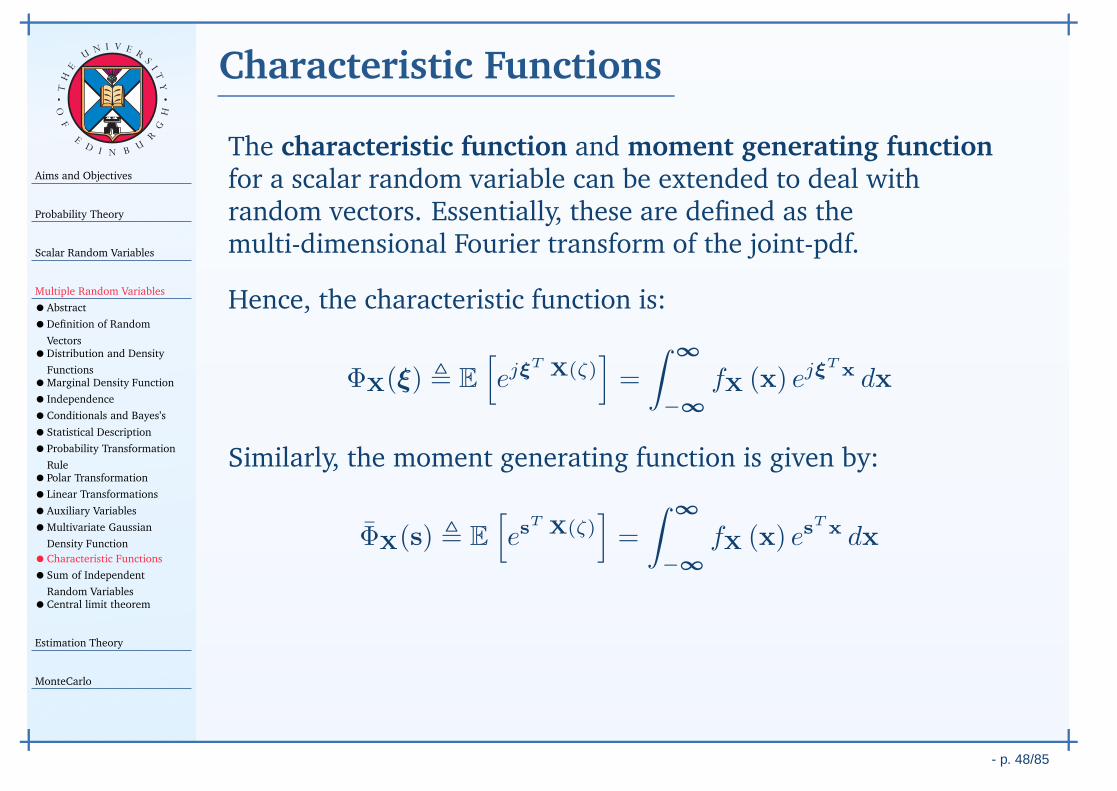
Similarly, the moment generating function is given by:
ΦX(s) , E
[
esT X(ζ)
]
=
∫∞
−∞
fX (x) esTx dx

Aims and Objectives
Probability Theory
Scalar Random Variables
Multiple Random Variables
•Abstract
•Definition of Random
Vectors•Distribution and Density
Functions•Marginal Density Function
• Independence
•Conditionals and Bayes’s
•Statistical Description
•Probability Transformation
Rule•Polar Transformation
•Linear Transformations
•Auxiliary Variables
•Multivariate Gaussian
Density Function
•Characteristic Functions
•Sum of Independent
Random Variables•Central limit theorem
Estimation Theory
MonteCarlo
- p. 48/85
TH
E
UN I V E
RS
IT
Y
OF
ED
I N BU
R
GH
Characteristic Functions
The characteristic function for a Gaussian random vector is
ΦX(ξ) =
∫∞
−∞
fX (x) ejξTx dx
=1
(2π)N2 |ΓX| 12
∫∞
−∞
exp
[
−1
2(x− µX)
TΓ−1X (x− µX)
]
ejξTx dx
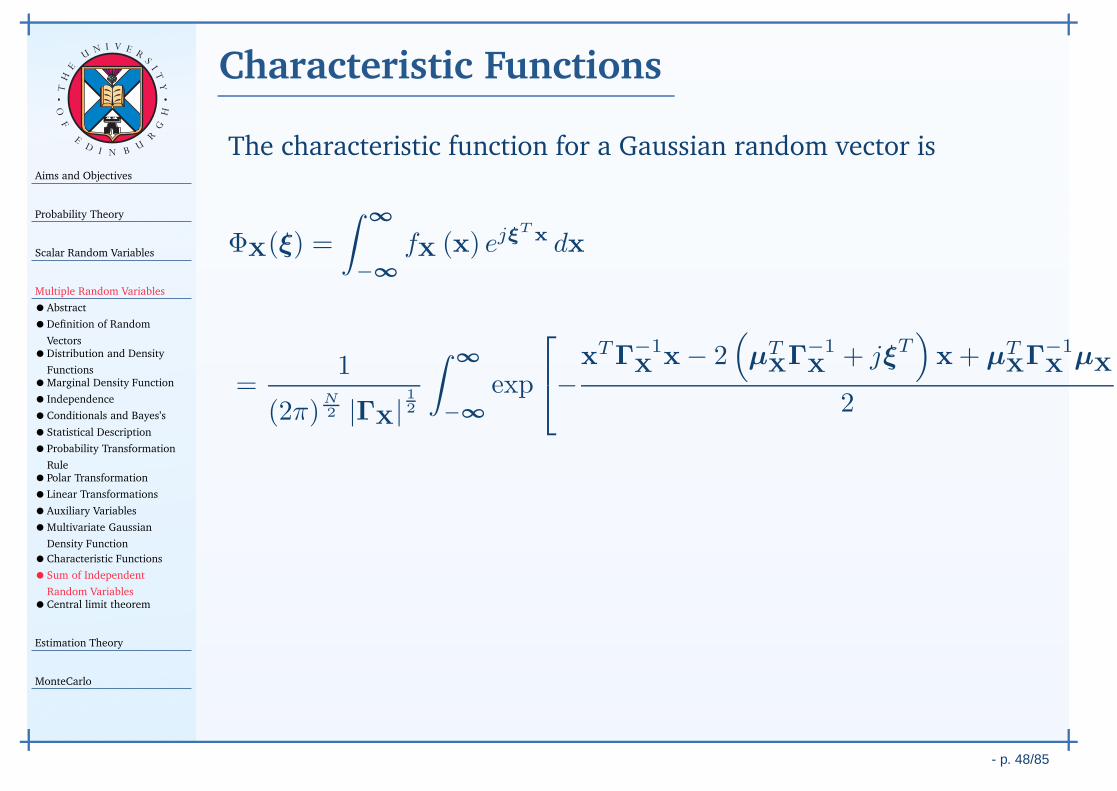
Aims and Objectives
Probability Theory
Scalar Random Variables
Multiple Random Variables
•Abstract
•Definition of Random
Vectors•Distribution and Density
Functions•Marginal Density Function
• Independence
•Conditionals and Bayes’s
•Statistical Description
•Probability Transformation
Rule•Polar Transformation
•Linear Transformations
•Auxiliary Variables
•Multivariate Gaussian
Density Function
•Characteristic Functions
•Sum of Independent
Random Variables•Central limit theorem
Estimation Theory
MonteCarlo
- p. 48/85
TH
E
UN I V E
RS
IT
Y
OF
ED
I N BU
R
GH
Characteristic Functions
The characteristic function for a Gaussian random vector is
ΦX(ξ) =
∫∞
−∞
fX (x) ejξTx dx
=1
(2π)N2 |ΓX| 12
∫∞
−∞
exp
−xTΓ−1
X x− 2(
µTXΓ−1
X + jξT)
x+ µTXΓ−1
X µX
2
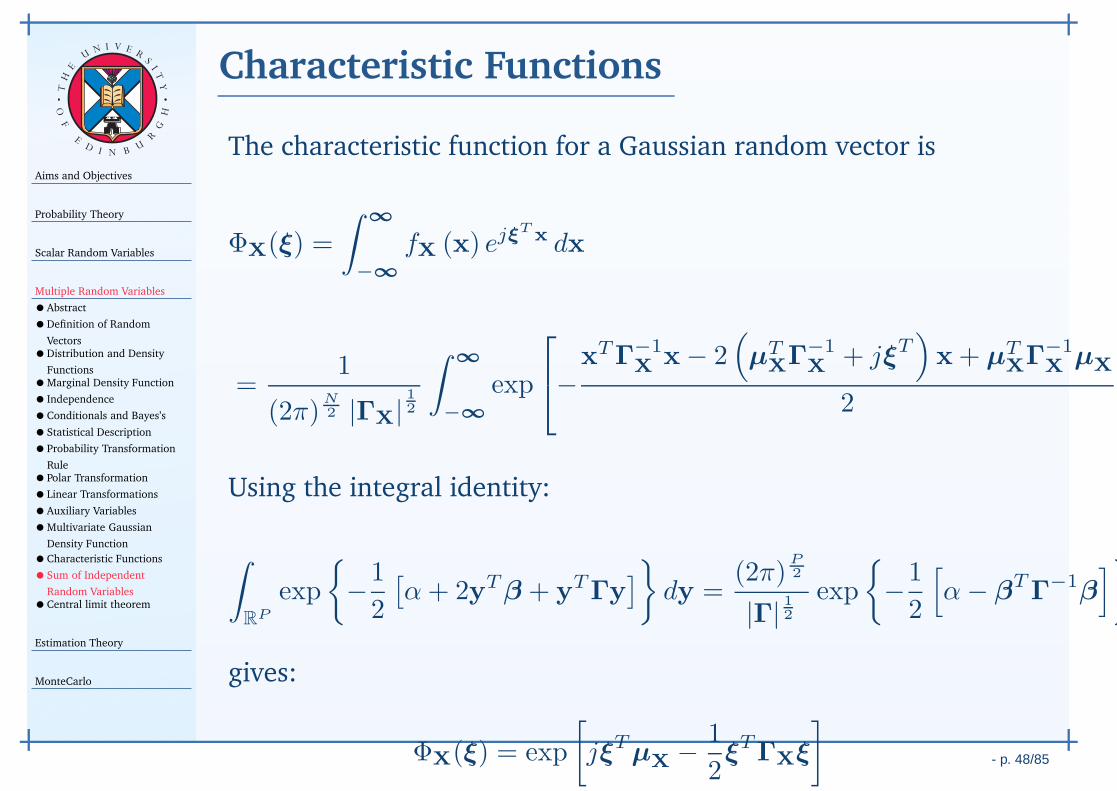
Using the integral identity:
∫
RP
exp
−1
2
[α+ 2yTβ + yTΓy
]
dy =(2π)
P2
|Γ| 12exp
−1
2
[
α− βTΓ−1β]
gives:
ΦX(ξ) = exp
[
jξTµX − 1
2ξTΓXξ
]
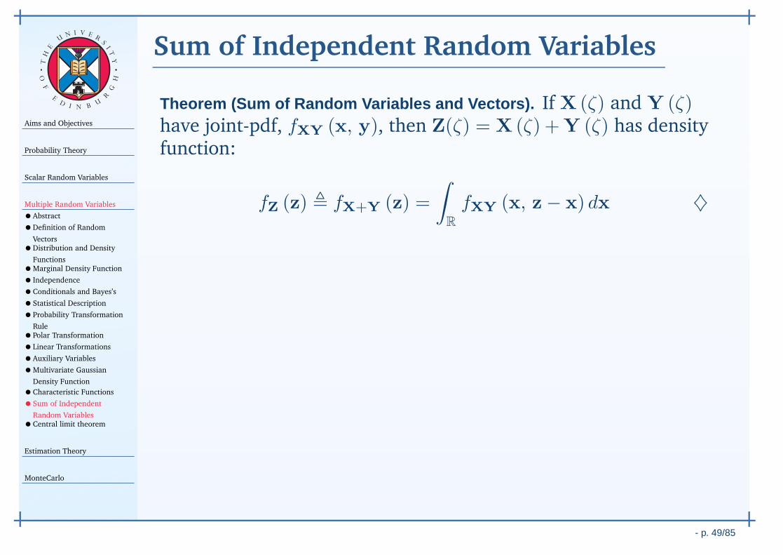
Aims and Objectives
Probability Theory
Scalar Random Variables
Multiple Random Variables
•Abstract
•Definition of Random
Vectors•Distribution and Density
Functions•Marginal Density Function
• Independence
•Conditionals and Bayes’s
•Statistical Description
•Probability Transformation
Rule•Polar Transformation
•Linear Transformations
•Auxiliary Variables
•Multivariate Gaussian
Density Function
•Characteristic Functions
•Sum of Independent
Random Variables•Central limit theorem
Estimation Theory
MonteCarlo
- p. 49/85
TH
E
UN I V E
RS
IT
Y
OF
ED
I N BU
R
GH
Sum of Independent Random Variables
Theorem (Sum of Random Variables and Vectors). If X (ζ) and Y (ζ)have joint-pdf, fXY (x, y), then Z(ζ) = X (ζ) +Y (ζ) has densityfunction:
fZ (z) , fX+Y (z) =
∫
R
fXY (x, z− x) dx ♦
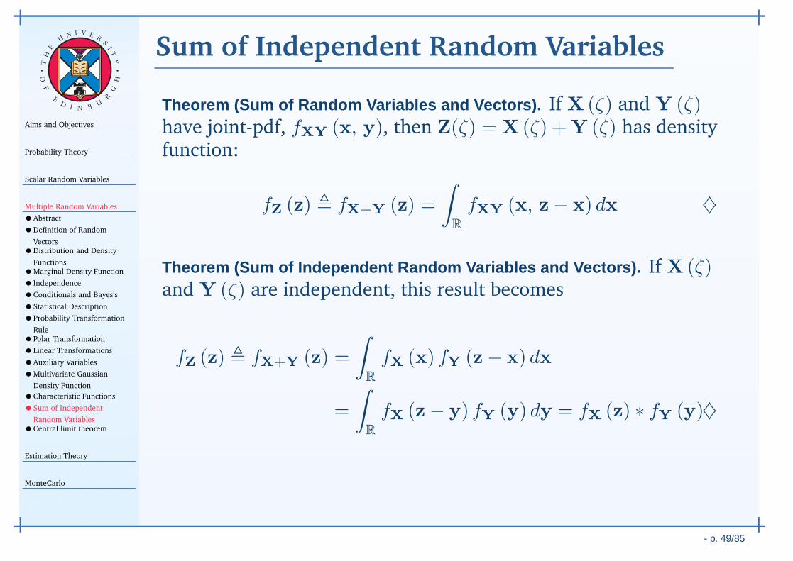
Theorem (Sum of Independent Random Variables and Vectors). If X (ζ)and Y (ζ) are independent, this result becomes
fZ (z) , fX+Y (z) =
∫
R
fX (x) fY (z− x) dx
=
∫
R
fX (z− y) fY (y) dy = fX (z) ∗ fY (y)♦
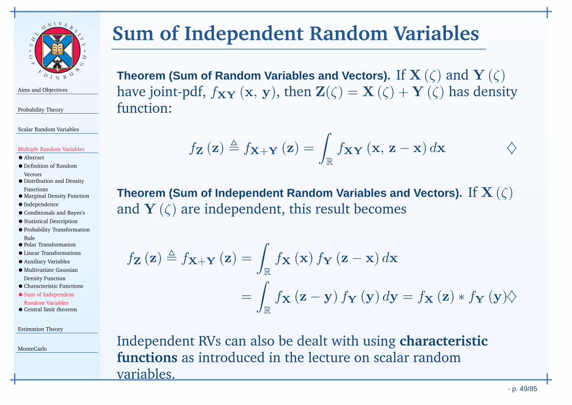
Independent RVs can also be dealt with using characteristicfunctions as introduced in the lecture on scalar randomvariables.
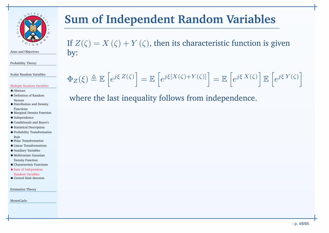
Aims and Objectives
Probability Theory
Scalar Random Variables
Multiple Random Variables
•Abstract
•Definition of Random
Vectors•Distribution and Density
Functions•Marginal Density Function
• Independence
•Conditionals and Bayes’s
•Statistical Description
•Probability Transformation
Rule•Polar Transformation
•Linear Transformations
•Auxiliary Variables
•Multivariate Gaussian
Density Function
•Characteristic Functions
•Sum of Independent
Random Variables•Central limit theorem
Estimation Theory
MonteCarlo
- p. 49/85
TH
E
UN I V E
RS
IT
Y
OF
ED
I N BU
R
GH
Sum of Independent Random Variables
If Z(ζ) = X (ζ) + Y (ζ), then its characteristic function is givenby:
ΦZ(ξ) , E
[
ejξ Z(ζ)]
= E
[
ejξ[X(ζ)+Y (ζ)]]
= E
[
ejξ X(ζ)]
E
[
ejξ Y (ζ)]
where the last inequality follows from independence.
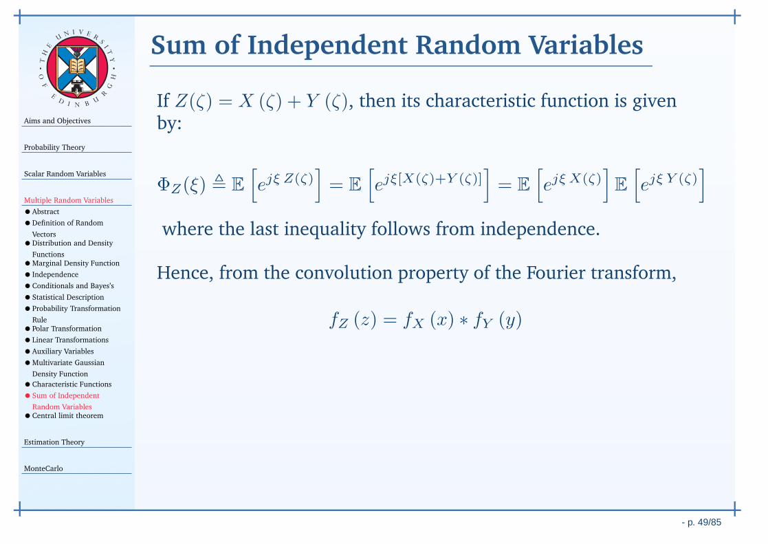
Hence, from the convolution property of the Fourier transform,
fZ (z) = fX (x) ∗ fY (y)
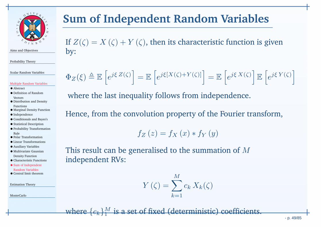
This result can be generalised to the summation of Mindependent RVs:
Y (ζ) =M∑
k=1
ck Xk(ζ)
where ckM1 is a set of fixed (deterministic) coefficients.
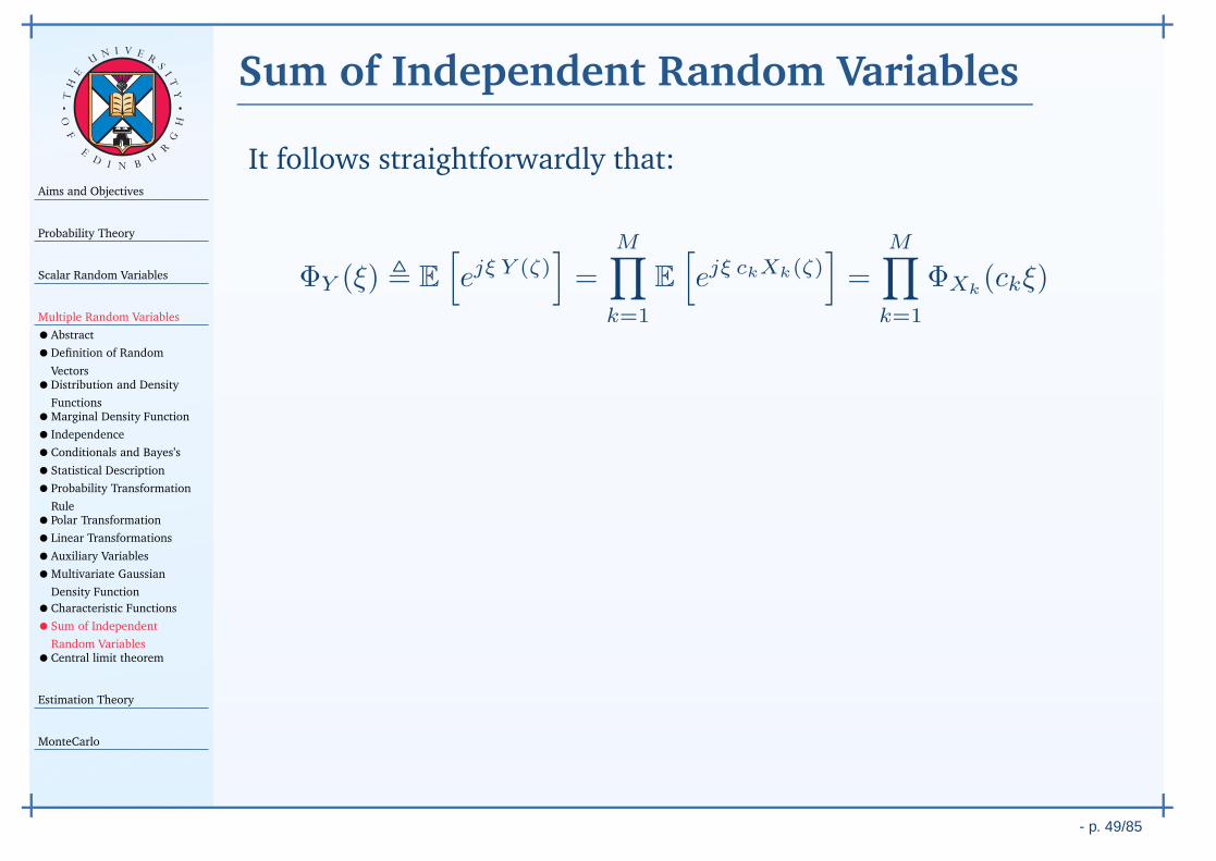
Aims and Objectives
Probability Theory
Scalar Random Variables
Multiple Random Variables
•Abstract
•Definition of Random
Vectors•Distribution and Density
Functions•Marginal Density Function
• Independence
•Conditionals and Bayes’s
•Statistical Description
•Probability Transformation
Rule•Polar Transformation
•Linear Transformations
•Auxiliary Variables
•Multivariate Gaussian
Density Function
•Characteristic Functions
•Sum of Independent
Random Variables•Central limit theorem
Estimation Theory
MonteCarlo
- p. 49/85
TH
E
UN I V E
RS
IT
Y
OF
ED
I N BU
R
GH
Sum of Independent Random Variables
It follows straightforwardly that:
ΦY (ξ) , E
[
ejξ Y (ζ)]
=
M∏
k=1
E
[
ejξ ckXk(ζ)]
=
M∏
k=1
ΦXk(ckξ)
Hence, the pdf of Y (ζ) is given by:
fY (y) =1
|c1|fX1
(y
c1
)
∗ 1
|c2|fX2
(y
c2
)
∗ · · · ∗ 1
|cM |fXM
(y
cM
)
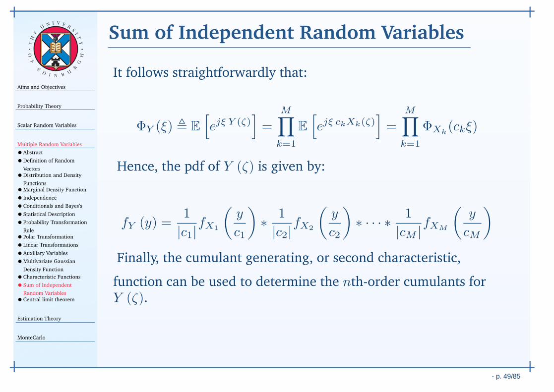
Finally, the cumulant generating, or second characteristic,
function can be used to determine the nth-order cumulants forY (ζ).
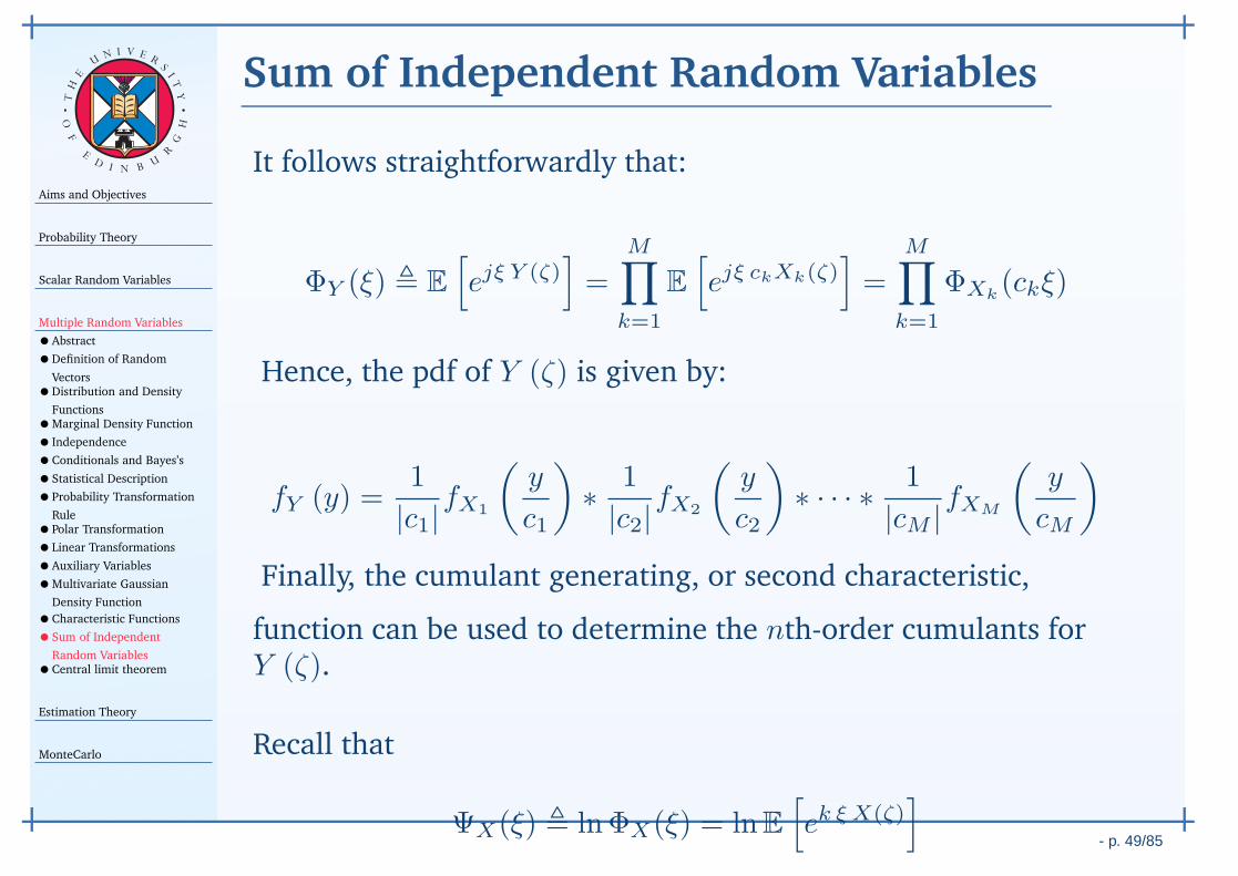
Recall that
ΨX(ξ) , ln ΦX(ξ) = lnE[
ek ξ X(ζ)]
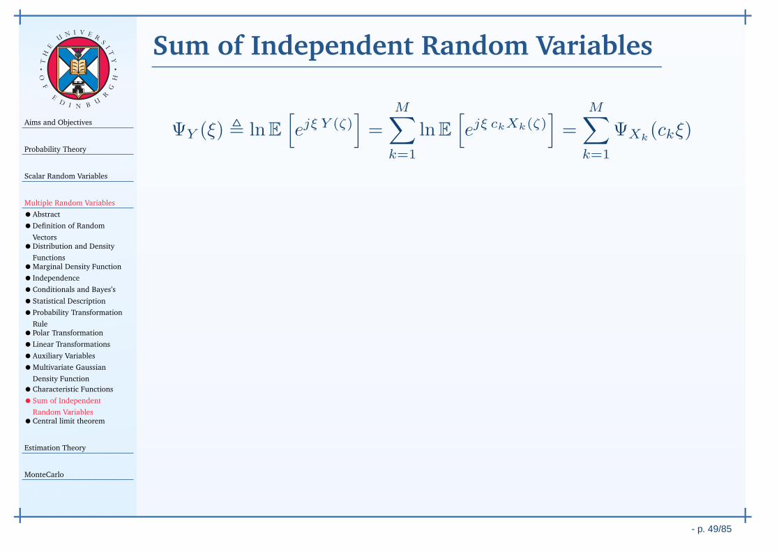
Aims and Objectives
Probability Theory
Scalar Random Variables
Multiple Random Variables
•Abstract
•Definition of Random
Vectors•Distribution and Density
Functions•Marginal Density Function
• Independence
•Conditionals and Bayes’s
•Statistical Description
•Probability Transformation
Rule•Polar Transformation
•Linear Transformations
•Auxiliary Variables
•Multivariate Gaussian
Density Function
•Characteristic Functions
•Sum of Independent
Random Variables•Central limit theorem
Estimation Theory
MonteCarlo
- p. 49/85
TH
E
UN I V E
RS
IT
Y
OF
ED
I N BU
R
GH
Sum of Independent Random Variables
ΨY (ξ) , lnE[
ejξ Y (ζ)]
=M∑
k=1
lnE[
ejξ ckXk(ζ)]
=M∑
k=1
ΨXk(ckξ)
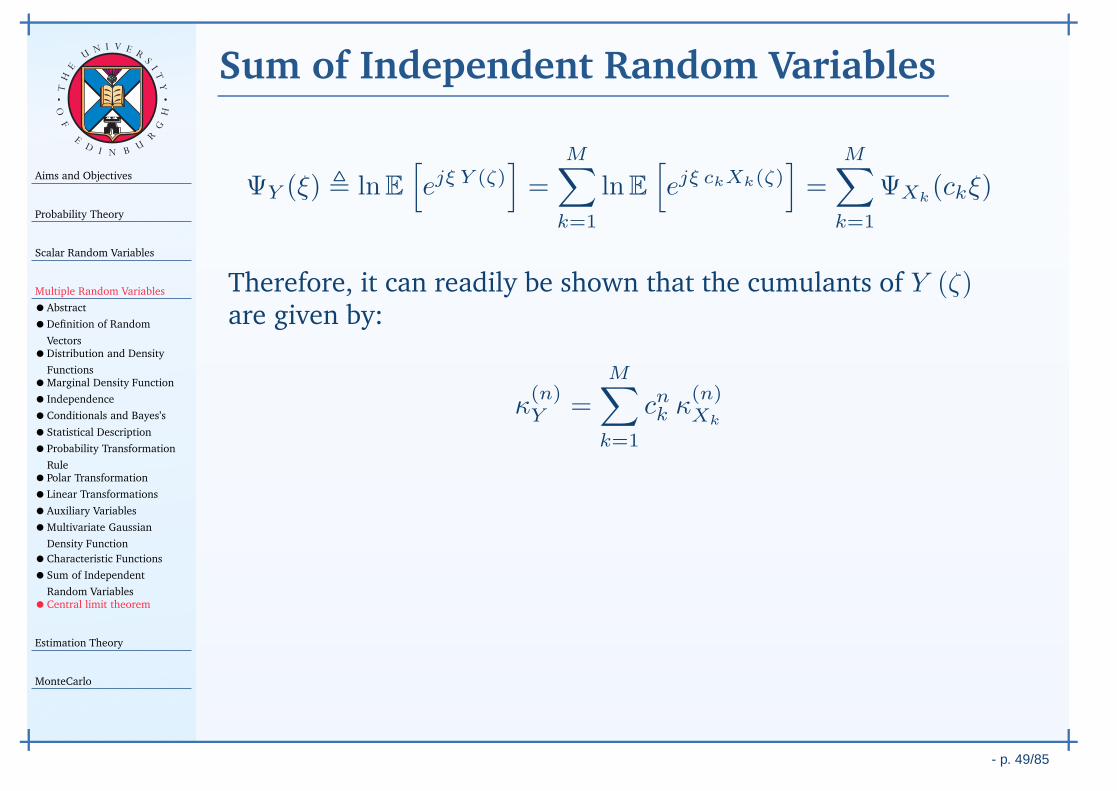
Therefore, it can readily be shown that the cumulants of Y (ζ)are given by:
κ(n)Y =
M∑
k=1
cnk κ(n)Xk
When these results are extended to the sum of an infinitenumber of statistically independent random variables, a powerfultheorem known as the central limit theorem (CLT) is obtained.
Another interesting concept develops when the sum ofindependent and identically distributed (i. i. d.) randomvariables preserve their distribution, which results in so-calledstable distributions.
Aims and Objectives
Probability Theory
Scalar Random Variables
Multiple Random Variables
•Abstract
•Definition of Random
Vectors•Distribution and Density
Functions•Marginal Density Function
• Independence
•Conditionals and Bayes’s
•Statistical Description
•Probability Transformation
Rule•Polar Transformation
•Linear Transformations
•Auxiliary Variables
•Multivariate Gaussian
Density Function
•Characteristic Functions
•Sum of Independent
Random Variables•Central limit theorem
Estimation Theory
MonteCarlo
- p. 50/85
TH
E
UN I V E
RS
IT
Y
OF
ED
I N BU
R
GH
Central limit theorem
Consider the random variable Y (ζ) given by:
YM (ζ) =
M∑
k=1
ck Xk(ζ)
What is the distribution of YM (ζ) as M → ∞?
Theorem (Central limit theorem). Let Xk(ζ)Mk=1 be a collection ofRVs that are independent and identically distributed for allk = 1, . . . ,M. Then the distribution of
YM (ζ) =YM (ζ)− µYM
σYM
where YM (ζ) =M∑
k=1
Xk(ζ)
approaches
limM→∞
fYM(y) = N
(y∣∣ 0, 1
)♦

- p. 51/85
Handout 5Estimation Theory
Aims and Objectives
Probability Theory
Scalar Random Variables
Multiple Random Variables
Estimation Theory
• Introduction
•Properties of Estimators
•Bias of estimator
•Variance of estimator
•Mean square error
•Cramer-Rao Lower Bound
•Consistency of an Estimator
•Estimating Multiple
Parameters•Maximum Likelihood
Estimation•Properties of the
maximum-likelihood
estimate (MLE)
•DC Level in white Gaussian
noise•MLE for Transformed
Parameter•Least Squares
•The Least Squares
Approach
•DC Level
•Linear Least Squares
MonteCarlo
- p. 52/85
TH
E
UN I V E
RS
IT
Y
OF
ED
I N BU
R
GH
Introduction
Thus far, have assumed that either the pdf or statistical values,such as mean, covariance, or higher order statistics,associated with a problem are fully known.
Aims and Objectives
Probability Theory
Scalar Random Variables
Multiple Random Variables
Estimation Theory
• Introduction
•Properties of Estimators
•Bias of estimator
•Variance of estimator
•Mean square error
•Cramer-Rao Lower Bound
•Consistency of an Estimator
•Estimating Multiple
Parameters•Maximum Likelihood
Estimation•Properties of the MLE
•DC Level in white Gaussian
noise•MLE for Transformed
Parameter•Least Squares
•The Least Squares
Approach
•DC Level
•Linear Least Squares
MonteCarlo
- p. 52/85
TH
E
UN I V E
RS
IT
Y
OF
ED
I N BU
R
GH
Introduction
Thus far, have assumed that either the pdf or statistical values,such as mean, covariance, or higher order statistics,associated with a problem are fully known.
In most practical applications, this is the exception rather thanthe rule.
The properties and parameters of random events must beobtained by collecting and analysing finite set ofmeasurements.
This handout will consider the problem of ParameterEstimation. This refers to the estimation of a parameter thatis fixed, but is unknown.

Aims and Objectives
Probability Theory
Scalar Random Variables
Multiple Random Variables
Estimation Theory
• Introduction
•Properties of Estimators
•Bias of estimator
•Variance of estimator
•Mean square error
•Cramer-Rao Lower Bound
•Consistency of an Estimator
•Estimating Multiple
Parameters•Maximum Likelihood
Estimation•Properties of the MLE
•DC Level in white Gaussian
noise•MLE for Transformed
Parameter•Least Squares
•The Least Squares
Approach
•DC Level
•Linear Least Squares
MonteCarlo
- p. 53/85
TH
E
UN I V E
RS
IT
Y
OF
ED
I N BU
R
GH
Properties of Estimators
Consider the set of N observations, X = x[n]N−10 , from a
random experiment; suppose they are used to estimate aparameter θ of the process using some function:
θ = θ [X ] = θ[x[n]N−1
0
]
The function θ [X ] is known as an estimator whereas the valuetaken by the estimator, using a particular set of observations, iscalled a point-estimate.
An aim is to design an estimator, θ, that should be as close to thetrue value of the parameter, θ, as possible.
Since θ is a function of a number of particular realisations of arandom outcome (or experiment), then it is itself a RV, and thushas a mean and variance.
Aims and Objectives
Probability Theory
Scalar Random Variables
Multiple Random Variables
Estimation Theory
• Introduction
•Properties of Estimators
•Bias of estimator
•Variance of estimator
•Mean square error
•Cramer-Rao Lower Bound
•Consistency of an Estimator
•Estimating Multiple
Parameters•Maximum Likelihood
Estimation•Properties of the MLE
•DC Level in white Gaussian
noise•MLE for Transformed
Parameter•Least Squares
•The Least Squares
Approach
•DC Level
•Linear Least Squares
MonteCarlo
- p. 54/85
TH
E
UN I V E
RS
IT
Y
OF
ED
I N BU
R
GH
Bias of estimator
The bias of an estimator θ of a parameter θ is defined as:
B(θ) , E
[
θ]
− θ
If θ is large, then a small deviation would give what wouldappear to be a large bias. Thus, the normalised bias is oftenused instead:
ǫb(θ) ,B(θ)
θ=
E
[
θ]
θ− 1, θ 6= 0
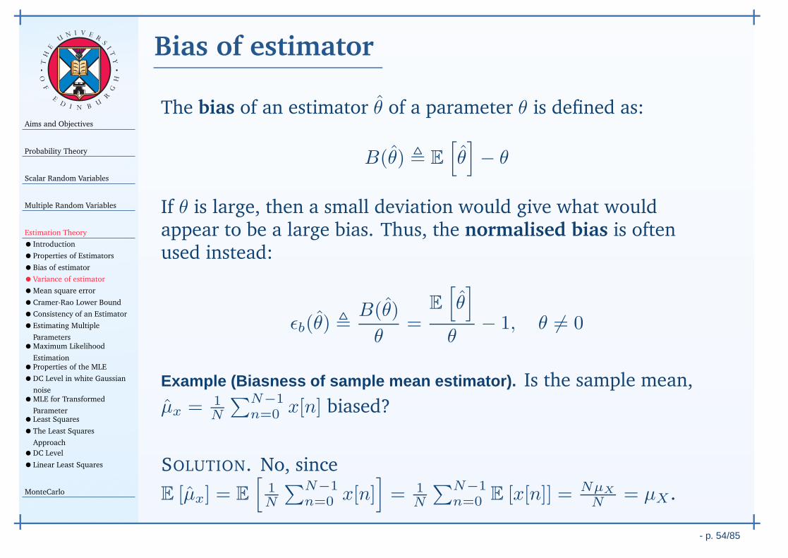
Example (Biasness of sample mean estimator). Is the sample mean,
µx = 1N
∑N−1n=0 x[n] biased?
SOLUTION. No, since
E [µx] = E
[1N
∑N−1n=0 x[n]
]
= 1N
∑N−1n=0 E [x[n]] = NµX
N= µX .
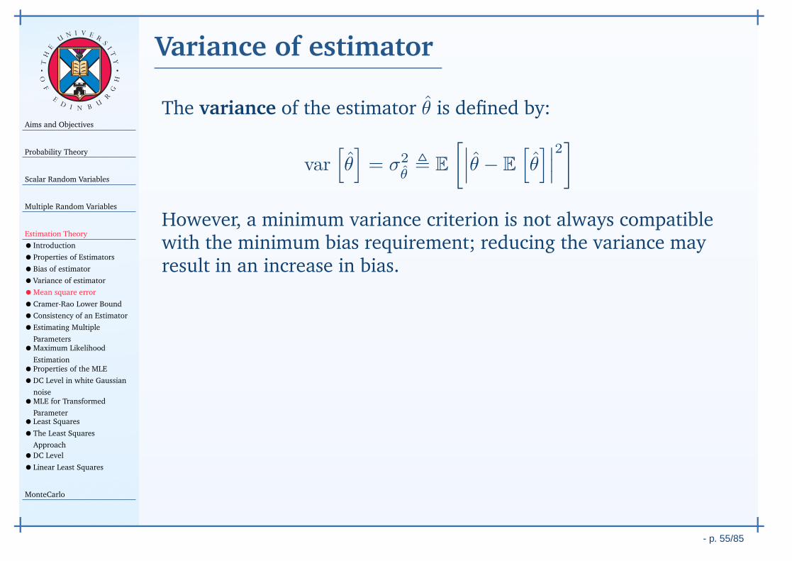
Aims and Objectives
Probability Theory
Scalar Random Variables
Multiple Random Variables
Estimation Theory
• Introduction
•Properties of Estimators
•Bias of estimator
•Variance of estimator
•Mean square error
•Cramer-Rao Lower Bound
•Consistency of an Estimator
•Estimating Multiple
Parameters•Maximum Likelihood
Estimation•Properties of the MLE
•DC Level in white Gaussian
noise•MLE for Transformed
Parameter•Least Squares
•The Least Squares
Approach
•DC Level
•Linear Least Squares
MonteCarlo
- p. 55/85
TH
E
UN I V E
RS
IT
Y
OF
ED
I N BU
R
GH
Variance of estimator
The variance of the estimator θ is defined by:
var[
θ]
= σ2θ, E
[∣∣∣θ − E
[
θ]∣∣∣
2]
However, a minimum variance criterion is not always compatiblewith the minimum bias requirement; reducing the variance mayresult in an increase in bias.
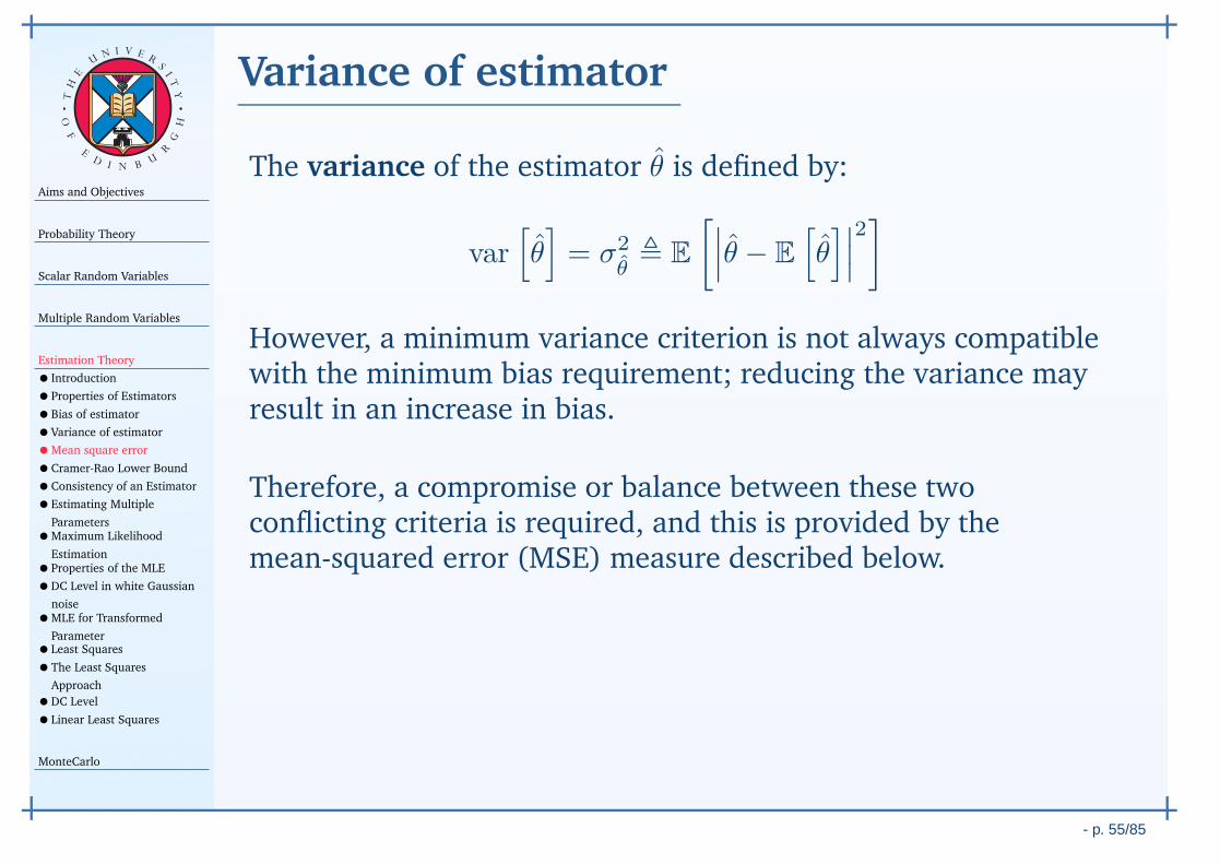
Therefore, a compromise or balance between these twoconflicting criteria is required, and this is provided by themean-squared error (MSE) measure described below.
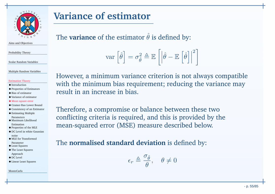
The normalised standard deviation is defined by:
ǫr ,σθ
θ, θ 6= 0
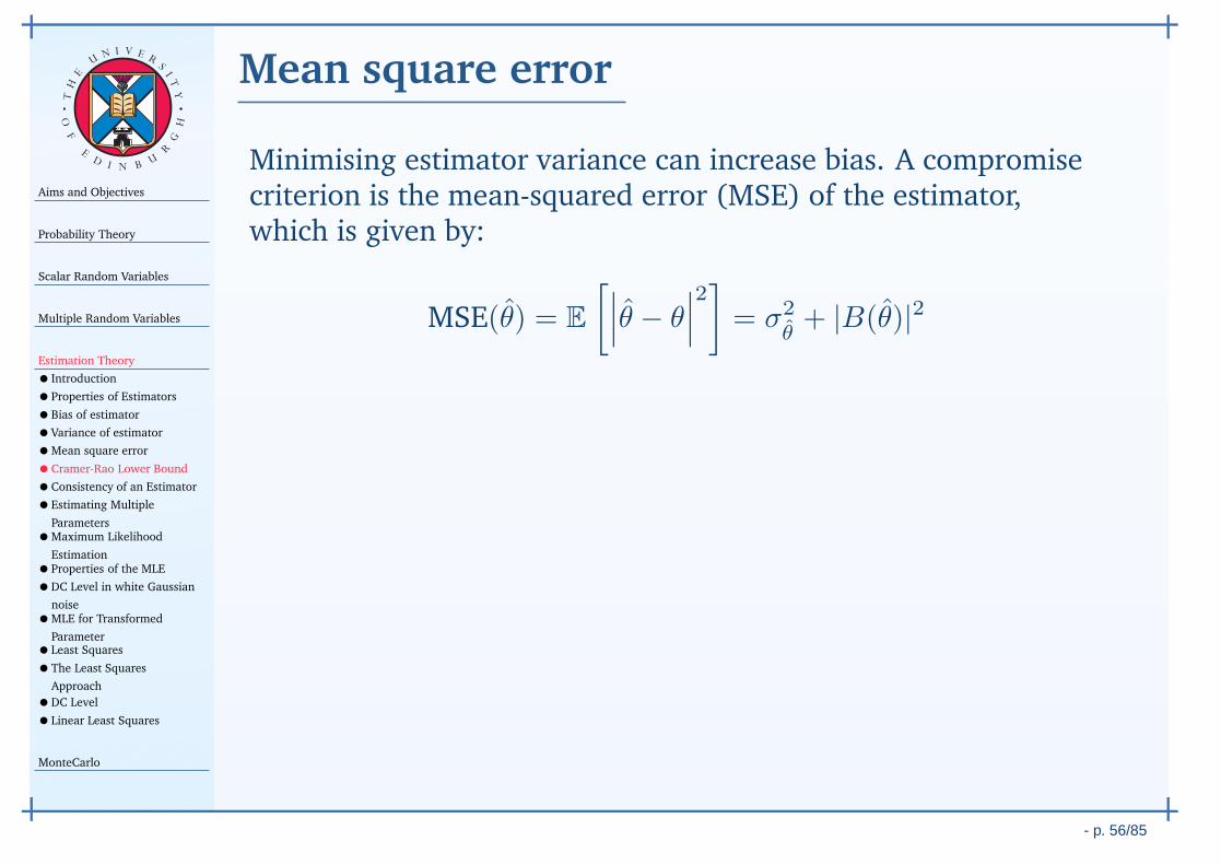
Aims and Objectives
Probability Theory
Scalar Random Variables
Multiple Random Variables
Estimation Theory
• Introduction
•Properties of Estimators
•Bias of estimator
•Variance of estimator
•Mean square error
•Cramer-Rao Lower Bound
•Consistency of an Estimator
•Estimating Multiple
Parameters•Maximum Likelihood
Estimation•Properties of the MLE
•DC Level in white Gaussian
noise•MLE for Transformed
Parameter•Least Squares
•The Least Squares
Approach
•DC Level
•Linear Least Squares
MonteCarlo
- p. 56/85
TH
E
UN I V E
RS
IT
Y
OF
ED
I N BU
R
GH
Mean square error
Minimising estimator variance can increase bias. A compromisecriterion is the mean-squared error (MSE) of the estimator,which is given by:
MSE(θ) = E
[∣∣∣θ − θ
∣∣∣
2]
= σ2θ+ |B(θ)|2
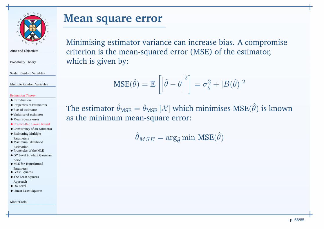
The estimator θMSE = θMSE [X ] which minimises MSE(θ) is knownas the minimum mean-square error:
θMSE = argθmin MSE(θ)
This measures the average mean squared deviation of theestimator from its true value.
Unfortunately, adoption of this natural criterion leads tounrealisable estimators; ones which cannot be written solely as afunction of the data.
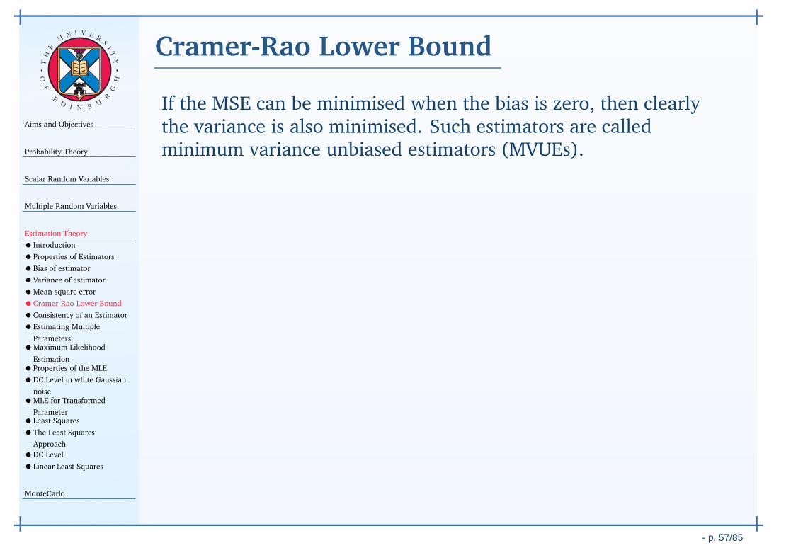
Aims and Objectives
Probability Theory
Scalar Random Variables
Multiple Random Variables
Estimation Theory
• Introduction
•Properties of Estimators
•Bias of estimator
•Variance of estimator
•Mean square error
•Cramer-Rao Lower Bound
•Consistency of an Estimator
•Estimating Multiple
Parameters•Maximum Likelihood
Estimation•Properties of the MLE
•DC Level in white Gaussian
noise•MLE for Transformed
Parameter•Least Squares
•The Least Squares
Approach
•DC Level
•Linear Least Squares
MonteCarlo
- p. 57/85
TH
E
UN I V E
RS
IT
Y
OF
ED
I N BU
R
GH
Cramer-Rao Lower Bound
If the MSE can be minimised when the bias is zero, then clearlythe variance is also minimised. Such estimators are calledminimum variance unbiased estimators (MVUEs).
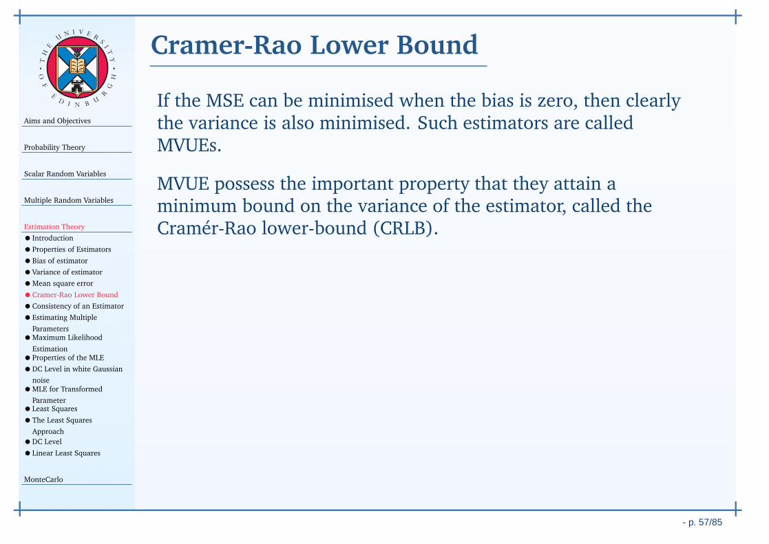
Aims and Objectives
Probability Theory
Scalar Random Variables
Multiple Random Variables
Estimation Theory
• Introduction
•Properties of Estimators
•Bias of estimator
•Variance of estimator
•Mean square error
•Cramer-Rao Lower Bound
•Consistency of an Estimator
•Estimating Multiple
Parameters•Maximum Likelihood
Estimation•Properties of the MLE
•DC Level in white Gaussian
noise•MLE for Transformed
Parameter•Least Squares
•The Least Squares
Approach
•DC Level
•Linear Least Squares
MonteCarlo
- p. 57/85
TH
E
UN I V E
RS
IT
Y
OF
ED
I N BU
R
GH
Cramer-Rao Lower Bound
If the MSE can be minimised when the bias is zero, then clearlythe variance is also minimised. Such estimators are calledMVUEs.
MVUE possess the important property that they attain aminimum bound on the variance of the estimator, called theCramér-Rao lower-bound (CRLB).

Aims and Objectives
Probability Theory
Scalar Random Variables
Multiple Random Variables
Estimation Theory
• Introduction
•Properties of Estimators
•Bias of estimator
•Variance of estimator
•Mean square error
•Cramer-Rao Lower Bound
•Consistency of an Estimator
•Estimating Multiple
Parameters•Maximum Likelihood
Estimation•Properties of the MLE
•DC Level in white Gaussian
noise•MLE for Transformed
Parameter•Least Squares
•The Least Squares
Approach
•DC Level
•Linear Least Squares
MonteCarlo
- p. 57/85
TH
E
UN I V E
RS
IT
Y
OF
ED
I N BU
R
GH
Cramer-Rao Lower Bound
Theorem (CRLB - scalar parameter). If
X(ζ) = [x[0, ζ] , · · · , x[N − 1, ζ]]T
and fX (x | θ) is the jointdensity of X(ζ) which depends on fixed but unknown parameter
θ, then the variance of the estimator θ is bounded by:
var[
θ]
≥ 1
E
[(∂ ln fX(x | θ)
∂θ
)2]
♦
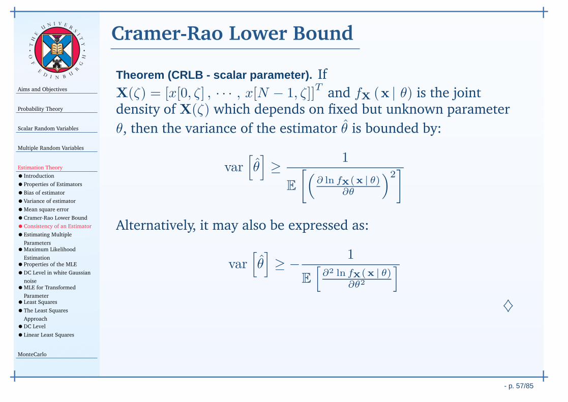
Aims and Objectives
Probability Theory
Scalar Random Variables
Multiple Random Variables
Estimation Theory
• Introduction
•Properties of Estimators
•Bias of estimator
•Variance of estimator
•Mean square error
•Cramer-Rao Lower Bound
•Consistency of an Estimator
•Estimating Multiple
Parameters•Maximum Likelihood
Estimation•Properties of the MLE
•DC Level in white Gaussian
noise•MLE for Transformed
Parameter•Least Squares
•The Least Squares
Approach
•DC Level
•Linear Least Squares
MonteCarlo
- p. 57/85
TH
E
UN I V E
RS
IT
Y
OF
ED
I N BU
R
GH
Cramer-Rao Lower Bound
Theorem (CRLB - scalar parameter). If
X(ζ) = [x[0, ζ] , · · · , x[N − 1, ζ]]T
and fX (x | θ) is the jointdensity of X(ζ) which depends on fixed but unknown parameter
θ, then the variance of the estimator θ is bounded by:
var[
θ]
≥ 1
E
[(∂ ln fX(x | θ)
∂θ
)2]
Alternatively, it may also be expressed as:
var[
θ]
≥ − 1
E
[∂2 ln fX(x | θ)
∂θ2
]
♦

Aims and Objectives
Probability Theory
Scalar Random Variables
Multiple Random Variables
Estimation Theory
• Introduction
•Properties of Estimators
•Bias of estimator
•Variance of estimator
•Mean square error
•Cramer-Rao Lower Bound
•Consistency of an Estimator
•Estimating Multiple
Parameters•Maximum Likelihood
Estimation•Properties of the MLE
•DC Level in white Gaussian
noise•MLE for Transformed
Parameter•Least Squares
•The Least Squares
Approach
•DC Level
•Linear Least Squares
MonteCarlo
- p. 57/85
TH
E
UN I V E
RS
IT
Y
OF
ED
I N BU
R
GH
Cramer-Rao Lower Bound
Theorem (CRLB - scalar parameter). If
X(ζ) = [x[0, ζ] , · · · , x[N − 1, ζ]]T
and fX (x | θ) is the jointdensity of X(ζ) which depends on fixed but unknown parameter
θ, then the variance of the estimator θ is bounded by:
var[
θ]
≥ 1
E
[(∂ ln fX(x | θ)
∂θ
)2]
Alternatively, it may also be expressed as:
var[
θ]
≥ − 1
E
[∂2 ln fX(x | θ)
∂θ2
] ♦
The function ln fX (x | θ) is called the log-likelihood of θ.
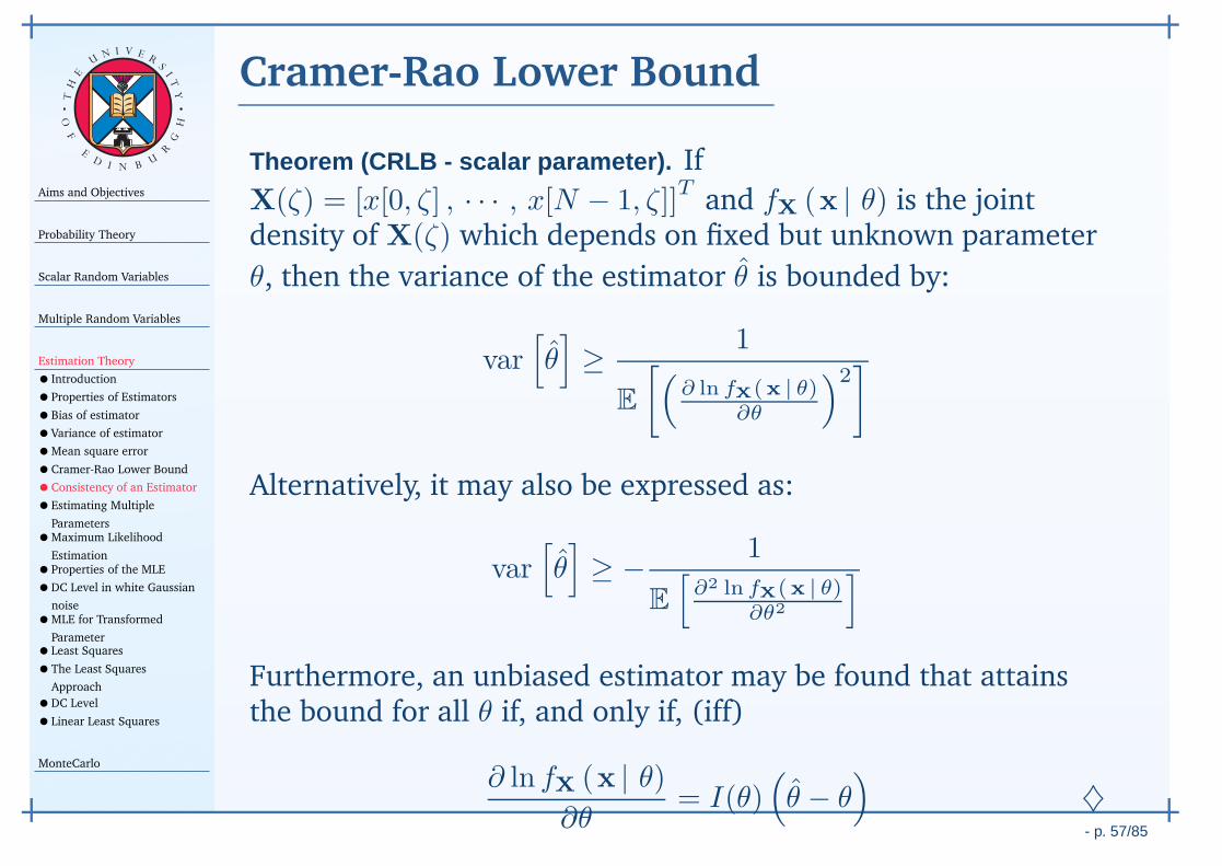
Aims and Objectives
Probability Theory
Scalar Random Variables
Multiple Random Variables
Estimation Theory
• Introduction
•Properties of Estimators
•Bias of estimator
•Variance of estimator
•Mean square error
•Cramer-Rao Lower Bound
•Consistency of an Estimator
•Estimating Multiple
Parameters•Maximum Likelihood
Estimation•Properties of the MLE
•DC Level in white Gaussian
noise•MLE for Transformed
Parameter•Least Squares
•The Least Squares
Approach
•DC Level
•Linear Least Squares
MonteCarlo
- p. 57/85
TH
E
UN I V E
RS
IT
Y
OF
ED
I N BU
R
GH
Cramer-Rao Lower Bound
Theorem (CRLB - scalar parameter). If
X(ζ) = [x[0, ζ] , · · · , x[N − 1, ζ]]T
and fX (x | θ) is the jointdensity of X(ζ) which depends on fixed but unknown parameter
θ, then the variance of the estimator θ is bounded by:
var[
θ]
≥ 1
E
[(∂ ln fX(x | θ)
∂θ
)2]
Alternatively, it may also be expressed as:
var[
θ]
≥ − 1
E
[∂2 ln fX(x | θ)
∂θ2
]
Furthermore, an unbiased estimator may be found that attainsthe bound for all θ if, and only if, (iff)
∂ ln fX (x | θ)∂θ
= I(θ)(
θ − θ)
♦
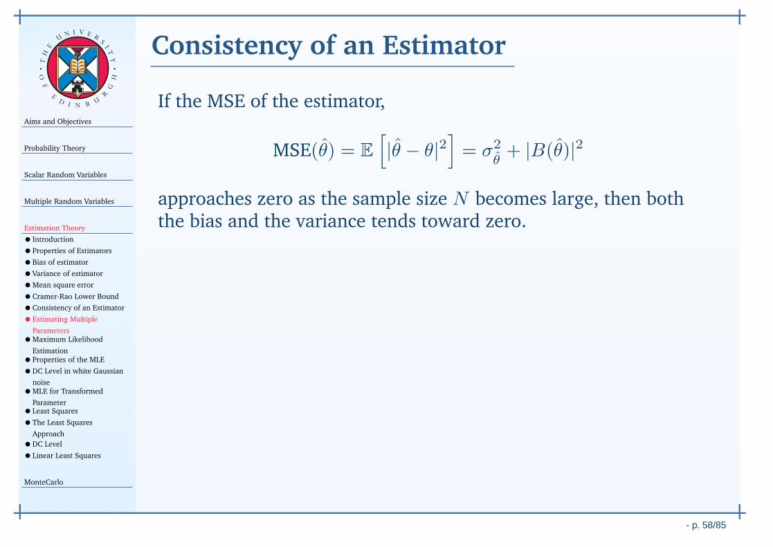
Aims and Objectives
Probability Theory
Scalar Random Variables
Multiple Random Variables
Estimation Theory
• Introduction
•Properties of Estimators
•Bias of estimator
•Variance of estimator
•Mean square error
•Cramer-Rao Lower Bound
•Consistency of an Estimator
•Estimating Multiple
Parameters•Maximum Likelihood
Estimation•Properties of the MLE
•DC Level in white Gaussian
noise•MLE for Transformed
Parameter•Least Squares
•The Least Squares
Approach
•DC Level
•Linear Least Squares
MonteCarlo
- p. 58/85
TH
E
UN I V E
RS
IT
Y
OF
ED
I N BU
R
GH
Consistency of an Estimator
If the MSE of the estimator,
MSE(θ) = E
[
|θ − θ|2]
= σ2θ+ |B(θ)|2
approaches zero as the sample size N becomes large, then boththe bias and the variance tends toward zero.
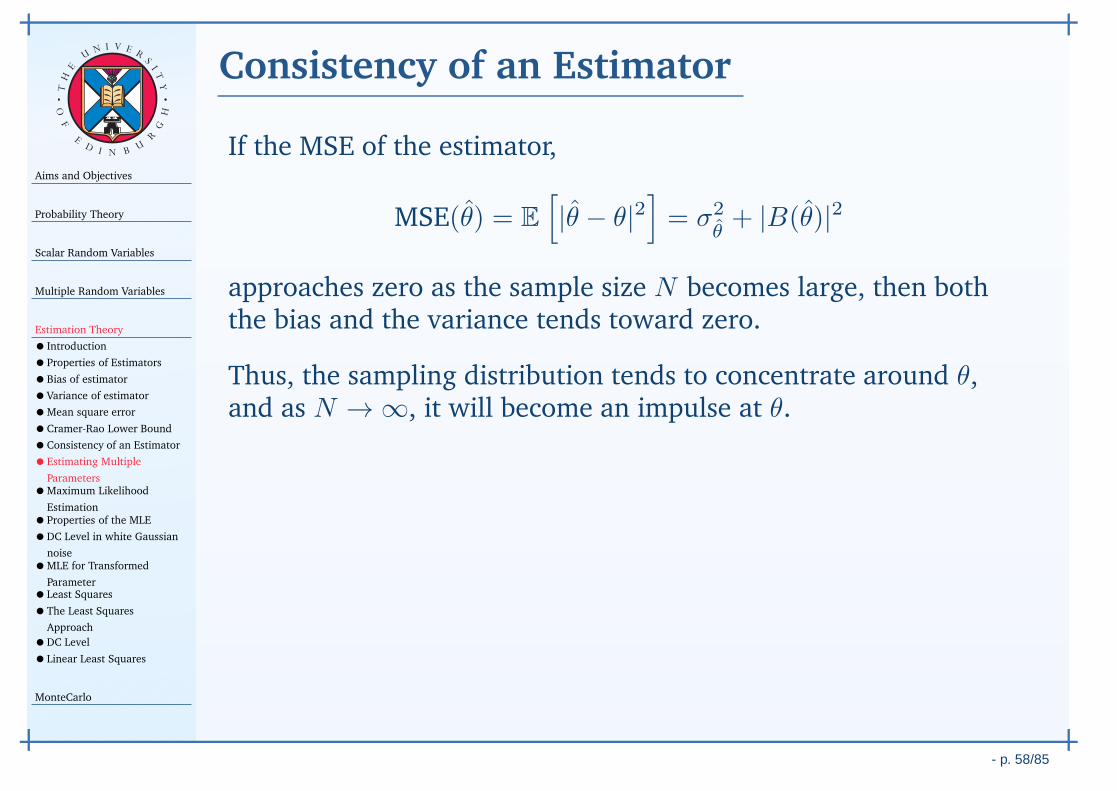
Thus, the sampling distribution tends to concentrate around θ,and as N → ∞, it will become an impulse at θ.
This is a very important and desirable property, and such anestimator is called a consistent estimator.

Aims and Objectives
Probability Theory
Scalar Random Variables
Multiple Random Variables
Estimation Theory
• Introduction
•Properties of Estimators
•Bias of estimator
•Variance of estimator
•Mean square error
•Cramer-Rao Lower Bound
•Consistency of an Estimator
•Estimating Multiple
Parameters•Maximum Likelihood
Estimation•Properties of the MLE
•DC Level in white Gaussian
noise•MLE for Transformed
Parameter•Least Squares
•The Least Squares
Approach
•DC Level
•Linear Least Squares
MonteCarlo
- p. 59/85
TH
E
UN I V E
RS
IT
Y
OF
ED
I N BU
R
GH
Estimating Multiple Parameters
Multiple parameters occur in, for example, estimating thestatistical properties of a random time-series, estimating theparameters of a curve fitted to a set of data, estimating anymodel described by a set of parameters.
A vector of parameters, θ, of a random event X (ζ) can be
estimated from a set of observations, X = x[n]N−10 , using some
function:
θ = θ [X ] = θ[x[n]N−1
0
]
The definitions of unbiasedness, consistency, and the CRLB areall straightforward extensions of the definitions and results forscalar parameter estimates.
Aims and Objectives
Probability Theory
Scalar Random Variables
Multiple Random Variables
Estimation Theory
• Introduction
•Properties of Estimators
•Bias of estimator
•Variance of estimator
•Mean square error
•Cramer-Rao Lower Bound
•Consistency of an Estimator
•Estimating Multiple
Parameters•Maximum Likelihood
Estimation•Properties of the MLE
•DC Level in white Gaussian
noise•MLE for Transformed
Parameter•Least Squares
•The Least Squares
Approach
•DC Level
•Linear Least Squares
MonteCarlo
- p. 60/85
TH
E
UN I V E
RS
IT
Y
OF
ED
I N BU
R
GH
Maximum Likelihood Estimation
The joint density of the RVs X(ζ) = x[n, ζ]N−10 , which depends
on fixed but unknown parameter θ, is fX (x | θ).
This same quantity, viewed as a function of the parameter θwhen a particular set of observations, x is given, is known as thelikelihood function.
The maximum-likelihood estimate (MLE) of the parameter θ,
denoted by θml, is defined as that value of θ that maximisesfX ( x | θ).
The MLE for θ is defined by:
θml(x) = argθ max fX (x | θ)
Note that since θml(x) depends on the random observationvector x, and so is itself a RV.
Aims and Objectives
Probability Theory
Scalar Random Variables
Multiple Random Variables
Estimation Theory
• Introduction
•Properties of Estimators
•Bias of estimator
•Variance of estimator
•Mean square error
•Cramer-Rao Lower Bound
•Consistency of an Estimator
•Estimating Multiple
Parameters•Maximum Likelihood
Estimation•Properties of the MLE
•DC Level in white Gaussian
noise•MLE for Transformed
Parameter•Least Squares
•The Least Squares
Approach
•DC Level
•Linear Least Squares
MonteCarlo
- p. 61/85
TH
E
UN I V E
RS
IT
Y
OF
ED
I N BU
R
GH
Properties of the MLE
1. The MLE satisfies
∇θfX (x | θ)|θ=θml
= 0P×1
∇θ ln fX (x | θ)|θ=θml
= 0P×1
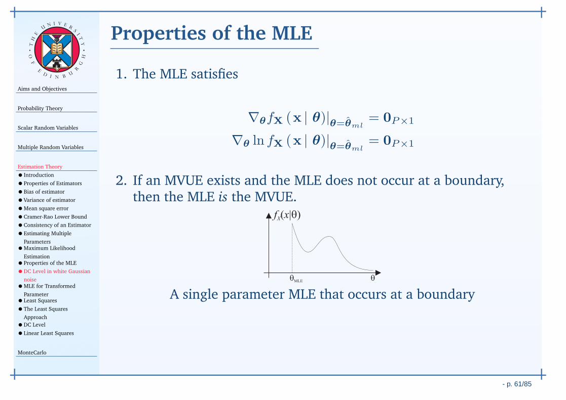
2. If an MVUE exists and the MLE does not occur at a boundary,then the MLE is the MVUE.
A single parameter MLE that occurs at a boundary
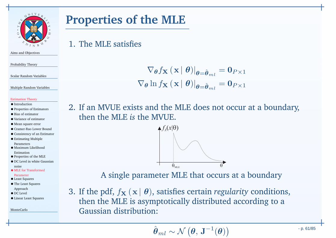
3. If the pdf, fX (x | θ), satisfies certain regularity conditions,then the MLE is asymptotically distributed according to aGaussian distribution:
θml ∼ N(θ, J−1(θ)
)
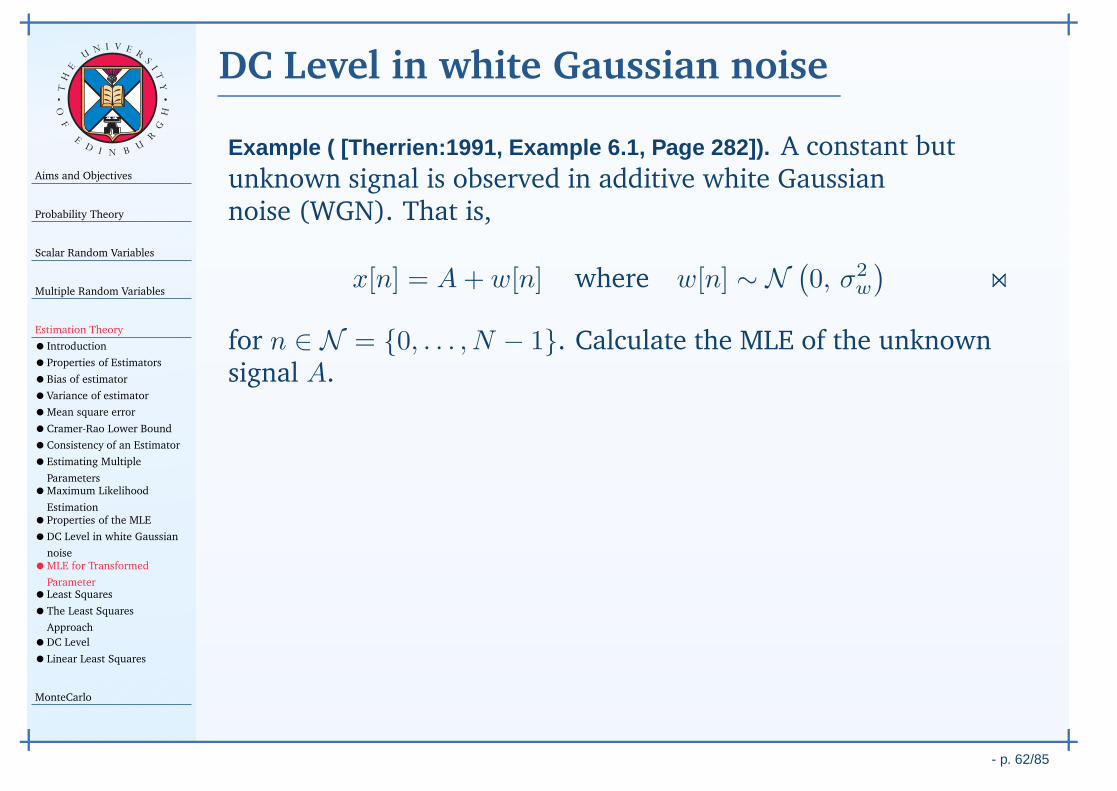
Aims and Objectives
Probability Theory
Scalar Random Variables
Multiple Random Variables
Estimation Theory
• Introduction
•Properties of Estimators
•Bias of estimator
•Variance of estimator
•Mean square error
•Cramer-Rao Lower Bound
•Consistency of an Estimator
•Estimating Multiple
Parameters•Maximum Likelihood
Estimation•Properties of the MLE
•DC Level in white Gaussian
noise•MLE for Transformed
Parameter•Least Squares
•The Least Squares
Approach
•DC Level
•Linear Least Squares
MonteCarlo
- p. 62/85
TH
E
UN I V E
RS
IT
Y
OF
ED
I N BU
R
GH
DC Level in white Gaussian noise
Example ( [Therrien:1991, Example 6.1, Page 282]). A constant butunknown signal is observed in additive white Gaussiannoise (WGN). That is,
x[n] = A+ w[n] where w[n] ∼ N(0, σ2
w
)⋊⋉
for n ∈ N = 0, . . . , N − 1. Calculate the MLE of the unknownsignal A.
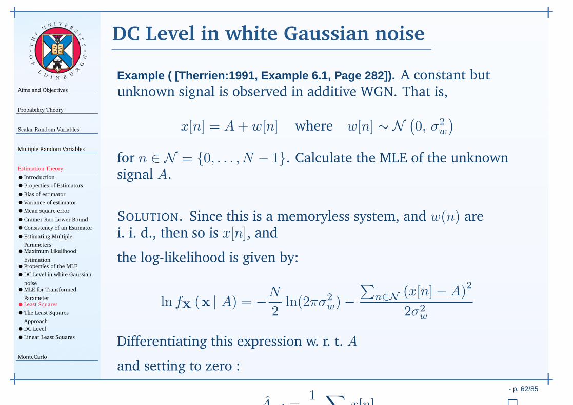
Aims and Objectives
Probability Theory
Scalar Random Variables
Multiple Random Variables
Estimation Theory
• Introduction
•Properties of Estimators
•Bias of estimator
•Variance of estimator
•Mean square error
•Cramer-Rao Lower Bound
•Consistency of an Estimator
•Estimating Multiple
Parameters•Maximum Likelihood
Estimation•Properties of the MLE
•DC Level in white Gaussian
noise•MLE for Transformed
Parameter•Least Squares
•The Least Squares
Approach
•DC Level
•Linear Least Squares
MonteCarlo
- p. 62/85
TH
E
UN I V E
RS
IT
Y
OF
ED
I N BU
R
GH
DC Level in white Gaussian noise
Example ( [Therrien:1991, Example 6.1, Page 282]). A constant butunknown signal is observed in additive WGN. That is,
x[n] = A+ w[n] where w[n] ∼ N(0, σ2
w
)
for n ∈ N = 0, . . . , N − 1. Calculate the MLE of the unknownsignal A.
SOLUTION. Since this is a memoryless system, and w(n) arei. i. d., then so is x[n], and
the log-likelihood is given by:
ln fX (x | A) = −N
2ln(2πσ2
w)−∑
n∈N (x[n]−A)2
2σ2w
Differentiating this expression w. r. t. A
and setting to zero :
Aml =1 ∑
x[n]
Aims and Objectives
Probability Theory
Scalar Random Variables
Multiple Random Variables
Estimation Theory
• Introduction
•Properties of Estimators
•Bias of estimator
•Variance of estimator
•Mean square error
•Cramer-Rao Lower Bound
•Consistency of an Estimator
•Estimating Multiple
Parameters•Maximum Likelihood
Estimation•Properties of the MLE
•DC Level in white Gaussian
noise•MLE for Transformed
Parameter•Least Squares
•The Least Squares
Approach
•DC Level
•Linear Least Squares
MonteCarlo
- p. 63/85
TH
E
UN I V E
RS
IT
Y
OF
ED
I N BU
R
GH
MLE for Transformed Parameter
Theorem (Invariance Property of the MLE). The MLE of the parameterα = g(θ), where g is an r-dimensional function of the P × 1parameter θ, and the pdf, fX (x | θ) is parameterised by θ, isgiven by
αml = g(θml) ♦
where θml is the MLE of θ.
Aims and Objectives
Probability Theory
Scalar Random Variables
Multiple Random Variables
Estimation Theory
• Introduction
•Properties of Estimators
•Bias of estimator
•Variance of estimator
•Mean square error
•Cramer-Rao Lower Bound
•Consistency of an Estimator
•Estimating Multiple
Parameters•Maximum Likelihood
Estimation•Properties of the MLE
•DC Level in white Gaussian
noise•MLE for Transformed
Parameter•Least Squares
•The Least Squares
Approach
•DC Level
•Linear Least Squares
MonteCarlo
- p. 63/85
TH
E
UN I V E
RS
IT
Y
OF
ED
I N BU
R
GH
MLE for Transformed Parameter
Theorem (Invariance Property of the MLE). The MLE of the parameterα = g(θ), where g is an r-dimensional function of the P × 1parameter θ, and the pdf, fX (x | θ) is parameterised by θ, isgiven by
αml = g(θml)
where θml is the MLE of θ.
The MLE of θ, θml, is obtained by maximising fX (x | θ). If thefunction g is not an invertible function, then α maximises themodified likelihood function pT (x | α) defined as:
pT (x | α) = maxθ:α=g(θ)
fX (x | θ) ♦
Aims and Objectives
Probability Theory
Scalar Random Variables
Multiple Random Variables
Estimation Theory
• Introduction
•Properties of Estimators
•Bias of estimator
•Variance of estimator
•Mean square error
•Cramer-Rao Lower Bound
•Consistency of an Estimator
•Estimating Multiple
Parameters•Maximum Likelihood
Estimation•Properties of the MLE
•DC Level in white Gaussian
noise•MLE for Transformed
Parameter•Least Squares
•The Least Squares
Approach
•DC Level
•Linear Least Squares
MonteCarlo
- p. 64/85
TH
E
UN I V E
RS
IT
Y
OF
ED
I N BU
R
GH
Least Squares
The estimators discussed so far have attempted to find anoptimal or nearly optimal (for large data records) estimator forexample, the MVUE.
An alternate philosophy is a class of estimators that in generalhave no optimality properties associated with them, but makegood sense for many problems of interest: the principle of leastsquares.
A salient feature of the method is that no probabilisticassumptions are made about the data; only a signal model isassumed.
As will be seen, it turns out that the least-squares estimate (LSE)can be calculated when just the first and second moments areknown, and through the solution of linear equations.
Aims and Objectives
Probability Theory
Scalar Random Variables
Multiple Random Variables
Estimation Theory
• Introduction
•Properties of Estimators
•Bias of estimator
•Variance of estimator
•Mean square error
•Cramer-Rao Lower Bound
•Consistency of an Estimator
•Estimating Multiple
Parameters•Maximum Likelihood
Estimation•Properties of the MLE
•DC Level in white Gaussian
noise•MLE for Transformed
Parameter•Least Squares
•The Least Squares
Approach
•DC Level
•Linear Least Squares
MonteCarlo
- p. 65/85
TH
E
UN I V E
RS
IT
Y
OF
ED
I N BU
R
GH
The Least Squares Approach
In the least-squares (LS) approach, it is sought to minimise thesquared difference between the given, or observed, data x[n] andthe assumed, or hidden, signal or noiseless data.
Aims and Objectives
Probability Theory
Scalar Random Variables
Multiple Random Variables
Estimation Theory
• Introduction
•Properties of Estimators
•Bias of estimator
•Variance of estimator
•Mean square error
•Cramer-Rao Lower Bound
•Consistency of an Estimator
•Estimating Multiple
Parameters•Maximum Likelihood
Estimation•Properties of the MLE
•DC Level in white Gaussian
noise•MLE for Transformed
Parameter•Least Squares
•The Least Squares
Approach
•DC Level
•Linear Least Squares
MonteCarlo
- p. 65/85
TH
E
UN I V E
RS
IT
Y
OF
ED
I N BU
R
GH
The Least Squares Approach
In the LS approach, it is sought to minimise the squareddifference between the given, or observed, data x[n] and theassumed, or hidden, signal or noiseless data.
Here it is assumed that the hidden or unobserved signal isgenerated by some model which, in turn, depends on someunknown parameter θ.
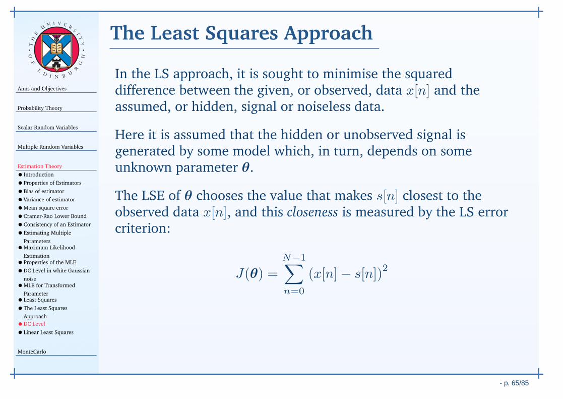
The LSE of θ chooses the value that makes s[n] closest to theobserved data x[n], and this closeness is measured by the LS errorcriterion:
J(θ) =N−1∑
n=0
(x[n]− s[n])2
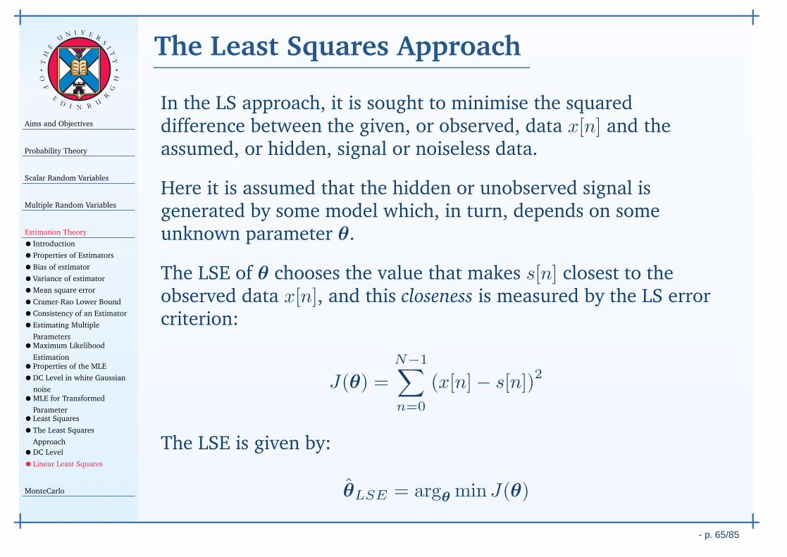
The LSE is given by:
θLSE = argθ min J(θ)
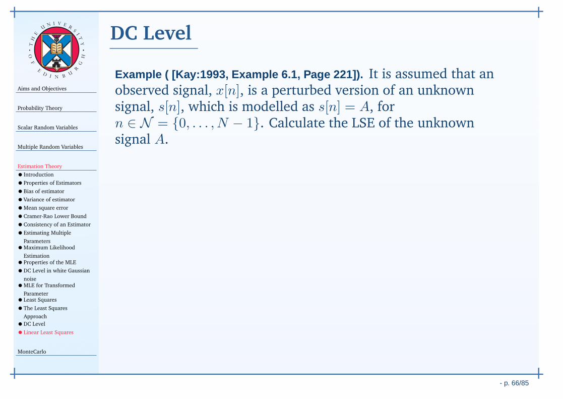
Aims and Objectives
Probability Theory
Scalar Random Variables
Multiple Random Variables
Estimation Theory
• Introduction
•Properties of Estimators
•Bias of estimator
•Variance of estimator
•Mean square error
•Cramer-Rao Lower Bound
•Consistency of an Estimator
•Estimating Multiple
Parameters•Maximum Likelihood
Estimation•Properties of the MLE
•DC Level in white Gaussian
noise•MLE for Transformed
Parameter•Least Squares
•The Least Squares
Approach
•DC Level
•Linear Least Squares
MonteCarlo
- p. 66/85
TH
E
UN I V E
RS
IT
Y
OF
ED
I N BU
R
GH
DC Level
Example ( [Kay:1993, Example 6.1, Page 221]). It is assumed that anobserved signal, x[n], is a perturbed version of an unknownsignal, s[n], which is modelled as s[n] = A, forn ∈ N = 0, . . . , N − 1. Calculate the LSE of the unknownsignal A.
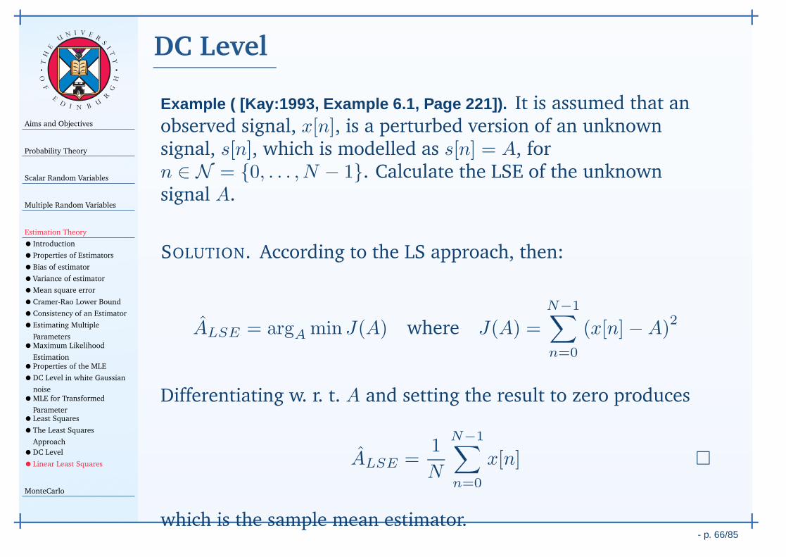
SOLUTION. According to the LS approach, then:
ALSE = argA minJ(A) where J(A) =
N−1∑
n=0
(x[n]−A)2
Differentiating w. r. t. A and setting the result to zero produces
ALSE =1
N
N−1∑
n=0
x[n]
which is the sample mean estimator.
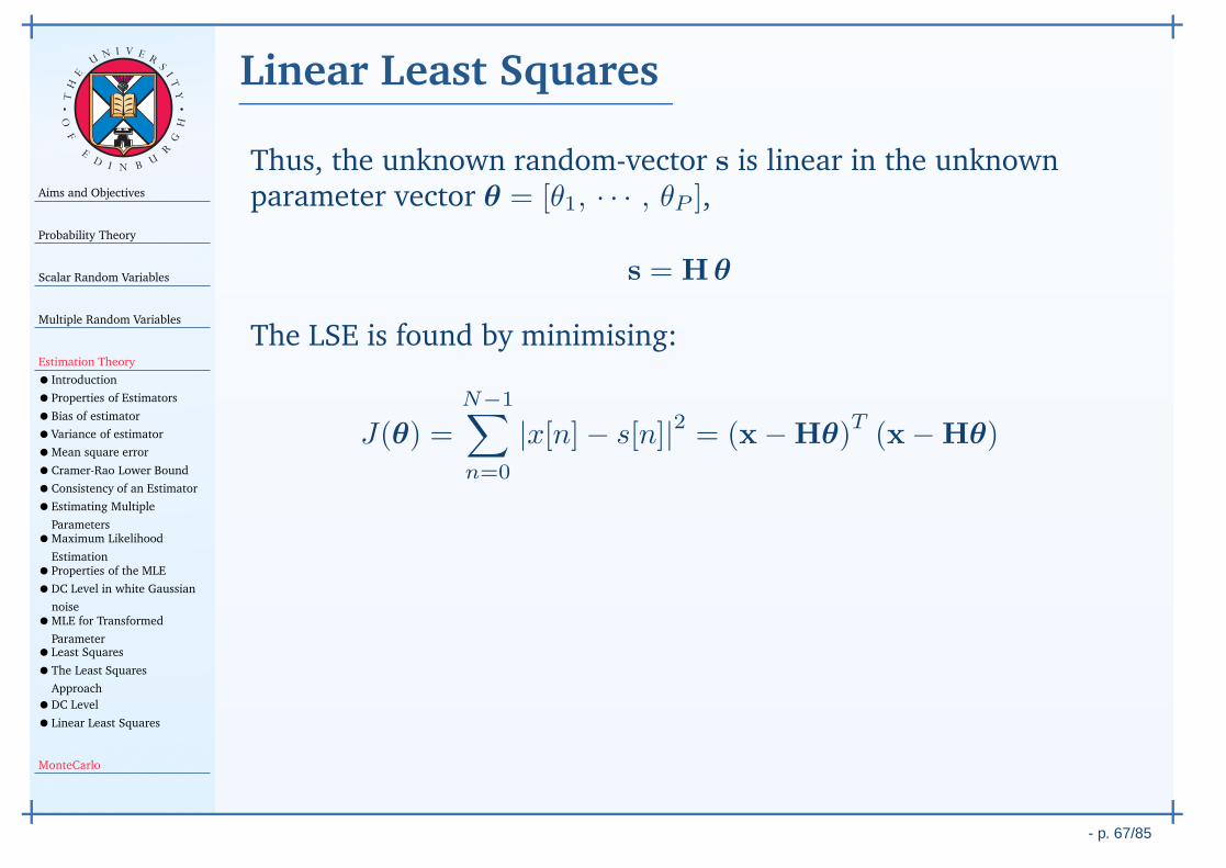
Aims and Objectives
Probability Theory
Scalar Random Variables
Multiple Random Variables
Estimation Theory
• Introduction
•Properties of Estimators
•Bias of estimator
•Variance of estimator
•Mean square error
•Cramer-Rao Lower Bound
•Consistency of an Estimator
•Estimating Multiple
Parameters•Maximum Likelihood
Estimation•Properties of the MLE
•DC Level in white Gaussian
noise•MLE for Transformed
Parameter•Least Squares
•The Least Squares
Approach
•DC Level
•Linear Least Squares
MonteCarlo
- p. 67/85
TH
E
UN I V E
RS
IT
Y
OF
ED
I N BU
R
GH
Linear Least Squares
Thus, the unknown random-vector s is linear in the unknownparameter vector θ = [θ1, · · · , θP ],
s = Hθ
The LSE is found by minimising:
J(θ) =N−1∑
n=0
|x[n]− s[n]|2 = (x−Hθ)T (x−Hθ)
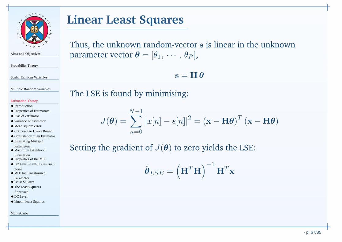
Setting the gradient of J(θ) to zero yields the LSE:
θLSE =(
HTH)−1
HTx
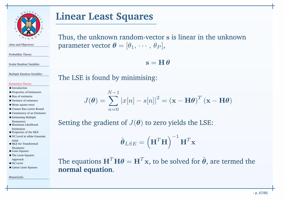
The equations HTHθ = HTx, to be solved for θ, are termed thenormal equation.

- p. 68/85
Handout 6MonteCarlo
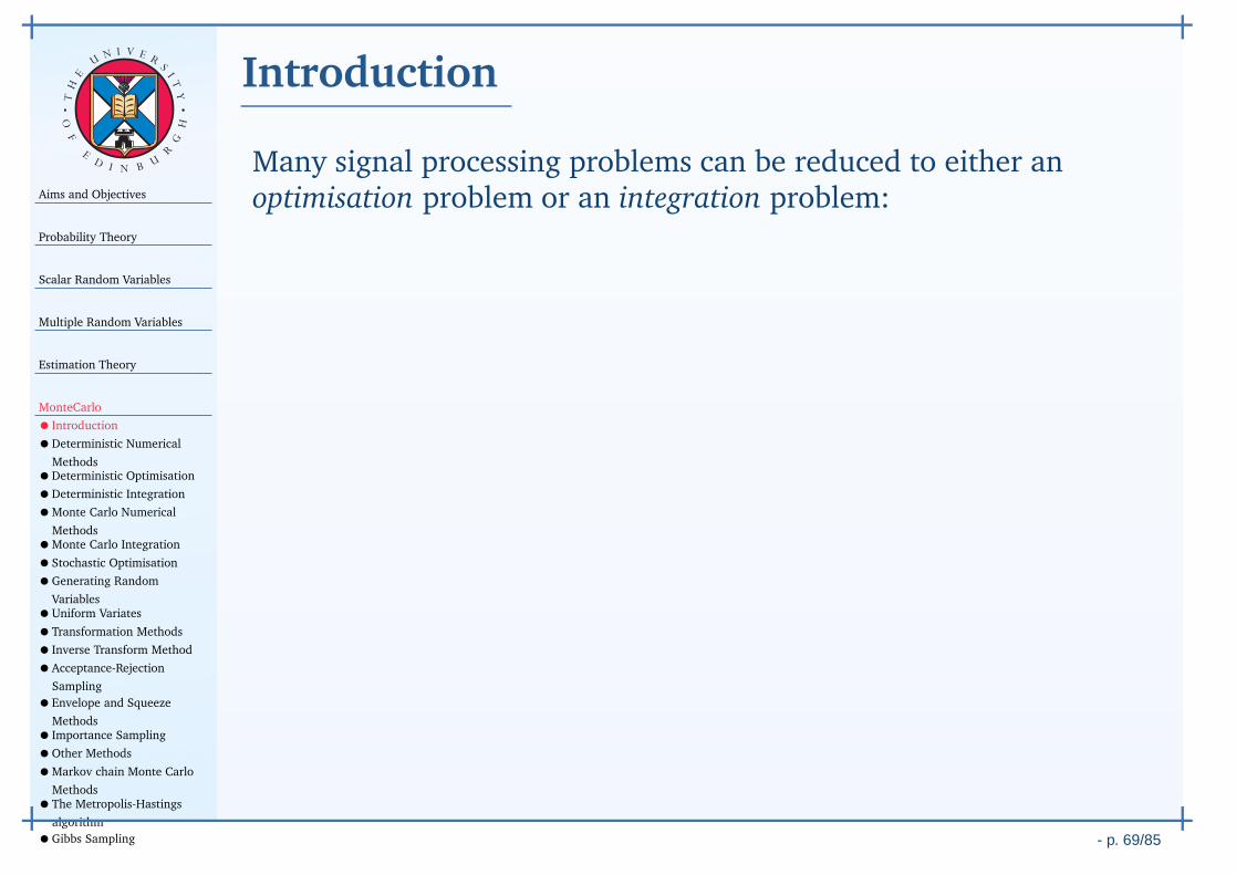
Aims and Objectives
Probability Theory
Scalar Random Variables
Multiple Random Variables
Estimation Theory
MonteCarlo
• Introduction
•Deterministic Numerical
Methods•Deterministic Optimisation
•Deterministic Integration
•Monte Carlo Numerical
Methods•Monte Carlo Integration
•Stochastic Optimisation
•Generating Random
Variables•Uniform Variates
•Transformation Methods
• Inverse Transform Method
•Acceptance-Rejection
Sampling
•Envelope and Squeeze
Methods• Importance Sampling
•Other Methods
•Markov chain Monte Carlo
Methods•The Metropolis-Hastings
algorithm
•Gibbs Sampling - p. 69/85
TH
E
UN I V E
RS
IT
Y
OF
ED
I N BU
R
GH
Introduction
Many signal processing problems can be reduced to either anoptimisation problem or an integration problem:
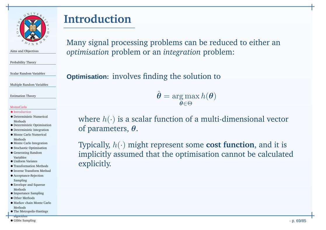
Optimisation: involves finding the solution to
θ = argmaxθ∈Θ
h(θ)
where h(·) is a scalar function of a multi-dimensional vectorof parameters, θ.
Typically, h(·) might represent some cost function, and it isimplicitly assumed that the optimisation cannot be calculatedexplicitly.
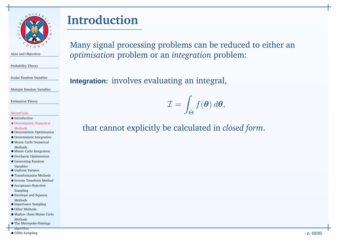
Aims and Objectives
Probability Theory
Scalar Random Variables
Multiple Random Variables
Estimation Theory
MonteCarlo
• Introduction
•Deterministic Numerical
Methods•Deterministic Optimisation
•Deterministic Integration
•Monte Carlo Numerical
Methods•Monte Carlo Integration
•Stochastic Optimisation
•Generating Random
Variables•Uniform Variates
•Transformation Methods
• Inverse Transform Method
•Acceptance-Rejection
Sampling
•Envelope and Squeeze
Methods• Importance Sampling
•Other Methods
•Markov chain Monte Carlo
Methods•The Metropolis-Hastings
algorithm
•Gibbs Sampling - p. 69/85
TH
E
UN I V E
RS
IT
Y
OF
ED
I N BU
R
GH
Introduction
Many signal processing problems can be reduced to either anoptimisation problem or an integration problem:
Integration: involves evaluating an integral,
I =
∫
Θ
f(θ) dθ,
that cannot explicitly be calculated in closed form.
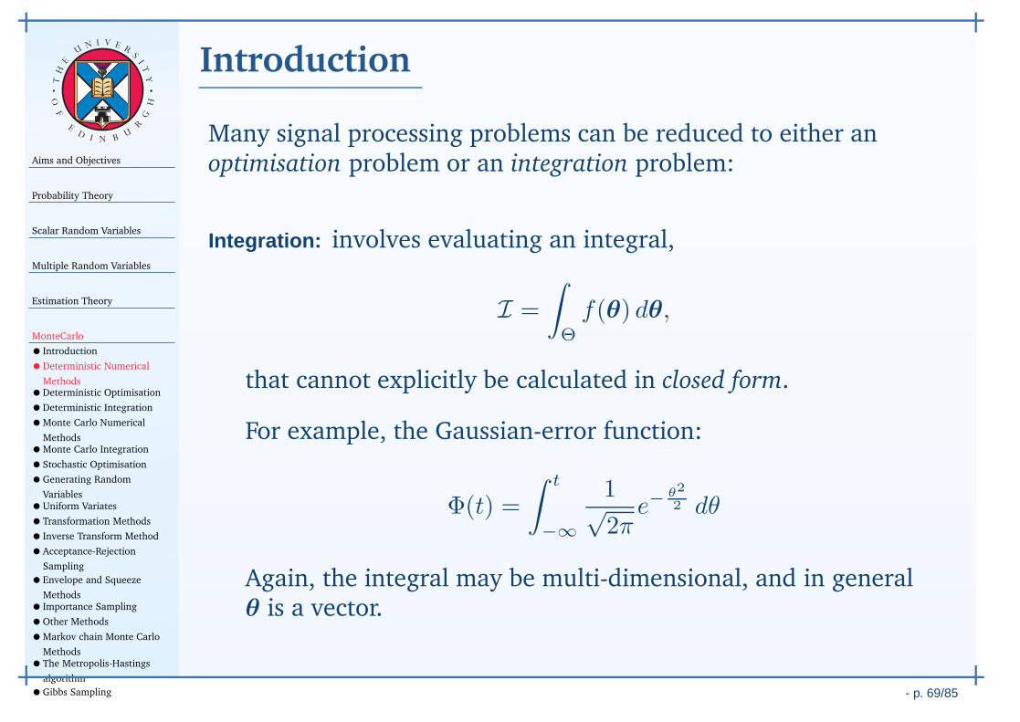
For example, the Gaussian-error function:
Φ(t) =
∫ t
−∞
1√2π
e−θ2
2 dθ
Again, the integral may be multi-dimensional, and in generalθ is a vector.

Aims and Objectives
Probability Theory
Scalar Random Variables
Multiple Random Variables
Estimation Theory
MonteCarlo
• Introduction
•Deterministic Numerical
Methods•Deterministic Optimisation
•Deterministic Integration
•Monte Carlo Numerical
Methods•Monte Carlo Integration
•Stochastic Optimisation
•Generating Random
Variables•Uniform Variates
•Transformation Methods
• Inverse Transform Method
•Acceptance-Rejection
Sampling
•Envelope and Squeeze
Methods• Importance Sampling
•Other Methods
•Markov chain Monte Carlo
Methods•The Metropolis-Hastings
algorithm
•Gibbs Sampling - p. 69/85
TH
E
UN I V E
RS
IT
Y
OF
ED
I N BU
R
GH
Introduction
Many signal processing problems can be reduced to either anoptimisation problem or an integration problem:
Optimisation and Integration Some problems involve bothintegration and optimisation: a fundamental problem is themaximisation of a marginal distribution:
θ = argmaxθ∈Θ
∫
Ω
f(θ, ω) dω
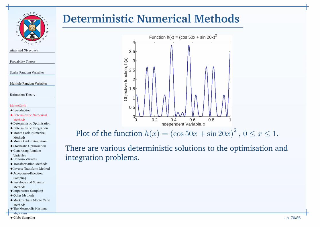
Aims and Objectives
Probability Theory
Scalar Random Variables
Multiple Random Variables
Estimation Theory
MonteCarlo
• Introduction
•Deterministic Numerical
Methods•Deterministic Optimisation
•Deterministic Integration
•Monte Carlo Numerical
Methods•Monte Carlo Integration
•Stochastic Optimisation
•Generating Random
Variables•Uniform Variates
•Transformation Methods
• Inverse Transform Method
•Acceptance-Rejection
Sampling
•Envelope and Squeeze
Methods• Importance Sampling
•Other Methods
•Markov chain Monte Carlo
Methods•The Metropolis-Hastings
algorithm
•Gibbs Sampling - p. 70/85
TH
E
UN I V E
RS
IT
Y
OF
ED
I N BU
R
GH
Deterministic Numerical Methods
0 0.2 0.4 0.6 0.8 10
0.5
1
1.5
2
2.5
3
3.5
4
Independent Variable, xO
bjec
tive
func
tion,
h(x
)
Function h(x) = (cos 50x + sin 20x)2
Plot of the function h(x) = (cos 50x+ sin 20x)2, 0 ≤ x ≤ 1.
There are various deterministic solutions to the optimisation andintegration problems.
Aims and Objectives
Probability Theory
Scalar Random Variables
Multiple Random Variables
Estimation Theory
MonteCarlo
• Introduction
•Deterministic Numerical
Methods•Deterministic Optimisation
•Deterministic Integration
•Monte Carlo Numerical
Methods•Monte Carlo Integration
•Stochastic Optimisation
•Generating Random
Variables•Uniform Variates
•Transformation Methods
• Inverse Transform Method
•Acceptance-Rejection
Sampling
•Envelope and Squeeze
Methods• Importance Sampling
•Other Methods
•Markov chain Monte Carlo
Methods•The Metropolis-Hastings
algorithm
•Gibbs Sampling - p. 70/85
TH
E
UN I V E
RS
IT
Y
OF
ED
I N BU
R
GH
Deterministic Numerical Methods
Optimisation: 1. Golden-section search and Brent’s Method in onedimension;
2. Nelder and Mead Downhill Simplex method inmulti-dimensions;
3. Gradient and Variable-Metric methods inmulti-dimensions, typically an extension ofNewton-Raphson methods.
Aims and Objectives
Probability Theory
Scalar Random Variables
Multiple Random Variables
Estimation Theory
MonteCarlo
• Introduction
•Deterministic Numerical
Methods•Deterministic Optimisation
•Deterministic Integration
•Monte Carlo Numerical
Methods•Monte Carlo Integration
•Stochastic Optimisation
•Generating Random
Variables•Uniform Variates
•Transformation Methods
• Inverse Transform Method
•Acceptance-Rejection
Sampling
•Envelope and Squeeze
Methods• Importance Sampling
•Other Methods
•Markov chain Monte Carlo
Methods•The Metropolis-Hastings
algorithm
•Gibbs Sampling - p. 70/85
TH
E
UN I V E
RS
IT
Y
OF
ED
I N BU
R
GH
Deterministic Numerical Methods
Integration: Most deterministic integration rely on classicformulas for equally spaced abscissas:
1. simple Riemann integration;
2. standard and extended Simpson’s and Trapezoidal rules;
3. refinements such as Romberg Integration.
Unfortunately, these methods are not easily extended tomulti-dimensions.
Aims and Objectives
Probability Theory
Scalar Random Variables
Multiple Random Variables
Estimation Theory
MonteCarlo
• Introduction
•Deterministic Numerical
Methods•Deterministic Optimisation
•Deterministic Integration
•Monte Carlo Numerical
Methods•Monte Carlo Integration
•Stochastic Optimisation
•Generating Random
Variables•Uniform Variates
•Transformation Methods
• Inverse Transform Method
•Acceptance-Rejection
Sampling
•Envelope and Squeeze
Methods• Importance Sampling
•Other Methods
•Markov chain Monte Carlo
Methods•The Metropolis-Hastings
algorithm
•Gibbs Sampling - p. 70/85
TH
E
UN I V E
RS
IT
Y
OF
ED
I N BU
R
GH
Deterministic Numerical Methods
Integration: Most deterministic integration rely on classicformulas for equally spaced abscissas:
1. simple Riemann integration;
2. standard and extended Simpson’s and Trapezoidal rules;
3. refinements such as Romberg Integration.
More sophisticated approaches allow non-uniformally spacedabscissas at which the function is evaluated.
These methods tend to use Gaussian quadratures andorthogonal polynomials. Splines are also used.
Unfortunately, these methods are not easily extended tomulti-dimensions.
Aims and Objectives
Probability Theory
Scalar Random Variables
Multiple Random Variables
Estimation Theory
MonteCarlo
• Introduction
•Deterministic Numerical
Methods•Deterministic Optimisation
•Deterministic Integration
•Monte Carlo Numerical
Methods•Monte Carlo Integration
•Stochastic Optimisation
•Generating Random
Variables•Uniform Variates
•Transformation Methods
• Inverse Transform Method
•Acceptance-Rejection
Sampling
•Envelope and Squeeze
Methods• Importance Sampling
•Other Methods
•Markov chain Monte Carlo
Methods•The Metropolis-Hastings
algorithm
•Gibbs Sampling - p. 71/85
TH
E
UN I V E
RS
IT
Y
OF
ED
I N BU
R
GH
Deterministic Optimisation
The Nelder-Mead Downhill Simplex method simply crawlsdownhill in a straightforward fashion that makes almost nospecial assumptions about your function.
This can be extremely slow, but it can be robust.

Aims and Objectives
Probability Theory
Scalar Random Variables
Multiple Random Variables
Estimation Theory
MonteCarlo
• Introduction
•Deterministic Numerical
Methods•Deterministic Optimisation
•Deterministic Integration
•Monte Carlo Numerical
Methods•Monte Carlo Integration
•Stochastic Optimisation
•Generating Random
Variables•Uniform Variates
•Transformation Methods
• Inverse Transform Method
•Acceptance-Rejection
Sampling
•Envelope and Squeeze
Methods• Importance Sampling
•Other Methods
•Markov chain Monte Carlo
Methods•The Metropolis-Hastings
algorithm
•Gibbs Sampling - p. 71/85
TH
E
UN I V E
RS
IT
Y
OF
ED
I N BU
R
GH
Deterministic Optimisation
Gradient methods are typically based on the Newton-Raphsonalgorithm which solves ∇h(θ) = 0.
For a scalar function, h(θ), of a vector of independent variablesθ, a sequence θn is produced such that:
θn+1 = θn −(∇∇Th (θn)
)−1 ∇h (θn)
Numerous variants of Newton-Raphson-type techniques exist,and include the steepest descent method, or theLevenberg-Marquardt method.
Aims and Objectives
Probability Theory
Scalar Random Variables
Multiple Random Variables
Estimation Theory
MonteCarlo
• Introduction
•Deterministic Numerical
Methods•Deterministic Optimisation
•Deterministic Integration
•Monte Carlo Numerical
Methods•Monte Carlo Integration
•Stochastic Optimisation
•Generating Random
Variables•Uniform Variates
•Transformation Methods
• Inverse Transform Method
•Acceptance-Rejection
Sampling
•Envelope and Squeeze
Methods• Importance Sampling
•Other Methods
•Markov chain Monte Carlo
Methods•The Metropolis-Hastings
algorithm
•Gibbs Sampling - p. 72/85
TH
E
UN I V E
RS
IT
Y
OF
ED
I N BU
R
GH
Deterministic Integration
The integral
I =
∫ b
a
f(θ) dθ,
where θ is a scalar, and b > a, can be solved with the trapezoidalrule using
I =1
2
N−1∑
k=0
(θk+1 − θk) (f(θk) + f(θk+1))
where the θk ’s constitute an ordered partition of [a, b].
Another formula is Simpson’s rule:
I =δ
3
f(a) + 4N∑
k=1
f(θ2k−1) + 2N∑
k=1
h(θ2k) + f(b)
in the case of equally spaced samples with δ = θk+1 − θk.
Aims and Objectives
Probability Theory
Scalar Random Variables
Multiple Random Variables
Estimation Theory
MonteCarlo
• Introduction
•Deterministic Numerical
Methods•Deterministic Optimisation
•Deterministic Integration
•Monte Carlo Numerical
Methods•Monte Carlo Integration
•Stochastic Optimisation
•Generating Random
Variables•Uniform Variates
•Transformation Methods
• Inverse Transform Method
•Acceptance-Rejection
Sampling
•Envelope and Squeeze
Methods• Importance Sampling
•Other Methods
•Markov chain Monte Carlo
Methods•The Metropolis-Hastings
algorithm
•Gibbs Sampling - p. 73/85
TH
E
UN I V E
RS
IT
Y
OF
ED
I N BU
R
GH
Monte Carlo Numerical Methods
Monte Carlo methods are stochastic techniques, in which randomnumbers are generated and use to examine some problem.

Aims and Objectives
Probability Theory
Scalar Random Variables
Multiple Random Variables
Estimation Theory
MonteCarlo
• Introduction
•Deterministic Numerical
Methods•Deterministic Optimisation
•Deterministic Integration
•Monte Carlo Numerical
Methods•Monte Carlo Integration
•Stochastic Optimisation
•Generating Random
Variables•Uniform Variates
•Transformation Methods
• Inverse Transform Method
•Acceptance-Rejection
Sampling
•Envelope and Squeeze
Methods• Importance Sampling
•Other Methods
•Markov chain Monte Carlo
Methods•The Metropolis-Hastings
algorithm
•Gibbs Sampling - p. 74/85
TH
E
UN I V E
RS
IT
Y
OF
ED
I N BU
R
GH
Monte Carlo Integration
Consider the integral,
I =
∫
Θ
f(θ) dθ.
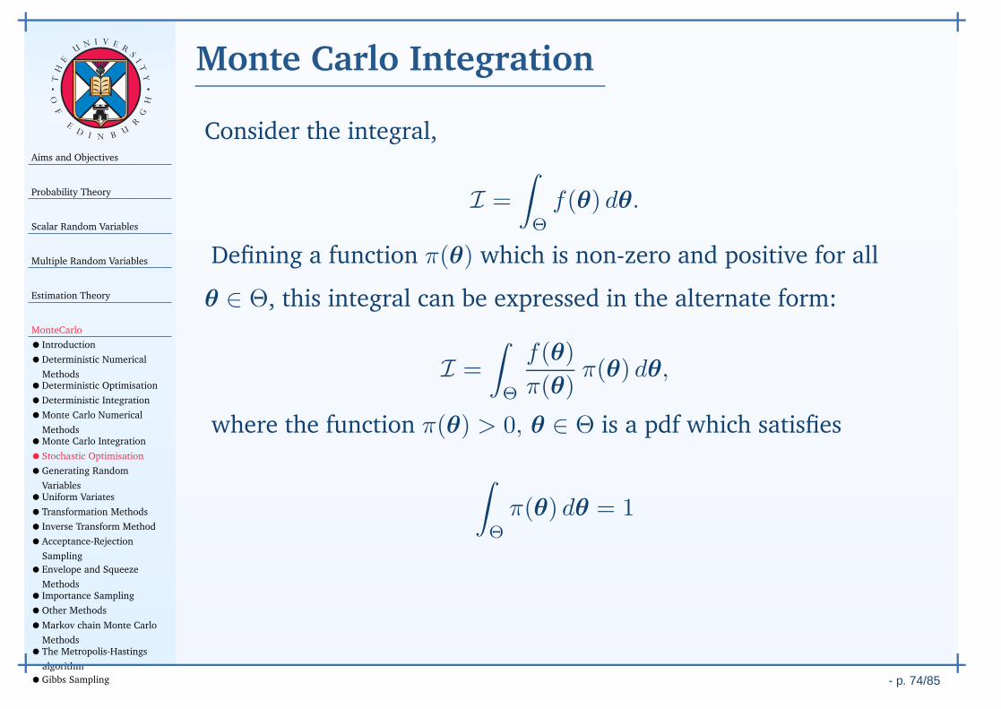
Defining a function π(θ) which is non-zero and positive for all
θ ∈ Θ, this integral can be expressed in the alternate form:
I =
∫
Θ
f(θ)
π(θ)π(θ) dθ,
where the function π(θ) > 0, θ ∈ Θ is a pdf which satisfies
∫
Θ
π(θ) dθ = 1
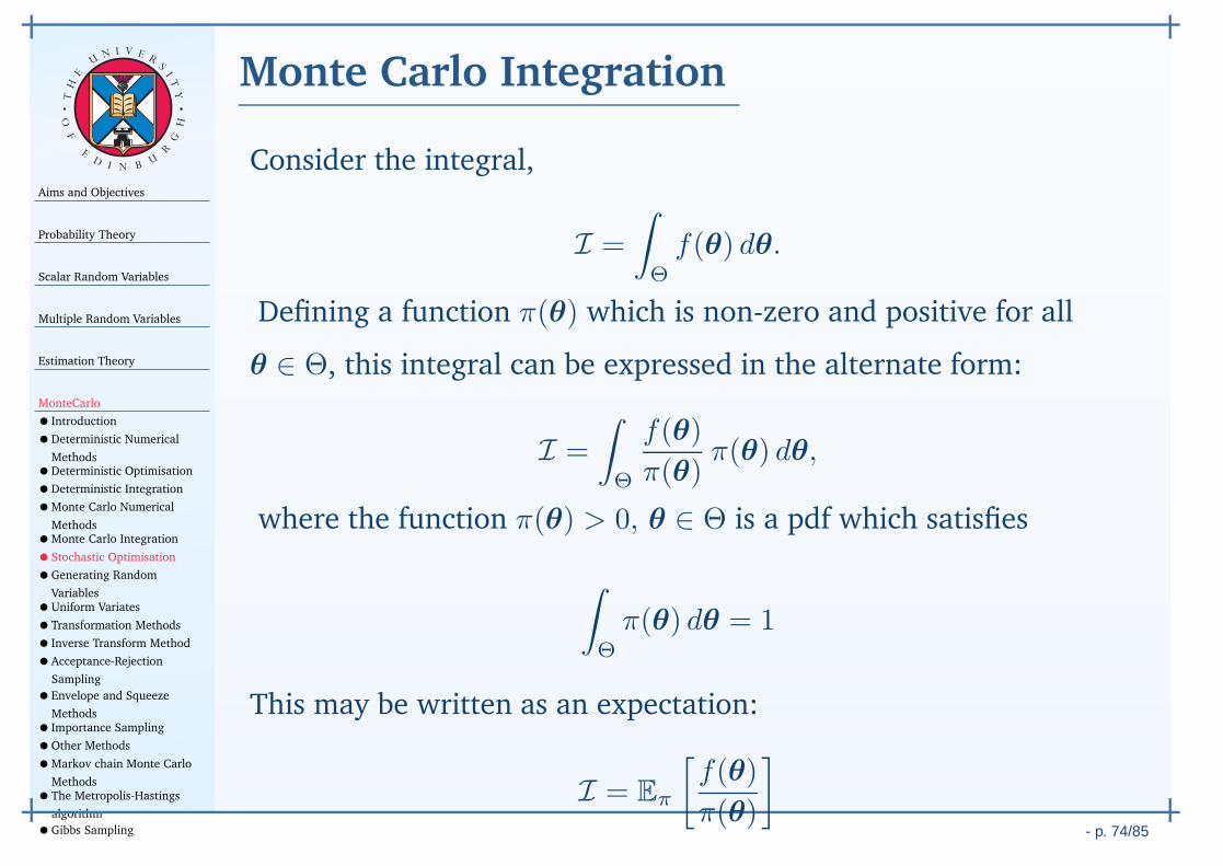
This may be written as an expectation:
I = Eπ
[f(θ)
π(θ)
]
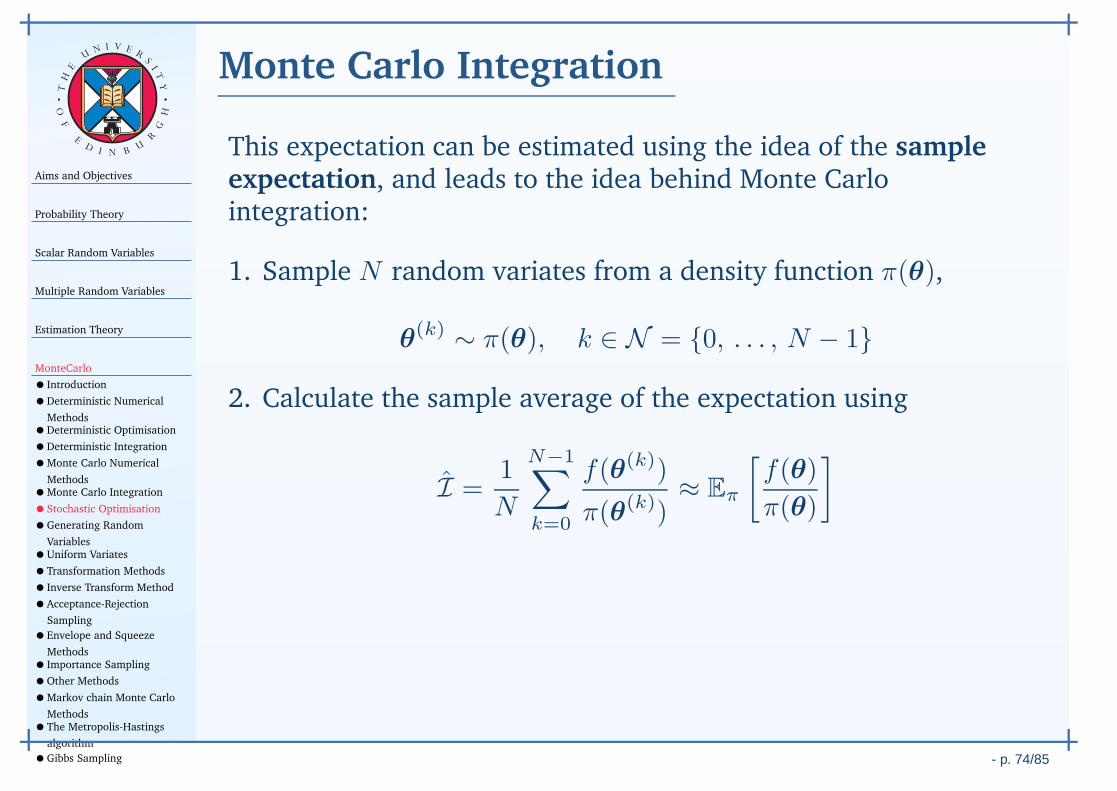
Aims and Objectives
Probability Theory
Scalar Random Variables
Multiple Random Variables
Estimation Theory
MonteCarlo
• Introduction
•Deterministic Numerical
Methods•Deterministic Optimisation
•Deterministic Integration
•Monte Carlo Numerical
Methods•Monte Carlo Integration
•Stochastic Optimisation
•Generating Random
Variables•Uniform Variates
•Transformation Methods
• Inverse Transform Method
•Acceptance-Rejection
Sampling
•Envelope and Squeeze
Methods• Importance Sampling
•Other Methods
•Markov chain Monte Carlo
Methods•The Metropolis-Hastings
algorithm
•Gibbs Sampling - p. 74/85
TH
E
UN I V E
RS
IT
Y
OF
ED
I N BU
R
GH
Monte Carlo Integration
This expectation can be estimated using the idea of the sampleexpectation, and leads to the idea behind Monte Carlointegration:
1. Sample N random variates from a density function π(θ),
θ(k) ∼ π(θ), k ∈ N = 0, . . . , N − 1
2. Calculate the sample average of the expectation using
I =1
N
N−1∑
k=0
f(θ(k))
π(θ(k))≈ Eπ
[f(θ)
π(θ)
]
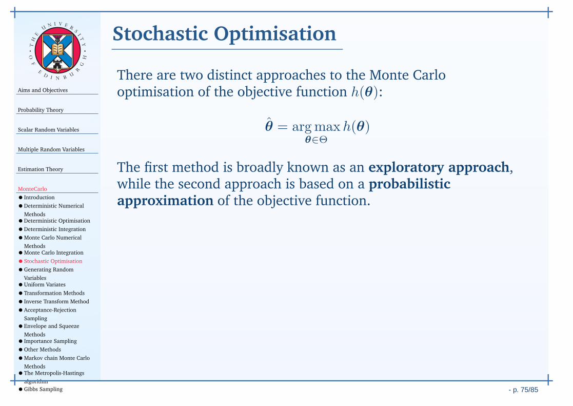
Aims and Objectives
Probability Theory
Scalar Random Variables
Multiple Random Variables
Estimation Theory
MonteCarlo
• Introduction
•Deterministic Numerical
Methods•Deterministic Optimisation
•Deterministic Integration
•Monte Carlo Numerical
Methods•Monte Carlo Integration
•Stochastic Optimisation
•Generating Random
Variables•Uniform Variates
•Transformation Methods
• Inverse Transform Method
•Acceptance-Rejection
Sampling
•Envelope and Squeeze
Methods• Importance Sampling
•Other Methods
•Markov chain Monte Carlo
Methods•The Metropolis-Hastings
algorithm
•Gibbs Sampling - p. 75/85
TH
E
UN I V E
RS
IT
Y
OF
ED
I N BU
R
GH
Stochastic Optimisation
There are two distinct approaches to the Monte Carlooptimisation of the objective function h(θ):
θ = argmaxθ∈Θ
h(θ)
The first method is broadly known as an exploratory approach,while the second approach is based on a probabilisticapproximation of the objective function.

Aims and Objectives
Probability Theory
Scalar Random Variables
Multiple Random Variables
Estimation Theory
MonteCarlo
• Introduction
•Deterministic Numerical
Methods•Deterministic Optimisation
•Deterministic Integration
•Monte Carlo Numerical
Methods•Monte Carlo Integration
•Stochastic Optimisation
•Generating Random
Variables•Uniform Variates
•Transformation Methods
• Inverse Transform Method
•Acceptance-Rejection
Sampling
•Envelope and Squeeze
Methods• Importance Sampling
•Other Methods
•Markov chain Monte Carlo
Methods•The Metropolis-Hastings
algorithm
•Gibbs Sampling - p. 75/85
TH
E
UN I V E
RS
IT
Y
OF
ED
I N BU
R
GH
Stochastic Optimisation
Exploratory approach This approach is concerned with fastexplorations of the sample space rather than working with theobjective function directly.
For example, maximisation can be solved by sampling a large
number, N , of independent random variables, θ(k), from apdf π(θ), and taking the estimate:
θ ≈ argmaxθ(k)
h(
θ(k))
Typically, when no specific features regarding the functionh (θ), are taken into account, π(θ) will take on a uniformdistribution over Θ.
Stochastic Approximation The Monte Carlo EM algorithm
Aims and Objectives
Probability Theory
Scalar Random Variables
Multiple Random Variables
Estimation Theory
MonteCarlo
• Introduction
•Deterministic Numerical
Methods•Deterministic Optimisation
•Deterministic Integration
•Monte Carlo Numerical
Methods•Monte Carlo Integration
•Stochastic Optimisation
•Generating Random
Variables•Uniform Variates
•Transformation Methods
• Inverse Transform Method
•Acceptance-Rejection
Sampling
•Envelope and Squeeze
Methods• Importance Sampling
•Other Methods
•Markov chain Monte Carlo
Methods•The Metropolis-Hastings
algorithm
•Gibbs Sampling - p. 76/85
TH
E
UN I V E
RS
IT
Y
OF
ED
I N BU
R
GH
Generating Random Variables
This section discusses a variety of techniques for generatingrandom variables from a different distributions.
Aims and Objectives
Probability Theory
Scalar Random Variables
Multiple Random Variables
Estimation Theory
MonteCarlo
• Introduction
•Deterministic Numerical
Methods•Deterministic Optimisation
•Deterministic Integration
•Monte Carlo Numerical
Methods•Monte Carlo Integration
•Stochastic Optimisation
•Generating Random
Variables•Uniform Variates
•Transformation Methods
• Inverse Transform Method
•Acceptance-Rejection
Sampling
•Envelope and Squeeze
Methods• Importance Sampling
•Other Methods
•Markov chain Monte Carlo
Methods•The Metropolis-Hastings
algorithm
•Gibbs Sampling - p. 77/85
TH
E
UN I V E
RS
IT
Y
OF
ED
I N BU
R
GH
Uniform Variates
The foundation underpinning all stochastic simulations is theability to generate a sequence of i. i. d. uniform random variatesover the range (0, 1].
Random variates are pseudo or synthetic and not truly randomsince they are usually generated using a recurrence of the form:
xn+1 = (a xn + b) mod m
This is known as the linear congruential generator.
However, suitable values of a, b and m can be chosen such thatthe random variates pass all statistical tests of randomness.
Aims and Objectives
Probability Theory
Scalar Random Variables
Multiple Random Variables
Estimation Theory
MonteCarlo
• Introduction
•Deterministic Numerical
Methods•Deterministic Optimisation
•Deterministic Integration
•Monte Carlo Numerical
Methods•Monte Carlo Integration
•Stochastic Optimisation
•Generating Random
Variables•Uniform Variates
•Transformation Methods
• Inverse Transform Method
•Acceptance-Rejection
Sampling
•Envelope and Squeeze
Methods• Importance Sampling
•Other Methods
•Markov chain Monte Carlo
Methods•The Metropolis-Hastings
algorithm
•Gibbs Sampling - p. 78/85
TH
E
UN I V E
RS
IT
Y
OF
ED
I N BU
R
GH
Transformation Methods
It is possible to sample from a number of extremely importantprobability distributions by applying various probabilitytransformation methods.
Theorem (Probability transformation rule). Denote the real roots ofy = g(x) by xn, n ∈ N, such that
y = g(x1) = · · · = g(xN )
PROOF. The proof is given in the handout on scalar randomvariables.

Aims and Objectives
Probability Theory
Scalar Random Variables
Multiple Random Variables
Estimation Theory
MonteCarlo
• Introduction
•Deterministic Numerical
Methods•Deterministic Optimisation
•Deterministic Integration
•Monte Carlo Numerical
Methods•Monte Carlo Integration
•Stochastic Optimisation
•Generating Random
Variables•Uniform Variates
•Transformation Methods
• Inverse Transform Method
•Acceptance-Rejection
Sampling
•Envelope and Squeeze
Methods• Importance Sampling
•Other Methods
•Markov chain Monte Carlo
Methods•The Metropolis-Hastings
algorithm
•Gibbs Sampling - p. 79/85
TH
E
UN I V E
RS
IT
Y
OF
ED
I N BU
R
GH
Inverse Transform Method
A simple derivation of the inverse transform method
X(ζ) and Y (ζ) are RVs related by the function Y (ζ) = Π(X(ζ)).
Π(ζ) is monotonically increasing so that there is only one
solution to the equation y = Π(x), x = Π−1(y).
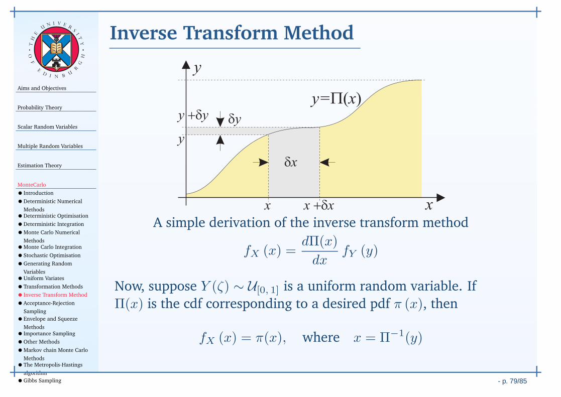
Aims and Objectives
Probability Theory
Scalar Random Variables
Multiple Random Variables
Estimation Theory
MonteCarlo
• Introduction
•Deterministic Numerical
Methods•Deterministic Optimisation
•Deterministic Integration
•Monte Carlo Numerical
Methods•Monte Carlo Integration
•Stochastic Optimisation
•Generating Random
Variables•Uniform Variates
•Transformation Methods
• Inverse Transform Method
•Acceptance-Rejection
Sampling
•Envelope and Squeeze
Methods• Importance Sampling
•Other Methods
•Markov chain Monte Carlo
Methods•The Metropolis-Hastings
algorithm
•Gibbs Sampling - p. 79/85
TH
E
UN I V E
RS
IT
Y
OF
ED
I N BU
R
GH
Inverse Transform Method
A simple derivation of the inverse transform method
fX (x) =dΠ(x)
dxfY (y)
Now, suppose Y (ζ) ∼ U[0, 1] is a uniform random variable. If
Π(x) is the cdf corresponding to a desired pdf π (x), then
fX (x) = π(x), where x = Π−1(y)

Aims and Objectives
Probability Theory
Scalar Random Variables
Multiple Random Variables
Estimation Theory
MonteCarlo
• Introduction
•Deterministic Numerical
Methods•Deterministic Optimisation
•Deterministic Integration
•Monte Carlo Numerical
Methods•Monte Carlo Integration
•Stochastic Optimisation
•Generating Random
Variables•Uniform Variates
•Transformation Methods
• Inverse Transform Method
•Acceptance-Rejection
Sampling
•Envelope and Squeeze
Methods• Importance Sampling
•Other Methods
•Markov chain Monte Carlo
Methods•The Metropolis-Hastings
algorithm
•Gibbs Sampling - p. 79/85
TH
E
UN I V E
RS
IT
Y
OF
ED
I N BU
R
GH
Inverse Transform Method
In otherwords, if
U(ζ) ∼ U[0, 1], X(ζ) = Π−1U(ζ) ∼ π (x)
Example (Exponential variable generation). If X(ζ) ∼ Exp(1), such
that π(x) = e−x and Π(x) = 1− e−x, then solving for x in terms
of u = 1− e−x gives x = − log(1− u).
Therefore, if U(ζ) ∼ U[0, 1], then the RV from the transformation
X(ζ) = − logU(ζ) has the exponential distribution (since U(ζ)and 1− U(ζ) are both uniform).

Aims and Objectives
Probability Theory
Scalar Random Variables
Multiple Random Variables
Estimation Theory
MonteCarlo
• Introduction
•Deterministic Numerical
Methods•Deterministic Optimisation
•Deterministic Integration
•Monte Carlo Numerical
Methods•Monte Carlo Integration
•Stochastic Optimisation
•Generating Random
Variables•Uniform Variates
•Transformation Methods
• Inverse Transform Method
•Acceptance-Rejection
Sampling
•Envelope and Squeeze
Methods• Importance Sampling
•Other Methods
•Markov chain Monte Carlo
Methods•The Metropolis-Hastings
algorithm
•Gibbs Sampling - p. 80/85
TH
E
UN I V E
RS
IT
Y
OF
ED
I N BU
R
GH
Acceptance-Rejection Sampling
For most distributions, it is often difficult or even impossible todirectly simulate using either the inverse transform or probabilitytransformations.
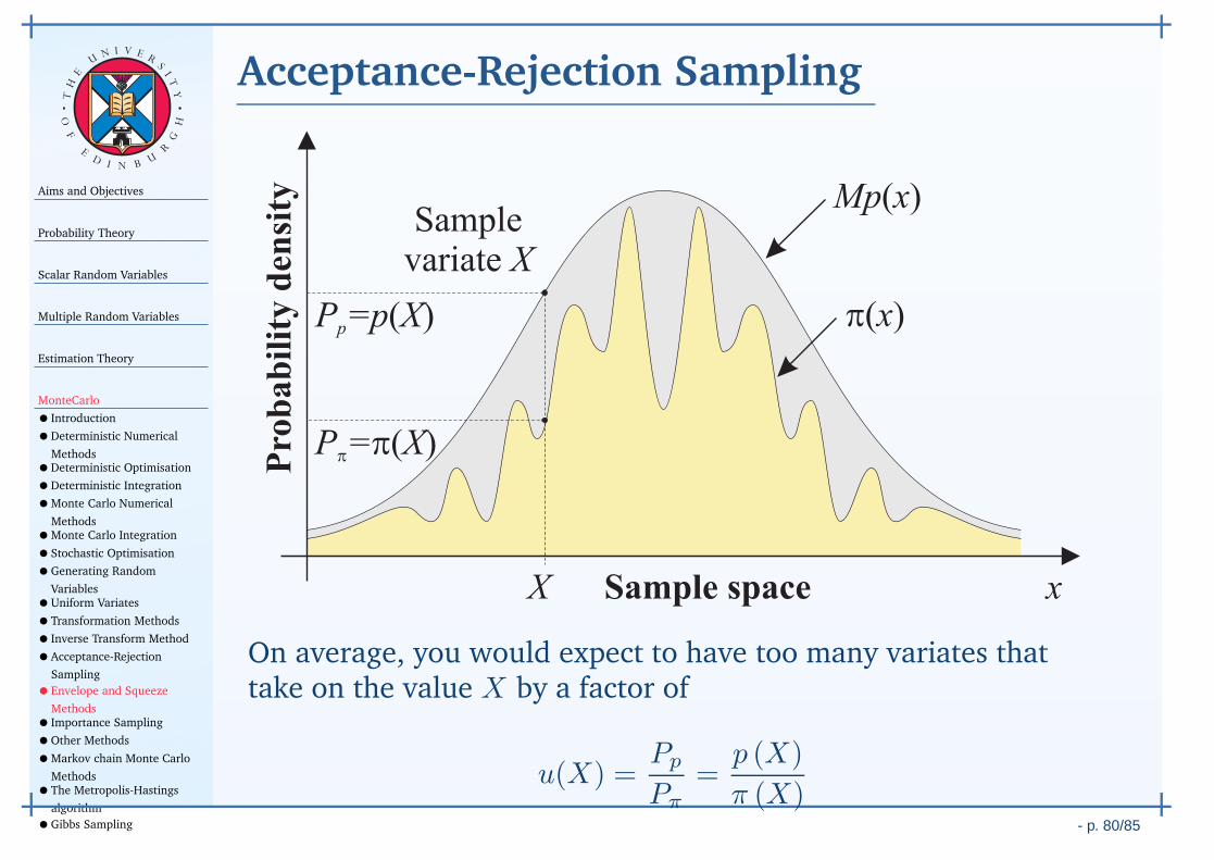
Aims and Objectives
Probability Theory
Scalar Random Variables
Multiple Random Variables
Estimation Theory
MonteCarlo
• Introduction
•Deterministic Numerical
Methods•Deterministic Optimisation
•Deterministic Integration
•Monte Carlo Numerical
Methods•Monte Carlo Integration
•Stochastic Optimisation
•Generating Random
Variables•Uniform Variates
•Transformation Methods
• Inverse Transform Method
•Acceptance-Rejection
Sampling
•Envelope and Squeeze
Methods• Importance Sampling
•Other Methods
•Markov chain Monte Carlo
Methods•The Metropolis-Hastings
algorithm
•Gibbs Sampling - p. 80/85
TH
E
UN I V E
RS
IT
Y
OF
ED
I N BU
R
GH
Acceptance-Rejection Sampling
On average, you would expect to have too many variates thattake on the value X by a factor of
u(X) =Pp
Pπ
=p (X)
π (X)
Aims and Objectives
Probability Theory
Scalar Random Variables
Multiple Random Variables
Estimation Theory
MonteCarlo
• Introduction
•Deterministic Numerical
Methods•Deterministic Optimisation
•Deterministic Integration
•Monte Carlo Numerical
Methods•Monte Carlo Integration
•Stochastic Optimisation
•Generating Random
Variables•Uniform Variates
•Transformation Methods
• Inverse Transform Method
•Acceptance-Rejection
Sampling
•Envelope and Squeeze
Methods• Importance Sampling
•Other Methods
•Markov chain Monte Carlo
Methods•The Metropolis-Hastings
algorithm
•Gibbs Sampling - p. 80/85
TH
E
UN I V E
RS
IT
Y
OF
ED
I N BU
R
GH
Acceptance-Rejection Sampling
Thus, to reduce the number of variates that take on a value of X ,simply throw away a number of samples in proportion to theamount of over sampling.
1. Generate the random variates X ∼ p(x) and U ∼ U[0, 1];
2. Accept X if U ≤ Pa = π(X)Mp(x) ;
3. Otherwise, reject and return to first step.
Aims and Objectives
Probability Theory
Scalar Random Variables
Multiple Random Variables
Estimation Theory
MonteCarlo
• Introduction
•Deterministic Numerical
Methods•Deterministic Optimisation
•Deterministic Integration
•Monte Carlo Numerical
Methods•Monte Carlo Integration
•Stochastic Optimisation
•Generating Random
Variables•Uniform Variates
•Transformation Methods
• Inverse Transform Method
•Acceptance-Rejection
Sampling
•Envelope and Squeeze
Methods• Importance Sampling
•Other Methods
•Markov chain Monte Carlo
Methods•The Metropolis-Hastings
algorithm
•Gibbs Sampling - p. 81/85
TH
E
UN I V E
RS
IT
Y
OF
ED
I N BU
R
GH
Envelope and Squeeze Methods
A problem with many sampling methods, which can make thedensity π (x) difficult to simulate, is that the function mayrequire substantial computing time at each evaluation.
It is possible to reduce the algorithmic complexity by looking foranother computationally simple function, q (x) which boundsπ (x) from below.
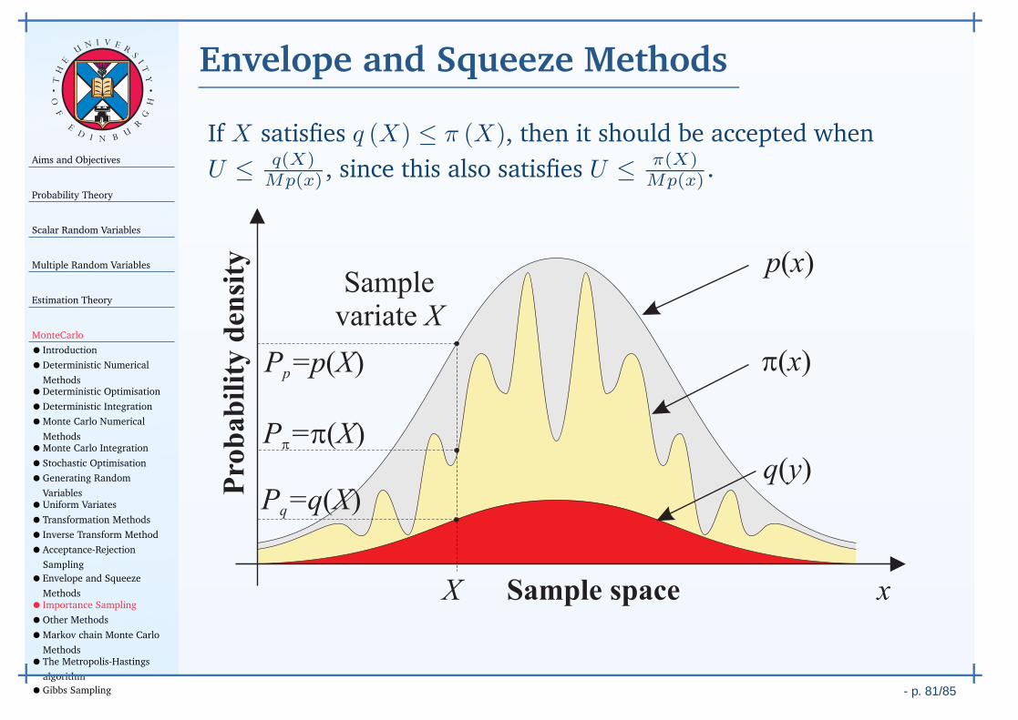
Aims and Objectives
Probability Theory
Scalar Random Variables
Multiple Random Variables
Estimation Theory
MonteCarlo
• Introduction
•Deterministic Numerical
Methods•Deterministic Optimisation
•Deterministic Integration
•Monte Carlo Numerical
Methods•Monte Carlo Integration
•Stochastic Optimisation
•Generating Random
Variables•Uniform Variates
•Transformation Methods
• Inverse Transform Method
•Acceptance-Rejection
Sampling
•Envelope and Squeeze
Methods• Importance Sampling
•Other Methods
•Markov chain Monte Carlo
Methods•The Metropolis-Hastings
algorithm
•Gibbs Sampling - p. 81/85
TH
E
UN I V E
RS
IT
Y
OF
ED
I N BU
R
GH
Envelope and Squeeze Methods
If X satisfies q (X) ≤ π (X), then it should be accepted when
U ≤ q(X)Mp(x) , since this also satisfies U ≤ π(X)
Mp(x) .
Aims and Objectives
Probability Theory
Scalar Random Variables
Multiple Random Variables
Estimation Theory
MonteCarlo
• Introduction
•Deterministic Numerical
Methods•Deterministic Optimisation
•Deterministic Integration
•Monte Carlo Numerical
Methods•Monte Carlo Integration
•Stochastic Optimisation
•Generating Random
Variables•Uniform Variates
•Transformation Methods
• Inverse Transform Method
•Acceptance-Rejection
Sampling
•Envelope and Squeeze
Methods• Importance Sampling
•Other Methods
•Markov chain Monte Carlo
Methods•The Metropolis-Hastings
algorithm
•Gibbs Sampling - p. 81/85
TH
E
UN I V E
RS
IT
Y
OF
ED
I N BU
R
GH
Envelope and Squeeze Methods
This leads to the envelope accept-reject algorithm:
1. Generate the random variates X ∼ p(x) and U ∼ U[0, 1];
2. Accept X if U ≤ q(X)Mp(x) ;
3. Otherwise, accept X if U ≤ π(X)Mp(x) ;
4. Otherwise, reject and return to first step.
By construction of a lower envelope on π (x), the number offunction evaluations is potentially decreased by a factor of
Pπ =1
M
∫
q (x) dx
which is the probability that π (x) is not evaluated.
Aims and Objectives
Probability Theory
Scalar Random Variables
Multiple Random Variables
Estimation Theory
MonteCarlo
• Introduction
•Deterministic Numerical
Methods•Deterministic Optimisation
•Deterministic Integration
•Monte Carlo Numerical
Methods•Monte Carlo Integration
•Stochastic Optimisation
•Generating Random
Variables•Uniform Variates
•Transformation Methods
• Inverse Transform Method
•Acceptance-Rejection
Sampling
•Envelope and Squeeze
Methods• Importance Sampling
•Other Methods
•Markov chain Monte Carlo
Methods•The Metropolis-Hastings
algorithm
•Gibbs Sampling - p. 82/85
TH
E
UN I V E
RS
IT
Y
OF
ED
I N BU
R
GH
Importance Sampling
The problem with accept-reject sampling methods is finding theenvelope functions and the constant M .
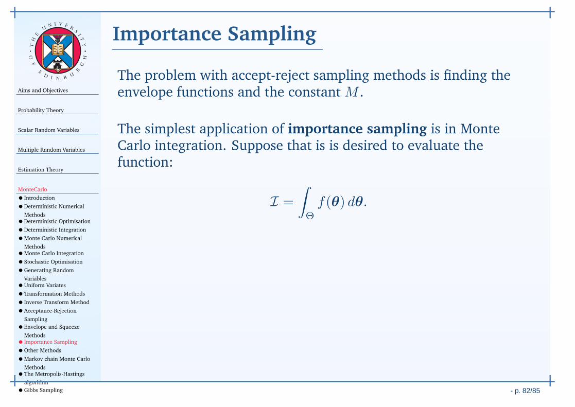
The simplest application of importance sampling is in MonteCarlo integration. Suppose that is is desired to evaluate thefunction:
I =
∫
Θ
f(θ) dθ.
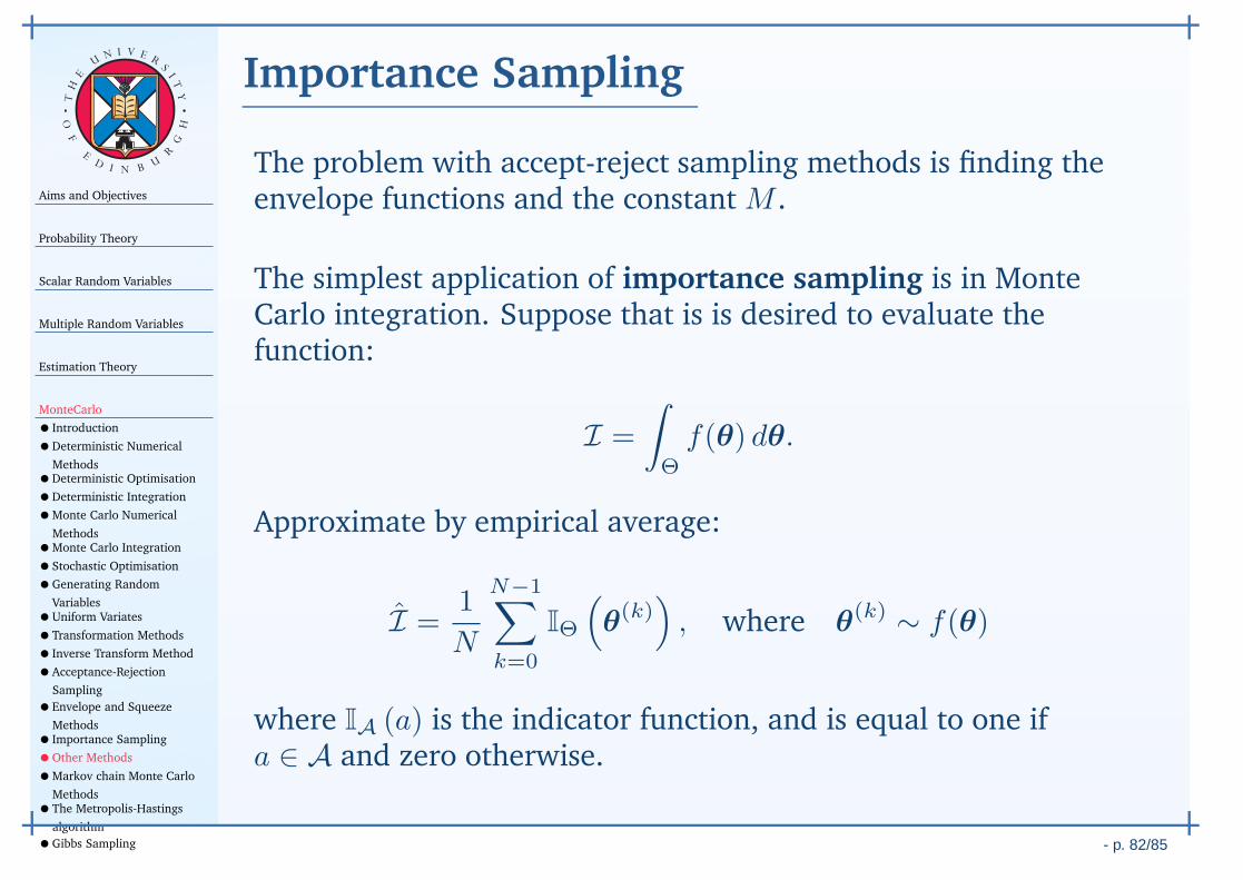
Approximate by empirical average:
I =1
N
N−1∑
k=0
IΘ
(
θ(k))
, where θ(k) ∼ f(θ)
where IA (a) is the indicator function, and is equal to one ifa ∈ A and zero otherwise.
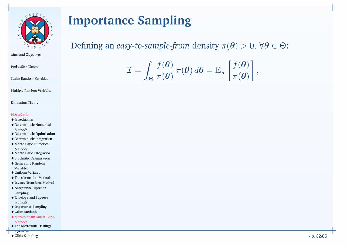
Aims and Objectives
Probability Theory
Scalar Random Variables
Multiple Random Variables
Estimation Theory
MonteCarlo
• Introduction
•Deterministic Numerical
Methods•Deterministic Optimisation
•Deterministic Integration
•Monte Carlo Numerical
Methods•Monte Carlo Integration
•Stochastic Optimisation
•Generating Random
Variables•Uniform Variates
•Transformation Methods
• Inverse Transform Method
•Acceptance-Rejection
Sampling
•Envelope and Squeeze
Methods• Importance Sampling
•Other Methods
•Markov chain Monte Carlo
Methods•The Metropolis-Hastings
algorithm
•Gibbs Sampling - p. 82/85
TH
E
UN I V E
RS
IT
Y
OF
ED
I N BU
R
GH
Importance Sampling
Defining an easy-to-sample-from density π(θ) > 0, ∀θ ∈ Θ:
I =
∫
Θ
f(θ)
π(θ)π(θ) dθ = Eπ
[f(θ)
π(θ)
]
,
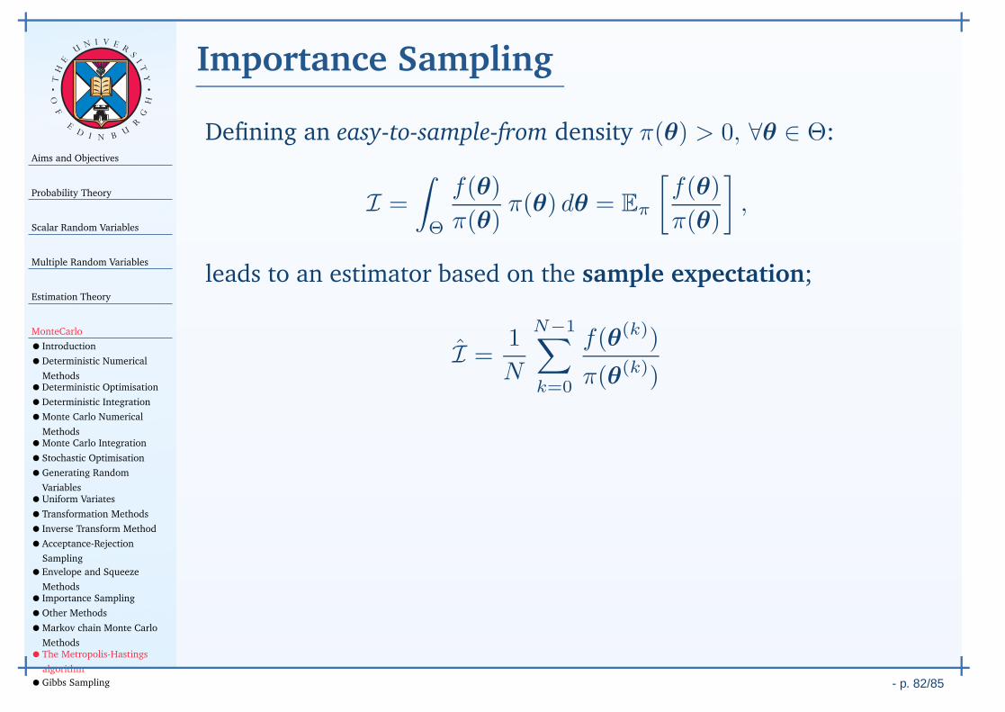
leads to an estimator based on the sample expectation;
I =1
N
N−1∑
k=0
f(θ(k))
π(θ(k))
Aims and Objectives
Probability Theory
Scalar Random Variables
Multiple Random Variables
Estimation Theory
MonteCarlo
• Introduction
•Deterministic Numerical
Methods•Deterministic Optimisation
•Deterministic Integration
•Monte Carlo Numerical
Methods•Monte Carlo Integration
•Stochastic Optimisation
•Generating Random
Variables•Uniform Variates
•Transformation Methods
• Inverse Transform Method
•Acceptance-Rejection
Sampling
•Envelope and Squeeze
Methods• Importance Sampling
•Other Methods
•Markov chain Monte Carlo
Methods•The Metropolis-Hastings
algorithm
•Gibbs Sampling - p. 83/85
TH
E
UN I V E
RS
IT
Y
OF
ED
I N BU
R
GH
Other Methods
Include:
representing pdfs as mixture of distributions;
algorithms for log-concave densities, such as the adaptiverejection sampling scheme;
generalisations of accept-reject;
method of composition (similar to Gibbs sampling);
ad-hoc methods, typically based on probabilitytransformations and order statistics (for example, generatingBeta distributions with integer parameters).

Aims and Objectives
Probability Theory
Scalar Random Variables
Multiple Random Variables
Estimation Theory
MonteCarlo
• Introduction
•Deterministic Numerical
Methods•Deterministic Optimisation
•Deterministic Integration
•Monte Carlo Numerical
Methods•Monte Carlo Integration
•Stochastic Optimisation
•Generating Random
Variables•Uniform Variates
•Transformation Methods
• Inverse Transform Method
•Acceptance-Rejection
Sampling
•Envelope and Squeeze
Methods• Importance Sampling
•Other Methods
•Markov chain Monte Carlo
Methods•The Metropolis-Hastings
algorithm
•Gibbs Sampling - p. 84/85
TH
E
UN I V E
RS
IT
Y
OF
ED
I N BU
R
GH
Markov chain Monte Carlo Methods
A Markov chain is the first generalisation of an independentprocess, where each state of a Markov chain depends on theprevious state only.
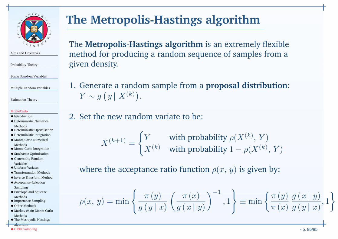
Aims and Objectives
Probability Theory
Scalar Random Variables
Multiple Random Variables
Estimation Theory
MonteCarlo
• Introduction
•Deterministic Numerical
Methods•Deterministic Optimisation
•Deterministic Integration
•Monte Carlo Numerical
Methods•Monte Carlo Integration
•Stochastic Optimisation
•Generating Random
Variables•Uniform Variates
•Transformation Methods
• Inverse Transform Method
•Acceptance-Rejection
Sampling
•Envelope and Squeeze
Methods• Importance Sampling
•Other Methods
•Markov chain Monte Carlo
Methods•The Metropolis-Hastings
algorithm
•Gibbs Sampling - p. 85/85
TH
E
UN I V E
RS
IT
Y
OF
ED
I N BU
R
GH
The Metropolis-Hastings algorithm
The Metropolis-Hastings algorithm is an extremely flexiblemethod for producing a random sequence of samples from agiven density.
1. Generate a random sample from a proposal distribution:
Y ∼ g(y | X(k)
).
2. Set the new random variate to be:
X(k+1) =
Y with probability ρ(X(k), Y )
X(k) with probability 1− ρ(X(k), Y )
where the acceptance ratio function ρ(x, y) is given by:
ρ(x, y) = min
π (y)
g (y | x)
(π (x)
g (x | y)
)−1
, 1
≡ min
π (y)
π (x)
g (x | y)g (y | x) , 1
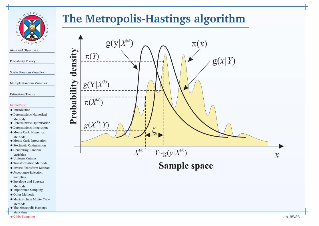
Aims and Objectives
Probability Theory
Scalar Random Variables
Multiple Random Variables
Estimation Theory
MonteCarlo
• Introduction
•Deterministic Numerical
Methods•Deterministic Optimisation
•Deterministic Integration
•Monte Carlo Numerical
Methods•Monte Carlo Integration
•Stochastic Optimisation
•Generating Random
Variables•Uniform Variates
•Transformation Methods
• Inverse Transform Method
•Acceptance-Rejection
Sampling
•Envelope and Squeeze
Methods• Importance Sampling
•Other Methods
•Markov chain Monte Carlo
Methods•The Metropolis-Hastings
algorithm
•Gibbs Sampling - p. 85/85
TH
E
UN I V E
RS
IT
Y
OF
ED
I N BU
R
GH
The Metropolis-Hastings algorithm
Aims and Objectives
Probability Theory
Scalar Random Variables
Multiple Random Variables
Estimation Theory
MonteCarlo
• Introduction
•Deterministic Numerical
Methods•Deterministic Optimisation
•Deterministic Integration
•Monte Carlo Numerical
Methods•Monte Carlo Integration
•Stochastic Optimisation
•Generating Random
Variables•Uniform Variates
•Transformation Methods
• Inverse Transform Method
•Acceptance-Rejection
Sampling
•Envelope and Squeeze
Methods• Importance Sampling
•Other Methods
•Markov chain Monte Carlo
Methods•The Metropolis-Hastings
algorithm
•Gibbs Sampling - p. 86/85
TH
E
UN I V E
RS
IT
Y
OF
ED
I N BU
R
GH
Gibbs Sampling
Gibbs sampling is a Monte Carlo method that facilitates samplingfrom a multivariate density function, π (θ0, θ1, . . . , θM ) bydrawing successive samples from marginal densities of smallerdimensions.
Using the probability chain rule,
π(θmMm=1
)= π
(θℓ | θmMm=1,m6=ℓ
)π(θmMm=1,m6=ℓ
)
The Gibbs sampler works by drawing random variates from the
marginal densities π(
θℓ | θmMm=1,m6=ℓ
)
in a cyclic iterative
pattern.
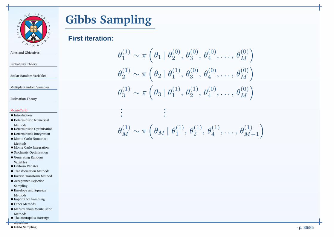
Aims and Objectives
Probability Theory
Scalar Random Variables
Multiple Random Variables
Estimation Theory
MonteCarlo
• Introduction
•Deterministic Numerical
Methods•Deterministic Optimisation
•Deterministic Integration
•Monte Carlo Numerical
Methods•Monte Carlo Integration
•Stochastic Optimisation
•Generating Random
Variables•Uniform Variates
•Transformation Methods
• Inverse Transform Method
•Acceptance-Rejection
Sampling
•Envelope and Squeeze
Methods• Importance Sampling
•Other Methods
•Markov chain Monte Carlo
Methods•The Metropolis-Hastings
algorithm
•Gibbs Sampling - p. 86/85
TH
E
UN I V E
RS
IT
Y
OF
ED
I N BU
R
GH
Gibbs Sampling
First iteration:
θ(1)1 ∼ π
(
θ1 | θ(0)2 , θ(0)3 , θ
(0)4 , . . . , θ
(0)M
)
θ(1)2 ∼ π
(
θ2 | θ(1)1 , θ(0)3 , θ
(0)4 , . . . , θ
(0)M
)
θ(1)3 ∼ π
(
θ3 | θ(1)1 , θ(1)2 , θ
(0)4 , . . . , θ
(0)M
)
......
θ(1)M ∼ π
(
θM | θ(1)1 , θ(1)2 , θ
(1)4 , . . . , θ
(1)M−1
)
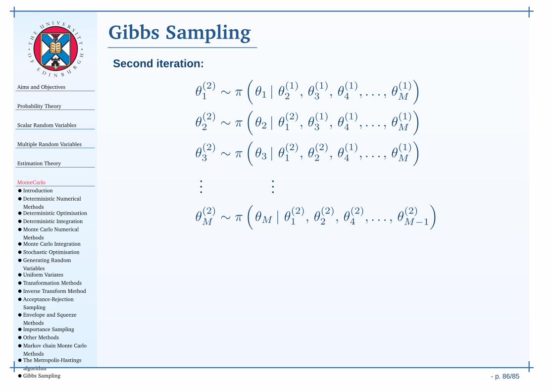
Aims and Objectives
Probability Theory
Scalar Random Variables
Multiple Random Variables
Estimation Theory
MonteCarlo
• Introduction
•Deterministic Numerical
Methods•Deterministic Optimisation
•Deterministic Integration
•Monte Carlo Numerical
Methods•Monte Carlo Integration
•Stochastic Optimisation
•Generating Random
Variables•Uniform Variates
•Transformation Methods
• Inverse Transform Method
•Acceptance-Rejection
Sampling
•Envelope and Squeeze
Methods• Importance Sampling
•Other Methods
•Markov chain Monte Carlo
Methods•The Metropolis-Hastings
algorithm
•Gibbs Sampling - p. 86/85
TH
E
UN I V E
RS
IT
Y
OF
ED
I N BU
R
GH
Gibbs Sampling
Second iteration:
θ(2)1 ∼ π
(
θ1 | θ(1)2 , θ(1)3 , θ
(1)4 , . . . , θ
(1)M
)
θ(2)2 ∼ π
(
θ2 | θ(2)1 , θ(1)3 , θ
(1)4 , . . . , θ
(1)M
)
θ(2)3 ∼ π
(
θ3 | θ(2)1 , θ(2)2 , θ
(1)4 , . . . , θ
(1)M
)
......
θ(2)M ∼ π
(
θM | θ(2)1 , θ(2)2 , θ
(2)4 , . . . , θ
(2)M−1
)
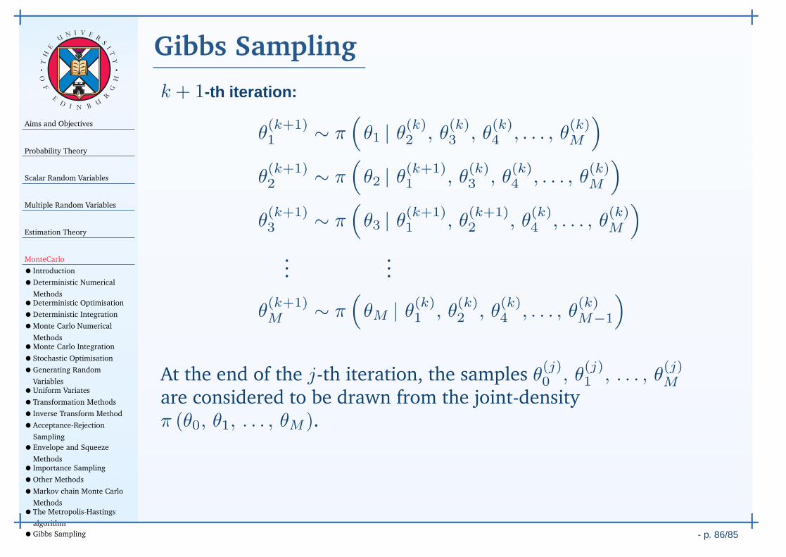
Aims and Objectives
Probability Theory
Scalar Random Variables
Multiple Random Variables
Estimation Theory
MonteCarlo
• Introduction
•Deterministic Numerical
Methods•Deterministic Optimisation
•Deterministic Integration
•Monte Carlo Numerical
Methods•Monte Carlo Integration
•Stochastic Optimisation
•Generating Random
Variables•Uniform Variates
•Transformation Methods
• Inverse Transform Method
•Acceptance-Rejection
Sampling
•Envelope and Squeeze
Methods• Importance Sampling
•Other Methods
•Markov chain Monte Carlo
Methods•The Metropolis-Hastings
algorithm
•Gibbs Sampling - p. 86/85
TH
E
UN I V E
RS
IT
Y
OF
ED
I N BU
R
GH
Gibbs Sampling
k + 1-th iteration:
θ(k+1)1 ∼ π
(
θ1 | θ(k)2 , θ(k)3 , θ
(k)4 , . . . , θ
(k)M
)
θ(k+1)2 ∼ π
(
θ2 | θ(k+1)1 , θ
(k)3 , θ
(k)4 , . . . , θ
(k)M
)
θ(k+1)3 ∼ π
(
θ3 | θ(k+1)1 , θ
(k+1)2 , θ
(k)4 , . . . , θ
(k)M
)
......
θ(k+1)M ∼ π
(
θM | θ(k)1 , θ(k)2 , θ
(k)4 , . . . , θ
(k)M−1
)
At the end of the j-th iteration, the samples θ(j)0 , θ
(j)1 , . . . , θ
(j)M
are considered to be drawn from the joint-densityπ (θ0, θ1, . . . , θM ).