Probabilistic Reasoning with Probabilistic Reasoning with

Uncertain DataUncertain Data

Yun Peng

and

Zhongli Ding, Rong Pan, Shenyong Zhang

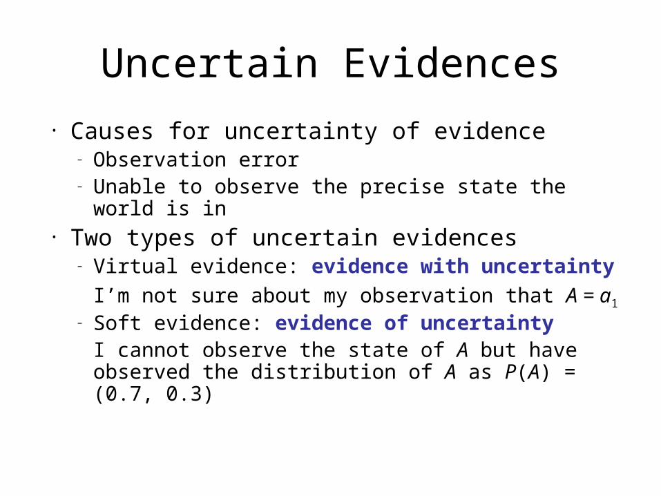
Uncertain Evidences

• Causes for uncertainty of evidence– Observation error– Unable to observe the precise state the world is in

• Two types of uncertain evidences– Virtual evidence: evidence with uncertainty

I’m not sure about my observation that A = a1

– Soft evidence: evidence of uncertaintyI cannot observe the state of A but have observed the distribution of A as P(A) = (0.7, 0.3)

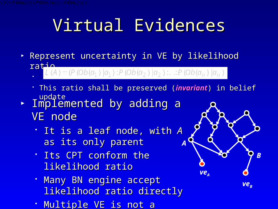
Virtual EvidencesVirtual Evidences

► Represent uncertainty in VE by likelihood ratioRepresent uncertainty in VE by likelihood ratio This ratio shall be preserved (This ratio shall be preserved (invariantinvariant) in belief update) in belief update

))|)((:...:)|)((:)|)((()( 2211 nn aaObPaaObPaaObPAL

► Implemented by adding a VE nodeImplemented by adding a VE node It is a leaf node, with It is a leaf node, with AA as its only as its only

parentparent Its CPT conform the likelihood ratioIts CPT conform the likelihood ratio Many BN engine accept likelihood Many BN engine accept likelihood

ratio directlyratio directly Multiple VE is not a problemMultiple VE is not a problem

A

veA

veB

B

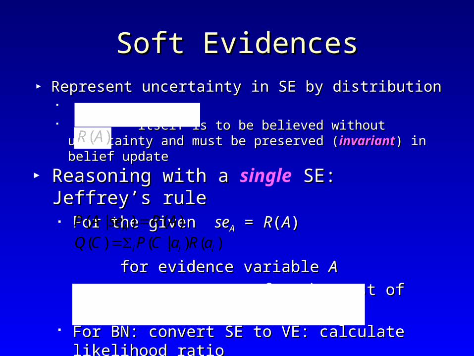
Soft EvidencesSoft Evidences► Represent uncertainty in SE by distributionRepresent uncertainty in SE by distribution

itself is to be believed without uncertainty and must itself is to be believed without uncertainty and must

be preserved (be preserved (invariantinvariant) in belief update) in belief update► Reasoning with a Reasoning with a single SE: Jeffrey’s ruleSE: Jeffrey’s rule

For the given For the given seseAA = = RR((AA))

for evidence variable for evidence variable AA

for the rest of variablesfor the rest of variables For BN: convert SE to VE: calculate likelihood ratioFor BN: convert SE to VE: calculate likelihood ratio

( ) ( | ) ( )i i iQ C P C a R a( | ) ( )AP A se R A

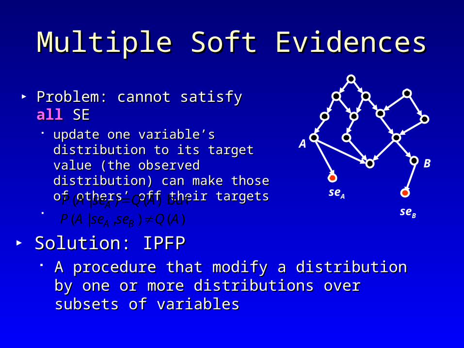
Multiple Soft EvidencesMultiple Soft Evidences

► Problem: cannot satisfy Problem: cannot satisfy allall SE SE update one variable’s distribution update one variable’s distribution

to its target value (the observed to its target value (the observed distribution) can make those of distribution) can make those of others’ off their targetsothers’ off their targets

A

seA

seB

► Solution: IPFPSolution: IPFP A procedure that modify a distribution by one or more A procedure that modify a distribution by one or more

distributions over subsets of variablesdistributions over subsets of variables

B

but)()|( AQseAP A )(),|( AQseseAP BA

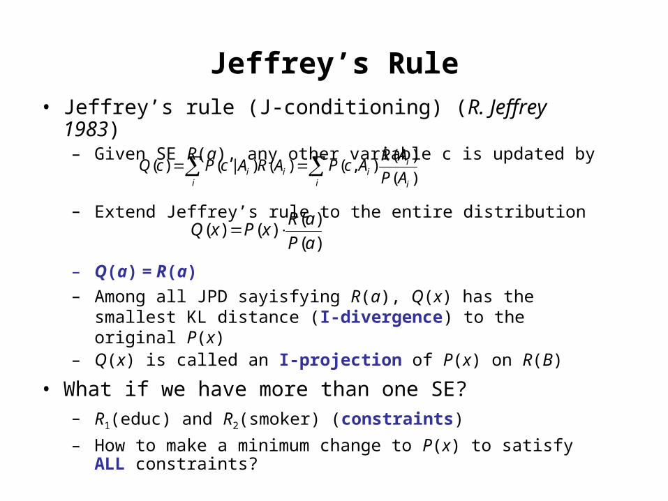
Jeffrey’s Rule• Jeffrey’s rule (J-conditioning) (R. Jeffrey 1983)

– Given SE R(a), any other variable c is updated by

– Extend Jeffrey’s rule to the entire distribution

– Q(a) = R(a)

– Among all JPD sayisfying R(a), Q(x) has the smallest KL distance (I-divergence) to the original P(x)

– Q(x) is called an I-projection of P(x) on R(B)

• What if we have more than one SE?– R1(educ) and R2(smoker) (constraints)

– How to make a minimum change to P(x) to satisfy ALL constraints?

( )( ) ( | ) ( ) ( , )

( )i

i i ii i i

R AQ c P c A R A P c A

P A

( )( ) ( )

( )

R aQ x P x

P a

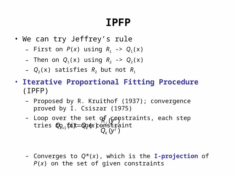
IPFP

• We can try Jeffrey’s rule– First on P(x) using R1 -> Q1(x)

– Then on Q1(x) using R2 -> Q2(x)

– Q2(x) satisfies R2 but not R1

• Iterative Proportional Fitting Procedure (IPFP)– Proposed by R. Kruithof (1937); convergence proved by I. Csiszar

(1975)

– Loop over the set of constraints, each step tries to fit one constraint

– Converges to Q*(x), which is the I-projection of P(x) on the set of given constraints

1

( )( ) ( )

( )

jj

k k jk

R yQ x Q x

Q y

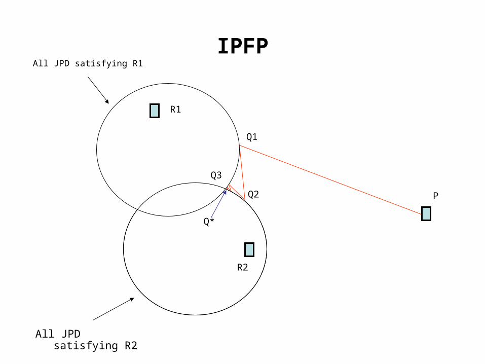
IPFPAll JPD satisfying R1

P

All JPD satisfying R2

R2

R1

Q1

Q2

Q3

Q*

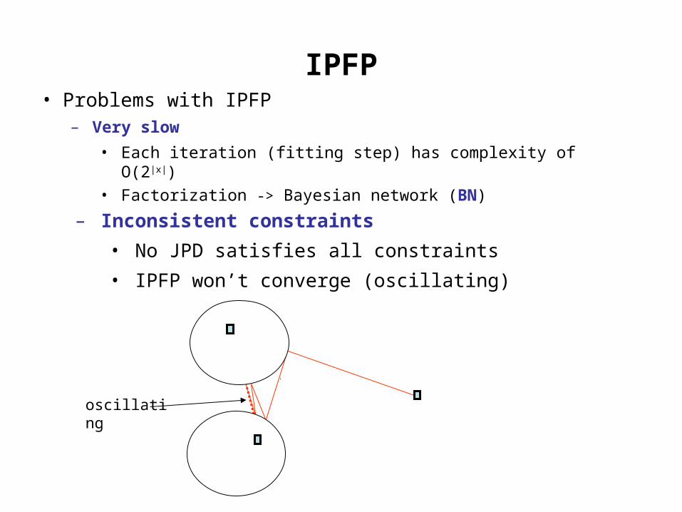
IPFP• Problems with IPFP

– Very slow

• Each iteration (fitting step) has complexity of O(2|x|)

• Factorization -> Bayesian network (BN)

oscillating

– Inconsistent constraints

• No JPD satisfies all constraints

• IPFP won’t converge (oscillating)

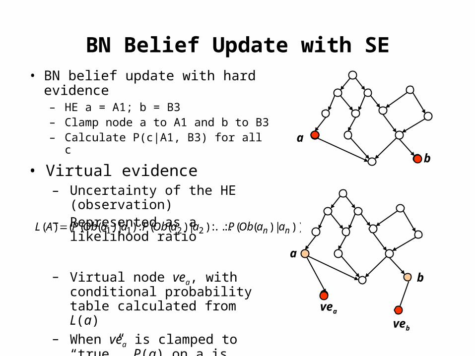
BN Belief Update with SE• BN belief update with hard

evidence– HE a = A1; b = B3– Clamp node a to A1 and b to B3– Calculate P(c|A1, B3) for all c

a

b

a

vea

veb

b

• Virtual evidence– Uncertainty of the HE (observation)– Represented as a likelihood ratio

– Virtual node vea, with conditional probability table calculated from L(a)

– When vea is clamped to “true”, P(a) on a is updated to have its likelihood ratio = L(a)

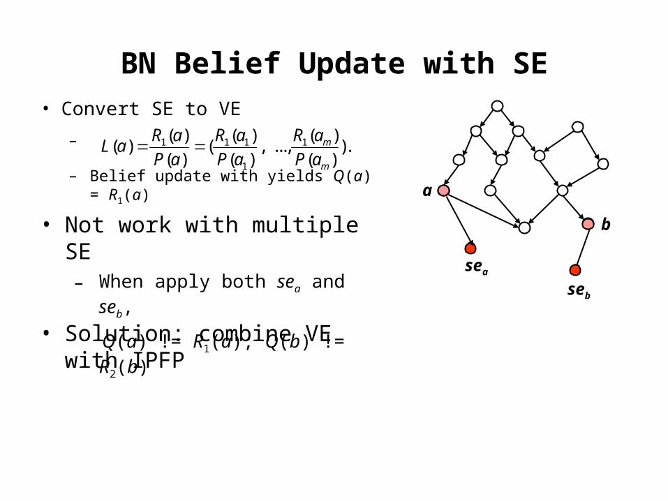
BN Belief Update with SE

• Convert SE to VE

–

– Belief update with yields Q(a) = R1(a)

1 1 1 1

1

( ) ( ) ( )( ) ( , ..., ).

( ) ( ) ( )m

m

R a R a R aL a

P a P a P a

sea

seb

a

b

• Solution: combine VE with IPFP

• Not work with multiple SE– When apply both sea and seb,

Q(a) != R1(a); Q(b) != R2(b)

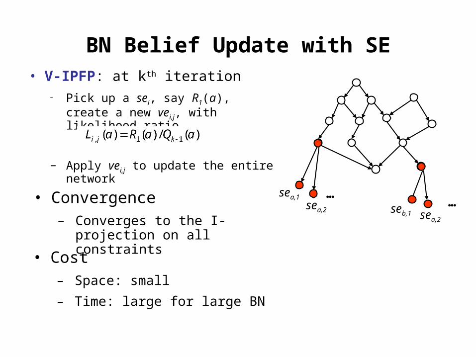
BN Belief Update with SE• V-IPFP: at kth iteration

– Pick up a sei, say R1(a), create a new vei,j, with likelihood ratio

– Apply vei,j to update the entire network

sea,1

seb,1sea,2

sea,2

……• Convergence

– Converges to the I-projection on all constraints

• Cost– Space: small

– Time: large for large BN

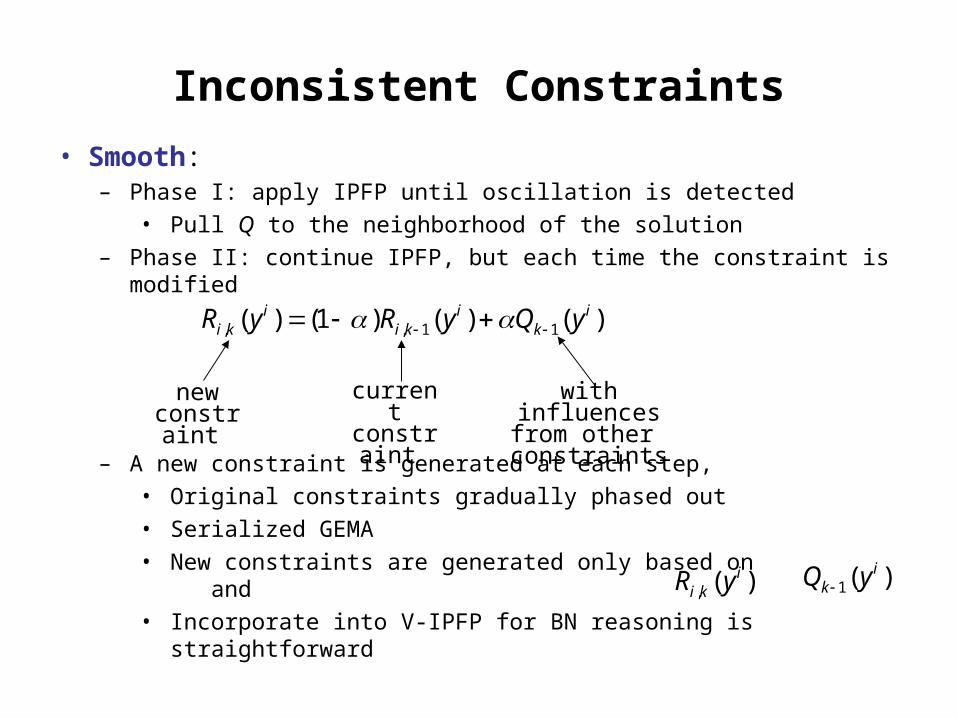
Inconsistent Constraints

• Smooth:– Phase I: apply IPFP until oscillation is detected

• Pull Q to the neighborhood of the solution

– Phase II: continue IPFP, but each time the constraint is modified

– A new constraint is generated at each step,

• Original constraints gradually phased out

• Serialized GEMA

• New constraints are generated only based on and

• Incorporate into V-IPFP for BN reasoning is straightforward

, , 1 1( ) (1 ) ( ) ( )i i ii k i k kR y R y Q y

current constraint

new constraint

with influences from other constraints

, ( )ii kR y 1( )i

kQ y

BN Learning with Uncertain Data

• Modify BN by a set of low dimensional PD (constraints)

– Approach 1: • Compute the JPD P(x) from BN,

• Modify P(x) to Q*(x) by constraints using IPFP

• Construct a new BN from Q*(x) (it may have different structure that the original BN

– Our approach: • Keep BN structure unchanged, only modify the CPTs

• Developed a localized version of IPFP

– Next step: • Dealing with inconsistency

• Change structure (minimum necessary)

• Learning both structure and CPT with mixed data (samples as low dimensional PDs)

Remarks• Wide potential applications

– Probabilistic resources are all over the places (survey data, databases, probabilistic knowledge bases of different kinds)

– This line of research may lead to effective ways to connect them• Problems with the IPFP based approaches

– Computationally expensive– Hard to do mathematical proofs

References:[1] Peng, Y., Zhang, S., Pan, R.: “Bayesian Network Reasoning with Uncertain Evidences”,

International Journal of Uncertainty, Fuzziness and Knowledge-Based Systems, 18 (5), 539-564, 2010

[2] Pan, R., Peng, Y., and Ding, Z: “Belief Update in Bayesian Networks Using Uncertain Evidence”, in Proceedings of the IEEE International Conference on Tools with Artificial Intelligence (ICTAI-2006), Washington, DC,13 – 15, Nov. 2006.

[3] Peng, Y. and Ding, Z.: “Modifying Bayesian Networks by Probability Constraints”, in Proceedings of 21st Conference on Uncertainty in Artificial Intelligence (UAI-2005), Edinburgh, Scotland, July 26-29, 2005