probabilistic precipitation type forecasting based on gefs

Probabilistic precipitation type forecasting based on GEFS ensemble1

forecasts of vertical temperature profiles2

Michael Scheuerer∗, Scott Gregory3

University of Colorado, Cooperative Institute for Research in Environmental Sciences, and

NOAA/ESRL, Physical Sciences Division

4

5

Thomas M. Hamill6

NOAA/ESRL, Physical Sciences Division7

Phillip E. Shafer8

NOAA/NWS/OST, Meteorological Development Laboratory9

∗Corresponding author address: Michael Scheuerer,

University of Colorado, Cooperative Institute for Research in Environmental Sciences, and

NOAA/ESRL, Physical Sciences Division 325 Broadway, R/PSD1, Boulder, CO 80305.

10

11

12

E-mail: [email protected]

Generated using v4.3.1 (5-19-2014) of the AMS LATEX template1

ABSTRACT

A Bayesian classification method for probabilistic forecasts of precipitation

type is presented. The method considers the vertical wetbulb temperature pro-

files associated with each precipitation type, transforms them into their prin-

cipal components, and models each of these principal components by a skew

normal distribution. A variance inflation technique is used to de-emphasize

the impact of principal components corresponding to smaller eigenvalues,

and Bayes’ theorem finally yields probability forecasts for each precipita-

tion type based on predicted wetbulb temperature profiles. Our approach is

demonstrated with reforecast data from the Global Ensemble Forecast Sys-

tem (GEFS) and observations at 551 METAR sites, using either the full en-

semble or the control run only. In both cases, reliable probability forecasts for

precipitation type being either rain, snow, ice pellets, freezing rain, or freez-

ing drizzle are obtained. Compared to the Model Output Statistics (MOS)

approach presently used by the National Weather Service, the skill of the pro-

posed method is comparable for rain and snow and significantly better for the

freezing precipitation types.

14

15

16

17

18

19

20

21

22

23

24

25

26

27

28

29

2

1. Introduction30

Some forms of winter precipitation can have a substantial impact on air and ground transporta-31

tion, and reliable predictions of them can help limit associated safety hazards and disruptions of32

travel and commerce (Stewart et al. 2015, and references therein). Among several factors that33

control the precipitation type at the surface, the vertical profile of wetbulb temperature Tw plays34

a key role (e.g. Bourgouin 2000), and a number of algorithms have been devised which deter-35

mine the precipitation type based on the Tw profile or quantities derived from it (e.g. Ramer 1993;36

Baldwin et al. 1994; Bourgouin 2000; Schuur et al. 2012). A major challenge herein is the model37

uncertainty about the Tw profile on the forecast day; while the above mentioned algorithms still38

show good skill in detecting snow (SN) and rain (RA), reliable distinction between ice pellets39

(IP) and freezing rain (FZRA) becomes increasingly difficult when this uncertainty is accounted40

for (Reeves et al. 2014). A recently proposed algorithm, the spectral bin classifier (Reeves et al.41

2016), pushes the limits of forecast accuracy for IP and FZRA by calculating the mass fraction of42

liquid water for a spectrum of hydrometeors as they descend from the cloud top to the surface, thus43

accounting for different rapidity of melting and refreezing of smaller hydrometeors compared to44

larger ones. Their results still confirm the sensitivity of classification algorithms to perturbations45

of the Tw profile. In a forecast setting where these profiles are derived from NWP model output46

deviations of the true from the predicted (and interpolated) wetbulb temperature profile can be47

substantial, especially for longer forecast lead times. In those situations with large uncertainty it48

may be more useful to provide probability forecasts of each precipitation type, thus communicat-49

ing the risk for precipitation to occur in the form of FZRA, say, instead of stating the most likely50

outcome only. Operationally, such probabilistic guidance is currently provided for the contiguous51

U.S. (CONUS) and Alaska by the Meteorological Development Laboratory (MDL) to support the52

3

National Digital Guidance Database (NDGD). It is based on a model output statistics (MOS) ap-53

proach that is described in Shafer (2010). This method links the probability of precipitation type54

(PoPT) to NWP model output of variables such as 2-m temperature, 850 hPa temperature, 1000-55

850 hPa thickness, 1000-500 hPa thickness, and freezing level. This approach yields conditional56

probabilities of freezing (IP or FZRA), frozen (SN) and liquid (RA) precipitation for forecast lead57

times up to 192 hours, but it does not attempt to distinguish the different freezing types. In this58

paper we describe an alternative method which uses (discretized) vertical wetbulb temperature59

profiles as a predictor, thus aiming to use more information from that profile as well as statisti-60

cally modeling the forecast uncertainty. In Sec. 2 we describe the forecast and observation data61

used in this study, which is identical to the data used by Shafer (2015), and which thus permits62

a direct comparison between our approach and the operational method. Our statistical model and63

the methods for fitting it to the training data are detailed in Sec. 3, while a detailed evaluation of64

the precipitation type probabilities obtained with this model is the subject of Sec. 4. We finally65

discuss the scope of our method and avenues for further improvement.66

2. Data used in this study67

a. Observations68

Adopting the setup used by Shafer (2015), our method is calibrated with and validated against69

weather observations at METAR (Meteorological Terminal Aviation Routine Weather Report) sites70

(Allen and Erickson 2001a,b). Precipitation type observations were considered for the period71

1996-2013 and all months between September and May (the period 09/1996 - 05/1997 will be72

referred to as the ’1996 cool season’), whenever precipitation was reported at the corresponding73

4

site. Following Shafer (2015), we discarded sites where more than 50% of the precipitation type74

reports were missing, leading to a set of 551 stations (506 CONUS, 26 Alaska, 19 Canada).75

The original precipitation type reports, valid at 0000, 0600, 1200, and 1800 UTC, were classi-76

fied into one of either three or five mutually exclusive categories. The first classification follows77

the MOS precipitation type categories shown e.g. in Table 1 by Shafer (2015), and distinguishes78

’freezing’, ’frozen’, and ’liquid’ precipitation, classifying sleet as ’freezing’ and any mixture of79

liquid precipitation with snow as ’liquid’ (Allen and Erickson 2001a,b; Shafer 2015). This three80

category classification permits a direct comparison with the MOS technique used operationally by81

the Meteorological Development Laboratory of the National Weather Service (NWS). In addition,82

we consider a five-category classification which differs from the previous one in that it splits the83

’freezing’ category up into freezing rain (FZRA), freezing drizzle (FZDZ), and ice pellets (IP),84

in order to study in how far our forecasts are able to provide probabilistic guidance that reflects85

the new certification standards of the federal aviation administration (FAA) allowing some aircraft86

to fly in FZDZ but not FZRA. The frozen and liquid types are relabeled as snow (SN) and rain87

(RA) respectively. The observation data set used here clearly is not optimal for performing a five-88

category classification. Only a subset of the 551 stations are augmented by human observers and89

are able to report IP and FZDZ; all other stations may erroneously report a different type and thus90

contaminate both training and verification samples with Tw profiles that should be associated with91

IP or FZDZ but aren’t. We accept the detrimental effect that this might have on the performance92

of our method because our priority is a direct comparison with Shafer (2015), but we note that our93

method might demonstrate somewhat better skill in distinguishing the different freezing precipi-94

tation types if it were trained with an observation data set like the one from the mPING project95

(Elmore et al. 2014) that is more consistent in how it reports IP, FZRA, and FZDZ.96

5

b. Forecasts97

Predictors used in this study were derived from the second-generation Global Ensemble Fore-98

cast System (GEFS) reforecast data set (Hamill et al. 2013). GEFS data were extracted for 2-m99

temperature and 2-m specific humidity on GEFS’s native Gaussian grid at ∼ 0.5 degree resolution100

in an area surrounding the CONUS, Alaska, and southern Canada over the period 1996-2013. Sur-101

face pressure and temperatures, specific humidities, and geopotential heights at the pressure levels102

1000, 925, 850, 700, 500, and 300 hPa were obtained on a ∼ 1 degree resolution grid covering the103

same area. Horizontal grids were bilinearly interpolated to the station locations and were used to104

convert the temperatures at the surface and at the pressure levels into wetbulb temperatures. Us-105

ing the geopotential height fields, the wetbulb tempertures at each pressure level were associated106

with a certain height above ground level (AGL) where ground level here refers to the GEFS model107

grid. Vertical wetbulb temperature profiles were obtained by linear interpolation between those108

pressure levels, and then discrete values were taken at fixed heights up to 3000 m AGL. As a result109

of the rather coarse model grid resolution of ∼ 0.5 degrees, the model grid elevation and the true110

elevation at the station locations differ substantially in regions with complex terrain. In order to111

adjust the resulting biases of the vertical wetbulb temperature profiles we:112

• calculate the biases at the surface as the annual average difference between observed and113

(horizontally interpolated) analyzed wetbulb temperatures at each location;114

• assume that the bias linearly decreases to zero at the 500 hPa level;115

• correct the entire vertical wetbulb temperature profile accordingly, i.e. apply the full (additive)116

bias correction at the surface and gradually reduce the correction to zero with increasing117

height above the ground.118

6

This procedure is not meant to correct complex forecast biases which potentially have a seasonal119

and diurnal cycle; these are somewhat implicitly addressed by the classification method described120

in the subsequent section. The procedure described here only tries to remove biases resulting from121

the mismatch between the terrain as represented by the forecast model and the true terrain.122

For the remainder of this paper it is our working assumption that the observed precipitation type123

only depends on the vertical wetbulb temperature profile above the ground, i.e. given two identical124

profiles the outcome is independent of the location and time of the year at which those profiles were125

observed. This is a simplification that does not account for the microphysical forcing (precipitation126

rate, degree of riming, etc.) but is necessary as it allows us to pool data across all stations and127

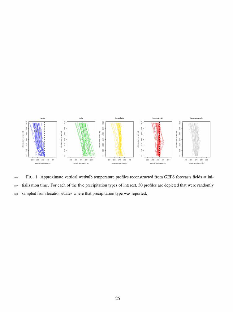
across all dates within the cool seasons considered here. Fig. 1 depicts examples of wetbulb128

temperature profiles at initialization time (i.e. based on GFS analyses) obtained as described above.129

There are typically only three or four pressure levels which data are used for the reconstruction130

of the section of the profiles shown in this figure. It is clear that the resulting interpolation error131

(compare e.g. with Fig. 2 in Reeves et al. 2014 who study wetbulb temperature profiles obtained132

from radiosonde observations) can be substantial, and adds to the overall uncertainty about the133

vertical profiles resulting from initial condition and forecast uncertainty.134

3. Regularized Bayesian Classification135

The method proposed in this paper is based on Bayes’ Theorem, which has recently been em-136

ployed by Hodyss et al. (2016) to derive optimal weights for different model forecasts and cli-137

matology in a statistical postprocessing approach for continuous predictands. In our setting, the138

predictand is categorical, but the same general principle can be used as a starting point. Assume139

that we know, for each location s and each date t (day of the year and time of the day), the cli-140

matological probability for each precipitation type k ∈ {1, ...,K} to occur. Denote this probability141

7

by πkst . Assume further that for each k we know the multivariate probability density function142

(PDF) ϕk that characterizes the distribution of the discretized, predicted vertical wetbulb temper-143

ature profiles that are compatible with the observed precipitation type k. For efficient statistical144

classification, we want these distributions to be as different as possible. Fig. 1 suggests that the145

differences between profiles corresponding to the different precipitation types are much more pro-146

nounced in the lower half of the sections depicted in the plots, and we therefore only consider147

wetbulb temperatures corresponding to heights above the surface up to 1500 m, even though the148

precipitation-generation layer is usually far outside this range. Sampling the profiles every 100 m149

then leaves us with a wetbulb temperature vector of dimension d = 16, and ϕk models the proba-150

bility distribution of this vector for each k. Due to our assumption that given two identical profiles151

the observed precipitation type should not depend on s and t, ϕk is assumed constant across the152

entire spatial domain and throughout the year (it may vary with lead time though since there is153

typically more dispersion around the mean profile for longer leads). According to Bayes’ The-154

orem (Wilks 2006, Eq. (13.32)), given the climatological probabilities πkst , the PDFs ϕk, and a155

new, predicted vector x of vertical wetbulb temperature profile values, the conditional probability156

P(k|x) of observing precipitation type k is157

P(k|x) = πkstϕk(x)

∑Ki=1 πistϕi(x)

. (1)

In this study we approximate the climatological probabilities πkst by the relative frequencies of158

observed precipitation types, calculated separately for each location s, each month (but pooling159

all days within a month and all years for which data are available), and each time of the day.160

The following subsections discuss how an adequate model for ϕk can be defined and fitted. Note161

that Eq. (1) is also the starting point for (quadratic) discriminant analysis, where a deterministic162

classification rule is derived from this equation.163

8

a. Basic model: multivariate normal distribution164

A standard assumption with this approach to probabilistic classification is to let be ϕk a multi-165

variate normal PDF (Wilks 2006, Sec. 13.3.3). This PDF is completely characterized by its mean166

vector µk and covariance matrix Σk. Given a set of training data we can estimate µk as the em-167

pirical mean and Σk as the empirical covariance matrix of the subset of the training profiles that168

correspond to an observed precipitation type k. In order to focus on situations where the out-169

come is truly uncertain, we only use locations/dates for the calculation of µk and Σk for which170

πkst < 0.99 for every k ∈ {1, ...,K}. This excludes, for example, precipitation events in January at171

high altitudes where precipitation most likely occurs in the form of snow, and precipitation events172

in May in Florida, where precipitation almost surely occurs in the form of rain. These events will173

still be used for validation, but excluding them for estimating the PDFs ϕk moves the mean vectors174

for rain and snow closer to the freezing point and improves the distribution fit in this tempera-175

ture range where classification is most challenging. This results in a noticeable improvement in176

probabilistic classification skill, and one could even try to optimize the probability threshold for177

omitting cases from the training data set. However, we do not expect much further improvement178

from lowering the threshold and keep it fixed at 0.99.179

Given µk,Σk, and a wetbulb temperature vector x, the likelihood ϕk(x) in Eq. (1) under the180

assumption of a multivariate normal distribution is given by181

ϕk(x) = (2π)−d2 |Σk|−

12 e−

12 (x−µk)

′Σ−1k (x−µk) (2)

where x′ denotes the transpose of x. Using the eigenvalue decomposition Σk = EkΛkE′k to182

transform x into vectors uk =E′k(x−µk) of centered principal components (PCs), this likelihood183

9

can be expressed as a product of univariate likelihoods184

ϕk(x) =d

∏j=1

φ0,λk, j(uk, j) , (3)

where φ(0,λk, j) is the PDF of a univariate normal distribution with mean 0 and variance equal to the185

j-th eigenvalue λk, j of Σk. This re-interpretation of ϕk(x) in terms of principal components will186

later be used to motivate an easily interpretable and computationally efficient generalization of the187

basic multivariate normal model discussed above. Fig. 2 shows the means of the K = 5 classes of188

interest and the variability around the respective mean in the direction of the first eigenvector of189

Σk. The different shapes of these eigenvectors suggest that there is structural information in the190

wetbulb temperature profiles beyond the mean that can be utilized for classification.191

b. First extension: introducing skewness192

Upon closer inspection, the assumption of a multivariate Gaussian distribution made above turns193

out to be a coarse approximation of the truth. For example, wetbulb temperature profiles much194

cooler than the mean profile are still compatible with observing snow, whereas the probability195

for observing snow but predicting a relatively warm profile decreases more rapidly (such profile196

would more be associated with observing rain). Applying a power transformation to each compo-197

nent of the wetbulb temperature vectors can make the distributions more symmetric (Wilks 2006,198

Sec. 3.4.1), but their direct physical interpretation is lost in that process. Alternatively, a more199

complex, multivariate skew normal distribution could be used to fit the untransformed data (Az-200

zalini and Capitanio 1999). In our setting with dimension d = 16, this requires estimating a large201

number of model parameters which is computationally and numerically challenging. Here, we202

propose a similar approach that permits an intuitive interpretation and straightforward statistical203

inference. We first proceed as described above, estimate µk and Σk as the as the empirical means204

10

and covariance matrices of the wetbulb temperature vectors associated with each precipitation205

type, and use them to calculate the centered PCs uk,1, . . . ,uk,d of each wetbulb temperature vector206

x. Possible skewness can then be addressed for each PC separately by modeling them by univari-207

ate skew normal distributions fξk, j,ωk, j,αk, jwith location parameter ξk, j, scale parameter ωk, j, and208

shape parameter αk, j. By construction, the PCs are centered and have variances λk, j, so for given209

αk, j the location and scale parameters are determined by210

ω2k, j = λk, j

(1−

2α2k, j

π(1+α2k, j)

)−1

and ξk, j =−ωk, j

√√√√ 2α2k, j

π(1+α2k, j)

. (4)

Using these relations, αk, j can be estimated via maximum likelihood. Since the impact of the PCs211

for smaller eigenvalues on classification will be de-emphasized as explained in the next subsection,212

we only bother to estimate αk, j for j ∈ {1,2}, and set αk, j = 0 (i.e. no skewness) for all other PCs.213

Fig. 3 shows histograms of the first three PCs and the fitted distributions. The variability in the214

direction of the first eigenvector corresponds to cooler/warmer than average wetbulb temperatures215

of the entire vertical profile (see Fig. 2), and the asymmetry of the associated PCs as described216

above for snow is clearly visible in those histograms. The fitted skew normal distributions are217

capable of modeling this asymmetry, and for calculating the likelihood ϕk(x) one only needs to218

replace Eq. (3) by219

ϕk(x) =d

∏j=1

fξk, j,ωk, j,αk, j(uk, j) . (5)

c. Second extension: regularization220

A further modification to the multivariate PDF ϕk is required to make this Bayesian classification221

method work efficiently. As pointed out in Sec. 2, the reconstruction of the vertical wetbulb222

temperature profile based on the GEFS model output at a few available pressure levels comes with223

substantial interpolation errors, and especially features at small vertical scales are not resolved.224

11

On the other hand, even if we could reconstruct those profiles at high vertical resolution, it is225

unclear whether their fine-scale structure carries any useful information for the discrimination226

between different precipitation types. In the light of the principal component interpretation of the227

multivariate likelihood ϕk(x) discussed above, it would seem natural to truncate after a few PCs228

and omit the last few terms in the product in Eq. (5), which typically correspond to eigenvectors229

representing the fine-scale structure of the vertical profiles. This is problematic, however, since the230

different precipitation types can have very different leading eigenvectors (see Fig. 2) and different231

spectra of eigenvalues, and so both the fractions of explained variances and the subspaces onto232

which the profiles are projected would be different. A more appropriate way to mute the effect of233

higher PCs on the likelihood ϕk(x) is to regularize the covariance matrix Σk, i.e. to replace it by234

Σk(ak,bk) := akΣk +bkI , (6)

where I is the identity matrix and ak,bk are positive coefficients for which selection will be dis-235

cussed later. This idea of regularization was introduced by Friedman (1989) in the context of a236

similar but deterministic classification technique referred to as regularized discriminant analysis.237

In our probabilistic setting we will refer to this idea as regularized Bayesian classification (RBC).238

It can easily be combined with our assumption of skew normal distributions of the PCs by noting239

that the regularization in Eq. (6) leaves the eigenvectors unchanged but turns the eigenvalues λk, j240

into241

λk, j = akλk, j +bk, j = 1, . . . ,d . (7)

Setting ak := 1− bk/λk,1 leaves the first eigenvalue λk,1 unchanged but increases all other eigen-242

value with the relative increase being larger for smaller eigenvalues. This implies an artificial infla-243

tion of the variances of the univariate, skew normal PDFs in Eq. (5), and causes the corresponding244

likelihoods to be relatively less sensitive to the PCs uk, j corresponding to the smaller eigenvalues.245

12

To find the optimal degree of inflation, i.e. optimal regularization parameters b1, . . . ,bK , we use246

the training data set (forecasts and observations) that was used to estimate µk and Σk, and proceed247

as follows:248

• for given parameters b1, . . . ,bK , and for every wetbulb temperature profile x in the training249

data set, use Eqs. (1), (5), (4), and (7) to calculate the likelihoods ϕk(x) and resulting forecast250

probabilities P(k|x) for each k; and251

• use the corresponding training observations to calculate the resulting Brier skill scores BSSk252

(see Sec. 4 for a definition) and choose b1, . . . ,bK such that the sum ∑Kk=1 BSSk is maximized.253

Note that the target function ∑Kk=1 BSSk that we seek to maximize gives the same weight to all254

precipitation type categories despite their very different frequencies of occurrence. This is done255

on purpose to foster good performance of our method with regard to the rare freezing precipitation256

types. Different priorities can be set, however, by introducing weights that increase or decrease257

the impact of the skill for certain precipitation types on the target function. In our example, the258

optimal values of bk were between 5 and 10 for all k, which is smaller than the second, but about259

2-3 times larger than the third eigenvalues of Σk (see Fig. 3). This suggests that useful information260

about the vertical structure of the wetbulb temperature profiles is limited to the first two principal261

components.262

d. Third extension: applying RBC to ensemble forecasts263

The RBC approach presented above yields forecast probabilities for the occurrence of each264

precipitation type given a single (i.e. deterministic) forecast of a vertical wetbulb temperature265

profile. In our situation where we have an ensemble of forecasts, this ensemble represents some266

13

of the uncertainty about the predicted vertical wetbulb temperature profiles, and its use can thus267

reduce the amount of variability that is modeled purely statistically.268

We proceed as before regarding the estimation ofµk,Σk, and the skewness parameters αk, j, con-269

sidering the forecast profiles x1, . . . ,xM of the M ensemble members as separate cases. Centering270

and projecting those profiles onto the eigenvectors of Σk yields principal components uk, j,m and271

M different likelihoods ϕk(xm) for each class. The resulting probability forecasts P(k|xm) can be272

combined to a single probability forecast by simply taking the mean for each class273

P(k|x1, . . . ,xM) =1M

M

∑m=1

P(k|xm) (8)

This way of linear pooling, however, does in general not yield reliable probability forecasts even274

if all of the individual member probability forecasts P(k|xm) are reliable (Ranjan and Gneiting275

2010). Indeed, as pointed out above, the simultaneous consideration of different ensemble member276

forecasts explains some of the variability of the forecast profiles, and so in return the statistically277

modeled variability needs to be reduced to avoid under-confident probability forecasts. We do this278

by replacing the variances λk, j of the principal component PDFs that were originally obtained as279

the eigenvalues of Σk by the empirical variances vk, j = var(uk, j) of the ensemble-mean PCs280

uk, j =1M

M

∑m=1

uk, j,m .

While this is equivalent to just operating on the ensemble-mean profiles, evaluating Eq. (1) with281

an ensemble-mean profile does not yield the same probabilities as Eq. (8) due to the non-linearity282

of the likelihood function; Eq. (8) averages the probabilities corresponding to the different atmo-283

spheric situations represented by the ensemble, as opposed to averaging the vertical profiles and284

deriving a probability from the averaged state of the atmosphere. In contrast to λk, j, which de-285

scribes the variability of a certain PC over all profiles in the training data set corresponding to a286

certain precipitation type, vk, j elides the variability within the ensemble, and is therefore smaller287

14

than λk, j. All subsequent steps, i.e. regularization according to Eq. (7), calculation of likelihoods288

according to Eqs. (5), (4), and calculation of probability forecasts according to Eqs. (1), (8), remain289

the same as before, but are carried out based on vk, j instead of λk, j. The results in the following290

section will show that this reduction of statistically modeled variability in favor of dynamically291

explained variability yields a noticeable improvement of predictive performance at longer forecast292

lead times.293

4. Results294

To test our RBC approach and compare it against the operational MOS technique, we adopt the295

verification setup used by Shafer (2015), but studying only the case of a training sample comprised296

of five cool seasons (see Sec. 2). Forecasts were produced and verified for the cool seasons 2001297

through 2012. For each of these verification seasons, the methods were trained with data from298

the previous five cool seasons, i.e. the statistical model used for producing probability forecasts299

for the cool season 2001 was set up based on data (forecasts and observations) from the cool300

seasons 1996 through 2000. For estimating the climatological frequencies, which are used as a301

reference forecast on the one hand, and as a prior distribution for our RBC technique on the other302

hand, the entire observation record was used. This may be justified by noting that in practice long303

time series of observations are often available while forecast systems keep evolving and available304

forecast time series from a stable system are typically much shorter.305

First, we assess the reliability of the RBC probability forecasts for different lead times separately306

for each precipitation type. Fig. 4 depicts reliability diagrams for probability forecasts generated307

by the ensemble-based version of the RBC method. For all forecast lead times considered in this308

study (including those not shown in this figure), the curves are close to the diagonal, which means309

15

that the relative frequency of occurrence of each precipitation type matches the probability with310

which it was predicted.311

The RBC probability forecasts based on the GEFS control run only were equally reliable (not312

shown here), so as a second validation tool we consider a quantitative performance measure, the313

Brier skill score (Wilks 2006, Eqs. 7.34 and 7.35). In addition to reliability, the Brier score evalu-314

ates the resolution of a forecast, i.e. its ability to distinguish situations with different frequencies315

of occurrence. A skill score relates the score of the forecast method of interest to a reference score316

(here: climatological frequency of occurrence, calculated separately for each location, each month,317

and each time of the day) and thus facilitates its interpretation (Wilks 2006, Sec. 7.33). Here, we318

compare the Brier skill scores (BSSs) of the generalized operator equation (GOE) implementation319

of the operational MOS PoPT technique described in (Shafer 2010, 2015) and GEFS ensemble320

mean forecasts, the RBC method based on the GEFS control run only, and the RBC method using321

each of the individual ensemble member forecasts for forecast lead times up to 192h. The MOS322

PoPT approach currently only distinguishes three classes: frozen (SN), liquid (RA), and freezing323

(IP, FZRA or FZDZ). To allow a direct comparison, we aggregate the five class RBC probabili-324

ties to three class probabilities, and compare the BSSs for the three class probabilities of all three325

methods on the one hand, and the BSSs for the IP, FZRA and FZDZ probabilities by the two RBC326

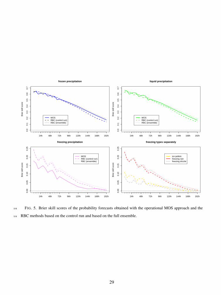
implementations on the other hand. The results depicted in Fig. 5 permit several conclusions:327

• the use of ensemble forecasts as opposed to a single deterministic run clearly benefits forecast328

performance, especially for longer forecast lead times;329

• for the frozen and liquid class, the improvement of the RBC ensemble method over the MOS330

PoPT approach is marginal; if the MOS PoPT approach were extended such as to use the331

16

individual ensemble member forecasts rather than the ensemble mean, there may be no im-332

provement at all;333

• for the particularly challenging, freezing category, however, there is a noticeable benefit of334

using a statistical method (such as RBC) that can use the full vertical wetbulb temperature335

profile as a predictor; and336

• the skill for the freezing categories (especially IP and FZDZ) is low compared to the skill337

for RA and SN; yet our RBC method can provide skillful probabilistic guidance on freezing338

precipitation several days ahead, and even has the potential to separate IP, FZRA and FZDZ.339

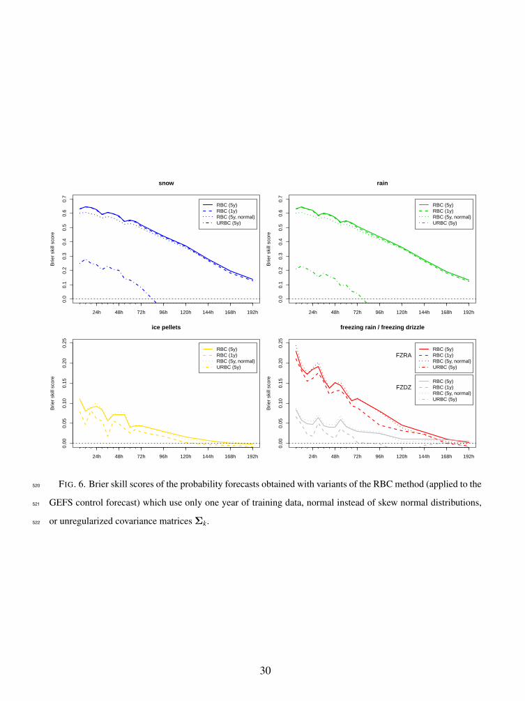
The results discussed above show the effectiveness of our RBC method in general and the utility340

of ensemble forecasts in particular. How about the other two extensions (modeling skewness of341

the PCs, regularization), how much do they contribute to the skill of the RBC approach? How342

much skill is lost if the available training data for estimating µk,Σk, bk, and αk, j is composited343

of just one instead of five cool seasons? To answer these questions we use the control run based344

RBC method (fitted with five years of training data, as above) as a benchmark and compare it345

to a) the same model fitted with training data from a single cool season, b) a simplified model346

that regularizes Σk according to (6) but assumes normal instead of skew normal distributions of347

the PCs, c) a simplified model that uses skew normal distributions but does not regularize the348

empirical covariance matrices. The following conclusions can be drawn from the results shown in349

Fig. 6:350

a) Reducing the training sample size hardly affects the performance in predicting SN and RA351

probabilities, but has a rather strong, negative impact on the predictive performance for IP,352

FZRA, and FZDZ. For the two former, there are still enough cases within a single cool season353

to warrant a good estimation of model parameters. Estimating the parameters for the rare,354

17

freezing precipitation types, however, requires either several years of training data or a much355

denser observation network. In addition to the issue of boundary discontinuity, this is also an356

argument in favor of a pooling data across all locations as opposed to partitioning the country357

into more homogeneous sub-domains. The latter might better account for different regional358

characteristics, but Fig. 6 suggests that these benefits could be nullified by the concomitant359

reduction of training sample size.360

b) Simplifying the RBC approach by assuming a multivariate normal distribution for the wetbulb361

temperature profiles affects the predictive performance in the opposite way. While the more362

flexible distribution model does not seem to benefit the freezing precipitation types, the better363

approximation of the distributions of SN and RA profiles that results from modeling skewness364

in the PCs translates into improved skill of the resulting probability forecasts.365

c) Finally, Fig. 6 highlights the necessity of regularizing the empirical covariance matrices.366

Without regularization, skill drops dramatically for SN and RA and becomes negative be-367

yond a forecast lead time of three days. For the freezing types the impact is even stronger and368

lack of regularization results in Brier skill scores around −1.0 for all lead times. Unregular-369

ized classification gives as much emphasis to the noisy, unwarranted fine scale structure of370

the wetbulb temperature profiles as it gives to the first PCs that represent meaningful features371

of these profiles, and this results in probability forecasts that are entirely off the mark.372

To illustrate the capabilities and limits of probabilistic guidance obtained with the RBC method373

applied to GEFS ensemble forecasts, two particular cases studies presented. Fig. 7 shows spatial374

maps of FZRA probabilities for 27 January 2009, 0000 UTC, with a forecast lead time of 2, 4,375

and 6 days ahead. This date is in the middle of a major ice storm that impacted parts of Okla-376

homa, Arkansas, Missouri, Illinois, Indiana, West Virginia, and Kentucky. The plots suggest that377

18

the GEFS captured the atmospheric situation well, and the RBC methods provides a strong prob-378

abilistic signal for freezing rain even at 6 days of lead time. For the event shown in Fig. 8 (also379

studied by Reeves et al. 2016) the situation is more complex. The plots show observed precipi-380

tation types and 2 day ahead RBC forecast probabilities for 22 February 2013, 0000 UTC. Even381

at this short lead time, the probabilistic signal for the freezing precipitation types is rather weak382

(note the different color scales) and no clear guidance is provided as to which particular freezing383

precipitation type will dominate in each geographical area. This underscores the inherent uncer-384

tainty in precipitation type forecasts based on a global ensemble prediction system, and illustrates385

the limits of such forecasts. Notwithstanding, the RBC probability forecasts indicate an increased386

risk of freezing precipitation, and we believe that there is substantial value in communicating that387

risk to decision makers.388

5. Discussion389

In this paper we have proposed a method for conditional probabilistic precipitation type fore-390

casting which is based on a statistical model for the predicted vertical wetbulb temperature profiles391

that are compatible with each precipitation type. Using Bayes’ theorem this model can be inverted392

such that it yields probability forecasts for each precipitation type given a new predicted profile.393

There were many sources of forecast and data uncertainty that needed to be accounted for in a394

precipitation typing methodology. These include forecast errors stemming from initial condition395

uncertainty, from model error, and in this case from the need to interpolate NWP model output396

from a relatively coarse horizontal grid and a few pressure levels to a much finer horizontal and397

vertical resolution and more complex orography at the surface level. Availability of sigma-level398

forecast data at a finer vertical resolution could reduce this last component of uncertainty, which399

contributes noticeably to the overall uncertainty about the wetbulb temperature profiles at short400

19

lead times. It is suggested that thermodynamic variables be archived at many vertical levels above401

the surface when generating future reforecasts. At longer lead times, forecast errors become the402

dominant source of uncertainty, and the interpolation error might be negligible. At short lead403

times, forecasts from a high resolution, limited-area NWP model might be available, which might404

be accurate enough to yield superior classification results using an explicit precipitation type di-405

agnosis scheme (e.g. Benjamin et al. 2016) or the spectral bin classifier proposed by Reeves et al.406

(2016), but such guidance could be leveraged in a probabilistic framework, too.407

The strength of the method proposed here is that it can handle the large uncertainty that in-408

evitably comes with predictions from a global forecast system, and that it can still provide reli-409

able, probabilistic precipitation type forecasts at forecast lead times up to seven days ahead. It has410

sufficient skill to give decision makers at least a heads up about precipitation type related weather411

risks, and it can easily be extended to distinguish further precipitation type classes like mixtures412

of snow and rain, mixtures of freezing precipitation types, and so forth, if they are reported accu-413

rately in the observations. The observation data set used here is not optimal in that regard as it is414

inconsistent in how it reports IP, FZRA, and FZDZ, and the skill of our method in distinguishing415

these types might actually be better than reported here if it were trained with an observation data416

set like the one from the mPING project (Elmore et al. 2014, 2015) in which IP, FZRA, and FZDZ417

are distinguished more systematically.418

We have focused on vertical profiles of wetbulb temperature as a predictor variable. However,419

by combining the statistical dimension reduction / regularization techniques used here with more420

physically motivated aggregation methods one might be able to further improve skill by using ad-421

ditional predictors such as relative humidity profiles. Alternatively, one could use modern machine422

learning techniques like neural networks to identify features of vertical wetbulb temperature and423

humidity profiles that determine the observed precipitation type. While extremely powerful, these424

20

techniques typically require large data sets for training, but these may become available once sev-425

eral years of mPING data have been collected, and allow one to explore the more data-intensive426

machine learning techniques.427

Acknowledgments. The authors thank Amanda Hering for useful discussions which inspired428

some of the refinements to our basic distribution model for the wetbulb temperature profiles. Our429

research was supported by grants from the NOAA/NWS Sandy Supplemental (Disaster Relief430

Appropriations Act of 2013) and the NOAA/NWS Research to Operations (R2O) initiative for the431

Next-Generation Global Prediction System (NGGPS), award # NA15OAR4320137.432

References433

Allen, R. L., and M. C. Erickson, 2001a: AVN-based MOS precipitation type guidance for the434

United States. NWS Technical Procedures Bulletin No. 476, NOAA, U.S. Dept. of Commerce,435

8 pp.436

Allen, R. L., and M. C. Erickson, 2001b: MRF-based MOS precipitation type guidance for the437

United States. NWS Technical Procedures Bulletin No. 485, NOAA, U.S. Dept. of Commerce,438

8 pp.439

Azzalini, A., and A. Capitanio, 1999: Statistical applications of the multivariate skew normal440

distribution. J. Roy. Stat. Soc. B, 61, 579–602.441

Baldwin, M., R. Treadon, and S. Contorno, 1994: Precipitation type prediction using a decision442

tree approach with NMCs mesoscale eta model. 10th Conf. on Numerical Weather Prediction,443

Portland, OR, Amer. Meteor. Soc., 30–31.444

21

Benjamin, S. G., J. M. Brown, and T. G. Smirnova, 2016: Explicit precipitation-type diagno-445

sis from a model using a mixed-phase bulk cloud-precipitation microphysics parameterization.446

Wea. Forecasting, 31, 609–619.447

Bourgouin, P., 2000: A method to determine precipitation type. Wea. Forecasting, 15, 583–592.448

Elmore, K. L., Z. L. Flamig, V. Lakshmanan, B. T. Kaney, V. Farmer, H. D. Reeves, and L. S.449

Rothfusz, 2014: mPING: Crowd-sourcing weather reports for research. Bull. Amer. Meteor.450

Soc., 95, 1335–1342.451

Elmore, K. L., H. M. Grams, D. Apps, and H. D. Reeves, 2015: Verifying forecast precipitation452

type with mPING. Wea. Forecasting, 30, 656–667.453

Friedman, J. H., 1989: Regularized discriminant analysis. J. Amer. Stat. Assoc., 84, 165–175.454

Hamill, T. M., G. T. Bates, J. S. Whitaker, D. R. Murray, M. Fiorino, T. J. G. Jr., Y. Zhu, and455

W. Lapenta, 2013: NOAA’s second-generation global medium-range ensemble reforecast data456

set. Bull. Amer. Meteor. Soc., 94, 1553–1565.457

Hodyss, D., E. Satterfield, J. McLay, T. M. Hamill, and M. Scheuerer, 2016: Inaccuracies with458

multimodel postprocessing methods involving weighted, regression-corrected forecasts. Mon.459

Wea. Rev., 144, 1649–1668.460

Ramer, J., 1993: An empirical technique for diagnosing precipitation type from model output.461

Fifth Int. Conf. on Aviation Weather Systems, Vienna, VA, Amer. Meteor. Soc., 227–230.462

Ranjan, R., and T. Gneiting, 2010: Combining probability forecasts. J. Roy. Stat. Soc. B, 32, 71–463

91.464

Reeves, H. D., K. L. Elmore, A. V. Ryzhkof, T. J. Schuur, and J. Krause, 2014: Sources of uncer-465

tainty in precipitation-type forecasting. Wea. Forecasting, 29, 936–953.466

22

Reeves, H. D., A. V. Ryzhkof, and J. Krause, 2016: Discrimination between winter precipitation467

types based on spectral-bin microphysical modeling. J. Appl. Meteor. Climatol., 55, 1747–1761.468

Schuur, T. J., H.-S. Park, A. V. Ryzhkof, and H. D. Reeves, 2012: Classification of precipitation469

types during transitional winter weather using the ruc model and polarimetric radar retrievals.470

J. Appl. Meteor. Climatol., 51, 763–779.471

Shafer, P., 2010: Logit transforms in forecasting precipitation type. 20th Conf. on Probability and472

Statistics in the Atmospheric Sciences, Atlanta, GA, Amer. Meteor. Soc., P222.473

Shafer, P. E., 2015: A sample size sensitivity test for MOS precipitation type. Special Symposium474

on Model Postprocessing and Downscaling, Phoenix, AZ, Amer. Meteor. Soc., 4.1.475

Stewart, R. E., J. M. Theriault, and W. Henson, 2015: On the characteristics of and processes476

producing winter precipitation types near 0◦C. Bull. Amer. Meteor. Soc., 96, 623–639.477

Wilks, D. S., 2006: Statistical Methods in the Atmospheric Sciences, International Geophysics478

Series, Vol. 91. 2nd ed., Elsevier Academic Press.479

23

LIST OF FIGURES480

Fig. 1. Approximate vertical wetbulb temperature profiles reconstructed from GEFS forecasts fields481

at initialization time. For each of the five precipitation types of interest, 30 profiles are482

depicted that were randomly sampled from locations/dates where that precipitation type was483

reported. . . . . . . . . . . . . . . . . . . . . . . . . 25484

Fig. 2. Empirical means (solid lines) and variability (two standard deviations, dashed lines) in the485

direction of the first eigenvector of Σk for each of the five precipitation types distinguished486

by our algorithm. . . . . . . . . . . . . . . . . . . . . . 26487

Fig. 3. Histograms and fitted skew normal distributions for the first three principal components of488

the wetbulb temperature profile vectors of each class. . . . . . . . . . . . . 27489

Fig. 4. Reliability diagrams for probability forecasts at various forecast lead times generated by490

the ensemble-based version of the RBC method with probabilities rounded to a precision491

of 0.05. The inset histograms depict the frequency (on a logarithmic scale) with which the492

respective probabilities were forecast (x-axes are the same as in the reliability diagrams).493

Points of the reliability curve associated with very infrequent forecast probabilities (< 25494

cases) are subject to substantial sampling variability and have therefore been omitted. . . . 28495

Fig. 5. Brier skill scores of the probability forecasts obtained with the operational MOS approach496

and the RBC methods based on the control run and based on the full ensemble. . . . . . 29497

Fig. 6. Brier skill scores of the probability forecasts obtained with variants of the RBC method498

(applied to the GEFS control forecast) which use only one year of training data, normal499

instead of skew normal distributions, or unregularized covariance matrices Σk. . . . . . 30500

Fig. 7. Observed precipitation types (shaded circles with color scheme as in previous figures) on 27501

January 2009, 0000 UTC, and predicted freezing rain probabilities by the ensemble-based502

RBC method for different forecast lead times. . . . . . . . . . . . . . . 31503

Fig. 8. Observed precipitation types on 22 February 2013, 0000 UTC, and predicted precipitation504

type probabilities by the ensemble-based RBC method with a forecast lead time of 48h. . . . 32505

24

250 260 270 280 290

050

010

0015

0020

0025

0030

00

snow

wetbulb temperature (K)

altit

ude

abov

e su

rfac

e (m

)

250 260 270 280 290

050

010

0015

0020

0025

0030

00

rain


altit

ude

abov

e su

rfac

e (m

)

250 260 270 280 290

050

010

0015

0020

0025

0030

00

ice pellets


altit

ude

abov

e su

rfac

e (m

)

250 260 270 280 290

050

010

0015

0020

0025

0030

00

freezing rain


altit

ude

abov

e su

rfac

e (m

)

250 260 270 280 290

050

010

0015

0020

0025

0030

00

freezing drizzle


altit

ude

abov

e su

rfac

e (m

)FIG. 1. Approximate vertical wetbulb temperature profiles reconstructed from GEFS forecasts fields at ini-

tialization time. For each of the five precipitation types of interest, 30 profiles are depicted that were randomly

sampled from locations/dates where that precipitation type was reported.

506

507

508

25

250 260 270 280 290

050

010

0015

00

snow


altit

ude

abov

e su

rfac

e (m

)

250 260 270 280 290

050

010

0015

00

rain


250 260 270 280 290

050

010

0015

00

ice pellets


250 260 270 280 290

050

010

0015

00

freezing rain


250 260 270 280 290

050

010

0015

00

freezing drizzle


FIG. 2. Empirical means (solid lines) and variability (two standard deviations, dashed lines) in the direction

of the first eigenvector of Σk for each of the five precipitation types distinguished by our algorithm.

509

510

26

1st PC (snow)

principal component scores

Den

sity

−50 0 50

0.00

00.

010

0.02

0 λ1,1 = 326

1st PC (rain)


Den

sity

−60 −40 −20 0 20 40 60

0.00

00.

010

0.02

0

λ2,1 = 381

1st PC (ice pellets)


Den

sity

−30 −20 −10 0 10 20

0.00

0.02

0.04

0.06

λ3,1 = 102

1st PC (freezing rain)


Den

sity

−40 −20 0 20

0.00

0.02

0.04 λ4,1 = 139

1st PC (freezing drizzle)


Den

sity

−40 −20 0 20 40

0.00

00.

015

0.03

0

λ5,1 = 242

2nd PC (snow)


Den

sity

−30 −20 −10 0 10

0.00

0.04

0.08 λ1,2 = 29.8

2nd PC (rain)


Den

sity

−20 −15 −10 −5 0 5 10

0.00

0.04

0.08

0.12

λ2,2 = 22.9

2nd PC (ice pellets)


Den

sity

−10 −5 0 5 10 15

0.00

0.04

0.08

0.12

λ3,2 = 39

2nd PC (freezing rain)


Den

sity

−15 −10 −5 0 5 10 15

0.00

0.04

0.08

λ4,2 = 28.8

2nd PC (freezing drizzle)


Den

sity

−15 −10 −5 0 5 10 15

0.00

0.04

0.08 λ5,2 = 29.6

3rd PC (snow)

Den

sity

−10 −5 0 5

0.00

0.15

0.30 λ1,3 = 2.42

3rd PC (rain)

Den

sity

−10 −5 0 5

0.0

0.1

0.2

0.3 λ2,3 = 1.92

3rd PC (ice pellets)

Den

sity

−8 −6 −4 −2 0 2 4

0.00

0.10

0.20

λ3,3 = 3.75

3rd PC (freezing rain)

Den

sity

−6 −4 −2 0 2 4

0.00

0.10

0.20 λ4,3 = 3.66

3rd PC (freezing drizzle)

Den

sity

−8 −6 −4 −2 0 2 4 60.

000.

100.

20

λ5,3 = 3.97

FIG. 3. Histograms and fitted skew normal distributions for the first three principal components of the wetbulb

temperature profile vectors of each class.

511

512

27

FIG. 4. Reliability diagrams for probability forecasts at various forecast lead times generated by the ensemble-

based version of the RBC method with probabilities rounded to a precision of 0.05. The inset histograms depict

the frequency (on a logarithmic scale) with which the respective probabilities were forecast (x-axes are the same

as in the reliability diagrams). Points of the reliability curve associated with very infrequent forecast probabilities

(< 25 cases) are subject to substantial sampling variability and have therefore been omitted.

513

514

515

516

517

28

frozen precipitation

Brie

r sk

ill s

core

24h 48h 72h 96h 120h 144h 168h 192h

0.0

0.1

0.2

0.3

0.4

0.5

0.6

0.7

MOSRBC (control run)RBC (ensemble)

liquid precipitation

Brie

r sk

ill s

core

24h 48h 72h 96h 120h 144h 168h 192h

0.0

0.1

0.2

0.3

0.4

0.5

0.6

0.7


freezing precipitation

Brie

r sk

ill s

core

24h 48h 72h 96h 120h 144h 168h 192h

0.00

0.05

0.10

0.15

0.20

0.25


freezing types separately

Brie

r sk

ill s

core

24h 48h 72h 96h 120h 144h 168h 192h

0.00

0.05

0.10

0.15

0.20

0.25

ice pelletsfreezing rainfreezing drizzle

FIG. 5. Brier skill scores of the probability forecasts obtained with the operational MOS approach and the

RBC methods based on the control run and based on the full ensemble.

518

519

29

snow

Brie

r sk

ill s

core

24h 48h 72h 96h 120h 144h 168h 192h

0.0

0.1

0.2

0.3

0.4

0.5

0.6

0.7

RBC (5y)RBC (1y)RBC (5y, normal)URBC (5y)

rain

Brie

r sk

ill s

core

24h 48h 72h 96h 120h 144h 168h 192h

0.0

0.1

0.2

0.3

0.4

0.5

0.6

0.7


ice pellets

Brie

r sk

ill s

core

24h 48h 72h 96h 120h 144h 168h 192h

0.00

0.05

0.10

0.15

0.20

0.25


freezing rain / freezing drizzle

Brie

r sk

ill s

core

24h 48h 72h 96h 120h 144h 168h 192h

0.00

0.05

0.10

0.15

0.20

0.25



FZRA

FZDZ

FIG. 6. Brier skill scores of the probability forecasts obtained with variants of the RBC method (applied to the

GEFS control forecast) which use only one year of training data, normal instead of skew normal distributions,

or unregularized covariance matrices Σk.

520

521

522

30

FIG. 7. Observed precipitation types (shaded circles with color scheme as in previous figures) on 27 January

2009, 0000 UTC, and predicted freezing rain probabilities by the ensemble-based RBC method for different

forecast lead times.

523

524

525

31

FIG. 8. Observed precipitation types on 22 February 2013, 0000 UTC, and predicted precipitation type

probabilities by the ensemble-based RBC method with a forecast lead time of 48h.

526

527

32

probabilistic precipitation type forecasting based on gefs

Documents