probabilistic graphical models - university of...

School of Computer Science

1

Probabilistic Graphical Models

Variational Inference III: Variational Principle I

Junming Yin Lecture 16, March 19, 2012

Reading:

X1

X4

X2 X3

X4

X2 X3

X1X1

X2

X1

X3

X1

X4

X2 X3

X4

X2 X3

X1X1

X2

X1

X3

What have we learned so far l  Free energy based approaches

l  Direct approximation of Gibbs free energy: Bethe free energy and loop BP

l  Restricting the family of approximation distribution: mean field method

l  Convex duality based approaches

2

Computing Mean Parameters Inference Variational

Principle

1. Exponential Families 2. Indicator Sufficient Statistics Convex Duality

Computing Mean Parameter: Bernoulli

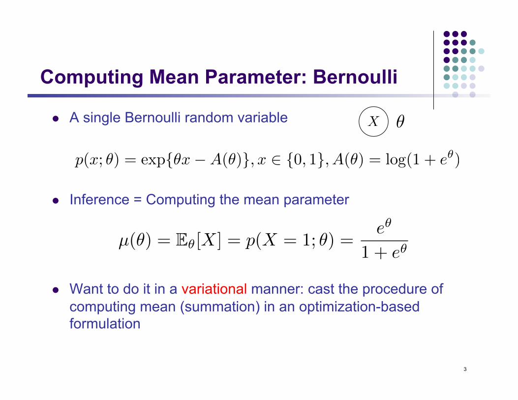
l  A single Bernoulli random variable

l  Inference = Computing the mean parameter

l  Want to do it in a variational manner: cast the procedure of computing mean (summation) in an optimization-based formulation

3

p(x; θ) = expθx−A(θ), x ∈ 0, 1, A(θ) = log(1 + eθ)

X θ

µ(θ) = Eθ[X] = p(X = 1; θ) =eθ

1 + eθ

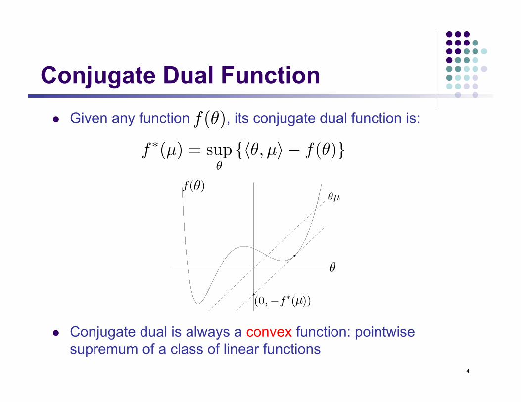
l  Given any function , its conjugate dual function is:

l  Conjugate dual is always a convex function: pointwise supremum of a class of linear functions

The conjugate function

the conjugate of a function f is

f!(y) = supx"dom f

(yTx! f(x))

f(x)

(0,#f!(y))

xy

x

• f! is convex (even if f is not)

• will be useful in chapter 5

Convex functions 3–21

θθµ

θ

µ

Conjugate Dual Function f(θ)

f∗(µ) = supθ

θ, µ − f(θ)

4

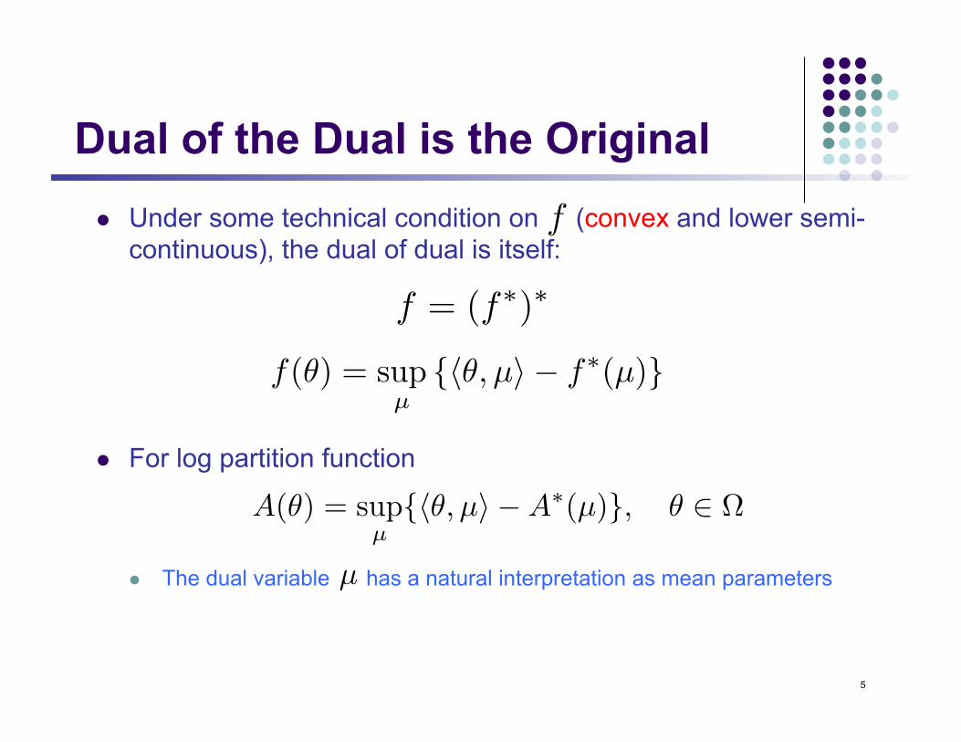
Dual of the Dual is the Original l  Under some technical condition on (convex and lower semi-

continuous), the dual of dual is itself:

l  For log partition function

l  The dual variable has a natural interpretation as mean parameters

5

f

f(θ) = supµ

θ, µ − f∗(µ)

f = (f∗)∗

A(θ) = supµθ, µ −A∗(µ), θ ∈ Ω

µ

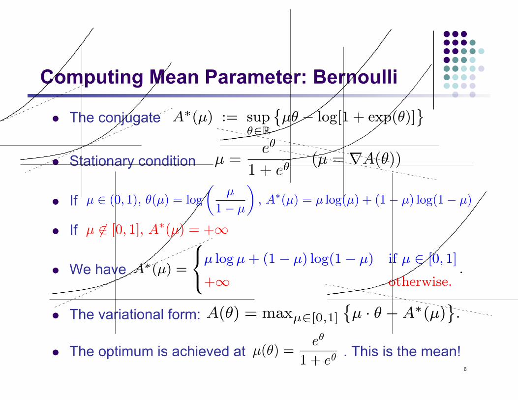
Computing Mean Parameter: Bernoulli

l  The conjugate

l  Stationary condition l  If

l  If l  We have

l  The variational form:

l  The optimum is achieved at . This is the mean!

Example: Single Bernoulli

Random variable X ! 0, 1 yields exponential family of the form:

p(x; !) " exp˘

! x¯

with A(!) = logˆ

1 + exp(!)˜

.

Let’s compute the dual A!(µ) := sup!"R

˘

µ! # log[1 + exp(!)]¯

.

(Possible) stationary point: µ = exp(!)/[1 + exp(!)].

PSfrag replacements

A(!)

!

!µ, !" # A!(µ)

PSfrag replacements

A(!)

!!µ, !" # c

(a) Epigraph supported (b) Epigraph cannot be supported

We find that: A!(µ) =

8

<

:

µ log µ + (1 # µ) log(1 # µ) if µ ! [0, 1]

+$ otherwise..

Leads to the variational representation: A(!) = maxµ"[0,1]

˘

µ · ! # A!(µ)¯

.

25



p(x; !) " exp˘

! x¯

with A(!) = logˆ

1 + exp(!)˜

.


˘

µ! # log[1 + exp(!)]¯

.


PSfrag replacements

A(!)

!

!µ, !" # A!(µ)

PSfrag replacements

A(!)

!!µ, !" # c



8

<

:

µ log µ + (1 # µ) log(1 # µ) if µ ! [0, 1]

+$ otherwise..


˘

µ · ! # A!(µ)¯

.

25



p(x; !) " exp˘

! x¯

with A(!) = logˆ

1 + exp(!)˜

.


˘

µ! # log[1 + exp(!)]¯

.


PSfrag replacements

A(!)

!

!µ, !" # A!(µ)

PSfrag replacements

A(!)

!!µ, !" # c



8

<

:

µ log µ + (1 # µ) log(1 # µ) if µ ! [0, 1]

+$ otherwise..


˘

µ · ! # A!(µ)¯

.

25

µ =eθ

1 + eθ(µ = ∇A(θ))

µ ∈ (0, 1), θ(µ) = log

µ

1− µ

, A∗(µ) = µ log(µ) + (1− µ) log(1− µ)

µ ∈ [0, 1], A∗(µ) = +∞

µ(θ) =eθ

1 + eθ

6

Remark l  The last few identities are not coincidental but rely on a deep

theory in general exponential family l  The dual function is the negative entropy function l  The mean parameter is restricted l  Solving the optimization returns the mean parameter

l  Next step: develop this framework for general exponential families/graphical models

7

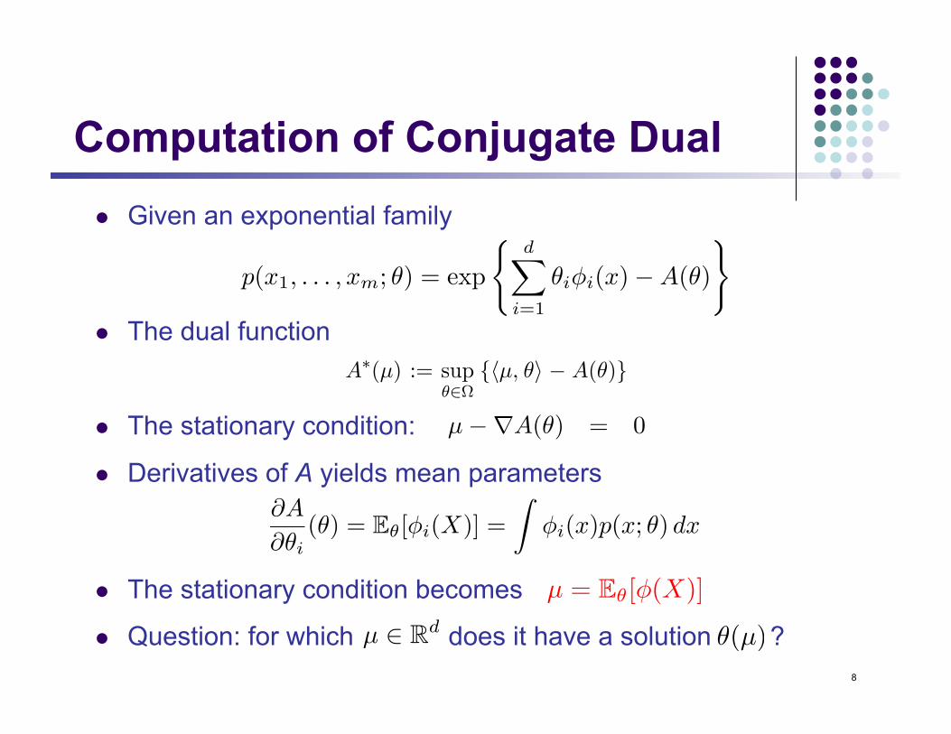
Computation of Conjugate Dual l  Given an exponential family

l  The dual function

l  The stationary condition:

l  Derivatives of A yields mean parameters

l  The stationary condition becomes

l  Question: for which does it have a solution ?

8

p(x1, . . . , xm; θ) = exp

d

i=1

θiφi(x)−A(θ)

66 Graphical Models as Exponential Families

between A and the maximum entropy principle is specified precisely interms of the conjugate dual function A!, to which we now turn.

3.6 Conjugate Duality: Maximum Likelihood andMaximum Entropy

Conjugate duality is a cornerstone of convex analysis [112, 203], andis a natural source for variational representations. In this section, weexplore the relationship between the log partition function A and itsconjugate dual function A!. This conjugate relationship is defined by avariational principle that is central to the remainder of this survey, inthat it underlies a wide variety of known algorithms, both of an exactnature (e.g., the junction tree algorithm and its special cases of Kalmanfiltering, the forward–backward algorithm, peeling algorithms) and anapproximate nature (e.g., sum-product on graphs with cycles, meanfield, expectation-propagation, Kikuchi methods, linear programming,and semidefinite relaxations).

3.6.1 General Form of Conjugate Dual

Given a function A, the conjugate dual function to A, which we denoteby A!, is defined as follows:

A!(µ) := sup!"!

!µ, !" # A(!). (3.42)

Here µ $ Rd is a fixed vector of so-called dual variables of the samedimension as !. Our choice of notation — i.e., using µ again —is deliberately suggestive, in that these dual variables turn out tohave a natural interpretation as mean parameters. Indeed, we havealready mentioned one statistical interpretation of this variational prob-lem (3.42); in particular, the right-hand side is the optimized value ofthe rescaled log likelihood (3.38). Of course, this maximum likelihoodproblem only makes sense when the vector µ belongs to the set M; anexample is the vector of empirical moments !µ = 1

n

"ni=1 "(Xi) induced

by a set of data Xn1 = X1, . . . ,Xn. In our development, we consider

the optimization problem (3.42) more broadly for any vector µ $ Rd. Inthis context, it is necessary to view A! as a function taking values in the

More general computation of the dual A!

• consider the definition of the dual function:

A!(µ) = sup!"Rd

!!µ, !" # A(!)

".

• taking derivatives w.r.t ! to find a stationary point yields:

µ #$A(!) = 0.

• Useful fact: Derivatives of A yield mean parameters:

"A

"!"(!) = E![#"(x)] :=

##"(x)p(x; !)!(x).

Thus, stationary points satisfy the equation:

µ = E!["(x)] (1)

26

θ(µ)µ ∈ Rd

∂A

∂θi(θ) = Eθ[φi(X)] =

φi(x)p(x; θ) dx

µ = Eθ[φ(X)]

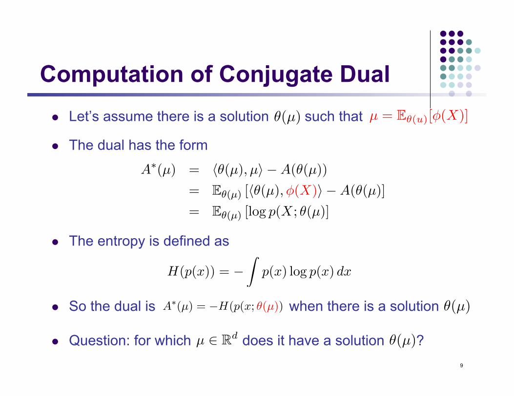
Computation of Conjugate Dual l  Let’s assume there is a solution such that

l  The dual has the form

l  The entropy is defined as

l  So the dual is when there is a solution

l  Question: for which does it have a solution ?

9

θ(µ) µ = Eθ(u)[φ(X)]

¡+Brief Article+¿

¡+The Author+¿

March 12, 2012

µ1 ≥ u12

µ2 ≥ u12

u12 ≥ 0

1 + µ12 ≥ u1 + u2

M(G) = µ ∈ Rd | ∃p with marginals µs;j , µst;jk

A∗(µ) = θ(µ), µ −A(θ(µ))

= Eθ(µ) [θ(µ),φ(X) −A(θ(µ)]

= Eθ(µ) [log p(X; θ(µ)]

1

H(p(x)) = −

p(x) log p(x) dx

µ ∈ Rd θ(µ)

¡+Brief Article+¿

¡+The Author+¿

March 12, 2012

µ1 ≥ u12

µ2 ≥ u12

u12 ≥ 0

1 + µ12 ≥ u1 + u2


A∗(µ) = θ(µ), µ −A(θ(µ))

= Eθ(µ) [θ(µ),φ(X) −A(θ(µ)]


A∗(µ) = −H(p(x; θ(µ))

1

θ(µ)

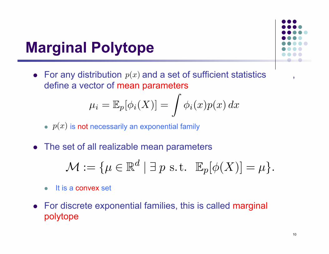
Marginal Polytope l  For any distribution and a set of sufficient statistics ,

define a vector of mean parameters

l  is not necessarily an exponential family

l  The set of all realizable mean parameters

l  It is a convex set

l  For discrete exponential families, this is called marginal polytope

10

3.5 Properties of A 63

=!

X m!!(x)

exp!", !(x)"#(dx)"X m exp!", !(u)"#(du)

= E"[!!(X)],

which establishes Equation (3.41a). The formula for the higher-orderderivatives can be proven in an entirely analogous manner.

Observe from Equation (3.41b) that the second-order partial deriva-tive #2A

#"!""2 is equal to the covariance element cov!!(X),!$(X).

Therefore, the full Hessian #2A(") is the covariance matrix of therandom vector !(X), and so is positive semidefinite on the open set!, which ensures convexity (see Theorem 4.3.1 of Hiriart-Urruty andLemarechal [112]). If the representation is minimal, there is no nonzerovector a $ Rd and constant b $ R such that !a, !(x)" = b holds #-a.e.This condition implies var"[!a, !(x)"] = aT #2A(")a > 0 for all a $ Rd

and " $ !; this strict positive definiteness of the Hessian on the openset ! implies strict convexity [112].

3.5.2 Forward Mapping to Mean Parameters

We now turn to an in-depth consideration of the forward mapping" %& µ, from the canonical parameters " $ ! defining a distribution p"

to its associated vector of mean parameters µ $ Rd. Note that the gradi-ent #A can be viewed as mapping from ! to Rd. Indeed, Proposition 3.1demonstrates that the range of this mapping is contained within theset M of realizable mean parameters, defined previously as

M := µ $ Rd | ' p s.t. Ep[!(X)] = µ.

We will see that a great deal hinges on the answers to the followingtwo questions:

(a) when does #A define a one-to-one mapping?(b) when does the image of ! under the mapping #A — that

is, the set #A(!) — fully cover the set M?

The answer to the first question is relatively straightforward, essen-tially depending on whether or not the exponential family is minimal.The second question is somewhat more delicate: to begin, note that our

µi = Ep[φi(X)] =

φi(x)p(x) dx

p(x)

p(x)

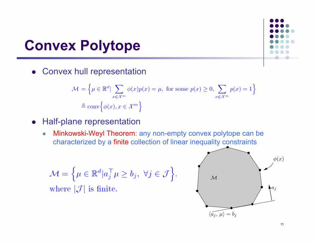
Convex Polytope l  Convex hull representation

l  Half-plane representation l  Minkowski-Weyl Theorem: any non-empty convex polytope can be

characterized by a finite collection of linear inequality constraints

11

3.4 Mean Parameterization and Inference Problems 55

Fig. 3.5 Generic illustration of M for a discrete random variable with |X m| finite. In thiscase, the set M is a convex polytope, corresponding to the convex hull of !(x) | x ! X m.By the Minkowski–Weyl theorem, this polytope can also be written as the intersectionof a finite number of half-spaces, each of the form µ ! Rd | "aj , µ# $ bj for some pair(aj , bj) ! Rd % R.

Example 3.8 (Ising Mean Parameters). Continuing from Exam-ple 3.1, the su!cient statistics for the Ising model are the singletonfunctions (xs, s ! V ) and the pairwise functions (xsxt, (s, t) ! E). Thevector of su!cient statistics takes the form:

!(x) :=!xs,s ! V ; xsxt, (s, t) ! E

"! R|V |+|E|. (3.30)

The associated mean parameters correspond to particular marginalprobabilities, associated with nodes and edges of the graph G as

µs = Ep[Xs] = P[Xs = 1] for all s ! V , and (3.31a)

µst = Ep[XsXt] = P[(Xs,Xt) = (1,1)] for all (s, t) ! E. (3.31b)

Consequently, the mean parameter vector µ ! R|V |+|E| consists ofmarginal probabilities over singletons (µs), and pairwise marginalsover variable pairs on graph edges (µst). The set M consists of theconvex hull of !(x),x ! 0,1m, where ! is given in Equation (3.30).In probabilistic terms, the set M corresponds to the set of allsingleton and pairwise marginal probabilities that can be realizedby some distribution over (X1, . . . ,Xm) ! 0,1m. In the polyhedralcombinatorics literature, this set is known as the correlation polytope,or the cut polytope [69, 187].

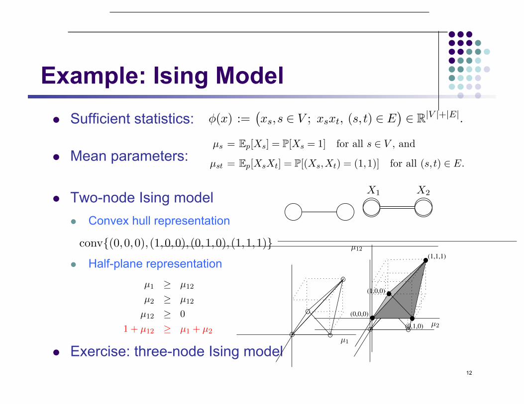
Example: Ising Model l  Sufficient statistics:

l  Mean parameters:

l  Two-node Ising model l  Convex hull representation

l  Half-plane representation

l  Exercise: three-node Ising model

12




!(x) :=!xs,s ! V ; xsxt, (s, t) ! E

"! R|V |+|E|. (3.30)





X1 X2

Example: Ising Model

!  Sufficient statistics:

!  Mean parameters:

!  Two-node Ising model !  Convex hull representation

!  Half-plane representation

!  Exercise: three-node Ising model

12




!(x) :=!xs,s ! V ; xsxt, (s, t) ! E

"! R|V |+|E|. (3.30)








!(x) :=!xs,s ! V ; xsxt, (s, t) ! E

"! R|V |+|E|. (3.30)






To make these ideas more concrete, consider the simplest nontrivialcase: namely, a pair of variables (X1,X2), and the graph consisting ofthe single edge joining them. In this case, the set M is a polytope inthree dimensions (two nodes plus one edge): it is the convex hull ofthe vectors (x1,x2,x1x2) | (x1,x2) ! 0,12, or more explicitly

conv(0,0,0),(1,0,0),(0,1,0),(1,1,1),

as illustrated in Figure 3.6.Let us also consider the half-space representation (3.29) for this

case. Elementary probability theory and a little calculation shows thatthe three mean parameters (µ1,µ2,µ12) must satisfy the constraints0 " µ12 " µi for i = 1,2 and 1 + µ12 # µ1 # µ2 $ 0. We can writethese constraints in matrix-vector form as

!

""""#

0 0 11 0 #10 1 #1

#1 #1 1

$

%%%%&

!

"#µ1

µ2

µ12

$

%& $

!

""""#

000

#1

$

%%%%&.

These four constraints provide an alternative characterization of the3D polytope illustrated in Figure 3.6.

Fig. 3.6 Illustration of M for the special case of an Ising model with two variables(X1,X2) ! 0,12. The four mean parameters µ1 = E[X1], µ2 = E[X2] and µ12 = E[X1X2]must satisfy the constraints 0 " µ12 " µi for i = 1,2, and 1 + µ12 # µ1 # µ2 $ 0. Theseconstraints carve out a polytope with four facets, contained within the unit hypercube[0,1]3.



conv(0,0,0),(1,0,0),(0,1,0),(1,1,1),



!

""""#

0 0 11 0 #10 1 #1

#1 #1 1

$

%%%%&

!

"#µ1

µ2

µ12

$

%& $

!

""""#

000

#1

$

%%%%&.



X1 X2

¡+Brief Article+¿

¡+The Author+¿

March 12, 2012

µ1 ≥ u12

µ2 ≥ u12

u12 ≥ 0

1 + µ12 ≥ u1 + u2

1



conv(0,0,0),(1,0,0),(0,1,0),(1,1,1),



!

""""#

0 0 11 0 #10 1 #1

#1 #1 1

$

%%%%&

!

"#µ1

µ2

µ12

$

%& $

!

""""#

000

#1

$

%%%%&.



¡+Brief Article+¿

¡+The Author+¿

March 12, 2012

µ1 ≥ µ12

µ2 ≥ µ12

µ12 ≥ 0

1 + µ12 ≥ µ1 + µ2


A∗(µ) = θ(µ), µ −A(θ(µ))

= Eθ(µ) [θ(µ),φ(X) −A(θ(µ)]


A∗(µ) = −H(p(x; θ(µ))

1

Example: Ising Model

!  Sufficient statistics:

!  Mean parameters:

!  Two-node Ising model !  Convex hull representation

!  Half-plane representation

!  Exercise: three-node Ising model

12




!(x) :=!xs,s ! V ; xsxt, (s, t) ! E

"! R|V |+|E|. (3.30)








!(x) :=!xs,s ! V ; xsxt, (s, t) ! E

"! R|V |+|E|. (3.30)







conv(0,0,0),(1,0,0),(0,1,0),(1,1,1),



!

""""#

0 0 11 0 #10 1 #1

#1 #1 1

$

%%%%&

!

"#µ1

µ2

µ12

$

%& $

!

""""#

000

#1

$

%%%%&.





conv(0,0,0),(1,0,0),(0,1,0),(1,1,1),



!

""""#

0 0 11 0 #10 1 #1

#1 #1 1

$

%%%%&

!

"#µ1

µ2

µ12

$

%& $

!

""""#

000

#1

$

%%%%&.



X1 X2

¡+Brief Article+¿

¡+The Author+¿

March 12, 2012

µ1 ≥ u12

µ2 ≥ u12

u12 ≥ 0

1 + µ12 ≥ u1 + u2

1

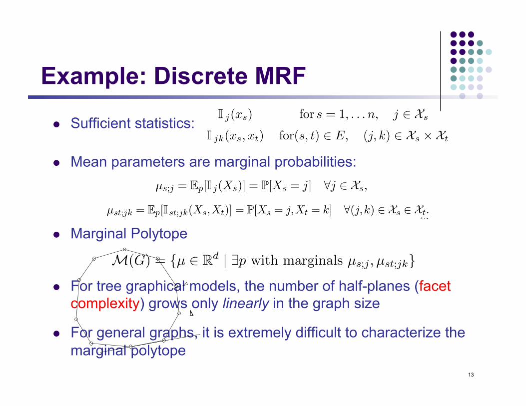
Example: Discrete MRF

l  Sufficient statistics:

l  Mean parameters are marginal probabilities:

l  Marginal Polytope

l  For tree graphical models, the number of half-planes (facet

complexity) grows only linearly in the graph size

l  For general graphs, it is extremely difficult to characterize the marginal polytope

13

Examples of M: Discrete MRF

• su!cient statistics:I j(xs) for s = 1, . . . n, j ! Xs

I jk(xs, xt) for(s, t) ! E, (j, k) ! Xs " Xt

• mean parameters are simply marginal probabilities, represented as:

µs(xs) :=X

j!Xs

µs;jI j(xs), µst(xs, xt) :=X

(j,k)!Xs"Xt

µst;jkI jk(xs, xt)

PSfrag replacements aj

MARG(G)

#aj , µ$ = bj

µe • denote the set of realizable µs and µst

by MARG(G)

• refer to it as the marginal polytope

• extremely di!cult to characterize for

general graphs

30


We refer to the su!cient statistics (3.34) as the standard overcom-plete representation. Its overcompleteness was discussed previously inExample 3.2.

With this choice of su!cient statistics, the mean parameters take avery intuitive form: in particular, for each node s ! V

µs;j = Ep[I j(Xs)] = P[Xs = j] "j ! Xs, (3.35)

and for each edge (s, t) ! E, we have

µst;jk = Ep[I st;jk(Xs,Xt)] = P[Xs = j,Xt = k] "(j,k) ! Xs ! Xt.(3.36)

Thus, the mean parameters correspond to singleton marginal distribu-tions µs and pairwise marginal distributions µst associated with thenodes and edges of the graph. In this case, we refer to the set M as themarginal polytope associated with the graph, and denote it by M(G).Explicitly, it is given by

M(G) := µ ! Rd | #p such that (3.35) holds "(s;j), and

(3.36) holds "(st;jk!. (3.37)

Note that the correlation polytope for the Ising model presentedin Example 3.8 is a special case of a marginal polytope, obtainedfor Xs ! 0,1 for all nodes s. The only di"erence is we have definedmarginal polytopes with respect to the standard overcomplete basis ofindicator functions, whereas the Ising model is usually parameterized asa minimal exponential family. The codeword polytope of Example 3.9 isanother special case of a marginal polytope. In this case, the reductionrequires two steps: first, we convert the factor graph representation ofthe code — for instance, as shown in Figure 3.7(a) — to an equiva-lent pairwise Markov random field, involving binary variables at eachbit node, and higher-order discrete variables at each factor node. (SeeAppendix E.3 for details of this procedure for converting from factorgraphs to pairwise MRFs.) The marginal polytope associated with thispairwise MRF is simply a lifted version of the codeword polytope. Wediscuss these and other examples of marginal polytopes in more detailin later sections.


We refer to the su!cient statistics (3.34) as the standard overcom-plete representation. Its overcompleteness was discussed previously inExample 3.2.

With this choice of su!cient statistics, the mean parameters take avery intuitive form: in particular, for each node s ! V

µs;j = Ep[I j(Xs)] = P[Xs = j] "j ! Xs, (3.35)

and for each edge (s, t) ! E, we have

µst;jk = Ep[I st;jk(Xs,Xt)] = P[Xs = j,Xt = k] "(j,k) ! Xs ! Xt.(3.36)

Thus, the mean parameters correspond to singleton marginal distribu-tions µs and pairwise marginal distributions µst associated with thenodes and edges of the graph. In this case, we refer to the set M as themarginal polytope associated with the graph, and denote it by M(G).Explicitly, it is given by

M(G) := µ ! Rd | #p such that (3.35) holds "(s;j), and

(3.36) holds "(st;jk!. (3.37)

Note that the correlation polytope for the Ising model presentedin Example 3.8 is a special case of a marginal polytope, obtainedfor Xs ! 0,1 for all nodes s. The only di"erence is we have definedmarginal polytopes with respect to the standard overcomplete basis ofindicator functions, whereas the Ising model is usually parameterized asa minimal exponential family. The codeword polytope of Example 3.9 isanother special case of a marginal polytope. In this case, the reductionrequires two steps: first, we convert the factor graph representation ofthe code — for instance, as shown in Figure 3.7(a) — to an equiva-lent pairwise Markov random field, involving binary variables at eachbit node, and higher-order discrete variables at each factor node. (SeeAppendix E.3 for details of this procedure for converting from factorgraphs to pairwise MRFs.) The marginal polytope associated with thispairwise MRF is simply a lifted version of the codeword polytope. Wediscuss these and other examples of marginal polytopes in more detailin later sections.

¡+Brief Article+¿

¡+The Author+¿

March 12, 2012

µ1 ≥ u12

µ2 ≥ u12

u12 ≥ 0

1 + µ12 ≥ u1 + u2


A∗(µ) = θ(µ), µ −A(θ(µ))

= Eθ(µ) [θ(µ),φ(X) −A(θ(µ)]


A∗(µ) = −H(p(x; θ(µ))

1

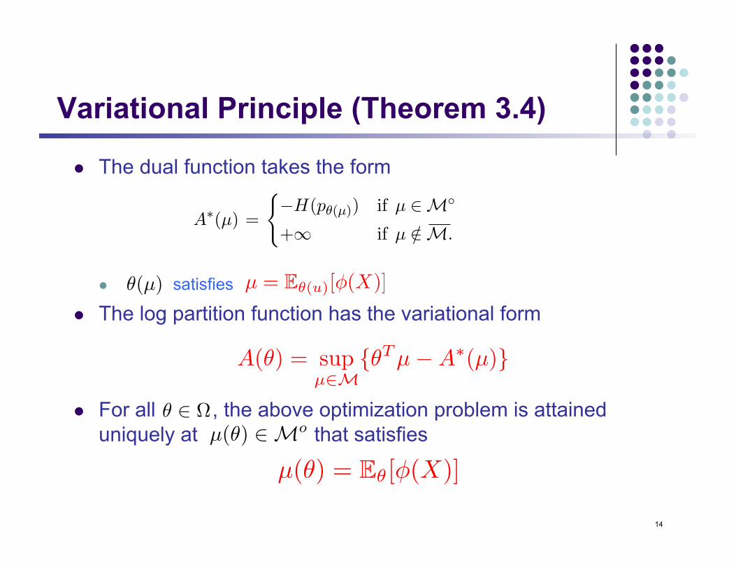
Variational Principle (Theorem 3.4)

l  The dual function takes the form

l  satisfies

l  The log partition function has the variational form

l  For all , the above optimization problem is attained uniquely at that satisfies

14

θ(µ) µ = Eθ(u)[φ(X)]

θ ∈ Ω

3.6 Conjugate Duality: Maximum Likelihood and Maximum Entropy 67

extended real line R! = R ! +", as is standard in convex analysis(see Appendix A.2.5 for more details).

As we have previously intimated, the conjugate dual function (3.42)is very closely connected to entropy. Recall the definition (3.2) of theShannon entropy. The main result of the following theorem is that whenµ # M", the value of the dual function A!(µ) is precisely the negativeentropy of the exponential family distribution p!(µ), where !(µ) is theunique vector of canonical parameters satisfying the relation

E!(µ)["(X)] = $A(!(µ)) = µ. (3.43)

We will also find it essential to consider µ /# M", in which case it isimpossible to find canonical parameters satisfying the relation (3.43). Inthis case, the behavior of the supremum defining A!(µ) requires a moredelicate analysis. In fact, denoting by M the closure of M, it turns outthat whenever µ /# M, then A!(µ) = +". This fact is essential in theuse of variational methods: it guarantees that any optimization probleminvolving the dual function can be reduced to an optimization problemover M. Accordingly, a great deal of our discussion in the sequel will beon the structure of M for various graphical models, and various approx-imations to M for models in which its structure is overly complex.

More formally, the following theorem, proved in Appendix B.2, providesa precise characterization of the relation between A and its conjugatedual A!:

Theorem 3.4.

(a) For any µ # M", denote by !(µ) the unique canonicalparameter satisfying the dual matching condition (3.43).The conjugate dual function A! takes the form

A!(µ) =

!%H(p!(µ)) if µ # M"

+" if µ /# M.(3.44)

For any boundary point µ # M\M" we haveA!(µ) = lim

n#+$A!(µn) taken over any sequence µn & M"

converging to µ.

A(θ) = supµ∈M

θTµ−A∗(µ)

µ(θ) ∈ Mo

µ(θ) = Eθ[φ(X)]

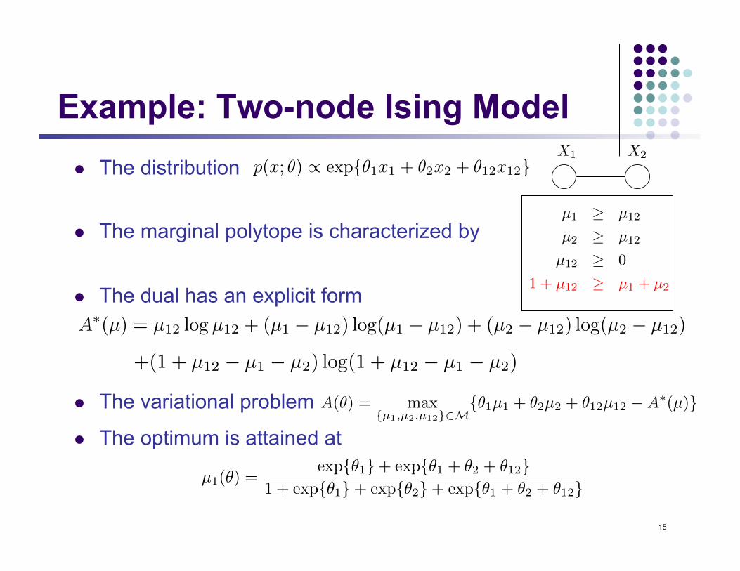
Example: Two-node Ising Model l  The distribution

l  The marginal polytope is characterized by l  The dual has an explicit form

l  The variational problem

l  The optimum is attained at

15

X1 X2p(x; θ) ∝ expθ1x1 + θ2x2 + θ12x12

A∗(µ) = µ12 logµ12 + (µ1 − µ12) log(µ1 − µ12) + (µ2 − µ12) log(µ2 − µ12)

+(1 + µ12 − µ1 − µ2) log(1 + µ12 − µ1 − µ2)

A(θ) = maxµ1,µ2,µ12∈M

θ1µ1 + θ2µ2 + θ12µ12 −A∗(µ)

µ1(θ) =expθ1+ expθ1 + θ2 + θ12

1 + expθ1+ expθ2+ expθ1 + θ2 + θ12

¡+Brief Article+¿

¡+The Author+¿

March 12, 2012

µ1 ≥ µ12

µ2 ≥ µ12

µ12 ≥ 0

1 + µ12 ≥ µ1 + µ2


A∗(µ) = θ(µ), µ −A(θ(µ))

= Eθ(µ) [θ(µ),φ(X) −A(θ(µ)]


A∗(µ) = −H(p(x; θ(µ))

1

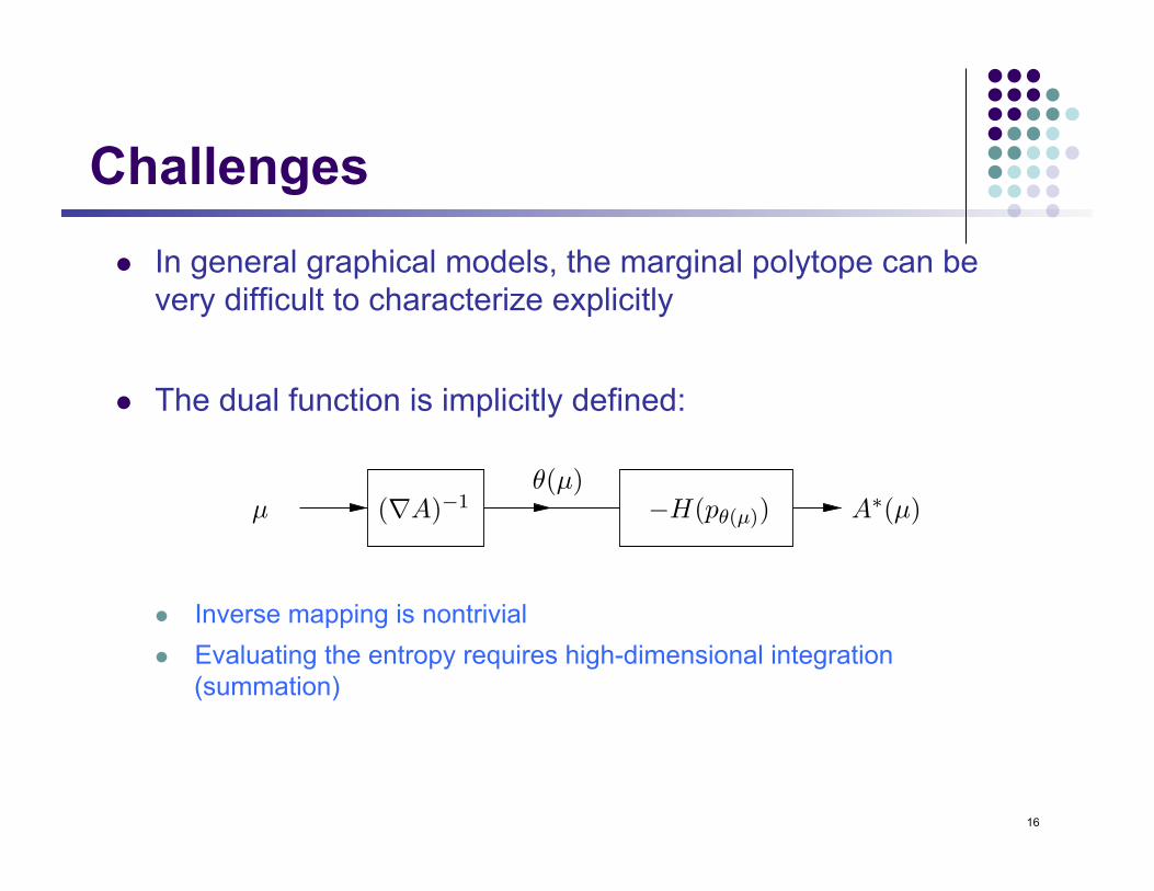
Challenges

l  In general graphical models, the marginal polytope can be very difficult to characterize explicitly

l  The dual function is implicitly defined:

l  Inverse mapping is nontrivial l  Evaluating the entropy requires high-dimensional integration

(summation)

16


Fig. 3.9 A block diagram decomposition of A! as the composition of two functions. Anymean parameter µ ! M" is first mapped back to a canonical parameter !(µ) in the inverseimage ("A)#1(µ). The value of A!(µ) corresponds to the negative entropy #H(p!(µ)) ofthe associated exponential family density p!(µ).

rapidly with the graph size. Indeed, unless fundamental conjectures incomplexity theory turn out to be false, it is not even possible to opti-mize a linear function over M for a general discrete MRF. In additionto the complexity of the constraint set, issue (b) highlights that evenevaluating the cost function at a single point µ ! M, let alone optimiz-ing it over M, is extremely di!cult.

To understand the complexity inherent in evaluating the dual valueA$(µ), note that Theorem 3.4 provides only an implicit characteri-zation of A$ as the composition of mappings: first, the inverse map-ping ("A)#1 : M% # ", in which µ maps to !(µ), corresponding to theexponential family member with mean parameters µ; and second, themapping from !(µ) to the negative entropy $H(p!(µ)) of the associ-ated exponential family density. This decomposition of the value A$(µ)is illustrated in Figure 3.9. Consequently, computing the dual valueA$(µ) at some point µ ! M% requires computing the inverse map-ping ("A)#1(µ), in itself a nontrivial problem, and then evaluatingthe entropy, which requires high-dimensional integration for generalgraphical models. These di!culties motivate the use of approximationsto M and A$. Indeed, as shown in the sections to follow, a broad classof methods for approximate marginalization are based on this strategyof finding an approximation to the exact variational principle, which isthen often solved using some form of message-passing algorithm.

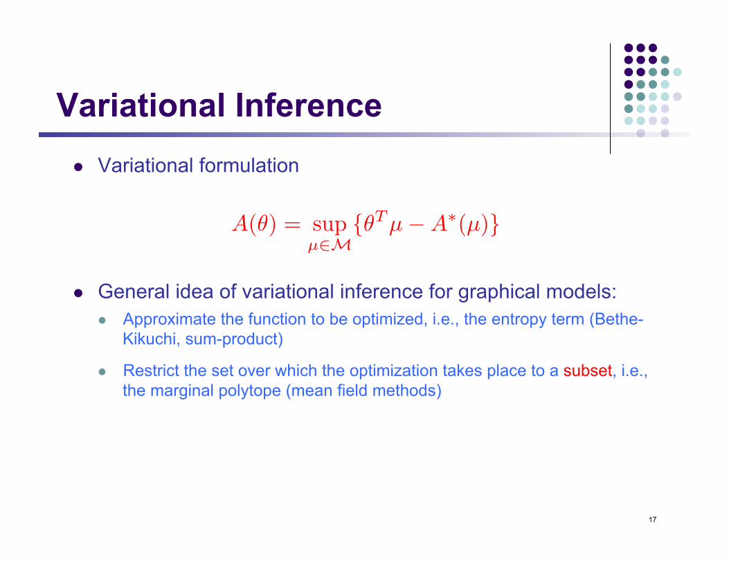
Variational Inference l  Variational formulation

l  General idea of variational inference for graphical models: l  Approximate the function to be optimized, i.e., the entropy term (Bethe-

Kikuchi, sum-product)

l  Restrict the set over which the optimization takes place to a subset, i.e., the marginal polytope (mean field methods)

17

A(θ) = supµ∈M

θTµ−A∗(µ)

probabilistic graphical models - university of...

Documents