probabilistic forecasts of solar irradiance by stochastic ... · probabilistic forecasts of solar...
TRANSCRIPT
General rights Copyright and moral rights for the publications made accessible in the public portal are retained by the authors and/or other copyright owners and it is a condition of accessing publications that users recognise and abide by the legal requirements associated with these rights.
Users may download and print one copy of any publication from the public portal for the purpose of private study or research.
You may not further distribute the material or use it for any profit-making activity or commercial gain
You may freely distribute the URL identifying the publication in the public portal If you believe that this document breaches copyright please contact us providing details, and we will remove access to the work immediately and investigate your claim.
Downloaded from orbit.dtu.dk on: Jul 03, 2020
Probabilistic Forecasts of Solar Irradiance by Stochastic Differential Equations
Iversen, Jan Emil Banning; Morales González, Juan Miguel; Møller, Jan Kloppenborg; Madsen, Henrik
Published in:Environmetrics
Link to article, DOI:10.1002/env.2267
Publication date:2014
Document VersionEarly version, also known as pre-print
Link back to DTU Orbit
Citation (APA):Iversen, J. E. B., Morales González, J. M., Møller, J. K., & Madsen, H. (2014). Probabilistic Forecasts of SolarIrradiance by Stochastic Differential Equations. Environmetrics, 25(3), 152-164. https://doi.org/10.1002/env.2267
Environmetrics 00, 1–22
DOI: 10.1002/env.XXXX
Probabilistic Forecasts of Solar Irradiance byStochastic Differential Equations
E. B. Iversena∗ J. M. Moralesa, J. K. Møllera, H. Madsena
Summary: Probabilistic forecasts of renewable energy production provide users with valuable information
about the uncertainty associated with the expected generation. Current state-of-the-art forecasts for solar
irradiance have focused on producing reliable point forecasts. The additional information included in
probabilistic forecasts may be paramount for decision makers to efficiently make use of this uncertain and
variable generation. In this paper, a stochastic differential equation (SDE) framework for modeling the
uncertainty associated with the solar irradiance point forecast is proposed. This modeling approach allows
for characterizing both the interdependence structure of prediction errors of short-term solar irradiance and
their predictive distribution. A series of different SDE models are fitted to a training set and subsequently
evaluated on a one-year test set. The final model proposed is defined on a bounded and time-varying state
space with zero probability almost surely of events outside this space.
Keywords: Forecasting; Stochastic differential equations; Solar power; Probabilistic forecast;
Predictive distributions.
1. INTRODUCTION
The operation of electric energy systems is today challenged by the increasing level of
uncertainty in the electricity supply brought in by the larger and larger share of renewables
in the generation mix. Decision-making, operational and planning problems in electricity
markets can be characterized by time-varying and asymmetric costs. These asymmetric
costs are caused by the need to continuously balance the electricity system to guarantee
a Technical University of Denmark, Asmussens Alle, building 322, DK-2800 Lyngby, Denmark.∗Correspondence to: Mr. E. B. Iversen, Technical University of Denmark, Asmussens Alle, building 322, DK-2800 Lyngby,
Denmark. Phone: +45 60 67 19 85, E-mail: [email protected]
This paper has been submitted for consideration for publication in Environmetrics
Environmetrics E. B. Iversen et al.
a reliable and secure supply of power. An understanding of the underlying uncertainty is,
therefore, essential to satisfactorily manage the electricity system. This introduces the need
for forecasts describing the entire variation of the renewable generation.
Solar irradiance is a source of renewable energy and, along with wind and hydro, is taking
shape as a potential driver for a future free of fossil fuels. The worldwide installed capacity of
photovoltaic energy systems has seen a rapid increase from 9.5 GW in 2007 to more than 100
GW by the end of 2012 (European Photovoltaic Industry Association (2013)). The energy
generation from solar irradiance is subject to weather conditions and, as such, it constitutes
a variable and uncertain energy source.
Current state-of-the-art forecasts for solar energy have focused on point forecasts, that is,
the most likely or the average outcome. Such point forecasts, however, do not adequately
describe the uncertainty of the power production. This is recognized by the abundance of
significant works on probabilistic forecasting for wind power, see for ex. Pinson et al. (2007)
and Zhou et al. (2013).
In the literature, a variety of different approaches have been taken to provide reliable solar
power forecasts, based on time series (Huang et al. (2013), Boland (2008), Ji and Chee (2011),
Bacher et al. (2009), Yang et al. (2012)), Artificial Neural Networks (Mihalakakou et al.
(2000), Chen et al. (2011)), cloud motion forecasts (Perez et al. (2010)) and statistical models
(Ridley et al. (2010), Kaplanis and Kaplani (2010)). A review of some of these approaches
is found in Pedro and Coimbra (2012). In Chen et al. (2011) Artifical Neural Networks are
used in combination with a weather type classification, to provide point forecasts of PV
production. In Lorenz et al. (2009), a forecast method that makes use of a clear sky model
and numerical weather predictions is developed, also accounting for orientation and tilt of
the PV panel. The paper by Bhardwaj et al. (2013) introduces a hidden Markov model for
solar irradiance based on fuzzy logic. They exploit inputs such as humidity, temperature,
2
Probabilistic Solar Forecasts by SDEs Environmetrics
air pressure and wind speed, among others. A time-series model for predicting one-hour-
ahead solar power production is considered in Yang et al. (2012). This paper employs a
cloud cover index to model the absorption and refraction of the incoming light through
the atmosphere. In Bacher et al. (2009), an auto-regressive model with exogenous input is
proposed. It predicts weighing the past observations and the numerical weather prediction
and introduces a clear sky model to capture the diurnal variation.
Probabilistic forecasting of solar irradiance is, though, in its infancy. One work in this area
is the one by Mathiesen et al. (2013), where post-processing of numerical weather predictions
are applied to obtain probabilistic forecasts. Previous work on stochastic differential
equations and solar irradiance is, to the best of our knowledge, limited to Soubdhan and
Emilion (2010), which formulates a very simple stochastic differential equation model for
solar irradiance. As a consequence of its simplicity, the model was largely unsuccessful at
forecasting. Stochastic differential equations are fruitfully used for wind power forecasting
in Møller et al. (2013) by considering state-dependent diffusions and external input.
This paper describes a new approach to solar irradiance forecasting based on stochastic
differential equations (SDEs). Modeling with SDEs has multiple benefits, among others:
• SDE models are able to produce reliable point forecasts as well as probabilistic forecasts.
• Model extensions are easy to formulate and have an intuitive interpretation. We can
start with a simplistic model and extend it to a sufficient degree of complexity.
• We can model processes that are bounded and assign zero probability to events outside
the bounded interval, which is essential for correct probabilistic forecasts of solar
irradiance.
• We leave the discrete-time realm of Gaussian innovations and consider instead the more
general class of continuous-time processes with continuous trajectories.
• SDEs span a large class of stochastic processes with classical time-series models as
special cases.
3
Environmetrics E. B. Iversen et al.
The rest of this paper is structured as follows: Section 2 gives a general introduction to the
stochastic differential equation framework and describes an estimation procedure. Section 3
starts with a simple SDE model. secondly we propose a mechanistic model which captures
some of the key physical qualities of solar irradiance. Lastly, in Section 3, we provide a
SDE model that extends the mechanistic model to overcome some statistical deficiencies. In
Section 4, the different models are compared to simple as well as complex benchmarks and
the performance of the finished model is assessed. Lastly, Section 5 concludes the paper.
2. STOCHASTIC DIFFERENTIAL EQUATIONS
Suppose that we have the continuous time processXt ∈ X ⊂ Rn. In general, it is only possible
to observe continuous time processes in discrete time. We observe the process Xt through
an observation equation at discrete times. Denote the observation at time tk by Yk ∈ Y ⊂ Rl
for k ∈ {0, . . . , N}. Let the observation equation be given by:
Yk = h(Xtk , tk, ek), (1)
where the variable tk allows for dependence on an external input at time tk, ek ∈ Rl is the
random observation error, and h(·) ∈ Rl is the function that links the process state to the
observation. The simplest form of the observation equation is h(·) = Xtk + ek.
2.1. Definition of Stochastic Differential Equations
In the ordinary differential equation setting, the evolution in time of the state variable Xt is
given by the deterministic system equation
dXt
dt= f(Xt, t), (2)
4
Probabilistic Solar Forecasts by SDEs Environmetrics
where t ∈ R and f(·) ∈ Rn. Complex systems such as weather systems are subject to random
perturbations of the input or processes that are not specified in the model description.
This suggests introducing a stochastic component in the state evolution to capture such
perturbations. This can be done by formulating the state evolution as a stochastic differential
equation (SDE), as done in Øksendal (2010). Thus, we can formulate the time evolution of
the state of the process by the form:
dXt
dt= f(Xt, t) + g(Xt, t)Wt, (3)
where Wt ∈ Rm is an m-dimensional standard Wiener process and g(·) ∈ Rn×m is a matrix
function (Øksendal, 2010). Multiplying with dt on both sides of (3) we get the standard SDE
formulation:
dXt = f(Xt, t)dt+ g(Xt, t)dWt. (4)
Notice that we allow for a complex dependence on t, including external input at time t.
While this form is the most common for SDEs, it is not well defined, as the derivative of
Wt, dWt, does not exist. Instead, it should be interpreted as an informal way of writing the
integral equation:
Xt = X0 +
∫ t
0
f(Xs, s)ds+
∫ t
0
g(Xs, s, )dWs. (5)
In Equation (5), the behavior of the continuous time stochastic process Xt is expressed as
the sum of an initial stochastic variable, an ordinary Lebesgue integral, and an Ito integral.
In a deterministic ordinary differential equation setting, the solution would be a single
point for each future time t. In the SDE setting, in contrast, the solution is the probability
density of Xt for any state, x, and any future time, t. For an Ito process given by the
stochastic differential equation defined in (4) with drift f(Xt, t) and diffusion coefficient
g(Xt, t) =√
2D(Xt, t), the probability density j(x, t) in the state x at time t of the random
5
Environmetrics E. B. Iversen et al.
variable Xt is given as the solution to the partial differential equation known as the Fokker-
Planck equation (Bjork, 2009):
∂
∂tj(x, t) = − ∂
∂x[f(x, t)j(x, t)] +
∂2
∂x2[D(x, t)j(x, t)] . (6)
Thus, given a specific SDE, we can find the density at any future time by solving a partial
differential equation.
SDEs are a general class of processes. This is stated by the Levy-Ito decomposition, which
says that, under sufficient regularity conditions, all stochastic processes with continuous
trajectories can be written as SDEs (Øksendal, 2010). Hence many of the ordinary discrete-
time stochastic processes can be seen as a SDE being sampled at discrete times, and
therefore, SDEs is a generalization of generic time-series models in discrete time. Other
useful introductions to SDEs are among others Kloeden and Pearson (1977) and Mikosch
(1998).
2.2. Parameter Estimation
In this section, we outline how to estimate parameters in a SDE of a general form and, in
particular, with a state-dependent diffusion term. A thorough description of the procedure
used here (and other estimation procedures) is found in Jazwinski (2007). First, we go into
detail on the estimation procedure of the parameters of a SDE with a state-independent
diffusion term. Second, we show how to transform a process with state-dependent diffusion
term into a process with a unit diffusion term, whereby the previously mentioned estimation
procedure can be applied.
Consider the model defined by Equations (1) and (4) given by:
dXt = f(Xt, t)dt+ g(Xt, t)dWt (7)
Yk = h(Xtk , tk, ek). (8)
6
Probabilistic Solar Forecasts by SDEs Environmetrics
On the basis that we want to estimate the parameters in the above model, the problem can
be formulated as follows: Find a parameter vector, θ ∈ Θ, that maximizes some objective
function of θ. There are several possible choices for an objective function. A natural choice
in this framework is to choose an objective function that maximizes the probability of seeing
the observations given by YN = {Y0, . . . , YN}. This leads to choosing the likelihood function
as objective function, i.e.,
L (θ;YN) = p (YN |θ) =
(N∏k=1
p (Yk|Yk−1, θ)
)p(Y0|θ). (9)
Even though this problem could, in principle, be solved using the Fokker-Planck equation,
this is only feasible for systems with simple structures, as it involves solving a complex partial
differential equation.
The estimation procedure, which we shall introduce next, relies on the system having a
specific form, namely:
dXt = f(Xt, t)dt+ g(t)dWt (10)
Yk = h(Xtk , tk) + ek. (11)
In the system defined by Equations (10) and (11), we assume that g(·) ∈ Rn×n does
not depend on the state Xt. Also, we assume that the observation noise is an additive
Gaussian white noise, i.e., ek ∼ N (0, Sk(tk)), where Sk(tk) is some covariance matrix,
possibly depending on time. It is clear that restricting g(·) to not depend on Xt limits
our model framework severely. As we shall see, this can, to some degree, be remedied by a
transformation using Ito-calculus. The restriction of having additive Gaussian measurement
noise should be dealt with by transformations of the observations.
As the system defined by Equations (10) and (11) is driven by Wiener noise, which has
Gaussian increments, and the observation noise is Gaussian, it is reasonable to assume
that the density of Yk|Yk−1 can be approximated by a Gaussian distribution. Note that the
7
Environmetrics E. B. Iversen et al.
Gaussian distribution is completely characterized by its mean and covariance. This implies
that using the extended Kalman filter, which is linear, is appropriate.
The one-step predictions for the mean and variance are defined as:
Yk|k−1 = E [Yk|Yk−1, θ] (12)
Rk|k−1 = V [Yk|Yk−1, θ] , (13)
where E [·] and V [·] denote the expectation and variance, respectively. The innovation is
given by
εk = Yk − Yk|k−1. (14)
Using this, we can now write the likelihood function as
L (θ;YN) =
N∏k=1
exp(−1
2ε>k R
−1k|k−1εk
)√
det(Rk|k−1
) (√2π)l p(Y0|θ), (15)
where l is the dimension of the sample space and (·)> denotes the vector transpose. The
estimate of θ can be found by solving the optimization problem
θ = arg maxθ∈Θ
(log(L (θ;YN))) . (16)
The Kalman gain governs how much the one-step prediction of the underlying state, Xk|k−1,
should be adjusted to form the state update, Xk|k, from the new observation. This is given
by
Kk = Pk|k−1C>R−1
k|k−1, (17)
8
Probabilistic Solar Forecasts by SDEs Environmetrics
where C is the first order expansion of h(·), i.e., the Jacobian, and Pk|k−1 is the covariance
of the one-step prediction. The state update is then given by
Xk|k = Xk|k−1 +Kkεk (18)
Pk|k = Pk|k−1 −KkR−1k|k−1K
>k . (19)
Hence, the state update is a combination of the previous state estimate and the new
information obtained from the k’th observation, Yk.
The procedure of estimating the parameters is currently being implemented as an R package
and is described in Juhl et al. (2013). The estimation procedure is done in the statistical
software R. we use the extended Kalman filter as provided by Juhl et al. (2013) to give
predictions of future observation and implement the likelihood function directly in R. The
likelihood function is then optimized using the nlminb routine for constrained optimization.
2.3. Ito Calculus and the Lamperti Transform
We will now discuss how a SDE of the form in Equation (7) can be transformed to the form in
Equation (10) to allow for the estimation procedure previously introduced. The fundamental
tool for the transformation of SDEs is Ito’s lemma, as stated in Øksendal (2010). Below we
introduce the 1-dimensional Ito formula and the Lamperti transform. The multidimensional
Ito formula is covered in Øksendal (2010). For a more detailed description of the Lamperti
transform and how to apply it to multivariate processes, see Møller and Madsen (2010).
Theorem 1 (The 1-dimensional Ito formula ) Let Xt be an Ito process given by
dXt = f(Xt, t)dt+ g(Xt, t)dWt. (20)
Let ψ(x, t) ∈ C2([0,∞))× R. Then
Zt = ψ(Xt, t) (21)
9

Environmetrics E. B. Iversen et al.
is again an Ito process, and
dZt =∂ψ
∂t(Xt, t)dt+
∂ψ
∂x(Xt, t)dXt +
1
2
∂2ψ
∂x2(Xt, t)(dXt)
2, (22)
where (dXt)2 is calculated according to the rules
dt · dt = dt · dWt = dWt · dt = 0, dWt · dWt = dt. (23)
The Ito formula stated in Theorem 1 can be used to transform the process to a SDE with
unit diffusion by the Lamperti transform.
Theorem 2 (Lamperti transform) Let Xt be an Ito process defined as in (20), and define
ψ(Xt, t) =
∫1
g(x, t)dx
∣∣∣∣x=Xt
. (24)
If ψ represents a one to one mapping from the state space of Xt onto R for every t ∈ [0,∞),
then choose Zt = ψ(Xt, t). Then Zt is governed by the SDE
dZt =
(ψt(ψ
−1(Zt, t), t) +f(ψ−1(Zt, t), t)
g(ψ−1(Zt, t), t)(25)
−1
2gx(ψ
−1(Zt, t), t)
)dt+ dWt, (26)
where gx(·) and gt(·) denote the derivatives of g(·) with regard to x and t, respectively, and
ψt denotes the derivative of ψ with respect to t.
This result is obtained by applying the Ito formula.
3. SOLAR IRRADIANCE
In this section we apply the theory in Section 2 to build a model for solar irradiance. The
approach is to start out with a simple model and extend it until we reach a model that
captures the dynamics adequately. Firstly we extend the simple model from a mechanistic
10
Probabilistic Solar Forecasts by SDEs Environmetrics
understanding of solar irradiance, for instance that solar irradiance is a bound process and
our dynamical model should reflect this. Secondly, we extend the mechanistic model by
identifying statistical deficiencies and extending the model to resolve those. Thus, we should
end up with a model, that captures the mechanics of the system and is statistically sound.
3.1. Data
The data set at our disposal belongs to a meteorological station located in the western part
of Denmark. The data include hourly observations of irradiance on a flat surface together
with predictions for irradiance based on a numerical weather prediction model from the
Danish Meteorological Institute. The numerical weather prediction (NWP) provides a 48-
hour forecast of the irradiance, which is updated every 6 hours. We use the most recent
forecast in the model. The data covers a period of three years from 01/01-2009 to 31/12-
2011. We divide the period into a training and a test set, with the training set covering the
first two years and the test set the last year.
3.2. Model 1: A Simple Model Tracking the NWP
We start by introducing a simple SDE model for solar irradiance that tracks the numerical
weather prediction provided by the Danish Meteorological Institute, i.e.,
dXt = θx(ptµx −Xt)dt+ σxdWt (27)
Yk = Xtk + εk. (28)
In this model and the following, we denote the observed solar irradiance at time tk by Yk.
pt, is an external input representing the predicted irradiance at time t. In the model, we
have parameter µx, which allows for a local scaling of the pt, such that it does not over or
under shoot on average. The parameter θx determines how rapidly the model reverts to the
11
Environmetrics E. B. Iversen et al.
predicted level of irradiance. The system noise is controlled by parameter σx. The observation
error is denoted εk and is a stochastic variable with distribution N (0, σε).
3.3. Model 2: A Mechanistic Extension
Some physical characteristics of solar irradiance are clearly not captured in Model 1. Among
these are issues related to the bounded nature of solar irradiance: It is never below zero and
also never above some upper bound determined by the light emitted by the sun and the
season. We will remedy this issue and others with the following model:
dXt = θx
(pt + βxγmt + δ
µx −Xt
)dt+ σxXt(1−Xt)dWt (29)
Yk = γmtkXtk + εk. (30)
Solar irradiance is highly cyclical. To capture this, we extend the simple SDE model defined
in (27)-(28) by introducing the maximum irradiance in hour t, mt, as a scaling factor. Here
we compute mt according to Bird and Hulstrom (1981), where the refraction and absorption
in the atmosphere is set to zero. This leads to a formulation where we let the stochastic
process Xt denote the proportion of extra terrestrial irradiance (i.e., the irradiance that
would arrive at the surface if there were no atmosphere) that reaches the surface.
The above process is, however, undefined at night, when mt = 0. To overcome this, we can
instead think of Xt as a process that describes the state of the atmosphere and how much
solar irradiance there would potentially be allowed through. In this context, it clearly makes
sense to have Xt defined at night. Thus, we can solve the issue of having mt = 0 by adding
a small constant, say δ = 0.01. Given that the pt is also equal to zero at night, we introduce
another parameter βx (to be estimated) that is added to pt such that Xt is not forced to
tend to zero at night.
Also we note that in this set-up the proportion of solar irradiance that reaches the surface
is naturally bounded to be between zero and one. Thus we want to introduce bounds for
12
Probabilistic Solar Forecasts by SDEs Environmetrics
the process Xt. This is easily done by introducing a state-dependent diffusion, where the
diffusion term decreases to zero as the process approaches the bounds. This implies that the
drift term takes over near the bounds. Furthermore, since we assume that θx > 0 and have
that 1 > pt+βxmt+δ
> 0, the drift term eventually pulls the process away from the bounds.
We have assumed the extra terrestrial irradiance, mt, as the upper limit for the solar
irradiance. It should be clear, however, that this level can never be attained, because there
will always be some refraction by the atmosphere. Hence, we can possibly scale down the
upper limit, mt, to improve the model. This is done by introducing a factor, γ, on the
maximum solar irradiance. An improvement of the model would be to consider the air mass
Kasten and Young (1989), which takes care of the fact that the distance the light travels
through the atmosphere is longer, when the sun is near the horizon. This, however, will be
left to future work.
In the estimation procedure we have assumed that the noise is non-state dependent, which
is clearly not the case here. Therefore, we need to work with the Lamperti transformed
process. The Lamperti transformation is given by:
Zt = ψ (Xt, t) =
∫1
σxx(1− x)dx
∣∣∣∣x=Xt
= − 1
σxlog
(1− xx
)(31)
Xt = ψ−1 (Zt, t) =1
1 + e−σxZt. (32)
Noting that ψt(·) = 0 and gx(x, t) = σx(1− 2x), we can now make use of the Lamperti
transform to obtain the process on the transformed Z-space, which becomes:
dZt =
θx
(pt+βxγmt+δ
µx − 11+e−σxZt
)σx
11+e−σxZt
(1− 1
1+e−σxZt
) − σx2
(1− 2
1
1 + e−σxZt
) dt+ dWt (33)
Yk = γmtk
1
1 + e−σxZt+ εk. (34)
In the sequel, we shall only state the model in the original domain and not in the Lamperti
transformed domain, as they are equivalent in the sense of yielding the same output
13
Environmetrics E. B. Iversen et al.
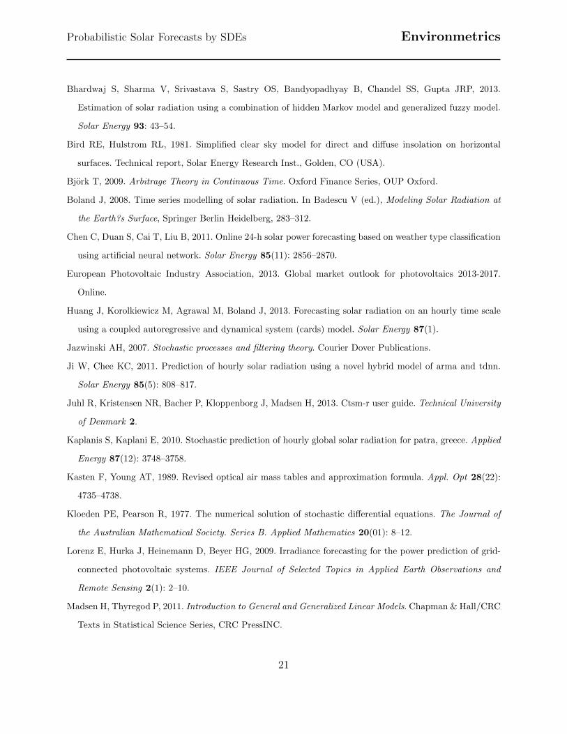
[Figure 1 about here.]
In this mechanistic model, we want to consider any deficiencies to improve. This can, among
other approaches, be done by considering the autocorrelation of the studentized residuals.
In Figure 1 we show the autocorrelation of the studentized residuals of Model 2. We see that
there are significant lags at the first lags and that there is some periodicity in the lags. This
points in the direction of some statistical improvements that can be made to the model,
which we consider next in Model 3.
3.4. Model 3: Statistical Extensions
How fast Xt is attracted to its predicted level may vary over time. This may be due to the
NWP being more accurate at some times than at others. Furthermore, there is a lag in the
numerical weather prediction as it takes 4 hours to solve the NWP model. As the NWP
model is only run every 6 hours, this leads to the NWP being between 4 and 10 hours old,
which may also cause us to have varying confidence in the NWP.
To address this issue, we have introduced the stochastic process At, which reverts to the
level µA. The speed at which this reversion occurs is determined by θA, while the system
noise is governed by σA. At governs how rapidly Xt tends to its predicted level. Also, there
might be variations over the day in the accuracy of the numerical weather prediction. This
leads to the following model:
dXt = eAt(pt + βxγmt + δ
(µx − ω1 sin
(2π
24t+ ω2
))−Xt
)dt (35)
+σxXt(1−Xt)dW1,t
dAt = θA(µA − At)dt+ σAdW2,t (36)
Yk = γmtkXtk + εk. (37)
Firstly, note that we use a sinusoid to describe a periodic behaviour. Secondly, we work in
14
Probabilistic Solar Forecasts by SDEs Environmetrics
hourly time steps, which explains 2π24t. We then introduce a period shift, ω2, and an amplitude,
ω1. The sinusoid is added to the scaling of the meteorological prediction, which translates
into the pt being more accurate in some hours of the day than in others.
We have ended up with a model that includes a maximum hourly irradiance, a numerical
weather prediction as external input, stochastic time constants, and a non-Gaussian system
noise that confines the process between zero and the extra terrestrial irradiance. In the
following section, validation results of the final model are presented.
4. MODEL VALIDATION
In this section, the different models are fitted to the data pertaining to the training set and
evaluated in terms of their likelihood and information criteria.
In terms of computational costs, we have done the computations on a network mainframe
with 20 1.8 GHz processors with a partial paralellization of the optimization problem. In this
setup and the models fitted to the test set of two years of hourly data Model 1 is optimized
in less than 3 minutes, Model 2 is optimized in just under 16 minutes and the fitting of
Model 3 is completed 41 minutes. It should be noted, however, that the paralellization has
diminishing returns to scale. For comparison we have fitted Model 3 on a personal computer
with a 2.7 GHz processor and 8 GB of ram in just over 2 hours.
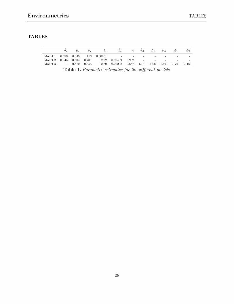
[Table 1 about here.]
As we propose a model for solar irradiance based partially on physical characteristics of
the system, a first step in validating the model is to consider if the parameter estimates are
feasible in terms of the physics of the system. Specifically, from the physics of the system,
we would expect µx around 1, βx to be smaller than 0.01 and γ close to, but smaller than 1.
We see that all these conditions are satisfied.
15
Environmetrics E. B. Iversen et al.
To compare the models with more classical alternatives, we consider an autoregressive
model with external input (ARX) and an autoregressive model with external input and
time-varying system variability, where the prediction variance is modelled using a generalized
linear model (ARX-GLM). The AR model is specified as follows:
Yk = ψ0 +
p∑i=1
ψiYk−i + εk, where εk ∼ N (0, σ2). (38)
The ARX model takes the form
Yk = ψ0 +
p∑i=1
ψiYk−i + φpk + εk, εk ∼ N (0, σ2). (39)
The ARX-GLM model is specified as
Yk = ψ0 +
p∑i=1
ψiYk−i + φpk + εk, εk+1 ∼ N(0, fε(·)2
). (40)
We find, after a fitting procedure, that an appropriate form of the variance scaling in the
generalized linear model is
fε(k + 1) = σ(mtk+1
)3/4, (41)
where mtk+1is specified as in Model 2. For a general introduction to generalized linear models
see Madsen and Thyregod (2011).
Additionally, we benchmark against climatological forecasts. The naıve forecast method is
to use the empirical distribution, with no time dependence, to predict the solar irradiance.
A slightly less naıve approach is to use the empirical distribution of irradiance as a function
of hour-of-day. A third climatological benchmark is to use both hour-of-day and month-of-
year to predict the distribution. These benchmarks are clearly naıve as they do not use the
previous observation to predict. Also, as the climatological approach is non-parametric, we
use the empirical likelihood, see for instance Bera and Bilias (2002), to evaluate the fit.
16
Probabilistic Solar Forecasts by SDEs Environmetrics
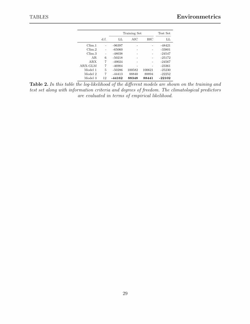
[Table 2 about here.]
The results of the different models are presented in Table 2. When computing the likelihood
values, we let only observations during the day contribute with likelihood. This is done as to
not obstruct the picture by fitting solar irradiance models at night. This holds true both for
the benchmarks as well as the fitted SDE models. We see that Model 3 best describes the
data in the training set, as well as in the test set. Furthermore note that the improvement
from the quite naıve Model 1 to Model 2 is huge, which justifies the change in the state
space.
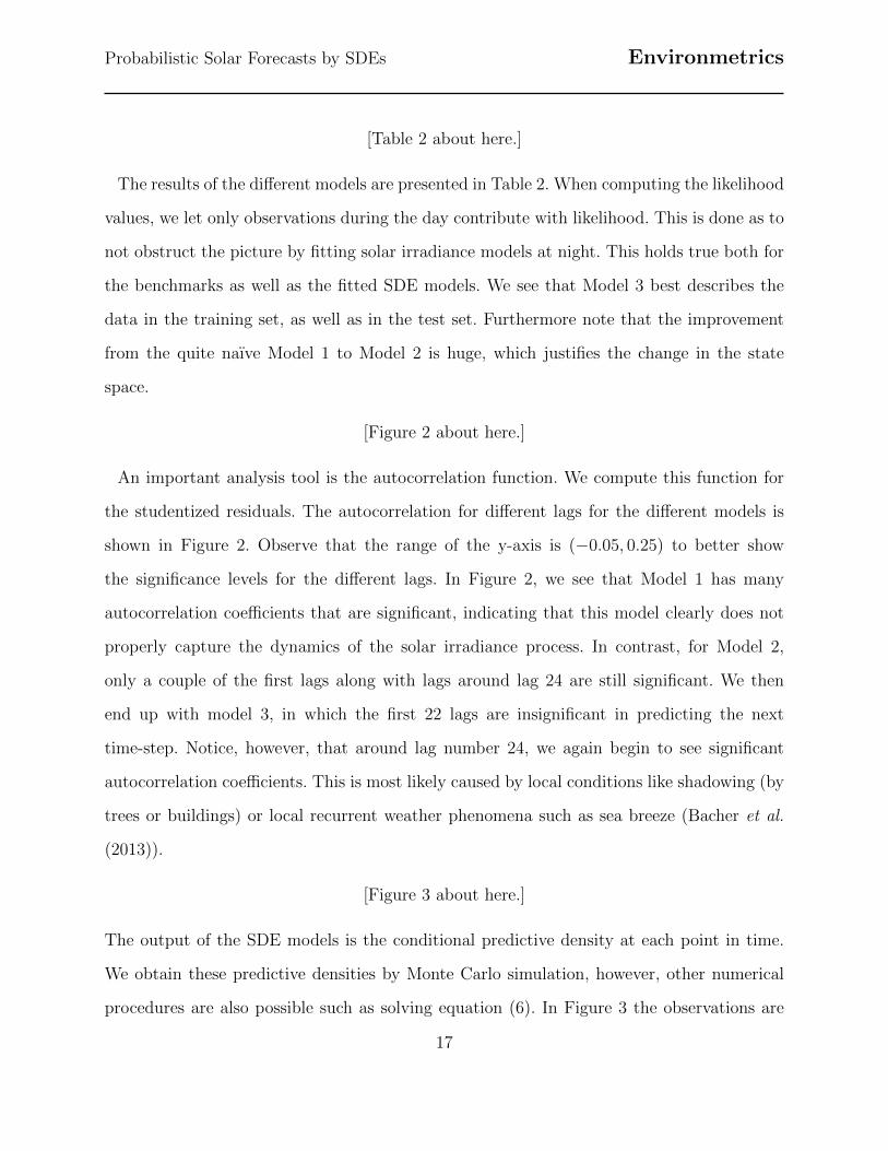
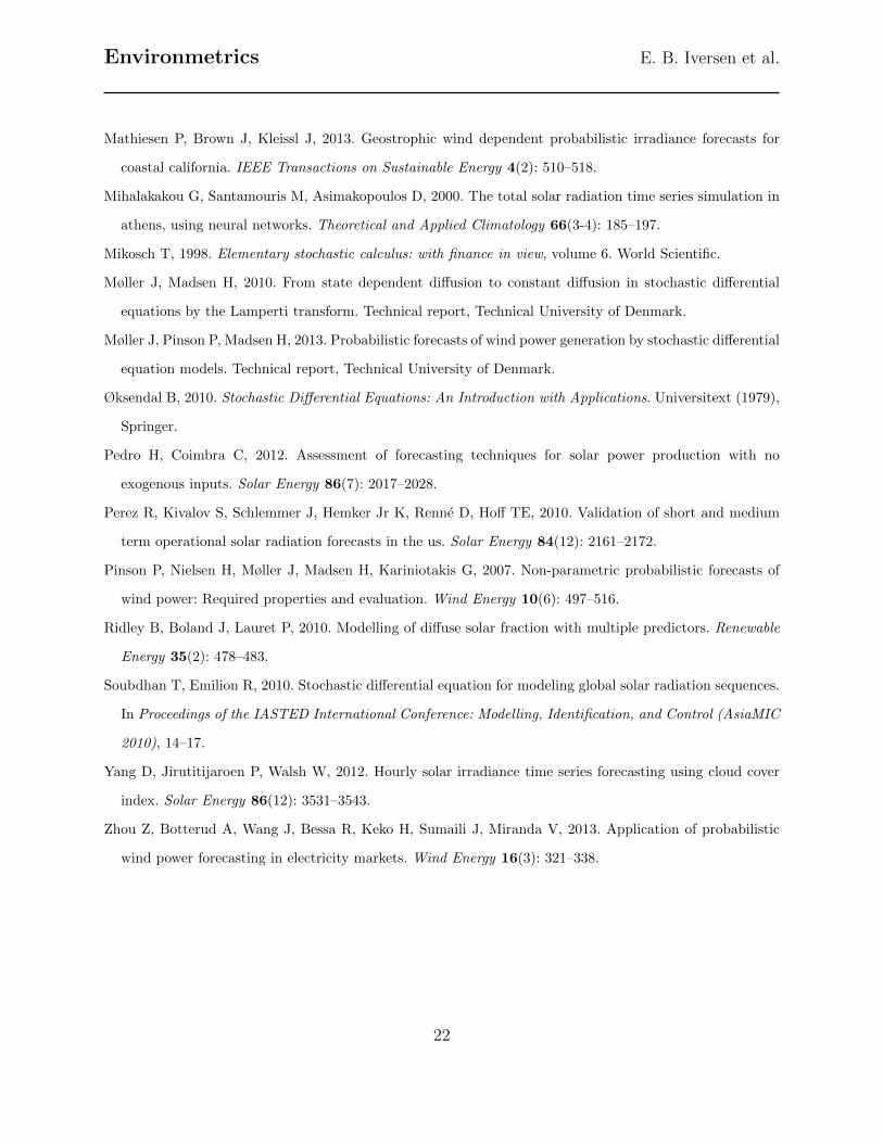
[Figure 2 about here.]
An important analysis tool is the autocorrelation function. We compute this function for
the studentized residuals. The autocorrelation for different lags for the different models is
shown in Figure 2. Observe that the range of the y-axis is (−0.05, 0.25) to better show
the significance levels for the different lags. In Figure 2, we see that Model 1 has many
autocorrelation coefficients that are significant, indicating that this model clearly does not
properly capture the dynamics of the solar irradiance process. In contrast, for Model 2,
only a couple of the first lags along with lags around lag 24 are still significant. We then
end up with model 3, in which the first 22 lags are insignificant in predicting the next
time-step. Notice, however, that around lag number 24, we again begin to see significant
autocorrelation coefficients. This is most likely caused by local conditions like shadowing (by
trees or buildings) or local recurrent weather phenomena such as sea breeze (Bacher et al.
(2013)).
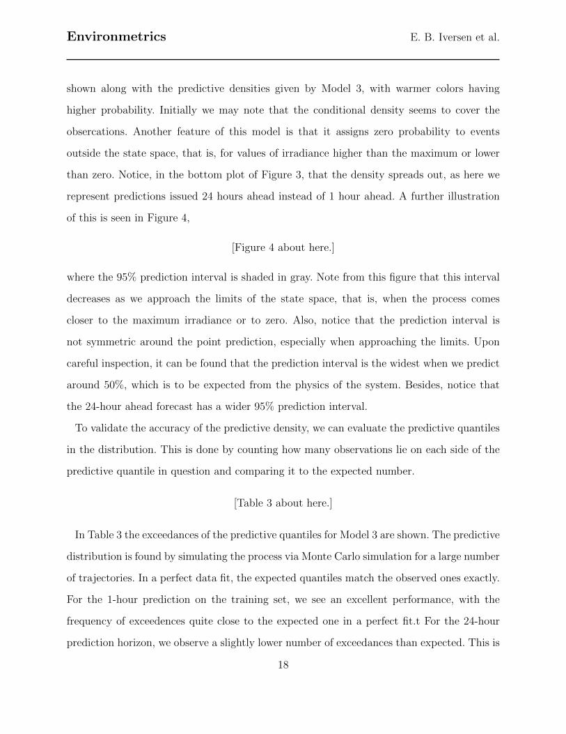
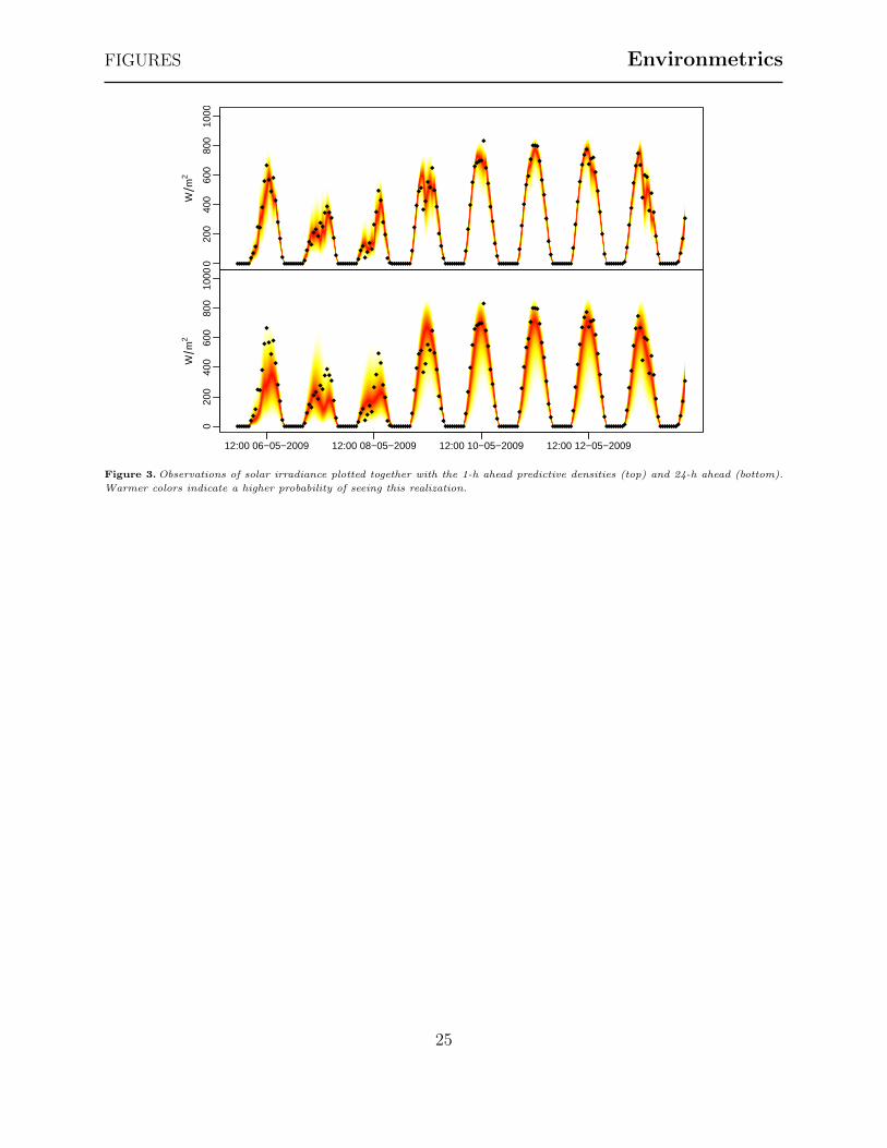
[Figure 3 about here.]
The output of the SDE models is the conditional predictive density at each point in time.
We obtain these predictive densities by Monte Carlo simulation, however, other numerical
procedures are also possible such as solving equation (6). In Figure 3 the observations are
17
Environmetrics E. B. Iversen et al.
shown along with the predictive densities given by Model 3, with warmer colors having
higher probability. Initially we may note that the conditional density seems to cover the
obsercations. Another feature of this model is that it assigns zero probability to events
outside the state space, that is, for values of irradiance higher than the maximum or lower
than zero. Notice, in the bottom plot of Figure 3, that the density spreads out, as here we
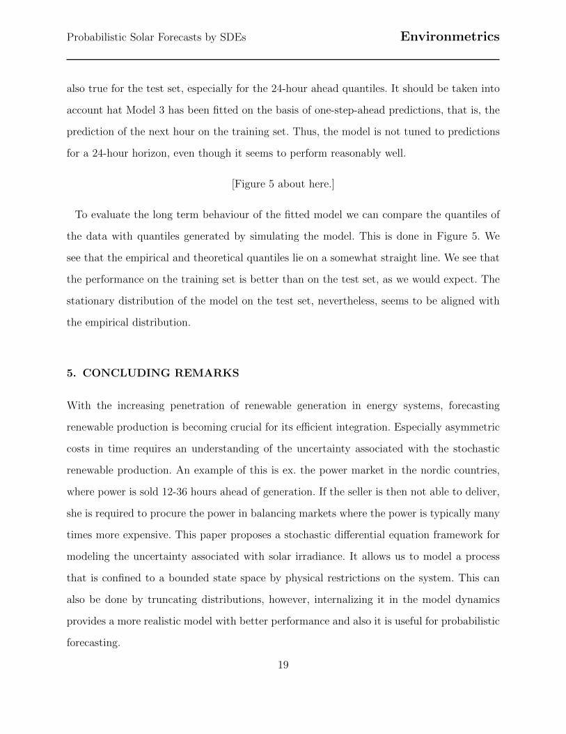
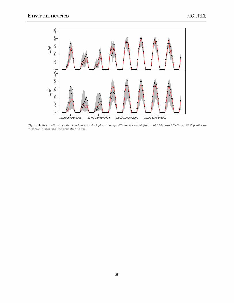
represent predictions issued 24 hours ahead instead of 1 hour ahead. A further illustration
of this is seen in Figure 4,
[Figure 4 about here.]
where the 95% prediction interval is shaded in gray. Note from this figure that this interval
decreases as we approach the limits of the state space, that is, when the process comes
closer to the maximum irradiance or to zero. Also, notice that the prediction interval is
not symmetric around the point prediction, especially when approaching the limits. Upon
careful inspection, it can be found that the prediction interval is the widest when we predict
around 50%, which is to be expected from the physics of the system. Besides, notice that
the 24-hour ahead forecast has a wider 95% prediction interval.
To validate the accuracy of the predictive density, we can evaluate the predictive quantiles
in the distribution. This is done by counting how many observations lie on each side of the
predictive quantile in question and comparing it to the expected number.
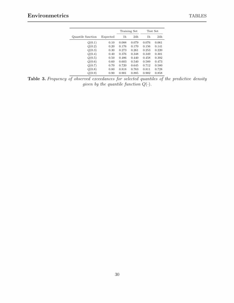
[Table 3 about here.]
In Table 3 the exceedances of the predictive quantiles for Model 3 are shown. The predictive
distribution is found by simulating the process via Monte Carlo simulation for a large number
of trajectories. In a perfect data fit, the expected quantiles match the observed ones exactly.
For the 1-hour prediction on the training set, we see an excellent performance, with the
frequency of exceedences quite close to the expected one in a perfect fit.t For the 24-hour
prediction horizon, we observe a slightly lower number of exceedances than expected. This is
18
Probabilistic Solar Forecasts by SDEs Environmetrics
also true for the test set, especially for the 24-hour ahead quantiles. It should be taken into
account hat Model 3 has been fitted on the basis of one-step-ahead predictions, that is, the
prediction of the next hour on the training set. Thus, the model is not tuned to predictions
for a 24-hour horizon, even though it seems to perform reasonably well.
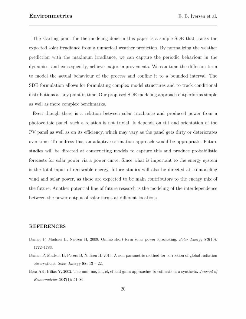
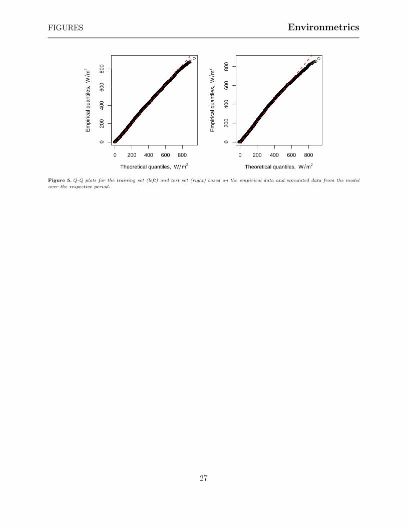
[Figure 5 about here.]
To evaluate the long term behaviour of the fitted model we can compare the quantiles of
the data with quantiles generated by simulating the model. This is done in Figure 5. We
see that the empirical and theoretical quantiles lie on a somewhat straight line. We see that
the performance on the training set is better than on the test set, as we would expect. The
stationary distribution of the model on the test set, nevertheless, seems to be aligned with
the empirical distribution.
5. CONCLUDING REMARKS
With the increasing penetration of renewable generation in energy systems, forecasting
renewable production is becoming crucial for its efficient integration. Especially asymmetric
costs in time requires an understanding of the uncertainty associated with the stochastic
renewable production. An example of this is ex. the power market in the nordic countries,
where power is sold 12-36 hours ahead of generation. If the seller is then not able to deliver,
she is required to procure the power in balancing markets where the power is typically many
times more expensive. This paper proposes a stochastic differential equation framework for
modeling the uncertainty associated with solar irradiance. It allows us to model a process
that is confined to a bounded state space by physical restrictions on the system. This can
also be done by truncating distributions, however, internalizing it in the model dynamics
provides a more realistic model with better performance and also it is useful for probabilistic
forecasting.
19
Environmetrics E. B. Iversen et al.
The starting point for the modeling done in this paper is a simple SDE that tracks the
expected solar irradiance from a numerical weather prediction. By normalizing the weather
prediction with the maximum irradiance, we can capture the periodic behaviour in the
dynamics, and consequently, achieve major improvements. We can tune the diffusion term
to model the actual behaviour of the process and confine it to a bounded interval. The
SDE formulation allows for formulating complex model structures and to track conditional
distributions at any point in time. Our proposed SDE modeling approach outperforms simple
as well as more complex benchmarks.
Even though there is a relation between solar irradiance and produced power from a
photovoltaic panel, such a relation is not trivial. It depends on tilt and orientation of the
PV panel as well as on its efficiency, which may vary as the panel gets dirty or deteriorates
over time. To address this, an adaptive estimation approach would be appropriate. Future
studies will be directed at constructing models to capture this and produce probabilistic
forecasts for solar power via a power curve. Since what is important to the energy system
is the total input of renewable energy, future studies will also be directed at co-modeling
wind and solar power, as these are expected to be main contributors to the energy mix of
the future. Another potential line of future research is the modeling of the interdependence
between the power output of solar farms at different locations.
REFERENCES
Bacher P, Madsen H, Nielsen H, 2009. Online short-term solar power forecasting. Solar Energy 83(10):
1772–1783.
Bacher P, Madsen H, Perers B, Nielsen H, 2013. A non-parametric method for correction of global radiation
observations. Solar Energy 88: 13 – 22.
Bera AK, Bilias Y, 2002. The mm, me, ml, el, ef and gmm approaches to estimation: a synthesis. Journal of
Econometrics 107(1): 51–86.
20
Probabilistic Solar Forecasts by SDEs Environmetrics
Bhardwaj S, Sharma V, Srivastava S, Sastry OS, Bandyopadhyay B, Chandel SS, Gupta JRP, 2013.
Estimation of solar radiation using a combination of hidden Markov model and generalized fuzzy model.
Solar Energy 93: 43–54.
Bird RE, Hulstrom RL, 1981. Simplified clear sky model for direct and diffuse insolation on horizontal
surfaces. Technical report, Solar Energy Research Inst., Golden, CO (USA).
Bjork T, 2009. Arbitrage Theory in Continuous Time. Oxford Finance Series, OUP Oxford.
Boland J, 2008. Time series modelling of solar radiation. In Badescu V (ed.), Modeling Solar Radiation at
the Earth?s Surface, Springer Berlin Heidelberg, 283–312.
Chen C, Duan S, Cai T, Liu B, 2011. Online 24-h solar power forecasting based on weather type classification
using artificial neural network. Solar Energy 85(11): 2856–2870.
European Photovoltaic Industry Association, 2013. Global market outlook for photovoltaics 2013-2017.
Online.
Huang J, Korolkiewicz M, Agrawal M, Boland J, 2013. Forecasting solar radiation on an hourly time scale
using a coupled autoregressive and dynamical system (cards) model. Solar Energy 87(1).
Jazwinski AH, 2007. Stochastic processes and filtering theory. Courier Dover Publications.
Ji W, Chee KC, 2011. Prediction of hourly solar radiation using a novel hybrid model of arma and tdnn.
Solar Energy 85(5): 808–817.
Juhl R, Kristensen NR, Bacher P, Kloppenborg J, Madsen H, 2013. Ctsm-r user guide. Technical University
of Denmark 2.
Kaplanis S, Kaplani E, 2010. Stochastic prediction of hourly global solar radiation for patra, greece. Applied
Energy 87(12): 3748–3758.
Kasten F, Young AT, 1989. Revised optical air mass tables and approximation formula. Appl. Opt 28(22):
4735–4738.
Kloeden PE, Pearson R, 1977. The numerical solution of stochastic differential equations. The Journal of
the Australian Mathematical Society. Series B. Applied Mathematics 20(01): 8–12.
Lorenz E, Hurka J, Heinemann D, Beyer HG, 2009. Irradiance forecasting for the power prediction of grid-
connected photovoltaic systems. IEEE Journal of Selected Topics in Applied Earth Observations and
Remote Sensing 2(1): 2–10.
Madsen H, Thyregod P, 2011. Introduction to General and Generalized Linear Models. Chapman & Hall/CRC
Texts in Statistical Science Series, CRC PressINC.
21
Environmetrics E. B. Iversen et al.
Mathiesen P, Brown J, Kleissl J, 2013. Geostrophic wind dependent probabilistic irradiance forecasts for
coastal california. IEEE Transactions on Sustainable Energy 4(2): 510–518.
Mihalakakou G, Santamouris M, Asimakopoulos D, 2000. The total solar radiation time series simulation in
athens, using neural networks. Theoretical and Applied Climatology 66(3-4): 185–197.
Mikosch T, 1998. Elementary stochastic calculus: with finance in view, volume 6. World Scientific.
Møller J, Madsen H, 2010. From state dependent diffusion to constant diffusion in stochastic differential
equations by the Lamperti transform. Technical report, Technical University of Denmark.
Møller J, Pinson P, Madsen H, 2013. Probabilistic forecasts of wind power generation by stochastic differential
equation models. Technical report, Technical University of Denmark.
Øksendal B, 2010. Stochastic Differential Equations: An Introduction with Applications. Universitext (1979),
Springer.
Pedro H, Coimbra C, 2012. Assessment of forecasting techniques for solar power production with no
exogenous inputs. Solar Energy 86(7): 2017–2028.
Perez R, Kivalov S, Schlemmer J, Hemker Jr K, Renne D, Hoff TE, 2010. Validation of short and medium
term operational solar radiation forecasts in the us. Solar Energy 84(12): 2161–2172.
Pinson P, Nielsen H, Møller J, Madsen H, Kariniotakis G, 2007. Non-parametric probabilistic forecasts of
wind power: Required properties and evaluation. Wind Energy 10(6): 497–516.
Ridley B, Boland J, Lauret P, 2010. Modelling of diffuse solar fraction with multiple predictors. Renewable
Energy 35(2): 478–483.
Soubdhan T, Emilion R, 2010. Stochastic differential equation for modeling global solar radiation sequences.
In Proceedings of the IASTED International Conference: Modelling, Identification, and Control (AsiaMIC
2010), 14–17.
Yang D, Jirutitijaroen P, Walsh W, 2012. Hourly solar irradiance time series forecasting using cloud cover
index. Solar Energy 86(12): 3531–3543.
Zhou Z, Botterud A, Wang J, Bessa R, Keko H, Sumaili J, Miranda V, 2013. Application of probabilistic
wind power forecasting in electricity markets. Wind Energy 16(3): 321–338.
22
FIGURES Environmetrics
FIGURES
0 10 20 30 40
−0.
050.
050.
150.
25
0 5 10 15 20 25 30 35 40
Figure 1. Autocorrelation function for the studentized residuals of Model 2.
23
Environmetrics FIGURES
0 10 20 30 40
−0.
050.
20
0 5 10 15 20 25 30 35 40
0 10 20 30 40
−0.
050.
20
0 5 10 15 20 25 30 35 40
01−2009 06−2009 12−2009 06−2010 12−2010 0 10 20 30 40−
0.05
0.20
0 5 10 15 20 25 30 35 40
Figure 2. Studentized residuals and autocorrelation function for the residuals. Here the plots in the top line are from Model 1
continueing to the plots in the bottom line from Model 3.
24
FIGURES Environmetrics
020
040
060
080
010
00
Wm
2
020
040
060
080
010
00
Wm
2
12:00 06−05−2009 12:00 08−05−2009 12:00 10−05−2009 12:00 12−05−2009
Figure 3.Observations of solar irradiance plotted together with the 1-h ahead predictive densities (top) and 24-h ahead (bottom).
Warmer colors indicate a higher probability of seeing this realization.
25
Environmetrics FIGURES
020
040
060
080
010
00
Wm
2
020
040
060
080
010
00
Wm
2
12:00 06−05−2009 12:00 08−05−2009 12:00 10−05−2009 12:00 12−05−2009
Figure 4.Observations of solar irradiance in black plotted along with the 1-h ahead (top) and 24-h ahead (bottom) 95 % prediction
intervals in gray and the prediction in red.
26
FIGURES Environmetrics
0 200 400 600 800
020
040
060
080
0
Theoretical quantiles, W m2
Em
piric
al q
uant
iles,
Wm
2
0 200 400 600 800
020
040
060
080
0
Theoretical quantiles, W m2
Em
piric
al q
uant
iles,
Wm
2
Figure 5.Q-Q plots for the training set (left) and test set (right) based on the empirical data and simulated data from the model
over the respective period.
27
Environmetrics TABLES
TABLES
θx µx σx σε βx γ θA µA σA ω1 ω2
Model 1 0.699 0.845 113 0.00101 - - - - - - -
Model 2 0.345 0.804 0.701 2.92 0.00409 0.902 - - - - -
Model 3 - 0.879 0.655 2.89 0.00298 0.887 1.16 -1.08 1.60 0.172 0.116
Table 1. Parameter estimates for the different models.
28
TABLES Environmetrics
Training Set Test Set
d.f. LL AIC BIC LL
Clim.1 - -96397 - - -48421
Clim.2 - -65060 - - -33801Clim.3 - -48038 - - -24547
AR 6 -50218 - - -25172
ARX 7 -49024 - - -24567ARX-GLM 7 -46904 - - -23361
Model 1 5 -50286 100582 100621 -25230
Model 2 7 -44413 88840 88894 -22252Model 3 12 -44162 88348 88441 -22102
Table 2. In this table the log-likelihood of the different models are shown on the training andtest set along with information criteria and degrees of freedom. The climatological predictors
are evaluated in terms of empirical likelihood.
29
Environmetrics TABLES
Training Set Test Set
Quantile function Expected 1h 24h 1h 24h
Q(0.1) 0.10 0.088 0.079 0.076 0.061
Q(0.2) 0.20 0.176 0.170 0.156 0.141Q(0.3) 0.30 0.273 0.261 0.253 0.220
Q(0.4) 0.40 0.376 0.348 0.349 0.301
Q(0.5) 0.50 0.486 0.440 0.458 0.392Q(0.6) 0.60 0.603 0.540 0.589 0.473
Q(0.7) 0.70 0.720 0.645 0.712 0.580
Q(0.8) 0.80 0.818 0.763 0.811 0.728Q(0.9) 0.90 0.901 0.885 0.902 0.858
Table 3. Frequency of observed exceedances for selected quantiles of the predictive densitygiven by the quantile function Q(·).
30