probabilistic analysis of shallow foundations resting on
TRANSCRIPT
UNIVERSITÉ DE NANTES
FACULTÉ DES SCIENCES ET DES TECHNIQUES
_____
ÉCOLE DOCTORALE : SPIGA
Année 2012
Probabilistic analysis of shallow foundations resting on spatially varying soils
___________
THÈSE DE DOCTORAT
Discipline : Génie Civil
Spécialité : Géotechnique
Présentée et soutenue publiquement par
Tamara AL-BITTAR Le 19 Novembre 2012, devant le jury ci-dessous
Rapporteurs
Examinateurs
M. Denys BREYSSE Professeur, Université Bordeaux 1 M. Bruno SUDRET Professeur, ETH Zürich M. Isam SHAHROUR Professeur, Université Lille 1 M. Panagiotis KOTRONIS Professeur, Ecole Centrale de Nantes M. Shadi NAJJAR Assistant Professor, American University of Beirut Mme. Dalia YOUSSEF Assistant Professor, Notre Dame University
Directeur de thèse : Pr. Abdul-Hamid SOUBRA
Co-directeur de thèse : Pr. Fadi HAGE CHEHADE

1

2
ACKNOWLEDGEMENTS
First and foremost I offer my most sincere gratitude to my thesis supervisor, Pr. Abdul-
Hamid Soubra, for his exceptional support and guidance throughout my research work. I attribute
the level of my Ph.D degree to his permanent encouragement and involvement, which allowed
among others the publication of many journal and conference papers. I could just not expect a
better supervisor.
I would also like to thank my Lebanese supervisor, Pr Fadi Hege Chehade for his
confidence during my work in Lebanon. My grateful thanks are also extended to Dr. Dalia
Youssef for her help in realizing the simulation of stochastic Ground-Motion, to Pr. Panagiotis
Kotronis, who helped me introduce the time variability of Ground-Motion in his macro-element
and to Ms. Nicolas Humbert and Mrs. Pauline Billion from EDF and Pr. Daniel Dias with whom
we had a scientific collaboration on the stochastic dymanic behaviour of a free field soil mass.
I wish to thank the members of my dissertation committe, namely Pr. Isam Shahrour for
having accepted to be its president, Pr. Bruno Sudret and Pr. Denys Breysse for their careful
reading and rating of my thesis report. I also thank all the jury members for having accepted to be
part of the jury and for their relevant questions after my presentation.
Throughout my three years of Ph.D I have meat my second half and the love of my life
Rachid Cortas to whom I would like to say thank you.
Last not least, I thank my parents, Antoine and Daad, for their support throughout all my
studies. Your encouragement always gave me the confidence to continue to pursue my goals. I
also wish to thank my brothers Michel and Fadi, and my sister Mira for their own way support.
Your sense of humor always gave me the power to continue what I started.
Finally, I am grateful to my big family and friends for their constant support through all
the important step of my life.
3
ABSTRACT
The aim of this thesis is to study the performance of shallow foundations resting on spatially
varying soils and subjected to a static or a dynamic (seismic) loading using probabilistic
approaches. In the first part of this thesis, a static loading was considered in the probabilistic
analysis. In this part, only the soil spatial variability was considered and the soil parameters were
modelled by random fields. In such cases, Monte Carlo Simulation (MCS) methodology is
generally used in literature. In this thesis, the Sparse Polynomial Chaos Expansion (SPCE)
methodology was employed. This methodology aims at replacing the finite element/finite
difference deterministic model by a meta-model. This leads (in the present case of highly
dimensional stochastic problems) to a significant reduction in the number of calls of the
deterministic model with respect to the crude MCS methodology. Moreover, an efficient
combined use of the SPCE methodology and the Global Sensitivity Analysis (GSA) was
proposed. The aim is to reduce once again the probabilistic computation time for problems with
expensive deterministic models. In the second part of this thesis, a seismic loading was
considered. In this part, the soil spatial variability and/or the time variability of the earthquake
Ground-Motion (GM) were considered. In this case, the earthquake GM was modelled by a
random process. Both cases of a free field and a Soil-Structure Interaction (SSI) problem were
investigated. The numerical results have shown the significant effect of the time variability of the
earthquake GM in the probabilistic analysis.
4
TABLE OF CONTENTS
Acknowledgements.........................................................................................................................2 Abstract .....................................................................................................................................3 Table of Contents ...........................................................................................................................4 Table of Figures..............................................................................................................................6 Table of tables...............................................................................................................................12 General introduction....................................................................................................................16 chapter I. Literature review.....................................................................................................20
I.1 Introduction .....................................................................................................................20 I.2 Sources of uncertainties ..................................................................................................21 I.3 Spatial variability of the soil properties ..........................................................................22
I.3.1 Statistical characterization of the soil spatial variability................................22 I.3.2 Practical modeling of the soil spatial variability using the Optimal Linear Estimation (OLE) method ...............................................................................................30 I.3.3 Brief overview of the numerical random fields discretization methods ........32 I.3.4 The expansion optimal linear estimation (EOLE) method for random field discretization ...................................................................................................................36
I.4 Time variability of the seismic loading...........................................................................39 I.4.1 Statistical characterization of the time variability of earthquake GMs..........40 I.4.2 Modeling of the stochastic earthquake GMs..................................................40
I.5 Probabilistic methods for uncertainty propagation .........................................................44 I.5.1 The simulation methods .................................................................................45 I.5.2 The metamodeling techniques........................................................................47
I.6 Conclusion.......................................................................................................................54 chapter II. Probabilistic analysis of strip footings resting on 2D spatially varying soils/rocks using sparse polynomial chaos expansion...............................................................56
II.1 Introduction .....................................................................................................................56 II.2 Adaptive sparse polynomial chaos expansion SPCE – the hyperbolic (q-norm)
truncation scheme............................................................................................................58 II.3 Probabilistic analysis of strip footings resting on a spatially varying soil mass
obeying Mohr-coulomb (Mc) failure criterion................................................................60 II.3.1 The ultimate limit state ULS case ..................................................................60 II.3.2 The serviceability limit state SLS case ..........................................................78
II.4 Probabilistic analysis of strip footings resting a spatially varying rock mass obeying Hoek-Brown (HB) failure criterion.................................................................................83 II.4.1 Global sensitivity analysis..............................................................................87 II.4.2 Probabilistic parametric study........................................................................88
II.5 Discussion .......................................................................................................................92 II.6 Conclusions .....................................................................................................................92
chapter III. Effect of the soil spatial variability in three dimensions on the ultimate bearing capacity of foundations ................................................................................................................96
III.1 Introduction .....................................................................................................................96
5
III.2 Probabilistic analysis of strip and square footings resting on a 3D spatially varying soil mass ..........................................................................................................................96
III.3 Numerical results ............................................................................................................98 III.3.1 Deterministic numerical results......................................................................99 III.3.2 Probabilistic numerical results .....................................................................100 III.3.3 Discussion ....................................................................................................108
III.4 Conclusions ...................................................................................................................109 chapter IV. Combined use of the Sparse Polynomial Chaos Expansion Methodology and the global sensitivity analysis for high-dimensional stochastic problems ...................................110
IV.1 Introduction ...................................................................................................................110 IV.2 Efficient combined use of the SPCE methodology and the global sensitivity
analysis GSA.................................................................................................................111 IV.3 Numerical results ..........................................................................................................113
IV.3.1 Validation of the SPCE/GSA procedure ......................................................113 IV.3.2 Probabilistic results of a ponderable soil for the two cases of 2D and 3D random fields.................................................................................................................120
IV.4 Conclusions ...................................................................................................................130 chapter V. Effect of the soil spatial variability and/or the time variability of the seismic loading on the dynamic responses of geotechnical structures................................................132
V.1 Introduction ...................................................................................................................132 V.2 Case of an elastic free field soil mass ...........................................................................133
V.2.1 Numerical modeling.....................................................................................134 V.2.2 Deterministic results.....................................................................................136 V.2.3 Probabilistic dynamic analysis .....................................................................140 V.2.4 Probabilistic results ......................................................................................144
V.3 Case of a Soil-Structure Interaction (SSI) problem ......................................................151 V.3.1 Numerical modeling.....................................................................................152 V.3.2 Probabilistic numerical results .....................................................................153
V.4 Conclusions ...................................................................................................................157 General conclusions....................................................................................................................160 References .................................................................................................................................166 Appendix A. ................................................................................................................................178 Appendix B. ................................................................................................................................180 Appendix C. ................................................................................................................................186 Appendix D. ................................................................................................................................190 Appendix E. ................................................................................................................................192 Appendix F..................................................................................................................................194 Appendix G. ................................................................................................................................204 Appendix H. ................................................................................................................................208

6
TABLE OF FIGURES
Figure I.1. Time-varying PSD function .........................................................................................40
Figure I.2. Predominant frequency and bandwidth........................................................................40
Figure I.3. General sketch for the probabilistic analyses ...............................................................45
Figure I.4. Nested Failure domain..................................................................................................47
Figure II.1. Mesh used for the computation of the ultimate bearing capacity: (a) for
moderate to great values of the autocorrelation distances ( 10xa m≥ and
1ya m≥ ), (b) for small values of the autocorrelation distances ( 10xa m< or
1ya m< ).......................................................................................................................62
Figure II.2. Number N of eigenmodes needed in the EOLE method: (a) isotropic case, (b)
anisotropic case .........................................................................................................64
Figure II.3. Typical realizations of the random fields :(a) [ax=100m, ay=1m, r(c, φ)=-0.5];
(b) [ax=10m, ay=1m, r(c, φ)=-0.5]; (c) [ax=10m, ay=1m, r(c, φ)=-0.9]....................66
Figure II.4. Bearing capacity and footing rotation for the reference case where ax=10m,
ay=1m, and r(c, φ)=-0.5: (a) PDF of the ultimate bearing capacity; and (b) PDF
of the footing rotation................................................................................................67
Figure II.5. Velocity field for a typical realization of the two random fields for the reference
case where ax=10m, ay=1m and r(c, φ) =-0.5............................................................67
Figure II.6. Influence of the isotropic autocorrelation distance ax=ay on the PDF of the
ultimate bearing capacity in the case where r(c, φ)=-0.5 ..........................................68
Figure II.7. Influence of the isotropic autocorrelation distance ax=ay on the probabilistic
mean of the ultimate bearing capacity in the case where r(c, φ)=-0.5 ......................68
Figure II.8. Influence of the vertical autocorrelation distance ay on the PDF of the ultimate
bearing capacity in the case where r(c, φ)=-0.5 and ax=10m....................................71
Figure II.9. Influence of the horizontal autocorrelation distance ax on the PDF of the
ultimate bearing capacity in the case where r(c, φ)=-0.5 and ay=1m........................71
Figure II.10. Influence of the vertical autocorrelation distance ay on the probabilistic mean
value of the ultimate bearing capacity in the case where r(c, φ)=-0.5 and
ax=10m.......................................................................................................................73
7
Figure II.11. Influence of the horizontal autocorrelation distance ax on the probabilistic
mean value of the ultimate bearing capacity in the case where r(c, φ)=-0.5 and
ay=1m.........................................................................................................................73
Figure II.12. Cohesion random field for different values of the autocorrelation distances ...........74
Figure II.13. Influence of the cross-correlation coefficient on the PDF of the ultimate
bearing capacity in the case where ax=10m and ay=1m ............................................76
Figure II.14. Effect of the coefficients of variation of the random fields on the PDF of the
ultimate bearing capacity in the case where ax=10m, ay=1m and r(c, φ)=-0.5 .........77
Figure II.15. Sobol indices of the two random fields [the Young modulus for ξi (i=1, …, 12)
and the Poisson ratio for ξi (i=13, …, 24)] ................................................................79
Figure II.16. Influence of the isotropic autocorrelation distance ax= ay on the PDF of the
footing vertical displacement ....................................................................................80
Figure II.17. Influence of the vertical autocorrelation distance ay on the PDF of the footing
vertical displacement in the case where ax=10m.......................................................80
Figure II.18. Influence of the horizontal autocorrelation distance ax on the PDF of the
footing vertical displacement in the case where ay=1m ............................................80
Figure II.19. Influence of the coefficient of variation COVE on the PDF of the footing
vertical displacement in the case where ax=10 and ay=1m........................................83
Figure II.20. Mesh used for the computation of the ultimate bearing capacity .............................85
Figure II.21. Sobol indices of the random variable GSI [i.e. ξi(i=1)] and the random field σc
[i.e. ξi(i=2, …, 36)] ....................................................................................................87
Figure II.22. Influence of the isotropic autocorrelation distance a on the PDF of the ultimate
bearing capacity.........................................................................................................88
Figure II.23. Influence of the isotropic autocorrelation distance a on the probabilistic mean
of the ultimate bearing capacity ................................................................................88
Figure II.24. Influence of the autocorrelation distance a on the Sobol indices of GSI and σc .......90
Figure II.25. Influence of the coefficients of variation COVs of the random variable GSI and
the random field σc on the PDF of the ultimate bearing capacity: (a) influence
of COVGSI; (b) influence of COVσc ............................................................................90
Figure III.1. Mesh used for the computation of the ultimate bearing capacity of (a) square
footing and (b) strip footing ......................................................................................98
8
Figure III.2. Perspective view of half of the soil domain showing (a) a random field
realization (the contour lines provide the distribution of the soil cohesion on
the envelope of this domain) and (b) the contours of the strain rate .......................102
Figure III.3. Influence of the mean value of the cohesion on the PDF of the bearing capacity
coefficient Nc of a strip footing when using 3D random field for ah=10m,
av=1m and COVc=25%............................................................................................103
Figure III.4. Comparison between the PDFs of the bearing capacity coefficient Nc of a
square footing when using 3D and 2D isotropic random fields ..............................105
Figure III.5. Comparison between the PDFs of the bearing capacity coefficient Nc of a
square footing when using 3D and 2D anisotropic random fields and for
ah=10m ....................................................................................................................107
Figure III.6. Comparison between the PDFs of the bearing capacity coefficient Nc of a
square footing when using 3D and 2D anisotropic random fields and for av=1m ..107
Figure IV.1. Sobol indices for SPCEs of orders 2, 3, and 4 using the total number of
eigenmodes ξi (i=1, ..., 24).......................................................................................115
Figure IV.2. PDF of the ultimate bearing capacity for both the classical SPCE method with
the total number of random variables NT =24 and the proposed SPCE/GSA
procedure with only five random variables Ne =5 when ax=10m, ay=1m and
r(c, φ)= -0.5 .............................................................................................................119
Figure IV.3. Adopted soil domain and the corresponding deterministic mesh............................121
Figure IV.4. Influence of the isotropic autocorrelation distance ax=ay on the PDF of the
ultimate bearing capacity in the case where r(c, φ)=-0.5 ........................................124
Figure IV.5. Influence of the vertical autocorrelation distance ay on the PDF of the ultimate
bearing capacity in the case where r(c, φ)=-0.5 and ax=10m..................................124
Figure IV.6. Influence of the horizontal autocorrelation distance ax on the PDF of the
ultimate bearing capacity in the case where r(c, φ)=-0.5 and ay=1m......................124
Figure IV.7. Influence of the isotropic autocorrelation distance ax=ay on the probabilistic
mean of the ultimate bearing capacity in the case where r(c, φ)=-0.5. ...................126
Figure IV.8. Influence of the vertical autocorrelation distance ay on the probabilistic mean
value of the ultimate bearing capacity in the case where ax=10m and r(c, φ)=-
0.5 ............................................................................................................................126
9
Figure IV.9. Influence of the horizontal autocorrelation distance ax on the probabilistic
mean value of the ultimate bearing capacity in the case where ay =1m and r(c,
φ)=-0.5 .....................................................................................................................126
Figure IV.10. Influence of the cross-correlation coefficient r(c, φ) on the PDF of the
ultimate bearing capacity in the case where ax=10m and ay=1m ............................128
Figure IV.11. PDFs of the ultimate bearing capacity for both the 2D and the 3D random
fields for the reference case where ah=10m, av=1m and r(c, φ)=-0.5 ....................130
Figure V.1. The two considered numerical models (a) 2D model and (b) 'column' model .........134
Figure V.2. (a) Accelerogram of the synthetic signal of Nice and (b) the corresponding
Fourier amplitude spectrum.....................................................................................136
Figure V.3. Distribution of the maximum acceleration as a function of depth for the three
cross-sections of the 2D model and for the 1D soil column....................................138
Figure V.4. Distribution of the maximum acceleration for different values of the shear
modulus G ...............................................................................................................139
Figure V.5. Variation of the maximum acceleration at the top of the column as a function of
the shear modulus G ................................................................................................139
Figure V.6. Variation of the maximum acceleration at the top of the column as a function of
the shear modulus G for three values of K ..............................................................139
Figure V.7. Identification of filter parameters for the synthetic Nice accelerogram, (a)
matching the cumulative number of zero level up-crossings (b) matching the
cumulative count of negative maxima and positive minima...................................143
Figure V.8. (a) Target and five simulated acceleration time-histories, and (b) their
corresponding Fourier amplitude spectrum.............................................................144
Figure V.9. (a) Mean and (b) coefficient of variation of Amax at the top of the soil column as
a function of the number of simulations when ay=0.5m..........................................145
Figure V.10. Influence of the vertical autocorrelation distance ay on the PDF of Amax at the
top of the soil column when (a) 1
72G MPaµ = and (b) 2
288G MPaµ = ........................149
Figure V.11. The five-storey building: (a) The CAMUS IV real model, and (b) the
simplified numerical lumped mass system..............................................................152
Figure V.12. PDF of the maximum horizontal displacement (a) at the centre of the footing,
and (b) at the top of the building .............................................................................155

10
Figure V.13. Fragility curves for different levels of damage (a) maximum horizontal
displacement at the top of the building, and (b) maximum moment at the
contact of the soil and the footing ...........................................................................156

11
12
TABLE OF TABLES
Table I.1. Theoretical ACF used to determine the autocorrelation distance (a) [Vanmarcke
(1983)] .......................................................................................................................24
Table I.2. Theoretical semivariograms used to determine the range of influence (a)
[Goovaerts (1998, 1999)] ..........................................................................................26
Table I.3. Coefficient of variation of the undrained soil cohesion.................................................27
Table I.4. Values of the coefficient of variation of the soil internal friction angle........................28
Table I.5. Values of the coefficient of variation of the Young’s modulus.....................................29
Table I.6. Values of the autocorrelation distances of some soil properties as given by several
authors (El-Ramly 2003) ...........................................................................................30
Table I.7. Usual probability density functions and their corresponding families of
orthogonal polynomials [Xiu and Karniadakis (2002)].............................................50
Table II.1. Number of random variables used to discretize the two random fields c and φ for
both cases of isotropic and anisotropic autocorrelation distances.............................64
Table II.2. Effect of the isotropic autocorrelation distance ax=ay on the statistical moments
of the ultimate bearing capacity ................................................................................69
Table II.3. Effect of the isotropic autocorrelation distance ax=ay on the Sobol indices of the
two random fields c and φ .........................................................................................70
Table II.4. Effect of the vertical autocorrelation distance ay on the statistical moments of the
ultimate bearing capacity...........................................................................................72
Table II.5. Effect of the horizontal autocorrelation distance ax on the statistical moments of
the ultimate bearing capacity.....................................................................................72
Table II.6. Effect of the vertical autocorrelation distance ay on the Sobol indices of c and φ .......75
Table II.7. Effect of the horizontal autocorrelation distance ax on the Sobol indices of c and
φ .................................................................................................................................75
Table II.8. Effect of the cross-correlation coefficient between the random fields of c and φ
on the statistical moments of the ultimate bearing capacity......................................76
Table II.9. Effect of the coefficient of correlation on the Sobol indices of the two random
fields c and φ .............................................................................................................76
Table II.10. Effect of the coefficients of variation of the random fields c and φ on the
statistical moments of the ultimate bearing capacity.................................................77
13
Table II.11. Effect of the coefficients of variation of the random fields c and φ on the Sobol
indices of the two random fields c and φ...................................................................77
Table II.12. Effect of the isotropic autocorrelation distance ax=ay on the statistical moments
of the footing vertical displacement ..........................................................................81
Table II.13. Effect of the vertical autocorrelation distance ay on the statistical moments of
the footing vertical displacement when ax=10m .......................................................82
Table II.14. Effect of the horizontal autocorrelation distance ax on the statistical moments of
the footing vertical displacement when ay=1m .........................................................82
Table II.15. Effect of the coefficient of variation (COVE) of the random field E on the
statistical moments of the footing vertical displacement when ax=10m, ay=1m.......83
Table II.16. Values of qult (MPa) as given by FLAC3D, by Merifield et al. (2006) and by
Mao et al. (2012) when D=0......................................................................................86
Table II.17. Number of random variables needed to discretize the random field σc......................86
Table II.18. Effect of the autocorrelation distance a on the statistical moments of the
ultimate bearing capacity...........................................................................................89
Table II.19. Influence of the autocorrelation distance a on the Sobol indices of GSI and σc ........90
Table II.20. Effect of the coefficients of variation (COVs) of the random field σc and the
random variable GSI on the statistical moments (µ, σ, δu, κu) of the ultimate
bearing capacity when a=2m.....................................................................................91
Table II.21. Effect of the coefficients of variation (COVs) of the random field σc and the
random variable GSI on the Sobol indices of GSI and σc when a=2m......................91
Table III.1. Number of random variables needed to discretize the 3D and 2D cohesion
random fields in the case of the square footing.......................................................101
Table III.2. Effect of the isotropic autocorrelation distance (a) on the statistical moments
cNµ and
cNσ of the bearing capacity coefficient Nc of square and strip
footings using both 3D and 2D random fields.........................................................104
Table III.3. Effect of the vertical autocorrelation distance (av) on the statistical moments
cNµ and
cNσ of the bearing capacity coefficient Nc of square and strip
footings using both 3D and 2D random fields.........................................................106
14
Table III.4. Effect of the horizontal autocorrelation distance (ah) on the statistical moments
cNµ and
cNσ of the bearing capacity coefficient Nc of square and strip
footings using both 3D and 2D random fields.........................................................106
Table III.5. Ratios between the coefficients of variation values of Nc (obtained using 3D and
2D random fields) for both the square and strip footings........................................108
Table IV.1. Sobol indices for the reference case where ax=10m, ay=1m, and r(c,φ)=-0.5 ..........115
Table IV.2. Number of unknown coefficients and model evaluations for different SPCE
orders .......................................................................................................................116
Table IV.3. Sobol indices Si of the different random variables ξi and the retained random
variables for the different values of the threshold of acceptance ta.........................117
Table IV.4. Coefficients of determination R2 and Q2 for different SPCE orders when using
the total and the reduced number of random variables............................................118
Table IV.5. Coefficients of determination R2 and Q2 of the SPCE and statistical moments
(µ, σ, δu and κu) of the ultimate bearing capacity as given by the classical SPCE
approach and by the present SPCE/GSA procedure................................................119
Table IV.6. Sobol indices as computed from the classical SPCE approach (with NT=24) and
the present SPCE/GSA procedure (with Ne=5). ......................................................120
Table IV.7. Number of random variables used to discretize the two random fields c and φ
for both cases of 2D and 3D random fields.............................................................122
Table IV.8. Effect of the isotropic autocorrelation distance ax=ay on the statistical moments
(µ, σ) of the ultimate bearing capacity.....................................................................125
Table IV.9. Effect of the vertical autocorrelation distance ay on the statistical moments (µ,
σ) of the ultimate bearing capacity when ax=10m...................................................125
Table IV.10. Effect of the horizontal autocorrelation distance ax on the statistical moments
(µ, σ) of the ultimate bearing capacity when ay=1m................................................125
Table IV.11. Effect of the isotropic autocorrelation distance ax=ay on the Sobol indices of
the two random fields c and φ .................................................................................127
Table IV.12. Effect of the vertical autocorrelation distance ay on the Sobol indices of the
two random fields c and φ when ax=10m ................................................................127
Table IV.13. Effect of the horizontal autocorrelation distance ax on the Sobol indices of the
two random fields c and φ when ay=1m ..................................................................127
15
Table IV.14. Effect of the cross-correlation coefficient r(c, φ) between the random fields of
c and φ on the statistical moments (µ, σ) of the ultimate bearing capacity when
ax=10m and ay=1m .................................................................................................128
Table IV.15. Effect of the coefficient of correlation on the Sobol indices of the two random
fields c and φ when ax=10m and ay=1m.................................................................128
Table IV.16. Effect of the coefficients of variation (COVc, COVφ) of the random fields c
and φ on the statistical moments (µ, σ) of the ultimate bearing capacity when
ax=10m, ay=1m and r(c, φ)= -0.5............................................................................129
Table IV.17. Effect of the coefficients of variation (COVc, COVφ) of the random fields c
and φ on the Sobol indices of the two random fields c and φ when ax=10m,
ay=1m and r(c, φ)= -0.5...........................................................................................129
Table IV.18. Statistical moments (µ, σ) of the ultimate bearing capacity using both 2D and
3D random fields for the reference case where ah=10m, av=1m and r(c, φ)=-
0.5 ............................................................................................................................130
Table IV.19. Sobol indices of the two random fields c and φ in both the 2D and the 3D
cases for the reference case where ah=10m, av=1m and r(c, φ)=-0.5.....................130
Table V.1. Values of the three physical parameters and the corresponding values of the time
modulation function parameters for the synthetic Nice accelerogram....................142
Table V.2. Effect of the soil spatial variability and/or the time variability of the earthquake
GM on the maximum acceleration at the top of the soil column ............................147
Table V.3. Effect of the coefficient of variation of G on Amax at the top of the soil column
considering deterministic and stochastic earthquake GM.......................................148
Table V.4. Number of random variables needed to discretize the random field G......................149
Table V.5. Comparison between the statistical moments (µ, σ) of Amax at the top of the soil
column as obtained using both the MCS and the SPCE methodologies .................150
Table V.6. Parameters used to model the five-storey building ....................................................153
Table V.7. Parameters used to model the soil-foundation (macro-element)................................153
Table V.8. Effect of stochastic Ground-Motion on the statistical moments (µ, σ) of the seven
dynamic responses...................................................................................................155

16
GENERAL INTRODUCTION
Traditionally, the analysis and design of geotechnical structures are based on deterministic
approaches. In these approaches, constant conservative values of the soil and/or the loading
parameters are considered with no attempt to characterize and model the uncertainties related to
these parameters. In such approaches, a global safety factor is applied to take into account the soil
and loading uncertainties. The choice of this factor is based on the judgment of the engineer
based on his past experience.
During the last recent years, much effort has been paid for the establishment of more reliable and
efficient methods based on probabilistic analysis. It should be mentioned here that in any
probabilistic analysis, there are two tasks that must be performed. First, it is necessary to identify
and quantify the soil and/or loading uncertainties. This task is usually carried out through
experimental investigations and expert judgment. Although this first step is extremely important,
it will not be considered throughout this work. The values of the soil and loading uncertainties
used in the analysis are taken from the literature. After the input uncertainties have been
appropriately quantified, the task remains to quantify the influence of these uncertainties on the
output of the model. This task is referred to as uncertainty propagation. In other words, the
uncertainty propagation aims to study the impact of the input uncertainty on the variation of a
model output (response).
In nature, the soil parameters (shear strength parameters, elastic properties, etc.) vary spatially in
both the horizontal and the vertical directions as a result of depositional and post-depositional
processes. On the other hand, the seismic loading is time varying due to the fact that the fault
break is random which gives the earthquake this variable aspect. This leads to the necessity of
modeling the soil uncertain parameters by random fields and the seismic loading by a random
process. As for the uncertainty propagation, different approaches (especially the meta-modeling
techniques) were developed during the recent years. Of particular interest are the Polynomial
Chaos Expansion (PCE) methodology and its extension the Sparse Polynomial Chaos Expansion
(SPCE) methodology which are used in the framework of this thesis to perform the probabilistic
analysis.
The ultimate aim of this work is to study the performance of shallow foundations resting on
spatially varying soils and subjected to static or dynamic (seismic) loading using probabilistic
approaches. In the first part of this thesis (i.e. chapters II, III and IV), static loading cases were
considered in the probabilistic analysis. In this part, only the soil spatial variability was
17
considered and the soil parameters were modelled by random fields. The system responses were
the ultimate bearing capacity of the foundation and the footing displacement. However, in the
second part of this thesis (i.e. chapter V), dynamic (or seismic) loading cases were considered in
the probabilistic analysis. In this part, both the soil spatial variability and/or the time variability of
the earthquake Ground-Motion (GM) were considered. The system response was the
amplification of the acceleration.
Before the presentation of the different probabilistic analyses performed in this thesis, a literature
review is presented in chapter I. It presents (i) the different sources of uncertainties, (ii) the soil
spatial variability and the time variability of the earthquake ground-motion, (iii) the different
meta-modeling techniques for uncertainty propagation and finally, (iv) the PCE and the SPCE
methodologies which are the methods used in this thesis.
Contrary to the existing literature where the very computationally-expensive Monte Carlo
Simulation (MCS) methodology is generally used to determine the probability density function
(PDF) of a high-dimensional stochastic system involving spatially varying soil/rock properties; in
chapters II, III and IV, the Sparse Polynomial Chaos Expansion (SPCE) and its extension 'the
combined use of the SPCE and the Global Sensitivity Analysis (GSA)' are employed in the
framework of the probabilistic analysis. Notice that the sparse polynomial chaos expansion is an
extension of the Polynomial Chaos Expansion (PCE). A PCE or a SPCE methodology aims at
replacing the finite element/finite difference deterministic model by a meta-model (i.e. a simple
analytical equation). Thus, within the framework of the PCE or the SPCE methodology, the PDF
of the system response can be easily obtained. This is because MCS is no longer applied on the
original computationally-expensive deterministic model, but on the meta-model. The
deterministic models used to calculate the system responses are based on numerical simulations
using the commercial software FLAC3D.
Contrary to the SLS analysis where the computation time of a footing deterministic displacement
is not significant, the computational time of the deterministic ultimate bearing capacity varies in a
wide range depending on the soil type and the footing geometry. The computation time of the
ultimate bearing capacity of a rectangular or a circular footing is several times greater than that of
a strip footing. For a given footing geometry, the time cost is the smallest in the case of a purely
cohesive soil (i.e. for the computation of the Nc coefficient for φ=0). It increases in the case of a
weightless soil (i.e. for the computation of the Nc coefficient for φ#0) and becomes the most
18
significant in the case of a ponderable soil. The time cost is thus the most significant in the case
of a 3D (circular or rectangular) foundation resting on a ponderable soil.
In chapter II, the SPCE methodology was employed to perform a probabilistic analysis at both
ultimate limit state (ULS) and serviceability limit state (SLS) of strip footings. Relatively non-
expensive deterministic models were used in this chapter since the ULS analysis was performed
in the case of a weightless material. Two case studies were considered. The first one involves the
case of strip footings resting on a weightless spatially varying soil mass obeying the Mohr-
Coulomb failure criterion and the second one considers the case of strip footings resting on a
weightless spatially varying rock mass obeying the Hoek-Brown (HB) failure criterion.
As for chapter III, the SPCE methodology was used to investigate the effect of the spatial
variability in three dimensions (3D) through the study of the ultimate bearing capacity of strip
and square foundations resting on a purely cohesive soil with a spatially varying cohesion in the
three dimensions. Although a 3D mechanical problem (with a greater computation time with
respect to the models of chapter II) was considered herein, the deterministic model can still be
classified as a relatively non-expensive model because it considers a purely cohesive soil.
Chapter IV presents a combination between the SPCE methodology and the Global Sensitivity
Analysis (GSA). This combination is refered to in this thesis as SPCE/GSA procedure. The aim
of this procedure is to reduce the probabilistic computation time of high-dimensional stochastic
problems involving expensive deterministic models. This procedure was illustrated through the
probabilistic analysis at ULS of a strip footing resting on a ponderable soil with 2D and 3D
random fields and subjected to a central vertical load.
Finally, chapter V is devoted to the presentation of the probabilistic analysis performed when a
dynamic (or seismic) loading is considered. The soil spatial variability and/or the time variability
of the earthquake Ground-Motion (GM) were considered. In this case, the soil parameters were
modelled by random fields and the earthquake GM was modelled by a random process. Given the
scarcity of studies involving the probabilistic seismic responses, a free field soil medium
subjected to a seismic loading was firstly considered. The aim is to investigate the effect of the
soil spatial variability and/or the time variability of the earthquake GM using a simple model.
Then, a SSI problem was investigated in the second part of this chapter.
The study ends by a general conclusion of the principal results obtained from the analyses.

19
20
CHAPTER I. LITERATURE REVIEW
I.1 INTRODUCTION
Traditionally, the analysis and design of geotechnical structures are based on deterministic
approaches. In these approaches, constant conservative values of the soil and/or the loading
parameters are considered with no attempt to characterize and model the uncertainties related to
these parameters.
Many sources of uncertainties may be encountered in geotechnical engineering problems. Some
of these uncertainties result from natural variation and thus are considered as inherent (or
aleatory). Others (called epistemic) arise from a lack of knowledge or ignorance. The aleatory
sources of uncertainty cannot be reduced or resolved through the collection of additional
information or from expert knowledge. Examples of aleatory uncertainty include the natural
spatial variability of the soil properties as a result of depositional and post-depositional processes
and the time variability of the earthquake ground-motion. As for the epistemic sources of
uncertainty, they may be reduced through more careful measurement or additional data
collection. In this thesis, only the aleatory uncertainties and more precisely the spatial variability
of the soil properties and the time variability of the earthquake ground-motion (when a seismic
loading is involved) are considered.
It should be mentioned here that in any probabilistic analysis, there are two tasks that must be
performed. First, it is necessary to identify and quantify the sources of uncertainty (i.e. the soil
spatial variability and the time variability of the earthquake ground motion in our study). This
task is usually carried out through experimental investigations and expert judgment. Although
this first step is extremely important, it will not be considered throughout this work. Instead, the
values of the soil and loading uncertainties used in the analysis are taken from the literature. After
the input uncertainties have been appropriately quantified, the task remains to quantify the
influence of these uncertainties on the output of the model. This task is referred to as the
uncertainty propagation. In other words, the uncertainty propagation aims to study the impact of
the input uncertainty on the variation of a model output (response).
During the recent years, different approaches (especially the meta-modeling techniques) were
developed for the uncertainty propagation. These approaches are detailed later in this chapter. Of
particular interest are the Polynomial Chaos Expansion (PCE) methodology and its extension the
21
Sparse Polynomial Chaos Expansion (SPCE) methodology which are used in the framework of
this thesis to perform the probabilistic analysis.
The aim of this thesis is to investigate the effect of the soil spatial variability and the time
variability of the seismic loading (when a seismic loading is considered) on the response of
geotechnical structures. More specifically, the probabilistic analyses were performed in the case
of a strip footing resting on a spatially varying soil or rock medium and subjected to a static or a
seismic load.
This chapter aims at first presenting the different sources of uncertainties. Then, the soil spatial
variability and the time variability of the earthquake ground-motion are explained in some detail.
This is followed by a brief presentation of the different meta-modeling techniques. Finally, the
PCE and the SPCE methodologies which are the methods used in this thesis are presented in
some detail.
I.2 SOURCES OF UNCERTAINTIES
While many sources of uncertainties may exist, they are generally categorized as either aleatory
or epistemic [Der Kiureghian and Ditlevsen (2009)]. Uncertainties are characterized as epistemic
if the modeler sees a possibility to reduce them by gathering more data or by refining the
transformation models as explained later. Uncertainties are categorized as aleatory if the modeler
does not foresee the possibility of reducing them through the collection of additional information.
In geotechnical engineering, two types of epistemic uncertainties can be faced: The
measurements and the transformation uncertainties. The first one is due to the sampling error that
results from limited amount of information. This uncertainty can be minimized by considering
more samples. The second one is introduced when field or laboratory measurements are
transformed into design soil properties using empirical or other correlation models. This
uncertainty can be reduced by considering more refined mathematical or empirical models.
As for the aleatory (inherent) uncertainties, the soil material itself is spatially variable and the
earthquake is temporally variable. The inherent soil variability primarily results from the natural
geologic processes which modify the in-situ soil mass. As for the seismic loading, the time
variability results from the fact that the values of the acceleration at the different time steps are
random.
In this thesis, only two aleatory uncertainties which are the spatial variability of the soil
properties and the time variability of the earthquake ground-motion are considered. The next two
22
sections aim at presenting both the soil spatial variability and the time variability of the ground
motion.
I.3 SPATIAL VARIABILITY OF THE SOIL PROPERTIES
In this section, one presents (i) the statistical characterization of the soil spatial variability, (ii) the
method used to model (i.e. calculate at unsampled points) this spatial variability, (iii) an overview
of the random fields discretization methods and finally (iv) the expansion optimal linear
estimation (EOLE) method which is the method of random field discretization used in this thesis
to perform the probabilistic analysis.
I.3.1 Statistical characterization of the soil spatial variability
In order to statistically characterize the spatial variability of a soil property, VanMarcke (1977)
stated that three statistical parameters are needed: (i) the mean; (ii) the variance (or standard
deviation or coefficient of variation); and (iii) the autocorrelation distance (a) (or more generally
the autocorrelation function).
The coefficient of variation and the autocorrelation distance are measures of the randomness of
the uncertain soil property. An almost homogenous soil will have a large value of (a), whereas
one whose property exhibits strong variation over small distances has a low value of (a). In other
words, the autocorrelation distance is the distance over which the values of the soil parameter
exhibit strong correlation and beyond which, they may be treated as independent random
variables [Jaksa (1995)].
When performing probabilistic studies in geotechnical engineering (e.g. determining the
probabilistic ultimate bearing capacity or the probabilistic settlement of foundations), it is
important to use realistic values of the mean, the standard deviation and the autocorrelation
distance (a) of the uncertain soil property. For that purpose, several investigations should be
undertaken to quantify these quantities. This is done by performing geotechnical or geophysical
tests. In general, the geotechnical tests involve a small area. They are performed to obtain direct
information on the soil property at different locations. In general, one needs to perform a large
number of tests in order to characterize the variability of the soil property. As for the geophysical
tests, they are an efficient alternative to the geotechnical investigations since they allow one to
explore a large area with a smaller number of tests. They are performed to obtain indirect
measures of the soil property and mainly comprise interpretation of signals (e.g. electrical
conductivity, dielectric constant, density, elastic properties, thermal properties, and radioactivity)

23
to characterize a site. For more details on the site investigation methods, the reader may refer to
Breysse and Kastner (2003) among others.
After the collection of different values of a given soil property, the determination of the mean and
standard deviation of this property is performed using the conventional statistical analysis. This
analysis provides the variability of the soil property; however, it does not provide the spatial
trend. Thus; to characterize the spatial variation of the soil property, one needs to characterize the
autocorrelation distance (a). For this purpose, two mathematical techniques can be found in
literature to identify the autocorrelation structure of a soil property. These are the random field
theory and the geostatistics tools. In this thesis, the random field theory is the method used when
performing the probabilistic analysis.
I.3.1.1 Random field theory
The random field theory is commonly used in literature to describe the soil spatial variability.
According to VanMarcke (1983), the random field theory should incorporate the observed
behavior that values at adjacent locations are more related than those separated by some distance.
For this purpose, a fundamental statistical property which is the autocorrelation function (ACF) is
introduced in addition to the classical statistical parameters (i.e. the mean and standard deviation
or coefficient of variation). The ACF is a plot of the correlation coefficient versus the distance.
This ACF may be used to identify (i) the autocorrelation distance (a) or (ii) the scale of
fluctuation (δ). If the soil property of interest is denoted by Z, the correlation coefficient ρ
between the values of that property at two different locations is defined as follows:
( ) ( ) ( ) ( ) ( ) 2 2
, 1i i h
i Z i h ZZ Z
C Z X Z Xh E Z X Z Xρ µ µ
σ σ+∆
+∆
∆ = = − − ( I.1)
Where X is the vector which represents the location. It is given by ( )X x= in the case of a one-
dimensional random field, ( ),X x y= in the case of a two-dimensional (2D) random field and
( ), ,X x y z= in the case of a three-dimensional (3D) random field. On the other hand, Z(Xi) is
the value of the property Z at location Xi; Z(Xi+ ∆h) is the value of the property Z at location, Xi+ ∆h;
∆h is the separation distance between the data pairs; E[.] is the expected value; C is the
covariance and µZ and σZ are respectively the mean and standard deviation of the property Z. It
should be emphasized here that it is not possible to know the value of ρ between any two
arbitrary points. Thus; in practice, one needs to determine the ACF which allows one to calculate
the value of the correlation coefficient between any two arbitrary points. This can be done by
24
collecting some values of the property Z (also known as the data samples) at equally separation
distance ∆h. These values are gathered in the vector ( ) ( ) 1 ,..., sZ X Z Xχ = where s is the
number of these data samples and Xi+ 1=Xi + ∆h. These data samples are then used to determine
the sample ACF as follows:
( )( ) ( )
( )1
2
1
s k
i Z i k Zi
k N
i Zi
Z X Z Xk h
Z X
µ µρ ρ
µ
−
+=
=
− − = ∆ =
−
∑
∑ k=0, 1, …, K ( I.2)
The sample ACF is the graph of ρk for k=0, 1, 2, ..., K, where K is the maximum allowable
number of lags (data intervals). Generally, K=s/4 (Box and Jenkins 1970), where s is the total
number of data samples.
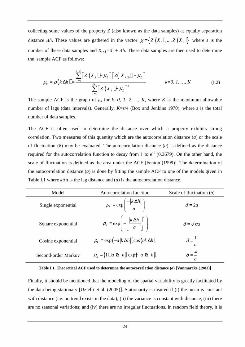
The ACF is often used to determine the distance over which a property exhibits strong
correlation. Two measures of this quantity which are the autocorrelation distance (a) or the scale
of fluctuation (δ) may be evaluated. The autocorrelation distance (a) is defined as the distance
required for the autocorrelation function to decay from 1 to e-1 (0.3679). On the other hand, the
scale of fluctuation is defined as the area under the ACF [Fenton (1999)]. The determination of
the autocorrelation distance (a) is done by fitting the sample ACF to one of the models given in
Table I.1 where k∆h is the lag distance and (a) is the autocorrelation distance.
Model Autocorrelation function Scale of fluctuation (δ)
Single exponential expk
k h
aρ
− ∆ =
2aδ =
Square exponential
2
expk
k h
aρ
∆ = −
aδ π=
Cosine exponential ( ) ( )exp cosk a k h ak hρ = − ∆ ∆ 1
aδ =
Second-order Markov ( ) ( )1 expk a k h a k hρ = + ∆ − ∆ 4
aδ =
Table I.1. Theoretical ACF used to determine the autocorrelation distance (a) [Vanmarcke (1983)]
Finally, it should be mentioned that the modeling of the spatial variability is greatly facilitated by
the data being stationary [Uzielli et al. (2005)]. Stationarity is insured if (i) the mean is constant
with distance (i.e. no trend exists in the data); (ii) the variance is constant with distance; (iii) there
are no seasonal variations; and (iv) there are no irregular fluctuations. In random field theory, it is
25
a common practice to transform a non-stationary data set to a stationary one by removing a low-
order polynomial trend (i.e. a first or a second order polynomial) using the ordinary least square
method.
I.3.1.2 Geostatistics
Geostatistics was firstly developed by Krige and Matheron in the early 1960s and has since been
applied to many disciplines including: groundwater hydrology and hydrogeology; surface
hydrology; earthquake engineering and seismology; pollution control; geochemical exploration;
and geotechnical engineering. In fact, geostatistics can be applied to any natural phenomena that
vary spatially or temporally [Journel and Huijbregts (1978)]. Just as random field theory makes
use of the ACF, geostatistics utilizes the 'semivariogram'. The semivariogram is a plot of
semivariances versus the distance. This semivariogram may be used to identify the range of
influence (a) which is analogue to the autocorrelation distance in the random field theory. If the
soil property of interest is denoted by Z, the semivariance is defined as follows:
( ) ( ) ( ) 21
2 i h ih E Z X Z Xγ +∆∆ = − ( I.3)
where Z(Xi) is the value of the property Z at location Xi; Z(Xi+ ∆h) is its value at location, Xi+ ∆h; ∆h
is the separation distance between the data pairs; and E[.] is the expectation operator. Thus, the
semivariance is defined as half the expectation value (or the mean) of the squared difference
between Z(Xi) and Z(Xi+ ∆h). Like the ACF, one needs to determine the semivariogram which
allows one to calculate the value of the semivariance between any two arbitrary points. This can
be done by collecting some values of the property Z (also known as the data samples) at equally
separation distance ∆h. These values are gathered in the vector ( ) ( ) 1 ,..., sZ X Z Xχ = where s
is the number of these data samples and Xi+ 1.=Xi + ∆h. These data samples are then used to
determine the sample semivariogram as follows:
( ) ( ) ( ) ( ) 2
1
1
2
s
k i k ii
k h Z X Z XN k
γ γ +=
= ∆ = − ∑ k=0, 1, …, K ( I.4)
The samples semivariogram is thus the graph of kγ for k=0, 1, 2, ..., K, where K is the maximum
allowable number of lags (data intervals) and N(k) is the number of data pairs corresponding to a
given value of k.
As the experimental semivariogram is a discrete function, it is desirable in geostatistics to adopt a
continuous semivariogram. Hence, analytical models are generally fitted to the experimental
26
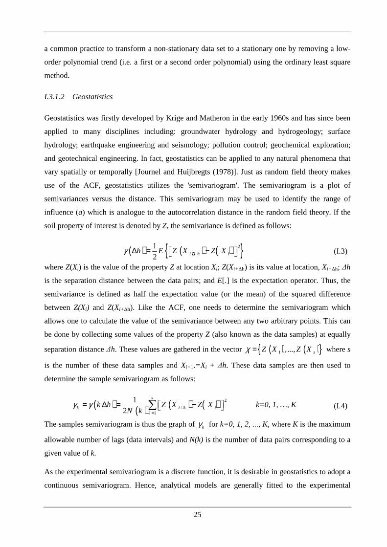
semivariogram [Journel and Huijbregts (1978)]. The most common theoretical models of
semivariograms are summarized in Table I.2, where the range of influence (a) is analogue to the
autocorrelation distance in the random field theory.
Model Semivariogram Scale of fluctuation (δ)
Spherical
3
1.5 0.5
1k
k h k hif k h a
a a
otherwise
γ ∆ ∆ − ∆ < =
aδ =
Exponential 1 expk
k h
aγ ∆ = − −
3aδ =
Gaussian ( )2
21 expk
k h
aγ
∆= − −
3aδ =
Table I.2. Theoretical semivariograms used to determine the range of influence (a) [Goovaerts (1998, 1999)]
It should be mentioned here that if the data samples are stationary and normalised to have a mean
of zero and a variance of 1.0, the semivariogram is the mirror image of the ACF. The
semivariogram and the ACF are related via the following relationship given by Fenton (1999):
( )2 1k kγ σ ρ= − ( I.5)
where σ is the standard deviation of the data samples.
I.3.1.3 Values of the statistical parameters of some geotechnical properties
This section aims at providing the commonly used values of (i) the coefficients of variation COVs
of some soil/rock properties, (ii) the coefficients of correlation between these parameters, and (iii)
the autocorrelation distance (a).
Values of the coefficients of variation COVs
The aim of this section is to provide the different values of the coefficients of variation as given
in literature for the soil shear strength parameters (cohesion c, angle of internal friction φ), the
soil elastic properties (Young modulus E, Poisson ratio υ) and the rock mass parameters
(Geological Strength Index GSI, uniaxial compressive strength σc) used in this thesis.
Concerning the type of the PDF of the different uncertain parameters; unfortunately, there is no
sufficient data to give a comprehensive and complete description of the type of the PDF to be
used in the numerical simulations. The existing literature [e.g. Griffiths and Fenton (2001),
Griffiths et al. (2002), Fenton and Griffiths (2002, 2003, 2005), Fenton et al. (2003)] tends to
27
recommend the use of a lognormal PDF for the Young’s modulus E, Poisson’s ratio ν and
cohesion c. This recommendation is motivated by the fact that the values of these parameters are
strictly positive. Concerning the internal friction angle φ, it is recommended to adopt a beta
distribution for this parameter to limit its variation in the range of practical values. Finally,
concerning the parameters GSI and σc, Hoek (1998) has recommended the use of a lognormal
PDF for these parameters.
Soil cohesion c
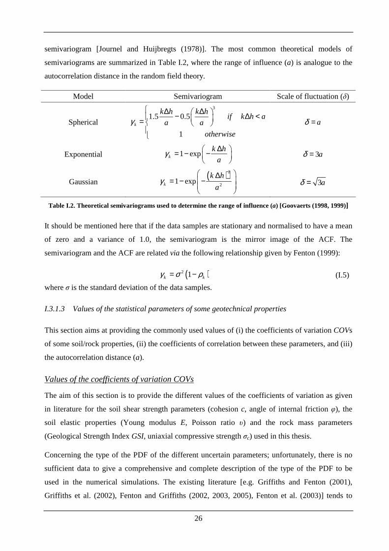
For the undrained cohesion cu of a clay, Cherubini et al. (1993) found that the coefficient of
variation of this property decreases with the increase in its mean value. They recommended a
range of 12% to 45% for moderate to stiff soil.
Author ucCOV (%)
Lumb (1972) 30 - 50 (UC test)
60 - 85 (highly variable clay)
Morse (1972) 30 - 50 (UC test)
Fredlund and Dahlman (1972) 30 - 50 (UC test)
Lee et al. (1983) 20 - 50 (clay) 25 - 30 (sand)
Ejezie and Harrop-Williams (1984) 28 – 96
Cherubini et al. (1993) 12 - 145
12 - 45 (medium to stiff clay)
Lacasse and Nadim (1996) 5 - 20 (clay – triaxial test)
10 - 30 (clay loam)
Zimbone et al. (1996) 43 – 46 (sandy loam) 58 – 77 (silty loam)
10 – 28 (clay)
Duncan (2000) 13 – 40
Table I.3. Coefficient of variation of the undrained soil cohesion
Phoon et al. (1995) stated that the variability of the undrained soil cohesion depends on the
quality of the measurements. Low variability corresponds to good quality and direct laboratory or
field tests. In this case, ucCOV ranges between 10% and 30%. Medium variability corresponds to
indirect tests. In this case, ucCOV lies in a range from 30% to 50%. Finally, high variability
corresponds to empirical correlations between the measured property and the uncertain
28
parameter. In this case, ucCOV ranges between 50% and 70%. The values of
ucCOV as proposed
by other authors in literature are summarized in Table I.3.
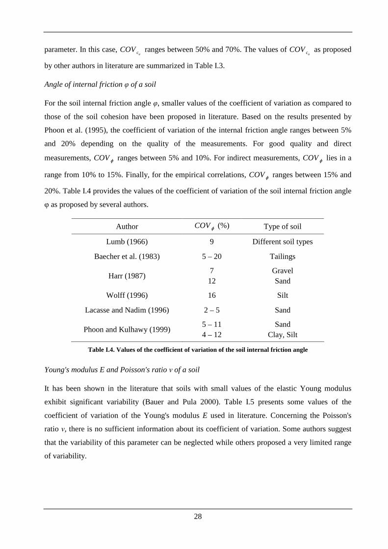
Angle of internal friction φ of a soil
For the soil internal friction angle φ, smaller values of the coefficient of variation as compared to
those of the soil cohesion have been proposed in literature. Based on the results presented by
Phoon et al. (1995), the coefficient of variation of the internal friction angle ranges between 5%
and 20% depending on the quality of the measurements. For good quality and direct
measurements, COVϕ ranges between 5% and 10%. For indirect measurements, COVϕ lies in a
range from 10% to 15%. Finally, for the empirical correlations, COVϕ ranges between 15% and
20%. Table I.4 provides the values of the coefficient of variation of the soil internal friction angle
φ as proposed by several authors.
Author COVϕ (%) Type of soil
Lumb (1966) 9 Different soil types
Baecher et al. (1983) 5 – 20 Tailings
Harr (1987) 7 12
Gravel Sand
Wolff (1996) 16 Silt
Lacasse and Nadim (1996) 2 – 5 Sand
Phoon and Kulhawy (1999) 5 – 11 4 – 12
Sand Clay, Silt
Table I.4. Values of the coefficient of variation of the soil internal friction angle
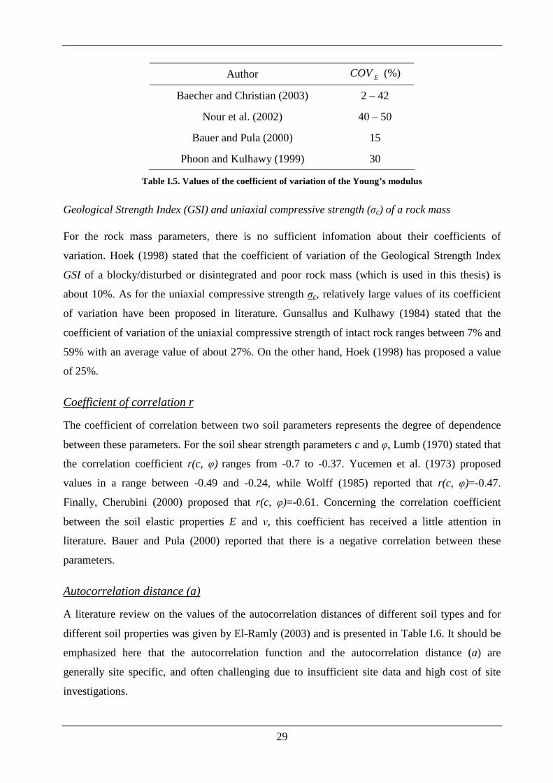
Young's modulus E and Poisson's ratio ν of a soil
It has been shown in the literature that soils with small values of the elastic Young modulus
exhibit significant variability (Bauer and Pula 2000). Table I.5 presents some values of the
coefficient of variation of the Young's modulus E used in literature. Concerning the Poisson's
ratio ν, there is no sufficient information about its coefficient of variation. Some authors suggest
that the variability of this parameter can be neglected while others proposed a very limited range
of variability.
29
Author ECOV (%)
Baecher and Christian (2003) 2 – 42
Nour et al. (2002) 40 – 50
Bauer and Pula (2000) 15
Phoon and Kulhawy (1999) 30
Table I.5. Values of the coefficient of variation of the Young’s modulus
Geological Strength Index (GSI) and uniaxial compressive strength (σc) of a rock mass
For the rock mass parameters, there is no sufficient infomation about their coefficients of
variation. Hoek (1998) stated that the coefficient of variation of the Geological Strength Index
GSI of a blocky/disturbed or disintegrated and poor rock mass (which is used in this thesis) is
about 10%. As for the uniaxial compressive strength σc, relatively large values of its coefficient
of variation have been proposed in literature. Gunsallus and Kulhawy (1984) stated that the
coefficient of variation of the uniaxial compressive strength of intact rock ranges between 7% and
59% with an average value of about 27%. On the other hand, Hoek (1998) has proposed a value
of 25%.
Coefficient of correlation r
The coefficient of correlation between two soil parameters represents the degree of dependence
between these parameters. For the soil shear strength parameters c and φ, Lumb (1970) stated that
the correlation coefficient r(c, φ) ranges from -0.7 to -0.37. Yucemen et al. (1973) proposed
values in a range between -0.49 and -0.24, while Wolff (1985) reported that r(c, φ)=-0.47.
Finally, Cherubini (2000) proposed that r(c, φ)=-0.61. Concerning the correlation coefficient
between the soil elastic properties E and ν, this coefficient has received a little attention in
literature. Bauer and Pula (2000) reported that there is a negative correlation between these
parameters.
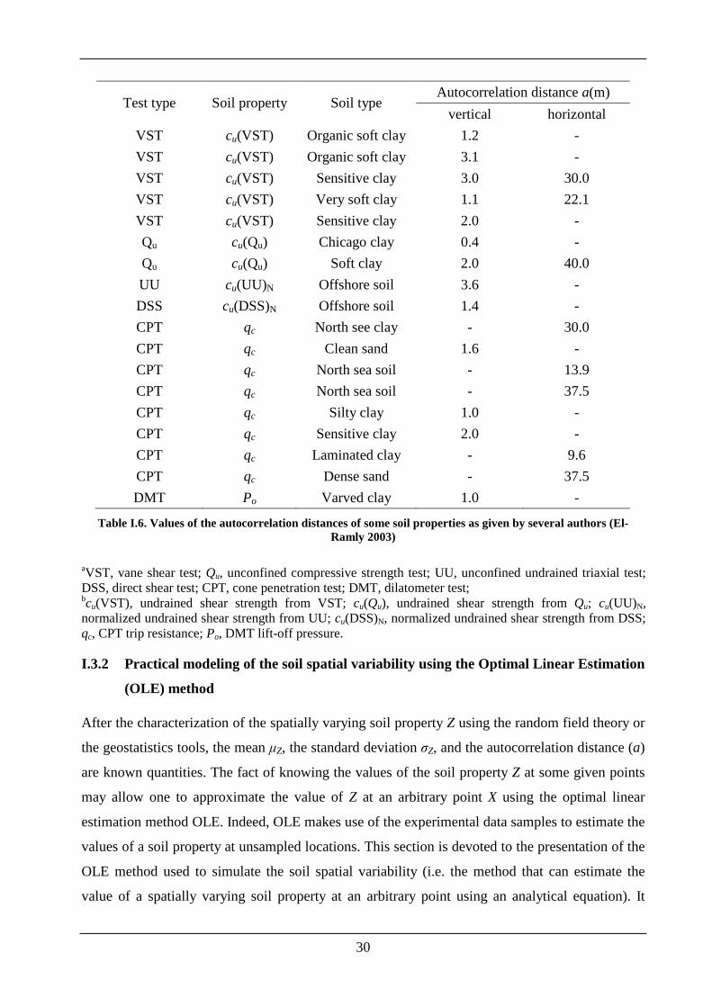
Autocorrelation distance (a)
A literature review on the values of the autocorrelation distances of different soil types and for
different soil properties was given by El-Ramly (2003) and is presented in Table I.6. It should be
emphasized here that the autocorrelation function and the autocorrelation distance (a) are
generally site specific, and often challenging due to insufficient site data and high cost of site
investigations.
30
Autocorrelation distance a(m) Test type Soil property Soil type
vertical horizontal
VST cu(VST) Organic soft clay 1.2 -
VST cu(VST) Organic soft clay 3.1 -
VST cu(VST) Sensitive clay 3.0 30.0
VST cu(VST) Very soft clay 1.1 22.1
VST cu(VST) Sensitive clay 2.0 -
Qu cu(Qu) Chicago clay 0.4 -
Qu cu(Qu) Soft clay 2.0 40.0
UU cu(UU)N Offshore soil 3.6 -
DSS cu(DSS)N Offshore soil 1.4 -
CPT qc North see clay - 30.0
CPT qc Clean sand 1.6 -
CPT qc North sea soil - 13.9
CPT qc North sea soil - 37.5
CPT qc Silty clay 1.0 -
CPT qc Sensitive clay 2.0 -
CPT qc Laminated clay - 9.6
CPT qc Dense sand - 37.5
DMT Po Varved clay 1.0 -
Table I.6. Values of the autocorrelation distances of some soil properties as given by several authors (El-Ramly 2003)
aVST, vane shear test; Qu, unconfined compressive strength test; UU, unconfined undrained triaxial test; DSS, direct shear test; CPT, cone penetration test; DMT, dilatometer test; bcu(VST), undrained shear strength from VST; cu(Qu), undrained shear strength from Qu; cu(UU)N, normalized undrained shear strength from UU; cu(DSS)N, normalized undrained shear strength from DSS; qc, CPT trip resistance; Po, DMT lift-off pressure.
I.3.2 Practical modeling of the soil spatial variability using the Optimal Linear Estimation
(OLE) method
After the characterization of the spatially varying soil property Z using the random field theory or
the geostatistics tools, the mean µZ, the standard deviation σZ, and the autocorrelation distance (a)
are known quantities. The fact of knowing the values of the soil property Z at some given points
may allow one to approximate the value of Z at an arbitrary point X using the optimal linear
estimation method OLE. Indeed, OLE makes use of the experimental data samples to estimate the
values of a soil property at unsampled locations. This section is devoted to the presentation of the
OLE method used to simulate the soil spatial variability (i.e. the method that can estimate the
value of a spatially varying soil property at an arbitrary point using an analytical equation). It
31
should be noted that the concepts used in OLE method will be employed for the discretization of
a random field by the expansion optimal linear estimation EOLE method as will be seen later in
this chapter.
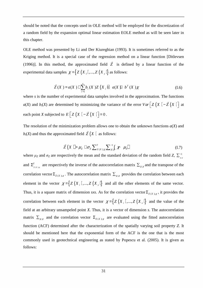
OLE method was presented by Li and Der Kiureghian (1993). It is sometimes referred to as the
Kriging method. It is a special case of the regression method on a linear function [Ditlevsen
(1996)]. In this method, the approximated field Zɶ is defined by a linear function of the
experimental data samples ( ) ( ) 1 ,..., sZ X Z Xχ = as follows:
( )1
( ) ( ) ( ) ( ) ( )s
Ti i
i
Z X a X b X Z X a X b Xχ=
= + = +∑ɶ ( I.6)
where s is the number of experimental data samples involved in the approximation. The functions
a(X) and bi(X) are determined by minimizing the variance of the error ( ) ( )Var Z X Z X − ɶ at
each point X subjected to ( ) ( ) 0E Z X Z X − = ɶ .
The resolution of the minimization problem allows one to obtain the unknown functions a(X) and
bi(X) and thus the approximated field ( )Z Xɶ as follows:
( ) ( )1
( ); ;
T
Z Z ZZ XZ X
χ χ χµ σ χ µ−= + −∑ ∑ɶ ( I.7)
where µZ and σZ are respectively the mean and the standard deviation of the random field Z, ;
1
χ χ
−∑
and ( );Z X
T
χΣ are respectively the inverse of the autocorrelation matrix ;χ χ∑ and the transpose of the
correlation vector ( );Z X χΣ . The autocorrelation matrix ;χ χ∑ provides the correlation between each
element in the vector ( ) ( ) ,...,i sZ X Z Xχ = and all the other elements of the same vector.
Thus, it is a square matrix of dimension sxs. As for the correlation vector ( );Z X χΣ , it provides the
correlation between each element in the vector ( ) ( ) ,...,i sZ X Z Xχ = and the value of the
field at an arbitrary unsampeled point X. Thus, it is a vector of dimension s. The autocorrelation
matrix ;χ χ∑ and the correlation vector ( );Z X χΣ are evaluated using the fitted autocorrelation
function (ACF) determined after the characterization of the spatially varying soil property Z. It
should be mentioned here that the exponential form of the ACF is the one that is the most
commonly used in geotechnical engineering as stated by Popescu et al. (2005). It is given as
follows:
32
'[( ), ( ')] exp
n
X
X XX X
aρ
− = −
( I.8)
Where a is a vector that contains the values of the autocorrelation distances as follows; ( )xa a=
in the case of a one-dimensional random field, ( ),x ya a a= in the case of a two-dimensional (2D)
random field and ( ), ,x y za a a a= in the case of a three-dimensional (3D) random field. For n=1,
the autocorrelation function is said to be exponential of order 1; however, for n=2, it is said to be
square exponential.
Each element ( ); ,i jχ χΣ of the autocorrelation matrix ;χ χ∑ and each element
( )( );Z X iχΣ of the
correlation vector ( );Z X χΣ are calculated using Equation ( I.8) as follows:
( ); ,,Z i ji j
X Xχ χ ρ Σ = ( I.9)
( )( ) [ ]; ,Z iZ Xi
X Xχ ρΣ = ( I.10)
where i=1, …, s, j=1, …, s and X is the arbitrary unsampled point.
Finally, one can see that in Equation ( I.7), the approximated random field ( )Z Xɶ is only a
function of the location X because all the other terms in this equation are known. As a result, one
needs to introduce a value for the location X to obtain an approximated value of the
corresponding property ( )Z Xɶ .
I.3.3 Brief overview of the numerical random fields discretization methods
For computational purposes, the real random field Z which may be represented by an infinite set
of random variables has to be discretized in order to yield a finite set of random variables
, 1,...,j j sχ = , which are assigned to discrete locations. If the finite element/finite difference
method is the method used in the mechanical analysis, it is convenient to evaluate the random
field values in the same way as the finite element/finite difference model (i.e. at the nodes of the
deterministic mesh or at the element mid points of this deterministic mesh). The discretization
methods can be divided into three main groups [Sudret and Der Kiureghian (2000)]. Each group
involves a number of discretization methods as may be seen below. After a brief presentation of
the different methods of the three groups, the EOLE method used in this thesis will be presented
in more detail.
33
I.3.3.1 Point discretization methods
In these methods, the random variables jχ used in the analysis are selected values of Z at some
given points Xj. This group involves the following methods:
a) Midpoint (MP) method
This method was introduced by Der Kiureghian and Ke (1998). In this method, the random field
is discretized by associating to each element of the finite element/finite difference mesh, a single
random variable defined as the value of the field at the centroid of that element.
b) Shape function (SF) method
This method was presented by Liu et al. (1986a,b). It is similar to the MP method with the
difference that the random field is discretized by associating a single random variable to each
node of the finite element/finite difference mesh. Thus, the value of the random field within an
element is described in term of these nodal values and the corresponding shape functions.
c) Integration point (IP) method
In this method, the random field is discretized by associating a single random variable to each of
the integration points appearing in the finite element resolution scheme.
I.3.3.2 Average discretization methods
a) Spatial average (SA) method
This method was proposed by VanMarcke and Grigoriu (1983). It consists in approximating the
random field in each element of the finite element/finite difference mesh by a constant computed
as the average of the original field over that element. This method was extensively used in
geotechnical engineering for the study of the effect of the soil spatial variability.
I.3.3.3 Series expansion methods
In the series expansion discretization methods, the random field is approximated by an expansion
that involves deterministic and stochastic functions. The deterministic functions depend on the
coordinates of the point at which the value of the random field is to be calculated. This group
involves the following methods:
a) Karhunen-Loeve (KL) expansion method
34
This method was presented by Spanos and Ghanem (1989). In this method, the random field is
expressed as follows:
1
( ) ( )N
Z Z j j jj
Z X Xµ σ λ ξ φ=
= + ∑ɶ ( I.11)
Where Zµ and Zσ are the mean and standard deviation of the random field Z, ( ,j jλ φ ) are the
eigenvalues and eigenfunctions of the autocorrelation function Zρ of the random field Z, ξj is a
vector of uncorrelated standard normal random variables and N is the number of terms retained in
the KL expansion. It should be noticed here that ξj are stochastic variables that represent the
random nature of the uncertain soil parameter. However, the eigenfunctions ( )j Xφ are the
deterministic functions of the KL expansion. They can be evaluated as the solution of the
following integral equation:
( ) ( ) ( ), ' ' 'Z j j jX X f X dX f Xρ λΩ
=∫ ( I.12)
This integral can be solved analytically only for few types of the autocorrelation functions
(triangular and first order exponential functions) and for simple geometries. Otherwise, it has to
be solved numerically.
b) Orthogonal series expansion (OSE) method
This method was proposed by Zhang and Ellingwood (1994). It was introduced to avoid solving
the eigenvalue integral of Equation ( I.12) using a complete set of orthogonal functions ( )jh X
(i.e. Legendre or Hermite polynomials). Thus, in this method, the random field is expressed as
follows:
1
( ) ( )N
Z Z j jj
Z X h Xµ σ χ=
= + ∑ɶ ( I.13)
where jχ are zero mean random variables with unit variance and N is the number of terms
retained in the expansion.
c) Expansion optimal linear estimation (EOLE) method
This method was introduced by Li and Der Kiureghian (1993). It makes use of the (OLE) or the
kriging method concept in the special case of a Gaussian random field. This method uses a
spectral representation of the autocorrelation matrix of the Gaussian random field and it is used in
this thesis. Thus, it will be presented in more detail hereafter.
35
I.3.3.4 Conclusions
As stated by Sudret and Der Kiureghian (2000), in the MP, SF, IP, and SA methods, the
discretized random field can be expressed as a finite summation as follows:
1
( ) ( )N
j jj
Z X Xχ φ=
=∑ɶ ( I.14)
where N is the number of terms retained in the discretization procedure, ( )j Xφ are deterministic
functions and jχ are random variables obtained from the discretization procedure. They can be
expressed as weighed integrals of the real random field Z over the volume Ω of the system as
follows:
( ) ( )j Z X X dχ ωΩ
= Ω∫ ( I.15)
where ( )Xω is the weight function. The values of the weight functions and the deterministic
functions for all the above mentioned methods are given in Sudret and Der Kiureghian (2000)
and they are reported in Appendix A of this thesis.
Sudret and Der Kiureghian (2000) have stated that the deterministic functions jφ given in
Equation ( I.14) are not optimal in the case of mid point (MP), spatial average (SA), shape
function (SF) and integration point (IP) methods. This means that the number of random
variables involved in the discretization scheme is not minimal. Thus, of particular interest are the
series expansion methods. In all these methods, the number of the deterministic functions jφ is
optimal and thus, the number of random variables involved is minimal.
As a conclusion, all the discretization methods presented in the first two groups provide non
optimal solution which makes them unattractive tools for random field discretization. This is
because the number of random variables needed to discretize the random fields using these
methods is mesh depending. Thus, one obtains a large number of random variables for large finite
element/finite difference models. The series expansion methods solve this problem. They provide
the optimal number of random variables needed to accurately discretize the random field which
makes them powerful tools for random field discretization. From this group, the eigenvalue
problem of the KL method given in Equation ( I.12) can be solved analytically only for few types
of autocorrelation functions and geometries. As for the OSE method, it avoids solving the
eigenvalue problem of the KL method given in Equation ( I.12). On the other hand, this method is
less attractive in terms of accuracy when compared to the KL and the EOLE method [cf. Sudret
36
and Der Kiureghian (2000)]. For this reason, the EOLE method which uses the concept of OLE
method is selected herein to perform the random field discretization. This method is described in
some details in the following section.
I.3.4 The expansion optimal linear estimation (EOLE) method for random field
discretization
The expansion optimal linear estimation method (EOLE) was proposed by Li and Der Kiureghian
(1993). It makes use of the concepts employed in OLE (or the kriging method) which was
presented in a previous section. This method only deals with uncorrelated Gaussian random fields
because it uses a spectral representation of the vector ( ) ( ) 1 ,..., sZ X Z Xχ = . To overcome the
inconvenience of modeling only uncorrelated Gaussian random fields, Vořechovsky (2008) has
extended this method to cover the general case of cross-correlated non-Gaussian random fields.
In this section one first presents EOLE method proposed by Li and Der Kiureghian (1993) to
model uncorrelated Gaussian random fields. Then, the extension by Vořechovsky (2008) to cover
the general case of two cross-correlated non-Gaussian random fields is presented.
In EOLE method, the fact that the spatially varying soil property is assumed to be Gaussian
allows one to spectrally decompose its autocorrelation matrix ;χ χΣ that includes the correlation
between each element of the vector ( ) ( ) 1 ,..., sZ X Z Xχ = with all the elements of this same
vector. Thus ( ) ( ) 1 ,..., sZ X Z Xχ = can be written as follows:
1
s
Z Z j j jj
χ µ σ λ ξ φ=
= + ∑ ( I.16)
where jξ (j=1, …, s) are independent standard normal random variables and ( ,j jλ φ ) are the
eigenvalues and eigenvectors of the autocorrelation matrix ;χ χΣ verifying ; j j jχ χφ λ φΣ = .
Substituting Equation ( I.16) in to Equation ( I.6) and solving the OLE problem leads to the
following representation of the approximated random field ( )Z Xɶ :
( ) ( );1
( ) . .s Tj
Z Z j Z Xj j
Z X µ χ
ξσ φ
λ=
= + Σ∑ɶ ( I.17)
where µZ and σZ are respectively the mean and the standard deviation of the Gaussian random
field Z, ( , );Z x y χΣ is the correlation vector between each element in the vector χ and the value of
37
the field at an arbitrary point X, jξ is a standard normal random variable, and s is the total number
of point samples.
It should be mentioned that the series expansion given in Equation ( I.17) can be truncated after
N<s terms. This can be done by sorting the eigenvalues λj in a descending order. This number N
should assure that the variance of the error is smaller than a prescribed tolerance 10%ε ≈ .
Notice that the variance of the error for EOLE is given by Sudret and Der Kiureghian (2000) as
follows:
( )( )22
( );1
1( ) ( ) 1
N T
Z j Z Xj j
Var Z X Z X χσ φλ=
− = − Σ
∑ɶ ( I.18)
where ( )Z X and ( )Z Xɶ are respectively the exact and the approximate values of the random
field at a given point X and ( )Tjφ is the transpose of the eigenvector jφ .
I.3.4.1 Extension of EOLE for the generation of two cross-correlated non-Gaussian random
fields
Let us consider two cross-correlated non-Gaussian random fields ( )NGiZ X ( 1,2i = ) described
by: (i) constant means and standard deviations (µZi, σZi; 1,2i = ), (ii) non-Gaussian marginal
cumulative density functions Gi ( 1,2i = ), (iii) a target cross-correlation matrix
1,1 1,2
2.1 2,2
NGr r
Cr r
=
and (iv) a common autocorrelation function NGZρ [(X), (X')].
Since EOLE only deals with uncorrelated Gaussian random fields, the common non-Gaussian
autocorrelation matrix ;
NG
χ χΣ evaluated using Equation ( I.9) (where Zρ in this equation is the non-
Gaussian autocorrelation function NGZρ ) and the target non-Gaussian cross-correlation matrix CNG
should be transformed into the Gaussian space using the Nataf correction functions proposed by
Nataf (1962). This can be done by applying the following formulas:
( ) ( ); , ;, ,
k NGi ji j i jχ χ χ χωΣ = Σ ; i=1,…, s; j=1,…, s and k= 1, 2 ( I.19)
, , ,NG
i j i j i jC Cω= ; i=1, 2 and j= 1, 2. ( I.20)
where ,i jω is the correction factor.
38
As a result, one obtains two Gaussian autocorrelation matrices 1;χ χΣ and 2
;χ χΣ , and a Gaussian
cross-correlation matrix C that can be used to discretize the two Gaussian random fields (of zero
mean and unit variance) using EOLE as follows:
( )( );
,
1
( ) . .Z X
j
DN Ti jG i ii ji
j
Z Xχ
κφ
λ=
= Σ∑ɶ ; i=1, 2 ( I.21)
where ( ,i ij jλ φ ; i=1, 2) are the eigenvalues and eigenvectors of the two Gaussian autocorrelation
matrices ( ;iχ χΣ ; i=1, 2) respectively, ( );Z X χΣ is the correlation vector between the random vector
χ and the value of the field at an arbitrary point X as obtained using Equation ( I.10), and finally N
is the number of terms (expansion order) retained in the EOLE method. Notice finally that (,Di jκ ;
i=1, 2) are two cross-correlated blocks of independent standard normal random variables
obtained using the Gaussian cross-correlation matrix C between the two fields as follows: (i) one
should compute the diagonal eigenvalues matrix ΛC with its corresponding eigenvectors matrix
ΦC of the Gaussian cross-correlation matrix C using the spectral decomposition of the cross-
correlation matrix C, and (ii) generate the block sample vector Dκ which contains the two cross-
correlated blocks ( ,Di jκ ; i=1, 2) of independent standard random variables using the following
formula:
( ) 12( )
TD D D Tκ ξ= Φ Λ ( I.22)
where ΦD is a (2Nx2N) block matrix resulting from the multiplication of each element in the
matrix ΦC by the unit matrix of order N (the expansion order), ΛD is a (2Nx2N) block matrix
resulting from the multiplication of each element in the matrix ΛC by the unit matrix of order N
and ( ) ( ) 1 1
1 1 1 2 2 2,..., , ,...,NNξ ξ ξ ξ ξ ξ ξ= = = is a block vector which contains two blocks (iξ ; i=1,
2) of N standard Gaussian independent random variables for each one.
Once the two Gaussian cross-correlated random fields are obtained, they should be transformed
to the non-Gaussian space by applying the following formula:
1( ) ( ) 1, 2NG Gi i iZ X G Z X i− = Φ = ɶ ɶ ( I.23)
where (.)Φ is the standard normal cumulative density function. It should be mentioned here that
the series given by Equation ( I.21) are truncated for a number of terms N (expansion order)
smaller than the number of grid points s, after sorting the eigenvalues (ijλ ; j=1, …, N) in a
39
descending order. This number should assure that the variance of the error given in Equation
( I.18) is smaller than a prescribed tolerance as previously mentioned. In order to clarify the
EOLE method and its extension by Vořechovsky (2008), a detailed numerical example is
presented in Appendix B to illustrate the different steps for generating cross-correlated non-
Gaussian random fields.
I.4 TIME VARIABILITY OF THE SEISMIC LOADING
An earthquake is usually initiated by a series of irregular slippages along faults, followed by a
large number of random reflections, refractions, dispersions and attenuations of the seismic
waves within the complex ground formations through which they travel. Consequently, an
earthquake Ground-Motion (GM) exhibits nonstationarity in both time and frequency domains
[Rezaeian and Der Kiureghian (2008)]. The temporal nonstationarity is due to the variation of the
intensity of the earthquake GM over time. This intensity evolves with time from zero to a roughly
constant value representing the phase of strong motion, and then decreases gradually to zero. The
frequency (or spectral) nonstationarity is the change of the frequency content of the earthquake
GM over time. Typically, high-frequency compressional (P) waves tend to dominate the initial
few seconds of the motion. These are followed by moderate-frequency shear (S) waves, which
tend to dominate the strong-motion phase of the ground-motion. Finally, low-frequency surface
waves tend to dominate the end of the motion.
The growing interest to perform probabilistic dynamic analysis in recent years has further
increased the need for stochastic modeling of earthquake GMs. This is because in such analysis,
one needs a large number of recorded ground motions. However, for many regions, the database
of recorded motions is not sufficient. As a result, there is an increasing interest in methods for
generation of synthetic GMs.
For many years, stochastic processes and more precisely the zero-mean Gaussian process have
been used to model earthquake GMs [cf. Shinozuka and Sato (1967), Liu (1970), Ahmadi (1979),
Kozin (1988), Shinozuka and Deodatis (1988), Zerva (1988), Papadimitriou (1990), Conte and
Peng (1997), Rezaeian and Der Kiureghian (2008) and Rezaeian and Der Kiureghian (2010)]. In
order to establish a valid model to simulate stochastic earthquake GMs, statistical
characterization of existing earthquake GM is necessary to correctly model the corresponding
nonstationarities [cf. Liu (1970), Ahmadi (1979), Zerva (2009) and Rezaeian and Der Kiureghian
(2008)].
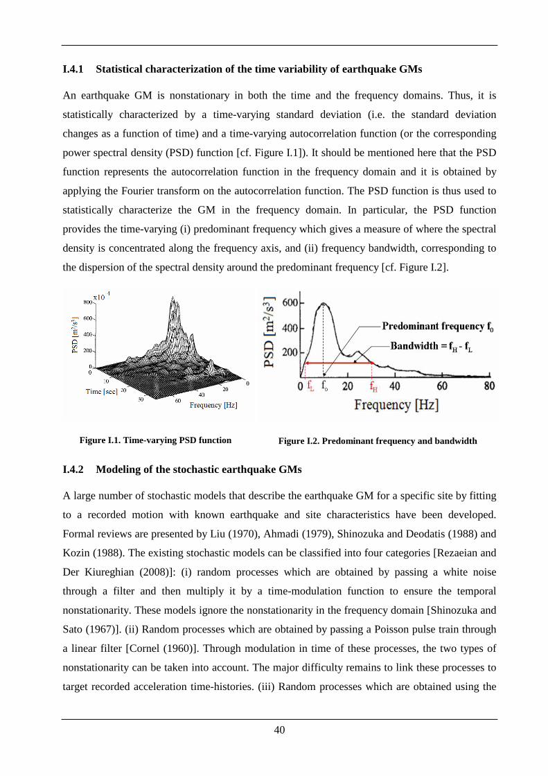
40
I.4.1 Statistical characterization of the time variability of earthquake GMs
An earthquake GM is nonstationary in both the time and the frequency domains. Thus, it is
statistically characterized by a time-varying standard deviation (i.e. the standard deviation
changes as a function of time) and a time-varying autocorrelation function (or the corresponding
power spectral density (PSD) function [cf. Figure I.1]). It should be mentioned here that the PSD
function represents the autocorrelation function in the frequency domain and it is obtained by
applying the Fourier transform on the autocorrelation function. The PSD function is thus used to
statistically characterize the GM in the frequency domain. In particular, the PSD function
provides the time-varying (i) predominant frequency which gives a measure of where the spectral
density is concentrated along the frequency axis, and (ii) frequency bandwidth, corresponding to
the dispersion of the spectral density around the predominant frequency [cf. Figure I.2].
Figure I.1. Time-varying PSD function
Figure I.2. Predominant frequency and bandwidth
I.4.2 Modeling of the stochastic earthquake GMs
A large number of stochastic models that describe the earthquake GM for a specific site by fitting
to a recorded motion with known earthquake and site characteristics have been developed.
Formal reviews are presented by Liu (1970), Ahmadi (1979), Shinozuka and Deodatis (1988) and
Kozin (1988). The existing stochastic models can be classified into four categories [Rezaeian and
Der Kiureghian (2008)]: (i) random processes which are obtained by passing a white noise
through a filter and then multiply it by a time-modulation function to ensure the temporal
nonstationarity. These models ignore the nonstationarity in the frequency domain [Shinozuka and
Sato (1967)]. (ii) Random processes which are obtained by passing a Poisson pulse train through
a linear filter [Cornel (1960)]. Through modulation in time of these processes, the two types of
nonstationarity can be taken into account. The major difficulty remains to link these processes to
target recorded acceleration time-histories. (iii) Random processes which are obtained using the
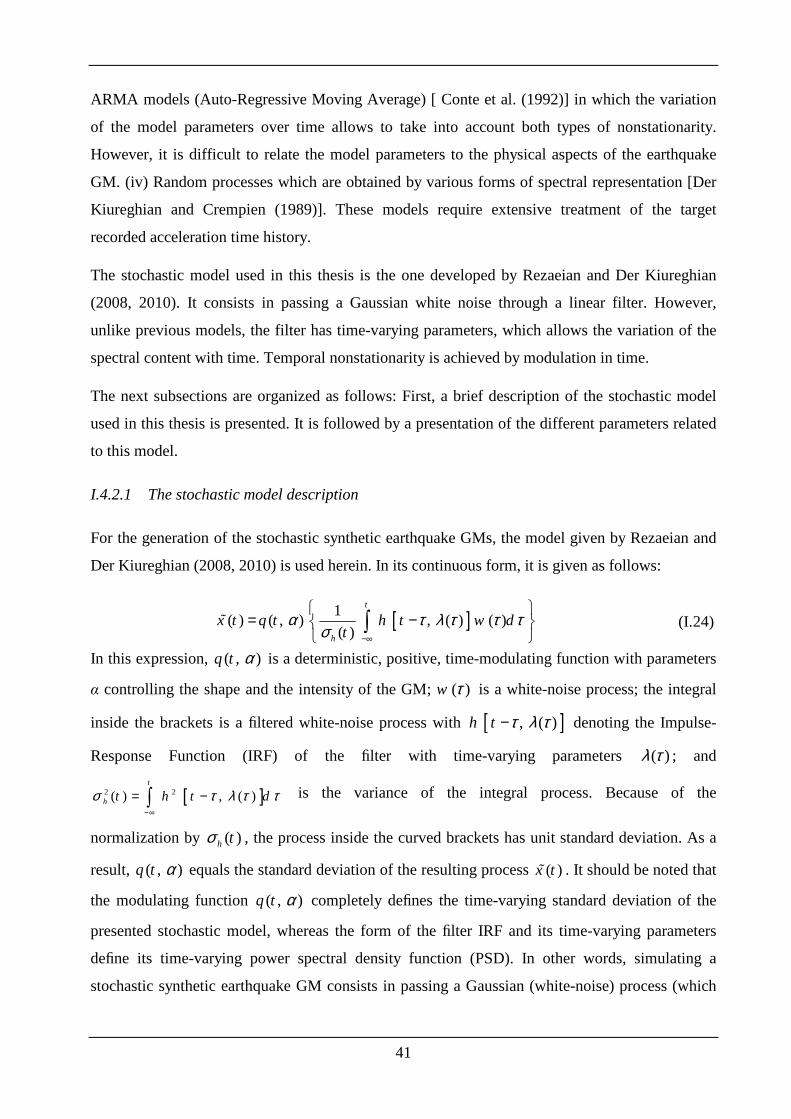
41
ARMA models (Auto-Regressive Moving Average) [ Conte et al. (1992)] in which the variation
of the model parameters over time allows to take into account both types of nonstationarity.
However, it is difficult to relate the model parameters to the physical aspects of the earthquake
GM. (iv) Random processes which are obtained by various forms of spectral representation [Der
Kiureghian and Crempien (1989)]. These models require extensive treatment of the target
recorded acceleration time history.
The stochastic model used in this thesis is the one developed by Rezaeian and Der Kiureghian
(2008, 2010). It consists in passing a Gaussian white noise through a linear filter. However,
unlike previous models, the filter has time-varying parameters, which allows the variation of the
spectral content with time. Temporal nonstationarity is achieved by modulation in time.
The next subsections are organized as follows: First, a brief description of the stochastic model
used in this thesis is presented. It is followed by a presentation of the different parameters related
to this model.
I.4.2.1 The stochastic model description
For the generation of the stochastic synthetic earthquake GMs, the model given by Rezaeian and
Der Kiureghian (2008, 2010) is used herein. In its continuous form, it is given as follows:
[ ]1( ) ( , ) , ( ) ( )
( )
t
h
x t q t h t w dt
α τ λ τ τ τσ −∞
= −
∫ɶ ( I.24)
In this expression, ( , )q t α is a deterministic, positive, time-modulating function with parameters
α controlling the shape and the intensity of the GM; ( )w τ is a white-noise process; the integral
inside the brackets is a filtered white-noise process with [ ], ( )h t τ λ τ− denoting the Impulse-
Response Function (IRF) of the filter with time-varying parameters ( )λ τ ; and
[ ]2 2( ) , ( )t
h t h t dσ τ λ τ τ−∞
= −∫ is the variance of the integral process. Because of the
normalization by ( )h tσ , the process inside the curved brackets has unit standard deviation. As a
result, ( , )q t α equals the standard deviation of the resulting process ( )x tɶ . It should be noted that
the modulating function ( , )q t α completely defines the time-varying standard deviation of the
presented stochastic model, whereas the form of the filter IRF and its time-varying parameters
define its time-varying power spectral density function (PSD). In other words, simulating a
stochastic synthetic earthquake GM consists in passing a Gaussian (white-noise) process (which
42
is the source of stochasticity) through a linear filter with time-varying parameters. The obtained
filtered white noise (which represents the time-varying PSD function of the model) is then
normalized it by dividing it by its standard deviation. Thus, one obtains a normalized filtered
white-noise with nonstationarity in the frequency domain. Finally, the temporal nonstationarity is
insured by multiplying the normalized filtered white-noise by a time-modulation function (which
represents the time-varying standard deviation of the model).
In order to facilitate digital simulation, the stochastic model given in Equation ( I.24) is
discretized in the time domain as follows [cf. Rezaeian and Der Kiureghian (2008)]:
[ ]
[ ]1
2
1
, ( ), ( )ˆ ( ) ( , )
, ( ), ( )
N
i f i f i ii
N
i f i f ii
h t t t t ux t q t
h t t t t
ω ζα
ω ζ
=
=
−
=
−
∑
∑ ( I.25)
where it i t= × ∆ for i=0, 1, …, N, t∆ is a small time step and 1T
Nt
= +∆
with T being the total
duration of the motion. In most earthquake engineering applications, 0.01t s∆ = . Finally, ui are a
set of standard normal random variables representing random pulses at the discrete time points ti.
Thus, these random variables ui may be regarded as a train of random pulses that represent
intermittent ruptures at the fault. The filter [ ], ( )h t τ λ τ− may represent the medium through
which the seismic waves travel (i.e. the soil medium). Thus, the obtained earthquake GM is the
superposition of the filter response to those random pulses.
For a given modulating function and filter IRF, a realization of the process in Equation ( I.25) is
obtained by simulating at set of standard normal random variables ui. for i=1, …, N.
I.4.2.2 The model parameters
In the current work, a ‘Gamma’ modulating function was selected. This choice was justified by
the fact that this type of function captures the time-evolution of the intensity using a small
number of parameters [Rezaeian (2010)]. It is given as follows:
2 11 3( , ) exp( )q t t tαα α α−= − ( I.26)
where 1 2 3( 0, 1, 0)α α α α= > > > . Of the three parameters, α1 controls the intensity of the
process, α2 controls the shape of the modulating function and α3 controls the duration of the
motion. These parameters 1 2 3( , , )α α α α= are related to three physically based parameters
43
5 95( , , )a midI D t− which describe the real recorded GM in the time domain. The first variable, aI
is the so-called Arias Intensity (aI ) given by: [ ]2
0
( )2
nt
aI a t dtg
π= ∫ [Kramer (1996)]. The
second variable D5−95 represents the effective duration of the motion. It is defined as the time
interval between the instants at which 5% and 95% of the expected aI are reached respectively.
Finally, the third variable tmid is the time at the middle of the strong-shaking phase. It is selected
as the time at which 45% level of the expected aI is reached. The relationships between
1 2 3( , , )α α α α= and 5 95( , , )a midI D t− are given in Appendix C.
For the filter IRF, a form that corresponds to the pseudo-acceleration response of a single-degree-
of-freedom linear oscillator was selected. For more details on the pseudo-acceleration response of
a single-degree-of-freedom linear oscillator, the reader may refer to Appendix D. It is given by:
[ ] [ ] 2
2
( ), ( ) exp ( ) ( )( ) sin ( ) 1 ( ) ( )
1 ( )
0 otherwise
ff f f f
f
h t t t tω ττ λ τ ζ τ ω τ τ ω τ ζ τ τ τ
ζ τ − = − − × − − ≤ −
=
( I.27)
where ( ) ( ( ), ( ))f fλ τ ω τ ζ τ= is the set of time-varying parameters of the IRF with ( )fω τ
denoting the frequency of the filter and ( )fζ τ denoting its damping ratio. Of these two
parameters, ( )fω τ controls the predominant frequency of the process and ( )fζ τ controls its
bandwidth. These two parameters ( )fω τ and ( )fζ τ are related to two physical parameters that
describe the recorded GM in the frequency domain and which are respectively the predominant
frequency and the bandwidth of the GM. As a measure of the evolving predominant frequency of
the recorded GM, the rate of zero-level up-crossings is considered, and as a measure of its
bandwidth, the rate of negative maxima (peaks) and positive minima (valleys) is considered. In
Rezaeian and Der Kiureghian (2008), the evolution of the predominant frequency was determined
by minimizing the difference between the cumulative mean number of zero-level up-crossings of
the process in time with the cumulative count of the zero-level up-crossings of the recorded
accelerogram. The mean number of zero-level up-crossings being the mean number of time per
unit time that the process crosses the level zero from below. The bandwidth parameter ( )fζ τ ,
was determined by minimizing the difference between the mean rate of negative maxima and
positive minima with the observed rate of the same quantity in the recorded accelerogram. Details
on the chosen filter IRF which has a form that corresponds to the pseudo-acceleration response of
44
a single-degree-of-freedom linear oscillator, in addition to the procedure used to determine the
parameters ( ) ( ( ), ( ))f fλ τ ω τ ζ τ= of this filter are given in Appendix C.
I.5 PROBABILISTIC METHODS FOR UNCERTAINTY PROPAGATI ON
Development of efficient methods for uncertainty propagation in order to perform the
probabilistic analyses has gained much attention in recent years due to the importance of
introducing uncertainties in the model parameters. The uncertainty propagation aims to study the
impact of input uncertainty on the variation of a model output (response). This can be done by
first defining the analytical/numerical deterministic model. It should be mentioned here that the
chosen deterministic model can be complex and/or computationally-expensive (Step B in Figure
I.3). The second step consists in identifying the uncertain input parameters and modeling them by
random variables or random fields (Step A in Figure I.3). The final step consists in propagating
the uncertainty in the input parameters through the deterministic model (Step C in Figure I.3). In
the probabilistic framework, all of the relevant information regarding the uncertainty of the model
output is contained in its PDF. Thus, determining the PDF of the system response is the main
goal in all uncertainty propagation methods. However, the fact that we are considering numerical
models implies that the relation between the model uncertain inputs and the system response can
not be represented by an analytical expression. Consequently, it is impossible to obtain a simple
analytical expression of the PDF of the system response. However, for design purposes, all the
information contained in the PDF are not necessary. Thus, depending on the type of study that is
carried out, only a set of probabilistic outputs can be used. These probabilistic outputs may be the
statistical moments (mean and standard deviation) or the probability of failure (or the probability
of exceeding a given threshold value). The different probabilistic outputs may be computed as
follows:
Consider M input random variables (X1, …, XM) gathered in a vector X, and let fX(X) denote the
joint PDF of the set X. Furthermore, we note that the system output Γ=g(X). is a function of the
input vector X. The expressions of the first two statistical moments of the system response are
given by:
( ) ( )Xg X f X dXµΓ = ∫ ( I.28)
( ) ( )2
Xg X f X dXσ µΓ Γ = − ∫ ( I.29)
As for the probability of exceeding a threshold Γmax, its expression is given as follows:
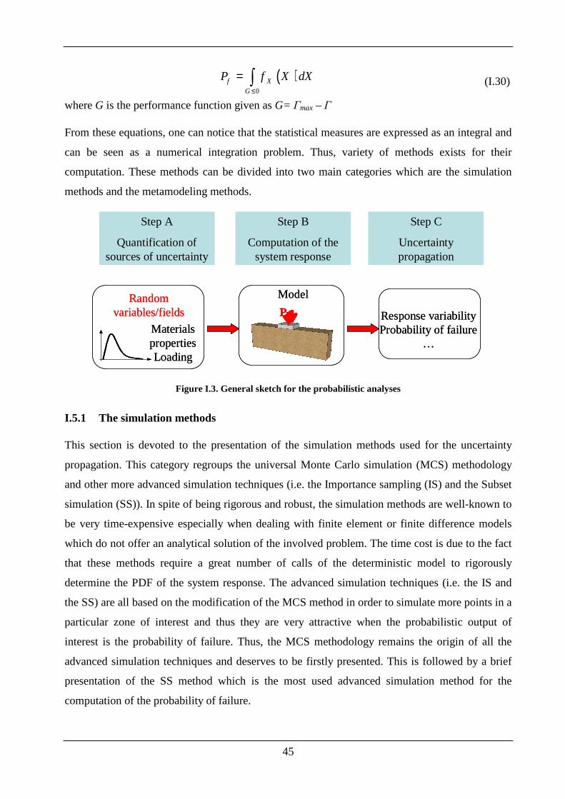
45
( )0
f X
G
P f X dX≤
= ∫ ( I.30)
where G is the performance function given as G= Γmax – Γ
From these equations, one can notice that the statistical measures are expressed as an integral and
can be seen as a numerical integration problem. Thus, variety of methods exists for their
computation. These methods can be divided into two main categories which are the simulation
methods and the metamodeling methods.
Step A
Quantification of sources of uncertainty
Step B
Computation of the system response
Step C
Uncertainty propagation
Pu
ModelRandom variables/fields
Materials propertiesLoading
Response variabilityProbability of failure
…
Step A
Quantification of sources of uncertainty
Step B
Computation of the system response
Step C
Uncertainty propagation
PuPu
ModelRandom variables/fields
Materials propertiesLoading
Response variabilityProbability of failure
…
Figure I.3. General sketch for the probabilistic analyses
I.5.1 The simulation methods
This section is devoted to the presentation of the simulation methods used for the uncertainty
propagation. This category regroups the universal Monte Carlo simulation (MCS) methodology
and other more advanced simulation techniques (i.e. the Importance sampling (IS) and the Subset
simulation (SS)). In spite of being rigorous and robust, the simulation methods are well-known to
be very time-expensive especially when dealing with finite element or finite difference models
which do not offer an analytical solution of the involved problem. The time cost is due to the fact
that these methods require a great number of calls of the deterministic model to rigorously
determine the PDF of the system response. The advanced simulation techniques (i.e. the IS and
the SS) are all based on the modification of the MCS method in order to simulate more points in a
particular zone of interest and thus they are very attractive when the probabilistic output of
interest is the probability of failure. Thus, the MCS methodology remains the origin of all the
advanced simulation techniques and deserves to be firstly presented. This is followed by a brief
presentation of the SS method which is the most used advanced simulation method for the
computation of the probability of failure.
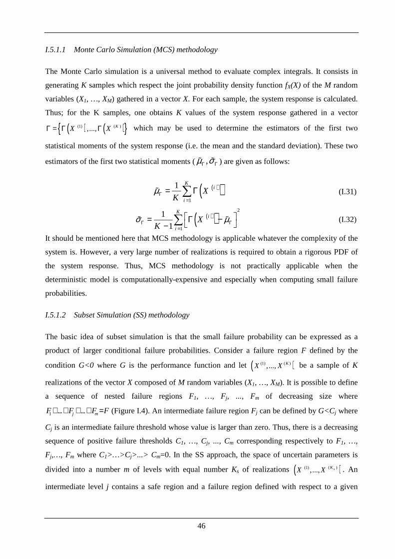
46
I.5.1.1 Monte Carlo Simulation (MCS) methodology
The Monte Carlo simulation is a universal method to evaluate complex integrals. It consists in
generating K samples which respect the joint probability density function fX(X) of the M random
variables (X1, …, XM) gathered in a vector X. For each sample, the system response is calculated.
Thus; for the K samples, one obtains K values of the system response gathered in a vector
( ) ( ) (1) ( ),..., KX XΓ = Γ Γ which may be used to determine the estimators of the first two
statistical moments of the system response (i.e. the mean and the standard deviation). These two
estimators of the first two statistical moments (,µ σΓ Γɶ ɶ ) are given as follows:
( )( )1
1 Ki
i
XK
µΓ=
= Γ∑ɶ ( I.31)
( )( )2
1
1
1
Ki
i
XK
σ µΓ Γ=
= Γ − − ∑ɶ ɶ ( I.32)
It should be mentioned here that MCS methodology is applicable whatever the complexity of the
system is. However, a very large number of realizations is required to obtain a rigorous PDF of
the system response. Thus, MCS methodology is not practically applicable when the
deterministic model is computationally-expensive and especially when computing small failure
probabilities.
I.5.1.2 Subset Simulation (SS) methodology
The basic idea of subset simulation is that the small failure probability can be expressed as a
product of larger conditional failure probabilities. Consider a failure region F defined by the
condition G<0 where G is the performance function and let ( )(1) ( ),..., KX X be a sample of K
realizations of the vector X composed of M random variables (X1, …, XM). It is possible to define
a sequence of nested failure regions F1, …, Fj, ..., Fm of decreasing size where
1 ... ...j mF F F F⊃ ⊃ ⊃ ⊃ = (Figure I.4). An intermediate failure region Fj can be defined by G<Cj where
Cj is an intermediate failure threshold whose value is larger than zero. Thus, there is a decreasing
sequence of positive failure thresholds C1, …, Cj, ..., Cm corresponding respectively to F1, …,
Fj,…, Fm where C1>…>Cj>...> Cm=0. In the SS approach, the space of uncertain parameters is
divided into a number m of levels with equal number Ks of realizations ( )( )(1),..., sKX X . An
intermediate level j contains a safe region and a failure region defined with respect to a given
47
failure threshold Cj. The failure probability corresponding to this intermediate level j is calculated
as follows:
( )( )11
1( )
s
j
Kk
j j Fks
P F F I XK−
=
= ∑ ( I.33)
where ( )( ) 1j
k
FI X = if ( )kjX F∈ and ( )( ) 0
j
k
FI X = otherwise. Notice that in the SS approach, the
first Ks realizations are generated using MCS methodology according a target joint probability
density function fX(X). The next Ks realizations of each subsequent level are obtained using
Markov chain method based on Metropolis-Hastings (M-H) algorithm.
Figure I.4. Nested Failure domain
The failure probability ( ) ( )mP F P F= of the failure region F can be calculated from the
sequence of conditional failure probabilities as follows [Au and Beck (2001)]:
( ) ( ) ( ) ( )1 12
|m
m j jj
P F P F P F P F F−=
= = ∏ ( I.34)
For more details on the SS approach and its extension to the case of spatially varying soil
properties, the reader may refer to Ahmed and Soubra (2012) and Ahmed (2012).
I.5.2 The metamodeling techniques
To overcome the inconvenience of the simulation methods, the metamodeling techniques are
proposed in this regard. The aim of these techniques is to replace the original computationally-
48
expensive deterministic model by a meta-model (i.e. an analytical equation). A variety of
metamodeling techniques exist. The Response Surface Methodology (RSM) [Box et al. (1978),
Bucher and Bourgund (1990), Myers and Montgomery (1995)] is a well known approach for
constructing simple approximation of complex numerical model using polynomial regression.
Another interesting metamodeling technique is the Kriging method [Sacks et al. (1989), Booker
et al. (1999)] which is based on interpolation. Finally, the Polynomial Chaos Expansion (PCE)
[Spanos and Ghanem (1989), Isukapalli et al. (1998), Xiu and Karniadakis (2002), Berveiller et
al. (2006), Sudret et al. (2006), Sudret and Berveiller (2008), Huang et al. (2009), Blatman and
Sudret (2010)] provides a rigorous approximation of complex numerical models with reasonable
computation effort. This method has gained large attention due to its efficiency. The next
subsections aim to briefly present the RSM and the Kriging method. They are followed by a more
detailed presentation of the PCE methodology which is the metamodeling technique employed in
this thesis.
I.5.2.1 The Response Surface Methodology (RSM)
The Response Surface Methodology (RSM) aims at approximating the system response Γ(X) by
an explicit function of the random variables. The most popular form of this function is a second
order polynomial model, which can be expressed as:
( ) 20
1 1
M M
RSM i i i ii i
X a a X b X= =
Γ = + +∑ ∑ ( I.35)
where Xi are the random variables, M is the number of random variables and ( )ii b,a are
coefficients obtained by the least squares method, which minimizes the sum of the squares
between the predicted values ( )( )iRSM XΓ and the model values ( ) ( ) (1) ( ),..., KX XΓ = Γ Γ where
K is the number of samples points. It should be emphasized here that the second order polynomial
used in the RSM method has limited capability to accurately model highly nonlinear response
surfaces. Higher-order polynomial models can be used to model a highly nonlinear response
surfaces; however, instabilities may arise [cf. Barton (1992)]. Furthermore, this requires a large
number of sample points. This enormously increases the computation time and make the RSM
solution inadequate in this case.
49
I.5.2.2 The Kriging Method
This method was presented and detailed in section I.3.2 for the approximation of a random field
at unsampled points using the values of this field at sampled points. This method is used herein to
approximate the system response Γ(X) at any point X where the sample points are obtained in this
case using a simulation technique (e.g. the Monte Carlo simulation). Thus, for K sample points,
one obtains K values of the system response gathered in a vector ( ) ( ) (1) ( ),..., KX XΓ = Γ Γ
which may be used to obtain the approximated system response using the Kriging method as
follows [Jin (2005)]:
( ) ( )1
0 0 0( ); ;
T
Kriging XX a b a
−
Γ Γ Γ ΓΓ = + Γ −∑ ∑ ( I.36)
where a0 and b0 are respectively the mean the standard deviation of the system responses
( ) ( ) (1) ( ),..., KX XΓ = Γ Γ , ;
1
Γ Γ
−∑ and ( );X
T
Γ ΓΣ are respectively the inverse of the autocorrelation
matrix ;Γ Γ∑ and the transpose of the correlation vector( );XΓ ΓΣ . It should be mentioned that a row
i of the autocorrelation matrix gives the values of the correlation between the value of the
response at the sampled point ( )( )iXΓ and all the values of the response at the sampled points
( ) ( ) (1) ( ),..., KX XΓ = Γ Γ and ( );XΓ ΓΣ is a vector whose elements provide the correlation
between the value of the response at the unsampled point Γ(X) and the values of the response at
the sampled points gathered in the vector ( ) ( ) (1) ( ),..., KX XΓ = Γ Γ . Notice however that the
ACF used to determine the autocorrelation matrix ;Γ Γ∑ and the correlation vector ( );XΓ ΓΣ is
obtained by fitting one of the analytical ACF given in Table I.1 to the sample ACF obtained using
the available system responses ( ) ( ) (1) ( ),..., KX XΓ = Γ Γ .
I.5.2.3 The Polynomial chaos expansion PCE methodology - the classical truncation scheme
The polynomial chaos expansion (PCE) aims at replacing a complex deterministic model (i.e.
finite element/finite difference numerical model) by a meta-model. This allows one to calculate
the system response (when performing MCS) using an approximate simple analytical equation
[Spanos and Ghanem (1989), Isukapalli et al. (1998, 1999), Xiu and Karniadakis (2002),
Berveiller et al. (2006), Huang et al. (2009), Blatman and Sudret (2010), Li et al (2011), Mollon
et al. (2011), Houmadi et al. (2011), Mao et al. (2012), Al-Bittar and Soubra (2012)]. Thus, the
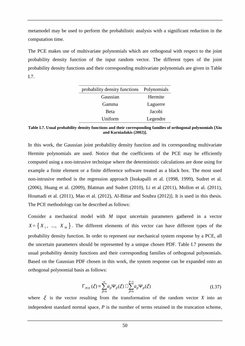
50
metamodel may be used to perform the probabilistic analysis with a significant reduction in the
computation time.
The PCE makes use of multivariate polynomials which are orthogonal with respect to the joint
probability density function of the input random vector. The different types of the joint
probability density functions and their corresponding multivariate polynomials are given in Table
I.7.
probability density functions Polynomials
Gaussian Hermite
Gamma Laguerre
Beta Jacobi
Uniform Legendre
Table I.7. Usual probability density functions and their corresponding families of orthogonal polynomials [Xiu and Karniadakis (2002)].
In this work, the Gaussian joint probability density function and its corresponding multivariate
Hermite polynomials are used. Notice that the coefficients of the PCE may be efficiently
computed using a non-intrusive technique where the deterministic calculations are done using for
example a finite element or a finite difference software treated as a black box. The most used
non-intrusive method is the regression approach [Isukapalli et al. (1998, 1999), Sudret et al.
(2006), Huang et al. (2009), Blatman and Sudret (2010), Li et al (2011), Mollon et al. (2011),
Houmadi et al. (2011), Mao et al. (2012), Al-Bittar and Soubra (2012)]. It is used in this thesis.
The PCE methodology can be described as follows:
Consider a mechanical model with M input uncertain parameters gathered in a vector
1 MX= X , ..., X . The different elements of this vector can have different types of the
probability density function. In order to represent our mechanical system response by a PCE, all
the uncertain parameters should be represented by a unique chosen PDF. Table I.7 presents the
usual probability density functions and their corresponding families of orthogonal polynomials.
Based on the Gaussian PDF chosen in this work, the system response can be expanded onto an
orthogonal polynomial basis as follows:
1
0 0
( ) ( ) ( )P
PCE a aβ β β ββ β
ξ ξ ξ∞ −
= =
Γ = Ψ ≅ Ψ∑ ∑ ( I.37)
where ξ is the vector resulting from the transformation of the random vector X into an
independent standard normal space, P is the number of terms retained in the truncation scheme,
51
aβ are the unknown PCE coefficients to be computed and βΨ are multivariate (or
multidimensional) Hermite polynomials which are orthogonal with respect to the joint probability
density function of the standard normal random vector ξ. These multivariate Hermite polynomials
can be obtained from the product of one-dimensional Hermite polynomials of the different
random variables as follows:
1
( )i
M
i
Hβ α ξ=
Ψ = ∏ ( I.38)
Where (.)i
Hα is the αi-th one-dimensional Hermite polynomial and αi are a sequence of M non-
negative integers 1, ..., Mα α . The expressions of the one-dimensional Hermite polynomials are
given in Appendix E. In practice, one should truncate the PCE representation by retaining only
the multivariate polynomials of degree less than or equal to the PCE order p (i.e. the classical
truncation scheme). Notice that the classical truncation scheme suggests that the first order norm
1. of any multivariate polynomial βΨ should be less than or equal to the order p of the PCE as
follows [Blatman (2009)]:
11
M
ii
pα α=
= ≤∑ ( I.39)
Using this method of truncation, the number P of unknown PCE coefficients is given by:
( )!
! !
M pP
M p
+= ( I.40)
As may be seen from Equation ( I.40), the number P of the PCE coefficients which is the number
of terms retained in Equation ( I.37) dramatically increases with the number M of random
variables and the order p of the PCE. This number becomes very high in the case of random
fields where the number of random variables is significant.
Once the coefficients aβ of the PCE given by Equation ( I.37) have been computed, the statistical
moments (mean, standard deviation, skewness, and kurtosis) can be calculated with no additional
cost. This can be done by performing Monte Carlo simulations on the meta-model and not on the
original computationally-expensive finite element/finite difference numerical model. This
significantly reduces the cost of the probabilistic analysis since a large number of Monte Carlo
simulations (say 1,000,000) can be performed in a negligible time when using the metamodel.
The next subsection is devoted to the method used for the computation of the coefficients aβ of
the PCE using the regression approach.

52
Computation of the PCE coefficients by the regression approach
Consider a set of K realizations ( ) ( )(1) ( )1 1 ,..., ,..., ,..., K
M Mξ ξ ξ ξ ξ ξ= = of the standard normal
random vector ξ. These realizations are called experimental design (ED) and can be obtained
from Monte Carlo (MC) simulations or any other sampling scheme (e.g. Latin Hypercube (LH)
sampling or Sobol set). We note ( ) ( ) (1) ( ),..., Kξ ξΓ = Γ Γ , the corresponding values of the
response determined by deterministic calculations. The computation of the PCE coefficients
using the regression approach is performed using the following equation:
1( )T Ta η η η−= Γ ( I.41)
where the data matrix η is defined by:
( )( ), 1,..., , 0,..., 1ii i K Pβ βη ξ β= Ψ = = − ( I.42)
In order to ensure the numerical stability of the treated problem in Equation ( I.41), the size K of
the ED must be selected in such a way that the matrix 1( )Tη η − is well-conditioned. This implies
that the rank of this matrix should be larger than or equal to the number of unknown coefficients.
This test was systematically performed while solving the linear system of equations of the
regression approach.
Computation of the PCE coefficient of determination
The quality of the output approximation via a PCE closely depends on the PCE order p. To
ensure a good fit between the meta-model and the true deterministic model (i.e. to obtain the
optimal PCE order), one successively increases the PCE order until a prescribed accuracy was
obtained. The simplest indicator of the fit quality is the well-known coefficient of determination
R2 given by:
( )( ) ( )( )( )( )
K 2i i
SPCE2 i 1
K 2i
i 1
1
KR 1
1
K 1
Γ ξ Γ ξ
Γ ξ Γ=
=
−
= − − −
∑
∑
where
( I.43)
( )( )K
i
i 1
1
KΓ Γ ξ
=
= ∑ ( I.44)
The value 2R 1= indicates a perfect fit of the true model response Γ, whereas 2R 0= indicates
a nonlinear relationship between the true model response Γ and the PCE model response PCEΓ .
The coefficient R2 may be a biased estimate since it does not take into account the robustness of
53
the meta-model (i.e. its capability of correctly predicting the model response at any point which
does not belong to the experimental design). As a consequence, one makes use of a more reliable
and rigorous coefficient of determination denoted Q2 [Blatman (2009)]. In order to compute this
coefficient of determination Q2, one needs to sequentially remove a point from the experiment
design composed of K points. Let \iξΓ be the meta-model that has been built from the experiment
design after removing the i th observation and let i ( i ) ( i )\i( ) ( )ξ∆ Γ ξ Γ ξ= − be the predicted
residual between the model evaluation at point ( i )ξ and its prediction based on \iξΓ . Thus, the
corresponding coefficient of determination Q2 is obtained as follows:
( )( )( )
2Ki
2 i 1K 2
i
i 1
1
KQ 1
1
K 1
∆
Γ ξ Γ=
=
= − − −
∑
∑ ( I.45)
The two coefficients R2 and Q2 will be used in this thesis to check the accuracy of the fit.
Global sensitivity analysis (GSA)
Once the PCE coefficients are determined, a global sensitivity analysis (GSA) based on Sobol
indices can be easily performed. Notice that the first order Sobol index of a given random
variable ξi (i=1,…, M) gives the contribution of this variable in the variability of the system
response. The first order Sobol index is given by Salteli (2000) and Sobol (2001) as follows:
( )( )
|( ) i
i
Var E YS
Var Y
ξξ
= ( I.46)
where Y is the system response, ( )| iE Y ξ is the expectation of Y conditional on a fixed value of
iξ , and Var denotes the variance. In the present work, the system response is represented by a
PCE. Thus, by replacing Y in Equation ( I.46) with the PCE expression, one obtains the Sobol
index formula as a function of the different terms of the PCE [Sudret (2008)]. This formula is
given by:
( ) ( )2 2
( ) iIi
PCE
a E
SD
β ββξ ∈
Ψ =∑
( I.47)
where aβ are the obtained PCE coefficients, βΨ are the multivariate Hermite polynomials, [ ].E
is the expectation operator, and PCED is the variance of the response approximated by the PCE.
The response variance PCED is given by Sudret (2008) as follows:
54
( ) ( )21 2
0
P
PCED a Eβ ββ
−
=
= Ψ ∑ ( I.48)
Notice that the term ( )2E β Ψ
that appears in both Equation ( I.47) and Equation ( I.48) is given
by Sudret (2008) as follows:
( )2
1
!M
ii
E β α=
Ψ = ∏ ( I.49)
where the αi are the same sequence of M non-negative integers 1, ....., Mα α used in Equation
( I.38). Notice that I i in Equation ( I.47) denotes the set of indices β for which the corresponding
βΨ terms are only functions of the random variable ξi (i.e. they only contain the variable ξi). It
should be emphasized that Equation ( I.47) used to compute the Sobol indices can only be used
when uncorrelated random variables are involved. Notice however that this equation was used in
this thesis to determine the contribution of correlated random fields. For both uncorrelated or
correlated variables, it was assumed that a direct relationship exist between each physical variable
and its corresponding standard variable. Although this assumption is exact in the case of
uncorrelated variables, it is not true in the case of correlated variables. This means that the
computed Sobol indices using this assumption should be handled with care in the case of
correlated variables. An ongoing research on this topic is necessary to lead to rigorous values of
the Sobol indices in this case. Some interesting and recent papers on this subject may be found in
Kucherenko et al. (2012), Li et al. (2010), Da Veiga et al. (2009) and Caniou et al. (2012).
In order to illustrate the construction of a PCE and the derivation of the equations providing
Sobol indices, an illustrative example of a PCE of order p=3 using only M=2 random variables
(ξ1 and ξ2) is presented in Appendix E.
I.6 CONCLUSION
In this chapter, a literature review on the spatial variability of the soil properties and the time
variability of the seismic loading was presented. The characterization and modeling of the soil
spatial variability were firstly presented. This was followed by the characterization and the
modeling of the time variability of seismic loading. In this thesis, the soil spatial variability will
be modeled by random fields characterized by their probability density functions PDFs and their
autocorrelation functions. As for the time variability of seismic loading, it was modeled by a
parameterized stochastic model that is based on a modulated, filtered white-noise process which
should be fitted to a real target acceleration time history. Finally, the different methods of
55
uncertainties propagation used to perform the probabilistic analyses were presented. These
methods were divided into two main categories which are the simulation methods and the
metamodeling techniques. The simulation methods involve the Monte Carlo simulation (MCS)
methodology which is known to be the most rigorous and robust probabilistic method and other
more advanced simulation techniques (i.e. the Importance sampling (IS) and the Subset
simulation (SS)). As for the metamodeling techniques, three well known methods were presented
which are (i) the Response Surface Methodology (RSM), (ii) the Kriging method and finally (iii)
the Polynomial Chaos Expansion (PCE). This last method is of particular interest. It is the
method used in the present work. In this method, the meta-model is obtained by expanding the
system response on a suitable basis, which is a series of multivariate polynomials that are
orthogonal with respect to the joint probability density function of the input random variables.
Consequently, the characterization of the PDF of the system response is equivalent to the
evaluation of the PCE coefficients. In addition to the PDF, this method allows the computation of
the PCE-based Sobol indices. These indices provide the contribution of each uncertain parameter
in the variability of the system response.
56
CHAPTER II. PROBABILISTIC ANALYSIS OF STRIP FOOTING S
RESTING ON 2D SPATIALLY VARYING SOILS/ROCKS USING S PARSE
POLYNOMIAL CHAOS EXPANSION
II.1 INTRODUCTION
The spatial variability of the soil/rock properties affects the behavior of geotechnical structures
(bearing capacity, foundation settlement, slope stability, etc.). Several probabilistic analyses on
foundations have considered the effect of the spatial variability of the soil properties [Griffiths
and Fenton (2001), Griffiths et al. (2002), Fenton and Griffiths (2002), Nour et al. (2002), Fenton
and Griffiths (2003), Popescu et al. (2005), Breysse et al. (2005), Breysse et al. (2007), Niandou
and Breysse (2007), Youssef Abdel Massih (2007), Soubra et al. (2008), Jimenez and Sitar
(2009), Cho and Park (2010) and Breysse (2011)]. As for the probabilistic analyses of
foundations resting on a spatially varying rock mass, only few studies may be found in literature
[Ching et al. (2011)].
It should be mentioned that when dealing with probabilistic studies that involve spatially varying
soil/rock properties, the classical Monte Carlo Simulation (MCS) methodology is generally used
to determine the probability density function (PDF) of the system response. It is well known that
this method is a very time-expensive approach. This is because (i) it generally makes use of finite
element or finite difference models which are generally time-expensive and (ii) it requires a great
number of calls of the deterministic model.
To overcome the inconvenience of the time cost, the Sparse Polynomial Chaos Expansion
(SPCE) methodology was proposed in this regard. Notice that the sparse polynomial chaos
expansion is an extension of the Polynomial Chaos Expansion (PCE). A PCE or a SPCE
methodology aims at replacing the finite element/finite difference deterministic model by a meta-
model (i.e. a simple analytical equation).
Within the framework of the PCE or the SPCE methodology, the PDF of the system response can
be easily obtained. This is because MCS is no longer applied on the original computationally-
expensive deterministic model, but on the meta-model. This consists in performing a great
number of simulations on the meta-model. The other significant advantage of the present SPCE
methodology with respect to the classical crude MCS method is that it allows one to easily
perform a global sensitivity analysis based on Sobol indices using the SPCE coefficients. These
indices give the contribution of each random field to the variability of the system response.
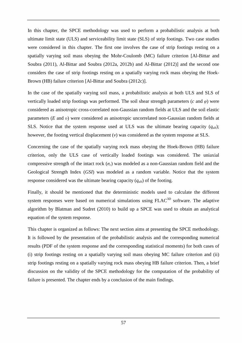
57
In this chapter, the SPCE methodology was used to perform a probabilistic analysis at both
ultimate limit state (ULS) and serviceability limit state (SLS) of strip footings. Two case studies
were considered in this chapter. The first one involves the case of strip footings resting on a
spatially varying soil mass obeying the Mohr-Coulomb (MC) failure criterion [Al-Bittar and
Soubra (2011), Al-Bittar and Soubra (2012a, 2012b) and Al-Bittar (2012)] and the second one
considers the case of strip footings resting on a spatially varying rock mass obeying the Hoek-
Brown (HB) failure criterion [Al-Bittar and Soubra (2012c)].
In the case of the spatially varying soil mass, a probabilistic analysis at both ULS and SLS of
vertically loaded strip footings was performed. The soil shear strength parameters (c and φ) were
considered as anisotropic cross-correlated non-Gaussian random fields at ULS and the soil elastic
parameters (E and υ) were considered as anisotropic uncorrelated non-Gaussian random fields at
SLS. Notice that the system response used at ULS was the ultimate bearing capacity (qult);
however, the footing vertical displacement (v) was considered as the system response at SLS.
Concerning the case of the spatially varying rock mass obeying the Hoek-Brown (HB) failure
criterion, only the ULS case of vertically loaded footings was considered. The uniaxial
compressive strength of the intact rock (σc) was modeled as a non-Gaussian random field and the
Geological Strength Index (GSI) was modeled as a random variable. Notice that the system
response considered was the ultimate bearing capacity (qult) of the footing.
Finally, it should be mentioned that the deterministic models used to calculate the different
system responses were based on numerical simulations using FLAC3D software. The adaptive
algorithm by Blatman and Sudret (2010) to build up a SPCE was used to obtain an analytical
equation of the system response.
This chapter is organized as follows: The next section aims at presenting the SPCE methodology.
It is followed by the presentation of the probabilistic analysis and the corresponding numerical
results (PDF of the system response and the corresponding statistical moments) for both cases of
(i) strip footings resting on a spatially varying soil mass obeying MC failure criterion and (ii)
strip footings resting on a spatially varying rock mass obeying HB failure criterion. Then, a brief
discussion on the validity of the SPCE methodology for the computation of the probability of
failure is presented. The chapter ends by a conclusion of the main findings.
58
II.2 ADAPTIVE SPARSE POLYNOMIAL CHAOS EXPANSION SPC E – THE
HYPERBOLIC (Q-NORM) TRUNCATION SCHEME
The sparse polynomial chaos expansion (SPCE) which is an extension of the PCE methodology
(cf. section I.5.2.3) was proposed by Blatman and Sudret (2009, 2010) to deal with high
dimensional stochastic problems (i.e. when a large number of random variables is involved). The
idea behind the SPCE came from the fact that the number of significant terms in a PCE is
relatively small [see Blatman (2009)] since the multidimensional polynomials βΨ corresponding
to high-order interaction (i.e. those resulting from the multiplication of the i
H α with increasing αi
values) are associated with very small values of coefficients aβ. Blatman (2009) also stated that
the term resulting from the multiplication of the i
H α with all αi=0 (i=1, …, M) leads to a
significant coefficient a0 in the PCE. This coefficient represents the probabilistic mean value of
the system response. Based on these observations, a new truncation strategy was proposed by
Blatman and Sudret (2009, 2010) in which the multidimensional polynomials βΨ corresponding
to high-order interaction were penalized. This was performed by considering that the q-norm (not
the first ordre norm) should be smaller than the PCE order p as follows [Blatman (2009)]:
( )1
1
qMq
iqi
pα α=
= ≤ ∑ ( II.1)
where q is a coefficient (0<q<1). In this formula, q can be chosen arbitrarily. Blatman and Sudret
(2010) have shown that sufficient accuracy is obtained when using 0.5q ≥ .
The proposed SPCE methodology leads to a sparse polynomial chaos expansion that contains a
small number of unknown coefficients. These coefficients can be calculated from a reduced
number of calls of the deterministic model with respect to the classical PCE methodology. This is
of particular interest in the present case of random fields which involve a significant number of
random variables. Notice that the SPCE methodology as proposed by Blatman and Sudret (2010)
is based on an iterative procedure to arrive to a minimal number for the SPCE coefficients. This
procedure is briefly described as follows:
1. Prescribe a target accuracy 2TARGETQ , a q value that satisfies 0.5q ≥ , and a maximal value of the
SPCE order p. In this chapter, a target accuracy 2 0.999TARGETQ = , a coefficient q=0.7, and a
maximal SPCE order p=5 were used.
59
2. Consider a set of K realizations of the standard normal random vector ξ (called experimental
design ED) and collect the corresponding model evaluations in the vector Γ. Consider also an
empty matrix η. It should be noted here that the random vector ξ describes the soil spatial
variability within a given realization. As it will be shown later, the dimension of this vector
increases for smaller values of the autocorrelation distances.
3. Initialization (p=0): add to η (in the first column) the vector ( )0 0( )i
iη ξ= Ψ for i= 1, …, K (see
Equation ( I.42) where ( )iξ is the vector of independent standard normal random variables
corresponding to the i th realization and 0iη is a vector that includes the multidimensional Hermite
Polynomial of order 0 (i.e. 0Ψ ) for the different K realizations. Notice that the 0Ψ term results
from the multiplication of the Hαi where all the αi (i=0, 1, …, M) are equal to zero.
4. Enrichment of the SPCE basis (p=p+1): Two sub steps are performed within this step as
follows:
- Forward step: Add to η (in the subsequent columns) the different vectors ( )( )ii β βη ξ= Ψ
corresponding to increasing β values (β>0) for which the βΨ terms have a q-norm satisfying
1q
p pα− ≤ ≤ . Then, use the obtained η matrix to solve the regression problem using Equation
( I.41). Save only the vectors ( )( )ii β βη ξ= Ψ for which a significant increase in the coefficient of
determination Q2 is obtained.
- Backward step: Discard from η the vectors ( )( )ii β βη ξ= Ψ for which the βΨ terms having a q-
norm strictly less than p (i.e. q
pα < ) lead to a negligible decrease in the coefficient of
determination Q2.
5. Go to step 4 to perform an enrichment of the (ED) by adding K' realizations of the vector ξ if
the regression problem is ill-posed. Otherwise go to step 6.
6. Stop if either the target accuracy 2TARGETQ is achieved or if p reached the order fixed by the user,
otherwise go to step 4.
One should remember that the coefficient of determination Q2 used to check the goodness of the
fit of the SPCE was presented in section I.5.2.3. Blatman and Sudret (2010) have stated that a
value of 2TARGETQ =0.99 provides accurate estimates of the two first statistical moments (i.e. mean
and standard deviation). However, the estimates of the third and fourth moments need a larger
60
2TARGETQ value (i.e. 2
TARGETQ =0.999). This value is the one used in this thesis. Concerning the
number of realizations K and K' employed in the above procedure, relatively high values of K and
K' (say K=200 and K'=100) were used in case where the deterministic models are relatively non-
expensive as the ULS analysis of strip footings resting on a weightless soil/rock mass (see
sections II.3.1 and II.4). In this case, one may avoid the successive post-treatment which may be
computationally-expensive. On the contrary, smaller values of K and K' (say K=100 and K'=20)
were used in case of more computationally-expensive deterministic models as the case of the
square footings resting on a purely cohesive soil (see chapter III).
Once the unknown coefficients of the SPCE are determined, the PDF of the system response and
its corresponding statistical moments (i.e. mean µ, standard deviation σ, skewness δu, and kurtosis
κu) can be easily estimated. This can be done by simulating a large number of realizations (using
Monte Carlo technique) of the independent standard normal random variables. Simulating a large
number of realizations and their corresponding responses using the meta-model dramatically
reduces the computation time.
II.3 PROBABILISTIC ANALYSIS OF STRIP FOOTINGS RESTI NG ON A
SPATIALLY VARYING SOIL MASS OBEYING MOHR-COULOMB (M C)
FAILURE CRITERION
The aim of this section is to present the probabilistic numerical results in the case of strip footings
resting on a spatially varying soil mass and subjected to a vertical loading. Both the ultimate and
the serviceability limit states (i.e. ULS and SLS) are considered herein.
II.3.1 The ultimate limit state ULS case
In this section, the probabilistic numerical results obtained from the ULS analysis are presented
and discussed. This analysis involves the computation of the ultimate bearing capacity (qult) of a
strip footing resting on a weightless spatially varying soil mass. The soil shear strength
parameters (c and φ) were considered as anisotropic cross-correlated non-Gaussian random fields.
The soil dilation angle ψ was considered to be related to the soil friction angle φ by 2 / 3ψ ϕ= .
This means that the soil dilation angle was implicitly assumed as a random field that is perfectly
correlated to the soil friction angle random field.
Notice that the same autocorrelation function (square exponential) was used for both c and φ. As
for the autocorrelation distances ax and ay of the two random fields c and φ, both cases of
isotropic (i.e. ax=ay) and anisotropic (i.e. ax#ay) random fields will be treated although the soil is
61
rarely isotropic in reality. For the isotropic case, a range of 1.5-100m was considered. For the
anisotropic case, El-Ramly et al. (2003) have shown that ax is within a range of 10-40m, while ay
ranges from 1 to 3m. These values are in accordance with those given by Phoon and Kulhawy
(1999). In our study, the reference values adopted for ax and ay were ax=10m and ay=1m while the
wide ranges of 2-50m and 0.5-50m were considered respectively for ax and ay when performing
the parametric study in order to explore the possible existence of a minimum value for the
probabilistic mean.
The soil cohesion c was assumed to be lognormally distributed. Its mean value and coefficient of
variation (referred to as reference values) were taken as follows: 20 , 25%c ckPa Covµ = = . On
the other hand, the soil friction angle φ was assumed to be bounded (i.e. 0 45≤ ≤ oϕ ). A beta
distribution was selected for this parameter with a mean value and a coefficient of variation given
as follows: 030 , 10%Covϕ ϕµ = = . In order to incorporate the dependence between the soil shear
strength parameters, the cross-correlation coefficient r(c, φ) is needed. Yucemen et al. (1973)
reported values that are in a range of 0.49 0.24r− ≤ ≤ − , while Lumb (1970) suggested values of
0.7 0.37r− ≤ ≤ − . In this study, a value of -0.5 was taken as the reference value, and the range of
0.5 0r− ≤ ≤ was considered in the parametric study. The reference cross-correlation matrix
between the two random fields (c, φ) is thus given by 1 0.5
0.5 1NGC
− = −
.
The deterministic model was based on numerical simulations using the finite difference code
FLAC3D. The soil behavior was modeled using a conventional elastic-perfectly plastic model
based on Mohr-Coulomb (MC) failure criterion. Notice that the Young modulus E and the
Poisson ratio υ were assumed to be deterministic since the ultimate bearing capacity is not
sensitive to these parameters. Their corresponding values were respectively 60=E MPa and
0.3=ν . Concerning the footing, a weightless strip foundation of 2m width and 0.5m height was
used. It was assumed to follow an elastic linear model ( 25E GPa= , 0.4ν = ). Finally, the
connection between the footing and the soil mass was modeled by interface elements having the
same mean values of the soil shear strength parameters in order to simulate a perfectly rough soil-
footing interface. These parameters have been considered as deterministic in this study.
Concerning the elastic properties of the interface, they also have been considered as deterministic
and their values were as follows: 1sK GPa= , 1nK GPa= where Ks and Kn are respectively the
shear and normal stiffnesses of the interface.

62
As shown in Figure II.1, the adopted soil domain considered in the analysis is 15m wide by 6m
deep. It should be noted that the size of a given element in the deterministic mesh depends on the
autocorrelation distances of the soil properties. Der Kiureghian and Ke (1988) have suggested
that the length of the largest element of the deterministic mesh in a given direction (horizontal or
vertical) should not exceed 0.5 times the autocorrelation distance in that direction. In order to
respect this criterion for the different autocorrelation distances, two different deterministic
meshes were considered in FLAC3D. The first one is devoted to the case of moderate to large
values of the autocorrelation distances (i.e. when 10xa m≥ and 1ya m≥ ) [see Figure II.1(a)] and
the second one for the small values of the autocorrelation distances (i.e. when 1.5 10xm a m≤ < or
0.5 1ym a m≤ < ) [see Figure II.1(b)]. For the boundary conditions, the horizontal movement on
the vertical boundaries of the grid was restrained, while the base of the grid was not allowed to
move in both the horizontal and the vertical directions.
Figure II.1. Mesh used for the computation of the ultimate bearing capacity: (a) for moderate to great values of the autocorrelation distances ( 10xa m≥ and 1ya m≥ ), (b) for small values of the autocorrelation distances
( 10xa m< or 1ya m< )
The following sections are organized as follows: First, a step-by-step procedure used to obtain the
probabilistic results is presented. It is followed by the presentation of some realizations of the
random fields and the PDFs of the system responses. Finally, the effect of the different
probabilistic governing parameters on the PDF of the ultimate bearing capacity (qult) is presented
and discussed.
II.3.1.1 Step-by-step procedure used for the computation of the probabilistic results
A Matlab 7.0 code was implemented to obtain the probabilistic results. The different steps of this
code in the general case of two anisotropic cross-correlated non-Gaussian random fields are as
follows:
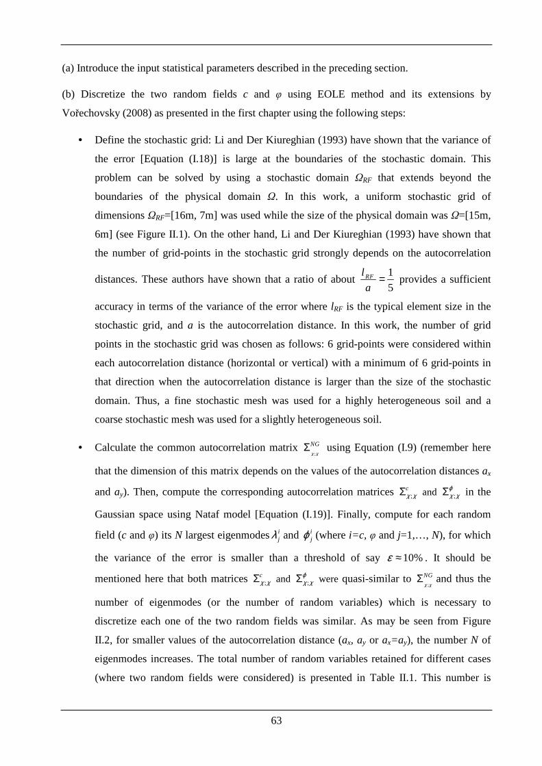
63
(a) Introduce the input statistical parameters described in the preceding section.
(b) Discretize the two random fields c and φ using EOLE method and its extensions by
Vořechovsky (2008) as presented in the first chapter using the following steps:
• Define the stochastic grid: Li and Der Kiureghian (1993) have shown that the variance of
the error [Equation ( I.18)] is large at the boundaries of the stochastic domain. This
problem can be solved by using a stochastic domain ΩRF that extends beyond the
boundaries of the physical domain Ω. In this work, a uniform stochastic grid of
dimensions ΩRF=[16m, 7m] was used while the size of the physical domain was Ω=[15m,
6m] (see Figure II.1). On the other hand, Li and Der Kiureghian (1993) have shown that
the number of grid-points in the stochastic grid strongly depends on the autocorrelation
distances. These authors have shown that a ratio of about 1
5RFl
a= provides a sufficient
accuracy in terms of the variance of the error where lRF is the typical element size in the
stochastic grid, and a is the autocorrelation distance. In this work, the number of grid
points in the stochastic grid was chosen as follows: 6 grid-points were considered within
each autocorrelation distance (horizontal or vertical) with a minimum of 6 grid-points in
that direction when the autocorrelation distance is larger than the size of the stochastic
domain. Thus, a fine stochastic mesh was used for a highly heterogeneous soil and a
coarse stochastic mesh was used for a slightly heterogeneous soil.
• Calculate the common autocorrelation matrix ;
NG
χ χΣ using Equation ( I.9) (remember here
that the dimension of this matrix depends on the values of the autocorrelation distances ax
and ay). Then, compute the corresponding autocorrelation matrices ;cχ χΣ and ;
ϕχ χΣ in the
Gaussian space using Nataf model [Equation ( I.19)]. Finally, compute for each random
field (c and φ) its N largest eigenmodesijλ and ijϕ (where i=c, φ and j=1,…, N), for which
the variance of the error is smaller than a threshold of say 10%ε ≈ . It should be
mentioned here that both matrices ;cχ χΣ and ;
ϕχ χΣ were quasi-similar to
;
NG
χ χΣ and thus the
number of eigenmodes (or the number of random variables) which is necessary to
discretize each one of the two random fields was similar. As may be seen from Figure
II.2, for smaller values of the autocorrelation distance (ax, ay or ax=ay), the number N of
eigenmodes increases. The total number of random variables retained for different cases
(where two random fields were considered) is presented in Table II.1. This number is
64
equal to the number of eigenmodes N of a single random field multiplied by 2 since two
random fields were considered in the analysis. It should be noticed that the cases where a
significant number of random variables (>88) are needed correspond to very small
autocorrelation distances (i.e. ay<1m and ax<2m). These autocorrelation distances are not
of practical interest [see El-Ramly et al. (2003)], and can thus be neglected in this study.
0.00
0.10
0.20
0.30
0.40
0.50
0.60
0.70
0.80
0.90
1.00
0 5 10 15 20 25 30 35 40 45
Number N of eigenmodes(a)
Var
ianc
e o
f th
e e
rror
ax=ay=1.5m ax=ay=1.8max=ay=2max=ay=3max=ay=5max=ay=10m
0.00
0.10
0.20
0.30
0.40
0.50
0.60
0.70
0.80
0.90
1.00
0 5 10 15 20 25 30 35 40 45 50
Number N of eigenmodes(b)
Va
rian
ce o
f th
e e
rro
r
ax=10m, ay=1m ax=10m, ay=0.8max=10m, ay=0.5max=4m, ay=1max=2m, ay=1m
Figure II.2. Number N of eigenmodes needed in the EOLE method: (a) isotropic case, (b) anisotropic case
Total number of random variables used to
discretize the two random fields (c, φ)
1.5x ya a m= = 70
1.8x ya a m= = 60
2x ya a m= = 50
3x ya a m= = 24
5x ya a m= = 20 Isot
ropi
c ca
se
10x ya a m= = 10
10 , 1x ya m a m= = 24
10 , 0.8x ya m a m= = 30
10 , 0.5x ya m a m= = 44
4 , 1x ya m a m= = 48
Ani
sotr
opic
cas
e
2 , 1x ya m a m= = 88
Table II.1. Number of random variables used to discretize the two random fields c and φ for both cases of isotropic and anisotropic autocorrelation distances
65
• Calculate the Gaussian cross-correlated matrix C by applying the Nataf model on the
original non-Gaussian cross-correlation matrix CNG. This was performed using Equation
( I.20).
• Discretize the two anisotropic cross-correlated Gaussian fields c and φ using Equation
( I.21) where κD was computed using Equation ( I.22); the transformation to the non-
Gaussian space being done by applying Equation ( I.23).
(c) Use the adaptive SPCE methodology by Blatman and Sudret (2010) to determine the meta-
model as follows: First, it should be noted that for each realization, the values of the two random
fields (c and φ) were determined at the centroid of each element of the deterministic mesh using
Equations ( I.21) and ( I.23). Once the different elements of the mesh are filed with values of c and
φ, the ultimate bearing capacity (qult) for this specific realization can be determined. The
experimental design (ED) was obtained by first simulating the initial number of realizations
K=200 of the two random fields (c and φ) using MCS technique. The relatively large number of
additional simulations K' =100 is used each time the regression problem is ill-posed (i.e. when the
rank of the matrix used in the regression approach is smaller than the number of unknown
coefficients). The algorithm stops if either the target accuracy 2TARGETQ is achieved or if p reached
the maximal order fixed by the user. In this work, a target accuracy 2 0.999TARGETQ = , a coefficient
q=0.7, and a maximal order p=5 were used. Notice that for the reference case [ax=10m, ay=1m,
r(c, φ) =-0.5], the algorithm have stopped when the target accuracy was reached. The
corresponding order of the SPCE was equal to 4. In this case, where 24 random variables were
needed (see Table II.1), the PCE in its "full" truncation schemes leads to P=20,475 unknown
coefficients. This means that a minimum of 20,475 collocation points (i.e. a minimum of 20,475
calls of the deterministic model) were needed to accurately represent the ultimate bearing
capacity by a meta-model. Using the SPCE methodology, only P=186 unknown coefficients were
retained and only 800 calls of the deterministic model were found to be largely sufficient to
construct the meta-model. Consequently, an important reduction in the number of calls of the
deterministic model can be obtained using the SPCE. This greatly facilitates the solution of the
problem of random fields.
(d) Use the meta-model to perform the post-treatment. This consists in determining: (i) the PDF
of the ultimate bearing capacity and the corresponding statistical moments (mean, variance,
skewness, and kurtosis) and (ii) the Sobol indices for each random field (c and φ).
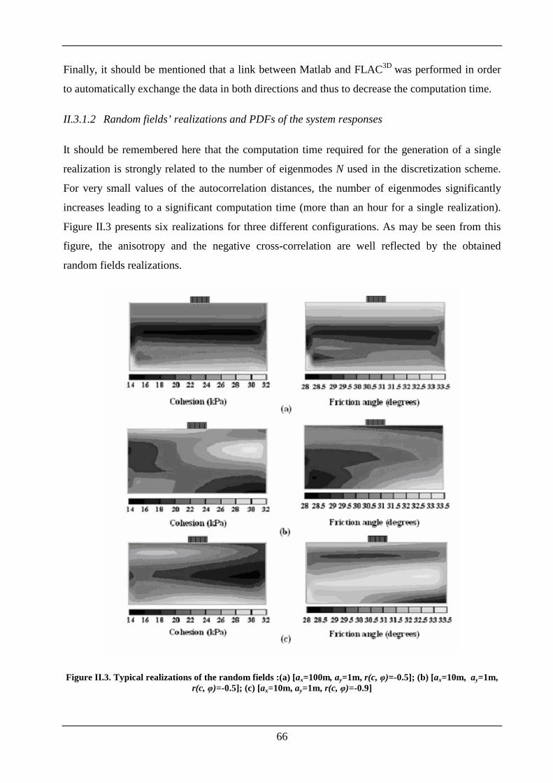
66
Finally, it should be mentioned that a link between Matlab and FLAC3D was performed in order
to automatically exchange the data in both directions and thus to decrease the computation time.
II.3.1.2 Random fields’ realizations and PDFs of the system responses
It should be remembered here that the computation time required for the generation of a single
realization is strongly related to the number of eigenmodes N used in the discretization scheme.
For very small values of the autocorrelation distances, the number of eigenmodes significantly
increases leading to a significant computation time (more than an hour for a single realization).
Figure II.3 presents six realizations for three different configurations. As may be seen from this
figure, the anisotropy and the negative cross-correlation are well reflected by the obtained
random fields realizations.
Figure II.3. Typical realizations of the random fields :(a) [ax=100m, ay=1m, r(c, φ)=-0.5]; (b) [ax=10m, ay=1m, r(c, φ)=-0.5]; (c) [ax=10m, ay=1m, r(c, φ)=-0.9]

67
Figure II.4 presents the PDFs of the footing ultimate bearing capacity and the footing rotation for
the reference case where ax=10m, ay=1m, and r(c, φ)=-0.5. Figure II.5 presents the velocity field
for one single simulation (i.e. a single realization of the two random fields c and φ). As may be
seen from this figure, the spatial variability of the soil properties can produce a non-symmetrical
mechanism even though the footing is subjected to a symmetrical vertical load. Although the
footing rotation of a single realization is not null as may be seen from Figure II.5, the mean value
of the rotation for the whole number of realizations is null [see Figure II.4(b)], and the standard
deviation of this rotation was found equal to 1.6x10⁻⁴ radians. Concerning the ultimate bearing
capacity, its mean and standard deviation values are equal to 658.2kPa and 93.57kPa
respectively.
0.0
0.5
1.0
1.5
2.0
2.5
3.0
3.5
4.0
4.5
5.0
0 200 400 600 800 1000 1200 1400
Ultimate bearing capacity (kPa)(a)
PD
F(x
10-3
)
0.0
0.5
1.0
1.5
2.0
2.5
-10 -5 0 5 10
Footing rotation (%)(b)
PD
F(x
103 )
Figure II.4. Bearing capacity and footing rotation for the reference case where ax=10m, ay=1m, and r(c, φ)=-
0.5: (a) PDF of the ultimate bearing capacity; and (b) PDF of the footing rotation
Figure II.5. Velocity field for a typical realization of the two random fields for the reference case where ax=10m, ay=1m and r(c, φ) =-0.5
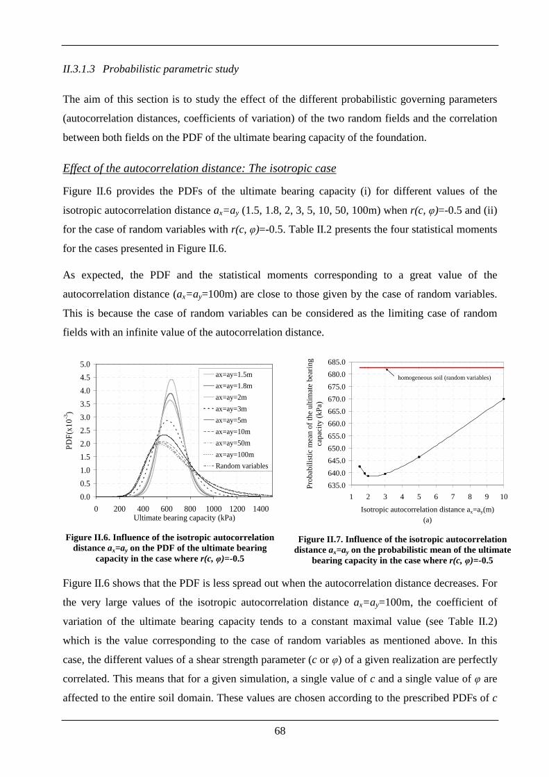
68
II.3.1.3 Probabilistic parametric study
The aim of this section is to study the effect of the different probabilistic governing parameters
(autocorrelation distances, coefficients of variation) of the two random fields and the correlation
between both fields on the PDF of the ultimate bearing capacity of the foundation.
Effect of the autocorrelation distance: The isotropic case
Figure II.6 provides the PDFs of the ultimate bearing capacity (i) for different values of the
isotropic autocorrelation distance ax=ay (1.5, 1.8, 2, 3, 5, 10, 50, 100m) when r(c, φ)=-0.5 and (ii)
for the case of random variables with r(c, φ)=-0.5. Table II.2 presents the four statistical moments
for the cases presented in Figure II.6.
As expected, the PDF and the statistical moments corresponding to a great value of the
autocorrelation distance (ax=ay=100m) are close to those given by the case of random variables.
This is because the case of random variables can be considered as the limiting case of random
fields with an infinite value of the autocorrelation distance.
0.0
0.5
1.0
1.5
2.0
2.5
3.0
3.5
4.0
4.5
5.0
0 200 400 600 800 1000 1200 1400Ultimate bearing capacity (kPa)
PD
F(x
10-3
)
ax=ay=1.5m
ax=ay=1.8m
ax=ay=2m
ax=ay=3m
ax=ay=5m
ax=ay=10m
ax=ay=50m
ax=ay=100m
Random variables
Figure II.6. Influence of the isotropic autocorrelation
distance ax=ay on the PDF of the ultimate bearing capacity in the case where r(c, φ)=-0.5
635.0
640.0
645.0
650.0
655.0
660.0
665.0
670.0
675.0
680.0
685.0
1 2 3 4 5 6 7 8 9 10
Isotropic autocorrelation distance ax=ay(m)(a)
Pro
babi
listic
mea
n o
f th
e ul
timat
e be
arin
g ca
paci
ty (
kPa)
homogeneous soil (random variables)
Figure II.7. Influence of the isotropic autocorrelation
distance ax=ay on the probabilistic mean of the ultimate bearing capacity in the case where r(c, φ)=-0.5
Figure II.6 shows that the PDF is less spread out when the autocorrelation distance decreases. For
the very large values of the isotropic autocorrelation distance ax=ay=100m, the coefficient of
variation of the ultimate bearing capacity tends to a constant maximal value (see Table II.2)
which is the value corresponding to the case of random variables as mentioned above. In this
case, the different values of a shear strength parameter (c or φ) of a given realization are perfectly
correlated. This means that for a given simulation, a single value of c and a single value of φ are
affected to the entire soil domain. These values are chosen according to the prescribed PDFs of c
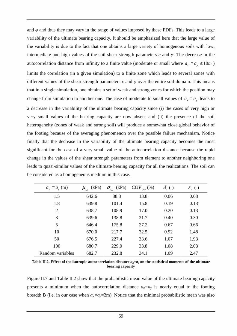
69
and φ and thus they may vary in the range of values imposed by these PDFs. This leads to a large
variability of the ultimate bearing capacity. It should be emphasized here that the large value of
the variability is due to the fact that one obtains a large variety of homogenous soils with low,
intermediate and high values of the soil shear strength parameters c and φ. The decrease in the
autocorrelation distance from infinity to a finite value (moderate or small where 10x ya a m= ≤ )
limits the correlation (in a given simulation) to a finite zone which leads to several zones with
different values of the shear strength parameters c and φ over the entire soil domain. This means
that in a single simulation, one obtains a set of weak and strong zones for which the position may
change from simulation to another one. The case of moderate to small values of x ya a= leads to
a decrease in the variability of the ultimate bearing capacity since (i) the cases of very high or
very small values of the bearing capacity are now absent and (ii) the presence of the soil
heterogeneity (zones of weak and strong soil) will produce a somewhat close global behavior of
the footing because of the averaging phenomenon over the possible failure mechanism. Notice
finally that the decrease in the variability of the ultimate bearing capacity becomes the most
significant for the case of a very small value of the autocorrelation distance because the rapid
change in the values of the shear strength parameters from element to another neighboring one
leads to quasi-similar values of the ultimate bearing capacity for all the realizations. The soil can
be considered as a homogeneous medium in this case.
x ya a= (m) (kPa)ultqµ (kPa)
ultqσ (%)qultCOV (-)uδ (-)uκ
1.5 642.6 88.8 13.8 0.06 0.08
1.8 639.8 101.4 15.8 0.19 0.13
2 638.7 108.9 17.0 0.20 0.13
3 639.6 138.8 21.7 0.40 0.30
5 646.4 175.8 27.2 0.67 0.66
10 670.0 217.7 32.5 0.92 1.48
50 676.5 227.4 33.6 1.07 1.93
100 680.7 229.9 33.8 1.08 2.03
Random variables 682.7 232.8 34.1 1.09 2.47
Table II.2. Effect of the isotropic autocorrelation distance ax=ay on the statistical moments of the ultimate bearing capacity
Figure II.7 and Table II.2 show that the probabilistic mean value of the ultimate bearing capacity
presents a minimum when the autocorrelation distance ax=ay is nearly equal to the footing
breadth B (i.e. in our case when ax=ay=2m). Notice that the minimal probabilistic mean was also
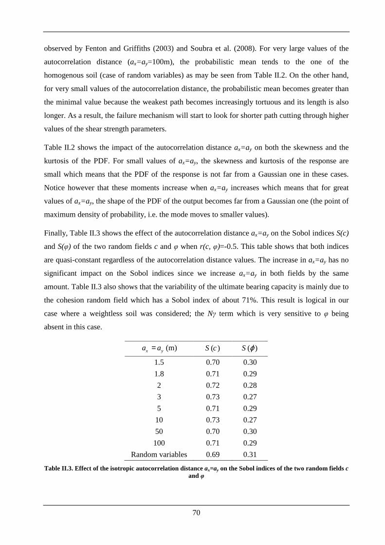
70
observed by Fenton and Griffiths (2003) and Soubra et al. (2008). For very large values of the
autocorrelation distance (ax=ay=100m), the probabilistic mean tends to the one of the
homogenous soil (case of random variables) as may be seen from Table II.2. On the other hand,
for very small values of the autocorrelation distance, the probabilistic mean becomes greater than
the minimal value because the weakest path becomes increasingly tortuous and its length is also
longer. As a result, the failure mechanism will start to look for shorter path cutting through higher
values of the shear strength parameters.
Table II.2 shows the impact of the autocorrelation distance ax=ay on both the skewness and the
kurtosis of the PDF. For small values of ax=ay, the skewness and kurtosis of the response are
small which means that the PDF of the response is not far from a Gaussian one in these cases.
Notice however that these moments increase when ax=ay increases which means that for great
values of ax=ay, the shape of the PDF of the output becomes far from a Gaussian one (the point of
maximum density of probability, i.e. the mode moves to smaller values).
Finally, Table II.3 shows the effect of the autocorrelation distance ax=ay on the Sobol indices S(c)
and S(φ) of the two random fields c and φ when r(c, φ)=-0.5. This table shows that both indices
are quasi-constant regardless of the autocorrelation distance values. The increase in ax=ay has no
significant impact on the Sobol indices since we increase ax=ay in both fields by the same
amount. Table II.3 also shows that the variability of the ultimate bearing capacity is mainly due to
the cohesion random field which has a Sobol index of about 71%. This result is logical in our
case where a weightless soil was considered; the Nγ term which is very sensitive to φ being
absent in this case.
x ya a= (m) ( )S c ( )S ϕ
1.5 0.70 0.30
1.8 0.71 0.29
2 0.72 0.28
3 0.73 0.27
5 0.71 0.29
10 0.73 0.27
50 0.70 0.30
100 0.71 0.29
Random variables 0.69 0.31
Table II.3. Effect of the isotropic autocorrelation distance ax=ay on the Sobol indices of the two random fields c and φ
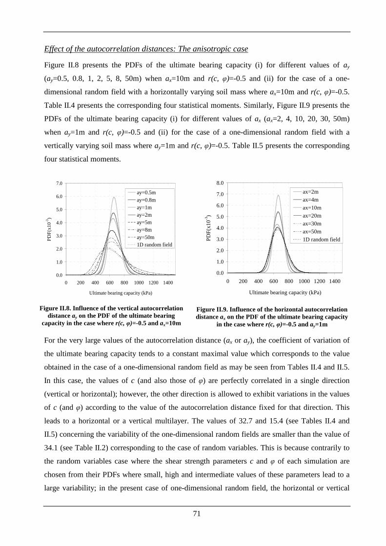
71
Effect of the autocorrelation distances: The anisotropic case
Figure II.8 presents the PDFs of the ultimate bearing capacity (i) for different values of ay
(ay=0.5, 0.8, 1, 2, 5, 8, 50m) when ax=10m and r(c, φ)=-0.5 and (ii) for the case of a one-
dimensional random field with a horizontally varying soil mass where ax=10m and r(c, φ)=-0.5.
Table II.4 presents the corresponding four statistical moments. Similarly, Figure II.9 presents the
PDFs of the ultimate bearing capacity (i) for different values of ax (ax=2, 4, 10, 20, 30, 50m)
when ay=1m and r(c, φ)=-0.5 and (ii) for the case of a one-dimensional random field with a
vertically varying soil mass where ay=1m and r(c, φ)=-0.5. Table II.5 presents the corresponding
four statistical moments.
0.0
1.0
2.0
3.0
4.0
5.0
6.0
7.0
0 200 400 600 800 1000 1200 1400
Ultimate bearing capacity (kPa)
PD
F(x
10-3
)
ay=0.5may=0.8may=1may=2may=5may=8may=50m1D random field
Figure II.8. Influence of the vertical autocorrelation
distance ay on the PDF of the ultimate bearing capacity in the case where r(c, φ)=-0.5 and ax=10m
0.0
1.0
2.0
3.0
4.0
5.0
6.0
7.0
8.0
0 200 400 600 800 1000 1200 1400
Ultimate bearing capacity (kPa)
PD
F(x
10-3
)
ax=2m
ax=4m
ax=10m
ax=20m
ax=30m
ax=50m
1D random field
Figure II.9. Influence of the horizontal autocorrelation distance ax on the PDF of the ultimate bearing capacity
in the case where r(c, φ)=-0.5 and ay=1m
For the very large values of the autocorrelation distance (ax or ay), the coefficient of variation of
the ultimate bearing capacity tends to a constant maximal value which corresponds to the value
obtained in the case of a one-dimensional random field as may be seen from Tables II.4 and II.5.
In this case, the values of c (and also those of φ) are perfectly correlated in a single direction
(vertical or horizontal); however, the other direction is allowed to exhibit variations in the values
of c (and φ) according to the value of the autocorrelation distance fixed for that direction. This
leads to a horizontal or a vertical multilayer. The values of 32.7 and 15.4 (see Tables II.4 and
II.5) concerning the variability of the one-dimensional random fields are smaller than the value of
34.1 (see Table II.2) corresponding to the case of random variables. This is because contrarily to
the random variables case where the shear strength parameters c and φ of each simulation are
chosen from their PDFs where small, high and intermediate values of these parameters lead to a
large variability; in the present case of one-dimensional random field, the horizontal or vertical
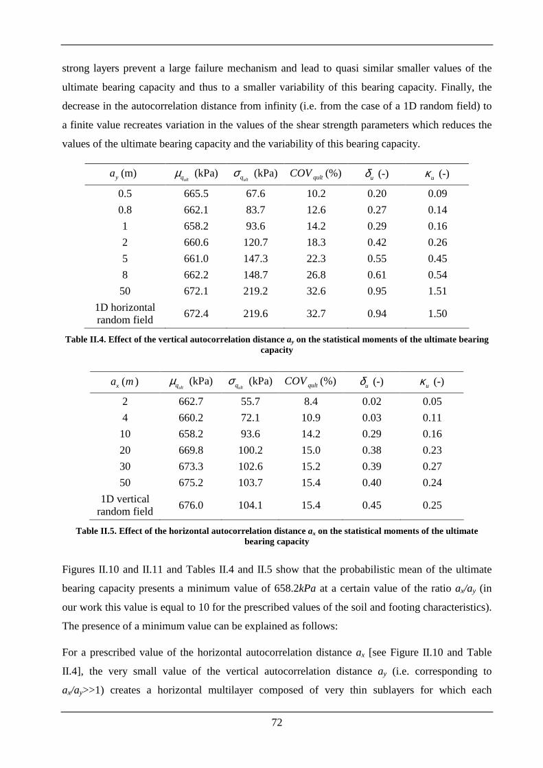
72
strong layers prevent a large failure mechanism and lead to quasi similar smaller values of the
ultimate bearing capacity and thus to a smaller variability of this bearing capacity. Finally, the
decrease in the autocorrelation distance from infinity (i.e. from the case of a 1D random field) to
a finite value recreates variation in the values of the shear strength parameters which reduces the
values of the ultimate bearing capacity and the variability of this bearing capacity.
(m) ya (kPa)ultqµ (kPa)
ultqσ (%)qultCOV (-)uδ (-)uκ
0.5 665.5 67.6 10.2 0.20 0.09
0.8 662.1 83.7 12.6 0.27 0.14
1 658.2 93.6 14.2 0.29 0.16
2 660.6 120.7 18.3 0.42 0.26
5 661.0 147.3 22.3 0.55 0.45
8 662.2 148.7 26.8 0.61 0.54
50 672.1 219.2 32.6 0.95 1.51
1D horizontal random field
672.4 219.6 32.7 0.94 1.50
Table II.4. Effect of the vertical autocorrelation distance ay on the statistical moments of the ultimate bearing capacity
( )xa m (kPa)ultqµ (kPa)
ultqσ (%)qultCOV (-)uδ (-)uκ
2 662.7 55.7 8.4 0.02 0.05
4 660.2 72.1 10.9 0.03 0.11
10 658.2 93.6 14.2 0.29 0.16
20 669.8 100.2 15.0 0.38 0.23
30 673.3 102.6 15.2 0.39 0.27
50 675.2 103.7 15.4 0.40 0.24
1D vertical random field
676.0 104.1 15.4 0.45 0.25
Table II.5. Effect of the horizontal autocorrelation distance ax on the statistical moments of the ultimate bearing capacity
Figures II.10 and II.11 and Tables II.4 and II.5 show that the probabilistic mean of the ultimate
bearing capacity presents a minimum value of 658.2kPa at a certain value of the ratio ax/ay (in
our work this value is equal to 10 for the prescribed values of the soil and footing characteristics).
The presence of a minimum value can be explained as follows:
For a prescribed value of the horizontal autocorrelation distance ax [see Figure II.10 and Table
II.4], the very small value of the vertical autocorrelation distance ay (i.e. corresponding to
ax/ay>>1) creates a horizontal multilayer composed of very thin sublayers for which each
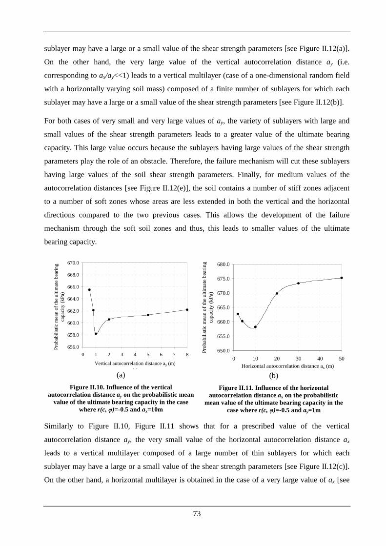
73
sublayer may have a large or a small value of the shear strength parameters [see Figure II.12(a)].
On the other hand, the very large value of the vertical autocorrelation distance ay (i.e.
corresponding to ax/ay<<1) leads to a vertical multilayer (case of a one-dimensional random field
with a horizontally varying soil mass) composed of a finite number of sublayers for which each
sublayer may have a large or a small value of the shear strength parameters [see Figure II.12(b)].
For both cases of very small and very large values of ay, the variety of sublayers with large and
small values of the shear strength parameters leads to a greater value of the ultimate bearing
capacity. This large value occurs because the sublayers having large values of the shear strength
parameters play the role of an obstacle. Therefore, the failure mechanism will cut these sublayers
having large values of the soil shear strength parameters. Finally, for medium values of the
autocorrelation distances [see Figure II.12(e)], the soil contains a number of stiff zones adjacent
to a number of soft zones whose areas are less extended in both the vertical and the horizontal
directions compared to the two previous cases. This allows the development of the failure
mechanism through the soft soil zones and thus, this leads to smaller values of the ultimate
bearing capacity.
656.0
658.0
660.0
662.0
664.0
666.0
668.0
670.0
0 1 2 3 4 5 6 7 8
Vertical autocorrelation distance ay (m)(a)
Pro
bab
ilist
ic m
ean
of t
he u
ltim
ate
bear
ing
ca
paci
ty (
kPa)
(a)
Figure II.10. Influence of the vertical autocorrelation distance ay on the probabilistic mean
value of the ultimate bearing capacity in the case where r(c, φ)=-0.5 and ax=10m
650.0
655.0
660.0
665.0
670.0
675.0
680.0
0 10 20 30 40 50Horizontal autocorrelation distance ax (m)
Pro
bab
ilist
ic m
ean o
f th
e ulti
mat
e bea
ring
capac
ity (
kPa)
(b)
Figure II.11. Influence of the horizontal autocorrelation distance ax on the probabilistic
mean value of the ultimate bearing capacity in the case where r(c, φ)=-0.5 and ay=1m
Similarly to Figure II.10, Figure II.11 shows that for a prescribed value of the vertical
autocorrelation distance ay, the very small value of the horizontal autocorrelation distance ax
leads to a vertical multilayer composed of a large number of thin sublayers for which each
sublayer may have a large or a small value of the shear strength parameters [see Figure II.12(c)].
On the other hand, a horizontal multilayer is obtained in the case of a very large value of ax [see
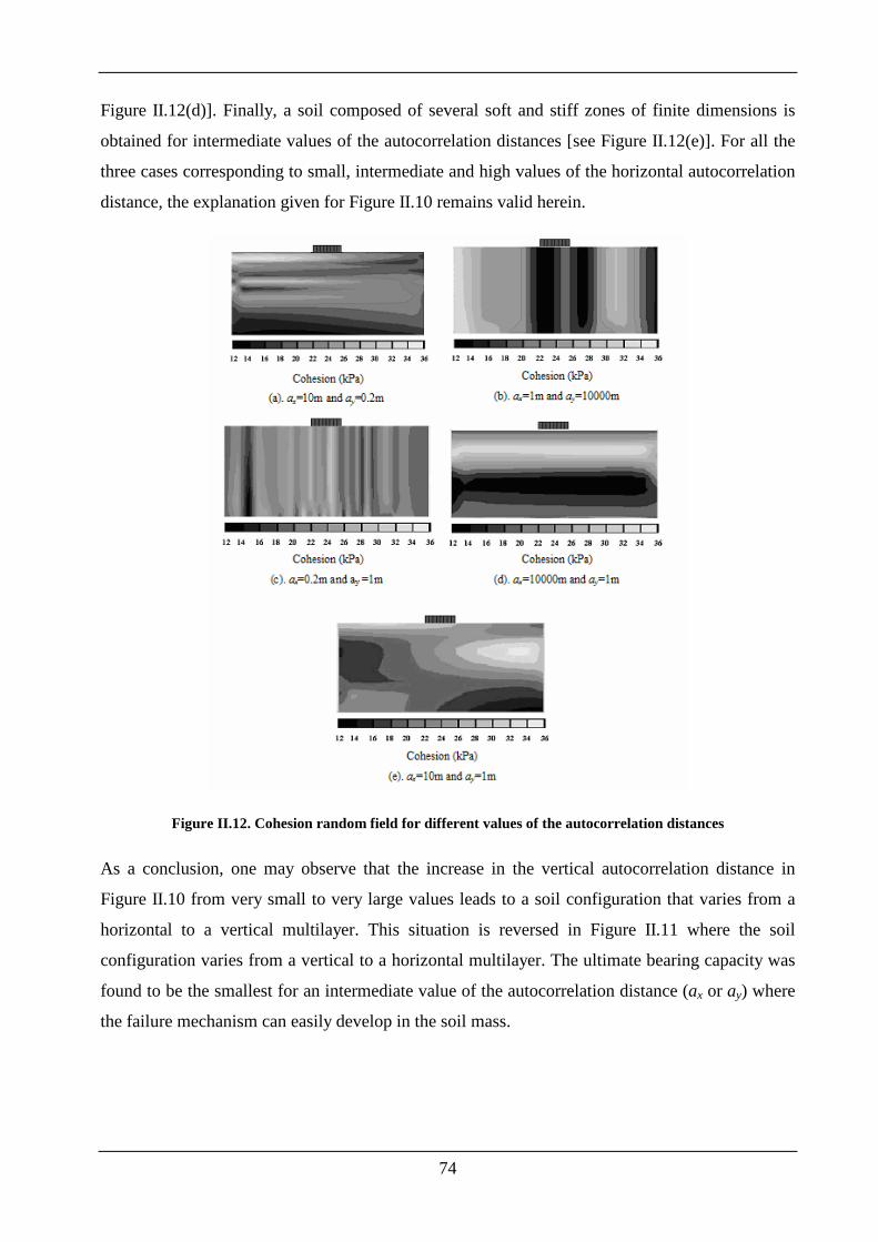
74
Figure II.12(d)]. Finally, a soil composed of several soft and stiff zones of finite dimensions is
obtained for intermediate values of the autocorrelation distances [see Figure II.12(e)]. For all the
three cases corresponding to small, intermediate and high values of the horizontal autocorrelation
distance, the explanation given for Figure II.10 remains valid herein.
Figure II.12. Cohesion random field for different values of the autocorrelation distances
As a conclusion, one may observe that the increase in the vertical autocorrelation distance in
Figure II.10 from very small to very large values leads to a soil configuration that varies from a
horizontal to a vertical multilayer. This situation is reversed in Figure II.11 where the soil
configuration varies from a vertical to a horizontal multilayer. The ultimate bearing capacity was
found to be the smallest for an intermediate value of the autocorrelation distance (ax or ay) where
the failure mechanism can easily develop in the soil mass.
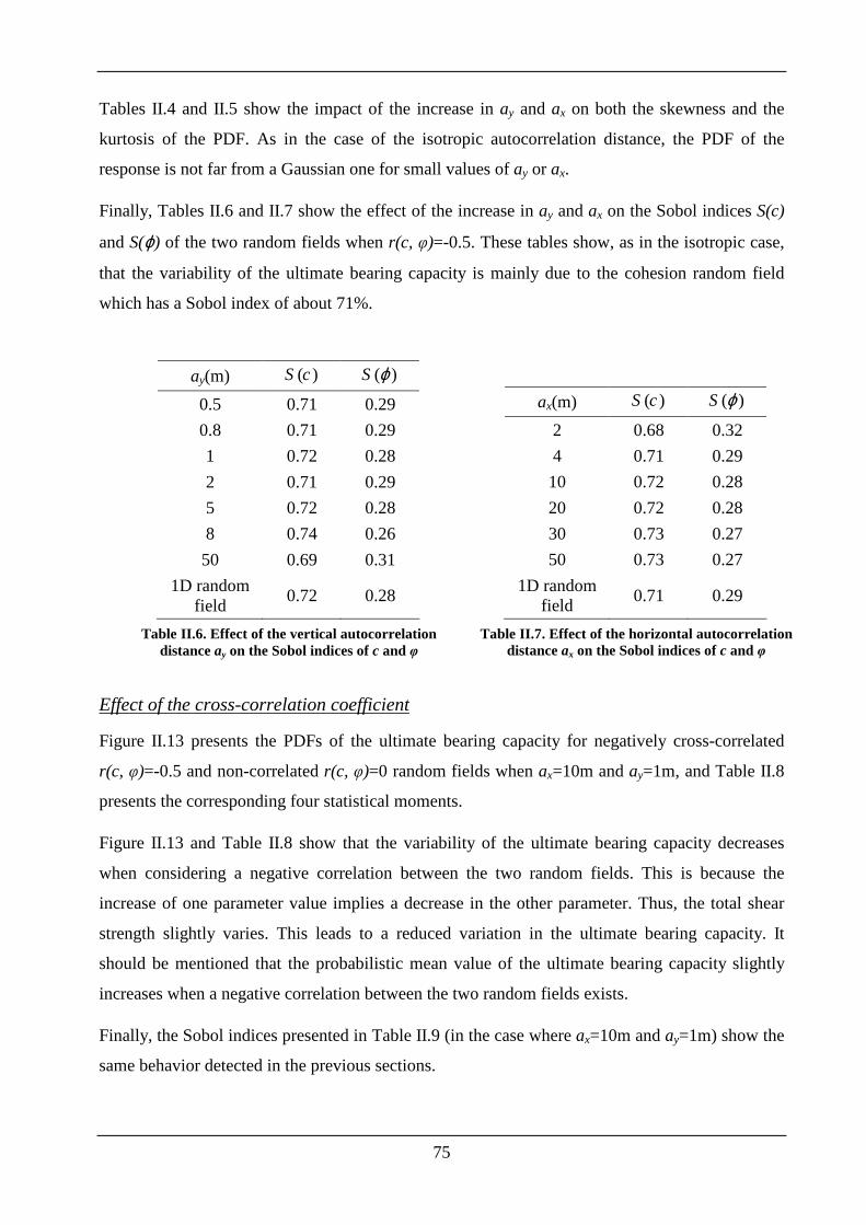
75
Tables II.4 and II.5 show the impact of the increase in ay and ax on both the skewness and the
kurtosis of the PDF. As in the case of the isotropic autocorrelation distance, the PDF of the
response is not far from a Gaussian one for small values of ay or ax.
Finally, Tables II.6 and II.7 show the effect of the increase in ay and ax on the Sobol indices S(c)
and S(ϕ) of the two random fields when r(c, φ)=-0.5. These tables show, as in the isotropic case,
that the variability of the ultimate bearing capacity is mainly due to the cohesion random field
which has a Sobol index of about 71%.
Table II.6. Effect of the vertical autocorrelation distance ay on the Sobol indices of c and φ
ay(m) ( )S c ( )S ϕ
0.5 0.71 0.29
0.8 0.71 0.29
1 0.72 0.28
2 0.71 0.29
5 0.72 0.28
8 0.74 0.26
50 0.69 0.31
1D random field
0.72 0.28
Table II.7. Effect of the horizontal autocorrelation distance ax on the Sobol indices of c and φ
ax(m) ( )S c ( )S ϕ
2 0.68 0.32
4 0.71 0.29
10 0.72 0.28
20 0.72 0.28
30 0.73 0.27
50 0.73 0.27
1D random field
0.71 0.29
Effect of the cross-correlation coefficient
Figure II.13 presents the PDFs of the ultimate bearing capacity for negatively cross-correlated
r(c, φ)=-0.5 and non-correlated r(c, φ)=0 random fields when ax=10m and ay=1m, and Table II.8
presents the corresponding four statistical moments.
Figure II.13 and Table II.8 show that the variability of the ultimate bearing capacity decreases
when considering a negative correlation between the two random fields. This is because the
increase of one parameter value implies a decrease in the other parameter. Thus, the total shear
strength slightly varies. This leads to a reduced variation in the ultimate bearing capacity. It
should be mentioned that the probabilistic mean value of the ultimate bearing capacity slightly
increases when a negative correlation between the two random fields exists.
Finally, the Sobol indices presented in Table II.9 (in the case where ax=10m and ay=1m) show the
same behavior detected in the previous sections.
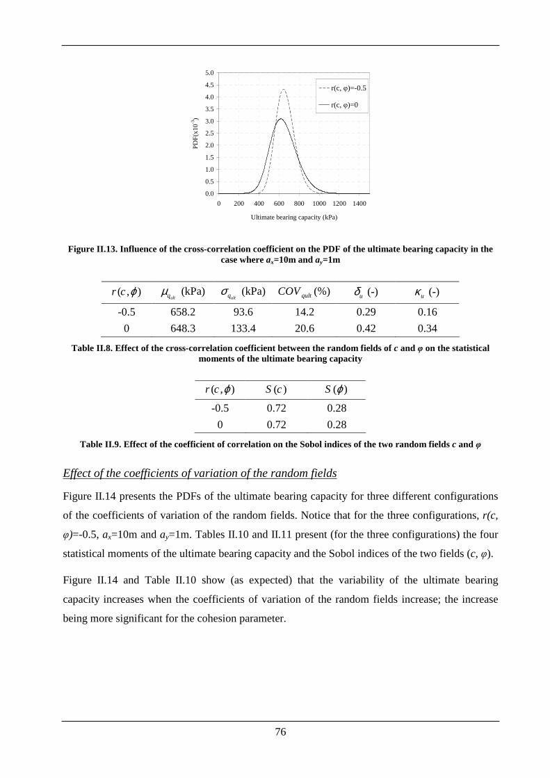
76
0.0
0.5
1.0
1.5
2.0
2.5
3.0
3.5
4.0
4.5
5.0
0 200 400 600 800 1000 1200 1400
Ultimate bearing capacity (kPa)
PD
F(x
10-3)
r(c, φ)=-0.5
r(c, φ)=0
Figure II.13. Influence of the cross-correlation coefficient on the PDF of the ultimate bearing capacity in the case where ax=10m and ay=1m
( , )r c ϕ (kPa)ultqµ (kPa)
ultqσ (%)qultCOV (-)uδ (-)uκ
-0.5 658.2 93.6 14.2 0.29 0.16
0 648.3 133.4 20.6 0.42 0.34
Table II.8. Effect of the cross-correlation coefficient between the random fields of c and φ on the statistical moments of the ultimate bearing capacity
( , )r c ϕ ( )S c ( )S ϕ
-0.5 0.72 0.28
0 0.72 0.28
Table II.9. Effect of the coefficient of correlation on the Sobol indices of the two random fields c and φ
Effect of the coefficients of variation of the random fields
Figure II.14 presents the PDFs of the ultimate bearing capacity for three different configurations
of the coefficients of variation of the random fields. Notice that for the three configurations, r(c,
φ)=-0.5, ax=10m and ay=1m. Tables II.10 and II.11 present (for the three configurations) the four
statistical moments of the ultimate bearing capacity and the Sobol indices of the two fields (c, φ).
Figure II.14 and Table II.10 show (as expected) that the variability of the ultimate bearing
capacity increases when the coefficients of variation of the random fields increase; the increase
being more significant for the cohesion parameter.
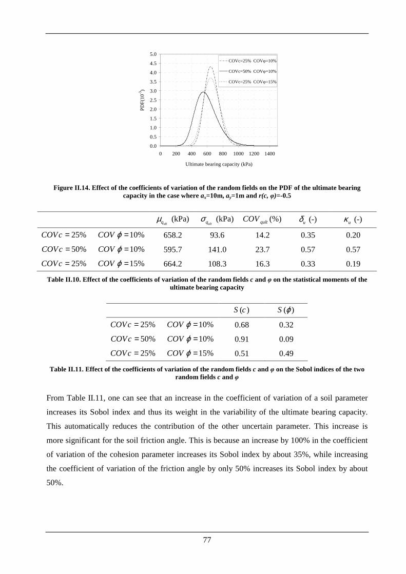
77
0.0
0.5
1.0
1.5
2.0
2.5
3.0
3.5
4.0
4.5
5.0
0 200 400 600 800 1000 1200 1400
Ultimate bearing capacity (kPa)
PD
F(1
0-3)
COVc=25% COVφ=10%
COVc=50% COVφ=10%
COVc=25% COVφ=15%
Figure II.14. Effect of the coefficients of variation of the random fields on the PDF of the ultimate bearing capacity in the case where ax=10m, ay=1m and r(c, φ)=-0.5
(kPa)ultqµ (kPa)
ultqσ (%)qultCOV (-)uδ (-)uκ
25% 10%COVc COVϕ= = 658.2 93.6 14.2 0.35 0.20
50% 10%COVc COVϕ= = 595.7 141.0 23.7 0.57 0.57
25% 15%COVc COVϕ= = 664.2 108.3 16.3 0.33 0.19
Table II.10. Effect of the coefficients of variation of the random fields c and φ on the statistical moments of the ultimate bearing capacity
( )S c ( )S ϕ
25% 10%COVc COVϕ= = 0.68 0.32
50% 10%COVc COVϕ= = 0.91 0.09
25% 15%COVc COVϕ= = 0.51 0.49
Table II.11. Effect of the coefficients of variation of the random fields c and φ on the Sobol indices of the two random fields c and φ
From Table II.11, one can see that an increase in the coefficient of variation of a soil parameter
increases its Sobol index and thus its weight in the variability of the ultimate bearing capacity.
This automatically reduces the contribution of the other uncertain parameter. This increase is
more significant for the soil friction angle. This is because an increase by 100% in the coefficient
of variation of the cohesion parameter increases its Sobol index by about 35%, while increasing
the coefficient of variation of the friction angle by only 50% increases its Sobol index by about
50%.
78
II.3.2 The serviceability limit state SLS case
The aim of this section is to present the probabilistic numerical results obtained from the analysis
at the serviceability limit state (SLS) of strip footings resting on a spatially varying soil and
subjected to a central vertical load (Pv). It involves the computation of the central vertical footing
displacement (v).
Both the soil Young modulus E and the soil Poisson ratio υ were firstly considered as random
fields in order to determine the weight of each random field in the variability of the system
response. In a second stage, only the uncertain parameter with a significant weight in the
variability of the system response will be considered as a random field. Notice that the same
autocorrelation function (square exponential) was used for both random fields. Both cases of
isotropic (i.e. ax=ay) and anisotropic (i.e. ax#ay) random fields will be treated and the same values
of the autocorrelation distances employed in the ULS case are used herein.
The soil Young modulus E was assumed to be lognormally distributed. Its mean value and
coefficient of variation (referred to as reference values) were taken as
follows: 60 , 15%E EMPa Covµ = = . Similarly, the soil Poisson ratio υ was assumed to be
lognormally distributed with a mean value and a coefficient of variation given as follows:
0.3, 5%Covν νµ = = .
The deterministic model was based on numerical simulations using the finite difference code
FLAC3D. Even though a serviceability limit state is considered, the soil behavior was modeled
using a conventional elastic-perfectly plastic model based on Mohr-Coulomb failure criterion in
order to consider the plasticity that may occur at the footing edges even under the service loads.
Notice that the soil cohesion c, the soil angle of internal friction φ and the soil dilation angle ψ
were assumed to be deterministic since the footing vertical displacement is not sensitive to these
variables. Their corresponding values were respectively 20c kPa= , 30oϕ = and 20oψ = .
Concerning the footing and the interface properties, they were considered as deterministic. The
same mean values used for these properties in the ULS case were employed herein. Moreover,
the soil domain and mesh used in the ULS analysis (cf. Figure II.1) were also utilized in this case.
Finally, notice that the footing was subjected to a vertical applied pressure qa=500kPa.
The following sections are organized as follows: First, a global sensitivity analysis is performed
considering both the soil Young modulus E and the soil Poisson ratio υ as random fields. This is
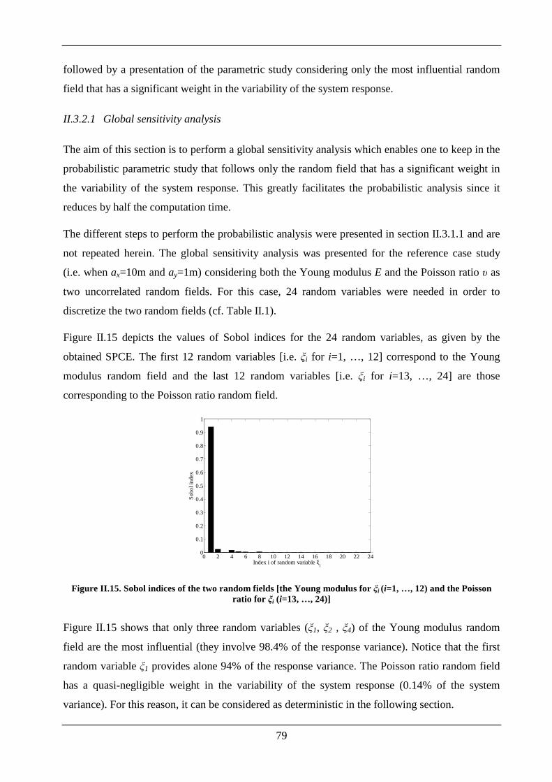
79
followed by a presentation of the parametric study considering only the most influential random
field that has a significant weight in the variability of the system response.
II.3.2.1 Global sensitivity analysis
The aim of this section is to perform a global sensitivity analysis which enables one to keep in the
probabilistic parametric study that follows only the random field that has a significant weight in
the variability of the system response. This greatly facilitates the probabilistic analysis since it
reduces by half the computation time.
The different steps to perform the probabilistic analysis were presented in section II.3.1.1 and are
not repeated herein. The global sensitivity analysis was presented for the reference case study
(i.e. when ax=10m and ay=1m) considering both the Young modulus E and the Poisson ratio υ as
two uncorrelated random fields. For this case, 24 random variables were needed in order to
discretize the two random fields (cf. Table II.1).
Figure II.15 depicts the values of Sobol indices for the 24 random variables, as given by the
obtained SPCE. The first 12 random variables [i.e. ξi for i=1, …, 12] correspond to the Young
modulus random field and the last 12 random variables [i.e. ξi for i=13, …, 24] are those
corresponding to the Poisson ratio random field.
0 2 4 6 8 10 12 14 16 18 20 22 240
0.1
0.2
0.3
0.4
0.5
0.6
0.7
0.8
0.9
1
Index i of random variable ξi
Sob
ol in
dex
Figure II.15. Sobol indices of the two random fields [the Young modulus for ξi (i=1, …, 12) and the Poisson ratio for ξi (i=13, …, 24)]
Figure II.15 shows that only three random variables (ξ1, ξ2 , ξ4) of the Young modulus random
field are the most influential (they involve 98.4% of the response variance). Notice that the first
random variable ξ1 provides alone 94% of the response variance. The Poisson ratio random field
has a quasi-negligible weight in the variability of the system response (0.14% of the system
variance). For this reason, it can be considered as deterministic in the following section.
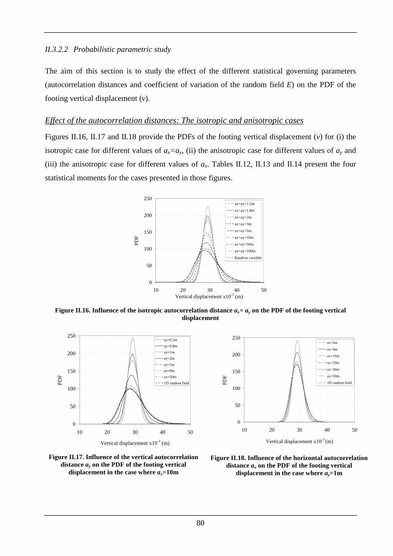
80
II.3.2.2 Probabilistic parametric study
The aim of this section is to study the effect of the different statistical governing parameters
(autocorrelation distances and coefficient of variation of the random field E) on the PDF of the
footing vertical displacement (v).
Effect of the autocorrelation distances: The isotropic and anisotropic cases
Figures II.16, II.17 and II.18 provide the PDFs of the footing vertical displacement (v) for (i) the
isotropic case for different values of ax=ay, (ii) the anisotropic case for different values of ay and
(iii) the anisotropic case for different values of ax. Tables II.12, II.13 and II.14 present the four
statistical moments for the cases presented in those figures.
0
50
100
150
200
250
10 20 30 40 50Vertical displacement x10-3 (m)
PD
F
ax=ay=1.5m
ax=ay=1.8m
ax=ay=2m
ax=ay=3m
ax=ay=5m
ax=ay=10m
ax=ay=50m
ax=ay=100m
Random variable
Figure II.16. Influence of the isotropic autocorrelation distance ax= ay on the PDF of the footing vertical
displacement
0
50
100
150
200
250
10 20 30 40 50
Vertical displacement x10-3 (m)
PD
F
ay=0.5m
ay=0.8m
ay=1m
ay=2m
ay=5m
ay=8m
ay=50m
1D random field
Figure II.17. Influence of the vertical autocorrelation
distance ay on the PDF of the footing vertical displacement in the case where ax=10m
0
50
100
150
200
250
10 20 30 40 50
Vertical displacement x10-3 (m)
PD
F
ax=2m
ax=4m
ax=10m
ax=20m
ax=30m
ax=50m
1D random field
Figure II.18. Influence of the horizontal autocorrelation
distance ax on the PDF of the footing vertical displacement in the case where ay=1m
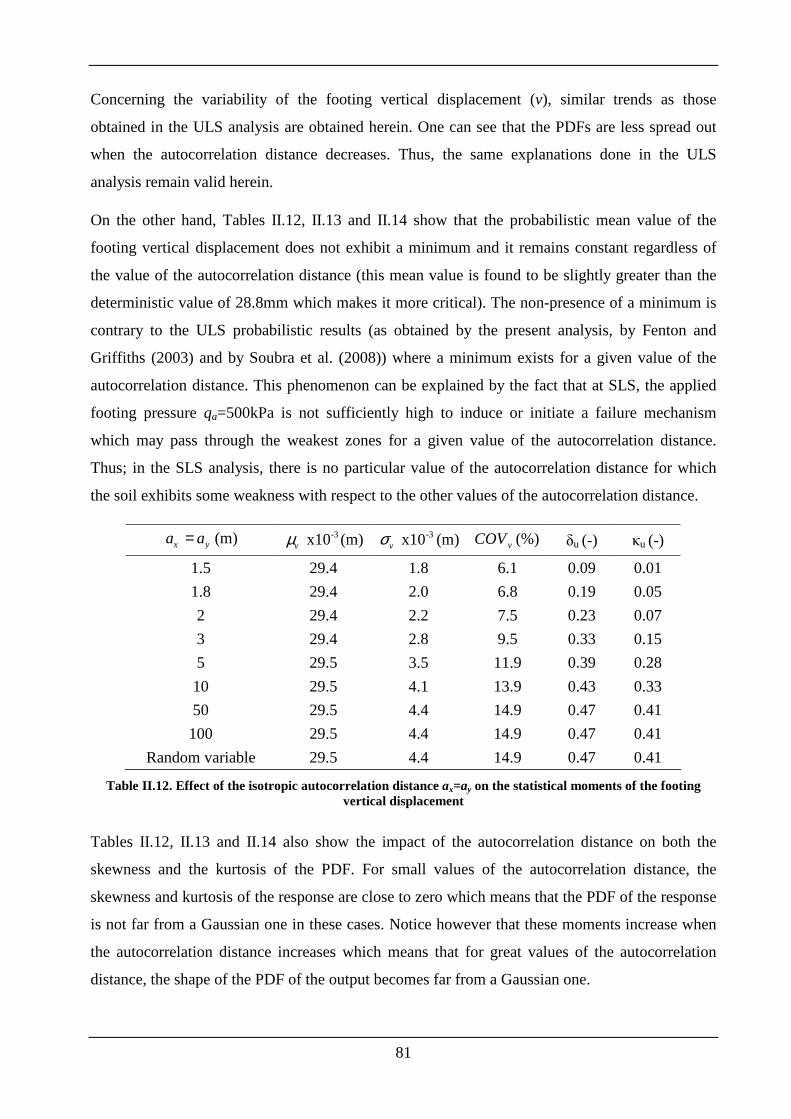
81
Concerning the variability of the footing vertical displacement (v), similar trends as those
obtained in the ULS analysis are obtained herein. One can see that the PDFs are less spread out
when the autocorrelation distance decreases. Thus, the same explanations done in the ULS
analysis remain valid herein.
On the other hand, Tables II.12, II.13 and II.14 show that the probabilistic mean value of the
footing vertical displacement does not exhibit a minimum and it remains constant regardless of
the value of the autocorrelation distance (this mean value is found to be slightly greater than the
deterministic value of 28.8mm which makes it more critical). The non-presence of a minimum is
contrary to the ULS probabilistic results (as obtained by the present analysis, by Fenton and
Griffiths (2003) and by Soubra et al. (2008)) where a minimum exists for a given value of the
autocorrelation distance. This phenomenon can be explained by the fact that at SLS, the applied
footing pressure qa=500kPa is not sufficiently high to induce or initiate a failure mechanism
which may pass through the weakest zones for a given value of the autocorrelation distance.
Thus; in the SLS analysis, there is no particular value of the autocorrelation distance for which
the soil exhibits some weakness with respect to the other values of the autocorrelation distance.
x ya a= (m) -3 x10vµ (m) -3 x10vσ (m) (%)vCOV δu (-) κu (-)
1.5 29.4 1.8 6.1 0.09 0.01
1.8 29.4 2.0 6.8 0.19 0.05
2 29.4 2.2 7.5 0.23 0.07
3 29.4 2.8 9.5 0.33 0.15
5 29.5 3.5 11.9 0.39 0.28
10 29.5 4.1 13.9 0.43 0.33
50 29.5 4.4 14.9 0.47 0.41
100 29.5 4.4 14.9 0.47 0.41
Random variable 29.5 4.4 14.9 0.47 0.41
Table II.12. Effect of the isotropic autocorrelation distance ax=ay on the statistical moments of the footing vertical displacement
Tables II.12, II.13 and II.14 also show the impact of the autocorrelation distance on both the
skewness and the kurtosis of the PDF. For small values of the autocorrelation distance, the
skewness and kurtosis of the response are close to zero which means that the PDF of the response
is not far from a Gaussian one in these cases. Notice however that these moments increase when
the autocorrelation distance increases which means that for great values of the autocorrelation
distance, the shape of the PDF of the output becomes far from a Gaussian one.
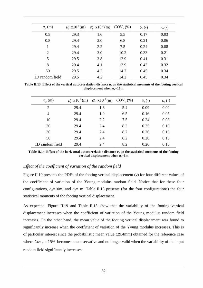
82
ya (m) -3 x10vµ (m) -3 x10vσ (m) (%)vCOV δu (-) κu (-)
0.5 29.3 1.6 5.5 0.17 0.03
0.8 29.4 2.0 6.8 0.21 0.06
1 29.4 2.2 7.5 0.24 0.08
2 29.4 3.0 10.2 0.33 0.21
5 29.5 3.8 12.9 0.41 0.31
8 29.4 4.1 13.9 0.42 0.32
50 29.5 4.2 14.2 0.45 0.34
1D random field 29.5 4.2 14.2 0.45 0.34
Table II.13. Effect of the vertical autocorrelation distance ay on the statistical moments of the footing vertical displacement when ax=10m
xa (m) -3 x10vµ (m) -3 x10vσ (m) (%)vCOV δu (-) κu (-)
2 29.4 1.6 5.4 0.09 0.02
4 29.4 1.9 6.5 0.16 0.05
10 29.4 2.2 7.5 0.24 0.08
20 29.4 2.4 8.2 0.25 0.10
30 29.4 2.4 8.2 0.26 0.15
50 29.4 2.4 8.2 0.26 0.15
1D random field 29.4 2.4 8.2 0.26 0.15
Table II.14. Effect of the horizontal autocorrelation distance ax on the statistical moments of the footing vertical displacement when ay=1m
Effect of the coefficient of variation of the random field
Figure II.19 presents the PDFs of the footing vertical displacement (v) for four different values of
the coefficient of variation of the Young modulus random field. Notice that for these four
configurations, ax=10m, and ay=1m. Table II.15 presents (for the four configurations) the four
statistical moments of the footing vertical displacement.
As expected, Figure II.19 and Table II.15 show that the variability of the footing vertical
displacement increases when the coefficient of variation of the Young modulus random field
increases. On the other hand, the mean value of the footing vertical displacement was found to
significantly increase when the coefficient of variation of the Young modulus increases. This is
of particular interest since the probabilistic mean value (29.4mm) obtained for the reference case
where 15%ECov = becomes unconservative and no longer valid when the variability of the input
random field significantly increases.
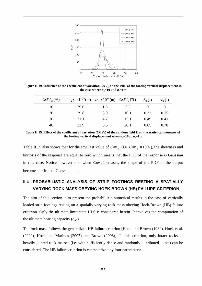
83
0
50
100
150
200
250
300
10 20 30 40 50 60Vertical displacement x10-3(m)
PD
F
COVE 10%
COVE 20%
COVE 30%
COVE 40%
Figure II.19. Influence of the coefficient of variation COVE on the PDF of the footing vertical displacement in the case where ax=10 and ay=1m
(%)ECOV -3 x10vµ (m) -3 x10vσ (m) (%)vCOV δu (-) κu (-)
10 29.0 1.5 5.2 0 0
20 29.8 3.0 10.1 0.32 0.15
30 31.1 4.7 15.1 0.49 0.41
40 32.9 6.6 20.1 0.65 0.78
Table II.15. Effect of the coefficient of variation (COVE) of the random field E on the statistical moments of the footing vertical displacement when ax=10m, ay=1m
Table II.15 also shows that for the smallest value of ECov (i.e. 10%ECov = ), the skewness and
kurtosis of the response are equal to zero which means that the PDF of the response is Gaussian
in this case. Notice however that when ECov increases, the shape of the PDF of the output
becomes far from a Gaussian one.
II.4 PROBABILISTIC ANALYSIS OF STRIP FOOTINGS RESTI NG A SPATIALLY
VARYING ROCK MASS OBEYING HOEK-BROWN (HB) FAILURE C RITERION
The aim of this section is to present the probabilistic numerical results in the case of vertically
loaded strip footings resting on a spatially varying rock mass obeying Hoek-Brown (HB) failure
criterion. Only the ultimate limit state ULS is considered herein. It involves the computation of
the ultimate bearing capacity (qult).
The rock mass follows the generalized HB failure criterion [Hoek and Brown (1980), Hoek et al.
(2002), Hoek and Marinos (2007) and Brown (2008)]. In this criterion, only intact rocks or
heavily jointed rock masses (i.e. with sufficiently dense and randomly distributed joints) can be
considered. The HB failure criterion is characterized by four parameters:
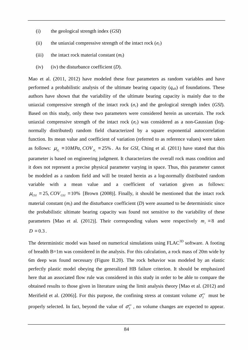
84
(i) the geological strength index (GSI)
(ii) the uniaxial compressive strength of the intact rock (σc)
(iii) the intact rock material constant (mi)
(iv) (iv) the disturbance coefficient (D).
Mao et al. (2011, 2012) have modeled these four parameters as random variables and have
performed a probabilistic analysis of the ultimate bearing capacity (qult) of foundations. These
authors have shown that the variability of the ultimate bearing capacity is mainly due to the
uniaxial compressive strength of the intact rock (σc) and the geological strength index (GSI).
Based on this study, only these two parameters were considered herein as uncertain. The rock
uniaxial compressive strength of the intact rock (σc) was considered as a non-Gaussian (log-
normally distributed) random field characterized by a square exponential autocorrelation
function. Its mean value and coefficient of variation (referred to as reference values) were taken
as follows: 10 , 25%c c
MPa COVσ σµ = = . As for GSI, Ching et al. (2011) have stated that this
parameter is based on engineering judgment. It characterizes the overall rock mass condition and
it does not represent a precise physical parameter varying in space. Thus, this parameter cannot
be modeled as a random field and will be treated herein as a log-normally distributed random
variable with a mean value and a coefficient of variation given as follows:
25, 10%GSI GSICOVµ = = [Brown (2008)]. Finally, it should be mentioned that the intact rock
material constant (mi) and the disturbance coefficient (D) were assumed to be deterministic since
the probabilistic ultimate bearing capacity was found not sensitive to the variability of these
parameters [Mao et al. (2012)]. Their corresponding values were respectively 8im = and
0.3D = .
The deterministic model was based on numerical simulations using FLAC3D software. A footing
of breadth B=1m was considered in the analysis. For this calculation, a rock mass of 20m wide by
6m deep was found necessary (Figure II.20). The rock behavior was modeled by an elastic
perfectly plastic model obeying the generalized HB failure criterion. It should be emphasized
here that an associated flow rule was considered in this study in order to be able to compare the
obtained results to those given in literature using the limit analysis theory [Mao et al. (2012) and
Merifield et al. (2006)]. For this purpose, the confining stress at constant volume cv3σ must be
properly selected. In fact, beyond the value of cv3σ , no volume changes are expected to appear.
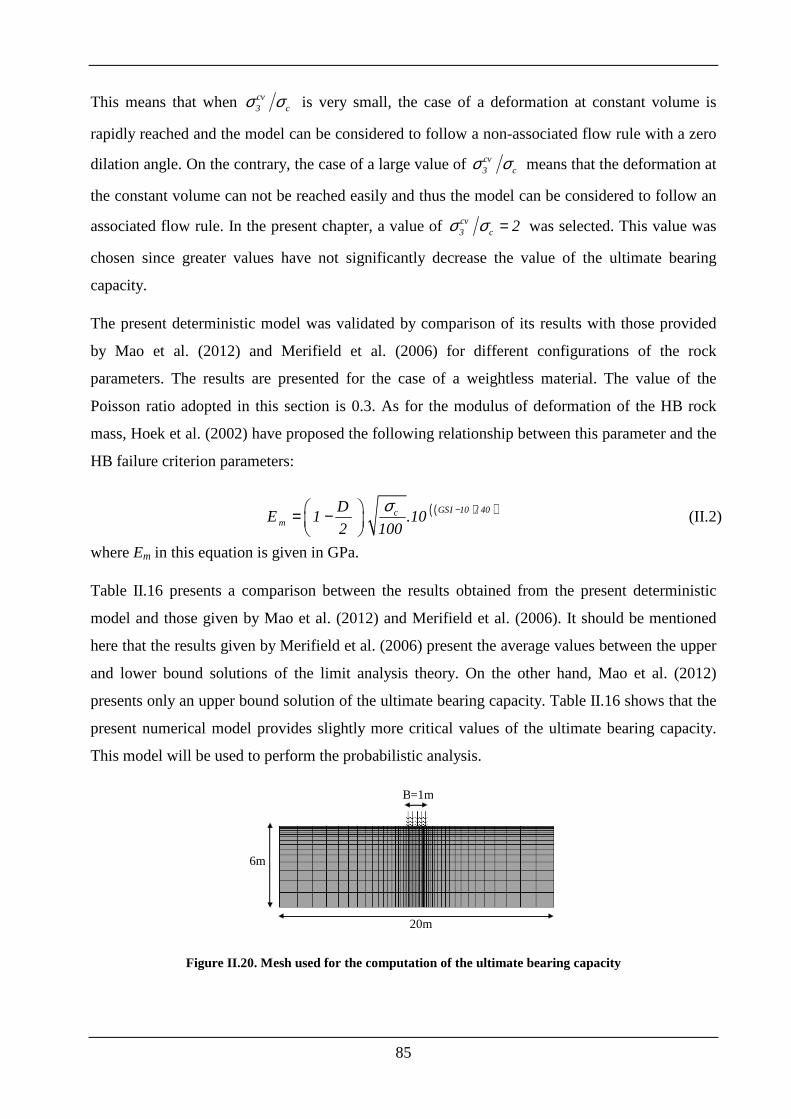
85
This means that when cv3 cσ σ is very small, the case of a deformation at constant volume is
rapidly reached and the model can be considered to follow a non-associated flow rule with a zero
dilation angle. On the contrary, the case of a large value of cv3 cσ σ means that the deformation at
the constant volume can not be reached easily and thus the model can be considered to follow an
associated flow rule. In the present chapter, a value of cv3 c 2σ σ = was selected. This value was
chosen since greater values have not significantly decrease the value of the ultimate bearing
capacity.
The present deterministic model was validated by comparison of its results with those provided
by Mao et al. (2012) and Merifield et al. (2006) for different configurations of the rock
parameters. The results are presented for the case of a weightless material. The value of the
Poisson ratio adopted in this section is 0.3. As for the modulus of deformation of the HB rock
mass, Hoek et al. (2002) have proposed the following relationship between this parameter and the
HB failure criterion parameters:
( )( )GSI 10 / 40cm
DE 1 .10
2 100
σ − = −
( II.2)
where Em in this equation is given in GPa.
Table II.16 presents a comparison between the results obtained from the present deterministic
model and those given by Mao et al. (2012) and Merifield et al. (2006). It should be mentioned
here that the results given by Merifield et al. (2006) present the average values between the upper
and lower bound solutions of the limit analysis theory. On the other hand, Mao et al. (2012)
presents only an upper bound solution of the ultimate bearing capacity. Table II.16 shows that the
present numerical model provides slightly more critical values of the ultimate bearing capacity.
This model will be used to perform the probabilistic analysis.
20m
6m
B=1m
Figure II.20. Mesh used for the computation of the ultimate bearing capacity

86
GSI (-)
σc
(MPa) mi
(MPa) FLAC3D
Mao et al. (2012)
Merifield et al. (2006)
20 7.5 10 1.460 1.600 1.568
20 10 10 1.960 2.130 2.090
20 12.5 10 2.450 2.670 2.613
20 15 10 2.930 3.200 3.135
20 20 10 3.920 4.270 4.180
30 7.5 10 2.784 3.040 2. 978
30 10 10 3.710 4.060 3.970
30 12.5 10 4.660 5.070 4.963
30 15 10 5.605 6.120 5.955
30 20 10 7.498 8.080 7.940
Table II.16. Values of qult (MPa) as given by FLAC3D, by Merifield et al. (2006) and by Mao et al. (2012) when D=0
As for the autocorrelation distances ax and ay of the random field (σc), it was assumed here that
a=ax=ay. Notice that the adopted reference value of the autocorrelation distance (a) is 2m;
however, a range of 0.5-100m was considered for the parametric study. For the different values of
the autocorrelation distance (a), the total number N of random variables (or eigenmodes) that
should be used to discretize the random field of σc within a prescribed value of 10% for the
variance of the error is presented in Table II.17. Notice that the numbers given in Table II.17 are
those corresponding to the rock domain [20m, 6m] presented in Figure II.20.
Autocorrelation distance a(m)
Total number of random variables used to discretize the uniaxial compression strength
random field
0.5 120
1 99
2 35
5 8
10 5
50 5
100 5
Table II.17. Number of random variables needed to discretize the random field σc
The following subsections are organized as follows: First, a global sensitivity analysis is
performed. This is followed by a presentation of the parametric study. The aim of this parametric
study is to show the effect of the different governing statistical parameters (autocorrelation
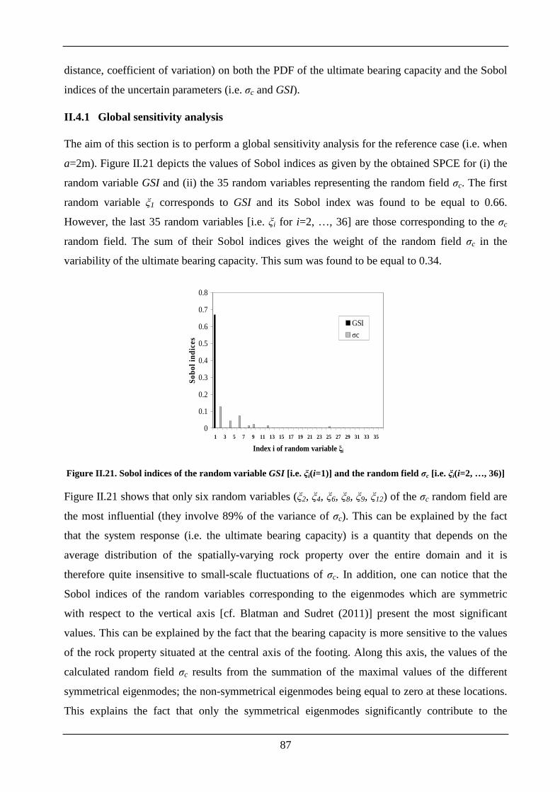
87
distance, coefficient of variation) on both the PDF of the ultimate bearing capacity and the Sobol
indices of the uncertain parameters (i.e. σc and GSI).
II.4.1 Global sensitivity analysis
The aim of this section is to perform a global sensitivity analysis for the reference case (i.e. when
a=2m). Figure II.21 depicts the values of Sobol indices as given by the obtained SPCE for (i) the
random variable GSI and (ii) the 35 random variables representing the random field σc. The first
random variable ξ1 corresponds to GSI and its Sobol index was found to be equal to 0.66.
However, the last 35 random variables [i.e. ξi for i=2, …, 36] are those corresponding to the σc
random field. The sum of their Sobol indices gives the weight of the random field σc in the
variability of the ultimate bearing capacity. This sum was found to be equal to 0.34.
0
0.1
0.2
0.3
0.4
0.5
0.6
0.7
0.8
1 3 5 7 9 11 13 15 17 19 21 23 25 27 29 31 33 35
Index i of random variable ξi
Sob
ol in
dice
s
GSI
σc
Figure II.21. Sobol indices of the random variable GSI [i.e. ξi(i=1)] and the random field σc [i.e. ξi(i=2, …, 36)]
Figure II.21 shows that only six random variables (ξ2, ξ4, ξ6, ξ8, ξ9, ξ12) of the σc random field are
the most influential (they involve 89% of the variance of σc). This can be explained by the fact
that the system response (i.e. the ultimate bearing capacity) is a quantity that depends on the
average distribution of the spatially-varying rock property over the entire domain and it is
therefore quite insensitive to small-scale fluctuations of σc. In addition, one can notice that the
Sobol indices of the random variables corresponding to the eigenmodes which are symmetric
with respect to the vertical axis [cf. Blatman and Sudret (2011)] present the most significant
values. This can be explained by the fact that the bearing capacity is more sensitive to the values
of the rock property situated at the central axis of the footing. Along this axis, the values of the
calculated random field σc results from the summation of the maximal values of the different
symmetrical eigenmodes; the non-symmetrical eigenmodes being equal to zero at these locations.
This explains the fact that only the symmetrical eigenmodes significantly contribute to the
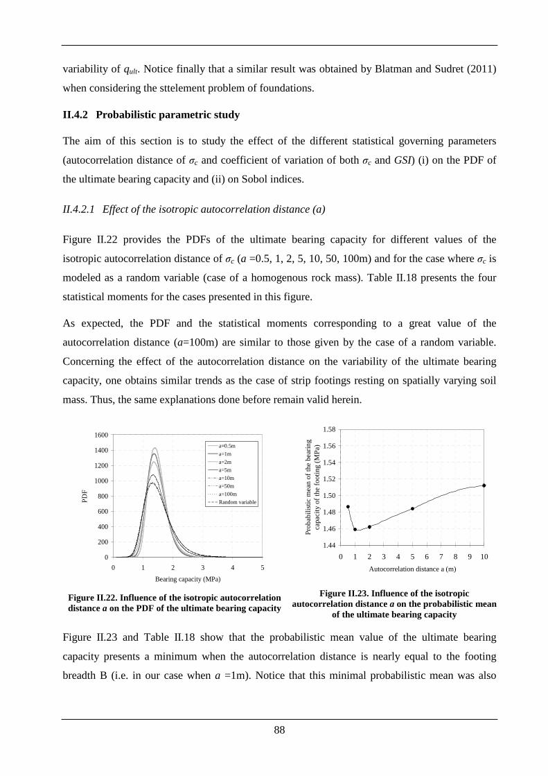
88
variability of qult. Notice finally that a similar result was obtained by Blatman and Sudret (2011)
when considering the sttelement problem of foundations.
II.4.2 Probabilistic parametric study
The aim of this section is to study the effect of the different statistical governing parameters
(autocorrelation distance of σc and coefficient of variation of both σc and GSI) (i) on the PDF of
the ultimate bearing capacity and (ii) on Sobol indices.
II.4.2.1 Effect of the isotropic autocorrelation distance (a)
Figure II.22 provides the PDFs of the ultimate bearing capacity for different values of the
isotropic autocorrelation distance of σc (a =0.5, 1, 2, 5, 10, 50, 100m) and for the case where σc is
modeled as a random variable (case of a homogenous rock mass). Table II.18 presents the four
statistical moments for the cases presented in this figure.
As expected, the PDF and the statistical moments corresponding to a great value of the
autocorrelation distance (a=100m) are similar to those given by the case of a random variable.
Concerning the effect of the autocorrelation distance on the variability of the ultimate bearing
capacity, one obtains similar trends as the case of strip footings resting on spatially varying soil
mass. Thus, the same explanations done before remain valid herein.
0
200
400
600
800
1000
1200
1400
1600
0 1 2 3 4 5
Bearing capacity (MPa)
PD
F
a=0.5m
a=1m
a=2m
a=5m
a=10m
a=50m
a=100m
Random variable
Figure II.22. Influence of the isotropic autocorrelation distance a on the PDF of the ultimate bearing capacity
1.44
1.46
1.48
1.50
1.52
1.54
1.56
1.58
0 1 2 3 4 5 6 7 8 9 10
Autocorrelation distance a (m)
Pro
bab
ilist
ic m
ean
of t
he b
earin
g
capa
city
of t
he
foo
ting
(M
Pa)
Figure II.23. Influence of the isotropic
autocorrelation distance a on the probabilistic mean of the ultimate bearing capacity
Figure II.23 and Table II.18 show that the probabilistic mean value of the ultimate bearing
capacity presents a minimum when the autocorrelation distance is nearly equal to the footing
breadth B (i.e. in our case when a =1m). Notice that this minimal probabilistic mean was also
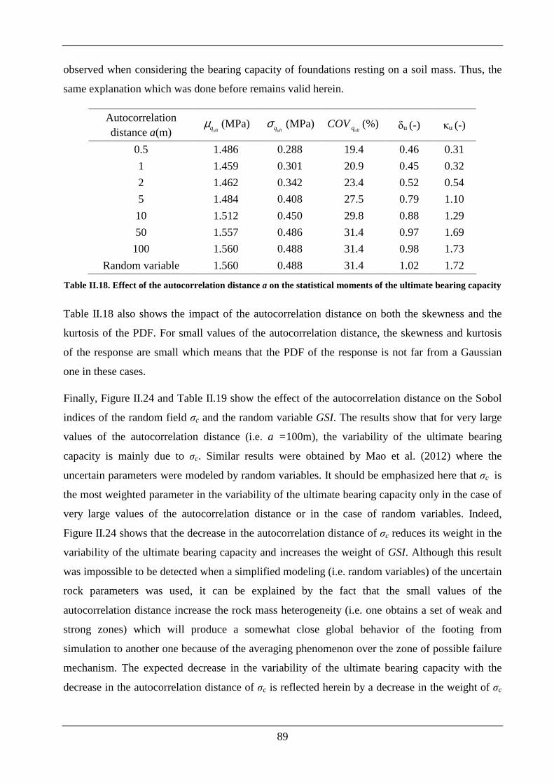
89
observed when considering the bearing capacity of foundations resting on a soil mass. Thus, the
same explanation which was done before remains valid herein.
Autocorrelation distance a(m) ultqµ (MPa)
ultqσ (MPa) (%)ultqCOV δu (-) κu (-)
0.5 1.486 0.288 19.4 0.46 0.31
1 1.459 0.301 20.9 0.45 0.32
2 1.462 0.342 23.4 0.52 0.54
5 1.484 0.408 27.5 0.79 1.10
10 1.512 0.450 29.8 0.88 1.29
50 1.557 0.486 31.4 0.97 1.69
100 1.560 0.488 31.4 0.98 1.73
Random variable 1.560 0.488 31.4 1.02 1.72
Table II.18. Effect of the autocorrelation distance a on the statistical moments of the ultimate bearing capacity
Table II.18 also shows the impact of the autocorrelation distance on both the skewness and the
kurtosis of the PDF. For small values of the autocorrelation distance, the skewness and kurtosis
of the response are small which means that the PDF of the response is not far from a Gaussian
one in these cases.
Finally, Figure II.24 and Table II.19 show the effect of the autocorrelation distance on the Sobol
indices of the random field σc and the random variable GSI. The results show that for very large
values of the autocorrelation distance (i.e. a =100m), the variability of the ultimate bearing
capacity is mainly due to σc. Similar results were obtained by Mao et al. (2012) where the
uncertain parameters were modeled by random variables. It should be emphasized here that σc is
the most weighted parameter in the variability of the ultimate bearing capacity only in the case of
very large values of the autocorrelation distance or in the case of random variables. Indeed,
Figure II.24 shows that the decrease in the autocorrelation distance of σc reduces its weight in the
variability of the ultimate bearing capacity and increases the weight of GSI. Although this result
was impossible to be detected when a simplified modeling (i.e. random variables) of the uncertain
rock parameters was used, it can be explained by the fact that the small values of the
autocorrelation distance increase the rock mass heterogeneity (i.e. one obtains a set of weak and
strong zones) which will produce a somewhat close global behavior of the footing from
simulation to another one because of the averaging phenomenon over the zone of possible failure
mechanism. The expected decrease in the variability of the ultimate bearing capacity with the
decrease in the autocorrelation distance of σc is reflected herein by a decrease in the weight of σc
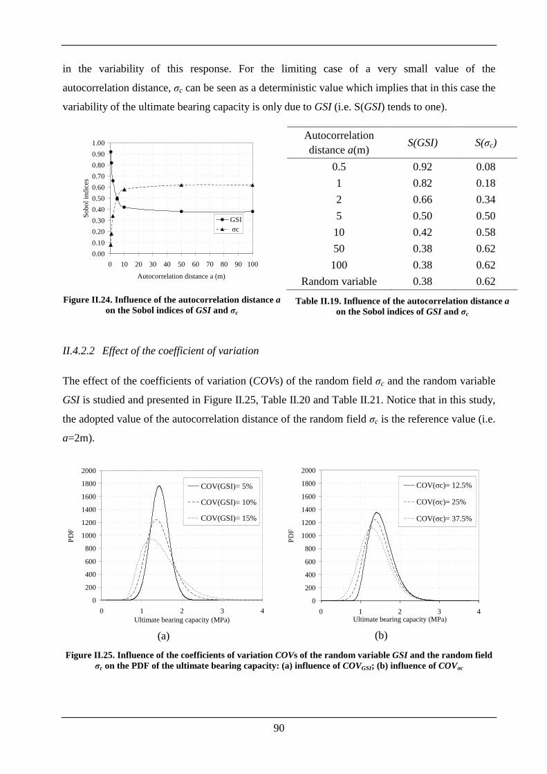
90
in the variability of this response. For the limiting case of a very small value of the
autocorrelation distance, σc can be seen as a deterministic value which implies that in this case the
variability of the ultimate bearing capacity is only due to GSI (i.e. S(GSI) tends to one).
0.00
0.10
0.20
0.30
0.40
0.50
0.60
0.70
0.80
0.90
1.00
0 10 20 30 40 50 60 70 80 90 100
Autocorrelation distance a (m)
So
bol i
ndic
es
GSI σc
Figure II.24. Influence of the autocorrelation distance a
on the Sobol indices of GSI and σc
Autocorrelation distance a(m)
S(GSI) S(σc)
0.5 0.92 0.08
1 0.82 0.18
2 0.66 0.34
5 0.50 0.50
10 0.42 0.58
50 0.38 0.62
100 0.38 0.62
Random variable 0.38 0.62
Table II.19. Influence of the autocorrelation distance a on the Sobol indices of GSI and σc
II.4.2.2 Effect of the coefficient of variation
The effect of the coefficients of variation (COVs) of the random field σc and the random variable
GSI is studied and presented in Figure II.25, Table II.20 and Table II.21. Notice that in this study,
the adopted value of the autocorrelation distance of the random field σc is the reference value (i.e.
a=2m).
0
200
400
600
800
1000
1200
1400
1600
1800
2000
0 1 2 3 4Ultimate bearing capacity (MPa)
PD
F
COV(GSI)= 5%
COV(GSI)= 10%
COV(GSI)= 15%
(a)
0
200
400
600
800
1000
1200
1400
1600
1800
2000
0 1 2 3 4Ultimate bearing capacity (MPa)
PD
F
COV(σc)= 12.5%
COV(σc)= 25%
COV(σc)= 37.5%
(b)
Figure II.25. Influence of the coefficients of variation COVs of the random variable GSI and the random field σc on the PDF of the ultimate bearing capacity: (a) influence of COVGSI; (b) influence of COVσc
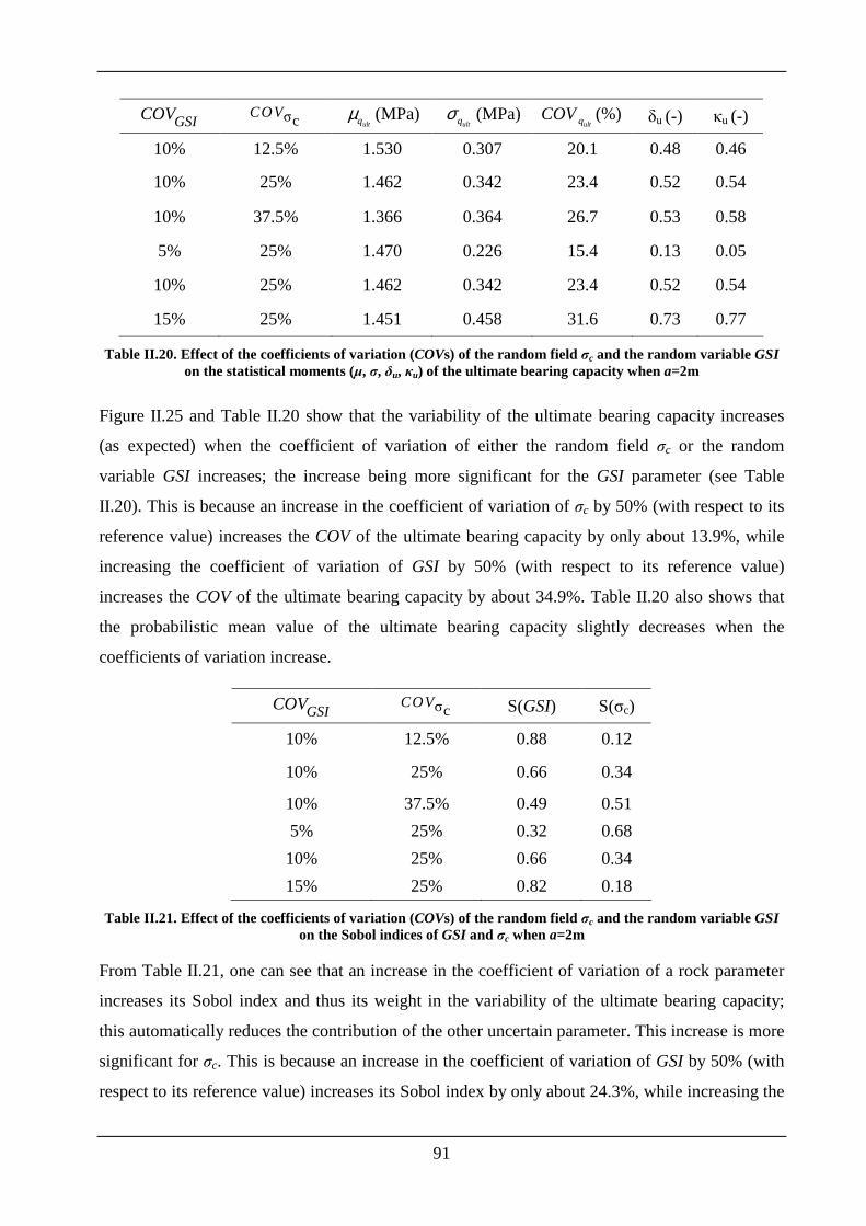
91
GSICOV σcCOV
ultqµ (MPa) ultqσ (MPa) (%)
ultqCOV δu (-) κu (-)
10% 12.5% 1.530 0.307 20.1 0.48 0.46
10% 25% 1.462 0.342 23.4 0.52 0.54
10% 37.5% 1.366 0.364 26.7 0.53 0.58
5% 25% 1.470 0.226 15.4 0.13 0.05
10% 25% 1.462 0.342 23.4 0.52 0.54
15% 25% 1.451 0.458 31.6 0.73 0.77
Table II.20. Effect of the coefficients of variation (COVs) of the random field σc and the random variable GSI on the statistical moments (µ, σ, δu, κu) of the ultimate bearing capacity when a=2m
Figure II.25 and Table II.20 show that the variability of the ultimate bearing capacity increases
(as expected) when the coefficient of variation of either the random field σc or the random
variable GSI increases; the increase being more significant for the GSI parameter (see Table
II.20). This is because an increase in the coefficient of variation of σc by 50% (with respect to its
reference value) increases the COV of the ultimate bearing capacity by only about 13.9%, while
increasing the coefficient of variation of GSI by 50% (with respect to its reference value)
increases the COV of the ultimate bearing capacity by about 34.9%. Table II.20 also shows that
the probabilistic mean value of the ultimate bearing capacity slightly decreases when the
coefficients of variation increase.
GSICOV σcCOV S(GSI) S(σc)
10% 12.5% 0.88 0.12
10% 25% 0.66 0.34
10% 37.5% 0.49 0.51
5% 25% 0.32 0.68
10% 25% 0.66 0.34
15% 25% 0.82 0.18
Table II.21. Effect of the coefficients of variation (COVs) of the random field σc and the random variable GSI on the Sobol indices of GSI and σc when a=2m
From Table II.21, one can see that an increase in the coefficient of variation of a rock parameter
increases its Sobol index and thus its weight in the variability of the ultimate bearing capacity;
this automatically reduces the contribution of the other uncertain parameter. This increase is more
significant for σc. This is because an increase in the coefficient of variation of GSI by 50% (with
respect to its reference value) increases its Sobol index by only about 24.3%, while increasing the
92
coefficient of variation of σc by 50% (with respect to its reference value) increases its Sobol index
by about 50%.
II.5 DISCUSSION
Although the focus of this chapter involves the computation of the statistical moments of the
different system responses, the aim of this section is to briefly discuss the validity of the present
SPCE methodology for the computation of the probability of failure Pf. For this purpose, a
comparison between the results obtained using the Subset Simulation (SS) method by Ahmed and
Soubra (2012) (see section I.5.1.2) and those obtained with the proposed SPCE methodology are
presented herein. The comparison was performed in the ULS case of a strip footing resting on a
weightless c-φ soil for the reference case where ax=10m, ay=1m, and r(c, φ)=-0.5. (cf. section
II.3.1.2). The footing is subjected to a vertical load Ps=400kN/m. The performance function used
to calculate the failure probability is 1u
s
PG
P= − where Pu is the ultimate footing load.
In order to calculate the failure probability Pf by SS method, an optimal number Ks of simulations
per level should be selected. This number should be greater than 100 to provide a small bias in
the calculated Pf value [Honjo 2008]. In this case study, a number of simulation per level Ks=200
was chosen. The obtained Pf value was equal to 3.5x10⁻⁴. Notice that four levels of SS were
required to calculate this Pf value. The total number of simulations K is equal to 740. The Pf value
obtained by SS is to be compared to the Pf value of 4.72x10⁻⁴ obtained using the SPCE
methodology. One can observe a small difference between the two methods. It should be
emphasized that this is a preliminary validation of the SPCE methodology for the computation of
the failure probability. Further tests are necessary to confirm the agreement between the results of
the two methods.
II.6 CONCLUSIONS
In this chapter, a probabilistic analysis at both ultimate limit state (ULS) and serviceability limit
state (SLS) of strip footings was performed. Two case studies were considered in this chapter.
The first one involves the case of strip footings resting on a 2D spatially varying soil mass
obeying the Mohr-Coulomb (MC) failure criterion and the second one considers the case of strip
footings resting on a 2D spatially varying rock mass obeying the Hoek-Brown (HB) failure
criterion.
93
In the case of the spatially varying soil mass, a probabilistic analysis at both ULS and SLS of
vertically loaded strip footings was performed. The soil shear strength parameters (c and φ) were
considered as anisotropic cross-correlated non-Gaussian random fields at ULS and the soil elastic
parameters (E and υ) were considered as anisotropic uncorrelated non-Gaussian random fields at
SLS. Notice that the system response used at ULS was the ultimate bearing capacity (qult);
however, the footing vertical displacement (v) was considered as the system response at SLS.
Concerning the case of the spatially varying rock mass, only the ULS case was considered. The
methodology proposed by Vořechovsky (2008) was used to generate the two random fields. The
sparse polynomial chaos expansion (SPCE) methodology was employed for the probabilistic
analysis. The adaptive algorithm suggested by Blatman and Sudret (2010) to build up a SPCE
was adopted to obtain a meta-model (i.e. an approximate analytical expression) of the system
responses. These meta-models were employed to perform the probabilistic analysis using Monte
Carlo simulation technique. Notice finally; that at the ULS analysis, only weightless soil and
weightless rock masses were considered. This is because introducing the soil/rock weight in the
deterministic model increases the computation time from 5 to 10 min per simulation. Although
this difference may not seem to be significant for a single simulation, it becomes dramatically
important during the probabilistic analyses where a large number of simulations is needed for
each probabilistic analysis.
The numerical results have shown the interest of the SPCE methodology with respect to the
classical PCE method in the case of random fields where a significant number of random
variables were used in the analysis. The numerical results have also shown that the variability of
the system responses (i.e. the ultimate bearing capacity in the ULS analysis and the vertical
displacement of the footing in the SLS analysis) increases (as expected) with the increase in the
coefficients of variation of the random fields. It was also shown that an increase in the coefficient
of variation of a random field increases its Sobol index and thus its weight in the variability of the
system response and decreases the weight of the other parameter. The negative correlation
between the random fields decreases the response variability.
With a decrease in the autocorrelation distances (ax or ay or ax=ay), a less spread out PDF of the
system response was obtained. The probabilistic mean value of the ultimate bearing capacity (in
both cases of soil and rock masses) presents a minimum. This minimum was obtained in the
isotropic case when the autocorrelation distance is nearly equal to the footing breadth B; while
for the anisotropic case (presented only when a soil mass is considered), this minimum was
obtained (for prescribed footing and soil characteristics) at a given value of the ratio between the
94
horizontal and the vertical autocorrelation distances. Small values of the autocorrelation distances
lead to small values of the skewness and kurtosis of the system responses. Thus, a PDF of the
system response that is not far from a Gaussian one was obtained in these cases. Finally, the
obtained results show the importance of considering the spatial variability of the soil/rock
properties in the probabilistic studies since some observed phenomena (such as the non-
symmetrical soil failure and the variation in the weight of parameters with the autocorrelation
distance) can not be seen when homogenous soils are considered.

95
96
CHAPTER III. EFFECT OF THE SOIL SPATIAL VARIABILITY IN
THREE DIMENSIONS ON THE ULTIMATE BEARING CAPACITY O F
FOUNDATIONS
III.1 INTRODUCTION
The effect of the spatial variability of a soil/rock property was extensively investigated in the
previous chapter using a two-dimensional (2D) analysis. In this case, the soil/rock mass exhibits
spatial variability in a given plane and remains uniform in the direction normal to this plane
where the autocorrelation distance is implicitly taken as infinite.
Few authors have investigated the effect of the 3D soil spatial variability. One may cite among
others Fenton and Griffiths (2005) for the foundation settlement problem, Griffiths et al. (2009)
for the slope stability analysis and Popescu et al. (2005) for the seismic liquefaction problem. To
the best of the authors’ knowledge, there are no investigations on the effect of the 3D soil spatial
variability on the ultimate bearing capacity of foundations. This chapter fills this gap.
The effect of the soil spatial variability in three dimensions is investigated in this chapter through
the study of the ultimate bearing capacity of strip and square foundations resting on a purely
cohesive soil with a spatially varying cohesion in the three dimensions [Al-Bittar and Soubra
(2012d)]. For this purpose, the soil cohesion was modeled as a 3D random field. Both cases of
isotropic and anisotropic random fields were considered.
In order to investigate the effect of the spatial variability in the third direction, the results of the
ultimate bearing capacity of foundations obtained using a 3D random field were compared to
those corresponding to a 2D random field for two cases of a strip and a square footing. The
objective is to check the validity of considering a 2D random field in both cases of plane strain
and three-dimensional problems.
III.2 PROBABILISTIC ANALYSIS OF STRIP AND SQUARE FO OTINGS RESTING
ON A 3D SPATIALLY VARYING SOIL MASS
The aim of this section is to perform a probabilistic analysis of shallow foundations taking into
account the soil spatial variability in three dimensions. More specifically, the analysis involves
the computation of the ultimate bearing capacity (qult) of square and strip footings resting on a
purely cohesive soil that exhibits spatial variability in three dimensions. Notice that for both the
square and strip footings considered in the analysis, the cases of 2D and 3D anisotropic non-
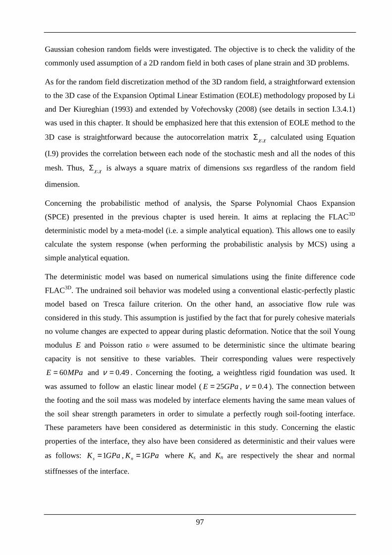
97
Gaussian cohesion random fields were investigated. The objective is to check the validity of the
commonly used assumption of a 2D random field in both cases of plane strain and 3D problems.
As for the random field discretization method of the 3D random field, a straightforward extension
to the 3D case of the Expansion Optimal Linear Estimation (EOLE) methodology proposed by Li
and Der Kiureghian (1993) and extended by Vořechovsky (2008) (see details in section I.3.4.1)
was used in this chapter. It should be emphasized here that this extension of EOLE method to the
3D case is straightforward because the autocorrelation matrix ;χ χΣ calculated using Equation
( I.9) provides the correlation between each node of the stochastic mesh and all the nodes of this
mesh. Thus, ;χ χΣ is always a square matrix of dimensions sxs regardless of the random field
dimension.
Concerning the probabilistic method of analysis, the Sparse Polynomial Chaos Expansion
(SPCE) presented in the previous chapter is used herein. It aims at replacing the FLAC3D
deterministic model by a meta-model (i.e. a simple analytical equation). This allows one to easily
calculate the system response (when performing the probabilistic analysis by MCS) using a
simple analytical equation.
The deterministic model was based on numerical simulations using the finite difference code
FLAC3D. The undrained soil behavior was modeled using a conventional elastic-perfectly plastic
model based on Tresca failure criterion. On the other hand, an associative flow rule was
considered in this study. This assumption is justified by the fact that for purely cohesive materials
no volume changes are expected to appear during plastic deformation. Notice that the soil Young
modulus E and Poisson ratio υ were assumed to be deterministic since the ultimate bearing
capacity is not sensitive to these variables. Their corresponding values were respectively
60=E MPa and 0.49ν = . Concerning the footing, a weightless rigid foundation was used. It
was assumed to follow an elastic linear model ( 25E GPa= , 0.4ν = ). The connection between
the footing and the soil mass was modeled by interface elements having the same mean values of
the soil shear strength parameters in order to simulate a perfectly rough soil-footing interface.
These parameters have been considered as deterministic in this study. Concerning the elastic
properties of the interface, they also have been considered as deterministic and their values were
as follows: 1sK GPa= , 1nK GPa= where Ks and Kn are respectively the shear and normal
stiffnesses of the interface.
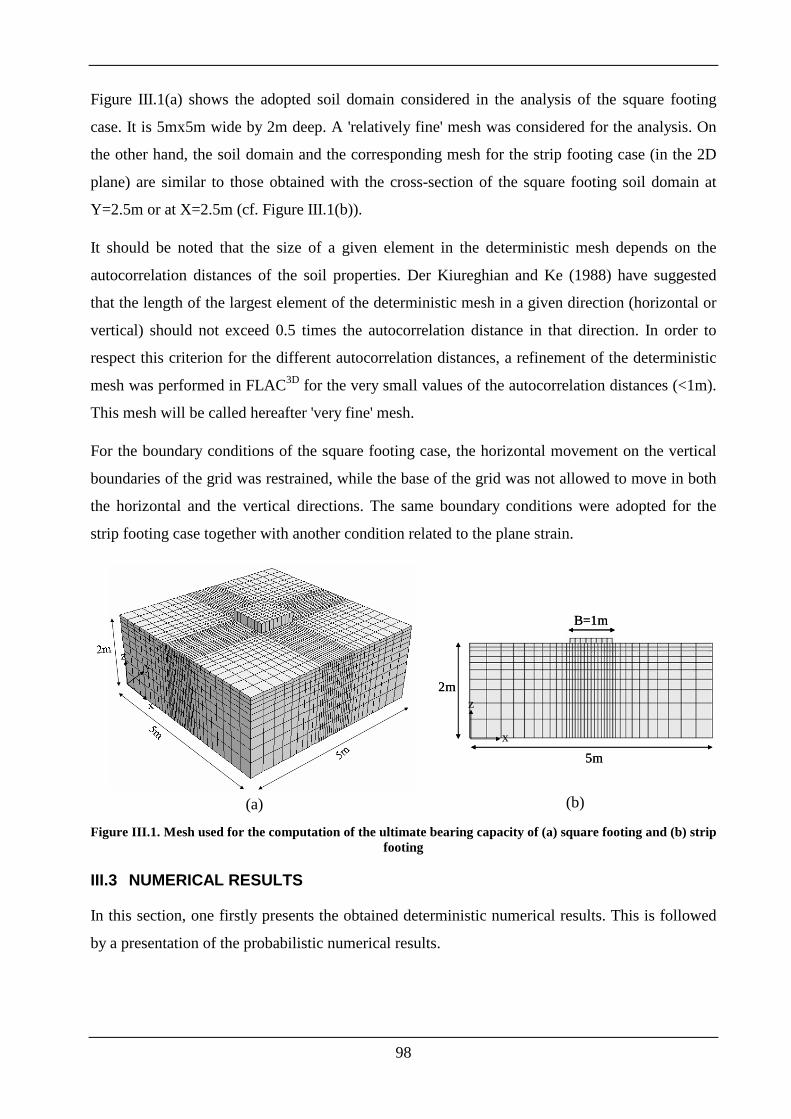
98
Figure III.1(a) shows the adopted soil domain considered in the analysis of the square footing
case. It is 5mx5m wide by 2m deep. A 'relatively fine' mesh was considered for the analysis. On
the other hand, the soil domain and the corresponding mesh for the strip footing case (in the 2D
plane) are similar to those obtained with the cross-section of the square footing soil domain at
Y=2.5m or at X=2.5m (cf. Figure III.1(b)).
It should be noted that the size of a given element in the deterministic mesh depends on the
autocorrelation distances of the soil properties. Der Kiureghian and Ke (1988) have suggested
that the length of the largest element of the deterministic mesh in a given direction (horizontal or
vertical) should not exceed 0.5 times the autocorrelation distance in that direction. In order to
respect this criterion for the different autocorrelation distances, a refinement of the deterministic
mesh was performed in FLAC3D for the very small values of the autocorrelation distances (<1m).
This mesh will be called hereafter 'very fine' mesh.
For the boundary conditions of the square footing case, the horizontal movement on the vertical
boundaries of the grid was restrained, while the base of the grid was not allowed to move in both
the horizontal and the vertical directions. The same boundary conditions were adopted for the
strip footing case together with another condition related to the plane strain.
(a)
5m
2m
B=1m
x
z
5m
2m
B=1m
x
z
(b)
Figure III.1. Mesh used for the computation of the ultimate bearing capacity of (a) square footing and (b) strip footing
III.3 NUMERICAL RESULTS
In this section, one firstly presents the obtained deterministic numerical results. This is followed
by a presentation of the probabilistic numerical results.
99
III.3.1 Deterministic numerical results
The aim of this section is to present the deterministic numerical results for both the square and
the strip footings considered in the analysis.
The three-dimensional 'relatively fine' mesh has led to a deterministic value of ultimate bearing
capacity coefficient Nc=6.54 for the square footing case. The difference with the recent finite
element solution (Nc=5.91) by Gourvenec et al. (2006) and the recent upper-bound solution
(Nc=6.41) by Gourvenec et al. (2006) was respectively about 9% and 2%. It should be
emphasized here that a ‘very fine’ mesh has led to a value of Nc=6.15 which is only 5% smaller
(i.e. better) than the value of 6.54 obtained using the 'relatively fine' mesh. Notice however that
this solution requires an increase in the computation time by 2 hours and thus, this 'very fine'
mesh was not retained in the present probabilistic analysis. A similar procedure that makes use of
a 'relatively fine' (not 'very fine') mesh was advocated by Griffiths et al. (2002) when performing
a probabilistic analysis. It should be emphasized herein that when dealing with probabilistic
studies based on three-dimensional finite element/finite difference deterministic models, the time
cost is very important especially when the soil spatial variability (and more specifically the
variability of the soil property in three dimensions) is introduced. The reasons are:
(i) The computation time of a single deterministic solution significantly increases with
the increase in the density of the three-dimensional deterministic mesh.
(ii) The fact of providing (for each simulation of a single probabilistic analysis) different
values of the soil cohesion to the different elements of the mesh, will add a dramatic
computation time especially for very fine meshes.
(iii) The large number of simulations required for each probabilistic analysis.
Thus, in order to enable the investigation of the effect of the soil spatial variability in the three
dimensions for the present three-dimensional mechanical problem, a 'relatively fine' (not 'very
fine') mesh was considered in the square footing case. This is a compromise between the
computation time and the accuracy of the probabilistic solution.
Concerning the strip footing case, it should be remembered that the same ‘relatively fine’ mesh
used in the central plane of the square footing was adopted for the values of the autocorrelation
distances greater than 1m (cf. Figure III.1(b)), although a finer mesh would be possible because
of the relatively small computation time in this case. This choice was adopted in order to
maintain a similarity with the mesh employed for the square footing. Notice that a 'very fine'
100
mesh has led in this case to a value of Nc=5.43 which is about 5% larger that the closed form
solution Nc=5.14 and it is about 2% larger than the recent finite element solution Nc=5.31 by
Gourvenec et al. (2006). The adopted ‘relatively fine' mesh has led to a value Nc=5.74 which is
about 10% higher than the closed form solution Nc=5.14 and is only 5% higher than the solution
given by the 'very fine' mesh.
III.3.2 Probabilistic numerical results
In this section, the probabilistic numerical results of both the square and strip footings resting on
a purely cohesive spatially varying soil are presented. The soil cohesion parameter was modeled
as anisotropic non-Gaussian (log-normal) random field using a square exponential autocorrelation
function. Its mean value and coefficient of variation (referred to as reference values) were taken
as follows: 20 , 25%c ckPa COVµ = = .
It should be emphasized here that for both the square and strip footings considered in the
analysis, the cases of 2D and 3D cohesion random fields were investigated. As for the
autocorrelation distances ax, ay and az of the cohesion random field, both cases of isotropic
random fields (i.e. ax=ay=az for the 3D random field case and ax=az for the 2D random field case)
and anisotropic random fields (i.e. ax=ay#az for the 3D random field case and ax#az for the 2D
random field case) will be treated although the soil is rarely isotropic in reality.
When isotropic random fields are used, the autocorrelation distance for both the 2D and the 3D
random fields will be denoted by (a) later on in this chapter (i.e. a=ax=ay=az for the 3D random
field case and a=ax=az for the 2D random field case). Also, when referring to anisotropic random
fields, the horizontal autocorrelation distance for both the 2D and the 3D random fields will be
denoted by ah (i.e. ah=ax=ay for the 3D random field case and ah=ax for the 2D random field
case). Furthermore, the vertical autocorrelation distance for both the 2D and the 3D random fields
will be denoted by av (i.e. av=az for both the 3D and 2D random fields cases).
For the isotropic case, a range of 0.5-10m was considered (cf. Table III.1). For the anisotropic
case, the reference values adopted for the horizontal and the vertical autocorrelation distances
were 10m and 1m while the wide ranges of 0.5-10m and 0.15-10m were considered respectively
for the horizontal and the vertical autocorrelation distances when performing the parametric study
for both the square and the strip footings (cf. Table III.1).
For the considered soil domain and for the different values of the autocorrelation distances (a, ah
or av) used in the analysis, the total number N of random variables (or eigenmodes) that should be
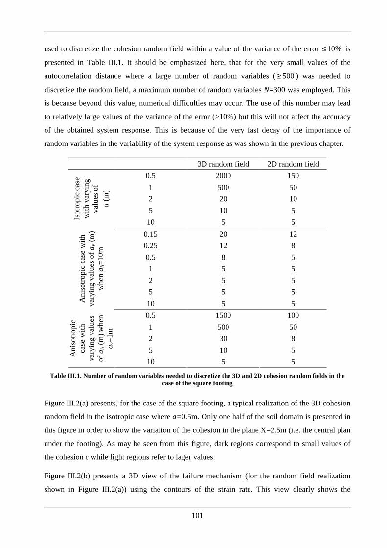
101
used to discretize the cohesion random field within a value of the variance of the error 10%≤ is
presented in Table III.1. It should be emphasized here, that for the very small values of the
autocorrelation distance where a large number of random variables ( 500≥ ) was needed to
discretize the random field, a maximum number of random variables N=300 was employed. This
is because beyond this value, numerical difficulties may occur. The use of this number may lead
to relatively large values of the variance of the error (>10%) but this will not affect the accuracy
of the obtained system response. This is because of the very fast decay of the importance of
random variables in the variability of the system response as was shown in the previous chapter.
3D random field 2D random field
0.5 2000 150
1 500 50
2 20 10
5 10 5
Isot
ropi
c ca
se
with
var
ying
va
lues
of
a (m
)
10 5 5
0.15 20 12
0.25 12 8
0.5 8 5
1 5 5
2 5 5
5 5 5
Ani
sotr
opic
cas
e w
ith
vary
ing
valu
es o
f av (
m)
whe
n a h
=10
m
10 5 5
0.5 1500 100
1 500 50
2 30 8
5 10 5 Ani
sotr
opic
ca
se w
ith
vary
ing
valu
es
of a
h (m
) w
hen
a v=
1m
10 5 5
Table III.1. Number of random variables needed to discretize the 3D and 2D cohesion random fields in the case of the square footing
Figure III.2(a) presents, for the case of the square footing, a typical realization of the 3D cohesion
random field in the isotropic case where a=0.5m. Only one half of the soil domain is presented in
this figure in order to show the variation of the cohesion in the plane X=2.5m (i.e. the central plan
under the footing). As may be seen from this figure, dark regions correspond to small values of
the cohesion c while light regions refer to lager values.
Figure III.2(b) presents a 3D view of the failure mechanism (for the random field realization
shown in Figure III.2(a)) using the contours of the strain rate. This view clearly shows the
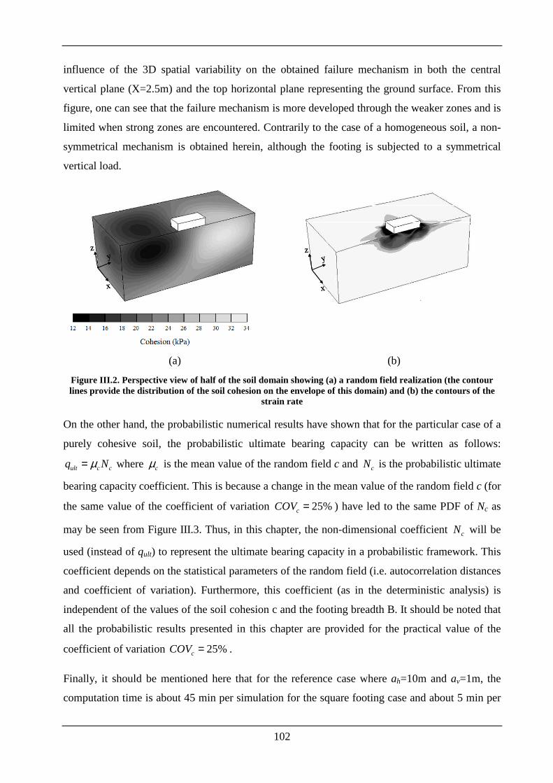
102
influence of the 3D spatial variability on the obtained failure mechanism in both the central
vertical plane (X=2.5m) and the top horizontal plane representing the ground surface. From this
figure, one can see that the failure mechanism is more developed through the weaker zones and is
limited when strong zones are encountered. Contrarily to the case of a homogeneous soil, a non-
symmetrical mechanism is obtained herein, although the footing is subjected to a symmetrical
vertical load.
x
yz
x
yz
x
yz
x
yz
x
yz
x
yz
(a) (b)
Figure III.2. Perspective view of half of the soil domain showing (a) a random field realization (the contour lines provide the distribution of the soil cohesion on the envelope of this domain) and (b) the contours of the
strain rate
On the other hand, the probabilistic numerical results have shown that for the particular case of a
purely cohesive soil, the probabilistic ultimate bearing capacity can be written as follows:
ult c cq Nµ= where cµ is the mean value of the random field c and cN is the probabilistic ultimate
bearing capacity coefficient. This is because a change in the mean value of the random field c (for
the same value of the coefficient of variation 25%cCOV = ) have led to the same PDF of Nc as
may be seen from Figure III.3. Thus, in this chapter, the non-dimensional coefficient cN will be
used (instead of qult) to represent the ultimate bearing capacity in a probabilistic framework. This
coefficient depends on the statistical parameters of the random field (i.e. autocorrelation distances
and coefficient of variation). Furthermore, this coefficient (as in the deterministic analysis) is
independent of the values of the soil cohesion c and the footing breadth B. It should be noted that
all the probabilistic results presented in this chapter are provided for the practical value of the
coefficient of variation 25%cCOV = .
Finally, it should be mentioned here that for the reference case where ah=10m and av=1m, the
computation time is about 45 min per simulation for the square footing case and about 5 min per
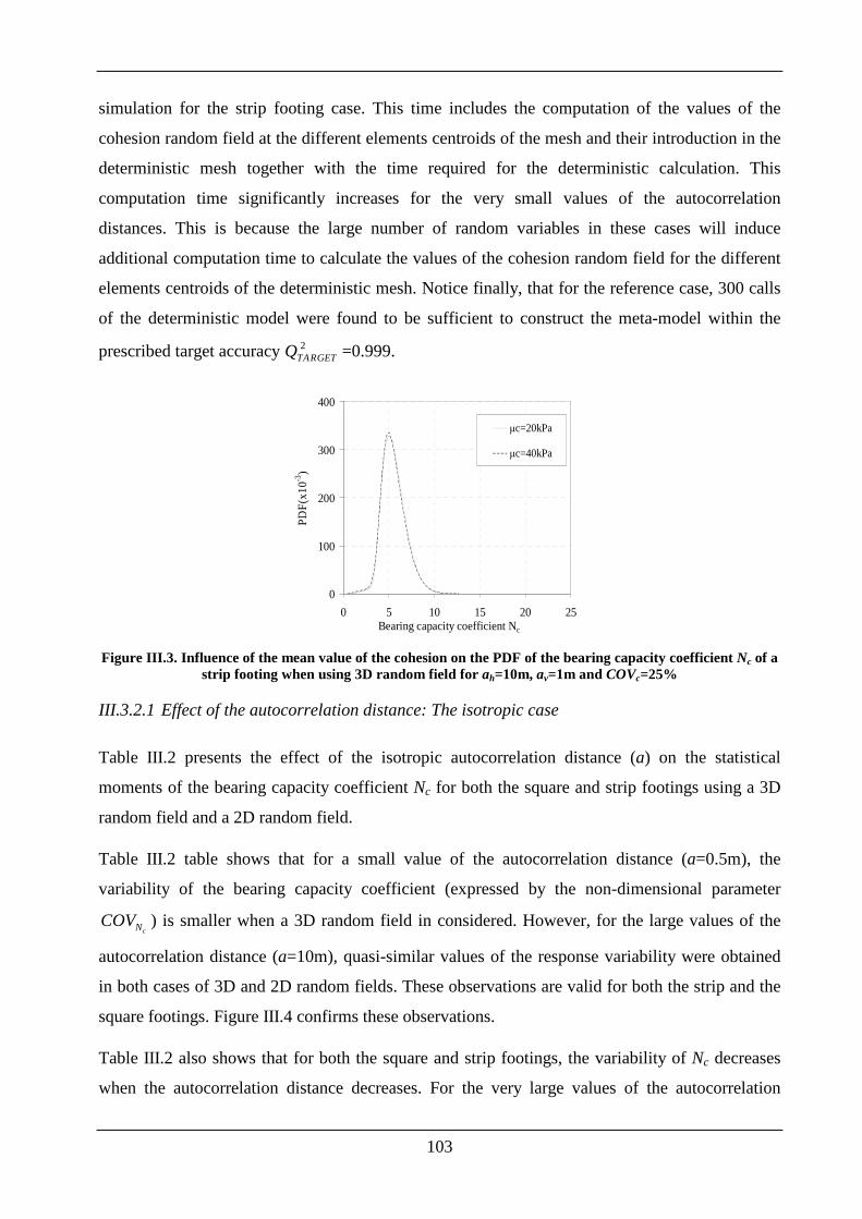
103
simulation for the strip footing case. This time includes the computation of the values of the
cohesion random field at the different elements centroids of the mesh and their introduction in the
deterministic mesh together with the time required for the deterministic calculation. This
computation time significantly increases for the very small values of the autocorrelation
distances. This is because the large number of random variables in these cases will induce
additional computation time to calculate the values of the cohesion random field for the different
elements centroids of the deterministic mesh. Notice finally, that for the reference case, 300 calls
of the deterministic model were found to be sufficient to construct the meta-model within the
prescribed target accuracy 2TARGETQ =0.999.
0
100
200
300
400
0 5 10 15 20 25Bearing capacity coefficient Nc
PD
F(x
10-3
)
µc=20kPa
µc=40kPa
Figure III.3. Influence of the mean value of the cohesion on the PDF of the bearing capacity coefficient Nc of a
strip footing when using 3D random field for ah=10m, av=1m and COVc=25%
III.3.2.1 Effect of the autocorrelation distance: The isotropic case
Table III.2 presents the effect of the isotropic autocorrelation distance (a) on the statistical
moments of the bearing capacity coefficient Nc for both the square and strip footings using a 3D
random field and a 2D random field.
Table III.2 table shows that for a small value of the autocorrelation distance (a=0.5m), the
variability of the bearing capacity coefficient (expressed by the non-dimensional parameter
cNCOV ) is smaller when a 3D random field in considered. However, for the large values of the
autocorrelation distance (a=10m), quasi-similar values of the response variability were obtained
in both cases of 3D and 2D random fields. These observations are valid for both the strip and the
square footings. Figure III.4 confirms these observations.
Table III.2 also shows that for both the square and strip footings, the variability of Nc decreases
when the autocorrelation distance decreases. For the very large values of the autocorrelation
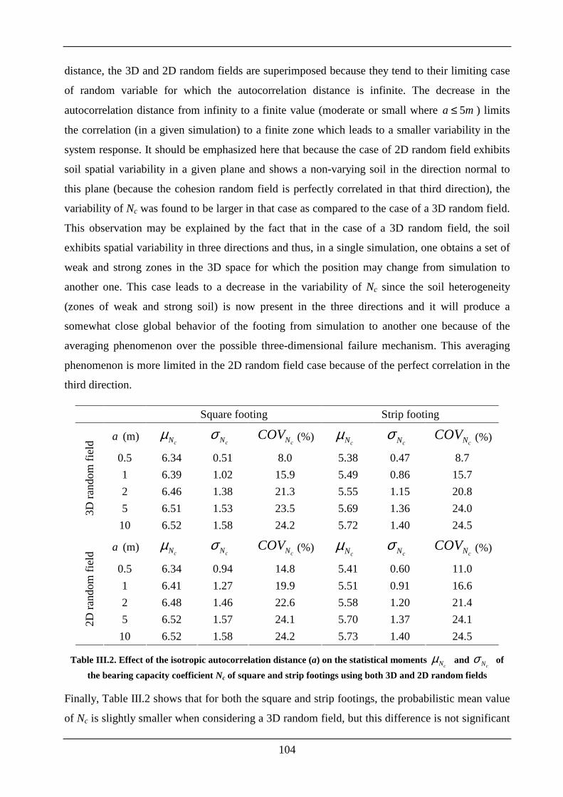
104
distance, the 3D and 2D random fields are superimposed because they tend to their limiting case
of random variable for which the autocorrelation distance is infinite. The decrease in the
autocorrelation distance from infinity to a finite value (moderate or small where 5a m≤ ) limits
the correlation (in a given simulation) to a finite zone which leads to a smaller variability in the
system response. It should be emphasized here that because the case of 2D random field exhibits
soil spatial variability in a given plane and shows a non-varying soil in the direction normal to
this plane (because the cohesion random field is perfectly correlated in that third direction), the
variability of Nc was found to be larger in that case as compared to the case of a 3D random field.
This observation may be explained by the fact that in the case of a 3D random field, the soil
exhibits spatial variability in three directions and thus, in a single simulation, one obtains a set of
weak and strong zones in the 3D space for which the position may change from simulation to
another one. This case leads to a decrease in the variability of Nc since the soil heterogeneity
(zones of weak and strong soil) is now present in the three directions and it will produce a
somewhat close global behavior of the footing from simulation to another one because of the
averaging phenomenon over the possible three-dimensional failure mechanism. This averaging
phenomenon is more limited in the 2D random field case because of the perfect correlation in the
third direction.
Square footing Strip footing
a (m) cNµ
cNσ cNCOV (%)
cNµ cNσ
cNCOV (%)
0.5 6.34 0.51 8.0 5.38 0.47 8.7
1 6.39 1.02 15.9 5.49 0.86 15.7
2 6.46 1.38 21.3 5.55 1.15 20.8
5 6.51 1.53 23.5 5.69 1.36 24.0 3D r
ando
m fi
eld
10 6.52 1.58 24.2 5.72 1.40 24.5
a (m) cNµ
cNσ cNCOV (%)
cNµ cNσ
cNCOV (%)
0.5 6.34 0.94 14.8 5.41 0.60 11.0
1 6.41 1.27 19.9 5.51 0.91 16.6
2 6.48 1.46 22.6 5.58 1.20 21.4
5 6.52 1.57 24.1 5.70 1.37 24.1 2D r
ando
m fi
eld
10 6.52 1.58 24.2 5.73 1.40 24.5
Table III.2. Effect of the isotropic autocorrelation distance (a) on the statistical moments cNµ and
cNσ of
the bearing capacity coefficient Nc of square and strip footings using both 3D and 2D random fields
Finally, Table III.2 shows that for both the square and strip footings, the probabilistic mean value
of Nc is slightly smaller when considering a 3D random field, but this difference is not significant
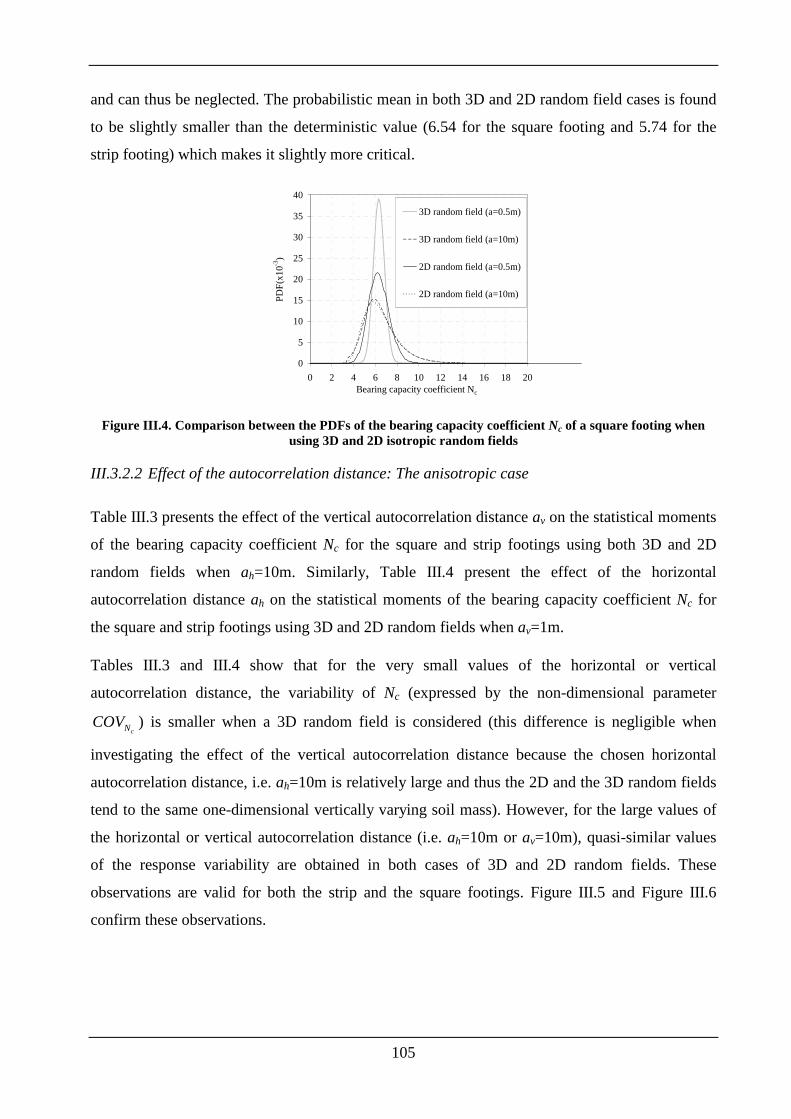
105
and can thus be neglected. The probabilistic mean in both 3D and 2D random field cases is found
to be slightly smaller than the deterministic value (6.54 for the square footing and 5.74 for the
strip footing) which makes it slightly more critical.
0
5
10
15
20
25
30
35
40
0 2 4 6 8 10 12 14 16 18 20Bearing capacity coefficient Nc
PD
F(x
10-3
)
3D random field (a=0.5m)
3D random field (a=10m)
2D random field (a=0.5m)
2D random field (a=10m)
Figure III.4. Comparison between the PDFs of the bearing capacity coefficient Nc of a square footing when using 3D and 2D isotropic random fields
III.3.2.2 Effect of the autocorrelation distance: The anisotropic case
Table III.3 presents the effect of the vertical autocorrelation distance av on the statistical moments
of the bearing capacity coefficient Nc for the square and strip footings using both 3D and 2D
random fields when ah=10m. Similarly, Table III.4 present the effect of the horizontal
autocorrelation distance ah on the statistical moments of the bearing capacity coefficient Nc for
the square and strip footings using 3D and 2D random fields when av=1m.
Tables III.3 and III.4 show that for the very small values of the horizontal or vertical
autocorrelation distance, the variability of Nc (expressed by the non-dimensional parameter
cNCOV ) is smaller when a 3D random field is considered (this difference is negligible when
investigating the effect of the vertical autocorrelation distance because the chosen horizontal
autocorrelation distance, i.e. ah=10m is relatively large and thus the 2D and the 3D random fields
tend to the same one-dimensional vertically varying soil mass). However, for the large values of
the horizontal or vertical autocorrelation distance (i.e. ah=10m or av=10m), quasi-similar values
of the response variability are obtained in both cases of 3D and 2D random fields. These
observations are valid for both the strip and the square footings. Figure III.5 and Figure III.6
confirm these observations.

106
Square footing Strip footing
va (m) cNµ
cNσ cNCOV (%)
cNµ cNσ
cNCOV (%)
0.15 6.24 0.96 15.3 5.38 0.66 12.2
0.25 6.27 1.15 18.3 5.39 0.82 15.3
0.5 6.38 1.38 21.7 5.45 1.04 19.2
1 6.48 1.52 23.5 5.58 1.24 22.3
2 6.51 1.57 24.1 5.67 1.36 23.9
5 6.51 1.58 24.2 5.71 1.39 24.4
3D r
ando
m fi
eld
10 6.52 1.58 24.2 5.72 1.40 24.5
va (m) cNµ
cNσ cNCOV (%)
cNµ cNσ
cNCOV (%)
0.15 6.24 0.97 15.5 5.39 0.67 12.5
0.25 6.27 1.16 18.5 5.41 0.84 15.5
0.5 6.38 1.39 21.8 5.47 1.06 19.3
1 6.48 1.53 23.5 5.59 1.25 22.4
2 6.51 1.57 24.1 5.69 1.36 24.0
5 6.51 1.58 24.2 5.72 1.40 24.4
2D r
ando
m fi
eld
10 6.52 1.58 24.2 5.73 1.40 24.5
Table III.3. Effect of the vertical autocorrelation distance (av) on the statistical moments cNµ and
cNσ of
the bearing capacity coefficient Nc of square and strip footings using both 3D and 2D random fields
Square footing Strip footing
ha (m) cNµ
cNσ cNCOV (%)
cNµ cNσ
cNCOV (%)
0.5 6.34 0.48 7.6 5.41 0.50 9.3
1 6.39 1.02 15.9 5.49 0.86 15.7
2 6.44 1.32 20.4 5.51 1.07 19.5
5 6.46 1.48 22.9 5.56 1.20 21.6 3D r
ando
m fi
eld
10 6.48 1.52 23.5 5.58 1.24 22.3
ha (m) cNµ
cNσ cNCOV (%)
cNµ cNσ
cNCOV (%)
0.5 6.35 1.01 15.9 5.43 0.70 12.8
1 6.41 1.27 19.9 5.51 0.91 16.6
2 6.47 1.39 21.5 5.53 1.10 19.9
5 6.47 1.48 22.8 5.57 1.21 21.7 2D r
ando
m fi
eld
10 6.48 1.53 23.5 5.59 1.25 22.4
Table III.4. Effect of the horizontal autocorrelation distance (ah) on the statistical moments cNµ and
cNσ of
the bearing capacity coefficient Nc of square and strip footings using both 3D and 2D random fields
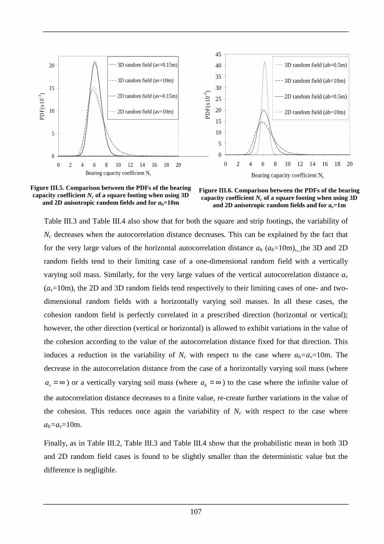
107
0
5
10
15
20
0 2 4 6 8 10 12 14 16 18 20Bearing capacity coefficient Nc
PD
F(x
10-3
)
3D random field (av=0.15m)
3D random field (av=10m)
2D random field (av=0.15m)
2D random field (av=10m)
Figure III.5. Comparison between the PDFs of the bearing capacity coefficient Nc of a square footing when using 3D
and 2D anisotropic random fields and for ah=10m
0
5
10
15
20
25
30
35
40
45
0 2 4 6 8 10 12 14 16 18 20
Bearing capacity coefficient Nc
PD
F(x
10-3
)
3D random field (ah=0.5m)
3D random field (ah=10m)
2D random field (ah=0.5m)
2D random field (ah=10m)
Figure III.6. Comparison between the PDFs of the bearing capacity coefficient Nc of a square footing when using 3D
and 2D anisotropic random fields and for av=1m
Table III.3 and Table III.4 also show that for both the square and strip footings, the variability of
Nc decreases when the autocorrelation distance decreases. This can be explained by the fact that
for the very large values of the horizontal autocorrelation distance ah (ah=10m),_the 3D and 2D
random fields tend to their limiting case of a one-dimensional random field with a vertically
varying soil mass. Similarly, for the very large values of the vertical autocorrelation distance av
(av=10m), the 2D and 3D random fields tend respectively to their limiting cases of one- and two-
dimensional random fields with a horizontally varying soil masses. In all these cases, the
cohesion random field is perfectly correlated in a prescribed direction (horizontal or vertical);
however, the other direction (vertical or horizontal) is allowed to exhibit variations in the value of
the cohesion according to the value of the autocorrelation distance fixed for that direction. This
induces a reduction in the variability of Nc with respect to the case where ah=av=10m. The
decrease in the autocorrelation distance from the case of a horizontally varying soil mass (where
va = ∞ ) or a vertically varying soil mass (where ha = ∞ ) to the case where the infinite value of
the autocorrelation distance decreases to a finite value, re-create further variations in the value of
the cohesion. This reduces once again the variability of Nc with respect to the case where
ah=av=10m.
Finally, as in Table III.2, Table III.3 and Table III.4 show that the probabilistic mean in both 3D
and 2D random field cases is found to be slightly smaller than the deterministic value but the
difference is negligible.
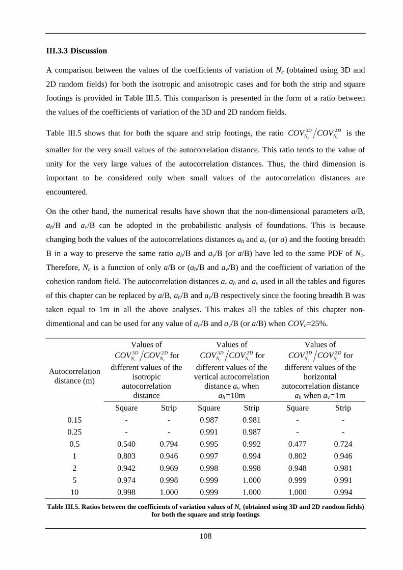
108
III.3.3 Discussion
A comparison between the values of the coefficients of variation of Nc (obtained using 3D and
2D random fields) for both the isotropic and anisotropic cases and for both the strip and square
footings is provided in Table III.5. This comparison is presented in the form of a ratio between
the values of the coefficients of variation of the 3D and 2D random fields.
Table III.5 shows that for both the square and strip footings, the ratio 3 2
c c
D DN NCOV COV is the
smaller for the very small values of the autocorrelation distance. This ratio tends to the value of
unity for the very large values of the autocorrelation distances. Thus, the third dimension is
important to be considered only when small values of the autocorrelation distances are
encountered.
On the other hand, the numerical results have shown that the non-dimensional parameters a/B,
ah/B and av/B can be adopted in the probabilistic analysis of foundations. This is because
changing both the values of the autocorrelations distances ah and av (or a) and the footing breadth
B in a way to preserve the same ratio ah/B and av/B (or a/B) have led to the same PDF of Nc.
Therefore, Nc is a function of only a/B or (ah/B and av/B) and the coefficient of variation of the
cohesion random field. The autocorrelation distances a, ah and av used in all the tables and figures
of this chapter can be replaced by a/B, ah/B and av/B respectively since the footing breadth B was
taken equal to 1m in all the above analyses. This makes all the tables of this chapter non-
dimentional and can be used for any value of ah/B and av/B (or a/B) when COVc=25%.
Values of 3 2
c c
D DN NCOV COV for
different values of the isotropic
autocorrelation distance
Values of 3 2
c c
D DN NCOV COV for
different values of the vertical autocorrelation
distance av when ah=10m
Values of 3 2
c c
D DN NCOV COV for
different values of the horizontal
autocorrelation distance ah when av=1m
Autocorrelation distance (m)
Square Strip Square Strip Square Strip
0.15 - - 0.987 0.981 - -
0.25 - - 0.991 0.987 - -
0.5 0.540 0.794 0.995 0.992 0.477 0.724
1 0.803 0.946 0.997 0.994 0.802 0.946
2 0.942 0.969 0.998 0.998 0.948 0.981
5 0.974 0.998 0.999 1.000 0.999 0.991
10 0.998 1.000 0.999 1.000 1.000 0.994
Table III.5. Ratios between the coefficients of variation values of Nc (obtained using 3D and 2D random fields) for both the square and strip footings
109
III.4 CONCLUSIONS
A probabilistic analysis that considers the effect of the spatial variability in three dimensions was
investigated through the study of the ultimate bearing capacity of strip and square foundations
resting on a purely cohesive soil with a spatially varying cohesion in the three dimensions. The
main reason for which a purely cohesive soil was used is to investigate the effect of the spatial
variability in the third direction with the use of a relatively non-expensive deterministic model.
In order to investigate the effect of the spatial variability in the third direction on the ultimate
bearing capacity of foundations, the results obtained using a 3D random field were compared to
those corresponding to a 2D random field for the two cases of strip and square footings. The
objective is to check the validity of a 2D random field in both cases of plane strain and three-
dimensional problems.
The soil cohesion parameter was modeled as anisotropic non-Gaussian (log-normal) random field
with a square exponential autocorrelation function. A straightforward extension to the 3D case of
the Expansion Optimal Linear Estimation (EOLE) methodology proposed by Li and Der
Kiureghian (1993) and extended by Vořechovsky (2008) was used in this chapter. The
deterministic model was based on 3D numerical simulations using FLAC3D software. An efficient
uncertainty propagation methodology that makes use of a non-intrusive approach to build up a
sparse polynomial chaos expansion for the system response was employed.
The probabilistic numerical results have shown that for small values of the autocorrelation
distances, the variability of the ultimate bearing capacity computed by considering a 3D random
field is smaller than the one obtained with the 2D random field for both cases of square and strip
footings. The ratio 3 2
c c
D DN NCOV COV between the values of the coefficients of variation of Nc
using the 3D and 2D random fields is the smaller for the very small values of the autocorrelation
distance. This ratio tends to the value of unity for the very large values of the autocorrelation
distances. Thus, the third dimension is important to be considered when small autocorrelation
distances are encountered. As for the probabilistic mean values, slightly smaller values were
obtained in the case of the 3D random field but the difference is negligible.
110
CHAPTER IV. COMBINED USE OF THE SPARSE POLYNOMIAL
CHAOS EXPANSION METHODOLOGY AND THE GLOBAL SENSITIV ITY
ANALYSIS FOR HIGH-DIMENSIONAL STOCHASTIC PROBLEMS
IV.1 INTRODUCTION
In the previous two chapters, an efficient approach to deal with uncertainty propagation in the
case of high-dimensional problems (i.e. when a large number of random variables is involved)
was presented. This approach is based on the sparse polynomial chaos expansion (SPCE) for the
system response and leads to a reduced computational cost as compared to the classical
polynomial chaos expansion (PCE) methodology. Notice that both, the PCE and the SPCE
methodologies, aim at replacing the original complex deterministic model which may be an
analytical model or a finite element/finite difference model by a meta-model. This allows one to
easily calculate the system response (when performing MCS) using a simple analytical equation.
When dealing with high-dimensional stochastic problems making use of computationally-
expensive deterministic models (e.g. three-dimensional analysis of shallow rectangular or circular
footings resting on 3D spatially varying ponderable soils), the time cost remains important even
with the use of the SPCE. Consequently, a method that can reduce once again the cost of the
probabilistic analysis (i.e. the number of calls of the deterministic model) is needed.
In this chapter, an efficient combined use of the SPCE methodology and the Global Sensitivity
Analysis (GSA) is proposed [Al-Bittar and Soubra (2012e, 2012f, 2012g)]. The basic idea of this
combination is that, for a given discretized random field, the obtained random variables do not
have the same weight in the variability of the system response. The variables with a very small
contribution in the variability of the system response can be discarded which significantly
reduces the dimensionality of the treated problem. This allows one to perform a probabilistic
analysis using a reduced Experiment Design (ED) and thus a smaller number of calls of the
computationally-expensive deterministic model. The main challenge remains in detecting the
most influential random variables in order to reduce the dimensionality of the problem. For this
purpose, a procedure that makes use of both the SPCE and the GSA (denoted hereafter by
SPCE/GSA) is proposed in this regard.
The proposed methodology was firstly validated using a relatively non-expensive model. This
model was extensively investigated in the second chapter of this thesis using the SPCE
methodology. It involves the computation of the ultimate bearing capacity of a strip footing
111
resting on a weightless spatially varying soil where the soil cohesion and angle of internal friction
(c and φ) were modeled by two anisotropic non-Gaussian cross-correlated random fields.
Secondly, the SPCE/GSA procedure was applied to two computationally-expensive deterministic
models that involve the computation of the PDF of the ultimate bearing capacity of a strip footing
resting on a ponderable soil in both cases of (i) 2D random fields and (ii) 3D random fields.
While an extensive parametric study was undertaken in the case of the 2D spatially varying soil,
only a single soil configuration was considered in the case of the 3D spatially varying soil. The
study of the case of rectangular or circular footings resting on a ponderable 3D spatially varying
soil will be the subject of future studies.
This chapter is organized as follows: The proposed SPCE/GSA procedure is firstly presented. It
is followed by the numerical results. The chapter ends by a conclusion of the main findings
IV.2 EFFICIENT COMBINED USE OF THE SPCE METHODOLOGY AND THE
GLOBAL SENSITIVITY ANALYSIS GSA
As mentioned previously, the time cost of the probabilistic analysis remains important even with
the use of the SPCE when dealing with computationally-expensive deterministic models.
Consequently, a procedure that can reduce once again this time cost is needed.
An efficient combined use of the SPCE methodology and the GSA is proposed in this section. In
this method, a small SPCE order is firstly selected to approximate the system response by a meta-
model. It should be noted that the random variables involved in the system response are those that
result from the discretization of the random fields into a finite number of random variables. A
GSA based on Sobol indices is then performed on this small SPCE order to determine the weight
of each random variable in the variability of the system response. As a result, the variables with
very small values of their Sobol indices (i.e. those that have a small weight in the variability of
the system response) can be discarded. Consequently, a response which only depends on a
smaller number of random variables is obtained. In other words, one obtains a response with an
'effective dimension'. This dimension is smaller than the initial dimension where the total number
of random variables was considered. As it will be shown later, the use of a small SPCE order to
perform the GSA is not a concern since higher SPCE orders lead to the same influential random
variables. Once the 'effective dimension' was determined, a higher SPCE order that makes use of
only the most influential random variables can be used. This significantly reduces the
computation time. The use of a higher SPCE order is necessary in order to lead to an improved fit
of the SPCE. The SPCE/GSA procedure can be described in more details by the following steps:
112
• Discretize the random field(s): This step may be made using EOLE method and its
extensions by Vořechovsky (2008) (see section I.3.4). After the discretization procedure,
a random field is represented by N independent standard normal random variables. If the
total number of random fields involved in the analysis is equal to NRF, the total number of
random variables is thus given by NT= NRFxN which can be relatively large especially for
small values of the autocorrelation distances as was seen in the previous chapters. Notice
that the equation NT=NRFxN is only applicable if all the random fields share the same
autocorrelation function.
• Select a preliminary small order of the sparse polynomial chaos expansion (e.g. p=2) to
approximate the system response by a meta-model. The main reason for selecting a small
order is the exploration of the most influential random variables (i.e. those that have a
significant weight in the variability of the system response) using a small Experiment
Design (ED). It should be emphasized here that the small value of the SPCE order leads to
a significant decrease in the size of the experiment design, i.e. in the number of calls of
the deterministic model.
• Perform a GSA based on Sobol indices (using the obtained second order SPCE) to
determine the weight of each random variable (of the different random fields) in the
variability of the system response. The variables with very small values of their Sobol
indices have no significant weight in the variability of the system response and can thus
be discarded. Consequently, a response that only depends on a smaller number of random
variables is obtained. In other words, one obtains a response with an 'effective dimension'
Ne that is smaller than the initial dimension where the total number NT of random
variables was considered. It should be mentioned here that the small SPCE order (i.e.
p=2) used firstly to perform the GSA is sufficient to provide the weight of each random
variable in the variability of the system response since higher SPCE orders lead to the
same influential random variables as will be seen later in the numerical results.
• Use the same Experiment Design (ED) which was employed before but this time by only
keeping the most influential random variables. By reducing the number of random
variables from NT to Ne (where Ne<NT), one has the possibility to use a higher SPCE order
(i.e. p>2). The use of a higher SPCE order is necessary to lead to an improved fit of the
SPCE since the coefficient of determination Q2 given in Equation ( I.45) increases when
the SPCE order increases as it will be shown in the numerical results.
113
As a conclusion, the use of the SPCE/GSA procedure is expected to provide a good fit of the
deterministic model with a reduced number of model evaluations as compared to the classical
SPCE approach.
IV.3 NUMERICAL RESULTS
The aim of this section is to make use of the SPCE/GSA approach for the determination of the
probabilistic numerical results of two computationally-expensive deterministic models. More
specifically, one focuses on the computation of the probability density function (PDF) of the
ultimate bearing capacity (qult) of a strip footing resting on a ponderable soil in both cases of (i)
2D random fields and (ii) 3D random fields. It should be mentioned here that a somewhat similar
problem was considered in chapter II using the SPCE approach: Since the SPCE approach was
unable to consider the case of a ponderable soil because of the significant computational cost,
only the case of a weightless soil was considered. Also, only 2D random fields were investigated.
The soil cohesion c and friction angle φ were modeled by two anisotropic cross-correlated non-
Gaussian random fields. The deterministic model was based on numerical simulations using
FLAC3D. The inputs of the deterministic and probabilistic models are the same as those
considered in chapter II and more precisely in section II.3.1 where a probabilistic analysis of a
strip footing resting on a weightless 2D spatially varying (c, φ) soil mass was undertaken. The
only additional parameter used herein is the soil unit weight γ whose value is considered to be
equal to 18 kN/m3.
Before the presentation of the probabilistic results of a ponderable soil for both cases of 2D and
3D random fields, it seems necessary to validate the present SPCE/GSA procedure by
comparison of its results with those obtained by the use of the classical SPCE (in the case of a
weightless soil). This is the aim of the next subsection.
IV.3.1 Validation of the SPCE/GSA procedure
The aim of this section is the validation of the present SPCE/GSA approach. For this purpose, a
comparison between the results obtained using the classical SPCE method and those obtained
with the proposed SPCE/GSA procedure is presented in the case of a weightless soil (which is a
relatively non-expensive deterministic model). It should be mentioned here that when neglecting
the soil weight γ, the computation time decreases from 10 to 5 min per simulation. Although this
difference may not seem to be significant for a single simulation, it becomes dramatically
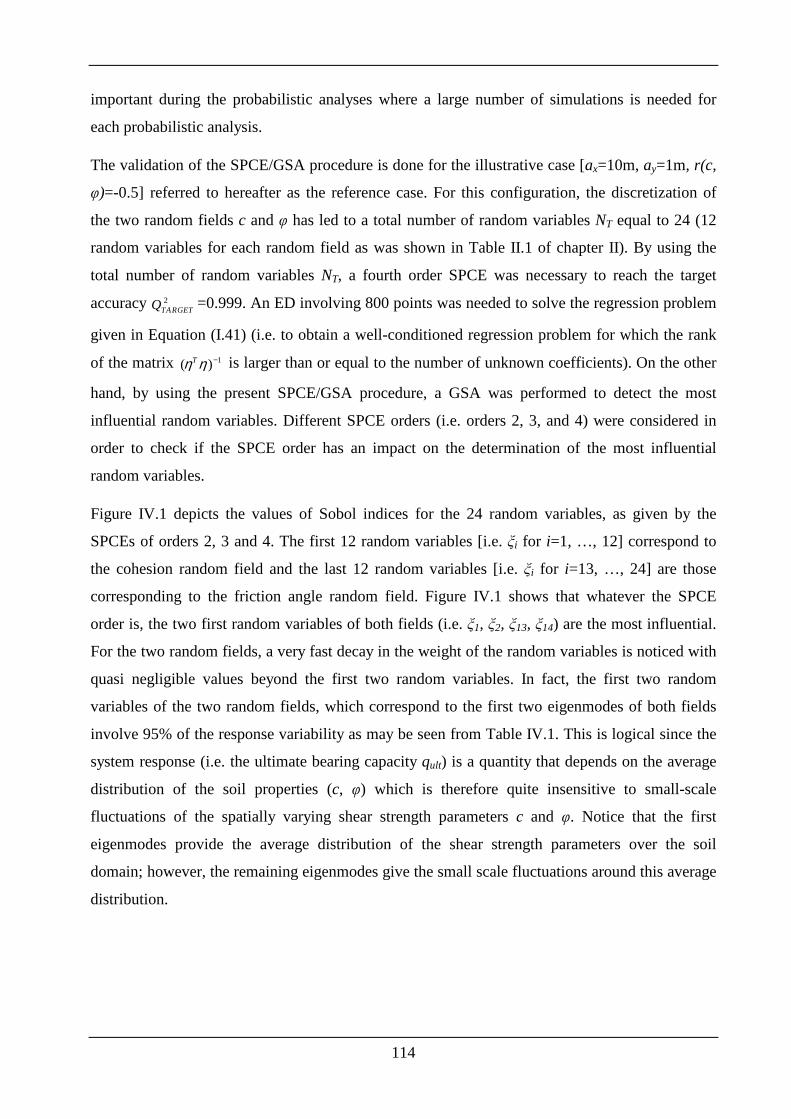
114
important during the probabilistic analyses where a large number of simulations is needed for
each probabilistic analysis.
The validation of the SPCE/GSA procedure is done for the illustrative case [ax=10m, ay=1m, r(c,
φ)=-0.5] referred to hereafter as the reference case. For this configuration, the discretization of
the two random fields c and φ has led to a total number of random variables NT equal to 24 (12
random variables for each random field as was shown in Table II.1 of chapter II). By using the
total number of random variables NT, a fourth order SPCE was necessary to reach the target
accuracy 2TARGETQ =0.999. An ED involving 800 points was needed to solve the regression problem
given in Equation ( I.41) (i.e. to obtain a well-conditioned regression problem for which the rank
of the matrix 1( )Tη η − is larger than or equal to the number of unknown coefficients). On the other
hand, by using the present SPCE/GSA procedure, a GSA was performed to detect the most
influential random variables. Different SPCE orders (i.e. orders 2, 3, and 4) were considered in
order to check if the SPCE order has an impact on the determination of the most influential
random variables.
Figure IV.1 depicts the values of Sobol indices for the 24 random variables, as given by the
SPCEs of orders 2, 3 and 4. The first 12 random variables [i.e. ξi for i=1, …, 12] correspond to
the cohesion random field and the last 12 random variables [i.e. ξi for i=13, …, 24] are those
corresponding to the friction angle random field. Figure IV.1 shows that whatever the SPCE
order is, the two first random variables of both fields (i.e. ξ1, ξ2, ξ13, ξ14) are the most influential.
For the two random fields, a very fast decay in the weight of the random variables is noticed with
quasi negligible values beyond the first two random variables. In fact, the first two random
variables of the two random fields, which correspond to the first two eigenmodes of both fields
involve 95% of the response variability as may be seen from Table IV.1. This is logical since the
system response (i.e. the ultimate bearing capacity qult) is a quantity that depends on the average
distribution of the soil properties (c, φ) which is therefore quite insensitive to small-scale
fluctuations of the spatially varying shear strength parameters c and φ. Notice that the first
eigenmodes provide the average distribution of the shear strength parameters over the soil
domain; however, the remaining eigenmodes give the small scale fluctuations around this average
distribution.
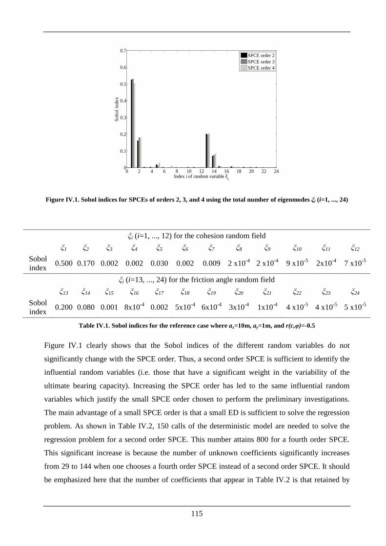
115
0 2 4 6 8 10 12 14 16 18 20 22 240
0.1
0.2
0.3
0.4
0.5
0.6
0.7
Index i of random variable ξi
Sob
ol in
dex
SPCE order 2SPCE order 3SPCE order 4
Figure IV.1. Sobol indices for SPCEs of orders 2, 3, and 4 using the total number of eigenmodes ξi (i=1, ..., 24)
ξi (i=1, ..., 12) for the cohesion random field
ξ1 ξ2 ξ3 ξ4 ξ5 ξ6 ξ7 ξ8 ξ9 ξ10 ξ11 ξ12
Sobol index
0.500 0.170 0.002 0.002 0.030 0.002 0.009 2 x10⁻⁴ 2 x10⁻⁴ 9 x10⁻⁵ 2x10⁻⁴ 7 x10⁻⁵
ξi (i=13, ..., 24) for the friction angle random field
ξ13 ξ14 ξ15 ξ16 ξ17 ξ18 ξ19 ξ20 ξ21 ξ22 ξ23 ξ24
Sobol index
0.200 0.080 0.001 8x10⁻⁴ 0.002 5x10⁻⁴ 6x10⁻⁴ 3x10⁻⁴ 1x10⁻⁴ 4 x10⁻⁵ 4 x10⁻⁵ 5 x10⁻⁵
Table IV.1. Sobol indices for the reference case where ax=10m, ay=1m, and r(c,φ)=-0.5
Figure IV.1 clearly shows that the Sobol indices of the different random variables do not
significantly change with the SPCE order. Thus, a second order SPCE is sufficient to identify the
influential random variables (i.e. those that have a significant weight in the variability of the
ultimate bearing capacity). Increasing the SPCE order has led to the same influential random
variables which justify the small SPCE order chosen to perform the preliminary investigations.
The main advantage of a small SPCE order is that a small ED is sufficient to solve the regression
problem. As shown in Table IV.2, 150 calls of the deterministic model are needed to solve the
regression problem for a second order SPCE. This number attains 800 for a fourth order SPCE.
This significant increase is because the number of unknown coefficients significantly increases
from 29 to 144 when one chooses a fourth order SPCE instead of a second order SPCE. It should
be emphasized here that the number of coefficients that appear in Table IV.2 is that retained by
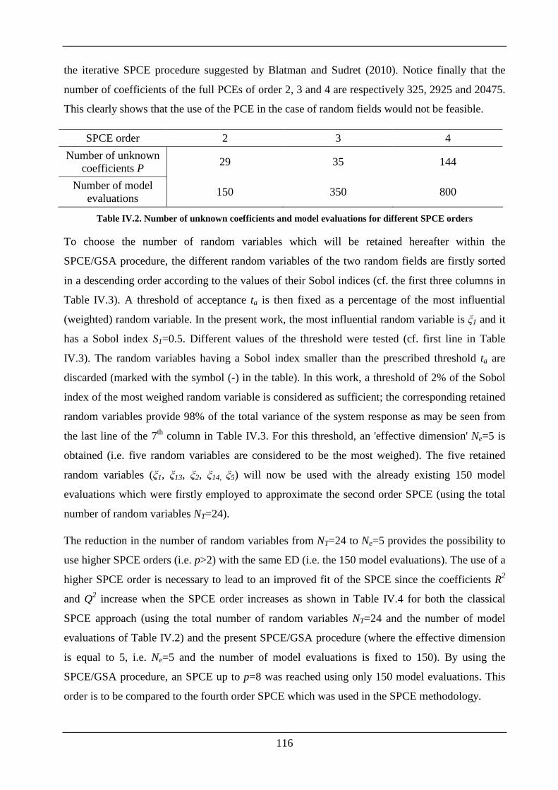
116
the iterative SPCE procedure suggested by Blatman and Sudret (2010). Notice finally that the
number of coefficients of the full PCEs of order 2, 3 and 4 are respectively 325, 2925 and 20475.
This clearly shows that the use of the PCE in the case of random fields would not be feasible.
SPCE order 2 3 4
Number of unknown coefficients P
29 35 144
Number of model evaluations
150 350 800
Table IV.2. Number of unknown coefficients and model evaluations for different SPCE orders
To choose the number of random variables which will be retained hereafter within the
SPCE/GSA procedure, the different random variables of the two random fields are firstly sorted
in a descending order according to the values of their Sobol indices (cf. the first three columns in
Table IV.3). A threshold of acceptance ta is then fixed as a percentage of the most influential
(weighted) random variable. In the present work, the most influential random variable is ξ1 and it
has a Sobol index S1=0.5. Different values of the threshold were tested (cf. first line in Table
IV.3). The random variables having a Sobol index smaller than the prescribed threshold ta are
discarded (marked with the symbol (-) in the table). In this work, a threshold of 2% of the Sobol
index of the most weighed random variable is considered as sufficient; the corresponding retained
random variables provide 98% of the total variance of the system response as may be seen from
the last line of the 7th column in Table IV.3. For this threshold, an 'effective dimension' Ne=5 is
obtained (i.e. five random variables are considered to be the most weighed). The five retained
random variables (ξ1, ξ13, ξ2, ξ14, ξ5) will now be used with the already existing 150 model
evaluations which were firstly employed to approximate the second order SPCE (using the total
number of random variables NT=24).
The reduction in the number of random variables from NT=24 to Ne=5 provides the possibility to
use higher SPCE orders (i.e. p>2) with the same ED (i.e. the 150 model evaluations). The use of a
higher SPCE order is necessary to lead to an improved fit of the SPCE since the coefficients R2
and Q2 increase when the SPCE order increases as shown in Table IV.4 for both the classical
SPCE approach (using the total number of random variables NT=24 and the number of model
evaluations of Table IV.2) and the present SPCE/GSA procedure (where the effective dimension
is equal to 5, i.e. Ne=5 and the number of model evaluations is fixed to 150). By using the
SPCE/GSA procedure, an SPCE up to p=8 was reached using only 150 model evaluations. This
order is to be compared to the fourth order SPCE which was used in the SPCE methodology.
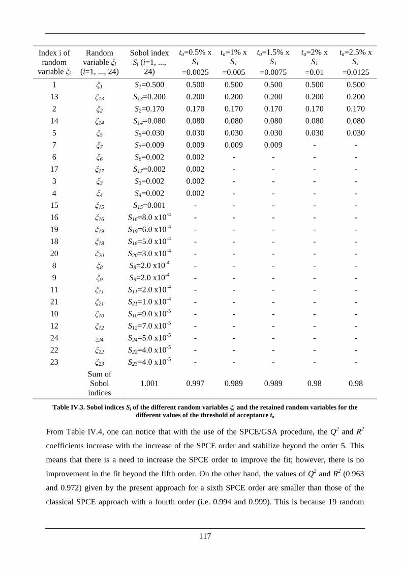
117
Index i of random
variable ξi
Random variable ξi
(i=1, ..., 24)
Sobol index Si (i=1, ...,
24)
ta=0.5% x S1
=0.0025
ta=1% x S1
=0.005
ta=1.5% x S1
=0.0075
ta=2% x S1
=0.01
ta=2.5% x S1
=0.0125
1 ξ1 S1=0.500 0.500 0.500 0.500 0.500 0.500
13 ξ13 S13=0.200 0.200 0.200 0.200 0.200 0.200
2 ξ2 S2=0.170 0.170 0.170 0.170 0.170 0.170
14 ξ14 S14=0.080 0.080 0.080 0.080 0.080 0.080
5 ξ5 S5=0.030 0.030 0.030 0.030 0.030 0.030
7 ξ7 S7=0.009 0.009 0.009 0.009 - -
6 ξ6 S6=0.002 0.002 - - - -
17 ξ17 S17=0.002 0.002 - - - -
3 ξ3 S3=0.002 0.002 - - - -
4 ξ4 S4=0.002 0.002 - - - -
15 ξ15 S15=0.001 - - - - -
16 ξ16 S16=8.0 x10⁻⁴ - - - - -
19 ξ19 S19=6.0 x10⁻⁴ - - - - -
18 ξ18 S18=5.0 x10⁻⁴ - - - - -
20 ξ20 S20=3.0 x10⁻⁴ - - - - -
8 ξ8 S8=2.0 x10⁻⁴ - - - - -
9 ξ9 S9=2.0 x10⁻⁴ - - - - -
11 ξ11 S11=2.0 x10⁻⁴ - - - - -
21 ξ21 S21=1.0 x10⁻⁴ - - - - -
10 ξ10 S10=9.0 x10⁻⁵ - - - - -
12 ξ12 S12=7.0 x10⁻⁵ - - - - -
24 ξ24 S24=5.0 x10⁻⁵ - - - - -
22 ξ22 S22=4.0 x10⁻⁵ - - - - -
23 ξ23 S23=4.0 x10⁻⁵ - - - - -
Sum of Sobol indices
1.001 0.997 0.989 0.989 0.98 0.98
Table IV.3. Sobol indices Si of the different random variables ξi and the retained random variables for the different values of the threshold of acceptance ta
From Table IV.4, one can notice that with the use of the SPCE/GSA procedure, the Q2 and R2
coefficients increase with the increase of the SPCE order and stabilize beyond the order 5. This
means that there is a need to increase the SPCE order to improve the fit; however, there is no
improvement in the fit beyond the fifth order. On the other hand, the values of Q2 and R2 (0.963
and 0.972) given by the present approach for a sixth SPCE order are smaller than those of the
classical SPCE approach with a fourth order (i.e. 0.994 and 0.999). This is because 19 random
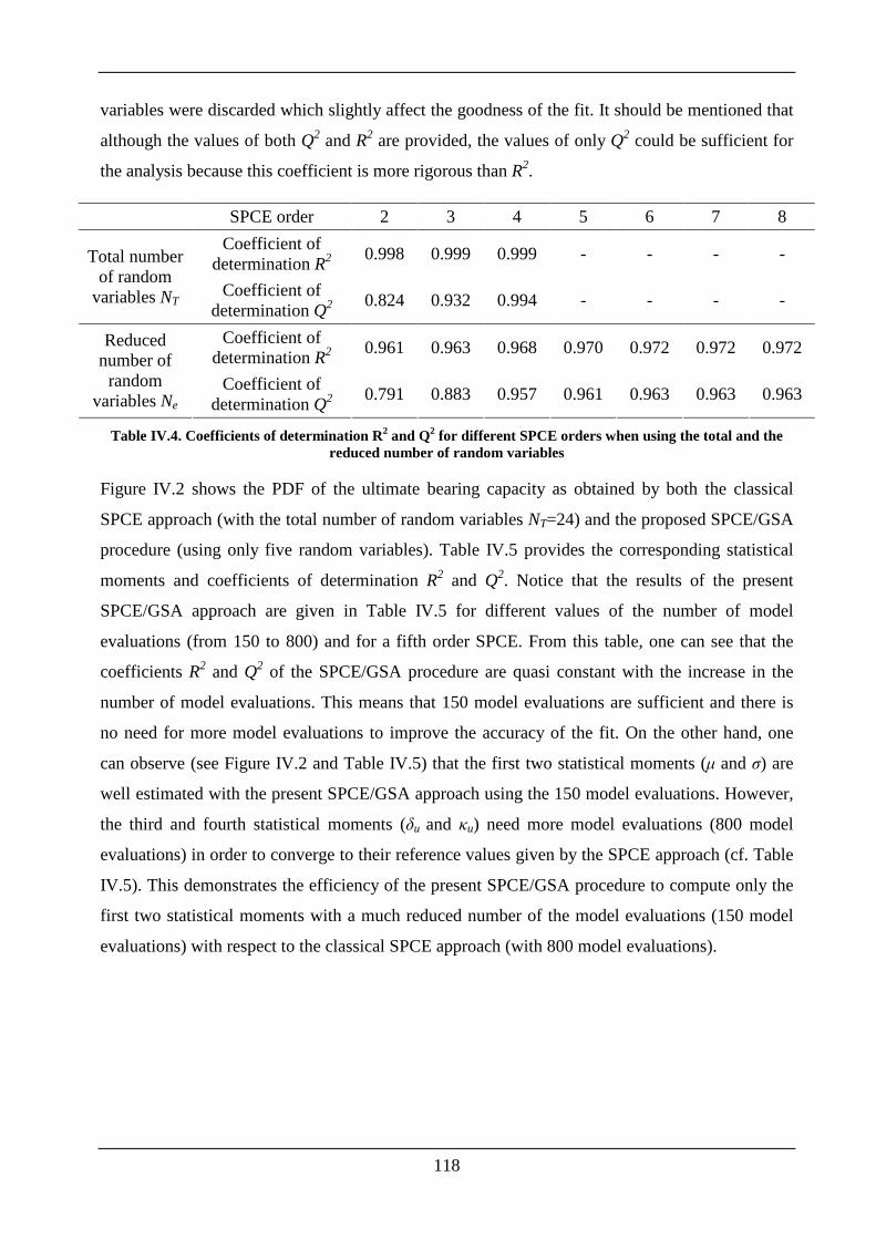
118
variables were discarded which slightly affect the goodness of the fit. It should be mentioned that
although the values of both Q2 and R2 are provided, the values of only Q2 could be sufficient for
the analysis because this coefficient is more rigorous than R2.
SPCE order 2 3 4 5 6 7 8
Coefficient of determination R2
0.998 0.999 0.999 - - - - Total number of random
variables NT Coefficient of determination Q2
0.824 0.932 0.994 - - - -
Coefficient of determination R2
0.961 0.963 0.968 0.970 0.972 0.972 0.972 Reduced number of random
variables Ne Coefficient of
determination Q2 0.791 0.883 0.957 0.961 0.963 0.963 0.963
Table IV.4. Coefficients of determination R2 and Q2 for different SPCE orders when using the total and the reduced number of random variables
Figure IV.2 shows the PDF of the ultimate bearing capacity as obtained by both the classical
SPCE approach (with the total number of random variables NT=24) and the proposed SPCE/GSA
procedure (using only five random variables). Table IV.5 provides the corresponding statistical
moments and coefficients of determination R2 and Q2. Notice that the results of the present
SPCE/GSA approach are given in Table IV.5 for different values of the number of model
evaluations (from 150 to 800) and for a fifth order SPCE. From this table, one can see that the
coefficients R2 and Q2 of the SPCE/GSA procedure are quasi constant with the increase in the
number of model evaluations. This means that 150 model evaluations are sufficient and there is
no need for more model evaluations to improve the accuracy of the fit. On the other hand, one
can observe (see Figure IV.2 and Table IV.5) that the first two statistical moments (µ and σ) are
well estimated with the present SPCE/GSA approach using the 150 model evaluations. However,
the third and fourth statistical moments (δu and κu) need more model evaluations (800 model
evaluations) in order to converge to their reference values given by the SPCE approach (cf. Table
IV.5). This demonstrates the efficiency of the present SPCE/GSA procedure to compute only the
first two statistical moments with a much reduced number of the model evaluations (150 model
evaluations) with respect to the classical SPCE approach (with 800 model evaluations).
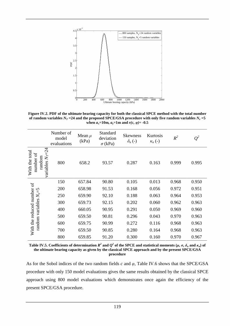
119
0 200 400 600 800 1000 1200 1400 1600 1800 20000
0.5
1
1.5
2
2.5
3
3.5
4
4.5x 10⁻³
Ultimate bearing capacity (kPa)
PD
F
800 samples, N
T=24 random variables
150 samples, Ne=5 random variables
Figure IV.2. PDF of the ultimate bearing capacity for both the classical SPCE method with the total number of random variables NT =24 and the proposed SPCE/GSA procedure with only five random variables Ne =5
when ax=10m, ay=1m and r(c, φ)= -0.5
Number of
model evaluations
Mean µ (kPa)
Standard deviation σ (kPa)
Skewness δu (-)
Kurtosis κu (-)
R2 Q2
With
the
tota
l nu
mbe
r of
ra
ndom
va
riabl
es N
T=
24
800 658.2 93.57 0.287 0.163 0.999 0.995
150 657.84 90.80 0.105 0.013 0.968 0.950
200 658.98 91.53 0.168 0.056 0.972 0.951
250 659.90 92.10 0.188 0.063 0.964 0.953
300 659.73 92.15 0.202 0.060 0.962 0.963
400 660.05 90.95 0.291 0.050 0.969 0.960
500 659.50 90.81 0.296 0.043 0.970 0.963
600 659.75 90.99 0.272 0.116 0.968 0.963
700 659.50 90.85 0.280 0.164 0.968 0.963
With
the
redu
ced
num
ber
of
rand
om v
aria
bles
Ne=
5
800 659.85 91.20 0.300 0.160 0.970 0.967
Table IV.5. Coefficients of determination R2 and Q2 of the SPCE and statistical moments (µ, σ, δu and κu) of the ultimate bearing capacity as given by the classical SPCE approach and by the present SPCE/GSA
procedure
As for the Sobol indices of the two random fields c and φ, Table IV.6 shows that the SPCE/GSA
procedure with only 150 model evaluations gives the same results obtained by the classical SPCE
approach using 800 model evaluations which demonstrates once again the efficiency of the
present SPCE/GSA procedure.
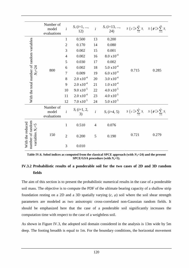
120
Number of
model evaluations
i Si (i=1, ...,
12) i
Si (i=13, ..., 24)
( )12
1i
i
S c S=
=∑ ( )24
13i
i
S Sϕ=
=∑
1 0.500 13 0.200
2 0.170 14 0.080
3 0.002 15 0.001
4 0.002 16 8.0 x10⁻⁴
5 0.030 17 0.002
6 0.002 18 5.0 x10⁻⁴
7 0.009 19 6.0 x10⁻⁴
8 2.0 x10⁻⁴ 20 3.0 x10⁻⁴
9 2.0 x10⁻⁴ 21 1.0 x10⁻⁴
10 9.0 x10⁻⁵ 22 4.0 x10⁻⁵
11 2.0 x10⁻⁴ 23 4.0 x10⁻⁵
With
the
tota
l num
ber
of r
ando
m v
aria
bles
N
T=
24
800
12 7.0 x10⁻⁵ 24 5.0 x10⁻⁵
0.715 0.285
Number of
model evaluations
i Si (i=1, 2,
3) i Si (i=4, 5) ( )
3
1i
i
S c S=
=∑ ( )5
4i
i
S Sϕ=
=∑
1 0.510 4 0.076
2 0.200 5 0.190
With
the
redu
ced
num
ber
of r
ando
m
varia
bles
Ne=
5 150
3 0.010
0.721 0.279
Table IV.6. Sobol indices as computed from the classical SPCE approach (with NT=24) and the present SPCE/GSA procedure (with Ne=5).
IV.3.2 Probabilistic results of a ponderable soil for the two cases of 2D and 3D random
fields
The aim of this section is to present the probabilistic numerical results in the case of a ponderable
soil mass. The objective is to compute the PDF of the ultimate bearing capacity of a shallow strip
foundation resting on a 2D and a 3D spatially varying (c, φ) soil where the soil shear strength
parameters are modeled as two anisotropic cross-correlated non-Gaussian random fields. It
should be emphasized here that the case of a ponderable soil significantly increases the
computation time with respect to the case of a weightless soil.
As shown in Figure IV.3, the adopted soil domain considered in the analysis is 13m wide by 5m
deep. The footing breadth is equal to 1m. For the boundary conditions, the horizontal movement
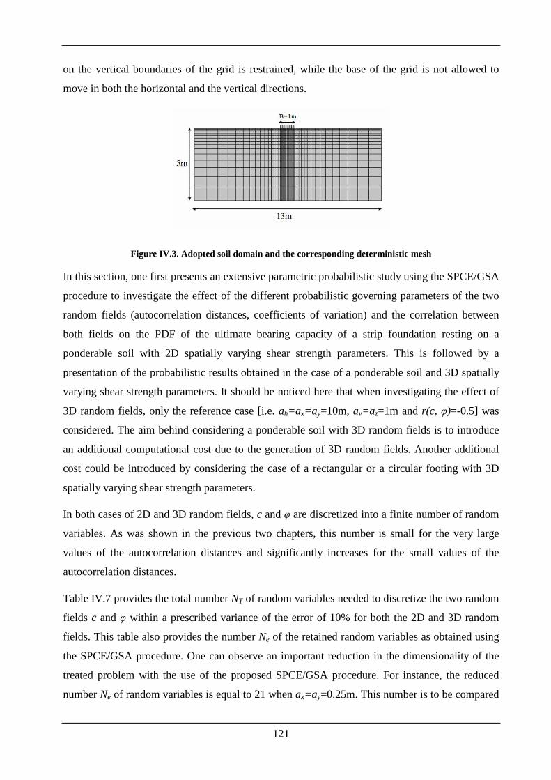
121
on the vertical boundaries of the grid is restrained, while the base of the grid is not allowed to
move in both the horizontal and the vertical directions.
Figure IV.3. Adopted soil domain and the corresponding deterministic mesh
In this section, one first presents an extensive parametric probabilistic study using the SPCE/GSA
procedure to investigate the effect of the different probabilistic governing parameters of the two
random fields (autocorrelation distances, coefficients of variation) and the correlation between
both fields on the PDF of the ultimate bearing capacity of a strip foundation resting on a
ponderable soil with 2D spatially varying shear strength parameters. This is followed by a
presentation of the probabilistic results obtained in the case of a ponderable soil and 3D spatially
varying shear strength parameters. It should be noticed here that when investigating the effect of
3D random fields, only the reference case [i.e. ah=ax=ay=10m, av=az=1m and r(c, φ)=-0.5] was
considered. The aim behind considering a ponderable soil with 3D random fields is to introduce
an additional computational cost due to the generation of 3D random fields. Another additional
cost could be introduced by considering the case of a rectangular or a circular footing with 3D
spatially varying shear strength parameters.
In both cases of 2D and 3D random fields, c and φ are discretized into a finite number of random
variables. As was shown in the previous two chapters, this number is small for the very large
values of the autocorrelation distances and significantly increases for the small values of the
autocorrelation distances.
Table IV.7 provides the total number NT of random variables needed to discretize the two random
fields c and φ within a prescribed variance of the error of 10% for both the 2D and 3D random
fields. This table also provides the number Ne of the retained random variables as obtained using
the SPCE/GSA procedure. One can observe an important reduction in the dimensionality of the
treated problem with the use of the proposed SPCE/GSA procedure. For instance, the reduced
number Ne of random variables is equal to 21 when ax=ay=0.25m. This number is to be compared
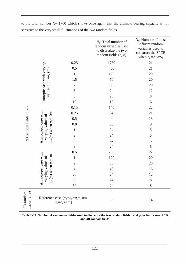
122
to the total number NT=1760 which shows once again that the ultimate bearing capacity is not
sensitive to the very small fluctuations of the two random fields.
NT: Total number of random variables used to discretize the two random fields (c, φ)
Ne: Number of most influent random variables used to
construct the SPCE when ta =2%xS1
0.25 1760 21
0.5 460 21
1 120 20
1.5 70 20
2 50 20
3 24 12
5 20 8
Isot
ropi
c ca
se w
ith v
aryi
ng
valu
es o
f ax=
ay (m
)
10 10 6
0.15 140 22
0.25 84 21
0.5 44 13
0.8 30 9
1 24 5
2 24 5
5 24 5 Ani
sotr
opic
cas
e w
ith
vary
ing
valu
es o
f a y
(m
) w
hen a
x=10
m
8 24 5
0.5 200 22
1 120 20
2 88 20
4 48 16
20 24 12
30 24 8
2D r
ando
m fi
elds
(c, φ
)
Ani
sotr
opic
cas
e w
ith
vary
ing
valu
es o
f a x
(m
) w
hen a
y=1m
50 24 8
3D r
ando
m
field
s (c
, φ)
Reference case [ah=ax=ay=10m, av=az=1m]
50 14
Table IV.7. Number of random variables used to discretize the two random fields c and φ for both cases of 2D and 3D random fields
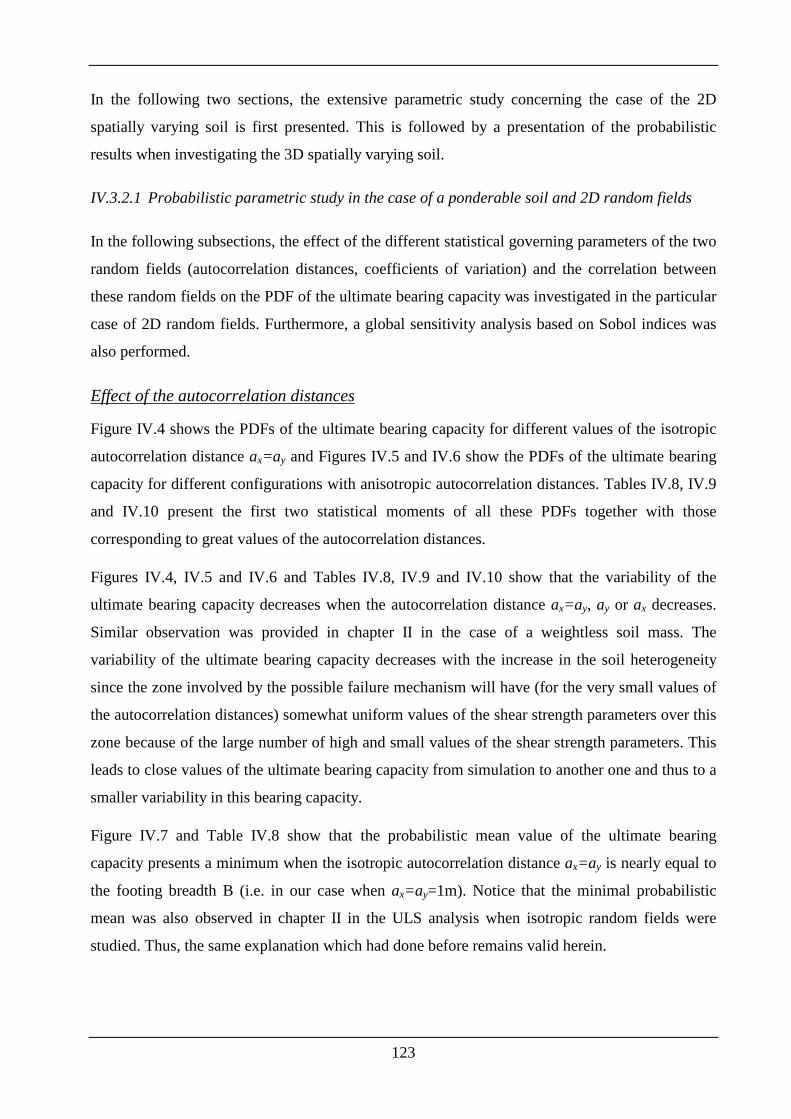
123
In the following two sections, the extensive parametric study concerning the case of the 2D
spatially varying soil is first presented. This is followed by a presentation of the probabilistic
results when investigating the 3D spatially varying soil.
IV.3.2.1 Probabilistic parametric study in the case of a ponderable soil and 2D random fields
In the following subsections, the effect of the different statistical governing parameters of the two
random fields (autocorrelation distances, coefficients of variation) and the correlation between
these random fields on the PDF of the ultimate bearing capacity was investigated in the particular
case of 2D random fields. Furthermore, a global sensitivity analysis based on Sobol indices was
also performed.
Effect of the autocorrelation distances
Figure IV.4 shows the PDFs of the ultimate bearing capacity for different values of the isotropic
autocorrelation distance ax=ay and Figures IV.5 and IV.6 show the PDFs of the ultimate bearing
capacity for different configurations with anisotropic autocorrelation distances. Tables IV.8, IV.9
and IV.10 present the first two statistical moments of all these PDFs together with those
corresponding to great values of the autocorrelation distances.
Figures IV.4, IV.5 and IV.6 and Tables IV.8, IV.9 and IV.10 show that the variability of the
ultimate bearing capacity decreases when the autocorrelation distance ax=ay, ay or ax decreases.
Similar observation was provided in chapter II in the case of a weightless soil mass. The
variability of the ultimate bearing capacity decreases with the increase in the soil heterogeneity
since the zone involved by the possible failure mechanism will have (for the very small values of
the autocorrelation distances) somewhat uniform values of the shear strength parameters over this
zone because of the large number of high and small values of the shear strength parameters. This
leads to close values of the ultimate bearing capacity from simulation to another one and thus to a
smaller variability in this bearing capacity.
Figure IV.7 and Table IV.8 show that the probabilistic mean value of the ultimate bearing
capacity presents a minimum when the isotropic autocorrelation distance ax=ay is nearly equal to
the footing breadth B (i.e. in our case when ax=ay=1m). Notice that the minimal probabilistic
mean was also observed in chapter II in the ULS analysis when isotropic random fields were
studied. Thus, the same explanation which had done before remains valid herein.
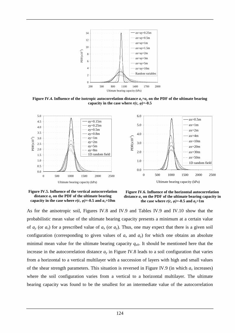
124
0
2
4
6
8
10
12
14
200 500 800 1100 1400 1700 2000
Ultimate bearing capacity (kPa)
PD
F(x
10-3
)
ax=ay=0.25m
ax=ay=0.5m
ax=ay=1m
ax=ay=1.5m
ax=ay=2m
ax=ay=3m
ax=ay=5m
ax=ay=10m
Random variables
Figure IV.4. Influence of the isotropic autocorrelation distance ax=ay on the PDF of the ultimate bearing
capacity in the case where r(c, φ)=-0.5
0.0
0.5
1.0
1.5
2.0
2.5
3.0
3.5
4.0
4.5
5.0
0 500 1000 1500 2000 2500
Ultimate bearing capacity (kPa)
PD
F(x
10-3
)
ay=0.15may=0.25may=0.5may=0.8may=1may=2may=5may=8m1D random field
Figure IV.5. Influence of the vertical autocorrelation
distance ay on the PDF of the ultimate bearing capacity in the case where r(c, φ)=-0.5 and ax=10m
0.0
1.0
2.0
3.0
4.0
5.0
6.0
0 500 1000 1500 2000 2500
Ultimate bearing capacity (kPa)
PD
F(x
10-3)
ax=0.5m
ax=1m
ax=2m
ax=4m
ax=10m
ax=20m
ax=30m
ax=50m
1D random field
Figure IV.6. Influence of the horizontal autocorrelation
distance ax on the PDF of the ultimate bearing capacity in the case where r(c, φ)=-0.5 and ay=1m
As for the anisotropic soil, Figures IV.8 and IV.9 and Tables IV.9 and IV.10 show that the
probabilistic mean value of the ultimate bearing capacity presents a minimum at a certain value
of ay (or ax) for a prescribed value of ax (or ay). Thus, one may expect that there is a given soil
configuration (corresponding to given values of ax and ay) for which one obtains an absolute
minimal mean value for the ultimate bearing capacity qult. It should be mentioned here that the
increase in the autocorrelation distance ay in Figure IV.8 leads to a soil configuration that varies
from a horizontal to a vertical multilayer with a succession of layers with high and small values
of the shear strength parameters. This situation is reversed in Figure IV.9 (in which ax increases)
where the soil configuration varies from a vertical to a horizontal multilayer. The ultimate
bearing capacity was found to be the smallest for an intermediate value of the autocorrelation
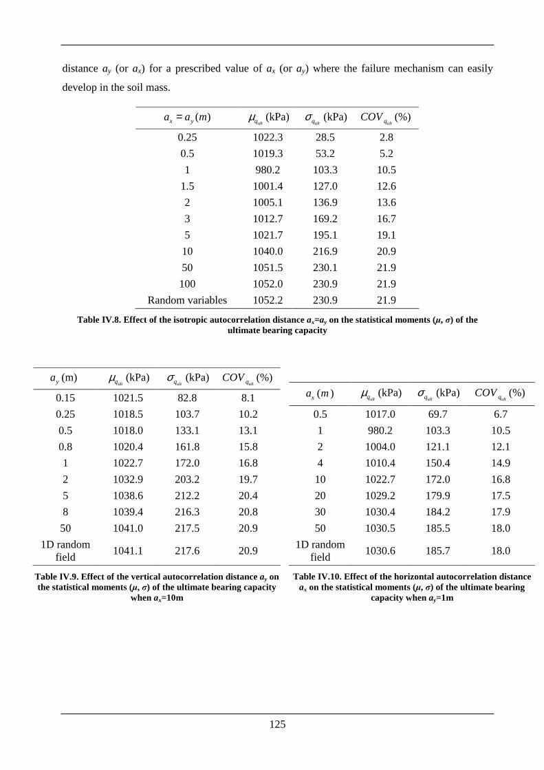
125
distance ay (or ax) for a prescribed value of ax (or ay) where the failure mechanism can easily
develop in the soil mass.
( )x ya a m= ultqµ (kPa)
ultqσ (kPa) (%)ultqCOV
0.25 1022.3 28.5 2.8
0.5 1019.3 53.2 5.2
1 980.2 103.3 10.5
1.5 1001.4 127.0 12.6
2 1005.1 136.9 13.6
3 1012.7 169.2 16.7
5 1021.7 195.1 19.1
10 1040.0 216.9 20.9
50 1051.5 230.1 21.9
100 1052.0 230.9 21.9
Random variables 1052.2 230.9 21.9
Table IV.8. Effect of the isotropic autocorrelation distance ax=ay on the statistical moments (µ, σ) of the ultimate bearing capacity
(m) ya ultqµ (kPa)
ultqσ (kPa) (%)ultqCOV
0.15 1021.5 82.8 8.1
0.25 1018.5 103.7 10.2
0.5 1018.0 133.1 13.1
0.8 1020.4 161.8 15.8
1 1022.7 172.0 16.8
2 1032.9 203.2 19.7
5 1038.6 212.2 20.4
8 1039.4 216.3 20.8
50 1041.0 217.5 20.9
1D random field
1041.1 217.6 20.9
Table IV.9. Effect of the vertical autocorrelation distance ay on the statistical moments (µ, σ) of the ultimate bearing capacity
when ax=10m
( )xa m ultqµ (kPa) ultqσ (kPa) (%)
ultqCOV
0.5 1017.0 69.7 6.7
1 980.2 103.3 10.5
2 1004.0 121.1 12.1
4 1010.4 150.4 14.9
10 1022.7 172.0 16.8
20 1029.2 179.9 17.5
30 1030.4 184.2 17.9
50 1030.5 185.5 18.0
1D random field
1030.6 185.7 18.0
Table IV.10. Effect of the horizontal autocorrelation distance ax on the statistical moments (µ, σ) of the ultimate bearing
capacity when ay=1m
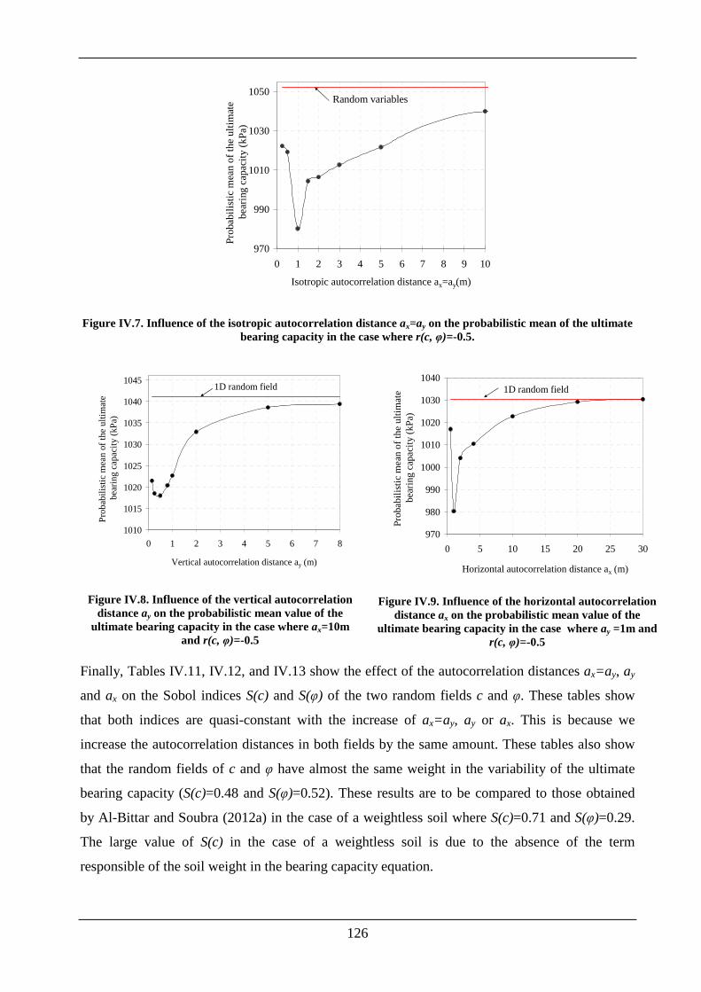
126
970
990
1010
1030
1050
0 1 2 3 4 5 6 7 8 9 10
Isotropic autocorrelation distance ax=ay(m)
Pro
bab
ilist
ic m
ean
of t
he
ulti
mat
e
be
ari
ng c
ap
aci
ty (
kPa
)
Random variables
Figure IV.7. Influence of the isotropic autocorrelation distance ax=ay on the probabilistic mean of the ultimate bearing capacity in the case where r(c, φ)=-0.5.
1010
1015
1020
1025
1030
1035
1040
1045
0 1 2 3 4 5 6 7 8
Vertical autocorrelation distance ay (m)
Pro
babi
listic
mea
n of
the
ulti
mat
e be
arin
g ca
paci
ty (
kPa)
1D random field
Figure IV.8. Influence of the vertical autocorrelation distance ay on the probabilistic mean value of the
ultimate bearing capacity in the case where ax=10m and r(c, φ)=-0.5
970
980
990
1000
1010
1020
1030
1040
0 5 10 15 20 25 30
Horizontal autocorrelation distance ax (m)
Pro
babi
listic
me
an o
f th
e ul
timat
e be
arin
g ca
paci
ty (
kPa)
1D random field
Figure IV.9. Influence of the horizontal autocorrelation distance ax on the probabilistic mean value of the
ultimate bearing capacity in the case where ay =1m and r(c, φ)=-0.5
Finally, Tables IV.11, IV.12, and IV.13 show the effect of the autocorrelation distances ax=ay, ay
and ax on the Sobol indices S(c) and S(φ) of the two random fields c and φ. These tables show
that both indices are quasi-constant with the increase of ax=ay, ay or ax. This is because we
increase the autocorrelation distances in both fields by the same amount. These tables also show
that the random fields of c and φ have almost the same weight in the variability of the ultimate
bearing capacity (S(c)=0.48 and S(φ)=0.52). These results are to be compared to those obtained
by Al-Bittar and Soubra (2012a) in the case of a weightless soil where S(c)=0.71 and S(φ)=0.29.
The large value of S(c) in the case of a weightless soil is due to the absence of the term
responsible of the soil weight in the bearing capacity equation.
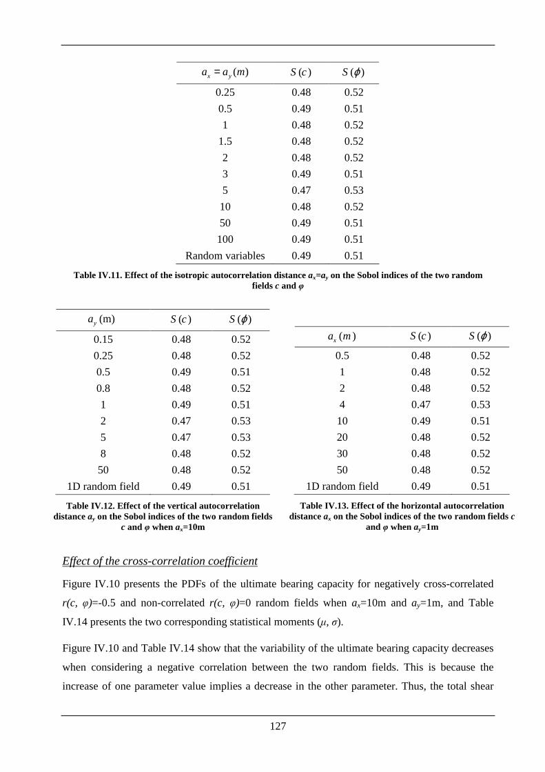
127
( )x ya a m= ( )S c ( )S ϕ
0.25 0.48 0.52
0.5 0.49 0.51
1 0.48 0.52
1.5 0.48 0.52
2 0.48 0.52
3 0.49 0.51
5 0.47 0.53
10 0.48 0.52
50 0.49 0.51
100 0.49 0.51
Random variables 0.49 0.51
Table IV.11. Effect of the isotropic autocorrelation distance ax=ay on the Sobol indices of the two random fields c and φ
(m) ya ( )S c ( )S ϕ
0.15 0.48 0.52
0.25 0.48 0.52
0.5 0.49 0.51
0.8 0.48 0.52
1 0.49 0.51
2 0.47 0.53
5 0.47 0.53
8 0.48 0.52
50 0.48 0.52
1D random field 0.49 0.51
Table IV.12. Effect of the vertical autocorrelation distance ay on the Sobol indices of the two random fields
c and φ when ax=10m
( )xa m ( )S c ( )S ϕ
0.5 0.48 0.52
1 0.48 0.52
2 0.48 0.52
4 0.47 0.53
10 0.49 0.51
20 0.48 0.52
30 0.48 0.52
50 0.48 0.52
1D random field 0.49 0.51
Table IV.13. Effect of the horizontal autocorrelation distance ax on the Sobol indices of the two random fields c
and φ when ay=1m
Effect of the cross-correlation coefficient
Figure IV.10 presents the PDFs of the ultimate bearing capacity for negatively cross-correlated
r(c, φ)=-0.5 and non-correlated r(c, φ)=0 random fields when ax=10m and ay=1m, and Table
IV.14 presents the two corresponding statistical moments (µ, σ).
Figure IV.10 and Table IV.14 show that the variability of the ultimate bearing capacity decreases
when considering a negative correlation between the two random fields. This is because the
increase of one parameter value implies a decrease in the other parameter. Thus, the total shear
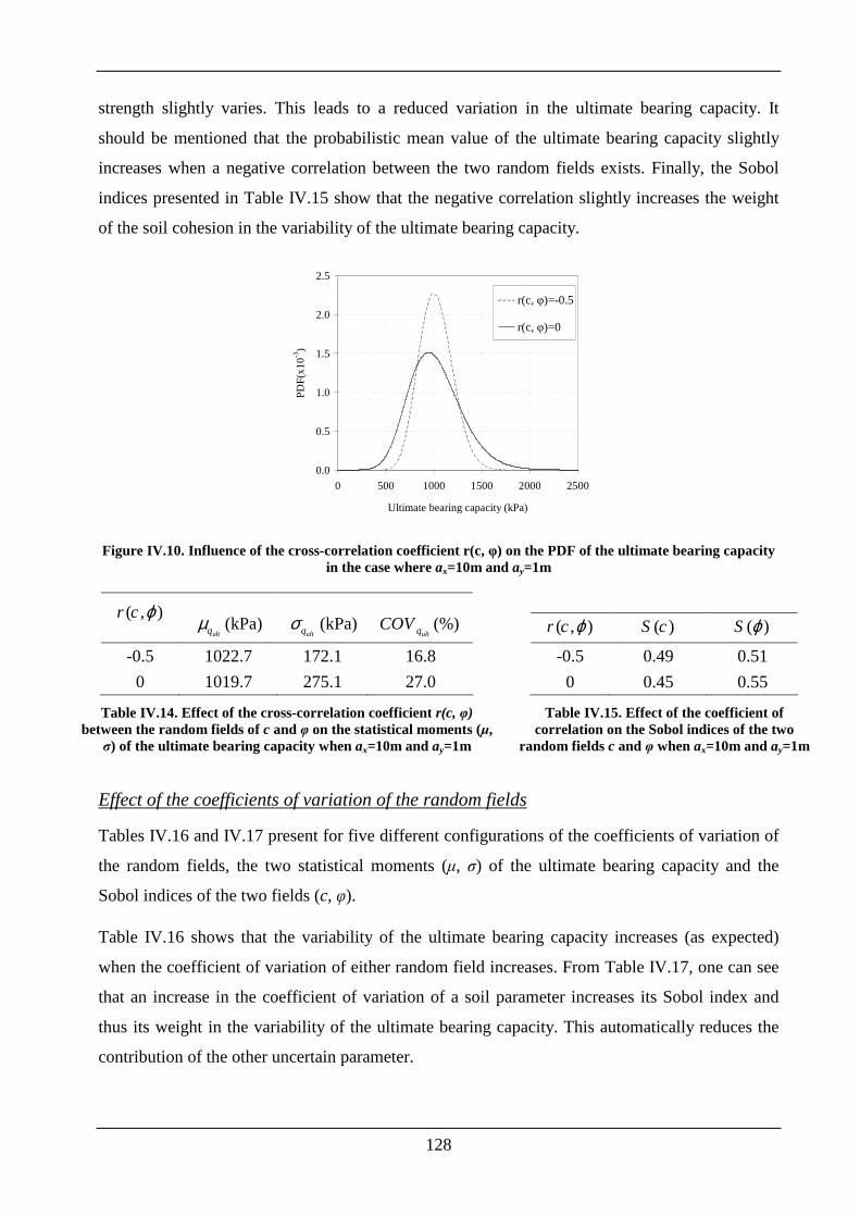
128
strength slightly varies. This leads to a reduced variation in the ultimate bearing capacity. It
should be mentioned that the probabilistic mean value of the ultimate bearing capacity slightly
increases when a negative correlation between the two random fields exists. Finally, the Sobol
indices presented in Table IV.15 show that the negative correlation slightly increases the weight
of the soil cohesion in the variability of the ultimate bearing capacity.
0.0
0.5
1.0
1.5
2.0
2.5
0 500 1000 1500 2000 2500
Ultimate bearing capacity (kPa)
PD
F(x
10-3
)r(c, φ)=-0.5
r(c, φ)=0
Figure IV.10. Influence of the cross-correlation coefficient r(c, φ) on the PDF of the ultimate bearing capacity in the case where ax=10m and ay=1m
( , )r c ϕ ultqµ (kPa)
ultqσ (kPa) (%)ultqCOV
-0.5 1022.7 172.1 16.8
0 1019.7 275.1 27.0
Table IV.14. Effect of the cross-correlation coefficient r(c, φ) between the random fields of c and φ on the statistical moments (µ, σ) of the ultimate bearing capacity when ax=10m and ay=1m
( , )r c ϕ ( )S c ( )S ϕ
-0.5 0.49 0.51
0 0.45 0.55
Table IV.15. Effect of the coefficient of correlation on the Sobol indices of the two
random fields c and φ when ax=10m and ay=1m
Effect of the coefficients of variation of the random fields
Tables IV.16 and IV.17 present for five different configurations of the coefficients of variation of
the random fields, the two statistical moments (µ, σ) of the ultimate bearing capacity and the
Sobol indices of the two fields (c, φ).
Table IV.16 shows that the variability of the ultimate bearing capacity increases (as expected)
when the coefficient of variation of either random field increases. From Table IV.17, one can see
that an increase in the coefficient of variation of a soil parameter increases its Sobol index and
thus its weight in the variability of the ultimate bearing capacity. This automatically reduces the
contribution of the other uncertain parameter.
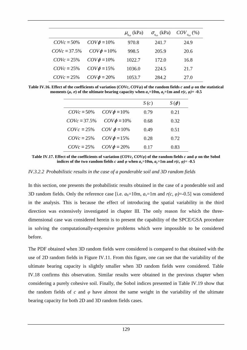
129
ultqµ (kPa)
ultqσ (kPa) (%)ultqCOV
50% 10%COVc COVϕ= = 970.8 241.7 24.9
37.5% 10%COVc COVϕ= = 998.5 205.9 20.6
25% 10%COVc COVϕ= = 1022.7 172.0 16.8
25% 15%COVc COVϕ= = 1036.0 224.5 21.7
25% 20%COVc COVϕ= = 1053.7 284.2 27.0
Table IV.16. Effect of the coefficients of variation (COVc, COVφ) of the random fields c and φ on the statistical moments (µ, σ) of the ultimate bearing capacity when ax=10m, ay=1m and r(c, φ)= -0.5
( )S c ( )S ϕ
50% 10%COVc COVϕ= = 0.79 0.21
37.5% 10%COVc COVϕ= = 0.68 0.32
25% 10%COVc COVϕ= = 0.49 0.51
25% 15%COVc COVϕ= = 0.28 0.72
25% 20%COVc COVϕ= = 0.17 0.83
Table IV.17. Effect of the coefficients of variation (COVc, COVφ) of the random fields c and φ on the Sobol indices of the two random fields c and φ when ax=10m, ay=1m and r(c, φ)= -0.5
IV.3.2.2 Probabilistic results in the case of a ponderable soil and 3D random fields
In this section, one presents the probabilistic results obtained in the case of a ponderable soil and
3D random fields. Only the reference case [i.e. ah=10m, av=1m and r(c, φ)=-0.5] was considered
in the analysis. This is because the effect of introducing the spatial variability in the third
direction was extensively investigated in chapter III. The only reason for which the three-
dimensional case was considered herein is to present the capability of the SPCE/GSA procedure
in solving the computationally-expensive problems which were impossible to be considered
before.
The PDF obtained when 3D random fields were considered is compared to that obtained with the
use of 2D random fields in Figure IV.11. From this figure, one can see that the variability of the
ultimate bearing capacity is slightly smaller when 3D random fields were considered. Table
IV.18 confirms this observation. Similar results were obtained in the previous chapter when
considering a purely cohesive soil. Finally, the Sobol indices presented in Table IV.19 show that
the random fields of c and φ have almost the same weight in the variability of the ultimate
bearing capacity for both 2D and 3D random fields cases.
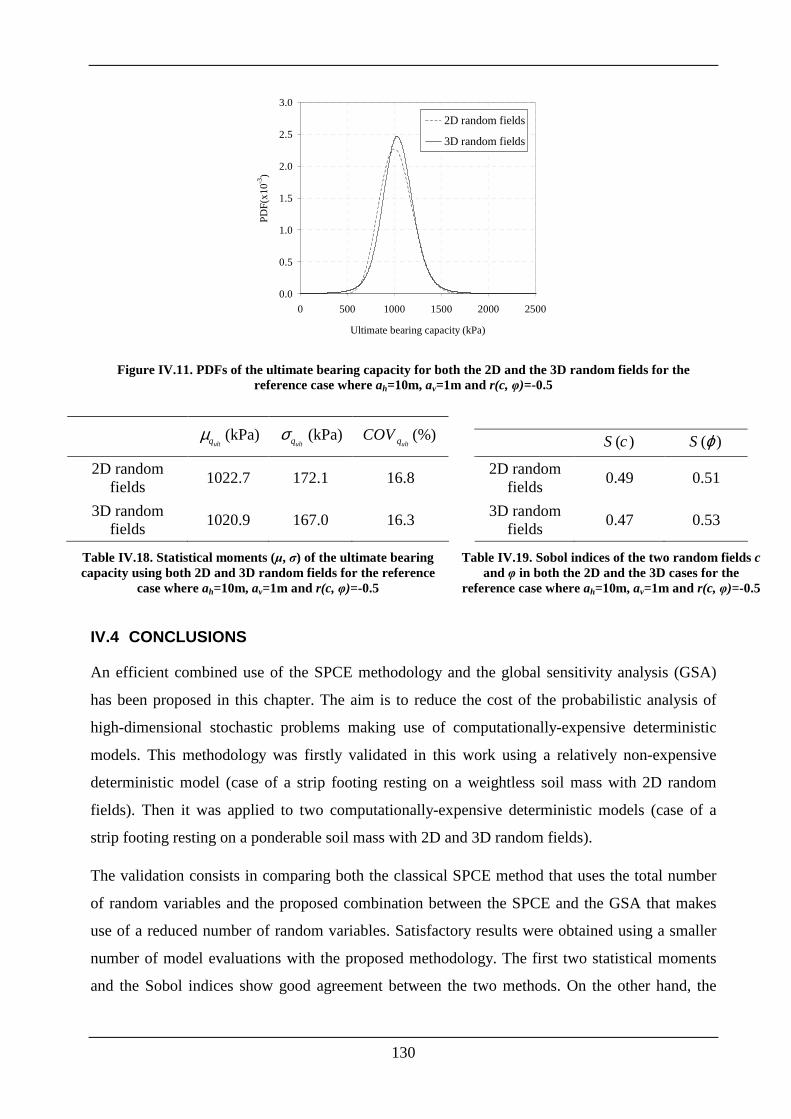
130
0.0
0.5
1.0
1.5
2.0
2.5
3.0
0 500 1000 1500 2000 2500
Ultimate bearing capacity (kPa)
PD
F(x
10-3
)
2D random fields
3D random fields
Figure IV.11. PDFs of the ultimate bearing capacity for both the 2D and the 3D random fields for the reference case where ah=10m, av=1m and r(c, φ)=-0.5
ultqµ (kPa)
ultqσ (kPa) (%)ultqCOV
2D random fields
1022.7 172.1 16.8
3D random fields
1020.9 167.0 16.3
Table IV.18. Statistical moments (µ, σ) of the ultimate bearing capacity using both 2D and 3D random fields for the reference
case where ah=10m, av=1m and r(c, φ)=-0.5
( )S c ( )S ϕ
2D random fields
0.49 0.51
3D random fields
0.47 0.53
Table IV.19. Sobol indices of the two random fields c and φ in both the 2D and the 3D cases for the
reference case where ah=10m, av=1m and r(c, φ)=-0.5
IV.4 CONCLUSIONS
An efficient combined use of the SPCE methodology and the global sensitivity analysis (GSA)
has been proposed in this chapter. The aim is to reduce the cost of the probabilistic analysis of
high-dimensional stochastic problems making use of computationally-expensive deterministic
models. This methodology was firstly validated in this work using a relatively non-expensive
deterministic model (case of a strip footing resting on a weightless soil mass with 2D random
fields). Then it was applied to two computationally-expensive deterministic models (case of a
strip footing resting on a ponderable soil mass with 2D and 3D random fields).
The validation consists in comparing both the classical SPCE method that uses the total number
of random variables and the proposed combination between the SPCE and the GSA that makes
use of a reduced number of random variables. Satisfactory results were obtained using a smaller
number of model evaluations with the proposed methodology. The first two statistical moments
and the Sobol indices show good agreement between the two methods. On the other hand, the
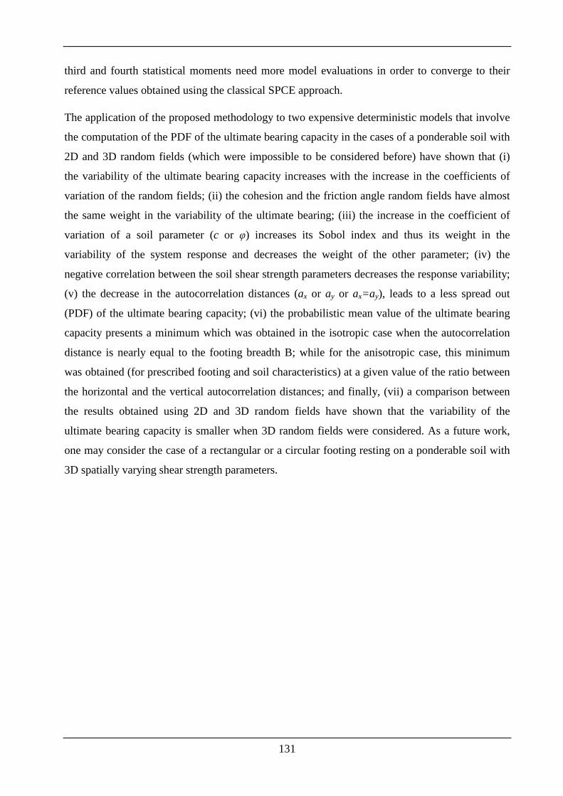
131
third and fourth statistical moments need more model evaluations in order to converge to their
reference values obtained using the classical SPCE approach.
The application of the proposed methodology to two expensive deterministic models that involve
the computation of the PDF of the ultimate bearing capacity in the cases of a ponderable soil with
2D and 3D random fields (which were impossible to be considered before) have shown that (i)
the variability of the ultimate bearing capacity increases with the increase in the coefficients of
variation of the random fields; (ii) the cohesion and the friction angle random fields have almost
the same weight in the variability of the ultimate bearing; (iii) the increase in the coefficient of
variation of a soil parameter (c or φ) increases its Sobol index and thus its weight in the
variability of the system response and decreases the weight of the other parameter; (iv) the
negative correlation between the soil shear strength parameters decreases the response variability;
(v) the decrease in the autocorrelation distances (ax or ay or ax=ay), leads to a less spread out
(PDF) of the ultimate bearing capacity; (vi) the probabilistic mean value of the ultimate bearing
capacity presents a minimum which was obtained in the isotropic case when the autocorrelation
distance is nearly equal to the footing breadth B; while for the anisotropic case, this minimum
was obtained (for prescribed footing and soil characteristics) at a given value of the ratio between
the horizontal and the vertical autocorrelation distances; and finally, (vii) a comparison between
the results obtained using 2D and 3D random fields have shown that the variability of the
ultimate bearing capacity is smaller when 3D random fields were considered. As a future work,
one may consider the case of a rectangular or a circular footing resting on a ponderable soil with
3D spatially varying shear strength parameters.
132
CHAPTER V. EFFECT OF THE SOIL SPATIAL VARIABILITY A ND/OR
THE TIME VARIABILITY OF THE SEISMIC LOADING ON THE DYNAMIC
RESPONSES OF GEOTECHNICAL STRUCTURES
V.1 INTRODUCTION
This chapter focuses on the dynamic responses induced by an earthquake Ground-Motion (GM)
taking into account the soil spatial variability and/or the time variability of the seismic loading.
Contrarily to the case of the static loading considered in the previous chapters where only the soil
and the footing were considered in the analysis (because the system response was mainly the
ultimate bearing capacity of the footing), the case of a seismic loading should consider the soil,
the footing and the superstructure since the seismic energy will be dissipated in both the soil and
the superstructure [Sadek (2012)]. Thus, a proper modeling of the entire soil-footing-structure
system including the interaction between the soil and the footing should be considered in order to
lead to reliable solutions.
The response of a soil-footing-structure system subjected to seismic loading has been extensively
investigated in literature using deterministic approaches where average values of the soil
properties (shear modulus, angle of internal friction, cohesion, etc.) and deterministic recorded
acceleration time-histories were used [Chen and Sawada (1983), Leshchinsky and San (1994),
You and Michalowski (1999), Michalowski (2002), Loukidis et al. (2003), Sadek and Shahrour
(2004) and Grange et al. (2009a, 2009b) among others].
It should be mentioned here that when dealing with seismic loads, an aleatory uncertainty related
to the earthquake Ground-Motion (GM) appears in addition to the soil spatial variability and the
variability of the superstructure. This additional source of aleatory uncertainty is the time
variability of the earthquake Ground-Motion (GM). Consequently, reliable responses of the
superstructure cannot be predicted using a deterministic approach; a probabilistic technique
seems to be necessary. The probabilistic techniques enable the rigourous propagation of the
different uncertainties from the input parameters to the system responses.
In this chapter, the effect of the soil spatial variability and/or the time variability of the
earthquake GM on the seismic responses of geotechnical structures is investigated. The
variability of the superstructure was not considered in the analysis. Given the scarcity of studies
involving the probabilistic seismic responses, a free field soil medium subjected to a seismic
133
loading was firstly considered. The aim is to investigate the effect of the soil spatial variability
and/or the time variability of the earthquake GM using a simple model. Then, a soil-structure
interaction SSI problem was investigated in the second part of this chapter.
It should be emphasized here that few authors have worked on the analysis of the seismic
responses using probabilistic approaches [Koutsourelakis et al. (2002), Wang and Hao (2002),
Nour et al. (2003), Popescu et al. (2005, 2006) and Lopez-Caballero and Modaressi-Farahmand-
Rasavi (2010)]. In all these works, the classical Monte Carlo Simulation (MCS) methodology
with a very small number of realizations was used to determine the probability density function
(PDF) of the seismic response [e.g. only 50 simulations were used in Koutsourelakis et al
(2002)]. This is because of the significant computation time required per simulation when using
finite element/finite difference dynamic models.
As for the probabilistic methods used in this chapter, two methods were employed. The first one
is the classical Monte Carlo Simulation (MCS) methodology and the second one is the Sparse
Polynomial Chaos Expansion (SPCE) methodology which consists in substituting the system
response by a meta-model.
This chapter is organized as follows: First, the case of an elastic free field soil mass is
investigated. This is followed by the SSI problem. The chapter ends by a conclusion of the main
findings.
V.2 CASE OF AN ELASTIC FREE FIELD SOIL MASS
In this section, the effect of the soil spatial variability and/or the time variability of the earthquake
GM was firstly investigated through the study of an elastic free field soil mass.
The soil shear modulus G was modeled as a non-Gaussian random field and the earthquake GM
was modeled as a random process. The EOLE methodology presented in chapter I was used to
discretize the shear modulus random field. As for the earthquake GM, the method proposed by
Rezaeian and Der Kiureghian (2010) which consists in fitting a parameterized stochastic model to
the real recorded earthquake GM was utilized. The deterministic model was based on numerical
simulations using the dynamic option of the finite difference code FLAC3D. The dynamic
response considered in the analysis was the amplification of the maximum acceleration at the soil
surface.
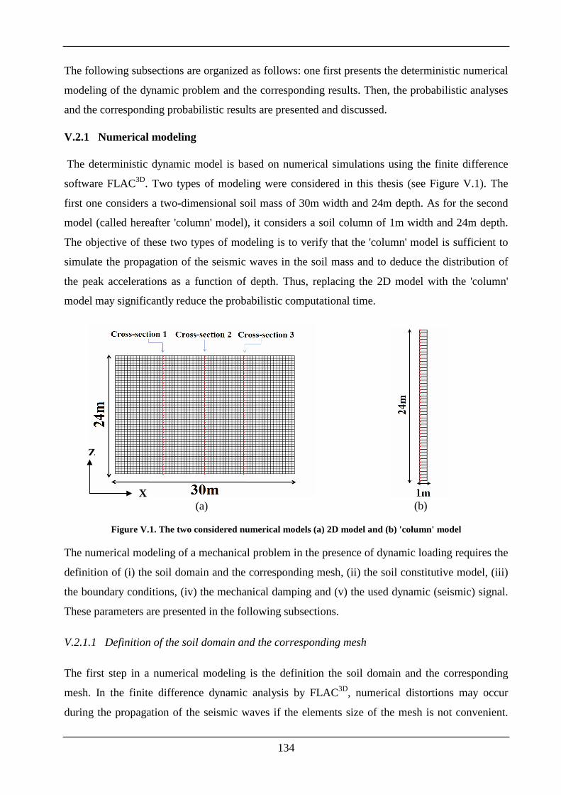
134
The following subsections are organized as follows: one first presents the deterministic numerical
modeling of the dynamic problem and the corresponding results. Then, the probabilistic analyses
and the corresponding probabilistic results are presented and discussed.
V.2.1 Numerical modeling
The deterministic dynamic model is based on numerical simulations using the finite difference
software FLAC3D. Two types of modeling were considered in this thesis (see Figure V.1). The
first one considers a two-dimensional soil mass of 30m width and 24m depth. As for the second
model (called hereafter 'column' model), it considers a soil column of 1m width and 24m depth.
The objective of these two types of modeling is to verify that the 'column' model is sufficient to
simulate the propagation of the seismic waves in the soil mass and to deduce the distribution of
the peak accelerations as a function of depth. Thus, replacing the 2D model with the 'column'
model may significantly reduce the probabilistic computational time.
(a)
(b)
Figure V.1. The two considered numerical models (a) 2D model and (b) 'column' model
The numerical modeling of a mechanical problem in the presence of dynamic loading requires the
definition of (i) the soil domain and the corresponding mesh, (ii) the soil constitutive model, (iii)
the boundary conditions, (iv) the mechanical damping and (v) the used dynamic (seismic) signal.
These parameters are presented in the following subsections.
V.2.1.1 Definition of the soil domain and the corresponding mesh
The first step in a numerical modeling is the definition the soil domain and the corresponding
mesh. In the finite difference dynamic analysis by FLAC3D, numerical distortions may occur
during the propagation of the seismic waves if the elements size of the mesh is not convenient.
X
Z
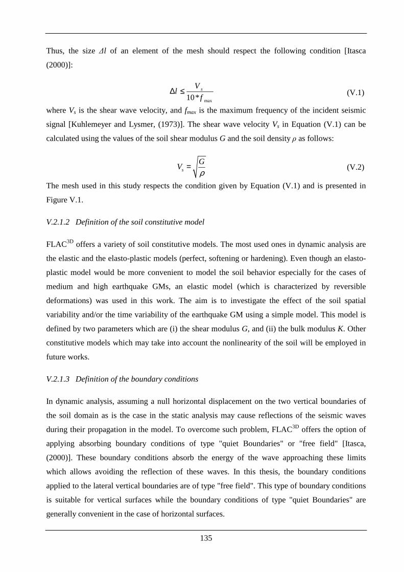
135
Thus, the size ∆l of an element of the mesh should respect the following condition [Itasca
(2000)]:
max10*sV
lf
∆ ≤ ( V.1)
where Vs is the shear wave velocity, and fmax is the maximum frequency of the incident seismic
signal [Kuhlemeyer and Lysmer, (1973)]. The shear wave velocity Vs in Equation ( V.1) can be
calculated using the values of the soil shear modulus G and the soil density ρ as follows:
s
GV
ρ= ( V.2)
The mesh used in this study respects the condition given by Equation ( V.1) and is presented in
Figure V.1.
V.2.1.2 Definition of the soil constitutive model
FLAC3D offers a variety of soil constitutive models. The most used ones in dynamic analysis are
the elastic and the elasto-plastic models (perfect, softening or hardening). Even though an elasto-
plastic model would be more convenient to model the soil behavior especially for the cases of
medium and high earthquake GMs, an elastic model (which is characterized by reversible
deformations) was used in this work. The aim is to investigate the effect of the soil spatial
variability and/or the time variability of the earthquake GM using a simple model. This model is
defined by two parameters which are (i) the shear modulus G, and (ii) the bulk modulus K. Other
constitutive models which may take into account the nonlinearity of the soil will be employed in
future works.
V.2.1.3 Definition of the boundary conditions
In dynamic analysis, assuming a null horizontal displacement on the two vertical boundaries of
the soil domain as is the case in the static analysis may cause reflections of the seismic waves
during their propagation in the model. To overcome such problem, FLAC3D offers the option of
applying absorbing boundary conditions of type "quiet Boundaries" or "free field" [Itasca,
(2000)]. These boundary conditions absorb the energy of the wave approaching these limits
which allows avoiding the reflection of these waves. In this thesis, the boundary conditions
applied to the lateral vertical boundaries are of type "free field". This type of boundary conditions
is suitable for vertical surfaces while the boundary conditions of type "quiet Boundaries" are
generally convenient in the case of horizontal surfaces.
136
V.2.1.4 Definition of the mechanical damping
In the natural dynamic systems, the internal friction may lead to partial dissipation of the energy
of vibration. The software FLAC3D provides a damping of type "Rayleigh damping" (among
other types of damping) which is based on two parameters: (i) the natural frequency of the system
and (ii) the damping ratio (defined as a percentage of the critical damping). This type of damping
is used in this chapter. The damping ratio used in the dynamic models presented in this work is
equal to 5% of the critical damping [Bourdeau (2005)]. Notice that in most geological materials,
the natural damping ratio is in the range of 2 to 5% of the critical damping.
V.2.1.5 Input seismic signal
The input seismic signal used in this work is the synthetic signal of Nice for which the
corresponding accelerogram is presented in Figure V.2(a). This signal is used because it is
representative of the French design spectrum [Grange (2008)]. It has a maximum acceleration
equal to 0.33g. Its corresponding Fourier amplitude spectrum is shown in Figure V.2(b). It should
be mentioned here that the use of a different seismic signal may lead to different results.
0 5 10 15 20
-3
-2
-1
0
1
2
3
4
Time (sec)
Acc
ele
ratio
n (m
/s2 )
Target a(t)
amax=0.33g
0 5 10 15 20
-3
-2
-1
0
1
2
3
4
Time (sec)
Acc
ele
ratio
n (m
/s2 )
Target a(t)
amax=0.33g
(a)
0 10 20 30 40 500
0.02
0.04
0.06
0.08
0.1
0.12
0.14
0.16
0.18Amplitude Spectrum of target a(t)
Frequency (Hz)
|Y(f)|
(b)
Figure V.2. (a) Accelerogram of the synthetic signal of Nice and (b) the corresponding Fourier amplitude spectrum
V.2.2 Deterministic results
V.2.2.1 Validation of the 'column' model
The aim of this section is to check the validity of the 'column' model for its use in the
probabilistic analyses. The main reason for which it is desirable to use the 'column' model instead
of a two-dimensional (2D) soil domain is its reasonable computation time (40 min per
137
simulation). This computation time enormously increases when a 2D model is used (24 hours per
simulation). Remember that the 2D model involves a two-dimensional soil mass (see Figure
V.1(a)) and the 'column' model involves a one-dimensional soil column (see Figure V.1(b)). For
both models, the considered dynamic response was the distribution of the maximum acceleration
along a vertical cross-section.
For the dynamic analyses, an elastic constitutive model was used to describe the soil behavior.
The values of the shear modulus, bulk modulus and density of the soil were as follows:
G=100MPa, K=250MPa, and ρ=1800 kg/m3.
In order to avoid the numerical distortion that may occur during the propagation of the seismic
waves in the model, the element size ∆l must satisfy the condition given by Equation ( V.1).
Using Equation ( V.2) which provides the value of the shear wave velocity as a function of the
values of G and ρ, the shear wave velocity was found to be equal to 235.7m/s. From Figure
V.2(b), one can see that the maximal frequency fmax is equal to 40Hz. Thus, the maximum
element size must be less than or equal to 0.59m. In the studied model, the selected element size
∆l was taken equal to 0.5m (see Figure V.1).
Concerning the boundary conditions, the lower horizontal boundary (along X) was subjected to
the seismic load (i.e. the synthetic accelerogram of Nice). Boundary conditions of type "free
field" were applied along the lateral vertical boundaries of the model [Bourdeau (2005)].
As for the mechanical damping, Rayleigh damping was used with a central frequency (natural
frequency) fc=2.5Hz and a damping ratio equal to 5% of the critical damping. Notice that the
approximate formula of the natural frequency of a soil column given by Widmer (2003) (i.e.
fo=Vs/4H where Vs is the shear wave velocity calculated using Equation ( V.2) and H is the height
of the soil column) was used to calculate the value of the central frequency fc=2.5Hz. As for the
damping ratio, the value of 5% used by Bourdeau (2005) was adopted in this thesis.
Figure V.3 shows the distribution of the maximum acceleration as a function of depth for the
three cross-sections of the 2D soil mass and for the 1D soil column. This figure shows that the
four distributions are superimposed, which makes valid the hypothesis of using a soil column
instead of a 2D soil mass when performing the probabilistic analysis.
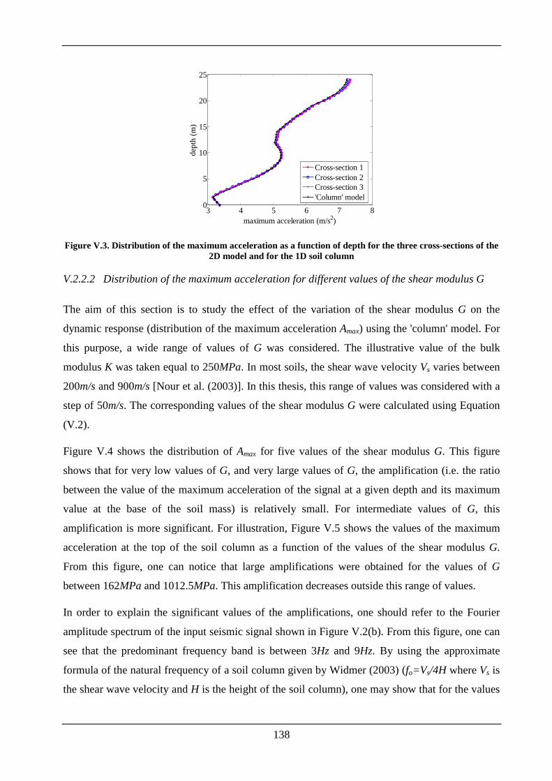
138
3 4 5 6 7 80
5
10
15
20
25
maximum acceleration (m/s2)
dept
h (m
)
Cross-section 1Cross-section 2Cross-section 3'Column' model
Figure V.3. Distribution of the maximum acceleration as a function of depth for the three cross-sections of the 2D model and for the 1D soil column
V.2.2.2 Distribution of the maximum acceleration for different values of the shear modulus G
The aim of this section is to study the effect of the variation of the shear modulus G on the
dynamic response (distribution of the maximum acceleration Amax) using the 'column' model. For
this purpose, a wide range of values of G was considered. The illustrative value of the bulk
modulus K was taken equal to 250MPa. In most soils, the shear wave velocity Vs varies between
200m/s and 900m/s [Nour et al. (2003)]. In this thesis, this range of values was considered with a
step of 50m/s. The corresponding values of the shear modulus G were calculated using Equation
( V.2).
Figure V.4 shows the distribution of Amax for five values of the shear modulus G. This figure
shows that for very low values of G, and very large values of G, the amplification (i.e. the ratio
between the value of the maximum acceleration of the signal at a given depth and its maximum
value at the base of the soil mass) is relatively small. For intermediate values of G, this
amplification is more significant. For illustration, Figure V.5 shows the values of the maximum
acceleration at the top of the soil column as a function of the values of the shear modulus G.
From this figure, one can notice that large amplifications were obtained for the values of G
between 162MPa and 1012.5MPa. This amplification decreases outside this range of values.
In order to explain the significant values of the amplifications, one should refer to the Fourier
amplitude spectrum of the input seismic signal shown in Figure V.2(b). From this figure, one can
see that the predominant frequency band is between 3Hz and 9Hz. By using the approximate
formula of the natural frequency of a soil column given by Widmer (2003) (fo=Vs/4H where Vs is
the shear wave velocity and H is the height of the soil column), one may show that for the values
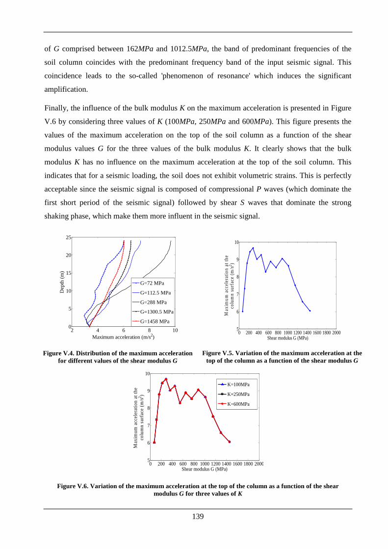
139
of G comprised between 162MPa and 1012.5MPa, the band of predominant frequencies of the
soil column coincides with the predominant frequency band of the input seismic signal. This
coincidence leads to the so-called 'phenomenon of resonance' which induces the significant
amplification.
Finally, the influence of the bulk modulus K on the maximum acceleration is presented in Figure
V.6 by considering three values of K (100MPa, 250MPa and 600MPa). This figure presents the
values of the maximum acceleration on the top of the soil column as a function of the shear
modulus values G for the three values of the bulk modulus K. It clearly shows that the bulk
modulus K has no influence on the maximum acceleration at the top of the soil column. This
indicates that for a seismic loading, the soil does not exhibit volumetric strains. This is perfectly
acceptable since the seismic signal is composed of compressional P waves (which dominate the
first short period of the seismic signal) followed by shear S waves that dominate the strong
shaking phase, which make them more influent in the seismic signal.
2 4 6 8 100
5
10
15
20
25
Maximum acceleration (m/s2)
Dep
th (
m)
G=72 MPa
G=112.5 MPa
G=288 MPa
G=1300.5 MPa
G=1458 MPa
Figure V.4. Distribution of the maximum acceleration for different values of the shear modulus G
0 200 400 600 800 1000120014001600180020005
6
7
8
9
10
Shear modulus G (MPa)
Max
imum
acc
eler
atio
n at
the
colu
mn
surf
ace
(m/s2 )
Figure V.5. Variation of the maximum acceleration at the top of the column as a function of the shear modulus G
0 200 400 600 800 1000120014001600180020005
6
7
8
9
10
Shear modulus G (MPa)
Max
imum
acc
eler
atio
n a
t th
e co
lum
n s
urf
ace
(m/s2 )
K=100MPa
K=250MPa
K=600MPa
Figure V.6. Variation of the maximum acceleration at the top of the column as a function of the shear modulus G for three values of K
140
V.2.3 Probabilistic dynamic analysis
The aim of this section is to present the probabilistic dynamic analysis. It should be remembered
here that the dynamic system response involves the maximum acceleration (Amax) at the top of the
soil column. In this study, the effect of both the soil spatial variability and the time variability of
the earthquake GM on the dynamic response were considered.
The soil shear modulus G was considered as a one-dimensional (1D) non-Gaussian random field
varying in the vertical direction. It was described by a square exponential autocorrelation function
and was assumed to be log-normally distributed. Two reference mean values of the shear
modulus were considered. The first one is 1
72G MPaµ = corresponding to a non resonant value
(i.e. this value is located on the left hand part of the curve in Figure V.5) and the second one is
2288G MPaµ = corresponding to a resonant value. For both mean values (
172G MPaµ = and
2288G MPaµ = ), a coefficient of variation equal to 30% was considered as the reference value.
As for the vertical autocorrelation distance ay, the adopted reference value was equal to 2m while
the range of 0.5m-20m was considered when performing the parametric study. The computation
time that was necessary for the generation of the random field increases when the autocorrelation
distance decreases. Notice however that this time was relatively small in the case of the 1D
random field for the range of autocorrelation distances considered in the analysis.
In order to simulate the stochastic synthetic earthquake GMs using the method given by Rezaeian
and Der Kiureghian (2010), the synthetic signal of Nice (for which the corresponding
accelerogram is presented in Figure V.2(a)) was used as a target accelerogram.
The deterministic model was based on numerical simulations using the dynamic option of the
finite difference code FLAC3D. It was presented and detailed in the previous section. It should be
noted here that in dynamic analysis, the size of a given element in the mesh depends on both the
autocorrelation distances of the soil properties and the wavelength λ associated with the highest
frequency component fmax of the input seismic signal.
For the autocorrelation distances of the soil properties, Der Kiureghian and Ke (1988) have
suggested that the length of the largest element in a given direction (horizontal or vertical) should
not exceed 0.5 times the autocorrelation distance in that direction. As for the wavelength λ
associated with the highest frequency component fmax of the input signal, Itasca (2000) has
suggested that the element size should not exceed 1/10 to 1/8 this wavelength λ in order to avoid
numerical distortion of the propagating waves (see Equation ( V.1)). Figure V.2(b) shows that the
141
value of the maximum frequency is fmax=40Hz. In order to respect the two mentioned criterions,
two different deterministic meshes were considered in FLAC3D. The first one was devoted to the
case of moderate to great values of ay and Vs where an element size of 0.5m was chosen to
perform the dynamic analysis (i.e. when 200 /sV m s≥ and 1ya m≥ ), and the second one for
small values of ay or Vs where the element size was adjusted in order to respect the previous two
conditions.
The following subsections are organized as follows: First, a brief description of a step-by-step
procedure used to generate the stochastic earthquake GM is presented. It is followed by a
presentation of some realizations of this stochastic earthquake GM. Finally, one examines the
effect of (i) the soil spatial variability considered alone with a deterministic earthquake GM, (ii)
the time variability of the earthquake GM considered alone with a homogenous soil mass and (iii)
both the soil spatial variability combined with the time variability of the earthquake GM.
V.2.3.1 Step-by-step procedure used to generate the stochastic earthquake GM
The different steps used to generate the stochastic earthquake GMs are summarized as follows:
(a) Introduce the target input seismic signal and the corresponding time step ∆t and total duration
T. In this work, the target input seismic signal is the synthetic Nice accelerogram presented in
Figure V.2 which has a time step ∆t=0.01s and a total duration T=20s.
(b) Determine the parameters 1 2 3( , , )α α α α= of the time modulation function as follows:
First, calculate the three physically-based parameters 5 95( , , )a midI D t− which describe the real
recorded GM in the time domain. The first variable, aI is calculated using Equation (C.1). The
second variable D5−95 is the time interval between the instants at which 5% and 95% of aI are
reached respectively (cf. Figure C.1). Finally, the third variable tmid is the time at which 45% of
aI is reached (cf. Figure C.1). Then, use these three physical parameters to deduce the values of
the parameters 1 2 3( , , )α α α α= of the time modulation function using Equations (C.2), (C.3) and
(C.4). The values of the three physical parameters 5 95( , , )a midI D t− and the corresponding values
of the time modulation function parameters 1 2 3( , , )α α α α= for the synthetic Nice accelerogram
used in this thesis are presented in Table V.1.
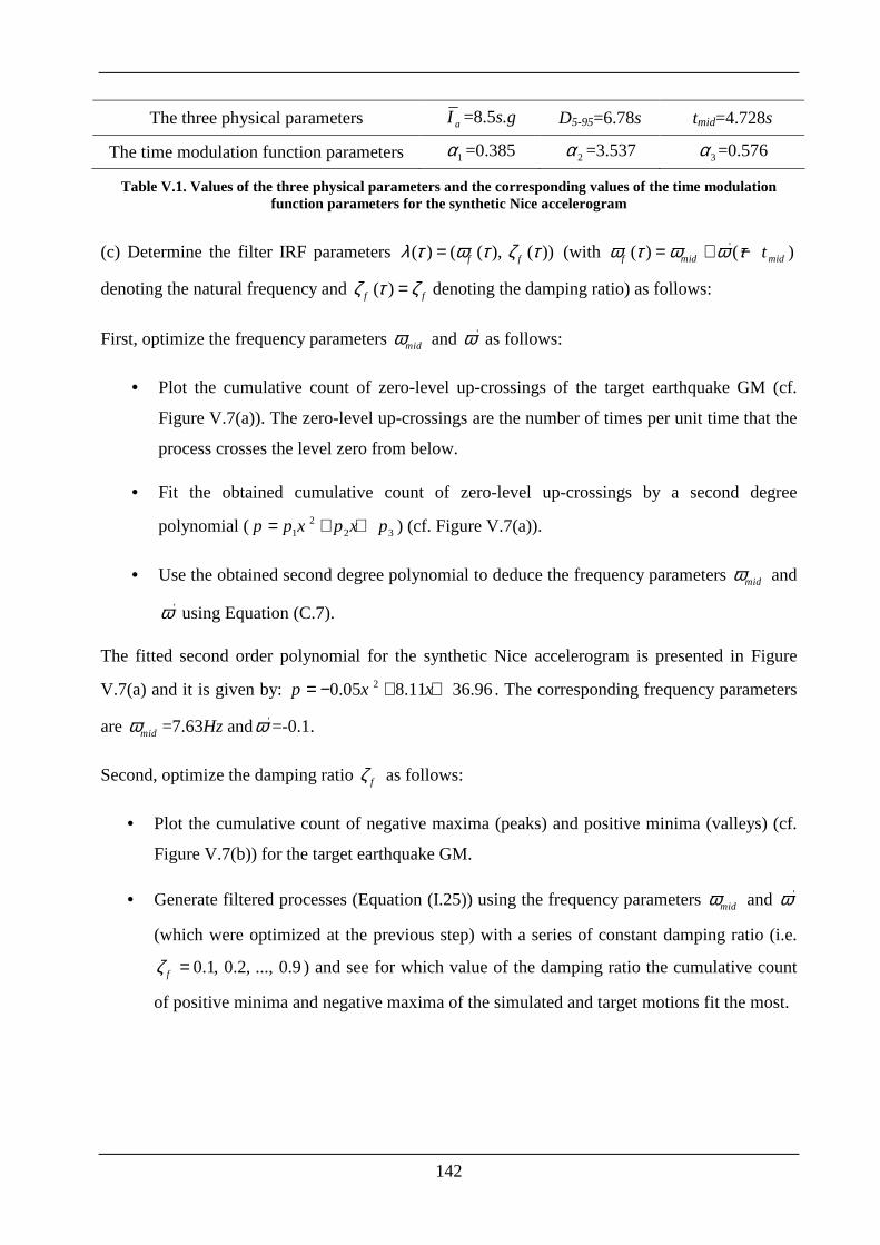
142
The three physical parameters aI =8.5s.g D5-95=6.78s tmid=4.728s
The time modulation function parameters 1α =0.385 2α =3.537 3α =0.576
Table V.1. Values of the three physical parameters and the corresponding values of the time modulation function parameters for the synthetic Nice accelerogram
(c) Determine the filter IRF parameters ( ) ( ( ), ( ))f fλ τ ω τ ζ τ= (with '( ) ( )f mid midtω τ ω ω τ= + −
denoting the natural frequency and ( )f fζ τ ζ= denoting the damping ratio) as follows:
First, optimize the frequency parameters midω and 'ω as follows:
• Plot the cumulative count of zero-level up-crossings of the target earthquake GM (cf.
Figure V.7(a)). The zero-level up-crossings are the number of times per unit time that the
process crosses the level zero from below.
• Fit the obtained cumulative count of zero-level up-crossings by a second degree
polynomial ( 21 2 3p p x p x p= + + ) (cf. Figure V.7(a)).
• Use the obtained second degree polynomial to deduce the frequency parameters midω and
'ω using Equation (C.7).
The fitted second order polynomial for the synthetic Nice accelerogram is presented in Figure
V.7(a) and it is given by: 20.05 8.11 36.96p x x= − + + . The corresponding frequency parameters
are midω =7.63Hz and 'ω =-0.1.
Second, optimize the damping ratio fζ as follows:
• Plot the cumulative count of negative maxima (peaks) and positive minima (valleys) (cf.
Figure V.7(b)) for the target earthquake GM.
• Generate filtered processes (Equation ( I.25)) using the frequency parameters midω and 'ω
(which were optimized at the previous step) with a series of constant damping ratio (i.e.
0.1, 0.2, ..., 0.9fζ = ) and see for which value of the damping ratio the cumulative count
of positive minima and negative maxima of the simulated and target motions fit the most.
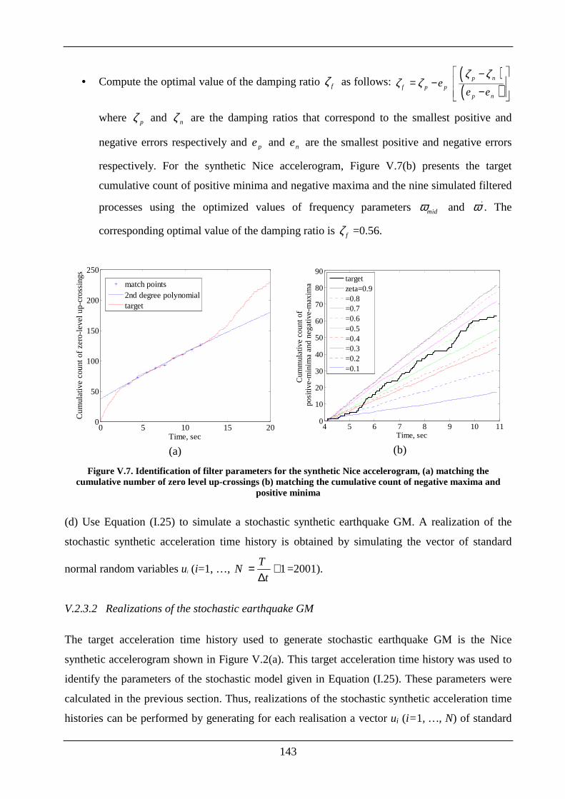
143
• Compute the optimal value of the damping ratio fζ as follows: ( )( )
p n
f p p
p n
ee e
ζ ζζ ζ
− = −
−
where pζ and nζ are the damping ratios that correspond to the smallest positive and
negative errors respectively and pe and ne are the smallest positive and negative errors
respectively. For the synthetic Nice accelerogram, Figure V.7(b) presents the target
cumulative count of positive minima and negative maxima and the nine simulated filtered
processes using the optimized values of frequency parameters midω and 'ω . The
corresponding optimal value of the damping ratio is fζ =0.56.
0 5 10 15 200
50
100
150
200
250
Time, sec
Cu
mul
ativ
e c
ount
of
zero
-leve
l up-
cros
sing
s
match points2nd degree polynomialtarget
(a)
4 5 6 7 8 9 10 110
10
20
30
40
50
60
70
80
90
Time, sec
Cum
mul
ativ
e c
oun
t o
f po
sitiv
e-m
inim
a a
nd
ne
ga
tive
-ma
xim
a
targetzeta=0.9=0.8=0.7=0.6=0.5=0.4=0.3=0.2=0.1
(b)
Figure V.7. Identification of filter parameters for the synthetic Nice accelerogram, (a) matching the cumulative number of zero level up-crossings (b) matching the cumulative count of negative maxima and
positive minima
(d) Use Equation ( I.25) to simulate a stochastic synthetic earthquake GM. A realization of the
stochastic synthetic acceleration time history is obtained by simulating the vector of standard
normal random variables ui (i=1, …, 1T
Nt
= +∆
=2001).
V.2.3.2 Realizations of the stochastic earthquake GM
The target acceleration time history used to generate stochastic earthquake GM is the Nice
synthetic accelerogram shown in Figure V.2(a). This target acceleration time history was used to
identify the parameters of the stochastic model given in Equation ( I.25). These parameters were
calculated in the previous section. Thus, realizations of the stochastic synthetic acceleration time
histories can be performed by generating for each realisation a vector ui (i= 1, …, N) of standard
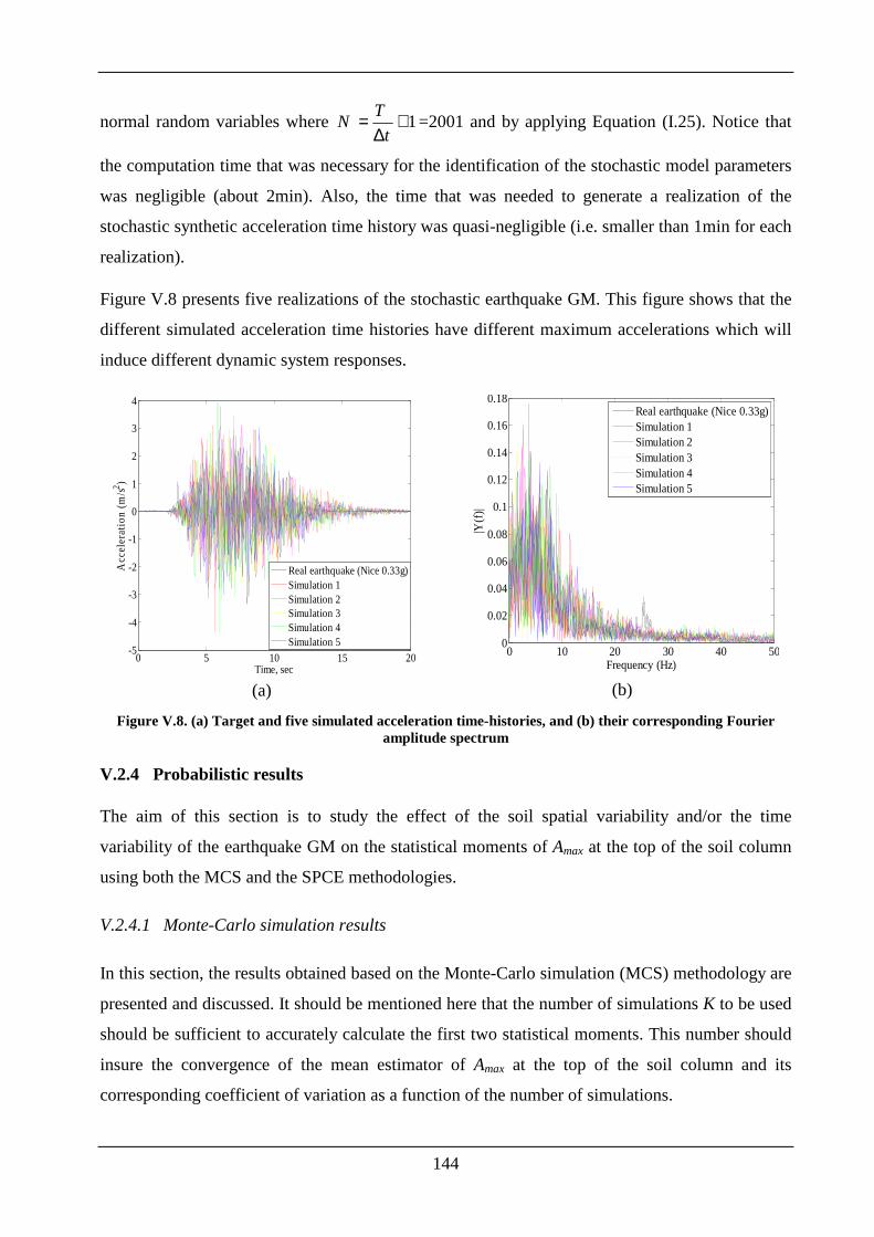
144
normal random variables where 1T
Nt
= +∆
=2001 and by applying Equation ( I.25). Notice that
the computation time that was necessary for the identification of the stochastic model parameters
was negligible (about 2min). Also, the time that was needed to generate a realization of the
stochastic synthetic acceleration time history was quasi-negligible (i.e. smaller than 1min for each
realization).
Figure V.8 presents five realizations of the stochastic earthquake GM. This figure shows that the
different simulated acceleration time histories have different maximum accelerations which will
induce different dynamic system responses.
0 5 10 15 20-5
-4
-3
-2
-1
0
1
2
3
4
Time, sec
Acc
eler
atio
n (
m/s2 )
Real earthquake (Nice 0.33g)Simulation 1Simulation 2Simulation 3Simulation 4Simulation 5
(a)
0 10 20 30 40 500
0.02
0.04
0.06
0.08
0.1
0.12
0.14
0.16
0.18
Frequency (Hz)
|Y(f
)|
Real earthquake (Nice 0.33g)Simulation 1Simulation 2Simulation 3Simulation 4Simulation 5
(b)
Figure V.8. (a) Target and five simulated acceleration time-histories, and (b) their corresponding Fourier amplitude spectrum
V.2.4 Probabilistic results
The aim of this section is to study the effect of the soil spatial variability and/or the time
variability of the earthquake GM on the statistical moments of Amax at the top of the soil column
using both the MCS and the SPCE methodologies.
V.2.4.1 Monte-Carlo simulation results
In this section, the results obtained based on the Monte-Carlo simulation (MCS) methodology are
presented and discussed. It should be mentioned here that the number of simulations K to be used
should be sufficient to accurately calculate the first two statistical moments. This number should
insure the convergence of the mean estimator of Amax at the top of the soil column and its
corresponding coefficient of variation as a function of the number of simulations.
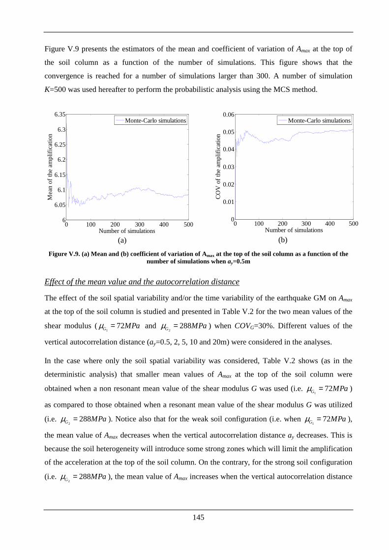
145
Figure V.9 presents the estimators of the mean and coefficient of variation of Amax at the top of
the soil column as a function of the number of simulations. This figure shows that the
convergence is reached for a number of simulations larger than 300. A number of simulation
K=500 was used hereafter to perform the probabilistic analysis using the MCS method.
0 100 200 300 400 5006
6.05
6.1
6.15
6.2
6.25
6.3
6.35
Number of simulations
Mea
n of
the
ampl
ifica
tion
Monte-Carlo simulations
(a)
0 100 200 300 400 5000
0.01
0.02
0.03
0.04
0.05
0.06
Number of simulations
CO
V o
f th
e am
plifi
catio
n
Monte-Carlo simulations
(b)
Figure V.9. (a) Mean and (b) coefficient of variation of Amax at the top of the soil column as a function of the number of simulations when ay=0.5m
Effect of the mean value and the autocorrelation distance
The effect of the soil spatial variability and/or the time variability of the earthquake GM on Amax
at the top of the soil column is studied and presented in Table V.2 for the two mean values of the
shear modulus (1
72G MPaµ = and 2
288G MPaµ = ) when COVG=30%. Different values of the
vertical autocorrelation distance (ay=0.5, 2, 5, 10 and 20m) were considered in the analyses.
In the case where only the soil spatial variability was considered, Table V.2 shows (as in the
deterministic analysis) that smaller mean values of Amax at the top of the soil column were
obtained when a non resonant mean value of the shear modulus G was used (i.e. 1
72G MPaµ = )
as compared to those obtained when a resonant mean value of the shear modulus G was utilized
(i.e. 2
288G MPaµ = ). Notice also that for the weak soil configuration (i.e. when 1
72G MPaµ = ),
the mean value of Amax decreases when the vertical autocorrelation distance ay decreases. This is
because the soil heterogeneity will introduce some strong zones which will limit the amplification
of the acceleration at the top of the soil column. On the contrary, for the strong soil configuration
(i.e. 2
288G MPaµ = ), the mean value of Amax increases when the vertical autocorrelation distance
146
ay decreases. This is because the soil heterogeneity will introduce some weakness zones which
will increase the amplification of the acceleration at the top of the soil column.
On the other hand, Table V.2 shows that the variability of Amax is maximal for the very large
values of the autocorrelation distance (ay=20m). This variability decreases when the vertical
autocorrelation distance ay decreases. The same trend was obtained in the three previous chapters
where static loading cases were considered. In these cases, the small values of the autocorrelation
distances produce the so-called 'averaging phenomenon' for which the rapid change in the values
of a soil property from element to another neighboring one leads to quasi-similar behavior for all
the realizations. In the dynamic loading cases, this 'averaging phenomenon' is also produced but
along the wave’s path. Thus, the rapid change in the values of the shear modulus along the wave
path leads to quasi-similar behavior for all the realizations. This leads to close values of Amax at
the top of the soil column and thus to a smaller variability in this response. Notice that similar
results were obtained by Al-Bittar et al. (2012a) when the dynamic behavior of a spatially varying
slope subjected to stochastic GM was investigated (cf. Appendix F). From Table V.2, one can
also observe that the variability of Amax is larger for the case of the weak soil corresponding to a
small mean value of the shear modulus G (i.e. 1
72G MPaµ = ).
The maximum variability obtained when only the soil spatial variability was considered is largely
smaller than the one obtained when only the time variability of the earthquake GM was
considered as may be seen from Table V.2. The values of the variability of Amax obtained when
only the time variability of the earthquake GM was considered (i.e. 20.64% for 1
72G MPaµ =
and 18.70% for 2
288G MPaµ = ) are about two times larger than those obtained when only the
soil spatial variability was taken into account. Notice however that the obtained results may
change in the case where a different seismic loading was considered.
Finally, when both the soil spatial variability and the time variability of the GM have been
considered in the analysis, one obtains a variability of Amax which is far below the one obtained
by superposition of the variabilities of Amax as obtained from the soil spatial variability and the
time variability of the earthquake GM considered separately. Thus, if one applies the
superposition method to obtain the variability of the dynamic responses, the obtained variability
may be largely overestimated.
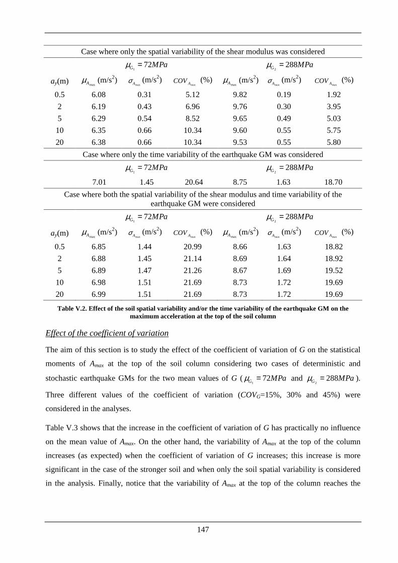
147
Case where only the spatial variability of the shear modulus was considered
1
72G MPaµ = 2
288G MPaµ =
ay(m) maxAµ (m/s2)
maxAσ (m/s2) max
ACOV (%) maxAµ (m/s2)
maxAσ (m/s2) max
ACOV (%)
0.5 6.08 0.31 5.12 9.82 0.19 1.92
2 6.19 0.43 6.96 9.76 0.30 3.95
5 6.29 0.54 8.52 9.65 0.49 5.03
10 6.35 0.66 10.34 9.60 0.55 5.75
20 6.38 0.66 10.34 9.53 0.55 5.80
Case where only the time variability of the earthquake GM was considered
1
72G MPaµ = 2
288G MPaµ =
7.01 1.45 20.64 8.75 1.63 18.70
Case where both the spatial variability of the shear modulus and time variability of the earthquake GM were considered
1
72G MPaµ = 2
288G MPaµ =
ay(m) maxAµ (m/s2)
maxAσ (m/s2) max
ACOV (%) maxAµ (m/s2)
maxAσ (m/s2) max
ACOV (%)
0.5 6.85 1.44 20.99 8.66 1.63 18.82
2 6.88 1.45 21.14 8.69 1.64 18.92
5 6.89 1.47 21.26 8.67 1.69 19.52
10 6.98 1.51 21.69 8.73 1.72 19.69
20 6.99 1.51 21.69 8.73 1.72 19.69
Table V.2. Effect of the soil spatial variability and/or the time variability of the earthquake GM on the maximum acceleration at the top of the soil column
Effect of the coefficient of variation
The aim of this section is to study the effect of the coefficient of variation of G on the statistical
moments of Amax at the top of the soil column considering two cases of deterministic and
stochastic earthquake GMs for the two mean values of G (1
72G MPaµ = and 2
288G MPaµ = ).
Three different values of the coefficient of variation (COVG=15%, 30% and 45%) were
considered in the analyses.
Table V.3 shows that the increase in the coefficient of variation of G has practically no influence
on the mean value of Amax. On the other hand, the variability of Amax at the top of the column
increases (as expected) when the coefficient of variation of G increases; this increase is more
significant in the case of the stronger soil and when only the soil spatial variability is considered
in the analysis. Finally, notice that the variability of Amax at the top of the column reaches the
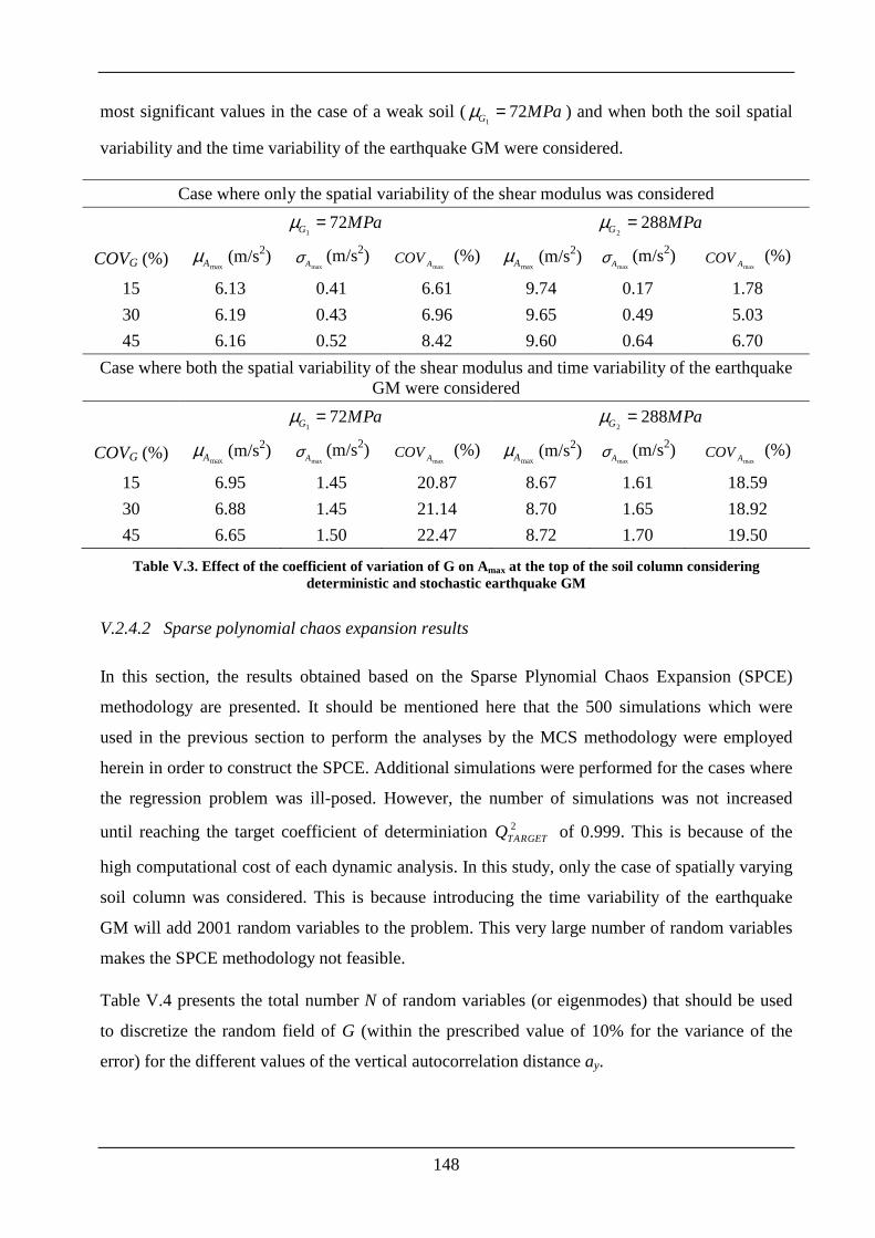
148
most significant values in the case of a weak soil (1
72G MPaµ = ) and when both the soil spatial
variability and the time variability of the earthquake GM were considered.
Case where only the spatial variability of the shear modulus was considered
1
72G MPaµ = 2
288G MPaµ =
COVG (%) maxAµ (m/s2)
maxAσ (m/s2) max
ACOV (%) maxAµ (m/s2)
maxAσ (m/s2) max
ACOV (%)
15 6.13 0.41 6.61 9.74 0.17 1.78
30 6.19 0.43 6.96 9.65 0.49 5.03
45 6.16 0.52 8.42 9.60 0.64 6.70
Case where both the spatial variability of the shear modulus and time variability of the earthquake GM were considered
1
72G MPaµ = 2
288G MPaµ =
COVG (%) maxAµ (m/s2)
maxAσ (m/s2) max
ACOV (%) maxAµ (m/s2)
maxAσ (m/s2) max
ACOV (%)
15 6.95 1.45 20.87 8.67 1.61 18.59
30 6.88 1.45 21.14 8.70 1.65 18.92
45 6.65 1.50 22.47 8.72 1.70 19.50
Table V.3. Effect of the coefficient of variation of G on Amax at the top of the soil column considering deterministic and stochastic earthquake GM
V.2.4.2 Sparse polynomial chaos expansion results
In this section, the results obtained based on the Sparse Plynomial Chaos Expansion (SPCE)
methodology are presented. It should be mentioned here that the 500 simulations which were
used in the previous section to perform the analyses by the MCS methodology were employed
herein in order to construct the SPCE. Additional simulations were performed for the cases where
the regression problem was ill-posed. However, the number of simulations was not increased
until reaching the target coefficient of determiniation 2TARGETQ of 0.999. This is because of the
high computational cost of each dynamic analysis. In this study, only the case of spatially varying
soil column was considered. This is because introducing the time variability of the earthquake
GM will add 2001 random variables to the problem. This very large number of random variables
makes the SPCE methodology not feasible.
Table V.4 presents the total number N of random variables (or eigenmodes) that should be used
to discretize the random field of G (within the prescribed value of 10% for the variance of the
error) for the different values of the vertical autocorrelation distance ay.
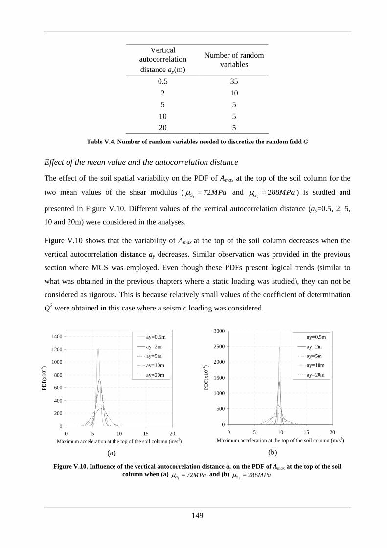
149
Vertical autocorrelation distance ay(m)
Number of random variables
0.5 35
2 10
5 5
10 5
20 5
Table V.4. Number of random variables needed to discretize the random field G
Effect of the mean value and the autocorrelation distance
The effect of the soil spatial variability on the PDF of Amax at the top of the soil column for the
two mean values of the shear modulus (1
72G MPaµ = and 2
288G MPaµ = ) is studied and
presented in Figure V.10. Different values of the vertical autocorrelation distance (ay=0.5, 2, 5,
10 and 20m) were considered in the analyses.
Figure V.10 shows that the variability of Amax at the top of the soil column decreases when the
vertical autocorrelation distance ay decreases. Similar observation was provided in the previous
section where MCS was employed. Even though these PDFs present logical trends (similar to
what was obtained in the previous chapters where a static loading was studied), they can not be
considered as rigorous. This is because relatively small values of the coefficient of determination
Q2 were obtained in this case where a seismic loading was considered.
0
200
400
600
800
1000
1200
1400
0 5 10 15 20
Maximum acceleration at the top of the soil column (m/s2)
PD
F(x
10-3)
ay=0.5m
ay=2m
ay=5m
ay=10m
ay=20m
(a)
0
500
1000
1500
2000
2500
3000
0 5 10 15 20
Maximum acceleration at the top of the soil column (m/s2)
PD
F(x
10-3)
ay=0.5m
ay=2m
ay=5m
ay=10m
ay=20m
(b)
Figure V.10. Influence of the vertical autocorrelation distance ay on the PDF of Amax at the top of the soil column when (a)
172G MPaµ = and (b)
2288G MPaµ =
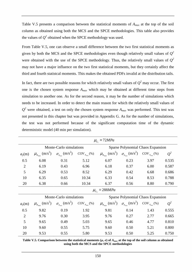
150
Table V.5 presents a comparison between the statistical moments of Amax at the top of the soil
column as obtained using both the MCS and the SPCE methodologies. This table also provides
the values of Q2 obtained when the SPCE methodology was used.
From Table V.5, one can observe a small difference between the two first statistical moments as
given by both the MCS and the SPCE methodologies even though relatively small values of Q2
were obtained with the use of the SPCE methodology. Thus, the relatively small values of Q2
may not have a major influence on the two first statistical moments, but they certainly affect the
third and fourth statistcal moments. This makes the obtained PDFs invalid at the distribution tails.
In fact, there are two possible reasons for which relatively small values of Q2 may occur. The first
one is the chosen system response Amax which may be obtained at different time steps from
simulation to another one. As for the second reason, it may be the number of simulations which
needs to be increased. In order to detect the main reason for which the relatively small values of
Q2 were obtained, a test on only the chosen system response Amax was performed. This test was
not presented in this chapter but was provided in Appendix G. As for the number of simulations,
the test was not performed because of the significant computation time of the dynamic
deterministic model (40 min per simulation).
1
72G MPaµ =
Monte-Carlo simulations Sparse Polynomial Chaos Expansion
ay(m) maxAµ (m/s2)
maxAσ (m/s2) max
(%)ACOV maxAµ (m/s2)
maxAσ (m/s2) max
(%)ACOV Q2
0.5 6.08 0.31 5.12 6.07 0.23 3.97 0.535
2 6.19 0.43 6.96 6.18 0.37 6.00 0.587
5 6.29 0.53 8.52 6.29 0.42 6.68 0.686
10 6.35 0.65 10.34 6.33 0.54 8.53 0.788
20 6.38 0.66 10.34 6.37 0.56 8.80 0.790
2
288G MPaµ =
Monte-Carlo simulations Sparse Polynomial Chaos Expansion
ay(m) maxAµ (m/s2)
maxAσ (m/s2) max
(%)ACOV maxAµ (m/s2)
maxAσ (m/s2) max
(%)ACOV Q2
0.5 9.82 0.19 1.92 9.81 0.14 1.43 0.555
2 9.76 0.30 3.95 9.76 0.27 2.77 0.665
5 9.65 0.49 5.03 9.65 0.46 4.77 0.810
10 9.60 0.55 5.75 9.60 0.50 5.21 0.800
20 9.53 0.55 5.80 9.53 0.50 5.25 0.750
Table V.5. Comparison between the statistical moments (µ, σ) of Amax at the top of the soil column as obtained using both the MCS and the SPCE methodologies
151
V.3 CASE OF A SOIL-STRUCTURE INTERACTION (SSI) PROB LEM
In this section, the SSI problem was investigated through the analysis of a five storey building
[Al-Bittar et al. (2012b)]. In order to study a SSI problem, three methods can be found in
literature [Pecker (1984)]:
(i) The superposition method which subdivides the complex SSI problem into simpler
problems (kinematics interaction and inertial interaction [Kausel et al. (1978)]), this
method being valid only for linear problems.
(ii) The direct methods that use a classical finite element/finite difference approaches
[Prevost (1999)], but these methods require good knowledge of the constitutive laws
and are very computationally-expensive.
(iii) The hybrid methods that are a combination of the two previous methods and therefore
they are more attractive because of their computational cost.
The macro-element approach belongs to the last category and it is used to model the present SSI
problem. The macro-element concept developed by Nova and Montrasio (1991) consists in
condensing the soil (material) and interface (geometric) nonlinearities into a representative point
(the centre of the foundation) and it works with generalized variables (forces and displacements).
It thus allows the simulation of the behaviour of shallow foundations in a simplified way.
The main reason for which the macro-element concept is chosen to perform the probabilistic
analysis is that the time cost for a single deterministic calculation is relatively small (five minutes
per simulation). Thus, this model is suitable for the probabilistic analysis which requires a great
number of calls of the deterministic model. In this thesis, only the time variability of the seismic
loading was considered in the analysis.
Finally, notice that the dynamic system responses retained for the probabilistic analysis are:
(i) The maximum horizontal displacement at the top of the building.
(ii) The three maximum displacements of the footing centre.
(iii) The three maximum reaction forces at the contact of the soil and the footing.
The probabilistic results are presented in the form of statistical moments and in the form of
probability of exceeding of predefined thresholds.
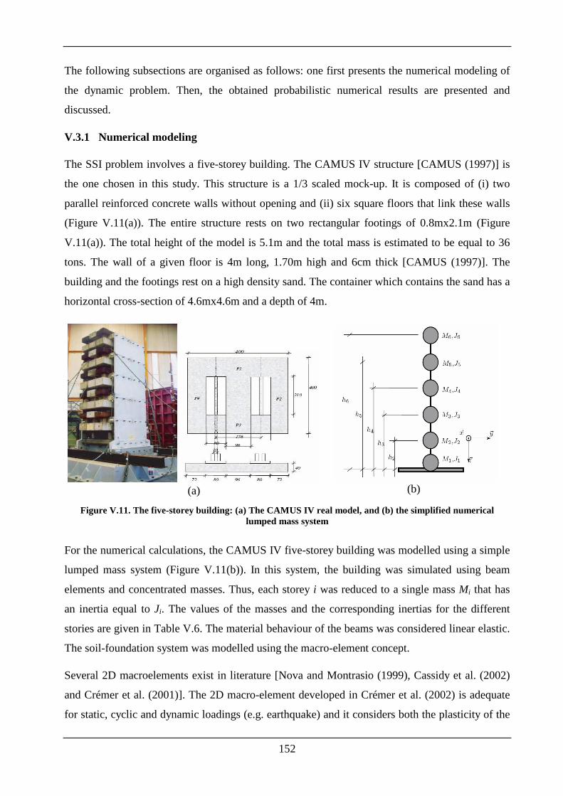
152
The following subsections are organised as follows: one first presents the numerical modeling of
the dynamic problem. Then, the obtained probabilistic numerical results are presented and
discussed.
V.3.1 Numerical modeling
The SSI problem involves a five-storey building. The CAMUS IV structure [CAMUS (1997)] is
the one chosen in this study. This structure is a 1/3 scaled mock-up. It is composed of (i) two
parallel reinforced concrete walls without opening and (ii) six square floors that link these walls
(Figure V.11(a)). The entire structure rests on two rectangular footings of 0.8mx2.1m (Figure
V.11(a)). The total height of the model is 5.1m and the total mass is estimated to be equal to 36
tons. The wall of a given floor is 4m long, 1.70m high and 6cm thick [CAMUS (1997)]. The
building and the footings rest on a high density sand. The container which contains the sand has a
horizontal cross-section of 4.6mx4.6m and a depth of 4m.
(a) (b)
Figure V.11. The five-storey building: (a) The CAMUS IV real model, and (b) the simplified numerical lumped mass system
For the numerical calculations, the CAMUS IV five-storey building was modelled using a simple
lumped mass system (Figure V.11(b)). In this system, the building was simulated using beam
elements and concentrated masses. Thus, each storey i was reduced to a single mass Mi that has
an inertia equal to Ji. The values of the masses and the corresponding inertias for the different
stories are given in Table V.6. The material behaviour of the beams was considered linear elastic.
The soil-foundation system was modelled using the macro-element concept.
Several 2D macroelements exist in literature [Nova and Montrasio (1999), Cassidy et al. (2002)
and Crémer et al. (2001)]. The 2D macro-element developed in Crémer et al. (2002) is adequate
for static, cyclic and dynamic loadings (e.g. earthquake) and it considers both the plasticity of the
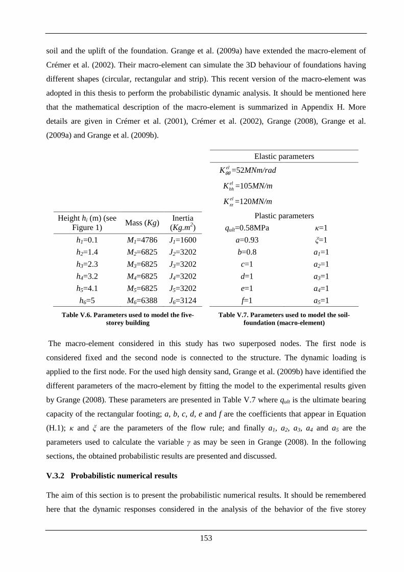
153
soil and the uplift of the foundation. Grange et al. (2009a) have extended the macro-element of
Crémer et al. (2002). Their macro-element can simulate the 3D behaviour of foundations having
different shapes (circular, rectangular and strip). This recent version of the macro-element was
adopted in this thesis to perform the probabilistic dynamic analysis. It should be mentioned here
that the mathematical description of the macro-element is summarized in Appendix H. More
details are given in Crémer et al. (2001), Crémer et al. (2002), Grange (2008), Grange et al.
(2009a) and Grange et al. (2009b).
Height hi (m) (see Figure 1)
Mass (Kg) Inertia (Kg.m2)
h1=0.1 M1=4786 J1=1600
h2=1.4 M2=6825 J2=3202
h3=2.3 M3=6825 J3=3202
h4=3.2 M4=6825 J4=3202
h5=4.1 M5=6825 J5=3202
h6=5 M6=6388 J6=3124
Table V.6. Parameters used to model the five-storey building
Elastic parameters elKθθ =52MNm/rad
elhhK =105MN/m
elzzK =120MN/m
Plastic parameters
qult=0.58MPa κ=1
a=0.93 ξ=1
b=0.8 a1=1
c=1 a2=1
d=1 a3=1
e=1 a4=1
f=1 a5=1
Table V.7. Parameters used to model the soil-foundation (macro-element)
The macro-element considered in this study has two superposed nodes. The first node is
considered fixed and the second node is connected to the structure. The dynamic loading is
applied to the first node. For the used high density sand, Grange et al. (2009b) have identified the
different parameters of the macro-element by fitting the model to the experimental results given
by Grange (2008). These parameters are presented in Table V.7 where qult is the ultimate bearing
capacity of the rectangular footing; a, b, c, d, e and f are the coefficients that appear in Equation
(H.1); κ and ξ are the parameters of the flow rule; and finally a1, a2, a3, a4 and a5 are the
parameters used to calculate the variable γ as may be seen in Grange (2008). In the following
sections, the obtained probabilistic results are presented and discussed.
V.3.2 Probabilistic numerical results
The aim of this section is to present the probabilistic numerical results. It should be remembered
here that the dynamic responses considered in the analysis of the behavior of the five storey
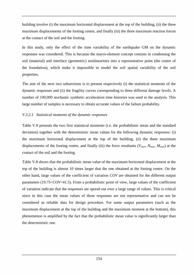
154
building involve (i) the maximum horizontal displacement at the top of the building, (ii) the three
maximum displacements of the footing centre, and finally (iii) the three maximum reaction forces
at the contact of the soil and the footing.
In this study, only the effect of the time variability of the earthquake GM on the dynamic
responses was considered. This is because the macro-element concept consists in condensing the
soil (material) and interface (geometric) nonlinearities into a representative point (the centre of
the foundation), which make it impossible to model the soil spatial variability of the soil
properties.
The aim of the next two subsections is to present respectively (i) the statistical moments of the
dynamic responses and (ii) the fragility curves corresponding to three different damage levels. A
number of 100,000 stochastic synthetic acceleration time histories was used in the analysis. This
large number of samples is necessary to obtain accurate values of the failure probability.
V.3.2.1 Statistical moments of the dynamic responses
Table V.8 presents the two first statistical moments (i.e. the probabilistic mean and the standard
deviation) together with the deterministic mean values for the following dynamic responses: (i)
the maximum horizontal displacement at the top of the building, (ii) the three maximum
displacements of the footing centre, and finally (iii) the force resultants (Vmax, Nmax, Mmax) at the
contact of the soil and the footing.
Table V.8 shows that the probabilistic mean value of the maximum horizontal displacement at the
top of the building is almost 10 times larger that the one obtained at the footing centre. On the
other hand, large values of the coefficient of variation COV are obtained for the different output
parameters (19.75<COV<41.5). From a probabilistic point of view, large values of the coefficient
of variation indicate that the responses are spread out over a large range of values. This is critical
since in this case the mean values of these responses are not representative and can not be
considered as reliable data for design procedure. For some output parameters (such as the
maximum displacement at the top of the building and the maximum moment at the bottom), this
phenomenon is amplified by the fact that the probabilistic mean value is significantly larger than
the deterministic one.
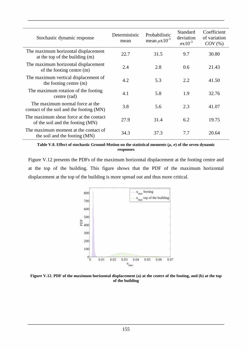
155
Stochastic dynamic response Deterministic
mean Probabilistic mean µx10-3
Standard deviation σx10-3
Coefficient of variation COV (%)
The maximum horizontal displacement at the top of the building (m)
22.7 31.5 9.7 30.80
The maximum horizontal displacement of the footing centre (m)
2.4 2.8 0.6 21.43
The maximum vertical displacement of the footing centre (m)
4.2 5.3 2.2 41.50
The maximum rotation of the footing centre (rad)
4.1 5.8 1.9 32.76
The maximum normal force at the contact of the soil and the footing (MN)
3.8 5.6 2.3 41.07
The maximum shear force at the contact of the soil and the footing (MN)
27.9 31.4 6.2 19.75
The maximum moment at the contact of the soil and the footing (MN)
34.3 37.3 7.7 20.64
Table V.8. Effect of stochastic Ground-Motion on the statistical moments (µ, σ) of the seven dynamic responses
Figure V.12 presents the PDFs of the maximum horizontal displacement at the footing centre and
at the top of the building. This figure shows that the PDF of the maximum horizontal
displacement at the top of the building is more spread out and thus more critical.
0 0.01 0.02 0.03 0.04 0.05 0.06 0.070
100
200
300
400
500
600
700
800
umax
PD
F
umax
footing
umax
top of the building
Figure V.12. PDF of the maximum horizontal displacement (a) at the centre of the footing, and (b) at the top of the building
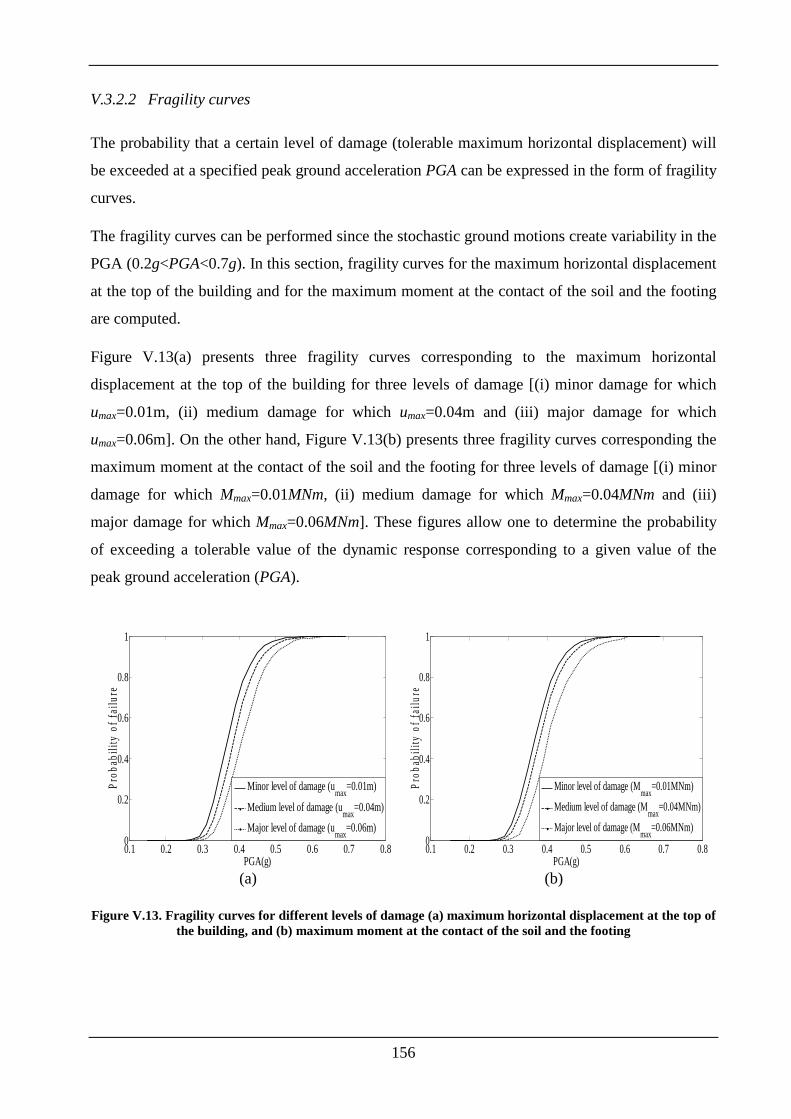
156
V.3.2.2 Fragility curves
The probability that a certain level of damage (tolerable maximum horizontal displacement) will
be exceeded at a specified peak ground acceleration PGA can be expressed in the form of fragility
curves.
The fragility curves can be performed since the stochastic ground motions create variability in the
PGA (0.2g<PGA<0.7g). In this section, fragility curves for the maximum horizontal displacement
at the top of the building and for the maximum moment at the contact of the soil and the footing
are computed.
Figure V.13(a) presents three fragility curves corresponding to the maximum horizontal
displacement at the top of the building for three levels of damage [(i) minor damage for which
umax=0.01m, (ii) medium damage for which umax=0.04m and (iii) major damage for which
umax=0.06m]. On the other hand, Figure V.13(b) presents three fragility curves corresponding the
maximum moment at the contact of the soil and the footing for three levels of damage [(i) minor
damage for which Mmax=0.01MNm, (ii) medium damage for which Mmax=0.04MNm and (iii)
major damage for which Mmax=0.06MNm]. These figures allow one to determine the probability
of exceeding a tolerable value of the dynamic response corresponding to a given value of the
peak ground acceleration (PGA).
0.1 0.2 0.3 0.4 0.5 0.6 0.7 0.80
0.2
0.4
0.6
0.8
1
PGA(g)
Pro
babi
lity
of f
ailu
re
Minor level of damage (umax
=0.01m)
Medium level of damage (umax
=0.04m)
Major level of damage (umax
=0.06m)
(a)
0.1 0.2 0.3 0.4 0.5 0.6 0.7 0.80
0.2
0.4
0.6
0.8
1
PGA(g)
Pro
babi
lity
of f
ailu
re
Minor level of damage (Mmax
=0.01MNm)
Medium level of damage (Mmax
=0.04MNm)
Major level of damage (Mmax
=0.06MNm)
(b)
Figure V.13. Fragility curves for different levels of damage (a) maximum horizontal displacement at the top of the building, and (b) maximum moment at the contact of the soil and the footing
157
V.4 CONCLUSIONS
In this chapter, the dynamic responses induced by an earthquake Ground-Motion (GM) taking
into account the soil spatial variability and/or the time variability of the seismic loading were
investigated. It should be mentioned here that when dealing with seismic loads, an aleatory
uncertainty which is the time variability of the earthquake GM appears in addition to the soil
spatial variability and the variability of the superstructure. Given the scarcity of studies involving
the probabilistic seismic responses, a free field soil medium subjected to a seismic loading was
firstly considered. The aim is to investigate the effect of the soil spatial variability and/or the time
variability of the earthquake GM using a simple model. Then, a SSI problem was investigated in
the second part of this chapter.
In the case where a free field medium was considered, the effect of the soil spatial variability
and/or the time variability of the earthquake GM was investigated through the study of an elastic
free field soil mass. The soil shear modulus G was modeled as a non-Gaussian random field and
the earthquake GM was modeled as a random process. The EOLE methodology was used to
discretize the shear modulus random field. As for the earthquake GM, the method proposed by
Rezaeian and Der Kiureghian (2010) which consists in fitting a parameterized stochastic model to
the real recorded earthquake GM was utilized. The dynamic response considered in the analysis
was the amplification of the maximum acceleration at the soil surface. The deterministic dynamic
numerical model was based on numerical simulations using the finite difference software
FLAC3D. Two types of modeling were considered in this chapter. The first one considers a two-
dimensional soil mass and the second model considers a soil column. The objective of these two
types of modeling was to verify the validity of the 'column' model in simulating the propagation
of the seismic waves in the soil mass. This permits to replace the 2D computationally-expensive
model with the relatively non-expensive 'column' model which may significantly reduce the
probabilistic computational time. As for the probabilistic methods used in this chapter, two
methods were used. The first one is the classical Monte Carlo Simulation (MCS) methodology
and the second one is the Sparse Polynomial Chaos Expansion (SPCE) methodology which
consists in substituting the original deterministic model by a meta-model.
The deterministic numerical results of the free field case have shown that the 'column' model is
sufficient to study the evolution of the maximum acceleration in the soil mass. This result is of
particular interest for the probabilistic analyses which require a large number of calls to the
deterministic model. On the other hand, the evolution of the maximum acceleration as a function
158
of the shear modulus have shown that for a given range of the shear modulus values, an important
increase in the maximum acceleration was obtained. For this range of values of G, the
predominant frequency band of the soil 'column' corresponds to the predominant frequency band
of the seismic loading, which leads to resonance phenomenon.
As for the probabilistic results of the free field case, the MCS methodology has shown that for the
Nice accelerogram used in this thesis, the variability obtained when only the soil spatial
variability was considered is largely smaller than the one obtained when only the time variability
of the earthquake GM was considered. This result may change in the case where a different
seismic signal is used. Considering both the soil spatial variability and the time variability of the
GM has led to a variability of Amax which is far below from that obtained by superposition of the
variabilities of Amax as obtained from the soil spatial variability and the time variability of the
earthquake GM considered separately. As for the SPCE methodology results, the obtained
statistical moments of Amax at the top of the soil column are close to those resulting from the MCS
methodology, but the obtained PDFs can not be considered as rigorous because relatively small
values of Q2 were obtained in this case.
In the case where the SSI problem was considered, a probabilistic dynamic analysis of a five-
storey building founded on two rigid rectangular footings was presented. The entire soil-structure
system was considered in the analysis in which the soil and soil-footing interface were modelled
by a macro-element. The main reason for which the macro-element concept was chosen to
perform the probabilistic analysis is that the time cost for a single deterministic calculation is
relatively small (five minutes per simulation). Only the time variability of the seismic loading
was introduced in the computations; the soil spatial variability was not considered in the analysis.
The probabilistic dynamic analyses were performed using the classical Monte Carlo Simulation
(MCS) methodology.
The dynamic system responses retained for the probabilistic analysis of the SSI problem were (i)
the maximum horizontal displacement at the top of the building, (ii) the three maximum
displacements of the footing centre, and finally (iii) the three maximum reaction forces at the
contact of the soil and the footing.
The probabilistic numerical results of the SSI problem have shown that (i) the probabilistic mean
value of the maximum horizontal displacement at the top of the building was almost 10 times
larger that the one obtained at the footing centre; (ii) large values of the coefficient of variation
were obtained for the different output parameters; and finally (iii) stochastic ground motion time

159
histories create variability in the PGA which allows one to perform fragility curves for the
different dynamic responses.
160
GENERAL CONCLUSIONS
This study focuses on the probabilistic analysis of shallow foundations resting on spatially
varying soils or rocks and subjected to either a static or a dynamic (seismic) loading. Two
aleatory sources of uncertainty were considered. The first one is the soil (or rock) spatial
variability which was modeled by random fields. The second one is the time variability of the
earthquake GM (when seismic loads were considered) which was modeled by a random process.
Both types of variabilities lead to high dimensional stochastic problems.
In this thesis, a literature review on the soil and the earthquake GM variabilities and the meta-
modeling techniques was first presented. It was followed by two main parts.
The first part (which is composed of chapters II, III and IV) presents a probabilistic analysis of
shallow foundations resting on spatially varying soils or rocks and subjected to a static loading.
Both cases of strip and square footings were studied. Also, 2D and 3D random fields were
considered in the analysis. In this part, the probabilistic method used to calculate the different
probabilistic outputs was the Sparse Polynomial Chaos Expansion (SPCE) methodology and its
extension the SPCE/GSA procedure.
In chapter II, a probabilistic analysis of shallow strip foundations resting on spatially varying
soils or rocks was presented. Relatively non-expensive deterministic models were used in this
chapter since the ULS analysis was performed in the case of a weightless material. The resulting
ultimate bearing capacity is the one related to the Nc coefficient in the bearing capacity equation.
In the case of spatially varying soil mass, a probabilistic analysis at both ULS and SLS of
vertically loaded strip footings was performed. The soil shear strength parameters (c and φ) were
considered as anisotropic cross-correlated non-Gaussian random fields at ULS and the soil elastic
parameters (E and υ) were considered as anisotropic uncorrelated non-Gaussian random fields at
SLS. Notice that the system response used at ULS was the ultimate bearing capacity; however,
the footing vertical displacement was considered as the system response at SLS. Concerning the
case of the spatially varying rock mass obeying the Hoek-Brown failure criterion, only the ULS
case of vertically loaded footings was considered. The uniaxial compressive strength of the intact
rock (σc) was considered as a non-Gaussian random field and the Geological Strength Index
(GSI) was considered as a random variable. Notice that the system response considered was the
ultimate bearing capacity of the footing in the case of a weightless rock mass. The methodology
proposed by Vořechovsky (2008) was used to generate the random fields. The Sparse Polynomial
Chaos Expansion (SPCE) methodology was used to perform the probabilistic analysis.
161
In chapter III, the effect of the spatial variability in three dimensions (3D) was investigated
through the study of the ultimate bearing capacity of strip and square foundations resting on a
purely cohesive soil with a spatially varying cohesion in the three dimensions. This case involves
relatively non-expensive deterministic models although a 3D mechanical model (with a greater
computation time with respect to the models of chapter II) was used. This is because of the use of
a purely cohesive soil.
In chapter IV, an efficient combined use of the SPCE methodology and the Global Sensitivity
Analysis (GSA) was proposed. The aim is to reduce the probabilistic computation time for high-
dimensional stochastic problems involving expensive deterministic models. This procedure was
illustrated through the probabilistic analysis at ULS of a strip footing resting on a ponderable soil
with 2D and 3D random fields and subjected to a central vertical load.
The main findings of the first part can be summarized as follows:
• Chapters II and III have shown the superiority of the SPCE with respect to the classical
MCS commonly used in geotechnical engineering problems involving spatially varying
soils. The superiority comes from the small number of calls of the deterministic model. In
addition to the determination of the PDF of the system response, the SPCE allows one to
easily perform a global sensitivity analysis based on Sobol indices using the SPCE
coefficients. These indices give the contribution of each random field in the variability of
the system response.
• The classical SPCE methodology was found to be efficient when relatively non-expensive
deterministic models are involved in the analysis (e.g. the ULS analysis of strip footings
on a weightless material or the ULS analysis of 3D footings on a purely cohesive soil).
• The efficient combined use of the SPCE methodology and the Global Sensitivity Analysis
(GSA) is needed when expensive deterministic models (e.g. strip, rectangular or circular
footings resting on a ponderable soil with 2D/3D random fields) are involved in the
analysis.
• The variability of the system responses (i.e. the ultimate bearing capacity in the ULS
analysis and the vertical displacement of the footing in the SLS analysis) increases (as
expected) with the increase in the coefficients of variation of the random fields. It was
also shown that an increase in the coefficient of variation of a random field increases its
162
Sobol index and thus its weight in the variability of the system response and decreases the
weight of the other random field.
• The negative correlation between the random fields decreases the response variability.
• The decrease in the autocorrelation distances (ax or ay or ax=ay), lead to a less spread out
PDF of the system response
• The probabilistic mean value of the ultimate bearing capacity of strip footings (in both
cases of soil and rock masses) presents a minimum. This minimum was obtained in the
isotropic case when the autocorrelation distance is nearly equal to the footing breadth B;
while for the anisotropic case (presented only when a soil mass is considered), this
minimum was obtained (for prescribed footing and soil characteristics) at a given value of
the ratio between the horizontal and the vertical autocorrelation distances.
• The small values of the autocorrelation distances lead to small values of the skewness and
kurtosis of the system responses. Thus, a PDF of the system response that is not far from a
Gaussian one is obtained in these cases.
• For small values of the autocorrelation distances, the variability of the ultimate bearing
capacity computed by considering a 3D random field is smaller than the one obtained with
the 2D random field for both cases of square and strip footings. Thus, the third dimension
is important to be considered only when small autocorrelation distances are encountered.
• Some observed phenomena which can not be seen when homogenous soils are considered
(such as the non-symmetrical soil failure and the variation in Sobol indices with the
autocorrelation distance) are obtained when considering the spatial variability of the
soil/rock properties in the probabilistic analysis.
The second part (which is composed of chapter V) presents a probabilistic analysis of the
dynamic responses induced by a specific earthquake Ground-Motion (GM) (which is the Nice
synthetic accelerogram), taking into account the soil spatial variability and/or the time variability
of the seismic loading. Two cases involving (i) a free field and (ii) a SSI problem were
considered in the analysis. In this part, the probabilistic methods used to calculate the
probabilistic outputs were the classical Monte-Carlo simulation (MCS) method and the Sparse
Polynomial Chaos Expansion (SPCE) methodology.
163
In the case where a free field medium was considered, the effect of the soil spatial variability
and/or the time variability of the earthquake GM was investigated. The soil shear modulus G was
modeled as a non-Gaussian random field and the earthquake GM was modeled as a random
process. The dynamic response considered in the analysis was the amplification of the maximum
acceleration at the soil surface. Two types of modeling were considered herein. The first one
considers a two-dimensional soil mass and the second model considers a soil column. The
objective of these two types of modeling was to verify the validity of the 'column' model in
simulating the propagation of the seismic waves in the soil mass. As for the case where a SSI
problem was considered, a probabilistic dynamic analysis of a five-storey building founded on
two rigid rectangular footings was presented. The soil and soil-footing interface were modelled
by a macro-element. The main reason for which the macro-element concept was used is the
relatively small computation cost of the deterministic model. Only the time variability of the
seismic loading was introduced in the computations; the soil spatial variability was not
considered in the analysis. The dynamic system responses retained for the probabilistic analysis
were: (i) the maximum horizontal displacement at the top of the building, (ii) the three maximum
displacements of the footing centre, and finally (iii) the three maximum reaction forces at the
contact of the soil and the footing. In this part, the main findings can be summarized as follows:
• The 'column' model was found sufficient to study the distribution of the maximum
acceleration in the soil mass. This result is of particular interest for the probabilistic
analyses which require a large number of calls to the deterministic model.
• The evolution of the maximum acceleration as a function of the shear modulus have
shown that for a given range of the shear modulus values, an important increase in the
maximum acceleration was obtained. For this range of values of G, the predominant
frequency band of the soil 'column' corresponds to the predominant frequency band of the
seismic loading, which leads to the resonance phenomenon.
• When using the Nice accelerogram, the variability obtained when only the soil spatial
variability was considered was found largely smaller than the one obtained when only the
time variability of the earthquake GM was considered.
• Considering both the soil spatial variability and the time variability of the earthquake GM
has led to a variability of Amax which is far below from that obtained by superposition of
the variabilities of Amax as obtained from the soil spatial variability and the time variability
of the earthquake GM considered separately.
164
• The PDFs of Amax at the top of the soil column obtained using the SPCE methodology
show similar trends as those obtained when static loading cases were considered, but these
PDFs can not be considered as rigorous because relatively small values of Q2 were
obtained in this case.
• When considering the SSI problem involving the study of a five-storey building, large
values of the coefficients of variation were obtained for the different system responses.
• The stochastic ground motion time histories create variability in the PGA which allows
one to perform fragility curves for the different dynamic responses
Ongoing research topics may involve the following items:
For the static loading case:
• Consider the case of a rectangular or a circular footing resting on a ponderable soil with
3D spatially varying shear strength parameters using the SPCE/GSA procedure.
• Validate of the SPCE methodology for the computation of the failure probability.
• Use of a rigorous approach for the computation of Sobol indices in the case of correlated
random variables.
For the seismic loading case:
• Investigate the effect of 2D random fields (instead of the 1D random fields) on the
dynamic response in the case of the free field soil medium.
• Investigate the effect of changing the input seismic signal on the obtained probabilistic
results.
• In the SSI problem, introduce the soil spatial variability in the macro-element. This can be
done by first computing the PDF of the ultimate bearing capacity. Then, one may use the
obtained PDF (instead of the deterministic value of qult) in the macro-element
formulation.
• Explore new methodologies which may improve the meta-model in the case of highly
nonlinear models.

165
166
REFERENCES
1. Ahmadi, G. (1979). “Generation of artificial time-histories compatible with given response spectra-a review.” Solid Mechanics Archives, 4: 207-239.
2. Ahmed, A., and Soubra, A.H. (2012). “Probabilistic analysis of strip footings resting on a spatially random soil using subset simulation approach.” Georisk: Assessment and Management of Risk for Engineered Systems and Geohazards, 6(3): 188-201.
3. Ahmed, A. (2012). “Simplified and Advanced Approaches for the Probabilistic Analysis of Shallow Foundations.” PhD. Thesis, University of Nantes, France.
4. Al-Bittar, T., and Soubra, A.H. (2011). “Bearing capacity of strip footing on spatially random soils using sparse polynomial chaos expansion.” GeoRisk (GSP 224), ASCE, Atlanta, USA, 26-28 June 2011.
5. Al-Bittar, T., and Soubra, A.H. (2012a). “Bearing capacity of strip footing on spatially random soils using sparse polynomial chaos expansion.” International Journal for Numerical and Analytical Methods in Geomechanics, DOI: 10.1002/nag.2120.
6. Al-Bittar, T., and Soubra, A.H. (2012b). “Analysis at the serviceability limit state of strip footings resting on spatially varying soils using sparse polynomial chaos expansion.” Journal of Geotechnical and Geoenvironmental Engineering, ASCE, under review.
7. Al-Bittar, T., and Soubra, A.H. (2012c). “Bearing capacity of spatially random rock masses obeying Hoek-Brown failure criterion.” International Journal of Rock Mechanics and Mining Sciences, under review.
8. Al-Bittar, T., and Soubra, A.H. (2012d). “Effect of the soil spatial variability in three dimensions on the undrained bearing capacity of footings.” Géotechnique, under revision.
9. Al-Bittar, T., and Soubra, A.H. (2012e). “Efficient sparse polynomial chaos expansion methodology for the probabilistic analysis of computationally-expensive deterministic models.” International Journal for Numerical and Analytical Methods in Geomechanics, under review.
10. Al-Bittar, T., and Soubra, A.H. (2012f). “Efficient sparse polynomial chaos expansion methodology for computationally expensive deterministic models.” Proceedings of the 5th International Conference on Reliable Engineering Computing: Practical Applications and Practical Challenges, Brno, Czech Republic, 13–15 June 2012.
11. Al-Bittar, T., and Soubra, A.H. (2012g). “Calcul probabiliste de la portance des fondations superficielles par l'utilisation du chaos polynomial creux et de l'analyse de sensibilité globale.” Compte-rendu des 7èmes Journées Nationales sur la Fiabilité, Chambéry, France, 4-6 Juin 2012.
12. Al-Bittar, T. (2012). “Calcul de la capacité portante ultime des fondations superficielles filantes avec prise en compte de la variabilité spatiale.” Concours Jeunes Chercheurs, obtention du 4ème prix. XXXe Rencontres AUGC-IBPSA, Chambéry, Savoie, 6-8 juin 2012.
167
13. Al-Bittar, T., Youssef Abdel-Massih, D., Soubra, A.H., and Hage-Chehade. F. (2012a). “Influence of soil spatial variability and stochastic ground-motion on the dynamic behavior of a slope.” Geocongress, State of the Art and Practice in Geotechnical Engineering, ASCE, Oakland, CA, USA, 25-29 March 2012.
14. Al-Bittar, T., Kotronis, P., Grange, S., and Soubra, A.H. (2012b). “Probabilistic dynamic analysis of a soil-structure system subjected to a stochastic earthquake Ground-Motion.” Proceedings of the 10th World Congress on Computational Mechanics, WCCM, São Paulo, Brazil, 8-13 July 2012.
15. Au, S.K., and Beck, J.L. (2001). “Estimation of small failure probabilities in high dimensions by subset simulation.” Probabilistic Engineering Mechanics, 16: 263-277
16. Baecher, G.B., and Christian, J.T. (2003). “Reliability and statistics in geotechnical engineering.” John Wiley & Sons Ltd, The Atrium, Southern Gate, Chichewter, West Sussex PO19 8SQ, England, 205-242.
17. Baecher, G.B., Marr, W.A., Lin, J.S., and Consla, J. (1983). “Critical parameters of mine tailings embankments.” Denver, CO, U.S., Bureau of Mines.
18. Barton, R.R. (1992). “Metamodels for Simulation Input-Output Relations.” Proceedings of the 1992 Winter Simulation Conference. Swain, J. J., et al. (eds.), Arlington, VA: 289-299.
19. Bauer, J. and Pula, W. (2000). “Reliability with respect to settlement limit-states of shallow foundations on linearly-deformable subsoil.” Computers and Geotechnics, 26: 281-308.
20. Berveiller, M., Sudret, B., and Lemaire, M. (2006). "Stochastic finite element: a non intrusive approach by regression." Revue Européenne de Mécanique Numérique, 15(1-2-3): 8-92.
21. Blatman, G., (2009). “Adaptive sparse polynomial chaos expansions for uncertainty propagation and sensitivity analysis.” Ph.D thesis, Université Blaise Pascal, Clermont-Ferrand.
22. Blatman, G., and Sudret, B. (2010). “An adaptive algorithm to build up sparse polynomial chaos expansions for stochastic finite element analysis.” Probabilistic Engineering Mechanics, 25: 183–97.
23. Blatman, G., and Sudret, B. (2011). “Adaptive sparse polynomial chaos expansion based on least angle regression.” Journal of Computational Physics, 230: 2345–2367.
24. Blatman, G., and Sudret, B. (2011). “Principal component analysis and Least Angle Regression in spectral stochastic finite element analysis.” Applications of Statistics and Probability in Civil Engineering. 669-676.
25. Booker, A.J., Dennis, J.E., Frank, P.D., Serafini, D.B., Torczon, V., and Trosset, M.W. (1999). “A rigorous framework For optimization of expensive functions by surrogates.” Structural Optimization, 17: 1-13.
26. Bourdeau, C. (2005). “Effet de site et mouvements de versant en zones sismiques: apport de la modélisation numérique.” Ph.D thesis, Ecole de mines de Paris, 266 p.
168
27. Box, G.E.P., Hunter, W.G., and Hunter, J.S. (1978). “Statistics for experimenters.” John Wiley and Sons.
28. Box, G.E.P., and Jenkins, G.M. (1970). “Time series analysis: forecasting and control.” Holden-Day, San Fransisco, 553 p.
29. Breysse, D., and Kastner, R. (2003). “Sols urbains.” Hermès Science Publications, 462 pages.
30. Breysse, D., Niandou, H., Elchachi, S.M., and Houy, L. (2005). “Generic approach of soil-structure interaction considering the effects of soil heterogeneity.” Symposium in print "Risk and variability in geotechnical engineering", Geotechnique, 2: 143-150.
31. Breysse, D., La Borderie, C., Elchachi, S.M., and Niandou, H. (2007). “Spatial variations in soil properties and their consequences on structural reliability.” Civil Engineering and Environmental Systems, 4(2): 73-83.
32. Breysse, D. (2011). “Reliability of a shallow foundation footing.” Chap. 6, pp. 97-118, in Baroth, J., Breysse, D., Schoefs, F., Construction reliability: safety, variability and sustainability, ISTE Wiley.
33. Brown, E.T. (2008). “Estimating the mechanical properties of rock masses.” In: Potvin Y, Carter J, Dyskin A, Jeffrey R, editors. Proceedings of the 1st southern hemisphere international rock mechanics symposium: SHIRMS 2008, Perth, Western Australia, 1: 3-21.
34. Bucher, C.G. and Bourgund, U. (1990). “A fast and e_cient response surface approach for structural reliability problems.” Structural Safety, 7: 57-66.
35. CAMUS International Benchmark. (1997). “Mock-up and loading characteristics, specifications for the participants report.” Report I, CEA and GEO.
36. Caniou, Y.; Sudret, B. and Micol, A. (2012). “Analyse de sensibilité globale pour des variables corrélées -- Application aux modèles imbriqués et multiéchelles.” Compte-rendu des 7èmes Journées Nationales sur la Fiabilité, Chambéry, France, 4-6 Juin 2012.
37. Cassidy, M.J., Byrne, B.W,, Houlsby, G.T. (2002). “Modelling the behaviour of circular footings under combined loading on loose carbonate sand.” Géotechnique, 52(10):705–712.
38. Chen, W.F., and Sawada, T. (1983). “Earthquake-induced slope failure in nonhomogeneous, anisotropic soils.” Soils and Foundations, 23(2): 125-139.
39. Cherubini, C. (2000), “Reliability evaluation of shallow foundation bearing capacity on c', φ' soils.” Canadian Geotechnical Journal, 37: 264-269.
40. Cherubini, C., Giasi, I., and Rethati, L. (1993). “The coefficient of variation of some geotechnical parameters.” Probabilistic Methods in Geotechnical Engineering. Edited by Li, K.S., and Lo, S-C.R., A.A. Balkema, Rotterdam, 179-183.
41. Ching, J., Hu, Y.G., Yang, Z.Y., Shiau, J.Q., Chen, J.C., and Li, Y.S. (2011). “Reliability-based design for allowable bearing capacity of footings on rock masses by considering
169
angle of distortion.” International Journal of Rock Mechanics and Mining Sciences, 48: 728-740.
42. Cho, S.E., and Park, H.C. (2010). “Effect of spatial variability of cross-correlated soil properties on bearing capacity of strip footing.” International Journal for Numerical and Analytical Methods in Geomechanics, 34: 1-26.
43. Conte, JP., Pister, KS., Mahin, SA. (1992). “Nonstationary ARMA modeling of seismic motions.” Soil Dynamics and Earthquake Engineering, 11: 411-426.
44. Conte, JP., and Peng, BF. (1997). “Fully nonstationary analytical earthquake ground-motion model.” Journal of Engineering Mechanics (ASCE), 12: 15-24.
45. Cornell, CA. (1960). “Stochastic process models in structural engineering.” Technical Report No. 34, Department of Civil Engineering, Stanford University, Stanford, CA.
46. Crémer, C., Pecker, A., and Davenne, L. (2001). “Cyclic macro-element for soil–structure interaction: material and geometrical non-linearities.” International Journal for Numerical and Analytical Methods in Geomechanics, 25(13): 1257–1284.
47. Crémer, C., Pecker, A., and Davenne, L. (2002). “Modelling of nonlinear dynamic behaviour of a shallow strip foundation with macro-element.” Journal of Earthquake Engineering, 6(2):175–211.
48. Da Veiga, S.; Wahl, F. and Gamboa, F. (2009). “Local polynomial estimation for sensitivity analysis on models with correlated inputs.” Technometrics, 51: 452-463
49. Der Kiureghian, A., and Ditlevsen, O. (2009). “Aleatory or epistemic? Does it matter?” Structural Safety, 31(2): 105-112.
50. Der Kiureghian, A., and Ke, J.-B. (1988). “The stochastic finite element method in structural reliability.” Probabilistic Engineering Mechanics, 3(2): 83-91.
51. Der Kiureghian, A., and Crempien, J. (1989). “An evolutionary model for earthquake ground motion.” Structural Safety; 6: 235-246.
52. Ditlevsen, O. (1996). “Dimension reduction and discretization in stochastic problems by regression method.” in F. Casciati and B. Roberts, Editors, Mathematical models for structural reliability analysis, CRC Mathematical Modelling Series, 2, 51-138.
53. Duncan, J.M. (2000). “Factors of safety and reliability in geotechnical engineering.” Journal of Geotechnical and Geoenvironmental Engineering, ASCE, 126(4): 307-316.
54. Ejezie, S., and Harrop-Williams, K. (1984). “Probabilistic characterization of Nigerian soils.” In Probabilistic Characterization of Soil Properties, Bridge Between Theory and Practice, ASCE, 140-156.
55. El-Ramly, H., Morgenstern, N.R., and Cruden, D.M. (2003). “Probabilistic stability analysis of a tailings dyke on presheared clay-shale.” Canadian Geotechnical Journal, 40: 192-208.
170
56. Fenton, G.A., (1999). “Estimation for stochastic soil models.” Journal of Geotechnical and Geoenvironmental Engineering, ASCE, 125(6): 470-485.
57. Fenton, G.A., and Griffiths, D.V. (2002), “Probabilistic foundation settlement on spatially random soil.” Journal of Geotechnical and Geoenvironmental Engineering, ASCE, 128(5): 381-390.
58. Fenton, G.A., and Griffiths, D.V. (2003). "Bearing capacity prediction of spatially random c-φ soils." Canadian Geotechnical Journal, 40: 54-65.
59. Fenton, G.A., and Griffiths, D.V. (2005). “Three-dimensional probabilistic foundation settlement.” Journal of Geotechnical and Geoenvironmental Engineering, ASCE, 131(2): 232-239.
60. Fenton, G.A., Zhou, H., Jaksa, M.B., and Griffiths, D.V. (2003). “Reliability analysis of a strip footing designed against settlement.” Applications of statistics and probability in civil engineering, Der Kiureghian, Madanat & Pestana (eds) © 2003 Millpress, Rotterdam.
61. Fredlund, D.G., and Dahlman, A.E. (1972). “Statistical geotechnical properties of glacial lake Edmonton sediments.” In Statistics and Probability in Civil Engineering, Hong Kong University Press.
62. Ghanem, R., and Spanos, P. (1991). “Stochastic finite elements – A spectral approach.” Springer, New York.
63. Goovaerts, P. (1998). “Geostatistical tools for characterizing the spatial variability of microbiological and physico-chemical soil properties.” Biol Fertil Soils, 27: 315–334.
64. Goovaerts, P. (1999). “Geostatistics in soil science: state-of-the-art and perspectives.” Geoderma, 89: 1-45.
65. Gourvenec, S., Randolph, M. F., and Kingsnorth, O. (2006). “Undrained bearing capacity of square and rectangular footings.” Internatinal Jounal of Geomechanics, 6(3): 147–157.
66. Grange, S., Kotronis, P., and Mazars, J. (2009a). “A macro-element to simulate 3D soil–structure interaction considering plasticity and uplift.” International Journal of Solids and Structures, 46: 3651–3663.
67. Grange, S., Kotronis, P., and Mazars, J (2009b). “A macro-element to simulate dynamic Soil-Structure Interaction.” Engineering Structures, 31: 3034–3046
68. Grange, S. (2008). “Risque sismique: stratégie de modélisation pour simuler la réponse des structures en béton et leurs interactions avec le sol.” Ph.D thesis, INPG.
69. Griffiths, D.V., and Fenton, G.A. (2001). “Bearing capacity of spatially random soil. The undrained clay Prandtl problem revisited.” Géotechnique, 51(4): 351-359.
70. Griffiths, D.V., Fenton, G.A., and Manoharan, N. (2002). “Bearing capacity of rough rigid strip footing on cohesive soil: Probabilistic study.” Journal of Geotechnical and Geoenvironmental Engineering, ASCE, 128(9): 743-755.
171
71. Griffiths, DV., Huang, J., and Fenton, GA. (2009). “On the reliability of earth slopes in three dimensions.” Proceedings of the Royal Society A, 465: 3145-3164.
72. Gunsallus, KL., and Kulhawy, F.H. (1984) “A comparative evaluation of rock strength measures.” International Journal of Rock Mechanics and Mining Sciences & Geomechanics Abstracts, 21: 233-248.
73. Harr, M.E. (1987). “Reliability-based design in civil engineering.” McGraw-Hill Book Company, New York, 290p.
74. Hoek, E. (1998). “Reliability of Hoek-Brown estimates of rock mass properties and their impact on design.” International Journal of Rock Mechanics and Mining Sciences, 35(1): 63-68.
75. Hoek, E., and Brown, E. (1980). “Empirical strength criterion for rock masses.” Journal of the Geotechnical Engineering Division, 106: 1013-35.
76. Hoek, E., Carranze-Torres, C., and Corkum, B. (2002). “Hoek-Brown failure criterion.” 2002 edition. In: Proceeding of the North American rock mechanics society meeting, Toronto, July,. 267-73.
77. Hoek, E., and Marinos, P. (2007). “A brief history of the development of the Hoek-Brown failure criterion.” Soils Rocks, 30(2): 85-92.
78. Honjo, Y. (2008). “Monte Carlo Simulation in reliability analysis.” In: Phoon, K.K., ed. Reliability-based design in Geotechnical Engineering: Computations and applications. Taylor & Francis: 169-171.
79. Houmadi, Y., Ahmed, A., and Soubra, A.-H. (2012). “Probabilistic analysis of a one-dimensional soil consolidation problem.” Georisk: Assessment and Management of Risk for Engineered Systems and Geohazards, 6 (1): 36-49.
80. Huang, S., Liang, B., and Phoon, K.K. (2009). "Geotechnical probabilistic analysis by collocation-based stochastic response surface method: An EXCEL add-in implementation." Georisk: Assessment and Management of Risk for Engineered Systems and Geohazards, 3(2): 75-86.
81. Isukapalli, S.S. (1999). “Uncertainty analysis of transport-transformation models.” Ph.D thesis, the state university of New Jersey.
82. Isukapalli, S.S., Roy, A., and Georgopoulos, P.G. (1998). “Stochastic response surface methods (SRSMs) for uncertainty propagation: Application to environmental and biological systems.” Risk Analysis, 18(3): 357-363.
83. Itasca. (2000). “FLAC 4.0 Manuals.” – Minnesota, ITASCA Consulting Group, Inc 2000.
84. Jaksa, M.B. (1995). “The influence of spatial variability on the geotechnical design properties of a stiff, overconsolidated clay.” Ph.D. Thesis, Faculty of Engineering, University of Adelaide.
85. Jimenez, R., and Sitar, N. (2009). “The importance of distributions types on finite element analyses of foundation settlement.” Computers and Geotechnics, 36: 474-483.
172
86. Jin, Y. (2005). “A comprehensive survey of fitness approximation in evolutionary computation.” Soft Computing - A Fusion of Foundations, Methodologies and Applications, 9(1): 3-12.
87. Journel, A.G., and Huijbregts, Ch J. (1978). “Mining Geostatistics.” Academic Press.
88. Kausel, E., Whitman, A., Murray, J., and Elsabee, F. (1978). “The spring method for embedded foundations.” Nuclear Engineering and Design, 48: 377-392.
89. Koutsourelakis, S., Prevost, J.H., and Deodatis, G. “Risk assessement of an interacting structure-soil system due to liquefaction.” Earthquake Engineering and Structural Dynamic, 31: 851-879.
90. Kozin, F. (1988). “Autoregressive moving average models of earthquake records.” Probabilistic Engineering Mechanics, 3: 58-63.
91. Kramer, S. L. (1996). “Geothechnical earthquake engineering.” Prentice Hall, New Jersey.
92. Kucherenko, S., Tarantola, A. and Annoni, P. (2012). “Estimation of global sensitivity indices for models with dependent variables.” Computer Physics Communications, 183: 937-946
93. Kuhlemeyer, R. L., and Lysmer, J. (1973). “Finite element method accuracy for wave propagation problems.” Journal of Soil Mechanics & Foundations, 99: 421-427.
94. Lacasse, S., and Nadim, F. (1996). “Uncertainties in characterizing soil properties.” Uncertainty in the Geologic Environment, ASCE, Madison, 49-75.
95. Lee, I.K., White, W., and Ingles, O.G. (1983). “Geotechnical Engineering.” Pitman, London, England.
96. Leshchinsky, D., and San, K.C. (1994). “Pseudostatic seismic stability of slopes: Design charts.” Journal of Geotechnical Engineering, ASCE, 120(9): 1514-1532.
97. Li, C.C., and Der Kiureghian, A. (1993). “Optimal discretization of random fields.” Journal of Engineering Mechanics, 119(6): 1136-1154.
98. Li, D., Chen, Y., Lu, W., and Zhou, C. (2011). “Stochastic response surface method for reliability analysis of rock slopes involving correlated non-normal variables.” Computers. and Geotechnics, 38(1): 58-68.
99. Li, G., Rabitz, H., Yelvington, P., Oluwole, O., Bacon, F.; Kolb, C. and Schoendorf, J. (2010). “Global sensitivity analysis for systems with independent and/or correlated inputs.” The Journal of Physical Chemistry, 114: 6022-6032
100. Liu, S.C. (1970). “Synthesis of stochastic representations of ground motions.” The Bell Systems Technical Journal, 49: 521-541.
101. Liu, W.-K., Belytschko, T., and Mani, A. (1986a). “Probabilistic finite elements for non linear structural dynamics.” Computer Methods in Applied Mechanics and Engineering, 56: 61-86.
173
102. Liu, W.-K., Belytschko, T., and Mani, A. (1986b), “Random field finite elements.” International Journal for Numerical Methods in Engineering, 23(10): 1831-1845.
103. Lopez-Caballero, F., and Modaressi Farahmand-Razavi, A. (2010). “Assessment of variability and uncertainties effects on the seismic response of a liquefiable soil profile.” Soil Dynamics and Earthquake Engineering, 30(7): 600-613.
104. Loukidis, D., Bandini, P., and Salgado, R. (2003). “Stability of seismically loaded slopes using limit analysis.” Géotechnique, 53(5): 463-479.
105. Lumb, P. (1966). “The variability of natural soils.” Canadian Geotechnical Journal, 3: 74-97.
106. Lumb, P. (1970). “Safety factors and the probability distribution of soil strength.” Canadian Geotechnical Journal, 7: 225-242.
107. Lumb, P. (1972). “Precision and accuracy of soil tests.” In Statistics and Probability in Civil Engineering, Hong Kong University Press.
108. Mao, N., Al-Bittar, T., and Soubra, A.-H. (2011). “Probabilistic analysis of shallow foundations on rocks obeying Hoek-Brown failure criterion.” GeoRisk (GSP 224), ASCE, Atlanta, USA, 26-28 June.
109. Mao, N., Al-Bittar, T., and Soubra, A.-H. (2012). “Probabilistic analysis and design of strip foundations resting on rocks obeying Hoek-Brown failure criterion.” International Journal of Rock Mechanics and Mining Sciences, 49: 45–58.
110. Merifield, RS., Lyamin, AV., and Sloan, SW. (2006). “Limit analysis solutions for the bearing capacity of rock masses using the generalized Hoek-Brown criterion.” International Journal of Rock Mechanics and Mining Sciences, 43: 920-937.
111. Michalowski, R.L. (2002). “Stability charts for uniform slopes.” Journal of Geotechnical and Geoenvironmental Engineering, ASCE, 128(4): 351-355.
112. Mollon, G., Dias, D., and Soubra, A.-H. (2011). “Probabilistic analysis of pressurized tunnels against face stability using collocation-based stochastic response surface method.” Journal of Geotechnical and Geoenvironmental Engineering, ASCE, 137(4): 385-397.
113. Morse, R.K. (1972). “The importance of proper soil units for statistical analysis.” In Statistics and Probability in Civil Engineering, Hong Kong University Press.
114. Myers, R.H., and Montgomery, D.C. (1995). “Response surface methodology: process and product optimization using designed experiments.” Wiley and Sons.
115. Nataf, A. (1962). “Détermination des distributions de probabilités dont les marges sont données.” CR Acad Sci, 225: 42-3 (in French).
116. Niandou, H., and Breysse, D. (2007). “Reliability analysis of a piled raft accounting for soil spatial variability.” Computer and Geotechnics, 34: 71-80.
117. Nour, A., Slimani, A. and Laouami N. (2002). “Foundation settlement statistics via finite element analysis.” Computers and Geotechnics, 29: 641–672.
174
118. Nour, A., Slimania, A., Laouamia, N., and Afraa, H. (2003). “Finite element model for the probabilistic seismic response of heterogeneous soil profile.” Soil Dynamics and Earthquake Engineering, 23: 331-348.
119. Nova, R., and Montrasio, L. (1991). “Settlements of shallow foundations on sand.” Géotechnique, 41(2): 243 256.
120. Papadimitriou, K. (1990). “Stochastic characterization of strong ground motion and application to structural response.” Report No. EERL 90-03, Earthquake Engineering Research Laboratory, California Institute of Technology, Pasadena, CA.
121. Pecker, A. (1984). “Dynamique des Sols.” Presse, ENPC: Paris, France.
122. Phoon, K.K., and Kulhawy, F.H., (1999). “Evaluation of geotechnical property variability.” Canadian Geotechnical Journal, 36: 625-639.
123. Phoon, K.K., Kulhawy, F.H., and Grigoriu, M.D. (1995). “Reliability-based design of foundations for transmission line structures.” Rpt. TR-105000, Electric Power Research Inst., Palo Alto (CA), 380p.
124. Popescu, R., Deodatis, G., and Nobahar, A. (2005). “Effect of random heterogeneity of soil properties on bearing capacity.” Probabilistic Engineering Mechanics, 20: 324-341.
125. Popescu, R., Prevost, J.H., and Deodatis, G. (2005). “3D effects in seismic liquefaction of stochastically variable soil deposits.” Géotechnique, 55(1): 21-31.
126. Popescu, R., Prevost, J.H., Deodatis, G., and Chakrabortty, P. (2006). “Dynamics of nonlinear porous media with applications to soil liquefaction.” Soil Dynamics and Earthquake Engineering, 26(6-7): 648-665.
127. Prévost, J.H. (1999). “DYNAFLOW. A finite element analysis program for static and transient response of linear and nonlinear two and three dimensional systems.” User Manual, Department of Civil Engineering, Princeton University.
128. Rezaeian, S., and Der Kiureghian, A. (2008). “A stochastic ground motion model with separable temporal and spectral nonstationarity.” Earthquake Engineering and Structural Dynamics, 37: 1565-1584.
129. Rezaeian, S., and Der Kiureghian, A. (2010). “Simulation of synthetic ground motions for specified earthquake and site characteristics.” Earthquake Engineering and Structural Dynamics, 39: 1155-1180.
130. Sacks, J., Welch, W. J., Mitchell, T. J. and Wynn, H. P. (1989). “Design and analysis of computer experiments.” Statistical Science, 4(4): 409-435.
131. Sadek, M., and Shahrour, I. (2004). “Three-dimensional finite element analysis of the seismic behavior of inclined micropiles.” Soil Dynamics and Earthquake Engineering, 24(6): 473-485.
132. Sadek, M. (2012). “Problèmes d'Interaction Sol Structure sous chargements statique et dynamique. ” Laboratoire Génie Civil et géo-Environnement, Université Lille 1, France.

175
133. Saltelli, A., Chan, K., and Scott, E. M. (2000). “Sensitivity Analysis.” John wiley and sons.
134. Shinozuka, M., and Deodatis, G. (1988). “Stochastic process models for earthquake ground motion.” Probabilistic Engineering Mechanics, 3: 114-123.
135. Shinozuka, M., and Sato, Y. (1967). “Simulation of nonstationary random process.” Journal of Engineering Mechanics (ASCE), 93: 11-40.
136. Sobol, I.M. (2001). “Global sensitivity indices for nonlinear mathematical models and their Monte Carlo estimates.” Mathmatics and Computers in Simulation, 55: 271-280.
137. Soubra, A.-H., Youssef Abdel Massih, D., and Kalfa, M. (2008). “Bearing capacity of foundations resting on a spatially random soil.” GeoCongress 2008, ASCE, GSP N° 178, New Orleans, Louisiana, USA, 9-12 March, 66-73.
138. Spanos, P.D., and Ghanem, R. (1989). “Stochastic finite element expansion for random media.” Journal of Engineering Mechanics, ASCE, 115(5): 1035-1053.
139. Stuedlein, A.,W., Kramer, S., and Arduino, P. (2012). “Geotechnical characterization and random field modeling of desiccated clay.” Journal of Geotechnical and Geoenvironmental Engineering, ASCE, http://dx.doi.org/10.1061/(ASCE)GT.1943-5606.0000723
140. Sudret, B. (2008). “Global sensitivity analysis using polynomial chaos expansion.” Reliability Engineering and System Safety, 93: 964-979.
141. Sudret, B., and Berveiller, M. (2008). “Stochastic finite element methods in geotechnical engineering.” In: Phoon, K.K., ed. Reliability-Based design in Geotechnical Engineering: Computations and applications. Taylor & Francis: 260-296.
142. Sudret, B., and Der Kiureghian, A. (2000). “Stochastic finite element methods and reliability: A State-of-the-Art Report.” Report No. UCB/SEMM-2000/08 Structural Engineering, Mechanics and Materials Department of Civil & Environmental Engineering, University of California, Berkeley
143. Sudret, B., Berveiller, M., and Lemaire, M. (2006). “A stochastic finite element procedure for moment and reliability analysis.” Eur. J. Comput. Mech., 15 (7-8): 825–866.
144. Uzielli, M.,Vannucchi, G., and Phoon, K.K. (2005). “Normal field characterization of stress-normalised cone penetration testing parameters.” Geotechnique, 55(1): 3-20.
145. Vanmarcke, E.H. (1977). “Probabilistic modeling of soil profiles.” Journal of the Geotechnical Engineering Division, ASCE, 103(11): 1227-1246.
146. Vanmarcke, E.H. (1983). “Random fields: Analysis and synthesis.” M.I.T, Press, Cambridge, Mass., 382 p.
147. Vanmarcke, E., and Grigoriu, M., (1983). “Stochastic finite analysis of simple beams.” Journal of Engineering Mechanics, 109: 1203-1214.
148. Vořechovský, M. (2008). “Simulation of simply cross-correlated random fields by series expansion methods.” Structural Safety, 30: 337-363.
176
149. Wang, S., and Hao, H. (2002). “Effects of random variations of soil properties on site amplification of seismic ground motions.” Soil Dynamics and Earthquake Engineering, 22(7): 551-564.
150. Widmer, F., Duvernay, B., Fäh, D., and Parriaux, A. (2003). “Projet pilote de microzonage sismique à Yverdon (VD).” Bulletin for Applied Geology, 8: 5-16.
151. Wolff, T.H. (1985). “Analysis and design of embankment dam slopes: A probabilistic approach." Ph.D thesis, Purdue Univ., Lafayette, Ind.
152. Wolff, T.H. (1996). “Probabilistic slope stability in theory and practice.” Uncertainty in Geological Environment, Madison, WI, ASCE, 419-433.
153. Xiu, D., and Karniadakis, G.E. (2002). “The Wiener-Askey polynomial chaos for stochastic differential equations.” SIAM J. on Scientific Computing, 24(2): 619-44.
154. You, L., and Michalowski, R.L. (1999). “Displacement charts for slopes subjected to seismic loads.” Computers and Geotechnics, 25(4): 45-55.
155. Youssef Abdel Massih, D. (2007). “Analyse du comportement des fondations superficielles filantes par des approches fiabilistes.” Ph.D thesis, university of Nantes, France.
156. Yuceman, M.S., Tang, W.H. and Ang, A.H.S. (1973). “A probabilistic study of safety and design of earth slopes.” Civil Engineering Studies, Structural Research Series 402, University of Illinois, Urbana.
157. Zerva, A. (2009). “Spatial variation of seismic Ground-Motions.” Haym Benaroya.
158. Zerva, A. (1988). “Seismic source mechanisms and ground motion models, review paper.” Probabilistic Engineering Mechanics, 3: 64-74.
159. Zhang, J., and Ellingwood, B. (1994). “Orthogonal series expansion of random fields in reliability analysis.” Journal of Engineering Mechanics, ASCE, 120(12): 2660-2677.
160. Zimbone, S.M., Vickers, A., Morgan, R.P.C., and Vella, P. (1996). “Field investigations of different techniques for measuring surface soil shear strength.” Soil Technology, 9: 101-111.

177
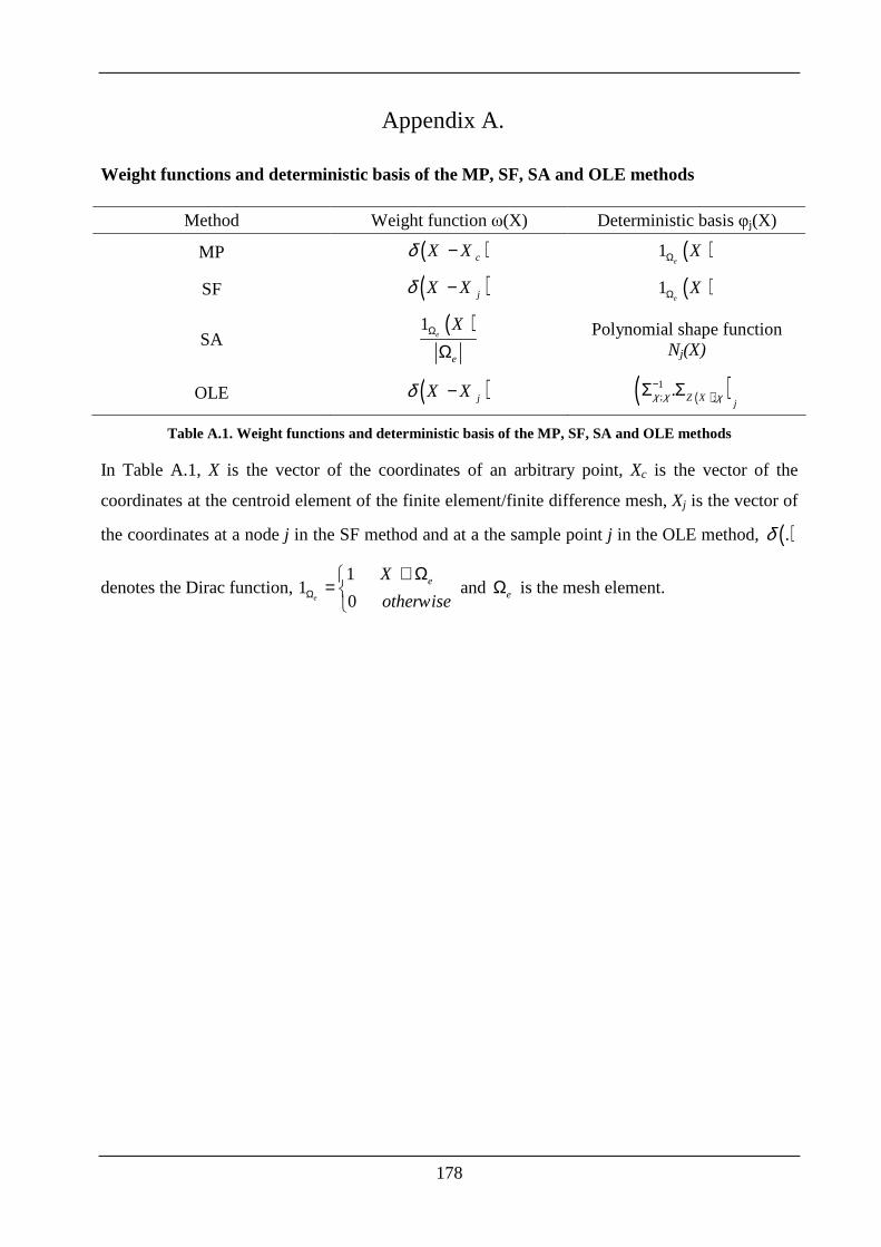
178
Appendix A.
Weight functions and deterministic basis of the MP, SF, SA and OLE methods
Method Weight function ω(X) Deterministic basis φj(X)
MP ( )cX Xδ − ( )1e
XΩ
SF ( )jX Xδ − ( )1e
XΩ
SA ( )1
e
e
XΩ
Ω Polynomial shape function
Nj(X)
OLE ( )jX Xδ − ( )( )1; ;. Z X
jχ χ χ−Σ Σ
Table A.1. Weight functions and deterministic basis of the MP, SF, SA and OLE methods
In Table A.1, X is the vector of the coordinates of an arbitrary point, Xc is the vector of the
coordinates at the centroid element of the finite element/finite difference mesh, Xj is the vector of
the coordinates at a node j in the SF method and at a the sample point j in the OLE method, ( ).δ
denotes the Dirac function, 1
10e
eX
otherwiseΩ
∈Ω=
and eΩ is the mesh element.

179
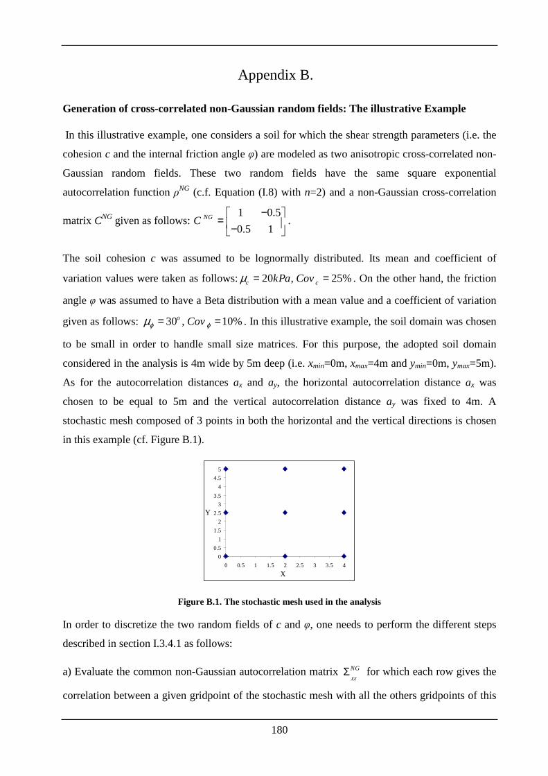
180
Appendix B.
Generation of cross-correlated non-Gaussian random fields: The illustrative Example
In this illustrative example, one considers a soil for which the shear strength parameters (i.e. the
cohesion c and the internal friction angle φ) are modeled as two anisotropic cross-correlated non-
Gaussian random fields. These two random fields have the same square exponential
autocorrelation function ρNG (c.f. Equation ( I.8) with n=2) and a non-Gaussian cross-correlation
matrix CNG given as follows: 1 0.5
0.5 1NGC
− = −
.
The soil cohesion c was assumed to be lognormally distributed. Its mean and coefficient of
variation values were taken as follows: 20 , 25%c ckPa Covµ = = . On the other hand, the friction
angle φ was assumed to have a Beta distribution with a mean value and a coefficient of variation
given as follows: 30 , 10%o Covϕ ϕµ = = . In this illustrative example, the soil domain was chosen
to be small in order to handle small size matrices. For this purpose, the adopted soil domain
considered in the analysis is 4m wide by 5m deep (i.e. xmin=0m, xmax=4m and ymin=0m, ymax=5m).
As for the autocorrelation distances ax and ay, the horizontal autocorrelation distance ax was
chosen to be equal to 5m and the vertical autocorrelation distance ay was fixed to 4m. A
stochastic mesh composed of 3 points in both the horizontal and the vertical directions is chosen
in this example (cf. Figure B.1).
0
0.5
1
1.5
2
2.5
3
3.5
4
4.5
5
0 0.5 1 1.5 2 2.5 3 3.5 4
X
Y
Figure B.1. The stochastic mesh used in the analysis
In order to discretize the two random fields of c and φ, one needs to perform the different steps
described in section I.3.4.1 as follows:
a) Evaluate the common non-Gaussian autocorrelation matrix NG
χχΣ for which each row gives the
correlation between a given gridpoint of the stochastic mesh with all the others gridpoints of this
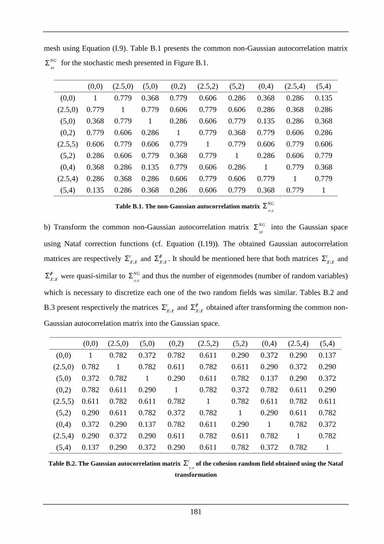
181
mesh using Equation ( I.9). Table B.1 presents the common non-Gaussian autocorrelation matrix
NG
χχΣ for the stochastic mesh presented in Figure B.1.
(0,0) (2.5,0) (5,0) (0,2) (2.5,2) (5,2) (0,4) (2.5,4) (5,4)
(0,0) 1 0.779 0.368 0.779 0.606 0.286 0.368 0.286 0.135
(2.5,0) 0.779 1 0.779 0.606 0.779 0.606 0.286 0.368 0.286
(5,0) 0.368 0.779 1 0.286 0.606 0.779 0.135 0.286 0.368
(0,2) 0.779 0.606 0.286 1 0.779 0.368 0.779 0.606 0.286
(2.5,5) 0.606 0.779 0.606 0.779 1 0.779 0.606 0.779 0.606
(5,2) 0.286 0.606 0.779 0.368 0.779 1 0.286 0.606 0.779
(0,4) 0.368 0.286 0.135 0.779 0.606 0.286 1 0.779 0.368
(2.5,4) 0.286 0.368 0.286 0.606 0.779 0.606 0.779 1 0.779
(5,4) 0.135 0.286 0.368 0.286 0.606 0.779 0.368 0.779 1
Table B.1. The non-Gaussian autocorrelation matrix ;
NG
χ χΣ
b) Transform the common non-Gaussian autocorrelation matrix NG
χχΣ into the Gaussian space
using Nataf correction functions (cf. Equation ( I.19)). The obtained Gaussian autocorrelation
matrices are respectively ;cχ χΣ and ;
ϕχ χΣ . It should be mentioned here that both matrices ;
cχ χΣ and
;ϕχ χΣ were quasi-similar to
;
NG
χ χΣ and thus the number of eigenmodes (number of random variables)
which is necessary to discretize each one of the two random fields was similar. Tables B.2 and
B.3 present respectively the matrices ;cχ χΣ and ;
ϕχ χΣ obtained after transforming the common non-
Gaussian autocorrelation matrix into the Gaussian space.
(0,0) (2.5,0) (5,0) (0,2) (2.5,2) (5,2) (0,4) (2.5,4) (5,4)
(0,0) 1 0.782 0.372 0.782 0.611 0.290 0.372 0.290 0.137
(2.5,0) 0.782 1 0.782 0.611 0.782 0.611 0.290 0.372 0.290
(5,0) 0.372 0.782 1 0.290 0.611 0.782 0.137 0.290 0.372
(0,2) 0.782 0.611 0.290 1 0.782 0.372 0.782 0.611 0.290
(2.5,5) 0.611 0.782 0.611 0.782 1 0.782 0.611 0.782 0.611
(5,2) 0.290 0.611 0.782 0.372 0.782 1 0.290 0.611 0.782
(0,4) 0.372 0.290 0.137 0.782 0.611 0.290 1 0.782 0.372
(2.5,4) 0.290 0.372 0.290 0.611 0.782 0.611 0.782 1 0.782
(5,4) 0.137 0.290 0.372 0.290 0.611 0.782 0.372 0.782 1
Table B.2. The Gaussian autocorrelation matrix ;
c
χ χΣ of the cohesion random field obtained using the Nataf
transformation
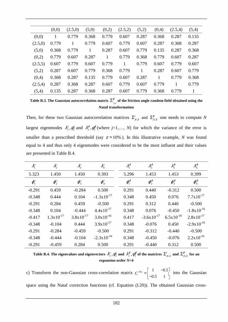
182
(0,0) (2.5,0) (5,0) (0,2) (2.5,2) (5,2) (0,4) (2.5,4) (5,4)
(0,0) 1 0.779 0.368 0.779 0.607 0.287 0.368 0.287 0.135
(2.5,0) 0.779 1 0.779 0.607 0.779 0.607 0.287 0.368 0.287
(5,0) 0.368 0.779 1 0.287 0.607 0.779 0.135 0.287 0.368
(0,2) 0.779 0.607 0.287 1 0.779 0.368 0.779 0.607 0.287
(2.5,5) 0.607 0.779 0.607 0.779 1 0.779 0.607 0.779 0.607
(5,2) 0.287 0.607 0.779 0.368 0.779 1 0.287 0.607 0.779
(0,4) 0.368 0.287 0.135 0.779 0.607 0.287 1 0.779 0.368
(2.5,4) 0.287 0.368 0.287 0.607 0.779 0.607 0.779 1 0.779
(5,4) 0.135 0.287 0.368 0.287 0.607 0.779 0.368 0.779 1
Table B.3. The Gaussian autocorrelation matrix ;χ χ
ϕΣ of the friction angle random field obtained using the
Nataf transformation
Then, for these two Gaussian autocorrelation matrices ;cχ χΣ and ;
ϕχ χΣ one needs to compute N
largest eigenmodes ,c cj jλ φ and ,j j
ϕ ϕλ φ (where j=1,…, N) for which the variance of the error is
smaller than a prescribed threshold (say 10%ε ≈ ). In this illustrative example, N was found
equal to 4 and thus only 4 eigenmodes were considered to be the most influent and their values
are presented in Table B.4.
1cλ 2
cλ 3cλ 4
cλ 1ϕλ 2
ϕλ 3ϕλ 4
ϕλ
5.323 1.450 1.450 0.393 5.296 1.453 1.453 0.399
1cϕ 2
cϕ 3cϕ 4
cϕ 1ϕϕ 2
ϕϕ 3ϕϕ 4
ϕϕ
-0.291 0.459 -0.284 0.500 0.291 0.440 -0.312 0.500
-0.348 0.444 0.104 -1.3x10⁻¹⁷ 0.348 0.450 0.076 7.7x10⁻¹⁷
-0.291 0.284 0.459 -0.500 0.291 0.312 0.440 -0.500
-0.348 0.104 -0.444 4.4x10⁻¹⁷ 0.348 0.076 -0.450 -1.8x10⁻¹⁶
-0.417 1.3x10⁻¹⁷ 3.8x10⁻¹⁷ 3.0x10⁻¹⁶ 0.417 -3.6x10⁻¹⁷ 6.5x10⁻¹⁸ 2.8x10⁻¹⁷
-0.348 -0.104 0.444 3.9x10⁻¹⁷ 0.348 -0.076 0.450 -2.9x10⁻¹⁶
-0.291 -0.284 -0.459 -0.500 0.291 -0.312 -0.440 -0.500
-0.348 -0.444 -0.104 -2.3x10⁻¹⁶ 0.348 -0.450 -0.076 2.2x10⁻¹⁶
-0.291 -0.459 0.284 0.500
0.291 -0.440 0.312 0.500
Table B.4. The eigenvalues and eigenvectors ,c cj jλ φ and ,j j
ϕ ϕλ φ of the matrices ;cχ χΣ and ;
ϕχ χΣ for an
expansion order N=4
c) Transform the non-Gaussian cross-correlation matrix 1 0.5
0.5 1NGC
− = −
into the Gaussian
space using the Nataf correction functions (cf. Equation ( I.20)). The obtained Gaussian cross-
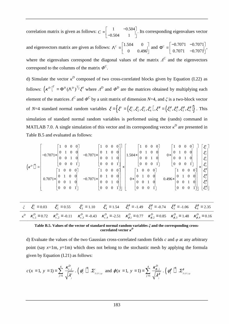
183
correlation matrix is given as follows: 1 0.504
0.504 1C
− = −
. Its corresponding eigenvalues vector
and eigenvectors matrix are given as follows: 1.504 0
0 0.496C
Λ =
and 0.7071 0.7071
0.7071 0.7071C − −
Φ = − ,
where the eigenvalues correspond the diagonal values of the matrix ΛC and the eigenvectors
correspond to the columns of the matrix ΦC.
d) Simulate the vector κD composed of two cross-correlated blocks given by Equation ( I.22) as
follows: ( ) 12( )
TD D D Tκ ξ= Φ Λ where ΛD and ΦD are the matrices obtained by multiplying each
element of the matrices ΛC and ΦC by a unit matrix of dimension N=4, and ξ is a two-block vector
of N=4 standard normal random variables ( ) ( ) 1 2 3 4 1 2 3 4, , , , , , ,c c c c c ϕ ϕ ϕ ϕ ϕξ ξ ξ ξ ξ ξ ξ ξ ξ ξ ξ= = = . This
simulation of standard normal random variables is performed using the (randn) command in
MATLAB 7.0. A single simulation of this vector and its corresponding vector κD are presented in
Table B.5 and evaluated as follows:
( )
1 0 0 0 1 0 0 0 1 0 0 0
0 1 0 0 0 1 0 0 0 1 0 00.7071 0.7071 1.504
0 0 1 0 0 0 1 0 0 0 1 0
0 0 0 1 0 0 0 1 0 0 0 1
1 0 0 0 1 0 0 0
0 1 0 0 0 1 0 00.7071 0.7071
0 0 1 0 0 0 1 0
0 0 0 1 0 0 0 1
TDκ
− × − × ×
= × × − ×
1
2
3
4
1
2
3
4
1 0 0 0
0 1 0 00
0 0 1 0
0 0 0 1
1 0 0 0 1 0 0 0
0 1 0 0 0 1 0 00 0.496
0 0 1 0 0 0 1 0
0 0 0 1 0 0 0 1
c
c
c
c
ϕ
ϕ
ϕ
ϕ
ξξξξξξξξ
×
× × ×
ξ 1cξ = 0.03 2
cξ = 0.55 3cξ = 1.10 4
cξ = 1.54 1ϕξ = -1.49 2
ϕξ = -0.74 3ϕξ = -1.06 4
ϕξ = 2.35
κD ,1
Dcκ = 0.72 ,2
Dcκ = -0.11 ,3
Dcκ = -0.43 ,4
Dcκ = -2.51 ,1
Dϕκ = 0.77 ,2
Dϕκ = 0.85 ,3
Dϕκ = 1.48 ,4
Dϕκ = 0.16
Table B.5. Values of the vector of standard normal random variables ξ and the corresponding cross-correlated vector κD
d) Evaluate the values of the two Gaussian cross-correlated random fields c and φ at any arbitrary
point (say x=1m, y=1m) which does not belong to the stochastic mesh by applying the formula
given by Equation ( I.21) as follows:
( )( );
4,
1
( 1, 1) . .Z X
j
DTc j c c
jcj
c x yχ
κφ
λ=
= = = Σ∑ and ( )( );
4,
1
( 1, 1) . .Z X
j
DTj
jj
x yχ
ϕ ϕ ϕϕ
κϕ φ
λ=
= = = Σ∑
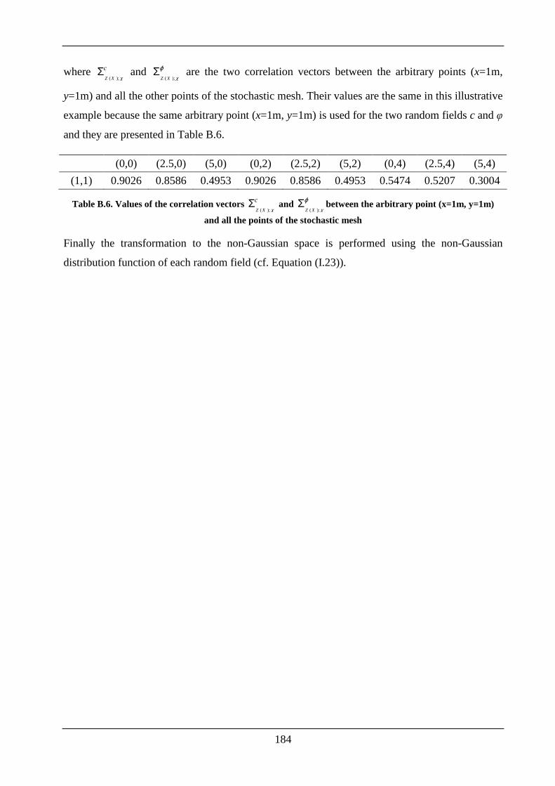
184
where ( );Z X
c
χΣ and
( );Z X χ
ϕΣ are the two correlation vectors between the arbitrary points (x=1m,
y=1m) and all the other points of the stochastic mesh. Their values are the same in this illustrative
example because the same arbitrary point (x=1m, y=1m) is used for the two random fields c and φ
and they are presented in Table B.6.
(0,0) (2.5,0) (5,0) (0,2) (2.5,2) (5,2) (0,4) (2.5,4) (5,4)
(1,1) 0.9026 0.8586 0.4953 0.9026 0.8586 0.4953 0.5474 0.5207 0.3004
Table B.6. Values of the correlation vectors ( );Z X
c
χΣ and
( );Z X χ
ϕΣ between the arbitrary point (x=1m, y=1m)
and all the points of the stochastic mesh
Finally the transformation to the non-Gaussian space is performed using the non-Gaussian
distribution function of each random field (cf. Equation ( I.23)).

185
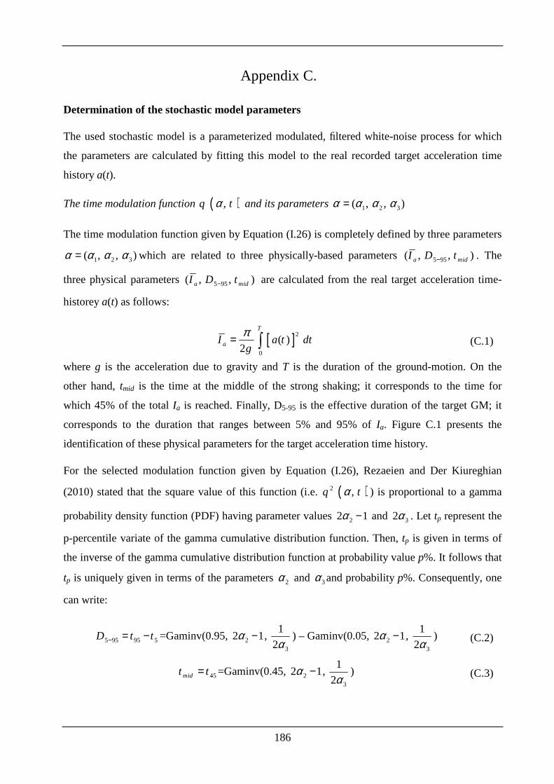
186
Appendix C.
Determination of the stochastic model parameters
The used stochastic model is a parameterized modulated, filtered white-noise process for which
the parameters are calculated by fitting this model to the real recorded target acceleration time
history a(t).
The time modulation function ( ),q tα and its parameters 1 2 3( , , )α α α α=
The time modulation function given by Equation ( I.26) is completely defined by three parameters
1 2 3( , , )α α α α= which are related to three physically-based parameters 5 95( , , )a midI D t− . The
three physical parameters 5 95( , , )a midI D t− are calculated from the real target acceleration time-
historey a(t) as follows:
[ ]2
0
( )2
T
aI a t dtg
π= ∫ (C.1)
where g is the acceleration due to gravity and T is the duration of the ground-motion. On the
other hand, tmid is the time at the middle of the strong shaking; it corresponds to the time for
which 45% of the total Ia is reached. Finally, D5-95 is the effective duration of the target GM; it
corresponds to the duration that ranges between 5% and 95% of Ia. Figure C.1 presents the
identification of these physical parameters for the target acceleration time history.
For the selected modulation function given by Equation ( I.26), Rezaeien and Der Kiureghian
(2010) stated that the square value of this function (i.e. ( )2 ,q tα ) is proportional to a gamma
probability density function (PDF) having parameter values 22 1α − and 32α . Let tp represent the
p-percentile variate of the gamma cumulative distribution function. Then, tp is given in terms of
the inverse of the gamma cumulative distribution function at probability value p%. It follows that
tp is uniquely given in terms of the parameters 2α and 3α and probability p%. Consequently, one
can write:
5 95 95 5D t t− = − =Gaminv(0.95, 22 1α − , 3
1
2α) – Gaminv(0.05, 22 1α − ,
3
1
2α) (C.2)
45midt t= =Gaminv(0.45, 22 1α − , 3
1
2α) (C.3)
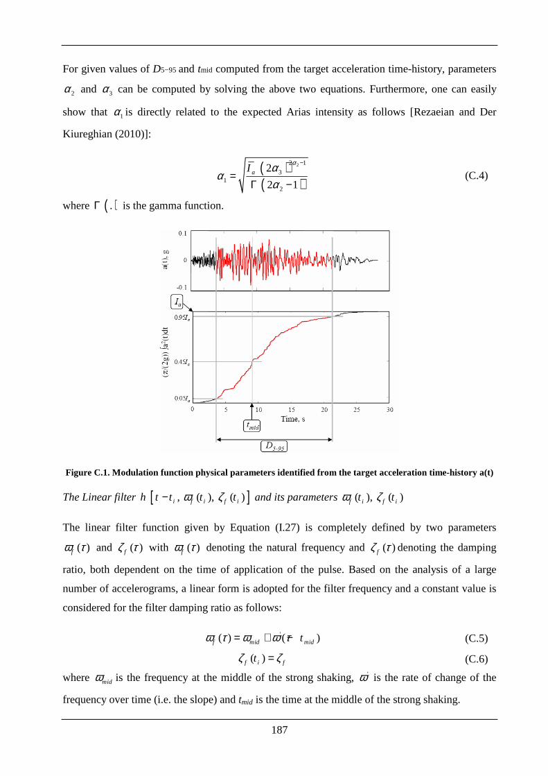
187
For given values of D5−95 and tmid computed from the target acceleration time-history, parameters
2α and 3α can be computed by solving the above two equations. Furthermore, one can easily
show that 1α is directly related to the expected Arias intensity as follows [Rezaeian and Der
Kiureghian (2010)]:
( )( )
22 1
31
2
2
2 1aI
ααα
α
−
=Γ −
(C.4)
where ( ).Γ is the gamma function.
Figure C.1. Modulation function physical parameters identified from the target acceleration time-history a(t)
The Linear filter [ ], ( ), ( )i f i f ih t t t tω ζ− and its parameters ( ), ( )f i f it tω ζ
The linear filter function given by Equation ( I.27) is completely defined by two parameters
( )fω τ and ( )fζ τ with ( )fω τ denoting the natural frequency and ( )fζ τ denoting the damping
ratio, both dependent on the time of application of the pulse. Based on the analysis of a large
number of accelerograms, a linear form is adopted for the filter frequency and a constant value is
considered for the filter damping ratio as follows:
'( ) ( )f mid midtω τ ω ω τ= + − (C.5)
( )f i ftζ ζ= (C.6)
where midω is the frequency at the middle of the strong shaking, 'ω is the rate of change of the
frequency over time (i.e. the slope) and tmid is the time at the middle of the strong shaking.
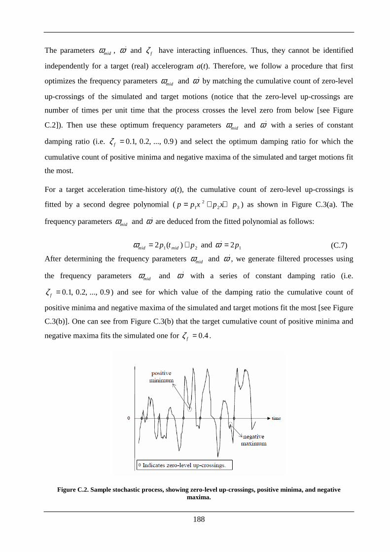
188
The parameters midω , 'ω and fζ have interacting influences. Thus, they cannot be identified
independently for a target (real) accelerogram a(t). Therefore, we follow a procedure that first
optimizes the frequency parameters midω and 'ω by matching the cumulative count of zero-level
up-crossings of the simulated and target motions (notice that the zero-level up-crossings are
number of times per unit time that the process crosses the level zero from below [see Figure
C.2]). Then use these optimum frequency parameters midω and 'ω with a series of constant
damping ratio (i.e. 0.1, 0.2, ..., 0.9fζ = ) and select the optimum damping ratio for which the
cumulative count of positive minima and negative maxima of the simulated and target motions fit
the most.
For a target acceleration time-history a(t), the cumulative count of zero-level up-crossings is
fitted by a second degree polynomial ( 21 2 3p p x p x p= + + ) as shown in Figure C.3(a). The
frequency parameters midω and 'ω are deduced from the fitted polynomial as follows:
1 22 ( )mid midp t pω = + and '12pω = (C.7)
After determining the frequency parameters midω and 'ω , we generate filtered processes using
the frequency parameters midω and 'ω with a series of constant damping ratio (i.e.
0.1, 0.2, ..., 0.9fζ = ) and see for which value of the damping ratio the cumulative count of
positive minima and negative maxima of the simulated and target motions fit the most [see Figure
C.3(b)]. One can see from Figure C.3(b) that the target cumulative count of positive minima and
negative maxima fits the simulated one for 0.4fζ = .
Figure C.2. Sample stochastic process, showing zero-level up-crossings, positive minima, and negative maxima.
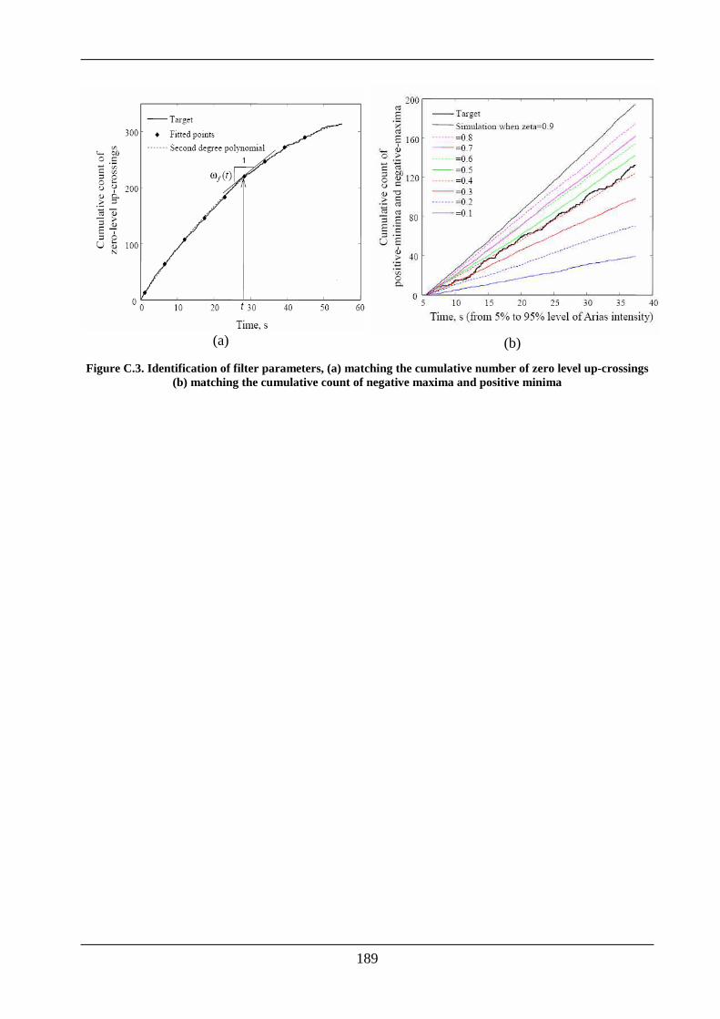
189
(a) (b)
Figure C.3. Identification of filter parameters, (a) matching the cumulative number of zero level up-crossings (b) matching the cumulative count of negative maxima and positive minima
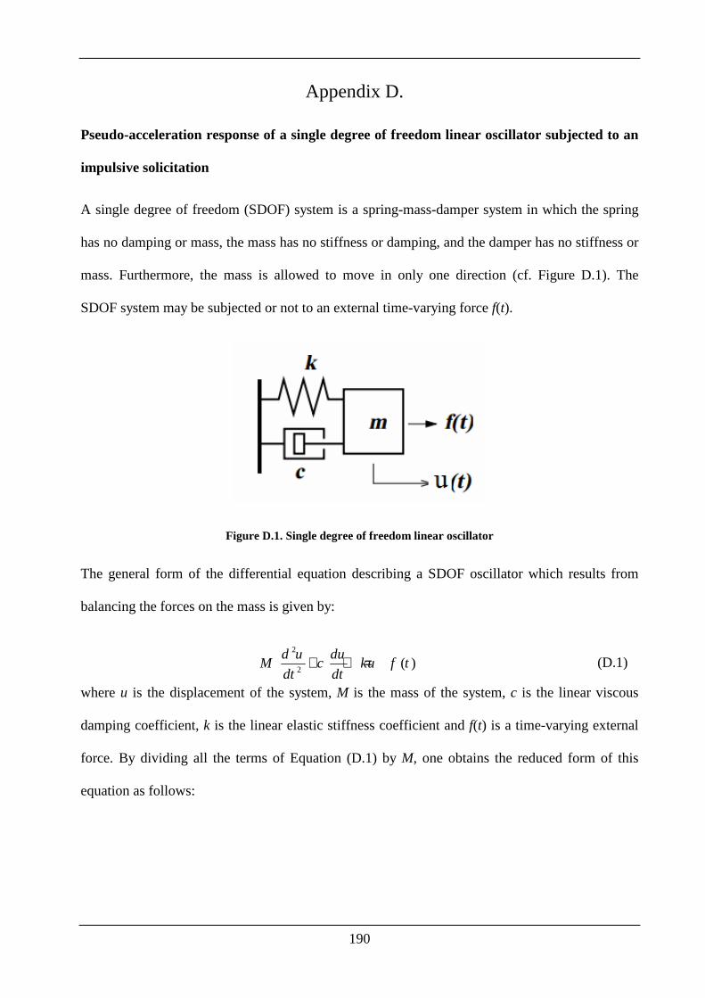
190
Appendix D.
Pseudo-acceleration response of a single degree of freedom linear oscillator subjected to an
impulsive solicitation
A single degree of freedom (SDOF) system is a spring-mass-damper system in which the spring
has no damping or mass, the mass has no stiffness or damping, and the damper has no stiffness or
mass. Furthermore, the mass is allowed to move in only one direction (cf. Figure D.1). The
SDOF system may be subjected or not to an external time-varying force f(t).
Figure D.1. Single degree of freedom linear oscillator
The general form of the differential equation describing a SDOF oscillator which results from
balancing the forces on the mass is given by:
2
2( )
d u duM c ku f t
dt dt+ + = (D.1)
where u is the displacement of the system, M is the mass of the system, c is the linear viscous
damping coefficient, k is the linear elastic stiffness coefficient and f(t) is a time-varying external
force. By dividing all the terms of Equation (D.1) by M, one obtains the reduced form of this
equation as follows:
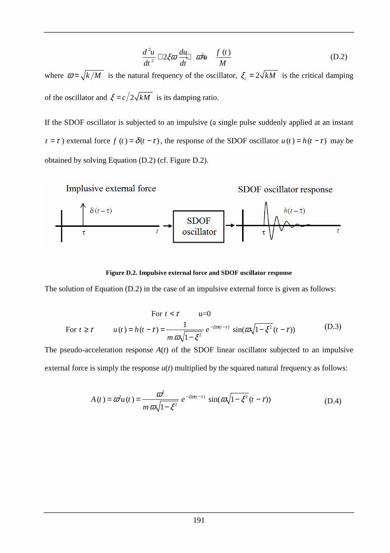
191
22
2
( )2
d u du f tu
dt dt Mξω ω+ + = (D.2)
where k Mω = is the natural frequency of the oscillator, 2c kMξ = is the critical damping
of the oscillator and 2c kMξ = is its damping ratio.
If the SDOF oscillator is subjected to an impulsive (a single pulse suddenly applied at an instant
t τ= ) external force ( ) ( )f t tδ τ= − , the response of the SDOF oscillator ( ) ( )u t h t τ= − may be
obtained by solving Equation (D.2) (cf. Figure D.2).
Figure D.2. Impulsive external force and SDOF oscillator response
The solution of Equation (D.2) in the case of an impulsive external force is given as follows:
For t τ< u=0
For t τ≥ ( ) 2
2
1( ) ( ) sin( 1 ( ))
1
tu t h t e tm
ξω ττ ω ξ τω ξ
− −= − = − −−
(D.3)
The pseudo-acceleration response A(t) of the SDOF linear oscillator subjected to an impulsive
external force is simply the response u(t) multiplied by the squared natural frequency as follows:
22 ( ) 2
2( ) ( ) sin( 1 ( ))
1
tA t u t e tm
ξω τωω ω ξ τω ξ
− −= = − −−
(D.4)
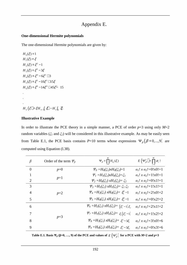
192
Appendix E.
One-dimensional Hermite polynomials
The one-dimensional Hermite polynomials are given by:
( ) ( ) ( )
0
1
22
33
4 24
5 35
6 4 26
'2 1
( ) 1
( )
( ) 1
( ) 3
( ) 6 3
( ) 10 15
( ) 14 45 15
.
.
.
n n n
H
H
H
H
H
H
H
H H H
ξξ ξξ ξξ ξ ξξ ξ ξξ ξ ξ ξξ ξ ξ ξ
ξ ξ ξ ξ− −
==
= −
= −
= − +
= − +
= − + −
= −
Illustrative Example
In order to illustrate the PCE theory in a simple manner, a PCE of order p=3 using only M=2
random variables (ξ1 and ξ2) will be considered in this illustrative example. As may be easily seen
from Table E.1, the PCE basis contains P=10 terms whose expressions ( )0,...,9β βΨ = are
computed using Equation ( I.38).
β Order of the term Ψβ 1
( )=
Ψ = ∏ i
M
ii
Hβ α ξ
( )2
1
!M
ii
E β α=
Ψ = ∏
0 p=0 Ψ0 =H0(ξ1)xH0(ξ2)=1 α1! x α2!= 0!x0!=1
1 Ψ1 =H1(ξ1)xH0(ξ2)=ξ1 α1! x α2!= 1!x0!=1
2 p=1
Ψ2 =H0(ξ1) xH1(ξ2)= ξ2 α1! x α2!= 0!x1!=1
3 Ψ3 =H1(ξ1) xH1(ξ2)= ξ1 ξ2 α1! x α2!= 1!x1!=1
4 Ψ4 =H2(ξ1) xH0(ξ2)= 21 1ξ − α1! x α2!= 2!x0!=2
5
p=2
Ψ5 =H0(ξ1) xH2(ξ2)= 22 1ξ − α1! x α2!= 0!x2!=2
6 Ψ6 =H2(ξ1) xH1(ξ2)= ( )21 21ξ ξ− α1! x α2!= 2!x1!=2
7 Ψ7 =H1(ξ1) xH2(ξ2)= ( )21 2 1ξ ξ − α1! x α2!= 1!x2!=2
8 Ψ8 =H3(ξ1) xH0(ξ2)= 31 13ξ ξ− α1! x α2!= 3!x0!=6
9
p=3
Ψ9 =H0(ξ1) xH3(ξ2)= 32 23ξ ξ− α1! x α2!= 0!x3!=6
Table E.1. Basis Ψβ (β=0, …, 9) of the PCE and values of ( )2E βΨ for a PCE with M=2 and p=3
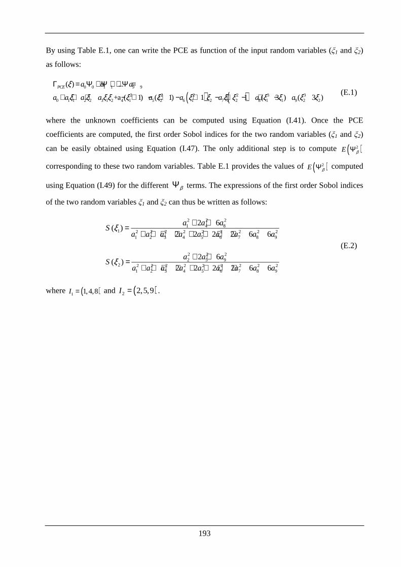
193
By using Table E.1, one can write the PCE as function of the input random variables (ξ1 and ξ2)
as follows:
( ) ( )0 0 1 1 9 9
2 2 2 2 3 30 1 1 2 2 3 1 2 4 1 5 2 6 1 2 7 1 2 8 1 1 9 2 2
( ) ...
+a ( 1) ( 1) 1 1 ( 3 ) ( 3 )
PCE a a a
a a a a a a a a a
ξ
ξ ξ ξξ ξ ξ ξ ξ ξ ξ ξ ξ ξ ξ
Γ = Ψ + Ψ + + Ψ =
+ + + − + − + − + − + − + − (E.1)
where the unknown coefficients can be computed using Equation ( I.41). Once the PCE
coefficients are computed, the first order Sobol indices for the two random variables (ξ1 and ξ2)
can be easily obtained using Equation ( I.47). The only additional step is to compute ( )2E βΨ
corresponding to these two random variables. Table E.1 provides the values of ( )2E βΨ computed
using Equation ( I.49) for the different βΨ terms. The expressions of the first order Sobol indices
of the two random variables ξ1 and ξ2 can thus be written as follows:
2 2 21 4 8
1 2 2 2 2 2 2 2 2 21 2 3 4 5 6 7 8 9
2 6( )
2 2 2 2 6 6
a a aS
a a a a a a a a aξ + +=
+ + + + + + + +
2 2 22 5 9
2 2 2 2 2 2 2 2 2 21 2 3 4 5 6 7 8 9
2 6( )
2 2 2 2 6 6
a a aS
a a a a a a a a aξ + +=
+ + + + + + + +
(E.2)
where ( )1 1,4,8I = and ( )2 2,5,9I = .
194
Appendix F.
Introduction
The seismic stability of slopes is widely investigated in literature using deterministic approaches.
However, the material properties of soils are known to vary greatly from point to another, and
many of these older pen and paper methods have difficulty to successfully model this
heterogeneity. Things are more complicated when dealing with dynamic loading situations. In
this paper, the effect of both the soil spatial variability and the time variability of Ground-Motion
(GM) on the dynamic responses of a simple slope are studied. Few authors have worked on the
analysis of the dynamic horizontal soil behavior using probabilistic approaches where the spatial
variability of soil properties and the time variability of seismic excitations were considered
[Koutsourelakis et al (2002), Popescu et al (2006), ...]. In these works, three main deficiencies
can be detected: First, the classical Monte Carlo Simulation (MCS) methodology with a small
number of realizations is used to determine the probability density function (PDF) of the system
responses (e.g. 50 simulations). It is well known that in order to be a rigorous approach, MCS is
very time-expensive. Second, the stochastic model for generating synthetic acceleration time-
histories is based on the spectral representation in order to simulate accelerograms which are
compatible with a prescribed response spectrum and not real GM acceleration. Finally, the spatial
variability of soil properties is studied for specific autocorrelation distances.
In this study, the three mentioned deficiencies will be improved by (i) using a more efficient
probabilistic approach instead of the crude MCS which is the Sparse Polynomial Chaos
Expansion (SPCE) [Blatman and Sudret (2010), Al-Bittar and Soubra (2011)]; (ii) simulating the
stochastic accelerogram using the method given by Rezaeian and Der Kiureghian (2010). This
method has the advantage of solving the majority of problems encountered in the previous
models [Rezaeian and Der Kiureghian (2008)]; (iii) considering a large range of autocorrelation
distances for the soil shear modulus G modeled as an isotropic non-Gaussian random field. The
Expansion Optimal Linear Estimation (EOLE) methodology proposed by Li and Der Kiureghian
(1993) is used to generate this random field.
The deterministic model is based on numerical simulations using the dynamic option of the finite
difference code FLAC3D. Samples of the synthetic GM time-histories were generated and a
dynamic stochastic calculation for each realization was performed to compute the dynamic
responses (i.e. the permanent displacement at the toe of the slope and the maximum amplification
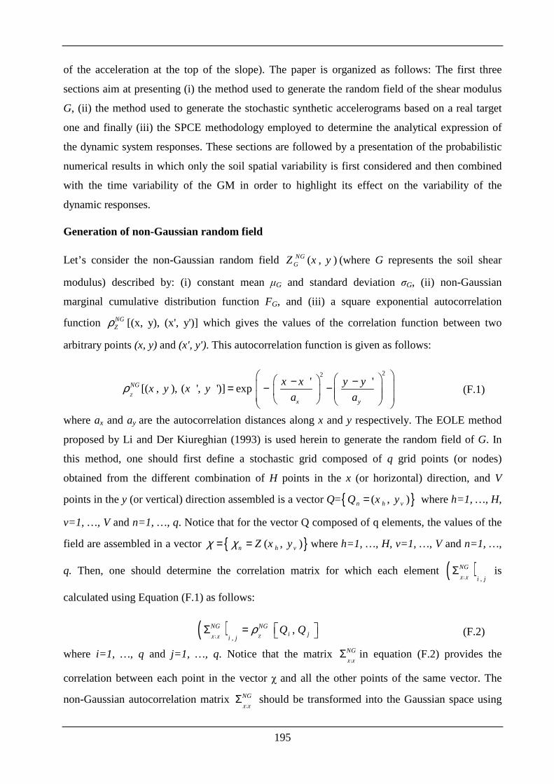
195
of the acceleration at the top of the slope). The paper is organized as follows: The first three
sections aim at presenting (i) the method used to generate the random field of the shear modulus
G, (ii) the method used to generate the stochastic synthetic accelerograms based on a real target
one and finally (iii) the SPCE methodology employed to determine the analytical expression of
the dynamic system responses. These sections are followed by a presentation of the probabilistic
numerical results in which only the soil spatial variability is first considered and then combined
with the time variability of the GM in order to highlight its effect on the variability of the
dynamic responses.
Generation of non-Gaussian random field
Let’s consider the non-Gaussian random field ( , )NGGZ x y (where G represents the soil shear
modulus) described by: (i) constant mean µG and standard deviation σG, (ii) non-Gaussian
marginal cumulative distribution function FG, and (iii) a square exponential autocorrelation
function NGZρ [(x, y), (x', y')] which gives the values of the correlation function between two
arbitrary points (x, y) and (x', y'). This autocorrelation function is given as follows:
22' '
[( , ), ( ', ')] expZ
NG
x y
x x y yx y x y
a aρ
− − = − −
(F.1)
where ax and ay are the autocorrelation distances along x and y respectively. The EOLE method
proposed by Li and Der Kiureghian (1993) is used herein to generate the random field of G. In
this method, one should first define a stochastic grid composed of q grid points (or nodes)
obtained from the different combination of H points in the x (or horizontal) direction, and V
points in the y (or vertical) direction assembled is a vector Q= ( , )n h vQ x y= where h=1, …, H,
v=1, …, V and n=1, …, q. Notice that for the vector Q composed of q elements, the values of the
field are assembled in a vector ( , )n h vZ x yχ χ= = where h=1, …, H, v=1, …, V and n=1, …,
q. Then, one should determine the correlation matrix for which each element ( ); ,
NG
i jχ χΣ is
calculated using Equation (F.1) as follows:
( ); ,,
Z
NG NGi j
i jQ Q
χ χρ Σ = (F.2)
where i=1, …, q and j=1, …, q. Notice that the matrix ;
NG
χ χΣ in equation (F.2) provides the
correlation between each point in the vector χ and all the other points of the same vector. The
non-Gaussian autocorrelation matrix ;
NG
χ χΣ should be transformed into the Gaussian space using
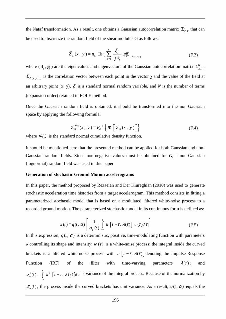
196
the Nataf transformation. As a result, one obtains a Gaussian autocorrelation matrix ;Gχ χΣ that can
be used to discretize the random field of the shear modulus G as follows:
( , );1
( , ) . .Z x y
Nj
G G G jj j
Z x y µχ
ξσ φ
λ=
= + Σ∑ɶ (F.3)
where ( ,j jλ φ ) are the eigenvalues and eigenvectors of the Gaussian autocorrelation matrix ;Gχ χΣ ,
( , );Z x y χΣ is the correlation vector between each point in the vector χ and the value of the field at
an arbitrary point (x, y), jξ is a standard normal random variable, and N is the number of terms
(expansion order) retained in EOLE method.
Once the Gaussian random field is obtained, it should be transformed into the non-Gaussian
space by applying the following formula:
1( , ) ( , )NGG G GZ x y F Z x y− = Φ ɶ ɶ (F.4)
where (.)Φ is the standard normal cumulative density function.
It should be mentioned here that the presented method can be applied for both Gaussian and non-
Gaussian random fields. Since non-negative values must be obtained for G, a non-Gaussian
(lognormal) random field was used in this paper.
Generation of stochastic Ground Motion accelerograms
In this paper, the method proposed by Rezaeian and Der Kiureghian (2010) was used to generate
stochastic acceleration time histories from a target accelerogram. This method consists in fitting a
parameterized stochastic model that is based on a modulated, filtered white-noise process to a
recorded ground motion. The parameterized stochastic model in its continuous form is defined as:
[ ]1( ) ( , ) , ( ) ( )
( )
t
f
x t q t h t w dt
α τ λ τ τ τσ −∞
= −
∫ (F.5)
In this expression, ( , )q t α is a deterministic, positive, time-modulating function with parameters
α controlling its shape and intensity; ( )w τ is a white-noise process; the integral inside the curved
brackets is a filtered white-noise process with [ ], ( )h t τ λ τ− denoting the Impulse-Response
Function (IRF) of the filter with time-varying parameters ( )λ τ ; and
[ ]2 2( ) , ( )t
h t h t dσ τ λ τ τ−∞
= −∫ is variance of the integral process. Because of the normalization by
( )h tσ , the process inside the curved brackets has unit variance. As a result, ( , )q t α equals the
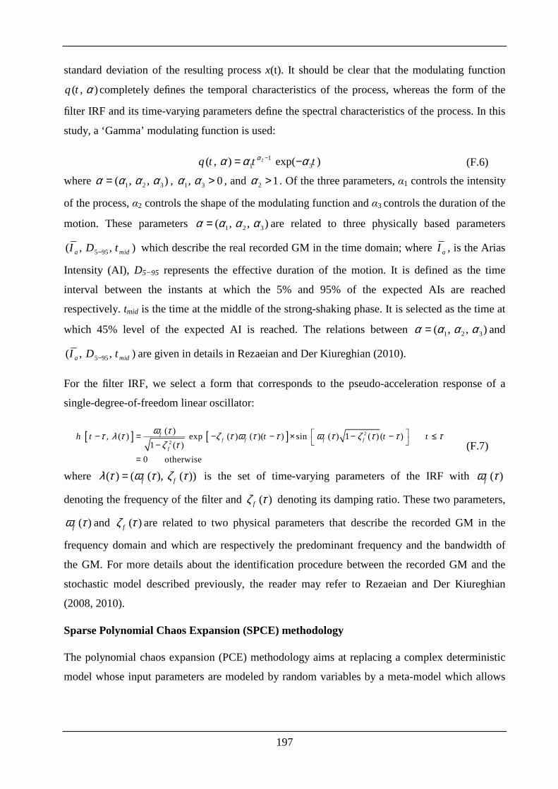
197
standard deviation of the resulting process x(t). It should be clear that the modulating function
( , )q t α completely defines the temporal characteristics of the process, whereas the form of the
filter IRF and its time-varying parameters define the spectral characteristics of the process. In this
study, a ‘Gamma’ modulating function is used:
2 11 3( , ) exp( )q t t tαα α α−= − (F.6)
where 1 2 3( , , )α α α α= , 1 3, 0α α > , and 2 1α > . Of the three parameters, α1 controls the intensity
of the process, α2 controls the shape of the modulating function and α3 controls the duration of the
motion. These parameters 1 2 3( , , )α α α α= are related to three physically based parameters
5 95( , , )a midI D t− which describe the real recorded GM in the time domain; where aI , is the Arias
Intensity (AI), D5−95 represents the effective duration of the motion. It is defined as the time
interval between the instants at which the 5% and 95% of the expected AIs are reached
respectively. tmid is the time at the middle of the strong-shaking phase. It is selected as the time at
which 45% level of the expected AI is reached. The relations between 1 2 3( , , )α α α α= and
5 95( , , )a midI D t− are given in details in Rezaeian and Der Kiureghian (2010).
For the filter IRF, we select a form that corresponds to the pseudo-acceleration response of a
single-degree-of-freedom linear oscillator:
[ ] [ ] 2
2
( ), ( ) exp ( ) ( )( ) sin ( ) 1 ( ) ( )
1 ( )
0 otherwise
ff f f f
f
h t t t tω ττ λ τ ζ τ ω τ τ ω τ ζ τ τ τ
ζ τ − = − − × − − ≤ −
=
(F.7)
where ( ) ( ( ), ( ))f fλ τ ω τ ζ τ= is the set of time-varying parameters of the IRF with ( )fω τ
denoting the frequency of the filter and ( )fζ τ denoting its damping ratio. These two parameters,
( )fω τ and ( )fζ τ are related to two physical parameters that describe the recorded GM in the
frequency domain and which are respectively the predominant frequency and the bandwidth of
the GM. For more details about the identification procedure between the recorded GM and the
stochastic model described previously, the reader may refer to Rezaeian and Der Kiureghian
(2008, 2010).
Sparse Polynomial Chaos Expansion (SPCE) methodology
The polynomial chaos expansion (PCE) methodology aims at replacing a complex deterministic
model whose input parameters are modeled by random variables by a meta-model which allows
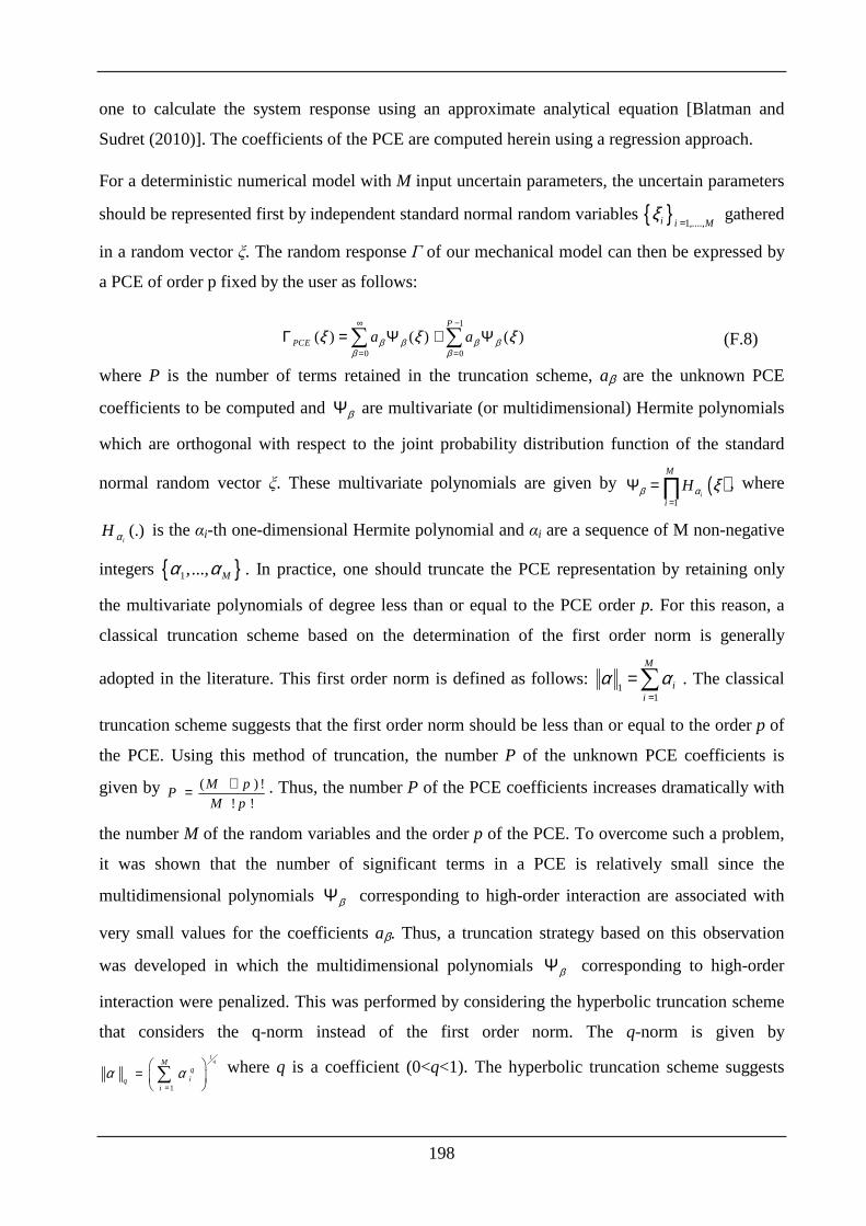
198
one to calculate the system response using an approximate analytical equation [Blatman and
Sudret (2010)]. The coefficients of the PCE are computed herein using a regression approach.
For a deterministic numerical model with M input uncertain parameters, the uncertain parameters
should be represented first by independent standard normal random variables 1,....,i i Mξ
= gathered
in a random vector ξ. The random response Γ of our mechanical model can then be expressed by
a PCE of order p fixed by the user as follows:
1
0 0
( ) ( ) ( )P
PCE a aβ β β ββ β
ξ ξ ξ∞ −
= =
Γ = Ψ ≅ Ψ∑ ∑ (F.8)
where P is the number of terms retained in the truncation scheme, aβ are the unknown PCE
coefficients to be computed and βΨ are multivariate (or multidimensional) Hermite polynomials
which are orthogonal with respect to the joint probability distribution function of the standard
normal random vector ξ. These multivariate polynomials are given by ( )1
i
M
i
Hβ α ξ=
Ψ = ∏ , where
(.)i
H α is the αi-th one-dimensional Hermite polynomial and αi are a sequence of M non-negative
integers 1,..., Mα α . In practice, one should truncate the PCE representation by retaining only
the multivariate polynomials of degree less than or equal to the PCE order p. For this reason, a
classical truncation scheme based on the determination of the first order norm is generally
adopted in the literature. This first order norm is defined as follows: 1
1
M
ii
α α=
=∑ . The classical
truncation scheme suggests that the first order norm should be less than or equal to the order p of
the PCE. Using this method of truncation, the number P of the unknown PCE coefficients is
given by ( ) !
! !
M pP
M p
+= . Thus, the number P of the PCE coefficients increases dramatically with
the number M of the random variables and the order p of the PCE. To overcome such a problem,
it was shown that the number of significant terms in a PCE is relatively small since the
multidimensional polynomials βΨ corresponding to high-order interaction are associated with
very small values for the coefficients aβ. Thus, a truncation strategy based on this observation
was developed in which the multidimensional polynomials βΨ corresponding to high-order
interaction were penalized. This was performed by considering the hyperbolic truncation scheme
that considers the q-norm instead of the first order norm. The q-norm is given by 1
1
qMqiq
i
α α=
= ∑ where q is a coefficient (0<q<1). The hyperbolic truncation scheme suggests
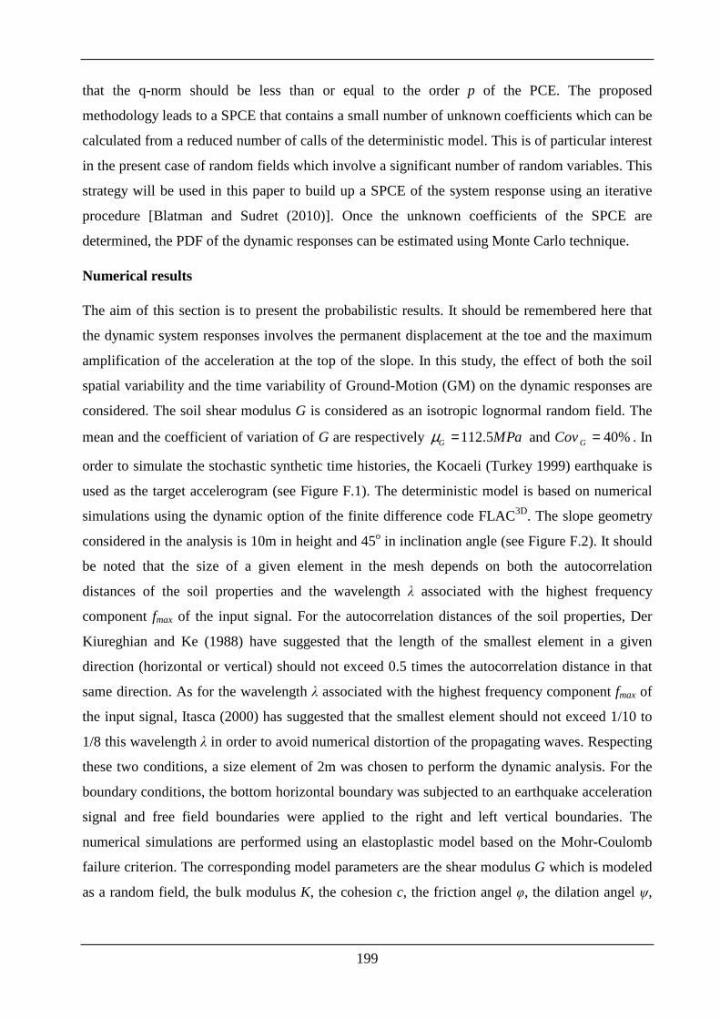
199
that the q-norm should be less than or equal to the order p of the PCE. The proposed
methodology leads to a SPCE that contains a small number of unknown coefficients which can be
calculated from a reduced number of calls of the deterministic model. This is of particular interest
in the present case of random fields which involve a significant number of random variables. This
strategy will be used in this paper to build up a SPCE of the system response using an iterative
procedure [Blatman and Sudret (2010)]. Once the unknown coefficients of the SPCE are
determined, the PDF of the dynamic responses can be estimated using Monte Carlo technique.
Numerical results
The aim of this section is to present the probabilistic results. It should be remembered here that
the dynamic system responses involves the permanent displacement at the toe and the maximum
amplification of the acceleration at the top of the slope. In this study, the effect of both the soil
spatial variability and the time variability of Ground-Motion (GM) on the dynamic responses are
considered. The soil shear modulus G is considered as an isotropic lognormal random field. The
mean and the coefficient of variation of G are respectively 112.5G MPaµ = and 40%GCov = . In
order to simulate the stochastic synthetic time histories, the Kocaeli (Turkey 1999) earthquake is
used as the target accelerogram (see Figure F.1). The deterministic model is based on numerical
simulations using the dynamic option of the finite difference code FLAC3D. The slope geometry
considered in the analysis is 10m in height and 45o in inclination angle (see Figure F.2). It should
be noted that the size of a given element in the mesh depends on both the autocorrelation
distances of the soil properties and the wavelength λ associated with the highest frequency
component fmax of the input signal. For the autocorrelation distances of the soil properties, Der
Kiureghian and Ke (1988) have suggested that the length of the smallest element in a given
direction (horizontal or vertical) should not exceed 0.5 times the autocorrelation distance in that
same direction. As for the wavelength λ associated with the highest frequency component fmax of
the input signal, Itasca (2000) has suggested that the smallest element should not exceed 1/10 to
1/8 this wavelength λ in order to avoid numerical distortion of the propagating waves. Respecting
these two conditions, a size element of 2m was chosen to perform the dynamic analysis. For the
boundary conditions, the bottom horizontal boundary was subjected to an earthquake acceleration
signal and free field boundaries were applied to the right and left vertical boundaries. The
numerical simulations are performed using an elastoplastic model based on the Mohr-Coulomb
failure criterion. The corresponding model parameters are the shear modulus G which is modeled
as a random field, the bulk modulus K, the cohesion c, the friction angel φ, the dilation angel ψ,
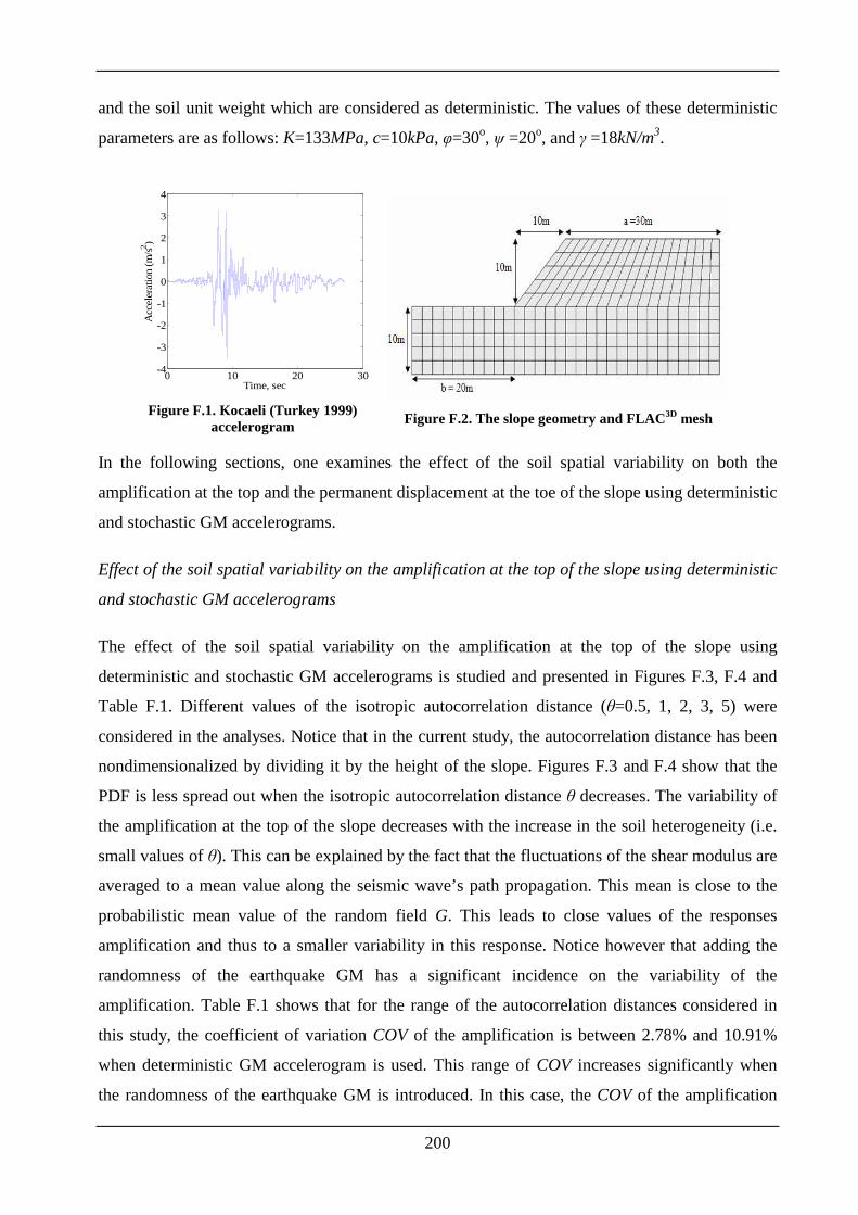
200
and the soil unit weight which are considered as deterministic. The values of these deterministic
parameters are as follows: K=133MPa, c=10kPa, φ=30o, ψ =20o, and γ =18kN/m3.
In the following sections, one examines the effect of the soil spatial variability on both the
amplification at the top and the permanent displacement at the toe of the slope using deterministic
and stochastic GM accelerograms.
Effect of the soil spatial variability on the amplification at the top of the slope using deterministic
and stochastic GM accelerograms
The effect of the soil spatial variability on the amplification at the top of the slope using
deterministic and stochastic GM accelerograms is studied and presented in Figures F.3, F.4 and
Table F.1. Different values of the isotropic autocorrelation distance (θ=0.5, 1, 2, 3, 5) were
considered in the analyses. Notice that in the current study, the autocorrelation distance has been
nondimensionalized by dividing it by the height of the slope. Figures F.3 and F.4 show that the
PDF is less spread out when the isotropic autocorrelation distance θ decreases. The variability of
the amplification at the top of the slope decreases with the increase in the soil heterogeneity (i.e.
small values of θ). This can be explained by the fact that the fluctuations of the shear modulus are
averaged to a mean value along the seismic wave’s path propagation. This mean is close to the
probabilistic mean value of the random field G. This leads to close values of the responses
amplification and thus to a smaller variability in this response. Notice however that adding the
randomness of the earthquake GM has a significant incidence on the variability of the
amplification. Table F.1 shows that for the range of the autocorrelation distances considered in
this study, the coefficient of variation COV of the amplification is between 2.78% and 10.91%
when deterministic GM accelerogram is used. This range of COV increases significantly when
the randomness of the earthquake GM is introduced. In this case, the COV of the amplification
0 10 20 30-4
-3
-2
-1
0
1
2
3
4
Time, sec
Acc
ele
ratio
n (
m/s2 )
Figure F.1. Kocaeli (Turkey 1999)
accelerogram
Figure F.2. The slope geometry and FLAC3D mesh
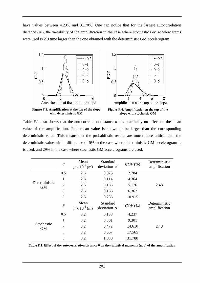
201
have values between 4.23% and 31.78%. One can notice that for the largest autocorrelation
distance θ=5, the variability of the amplification in the case where stochastic GM accelerograms
were used is 2.9 time larger than the one obtained with the deterministic GM accelerogram.
Table F.1 also shows that the autocorrelation distance θ has practically no effect on the mean
value of the amplification. This mean value is shown to be larger than the corresponding
deterministic value. This means that the probabilistic results are much more critical than the
deterministic value with a difference of 5% in the case where deterministic GM accelerogram is
is used, and 29% in the case where stochastic GM accelerograms are used.
Table F.1. Effect of the autocorrelation distance θ on the statistical moments (µ, σ) of the amplification
Figure F.3. Amplification at the top of the slope
with deterministic GM
Figure F.4. Amplification at the top of the
slope with stochastic GM
θ Mean
µ x 10-2 (m) Standard
deviation σ COV (%)
Deterministic amplification
0.5 2.6 0.073 2.784
1 2.6 0.114 4.364
2 2.6 0.135 5.176
3 2.6 0.166 6.362
Deterministic GM
5 2.6 0.285 10.915
2.48
θ Mean
µ x 10-2 (m) Standard
deviation σ COV (%)
Deterministic amplification
0.5 3.2 0.138 4.237
1 3.2 0.301 9.301
2 3.2 0.472 14.610
3 3.2 0.567 17.565
Stochastic GM
5 3.2 1.030 31.780
2.48
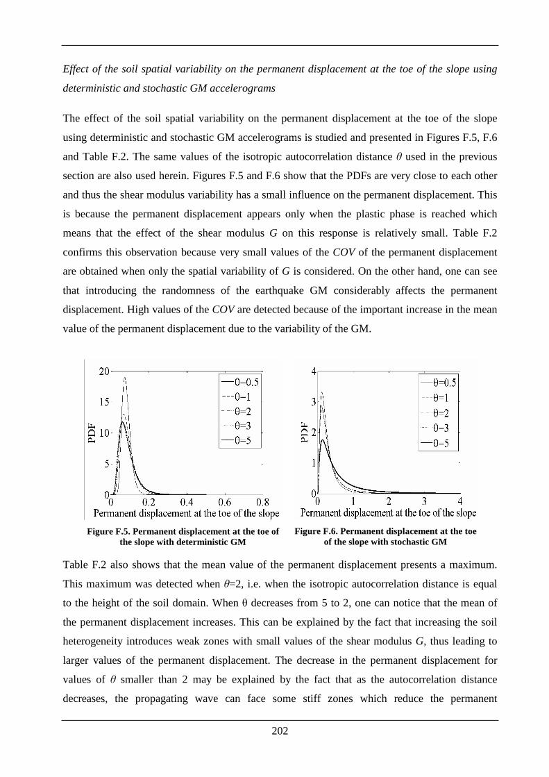
202
Effect of the soil spatial variability on the permanent displacement at the toe of the slope using
deterministic and stochastic GM accelerograms
The effect of the soil spatial variability on the permanent displacement at the toe of the slope
using deterministic and stochastic GM accelerograms is studied and presented in Figures F.5, F.6
and Table F.2. The same values of the isotropic autocorrelation distance θ used in the previous
section are also used herein. Figures F.5 and F.6 show that the PDFs are very close to each other
and thus the shear modulus variability has a small influence on the permanent displacement. This
is because the permanent displacement appears only when the plastic phase is reached which
means that the effect of the shear modulus G on this response is relatively small. Table F.2
confirms this observation because very small values of the COV of the permanent displacement
are obtained when only the spatial variability of G is considered. On the other hand, one can see
that introducing the randomness of the earthquake GM considerably affects the permanent
displacement. High values of the COV are detected because of the important increase in the mean
value of the permanent displacement due to the variability of the GM.
Table F.2 also shows that the mean value of the permanent displacement presents a maximum.
This maximum was detected when θ=2, i.e. when the isotropic autocorrelation distance is equal
to the height of the soil domain. When θ decreases from 5 to 2, one can notice that the mean of
the permanent displacement increases. This can be explained by the fact that increasing the soil
heterogeneity introduces weak zones with small values of the shear modulus G, thus leading to
larger values of the permanent displacement. The decrease in the permanent displacement for
values of θ smaller than 2 may be explained by the fact that as the autocorrelation distance
decreases, the propagating wave can face some stiff zones which reduce the permanent
Figure F.5. Permanent displacement at the toe of
the slope with deterministic GM
Figure F.6. Permanent displacement at the toe
of the slope with stochastic GM
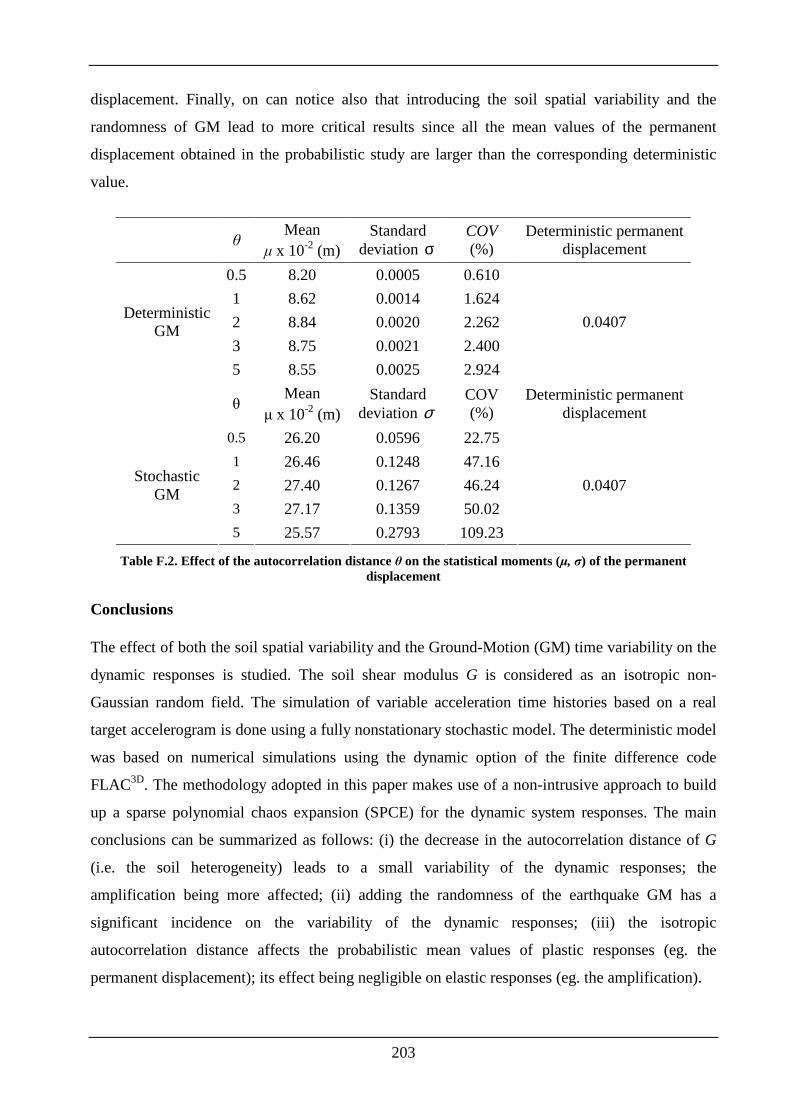
203
displacement. Finally, on can notice also that introducing the soil spatial variability and the
randomness of GM lead to more critical results since all the mean values of the permanent
displacement obtained in the probabilistic study are larger than the corresponding deterministic
value.
Table F.2. Effect of the autocorrelation distance θ on the statistical moments (µ, σ) of the permanent displacement
Conclusions
The effect of both the soil spatial variability and the Ground-Motion (GM) time variability on the
dynamic responses is studied. The soil shear modulus G is considered as an isotropic non-
Gaussian random field. The simulation of variable acceleration time histories based on a real
target accelerogram is done using a fully nonstationary stochastic model. The deterministic model
was based on numerical simulations using the dynamic option of the finite difference code
FLAC3D. The methodology adopted in this paper makes use of a non-intrusive approach to build
up a sparse polynomial chaos expansion (SPCE) for the dynamic system responses. The main
conclusions can be summarized as follows: (i) the decrease in the autocorrelation distance of G
(i.e. the soil heterogeneity) leads to a small variability of the dynamic responses; the
amplification being more affected; (ii) adding the randomness of the earthquake GM has a
significant incidence on the variability of the dynamic responses; (iii) the isotropic
autocorrelation distance affects the probabilistic mean values of plastic responses (eg. the
permanent displacement); its effect being negligible on elastic responses (eg. the amplification).
θ Mean
µ x 10-2 (m) Standard
deviation σ COV (%)
Deterministic permanent displacement
0.5 8.20 0.0005 0.610
1 8.62 0.0014 1.624
2 8.84 0.0020 2.262
3 8.75 0.0021 2.400
Deterministic GM
5 8.55 0.0025 2.924
0.0407
θ Mean
µ x 10-2 (m) Standard
deviation σ COV (%)
Deterministic permanent displacement
0.5 26.20 0.0596 22.75
1 26.46 0.1248 47.16
2 27.40 0.1267 46.24
3 27.17 0.1359 50.02
Stochastic GM
5 25.57 0.2793 109.23
0.0407
204
Appendix G.
The purpose of this Appendix is to check if the possible reason for which relatively small values
of Q2 were obtained (when the SPCE methodology was applied in chapter V) is linked to the
chosen system response (i.e. Amax). Notice that the test was performed using the 'column' model
and the reference case where 1
72G MPaµ = and ay=2m.
The test consists in constructing the SPCE not only for Amax at the top of the soil column but for
all the accelerations at the top of the soil column at the different time steps (the value of Amax can
be deduced from the different SPCEs constructed at the different time steps). This test allows one
to detect if the fact of considering directly Amax as a system response is the reason for which the
relatively small values of Q2 were obtained.
Notice that a seismic loading of total duration T=15s and time step ∆t=0.05s was considered in
the analysis. Thus, it is composed of 301 registration points (or acceleration values). The
construction of the SPCE 301 times is a difficult task. Blatman and Sudret (2011) have suggested
an efficient and fast alternative approach. To obtain the SPCEs for all the accelerations at the
different time steps, Blatman and Sudret (2011) have proposed the use of the so-called principal
component analysis (PCA). The aim is to capture the main stochastic feature of the response
using a small number of (non physical) variables compared to the original number of variables
(i.e. 301 in the present analysis). This enormously reduces the computational cost since the
SPCEs are no longer evaluated for all the accelerations at the different time steps, but on a small
number of non physical variables. In the next section, one presents the so-called principal
component analysis (PCA). It is followed by the obtained numerical results.
Principal component analysis (PCA)
Consider an experimental design (ED) ( ) ( )(1) ( )1 1 ,..., ,..., ,..., K
M Mξ ξ ξ ξ ξ ξ= = and the
corresponding set of model evaluations ( ) ( ) (1) ( ),..., Kξ ξΓ = Γ Γ where K is the number of
realizations. Notice here that each element ( )( )iξΓ is a vector composed of Q elements where Q
is the number of response components. In our case where the acceleration at the top of the
column at different time steps is considered, Q=301 which is the number of registration points.
Thus, Γ is a matrix composed of K rows and Q columns. In order to perform the principal
components analysis, the following steps must be considered:
205
• For each column in matrix Γ , one needs to compute the mean value and then to subtract
this mean value from each element in this same column. This provide a new matrix Γ'.
• Compute the covariance matrix as follows: ' ' 'TC xΓ = Γ Γ
Compute the eigenvalues and eigenvectors of 'CΓ by solving the matrix system
'C V VDΓ = where V is a matrix whose columns are the eigenvectors and D is a diagonal
matrix whose entries are the eigenvalues (1,..., Kλ λ ).
• Sort the eigenvalues and the corresponding eigenvectors in a descending order and retain
only the K' largest eigenvalues. Notice that the value of K' may be selected such that the
relative PCA induced error given by '
1 1
1K K
PCA i ii i
ε λ λ= =
= −∑ ∑ is less than a prescribed
value (say 5%PCAε ≤ ). Notice that 'KV of dimensions [Q, K'] is a matrix whose columns
are the eigenvectors of the K' largest eigenvalues.
• Compute the transformed and reduced response matrix (called PCA matrix) as follows:
' ''K KY V= Γ .
where 'KY is a matrix composed of K rows and K' columns.
Notice that obtaining the orginal model from the PCA matrix 'KY is straighforwad. This can be
performed by applying the following equation: ' '' K KV YΓ = . Thus, characterizing the model
response Γ' or Γ can be achieved indirectly by identifying a functional relationship between the
input random vector ξ and the PCA output matrix 'KY .
Numerical results
In this section, one presents the numerical results obtained using the PCA which was previously
presented. The aim is to capture the main stochastic feature of the response using a small number
of (non physical) variables compared to the original number of variables (i.e. 301 in the present
analysis). This enormously reduces the computational cost since the SPCEs are no longer
evaluated for all the accelerations at the different time steps, but on a small number of non
physical variables. The SPCEs computed for the non-physical variables are then used to deduce
the SPCEs for all the accelerations at the different time steps.
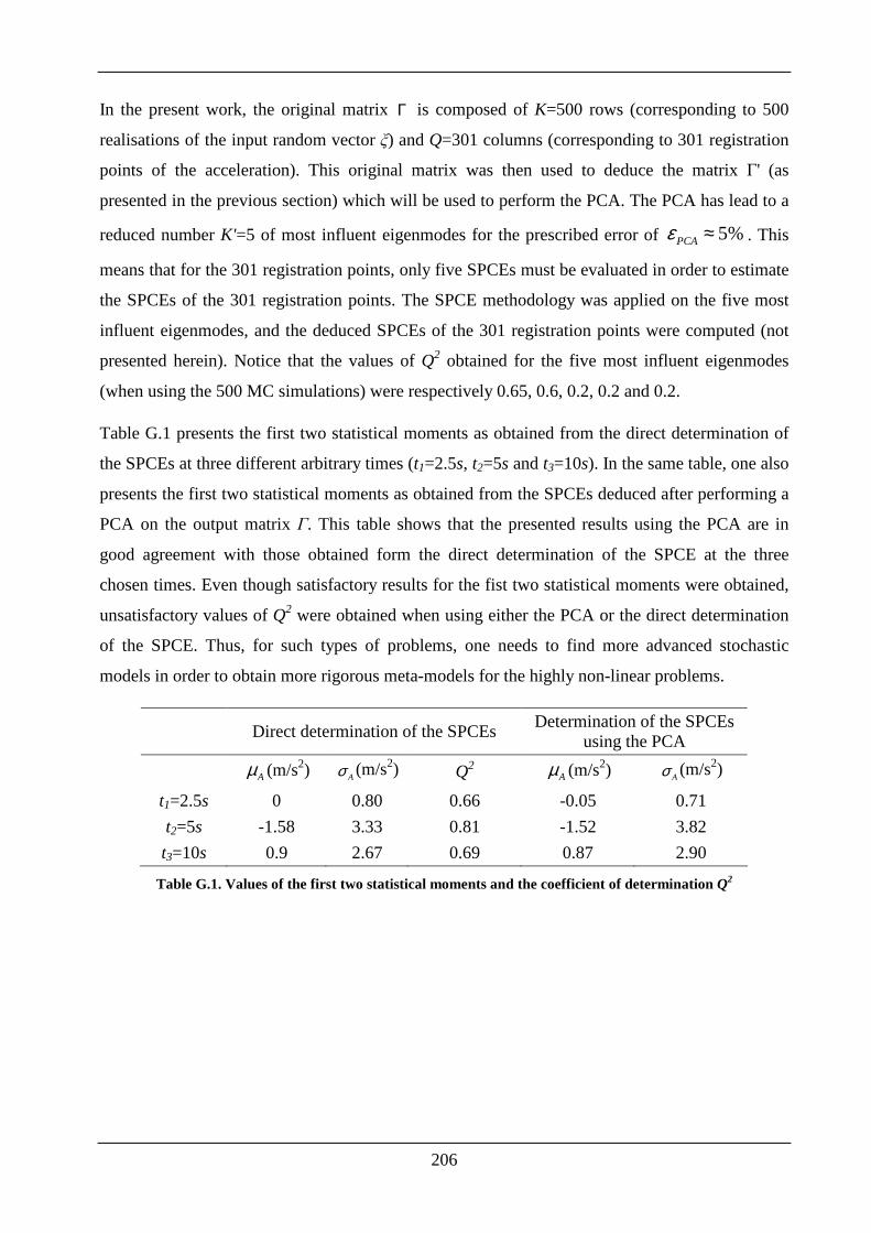
206
In the present work, the original matrix Γ is composed of K=500 rows (corresponding to 500
realisations of the input random vector ξ) and Q=301 columns (corresponding to 301 registration
points of the acceleration). This original matrix was then used to deduce the matrix Γ' (as
presented in the previous section) which will be used to perform the PCA. The PCA has lead to a
reduced number K'=5 of most influent eigenmodes for the prescribed error of 5%PCAε ≈ . This
means that for the 301 registration points, only five SPCEs must be evaluated in order to estimate
the SPCEs of the 301 registration points. The SPCE methodology was applied on the five most
influent eigenmodes, and the deduced SPCEs of the 301 registration points were computed (not
presented herein). Notice that the values of Q2 obtained for the five most influent eigenmodes
(when using the 500 MC simulations) were respectively 0.65, 0.6, 0.2, 0.2 and 0.2.
Table G.1 presents the first two statistical moments as obtained from the direct determination of
the SPCEs at three different arbitrary times (t1=2.5s, t2=5s and t3=10s). In the same table, one also
presents the first two statistical moments as obtained from the SPCEs deduced after performing a
PCA on the output matrix Γ. This table shows that the presented results using the PCA are in
good agreement with those obtained form the direct determination of the SPCE at the three
chosen times. Even though satisfactory results for the fist two statistical moments were obtained,
unsatisfactory values of Q2 were obtained when using either the PCA or the direct determination
of the SPCE. Thus, for such types of problems, one needs to find more advanced stochastic
models in order to obtain more rigorous meta-models for the highly non-linear problems.
Direct determination of the SPCEs Determination of the SPCEs
using the PCA
Aµ (m/s2) Aσ (m/s2) Q2 Aµ (m/s2) Aσ (m/s2)
t1=2.5s 0 0.80 0.66 -0.05 0.71
t2=5s -1.58 3.33 0.81 -1.52 3.82
t3=10s 0.9 2.67 0.69 0.87 2.90
Table G.1. Values of the first two statistical moments and the coefficient of determination Q2

207
208
Appendix H.
Mathematical description of the macro-element
The purpose of this Appendix is to describe a theoretical model based on strain hardening
plasticity theory which is capable of describing the behavior of a shallow footing when it is
subjected to all possible combinations of vertical, horizontal and moment loading using the
macro-element.
In the framework of the macro-element theory, any load or deformation path can be applied to the
footing and the corresponding unknowns (deformations or loads) can be calculated.
The foundation is assumed to be rigid and the nonlinearities of the soil and interface are assumed
to be condensed in a representative point which is the footing centre. Within that framework, it is
suggested to work with generalized (global) variables: (i) the force resultants, i.e. the vertical
force V, the horizontal forces Hx, Hy, and the moments Mx, My and (ii) the corresponding
displacements; i.e. the vertical displacement uz, the horizontal displacements ux and uy, and the
rotations θx and θy. The torque moment (Mz) and the corresponding displacement are not taken
into account in the present analysis.
The three-dimensional SSI macro-element takes into account three different mechanisms: the soil
elasticity, the possible soil plasticity and the possible uplift of the foundation. The total
displacement can thus be considered as a sum of three components related to the elastic and
plastic behavior of the soil and the uplift behavior of the foundation. These three different
mechanisms and their mathematical development are extensively presented in Crémer et al.
(2002), Grange et al. (2009a) and Grange et al. (2009b) and are briefly described herein.
Elastic behaviour
The elastic constitutive model can be written as ( )el plF K u u= −
where
( )' ' ' ' 'z x y y xu u u uθ θ= and ( )' ' ' ' 'x y y xF V H M H M=
are the vectors that
represent the dimensionless generalized displacements and forces and Kel is the elastic stiffness
matrix [Grange et al. (2009a)].
Plastic behaviour - failure criterion and loading surface
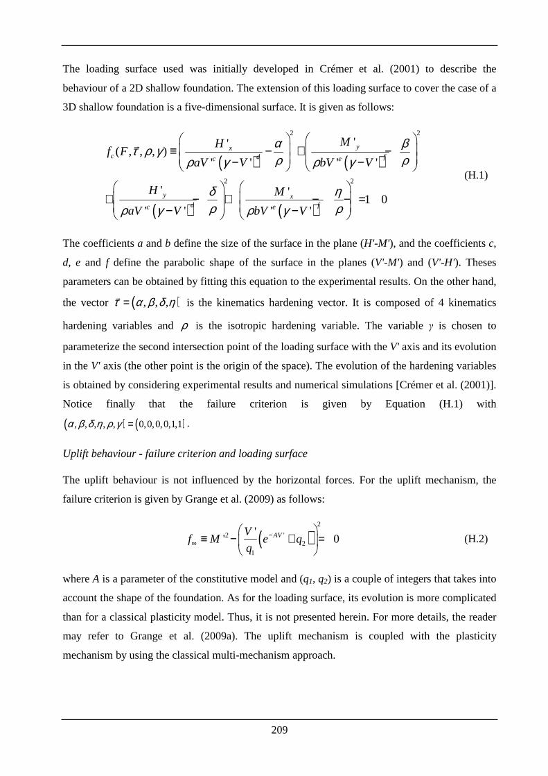
209
The loading surface used was initially developed in Crémer et al. (2001) to describe the
behaviour of a 2D shallow foundation. The extension of this loading surface to cover the case of a
3D shallow foundation is a five-dimensional surface. It is given as follows:
( ) ( )
( ) ( )
2 2
2 2
''( , , , )
' ' ' '
' '1 0
' ' ' '
yxc d fc e
y xd fc e
MHf F
aV V bV V
H M
aV V bV V
α βτ ρ γρ ρρ γ ρ γ
δ ηρ ρρ γ ρ γ
≡ − + − − −
+ − + − − = − −
(H.1)
The coefficients a and b define the size of the surface in the plane (H'-M'), and the coefficients c,
d, e and f define the parabolic shape of the surface in the planes (V'-M') and (V'-H'). Theses
parameters can be obtained by fitting this equation to the experimental results. On the other hand,
the vector ( ), , ,τ α β δ η= is the kinematics hardening vector. It is composed of 4 kinematics
hardening variables and ρ is the isotropic hardening variable. The variable γ is chosen to
parameterize the second intersection point of the loading surface with the V' axis and its evolution
in the V' axis (the other point is the origin of the space). The evolution of the hardening variables
is obtained by considering experimental results and numerical simulations [Crémer et al. (2001)].
Notice finally that the failure criterion is given by Equation (H.1) with
( ) ( ), , , , , 0,0,0,0,1,1α β δ η ρ γ = .
Uplift behaviour - failure criterion and loading surface
The uplift behaviour is not influenced by the horizontal forces. For the uplift mechanism, the
failure criterion is given by Grange et al. (2009) as follows:
( )2
2 '2
1
'' 0AVV
f M e qq
−∞
≡ − + =
(H.2)
where A is a parameter of the constitutive model and (q1, q2) is a couple of integers that takes into
account the shape of the foundation. As for the loading surface, its evolution is more complicated
than for a classical plasticity model. Thus, it is not presented herein. For more details, the reader
may refer to Grange et al. (2009a). The uplift mechanism is coupled with the plasticity
mechanism by using the classical multi-mechanism approach.