pricing and revenue management with limited market ... · pricing and revenue management with...

Pricing and Revenue Management with Limited Market Information

Serkan S. Eren

Submitted in partial fulfillment of the

requirements for the degree

of Doctor of Philosophy

under the Executive Committee of the

Graduate School of Arts and Sciences

COLUMBIA U N I V E R S I T Y

2008

UMI Number: 3333334

INFORMATION TO USERS

The quality of this reproduction is dependent upon the quality of the copy

submitted. Broken or indistinct print, colored or poor quality illustrations and

photographs, print bleed-through, substandard margins, and improper

alignment can adversely affect reproduction.

In the unlikely event that the author did not send a complete manuscript

and there are missing pages, these will be noted. Also, if unauthorized

copyright material had to be removed, a note will indicate the deletion.

®

UMI UMI Microform 3333334

Copyright 2008 by ProQuest LLC.

All rights reserved. This microform edition is protected against

unauthorized copying under Title 17, United States Code.

ProQuest LLC 789 E. Eisenhower Parkway

PO Box 1346 Ann Arbor, Ml 48106-1346

©2008

Serkan S. Eren

All Rights Reserved

ABSTRACT

Pricing and Revenue Management with Limited Market Information

Serkan S. Eren

Traditional models from the revenue management literature assume that firms

have full information about the market demand and consumer preferences. This thesis

studies pricing, capacity allocation and product line positioning models for a firm with

limited market information using relative performance criteria and maximum entropy

estimation.

In our first essay, we examine different monopoly pricing mechanisms under lim

ited customer willingness-to-pay (WtP) information. We use the competitive ratio

and the maximum regret criteria to study a dynamic pricing, a third-degree price

discrimination, and a second-price sealed-bid auction setting, where customers have

private WtP drawn from common distribution that is unknown to the seller. We

provide closed-form solutions for the optimal pricing policies and highlight impor

tant structural insights. We show that price skimming arises naturally as a hedging

mechanism against two principal risks that the firm faces: first, the risk of foregoing

revenue from pricing too low, and second, the risk of foregoing sales from pricing too

high. We focus on the competitive ratio criterion and the dynamic pricing setting

to illustrate how learning and partial information can be incorporated. Even limited

learning, e.g., market information at a few price points, leads to significant perfor

mance gains with relative performance criteria, and the resulting policies have very

good revenue performance across all distributions.

In our second essay, we study the joint problem of product line positioning and

pricing for a monopolist when consumer preferences and WtP are unknown. We

extend classical models of horizontal and vertical differentiation to cover this uncer

tainty again using the relative performance criteria. Our analysis provides insights

into practices observed in many real world markets. For the horizontal differentiation

case, we show that the optimal decision for both criteria is to position products at

equal intervals in the attribute space and to price them identically. For the vertically

differentiated case, we show that the optimal policy consists of offering a number of

the highest quality versions, and that the more ambiguity over customers' taste for

quality, the more versions the firm should offer.

In our last essay, we change our focus to incorporating partial information in a

dynamic forecasting and optimization cycle of capacity allocation. [21] illustrate,

using a two class example, that most common forecasting methods lead to divergence

and degeneration of optimal policies when used jointly with optimization routines

in such a cycle; and call this phenomenon the "spiral-down effect". We propose a

tractable and intuitive approach based on maximum entropy (ME) distributions that

readily incorporates and apply uncensoring to censored sales data in an intuitive

manner. We show that the protection levels given by our algorithm avoids "spiral

down" and converge to optimal values.

Contents

1 Introduction 1

1.1 An essay about monopoly pricing schemes with limited demand infor

mation 8

1.2 An essay about product line positioning without market information . 16

1.3 An essay about maximum entropy estimation in capacity allocation

problems 24

2 Monopoly Pricing with Limited Demand Information 30

2.1 Dynamic pricing with no market information 32

2.1.1 Problem formulation 32

2.1.2 Characterization of the optimal pricing policy 34

2.1.3 Maximum regret 39

2.2 The effect of learning 42

2.2.1 Unconstrained learning 44

2.2.2 Constrained learning 46

2.2.3 Discussion and numerical results 50

2.3 Learning with limited price experimentation 51

2.3.1 Single price in period one 51

i

2.3.2 Multiple prices and incorporating partial demand information 55

2.3.3 Numerical examples 62

2.4 Other pricing mechanisms 66

2.4.1 Third degree price discrimination 66

2.4.1.1 Competitive ratio 67

2.4.1.2 Maximum regret 70

2.4.2 Second price auction 74

2.4.2.1 Competitive ratio 76

2.4.2.2 Maximum regret 79

3 Product Line Positioning without Market Information 82

3.1 Horizontal product line positioning 83

3.1.1 Model 83

3.1.2 Product line positioning and pricing decision 86

3.1.3 Competitive ratio 87


3.2 Vertical product line positioning 98

3.2.1 Competitive ratio 99


4 Revenue Management Heuristics Under Limited Market Informa

tion: A Maximum Entropy Approach 112

4.1 Single-resource capacity control with two fare-classes 113

4.1.1 Full information model 113

ii

4.1.2 Unknown demand distribution 114

4.1.3 Proposed solution based on the ME distributions 117

4.2 Convergence analysis for the two fare-class problem 121

4.2.1 Outline of analysis 121

4.2.2 Analysis of the ODE 124

4.2.3 Proof of convergence 126

4.3 Extension to multifare problem 129

5 Conclusions 133

References 145

A Supplement to Chapter 2: Proofs of Remaining Results 146

B Supplement to Chapter 3: Proofs of Remaining Results 158

C Supplement to Chapter 4: Proofs of Remaining Results 173

C.l Theorem 2.1 of Kushner and Yin (2003) 173

C.2 Proofs of remaining results 175

in

List of Figures

2.1 Structure of the worst-case distribution with one test price 56

2.2 Optimal vs revenue maximizing reserve price comparison 80

3.1 Horizontal differentiation on a unit circle 85

3.2 Vertical product positioning example 102

4.1 ME algorithm example with two fare-classes 127

4.2 Extension of ME algorithm to multiple fare-classes 132

B.l Example: a policy improving the competitive ratio 161

B.2 Example: increasing the prices improves the competitive ratio . . . . 167

IV

List of Tables

1.1 Some common examples of maximum entropy distributions 26

2.1 Performance gains due to constrained and unconstrained learning . . 50

2.2 WtP distributions and corresponding demand models 63

2.3 CR policy performance with fractile information. Example 1 64




v

1

Chapter 1

Introduction

Classical models from the economics, marketing, and revenue management litera

ture assume that firms have accurate characterizations of the market demand and

consumer preferences. In practice, however, there are many settings, such as intro

duction of new and innovative products, where one rarely has such full and accurate

information. This source of model uncertainty may lead to significant revenue loss and

may be insufficiently hedged against through the use of policies that do not explicitly

incorporate it in their derivation. This thesis studies these issues for a monopolist

operating in settings with limited market demand and consumer preference informa

tion. In our first two essays, we study different pricing mechanisms and the joint

problem of product line positioning and pricing, respectively, under limited customer

willingness-to-pay and preference information using competitive ratio and maximum

regret criteria. In our third essay, we focus on incorporating partial information in

a dynamic forecasting and optimization cycle of capacity allocation using maximum

entropy distributions.

2

As a motivating example, consider a monopolist firm that offers a new prod

uct to a set of risk-neutral, heterogenous consumers, each endowed with a private

willingness-to-pay (WtP or valuation), which is an independent draw from a com

mon distribution. The market information is summarized by the number of potential

consumers, i.e., the market size, and the WtP distribution. Classical models would

assume that both of these elements are known to the firm, and are used to determine

the expected revenue maximizing price. How should the seller approach this problem

if the market size and WtP distribution were unknown? What should be the form of

seller's pricing policy in that case? How should that be adjusted to take advantage

of partial demand information extracted, for example, from experimenting at a few

price points?

There are two natural ways to specify this type of model uncertainty that lead to

different formulations and different policy recommendations. The first one is stochas

tic, wherein the unknown preference and WtP distributions are assumed to be drawn

from a given set of possible distributions according to some known probability law.

The firm's goal is to optimize her expected revenues over all possible market model re

alizations. Main shortcoming of this approach is that it requires detailed information

on the distribution of the model uncertainty, which itself may not be available.

The second approach is to use a formulation that adopts a worst-case perspec

tive via a max-min criterion on expected revenue or profit. That is, one treats the

unknown information as being controlled by an adversary ("nature") who seeks to

construct instances that minimize the firms profits for any given decision it makes.

The firm then seeks policies that produce the maximum profit against this adversary.

The difficulty with this approach is that it can lead to decisions that are driven by

excessively extreme and pessimistic scenarios about the unknown information, e.g.,

3

by setting the WtP of all consumers equal to its minimum allowed value in the above

pricing example irrespective of the firm's pricing decision. To reduce this inherent

conservatism, one typically imposes constraints on the decision set of the adversary,

that are either ellipsoidals (see BenTal and Nemirovski [6], and ElGhaoui and Lebret

[23]), or polyhedra (see Bertsimas and Sim [10], as well as Bertsimas and Thiele [11],

Perakis and Sood [63]). In a similar vein, Lim and Shanthikumar [49] suggests using

a relative entropy constraint to bound the distance of the WtP distribution from

a nominal one. These approaches are usually grouped under the name robust opti

mization. Robust optimization essentially imposes an uncertainty "budget" to the

adversary in the form of additional constraints exemplified above so as to reduce the

pessimistic nature of the associated solution. However, the selection of this budget

is often arbitrary, and therefore, amounts to a statement about the degree of uncer

tainty in the information, which is not easy-to-interpret. More to the point, robust

optimization is often a computational formalism and does not usually lend itself to

finding analytic solutions that provide structural insights.

An alternative approach to reduce the conservatism of max-min formulations,

while maintaining their appealing low informational requirements, is through the use

of relative performance criteria such as competitive ratio and maximum regret. These

measure the performance relative to a fully-informed decision maker. In broad terms,

they are defined as follows: the firm first selects a policy 7r, and the adversary selects

a worst-case distribution function for the unknown consumer attribute, F(-); in the

above example, n could be the posted price, and F(-) the WtP distribution. Let

R(TT, F) be the actual expected revenue earned for the pair of actions 7r and F(-), and

R(n* (F), F) be the maximum expected revenue the firm could have extracted if she

knew the selected distribution F(-); here n*(F) denotes the optimal policy if F was

known. Then, the competitive ratio is given by

R(ir,F) c = max mm * F R(n*(F),F)'

while the minimum regret is

r* = min max [R(n*(F), F) - R(TT, F)]. ir F

That is, in both cases, the firm strives to minimize the relative difference from the

maximum revenues it could have extracted in the full-information case. To contrast,

the max-min criterion takes the form

max min R(ir, F). •K F

Relative performance criteria implicitly constrain the actions of the adversary

without having to impose additional constraints, and often result in intuitive policy

recommendations. They prevent trivial choices for the adversary, such as choosing

the minimal WtP for all consumers in the above example, which would result in a bad

revenue outcome for the firm no matter what the policy, because the fully-informed

manager would also be harmed in such instances. In that sense, they allow us to

distinguish between "bad market conditions" and "bad decisions". Our belief is that

these criteria might be of particular value in explaining some observed behavior in

product and revenue management practice due to its proximity to common perfor

mance evaluation schemes: for example, a revenue/product manager often has to

select a policy before the uncertainty of the market reveals itself. However, her own

performance is usually evaluated after the selling horizon, when the uncertainty is at

least partially revealed, e.g., good/bad season; and her actions are often compared

to what could have been optimally done in such conditions. Therefore, it is plausible

5

to hypothesize that a risk averse revenue/product manager, given the opportunity,

could (to some extend) choose to hedge her own performance evaluation risk. In fact,

these criteria gained significant popularity in decision theory literature in economics

during the last decade.

Relative performance criteria originate from and are used extensively in the statis

tics and the computer science literature, and have recently been applied in pricing and

operations management problems. Specifically, Ball and Queyranne [4] use a competi

tive ratio criterion for a single-resource capacity allocation problem, while Bergemann

and Schlag [8] and Perakis and Roels [61] adopt the regret criterion to study the mo

nopolist pricing and the newsvendor problems, respectively. Lan et al. [43] generalize

Ball and Queyranne's analysis and extend it to cover the regret criterion. Perakis

and Roels [62] apply similar techniques for network revenue management.

Some weaker notions of adversary for relative performance criteria have also been

studied. Alternatively, the "algorithm designer" (e.g. the firm in our case) has been

allowed to randomize over different strategies. For example, the so-called "oblivious

adversary" selects the distribution function F(-) without observing the firm's pricing

policy. As another example, the "adaptive online adversary" is only allowed to see the

decisions of the firm in the past stages in a dynamic setting before selecting the input

for the next stage. The adversary in our work corresponds to the notion of "offline

adversary". Ben-David et al. [5] examine and compare above notions of adversary

as well as randomized policies. They show that randomized policies offer no benefit

for the firm in the presence of an offline adversary, which implies that the optimal

competitive ratios we drive for the pricing mechanisms below remain valid even when

the firm is allowed randomization.

In our first two essays, we also use competitive ratio and maximum regret criteria

6

to study pricing and product line positioning decisions of a monopolist in settings

where the firm has limited information about the WtP distribution (for the pricing

problems in the first essay), and the distribution that characterizes the consumers'

preferences over product variety and quality (for the product positioning problems

in the second essay). First, we examine monopoly pricing mechanisms of dynamic

pricing, third-degree price discrimination, and second-price sealed-bid auction under

limited WtP information. We assume customers have private WtP drawn from com

mon distribution that is unknown to the seller. We provide closed-form solutions for

the optimal pricing policies and highlight important structural insights. We show

that price skimming arises naturally as a hedging mechanism against two principal

risks that the firm faces: first, the risk of foregoing revenue from pricing too low, and

second, the risk of foregoing sales from pricing too high. We focus on competitive

ratio criterion and the dynamic pricing setting in detail to illustrate how learning

and partial information can be incorporated. We show that even limited learning,

e.g., market information at a few price points, leads to significant performance gains

with relative performance criteria, and the resulting policies have very good revenue

performance across all distributions.


pricing for a monopolist when consumer preferences and WtP are unknown. We

extend classical models of horizontal and vertical differentiation to cover this uncer

tainty again using the relative performance criteria. Our analysis provides insights

into practices observed in many real world markets. For the horizontal differentiation

case, we show that the optimal decision for both criteria is to position products at

equal intervals in the attribute space and to price them identically. For the vertically

differentiated case, we show that the optimal policy consists of offering a number of

7

the highest quality versions, and that the more ambiguity over customers' taste for

quality, the more versions the firm should offer.

A potential practical shortcoming of an approach based on the relative perfor

mance criteria is that it may lose analytic and computational tractability as one tries

to incorporate partial information about the unknown demand model primitives. In

that respect, most papers adopt this framework to derive insights about the structure

of good policies and the effect of ambiguity on system performance, as opposed to

the computation of implementable policies. One exemption is Perakis and Roels [62],

which incorporates partial demand information using the probabilistic tight bounds

for mean and variance specifications derived by Bertsimas and Popescu [9]. Another

is Bergemann and Schlag [8], which allows for the unknown distribution to be within

a distance of a nominal distribution that could encapsulate prior information. Both

papers work only with the regret criterion and do not generalize easily to the compet

itive ratio criterion, and neither framework seems to allow for an easy way in which

to incorporate intuitive information extracted from past sales that usually translate

to fractiles of the WtP distribution. We illustrate how to incorporate the latter type

of demand information in a tractable way in the dynamic pricing section of our first

essay. Through numerical examples, we show that relative performance criteria, com

bined with partial information, not only provides structural insights but also robust

policies that have very good revenue performance across many market conditions.

Our models in the first two essays are mainly static in nature in that the basic

problems boil down to one-stage (or two-stage for learning) dynamic games between

the firm and the adversary. In a more dynamic setting, where available information

is constantly updated, a different perspective may be needed to incorporate available

stream of information, as the inherent complexity of the relative performance criteria

8

often hinder integration of such dynamic information. In this respect, we change

our focus to incorporating a continuous stream of partial information in a dynamic

forecasting and optimization cycle of capacity allocation in our last essay. Using

a capacity allocation example with two demand classes, Cooper et al. [21] illustrate

that most common forecasting methods lead to degeneration of optimal policies when

used jointly with optimization in such a cycle; and call this phenomenon the "spiral-

down effect". We propose a tractable and intuitive approach based on maximum

entropy (ME) distributions that readily incorporates partial demand information in

the form of censored sales data. We show that the capacity controls given by the ME

algorithm we propose avoids the spiral down effect and converge to the optimal values.

We make use of adaptive algorithms and stochastic approximations in our analysis

for two fare-classes and provide a heuristic algorithm for the multifare problem. The

solution to the ME problem simultaneously applies uncensoring to the raw sales data

in an intuitive and statistically sound manner.

In the remainder of this chapter, we introduce the specifics of our three essays,

review the relevant literature, and provide a general outline of our results.

1.1. An essay about monopoly pricing schemes with

limited demand information

Our first essay adopts relative performance criteria introduced above to study three

classical pricing settings. Specifically, we look at the settings where a monopolist offers

one product to a market of heterogenous consumers, each endowed with a private

WtP, which is an independent draw from a common but unknown distribution. We

9

study three variants of the firm's pricing problem that differ in terms of their selling

format. In the first one, the firm has the ability to change its price over time, and

its key decision is to figure out a pricing policy (how much to charge and for how

long to stay at each price point) that would perform well even though the firm does

not know the underlying consumers' WtP distribution. We also analyze the effects of

learning in this setting. The second variant looks at the case in which the firm can

(third-degree) price discriminate its market, i.e. segment the market into subgroups

that each can be charged a different price, but where the firm does not know what

the representative WtP and relative size of each of these market segments are. As

a special case of that model as the number of market segments grows large, we also

discuss the case of first degree price discrimination, where a different price is offered to

each customer. In the third variant, the firm attempts to sell one unit of the product

using a second-price sealed-bid auction, again without knowing the underlying WtP

distribution.

The first of the common pricing schemes we consider is the dynamic pricing. We

allocate majority of our discussion to this setting, as it is the most commonly ap

plied one in revenue management practice; and, as it provides practical extensions to

learning as well as insights into the tradeoffs of the firm when faced with uncertainty.

Dynamic pricing is concerned with adjusting prices to regulate demand over a finite

sales horizon to maximize revenue. Price skimming is a commonly used example of

such a policy in many industries like airlines, hospitality and fashion goods. Clearing

excess inventory and perishable products -rather than salvaging leftover items at low

value at the end of the sales horizon- has been proposed as a possible explanation

for this practice; see Talluri and van Ryzin [73] for a review of this body of work.

Another possible explanation for the use of dynamic pricing policies is as a hedging

10

mechanism in settings where demand is uncertain; see Lazear [46] for an analysis of

this problem and Pashigan [59], and Pashigan and Bowen [60] for empirical evidence

of this explanation. Harris and Raviv [34] showed that a price skimming policy may

emerge as the optimal mechanism when demand is uncertain. Our work shows that

such a policy will optimize the firm's relative revenue performance when the demand

model is unknown.

In our dynamic pricing setting, the firm has the ability to change its price over

time, and its key decision is to figure out a pricing policy (how much to charge

and for how long to stay at each price point) that would perform well even though

the firm does not know the underlying consumers' WtP distribution. An alternate

interpretation of this price skimming policy is to treat the relative length of time

over which a price is offered as a probability of that price point, thus interpreting the

proposed price scheme as a randomizing pricing policy; this was done in Bergemann

and Schlag [8].

Our model is deterministic, disregarding the stochastic variability of the sales

process, e.g., due to its Poisson nature. This allows us to emphasize the effects of

"first order" uncertainty introduced by not knowing the sales rate itself at a selected

price point, as opposed to "second order" fluctuation due to stochastic nature of the

process. Our analytical contributions are the following: 1) The competitive ratio and

maximum regret optimization problems are solvable in closed form, offering a detailed

description of the optimal policies for the seller and the adversary, the tradeoffs faced

by the seller, and a precise characterization of the resulting revenue loss. 2) We

extend our formulation and results to a two period setting that allows the seller

to learn from the sales observations in period one. 3) We address the situation

where the seller only has limited price experimentation capability, or has limited past

11

sales information. Observing the demand at a price point gives cumulative demand

information above and below that price point and essentially decomposes the problem

into simpler subproblems in the respective regions that are readily solvable using linear

programming techniques. As a special case of practical interest, we also study the "ex-

post" problem that allows the seller to take into account actual demand observation

data in her price optimization and performance analysis decisions.

We highlight three observations from our work that are of potential interest. First,

the worse case market scenarios for the firm, as captured by the WtP distribution

selected by the adversary, correspond to homogeneous markets where all consumers

have the same, yet unknown, valuation. Mathematically, this corresponds to an

extreme point -unit mass- distribution whose exact position is uncertain, forcing the

firm hedge against opposing risks at each price point: first, the risk of foregoing


high. In response, the firm's strategy tries to hedge against this exposure.

The extreme point nature of the adversary's strategy has appeared elsewhere

in the literature. One example from decision theory is Smith [71], which studies

the expectation maximization problem among a set of probability distributions. He

shows the equivalence of that problem to a linear program and, as a result, recovers

extreme point distributions as potential solution points. Our objective function is not

linear (and not even convex), and our results do not follow from Smith's observation.

However, such a structure emerges in many papers because the inner optimization step

can often be reduced to a quasi-convex maximization problem over the probability

simplex, which admits an extreme point solution. In settings with learning or with

partial demand information, the worst-case distribution retains some of its structural

form by having point masses at distinct valuations, but becomes more dispersed. We

12

give a complete characterization of the latter and discuss several examples in Section

4.

Second, we highlight that in settings with limited or no market information it is

optimal for the firm to adopt a price skimming policy to minimize the risk of lost sales

and foregone revenue that could result from mis-estimating the market characteristics.

To contrast, if the firm knew the customer WtP distribution, then it would be optimal

to charge a static price over the entire sales horizon. This result suggests that lack

of market information could offer one possible justification for the use of dynamic

pricing policies. Analytically, the precise form of the resulting pricing policy ensures

that both the firm and the adversary are indifferent with regard to the positioning

(i.e., the representative valuation) of the market.

Third, the effect of learning is both significant and quick in the sense that even a

few observations at different price points can provide considerable lift in the revenue

performance of the proposed policies. Both the resulting competitive ratio, which is

a worse case bound, and the actual performance relative to some underlying WtP

distribution unknown to the seller, improve considerably. In the case where the seller

is not restricted in the number of price points that she can experiment at, we show

that it is optimal to use a price skimming policy during a "learning" period. This

achieves full learning of the demand model and allows the seller to charge the optimal

(full-information) price in the remainder of the sales horizon. Often, there may be

practical constraints that link the firm's pricing decision over time, e.g. retailers

hesitate to increase prices after an early mark down. We show that in such settings it

is still optimal to adopt a price skimming policy, but in this case the seller is willing

to sacrifice performance due to the learning phase so as to retain adequate pricing

flexibility in the remainder of the sales horizon.

13

Incorporation of partial information is typically done in a Bayesian setting under

some parametric assumptions for the WtP distribution and using conjugate pairs of

distributions to maintain tractability; see, e.g., Lobo and Boyd [51], Aviv and Pazgal

[3], Araman and Caldentey [2], and Farias and Van Roy [25]. Assuming a parametric

family of distributions for the unknown demand runs the risk of model misspecifica-

tion due to the arbitrariness of that assumption. Similar to our work, another subset

of literature uses non-parametric approaches, which make minimal distributional as

sumptions and often involve some form of an adaptive learning algorithm; see, e.g.,

McGill and van Ryzin [55], Huh and Rusmevichientong [36], and Eren and Maglaras

[24]. An interesting recent paper in the latter set is Besbes and Zeevi [12] that studies

a prototypical dynamic pricing problem in a stochastic environment. Two important

insights from their work for purposes of our work is that they show that: a) in settings

with long sales horizons and large market sizes, an asymptotically optimal policy in

terms of its relative regret is to divide the sales horizon in two phases that are dedi

cated to learning and revenue optimization, respectively; and b) the uncertainty due

to the stochastic nature of the demand arrival process is indeed negligible in such

settings.

The second pricing scheme we study is the third degree price discrimination set

ting. Price discrimination is the practice of charging different people different prices

for the same goods or services. In the third degree price discrimination case, the

monopolist firm is capable of accurately differentiating between consumer segments

through an observable attribute. Each segment pays a different price for the same

product, and the segments with higher valuations pay more than those with lower

valuations. Student or senior citizen discounts are common examples of this practice.

A more recent application domain is in cross-selling that is done in call centers. This

14

is the practice that the agent attempts to cross sell some product or service after

completing the handling of the original customer request. At the time of that cross

selling opportunity, the call center can indeed classify the customer to a particular

segment and tailor its product offering.

Pigou was the first one to formally study this practice [65], which was further

studied by Robinson [67]. Since then, this setting received substantial attention in

economics literature and was extended to cover more general setups. The main focus

in economics literature has been the output level and the welfare impact of price

discrimination with respect to a monopolist charging a single uniform price to the

whole market. For a contemporary treatment and substantial recent contributions,

the reader is referred to Schmalensee [56] and Varian [74] [75].

For the third degree price discrimination case, assuming that the market can be

segmented on the basis of the customers' WtP, we show that it is optimal for the firm

to set the price for a particular segment equal to its minimum WtP value within the

segment. Moreover, if the firm has the ability to choose the market segmentation, it

will set equal the (absolute or relative) sizes of the WtP intervals. This is somewhat

a similar strategy to the price skimming policy above in that the firm segments the

total market size into smaller subgroups by skimming through the whole valuation

range. However, the adversary is strong enough to force the firm to price at the

lowest WtP value within each segment. Combined with the segmentation strategy,

this results in a piecewise (step-like) price menu being offered to the market.

The third pricing mechanism we consider is the the second price, sealed-bid auc

tion. The choice of this mechanism is motivated by the fact that irrespective of the

number of bidders and the underlying WtP distribution, it is still a dominant strat

egy for each potential buyer to bid her/his true WtP within this mechanism, thus

15

simplifying the analysis of the buyer's decision using relative performance criteria.

The second price auction setting we consider is a sealed-bid auction, where bidders

submit written bids without knowing bids of the other people in the auction. The

rules of the auction is such that the highest bidder wins, but pays a price equivalent

to the second highest bid. This auction was first proposed and studied by Vickrey

[76], and is therefore also named the "Vickrey auction". In his seminal 1961 paper,

Vickrey not only showed that each bidder has a dominant strategy of bidding her true

value, but also established an early form of the " revenue equivalence" theorem. The

second price auction is an optimal ex-post efficient pricing mechanism that requires

very few assumptions, and is therefore robust in nature. Truthful bidding remains

a dominant strategy (and the mechanism works) in the absence of assumptions such

as "independent valuations", "identical valuation distributions", or "risk neutrality",

which are usually necessary for other auction types. For a contemporary treatment

of auctions and literature survey, the reader is referred to McAfee and McMillan [54]

and Klemperer [64].

Ambiguity in auctions is a recent topic in the literature. Lo [50] analyzes sealed

bid auctions within a max-min expected utility framework for risk averse bidders.

Ozdenoren [58] extends and generalizes Lo's results. Bose et. al. [16] show that the

seller needs to fully insure risk averse buyers in a max-min expected utility frame

work. Levin and Ozdenoren [47] analyze auctions where the number of bidders is

uncertain. Chen et. al. [20] consider a setting where both ambiguity averse and

ambiguity loving behavior is allowed. For interesting empirical experiments involving

ambiguity in auctions, we refer the reader to Sarin and Weber [68], and to Chen et.

al. [20]. For competitive analysis of auction mechanisms with respect to "other selling

mechanisms", we refer the reader to Goldberg et al. [29], [30].

16

In the second-price auction setting, with only range information about the buyers'

WtP, we show that it is optimal for the seller to set his reservation price so as to

balance the risks of not selling the item with the risk of selling it at a low price just

as in the dynamic pricing setting above. The resulting reservation price has similar

properties to the one derived under the classical revenue maximizing setting, but, is

slightly lower, reflecting risk aversion.

The outline of our first essay is as follows: Section 2.1 introduces the prototypical

dynamic pricing problem with no market information and no learning. Sections 2.2

and 2.3 study two period extensions that allow for different degrees of learning. We

study the third degree price discrimination and the second-price auction settings in

Section 2.4.

1.2. An essay about product line positioning with

out market information

Positioning and pricing a product line is a central problem in marketing. (See the

survey papers Dobson and Yano [22], Green and Krieger [31], Krishnan and Ulrich

[41], Manez and Waterson [52], Ramdas [66].) In product line positioning, a firm must

decide which different versions of a product to offer. Versions may differ in ways that

appeal to the heterogeneous tastes of consumers, such as offering different colors, sizes

or flavors - called horizontal differentiation - or they may differ in their level of quality

and performance - called vertical differentiation. Product line positioning decisions

are intimately related to the prices charged, too; because product versions closer

to customers' preferences for variety or quality provide them more utility and can

17

therefore support higher prices. At the same time, differentiated versions of the same

product are almost always substitutes, so that lower prices for one version cannibalize

demand from the other versions in the product line. Hence, positioning and pricing

a product line should be coordinated decisions.

The difficulty in practice is that in many cases little is known about customer pref

erences for various product attributes and the experimentation necessary to determine

their preferences (e.g., conjoint analysis, (see Green and Srinivasan [32], Green et al.

[33])) may be either too costly or too time consuming and/or potentially unreliable,

as in the case of an innovative product that customers have never experienced using.

In such cases, firms must make product line positioning and pricing decisions with

little information about customer preferences. Most of the literature on product line

positioning and pricing assume the firm has full information on preference. In our

work, we consider the opposite extreme in which the firm has minimal information

about customer preferences. Understanding both these extremes helps build intu

ition because real life practice lies somewhere between the two. However, the case of

limited information has received no attention to date in the research literature. Our

work fills this gap. Even when firms have some preference information, it is often

limited and unstructured. The issues then are filtering out and organizing the useful

information, and incorporating these into the decision making process in a meaningful

manner. We try to address some of these issues in our first and third essays.

We use competitive ratio and maximum regret criteria to study product line po

sitioning and pricing decisions in a setting where the firm does not have information

about the distribution that characterizes the consumers' preferences over product

variety (in the case of horizontal differentiation) or quality (in the case of vertical

differentiation).

18

Our approach to modeling horizontal product variety is based on classical loca-

tional models, in which each version of the product is mapped into a location in a

product attribute space and each consumer's location represents her most preferred

values of the product attributes (her "ideal point"). The distance between a cus

tomer's ideal point and the locations of different product versions provides a measure

of their disutility from consuming a less-than-ideal product. Given a distribution of

customer locations or preferences, one can then analyze issues of optimal product line

design, positioning and pricing. Of course in our case, this distributional information

is what is unknown.

The seminal paper in this area belongs to Hotelling [35], who considers a linear

one-dimensional attribute space. Vickrey [77] is credited for formulating the circular

model, which gets rid of the boundary effects of the linear model. In 1966, Lancaster

[44] offered an alternative approach in which the utility of a choice is determined by

a parametric function of the consumer characteristics and product attributes. This

theory significantly increased interest in locational product differentiation models.

Salop [69] provides the most complete treatment of this setup in his seminal paper

for monopolistic competition, where he shows a symmetric equilibrium along the

product space (i.e. the circle) exists with equal prices, and all the consumers in the

market (i.e. around the circle) are served. Several extensions of this basic game

theoretical model has been made covering different scenarios of the market structure.

Further interested reader is referred to Lancaster [45], Manez and Waterson [52], and

Ramdas [66].

Our work is also closely related to the product line positioning literature. The

product line positioning problem itself is a complex multi-facet problem touching on

marketing concerns (consumer utility and product attributes modeling, pricing and

19

positioning to maximize market share or revenues, etc.), operations concerns (costs

of production, configuration of supply chains for variety, etc.), and engineering design

concerns (product architecture, shared versus unique components, etc.). There are

several survey papers structuring the literature around these three areas. (Again, see

the survey papers of Dobson and Yano [22], Green and Krieger [31], Krishnan and

Ulrich [41], Manez and Waterson [52], Ramdas [66].) Prior work in the literature

can be roughly characterized as follows: most directly uses or is inspired by the

utility framework of spatial differentiation models. Generally, models consider a finite

number of possible product offerings and the aim is to choose which of these to offer

with the objective of maximizing market share, revenues, or profits. However, there

are a number of papers in operations literature that solely consider cost minimization

or supply chain configuration. It is assumed in all this literature that customer

preferences/valuations for each possible product offering and the potential market size

at each such point are known or can be estimated using conjoint analysis. Moreover,

most of the models do not treat price as a decision variable, though several treat it

as part of the attribute space. The corresponding problems are usually mixed integer

programs and exact analytical solutions are generally not available. Algorithmic

solutions usually consist of greedy or simulation based heuristics (e.g., simulated

annealing).

Our work is aligned more closely with the marketing view of the problem ex

plained above. We base our model on the classical locational attributes and linear

utility framework as above. However, unlike the product line positioning literature

above, we try to avoid additional assumptions on top of this basic utility set up.

Specifically, we allow for uncertainty/ambiguity in customer valuations, and are in

terested in analyzing the effects of this uncertainty on optimal policies. Our objective

20

is to maximize revenues; we do not consider production costs (though variable costs

can be added without much change). Further, we only consider a single dimension

of variety for simplicity. Unlike most of the literature, we treat both variety and

price as continuous decision variables; hence, an infinite number of possible product

offerings/locations is allowed. While these assumptions are highly stylized, we are

able to derive analytical closed-form solutions for optimal positioning and pricing

policies which provide structural insights and permit sensitivity analysis with respect

to problem primitives, allowing us to gain intuitive understanding of the underlying

issues related to uncertainty.

As mentioned, we also analyze the case of vertical positioning, in which all con

sumers have a common ordering of their preferences for different versions, i.e. every

consumer agrees that a certain version i is better (in terms of what literature de

notes as "quality") than another version j . Our model of vertical positioning is also

classical, and is based on the early influential work of Mussa and Rosen [57], who in

troduce a framework that makes use of a linear utility function of quality. This utility

framework has been widely adopted by both following researchers and practitioners.

In their seminal paper, Shaked and Sutton [70] use this model to show that firms

can sustain positive profits even under price competition, contrary to the classical

"zero-profit" result of Bertrand price competition, when they are allowed to choose

the quality levels of their products under monopolistic competition. Assuming convex

costs as a function of product quality, Mussa and Rosen [57], and later Maskin and

Riley [53] and Kim [40], show that a firm can increase profits by offering vertically

differentiated products to customers with heterogeneous tastes for quality.

These models were widely adopted as they successfully explained product differ

entiation seen in the traditional manufactured goods. However, the theory fell short

21

of explaining product differentiation, or "versioning", for information goods. Infor

mation goods are particularly relevant in our case since most production costs are

sunk development costs and thus profits maximization coincides with revenue maxi

mization, which is the case we analyze. Early works using the linear utility function

for information goods conclude that there are no gains to product differentiation for

information goods and the product should be produced and supplied only at the high

est quality levels to prevent cannibalization (see Bhargava and Choudhary [13], Jones

and Mendelson [39], Acharyya [1]). However, empirical evidence (see Ghose and Sun-

dararajan [28]) shows that information goods have high levels of differentiation. Only

the highest quality is produced, as predicted by the above works, but the product is

then degraded afterwards and offered at varying levels of quality in the market. In

order to explain this practice, several models with different and more complex utility

functions have been proposed, but none has been as widely accepted as the linear

utility function of quality. Finally, Bhargava and Choudhary [14] demonstrated that

previous insights about suboptimality of vertical differentiation are not robust, and

showed that quality differentiation does indeed occur under a general class of utility

functions and sunk costs assumptions. They conclude that the higher the heterogene

ity in consumers' taste for quality, the more likely vertical differentiation is and that

the highest quality version is always offered in the product bundle. Other popular

marketing texts (see for example, Lilien et al. [48]) also conclude that versioning is

attractive when consumers are sufficiently heterogeneous.

More recently, there have been attempts to combine vertical and horizontal differ

entiation models by allowing firms to compete on both dimensions at the same time.

There are also numerous other work that provide extensions to the above product

differentiation settings which we cannot mention due to space limitations. We refer

22

the interested reader to the survey papers of Manez and Waterson [52], and Ramdas

[66] to learn more about these.

Finally, a remark on terminology related to competition is in order. Almost all

the works mentioned above study "monopolistic competition", in which different firms

compete with each other across vertical and/or horizontal product attributes in the

same market space under full information about customer preferences. Our work

differs in two fundamental ways. First, we focus on the product line decisions of a

monopolist. Second, our monopolist "competes against nature" rather than compet

ing against other firms, in the sense that it is the unknown customer preferences that

drive the firm's decision making rather than the actions of other firms. In particu

lar, we caution the reader not to confuse the "competitive ratio" criterion with the

"monopolistic competition" concept found in prior'literature. The competitive ratio

term used here originates from statistics and computer science literature.

Our findings and contributions can be summarized as follows: in Section 3.1, we

consider the horizontal positioning of a monopolist's product line using Salop's classi

cal circular model of spatial differentiation. For both competitive ratio and maximum

regret criteria, we first derive the optimal pricing policy for a given product line with

fixed attributes. We show that the optimal price vector depends on the maximum

attribute difference among neighboring products. We also show that the worst-case

performance decreases (i.e. the competitive ratio decreases or the regret increases)

as the consumers' sensitivity for differentiating attribute increases, consumers' nomi

nal valuations for their ideal product decreases, or the maximum attribute difference

among neighboring products increases. Then, we show that for both criteria, the

optimal positioning and pricing policy is to position products at equal intervals in

the attribute space and to price them identically; that is, to evenly span the product

23

space with uniformly priced versions of the product. This type of positioning and

pricing of a product line is frequently observed in practice (e.g. colors of a t-shirt,

flavors of ice cream, i-Tunes downloads, etc.) and our results are consistent with

these observations. Of course there are other explanations for such practices, such as

operational simplicity and concern for perceived fairness. Still, there has been little

formal theoretical justification of the optimality of such policies in the literature; our

theory provides one explanation. It also provides closed-form pricing policies and

performance measures which give insight into the economics of product positioning

with minimal market information.

In Section 3.2, we study the vertical positioning of a product line using the linear

utility of quality framework of Mussa and Rosen. Again, we first derive the optimal

pricing policy for a fixed number of versions with given quality levels. Furthermore,

consistent with Bhargava and Choudhary's results, we show that the optimal policy

consists of offering some number of highest quality versions, which we call nested

quality offerings; and that the number of versions offered increase as the heterogeneity

and ambiguity in consumers' taste for quality increases. This result is consistent

with empirical evidence and conclusions about versioning in information goods in

literature. (See again Ghose and Sundararajan [28] and Lilien et al. [48].)

For both the case of horizontal and vertical positioning, we solve for the optimal

policy in closed form, which provides a detailed description of the optimal pricing

and positioning strategies for the firm and the resulting worst-case revenue loss. Our

analysis, while stylized, provides insights into practices observed in many real world

markets.

24

1.3. An essay about maximum entropy estimation

in capacity allocation problems

One of the key challenges of revenue management systems in dynamic settings is to

accurately forecast demand when one only has access to observed (censored) sales

data. As is well known in the area, common uncensoring techniques and the interac

tion of forecasting and revenue optimization routines may prevent these systems from

making optimal decisions in a dynamic setting; c.f., Boyd et al. [17] and Cooper et al.

[21]. In this essay, we propose a tractable and intuitive algorithm for the dynamic

(airline) capacity allocation problem based on maximum entropy (ME) distributions.

We show that the proposed ME algorithm can readily incorporate censored sales data

and that it leads to control decisions (in the form of capacity protection levels) that

converge to optimal ones for the underlying demand distribution.

Revenue management systems consist mainly of forecasting and optimization mod

ules that operate jointly. Main goal of the former module is to provide accurate de

mand forecasts. Once such a forecast is available, the optimization module provides

policies to be implemented, and as a result, the new sales observation are used to

update the previous forecast. We denote this iterative feedback loop as the "cycle of

joint forecast and optimization". One of the main issues in practice is the effect of

optimization on future forecasts in such interactive systems, which result in possible

accumulation of errors through time. In the scope of the airline capacity allocation

problem we study, this can described as follows: consider a setting with two fare-

classes with independent random demands that arrive sequentially in nonoverlapping

intervals. The low fare demand is realized before the high fare demand; and the

airline's problem is to decide on the number of seats to reserve for the random high

25

fare demand in the future. This form of capacity control is denoted as the protection-

level. In order to find protection levels at any period, past sales data is accumulated

to form demand forecasts. Note, however, that the sales data is censored and has to

go through some uncensoring step first. The airline uses its forecast to optimize its

protection level, implements this control, and observes the corresponding new sales,

which is then used as the input for the next period's forecasting step. However, if the

airline gets an incorrect forecast at any iteration, it could lead to a wrong protection-

level; and the resulting new observation would be biased as well, which could in return

make the next forecast even less accurate. This bad cycle may produce protection-

levels that degenerate further away from the optimal ones at each iteration. This

phenomenon has been named as the "spiral-down effect". Cooper et al. [21] ana

lyze this effect and show that the protection levels and forecasts produced by many

common algorithms degenerate consistently and converge to suboptimal levels due

to joint optimization/forecasting interaction. Converging to suboptimal levels is a

particularly dangerous scenario in practice, as forecasts consistently (and incorrectly)

match observations, making the problem harder to detect.

At the core of the above problem lies the issue of uncensoring the sales observa

tions. Censored demand observations provide only information about the fractiles of

the underlying demand distribution. For example, if the number of available seats is

L = 50 and the observed sales is S = 50, this observation corresponds to the event

{D > 50} for random demand D. Majority of the existing uncensoring techniques

in practice consist of discarding such censored events or inflating uncensored obser

vations heuristically. Weatherford and Polt [78] show that none of these uncensoring

techniques avoid the "spiral-down" effect. Rather than trying to heuristically inter

pret the event {D > 50} in the above example, we propose to use the framework of

26

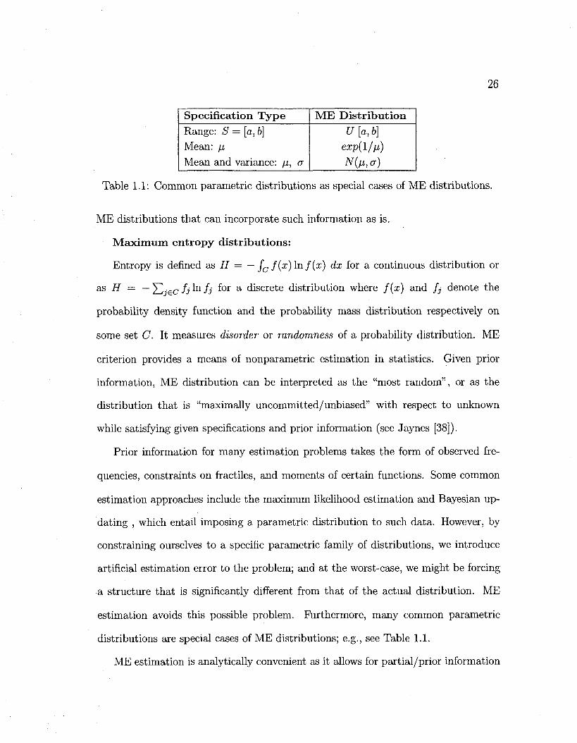
Specification Type Range: S = [a,b]

Mean: fi

Mean and variance: //, a

ME Distribution U [a, b]

exp(l/fj)

Nfacr)

Table 1.1: Common parametric distributions as special cases of ME distributions.

ME distributions that can incorporate such information as is.

Maximum entropy distributions:

Entropy is defined as H — — Jc f(x)lnf(x) dx for a continuous distribution or

as H = —J2jecfi^nfj ^or a discrete distribution where f(x) and fj denote the

probability density function and the probability mass distribution respectively on

some set C. It measures disorder or randomness of a probability distribution. ME

criterion provides a means of nonparametric estimation in statistics. Given prior

information, ME distribution can be interpreted as the "most random", or as the

distribution that is "maximally uncommitted/unbiased" with respect to unknown

while satisfying given specifications and prior information (see Jaynes [38]).

Prior information for many estimation problems takes the form of observed fre

quencies, constraints on fractiles, and moments of certain functions. Some common

estimation approaches include the maximum likelihood estimation and Bayesian up

dating , which entail imposing a parametric distribution to such data. However, by

constraining ourselves to a specific parametric family of distributions, we introduce

artificial estimation error to the problem; and at the worst-case, we might be forcing

a structure that is significantly different from that of the actual distribution. ME

estimation avoids this possible problem. Furthermore, many common parametric

distributions are special cases of ME distributions; e.g., see Table 1.1.

ME estimation is analytically convenient as it allows for partial/prior information

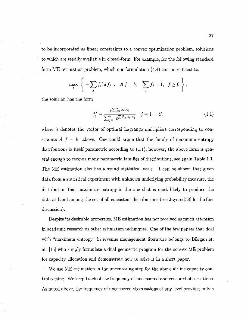
27

to be incorporated as linear constraints to a convex optimization problem, solutions

to which are readily available in closed-form. For example, for the following standard

form ME estimation problem, which our formulation (4.4) can be reduced to,

the solution has the form

^ V E - u . J = l - - 5 , (1-1)

where A denotes the vector of optimal Lagrange multipliers corresponding to con

straints A f = b above. One could argue that the family of maximum entropy

distributions is itself parametric according to (1.1), however, the above form is gen

eral enough to recover many parametric families of distributions; see again Table 1.1.

The ME estimation also has a sound statistical basis. It can be shown that given

data from a statistical experiment with unknown underlying probability measure, the

distribution that maximizes entropy is the one that is most likely to produce the

data at hand among the set of all consistent distributions (see Jaynes [38] for further

discussion).

Despite its desirable properties, ME estimation has not received as much attention

in academic research as other estimation techniques. One of the few papers that deal

with "maximum entropy" in revenue management literature belongs to Bilegan et.

al. [15] who simply formulate a dual geometric program for the convex ME problem

for capacity allocation and demonstrate how to solve it in a short paper.

We use ME estimation in the uncensoring step for the above airline capacity con

trol setting. We keep track of the frequency of uncensored and censored observations.

As noted above, the frequency of uncensored observations at any level provides only a

28

lower bound for the actual empirical demand distribution at that level, because some

of the actual demand might have been realized as censored observations at lower lev

els. These can be incorporated as fractile constraints to our ME formulation in (4.4).

Actually, censored observations also supply additional information (and constraints)

as explained further below. Other information in the form of seasonal data or sub

jective opinion can be incorporated as linear constraints as well. In our analysis, we

first describe our ME algorithm for the two fare-class problem in Section 4.1, prove

the convergence of protection levels produced to the optimal ones for the underlying

demand in Section 4.2, and finally, provide an extension of the algorithm to multifare

problems in Section 4.3.

The idea behind our ME approach is that the algorithm tries to push the current

control a little upwards (or downwards respectively) by changing the underlying es

timate distribution a little bit (by 0(1 /k) at each step k), when we have a censored

(or uncensored respectively) observation. Therefore, the algorithm can be thought

of moving in the right direction locally at each step. The formal analysis of such

stochastic processes that are controlled locally in the right direction is given by the

theory of adaptive algorithms and stochastic approximations. (See Kushner and Yin

[42], Chen [19], and Benveniste et al. [7].) McGill and van Ryzin [55] propose a simple

adaptive algorithm -a Robins-Monro algorithm-, which increases the protection level

a little when the allocated seats sell out and reduces it a little otherwise. Similarly,

a concurrent working paper by Huh and Rusmevichientong [37] provides an adaptive

algorithm that adjusts protection levels by making use of stochastic online convex op

timization and adjusting the protection levels based on a gradient ascent algorithm.

However, these papers take the approach of directly adjusting the protection levels

by bypassing the forecasting step, whereas we establish the equivalence of the joint

29

optimization/forecasting iteration to an adaptive algorithm when ME distributions

are used in the forecasting step. In that respect, the adaptive algorithm should be

seen as a mathematical tool for proving convergence in our essay, rather than the

focus of our work. Our contribution can be seen as augmenting the effectiveness of

legacy optimization/forecasting routines in practice by use of ME estimation.

30

Chapter 2

Monopoly Pricing with Limited

Demand Information

In our first essay, we study the dynamic pricing, the third-degree price discrimination,

and the second-price sealed-bid auction pricing schemes for a monopolist with limited

WtP information using competitive ratio and maximum regret criteria. We assume

customers have private WtP drawn from common distribution that is unknown to the

seller. We focus more on the dynamic pricing scheme to illustrate the use of partial

information. For the simplest case in Section 2.1, we solve the resulting optimization

problem in closed form and provide a description of the optimal policies for the

seller and the adversary. Price skimming arises naturally as a hedging mechanism

against uncertainty in this setting. In Section 2.2, we analyze the effects of learning

in a two period setting that allows the seller to learn from the sales observations in

period one. Depending on the level of restrictions on the firm, experimenting with

as many price points as possible through a price skimming policy is optimal in the

learning period. In Section 2.3, we study the case where the seller only has limited

31

price experimentation capability or has limited past sales information. We show

that partial sales information can be easily incorporated into our setting, and that

even with limited learning, the resulting policies have very good revenue performance

across many common demand distributions. Finally, in Section 2.4, we analyze the

other two monopoly pricing schemes. We first consider the case in which the firm

can (third-degree) price discriminate its market. We show that it is optimal for the

firm to set the sizes of the WtP intervals equally and to set the price for a particular

segment equal to its minimum WtP value within the segment. Lastly, we also study

the the second price sealed-bid auction. The optimal reservation price balances risks

related to uncertainty in WtP and is similar to the one derived under the revenue

maximizing criterion, but, is slightly lower, reflecting risk aversion.

One observation from many cases considered is that the adversary's policy often

takes the form of an extreme point distribution. This follows from the fact that the

inner optimization step can often be reduced to a quasi-convex maximization problem

over the probability simplex, which admits an extreme point soution. This setting

accentuates the two types of risk faced by the firm: first, the risk of foregoing to much


high. In response, the firm's strategy focuses on hedging against this exposure.

As a side note, for some of the models studied, the adversary's best response

is achieved only in the limit. In other words, the point mass of the extreme point

distribution is allocated to some valuation v — e for some v and an arbitrarily small

e > 0 chosen by the adversary, resulting in a, say, competitive ratio of c -f- 5(e) where

5(-) is monotone increasing with 8(e) —> 0 as e —>• 0. Consequently, the competitive

ratio achieves the value c in the limit. This limiting response of the adversary will be

stated in detail using arbitrarily small constants 8, e as in the above sense wherever

needed in this essay.

32

2.1. Dynamic pricing with no market information

2.1.1 Problem formulation

We consider a monopolist selling a homogeneous good over a sales horizon that is nor

malized to have length one. The firm's is assumed to have ample capacity. Potential

customers arrive at the firm according to a deterministic arrival process with rate A,

each with a WtP for one unit of that product, denoted by v, which is an independent

draw from a common discrete distribution F on the set {pi,... ,pK} where p\ = v

and PK = v. That is the support of the WtP distribution is an appropriate discretiza

tion of the range [v,v], e.g., in $1 or 5% increments. It is common to assume that

the customer arrival process is Poisson in the literature with the excepted revenue

maximization criterion, but in the sequel we will restrict attention to a deterministic

model where, in addition, customers are assumed to arrive continuously as opposed

to in unit increments. This corresponds to the fluid approximation to the common

Poisson (or other stochastic arrival process) setting, and allows us to emphasize the

effects of "first order" uncertainty introduced by not knowing the sales rate itself at a

selected price point, as opposed to "second order" fluctuation due to stochastic nature

of the process. The rate A can also be interpreted as the "market size." Assuming

that the price at time t is equal to p(t), then the sale rate at that instant is given

by X(t) = AP(v > p(t)) = AF(p(t)), where F(-) = 1 - F(-), and the corresponding

revenue rate is p(t)AF(p(t)).

The firm's goal is to maximize the total revenues accrued in [0,1]. When the WtP

33

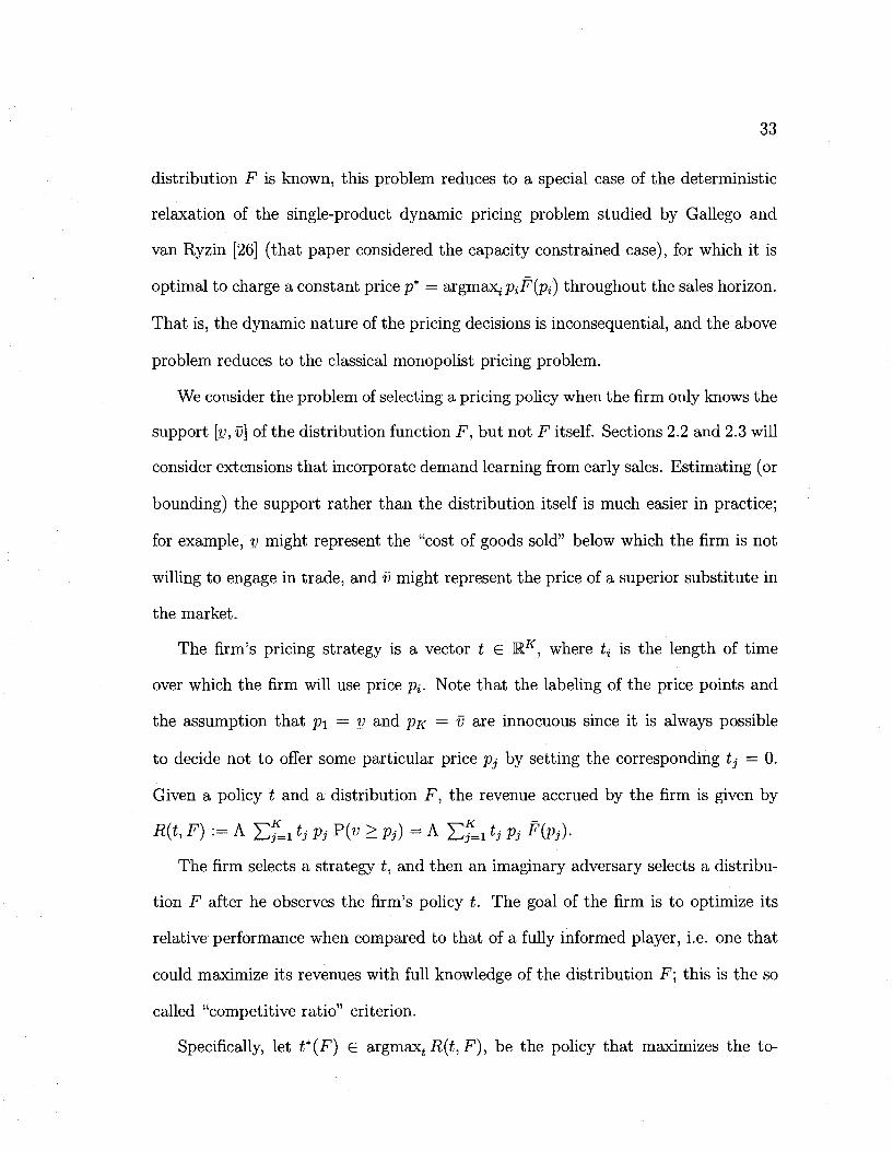
distribution F is known, this problem reduces to a special case of the deterministic

relaxation of the single-product dynamic pricing problem studied by Gallego and

van Ryzin [26] (that paper considered the capacity constrained case), for which it is

optimal to charge a constant price p* = argmeixipiF(pi) throughout the sales horizon.

That is, the dynamic nature of the pricing decisions is inconsequential, and the above

problem reduces to the classical monopolist pricing problem.

We consider the problem of selecting a pricing policy when the firm only knows the

support [v, v] of the distribution function F, but not F itself. Sections 2.2 and 2.3 will

consider extensions that incorporate demand learning from early sales. Estimating (or

bounding) the support rather than the distribution itself is much easier in practice;

for example, y might represent the "cost of goods sold" below which the firm is not

willing to engage in trade, and v might represent the price of a superior substitute in

the market.

The firm's pricing strategy is a vector t G M.K, where U is the length of time

over which the firm will use price Pi. Note that the labeling of the price points and

the assumption that p\ = y and PK = v are innocuous since it is always possible

to decide not to offer some particular price pj by setting the corresponding tj = 0.

Given a policy t and a distribution F, the revenue accrued by the firm is given by

R(t, F) := A Ef=i *i Pj P(« > Pj) = A Ef= 11* Pj F{pj).

The firm selects a strategy t, and then an imaginary adversary selects a distribu

tion F after he observes the firm's policy t. The goal of the firm is to optimize its

relative performance when compared to that of a fully informed player, i.e. one that

could maximize its revenues with full knowledge of the distribution F; this is the so

called "competitive ratio" criterion.

Specifically, let t*(F) G argmax^ R(t, F), be the policy that maximizes the to-

34

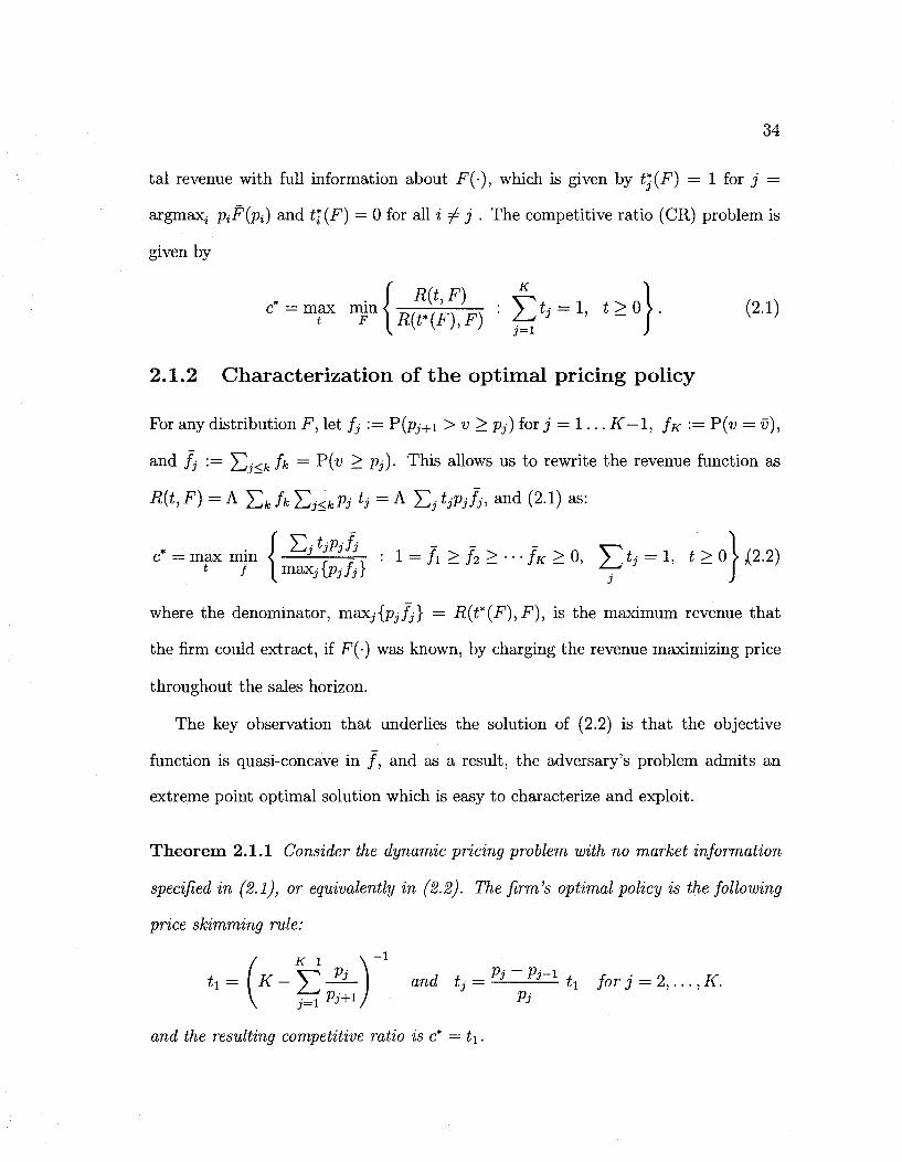
tal revenue with full information about F(-), which is given by t^(F) = 1 for j =

argmaXj piF(pi) and t*(F) = 0 for all i ^ j . The competitive ratio (CR) problem is

given by

c* = max min l n, , ' „ . : V \ - = 1, £ > 0 I . (2.1) t F \R(t*{F),F) j ^ 3 ~ j y }

2.1.2 Characterization of the optimal pricing policy

For any distribution F, let fj :— P(pj+i > v > pf) for j = 1 . . . K—l, fa '•= P(v = v),

and fj := J2j<kfk = P(v > Pj)- This allows us to rewrite the revenue function as

R(t,F) = A J2k fkEj<kPj tj = A EjtjPjfj, and (2.1) as:

c = max mm * / I max

'-PJT • l = fi>h>---fa>0, J > = 1, t>0W2.2) •jXPjJJJ j )

where the denominator, meotj{pjfj} = R(t*(F),F), is the maximum revenue that

the firm could extract, if F(-) was known, by charging the revenue maximizing price

throughout the sales horizon.

The key observation that underlies the solution of (2.2) is that the objective

function is quasi-concave in / , and as a result, the adversary's problem admits an

extreme point optimal solution which is easy to characterize and exploit.

Theorem 2.1.1 Consider the dynamic pricing problem with no market information

specified in (2.1), or equivalently in (2.2). The firm's optimal policy is the following

price skimming rule:

t1={K-,y—] and tj = Pj~Pj~1 h for j = 2,..., K.

V UP^J P> and the resulting competitive ratio is c* =t\.

35

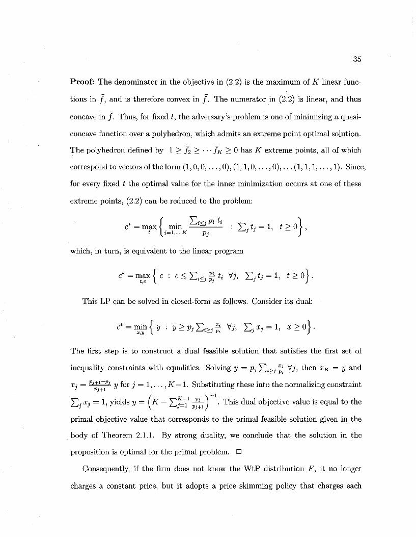
Proof: The denominator in the objective in (2.2) is the maximum of K linear func

tions in / , and is therefore convex in / . The numerator in (2.2) is linear, and thus

concave in / . Thus, for fixed t, the adversary's problem is one of minimizing a quasi-

concave function over a polyhedron, which admits an extreme point optimal solution.

The polyhedron defined by 1 > j ^ > • • • / « • > 0 has K extreme points, all of which

correspond to vectors of the form (1,0,0, . . . ,0), (1,1,0, . . . , 0 ) , . . . (1 ,1 ,1 , . . . ,1). Since,

for every fixed t the optimal value for the inner minimization occurs at one of these

extreme points, (2.2) can be reduced to the problem:

* J . Z^iKjPi *i ^ , n , . „ I c = max < mm —— : > • £-• = 1, t > 0 > ,

t \j=l,...,K Pj ^ ° J

which, in turn, is equivalent to the linear program

c ' = m a x { c : c < £.<,• g U Vj, E ^ i = 1, * > o} •

This LP can be solved in closed-form as follows. Consider its dual:

The first step is to construct a dual feasible solution that satisfies the first set of

inequality constraints with equalities. Solving y — PjYli>j ~ Y?> ^ n e n XK = V and

Xj = pi+1~pi y for j = l,...,K — \. Substituting these into the normalizing constraint

]T\- Xj — 1, yields y = f K — Ylj=\ ~~^~) • This dual objective value is equal to the

primal objective value that corresponds to the primal feasible solution given in the

body of Theorem 2.1.1. By strong duality, we conclude that the solution in the

proposition is optimal for the primal problem. •

Consequently, if the firm does not know the WtP distribution F, it no longer

charges a constant price, but it adopts a price skimming policy that charges each

36

price point for an appropriate amount of time. As mentioned earlier, an alternative

interpretation is to treat the t/s as probabilities and t as a randomized pricing policy;

see Bergemann and Schlag [8]. To gain some intuition behind this result, recall that

the worst case scenario for the firm occurs when the market is homogeneous and every

potential customer shares the same WtP. This setting raises two types of opposing

risk for the firm at each price. First, if the firm prices too high for a significant portion

of its sales horizon, it may suffer low sales when the market's WtP is low. Second,

if the firm prices too low for a significant portion of its sales horizon, it may forego

a significant revenue opportunity when the market's WtP is high. In both cases,

the resulting competitive ratio would be low. Our analysis specifies how to balance

these two effects in constructing the optimal pricing policy, which essentially makes

the adversary indifferent between the extreme market scenarios that is optimal for

him to choose. It is also worth comparing the above behavior against the solution to

the maxmin formulation with objective maxt minp R(t, F). In this case, the optimal

strategy for the adversary is to put all of the probability at v, while the firm would also

price at v for the entire sales horizon, making the result too conservative. Actually,

the revenue performance of the resulting policy is typically much higher than the

competitive ratio as illustrated by the numerical examples in Sections 2.2 and 2.3.

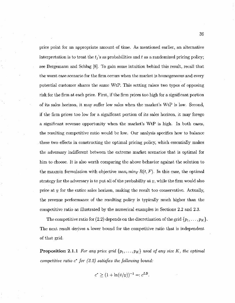
The competitive ratio for (2.2) depends on the discretization of the grid {pi , . . . ,PK}-

The next result derives a lower bound for the competitive ratio that is independent

of that grid.

Proposition 2.1.1 For any price grid {pi,... ,pK} used of any size K, the optimal

competitive ratio c* for (2.2) satisfies the following bound:

c* > (1 + Hv/v))'1 =: cLB.

37

Proof: Note that

K-l K-\ K-\

j - l J j=l J-r j .

K-\

<1 + 3=

dx Pj+i

2 _ / - dx = l + - dx = l + )n(v/y) 7 = 1 ^ P j X Ju ^

Then, c* satisfies

A"-l - l

K _ y _ Z_ ] > (i + ln^/v))"1 = cLB. D c . = . , . p.-

The lower bound is achieved as the number of prices grows large and {pi,... ,pK}

becomes a dense covering of the range [v,v]. We note that Ball and Queyranne [4]

recover similar results in their study of the single-resource (airline) capacity allocation

problem under a competitive ratio criterion. Similarly, Bergemann and Schlag [8]

obtained analogous results using the maximum regret criterion.

A somewhat crude upper bound on the competitive ratio can be obtained if we

allow the firm to optimize over its offered price grid, but simultaneously restrict the

adversary to also price on that grid.

Proposition 2.1.2 For any set of price points v = pi < • • • < px — v and any

number K, the optimal competitive ratio c*(p) for (2.2) satisfies the following bound:

c*(p)< (2-v/v)-l=:cUB.

Proof: To achieve the upper bound we maximize the competitive ratio derived in

Proposition 2.1.1, c*(p) = (K — ^jS^ - ^ - ) with respect to the price vector p\ <

• • • < PK- This is equivalent to maximizing J2j=i ~^~ o v e r V\ < " ' < PK, which can

be written as the following problem:

K-2 ~\

max < — + V -£*- + P^- : v < p2 < • • • < pK.x < v I , (2.3) P \Pi t^Pj+i v

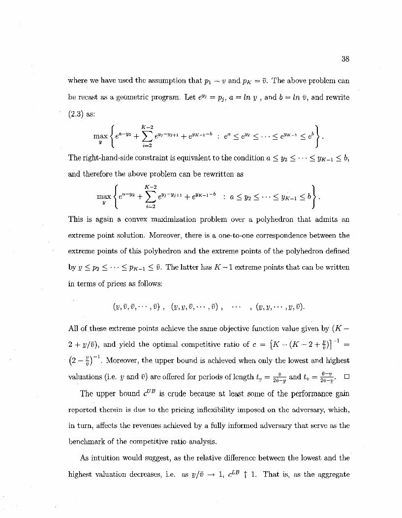
38

where we have used the assumption that p\ — v and px — v. The above problem can

be recast as a geometric program. Let eyi = Pj, a = In y , and b = In v, and rewrite

(2.3) as:

{ K-2 ea-y2 + y* ewrw+i + eVK-i-b . e« < ey2 < . . . < eyK-i < J>

The right-hand-side constraint is equivalent to the condition a < yi < • • • < yx-i < b,

and therefore the above problem can be rewritten as

( K-2 ea-V2 + y^ eyj-vj+i + eyK-i-b . a<y2<---< yK^ < b

This is again a convex maximization problem over a polyhedron that admits an

extreme point solution. Moreover, there is a one-to-one correspondence between the

extreme points of this polyhedron and the extreme points of the polyhedron defined

by v < P2 < • • • < PK-I < v. The latter has K — \ extreme points that can be written

in terms of prices as follows:

(v,v,v,--- ,v) , (v,v,v,• • • ,v) , ••• , (v,v,---,v,v).

All of these extreme points achieve the same objective function value given by (K —

2 + v/v), and yield the optimal competitive ratio of c = [K — (K — 2 + | ) j —

(2 — | ) . Moreover, the upper bound is achieved when only the lowest and highest

valuations (i.e. v and v) are offered for periods of length tv = ^ ^ and ty = ^ ^ . D

The upper bound cUB is crude because at least some of the performance gain

reported therein is due to the pricing inflexibility imposed on the adversary, which,

in turn, affects the revenues achieved by a fully informed adversary that serve as the

benchmark of the competitive ratio analysis.

As intuition would suggest, as the relative difference between the lowest and the

highest valuation decreases, i.e. as v/v —> 1, cLB | 1. That is, as the aggregate

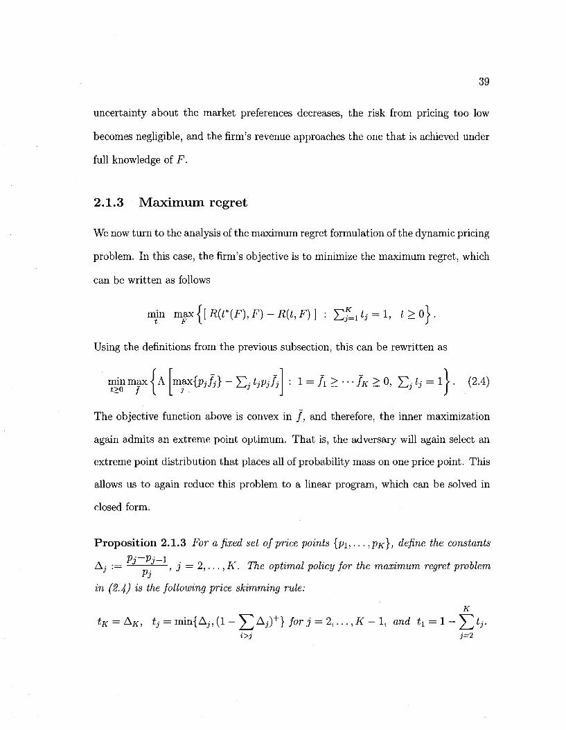
39

uncertainty about the market preferences decreases, the risk from pricing too low

becomes negligible, and the firm's revenue approaches the one that is achieved under

full knowledge of F.

2.1.3 Maximum regret

We now turn to the analysis of the maximum regret formulation of the dynamic pricing

problem. In this case, the firm's objective is to minimize the maximum regret, which

can be written as follows

nun max j [ R(t*(F), F) - R(t, F) ] : £JLj tj = 1, t > o} .

Using the definitions from the previous subsection, this can be rewritten as

min max < A t>o f I

maxlpjfj} - V . tjprfj : l = / i > - " / * > 0 , E ^ = l } - (2-4)

The objective function above is convex in / , and therefore, the inner maximization

again admits an extreme point optimum. That is, the adversary will again select an

extreme point distribution that places all of probability mass on one price point. This

allows us to again reduce this problem to a linear program, which can be solved in

closed form.

Proposition 2.1.3 For a fixed set of price points {pi,... ,PK}, define the constants

Pj-Pj-1 Pj

in (2.4) is the following price skimming rule:

Aj := — , j = 2 , . . . ,K. The optimal policy for the maximum regret problem

tK = AK, tj = min{ Aj: (1 - J ] Aj)+} for j = 2 , . . . , K - 1, and tx = 1 - ^ t i>j j=2

K

r

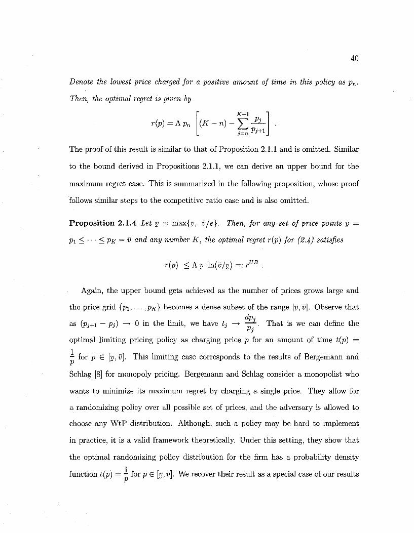
40

Denote the lowest price charged for a positive amount of time in this policy as pn.

Then, the optimal regret is given by

K-\ r(p) = A p „

The proof of this result is similar to that of Proposition 2.1.1 and is omitted. Similar

to the bound derived in Propositions 2.1.1, we can derive an upper bound for the

maximum regret case. This is summarized in the following proposition, whose proof

follows similar steps to the competitive ratio case and is also omitted.

Proposition 2.1.4 Let y = max{t», v/e}. Then, for any set of price points v =

Pi < • • • < PK = v and any number K, the optimal regret r(p) for (2.4) satisfies

UB f(p) < A y \n(v/y) =: r'

Again, the upper bound gets achieved as the number of prices grows large and

the price grid {pi,... ,PK} becomes a dense subset of the range [y,v]. Observe that dpj

as (pj+i — Pj) —* 0 in the limit, we have tj —> . That is we can define the Pj

optimal limiting pricing policy as charging price p for an amount of time t(p) =

- for p G [y,v]. This limiting case corresponds to the results of Bergemann and

Schlag [8] for monopoly pricing. Bergemann and Schlag consider a monopolist who

wants to minimize its maximum regret by charging a single price. They allow for

a randomizing policy over all possible set of prices, and the adversary is allowed to

choose any WtP distribution. Although, such a policy may be hard to implement

in practice, it is a valid framework theoretically. Under this setting, they show that

the optimal randomizing policy distribution for the firm has a probability density

function t(p) = - for pG \y,v]. We recover their result as a special case of our results

41

in the limit. Our dynamic pricing model offers an alternative interpretation of their

randomizing pricing policy.

In common with the results of the competitive ratio analysis, the worst case sce

nario for the firm is a homogeneous market whose representative WtP is unknown.

The structure of the optimal firm's response is a price skimming policy that is also

similar to the one obtained under the competitive ratio criterion, making both of

these findings fairly insensitive to the particular criterion in use. The two policies,

however, have some important differences. The first one is that it is no longer optimal

to charge all available prices for some positive amount of time as we got in the previ

ous subsection. Instead, the firm will start pricing at the highest possible price point,

and then gradually reduce its price until the sales horizon is depleted. It is possible

that some of the lower price points will never be used, as the potential revenue that

they may generate is small relative to the that at the higher price points. The em

phasis on absolute as opposed to relative revenue performance shifts the firm's focus

towards the risk of uncaptured revenue on high market scenarios, where customers

attach a high WtP to the offered product. A second consequence of the different per

formance criteria is that the maximum regret analysis produces an arithmetic price

skimming policy, whereas the competitive ratio one produces a geometric one. The

upper bound on regret is similar to the lower bound obtained under the competitive

ratio analysis. As the absolute uncertainty decreases, i.e., v — v —* 0, the upper bound

on the maximum regret go to zero as expected.

42

2.2. The effect of learning

We consider a version of the dynamic pricing problem with passive learning where:

a) the firm splits the sales horizon into two periods of length r 1 and r2 = 1 — r1; b)

selects a pricing strategy in [0, r1] without any information about F; and c) subse

quently selects a pricing strategy in (r1,1] that uses fractile information extracted in

[0, r1] for all price points charged in that period. Note that the adversary need only

commit to the underlying WtP distribution at the price points where the firm choose

to experiment in period one, and can select the remaining information, i.e. unob

served specifications of the distribution, in period two. We assume that the demand

measurements are noiseless, i.e. the firm observes F(pj) instead of a random variable

with that mean. The term "passive" learning indicates that the firm cannot update

its information set incrementally during [0, r1] or (r1,1]; instead, it only updates its

information at time r1, and makes use of this new information in (T 1 , ! . ] . In that

sense, the first period has a dual role of learning and revenue optimization, while the

second period is solely dedicated to revenue optimization. This structure is suggested

due to its simplicity and potential practical appeal, which was recently proposed and

analyzed in an asymptotic setting with large market size and large sales horizon by

Besbes and Zeevi [12].

An alternative interpretation of our model is one where the firm sells one product

through many potential stores, and where rather than dynamic pricing over time,

the fractions £*• represent the fraction of the stores that price at Pj in period i for

j = 1 , . . . , K and % — 1,2. [This is also an alternate interpretation for the random

ized policy of Bergemann and Schlag [8].] In that setting, the firm selects at how

many stores to apply each potential price point, and then combines the information

43

extracted from all these stores to update its demand information and optimize its

downstream pricing decisions. Gaur and Fisher [27] have studied this problem, al

though the emphasis in their paper was the issue of how to combine the demand

information from each store taking into account the differences between the local

market conditions faced by each store; this feature is not considered in our work.

An important consideration is whether the prices used during the first period

constrain the firm's pricing options in the second period. We study two variants:

a) Unconstrained learning: no downstream pricing constraints in period two; i.e.,

both markups and markdowns are allowed.

b) Constrained learning: the firm can only apply price markdowns in period

two. This is easiest understood through the interpretation of a firm selecting how

to price a product across many stores, in which case in a constrained setting, if a

particular store priced at pj in period one, then the same store can only price at Pj

or lower in period two. This constraint -or slight variation thereof- is plausible from

a practical viewpoint, and creates a clear tradeoff between the pricing decisions in

the two periods. Algebraically, this constraint translates into Ylj>k *} — Sj>fe *| f° r

all k, where i] and t | are the fractions of the intervals [OjT1] and (r1,1] respectively

dedicated to price pj and V . **• = 1 for i = 1, 2.

The analysis and the notation of the learning case is heavier than the single

period problem of the previous section. Therefore, for brevity, we focus on only the

competitive ratio criterion to analyze these two variants in the following subsections.

The analysis of the maximum regret criterion would follow similar steps. As it will

be apparent, an important feature of the emerging solution for both variants is that

the firm chooses to experiment on all possible price points in {pi,... ,px} in period

one, so as to price under full information in period two. Section 2.3 will study more

44

restricted settings where the firm can only experiment on a few price points in period

one.

2.2.1 Unconstrained learning

Adopting our previous notation, we will normalize the length of each period to one but

scale the market size that corresponds to each period to A1 and A2, where A1 = AT1

for % = 1,2. This problem can be formulated as the following two-stage dynamic

game:

c* — maxminmaxmin — - —r r r 3 -L—- (2.5)

t l jx t2 / A 1 , A 9 \ f_ .T21 V /

. A ^ * } P i / ? + A a E ^ f t ^ P (Ai + A^max,-^2}

s.t. Ejt) = h **>0

l = fi>tt>---f}<>0

t){]) - /?) = 0,

i = l, 2

2 = 1, 2

Vj

where tj is the proportion of time spent at price j during period i for j = 1 , . . . , K

and i — 1,2. fj,j = l,...,K are the fractiles of the WtP distribution chosen by

the adversary in period two, while fj represent the information revealed to the firm

at the end of period one. The constraints tj(fj — fj) = 0 force the adversary to

be consistent in the choice of the WtP distribution and the information revealed to

the firm in the first period. There are no constraints linking the pricing decisions in

periods one and two.

We first prove that the firm tests all prices in period one. The proof is relegated

to Appendix A.

Proposition 2.2.1 Let (ij,<») denote the solution of (2.5). Then, t\^ > 0 for j —

1,...,K.

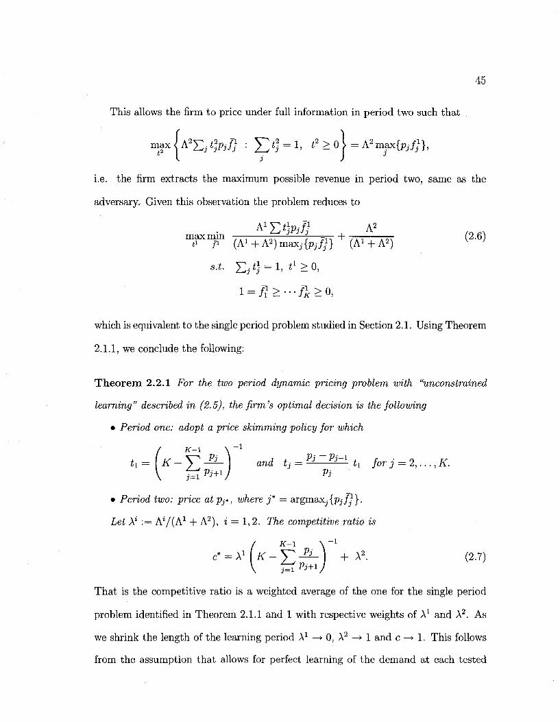
45

This allows the firm to price under full information in period two such that

max J A 2 E , t]Pjf} : £ t) = 1, t 2 > o U 2 maxfo / J} ,

i.e. the firm extracts the maximum possible revenue in period two, same as the

adversary. Given this observation the problem reduces to

• AlE*fei/? , A2

m ^ T (Ai+A^max,-^} + ( A ^ A 2 ! (2"6)

s.t. Ej*} = i. *x>o»

which is equivalent to the single period problem studied in Section 2.1. Using Theorem

2.1.1, we conclude the following:

Theorem 2.2.1 For the two period dynamic pricing problem with "unconstrained

learning" described in (2.5), the firm's optimal decision is the following

• Period one: adopt a price skimming policy for which

t x = \ K - Y — \ and ti = Vi~Vi-x tx forj = 2,...,K.

• Period two: price at Pj*, where j * = argmaXjjpy/l}.

Let A* :== A*/(A1 + A2), % — 1,2. The competitive ratio is

c* = \ x \ K - Y — I + A2. (2.7)

That is the competitive ratio is a weighted average of the one for the single period

problem identified in Theorem 2.1.1 and 1 with respective weights of A1 and A2. As

we shrink the length of the learning period A1 —> 0, A2 —> 1 and c —* 1. This follows

from the assumption that allows for perfect learning of the demand at each tested

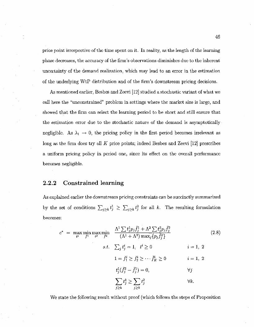
46

price point irrespective of the time spent on it. In reality, as the length of the learning

phase decreases, the accuracy of the firm's observations diminishes due to the inherent

uncertainty of the demand realization, which may lead to an error in the estimation

of the underlying WtP distribution and of the firm's downstream pricing decisions.

As mentioned earlier, Besbes and Zeevi [12] studied a stochastic variant of what we

call here the "unconstrained" problem in settings where the market size is large, and

showed that the firm can select the learning period to be short and still ensure that

the estimation error due to the stochastic nature of the demand is asymptotically

negligible. As Ai —> 0, the pricing policy in the first period becomes irrelevant as

long as the firm does try all K price points; indeed Besbes and Zeevi [12] prescribes

a uniform pricing policy in period one, since its effect on the overall performance

becomes negligible.

2.2.2 Constrained learning

As explained earlier the downstream pricing constraints can be succinctly summarized

by the set of conditions Ej>fc*} > J2j>ktf f° r a ^ ^- The resulting formulation

becomes:

c = max mm max mm ———-——£ —i_, (2.8) t1 f1 <2 P (A1+A2)maix:j{pjf?}

s.t. Ej*$ = l. **>0 i = l, 2

l = fi>n>---fK>0 z = l, 2

*}(£-/7) = o, v; X>]>X>? v*. j>k 3>.k

We state the following result without proof (which follows the steps of Proposition

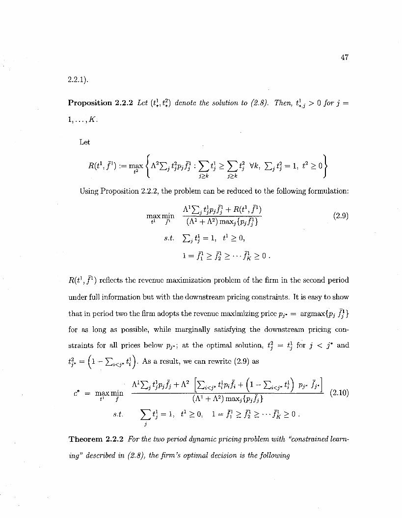
47

2.2.1).

Proposition 2.2.2 Let (tl,tl) denote the solution to (2.8). Then, £* • > 0 for j =

1,.. . ,K.

Let

R(t\ p) := max ( A 2 £ \ t)Vif) : £ t) > £ * ? Vfc, E ; *? = *> ^ ^ ° 1 I j>k j>k )

Using Proposition 2.2.2, the problem can be reduced to the following formulation:

max mm . , , , „, —=r-r- (2.9) t* /i ( A i + A ^ m a x ^ - / / } V y

i = / 7 > £ > - - - / l > o .

R{tl,fx) reflects the revenue maximization problem of the firm in the second period

under full information but with the downstream pricing constraints. It is easy to show

that in period two the firm adopts the revenue maximizing price Pj* = argmax{pj fj}

for as long as possible, while marginally satisfying the downstream pricing con

straints for all prices below p^; at the optimal solution, t? = t] for j < j * and

ft* — (1 — £i<7* t\\. As a result, we can rewrite (2.9) as

A T , t)Pjfs + A2 [J2i<r t\Vi]{ + (l - ?«<? t]) Pr fr max mm t1 / (A1 + A2)msxj{pjfj}

s.t. £>] = !, tx>0, l = fi>ft>---fk>0.

(2.10)

3

Theorem 2.2.2 For the two period dynamic pricing problem with "constrained learn

ing" described in (2.8), the firm's optimal decision is the following

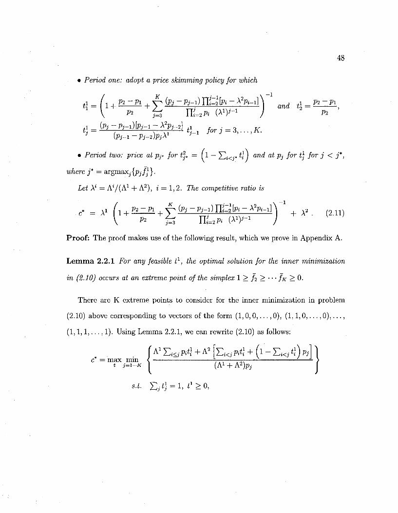
48

• Period one: adopt a price skimming policy for which

tl=(1 + ZLZlL + y fa ~Pi-}) E 2 \ P i - A V i ] \ l and tL = ?lZPL

t] = fe^zlfci^zHl t U forj=3,...,K. 3 (pj-x-pj^PjX1 3

• Period two: price at pj* for £2» = (1 — X)»<j* ^ ) and a^ Pj for *} for J < 3*>

where j * = argmaXj-jjpj/^}.

Let Xi = A*/(A1 + A2), i = 1,2. TTie competitive ratio is

e = Ai f! + gLZfi + y fa - Pi-i) n S b* - AVi] \ - 1 A2 (211)

V » ^ uupi (A1)-1 y

Proof: The proof makes use of the following result, which we prove in Appendix A.

Lemma 2.2.1 For any feasible t1, the optimal solution for the inner minimization

in (2.10) occurs at an extreme point of the simplex 1 > fi > • • • fx > 0.

There are K extreme points to consider for the inner minimization in problem

(2.10) above corresponding to vectors of the form (1,0 ,0 , . . . , 0), (1 ,1 ,0 , . . . , 0 ) , . . . ,

( 1 ,1 ,1 , . . . , 1). Using Lemma 2.2.1, we can rewrite (2.10) as follows:

A1 £,<, Pit} + A2 [EiKj M1 + (l - £i<, tj) Pj

c = max mm t j=i-K 1 (Ai + A2)^-

s.t. E i ^ = i. ^ > o ,

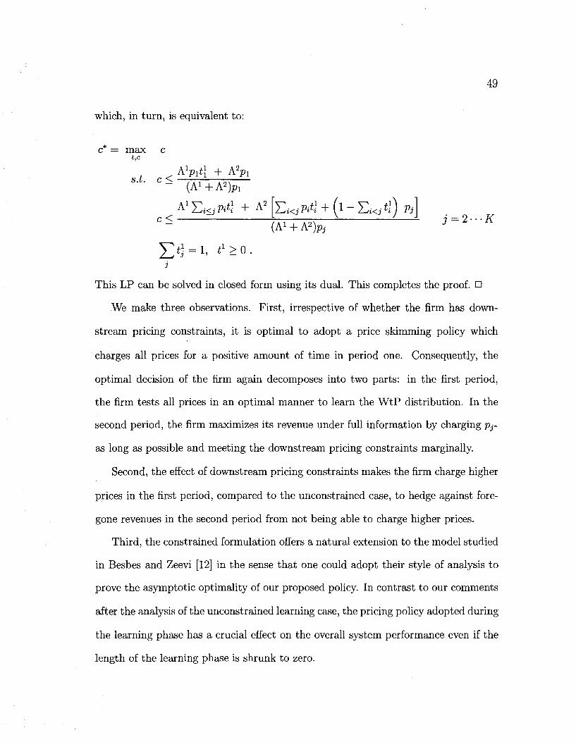
which, in turn, is equivalent to:

c = max t,c

S.t. C < ( A i + A 2 ) ^

c < A ^ f t t J + A2 [E^M1 + (l " £*,-**) Pj

(Ai+A2)^-

E*} = i, ^>o

49

j = 2- - -K

This LP can be solved in closed form using its dual. This completes the proof. •

We make three observations. First, irrespective of whether the firm has down

stream pricing constraints, it is optimal to adopt a price skimming policy which

charges all prices for a positive amount of time in period one. Consequently, the

optimal decision of the firm again decomposes into two parts: in the first period,

the firm tests all prices in an optimal manner to learn the WtP distribution. In the

second period, the firm maximizes its revenue under full information by charging pj*

as long as possible and meeting the downstream pricing constraints marginally.

Second, the effect of downstream pricing constraints makes the firm charge higher

prices in the first period, compared to the unconstrained case, to hedge against fore

gone revenues in the second period from not being able to charge higher prices.

Third, the constrained formulation offers a natural extension to the model studied

in Besbes and Zeevi [12] in the sense that one could adopt their style of analysis to

prove the asymptotic optimality of our proposed policy. In contrast to our comments

after the analysis of the unconstrained learning case, the pricing policy adopted during

the learning phase has a crucial effect on the overall system performance even if the

length of the learning phase is shrunk to zero.

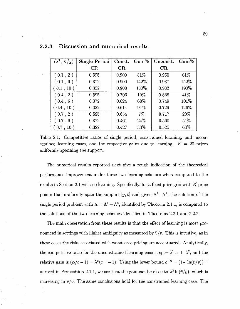
50

2 . 2 . 3 D i s c u s s i o n a n d n u m e r i c a l r e s u l t s

(A1, v /v)

( 0.1 , 2 )

( 0.1 , 6 ) ( 0.1 , 10 ) ( 0.4 , 2 ) ( 0.4 , 6 ) ( 0.4 , 10 ) ( 0.7 , 2 ) ( 0.7 , 6 ) ( 0.7 , 10 )

Single Period CR

0.595 0.372 0.322

0.595 0.372 0.322

0.595

0.372

0.322

Const. Gain% CR

0.900 51%

0.900 142%

0.900 180%

0.706 19% 0.624 68% 0.614 91%

0.634 7%

0.461 24%

0.427 33%

Unconst. Gain%

CR 0.960 61% 0.937 152% 0.932 190%

0.838 41% 0.749 101% 0.729 126%

0.717 20%

0.560 51%

0.525 63%

Table 2.1: Competitive ratios of single period, constrained learning, and unconstrained learning cases, and the respective gains due to learning. K = 20 prices uniformly spanning the support.

The numerical results reported next give a rough indication of the theoretical

performance improvement under these two learning schemes when compared to the

results in Section 2.1 with no learning. Specifically, for a fixed price grid with K price

points that uniformly span the support [v,v] and given A1, A2, the solution of the

single period problem with A = A1 + A2, identified by Theorem 2.1.1, is compared to

the solutions of the two learning schemes identified in Theorems 2.2.1 and 2.2.2.

The main observation from these results is that the effect of learning is most pro

nounced in settings with higher ambiguity as measured by v/v. This is intuitive, as in

these cases the risks associated with worst-case pricing are accentuated. Analytically,

the competitive ratio for the unconstrained learning case is Q := A1 c + A2, and the

relative gain is (Q/C— 1) = A2(c_1 — 1). Using the lower bound cLB = (l + \n(v/v))~l

derived in Proposition 2.1.1, we see that the gain can be close to X2ln(v/v), which is

increasing in v/v. The same conclusions hold for the constrained learning case. The

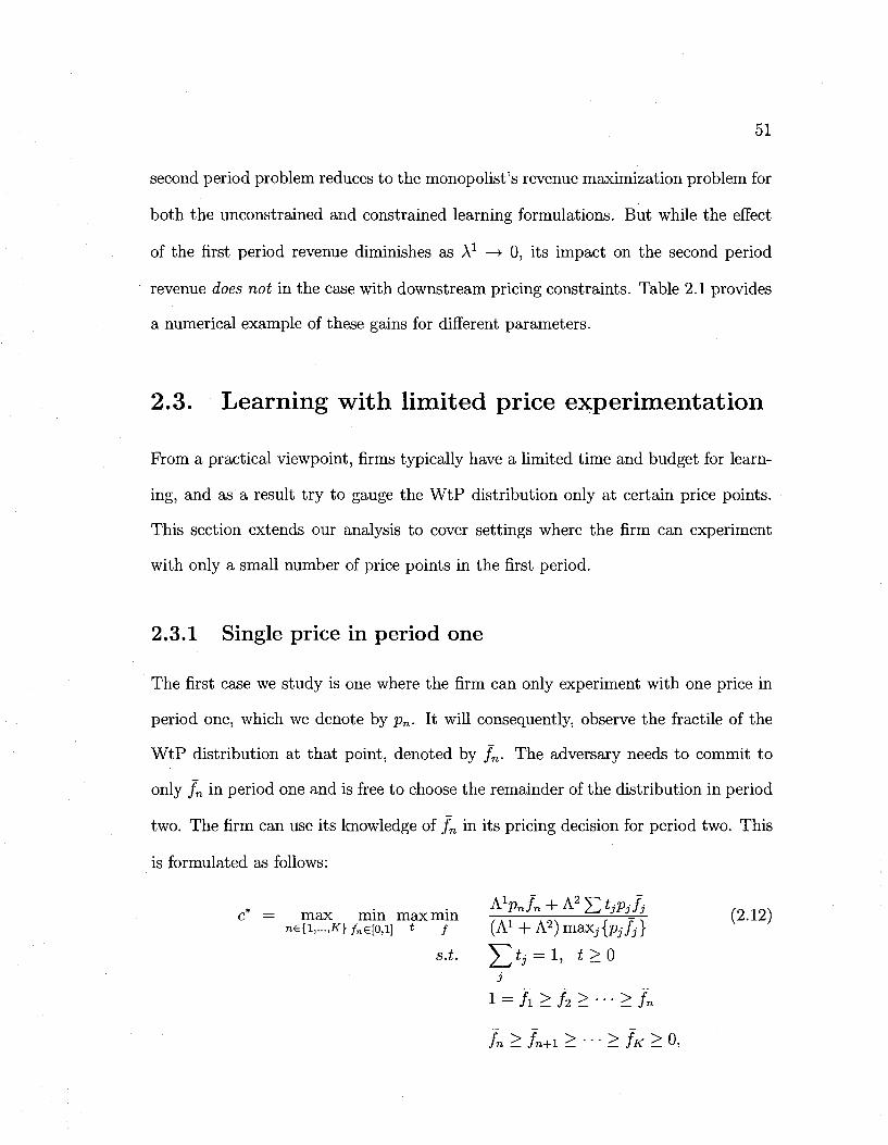
51

second period problem reduces to the monopolist's revenue maximization problem for

both the unconstrained and constrained learning formulations. But while the effect

of the first period revenue diminishes as A1 —> 0, its impact on the second period

revenue does not in the case with downstream pricing constraints. Table 2.1 provides

a numerical example of these gains for different parameters.

2.3. Learning with limited price experimentation

Prom a practical viewpoint, firms typically have a limited time and budget for learn

ing, and as a result try to gauge the WtP distribution only at certain price points.

This section extends our analysis to cover settings where the firm can experiment

with only a small number of price points in the first period.

2.3.1 Single price in period one

The first case we study is one where the firm can only experiment with one price in

period one, which we denote by pn. It will consequently, observe the fractile of the

WtP distribution at that point, denoted by fn. The adversary needs to commit to

only fn in period one and is free to choose the remainder of the distribution in period

two. The firm can use its knowledge of fn in its pricing decision for period two. This

is formulated as follows:

A1Pnfn + A2^2tjPjfj

c — max mm max mm —— — / -:; (2.12) n€{i,...,A-}/„e[o,i] * / (A1+A2)maxj{pjfj}

s.t. ^rt, = i, t>o j

1 = h > h > • • • > fn

j n > / n + l > " - - > J X > 0 ,

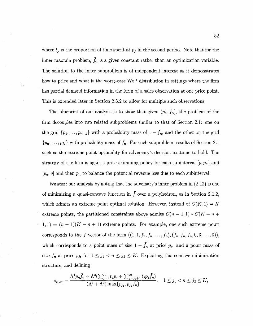
52

where tj is the proportion of time spent at pj in the second period. Note that for the

inner maxmin problem, fn is a given constant rather than an optimization variable.

The solution to the inner subproblem is of independent interest as it demonstrates

how to price and what is the worst-case WtP distribution in settings where the firm

has partial demand information in the form of a sales observation at one price point.

This is extended later in Section 2.3.2 to allow for multiple such observations.

The blueprint of our analysis is to show that given (pn,fn), the problem of the

firm decouples into two related subproblems similar to that of Section 2.1: one on

the grid {pi,,.. ,pn-i} with a probability mass of 1 — fn, and the other on the grid

{pn,... ,PK} with probability mass of fn. For each subproblem, results of Section 2.1

such as the extreme point optimality for adversary's decision continue to hold. The

strategy of the firm is again a price skimming policy for each subinterval [v,pn) and

\pn, v] and then pn to balance the potential revenue loss due to each subinterval.

We start our analysis by noting that the adversary's inner problem in (2.12) is one

of minimizing a quasi-concave function in / over a polyhedron, as in Section 2.1.2,

which admits an extreme point optimal solution. However, instead of C(K, 1) = K

extreme points, the partitioned constraints above admits C(n — 1,1) * C(K — n +

1,1) = (n — 1)(K — n + 1) extreme points. For example, one such extreme point

corresponds to the / vector of the form ((1,1, /„, / „ , . . . , /„), (/„, /„, /„, 0 ,0 , . . . , 0)),

which corresponds to a point mass of size 1 — fn at price Pjx and a point mass of

size fn at price Pj2 for l<ji<n<J2<K. Exploiting this concave minimization

structure, and defining

_ AW„ + A2(EjLi tjPj + Ef=J1+i tjPjfn) -h,h (A i + A2)maxfe i , P j 2 / n } ch,h = , A I , A ^ F H i ' 1<h<n<j2<K,

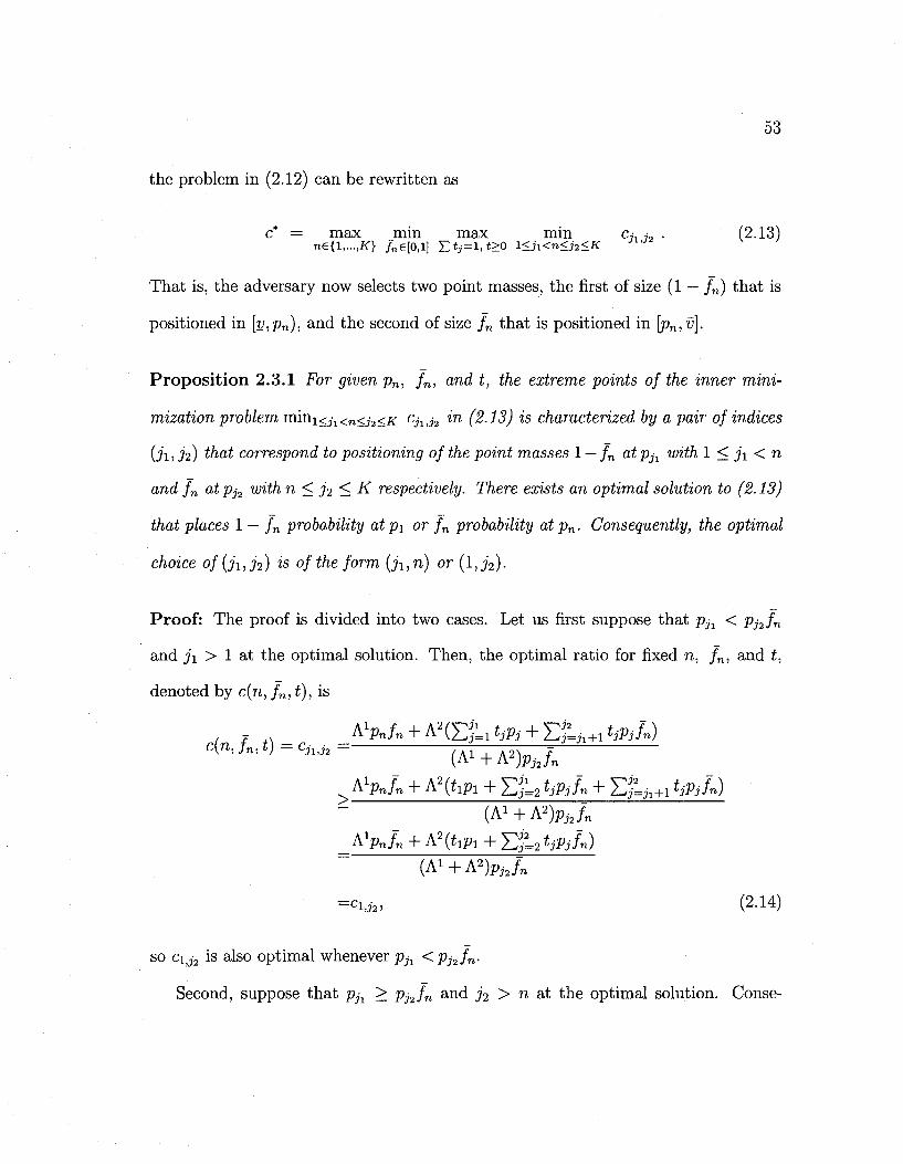
53

the problem in (2.12) can be rewritten as

c* = max min max min c,-, ,-, . (2.13) ne{l,...,K} /„€[0,1] E*j=M>0 l<h<n<J2<K

That is, the adversary now selects two point masses, the first of size (1 — fn) that is

positioned in [y,pn), and the second of size fn that is positioned in [pnj^]-

Proposition 2.3.1 For given pn, fn, and t, the extreme points of the inner mini

mization problem mini<j1<n<j2<^- Cjuj2 in (2.13) is characterized by a pair of indices

{J11J2) that correspond to positioning of the point masses 1 — fn atpjx with 1 < ji < n

and fn atpj2 with n < j 2 < K respectively. There exists an optimal solution to (2.13)

that places 1 — /„ probability atpi or fn probability atpn. Consequently, the optimal

choice of(ji,j2) is of the form (ji,n) or(l,j2).

Proof: The proof is divided into two cases. Let us first suppose that p^ < Pj2fn

and ji > 1 at the optimal solution. Then, the optimal ratio for fixed n, fn, and t,

denoted by c(n, fn,t), is

Cy^i Jnit) Cjlt

A W n + A2(EjLl tjPj + Sf=il+1 tjpjn) (V+A^PjJn

^ AlPJn + A2 (tlPl + Ef=2 tjPjfn + Ef=il+1 tjPifn)

{^+h?)PjJn

_A'Pn/n + A2(tlPl + Ef=2 tjPjfn)

(Ai + A*)PjJn

=d,h, (2-14)

so Citj2 is also optimal whenever pj± < Pj2fn.

Second, suppose that Pjx > Pj2fn and j2 > n at the optimal solution. Conse-

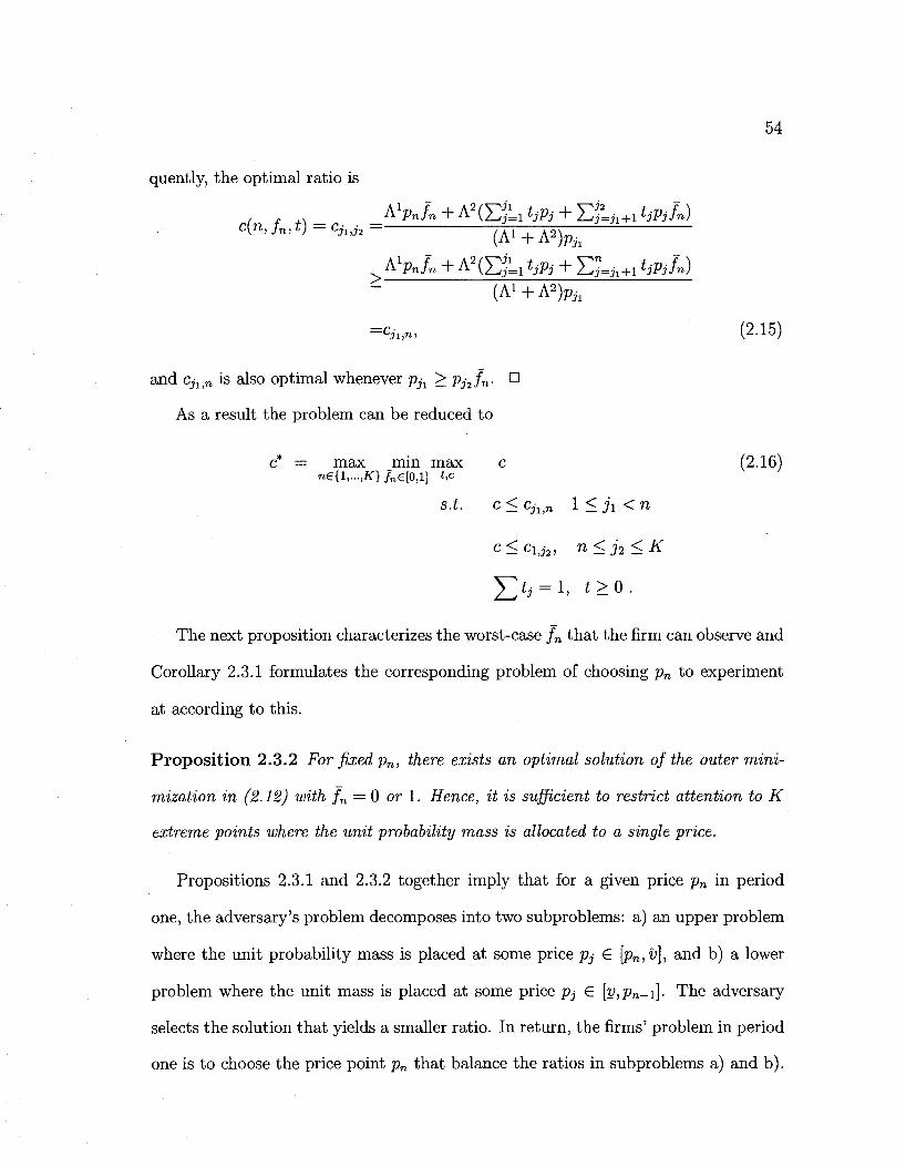
54

quently, the optimal ratio is

AVA + A 2 (£ t l tjPj + YSLh+1 tjPjfn) c\n> Jn>t) — cji,J2

>

(A1 + A2K Vpnfn + A2(EjLl tjPj + S;=J1+1 tjPjfn)

(A*+A*)Pil

~Cjl,nj (2.15)

and CjljTl is also optimal whenever pjx > Pj2fn- n

As a result the problem can be reduced to

c* = max min max c (2.16) n€{l,...,K} /„e[0,l] t,c

s.t. c < CjltJl 1 < ji < n

c<ci,j2, n<j2<K

The next proposition characterizes the worst-case fn that the firm can observe and

Corollary 2.3.1 formulates the corresponding problem of choosing pn to experiment

at according to this.

Proposition 2.3.2 For fixed pn, there exists an optimal solution of the outer mini

mization in (2.12) with fn = 0 or 1. Hence, it is sufficient to restrict attention to K

extreme points where the unit probability mass is allocated to a single price.

Propositions 2.3.1 and 2.3.2 together imply that for a given price pn in period

one, the adversary's problem decomposes into two subproblems: a) an upper problem

where the unit probability mass is placed at some price pj G [pn,^], and b) a lower

problem where the unit mass is placed at some price pj e [2;,p„_!]. The adversary

selects the solution that yields a smaller ratio. In return, the firms' problem in period

one is to choose the price point pn that balance the ratios in subproblems a) and b).

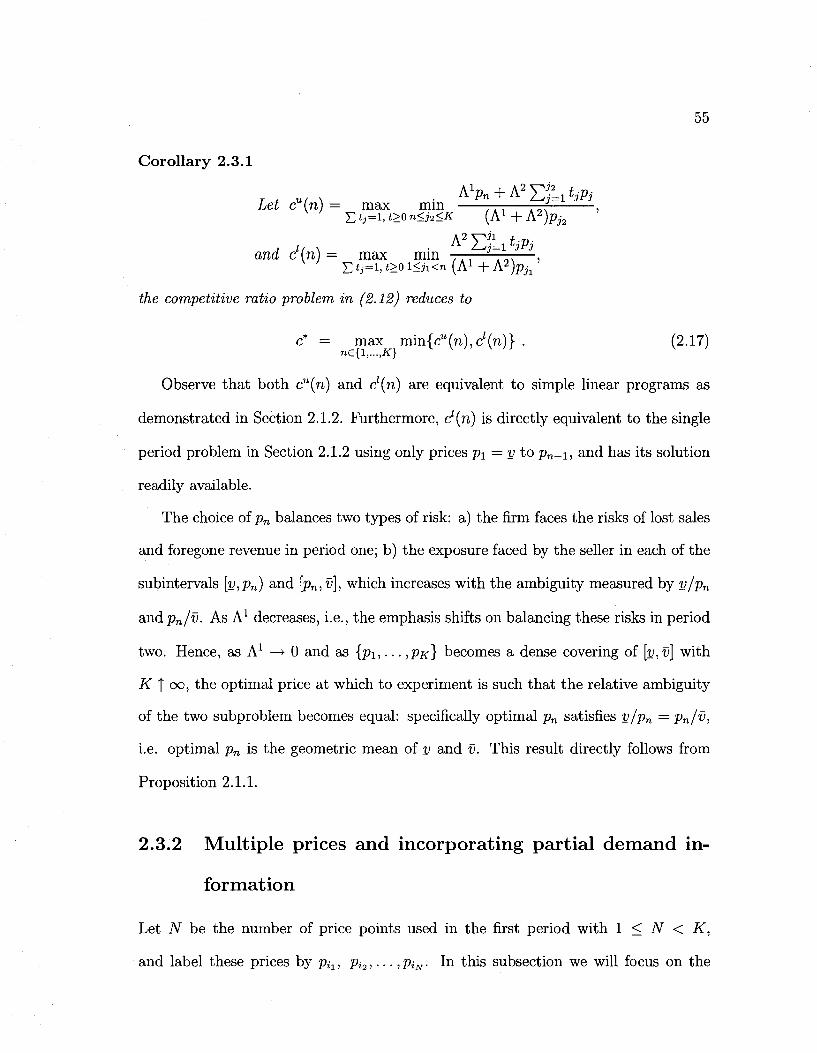
55

Corollary 2.3.1

Let c (n) = max mm — -^ ,

T,tj=l,t>0n<j2<K (A^+A^Pjz

ana c (n) — max mm - — - — — T : — , £ *j=i. *>o i<n<« (A1 + A 2 ) ^

the competitive ratio problem in (2.12) reduces to

c* = max mm{cu(n),cl(n)} . (2.17) n£{l,...,K}

Observe that both cu(n) and cl(n) are equivalent to simple linear programs as

demonstrated in Section 2.1.2. Furthermore, cl(n) is directly equivalent to the single

period problem in Section 2.1.2 using only prices p\ = v to pn-i, and has its solution

readily available.

The choice of pn balances two types of risk: a) the firm faces the risks of lost sales

and foregone revenue in period one; b) the exposure faced by the seller in each of the

subintervals [v,pn) and [pn, v], which increases with the ambiguity measured by v/pn

and pn/v. As A1 decreases, i.e., the emphasis shifts on balancing these risks in period

two. Hence, as A1 —> 0 and as {pi,... ,PK} becomes a dense covering of [v, v] with

K | oo, the optimal price at which to experiment is such that the relative ambiguity

of the two subproblem becomes equal: specifically optimal pn satisfies v/pn = pn/v,

i.e. optimal pn is the geometric mean of v and v. This result directly follows from

Proposition 2.1.1.

2.3.2 Multiple prices and incorporating partial demand in

formation

Let N be the number of price points used in the first period with 1 < N < K,

and label these prices by Pii: pi2,...,piN. In this subsection we will focus on the

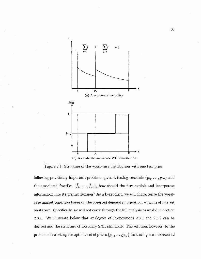
56

t • x

(a) A representative policy

F(x)

K

• * • x Y P„ v

(b) A candidate worst-case W t P distribution

Figure 2.1: Structure of the worst-case distribution with one test price

following practically important problem: given a testing schedule {pil1... ,PiN} and

the associated fractiles {fa,... ,fiN}, how should the firm exploit and incorporate

information into its pricing decision? As a byproduct, we will characterize the worst-

case market condition based on the observed demand information, which is of interest

on its own. Specifically, we will not carry through the full analysis as we did in Section

2.3.1. We illustrate below that analogues of Propositions 2.3.1 and 2.3.2 can be

derived and the structure of Corollary 2.3.1 still holds. The solution, however, to the

problem of selecting the optimal set of prices {pix,..., PiN } for testing is combinatorial

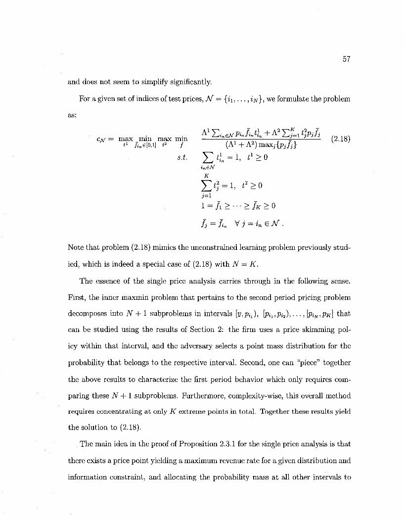
57

and does not seem to simplify significantly.

For a given set of indices of test prices, J\f = {ii,..., i^}, we formulate the problem

as:

CM = max mm max mm v—— — —f^—- (2.18) *x /<„€[o,i] *2 / (A1+A2)maxj{pjfj}

JnG.A/'

K

1 = /i > • • • > h > 0

Ij = Iin Vj = ineN-

Note that problem (2.18) mimics the unconstrained learning problem previously stud

ied, which is indeed a special case of (2.18) with N = K.

The essence of the single price analysis carries through in the following sense.

First, the inner maxmin problem that pertains to the second period pricing problem

decomposes into iV + 1 subproblems in intervals [VJP^), \pii:Pi2), • • •, \piN,Pi<} that

can be studied using the results of Section 2: the firm uses a price skimming pol

icy within that interval, and the adversary selects a point mass distribution for the

probability that belongs to the respective interval. Second, one can "piece" together

the above results to characterize the first period behavior which only requires com

paring these N + 1 subproblems. Furthermore, complexity-wise, this overall method

requires concentrating at only K extreme points in total. Together these results yield

the solution to (2.18).

The main idea in the proof of Proposition 2.3.1 for the single price analysis is that

there exists a price point yielding a maximum revenue rate for a given distribution and

information constraint, and allocating the probability mass at all other intervals to

58

the lowest possible price can only improve the objective function of the adversary (i.e.

reduce the ratio), because it potentially reduces the numerator with the denominator

unchanged (see equations (2.14) and (2.15)). The same argument goes through when

we have more fractile observations with the same steps for each interval. We state

this in the following, the proof of which follows similar steps to Proposition 2.3.1 and

is therefore omitted.

Proposition 2.3.3 If fractile information at N < K points are given, one can still

restrict attention to K extreme points for the inner minimization problem. For rj —

1 . . . N — 1, each extreme point is of the form fj = fin — fa +1 for some iv < j < iv+\

and fin = fin - fin+1 for all other n^rj.

That is we consider a price interval [p^,Pi^+1) one at a time and fix the probability

mass for all other intervals at the lowest price possible, ie. fcn = /;n - fin+1, n ^ r),

while assuming the mass at this interval is at one of the price points within the

interval. Consequently, it is sufficient again to concentrate on a total of K extreme

points.

This seemingly simple result is important because the number of extreme points

can in general grow exponentially with additional information as explained before.

For example, while adding a constraint on the mean of the WtP distribution will

increase the number of extreme points to 0(K2), fractile information can be in

corporated without effectively increasing the number of extreme points to consider.

Furthermore, given the fractile information the resulting competitive ratio problem

for the remaining sales horizon can be solved using a simple LP formulation which

will be illustrated later in this section.

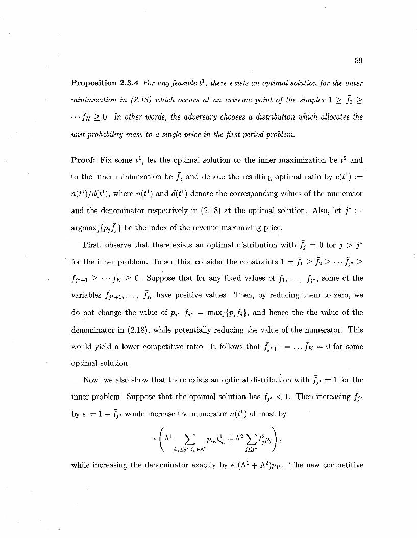
59

Proposition 2.3.4 For any feasible t1, there exists an optimal solution for the outer

minimization in (2.18) which occurs at an extreme point of the simplex 1 > fi >

• • • fx > 0. In other words, the adversary chooses a distribution which allocates the

unit probability mass to a single price in the first period problem.

Proof: Fix some t1, let the optimal solution to the inner maximization be t2 and

to the inner minimization be / , and denote the resulting optimal ratio by c(tx) :=

n(i1)/d(i1), where n(tl) and dft1) denote the corresponding values of the numerator

and the denominator respectively in (2.18) at the optimal solution. Also, let j * :=

argmaXj{pj/j} be the index of the revenue maximizing price.

First, observe that there exists an optimal distribution with fj = 0 for j > j *

for the inner problem. To see this, consider the constraints 1 = / i > fi > • • • fj* >

fj*+i > '"" fx > 0. Suppose that for any fixed values of / i , . . . , fj*, some of the

variables fj*+i, • • •, JK have positive values. Then, by reducing them to zero, we

do not change the value of Pj* fj* = max.j{pjfj}, and hence the the value of the

denominator in (2.18), while potentially reducing the value of the numerator. This

would yield a lower competitive ratio. It follows that fj*+i = . . . /«• = 0 for some

optimal solution.

Now, we also show that there exists an optimal distribution with fj* = 1 for the

inner problem. Suppose that the optimal solution has fj* < 1. Then increasing fj*

by e := 1 — fj* would increase the numerator n(tl) at most by

while increasing the denominator exactly by e (A1 + A2)pj*. The new competitive

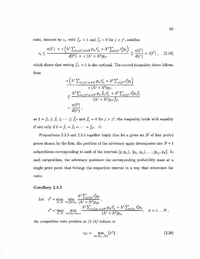
60

<

ratio, denoted by ce, with fj* = 1 and /_,- = 0 for j > j * , satisfies

"('1) + <A1E„a.,i,^ft„t;.+A'EJ<J.»J) n((1) _ ' S d(t') + e (A1 + A2)ft. S d((i) ~ Cl ' ' l a )

which shows that setting fj* = 1 is also optimal. The second inequality above follows

from

e (A1 J2in<r,ineArPintl + A2 S J < J . foj)

e (A 1 +A 2 )p j .

A }-*lin<j*,ineArPinJintin+ A 2^j<j*tjPjjj

(Ai + A^p,-.^.

as 1 = / i > /2 > • • • > / j * and fj = 0 for j > j * ; the inequality holds with equality

if and only if 1 = /x = /2 = • • • = fj*. •

Propositions 2.3.3 and 2.3.4 together imply that for a given set N of first period

prices chosen by the firm, the problem of the adversary again decomposes into N + 1

subproblems corresponding to each of the intervals [v,;Pti)> \Pi1,Pi2)> • • • > b*jv>Ptfl- I*1

each subproblem, the adversary positions the corresponding probability mass at a

single price point that belongs the respective interval in a way that minimizes the

ratio.

Corollary 2.3.2

T , 0 . A }_/j<jotjPj Let c = max mm . A1 ~ o s — ,

t1,*2 I<JO<I„ (A1+A2)p:,o

cf = max min A* ^ < ^ P ^ l + A2 E ^ % n = = 1 < _ ^ t1,*2 Jn<jn<i„+1 ( A 1 + A 2 ) P j n

i/ie competitive ratio problem in (2.18) reduces to

cM = min {cn} . (2.20) n€{0,...,N}

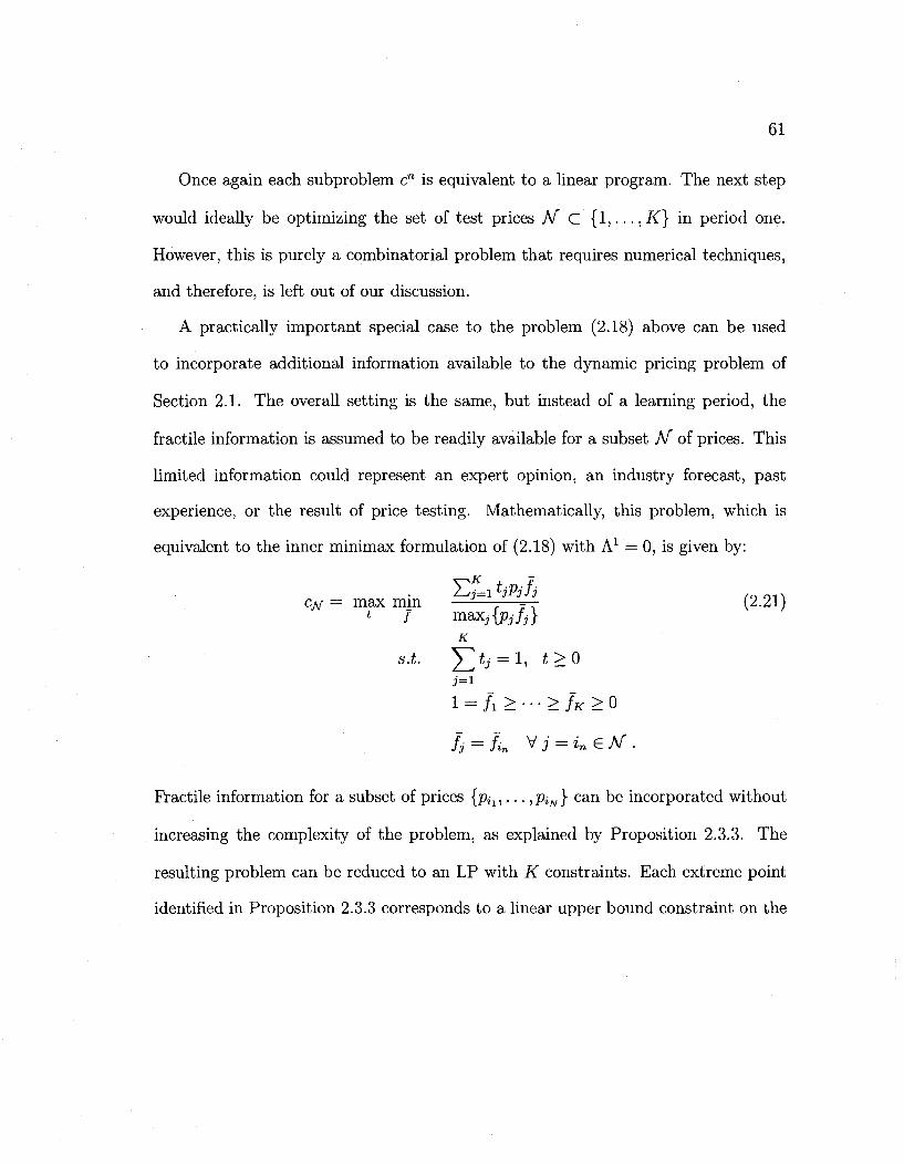
61

Once again each subproblem c" is equivalent to a linear program. The next step

would ideally be optimizing the set of test prices M C { 1 , . . . ,K} in period one.

However, this is purely a combinatorial problem that requires numerical techniques,

and therefore, is left out of our discussion.

A practically important special case to the problem (2.18) above can be used

to incorporate additional information available to the dynamic pricing problem of

Section 2.1. The overall setting is the same, but instead of a learning period, the

fractile information is assumed to be readily available for a subset J\f of prices. This

limited information could represent an expert opinion, an industry forecast, past

experience, or the result of price testing. Mathematically, this problem, which is

equivalent to the inner minimax formulation of (2.18) with A1 = 0, is given by:

CM — max mm —-—-—=— (2-21) t f m^iiPjfj}

K

s.t. ^ t , = l, £ > 0

1 = A > • • • > IK > 0

Fractile information for a subset of prices {pix,..., piN} can be incorporated without

increasing the complexity of the problem, as explained by Proposition 2.3.3. The

resulting problem can be reduced to an LP with K constraints. Each extreme point

identified in Proposition 2.3.3 corresponds to a linear upper bound constraint on the

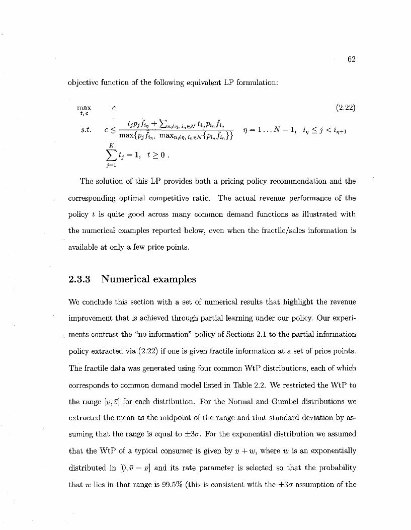
62

objective function of the following equivalent LP formulation:

max c (2.22) t, c

S.i. C < ? = ^ T—- r]=l...N-l, lv<J<lr,+l

K

J > = i, *>o. j = l

The solution of this LP provides both a pricing policy recommendation and the

corresponding optimal competitive ratio. The actual revenue performance of the

policy t is quite good across many common demand functions as illustrated with

the numerical examples reported below, even when the fractile/sales information is

available at only a few price points.

2.3.3 Numerical examples

We conclude this section with a set of numerical results that highlight the revenue

improvement that is achieved through partial learning under our policy. Our experi

ments contrast the "no information" policy of Sections 2.1 to the partial information

policy extracted via (2.22) if one is given fractile information at a set of price points.

The fractile data was generated using four common WtP distributions, each of which

corresponds to common demand model listed in Table 2.2. We restricted the WtP to

the range [v,v] for each distribution. For the Normal and Gumbel distributions we

extracted the mean as the midpoint of the range and that standard deviation by as

suming that the range is equal to ±3<r. For the exponential distribution we assumed

that the WtP of a typical consumer is given by v + w, where w is an exponentially

distributed in [0, v — v] and its rate parameter is selected so that the probability

that w lies in that range is 99.5% (this is consistent with the ±3<r assumption of the

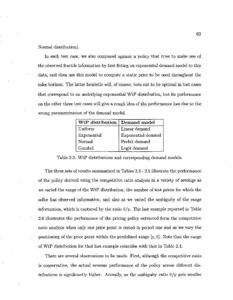
63

Normal distribution).

In each test case, we also compared against a policy that tries to make use of

the observed fractile information by first fitting an exponential demand model to this

data, and then use this model to compute a static price to be used throughout the

sales horizon. The latter heuristic will, of course, turn out to be optimal in test cases

that correspond to an underlying exponential WtP distribution, but its performance

on the other three test cases will give a rough idea of the performance loss due to the

wrong parametrization of the demand model.

W t P distribution Uniform

Exponential

Normal

Gumbel

Demand model Linear demand

Exponential demand

Probit demand

Logit demand

Table 2.2: WtP distributions and corresponding demand models.

The three sets of results summarized in Tables 2.3-2.5 illustrate the performance

of the policy derived using the competitive ratio analysis in a variety of settings as

we varied the range of the WtP distribution, the number of test prices for which the

seller has observed information, and also as we varied the ambiguity of the range

information, which is captured by the ratio v/v. The last example reported in Table

2.6 illustrates the performance of the pricing policy extracted form the competitive

ratio analysis when only one price point is tested in period one and as we vary the

positioning of the price point within the predefined range [y,v]. Note that the range

of WtP distribution for that last example coincides with that in Table 2.4.

There are several observations to be made. First, although the competitive ratio

is conservative, the actual revenue performance of the policy across different dis

tributions is significantly higher. Actually, as the ambiguity ratio v/v gets smaller

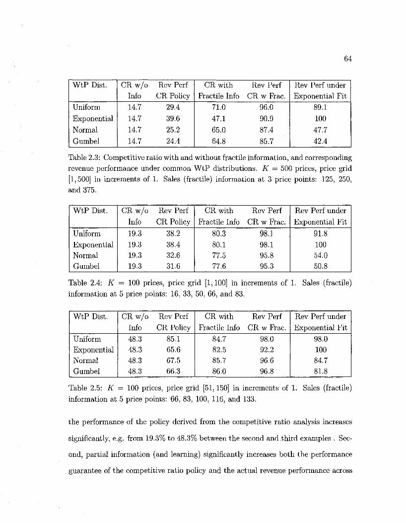
64

WtP Dist.

Uniform

Exponential

Normal

Gumbel

CRw/o Info

14.7

14.7

14.7

14.7

Rev Perf CR Policy

29.4

39.6

25.2

24.4

CR with Fractile Info

71.0

47.1

65.0

64.8

Rev Perf CR w Frac.

96.0

90.9

87.4

85.7

Rev Perf under Exponential Fit

89.1

100

47.7

42.4

Table 2.3: Competitive ratio with, and without fractile information, and corresponding revenue performance under common WtP distributions. K = 500 prices, price grid [1,500] in increments of 1. Sales (fractile) information at 3 price points: 125, 250, and 375.

WtP Dist.

Uniform

Exponential Normal Gumbel

CRw/o

Info

19.3 19.3 19.3 19.3

Rev Perf

CR Policy

38.2 38.4 32.6 31.6

CR with

Fractile Info

80.3

80.1 77.5 77.6

Rev Perf

CR w Frac.

98.1 98.1 95.8 95.3

Rev Perf under

Exponential Fit

91.8 100 54.0 50.8

Table 2.4: K — 100 prices, price grid [1,100] in increments of 1. Sales (fractile)

information at 5 price points: 16, 33, 50, 66, and 83.

WtP Dist.

Uniform Exponential Normal Gumbel

CRw/o

Info

48.3 48.3 48.3 48.3

Rev Perf

CR Policy

85.1 65.6 67.5 66.3

CR with

Fractile Info

84.7 82.5 85.7 86.0

Rev Perf

CR w Frac.

98.0 92.2 96.6 96.8

Rev Perf under

Exponential Fit

98.0 100 84.7 81.8

Table 2.5: K = 100 prices, price grid [51,150] in increments of 1. Sales (fractile)

information at 5 price points: 66, 83, 100, 116, and 133.

the performance of the policy derived from the competitive ratio analysis increases

significantly, e.g. from 19.3% to 48.3% between the second and third examples . Sec

ond, partial information (and learning) significantly increases both the performance

guarantee of the competitive ratio policy and the actual revenue performance across

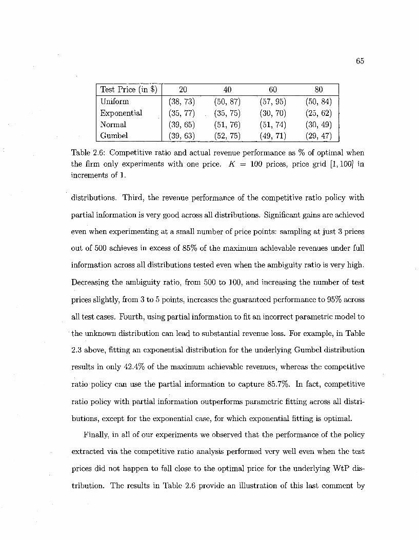
65

Test Price (in $)

Uniform

Exponential

Normal Gumbel

20

(38, 73)

(35, 77)

(39, 65) (39, 63)

40

(50, 87)

(35, 75)

(51, 76) (52, 75)

60

(57, 95)

(30, 70)

(51, 74) (49, 71)

80

(50, 84)

(25, 62)

(30, 49) (29, 47)

Table 2.6: Competitive ratio and actual revenue performance as % of optimal when the firm only experiments with one price. K = 100 prices, price grid [1,100] in increments of 1.

distributions. Third, the revenue performance of the competitive ratio policy with

partial information is very good across all distributions. Significant gains are achieved

even when experimenting at a small number of price points: sampling at just 3 prices

out of 500 achieves in excess of 85% of the maximum achievable revenues under full

information across all distributions tested even when the ambiguity ratio is very high.

Decreasing the ambiguity ratio, from 500 to 100, and increasing the number of test

prices slightly, from 3 to 5 points, increases the guaranteed performance to 95% across

all test cases. Fourth, using partial information to fit an incorrect parametric model to

the unknown distribution can lead to substantial revenue loss. For example, in Table

2.3 above, fitting an exponential distribution for the underlying Gumbel distribution

results in only 42.4% of the maximum achievable revenues, whereas the competitive

ratio policy can use the partial information to capture 85.7%. In fact, competitive

ratio policy with partial information outperforms parametric fitting across all distri

butions, except for the exponential case, for which exponential fitting is optimal.

Finally, in all of our experiments we observed that the performance of the policy

extracted via the competitive ratio analysis performed very well even when the test

prices did not happen to fall close to the optimal price for the underlying WtP dis

tribution. The results in Table 2.6 provide an illustration of this last comment by

66

focusing at the performance of the policy extracted via the competitive ratio anal

ysis as we vary the position of a single price point for which the seller has fractile

information. As a benchmark we note that the competitive ratio and actual revenue

performance of the policy based on the competitive ratio analysis without the fractile

information was reported in the first and second columns of Table 2.4. In addition,

the optimal prices that would correspond to each of the WtP distributions that we

tried were 50 for the Uniform, 19 for the Exponential, 39 for the Normal and the

Gumbel distributions.

2.4. Other pricing mechanisms

2.4.1 Third degree price discrimination

We consider the problem of revenue maximization for a monopolist firm that offers

a product to a market of size A. Each consumer has a WtP for one unit of that

product, denoted by v, that is an independent draw form a common distribution F

with support [v, v]. We assume that the market can be segmented into distinct groups,

e.g., through the observation of a consumer attribute or -as in the case of call centers-

using consumer information that has been collected through prior interactions that

the firm may have had with each consumer. This segmentation procedure separates

the market, and the WtP distribution, into K contiguous groups, where segment j

comprises of consumers with WtP v e [VJ,VJ+I). Let v = {vi,... ,VK} and VQ — v

to reduce the notation. The firm can customize its price to each segment. For a

price vector p, the firm's revenue is given by R(v,p,F) = Ylj=o Pj - ^(vj+i > v —

Pj)+pK AP(v >v >pK)-

67

The full information problem has two parts: the first is to select its pricing vector

p to optimize her revenues under a given segmentation rule v, and the second is to

also optimize over its choice of segments as well. The solution of the first question

is easy to describe: for each segment the firm selects a price to maximize revenues

form that segment that is characterized by the conditional WtP distribution on the

subinterval [VJ,VJ+I), and the pricing decisions across segments are decoupled (this

follows from the absence of the capacity constraint). The problem of selecting the

segments within the WtP distribution can also be formulated as an optimization

problem, whose tractability, however, depends on the structure of the distribution

F. In the sequel, we will denote by p*(v) the optimal pricing rule given v for the

competitive ratio or maximum regret problem, by v* the optimal segmentation rule,

and by v*(F) and p*(v, F) the revenue maximizing segmentation and price vector for

given v respectively under full information about distribution F. In the remainder of

this section we will study the above two questions in a setting where the firm knows

-or can choose- the segmentation rule v and the price vector p(v), but does not know

the WtP distribution F.

2.4.1.1 Competitive ratio

Taking the segmentation decision v as fixed to start with, the firm's third degree

price discrimination problem under the competitive ratio criterion is the following:

R(v,p,F) max mm Pj € [vj,vj+1) for j = 0 , . . . , K - 1, pK e [vK, v] >

v F \R{v,p*(v,F),F)

(2.23)

Proposition 2.4.1 Given a segmentations, the optimal price vector p for (2.23) is:

p* = VJ for allj.

68

Proof: Assume by contradiction Pj > Vj for some j . Then, the adversary can set

everyone's valuation at Vj deterministically, which would result in zero revenues, and

therefore, a competitive ratio of zero. Setting p*, = Vj for all j would guarantee a

positive ratio. •

The above result is somewhat expected, since both the firm's and adversary's

decisions are essentially decoupled across segments, and the above strategy is the only

one that will result in non-zero revenues. Consequently, the total revenue extracted

by the firm is given by K-\ K

R(v,p*, F) = Y^ VJ A pfe+i > v ^ vi) +vKAP(v>v>vK)=A J^Vj /,-, j=o j=o

where fj = P(fj+i > v > Vj) for j = 0 , . . . , K — 1 and fa = P(v > v > vK) . Note

that for a given segmentation rule v, the revenue earned by the firm under the optimal

pricing policy does not depend on the particular specification of the distribution F(-)

on the interval [vj,Vj+x), but only on the total probability mass fj allocated to each

such interval. However, the competitive ratio may potentially depend on the specifics

of the distribution F(-) on each such interval, as different WtP distributions yield

different first-best revenues. The next result characterizes the optimal competitive

ratio for a given a segmentation and the WtP distribution that is selected by the

adversary.

Proposition 2.4.2 Let j * = argmin^ {VJ/VJ+I}. Given a segmentation v, the adver

sary's strategy is to set the WtP of every customer equal to (i>j*+i — e), where e > 0 is

an arbitrarily small constant chosen by the adversary. The optimal competitive ratio

for (2.23) is

c(v) = Vj./vj.+1 + 5, (2.24)

where S = e Vj*/{v?,+l — e Vj*+i) is also arbitrarily small.

69

Proof: By Proposition 2.4.1, the firm selects the price vector p* = v for given v.

Also, note that the full information revenue for given v satisfies

(_ _ px pv

] T lim v dF(v) + v dF{v)

as the right hand side of the inequality would correspond to potential maximum

revenue that could be extracted if we could charge every single customer their WtP.

Then,

, * A Y,?=oVjfj c(v) = mm

> min

F R(v,p*{v,F),F)

*" E S l i m _ - + i / * v dF(v) + Si v dF(v) yK

> mm — — p TT^K-1 1 : E S 1 l i m ^ - + 1 / ; vj+1 dF(v) + SI v dF(v)

E f = o ^ min _ J^=° 3J\ (2.25)

mm

where the third equality follows from the fact that the function in (2.25) above is

quasi-concave in / , and therefore the minima is attained at one of the extreme points

of the polyhedron defined by £ , • / , = 1> / > 0. Each of the K extreme points

corresponds to a policy that allocates all probability mass at the right end point of

one of the segments Vj+i, and the minimum occurs at j * .

To complete the proof we verify that the above lower bound can be approached

arbitrarily under the adversary strategy that allocates all probability mass at (ty+i —

e) for arbitrarily small e > 0; the resulting competitive ratio is c(v) = Vj*/(vj*+i — e) —

VJ*/VJ*+I + 8 for 5 specified above. •

70

Consequently, the competitive ratio is arbitrarily close to VJ*/VJ*+I in the limit.

The next result determines the most favorable segmentation v for firm. This could

either be selected by the firm to be such, or it could be exogenously specified; indeed,

in many settings where the firm can third degree price discriminate its market, the

segments are fixed by exogenous factors (predetermined age groups, laws, etc.) that

are not controllable by the firm. The optimization problem that determines the most

favorable segmentation v is as follows:

max { c : c< Vj/vi+i j = 0 , . . . , K, v < vi < • • • < vK < v} . (2.26) v,c

This formulation can be reduced to a linear program by taking logarithms and solved

analytically.

Proposition 2.4.3 The optimal competitive ratio achievable if the firm segments its

market into K segments is c = (y/vY^K+1^ +6, for an arbitrarily small 5 > 0 chosen

by the adversary. The optimal segmentation v* corresponds to Vj = v c~j, j =

0 , . . . , K, and the optimal pricing rule is p* = v^ = v c~\ j = 0 , . . . , K.

Proof: Taking logarithms of the variables in (2.26), and defining c = ln(c) and

Vj — ln(vj) the formulation can be reduced to the following LP

max { c : c<Vj — Vj+\ j = 0 , . . . , K, ln(v) < v\ < • • • < VK < m(^)} •

Solving this LP analytically using its dual, we see that the optimal dual variables for

the constraints c < Vj — vj+i are all strictly positive, which yields c* = f- = ^ =

. . . = VJ*-. Solving these equalities recursively yields the result. •

2.4.1.2 Maximum regret

The analysis of the maximum regret criterion for the third degree price discrimination

problem is similar. We will start by fixing a segmentation rule v, and focus on the

71

optimal pricing strategy.

Proposition 2.4.4 Given a segmentation v, the optimal price vector p is given by

p) = max{uj, vj+1/2} for all j .

Proof: Given v and a price vector p, we first consider the adversary's strategy

in a given segment [VJ,VJ+I). [To keep things brief, the argument that follows only

outlines a skeleton of the main results that need to be established, which could be done

following the approach of the previous subsection.] As outlined in Lemma 2.4.2 above,

for a given distribution F(-), the maximum revenue that can be extracted from this

segment is upper-bounded by limx^v- j * v dF(v) < Vj+i fj. Consequently, when

Pj = Vj, the optimal response of the adversary is again to allocate the probability

mass fj arbitrarily close to valuation Vj+i, that is F(v = Vj+i — e) = fj for arbitrarily

small e > 0, resulting in a regret of (VJ+I — Vj — e) A fj for this segment. Similarly,

one can show that when pj > Vj, the optimal response is to allocate the probability

mass fj arbitrarily close to either Vj+\, resulting in a regret of (vj+\ — Pj — e) A fj,

or to pj, resulting in a regret of (j>j — e) A fj as no customer in segment j makes a

purchase under this scenario. As a result, defining

(vj+l -Vj)-e if pj = Vj

max{(v,-+1 -pj),pj}-e if pj > Vj ,

where e > 0 chosen to be arbitrarily small, the maximum regret problem can be

written as

K

r* = min min max A V^ r,(v,p) fj 3=0

subject to the constraints v = v0 < vi < • • • < VK < VK+I = v and Pj(v) G [VJ, Vj+i)

for j = 0 . . . K - 1, and pK(y) e [vK,vK+1].

i(v,p)

72

Using the minimax inequality, we have K

r* = min min max A YJ Tj(y,p) fj P f j = o

K

— min max min A 2_] rj(v>P) fj 1 P j=0

= min max A V min r ^ v . p ) ) fj, (2.27)

where the first step follows because the minimax inequality holds with equality since

the objective function is linear in / and convex in p, and the second follows from the

fact that the inner minimization is separable in prices.

As a result, for a fixed v, the optimal pricing policy solves the problem mmPje[VjjVj+1) Vj (v, p)

for all j . By definition of rj(v,p), we have

min fj{v,p)= min < (fj+i — Vj — e), min max{(vj+1 — Pj),Pj} — e } = [Vj,Vj+l) t «J + l > P j > f j J

> min < (VJ+I — Vj — e), min max.{(vj+i — Pj),Pj} — e > (_ Vj + 1>Pj>Vj J

= min I (VJ+I — Vj — e), max.{vj, ~4r-} — e \

vi+l •£ ^ vi+l

- ^ - € , i f Vj < -f-

vj+i — Vj — e, i f Vj > ^ -

= min{(vj+1-Vj),^}-e, (2.28)

for arbitrarily small e > 0, which is the regret from segment j that is achieved by

setting p* = max.{vj,Vj+i/2}. •

Below, we provide the main result of the section. The proof is relegated to Ap

pendix A.

Proposition 2.4.5 Let v = max-fi;, v/(K+2)}. The optimal regret is r* = A j ^ —

e for an arbitrarily small e > 0 chosen by the adversary. The optimal segmenting

Pje[

73

and pricing strategy spans the range [v,v] in a uniform manner, i.e. vj=Pj =

v + j -r^ j , j = 1 , . . . , K, and the customers in the range [v, v) are not served when

v < v.

We see that the worst-case performance of each criterion deteriorates as a function

of the relative or the absolute difference between the lowest and the highest valuations,

which measures the inherent uncertainty of the underlying customer WtP distribution

in each case. Under both criteria, the worst-case performance improves as the number

of segments (and price points) K increases. As K —> oo, the firm can (perfectly) first-

degree price discriminate the market, and the effect of market uncertainty becomes

irrelevant.

The stylized analysis of this section highlighted the structure of the worse case

market scenarios for the firm under which each segment is homogeneous but has

an uncertain representative WtP, and where the size of each of these segments is

uncertain itself. The firm's best response is to price conservatively in each of these

segments. One important aspect of the third degree price discrimination problem

that has been suppressed in this formulation is on the relation between the observable

consumer attribute along which the market is segmented and the corresponding WtP.

We have assumed that the firm can separate the market into segments that form

contiguous intervals in terms of their WtP, which need not be the case. A more

elaborate model would allow these intervals to be overlapping and allow the firm

to dynamically price within each segment. Given that there few or no constraints

that link the pricing decisions across segments, the resulting solution would be to

adopt appropriate price skimming policies within each segment; this follows from our

analysis in the previous section.

74

2.4.2 Second price auct ion

Another popular sales format that has attracted increased attention lately is the use

of auctions. The analysis of most auction mechanisms requires strong informational

requirements such as that the bidders' valuations to be independent and identically

distributed random variables drawn from some common distribution, which, more

over, must be known to all bidders and the seller. Both of these assumptions are

hard to justify in many application settings, raising the question of designing auction

mechanisms with low informational requirements. One way to approach this problem

is to search for the mechanism that optimizes some appropriate minimax (robust) or

relative performance criterion among all possible mechanisms; the related literature

was briefly discussed in the introduction. Another approach, which we follow in our

work, is to fix the auction mechanism itself, and to optimize over its design parame

ters in order to optimize the respective performance criterion. Specifically, we adopt

the so called independent private value (IPV) model (see Vickrey [76], McAfee and

McMillan [54]) under the assumption that the valuation distribution F is unknown

to the seller and the bidders. A natural auction format to consider is that of the

second price, sealed-bid auction, which has low informational requirements, and for

which it is known that truthful bidding remains a dominant strategy even when the

valuation distribution is unknown to the bidders; i.e., it is optimal for each bidder to

bid their true valuation irrespective of what other bidders may do. Given this selling

mechanism, the remaining decision for the seller is to select the reserve price, i.e., the

minimum bid that the seller is willing to accept in order to allocate the good.

In more detail, we consider a seller with a single indivisible good, and N bidders

trying to buy the good through a second price auction mechanism. The seller's own

75

valuation of the product is denoted by v0. Bidder i knows her own valuation Vi, which

is assumed to be an independent draw from a common distribution denoted by F(-)

that takes values on some support v 6 [v,v\. The seller sets a reserve price vs, below

which he is not willing to allocate the good. Each bidder i submits a sealed bid 6j for

the good. Let fyi] and ftp] denote the highest and second highest bids, respectively.

Then, in the second price auction, the highest bidder provided that fyi] > vs gets

awarded the good and pays the seller max(fs,6[2]); all other bidders do not pay the

seller. If 6[i] < v3, then the good is not awarded. It is well known that it is a dominant

strategy for each bidder to bid truthfully, i.e., hi = v^ even if the valuation distribution

is unknown to the bidders, and potentially, is not common across all bidders (see

again Vickrey [76]). Assuming that the seller knows the valuation distribution F, the

reserve price given by

va = argmax{u : v - (1 - F{v))/J{v) = 0} (2.29)

optimizes the seller's expected revenue among all possible mechanisms. We let R(vs, F)

denote the expected revenue achieved under this auction when the reserve price is

set equal to vs, and R(va, F) be the maximum expected revenue achieved under the

optimal reserve price va. Note that while the optimal reserve price is independent of

the number of bidders N, the expected revenue R(vs,F) will depend on N, which

captures the scarcity of the good.

The following two subsections will address the above problem in a setting where

the seller does not know the valuation distribution F but knows its support [y,v],

under the competitive ratio and maximum regret criteria, respectively. In both cases,

we assume that an imaginary adversary is selecting the valuation distribution and

that this adversary knows the seller's valuation v0. Given the valuation distribution

76

F chosen, bidders' behavior satisfy the assumptions of the independent private value

model. The seller is interested in selecting a reserve price that hedges against the

worst-case valuation distribution selected by the adversary. We assume that the

dynamics of the system is as follows: first, the seller selects a reserve price vs without

knowing the valuation distribution of the bidders, and then, the nature selects a

worst-case valuation distribution to minimize the relative performance measure used

by the firm.

2.4.2.1 Competitive ratio

Note that the seller never selects a reserve price lower than her own valuation VQ, or

the lowest possible bidder valuation v, as she can guarantee that much utility with

probability one. That is, the seller will select a reserve price vs in the interval [v,v],

where v := max.{vo,y}. Given the above definitions, the competitive ratio criterion

is the following:

c = max mm — —. (2.30)

Given vs, the distribution selection problem of the adversary can be viewed as first

deciding on the revenue maximizing reservation price va implied, and then selecting

the worst-case distribution implying that reservation price. The revenue expressions

and the competitive ratio depends on whether va > vs or va < vs. The following

lemma shows that indeed the problem can be partitioned into dealing with these two

respective cases separately; the proof of the lemma is given in Appendix A.

Lemma 2.4.1 Let q <G (0,1) denote the root of the polynomial (v — v0)qN — Nvq +

(N — l)v = 0. For any reserve price vs set by the seller, nature's response is one of

the following two:

77

• select a deterministic valuation at vs — e for some arbitrarily small e > 0,

• select a valuation distribution with P(v = v) = 1 — q, P(v — v) = q ,

whichever yields a lower competitive ratio. The resulting competitive ratio of the seller

is

f N • f « 0 VPa + Vspb + V0pc\ . . c(vs) := mm i , — • \ (2.31)

{vs-e v pa + v pb + v0 pc J

where pa, pb andpc denotes respectively the probabilities of seeing at least two bids at

v, exactly one bid at v, and no bids at v out of N bidders under the second strategy

above.

The two cases identified in the above lemma highlight the risks faced by the seller.

The adversary selects either an extreme point valuation distribution concentrated

arbitrarily close to vs, or a Bernoulli type random valuation that allocates considerable

amount of mass at v. The former option creates a lost sales risk when vs is high,

while the latter option creates a risk of foregone revenue when vs is low. The optimal

policy of the seller is to try to balance these two risks. This is reminiscent of our

analysis in §2.1. The first argument of the minimum formula for c(vs) in (2.31) is

strictly decreasing function in vs. Quantities q, pa, Pb, Pc are independent of vs, and

therefore the second argument in (2.31) is strictly increasing in vs. It follows from

this monotonicity observations that c(vs) is maximized by setting a reserve price v*

where these two expressions are equal.

Proposition 2.4.6 The optimal reserve price of the seller for the competitive ratio

problem solves the equation

* = ^0 = VPa + V*sPb + VO PC

V*s - e VPa+V Pb + VoPc'

where e > 0 is chosen by the adversary to be arbitrarily small.

78

Proof: Using Lemma 2.4.1, the competitive ratio is given by

v0 vp*a + vsp*b+ v0 p*c c — max min{ci(fs) , C2(vs)} = max min vs£[v,v] vs£[v,v] {Vs-e V p*a + V pi + VQ p* J

for an arbitrarily small e > 0 chosen by the adversary. ci(vs) = ^ ^ is a strictly

decreasing function of vs. Also, as pa, pi, p*c are independent of vs, c2(vs) =

1)-Pa» ."fp . v° Pc is a linear increasing function of v.. Therefore, the optimal reserve

price occurs where these two functions have equal value. •

Solving for v* is equivalent to solving the higher order polynomial equation in

Lemma 2.4.1, which is not doable in closed-form, in general. It is easily solvable

numerically for any specific value for number of bidders, N.

Proposition 2.4.7 If the adversary is also allowed to choose the number of bidders

N E [N, N] in the above setting, she selects it to be as small as possible, i.e. N* = N.

Proof: We now consider the problem

c = max mm mm —7 —-. (2.32) vs€[v,v] N<=[N,N] F R(va,F)

For fixed vs and N the solution to the inner minimization problem is

f AT\ • f o vPa + vspb + v0pc\ c{vB, N) := mm \ , _^ | _^ | \ "' " " " " Pc )

mm

vs - e v pa + v pb + v0 Pc

v0 v[l- (N(l - q)qN~1 + qN)} + vs N{1 - q)qN~1 + v0 qN'

- e ' v(l-qN) + v0qN J

as characterized by Lemma 2.4.1. For fixed vs, the second term is a strictly increasing

function of N, and therefore c(vs, N) is a non-decreasing function of N. Consequently,

the adversary's response is to select as small an N as possible in the outer minimiza

tion problem, i.e. iV — N. •

79

2.4.2.2 Maximum regret

The regret formulation of the above problem is given below:

r = min max [R(va, F) - R(vs, F)] . (2.33) t's6['D,f] F

The proof of Lemma 2.4.1 in the competitive ratio section proceed by lower bound

ing the actual expected revenue earned by the firm and upper bounding the maximum

revenue the firm could extract if she knew about the valuation distribution. Therefore,

this proof can be directly extended to the maximum regret criterion with identical

steps as regret is the difference between the latter and the former. Consequently, the

nature's response is similar to the previous case, which is formalized by the following

result proof of which is omitted.

Lemma 2.4.2 For any reserve price vs set by the seller, nature's response is one of

the following two:

• select a deterministic valuation at vs — e for some arbitrarily small e > 0,

• select a valuation distribution with ~P(v = v) — p = N"1, P(v = v) — 1 — p ,

whichever yields a higher regret. The resulting regret of the seller is

r(vs) := max {vs - v0 - e , (v - vs) (1 - iV - 1 )^ - 1 } ,

for an arbitrarily small e > 0 chosen by the adversary.

Again, the first part in (2.34) is strictly increasing, while the second part is a

strictly decreasing linear function in vs. Thus, the optimal strategy for the seller is to

set a reserve price v* that equates these two terms, which yields the following result.

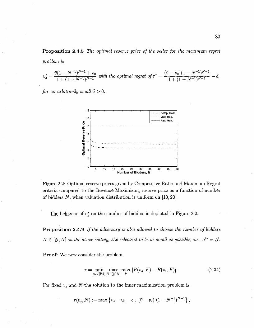
80

Proposition 2.4.8 The optimal reserve price of the seller for the maximum regret

problem is

v* = Vx + (x _ N-i)N-T with the °Ptimal re9ret of r* = ^ ^ _ j y - i w - i 5>

for an arbitrarily small 8 > 0.

1/

16 0)

1 -

Op

timal

Res

erve

11

Comp. Ratio Max. Reg.

•

-

5 10 15 20 25 30 35 40 45 50 Number of Bidders, N

Figure 2.2: Optimal reserve prices given by Competitive Ratio and Maximum Regret criteria compared to the Revenue Maximizing reserve price as a function of number of bidders iV, when valuation distribution is uniform on [10,20].

The behavior of -y* on the number of bidders is depicted in Figure 2.2.

Proposition 2.4.9 / / the adversary is also allowed to choose the number of bidders

N G [N, N] in the above setting, she selects it to be as small as possible, i.e. N* — N.

Proof: We now consider the problem

r= min max max \R(va,F) — R(vs, F)\ . vse[v,v]Ne[N,N] F

For fixed vs and iV the solution to the inner maximization problem is

(2.34)

r(vs,N) := max{t)s vQ e, (v - v.) (1 - N'Y-1} ,

81

as characterized by Lemma 2.4.2. The second term is a strictly decreasing function

of N, and therefore r(vs,N) is a non-increasing function of N. Consequently, the

adversary's response is to select as small an N as possible in the outer maximization

problem, i.e. N = N, and the resulting regret is

r{va) := max {vs - v0 - e , (v - vs) (1 - N'Y'1} D

Observe that the optimal reserve price, which is a decreasing function of the

number of bidders, is actually relatively insensitive to the exact value of N for both

criteria as indicated by Figure 2.2. This resembles the classical second price auction

setting where the reserve price is independent of the number of bidders. Actually,

it is easily seen from the formula of the reserve price for the regret that its limit is

limAr oo v* = v^ZQee, which has a similar structure to that of the revenue maximizing

reserve price for the uniform distribution on [fo,^], i.e. t>" := £ : j 2 1 , but which is

slightly lower, reflecting the risk averseness or conservatism of the regret criteria.

Also, note that the optimal regret is directly proportional to the term (v — VQ), which

reflects the level of uncertainty in the problem.

82

Chapter 3

Product Line Positioning without

Market Information

In this essay, we study the joint problem of product line positioning and pricing for

a monopolist when consumer preferences and WtP are unknown. We extend classi

cal models of horizontal and vertical differentiation to cover uncertainty in customer

preferences using relative performance criteria. In Section 3.1, we consider the hori

zontal positioning of a monopolist's product line using Salop's classical circular model

of spatial differentiation. We show that the optimal decision for both criteria is to

position products at equal intervals in the attribute space and to price them identi

cally. We next study the vertical positioning of a product line using the linear utility

of quality framework of Mussa and Rosen in Section 3.2. We show that the optimal

policy consists of offering a number of the highest quality versions, and that the op

timal number of versions offered increases with the uncertainty over customers' taste

for quality.

Similar to the previous essay, adversary's best response is sometimes achieved

83

only in the limit. However, unlike the previous essay, we do not explicitly explain

these using arbitrarily small constants 8, e in our analysis below, as the analysis and

notation are significantly heavier here. Whenever, such limiting policies come into

play, we note them verbally to keep the notation simpler.

3.1. Horizontal product line positioning

We first look at the case of horizontal positioning. We begin by denning the model

and the formulation of the basic competitive ratio and maximum regret problems.

We then analyze each of these problems in turn.

3.1.1 Model

We use Salop's classical model of spatial differentiation, also known as the circular

Hotelling model. In it, versions of the product are differentiated along a single at

tribute, represented by a location on the unit circle (attribute space). Each version j

is represented by a location lj in this attribute space.

We assume the firm can offer at most K versions of a product. Such a limitation

could, for example, reflect minimum efficient economies of scale needed for production.

We do not incorporate fixed or variable costs of producing up to this upper limit of

K versions; rather, our analysis concentrates on revenue maximization. However, it

is easy to incorporate linear variable costs in our analysis simply by rescaling the

nominal valuations for products. If one wanted to analyze the optimal level of variety

given such costs, it is possible to solve our model for different values of K and use

the solutions to determine if changes in revenue off-set the costs of production and

warrant increasing or decreasing the level of variety. But again in what follows below,

84

we shall assume K is fixed.

Consumer preferences are also represented by locations on the unit circle. A

randomly selected customer location is denoted I with distribution F(-). Our key

assumption is that this preference distribution F(-) is unknown to the firm and it

must therefore make its positioning and pricing decisions accounting for this missing

information.

Consumers have a common deterministic nominal valuation, v, for the product,

which represents the maximum amount they would be willing to pay if the product

were at their preferred location. The market size ("number of customers"), denoted

A, is assumed fixed and continuous. We do not claim that these parameters are known

in a real-life setting; a more complete analysis would certainly allow for uncertainty

in these parameters as well. However, this would make model intractable. Instead,

we isolate and focus on understanding the effects of consumer preference uncertainty.

Furthermore, the structure of the results we provide are independent of the specific

values of A and v, e.g., the symmetric positioning and pricing strategy holds for any

value of A and v. And often retailers do have a sense of the overall market size from

past experience even though the preferences for individual versions is highly uncertain

(e.g., ski jackets). One can see evidence of this in the typical retail planning process,

where budgets are allocated to categories of products based on past sales and the

primary uncertainty is over how to allocate that budget to different products within

the category. The valuation v, similarly, can be thought of as a historical "price point"

for the given category that is relatively well understood from historical experience

even though the preference for individual version is unknown.

Consumers incur a disutility that depends on the distance the product location

to their preferred location, given by 6\l — lj\ where 6 is a known disutility coefficient,

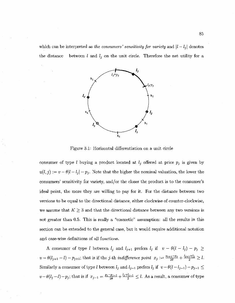
85

which can be interpreted as the consumers' sensitivity for variety and \l — lj\ denotes

the distance between I and lj on the unit circle. Therefore the net utility for a

x5

Figure 3.1: Horizontal differentiation on a unit circle

consumer of type I buying a product located at lj offered at price pj is given by

u(l,j) := v — 9\l — lj\ —Pj. Note that the higher the nominal valuation, the lower the

consumers' sensitivity for variety, and/or the closer the product is to the consumer's

ideal point, the more they are willing to pay for it. For the distance between two

versions to be equal to the directional distance, either clockwise of counter-clockwise,

we assume that K > 3 and that the directional distance between any two versions is

not greater than 0.5. This is really a "cosmetic" assumption: all the results in this

section can be extended to the general case, but it would require additional notation

and case-wise definitions of all functions.

A consumer of type I between /_,• and (,+i prefers lj if v — 9(1 — lj) — Pj >

v — 9(lj+i — 1) — Pj+i] that is if the j-th indifference point Xj := PJ+2^~PJ + *+12

} ^ I-

Similarly a consumer of type I between lj and Zj_i prefers lj if v — 9(1 — lj-\) —Pj-i <

v — 9(1 j — I) —pj] that is if Xj-i = P,'~2P/~1 + J+

2-'~1 <l. As a result, a consumer of type

86

I G [xj-i, Xj] prefers product j to its neighboring products. Without loss of generality

we denote the location of first version to be l\ = 0 (thus, also l\ = 1 depending on

the context). Consequently, in the remainder of the section whenever j = K, j + 1

denotes 1; and xi := m^x + \ and XK '•= V^K + ^ ^ above. Observe that the

coefficient 6 effects the aggregate demand in the sense that higher values of 6 make

all consumers less willing to pay for each version irrespective of its location and price,

reducing the over all demand faced by the firm.

Each consumer has a most preferred product, which yields a utility of u(l) :=

maxj{u(l, j)} for a given price vector p, and which is purchased iff u(l) is nonnegative.

Note that if a version with a relatively low price is placed close enough to a version

with a high price, the low price version may be preferred over the high price version

by every consumer location on the unit circle. In this case, we say that the low price

version dominates the high price version.

3.1.2 Product line positioning and pricing decision

Having introduced the model, let us describe the firm's decision making process.

First, the firm chooses how many of the K possible versions to offer, the positions

of these versions, i.e. vector I = {IJ}J=\..K, on the unit circle, and their prices, i.e.

the vector p. Then, it evaluates this decision against the "worst-case" outcome of

customer preferences. To do so, we imagine an adversary (nature) that selects a

worst-case preference distribution F(-) in order to minimize the competitive ratio or

maximum regret. Thus, the competitive ratio problem is

mP f T 1 R(l*(F),p*(F)-Fy

87

where (I* (F), p* (F)) is the revenue maximizing strategy of the firm given the distribu

tion F(-). Here the firm seeks a policy which maximizes its revenue as a percentage of

the full-information revenue under worst-case outcomes. For example, a competitive

ratio of 1/2 would say the firm is guaranteed to get at least 50% of the revenue it

could have gotten had it known the exact customer preference distribution. Similarly,

the maximum regret problem is

min max [R(l*(F),p*(F);F) - R(l,p;F)}. p,l F

Here the firm seeks a policy which minimizes the difference between its revenues and

the full-information revenue under worst-case outcomes. For example, a maximum

regret value of $1,000 would say that the revenue the firm achieves with the policy

is guaranteed to be no more than $1,000 below the revenue it would have obtained

with exact information on the customer preference distribution.

Our goal is to specify the optimal pricing and product line positioning strategy

of the firm for these two relative performance objectives. Specifically, how many

versions should the firm offer? Where should these versions be positioned on the unit

circle? What prices should we charge for the different versions? We also would like to

explain how the answers depend on the nominal valuation, the disutility coefficient,

the maximum number of products, and their relative positions. We begin with the

competitive ratio case.

3.1.3 Competitive ratio

We begin by assuming a fixed number of versions, K, is offered with fixed attributes

(locations on the unit circle), denoted by vector I € [0,1}K, and consider the pricing

decision of the firm. We say a product i at price p; dominates product j at price Pj if

88

every customer (regardless of location) prefers % to j . Firstly, we have the following

result:

Proposition 3.1.1 There exists an optimal pricing policy where no version domi

nates any other version.

Proof: By contradiction assume at all optimal solutions, there exist a price, pj

which dominates its neighboring price Pj+i, i.e. Xj > lj+i or equivalently Pj+i >

Pj + 9(lj+i — lj). Then, for any distribution the adversary chooses, the firm earns

Pj from those who choose to buy in the interval, [XJ-I,XJ\. However, decreasing the

price pj+i to Pj + 0(lj+\ — lj), the firm can earn pj + 0(lj+i - lj) from those in the

interval [XJ, lj+i], plus pj from those in the interval ja^-i, lj+i] without changing any

other prices or affecting revenues of other regions, which yields a revenue as at least

high as the optimal revenue. Repeating this augmentation for every dominating price

we achieve a price vector where there is no price strictly dominating any other. •

Thus, for the rest of the analysis, we restrict our attention only to such non-

dominating pricing policies, in which case all the consumers of type I G [XJ-\,XJ]

prefer product version j , and Xj G [lj, lj+i] holds for all j . Also, defining the lengths

Vi :~ ^T^i w e s e e ^na^ e v e r v o n e within yj distance of the location lj finds that buying

version j yields a nonnegative net utility. Therefore, everyone with I G [kj, Zj] prefers

and buys product j , where kj and Zj are the points defined as Zj := mm(xj,lj +

yj), kj :— max(xj_i,/j — yj) for j — 2...K, and z\ :— min(a;i,yi) and k\ :—

max(iX) 1 — yi)- Consequently, the revenue of the firm can be written as

K

R(l,p; F) = A ] > > (F(Zj) - F(kj)) . (3.1) 3=1

For the competitive ratio problem, we can further characterize the revenue func

tions using the following result:

89

Lemma 3.1.1 The firm does not enter the market unless Omaxj \lj — Zj_i| < 2v. If

the firm chooses to enter the market, the prices are set such that the whole market is

served at the optimal solution, i.e. Xj < Ij + Vj and Xj_\ > lj — yj holds for all j , and

consequently, we have that [zj,kj] = [XJ,XJ+I] for allj.

Proof: First, assume that 9max.j \lj — lj^t\ > 2v. Using the definitions of Xj and yj,

we see that requiring Xj < lj + yj and Xj~\ > lj — yj for all j implies the constraints

Pj + Pj-i + 9\lj — lj-i\ < 2v, Vj. However, it is clear that some price Pj must be

negative for some variant j (which could be thought as providing positive subsidies

or rebates) to satisfy these inequalities, or otherwise (i.e. in the case Xj > lj + yj

or Xj-i < lj — yj for some j) not all the consumers of type / will choose to buy in

the corresponding preference region [XJ-I,XJ] of variant j . If the former is the case,

the adversary would allocate all the probability mass of consumers to this region

resulting in a negative revenue and competitive ratio. If the latter is the case, the

adversary would allocate the unit probability mass to the region that is not covered,

and hence, the revenue would be zero. Consequently, by entering the market when

#maxj \lj — lj-i\ > 2v, the firm can never do better that earning zero revenues and

achieving a competitive ratio of zero.

Similarly, when 8 max,- \lj — lj_i \ < 2v, if the optimal prices are such that for some

lj we have that Xj > lj + yj (or £j_i < lj — yj), the adversary would again allocate

all the probability mass to the interval [lj + yj,Xj] (or [XJ-I,IJ — yj] respectively),

resulting in zero sales, and thus, achieving a competitive ratio of zero. On the other

hand, any price policy that satisfies inequalities Xj < lj + yj and Xj-\ > lj — yj for all

j guarantees a positive ratio when 0maxj \lj — lj-\\ < 2v. •

90

As a result of this lemma, we can restrict our attention to the case with 9 max, \lj —

lj-i | < 2v and to the pricing policies in which the firm collects pj from everybody

within the interval [XJ,XJ+I] for all j . For a distribution function F(-), define the

probability mass allocated to each such interval as fj := F(XJ+I) — F(XJ) for j =

1 . . . K — 1 and fx '•— F(xi) +1 — F{XK) • Using the above result, we can characterize

the worst-case distribution as follows:

Lemma 3.1.2 The worst-case competitive ratio distribution function F(-) allocates

the mass fj to location lj for all j .

Proof: Under a price policy that satisfies Xj < lj + yj and Xj-.\ > lj — yj for all j ,

note that the revenue in equation (3.1) depends only on how much probability mass

exists within each interval [XJ, xj+i], that is on /_,- = F(zj) — F(kj) = F(XJ+I) — F(XJ).

However, the specifics of the distribution function matters for the adversary, as the

maximum revenue that can be achieved, which appears in the denominator of the

competitive ratio to be minimized, depends on this distribution. On the other hand,

the value of the maximum revenue is always less than Av. Also note that given an

aggregate decision as to how much probability mass to put on each interval, i.e. the

vector / , the adversary can achieve the maximum revenue Av in the denominator of

the competitive ratio by allocating each mass fj on the point lj for all j . Therefore,

such an allocation is a dominant strategy for the adversary for all F(-). •

Corollary 3.1.1 The revenue function can be written as R(l,p;F) = A Ylj=iPjfj>

and the maximum revenue the firm could extract under full information is R(p*(F), F) =

Av.

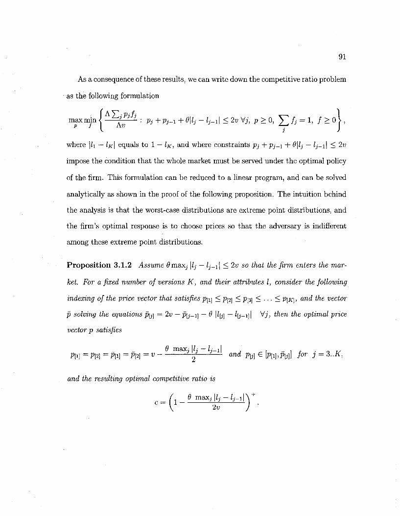
91

As a consequence of these results, we can write down the competitive ratio problem

as the following formulation

-j^ : pj +P3-1 + 6\lj - lj-i\ < 2v Vj, p > 0, 2_, fj = 1. / > 0 > ,

where |Zx — IK\ equals to 1 — IK, and where constraints pj + Pj-i + 0\lj — lj-i\ < 2v

impose the condition that the whole market must be served under the optimal policy

of the firm. This formulation can be reduced to a linear program, and can be solved

analytically as shown in the proof of the following proposition. The intuition behind

the analysis is that the worst-case distributions are extreme point distributions, and

the firm's optimal response is to choose prices so that the adversary is indifferent

among these extreme point distributions.

Proposition 3.1.2 Assume Om&Xj \lj — ^_ i | < 2v so that the firm enters the mar

ket. For a fixed number of versions K, and their attributes I, consider the following

indexing of the price vector that satisfies pm < pp] < pm < ... < P[K], and the vector

p solving the equations py] = 2v — p\j-i\ — 0 \ly] — ly-i\\ Vj, then the optimal price

vector p satisfies

0 max,-IL — L_i| Pw = p p ] = P[i] = Pm = v 2 Pb] e WW'1™ *or 3 = 3- '

and the resulting optimal competitive ratio is

n mux.- i;.„- — /„• i i \ 9 m a X j \lj — Zj_i|

2v

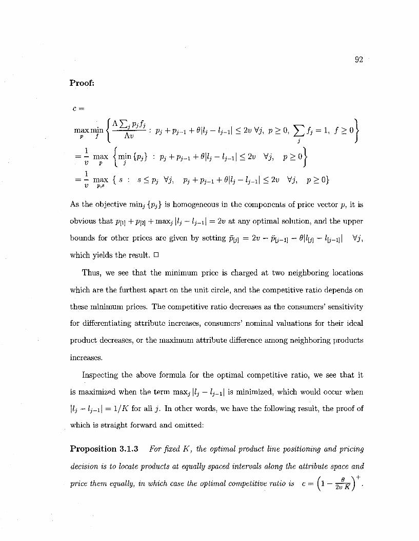
Proof:

92

max nun < ^ : Pj +Pj-i + 9\l5 - lj-i\ < 2v Vj, p > 0, ^ /,• = 1, / > 0

= - max < min{pj} : pj +Pj-i + 6\lj — lj-\\ < 2v Vj, p > 0 > v v \ j J 1

= - max { s : s < pj Vj, Pj + Pj-i + 6\lj — lj-\\ < 2v Vj, p > 0}

As the objective min^ {pj} is homogeneous in the components of price vector p, it is

obvious that p^\ +P[2] + max^ \lj — lj-i\ = 2u at any optimal solution, and the upper

bounds for other prices are given by setting p^ — 2v — p\j-\\ — 9\l\j\ — l\j-\}\ Vj,

which yields the result. •

Thus, we see that the minimum price is charged at two neighboring locations

which are the furthest apart on the unit circle, and the competitive ratio depends on

these minimum prices. The competitive ratio decreases as the consumers' sensitivity

for differentiating attribute increases, consumers' nominal valuations for their ideal

product decreases, or the maximum attribute difference among neighboring products

increases.

Inspecting the above formula for the optimal competitive ratio, we see that it

is maximized when the term maxj \lj — lj-^\ is minimized, which would occur when

\lj — lj-\\ = 1/K for all j . In other words, we have the following result, the proof of

which is straight forward and omitted:

Proposition 3.1.3 For fixed K, the optimal product line positioning and pricing

decision is to locate products at equally spaced intervals along the attribute space and

price them equally, in which case the optimal competitive ratio is c = (1 — 2 v-) •

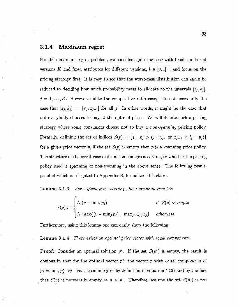
93


For the maximum regret problem, we consider again the case with fixed number of

versions K and fixed attributes for different versions, I £ [0,1}K, and focus on the

pricing strategy first. It is easy to see that the worst-case distribution can again be

reduced to deciding how much probability mass to allocate to the intervals [zj,kj],

j = 1 , . . . ,K. However, unlike the competitive ratio case, it is not necessarily the

case that [zj,kj] = [XJ,XJ+I] for all j . In other words, it might be the case that

not everybody chooses to buy at the optimal prices. We will denote such a pricing

strategy where some consumers choose not to buy a non-spanning pricing policy.

Formally, defining the set of indices S(p) = {j \ Xj > lj + y^ or Xj_i < lj — yj)}

for a given price vector p, if the set S(p) is empty then p is a spanning price policy.

The structure of the worst-case distribution changes according to whether the pricing

policy used is spanning or non-spanning in the above sense. The following result,

proof of which is relegated to Appendix B, formalizes this claim:

Lemma 3.1.3 For a given price vector p, the maximum regret is

A (v — minjPj) if S(p) is empty

A max{(v — mm j Pj) , maxjes(p)Pj} otherwise

Furthermore, using this lemma one can easily show the following:

Lemma 3.1.4 There exists an optimal price vector with equal components.

Proof: Consider an optimal solution p*. If the set S(p*) is empty, the result is

obvious in that for the optimal vector p*, the vector p with equal components of

Pj = min,,^ \fj has the same regret by definition in equation (3.2) and by the fact

that S(p) is necessarily empty as p < p*. Therefore, assume the set S(p*) is not

r(p) := I

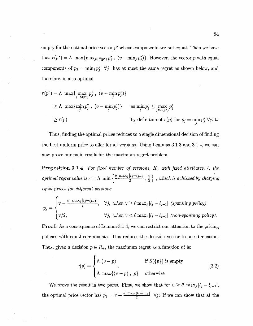
94

empty for the optimal price vector p* whose components are not equal. Then we have

that r(p*) — A max{maxjes(p*) p* , (v — rnin,-p£)}. However, the vector p with equal

components of Pj = mio,- p* V? has at most the same regret as shown below, and

therefore, is also optimal

r(p*) = A max{ max p* , (v — minp*)} jeS(P*) J j J

> A max{minp* , (v — minp*)} as minp* < max p* 3 J 3 J 3 J j€S(p*) J

> r(p) by definition of r(p) for pj = minp* Vj. • 3 J

Thus, finding the optimal prices reduces to a single dimensional decision of finding

the best uniform price to offer for all versions. Using Lemmas 3.1.3 and 3.1.4, we can

now prove our main result for the maximum regret problem:

Proposition 3.1.4 For fixed number of versions, K, with fixed attributes, I, the

optimal regret value isr = A min I ^ — l z ^ ~ , | > , which is achieved by charging

equal prices for different versions

v LU.—3^11^ y^ when v > 9max.j\lj — lj_i\ (spanning policy)

v/2, Vj, when v < 9max.j\lj — lj^i\ (non-spanning policy).

Proof: As a consequence of Lemma 3.1.4, we can restrict our attention to the pricing

policies with equal components. This reduces the decision vector to one dimension.

Thus, given a decision p G R+, the maximum regret as a function of is:

A (v — p) if S({p}) is empty r(p) = { (3.2)

A max{(w — p) , p} otherwise

We prove the result in two parts. First, we show that for v > 6 maxj \lj — lj-i\,

the optimal price vector has p3—v ma3C;u~ j-il \ / j . jf w e c a n s n o w that at the

95

optimal price {p} with equal components of p, the set S({p}) is empty, then the result

follows directly from the analog steps of competitive ratio analysis which shows that

minimum value of maximum regret is achieved for p = (v maxj\?- j-u^ whjch yields

minimum value of A[v — (v maxj h~ j-il)j _ ^—maxjli~ j - 1 ' . Therefore assume by

contradiction that the set S({p}) is not empty. Then, we have that

r{p) > A pj > A (v ^ r L-±L) > A ^ —-

where the first inequality follows from definition of rip) in equation (3.2) , the strict

inequality follows from the fact that {p} must violate the inequality pj + pj+\ +

6 maxj \lj — lj-\\ = 2p + 9 max^ \lj — lj-\\ < 2v as the set S({p}) is not empty,

and last inequality follows by the specification of v in this region. Therefore, the

non-spanning policy {p} gives strictly more regret, and cannot be optimal in this

case.

Second, for v < 9 max, \lj — lj-\\, we show that the optimal price vector has

Pj = \ Vj below. Using the previous case, we know that the firm can guarantee a

regret value of A—ma3V b - ? - 1 ' using a price policy low enough to span the whole unit

circle. Now, we show that a strictly less regret is possible by charging pj = | \/j,

which is a non-spanning policy for values of v in this region, therefore <S({|}) is

not empty. If the firm uses a non-spanning pricing policy the maximum regret is

given by A max{p , (v — p)} by equation (3.2). However, this function is minimized

when p — | , as it is the maximum of two linear functions one increasing the other

decreasing in p. As this yields a regret value of A | < A—max^J~ .7-1', the optimal

price of Pj = | \/j for this region. Combining the two cases yields the result. •

The intuition lying behind this result is as follows: when 9 is high or v is low,

the firm faces a linear demand curve with downward slope of 6 for each version,

96

because cannibalization is not an issue as it is too costly for a customer close to a

version to consider some other version. As a result, the firm charges the revenue

maximizing price for a monopolist, i.e. v/2, which corresponds to a non-spanning

pricing policy. On the other hand, when 9 is low or v is high, it is less costly for

consumers close to a version to consider other versions; and therefore, cannibalization

is an issue. Charging the revenue maximizing price v/2 for a version cannibalizes

neighboring versions. Therefore, the firm charges a higher price for the version, i.e.

6 max,- IL—L_i| ln

V ^ — • * — - > v/2.

Note the regret above is minimized irrespective of v when max.,- \lj — ZJ_1| is min

imized, which again occurs when \lj — lj-\\ = 1/K for all j . Thus, we have the same

result as in the competitive ratio case:

Proposition 3.1.5 For fixed K, the optimal product line positioning decision is

to locate versions at equally spaced intervals along the attribute space and to price

them equally according to Proposition 3.1.4, in which case the optimal regret is r =

Amin{^,f}.

We therefore have shown that for both the competitive ratio and maximum re

gret criteria, the optimal pricing policy is a function of attribute differences between

neighboring versions. This policy reflects the firm's sensitivity for potential canni

balization among versions (e.g., non-dominating pricing policies). The worst-case

performance decreases (i.e. the competitive ratio decreases or the regret increases)

as the consumers' sensitivity for differentiating attribute increases, consumers' nomi

nal valuations for their ideal product decreases, or the maximum attribute difference

among neighboring products increases. The optimal positioning decision is to span

the attribute space with equally spaced product versions and to sell them at a uniform

97

price. In other words, to cover the product space uniformly with a collection of prod

ucts offered at a single price. Coincidentally, this "equally-space and equally-price"

strategy is a celebrated Nash Equilibrium for the classical monopolistic competition

model where each version is controlled by a different firm, which is well studied by

Salop and others. (See Salop [69].) In the monopolistic competition case, this arises

as an equilibrium response among competing firms. In our case, it arises as an opti

mal hedge against another sort of adversary: "nature" - the unknown preferences of

customers.

While stylized, as noted above this uniform positioning and pricing structure is

seen commonly in real-world markets. For example, iTunes offers music downloads

spanning all genres and artists at a uniform price of $0.99; apparel retailers normally

charge the same price for a garment sold in different colors and sizes; ice cream shops

carry a range of flavors sold at the same price-per-cone, etc. While a firm could charge

different prices if it knew customer preferences certainly, if it makes an error and the

actual distribution of preference is different than the firm's estimate, they could do

much worse. The uniform positioning and pricing policy serves as a defensive strategy

against this risk. Again, there are clearly other considerations that could influence

a retailer to price uniformly, such as operational simplicity and customer goodwill,

but our results suggest that avoiding risk from lack of information about consumer

preferences is another plausible motivation.

Notice also that the optimal prices charged, and thus, revenues earned increases

with the number of versions K, increasing the competitive ratio and decreasing the

regret. This is the typical profit maximization response when there are no economies

of scale to production of variety. However, when there are economies of scale, one

needs to balance the revenue gain of more variety against the cost of producing many

98

versions.

As we have noted above we have focused on consumer preference uncertainty;

a more complete approach would be to assume uncertainty in other model param

eters such as v and A. However, it is not hard to extend our analysis to include

the above parameters since we provide closed-form solutions to what would be the

inner-optimization problems in such a generalization and the structure of the uniform

pricing and differentiation policy is independent of the market size parameter A.

3.2. Vertical product line positioning

We next consider the case of vertical product positioning, in which versions correspond

to different quality levels over which consumers share a common ranking (though with

heterogenous willingness-to-pay for quality).

Specifically, there are K distinct quality versions of a product that the firm consid

ers potentially offering. The quality level of version j is denoted by lj. The indexing

satisfies li < /2 < • • • < IK, SO that li is the lowest quality level, whereas IK is the

highest. In order to reduce the heavy notation induced by the analysis of this setting,

we assume there is a continuum of consumers of unit mass. All the results can be

scaled to any market size without changing the optimal policy.

Each consumer has a distinct taste for quality, denoted by v, which is an indepen

dent and identically distributed random variable with unknown distribution F(-) on

a known interval [v,v]. This distribution is the key missing information to the firm

in our model.

We adopt the classical "linear utility function of quality" framework of Mussa and

Rosen [57]. If a consumer has a quality taste level of v and purchases product version

99

j , her net utility is given by u(v,j) :— v lj — Pj, where pj is the price of product

j . Consequently, the higher the taste for quality or the higher the quality level,

the more a consumer is willing to pay for a particular version. A consumer prefers

version j over version i if u(v,j) = v lj — pj > v /» — pi = u(v,i) holds. Therefore,

unlike the horizontal differentiation model in the previous section, each consumer

enjoys the higher quality versions more. As a tie-breaking assumption, we assume

that a consumer prefers the higher quality version when faced with two versions

giving the same utility. For a given vector of prices p, a consumer buys the version

of the product which yields the highest net utility provided that is nonnegative, i.e.

u(v) := ma.Xj{v lj — Pj} > 0, or will not buy any product otherwise.

The sequence of events is as follows: first, the firm decides on how many versions to

offer at what quality levels, and chooses their prices without knowing the distribution

of the random taste for quality. Then, we evaluate the decision against the worst-case

distribution F(-) of the taste for quality. Our goal is again to find the optimal product

line positioning (this time in terms of quality levels) and pricing policy of the firm.

Specifically, we want to answer the questions about how many versions to offer, their

quality levels and prices. Also of particular interest is how these decisions change

with respect to the uncertainty level of costumer taste for quality. We begin with the

competitive ratio case and then analyze the case of maximum regret.

3.2.1 Competitive ratio

First, let us assume for the moment that the firm offers all K quality levels of the

product. Similar to the horizontal differentiation setting we define indifference points:

Vj as the quality level where a consumer switches from version j to version (j + 1),

100

then Vj must satisfy Vj lj -pj = Vj lj+i -Pj+i, yielding Vj — +1~^' for j = 1 . . . K—1.

Using the definition of u(v,j), it is easy to see that version j is preferred over version

(j +1) by those consumers with v < Vj, and similarly, version (j + l) is preferred over

version j , when v > Vj. We say version j is strictly dominated by versions (j — 1)

and (j + l), if version (j — 1) or version (j + l) yields strictly more utility for every

consumers type v G [y,v] than version j . The necessary and sufficient condition for

this is Vj-i > Vj, which can be easily seen graphically in Figure 3.2.

Note the product line positioning and pricing decisions of the firm can be ag

gregated into the single decision of offering all K quality levels of the product and

choosing only the prices offered. To see this, assume that some version j is not of

fered under some policy. Analytically, this is equivalent to offering that version at

some price pj that satisfies Vj-i = Vj, because at that price level no consumer strictly

prefers version j , but a consumer of type v = Vj-i = Vj has the same value of utility

for consuming versions (j — 1), j and (j + l). However, she prefers version (j + l)

over others due to the tie-breaking assumption. Therefore, at price Pj version j is

effectively a "dummy version" which is not chosen by any consumer, and this case is

therefore analytically equivalent to not offering version j .

For the competitive ratio problem, we first prove that there exists an optimal price

vector where no product strictly dominates any other product at the optimal solution

and further that the consumer with the lowest taste for quality earns zero utility at

the optimal solution. These properties are formalized in the following proposition,

proof of which is given in Appendix B:

Proposition 3.2.1 There exists an optimal price vector where no product strictly

dominates any other product and which satisfies y < vi < v-i < ... < v^-i < v.

101

The next result shows that there exists an optimal policy where only some number

of highest quality versions of the product are offered:

Proposition 3.2.2 (Nested Quality Offers) There exists an optimal solution

where only the (K — j + 1) highest quality products are offered for some j = 1 . . . K.

Proof: Using the previous proposition, the result is trivially true for j = 1 if v < vi

in the optimal solution. If y = v\ — ... = Vj_x < Vj for some j = 2 . . . K — 1, we

can solve for the optimal price components of the first j versions as p\ = yl\, p<i —

yl2,..., Vj — vlj using the definitions of Vi for i = 1 . . . j . Thus, the customer with

lowest quality taste chooses version j by the tie-breaking assumption as u(y, 1) =

u(y,2) = ... = u(v,j). Furthermore, u(v,l) < u(v,2) < . . . < u(y,j) for W > y

as li < l2 < • • • < lj. Consequently, the versions 1 to j — 1 are not bought by

any type of customers. Therefore, offering only the (K — j + 1) highest quality

version with their optimal prices achieves the same product selection for each type

of customer for \/v £ [y, v] with same prices, resulting in the same revenue collected

by the firm and the same response chosen by the adversary, therefore achieving the

optimal competitive ratio. •

Using Proposition 3.2.1 and our previous observations, we conclude that offering

only the (K — j + 1) highest quality products is analytically equivalent to offering all

K quality levels of the product, but fixing the prices of the first j quality versions to

be pi = yli, P2 — vh, • • •, Pj — vlj. This is illustrated in Figure 3.2.

The remainder of the competitive ratio section tries to identify the best com

petitive ratio that can be achieved by the firm using a policy which offers only the

(K — j + 1) highest quality versions, denoted by c,-. Then, the optimal value of the

competitive ratio problem satisfies c = max^c,}.

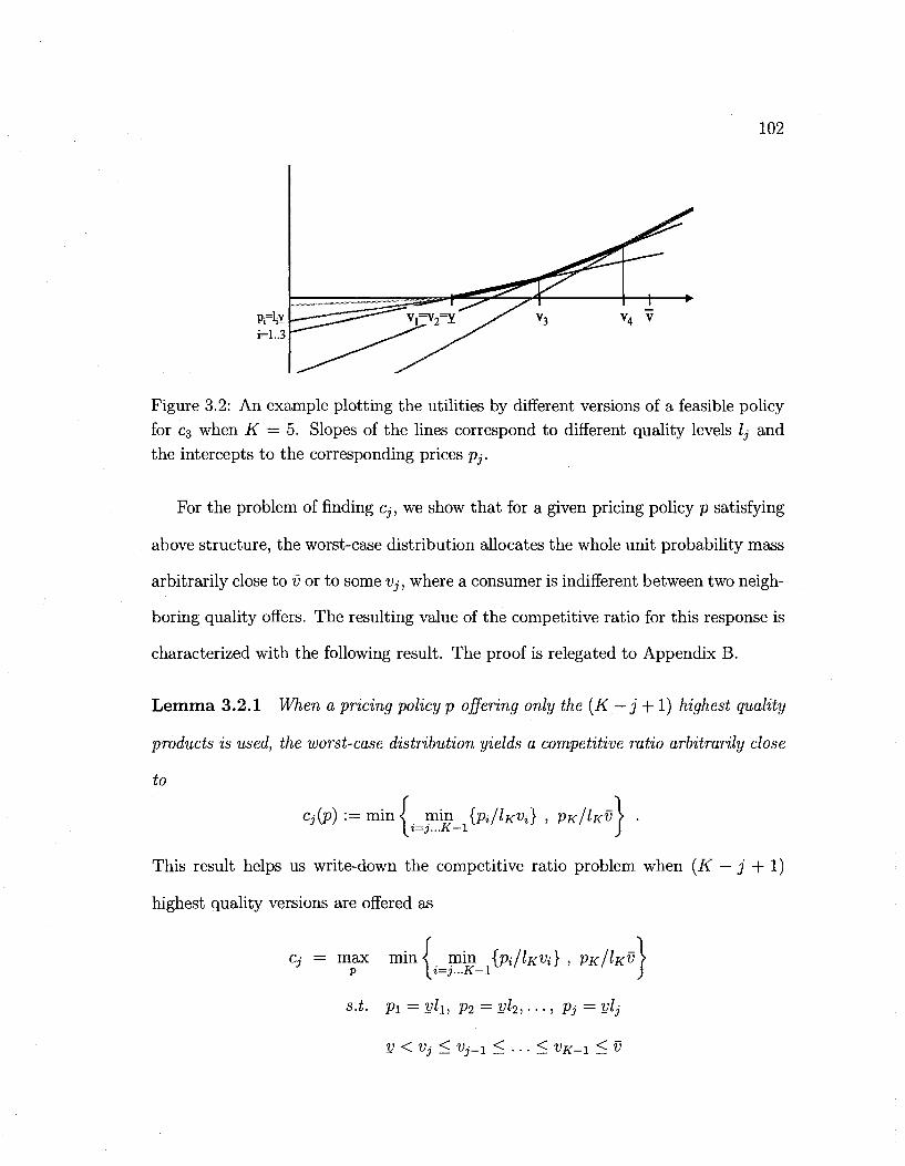
102

Figure 3.2: An example plotting the utilities by different versions of a feasible policy for c3 when K = 5. Slopes of the lines correspond to different quality levels lj and the intercepts to the corresponding prices pj.

For the problem of finding Cj, we show that for a given pricing policy p satisfying

above structure, the worst-case distribution allocates the whole unit probability mass

arbitrarily close to v or to some Vj, where a consumer is indifferent between two neigh

boring quality offers. The resulting value of the competitive ratio for this response is

characterized with the following result. The proof is relegated to Appendix B.

Lemma 3.2.1 When a pricing policy p offering only the (K — j +1) highest quality

products is used, the worst-case distribution yields a competitive ratio arbitrarily close

to

Cj(p):= mm I min {pi/lKVi} , PK/IRV \ • \%=3...K-\ J

This result helps us write-down the competitive ratio problem when (K — j + 1)

highest quality versions are offered as

Cj = max min \ min {pi/lKVi} , PK/IKV > p \i=j...K-l J

s.t. pi = vh, p2 = vl2,.. •, Pj = vlj

V < Vj < Vj+i < . . . < VK-\ < V

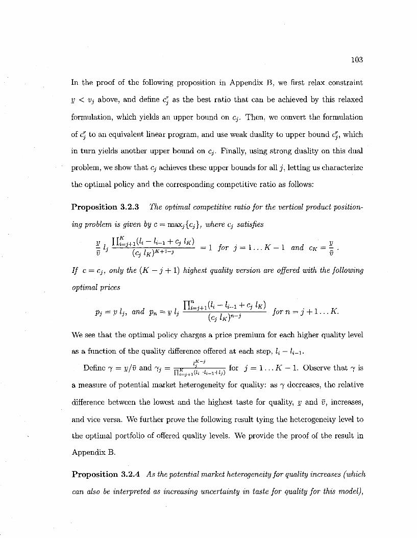
103

In the proof of the following proposition in Appendix B, we first relax constraint

v < Vj above, and define cj as the best ratio that can be achieved by this relaxed

formulation, which yields an upper bound on Cj. Then, we convert the formulation

of crj to an equivalent linear program, and use weak duality to upper bound c£, which

in turn yields another upper bound on Cj. Finally, using strong duality on this dual

problem, we show that Cj achieves these upper bounds for all j , letting us characterize

the optimal policy and the corresponding competitive ratio as follows:

Proposition 3.2.3 The optimal competitive ratio for the vertical product position

ing problem is given by c = maxj{cj}, where Cj satisfies

V Ui=j+l(li ~ li-l + CJ lK) . V - lj —,—, ^+1_7- = 1 for j = l...K -1 and cK = - • v {Cj IK)

+ 3 v

If c = Cj, only the (K — j + 1) highest quality version are offered with the following

optimal prices

Y\.i=j+iih ~~ ^-i"+" cj IK) PJ = v lj, and pn = v lj —-.— . for n — j + 1... K.

(Cj IK)U 3

We see that the optimal policy charges a price premium for each higher quality level

as a function of the quality difference offered at each step, U — Z»_i. iK-j

Define 7 = y/v and 7, = ^n?—f,—;—777 for j = 1 . . . K — 1. Observe that 7 is

a measure of potential market heterogeneity for quality: as 7 decreases, the relative

difference between the lowest and the highest taste for quality, y and v, increases,

and vice versa. We further prove the following result tying the heterogeneity level to the optimal portfolio of offered quality levels. We provide the proof of the result in

Appendix B.

Proposition 3.2.4 As the potential market heterogeneity for quality increases (which

can also be interpreted as increasing uncertainty in taste for quality for this model),

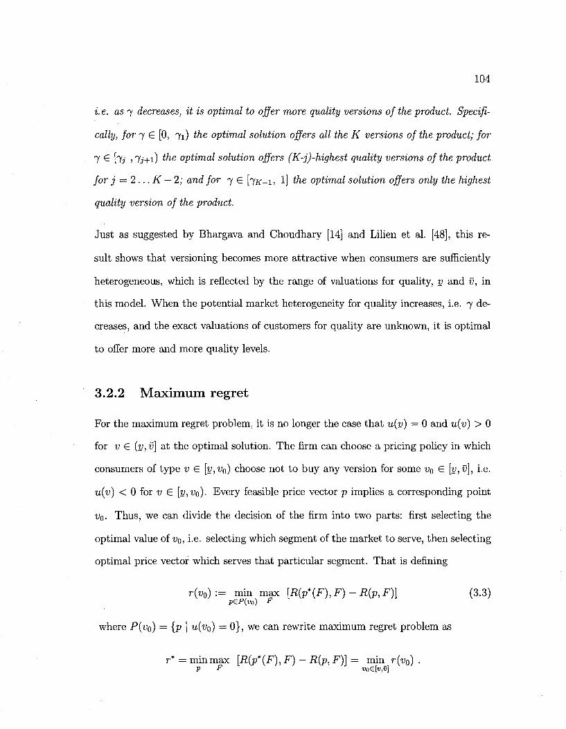
104

i. e. as 7 decreases, it is optimal to offer more quality versions of the product. Specifi

cally, for 7 G [0, 71) the optimal solution offers all the K versions of the product; for

7 G [7, , 7 J+I ) the optimal solution offers (K-j)-highest quality versions of the product

for j = 2 . . . K — 2; and for 7 G [TK-I, 1] the optimal solution offers only the highest

quality version of the product.

Just as suggested by Bhargava and Choudhary [14] and Lilien et al. [48], this re

sult shows that versioning becomes more attractive when consumers are sufficiently

heterogeneous, which is reflected by the range of valuations for quality, y and v, in

this model. When the potential market heterogeneity for quality increases, i.e. 7 de

creases, and the exact valuations of customers for quality are unknown, it is optimal

to offer more and more quality levels.


For the maximum regret problem, it is no longer the case that u(y) — 0 and u(v) > 0

for v G (y, v] at the optimal solution. The firm can choose a pricing policy in which

consumers of type v G [y,v0) choose not to buy any version for some v0 G [y,v], i.e.

u(v) < 0 for v G [V,VQ). Every feasible price vector p implies a corresponding point

VQ. Thus, we can divide the decision of the firm into two parts: first selecting the

optimal value of v0, i.e. selecting which segment of the market to serve, then selecting

optimal price vector which serves that particular segment. That is defining

r(v0):= min max [R(p*(F), F) - R(p, F)} (3.3) p£P(v0) F

where P(^o) = {p I u(v0) = 0 } , we can rewrite maximum regret problem as

r* = min max [R(p*(F),F) - R(p,F)] = min r(v0) . V F i>oG[u,i>]

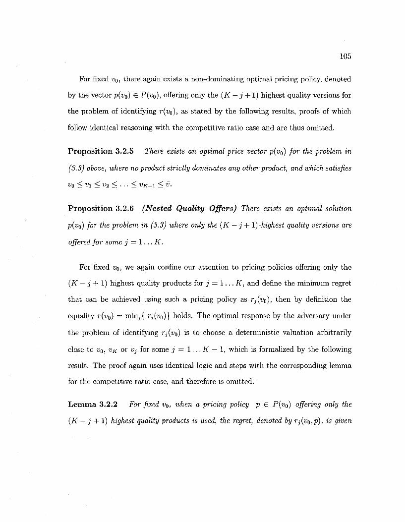
105

For fixed Vo, there again exists a non-dominating optimal pricing policy, denoted

by the vector p(v0) G P{VQ), offering only the (K — j + 1) highest quality versions for

the problem of identifying r(vo), as stated by the following results, proofs of which

follow identical reasoning with the competitive ratio case and are thus omitted.

Proposition 3.2.5 There exists an optimal price vector P(VQ) for the problem in

(3.3) above, where no product strictly dominates any other product, and which satisfies

^0 5: Vi < V2 < • • • < VK-1 < V.

Proposition 3.2.6 (Nested Quality Offers) There exists an optimal solution

p(vo) for the problem in (3.3) where only the (K — j + 1)-highest quality versions are

offered for some j = 1... K.

For fixed v0, we again confine our attention to pricing policies offering only the

(K — j + 1) highest quality products for j = 1 . . . K, and define the minimum regret

that can be achieved using such a pricing policy as rj(v0), then by definition the

equality r(vo) = minj{ rj(vo)} holds. The optimal response by the adversary under

the problem of identifying rj(vo) is to choose a deterministic valuation arbitrarily

close to v0, vK or Vj for some j = 1 . . . K — 1, which is formalized by the following

result. The proof again uses identical logic and steps with the corresponding lemma

for the competitive ratio case, and therefore is omitted.

Lemma 3.2.2 For fixed VQ, when a pricing policy p G -P(fo) offering only the

(K — j + 1) highest quality products is used, the regret, denoted by rj(vo,p), is given

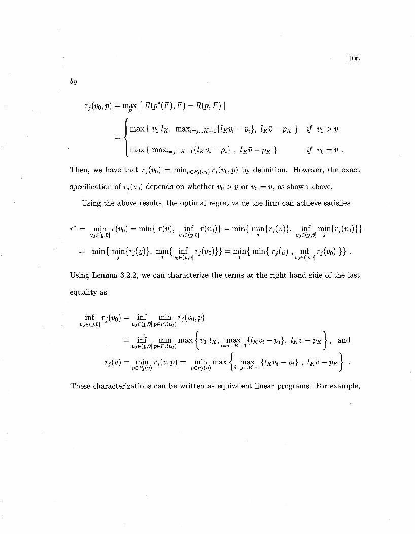
106

by

rj{v0,p) = max [ R(p*(F), F) - R(p, F)}

max{ v0 lK, maxi=j...K-.1{lKVi - # } , lKv ~VK) if v0>y

max{ maXi-j...K-i{lKVi - Pi} , IRV - pK } if v0 = v .

Then, we have that rj(vQ) = mmpep^vo)rj(vo,p) by definition. However, the exact

I specification of rj(v0) depends on whether VQ > v or v0 = y, as shown above.

Using the above results, the optimal regret value the firm can achieve satisfies

r* = min r(vo) = min{ r(y), inf r(v0)} — min{ min{r,-(u)}, inf m.in{rj(vo)}} vo£]v,v] vo&(y,v] j voe{v,v] 3

= min{ min{rj(:y)}, min{ inf r,-(vo)}} = min{ min{ rj(y) , inf fj(vo) }} • j j vo€(y,v] j vo€(y,v]

Using Lemma 3.2.2, we can characterize the terms at the right hand side of the last

equality as

inf rj(vQ) = inf_ min TJ{VQ,P) voe(y,v] vQe(y,v]pePj{v0)

= inf min vo€(y,v}pePj(vo)

max < v0 lK, max {lKVi - p{}, IKV ~PK> , and I ^ i=j...K-l J

Tj(y) = min rAy,p) = min max < max {IRV% — p%} , IKV — PK\ • p&Pjiv) pePjiv) [i=j...K-l J

These characterizations can be written as equivalent linear programs. For example,

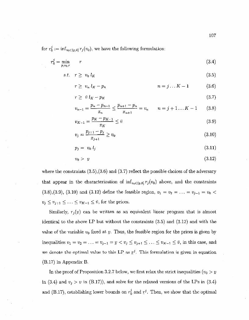
107

for TQ := mf„oG(3,jS] rj(v0), we have the following formulation:

rl = min r (3.4) P,vo,r

s.t. r > v0 IK (3.5)

r> vnlK-pn n = j...K-l (3.6)

r> vlK-pK (3.7)

V„_l = < =Vn U=J + 1...K-1 (3.8)

VK-I = < f (3.9)

= Pj+i-Pi > VQ ( 3 1 0 )

Pj = v0 Ij (3.11)

wo > V (3.12)

where the constraints (3.5),(3.6) and (3.7) reflect the possible choices of the adversary

that appear in the characterization of miVo^v^rj{yo) above, and the constraints

(3.8),(3.9), (3.10) and (3.12) define the feasible region, v\ = v2 = . . . = fj-i = vQ <

Vj < Vj+i < . . . < VK-I < v, for the prices.

Similarly, Tj(v) can be written as an equivalent linear program that is almost

identical to the above LP but without the constraints (3.5) and (3.12) and with the

value of the variable v0 fixed at v. Thus, the feasible region for the prices is given by

inequalities v\ — v % — ... — Vj-i = v < vj < Vj+\ < ... < VK-I < v, in this case, and

we denote the optimal value to this LP as rK This formulation is given in equation

(B.17) in Appendix B.

In the proof of Proposition 3.2.7 below, we first relax the strict inequalities (v0 > v

in (3.4) and Vj > v in (B.17)), and solve for the relaxed versions of the LPs in (3.4)

and (B.17), establishing lower bounds on rJ0 and rj. Then, we show that the optimal

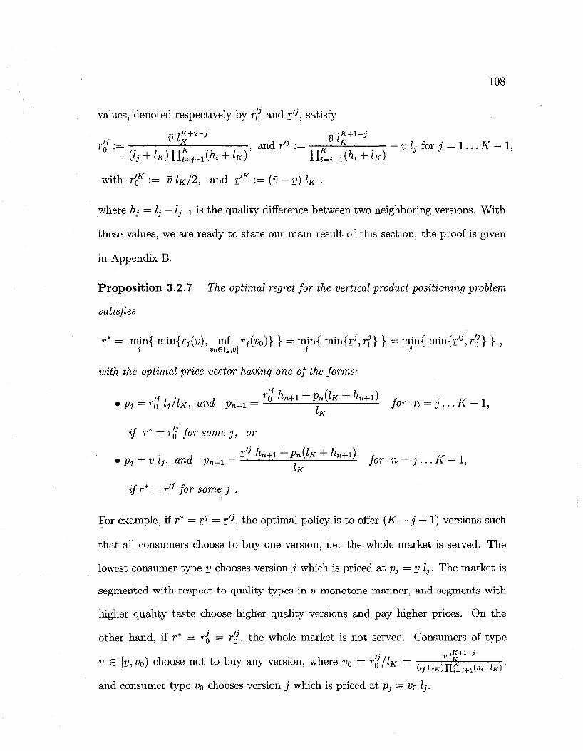
108

values, denoted respectively by T'Q and r'-7, satisfy

r'> : = V-% , and ^ : = — ^ v L for j = 1 . . . K - 1,

with r'f := v lK/2, and r'K := (?) - u) lK .

where hj = £j — Zj_i is the quality difference between two neighboring versions. With

these values, we are ready to state our main result of this section; the proof is given

in Appendix B.

Proposition 3.2.7 The optimal regret for the vertical product positioning problem

satisfies

r* = min{ mm{rj(v), inf rj(v0)} } = min{ min{rJ, T^} } = min{ min{r/J, r^ } } , j VQ€{V,V] j 3

with the optimal price vector having one of the forms:

/j , ;, , o hn+1 + pn(lK + hn+i) • Pj — ro h/lic, and pn+1 = for n = j ... K - 1,

if r* = r'(l for some j , or

j , r'j hn+i -\-PU{IK + K+i) t j . , • Pj —v lj, and pn+i = for n = j ... K — 1,

IK

if r* = r'j for some j .

For example, if r* =r:> = r ° , the optimal policy is to offer (K — j + 1) versions such

that all consumers choose to buy one version, i.e. the whole market is served. The

lowest consumer type v chooses version j which is priced at pj = V lj. The market is

segmented with respect to quality types in a monotone manner, and segments with

higher quality taste choose higher quality versions and pay higher prices. On the

other hand, if r* = TQ = r'l, the whole market is not served. Consumers of type - iK+l-j

v €. [y,v0) choose not to buy any version, where VQ = r'Z /IK = „ , ^-Jk—,.,, N,

and consumer type v0 chooses version j which is priced at Pj = o lj.

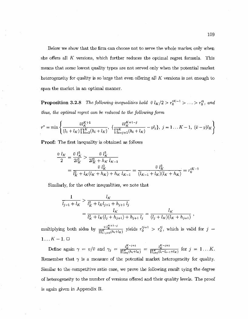
109

Below we show that the firm can choose not to serve the whole market only when

she offers all K versions, which further reduces the optimal regret formula. This

means that some lowest quality types are not served only when the potential market

heterogeneity for quality is so large that even offering all K versions is not enough to

span the market in an optimal manner.

Proposition 3.2.8 The following inequalities hold v IK/2 > r'^"1 > ... > T'Q , and

thus, the optimal regret can be reduced to the following form

vl«+1 , vlK+1~j

mm bK

(h + IK) UL(hi + IK) ' Ulj+t(hi + IK)

Proof: The first inequality is obtained as follows

vlK _vlK vlK

' ^ K *,,, r T - ^ > ' j = l...K-l, (v-v)lK

21% 2l2K + hKlK-i

V^K V^K „<K-\ = rn l2

K + IK(IK + hK) + hK lK-i (lK-i + IK)(IK + hK) °

Similarly, for the other inequalities, we note that

1 > IK

lj+i + IK IK + falj+i + hj+\ lj

IK IK

l\ + 1K(IJ + hj+1) + hj+1 lj (lj + IK){IK + hj+1) '

multiplying both sides by % * yields r'j+1 > rv?, which is valid for j =

1...K-1. D

lK-j+1 lK-j+1

Define again 7 = v/v and 7,- = „uK^—7-7 = „# ,f , r r for 7' = 1 . . . K.

Remember that 7 is a measure of the potential market heterogeneity for quality.

Similar to the competitive ratio case, we prove the following result tying the degree

of heterogeneity to the number of versions offered and their quality levels. The proof

is again given in Appendix B.

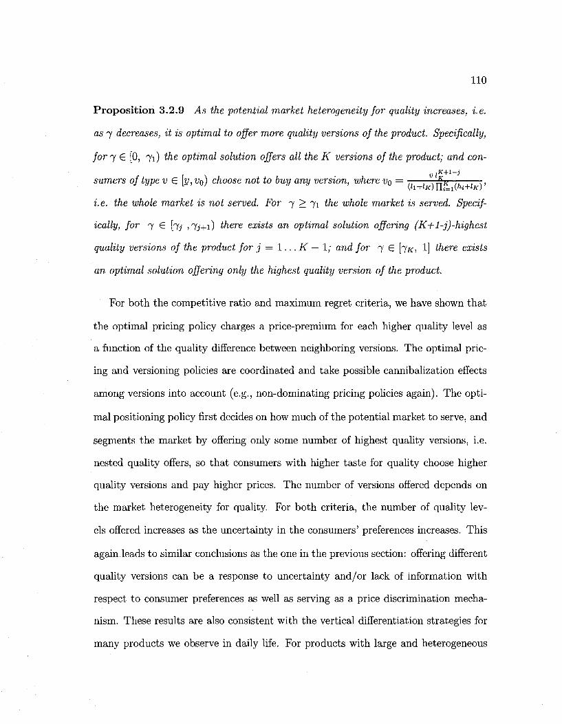
110

Proposition 3.2.9 As the potential market heterogeneity for quality increases, i.e.

as 7 decreases, it is optimal to offer more quality versions of the product. Specifically,

for 7 € [0, 71) the optimal solution offers all the K versions of the product; and con

sumers of type v G [v, v0) choose not to buy any version, where vQ = -— v £K ——,

i.e. the whole market is not served. For 7 > 71 the whole market is served. Specif

ically, for 7 € [7,- , 7J+I) there exists an optimal solution offering (K+l-j)-highest

quality versions of the product for j = 1 . . . K — 1; and for 7 € [7^-, 1] there exists

an optimal solution offering only the highest quality version of the product.

For both the competitive ratio and maximum regret criteria, we have shown that

the optimal pricing policy charges a price-premium for each higher quality level as

a function of the quality difference between neighboring versions. The optimal pric

ing and versioning policies are coordinated and take possible cannibalization effects

among versions into account (e.g., non-dominating pricing policies again). The opti

mal positioning policy first decides on how much of the potential market to serve, and

segments the market by offering only some number of highest quality versions, i.e.

nested quality offers, so that consumers with higher taste for quality choose higher

quality versions and pay higher prices. The number of versions offered depends on

the market heterogeneity for quality. For both criteria, the number of quality lev

els offered increases as the uncertainty in the consumers' preferences increases. This

again leads to similar conclusions as the one in the previous section: offering different

quality versions can be a response to uncertainty and/or lack of information with

respect to consumer preferences as well as serving as a price discrimination mecha

nism. These results are also consistent with the vertical differentiation strategies for

many products we observe in daily life. For products with large and heterogeneous

I l l

customer bases, such as micro processors with different speeds and high or low cache

memories, professional, standard and student versions of software, and consumer elec

tronics product lines with models having increasing functionality with higher prices,

we see many different quality versions offered at different prices.

112

Chapter 4

Revenue Management Heuristics

Under Limited Market

Information: A Maximum Entropy

Approach

In this essay, we consider incorporating censored sales information in a dynamic

forecasting and optimization cycle for (airline) capacity allocation problems. Using a

two demand class example, Cooper et al. [21] illustrate that most common forecasting

methods, when used jointly with optimization routines, produce capacity controls

that degenerate and call this phenomenon the "spiral-down effect". We propose a

tractable and intuitive approach based on maximum entropy (ME) distributions to

incorporate censored sales information in such dynamic settings. We show that ME

algorithm we propose provides capacity controls that avoid the "spiral down" effect

and converge to the optimal values, making this approach attractive for problems

113

of joint forecasting and revenue optimization. In our analysis, we first describe the

ME algorithm for the two fare-classes in Section 4.1. In Section 4.2, we prove the

convergence of the protection levels produced by the ME algorithm to the optimal

values for the underlying unknown demand. Finally, we provide an extension of the

algorithm to multifare problems in Section 4.3.

4.1. Single-resource capacity control with two fare-

classes

4.1.1 Full information model

We consider the capacity-control problem of an airline with two fare-classes. The

demands for the two fare-classes are independent random variables that arrive se

quentially in nonoverlapping intervals. The low fare demand, denoted by D2, is

realized before the high fare demand, denoted by D\. The demand for each class

is also independent of the capacity controls and remaining capacity at any stage. If

there are group bookings, they can be partially accepted. The control variable of the

airline is the protection level, denoted by L, which, as mentioned above, is the number

of seats to be reserved for the future high fare-class demand. This setup is usually

referred to as the Littlewood's setting. The objective of the firm is to maximize its

expected revenue, that is

max E [pi min {Di, max(C — D2, L)\ + p2 mm(D2, C — L)\, 0<L<C

where C denotes the total available capacity. The term mm(D2, C — L) is the sales

for the low fare-class which arrives first; and consequently, the high fare-class sales is

114

the minimum of demand Dx and the remaining number of seats C — min(D2, C — L) =

max(C — D2,L).

If D\ and D2 are continuous random variables, the optimal protection-level L* is

given by the following equality

p1P(D1>L*)=p2 «=» F ( L * ) = 7 : = l - p 2 / P l , (4.1)

where F(-) is the cumulative probability distribution function for D\. This equality

is commonly referred to as Littlewood's rule, and is a special case of the more general

economical understanding which states "marginal cost = marginal revenue". The

intuitive reasoning behind Littlewood's rule can be explained as follows: if we protect

L* seats for the high fare customers, we could sell the last (marginal) seat only if

D\ > L* to earn pi, resulting in the opportunity cost of p\ P(Z?i > L*); whereas

we could sell the same seat now to low fare customers for p2. For integer values of

demand and protection levels, we use the definition

L* = min{L | F(L) > 7}. (4.2)

Note that the optimal protection level is independent of the low fare-class demand

D2.

4.1.2 Unknown demand distribution

If we do not know the distribution of the high fare-class demand in a dynamic setting

where the problem repeats at each iteration k, e.g., everyday flights from New York

JFK to Atlanta International by a particular airline, we can try to learn the demand

using past observations. Common practice involves using passive learning routines

where one forecasts the distribution from past sales observations at each iteration k,

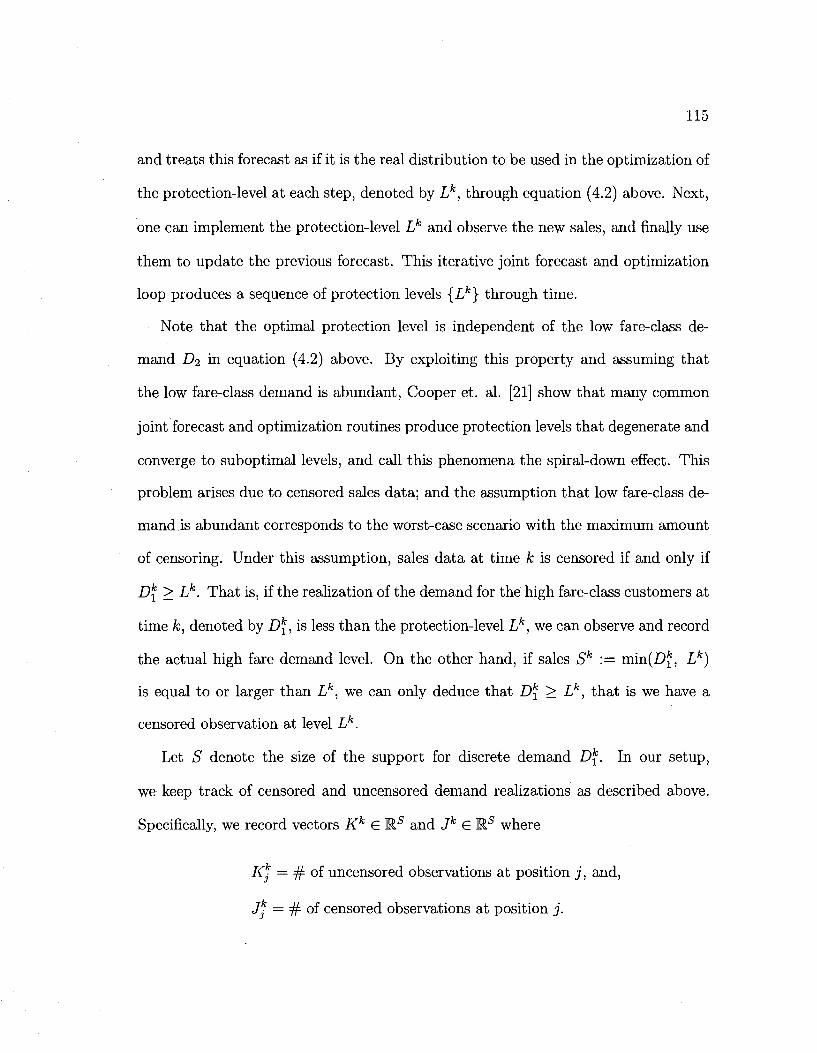
115

and treats this forecast as if it is the real distribution to be used in the optimization of

the protection-level at each step, denoted by Lk, through equation (4.2) above. Next,

one can implement the protection-level Lk and observe the new sales, and finally use

them to update the previous forecast. This iterative joint forecast and optimization

loop produces a sequence of protection levels {Lk} through time.

Note that the optimal protection level is independent of the low fare-class de

mand Di in equation (4.2) above. By exploiting this property and assuming that

the low fare-class demand is abundant, Cooper et. al. [21] show that many common

joint forecast and optimization routines produce protection levels that degenerate and

converge to suboptimal levels, and call this phenomena the spiral-down effect. This

problem arises due to censored sales data; and the assumption that low fare-class de

mand is abundant corresponds to the worst-case scenario with the maximum amount

of censoring. Under this assumption, sales data at time k is censored if and only if

Dk > Lk. That is, if the realization of the demand for the high fare-class customers at

time k, denoted by Dk, is less than the protection-level Lk, we can observe and record

the actual high fare demand level. On the other hand, if sales Sk :— min(Dk, Lk)

is equal to or larger than Lk, we can only deduce that Dk > Lk, that is we have a

censored observation at level Lk.

Let S denote the size of the support for discrete demand Dk. In our setup,

we keep track of censored and uncensored demand realizations as described above.

Specifically, we record vectors Kk G M.s and Jk G R5 where

Kk — # of uncensored observations at position j , and,

Jk = # of censored observations at position j .

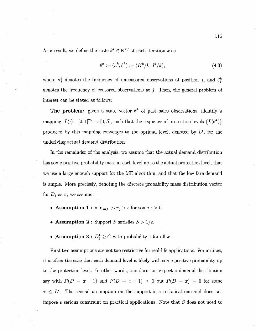
116

As a result, we define the state Ok e R25 at each iteration k as

ek : = (K\ Cfe) := (Kk/k, Jk/k), (4.3)

where Kk denotes the frequency of uncensored observations at position j , and C,k

denotes the frequency of censored observations at j . Then, the general problem of

interest can be stated as follows:

The problem: given a state vector 9k of past sales observations, identify a

mapping L(-) : [0, l ] 2 5 —>• [0, S], such that the sequence of protection levels {L(6k)}

produced by this mapping converges to the optimal level, denoted by L*, for the

underlying actual demand distribution.

In the remainder of the analysis, we assume that the actual demand distribution

has some positive probability mass at each level up to the actual protection level, that

we use a large enough support for the ME algorithm, and that the low fare demand

is ample. More precisely, denoting the discrete probability mass distribution vector

for D\ as 7r, we assume:

• Assumption 1 : min^-.../,* TTJ > e for some e > 0.

• Assumption 2 : Support S satisfies S > 1/e.

• Assumption 3 : Dk > C with probability 1 for all k.

First two assumptions are not too restrictive for real-life applications. For airlines,

it is often the case that each demand level is likely with some positive probability up

to the protection level. In other words, one does not expect a demand distribution

say with P(D = x - 1) and P(D = x + 1) > 0 but P(D = x) = 0 for some

x < L*. The second assumption on the support is a technical one and does not

impose a serious constraint on practical applications. Note that S does not need to

117

correspond to any physical quantity, such as the capacity level or actual support,

which might not be known to begin with, and that we are only interested in getting

the distribution right up to the correct protection level L*. The third assumption is

imposed to simplify the analysis and to establish a worst-case benchmark. In general,

the optimal protection level is independent of the low fare-class demand distribution as

also seen in equation (4.2), and assuming ample low fare-class demand corresponds to

the worst-case censoring scenario. We establish in the following analysis that the ME

algorithm provides protection levels that converge to the optimal value even under

this worst-case censoring scenario. Considering that spiral-down is a phenomenon

caused by censoring, this would guarantee the convergence of our algorithm in other

demand realizations. In Section 4.3, we show that Assumption 3 can be relaxed

without any major change in the analysis.

4.1.3 Proposed solution based on the ME distributions

Given the frequency of uncensored and censored observations 6k = (nkXk), let us

define r)k = K* + (j as the frequency of total observations at j . The key question is

now to decide how to "allocate" the censored mass (fe. The proposed approach is to

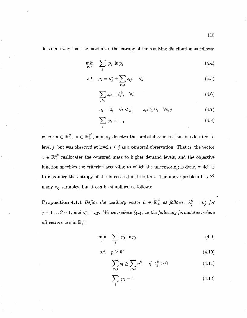
118

do so in a way that the maximizes the entropy of the resulting distribution as follows:

min 2_] Pj m P j 3

s.t. Pj = Kj -\- y j Zjj, i<j

£*« = <?, Vi

3>i

Zij = 0, Vi < j ,

Y.Pi = 1'

Vj

z^ > 0, Vi,3

(4.4)

(4.5)

(4.6)

(4.7)

(4.8) 3

where p € R+, z e l j , and z^ denotes the probability mass that is allocated to

level j , but was observed at level i < j as a censored observation. That is, the vector

z € R+ reallocates the censored mass to higher demand levels, and the objective

function specifies the criterion according to which the uncensoring is done, which is

to maximize the entropy of the forecasted distribution. The above problem has S2

many z^ variables, but it can be simplified as follows:

Proposition 4.1.1 Define the auxiliary vector k G M+ as follows: kh = Kj for

j = 1 . . . S — 1, and hks = r)s- We can reduce (4-4) t° ^ e following formulation where

all vectors are in R+ :

min V^ pj hipj (4.9) j

s.t. p>kk (4.10)

X > > $ > f e * / ^ > 0 (4.11) i>3 i>j

£ Pi = 1 (4-12)

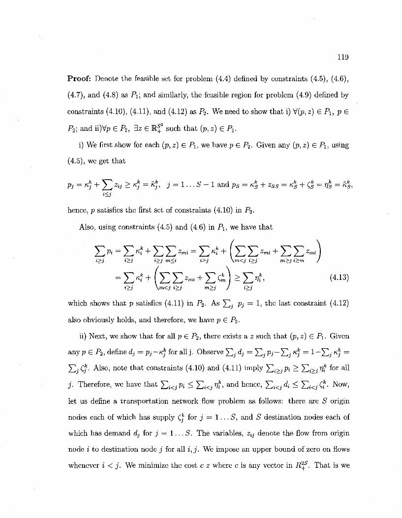
119

Proof: Denote the feasible set for problem (4.4) defined by constraints (4.5), (4.6),

(4.7), and (4.8) as P\\ and similarly, the feasible region for problem (4.9) defined by

constraints (4.10), (4.11), and (4.12) as P2. We need to show that i) V(p, z) e Pi, p G

P2; and ii)Vp e P2, 3z G R f such that (p, z) e Pi.

i) We first show for each (p, z) G Pi, we have p € P2. Given any (p, z) € Pi, using

(4.5), we get that

Pi = «i + X ^ ' ^ «j = *5> J = 1 • • • ^ - 1 and p 5 = 4 + *ssr = 4 + C| = Vs = 4>

hence, p satisfies the first set of constraints (4.10) in P2.

Also, using constraints (4.5) and (4.6) in Pi, we have that

][> = l>f+]r j>mi = j>* + (5^j>™ + ^ j>™) i > j i > j i > j m j \m<j i>j " i > j i > m /

= EK '+(EE 2". .+E^)>E"<. (4-13) i > j \ i n < j i > j m>j / i>j

which shows that p satisfies (4.11) in P2. As V - ^- = 1, the last constraint (4.12)

also obviously holds, and therefore, we have p & P2.

ii) Next, we show that for all p G P2, there exists a z such that (p, z) G Pi. Given

any p G P2, define dj = PJ-K) for all j . Observe £ \ dj = X)jPj_Z)j Kj = 1 _ S j Kj =

XLCj5- Also, note that constraints (4.10) and (4.11) imply J2i>jPi ^ Yli>jVi f° r all

j . Therefore, we have that J2i<jPi < J2i<jVi, and hence, X ^ d ; < E«,-C*- Now>

let us define a transportation network flow problem as follows: there are S origin

nodes each of which has supply (j for j = 1 . . . S, and S destination nodes each of

which has demand dj for j = 1 . . . S. The variables, z^ denote the flow from origin

node % to destination node j for all i, j . We impose an upper bound of zero on flows

whenever i < j . We minimize the cost c z where c is any vector in R2^. That is we

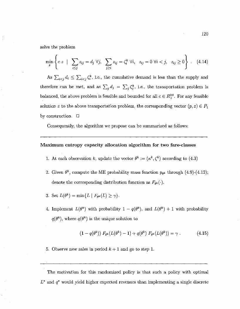
120

solve the problem

nun I c z | ^2 % = di V-?' Yl Zii = $ V i ' ^i = ° v* < h % >0j • (4-14)

As 12i<jdi < H2i<jCi, i-e-> the cumulative demand is less than the supply and

therefore can be met, and as Yljdj = ^ZJCJJ i-e-> the transportation problem is

balanced, the above problem is feasible and bounded for all c € R?f. For any feasible

solution z to the above transportation problem, the corresponding vector (p, z) G P\

by construction. •

Consequently, the algorithm we propose can be summarized as follows:

Maximum entropy capacity allocation algorithm for two fare-classes

1. At each observation k, update the vector 9k := (/sfc,Cfe) according to (4.3)

2. Given 9k, compute the ME probability mass function pek through (4.9)-(4.12);

denote the corresponding distribution function as Fgk(-).

3. Set L{6k) = min{L | Fek(L) > 7}.

4. Implement L(6k) with probability 1 — q{6k), and L(9k) + 1 with probability

q(9k), where q(6k) is the unique solution to

(1 - g(9k)) Fek(L(9k) - 1) + q(9k) Fek(L(9k)) == 7 . (4.15)

5. Observe new sales in period k + 1 and go to step 1.

The motivation for this randomized policy is that such a policy with optimal

L* and q* would yield higher expected revenues than implementing a single discrete

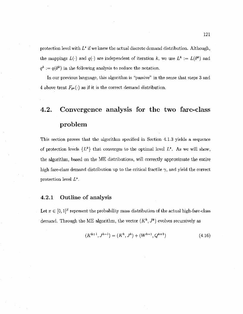
121

protection level with L* if we knew the actual discrete demand distribution. Although,

the mappings L(-) and q(-) are independent of iteration k, we use Lk := L(9k) and

qk := q(9k) in the following analysis to reduce the notation.

In our previous language, this algorithm is "passive" in the sense that steps 3 and

4 above treat F9k(-) as if it is the correct demand distribution.

4.2. Convergence analysis for t he two fare-class

problem

This section proves that the algorithm specified in Section 4.1.3 yields a sequence

of protection levels {Lk} that converges to the optimal level L*. As we will show,

the algorithm, based on the ME distributions, will correctly approximate the entire

high fare-class demand distribution up to the critical fractile 7, and yield the correct

protection level L*.

4.2.1 Outline of analysis

Let 7r € [0, l ] 5 represent the probability mass distribution of the actual high-fare-class

demand. Through the ME algorithm, the vector (Kk, Jk) evolves recursively as

(Kk+\ Jk+1) = (Kk, Jk) + (Wk+1, Qk+1) (4.16)

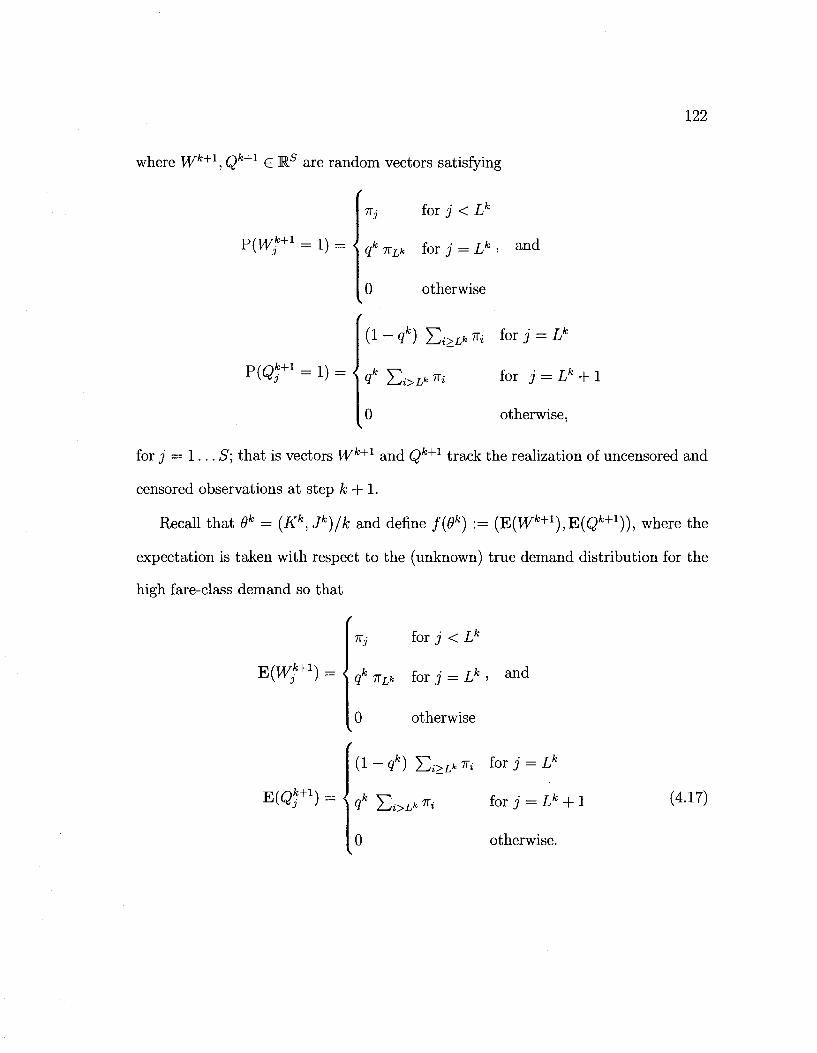
122

where Wk+1,Qk+1 € Rs are random vectors satisfying

%j for j < Lk

qk -KLk for j = Lk i a n d P ( V ^ + 1 = l ) = <

0 otherwise

P(Qk+l = !) = {

(1 - 9*) Ei>L« *i ^ j = Lk

Qk Ei>L^ T» for i = £* + 1

0 otherwise,

for j = 1 . . . S; that is vectors Wk+1 and Qfe+1 track the realization of uncensored and

censored observations at step k + 1.

Recall that 6k = (Kk,Jk)/k and define f{0k) := (E(Wfe+1),E(Qfe+1)), where the

expectation is taken with respect to the (unknown) true demand distribution for the

high fare-class demand so that

E{Wk+1)

7T. for j < Lk

qknLk for j = Lfc> & n d

0 otherwise

E ( Q * + 1 )

( 1 - 9 * ) Zi>L»*i tor j = Lk

<lk J2i>L* "•< f o r J = Lk + l

0 otherwise.

(4.17)

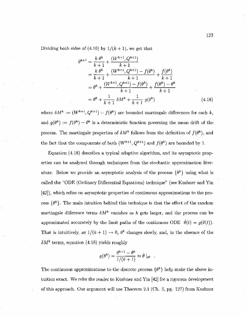
123

Dividing both sides of (4.16) by l/(k + 1), we get that

0*+i = ML+(wh+\Qk+i) k + l k + l

_ k9k {Wk+\Qk+1)-f{6k) f{9k)

k + l k + l k + l _ g f c • (Wk+1,Qk+l)-f(9k) f(9k)-9k

k+l k+l

= 0k + kTi5Mk + k+~l 9{°k) (4,18)

where 8Mk := (Wk+1,Qk+l) — f(9k) are bounded martingale differences for each k,

and g(9k) :— f(9k) — 9k is a deterministic function governing the mean drift of the

process. The martingale properties of 8Mk follows from the definition of f(9k), and

the fact that the components of both (Wk+1, Qk+1) and f(9k) are bounded by 1.

Equation (4.18) describes a typical adaptive algorithm, and its asymptotic prop

erties can be analyzed through techniques from the stochastic approximation liter

ature. Below we provide an asymptotic analysis of the process {9k} using what is

called the "ODE (Ordinary Differential Equations) technique" (see Kushner and Yin

[42]), which relies on asymptotic properties of continuous approximations to the pro

cess {9k}. The main intuition behind this technique is that the effect of the random

martingale difference terms 5Mk vanishes as k gets larger, and the process can be

approximated accurately by the limit paths of the continuous ODE 9(t) = g(9(t)).

That is intuitively, as !/(£; + 1 ) —> 0, 9k changes slowly, and, in the absence of the

5Mk terms, equation (4.18) yields roughly

Qk+l ok

g(ek) = l— -&9\gk . ^^ ' l/(fc + l)

The continuous approximations to the discrete process {9k} help make the above in

tuition exact. We refer the reader to Kushner and Yin [42] for a rigorous development

of this approach. Our argument will use Theorem 2.1 (Ch. 5, pg. 127) from Kushner

124

and Yin [42]. For completeness we state a specific version of this theorem, which

is adopted for the special case of bounded {9k} process with bounded martingale

differences, in Appendix C.l together with its necessary conditions (A.4.3.1), and

(A.5.2.1)-(A.5.2.6). Below we provide the outline of our argument for establishing

limfc_>00Lfe = L*:

1. Section 4.2.2 studies the asymptotic behavior of the continuous, deterministic

dynamical system governed by the ODE 9{t) = g(9(t)).

2. Section 4.2.3 verifies that the conditions (A.4.3.1), and (A.5.2.1)-(A.5.2.6) needed

by Kushner and Yin's theorem are satisfied by the process {9k} and the ODE,

and invokes their result to complete our proof.

4.2.2 Analysis of the ODE

Denote the domain of problem (4.9) as V{9) e M.s for any given 9 = [«,£]. Let

Pe £. 2?(#) be the optimal solution of problem (4.9) for a given 9, and let [K^CS]

denote the corresponding vectors of reallocated uncensored and censored observation

frequencies at this solution such that KQ = K and pe,j — KQJ + Q,j for all j . Hence,

Pe is the probability mass function of the ME distribution implied by any given 9

through problem (4.9), and FQ(-) is the corresponding cumulative distribution func

tion. Hence, the corresponding protection level produced by the ME algorithm is

L(9) := min{L | Fg(L) > 7}, and qe is the associated randomization probability

specified in (4.15).

We start with some preliminary lemmas that establish some of the necessary

structural properties of the ODE 9{t) = g(9(t)); their proofs are given in Appendix

C.2.

125

Lemma 4.2.1 T>(9) is a continuous correspondence.

Lemma 4.2.2 The maximum entropy distribution is continuous in 9, i.e., po is con

tinuous in 6.

Lemma 4.2.3 The function g{9) — f{9) —9 is continuous in 6.

The next proposition identifies the unique stationary solution of the continuous

ODE equation 9{t) = g(9(t)). This solution point, denoted by 9S, would serve as

the candidate unique limit of the process {9k} if the process converged to a unique

equilibrium point. In our case, the process converges to a stable set rather than

a unique point as shown further below. When this is the case, all the stationary

solutions of the continuous ODE equation must also converge to this stable set. The

proof of the proposition is relegated to Appendix C.2.

Proposition 4.2.1 Under assumptions 1, 2, and 3, 9(t) = g(9(t)) has a unique

stationary solution point 9S which satisfies:

rra^ r* A (a\ ft ~ Df-i"17ri)(min{S', Sw} - L* + 1) L(9S) = L*, and q(9s) = — ^ ^ ^ ——L._1

J -, where

Sw = -=t ^i=lJ\ +L*-1 .

We next characterize a candidate limit set of the continuous ODE and the process

{9k}; and show that it is asymptotically stable for the ODE 9(t) = g(9(t)). This will

be needed to prove convergence of {9k} further below. The proof is given in Appendix

C.2. We use the candidate Lyapunov function

v(9) = J2 IK' -*;ll + (7 - E *>- ^*)+> (419) j<L* j<L*

126

where ||x|| := V r is the I? norm on R, and x+ — max{x, 0} is the positive part

of x. This function is continuous everywhere and continuously differentiate almost

everywhere, and the left and right derivatives are strictly negative at breakpoints of

V(6). 1

Proposition 4.2.2 Under assumptions 1, 2, and 3, the set 0 = {9 \ Kj = TTJ, Vj <

L*, 7—X)I<L* ^3 — KL*} ^S 9l°bally asymptotically stable for the ODE 6(t) = g(6(t)).

Observe that, by assumptions 1 and 2 and the definition of L*, we have Lg = L* for

V0 G O as

S Pej = 5Z *i < 7 and ^ pe>j > J^ ^ + KL. > 7, V0 € 0. (4.20) j<L* j<L* jf<Z,* j<L*

The proof of the following result is also given in Appendix C.2.

Proposition 4.2.3 The stationary solution of 9(t) = g(0(t)) belongs to the set Q,

i.e., 9S e 0 .

4.2.3 Proof of convergence

Finally, having established a candidate limit set that is asymptotically stable in which

the desired result for the protection level is guaranteed, we show that the process {9k}

indeed converges to this set 0 by using a theorem provided by Kushner and Yin [42].

Theorem 4.2.1 Denote the state vector given by the ME algorithm at step k as

0k = [nk, (k], and the protection level implied as Lk. Then, limfc_>oo Lk — L*.

1 These conditions are sufficient for asymptotic stability.

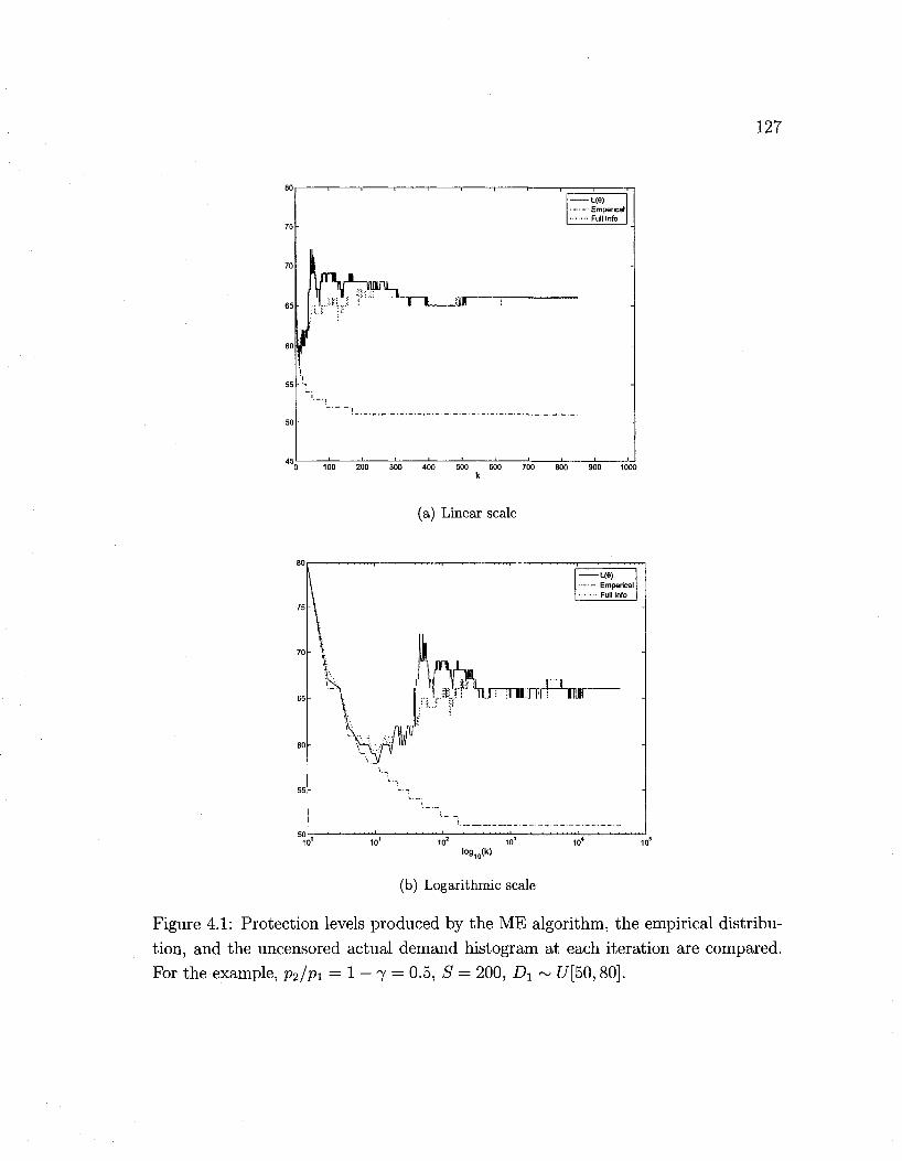
127

- i 1 --L<8) ' Emperical • Full Info

0 100 200 300 400 500 600 700 800 900 1000 k

(a) Linear scale

(b) Logarithmic scale

Figure 4.1: Protection levels produced by the ME algorithm, the empirical distribu

tion, and the uncensored actual demand histogram at each iteration are compared.

For the example, p2/pi = 1 - 7 = 0.5, S = 200, Dx ~ £7[50,80].

128

Proof: The proof follows from Kushner and Yin's [42] Theorem 2.1 (Ch. 5, pg.

127) for identifying limits of adaptive algorithms making use of continuous time or

dinary differential equations (ODE). This theorem and its conditions, (A.4.3.1) and

(A.5.2.1)-(A.5.2.6), are supplied in Appendix C.l.

In our case the process {9k} is bounded in the hyperrectangle H := [0, l ] 2 5 with

probability 1 by construction; hence condition (A.4.3.1) is satisfied. For the ME al

gorithm, we have that fik = 0 and ek = 1/fc, and E[Yk \ 9°, Y\ i < k] = g(6k) =

f(6k) - dk. Consequently, conditions (A.5.2.2), (A.5.2.4) and (A.5.2.5) are trivially

satisfied. We also satisfy condition (A.5.2.3) as shown in Lemma 4.2.3 above. Condi

tion (A.5.2.1) is satisfied as supfe E |Yfe|2 < S < oo by construction. We have that the

ODE 6{t) = g(0(t)) has a unique stationary point 6s E O as identified by Proposition

4.2.1, and hence, the set LH of the stationary solutions for the ODE, as defined in

condition (A.5.2.6), has a single member 6S. Also, we have shown in Proposition

4.2.2 that the set AH = 6 is globally asymptotically stable. Also, we have that

LH U AH = G by Proposition 4.2.3. Consequently, applying Theorem 2.1 of Kushner

and Yin, we conclude that limit points of the process {6k} are in © with probability

1. However, as shown before in equation (4.20) above, we have that LQ — L* for all

eee.D

Figure 4.1 provides an example of the ME algorithm and the spiral-down effect.

As illustrated, the protection levels attained by the empirical distribution of observa

tions spiral down as predicted by Cooper et al. [21]. The protection levels L\ provided

by the ME algorithm converge to the correct level. Also, observe that the controls

obtained by accumulating the true (uncensored) demand observations, which corre

sponds to the (first) best case for the firm, seem to converge almost at the same rate

as those provided by the ME algorithm. The uncensored full information controls

129

seem to under protect for the high fare-class demand while approaching the optimal

level; whereas the protection levels {Lg} over protect. In general, in the presence of

censored observations, no algorithm can produce protection levels that converge to

the correct level by consistently under protecting.

4.3. Extension to multifare problem

The corresponding multifare model, where demand for the different classes arrives in

nonoverlapping intervals in the order of increasing prices, was studied by Brumelle

and McGill [18] using a stochastic dynamic program. Labeling each class such that

the fares satisfy p\ > p2 > . . . > pn, the Bellman equation for each fare-class can be

written as (see Talluri and van Ryzin [73]):

Vn(x) = E max (pn u + yn_i (x-u)) 0<u<mm{Dn,x}

with boundary conditions VQ(X) = 0, Vaj, where x denotes the capacity available at

stage n, and u is the optimal sales amount. Brumelle and McGill [18] show that the

optimal controls take the form of nested protection levels; that is protection level Ln

denotes the number of seats to be reserved for the n highest fare-classes n, n—1,..., 1.

For the continuous problem, the optimal levels for the vector L can be found using

the following formulae, which generalize the Littlewood's rule in (4.1):

n

Pl P(£>! > A , D1 + D2 > L2, . . . , J ^ A > in) = Pn+u Vn . (4.21)

A brute force application of the ME approach to the multifare problem would

require estimating the joint probability distribution of the demand vector for all

classes using a ME formulation analogous to (4.9). Clearly, the number of variables

130

and problem complexity in such a formulation would increase substantially relatively

to that of (4.9).

In the sequel we will focus on a more efficient, albeit a heuristic, approach that

exploits the optimality of equations in (4.21). We will describe an algorithm for the

general N fare-class problem, but to motivate our discussion, we will first illustrate

the main ideas using a three fare-class example below for ease of exposition.

Let 7rn G [0, l]s represent the probability mass distribution of nth fare-class de

mand Dn for n = 1 ,2, 3. Assume again the lowest fare-class demand D$ is abundant,

and we are interested in finding L\ and L2. For n = 1, the equation (4.21) yields

the Littlewood's formula above, and the ME algorithm that is applied as above by

observing censored and uncensored high-class demand D\ is guaranteed to converge

to L\ as demonstrated before. Furthermore, by equation (4.17), the algorithm will

also yield the actual demand distribution ix1 correctly up to L\ in the limit. However,

considering the fill event equation for j' = 2,

P(Di > Lu D, + D2> L2) = P(DX >L2)+Y1 P ( D i = J')P(#2 > L* ~ i) = W P I .

we see that we also need to estimate distribution of Di between L\ and L2. Obviously,

the frequency of observations for D\ between L\ and L2 depend on the distribution

of D2 up to L2 — Li; as D2 is realized before D\, and we can observe a 1st fare-class

sales in this region only when D2 is small enough.

Assume for the moment that we somehow know both actual L\ and L2, and use

them in the above dynamic setting for a long time. In the limit, we would observe

uncensored second class demand at level j with frequency 7r| for j = 1 . . . L2 — L\ as

D2 is realized before D\ at each iteration, and uncensored high-class demand at level

Lx +j with frequency 7ri i+. P(D2 <L2-LX- j) = irli+j E S ^ 1 " ^ 1 <• Therefore,

131

if we used formulation (4.9) to estimate the distribution of Di using the ME method,

we would get it correctly up to L2 — L\. Then, dividing the uncensored high-class

demand observed frequencies by Yli=i 1~j~1 7if, we could find the distribution of Di

between L\ and L2, too. Consequently, assuming again the lowest fare demand D^

is abundant, the heuristic we propose iteratively estimates demand and protection

levels for fare-classes in increasing order of fares as follows:

1. At each observation k, treat the previous estimates of L„ for each class n as the

actual protection levels

2. Update the frequency vector of uncensored and censored observations for Dn,

i.e., 6„, using past sales data.

3. Use 9%_x in ME formulation (4.9) to find the estimate TtN~x.

4. For each n = N — 2 , . . . , 1 do the following in reverse order of fares:

• Scale up each component of «£, i.e., the vector of uncensored observations rfc _[Jk_j_\ . -,

for Dn, between Ln and Ln+i by dividing it by 'Yji2\1 n n? for

j = 1 . . . Ln+i — Ln. That is assign

„k . 1Ln+j 1 — 1 T , — T Klr J.A rk rk • i J — -1 • • • J-'n+l -i-in-

• Use the updated Q\ in ME formulation (4.9) to find the estimate Tvn. Go

back to previous step for n — 1.

5. Use 7rn to calculate the next estimate protection level vector Lk+1 according to

fill event equation (4.21) above.

6. Implement the protection levels and observe new sales in period k + 1 and go

to step 1.

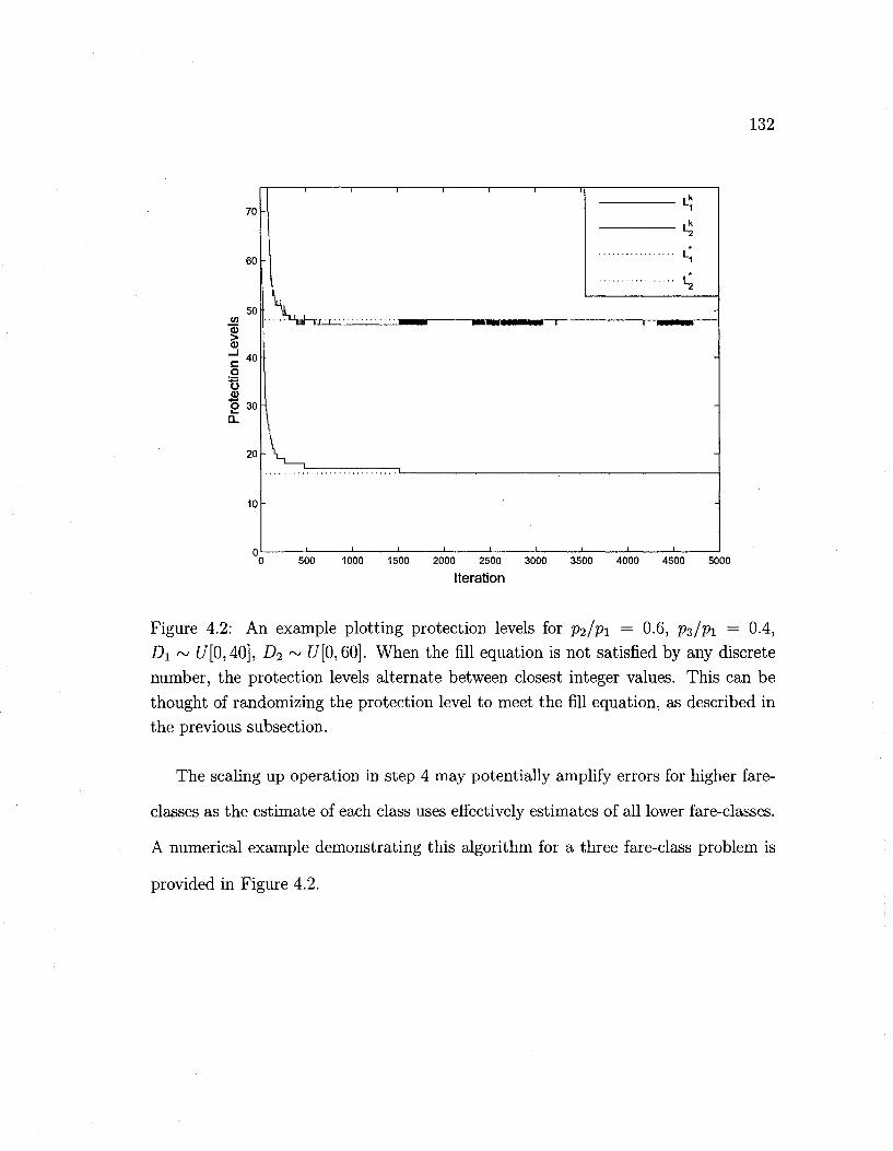
132

70

60

50 <n

> a>

_ i c o t) a> "2 30 a.

40

20 -

10

4

I , \-^-.

. . . . . ' I

500 1000 1500 2000 2500 3000

Iteration 3500 4000 4500 5000

Figure 4.2: An example plotting protection levels for P2/P1 = 0.6, P3/P1 = 0.4,

D\ ~ f7[0,40], D2 ~ U[0,60]. When the fill equation is not satisfied by any discrete

number, the protection levels alternate between closest integer values. This can be

thought of randomizing the protection level to meet the fill equation, as described in

the previous subsection.

The scaling up operation in step 4 may potentially amplify errors for higher fare-

classes as the estimate of each class uses effectively estimates of all lower fare-classes.

A numerical example demonstrating this algorithm for a three fare-class problem is

provided in Figure 4.2.

133

Chapter 5

Conclusions

In this thesis, we studied some classical marketing and revenue management mod

els under the assumption that the monopolist seller does not have full information

about the the market demand, consumer preferences and willingness-to-pay. We

demonstrated that this new source of uncertainty may lead to optimal policies that

are significantly different from their classical counterparts in the literature when com

bined with different performance criteria that are suitable for such uncertain settings.

Many of our results are consistent with policies observed in practice.

Our first two essays study the pricing and product line positioning problems when

the seller has limited information about consumers' preferences and valuation using

the relative performance criteria of competitive ratio and maximum regret. These cri

teria measure the performance relative to a fully-informed decision maker, and allow

us to distinguish between bad market conditions and bad decisions. They produce

less conservative results when compared to more common maxmin type performance

criteria.

In our first essay, we examine monopoly pricing mechanisms of dynamic pricing,

134

third-degree price discrimination, and second-price sealed-bid auction under limited

WtP information. We assume customers have private WtP drawn from a common

distribution that is unknown to the seller. We provide closed-form solutions for the

optimal pricing policies and highlight important structural insights for all three pric

ing schemes. In the dynamic pricing setting, the firm has the ability to change its price

over time, and its key decision is to figure out a pricing policy that would perform

well when the firm does not know the underlying consumers' WtP distribution. The

firm's optimal policy is to adopt a price skimming scheme to minimize and balance

the risk of lost sales and foregone revenue under unknown market characteristics. To

contrast, if the firm knew the customer WtP distribution, then it would be optimal

to charge a static price over the entire sales horizon. Hence, the lack of market infor

mation could offer one possible justification for the use of dynamic pricing policies.

Analytically, the precise form of the resulting pricing policy ensures that both the

firm and the adversary are indifferent with regard to positioning of the representative

valuation of the market.

We also analyze the effects of learning in this setting and illustrate how learning

and partial information can be incorporated. We consider a version where the firm

splits the sales horizon into two periods to use the information extracted in period

one to optimize its decisions in period two. When the seller is not restricted in the

number of price points that she can experiment with, it is optimal to use a price

skimming policy during the learning period and a single price in the remainder of the

sales horizon. When there are constraints linking the firm's pricing decision over time,

we show that the seller is willing to sacrifice performance to retain pricing flexibility.

We also show how to incorporate partial sales information in the form of fractiles of

the representative WtP distribution. Through numerical examples, we demonstrate

135

that even limited learning, e.g., information gained by testing a few price points, leads

to significant performance gains with relative performance criteria, and the resulting

policies have very good revenue performance across common demand distributions.

The second pricing scheme we study is the third degree price discrimination set

ting, where the monopolist firm segments the market into subgroups that can be

charged different prices. However, in our setting, the firm does not know the repre

sentative WtP and relative size of each of these market segments. We show that it is

optimal for the firm to set the price for a particular segment equal to its minimum

WtP value within the segment. Moreover, if the firm has the ability to choose the

market segmentation, it will set equal the (absolute or relative) sizes of the WtP

intervals. This strategy is similar to the price skimming policy above in that the

firm segments the total market size into smaller subgroups by skimming through the

whole valuation range. However, the adversary is strong enough to force the firm to

price at the lowest WtP value within each segment. Combined with the segmentation

strategy, this results in a piecewise price menu being offered to the market.

The third pricing mechanism we consider is the second price, sealed-bid auction.

The choice of this mechanism is motivated by the fact that irrespective of the number

of bidders and the underlying WtP distribution, it is still a dominant strategy for each

potential buyer to bid her/his true WtP within this mechanism. We show that it is

optimal for the seller to set his reservation price so as to balance again the risks of

not selling the item with the risk of selling it at a low price. The resulting reservation

price has similar properties to the one derived under the classical revenue maximizing

setting, but, is slightly lower, reflecting risk aversion of the seller.


pricing for a monopolist when consumer preferences and WtP are unknown. We con-

136

sider a firm that must decide which different versions of a product to offer and how-

to price each version so as to maximize the performance of the whole product line.

Horizontal differentiation is the case where the versions differ in ways that appeal

to the heterogeneous tastes of consumers, such as different colors, sizes or flavors.

Vertical differentiation describes offering versions that differ in their level of quality

and performance. Product line positioning must be coordinated with pricing policies

to maximize revenues and prevent cannibalization effect among versions. We extend

some classical models of horizontal and vertical differentiation to cover uncertainty in

preferences and WtP using the relative performance criteria. Our analysis provides

insights into practices observed in many real world markets. For the horizontal dif

ferentiation case, we show that the optimal decision for both criteria is to position

products at equal intervals in the attribute space and to price them identically. For

the vertically differentiated case, we show that the optimal policy consists of offering a

number of the highest quality versions, and that the more ambiguity over customers'

taste for quality, the more versions the firm should offer. Our results can successfully

explain frequently observed versioning practice in information and technology goods

by using the classical framework of linear utility functions, as opposed to many earlier

work in the marketing literature that failed to do so and concluded that versioning is

not optimal for such goods, despite the empirical evidence.

In our first two essays, we study uncertainty in demand information for a single

sales horizon only. We change our focus to incorporating continuous stream of partial

information in a dynamic capacity allocation setting in our last essay. The inherent

complexity of the relative performance criteria often hinder integration of such dy

namic information. Therefore, we use a different approach to incorporate partial sales

information in such dynamic settings. Revenue management systems consist of joint

137

forecasting and optimization modules that work in an iterative manner. However, the

effect of optimization on future forecasts via policies implemented may result in possi

ble accumulation of errors through time as a result of censored demand observations.

Many common uncensoring techniques fail to avoid the producing controls that de

generate, i.e., the "spiral-down" effect, in such settings as illustrated by Weatherford

and Polt [78]. We propose a tractable and intuitive approach based on maximum

entropy (ME) distributions that easily incorporates partial demand information in

the form of censored sales data. Considering an airline capacity control problem

where demand for lower fare-classes show up before higher ones in nonoverlaping in

tervals, we show that the protection levels given by the ME algorithm we propose

avoids the "spiral down" effect and converge to the optimal values. We make use of

adaptive algorithms and stochastic approximations in our analysis for two fare-classes

and provide a heuristic algorithm for the multifare problem. The solution to the ME

problem simultaneously applies uncensoring to the raw sales data in an intuitive and

statistically sound manner.

Future research opportunities related to our work include establishing possible

connections between decision theory, incentive systems and revenue management

through relative performance criteria. As previously noted, these criteria success

fully explains some of the observed practices in product and revenue management,

for which other criteria have failed to do so. It is plausible to hypothesize that a

risk averse revenue/product manager could choose to deviate from the firm's revenue

maximization goal in a moral hazard setting to hedge her own performance evalua

tion risk, which can be successfully modeled using these criteria. Another possible

research direction is inclusion of partial demand and preference information of some

of the models considered here. We illustrated in the dynamic pricing setting that par-

138

tial information through limited learning can lead to robust implementable policies

with good revenue performance across many demand distributions. We believe simi

lar practical results can be established for other models considered in this thesis. And

finally, we believe that the ME approach holds a good potential for future revenue

management research. In addition to our theoretical results for the capacity alloca

tion setting in this thesis, our preliminary numerical experiments indicate that this

approach can also produce intuitive policies with good performance for monopolistic

pricing settings as well.

139

References

[1] R. Acharyya. Monopoly and product quality: Separating or pooling menu?

Economics Letters, 61:187-194, 1998.

[2] V. F. Araman and R. A. Caldentey. Dynamic pricing for non-perishable products with demand learning. Working Paper, New York University, New York, NY 10012, 2005.

[3] Y. Aviv and A. Pazgal. Pricing of short life-cycle products through active learning. Working Paper, Washington University, St. Louis, MO 63130, 2005.

[4] M. Ball and M. Queyranne. Competitive analysis of on-line booking: Dynamic

policies. Working Paper, University of Maryland, College Park, MD, 2004.

[5] S. Ben-David, A. Borodin, R. Karp, G. Tardos, and A. Wigderson. On the power of randomization in online algorithms. In the proceedings of 22nd ACM Symposium on Theory of Computing,, pages 379-386, 1990.

[6] A. Ben-Tal and A. Nemirovski. Robust convex optimization. Math. Oper. Res.,

23(4):769-805, 1998.

[7] A. Benveniste, A. M. Mtivier, and P. Priouret. Adaptive algorithms and stochas

tic approximations. Springer Verlag, Applications of Mathematics, vol. 22,

Berlin, Heidelberg, New York,, 1990.

[8] D. Bergemann and K. Schlag. Robust monopoly pricing: The case of regret. Working Paper, Yale University, New Haven, Connecticut 06520-8281, 2005.

[9] D. Bertsimas and I. Popescu. Optimal inequalities in probability theory: A

convex optimization approach. SI AM Journal of Optimization, 15(3):780-804,

2005.

[10] D. Bertsimas and M. Sim. The price of robustness. Operations Research, 52:

35-53, 2003.

140

[11] D. Bertsimas and A. Thiele. A robust optimization approach to supply chain management. Proceedings of the 14th IP CO, pages 86-100, 2004.

[12] O. Besbes and A. Zeevi. Dynamic pricing without knowing the demand function: Risk bounds and near optimal algorithms. Working Paper, Columbia University,

New York, NY 10027, 2006.

[13] H. Bhargava and V. Choudhary. Information goods and vertical differentiation.

Journal of Management Information Systems, 18(2):85—102, 2001.

[14] H. Bhargava and V. Choudhary. Research note: One size fits all? optimality conditions for versioning information goods. University of California Irvine, Irvine, CA 92697, 2004.

[15] Ioana C. Bilegan, Carlos A. N. Cosenza, Sergio Gonzlez-Rojo, and Flix Mora-

Camino. A maximum entropy approach to update airlines demand distributions.

Inverse Problems, Design and Optimization Symposium. Rio de Janerio, Brazil,

2004.

[16] S. Bose, E. Ozdenoren, and A. Pape. Optimal auctions with ambiguity. Working

Paper, University of Michigan, Ann Arbor, MI 48109, 2006.

[17] E. A. Boyd, E. Kambour, and J. Tama. The impact of buy down on sell up, unconstraining, and spiral down. Presented at 1st Annual INFORMS Revenue Management Section Conference, New York, 2001.

[18] S. Brumelle and J. McGill. Airline seat allocation with multiple nested fare

classes. Operations Research, 41:127-137, 1993.

[19] Han-Fu Chen. Stochastic approximation and its applications, volume 64 of Non-convex Optimization and its Applications. Kluwer Academic Publishers, Dordrecht, 2002. ISBN 1-4020-0806-6.

[20] Y. Chen, P. Katuscak, and E. Ozdenoren. Sealed bid auctions with ambiguity: An experimental study. Working Paper. Academy of Sciences of the Czech Republic. Prague, 2005.

[21] W. L. Cooper, T. Homem-de Mello, and A. J. Kleywegt. Models of the spiral-

down effect in revenue management. Operations Research, 54(5):968-987, 2006.

141

[22] G. Dobson and C. A. Yano. Profit optimizing product line design, selection and pricing with manufacturing cost considerations: A survey, in Product Va

riety Management: Research Advances (T.-H. Ho and C.S. Tang, eds.), Kluwer

Academic Publisher, pages 145-175, 1998.

[23] L. El Ghaoui and H. Lebret. Robust solutions to least-squares problems with

uncertain data. SI AM J. on Matrix Analysis and Applications, 18(4): 1035-1064,

1997.

[24] S. Eren and C. Maglaras. Revenue management heuristics under limited market information: A maximum entropy approach. Working Paper, Columbia University, New York, NY 10027, 2006.

[25] V. F. Farias and B. Van Roy. Dynamic pricing with a prior on market response.

Working Paper, Stanford University, Stanford, CA 94305, 2006.

[26] G. Gallego and G. van Ryzin. Optimal dynamic pricing of inventories with stochastic demand over finite horizons. Management Science, 40(8):999-1020, 1994.

[27] V. Gaur and M. L. Fisher. In-store experiments to determine the impact of price on sales. Production and Operations Management, 14(4):377-387, 2005.

[28] A. Ghose and A. Sundararajan. Software versioning and quality degradation? an

exploratory study of the evidence. Working Paper, New York University, New

York, NY 10012, 2005.

[29] A. V. Goldberg, J. D. Hartline, and A. Wright. Competitive auctions and digital goods. Technical Report STAR-TR-99.09.01, STAR Laboratory, InterTrust Tech. Corp., Santa Clara, CA, 1999.

[30] A. V. Goldberg, J. D. Hartline, and A. Wright. Competitive auctions and digital

goods. In Proc. 12th Symp. on Discrete Alg. ACM/SIAM, pages 735-744, 2001.

[31] P. E. Green and A. M. Krieger. Recent contributions to optimal product positioning and buyer segmentation. European Journal Operational Research, 41(2): 127-141, 1989.

[32] P. E. Green and V. Srinivasan. Conjoint analysis in consumer research: Issues and outlook. Journal of Consumer Research, 5:103-123, 1978.

142

[33] P. E. Green, J. Carroll, and S. Goldberg. A general approach to product design optimization via conjoint analysis. Journal of Marketing, 43:17-35, 1981.

[34] M. Harris and A. Raviv. A theory of monopoly pricing schemes with demand

uncertainty. American Economic Review, 71 (3): 347-365, 1981.

[35] H. Hotelling. Stability in competition. Economic Journal, 39:41-57, 1929.

[36] W. T. Huh and P. Rusmevichientong. An adaptive algorithm for multiple-fare-class capacity control problems. Working Paper, Columbia University, New York, NY 10027, 2006.

[37] W.T. Huh and P. Rusmevichientong. Online sequential optimization with bi

ased gradients: Theory and applications to censored demand. Working Paper,

Columbia University, New York, NY 10027, 2007.

[38] E. T. Jaynes. On the rationale of maximum-entropy methods. Proceedings of the IEEE, 70(9):939-952, 1982.

[39] R. Jones and H. Mendelson. Product and price competition for information goods. Discussion paper, Stanford University, 1998.

[40] Jong Seok Kim. Optimal price-quality schedules and sustainability. Journal of

Industrial Economics, 36(2):231-44, 1987.

[41] V. Krishnan and K. T. Ulrich. Product development decisions: A review of the literature. Management Science, 47(1):1-21, 1990.

[42] H. J. Kushner and G. Yin. Stochastic approximation and recursive algorithms and applications. Springer New York, 2003.

[43] Lan, Gao, M. Ball, and I Karaesmen. Revenue management with limited demand

information. Working Paper, University of Maryland, College Park, MD, 2006.

[44] K. Lancaster. A new approach to consumer theory. Journal of Political Economy, 74:132-157, 1966.

[45] K. Lancaster. The economics of product variety: A survey. Marketing Science,

9(3): 189-206, 1990.

[46] E.P. Lazear. Retail pricing and clearance sales. American Economic Review, 76: 14-32, 1986.

143

[47] D. Levin and E. Ozdenoren. Auctions with a set of priors: Uncertain number of

bidders. Journal of Economic Theory, 118(2) :229-251, 2004.

[48] G. L. Lilien, P. Kotler, and K. Moorthy. Marketing models. Prentice Hall, 1992.

[49] A.E.B. Lim and J.G. Shanthikumar. Relative entropy, exponential utility, and robust dynamic pricing. Working Paper, University of California Berkeley, CA, 2004.

[50] K. Lo. Sealed bid auctions with uncertainty bidders. Economic Theory, 12:1-20,

1998.

[51] M. S. Lobo and S. Boyd. Pricing and learning with uncertain demand. Working

Paper, Duke University, Durham, NC 27708, 2003.

[52] J.A. Manez and M. Waterson. Multiproduct firms and product differentiation: a survey. The Warwick Economics Research Paper Series (TWERPS) 594, University of Warwick, Department of Economics, 2001.

[53] Eric Maskin and John Riley. Monopoly with incomplete information. RAND

Journal of Economics, 15(2):171-196, 1984.

[54] R. P. McAfee and J. McMillan. Auctions and bidding. Journal of Economic

Literature, 25(2):699-738, 1987.

[55] J. McGill and G. van Ryzin. Revenue management without forecasting or optimization: An adaptive algorithm for determining airline seat protection levels. Management Science, 46 (6): 760-775, 2000.

[56] H. Milton and R. Artur. A theory of monopoly pricing schemes with demand

uncertainty. American Economic Review, 71(3):347-365, 1981.

[57] M. Mussa and S. Rosen. Monopoly and product quality. Journal of Economic

Theory, 18:301-317, 1978.

[58] E. Ozdenoren. Auctions and bargaining with a set of priors. Working Paper, University of Michigan, Ann Arbor, MI 48109, 2002.

[59] B.P. Pashigan. Demand uncertainty and sales: a study of fashion and markdown pricing. American Economic Review, 78(5):936-953, 1988.

[60] B.P. Pashigan and B. Bowen. Why are products sold on sale? explanations of

pricing regularities. Quarterly Journal of Economics, pages 1014-38, 1991.

144

[61] G. Perakis and G. Roels. Regret in the newsvendor model with partial informa

tion. Working Paper, MIT, Cambridge, MA„ 2004.

[62] G. Perakis and G. Roels. Robust controls for network revenue management. Working Paper, UCLA, Los Angeles, CA 90095, 2007.

[63] G. Perakis and A. Sood. Competitive multi-period pricing with fixed inventories.

Working Paper, MIT, Cambridge, MA„ 2003.

[64] A. C. Pigou. Auction theory: A guide to the literature. Journal of Economic

Surveys, 13(3):227-86, 1999.

[65] A. C. Pigou. The economics of welfare. Macmillan Co., London, 1920.

[66] K. Ramdas. Managing product variety: An integrative review and research directions. Production and Operations Management, 12(1):79101, 2003.

[67] J. Robinson. Economics of imperfect competition. Macmillan Co., London, 1933.

[68] A. Salo and M. Weber. Ambiguity aversion in first-price sealed-bid auctions.

Journal of Risk and Uncertainty, 11:123-137, 1995.

[69] S. Salop. Monopolistic competition with outside goods. Bell Journal of Economics, 10:141-156, 1979.

[70] A Shaked and J. Sutton. Relaxing price competition through product differentiation. Review of Economic Studies, 49:3-14, 1982.

[71] J. Smith. Generalized chebyshev inequalities: Theory and applications in deci

sion analysis. Operations Research, 43(5):807825, 1995.

[72] R. K. Sundaram. A First Course in Optimization Theory. Cambridge University

Press, Cambridge and New York, 1996.

[73] K.T. Talluri and G. van Ryzin. The theory and practice of revenue management. Kluwer Academic Publishers, Norwell, Mass., 2004.

[74] H.R. Varian. Price discrimination and social welfare. American Economic Re

view, 75(4):870-875, 1985.

[75] H.R. Varian. Differential pricing and efficiency. First Monday, 1(2), 1996. Avail

able on the World Wide Web.

145

[76] W. Vickrey. Counterspeculation, auctions, and competitive sealed tenders. Journal of Finance, 16:8-37, 1961.

[77] W. S. Vickrey. Microstatics. Harcourt, Brace and World, New York., 1964.

[78] L.R. Weatherford and S. Polt. Better unconstraining of airline demand data in

revenue management systems for improved forecast accuracy and greater rev

enues. Journal of Revenue and Pricing Management, 1:234-254(21), 2002.

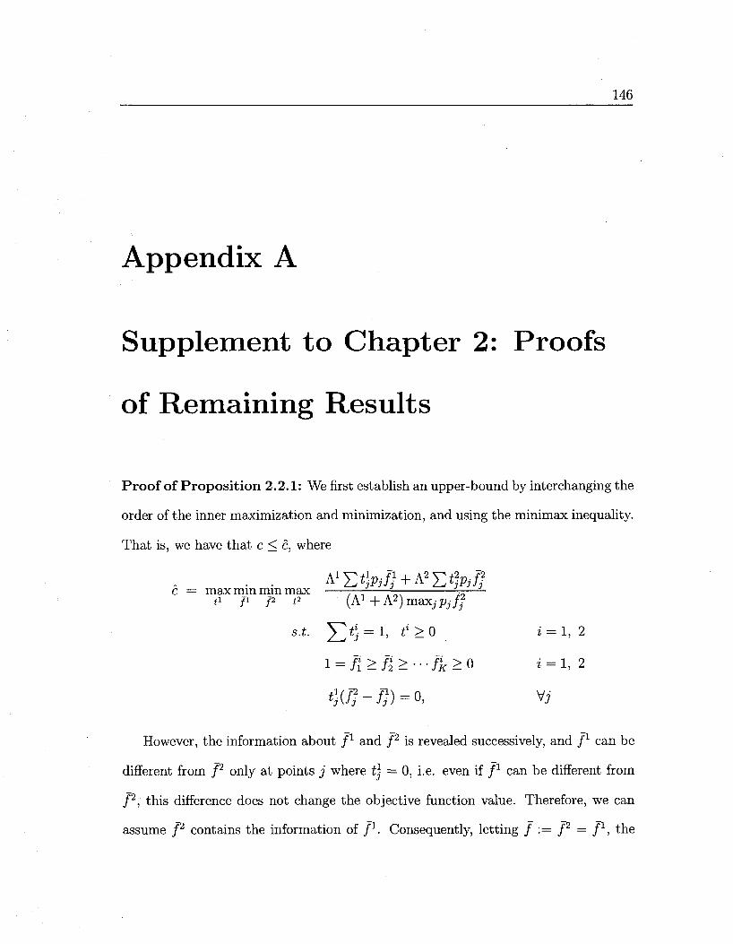
146

Appendix A

Supplement to Chapter 2: Proofs

of Remaining Results

Proof of Proposit ion 2.2.1: We first establish an upper-bound by interchanging the

order of the inner maximization and minimization, and using the minimax inequality.

That is, we have that c < c, where

c = max mm mm max —r-—^— ===—-t1 p- p t2 (A1+A2)maxjpjff

s.t. 5^*5 = 1, ? > 0 « = 1, 2

i = fi>n>---fK>o 2 = 1,2

*}(5-/7) = o. vi

However, the information about Z1 and / 2 is revealed successively, and f1 can be

different from f2 only at points j where t] = 0, i.e. even if f1 can be different from

f2, this difference does not change the objective function value. Therefore, we can

assume f2 contains the information of f1. Consequently, letting / := / 2 = f1, the

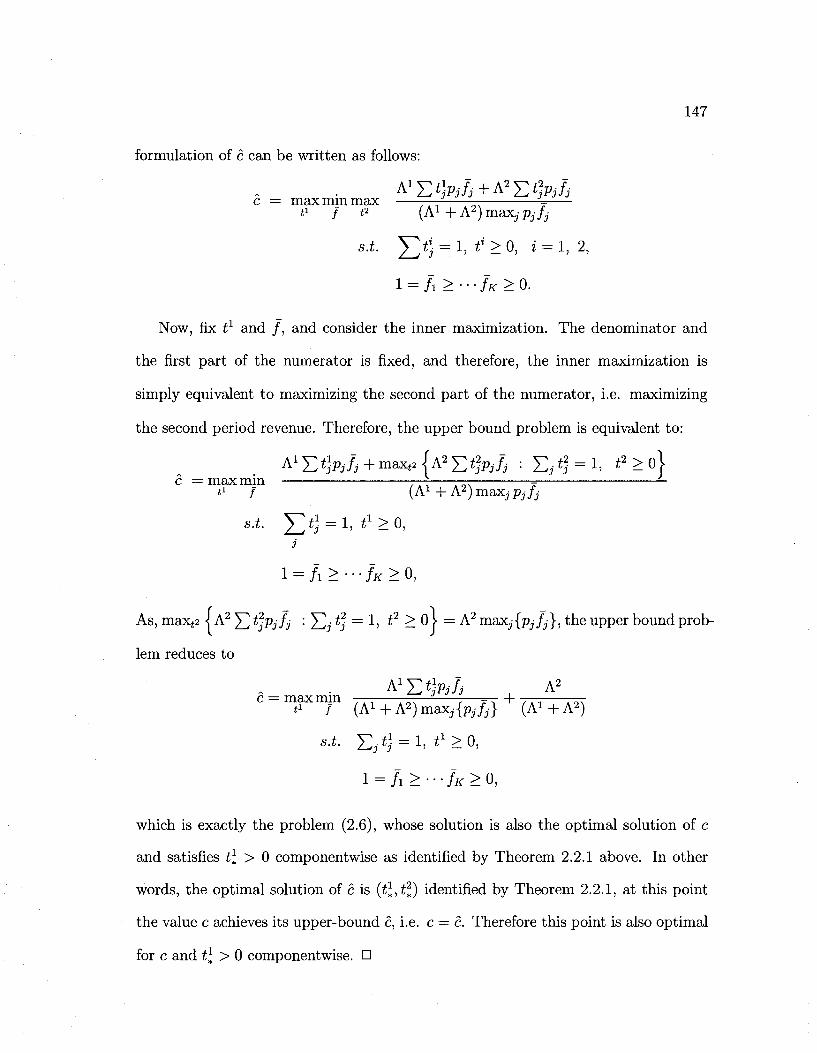
147

formulation of c can be written as follows:

A1 £*>;/; +A2 E ^ A -c = max mm max t1 f i2 (A1 + A2)max.jpjfj

s.t. y£2t) = l, f >0, i = l, 2,

l = fi>---fK>0.

Now, fix t1 and / , and consider the inner maximization. The denominator and

the first part of the numerator is fixed, and therefore, the inner maximization is

simply equivalent to maximizing the second part of the numerator, i.e. maximizing

the second period revenue. Therefore, the upper bound problem is equivalent to:

A1 £ tyj, + maxt2 JA2 £ tfcfj : £ . t) = 1, i2 > o} c = maxmin —7 — = —

t1 / (A1 + A2) max, pjfj

s.t. J^tJ = 1, t1 >0, 3

l = fl>---fK>0,

As, maxt21 A2 £ tfyfj : £ • £2 = 1, i2 > 0 > = A2 max.j{pjfj}, the upper bound prob

lem reduces to

. ^Y,t)pJi A2

c = max mm — rrr— -r—^r + * f (Ai + A^maxjfafj} (A*+A2)

s.t. E i * i = l» ^ > 0 ,

l = fi>---fK>0,

which is exactly the problem (2.6), whose solution is also the optimal solution of c

and satisfies t\ > 0 componentwise as identified by Theorem 2.2.1 above. In other

words, the optimal solution of c is (t\,t1) identified by Theorem 2.2.1, at this point

the value c achieves its upper-bound c, i.e. c = c. Therefore this point is also optimal

for c and t\ > 0 componentwise. •

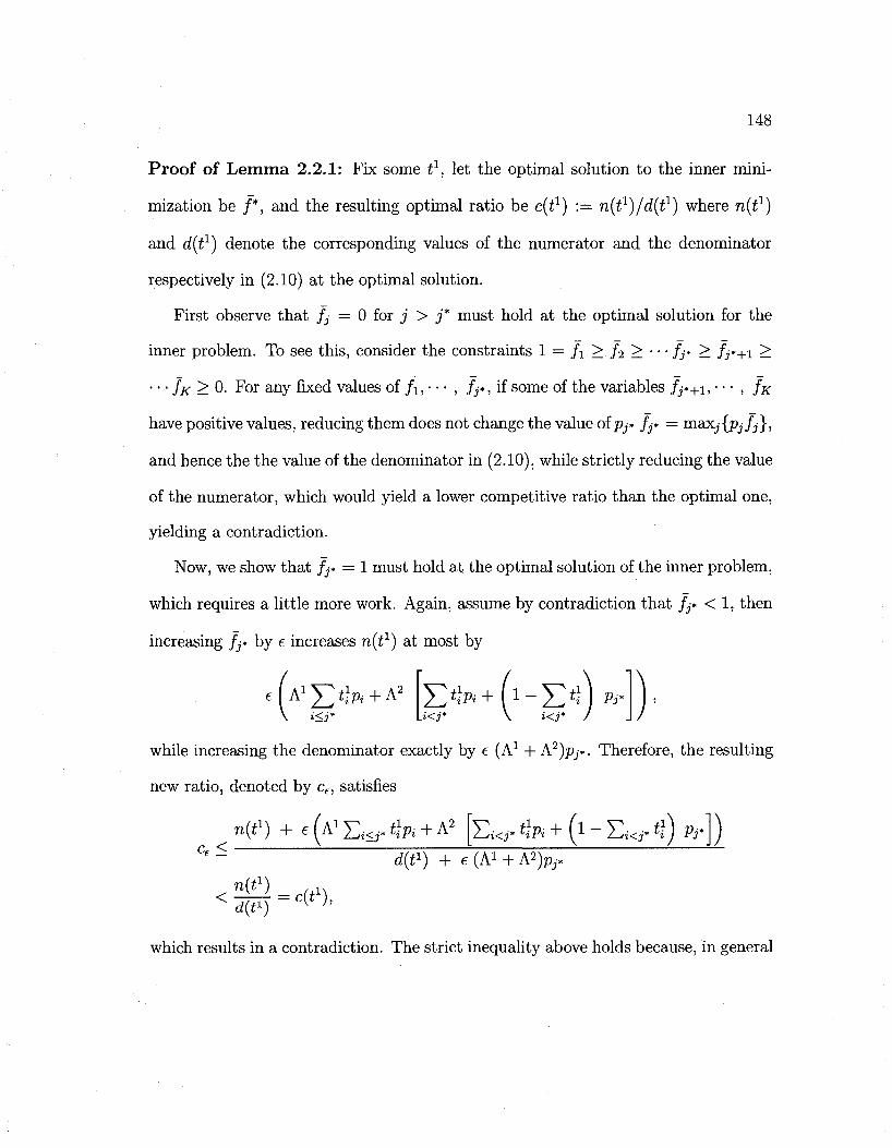
148

Proof of Lemma 2.2.1: Fix some t1, let the optimal solution to the inner mini

mization be /*, and the resulting optimal ratio be c(t1) := n{tl)ld{bl) where n(i1)

and d^t1) denote the corresponding values of the numerator and the denominator

respectively in (2.10) at the optimal solution.

First observe that fj=0 for j > j * must hold at the optimal solution for the

inner problem. To see this, consider the constraints 1 = f\ > f% > • • • fj* > fj*+i >

• • • IK > 0. For any fixed values of / i , • • • , fj*, if some of the variables fj*+i, • • • , JK

have positive values, reducing them does not change the value of pj* fj* = maxj{pj/j},

and hence the the value of the denominator in (2.10), while strictly reducing the value

of the numerator, which would yield a lower competitive ratio than the optimal one,

yielding a contradiction.

Now, we show that fj* =1 must hold at the optimal solution of the inner problem,

which requires a little more work. Again, assume by contradiction that fj* < 1, then

increasing fj* by e increases n(tx) at most by

e U £ t]Pi + A2 [ £ t\Vi + f 1 - £ t\\ Pj* \ i<3* \J<j* \ i<3* J

while increasing the denominator exactly by e (A1 + A2)pj*. Therefore, the resulting

new ratio, denoted by ce, satisfies

lit1) + e (A1 Ei<,- t\Vi + A2 [ E ^ . t\Pi + (l - EKJ* tj) Pj*]) ce<

dit1) + e (A1 + A > T

nit1) , , ,

which results in a contradiction. The strict inequality above holds because, in general

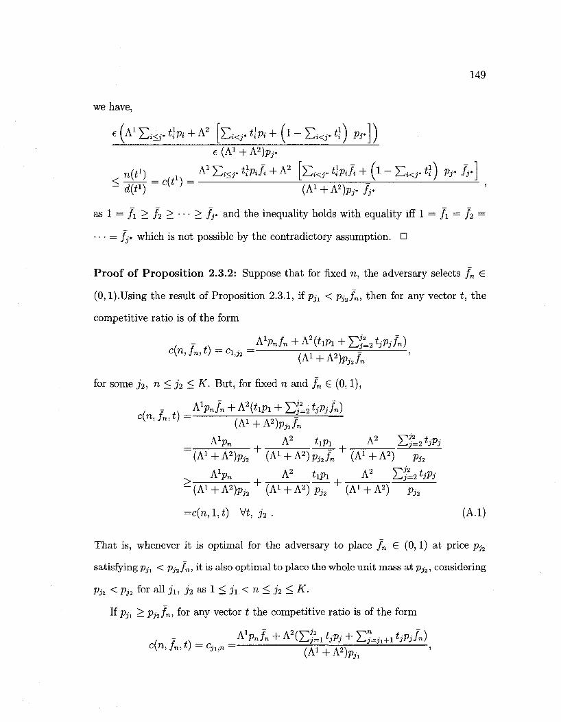
149

we have,

g (A1 £*<,-. t}Pi + A2 [ Z W t\vi + (i - S ^ . t?) P i .]) e (A1 + A2)p r

A1 Ei<i- *.Wi + A2 [Ei<i* t}Pifi + ( l - Ei<r %) Pr fr

dit1) v ' (A1 + A2)Pi. £ .

as 1 = j x > f2 > • • • > fo and the inequality holds with equality iff 1 = / i = /2 =

• • • = fj* which is not possible by the contradictory assumption. •

Proof of Proposition 2.3.2: Suppose that for fixed n, the adversary selects fn G

(0,1).Using the result of Proposition 2.3.1, if p^ < Pj2fn, then for any vector t, the

competitive ratio is of the form

c(n,fn,t) =c i , tfPnfn + A2(tlPl + Ef=2 tjpjn)

for some j 2 , n < h < K- But, for fixed n and /„ G (0,1),

c(n,/„,t) A 1 ^ + A2(tlPl + Ef=2 ^ i /n )

(Ai + A2)p,2/n

AVn A2 t lPl A2 EJLato ' / A "t . A 0 \ 7" ' (A* + A > J 2 (A* + A2) PjJn (A* + A2) P j2

> AV A2 txPl A2 E f = 2 ^ i - (A* + A2)p,2

+ (A* + A2) P j2 + (A* + A2) Ph

=c(n, l , t ) Vt, j 2 . (A.l)

That is, whenever it is optimal for the adversary to place fn G (0,1) at price pj2

satisfying p^ < Pj2fn, it is also optimal to place the whole unit mass at pj2, considering

Ph < Ph for a11 Ji) h as 1 < jx < n < j 2 < K.

If Ph ^ Phfni f° r anY vector t the competitive ratio is of the form

c(n,fn,t) =c . VPnfn + A 2 ( E ; L X *jPj + E;= J 1 +1 tjPjfn)

±,n {A}+A2)Pjl

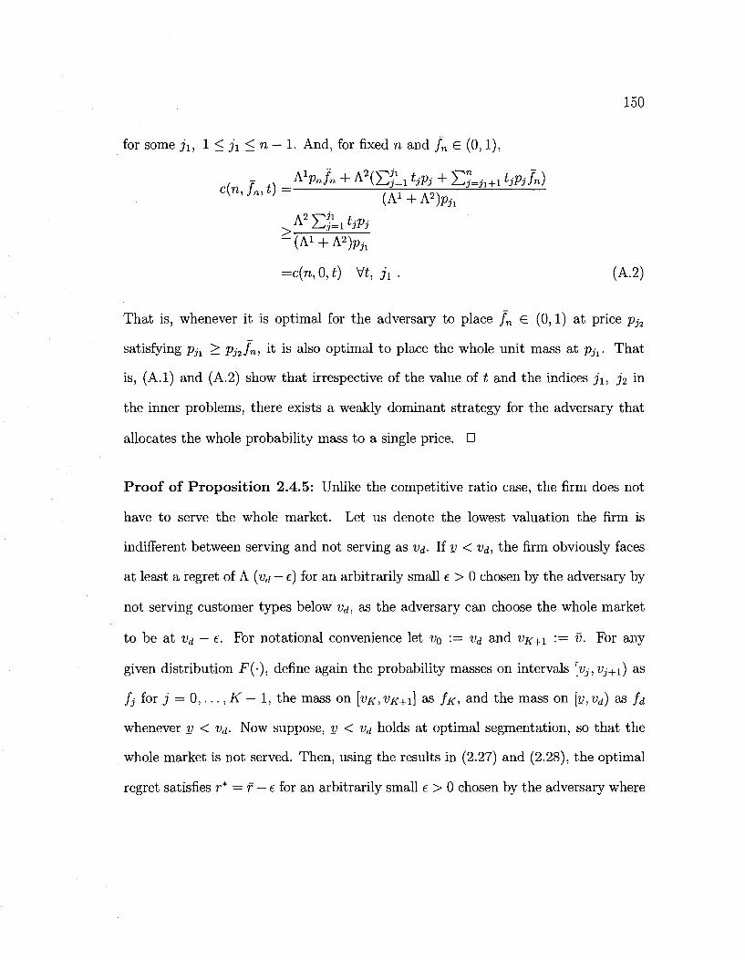
150

for some ji, 1 < j i < n — 1. And, for fixed n and /„ G (0,1),

C(n' ^ t } = (Ai+A*K A 2 E j U ^

- (A* + A2)Pj l

=c(n,0,t) W, J L (A.2)

That is, whenever it is optimal for the adversary to place fn G (0,1) at price Pj2

satisfying pjx > Pj2fn, it is also optimal to place the whole unit mass at pjt. That

is, (A.l) and (A.2) show that irrespective of the value of t and the indices ji, j2 in

the inner problems, there exists a weakly dominant strategy for the adversary that

allocates the whole probability mass to a single price. •

Proof of Proposition 2.4.5: Unlike the competitive ratio case, the firm does not

have to serve the whole market. Let us denote the lowest valuation the firm is

indifferent between serving and not serving as v&- If V < vj, the firm obviously faces

at least a regret of A (vd — e) for an arbitrarily small e > 0 chosen by the adversary by

not serving customer types below Vd, as the adversary can choose the whole market

to be at Vd — e. For notational convenience let VQ := Vd and VK+I '•= v. For any

given distribution F(-), define again the probability masses on intervals [VJ,VJ+I) as

fj for j = 0 , . . . , K — 1, the mass on [VK, VK+I] as fx, and the mass on [v, Vd) as fd

whenever v < Vd- Now suppose, v < va holds at optimal segmentation, so that the

whole market is not served. Then, using the results in (2.27) and (2.28), the optimal

regret satisfies r* = f — e for an arbitrarily small e > 0 chosen by the adversary where

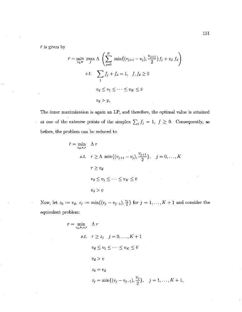
151

f is given by

f = min max A I V ] min{(u,+1 - vj), ~-}fj + vdfd] Vd'v f \U 2 J s-t. ^ / i + /«i = l, fjd>0

i

Vd < V i < • • • < VK < V

vd >V,

The inner maximization is again an LP, and therefore, the optimal value is attained

at one of the extreme points of the simplex V • fj = 1, / > 0. Consequently, as

before, the problem can be reduced to

f = min A r Vd,v,r

s.t. r > A min{(vi+i - Vj), - ^ } , j = 0,...,K

r>vd

Vd < Vi < • • • < VK < V

Vd>V

Now, let z0 := i>d, Zj := min{(vj — Uj-i), ^f} for j = 1 , . . . , K + 1 and consider the

equivalent problem:

f = min A r

s.t. r>Zj j = 0,...,K + l

vd < vl < - - " < ^K < V

I'd > £

20 = Vd

*i = m in{K- - v,-_i), y } , j = l,...,K + l,

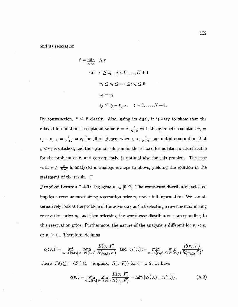
and its relaxation

152

f = min A r z>v,r

s.t. r>Zj j = 0 , . . . , K + 1

Vd < V\ < • • • < VK < V

zo = vd

Zj^Vj-Vj-!, j = 1, ...,K + 1.

By construction, r < f clearly. Also, using its dual, it is easy to show that the

relaxed formulation has optimal value r — A j ^ with the symmetric solution Vd =

Vj - Vj-i = ^ 3 = zi ^or a u J- Hence, when v < j ^ , our initial assumption that

v < Vd is satisfied, and the optimal solution for the relaxed formulation is also feasible

for the problem of f, and consequently, is optimal also for this problem. The case

with v > jjrr^ is analyzed in analogous steps to above, yielding the solution in the

statement of the result. •

Proof of Lemma 2.4.1: Fix some vs G [v,v\. The worst-case distribution selected

implies a revenue maximizing reservation price va under full information. We can al

ternatively look at the problem of the adversary as first selecting a revenue maximizing

reservation price va and then selecting the worst-case distribution corresponding to

this reservation price. Furthermore, the nature of the analysis is different for va < vs

or va> vs. Therefore, defining

Ci(vsj := ml mm — — and c2(i;s) := mm mm — —-, va,i£[v,vs) F£Fi{v*.i) R{va,l, F) va,2e[vs,v] FeF2(va,2) R{Vat2,F)

where Fi(vla) = {F | v\ = argmax„ R(v, F)} for i = 1,2, we have

R(v F) c{vs) = min min " = min {a(vs) , c2(vs)}. (A.3)

vae[v,v] FeF(va) R(va, r)

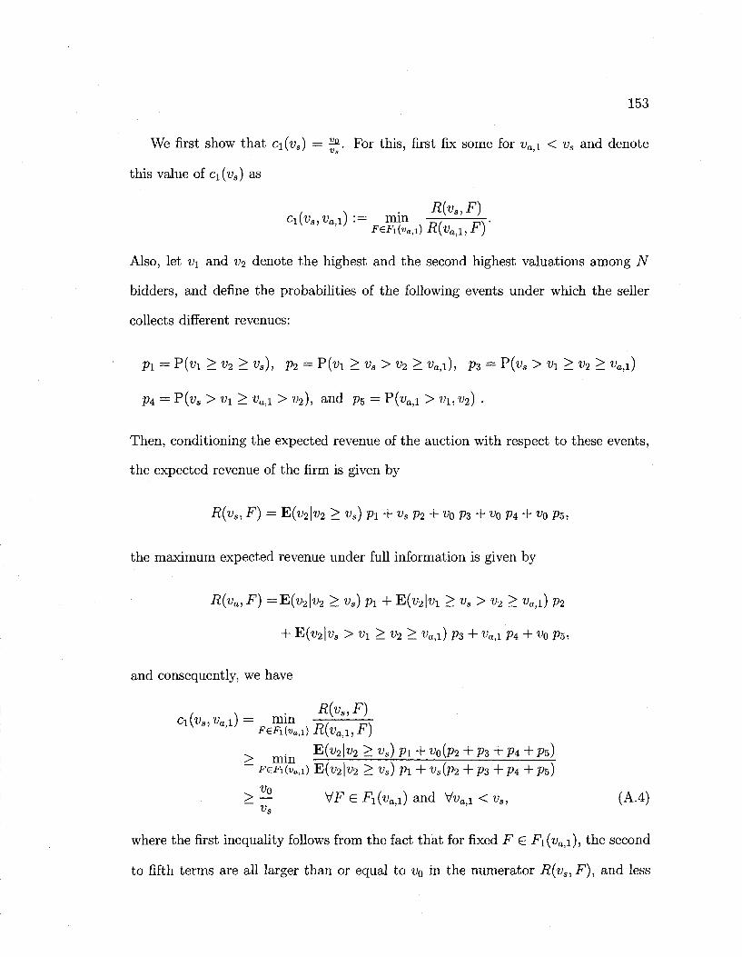
153

We first show t h a t C\(vs) = ^ . For this, first fix some for va>i < vs and denote

this value of Ci(vs) as

. R(v.,F) ci{vs,vaji) := mm — —.

Also, let v\ and v2 denote the highest and the second highest valuations among N

bidders, and define the probabilities of the following events under which the seller

collects different revenues:

Pi = P(« i > v2 > Vs), p2 = P(« i > vs > v2 > u a , i) , pz = P(vs >vx>v2> va,i)

P4 = V(vs >vx> vaA > v2), and p5 = P(va>i > vx, v2) .

Then, conditioning the expected revenue of the auction with respect to these events,

the expected revenue of the firm is given by

R(vs, F) = E(v2\v2 > vs) pi + vsp2 + vQ pz + v0 pA + v0 p 5 ,

the maximum expected revenue under full information is given by

R(Va, F) = E(v2\v2 > Vs) Pi + E(U2|Vi > Vs > V2 > V0>i) p 2

+ E(v2\vs >vx>v2> va>1) pz + w0,i Pi + v0 p 5 ,

and consequently, we have

R{vs,F) ci{vs,vati)= min

FeFi(va,i)R(va>1,F)

> m i n E(t;2|-u2 > vt) Pi + Vpfa + Pz + P\ + Ps) ~ FeFiK.i) E(v2\v2 > vs) p \ + vs(p2 +p3+P4 +P5)

> VA V F e Ft(va>1) and Wva>1 < vs, (A.4)

where the first inequality follows from the fact that for fixed F G Fi(vati), the second

to fifth terms are all larger than or equal to VQ in the numerator R(vs,F), and less

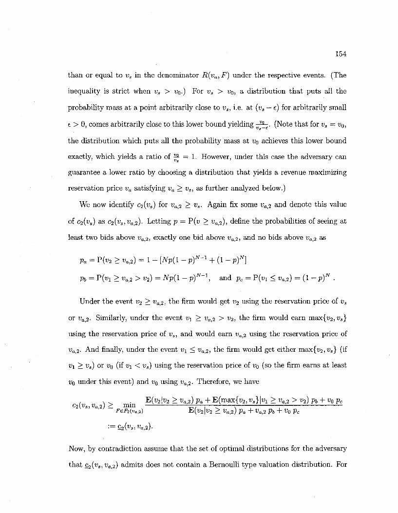
154

than or equal to vs in the denominator R(va,F) under the respective events. (The

inequality is strict when vs > v0.) For vs > v0, a distribution that puts all the

probability mass at a point arbitrarily close to vs, i.e. at (vs — e) for arbitrarily small

e > 0, comes arbitrarily close to this lower bound yielding ^ ^ . (Note that for vs = v0,

the distribution which puts all the probability mass at VQ achieves this lower bound

exactly, which yields a ratio of ^ = 1. However, under this case the adversary can

guarantee a lower ratio by choosing a distribution that yields a revenue maximizing

reservation price va satisfying va > vs, as further analyzed below.)

We now identify c2(vs) for va>2 > vs. Again fix some va>2 and denote this value

of C2(vs) as 02(^3)^0,2)- Letting p = P(v > 1 ,2), define the probabilities of seeing at

least two bids above va^, exactly one bid above vat2, and no bids above va>2 as

Pa = P(V2 > Va,2) = 1 - [NP(1 - p)N~l + (1 - pf]

Pb = P(«i > va,2 > v2) = Np(l - p)N~\ and pc = P(Vl < va,2) = (1 - p)N .

Under the event v2 > va>2, the firm would get v2 using the reservation price of vs

or va>2- Similarly, under the event v\ > va^ > v2, the firm would earn max{v2,fs}

using the reservation price of i;8, and would earn vaj2 using the reservation price of

va<2- And finally, under the event vi < va>2, the firm would get either max{^, w j (if

vi >-vs) o r o (if ^I < vs) using the reservation price of VQ (so the firm earns at least

VQ under this event) and VQ using va^,- Therefore, we have

. E(V2|V2 > «a,2) Pa + E ( m a x { v 2 , VS}\V! > Vat2 > V2) pb + VQ pc

C2{vs,va2) > m m ——j — r • • F€F2(va,2) E{V2 \V2 > Vaj2) Pa + Va,2 Pb + V0 pc

•=C2(vs,Vai2).

Now, by contradiction assume that the set of optimal distributions for the adversary

that c2(v3,Vat2) admits does not contain a Bernoulli type valuation distribution. For

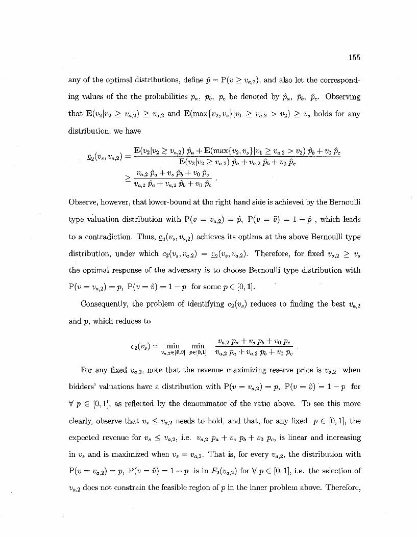
155

any of the optimal distributions, define fi — P(v > vaj2), and also let the correspond

ing values of the the probabilities pa, pb, pc be denoted by fia, fib, pc. Observing

that E(t»2|f2 > va2) > va>2 and E(max{f2 , t ' s}|f i > f0,2 > v2) > vs holds for any

distribution, we have

E(v2\v2 > va,2) pa + E(max{w2, vs}\v! > va,2 > v2) pb + vQ fic c2(vS7va,2) =

>

E ^ K > Vafi) Pa + Va,1 fib + V0 fie Va,2 Pa + Vsfib + V0 fic

Va,2 Pa + Va>2 Pb + V0 pc

Observe, however, that lower-bound at the right hand side is achieved by the Bernoulli

type valuation distribution with P(v = va,2) = fi, P(v = v) = 1 — p , which leads

to a contradiction. Thus, c2(vs,vat2) achieves its optima at the above Bernoulli type

distribution, under which c2(vs,va,2) = c2(vs,vat2). Therefore, for fixed va,2 > vs

the optimal response of the adversary is to choose Bernoulli type distribution with

P(u = ^0,2) = P, P(v — v) = l—p for some p G [0,1].

Consequently, the problem of identifying c2(vs) reduces to finding the best va,2

and p, which reduces to

/ N • • Va>2 pa + Vs pb + V0 pc

c2(vs) = mm mm —• . v«l2e[i;,tJ] P€[0,1] Va<2 pa + Va>2 Pb + V0 Pc

For any fixed vai2, note that the revenue maximizing reserve price is va,2 when

bidders' valuations have a distribution with P(v = va,2) = p, P(t> — v) = 1 — p for

V p e [0,1], as reflected by the denominator of the ratio above. To see this more

clearly, observe that vs < va,2 needs to hold, and that, for any fixed p G [0,1], the

expected revenue for vs < va,2, i.e. va,2 pa + vs pb + v0 pc, is linear and increasing

in vs and is maximized when vs = vaj2- That is, for every va>2, the distribution with

P(f = vai2) = p, P(v = v) = 1 — p is in F2(vat2) for V p G [0,1], i.e. the selection of

va,2 does not constrain the feasible region of p in the inner problem above. Therefore,

156

we can interchange the order of minimization operators above to get

/ \ • • va2Pa + vspb + v0pc C2\Vs) — nun mm —• .

pe[o,i] va,2e[v.,v] va>2 pa + va,2 Pb + vo Pc

For fixed p G [0,1], the probabilities pa, pb, pc are fixed, and therefore, the ratio

above is decreasing in va^-, letting us to conclude optimal reservation price choice of

the adversary satisfies t>0i2 = v independent of chosen p. Therefore, the adversary's

problem reduces to

/ v • VPa + VsPb + VoPc C2\vs) = mm — = pe[o,i] vpa + vpb + Vopc

= m i n ^ [1 ~ (Np(l - p)"-1 + (1 - p)N)] + vs Np(l - p)"-1 + v0(l- p)N

P S S ] v (1 - (1 - p)N) + v0 (1 - p)N

The ratio within the minimization argument above, call C2(p), is continuous and

differentiate in p on the interval [0,1], and attains the value of c2(l) = 1 for p = 1 and

C2(0) = 1 for p = 0 . Thus, the minimum value of c2(p) attained for some p G (0,1).

We finally show that ca(p) is decreasing on the interval (0,p*] and increasing on the

interval-[p*, 1) for p* = 1 — q, and therefore minimized at p*, where q is the value

identified in the statement of the lemma. Differentiating the ratio with respect to p,

we get

c, iV(l - p)N~2 (v - Vs) [{v - v0){l - p)N - Nv(l -p) + (N- l)v]

with c'2(p) = 0, if and only if (v — v0)(l —p)N — Nv(l—p) + (N — l)v := c2(p) = 0 on

the open interval (0,1). Differentiating the function C2(p), we get cf2(p) = Nv — N(l —

p)N~x{v — vo) > 0, where the strict inequality holds for every p G (0,1). As a result,

the function c2(p) is strictly increasing in p e (0,1), with values of c2(0) = —v0 < 0

and c(l) = (N — l)v > 0 . Thus, this function crosses 0 only once at the point

p* satisfying c2(p*) = 0, which implies there is only a single local optimum for the

157

competitive ratio above. c'2(p) is negative for (0,p*], and positive on the interval

[p*,l), implying the ratio is first decreasing and then increasing, and minimized at

the point p* satisfying 62 (p*) = 0.

Obviously, p* solving the polynomial (v — VQ)(1 — p)N — Nv(l — p) + (N — l)^ = 0

is independent of i;s and thus, so are p*a, p*b, ,p*c. Therefore, the optimal ratio for

va,2 > vs is of the form

c t v \ = vP*a + vs Pt + ^0 P*c vp*a + vp*b+v0p*c'

and consequently, we have

/ \ • r t \ t M • f v0 v p*a + vs p*b + v0 p*c\ c(v3) = nun{ci(ua) , c2(u,)} = mm < , _ ° _ " f \ . •

^ t> s -e v p*a + vpl +v0p* J

158

Appendix B



Proof of Lemma 3.1.3: The part of the result for when S(p) is empty is obvious

using the arguments of the previous section as explained above: when S(p) is empty,

we have [ZJ, kj] = [x,-, Xj+X] for all j , and the firm collects Pj from everybody within the

interval [XJ, Xj+\] for all j . Also, the maximum revenue that can be achieved is always

less than Av. Thus the adversary restricts her decision to how much probability mass

fj to put on each interval [XJ, Xj+i], and allocates each mass fj on the point lj for all

j , achieving the maximum regret of A (v — min,pj).

For the other part, fix some price p for which S(jp) is not empty ( i.e. p is a

non-spanning price policy), and define the regret as a function of distribution F as

r(p,F) := R{p*(F),F) - R(p,F). For a given F, define od = F(zd) - F{kj) and

Tj — F(kj+i) — F(ZJ), i.e. Oj is the fraction of customers that are served by price pj,

and Tj is the fraction of customers that are not served either by price Pj or Pj+i, so

that J2 °j + H rj = 1-

159

Now, we can see the adversary's problem of finding the best distribution to max

imize the regret function as a two-step optimization of first choosing o and r vectors,

then choosing a distribution function satisfying the requirements of these vectors.

That is,

max r(p,F) = max max{ r(p,F) : Oj = F{ZJ) - F(kj), r, = F(kj+1) - F(zj), Vj} t o,r b

If we concentrate on the inner maximization for given vectors of o and r, we see that

R(p,F) = A Y^°jPj- As for the function R(p*(F),F), the revenue generated by the

optimal price vector p*(F) at each region [%,^] is obviously bounded by A o,- v.

In addition, for the vector p*(F) to be able to sell to customers with preferences

in the region [zj,kj+i] either p){F) < pj or p*j+1(F) < pj+i must hold. Therefore,

the revenue generated by the optimal price vector p*(F) at each region [zj,kj+x] is

bounded by A Tj m&x(pj,pj+i). Also observe that whenever r,- > 0, the prices Pj

and Pj+i has to satisfy pj + Pj+i + 9\lj+i — lj\ > 2t>, which implies Xj > lj + i/j, and

Xj < lj+i — Vj+i, thus both j , j + l G S(p). Combining these observations, we see

that the regret function for any given F satisfies:

r(p, F)<^2Aojv + J2Arj max(pj, pj+1) - ] T A o Pj

<^2Aoiv + ^2ArJ J^^M ~ YlA °i m/nfe'}

< A max{(t> — mm{pj}) , maxfe}} . i jes(p)

Therefore, independent of F, the regret function r(p, F) is upper-bounded by A max{(i>-

minj{pj}), m8iXjes(p){pj}}. However, as explained above, the adversary can achieve

this bound by putting the whole unit mass to the location of the product with the

minimum price achieving a maximum regret of A(v — min^ pj) when S{p) is empty, or

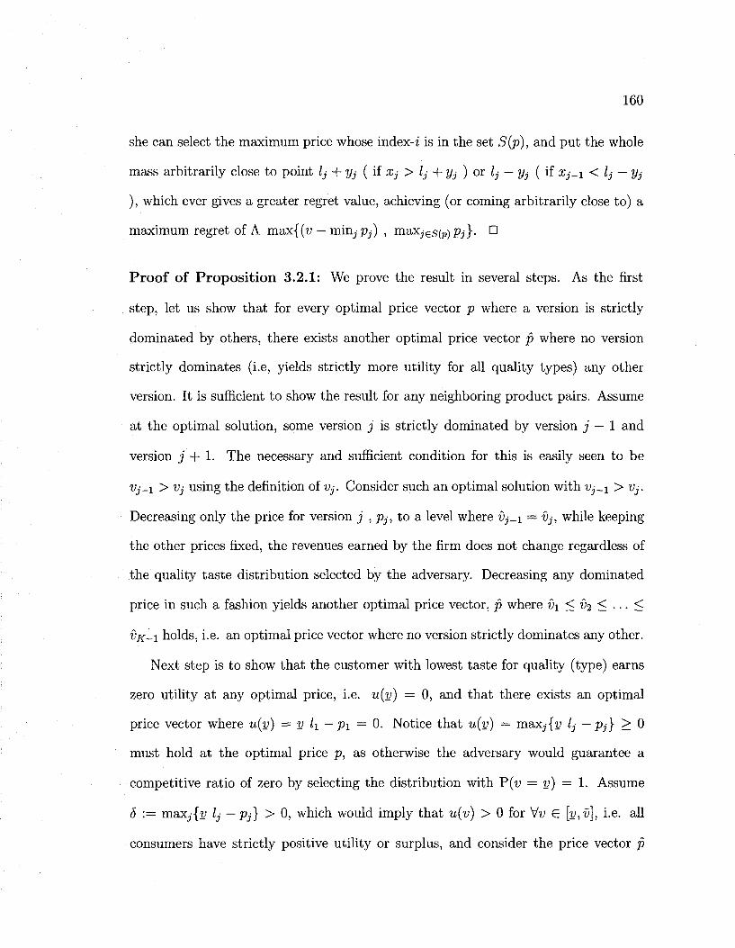
160

she can select the maximum price whose index-z is in the set S(p), and put the whole

mass arbitrarily close to point lj + yj ( if Xj > lj + yj ) or lj — yj ( if Xj^i < lj — yj

), which ever gives a greater regret value, achieving (or coming arbitrarily close to) a

maximum regret of A max{(f — min.jPj) , max.jes(p)Pj}- E

Proof of Proposition 3.2.1: We prove the result in several steps. As the first

step, let us show that for every optimal price vector p where a version is strictly

dominated by others, there exists another optimal price vector p where no version

strictly dominates (i.e, yields strictly more utility for all quality types) any other

version. It is sufficient to show the result for any neighboring product pairs. Assume

at the optimal solution, some version j is strictly dominated by version j — 1 and

version j + 1. The necessary and sufficient condition for this is easily seen to be

Vj_i > Vj using the definition of Vj. Consider such an optimal solution with Vj-i > Vj.

Decreasing only the price for version j , pj, to a level where i)j-i — Vj, while keeping

the other prices fixed, the revenues earned by the firm does not change regardless of

the quality taste distribution selected by the adversary. Decreasing any dominated

price in such a fashion yields another optimal price vector, p where V\ < x>2 < . . . <

VK-I holds, i.e. an optimal price vector where no version strictly dominates any other.

Next step is to show that the customer with lowest taste for quality (type) earns

zero utility at any optimal price, i.e. u(v) — 0, and that there exists an optimal

price vector where u(v) = v l\ — p\ = 0. Notice that u(v) — max.j{v lj — pj} > 0

must hold at the optimal price p, as otherwise the adversary would guarantee a

competitive ratio of zero by selecting the distribution with P(i> = v) = 1. Assume

5 := maxj{:u lj — Pj} > 0, which would imply that u(v) > 0 for Vt> € [v,v], i.e. all

consumers have strictly positive utility or surplus, and consider the price vector p

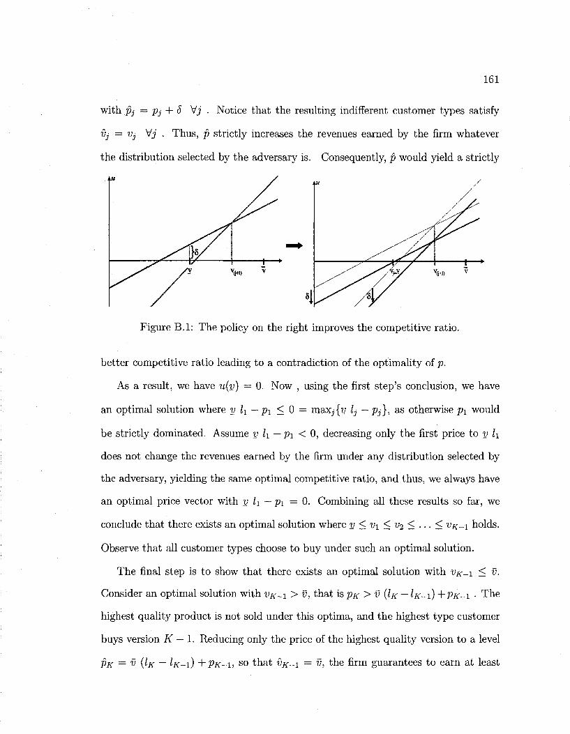
161

with pj — pj + 5 Vj . Notice that the resulting indifferent customer types satisfy

Vj = Vj Vj . Thus, p strictly increases the revenues earned by the firm whatever

the distribution selected by the adversary is. Consequently, p would yield a strictly

Figure B.l: The policy on the right improves the competitive ratio.

better competitive ratio leading to a contradiction of the optimality of p.

As a result, we have u(v) = 0. Now , using the first step's conclusion, we have

an optimal solution where v l\ — p\ < 0 = maxj{t> lj — Pj}, as otherwise p\ would

be strictly dominated. Assume v l\ — p\ < 0, decreasing only the first price to y l\

does not change the revenues earned by the firm under any distribution selected by

the adversary, yielding the same optimal competitive ratio, and thus, we always have

an optimal price vector with y h — p\ = 0. Combining all these results so far, we

conclude that there exists an optimal solution where y < V\ < v2 < • • • < ^ K - I holds.

Observe that all customer types choose to buy under such an optimal solution.

The final step is to show that there exists an optimal solution with VK-X < v.

Consider an optimal solution with VK-\ > v, that is PK > v (IK — IK-I) +PK-I • The

highest quality product is not sold under this optima, and the highest type customer

buys version K — 1. Reducing only the price of the highest quality version to a level

PK = v {IK ~ IK-\) +PK-I, S O that VK-I = v> the firm guarantees to earn at least

162

the same revenue regardless of the distribution selected by the adversary. Thus, we

achieve another optimal solution satisfying vK-\ < v. Combining all of the arguments

above yields the result of the proposition. •

Proof of Lemma 3.2.1: For the problem where only the (K — j + 1) highest

quality versions are offered, observe that the best competitive ratio satisfies CK =

•2f- — | - p = | . Let us now consider the problem of finding c,- for j = 1 . . . K — 1.

Defining fj = P(v < Vj), and fi = P(v > t>;_i) — P(v > Vi) for i — j + 1 . . . K — 1,

and fx = P(f > vx-i) the competitive ratio achieved by a pricing policy satisfying

v — ... = Vj-i < Vj < Vj+i < ... < VK-X < v is given by:

2~/i=j Ji Pi Cj = max mm — ^ » „„ -= 3 V F ff pF{v) dF{v) + £*"* J^i Mv) dF{v) + J ^ Mv) dF{v)

(B.l)

where PF(V) is the price paid by a customer of type v for her best choice under the

revenue maximizing pricing scheme PF{-) for a given quality taste distribution F(-).

Now fix some p offering only the (K — j + 1) highest quality versions, then the

ratio for this fixed price, denoted by Cj(p), is given by

2-*ii=j Ji Pi CAP) mm

> min

F" J 7 PF(v) dF(v) + E f i 2 i:r PF(V) dF(v) + X;_x pF{v) dF{v)

Ylfj1 fi Pi + fa PK yK-l F YZifilKVi + ftclKV

> min < min {pi/lKVi} , Px/fav \ \^%=j...K-\ J

where the first inequality follows from the fact that every fixed F(-), PF(V) < IRVJ

for v G [v, Vj], PF(V) < In^i+i f° r v £ b;> vi+i], i = j ...K — 2, and PF(V) < IRV for

v € [i>#_i,w]. However, selecting a distribution satisfying Pr(v = v^ — e) = 1, where

Vi* is the point where the lower bound above achieves its minima, for some arbitrarily

163

small e € R+, the adversary can achieve a competitive ratio that is arbitrarily close

to the lower bound above.•

Proof of Proposition 3.2.3: Using the previous lemma, the problem of finding Cj

can be written as:

Cj = max min < min {pi/lK^i) > PK/IRV \ (B-2) p [i=j...K-l J

s.t. -un_i = < —j- = vn n = j + I...K -I (B.3)

PK-PK-I ^ - (x> A\ VK-I = -j -, < v (B.4)

I'K — lK-1

Vj = Pj+l^ > v ( B 5 )

Pj = V I. 3

where the constraints (B.3), (B.4) and (B.5) imposes the structure v < Vj < vj+1 <

. . . < vK-i < v for the pricing policy.

We will first relax constraint (B.5) above. Define c as the best ratio that can

be achieved by relaxing the constraint (B.5), which yields an upper bound on Cj.

Below we provide an equivalent linear program for the formulation of cj, then use

weak duality to upper bound cj, which in turn yields another upper bound on Cj.

Finally, using strong duality on this dual problem, we will show that Cj achieves these

upper bounds. We first relax constraint (B.5), and consider the following equivalent

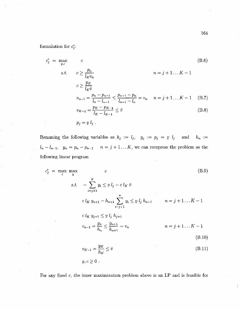
164

mute

3 -

ition for c^:

= max c p,c

. ^ Pn s.t. c >

IRV„ . PK

c> _ lKV

Pn - Pn-1 ^ Pn+1 Vn-l = <

'n 'n—1 nM-l

VK-I - , . < u

Pi = v h •

~Pn

(B.6)

n = j + l...K-l

= vn n = j + l...K-l (B.7)

(B.8)

Renaming the following variables as hj := Zj, yj := Pj = v lj and /in :=

ln — ln-i, yn — pn — Pn-i ^ = j + 1 • • • K, we can reexpress the problem as the

following linear program

<£ = max max c (B.9) c y

K

i.t. — 2_] Hi ^ V lj — Clx V

c Z*r yn+i - hn+i ^2/Vi^v lj hn+t n = j + l...K-l

c IK VJ+I < V lj hj+1

Un - Vn+1 • -, Tr -i

Vn-1 = T - < 7 = «n n = J + l . . . A - l

(B.10)

w«:-i = | ^ < v (B.ll)

y , c > 0 .

For any fixed c, the inner maximization problem above is an LP and is feasible for

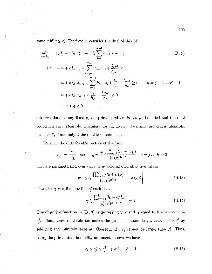
165

some y iff c < c£. For fixed c, consider the dual of this LP:

min (y lj — c IK v) w + y L 7 hi+i Zi + v q (B.12) w.z.t.a ' J

K-\

s.t. —w + clKZj— 2_\ hi+i Zi 4- •—- > 0

K-\ W

hj+i

tn-l + clK Zn-i - ^2 ^+1 2* + T~ ~ ~T~ ^ ° n = j ' + 2 . . . K - l

- W + C ZK 2K-1 + T 7 > °

hK hK

w,z,t,q>0

Observe that for any fixed c, the primal problem is always bounded and the dual

problem is always feasible. Therefore, for any given c, the primal problem is infeasible,

i.e. c > crp if and only if the dual is unbounded .

Consider the dual feasible vectors of the form

^ I = — and z, = '^)K_n «=,...K-2

that are parameterized over variable w yielding dual objective values

w . TiOLj+iihi + clK) . _

vl* (clK)"S °1KV (B.13)

Then, let 7 = y/v and define d\ such that 3

n f 44.Ahi+-djlK) ry I. iXt=J+ lV L—L _ 1 m 141 1 3 (c*lK)K+1-j [ '

The objective function in (B.13) is decreasing in c and is equal to 0 whenever c =

Cj. Thus, above dual solution makes the problem unbounded, whenever c > dj by

selecting and infinitely large w. Consequently, c cannot be larger than cj. Thus,

using the primal-dual feasibility arguments above, we have

Cj<j;<ci j = l...K-l (B.15)

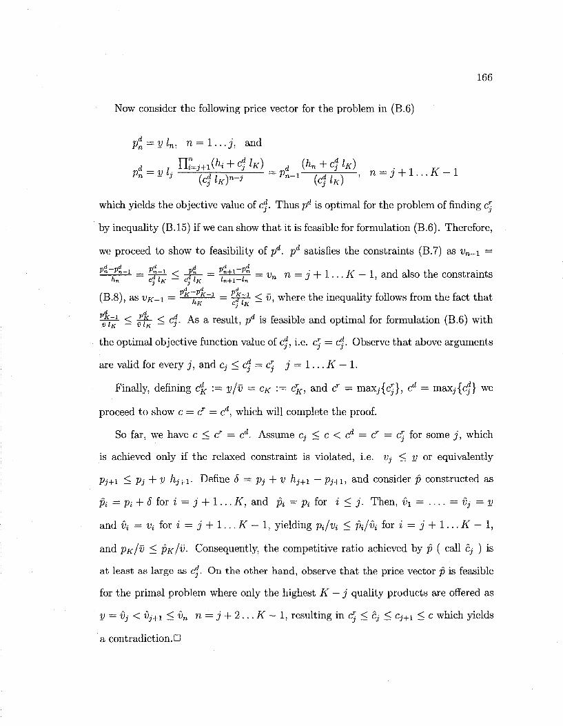
166

Now consider the following price vector for the problem in (B.6)

Pdn = vk, n=l...j, and

which yields the objective value of cd. Thus pd is optimal for the problem of finding c

by inequality (B.15) if we can show that it is feasible for formulation (B.6). Therefore,

we proceed to show to feasibility of pd. pd satisfies the constraints (B.7) as vn-\ =

p " 7 " - 1 = ^ r 1 < -$- = p}+1~fn =vn n = j + 1 . . . K - 1, and also the constraints pd pd „d

(B.8), as VK-I = K , K~1 = - lyi < v, where the inequality follows from the fact that hK cf lK

PK-I v t < §f- < Cj- As a result, pd is feasible and optimal for formulation (B.6) with

the optimal objective function value of cd, i.e. c£ = cd. Observe that above arguments

are valid for every j , and Cj < cd — c j — 1... K — 1.

Finally, defining cdK := v/v = CK •— cr

K, and cr = maxj{c^}, cd = max,-{c^} we

proceed to show c = cr = cd, which will complete the proof.

So far, we have c < cr — cd. Assume Cj < c < cd = cr = cj for some j , which

is achieved only if the relaxed constraint is violated, i.e. Vj < v or equivalently

Pj+i < Pj + V hj+1. Define 8 = Pj + y hj+\ — Pj+i, and consider p constructed as

Pi = Pi + S ion i = j + 1...K, and p; = Pi for i < j . Then, v\ — — = vj = v

and V{ — Vi for i = j + 1 . . . K — 1, yielding p^/vj < pi/t)j for i = j + 1...K — 1,

and PA-/V < PK/V- Consequently, the competitive ratio achieved by p ( call Cj ) is

at least as large as cd. On the other hand, observe that the price vector p is feasible

for the primal problem where only the highest K — j quality products are offered as

v = iij < Vj+i < vn n = j + 2...K — 1, resulting in c < Cj < c,-+i < c which yields

a contradiction.•

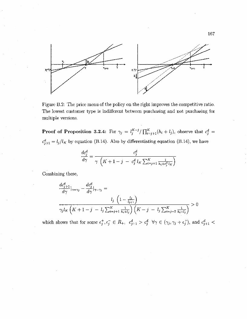
167

Figure B.2: The price menu of the policy on the right improves the competitive ratio.

The lowest customer type is indifferent between purchasing and not purchasing for

multiple versions.

Proof of Proposit ion 3.2.4: For 7, = lf~j/TliLj+i(hi + lj), observe that cj =

dj+1 = IJ/IK by equation (B.14). Also by differentiating equation (B.14), we have

f = i

Combining these,

1A lj+±l >o

7 A (K + l - j - I, E £ i + 1 ^ - ) (K-j- k Ef=J+2 rilj)

which shows that for some e^ej G R+, dj+1 > ri- V7 G (7j,7j + e+), and c^+1 <

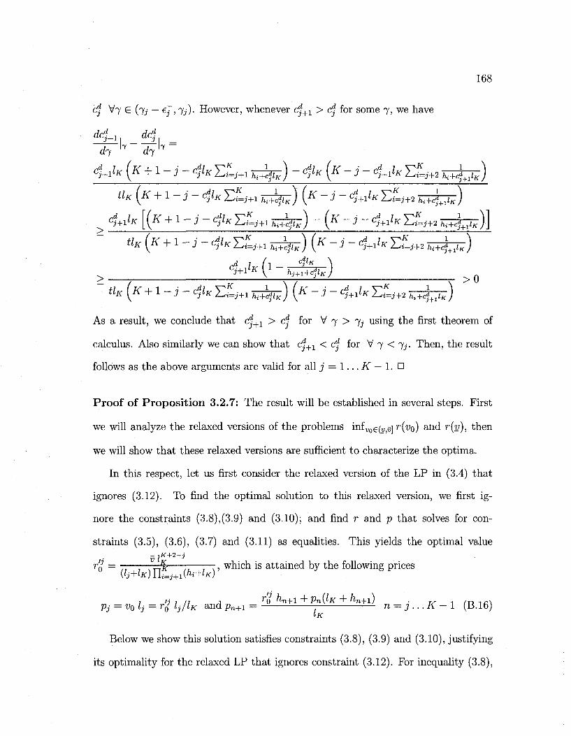
168

cd V7 e (7j — €j ,7j)- However, whenever cd+1 > cd for some 7, we have

d1 h d 7 ' 7 ~

CUK (K + 1-J- C% Tlj+1 j ^ ) - cpK (K-j- CUIK Ylj+2 ^ j ^ )

tiK (K + 1-J-c%Ef=J+1 ^ ) (K-J-dj+xiKEf=j+21^J)

&ifc [(K + l-3- djlK J2lJ+1 j ^ ) -(K-j- dj+1lK ££ , + 2 ^ ^ ) >

«» K(K + I-J-djiKEUiH^) (K~J-cUl*Ef=i+2j^^)

-nK(K + I-J-4KTlj+l^) (K-J-4+1iKEf=j+2s^)

As a result, we conclude that c^+1 > c for V 7 > 7 using the first theorem of

calculus. Also similarly we can show that cd+1 < cd for V 7 < 7^. Then, the result

follows as the above arguments are valid for all j = 1 . . . K — 1. •

Proof of Proposition 3.2.7: The result will be established in several steps. First

we will analyze the relaxed versions of the problems inf„o€(„jS] r(v0) and r(v), then

we will show that these relaxed versions are sufficient to characterize the optima.

In this respect, let us first consider the relaxed version of the LP in (3.4) that

ignores (3.12). To find the optimal solution to this relaxed version, we first ig

nore the constraints (3.8),(3.9) and (3.10); and find r and p that solves for con

straints (3.5), (3.6), (3.7) and (3.11) as equalities. This yields the optimal value

,- vlK+2~j

TQ = —=&—; — , which is attained by the following prices {lj+lK)l{i=j+1{hi+lK)

1 'ji/i A r o hn+i + PU(IK + hn+i) . . .

Pj = v0 Ij = rj IJ/IK and pn+1 = n = j...K-l (B.16) IK

Below we show this solution satisfies constraints (3.8), (3.9) and (3.10), justifying

its optimality for the relaxed LP that ignores constraint (3.12). For inequality (3.8),

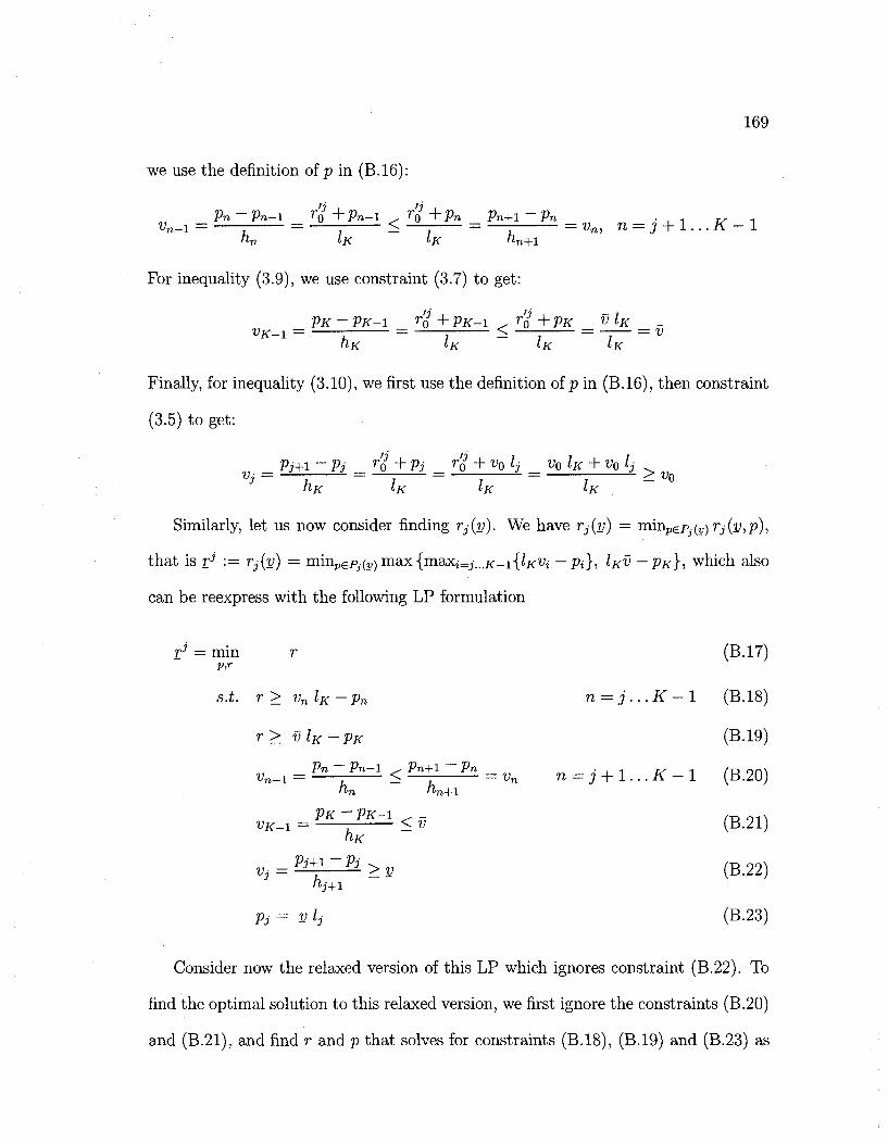
169

we use the definition of p in (B.16):

Vn-Vn-\ r'l + p n _ i r'l + pn Pn+l-Pn . . . . ^ 1 vn-i = 7 = • < —: = — = vn, n = j + l...K-l

nn IK LK «n+i

For inequality (3.9), we use constraint (3.7) to get:

PK-PK-I r%+pK-1 r'J+pK v lK

VK-I = r = -j < —j = -j— = v HK <>K <>K ^K

Finally, for inequality (3.10), we first use the definition of p in (B.16), then constraint

(3.5) to get:

_ pj+1 - pj _ r'j + pj _ r'J + v0 lj _ vo lK + v0 l5 Vj 7 7 7 7 _ ^ 0

tlK lK I>K I'K

Similarly, let us now consider finding Tj(v). We have rj(v) = rmnJ)ep.(v)rj(v,p),

that is r7 := rj(v) = minpep;.(1,)max{maxj=j...^_1{^Wj —pi}, IKV — PK}, which also

can be reexpress with the following LP formulation

r1 = min r (B-17) p,r

s.t. r > vnlK —pn n = j . . . K — 1 (B.18)

r> VIK-PK (B.19)

Pn Pn—X ., Pn+1 ~~ Pn • . -. TS -\ IT> <-,n\

vn-i = T < —r = vn n = j + l...K-l (B.20) "n <Wl

PK - PK-X , - m oi \ VK-X = 7 < v (B.21)

tlK v, = Pj+x-Pj > v ( B 2 2 )

hj+1

Pj = v l5 (B.23)

Consider now the relaxed version of this LP which ignores constraint (B.22). To

find the optimal solution to this relaxed version, we first ignore the constraints (B.20)

and (B.21), and find r and p that solves for constraints (B.18), (B.19) and (B.23) as

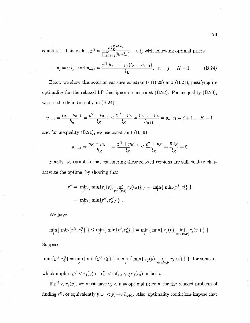
170

v lK+1~j

equalities. This yields, r'3 — K K — — — y L with following optimal prices

i[i=j + l\hi+lK)

r'3 hn+1 + pn(lK + hn+1) . Pj = vlj andp n + i = — ^—L, n = j ...K — 1 (B.24)

IK

Below we show this solution satisfies constraints (B.20) and (B.21), justifying its

optimality for the relaxed LP that ignores constraint (B.22). For inequality (B.20),

we use the definition of p in (B.24): Pn-Pn-l r'3 + Pn-1 , l'3 + pn Pn+l ~ Pn . , - , v ,

Vn-i = r = ; < —j = —r =vn n = j + I...K -I nn LK LK nn+i

and for inequality (B.21), we use constraint (B.19)

PK - PK-I r'3' + pK^i r'3 +pK v lK

VK-I = r = : < —j = -j— = v nK iK iK iK

Finally, we establish that considering these relaxed versions are sufficient to char

acterize the optima, by showing that

r* = min{ mm{rj(y), inf _ rj(vo)} } = min{ mm{r3,r3^} } j v0€(v,v] j

= min{ mm{r'3, rtf} } . i

We have

min{ minlr'-7, TQ} } < min{ min{rJ, rJ0} } — min{ min{ rj(v), inf rj(vo) } } .

j j 3 v0€(v,v]

Suppose

min{r°,TQ } = min{ vain{r'3,T'Q } }'< min{ min{ rj(v), inf rj(v0) } } for some j , 3 3 v0€(v,v]

which implies r'3 < rj(v) or T'Q < inf^g^^j rj(v0) or both.

If r'3 < Tj(y), we must have Vj < y at optimal price p for the relaxed problem of

finding r'3, or equivalently Pj+i < Pj+y hj+j. Also, optimality conditions impose that

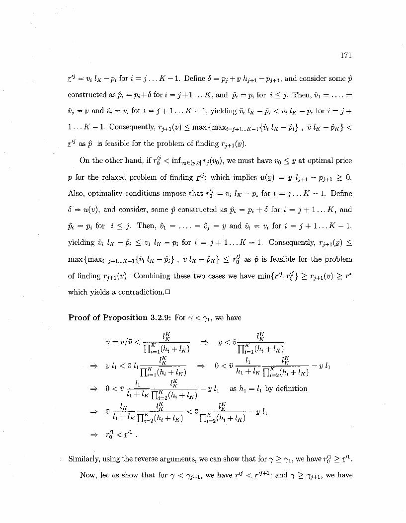
171

r'o =z Vi IK — Pi tor i = j ... K — I. Define 5 — Pj+y hj+i — Pj+i, and consider some p

constructed as pi = Pi + 8 for i = j +1... K, and pi — Pi for i < j . Then, v\ = =

Vj = v and Vi = Vi iox i — j + 1... K — 1, yielding i>i IK — Pi < ty IK — Pi for i = j +

1 . . . K — 1. Consequently, Tj+\{v) < max{maxi=j+i.../<-_1{'0j IK — Pi} , v IK — PK} <

r'j as p is feasible for the problem of finding Tj+i(v).

On the other hand, if TQ < inf^g^j rj(v0), we must have v0 < v at optimal price

p for the relaxed problem of finding rlj; which implies u(v) — v lj+i — Pj+i > 0.

Also, optimality conditions impose that r'£ = vi IK — Pi for i = j •.. K — 1. Define

5 = w(w), and consider, some p constructed as pi — Pi + 6 for i = j; + 1 . . . K, and

pi = pi for % < j . Then, v\ = . . . . = Vj = v and v* = i>j for z = j ' + 1 . . . K — 1,

yielding Vi IK — Pi < « IK — Pi for i = j + 1 . . . K — 1. Consequently, rj+i(v) <

max{maXj=j+i...i<-_i{'0j IK — Pi} , v IK — PK} < ?"o a s P ^S feasible for the problem

of finding Tj+i(v). Combining these two cases we have min{r'J', T'Q } > Vj+i(y) > r*

which yields a contradiction. •

Proof of Proposition 3.2.9: For 7 < 7x, we have

]K iK 1- "K - LK

7 = y/v < —77— =>• y < v-Il*Li(hi + lK) " Uliihi + lx)

vh<vh—j?—- => 0<v- v—- vl\ U^ihi + lK) ^ + lKUl2(hi + lK) "

=4> 0 < v j ^—— y l\ as h\ = li by definition 1 IK

J l lK_

b + kltiUihi + lK) l>K lK ^ - LK 1

< V j? V lx

li+lKUt2(hi + lK) UL^ + IK)

r'0l < r'1

Similarly, using the reverse arguments, we can show that for 7 > 71, we have rfi > r'1.

Now, let us show that for 7 < 7^+1, we have r 0 < r/J'+1; and 7 > 7^+1, we have

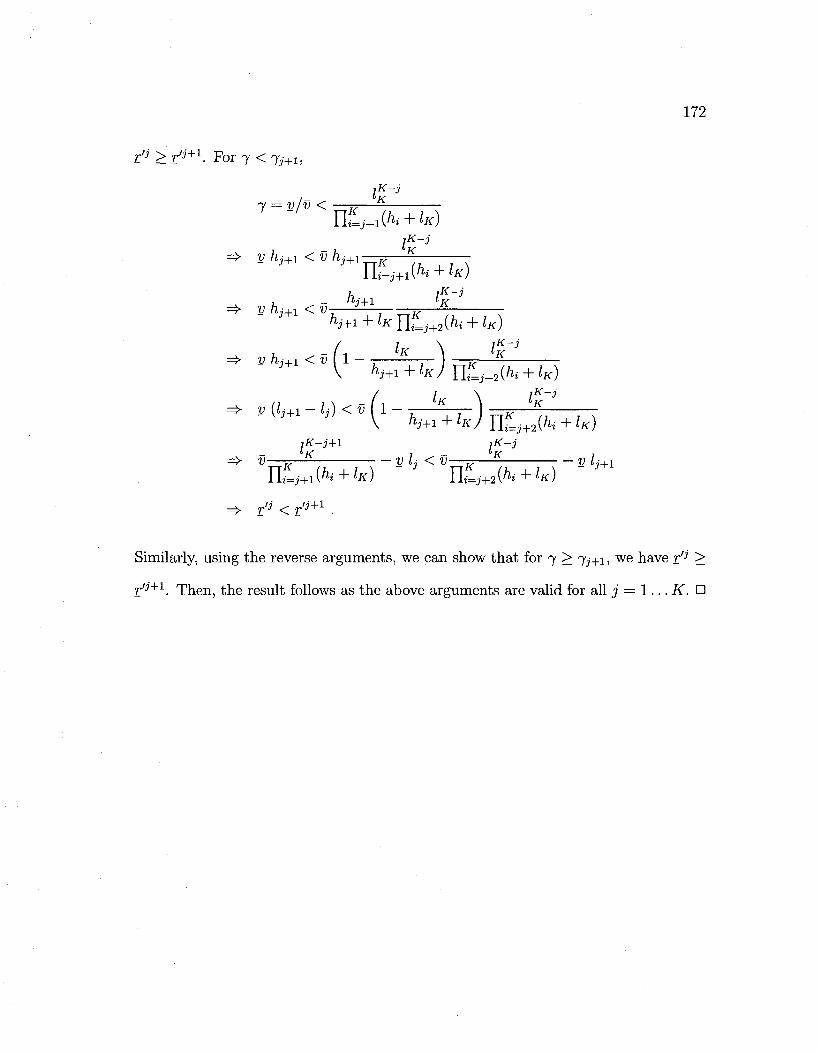
fj > r ' i + i . For 7 < 7 i + i ,

iK-j I— ^K

7 = v/v < — T ? —

=* g h j + i < S fcj+i * rit=i+i(/i<+^)

=> f / l 7 - + 1 V hj+1 < v ( l - , lK , ) K ^

jK-j+l ,K-j

=> V rr—^ V L < V „ V L+l

Similarly, using the reverse arguments, we can show that for 7 > TJ+I, we have r° >

r'j+1. Then, the result follows as the above arguments are valid for all j = 1 . . . K. •

173

Appendix C



C. l . Theorem 2.1 of Kushner and Yin (2003)

Kushner and Yin consider an adaptive process {6k} on some connected compact set

H G Rn. The adaptive algorithm they analyze is of the form 6k+l = 6k + ekYk + ekZk

where ek is the step size, ekZk are correction terms that take the process back to the

nearest point in the set H when 9k + ekYk is out of this set, and Yk are random

variables satisfying the below conditions.

The compact set H and the corresponding correction terms are allowed to take

one of several specific forms in their Theorem 2.1; and consequently, the original

statement of the theorem is long, accounting for several possible cases. The {6k}

process in our problem satisfies a much simpler structure in that it is bounded with

probability 1 on a hyperrectangle. Hence, no correction terms ekZk are necessary, and

the simplest specification for set H, which is stated below, is sufficient. Therefore,

174

we adopt and state the theorem below in a simpler form as it applies to our setting,

with only the conditions that are required for our specific structure.

• (A.4.3.1) H is a hyperrectangle, i.e., 3 a; < hi i = 1 , . . . , n such that H = {9 :

Oi<0< bh Vi}.

• (A.5.2.1) sup f cE|Y f c |2<oo

• (A.5.2.2) There is a measurable function g(-) of 9 and random variables (3k such

that E[Yk | 9°, Y\ i<k}= g(9k)+fik.

• (A.5.2.3) g(-) is continuous.

• (A.5.2.4) J2i(^)2 < oo

• (A.5.2.5) Ei(e0 1 1 < oo w-P-1-

Theorem 2.1 of Kushner and Yin (2003), (Ch. 5, pg. 127) Let LH denote

the set of limit points of the mean limit ODE 9(t) = g(9(t)) in the set H over all

initial conditions. Also let LlH C LH be the set of all stationary points of the ODE,

and AH be a set that is locally asymptotically stable in the sense of Lyapunov. Assume

that

• (A.5.2.6) For any initial condition not in LH the trajectories of 9(t) — g(9(t))

goes to AH.

Then, the limit points of the process {9k} are in LH U AH w.p.l.

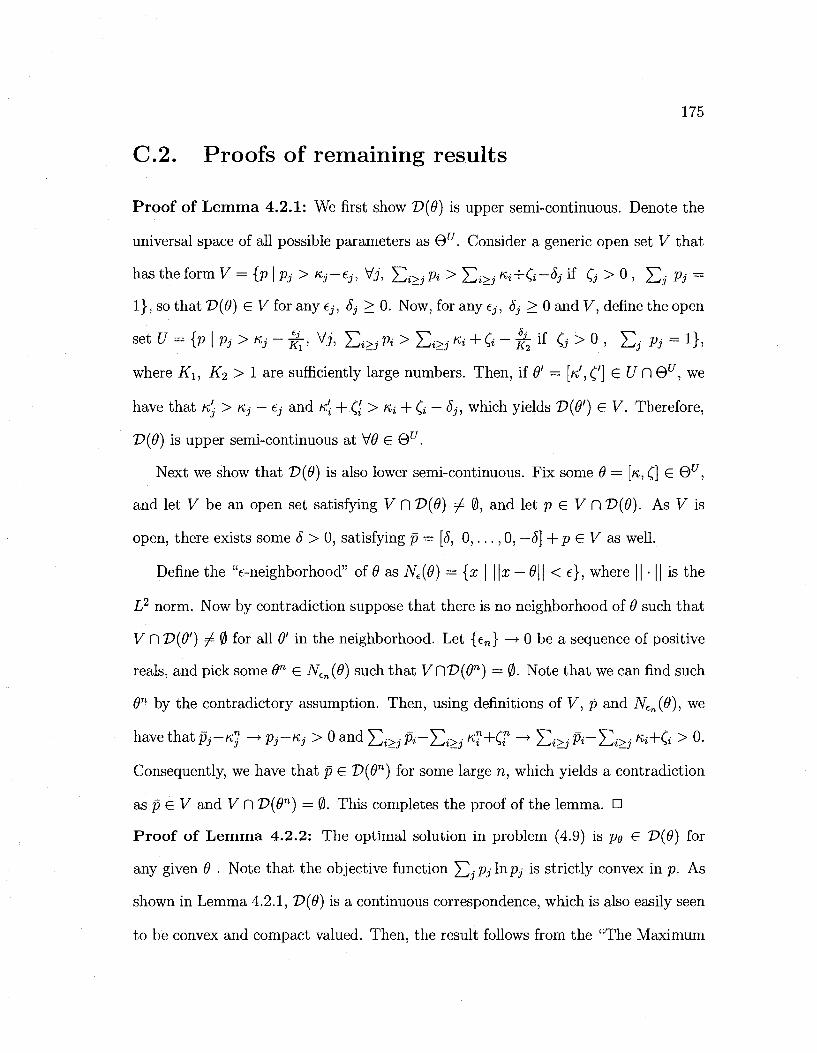
175

C.2. Proofs of remaining results

Proof of Lemma 4.2.1: We first show V(9) is upper semi-continuous. Denote the

universal space of all possible parameters as Qu. Consider a generic open set V that

has the form V = {p \ Pj > Kj-Cj, Vj, Yli>jPi > J2i>j *i+Ci-&j i f 0 > 0 , £ \ Vj =

1}, so that T>(9) G V for any tj, 5j > 0. Now, for any e,-, 5j > 0 and V, define the open

set U = {p\pj>Kj-jfc, Vj, X)i>j ft > Ei>j Ki + d - ^ i i 0 > 0 , £ j p, - 1},

where K\, K2 > 1 are sufficiently large numbers. Then, if 0' — [«', ('] G ?7 D 0^ , we

have that K'J > Kj — e and ^ + ^ > Kj + Q — 5j, which yields V(8') G V. Therefore,

T>(9) is upper semi-continuous at V0 G Qu.

Next we show that V(9) is also lower semi-continuous. Fix some 9 = [«, C] € O17,

and let V be an open set satisfying V fl £>(#) ^ 0, and let p e V f l Z>(0). As V is

open, there exists some 5 > 0, satisfying p = [5, 0 , . . . , 0, —5] i p e ^ a s well.

Define the "e-neighborhood" of 9 as Ne(9) = {x \ \\x — 9\\ < e}, where || • || is the

I? norm. Now by contradiction suppose that there is no neighborhood of 9 such that

V D V(9') 7 0 for all 9' in the neighborhood. Let {e„} - ^ O b e a sequence of positive

reals, and pick some 9n G N£n(9) such that VDV(9n) = 0. Note that we can find such

9n by the contradictory assumption. Then, using definitions of V, p and N€n(9), we

have that pj-n] -»• p—Kj- > 0 and £i>jjp—Ei>j «?+CT - • E i > j P ~ E i > j K i+0 > 0.

Consequently, we have that p G V(9n) for some large n, which yields a contradiction

as p G V and V fl V(9n) = 0. This completes the proof of the lemma. •

Proof of Lemma 4.2.2: The optimal solution in problem (4.9) is pe G T>(9) for

any given 9 . Note that the objective function YljPj m P j is strictly convex in p. As

shown in Lemma 4.2.1, V{9) is a continuous correspondence, which is also easily seen

to be convex and compact valued. Then, the result follows from the "The Maximum

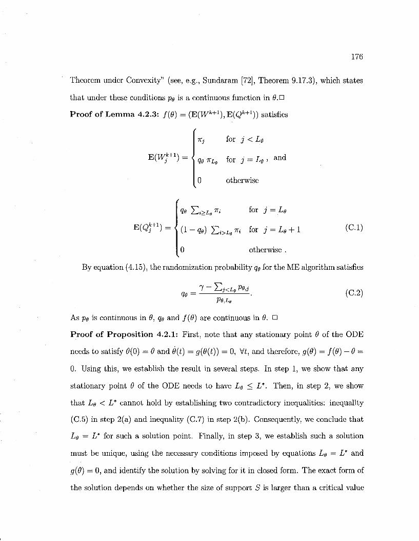
176

Theorem under Convexity" (see, e.g., Sundaram [72], Theorem 9.17.3), which states

that under these conditions pg is a continuous function in 9.U

Proof of Lemma 4.2.3: /(0) = (E(Wk+1),E(Qk+1)) satisfies

ixj for j < Lg

E(Wk+1) = \ qe nLg f o r j = Lg, and

0 otherwise

E(Q*+1) = { (C.l)

QO T,i>Le *i for 3 = U

(i - qe) E J > L S ** f o r J = ^ + 1

0 otherwise .

By equation (4.15), the randomization probability qe for the ME algorithm satisfies

Qe Pe,Le

(C.2)

As pe is continuous in 6, qg and f(9) are continuous in 0. •

Proof of Proposition 4.2.1: First, note that any stationary point 0 of the ODE

needs to satisfy 9(0) = 9 and 9(t) = g(9(t)) = 0, Vt, and therefore, g(9) = f(9) -9 =

0. Using this, we establish the result in several steps. In step 1, we show that any

stationary point 9 of the ODE needs to have Lg < L*. Then, in step 2, we show

that Lg < L* cannot hold by establishing two contradictory inequalities: inequality

(C.5) in step 2(a) and inequality (C.7) in step 2(b). Consequently, we conclude that

Lg = L* for such a solution point. Finally, in step 3, we establish such a solution

must be unique, using the necessary conditions imposed by equations Lg = L* and

g(9) = 0, and identify the solution by solving for it in closed form. The exact form of

the solution depends on whether the size of support S is larger than a critical value

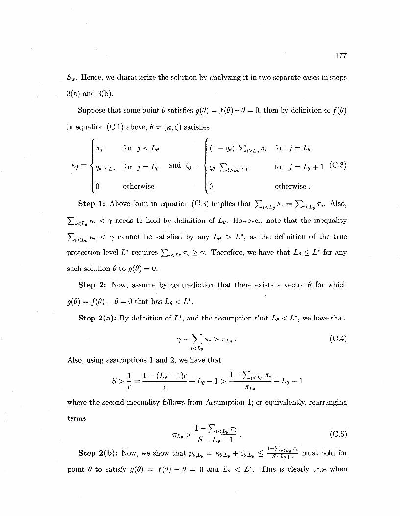
177

Sw. Hence, we characterize the solution by analyzing it in two separate cases in steps

3(a) and 3(b).

Suppose that some point 9 satisfies g(9) = f(9) — 6 = 0, then by definition of f(9)

in equation (C.l) above, 9 = (K, C) satisfies

« j = <

itj for j < Le

qe -KLB for j = Le a n d 0 = <

0 otherwise

(1 - qe) Ei>Lfl T» f o r 3 = U

Qe T,i>L^i for j = L0 + l (C-3)

0 otherwise .

Step 1: Above form in equation (C.3) implies that Yli<L K* = XW<L ^ Also,

Si<L K» < 7 needs to hold by definition of LQ. However, note that the inequality

lLii<Le Ki < 1 cannot be satisfied by any Le > L*, as the definition of the true

protection level L* requires Yli<L* ni — 7- Therefore, we have that Le < L* for any

such solution 9 to g{9) = 0.

Step 2: Now, assume by contradiction that there exists a vector 9 for which

g(6) = f(d) -9 = 0 that has Le<L*.

Step 2(a): By definition of L*, and the assumption that Le < L*, we have that

Also, using assumptions 1 and 2, we have that

s > l = l-(L0-l)e , _ 1 >1 - ^ < L e

(C.4)

7T,;

+ £fl e e 7TLe

where the second inequality follows from Assumption 1; or equivalently, rearranging

terms 1 - Ei<L„ T*

7TLe > 5 - Le + 1

Step 2(b): Now, we show that pe,Le = «0,L9 + C<?,L9 < S-L9+I

(C.5)

t<L^r^ must hold for

point 9 to satisfy g(9) — /(#) — 9 = 0 and Le < L*. This is clearly true when

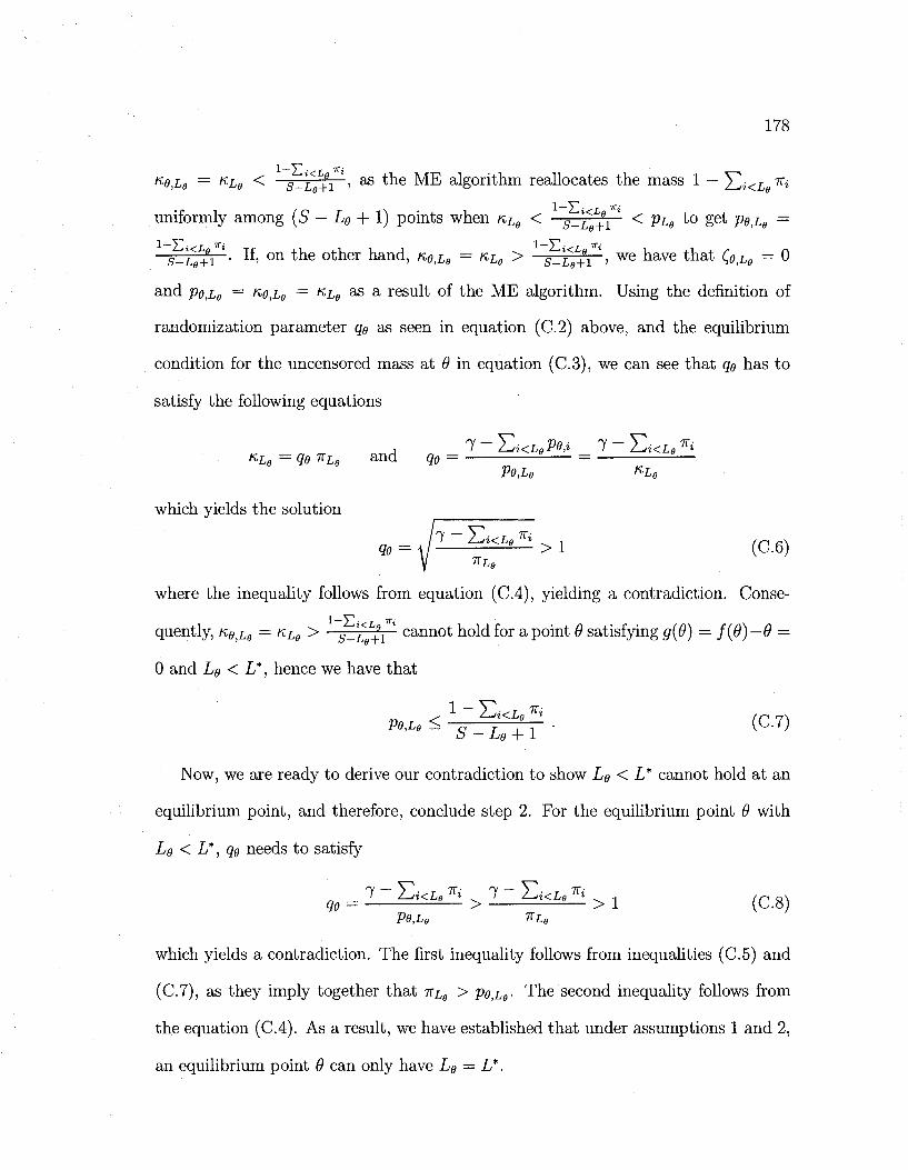
178

i -E i^LgTi Ke,L9 = KL9 < S_

ZL +! ; as t h e M E algor i thm reallocates t h e mass 1 — Yli<L ^

uniformly among (S - Le + 1) points when K£e < g _ ^ < z j 91 ' < pLg t o get pg,LB =

s-Lg-ti ' • If> o n t n e o t n e r hand , / t y ^ = /C£,e > g_£<^?1 ' , we have t h a t (0,L$ — 0

and pe,Le = KQ,L0 = K L 9 a s a result of the ME algorithm. Using the definition of

randomization parameter qe as seen in equation (C.2) above, and the equilibrium

condition for the uncensored mass at 8 in equation (C.3), we can see that qe has to

satisfy the following equations

j 7 ~ l^i<Le P0,i 7 — Zsi<Le ^ KL9 = Qe KLB and q9 = °- =

Pe,Le KLe

which yields the solution

qe = h-^*** > ! (c.6) V ^Le

where the inequality follows from equation (C.4), yielding a contradiction. Conse-

quently, Kg^e = KL0 > S-LL+I ' c a n n ° t n o ^ f° r a point 0 satisfying g(6) = f(9)—6 =

0 and Le < L*, hence we have that

1 - E i < L s Ti

Now, we are ready to derive our contradiction to show Lg < L* cannot hold at an

equilibrium point, and therefore, conclude step 2. For the equilibrium point 0 with

Le < L*, qe needs to satisfy

qe = 7 ~ E * < ^ ** > 7 " E > < ^ ff< > 1 (C.8)

which yields a contradiction. The first inequality follows from inequalities (C.5) and

(C.7), as they imply together that TTL$ > Pe,Le- The second inequality follows from

the equation (C.4). As a result, we have established that under assumptions 1 and 2,

an equilibrium point 0 can only have Le — L*.

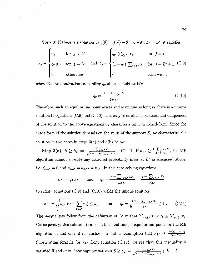
179

Step 3: If there is a solution to g(6) = f(9) — 9 = 0 with Lg = L*, it satisfies

t\jq

•Ki for j < L"

qe KL* f° r 3 — L* a n a- 0 = <

0 otherwise

where the randomization probability qg above should satisfy

7 ~ Ei<L* ni

Qe Ei>L* *i for 3 = L*

0 otherwise ,

Qe Pe,L*

(CIO)

Therefore, such an equilibrium point exists and is unique as long as there is a unique

solution to equations (C.9) and (CIO). It is easy to establish existence and uniqueness

of the solution to the above equations by characterizing it in closed-form. Since the

exact form of the solution depends on the value of the support S, we characterize the

solution in two cases in steps 3(a) and 3(b) below.

Step 3(a), S > Sw := i-E i<L* ^ _ — = + L* - 1: If KL* > 1^L*Vi, the ME

algorithm cannot allocate any censored probability mass at L* as discussed above,

i-e. (e,L* — 0 and pe,L* = K>O,L* = ^L* • In this case solving equations

7 - J2i<L* Pe,i _ 7 - Y^iKL* *j K>L* = Qe TTL* and Qe

Pe,L* K-L*

to satisfy equations (C.9) and (CIO) yields the unique solution

KL> = , UL* (7 ~ $3 *i) < TVL* and Qe /7-E, <L> Ki

< 1 i<L*

T T L *

(C.ll)

The inequalities follow from the definition of L* in that Ej<£* ni < 7 — Ei<L* ^

Consequently, this solution is a consistent and unique equilibrium point for the ME

algorithm if and only if it satisfies our initial assumption that KL* > i-E i<L* S-L*+l •

Substituting formula for KL* from equation (C.ll), we see that this inequality is

i—Ei<z,* "» i r * satisfied if and only if the support satisfies S > Sw = y/irL* ( 7 - E i < i * f i )

+ L*-1.

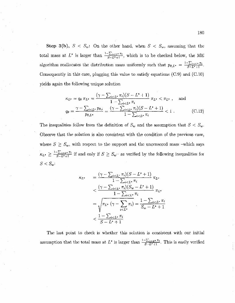
180

Step 3(b), S < Sw: On the other hand, when S < Sw, assuming that the

total mass at L* is larger than gZ^+y^, which is to be checked below, the ME

algorithm reallocates the distribution mass uniformly such that p#,L* = "g-^+V''' •

Consequently in this case, plugging this value to satisfy equations (C.9) and (CIO)

yields again the following unique solution

nL* = qg 7rL. = 1 _ v* ^L* < KL* , and

qe = = : ^ < J- • K'^-12') P9,L* 1 - 2^i<L* *i

The inequalities follow from the definition of Sw and the assumption that S < Sw.

Observe that the solution is also consistent with the condition of the previous case,

where S > Sw, with respect to the support and the uncensored mass -which says

KL* > g_j +*i ' ^ a n d only if S > Sw- as verified by the following inequaUties for

S<S< w

«L* = : ^ T*L* 1 ~ l^i<L* ni

< : F^ KL* 1 - L i<L* Ti

S-L* + l

The last point to check is whether this solution is consistent with our initial

assumption that the total mass at L* is larger than S^L*L+\ ' • ^ i s *s e a s u v verified

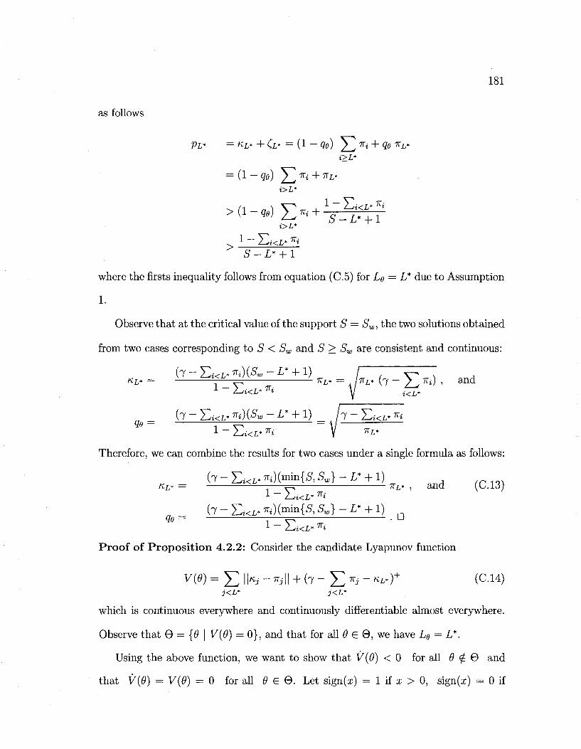
181

as follows

PL* = KL* + CL* = (1 - qe) ^2î + qe nL* i>L*

= (1 - qe) ^2 TTi + TIL* i>L*

! - E^<L* ^ 5 - L* + 1

where the firsts inequality follows from equation (C.5) for LQ = L* due to Assumption

1.

Observe that at the critical value of the support S = Sw, the two solutions obtained

from two cases corresponding to S < Sw and S > Sw are consistent and continuous:

«L* = Y _v^ ^ = /7ri* w - 2-< ' a n d

1 lîKL'î A/ i < L »

(7 - Ei<L* TTO(5W - L* + 1) /7 - E*<L* T< 90 = - ' 1 - Ei<L* *i V 7FL*

Therefore, we can combine the results for two cases under a single formula as follows:

( 7 - E ^ * < K m i n { f f , f f w } - L * + l) «£,* = = 7rL* , and (C.13)

1 - EJ<L* ^ ( 7 - E ^ ^ ) ( m i n { 5 , ^ } - L - + l)

^ _ _ u 1 - E*<L* Ti

Proof of Proposition 4.2.2: Consider the candidate Lyapunov function

vie) = J2 IK' - "ill + (7 - E *i - *i-)+ (°-14)

which is continuous everywhere and continuously differentiate almost everywhere.

Observe that 6 = {9 \ V{9) = 0}, and that for all 9 e 6 , we have Le = L*.

Using the above function, we want to show that V(9) < 0 for all 9 ^ © and

that V(9) = V{9) = 0 for all 9 e 9. Let sign(x) = 1 if x > 0, sign(a;) = 0 if

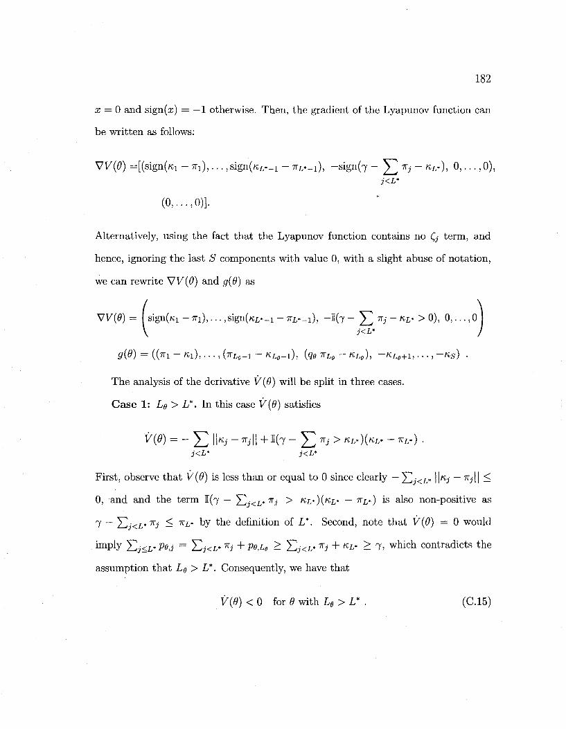
182

x = 0 and sign(x) = —1 otherwise. Then, the gradient of the Lyapunov function can

be written as follows:

W ( 0 ) =[(sign(/ci - 7Ti),... ,sign(«L._i - TTL*_I), -sign(7 - ^ TX3- - nL*), 0 , . . . ,0), j<L*

(0.....0)].

Alternatively, using the fact that the Lyapunov function contains no Q term, and

hence, ignoring the last S components with value 0, with a slight abuse of notation,

we can rewrite VV(#) and g(6) as

W(0) = sign(KX - TTI), ... ,sign(«L*_i - irL'-i), -1(7 ~ X ! ^ ~ KL* > ° ' °''"'' °

g(Q) = ((TTi - Ki), . . . , {-KLe-l - «L«- l ) , fa ^Le ~ « i « ) , - « L 9 + 1 , • • • > ~ « s ) •

The analysis of the derivative V{6) will be split in three cases.

Case 1: Lg > L*. In this case V(9) satisfies

HO) = - X) H«i -^11 + % - X) ^ > «i*)(«L« -TL-) •

First, observe that V"(#) is less than or equal to 0 since clearly — J2J<L* \\KJ ~~%J\\ —

0, and and the term 1(7 — ]T\-<z,* nj > KL*){KL* — KL*) is also non-positive as

7 — J2J<L* nj — ^L* by the definition of L*. Second, note that V(9) = 0 would

imply Y,j<L* Pv,j = YSJ<L* Kj + Pe,LB > J2J<L* ^3 + KL* > 7, which contradicts the

assumption that Lg > L*. Consequently, we have that

V(9) < 0 for 0 with Lg>L* . (C.15)

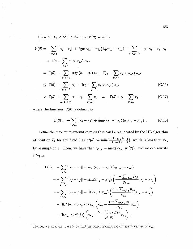
183

Case 2: Lg < L*. In this case V{6) satisfies

Kj

j<L9 Le<j<L*

+ 1 ( 7 - 5^7Tj >KL*) «L*

= r(0) - J ^ sign(/% - TTj) Kj- + I ( 7 ~ 5 ^ ^ > K L") KL* Le<j<L* j<L*

Le<j<L* j<L*

<v(e)+ J2 *; + 7 - I > = r( ) + 7-^7r j. (c.i7) Le<j<L* j<Le j<Lg

where the function T(6) is defined as

T(e) : = - 5 3 HKJ ~ ^'H + S i § n (^e - nLe) (qe^Le ~ ^Le) • (C.18)

Define the maximum amount of mass that can be reallocated by the ME algorithm

at position Lg for any fixed 6 as pw(9) := min{ s _ j ^ ^ ' , | } , which is less than 7r^

by assumption 1. Then, we have that pg^g = max{«Le, pu(6)}, and we can rewrite

r(0) as

j<L9

%<L" 'X1tLe - KL„ P6>L° }

E ii 11 1 ire \ s (^ ~L^i<uVQ,i \

ll«i - *jll + I(«L9 > TTLj I " *Lfl - KLg J<Le

+ I(pu(8) < KLe < nLe) LLg - 7 ~ E i < L e ^ 7 r L 6

+ I(nLe <p«(<9)) (KLB - 7 ^ P 8 ' i ^ . ) •

Hence, we analyze Case 2 by further conditioning for different values of KL9.

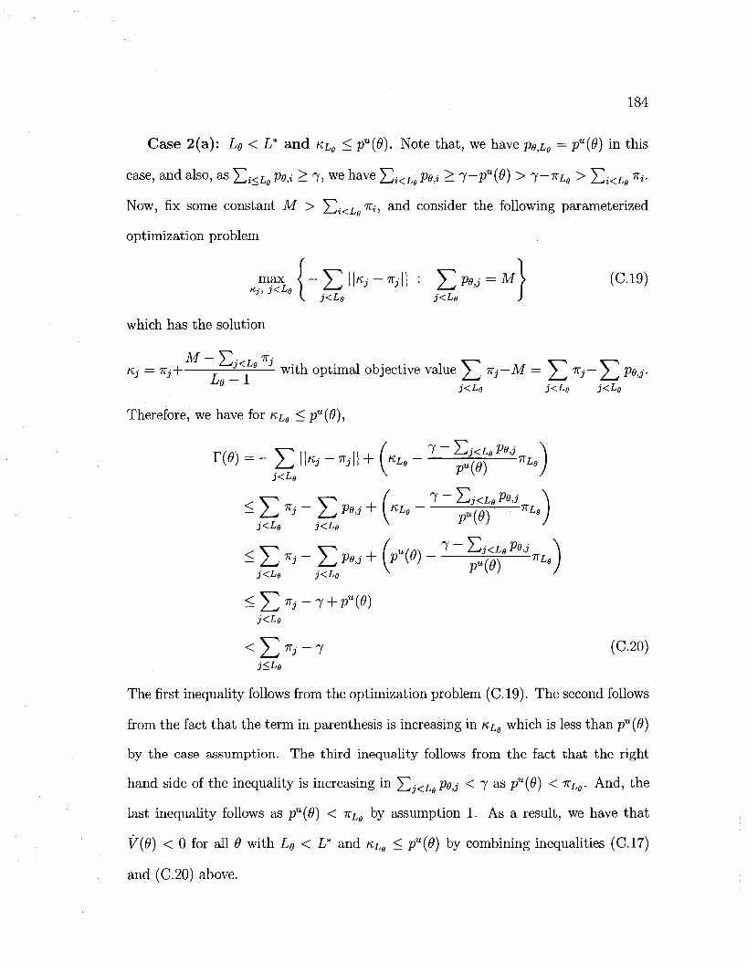
184

Case 2(a): LQ < L* and KL0 < pu(0). Note that, we have pgtie — pu{9) in this

case, and also, as £\<Lfl pe,i > 7, we have £ \ < L e Pe,i > 1~PU{9) > l~^u > J2i<Le *t-

Now, fix some constant M > ^2i<L iti, and consider the following parameterized

optimization problem

mtxr I - E H ^ - ^ I I : E ^ = M 1 (°-19)

\ 3<Lg j<LB )

which has the solution

Kj ~~ nj~ T—°~^"— w ^ h optimal objective value V^ TTJ—M= \ J nj~Z, Vo,j-j<Le 3<Lg j<Le

Therefore, we have for KL9 < pu(0),

j<Lg j<Le V F V > J

j<Lg j<Lg V y V '

< E ** -1 (c-2°)

The first inequality follows from the optimization problem (C.19). The second follows

from the fact that the term in parenthesis is increasing in KL9 which is less than pu{9)

by the case assumption. The third inequality follows from the fact that the right

hand side of the inequality is increasing in ^2j<L$Pe,j < 7 as pu(9) < TVLg- And, the

last inequality follows as pu(9) < 7rLe by assumption 1. As a result, we have that

V(9) < 0 for all 9 with Lg < L* and KL9 < pu(9) by combining inequalities (C.17)

and (C.20) above.

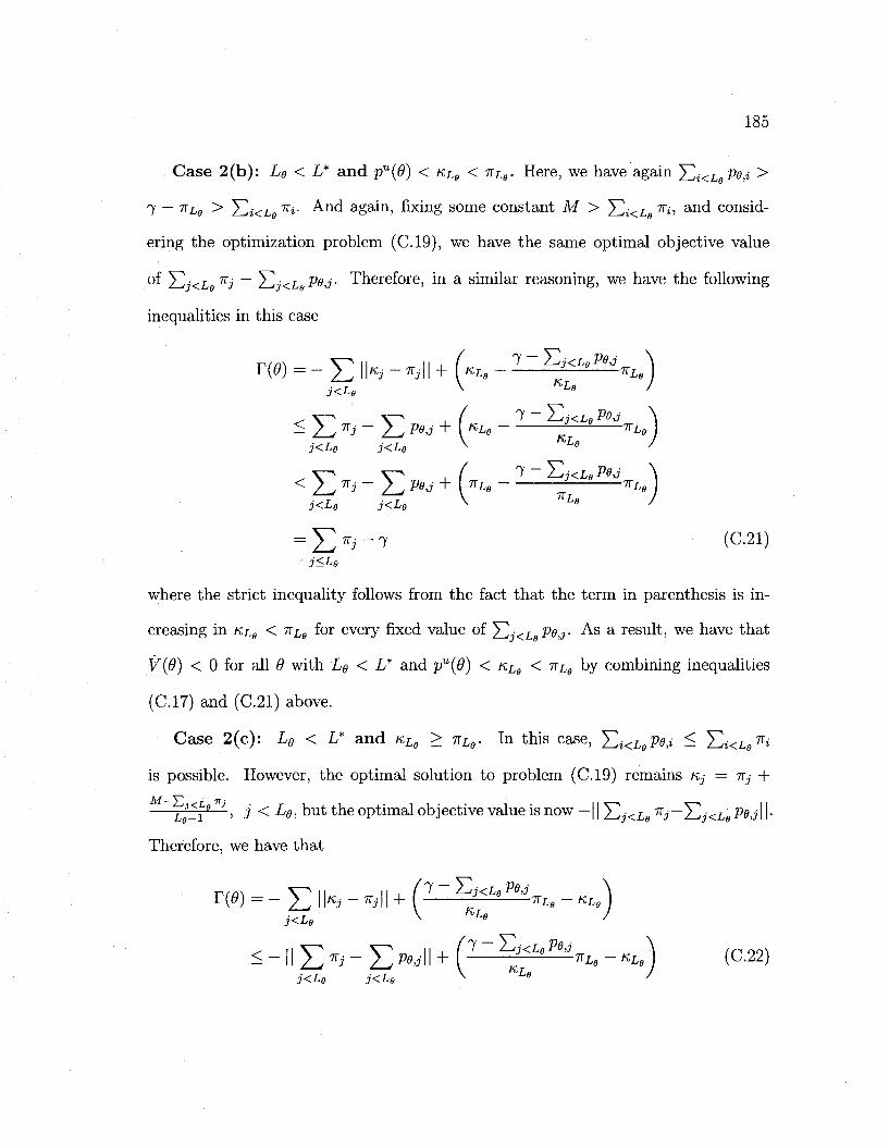
185

Case 2(b): Lg < L* and pu(9) < KL$ < ^LB- Here, we have again ^2i<L Vo,i >

7 — T^LB > ]C;<L9

ni- And again, fixing some constant M > ^2i<Lg î, and consid

ering the optimization problem (C.19), we have the same optimal objective value

of Y1J<L ^3 ~ ^2j<L P^,j- Therefore, in a similar reasoning, we have the following

inequalities in this case

m V ^ II I I I / ' ^ ~ £->3i +{KLe -T~^ *Le

J<L9 j<Le V *L

< 2 ^ ~ 1^ P°>i + [ê T *U ) J<Lg j<LB

V nLe J

3<Le

where the strict inequality follows from the fact that the term in parenthesis is in

creasing in KL6 < iTLe for every fixed value of "Y^j<LeVe,j- As a result, we have that

V{9) < 0 for all 9 with Lg < L* and pu(9) < «L9 < 7TL8 by combining inequalities

(C.17) and (C.21) above.

Case 2(c): Lg < L* and KLg > 7cLe. In this case, Ei<z,eP<M ^ Z)«L87r»

is possible. However, the optimal solution to problem (C.19) remains Kj = TTJ +

L'ti9 ) J < £>e, but the optimal objective value is now — 11 Y1J<L0 7r3~^2j<L9 Ps,j 11 •

Therefore, we have that

\\K3 ^ j l l + I 3<Le

< - II E *i - E »J\\ + ( 7 ~ E ; < L 9 ^ ^ - -LS) (C.22) 3<U 3<Le V KL» J

m=- E IK- -*iii + C E:<LeP0'jê - «*)

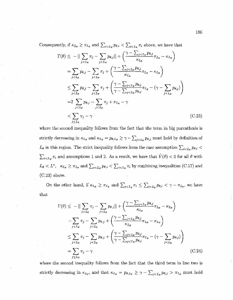
186

Consequently, if KL$ > -KLB and Yî<Le Vo,i < !C;<z,e î above, we have that

'7 -Ei<L f l P*J yo,j 11 -r y

j<Le j<Le

m < - H £ ** - £ ^H + (7 zj<L°Pe'\Le - KLe)

= £ ^' - £ ^ +1 — ^ - ^

^ £ ^ - E ^ + (l-y j<Lele"nL° ~ ^ ~ E***)

=2 E PW - E ^ + ^ ~ 7

< £ ^ - 7 (c-23) 3<Lg

where the second inequality follows from the fact that the term in big parenthesis is

strictly decreasing in KL9 and KLB — Pe,Lg > 7 — Y1J<L Pe>3 m u s t h°ld by definition of

Le in this region. The strict inequality follows from the case assumption Yî<Le Pe^ <-

J2i<L î an<^ assumptions 1 and 2. As a result, we have that V{6) < 0 for all 6 with

Le < L*, KLB > -KLg and Yî<Le Po,i < E;<z,9 ^ by combining inequalities (C.17) and

(C.23) above.

On the other hand, if KL„ > irLe and J2i<Lg ^ ^ E;<z,eP<M < 7 ~ ^Lg, we have

that

m < - II £ *>• - £ m \ \ + C~EJ<LsPejnLe - KL.) 3<Le j<Le V KL' '

= 1^^~Z^ Pe>i + " nL» ~ KL» J<Le j<Le V KL° /

^ E ni - E p°j + u - r<Le Z**Le ~ ( 7 ~ E pn) j<Le j<Le \ l ^>3 7 — Y1J<L9 POJ > nLg must hold

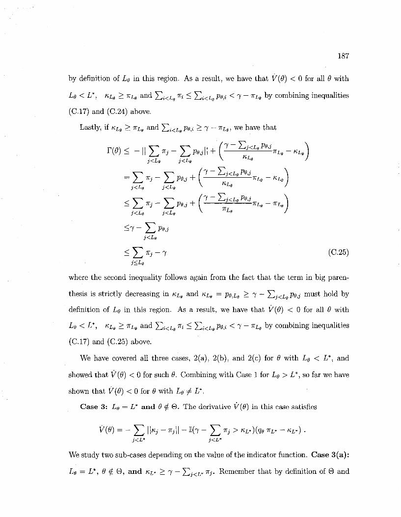
187

by definition of Lg in this region. As a result, we have that V{9) < 0 for all 9 with

Lg < L*, KLg > -KU and Yai<Le ni ^ E ; < L 9 Pe,i <1~^LB by combining inequalities


Lastly, if nLe > nLe and ] u < L e £>0,i > 7 - ^Le, we have that

Poj\\+ { j<le j<Le

m < - 1 1 E ^ - E ^ n + C EK

j<LePe,j^ -^

*3 - 2_> POJ + [ *Le ~ KLe

j<Lg j<Lg V Le

y-^ y—^ ( l Z^j<LePe>J

3<Le j<Le V HLe

<7 - E Pe'->,3

3 7 — X ^ < L POJ must hold by

definition of Lg in this region. As a result, we have that V(9) < 0 for all 9 with

Le<L*, nLg > nLe and J2i<Le ^ ^ T,i<Lg Po,i < 7 - ^Lfl by combining inequalities


We have covered all three cases, 2(a), 2(b), and 2(c) for 8 with Lg < L*, and

showed that V{9) < 0 for such 9. Combining with Case 1 for Lg > L*, so far we have

shown that V{9) < 0 for 9 with Lg ^ L*.

Case 3: L0 = L* and 9 £ €>. The derivative V{9) in this case satisfies

We study two sub-cases depending on the value of the indicator function. Case 3(a):

Lg — L*, 9 <£ Q, and KL* > 7 — ]CJ<L* ^J- Remember that by definition of 0 and

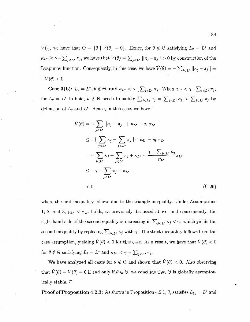
188

V(-), we have that 6 = {9 \ V{9) = 0}. Hence, for 9 i G satisfying Le = L* and

K>L* > 7 — Y1J<L* ^31 w e n a v e that V(Q) = X^<L* llKj — ill > 0 by construction of the

Lyapunov function. Consequently, in this case, we have V(9) = - J^j<L* \\KJ-'KJ\\ =

-V{9) < 0.

Case 3(b): Le = L*,9 <£B, and KL* < 'J-J2J<L* nj- When KL* < 1~J2J<L*

ni>

for Lg = L* to hold, 9 ^ 0 needs to satisfy ^2j<L Kj = Y1J<L* KJ >

S I < L * %j by

definition of L<? and L*. Hence, in this case, we have

V(9) ~ - Z HKJ" ~ ^'H + KL* ~ qe nL* j<L*

= - Z '+ S + 7 - E j < £ . «i

B r .

< -7 - Z n3 + KL* j<L*

< 0, (C.26)

where the first inequality follows due to the triangle inequality. Under Assumptions

1, 2, and 3, PL* < KL* holds, as previously discussed above, and consequently, the

right hand side of the second equality is increasing in 5ZJ<L* Kj < 7> which yields the

second inequality by replacing J2J<L* Ki w ^ n 7- ^he strict inequality follows from the

case assumption, yielding V{9) < 0 for this case. As a result, we have that V(9) < 0

for 6 £ 0 satisfying Lg — L* and KL* < 7 — Y1J<L* ^r

We have analyzed all cases for 9 £ 0 and shown that V{9) < 0. Also observing

that V(9) = V{9) = 0 if and only if 9 € ©, we conclude that © is globally asymptot

ically stable. •

Proof of Proposition 4.2.3: As shown in Proposition 4.2.1, 9S satisfies Lgs = L* and

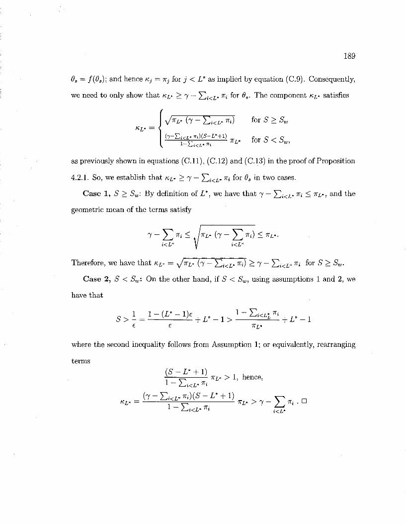
189

6S = f(9s); and hence Kj = TVJ for j < L* as implied by equation (C.9). Consequently,

we need to only show that KL* > 7 — $ i<x,* ^ for #s. The component KL» satisfies

V71^* (7 - Y,i<L* **) f o r # > #« «L* =

• ( 7 - E r - « ) ( * - L * + l ) f o r 5 < ^ , J-—2-ii<L* "i

as previously shown in equations (C.ll), (C.12) and (C.13) in the proof of Proposition

4.2.1. So, we establish that KL* > 7 — Yli<L* ni f° r ^s m ^w o c a s e s-

Case 1, S > Sw: By definition of L*, we have that 7 — Jî<L* ^ — nL*i an<l the

geometric mean of the terms satisfy

7 ~ J ^ Tt < ,/TTL* (7 - 5 3 ^ - 7rL*-i<L* y i<£*

Therefore, we have that KL . = ^/V/,. (7 — Y1I<L* Ô — 7 — X^<L* ^ f° r 8 > Sw.

Case 2, 51 < Sw: On the other hand, if S < Sw, using assumptions 1 and 2, we

have that

_ 1 l - ( L * - l ) e „ 1 ^-EiKLiî- „ , S > - = - L_ + 1* - 1 > £ + L* - 1

where the second inequality follows from Assumption 1; or equivalently, rearranging

terms

(S-L* + l) = 7T£,» > 1, hence,

1 - Zî<L* Ki

KL* = y ^ *L* > 7 - 2 ^ ^ • D

1 2î<L* n* i<L*

pricing and revenue management with limited market ... · pricing and revenue management with...

Documents