pricing and diffusion of primary and contingent...

TECHNOLOGICAL FORECASTING AND SOCIAL CHANGE 39, 291-307 (1991)

Pricing and Diffusion of Primary and

Contingent Products

VIJAY MAHAJAN and EITAN MULLER

ABSTRACT

Companies in certain industries produce products, called contingent products, that must be used with

another primary product. Consequently, the price of the primary product can influence the adoption of the

contingent product and vice versa. In this situation, the question is, What pricing strategy should be used to

set prices on the primary and contingent products to maximize the profits of the total product mix? In this paper

we study various types of contingent product relationships and develop propositions to specify pricing strategy

for primary and contingent products. An analytical investigation of these propositions provides guidelines for

developing pricing strategies for primary and contingent products and challenges some beliefs regarding the

relative contribution of the primary and contingent products to the overall profitability of the product mix. Our

results indicate that (a) an integrated firm that produces both products should price the primary as well as the

contingent product lower than two firms that independently produce each of the products (as a result, the

diffusion of the two products will be faster) and (b) contrary to common belief, the firm will make more money

from the primary product than from the contingent product. Managerial and public policy implications of these results are discussed.

Introduction All profit-making organizations face the challenge of setting a price on their products.

Pricing strategies usually change as the product passes through the product life cycle. At the introductory stage, for example, companies launching a new product can choose between two distinct pricing strategies-a market-skimming strategy and a market-penetration strategy. A market-skimming strategy uses a high price initially to “skim” the market when the market is still developing. The market-penetration strategy, on the other hand, uses a low price initially to capture a large market share.

The rationale of setting a price on a product has to be changed when the product is part of a product mix. In such a case, the firm searches for a set of prices that collectively maximize the profits on the total product mix. The determination of pricing strategies for the various products in the product mix, however, is complicated by the fact that (a) the demands for the various products are interrelated, (b) their costs of production and distribution are interrelated, (c) both costs and demands are interrelated, and (d) the various products face different degrees of competition.

VIJAY MAHAJAN is the James L. Bayless/ENSTAR Corporation Chair in Business Administration, Graduate School of Business, University of Texas, Austin, Texas. EITAN MULLER is Associate Professor,

Recanati Graduate School of Business Administration, Tel Aviv University, Tel Aviv, Israel 69978.

Address reprint requests to Prof. Vijay Mahajan, Department of Marketing, University of Texas, Austin, TX 78712.

0 1991 by Elsevier Science Publishing Co., Inc. 0040-1625/91/$3.50

292 V. MAHAJAN AND E. MULLER

Presenting options for product-mix pricing strategies, Kotler [ 1, pp. 5 16-5 17) has suggested the following situations:

1. Optional product pricing: Optional or accessory products are priced and offered separately from the primary product to attract customers to buy the primary product (e.g., defoggers for cars).

2. Captive product pricing: This is a situation where companies offer products that must be used with the primary product (e.g., razor blades and camera films). Manufacturers of primary products (razors and cameras) often price them low and set high markups on captive products (i.e., they make more money on captive products). Manufacturers who offer only the primary product have to price their product higher in order to make the same overall profit.

The common theme between these two situations is that the adoption of the second product (optional or captive) is contingent upon the adoption of the primary product. Such products have been termed contingent products by Peterson and Mahajan [2] and were further empirically investigated by Bayus [3].

Although both optional and captive products are contingent products, there is a difference in the contingency relationship of these two product types. The captive situation represents a contingency relationship where the primary product (e.g., camera) cannot be used without the contingent product (e.g., camera film) and vice versa. The optional relationship, on the other hand, represents a situation where, although the primary product (e.g., a car) can be used without the contingent product (i.e., defoggers for cars), the contingent product cannot be used without the primary product.

In the case of optional relationship, two types of contingency relationships can be further conceptualized. The first optional relationship involves a situation where the primary product (e.g., a car) is generally offered with or without the contingent product

(e.g., electric windows in a car) at the time of purchase only. This situation can be referred to as the static optional relationship. The second optional relationship, on the other hand, involves a situation where the contingent product (e.g., videocassette recorder) can be purchased at any time after the primary product (e.g., television) has been adopted. This can be referred to as the dynamic optional relationship.

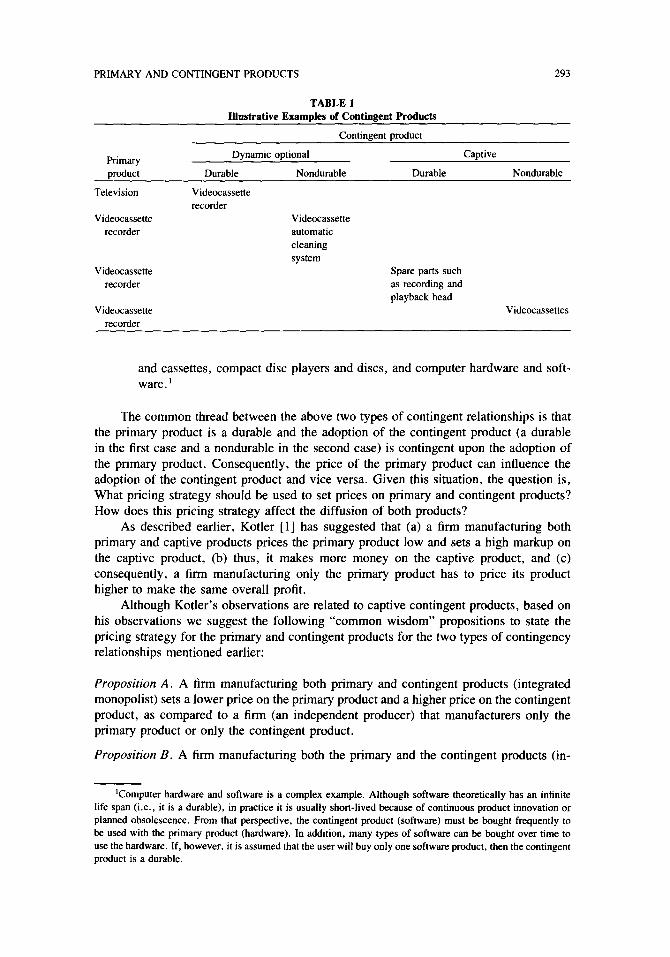
A further distinction can be made with respect to the durability of the contingent product. As summarized in Table 1, the more common types of contingent relationship occur when the contingent optional product is durable and the captive product is nondurable. Such is the case, for example, with washers and dryers for the first case, and camera and film for the latter.

Our objective in this paper is, therefore, to study analytically the pricing and diffusion of the following two types of contingency relationships:

1. Dynamic optional durable contingent product. The primary product is durable and can be used without the contingent product. The contingent product is also durable but cannot be used without the primary product and can be purchased at any time after the primary product has been purchased. Examples include televisions and videocassette recorders, washers and dryers.

2. Captive nondurable contingent product. The primary product is a durable but cannot be used without the contingent product and vice versa. Furthermore, the contingent product must be bought frequently to use the primary product on a regular basis. Examples include cameras and camera film, videocassette recorders

PRIMARY AND CONTINGENT PRODUCTS 293

TABLE 1 Illustrative Examples of Contingent Products

Contingent product

Primary

product

Dynamic optional

Durable Nondurable Durable

Captive

Nondurable

Videocassette

automatic

cleaning

system Spare parts such

as recording and

playback head

Television

Videocassette

recorder

Videocassette

recorder

Videocassette

recorder

Videocassette

recorder

Videocassettes

and cassettes, compact disc players and discs, and computer hardware and software. ’

The common thread between the above two types of contingent relationships is that the primary product is a durable and the adoption of the contingent product (a durable in the first case and a nondurable in the second case) is contingent upon the adoption of the primary product. Consequently, the price of the primary product can influence the adoption of the contingent product and vice versa. Given this situation, the question is, What pricing strategy should be used to set prices on primary and contingent products? How does this pricing strategy affect the diffusion of both products?

As described earlier, Kotler [l] has suggested that (a) a firm manufacturing both primary and captive products prices the primary product low and sets a high markup on the captive product, (b) thus, it makes more money on the captive product, and (c) consequently, a firm manufacturing only the primary product has to price its product higher to make the same overall profit.

Although Kotler’s observations are related to captive contingent products, based on his observations we suggest the following “common wisdom” propositions to state the pricing strategy for the primary and contingent products for the two types of contingency relationships mentioned earlier:

Proposition A. A firm manufacturing both primary and contingent products (integrated monopolist) sets a lower price on the primary product and a higher price on the contingent product, as compared to a firm (an independent producer) that manufacturers only the primary product or only the contingent product.

Proposition B. A firm manufacturing both the primary and the contingent products (in-

‘Computer hardware and software is a complex example. Although software theoretically has an infinite

life span (i.e., it is a durable), in practice it is usually short-lived because of continuous product innovation or planned obsolescence. From that perspective, the contingent product (software) must be. bought frequently to

be used with the primary product (hardware). In addition, many types of software can be bought over time to

use the hardware. If, however, it is assumed that the user will buy only one software product, then the contingent product is a durable.


tegrated monopolist) sets a high markup on the contingent product and makes most of the profits on the contingent product rather than on the primary product.

An investigation of the above two propositions and their impact on the diffusion patterns of the primary and contingent products constitute the major focus of this paper.*

The organization of this paper is as follows: in the next section we present the basic framework used to study the two propositions. We then discuss these propositions for dynamic durable contingent products and captive nondurable contingent products. The paper concludes with implications of our results.

The Framework In recent years, a number of innovation diffusion models have been proposed to

represent first-purchase growth of a durable product over time (for a recent review, see Mahajan et al. [4]). The underlying behavioral theory in the development of these models is that the innovation is first adopted by a select few innovators who, in turn, influence others (by word of mouth) to adopt it. Among all the proposed innovation diffusion models, the model that has served as the main impetus for the studies exploring the impact of pricing strategies on new product growth is the new product growth model proposed by Bass [5] (for a review of these studies, see Kalish and Sen [6]). The Bass model describes the diffusion process by the following differential equation:

i(t) = aWdt = (a + bx(t))(N - x(t), (1)

where x(t) is the cumulative number of adopters at time f, N is the constant ceiling or the population of potential adopters, i(t) = dx(t)ldt is the rate of diffusion at time t, a is the coefficient of innovation, and b = b’lN, where b’ is the coefficient of imitation (for the sake of brevity, the symbol t will not be used in the remainder of the paper to describe the time-dependent aspect of the diffusion process).

The introduction of the impact of price in the framework of the Bass model has generally resulted in two types of normative pricing strategies for a durable.

The first derived pricing strategy states that, in the presence of a strong word-of- mouth effect, as measured by the coefficient b, price will increase at introduction, peak, and decrease later [7-lo]. As articulated by Kalish and Sen [6, p. 941, the intuitive explanation for this pricing strategy is that if early adopters have a strong positive effect on later adopters, a low introductory price should encourage them to adopt the product. Consequently, once a product is established, the price can be raised because the contribution to the sales due to additional adopters decreases over time. This pricing strategy will be termed the diffusion-based pricing strategy. Studies deriving this pricing strategy generally assume that price does not affect the population of the potential adopters (i.e., N) and produces a multiplicative effect on the rate of diffusion. That is,

i = (a + bx)(N - x&(p),

where g@) is the price response function for the price p at time t.

(2)

*Our problem of primary and contingent products should be distinguished from the standard economic notion of a discriminating monopolist who charges different prices to two different consumer segments and the

total demand is the horizontal summation of both demands. The problem does have some resemblance to a

two-part tariff pricing of a monopolist who charges a fixed price plus a reduced price on each product bought; such is the case for an amusement park that charges an entrance fee in addition to the charges for specific rides.

In our case, however, the two products, although interrelated, are distinct, and the summation of demand is one of the key issues that is much more complex than the above two cases.


The second derived pricing strategy states that, for durable goods, price is more likely to decrease over time, supporting the market-skimming strategy [ 10, 1 I]. Assuming that price determines the population of potential adopters, these studies, however, caution that if the effect of early adopters on future demand (as reflected by b) is high, the first strategy (price increasing initially and decreasing later) is better than the market-skimming strategy [lo]. A further comparison of these two approaches can be found in Horsky

WI. The above two pricing strategies have been derived for a single durable product. As

mentioned earlier, the question now is what pricing strategies should be used for a product mix where the adoption of the contingent product (durable or nondurable) is contingent on the adoption of the primary durable product. In order to examine this question and, more specifically, the two propositions mentioned earlier, we will also use the framework of the Bass model in which it is assumed that price produces a multiplicative effect on the rate of diffusion [i.e., eq. (2)]. Empirical evidence in support of this approach has been reported by Jain and Rao [ 131.

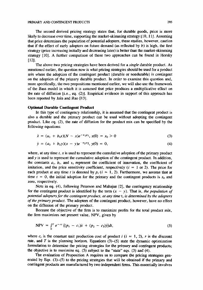
Optional Durable Contingent Product In this type of contingency relationship, it is assumed that the contingent product is

also a durable and the primary product can be used without adopting the contingent product. Like eq. (2), the rate of diffusion for the product mix can be specified by the following equations:

i = (al + b,x)(N - x)e-E*P*, x(O) = x0 > Cl

j, = (a2 + &y)(x - y)eCEZP2, y(0) = 0,

(3)

(4)

where, at any time t, x is used to represent the cumulative adoption of the primary product and y is used to represent the cumulative adoption of the contingent product. In addition, the constants ai, bi, and ei represent the coefficient of innovation, the coefficient of imitation, and the price sensitivity coefficient, respectively (i = 1 or 2). The price for each product at any time t is denoted by pi (i = 1, 2). Furthermore, we assume that at time t = 0, the initial adoption for the primary and the contingent products is x0 and zero, respectively.

Note in eq. (4), following Peterson and Mahajan [2], the contingency relationship for the contingent product is identified by the term (X - y). That is, the population of potential adopters for the contingent product, at any time t, is determined by the adopters of the primary product. The adopters of the contingent product, however, have no effect on the diffusion of the primary product.

Because the objective of the firm is to maximize profits for the total product mix, the firm maximizes net present value, NPV, given by

NPV = $‘e-” {(PI - c& + (~2 - c2Mdf, 0

(5)

where ci is the constant unit production cost of product i (i = 1, 2), r is the discount rate, and T is the planning horizon. Equations (3)-(5) state the dynamic optimization formulation to determine the pricing strategies for the primary and contingent products; the objective is to maximize eq. (5) subject to the “state” eqs. (3) and (4).

The evaluation of Proposition A requires us to compare the pricing strategies generated by Eqs. (3)-(5) to the pricing strategies that will be obtained if the primary and contingent products are manufactured by two independent firms. This essentially involves


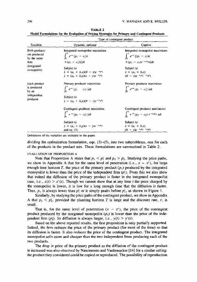
TABLE 2 Model Formulations for the Evaluation of Pricing Strategies for Primary and Contingent Products

Situation

Type of contingent product

Dynamic optional Captive

Both products

are produced

by the same

Integrated monopolist maximizes r

e-” Ip, - ci)i

Integrated monopolist maximizes

r e-” {(pi - cl);

film + (pz - cz)e-‘2P2x}dr

(integrated

monopolist)

Each product

is produced

by an

Subject to Subject to

i = (al + bix)(N - x)eK”iQ x = (ai + 6,x)

j, = (a~ + bly)(x - y)e-“~~2 (N - .qe-wv”m

Primary producer maximizes

I

T

0 em” (p, - c,) id1

Primary producer maximizes

I

T

II 6’ (p, - c,) idr

independent

producer Subject to

X = (a, + bix)(N - .r)e-‘rPi

Contingent producer maximizes

I

T

Cl e-” (pz - cz) $dr

Subject to

Jo = (a~ + bu)(x - y)e-“2Pz and eq. (1)

Definitions of the variables are included in the paper.

Contingent producer maximizes

I

T

0 em” (~2 - CZ) ec”zPz xdf

Subject to

i = (a, + b,x) (N - ~)c~~lP1-E12PZ

dividing the optimization formulation, eqs. (3)-(5), into two subproblems, one for each of the products in the product mix. These formulations are summarized in Table 2.

EVALUATION OF PROPOSITION A

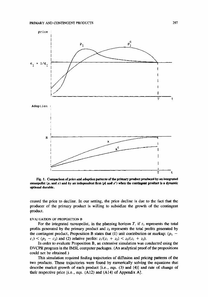
Note that Proposition A states that pI < pf and p2 > ~5. Studying the price paths, we show in Appendix A that for the same level of penetration (i.e., x = x’), for large enough time horizon T, the price of the primary product (pl) produced by the integrated monopolist is lower than the price of the independent firm (pi). From this we also show that indeed the diffusion of the primary product is faster in the integrated monopolist case, i.e., x(t) > Y(t). Though we cannot show that at any time t the price charged by the monopolist is lower, it is low for a long enough time that the diffusion is faster. Thus, p1 is always lower than pf or it simply peaks before pf, as shown in Figure 1.

Similarly, by studying the price paths of the contingent product, we show in Appendix A that p2 < ~5, provided the planning horizon T is large and the discount rate, r, is small.

That is, for the same level of penetration (n = x”), the price of the contingent product produced by the integrated monopolist (pz) is lower than the price of the independent firm @$). Its diffusion is always larger, i.e., y(t) > y’(t).

Based on the above reported results, the first proposition is only partially supported. Indeed, the firm reduces the price of the primary product (for most of the time) so that its diffusion is faster. It also reduces the price of the contingent product. The integrated monopolist sells more and cheaper than the two independent firms producing each of the two products.

The drop in price of the primary product as the diffusion of the contingent product is increased was also observed by Nascimento and Vanhonacker [ 141 for a similar setting: the product they considered could be copied or reproduced. The possibility of reproduction

PRIMARY AND CONTINGENT PRODUCTS

price !

291

5 +

Adoption !

I N / I

x ’ X I 11 ’ I

I I T t

Fig. 1. Comparison of price and adoption patterns of the primary product produced by an integrated monopolist (pl and x) and by an independent firm (PT and x’) when the contingent product is a dynamic optional durable.

caused the price to decline. In our setting, the price decline is due to the fact that the producer of the primary product is willing to subsidize the growth of the contingent product.

EVALUATION OF PROPOSITION B

For the integrated monopolist, in the planning horizon T, if z1 represents the total profits generated by the primary product and z2 represents the total profits generated by the contingent product, Proposition B states that (1) unit contribution or markup: (pi - cr) < (p2 - c2) and (2) relative profits: zi/(zi + z2) C z2/(z1 + z2).

In order to evaluate Proposition B, an extensive simulation was conducted using the DVCPR program in the IMSL computer packages. (An analytical proof of the propositions could not be obtained.)

This simulation required finding trajectories of diffusion and pricing patterns of the two products. These trajectories were found by numerically solving the equations that describe market growth of each product [i.e., eqs. (3) and (4)] and rate of change of their respective price [i.e., eqs. (A12) and (A14) of Appendix A].


In order to study the sensitivity of the relative contributions to the profitability of the two products, the relevant set of equations was solved assuming four common values of E (.005 to .020 in increments of .005), two values of T (10 or 20 periods), five values of x0 or y. (2,000 to 10,000 in increments of 2,000), four values of N (40,000 to 1 $00,000 in increments of 20,000), and five common values of c (20 to 100 increments of 20).

In all the 800 solutions, rrl was found to be greater than 7~~. That is, these results suggest that ajrm offering a dynamic optional contingent product along with the primary product actually makes more money on the primary product rather than on the contingent

product. As a matter of fact, for T = 10, relative contribution to the total profits by the primary product varied from 72% to 98%, and for T = 20 it varied from 61% to 97%. Note that since we have assumed that the coefficients a and b are identical for both products, when there is no contingent relationship between the two products, the price and diffusion trajectories will be identical. Therefore, the profits are equally contributed by these two products. The variation in contributions to the total profits in the presence of a contingent relationship, therefore, strongly suggests a need to explicitly identify product relationships in a product mix.

Note that, initially, market potential for the primary product is N, while for the contingent product it is x. At time zero, x(0) is much smaller than N, and thus, clearly, profits of the first few periods of the primary product are much larger than those of the contingent product. Later, the difference becomes smaller. With a long time horizon (t = 20), the profits of the contingent product becomes larger, and so it could be expected that with a large discount rate the first few periods would have the most influence on total discounted profits and that this will drive up the profits of the primary product. The most forthcoming situation to high profits on a contingent product is when the discount rate is zero. This is exactly the situation in our numerical analysis, and under this situation relative profits of the primary product are higher than those of the contingent product.

The 800 numerical solutions were also examined to study the relationships between markups. No unidirectional pattern was observed. In fact, in many solutions, for certain time periods, the markup for the primary product was higher than the contingent product.3

Based on the above results (since the parameter b is larger than a), Proposition B cannot be supported. In fact, the results suggest that the relative contribution of the primary product to the total profits of the product mix is larger than the contingent product and the markup for the contingent product may or may not be larger than the primary product.

‘The issue of markup can be analytically investigated for the case in which b, = bz = 0, i.e., there is

no diffusion effect, only market potential effect. Three assumptions are needed in order to achieve the results.

These assumptions are critical in the sense that if one (or more) is violated, the proposition does not hold.

Assumption I: The diffusion effect in eqs. (3) and (4) is negligible, i.e., b, = b2 = 0.

Assumption 2: Price elasticity of demand of the primary product is not smaller than the one of the contingent

product, i.e., er 2 e2.

Assumption 3: The relationship between the costs of producing the two products is as follows: either cl/c? 2

1 or EdF, 6 c,icz < 1.

Thus, either c, is larger than cl or, if it is smaller, it cannot be much smaller than c2. i.e., the ratio ct/cz

is bounded from below.

The proof of the following proposition is available from the authors: under Assumptions 1-3, the integrated monopolist’s profit margin is higher on the contingent product than on the primary product. In practice, however,

the diffusion effect is not only nonnegligible, but is always larger than the innovation effect [i.e., b > (I in eq. (l)]. Thus, !his proposition carries little empirical consequence. We report it here for the sake of com- pleteness.


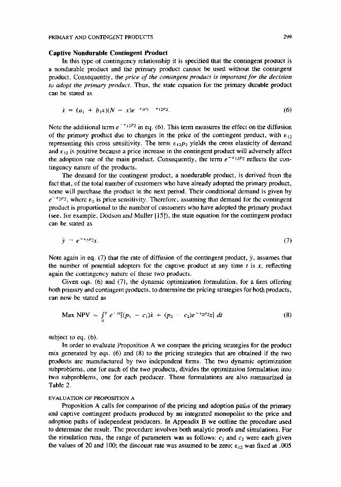
Captive Nondurable Contingent Product In this type of contingency relationship it is specified that the contingent product is

a nondurable product and the primary product cannot be used without the contingent product. Consequently, the price of the conrmgent product is important for the decision to adopt the primary product. Thus, the state equation for the primary durable product can be stated as

i = (a, + b,x)(N - x)eCelP1 -E1p2. (6)

Note the additional term e E12P2 in eq. (6). This term measures the effect on the diffusion of the primary product due to changes in the price of the contingent product, with E,~

representing this cross sensitivity. The term ~~~~~ yields the cross elasticity of demand and E,~ is positive because a price increase in the contingent product will adversely affect the adoption rate of the main product. Consequently, the term e-Ei2P2 reflects the contingency nature of the products.

The demand for the contingent product, a nondurable product, is derived from the fact that, of the total number of customers who have already adopted the primary product, some will purchase the product in the next period. Their conditional demand is given by e-QP*, where &2 is price sensitivity. Therefore, assuming that demand for the contingent product is proportional to the number of customers who have adopted the primary product (see, for example, Godson and Muller [ 15 I), the state equation for the contingent product can be stated as

j = e-“2P2x, (7)

Note again in eq. (7) that the rate of diffusion of the contingent product, Jo, assumes that the number of potential adopters for the captive product at any time t is X, reflecting again the contingency nature of these two products.

Given eqs. (6) and (7), the dynamic optimization formulation, for a firm offering both primary and contingent products, to determine the pricing strategies for both products, can now be stated as

Max NYV = j’ e-“{(p, - c,)i + (p2 - c,)e-“2%} dt 0

subject to eq. (6). In order to evaluate Proposition A we compare the pricing strategies for the product

mix generated by eqs. (6) and (8) to the pricing strategies that are obtained if the two products are manufactured by two independent firms. The two dynamic optimization subproblems, one for each of the two products, divides the optimization formulation into two subproblems, one for each producer. These formulations are also summarized in Table 2.

EVALUATION OF PROPOSITION A

Proposition A calls for comparison of the pricing and adoption paths of the primary and captive contingent products produced by an integrated monopolist to the price and adoption paths of independent producers. In Appendix B we outline the procedure used to determine the result. The procedure involves both analytic proofs and simulations. For the simulation runs, the range of parameters was as follows: cl and c2 were each given the values of 20 and 100; the discount rate was assumed to be zero; tsi2 was fixed at .005


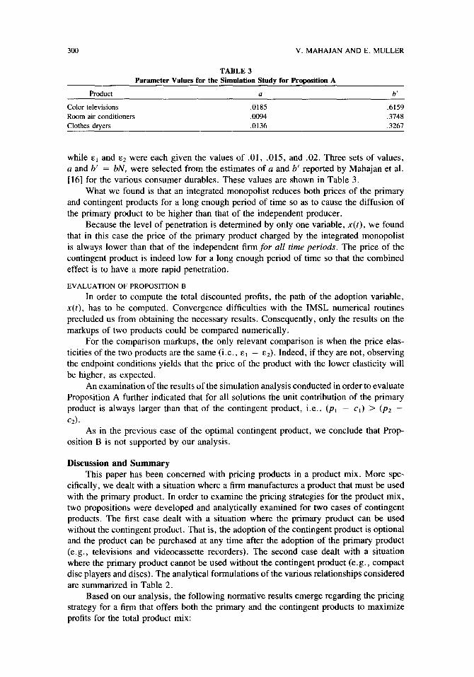
TABLE 3 Parameter Values for the Simulation Study for Proposition A

Product a

Color televisions .0185

Room air conditioners .0094

Clothes dryers .0136

b’

.6159

.3748

.3267

while E, and t52 were each given the values of .Ol, .015, and .02. Three sets of values, a and b’ = bN, were selected from the estimates of a and b’ reported by Mahajan et al. [ 161 for the various consumer durables. These values are shown in Table 3.

What we found is that an integrated monopolist reduces both prices of the primary and contingent products for a long enough period of time so as to cause the diffusion of the primary product to be higher than that of the independent producer.

Because the level of penetration is determined by only one variable, x(t), we found that in this case the price of the primary product charged by the integrated monopolist is always lower than that of the independent firm for all time periods. The price of the contingent product is indeed low for a long enough period of time so that the combined effect is to have a more rapid penetration.

EVALUATION OF PROPOSITION B

In order to compute the total discounted profits, the path of the adoption variable, x(t), has to be computed. Convergence difficulties with the IMSL numerical routines precluded us from obtaining the necessary results. Consequently, only the results on the markups of two products could be compared numerically.

For the comparison markups, the only relevant comparison is when the price elasticities of the two products are the same (i.e., E, = Ed). Indeed, if they are not, observing the endpoint conditions yields that the price of the product with the lower elasticity will be higher, as expected.

An examination of the results of the simulation analysis conducted in order to evaluate Proposition A further indicated that for all solutions the unit contribution of the primary product is always larger than that of the contingent product, i.e., (p, - cl) > (p2 -

c2).

As in the previous case of the optimal contingent product, we conclude that F’rop- osition B is not supported by our analysis.

Discussion and Summary This paper has been concerned with pricing products in a product mix. More spe-

cifically, we dealt with a situation where a firm manufactures a product that must be used with the primary product. In order to examine the pricing strategies for the product mix, two propositions were developed and analytically examined for two cases of contingent products. The first case dealt with a situation where the primary product can be used without the contingent product. That is, the adoption of the contingent product is optional and the product can be purchased at any time after the adoption of the primary product (e.g., televisions and videocassette recorders). The second case dealt with a situation where the primary product cannot be used without the contingent product (e.g., compact disc players and discs). The analytical formulations of the various relationships considered are summarized in Table 2.

Based on our analysis, the following normative results emerge regarding the pricing strategy for a firm that offers both the primary and the contingent products to maximize profits for the total product mix:


1. The firm should price the primary product as well as the contingent product lower than two firms that independently produce each of the two products. As a result, the diffusion of the two products will be faster. This holds true for both optional as well as captive contingent products.

2. Contrary to common belief, the firm makes more money from the primary product than from the contingent product.

The reasoning underlying the above results is as follows. First, consider the primary product. As compared to the independent producer, because the integrated monopolist is also concerned with the market potential of the contingent product, each adopter is valued more by the monopolist than by the independent producer. Consequently, in order to entice the adopter, the price of the primary product is reduced. The same reasoning applies to the contingent product. Consider the captive contingent product. For both the integrated monopolist and the independent producer, the price of the contingent product affects the sales of the contingent product [see eq. (7)] and the rate of the adoption of the primary product [see eq. (6)], which, in turn, affects the market potential of the contingent product. The integrated monopolist, however, is also concerned with an additional effect: because a high price for the contingent product causes a low adoption rate for the primary product, it has a direct negative impact on the monopolist’s profits from the primary product. The independent producer, who does not produce the primary product, is able to price the contingent product higher than the integrated monopolist.

Some of our results merit highlighting and additional discussion. Consider the situation in which the primary product is produced by one firm while the contingent product (dynamic optional or captive) is produced by another independent firm. When we compare this situation to the situation in which both products are produced by an integrated firm, we find that the prices of both products are lower for the integrated firm. From a public policy perspective, these results are clearly interesting because they suggest that a ver- tically integrated firm can offer the two products at a lower price to customers than two firms offering each product independently. This result is similar in spirit to the one by McGuire and Staelin [ 171. When discussing the problem of manufacturers who behave cooperatively, they note that profits are higher and prices lower for the integrated channel than when channel members are independent enterprises. Our setting does not match theirs, however, since the producer of the primary product produces and markets its own product, and thus its price is a retail price and not the price charged to the producer of the contingent product or a transfer price.

Observe that all of our results are derived for a monopolistic situation. We have left for future research the intricate problem in which one oligopoly produces one product and another oligopoly, or competitive industry, produces a second product. Also, an important question with which we have not dealt is a situation in which the industry starts as a monopoly producing the two products. The problem is to discover the conditions, if any, under which it will be beneficial for the monopolist to allow entry into any of its markets (either primary or contingent). This is of special interest when the monopoly is protected by patents and the monopolist can promote entry by subcontracting or licensing. We have not dealt with this subject formally, but would like to speculate on it here.

It seems that institutional reasons that are idiosyncratic to the firm can be the only ones promoting such behavior. For example, if the monopolist does not have the distribution network for the primary product (but does have the contingent product), then it might compare the fixed costs of establishing a network of its own to the additional profits that it will gain from prodacing the primary product in its decision to license the primary product to the producers whose fixed costs are much lower. The same is true regarding

302 V. MAHASAN AND E. MULLER

other instirutlonat factors, such as orner differences in fixed costs, information, perceived risk, and availability of production tectmoIogy. The fact that the products are dependent- primary and contmgent-aoes not seem by itseif to be a reason for such behavior.

An interestmg issue arises witn respect to classicai economic definitions of complementary and substlture products. The common textbook definition of complementary producrs is that me cross elasticity of demana is negative, i.e., (d.ildp2) (p&i) and (djidp,) (p,/j) are negative. l’his implies, of course, that boii dicidp, and djlldp, are negative. Wore that the cunent demand is i and not X, tine latter being cumulative adoption. In the standard case, wasners and dryers or TV sets and video recorders are considered com- plernenrary proaucrs. Observe eqs. (3) and (4) that describe the market behavior of these primary and conrmgent products. An increase in the price of the primary product p, will cause its adoption rare X to become smaller, causing the adoption rate of the contingent product (jl) to become smaller, confirming the presumed complementary nature of the two products. Observe now that a change in the price of the contingent product p2 will have no effect on X. l’hus, the classical economic checks would reveal that the products are eitner complementary or independent, depending on the specific check. Furthermore, for most time penoas (other than final ones), we find in our simulation results that as iong as pI and p2 are increasing, X and j are increasing as well. This implies positive cross elasticities, implying that the products are substitutes. Observe that only dicldp,,

for example, is positive, but this happens at a time when Its own price p, is increasing, which should have led to a decrease in its own demand. Thus, we should have confirmed strong substitutability between the two products, the true nature of the relation being contmgency, whicn is closer to compiementary.

With respect to the division of profits of a firm producing two durable dependent products, we found that the firm receives a relatively higher profit from the primary product tnan it receives from the contingent product. Based on our results we conclude that the common belief that a firm will make most of the projits on the contingent product,

when Irue, is due to dijjerences m cost and elasticities and not because of the nature of the products, one bemg prtmary and other being contingent.

It shouid be pointed out that all of our analyses assumed that (a) the cost of each product remains constant durmg the entire planning penod, (b) there is no economy of scope (i.e., the costs of two products are not interrelated), and (c) the population of potermai adopters remains constant for the entire planning period and is not influenced by price. These assumptions, although important, should provide avenues for future research.

Finally, our mvestlgatlon of the propositions is analytical rather than empirical. Do these propositions hold good in practice? Empirical studies employing case analysis of several iaunched contmgent products can shed light on this question.

The authors acknowledge the many helpjid suggestions and comments provided by Dipak Jain, Abhay Jajoo, and the members of workshops at the Business Schools of Southern Methodist University, Tel Aviv University, University of Pennsylvania, and Northwestern Universtty.

Appendix A In this appendix we compare the pricing strategy of a monopolist producing the two

products (the integrated monopolist) to the pricing strategies of the two independent firms; the first producing the primary product and the second producing the optional contingent product.


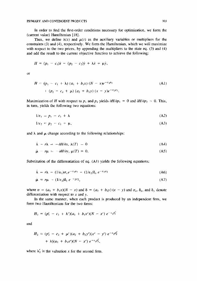
In order to find the first-order conditions necessary for optimization, we form the (current value) Hamiltonian [ 181.

Thus, we define A(t) and p.(r) as the auxiliary variables or multipliers for the constraints (3) and (4), respectively. We form the Hamiltonian, which we will maximize with respect to the two prices, by appending the multipliers to the state eq. (3) and (4) and add the result to the current objective function to achieve the following:

H = (p, - c&i + (pz - cz)j + ti + ~j,

or

H = (p, - cl + A) (a, + b,x) (I’.’ - x)C~‘~

+ (p* - c2 + p) (a2 + b*y) (x - y)e-“zP*.

Maximization of H with respect to p, and p2 yields dH/dp, = 0 and aHlap, in turn, yields the following two equations:

l/&i = p, - c, + A

I/&* = p2 - c, + IL,

and A and l_~ change according to the following relationships:

A - rA = - aHlax, A(T) = 0

I; - rp = -aHlay, p(T) = 0.

Substitution of the differentiation of eq. (Al) yields the following equations:

A = rA - (l/s,)o,e-“iPi - (l/~~)& e-QP*

b = rp - (l/~*)$ edEzp*,

= 0. This,

(Al)

(AZ)

(A3)

(A4)

(As)

(A@

647)

where cr = (a, + b,x)(N - X) and 6 = (a2 + b2y) (X - y) and uXx, 6,, and 6, denote differentiation with respect to x and y.

In the same manner, when each product is produced by an independent firm, we form two Hamiltonians for the two firms:

HI = (pi’ - c, + A’)(a, + b,x’)(N - xc) e-“d

and

H2 = (pz - c2 + pc)(a2 + b,y’)(x’ - y’) e-“*d

+ A$(ui + bix’)(N - xc) e-“iPr,

where A; is the valuation x for the second firm.


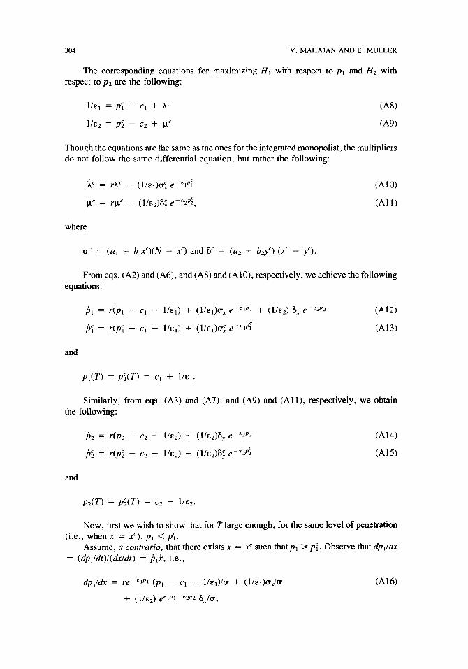
The corresponding equations for maximizing H, with respect to p, and HZ with respect to p2 are the following:

l/E, = p; - c, + h’

l/E* = pc2 - c2 + CLr.

(‘48)

(A9)

Though the equations are the same as the ones for the integrated monopolist, the multipliers do not follow the same differential equation, but rather the following:

ti = rh’ - (t/E&; e-V:

$ = r(lc _ (1/E2)6; e-“2$

(AlO)

(All)

where

a“ = (a, + b,x’)(N - xc) and 6’ = (a2 + b&) (x“ - y’).

From eqs. (A2) and (A6), and (A8) and (AlO), respectively, we achieve the following equations:

b, = r(p, - cl - l/~,) + (l/~,)u, emEIP, + (l/~~) S, e-&p2

p; = r(p; - c, - l/E,) + (l/&,)u; e-&,PF

(A12)

(A13)

and

p,(T) = pf(T) = c, + l/E,.

Similarly, from eqs. (A3) and (A7), and (A9) and (All), respectively, we obtain the following:

b2 = r(p2 - c2 - 1/e2) + (I/E~)$ emEp2 (A14)

Ij: = r(p$ - C2 - l/Ez) + (1/E2)% e-“26 (Al%

and

P2(T) = pS(T) = c2 + l/&2.

Now, first we wish to show that for T large enough, for the same level of penetration (i.e., when x = Y), p, <pt.

Assume, a contrario, that there exists x = Y such that p, 2 pf. Observe that dp,lu!x = (dp,ldf)l(dx/dr) = j+i, i.e.,

dp,/dr = re-E,P, (p, - c, - l/E,)/U + (l/~,)U&r

+ (1/E2) e”lP1-Ew2 6,/u,

(A16)


I >

x.x C

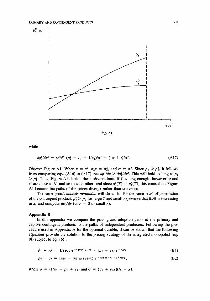
Fig. Al

while

dp;l& = re’~~f (p; - c, - lIEr)IUC + (l/&J CJi/d. (A17)

Observe Figure Al. When x = Y, cr,c = a;, and u = uc. Since p1 3 pf. it follows from comparing eqs. (A16) to (A17) that dp,ldx > &,;ldf. This will hold as long as pl > p:. Thus, Figure Al depicts these observations. If T is long enough, however, x and x’ are close to N, and so to each other, and since p;(T) = p:(T), this contradicts Figure Al because the paths of the prices diverge rather than converge.

The same proof, murutis muzundis, will show that for the same level of penetration of the contingent product, p5 > pz for large T and small r (observe that 6,/6 is increasing in x, and compute dp21dy for r = 0 or small r).

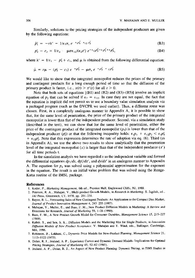
Appendix B In this appendix we compare the pricing and adoption paths of the primary and

captive contingent products to the paths of independent producers. Following the procedure used in Appendix A for the optional durable, it can be shown that the following equations provide the solution to the pricing strategy of the integrated monopolist [eq. (8) subject to eq. (6)]:

PI = ?.A + l/ElU, s?-EIP1E12 p2 + (p2 - c2) e-E2P2

P2 - c2 = l/E2 - UE,2/(ElEfi) 6’ -ElzPZ-El Pl+q!P2 ,

(Bl)

032)

where A = (l/&r - p1 + c,) and u = (al + b,x)(N - x).


Similarly, solutions to the pricing strategies of the independent producers are given by the following equations:

Jj; = -rh’ + l/s,oX c-E,PF--E,* p; (B3)

where h’ = I/E I - p;‘ + cl, and p is obtained from the following differential equation:

h = i-p, - (p5 - c-J e-%7!G - po, e-E&E 12p; (BY

We would like to show that the integrated monopolist reduces the prices of the primary and contingent products for a long enough period of time so that the diffusion of the primary product is faster, i.e., x(t) > xc(t) for all t > 0.

Note that both sets of equations [(Bl) and (B2) and (B3)-(B5)] involve an implicit equation of pz that can be solved if ~~ = Ebb. In case they are not equal, the fact that the equation is implicit did not permit us to use a boundary value simulation analysis via a packaged program (such as the DVCPR we used earlier). Thus, a different route was chosen. First, in a completely analogous manner to Appendix A, it is possible to show that, for the same level of penetration, the price of the primary product of the integrated monopolist is lower than that of the independent producer. Second, via a simulation study (described in the text), we can show that for the same level of penetration, either the price of the contingent product of the integrated monopolist (p2) is lower than that of the independent producer (p;) or that the following inequality holds: up, + ~~~~ < E tp;

+ E&. Note that this expression determines the rate of adoption via eq. (6). Third (as in Appendix A), we use the above two results to show analytically that the penetration level of the integrated monopolist (x) is larger than that of the independent producer (x“) for all time periods t.

In the simulation analysis we have regarded x as the independent variable and formed the differential equations dp,ldx, dp?l&‘, and dyldr” in an analogous manner to Appendix A. The equation for p2 was solved using a polynomial approximation for the exponent in the equation. The result is an initial value problem that was solved using the Runge-

Kutta routine of the IMSL package.

References 1. Kotler, P., Marketing Management, 6th ed., Prentice Hall, Englewood Cliffs, NJ, 1988.

2. Peterson, R. A., Mahajan, V., Multi-product Growth Models, in Research in Marketing. S. Jagdish, ed.,

JAI Press, Greenwich, CT, 1978, pp. 201-231. 3. Bayus, B. L., Forecasting Sales of New Contingent Products: An Application to the Compact Disc Market,

Journal of Product Innovation Management 4, 243-255 (1987). 4. Mahajan, V., Muller, E., and Bass, F. M., New Product Diffusion Models in Marketing: A Review and

Directions for Research, Journal of Marketing 59, l-26 (1990). 5. Bass, F. M., A New Product Growth Model for Consumer Durables, Management Science 15, 215-227

(1969). 6. Kalish, S., and Sen, S. K., Diffusion Models and the Marketing Mix for Single Products, in Innovation

Diffusion Models of New Product Acceptance. V. Mahajan and Y. Wind, eds., Batlinger, Cambridge,

MA, 1986. 7. Robinson, B., Lakhani, C., Dynamic Price Models for New-Product Planning, Management Science 21,

1113-1122 (1975). 8. Dolan, R. J., Jeuland, A. P., Experience Curves and Dynamic Demand Models: Implications for Optimal

Pricing Strategies, Journal of Marketing 45, 52-62 (1981). 9. Jeuland, A. P., Dolan, R. J., An Aspect of New Product Planning: Dynamic Pricing, in TIMS Studies in


the Management Sciences, Vol. 18: Marketing Planning Models. A. A. Zoltners, ed., Elsevier, New York,

1981, pp. 1-21.

10. Kalish, S., Monopolistic Pricing with Dynamic Demand and Production Cost, Marketing Science 2, 135%

1.59 (1983).

11. Bass, F. M., Bultez, A., A Note on Optimal Strategic Pricing of Technological Innovations, Marketing

Science 1, 371-378 (1982). 12. Horsky, D., The Effects of Income, Price and Information on the Diffusion of New Consumer Durables,

Marketing Science, forthcoming (1990). 13. Jam, D., and Rao, R. C., Effects of Price on the Demand for Durables: Modeling, Estimation and Findings,

Journal of Business and Economic Statistics 2, 163-170 (1990).

14. Nascimento, F., and Vanhonacker, W. R., Optimal Strategic Pricing of Reproducible Consumer Products,

Management Science 34, 921-937 (1988).

15. Dodson, J. A., and Muller, E., Models of New Product Diffusion Through Advertising and Word-of-

Mouth, Management Science 24, 1568-1578 (1978).

16. Mahajan, V., Mason, C. H., Srinivasan, V., An Evaluation of Estimation Procedures for New Product

Diffusion Models, in Innovation Diffusion Models of New Product Acceptance. V. Mahajan and Y. Wind,

eds., Ballinger, Cambridge, MA, 1986.

17. McGuire, T. W., and Staelin, R., An Industry Equilibrium Analysis of Downstream Vertical Integration,

Marketing Science 2, 161-192 (1983).

18. Kamien, M. I., and Schwartz, N. L., Dynamic Opfimization: The Calculus of Variations and Optimal

Control in Economics and Management, North Holland, New York, 1981.

Received 6 December 1989

pricing and diffusion of primary and contingent...

Documents