A C T A G E O P H Y S I C A P O L O N I C A

Vol. 53, no. 3, pp. 311-324 2005

PRESTACK DEPTH MIGRATION VELOCITY MODEL BUILDING IN COMPLEX CARPATHIANS GEOLOGY

Krzysztof Karol ŚLIŻ

AGH University of Science and Technology Faculty of Geology, Geophysics and Environmental Protection

Al. Mickiewicza 30, 30-059 Kraków, Poland

Geofizyka Kraków Ltd. ul. Łukasiewicza 3, 31-429 Kraków, Poland e-mail: krzysztof.sliz@geofizyka.krakow.pl

A b s t r a c t

Carpathians geology is very complex and seismic horizons are highly de-formed by tectonic movements, existence of thrusts, numerous faults and frac-ture zones. Therefore, the geological interpretation beneath the overthrust is un-certain and wells cannot be reliably located. Under complex geological condi-tions, time migration algorithms generate errors resulting from strong horizontal velocity changes. Moreover, the proper focusing of dissipated energy requires application of a PreStack Depth Migration (PreSDM). Proper depth imaging de-pends on appropriateness of velocity model used for PreSDM. Unfortunately the complexity of velocity changes limits the effectiveness of conventional velocity analysis techniques.

The article focuses on PreSDM velocity model building process for data acquired in complex overthrust environment. The method is based on dual usage of tomographic inversion together with combination of non-seismic information. Combination of tomographic results with well velocities increases convergence of the method. It also limits an ambiguity and improves reliability of final veloc-ity model.

To justify the proposed method, the border value of possible tomographic velocity updates was evaluated. The method was tested on two different datasets acquired in the Polish Carpathians.

Key words: PreStack Depth Migration, velocity model building, seismic tomo-graphy, overthrust, Carpathians.

K.K. ŚLIŻ 312

1. INTRODUCTION

PreStack Depth Migration (PreSDM) is a robust method for obtaining proper image of complex subsurface. In areas of rapid lateral and vertical velocity changes, energy is dispersed in such a way that conventional stacking with hyperbolic moveout dimin-ishes both noise and signal. The PreSDM focuses scattered energy by moving it to a proper subsurface position. Only when energy is properly focused, stacking improves the quality of signals and eliminates noise.

There are several situations where PreSDM could bring good effects. Some of them are environments of complex sedimentation structures, robust tectonics, presence of salt or basalt bodies and, for some migration codes, influences of anisotropy. Ap-plying a proper velocity model to PreSDM, we can expect significant improvement of seismic data quality (both resolution and continuity) and proper spatial structural posi-tioning. Additionally, which is not commonly acknowledged, the velocity model cre-ated for PreSDM carries direct knowledge about geology. For these reasons, velocity estimation process is the main task in depth imaging. Fortunately, iterative PreSDM is a good tool for velocity analysis due to its high sensitivity to velocity errors.

Data quality in areas of complicated geology is usually very poor. This compli-cates the process of velocity model building. Conventional methods fail in the areas of tectonic deformations and strong lateral velocity changes. These problems make ve-locity model building a difficult and ambiguous process (Lines et al., 2000).

Methods for migration velocity analysis

In general, the process of velocity model building can be split into two phases: prepa-ration of initial model and its updating. The initial model should be simple but it should describe general velocity trend. The detailed velocity changes are found during the Migration Velocity Analysis (MVA). The concept of using PreStack Depth Migra-tion for velocity analysis is related to the idea that correct velocity used to PreSDM results in flat reflections for all offsets on the Common Reflection Points (CRPs). When images from different offsets are not lined up, a residual moveout can be used to correct the velocity model.

The MVA methods usually require “picking” of residual arrival times and inver-sion of picks for velocity changes (Jones, 2003). The criteria used in velocity model determination are based on the “flatness” of pre-stack migrated gathers or the quality of a stacked image. Unfortunately, there can be several subsurface velocity models, which straighten migrated gathers equally well. This leads to a problem of receiving an unique solution.

There are three commonly known approaches to migration velocity analysis: De-regovski Loop (DL) (Deregowski, 1990) and its modification, Layer Striping Method (Bleistein and Liu, 1992) and global methods (Stork, 1992). Each of them is useful under special circumstances. DL is the fastest and the easiest approach but it is valid only when velocity variations are medium. Layer Striping Method accumulates mis-

PRESTACK DEPTH MIGRATION VELOCITY MODEL 313

takes made just at the beginning and is useful in areas of visible seismic horizons on common offset planes. Global velocity updating methods like tomography perform velocity updating for the whole subsurface, or at least a large portion of it. The process uses data from a large number of migrated gathers simultaneously.

Reflection tomography

In tomographic approach to the inverse problem, the medium velocity is determined by minimizing misfit function between measured and computed travel-times. The solution is usually computed by introducing deviation in travel-times. Deviation am-plitude cannot be too big, which results in limitations of finding a new model which would be too different from the input one. Besides, there are several other problems which must be handled by reflection tomography. Firstly, picking reflected events from seismic signal is much more difficult than the estimation of first arrivals in re-fraction tomography. The events are frequently distorted by coherent noise and dislo-cations. Secondly, the inversion problem is very ill-posed. The raypath coverage in reflection method is sparser, and therefore there is a possibility of multiple solutions and a problem of uniqueness (Kasina, 2001). Finally, the construction of raypaths strongly relies on the reflector position, on both depths and slopes (Liu, 1995). Ac-cordingly, the problem of convergence and ambiguity of the model is a general issue. In spite of these difficulties, tomographic inversion is a convenient and reliable method to obtain a good and detailed velocity model and it is reasonable to use it for determination of rapid velocity changes in complex regions. The final result depends on boundary conditions and proper initial velocity model is among the most important ones. This is why the key to success is the ability to construct a proper starting model. Then the results of tomographic inversion should converge to a plausible geological solution.

2. DATA AND GEOLOGY

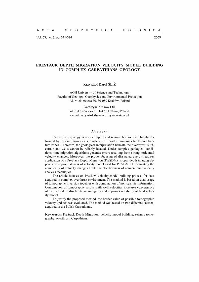
The method was tested on 2 datasets from different areas acquired in southeast Poland (Fig. 1). Both regions are situated on the edge of the Carpathian overthrust. All pro-files were situated perpendicular to the Carpathian overthrust. The general direction of lines was from S-W to N-E. Acquisition was made in 1992 and 1993 by Geofizyka Kraków Ltd. using vibrator sources; CDP coverage varied from 24 to 64 and maxi-mum offset was from 1240 to 2550 m, length being from 12 to 22 km. The well in-formation was sparse and unevenly distributed (Górecki et al., 2004).

The Outer Carpathians are built of sandy-shaly rocks of Cretaceous through Oli-gocen age. These rocks together with older folded Miocene deposits are thrust over autochthonous deposits of younger Miocene of the Carpathian Foredeep. The Flysch Carpathians in their marginal, northern part lie on Miocene rocks of the Carpathian Foredeep, whereas in the southern part they probably rest on the diversified Meso- zoic-Paleozoic and Precambrian basement (Karnkowski, 1993). The Carpathian over-

K.K. ŚLIŻ 314

Fig. 1. The map of the area where test data were gathered. Solid lines indicate profiles chosen for modelling. Yellow markers show position of well with velocity information. Black dashed line indicates schematic frontier of the Carpathian overthrust. Scale: 1 cm = 5 km.

? ?

?

?

thrust is built of strongly folded, cut by tectonic zones, flysch sediments in which al-ternating silty-clayey and sandstone layers of varied thickness dominate. Layers build numerous thrust sheets and scales. They are formed of partly differentiated sediments showing evidence that they originated in various sedimentary basins (Krzywiec, 1999). Partly due to these reasons, velocity changes in the Carpathian environment are severe but sometimes can be associated with specific scales. In contrast, Miocene en-vironment is less complex but velocities can be disturbed by stratygraphic changes, possible gas accumulations and some general, regional dislocations. Deposits of autochtonous Miocene in the presented area are prospective for finding high quality gas accumulations (Karnkowski, 1993).

3. METHOD

The key to the success of tomographic inversion is a proper starting model. Unfortu-nately, there are several reasons why traditional initial model building techniques (model from RMS velocities or based on gradient functions) fail in overthrusted areas. Some of them are as follows:

PRESTACK DEPTH MIGRATION VELOCITY MODEL 315

• low resolution of stacking velocities, • fast lateral velocity changes and sparse coverage of well information, • strong influence of noise and steep horizons for estimated velocities, • problems with assigning a single gradient function for a given zone. The author assumed that correct model can be built when the lateral resolution of

initial model will be close to smoothed velocity function obtained from wells. For this reason, the first phase of the method defines proper trend of lateral velocity changes. The obtained result can be combined with well velocities. When appropriate starting velocity model is created, the proper border conditions appear for tomographic inver-sion. The proposed method is composed of dual usage of tomographic inversion and iterative adjustment of the model to changes in structural interpretation. The first phase of tomographic inversions is based on prototype model. In the very first stage of velocity updates, the main interest is in reliability of structural image obtained by PreSDM and in correct horizontal velocities trend. Furthermore, image obtained in the first phase of the method is used to define structural polygons. The polygons are em-ployed for edition of tomographic inversion results and for future combination of mi-gration velocities with well information. In the second phase of the method, the reso-lution of model is increased and inversions are continued until the results converge.

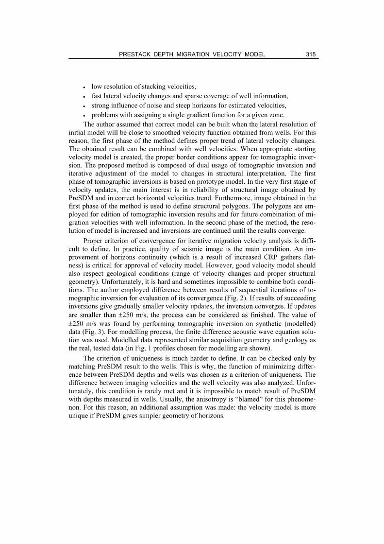
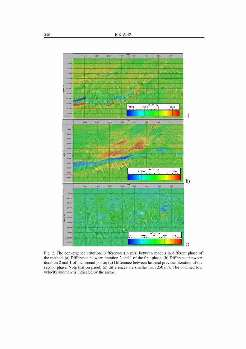
Proper criterion of convergence for iterative migration velocity analysis is diffi-cult to define. In practice, quality of seismic image is the main condition. An im-provement of horizons continuity (which is a result of increased CRP gathers flat-ness) is critical for approval of velocity model. However, good velocity model should also respect geological conditions (range of velocity changes and proper structural geometry). Unfortunately, it is hard and sometimes impossible to combine both condi-tions. The author employed difference between results of sequential iterations of to-mographic inversion for evaluation of its convergence (Fig. 2). If results of succeeding inversions give gradually smaller velocity updates, the inversion converges. If updates are smaller than ±250 m/s, the process can be considered as finished. The value of ±250 m/s was found by performing tomographic inversion on synthetic (modelled) data (Fig. 3). For modelling process, the finite difference acoustic wave equation solu-tion was used. Modelled data represented similar acquisition geometry and geology as the real, tested data (in Fig. 1 profiles chosen for modelling are shown).

The criterion of uniqueness is much harder to define. It can be checked only by matching PreSDM result to the wells. This is why, the function of minimizing differ-ence between PreSDM depths and wells was chosen as a criterion of uniqueness. The difference between imaging velocities and the well velocity was also analyzed. Unfor-tunately, this condition is rarely met and it is impossible to match result of PreSDM with depths measured in wells. Usually, the anisotropy is “blamed” for this phenome-non. For this reason, an additional assumption was made: the velocity model is more unique if PreSDM gives simpler geometry of horizons.

K.K. ŚLIŻ 316

a)

b)

c)

Fig. 2. The convergence criterion. Differences (in m/s) between models in different phase of the method. (a) Difference between iteration 2 and 1 of the first phase; (b) Difference between iteration 2 and 1 of the second phase; (c) Difference between last and previous iteration of the second phase. Note that on panel; (c) differences are smaller than 250 m/s. The obtained low velocity anomaly is indicated by the arrow.

PRESTACK DEPTH MIGRATION VELOCITY MODEL 317

Fig. 3. Evaluation of tomographic inversion results, PreSDM, done on modelled data. True velocity model smoothed by operator 250 × 250 m was used. On the picture, tomographic inversion result is shown. The visible anomalies cannot be associated with real velocity changes. Note that the accuracy of the method for this type of the data is ±250 m/s.

Process of prototype velocity model building

Prototype velocity model is used for the first phase of tomographic inversion. It can be built by the gradient’s functions or RMS stacking velocities can be used.

Prototype velocity model based on stacking velocity. Stacking velocities are con-verted to interval velocities in depth. Then the process of adjustment to geological values and structural interpretation is performed. The anomaly velocities are edited. This phase is iterative and feed backed by PostSDM results (in the beginning) and later by PreSDM. Special attention should be paid to unwanted structural anomalies. If observed, severe smoothing of RMS and interval velocities must be performed. The process of smoothing and RMS velocity edition is driven by structural polygons and initial PostSDMs/PreSDMs are repeated several times until a reasonable structural definition is observed.

Prototype velocity model based on gradient functions. Alternatively to RMS veloci-ties, gradient functions can be used to create a prototype velocity model. The functions are described as: V(x, z) = V0 + kx x + kz z, where coefficients kx and kz represent hori-zontal and vertical gradients computed from average velocity or acoustic logging. In each well, several kz are derived with respect to velocity changes in main geological

K.K. ŚLIŻ 318

layers. Then the coefficients kx are computed in such a way that kz z functions can be smoothly converted from one well into another. Unfortunately, usage of these func-tions may lead to ambiguity since they are based on the process of averaging velocities inside previously defined layers. For this reason, proper definition of zones where velocity changes linearly and calibration of wells to the seismic image are critical at this stage of work (Jarzyna et al., 1999). One of the main advantages of gradient func-tions is the possibility of creating consistent model of 2D multiple lines.

First phase of tomographic inversion

otype model is updated by tomographic inver-

method, improvements in seismic image quality were

implementation of strong smoothing, the resolution of mod

Velocity model building

od is combination of well velocities (hard data) with model

Besides, the real wells are usually located in uneven pattern, which usually causes

In the first phase of the method the protsions and lateral velocity changes are defined. Prototype model in complex environ-ment is far from being correct. One solution for handling non-uniqueness at this stage of the method is to use geologic information to constrain the model. Very often the velocity varies smoothly within geological formations. If it is possible to identify key formations on migrated sections, a smooth velocity function can be sought within each formation while allowing higher velocity changes across interfaces separating differ-ent layers. Therefore, strong constrains (edition of minimum and maximum changes in the model and smoothing) can be applied to tomographic inversions results inside previously identified formations.

During the first phase of the observed, although tomographic updates could not converge. Results from one

iteration to another changed significantly and it was impossible to obtain ±250 m/s limit. Besides, each velocity update leaded to strong changes in structural interpreta-tion. Fortunately, proper horizontal velocity gradient could be found inside each de-fined geological formation.

Additionally, despite ofel increased, which resulted in narrowing the difference between well velocities

and prototype model. Apart from this, better definition and continuity of horizons were received at this stage of the work. This led to more reliable structural definition of the model. The number of iteration was data-dependent but usually 2-6 iterations were sufficient.

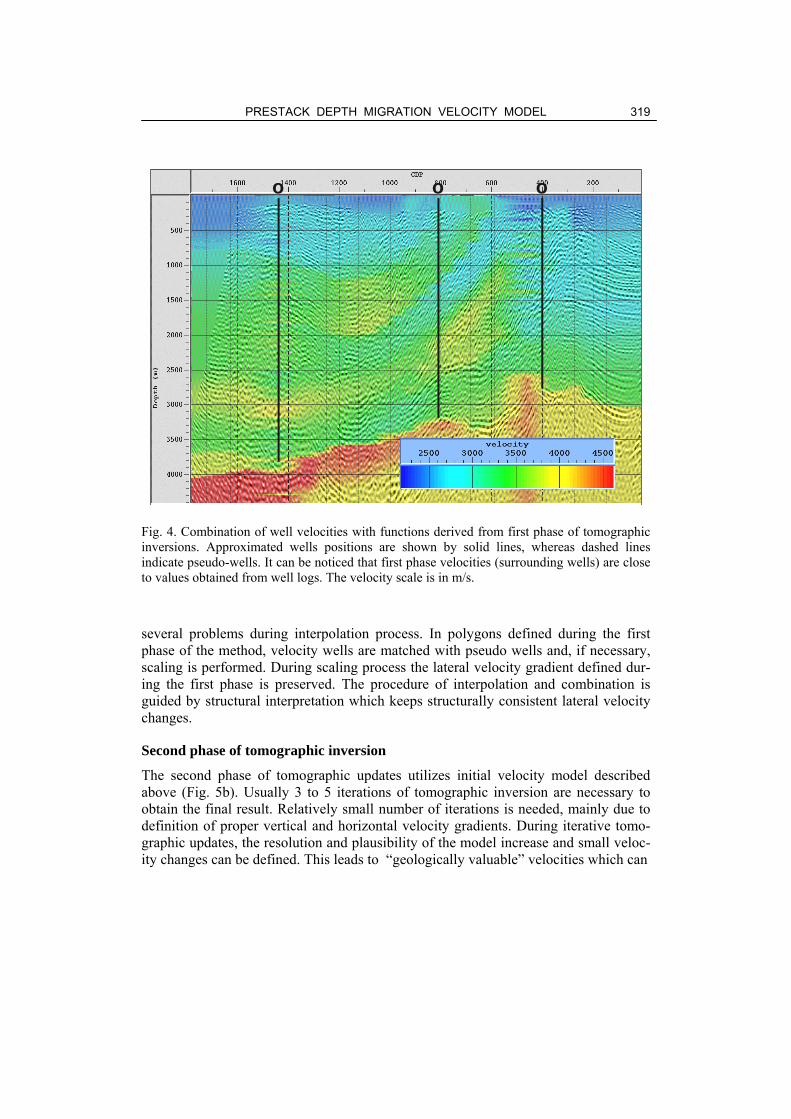
Important part of the methobtained during first phase of the tomographic inversions (soft data). This is per-formed in geostatistical manner; weights are assigned to data according to their reli-ability and distance from wells. The whole process is performed utilizing idea of pseudo-well logs. They represent vertical parameter changes in a possible position of well. Location of pseudo-wells is introduced to stabilize process of inter-polation of true well’s velocity (Fig. 4). Usually, pseudo-well velocities differ from real ones.

PRESTACK DEPTH MIGRATION VELOCITY MODEL 319

Fig. 4. Combination of well velocities with functions derived from first phase of tomographic inversions. Approximated wells positions are shown by solid lines, whereas dashed lines

several problems during interpolation process. In polygons defined during the first phase of the method, velocity wells are matched with pseudo wells and, if necessary,

The second phase of tomographic updates utilizes initial velocity model described of tomographic inversion are necessary to

indicate pseudo-wells. It can be noticed that first phase velocities (surrounding wells) are close to values obtained from well logs. The velocity scale is in m/s.

o o o

scaling is performed. During scaling process the lateral velocity gradient defined dur-ing the first phase is preserved. The procedure of interpolation and combination is guided by structural interpretation which keeps structurally consistent lateral velocity changes.

Second phase of tomographic inversion

above (Fig. 5b). Usually 3 to 5 iterations obtain the final result. Relatively small number of iterations is needed, mainly due to definition of proper vertical and horizontal velocity gradients. During iterative tomo-graphic updates, the resolution and plausibility of the model increase and small veloc-ity changes can be defined. This leads to “geologically valuable” velocities which can

K.K. ŚLIŻ 320

a)

c)

b)

PRESTACK DEPTH MIGRATION VELOCITY MODEL 321

a)

b)

500 CDP

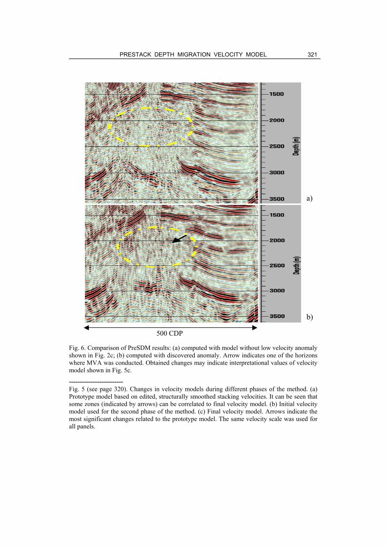
Fi low velocity anomaly shown in Fig. 2c; (b) computed with discovered anomaly. Arrow indicates one of the horizons where MVA was conducted. Obtained changes may indicate interpretational values of velocity model shown in Fig. 5c.

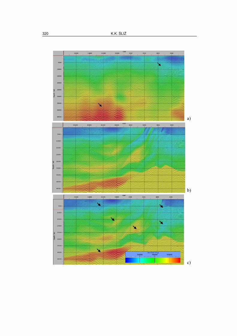
------------------------- Fig. 5 (see page 320). Changes in velocity models during different phases of the method. (a) Prototype model based on edited, structurally smoothed stacking velocities. It can be seen that some zones (indicated by arrows) can be correlated to final velocity model. (b) Initial velocity model used for the second phase of the method. (c) Final velocity model. Arrows indicate the most significant changes related to the prototype model. The same velocity scale was used for all panels.

g. 6. Comparison of PreSDM results: (a) computed with model without

K.K. ŚLIŻ 322

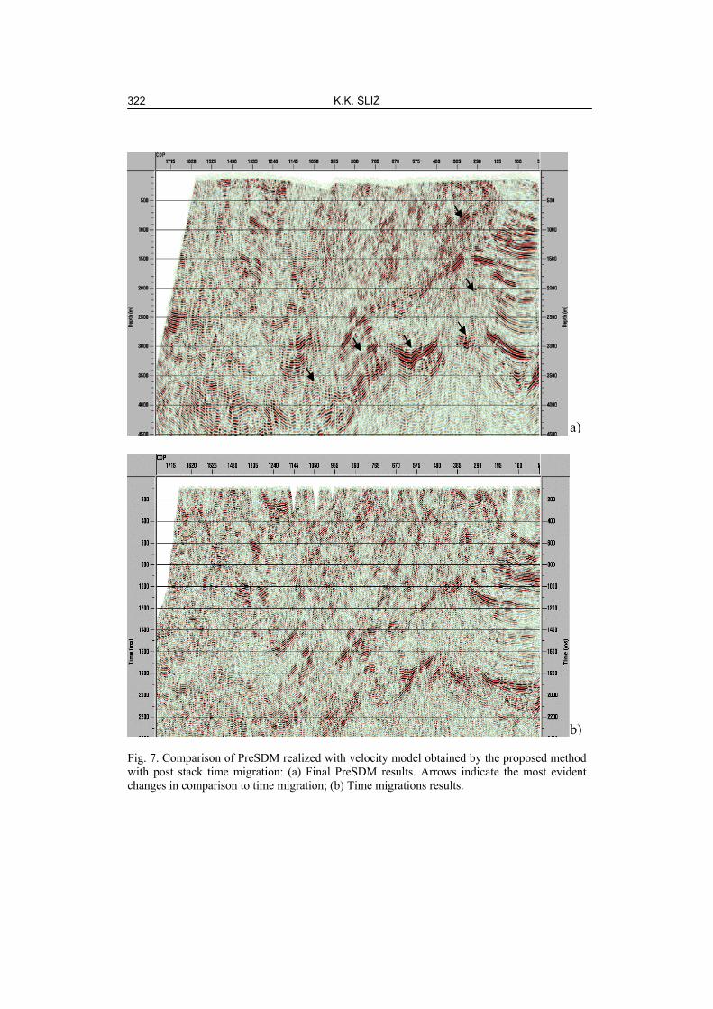
Fig. 7. Comparison of PreSDM realized with velocity model obtained by the proposed methwith post stack time migration: (a) Final PreSDM results. Arrows indicate the most evidchanges in comparison to time migration; (b) Time migrations results.

a)

)

b

od ent

PRESTACK DEPTH MIGRATION VELOCITY MODEL 323

be used in more detailed stratigraphic interpretation (Fig. 2c and Fig. 6). It is also pos-sible to gradually increase the offset range (in both the process of ray tracing and re-sidual moveout analysis). This helps to diminish possible velocity errors and improves final seismic image (Fagin, 1999).

4. RESULTS

Construction of a velocity model for PreStack Depth Migration was conducted in two phases. Tomographic inversion results were combined with well velocities. It was possible to develop good interpretational velocity distribution and improve quality of seismic image. PreSDM correctly focused dispersed energy, which allowed for quality improvement of the inner Carpathian horizons, the bottom of the Carpathian over-thrust, Miocene horizons, and Miocene substratum of different age (Fig. 7). Previously invisible faults and structures were also imaged. This would not be possible without a proper velocity model.

5. CONCLUSIONS

The quality of initial velocity distribution has the greatest influence on tomographic inversion process. A good initial model limits ambiguity and increases convergenc

mographic solutions. Therefore, an initial model plays key role in a process of mi-gration velocity analysis for complex structures. In the case of tomographic inversion, a wrong provisional velocity distribution makes it impossible to obtain convergent results. The approach used in this study estimated the initial velocity field by means of combination of tomographic results with well velocities. Successive iterations are performed until the obtained structural model could be accepted and tomographic in-version velocities updates reached limits of ±250 m/s. The tomographic inversion requires the imposition of geological constraints and manual edition of results of each iteration.

The proposed method allows to obtain geologically plausible velocity model even in the areas where wells are not uniformly located. Significantly small velocity changes received during final tomographic inversion to some extent prove the correct-ness of the final solution. When analyzing structural changes on the seismic sections after final PreSDM, one can see a varied geometry of reflections beneath the Carpa-thian overthrust. As compared to the time migration result, a characteristic horizontal shift of culmination of structures can be observed after depth migration (Górecki et al., 2004).

PreSDM is a powerful method and is proven to give results of a remarkable qual-ity. As mentioned previously, such results are obtained only provided that a proper velocity model is used.

e ofto

K.K. ŚLIŻ 324

A c k n o w l e d g e m e n t s. The paper represents part of author’s PhD re-search. The AGH University of Science and Technology and the author acknowledge support of this investigation by Landmark Graphic software via the Landmark Univer-sity Grant. Research was partly conducted in the framework of grants led by Professor

R e f e r e n c e s

Bleistein, N., and Z. Liu, 1992, Velocity analysis by residual moveout, 1992 SEG Annual Expanded Abstracts, p. 1034.

Górecki, W., M. Stefaniuk, T. Maćkowski, B. Reicher, K.K. Śliż, A. Maksym and J. Siupik, 2004, Joint interpretation of seismic and MT data beneath the Polish Carpathians

E Annual Meeting, Paris, Expanded Abstracts.

Received in revised form 16 February 2005 Accepted 22 February 2005

Wojciech Górecki.

Meeting,Deregowski, S.M., 1990, Common offset migration and velocity analysis, First Break 8, 225-

234. Domagała, K., K. Lisowski, M. Oniszk, A. Wójcicki, T. Adamczyk and A. Maksym, 2002,

Integrated interpretation of geophysical and geological data in Hermanowa, Babicy and Strzyżowa Area (in Polish), Archives of the PGNiG, Geonafta, Jasło (unpub-lished).

Fagin, S., 1999, Model-Based Depth Imaging, Society of Exploration Geophysicists, Tulsa, 173 pp.

overthrust, EAGJarzyna, J., M. Bała and T. Zorski, 1999, Well logging methods – logging and interpretation

(in Polish), Uczeln. Wyd. Nauk.-Dydakt., AGH, Kraków 19, 91. Jones, I.F., 2003, A review of 3D PreSDM model building techniques, First Break 3, 53. Karnkowski, P., 1993, Oil and gas fields in Poland, Carpathians and Carpathian foredeep (in

Polish), Towarzystwo Geosynoptyków “Geos”, AGH, Kraków 247. Kasina, Z., 2001, Seismic Tomography (in Polish), Wyd. Inst. GSMiE PAN, Kraków, 13-28. Krzywiec, P., 1999, Tectonic evolution of Miocene formation in east part of the Carpathian

foredeep (in Polish). In: “Analysis of Tertiary Carpathian Basin”, Prace Państw. Inst. Geol. 168.

Lines, R.L., S.H. Gray and D.C. Lawton, 2000, Depth imaging of foothills seismic data, Cana-dian SEG Publ., Calgary, 31-32.

Liu, Z., 1995, Migration velocity analysis, PhD Thesis, Center for Wave Phenomena, Colorado School of Mines, Golden CO, USA 168, 78, 82.

Stork, C., 1992, Reflection tomography in postmigrated domain, Geophysics 57, 680-692.

Received 5 April 2004