Preliminary Report on the Prognostic Value of Barotropic Models in the Forecasting of 500 mb Height Changes'

By STAFF MEMBERS OF THE INSTITUTE OF METEOROLOGY, University of Stockholm

Manuscript received 8 March 1952)

Abstract Some general coniinents are given regarding numerical methods of integrating the

hydro-d ynamic equations. A series of tendency computations for Europe and eastern At- 'lantic are presented, by and large following the scheme given by BOLIN and CHARNEY

(1951). Data requirements for this kind of computations are discussed on the basis of the difference in the success of the method over regions with poor and with good data.

During the last few years several groups of meteorological research workers have devoted an increasing amount of effort to the problem of translating basic dynamic principles into practically usable methods for quantitative objective forecasting of changes in the large- scale flow atterns of the atmosphere. The

machines has been a factor of decisive impor- tance in this development; the fact that we now at long last seem to know how to construct theoretical models of the atmosphere which combine simplicity with the ability to repro- duce several highly characteristic features of the observed atmospheric motions has un- doubtedly contributed to the growing interest in the development of forecasting methods based on dynamical principles.

The most systematic approach in this field has been made by the group working at the Insti- tute for Advanced Study in Princeton under the dxection of J. Charney and J. von Neu- mann. They started with a very simple madel

advent of fl igh-speed electronic computing

The investigation described in this report has been supported primarily by a grant froni the U.S. Weather Bureau.

of the atmosphere by assuming autobarotropy and two-hmensional flow, but retaining the principle dynamic consequence of the s herical shape of the rotating atmospheric she P 1. With this model as a starting point they were then able to build up more complex structures capa- ble of accounting for atmospheric features not contained in this initial model. After relimi- nary tests with a one-dimensional mode P (CHAR- NEY and ELIASSEN, 1949) the results of the first attempts to make complete 24-hour forecasts using the two-dimensional model were pub- lished little more than a year ago in an article by CHARNEY, FJORTOFT and VON NEUMANN 1950). As one mi ht expect the results were b y no

However, only four complete forecasts were made; high speed electronic computing ma- chines and dependable 500 mb charts, carefully analyzed with reference to the vorticity distri- bution, must be available before a systematic testing program can be carried out.

If the hydrostatic and geostrophic assump- tions are introduced in the equations of motion as proposed by CHARNEY (1948) the system of differential equations may be reduced to one

means per B ect but at least very promising.

22 STAFF MEMBERS OF THE INSTITUTE OF METEOROLOGY

equation which is only of the first order with respect to time, in other words the changes of the j h t v to be c~xpcctcd are completely determined by the state of motiotr of the atmosphere while no knowledge of the rate of change of this state is necessary. It is this fact that provides the basis for all the numerical integrations through iterative processes which have been proposed until now. Regardless of the ultimate prognostic value of this fundamental result it is evidently of great scientific interest to explore its validity further. It is in this connection of particular interest to know to what extent this is true for the still more simplified barotropic model of the atmosphere, e.g. to determine the extent to which the observed motions in the 500 mb level, interpreted as if they were motions of an equivalent barotropic atmos here, deter- mine tJle short range evolution o P the circula- tion at that level. For this reason the Princeton group working under Charney’s direction in 1951 initiated a series of tendency computa- tions from selected 500 mb charts and the results of these were recently set forth in a paper by BOLIN and CHARNEY (195 I) .

Before proceeding to a discussion of thc results of the series of similar computations carried out here a few further remarks should be made.

In any attempt to develop objective methods for forecasting it is extremely important to keep in mind the limitations that are prescribed by the amount of observational data that is available as well as the accuracy of these data. It is already obvious from the previous investi- gations that not even the two-dimensional barotropic model in its present form can be used to its fullest extent over the oceans where the aerological network is sparse. It would then be very unrealistic to try to apply a de- tailed three dimensional model of the atmos- phere over such an area. On the other hand we know from experience that it is possible with existing subjective methods to forecast at least some large scale phenomena even with the small amount of data that now is at our disposal. As these large-scale processes in the atmosphere undoubtedly to a large extent are barotropic in their character it seems that one of the most important problems at present is to develop methods that make it possible also to forecast such developments objectively. In such a method it should then in principle not be ncc-

essary to consider the detailed structure of the flow as is done at present since such details are not known.

There is another reason for studying the two- dimensional barotropic model in order to utilize its potentialities more fully before at- tempting to integrate the three-dimensional vorticity equation. Such an integration means such an extension of the computational pro- gram that there would be great difficulties to utilize the results in practice, due to the lim- ited capacity of present electronic computers. From a practical point of view it therefore seems as essential to improve this barotropic model as to attempt to introduce new phys- ical factors which, though important, would also increase the computational work con- siderably.

As is seen from the basic equation for the barotropic model the computations involve the evaluation of vorticity advection, which means a differentiation of the initial contour field three times. It is obvious that no great accuracy can be obtained for such a quantity, in particular if no objective method of smooth- ing the original contour field is used. However, these inaccuracies are of relatively small con- sequence for the accuracy of the final tenden- cies because an integration is performed twice in order to obtain them, which means a smoothing and elimination of random errors. From a practical point of view then the ques- tion arises: Is the procedure of first differen- tiating three times and then integrating twice necessary in order to obtain the tendency field?

In view of what has been said above and the benefits that would result from the successful development of an adequate technique for numerical prediction it was decided to make this one of the principle fields of research at the expanded and reorganized Institute of Meteoro- logy of the University of Stockholm. As a first step it was decided to perform a series of baro- tropic tendency computations of the type re- ferred to above, in order to enable the various members of the research group to become familiar with the technique of the computa- tion methods. Future reports will deal much more fully with these investigations. At the present time we shall restrict ourselves to a brief preliminary discussion of these tendency calculations, which for the first time provide us with some information concerning the

REPORT ON THE PROGNOSTIC VALUE OF BAROTROPIC MODELS 23

- -- q$o m --

I 7 20

-21 -22 -46

-16 -20 -28

-

-3 I -30 -40

12 8 21

2 3 22 I

90 73 57

71 65 19

17- I - 5

-50 -52 -28

6 - 6 - 7

-29-47 12

-13 12-26

13-20 46

4 - 3 - 2

- - -

applicability of the barotropic model in North- western Europe.

The active work of our group is at present supported by grants from the Swedish Natural Science Research Council, the Knut and Alice Wallenberg Foundation, the University of Chicago and the U.S. Weather Bureau. We are also deeply indebted to the various organiza- tions in Sweden and abroad who have contri- buted to our project by making professional personnel available. The participants in the tendency computations reported here have been: Mr G. Arnason, Iceland; Mr B. Bolinl, Sweden; Mr Ph. Clapp, USA; Dr A. Ehassenl, Norway; Mr K. Hinkelmann, Germany; Mr E. Hovmoller, Denmark; Lt. W . Hubert, USA; Dr E. Kleinschmidt, Jr., Germany; Dr C. W. Newton1, USA; Mrs H. Newton, USA; Dr H. Schweitzer, Germany; Miss Ch. Steyer, Germany.

The method used in these computations is the same as that used at Princeton and described by BOLIN and CHARNEY (1951). Computations were made on a rectangular grid, with grid interval of approximately 310 km at latitude 50' N. Because of time limitations, com uta- tions of vorticity, vorticity advection ancften- dency were made only at alternate points on the grid, in the manner discussed by Bolin and Charney. It was necessary to restrict the area over which the computations were made to a re- gion about 4,000 km square, with its center near the British Isles (see figure 6) . An important part of this region lay over the Atlantic Ocean so that errors both in computation and in veri- fication arise from the uncertainty of analysis over this region with sparse observations.

Two methods of verification of the com- puted tendencies were used. The first of these is the method used at Princeton, that is, to compare the computed value of

with the observed height changes

.To = Zr=ro+dr - Zr=r.,

Project leadcrs.

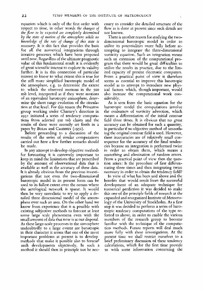
A t being 12 hours. z is the height of the 500 mb surface. In all, 14 pairs of tendency computa- tions at the 500 mb level have been made here. As pointed out by Bolin and Charney, verifica- tion by the above method tends, for fast- moving systems of period less than 36 to 48 hours, to give poor results which are not related to the efficiency of the com utation method itself. In the second metho{ use was made of the frequent upper-air observations from Great Britain, in a manner to be discussed later.

Since in solving for the tendencies it is necessary to make some assumption regarding

Table I

STAFF MEMBERS OF THE INSTITUTE OF METEOROLOGY 2 4

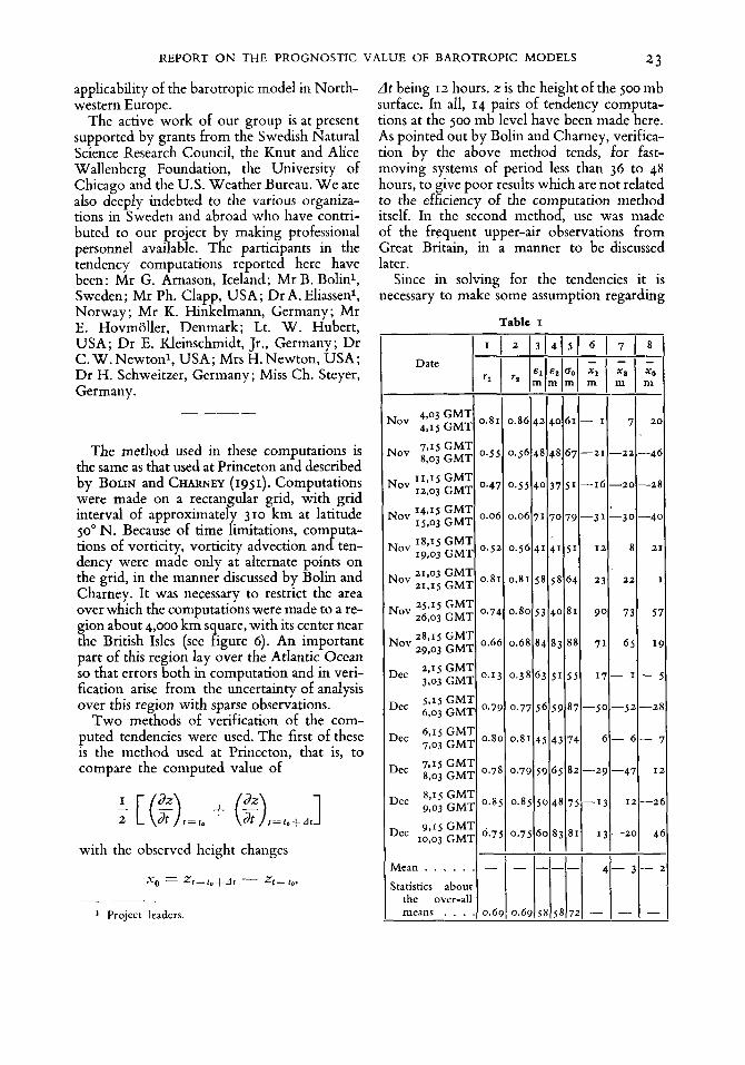
Fig. I a Fig. I b Fig. I . Contours (solid lines) and computed tendencies (dashed lines), (a) 1300 GMT 18 November 1951; (b) 0300 GMT 19 November 1951. Contours labelled in tens of meters, interval 40 m, tendencies in tens of

meters per 12 hours. In wind symbols, solid triangles represent 50 knots, full barbs 10 knots.

the tendencies at the boundaries, the verifica- tion procedure was applied only in the central part of the region, excluding that art (two grid points from the boundary of t K e region over which computations were made) which is strongly affected by boundary conditions. Computations were made first on the assump- tion .that the tendencies at the boundary are zero, and then repeated using, for each pair of computations, the actual Iz-hour changes at the boundaries. The results of the verification are presented in table I. y1 denotes the value of the mean tendency when it is assumed that the tendency on the boundary is zero and x2 is the value when the observed values xo are used as boundary values. A bar indicates a mean value over the area of verification. rl is the correlation coefficient between xl and xo, r2 the correlation coefficient between x2 and xo. c1 = \i (xl - ~ , ) ~ / n , i.e. gives the root- mean square of the error in x1 and correspond- ingly .s2 gives the error of x2. Finally a, denotes the root mean square of the observed changes (xo), in other words a, is the error of a forecast of no change.

The following should be noticed: I. From all cases combined, an overall corre-

lation coefficient of 0.7 was obtained, somewhat lower than that reported by Bolin and Charney. The difference is hardly significant. On the other hand these values on the average are con-

_.

siderably higher than those given by SAWYER and BUSHBY ( 1 9 ~ 1 ) for two computations. It seems safe to conclude from the computations made at Princeton and those re orted here that the results of Sawyer and Bus K by are not re- presentative for computations of this kind. As seen from the table poor correlation was ob- tained in two cases. In both these cases (as well as in some of the others with fairly low correla- tion) the continuity of the analyses was not the very best. To a certain extent this depended upon the fact that the analyses were made by different members of the group. However, the last ten maps (Dec. 5 , 15-Dec. 10, 0 3 ) were analyzed by one of us with special attention to continuity in particular over the Atlantic Ocean, where the data are not sufficient to determine the flow patterns completely. Here the correlation is considerably higher. It should be noted that in no case correlation below 0.5 was obtained in the computations at Princeton, which also suggests that such low values are mainly due to inadequacy of the initial data. In those cases all computations were made over the North American Continent where quite a dense net of radiosonde observations is available.

2 . By and large there is a very little difference between the values obtained by using x1 or x2 in the verification, which indicates that the boundary influence in most cases is negligible

2s REPORT O N THE PROGNOSTIC VALUE OF BAROTROPIC MODELS

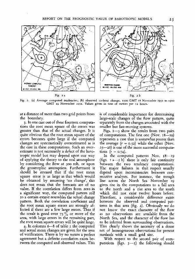
Fig. z a Fig. z b Fig. 2. (a) Average computed tendencies; (b) observed 12-hour change, 1500 GMT 18 November 1951 to 0300

GMT I9 November 1951. Values given in tens of meters per 12 hours.

at a distance of more than two grid points from the boundary.

3 . In one case out of these fourteen computa- tions the root mean s uare of the errors was

quite obvious that the root mean square of the errors becomes quite large if the computed changes are systematically overestimated as is the case in these computations. Such an over- estimate is not necessarily a defect of the baro- tropic model but may depend upon our way of applying the theory to the real atmosphere by considering the flow at 500 mb, or upon the geostrophic assumption. Furthermore it should be stressed that if the root mean square error is as large as that which would be obtained by assuming ‘no change’, this does not mean that the forecasts are of no value. If the correlation differs from zero in a significant way, the computed pattern still to a certain extent resembles the actual change pattern. Both the correlation coefficient and the root mean square errors are strongly af- fected if there are a few large errors. Thus if the result is good over 75 yo or more of the area, with large errors in the remaining part, the root mean square errors will be quite large. 4. In columns 6-8 of table I the computed

and actual mean changes are given for the area of verification. There is by no means a perfect agreement but a definite correlation exists be- tween the computed and observed values. This

greater than that of t 1 e actual changes. It is

is of considerable importance for determining large-scale changes of the flow pattern, quite separately from the changes associated with the smaller but fast-moving systems.

Figs. 1-5 show the results from two pairs of computations. The first one (Nov. 18-19) represents a case that is somewhat poorer than the average (r = 0.52) while the other (Nov. 25-26) is one of the more successful computa- tions (r = 0.74).

In the computed patterns Nov. 18-19 (figs. I a-1 b) there is only fair continuity between the two tendency computations. The major failures in that respect usually depend upon inconsistencies between con- secutive analyses. For instance, the trough line across the North Sea November 19 gives rise in the computations to a fall area to the north and a rise area to the south which did not exist twelve hours before. Therefore, a considerable difference exists between the observed and computed pat- terns in that area (fig. 2) . Obviously we do not know the exact character of the flow as no observations are available from the North Sea, and the character of the flow has to be inferred from surrounding observations. This clearly shows the necessity of a dense net of homogeneous observations for present methods with a small grid size.

With respect to the second pair of com- putations (figs. 3-5) the following should

26

Fig. 3 a

Fig. 3 b

STAFF MEMBERS OF THE INSTITUTE OF METEOROLOGY

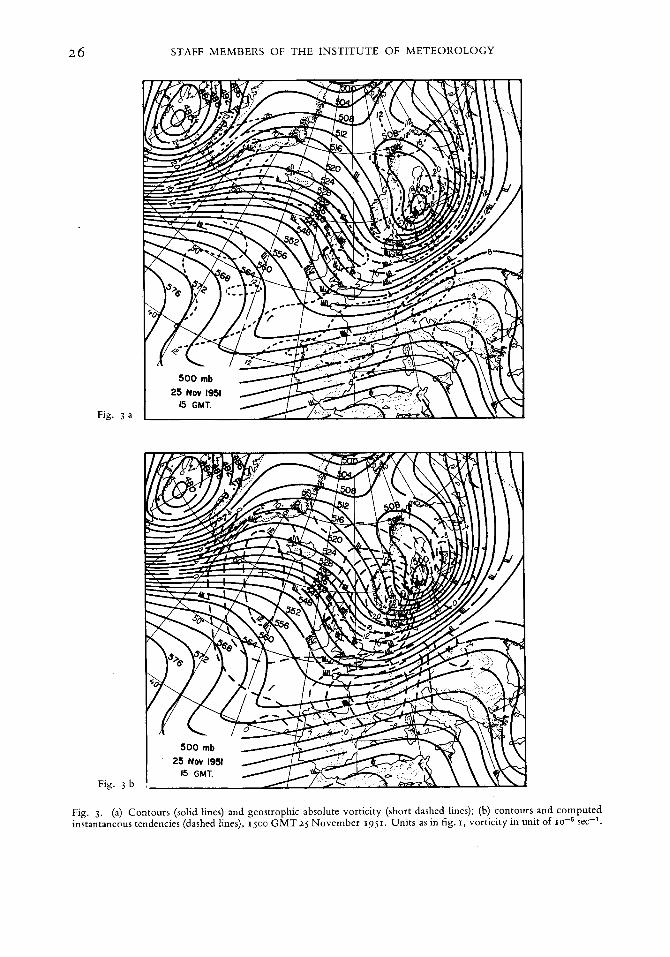
Fig. 3. (a) Contours (solid lines) and geostrophic absolute vorticity (short dashed lines); (b) contours and computed instantaneous tendencies (dashed lines), 1500 G M T z s November 1951. Units as in fig. I, vorticity in unit of I O - ~ sec-I.

REPORT O N THE PROGNOSTIC VALUE OF BAROTROPIC MODELS 27

Fig. 4 a

Fig. 4 b

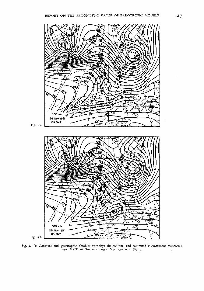
Flg. 4. (a) Contours and geostrophic absolute vorticity ; (b) contours and computed instantaneous tendencies, 0300 GMT 26 November 1951. Notations as in Fig. 3 .

28 STAFF MEMBERS O F THE INSTITUTE O F METEOROLOGY

Fig. 5 a Fig. 5 b

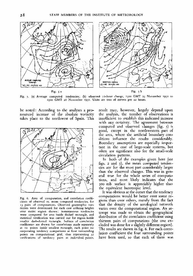
Fig. 5 . (a) Average computed tendencies; (b) observed Iz-hour change, 1500 G M T 25 November 1951 to 0300 G M T 26 November 1951. Units are tens of meters per IZ hours.

be noted: According to the analyses a pro- nounced increase of the absolute vorticity takes place to the northwest of Spain. Ths

Fig. 6. Area of computation, and correlation coeffi- cients of observed us. mean computed tendencies, for 13 pairs of computattons. Observed geostrophic vor- ticities were determined for each case utilizing heights over entire region shown ; instantaneous tendencies were computed for area inside dashed rectangle, and statistical verification was carried out for region inside smaller dash-dotted rectangle. Isolines of correlation coefficients are drawn for correlations made separately at I Z points inside smallest rectangle, each point in- corporating tendency comparisons at four surrounding points on computational grid, thus representing 52 verifications of tendency pairs at individual point$.

result may, however, largely depend upon the analysis, the number of observations is insufficient to establish this indicated increase with any certainty. The agreement between computed and observed changes (fig. 5 ) is good, except in the northwestern part of the area, where the artificial boundary con- ditions influence the results considerably. Boundary assumptions are especially impor- tant in the case of large-scale systems, but often are significant also for the small-scale circulation patterns.

In both of the examples given here (see figs. 2 and s), the mean computed tenden- cies are for the most part considerably larger than the observed changes. This was in gen- eral true for the whole series of computa- tions, and most likely indicates that the 500 mb surface is appreciably higher than the equivalent barotropic level.

It was obvious at the outset that the tendency computations would be better over some re- gions than over others, merely from the fact that the density of the aerological network varies over the computational region. An at- tempt was made to obtain the distribution of the correlation coe ficient using thirteen pairs of computations (the one ex- cluded was done for a slightly different region). The results are shown in fig. 6 . For each corrc- lation coefficient the four surrounding points have been used, so that each of them was

Beographical

REPORT ON THE PROGNOSTIC VALUE OF BAROTROPIC MODELS 29

Lerwick . . . . . . . . . . . . . . . . Stornoway.. . . . . . . . . . . . . Leuchars.. . . . . . . . . . . . . . . Aldergrove. . . . . . . . . . . . . . Liverpool . . . . . . . . . . . . . . Downham (Hemsby) . . . . Larkhill . . . . . . . . . . . . . . . . Camborne . . . . . . . . . . . . . . Statistics about the 'overall

means ................

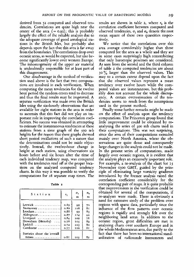
derived from 52 computed and observed ten- dencies. Correlations are quite high near the center of the area (= 0.92) ; this is probably largely the effect of the reliable analysis due to the adequate coverage of good aerological sta- tions in the British Isles, but probably also depends upon the fact that t h s area is far away from the boundaries. The correlations drop over oceanic areas, as would be expected, but also be- come significantly lower over western Europe. The inhomogeneity of the upper air material is undoubtedly responsible for at least part of this disagreement.

One disadvantage in the method of verifica- tion used above is the fact that two computa- tions are involved in each verification. When computing the mean tendencies for the twelve hour eriod the random errors tend to decrease and t R us the final results may be improved. A se arate verification was made over the British

available for eight stations in the area in order to ascertain that t h s fact did not play an im-

ortant role in improving the correlation coef- icients. No success was obtained in attempting to estimate the instantaneous tendencies at these stations from a time graph of the 500 mb heights for the reason that these graphs showed short period oscillations of such a nature that the determinations could not be made objec- tively. Instead, the twelve-hour change in height at each station, using observations six hours before and six hours after the time of each individual tendency map, was compared with the tendencies read off at the proper loca- tions on the analyzed computed tendency charts. In this way it was possible to verify the computations for 28 separate map times. The

Is P es using the six-hourly observations that are

0.89 0.80 0.88 0.87 0.84 0.78 0.72 0.77

0 . 8 1

Table 2

I " S t a t i o n

99 114 109 10s 1 0 3 106

10s

83

78 89 80 8 1

92

82

0 1 1 0 0

m m

99 1 70 106 8 1

results are shown in table 2, where r, is the correlation coefficient between computed and observed tendencies, c1 and o,, denote the root mean square of these two quantities respec- tively.

W e notice that the correlations over this area average considerably higher than those computed for the area as a whole and they are in some cases surprisingly high remembering that only barotropic processes are considered. As seen from the second and the th rd column of table 2 the computed tendencies are about 30% larger than the observed values. This may to a certain extent depend upon the fact that the observed values represent a mean tendency over twelve hours while the com- puted values are instantaneous, but this prob- ably does not account for the whole discrep- ancy. A certain overestimation of the ten- dencies seems to result from the assumptions used in the present method.

Finally some further remarks might be made on the effect of analysis upon the tendency computations. The Princeton group found that little improvement could be obtained by re- analysing the series of 500 mb charts used in their computations. This was not surprising, since the area of their computations extended mainly over North America, where the ob- servations are quite dense and consequently large changes in the analysis could not be made. In the present series of computations, made largely over oceanic regions, it is evident that the analysis plays an extremely important role. For example, a re-analysis of the chart for IS November 0300 GMT, guided by the rin- ciple of eliminating large vorticity gra B ients introduced by the former analysis raised the correlation coefficient considerably for the corresponding pair of maps. It is quite probable that improvements in the verification could be obtained for several of the computations, if re-analyses were made. There is obviously a need for extensive study of the problem over regions with s arse data, particularly since the

regions is rapidly and strongly felt over the neighboring land areas. In addition to the oceanic region, great difficulties are met in analysing charts over southern Europe and in the whole Mediterranean area, due partly to the fact that there has been no international stand- adzation of radiosonde instruments and

influence of t K e flow patterns over oceanic

STAFF MEMBERS OF THE INSTITUTE OF METEOROLOGY 3 0

possibly also to errors in taking observations, as well as irregular reception of the observa- tions. Hence it is often quite difficult to arrive at a satisfactory picture of the flow pattern in this region. A definite need is also felt for an increase of radio wind observations, a field in which the British have an out- standing lead.

In conclusion, we may let the data presented above and those given by BOLIN and CHARNEY (195 I) speak for themselves. Although nothing concrete can be said about the sigdicance of the statistical quantities given above in regard to what will be obtained by further iterative

forecasts made on high-speed computing machines, the agreement between computed and observed tendencies is certainly close enough to be very encouraging. This suggests that the effect of conservation of vorticity contributes for short periods of time by far the largest share to the observed pressure changes in the atmosphere. Other effects including baroclinic development of the type discussed by SUTCLIFFE (1947) are obviously of great im- portance for large-scale slow changes, and for more rapid changes in smaller regions of the atmosphere.

R E F E R E N C E S

BOLIN, U., and, CHARNEY, J. G., 1951 : Numerical tcn- dency computations from the barotropic vorticity equation. Tellrrs 3, 4, pp 248-257.

CHARNEY, J. G., 1948: On the scale of atmospheric motions. Geqlys. Pirbl., 17, 2, I 7 pp.

CHARNEY, J. G., and ELIASSEN, A,, 1949: A numerical method for predicting perturbations of the middle latitude westerlies. Tellus I , 2, pp 38-54.

CHARNEY, J. G., FJ(jRTOFT, R. , and VON NEUMANN, J.,

1951 : Numerical intcgration of the barotropic vorti- city equation. Tellits, 2, 4, pp 237-254.

SAWYER, J. S., and, BUSHBY, F. H., 1951: Note on the numerical integration of the equations of meteorolo- gical dynamics. Tellrrs, 3. 3. pp 201-202.

SUTCLIFFE, R. C., 1947: A contribution to the problem of development. Quart. /. R. Meteor. SOL, 73, pp 370-383.