TRANSPORTATION RESEARCH RECORD 1288 175

Predictive Modeling of Roadway Costs Northeastern Nigeria

• In

JOSEPH 0. AKINYEDE, A. KEITH TURNER, AND NIEK RENGERS

Road investment often exceed 20 percent of the development budget in 1110 t developing cow1lries. such as igeria. Fast-growing population and economi developmem require an expanded road network. Applic11lion of probabilistic analysis methods during the early planning, or I re- ngineering, phi e allows for the predic­tion of probable construction and maintenance co ts. a1ellite remote sensor imagery can supply quantified descriptions or ter­rain conditions. When this information i digitized and stored in a Geographic information y tem, a data base i created that can be queried 10 produce appn prhte pred ictive model for roadway con ·truction and maintenance co ·ts . Tho e can. in turn , create a cries of pred.ictive economic roadway devel pment m dels that

reflect alternative design ·cenarios. Definition of the most co­nomical routes that sari fy the con. lraints can be automatically produced by opcimiza ti()n algorithms based on li1rnar progra m­ming technique . The result arc ·ummarized of a tu<ly con­ducted over the past 3 years at the ln1e.rna.tiom1l In titute for Aerospace urvcy and arth cience · (IT ) , in Enschede. '!lie Netherlands , which deve loped and tested those method for road planning in northeastern Nigeria.

Investment on roads accounts for a substantial proportion, often in excess of 20 percent, of the development budget in most developing countries, such as Nigeria. Fast-growing pop­ulation and economic development require an expanded road network. Previously, the identification of routes with the low­est construction and maintenance costs had been based mainly on scanty information from small-scale geological maps and from often inadequate topographic data. As a consequence, unforeseen geotechnical problems frequently were encoun­tered at the time of detailed final ground surveys or during construction and, because the problems could affect a con­siderable length of road , led to greatly increased construction or maintenance costs.

A number of researchers in the 1970s began to quantify road construction and maintenance costs. The MIT Highway Cost Model (1) and the subsequent Road Transport Invest­ment Model developed by the British Transport and Road Research Laboratory (2) were used to study the design and operation of specified roadway links in developing countries . Tho c models required a detailed pecification of the a lign­ment and were suitable for engineering design support, the evaluation of alternatives, and similar activities in the pre­construction phase . Those models do not address the selection of the general transportation corridor or route.

J . 0 . Akinycde. nnd I. N. Rengcr. Department of Ea rth Resource urvey . lntcrnaiional lnstitutc for Acro5pacc urvcy and Earth ci·

cuces (IT ). 7500 AA Enschcde, The Ne1hcrlancl . A. K. Turner, D pamncnt of Geology and Geological ngineering. olorado School of Mines, Golden, Colo. 80401.

Application of similar, but more generalized, probabilis­tic analysis methods during the earlier planning, or pre­engineering, phase should allow the prediction of probable construction and maintenance costs. The use of satellite remote sensor imagery, supplemented by aerial photography when available, can supply quantified descriptions of terrain con­ditions. Those data sources greatly improve the information available to the road system planners. When this information is digitized and tored in a Geographic Jnformatioa y. tem (GIS), a data ba e is created that can e qucric I to produce appropriat predictive model for roadway con ·truction and maintenance costs and can, in turn create a se ries of predic­tive economic roadway development models that reflect alter­native design scenarios. Definition of the most economical routes that satisfy the constraints can be automatically pro­duced by optimiUtLion algorithms ba ed on linear pr gram­ming techniques . The fea ibility of tho ·e techniques has beeD

studied by Akinyede (J) during the past 3 years a l the Jnter­national Institute for Aerospace Survey and Earth Sciences (ITC), in Enschede, The Netherlands.

DEVELOPMENT OF THE TERRAIN DATA BASE

An initial test area, covering about 25,000 km2 in northeastern Nigeria was selected for study in cooperation with the Nige­rian Federal Ministry of Works. Following extensive regional terrain analysis by using a variety of satellite remote sensor systems, two smaller test areas, 4500 and 600 km2 , were selected for detailed study.

Description of the Test Area

Northeastern Nigeria includes a geological rift zone, the Benue Trough, crea ted wh n South America separated from Africa. As a consequence th area is variable both top graphically and geologically. The terrain is characte rized by rugged hilly regions underlain by granite and sandstone, sedimentary and volcanic plateaux, isolated steep volcanic plugs, and low swampy plains. These features combine to form some of the most variable and attractive scenery in Nigeria.

A Precambrian basement complex, dominated by granites and gneisses, underlies considerable areas. The rocks are overlain by Cretaceous sedimentary rocks, predominantly sandstones and shales of both marine and continental origin . The older sedimentary rocks are complexly folded and create long ridges. The younger ro k · are more gently folded . All are faulted. Younger Quaternary sediments are found in the

176

northern portions of the area and to the south are volcanic flows and vents. The geology has been mapped and described in detail (4, 5).

This variety of conditions creates potential problems and opportunities for road construction. Some regions have abun­dant high quality sources of aggregates and others have few or none. Highly plastic "black cotton" clay soils are found in areas of basalt flows. Laterite soils are common in many areas and arc especially persistent in lht: 11orlh.

Definition of the Land Systems Mapping Units

Terrain information was developed by applying techniques of land systems classification. The terrain is assessed on the basis of certain geologic, geomo1 ].!hie, aml geotechnical character­istics spatially related to the ground by defining areas (land systems and land facets), each of which is characterized by essentially uniform characteristic~.

The method is hierarchical. Over broad regions, and at small scales of mapping, major land systems are defined on the basis of similar landforms, rocks, and soils. At a more detailed level, land facets may be defined that have uniform slopes , soils, and hydrologic conditions . The land systems classification has gained wide acceptance as a highway plan­ning methodology in many developing countries, including Nigerfa (6-8).

Initial land systems were defined in this project by applying standard visual ph tointerpretation methods to Land at The­matic Mapper (TM) satellite imagery and to Side Looking Airborne Radar (SLAR) imagery . Subsequently, two more detailed test areas (the Ngamdu and Gongola areas) were selected and further evaluated by using SPOT satellite images and some aerial photography . Those studies developed 8 major land system units, 19 major sub-units, and 30 detailed Land System Mapping Units (LSMUs) within the two test areas.

Geographic Information System

The outlines of tho ·e LSMU . were digitized and stored, along with their attribute , in a GIS relati nal data base. An IBM­PC-based software system was used. The system, called lLWlS, was developed at the ITC for use in developing countries (9). Figure 1 presents the basic sy em.

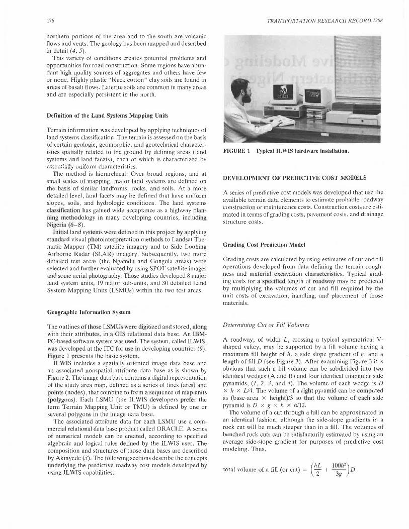
IL WIS includes a spatially oriented image data base and an associated nonspatial attribute data base as is shown by Figure 2. The image data base contains a digital representation of the study area map , defined as a series of lines (arcs) and points (nodes), that combine to form a sequence of map units (polygons). Each LSMU (the ILWIS levelopers prefer the term Terrain Mapping Unit or TMU) is defined by one or several polygons in the image data base .

The associated attribute data for each LSMU use a com­mercial relational data base product called ORACLE. A series of numerical models can be created, according to specified algebraic and logical rules defined by the IL WIS user. The composition and structures of those data bases are described by Akinyede (3). The following sections describe the concepts underlying the predictive roadway cost models developed by using ILWIS capabilities.

TRANSPORTATION RESEARCH RECORD 1288

FIGURE 1 Typical ILWIS hardware installation.

DEVELOPMENT OF PREDICTIVE COST MODELS

A series of predictive cost models was developed that use the available terrain data elements to estimate probable roadway construction or maintenance costs. Construction costs are esti­mated in terms of grading costs, pavement costs, and drainage structure costs.

Grading Cost Prediction Model

Grading costs are calculated by using estimates of cut and fill operations developed from data defining the terrain rough­ness and material excavation characteristics. Typical grad­ing costs for n ·pecified length of roadway may be predicted by multiplying the volumes of cut and fill required by the unit costs of excavation, handling, and placement of those materials.

Determining Cut or Filf Volumes

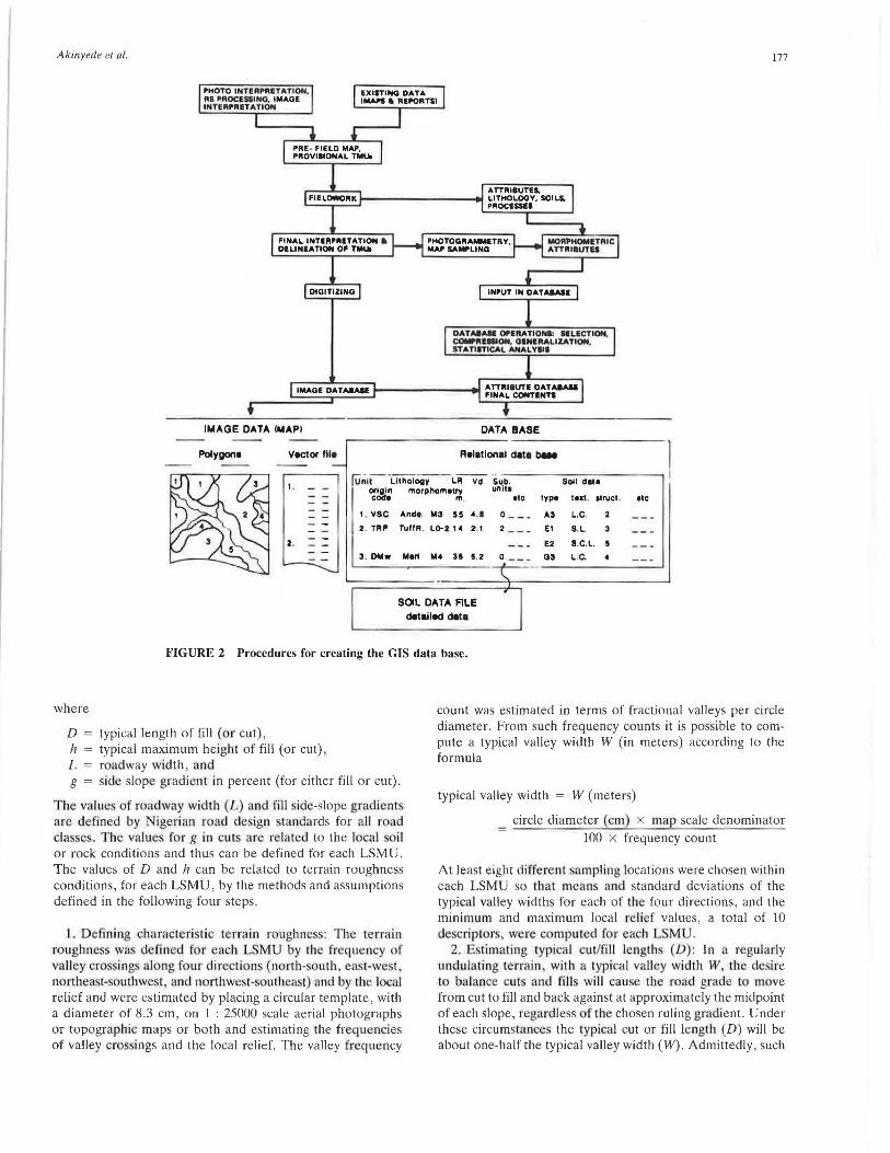
A roadway, of width L, crossing a typical symmetrical V­shaped valley, may be supported by a fill volume having a maximum fill height of h, a side slope gradient of g, and a length of fill D (see Figure 3). After examining Figure 3 it is obvious that such a fill volume can be subdivided into two identical wedges (A and B) and four identical triangular side pyramids, (1, 2, 3, and 4). The volume of each wedge is D x h x L/4. The volume of a right pyramid can be c mputed as (base-area x height)/3 so that the volume of each side pyramid is D x g x h x h/12.

The volume of a cut through a hill can be approximated in an identical fashion, although the side-slope gradients in a rock cut will be much steeper than in a fill. The volumes of benched rock cuts can be satisfactorily estimated by using an average side-slope gradient for purposes of predictive cost modeling . Thus,

total volume of a fill (or cut) (hL IOOh~) -+ -- D 2 3g

Akinyede et al.

PHOTO INTeAPllETl'TION, AS Pl\OCESSING, IMl'GE INTeAPlllTl'TION

EXISTING Ol'TI' (MN'S • AEPOATSI

PAE- FIELD MIU', PllOVlllONl'L TMU.

177

FINl'L INTEllPlllTl'TION • 0£LINEl'TION OF TMUI

PHOTOGll-'-TAY. MAPSAWLING

MOAPHOMtTAIC l'TTll l•UTU

IMAGE DATA IMAPI

Polygon• Vector Ille

Ol'TAa.\81 OPl llATIONli llLI CTION. coi.tll• ON. GINlllALIZATION, I TATllTICAL ANl'LYlll

DATA BASE

Relational data bue

,..._ .. - ·--- - - --- .. - --- --------. Unit Lithology LA Vd Sub. Soil d811

~::}; morphom•~- unil1 •le lypa IHI. struet . •le

1. VSC Ando. M3 5 5 4 .1 o __ _ A3 l.C.

2 . TAI' TullFL l0-2 14 ~. 1 2 -- _ E1 S.l .

E2 S.C.l . 5

3. Dlilw Mui M4 31 5 .2 0 -- _ G3 l .C.

SOIL DATA FILE detailed data

FIGURE 2 Procedures for creating the GIS data base.

where

D typical length of fill (or cut), h typical maximum he ight of fill (or cut), L r adway width, and g = side slope gradient in percent (for either fill or cut).

T he values of roadway width (u) and fill side-slope gradients are defi ned by Nigerian road design rnndards for all road clas . The values for g in cuts are related to the local oil or rock conditions and thus can be defined for each LSMU. The values of D and h can be related to terrain roughness conditions, for each LSMU, by the methods and assumptions defined in the following four steps.

L. Defining characteristic terrain r ughne : The terrnin roughness was d fined for each LSMU by th freq uency of valley cros ings along four directi ns (north-south , east-west northeast-southwe t, and northwest-southea 1) and by the local relief and were estimated by placing a circular template, with a diameter of 8.3 cm, on 1 : 25000 scale aerial photographs or topographic maps or both and estimating the frequencies of valley crossings and the local relief. The valley freq uency

count was estimated in terms of fractional valleys per circle diameter. From such frequency counts it is possible to com­pute a typical valley width W (in meters) according to the formula

typical valley width = W (meters)

circle diameter (cm) x map scale denominator - 100 x frequency count

At least eight different ·ampli ng locations were chosen within each LSMU so that means and standard deviations of the typical valley widths for each of the four directions, and the minim um and maximum local r lief values, a total of 10 descriptors were computed for each L MU .

2. Estimat ing typical cut/fill lengths (D) : In a regularly undulating terrain with a typical vaUey width W, th desire to balance cuts and fi ll wi lJ cause the road grade to move from cut to fill and back against at approximately the midpoint of each slope, regardless of the chosen ruling gradient. Under these circumstances the typical cut or fill length (D) will be about one-half the typical valley width (W). Admittedly, such

178

FIGURE 3 Geometrical represenlaliun uf an idealized roadway fill.

a relationship includes a number of simplying assumptions that include (a) roughly equal side-slope gradients in cuts and fill , (b) local mass-balance equali ties can be readily achieved, (c) material l ulking and hrinkag ratios are either very small or offsetting and can be neglected, and ( d) the amount of excavated material unsuitable for placement in fills, and thus must be wasted, is small and can be neglected . A correction factor is used to account for the necessary "wastage" of mate­rial excavated in a cut but unsuitable for a fill. Each LSMU is supplied with an estimate of the fraction of such unsuitable material that is likely to be encountered, and the total volume of material is increased by this amount. Adjustments can also correct for volume imbalances owing to other reasons, includ­ing differences in cut and fill side-slopes (3).

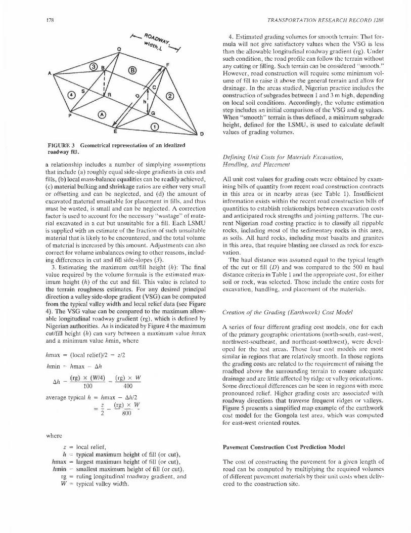
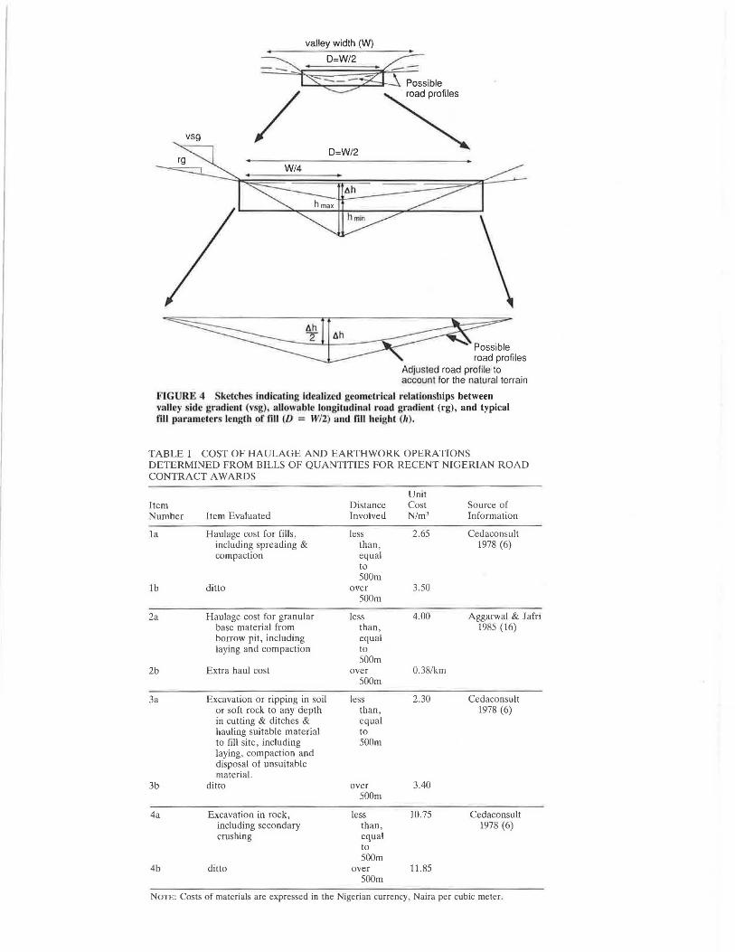
3. Estimating the maximum cut/fill height (h): The final value required by the volume formula is the estimated max­imum height (h) of the cut and fill. This value is related to the leHain roughnes estimates. or any desired principal direction a valley side- -[ pe gradient (VS ) can be computed from the typical valley width and local relief data (see Figure 4). The V value can be compared to the maxim um allow­able longitudinal roadway gradient (rg), which is defined by Nigerian authorities. As is indicated by Figure 4 the maximum cut/fill height (h) can vary between a maximum value hmax and a minimum value hmin, where

hmax

hmin

(local relief)/2 = z/2

hmax - t:i.h

(rg) x (W/4) 100

(rg) x W

400

average typical h = hmax - t:i.h/2

= z (rg) x W

2 800

where

z local relief, h typical maximum height of fill (or cur),

hmax la rgest maximum height of fill (or cut) hmin = smallest maximum height of fill (or cu t),

rg = ruling longitudim1l rmioway gradient, and W = typical valley width.

TRANSPORTATION RESEARCH RECORD 1288

4. Estimated grading volumes for smooth terrain: That for­mula will not give satisfactory values when the VSG is less than the allowable longitudinal roadway gradient (rg). Under such condition, the road profile can follow the terrain without any cutting or filling. Such terrain can be considered "smooth." However, road construction will require some minimum vol­ume of fill to raise it above the general terrain and allow for drainage. In the areas studied, Nigerian practice includes the construction of subgrade b tween I and 3 m high, dep nding on local soil conditions. Accordingly, the volume e timation step includes an initial comparison of the SG and rg valu . When "smooth" terrain is thu defined, a minimum subgrade height , d · fined f r the LSMU i u ed t calculate default values of grading volumes.

Defining Unit Costs for Materials Excavation, Handling, and P/acen1cnt

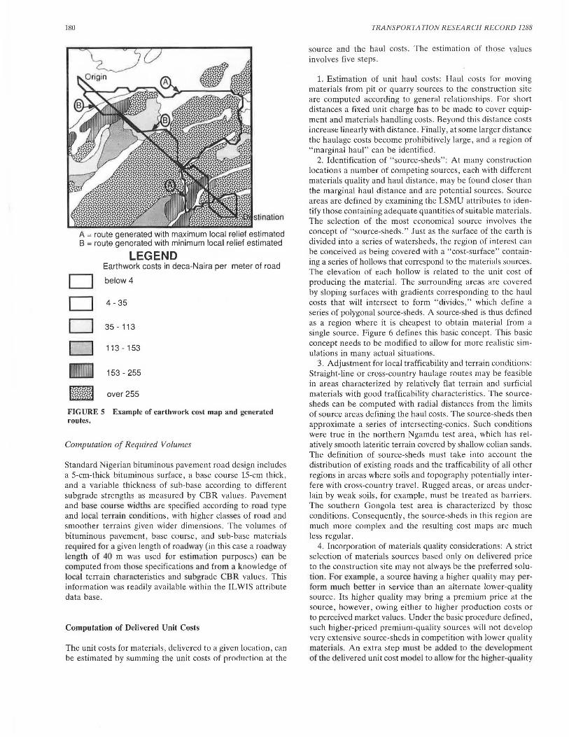
All unit cost values for grading costs were btained by exam­ining bills of quantity from ree::ent road con tru tion contracts in this area or in nearby areas (see Table 1). Insufficient information exists within the recent road construction bills of quantities to establish relationships between excavation costs and anticipated rock strengths and jointing patterns. The cur­rent Nigerian road costing practice is to cla sify all rippable rocks, including most of the sedimentary r c)<s in this area, as soils. All hard rocks, including most basalts and granites in this area, that require bla ·ting are classed as rock for exca­vation .

The haul distance was assumed equal to the typical length of the cut or fill (D) and was compared to the 500 m haul distance criteria in Table 1 and the appropriate cost, for either soil or rock, was selected. Those include the entire costs for excavation, handling, and placement of the materials.

Creation of the Grading (Earthwork) Cost Model

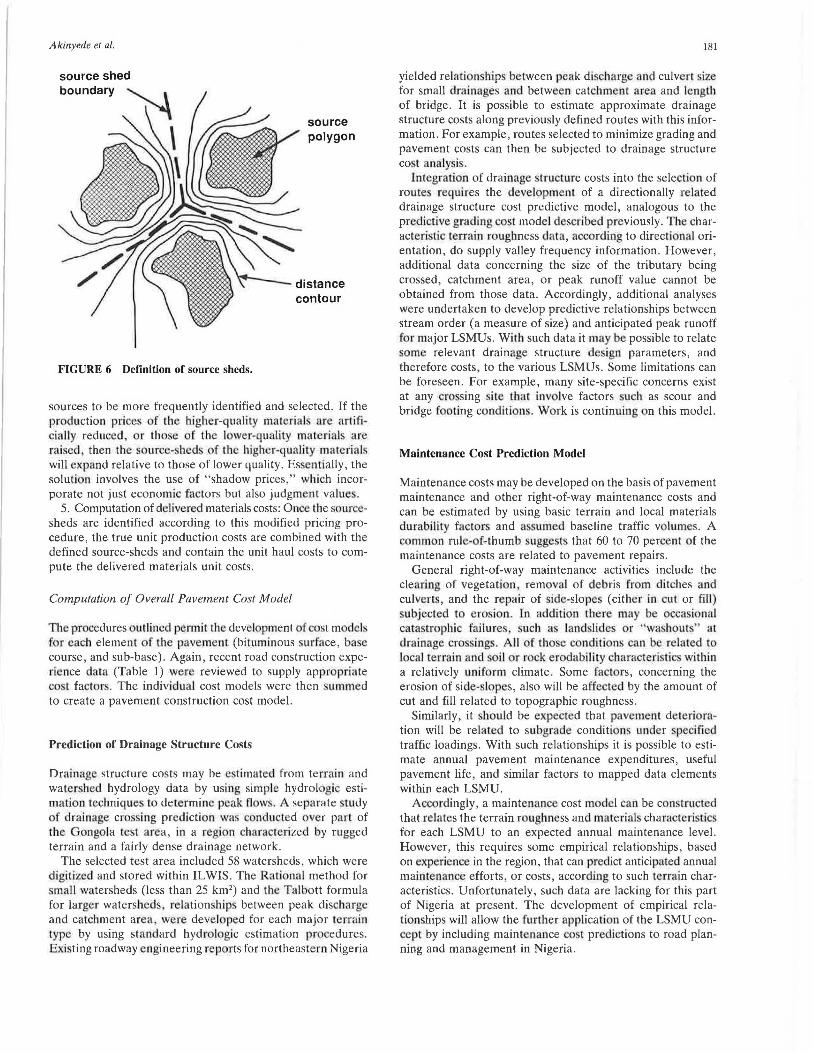
A series of four different grading cost models, one for each of the primary geographic orientations (north-south, east-west, northwest-southeast, and northeast-southwest), were devel­oped for the test areas. Those four cost models are most similar in regions that are relatively smooth. In those regions the grading costs are related to the requirement f raising the roadb~d above the ·urrounding terrain to enmre adequate drainage and are littl •affected by ridge or valley orientations. Some directional differences can be seen in regions with more pronounced relief. Higher grading costs are associated with roadway directions that traverse frequent ridges or vall y . Figure 5 pre ent · a simplified map example of the earthw rk cost model for the ongola test area, which was computed for east-west oriented rout s.

Pavement Construction Cost Prediction Model

The cost of constructing the pavement for a given length of road can be computed by multiplying the required volumes of different pavement materials by their unit costs when tleliv­ered to the construction site.

valley width (W)

t.h Possible road profiles

Adjusted road profile to account for the natural terrain

FIG UR • 4 ketches indica ting idealized geomclrical relationships between valley side gradient (vsg), allowable longiludinal road gradient (rg), and typical till pa rameters length of fill (D = W/2) and till height (II ).

TABLE I COST OF HAULAGE AND EARTHWORK OPERATIONS DETERMINED FROM BILLS OF QUANTITIES FOR RECENT NIGERIAN ROAD CONTRACT AWARDS

Unit Item Distance Cost Source of Number Item Evaluated Involved N/m3 Information

la Haulage cost for fills, less 2.65 Cedaconsult including spreading & than, 1978 (6) compaction equal

to 500m

lb ditto over 3.50 500m

2a Haulage cost for granular less 4.00 Aggarwal & Jafri base material from than, 1985 (16) borrow pit, including equal laying and compaction to

500m 2b Extra haul cost over 0.38/km

500m

3a Excavation or ripping in soil less 2.30 Cedaconsult or soft rock to any depth than, 1978 (6) in cutting & ditches & equal hauling suitable material to to fill site, including 500m laying, compaction and disposal of unsuitable material.

3b ditto over 3.40 500m

4a Excavation in rock, less 10.75 Cedaconsult including secondary than, 1978 (6) crushing equal

to 500m

4b ditto over 11.85 500m

NOTE: Costs of materials are expressed in the Nigerian currency, Naira per cubic meter.

180

A = route generated with maximum local relief estimated B = route generated with minimum local relief estimated

D D D D

•

LEGEND Earthwork costs in deca-Naira per meter of road

below 4

4 - 35

35 - 113

113 - 153

153 - 255

over255

FIGURE S Example of earthwork cost map and generated routes.

Computation of Required Volumes

Standard Nigerian bituminous pavement road design includes a 5-cm-thick bituminous surface, a base course 15-cm thick, and a variable thickness of sub-base according to different subgrade strengths as measured by CBR values. Pavement and bas cour e widths are specified according to road type and local terrain conditions, with higher classes of road and smoother terrains given wider dimensions. The volumes of bituminous pavement, base course, and sub-base materials required for a given length of roadway (in this case a roadway length of 40 m was used for estimation purposes) can be computed from tho e specification and from a knowledge of local terrain characteristics and subgrade CBR values. This information was readily available within the ILWIS attribute data base.

Computation of Delivered Unit Costs

The unit costs for materials, delivered to a given location, can be estimated by summing the unit costs of prmlnction at the

TRANSPORTATION RESEARCH RECORD 1288

source and the haul costs. The estimation of those values involves five steps.

1. Estimation of unit haul costs: Haul costs for moving materials from pit or quarry sources to the construction site are computed according to general relationships. For short distances a fixed unit charge has to be made to cover equip­ment and materials handling costs . Beyond this distance costs increase linearly with distance. Finally, at some larger distance the haulage costs become prohibitively large, and a region of "marginal haul" can be identified.

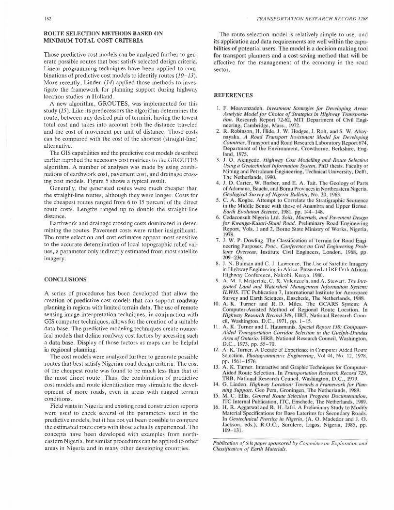
2. Identification of "source-sheds": At many construction locations a number of competing sources, each with different materials quality and haul distance, may be found closer than the marginal haul distance and are potential sources. Source areas are defined by examining the LSMU attributes to iden­tify those containing adequate quantities of suitable materials. The selection of the most economical source involves the concept of "source-sheds." Just as the surface of the earth is divided into a series of watersheds, the region of interest can be conceived as being covered with a "cost-surface" contain­ing a series of hollows that correspond to the materials sources. The elevation of each hollow is related to the unit cost of producing the material. The surrounding areas are covered by sloping surfaces with gradients corresponding to the haul costs that will intersect to form "divides," which define a series of polygonal source-sheds. A source-shed is thus defined as a region where it is cheapest to obtain material from a single source. Figure 6 defines this basic concept. This basic concept needs to be modified to allow for more realistic sim­ulations in many actual situations.

3. Adjustment for local trafficability and terrain conditions: Straight-line or cross-country haulage routes may be feasible in areas characterized by relatively flat terrain and surficial materials with good trafficability characteristics. The source­sheds can be computed with radial distances from the limits of source areas defining the haul costs. The source-sheds then approximate a series of intersecting-conics. Such conditions were true in the northern Ngamdu test area, which has rel­atively smooth lateritic terrain covered by shallow eolian sands. The definition of source-sheds must take into account the distribution of existing roads and the trafficability of all other regions in areas where soils and topography potentially inter­fere with cross-country travel. Rugged areas, or areas under­lain by weak soils, for example, must be treated as barriers. The southern Gongola test area is characterized by those conditions. Consequently, the source-sheds in this region are much more complex and the resulting cost maps are much less regular.

4. Incorporation of materials quality considerations: A strict selection of materials sources based only on delivered price to the construction site may not always be the preferred solu­tion. For example, a source having a higher quality may per­form much better in service than an alternate lower-quality source . Its higher quality may bring a premium price at the source, however, owing either to higher production costs or to perceived market values. Under the basic procedure defined, such higher-priced premium-quality sources will not develop very extensive source-sheds in competition with lower quality material . An extra step mu t be added to the development of the delivered unit cost model to oil w f r the higher-quality

Akinyede et al.

source shed boundary

FIGURE 6 Definition of source sheds.

source polygon

sources to be more frequently identified and selected. If the production prices of the bigher-qualjty materia l are artifi­cially reduced , or those of the lower-quality material are raised, then the source- he_d of the higher-quality material. will expand relative to those of lower quality. Es en ti ally, the solution involves the use of "shadow prices," which incor­porate not just economic factors but also judgment values.

5. Computation of delivered materials costs: Once the sour e­sheds are identified according to this modified pricing pro­cedure, the true unit production costs are combined with the defined source-sheds and contain the unit haul costs to com­pute the delivered materials unit costs.

Computation of Overall Pavement Cost Model

The procedures outlined permit the development o'f cost models for each element of the pavemenl (bituminous urface, base course, and sub-base). Again, recent road construction expe­ri nee data (Table 1) were reviewed to supply appropriate w t factor . The individual cost models were then ummed to create a pavement construction cost model.

Prediction of Drainage Structure Costs

Drainage structure costs may be estimated from terrain and water hed hydrology data by using simple hydrologic esti­mation technique · to determine peak flow . A separate tudy of drainage er ·ing prediction was conducted over part of the Gongo la te t area, in a r gion characterized by rugged terrain and a fairly dense drainage network .

The selected test area included 58 watersheds, which were digitized and stored within ILWIS . The Rational method for mall watersheds (less than 25 km2) and the Talbott formula

for larger watersheds , relation hip. between peak discharge and catchment area , were developed for each major terrain type by using standard hydrologic estimation procedures. Existing roadway engineering reports for northeaste rn Nigeria

181

yielded relation hip between peak discharge and culvert size for small drainages and between catchment area and length of bridge. It is possible to estimate approximate drainage structure costs along previously defined routes with this infor­mation. For example, routes selected to minimize grading and pavement costs can then be subjected to drainage structure cost analysis.

Integration of drainage tructure costs into the selection of route requires the development of a directionally related drainage structure cost predictive model, analogous to the predictive grading cost model described previously. The char­acteri ti terrain roughness data, according to directional ori­entation, do supply valley frequency information . However , additional data concerning the size of the tributary being crossed, catchment area, or peak runoff value cannot be obtained from those data. Accordingly, additional analyses were undertaken to develop predictive relationships between stream order (a measure of size) and anticipated peak runoff for major LSMUs. With such data it may be possible to relate ome relevant drainage structure de ·ign parameters, and

therefore costs, to the various LSMUs. Some limitations can be foreseen. For example, many site-specific concerns exist at any cro sing site that involve factors uch as scour and bridge footing conditions. Work is continuing on this model.

Maintenance Cost Prediction Model

Maintenance costs may be developed on the basis of pavement maintenance and other right-of-way maintenance costs and can be estimated by using basic terrain and local materials durability factors and assumed baseline traffic volumes. A common rule-of-thumb suggest that 60 to 70 percent of the maintenance costs are related to pavement repairs .

General right-of-way maintenance activities include the clearing of vegetation , removal of debris from ditches and culvert. , and the repair of side-slopes (either in cut or fill) ubjected to erosion. ln addition the re may be occasional

catastrophic failures , uch as landslides or "washout • at drainage crossing . All of tho e condition · can be related to local terrain and oil or rock erodability characteristic. within a relatively uniform climate. Some factors, concerning the erosion of side-slopes, also will be affected by the amount of cut and fill related to topographic roughness .

Similarly, it should be expected that pavement deteriora­tion will be related to subgrad conditions under pecifiecl traffic loadings. With such relationships it is possible to esti­mate annual pavement maintenance expenditures, useful pavement life , and similar factors to mapped data elements within each LSMU.

Accordingly, a maintenance cost model can be con tructed that relates the terrain roughness and mate1:ial characteri tic for each LSMU to an expected annual maintenance level. However, this requires some empirical relationships, based on experience in the region, that can predict anticipated annual maintenance efforts, or costs, according to such terrain char­acteristics. Unfortunately, such data are lacking for this part of Nigeria at present. The development of empirical rela­tionships will allow the further application of the LSMU con­cept by including maintenance co t pred ictions to road plan­ning and management in Nigeria.

182

ROUTE SELECTION METHODS BASED ON MINIMUM TOTAL COST CRITERIA

Those predictive cost models can be analyzed further to gen­erate possible routes that best satisfy selected design criteria. Linear programming techniques have been applied to com­binations of predictive cost models to identify routes (10-13). More recently, Linden (14) applied those methods to inves­tigate the framework for planning support during highway location studies in Holland.

A new algorithm, GROUTES, was implemented for this study (15). Like its predecessors the algorithm determines the route, between any desired pair of termini, having the lowest total cost and takes into account both the distance traveled and the cost of movement per unit of distance. Those costs can be compared with the cost of the shortest (straight-Jim:) alternative.

The GIS capabilities and the predictive cost models described earlier supplied the necessary cost matrices to the GROUTES algorithm . A number of analyses was made by using combi­nations of earthwork cost, pavement cost, and drainage cross­ing cost models . Figure 5 shows a typical result.

Generally, the generated routes were much cheaper than the straight-line routes, although they were longer. Costs for the cheapest routes ranged from 6 to 15 percent of the direct route costs. Lengths ranged up to double the straight-line distance.

Earthwork and drainage crossing costs dominated in deter­mining the routes. Pavement costs were rather insignificant. The route selection and cost estimates appear most sensitive to the accurate determination of local topographic relief val­ues, a parameter only indirectly estimated from most satellite imagery.

CONCLUSIONS

A series of procedures has been developed that allow the creation of predictive cost models tbat can support roadway planning in regions with limited terrain data . The use of remote sensing image interpretation techniques, in conjunction with GIS computer techniques, allows for the creation of a suitable data base. The predictive modeling techniques create numer­ical models that define roadway cost factors by accessing such a data base. Di play of those factors as maps can be helpful in regional planning.

The cost models were analyzed further to generate possible routes that best satisfy Nigerian road design criteria. The cost of the cheapest route was found to be much less than that of the most direct route . Thus, the combination of predictive cost models and route identification may stimulate the devel­opment of more roads, even in areas with rugged terrain conditions.

Field visits in Nigeria and existing road construction reports were used to check several of the parameters used in the predictive models, but it has not yet been possible to compare the estimated route costs with those actually expe rienced. The concepts have been developed with examples from north­eastern Nigeria, but similar procedures can be applied to other areas in Nigeria and in many other developing countries.

TRANSPORTATION RESEARCH RECORD 1288

The route selection model is relatively simple to use , and it application and data requirements are well within the capa­bili.ti f pote ntial u. er . T he model is a decision making tool for tran port planners and a co t- a ing method that will be effective for the management of the economy in the road sector.

REFERENCES

1. F. Moavenzadeh. L11 vestme111 trml!gies for Developing Areas: Analytic Model for Choice of /rategie. i11 Higlnvay Tra11Sp(J1'f(l­tio11. Resea rch Repori 72-62. MfT Dcprmmcnt of ivil - ngi­neering, Cambridge, Mass., 1972.

2. R. Robinson , H. Hide. J. W. H dgc-. J . R It 11 nd S. W. Abay­nayaka . A Rood Transport l11ves1111e111 Model fur Developing '01mtries. Transport and Road Resea rch Laboratory Report 674 ,

Department of the Environment , Crowthornc. 13crkshirc, ng­land, 1975.

3. J. 0. Akinycde. Higl11v(ly -·ost 1odelli11g and Rowe election Using a Geotec/111ical blfomwtio11 . • tem . PhD thesis. Faculty of Mining and Petroleum nginceri ng, Technical Univer i1y . Delft, The Netherlands, 1990.

4. J. D. Carter, W. Barber, and E. A. Tait. The Geology of Parts of Adamana, Bauchi and Bornu Province.~ in ortheastcm igcria. Geological Survey of Nigeria 811/le1i11 , o. 30, 1963.

5. . A. Kogbe. Attempt to orrelare the tratigraphi Se 111cncc in the Middle Benue with those of Arrnrnbra 11nd Upp r Benuc. Earth Evol111io11 Science, 19 I . pp. 144- 148.

6. edaconsult Nigeria Ltd. Soils, Materials. and Pa ve111e111 Design for Kwa,,ga-Ku ari- lu111i Road. Preliminary Road Engineerin • Report , Vols. I and 2, Borno State Ministry of Works, Nigeria, 1978.

7. J . w. P. Dowling. The Ctassific:Hion of Terrain for R a I ngi­ncering Purpo es. Proc., 011fere11ce c>11 ;,,;1 £11gilleeri11g Prob­lems 011erseas, lnstit.ute ivil Engineers. London, 1968, pp. 209- 236,

8. J. N. Bulman and C. J . Lawrence. The Use of Satellite Imagery in Highway Engineering in Africa. Presented at IRF IV th i\Jrican Highway Conference, Nairobi , Kenya, 1980.

9. A. M. J. Meijerink, C. R. Valenzuela, and A. Stewart. The lnte­gmted l.1111d a11d Wmerslied Ma11(1g1m1e111 /11j(>r111atlo11 ys1e111: IL WI . IT Publica1ion 7 International Institute ro r Aerospace

urvcy 11nd Earth cicnce n chede, The Netherlands. 1988. 10. A. K. Turner and R. D. Milos. The G ARS y tern : A

omputcr-Assisted Method of Regional Route Loc11tion . ln Nigliway Re enrch Record 346', HRB. Nmional Research min­cil, Wa hingtoll , D.C. 197L. pp. 1- 15.

11. A. K. Turner and T. Hnusmnnis. peci11l Re1>or1 138: om11111er­l\ided Trn11spor1a1io11. Corridor Selection i11 the G1u:lph-D1111d11s Area of 01111.1.rio. HRB , National Research Council. Wa hington, D. . 1973. pp. 55-70.

12. A. K. Turner. A Decade of Experience in Computer Aided Route Selecti n. Pltotc>grammetric Engi11ccri11g, Vol 44, No. 12, 1978, pp. 1561 - 1576.

13. A. K. Turner. lntcractivc and Graphic cclmiques for omputcr­Aided Route Selection. !11 Transpor1111io11 f?esearc/1 Record 729, TRB, NatioDa l Research oundl , Washington . D . .. 1979.

14 . G. Linden. Highway Location: Tow(lrds a Framework for Pla11-11i11g Support. Geo Pers. Groningcn, The Netherlands , 1989.

15. M. . Ellis. General Rowe electio11 Progmm Doc11111e111t11io11, IT Internal Publicati 11 , lT , Enschcdc, The etherland , 19 9.

16. H. R. Agga.rwnl and R 1-1 . Jafri. A Pr Jiminary Sludy to Modify Material pecifications for Base Latcritc for ccondi1ry Road . In Geowcl111i al Pmdice i11 Nigeria . (A. 0 . Madedor and J. O. Jackson, eds.) , R.O. .. urulere Lagos, igerin, 19 5. pp. 109-131.

P11b/icatio11 of this paper spo11. ored by Committee on Exploration and /11ssificmio11 of £artft Material .