Predictive Modeling and Analytics

By

Jeffrey S. Strickland

Simulation Educators

Colorado Springs, CO

Predictive Modeling and Analytics

Copyright 2014 by Jeffrey S. Strickland. All rights Reserved

ISBN 978-1-312-37544-4

Published by Lulu, Inc. All Rights Reserved

v

Acknowledgements

The author would like to thank colleagues Adam Wright, Adam Miller,

Matt Santoni. And Olaf Larson of Clarity Solution Group. Working with

them over the past two years has validated the concepts presented

herein.

A special thanks to Dr. Bob Simmonds, who mentored me as a senior

operations research analyst.

vi

vii

Contents

Acknowledgements ................................................................................. v

Contents ................................................................................................. vii

Preface ................................................................................................ xxiii

More Books by the Author .................................................................. xxv

1. Predictive analytics ............................................................................ 1

Definition ........................................................................................... 1

Types ................................................................................................. 2

Predictive models ....................................................................... 2

Descriptive models ..................................................................... 3

Decision models .......................................................................... 3

Applications ....................................................................................... 3

Analytical customer relationship management (CRM) ............... 4

Clinical decision support systems ............................................... 4

Collection analytics ..................................................................... 5

Cross-sell ..................................................................................... 5

Customer retention .................................................................... 5

Direct marketing ......................................................................... 6

Fraud detection ........................................................................... 6

Portfolio, product or economy-level prediction ......................... 7

Risk management ....................................................................... 7

Underwriting ............................................................................... 8

Technology and big data influences .................................................. 8

Analytical Techniques ........................................................................ 9

viii

Regression techniques ................................................................ 9

Machine learning techniques ................................................... 16

Tools ................................................................................................ 19

Notable open source predictive analytic tools include: ........... 20

Notable commercial predictive analytic tools include: ............ 20

PMML ........................................................................................ 21

Criticism ........................................................................................... 21

2. Predictive modeling......................................................................... 23

Models ............................................................................................. 23

Formal definition ............................................................................. 24

Model comparison .......................................................................... 24

An example ...................................................................................... 25

Classification .................................................................................... 25

Other Models .................................................................................. 26

Presenting and Using the Results of a Predictive Model ................ 26

Applications ..................................................................................... 27

Uplift Modeling ......................................................................... 27

Archaeology .............................................................................. 27

Customer relationship management ........................................ 28

Auto insurance .......................................................................... 29

Health care ................................................................................ 29

Notable failures of predictive modeling .......................................... 29

Possible fundamental limitations of predictive model based on data

fitting ............................................................................................... 30

Software .......................................................................................... 31

Open Source ............................................................................. 31

ix

Commercial ............................................................................... 33

Introduction to R ............................................................................. 34

3. Empirical Bayes method .................................................................. 37

Introduction ..................................................................................... 37

Point estimation .............................................................................. 39

Robbins method: non-parametric empirical Bayes (NPEB) ...... 39

Example - Accident rates .......................................................... 40

Parametric empirical Bayes ...................................................... 41

Poisson–gamma model ............................................................. 41

Bayesian Linear Regression ....................................................... 43

Software .......................................................................................... 44

Example Using R .............................................................................. 44

Model Selection in Bayesian Linear Regression........................ 44

Model Evaluation ...................................................................... 46

4. Naïve Bayes classifier ...................................................................... 47

Introduction ..................................................................................... 47

Probabilistic model .......................................................................... 48

Constructing a classifier from the probability model ............... 50

Parameter estimation and event models ........................................ 50

Gaussian Naïve Bayes ............................................................... 51

Multinomial Naïve Bayes .......................................................... 51

Bernoulli Naïve Bayes ............................................................... 53

Discussion ........................................................................................ 53

Examples.......................................................................................... 54

Sex classification ....................................................................... 54

x

Training ..................................................................................... 54

Testing....................................................................................... 55

Document classification ............................................................ 56

Software .......................................................................................... 59

Example Using R .............................................................................. 60

5. Decision tree learning ..................................................................... 67

General ............................................................................................ 67

Types ............................................................................................... 69

Metrics ............................................................................................ 70

Gini impurity ............................................................................. 71

Information gain ....................................................................... 71

Decision tree advantages ................................................................ 73

Limitations ....................................................................................... 74

Extensions ....................................................................................... 75

Decision graphs ......................................................................... 75

Alternative search methods ..................................................... 75

Software .......................................................................................... 76

Examples Using R ............................................................................ 76

Classification Tree example ...................................................... 76

Regression Tree example .......................................................... 83

6. Random forests ............................................................................... 87

History ............................................................................................. 87

Algorithm ......................................................................................... 88

Bootstrap aggregating ..................................................................... 89

Description of the technique .................................................... 89

xi

Example: Ozone data ................................................................ 90

History ....................................................................................... 92

From bagging to random forests ..................................................... 92

Random subspace method .............................................................. 92

Algorithm .................................................................................. 93

Relationship to Nearest Neighbors ................................................. 93

Variable importance ........................................................................ 95

Variants ........................................................................................... 96

Software .......................................................................................... 96

Example Using R .............................................................................. 97

Description ................................................................................ 97

Model Comparison ................................................................... 97

7. Multivariate adaptive regression splines ...................................... 101

The basics ...................................................................................... 101

The MARS model ........................................................................... 104

Hinge functions ............................................................................. 105

The model building process .......................................................... 106

The forward pass .................................................................... 107

The backward pass .................................................................. 107

Generalized cross validation (GCV) ......................................... 108

Constraints .............................................................................. 109

Pros and cons ................................................................................ 110

Software ........................................................................................ 112

Example Using R ............................................................................ 113

Setting up the Model .............................................................. 113

xii

Model Generation .................................................................. 115

8. Ordinary least squares .................................................................. 119

Linear model .................................................................................. 120

Assumptions ........................................................................... 120

Classical linear regression model ............................................ 121

Independent and identically distributed ................................ 123

Time series model ................................................................... 124

Estimation ..................................................................................... 124

Simple regression model ........................................................ 126

Alternative derivations .................................................................. 127

Geometric approach ............................................................... 127

Maximum likelihood ............................................................... 128

Generalized method of moments ........................................... 129

Finite sample properties ............................................................... 129

Assuming normality ................................................................ 130

Influential observations .......................................................... 131

Partitioned regression ............................................................ 132

Constrained estimation .......................................................... 133

Large sample properties ................................................................ 134

Example with real data .................................................................. 135

Sensitivity to rounding ............................................................ 140

Software ........................................................................................ 141

Example Using R ............................................................................ 143

9. Generalized linear model .............................................................. 153

Intuition ......................................................................................... 153

xiii

Overview ....................................................................................... 155

Model components ....................................................................... 155

Probability distribution ........................................................... 156

Linear predictor ...................................................................... 157

Link function ........................................................................... 157

Fitting............................................................................................. 159

Maximum likelihood ............................................................... 159

Bayesian methods ................................................................... 160

Examples........................................................................................ 160

General linear models ............................................................. 160

Linear regression ..................................................................... 160

Binomial data .......................................................................... 161

Multinomial regression ........................................................... 162

Count data .............................................................................. 163

Extensions...................................................................................... 163

Correlated or clustered data ................................................... 163

Generalized additive models .................................................. 164

Generalized additive model for location, scale and shape ..... 165

Confusion with general linear models........................................... 167

Software ........................................................................................ 167

Example Using R ............................................................................ 167

Setting up the Model .............................................................. 167

Model Quality ......................................................................... 169

10. Logistic regression ......................................................................... 173

Fields and examples of applications .............................................. 173

xiv

Basics ............................................................................................. 174

Logistic function, odds ratio, and logit .......................................... 175

Multiple explanatory variables ............................................... 178

Model fitting .................................................................................. 178

Estimation ............................................................................... 178

Evaluating goodness of fit ....................................................... 180

Coefficients .................................................................................... 184

Likelihood ratio test ................................................................ 185

Wald statistic .......................................................................... 185

Case-control sampling ............................................................ 186

Formal mathematical specification ............................................... 186

Setup ....................................................................................... 186

As a generalized linear model ................................................. 190

As a latent-variable model ...................................................... 192

As a two-way latent-variable model ....................................... 194

As a “log-linear” model ........................................................... 198

As a single-layer perceptron ................................................... 201

In terms of binomial data ....................................................... 201

Bayesian logistic regression .......................................................... 202

Gibbs sampling with an approximating distribution .............. 204

Extensions ..................................................................................... 209

Model suitability ............................................................................ 209

Software ........................................................................................ 210

Examples Using R .......................................................................... 211

Logistic Regression: Multiple Numerical Predictors ............... 211

xv

Logistic Regression: Categorical Predictors ............................ 216

11. Robust regression .......................................................................... 223

Applications ................................................................................... 223

Heteroscedastic errors ............................................................ 223

Presence of outliers ................................................................ 224

History and unpopularity of robust regression ............................. 224

Methods for robust regression ..................................................... 225

Least squares alternatives ...................................................... 225

Parametric alternatives........................................................... 226

Unit weights ............................................................................ 227

Example: BUPA liver data .............................................................. 228

Outlier detection ..................................................................... 228

Software ........................................................................................ 230

Example Using R ............................................................................ 230

12. k-nearest neighbor algorithm ....................................................... 237

Algorithm ....................................................................................... 238

Parameter selection ...................................................................... 239

Properties ...................................................................................... 240

Feature extraction ......................................................................... 241

Dimension reduction ..................................................................... 241

Decision boundary ......................................................................... 242

Data reduction ............................................................................... 242

Selection of class-outliers .............................................................. 243

CNN for data reduction ................................................................. 243

CNN model reduction for 𝑘-NN classifiers .............................. 246

xvi

k-NN regression ............................................................................. 248

Validation of results ...................................................................... 248

Algorithms for hyperparameter optimization ............................... 249

Grid search .............................................................................. 249

Alternatives ............................................................................. 250

Software ........................................................................................ 250

Example Using R ............................................................................ 250

13. Analysis of variance ....................................................................... 257

Motivating example ...................................................................... 257

Background and terminology ........................................................ 260

Design-of-experiments terms ................................................. 262

Classes of models .......................................................................... 264

Fixed-effects models ............................................................... 264

Random-effects models .......................................................... 264

Mixed-effects models ............................................................. 264

Assumptions of ANOVA ................................................................. 265

Textbook analysis using a normal distribution ....................... 265

Randomization-based analysis ............................................... 266

Summary of assumptions ....................................................... 268

Characteristics of ANOVA .............................................................. 269

Logic of ANOVA ............................................................................. 269

Partitioning of the sum of squares ......................................... 269

The F-test ................................................................................ 270

Extended logic ......................................................................... 271

ANOVA for a single factor ............................................................. 272

xvii

ANOVA for multiple factors ........................................................... 272

Associated analysis ........................................................................ 273

Preparatory analysis ............................................................... 274

Followup analysis .................................................................... 275

Study designs and ANOVAs ........................................................... 276

ANOVA cautions ............................................................................ 277

Generalizations .............................................................................. 278

History ........................................................................................... 278

Software ........................................................................................ 279

Example Using R ............................................................................ 279

14. Support vector machines .............................................................. 283

Definition ....................................................................................... 283

History ........................................................................................... 284

Motivation ..................................................................................... 284

Linear SVM .................................................................................... 285

Primal form ............................................................................. 287

Dual form ................................................................................ 289

Biased and unbiased hyperplanes .......................................... 289

Soft margin .................................................................................... 290

Dual form ................................................................................ 291

Nonlinear classification ................................................................. 291

Properties ...................................................................................... 293

Parameter selection ................................................................ 293

Issues ....................................................................................... 293

Extensions...................................................................................... 294

xviii

Multiclass SVM........................................................................ 294

Transductive support vector machines .................................. 295

Structured SVM ....................................................................... 295

Regression ............................................................................... 295

Interpreting SVM models .............................................................. 296

Implementation ............................................................................. 296

Applications ................................................................................... 297

Software ........................................................................................ 297

Example Using R ............................................................................ 298

Ksvm in kernlab .................................................................. 298

svm in e1071 ......................................................................... 302

15. Gradient boosting.......................................................................... 307

Algorithm ....................................................................................... 307

Gradient tree boosting .................................................................. 310

Size of trees ................................................................................... 311

Regularization ................................................................................ 311

Shrinkage ................................................................................ 311

Stochastic gradient boosting .................................................. 312

Number of observations in leaves .......................................... 313

Usage ............................................................................................. 313

Names............................................................................................ 313

Software ........................................................................................ 314

Example Using R ............................................................................ 314

16. Artificial neural network ............................................................... 319

Background.................................................................................... 319

xix

History ........................................................................................... 321

Recent improvements............................................................. 322

Successes in pattern recognition contests since 2009 ........... 323

Models ........................................................................................... 324

Network function .................................................................... 324

Learning .................................................................................. 327

Choosing a cost function ......................................................... 328

Learning paradigms ....................................................................... 328

Supervised learning ................................................................ 328

Unsupervised learning ............................................................ 329

Reinforcement learning .......................................................... 330

Learning algorithms ................................................................ 331

Employing artificial neural networks ............................................. 331

Applications ................................................................................... 332

Real-life applications ............................................................... 332

Neural networks and neuroscience .............................................. 333

Types of models ...................................................................... 333

Types of artificial neural networks ................................................ 334

Theoretical properties ................................................................... 334

Computational power ............................................................. 334

Capacity................................................................................... 334

Convergence ........................................................................... 335

Generalization and statistics ................................................... 335

Dynamic properties................................................................. 337

Criticism ......................................................................................... 337

xx

Neural network software .............................................................. 340

Simulators ............................................................................... 340

Development Environments ................................................... 343

Component based ................................................................... 343

Custom neural networks......................................................... 344

Standards ................................................................................ 345

Example Using R ............................................................................ 346

17. Uplift modeling .............................................................................. 353

Introduction .................................................................................. 353

Measuring uplift ............................................................................ 353

The uplift problem statement ....................................................... 353

Traditional response modeling...................................................... 357

Example: Simulation-Educators.com ...................................... 358

Uplift modeling approach—probability decomposition models

................................................................................................ 360

Summary of probability decomposition modeling process: ... 361

Results of the probability decomposition modeling process . 361

Return on investment ................................................................... 362

Removal of negative effects .......................................................... 362

Application to A/B and Multivariate Testing ................................. 363

Methods for modeling .................................................................. 363

Example of Logistic Regression ............................................... 363

Example of Decision Tree ....................................................... 364

History of uplift modeling ............................................................. 368

Implementations ........................................................................... 368

Example Using R ............................................................................ 368

xxi

upliftRF .................................................................................... 368

Output ..................................................................................... 370

predict ..................................................................................... 370

modelProfile ........................................................................... 370

Output ..................................................................................... 371

varImportance ........................................................................ 372

Performance ........................................................................... 373

18. Time Series .................................................................................... 375

Methods for time series analyses ................................................. 376

Analysis .......................................................................................... 377

Motivation .............................................................................. 377

Exploratory analysis ................................................................ 377

Prediction and forecasting ...................................................... 378

Classification ........................................................................... 378

Regression analysis (method of prediction) ........................... 378

Signal estimation..................................................................... 378

Segmentation .......................................................................... 379

Models ........................................................................................... 379

Notation .................................................................................. 381

Conditions ............................................................................... 381

Autoregressive model ................................................................... 381

Definition ................................................................................ 382

Graphs of AR(p) processes ............................................................ 383

Partial autocorrelation function .................................................... 384

Description .............................................................................. 384

xxii

Example Using R ............................................................................ 385

Notation Used ...................................................................................... 401

Set Theory ..................................................................................... 401

Probability and statistics ............................................................... 401

Linear Algebra ............................................................................... 402

Algebra and Calculus ..................................................................... 402

Glossary................................................................................................ 405

References ........................................................................................... 419

Index .................................................................................................... 453

xxiii

Preface

This book is about predictive modeling. Yet, each chapter could easily

be handled by an entire volume of its own. So one might think of this a

survey of predictive models, both statistical and machine learning. We

define predictive model as a statistical model or machine learning

model used to predict future behavior based on past behavior.

This was a three year project that started just before I ventured away

from DoD modeling and simulation. Hoping to transition to private

industry, I began to look at way in which my modeling experience

would be a good fit. I had taught statistical modeling and machine

learning (e.g., neural networks) for years, but I had not applied these

on the scale of “Big Data”. I have now done so, many times over—often

dealing with data sets containing 2000+ variables and 20 million

observations (records).

In order to use this book, one should have a basic understanding of

mathematical statistics (statistical inference, models, tests, etc.)—this

is an advanced book. Some theoretical foundations are laid out

(perhaps subtlety) but not proven, but references are provided for

additional coverage. Every chapter culminates in an example using R. R

is a free software environment for statistical computing and graphics. It

compiles and runs on a wide variety of UNIX platforms, Windows and

MacOS. To download R, please choose your preferred CRAN mirror at

http://www.r-project.org/. An introduction to R is also available at

http://cran.r-project.org/doc/manuals/r-release/R-intro.html.

The book is organized so that statistical models are presented first

(hopefully in a logical order), followed by machine learning models, and

then applications: uplift modeling and time series. One could use this a

textbook with problem solving in R—but there are no “by-hand”

exercises.

xxiv

This book is self-published and print-on-demand. I do not use an editor

in order to keep the retail cost near production cost. The best discount

is provided by the publisher, Lulu.com. If you find errors as you read,

please feel free to contact me at jeff@sumulation-educators.com.

xxv

More Books by the Author

Discrete Event Simulation using ExtendSim 8. Copyright © 2010 by

Jeffrey S. Strickland. Lulu.com. ISBN 978-0-557-72821-3

Fundamentals of Combat Modeling. Copyright © 2010 by Jeffrey S.

Strickland. Lulu.com. ISBN 978-1-257-00583-3

Missile Flight Simulation - Surface-to-Air Missiles. Copyright © 2010 by

Jeffrey S. Strickland. Lulu.com. ISBN 978-0-557-88553-4

Systems Engineering Processes and Practice. Copyright © 2010 by

Jeffrey S. Strickland. Lulu.com. ISBN 978-1-257-09273-4

Mathematical Modeling of Warfare and Combat Phenomenon.

Copyright © 2011 by Jeffrey S. Strickland. Lulu.com. ISBN 978-1-4583-

9255-8

Simulation Conceptual Modeling. Copyright © 2011 by Jeffrey S.

Strickland. Lulu.com. ISBN 978-1-105-18162-7.

Men of Manhattan: Creators of the Nuclear Age. Copyright © 2011 by

Jeffrey S. Strickland. Lulu.com. ISBN 978-1-257-76188-3

Quantum Phaith. Copyright © 2011 by Jeffrey S. Strickland. Lulu.com.

ISBN 978-1-257-64561-9

Using Math to Defeat the Enemy: Combat Modeling for Simulation.

Copyright © 2011 by Jeffrey S. Strickland. Lulu.com. 978-1-257-83225-5

Albert Einstein: “Nobody expected me to lay golden eggs”. Copyright ©

2011 by Jeffrey S. Strickland. Lulu.com. ISBN 978-1-257-86014-2.

Knights of the Cross. Copyright © 2012 by Jeffrey S. Strickland.

Lulu.com. ISBN 978-1-105-35162-4.

Introduction to Crime Analysis and Mapping. Copyright © 2013 by

Jeffrey S. Strickland. Lulu.com. ISBN 978-1-312-19311-6.

1

1. Predictive analytics

Predictive analytics—sometimes used synonymously with predictive

modeling—encompasses a variety of statistical techniques from

modeling, machine learning, and data mining that analyze current and

historical facts to make predictions about future, or otherwise

unknown, events (Nyce, 2007) (Eckerson, 2007).

In business, predictive models exploit patterns found in historical and

transactional data to identify risks and opportunities. Models capture

relationships among many factors to allow assessment of risk or

potential associated with a particular set of conditions, guiding decision

making for candidate transactions.

Predictive analytics is used in actuarial science (Conz, 2008), marketing

(Fletcher, 2011), financial services (Korn, 2011), insurance,

telecommunications (Barkin, 2011), retail (Das & Vidyashankar, 2006),

travel (McDonald, 2010), healthcare (Stevenson, 2011),

pharmaceuticals (McKay, 2009) and other fields.

One of the most well-known applications is credit scoring (Nyce, 2007),

which is used throughout financial services. Scoring models process a

customer’s credit history, loan application, customer data, etc., in

order to rank-order individuals by their likelihood of making future

credit payments on time. A well-known example is the FICO® Score.

Definition

Predictive analytics is an area of data mining that deals with extracting

information from data and using it to predict trends and behavior

patterns. Often the unknown event of interest is in the future, but

predictive analytics can be applied to any type of unknown whether it

be in the past, present or future. For example, identifying suspects

after a crime has been committed, or credit card fraud as it occurs

(Strickland J. , 2013). The core of predictive analytics relies on capturing

relationships between explanatory variables and the predicted

2

variables from past occurrences, and exploiting them to predict the

unknown outcome. It is important to note, however, that the accuracy

and usability of results will depend greatly on the level of data analysis

and the quality of assumptions.

Types

Generally, the term predictive analytics is used to mean predictive

modeling, “scoring” data with predictive models, and forecasting.

However, people are increasingly using the term to refer to related

analytical disciplines, such as descriptive modeling and decision

modeling or optimization. These disciplines also involve rigorous data

analysis, and are widely used in business for segmentation and decision

making, but have different purposes and the statistical techniques

underlying them vary.

Predictive models

Predictive models are models of the relation between the specific

performance of a unit in a sample and one or more known attributes or

features of the unit. The objective of the model is to assess the

likelihood that a similar unit in a different sample will exhibit the

specific performance. This category encompasses models that are in

many areas, such as marketing, where they seek out subtle data

patterns to answer questions about customer performance, such as

fraud detection models. Predictive models often perform calculations

during live transactions, for example, to evaluate the risk or

opportunity of a given customer or transaction, in order to guide a

decision. With advancements in computing speed, individual agent

modeling systems have become capable of simulating human behavior

or reactions to given stimuli or scenarios.

The available sample units with known attributes and known

performances is referred to as the “training sample.” The units in other

sample, with known attributes but un-known performances, are

referred to as “out of [training] sample” units. The out of sample bear

no chronological relation to the training sample units. For example, the

3

training sample may consists of literary attributes of writings by

Victorian authors, with known attribution, and the out-of sample unit

may be newly found writing with unknown authorship; a predictive

model may aid the attribution of the unknown author. Another

example is given by analysis of blood splatter in simulated crime scenes

in which the out-of sample unit is the actual blood splatter pattern

from a crime scene. The out of sample unit may be from the same time

as the training units, from a previous time, or from a future time.

Descriptive models

Descriptive models quantify relationships in data in a way that is often

used to classify customers or prospects into groups. Unlike predictive

models that focus on predicting a single customer behavior (such as

credit risk), descriptive models identify many different relationships

between customers or products. Descriptive models do not rank-order

customers by their likelihood of taking a particular action the way

predictive models do. Instead, descriptive models can be used, for

example, to categorize customers by their product preferences and life

stage. Descriptive modeling tools can be utilized to develop further

models that can simulate large number of individualized agents and

make predictions.

Decision models

Decision models describe the relationship between all the elements of

a decision—the known data (including results of predictive models),

the decision, and the forecast results of the decision—in order to

predict the results of decisions involving many variables. These models

can be used in optimization, maximizing certain outcomes while

minimizing others. Decision models are generally used to develop

decision logic or a set of business rules that will produce the desired

action for every customer or circumstance.

Applications

Although predictive analytics can be put to use in many applications,

4

we outline a few examples where predictive analytics has shown

positive impact in recent years.

Analytical customer relationship management (CRM)

Analytical Customer Relationship Management is a frequent

commercial application of Predictive Analysis. Methods of predictive

analysis are applied to customer data to pursue CRM objectives, which

involve constructing a holistic view of the customer no matter where

their information resides in the company or the department involved.

CRM uses predictive analysis in applications for marketing campaigns,

sales, and customer services to name a few. These tools are required in

order for a company to posture and focus their efforts effectively

across the breadth of their customer base. They must analyze and

understand the products in demand or have the potential for high

demand, predict customers’ buying habits in order to promote relevant

products at multiple touch points, and proactively identify and mitigate

issues that have the potential to lose customers or reduce their ability

to gain new ones. Analytical Customer Relationship Management can

be applied throughout the customer lifecycle (acquisition, relationship

growth, retention, and win-back). Several of the application areas

described below (direct marketing, cross-sell, customer retention) are

part of Customer Relationship Managements.

Clinical decision support systems

Experts use predictive analysis in health care primarily to determine

which patients are at risk of developing certain conditions, like

diabetes, asthma, heart disease, and other lifetime illnesses.

Additionally, sophisticated clinical decision support systems

incorporate predictive analytics to support medical decision making at

the point of care. A working definition has been proposed by Robert

Hayward of the Centre for Health Evidence: “Clinical Decision Support

Systems link health observations with health knowledge to influence

health choices by clinicians for improved health care.” (Hayward, 2004)

5

Collection analytics

Every portfolio has a set of delinquent customers who do not make

their payments on time. The financial institution has to undertake

collection activities on these customers to recover the amounts due. A

lot of collection resources are wasted on customers who are difficult or

impossible to recover. Predictive analytics can help optimize the

allocation of collection resources by identifying the most effective

collection agencies, contact strategies, legal actions and other

strategies to each customer, thus significantly increasing recovery at

the same time reducing collection costs.

Cross-sell

Often corporate organizations collect and maintain abundant data (e.g.

customer records, sale transactions) as exploiting hidden relationships

in the data can provide a competitive advantage. For an organization

that offers multiple products, predictive analytics can help analyze

customers’ spending, usage and other behavior, leading to efficient

cross sales, or selling additional products to current customers. This

directly leads to higher profitability per customer and stronger

customer relationships.

Customer retention

With the number of competing services available, businesses need to

focus efforts on maintaining continuous consumer satisfaction,

rewarding consumer loyalty and minimizing customer attrition.

Businesses tend to respond to customer attrition on a reactive basis,

acting only after the customer has initiated the process to terminate

service. At this stage, the chance of changing the customer's decision is

almost impossible. Proper application of predictive analytics can lead to

a more proactive retention strategy. By a frequent examination of a

customer’s past service usage, service performance, spending and

other behavior patterns, predictive models can determine the

likelihood of a customer terminating service sometime soon (Barkin,

2011). An intervention with lucrative offers can increase the chance of

6

retaining the customer. Silent attrition, the behavior of a customer to

slowly but steadily reduce usage, is another problem that many

companies face. Predictive analytics can also predict this behavior, so

that the company can take proper actions to increase customer

activity.

Direct marketing

When marketing consumer products and services, there is the

challenge of keeping up with competing products and consumer

behavior. Apart from identifying prospects, predictive analytics can also

help to identify the most effective combination of product versions,

marketing material, communication channels and timing that should be

used to target a given consumer. The goal of predictive analytics is

typically to lower the cost per order or cost per action.

Fraud detection

Fraud is a big problem for many businesses and can be of various types:

inaccurate credit applications, fraudulent transactions (both offline and

online), identity thefts and false insurance claims. These problems

plague firms of all sizes in many industries. Some examples of likely

victims are credit card issuers, insurance companies (Schiff, 2012),

retail merchants, manufacturers, business-to-business suppliers and

even services providers. A predictive model can help weed out the

“bads” and reduce a business's exposure to fraud.

Predictive modeling can also be used to identify high-risk fraud

candidates in business or the public sector. Mark Nigrini developed a

risk-scoring method to identify audit targets. He describes the use of

this approach to detect fraud in the franchisee sales reports of an

international fast-food chain. Each location is scored using 10

predictors. The 10 scores are then weighted to give one final overall

risk score for each location. The same scoring approach was also used

to identify high-risk check kiting accounts, potentially fraudulent travel

agents, and questionable vendors. A reasonably complex model was

used to identify fraudulent monthly reports submitted by divisional

7

controllers (Nigrini, 2011).

The Internal Revenue Service (IRS) of the United States also uses

predictive analytics to mine tax returns and identify tax fraud (Schiff,

2012).

Recent advancements in technology have also introduced predictive

behavior analysis for web fraud detection. This type of solution utilizes

heuristics in order to study normal web user behavior and detect

anomalies indicating fraud attempts.

Portfolio, product or economy-level prediction

Often the focus of analysis is not the consumer but the product,

portfolio, firm, industry or even the economy. For example, a retailer

might be interested in predicting store-level demand for inventory

management purposes. Or the Federal Reserve Board might be

interested in predicting the unemployment rate for the next year.

These types of problems can be addressed by predictive analytics using

time series techniques (see Chapter 18). They can also be addressed via

machine learning approaches which transform the original time series

into a feature vector space, where the learning algorithm finds patterns

that have predictive power.

Risk management

When employing risk management techniques, the results are always

to predict and benefit from a future scenario. The Capital asset pricing

model (CAM-P) and Probabilistic Risk Assessment (PRA) examples of

approaches that can extend from project to market, and from near to

long term. CAP-M (Chong, Jin, & Phillips, 2013) “predicts” the best

portfolio to maximize return. PRA, when combined with mini-Delphi

Techniques and statistical approaches, yields accurate forecasts (Parry,

1996). @Risk is an Excel add-in used for modeling and simulating risks

(Strickland, 2005). Underwriting (see below) and other business

approaches identify risk management as a predictive method.

8

Underwriting

Many businesses have to account for risk exposure due to their

different services and determine the cost needed to cover the risk. For

example, auto insurance providers need to accurately determine the

amount of premium to charge to cover each automobile and driver. A

financial company needs to assess a borrower's potential and ability to

pay before granting a loan. For a health insurance provider, predictive

analytics can analyze a few years of past medical claims data, as well as

lab, pharmacy and other records where available, to predict how

expensive an enrollee is likely to be in the future. Predictive analytics

can help underwrite these quantities by predicting the chances of

illness, default, bankruptcy, etc. Predictive analytics can streamline the

process of customer acquisition by predicting the future risk behavior

of a customer using application level data. Predictive analytics in the

form of credit scores have reduced the amount of time it takes for loan

approvals, especially in the mortgage market where lending decisions

are now made in a matter of hours rather than days or even weeks.

Proper predictive analytics can lead to proper pricing decisions, which

can help mitigate future risk of default.

Technology and big data influences

Big data is a collection of data sets that are so large and complex that

they become awkward to work with using traditional database

management tools. The volume, variety and velocity of big data have

introduced challenges across the board for capture, storage, search,

sharing, analysis, and visualization. Examples of big data sources

include web logs, RFID and sensor data, social networks, Internet

search indexing, call detail records, military surveillance, and complex

data in astronomic, biogeochemical, genomics, and atmospheric

sciences. Thanks to technological advances in computer hardware—

faster CPUs, cheaper memory, and MPP architectures—and new

technologies such as Hadoop, MapReduce, and in-database and text

analytics for processing big data, it is now feasible to collect, analyze,

and mine massive amounts of structured and unstructured data for

9

new insights (Conz, 2008). Today, exploring big data and using

predictive analytics is within reach of more organizations than ever

before and new methods that are capable for handling such datasets

are proposed (Ben-Gal I. Dana A., 2014).

Analytical Techniques

The approaches and techniques used to conduct predictive analytics

can broadly be grouped into regression techniques and machine

learning techniques.

Regression techniques

Regression models are the mainstay of predictive analytics. The focus

lies on establishing a mathematical equation as a model to represent

the interactions between the different variables in consideration.

Depending on the situation, there is a wide variety of models that can

be applied while performing predictive analytics. Some of them are

briefly discussed below.

Linear regression model

The linear regression model analyzes the relationship between the

response or dependent variable and a set of independent or predictor

variables. This relationship is expressed as an equation that predicts

the response variable as a linear function of the parameters. These

parameters are adjusted so that a measure of fit is optimized. Much of

the effort in model fitting is focused on minimizing the size of the

residual, as well as ensuring that it is randomly distributed with respect

to the model predictions (Draper & Smith, 1998).

The goal of regression is to select the parameters of the model so as to

minimize the sum of the squared residuals. This is referred to as

ordinary least squares (OLS) estimation and results in best linear

unbiased estimates (BLUE) of the parameters if and only if the Gauss-

Markov assumptions are satisfied (Hayashi, 2000).

Once the model has been estimated we would be interested to know if

10

the predictor variables belong in the model – i.e. is the estimate of

each variable’s contribution reliable? To do this we can check the

statistical significance of the model’s coefficients which can be

measured using the 𝑡-statistic. This amounts to testing whether the

coefficient is significantly different from zero. How well the model

predicts the dependent variable based on the value of the independent

variables can be assessed by using the 𝑅² statistic. It measures

predictive power of the model, i.e., the proportion of the total

variation in the dependent variable that is “explained” (accounted for)

by variation in the independent variables.

Discrete choice models

Multivariate regression (above) is generally used when the response

variable is continuous and has an unbounded range (Greene, 2011).

Often the response variable may not be continuous but rather discrete.

While mathematically it is feasible to apply multivariate regression to

discrete ordered dependent variables, some of the assumptions behind

the theory of multivariate linear regression no longer hold, and there

are other techniques such as discrete choice models which are better

suited for this type of analysis. If the dependent variable is discrete,

some of those superior methods are logistic regression, multinomial

logit and probit models. Logistic regression and probit models are used

when the dependent variable is binary.

Logistic regression

For more details on this topic, see Chapter 12, Logistic Regression.

In a classification setting, assigning outcome probabilities to

observations can be achieved through the use of a logistic model,

which is basically a method which transforms information about the

binary dependent variable into an unbounded continuous variable and

estimates a regular multivariate model (Hosmer & Lemeshow, 2000).

The Wald and likelihood-ratio test are used to test the statistical

significance of each coefficient 𝑏 in the model (analogous to the 𝑡-tests

used in OLS regression; see Chapter 8). A test assessing the goodness-

11

of-fit of a classification model is the “percentage correctly predicted”.

Multinomial logistic regression

An extension of the binary logit model to cases where the dependent

variable has more than 2 categories is the multinomial logit model. In

such cases collapsing the data into two categories might not make

good sense or may lead to loss in the richness of the data. The

multinomial logit model is the appropriate technique in these cases,

especially when the dependent variable categories are not ordered (for

examples colors like red, blue, green). Some authors have extended

multinomial regression to include feature selection/importance

methods such as Random multinomial logit.

Probit regression

Probit models offer an alternative to logistic regression for modeling

categorical dependent variables. Even though the outcomes tend to be

similar, the underlying distributions are different. Probit models are

popular in social sciences like economics (Bliss, 1934).

A good way to understand the key difference between probit and logit

models is to assume that there is a latent variable 𝑧. We do not

observe 𝑧 but instead observe 𝑦 which takes the value 0 or 1. In the

logit model we assume that 𝑦 follows a logistic distribution. In the

probit model we assume that 𝑦 follows a standard normal distribution.

Note that in social sciences (e.g. economics), probit is often used to

model situations where the observed variable 𝑦 is continuous but takes

values between 0 and 1.

Logit versus probit

The Probit model has been around longer than the logit model (Bishop,

2006). They behave similarly, except that the logistic distribution tends

to be slightly flatter tailed. One of the reasons the logit model was

formulated was that the probit model was computationally difficult

due to the requirement of numerically calculating integrals. Modern

computing however has made this computation fairly simple. The

coefficients obtained from the logit and probit model are fairly close.

12

However, the odds ratio is easier to interpret in the logit model

(Hosmer & Lemeshow, 2000).

Practical reasons for choosing the probit model over the logistic model

would be:

• There is a strong belief that the underlying distribution is

normal

• The actual event is not a binary outcome (e.g., bankruptcy

status) but a proportion (e.g., proportion of population at

different debt levels).

Time series models

Time series models are used for predicting or forecasting the future

behavior of variables. These models account for the fact that data

points taken over time may have an internal structure (such as

autocorrelation, trend or seasonal variation) that should be accounted

for. As a result standard regression techniques cannot be applied to

time series data and methodology has been developed to decompose

the trend, seasonal and cyclical component of the series. Modeling the

dynamic path of a variable can improve forecasts since the predictable

component of the series can be projected into the future (Imdadullah,

2014).

Time series models estimate difference equations containing stochastic

components. Two commonly used forms of these models are

autoregressive models (AR) and moving average (MA) models. The Box-

Jenkins methodology (1976) developed by George Box and G.M.

Jenkins combines the AR and MA models to produce the ARMA

(autoregressive moving average) model which is the cornerstone of

stationary time series analysis (Box & Jenkins, 1976). ARIMA

(autoregressive integrated moving average models) on the other hand

are used to describe non-stationary time series. Box and Jenkins

suggest differencing a non-stationary time series to obtain a stationary

series to which an ARMA model can be applied. Non stationary time

series have a pronounced trend and do not have a constant long-run

13

mean or variance.

Box and Jenkins proposed a three stage methodology which includes:

model identification, estimation and validation. The identification stage

involves identifying if the series is stationary or not and the presence of

seasonality by examining plots of the series, autocorrelation and partial

autocorrelation functions. In the estimation stage, models are

estimated using non-linear time series or maximum likelihood

estimation procedures. Finally the validation stage involves diagnostic

checking such as plotting the residuals to detect outliers and evidence

of model fit (Box & Jenkins, 1976).

In recent years, time series models have become more sophisticated

and attempt to model conditional heteroskedasticity with models such

as ARCH (autoregressive conditional heteroskedasticity) and GARCH

(generalized autoregressive conditional heteroskedasticity) models

frequently used for financial time series. In addition time series models

are also used to understand inter-relationships among economic

variables represented by systems of equations using VAR (vector

autoregression) and structural VAR models.

Survival or duration analysis

Survival analysis is another name for time-to-event analysis. These

techniques were primarily developed in the medical and biological

sciences, but they are also widely used in the social sciences like

economics, as well as in engineering (reliability and failure time

analysis) (Singh & Mukhopadhyay, 2011).

Censoring and non-normality, which are characteristic of survival data,

generate difficulty when trying to analyze the data using conventional

statistical models such as multiple linear regression. The normal

distribution, being a symmetric distribution, takes positive as well as

negative values, but duration by its very nature cannot be negative and

therefore normality cannot be assumed when dealing with

duration/survival data. Hence the normality assumption of regression

models is violated.

14

The assumption is that if the data were not censored it would be

representative of the population of interest. In survival analysis,

censored observations arise whenever the dependent variable of

interest represents the time to a terminal event, and the duration of

the study is limited in time.

An important concept in survival analysis is the hazard rate, defined as

the probability that the event will occur at time 𝑡 conditional on

surviving until time 𝑡. Another concept related to the hazard rate is the

survival function which can be defined as the probability of surviving to

time 𝑡.

Most models try to model the hazard rate by choosing the underlying

distribution depending on the shape of the hazard function. A

distribution whose hazard function slopes upward is said to have

positive duration dependence, a decreasing hazard shows negative

duration dependence whereas constant hazard is a process with no

memory usually characterized by the exponential distribution. Some of

the distributional choices in survival models are: 𝐹, gamma, Weibull,

log normal, inverse normal, exponential, etc. All these distributions are

for a non-negative random variable.

Duration models can be parametric, non-parametric or semi-

parametric. Some of the models commonly used are Kaplan-Meier and

Cox proportional hazard model (nonparametric) (Kaplan & Meier,

1958).

Classification and regression trees

Hierarchical Optimal Discriminant Analysis (HODA), (also called

classification tree analysis) is a generalization of Optimal Discriminant

Analysis that may be used to identify the statistical model that has

maximum accuracy for predicting the value of a categorical dependent

variable for a dataset consisting of categorical and continuous variables

(Yarnold & Soltysik, 2004). The output of HODA is a non-orthogonal

tree that combines categorical variables and cut points for continuous

variables that yields maximum predictive accuracy, an assessment of

15

the exact Type I error rate, and an evaluation of potential cross-

generalizability of the statistical model. Hierarchical Optimal

Discriminant analysis may be thought of as a generalization of Fisher’s

linear discriminant analysis. Optimal discriminant analysis is an

alternative to ANOVA (analysis of variance) and regression analysis,

which attempt to express one dependent variable as a linear

combination of other features or measurements. However, ANOVA and

regression analysis give a dependent variable that is a numerical

variable, while hierarchical optimal discriminant analysis gives a

dependent variable that is a class variable.

Classification and regression trees (CART) is a non-parametric decision

tree learning technique that produces either classification or regression

trees, depending on whether the dependent variable is categorical or

numeric, respectively (Rokach & Maimon, 2008).

Decision trees are formed by a collection of rules based on variables in

the modeling data set:

• Rules based on variables’ values are selected to get the best

split to differentiate observations based on the dependent

variable

• Once a rule is selected and splits a node into two, the same

process is applied to each “child” node (i.e. it is a recursive

procedure)

• Splitting stops when CART detects no further gain can be made,

or some pre-set stopping rules are met. (Alternatively, the data

are split as much as possible and then the tree is later pruned.)

Each branch of the tree ends in a terminal node. Each observation falls

into one and exactly one terminal node, and each terminal node is

uniquely defined by a set of rules.

A very popular method for predictive analytics is Leo Breiman’s

Random forests (Breiman L. , Random Forests, 2001) or derived

versions of this technique like Random multinomial logit (Prinzie,

16

2008).

Multivariate adaptive regression splines

Multivariate adaptive regression splines (MARS) is a non-parametric

technique that builds flexible models by fitting piecewise linear

regressions (Friedman, 1991).

An important concept associated with regression splines is that of a

knot. Knot is where one local regression model gives way to another

and thus is the point of intersection between two splines.

In multivariate and adaptive regression splines, basis functions are the

tool used for generalizing the search for knots. Basis functions are a set

of functions used to represent the information contained in one or

more variables. MARS model almost always creates the basis functions

in pairs.

Multivariate and adaptive regression spline approach deliberately over-

fits the model and then prunes to get to the optimal model. The

algorithm is computationally very intensive and in practice we are

required to specify an upper limit on the number of basis functions.

Machine learning techniques

Machine learning, a branch of artificial intelligence, was originally

employed to develop techniques to enable computers to learn. Today,

since it includes a number of advanced statistical methods for

regression and classification, it finds application in a wide variety of

fields including medical diagnostics, credit card fraud detection, face

and speech recognition and analysis of the stock market. In certain

applications it is sufficient to directly predict the dependent variable

without focusing on the underlying relationships between variables. In

other cases, the underlying relationships can be very complex and the

mathematical form of the dependencies unknown. For such cases,

machine learning techniques emulate human cognition and learn from

training examples to predict future events.

17

A brief discussion of some of these methods used commonly for

predictive analytics is provided below. A detailed study of machine

learning can be found in Mitchell’s Machine Learning (Mitchell, 1997).

Neural networks

Neural networks are nonlinear sophisticated modeling techniques that

are able to model complex functions (Rosenblatt, 1958). They can be

applied to problems of prediction, classification or control in a wide

spectrum of fields such as finance, cognitive psychology/neuroscience,

medicine, engineering, and physics.

Neural networks are used when the exact nature of the relationship

between inputs and output is not known. A key feature of neural

networks is that they learn the relationship between inputs and output

through training. There are three types of training in neural networks

used by different networks, supervised and unsupervised training,

reinforcement learning, with supervised being the most common one.

Some examples of neural network training techniques are back

propagation, quick propagation, conjugate gradient descent, projection

operator, Delta-Bar-Delta etc. Some unsupervised network

architectures are multilayer perceptrons (Freund & Schapire, 1999),

Kohonen networks (Kohonen & Honkela, 2007), Hopfield networks

(Hopfield, 2007), etc.

Multilayer Perceptron (MLP)

The Multilayer Perceptron (MLP) consists of an input and an output

layer with one or more hidden layers of nonlinearly-activating nodes or

sigmoid nodes. This is determined by the weight vector and it is

necessary to adjust the weights of the network. The back-propagation

employs gradient fall to minimize the squared error between the

network output values and desired values for those outputs. The

weights adjusted by an iterative process of repetitive present of

attributes. Small changes in the weight to get the desired values are

done by the process called training the net and is done by the training

set (learning rule) (Riedmiller, 2010).

18

Radial basis functions

A radial basis function (RBF) is a function which has built into it a

distance criterion with respect to a center. Such functions can be used

very efficiently for interpolation and for smoothing of data. Radial basis

functions have been applied in the area of neural networks where they

are used as a replacement for the sigmoidal transfer function. Such

networks have 3 layers, the input layer, the hidden layer with the RBF

non-linearity and a linear output layer. The most popular choice for the

non-linearity is the Gaussian. RBF networks have the advantage of not

being locked into local minima as do the feedforward networks such as

the multilayer perceptron (Łukaszyk, 2004).

Support vector machines

Support Vector Machines (SVM) are used to detect and exploit complex

patterns in data by clustering, classifying and ranking the data (Cortes

& Vapnik, 1995). They are learning machines that are used to perform

binary classifications and regression estimations. They commonly use

kernel based methods to apply linear classification techniques to non-

linear classification problems. There are a number of types of SVM such

as linear, polynomial, sigmoid etc.

Naïve Bayes

Naïve Bayes based on Bayes conditional probability rule is used for

performing classification tasks. Naïve Bayes assumes the predictors are

statistically independent which makes it an effective classification tool

that is easy to interpret. It is best employed when faced with the

problem of ‘curse of dimensionality’ i.e. when the number of predictors

is very high (Rennie, Shih, Teevan, & Karger, 2003).

k-nearest neighbors

The nearest neighbor algorithm 𝑘-NN belongs to the class of pattern

recognition statistical methods (Altman, 1992). The method does not

impose a priori any assumptions about the distribution from which the

modeling sample is drawn. It involves a training set with both positive

and negative values. A new sample is classified by calculating the

distance to the nearest neighboring training case. The sign of that point

19

will determine the classification of the sample. In the 𝑘-nearest

neighbor classifier, the 𝑘 nearest points are considered and the sign of

the majority is used to classify the sample. The performance of the 𝑘-

NN algorithm is influenced by three main factors: (1) the distance

measure used to locate the nearest neighbors; (2) the decision rule

used to derive a classification from the 𝑘-nearest neighbors; and (3) the

number of neighbors used to classify the new sample. It can be proved

that, unlike other methods, this method is universally asymptotically

convergent, i.e.: as the size of the training set increases, if the

observations are independent and identically distributed (i.i.d.),

regardless of the distribution from which the sample is drawn, the

predicted class will converge to the class assignment that minimizes

misclassification error (Devroye, Györfi, & Lugosi, 1996).

Geospatial predictive modeling

Conceptually, geospatial predictive modeling is rooted in the principle

that the occurrences of events being modeled are limited in

distribution. Occurrences of events are neither uniform nor random in

distribution – there are spatial environment factors (infrastructure,

sociocultural, topographic, etc.) that constrain and influence where the

locations of events occur. Geospatial predictive modeling attempts to

describe those constraints and influences by spatially correlating

occurrences of historical geospatial locations with environmental

factors that represent those constraints and influences. Geospatial

predictive modeling is a process for analyzing events through a

geographic filter in order to make statements of likelihood for event

occurrence or emergence.

Tools

Historically, using predictive analytics tools—as well as understanding

the results they delivered—required advanced skills. However, modern

predictive analytics tools are no longer restricted to IT specialists. As

more organizations adopt predictive analytics into decision-making

processes and integrate it into their operations, they are creating a

shift in the market toward business users as the primary consumers of

20

the information. Business users want tools they can use on their own.

Vendors are responding by creating new software that removes the

mathematical complexity, provides user-friendly graphic interfaces

and/or builds in short cuts that can, for example, recognize the kind of

data available and suggest an appropriate predictive model (Halper,

2011). Predictive analytics tools have become sophisticated enough to

adequately present and dissect data problems, so that any data-savvy

information worker can utilize them to analyze data and retrieve

meaningful, useful results (Eckerson, 2007). For example, modern tools

present findings using simple charts, graphs, and scores that indicate

the likelihood of possible outcomes (MacLennan, 2012).

There are numerous tools available in the marketplace that help with

the execution of predictive analytics. These range from those that need

very little user sophistication to those that are designed for the expert

practitioner. The difference between these tools is often in the level of

customization and heavy data lifting allowed.

Notable open source predictive analytic tools include:

• scikit-learn

• KNIME

• OpenNN

• Orange

• R

• RapidMiner

• Weka

• GNU Octave

• Apache Mahout

Notable commercial predictive analytic tools include:

• Alpine Data Labs

• BIRT Analytics

• Angoss KnowledgeSTUDIO

• IBM SPSS Statistics and IBM SPSS Modeler

• KXEN Modeler

21

• Mathematica

• MATLAB

• Minitab

• Oracle Data Mining (ODM)

• Pervasive

• Predixion Software

• Revolution Analytics

• SAP

• SAS and SAS Enterprise Miner

• STATA

• STATISTICA

• TIBCO

PMML

In an attempt to provide a standard language for expressing predictive

models, the Predictive Model Markup Language (PMML) has been

proposed. Such an XML-based language provides a way for the

different tools to define predictive models and to share these between

PMML compliant applications. PMML 4.0 was released in June, 2009.

Criticism

There are plenty of skeptics when it comes to computers and

algorithms abilities to predict the future, including Gary King, a

professor from Harvard University and the director of the Institute for

Quantitative Social Science. People are influenced by their

environment in innumerable ways. Trying to understand what people

will do next assumes that all the influential variables can be known and

measured accurately. “People’s environments change even more

quickly than they themselves do. Everything from the weather to their

relationship with their mother can change the way people think and

act. All of those variables are unpredictable. How they will impact a

person is even less predictable. If put in the exact same situation

tomorrow, they may make a completely different decision. This means

that a statistical prediction is only valid in sterile laboratory conditions,

22

which suddenly isn't as useful as it seemed before.” (King, 2014)

23

2. Predictive modeling

Predictive modeling is the process by which a model is created or

chosen to try to best predict the probability of an outcome (Geisser,

1993). In many cases the model is chosen on the basis of detection

theory to try to guess the probability of an outcome given a set amount

of input data, for example, given an email determining how likely that

it is spam. Models can use one or more classifiers in trying to

determine the probability of a set of data belonging to another set, say

spam or ‘ham’.

Models

Nearly any regression model can be used for prediction purposes.

Broadly speaking, there are two classes of predictive models:

parametric and non-parametric. A third class, semi-parametric models,

includes features of both. Parametric models make “specific

assumptions with regard to one or more of the population parameters

that characterize the underlying distribution(s)” (Sheskin, 2011), while

non-parametric regressions make fewer assumptions than their

parametric counterparts. These models fall under the class of statistical

models (Marascuilo, 1977).

A statistical model is a formalization of relationships between variables

in the form of mathematical equations. A statistical model describes

how one or more random variables are related to one or more other

variables. The model is statistical as the variables are not

deterministically but stochastically related. In mathematical terms, a

statistical model is frequently thought of as a pair (𝑌, 𝑃) where 𝑌 is the

set of possible observations and 𝑃 the set of possible probability

distributions on 𝑌. It is assumed that there is a distinct element of 𝑃

which generates the observed data. Statistical inference enables us to

make statements about which element(s) of this set are likely to be the

true one.

Most statistical tests can be described in the form of a statistical

24

model. For example, the Student’s 𝑡-test for comparing the means of

two groups can be formulated as seeing if an estimated parameter in

the model is different from 0. Another similarity between tests and

models is that there are assumptions involved. Error is assumed to be

normally distributed in most models.

Formal definition

A statistical model is a collection of probability distribution functions or

probability density functions (collectively referred to as distributions

for brevity). A parametric model is a collection of distributions, each of

which is indexed by a unique finite-dimensional parameter: 𝑃{𝑃0: 𝜃 ∈

𝛩} , where 𝜃 is a parameter and 𝛩 ⊆ 𝑅𝑑 is the feasible region of

parameters, which is a subset of 𝑑-dimensional Euclidean space. A

statistical model may be used to describe the set of distributions from

which one assumes that a particular data set is sampled. For example,

if one assumes that data arise from a univariate Gaussian distribution,

then one has assumed a Gaussian model

𝒫 = {ℙ(𝑥; 𝜇, 𝜎) =1

√2𝜋𝜎exp {−

1

2𝜎2(𝑥 − 𝜇)2} : 𝜇 ∈ ℝ, 𝜎 > 0}.

A non-parametric model is a set of probability distributions with

infinite dimensional parameters, and might be written as 𝒫 =

{all distributions}. A semi-parametric model also has infinite

dimensional parameters, but is not dense in the space of distributions.

For example, a mixture of Gaussians with one Gaussian at each data

point is dense in the space of distributions. Formally, if 𝑑 is the

dimension of the parameter, and 𝑛 is the number of samples, if 𝑑 →

∞as 𝑛 → ∞ and 𝑑 𝑛⁄ → 0 as 𝑛 → ∞, then the model is semi-

parametric.

Model comparison

Models can be compared to each other. This can either be done when

you have performed an exploratory data analysis or a confirmatory

data analysis. In an exploratory analysis, you formulate all models you

25

can think of, and see which describes your data best. In a confirmatory

analysis you test which of your models you have described before the

data was collected fits the data best, or test if your only model fits the

data. In linear regression analysis you can compare the amount of

variance explained by the independent variables, 𝑅2, across the

different models. In general, you can compare models that are nested

by using a Likelihood-ratio test. Nested models are models that can be

obtained by restricting a parameter in a more complex model to be

zero.

An example

Height and age are probabilistically distributed over humans. They are

stochastically related; when you know that a person is of age 10, this

influences the chance of this person being 6 feet tall. You could

formalize this relationship in a linear regression model of the following

form: height𝑖 = 𝑏0 + 𝑏1age𝑖 + 휀𝑖, where 𝑏0 is the intercept, 𝑏1 is a

parameter that age is multiplied by to get a prediction of height, 휀 is

the error term, and 𝑖 is the subject. This means that height starts at

some value, there is a minimum height when someone is born, and it is

predicted by age to some amount. This prediction is not perfect as

error is included in the model. This error contains variance that stems

from sex and other variables. When sex is included in the model, the

error term will become smaller, as you will have a better idea of the

chance that a particular 16-year-old is 6 feet tall when you know this

16-year-old is a girl. The model would become height𝑖 = 𝑏0 +

𝑏1age𝑖 + 𝑏2sex𝑖 + 휀𝑖, where the variable sex is dichotomous. This

model would presumably have a higher 𝑅2. The first model is nested in

the second model: the first model is obtained from the second when 𝑏2

is restricted to zero.

Classification

According to the number of the endogenous variables and the number

of equations, models can be classified as complete models (the number

of equations equal to the number of endogenous variables) and

26

incomplete models. Some other statistical models are the general

linear model (restricted to continuous dependent variables), the

generalized linear model (for example, logistic regression), the

multilevel model, and the structural equation model.

Other Models

The remainder of the book deals mostly with various statistical models

as briefly mentioned in Chapter 1. However, we will discuss other

classes of models, including mathematical models (e.g., GMDH),

computational models (e.g., neural networks).

Presenting and Using the Results of a Predictive

Model

Predictive models can either be used directly to estimate a response

(output) given a defined set of characteristics (input), or indirectly to

drive the choice of decision rules (Steyerberg, 2010).

Depending on the methodology employed for the prediction, it is often

possible to derive a formula that may be used in a spreadsheet

software. This has some advantages for end users or decision makers,

the main one being familiarity with the software itself, hence a lower

barrier to adoption.

Nomograms are useful graphical representation of a predictive model.

As in spreadsheet software, their use depends on the methodology

chosen. The advantage of nomograms is the immediacy of computing

predictions without the aid of a computer.

Point estimates tables are one of the simplest form to represent a

predictive tool. Here combination of characteristics of interests can

either be represented via a table or a graph and the associated

prediction read off the 𝑦-axis or the table itself.

Tree based methods (e.g. CART, survival trees) provide one of the most

graphically intuitive ways to present predictions. However, their usage

27

is limited to those methods that use this type of modeling approach

which can have several drawbacks (Breiman L. , 1996). Trees can also

be employed to represent decision rules graphically.

Score charts are graphical tabular or graphical tools to represent either

predictions or decision rules.

A new class of modern tools are represented by web based

applications. For example, Shiny is a web based tool developed by

Rstudio, an R IDE (integrated development environment). With a Shiny

app, a modeler has the advantage to represent any which way he or

she chooses to represent the predictive model while allowing the user

some control. A user can choose a combination of characteristics of

interest via sliders or input boxes and results can be generated, from

graphs to confidence intervals to tables and various statistics of

interests. However, these tools often require a server installation of

Rstudio.

Applications

Uplift Modeling

Uplift Modeling (see Chapter 17) is a technique for modeling the

change in probability caused by an action. Typically this is a marketing

action such as an offer to buy a product, to use a product more or to

re-sign a contract. For example in a retention campaign you wish to

predict the change in probability that a customer will remain a

customer if they are contacted. A model of the change in probability

allows the retention campaign to be targeted at those customers on

whom the change in probability will be beneficial. This allows the

retention program to avoid triggering unnecessary churn or customer

attrition without wasting money contacting people who would act

anyway.

Archaeology

Predictive modeling in archaeology gets its foundations from Gordon

28

Willey's mid-fifties work in the Virú Valley of Peru (Willey, 1953).

Complete, intensive surveys were performed then covariability

between cultural remains and natural features such as slope, and

vegetation were determined. Development of quantitative methods

and a greater availability of applicable data led to growth of the

discipline in the 1960s and by the late 1980s, substantial progress had

been made by major land managers worldwide.

Generally, predictive modeling in archaeology is establishing

statistically valid causal or covariable relationships between natural

proxies such as soil types, elevation, slope, vegetation, proximity to

water, geology, geomorphology, etc., and the presence of

archaeological features. Through analysis of these quantifiable

attributes from land that has undergone archaeological survey,

sometimes the “archaeological sensitivity” of unsurveyed areas can be

anticipated based on the natural proxies in those areas. Large land

managers in the United States, such as the Bureau of Land

Management (BLM), the Department of Defense (DOD) (Altschul,

Sebastian, & Heidelberg, 2004), and numerous highway and parks

agencies, have successfully employed this strategy. By using predictive

modeling in their cultural resource management plans, they are

capable of making more informed decisions when planning for

activities that have the potential to require ground disturbance and

subsequently affect archaeological sites.

Customer relationship management

Predictive modeling is used extensively in analytical customer

relationship management and data mining to produce customer-level

models that describe the likelihood that a customer will take a

particular action. The actions are usually sales, marketing and customer

retention related.

For example, a large consumer organization such as a mobile

telecommunications operator will have a set of predictive models for

product cross-sell, product deep-sell and churn. It is also now more

29

common for such an organization to have a model of “savability” using

an uplift model. This predicts the likelihood that a customer can be

saved at the end of a contract period (the change in churn probability)

as opposed to the standard churn prediction model.

Auto insurance

Predictive Modeling is utilized in vehicle insurance to assign risk of

incidents to policy holders from information obtained from policy

holders. This is extensively employed in usage-based insurance

solutions where predictive models utilize telemetry based data to build

a model of predictive risk for claim likelihood. Black-box auto insurance

predictive models utilize GPS or accelerometer sensor input only. Some

models include a wide range of predictive input beyond basic telemetry

including advanced driving behavior, independent crash records, road

history, and user profiles to provide improved risk models.

Health care

In 2009 Parkland Health & Hospital System began analyzing electronic

medical records in order to use predictive modeling to help identify

patients at high risk of readmission. Initially the hospital focused on

patients with congestive heart failure, but the program has expanded

to include patients with diabetes, acute myocardial infarction, and

pneumonia.

Notable failures of predictive modeling

Although not widely discussed by the mainstream predictive modeling

community, predictive modeling is a methodology that has been widely

used in the financial industry in the past and some of the spectacular

failures have contributed to the financial crisis of 2008. These failures

exemplify the danger of relying blindly on models that are essentially

backforward looking in nature. The following examples are by no mean

a complete list:

1) Bond rating. S&P, Moody's and Fitch quantify the probability of

30

default of bonds with discrete variables called rating. The rating can

take on discrete values from AAA down to D. The rating is a predictor

of the risk of default based on a variety of variables associated with the

borrower and macro-economic data that are drawn from historicals.

The rating agencies failed spectacularly with their ratings on the 600

billion USD mortgage backed CDO market. Almost the entire AAA

sector (and the super-AAA sector, a new rating the rating agencies

provided to represent super safe investment) of the CDO market

defaulted or severely downgraded during 2008, many of which

obtained their ratings less than just a year ago.

2) Statistical models that attempt to predict equity market prices based

on historical data. So far, no such model is considered to consistently

make correct predictions over the long term. One particularly

memorable failure is that of Long Term Capital Management, a fund

that hired highly qualified analysts, including a Nobel Prize winner in

economics, to develop a sophisticated statistical model that predicted

the price spreads between different securities. The models produced

impressive profits until a spectacular debacle that caused the then

Federal Reserve chairman Alan Greenspan to step in to broker a rescue

plan by the Wall Street broker dealers in order to prevent a meltdown

of the bond market.

Possible fundamental limitations of predictive model

based on data fitting

1) History cannot always predict future: using relations derived from

historical data to predict the future implicitly assumes there are certain

steady-state conditions or constants in the complex system. This is

almost always wrong when the system involves people.

2) The issue of unknown unknowns: in all data collection, the collector

first defines the set of variables for which data is collected. However,

no matter how extensive the collector considers his selection of the

variables, there is always the possibility of new variables that have not

been considered or even defined, yet critical to the outcome.

31

3) Self-defeat of an algorithm: after an algorithm becomes an accepted

standard of measurement, it can be taken advantage of by people who

understand the algorithm and have the incentive to fool or manipulate

the outcome. This is what happened to the CDO rating. The CDO

dealers actively fulfilled the rating agencies input to reach an AAA or

super-AAA on the CDO they are issuing by cleverly manipulating

variables that were “unknown” to the rating agencies' “sophisticated”

models.

Software

Throughout the main chapters (3-16) we will give examples of software

packages that have the functionality to perform the modeling

discussed in a chapter. The “main” software packages are discussed

here, due to the expanse of functionality. Software packages built

specifically for a functionality, like Support Vector Machines, will be

addressed further in the chapters. We will not address software for

Uplift models and Time Series models, since they are applications of

methods discussed in the main chapters.

Open Source

DAP – GNU Dap is a statistics and graphics program, that performs data

management, analysis, and graphical visualization tasks which are

commonly required in statistical consulting practice. Dap was written

to be a free replacement for SAS, but users are assumed to have a basic

familiarity with the C programming language in order to permit greater

flexibility. Unlike R it has been designed to be used on large data sets.

KNIME – GNU KNIME, the Konstanz Information Miner, is an open

source data analytics, reporting and integration platform. KNIME

integrates various components for machine learning and data mining

through its modular data pipelining concept. A graphical user interface

allows assembly of nodes for data preprocessing (ETL: Extraction,

Transformation, Loading), for modeling and data analysis and

visualization.

32

Octave – GNU Octave is a high-level programming language, primarily

intended for numerical computations. It provides a command-line

interface for solving linear and nonlinear problems numerically, and for

performing other numerical experiments using a language that is

mostly compatible with MATLAB. WE have used Octave extensively for

predictive modeling.

Orange – GNU Orange is a component-based data mining and machine

learning software suite, featuring a visual programming front-end for

explorative data analysis and visualization, and Python bindings and

libraries for scripting. It includes a set of components for data

preprocessing, feature scoring and filtering, modeling, model

evaluation, and exploration techniques. It is implemented in C++ and

Python.

PNL (Probabilistic Networks Library) – is a tool for working with

graphical models, supporting directed and undirected models, discrete

and continuous variables, various inference and learning algorithms.

R – GNU R is an open source software environment for statistical

computing. It uses “packages”, which are loaded with commands in a

console, to provide modeling functionality. As mentioned, all the

computer examples in the book are implementations of R packages.

The R language is widely used among statisticians and data miners for

developing statistical software and data analysis. R is an

implementation of the S programming language. We have used R

extensively for predictive modeling, using fairly large data sets, but not

greater than 900,000 records.

scikit-learn – GNU scikit-learn (formerly scikits.learn) is an open source

machine learning library for the Python programming language. It

features various classification, regression and clustering algorithms

including support vector machines, logistic regression, naive Bayes,

random forests, gradient boosting, k-means and DBSCAN, and is

designed to interoperate with the Python numerical and scientific

libraries NumPy and SciPy.

33

Weka – GNU Weka (Waikato Environment for Knowledge Analysis) is a

popular suite of machine learning software written in Java, developed

at the University of Waikato, New Zealand. Weka is free software

available under the GNU General Public License.

Commercial

Analytica – by Lumina Decision Systems, is an influence diagram-based,

visual environment for creating and analyzing probabilistic models.

IBM SPSS Modeler – is a data mining and text analytics software

application built by IBM. It is used to build predictive models and

conduct other analytic tasks. It has a visual interface which allows users

to leverage statistical and data mining algorithms without

programming. We will refer to it later as SPSS Modeler.

MATLAB – (matrix laboratory) is a multi-paradigm numerical

computing environment and fourth-generation programming language.

Developed by MathWorks, MATLAB allows matrix manipulations,

plotting of functions and data, implementation of algorithms, creation

of user interfaces, and interfacing with programs written in other

languages, including C, C++, Java, and Fortran. An additional package,

Simulink, adds graphical multi-domain simulation and Model-Based

Design for dynamic and embedded systems. We have used MATLAB

and Simulink extensively for predictive modeling.

RapidMiner – is a software platform developed by the company of the

same name that provides an integrated environment for machine

learning, data mining, text mining, predictive analytics and business

analytics.

SAS Enterprise Miner – SAS (Statistical Analysis System) is a software

suite developed by SAS Institute for advanced analytics, business

intelligence, data management, and predictive analytics. Enterprise

Miner, as the name suggests, is the SAS data mining and modeling tool.

STATISTICA – is a statistics and analytics software package developed

34

by StatSoft. STATISTICA provides data analysis, data management,

statistics, data mining, and data visualization procedures.

Introduction to R

This introduction serves as background material for our examples with

R. The only hardware requirement for is a PC with the latest free open

source R software installed. R has extensive documentation and active

online community support. It is the perfect environment to get started

in predictive modeling.

Installation. R can be downloaded from one of the mirror sites in

http://cran.r-project.org/mirrors.html. You should pick your nearest

location.

Using External Data. R offers plenty of options for loading external

data, including Excel, Minitab and SPSS files.

R Session. After R is started, there is a console awaiting for input. At

the prompt (>), you can enter numbers and perform calculations.

> 1 + 2 [1] 3

Variable Assignment. We assign values to variables with the

assignment operator "=". Just typing the variable by itself at the

prompt will print out the value. We should note that another form of

assignment operator "<-" is also in use.

> x = 1 > x [1] 1

Functions. R functions are invoked by its name, then followed by the

parenthesis, and zero or more arguments. The following apply the

function c to combine three numeric values into a vector.

> c(1, 2, 3) [1] 1 2 3

Comments. All text after the pound sign "#" within the same line is

35

considered a comment.

> 1 + 1 # this is a comment [1] 2

Extension Package. Sometimes we need additional functionality

beyond those offered by the core R library. In order to install an

extension package, you should invoke the install.packages function at

the prompt and follow the instruction.

> install.packages()

Getting Help. R provides extensive documentation. For example,

entering ?c or help(c) at the prompt gives documentation of the

function c in R.

> help(c)

If you are not sure about the name of the function you are looking for,

you can perform a fuzzy search with the apropos function.

> apropos("nova") [1] "anova" "anova.glm" ....

Finally, there is an R specific Internet search engine at

http://www.rseek.org for more assistance.

36

37

3. Empirical Bayes method

Empirical Bayes methods are procedures for statistical inference in

which the prior distribution is estimated from the data. This approach

stands in contrast to standard Bayesian methods, for which the prior

distribution is fixed before any data are observed. Despite this

difference in perspective, empirical Bayes may be viewed as an

approximation to a fully Bayesian treatment of a hierarchical model

wherein the parameters at the highest level of the hierarchy are set to

their most likely values, instead of being integrated out. Empirical

Bayes, also known as maximum marginal likelihood (Bishop, Neural

networks for pattern recognition, 2005), represents one approach for

setting hyperparameters.

Introduction

Empirical Bayes methods can be seen as an approximation to a fully

Bayesian treatment of a hierarchical Bayes model.

In, for example, a two-stage hierarchical Bayes model, observed data

𝑦 = {𝑦1, 𝑦2, … , 𝑦𝑁} are assumed to be generated from an unobserved

set of parameters 𝜃 = {𝜃1, 𝜃2, … , 𝜃𝜂} according to a probability

distribution. In turn, the parameters 𝜃 can be considered samples

drawn from a population characterized by hyperparameters 𝜂

according to a probability distribution 𝑝(𝜃|𝜂). In the hierarchical Bayes

model, though not in the empirical Bayes approximation, the

hyperparameters 𝜂 are considered to be drawn from an

unparameterized distribution 𝑝(𝜃|𝜂).

Information about a particular quantity of interest 𝜃𝑖 therefore comes

not only from the properties of those data which directly depend on it,

but also from the properties of the population of parameters 𝜃 as a

38

whole, inferred from the data as a whole, summarized by the

hyperparameters 𝜂.

Using Bayes' theorem,

𝑝(𝜃|𝑦) =𝑝(𝑦|𝜃)𝑝(𝜃)

𝑝(𝑦)=

𝑝(𝑦|𝜃)𝑝

𝑝(𝑦)∫ 𝑝(𝜃|𝜂)𝑝(𝜂)𝑑𝜂.

In general, this integral will not be tractable analytically and must be

evaluated by numerical methods. Stochastic approximations using, e.g.,

Markov Chain Monte Carlo sampling or deterministic approximations

such as quadrature are common.

Alternatively, the expression can be written as

𝑝(𝜃|𝑦) = ∫ 𝑝(𝜃|𝜂, 𝑦)𝑝(𝜂|𝑦)𝑑𝜂 = ∫𝑝(𝑦|𝜃)𝑝(𝜃|𝜂)

𝑝(𝑦|𝜂)𝑝(𝜂|𝑦)𝑑𝜂,

and the term in the integral can in turn be expressed as

𝑝(𝜂|𝑦) = ∫ 𝑝(𝜂|𝜃)𝑝(𝜃|𝑦)𝑑𝜃.

These suggest an iterative scheme, qualitatively similar in structure to a

Gibbs sampler, to evolve successively improved approximations to

𝑝(𝜃|𝑦) and 𝑝(𝜂|𝑦). First, we calculate an initial approximation to

𝑝(𝜃|𝑦) ignoring the 𝜂 dependence completely; then we calculate an

approximation to 𝑝(𝜂|𝑦) based upon the initial approximate

distribution of 𝑝(𝜃|𝑦); then we use this 𝑝(𝜂|𝑦) to update the

approximation for 𝑝(𝜃|𝑦); then we update 𝑝(𝜂|𝑦); and so on.

When the true distribution 𝑝(𝜂|𝑦) is sharply peaked, the integral

determining 𝑝(𝜃|𝑦) may not be changed much by replacing the

probability distribution over 𝜂 with a point estimate 𝜂∗ representing

the distribution’s peak (or, alternatively, its mean),

39

𝑝(𝜃|𝑦) ≈𝑝(𝑦|𝜃)𝑝(𝜃|𝜂∗)

𝑝(𝑦|𝜂∗)

With this approximation, the above iterative scheme becomes the EM

algorithm.

The term “Empirical Bayes” can cover a wide variety of methods, but

most can be regarded as an early truncation of either the above

scheme or something quite like it. Point estimates, rather than the

whole distribution, are typically used for the parameter(s) 𝜂. The

estimates for 𝜂∗ are typically made from the first approximation to

𝑝(𝜃|𝑦) without subsequent refinement. These estimates for 𝜂∗ are

usually made without considering an appropriate prior distribution for

𝜂.

Point estimation

Robbins method: non-parametric empirical Bayes (NPEB)

Robbins (Robbins, 1956) considered a case of sampling from a

compound distribution, where probability for each 𝑦𝑖 (conditional on

𝜃𝑖) is specified by a Poisson distribution,

𝑝(𝑦𝑖|𝜃𝑖) =𝜃𝑖

𝑦𝑖𝑒−𝜃𝑖

𝑦𝑖!,

while the prior is unspecified except that it is also i.i.d. from an

unknown distribution, with cumulative distribution function 𝐺(𝜃).

Compound sampling arises in a variety of statistical estimation

problems, such as accident rates and clinical trials. We simply seek a

point prediction of 𝜃𝑖 given all the observed data. Because the prior is

unspecified, we seek to do this without knowledge of 𝐺 (Carlin & Louis,

2000).

Under mean squared error loss (SEL), the conditional expectation

𝐸(𝜃𝑖|𝑌𝑖) is a reasonable quantity to use for prediction (Nikulin, 2001).

For the Poisson compound sampling model, this quantity is

40

𝐸(𝜃𝑖|𝑦𝑖) =∫(𝜃𝑦+1𝑒−𝜃 𝑦𝑖!⁄ )𝑑𝐺(𝜃)

∫(𝜃𝑦𝑒−𝜃 𝑦𝑖!⁄ ) 𝑑𝐺(𝜃).

This can be simplified by multiplying the expression by

(𝑦𝑖 + 1 𝑦𝑖 + 1⁄ ), yielding

𝐸(𝜃𝑖|𝑦𝑖) =(𝑦𝑖 + 1)𝑝𝐺(𝑦𝑖 + 1)

𝑝𝐺(𝑦𝑖),

where 𝑝𝐺 is the marginal distribution obtained by integrating out 𝜃

over 𝐺 (Wald, 1971).

To take advantage of this, Robbins (Robbins, 1956) suggested

estimating the marginals with their empirical frequencies, yielding the

fully non-parametric estimate as:

𝐸(𝜃𝑖|𝑦𝑖) = (𝑦𝑖 + 1)#{𝑌𝑗 = 𝑦𝑖 + 1}

#{𝑌𝑗 = 𝑦𝑖},

where # denotes “number of” (Good, 1953).

Example - Accident rates

Suppose each customer of an insurance company has an “accident

rate” 𝛩 and is insured against accidents; the probability distribution of

𝛩 is the underlying distribution, and is unknown. The number of

accidents suffered by each customer in a specified time period has a

Poisson distribution with expected value equal to the particular

customer’s accident rate. The actual number of accidents experienced

by a customer is the observable quantity. A crude way to estimate the

underlying probability distribution of the accident rate 𝛩 is to estimate

the proportion of members of the whole population suffering

0, 1, 2, 3, … accidents during the specified time period as the

corresponding proportion in the observed random sample. Having

done so, we then desire to predict the accident rate of each customer

in the sample. As above, one may use the conditional expected value of

the accident rate 𝛩 given the observed number of accidents during the

41

baseline period. Thus, if a customer suffers six accidents during the

baseline period, that customer's estimated accident rate is

7 × [𝑡ℎ𝑒 𝑝𝑟𝑜𝑝𝑜𝑟𝑡𝑖𝑜𝑛 𝑜𝑓 𝑡ℎ𝑒 𝑠𝑎𝑚𝑝𝑙𝑒 𝑤ℎ𝑜 𝑠𝑢𝑓𝑓𝑒𝑟𝑒𝑑 7 𝑎𝑐𝑐𝑖𝑑𝑒𝑛𝑡𝑠] /

[𝑡ℎ𝑒 𝑝𝑟𝑜𝑝𝑜𝑟𝑡𝑖𝑜𝑛 𝑜𝑓 𝑡ℎ𝑒 𝑠𝑎𝑚𝑝𝑙𝑒 𝑤ℎ𝑜 𝑠𝑢𝑓𝑓𝑒𝑟𝑒𝑑 6 𝑎𝑐𝑐𝑖𝑑𝑒𝑛𝑡𝑠].

Note that if the proportion of people suffering 𝑘 accidents is a

decreasing function of 𝑘, the customer’s predicted accident rate will

often be lower than their observed number of accidents. This shrinkage

effect is typical of empirical Bayes analyses.

Parametric empirical Bayes

If the likelihood and its prior take on simple parametric forms (such as

1- or 2-dimensional likelihood functions with simple conjugate priors),

then the empirical Bayes problem is only to estimate the marginal

𝑚(𝑦|𝜂) and the hyperparameters 𝜂 using the complete set of empirical

measurements. For example, one common approach, called parametric

empirical Bayes point estimation, is to approximate the marginal using

the maximum likelihood estimate (MLE), or a Moments expansion,

which allows one to express the hyperparameters 𝜂 in terms of the

empirical mean and variance. This simplified marginal allows one to

plug in the empirical averages into a point estimate for the prior 𝜃. The

resulting equation for the prior 𝜃 is greatly simplified, as shown below.

There are several common parametric empirical Bayes models,

including the Poisson–gamma model (below), the Beta-binomial model,

the Gaussian–Gaussian model, the Dirichlet-multinomial model

(Johnson, Kotz, & Kemp, 1992), as well specific models for Bayesian

linear regression (see below) and Bayesian multivariate linear

regression. More advanced approaches include hierarchical Bayes

models and Bayesian mixture models.

Poisson–gamma model

For example, in the example above, let the likelihood be a Poisson

distribution, and let the prior now be specified by the conjugate prior,

which is a gamma distribution (𝐺(𝛼, 𝛽)) (where 𝜂 = (𝛼, 𝛽)):

42

𝜌(𝜃|𝛼, 𝛽) =𝜃𝛼−1𝑒−𝜃 𝛽⁄

𝛽𝛼Γ(𝛼), for 𝜃 > 0, 𝛼 > 0, 𝛽 > 0.

It is straightforward to show the posterior is also a gamma distribution.

Write

𝜌(𝜃|𝑦) ∝ 𝜌(𝑦|𝜃)𝜌(𝜃|𝛼, 𝛽),

where the marginal distribution has been omitted since it does not

depend explicitly on 𝜃. Expanding terms which do depend on 𝜃 gives

the posterior as:

𝜌(𝜃|𝑦) ∝ (𝜃𝑦𝑒−𝜃)(𝜃𝛼−1𝑒−𝜃 𝛽⁄ ) = 𝜃𝑦+𝛼−1𝑒−𝜃(1+1 𝛽⁄ ).

So the posterior density is also a gamma distribution 𝐺(𝛼′, 𝛽′), where

𝛼′ = 𝑦 + 𝛼, and 𝛽′ = (1 + 1 𝛽⁄ )−1. Also notice that the marginal is

simply the integral of the posterior over all Θ, which turns out to be a

negative binomial distribution.

To apply empirical Bayes, we will approximate the marginal using the

maximum likelihood estimate (MLE). However, since the posterior is a

gamma distribution, the MLE of the marginal turns out to be just the

mean of the posterior, which is the point estimate 𝐸(𝜃|𝑦) we need.

Recalling that the mean 𝜇 of a gamma distribution 𝐺(𝛼′, 𝛽′) is simply

𝛼′𝛽′, we have

𝐸(𝜃|𝑦) = 𝛼′𝛽′ =�̅� + 𝛼

1 + 1 𝛽⁄=

𝛽

1 + 𝛽�̅� +

1

1 + 𝛽(𝛼𝛽).

To obtain the values of 𝛼 and 𝛽, empirical Bayes prescribes

estimating mean 𝛼𝛽 and variance 𝛼𝛽2 using the complete set of

empirical data.

The resulting point estimate 𝐸(𝜃|𝑦) is therefore like a weighted

average of the sample mean �̅� and the prior mean 𝜇 = 𝛼𝛽. This turns

out to be a general feature of empirical Bayes; the point estimates for

the prior (i.e., mean) will look like a weighted averages of the sample

estimate and the prior estimate (likewise for estimates of the variance).

43

Bayesian Linear Regression

Bayesian linear regression is an approach to linear regression in which

the statistical analysis is undertaken within the context of Bayesian

inference. When the regression model has errors that have a normal

distribution, and if a particular form of prior distribution is assumed,

explicit results are available for the posterior probability distributions

of the model's parameters.

Consider a standard linear regression problem, in which for 𝑖 =

1, . . . , 𝑛. We specify the conditional distribution of 𝒚𝑖 given a 𝑘 × 1

predictor vector 𝒙𝒊:

𝒚𝑖 = 𝑿𝑖𝑇𝜷 + 휀𝑖 ,

where 𝜷 is a 𝑘 × 1 vector, and the 휀𝑖 are independent and identical

normally distributed random variables:

휀𝑖~𝑁(𝜇, 𝜎2).

This corresponds to the following likelihood function:

𝜌(𝒚|𝑿, 𝜷, 𝜎2) ∝ (𝜎2)−𝑛 2⁄ exp (−1

2𝜎2(𝒚 − 𝑿𝜷)𝑇(𝒚 − 𝑿𝜷)) .

The ordinary least squares solution is to estimate the coefficient vector

using the Moore-Penrose pseudoinverse (Penrose, 1955) (Ben-Israel &

Greville, 2003):

�̂� = (𝑿𝑇𝑿)−1𝑿𝑇𝒚,

Where 𝑿 is the 𝑛 × 𝑘 design matrix, each row of which is a predictor

vector 𝑿𝑖𝑇; and 𝒚 is the column 𝑛-vector [𝑦1 ⋯ 𝑦𝑛]𝑇.

This is a “frequentist” approach (Neyman, 1937), and it assumes that

there are enough measurements to say something meaningful about 𝜷.

In the Bayesian approach, the data are supplemented with additional

information in the form of a prior probability distribution. The prior

belief about the parameters is combined with the data’s likelihood

44

function according to Bayes theorem to yield the posterior belief about

the parameters 𝜷 and 𝜎. The prior can take different functional forms

depending on the domain and the information that is available a priori.

Software

Several software packages are available that perform Empirical Bayes,

including the Open Source software R with the limma package. Tos

start the package in R, one simply enters the following in the R console

at the prompt

> source("http://bioconductor.org/biocLite.R")biocLite("limma").

Commercial software includes MATLAB, SAS and SPSS.

Example Using R

Model Selection in Bayesian Linear Regression

Consider data generated by 𝑦𝑖 = 𝑏1𝑥𝑖 + 𝑏3𝑥𝑖3 + 휀𝑖, and suppose we

wish to fit a polynomial of degree 3 to the data. There are then 4

regression coefficients, namely, the intercept and the three coefficients

of the power of x. This yields 24 = 16 models possible models for the

data. Let 𝑏1 = 8 and 𝑏3 = −0.5 so that the data looks like this in R:

> rm(list=ls()) > x=runif(200,-10,10) > a=c(18,0,-0.5,0) > Y=a[1]*x^1+a[2]*x^2+a[3]*x^3+a[4] > Y=Y+rnorm(length(Y),0,5) > plot(x,Y)

45

The code to generate the data and calculate the log marginal likelihood

for the different models appears below. > p=4 > X=cbind(x,x^2,x^3,1) > tf <- c(TRUE, FALSE) > models <- expand.grid(replicate(p,tf,simplify=FALSE)) > names(models) <- NULL > models=as.matrix(models) > models=models[-dim(models)[1],] > a_0=100 > b_0=0.5 > mu_0=rep(0,p) > lambda_0=diag(p) > lml <- function(model){ + n=length(Y) + Y=as.matrix(Y) + X=as.matrix(X[,model]) + mu_0=as.matrix(mu_0[model]) + lambda_0=as.matrix(lambda_0[model,model]) + XtX=t(X)%*%X + lambda_n=lambda_0 + XtX + BMLE=solve(XtX)%*%t(X)%*%Y + mu_n=solve(lambda_n)%*%(t(X)%*%Y+lambda_0%*%mu_0)

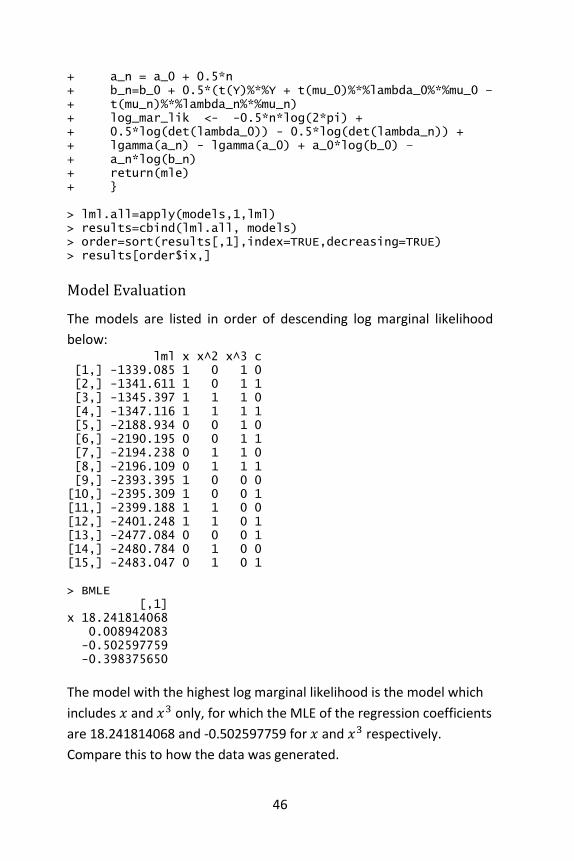
46

+ a_n = a_0 + 0.5*n + b_n=b_0 + 0.5*(t(Y)%*%Y + t(mu_0)%*%lambda_0%*%mu_0 – + t(mu_n)%*%lambda_n%*%mu_n) + log_mar_lik <- -0.5*n*log(2*pi) + + 0.5*log(det(lambda_0)) - 0.5*log(det(lambda_n)) + + lgamma(a_n) - lgamma(a_0) + a_0*log(b_0) – + a_n*log(b_n) + return(mle) + } > lml.all=apply(models,1,lml) > results=cbind(lml.all, models) > order=sort(results[,1],index=TRUE,decreasing=TRUE) > results[order$ix,]

Model Evaluation

The models are listed in order of descending log marginal likelihood

below: lml x x^2 x^3 c [1,] -1339.085 1 0 1 0 [2,] -1341.611 1 0 1 1 [3,] -1345.397 1 1 1 0 [4,] -1347.116 1 1 1 1 [5,] -2188.934 0 0 1 0 [6,] -2190.195 0 0 1 1 [7,] -2194.238 0 1 1 0 [8,] -2196.109 0 1 1 1 [9,] -2393.395 1 0 0 0 [10,] -2395.309 1 0 0 1 [11,] -2399.188 1 1 0 0 [12,] -2401.248 1 1 0 1 [13,] -2477.084 0 0 0 1 [14,] -2480.784 0 1 0 0 [15,] -2483.047 0 1 0 1 > BMLE [,1] x 18.241814068 0.008942083 -0.502597759 -0.398375650

The model with the highest log marginal likelihood is the model which

includes 𝑥 and 𝑥3 only, for which the MLE of the regression coefficients

are 18.241814068 and -0.502597759 for 𝑥 and 𝑥3 respectively.

Compare this to how the data was generated.

47

4. Naïve Bayes classifier

In machine learning, Naïve Bayes classifiers are a family of simple

probabilistic classifiers based on applying Bayes’ theorem with strong

(naive) independence assumptions between the features.

Naïve Bayes is a popular (baseline) method for text categorization, the

problem of judging documents as belonging to one category or the

other (such as spam or legitimate, sports or politics, etc.) with word

frequencies as the features. With appropriate preprocessing, it is

competitive in this domain with more advanced methods including

support vector machines (Rennie, Shih, Teevan, & Karger, 2003).

Training Naïve Bayes can be done by evaluating an approximation

algorithm in closed form in linear time, rather than by expensive

iterative approximation.

Introduction

In simple terms, a Naïve Bayes classifier assumes that the value of a

particular feature is unrelated to the presence or absence of any other

feature, given the class variable. For example, a fruit may be

considered to be an apple if it is red, round, and about 3” in diameter.

A Naïve Bayes classifier considers each of these features to contribute

independently to the probability that this fruit is an apple, regardless of

the presence or absence of the other features.

For some types of probability models, Naïve Bayes classifiers can be

trained very efficiently in a supervised learning setting. In many

practical applications, parameter estimation for Naïve Bayes models

uses the method of maximum likelihood; in other words, one can work

with the Naïve Bayes model without accepting Bayesian probability or

using any Bayesian methods.

Despite their naive design and apparently oversimplified assumptions,

48

Naïve Bayes classifiers have worked quite well in many complex real-

world situations. In 2004, an analysis of the Bayesian classification

problem showed that there are sound theoretical reasons for the

apparently implausible efficacy of Naïve Bayes classifiers (Zhang, 2004).

Still, a comprehensive comparison with other classification algorithms

in 2006 showed that Bayes classification is outperformed by other

approaches, such as boosted trees or random forests (Caruana &

Niculescu-Mizil, 2006).

An advantage of Naïve Bayes is that it only requires a small amount of

training data to estimate the parameters (means and variances of the

variables) necessary for classification. Because independent variables

are assumed, only the variances of the variables for each class need to

be determined and not the entire covariance matrix.

Probabilistic model

Abstractly, the probability model for a classifier is a conditional model

𝑝(𝐶|𝐹1, … , 𝐹𝑛)

over a dependent class variable C with a small number of outcomes or

classes, conditional on several feature variables 𝐹1 through 𝐹𝑛. The

problem is that if the number of features n is large or if a feature can

take on a large number of values, then basing such a model on

probability tables is infeasible. We therefore reformulate the model to

make it more tractable.

Using Bayes’ theorem, this can be written

𝑝(𝐶|𝐹1, … , 𝐹𝑛) =𝑝(𝐶)𝑝(𝐹1, … , 𝐹𝑛|𝐶)

𝑝(𝐹1, … , 𝐹𝑛).

In plain English, using Bayesian Probability terminology, the above

equation can be written as

posterior=prior × likelihood

evidence.

49

In practice, there is interest only in the numerator of that fraction,

because the denominator does not depend on C and the values of the

features 𝐹𝑖 are given, so that the denominator is effectively constant.

The numerator is equivalent to the joint probability model

𝑝(𝐶|𝐹1, … , 𝐹𝑛),

which can be rewritten as follows, using the chain rule for repeated

applications of the definition of conditional probability:

𝑝(𝐶|𝐹1, … , 𝐹𝑛) = 𝑝(𝐶)𝑝(𝐹1, … , 𝐹𝑛|𝐶) = 𝑝(𝐶)𝑝(𝐹1|𝐶)𝑝(𝐹2, … , 𝐹𝑛|𝐶, 𝐹1) = 𝑝(𝐶)𝑝(𝐹1|𝐶)𝑝(𝐹2|𝐶, 𝐹1)𝑝(𝐹3, … , 𝐹𝑛|𝐶, 𝐹1,𝐹2)

= 𝑝(𝐶)𝑝(𝐹1|𝐶)𝑝(𝐹2|𝐶, 𝐹1)𝑝(𝐹3|𝐶, 𝐹1, 𝐹2) 𝑝(𝐹4, … , 𝐹𝑛|𝐶, 𝐹1,𝐹2, 𝐹3)

= 𝑝(𝐶)𝑝(𝐹1|𝐶)𝑝(𝐹2|𝐶, 𝐹1) … 𝑝(𝐹𝑛|𝐶, 𝐹1,𝐹2, 𝐹3, … , 𝐹𝑛)

Now the “naïve” conditional independence assumptions come into

play: assume that each feature 𝐹𝑖 is conditionally independent of every

other feature 𝐹𝑗 for 𝑖 ≠ 𝑗 given the category C. This means that

𝑝(𝐹𝑖|𝐶, 𝐹𝑗) = 𝑝(𝐹𝑖|𝐶)

𝑝(𝐹𝑖|𝐶, 𝐹𝑗 , 𝐹𝑘) = 𝑝(𝐹𝑖|𝐶)

𝑝(𝐹𝑖|𝐶, 𝐹𝑗, 𝐹𝑘 , 𝐹𝑙) = 𝑝(𝐹𝑖|𝐶)

and so on, for 𝑖 ≠ 𝑗, 𝑘, 𝑙. Thus, the joint model can be expressed as

𝑝(𝐶|𝐹1, … , 𝐹𝑛) ∝ 𝑝(𝐶, 𝐹1, … , 𝐹𝑛)

∝ 𝑝(𝐶)𝑝(𝐹1|𝐶)𝑝(𝐹2|𝐶)𝑝(𝐹3|𝐶) ⋯

∝ 𝑝(𝐶) ∏ 𝑝(𝐹𝑖|𝐶).

𝑛

𝑖−1

This means that under the above independence assumptions, the

conditional distribution over the class variable C is:

50

𝑝(𝐶|𝐹1, … , 𝐹𝑛) =1

𝑍𝑝(𝐶) ∏ 𝑝(𝐹𝑖|𝐶)

𝑛

𝑖−1

,

where the evidence 𝑍 = 𝑝(𝐹1, … , 𝐹𝑛) is a scaling factor dependent only

on 𝐹1, … , 𝐹𝑛, that is, a constant if the values of the feature variables are

known (Rish, 2001).

Constructing a classifier from the probability model

The discussion so far has derived the independent feature model, that

is, the Naïve Bayes probability model. The Naïve Bayes classifier

combines this model with a decision rule. One common rule is to pick

the hypothesis that is most probable; this is known as the maximum a

posteriori or MAP decision rule. The corresponding classifier, a Bayes

classifier, is the function classify defined as follows:

classify(𝑓1, … , 𝑓𝑛) = argmax𝐶

𝑝(𝐶 = 𝑐) ∏ 𝑝(𝐹𝑖 = 𝑓𝑖|𝐶 = 𝑐)

𝑛

𝑖=1

Parameter estimation and event models

All model parameters (i.e., class priors and feature probability

distributions) can be approximated with relative frequencies from the

training set. These are maximum likelihood estimates of the

probabilities. A class’ prior may be calculated by assuming

equiprobable classes (i.e., 𝑝𝑟𝑖𝑜𝑟𝑠 = 1 / (𝑛𝑢𝑚𝑏𝑒𝑟 𝑜𝑓 𝑐𝑙𝑎𝑠𝑠𝑒𝑠)), or by

calculating an estimate for the class probability from the training set

(i.e., (prior for a given class) = (number of samples in the class) /

(total number of samples)). To estimate the parameters for a

feature’s distribution, we must assume a distribution or generate

nonparametric models for the features from the training set (John &

Langley, 1995).

The assumptions on distributions of features are called the event

model of the Naïve Bayes classifier. For discrete features like the ones

encountered in document classification (include spam filtering),

51

multinomial and Bernoulli distributions are popular. These assumptions

lead to two distinct models, which are often confused (McCallum &

Nigam, 1998) (Metsis, Androutsopoulos, & Paliouras, 2006).

Gaussian Naïve Bayes

When dealing with continuous data, a typical assumption is that the

continuous values associated with each class are distributed according

to a Gaussian distribution. For example, suppose the training data

contain a continuous attribute, 𝑥. We first segment the data by the

class, and then compute the mean and variance of 𝑥 in each class. Let

𝜇𝑐 be the mean of the values in associated with class 𝑐, and let 𝜎𝑐2 be

the variance of the values in associated with class 𝑐. Then, the

probability density of some value given a class, 𝑃(𝑥 = 𝑣|𝑐), can be

computed by plugging 𝑣 into the equation for a Normal distribution

parameterized by 𝜇𝑐 and 𝜇𝑐. That is,

𝑃(𝑥 = 𝑣|𝑐) =1

√2𝜋𝜎𝑐2

𝑒−

(𝑣−𝜇𝑐)2

2𝜎𝑐2

Another common technique for handling continuous values is to use

binning to discretize the feature values, to obtain a new set of

Bernoulli-distributed features. In general, the distribution method is a

better choice if there is a small amount of training data, or if the

precise distribution of the data is known. The discretization method

tends to do better if there is a large amount of training data because it

will learn to fit the distribution of the data. Since Naïve Bayes is

typically used when a large amount of data is available (as more

computationally expensive models can generally achieve better

accuracy), the discretization method is generally preferred over the

distribution method.

Multinomial Naïve Bayes

With a multinomial event model, samples (feature vectors) represent

the frequencies with which certain events have been generated by a

multinomial (𝑝1, … , 𝑝𝑛) where 𝑝𝑖 is the probability that event i occurs

52

(or k such multinomials in the multiclass case). This is the event model

typically used for document classification; the feature values are then

term frequencies, generated by a multinomial that produces some

number of words (“bag of words” assumption, where word order is

ignored). The likelihood of observing a feature vector (histogram) F is

given by

𝑝(𝐹|𝐶) =(∑ 𝐹𝑖𝑖 )!

∏ 𝐹𝑖!𝑖∏ 𝑝𝑖

𝐹𝑖

𝑖

The multinomial Naïve Bayes classifier becomes a linear classifier when

expressed in log-space:

log 𝑝(𝐶|𝐹) = log (𝑝(𝐶) ∏ 𝑝(𝐹𝑖|𝐶)

𝑛

𝑖=1

)

= log 𝑝(𝐶) + ∑ log 𝑝(𝐹𝑖|𝐶)

𝑛

𝑖=1

= 𝑏 + 𝒘𝐶𝑇𝑭

Where 𝑏 = log 𝑝(𝐶) and 𝑤𝑐𝑖= log 𝑝(𝐹𝑖|𝐶).

If a given class and feature value never occur together in the training

data, then the frequency-based probability estimate will be zero. This is

problematic because it will wipe out all information in the other

probabilities when they are multiplied. Therefore, it is often desirable

to incorporate a small-sample correction, called pseudo-count, in all

probability estimates such that no probability is ever set to be exactly

zero. This way of regularizing Naïve Bayes is called Additive smoothing

when the pseudo-count is one, and Lidstone smoothing in the general

case.

Rennie et al. (Rennie, Lawrence, Teevan, & Karger, 2003) discuss

problems with the multinomial assumption in the context of document

classification and possible ways to alleviate those problems, including

the use of tf–idf weights instead of raw term frequencies and

document length normalization, to produce a Naïve Bayes classifier

53

that is competitive with support vector machines.

Bernoulli Naïve Bayes

In the multivariate Bernoulli event model, features are independent

Booleans (binary variables) describing inputs. This model is also popular

for document classification tasks, where binary term occurrence

features are used rather than term frequencies. If 𝐹𝑖 is a Boolean

expressing the occurrence or absence of the 𝑖-th term from the

vocabulary, then the likelihood of a document given a class 𝐶 is given

by

𝑝(𝐹1, … , 𝐹𝑛|𝐶) = ∏[𝐹𝑖𝑝(𝑤𝑖|𝐶) + (1 − 𝐹𝑖)(1 − 𝑝(𝑤𝑖|𝐶))]

𝑛

𝑖=1

where 𝑝(𝑤𝑖|𝐶) is the probability of class 𝐶 generating the term 𝑤𝑖. This

event model is especially popular for classifying short texts. It has the

benefit of explicitly modeling the absence of terms. Note that a Naïve

Bayes classifier with a Bernoulli event model is not the same as a

multinomial NB classifier with frequency counts truncated to one.

Discussion

Despite the fact that the far-reaching independence assumptions are

often inaccurate, the Naïve Bayes classifier has several properties that

make it surprisingly useful in practice. In particular, the decoupling of

the class conditional feature distributions means that each distribution

can be independently estimated as a one-dimensional distribution. This

helps alleviate problems stemming from the curse of dimensionality,

such as the need for data sets that scale exponentially with the number

of features. While Naïve Bayes often fails to produce a good estimate

for the correct class probabilities, this may not be a requirement for

many applications. For example, the Naïve Bayes classifier will make

the correct MAP decision rule classification so long as the correct class

is more probable than any other class. This is true regardless of

whether the probability estimate is slightly, or even grossly inaccurate.

54

In this manner, the overall classifier can be robust enough to ignore

serious deficiencies in its underlying naive probability model. Other

reasons for the observed success of the Naïve Bayes classifier are

discussed in the literature cited below.

Examples

Sex classification

Problem: classify whether a given person is a male or a female based

on the measured features. The features include height, weight, and

foot size.

Training

Example training set below.

sex height

(feet)

weight (lbs) foot

size(inch

es) male 6 180 12

male 5.92

(5'11”)

190 11

male 5.58

(5'7”)

170 12

male 5.92

(5'11”)

165 10

female 5 100 6

female 5.5

(5'6”)

150 8

female 5.42

(5'5”)

130 7

female 5.75

(5'9”)

150 9

The classifier created from the training set using a Gaussian distribution

assumption would be (given variances are sample variances):

sex mean

(height)

variance

(height)

mean

(weight)

variance

(weight)

Mean

(foot size)

Variance

(foot size)

male 5.8550 3.50e-02 176.25 1.23e+02 11.25 9.16e-01

female 5.4175 9.72e-02 132.50 5.58e+02 7.50 1.66e+00

55

Let's say we have equiprobable classes so 𝑃(male) = 𝑃(female) =

0.5. This prior probability distribution might be based on our

knowledge of frequencies in the larger population, or on frequency in

the training set.

Testing

Below is a sample to be classified as a male or female.

sex height

(feet)

weight

(lbs)

foot

size(inches) sample 6 130 8

We wish to determine which posterior is greater, male or female. For

the classification as male the posterior is given by

𝑝𝑜𝑠𝑡𝑒𝑟𝑖𝑜𝑟(male)

=𝑃(male)𝑝(height|male)𝑝(weight|male)𝑝(foot size|male)

evidence

For the classification as female the posterior is given by

𝑝𝑜𝑠𝑡𝑒𝑟𝑖𝑜𝑟(female)

=𝑃(female)𝑝(height|female)𝑝(weight|female)𝑝(foot size|female)

evidence

The evidence (also termed normalizing constant) may be calculated:

𝑒𝑣𝑖𝑑𝑒𝑛𝑐𝑒

= 𝑃(male)𝑝(height|male)𝑝(weight|male)𝑝(foot size|male)

+ 𝑃(female)𝑝(height|female)𝑝(weight|female)𝑝(foot size|female)

However, given the sample the evidence is a constant and thus scales

both posteriors equally. It therefore does not affect classification and

can be ignored. We now determine the probability distribution for the

sex of the sample.

56

𝑃(male) = 0.5

𝑝(height|male) =1

√2𝜋𝜎2exp (

−(6 − 𝜇)2

2𝜎3 )

where 𝜇 = 5.855 and 𝜎2 = 3.5033 ∙ 10−2 are the parameters of

normal distribution which have been previously determined from the

training set. Note that a value greater than 1 is OK here—it is a

probability density rather than a probability, because height is a

continuous variable.

𝑝(weight|male) = 5.9881 ∙ 10−6

𝑝(foot size|male) = 1.3112 ∙ 10−3

posterior numerator (male)=their product = 6.1984 ∙ 10−9

𝑃(female) = 0.5

𝑝(height|female) = 2.2346 ∙ 10−1

𝑝(weight|female) = 1.6789 ∙ 10−2

𝑝(foot size|female) = 2.8669 ∙ 10−3

posterior numerator (female)=their product = 5.3378 ∙ 10−4

Since posterior numerator is greater in the female case, we predict the

sample is female.

Document classification

Here is a worked example of Naïve Bayesian classification to the

document classification problem. Consider the problem of classifying

documents by their content, for example into spam and non-spam e-

mails. Imagine that documents are drawn from a number of classes of

documents which can be modelled as sets of words where the

(independent) probability that the 𝑖-th word of a given document

occurs in a document from class 𝐶 can be written as

57

𝑝(𝑤𝑖|𝐶)

(For this treatment, we simplify things further by assuming that words

are randomly distributed in the document—that is, words are not

dependent on the length of the document, position within the

document with relation to other words, or other document-context.)

Then the probability that a given document 𝐷 contains all of the words

𝑤𝑖, given a class 𝐶, is

𝑝(𝐷|𝐶) = ∏ 𝑝(𝑤𝑖|𝐶)

𝑖

The question that we desire to answer is: “what is the probability that a

given document 𝐷 belongs to a given class 𝐶?” In other words, what is

𝑝(𝐶|𝐷)? Now by definition

𝑝(𝐷|𝐶) =𝑝(𝐷 ∩ 𝐶)

𝑝(𝐶)

and

𝑝(𝐶|𝐷) =𝑝(𝐷 ∩ 𝐶)

𝑝(𝐷)

Bayes’ theorem manipulates these into a statement of probability in

terms of likelihood.

𝑝(𝐶|𝐷) =𝑝(𝐶)

𝑝(𝐶)𝑝(𝐷|𝐶)

Assume for the moment that there are only two mutually exclusive

classes, 𝑆 and ¬𝑆 (e.g. spam and not spam), such that every element

(email) is in either one or the other;

𝑝(𝐷|𝑆) = ∏ 𝑝(𝑤𝑖|𝑆)

𝑖

And

58

𝑝(𝐷|¬𝑆) = ∏ 𝑝(𝑤𝑖|¬𝑆)

𝑖

Using the Bayesian result above, we can write:

𝑝(𝑆|𝐷) =𝑝(𝑆)

𝑝(𝐷)∏ 𝑝(𝑤𝑖|𝑆)

𝑖

𝑝(¬𝑆|𝐷) =𝑝(¬𝑆)

𝑝(𝐷)∏ 𝑝(𝑤𝑖|¬𝑆)

𝑖

Dividing one by the other gives:

𝑝(𝑆|𝐷)

𝑝(¬𝑆|𝐷)=

𝑝(𝑆) ∏ 𝑝(𝑤𝑖|𝑆)𝑖

𝑝(¬𝑆) ∏ 𝑝(𝑤𝑖|¬𝑆)𝑖

Which can be re-factored as:

𝑝(𝑆|𝐷)

𝑝(¬𝑆|𝐷)=

𝑝(𝑆)

𝑝(¬𝑆)∏

𝑝(𝑤𝑖|𝑆)

𝑝(𝑤𝑖|¬𝑆)𝑖

Thus, the probability ratio 𝑝(𝑆|𝐷) 𝑝(¬𝑆|𝐷)⁄ can be expressed in terms

of a series of likelihood ratios. The actual probability 𝑝(𝑆|𝐷) can be

easily computed from log(𝑝(𝑆|𝐷) 𝑝(¬𝑆|𝐷)⁄ ) based on the observation

that 𝑝(𝑆|𝐷) + 𝑝(¬𝑆|𝐷) = 1.

Taking the logarithm of all these ratios, we have:

ln𝑝(𝑆|𝐷)

𝑝(¬𝑆|𝐷)= ln

𝑝(𝑆)

𝑝(¬𝑆)= ∑ ln

𝑝(𝑤𝑖|𝑆)

𝑝(𝑤𝑖|¬𝑆)𝑖

(This technique of “log-likelihood ratios” is a common technique in

statistics. In the case of two mutually exclusive alternatives (such as

this example), the conversion of a log-likelihood ratio to a probability

takes the form of a sigmoid curve: see logit for details.)

Finally, the document can be classified as follows. It is spam if

59

𝑝(𝑆|𝐷) > 𝑝(¬𝑆|𝐷) (i.e., ln𝑝(𝑆|𝐷)

𝑝(¬𝑆|𝐷)> 0), otherwise it is not spam

(Kibriya, Frank, Pfahringer, & Holmes, 2008).

Software

Open Source software packages include PNL and R. Software packages

that are specifically designed for this function include:

Bayesian belief network software – from J. Cheng, includes:

o BN PowerConstructor: An efficient system for learning BN

structures and parameters from data;

o BN PowerPredictor: A data mining program for data

modeling/classification/prediction.

Bayesian Network tools in Java (BNJ) – is an open-source suite of

Java tools for probabilistic learning and reasoning (Kansas State

University KDD Lab)

GeNIe – is a decision modeling environment implementing

influence diagrams and Bayesian networks.

JNCC2 (Naive Credal Classifier 2) – is an extension of Naive Bayes

towards imprecise probabilities; it is designed to return robust

classification, even on small and/or incomplete data sets.

Commercial software packages include:

AgenaRisk – by Ajena, is a visual tool, combining Bayesian

networks and statistical simulation.

BayesiaLab – by, Bayesia is a complete set of Bayesian network

tools, including supervised and unsupervised learning, and analysis

toolbox.

BNet – by Charles River Analytics, includes BNet.Builder for rapidly

creating Belief Networks, entering information, and getting results

and BNet.EngineKit for incorporating Belief Network Technology in

your applications.

Flint – by Logic Programming Associates, combines bayesian

networks, certainty factors and fuzzy logic within a logic

60

programming rules-based environment.

Netica – by NORSYS, is Bayesian network development software

provides Bayesian network tools.

PrecisionTree – by Paslisade (makers of @Risk), is an add-in for

Microsoft Excel for building decision trees and influence diagrams

directly in the spreadsheet

Example Using R

The Iris dataset is pre-installed in R, since it is in the standard

datasets package. To access its documentation, click on 'Packages' at

the top-level of the R documentation, then on 'datasets' and then on

'iris'. As explained, there are 150 data points and 5 variables. Each data

point concerns a particular iris flower and gives 4 measurements of the

flower: Sepal.Length, Sepal.Width, Petal.Length and Petal.Width

together with the flower's Species. The goal is to build a classifier that

predicts species from the 4 measurements, so species is the class

variable.

To get the iris dataset into your R session, do:

> data(iris)

at the R prompt. As always, it makes sense to look at the data. The

following R command (from the Wikibook) does a nice job of this.

> pairs(iris[1:4],main="Iris Data + (red=setosa,green=versicolor,blue=virginica)", pch=21, + bg=c("red","green3","blue")[unclass(iris$Species)])

The ‘pairs’ command creates a scatterplot. Each dot is a data point and

its position is determined by the values that data point has for a pair of

variables. The class determines the color of the data point. From the

plot note that Setosa irises have smaller petals than the other two

species.

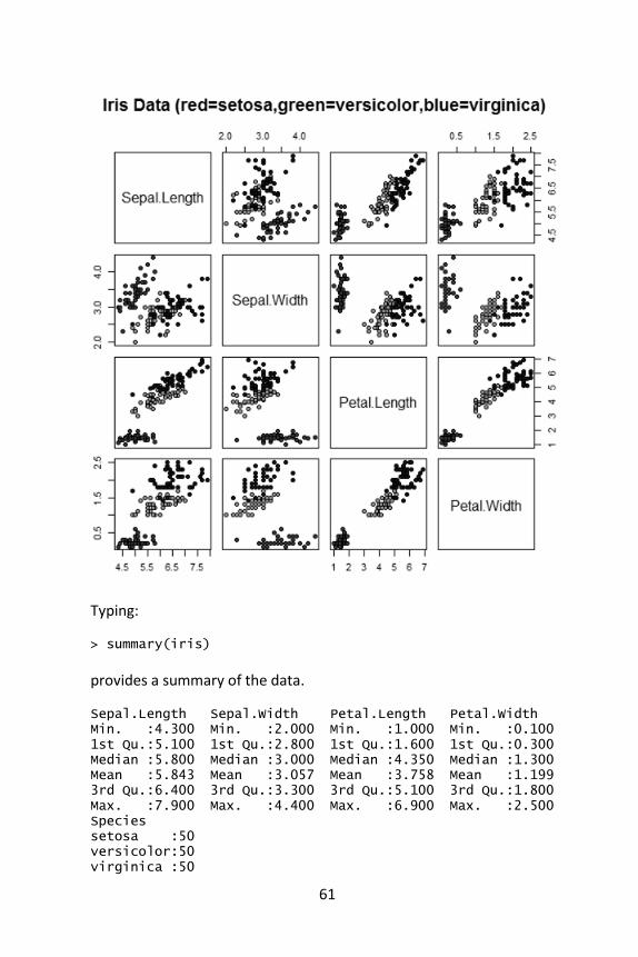
61

Typing:

> summary(iris)

provides a summary of the data.

Sepal.Length Sepal.Width Petal.Length Petal.Width Min. :4.300 Min. :2.000 Min. :1.000 Min. :0.100 1st Qu.:5.100 1st Qu.:2.800 1st Qu.:1.600 1st Qu.:0.300 Median :5.800 Median :3.000 Median :4.350 Median :1.300 Mean :5.843 Mean :3.057 Mean :3.758 Mean :1.199 3rd Qu.:6.400 3rd Qu.:3.300 3rd Qu.:5.100 3rd Qu.:1.800 Max. :7.900 Max. :4.400 Max. :6.900 Max. :2.500 Species setosa :50 versicolor:50 virginica :50

62

Typing:

> iris

prints out the entire dataset to the screen.

Sepal.Length Sepal.Width Petal.Length Petal.Width Species 1 5.1 3.5 1.4 0.2 setosa 2 4.9 3 1.4 0.2 setosa 3 4.7 3.2 1.3 0.2 setosa 4 4.6 3.1 1.5 0.2 setosa 5 5 3.6 1.4 0.2 setosa -----------------------------Data omitted------------------------- 149 6.2 3.4 5.4 2.3 virginica 150 5.9 3 5.1 1.8 virginica

Constructing a Naïve Bayes classifier

We will use the e1071 R package to build a Naïve Bayes classifier. Firstly

you need to download the package (since it is not pre-installed here).

Do:

> install.packages("e1071")

Choose a mirror in US from the menu that will appear. You will be

prompted to create a personal R library (say yes) since you don't have

permission to put e1071 in the standard directory for R packages.

To (1) load e1071 into your workspace (2) build a Naïve Bayes classifier

and (3) make some predictions on the training data, do:

> library(e1071) > classifier<-naiveBayes(iris[,1:4], iris[,5]) > table(predict(classifier, iris[,-5]), iris[,5], + dnn=list('predicted','actual'))

As you should see the classifier does a pretty good job of classifying.

Why is this not surprising?

predicted setosa versicolor virginica setosa 50 0 0 versicolor 0 47 3 virginica 0 3 47

63

To see what's going on ‘behind-the-scenes’, first do:

> classifier$apriori

This gives the class distribution in the data: the prior distribution of the

classes. ('A priori' is Latin for 'from before'.)

iris[, 5] setosa versicolor virginica 50 50 50

Since the predictor variables here are all continuous, the Naïve Bayes

classifier generates three Gaussian (Normal) distributions for each

predictor variable: one for each value of the class variable Species. If

you type:

> classifier$tables$Petal.Length

You will see the mean (first column) and standard deviation (second

column) for the 3 class-dependent Gaussian distributions:

Petal.Length iris[, 5] [,1] [,2] setosa 1.462 0.1736640 versicolor 4.260 0.4699110 virginica 5.552 0.5518947

You can plot these 3 distributions against each other with the following

three R commands:

> plot(function(x) dnorm(x, 1.462, 0.1736640), 0, 8, + col="red", main="Petal length distribution for the 3 + different species") > curve(dnorm(x, 4.260, 0.4699110), add=TRUE, col="blue") > curve(dnorm(x, 5.552, 0.5518947), add=TRUE, col="green")

Note that setosa irises (the red curve) tend to have smaller petals

(mean value = 1.462) and there is less variation in petal length

(standard deviation is only 0.1736640).

64

Understanding Naïve Bayes

In the previous example you were given a recipe which allowed you to

construct a Naïve Bayes classifier. This was for a case where we had

continuous predictor variables. In this question you have to work out

what the parameters of a Naïve Bayes model should be for some

discrete data.

The dataset in question is called HairEyeColor and has three variables:

Sex, Eye and Hair, giving values for these 3 variables for each of 592

students from the University of Delaware. First have a look at the

numbers:

65

> HairEyeColor , , Sex = Male Eye Hair Brown Blue Hazel Green Black 32 11 10 3 Brown 53 50 25 15 Red 10 10 7 7 Blond 3 30 5 8 , , Sex = Female Eye Hair Brown Blue Hazel Green Black 36 9 5 2 Brown 66 34 29 14 Red 16 7 7 7 Blond 4 64 5 8

You can also plot it as a 'mosaic' plot which uses rectangles to

represent the numbers in the data:

> mosaicplot(HairEyeColor)

Your job here is to compute the parameters for a Naïve Bayes classifier

which attempts to predict Sex from the other two variables. The

parameters should be estimated using maximum likelihood. To save

you the tedium of manual counting, here's how to use margin.table

to get the counts you need:

> margin.table(HairEyeColor,3) Sex Male Female 279 313

66

Mosaic plot

> margin.table(HairEyeColor,c(1,3)) Sex Hair Male Female Black 56 52 Brown 143 143 Red 34 37 Blond 46 81

Note that Sex is variable 3, and Hair is variable 1. Once you think you

have the correct parameters speak to me or one of the demonstrators

to see if you have it right. (Or if you can manage it, construct the Naïve

Bayes model using the naiveBayes function and yank out the

parameters from the model. Read the documentation to do this.)

67

5. Decision tree learning

Decision tree learning uses a decision tree as a predictive model which

maps observations about an item to conclusions about the item’s

target value. It is one of the predictive modeling approaches used in

statistics, data mining and machine learning. More descriptive names

for such tree models are classification trees or regression trees. In

these tree structures, leaves represent class labels and branches

represent conjunctions of features that lead to those class labels.

In decision analysis, a decision tree can be used to visually and explicitly

represent decisions and decision making. In data mining, a decision

tree describes data but not decisions; rather the resulting classification

tree can be an input for decision making. This chapter deals with

decision trees in data mining.

General

Decision tree learning is a method commonly used in data mining

(Rokach & Maimon, 2008). The goal is to create a model that predicts

the value of a target variable based on several input variables. An

example is shown on the right. Each interior node corresponds to one

of the input variables; there are edges to children for each of the

possible values of that input variable. Each leaf represents a value of

the target variable given the values of the input variables represented

by the path from the root to the leaf.

A decision tree is a simple representation for classifying examples.

Decision tree learning is one of the most successful techniques for

supervised classification learning. For this section, assume that all of

the features have finite discrete domains, and there is a single target

feature called the classification. Each element of the domain of the

classification is called a class. A decision tree or a classification tree is a

tree in which each internal (non-leaf) node is labeled with an input

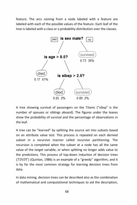
68

feature. The arcs coming from a node labeled with a feature are

labeled with each of the possible values of the feature. Each leaf of the

tree is labeled with a class or a probability distribution over the classes.

A tree showing survival of passengers on the Titanic (“sibsp” is the

number of spouses or siblings aboard). The figures under the leaves

show the probability of survival and the percentage of observations in

the leaf.

A tree can be “learned” by splitting the source set into subsets based

on an attribute value test. This process is repeated on each derived

subset in a recursive manner called recursive partitioning. The

recursion is completed when the subset at a node has all the same

value of the target variable, or when splitting no longer adds value to

the predictions. This process of top-down induction of decision trees

(𝑇𝐷𝐼𝐷𝑇) (Quinlan, 1986) is an example of a “greedy” algorithm, and it

is by far the most common strategy for learning decision trees from

data.

In data mining, decision trees can be described also as the combination

of mathematical and computational techniques to aid the description,

69

categorization and generalization of a given set of data.

Data comes in records of the form:

(𝒙, 𝑌) = (𝑥1, 𝑥2, 𝑥3, … , 𝑥𝑘 , 𝑌).

The dependent variable, 𝑌, is the target variable that we are trying to

understand, classify or generalize. The vector 𝒙 is composed of the

input variables, 𝑥1, 𝑥2, 𝑥3, etc., that are used for that task.

Types

Decision trees used in data mining are of two main types:

• Classification tree analysis is when the predicted outcome is

the class to which the data belongs.

• Regression tree analysis is when the predicted outcome can be

considered a real number (e.g. the price of a house, or a

patient’s length of stay in a hospital).

The term Classification And Regression Tree (CART) analysis is an

umbrella term used to refer to both of the above procedures, first

introduced by Breiman et al. (Breiman, Friedman, Olshen, & Stone,

1984). Trees used for regression and trees used for classification have

some similarities—but also some differences, such as the procedure

used to determine where to split.

Some techniques, often called ensemble methods, construct more than

one decision tree:

• Bagging decision trees, an early ensemble method, builds

multiple decision trees by repeatedly resampling training data

with replacement, and voting the trees for a consensus

prediction (Breiman L. , Bagging predictors, 1996).

• A Random Forest classifier uses a number of decision trees, in

order to improve the classification rate.

• Boosted Trees can be used for regression-type and

classification-type problems (Friedman, Stochastic Gradient

70

Boosting, 1999) (Hastie, Tibshirani, & Friedman, The elements

of statistical learning : Data mining, inference, and prediction,

2001).

• Rotation forest, in which every decision tree is trained by first

applying principal component analysis (PCA) on a random

subset of the input features (Rodriguez, Kuncheva, & Alonso,

2006).

Decision tree learning is the construction of a decision tree from class-

labeled training tuples. A decision tree is a flow-chart-like structure,

where each internal (non-leaf) node denotes a test on an attribute,

each branch represents the outcome of a test, and each leaf (or

terminal) node holds a class label. The topmost node in a tree is the

root node.

There are many specific decision-tree algorithms. Notable ones include:

• ID3 (Iterative Dichotomiser 3)

• C4.5 (successor of ID3)

• CART (Classification And Regression Tree)

• CHAID (CHi-squared Automatic Interaction Detector). Performs

multi-level splits when computing classification trees (Kass,

1980).

• MARS: extends decision trees to handle numerical data better.

• Conditional Inference Trees. Statistics-based approach that

uses non-parametric tests as splitting criteria, corrected for

multiple testing to avoid overfitting. This approach results in

unbiased predictor selection and does not require pruning

(Hothorn, Hornik, & Zeileis, 2006).

ID3 and CART were invented independently at around same time

(between 1970-1980), yet follow a similar approach for learning

decision tree from training tuples.

Metrics

Algorithms for constructing decision trees usually work top-down, by

71

choosing a variable at each step that best splits the set of items

(Rokach & Maimon, Top-down induction of decision trees classifiers-a

survey, 2005). Different algorithms use different metrics for measuring

“best”. These generally measure the homogeneity of the target

variable within the subsets. Some examples are given below. These

metrics are applied to each candidate subset, and the resulting values

are combined (e.g., averaged) to provide a measure of the quality of

the split.

Gini impurity

Used by the CART (classification and regression tree) algorithm, Gini

impurity is a measure of how often a randomly chosen element from

the set would be incorrectly labeled, if it were randomly labeled

according to the distribution of labels in the subset. Gini impurity can

be computed by summing the probability of each item being chosen

times the probability of a mistake in categorizing that item. It reaches

its minimum (zero) when all cases in the node fall into a single target

category. This should not be confused with Gini coefficient.

To compute Gini impurity for a set of items, suppose 𝑖 takes on values

in {1,2, … , 𝑚}, and let 𝑓𝑖 be the fraction of items labeled with value 𝑖 in

the set.

𝐼𝐺(𝑓) = ∑ 𝑓𝑖(1 − 𝑓𝑖)

𝑚

𝑖=1

= ∑(𝑓𝑖 − 𝑓𝑖2)

𝑚

𝑖=1

= ∑ 𝑓𝑖

𝑚

𝑖=1

− ∑ 𝑓𝑖2

𝑚

𝑖=1

= 1 − ∑ 𝑓𝑖2

𝑚

𝑖=1

Information gain

In information theory and machine learning, information gain is a

synonym for Kullback–Leibler divergence. However, in the context of

decision trees, the term is sometimes used synonymously with mutual

information, which is the expectation value of the Kullback–Leibler

divergence of a conditional probability distribution.

In particular, the information gain about a random variable 𝑋 obtained

from an observation that a random variable 𝐴 takes the value 𝐴 = 𝑎 is

72

the Kullback-Leibler divergence 𝐷𝐾𝐿(𝑝(𝑥|𝑎)||𝑝(𝑥|𝐼)) of the prior

distribution 𝑝(𝑥|𝐼) for 𝑥 from the posterior distribution 𝑝(𝑥|𝑎) for 𝑥

given 𝑎.

The expected value of the information gain is the mutual information

𝐼(𝑋; 𝐴) of 𝑋 and 𝐴, i.e., the reduction in the entropy of 𝑋 achieved by

learning the state of the random variable 𝐴.

In machine learning, this concept can be used to define a preferred

sequence of attributes to investigate to most rapidly narrow down the

state of 𝑋. Such a sequence (which depends on the outcome of the

investigation of previous attributes at each stage) is called a decision

tree. Usually an attribute with high mutual information should be

preferred to other attributes.

General definition

In general terms, the expected information gain is the change in

information entropy 𝐻 from a prior state to a state that takes some

information as given:

𝐼𝐺(𝑇, 𝑎) = 𝐻(𝑇) − 𝐻(𝑇|𝑎).

Formal Definition

Let 𝑇 denote a set of training examples, each of the form (𝒙, 𝑦) =

(𝑥1, 𝑥2, 𝑥3, … , 𝑥𝑘 , 𝑦) where 𝑥𝑎 ∈ 𝑣𝑎𝑙𝑠(𝑎) is the value of the th

attribute of example 𝒙 and 𝑦 is the corresponding class label. The

information gain for an attribute 𝑎 is defined in terms of entropy 𝐻( )

as follows:

𝐼𝐺(𝑇, 𝑎) = 𝐻(𝑇) − ∑|{𝑥 ∈ 𝑇|𝑥𝑎 = 𝑣}|

|𝑇|∙ 𝐻({𝑥 ∈ 𝑇|𝑥𝑎 = 𝑣}).

𝑣∈𝑣𝑎𝑙𝑠(𝑎)

The mutual information is equal to the total entropy for an attribute if

for each of the attribute values a unique classification can be made for

the result attribute. In this case, the relative entropies subtracted from

the total entropy are 0.

73

Drawbacks

Although information gain is usually a good measure for deciding the

relevance of an attribute, it is not perfect. A notable problem occurs

when information gain is applied to attributes that can take on a large

number of distinct values. For example, suppose that one is building a

decision tree for some data describing the customers of a business.

Information gain is often used to decide which of the attributes are the

most relevant, so they can be tested near the root of the tree. One of

the input attributes might be the customer's credit card number. This

attribute has a high mutual information, because it uniquely identifies

each customer, but we do not want to include it in the decision tree:

deciding how to treat a customer based on their credit card number is

unlikely to generalize to customers we haven't seen before

(overfitting).

Information gain ratio is sometimes used instead. This biases the

decision tree against considering attributes with a large number of

distinct values. However, attributes with very low information values

then appeared to receive an unfair advantage. In addition, methods

such as permutation tests have been proposed to correct the bias

(Deng, Runger, & Tuv, 2011).

Decision tree advantages

Amongst other data mining methods, decision trees have various

advantages:

• Simple to understand and interpret. People are able to understand

decision tree models after a brief explanation.

• Requires little data preparation. Other techniques often require

data normalization, dummy variables need to be created and blank

values to be removed.

• Able to handle both numerical and categorical data. Other

techniques are usually specialized in analyzing datasets that have

only one type of variable. (For example, relation rules can be used

only with nominal variables while neural networks can be used only

74

with numerical variables.)

• Uses a white box model. If a given situation is observable in a

model the explanation for the condition is easily explained by

Boolean logic. (An example of a black box model is an artificial

neural network since the explanation for the results is difficult to

understand.)

• Possible to validate a model using statistical tests. That makes it

possible to account for the reliability of the model.

• Robust. Performs well even if its assumptions are somewhat

violated by the true model from which the data were generated.

• Performs well with large datasets. Large amounts of data can be

analyzed using standard computing resources in reasonable time.

Limitations

• The problem of learning an optimal decision tree is known to be

NP-complete under several aspects of optimality and even for

simple concepts (Hyafil & Rivest, 1976). Consequently, practical

decision-tree learning algorithms are based on heuristics such as

the greedy algorithm where locally-optimal decisions are made at

each node. Such algorithms cannot guarantee to return the

globally-optimal decision tree. To reduce the greedy effect of local-

optimality some methods such as the dual information distance

(𝐷𝐼𝐷) tree were proposed (I., A., N., & Singer, 2014).

• Decision-tree learners can create over-complex trees that do not

generalize well from the training data. (This is known as overfitting

(Bramer, 2007).) Mechanisms such as pruning are necessary to

avoid this problem (with the exception of some algorithms such as

the Conditional Inference approach, which does not require

pruning (Strobl, Malley, & Tutz, 2009) (Hothorn, Hornik, & Zeileis,

2006)).

• There are concepts that are hard to learn because decision trees do

not express them easily, such as XOR, parity or multiplexer

problems. In such cases, the decision tree becomes prohibitively

large. Approaches to solve the problem involve either changing the

75

representation of the problem domain (known as

propositionalization) (Horváth & Yamamoto, 2003) or using

learning algorithms based on more expressive representations

(such as statistical relational learning or inductive logic

programming).

• For data including categorical variables with different numbers of

levels, information gain in decision trees is biased in favor of those

attributes with more levels (Deng, Runger, & Tuv, 2011). However,

the issue of biased predictor selection is avoided by the Conditional

Inference approach.

Extensions

Decision graphs

In a decision tree, all paths from the root node to the leaf node

proceed by way of conjunction, or AND. In a decision graph, it is

possible to use disjunctions (ORs) to join two more paths together

using Minimum message length (MML) (Tan & Dowe, 2004). Decision

graphs have been further extended to allow for previously unstated

new attributes to be learnt dynamically and used at different places

within the graph. The more general coding scheme results in better

predictive accuracy and log-loss probabilistic scoring. In general,

decision graphs infer models with fewer leaves than decision trees.

Alternative search methods

Evolutionary algorithms have been used to avoid local optimal

decisions and search the decision tree space with little a priori bias

(Papagelis, 2001) (Barros, Basgalupp, Carvalho, & Freitas, 2011).

It is also possible for a tree to be sampled using MCMC in a Bayesian

paradigm (Chipman, George, & McCulloch, 1998).

The tree can be searched for in a bottom-up fashion (Barros, Cerri,

Jaskowiak, & Carvalho, 2011).

76

Software

Many data mining software packages provide implementations of one

or more decision tree algorithms. Open Source software packages for

decision tree modeling include KNIME, Orange, R, scikit-learn, and

Weka.

Commercial packages include RapidMiner, SAS Enterprise Miner, and

SPSS Modeler. CART, by Salford Systems, is the licensed proprietary

code of the original CART authors.

Examples Using R

Classification Tree example

Let's use the data frame kyphosis to predict a type of deformation

(kyphosis) after surgery, from age in months (Age), number of

vertebrae involved (Number), and the highest vertebrae operated on

(Start).

In R, call the rpart library. Recursive partitioning for classification,

regression and survival trees. An implementation of most of the

functionality of the 1984 book by Breiman, Friedman, Olshen and Stone

(Breiman, Friedman, Olshen, & Stone, 1984).

# Classification Tree with rpart > library(rpart) We will not grow the tree with the fit() and rpart functions. # grow tree > fit <- rpart(Kyphosis ~ Age + Number + Start, + method="class", data=kyphosis)

where kyphosis is the response, with variables Age, Number, and

Start. Class in the method and kyphosis is the data set. Next, we

display the results.

> printcp(fit) # display the results Classification tree:

77

rpart(formula = Kyphosis~Age + Number + Start, data = kyphosis, method = "class") Variables actually used in tree construction: [1] Age Start Root node error: 17/81 = 0.20988 n= 81 CP nsplit rel error xerror xstd 1 0.176471 0 1.00000 1.0000 0.21559 2 0.019608 1 0.82353 1.2353 0.23200 3 0.010000 4 0.76471 1.2941 0.23548

Now, we plot the tree to visualize the cross validation results.

> plotcp(fit) # visualize cross-validation results

Next, we display a summary of the model.

> summary(fit) # detailed summary of splits

78

Call: rpart(formula = Kyphosis ~ Age + Number + Start, data = kyphosis, method = "class") n= 81 CP nsplit rel error xerror xstd 1 0.17647059 0 1.0000000 1.000000 0.2155872 2 0.01960784 1 0.8235294 1.117647 0.2243268 3 0.01000000 4 0.7647059 1.117647 0.2243268 Variable importance Start Age Number 64 24 12 Node number 1: 81 observations, complexity param=0.1764706 predicted class=absent expected loss=0.2098765 P(node) =1 class counts: 64 17 probabilities: 0.790 0.210 left son=2 (62 obs) right son=3 (19 obs) Primary splits: Start < 8.5 to the right, improve=6.762330, (0 missing) Number < 5.5 to the left, improve=2.866795, (0 missing) Age < 39.5 to the left, improve=2.250212, (0 missing) Surrogate splits: Number < 6.5 to the left, agree=0.802, adj=0.158, (0 split) Node number 2: 62 observations, complexity param=0.01960784 predicted class=absent expected loss=0.09677419 P(node) =0.7654321 class counts: 56 6 probabilities: 0.903 0.097 left son=4 (29 obs) right son=5 (33 obs) Primary splits: Start < 14.5 to the right, improve=1.0205280, (0 missing) Age < 55 to the left, improve=0.6848635, (0 missing) Number < 4.5 to the left, improve=0.2975332, (0 missing) Surrogate splits: Number < 3.5 to the left, agree=0.645, adj=0.241, (0 split) Age < 16 to the left, agree=0.597, adj=0.138, (0 split) Node number 3: 19 observations predicted class=present expected loss=0.4210526 P(node) =0.2345679 class counts: 8 11 probabilities: 0.421 0.579 Node number 4: 29 observations predicted class=absent expected loss=0 P(node) =0.3580247 class counts: 29 0 probabilities: 1.000 0.000 Node number 5: 33 observations, complexity param=0.01960784 predicted class=absent expected loss=0.1818182 P(node) =0.4074074 class counts: 27 6

79

probabilities: 0.818 0.182 left son=10 (12 obs) right son=11 (21 obs) Primary splits: Age < 55 to the left, improve=1.2467530, (0 missing) Start < 12.5 to the right, improve=0.2887701, (0 missing) Number < 3.5 to the right, improve=0.1753247, (0 missing) Surrogate splits: Start < 9.5 to the left, agree=0.758, adj=0.333, (0 split) Number < 5.5 to the right, agree=0.697, adj=0.167, (0 split) Node number 10: 12 observations predicted class=absent expected loss=0 P(node) =0.1481481 class counts: 12 0 probabilities: 1.000 0.000 Node number 11: 21 observations, complexity param=0.01960784 predicted class=absent expected loss=0.2857143 P(node) =0.2592593 class counts: 15 6 probabilities: 0.714 0.286 left son=22 (14 obs) right son=23 (7 obs) Primary splits: Age < 111 to the right, improve=1.71428600, (0 missing) Start < 12.5 to the right, improve=0.79365080, (0 missing) Number < 4.5 to the left, improve=0.07142857, (0 missing) Node number 22: 14 observations predicted class=absent expected loss=0.1428571 P(node) =0.1728395 class counts: 12 2 probabilities: 0.857 0.143 Node number 23: 7 observations predicted class=present expected loss=0.4285714 P(node) =0.08641975 class counts: 3 4 probabilities: 0.429 0.571

We will now display a “rough” plot of the classification tree.

# plot tree > plot(fit, uniform=TRUE, + main="Classification Tree for Kyphosis") > text(fit, use.n=TRUE, all=TRUE, cex=.8)

80

Now, we display a more refined plot of the tree.

# create attractive postscript plot of tree > post(fit, file = "c:/tree.ps", + title = "Classification Tree for Kyphosis")

81

We now “prune” the tree and display its plot.

# prune the tree > Pfit <- prune(fit,cp= fit$cptable [which.min( + fit$cptable[,"xerror"]),"CP"]) # plot the pruned tree > plot(pfit, uniform=TRUE, + main="Pruned Classification Tree for Kyphosis") > text(pfit, use.n=TRUE, all=TRUE, cex=.8) > post(pfit, file = "c:/ptree.ps", + title = "Pruned Classification Tree for Kyphosis")

82

83

Regression Tree example

In this example we will predict car mileage from price, country,

reliability, and car type. The data frame is cu.summary. We will only

show the R inputs and plots here.

# Regression Tree Example > library(rpart) # grow tree > fit <- rpart(Mileage~Price + Country + Reliability + + Type, method="anova", data=cu.summary) > printcp(fit) # display the results > plotcp(fit) # visualize cross-validation results > summary(fit) # detailed summary of splits # create additional plots > par(mfrow=c(1,2)) # two plots on one page > rsq.rpart(fit) # visualize cross-validation results # plot tree > plot(fit, uniform=TRUE, + main="Regression Tree for Mileage ")

84

> text(fit, use.n=TRUE, all=TRUE, cex=.8) # create attractive postcript plot of tree > post(fit, file = "c:/tree2.ps", + title = "Regression Tree for Mileage ")

85

86

# prune the tree > pfit<- prune(fit, cp=0.01160389) # from cptable # plot the pruned tree > plot(pfit, uniform=TRUE, + main="Pruned Regression Tree for Mileage") > text(pfit, use.n=TRUE, all=TRUE, cex=.8) > post(pfit, file = "c:/ptree2.ps", + title = "Pruned Regression Tree for Mileage")

It turns out that this produces the same tree as the original.

87

6. Random forests

Random forests are an ensemble learning method for classification

(and regression) that operate by constructing a multitude of decision

trees at training time and outputting the class that is the mode of the

classes output by individual trees. The algorithm for inducing a random

forest was developed by Leo Breiman (Breiman L. , Random Forests,

2001) and Adele Cutler (Liaw, 2012), and “Random Forests” is their

trademark. The term came from random decision forests that was first

proposed by Tin Kam Ho of Bell Labs in 1995. The method combines

Breiman’s “bagging” idea and the random selection of features,

introduced independently by Ho (Ho T. , 1995) (Ho T. , 1998) and Amit

and Geman (Amit & Geman, 1997) in order to construct a collection of

decision trees with controlled variance.

The selection of a random subset of features is an example of the

random subspace method, which, in Ho’s formulation, is a way to

implement classification proposed by Eugene Kleinberg (Kleinberg,

1996).

History

The early development of random forests was influenced by the work

of Amit and Geman (Amit & Geman, 1997) which introduced the idea

of searching over a random subset of the available decisions when

splitting a node, in the context of growing a single tree. The idea of

random subspace selection from Ho (Ho T. , 1998) was also influential

in the design of random forests. In this method a forest of trees is

grown, and variation among the trees is introduced by projecting the

training data into a randomly chosen subspace before fitting each tree.

Finally, the idea of randomized node optimization, where the decision

at each node is selected by a randomized procedure, rather than a

deterministic optimization was first introduced by Dietterich (Dietterich

T. , 2000).

88

The introduction of random forests proper was first made in a paper by

Leo Breiman (Breiman L. , Random Forests, 2001). This paper describes

a method of building a forest of uncorrelated trees using a CART like

procedure, combined with randomized node optimization and bagging.

In addition, this paper combines several ingredients, some previously

known and some novel, which form the basis of the modern practice of

random forests, in particular:

1. Using out-of-bag error as an estimate of the generalization error.

2. Measuring variable importance through permutation.

The report also offers the first theoretical result for random forests in

the form of a bound on the generalization error which depends on the

strength of the trees in the forest and their correlation.

More recently several major advances in this area have come from

Microsoft Research (Criminisi, Shotton, & Konukoglu, 2011), which

incorporate and extend the earlier work from Breiman.

Algorithm

The training algorithm for random forests applies the general

technique of bootstrap aggregating (see Bootstrap aggregating), or

bagging, to tree learners. Given a training set 𝑋 = 𝑥1, … , 𝑥𝑛 with

responses 𝑌 = 𝑦1 through 𝑦𝑛, bagging repeatedly selects a bootstrap

sample of the training set and fits trees to these samples:

For 𝑏 = 1 through 𝐵:

1. Sample, with replacement, 𝑛 training examples from 𝑋, 𝑌; call these

𝑋𝑏 , 𝑌𝑏 .

2. Train a decision or regression tree 𝑓𝑏 on 𝑋𝑏 , 𝑌𝑏.

After training, predictions for unseen samples 𝑥′ can be made by

averaging the predictions from all the individual regression trees on 𝑥′:

89

𝑓 =1

𝐵∑ 𝑓𝑏(𝑥′)

𝐵

𝑏=1

,

or by taking the majority vote in the case of decision trees.

In the above algorithm, 𝐵 is a free parameter. Typically, a few hundred

to several thousand trees are used, depending on the size and nature

of the training set. Increasing the number of trees tends to decrease

the variance of the model, without increasing the bias. As a result, the

training and test error tend to level off after some number of trees

have been fit. An optimal number of trees 𝐵 can be found using cross-

validation, or by observing the out-of-bag error: the mean prediction

error on each training sample 𝑥ᵢ, using only the trees that did not have

𝑥ᵢ in their bootstrap sample (James, Witten, Hastie, & Tibshirani, 2013).

Bootstrap aggregating

Bootstrap aggregating, also called bagging, is a machine learning

ensemble meta-algorithm designed to improve the stability and

accuracy of machine learning algorithms used in statistical classification

and regression. It also reduces variance and helps to avoid overfitting.

Although it is usually applied to decision tree methods, it can be used

with any type of method. Bagging is a special case of the model

averaging approach.

Description of the technique

Given a standard training set 𝐷 of size 𝑛, bagging generates m new

training sets 𝐷𝑖, each of size 𝑛′, by sampling from 𝐷 uniformly and with

replacement. By sampling with replacement, some observations may

be repeated in each. If 𝑛′ = 𝑛, then for large n the set is expected to

have the fraction (1 − 1/𝑒) (≈ 63.2%) of the unique examples of 𝐷,

the rest being duplicates (Aslam, Popa, & Rivest, 2007). This kind of

sample is known as a bootstrap sample. The 𝑚 models are fitted using

the above 𝑚 bootstrap samples and combined by averaging the output

(for regression) or voting (for classification). Bagging leads to

90

“improvements for unstable procedures” (Breiman L. , Random Forests,

2001), which include, for example, neural nets, classification and

regression trees, and subset selection in linear regression (Breiman L. ,

1996). An interesting application of bagging showing improvement in

preimage learning is provided here (Sahu, Runger, & Apley, 2011)

(Shinde, Sahu, Apley, & Runger, 2014). On the other hand, it can mildly

degrade the performance of stable methods such as 𝐾-nearest

neighbors (Breiman, 1996).

Example: Ozone data

To illustrate the basic principles of bagging, below is an analysis on the

relationship between ozone and temperature (data from Rousseeuw

and Leroy (Rousseeuw & Leroy, 2003), available at classic data sets,

analysis done in R).

The relationship between temperature and ozone in this data set is

apparently non-linear, based on the scatter plot. To mathematically

describe this relationship, LOESS smoothers (with span 0.5) are used.

Instead of building a single smoother from the complete data set, 100

bootstrap samples of the data were drawn. Each sample is different

from the original data set, yet resembles it in distribution and

variability. For each bootstrap sample, a LOESS smoother was fit.

Predictions from these 100 smoothers were then made across the

range of the data. The first 10 predicted smooth fits appear as grey

lines in the figure below. The lines are clearly very wiggly and they

overfit the data - a result of the span being too low.

But taking the average of 100 smoothers, each fitted to a subset of the

original data set, we arrive at one bagged predictor (red line). Clearly,

the mean is more stable and there is less overfit.

91

Bagging for nearest neighbor classifiers

It is well known that the risk of a 1 nearest neighbor (1NN) classifier is

at most twice the risk of the Bayes classifier, but there are no

guarantees that this classifier will be consistent. By careful choice of

the size of the resamples, bagging can lead to substantial

improvements of the performance of the 1NN classifier. By taking a

large number of resamples of the data of size 𝑛’ , the bagged nearest

neighbor classifier will be consistent provided 𝑛′ → ∞ diverges but

𝑛′ 𝑛 → 0⁄ as the sample size 𝑛 → ∞.

Under infinite simulation, the bagged nearest neighbor classifier can be

viewed as a weighted nearest neighbor classifier. Suppose that the

feature space is 𝑑 dimensional and denote by 𝐶𝑛,𝑛′𝑏𝑛𝑛 the bagged nearest

neighbor classifier based on a training set of size 𝑛, with resamples of

size 𝑛′. In the infinite sampling case, under certain regularity conditions

on the class distributions, the excess risk has the following asymptotic

92

expansion

ℛℛ(𝐶𝑛,𝑛′𝑏𝑛𝑛) − ℛℛ(𝐶𝑏𝑎𝑦𝑒𝑠) = (𝐵1

𝑛′

𝑛+ 𝐵2

1

(𝑛′)4 𝑑⁄) {1 + 𝑜(1)},

for some constants 𝐵1 and 𝐵2. The optimal choice of 𝑛′, that balances

the two terms in the asymptotic expansion, is given by 𝑛′ =

𝐵𝑛𝑑 (𝑑+4)⁄ for some constant 𝐵.

History

Bagging (Bootstrap aggregating) was proposed by Leo Breiman in 1994

to improve the classification by combining classifications of randomly

generated training sets. See Breiman (Breiman L. , Bagging Predictors,

1994).

From bagging to random forests

The above procedure describes the original bagging algorithm for trees.

Random forests differ in only one way from this general scheme: they

use a modified tree learning algorithm that selects, at each candidate

split in the learning process, a random subset of the features. The

reason for doing this is the correlation of the trees in an ordinary

bootstrap sample: if one or a few features are very strong predictors

for the response variable (target output), these features will be

selected in many of the 𝐵 trees, causing them to become correlated.

Typically, for a dataset with 𝑝 features, √𝑝 features are used in each

split.

Random subspace method

Random subspace method (or attribute bagging (Bryll, 2003)) is an

ensemble classifier that consists of several classifiers and outputs the

class based on the outputs of these individual classifiers. Random

subspace method is a generalization of the random forest algorithm

(Ho T. , 1998). Whereas random forests are composed of decision

trees, a random subspace classifier can be composed from any

93

underlying classifiers. Random subspace method has been used for

linear classifiers (Skurichina, 2002), support vector machines (Tao,

2006), nearest neighbors (Tremblay, 2004) and other types of

classifiers. This method is also applicable to one-class classifiers.

The algorithm is an attractive choice for classification problems where

the number of features is much larger than the number of training

objects, such as fMRI data or gene expression data (Kuncheva,

Rodríguez, Plumpton, Linden, & Johnston, 2010).

Algorithm

The ensemble classifier is constructed using the following algorithm:

1. Let the number of training objects be 𝑁 and the number of features

in the training data be 𝐷.

2. Choose 𝐿 to be the number of individual classifiers in the ensemble.

3. For each individual classifier, 𝑙, Choose 𝑑𝑙(𝑑𝑙 < 𝐷) to be the number

of input variables for 𝑙. It is common to have only one value of 𝑑𝑙 for all

the individual classifiers

4. For each individual classifier, 𝑙, create a training set by choosing 𝑑𝑙

features from 𝐷 without replacement and train the classifier.

5. For classifying a new object, combine the outputs of the L individual

classifiers by majority voting or by combining the posterior

probabilities.

Relationship to Nearest Neighbors

Given a set of training data

𝒟𝑛 = {(𝑋𝑖 , 𝑌𝑖)}𝑖=1𝑛

a weighted neighborhood scheme makes a prediction for a query point

𝑋, by computing

94

�̂� = ∑ 𝑊𝑖(𝑋)

𝑛

𝑖=1

𝑌𝑖 ,

for some set of non-negative weights {𝑊𝑖(𝑋)}𝑖=1𝑛 which sum to 1. The

set of points 𝑋𝑖 where 𝑊𝑖(𝑋) > 0 are called the neighbors of 𝑋. A

common example of a weighted neighborhood scheme is the k-NN

algorithm which sets 𝑊𝑖(𝑋) = 1 𝑘⁄ if 𝑋𝑖 is among the 𝑘 closest points

to 𝑋 in 𝒟𝑛 and 0 otherwise.

Random forests with constant leaf predictors can be interpreted as a

weighted neighborhood scheme in the following way. Given a forest of

𝑀 trees, the prediction that the 𝑚-th tree makes for 𝑋 can be written

as

𝑇𝑚(𝑋) = ∑ 𝑊𝑖𝑚(𝑋)𝑌𝑖,

𝑛

𝑖=1

where 𝑊𝑖𝑚(𝑋) is equal to 1 𝑘𝑚⁄ if 𝑋 and 𝑋𝑖 are in the same leaf in the

𝑚-th tree and 0 otherwise, and 𝑘𝑚 is the number of training data

which fall in the same leaf as 𝑋 in the 𝑚-th tree. The prediction of the

whole forest is

𝐹(𝑋) = ∑ 𝑇𝑚(𝑋)

𝑛

𝑖=1

=1

𝑀∑ ∑ 𝑊𝑖𝑚(𝑋)

𝑛

𝑖=1

𝑌𝑖

𝑀

𝑚=1

= ∑ (1

𝑀∑ 𝑊𝑖𝑚(𝑋)

𝑀

𝑚=1

) 𝑌𝑖

𝑛

𝑖=1

,

which shows that the random forest prediction is a weighted average

of the 𝑌𝑖 's, with weights

𝑊𝑖(𝑋) =1

𝑀∑ 𝑊𝑖𝑚(𝑋)

𝑀

𝑚=1

.

The neighbors of 𝑋 in this interpretation are the points 𝑋𝑖 which fall in

the same leaf as 𝑋 in at least one tree of the forest. In this way, the

neighborhood of 𝑋 depends in a complex way on the structure of the

trees, and thus on the structure of the training set.

95

This connection was first described by Lin and Jeon in a technical report

from 2001 where they show that the shape of the neighborhood used

by a random forest adapts to the local importance of each feature (Lin

& Jeon, 2001).

Variable importance

Random forests can be used to rank the importance of variables in a

regression or classification problem in a natural way. The following

technique was described in Breiman’s original paper (Breiman L. ,

Random Forests, 2001) and is implemented in the R package

randomForest (Liaw, 2012).

The first step in measuring the variable importance in a data set

𝒟𝑛 = {(𝑋𝑖, 𝑌𝑖)}𝑖=1𝑛 is to fit a random forest to the data. During the

fitting process the out-of-bag error for each data point is recorded and

averaged over the forest (errors on an independent test set can be

substituted if bagging is not used during training).

To measure the importance of the 𝑗-th feature after training, the values

of the 𝑗-th feature are permuted among the training data and the out-

of-bag error is again computed on this perturbed data set. The

importance score for the 𝑗-th feature is computed by averaging the

difference in out-of-bag error before and after the permutation over all

trees. The score is normalized by the standard deviation of these

differences.

Features which produce large values for this score are ranked as more

important than features which produce small values.

This method of determining variable importance has some drawbacks.

For data including categorical variables with different number of levels,

random forests are biased in favor of those attributes with more levels.

Methods such as partial permutations can be used to solve the

problem (Deng, Runger, & Tuv, 2011) (Altmann, Tolosi, Sander, &

Lengauer, 2010). If the data contain groups of correlated features of

similar relevance for the output, then smaller groups are favored over

96

larger groups (Tolosi & Lengauer, 2011).

Variants

Instead of decision trees, linear models have been proposed and

evaluated as base estimators in random forests, in particular

multinomial logistic regression and Naïve Bayes classifiers (Prinzie &

Van den Poel, 2008).

Software

Open Source software package that have random forest functionality

include R, and one specifically designed for this purpose:

R – GNU R has several packages that perform random forest.

Specifically, cforest() from library "party" or

randomForest() from library "randomForest".

Random Forest™ - GNU Random Forests(tm) is a trademark of Leo

Breiman and Adele Cutler. Runs can be set up with no knowledge

of FORTRAN 77. The user is required only to set the right zero-one

switches and give names to input and output files. This is done at

the start of the program. It is licensed exclusively to Salford

Systems for the commercial release of the software (see below).

Their trademarks also include RF™, RandomForests™,

RandomForest™ and Random Forest™.

Commercial software package that have random forest functionality

include SPSS Modeler, and two specifically designed for this purpose:

Random Forests – by Salford Systems, is a bagging tool that apply

methods applied after the trees are grown and include new

technology for identifying clusters or segments in data as well as

new methods for ranking the importance of variables.

RapidMiner – is a software platform developed by the company of

the same name that provides an integrated environment for

machine learning, data mining, text mining, predictive analytics and

business analytics. It performs random forest.

97

Example Using R

Description

randomForest implements Breiman’s random forest algorithm (based

on Breiman and Cutler's original Fortran code) for classification and

regression in R. It can also be used in unsupervised mode for assessing

proximities among data points.

We use the Forensic Glass data set was used in Chapter 12 of MASS4

(Venables and Ripley, 2002) to show how random forests work:

> library(randomForest) > library(MASS) > data(fgl) > set.seed(17) > fgl.rf <- randomForest(type ~ ., data = fgl, + mtry = 2, importance = TRUE, + do.trace = 100) ntree OOB 1 2 3 4 5 6 100: 21.50% 14.29% 21.05% 64.71% 30.77% 11.11% 13.79% 200: 19.63% 11.43% 21.05% 58.82% 23.08% 11.11% 13.79% 300: 19.16% 11.43% 19.74% 58.82% 23.08% 11.11% 13.79% 400: 18.69% 10.00% 18.42% 64.71% 23.08% 11.11% 13.79% 500: 18.69% 10.00% 18.42% 64.71% 23.08% 11.11% 13.79% > print(fgl.rf) Call: randomForest(formula = type ~ ., data = fgl, mtry = 2, + importance = TRUE, do.trace = 100) Type of random forest: classification Number of trees: 500 No. of variables tried at each split: 2 OOB estimate of error rate: 18.69% Confusion matrix: WinF WinNF Veh Con Tabl Head class.error WinF 63 6 1 0 0 0 0.1000000 WinNF 10 62 1 1 2 0 0.1842105 Veh 9 2 6 0 0 0 0.6470588 Con 0 2 0 10 0 1 0.2307692 Tabl 0 1 0 0 8 0 0.1111111 Head 1 3 0 0 0 25 0.1379310

Model Comparison

We can compare random forests with support vector machines by

doing ten repetitions of 10-fold cross-validation, using the errorest

98

functions in the ipred package:

> library(ipred) > set.seed(131) > error.RF <- numeric(10) > for(i in 1:10) error.RF[i] <- + errorest(type ~ ., data = fgl, + model = randomForest, mtry = 2)$error > summary(error.RF) Min. 1st Qu. Median Mean 3rd Qu. Max. 0.1869 0.1974 0.2009 0.2009 0.2044 0.2103 > library(e1071) > set.seed(563) > error.SVM <- numeric(10) > for (i in 1:10) error.SVM[i] <- + errorest(type ~ ., data = fgl, + model = svm, cost = 10, gamma = 1.5)$error > summary(error.SVM) Min. 1st Qu. Median Mean 3rd Qu. Max. 0.1822 0.1974 0.2079 0.2051 0.2138 0.2290

We see that the random forest compares quite favorably with SVM.

We have found that the variable importance measures produced by

random forests can sometimes be useful for model reduction (e.g., use

the “important” variables to build simpler, more readily interpretable

models). Figure 1 shows the variable importance of the Forensic Glass

data set, based on the fgl.rf object created above. Roughly, it is

created by

> par(mfrow = c(2, 2)) > for (i in 1:4) + plot(sort(fgl.rf$importance[,i], dec = TRUE), + type = "h", main = paste("Measure", i))

We can see that measure 1 most clearly differentiates the variables. If

we run random forest again dropping Na, K, and Fe from the model,

the error rate remains below 20%.

99

Figure 1: Variable importance for the Forensic Glass data.

100

101

7. Multivariate adaptive regression splines

Multivariate adaptive regression splines (MARS) is a form of regression

analysis introduced by Jerome H. Friedman in 1991 (Friedman,

Multivariate Adaptive Regression Splines, 1991). It is a non-parametric

regression technique and can be seen as an extension of linear models

that automatically models non-linearities and interactions between

variables.

The term “MARS” is trademarked and licensed to Salford Systems. In

order to avoid trademark infringements, many open source

implementations of MARS are called “Earth” (Milborrow, Multivariate

Adaptive Regression Spline Models, 2011) (Milborrow, 2014).

The basics

This section introduces MARS using a few examples. We start with a set

of data: a matrix of input variables 𝒙, and a vector of the observed

responses y, with a response for each row in 𝒙. For example, the data

could be:

𝒙 𝒚

10.5 16.4

10.7 18.8

10.8 19.7

... ...

20.6 77.0

Here there is only one independent variable, so the 𝒙 matrix is just a

single column. Given these measurements, we would like to build a

model which predicts the expected 𝒚 for a given 𝒙.

A linear model for the above data is

102

�̂� = −37 + 5.1𝑥.

The hat on the �̂� indicates that �̂� is estimated from the data. The figure

on the right shows a plot of this function: a line giving the predicted �̂�

versus 𝑥, with the original values of 𝑦 shown as red dots. The data at

the extremes of x indicates that the relationship between 𝑦 and 𝑥 may

be non-linear (look at the red dots relative to the regression line at low

and high values of 𝑥).

A liner model

We thus turn to MARS to automatically build a model taking into

account non-linearities. MARS software constructs a model from the

given x and y as follows

�̂� = 25 + 6.1 𝑚𝑎𝑥(0, 𝑥 − 13) − 3.1 𝑚𝑎𝑥(0,13 − 𝑥).

The figure on the right shows a plot of this function: the predicted �̂�

versus 𝑥, with the original values of 𝑦 once again shown as red dots.

The predicted response is now a better fit to the original 𝑦 values.

103

A simple MARS model of the same data

MARS has automatically produced a kink in the predicted 𝑦 to take into

account non-linearity. The kink is produced by hinge functions. The

hinge functions are the expressions starting with (where 𝑚𝑎𝑥(𝑎, 𝑏) is 𝑎

if 𝑎 > 𝑏, else 𝑏). Hinge functions are described in more detail below.

In this simple example, we can easily see from the plot that 𝑦 has a

non-linear relationship with 𝑥 (and might perhaps guess that 𝑦 varies

with the square of 𝑥). However, in general there will be multiple

independent variables, and the relationship between 𝑦 and these

variables will be unclear and not easily visible by plotting. We can use

MARS to discover that non-linear relationship.

An example MARS expression with multiple variables is

𝑂𝑧𝑜𝑛𝑒 = 5.2

+0.93 max(0, 𝑡𝑒𝑚𝑝 − 58)

−0.64 max(0, 𝑡𝑒𝑚𝑝 − 68)

−0.046 max(0,234 − 𝑖𝑏𝑡)

−0.016 𝑚𝑎𝑥(0, 𝑤𝑖𝑛𝑑 − 7)𝑚𝑎𝑥(0,200 − 𝑣𝑖𝑠).

This expression models air pollution (the ozone level) as a function of

the temperature and a few other variables. Note that the last term in

the formula (on the last line) incorporates an interaction between

wind and vis.

104

The figure on the right plots the predicted 𝑜𝑧𝑜𝑛𝑒 as 𝑤𝑖𝑛𝑑 and 𝑣𝑖𝑠 vary,

with the other variables fixed at their median values. The figure shows

that wind does not affect the ozone level unless visibility is low. We see

that MARS can build quite flexible regression surfaces by combining

hinge functions.

Variable interaction in a MARS model

To obtain the above expression, the MARS model building procedure

automatically selects which variables to use (some variables are

important, others not), the positions of the kinks in the hinge functions,

and how the hinge functions are combined.

The MARS model

MARS builds models of the form

𝑓(𝑥) = ∑ 𝑐𝑖𝐵𝑖(𝑥)

𝑘

𝑖=1

.

The model is a weighted sum of basis functions 𝐵𝑖(𝑥). Each 𝑐𝑖 is a

constant coefficient. For example, each line in the formula for ozone

105

above is one basis function multiplied by its coefficient.

Each basis function 𝐵𝑖(𝑥) takes one of the following three forms:

1) a constant 1. There is just one such term, the intercept. In the ozone

formula above, the intercept term is 5.2.

2) a hinge function. A hinge function has the form 𝑚𝑎𝑥(0, 𝑥 − 𝑐𝑜𝑛𝑠𝑡)

or 𝑚𝑎𝑥(0, 𝑐𝑜𝑛𝑠𝑡 − 𝑥). MARS automatically selects variables and values

of those variables for knots of the hinge functions. Examples of such

basis functions can be seen in the middle three lines of the ozone

formula.

3) a product of two or more hinge functions. These basis function can

model interaction between two or more variables. An example is the

last line of the ozone formula.

Hinge functions

Hinge functions are a key part of MARS models. A hinge function takes

the form

𝑚𝑎𝑥(0, 𝑥 − 𝑐),

or

𝑚𝑎𝑥(0, 𝑐 − 𝑥),

where is 𝑐 a constant, called the knot. The figure below shows a

mirrored pair of hinge functions with a knot at 3.1.

106

A mirrored pair of hinge functions with a knot at 𝑥 = 3.1

A hinge function is zero for part of its range, so can be used to partition

the data into disjoint regions, each of which can be treated

independently. Thus for example a mirrored pair of hinge functions in

the expression

6.1 𝑚𝑎𝑥(0, 𝑥 − 13) − 3.1 𝑚𝑎𝑥(0,13 − 𝑥)

creates the piecewise linear graph shown for the simple MARS model

in the previous section.

One might assume that only piecewise linear functions can be formed

from hinge functions, but hinge functions can be multiplied together to

form non-linear functions.

Hinge functions are also called hockey stick functions. Instead of the

𝑚𝑎𝑥 notation used in this article, hinge functions are often

represented by [±(𝑥𝑖 − 𝑐)]+ where means [. ]+ take the positive part.

The model building process

MARS builds a model in two phases: the forward and the backward

pass. This two stage approach is the same as that used by recursive

partitioning trees.

107

The forward pass

MARS starts with a model which consists of just the intercept term

(which is the mean of the response values). MARS then repeatedly

adds basis function in pairs to the model. At each step it finds the pair

of basis functions that gives the maximum reduction in sum-of-squares

residual error (it is a greedy algorithm). The two basis functions in the

pair are identical except that a different side of a mirrored hinge

function is used for each function. Each new basis function consists of a

term already in the model (which could perhaps be the intercept i.e. a

constant 1) multiplied by a new hinge function. A hinge function is

defined by a variable and a knot, so to add a new basis function, MARS

must search over all combinations of the following:

1) existing terms (called parent terms in this context)

2) all variables (to select one for the new basis function)

3) all values of each variable (for the knot of the new hinge function).

This process of adding terms continues until the change in residual

error is too small to continue or until the maximum number of terms is

reached. The maximum number of terms is specified by the user before

model building starts.

The search at each step is done in a brute force fashion, but a key

aspect of MARS is that because of the nature of hinge functions the

search can be done relatively quickly using a fast least-squares update

technique. Actually, the search is not quite brute force. The search can

be sped up with a heuristic that reduces the number of parent terms to

consider at each step (“Fast MARS” (Friedman, Fast MARS, 1993)).

The backward pass

The forward pass usually builds an overfit model. (An overfit model has

a good fit to the data used to build the model but will not generalize

well to new data.) To build a model with better generalization ability,

the backward pass prunes the model. It removes terms one by one,

108

deleting the least effective term at each step until it finds the best

submodel. Model subsets are compared using the GCV criterion

described below.

The backward pass has an advantage over the forward pass: at any step

it can choose any term to delete, whereas the forward pass at each

step can only see the next pair of terms.

The forward pass adds terms in pairs, but the backward pass typically

discards one side of the pair and so terms are often not seen in pairs in

the final model. A paired hinge can be seen in the equation for �̂� in the

first MARS example above; there are no complete pairs retained in the

ozone example.

Generalized cross validation (GCV)

The backward pass uses generalized cross validation (GCV) to compare

the performance of model subsets in order to choose the best subset:

lower values of GCV are better. The GCV is a form of regularization: it

trades off goodness-of-fit against model complexity.

(We want to estimate how well a model performs on new data, not on

the training data. Such new data is usually not available at the time of

model building, so instead we use GCV to estimate what performance

would be on new data. The raw residual sum-of-squares (RSS) on the

training data is inadequate for comparing models, because the RSS

always increases as MARS terms are dropped. In other words, if the RSS

were used to compare models, the backward pass would always

choose the largest model—but the largest model typically does not

have the best generalization performance.)

The formula for the GCV is

𝐺𝐶𝑉 =𝑅𝑆𝑆

𝑁 ∙ (1 −𝐸𝑓𝑓𝑒𝑐𝑡𝑖𝑣𝑒𝑁𝑢𝑚𝑏𝑒𝑟𝑂𝑓𝑃𝑎𝑟𝑎𝑚𝑒𝑡𝑒𝑟𝑠

𝑁 )2,

where 𝑅𝑆𝑆 is the residual sum-of-squares measured on the training

109

data and 𝑁 is the number of observations (the number of rows in the 𝒙

matrix).

The 𝐸𝑓𝑓𝑒𝑐𝑡𝑖𝑣𝑒𝑁𝑢𝑚𝑏𝑒𝑟𝑂𝑓𝑃𝑎𝑟𝑎𝑚𝑒𝑡𝑒𝑟𝑠 is defined in the MARS

context as

𝐸𝑓𝑓𝑒𝑐𝑡𝑖𝑣𝑒𝑁𝑢𝑚𝑏𝑒𝑟𝑂𝑓𝑃𝑎𝑟𝑎𝑚𝑒𝑡𝑒𝑟𝑠

= 𝑁𝑢𝑚𝑏𝑒𝑟𝑂𝑓𝑀𝑎𝑟𝑠𝑇𝑒𝑟𝑚𝑠 + 𝑃𝑒𝑛𝑎𝑙𝑡𝑦

× (𝑁𝑢𝑚𝑏𝑒𝑟𝑂𝑓𝑀𝑎𝑟𝑠𝑇𝑒𝑟𝑚𝑠 − 1)

2,

where 𝑃𝑒𝑛𝑎𝑙𝑡𝑦 is about 2 or 3 (the MARS software allows the user to

preset 𝑃𝑒𝑛𝑎𝑙𝑡𝑦).

Note that (𝑁𝑢𝑚𝑏𝑒𝑟𝑂𝑓𝑀𝑎𝑟𝑠𝑇𝑒𝑟𝑚𝑠 − 1)/2 is the number of hinge-

function knots, so the formula penalizes the addition of knots. Thus the

GCV formula adjusts (i.e. increases) the training 𝑅𝑆𝑆 to take into

account the flexibility of the model. We penalize flexibility because

models that are too flexible will model the specific realization of noise

in the data instead of just the systematic structure of the data.

Generalized Cross Validation is so named because it uses a formula to

approximate the error that would be determined by leave-one-out

validation. It is just an approximation but works well in practice. GCVs

were introduced by Craven and Wahba and extended by Friedman for

MARS.

Constraints

One constraint has already been mentioned: the user can specify the

maximum number of terms in the forward pass. A further constraint

can be placed on the forward pass by specifying a maximum allowable

degree of interaction.

Typically only one or two degrees of interaction are allowed, but higher

degrees can be used when the data warrants it. The maximum degree

of interaction in the first MARS example above is one (i.e. no

interactions or an additive model); in the ozone example it is two.

110

Other constraints on the forward pass are possible. For example, the

user can specify that interactions are allowed only for certain input

variables. Such constraints could make sense because of knowledge of

the process that generated the data.

Pros and cons

No regression modeling technique is best for all situations. The

guidelines below are intended to give an idea of the pros and cons of

MARS, but there will be exceptions to the guidelines. It is useful to

compare MARS to recursive partitioning and this is done below.

(Recursive partitioning is also commonly called regression trees,

decision trees, or CART; see the recursive partitioning article for

details).

• MARS models are more flexible than linear regression models.

• MARS models are simple to understand and interpret. Compare the

equation for ozone concentration above to, say, the innards of a

trained neural network or a random forest.

• MARS can handle both continuous and categorical data (Friedman,

Estimating Functions of Mixed Ordinal and Categorical Variables

Using Adaptive Splines, 1993). MARS tends to be better than

recursive partitioning for numeric data because hinges are more

appropriate for numeric variables than the piecewise constant

segmentation used by recursive partitioning.

• Building MARS models often requires little or no data preparation.

The hinge functions automatically partition the input data, so the

effect of outliers is contained. In this respect MARS is similar to

recursive partitioning which also partitions the data into disjoint

regions, although using a different method. (Nevertheless, as with

most statistical modeling techniques, known outliers should be

considered for removal before training a MARS model.)

• MARS (like recursive partitioning) does automatic variable selection

(meaning it includes important variables in the model and excludes

unimportant ones). However, bear in mind that variable selection is

not a clean problem and there is usually some arbitrariness in the

111

selection, especially in the presence of collinearity and ‘concurvity’.

• MARS models tend to have a good bias-variance trade-off. The

models are flexible enough to model non-linearity and variable

interactions (thus MARS models have fairly low bias), yet the

constrained form of MARS basis functions prevents too much

flexibility (thus MARS models have fairly low variance).

• MARS is suitable for handling fairly large datasets. It is a routine

matter to build a MARS model from an input matrix with, say, 100

predictors and 105 observations. Such a model can be built in

about a minute on a 1 GHz machine, assuming the maximum

degree of interaction of MARS terms is limited to one (i.e. additive

terms only). A degree two model with the same data on the same 1

GHz machine takes longer—about 12 minutes. Be aware that these

times are highly data dependent. Recursive partitioning is much

faster than MARS.

• With MARS models, as with any non-parametric regression,

parameter confidence intervals and other checks on the model

cannot be calculated directly (unlike linear regression models).

Cross-validation and related techniques must be used for validating

the model instead.

• MARS models do not give as good fits as boosted trees, but can be

built much more quickly and are more interpretable. (An

‘interpretable’ model is in a form that makes it clear what the

effect of each predictor is.)

• The earth, mda, and polspline implementations do not allow

missing values in predictors, but free implementations of

regression trees (such as rpart and party) do allow missing values

using a technique called surrogate splits.

• MARS models can make predictions quickly. The prediction

function simply has to evaluate the MARS model formula. Compare

that to making a prediction with say a Support Vector Machine,

where every variable has to be multiplied by the corresponding

element of every support vector. That can be a slow process if

there are many variables and many support vectors.

112

Software

Open Source software package that have MARS functionality include:

R – GNU R has several R packages fit MARS-type models:

• earth function in the earth (Milborrow, Multivariate

Adaptive Regression Spline Models, 2011) package

• mars function in the mda (Leisch, Hornik, & Ripley, 2013)

package

• polymars function in the polspline package (Kooperberg,

2013). Not Friedman's MARS.

• Matlab code:

• ARESLab: Adaptive Regression Splines toolbox for Matlab

(Jekabsons, 2011)

• Python

• Earth - Multivariate adaptive regression splines (Milborrow,

Earth - Multivariate adaptive regression splines , 2011)

• py-earth (Rudy, 2013)

Commercial software package that have MARS functionality include:

• MARS (MARS - Multivariate Adaptive Regression Splines , n.d.)

from Salford Systems. Based on Friedman's implementation

(Friedman, Multivariate Adaptive Regression Splines, 1991).

• MARSSpines from StatSoft (Multivariate Adaptive Regression

Splines (MARSplines), n.d.)

• STATISTICA Data Miner from StatSoft (STATISTICA Data Miner ,

2012)

• ADAPTIVEREG from SAS (The ADAPTIVEREG Procedure, n.d.).

113

Example Using R

This exercise uses multivariate adaptive regression splines (MARS) to

develop an additive model allowing the estimation of body fat for men.

The body fat data was sourced from the “fat” dataset contained in the

R library “faraway”. The R library “mda” was used as open-source

implementation of MARS. The outcome variable was “siri”, which

represents a gold standard body fat measurement using the Siri

underwater technique. Fourteen feature variables were considered

during model development. These variables included age, weight,

height, adiposity index, and the circumference measurements of

various limbs and body areas such as the abdomen, biceps, and hip.

Setting up the Model

We first load the required libraries, and perform some basic data

management.

### Instructions # Download the faraway library which has the 'fat' dataset # Develop an additive model that allows estimation of body # fat for men using only a scale and a measuring tape. # Your model should predict %bodyfat according to the Siri # method. # Do not use the Brozek %bodyfat, density or fat free # weight as predictors. > library(faraway) # Functions and datasets for books by # Julian Faraway > library(mda) # Mixture and flexible discriminant analysis ### ---- Dataset 'fat' ---- > data(fat) # Percentage of Body Fat and Body Measurements ### Description: # Age, weight, height, and 10 body circumference # measurements are recorded for 252 men. Each # manâs percentage of body fat was accurately estimated by # an underwater weighing technique. ### Format: # A data frame with 252 observations on the following 18 # variables. # brozek Percent body fat using Brozekâs equation, # 457/Density - 414.2 # siri Percent body fat using Siriâs equation, # 495/Density - 450

114

# density Density (gm/$cm^3$) # age Age (yrs) # weight Weight (lbs) # height Height (inches) # adipos Adiposity index = Weight/Height$^2$ (kg/$m^2$) # free Fat Free Weight = (1 - fraction of body fat) * # Weight, using Brozek’s formula (lbs) # neck Neck circumference (cm) # chest Chest circumference (cm) # abdom Abdomen circumference (cm) at the umbilicus and # level with the iliac crest # hip Hip circumference (cm) # thigh Thigh circumference (cm) # knee Knee circumference (cm) # ankle Ankle circumference (cm) # biceps Extended biceps circumference (cm) # forearm Forearm circumference (cm) # wrist Wrist circumference (cm) distal to the styloid # processes ### Outcome variable of interest: siri # ---- remove unwanted variables ---- > df <- fat[c(-1, -3, -8)] # Remove Brozek measurement, + density, and fat free weight > head(df) siri age weight height adipos neck chest abdom 1 12.3 23 154.25 67.75 23.7 36.2 93.1 85.2 2 6.1 22 173.25 72.25 23.4 38.5 93.6 83 3 25.3 22 154 66.25 24.7 34 95.8 87.9 4 10.4 26 184.75 72.25 24.9 37.4 101.8 86.4 5 28.7 24 184.25 71.25 25.6 34.4 97.3 100 6 20.9 24 210.25 74.75 26.5 39 104.5 94.4 hip thigh knee ankle biceps forearm wrist 1 94.5 59 37.3 21.9 32 27.4 17.1 2 98.7 58.7 37.3 23.4 30.5 28.9 18.2 3 99.2 59.6 38.9 24 28.8 25.2 16.6 4 101.2 60.1 37.3 22.8 32.4 29.4 18.2 5 101.9 63.2 42.2 24 32.2 27.7 17.7

115

6 107.8 66 42 25.6 35.7 30.6 18.8

Next, we use the default parameters for MARS. Specifically, an additive

model was desired, which calls for degree to be one. We also wanted

to enable pruning; thus, prune = T.

Model Generation

# ---- apply mars to fat dataset ---- # default choice is only additive (first order) predictors # and chooses the # model size using a GCV criterion. The basis functions # can be # used as predictors in a linear regression model > fatfit <- mars(df[, -1], # matrix containing the > # independent variables + df[, 1], # vector containing the response variable + degree = 1, # default: 1 -- no interaction terms + prune = T) # default: TRUE -- backward-selection- > # like pruning > summary(lm(df[,1] ~ fatfit$x-1)) Call: lm(formula = df[, 1] ~ fatfit$x - 1) Residuals: Min 1Q Median 3Q Max -12.7595 -2.5925 -0.0623 2.5263 10.9438 Coefficients: Estimate Std. Error t value Pr(>|t|) fatfit$x1 14.80796 1.26879 11.671 < 2e-16 *** fatfit$x2 -0.10716 0.03394 -3.158 0.00179 ** fatfit$x3 2.84378 0.58813 4.835 2.38e-06 *** fatfit$x4 -1.26743 0.46615 -2.719 0.00703 ** fatfit$x5 -0.43375 0.15061 -2.880 0.00434 ** fatfit$x6 1.81931 0.76495 2.378 0.01817 * fatfit$x7 -0.08755 0.02843 -3.079 0.00232 ** fatfit$x8 -1.50179 0.27705 -5.421 1.45e-07 *** fatfit$x9 1.15735 0.09021 12.830 < 2e-16 *** fatfit$x10 -0.57252 0.14433 -3.967 9.62e-05 *** fatfit$x11 0.65233 0.27658 2.359 0.01915 * fatfit$x12 -1.94923 0.64968 -3.000 0.00298 ** --- Signif. codes: 0 ‘***’ 0.001 ‘**’ 0.01 ‘*’ 0.05 ‘.’ 0.1 ‘ ’ 1 Residual standard error: 3.922 on 240 degrees of freedom Multiple R-squared: 0.9664, Adjusted R-squared: 0.9648

116

F-statistic: 575.9 on 12 and 240 DF, p-value: < 2.2e-16 > fatfit$gcv [1] 17.74072 > sum(fatfit$res^2) [1] 3691.83 # fit is good in terms of R2

With the default parameters, we note that MARS has generated a

model with twelve basis functions, with a generalized cross-validation

(GCV) error of 17.74072 and a total sum of squared residuals (SSR) of

3691.83.

These basis functions can be tabulated.

# ---- Visualize the cut points > cuts <- fatfit$cuts[fatfit$selected.terms, ] > dimnames(cuts) <- list(NULL, names(df[-1])) # dimnames must be a list > cuts age weight height adipos neck chest abdom [1,] 0 0 0 0 0 0 0 [2,] 0 166.75 0 0 0 0 0 [3,] 0 0 0 0 0 0 0 [4,] 0 0 0 0 0 0 0 [5,] 0 0 0 0 0 0 0 [6,] 0 0 0 0 37 0 0 [7,] 57 0 0 0 0 0 0 [8,] 0 0 0 0 0 0 0 [9,] 0 0 0 0 0 0 83.3 [10,] 0 0 0 0 0 0 94.1 [11,] 0 0 0 25 0 0 0 [12,] 0 0 0 0 35.6 0 0 hip thigh knee ankle bicepsforearm wrist [1,] 0 0 0 0 0 0 0 [2,] 0 0 0 0 0 0 0 [3,] 0 0 0 0 0 0 18.5 [4,] 0 0 0 0 35.7 0 0 [5,] 0 0 0 0 35.7 0 0 [6,] 0 0 0 0 0 0 0 [7,] 0 0 0 0 0 0 0 [8,] 0 54.7 0 0 0 0 0 [9,] 0 0 0 0 0 0 0 [10,] 0 0 0 0 0 0 0 [11,] 0 0 0 0 0 0 0 [12,] 0 0 0 0 0 0 0 > factor <- fatfit$factor[fatfit$selected.terms, ] dimnames(factor) <- list(NULL, names(df[-1])) # dimnames

117

must be a list factor age weight height adipos neck chest abdom [1,] 0 0 0 0 0 0 0 [2,] 0 1 0 0 0 0 0 [3,] 0 0 0 0 0 0 0 [4,] 0 0 0 0 0 0 0 [5,] 0 0 0 0 0 0 0 [6,] 0 0 0 0 1 0 0 [7,] -1 0 0 0 0 0 0 [8,] 0 0 0 0 0 0 0 [9,] 0 0 0 0 0 0 1 [10,] 0 0 0 0 0 0 1 [11,] 0 0 0 1 0 0 0 [12,] 0 0 0 0 1 0 0 hip thigh knee ankle bicepsforearm wrist [1,] 0 0 0 0 0 0 0 [2,] 0 0 0 0 0 0 0 [3,] 0 0 0 0 0 0 -1 [4,] 0 0 0 0 1 0 0 [5,] 0 0 0 0 -1 0 0 [6,] 0 0 0 0 0 0 0 [7,] 0 0 0 0 0 0 0 [8,] 0 -1 0 0 0 0 0 [9,] 0 0 0 0 0 0 0 [10,] 0 0 0 0 0 0 0 [11,] 0 0 0 0 0 0 0 [12,] 0 0 0 0 0 0 0

This gives us the model:

siri = 14.69871 1 *** - 0.10716 * [166.75 - weight] 2 ** + 2.84378 * [wrist - 18.5] 3 *** - 1.26743 * [35.7 - biceps] 4 ** - 0.43375 * [35.7 - biceps] 5 ** + 1.81931 * [necck -37] 6 * - 0.08755 * [57 - age] 7 ** - 1.50179 * [54.7 - thigh] 8 *** + 1.15735 * [abdom - 83.3] 9 *** - 0.57252 * [abdom - 94.1] 10 *** + 0.65233 * [adips - 25 ] 11 * - 1.94923 * [neck - 35.6] 12 ***

These basis functions can also be plotted, individually.

> par(mfrow = c(3, 5), # c(nrows, ncols) + mar = c(2, 2, 2, 2), # margin: bottom-left-top-right + pty = "s") > for (i in 2:15) { + j <- i – 1} # adjust index for matrices below

118

# Next is a 252x14 double matrix > xp <- matrix(sapply(df[2:15], mean), + nrow(df), + ncol(df) - 1, + byrow = TRUE); > colnames(xp) <- names(df[2:15]) > xr <- sapply(df, range); # 2x15 double matrix > xp[, j] <- seq(xr[1, i], # minimum of variable i + xr[2, i], # maximum of variable i + len = nrow(df)); > xf <- predict(fatfit, xp); > plot(xp[, j], xf, + xlab = names(df)[i], + ylab = "", + ylim = c(0, 50), + type = "l");

119

8. Ordinary least squares

In statistics, ordinary least squares (OLS) or linear least squares is a

method for estimating the unknown parameters in a linear regression

model. This method minimizes the sum of squared vertical distances

between the observed responses in the dataset and the responses

predicted by the linear approximation. The resulting estimator can be

expressed by a simple formula, especially in the case of a single

regressor on the right-hand side.

The OLS estimator is consistent when the regressors are exogenous

and there is no perfect multicollinearity, and optimal in the class of

linear unbiased estimators when the errors are homoscedastic and

serially uncorrelated. Under these conditions, the method of OLS

provides minimum-variance mean-unbiased estimation when the

errors have finite variances. Under the additional assumption that the

errors be normally distributed, OLS is the maximum likelihood

estimator. OLS is used in economics (econometrics), political science

and electrical engineering (control theory and signal processing),

among many areas of application.

Okun's law in macroeconomics states that in an economy the GDP

growth should depend linearly on the changes in the unemployment

120

rate. Here the ordinary least squares method is used to construct the

regression line describing this law.

Linear model

Suppose the data consists of 𝑛 observations {𝑦𝑖, 𝑥𝑖}𝑖=1𝑛 . Each

observation includes a scalar response 𝑦𝑖 and a vector of 𝒑 predictors

(or regressors) 𝑥𝑖. In a linear regression model the response variable is

a linear function of the regressors:

𝑦𝑖 = 𝑥𝑖′𝛽 + 휀𝑖,

where 𝛽 is a 𝑝 × 1 vector of unknown parameters; 휀𝑖 's are unobserved

scalar random variables (errors) which account for the discrepancy

between the actually observed responses 𝑦𝑖 and the “predicted

outcomes” 𝑥𝑖′𝛽; and 𝒙′ denotes matrix transpose, so that 𝒙′𝜷 is the dot

product between the vectors 𝒙 and 𝜷. This model can also be written

in matrix notation as

𝑦 = 𝑿𝛽 + 휀,

where 𝒚 and 𝜺 are 𝑛 × 1 vectors, and 𝑿 is an 𝑛 × 𝑝 matrix of

regressors, which is also sometimes called the design matrix.

As a rule, the constant term is always included in the set of regressors

𝑿, say, by taking 𝑥𝑖1 = 11 for all 𝑖 = 1, … , 𝑛.

The coefficient 𝛽1 corresponding to this regressor is called the

intercept.

There may be some relationship between the regressors. For instance,

the third regressor may be the square of the second regressor. In this

case (assuming that the first regressor is constant) we have a quadratic

model in the second regressor. But this is still considered a linear

model because it is linear in the 𝛽s.

Assumptions

There are several different frameworks in which the linear regression

121

model can be cast in order to make the OLS technique applicable. Each

of these settings produces the same formulas and same results. The

only difference is the interpretation and the assumptions which have to

be imposed in order for the method to give meaningful results. The

choice of the applicable framework depends mostly on the nature of

data in hand, and on the inference task which has to be performed.

One of the lines of difference in interpretation is whether to treat the

regressors as random variables, or as predefined constants. In the first

case (random design) the regressors 𝑥𝑖 are random and sampled

together with the 𝑦𝑖 's from some population, as in an observational

study. This approach allows for more natural study of the asymptotic

properties of the estimators. In the other interpretation (fixed design),

the regressors 𝑋 are treated as known constants set by a design, and 𝑦

is sampled conditionally on the values of 𝑋 as in an experiment. For

practical purposes, this distinction is often unimportant, since

estimation and inference is carried out while conditioning on 𝑋. All

results stated in this article are within the random design framework.

The primary assumption of OLS is that there is zero or negligible errors

in the independent variable, since this method only attempts to

minimize the mean squared error in the dependent variable.

Classical linear regression model

The classical model focuses on the “finite sample” estimation and

inference, meaning that the number of observations n is fixed. This

contrasts with the other approaches, which study the asymptotic

behavior of OLS, and in which the number of observations is allowed to

grow to infinity.

• Correct specification. The linear functional form is correctly

specified.

• Strict exogeneity. The errors in the regression should have

conditional mean zero (Hayashi, 2000):

𝐸[휀|𝑋] = 0.

122

The immediate consequence of the exogeneity assumption is that

the errors have mean zero: 𝐸[휀] = 0, and that the regressors are

uncorrelated with the errors: 𝐸[𝑋′휀] = 0.

The exogeneity assumption is critical for the OLS theory. If it holds

then the regressor variables are called exogenous (Hayashi, 2000).

If it doesn't, then those regressors that are correlated with the

error term are called endogenous, and then the OLS estimates

become invalid. In such case the method of instrumental variables

may be used to carry out inference.

• No linear dependence. The regressors in 𝑋 must all be linearly

independent. Mathematically it means that the matrix 𝑋 must have

full column rank almost surely (Hayashi, 2000):

𝑃𝑟[rank(𝑋) = 𝑝] = 1

Usually, it is also assumed that the regressors have finite moments

up to at least second. In such case the matrix 𝑄𝑥𝑥 = 𝐸[𝑋′𝑋/𝑛] will

be finite and positive semi-definite. When this assumption is

violated the regressors are called linearly dependent or perfectly

multicollinear. In such case the value of the regression coefficient 𝛽

cannot be learned, although prediction of 𝑦 values is still possible

for new values of the regressors that lie in the same linearly

dependent subspace.

• Spherical errors:

𝑉𝑎𝑟[휀|𝑋] = 𝜎2𝐼𝑛

where 𝐼𝑛 is an 𝑛 × 𝑛 identity matrix, and 𝜎2 is a parameter which

determines the variance of each observation. This 𝜎2 is considered

a nuisance parameter in the model, although usually it is also

estimated. If this assumption is violated then the OLS estimates are

still valid, but no longer efficient. It is customary to split this

assumption into two parts:

123

• Homoscedasticity: 𝐸[휀𝑖2|𝑋] = 𝜎2, which means that the error

term has the same variance 𝜎2 in each 𝑖 observation. When

this requirement is violated this is called heteroscedasticity, in

such case a more efficient estimator would be weighted least

squares. If the errors have infinite variance then the OLS

estimates will also have infinite variance (although by the law

of large numbers they will nonetheless tend toward the true

values so long as the errors have zero mean). In this case,

robust estimation techniques are recommended.

• Nonautocorrelation: the errors are uncorrelated between

observations: 𝐸[휀𝑖휀𝑗|𝑋] = 0 for 𝑖 ≠ 𝑗. This assumption may be

violated in the context of time series data, panel data, cluster

samples, hierarchical data, repeated measures data,

longitudinal data, and other data with dependencies. In such

cases generalized least squares provides a better alternative

than the OLS.

• Normality. It is sometimes additionally assumed that the errors

have normal distribution conditional on the regressors (Hayashi,

2000):

휀|𝑋~𝒩(0, 𝜎2𝐼𝑛).

This assumption is not needed for the validity of the OLS method,

although certain additional finite-sample properties can be

established in case when it does (especially in the area of

hypotheses testing). Also when the errors are normal, the OLS

estimator is equivalent to the maximum likelihood estimator (MLE),

and therefore it is asymptotically efficient in the class of all regular

estimators.

Independent and identically distributed

In some applications, especially with cross-sectional data, an additional

assumption is imposed — that all observations are independent and

identically distributed (iid). This means that all observations are taken

124

from a random sample which makes all the assumptions listed earlier

simpler and easier to interpret. Also this framework allows one to state

asymptotic results (as the sample size 𝑛 → ∞), which are understood

as a theoretical possibility of fetching new independent observations

from the data generating process. The list of assumptions in this case

is:

• iid observations: (𝑥𝑖, 𝑦𝑖) is independent from, and has the same

distribution as, (𝑥𝑗 , 𝑦𝑗) for all 𝑖 ≠ 𝑗;

• no perfect multicollinearity: 𝑄𝑥𝑥 = 𝐸[𝑥𝑖𝑥𝑗′]is a positive-definite

matrix;

• exogeneity: 𝐸[휀𝑖|𝑥𝑖] = 0

• homoscedasticity: 𝑉𝑎𝑟[휀𝑖|𝑥𝑖] = 𝜎2

Time series model

• The stochastic process {𝑥𝑖, 𝑦𝑖} is stationary and ergodic;

• The regressors are predetermined: 𝐸[𝑥𝑖휀𝑖] = 0 for all 𝑖 = 1, … , 𝑛;

• The 𝑝 × 𝑝 matrix 𝑄𝑥𝑥 = 𝐸[𝑥𝑖𝑥𝑗′] is of full rank, and hence positive-

definite;

• {𝑥𝑖휀𝑖} is a martingale difference sequence, with a finite matrix of

second moments 𝑄𝑥𝑥𝜀2 = 𝐸[휀𝑖2𝑥𝑖𝑥𝑗

′]

Estimation

Suppose 𝑏 is a “candidate” value for the parameter 𝛽. The quantity

𝑦𝑖 − 𝑥𝑖′𝑏 is called the residual for the 𝑖-th observation, it measures the

vertical distance between the data point (𝑥𝑖, 𝑦𝑖) and the hyperplane

𝑦 = 𝑥′𝑏, and thus assesses the degree of fit between the actual data

and the model. The sum of squared residuals (SSR) (also called the

error sum of squares (ESS) or residual sum of squares (RSS)) (Hayashi,

2000) is a measure of the overall model fit:

𝑆(𝑏) = ∑(𝑦𝑖 − 𝑥𝑖′𝑏)2

𝑛

𝑖=1

= (𝑦 − 𝑋𝑏)𝑇(𝑦 − 𝑋𝑏),

125

where 𝑇 denotes the matrix transpose. The value of 𝑏 which minimizes

this sum is called the OLS estimator for 𝛽. The function 𝑆(𝑏) is

quadratic in 𝑏 with positive-definite Hessian, and therefore this

function possesses a unique global minimum at 𝑏 = �̂�, which can be

given by the explicit formula (Hayashi, 2000):

�̂� = arg min𝑏∈ℝ𝑝

𝑆(𝑏) = (1

𝑛∑ 𝑥𝑖𝑥𝑖

′

𝑛

𝑖=1

)

−1

∙1

𝑛∑ 𝑥𝑖𝑦𝑖

𝑛

𝑖=1

or equivalently in matrix form,

�̂� = (𝑋𝑇𝑋)−1𝑋𝑇𝑦.

After we have estimated 𝛽, the fitted values (or predicted values) from

the regression will be

�̂� = 𝑋�̂� = 𝑃𝑦,

where 𝑃 = 𝑋(𝑋𝑇𝑋)−1𝑋𝑇 is the projection matrix onto the space

spanned by the columns of 𝑋. This matrix 𝑃 is also sometimes called

the hat matrix because it “puts a hat” onto the variable 𝑦. Another

matrix, closely related to 𝑃 is the annihilator matrix 𝑀 = 𝐼𝑛 − 𝑃, this is

a projection matrix onto the space orthogonal to 𝑋. Both matrices 𝑃

and 𝑀 are symmetric and idempotent (meaning that 𝑃2 = 𝑃), and

relate to the data matrix 𝑋 via identities 𝑃𝑋 = 𝑋 and 𝑀𝑋 = 0 (Hayashi,

2000).

Matrix 𝑀 creates the residuals from the regression:

휀̂ = 𝑦 − 𝑋�̂� = 𝑀𝑦 = 𝑀휀

Using these residuals we can estimate the value of 𝜎2:

𝑠2 =휀̂′휀̂

𝑛 − 𝑝=

𝑦′𝑀𝑦

𝑛 − 𝑝=

𝑆(�̂�)

𝑛 − 𝑝, �̂�2 =

𝑛 − 𝑝

𝑛𝑠2

126

The numerator, 𝑛 − 𝑝, is the statistical degrees of freedom. The first

quantity, 𝑠2, is the OLS estimate for 𝜎2, whereas the second, �̂�2, is the

MLE estimate for 𝜎2. The two estimators are quite similar in large

samples; the first one is always unbiased, while the second is biased

but minimizes the mean squared error of the estimator. In practice 𝑠2

is used more often, since it is more convenient for the hypothesis

testing. The square root of 𝑠2 is called the standard error of the

regression (SER), or standard error of the equation (SEE).

It is common to assess the goodness-of-fit of the OLS regression by

comparing how much the initial variation in the sample can be reduced

by regressing onto 𝑋. The coefficient of determination 𝑅2 is defined as

a ratio of “explained” variance to the “total” variance of the dependent

variable 𝑦 (Hayashi, 2000):

𝑅2 =∑(�̂�𝑖 − �̅�)2

∑(𝑦𝑖 − �̅�)2=

𝑦′𝑃′𝐿𝑃𝑦

𝑦′𝐿𝑦= 1 −

𝑦′𝑀𝑦

𝑦′𝐿𝑦= 1 −

𝑆𝑆𝑅

𝑇𝑆𝑆

where TSS is the total sum of squares for the dependent variable, 𝐿 =

𝐼𝑛 − 𝟏𝟏′/𝑛, and 𝟏 is an 𝑛 × 1 vector of ones. (𝐿 is a “centering matrix”

which is equivalent to regression on a constant; it simply subtracts the

mean from a variable.)

In order for 𝑅2 to be meaningful, the matrix 𝑋 of data on regressors

must contain a column vector of ones to represent the constant whose

coefficient is the regression intercept. In that case, 𝑅2 will always be a

number between 0 and 1, with values close to 1 indicating a good

degree of fit.

Simple regression model

If the data matrix 𝑋 contains only two variables: a constant, and a

scalar regressor 𝑥𝑖, then this is called the “simple regression model”

(Hayashi, 2000). This case is often considered in the beginner statistics

classes, as it provides much simpler formulas even suitable for manual

calculation. The vectors of parameters in such model is 2-dimensional,

and is commonly denoted as (𝛼, 𝛽):

127

𝑦𝑖 = 𝛼 + 𝛽𝑥𝑖 + 휀𝑖 .

The least squares estimates in this case are given by simple formulas

�̂� =∑ 𝑥𝑖𝑦𝑖 −

1𝑛

∑ 𝑥𝑖 ∑ 𝑦𝑖

∑ 𝑥𝑖2 −

1𝑛

(∑ 𝑥𝑖)2=

Cov[𝑥, 𝑦]

Var[𝑥], �̂� = �̅� − �̂��̅�

Alternative derivations

In the previous section the least squares estimator �̂� was obtained as a

value that minimizes the sum of squared residuals of the model.

However it is also possible to derive the same estimator from other

approaches. In all cases the formula for OLS estimator remains the

same: �̂� = (𝑋′𝑋)−1𝑋′𝑦, the only difference is in how we interpret this

result.

Geometric approach

For mathematicians, OLS is an approximate solution to an

overdetermined system of linear equations 𝑋𝛽 ≈ 𝑦, where 𝛽 is the

unknown. Assuming the system cannot be solved exactly (the number

of equations 𝑛 is much larger than the number of unknowns 𝑝), we are

looking for a solution that could provide the smallest discrepancy

between the right- and left- hand sides. In other words, we are looking

for the solution that satisfies

�̂� = arg min𝛽

‖𝑦 − 𝑋𝛽‖

where || · || is the standard 𝐿2 norm in the 𝑛-dimensional Euclidean

space 𝑅𝑛. The predicted quantity 𝑋𝛽 is just a certain linear

combination of the vectors of regressors. Thus, the residual vector 𝑦 −

𝑋𝛽 will have the smallest length when 𝑦 is projected orthogonally onto

the linear subspace spanned by the columns of 𝑋. The OLS estimator in

this case can be interpreted as the coefficients of vector decomposition

of �̂� = 𝑃𝑦 along the basis of 𝑋.

128

OLS estimation can be viewed as a projection onto the linear space

spanned by the regressors.

Another way of looking at it is to consider the regression line to be a

weighted average of the lines passing through the combination of any

two points in the dataset (Akbarzadeh, 2013). Although this way of

calculation is more computationally expensive, it provides a better

intuition on OLS.

Maximum likelihood

The OLS estimator is identical to the maximum likelihood estimator

(MLE) under the normality assumption for the error terms (Hayashi,

2000). This normality assumption has historical importance, as it

provided the basis for the early work in linear regression analysis by

Yule and Pearson. From the properties of MLE, we can infer that the

OLS estimator is asymptotically efficient (in the sense of attaining the

Cramér-Rao bound for variance) if the normality assumption is satisfied

(Hayashi, 2000).

129

Generalized method of moments

In iid case the OLS estimator can also be viewed as a GMM estimator

arising from the moment conditions

𝐸[𝑥𝑖(𝑦𝑖 − 𝑥𝑖′𝛽)] = 0.

These moment conditions state that the regressors should be

uncorrelated with the errors. Since 𝑥𝑖 is a 𝑝-vector, the number of

moment conditions is equal to the dimension of the parameter vector

𝛽, and thus the system is exactly identified. This is the so-called

classical GMM case, when the estimator does not depend on the

choice of the weighting matrix.

Note that the original strict exogeneity assumption 𝐸[휀𝑖|𝑥] = 0 implies

a far richer set of moment conditions than stated above. In particular,

this assumption implies that for any vector-function ƒ, the moment

condition 𝐸[ƒ(𝑥𝑖) · 휀𝑖] = 0 will hold. However it can be shown using the

Gauss–Markov theorem that the optimal choice of function ƒ is to take

ƒ(𝑥) = 𝑥, which results in the moment equation posted above.

Finite sample properties

First of all, under the strict exogeneity assumption the OLS estimators

�̂� and 𝑠2 are unbiased, meaning that their expected values coincide

with the true values of the parameters (Hayashi, 2000):

𝐸[�̂�|𝑋] = 𝛽, 𝐸[𝑠2|𝑋] = 𝜎2.

If the strict exogeneity does not hold (as is the case with many time

series models, where exogeneity is assumed only with respect to the

past shocks but not the future ones), then these estimators will be

biased in finite samples.

The variance-covariance matrix of �̂� is equal to (Hayashi, 2000)

Var[�̂�|𝑋] = 𝜎2(𝑋′𝑋)−1.

130

In particular, the standard error of each coefficient �̂�𝑗 is equal to

square root of the 𝑗-th diagonal element of this matrix. The estimate of

this standard error is obtained by replacing the unknown quantity 𝜎2

with its estimate 𝑠2.

Thus,

𝑠�̂�(�̂�𝑗) = √𝑠2(𝑋′𝑋)𝑗𝑗−1

It can also be easily shown that the estimator is �̂� uncorrelated with

the residuals from the model (Hayashi, 2000):

Cov[�̂�, 휀̂|𝑋] = 0.

The Gauss–Markov theorem states that under the spherical errors

assumption (that is, the errors should be uncorrelated and

homoscedastic) the estimator is efficient in the class of linear unbiased

estimators. This is called the best linear unbiased estimator (BLUE).

Efficiency should be understood as if we were to find some other

estimator �̂� which would be linear in y and unbiased, then (Hayashi,

2000)

Var[�̃�|𝑋] − Var[�̂�|𝑋]

in the sense that this is a nonnegative-definite matrix. This theorem

establishes optimality only in the class of linear unbiased estimators,

which is quite restrictive. Depending on the distribution of the error

terms 휀, other, non-linear estimators may provide better results than

OLS.

Assuming normality

The properties listed so far are all valid regardless of the underlying

distribution of the error terms. However if you are willing to assume

that the normality assumption holds (that is, that 휀~𝑁(0, 𝜎2𝐼𝑛)), then

additional properties of the OLS estimators can be stated.

131

The estimator �̂� is normally distributed, with mean and variance as

given before (Amemiya, 1985):

�̂�~𝒩(𝛽, 𝜎2(𝑋′𝑋)−1)

This estimator reaches the Cramér–Rao bound for the model, and thus

is optimal in the class of all unbiased estimators. Note that unlike the

Gauss–Markov theorem, this result establishes optimality among both

linear and non-linear estimators, but only in the case of normally

distributed error terms.

The estimator 𝑠2 will be proportional to the chi-squared distribution

(Amemiya, 1985):

𝑠2~𝜎2

𝑛 − 𝑝∙ 𝜒𝑛−𝑝

2

The variance of this estimator is equal to 2𝜎4/(𝑛 − 𝑝), which does

not attain the Cramér–Rao bound of 2𝜎4/𝑛. However it was shown

that there are no unbiased estimators of 𝜎2 with variance smaller than

that of the estimator 𝑠2 (Rao, 1973). If we are willing to allow biased

estimators, and consider the class of estimators that are proportional

to the sum of squared residuals (SSR) of the model, then the best (in

the sense of the mean squared error) estimator in this class will be

�̃�2 = 𝑆𝑆𝑅/(𝑛 − 𝑝 + 2), which even beats the Cramér–Rao bound in

case when there is only one regressor (𝑝 = 1) (Amemiya, 1985).

Moreover, the �̂� estimators and 𝑠2 are independent (Amemiya, 1985),

the fact which comes in useful when constructing the 𝑡- and 𝐹-tests for

the regression.

Influential observations

As was mentioned before, the estimator �̂� is linear in 𝑦, meaning that it

represents a linear combination of the dependent variables 𝑦𝑖 's. The

weights in this linear combination are functions of the regressors 𝑋,

and generally are unequal. The observations with high weights are

132

called influential because they have a more pronounced effect on the

value of the estimator.

To analyze which observations are influential we remove a specific 𝑗-th

observation and consider how much the estimated quantities are going

to change (similarly to the jackknife method). It can be shown that the

change in the OLS estimator for 𝛽 will be equal to (Davidson &

Mackinnon, 1993)

�̂�(𝑗) − �̂� = −1

1 − ℎ𝑗

(𝑋′𝑋)−1𝑥𝑗′휀𝑗,

where ℎ = 𝑥𝑗(𝑋′𝑋)−1𝑥𝑗 is the 𝑗-th diagonal element of the hat matrix

𝑃, and 𝑥𝑗 is the vector of regressors corresponding to the 𝑗-th

observation. Similarly, the change in the predicted value for 𝑗-th

observation resulting from omitting that observation from the dataset

will be equal to (Davidson & Mackinnon, 1993)

�̂�𝑗(𝑗)

− �̂�𝑗 = 𝑥𝑗′�̂�(𝑗) − 𝑥𝑗

′�̂� = −ℎ𝑗

1 − ℎ𝑗휀�̂�

From the properties of the hat matrix, 0 ≤ ℎ𝑗 ≤ 1, and they sum up to

𝑝, so that on average ℎ𝑗 ≈ 𝑝/𝑛. These quantities ℎ𝑗 are called the

leverages, and observations with high 𝒉𝒋's — leverage points

(Davidson & Mackinnon, 1993). Usually the observations with high

leverage ought to be scrutinized more carefully, in case they are

erroneous, or outliers, or in some other way atypical of the rest of the

dataset.

Partitioned regression

Sometimes the variables and corresponding parameters in the

regression can be logically split into two groups, so that the regression

takes form

𝑦 = 𝑋1𝛽1 + 𝑋2𝛽2 + 휀,

where 𝑋1 and 𝑋2 have dimensions 𝑛 × 𝑝 , 𝑛 × 𝑝 , and 𝛽1, 𝛽2 are 𝑝 × 1

133

and 𝑝 × 1 vectors, with 𝑝1 + 𝑝2 = 𝑝.

The Frisch–Waugh–Lovell theorem states that in this regression the

residuals 휀̂ and the OLS estimate �̂�2 will be numerically identical to the

residuals and the OLS estimate for 𝛽2 in the following regression

(Davidson & Mackinnon, 1993):

𝑀1𝑦 = 𝑀1𝑋2𝛽2 + 𝜂,

where 𝑀1 is the annihilator matrix for regressors 𝑋1 .

The theorem can be used to establish a number of theoretical results.

For example, having a regression with a constant and another regressor

is equivalent to subtracting the means from the dependent variable

and the regressor and then running the regression for the demeaned

variables but without the constant term.

Constrained estimation

Suppose it is known that the coefficients in the regression satisfy a

system of linear equations

𝐻0: 𝑄′𝛽 = 𝒄

where 𝑄 is a 𝑝 × 𝑞 matrix of full rank, and 𝒄 is a 𝑞 × 1 vector of known

constants, where 𝑞 < 𝑝. In this case least squares estimation is

equivalent to minimizing the sum of squared residuals of the model

subject to the constraint 𝐻0 .The constrained least squares (CLS)

estimator can be given by an explicit formula (Amemiya, 1985):

�̂�𝑐 = �̂� − (𝑋′𝑋)−1𝑄(𝑄′(𝑋′𝑋)−1𝑄)−1(𝑄′�̂� − 𝑐)

This expression for the constrained estimator is valid as long as the

matrix 𝑋′𝑋 is invertible. It was assumed from the beginning of this

article that this matrix is of full rank, and it was noted that when the

rank condition fails, 𝛽 will not be identifiable. However it may happen

that adding the restriction 𝐻0 makes 𝛽 identifiable, in which case one

would like to find the formula for the estimator. The estimator is equal

134

to (Amemiya, 1985)

�̂�𝑐 = 𝑅(𝑅′𝑋′𝑋𝑅)−1𝑅′𝑋′𝑦 + (𝐼𝑝 − 𝑅(𝑅′𝑋′𝑋𝑅)−1𝑅′𝑋′𝑋)𝑄(𝑄′𝑄)−1𝑐,

where 𝑅 is a 𝑝 × (𝑝 − 𝑞) matrix such that the matrix [𝑄𝑅] is non-

singular, and 𝑅′𝑄 = 0. Such a matrix can always be found, although

generally it is not unique. The second formula coincides with the first in

case when 𝑋′𝑋 is invertible (Amemiya, 1985).

Large sample properties

The least squares estimators are point estimates of the linear

regression model parameters 𝛽. However, generally we also want to

know how close those estimates might be to the true values of

parameters. In other words, we want to construct the interval

estimates.

Since we haven't made any assumption about the distribution of error

term 휀𝑖, it is impossible to infer the distribution of the estimators �̂� and

�̂�2. Nevertheless, we can apply the law of large numbers and central

limit theorem to derive their asymptotic properties as sample size n

goes to infinity. While the sample size is necessarily finite, it is

customary to assume that 𝑛 is “large enough” so that the true

distribution of the OLS estimator is close to its asymptotic limit, and the

former may be approximately replaced by the latter.

We can show that under the model assumptions, the least squares

estimator for 𝛽 is consistent (that is �̂� converges in probability to 𝛽)

and asymptotically normal:

√𝑛(�̂� − 𝛽)𝑑→ 𝒩(0, 𝜎2𝑄𝑥𝑥

−1),

where 𝑄𝑥𝑥 = 𝑋′𝑋.

Using this asymptotic distribution, approximate two-sided confidence

intervals for the 𝑗-th component of the vector �̂� can be constructed as

at the 1 − 𝛼 confidence level,

135

𝛽𝑗 ∈ [�̂�𝑗 ± 𝑞1−𝛼 2⁄𝒩(0,1)√

1

𝑛�̂�2[𝑄𝑥𝑥

−1]𝑗𝑗]

where 𝑞 denotes the quantile function of standard normal distribution,

and [·]𝑗𝑗 is the 𝑗-th diagonal element of a matrix.

Similarly, the least squares estimator for 𝜎2 is also consistent and

asymptotically normal (provided that the fourth moment of 휀𝑖 exists)

with limiting distribution

√𝑛(�̂�2 − 𝜎2)𝑑→ 𝒩(0, 𝐸[휀𝑖

4] − 𝜎4).

These asymptotic distributions can be used for prediction, testing

hypotheses, constructing other estimators, etc. As an example consider

the problem of prediction. Suppose 𝑥0 is some point within the domain

of distribution of the regressors, and one wants to know what the

response variable would have been at that point. The mean response is

the quantity 𝒚0 = 𝒙0′ 𝜷, whereas the predicted response is �̂�0 = 𝒙0

′ �̂�.

Clearly the predicted response is a random variable, its distribution can

be derived from that of :

√𝑛(�̂�0 − 𝑦0)𝑑→ 𝒩(0, 𝜎2𝑥0

′ 𝑄𝑥𝑥−1𝑥0),

which allows construct confidence intervals for mean response 𝑦0 to be

constructed:

𝑦0 ∈ [𝑥0′ �̂� ± 𝑞1−𝛼 2⁄

𝒩(0,1)√1

𝑛�̂�2𝑥0

′ 𝑄𝑥𝑥−1𝑥0]

at the 1 − 𝛼 confidence level.

Example with real data

This example exhibits the common mistake of ignoring the condition of

having zero error in the dependent variable.

136

The following data set gives average heights and weights for American

women aged 30–39 (source: The World Almanac and Book of Facts,

1975).

n 1 2 3 4 5 6 7 8

Height (m): 1.47 1.50 1.52 1.55 1.57 1.60 1.63 1.65

Weight (kg): 52.21 53.12 54.48 55.84 57.20 58.57 59.93 61.29

n 9 10 11 12 13 14 15

Height (m): 1.68 1.70 1.73 1.75 1.78 1.80 1.83

Weight (kg): 63.11 64.47 66.28 68.10 69.92 72.19 74.46

Scatterplot of the data; the relationship is slightly curved but close to

linear.

When only one dependent variable is being modeled, a scatterplot will

suggest the form and strength of the relationship between the

dependent variable and regressors. It might also reveal outliers,

137

heteroscedasticity, and other aspects of the data that may complicate

the interpretation of a fitted regression model. The scatterplot

suggests that the relationship is strong and can be approximated as a

quadratic function. OLS can handle non-linear relationships by

introducing the regressor 𝐻𝐸𝐼𝐺𝐻𝑇2. The regression model then

becomes a multiple linear model:

𝑤𝑖 = 𝛽1 + 𝛽2ℎ𝑖 + 𝛽𝑒ℎ𝑖2 + 휀𝑖.

The output from most popular statistical packages will look similar to

this:

Method: Least Squares Dependent variable: WEIGHT

Included observations: 15

Variable Coefficient Std. Error 𝑡-statistic 𝑝-value

𝛽 128.8128 16.3083 7.8986 0.0000

ℎ

–143.1620 19.8332 –7.2183 0.0000

ℎ2

61.9603 6.0084 10.3122 0.0000

𝑅2 0.9989 S.E. of regression 0.2516

Adjusted 𝑅2 0.9987 Model sum-of-sq 692.61

Log-likelihood 1.0890 Residual sum-of-sq 0.7595

Durbin–Watson stats. 2.1013 Total sum-of-sq 693.37

Akaike criterion 0.2548 F-statistic 5471.2

Schwarz criterion 0.3964 p-value (F-stat) 0.0000

In this table:

• The Coefficient column gives the least squares estimates of

parameters 𝛽𝑗

• The Std. errors column shows standard errors of each coefficient

138

estimate: (1

𝑛�̂�2[𝑄𝑥𝑥

−1]𝑗𝑗)1 2⁄

• The 𝑡-statistic and 𝑝-value columns are testing whether any of the

coefficients might be equal to zero. The 𝑡-statistic is calculated

simply as 𝑡 = �̂�𝑗 �̂�𝑗⁄ . If the errors ε follow a normal distribution, 𝑡

follows a Student-t distribution. Under weaker conditions, 𝑡 is

asymptotically normal. Large values of 𝑡 indicate that the null

hypothesis can be rejected and that the corresponding coefficient

is not zero. The second column, p-value, expresses the results of

the hypothesis test as a significance level. Conventionally, 𝑝-values

smaller than 0.05 are taken as evidence that the population

coefficient is nonzero.

• 𝑅-squared𝑅2 is the coefficient of determination indicating

goodness-of-fit of the regression. This statistic will be equal to one

if fit is perfect, and to zero when regressors 𝑋 have no explanatory

power whatsoever. This is a biased estimate of the population R-

squared, and will never decrease if additional regressors are added,

even if they are irrelevant.

• Adjusted 𝑅-squared𝑅2 is a slightly modified version of 𝑅2,

designed to penalize for the excess number of regressors which do

not add to the explanatory power of the regression. This statistic is

always smaller than 𝑅2𝑅2, can decrease as new regressors are

added, and even be negative for poorly fitting models:

�̅�2 = 1 −𝑛 − 1

𝑛 − 𝑝(1 − 𝑅2)

• Log-likelihood is calculated under the assumption that errors follow

normal distribution. Even though the assumption is not very

reasonable, this statistic may still find its use in conducting LR tests.

• Durbin–Watson statistic tests whether there is any evidence of

serial correlation between the residuals. As a rule of thumb, the

value smaller than 2 will be an evidence of positive correlation.

• Akaike information criterion and Schwarz criterion are both used

for model selection. Generally when comparing two alternative

models, smaller values of one of these criteria will indicate a better

139

model (Burnham & Anderson, 2002).

• Standard error of regression is an estimate of 𝜎, standard error of

the error term.

• Total sum of squares, model sum of squared, and residual sum of

squares tell us how much of the initial variation in the sample were

explained by the regression.

• 𝐹-statistic tries to test the hypothesis that all coefficients (except

the intercept) are equal to zero. This statistic has 𝐹(𝑝– 1, 𝑛– 𝑝)

distribution under the null hypothesis and normality assumption,

and its 𝑝-value indicates probability that the hypothesis is indeed

true. Note that when errors are not normal this statistic becomes

invalid, and other tests such as for example Wald test or LR test

should be used.

Fitted Regression

Ordinary least squares analysis often includes the use of diagnostic

plots designed to detect departures of the data from the assumed form

of the model. These are some of the common diagnostic plots:

• Residuals against the explanatory variables in the model. A non-

linear relation between these variables suggests that the linearity

of the conditional mean function may not hold. Different levels of

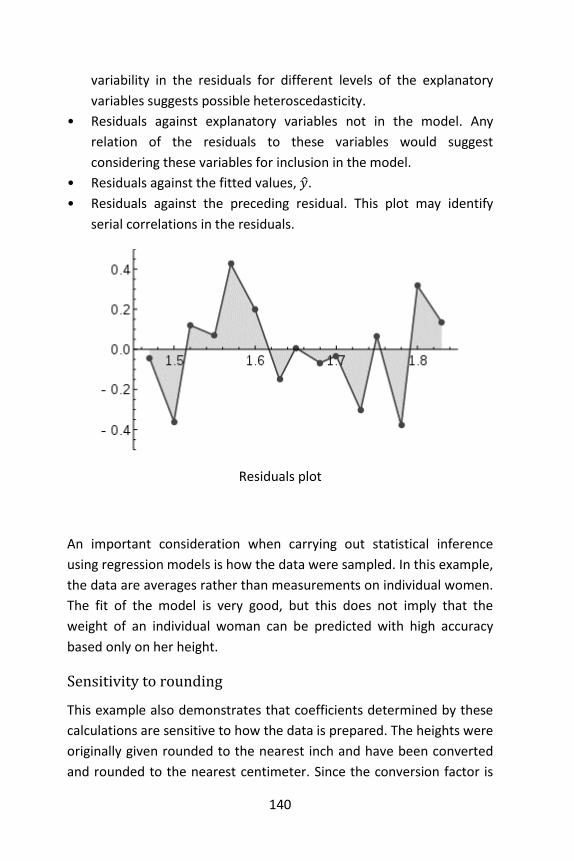
140

variability in the residuals for different levels of the explanatory

variables suggests possible heteroscedasticity.

• Residuals against explanatory variables not in the model. Any

relation of the residuals to these variables would suggest

considering these variables for inclusion in the model.

• Residuals against the fitted values, �̂�.

• Residuals against the preceding residual. This plot may identify

serial correlations in the residuals.

Residuals plot

An important consideration when carrying out statistical inference

using regression models is how the data were sampled. In this example,

the data are averages rather than measurements on individual women.

The fit of the model is very good, but this does not imply that the

weight of an individual woman can be predicted with high accuracy

based only on her height.

Sensitivity to rounding

This example also demonstrates that coefficients determined by these

calculations are sensitive to how the data is prepared. The heights were

originally given rounded to the nearest inch and have been converted

and rounded to the nearest centimeter. Since the conversion factor is

141

one inch to 2.54 cm this is not an exact conversion. The original inches

can be recovered by Round(x/0.0254) and then re-converted to metric

without rounding. If this is done the results become:

Constant Height Height2

128.8128 -143.1620 61.96033 Converted to metric with rounding.

119.0205 -131.5076 58.50460 Converted to metric without rounding.

Using either of these equations to predict the weight of a 5' 6”

(1.6764m) woman gives similar values: 62.94 kg with rounding vs.

62.98 kg without rounding. Thus a seemingly small variation in the data

has a real effect on the coefficients but a small effect on the results of

the equation.

While this may look innocuous in the middle of the data range it could

become significant at the extremes or in the case where the fitted

model is used to project outside the data range (extrapolation).

This highlights a common error: this example is an abuse of OLS which

inherently requires that the errors in the dependent variable (in this

case height) are zero or at least negligible. The initial rounding to

nearest inch plus any actual measurement errors constitute a finite and

non-negligible error. As a result the fitted parameters are not the best

estimates they are presumed to be. Though not totally spurious the

error in the estimation will depend upon relative size of the 𝑥 and 𝑦

errors.

Software

All major statistical software packages perform least squares regression

analysis and inference. Simple linear regression and multiple regression

using least squares can be done in some spreadsheet applications and

on some calculators. While many statistical software packages can

perform various types of nonparametric and robust regression, these

methods are less standardized; different software packages implement

different methods, and a method with a given name may be

142

implemented differently in different packages. Specialized regression

software has been developed for use in fields such as survey analysis

and neuroimaging.

Open Source software that perform OLS include DAP, Octave, R, and

Weke. Commercial software that perform OLS include Analytica, SPSS

Modeler, MATLAB, SAS Enterprise and STATISTICA.

143

Example Using R

Now let’s look at an example concerning the number of species of

tortoise on the various Galapagos Islands. There are 30 cases (Islands)

and 7 variables in the dataset. We start by reading the data into R and

examining it. Copy the following data and save it as a text file: gala.txt

(tab delimited) in a directory, like “C/mydata/”.

Species Endemics Area Elevation Nearest Scruz Adjacent Baltra 58 23 25.09 346 0.6 0.6 1.84 Bartolome 31 21 1.24 109 0.6 26.3 572.33 Caldwell 3 3 0.21 114 2.8 58.7 0.78 Champion 25 9 0.10 46 1.9 47.4 0.18 Coamano 2 1 0.05 77 1.9 1.9 903.82 Daphne.Major 18 11 0.34 119 8.0 8.0 1.84 Daphne.Minor 24 0 0.08 93 6.0 12.0 0.34 Darwin 10 7 2.33 168 34.1 290.2 2.85 Eden 8 4 0.03 71 0.4 0.4 17.95 Enderby 2 2 0.18 112 2.6 50.2 0.10 Espanola 97 26 58.27 198 1.1 88.3 0.57 Fernandina 93 35 634.49 1494 4.3 95.3 4669.32 Gardner1 58 17 0.57 49 1.1 93.1 58.27 Gardner2 5 4 0.78 227 4.6 62.2 0.21 Genovesa 40 19 17.35 76 47.4 92.2 129.49 Isabela 347 89 4669.32 1707 0.7 28.1 634.49 Marchena 51 23 129.49 343 29.1 85.9 59.56 Onslow 2 2 0.01 25 3.3 45.9 0.10 Pinta 104 37 59.56 777 29.1 119.6 129.49 Pinzon 108 33 17.95 458 10.7 10.7 0.03 Las.Plazas 12 9 0.23 94 0.5 0.6 25.09 Rabida 70 30 4.89 367 4.4 24.4 572.33 SanCristobal 280 65 551.62 716 45.2 66.6 0.57 SanSalvador 237 81 572.33 906 0.2 19.8 4.89 SantaCruz 444 95 903.82 864 0.6 0.0 0.52 SantaFe 62 28 24.08 259 16.5 16.5 0.52 SantaMaria 285 73 170.92 640 2.6 49.2 0.10 Seymour 44 16 1.84 147 0.6 9.6 25.09 Tortuga 16 8 1.24 186 6.8 50.9 17.95 Wolf 21 12 2.85 253 34.1 254.7 2.33

Change the working directory to "c:/mydata" (do this by choosing

"File"->"Change directory", and then inputting the directory name).

And now you can simply read the data into R by:

> gala <- read.table("gala.txt") # read the data into R

Now we can take a look at the data.

> data(gala) > gala Species Endemics Area Elevation Nearest Scruz Adjacent

144

Baltra 58 23 25.09 346 0.6 0.6 1.84 Bartolome 31 21 1.24 109 0.6 26.3 572.33 --- cases deleted --- Tortuga 16 8 1.24 186 6.8 50.9 17.95 Wolf 21 12 2.85 253 34.1 254.7 2.33

The variables are

Species The number of species of tortoise found on the island Endemics The number of endemic species Elevation The highest elevation of the island (m) Nearest The distance from the nearest island (km) Scruz The distance from Santa Cruz island

(km) Adjacent The area of the adjacent island (km2) The data were presented by Johnson and Raven (Johnson & Raven, 1973) and also appear in Weisberg (Weisberg, 2005). We have filled in some missing values for simplicity. Fitting a linear model in R is done using the lm() command. Notice the syntax for specifying the predictors in the model. This is the so-called Wilkinson-Rogers notation. In this case, since all the variables are in the gala data frame, we must use the data= argument. First, we generate a series of plots of various species-area relations. We

consider three models: Linear, Gleason, and log-Arrhenius.

1. Linear model: 𝑆~Normal(𝜇, 𝜎2) with identity link such that 𝜇 =

𝛽0 + 𝛽1𝐴.

2. Gleason model: 𝑆~Normal(𝜇, 𝜎2) with identity link such that 𝜇 =

𝛽0 + 𝛽1log𝐴.

3. log-Arrhenius model: 𝑆~Normal(𝜇, 𝜎2) with identity link such that

𝜇 = 𝛽0𝐴𝛽1.

Model 1 is a Linear Model. We fit a linear model on the original scale,

model 1 above and obtain the log-likelihood (with logLik) and the AIC

(with AIC).

> model1<-lm(Species~Area,data=gala) > logLik(model1) 'log Lik.' -177.0993 (df=3)

145

> AIC(model1) [1] 360.1985

We superimpose the fitted model on a scatter plot of the data.

> plot(gala$Area,gala$Species, xlab='Area', ylab='Species') > abline(model1,col=2, lty=2) > mtext('Model 1: linear model', side=3, line=.5)

Model 2 is a Gleason Model. The Gleason model requires a log-

transformed predictor, but an untransformed response.

> model2<-lm(Species~log(Area),data=gala) > logLik(model2) 'log Lik.' -169.9574 (df=3) > AIC(model2) [1] 345.9147 > plot(log(gala$Area), gala$Species, xlab='log(Area)', + ylab='Species') > abline(model2,col=2,lty=2)

146

> mtext( 'Model 2: Gleason model', side=3, line=.5)

Model 3 is a log-Arrhenius. The log-Arrhenius model is just an ordinary

regression model in which both the response and predictor are log-

transformed.

> model3<-lm(log(Species)~log(Area), data=gala) > logLik(model3) 'log Lik.' -34.23973 (df=3) > AIC(model3) [1] 74.47946 > plot(log(gala$Area), log(gala$Species), xlab='log(Area)', + ylab='log(Species)') > abline(model3,col=2,lty=2) > mtext('Model 3: log-Arrhenius model', side=3, line=.5)

147

Now we want to compare the models. We begin by collecting the

names of our models.

> model.names<-c('Linear', 'Gleason', 'Log-Arrhenius')

Next we concatenate all the calculated log-likelihoods together.

> loglike <-c(logLik(model1),logLik(model2),logLik(model3))

Next we concatenate a list of the number of parameters estimated for

each model. Each model has three parameters—𝛽0, 𝛽1, and 𝜎2.

> numparms<-c(3,3,3)

Finally, we create our function to carry out the calculations.

# LL is loglikelihood, # K is number of estimated parameters # n is the sample size

148

> AIC.func<-function(LL,K,n,modelnames) + { + AIC<- -2*LL + 2*K + AICc<-AIC + 2*K*(K+1)/(n-K-1) + output<-cbind(LL,K,AIC,AICc) + colnames(output)<-c('LogL','K','AIC','AICc') + minAICc<-min(output[,"AICc"]) + deltai<-output[,"AICc"]-minAICc + rel.like<-exp(-deltai/2) + wi<-round(rel.like/sum(rel.like),3) + out<-data.frame(modelnames,output,deltai,wi) + out + } > AIC.func(loglike,numparms,dim(gala)[1],model.names) modelnames LogL K AIC AICc deltai wi 1 Linear -177.09927 3 360.19853 361.12161 285.7191 0 2 Gleason -169.95737 3 345.91473 346.83781 271.4353 0 3 Log-Arrhenius -34.23973 3 74.47946 75.40253 0.0000 1

Based on the output we see there is only one model that has any

empirical support, the log-Arrhenius model. For reasons we will not

explain here, although the log-Arrhenius model fits well, it is not

guaranteed to be optimal. For the Galapagos data, a model that allows

there to be heteroscedasticity on the scale of the original response is to

be preferred.

The previous models only examine the Species-Area relationship. We

now consider additional variables: Endemics, Elevation, Nearest,

Scruz, and Adjacent. We will call our model gfit.

> gfit <- lm(Species~Area + Elevation + Nearest + Scruz + + Adjacent, data=gala) > summary(gfit) Call: > lm(formula = Species~Area + Elevation + Nearest + Scruz + + Adjacent, data=gala) > summary(gfit) Call: lm(formula = Species ~ Area + Elevation + Nearest + Scruz + Adjacent, data = gala) Residuals: Min 1Q Median 3Q Max -111.679 -34.898 -7.862 33.460 182.584

149

Coefficients: Estimate Std. Error t value Pr(>|t|) (Intercept) 7.068221 19.154198 0.369 0.715351 Area -0.023938 0.022422 -1.068 0.296318 Elevation 0.319465 0.053663 5.953 3.82e-06 *** Nearest 0.009144 1.054136 0.009 0.993151 Scruz -0.240524 0.215402 -1.117 0.275208 Adjacent -0.074805 0.017700 -4.226 0.000297 *** --- Signif. codes: 0 ‘***’ 0.001 ‘**’ 0.01 ‘*’ 0.05 ‘.’ 0.1 ‘ ’ 1

Residual standard error: 60.98 on 24 degrees of freedom Multiple R-squared: 0.7658, Adjusted R-squared: 0.7171 F-statistic: 15.7 on 5 and 24 DF, p-value: 6.838e-07

We can identify several useful quantities in this output. Other statistical

packages tend to produce output quite similar to this. One useful

feature of R is that it is possible to directly calculate quantities of

interest. Of course, it is not necessary here because the lm() function

does the job but it is very useful when the statistic you want is not part

of the pre-packaged functions.

First we make the 𝑋-matrix

> x <- cbind(1,gala[,-c(1,2)])

and here’s the response 𝑦:

> y <- gala$Species

Now let’s construct 𝑋’𝑋: t() does transpose and %*% does matrix

multiplication:

> t(x) %*% x Error: %*% requires numeric matrix/vector arguments

Gives a somewhat cryptic error. The problem is that matrix arithmetic

can only be done with numeric values but 𝑥 here derives from the

data frame type. Data frames are allowed to contain character

variables, which would disallow matrix arithmetic. We need to force 𝑥

into the matrix form:

> x <- as.matrix(x)

150

> t(x) %*% x 1 Area Elevation Nearest 1 30.00 7851.26 11041.0 301.80 Area 7851.26 23708665.46 10852798.5 39240.84 Elevation 11041.00 10852798.53 9218227.0 109139.20 Nearest 301.80 39240.84 109139.2 8945.30 Scruz 1709.30 275516.84 616237.8 34527.34 Adjacent 7832.95 5950313.65 8553187.9 37196.67 Scruz Adjacent 1 1709.30 7832.95 Area 275516.84 5950313.65 Elevation 616237.80 8553187.95 Nearest 34527.34 37196.67 Scruz 231613.77 534409.98 Adjacent 534409.98 23719568.46

Inverses can be taken using the solve() command:

> xtxi <- solve(t(x) %*% x) > xtxi 1 Area Elevation 1 9.867829e-02 3.778242e-05 -1.561976e-04 Area 3.778242e-05 1.352247e-07 -2.593617e-07 Elevation -1.561976e-04 -2.593617e-07 7.745339e-07 Nearest -2.339027e-04 1.294003e-06 -3.549366e-06 Scruz -3.760293e-04 -4.913149e-08 3.080831e-07 Adjacent 2.309832e-05 4.620303e-08 -1.640241e-07 Nearest Scruz Adjacent 1 -2.339027e-04 -3.760293e-04 2.309832e-05 Area 1.294003e-06 -4.913149e-08 4.620303e-08 Elevation -3.549366e-06 3.080831e-07 -1.640241e-07 Nearest 2.988732e-04 -3.821077e-05 1.424729e-06 Scruz -3.821077e-05 1.247941e-05 -1.958356e-07 Adjacent 1.424729e-06 -1.958356e-07 8.426543e-08

A somewhat more direct way to get _ (𝑋’𝑋)−1 is as follows:

> gfit <- lm(Species~Area+Elevation+Nearest+Scruz+Adjacent, + data=gala) > gs <- summary(gfit) > gs$cov.unscaled (Intercept) Area Elevation (Intercept) 9.867829e-02 3.778242e-05 -1.561976e-04 Area 3.778242e-05 1.352247e-07 -2.593617e-07 Elevation -1.561976e-04 -2.593617e-07 7.745339e-07 Nearest -2.339027e-04 1.294003e-06 -3.549366e-06 Scruz -3.760293e-04 -4.913149e-08 3.080831e-07 Adjacent 2.309832e-05 4.620303e-08 -1.640241e-07 Nearest Scruz Adjacent (Intercept) -2.339027e-04 -3.760293e-04 2.309832e-05

151

Area 1.294003e-06 -4.913149e-08 4.620303e-08 Elevation -3.549366e-06 3.080831e-07 -1.640241e-07 Nearest 2.988732e-04 -3.821077e-05 1.424729e-06 Scruz -3.821077e-05 1.247941e-05 -1.958356e-07 Adjacent 1.424729e-06 -1.958356e-07 8.426543e-08

The names()command is the way to see the components of an Splus

object - you can see that there are other useful quantities that are

directly available:

> names(gs) > names(gfit)

In particular, the fitted (or predicted) values and residuals are

> gfit$fit Baltra Bartolome Caldwell Champion 116.7259460 -7.2731544 29.3306594 10.3642660 Coamano Daphne.Major Daphne.Minor Darwin -36.3839155 43.0877052 33.9196678 -9.0189919 Eden Enderby Espanola Fernandina 28.3142017 30.7859425 47.6564865 96.9895982 Gardner1 Gardner2 Genovesa Isabela -4.0332759 64.6337956 -0.4971756 386.4035578 Marchena Onslow Pinta Pinzon 88.6945404 4.0372328 215.6794862 150.4753750 Las.Plazas Rabida SanCristobal SanSalvador 35.0758066 75.5531221 206.9518779 277.6763183 SantaCruz SantaFe SantaMaria Seymour 261.4164131 85.3764857 195.6166286 49.8050946 Tortuga Wolf 52.9357316 26.7005735 > gfit$res Baltra Bartolome Caldwell Champion -58.725946 38.273154 -26.330659 14.635734 Coamano Daphne.Major Daphne.Minor Darwin 38.383916 -25.087705 -9.919668 19.018992 Eden Enderby Espanola Fernandina -20.314202 -28.785943 49.343513 -3.989598 Gardner1 Gardner2 Genovesa Isabela 62.033276 -59.633796 40.497176 -39.403558 Marchena Onslow Pinta Pinzon -37.694540 -2.037233 -111.679486 -42.475375 Las.Plazas Rabida SanCristobal SanSalvador -23.075807 -5.553122 73.048122 -40.676318 SantaCruz SantaFe SantaMaria Seymour 182.583587 -23.376486 89.383371 -5.805095 Tortuga Wolf -36.935732 -5.700573

152

We can get �̂�directly:

> xtxi %*% t(x) %*% y [,1] 1 7.068220709 Area -0.023938338 Elevation 0.319464761 Nearest 0.009143961 Scruz -0.240524230 Adjacent -0.074804832

or in a computationally efficient and stable manner:

> solve(t(x) %*% x, t(x) %*% y) [,1] [1,] 7.068220709 [2,] -0.023938338 [3,] 0.319464761 [4,] 0.009143961 [5,] -0.240524230 [6,] -0.074804832

We can estimate 𝜎using the estimator in the text:

> root1<-sum((gfit$res)^2) > sqrt(root1/(30-6)) [1] 60.97519

Compare this to the results above (Residual standard error).

We may also obtain the standard errors for the coefficients. Also

diag() returns the diagonal of a matrix):

> sqrt(diag(xtxi))*60.97519 1 Area Elevation Nearest 19.15419834 0.02242235 0.05366281 1.05413598 Scruz Adjacent 0.21540225 0.01770019

Finally we may compute 𝑅2: > 1-sum((gfit$res)ˆ2)/sum((y-mean(y))ˆ2) [1] 0.7658469

153

9. Generalized linear model

In statistics, the generalized linear model (GLM)—not to be confused

with general linear model or generalized least squares—is a flexible

generalization of ordinary linear regression that allows for response

variables that have error distribution models other than a normal

distribution. The GLM generalizes linear regression by allowing the

linear model to be related to the response variable via a link function

and by allowing the magnitude of the variance of each measurement to

be a function of its predicted value.

Generalized linear models were formulated by John Nelder and Robert

Wedderburn as a way of unifying various other statistical models,

including linear regression, logistic regression and Poisson regression

(Nelder & Wedderburn, 1972). They proposed an iteratively

reweighted least squares method for maximum likelihood estimation

of the model parameters. Maximum-likelihood estimation remains

popular and is the default method on many statistical computing

packages. Other approaches, including Bayesian approaches and least

squares fits to variance stabilized responses, have been developed.

Intuition

Ordinary linear regression predicts the expected value of a given

unknown quantity (the response variable, a random variable) as a

linear combination of a set of observed values (predictors). This implies

that a constant change in a predictor leads to a constant change in the

response variable (i.e. a linear-response model). This is appropriate

when the response variable has a normal distribution (intuitively, when

a response variable can vary essentially indefinitely in either direction

with no fixed “zero value”, or more generally for any quantity that only

varies by a relatively small amount, e.g. human heights).

However, these assumptions are inappropriate for many types of

154

response variables. For example, in many cases when the response

variable must be positive and can vary over a wide scale, constant input

changes lead to geometrically varying rather than constantly varying

output changes. As an example, a model that predicts that each

decrease in 10 degrees Fahrenheit leads to 1,000 fewer people going to

a given beach is unlikely to generalize well over both small beaches

(e.g. those where the expected attendance was 50 at the lower

temperature) and large beaches (e.g. those where the expected

attendance was 10,000 at the lower temperature). An even worse

problem is that, since the model also implies that a drop in 10 degrees

leads 1,000 fewer people going to a given beach, a beach whose

expected attendance was 50 at the higher temperature would now be

predicted to have the impossible attendance value of -950. Logically, a

more realistic model would instead predict a constant rate of increased

beach attendance (e.g. an increase in 10 degrees leads to a doubling in

beach attendance, and a drop in 10 degrees leads to a halving in

attendance). Such a model is termed an exponential-response model

(or log-linear model, since the logarithm of the response is predicted to

vary linearly).

Similarly, a model that predicts a probability of making a yes/no choice

(a Bernoulli variable) is even less suitable as a linear-response model,

since probabilities are bounded on both ends (they must be between 0

and 1). Imagine, for example, a model that predicts the likelihood of a

given person going to the beach as a function of temperature. A

reasonable model might predict, for example, that a change in 10

degrees makes a person two times more or less likely to go to the

beach. But what does “twice as likely” mean in terms of a probability?

It cannot literally mean to double the probability value (e.g. 50%

becomes 100%, 75% becomes 150%, etc.). Rather, it is the odds that

are doubling: from 2:1 odds, to 4:1 odds, to 8:1 odds, etc. Such a model

is a log-odds model.

Generalized linear models cover all these situations by allowing for

response variables that have arbitrary distributions (rather than simply

155

normal distributions), and for an arbitrary function of the response

variable (the link function) to vary linearly with the predicted values

(rather than assuming that the response itself must vary linearly). For

example, the case above of predicted number of beach attendees

would typically be modeled with a Poisson distribution and a log link,

while the case of predicted probability of beach attendance would

typically be modeled with a Bernoulli distribution (or binomial

distribution, depending on exactly how the problem is phrased) and a

log-odds (or logit) link function.

Overview

In a generalized linear model (GLM), each outcome of the dependent

variables, 𝒀, is assumed to be generated from a particular distribution

in the exponential family, a large range of probability distributions that

includes the normal, binomial, Poisson and gamma distributions,

among others. The mean, 𝝁, of the distribution depends on the

independent variables, 𝑿, through:

𝐸(𝒀) = 𝝁 = 𝑔−1(𝑿𝜷),

where 𝐸(𝒀) is the expected value of 𝒀; 𝑿𝜷 is the linear predictor, a

linear combination of unknown parameters, 𝜷; 𝑔 is the link function.

In this framework, the variance is typically a function, 𝑉, of the mean:

Var(𝒀) = 𝑉(𝝁) = 𝑉(𝑔−1(𝑿𝜷)).

It is convenient if 𝑉 follows from the exponential family distribution,

but it may simply be that the variance is a function of the predicted

value.

The unknown parameters, 𝜷, are typically estimated with maximum

likelihood, maximum quasi-likelihood, or Bayesian techniques.

Model components

The GLM consists of three elements:

156

1. A probability distribution from the exponential family.

2. A linear predictor 𝜂 = 𝑿𝜷.

3. A link function g such that 𝐸(𝒀) = 𝝁 = 𝑔 − 1(𝜂).

Probability distribution

The overdispersed exponential family of distributions is a

generalization of the exponential family and exponential dispersion

model of distributions and includes those probability distributions,

parameterized by 𝜽 and , whose density functions f (or

probability mass function, for the case of a discrete distribution) can be

expressed in the form

𝑓𝑌(𝒚|𝜽, 𝜏) = ℎ(𝒚, 𝜏)exp (𝒃(𝜽)𝑻(𝑦) − 𝐴(𝜽)

𝑑(𝜏)).

𝜏, called the dispersion parameter, typically is known and is usually

related to the variance of the distribution. The functions ℎ(𝒚, 𝜏), 𝒃(𝜽),

𝑻(𝑦), 𝑨(𝜽), and 𝑑(𝜏) are known. Many common distributions are in

this family.

For scalar 𝑌 and 𝜃, this reduces to

𝑓𝑌(𝑦|𝜃, 𝜏) = ℎ(𝑦, 𝜏)exp (𝑏(𝜃)𝑇(𝑦) − 𝐴(𝜃)

𝑑(𝜏)).

𝜽 is related to the mean of the distribution. If 𝒃(𝜽) is the identity

function, then the distribution is said to be in canonical form (or

natural form). Note that any distribution can be converted to canonical

form by rewriting 𝜽 as 𝜽′ and then applying the transformation 𝜽 =

𝒃(𝜽′). It is always possible to convert 𝑨(𝜽) in terms of the new

parameterization, even if 𝒃(𝜽′)is not a one-to-one function; see

comments in the page on the exponential family. If, in addition, 𝑻(𝑦)is

the identity and 𝝉 is known, then 𝜽 is called the canonical parameter

(or natural parameter) and is related to the mean through

157

𝝁 = 𝐸(𝒀) = ∇𝐴(𝜽).

For scalar 𝑌 and 𝜃, this reduces to

𝜇 = 𝐸(𝑌) = 𝐴′(𝜃).

Under this scenario, the variance of the distribution can be shown to

be (McCullagh & Nelder, 1989)

Var(𝒀) = ∇∇𝑇𝐴(𝜽)𝑑(𝜏).

For scalar 𝑌 and 𝜃, this reduces to

Var(𝑌) = 𝐴′′(𝜃)𝑑(𝜏).

Linear predictor

The linear predictor is the quantity which incorporates the information

about the independent variables into the model. The symbol 𝜂 (Greek

“eta“) denotes a linear predictor. It is related to the expected value of

the data (thus, “predictor”) through the link function.

𝜂 is expressed as linear combinations (thus, “linear”) of unknown

parameters 𝜷. The coefficients of the linear combination are

represented as the matrix of independent variables 𝑿. 𝜂 can thus be

expressed as

𝜂 = 𝑿𝜷.

Link function

The link function provides the relationship between the linear predictor

and the mean of the distribution function. There are many commonly

used link functions, and their choice can be somewhat arbitrary. It

makes sense to try to match the domain of the link function to the

range of the distribution function's mean.

When using a distribution function with a canonical parameter 𝜃, the

canonical link function is the function that expresses 𝜃 in terms of 𝜇,

i.e. 𝜃 = 𝑏(𝜇). For the most common distributions, the mean 𝜇 is one of

158

the parameters in the standard form of the distribution's density

function, and then 𝑏(𝜇) is the function as defined above that maps the

density function into its canonical form. When using the canonical link

function, 𝑏(𝜇) = 𝜃 = 𝑿𝜷, which allows 𝑿𝑇Y to be a sufficient

statistic for 𝜷.

Following is a table of several exponential-family distributions in

common use and the data they are typically used for, along with the

canonical link functions and their inverses (sometimes referred to as

the mean function, as done here).

Common distributions with typical uses and canonical link functions

Distribution Support of distribution Typical uses Link name

Link function Mean function

Normal real: (−∞, ∞) Linear-response data Identity 𝑿𝜷 = 𝜇 𝜇 = 𝑿𝜷

Exponential real: (0, ∞) Exponential-response data, scale parameters

Inverse 𝑿𝜷 = −𝜇−1

𝜇 = (−𝑿𝜷)−1

Gamma

Inverse Gaussian

real: (0, ∞) Inverse squared

𝑿𝜷 = −𝜇−2

𝜇

= (−𝑿𝜷)−1 2⁄ Poisson integer: (0, ∞) count of occurrences in

fixed amount of time/space

Log 𝑿𝜷 = ln(𝜇)

𝜇 = 𝑒𝑿𝜷

Bernoulli integer: [0,1] outcome of single yes/no occurrence

Logit 𝑿𝜷

= ln (𝜇

1 − 𝜇)

𝜇 =1

1 + 𝑒𝑿𝜷

Binomial integer: [0, 𝑁] count of # of “yes” occurrences out of N yes/no occurrences

Categorical integer: [0, 𝐾] outcome of single K-way occurrence K-vector of integer:

[0,1], where exactly one element in the vector has the value 1

Multinomial K-vector of [0, 𝑁] count of occurrences of different types (1 .. K) out of N total K-way occurrences

In the cases of the exponential and gamma distributions, the domain of

the canonical link function is not the same as the permitted range of

159

the mean. In particular, the linear predictor may be negative, which

would give an impossible negative mean. When maximizing the

likelihood, precautions must be taken to avoid this. An alternative is to

use a noncanonical link function.

Note also that in the case of the Bernoulli, binomial, categorical and

multinomial distributions, the support of the distributions is not the

same type of data as the parameter being predicted. In all of these

cases, the predicted parameter is one or more probabilities, i.e. real

numbers in the range [0,1]. The resulting model is known as logistic

regression (or multinomial logistic regression in the case that 𝐾-way

rather than binary values are being predicted).

For the Bernoulli and binomial distributions, the parameter is a single

probability, indicating the likelihood of occurrence of a single event.

The Bernoulli still satisfies the basic condition of the generalized linear

model in that, even though a single outcome will always be either 0 or

1, the expected value will nonetheless be a real-valued probability, i.e.

the probability of occurrence of a “yes” (or 1) outcome. Similarly, in a

binomial distribution, the expected value is 𝑁𝑝, i.e. the expected

proportion of “yes” outcomes will be the probability to be predicted.

For categorical and multinomial distributions, the parameter to be

predicted is a 𝐾-vector of probabilities, with the further restriction that

all probabilities must add up to 1. Each probability indicates the

likelihood of occurrence of one of the 𝐾 possible values. For the

multinomial distribution, and for the vector form of the categorical

distribution, the expected values of the elements of the vector can be

related to the predicted probabilities similarly to the binomial and

Bernoulli distributions.

Fitting

Maximum likelihood

The maximum likelihood estimates can be found using an iteratively

reweighted least squares algorithm using either a Newton–Raphson

160

method with updates of the form:

𝜷(𝑡+1) = 𝜷(𝑡) + 𝒥−1(𝜷(𝑡))𝑢(𝜷(𝑡)),

where 𝒥(𝜷(𝑡))is the observed information matrix (the negative of the

Hessian matrix) and 𝑢(𝜷(𝑡)) is the score function; or a Fisher's scoring

method:

𝜷(𝑡+1) = 𝜷(𝑡) + 𝐼−1(𝜷(𝑡))𝑢(𝜷(𝑡)),

where 𝐼(𝜷(𝑡)) is the Fisher information matrix. Note that if the

canonical link function is used, then they are the same.

Bayesian methods

In general, the posterior distribution cannot be found in closed form

and so must be approximated, usually using Laplace approximations or

some type of Markov chain Monte Carlo method such as Gibbs

sampling.

Examples

General linear models

A possible point of confusion has to do with the distinction between

generalized linear models and the general linear model, two broad

statistical models. The general linear model may be viewed as a special

case of the generalized linear model with identity link and responses

normally distributed. As most exact results of interest are obtained

only for the general linear model, the general linear model has

undergone a somewhat longer historical development. Results for the

generalized linear model with non-identity link are asymptotic (tending

to work well with large samples).

Linear regression

A simple, very important example of a generalized linear model (also

an example of a general linear model) is linear regression. In linear

regression, the use of the least-squares estimator is justified by the

161

Gauss-Markov theorem, which does not assume that the distribution is

normal.

From the perspective of generalized linear models, however, it is useful

to suppose that the distribution function is the normal distribution with

constant variance and the link function is the identity, which is the

canonical link if the variance is known.

For the normal distribution, the generalized linear model has a closed

form expression for the maximum-likelihood estimates, which is

convenient. Most other GLMs lack closed form estimates.

Binomial data

When the response data, Y, are binary (taking on only values 0 and 1),

the distribution function is generally chosen to be the Bernoulli

distribution and the interpretation of 𝜇𝑖 is then the probability, 𝑝, of 𝑌𝑖

taking on the value one.

There are several popular link functions for binomial functions; the

most typical is the canonical logit link:

𝑔(𝑝) = ln (𝑝

1 − 𝑝).

GLMs with this setup are logistic regression models (or logit models).

In addition, the inverse of any continuous cumulative distribution

function (CDF) can be used for the link since the CDF's range is [0,1],

the range of the binomial mean. The normal CDF Φ is a popular choice

and yields the probit model. Its link is

𝑔(𝑝) = Φ−1(𝑝).

The reason for the use of the probit model is that a constant scaling of

the input variable to a normal CDF (which can be absorbed through

equivalent scaling of all of the parameters) yields a function that is

practically identical to the logit function, but probit models are more

tractable in some situations than logit models. (In a Bayesian setting in

162

which normally distributed prior distributions are placed on the

parameters, the relationship between the normal priors and the

normal CDF link function means that a probit model can be computed

using Gibbs sampling, while a logit model generally cannot.)

The complementary log-log function log(−log(1 − 𝑝)) may also be

used. This link function is asymmetric and will often produce different

results from the probit and logit link functions.

The identity link is also sometimes used for binomial data to yield the

linear probability model, but a drawback of this model is that the

predicted probabilities can be greater than one or less than zero. In

implementation it is possible to fix the nonsensical probabilities outside

of [0,1], but interpreting the coefficients can be difficult. The model's

primary merit is that near 𝑝 = 0.5 it is approximately a linear

transformation of the probit and logit―econometricians sometimes

call this the Harvard model.

The variance function for binomial data is given by:

Var(𝑌𝑖) = 𝜏𝜇𝑖(1 − 𝜇𝑖),

where the dispersion parameter 𝜏 is typically fixed at exactly one.

When it is not, the resulting quasi-likelihood model often described as

binomial with overdispersion or quasi-binomial.

Multinomial regression

The binomial case may be easily extended to allow for a multinomial

distribution as the response (also, a Generalized Linear Model for

counts, with a constrained total). There are two ways in which this is

usually done:

Ordered response

If the response variable is an ordinal measurement, then one may fit a

model function of the form:

𝑔(𝜇𝑚) = 𝜂𝑚 = 𝛽0 + 𝑋1𝛽1 + ⋯ + 𝑋𝑝𝛽𝑝 + 𝛾2 + ⋯ + 𝛾𝑚

163

= 𝜂1 + 𝛾2 + ⋯ + 𝛾𝑚,

where 𝜇𝑚 = 𝑃(𝑌 ≤ 𝑚), for 𝑚 > 2. Different links 𝑔 lead to

proportional odds models or ordered probit models.

Unordered response

If the response variable is a nominal measurement, or the data do not

satisfy the assumptions of an ordered model, one may fit a model of

the following form:

𝑔(𝜇𝑚) = 𝜂𝑚 = 𝛽𝑚,0 + 𝑋1𝛽𝑚,1 + ⋯ + 𝑋𝑝𝛽𝑚,𝑝,

where 𝜇𝑚 = 𝑃(𝑌 = 𝑚|𝑌 ∈ {1, 𝑚}), for 𝑚 > 2. Different links g lead to

multinomial logit or multinomial probit models. These are more

general than the ordered response models, and more parameters are

estimated.

Count data

Another example of generalized linear models includes Poisson

regression which models count data using the Poisson distribution. The

link is typically the logarithm, the canonical link. The variance function

is proportional to the mean

var(𝑌𝑖) = 𝜏𝜇𝑖,

where the dispersion parameter 𝜏 is typically fixed at exactly one.

When it is not, the resulting quasi-likelihood model is often described

as Poisson with overdispersion or quasi-Poisson.

Extensions

Correlated or clustered data

The standard GLM assumes that the observations are uncorrelated.

Extensions have been developed to allow for correlation between

observations, as occurs for example in longitudinal studies and

clustered designs:

164

• Generalized estimating equations (GEEs) allow for the correlation

between observations without the use of an explicit probability model

for the origin of the correlations, so there is no explicit likelihood. They

are suitable when the random effects and their variances are not of

inherent interest, as they allow for the correlation without explaining

its origin. The focus is on estimating the average response over the

population (“population-averaged” effects) rather than the regression

parameters that would enable prediction of the effect of changing one

or more components of 𝑿 on a given individual. GEEs are usually used

in conjunction with Huber-White standard errors (Zeger, Liang, &

Albert, 1988) (Hardin & Hilbe, 2003).

• Generalized linear mixed models (GLMMs) are an extension to GLMs

that includes random effects in the linear predictor, giving an explicit

probability model that explains the origin of the correlations. The

resulting “subject-specific” parameter estimates are suitable when the

focus is on estimating the effect of changing one or more components

of 𝑿 on a given individual. GLMMs are also referred to as multilevel

models and as mixed model. In general, fitting GLMMs is more

computationally complex and intensive than fitting GEEs.

Generalized additive models

Generalized additive models (GAMs) are another extension to GLMs in

which the linear predictor 𝜂 is not restricted to be linear in the

covariates 𝑿 but is the sum of smoothing functions applied to the 𝑥𝑖’s:

𝜂 = 𝛽0 + 𝑓1(𝑥1) + 𝑓2(𝑥2) + ⋯.

The smoothing functions 𝑓𝑖 are estimated from the data. In general this

requires a large number of data points and is computationally intensive

(Hastie & Tibshirani, 1990) (Wood, 2006).

The model relates a univariate response variable, 𝑌, to some predictor

variables, 𝑥𝑖. An exponential family distribution is specified for 𝑌 (for

example normal, binomial or Poisson distributions) along with a link

function 𝑔 (for example the identity or log functions) relating the

165

expected value of 𝑌 to the predictor variables via a structure such as

𝑔(𝐸(𝑌)) = 𝜂 = 𝛽0 + 𝑓1(𝑥1) + 𝑓2(𝑥2) + ⋯ 𝑓𝑚(𝑥𝑚).

The functions 𝑓𝑖(𝑥𝑖) may be functions with a specified parametric form

(for example a polynomial, or a coefficient depending on the levels of a

factor variable) or maybe specified non-parametrically, or semi-

parametrically, simply as ‘smooth functions’, to be estimated by non-

parametric means. So a typical GAM might use a scatterplot smoothing

function, such as a locally weighted mean, for 𝑓1(𝑥1), and then use a

factor model for 𝑓2(𝑥2). This flexibility to allow non-parametric fits

with relaxed assumptions on the actual relationship between response

and predictor, provides the potential for better fits to data than purely

parametric models, but arguably with some loss of interpretablity.

Generalized additive model for location, scale and shape

The generalized additive model location, scale and shape (GAMLSS) is a

class of statistical model that provides extended capabilities compared

to the simpler generalized linear models and generalized additive

models. These simpler models allow the typical values of a quantity

being modelled to be related to whatever explanatory variables are

available. Here the “typical value” is more formally a location

parameter, which only describes a limited aspect of the probability

distribution of the dependent variable. The GAMLSS approach allows

other parameters of the distribution to be related to the explanatory

variables; where these other parameters might be interpreted as scale

and shape parameters of the distribution, although the approach is not

limited to such parameters.

In GAMLSS the exponential family distribution assumption for the

response variable, (𝑌), (essential in GLMs and GAMs), is relaxed and

replaced by a general distribution family, including highly skew and/or

kurtotic continuous and discrete distributions.

The systematic part of the model is expanded to allow modeling not

only of the mean (or location) but other parameters of the distribution

166

of Y as linear and/or nonlinear, parametric and/or additive non-

parametric functions of explanatory variables and/or random effects.

GAMLSS is especially suited for modeling leptokurtic or platykurtic

and/or positive or negative skew response variable. For count type

response variable data it deals with over-dispersion by using proper

over-dispersed discrete distributions. Heterogeneity also is dealt with

by modeling the scale or shape parameters using explanatory variables.

There are several packages written in R related to GAMLSS models

(Stasinopoulos & Rigby, 2007).

A GAMLSS model assumes independent observations 𝑦𝑖 for 𝑖 = 1, … , 𝑛

with probability (density) function 𝑓(𝑦𝑖|𝜇𝑖 , 𝜎𝑖, 𝜈𝑖, 𝜏𝑖) conditional on

(𝜇𝑖 , 𝜎𝑖, 𝜈𝑖, 𝜏𝑖) a vector of four distribution parameters, each of which

can be a function to the explanatory variables. The first two population

distribution parameters 𝜇𝑖 and 𝜎𝑖 are usually characterized as location

and scale parameters, while the remaining parameter(s), if any, are

characterized as shape parameters, e.g. skewness and kurtosis

parameters, although the model may be applied more generally to the

parameters of any population distribution with up to four distribution

parameters, and can be generalized to more than four distribution

parameters (Stasinopoulos & Rigby, 2007).

𝑔1(𝜇) = 𝜂1 = 𝑋1𝛽1 + ∑ ℎ𝑗1(𝑥𝑗1)

𝐽1

𝑗=1

𝑔2(𝜇) = 𝜂2 = 𝑋2𝛽2 + ∑ ℎ𝑗2(𝑥𝑗2)

𝐽2

𝑗=1

𝑔3(𝜇) = 𝜂23 = 𝑋3𝛽3 + ∑ ℎ𝑗3(𝑥𝑗3)

𝐽3

𝑗=1

𝑔4(𝜇) = 𝜂4 = 𝑋4𝛽4 + ∑ ℎ𝑗4(𝑥𝑗4)

𝐽4

𝑗=1

.

167

Where 𝜇, 𝜎, 𝜈, 𝜏 and 𝑛𝑘 are vectors of length 𝑛, 𝛽𝑘𝑇 =

(𝛽1𝑘, 𝛽2𝑘 , … , 𝛽𝐽𝑘′ 𝑘) is a parameter vector of length 𝐽𝑘

′ , 𝑋𝑘 is a fixed

known design matrix of order 𝑛 × 𝐽𝑘′ and ℎ𝑗𝑘 is a smooth non-

parametric function of explanatory variable 𝑥𝑗𝑘, 𝑗 = 1, … , 𝑗𝑘 and 𝑘 =

1,2,3,4 (Nelder & Wedderburn, 1972).

Confusion with general linear models

The term “generalized linear model”, and especially its abbreviation

GLM, can be confused with general linear model. John Nelder has

expressed regret about this in a conversation with Stephen Senn:

Senn: I must confess to having some confusion when I was a young

statistician between general linear models and generalized linear

models. Do you regret the terminology?

Nelder: I think probably I do. I suspect we should have found some

more fancy name for it that would have stuck and not been

confused with the general linear model, although general and

generalized are not quite the same. I can see why it might have

been better to have thought of something else (Senn, 2003).

Software

All the primary software packages discussed in Chapter 2 have this

functionality.

Example Using R

Setting up the Model

Use data “rats” from “survival” package in R.

Data on 150 rats contain identifying “litter”, "”rx” (indicator of

injection of drug after initial administration of carcinogen), time in days

on study (ignored initially, and “status” which is indicator of tumor,

our binary response variable.

168

> library(survival) > fitB1 = glm(cbind(status,1-status) ~ rx, family=binomial, + data = rats)

NOTE you can use the column headers as variable names if you specify

the data-frame using "data="

> fitB1 Call: glm(formula = cbind(status, 1 - status) ~ rx, family = binomial, data = rats) Coefficients: (Intercept) rx -1.450 1.127 Degrees of Freedom: 149 Total (i.e. Null); 148 Residual Null Deviance: 174 Residual Deviance: 165.3 AIC: 169.3 > summary(fitB1)$coef Estimate Std. Error z value Pr(>|z|) (Intercept) -1.450010 0.2549063 -5.688404 1.282324e-08 rx 1.127237 0.3835089 2.939272 3.289845e-03

Coefficients fitted by MLE, link="logit" is default for binomial-family

data: this is logistic regression.

The standard error is found as sqrt of diagonal in variance:

> sqrt(diag(summary(fitB1)$cov.scaled)) (Intercept) rx 0.2549063 0.3835089 "Deviance" = "Residual Deviance" = -2*logLik > c(fitB1$deviance, -2*logLik(fitB1)) [1] 165.2738 165.2738

"Null.deviance" is -2 times the logLik for the same model with only

a constant term

> c(fitB1$null.dev, + -2*logLik(update(fitB1, formula = .~ 1)) + )

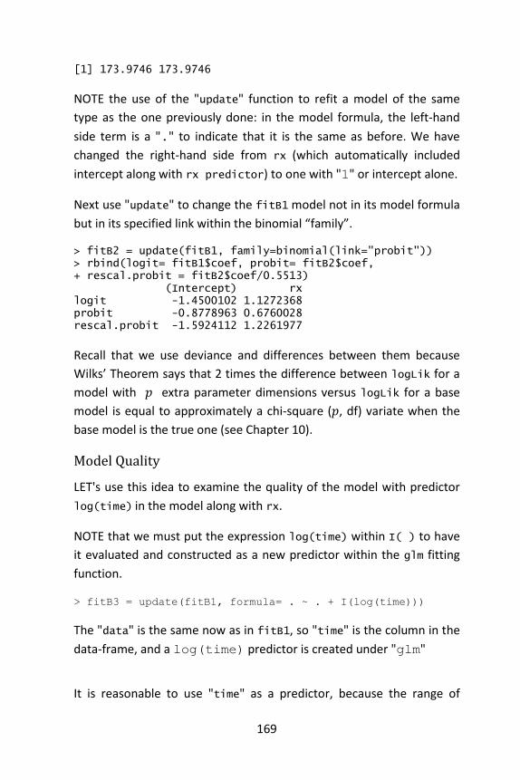
169

[1] 173.9746 173.9746

NOTE the use of the "update" function to refit a model of the same

type as the one previously done: in the model formula, the left-hand

side term is a "." to indicate that it is the same as before. We have

changed the right-hand side from rx (which automatically included

intercept along with rx predictor) to one with "1" or intercept alone.

Next use "update" to change the fitB1 model not in its model formula

but in its specified link within the binomial “family”.

> fitB2 = update(fitB1, family=binomial(link="probit")) > rbind(logit= fitB1$coef, probit= fitB2$coef, + rescal.probit = fitB2$coef/0.5513) (Intercept) rx logit -1.4500102 1.1272368 probit -0.8778963 0.6760028 rescal.probit -1.5924112 1.2261977

Recall that we use deviance and differences between them because

Wilks’ Theorem says that 2 times the difference between logLik for a

model with 𝑝 extra parameter dimensions versus logLik for a base

model is equal to approximately a chi-square (𝑝, df) variate when the

base model is the true one (see Chapter 10).

Model Quality

LET's use this idea to examine the quality of the model with predictor

log(time) in the model along with rx.

NOTE that we must put the expression log(time) within I( ) to have

it evaluated and constructed as a new predictor within the glm fitting

function.

> fitB3 = update(fitB1, formula= . ~ . + I(log(time)))

The "data" is the same now as in fitB1, so "time" is the column in the

data-frame, and a log(time) predictor is created under "glm"

It is reasonable to use "time" as a predictor, because the range of

170

times is not too different for rats who generate tumors, so "time" is

not really a response variable.

> summary(rats$time[rats$status==1]) Min. 1st Qu. Median Mean 3rd Qu. Max. 34.00 66.75 80.00 77.28 92.50 104.00 > summary(rats$time[rats$status==0]) Min. 1st Qu. Median Mean 3rd Qu. Max. 45.00 83.50 104.00 93.85 104.00 104.00

> cbind(rats[1:10,], model.matrix(fitB3)[1:10,]) litter rx time status (Intercept) rx I(log(time)) 1 1 1 101 0 1 1 4.615121 2 1 0 49 1 1 0 3.891820 3 1 0 104 0 1 0 4.644391 4 2 1 104 0 1 1 4.644391 5 2 0 102 0 1 0 4.624973 6 2 0 104 0 1 0 4.644391 7 3 1 104 0 1 1 4.644391 8 3 0 104 0 1 0 4.644391 9 3 0 104 0 1 0 4.644391 10 4 1 77 0 1 1 4.343805

The first 4 columns are the original "rats" data. The last 3 are the

design matrix columns created by glm. So we can look at the new

model fit for significance of coefficients:

> summary(fitB3)$coef Estimate Std. Error z value Pr(>|z|) (Intercept) 17.868661 4.4924813 3.977459 6.965559e-05 rx 1.194019 0.4284626 2.786751 5.323935e-03 I(log(time)) -4.355407 1.0180848 -4.278040 1.885462e-05

Or alternatvely compare deviances or logLik's with fitB1

> c(2*(logLik(fitB3)-logLik(fitB1)), fitB1$dev-fitB3$dev) [1] 24.37307 24.37307

This is LRT stat to be compared with chisq 1 df.

> 1-pchisq(24.373,1) [1] 7.937339e-07

This is still highly significant but somewhat different p-value from the

I(log(time)) coef probably because the model is still far from the

right one.

171

We could try to enter additional terms like log(time)^2 or rx * log(time)

> fitB4 = update(fitB3, .~. + I(rx*log(time)) + + I(log(time)^2)) > summary(fitB4)$coef Estimate Std. Error z value (Intercept) -9.784968 52.690740 -0.1857056 rx -13.501206 8.732837 -1.5460274 I(log(time)) 10.179730 24.364938 0.4178024 I(rx * log(time)) 3.324780 1.973389 1.6848069 I(log(time)^2) -1.871215 2.819823 -0.6635932 Pr(>|z|) (Intercept) 0.85267560 rx 0.12209794 I(log(time)) 0.67609159 I(rx * log(time)) 0.09202582 I(log(time)^2) 0.50695069

This time, the new variables do NOT look significant which we can

check also through deviances:

> fitB3$dev - fitB4$dev [1] 3.901065

This result is to be compared with chisq 2df, so it is not at all

significant.

We can also do these deviance comparisons all at once by looking at an

"analysis of deviance" table

> anova(fitB4) Analysis of Deviance Table Model: binomial, link: logit Response: cbind(status, 1 - status) Terms added sequentially (first to last) Df Deviance Resid. Df Resid. Dev NULL 149 173.97 rx 1 8.7008 148 165.27 I(log(time)) 1 24.3731 147 140.90 I(rx * log(time)) 1 3.4784 146 137.42 I(log(time)^2) 1 0.4226 145 137.00

As in an ANOVA table, in which RSS replaced Deviance these "Deviance

values" are the amounts by which the current model-fitting line

172

decreases the deviance: (recall that fitB1 uses rx only, fitB3

augments by log(time), and fitB4 by log(time) plus the 2

additional rx*log(tim) and log(time)^2 terms.

> Devs = c(fitB1$null.dev, fitB1$dev, fitB3$dev, + update(fitB3, .~.+I(rx*log(time)))$dev, + fitB4$dev) > Devs [1] 173.9746 165.2738 140.9007 137.4223 136.9997 > round (-diff(Devs), 3 )### successive differences of llks [1] 8.701 24.373 3.478 0.423 ### give Deviance col in "anova"

173

10. Logistic regression

In statistics, logistic regression, or logit regression, is a type of

probabilistic statistical classification model (Bishop, 2006). It is also

used to predict a binary response from a binary predictor, used for

predicting the outcome of a categorical dependent variable (i.e., a class

label) based on one or more predictor variables (features). That is, it is

used in estimating the parameters of a qualitative response model. The

probabilities describing the possible outcomes of a single trial are

modeled, as a function of the explanatory (predictor) variables, using a

logistic function. Frequently (and subsequently in this article) “logistic

regression” is used to refer specifically to the problem in which the

dependent variable is binary—that is, the number of available

categories is two—while problems with more than two categories are

referred to as multinomial logistic regression or, if the multiple

categories are ordered, as ordered logistic regression.

Logistic regression measures the relationship between a categorical

dependent variable and one or more independent variables, which are

usually (but not necessarily) continuous, by using probability scores as

the predicted values of the dependent variable (Bhandari & Joensson,

2008). As such it treats the same set of problems as does probit

regression using similar techniques.

Fields and examples of applications

Logistic regression was put forth in the 1940s as an alternative to

Fisher's 1936 classification method, linear discriminant analysis (James,

Witten, Hastie, & Tibshirani, 2013). It is used extensively in numerous

disciplines, including the medical and social science fields. For example,

the Trauma and Injury Severity Score (TRISS), which is widely used to

predict mortality in injured patients, was originally developed by Boyd

et al. using logistic regression (Boyd, Tolson, & Copes, 1987). Logistic

regression might be used to predict whether a patient has a given

174

disease (e.g. diabetes), based on observed characteristics of the patient

(age, gender, body mass index, results of various blood tests, etc.).

Another example might be to predict whether an American voter will

vote Democratic or Republican, based on age, income, gender, race,

state of residence, votes in previous elections, etc. (Harrell, 2010). The

technique can also be used in engineering, especially for predicting the

probability of failure of a given process, system or product (Strano &

Colosimo, 2006) (Palei & Das, 2009). It is also used in marketing

applications such as prediction of a customer's propensity to purchase

a product or cease a subscription, etc. In economics it can be used to

predict the likelihood of a person's choosing to be in the labor force,

and a business application would be to predict the likelihood of a

homeowner defaulting on a mortgage. Conditional random fields, an

extension of logistic regression to sequential data, are used in natural

language processing.

Basics

Logistic regression can be binomial or multinomial. Binomial or binary

logistic regression deals with situations in which the observed outcome

for a dependent variable can have only two possible types (for

example, “dead” vs. “alive”). Multinomial logistic regression deals with

situations where the outcome can have three or more possible types

(e.g., “disease A” vs. “disease B” vs. “disease C”). In binary logistic

regression, the outcome is usually coded as “0”or “1”, as this leads to

the most straightforward interpretation (Hosmer & Lemeshow, 2000).

If a particular observed outcome for the dependent variable is the

noteworthy possible outcome (referred to as a “success” or a “case”) it

is usually coded as “1” and the contrary outcome (referred to as a

“failure” or a “noncase”) as “0”. Logistic regression is used to predict

the odds of being a case based on the values of the independent

variables (predictors). The odds are defined as the probability that a

particular outcome is a case divided by the probability that it is a

noncase.

Like other forms of regression analysis, logistic regression makes use of

175

one or more predictor variables that may be either continuous or

categorical data. Unlike ordinary linear regression, however, logistic

regression is used for predicting binary outcomes of the dependent

variable (treating the dependent variable as the outcome of a Bernoulli

trial) rather than continuous outcomes. Given this difference, it is

necessary that logistic regression take the natural logarithm of the

odds of the dependent variable being a case (referred to as the logit or

log-odds) to create a continuous criterion as a transformed version of

the dependent variable. Thus the logit transformation is referred to as

the link function in logistic regression—although the dependent

variable in logistic regression is binomial, the logit is the continuous

criterion upon which linear regression is conducted (Hosmer &

Lemeshow, 2000).

The logit of success is then fit to the predictors using linear regression

analysis. The predicted value of the logit is converted back into

predicted odds via the inverse of the natural logarithm, namely the

exponential function. Therefore, although the observed dependent

variable in logistic regression is a zero-or-one variable, the logistic

regression estimates the odds, as a continuous variable, that the

dependent variable is a success (a case). In some applications the odds

are all that is needed. In others, a specific yes-or-no prediction is

needed for whether the dependent variable is or is not a case; this

categorical prediction can be based on the computed odds of a success,

with predicted odds above some chosen cut-off value being translated

into a prediction of a success.

Logistic function, odds ratio, and logit

An explanation of logistic regression begins with an explanation of the

logistic function, which always takes on values between zero and one

(Hosmer & Lemeshow, 2000):

𝐹(𝑡) =𝑒𝑡

𝑒𝑡 + 1=

1

1 + 𝑒𝑡,

and viewing 𝑡 as a linear function of an explanatory variable 𝑥 (or of a

176

linear combination of explanatory variables), the logistic function can

be written as:

𝐹(𝑥) =1

1 + 𝑒−(𝛽0+𝛽1𝑥).

This will be interpreted as the probability of the dependent variable

equaling a “success” or “case” rather than a failure or non-case. We

also define the inverse of the logistic function, the logit:

𝑔(𝑥) = ln𝐹(𝑥)

1 − 𝐹(𝑥)= 𝛽0 + 𝛽1𝑥,

and equivalently:

𝐹(𝑥)

1 − 𝐹(𝑥)= 𝑒(𝛽0+𝛽1𝑥).

A graph of the logistic function is shown in Figure 1. The input is the

value of and the output is 𝐹(𝑥). The logistic function is useful because

it can take an input with any value from negative infinity to positive

infinity, whereas the output is confined to values between 0 and 1 and

hence is interpretable as a probability. In the above equations, refers to

the logit function of some given linear combination of the predictors,

denotes the natural logarithm, is the probability that the dependent

variable equals a case, is the intercept from the linear regression

equation (the value of the criterion when the predictor is equal to

zero), is the regression coefficient multiplied by some value of the

predictor, and base e denotes the exponential function.

177

Figure 1. The logistic function, with 𝛽0 + 𝛽1 on the horizontal axis and

𝐹(𝑥) on the vertical axis

The formula for 𝐹(𝑥) illustrates that the probability of the dependent

variable equaling a case is equal to the value of the logistic function of

the linear regression expression. This is important in that it shows that

the value of the linear regression expression can vary from negative to

positive infinity and yet, after transformation, the resulting expression

for the probability 𝐹(𝑥) ranges between 0 and 1. The equation for

𝑔(𝑥) illustrates that the logit (i.e., log-odds or natural logarithm of the

odds) is equivalent to the linear regression expression. Likewise, the

next equation illustrates that the odds of the dependent variable

equaling a case is equivalent to the exponential function of the linear

regression expression. This illustrates how the logit serves as a link

function between the probability and the linear regression expression.

Given that the logit ranges between negative infinity and positive

infinity, it provides an adequate criterion upon which to conduct linear

regression and the logit is easily converted back into the odds (Hosmer

& Lemeshow, 2000).

178

Multiple explanatory variables

If there are multiple explanatory variables, then the above expression

𝛽0 + 𝛽1𝑥 can be revised to 𝛽0 + 𝛽1𝑥1 + 𝛽2𝑥1 + ⋯ + 𝛽𝑚𝑥𝑚. Then

when this is used in the equation relating the logged odds of a success

to the values of the predictors, the linear regression will be a multiple

regression with 𝑚 explanators; the parameters 𝛽𝑗 for all 𝑗 =

0,1,2, . . . , 𝑚 are all estimated.

Model fitting

Estimation

Maximum likelihood estimation

The regression coefficients are usually estimated using maximum

likelihood estimation (Menard, 2002). Unlike linear regression with

normally distributed residuals, it is not possible to find a closed-form

expression for the coefficient values that maximizes the likelihood

function, so an iterative process must be used instead, for example

Newton's method. This process begins with a tentative solution, revises

it slightly to see if it can be improved, and repeats this revision until

improvement is minute, at which point the process is said to have

converged (Menard, 2002).

In some instances the model may not reach convergence. When a

model does not converge this indicates that the coefficients are not

meaningful because the iterative process was unable to find

appropriate solutions. A failure to converge may occur for a number of

reasons: having a large proportion of predictors to cases,

multicollinearity, sparseness, or complete separation.

• Having a large proportion of variables to cases results in an overly

conservative Wald statistic (discussed below) and can lead to

nonconvergence.

• Multicollinearity refers to unacceptably high correlations between

predictors. As multicollinearity increases, coefficients remain

unbiased but standard errors increase and the likelihood of model

179

convergence decreases. To detect multicollinearity amongst the

predictors, one can conduct a linear regression analysis with the

predictors of interest for the sole purpose of examining the

tolerance statistic used to assess whether multicollinearity is

unacceptably high (Menard, 2002).

• Sparseness in the data refers to having a large proportion of empty

cells (cells with zero counts). Zero cell counts are particularly

problematic with categorical predictors. With continuous

predictors, the model can infer values for the zero cell counts, but

this is not the case with categorical predictors. The reason the

model will not converge with zero cell counts for categorical

predictors is because the natural logarithm of zero is an undefined

value, so final solutions to the model cannot be reached. To

remedy this problem, researchers may collapse categories in a

theoretically meaningful way or may consider adding a constant to

all cells (Menard, 2002).

• Another numerical problem that may lead to a lack of convergence

is complete separation, which refers to the instance in which the

predictors perfectly predict the criterion – all cases are accurately

classified. In such instances, one should reexamine the data, as

there is likely some kind of error (Hosmer & Lemeshow, 2000).

Although not a precise number, as a general rule of thumb, logistic

regression models require a minimum of 10 events per explaining

variable (where event denotes the cases belonging to the less frequent

category in the dependent variable) (Peduzzi, Concato, Kemper,

Holford, & Feinstein, 1996).

Minimum chi-squared estimator for grouped data

While individual data will have a dependent variable with a value of

zero or one for every observation, with grouped data one observation

is on a group of people who all share the same characteristics (e.g.,

demographic characteristics); in this case the researcher observes the

proportion of people in the group for whom the response variable falls

into one category or the other. If this proportion is neither zero nor one

180

for any group, the minimum chi-squared estimator involves using

weighted least squares to estimate a linear model in which the

dependent variable is the logit of the proportion: that is, the log of the

ratio of the fraction in one group to the fraction in the other group

(Greene, 2011).

Evaluating goodness of fit

Goodness of fit in linear regression models is generally measured using

the 𝑅2. Since this has no direct analog in logistic regression, various

methods (Greene, 2011) including the following can be used instead.

Deviance and likelihood ratio tests

In linear regression analysis, one is concerned with partitioning

variance via the sum of squares calculations – variance in the criterion

is essentially divided into variance accounted for by the predictors and

residual variance. In logistic regression analysis, deviance is used in lieu

of sum of squares calculations (Cohen, Cohen, West, & Aiken, 2002).

Deviance is analogous to the sum of squares calculations in linear

regression (Hosmer & Lemeshow, 2000) and is a measure of the lack of

fit to the data in a logistic regression model (Cohen, Cohen, West, &

Aiken, 2002). Deviance is calculated by comparing a given model with

the saturated model—a model with a theoretically perfect fit. This

computation is called the likelihood-ratio test (Hosmer & Lemeshow,

2000):

𝐷 = −2ln𝜆(𝑦𝑖) = −2 lnlikelihood of the fitted model

likelihood of the saturated model

In the above equation 𝐷 represents the deviance and ln represents the

natural logarithm, and Λ = 𝜆(𝑦𝑖). The log of the likelihood ratio (the

ratio of the fitted model to the saturated model) will produce a

negative value, so the product is multiplied by negative two times its

natural logarithm to produce a value with an approximate 𝜒2-squared

distribution (Hosmer & Lemeshow, 2000). Smaller values indicate

better fit as the fitted model deviates less from the saturated model.

When assessed upon a chi-square distribution, nonsignificant chi-

181

square values indicate very little unexplained variance and thus, good

model fit. Conversely, a significant chi-square value indicates that a

significant amount of the variance is unexplained.

Two measures of deviance are particularly important in logistic

regression: null deviance and model deviance. The null deviance

represents the difference between a model with only the intercept

(which means “no predictors”) and the saturated model (Cohen,

Cohen, West, & Aiken, 2002). And, the model deviance represents the

difference between a model with at least one predictor and the

saturated model. In this respect, the null model provides a baseline

upon which to compare predictor models. Given that deviance is a

measure of the difference between a given model and the saturated

model, smaller values indicate better fit. Therefore, to assess the

contribution of a predictor or set of predictors, one can subtract the

model deviance from the null deviance and assess the difference on a

𝜒𝑠−𝑝2 chi-square distribution with degree of freedom (Hosmer &

Lemeshow, 2000) equal to the difference in the number of parameters

estimated.

Let

𝐷𝑛𝑢𝑙𝑙 = −2lnlikelihood of the null model

likelihood of the saturated model

𝐷𝑓𝑖𝑡𝑡𝑒𝑑 = −2 lnlikelihood of the fitted model

likelihood of the saturated model

Then

𝐷𝑓𝑖𝑡𝑡𝑒𝑑−𝐷𝑛𝑢𝑙𝑙

= (−2 lnlikelihood of the fitted model

likelihood of the saturated model)

− (2lnlikelihood of the null model

likelihood of the saturated model)

182

= −2 (lnlikelihood of the fitted model

likelihood of the saturated model

− lnlikelihood of the null model

likelihood of the saturated model)

= −2 ln

likelihood of the fitted modellikelihood of the saturated model

likelihood of the null modellikelihood of the saturated model

= −2 lnlikelihood of the fitted model

likelihood of the null model.

If the model deviance is significantly smaller than the null deviance

then one can conclude that the predictor or set of predictors

significantly improved model fit. This is analogous to the 𝐹-test used in

linear regression analysis to assess the significance of prediction

(Cohen, Cohen, West, & Aiken, 2002). A convenient result, attributed

to Samuel S. Wilks, says that as the sample size 𝑛 approaches∞, the

test statistic −2ln(Λ) for a nested model will be asymptotically 𝜒2-

distributed with degrees of freedom equal to the difference in

dimensionality of the saturated model and null model (Wilks, 1938).

This means that for a great variety of hypotheses, a practitioner can

compute the likelihood ratio Λ for the data and compare −2ln(Λ) to

the 𝜒2 value corresponding to a desired statistical significance as an

approximate statistical test. This is often referred to a Wilks’ Theorem.

Pseudo-𝑅2s

In linear regression the squared multiple correlation, 𝑅2 is used to

assess goodness-of-fit as it represents the proportion of variance in the

criterion that is explained by the predictors (Cohen, Cohen, West, &

Aiken, 2002). In logistic regression analysis, there is no agreed upon

analogous measure, but there are several competing measures each

with limitations. Three of the most commonly used indices are

examined on this section beginning with the likelihood ratio 𝑅2, 𝑅𝐿2

(Cohen, Cohen, West, & Aiken, 2002):

𝑅𝐿2

𝐷𝑛𝑢𝑙𝑙 − 𝐷𝑚𝑜𝑑𝑒𝑙

𝐷𝑛𝑢𝑙𝑙.

183

This is the most analogous index to the squared multiple correlation in

linear regression (Menard, 2002). It represents the proportional

reduction in the deviance, wherein the deviance is treated as a

measure of variation analogous but not identical to the variance in

linear regression analysis (Menard, 2002). One limitation of the

likelihood ratio 𝑅2 is that it is not monotonically related to the odds

ratio (Cohen, Cohen, West, & Aiken, 2002), meaning that it does not

necessarily increase as the odds ratio increases, and does not

necessarily decrease as the odds ratio decreases.

The Cox and Snell 𝑅2 is an alternative index of goodness-of-fit related

to the 𝑅2 value from linear regression. The Cox and Snell index is

problematic as its maximum value is 0.75, when the variance is at its

maximum (0.25). The Nagelkerke 𝑅2 provides a correction to the Cox

and Snell 𝑅2 so that the maximum value is equal to one. Nevertheless,

the Cox and Snell and likelihood ratio 𝑅2s show greater agreement

with each other than either does with the Nagelkerke 𝑅2 (Cohen,

Cohen, West, & Aiken, 2002). Of course, this might not be the case for

values exceeding 0.75 as the Cox and Snell index is capped at this value.

The likelihood ratio 𝑅2 is often preferred to the alternatives as it is

most analogous to 𝑅2 in linear regression, is independent of the base

rate (both Cox and Snell and Nagelkerke 𝑅2s increase as the proportion

of cases increase from 0 to 0.5) and varies between 0 and 1.

A word of caution is in order when interpreting pseudo-𝑅2 statistics.

The reason these indices of fit are referred to as pseudo 𝑅2 is because

they do not represent the proportionate reduction in error as the 𝑅2 in

linear regression does (Cohen, Cohen, West, & Aiken, 2002). Linear

regression assumes homoscedasticity, that the error variance is the

same for all values of the criterion. Logistic regression will always be

heteroscedastic – the error variances differ for each value of the

predicted score. For each value of the predicted score there would be a

different value of the proportionate reduction in error. Therefore, it is

inappropriate to think of 𝑅2 as a proportionate reduction in error in a

universal sense in logistic regression (Cohen, Cohen, West, & Aiken,

184

2002).

Hosmer–Lemeshow test

The Hosmer–Lemeshow test uses a test statistic that asymptotically

follows a 𝜒2 distribution to assess whether or not the observed event

rates match expected event rates in subgroups of the model

population (Hosmer & Lemeshow, 2000).

Evaluating binary classification performance

If the estimated probabilities are to be used to classify each

observation of independent variable values as predicting the category

that the dependent variable is found in, the various methods below for

judging the model's suitability in out-of-sample forecasting can also be

used on the data that were used for estimation—accuracy, precision

(also called positive predictive value), recall (also called sensitivity),

specificity and negative predictive value. In each of these evaluative

methods, an aspect of the model's effectiveness in assigning instances

to the correct categories is measured.

Coefficients

After fitting the model, it is likely that researchers will want to examine

the contribution of individual predictors. To do so, they will want to

examine the regression coefficients. In linear regression, the regression

coefficients represent the change in the criterion for each unit change

in the predictor (Cohen, Cohen, West, & Aiken, 2002). In logistic

regression, however, the regression coefficients represent the change

in the logit for each unit change in the predictor. Given that the logit is

not intuitive, researchers are likely to focus on a predictor’s effect on

the exponential function of the regression coefficient – the odds ratio

(see definition). In linear regression, the significance of a regression

coefficient is assessed by computing a 𝑡-test. In logistic regression,

there are several different tests designed to assess the significance of

an individual predictor, most notably the likelihood ratio test and the

Wald statistic.

185

Likelihood ratio test

The likelihood-ratio test discussed above to assess model fit is also the

recommended procedure to assess the contribution of individual

“predictors” to a given model (Cohen, Cohen, West, & Aiken, 2002)

(Hosmer & Lemeshow, 2000) (Menard, 2002). In the case of a single

predictor model, one simply compares the deviance of the predictor

model with that of the null model on a chi-square distribution with a

single degree of freedom. If the predictor model has a significantly

smaller deviance (c.f chi-square using the difference in degrees of

freedom of the two models), then one can conclude that there is a

significant association between the “predictor” and the outcome.

Although some common statistical packages (e.g. SPSS) do provide

likelihood ratio test statistics, without this computationally intensive

test it would be more difficult to assess the contribution of individual

predictors in the multiple logistic regression case. To assess the

contribution of individual predictors one can enter the predictors

hierarchically, comparing each new model with the previous to

determine the contribution of each predictor (Cohen, Cohen, West, &

Aiken, 2002). (There is considerable debate among statisticians

regarding the appropriateness of so-called “stepwise” procedures.

They do not preserve the nominal statistical properties and can be very

misleading (Harrell, 2010).

Wald statistic

Alternatively, when assessing the contribution of individual predictors

in a given model, one may examine the significance of the Wald

statistic. The Wald statistic, analogous to the 𝑡-test in linear regression,

is used to assess the significance of coefficients. The Wald statistic is

the ratio of the square of the regression coefficient to the square of the

standard error of the coefficient and is asymptotically distributed as a

chi-square distribution (Menard, 2002).

𝑊𝑗 =𝐵𝑗

2

𝑆𝐸𝐵𝑗

2 .

186

Although several statistical packages (e.g., SPSS, SAS) report the Wald

statistic to assess the contribution of individual predictors, the Wald

statistic has limitations. When the regression coefficient is large, the

standard error of the regression coefficient also tends to be large

increasing the probability of Type-II error. The Wald statistic also tends

to be biased when data are sparse (Cohen, Cohen, West, & Aiken,

2002).

Case-control sampling

Suppose cases are rare. Then we might wish to sample them more

frequently than their prevalence in the population. For example,

suppose there is a disease that affects 1 person in 10,000 and to collect

our data we need to do a complete physical. It may be too expensive to

do thousands of physicals of healthy people in order to get data on

only a few diseased individuals. Thus, we may evaluate more diseased

individuals. This is also called unbalanced data. As a rule of thumb,

sampling controls at a rate of five times the number of cases is

sufficient to get enough control data (Prentice & Pyke, 1979).

If we form a logistic model from such data, if the model is correct, the

𝛽𝑗 parameters are all correct except for 𝛽0. We can correct 𝛽0 if we

know the true prevalence as follows (Prentice & Pyke, 1979):

�̂�0∗ = �̂�0 + log

𝜋

1 − 𝜋log

�̂�

1 − �̂�,

where 𝜋 is the true prevalence and �̂� is the prevalence in the sample.

Formal mathematical specification

There are various equivalent specifications of logistic regression, which

fit into different types of more general models. These different

specifications allow for different sorts of useful generalizations.

Setup

The basic setup of logistic regression is the same as for standard linear

187

regression.

It is assumed that we have a series of 𝑁 observed data points. Each

data point 𝑖 consists of a set of 𝑚 explanatory variables 𝑥1,𝑖, … , 𝑥𝑚,𝑖

(also called independent variables, predictor variables, input variables,

features, or attributes), and an associated binary-valued outcome

variable 𝑌𝑖 (also known as a dependent variable, response variable,

output variable, outcome variable or class variable), i.e. it can assume

only the two possible values 0 (often meaning “no” or “failure”) or 1

(often meaning “yes” or “success”). The goal of logistic regression is to

explain the relationship between the explanatory variables and the

outcome, so that an outcome can be predicted for a new set of

explanatory variables.

Some examples:

• The observed outcomes are the presence or absence of a given

disease (e.g. diabetes) in a set of patients, and the explanatory

variables might be characteristics of the patients thought to be

pertinent (sex, race, age, blood pressure, body-mass index, etc.).

• The observed outcomes are the votes (e.g. Democratic or

Republican) of a set of people in an election, and the explanatory

variables are the demographic characteristics of each person (e.g.

sex, race, age, income, etc.). In such a case, one of the two

outcomes is arbitrarily coded as 1, and the other as 0.

As in linear regression, the outcome variables 𝑌 are assumed to

depend on the explanatory variables 𝑥1,𝑖, … , 𝑥𝑚,𝑖.

Explanatory variables

As shown above in the above examples, the explanatory variables may

be of any type: real-valued, binary, categorical, etc. The main

distinction is between continuous variables (such as income, age and

blood pressure) and discrete variables (such as sex or race). Discrete

variables referring to more than two possible choices are typically

coded using dummy variables (or indicator variables), that is, separate

188

explanatory variables taking the value 0 or 1 are created for each

possible value of the discrete variable, with a 1 meaning “variable does

have the given value” and a 0 meaning “variable does not have that

value”. For example, a four-way discrete variable of blood type with

the possible values “A, B, AB, O” can be converted to four separate

two-way dummy variables, “is-A, is-B, is-AB, is-O”, where only one of

them has the value 1 and all the rest have the value 0. This allows for

separate regression coefficients to be matched for each possible value

of the discrete variable. (In a case like this, only three of the four

dummy variables are independent of each other, in the sense that once

the values of three of the variables are known, the fourth is

automatically determined. Thus, it is only necessary to encode three of

the four possibilities as dummy variables. This also means that when all

four possibilities are encoded, the overall model is not identifiable in

the absence of additional constraints such as a regularization

constraint. Theoretically, this could cause problems, but in reality

almost all logistic regression models are fit with regularization

constraints.)

Outcome variables

Formally, the outcomes 𝑌𝑖 are described as being Bernoulli-distributed

data, where each outcome is determined by an unobserved probability

𝑝𝑖 that is specific to the outcome at hand, but related to the

explanatory variables. This can be expressed in any of the following

equivalent forms:

𝑌𝑖|𝑥1,𝑖, … , 𝑥𝑚,𝑖~Bernoulli(𝑝𝑖)

𝐸[𝑌𝑖|𝑥1,𝑖, … , 𝑥𝑚,𝑖] = 𝑝𝑖

Pr(𝑌𝑖 = 𝑦𝑖|𝑥1,𝑖, … , 𝑥𝑚,𝑖) = {𝑝𝑖 if 𝑦𝑖 = 1

1 − 𝑝𝑖 if 𝑦𝑖 = 0

Pr(𝑌𝑖 = 𝑦𝑖|𝑥1,𝑖, … , 𝑥𝑚,𝑖) = 𝑝𝑖𝑦𝑖(1 − 𝑝𝑖)(1−𝑦𝑖)

The meanings of these four lines are:

1. The first line expresses the probability distribution of each 𝑌𝑖:

Conditioned on the explanatory variables, it follows a Bernoulli

189

distribution with parameters 𝑝𝑖, the probability of the outcome of 1 for

trial 𝑖. As noted above, each separate trial has its own probability of

success, just as each trial has its own explanatory variables. The

probability of success 𝑝𝑖 is not observed, only the outcome of an

individual Bernoulli trial using that probability.

2. The second line expresses the fact that the expected value of each 𝑌𝑖

is equal to the probability of success 𝑝𝑖, which is a general property of

the Bernoulli distribution. In other words, if we run a large number of

Bernoulli trials using the same probability of success 𝑝𝑖, then take the

average of all the 1 and 0 outcomes, then the result would be close to

𝑝𝑖. This is because doing an average this way simply computes the

proportion of successes seen, which we expect to converge to the

underlying probability of success.

3. The third line writes out the probability mass function of the

Bernoulli distribution, specifying the probability of seeing each of the

two possible outcomes.

4. The fourth line is another way of writing the probability mass

function, which avoids having to write separate cases and is more

convenient for certain types of calculations. This relies on the fact that

𝑌𝑖 can take only the value 0 or 1. In each case, one of the exponents

will be 1, “choosing” the value under it, while the other is 0, “canceling

out” the value under it. Hence, the outcome is either 𝑝𝑖 or 1 − 𝑝𝑖 , as in

the previous line.

Linear predictor function

The basic idea of logistic regression is to use the mechanism already

developed for linear regression by modeling the probability 𝑝𝑖 using a

linear predictor function, i.e. a linear combination of the explanatory

variables and a set of regression coefficients that are specific to the

model at hand but the same for all trials. The linear predictor function

𝑓(𝑖) for a particular data point 𝑖 is written as:

𝑓(𝑖) = 𝛽0 + 𝛽1𝑥1,𝑖 + 𝛽2𝑥1,𝑖 + ⋯ + 𝛽𝑚𝑥𝑚,𝑖,

190

where 𝛽0, … , 𝛽𝑚are regression coefficients indicating the relative effect

of a particular explanatory variable on the outcome.

The model is usually put into a more compact form as follows:

• The regression coefficients𝛽0, 𝛽1, … , 𝛽𝑚 β , β , ..., β are grouped

into a single vector 𝜷 of size 𝑚 + 1.

• For each data point 𝑖, an additional explanatory pseudo-variable

𝑥0,𝑖 is added, with a fixed value of 1, corresponding to the intercept

coefficient 𝛽0 .

• The resulting explanatory variables 𝑥0,𝑖, 𝑥1,𝑖, … , 𝑥𝑚,𝑖 are then

grouped into a single vector 𝑿𝑖 of size 𝑚 +1.

This makes it possible to write the linear predictor function as follows:

𝒇(𝑖) = 𝜷 ∙ 𝑿𝑖,

using the notation for a dot product between two vectors.

As a generalized linear model

The particular model used by logistic regression, which distinguishes it

from standard linear regression and from other types of regression

analysis used for binary-valued outcomes, is the way the probability of

a particular outcome is linked to the linear predictor function:

logit(𝐸[𝑌𝑖|𝑥1,𝑖, … , 𝑥𝑚,𝑖]) = logit(𝑝𝑖)

= ln (𝑝𝑖

1 − 𝑝𝑖) = 𝛽1𝑥1,𝑖 + 𝛽2𝑥1,𝑖 + ⋯ + 𝛽𝑚𝑥𝑚,𝑖

Written using the more compact notation described above, this is:

logit(𝐸[𝑌𝑖|𝑿𝑖]) = logit(𝑝𝑖) = ln (𝑝𝑖

1 − 𝑝𝑖) = 𝜷 ∙ 𝑿𝑖.

This formulation expresses logistic regression as a type of generalized

linear model, which predicts variables with various types of probability

distributions by fitting a linear predictor function of the above form to

some sort of arbitrary transformation of the expected value of the

191

variable.

The intuition for transforming using the logit function (the natural log

of the odds) was explained above. It also has the practical effect of

converting the probability (which is bounded to be between 0 and 1) to

a variable that ranges over (−∞, +∞) — thereby matching the

potential range of the linear prediction function on the right side of the

equation.

Note that both the probabilities 𝑝𝑖 and the regression coefficients are

unobserved, and the means of determining them is not part of the

model itself. They are typically determined by some sort of

optimization procedure, e.g. maximum likelihood estimation, which

finds values that best fit the observed data (i.e. that give the most

accurate predictions for the data already observed), usually subject to

regularization conditions that seek to exclude unlikely values, e.g.

extremely large values for any of the regression coefficients. The use of

a regularization condition is equivalent to doing maximum a posteriori

(MAP) estimation, an extension of maximum likelihood. (Regularization

is most commonly done using a squared regularizing function, which is

equivalent to placing a zero-mean Gaussian prior distribution on the

coefficients, but other regularizers are also possible.) Whether or not

regularization is used, it is usually not possible to find a closed-form

solution; instead, an iterative numerical method must be used, such as

iteratively reweighted least squares (IRLS) or, more commonly these

days, a quasi-Newton method such as the L-BFGS method.

The interpretation of the 𝛽𝑗 parameter estimates is as the additive

effect on the log of the odds for a unit change in the 𝑗th explanatory

variable. In the case of a dichotomous explanatory variable, for

instance gender, 𝑒𝛽 is the estimate of the odds of having the outcome

for, say, males compared with females.

An equivalent formula uses the inverse of the logit function, which is

the logistic function, i.e.:

192

𝐸[𝑌𝑖|𝑿𝑖] = 𝑝𝑖 = (𝜷 ∙ 𝑿𝑖) =1

1 + 𝑒−𝜷∙𝑿𝑖.

The formula can also be written (somewhat awkwardly) as a probability

distribution (specifically, using a probability mass function):

Pr(𝑌𝑖 = 𝑦𝑖|𝑿𝑖) = 𝑝𝑖𝑦𝑖(1 − 𝑝𝑖)(1−𝑦𝑖)

= (1

1 + 𝑒−𝜷∙𝑿𝑖)

𝑦𝑖

(1 −1

1 + 𝑒−𝜷∙𝑿𝑖)

1−𝑦𝑖

.

As a latent-variable model

The above model has an equivalent formulation as a latent-variable

model. This formulation is common in the theory of discrete choice

models, and makes it easier to extend to certain more complicated

models with multiple, correlated choices, as well as to compare logistic

regression to the closely related probit model.

Imagine that, for each trial 𝑖, there is a continuous latent variable 𝑌𝑖∗

(i.e. an unobserved random variable) that is distributed as follows:

𝑌𝑖∗ = 𝜷 ∙ 𝑿𝑖 + 휀,

Where

휀~Logistic(0,1),

i.e., the latent variable can be written directly in terms of the linear

predictor function and an additive random error variable that is

distributed according to a standard logistic distribution.

Then 𝑌𝑖 can be viewed as an indicator for whether this latent variable is

positive:

𝑌𝑖 = {1 if 𝑌𝑖

∗ > 0, 𝑖. 𝑒. −휀 < 𝜷 ∙ 𝑿𝑖

0 otherwise.

The choice of modeling the error variable specifically with a standard

193

logistic distribution, rather than a general logistic distribution with the

location and scale set to arbitrary values, seems restrictive, but in fact

it is not. It must be kept in mind that we can choose the regression

coefficients ourselves, and very often can use them to offset changes in

the parameters of the error variable's distribution. For example, a

logistic error-variable distribution with a non-zero location parameter 𝜇

(which sets the mean) is equivalent to a distribution with a zero

location parameter, where 𝜇 has been added to the intercept

coefficient. Both situations produce the same value for 𝑌𝑖∗ regardless

of settings of explanatory variables. Similarly, an arbitrary scale

parameter s is equivalent to setting the scale parameter to 1 and then

dividing all regression coefficients by s. In the latter case, the resulting

value of 𝑌𝑖∗ will be smaller by a factor of s than in the former case, for

all sets of explanatory variables — but critically, it will always remain on

the same side of 0, and hence lead to the same 𝑌𝑖 choice.

(Note that this predicts that the irrelevancy of the scale parameter

may not carry over into more complex models where more than two

choices are available.)

It turns out that this formulation is exactly equivalent to the preceding

one, phrased in terms of the generalized linear model and without any

latent variables. This can be shown as follows, using the fact that the

cumulative distribution function (CDF) of the standard logistic

distribution is the logistic function, which is the inverse of the logit

function, i.e.

𝑃𝑟(휀 < 𝑥) = (𝑥).

Then:

Pr(𝑌𝑖 = 1|𝑿𝑖) = Pr((𝑌𝑖∗ > 0)|𝑿𝑖)

= Pr(𝜷 ∙ 𝑿𝑖 + 휀 > 0)

= Pr(휀 > −𝜷 ∙ 𝑿𝑖)

= Pr(휀 < 𝜷 ∙ 𝑿𝑖)

= (𝜷 ∙ 𝑿𝑖)

= 𝑝𝑖 .

194

This formulation — which is standard in discrete choice models —

makes clear the relationship between logistic regression (the “logit

model”) and the probit model, which uses an error variable distributed

according to a standard normal distribution instead of a standard

logistic distribution. Both the logistic and normal distributions are

symmetric with a basic unimodal, “bell curve” shape. The only

difference is that the logistic distribution has somewhat heavier tails,

which means that it is less sensitive to outlying data (and hence

somewhat more robust to model misspecifications or erroneous data).

As a two-way latent-variable model

Yet another formulation uses two separate latent variables:

𝑌𝑖0∗ = 𝜷𝟎 ∙ 𝑿𝒊 + 휀0,

𝑌𝑖1∗ = 𝜷𝟎𝟏 ∙ 𝑿𝒊 + 휀1,

where

휀0~𝐸𝑉1(0,1),

휀1~𝐸𝑉1(0,1),

where 𝐸𝑉1(0,1) is a standard type-1 extreme value distribution: i.e.

𝑃𝑟(휀0 = 𝑥) = 𝑃𝑟(휀1 = 𝑥) = 𝑒−𝑥𝑒−𝑒−𝑥,

Then

𝑌𝑖 = {1 if 𝑌𝑖1∗ > 𝑌𝑖

0∗

0 otherwise.

This model has a separate latent variable and a separate set of

regression coefficients for each possible outcome of the dependent

variable. The reason for this separation is that it makes it easy to

extend logistic regression to multi-outcome categorical variables, as in

the multinomial logit model. In such a model, it is natural to model

each possible outcome using a different set of regression coefficients.

195

It is also possible to motivate each of the separate latent variables as

the theoretical utility associated with making the associated choice,

and thus motivate logistic regression in terms of utility theory. (In

terms of utility theory, a rational actor always chooses the choice with

the greatest associated utility.) This is the approach taken by

economists when formulating discrete choice models, because it both

provides a theoretically strong foundation and facilitates intuitions

about the model, which in turn makes it easy to consider various sorts

of extensions. (See the example below.)

The choice of the type-1 extreme value distribution seems fairly

arbitrary, but it makes the mathematics work out, and it may be

possible to justify its use through rational choice theory.

It turns out that this model is equivalent to the previous model,

although this seems non-obvious, since there are now two sets of

regression coefficients and error variables, and the error variables have

a different distribution. In fact, this model reduces directly to the

previous one with the following substitutions:

𝛽 = 𝛽1 − 𝛽0,

휀 = 휀1 − 휀0.

An intuition for this comes from the fact that, since we choose based

on the maximum of two values, only their difference matters, not the

exact values — and this effectively removes one degree of freedom.

Another critical fact is that the difference of two type-1 extreme-value-

distributed variables is a logistic distribution, i.e. if

휀 = 휀1 − 휀0~Logistic(0,1).

We can demonstrate the equivalent as follows:

Pr(𝑌𝑖 = 1|𝑿𝑖) = Pr(𝑌𝑖1∗ > 𝑌𝑖

0∗|𝑿𝑖)

= Pr(𝑌𝑖1∗ − 𝑌𝑖

0∗ > 0|𝑿𝑖)

= Pr(𝜷𝟏 ∙ 𝑿𝑖 + 휀1 − (𝜷𝟎 ∙ 𝑿𝑖 + 휀0) > 0)

196

= Pr((𝜷𝟏 ∙ 𝑿𝑖 − 𝜷𝟎 ∙ 𝑿𝑖) + (휀1 − 휀0) > 0)

= Pr((𝜷𝟏 − 𝜷𝟎) ∙ 𝑿𝑖 + (휀1 − 휀0) > 0)

= Pr((𝜷𝟏 − 𝜷𝟎) ∙ 𝑿𝑖 + 휀 > 0)

= Pr(𝜷 ∙ 𝑿𝑖 + 휀 > 0)

= Pr(휀 > −𝜷 ∙ 𝑿𝑖)

= Pr(휀 < 𝜷 ∙ 𝑿𝑖)

= (𝜷 ∙ 𝑿𝑖)

= 𝑝𝑖 .

Example

As an example, consider a province-level election where the choice is

between a right-of-center party, a left-of-center party, and a

secessionist party (e.g. the Parti Québécois, which wants Quebec to

secede from Canada (Hale & Hale, 2006)). We would then use three

latent variables, one for each choice. Then, in accordance with utility

theory, we can then interpret the latent variables as expressing the

utility that results from making each of the choices. We can also

interpret the regression coefficients as indicating the strength that the

associated factor (i.e. explanatory variable) has in contributing to the

utility — or more correctly, the amount by which a unit change in an

explanatory variable changes the utility of a given choice. A voter might

expect that the right-of-center party would lower taxes, especially on

rich people. This would give low-income people no benefit, i.e. no

change in utility (since they usually don't pay taxes); would cause

moderate benefit (i.e. somewhat more money, or moderate utility

increase) for middle-incoming people; and would cause significant

benefits for high-income people. On the other hand, the left-of-center

party might be expected to raise taxes and offset it with increased

welfare and other assistance for the lower and middle classes. This

would cause significant positive benefit to low-income people, perhaps

weak benefit to middle-income people, and significant negative benefit

to high-income people. Finally, the secessionist party would take no

direct actions on the economy, but simply secede. A low-income or

middle-income voter might expect basically no clear utility gain or loss

from this, but a high-income voter might expect negative utility, since

197

he/she is likely to own companies, which will have a harder time doing

business in such an environment and probably lose money.

These intuitions can be expressed as follows:

198

Estimated strength of regression coefficient for different outcomes

(party choices) and different values of explanatory variables

This clearly shows that

1. Separate sets of regression coefficients need to exist for each choice.

When phrased in terms of utility, this can be seen very easily. Different

choices have different effects on net utility; furthermore, the effects

vary in complex ways that depend on the characteristics of each

individual, so there need to be separate sets of coefficients for each

characteristic, not simply a single extra per-choice characteristic.

2. Even though income is a continuous variable, its effect on utility is

too complex for it to be treated as a single variable. Either it needs to

be directly split up into ranges, or higher powers of income need to be

added so that polynomial regression on income is effectively done.

As a “log-linear” model

Yet another formulation combines the two-way latent variable

formulation above with the original formulation higher up without

latent variables, and in the process provides a link to one of the

standard formulations of the multinomial logit (Greene, 2011).

Here, instead of writing the logit of the probabilities 𝑝𝑖 as a linear

predictor, we separate the linear predictor into two, one for each of

the two outcomes:

ln Pr(𝑌𝑖 = 0) = 𝜷𝟎 ∙ 𝑿𝑖 − ln 𝑍

ln Pr(𝑌𝑖 = 0) = 𝜷𝟏 ∙ 𝑿𝑖 − ln 𝑍.

Center-right Center-left Secessionist

High-income strong + strong − strong −

Middle-income moderate + weak + none

Low-income none strong + none

199

Note that two separate sets of regression coefficients have been

introduced, just as in the two-way latent variable model, and the two

equations appear a form that writes the logarithm of the associated

probability as a linear predictor, with an extra term – ln𝑍 at the end.

This term, as it turns out, serves as the normalizing factor ensuring that

the result is a distribution. This can be seen by exponentiating both

sides:

Pr(𝑌𝑖 = 0) =1

𝑍𝑒𝜷𝟎∙𝑿𝑖

Pr(𝑌𝑖 = 1) =1

𝑍𝑒𝜷𝟏∙𝑿𝑖 .

In this form it is clear that the purpose of 𝑍 is to ensure that the

resulting distribution over 𝑌𝑖 is in fact a probability distribution, i.e. it

sums to 1. This means that 𝑍 is simply the sum of all un-normalized

probabilities, and by dividing each probability by 𝑍, the probabilities

become “normalized”. That is:

𝑍 = 𝑒𝜷𝟎∙𝑿𝑖 + 𝑒𝜷𝟏∙𝑿𝑖 ,

and the resulting equations are

Pr(𝑌𝑖 = 0) =𝑒𝜷𝟎∙𝑿𝑖

𝑒𝜷𝟎∙𝑿𝑖 + 𝑒𝜷𝟏∙𝑿𝑖

Pr(𝑌𝑖 = 1) =𝑒𝜷𝟏∙𝑿𝑖

𝑒𝜷𝟎∙𝑿𝑖 + 𝑒𝜷𝟏∙𝑿𝑖.

Or generally:

Pr(𝑌𝑖 = 𝑐) =𝑒𝜷𝒄∙𝑿𝑖

∑ 𝑒𝜷𝒉∙𝑿𝑖ℎ.

This shows clearly how to generalize this formulation to more than two

outcomes, as in multinomial logit (Greene, 2011).

In order to prove that this is equivalent to the previous model, note

200

that the above model is over specified, in that Pr(𝑌𝑖 = 0) and

Pr(𝑌𝑖 = 1) cannot be independently specified: Pr(𝑌𝑖 = 0) +

Pr(𝑌𝑖 = 1) = 1 rather so knowing one automatically determines the

other. As a result, the model is nonidentifiable, in that multiple

combinations of 𝛽0 and 𝛽1 will produce the same probabilities for all

possible explanatory variables. In fact, it can be seen that adding any

constant vector to both of them will produce the same probabilities:

Pr(𝑌𝑖 = 1) =𝑒(𝜷𝟏+𝑪)∙𝑿𝑖

𝑒(𝜷𝟎+𝑪)∙𝑿𝑖 + 𝑒(𝜷𝟏+𝑪)∙𝑿𝑖

=𝑒𝜷𝟏∙𝑿𝑖𝑒𝑪∙𝑿𝑖

𝑒𝜷𝟎∙𝑿𝑖𝑒𝑪∙𝑿𝑖 + 𝑒𝜷𝟏∙𝑿𝑖𝑒𝑪∙𝑿𝑖

=𝑒𝜷𝟏∙𝑿𝑖𝑒𝑪∙𝑿𝑖

𝑒𝑪∙𝑿𝑖(𝑒𝜷𝟎∙𝑿𝑖 + 𝑒𝜷𝟏∙𝑿𝑖)

=𝑒𝜷𝟏∙𝑿𝑖

(𝑒𝜷𝟎∙𝑿𝑖 + 𝑒𝜷𝟏∙𝑿𝑖).

As a result, we can simplify matters, and restore identifiability, by

picking an arbitrary value for one of the two vectors. We choose to set

𝛽0 = 0. Then,

𝑒𝜷𝟎∙𝑿𝑖 = 𝑒𝟎∙𝑿𝑖 = 1,

and so

Pr(𝑌𝑖 = 1) =𝑒𝜷𝟏∙𝑿𝑖

1 + 𝑒𝜷𝟏∙𝑿𝑖=

1

1 + 𝑒−𝜷𝟏∙𝑿𝑖= 𝑝𝑖 ,

which shows that this formulation is indeed equivalent to the previous

formulation. (As in the two-way latent variable formulation, any

settings where 𝛽 = 𝛽1 − 𝛽0 will produce equivalent results.)

Note that most treatments of the multinomial logit model start out

either by extending the “log-linear” formulation presented here or the

two-way latent variable formulation presented above, since both

clearly show the way that the model could be extended to multi-way

outcomes (Greene, 2011). In general, the presentation with latent

201

variables is more common in econometrics and political science, where

discrete choice models and utility theory reign, while the “log-linear”

formulation here is more common in computer science, e.g. machine

learning and natural language processing.

As a single-layer perceptron

The model has an equivalent formulation

𝑝𝑖 =1

1 + 𝑒−(𝜷𝟏𝟎+𝜷𝟏∙𝑿1,𝑖+⋯+𝒌∙𝑿𝑘,𝑖).

This functional form is commonly called a single-layer perceptron or

single-layer artificial neural network (Da & Xiurun, 2005). A single-layer

neural network computes a continuous output instead of a step

function. The derivative of 𝑝𝑖 with respect to 𝑋 = (𝑥1, . . . , 𝑥𝑘) is

computed from the general form:

𝑦 =1

1 + 𝑒−𝑓(𝑥),

where 𝑓(𝑋) is an analytic function in 𝑋. With this choice, the single-

layer neural network is identical to the logistic regression model. This

function has a continuous derivative, which allows it to be used in

backpropagation. This function is also preferred because its derivative

is easily calculated:

𝑑𝑦

𝑑𝑋= 𝑦(1 − 4)

𝑑𝑓

𝑑𝑋.

In terms of binomial data

A closely related model assumes that each 𝑖 is associated not with a

single Bernoulli trial but with 𝑛𝑖 independent identically distributed

trials, where the observation 𝑌𝑖 is the number of successes observed

(the sum of the individual Bernoulli-distributed random variables), and

hence follows a binomial distribution:

𝑌𝑖~𝐵𝑖𝑛(𝑛𝑖, 𝑝𝑝), for 𝑖 = 1, … , 𝑛.

202

An example of this distribution is the fraction of seeds (𝑝𝑖) that

germinate after 𝑛𝑖 are planted. In terms of expected values, this model

is expressed as follows:

𝑝𝑖 = 𝐸 [𝑌𝑖

𝑛𝑖| 𝑿𝑖],

so that

logit (𝐸 [𝑌𝑖

𝑛𝑖| 𝑿𝑖]) = logit(𝑝𝑖) = ln (

𝑝𝑖

1 − 𝑝𝑖) = 𝜷 ∙ 𝑿𝑖,

Or equivalently:

Pr(𝑌𝑖 = 𝑦𝑖|𝑿𝒊) = (𝑛𝑖

𝑘𝑖) 𝑝𝑖

𝑦𝑖(1 − 𝑝𝑖)𝑛𝑖−𝑦𝑖

= (𝑛𝑖

𝑘𝑖) (

1

1 + 𝑒−𝜷∙𝑿𝑖)

𝑦𝑖

(1 −1

1 + 𝑒−𝜷∙𝑿𝑖)

1−𝑦𝑖

.

This model can be fit using the same sorts of methods as the above

more basic model.

Bayesian logistic regression

In a Bayesian statistics context, prior distributions are normally placed

on the regression coefficients, usually in the form of Gaussian

distributions. Unfortunately, the Gaussian distribution is not the

conjugate prior of the likelihood function in logistic regression; in fact,

the likelihood function is not an exponential family and thus does not

have a conjugate prior at all. As a result, the posterior distribution is

difficult to calculate, even using standard simulation algorithms (e.g.

Gibbs sampling).

There are various possibilities:

• Don't do a proper Bayesian analysis, but simply compute a

maximum a posteriori point estimate of the parameters. This is

common, for example, in “maximum entropy” classifiers in

machine learning.

203

• Use a more general approximation method such as the

Metropolis–Hastings algorithm.

• Draw a Markov chain Monte Carlo sample from the exact posterior

by using the Independent Metropolis–Hastings algorithm with

heavy-tailed multivariate candidate distribution found by matching

the mode and curvature at the mode of the normal approximation

to the posterior and then using the Student’s 𝑡 shape with low

degrees of freedom. This is shown to have excellent convergence

properties.

• Use a latent variable model and approximate the logistic

distribution using a more tractable distribution, e.g. a Student’s 𝑡-

distribution or a mixture of normal distributions.

• Do probit regression instead of logistic regression. This is actually a

special case of the previous situation, using a normal distribution in

place of a Student’s 𝑡, mixture of normals, etc. This will be less

accurate but has the advantage that probit regression is extremely

common, and a ready-made Bayesian implementation may already

be available.

• Use the Laplace approximation of the posterior distribution. This

approximates the posterior with a Gaussian distribution. This is not

a terribly good approximation, but it suffices if all that is desired is

an estimate of the posterior mean and variance. In such a case, an

approximation scheme such as variational Bayes can be used

(Bishop, 2006).

204

Comparison of logistic function with a scaled inverse probit function

(i.e. the CDF of the normal distribution), comparing 𝜎(𝑥) vs. Φ =

(√𝜋

8𝑥), which makes the slopes the same at the origin. This shows the

heavier tails of the logistic distribution.

Gibbs sampling with an approximating distribution

As shown above, logistic regression is equivalent to a latent variable

model with an error variable distributed according to a standard

logistic distribution. The overall distribution of the latent variable 𝒀𝒊∗ is

also a logistic distribution, with the mean equal to 𝜷 ∙ 𝑿𝒊 (i.e. the fixed

quantity added to the error variable). This model considerably

simplifies the application of techniques such as Gibbs sampling (George

205

& McCullochb, 1993). However, sampling the regression coefficients is

still difficult, because of the lack of conjugacy between the normal and

logistic distributions. Changing the prior distribution over the

regression coefficients is of no help, because the logistic distribution is

not in the exponential family and thus has no conjugate prior.

One possibility is to use a more general Markov chain Monte Carlo

technique (Walsh, 2004), such as the Metropolis–Hastings algorithm

(Chib & Greenberg, 1995), which can sample arbitrary distributions.

Another possibility, however, is to replace the logistic distribution with

a similar-shaped distribution that is easier to work with using Gibbs

sampling. In fact, the logistic and normal distributions have a similar

shape, and thus one possibility is simply to have normally distributed

errors. Because the normal distribution is conjugate to itself, sampling

the regression coefficients becomes easy. In fact, this model is exactly

the model used in probit regression.

However, the normal and logistic distributions differ in that the logistic

has heavier tails. As a result, it is more robust to inaccuracies in the

underlying model (which are inevitable, in that the model is essentially

always an approximation) or to errors in the data. Probit regression

loses some of this robustness.

Another alternative is to use errors distributed as a Student’s 𝑡-

distribution. The Student’s 𝑡-distribution has heavy tails, and is easy to

sample from because it is the compound distribution of a normal

distribution with variance distributed as an inverse gamma distribution.

In other words, if a normal distribution is used for the error variable,

and another latent variable, following an inverse gamma distribution, is

added corresponding to the variance of this error variable, the marginal

distribution of the error variable will follow a Student’s 𝑡-distribution.

Because of the various conjugacy relationships, all variables in this

model are easy to sample from.

The Student’s 𝑡-distribution that best approximates a standard logistic

distribution can be determined by matching the moments of the two

206

distributions. The Student's t-distribution has three parameters, and

since the skewness of both distributions is always 0, the first four

moments can all be matched, using the following equations:

𝜇 = 0

𝜈

𝜈 − 2𝑠2 =

𝜋2

3

6

𝜈 − 4=

6

5.

This yields the following values:

𝜇 = 0

𝑠 = √7

9

𝜋2

3

𝜈 = 9.

The following graphs compare the standard logistic distribution with

the Student’s 𝑡-distribution that matches the first four moments using

the above-determined values, as well as the normal distribution that

matches the first two moments. Note how much closer the Student’s 𝑡-

distribution agrees, especially in the tails. Beyond about two standard

deviations from the mean, the logistic and normal distributions diverge

rapidly, but the logistic and Student’s 𝑡-distributions don't start

diverging significantly until more than 5 standard deviations away.

(Another possibility, also amenable to Gibbs sampling, is to

approximate the logistic distribution using a mixture density of normal

distributions (Chen, Zhu, Wang, Zheng, & Zhang, 2013).)

207

Comparison of logistic and approximating distributions (𝑡, normal).

Tails of distributions.

208

Further tails of distributions.

Extreme tails of distributions.

209

Extensions

There are large numbers of extensions:

• Multinomial logistic regression (or multinomial logit) handles the

case of a multi-way categorical dependent variable (with

unordered values, also called “classification”). Note that the

general case of having dependent variables with more than two

values is termed polytomous regression.

• Ordered logistic regression (or ordered logit) handles ordinal

dependent variables (ordered values).

• Mixed logit is an extension of multinomial logit that allows for

correlations among the choices of the dependent variable.

• An extension of the logistic model to sets of interdependent

variables is the conditional random field.

Model suitability

A way to measure a model’s suitability is to assess the model against a

set of data that was not used to create the model (Mark & Goldberg,

2001). The class of techniques is called cross-validation. This holdout

model assessment method is particularly valuable when data are

collected in different settings (e.g., at different times or places) or

when models are assumed to be generalizable.

To measure the suitability of a binary regression model, one can

classify both the actual value and the predicted value of each

observation as either 0 or 1 (Myers & Forgy, 1963). The predicted value

of an observation can be set equal to 1 if the estimated probability that

the observation equals 1 is above 1/2, and set equal to 0 if the

estimated probability is below 1/2. Here logistic regression is being

used as a binary classification model. There are four possible combined

classifications:

1. prediction of 0 when the holdout sample has a 0 (True Negatives, the

number of which is TN)

210

2. prediction of 0 when the holdout sample has a 1 (False Negatives,

the number of which is FN)

3. prediction of 1 when the holdout sample has a 0 (False Positives, the

number of which is FP)

4. prediction of 1 when the holdout sample has a 1 (True Positives, the

number of which is TP)

These classifications are used to calculate accuracy, precision (also

called positive predictive value), recall (also called sensitivity),

specificity and negative predictive value:

Accuracy =𝑇𝑃 + 𝑇𝑁

𝑇𝑃 + 𝐹𝑃 + 𝐹𝑁 + 𝑇𝑁= fraction of observations with correct predicted classification

𝑃𝑟𝑒𝑐𝑖𝑠𝑖𝑜𝑛 = 𝑃𝑜𝑠𝑖𝑡𝑖𝑣𝑒𝑃𝑟𝑒𝑑𝑖𝑐𝑡𝑖𝑣𝑒𝑉𝑎𝑙𝑢𝑒 =𝑇𝑃

𝑇𝑃 + 𝐹𝑃= Fraction of predicted positives that are correct

𝑁𝑒𝑔𝑎𝑡𝑖𝑣𝑒𝑃𝑟𝑒𝑑𝑖𝑐𝑡𝑖𝑣𝑒𝑉𝑙𝑎𝑢𝑒 =𝑇𝑁

𝑇𝑁 + 𝐹𝑁= fraction of predicted negatives that are correct

𝑅𝑒𝑐𝑎𝑙𝑙 = 𝑆𝑒𝑛𝑠𝑖𝑡𝑖𝑣𝑖𝑡𝑦 =𝑇𝑃

𝑇𝑃 + 𝐹𝑁= fraction of observations that are actually 1 with

a correct predicted classification

𝑆𝑝𝑒𝑐𝑖𝑓𝑖𝑐𝑖𝑡𝑦 =𝑇𝑁

𝑇𝑁 + 𝐹𝑃= fraction of observations that are actually 0 with a correct predicted

Software

All the primary software packages discussed in Chapter 2 have this

functionality.

211

Examples Using R

Logistic Regression: Multiple Numerical Predictors

Inattentional Blindness (IB) refers to situations in which a person fails

to see an obvious stimulus right in front of his eyes. It is hypothesized

that IB could be predicted from performance on the Stroop Color Word

test. This test produces three scores: "W" (word alone, i.e., a score

derived from reading a list of color words such as red, green, black), "C"

(color alone, in which a score is derived from naming the color in which

a series of 𝑋s are printed), and "CW" (the Stroop task, in which a score

is derived from the subject's attempt to name the color in which a color

word is printed when the word and the color do not agree). The data

are in the following table, in which the response, "seen", is coded as

0=no and 1=yes...

seen W C CW 1 0 126 86 64 2 0 118 76 54 3 0 61 66 44 4 0 69 48 32 5 0 57 59 42 6 0 78 64 53 7 0 114 61 41 8 0 81 85 47 9 0 73 57 33 10 0 93 50 45 11 0 116 92 49 12 0 156 70 45 13 0 90 66 48 14 0 120 73 49 15 0 99 68 44 16 0 113 110 47 17 0 103 78 52 18 0 123 61 28 19 0 86 65 42 20 0 99 77 51 21 0 102 77 54 22 0 120 74 53 23 0 128 100 56 24 0 100 89 56 25 0 95 61 37 26 0 80 55 36 27 0 98 92 51 28 0 111 90 52 29 0 101 85 45

212

30 0 102 78 51 31 1 100 66 48 32 1 112 78 55 33 1 82 84 37 34 1 72 63 46 35 1 72 65 47 36 1 89 71 49 37 1 108 46 29 38 1 88 70 49 39 1 116 83 67 40 1 100 69 39 41 1 99 70 43 42 1 93 63 36 43 1 100 93 62 44 1 110 76 56 45 1 100 83 36 46 1 106 71 49 47 1 115 112 66 48 1 120 87 54 49 1 97 82 41

To get them into R, try this first...

> file = "http://ww2.coastal.edu/kingw/statistics/R- + tutorials/text/gorilla.csv" > read.csv(file) -> gorilla > str(gorilla) 'data.frame': 49 obs. of 4 variables: $ seen: int 0 0 0 0 0 0 0 0 0 0 ... $ W : int 126 118 61 69 57 78 114 81 73 93 ... $ C : int 86 76 66 48 59 64 61 85 57 50 ... $ CW : int 64 54 44 32 42 53 41 47 33 45 ...

If that doesn't work (and it should), try copying and pasting this script

into R at the command prompt...

### Begin copying here. gorilla = data.frame(rep(c(0,1),c(30,19)), c(126,118,61,69,57,78,114,81,73,93,116,156,90,120,99,113,103,123, 86,99,102,120,128,100,95,80,98,111,101,102,100,112,82,72,72, 89,108,88,116,100,99,93,100,110,100,106,115,120,97), c(86,76,66,48,59,64,61,85,57,50,92,70,66,73,68,110,78,61,65,

213

77,77,74,100,89,61,55,92,90,85,78,66,78,84,63,65,71,46,70, 83,69,70,63,93,76,83,71,112,87,82), c(64,54,44,32,42,53,41,47,33,45,49,45,48,49,44,47,52,28,42,51,54, 53,56,56,37,36,51,52,45,51,48,55,37,46,47,49,29,49,67,39,43,36, 62,56,36,49,66,54,41)) colnames(gorilla) = c("seen","W","C","CW") str(gorilla) ### End copying here.

And if that does not work, well, you know what you have to do! We

might begin like this...

> cor(gorilla) ### a correlation matrix seen W C CW seen 1.00000000 -0.03922667 0.05437115 0.06300865 W -0.03922667 1.00000000 0.43044418 0.35943580 C 0.05437115 0.43044418 1.00000000 0.64463361 CW 0.06300865 0.35943580 0.64463361 1.00000000

...or like this...

> with(gorilla, tapply(W, seen, mean)) 0 1 100.40000 98.89474 > with(gorilla, tapply(C, seen, mean)) 0 1 73.76667 75.36842 > with(gorilla, tapply(CW, seen, mean)) 0 1 46.70000 47.84211

The Stroop scale scores are moderately positively correlated with each

other, but none of them appears to be related to the "seen" response

variable, at least not to any impressive extent. There doesn't appear to

be much here to look at. Let's have a go at it anyway.

Since the response is a binomial variable, a logistic regression can be

done as follows...

> glm.out = glm(seen ~ W * C * CW, family=binomial(logit), + data=gorilla) > summary(glm.out)

214

Call: glm(formula = seen ~ W * C * CW, family = binomial(logit), data = gorilla) Deviance Residuals: Min 1Q Median 3Q Max -1.8073 -0.9897 -0.5740 1.2368 1.7362 Coefficients: Estimate Std. Error z value Pr(>|z|) (Intercept) -1.323e+02 8.037e+01 -1.646 0.0998 . W 1.316e+00 7.514e-01 1.751 0.0799 . C 2.129e+00 1.215e+00 1.753 0.0797 . CW 2.206e+00 1.659e+00 1.329 0.1837 W:C -2.128e-02 1.140e-02 -1.866 0.0621 . W:CW -2.201e-02 1.530e-02 -1.439 0.1502 C:CW -3.582e-02 2.413e-02 -1.485 0.1376 W:C:CW 3.579e-04 2.225e-04 1.608 0.1078 --- Signif.codes:0 '***' 0.001 '**' 0.01 '*' 0.05 '.' 0.1 ' ' 1 (Dispersion parameter for binomial family taken to be 1) Null deviance: 65.438 on 48 degrees of freedom Residual deviance: 57.281 on 41 degrees of freedom AIC: 73.281 Number of Fisher Scoring iterations: 5 > anova(glm.out, test="Chisq") Analysis of Deviance Table Model: binomial, link: logit Response: seen Terms added sequentially (first to last) Df Deviance Resid. Df Resid. Dev Pr(>Chi) NULL 48 65.438 W 1 0.0755 47 65.362 0.78351 C 1 0.3099 46 65.052 0.57775 CW 1 0.1061 45 64.946 0.74467 W:C 1 2.3632 44 62.583 0.12423 W:CW 1 0.5681 43 62.015 0.45103 C:CW 1 1.4290 42 60.586 0.23193 W:C:CW 1 3.3053 41 57.281 0.06906 . --- Signif.codes:0 ‘***’ 0.001 ‘**’ 0.01 ‘*’ 0.05 ‘.’ 0.1 ‘ ’ 1

Two different extractor functions have been used to see the results of

215

our analysis. What do they mean?

The first gives us what amount to regression coefficients with standard

errors and a 𝑧-test, as we saw in the single variable example above.

None of the coefficients are significantly different from zero (but a few

are close). The deviance was reduced by 8.157 points on 7 degrees of

freedom, for a p-value of...

> 1 - pchisq(8.157, df=7) [1] 0.3189537

Overall, the model appears to have performed poorly, showing no

significant reduction in deviance (no significant difference from the null

model).

The second print out shows the same overall reduction in deviance,

from 65.438 to 57.281 on 7 degrees of freedom. In this print out,

however, the reduction in deviance is shown for each term, added

sequentially first to last. Of note is the three-way interaction term,

which produced a nearly significant reduction in deviance of 3.305 on 1

degree of freedom (p = 0.069).

In the event you are encouraged by any of this, the following graph

might be revealing...

> plot(glm.out$fitted) > abline(v=30.5,col="red") > abline(h=.3,col="green") > abline(h=.5,col="green") > text(15,.9,"seen = 0") > text(40,.9,"seen = 1")

216

We leave it up to you to interpret this.

Logistic Regression: Categorical Predictors

Categorical data are commonly encountered in three forms: a

frequency table or cross-tabulation, a flat table, or a case-by-case data

frame. Let's begin with the last of these. Copy and paste the following

lines ALL AT ONCE into R. That is, highlight these lines with your mouse,

hit Ctrl-C on your keyboard, click at a command prompt in R, and hit

Ctrl-V on your keyboard, and hit Enter if necessary, i.e., if R hasn't

returned to a command prompt. On the Mac, use Command-C and

Command-V. This will execute these lines as a script and create a data

frame called "ucb" in your workspace. WARNING: Your workspace will

also be cleared, so save anything you don't want to lose first.

# Begin copying here. rm(list=ls())

217

gender = rep(c("female","male"),c(1835,2691)) admitted = rep(c("yes","no","yes","no"),c(557,1278,1198,1493)) dept = rep(c("A","B","C","D","E","F","A","B","C","D","E","F"), c(89,17,202,131,94,24,19,8,391,244,299,317)) dept2 = rep(c("A","B","C","D","E","F","A","B","C","D","E","F"), c(512,353,120,138,53,22,313,207,205,279,138,351)) department = c(dept,dept2) ucb = data.frame(gender,admitted,department) rm(gender,admitted,dept,dept2,department) ls() # End copying here. [1] "ucb"

Data sets that are purely categorical are not economically represented

in case-by-case data frames, and so the built-in data sets that are

purely categorical come in the form of tables (contingency tables or

crosstabulations). We have just taken the data from one of these (the

"UCBAdmissions" built-in data set) and turned it into a case-by-case

data frame. It's the classic University of California, Berkeley, admissions

data from 1973 describing admissions into six different graduate

programs broken down by gender. Let's examine the "UCBAdmissions"

data set.

> ftable(UCBAdmissions, col.vars="Admit") Admit Admitted Rejected Gender Dept Male A 512 313 B 353 207 C 120 205 D 138 279 E 53 138 F 22 351 Female A 89 19 B 17 8 C 202 391 D 131 244 E 94 299 F 24 317

The data are from 1973 and show admissions by gender to the top six

grad programs at the University of California, Berkeley. Looked at as a

two-way table, there appears to be a bias against admitting women...

218

> dimnames(UCBAdmissions) $Admit [1] "Admitted" "Rejected" $Gender [1] "Male" "Female" $Dept [1] "A" "B" "C" "D" "E" "F" > margin.table(UCBAdmissions, c(2,1)) Admit Gender Admitted Rejected Male 1198 1493 Female 557 1278

However, there are also relationships between "Gender" and "Dept" as

well as between "Dept" and "Admit", which means the above

relationship may be confounded by "Dept" (or "Dept" might be a

lurking variable, in the language of traditional regression analysis).

Perhaps a logistic regression with the binomial variable "Admit" as the

response can tease these variables apart.

If there is a way to conveniently get that flat table into a data frame

(without splitting an infinitive), I do not know it. So I had to do this...

> ucb.df = + data.frame(gender=rep(c("Male","Female"),c(6,6)), + dept=rep(LETTERS[1:6],2), + yes=c(512,353,120,138,53,22,89,17,202,131,94,24), + no=c(313,207,205,279,138,351,19,8,391,244,299,317)) > ucb.df gender dept yes no 1 Male A 512 313 2 Male B 353 207 3 Male C 120 205 4 Male D 138 279 5 Male E 53 138 6 Male F 22 351 7 Female A 89 19 8 Female B 17 8 9 Female C 202 391 10 Female D 131 244 11 Female E 94 299 12 Female F 24 317

Once again, we do not have a binary coded response variable, so the

219

last two columns of this data frame will have to be bound into the

columns of a table to serve as the response in the model formula...

> mod.form = "cbind(yes,no) ~ gender * dept" > glm.out = glm(mod.form, family=binomial(logit), + data=ucb.df)

We used a trick here of storing the model formula in a data object, and

then entering the name of this object into the glm( ) function. That

way, if we made a mistake in the model formula (or want to run an

alternative model), we have only to edit the "mod.form" object to do it.

Let's see what we have found...

> options(show.signif.stars=F) # turn off significance # stars (optional) > anova(glm.out, test="Chisq") Analysis of Deviance Table Model: binomial, link: logit Response: cbind(yes, no) Terms added sequentially (first to last) Df Deviance Resid. Df Resid. Dev Pr(>Chi) NULL 11 877.06 gender 1 93.45 10 783.61 < 2.2e-16 dept 5 763.40 5 20.20 < 2.2e-16 gender:dept 5 20.20 0 0.00 0.001144

This is a saturated model, meaning we have used up all our degrees of

freedom, and there is no residual deviance left over at the end.

Saturated models always fit the data perfectly. In this case, it appears

the saturated model is required to explain the data adequately. If we

leave off the interaction term, for example, we will be left with a

residual deviance of 20.2 on 5 degrees of freedom, and the model will

be rejected (𝑝 = 0.001144). It appears all three terms are making a

significant contribution to the model.

How they are contributing appears if we use the other extractor...

> summary(glm.out)

220

Call: glm(formula = mod.form, family = binomial(logit), data = ucb.df) Deviance Residuals: [1] 0 0 0 0 0 0 0 0 0 0 0 0 Coefficients: Estimate Std. Error z value Pr(>|z|) (Intercept) 1.5442 0.2527 6.110 9.94e-10 genderMale -1.0521 0.2627 -4.005 6.21e-05 deptB -0.7904 0.4977 -1.588 0.11224 deptC -2.2046 0.2672 -8.252 < 2e-16 deptD -2.1662 0.2750 -7.878 3.32e-15 deptE -2.7013 0.2790 -9.682 < 2e-16 deptF -4.1250 0.3297 -12.512 < 2e-16 genderMale:deptB 0.8321 0.5104 1.630 0.10306 genderMale:deptC 1.1770 0.2996 3.929 8.53e-05 genderMale:deptD 0.9701 0.3026 3.206 0.00135 genderMale:deptE 1.2523 0.3303 3.791 0.00015 genderMale:deptF 0.8632 0.4027 2.144 0.03206 (Dispersion parameter for binomial family taken to be 1) Null deviance: 8.7706e+02 on 11 degrees of freedom Residual deviance: -1.6676e-13 on 0 degrees of freedom AIC: 92.94 Number of Fisher Scoring iterations: 3

These are the regression coefficients for each predictor in the model,

with the base level of each factor being suppressed. Remember, we are

predicting log odd”...

> exp(-1.0521) # antilog of the genderMale coefficient [1] 0.3492037 > 1/exp(-1.0521) [1] 2.863658

This shows that men were actually at a significant disadvantage when

department and the interaction are controlled. The odds of a male

being admitted were only 0.35 times the odds of a female being

admitted. The reciprocal of this turns it on its head. All else being

equal, the odds of female being admitted were 2.86 times the odds of a

male being admitted.

221

Each coefficient compares the corresponding predictor to the base

level. So...

> exp(-2.2046) [1] 0.1102946

...the odds of being admitted to department C were only about 1/9th

the odds of being admitted to department A, all else being equal. If you

want to compare, for example, department C to department D, do

this...

> exp(-2.2046) / exp(-2.1662) # C:A / D:A leaves C:D [1] 0.9623279

All else equal, the odds of being admitted to department C were 0.96

times the odds of being admitted to department D. (To be honest, I am

not sure I am comfortable with the interaction in this model. You might

want to examine the interaction, and if you think it doesn't merit

inclusion, run the model again without it. Statistics are nice, but in the

end it's what makes sense that should rule the day.)

222

223

11. Robust regression

In robust statistics, robust regression is a form of regression analysis

designed to circumvent some limitations of traditional parametric and

non-parametric methods. Regression analysis seeks to find the

relationship between one or more independent variables and a

dependent variable. Certain widely used methods of regression, such

as ordinary least squares, have favorable properties if their underlying

assumptions are true, but can give misleading results if those

assumptions are not true; thus ordinary least squares is said to be not

robust to violations of its assumptions. Robust regression methods are

designed to be not overly affected by violations of assumptions by the

underlying data-generating process (Andersen, 2008).

In particular, least squares estimates for regression models are highly

sensitive to (not robust against) outliers. While there is no precise

definition of an outlier, outliers are observations which do not follow

the pattern of the other observations. This is not normally a problem if

the outlier is simply an extreme observation drawn from the tail of a

normal distribution, but if the outlier results from non-normal

measurement error or some other violation of standard ordinary least

squares assumptions, then it compromises the validity of the

regression results if a non-robust regression technique is used.

Applications

Heteroscedastic errors

One instance in which robust estimation should be considered is when

there is a strong suspicion of heteroscedasticity. In the homoscedastic

model, it is assumed that the variance of the error term is constant for

all values of x. Heteroscedasticity allows the variance to be dependent

on x, which is more accurate for many real scenarios. For example, the

variance of expenditure is often larger for individuals with higher

income than for individuals with lower incomes. Software packages

224

usually default to a homoscedastic model, even though such a model

may be less accurate than a heteroscedastic model. One simple

approach (Tofallis, 2008) is to apply least squares to percentage errors

as this reduces the influence of the larger values of the dependent

variable compared to ordinary least squares.

Presence of outliers

Another common situation in which robust estimation is used occurs

when the data contain outliers. In the presence of outliers that do not

come from the same data-generating process as the rest of the data,

least squares estimation is inefficient and can be biased. Because the

least squares predictions are dragged towards the outliers, and

because the variance of the estimates is artificially inflated, the result is

that outliers can be masked. (In many situations, including some areas

of geostatistics and medical statistics, it is precisely the outliers that are

of interest.)

Although it is sometimes claimed that least squares (or classical

statistical methods in general) are robust, they are only robust in the

sense that the type I error rate does not increase under violations of

the model. In fact, the type I error rate tends to be lower than the

nominal level when outliers are present, and there is often a dramatic

increase in the type II error rate. The reduction of the type I error rate

has been labelled as the conservatism of classical methods. Other

labels might include inefficiency or inadmissibility.

History and unpopularity of robust regression

Despite their superior performance over least squares estimation in

many situations, robust methods for regression are still not widely

used. Several reasons may help explain their unpopularity (Hampel,

Ronchetti, Rousseeuw, & Stahel, 2005). One possible reason is that

there are several competing methods and the field got off to many

false starts. Also, computation of robust estimates is much more

computationally intensive than least squares estimation; in recent

years however, this objection has become less relevant as computing

225

power has increased greatly. Another reason may be that some

popular statistical software packages failed to implement the methods

(Stromberg, 2004). The belief of many statisticians that classical

methods are robust may be another reason.

Although uptake of robust methods has been slow, modern

mainstream statistics text books often include discussion of these

methods (for example, the books by Seber and Lee (Seber, Lee, & J.,

2003), and by Faraway (Faraway, 2004); for a good general description

of how the various robust regression methods developed from one

another see Andersen's book (Andersen, 2008)). Also, modern

statistical software packages such as R, Stata and S-PLUS include

considerable functionality for robust estimation (see, for example, the

books by Venables and Ripley (Venables & Ripley, 2002), and by

Maronna et al. (Maronna, Martin, & Yohai, 2006)).

Methods for robust regression

Least squares alternatives

The simplest methods of estimating parameters in a regression model

that are less sensitive to outliers than the least squares estimates, is to

use least absolute deviations. Even then, gross outliers can still have a

considerable impact on the model, motivating research into even more

robust approaches.

In 1973, Huber introduced M-estimation for regression. The M in M-

estimation stands for “maximum likelihood type”. The method is

robust to outliers in the response variable, but turned out not to be

resistant to outliers in the explanatory variables (leverage points). In

fact, when there are outliers in the explanatory variables, the method

has no advantage over least squares.

In the 1980s, several alternatives to M-estimation were proposed as

attempts to overcome the lack of resistance. See the book by

Rousseeuw and Leroy for a very practical review. Least trimmed

squares (LTS) is a viable alternative and is currently (2007) the

226

preferred choice of Rousseeuw and Leroy (Rousseeuw & Leroy, 2003).

The Theil–Sen estimator has a lower breakdown point than LTS but is

statistically efficient and popular. Another proposed solution was S-

estimation. This method finds a line (plane or hyperplane) that

minimizes a robust estimate of the scale (from which the method gets

the S in its name) of the residuals. This method is highly resistant to

leverage points, and is robust to outliers in the response. However, this

method was also found to be inefficient.

MM-estimation attempts to retain the robustness and resistance of S-

estimation, whilst gaining the efficiency of M-estimation. The method

proceeds by finding a highly robust and resistant S-estimate that

minimizes an M-estimate of the scale of the residuals (the first M in the

method's name). The estimated scale is then held constant whilst a

close-by M-estimate of the parameters is located (the second M).

Parametric alternatives

Another approach to robust estimation of regression models is to

replace the normal distribution with a heavy-tailed distribution. A 𝑡-

distribution with between 4 and 6 degrees of freedom has been

reported to be a good choice in various practical situations. Bayesian

robust regression, being fully parametric, relies heavily on such

distributions.

Under the assumption of t-distributed residuals, the distribution is a

location-scale family. That is, 𝑥 ← (𝑥 − 𝜇) 𝜎⁄ . The degrees of freedom

of the 𝑡-distribution is sometimes called the kurtosis parameter. Lange,

Little and Taylor (1989) discuss this model in some depth from a non-

Bayesian point of view. A Bayesian account appears in Gelman et al.

(Gelman, 2005).

An alternative parametric approach is to assume that the residuals

follow a mixture of normal distributions; in particular, a contaminated

normal distribution in which the majority of observations are from a

specified normal distribution, but a small proportion are from a normal

distribution with much higher variance. That is, residuals have

227

probability 1 − 휀 of coming from a normal distribution with variance

𝜎2, where 휀 is small, and probability 휀 of coming from a normal

distribution with variance 𝑐𝜎2 for some 𝑐 > 1

𝑒𝑖~(1 − 휀)𝑁(0, 𝜎2) + 휀𝑁(0, 𝑐𝜎2).

Typically, 휀 < 0.1. This is sometimes called the 휀-contamination model.

Parametric approaches have the advantage that likelihood theory

provides an ‘off the shelf’ approach to inference (although for mixture

models such as the 휀-contamination model, the usual regularity

conditions might not apply), and it is possible to build simulation

models from the fit. However, such parametric models still assume that

the underlying model is literally true. As such, they do not account for

skewed residual distributions or finite observation precisions.

Unit weights

Another robust method is the use of unit weights (Wainer & Thissen,

1976), a method that can be applied when there are multiple

predictors of a single outcome. Ernest Burgess (Burgess, 1928) used

unit weights to predict success on parole. He scored 21 positive factors

as present (e.g., “no prior arrest” = 1) or absent (“prior arrest” = 0),

then summed to yield a predictor score, which was shown to be a

useful predictor of parole success. Samuel S. Wilks (Wilks, 1938)

showed that nearly all sets of regression weights sum to composites

that are very highly correlated with one another, including unit

weights, a result referred to as Wilk's theorem (Ree, Carretta, & Earles,

1998). Robyn Dawes (Dawes, 1979) examined decision making in

applied settings, showing that simple models with unit weights often

outperformed human experts. Bobko, Roth, and Buster (Bobko, Roth, &

Buster, 2007) reviewed the literature on unit weights, and they

concluded that decades of empirical studies show that unit weights

perform similar to ordinary regression weights on cross validation.

228

Example: BUPA liver data

The BUPA liver data have been studied by various authors, including

Breiman (Breiman L. , Statistical Modeling: the Two Cultures, 2001).

The data can be found via the classic data sets page and there is some

discussion in the article on the Box-Cox transformation. A plot of the

logs of ALT versus the logs of 𝛾𝐺𝑇 appears below. The two regression

lines are those estimated by ordinary least squares (OLS) and by robust

MM-estimation. The analysis was performed in R using software made

available by Venables and Ripley (Venables & Ripley, 2002).

The two regression lines appear to be very similar (and this is not

unusual in a data set of this size). However, the advantage of the

robust approach comes to light when the estimates of residual scale

are considered. For ordinary least squares, the estimate of scale is

0.420, compared to 0.373 for the robust method. Thus, the relative

efficiency of ordinary least squares to MM-estimation in this example is

1.266. This inefficiency leads to loss of power in hypothesis tests, and

to unnecessarily wide confidence intervals on estimated parameters.

Outlier detection

Another consequence of the inefficiency of the ordinary least squares

229

fit is that several outliers are masked. Because the estimate of residual

scale is inflated, the scaled residuals are pushed closer to zero than

when a more appropriate estimate of scale is used. The plots of the

scaled residuals from the two models appear below. The variable on

the x-axis is just the observation number as it appeared in the data set.

Rousseeuw and Leroy (Rousseeuw & Leroy, 2003) contains many such

plots.

The horizontal reference lines are at 2 and -2 so that any observed

scaled residual beyond these boundaries can be considered to be an

outlier. Clearly, the least squares method leads to many interesting

observations being masked.

While in one or two dimensions outlier detection using classical

methods can be performed manually, with large data sets and in high

dimensions the problem of masking can make identification of many

outliers impossible. Robust methods automatically detect these

observations, offering a serious advantage over classical methods when

outliers are present.

230

Software

The best packages for this functionality include R, MATLAB, and SAS.

Example Using R

For our data analysis in R below, we will use the crime dataset that

appears in Statistical Methods for Social Sciences, Fourth Edition by

Alan Agresti and Barbara Finlay (Argresti & Finlay, 2008). The variables

are state id (sid), state name (state), violent crimes per 100,000

people (crime), murders per 1,000,000 (murder), the percent of the

population living in metropolitan areas (pctmetro), the percent of the

population that is white (pctwhite), percent of population with a high

school education or above (pcths), percent of population living under

poverty line (poverty), and percent of population that are single

parents (single). It has 51 observations. We are going to use poverty

and single to predict crime.

> library(foreign) > cdata <- + read.dta("http://www.ats.ucla.edu/stat/data/crime.dta") > summary(cdata) sid state crime Min. : 1.0 Length:51 Min. : 82.0 1st Qu.:13.5 Class :character 1st Qu.: 326.5 Median :26.0 Mode :character Median : 515.0 Mean :26.0 Mean : 612.8 3rd Qu.:38.5 3rd Qu.: 773.0 Max. :51.0 Max. :2922.0 murder pctmetro pctwhite Min. : 1.600 Min. : 24.00 Min. :31.80 1st Qu.: 3.900 1st Qu.: 49.55 1st Qu.:79.35 Median : 6.800 Median : 69.80 Median :87.60 Mean : 8.727 Mean : 67.39 Mean :84.12 3rd Qu.:10.350 3rd Qu.: 83.95 3rd Qu.:92.60 Max. :78.500 Max. :100.00 Max. :98.50 pcths poverty single Min. :64.30 Min. : 8.00 Min. : 8.40 1st Qu.:73.50 1st Qu.:10.70 1st Qu.:10.05 Median :76.70 Median :13.10 Median :10.90 Mean :76.22 Mean :14.26 Mean :11.33 3rd Qu.:80.10 3rd Qu.:17.40 3rd Qu.:12.05 Max. :86.60 Max. :26.40 Max. :22.10

231

In most cases, we begin by running an OLS regression and doing some

diagnostics. We will begin by running an OLS regression and looking at

diagnostic plots examining residuals, fitted values, Cook's distance, and

leverage.

> summary(ols <- lm(crime ~ poverty + single, data = + cdata)) Call: lm(formula = crime ~ poverty + single, data = cdata) Residuals: Min 1Q Median 3Q Max -811.14 -114.27 -22.44 121.86 689.82 Coefficients: Estimate Std. Error t value Pr(>|t|) (Intercept) -1368.189 187.205 -7.308 2.48e-09 poverty 6.787 8.989 0.755 0.454 single 166.373 19.423 8.566 3.12e-11 Residual standard error: 243.6 on 48 degrees of freedom Multiple R-squared: 0.7072, Adjusted R-squared: 0.695 F-statistic: 57.96 on 2 and 48 DF, p-value: 1.578e-13 > opar <- par(mfrow = c(2, 2), oma = c(0, 0, 1.1, 0)) > plot(ols, las = 1)

232

From these plots, we can identify observations 9, 25, and 51as possibly

problematic to our model. We can look at these observations to see

which states they represent.

> cdata[c(9, 25, 51), 1:2] sid state 9 9 fl 25 25 ms 51 51 dc

DC, Florida and Mississippi have either high leverage or large residuals.

We can display the observations that have relatively large values of

Cook's D. A conventional cut-off point is \(\frac{4}{n}\), where n is the

number of observations in the data set. We will use this criterion to

select the values to display.

233

> library(MASS) > d1 <- cooks.distance(ols) > r <- stdres(ols) > a <- cbind(cdata, d1, r) > a[d1 > 4/51, ] sid state crime murder pctmetro pctwhite pcths poverty 1 1 ak 761 9.0 41.8 75.2 86.6 9.1 9 9 fl 1206 8.9 93.0 83.5 74.4 17.8 25 25 ms 434 13.5 30.7 63.3 64.3 24.7 51 51 dc 2922 78.5 100.0 31.8 73.1 26.4 single d1 r 1 14.3 0.1254750 -1.397418 9 10.6 0.1425891 2.902663 25 14.7 0.6138721 -3.562990 51 22.1 2.6362519 2.616447

We probably should drop DC to begin with since it is not even a state.

We include it in the analysis just to show that it has large Cook's D and

demonstrate how it will be handled by rlm. Now we will look at the

residuals. We will generate a new variable called absr1, which is the

absolute value of the residuals (because the sign of the residual doesn't

matter). We then print the ten observations with the highest absolute

residual values.

> rabs <- abs(r) > a <- cbind(cdata, d1, r, rabs) > asorted <- a[order(-rabs), ] > asorted[1:10, ] sid state crime murder pctmetro pctwhite pcths poverty 25 25 ms 434 13.5 30.7 63.3 64.3 24.7 9 9 fl 1206 8.9 93.0 83.5 74.4 17.8 51 51 dc 2922 78.5 100.0 31.8 73.1 26.4 46 46 vt 114 3.6 27.0 98.4 80.8 10.0 26 26 mt 178 3.0 24.0 92.6 81.0 14.9 21 21 me 126 1.6 35.7 98.5 78.8 10.7 1 1 ak 761 9.0 41.8 75.2 86.6 9.1 31 31 nj 627 5.3 100.0 80.8 76.7 10.9 14 14 il 960 11.4 84.0 81.0 76.2 13.6 20 20 md 998 12.7 92.8 68.9 78.4 9.7 single d1 r rabs 25 14.7 0.61387212 -3.562990 3.562990 9 10.6 0.14258909 2.902663 2.902663 51 22.1 2.63625193 2.616447 2.616447 46 11.0 0.04271548 -1.742409 1.742409 26 10.8 0.01675501 -1.460885 1.460885 21 10.6 0.02233128 -1.426741 1.426741 1 14.3 0.12547500 -1.397418 1.397418 31 9.6 0.02229184 1.354149 1.354149

234

14 11.5 0.01265689 1.338192 1.338192 20 12.0 0.03569623 1.287087 1.287087

Now let's run our first robust regression. Robust regression is done by

iterated re-weighted least squares (IRLS). The command for running

robust regression is rlm in the MASS package. There are several

weighting functions that can be used for IRLS. We are going to first use

the Huber weights in this example. We will then look at the final

weights created by the IRLS process. This can be very useful.

> summary(rr.huber <- rlm(crime ~ poverty + single, data = + cdata)) Call: rlm(formula = crime ~ poverty + single, data = cdata) Residuals: Min 1Q Median 3Q Max -846.09 -125.80 -16.49 119.15 679.94 Coefficients: Value Std. Error t value (Intercept) -1423.0373 167.5899 -8.4912 poverty 8.8677 8.0467 1.1020 single 168.9858 17.3878 9.7186 Residual standard error: 181.8 on 48 degrees of freedom > hweights <- data.frame(state = cdata$state, resid = + rr.huber$resid, weight = rr.huber$w) > hweights2 <- hweights[order(rr.huber$w), ] > hweights2[1:15, ] state resid weight 25 ms -846.08536 0.2889618 9 fl 679.94327 0.3595480 46 vt -410.48310 0.5955740 51 dc 376.34468 0.6494131 26 mt -356.13760 0.6864625 21 me -337.09622 0.7252263 31 nj 331.11603 0.7383578 14 il 319.10036 0.7661169 1 ak -313.15532 0.7807432 20 md 307.19142 0.7958154 19 ma 291.20817 0.8395172 18 la -266.95752 0.9159411 2 al 105.40319 1.0000000 3 ar 30.53589 1.0000000 4 az -43.25299 1.0000000

We can see that roughly, as the absolute residual goes down, the

235

weight goes up. In other words, cases with a large residuals tend to be

down-weighted. This output shows us that the observation for

Mississippi will be down-weighted the most. Florida will also be

substantially down-weighted. All observations not shown above have a

weight of 1. In OLS regression, all cases have a weight of 1. Hence, the

more cases in the robust regression that have a weight close to one,

the closer the results of the OLS and robust regressions.

Next, let's run the same model, but using the bisquare weighting

function. Again, we can look at the weights.

> rr.bisquare <- rlm(crime ~ poverty + single, data = + cdata, psi = psi.bisquare) > summary(rr.bisquare) Call: rlm(formula = crime ~ poverty + single, data = cdata, psi = psi.bisquare) Residuals: Min 1Q Median 3Q Max -905.59 -140.97 -14.98 114.65 668.38 Coefficients: Value Std. Error t value (Intercept) -1535.3338 164.5062 -9.3330 poverty 11.6903 7.8987 1.4800 single 175.9303 17.0678 10.3077 Residual standard error: 202.3 on 48 degrees of freedom

> biweights <- data.frame(state = cdata$state, resid = + rr.bisquare$resid, weight = rr.bisquare$w) > biweights2 <- biweights[order(rr.bisquare$w), ] > biweights2[1:15, ] state resid weight 25 ms -905.5931 0.007652565 9 fl 668.3844 0.252870542 46 vt -402.8031 0.671495418 26 mt -360.8997 0.731136908 31 nj 345.9780 0.751347695 18 la -332.6527 0.768938330 21 me -328.6143 0.774103322 1 ak -325.8519 0.777662383 14 il 313.1466 0.793658594 20 md 308.7737 0.799065530 19 ma 297.6068 0.812596833 51 dc 260.6489 0.854441716 50 wy -234.1952 0.881660897

236

5 ca 201.4407 0.911713981 10 ga -186.5799 0.924033113

We can see that the weight given to Mississippi is dramatically lower

using the bisquare weighting function than the Huber weighting

function and the parameter estimates from these two different

weighting methods differ. When comparing the results of a regular OLS

regression and a robust regression, if the results are very different, you

will most likely want to use the results from the robust regression.

Large differences suggest that the model parameters are being highly

influenced by outliers. Different functions have advantages and

drawbacks. Huber weights can have difficulties with severe outliers,

and bisquare weights can have difficulties converging or may yield

multiple solutions.

As you can see, the results from the two analyses are fairly different,

especially with respect to the coefficients of single and the constant

(intercept). While normally we are not interested in the constant, if

you had centered one or both of the predictor variables, the constant

would be useful. On the other hand, you will notice that poverty is

not statistically significant in either analysis, whereas single is

significant in both analyses.

237

12. k-nearest neighbor algorithm

In pattern recognition, the 𝑘-Nearest Neighbors algorithm (or k-NN for

short) is a non-parametric method used for classification and

regression (Altman N. , 1992). In both cases, the input consists of the 𝑘

closest training examples in the feature space. The output depends on

whether 𝑘-NN is used for classification or regression:

• In 𝑘-NN classification, the output is a class membership. An object

is classified by a majority vote of its neighbors, with the object

being assigned to the class most common among its k nearest

neighbors (𝑘 is a positive integer, typically small). If 𝑘 = 1, then the

object is simply assigned to the class of that single nearest

neighbor.

• In 𝑘-NN regression, the output is the property value for the object.

This value is the average of the values of its k nearest neighbors.

𝑘-NN is a type of instance-based learning, or lazy learning, where the

function is only approximated locally and all computation is deferred

238

until classification. The 𝑘-NN algorithm is among the simplest of all

machine learning algorithms.

Both for classification and regression, it can be useful to weight the

contributions of the neighbors, so that the nearer neighbors contribute

more to the average than the more distant ones. For example, a

common weighting scheme consists in giving each neighbor a weight of

1/d, where d is the distance to the neighbor.

The neighbors are taken from a set of objects for which the class (for 𝑘-

NN classification) or the object property value (for 𝑘-NN regression) is

known. This can be thought of as the training set for the algorithm,

though no explicit training step is required.

A shortcoming of the 𝑘-NN algorithm is that it is sensitive to the local

structure of the data.

Algorithm

The training examples are vectors in a multidimensional feature space,

each with a class label. The training phase of the algorithm consists

only of storing the feature vectors and class labels of the training

samples.

In the classification phase, k is a user-defined constant, and an

unlabeled vector (a query or test point) is classified by assigning the

label which is most frequent among the k training samples nearest to

that query point.

A commonly used distance metric for continuous variables is Euclidean

distance. For discrete variables, such as for text classification, another

metric can be used, such as the overlap metric (or Hamming distance).

Often, the classification accuracy of 𝑘-NN can be improved significantly

if the distance metric is learned with specialized algorithms such as

Large Margin Nearest Neighbor or Neighborhood components analysis.

A drawback of the basic “majority voting” classification occurs when

239

the class distribution is skewed. That is, examples of a more frequent

class tend to dominate the prediction of the new example, because

they tend to be common among the k nearest neighbors due to their

large number (Coomans & Massart, 1982). One way to overcome this

problem is to weight the classification, taking into account the distance

from the test point to each of its k nearest neighbors. The class (or

value, in regression problems) of each of the k nearest points is

multiplied by a weight proportional to the inverse of the distance from

that point to the test point. Another way to overcome skew is by

abstraction in data representation. For example in a self-organizing

map (SOM), each node is a representative (a center) of a cluster of

similar points, regardless of their density in the original training data.

𝑘-NN can then be applied to the SOM.

Example of k-NN classification.

The test sample (green circle) should be classified either to the first

class of blue squares or to the second class of red triangles. If k = 3

(solid line circle) it is assigned to the second class because there are 2

triangles and only 1 square inside the inner circle. If k = 5 (dashed line

circle) it is assigned to the first class (3 squares vs. 2 triangles inside the

outer circle).

Parameter selection

The best choice of k depends upon the data; generally, larger values of

240

k reduce the effect of noise on the classification (Everitt, Landau,

Leese, & Stahl), but make boundaries between classes less distinct. A

good k can be selected by various heuristic techniques (see

hyperparameter optimization). The special case where the class is

predicted to be the class of the closest training sample (i.e. when k =

1) is called the nearest neighbor algorithm.

The accuracy of the 𝑘-NN algorithm can be severely degraded by the

presence of noisy or irrelevant features, or if the feature scales are not

consistent with their importance. Much research effort has been put

into selecting or scaling features to improve classification. A

particularly popular approach is the use of evolutionary algorithms to

optimize feature scaling (Nigsch, et al., 2006). Another popular

approach is to scale features by the mutual information of the training

data with the training classes.

In binary (two class) classification problems, it is helpful to choose k to

be an odd number as this avoids tied votes. One popular way of

choosing the empirically optimal k in this setting is via bootstrap

method (Hall, Park, & Samworth, 2008).

Properties

𝑘-NN is a special case of a variable-bandwidth, kernel density “balloon”

estimator with a uniform kernel (Terrell & Scott, 1992).

The naive version of the algorithm is easy to implement by computing

the distances from the test example to all stored examples, but it is

computationally intensive for large training sets. Using an appropriate

nearest neighbor search algorithm makes 𝑘-NN computationally

tractable even for large data sets. Many nearest neighbor search

algorithms have been proposed over the years; these generally seek to

reduce the number of distance evaluations actually performed.

𝑘-NN has some strong consistency results. As the amount of data

approaches infinity, the algorithm is guaranteed to yield an error rate

no worse than twice the Bayes error rate (the minimum achievable

241

error rate given the distribution of the data) (Cover & Hart, 1967). 𝑘-

NN is guaranteed to approach the Bayes error rate for some value of k

(where k increases as a function of the number of data points). Various

improvements to 𝑘-NN are possible by using proximity graphs

(Toussaint, 2005).

Feature extraction

When the input data to an algorithm is too large to be processed and it

is suspected to be notoriously redundant (e.g. the same measurement

in both feet and meters) then the input data will be transformed into a

reduced representation set of features (also named features vector).

Transforming the input data into the set of features is called Feature

extraction. If the features extracted are carefully chosen it is expected

that the features set will extract the relevant information from the

input data in order to perform the desired task using this reduced

representation instead of the full size input. Feature extraction is

performed on raw data prior to applying 𝑘-NN algorithm on the

transformed data in feature space.

An example of a typical Computer vision computation pipeline for face

recognition using 𝑘-NN including feature extraction and dimension

reduction pre-processing steps (usually implemented with OpenCV):

1. Haar face detection

2. Mean-shift tracking analysis

3. PCA or Fisher LDA projection into feature space, followed by 𝑘-NN

classification

Dimension reduction

For high-dimensional data (e.g., with number of dimensions more than

10) dimension reduction is usually performed prior to applying the 𝑘-

NN algorithm in order to avoid the effects of the curse of

dimensionality (Beyer, 1999).

242

The curse of dimensionality in the 𝑘-NN context basically means that

Euclidean distance is unhelpful in high dimensions because all vectors

are almost equidistant to the search query vector (imagine multiple

points lying more or less on a circle of with the query point at the

center; the distance from the query to all data points in the search

space is almost the same).

Feature extraction and dimension reduction can be combined in one

step using principal component analysis (PCA), linear discriminant

analysis (LDA), or canonical correlation analysis (CCA) techniques as a

pre-processing step, followed by clustering by 𝑘-NN on feature vectors

in reduced-dimension space. In machine learning this process is also

called low-dimensional embedding (Shaw & Jebara, 2009).

For very-high-dimensional datasets (e.g. when performing a similarity

search on live video streams, DNA data or high-dimensional time

series) running a fast approximate 𝑘-NN search using locality sensitive

hashing, “random projections” (Bingham & M., 2001), “sketches”

(Shasha, 2004) or other high-dimensional similarity search techniques

from VLDB toolbox might be the only feasible option.

Decision boundary

Nearest neighbor rules in effect implicitly compute the decision

boundary. It is also possible to compute the decision boundary

explicitly, and to do so efficiently, so that the computational complexity

is a function of the boundary complexity (Bremne, et al., 2005).

Data reduction

Data reduction is one of the most important problems for work with

huge data sets. Usually, only some of the data points are needed for

accurate classification. Those data are called the prototypes and can be

found as follows:

1. Select the class-outliers, that is, training data that are classified

incorrectly by 𝑘-NN (for a given 𝑘)

243

2. Separate the rest of the data into two sets: (i) the prototypes that

are used for the classification decisions and (ii) the absorbed points

that can be correctly classified by 𝑘-NN using prototypes. The absorbed

points can then be removed from the training set.

Selection of class-outliers

A training example surrounded by examples of other classes is called a

class outlier. Causes of class outliers include:

• random error

• insufficient training examples of this class (an isolated example

appears instead of a cluster)

• missing important features (the classes are separated in other

dimensions which we do not know)

• too many training examples of other classes (unbalanced

classes) that create a “hostile” background for the given small

class

Class outliers with 𝑘-NN produce noise. They can be detected and

separated for future analysis. Given two natural numbers, 𝑘 > 𝑟 > 0, a

training example is called a (𝑘, 𝑟)NN class-outlier if its 𝑘 nearest

neighbors include more than r examples of other classes.

CNN for data reduction

Condensed nearest neighbor (CNN, the Hart algorithm) is an algorithm

designed to reduce the data set for 𝑘-NN classification (Hart, 1968). It

selects the set of prototypes 𝑈 from the training data, such that 1NN

with 𝑈 can classify the examples almost as accurately as 1NN does with

the whole data set.

Given a training set 𝑋, CNN works iteratively:

1. Scan all elements of 𝑋, looking for an element 𝑥 whose nearest

prototype from 𝑈 has a different label than 𝑥.

2. Remove 𝑥 from 𝑋 and add it to 𝑈

244

3. Repeat the scan until no more prototypes are added to 𝑈.

Use 𝑈 instead of 𝑋 for classification. The examples that are not

prototypes are called “absorbed” points.

It is efficient to scan the training examples in order of decreasing

border ratio (Mirkes, 2011).

The border ratio of a training example 𝑥 is defined as

𝑎(𝑥) = ‖𝑥′ − 𝑦‖ ‖𝑥 − 𝑦‖⁄

where ‖𝑥 − 𝑦‖ is the distance to the closest example 𝑦 having a

different color than x, and ‖𝑥′ − 𝑦‖is the distance from y to its closest

example 𝑥′ with the same label as 𝑥.

The border ratio is in the interval [0,1] because ‖𝑥′ − 𝑦‖ never exceeds

‖𝑥 − 𝑦‖. This ordering gives preference to the borders of the classes

for inclusion in the set of prototypes 𝑈. A point of a different label than

x is called external to 𝑥. The calculation of the border ratio is illustrated

by the figure on the right. The data points are labeled by colors: the

initial point is 𝑥 and its label is red. External points are blue and green.

The closest to x external point is 𝑦. The closest to y red point is 𝑥′. The

border ratio 𝑎(𝑥) = ‖𝑥′ − 𝑦‖ ‖𝑥 − 𝑦‖⁄ is the attribute of the initial

point 𝑥.

Calculation of the border ratio.

245

Three types of points: prototypes, class-outliers, and absorbed points.

Below is an illustration of CNN in a series of figures. There are three

classes (red, green and blue). Figure 1: initially there are 60 points in

each class. Figure 2 shows the 1NN classification map: each pixel is

classified by 1NN using all the data. Figure 3 shows the 5NN

classification map. White areas correspond to the unclassified regions,

where 5NN voting is tied (for example, if there are two green, two red

and one blue points among 5 nearest neighbors). Figure 4 shows the

reduced data set. The crosses are the class-outliers selected by the

(3,2)NN rule (all the three nearest neighbors of these instances belong

to other classes); the squares are the prototypes, and the empty circles

are the absorbed points. The left bottom corner shows the numbers of

the class-outliers, prototypes and absorbed points for all three classes.

The number of prototypes varies from 15% to 20% for different classes

in this example. Figure 5 shows that the 1NN classification map with

the prototypes is very similar to that with the initial data set. The

figures were produced using the Mirkes applet (Mirkes, 2011).

246

CNN model reduction for 𝑘-NN classifiers

Figure 1. The data Set

Figure 2. The 1NN classification map.

247

Figure 3. The 5NN classification map.

Figure 4. The CNN reduced dataset.

248

Figure 5. The 1NN classification map based on the CNN extracted

prototypes.

k-NN regression

In 𝑘-NN regression, the 𝑘-NN algorithm is used for estimating

continuous variables. One such algorithm uses a weighted average of

the k nearest neighbors, weighted by the inverse of their distance. This

algorithm works as follows:

1. Compute the Euclidean or Mahalanobis distance from the query

example to the labeled examples.

2. Order the labeled examples by increasing distance.

3. Find a heuristically optimal number 𝑘 of nearest neighbors, based on

RMSE. This is done using cross validation.

4. Calculate an inverse distance weighted average with the 𝑘-nearest

multivariate neighbors.

Validation of results

A confusion matrix or “matching matrix” is often used as a tool to

249

validate the accuracy of 𝑘-NN classification. More robust statistical

methods such as likelihood-ratio test can also be applied.

Algorithms for hyperparameter optimization

Grid search

The de facto standard way of performing hyperparameter optimization

is grid search, which is simply an exhaustive searching through a

manually specified subset of the hyperparameter space of a learning

algorithm. A grid search algorithm must be guided by some

performance metric, typically measured by cross-validation on the

training set (Hsu, Chang, & Lin, 2010) or evaluation on a held-out

validation set.

Since the parameter space of a machine learner may include real-

valued or unbounded value spaces for certain parameters, manually set

bounds and discretization may be necessary before applying grid

search.

For example, a typical soft-margin SVM classifier equipped with an RBF

kernel has at least two hyperparameters that need to be tuned for

good performance on unseen data: a regularization constant 𝐶 and a

kernel hyperparameter 𝛾. Both parameters are continuous, so to

perform grid search, one selects a finite set of "reasonable" values for

each, say

𝐶 ∈ {10,100,1000}

𝛾 ∈ {0.1,0.2,0.5,1.0}

Grid search then trains an SVM with each pair (𝐶, 𝛾) in the Cartesian

product of these two sets and evaluates their performance on a held-

out validation set (or by internal cross-validation on the training set, in

which case multiple SVMs are trained per pair). Finally, the grid search

algorithm outputs the settings that achieved the highest score in the

validation procedure.

250

Grid search suffers from the curse of dimensionality, but is often

embarrassingly parallel because typically the hyperparameter settings

it evaluates are independent of each other (Bergstra & Bengio, 2012).

Alternatives

Since grid searching is an exhaustive and therefore potentially

expensive method, several alternatives have been proposed. In

particular, a randomized search that simply samples parameter settings

a fixed number of times has been found to be more effective in high-

dimensional spaces than exhaustive search (Bergstra & Bengio, 2012).

For specific learning algorithms, specialized model selection algorithms

can be used. E.g., Chapelle et al. present a gradient descent algorithm

for minimizing the estimated generalization error of a support vector

machine (Chapelle, Vapnik, Bousquet, & Mukherjee, 2002).

Software

To perform the k-NN method, it is best to use R, k-NN Forest, or SPSS

Modeler.

Example Using R

In this example, we will show how to use R’s knn() function which

implements the k-Nearest Neighbors (𝑘𝑁𝑁) algorithm in a simple

scenario which you can extend to cover your more complex and

practical scenarios. The function knn() is part of the class package.

To simplify the demonstration of 𝑘𝑁𝑁 and make it easy to follow, we

will have only two classes used in object classification, which we label 𝐴

and 𝐵.

Objects in classes 𝐴 and 𝐵 have two numeric attributes/properties that

we map to 𝑋 and 𝑌 Cartesian coordinates so that we can plot class

instances (cases) as points on a 2-D chart. In other words, our cases are

represented as points with 𝑋 and 𝑌 coordinates (𝑝(𝑋, 𝑌)).

251

Our simple classes 𝐴 and 𝐵 will have 3 object instances (cases) each.

Class 𝐴 will include points with coordinates (0,0), (1,1), and (2,2).

Class 𝐵 will include points with coordinates (6,6), (5.5, 7), and (6.5, 5).

In R, we can write down the above arrangement as follows:

# Class 𝐴 training object instances (cases)

> A1=c(0,0) > A2=c(1,1) > A3=c(2,2)

# Class 𝐵 training objects instances (cases)

> B1=c(6,6) > B2=c(5.5,7) > B3=c(6.5,5)

Here is how the classification training objects for class 𝐴 and class 𝐵 are

arranged on the chart.

252

Figure 6. Classification Training Data Set, using plot(train ,main =

"The knn Algorithm Demo", xlab = "X-coordinate", ylab = "Y-

coordionate")

The knn() function is housed in the class package (it is also in the FNN

package) and is invoked as follows:

knn(train, test, cl, k),

where

• 𝐭𝐫𝐚𝐢𝐧 is a matrix or a data frame of training (classification) cases

• 𝐭𝐞𝐬𝐭 is a matrix or a data frame of test case(s) (one or more rows)

• 𝐜𝐥 is a vector of classification labels (with the number of elements

matching the number of classes in the training data set)

• 𝐤 is an integer value of closest cases (the k in the k-Nearest

Neighbor Algorithm); normally, it is a small odd integer number

For full description of the knn() function, read its help page that you

can see by typing ?knn in the R console.

The points (cases) from both classification classes 𝐴 and 𝐵 must be

packed in the same matrix used in the classification exercise.

In R you do this with a one-liner:

> train=rbind(A1,A2,A3, B1,B2,B3)

This command will build the following matrix:

A1: 0.0 0 A2: 1.0 1 A3: 2.0 2 B1: 6.0 6 B2: 5.5 7 B3: 6.5 5

Now, when we try out classification of a test object (with properties

expressed as 𝑋 and 𝑌 coordinates), the 𝑘𝑁𝑁 algorithm will use the

Euclidean distance metric calculated for every row (case) in the

training matrix to find the closest one for 𝑘 = 1 and the majority of

253

closest ones for 𝑘 > 1 (where 𝑘 should be an odd number).

We also need to construct the cl parameter (the vector of

classification labels). We can do this with this command:

> cl=factor(c(rep("A",3),rep("B",3)))

This command uses the factor() function to create a vector of factors

(discrete, enumerated values) that are used as class literals. In our

setup, we have two factors (a.k.a. levels): 𝐴 and 𝐵.

The rep() function replicates the first parameter (a printable symbol)

the number of times passed on to it as the second parameter.

The resulting factor vector has the following content: A A A B B B

(3 A’s followed by 3 B’s to match the layout of our train cases – we

have 3 cases of A followed by 3 cases of B).

To run the knn() function, we need to supply the test case(s). In our runs, we will start with a single test object that we create as follows: > test=c(4,4)

which corresponds to a point sitting approximately in the middle of the

distance between A and B.

At this point, we have everything in place to run knn(). Let’s do it for

𝑘 = 1 (classification by its proximity to a single neighbor).

For more informative reports of test object classification results, we are

going to use the summary() function that can polymorphically act on its

input parameter depending on its type. In our case, the input

parameter to the summary() function is the output of the knn() function.

This is how the nested call looks like:

> summary(knn(train, test, cl, k = 1))

Here is the complete code listing that you can copy and paste into the

254

R console.

# Class A cases A1=c(0,0) A2=c(1,1) A3=c(2,2) # Class B cases B1=c(6,6) B2=c(5.5,7) B3=c(6.5,5) # Build the classification matrix train=rbind(A1,A2,A3, B1,B2,B3) # Class labels vector (attached to each class instance) cl=factor(c(rep("A",3),rep("B",3))) # The object to be classified test=c(4, 4) # Load the class package that holds the knn() function library(class) # call knn() and get its summary summary(knn(train, test, cl, k = 1)) # End of listing

After pasting the above code in the R console, press ENTER to submit it

to the R interpreter for execution.

You should see the following output in your console:

A B 0 1

This result indicates that the test case has been classified as belonging

to class 𝐵.

Type in the following command in console:

> test=c(3.5, 3.5)

Visually, this test case point looks to be closer to the cluster of the 𝐴

class cases (points). Let’s verify our assumption.

255

Repeat the same knn summary command as we did a moment ago:

> summary(knn(train, test, cl, k = 1))

The result comes back as we expected:

A B 1 0

The point has been classified as belonging to class A.

Let’s increase the number of closest neighbors that are involved in

voting during the classification step.

Type in the following command:

> summary(knn(train, test, cl, k = 3))

Now, the positions of class 𝐵 points make them closer as a whole

(according to the Euclidean distance metric) to the test point, so the

(3.5, 3.5) case is classified as belonging to class 𝐵 this time.

A B 0 1

If you wish, you can further experiment with the k number (this is one

of the exercises data scientists perform trying out better fitting

classification models).

Now, let’s build a matrix of test cases containing four points:

(4,4) - should be classified as B (3,3) - should be classified as A (5,6) - should be classified as B (7,7) - should be classified as B

As a result, we should be expecting our test batch to have 3 cases

(points) classified as belonging to the 𝐵 class and one 𝐴 case.

Type in the following code:

> test = matrix (c(4,4,3,3,5,6,7,7), ncol=2, byrow=TRUE)

256

This command will help us map our points into a two-column matrix

containing the 𝑋 and 𝑌 coordinates of our test points.

Now run again the previous knn summary command:

> summary(knn(train, test, cl, k = 3))

R should print the following summary of its classification job:

A B 1 3

Which supports our assumptions.

257

13. Analysis of variance

Analysis of variance (ANOVA) is a collection of statistical models used

to analyze the differences between group means and their associated

procedures (such as “variation” among and between groups),

developed by R.A. Fisher. In the ANOVA setting, the observed variance

in a particular variable is partitioned into components attributable to

different sources of variation. In its simplest form, ANOVA provides a

statistical test of whether or not the means of several groups are equal,

and therefore generalizes the 𝑡-test to more than two groups. As doing

multiple two-sample 𝑡-tests would result in an increased chance of

committing a statistical type I error, ANOVAs are useful in comparing

(testing) three or more means (groups or variables) for statistical

significance.

Motivating example

The analysis of variance can be used as an exploratory tool to explain

observations. A dog show provides an example. A dog show is not a

random sampling of the breed: it is typically limited to dogs that are

male, adult, pure-bred and exemplary. A histogram of dog weights

from a show might plausibly be rather complex, like the yellow-orange

distribution shown in the illustrations. Suppose we wanted to predict

the weight of a dog based on a certain set of characteristics of each

dog. Before we could do that, we would need to explain the

distribution of weights by dividing the dog population into groups

based on those characteristics. A successful grouping will split dogs

such that a) each group has a low variance of dog weights (meaning the

group is relatively homogeneous) and b) the mean of each group is

distinct (if two groups have the same mean, then it isn't reasonable to

conclude that the groups are, in fact, separate in any meaningful way).

In the illustrations below, each group is identified as 𝑋1 , 𝑋2 , etc. In the

first illustration, we divide the dogs according to the product

(interaction) of two binary groupings: young vs old, and short-haired vs

long-haired (thus, group 1 is young, short-haired dogs, group 2 is

258

young, long-haired dogs, etc.). Since the distributions of dog weight

within each of the groups (shown in blue) has a large variance, and

since the means are very close across groups, grouping dogs by these

characteristics does not produce an effective way to explain the

variation in dog weights: knowing which group a dog is in does not

allow us to make any reasonable statements as to what that dog's

weight is likely to be. Thus, this grouping fails to fit the distribution we

are trying to explain (yellow-orange).

No fit.

An attempt to explain the weight distribution by grouping dogs as (pet

vs working breed) and (less athletic vs more athletic) would probably

be somewhat more successful (fair fit). The heaviest show dogs are

likely to be big strong working breeds, while breeds kept as pets tend

to be smaller and thus lighter. As shown by the second illustration, the

distributions have variances that are considerably smaller than in the

first case, and the means are more reasonably distinguishable.

259

Fair fit

Very good fit

However, the significant overlap of distributions, for example, means

that we cannot reliably say that 𝑋1 and 𝑋2 are truly distinct (i.e., it is

perhaps reasonably likely that splitting dogs according to the flip of a

coin—by pure chance—might produce distributions that look similar).

260

An attempt to explain weight by breed is likely to produce a very good

fit. All Chihuahuas are light and all St. Bernards are heavy. The

difference in weights between Setters and Pointers does not justify

separate breeds. The analysis of variance provides the formal tools to

justify these intuitive judgments. A common use of the method is the

analysis of experimental data or the development of models. The

method has some advantages over correlation: not all of the data must

be numeric and one result of the method is a judgment in the

confidence in an explanatory relationship.

Background and terminology

ANOVA is a particular form of statistical hypothesis testing heavily used

in the analysis of experimental data. A statistical hypothesis test is a

method of making decisions using data. A test result (calculated from

the null hypothesis and the sample) is called statistically significant if it

is deemed unlikely to have occurred by chance, assuming the truth of

the null hypothesis. A statistically significant result, when a probability

(𝑝-value) is less than a threshold (significance level), justifies the

rejection of the null hypothesis, but only if the a priori probability of

the null hypothesis is not high.

In the typical application of ANOVA, the null hypothesis is that all

groups are simply random samples of the same population. For

example, when studying the effect of different treatments on similar

samples of patients, the null hypothesis would be that all treatments

have the same effect (perhaps none). Rejecting the null hypothesis

would imply that different treatments result in altered effects.

By construction, hypothesis testing limits the rate of Type I errors (false

positives leading to false scientific claims) to a significance level.

Experimenters also wish to limit Type-II errors (false negatives resulting

in missed scientific discoveries). The Type II error rate is a function of

several things including sample size (positively correlated with

experiment cost), significance level (when the standard of proof is high,

the chances of overlooking a discovery are also high) and effect size

261

(when the effect is obvious to the casual observer, Type II error rates

are low).

The terminology of ANOVA is largely from the statistical design of

experiments. The experimenter adjusts factors and measures

responses in an attempt to determine an effect. Factors are assigned to

experimental units by a combination of randomization and blocking to

ensure the validity of the results. Blinding keeps the weighing impartial.

Responses show a variability that is partially the result of the effect and

is partially random error.

ANOVA is the synthesis of several ideas and it is used for multiple

purposes. As a consequence, it is difficult to define concisely or

precisely.

Classical ANOVA for balanced data does three things at once:

1. As exploratory data analysis, an ANOVA is an organization of an

additive data decomposition, and its sums of squares indicate the

variance of each component of the decomposition (or, equivalently,

each set of terms of a linear model).

2. Comparisons of mean squares, along with 𝐹-tests ... allow testing of

a nested sequence of models.

3. Closely related to the ANOVA is a linear model fit with coefficient

estimates and standard errors (Gelman, 2005).

In short, ANOVA is a statistical tool used in several ways to develop and

confirm an explanation for the observed data.

Additionally:

1. It is computationally elegant and relatively robust against violations

of its assumptions.

2. ANOVA provides industrial strength (multiple sample comparison)

statistical analysis.

262

3. It has been adapted to the analysis of a variety of experimental

designs.

As a result: ANOVA “has long enjoyed the status of being the most used

(some would say abused) statistical technique in psychological

research.” (Howell, 2002) ANOVA “is probably the most useful

technique in the field of statistical inference.” (Montgomery, 2001)

ANOVA is difficult to teach, particularly for complex experiments, with

split-plot designs being notorious (Gelman, 2005). In some cases the

proper application of the method is best determined by problem

pattern recognition followed by the consultation of a classic

authoritative test (Gelman, 2005).

Design-of-experiments terms

(Condensed from the NIST Engineering Statistics handbook: Section

5.7. A Glossary of DOE Terminology.) (NIST, 2012)

Balanced design

An experimental design where all cells (i.e. treatment combinations)

have the same number of observations.

Blocking

A schedule for conducting treatment combinations in an experimental

study such that any effects on the experimental results due to a known

change in raw materials, operators, machines, etc., become

concentrated in the levels of the blocking variable. The reason for

blocking is to isolate a systematic effect and prevent it from obscuring

the main effects. Blocking is achieved by restricting randomization.

Design

A set of experimental runs which allows the fit of a particular model

and the estimate of effects.

DOE

Design of experiments. An approach to problem solving involving

collection of data that will support valid, defensible, and supportable

263

conclusions (NIST, 2012).

Effect

How changing the settings of a factor changes the response. The effect

of a single factor is also called a main effect.

Error

Unexplained variation in a collection of observations. DOE's typically

require understanding of both random error and lack of fit error.

Experimental unit

The entity to which a specific treatment combination is applied.

Factors

Process inputs an investigator manipulates to cause a change in the

output.

Lack-of-fit error

Error that occurs when the analysis omits one or more important terms

or factors from the process model. Including replication in a DOE allows

separation of experimental error into its components: lack of fit and

random (pure) error.

Model

Mathematical relationship which relates changes in a given response to

changes in one or more factors.

Random error

Error that occurs due to natural variation in the process. Random error

is typically assumed to be normally distributed with zero mean and a

constant variance. Random error is also called experimental error.

Randomization

A schedule for allocating treatment material and for conducting

treatment combinations in a DOE such that the conditions in one run

neither depend on the conditions of the previous run nor predict the

conditions in the subsequent runs.

264

Replication

Performing the same treatment combination more than once.

Including replication allows an estimate of the random error

independent of any lack of fit error.

Responses

The output(s) of a process. Sometimes called dependent variable(s).

Treatment

A treatment is a specific combination of factor levels whose effect is to

be compared with other treatments.

Classes of models

There are three classes of models used in the analysis of variance, and

these are outlined here.

Fixed-effects models

The fixed-effects model of analysis of variance applies to situations in

which the experimenter applies one or more treatments to the

subjects of the experiment to see if the response variable values

change. This allows the experimenter to estimate the ranges of

response variable values that the treatment would generate in the

population as a whole.

Random-effects models

Random effects models are used when the treatments are not fixed.

This occurs when the various factor levels are sampled from a larger

population. Because the levels themselves are random variables, some

assumptions and the method of contrasting the treatments (a multi-

variable generalization of simple differences) differ from the fixed-

effects model (Montgomery, 2001).

Mixed-effects models

A mixed-effects model contains experimental factors of both fixed and

random-effects types, with appropriately different interpretations and

265

analysis for the two types.

Example: Teaching experiments could be performed by a university

department to find a good introductory textbook, with each text

considered a treatment. The fixed-effects model would compare a list

of candidate texts. The random-effects model would determine

whether important differences exist among a list of randomly selected

texts. The mixed-effects model would compare the (fixed) incumbent

texts to randomly selected alternatives.

Defining fixed and random effects has proven elusive, with competing

definitions arguably leading toward a linguistic quagmire (Gelman,

2005).

Assumptions of ANOVA

The analysis of variance has been studied from several approaches, the

most common of which uses a linear model that relates the response

to the treatments and blocks. Note that the model is linear in

parameters but may be nonlinear across factor levels. Interpretation is

easy when data is balanced across factors but much deeper

understanding is needed for unbalanced data.

Textbook analysis using a normal distribution

The analysis of variance can be presented in terms of a linear model,

which makes the following assumptions about the probability

distribution of the responses (Snedecor & Cochran, 1989) (Cochran &

Cox, 1992):

• Independence of observations – this is an assumption of the model

that simplifies the statistical analysis.

• Normality – the distributions of the residuals are normal.

• Equality (or “homogeneity”) of variances, called homoscedasticity

— the variance of data in groups should be the same.

The separate assumptions of the textbook model imply that the errors

are independently, identically, and normally distributed for fixed

266

effects models, that is, that the errors (휀's) are independent and

휀~𝑁(0, 𝜎2).

Randomization-based analysis

In a randomized controlled experiment, the treatments are randomly

assigned to experimental units, following the experimental protocol.

This randomization is objective and declared before the experiment is

carried out. The objective random-assignment is used to test the

significance of the null hypothesis, following the ideas of C. S. Peirce

(Peirce, 1992) and Ronald A. Fisher (Fisher & Prance, 1974). This

design-based analysis was discussed and developed by Francis J.

Anscombe at Rothamsted Experimental Station and by Oscar

Kempthorne (Hinkelmann & Kempthorne, 2008) at Iowa State

University (Anscombe, 1948). Kempthorne and his students make an

assumption of unit treatment additivity, which is discussed in the books

of Kempthorne and David R. Cox (Cox, 1992).

Unit-treatment additivity

In its simplest form, the assumption of unit-treatment additivity[ states

that the observed response 𝑦𝑖,𝑗 from experimental unit 𝑖 when

receiving treatment 𝑗 can be written as the sum of the unit's response

and the treatment-effect 𝑡𝑗, that is (Kempthorne, 1979) (Cox, 1992)

(Hinkelmann & Kempthorne, 2008)

𝑦𝑖,𝑗 = 𝑦𝑖 + 𝑡𝑗 .

The assumption of unit-treatment additivity implies that, for every

treatment 𝑗, the 𝑗th treatment have exactly the same effect 𝑡𝑗 on every

experiment unit.

The assumption of unit treatment additivity usually cannot be directly

falsified, according to Cox and Kempthorne (Cox, 1992) (Kempthorne,

1979). However, many consequences of treatment-unit additivity can

be falsified. For a randomized experiment, the assumption of unit-

treatment additivity implies that the variance is constant for all

treatments. Therefore, by contraposition, a necessary condition for

267

unit-treatment additivity is that the variance is constant.

The use of unit treatment additivity and randomization is similar to the

design-based inference that is standard in finite-population survey

sampling.

Derived linear model

Kempthorne uses the randomization-distribution and the assumption

of unit-treatment additivity to produce a derived linear model, very

similar to the textbook model discussed previously (Hinkelmann &

Kempthorne, 2008).] The test statistics of this derived linear model are

closely approximated by the test statistics of an appropriate normal

linear model, according to approximation theorems and simulation

studies (Hinkelmann & Kempthorne, 2008). However, there are

differences. For example, the randomization-based analysis results in a

small but (strictly) negative correlation between the observations

(Bailey, 2008) (Hinkelmann & Kempthorne, 2008). In the

randomization-based analysis, there is no assumption of a normal

distribution and certainly no assumption of independence. On the

contrary, the observations are dependent.

The randomization-based analysis has the disadvantage that its

exposition involves tedious algebra and extensive time. Since the

randomization-based analysis is complicated and is closely

approximated by the approach using a normal linear model, most

teachers emphasize the normal linear model approach. Few

statisticians object to model-based analysis of balanced randomized

experiments.

Statistical models for observational data

However, when applied to data from non-randomized experiments or

observational studies, model-based analysis lacks the warrant of

randomization (Kempthorne, 1979). For observational data, the

derivation of confidence intervals must use subjective models, as

emphasized by Ronald A. Fisher and his followers. In practice, the

estimates of treatment-effects from observational studies generally are

268

often inconsistent. In practice, “statistical models” and observational

data are useful for suggesting hypotheses that should be treated very

cautiously by the public (Freedman, 2005).

Summary of assumptions

The normal-model based ANOVA analysis assumes the independence,

normality and homogeneity of the variances of the residuals. The

randomization-based analysis assumes only the homogeneity of the

variances of the residuals (as a consequence of unit-treatment

additivity) and uses the randomization procedure of the experiment.

Both these analyses require homoscedasticity, as an assumption for the

normal-model analysis and as a consequence of randomization and

additivity for the randomization-based analysis.

However, studies of processes that change variances rather than

means (called dispersion effects) have been successfully conducted

using ANOVA (Montgomery, 2001). There are no necessary

assumptions for ANOVA in its full generality, but the 𝐹-test used for

ANOVA hypothesis testing has assumptions and practical limitations

which are of continuing interest.

Problems which do not satisfy the assumptions of ANOVA can often be

transformed to satisfy the assumptions. The property of unit-treatment

additivity is not invariant under a “change of scale”, so statisticians

often use transformations to achieve unit-treatment additivity. If the

response variable is expected to follow a parametric family of

probability distributions, then the statistician may specify (in the

protocol for the experiment or observational study) that the responses

be transformed to stabilize the variance (Hinkelmann & Kempthorne,

2008). Also, a statistician may specify that logarithmic transforms be

applied to the responses, which are believed to follow a multiplicative

model (Cox, 1992) (Bailey, 2008). According to Cauchy's functional

equation theorem, the logarithm is the only continuous transformation

that transforms real multiplication to addition.

269

Characteristics of ANOVA

ANOVA is used in the analysis of comparative experiments, those in

which only the difference in outcomes is of interest. The statistical

significance of the experiment is determined by a ratio of two

variances. This ratio is independent of several possible alterations to

the experimental observations: Adding a constant to all observations

does not alter significance. Multiplying all observations by a constant

does not alter significance. So ANOVA statistical significance results are

independent of constant bias and scaling errors as well as the units

used in expressing observations. In the era of mechanical calculation it

was common to subtract a constant from all observations (when

equivalent to dropping leading digits) to simplify data entry

(Montgomery, 2001) (Cochran & Cox, 1992). This is an example of data

coding.

Logic of ANOVA

The calculations of ANOVA can be characterized as computing a

number of means and variances, dividing two variances and comparing

the ratio to a handbook value to determine statistical significance.

Calculating a treatment effect is then trivial, “the effect of any

treatment is estimated by taking the difference between the mean of

the observations which receive the treatment and the general mean.”

(Cochran & Cox, 1992)

Partitioning of the sum of squares

ANOVA uses traditional standardized terminology. The definitional

equation of sample variance is 𝑠2 =1

𝑛−𝑞∑(𝑦𝑖 − �̅�)2, where the divisor

is called the degrees of freedom (DF), the summation is called the sum

of squares (SS), the result is called the mean square (MS) and the

squared terms are deviations from the sample mean. ANOVA estimates

3 sample variances: a total variance based on all the observation

deviations from the grand mean, an error variance based on all the

observation deviations from their appropriate treatment means and a

270

treatment variance. The treatment variance is based on the deviations

of treatment means from the grand mean, the result being multiplied

by the number of observations in each treatment to account for the

difference between the variance of observations and the variance of

means.

The fundamental technique is a partitioning of the total sum of squares

SS into components related to the effects used in the model. For

example, the model for a simplified ANOVA with one type of treatment

at different levels:

𝑆𝑆Total = 𝑆𝑆Error + 𝑆𝑆Treatments.

The number of degrees of freedom DF can be partitioned in a similar

way: one of these components (that for error) specifies a chi-squared

distribution which describes the associated sum of squares, while the

same is true for “treatments” if there is no treatment effect:

𝐷𝐹Total = 𝐷𝐹Error + 𝐷𝐹Treatments.

The F-test

The 𝐹-test is used for comparing the factors of the total deviation. For

example, in one-way, or single-factor ANOVA, statistical significance is

tested for by comparing the F test statistic

𝐹 =

variance between treatments/variance within treatments

𝐹 =𝑀𝑆Treatments

𝑀𝑆Error=

𝑆𝑆Treatments (𝐼 − 1)⁄

𝑆𝑆Error (𝑛𝑇 − 𝐼)⁄

where 𝑀𝑆 is mean square, 𝐼 = number of treatments and 𝑛𝑇 = total

number of cases to the 𝐹-distribution with 𝐼 − 1, 𝑛𝑇 − 𝐼 degrees of

freedom. Using the 𝐹-distribution is a natural candidate because the

test statistic is the ratio of two scaled sums of squares each of which

follows a scaled chi-squared distribution.

The expected value of 𝐹 is 1 + 𝑛𝜎Treatment2 𝜎Error

2⁄ (where 𝑛 is the

271

treatment sample size) which is 1 for no treatment effect. As values of

𝐹 increase above 1, the evidence is increasingly inconsistent with the

null hypothesis. Two apparent experimental methods of increasing 𝐹

are increasing the sample size and reducing the error variance by tight

experimental controls.

There are two methods of concluding the ANOVA hypothesis test, both

of which produce the same result:

• The textbook method is to compare the observed value of 𝐹 with

the critical value of F determined from tables. The critical value of

𝐹 is a function of the degrees of freedom of the numerator and the

denominator and the significance level (𝛼). If 𝐹 ≥ 𝐹Critical, the null

hypothesis is rejected.

• The computer method calculates the probability (𝑝-value) of a

value of F greater than or equal to the observed value. The null

hypothesis is rejected if this probability is less than or equal to the

significance level (𝛼).

The ANOVA 𝐹-test is known to be nearly optimal in the sense of

minimizing false negative errors for a fixed rate of false positive errors

(i.e. maximizing power for a fixed significance level). For example, to

test the hypothesis that various medical treatments have exactly the

same effect, the 𝐹-test’s 𝑝-values closely approximate the permutation

test’s 𝑝-values: The approximation is particularly close when the design

is balanced (Hinkelmann & Kempthorne, 2008). Such permutation tests

characterize tests with maximum power against all alternative

hypotheses, as observed by Rosenbaum (Rosenbaum, 2002). The

ANOVA 𝐹–test (of the null-hypothesis that all treatments have exactly

the same effect) is recommended as a practical test, because of its

robustness against many alternative distributions (Moore & McCabe,

2003).

Extended logic

ANOVA consists of separable parts; partitioning sources of variance and

hypothesis testing can be used individually. ANOVA is used to support

272

other statistical tools. Regression is first used to fit more complex

models to data, then ANOVA is used to compare models with the

objective of selecting simple(r) models that adequately describe the

data. “Such models could be fit without any reference to ANOVA, but

ANOVA tools could then be used to make some sense of the fitted

models, and to test hypotheses about batches of coefficients.”

(Gelman, 2005) “[W]e think of the analysis of variance as a way of

understanding and structuring multilevel models—not as an alternative

to regression but as a tool for summarizing complex high-dimensional

inferences ...” (Gelman, 2005)

ANOVA for a single factor

The simplest experiment suitable for ANOVA analysis is the completely

randomized experiment with a single factor. More complex

experiments with a single factor involve constraints on randomization

and include completely randomized blocks and Latin squares (and

variants: Graeco-Latin squares, etc.). The more complex experiments

share many of the complexities of multiple factors. A relatively

complete discussion of the analysis (models, data summaries, ANOVA

table) of the completely randomized experiment is available.

ANOVA for multiple factors

ANOVA generalizes to the study of the effects of multiple factors.

When the experiment includes observations at all combinations of

levels of each factor, it is termed factorial. Factorial experiments are

more efficient than a series of single factor experiments and the

efficiency grows as the number of factors increases (Montgomery,

2001). Consequently, factorial designs are heavily used.

The use of ANOVA to study the effects of multiple factors has a

complication. In a 3-way ANOVA with factors 𝑥, 𝑦 and 𝑧, the ANOVA

model includes terms for the main effects (𝑥, 𝑦, 𝑧) and terms for

interactions (𝑥𝑦, 𝑥𝑧, 𝑦𝑧, 𝑥𝑦𝑧). All terms require hypothesis tests. The

proliferation of interaction terms increases the risk that some

273

hypothesis test will produce a false positive by chance. Fortunately,

experience says that high order interactions are rare (Belle, 2008). The

ability to detect interactions is a major advantage of multiple factor

ANOVA. Testing one factor at a time hides interactions, but produces

apparently inconsistent experimental results (Montgomery, 2001).

Caution is advised when encountering interactions; Test interaction

terms first and expand the analysis beyond ANOVA if interactions are

found. Texts vary in their recommendations regarding the continuation

of the ANOVA procedure after encountering an interaction.

Interactions complicate the interpretation of experimental data.

Neither the calculations of significance nor the estimated treatment

effects can be taken at face value. “A significant interaction will often

mask the significance of main effects.” (Montgomery, 2001) Graphical

methods are recommended to enhance understanding. Regression is

often useful. A lengthy discussion of interactions is available in Cox

(1958) (Cox, 1992). Some interactions can be removed (by

transformations) while others cannot.

A variety of techniques are used with multiple factor ANOVA to reduce

expense. One technique used in factorial designs is to minimize

replication (possibly no replication with support of analytical trickery)

and to combine groups when effects are found to be statistically (or

practically) insignificant. An experiment with many insignificant factors

may collapse into one with a few factors supported by many

replications (Montgomery, 2001).

Worked numeric examples

Several fully worked numerical examples are available in Neter, J., et al,

Applied Linear Statistical Models. A simple case uses one-way (a single

factor) analysis. A more complex case uses two-way (two-factor)

analysis.

Associated analysis

Some analysis is required in support of the design of the experiment

274

while other analysis is performed after changes in the factors are

formally found to produce statistically significant changes in the

responses. Because experimentation is iterative, the results of one

experiment alter plans for following experiments.

Preparatory analysis

The number of experimental units

In the design of an experiment, the number of experimental units is

planned to satisfy the goals of the experiment. Experimentation is

often sequential.

Early experiments are often designed to provide mean-unbiased

estimates of treatment effects and of experimental error. Later

experiments are often designed to test a hypothesis that a treatment

effect has an important magnitude; in this case, the number of

experimental units is chosen so that the experiment is within budget

and has adequate power, among other goals.

Reporting sample size analysis is generally required in psychology.

“Provide information on sample size and the process that led to sample

size decisions.” (Wilkinson, 1999) The analysis, which is written in the

experimental protocol before the experiment is conducted, is

examined in grant applications and administrative review boards.

Besides the power analysis, there are less formal methods for selecting

the number of experimental units. These include graphical methods

based on limiting the probability of false negative errors, graphical

methods based on an expected variation increase (above the residuals)

and methods based on achieving a desired confident interval

(Montgomery, 2001).

Power analysis

Power analysis is often applied in the context of ANOVA in order to

assess the probability of successfully rejecting the null hypothesis if we

assume a certain ANOVA design, effect size in the population, sample

size and significance level. Power analysis can assist in study design by

275

determining what sample size would be required in order to have a

reasonable chance of rejecting the null hypothesis when the alternative

hypothesis is true (Moore & McCabe, 2003) (Howell, 2002).

Effect size

Several standardized measures of effect have been proposed for

ANOVA to summarize the strength of the association between a

predictor(s) and the dependent variable (e.g., 𝜂2, 𝜔2, or ƒ2) or the

overall standardized difference (𝛹) of the complete model.

Standardized effect-size estimates facilitate comparison of findings

across studies and disciplines. However, while standardized effect sizes

are commonly used in much of the professional literature, a non-

standardized measure of effect size that has immediately “meaningful”

units may be preferable for reporting purposes (Wilkinson, 1999).

Followup analysis

It is always appropriate to carefully consider outliers. They have a

disproportionate impact on statistical conclusions and are often the

result of errors.

Model confirmation

It is prudent to verify that the assumptions of ANOVA have been met.

Residuals are examined or analyzed to confirm homoscedasticity and

gross normality (Montgomery, 2001). Residuals should have the

appearance of (zero mean normal distribution) noise when plotted as a

function of anything including time and modeled data values. Trends

hint at interactions among factors or among observations. One rule of

thumb: “If the largest standard deviation is less than twice the smallest

standard deviation, we can use methods based on the assumption of

equal standard deviations and our results will still be approximately

correct.” (Moore & McCabe, 2003)

Follow-up tests

A statistically significant effect in ANOVA is often followed up with one

or more different follow-up tests. This can be done in order to assess

which groups are different from which other groups or to test various

276

other focused hypotheses. Follow-up tests are often distinguished in

terms of whether they are planned (a priori) or post hoc. Planned tests

are determined before looking at the data and post hoc tests are

performed after looking at the data.

Often one of the “treatments” is none, so the treatment group can act

as a control. Dunnett's test (a modification of the 𝑡-test) tests whether

each of the other treatment groups has the same mean as the control

(Montgomery, 2001).

Post hoc tests such as Tukey’s range test most commonly compare

every group mean with every other group mean and typically

incorporate some method of controlling for Type I errors. Comparisons,

which are most commonly planned, can be either simple or compound.

Simple comparisons compare one group mean with one other group

mean. Compound comparisons typically compare two sets of group

means where one set has two or more groups (e.g., compare average

group means of group A, B and C with group D). Comparisons can also

look at tests of trend, such as linear and quadratic relationships, when

the independent variable involves ordered levels.

Following ANOVA with pair-wise multiple-comparison tests has been

criticized on several grounds (Hinkelmann & Kempthorne, 2008)

(Wilkinson, 1999). There are many such tests (10 in one table) and

recommendations regarding their use are vague or conflicting (Howell,

2002) (Montgomery, 2001).

Study designs and ANOVAs

There are several types of ANOVA. Many statisticians base ANOVA on

the design of the experiment (Cochran & Cox, 1992), especially on the

protocol that specifies the random assignment of treatments to

subjects; the protocol's description of the assignment mechanism

should include a specification of the structure of the treatments and of

any blocking. It is also common to apply ANOVA to observational data

using an appropriate statistical model.

277

Some popular designs use the following types of ANOVA:

• One-way ANOVA is used to test for differences among two or more

independent groups (means), e.g., different levels of urea

application in a crop. Typically, however, the one-way ANOVA is

used to test for differences among at least three groups, since the

two-group case can be covered by a t-test. When there are only

two means to compare, the 𝑡-test and the ANOVA 𝐹-test are

equivalent; the relation between ANOVA and t is given by 𝐹 = 𝑡2.

• Factorial ANOVA is used when the experimenter wants to study the

interaction effects among the treatments.

• Repeated measures ANOVA is used when the same subjects are

used for each treatment (e.g., in a longitudinal study).

• Multivariate analysis of variance (MANOVA) is used when there is

more than one response variable.

ANOVA cautions

Balanced experiments (those with an equal sample size for each

treatment) are relatively easy to interpret; unbalanced experiments

offer more complexity. For single factor (one way) ANOVA, the

adjustment for unbalanced data is easy, but the unbalanced analysis

lacks both robustness and power (Montgomery, 2001). For more

complex designs the lack of balance leads to further complications.

“The orthogonality property of main effects and interactions present in

balanced data does not carry over to the unbalanced case. This means

that the usual analysis of variance techniques do not apply.

Consequently, the analysis of unbalanced factorials is much more

difficult than that for balanced designs.” (Montgomery, 2001) In the

general case, “The analysis of variance can also be applied to

unbalanced data, but then the sums of squares, mean squares, and F-

ratios will depend on the order in which the sources of variation are

considered.” (Gelman, 2005) The simplest techniques for handling

unbalanced data restore balance by either throwing out data or by

synthesizing missing data. More complex techniques use regression.

278

ANOVA is (in part) a significance test. The American Psychological

Association holds the view that simply reporting significance is

insufficient and that reporting confidence bounds is preferred

(Wilkinson, 1999).

While ANOVA is conservative (in maintaining a significance level)

against multiple comparisons in one dimension, it is not conservative

against comparisons in multiple dimensions (Wilkinson, 1999).

Generalizations

ANOVA is considered to be a special case of linear regression (Gelman,

2005) which in turn is a special case of the general linear model

(Howell, 2002). All consider the observations to be the sum of a model

(fit) and a residual (error) to be minimized. The Kruskal–Wallis test and

the Friedman test are nonparametric tests, which do not rely on an

assumption of normality (Montgomery, 2001).

History

While the analysis of variance reached fruition in the 20th century,

antecedents extend centuries into the past according to Stigler (Stigler,

1986). These include hypothesis testing, the partitioning of sums of

squares, experimental techniques and the additive model. Laplace was

performing hypothesis testing in the 1770s. The development of least-

squares methods by Laplace and Gauss circa 1800 provided an

improved method of combining observations (over the existing

practices of astronomy and geodesy). It also initiated much study of the

contributions to sums of squares. Laplace soon knew how to estimate a

variance from a residual (rather than a total) sum of squares. By 1827

Laplace was using least squares methods to address ANOVA problems

regarding measurements of atmospheric tides. Before 1800

astronomers had isolated observational errors resulting from reaction

times (the “personal equation”) and had developed methods of

reducing the errors. The experimental methods used in the study of the

personal equation were later accepted by the emerging field of

279

psychology which developed strong (full factorial) experimental

methods to which randomization and blinding were soon added. An

eloquent non-mathematical explanation of the additive effects model

was available in 1885 (Stigler, 1986).

Sir Ronald Fisher introduced the term “variance” and proposed a

formal analysis of variance in a 1918 article The Correlation Between

Relatives on the Supposition of Mendelian Inheritance (Fisher R. A.,

1918). His first application of the analysis of variance was published in

1921 (Fisher R. A., Probable Error" of a Coefficient of Correlation

Deduced from a Small Sample, 1921). Analysis of variance became

widely known after being included in Fisher's 1925 book, Statistical

Methods for Research Workers (Edwards, 1925).

Randomization models were developed by several researchers. The

first was published in Polish by Neyman in 1923 (Scheffé, 1959).

One of the attributes of ANOVA which ensured its early popularity was

computational elegance. The structure of the additive model allows

solution for the additive coefficients by simple algebra rather than by

matrix calculations. In the era of mechanical calculators this simplicity

was critical. The determination of statistical significance also required

access to tables of the 𝐹 function which were supplied by early

statistics texts.

Software

All the primary software packages discussed in Chapter 2 have this

functionality.

Example Using R

This example requires the R stats package. There are three groups

with seven observations per group. We denote group 𝑖 values by 𝑦𝑖:

> y1 = c(18.2, 20.1, 17.6, 16.8, 18.8, 19.7, 19.1) > y2 = c(17.4, 18.7, 19.1, 16.4, 15.9, 18.4, 17.7) > y3 = c(15.2, 18.8, 17.7, 16.5, 15.9, 17.1, 16.7) > local({pkg <- select.list(sort(.packages(all.available =

280

+ TRUE)), graphics=TRUE) + if(nchar(pkg)) library(pkg, character.only=TRUE)})

Now we combine them into one long vector, with a second vector,

group, identifying group membership:

> y = c(y1, y2, y3) > n = rep(7, 3) > n [1] 7 7 7 > group = rep(1:3, n) > group [1] 1 1 1 1 1 1 1 2 2 2 2 2 2 2 3 3 3 3 3 3 3

Here are summaries by group and for the combined data. First we

show stem-leaf diagrams.

> tmp = tapply(y, group, stem) The decimal point is at the | 16 | 8 17 | 6 18 | 28 19 | 17 20 | 1 The decimal point is at the | 15 | 9 16 | 4 17 | 47 18 | 47 19 | 1 The decimal point is at the | 15 | 29 16 | 57 17 | 17 18 | 8 > stem(y) The decimal point is at the | 15 | 299 16 | 4578

281

17 | 14677 18 | 24788 19 | 117 20 | 1

Now we show summary statistics by group and overall. We locally

define a temporary function, tmpfn, to make this easier.

> tmpfn = function(x) c(sum = sum(x), mean = mean(x), + var = var(x),n = length(x)) > tapply(y, group, tmpfn) $`1` sum mean var n 130.300000 18.614286 1.358095 7.000000 $`2` sum mean var n 123.600000 17.657143 1.409524 7.000000 $`3` sum mean var n 117.900000 16.842857 1.392857 7.000000 > tmpfn(y) sum mean var n 371.800000 17.704762 1.798476 21.000000

While we could show you how to use R to mimic the computation of SS

by hand, it is more natural to go directly to the ANOVA table.

> data = data.frame(y = y, group = factor(group)) > fit = lm(y ~ group, data) > anova(fit) Analysis of Variance Table Response: y Df Sum Sq Mean Sq F value Pr(>F) group 2 11.007 5.5033 3.9683 0.03735 * Residuals 18 24.963 1.3868 --- Signif. codes: 0 ‘***’ 0.001 ‘**’ 0.01 ‘*’ 0.05 ‘.’ 0.1 ‘ ’ 1

The anova(fit) object can be used for other computations on the

handout and in class. For instance, the tabled F values can be found by

the following. First we extract the treatment and error degrees of

freedom. Then we use qt to get the tabled 𝐹 values.

282

> df = anova(fit)[, "Df"] > names(df) = c("trt", "err") > df trt err 2 18 > alpha = c(0.05, 0.01) > qf(alpha, df["trt"], df["err"], lower.tail = FALSE) [1] 3.554557 6.012905

A confidence interval on the pooled variance can be computed as well

using the anova(fit) object. First we get the residual sum of squares,

SSTrt, then we divide by the appropriate chi-square tabled values.

> anova(fit)["Residuals", "Sum Sq"] [1] 24.96286 > anova(fit)["Residuals", "Sum Sq"]/qchisq(c(0.025, 0.975), 18) [1] 3.0328790 0.7918086 anova(fit)["Residuals", "Sum Sq"]/qchisq(c(0.025, 0.975), 18,lower.tail = FALSE) [1] 0.7918086 3.0328790

283

14. Support vector machines

In machine learning, support vector machines (SVMs, also support

vector networks (Cortes & Vapnik, 1995)) are supervised learning

models with associated learning algorithms that analyze data and

recognize patterns, used for classification and regression analysis.

Given a set of training examples, each marked as belonging to one of

two categories, an SVM training algorithm builds a model that assigns

new examples into one category or the other, making it a non-

probabilistic binary linear classifier. An SVM model is a representation

of the examples as points in space, mapped so that the examples of the

separate categories are divided by a clear gap that is as wide as

possible. New examples are then mapped into that same space and

predicted to belong to a category based on which side of the gap they

fall on.

In addition to performing linear classification, SVMs can efficiently

perform a non-linear classification using what is called the kernel trick,

implicitly mapping their inputs into high-dimensional feature spaces.

Definition

More formally, a support vector machine constructs a hyperplane or

set of hyperplanes in a high- or infinite-dimensional space, which can

be used for classification, regression, or other tasks. Intuitively, a good

separation is achieved by the hyperplane that has the largest distance

to the nearest training data point of any class (so-called functional

margin), since in general the larger the margin the lower the

generalization error of the classifier.

Whereas the original problem may be stated in a finite dimensional

space, it often happens that the sets to discriminate are not linearly

separable in that space. For this reason, it was proposed that the

original finite-dimensional space be mapped into a much higher-

dimensional space, presumably making the separation easier in that

space. To keep the computational load reasonable, the mappings used

284

by SVM schemes are designed to ensure that dot products may be

computed easily in terms of the variables in the original space, by

defining them in terms of a kernel function 𝐾(𝑥, 𝑦) selected to suit the

problem (Press, Teukolsky, Vetterling, & Flannery, 2007). The

hyperplanes in the higher-dimensional space are defined as the set of

points whose dot product with a vector in that space is constant. The

vectors defining the hyperplanes can be chosen to be linear

combinations with parameters 𝛼𝑖 of images of feature vectors that

occur in the data base. With this choice of a hyperplane, the points in

the feature space that are mapped into the hyperplane are defined by

the relation: ∑ 𝛼𝑖𝐾(𝑥𝑖 , 𝑥) = constant𝑖 . Note that if 𝐾(𝑥, 𝑦) becomes

small as grows further away from, each term in the sum measures the

degree of closeness of the test point to the corresponding data base

point 𝑥𝑖. In this way, the sum of kernels above can be used to measure

the relative nearness of each test point to the data points originating in

one or the other of the sets to be discriminated. Note the fact that the

set of points mapped into any hyperplane can be quite convoluted as a

result, allowing much more complex discrimination between sets which

are not convex at all in the original space.

History

The original SVM algorithm was invented by Vladimir N. Vapnik and the

current standard incarnation (soft margin) was proposed by Corinna

Cortes and Vapnik in 1993 and published in 1995 (Cortes & Vapnik,

1995).

Motivation

Classifying data is a common task in machine learning. Suppose some

given data points each belong to one of two classes, and the goal is to

decide which class a new data point will be in. In the case of support

vector machines, a data point is viewed as a 𝑝-dimensional vector (a list

of 𝑝 numbers), and we want to know whether we can separate such

points with a (𝑝 − 1)-dimensional hyperplane. This is called a linear

classifier. There are many hyperplanes that might classify the data. One

285

reasonable choice as the best hyperplane is the one that represents the

largest separation, or margin, between the two classes. So we choose

the hyperplane so that the distance from it to the nearest data point on

each side is maximized. If such a hyperplane exists, it is known as the

maximum-margin hyperplane and the linear classifier it defines is

known as a maximum margin classifier; or equivalently, the perceptron

of optimal stability.

𝐻1 does not separate the classes. 𝐻2 does, but small margin. 𝐻3

separates them with the maximum margin.

Linear SVM

Given some training data 𝒟 a set of n points of the form only with a

𝒟 = {(𝑥𝑖, 𝑦𝑖)|𝑥𝑖 ∈ ℝ𝑝, 𝑦𝑖 ∈ {−1,1}}𝑖=1𝑛

where the 𝑦𝑖 is either 1 or −1, indicating the class to which the point 𝑥𝑖

belongs. Each 𝑥𝑖 is a p-dimensional real vector. We want to find the

maximum-margin hyperplane that divides the points having 𝑦𝑖 = 1

from those having 𝑦𝑖 = −1. Any hyperplane can be written as the set

of points 𝒙 satisfying

286

𝒘 ⋅ 𝒙 − 𝑏 = 0,

where ⋅ denotes the dot product and 𝒘 the (not necessarily

normalized) normal vector to the hyperplane. The parameter 𝑏

‖𝑤‖

determines the offset of the from the origin along the normal vector 𝒘.

If the training data are linearly separable, we can select two

hyperplanes in a way that they separate the data and there are no

points between them, and then try to maximize their distance. The

region bounded by them is called “the margin”. These hyperplanes can

be described by the equations

𝒘 ⋅ 𝒙 − 𝑏 = 1,

and

𝒘 ⋅ 𝒙 − 𝑏 = −1,

Maximum-margin hyperplane and margins for an SVM trained with

samples from two classes. Samples on the margin are called the

287

support vectors.

By using geometry, we find the distance between these two

hyperplanes is 2

‖𝒘‖, so we want to minimize ‖𝒘‖. As we also have to

prevent data points from falling into the margin, we add the following

constraint: for each 𝑖 either

𝒘 ⋅ 𝒙 − 𝑏 ≥ 1, for 𝑥𝑖 of the first class,

or

This can be rewritten as:

𝒘 ⋅ 𝒙 − 𝑏 ≤ 1, for 𝑥𝑖 of the second class.

This can be written as:

𝑦𝑖(𝒘 ⋅ 𝒙𝑖 − 𝑏) ≥ 1, for all 1 ≤ 𝑖 ≤ 𝑛. (1)

We can put this together to get the optimization problem:

Minimize (in 𝒘, 𝑏)

‖𝒘‖

subject to (for any 𝑖 = 1, … , 𝑛 )

𝑦𝑖(𝒘 ⋅ 𝒙𝑖 − 𝑏) ≥ 1.

Primal form

The optimization problem presented in the preceding section is difficult

to solve because it depends on ||𝑤||, the norm of 𝒘, which involves a

square root. Fortunately it is possible to alter the equation by

substituting ‖𝒘‖ with 1

2‖𝒘‖2 (the factor of 1/2 being used for

mathematical convenience) without changing the solution (the

minimum of the original and the modified equation have the same 𝒘

and 𝑏). This is a quadratic programming optimization problem. More

clearly:

288

arg min(𝒘,𝑏)

1

2‖𝒘‖2,

subject to (for any 𝑖 = 1, … , 𝑛)

𝑦𝑖(𝒘 ⋅ 𝒙𝑖 − 𝑏) ≥ 1.

By introducing Lagrange multipliers 𝜶, the previous constrained

problem can be expressed as

arg min𝒘,𝑏

max𝜶≥0

{1

2‖𝑤‖2 − ∑ 𝜶𝑖[𝑦𝑖(𝒘 ⋅ 𝒙𝑖 − 𝑏) − 1]

𝑛

𝑖=1

},

that is, we look for a saddle point. In doing so all the points which can

be separated as 𝑦𝑖(𝒘 ⋅ 𝒙𝑖 − 𝑏) > 1 do not matter since we must set

the corresponding 𝜶𝑖 to zero.

This problem can now be solved by standard quadratic programming

techniques and programs. The “stationary” Karush–Kuhn–Tucker

condition implies that the solution can be expressed as a linear

combination of the training vectors

𝒘 = ∑ 𝛼𝑖𝑦𝑖𝒙𝑖

𝑛

𝑖=1

.

Only a few 𝛼𝑖 will be greater than zero. The corresponding 𝒙𝒊 are

exactly the support vectors, which lie on the margin and satisfy

𝑦𝑖(𝒘 ⋅ 𝒙𝑖 − 𝑏) = 1. From this one can derive that the support vectors

also satisfy

𝒘 ⋅ 𝒙𝑖 − 𝑏 = 1 𝑦𝑖 = 𝑦𝑖 ⟺ 𝑏 = 𝒘 ⋅ 𝒙𝒊 − 𝑦𝑖⁄ ,

which allows one to define the offset b. In practice, it is more robust to

average over all support vectors:

𝑏 =1

𝑁𝑆𝑉∑(𝒘 ⋅ 𝒙𝒊 − 𝑦𝑖).

𝑁𝑆𝑉

𝑖=1

289

Dual form

Writing the classification rule in its unconstrained dual form reveals

that the maximum-margin hyperplane and therefore the classification

task is only a function of the support vectors, the subset of the training

data that lie on the margin.

Using the fact that ‖𝑤‖2 = 𝑤 ⋅ 𝑤 and substituting

𝒘 = ∑ 𝛼𝑖𝑦𝑖𝒙𝑖𝑛𝑖=1 , one can show that the dual of the SVM reduces to

the following optimization problem: Maximize (in 𝛼𝑖)

�̃�(𝛼) = ∑ 𝛼𝑖

𝑛

𝑖=1

−1

2∑ 𝛼𝑖𝛼𝑗𝑦𝑖𝑦𝑗𝒙𝑖

𝑇𝒙𝑗

𝑖,𝑗

= ∑ 𝛼𝑖

𝑛

𝑖=1

−1

2∑ 𝛼𝑖𝛼𝑗𝑦𝑖𝑦𝑗𝑘(𝑥𝑖𝒙𝑗)

𝑖,𝑗

,

subject to (for any 𝑖 = 1, … , 𝑛)

𝛼𝑖 ≥ 0,

and to the constraint from the minimization in 𝑏

∑ 𝛼𝑖𝑦𝑖 = 0

𝑛

𝑖=1

.

Here the kernel is defined by 𝑘(𝒙𝑖, 𝒙𝑗) = 𝒙𝑖 ⋅ 𝒙𝑗. 𝑾 can be computed

thanks to the 𝛼 terms:

𝒘 = ∑ 𝛼𝑖𝑦𝑖𝒙𝑖

𝑖

.

Biased and unbiased hyperplanes

For simplicity reasons, sometimes it is required that the hyperplane

pass through the origin of the coordinate system. Such hyperplanes are

called unbiased, whereas general hyperplanes not necessarily passing

through the origin are called biased. An unbiased hyperplane can be

enforced by setting 𝑏 = 0 in the primal optimization problem. The

corresponding dual is identical to the dual given above without the

equality constraint

290

∑ 𝛼𝑖𝑦𝑖 = 0

𝑛

𝑖=1

.

Soft margin

In 1995, Corinna Cortes and Vladimir N. Vapnik suggested a modified

maximum margin idea that allows for mislabeled examples (Cortes &

Vapnik, 1995). If there exists no hyperplane that can split the “yes” and

“no” examples, the Soft Margin method will choose a hyperplane that

splits the examples as cleanly as possible, while still maximizing the

distance to the nearest cleanly split examples. The method introduces

non-negative slack variables, 𝜉𝑖, which measure the degree of

misclassification of the data 𝑥𝑖

𝑦𝑖(𝒘 ⋅ 𝒙𝑖 − 𝑏) ≥ 1 − 𝜉𝑖 , 1 ≤ 𝑖 ≤ 𝑛. (2)

The objective function is then increased by a function which penalizes

non-zero 𝜉𝑖, and the optimization becomes a trade-off between a large

margin and a small error penalty. If the penalty function is linear, the

optimization problem becomes:

arg min𝒘,𝜉,𝑏

{1

2‖𝒘‖2 + 𝐶 ∑ 𝜉𝑖

𝑛

𝑖=1

},

subject to (for any 𝑖 = 1, … , 𝑛)

𝑦𝑖(𝒘 ⋅ 𝒙𝑖 − 𝑏) ≥ 1 − 𝜉𝑖 , 𝜉𝑖 ≥ 0.

This constraint along with the objective of minimizing ‖𝒘‖ can be

solved using Lagrange multipliers as done above. One has then to solve

the following problem:

arg min𝒘,𝜉,𝑏

max𝜶,𝜷

{1

2‖𝒘‖2 + 𝐶 ∑ 𝜉𝑖

𝑛

𝑖=1

− ∑ 𝛼𝑖[𝑦𝑖(𝒘 ⋅ 𝒙𝒊 − 𝑏) − 1 + 𝜉𝑖] − ∑ 𝛽𝑖𝜉𝑖

𝑛

𝑖=1

𝑛

𝑖=1

},

291

with 𝛼𝑖 , 𝛽𝑖 ≥ 0. .

Dual form

Maximize (in 𝛼𝑖)

�̃�(𝛼) = ∑ 𝛼𝑖

𝑛

𝑖=1

−1

2∑ 𝛼𝑖𝛼𝑗𝑦𝑖𝑦𝑗𝑘(𝑥𝑖𝒙𝑗)

𝑖,𝑗

,

subject to (for any 𝑖 = 1, … , 𝑛)

0 ≤ 𝛼𝑖 ≤ 𝐶,

and

∑ 𝛼𝑖𝑦𝑖 = 0

𝑛

𝑖=1

.

The key advantage of a linear penalty function is that the slack

variables vanish from the dual problem, with the constant 𝐶 appearing

only as an additional constraint on the Lagrange multipliers. For the

above formulation and its huge impact in practice, Cortes and Vapnik

received the 2008 ACM Paris Kanellakis Award. Nonlinear penalty

functions have been used, particularly to reduce the effect of outliers

on the classifier, but unless care is taken the problem becomes non-

convex, and thus it is considerably more difficult to find a global

solution.

Nonlinear classification

The original optimal hyperplane algorithm proposed by Vapnik in 1963

was a linear classifier. However, in 1992, Bernhard E. Boser, Isabelle M.

Guyon and Vladimir N. Vapnik suggested a way to create nonlinear

classifiers by applying the kernel trick (originally proposed by Aizerman

et al. (Aizerman, Braverman, & Rozonoer, 1964)) to maximum-margin

hyperplanes (Boser, Guyon, & Vapnik, 1992). The resulting algorithm is

formally similar, except that every dot product is replaced by a

292

nonlinear kernel function. This allows the algorithm to fit the

maximum-margin hyperplane in a transformed feature space. The

transformation may be nonlinear and the transformed space high

dimensional; thus though the classifier is a hyperplane in the high-

dimensional feature space, it may be nonlinear in the original input

space.

Figure 1. Kernel machine

If the kernel used is a Gaussian radial basis function, the corresponding

feature space is a Hilbert space of infinite dimensions. Maximum

margin classifiers are well regularized, so the infinite dimensions do not

spoil the results. Some common kernels include:

• Polynomial (homogeneous): 𝑘(𝒙𝑖, 𝒙𝑗) = (𝒙𝑖 ⋅ 𝒙𝑗)𝑑

• Polynomial (inhomogeneous): 𝑘(𝒙𝑖, 𝒙𝑗) = (𝒙𝑖 ⋅ 𝒙𝑗 + 1)𝑑

• Gaussian radial basis function: 𝑘(𝒙𝑖, 𝒙𝑗) = exp (−𝛾‖𝒙𝑖 −

𝒙𝑗‖2

) , for 𝛾 > 0. Sometimes parametrized using 𝛾 = 1 2𝜎2⁄

• Hyperbolic tangent:, 𝑘(𝒙𝑖 , 𝒙𝑗) = tanh(𝜅𝒙𝑖 ⋅ 𝒙𝑗 + 𝑐) for some

(not every) 𝜅 > 0 and 𝑐 > 0.

The kernel is related to the transform 𝜑(𝒙𝑖) by the equation

𝑘(𝒙𝑖 , 𝒙𝑗) = 𝜑(𝒙𝑖) ⋅ 𝜑(𝒙𝑗). The value 𝒘 is also in the transformed

space, with 𝑤 = ∑ 𝛼𝑖𝑦𝑖𝜑(𝒙𝑖)𝑖 . Dot products with w for classification

293

can again be computed by the kernel trick, i.e. 𝒘 ⋅ 𝜑(𝒙𝑖) =

∑ 𝛼𝑖𝑦𝑖𝑘(𝒙𝑖, 𝒙)𝑖 . However, there does not in general exist a value w'

such that 𝒘 ⋅ 𝜑(𝒙𝑖) = 𝑘(𝒘′, 𝒘) .

Properties

SVMs belong to a family of generalized linear classifiers and can be

interpreted as an extension of the perceptron. They can also be

considered a special case of Tikhonov regularization. A special property

is that they simultaneously minimize the empirical classification error

and maximize the geometric margin; hence they are also known as

maximum margin classifiers.

A comparison of the SVM to other classifiers has been made by Meyer,

Leisch and Hornik (Meyer, Leisch, & Hornik, 2003).

Parameter selection

The effectiveness of SVM depends on the selection of kernel, the

kernel’s parameters, and soft margin parameter C. A common choice is

a Gaussian kernel, which has a single parameter 𝛾. The best

combination of 𝐶 and 𝛾 is often selected by a grid search with

exponentially growing sequences of 𝐶 and 𝛾, for example, 𝐶 ∈

{2−5, 2−3, … , 213, 215}; 𝛾 ∈ {2−15, 2−13, … , 21, 23}. Typically, each

combination of parameter choices is checked using cross validation,

and the parameters with best cross-validation accuracy are picked. The

final model, which is used for testing and for classifying new data, is

then trained on the whole training set using the selected parameters

(Hsu, Chang, & Lin, 2010).

Issues

Potential drawbacks of the SVM are the following three aspects:

• Uncalibrated class membership probabilities

• The SVM is only directly applicable for two-class tasks. Therefore,

algorithms that reduce the multi-class task to several binary

problems have to be applied; see the multi-class SVM section.

294

• Parameters of a solved model are difficult to interpret.

Extensions

Multiclass SVM

Multiclass SVM aims to assign labels to instances by using support

vector machines, where the labels are drawn from a finite set of

several elements.

The dominant approach for doing so is to reduce the single multiclass

problem into multiple binary classification problems (Duan & Keerthi,

2005). Common methods for such reduction include (Hsu, Chang, & Lin,

2010):

• Building binary classifiers which distinguish between (i) one of the

labels and the rest (one-versus-all) or (ii) between every pair of

classes (one-versus-one). Classification of new instances for the

one-versus-all case is done by a winner-takes-all strategy, in which

the classifier with the highest output function assigns the class (it is

important that the output functions be calibrated to produce

comparable scores). For the one-versus-one approach,

classification is done by a max-wins voting strategy, in which every

classifier assigns the instance to one of the two classes, then the

vote for the assigned class is increased by one vote, and finally the

class with the most votes determines the instance classification.

• Directed acyclic graph SVM (DAGSVM) (Platt, Cristianini, & Shawe-

Taylor, 2000).

• Error-correcting output codes (Dietterich & Bakiri, 1995).

Crammer and Singer proposed a multiclass SVM method which casts

the multiclass classification problem into a single optimization problem,

rather than decomposing it into multiple binary classification problems

(Crammer & Singer, 2001). See also Lee, Lin and Wahba (Lee, Lin, &

Wahba, 2001).

295

Transductive support vector machines

Transductive support vector machines extend SVMs in that they could

also treat partially labeled data in semi-supervised learning by

following the principles of transduction (Joachims, 1999). Here, in

addition to the training set 𝒟, the learner is also given a set

𝒟∗ = {𝒙𝑖∗|𝒙𝑖

∗ ∈ ℝ𝑝}𝑖=1𝑘

of test examples to be classified. Formally, a transductive support

vector machine is defined by the following primal optimization

problem:[2]

Minimize (in 𝒘, 𝑏, 𝒚∗)

1

2‖𝒘‖𝟐

subject to (for any 𝑖 = 1, … , 𝑛 and any𝑗 = 1, … , 𝑘)

𝑦𝑖(𝒘 ⋅ 𝒙𝑖 − 𝑏) ≥ 1,

𝑦𝑗∗(𝒘 ⋅ 𝒙𝒋

∗ − 𝑏) ≥ 1,

and

𝑦𝑗∗ ∈ {−1,1}.

Transductive support vector machines were introduced by Vladimir N.

Vapnik in 1998.

Structured SVM

SVMs have been generalized to structured SVMs, where the label space

is structured and of possibly infinite size.

Regression

A version of SVM for regression was proposed in 1996 by Vladimir N.

Vapnik, Harris Drucker, Christopher J. C. Burges, Linda Kaufman and

Alexander J. Smola (Drucker, Burges, Kaufman, Smola, & Vapnik, 1996).

296

This method is called support vector regression (SVR). The model

produced by support vector classification (as described above) depends

only on a subset of the training data, because the cost function for

building the model does not care about training points that lie beyond

the margin. Analogously, the model produced by SVR depends only on

a subset of the training data, because the cost function for building the

model ignores any training data close to the model prediction (within a

threshold). Another SVM version known as least squares support

vector machine (LS-SVM) has been proposed by Suykens and

Vandewalle (Suykens & Vandewalle, 1999).

Interpreting SVM models

The SVM algorithm has been widely applied in the biological and other

sciences. Permutation tests based on SVM weights have been

suggested as a mechanism for interpretation of SVM models (Cuingnet,

et al., 2011). Support vector machine weights have also been used to

interpret SVM models in the past. Posthoc interpretation of support

vector machine models in order to identify features used by the model

to make predictions is a relatively new area of research with special

significance in the biological sciences.

Implementation

The parameters of the maximum-margin hyperplane are derived by

solving the optimization. There exist several specialized algorithms for

quickly solving the QP problem that arises from SVMs, mostly relying

on heuristics for breaking the problem down into smaller, more-

manageable chunks. A common method is Platt's sequential minimal

optimization (SMO) algorithm, which breaks the problem down into 2-

dimensional sub-problems that may be solved analytically, eliminating

the need for a numerical optimization algorithm (Platt J. , 1999).

Another approach is to use an interior point method that uses Newton-

like iterations to find a solution of the Karush–Kuhn–Tucker conditions

of the primal and dual problems (Ferris & Munson, 2002). Instead of

297

solving a sequence of broken down problems, this approach directly

solves the problem as a whole. To avoid solving a linear system

involving the large kernel matrix, a low rank approximation to the

matrix is often used in the kernel trick.

The special case of linear support vector machines can be solved more

efficiently by the same kind of algorithms used to optimize its close

cousin, logistic regression; this class of algorithms includes sub-gradient

descent (e.g., PEGASOS (Shalev-Shwartz, Singer, & Srebro, 2007)) and

coordinate descent (e.g., LIBLINEAR (Fan, Chang, Hsieh, Wang, & C.J.,

2008)). The general kernel SVMs can also be solved more efficiently

using sub-gradient descent (e.g. P-packSVM (Zhu, Chen, Wang, Zhu, &

Chen, 2009)), especially when parallelization is allowed.

Kernel SVMs are available in many machine learning toolkits, including

LIBSVM, MATLAB, SVMlight, scikit-learn, Shogun, Weka, Shark [8],

JKernelMachines [9] and others.

Applications

SVMs can be used to solve various real world problems:

• SVMs are helpful in text and hypertext categorization as their

application can significantly reduce the need for labeled training

instances in both the standard inductive and transductive settings.

• Classification of images can also be performed using SVMs.

Experimental results show that SVMs achieve significantly higher

search accuracy than traditional query refinement schemes after

just three to four rounds of relevance feedback.

• SVMs are also useful in medical science to classify proteins with up

to 90% of the compounds classified correctly.

• Hand-written characters can be recognized using SVM

Software

Software for SVM modeling include Gini-SVM in Octave, kernlab in R,

SVMlight, SPSS Modeler, and MATLAB.

298

Example Using R

Ksvm in kernlab

Package kernlab (Karatzoglou, Smola, Hornik, & Zeileis, 2004) aims to

provide the R user with basic kernel functionality (e.g., like computing a

kernel matrix using a particular kernel), along with some utility

functions commonly used in kernel-based methods like a quadratic

programming solver, and modern kernel-based algorithms based on

the functionality that the package provides. It also takes advantage of

the inherent modularity of kernel-based methods, aiming to allow the

user to switch between kernels on an existing algorithm and even

create and use own kernel functions for the various kernel methods

provided in the package.

kernlab uses R’s new object model described in “Programming with

Data” (Chambers, 1998) which is known as the S4 class system and is

implemented in package methods. In contrast to the older S3 model

for objects in R, classes, slots, and methods relationships must be

declared explicitly when using the S4 system. The number and types of

slots in an instance of a class have to be established at the time the

class is defined. The objects from the class are validated against this

definition and have to comply with it at any time. S4 also requires

formal declarations of methods, unlike the informal system of using

function names to identify a certain method in S3. Package kernlab is

available from CRAN (http://CRAN.R-project. org/) under the GPL

license.

The ksvm() function, kernlab’s implementation of SVMs, provides a

standard formula interface along with a matrix interface. ksvm() is

mostly programmed in R but uses, through the .Call interface, the

optimizers found in bsvm and libsvm (Chang & Lin, 2011) which

provide a very efficient C++ version of the Sequential Minimization

Optimization (SMO). The SMO algorithm solves the SVM quadratic

problem (QP) without using any numerical QP optimization steps.

Instead, it chooses to solve the smallest possible optimization problem

299

involving two elements of 𝛼1 because the must obey one linear

equality constraint. At every step, SMO chooses two 𝛼1 to jointly

optimize and finds the optimal values for these 𝛼1 analytically, thus

avoiding numerical QP optimization, and updates the SVM to reflect

the new optimal values.

The SVM implementations available in ksvm() include the C-SVM

classification algorithm along with the ν-SVM classification. Also

included is a bound constraint version of C classification (C-BSVM)

which solves a slightly different QP problem ( (Mangasarian &

Musicant, 1999), including the offset 𝛽 in the objective function) using

a modified version of the TRON (Lin & More, 1999) optimization

software. For regression, ksvm() includes the E-SVM regression

algorithm along with the ν-SVM regression formulation. In addition, a

bound constraint version (E-BSVM) is provided, and novelty detection

(one-class classification) is supported.

For classification problems which include more than two classes (multi-

class case) two options are available: a one-against-one (pairwise)

classification method or the native multi-class formulation of the SVM

(spocsvc). The optimization problem of the native multi-class SVM

implementation is solved by a decomposition method proposed in Hsu

and Lin (Hsu & Lin, 2002) where optimal working sets are found (that is,

sets of 𝛼1 values which have a high probability of being non-zero). The

QP sub-problems are then solved by a modified version of the TRON

optimization software.

The ksvm() implementation can also compute class-probability output

by using Platt’s probability methods along with the multi-class

extension of the method in Wu et al. (Wu, Lin, & Weng, 2003). The

prediction method can also return the raw decision values of the

support vector model:

> library("kernlab") > data("iris") > irismodel <- ksvm(Species ~ ., data = iris, + type = "C-bsvc", kernel = "rbfdot", + kpar = list(sigma = 0.1), C = 10,

300

+ prob.model = TRUE) > irismodel Support Vector Machine object of class "ksvm" SV type: C-bsvc (classification) parameter : cost C = 10 Gaussian Radial Basis kernel function. Hyperparameter : sigma = 0.1 Number of Support Vectors : 32 Objective Function Value : -5.8442 -3.0652 -136.9786 Training error : 0.02 Probability model included. > predict(irismodel, iris[c(3, 10, 56, 68, 107, 120), -5] + , type = "probabilities") setosa versicolor virginica [1,] 0.985040508 0.007941886 0.007017606 [2,] 0.981634222 0.010962854 0.007402924 [3,] 0.004004929 0.970726183 0.025268888 [4,] 0.007777874 0.990465191 0.001756935 [5,] 0.012370962 0.103044282 0.884584756 [6,] 0.010869688 0.205778364 0.783351948 > predict(irismodel, iris[c(3, 10, 56, 68, 107, 120), -5] + , type = "decision") [,1] [,2] [,3] [1,] -1.460398 -1.1910251 -3.8868836 [2,] -1.357355 -1.1749491 -4.2107843 [3,] 1.647272 0.7655001 -1.3205306 [4,] 1.412721 0.4736201 -2.7521640 [5,] 1.844763 1.0000000 1.0000019 [6,] 1.848985 1.0069010 0.6742889

ksvm allows for the use of any valid user defined kernel function by just

defining a function which takes two vector arguments and returns its

Hilbert Space dot product in scalar form.

> k <- function(x, y) { (sum(x * y) + 1) * exp(0.001 + * sum((x - y)^2))} > class(k) <- "kernel" > data("promotergene") > gene <- ksvm(Class ~ ., data = promotergene, + kernel = k, C = 10, cross = 5) > gene Support Vector Machine object of class "ksvm" SV type: C-svc (classification)

301

parameter : cost C = 10 Number of Support Vectors : 44 Objective Function Value : -23.3052 Training error : 0.084906 Cross validation error : 0.151082

The implementation also includes the following computationally

efficiently implemented kernels: Gaussian RBF, polynomial, linear,

sigmoid, Laplace, Bessel RBF, spline, and ANOVA RBF.

N -fold cross-validation of an SVM model is also supported by ksvm,

and the training error is reported by default.

The problem of model selection is partially addressed by an empirical

observation for the popular Gaussian RBF kernel (Caputo, Sim, Furesjo,

& Smola), where the optimal values of the width hyper-parameter 𝜎

are shown to lie in between the 0.1 and 0.9 quantile of the ‖𝑥 − 𝑥′‖2

statistics. The sigest() function uses a sample of the training set to

estimate the quantiles and returns a vector containing the values of the

quantiles. Pretty much any value within this interval leads to good

performance.

The object returned by the ksvm() function is an S4 object of class

ksvm with slots containing the coefficients of the model (support

vectors), the parameters used (𝐶 , 𝜈, etc.), test and cross-validation

error, the kernel function, information on the problem type, the data

scaling parameters, etc. There are accessor functions for the

information contained in the slots of the ksvm object.

The decision values of binary classification problems can also be

visualized via a contour plot with the plot() method for the ksvm

objects. This function is mainly for simple problems. An example is

shown in Figure 2.

> x <- rbind(matrix(rnorm(120), , 2), matrix(rnorm(120, + mean = 3), , 2)) > y <- matrix(c(rep(1, 60), rep(-1, 60))) > svp <- ksvm(x, y, type = "C-svc", kernel = "rbfdot", + kpar = list(sigma = 2))

302

> plot(svp)

Figure 2: A contour plot of the fitted decision values for a simple binary

classification problem.

svm in e1071

Package e1071 provides an interface to libsvm (Chang and Lin 2001,

current version: 2.8 (Chang & Lin, 2011)), complemented by

visualization and tuning functions. libsvm is a fast and easy-to-use

implementation of the most popular SVM formulations (C and ν

classification, E and ν regression, and novelty detection). It includes the

most common kernels (linear, polynomial, RBF, and sigmoid), only

extensible by changing the C++ source code of libsvm. Multi-class

classification is provided using the one-against-one voting scheme.

Other features include the computation of decision and probability

values for predictions (for both classification and regression), shrinking

303

heuristics during the fitting process, class weighting in the classification

mode, handling of sparse data, and the computation of the training

error using cross-validation. libsvm is distributed under a very

permissive, BSD-like license.

The R implementation is based on the S3 class mechanisms. It basically

provides a training function with standard and formula interfaces, and

a predict() method. In addition, a plot() method visualizing data,

support vectors, and decision boundaries if provided. Hyper-

parameter tuning is done using the tune() framework in e1071

performing a grid search over specified parameter ranges.

The sample session starts with a 𝐶 classification task on the iris data,

using the radial basis function kernel with fixed hyperparameters 𝐶 and

𝛾:

> library("e1071") > model <- svm(Species ~ ., data = iris_train, + method = "C-classification", kernel = "radial", + cost = 10, gamma = 0.1) > summary(model) Call: svm(formula = Species ~ ., data = iris_train, method = + "C-classification", kernel = "radial", cost = 10, + gamma = 0.1) Parameters: SVM-Type: C-classification SVM-Kernel: radial cost: 10 gamma: 0.1 Number of Support Vectors: 27 ( 12 12 3 ) Number of Classes: 3 Levels: setosa versicolor virginica

We can visualize a 2-dimensional projection of the data with

highlighting classes and support vectors (see Figure 3.)

> plot(model, iris_train, Petal.Width ~ Petal.Length + , slice = list(Sepal.Width = 3, Sepal.Length = 4))

304

Predictions from the model, as well as decision values from the binary

classifiers, are obtained using the predict() method:

> (pred <- predict(model, head(iris), decision.values = TRUE)) [1] setosa setosa setosa setosa setosa setosa Levels: setosa versicolor virginica > attr(pred, "decision.values")

setosa/versicolor setosa/virginica versicolor/virginica 1 1.401032 1.185293 4.242854 2 1.27702 1.149088 4.240565 3 1.466205 1.191251 3.904643 4 1.376632 1.149488 3.799572 5 1.437044 1.191163 3.953461 6 1.168084 1.091338 3.86014 Levels: setosa versicolor virginica

305

Figure 3: SVM plot visualizing the iris data. Support vectors are shown

as ‘𝑋’, true classes are highlighted through symbol color, predicted

class regions are visualized using colored background.

Probability values can be obtained in a similar way.

306

307

15. Gradient boosting

Gradient boosting is a machine learning technique for regression

problems, which produces a prediction model in the form of an

ensemble of weak prediction models, typically decision trees. It builds

the model in a stage-wise fashion like other boosting methods do, and

it generalizes them by allowing optimization of an arbitrary

differentiable loss function. The gradient boosting method can also be

used for classification problems by reducing them to regression with a

suitable loss function.

The method was invented by Jerome H. Friedman in 1999 and was

published in a series of two papers, the first of which (Friedman,

Greedy Function Approximation: A Gradient Boosting Machine, 1995)

introduced the method, and the second one (Friedman, Stochastic

Gradient Boosting, 1999) described an important tweak to the

algorithm, which improves its accuracy and performance.

Algorithm

In many supervised learning problems one has an output variable y and

a vector of input variables 𝑥 connected together via a joint probability

distribution 𝑃(𝑥, 𝑦). Using a training set of known values of 𝑥 and

corresponding values of 𝑦, the goal is to find an approximation �̂�(𝑥) to

a function 𝐹∗(𝑥) that minimizes the expected value of some specified

loss function 𝐿(𝑦, 𝐹(𝑥)):

𝐹∗ = arg min𝐹

𝔼𝑥,𝑦[𝐿(𝑦, 𝐹(𝑥))]

Gradient boosting method assumes a real-valued 𝑦 and seeks an

approximation �̂�(𝑥) in the form of a weighted sum of functions ℎᵢ(𝑥)

from some class ℋ, called base (or weak) learners:

𝐹(𝑥) = ∑ 𝛾𝑖ℎ𝑖(𝑥) + constant

𝑀

𝑖=1

.

308

In accordance with the empirical risk minimization principle, the

method tries to find an approximation �̂�(𝑥) that minimizes the average

value of the loss function on the training set. It does so by starting with

a model, consisting of a constant function 𝐹0(𝑥), and incrementally

expanding it in a greedy fashion:

𝐹0(𝑥) = arg min𝛾

∑ 𝐿(𝑦𝑖 , 𝛾)

𝑛

𝑖=1

,

𝐹𝑚(𝑥) = 𝐹𝑚−1(𝑥) + arg min𝑓∈ℋ

∑ 𝐿(𝑦𝑖, 𝐹𝑚−1(𝑥𝑖) + 𝑓(𝑥𝑖)),

𝑛

𝑖=1

where 𝑓 is restricted to be a function from the class ℋ of base learner

functions.

However, the problem of choosing at each step the best 𝑓 for an

arbitrary loss function 𝐿 is a hard optimization problem in general, and

so we will “cheat” by solving a much easier problem instead.

The idea is to apply a steepest descent step to this minimization

problem. If we only cared about predictions at the points of the

training set, and 𝑓 were unrestricted, we'd update the model per the

following equation, where we view 𝐿(𝑦, 𝑓) not as a functional of 𝑓, but

as a function of a vector of values 𝑓(𝑥1), … , 𝑓(𝑥𝑛):

𝐹𝑚(𝑥) = 𝐹𝑚−1(𝑥) − 𝛾𝑚 ∑ ∇𝑓𝐿

𝑛

𝑖=1

(𝑦𝑖 , 𝐹𝑚−1(𝑥𝑖)),

𝛾𝑚 = arg min𝛾

∑ 𝐿 (𝑦𝑖 , 𝐹𝑚−1(𝑥𝑖) − 𝛾𝜕𝐿(𝑦𝑖, 𝐹𝑚−1(𝑥𝑖))

𝜕𝑓(𝑥𝑖))

𝑛

𝑖=1

.

But as 𝑓 must come from a restricted class of functions (that's what

allows us to generalize), we will just choose the one that most closely

approximates the gradient of 𝐿. Having chosen 𝑓, the multiplier 𝛾 is

then selected using line search just as shown in the second equation

above.

309

In pseudocode, the generic gradient boosting method is (Friedman,

Greedy Function Approximation: A Gradient Boosting Machine, 1995)

(Hastie, Tibshirani, & Friedman, 2009):

Input: training set {(𝑥𝑖, 𝑦𝑖)}𝑖=1𝑛 , a differentiable loss function

𝐿(𝑦, 𝐹(𝑥)) number of iterations 𝑀.

Algorithm:

1. Initialize model with a constant value:

𝐹0(𝑥) = arg min𝛾

∑ 𝐿(𝑦𝑖 , 𝛾)

𝑛

𝑖=1

,

2. For 𝑚 = 1 to 𝑀:

a. Compute so-called pseudo-residuals:

𝑟𝑖𝑚 = − [𝜕𝐿(𝑦𝑖 , 𝐹(𝑥𝑖))

𝜕𝐹(𝑥𝑖)]

𝐹(𝑥)=𝐹𝑚−1(𝑥)

, 𝑓𝑜𝑟 𝑖 = 1, … 𝑛.

b. Fit a base learner ℎ𝑚(𝑥) to pseudo-residuals, i.e. train it using

the training set {(𝑥𝑖, 𝑟𝑖𝑚)}𝑖=1𝑛 .

c. Compute multiplier 𝛾𝑚 by solving the following one-

dimensional optimization problem:

𝛾𝑚 = arg min𝛾

∑ 𝐿(𝑦𝑖 , 𝐹𝑚−1(𝑥𝑖) + 𝛾ℎ𝑚(𝑥𝑖))

𝑛

𝑖=1

.

d. Update the model:

𝐹𝑚(𝑥) = 𝐹𝑚−1(𝑥) + 𝛾𝑚ℎ𝑚(𝑥).

3. Output 𝐹𝑚(𝑥).

310

Gradient tree boosting

Gradient boosting is typically used with decision trees (especially CART

trees) of a fixed size as base learners. For this special case Friedman

proposes a modification to gradient boosting method which improves

the quality of fit of each base learner.

Generic gradient boosting at the 𝑚-th step would fit a decision tree

ℎ𝑚(𝑥) to pseudo-residuals. Let 𝐽 be the number of its leaves. The tree

partitions the input space into 𝐽 disjoint regions 𝑅1𝑚, … , 𝑅𝐽𝑚 and

predicts a constant value in each region. Using the indicator notation,

the output of ℎ𝑚(𝑥) for input 𝑥 can be written as the sum:

ℎ𝑚(𝑥) = ∑ 𝑏𝑗𝑚𝐼(𝑥 ∈ 𝑅𝑗𝑚),

𝐽

𝑗=1

Where 𝑏𝑗𝑚 is the value predicted in the region 𝑅𝑗𝑚.

Then the coefficients 𝑏𝑗𝑚 are multiplied by some value 𝛾𝑚, chosen

using line search so as to minimize the loss function, and the model is

updated as follows:

𝐹𝑚(𝑥) = 𝐹𝑚−1(𝑥) + 𝛾𝑚ℎ𝑚(𝑥),

𝛾𝑚 = arg min𝛾

∑ 𝐿(𝑦𝑖 , 𝐹𝑚−1(𝑥𝑖) + 𝛾ℎ𝑚(𝑥𝑖))

𝑛

𝑖=1

.

Friedman proposes to modify this algorithm so that it chooses a

separate optimal value 𝛾𝑗𝑚 for each of the tree's regions, instead of a

single 𝛾𝑚 for the whole tree. He calls the modified algorithm

“TreeBoost”. The coefficients from the tree-fitting procedure can be

then simply discarded and the model update rule becomes:

𝐹𝑚(𝑥) = 𝐹𝑚−1(𝑥) + ∑ 𝛾𝑗𝑚𝐼(𝑥 ∈ 𝑅𝑗𝑚),

𝐽

𝑗=1

311

𝛾𝑗𝑚 = arg min𝛾

∑ 𝐿(𝑦𝑖 , 𝐹𝑚−1(𝑥𝑖) + 𝛾ℎ𝑚(𝑥𝑖))

𝑛

𝑥𝑖∈𝑅𝑗𝑚

.

Size of trees

𝐽, the number of terminal nodes in trees, is the method's parameter

which can be adjusted for a data set at hand. It controls the maximum

allowed level of interaction between variables in the model. With 𝐽 = 2

(decision stumps), no interaction between variables is allowed. With

𝐽 = 3 the model may include effects of the interaction between up to

two variables, and so on.

Hastie et al. (Hastie, Tibshirani, & Friedman, 2009) comment that

typically 4 ≤ 𝐽 ≤ 8 work well for boosting and results are fairly

insensitive to the choice of 𝐽 in this range, 𝐽 = 2 is insufficient for many

applications, and 𝐽 > 10 is unlikely to be required.

Regularization

Fitting the training set too closely can lead to degradation of the

model's generalization ability. Several so-called regularization

techniques reduce this overfitting effect by constraining the fitting

procedure.

One natural regularization parameter is the number of gradient

boosting iterations 𝑀 (i.e. the number of trees in the model when the

base learner is a decision tree). Increasing 𝑀 reduces the error on

training set, but setting it too high may lead to overfitting. An optimal

value of 𝑀 is often selected by monitoring prediction error on a

separate validation data set. Besides controlling 𝑀, several other

regularization techniques are used.

Shrinkage

An important part of gradient boosting method is regularization by

shrinkage which consists in modifying the update rule as follows:

312

𝐹𝑚(𝑥) = 𝐹𝑚−1(𝑥) + 𝜈 ⋅ 𝛾𝑚ℎ𝑚(𝑥), 0 < 𝜈 ≤ 1,

where parameter 𝜈 is called the “learning rate”.

Empirically it has been found that using small learning rates (such as

𝜈 < 0.1) yields dramatic improvements in model's generalization ability

over gradient boosting without shrinking (𝜈 = 1) (Hastie, Tibshirani, &

Friedman, 2009). However, it comes at the price of increasing

computational time both during training and querying: lower learning

rate requires more iterations.

Stochastic gradient boosting

Soon after the introduction of gradient boosting Friedman proposed a

minor modification to the algorithm, motivated by Breiman’s bagging

method (Friedman, Stochastic Gradient Boosting, 1999). Specifically,

he proposed that at each iteration of the algorithm, a base learner

should be fit on a subsample of the training set drawn at random

without replacement. Friedman observed a substantial improvement in

gradient boosting's accuracy with this modification.

Subsample size is some constant fraction 𝑓 of the size of the training

set. When 𝑓 = 1, the algorithm is deterministic and identical to the

one described above. Smaller values of 𝑓 introduce randomness into

the algorithm and help prevent overfitting, acting as a kind of

regularization. The algorithm also becomes faster, because regression

trees have to be fit to smaller datasets at each iteration. Friedman

(Friedman, Stochastic Gradient Boosting, 1999) obtained that 0.5 ≤

𝑓 ≤ 0.8 leads to good results for small and moderate sized training

sets. Therefore, 𝑓 is typically set to 0.5, meaning that one half of the

training set is used to build each base learner.

Also, like in bagging, subsampling allows one to define an out-of-bag

estimate of the prediction performance improvement by evaluating

predictions on those observations which were not used in the building

of the next base learner. Out-of-bag estimates help avoid the need for

an independent validation dataset, but often underestimate actual

313

performance improvement and the optimal number of iterations

(Ridgeway, 2007).

Number of observations in leaves

Gradient tree boosting implementations often also use regularization

by limiting the minimum number of observations in trees’ terminal

nodes (this parameter is called n.minobsinnode in the R gbm

package). It is used in the tree building process by ignoring any splits

that lead to nodes containing fewer than this number of training set

instances.

Imposing this limit helps to reduce variance in predictions at leaves.

Usage

Recently, gradient boosting has gained some popularity in the field of

learning to rank. The commercial web search engines Yahoo (Ridgeway,

2007) and Yandex (Cossock & Zhang, 2008) use variants of gradient

boosting in their machine-learned ranking engines.

Names

The method goes by a wide variety of names. The title of the original

publication refers to it as a “Gradient Boosting Machine” (GBM). That

same publication and a later one by J. Friedman also use the names

“Gradient Boost”, “Stochastic Gradient Boosting” (emphasizing the

random subsampling technique), “Gradient Tree Boosting” and

“TreeBoost” (for specialization of the method to the case of decision

trees as base learners.)

A popular open-source implementation for R calls it “Generalized

Boosting Model”. Sometimes the method is referred to as “functional

gradient boosting”, “Gradient Boosted Models” and its tree version is

also called “Gradient Boosted Decision Trees” (GBDT) or “Gradient

Boosted Regression Trees” (GBRT). Commercial implementations from

Salford Systems use the names “Multiple Additive Regression Trees”

314

(MART) and TreeNet, both trademarked.

Software

Software packages for gradient boosting include Mboost in R,

sklearn.ensemble in scikit-learn, MATLAB, SPSS Modeler, and

STATISTICA.

Example Using R

The aim of this example is to compute accurate predictions for the

body fat of women based on available anthropometric measurements.

Observations of 71 German women are available with the data set

bodyfat (Nieto-Garcia, Bush, & Keyl, 1990) included in R’s mboost-

package. We first load the package and the data set.

> library("mboost") ## load package > data("bodyfat", package = "TH.data") ## load data

The response variable is the body fat measured by DXA (DEXfat), which

can be seen as the gold standard to measure body fat. However, DXA

measurements are too expensive and complicated for a broad use.

Anthropometric measurements as waist or hip circumferences are in

comparison very easy to measure in a standard screening. A prediction

formula only based on these measures could therefore be a valuable

alternative with high clinical relevance for daily usage. The available

variables and anthropometric measurements in the data set are

presented in Table 1.

Table 1: Available variables in the bodyfat data, for details see (Nieto-

Garcia, Bush, & Keyl, 1990).

Name Description

DEXfat body fat measured by DXA (response variable)

age age of the women in years

waistcirc waist circumference

hipcirc hip circumference

elbowbreadth breadth of the elbow

kneebreadth breadth of the knee

anthro3a sum of logarithm of three anthropometric measurements

anthro3b sum of logarithm of three anthropometric measurements

315

anthro3c sum of logarithm of three anthropometric measurements

anthro4 sum of logarithm of four anthropometric measurements

In the original publication, the presented prediction formula was based

on a linear model with backward-elimination for variable selection. The

resulting final model utilized hip circumference (hipcirc), knee

breadth (kneebreadth) and a compound covariate (anthro3a), which

is defined as the sum of the logarithmic measurements of chin skinfold,

triceps skinfold and subscapular skinfold: > ## Reproduce formula of Garcia et al., 2005 > lm1 <- lm(DEXfat ~ hipcirc + kneebreadth + anthro3a, data + = bodyfat) > coef(lm1) (Intercept) hipcirc kneebreadth anthro3a -75.2347840 0.5115264 1.9019904 8.9096375

A very similar model can be easily fitted by boosting, applying

glmboost() with default settings: > ## Estimate same model by glmboost > glm1 <- glmboost(DEXfat ~ hipcirc + kneebreadth + + anthro3a, data = bodyfat) > coef(glm1, off2int=TRUE) ## off2int adds the offset to the intercept (Intercept) hipcirc kneebreadth anthro3a -75.2073365 0.5114861 1.9005386 8.9071301

Note that in this case we used the default settings in control and the

default family Gaussian() leading to boosting with the 𝐿2 loss.

We now want to consider all available variables as potential predictors.

One way is to simply specify "." on the right side of the formula:

> glm2 <- glmboost(DEXfat ~ ., data = bodyfat)

As an alternative one can explicitly provide the whole formula by using

the paste() function. Therefore, one could essentially call:

> preds <- names(bodyfat[, names(bodyfat) != "DEXfat"]) ##names of predictors > fm <- as.formula(paste("DEXfat ~", paste(preds, collapse + = "+"))) ## build formula > fm

316

+ DEXfat ~ age+waistcirc + hipcirc + elbowbreadth + + kneebreadth + anthro3a + anthro3b + anthro3c + + anthro4

and provide fm to the formula argument in glmboost(). Note that a

solution using the paste() function is somewhat unavoidable when we

intend to combine different base-learners for plenty of predictors in

gamboost(). Note that at this iteration (mstop is still 100 as it is the

default value) anthro4a is not included in the resulting model as the

corresponding base-learner was never selected in the update step. The

function coef() by default only displays the selected variables but can

be forced to show all effects by specifying which = "":

> coef(glm2, ## usually the argument 'which' is used to ## specify single base- + which = "") ## learners via partial matching; With which ## = "" we select all. (Intercept) age waistcirc hipcirc elbowbreadth kneebreadth -98.816608 0.0136 0.1897 0.3516 -0.384 1.7366 anthro3a anthro3b anthro3c anthro4 3.326860 3.6565 0.5954 0 attr(,"offset") [1] 30.78282

A plot of the coefficient paths, similar to the ones commonly known

from the LARS algorithm (Efron et al. 2004), can be easily produced by

using plot() on the glmboost object (see Figure 1):

> plot(glm2, off2int = TRUE) ## default plot, offset added > ## to intercept > ## now change ylim to the range of the coefficients > ## without intercept (zoom-in) > plot(glm2, ylim = range(coef(glm2, which = preds)))

317

318

Figure 1: Coefficients paths for the body fat data: Here, the default plot

on the left leads to hardly readable variable names due to the inclusion

of the intercept. For the plot on the right we therefore adjusted the 𝑦-

scale to avoid this problem.

319

16. Artificial neural network

In computer science and related fields, artificial neural networks

(ANNs) are computational models inspired by an animal’s central

nervous systems (in particular the brain) which is capable of machine

learning as well as pattern recognition. Artificial neural networks are

generally presented as systems of interconnected “neurons” which can

compute values from inputs.

For example, a neural network for handwriting recognition is defined

by a set of input neurons which may be activated by the pixels of an

input image. After being weighted and transformed by a function

(determined by the network’s designer), the activations of these

neurons are then passed on to other neurons. This process is repeated

until finally, an output neuron is activated. This determines which

character was read.

Like other machine learning methods - systems that learn from data -

neural networks have been used to solve a wide variety of tasks that

are hard to solve using ordinary rule-based programming, including

computer vision and speech recognition.

Background

An artificial neural network is an interconnected group of nodes, akin

to the vast network of neurons in a brain. Here, each circular node

represents an artificial neuron and an arrow represents a connection

from the output of one neuron to the input of another.

Examinations of the human's central nervous system inspired the

concept of neural networks. In an Artificial Neural Network, simple

artificial nodes, known as “neurons“, “neurodes”, “processing

elements” or “units”, are connected together to form a network which

mimics a biological neural network.

There is no single formal definition of what an artificial neural network

is. However, a class of statistical models may commonly be called

320

“Neural” if they possess the following characteristics:

1. consist of sets of adaptive weights, i.e. numerical parameters that

are tuned by a learning algorithm, and

2. are capable of approximating non-linear functions of their inputs.

The adaptive weights are conceptually connection strengths between

neurons, which are activated during training and prediction.

Neural networks are similar to biological neural networks in performing

functions collectively and in parallel by the units, rather than there

being a clear delineation of subtasks to which various units are

assigned. The term “neural network” usually refers to models

employed in statistics, cognitive psychology and artificial intelligence.

Neural network models which emulate the central nervous system are

part of theoretical neuroscience and computational neuroscience.

In modern software implementations of artificial neural networks, the

approach inspired by biology has been largely abandoned for a more

practical approach based on statistics and signal processing. In some of

these systems, neural networks or parts of neural networks (like

artificial neurons) form components in larger systems that combine

both adaptive and non-adaptive elements. While the more general

approach of such systems is more suitable for real-world problem

solving, it has little to do with the traditional artificial intelligence

connectionist models. What they do have in common, however, is the

principle of non-linear, distributed, parallel and local processing and

adaptation. Historically, the use of neural networks models marked a

paradigm shift in the late eighties from high-level (symbolic) artificial

intelligence, characterized by expert systems with knowledge

embodied in if-then rules, to low-level (sub-symbolic) machine

learning, characterized by knowledge embodied in the parameters of a

dynamical system.

321

History

Warren McCulloch and Walter Pitts (McCulloch & Pitts, 1943) created a

computational model for neural networks based on mathematics and

algorithms. They called this model threshold logic. The model paved

the way for neural network research to split into two distinct

approaches. One approach focused on biological processes in the brain

and the other focused on the application of neural networks to artificial

intelligence.

In the late 1940s psychologist Donald Hebb (Hebb, 1949) created a

hypothesis of learning based on the mechanism of neural plasticity that

is now known as Hebbian learning. Hebbian learning is considered to

be a ‘typical’ unsupervised learning rule and its later variants were

early models for long term potentiation. These ideas started being

applied to computational models in 1948 with Turing’s B-type

machines.

Farley and Wesley A. Clark first used computational machines, then

called calculators, to simulate a Hebbian network at MIT (Farley &

Clark, 1954). Other neural network computational machines were

created by Rochester, Holland, Habit, and Duda (Rochester, Holland,

Habit, & Duda, 1956) .

Frank Rosenblatt created the perceptron, an algorithm for pattern

recognition based on a two-layer learning computer network using

simple addition and subtraction (Rosenblatt, 1958). With mathematical

notation, Rosenblatt also described circuitry not in the basic

perceptron, such as the exclusive-or circuit, a circuit whose

mathematical computation could not be processed until after the

backpropagation algorithm was created by Paul Werbos (Werbos,

1975).

Neural network research stagnated after the publication of machine

learning research by Marvin Minsky and Seymour Papert (Minsky &

Papert, 1969) . They discovered two key issues with the computational

322

machines that processed neural networks. The first issue was that

single-layer neural networks were incapable of processing the

exclusive-or circuit. The second significant issue was that computers

were not sophisticated enough to effectively handle the long run time

required by large neural networks. Neural network research slowed

until computers achieved greater processing power. Also key later

advances was the backpropagation algorithm which effectively solved

the exclusive-or problem (Werbos, 1975).

The parallel distributed processing of the mid-1980s became popular

under the name connectionism. The text by David E. Rumelhart and

James McClelland (Rumelhart & McClelland, 1986) provided a full

exposition on the use of connectionism in computers to simulate

neural processes.

Neural networks, as used in artificial intelligence, have traditionally

been viewed as simplified models of neural processing in the brain,

even though the relation between this model and brain biological

architecture is debated, as it is not clear to what degree artificial neural

networks mirror brain function (Russell, 1996).

In the 1990s, neural networks were overtaken in popularity in machine

learning by support vector machines and other, much simpler methods

such as linear classifiers. Renewed interest in neural nets was sparked

in the 2000s by the advent of deep learning.

Recent improvements

Computational devices have been created in CMOS, for both

biophysical simulation and neuromorphic computing. More recent

efforts show promise for creating nanodevices (Yang, et al., 2008) for

very large scale principal components analyses and convolution. If

successful, these efforts could usher in a new era of neural computing

(Strukov, Snider, Stewart, & Williams, 2008) that is a step beyond

digital computing, because it depends on learning rather than

programming and because it is fundamentally analog rather than

digital even though the first instantiations may in fact be with CMOS

323

digital devices.

Variants of the back-propagation algorithm as well as unsupervised

methods by Geoff Hinton and colleagues at the University of Toronto

(Hinton, Osindero, & Teh, 2006) can be used to train deep, highly

nonlinear neural architectures similar to the 1980 Neocognitron by

Kunihiko Fukushima (Fukushima, 1980), and the “standard architecture

of vision” (Riesenhuber & Poggio, 1999), inspired by the simple and

complex cells identified by David H. Hubel and Torsten Wiesel in the

primary visual cortex. Deep learning feedforward networks, such as

convolutional neural networks, alternate convolutional layers and max-

pooling layers, topped by several pure classification layers.

Successes in pattern recognition contests since 2009

Between 2009 and 2012, the recurrent neural networks and deep

feedforward neural networks developed in the research group of

Jürgen Schmidhuber at the Swiss AI Lab IDSIA have won eight

international competitions in pattern recognition and machine learning

(Schmidhuber, 2012). For example, multi-dimensional long short term

memory (LSTM) (Graves & Schmidhuber, 2009) won three competitions

in connected handwriting recognition at the 2009 International

Conference on Document Analysis and Recognition (ICDAR), without

any prior knowledge about the three different languages to be learned.

Fast GPU-based implementations of this approach by Dan Ciresan and

colleagues at IDSIA have won several pattern recognition contests,

including the IJCNN 2011 Traffic Sign Recognition Competition (Ciresan,

Meier, & Schmidhuber, 2012), the ISBI 2012 Segmentation of Neuronal

Structures in Electron Microscopy Stacks challenge (Ciresan, Giusti,

Gambardella, & Schmidhuber, 2012), and others. Their neural networks

also were the first artificial pattern recognizers to achieve human-

competitive or even superhuman performance (Ciresan, Giusti,

Gambardella, & Schmidhuber, 2012) on important benchmarks such as

traffic sign recognition (IJCNN 2012), or the MNIST handwritten digits

problem of Yann LeCun at NYU. Deep, highly nonlinear neural

324

architectures similar to the 1980 neocognitron by Kunihiko Fukushima

(Fukushima, 1980) and the “standard architecture of vision

(Riesenhuber & Poggio, 1999)” can also be pre-trained by unsupervised

methods (Hinton, Osindero, & Teh, 2006) of Geoff Hinton's lab at

University of Toronto. A team from this lab won a 2012 contest

sponsored by Merck to design software to help find molecules that

might lead to new drugs (Markoff, 2012).

Models

Neural network models in artificial intelligence are usually referred to

as artificial neural networks (ANNs); these are essentially simple

mathematical models defining a function 𝑓: 𝑥 → 𝑦 or a distribution

over 𝑥 or both 𝑥 and 𝑦, but sometimes models are also intimately

associated with a particular learning algorithm or learning rule. A

common use of the phrase ANN model really means the definition of a

class of such functions (where members of the class are obtained by

varying parameters, connection weights, or specifics of the architecture

such as the number of neurons or their connectivity).

Network function

The word network in the term ‘artificial neural network’ refers to the

inter–connections between the neurons in the different layers of each

system. An example system has three layers. The first layer has input

neurons which send data via synapses to the second layer of neurons,

and then via more synapses to the third layer of output neurons. More

complex systems will have more layers of neurons with some having

increased layers of input neurons and output neurons. The synapses

store parameters called “weights” that manipulate the data in the

calculations.

An ANN is typically defined by three types of parameters:

1. The interconnection pattern between the different layers of neurons

2. The learning process for updating the weights of the

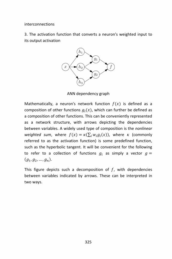
325

interconnections

3. The activation function that converts a neuron's weighted input to

its output activation

ANN dependency graph

Mathematically, a neuron's network function 𝑓(𝑥) is defined as a

composition of other functions 𝑔𝑖(𝑥), which can further be defined as

a composition of other functions. This can be conveniently represented

as a network structure, with arrows depicting the dependencies

between variables. A widely used type of composition is the nonlinear

weighted sum, where 𝑓(𝑥) = 𝜅(∑ 𝑤𝑖𝑔𝑖(𝑥)𝑖 ), where 𝜅 (commonly

referred to as the activation function) is some predefined function,

such as the hyperbolic tangent. It will be convenient for the following

to refer to a collection of functions 𝑔𝑖 as simply a vector 𝑔 =

(𝑔1, 𝑔2, … , 𝑔𝑛).

This figure depicts such a decomposition of 𝑓, with dependencies

between variables indicated by arrows. These can be interpreted in

two ways.

326

Two separate depictions of the recurrent ANN dependency graph

The first view is the functional view: the input 𝒙 is transformed into a 3-

dimensional vector 𝒉, which is then transformed into a 2-dimensional

vector 𝒈, which is finally transformed into 𝒇. This view is most

commonly encountered in the context of optimization.

The second view is the probabilistic view: the random variable 𝐹 =

𝑓(𝐺) depends upon the random variable 𝐺 = 𝑔(𝐻), which depends

upon 𝐻 = ℎ(𝑥), which depends upon the random variable 𝑥. This view

is most commonly encountered in the context of graphical models.

327

The two views are largely equivalent. In either case, for this particular

network architecture, the components of individual layers are

independent of each other (e.g., the components of 𝑔 are independent

of each other given their input ℎ). This naturally enables a degree of

parallelism in the implementation.

Networks such as the previous one are commonly called feedforward,

because their graph is a directed acyclic graph. Networks with cycles

are commonly called recurrent. Such networks are commonly depicted

in the manner shown at the top of the figure, where 𝑓 is shown as

being dependent upon itself. However, an implied temporal

dependence is not shown.

Learning

What has attracted the most interest in neural networks is the

possibility of learning. Given a specific task to solve, and a class of

functions 𝐹, learning means using a set of observations to find 𝑓∗ ∈ 𝐹

which solves the task in some optimal sense.

This entails defining a cost function 𝐶: 𝐹 → ℝ such that, for the optimal

solution 𝑓∗, 𝐶(𝑓∗) ≤ 𝐶(𝑓) ∀𝑓 ∈ 𝐹– i.e., no solution has a cost less

than the cost of the optimal solution.

The cost function 𝐶 is an important concept in learning, as it is a

measure of how far away a particular solution is from an optimal

solution to the problem to be solved. Learning algorithms search

through the solution space to find a function that has the smallest

possible cost.

For applications where the solution is dependent on some data, the

cost must necessarily be a function of the observations, otherwise we

would not be modeling anything related to the data. It is frequently

defined as a statistic to which only approximations can be made. As a

simple example, consider the problem of finding the model 𝑓, which

minimizes 𝐶 = 𝐸[(𝑓(𝑥) − 𝑦)2], for data pairs (𝑥, 𝑦) drawn from some

distribution 𝒟. In practical situations we would only have 𝑁 samples

328

from 𝒟 and thus, for the above example, we would only minimize �̂� =1

𝑁∑ (𝑓(𝑥𝑖) − 𝑦𝑖)2𝑁

𝑖=1 . Thus, the cost is minimized over a sample of the

data rather than the entire data set.

When 𝑁 → ∞ some form of online machine learning must be used,

where the cost is partially minimized as each new example is seen.

While online machine learning is often used when 𝒟 is fixed, it is most

useful in the case where the distribution changes slowly over time. In

neural network methods, some form of online machine learning is

frequently used for finite datasets.

Choosing a cost function

While it is possible to define some arbitrary ad hoc cost function,

frequently a particular cost will be used, either because it has desirable

properties (such as convexity) or because it arises naturally from a

particular formulation of the problem (e.g., in a probabilistic

formulation the posterior probability of the model can be used as an

inverse cost). Ultimately, the cost function will depend on the desired

task. An overview of the three main categories of learning tasks is

provided below:

Learning paradigms

There are three major learning paradigms, each corresponding to a

particular abstract learning task. These are supervised learning,

unsupervised learning and reinforcement learning.

Supervised learning

In supervised learning, we are given a set of example pairs (𝑥, 𝑦), 𝑥 ∈

𝑋, 𝑦 ∈ 𝑌and the aim is to find a function 𝑓: 𝑋 → 𝑌 in the allowed class

of functions that matches the examples. In other words, we wish to

infer the mapping implied by the data; the cost function is related to

the mismatch between our mapping and the data and it implicitly

contains prior knowledge about the problem domain.

329

A commonly used cost is the mean-square error, which tries to

minimize the average squared error between the network's output,

𝑓(𝑥), and the target value 𝑦 over all the example pairs. When one tries

to minimize this cost using gradient descent for the class of neural

networks called multilayer perceptrons, one obtains the common and

well-known backpropagation algorithm for training neural networks.

Tasks that fall within the paradigm of supervised learning are pattern

recognition (also known as classification) and regression (also known as

function approximation). The supervised learning paradigm is also

applicable to sequential data (e.g., for speech and gesture recognition).

This can be thought of as learning with a “teacher,” in the form of a

function that provides continuous feedback on the quality of solutions

obtained thus far.

Unsupervised learning

In unsupervised learning, some data 𝑥 is given and the cost function to

be minimized, that can be any function of the data 𝑥 and the network's

output, 𝑓.

The cost function is dependent on the task (what we are trying to

model) and our a priori assumptions (the implicit properties of our

model, its parameters and the observed variables).

As a trivial example, consider the model 𝑓(𝑥) = 𝑎 where 𝑎 is a

constant and the cost 𝐶 = 𝐸[(𝑓(𝑥) − 𝑦)2]. Minimizing this cost will

give us a value of 𝑎 that is equal to the mean of the data. The cost

function can be much more complicated. Its form depends on the

application: for example, in compression it could be related to the

mutual information between 𝑥 and 𝑓(𝑥), whereas in statistical

modeling, it could be related to the posterior probability of the model

given the data. (Note that in both of those examples those quantities

would be maximized rather than minimized).

Tasks that fall within the paradigm of unsupervised learning are in

general estimation problems; the applications include clustering, the

330

estimation of statistical distributions, compression and filtering.

Reinforcement learning

In reinforcement learning, data 𝑥 are usually not given, but generated

by an agent's interactions with the environment. At each point in time

𝑡, the agent performs an action 𝑦𝑡 and the environment generates an

observation 𝑥𝑡 and an instantaneous cost 𝑐𝑡, according to some

(usually unknown) dynamics. The aim is to discover a policy for

selecting actions that minimizes some measure of a long-term cost; i.e.,

the expected cumulative cost. The environment’s dynamics and the

long-term cost for each policy are usually unknown, but can be

estimated.

More formally the environment is modelled as a Markov decision

process (MDP) with states 𝑠1, … , 𝑠𝑛 ∈ 𝑆 and actions 𝑎1, … , 𝑎𝑚 ∈ 𝐴 with

the following probability distributions: the instantaneous cost

distribution 𝑃(𝑐𝑡|𝑠𝑡), the observation distribution 𝑃(𝑥𝑡|𝑠𝑡) and the

transition 𝑃(𝑠𝑡+1|𝑠𝑡, 𝑎𝑡), while a policy is defined as conditional

distribution over actions given the observations. Taken together, the

two then define a Markov chain (MC). The aim is to discover the policy

that minimizes the cost; i.e., the MC for which the cost is minimal.

ANNs are frequently used in reinforcement learning as part of the

overall algorithm (Hoskins & Himmelblau, 1992). Dynamic

programming has been coupled with ANNs (Neuro dynamic

programming) by Bertsekas and Tsitsiklis and applied to multi-

dimensional nonlinear problems (Bertsekas, 1996) such as those

involved in vehicle routing (Secomandi, 2000), natural resources

management (de Rigo, Rizzoli, Soncini-Sessa, Weber, & Zenesi, 2001)

(Damas, et al., 2000) or medicine (Deng & Ferris, 2008) because of the

ability of ANNs to mitigate losses of accuracy even when reducing the

discretization grid density for numerically approximating the solution of

the original control problems.

Tasks that fall within the paradigm of reinforcement learning are

control problems, games and other sequential decision making tasks.

331

Learning algorithms

Training a neural network model essentially means selecting one model

from the set of allowed models (or, in a Bayesian framework,

determining a distribution over the set of allowed models) that

minimizes the cost criterion. There are numerous algorithms available

for training neural network models; most of them can be viewed as a

straightforward application of optimization theory and statistical

estimation.

Most of the algorithms used in training artificial neural networks

employ some form of gradient descent. This is done by simply taking

the derivative of the cost function with respect to the network

parameters and then changing those parameters in a gradient-related

direction.

Evolutionary methods (de Rigo, Castelletti, Rizzoli, Soncini-Sessa, &

Weber, 2005), gene expression programming (Ferreira, 2006),

simulated annealing (Da & Xiurun, 2005), expectation-maximization,

non-parametric methods and particle swarm optimization (Wu & Chen,

2009) are some commonly used methods for training neural networks.

Employing artificial neural networks

Perhaps the greatest advantage of ANNs is their ability to be used as an

arbitrary function approximation mechanism that ‘learns’ from

observed data. However, using them is not so straightforward, and a

relatively good understanding of the underlying theory is essential.

• Choice of model: This will depend on the data representation and

the application. Overly complex models tend to lead to problems

with learning.

• Learning algorithm: There are numerous trade-offs between

learning algorithms. Almost any algorithm will work well with the

correct hyperparameters for training on a particular fixed data set.

However, selecting and tuning an algorithm for training on unseen

data requires a significant amount of experimentation.

332

• Robustness: If the model, cost function and learning algorithm are

selected appropriately the resulting ANN can be extremely robust.

With the correct implementation, ANNs can be used naturally in online

learning and large data set applications. Their simple implementation

and the existence of mostly local dependencies exhibited in the

structure allows for fast, parallel implementations in hardware.

Applications

The utility of artificial neural network models lies in the fact that they

can be used to infer a function from observations. This is particularly

useful in applications where the complexity of the data or task makes

the design of such a function by hand impractical.

Real-life applications

The tasks artificial neural networks are applied to tend to fall within the

following broad categories:

• Function approximation, or regression analysis, including time

series prediction, fitness approximation and modeling.

• Classification, including pattern and sequence recognition,

novelty detection and sequential decision making.

• Data processing, including filtering, clustering, blind source

separation and compression.

• Robotics, including directing manipulators, prosthesis.

• Control, including Computer numerical control.

Application areas include the system identification and control (vehicle

control, process control, natural resources management), quantum

chemistry (Balabin & Lomakina, 2009), game-playing and decision

making (backgammon, chess, poker), pattern recognition (radar

systems, face identification, object recognition and more), sequence

recognition (gesture, speech, handwritten text recognition), medical

diagnosis, financial applications (e.g. automated trading systems), data

mining (or knowledge discovery in databases, “KDD”), visualization and

333

e-mail spam filtering.

Artificial neural networks have also been used to diagnose several

cancers. An ANN based hybrid lung cancer detection system named

HLND improves the accuracy of diagnosis and the speed of lung cancer

radiology (Ganesan, 2010). These networks have also been used to

diagnose prostate cancer. The diagnoses can be used to make specific

models taken from a large group of patients compared to information

of one given patient. The models do not depend on assumptions about

correlations of different variables. Colorectal cancer has also been

predicted using the neural networks. Neural networks could predict the

outcome for a patient with colorectal cancer with more accuracy than

the current clinical methods. After training, the networks could predict

multiple patient outcomes from unrelated institutions (Bottaci, 1997).

Neural networks and neuroscience

Theoretical and computational neuroscience is the field concerned

with the theoretical analysis and the computational modeling of

biological neural systems. Since neural systems are intimately related

to cognitive processes and behavior, the field is closely related to

cognitive and behavioral modeling.

The aim of the field is to create models of biological neural systems in

order to understand how biological systems work. To gain this

understanding, neuroscientists strive to make a link between observed

biological processes (data), biologically plausible mechanisms for

neural processing and learning (biological neural network models) and

theory (statistical learning theory and information theory).

Types of models

Many models are used in the field, defined at different levels of

abstraction and modeling different aspects of neural systems. They

range from models of the short-term behavior of individual neurons,

models of how the dynamics of neural circuitry arise from interactions

between individual neurons and finally to models of how behavior can

334

arise from abstract neural modules that represent complete

subsystems. These include models of the long-term, and short-term

plasticity, of neural systems and their relations to learning and memory

from the individual neuron to the system level.

Types of artificial neural networks

Artificial neural network types vary from those with only one or two

layers of single direction logic, to complicated multi–input many

directional feedback loops and layers. On the whole, these systems use

algorithms in their programming to determine control and organization

of their functions. Most systems use “weights” to change the

parameters of the throughput and the varying connections to the

neurons. Artificial neural networks can be autonomous and learn by

input from outside “teachers” or even self-teaching from written-in

rules.

Theoretical properties

Computational power

The multi-layer perceptron (MLP) is a universal function approximator,

as proven by the Cybenko theorem. However, the proof is not

constructive regarding the number of neurons required or the settings

of the weights. Work by Hava Siegelmann and Eduardo D. Sontag has

provided a proof that a specific recurrent architecture with rational

valued weights (as opposed to full precision real number-valued

weights) has the full power of a Universal Turing Machine (Siegelmann

& Sontag, 1991) using a finite number of neurons and standard linear

connections. They have further shown that the use of irrational values

for weights results in a machine with super-Turing power.

Capacity

Artificial neural network models have a property called 'capacity',

which roughly corresponds to their ability to model any given function.

It is related to the amount of information that can be stored in the

335

network and to the notion of complexity.

Convergence

Nothing can be said in general about convergence since it depends on a

number of factors. Firstly, there may exist many local minima. This

depends on the cost function and the model. Secondly, the

optimization method used might not be guaranteed to converge when

far away from a local minimum. Thirdly, for a very large amount of data

or parameters, some methods become impractical. In general, it has

been found that theoretical guarantees regarding convergence are an

unreliable guide to practical application.

Generalization and statistics

In applications where the goal is to create a system that generalizes

well in unseen examples, the problem of over-training has emerged.

This arises in convoluted or over-specified systems when the capacity

of the network significantly exceeds the needed free parameters. There

are two schools of thought for avoiding this problem: The first is to use

cross-validation and similar techniques to check for the presence of

overtraining and optimally select hyperparameters such as to minimize

the generalization error. The second is to use some form of

regularization. This is a concept that emerges naturally in a

probabilistic (Bayesian) framework, where the regularization can be

performed by selecting a larger prior probability over simpler models;

but also in statistical learning theory, where the goal is to minimize

over two quantities: the 'empirical risk' and the 'structural risk', which

roughly corresponds to the error over the training set and the

predicted error in unseen data due to overfitting.

Supervised neural networks that use an MSE cost function can use

formal statistical methods to determine the confidence of the trained

model. The MSE on a validation set can be used as an estimate for

variance. This value can then be used to calculate the confidence

interval of the output of the network, assuming a normal distribution.

A confidence analysis made this way is statistically valid as long as the

336

output probability distribution stays the same and the network is not

modified.

Confidence analysis of a neural network

By assigning a softmax activation function, a generalization of the

logistic function, on the output layer of the neural network (or a

softmax component in a component-based neural network) for

categorical target variables, the outputs can be interpreted as posterior

probabilities. This is very useful in classification as it gives a certainty

measure on classifications. The softmax activation function is:

𝑦𝑖 =𝑒𝑥𝑖

∑ 𝑒𝑥𝑗𝑐𝑖=1

.

337

Dynamic properties

Various techniques originally developed for studying disordered

magnetic systems (i.e., the spin glass) have been successfully applied to

simple neural network architectures, such as the Hopfield network.

Influential work by E. Gardner and B. Derrida has revealed many

interesting properties about perceptrons with real-valued synaptic

weights, while later work by W. Krauth and M. Mezard has extended

these principles to binary-valued synapses.

Criticism

A common criticism of neural networks, particularly in robotics, is that

they require a large diversity of training for real-world operation. This is

not surprising, since any learning machine needs sufficient

representative examples in order to capture the underlying structure

that allows it to generalize to new cases. Dean Pomerleau, in his

research presented in the paper “Knowledge-based Training of Artificial

Neural Networks for Autonomous Robot Driving,” uses a neural

network to train a robotic vehicle to drive on multiple types of roads

(single lane, multi-lane, dirt, etc.). A large amount of his research is

devoted to (1) extrapolating multiple training scenarios from a single

training experience, and (2) preserving past training diversity so that

the system does not become overtrained (if, for example, it is

presented with a series of right turns – it should not learn to always

turn right). These issues are common in neural networks that must

decide from amongst a wide variety of responses, but can be dealt with

in several ways, for example by randomly shuffling the training

examples, by using a numerical optimization algorithm that does not

take too large steps when changing the network connections following

an example, or by grouping examples in so-called mini-batches.

A. K. Dewdney, a former Scientific American columnist, wrote in 1997,

“Although neural nets do solve a few toy problems, their powers of

computation are so limited that I am surprised anyone takes them

seriously as a general problem-solving tool.” (Dewdney, p. 82)

338

Arguments for Dewdney's position are that to implement large and

effective software neural networks, much processing and storage

resources need to be committed. While the brain has hardware

tailored to the task of processing signals through a graph of neurons,

simulating even a most simplified form on Von Neumann technology

may compel a neural network designer to fill many millions of database

rows for its connections – which can consume vast amounts of

computer memory and hard disk space. Furthermore, the designer of

neural network systems will often need to simulate the transmission of

signals through many of these connections and their associated

neurons – which must often be matched with incredible amounts of

CPU processing power and time. While neural networks often yield

effective programs, they too often do so at the cost of efficiency (they

tend to consume considerable amounts of time and money).

Arguments against Dewdney's position are that neural nets have been

successfully used to solve many complex and diverse tasks, ranging

from autonomously flying aircraft (NASA, 2003) to detecting credit card

fraud.

Technology writer Roger Bridgman commented on Dewdney's

statements about neural nets:

Neural networks, for instance, are in the dock not only because they

have been hyped to high heaven, (what hasn't?) but also because you

could create a successful net without understanding how it worked:

the bunch of numbers that captures its behavior would in all

probability be “an opaque, unreadable table...valueless as a scientific

resource”.

In spite of his emphatic declaration that science is not technology,

Dewdney seems here to pillory neural nets as bad science when

most of those devising them are just trying to be good engineers.

An unreadable table that a useful machine could read would still be

well worth having (Bridgman).

339

In response to this kind of criticism, one should note that although it is

true that analyzing what has been learned by an artificial neural

network is difficult, it is much easier to do so than to analyze what has

been learned by a biological neural network. Furthermore, researchers

involved in exploring learning algorithms for neural networks are

gradually uncovering generic principles which allow a learning machine

to be successful. For example, Bengio and LeCun (2007) wrote an

article regarding local vs non-local learning, as well as shallow vs deep

architecture. Some other criticisms came from believers of hybrid

models (combining neural networks and symbolic approaches). They

advocate the intermix of these two approaches and believe that hybrid

models can better capture the mechanisms of the human mind (Sun

and Bookman, 1990).

A single-layer feedforward artificial neural network. Arrows originating

from 𝑥2 are omitted for clarity. There are p inputs to this network and

𝑞 outputs. In this system, the value of the 𝑞th output, 𝑦𝑞 would be

calculated as 𝑦𝑞 = ∑(𝑥𝑖 ∗ 𝑤𝑖𝑞)

340

A two-layer feedforward artificial neural network.

Neural network software

Simulators

Neural network simulators are software applications that are used to

simulate the behavior of artificial or biological neural networks. They

focus on one or a limited number of specific types of neural networks.

They are typically stand-alone and not intended to produce general

neural networks that can be integrated in other software. Simulators

usually have some form of built-in visualization to monitor the training

process. Some simulators also visualize the physical structure of the

neural network.

341

Research simulators

SNNS research neural network simulator

Historically, the most common type of neural network software was

intended for researching neural network structures and algorithms.

The primary purpose of this type of software is, through simulation, to

gain a better understanding of the behavior and properties of neural

networks. Today in the study of artificial neural networks, simulators

have largely been replaced by more general component based

development environments as research platforms.

Commonly used artificial neural network simulators include the

Stuttgart Neural Network Simulator (SNNS), Emergent, JavaNNS, Neural

Lab and NetMaker

In the study of biological neural networks however, simulation

software is still the only available approach. In such simulators the

physical biological and chemical properties of neural tissue, as well as

342

the electromagnetic impulses between the neurons are studied.

Commonly used biological network simulators include Neuron,

GENESIS, NEST and Brian. Other simulators are XNBC and the NN

Toolbox for MATLAB.

Data analysis simulators

Unlike the research simulators, the data analysis simulators are

intended for practical applications of artificial neural networks. Their

primary focus is on data mining and forecasting. Data analysis

simulators usually have some form of preprocessing capabilities. Unlike

the more general development environments data analysis simulators

use a relatively simple static neural network that can be configured. A

majority of the data analysis simulators on the market use back

propagating networks or self-organizing maps as their core. The

advantage of this type of software is that it is relatively easy to use.

Some data analysis simulators are dedicated neural network packages,

such as Neural Designer. Some others work in conjunction with other

computational environments, such as NeuralTools for Microsoft Excel.

Simulators for teaching neural network theory

When the Parallel Distributed Processing volumes[1] [2][3] were

released in 1986-87, they provided some relatively simple software.

The original PDP software did not require any programming skills,

which led to its adoption by a wide variety of researchers in diverse

fields. The original PDP software was developed into a more powerful

package called PDP++, which in turn has become an even more

powerful platform called Emergent. With each development, the

software has become more powerful, but also more daunting for use

by beginners.

In 1997, the tLearn software was released to accompany a book.[4]

This was a return to the idea of providing a small, user-friendly,

simulator that was designed with the novice in mind. tLearn allowed

basic feed forward networks, along with simple recurrent networks,

both of which can be trained by the simple back propagation algorithm.

343

tLearn has not been updated since 1999.

In 2011, the Basic Prop simulator was released. Basic Prop is a self-

contained application, distributed as a platform neutral JAR file, that

provides much of the same simple functionality as tLearn.

Development Environments

Development environments for neural networks differ from the

software described above primarily on two accounts – they can be

used to develop custom types of neural networks and they support

deployment of the neural network outside the environment. In some

cases they have advanced preprocessing, analysis and visualization

capabilities.

Component based

A more modern type of development environments that are currently

favored in both industrial and scientific use are based on a component

based paradigm. The neural network is constructed by connecting

adaptive filter components in a pipe filter flow. This allows for greater

flexibility as custom networks can be built as well as custom

components used by the network. In many cases this allows a

combination of adaptive and non-adaptive components to work

together. The data flow is controlled by a control system which is

exchangeable as well as the adaptation algorithms. The other

important feature is deployment capabilities. With the advent of

component-based frameworks such as .NET and Java, component

based development environments are capable of deploying the

developed neural network to these frameworks as inheritable

components. In addition some software can also deploy these

components to several platforms, such as embedded systems.

344

Peltarion Synapse component based development environment.

Component based development environments include: Peltarion

Synapse, NeuroDimension NeuroSolutions, Scientific Software Neuro

Laboratory, and the LIONsolver integrated software. Free open source

component based environments include Encog and Neuroph.

Criticism

A disadvantage of component-based development environments is

that they are more complex than simulators. They require more

learning to fully operate and are more complicated to develop.

Custom neural networks

The majority implementations of neural networks available are

however custom implementations in various programming languages

and on various platforms. Basic types of neural networks are simple to

345

implement directly. There are also many programming libraries that

contain neural network functionality and that can be used in custom

implementations.

Standards

In order for neural network models to be shared by different

applications, a common language is necessary. Recently, the Predictive

Model Markup Language (PMML) has been proposed to address this

need.

PMML is an XML-based language which provides a way for applications

to define and share neural network models (and other data mining

models) between PMML compliant applications.

PMML provides applications a vendor-independent method of defining

models so that proprietary issues and incompatibilities are no longer a

barrier to the exchange of models between applications. It allows users

to develop models within one vendor's application, and use other

vendors' applications to visualize, analyze, evaluate or otherwise use

the models. Previously, this was very difficult, but with PMML, the

exchange of models between compliant applications is now

straightforward.

PMML Consumers and Producers

A range of products are being offered to produce and consume PMML.

This ever growing list includes the following neural network products:

• R: produces PMML for neural nets and other machine learning

models via the package pmml.

• SAS Enterprise Miner: produces PMML for several mining models,

including neural networks, linear and logistic regression, decision

trees, and other data mining models.

• SPSS: produces PMML for neural networks as well as many other

mining models.

• STATISTICA: produces PMML for neural networks, data mining

models and traditional statistical models.

346

Example Using R

In this example a neural network (or Multilayer perceptron depending

on naming convention) will be build that is able to take a number and

calculate the square root (or as close to as possible). The R library

‘neuralnet’ will be used to train and build the neural network.

The example will produce the neural network shown in the image

below. It is going to take a single input (the number that you want

square rooting) and produce a single output (the square root of the

input). The middle of the image contains 10 hidden neurons which will

be trained.

347

The output of the script will look like:

Input Expected Output Neural Net Output

Input Expected Output Neural Net Output 1 1 0.9623402772 4 2 2.0083461217 9 3 2.9958221776 16 4 4.0009548085 25 5 5.0028838579 36 6 5.9975810435 49 7 6.9968278722 64 8 8.0070028670 81 9 9.0019220736 100 10 9.9222007864

As you can see the neural network does a reasonable job at finding the

square root, the largest error in in finding the square root of 1 which is

out by ~4%

Onto the code:

install.packages('neuralnet') library("neuralnet") #Going to create a neural network to perform sqare #rooting #Type ?neuralnet for more information on the #neuralnet library #Generate 50 random numbers uniformly distributed #between 0 and 100 #And store them as a dataframe > traininginput <- as.data.frame(runif(50, min=0, + max=100)) > trainingoutput <- sqrt(traininginput) #Column bind the data into one variable > trainingdata <- cbind(traininginput,trainingoutput) > colnames(trainingdata) <- c("Input","Output") #Train the neural network #Going to have 10 hidden layers #Threshold is a numeric value specifying the threshold for the partial #derivatives of the error function as stopping criteria. > net.sqrt <- neuralnet(Output~Input,trainingdata, hidden=10, threshold=0.01) > print(net.sqrt)

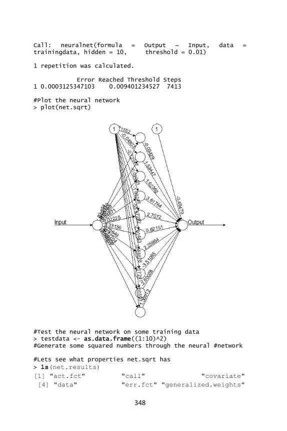
348

Call: neuralnet(formula = Output ~ Input, data = trainingdata, hidden = 10, threshold = 0.01) 1 repetition was calculated. Error Reached Threshold Steps 1 0.0003125347103 0.009401234527 7413 #Plot the neural network > plot(net.sqrt)

#Test the neural network on some training data > testdata <- as.data.frame((1:10)^2) #Generate some squared numbers through the neural #network #Lets see what properties net.sqrt has

> ls(net.results)

[1] "act.fct" "call" "covariate"

[4] "data" "err.fct" "generalized.weights"

349

[7] "linear.output" "model.list" "net.result"

[10] "response" "result.matrix" "startweights"

[13] "weights"

#Lets see the results > print(net.results$net.result) [[1]] [,1] 1 5.0490045485 2 7.4625475299 3 5.4268560491 4 9.3944183247 5 7.3261826045 6 9.7116754748 7 7.7005230133 8 6.1877876553 9 9.0208308800 10 5.7323789090 11 8.8662469974 12 9.6321471501 13 5.5556127899 14 8.8963448461 15 6.5228214924 16 4.6004103084 17 5.1903750160 18 7.4088926123 19 4.6820958475 20 8.7562521802 21 8.9002614981 22 9.9683150949 23 0.8709360456 24 5.7191690479 25 9.5527300575 26 4.2271915852 27 9.3130169284 28 6.6324229956 29 6.4189621322 30 9.0096296704 31 5.7399327728 32 3.5851960402 33 8.0773241098 34 9.3700866302 35 2.7618057270 36 8.8809443763 37 7.2225438175 38 3.5564655707 39 8.2756946858 40 4.2854133636 41 8.8574145651 42 5.8292858082 43 6.3127094368

350

44 2.6722212606 45 7.0154300338 46 8.3787559152 47 9.5958246251 48 4.8688678386 49 6.5017337465 50 8.3502796644 #Lets display a better version of the results > cleanoutput <- cbind(testdata,sqrt(testdata), + as.data.frame(net.results$net.result)) > colnames(cleanoutput) <- c("Input","Expected + Output","Neural Net Output") > print(cleanoutput) Input Expected Output Neural Net Output 1 1 1 5.0490045485 2 4 2 7.4625475299 3 9 3 5.4268560491 4 16 4 9.3944183247 5 25 5 7.3261826045 6 36 6 9.7116754748 7 49 7 7.7005230133 8 64 8 6.1877876553 9 81 9 9.0208308800 10 100 10 5.7323789090 11 1 1 8.8662469974 12 4 2 9.6321471501 13 9 3 5.5556127899 14 16 4 8.8963448461 15 25 5 6.5228214924 16 36 6 4.6004103084 17 49 7 5.1903750160 18 64 8 7.4088926123 19 81 9 4.6820958475 20 100 10 8.7562521802 21 1 1 8.9002614981 22 4 2 9.9683150949 23 9 3 0.8709360456 24 16 4 5.7191690479 25 25 5 9.5527300575 26 36 6 4.2271915852 27 49 7 9.3130169284 28 64 8 6.6324229956 29 81 9 6.4189621322 30 100 10 9.0096296704 31 1 1 5.7399327728 32 4 2 3.5851960402 33 9 3 8.0773241098 34 16 4 9.3700866302 35 25 5 2.7618057270 36 36 6 8.8809443763 37 49 7 7.2225438175

351

38 64 8 3.5564655707 39 81 9 8.2756946858 40 100 10 4.2854133636 41 1 1 8.8574145651 42 4 2 5.8292858082 43 9 3 6.3127094368 44 16 4 2.6722212606 45 25 5 7.0154300338 46 36 6 8.3787559152 47 49 7 9.5958246251 48 64 8 4.8688678386 49 81 9 6.5017337465 50 100 10 8.3502796644

352

353

17. Uplift modeling

Uplift modeling, also known as incremental modeling, true lift

modeling, or net-lift modeling is a predictive modeling technique that

directly models the incremental impact of a treatment (such as a direct

marketing action) on an individual's behavior.

Uplift modeling has applications in customer relationship management

for up-sell, cross-sell and retention modeling. It has also been applied

to personalized medicine. Unlike the related Differential Prediction

concept in psychology, Uplift modeling assumes an active agent.

Introduction

Uplift modeling uses a randomized scientific control to not only

measure the effectiveness of a marketing action but also to build a

predictive model that predicts the incremental response to the

marketing action. It is a data mining technique that has been applied

predominantly in the financial services, telecommunications and retail

direct marketing industries to up-sell, cross-sell, churn and retention

activities.

Measuring uplift

The uplift of a marketing campaign is usually defined as the difference

in response rate between a treated group and a randomized control

group. This allows a marketing team to isolate the effect of a marketing

action and measure the effectiveness or otherwise of that individual

marketing action. Honest marketing teams will only take credit for the

incremental effect of their campaign.

The uplift problem statement

The uplift problem can be stated as follow, given the following:

• cases 𝑃 = {1, . . , 𝑛},

• treatments 𝐽 = {1, … , 𝑈},

354

• expected return 𝑅(𝑖, 𝑡) for each case 𝑖 and treatment t,

• non-negative integers 𝑛1, … , 𝑛𝑈 such that

𝑛1 + ⋯ + 𝑛𝑈 = 𝑛

find a treatment assignment

𝑓: 𝑃 → 𝐽

So that the total return

∑ 𝑅𝑖𝑓(𝑖)

𝑛

𝑖=1

is maximized, subject to the constraints that the number of cases

assigned to treatment j is not to exceed 𝑛𝑗, (𝑗 = 1, . . , 𝑈).

Example: Marketing action case

• P: a group of customers,

• two treatments:

1. treatment 1: exercise some marketing action; 𝑅𝑖1 is the

expected return if treatment 1 is given to customer 𝑖,

2. treatment 2: exercise no the marketing action; let 𝑅𝑖2 be the

expected return if treatment 2 is given to customer 𝑖.

Solution to the maximization problem:

∑ 𝑅𝑖𝑓(𝑖)

𝑛

𝑖=1

= ( ∑ 𝑅𝑖1

𝑖∈(𝑓=1)

) + ( ∑ 𝑅𝑖2

𝑖∈(𝑓=2)

)

= ( ∑ 𝑅𝑖1

𝑖∈(𝑓=1)

) + (∑ 𝑅𝑖2

𝑛

𝑖=1

− ∑ 𝑅𝑖2

𝑖∈(𝑓=1)

)

= ( ∑ 𝑅𝑖1

𝑖∈(𝑓=1)

− 𝑅𝑖2) + (∑ 𝑅𝑖2

𝑛

𝑖=1

)

355

The second sum does not involve f, so maximizing total return is

equivalent to maximizing the first term

∑ (𝑅𝑖1 − 𝑅𝑖2)

𝑖∈(𝑓=1)

As for to the solution to the problem when we consider only the

reponses to treatment 1, to attain the maximum return:

• assign treatment 1 to the customers with the 𝑛1 largest values

of 𝑅𝑖1– 𝑅𝑖2

• assign treatment 2 to the remaining customers

The difference 𝑅𝑖1– 𝑅𝑖2 is called net lift, uplift, incremental response,

differential response, etc.

If we consider only the response to treatment 1, and base targeting on

a model built out of responses to previous marketing actions, we are

356

not proceeding as if to maximize ∑ 𝑅𝑖𝑓(𝑖)𝑛𝑖=1 . Such maximization would

not yield the maximum return. We need to consider the return from

cases subjected to no marketing action.

Now, consider a model with a binary response, e.g., Yes = 1, No = 0.

Then the netlift is:

𝑃𝑟𝑜𝑏(1) =exp(𝑠𝑐𝑜𝑟𝑒1)

1 + exp(𝑠𝑐𝑜𝑟𝑒1);

𝑃𝑟𝑜𝑏(0) =exp(𝑠𝑐𝑜𝑟𝑒0)

1 + exp(𝑠𝑐𝑜𝑟𝑒0);

𝑛𝑒𝑡𝑙𝑖𝑓𝑡 = 𝑃𝑟𝑜𝑏(1)– 𝑃𝑟𝑜𝑏(0),

where 𝑃𝑟𝑜𝑏(1) is the probability of a response equal to 1, 𝑃𝑟𝑜𝑏(0) is

the probability of a response = 0, 𝑠𝑐𝑜𝑟𝑒1 is the model scores for

responses equal to 1, and 𝑠𝑐𝑜𝑟𝑒0 is the model scores for responses

equal to 0.

The incremental response lift, with all initial vales set to 0, can be

obtained using the following pseudo code:

prob1 = exp(score_1)/(1+exp(score_1)); prob0 = exp(score_0)/(1+exp(score_0)); netlift = prob1 – prob0; if treatment flag = 1 then mail total = mail total + 1; if response = 1 then mail response = mail response + 1; expected netlift mailed = expected netlift mailed + netlift; expected anyway mailed = expected anyway mailed + prob(0); expected mail response = expected mail response + prob(1); end; else do; nomail totoal = nomail total + 1; if response = 1 then nomail response = nomail response + 1; end;

The associated probabilities and netlift pseudo code is:

if last pentile; empirical prob mail = mail response/mail total;

357

empirical prob nomail = nomail response/nomail total; empirical netlift = empirical prob mail - empirical prob

nomail; percent gain = 100* empirical netlift/ empirical prob

nomail; empirical expected buyanyway mailed = mail total* empirical

prob nomail; empirical expected netlift = mailresp - empirical expected

buyanyway mailed;

The table below shows the details of a campaign showing the number

of responses and calculated response rate for a hypothetical marketing

campaign. This campaign would be defined as having a response rate

uplift of 5%. It has created 50,000 incremental responses (100,000 -

50,000).

Group Number of Customers Responses Response Rate

Treated 1,000,000 100,000 10%

Control 1,000,000 50,000 5%

Traditional response modeling

Traditional response modeling typically takes a group of treated

customers and attempts to build a predictive model that separates the

likely responders from the non-responders through the use of one of a

number of predictive modeling techniques. Typically this would use

decision trees or regression analysis.

This model would only use the treated customers to build the model.

In contrast uplift modeling uses both the treated and control

customers to build a predictive model that focuses on the incremental

response. To understand this type of model it is proposed that there is

a fundamental segmentation that separates customers into the

following groups (Lo, 2002):

• The Persuadables : customers who only respond to the

marketing action because they were targeted

358

• The Sure Things : customers who would have responded

whether they were targeted or not

• The Lost Causes : customers who will not respond irrespective

of whether or not they are targeted

• The Do Not Disturbs or Sleeping Dogs : customers who are less

likely to respond because they were targeted

The only segment that provides true incremental responses is the

Persuadables.

Uplift modeling provides a scoring technique that can separate

customers into the groups described above. Traditional response

modeling often targets the Sure Things being unable to distinguish

them from the Persuadables.

Example: Simulation-Educators.com

Majority of direct marketing campaigns are based on purchase

propensity models, selecting customer email, paper mail or other

marketing contact lists based on customers’ probability to make a

purchase. Simulation-Educators.com offers training courses in

modeling and simulation topics. The following is an example of a of

standard purchase propensity model output for a mailing campaign for

such courses.

Scoring Rank Response Rate Lift

1 28.1% 3.41

2 17.3% 2.10

3 9.6% 1.17

4 8.4% 1.02

5 4.8% 0.58

6 3.9% 0.47

7 3.3% 0.40

8 3.4% 0.41

9 3.5% 0.42

10 0.1% 0.01

Total 8.2%

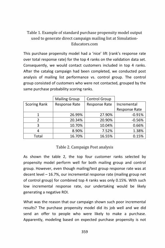
359

Table 1. Example of standard purchase propensity model output

used to generate direct campaign mailing list at Simulation-

Educators.com

This purchase propensity model had a ‘nice’ lift (rank’s response rate

over total response rate) for the top 4 ranks on the validation data set.

Consequently, we would contact customers included in top 4 ranks.

After the catalog campaign had been completed, we conducted post

analysis of mailing list performance vs. control group. The control

group consisted of customers who were not contacted, grouped by the

same purchase probability scoring ranks.

Mailing Group Control Group

Scoring Rank Response Rate Response Rate Incremental Response Rate

1 26.99% 27.90% -0.91%

2 20.34% 20.90% -0.56%

3 10.70% 10.04% 0.66%

4 8.90% 7.52% 1.38%

Total 16.70% 16.55% 0.15%

Table 2. Campaign Post analysis

As shown the table 2, the top four customer ranks selected by

propensity model perform well for both mailing group and control

group. However, even though mailing/test group response rate was at

decent level – 16.7%, our incremental response rate (mailing group net

of control group) for combined top 4 ranks was only 0.15%. With such

low incremental response rate, our undertaking would be likely

generating a negative ROI.

What was the reason that our campaign shown such poor incremental

results? The purchase propensity model did its job well and we did

send an offer to people who were likely to make a purchase.

Apparently, modeling based on expected purchase propensity is not

360

always the right solution for a successful direct marking campaign.

Since there was no increase in response rate over control group, we

could have been contacting customers who would have bought our

product without promotional direct mail. Customers in top ranks of

purchase propensity model may not need a nudge or they are buying in

response to a contact via other channels. If that is the case, the

customers in the lower purchase propensity ranks would be more

‘responsive’ to a marketing contact.

We should be predicting incremental impact – additional purchases

generated by a campaign, not purchases that would be made without

the contact. Our marketing mailing can be substantially more cost

efficient if we don’t mail customers who are going to buy anyway.

Since customers very rarely use promo codes from catalogs or click on

web display ads, it is difficult to identify undecided, swing customer

based on the promotion codes or web display click-throughs.

Net lift models predict which customer segments are likely to make a

purchase ONLY if prompted by a marketing undertaking.

Purchasers from mailing group include customers that needed a nudge,

however, all purchasers in the holdout/control group did not need our

catalog to make their purchasing decision. All purchasers in the control

group can be classified as ‘need no contact’. Since we need a model

that would separate ‘need contact’ purchasers from ‘no contact’

purchasers, the net lift models look at differences in purchasers in

mailing (contact) group versus purchasers from control group.

In order to classify our customers into these groups we need mailing

group and control group purchases results from similar prior

campaigns. If there are no comparable historic undertakings, we have

to create a small scale trial before the main rollout.

Uplift modeling approach—probability decomposition models

Segments used in probability decomposition models:

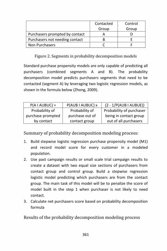
361

Contacted Group

Control Group

Purchasers prompted by contact A D

Purchasers not needing contact B E

Non Purchasers C F

Figure 2. Segments in probability decomposition models

Standard purchase propensity models are only capable of predicting all

purchasers (combined segments A and B). The probability

decomposition model predicts purchasers segments that need to be

contacted (segment A) by leveraging two logistic regression models, as

shown in the formula below (Zhong, 2009).

P(A I AUBUC) = P(AUB I AUBUC) x (2 - 1/P(AUB I AUBUE))

Probability of purchase prompted

by contact

Probability of purchase out of contact group

Probability of purchaser being in contact group out of all purchasers

Summary of probability decomposition modeling process:

1. Build stepwise logistic regression purchase propensity model (M1)

and record model score for every customer in a modeled

population.

2. Use past campaign results or small scale trial campaign results to

create a dataset with two equal size sections of purchasers from

contact group and control group. Build a stepwise regression

logistic model predicting which purchasers are from the contact

group. The main task of this model will be to penalize the score of

model built in the step 1 when purchaser is not likely to need

contact.

3. Calculate net purchasers score based on probability decomposition

formula

Results of the probability decomposition modeling process

362

Scoring Rank

Contact Group Response %

Control Group Response %

Incremental Response Rate

1 18.8% 12.9% 5.9% 2 7.8% 5.4% 2.4% 3 6.9% 4.5% 2.5% 4 4.3% 3.6% 0.7% 5 3.9% 3.5% 0.4% 6 4.1% 4.1% 0.0% 7 3.7% 4.0% -0.2% 8 4.7% 4.1% 0.6% 9 5.0% 6.7% -1.7%

10 11.0% 15.7% -4.7%

Table 3. Post analysis of campaign leveraging probability

decomposition model for Simulation-Educators.com

Scoring Ranks 1 thru 6 show positive incremental response rates. The

scoring ranks are ordered based on the incremental response rates.

Return on investment

Because uplift modeling focuses on incremental responses only, it

provides very strong return on investment cases when applied to

traditional demand generation and retention activities. For example, by

only targeting the persuadable customers in an outbound marketing

campaign, the contact costs and hence the return per unit spend can

be dramatically improved (Radcliffe & Surry, 2011).

Removal of negative effects

One of the most effective uses of uplift modeling is in the removal of

negative effects from retention campaigns. Both in the

telecommunications and financial services industries often retention

campaigns can trigger customers to cancel a contract or policy. Uplift

modeling allows these customers, the Do Not Disturbs, to be removed

from the campaign.

363

Application to A/B and Multivariate Testing

It is rarely the case that there is a single treatment and control group.

Often the “treatment” can be a variety of simple variations of a

message or a multi-stage contact strategy that is classed as a single

treatment. In the case of A/B or multivariate testing, uplift modeling

can help in understanding whether the variations in tests provide any

significant uplift compared to other targeting criteria such as

behavioral or demographic indicators.

Methods for modeling

Example of Logistic Regression

We now use a special case of binary response variable to describe our

proposed methodology. If 𝑌𝑖 is a binary response variable representing

whether customer 𝑖 responds to a campaign, we consider the following

set of independent variables: 𝑋𝑖, 𝑇𝑖, and 𝑋𝑖 ∗ 𝑇𝑖 where 𝑇𝑖 = 1 if 𝑖 is in

the treatment group and 𝑇𝑖 = 0 if 𝑖 is in the control group. We may

model the response rate using a linear logistic regression

𝑃𝑖 𝐸(𝑌𝑖|𝑋𝑖) =exp(𝛼 + 𝛽′𝑋𝑖 + 𝛾𝑇𝑖 + 𝛿′𝑋𝑖𝑇𝑖)

1 + exp(𝛼 + 𝛽′𝑋𝑖 + 𝛾𝑇𝑖 + 𝛿′𝑋𝑖𝑇𝑖),

where 𝛼, 𝛽, 𝛾, 𝛿 are parameters to be estimated.

In the logistic equation, 𝛼 denotes the intercept, 𝛽 is a vector of

parameters measuring the main effects of the independent variables, 𝛾

denotes the main treatment effect, and 𝛿 measures additional effects

of the independent variables due to treatment. In reality, some

variable reduction procedure will usually be applied to narrow down

the list of 𝑋𝑖, 𝑇𝑖, and 𝑋𝑖 ∗ 𝑇𝑖 first before estimating the parameters in

the equation.

Then

364

𝑃𝑖|treatment − 𝑃𝑖|control

=exp(𝛼 + 𝛾 + 𝛽′𝑋𝑖 + 𝛿′𝑋𝑖)

1 + exp(𝛼 + 𝛾 + 𝛽′𝑋𝑖 + 𝛿′𝑋𝑖)−

exp(𝛼 + 𝛽′𝑋𝑖)

1 + exp(𝛼 + 𝛽′𝑋𝑖).

That is, the parameter estimates obtained in first equation can be used

in this equation to predict the treatment and control difference in

response rate for each 𝑖 in a new data set. Then the data set can be

sorted by the predicted difference between treatment and control.

Those with high positive predicted differences will be selected for next

campaign targeting.

The procedure then is to build a logistic regression model for the

treatment sample and a separate one for the control sample. Then the

uplift model subtracts probabilities predicted by both.

Example of Decision Tree

Rzepakowski and Jaroszewicz (Rzepakowski & Jaroszewicz, 2010)

propose an approach that employs decision trees with:

• Spliting criteria based on Information Theory

• Pruning strategy designed for uplift modeling

• Multiclass problems and multiway splits possible

• If the control group is empty, the criterion should reduce to

one of classical splitting criteria used for decision tree learning

The approach uses splitting criteria based on three distribution

divergences. A distribution divergence is a measure of how much two

probability distributions differ. The Kullback-Leibler divergence is a

well-known and widely used information theoretic measure. It can be

used to measure the difference between treatment and control

groups:

𝐾𝐿(𝑃𝑇(𝐶𝑙𝑎𝑠𝑠): 𝑃𝐶(𝐶𝑙𝑎𝑠𝑠)) = 𝐾𝐿(𝑃𝑇(𝑌)|𝑃𝐶(𝑌))

= ∑ 𝑃𝑇(𝑦) log𝑃𝑇(𝑦)

𝑃𝐶(𝑦)𝑦∈Y

.

365

The squared Euclidean distance is less frequently applied to compare

distributions, but has been used in literature, and applied for example

to Schema Matching:

𝐸𝑢𝑐𝑙𝑖𝑑(𝑃𝑇(𝑌)|𝑃𝐶(𝑌)) = ∑ (𝑃𝑇𝑇(𝑦) − 𝑃𝐶(𝑦))

2

𝑦∈Dom (𝐶𝑙𝑎𝑠𝑠)

.

The third, Chi-squared divergence has been used, e.g., to measure

interestingness of rules:

𝜒2(𝑃𝑇(𝑌)|𝑃𝐶(𝑌)) = ∑(𝑃𝑇(𝑦) − 𝑃𝐶(𝑦))

2

𝑃𝐶(𝑦)𝑦∈Dom (𝐶𝑙𝑎𝑠𝑠)

.

Rzepakowski and Jaroszewicz (Rzepakowski & Jaroszewicz, 2010) argue

that the squared Euclidean distance has some important advantages

that make it an attractive alternative to the Kullback-Leibler and chi-

squared measures.

KL-divergence is conditional on a split Ω. The KL becomes

𝐾𝐿(𝑃𝑇(𝑌)|𝑃𝐶(𝑌)|Ω) = ∑𝑀(Ω)

𝑀𝐾𝐿(𝑃𝑇(𝑌|𝜔)|𝑃𝐶(𝑌|𝜔))

𝜔∈Ω

,

where 𝑀 = 𝑀𝑇 + 𝑀𝐶 (the sum of the training cases in the treatment

and control groups) and 𝑀(Ω) = 𝑀𝑇(Ω) + 𝑀𝐶(Ω) (the sum of the

number of training cases in which the outcome of the uplift Ω is 𝜔 in

treatment and control groups) (Rzepakowski & Jaroszewicz, 2010).

We then define 𝐾𝐿𝑔𝑎𝑖𝑛 as the increase in the KL divergence from a split

Ω relative to the KL-divergence in the parent node

𝐾𝐿𝑔𝑎𝑖𝑛(Ω) = 𝐾𝐿(𝑃𝑇(𝑌)|𝑃𝐶(𝑌)|Ω) − 𝐾𝐿(𝑃𝑇(𝑌)|𝑃𝐶(𝑌)).

The final split criterion is (Rzepakowski & Jaroszewicz, 2010)

𝐾𝐿𝑟𝑎𝑡𝑖𝑜(Ω) =𝐾𝐿𝑔𝑎𝑖𝑛(Ω)

𝐾𝐿𝑛𝑜𝑟𝑚 (Ω),

366

where 𝐾𝐿𝑛𝑜𝑟𝑚 (Ω) is a normalization factor that punishes:

• splits with different treatment/control proportions on each

branch

• splits with unbalanced number of cases on each branch

Decision tree pruning is a step which has decisive influence on the

generalization performance of the model. There are several pruning

methods, based on statistical tests, minimum description length

principle, etc.

The authors devised the maximum class probability difference which

can be viewed as a generalization of classification accuracy to the uplift

case. The idea is to look at the differences between treatment and

control probabilities in the root of the subtree and in its leaves, and

prune if, overall, the differences in leaves are not greater than the

difference in the root. In each node, they only look at the class for

which the difference was largest on the training set, and in addition,

remember the sign of that difference such that only differences that

have the same sign in the training and validation sets contribute to the

increase in our analog of accuracy. This procedure is consistent with

the goal of maximizing the difference between treatment and control

probabilities (Rzepakowski & Jaroszewicz, 2010). They define

𝐷𝑖𝑓𝑓 (𝐶𝑙𝑎𝑠𝑠, 𝑛𝑜𝑑𝑒) = 𝑃𝑇(𝐶𝑙𝑎𝑠𝑠|𝑛𝑜𝑑𝑒)– 𝑃𝐶(𝐶𝑙𝑎𝑠𝑠|𝑛𝑜𝑑𝑒)

Maximum class probability difference (MD) is

𝑀𝐷(𝑛𝑜𝑑𝑒) = 𝑚𝑎𝑥𝐶𝑙𝑎𝑠𝑠 |Diff (𝐶𝑙𝑎𝑠𝑠|𝑛𝑜𝑑𝑒)|,

and the sign of this difference

𝑠𝑖𝑔𝑛(𝑛𝑜𝑑𝑒) = 𝑠𝑔𝑛(Diff (𝐶𝑙𝑎𝑠𝑠∗, 𝑛𝑜𝑑𝑒)).

These are employed on separate validation sets using a bottom up

procedure. The subtree kept if

On validation set: MD of the subtree is greater than if it was

367

replaced with a leaf

And the sign of MD is the same in training and validation sets

In their experimental evaluation, Rzepakowski and Jaroszewicz

(Rzepakowski & Jaroszewicz, 2010) produce the following uplift curves

using for the splice dataset (The SPLICE dataset: Classification, 2010).

Note: The R package entropy provides the functionality for performing

Kullback-Leibler (KL.plugin) and chi-squared (chi2.plugin)

measures. Given two samples from splice, we have:

> data1<-mydata[sample(1:nrow(mydata),100,replace=FALSE),] > data2<-mydata[sample(1:nrow(mydata),100,replace=FALSE),] > colnames(data1)[colnames(data1)=="RESP"] <- "RESP1" > colnames(data2)[colnames(data2)=="RESP"] <- "RESP2" > RESP1 = c(0.21, 0.24, 0.55) > RESP2 = c(0.26, 0.25, 0.49) > KL.plugin(RESP1, RESP2) [1] 0.008884248 # the KL-distance > chi2.plugin(RESP1,RESP2) [1] 0.01736232 # the Chi2-distance

368

History of uplift modeling

The first appearance of true response modeling appears to be in the

work of Radcliffe and Surry (Radcliffe & Surry, 1999).

Victor Lo also published on this topic in The True Lift Model (Lo, 2002),

and more recently Radcliffe (Radcliffe, Using Control Groups to Target

on Predicted Lift: Building and Assessing Uplift Models, 2007). Radcliffe

also provides a very useful frequently asked questions (FAQ) section on

his web site, Scientific Marketer (Uplift Modelling FAQ, 2007).

Similar approaches have been explored in personalized medicine (Cai,

Tian, Wong, & Wei, 2009).

Uplift modeling is a special case of the older psychology concept of

Differential Prediction. In contrast to differential prediction, uplift

modeling assumes an active agent, and uses the uplift measure as an

optimization metric.

Implementations

• uplift package for R

• JMP by SAS

• Portrait Uplift by Pitney Bowes

• Uplift node for KNIME by Dymatrix

Example Using R

upliftRF

This example shows the function modelProfile (‘uplift’ package in

R), which can be used to profile a fitted uplift model—we use upliftRF

for this example. Given a vector of scores (uplift predictions), it

computes basic summary statistics for each predictor by score quantile.

> library(uplift) > ### Simulate data > set.seed(12345) > dd <- sim_pte(n = 1000, p = 5, rho = 0, sigma = sqrt(2),

369

+ beta.den = 4) > dd$treat <- ifelse(dd$treat == 1, 1, 0) # required coding # for upliftRF

upliftRF is the model used for predictions from a Fitted Uplift Random Forest Model (CRAN-project, 2012): > ### Fit upliftRF model > fit1 <- upliftRF(y ~ X1 + X2 + X3 + X4 + X5 + trt(treat), + data = dd, + mtry = 3, + ntree = 50, + split_method = "KL", + minsplit = 100, + verbose = TRUE)

where

data A data frame containing the variables in the model. It should include a variable reflecting the binary treatment assignment of each observation (coded as 0/1).

x, formula a data frame of predictors or a formula describing the model to be fitted. A special term of the form trt() must be used in the model equation to identify the binary treatment variable. For example, if the treatment is represented by a variable named treat, then the right hand side of the formula must include the term +trt(treat).

y a binary response (numeric) vector.

ct a binary (numeric) vector representing the treatment assignment (coded as 0/1).

mtry the number of variables to be tested in each node; the default is floor(sqrt(ncol(x))).

ntree the number of trees to generate in the forest; default is ntree = 100.

split_method the split criteria used at each node of each tree; Possible values are: "ED" (Euclidean distance), "Chisq" (Chi-squared divergence), "KL" (Kullback-Leibler divergence), "Int" (Interaction method).

interaction. depth

The maximum depth of variable interactions. 1 implies an additive model, 2 implies a model with up to 2-way interactions, etc. The default is to grow trees to maximal depth, constrained on the arguments specified in minsplit and minbucket.

370

bag.fraction the fraction of the training set observations randomly selected for the purpose of fitting each tree in the forest.

minsplit the minimum number of observations that must exist in a node in order for a split to be attempted.

minbucket_ct0 the minimum number of control observations in any terminal <leaf> node.

minbucket_ct1 the minimum number of treatment observations in any terminal <leaf> node.

keep.inbag if set to TRUE, an nrow(x) by ntree matrix is returned, whose entries are the “in-bag” samples in each tree.

verbose print status messages?

Output

uplift: status messages enabled; set "verbose" to false to disable upliftRF: starting. Sat Jul 12 16:11:35 2014 10 out of 50 trees so far... 20 out of 50 trees so far... 30 out of 50 trees so far... 40 out of 50 trees so far...

predict

predict is a generic function for predictions from the results of

various model fitting functions. In this instance we use fit1 derived

from fitting the data with the upliftRF model.

> ### Fitted values on train data > pred <- predict(fit1, dd) > ### Compute uplift predictions > uplift_pred <- pred[, 1] - pred[, 2] > ### Put together data, predictions and add some dummy > ### factors for illustration only > dd2 <- data.frame(dd, uplift_pred, F1 = gl(2, 50, labels + = c("A", "B")), + F2 = gl(4, 25, labels = c("a", "b", "c", "d")))

modelProfile

This function can be used to profile a fitted uplift model. Given a vector

of scores (uplift predictions), it computes basic summary statistics for

each predictor by score quantile (CRAN-project, 2012).

371

> ### Profile data based on fitted model > modelProfile(uplift_pred ~ X1 + X2 + X3 + F1 + F2, + data = dd2, + groups = 10, + group_label = "D", + digits_numeric = 2, + digits_factor = 4, + exclude_na = FALSE, + LaTex = FALSE)

where,

uplift_pred ~ X1 + X2 + X3 + F1 + F2

a formula expression of the form score ~ predictors, where the LHS of the model formula should include the predictions from a fitted model.

data a data.frame in which to interpret the variables named in the formula.

groups number of groups of equal observations in which to partition the data set to show results. The default value is 10 (deciles). Other possible values are 5 and 20.

group_label possible values are "I" or "D", for group number labels which are increasing or decreasing with the model score, respectively.

digits_numeric number of digits to show for numeric predictors.

digits_factor number of digits to show for factor predictors.

exclude_na should the results exclude observations with missing values in any of the variables named in the formula?

LaTex should the function output LaTex code?

Output

Group 1 2 3 4 5 n 102 98 100 100 100 uplift_pred Avg. 0.329 0.229 0.154 0.070 0.011 X1 Avg. 0.853 0.642 0.327 0.296 0.137 X2 Avg. -0.637 -0.483 -0.139 -0.133 -0.155 X3 Avg. 0.834 0.523 0.320 0.114 -0.103 F1 A Pctn. 43.140 48.980 52.000 54.000 50.000 B Pctn. 56.860 51.020 48.000 46.000 50.000 F2 a Pctn. 24.510 24.490 21.000 26.000 26.000 b Pctn. 18.630 24.490 31.000 28.000 24.000 c Pctn. 27.450 25.510 27.000 22.000 25.000 d Pctn. 29.410 25.510 21.000 24.000 25.000 6 7 8 9 10 All

372

100 100 100 100 100 1000 -0.054 -0.117 -0.194 -0.273 -0.387 -0.023 0.001 -0.266 -0.593 -0.676 -0.779 -0.005 0.287 0.067 0.056 0.346 0.957 0.016 -0.038 -0.339 -0.325 -0.499 -0.748 -0.026 48.00 51.000 52.000 51.000 50.000 50.000 52.00 49.000 48.000 49.000 50.000 50.000 24.00 34.000 21.000 20.000 29.000 25.000 24.00 17.000 31.000 31.000 21.000 25.000 27.00 22.000 20.000 29.000 25.000 25.000 25.00 27.000 28.000 20.000 25.000 25.000

The netlift for this model appears on the line labeled “uplift_pred”,

with the first four entries represent quantiles and the last entry

represent the overall model netlift of 1.1%

varImportance

This function extracts variable importance from upliftRF or ccif

fitted objects (CRAN-project, 2012).

> varImportance(fit1, plotit = TRUE, normalize = TRUE)

var rel.imp 1 X1 28.436811

373

2 X3 25.067272 3 X2 24.001705 4 X4 21.240306 5 X5 1.253906

Performance

This function provides a method for assessing performance for uplift

models (CRAN-project, 2012).

> dd_new <- sim_pte(n = 1000, p = 20, rho = 0, sigma = + sqrt(2), beta.den = 4) > dd_new$treat <- ifelse(dd_new$treat == 1, 1, 0) > > pred <- predict(fit1, dd_new) > perf <- performance(pred[, 1], pred[, 2], dd_new$y, + dd_new$treat, direction = 1) > plot(perf[, 8] ~ perf[, 1], type ="l", xlab = "Decile", + ylab = "uplift")

374

375

18. Time Series

A time series is a sequence of data points, measured typically at

successive points in time spaced at uniform time intervals. Examples of

time series are the daily closing value of the Dow Jones Industrial

Average and the annual flow volume of the Nile River at Aswan. Time

series are very frequently plotted via line charts. Time series are used

in statistics, signal processing, pattern recognition, econometrics,

mathematical finance, weather forecasting, earthquake prediction,

electroencephalography, control engineering, astronomy, and

communications engineering.

Time series analysis comprises methods for analyzing time series data

in order to extract meaningful statistics and other characteristics of the

data. Time series forecasting is the use of a model to predict future

values based on previously observed values. While regression analysis

is often employed in such a way as to test theories that the current

values of one or more independent time series affect the current value

of another time series, this type of analysis of time series is not called

“time series analysis”, which focuses on comparing values of a single

time series or multiple dependent time series at different points in

time (Imdadullah, 2014).

Time series data have a natural temporal ordering. This makes time

series analysis distinct from other common data analysis problems, in

which there is no natural ordering of the observations (e.g. explaining

people's wages by reference to their respective education levels, where

the individuals' data could be entered in any order). Time series

analysis is also distinct from spatial data analysis where the

observations typically relate to geographical locations (e.g. accounting

for house prices by the location as well as the intrinsic characteristics of

the houses). A stochastic model for a time series will generally reflect

376

the fact that observations close together in time will be more closely

related than observations further apart. In addition, time series models

will often make use of the natural one-way ordering of time so that

values for a given period will be expressed as deriving in some way

from past values, rather than from future values (see time

reversibility.)

Time series analysis can be applied to real-valued, continuous data,

discrete numeric data, or discrete symbolic data (i.e. sequences of

characters, such as letters and words in the English language) (Lin,

Keogh, Lonardi, & Chiu, 2003).

Methods for time series analyses

Methods for time series analyses may be divided into two classes:

frequency-domain methods and time-domain methods. The former

include spectral analysis and recently wavelet analysis; the latter

include auto-correlation and cross-correlation analysis. In time domain

correlation analyses can be made in a filter-like manner using scaled

correlation, thereby mitigating the need to operate in frequency

domain.

Additionally, time series analysis techniques may be divided into

parametric and non-parametric methods. The parametric approaches

assume that the underlying stationary stochastic process has a certain

structure which can be described using a small number of parameters

(for example, using an autoregressive or moving average model). In

these approaches, the task is to estimate the parameters of the model

that describes the stochastic process. By contrast, non-parametric

approaches explicitly estimate the covariance or the spectrum of the

process without assuming that the process has any particular structure.

Methods of time series analysis may also be divided into linear and

non-linear, and univariate and multivariate.

377

Analysis

There are several types of motivation and data analysis available for

time series which are appropriate for different purposes.

Motivation

In the context of statistics, econometrics, quantitative finance,

seismology, meteorology, and geophysics the primary goal of time

series analysis is forecasting. In the context of signal processing, control

engineering and communication engineering it is used for signal

detection and estimation, while in the context of data mining, pattern

recognition and machine learning time series analysis can be used for

clustering, classification, query by content, anomaly detection as well

as forecasting.

Exploratory analysis

The clearest way to examine a regular time series manually is with a

line chart such as the one shown for tuberculosis in the United States,

made with a spreadsheet program. The number of cases was

standardized to a rate per 100,000 and the percent change per year in

this rate was calculated. The nearly steadily dropping line shows that

the TB incidence was decreasing in most years, but the percent change

in this rate varied by as much as +/- 10%, with ‘surges’ in 1975 and

around the early 1990s. The use of both vertical axes allows the

comparison of two time series in one graphic. Other techniques

include:

Autocorrelation analysis to examine serial dependence

Spectral analysis to examine cyclic behavior which need not be

related to seasonality. For example, sun spot activity varies over 11

year cycles (Bloomfield, 1976). Other common examples include

celestial phenomena, weather patterns, neural activity, commodity

prices, and economic activity.

Separation into components representing trend, seasonality, slow

and fast variation, and cyclical irregularity: see trend estimation

378

and decomposition of time series

Prediction and forecasting

Fully formed statistical models for stochastic simulation purposes,

so as to generate alternative versions of the time series,

representing what might happen over non-specific time-periods in

the future

Simple or fully formed statistical models to describe the likely

outcome of the time series in the immediate future, given

knowledge of the most recent outcomes (forecasting).

Forecasting on time series is usually done using automated

statistical software packages and programming languages, such as

R, S, SAS, SPSS, Minitab, Pandas (Python) and many others.

Classification

Assigning time series pattern to a specific category, for example

identify a word based on series of hand movements in sign

language.

Regression analysis (method of prediction)

Estimating future value of a signal based on its previous behavior,

e.g. predict the price of AAPL stock based on its previous price

movements for that hour, day or month, or predict position of

Apollo 11 spacecraft at a certain future moment based on its

current trajectory (i.e. time series of its previous locations) (Lawson

& Hanson, 1995).

Regression analysis is usually based on statistical interpretation of

time series properties in time domain, pioneered by statisticians

George Box and Gwilym Jenkins in the 50s: see Box–Jenkins in

Chapter 1.

Signal estimation

This approach is based on harmonic analysis and filtering of signals

in the frequency domain using the Fourier transform, and spectral

379

density estimation, the development of which was significantly

accelerated during World War II by mathematician Norbert Wiener

(Wiener, 1942), electrical engineers Rudolf E. Kálmán (Kálmán,

1960), Dennis Gabor (Allibone, 1980) and others for filtering signals

from noise and predicting signal values at a certain point in time.

Segmentation

Splitting a time-series into a sequence of segments. It is often the

case that a time-series can be represented as a sequence of

individual segments, each with its own characteristic properties.

For example, the audio signal from a conference call can be

partitioned into pieces corresponding to the times during which

each person was speaking. In time-series segmentation, the goal is

to identify the segment boundary points in the time-series, and to

characterize the dynamical properties associated with each

segment. One can approach this problem using change-point

detection, or by modeling the time-series as a more sophisticated

system, such as a Markov jump linear system.

Models

Models for time series data can have many forms and represent

different stochastic processes. When modeling variations in the level of

a process, three broad classes of practical importance are the

autoregressive (AR) models, the integrated (I) models, and the moving

average (MA) models. These three classes depend linearly on previous

data points (Gershenfeld, 1999). Combinations of these ideas produce

autoregressive moving average (ARMA) and autoregressive integrated

moving average (ARIMA) models. The autoregressive fractionally

integrated moving average (ARFIMA) model generalizes the former

three. Extensions of these classes to deal with vector-valued data are

available under the heading of multivariate time-series models and

sometimes the preceding acronyms are extended by including an initial

“V” for “vector”, as in VAR for vector autoregression. An additional set

of extensions of these models is available for use where the observed

380

time-series is driven by some “forcing” time-series (which may not

have a causal effect on the observed series): the distinction from the

multivariate case is that the forcing series may be deterministic or

under the experimenter's control. For these models, the acronyms are

extended with a final “X” for “exogenous”.

Non-linear dependence of the level of a series on previous data points

is of interest, partly because of the possibility of producing a chaotic

time series. However, more importantly, empirical investigations can

indicate the advantage of using predictions derived from non-linear

models, over those from linear models, as for example in nonlinear

autoregressive exogenous models.

Among other types of non-linear time series models, there are models

to represent the changes of variance over time (heteroskedasticity).

These models represent autoregressive conditional heteroskedasticity

(ARCH) and the collection comprises a wide variety of representation

(GARCH, TARCH, EGARCH, FIGARCH, CGARCH, etc.). Here changes in

variability are related to, or predicted by, recent past values of the

observed series. This is in contrast to other possible representations of

locally varying variability, where the variability might be modelled as

being driven by a separate time-varying process, as in a doubly

stochastic model.

In recent work on model-free analyses, wavelet transform based

methods (for example locally stationary wavelets and wavelet

decomposed neural networks) have gained favor. Multiscale (often

referred to as multiresolution) techniques decompose a given time

series, attempting to illustrate time dependence at multiple scales. See

also Markov switching multifractal (MSMF) techniques for modeling

volatility evolution.

A Hidden Markov model (HMM) is a statistical Markov model in which

the system being modeled is assumed to be a Markov process with

unobserved (hidden) states. An HMM can be considered as the

simplest dynamic Bayesian network. HMM models are widely used in

381

speech recognition, for translating a time series of spoken words into

text.

Notation

A number of different notations are in use for time-series analysis. A

common notation specifying a time series 𝑋 that is indexed by the

natural numbers is written

𝑋 = {𝑋1, 𝑋2, … }.

Another common notation is

𝑌 = {𝑌1: 𝑡 ∈ 𝑇},

where 𝑇 is the index set.

Conditions

There are two sets of conditions under which much of the theory is

built:

Stationary process

Ergodic process

However, ideas of stationarity must be expanded to consider two

important ideas: strict stationarity and second-order stationarity. Both

models and applications can be developed under each of these

conditions, although the models in the latter case might be considered

as only partly specified.

In addition, time-series analysis can be applied where the series are

seasonally stationary or non-stationary. Situations where the

amplitudes of frequency components change with time can be dealt

with in time-frequency analysis which makes use of a time–frequency

representation of a time-series or signal (Boashash, 2003).

Autoregressive model

An autoregressive (AR) model is a representation of a type of random

382

process; as such, it describes certain time-varying processes in nature,

economics, etc. The autoregressive model specifies that the output

variable depends linearly on its own previous values. It is a special case

of the more general ARMA model of time series.

Definition

The notation AR(𝑝) indicates an autoregressive model of order 𝑝. The

AR(𝑝) model is defined as

𝑋𝑡 = 𝑐 ∑ 𝜑𝑖𝑋𝑡−1 + 휀𝑡

𝑝

𝑖=1

,

where 𝜑1, … , 𝜑𝑝 are the parameters of the model, 𝑐 is a constant, and

휀𝑡 is white noise. This can be equivalently written using the backshift

operator 𝐵 as

𝑋𝑡 = 𝑐 ∑ 𝜑𝑖𝐵𝑖𝑋𝑡 + 휀𝑡

𝑝

𝑖=1

,

so that, moving the summation term to the left side and using

polynomial notation, we have

𝜙(𝐵)𝑋𝑡 = 𝑐 + 휀𝑡 .

An autoregressive model can thus be viewed as the output of an all-

pole infinite impulse response filter whose input is white noise.

Some constraints are necessary on the values of the parameters of this

model in order that the model remains wide-sense stationary. For

example, processes in the AR(1) model with |𝜑1| ≥ 1 are not

stationary. More generally, for an AR(𝑝) model to be wide-sense

stationary, the roots of the polynomial 𝑧𝑝 − ∑ 𝜑𝑖𝑧𝑝−1𝑝𝑖=1 must lie

within the unit circle, i.e., each root 𝑧𝑖 must satisfy |𝑧𝑖| < 1.

Characteristic polynomial

383

The autocorrelation function of an AR(p) process can be expressed as

𝜌(𝜏) = ∑ 𝑎𝑘𝑦𝑘−|𝜏|

𝑝

𝑘=1

,

Where 𝑦𝑘 are the roots of the polynomial

𝜙(𝐵) = 1 − ∑ 𝜑𝑘𝐵𝑘

𝑝

𝑘=1

,

where 𝐵 is the backshift operator, where 𝜑(. ) is the function defining

the autoregression, and where 𝜑𝑘 are the coefficients in the

autoregression.

Graphs of AR(p) processes

The simplest AR process is AR(0), which has no dependence between

the terms. Only the error/innovation/noise term contributes to the

output of the process, so in the figure, AR(0) corresponds to white

noise.

For an AR(1) process with a positive 𝜑, only the previous term in the

process and the noise term contribute to the output. If 𝜑 is close to 0,

then the process still looks like white noise, but as 𝜑 approaches 1, the

output gets a larger contribution from the previous term relative to the

noise. This results in a "smoothing" or integration of the output, similar

to a low pass filter.

For an AR(2) process, the previous two terms and the noise term

contribute to the output. If both 𝜑1 and 𝜑2 are positive, the output will

resemble a low pass filter, with the high frequency part of the noise

decreased. If 𝜑1 is positive while 𝜑2 is negative, then the process

favors changes in sign between terms of the process. The output

oscillates. This can be likened to edge detection or detection of change

in direction.

384

AR(0); AR(1) with AR parameter 0.3; AR(1) with AR parameter 0.9;

AR(2) with AR parameters 0.3 and 0.3; and AR(2) with AR parameters

0.9 and −0.8.

Partial autocorrelation function

The partial autocorrelation function (PACF) plays an important role in

data analyses aimed at identifying the extent of the lag in an

autoregressive model. The use of this function was introduced as part

of the Box–Jenkins approach to time series modelling, where by

plotting the partial autocorrelative functions one could determine the

appropriate lags 𝑝 in an AR (𝑝) model or in an extended ARIMA (𝑝, 𝑑, 𝑞)

model.

Description

Given a time series 𝑧𝑡, the partial autocorrelation of lag 𝑘, denoted

𝛼(𝑘), is the autocorrelation between 𝑧𝑡 and 𝑧{𝑡+𝑘} with the linear

dependence of 𝑧{𝑡+1} through to 𝑧{𝑡+𝑘−1} removed; equivalently, it is

the autocorrelation between 𝑧𝑡 and 𝑧{𝑡+𝑘} that is not accounted for by

lags 1 to 𝑘 − 1, inclusive.

385

𝛼(1) = Cor(𝑧𝑡, 𝑧𝑡+1)

𝛼(𝑘) = Cor (𝑧𝑡+𝑘 − 𝑃𝑡,𝑘(𝑧𝑡+𝑘), 𝑧𝑡 − 𝑃𝑡,𝑘(𝑧𝑡)) , for 𝑘 ≥ 2.

where 𝑃𝑡,𝑘(𝑥) denotes the projection of x onto the space spanned by

𝑧{𝑡+1}, … , 𝑧{𝑡+𝑘−1}.

There are algorithms, not discussed here, for estimating the partial

autocorrelation based on the sample autocorrelations. See (Box,

Jenkins, & Reinsel, 2008) for the mathematical details. These

algorithms derive from the exact theoretical relation between the

partial autocorrelation function and the autocorrelation function.

Partial autocorrelation plots (Box & Jenkins, 1976) are a commonly

used tool for identifying the order of an autoregressive model. The

partial autocorrelation of an AR(𝑝) process is zero at lag 𝑝 + 1 and

greater. If the sample autocorrelation plot indicates that an AR model

may be appropriate, then the sample partial autocorrelation plot is

examined to help identify the order. One looks for the point on the plot

where the partial autocorrelations for all higher lags are essentially

zero. Placing on the plot an indication of the sampling uncertainty of

the sample PACF is helpful for this purpose: this is usually constructed

on the basis that the true value of the PACF, at any given positive lag, is

zero. This can be formalized as described below.

An approximate test that a given partial correlation is zero (at a 5%

significance level) is given by comparing the sample partial

autocorrelations against the critical region with upper and lower limits

given by±√1.96, where n is the record length (number of points) of the

time-series being analyzed. This approximation relies on the

assumption that the record length is moderately large (say 𝑛 > 30) and

that the underlying process has finite second moment.

Example Using R

The data sets used in this example are available in astsa, the R

package. We're going to get astsa by loading the package:

386

> install.packages("astsa") # install it ... you'll be # asked to choose the closest # CRAN mirror > require(astsa) # then load it (has to be done at # the start of each session)

We will examine the Johnson & Johnson data set. It is included in

astsa as jj. First, look at it.

> data(jj) # load the data - you don't have to do this # anymore with astsa, but you do in general > jj # print it to the screen Qtr1 Qtr2 Qtr3 Qtr4 1960 0.710000 0.630000 0.850000 0.440000 1961 0.610000 0.690000 0.920000 0.550000 1962 0.720000 0.770000 0.920000 0.600000 1963 0.830000 0.800000 1.000000 0.770000 1964 0.920000 1.000000 1.240000 1.000000 1965 1.160000 1.300000 1.450000 1.250000 1966 1.260000 1.380000 1.860000 1.560000 1967 1.530000 1.590000 1.830000 1.860000 1968 1.530000 2.070000 2.340000 2.250000 1969 2.160000 2.430000 2.700000 2.250000 1970 2.790000 3.420000 3.690000 3.600000 1971 3.600000 4.320000 4.320000 4.050000 1972 4.860000 5.040000 5.040000 4.410000 1973 5.580000 5.850000 6.570000 5.310000 1974 6.030000 6.390000 6.930000 5.850000 1975 6.930000 7.740000 7.830000 6.120000 1976 7.740000 8.910000 8.280000 6.840000 1977 9.540000 10.260000 9.540000 8.729999 1978 11.880000 12.060000 12.150000 8.910000 1979 14.040000 12.960000 14.850000 9.990000 1980 16.200000 14.670000 16.020000 11.610000

and you see that jj is a collection of 84 numbers called a time series

object.

If you're a Matlab (or similar) user, you may think jj is an 84 × 1 vector,

but it's not. It has order and length, but no dimensions (no rows, no

columns). R calls these kinds of objects “vectors” so you have to be

careful. In R, “matrices” have dimensions but “vectors” do not.

> jj[1] # the first element [1] 0.71 > jj[84] # the last element

387

[1] 11.61 > jj[1:4] # the first 4 elements [1] 0.71 0.63 0.85 0.44 > jj[-(1:80)] # everything EXCEPT the first 80 elements [1] 16.20 14.67 16.02 11.61 > length(jj) # the number of elements [1] 84 > dim(jj) # but no dimensions ... NULL > nrow(jj) # ... no rows NULL > ncol(jj) # ... and no columns NULL #-- if you want it to be a column vector (in R, a matrix), # an easy way to go is: > jjm = as.matrix(jj) > dim(jjm) [1] 84 1

Now, we will make a monthly time series object that starts in June of

the year 2293.

> options(digits=2) # the default is 7, but it's # more than I want now > ?options # to see your options (it's the # help file) > ?rnorm # we're using it on the next line > (zardoz = ts(rnorm(48), start=c(2293,6), frequency=12)) Jan Feb Mar Apr May Jun 2293 0.7068 2294 -0.7945 -0.3213 -0.6600 -1.7642 -0.1160 1.0249 2295 0.9165 -0.6305 0.1905 -0.6670 1.6646 1.3500 2296 0.1763 -1.1184 0.2646 0.4811 0.4172 -0.5041 2297 -0.5879 -0.5253 0.3565 0.1063 1.6780 Jul Aug Sep Oct Nov Dec 2293 0.5821 1.0142 -0.4541 2.0240 2.1897 0.0094 2294 0.1773 -0.1605 -0.3028 1.1558 0.6289 -0.4785 2295 0.8064 0.5731 -0.9938 -0.4923 1.5854 -0.1910 2296 -0.2051 -0.3705 -0.4146 0.7438 -1.3559 0.7894 2297 # use window() if you want a part of a ts object (oz = window(zardoz, start=2293, end=c(2295,12))) Jan Feb Mar Apr May Jun 2293 0.7068 2294 -0.7945 -0.3213 -0.6600 -1.7642 -0.1160 1.0249 2295 0.9165 -0.6305 0.1905 -0.6670 1.6646 1.3500 Jul Aug Sep Oct Nov Dec

388

2293 0.5821 1.0142 -0.4541 2.0240 2.1897 0.0094 2294 0.1773 -0.1605 -0.3028 1.1558 0.6289 -0.4785 2295 0.8064 0.5731 -0.9938 -0.4923 1.5854 -0.1910

Note that the Johnson and Johnson data are quarterly earnings, hence

it has frequency=4. The time series zardoz is monthly data, hence it

has frequency=12. You also get some nice things with the ts object,

for example:

> time(jj) Qtr1 Qtr2 Qtr3 Qtr4 1960 1960 1960 1960 1961 1961 1961 1961 1962 1962 1962 1962 1962 1962 1963 1963 1963 1963 1964 1964 1964 1964 1964 1964 1965 1965 1965 1965 1966 1966 1966 1966 1966 1966 1967 1967 1967 1967 1968 1968 1968 1968 1968 1968 1969 1969 1969 1969 1970 1970 1970 1970 1970 1970 1971 1971 1971 1971 1972 1972 1972 1972 1972 1972 1973 1973 1973 1973 1974 1974 1974 1974 1974 1974 1975 1975 1975 1975 1976 1976 1976 1976 1976 1976 1977 1977 1977 1977 1978 1978 1978 1978 1978 1978 1979 1979 1979 1979 1980 1980 1980 1980 1980 1980 1981 > cycle(jj) Qtr1 Qtr2 Qtr3 Qtr4 1960 1 2 3 4 1961 1 2 3 4 1962 1 2 3 4 1963 1 2 3 4 1964 1 2 3 4 1965 1 2 3 4 1966 1 2 3 4 1967 1 2 3 4 1968 1 2 3 4 1969 1 2 3 4 1970 1 2 3 4 1971 1 2 3 4 1972 1 2 3 4 1973 1 2 3 4

389

1974 1 2 3 4 1975 1 2 3 4 1976 1 2 3 4 1977 1 2 3 4 1978 1 2 3 4 1979 1 2 3 4 1980 1 2 3 4

Now try a plot of the Johnson and Johnson data:

> plot(jj, ylab="Earnings per Share", main="J & J")

Try these and see what happens:

> plot(jj, ylab="Earnings per Share", main="J & J") > plot(jj, type="o", col="blue", lty="dashed")

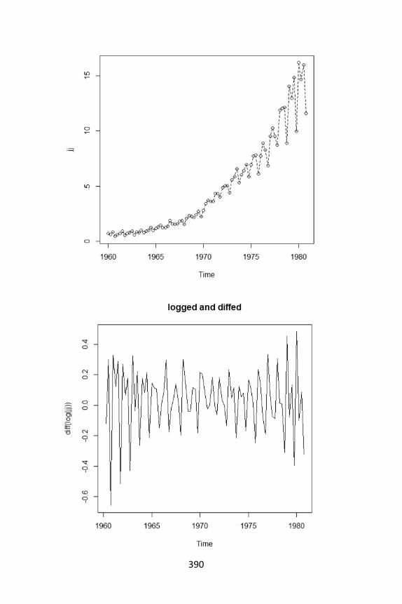
390

391

and while you're here try plot.ts and ts.plot:

> x = -5:5 # sequence of integers from -5 to 5 > y = 5*cos(x) # guess > par(mfrow=c(3,2)) # multifigure setup:3 rows,2 cols #--- plot: > plot(x, main="plot(x)") > plot(x, y, main="plot(x,y)")

#--- plot.ts: > plot.ts(x, main="plot.ts(x)") > plot.ts(x, y, main="plot.ts(x,y)")

#--- ts.plot: > ts.plot(x, main="ts.plot(x)") > ts.plot(ts(x), ts(y), col=1:2, main="ts.plot(x,y)")

392

# note- x and y are ts objects #--- the help files [? and help() are the same]: > ?plot.ts > help(ts.plot) > ?par # might as well skim the graphical # parameters help file while you're here

Note that if your data are a time series object, plot() will do the trick

(for a simple time plot, that is). Otherwise, plot.ts() will coerce the

graphic into a time plot.

We now look at filtering/smoothing the Johnson & Johnson series using

a two-sided moving average? Try this:

fjj(t)= ⅛ jj(t-2)+¼ jj(t-1)+¼ jj(t)+¼ jj(t+1)+⅛ jj(t+2)

and we'll add a lowess (?lowess) fit for fun.

> k = c(.5,1,1,1,.5) # k is the vector of # weights > (k = k/sum(k)) [1] 0.12 0.25 0.25 0.25 0.12

> fjj = filter(jj, sides=2, k) # ?filter for help > plot(jj) > lines(fjj, col="red") # adds a line to the # existing plot > lines(lowess(jj), col="blue", lty="dashed")

393

We difference the logged data and call it dljj. Then we examine dljj:

> dljj = diff(log(jj)) # difference the logged data > plot(dljj) # plot it (not shown) > shapiro.test(dljj) # test for normality Shapiro-Wilk normality test data: dljj W = 0.97, p-value = 0.07211 > par(mfrow=c(2,1)) # set up the graphics > hist(dljj, prob=TRUE, 12) # histogram > lines(density(dljj)) # smooth it - ?density for # details > qqnorm(dljj) # normal Q-Q plot qqline(dljj) # add a line

394

Let's check out the correlation structure of dljj using various

techniques. First, we'll look at a grid of scatterplots of dljj(t-lag) vs

dljj(t) for lag=1,2,...,9.

> lag.plot(dljj, 9, do.lines=FALSE) > lag1.plot(dljj, 9) # if you have astsa loaded (not # shown) # why the do.lines=FALSE? Because you get a phase # plane if it's TRUE

Notice the large positive correlation at lags 4 and 8 and the negative

correlations at a few other lags:

395

Now let's take a look at the ACF and PACF of dljj:

> par(mfrow=c(2,1)) # The power of accurate observation is commonly called cynicism # by those who have not got it. – # George Bernard Shaw > acf(dljj, 20) # ACF to lag 20 - no graph shown... # keep reading > pacf(dljj, 20) # PACF to lag 20 - no graph shown... # keep reading # !!NOTE!! acf2 on the line below is ONLY available in # astsa and tsa3 > acf2(dljj) # this is what you'll see below ACF PACF [1,] -0.51 -0.51 [2,] 0.07 -0.26 [3,] -0.40 -0.70 [4,] 0.73 0.27 [5,] -0.37 0.16 [6,] 0.00 -0.11

396

[7,] -0.25 -0.01 [8,] 0.56 0.11 [9,] -0.28 0.05 [10,] -0.01 0.12 [11,] -0.22 -0.03 [12,] 0.45 -0.03 [13,] -0.21 0.04 [14,] -0.04 -0.08 [15,] -0.15 -0.04 [16,] 0.35 -0.04 [17,] -0.14 -0.04 [18,] -0.08 -0.06 [19,] -0.09 -0.02 [20,] 0.27 0.01

Note that the LAG axis is in terms of frequency, so 1,2,3,4,5

correspond to lags 4,8,12,16,20 because frequency=4 here. If you

don't like this type of labeling, you can replace dljj in any of the above

by ts(dljj, freq=1); e.g., acf(ts(dljj, freq=1), 20)

397

Moving on, we will try a structural decomposition of log(jj) = trend

+ season + error using lowess. stl decomposes a time series into

seasonal, trend and irregular components using loess:

> plot(dog <- stl(log(jj), "per"))

Now we inspect the residuals. The third column of the resulting series

(the seasonal and trend components are in columns 1 and 2). Also,

check out the ACF of the residuals, acf(dog$time.series[,3]); the

residuals aren't white—not even close. You can do a little (very little)

better using a local seasonal window, plot(dog <- stl(log(jj),

s.win=4)), as opposed to the global one used by specifying "per".

Type ?stl for details. There is also something called StructTS that will

fit parametric structural models.

398

> dog$time.series[,3] Qtr1 Qtr2 Qtr3 Qtr4 1960 0.02215 -0.08811 0.17311 -0.19320 1961 -0.02563 0.00128 0.15874 -0.11700 1962 -0.00070 0.00594 0.07749 -0.10622 1963 0.06021 -0.05831 0.03865 -0.00231 1964 -0.01744 -0.03189 0.03428 0.02085 1965 -0.02364 0.00713 -0.01013 0.08639 1966 -0.07779 -0.07984 0.06758 0.11055 1967 -0.05578 -0.06423 -0.04485 0.19954 1968 -0.19148 0.02416 -0.02055 0.14136 1969 -0.07448 -0.00568 -0.01975 -0.01118 1970 -0.02523 0.04521 -0.05630 0.12087 1971 -0.07094 0.04718 -0.08955 0.04868 1972 0.04208 0.02030 -0.08487 0.00411 1973 0.03857 -0.00395 -0.00329 0.02490 1974 -0.00825 -0.00284 -0.03440 0.01659 1975 -0.00061 0.05262 -0.03305 -0.04415 1976 0.01273 0.09466 -0.08980 -0.06100 1977 0.07734 0.06977 -0.13041 -0.00992 1978 0.09135 0.04030 -0.04335 -0.12358 1979 0.14248 -0.01616 0.02089 -0.14976 1980 0.15572 0.00999 0.01320 -0.03985 > acf(dog$time.series[,3])

> (dog <- stl(log(jj), s.win=4)) Call: stl(x = log(jj), s.window = 4) Components seasonal trend remainder 1960 Q1 0.01916 -0.4519 0.09023 1960 Q2 0.01526 -0.4462 -0.03109 1960 Q3 0.26000 -0.4405 0.01801 1961 Q4 -0.28969 -0.4313 -0.09997 1961 Q1 0.01511 -0.4221 -0.08730

399

1961 Q2 0.01780 -0.4005 0.01163 1962 Q3 0.25312 -0.3789 0.04238 1962 Q4 -0.27300 -0.3492 0.02432 1962 Q1 -0.00453 -0.3194 -0.00455 1962 Q2 0.02202 -0.2988 0.01545 1962 Q3 0.21718 -0.2782 -0.02233 1963 Q4 -0.22169 -0.2524 -0.03669 1963 Q1 0.01153 -0.2266 0.02878 1963 Q2 0.00073 -0.1889 -0.03501 1964 Q3 0.16983 -0.1511 -0.01875 1964 Q4 -0.17003 -0.1023 0.01097 1964 Q1 -0.00309 -0.0535 -0.02677 1964 Q2 0.00602 0.0042 -0.01017 1964 Q3 0.14459 0.0618 0.00869 1965 Q4 -0.11427 0.1141 0.00018 1965 Q1 -0.04741 0.1664 0.02947 1965 Q2 0.00316 0.2085 0.05070 1966 Q3 0.14976 0.2507 -0.02886 1966 Q4 -0.06786 0.2918 -0.00078 1966 Q1 -0.06882 0.3329 -0.03298 1966 Q2 -0.02312 0.3742 -0.02902 1966 Q3 0.13941 0.4155 0.06564 1967 Q4 -0.01120 0.4497 0.00618 1967 Q1 -0.11103 0.4839 0.05242 1967 Q2 -0.02181 0.5131 -0.02753 1968 Q3 0.11854 0.5423 -0.05649 1968 Q4 0.02228 0.5864 0.01193 1968 Q1 -0.11897 0.6304 -0.08621 1968 Q2 0.01133 0.6855 0.03071 1968 Q3 0.08966 0.7406 0.01993 1969 Q4 -0.02660 0.7874 0.05012 1969 Q1 -0.09150 0.8343 0.02735 1969 Q2 0.04411 0.8823 -0.03847 1970 Q3 0.08638 0.9302 -0.02338 1970 Q4 -0.07156 0.9976 -0.11510 1970 Q1 -0.05319 1.0649 0.01429 1970 Q2 0.05824 1.1411 0.03030 1970 Q3 0.05955 1.2173 0.02882 1971 Q4 -0.08087 1.2810 0.08078 1971 Q1 -0.02609 1.3448 -0.03778 1971 Q2 0.06553 1.3931 0.00465 1972 Q3 0.03255 1.4414 -0.01064 1972 Q4 -0.08781 1.4816 0.00492 1972 Q1 0.01104 1.5219 0.04814 1972 Q2 0.05223 1.5619 0.00329 1972 Q3 0.04568 1.6019 -0.03018 1973 Q4 -0.12674 1.6418 -0.03116 1973 Q1 0.02589 1.6817 0.01164 1973 Q2 0.03871 1.7178 0.00992 1974 Q3 0.07733 1.7540 0.05121 1974 Q4 -0.13238 1.7827 0.01926 1974 Q1 0.00579 1.8115 -0.02051

400

1974 Q2 0.04614 1.8376 -0.02902 1974 Q3 0.08777 1.8638 -0.01568 1975 Q4 -0.14423 1.8943 0.01639 1975 Q1 0.00430 1.9248 0.00678 1975 Q2 0.08107 1.9535 0.01186 1976 Q3 0.06046 1.9822 0.01534 1976 Q4 -0.17937 2.0086 -0.01767 1976 Q1 0.03279 2.0350 -0.02141 1976 Q2 0.10977 2.0668 0.01060 1976 Q3 0.02502 2.0986 -0.00978 1977 Q4 -0.19056 2.1400 -0.02663 1977 Q1 0.06892 2.1814 0.00521 1977 Q2 0.10404 2.2287 -0.00448 1978 Q3 0.01320 2.2760 -0.03373 1978 Q4 -0.20842 2.3194 0.05578 1978 Q1 0.10866 2.3628 0.00340 1978 Q2 0.07325 2.3992 0.01741 1978 Q3 0.05540 2.4357 0.00627 1979 Q4 -0.24968 2.4681 -0.03123 1979 Q1 0.12905 2.5005 0.01236 1979 Q2 0.05291 2.5328 -0.02389 1980 Q3 0.08080 2.5652 0.05200 1980 Q4 -0.26610 2.5961 -0.02845 1980 Q1 0.13433 2.6271 0.02360 1980 Q2 0.04708 2.6576 -0.01892 1980 Q3 0.08768 2.6882 -0.00204 1981 Q4 -0.27051 2.7183 0.00406

401

Notation Used

Set Theory

Set: { }

A set: 𝐴

Element of a set: A 𝑎𝑖 for 𝑖 =

1, … , 𝑛

Set union: 𝐴 ∪ 𝐵

Set intersection: 𝐴 ∩ 𝐵

Set complement: 𝐴𝑐, ¬𝐴

Element of: 𝑎 ∈ 𝐴

Such that: |

Natural numbers: ℕ

Integers: ℤ

Real numbers: ℝ

Indexed set: {𝑦𝑖, 𝑥𝑖}𝑖=1𝑛

Probability and

statistics

Probability function: 𝑃(𝐴),

𝑃𝑟(𝑎), 𝑃𝑟𝑜𝑏(𝐴)

Conditional probability: 𝑃(𝐴|𝐵)

Probability of events

intersection: 𝑃(𝐴 ∩ 𝐵)

Probability of events union:

𝑃(𝐴 ∪ 𝐵)

probability density function

(pdf): 𝑓(𝑥)

Cumulative distribution

function (cdf): 𝐹(𝑥)

Paramete:r 𝑦

Parameter estimate: �̂�

population mean: 𝜇

expectation value: 𝐸(𝑥)

conditional expectation:

𝐸(𝑋|𝑌)

variance: 𝑉𝑎𝑟(𝑋)

variance: 𝜎2

standard deviation: 𝜎𝑋

covariance: 𝑐𝑜𝑣(𝑋, 𝑌)

correlation: 𝑐𝑜𝑟𝑟(𝑋, 𝑌)

correlation: 𝜌𝑋𝑌

lower / first quartile: Q1

median / second quartile: Q2

upper / third quartile: Q3

Sample mean: �̅�

402

Sample variance: 𝑠2

Sample standard deviation: 𝑠

Error: 휀

Regression coefficient: 𝛽𝑖

Regression coefficient

estimate: �̂�𝑖

distribution of X: 𝑋~

Normal (Gaussian) distribution:

𝑁(𝜇, 𝜎2)

uniform distribution: 𝑈(𝑎, 𝑏)

exponential distribution:

𝑒𝑥𝑝(𝜆) or 𝑒𝜆

gamma distribution:

𝑔𝑎𝑚𝑚𝑎(𝑐, 𝜆) or Γ(𝜆)

chi-square distribution: 𝜒2

F distribution: 𝐹(𝑘1, 𝑘2)

Poisson distribution:

𝑃𝑜𝑖𝑠𝑠𝑜𝑛(𝜆)

Bernoulli distribution: 𝐵𝑒𝑟𝑛(𝑝)

Linear Algebra

Vector 𝒙, �⃗�

Matrix 𝑋

Element of a vector 𝑥𝑖 for 𝑖 =

1, … , 𝑛

Element of a matrix 𝑥𝑚𝑛 for

𝑚=number of rows, 𝑛=number

of columns

Matrix size (dimension): 𝑚 × 𝑛

Vector cross product: ×

Vector dot product: ⋅

Norm: ‖𝑥‖

Rank of a matrix: 𝑟𝑎𝑛𝑘(𝐴)

Matrix transpose: 𝐴𝑇 or 𝐴′

Matrix inverse: 𝐴−1

Hermitian matrix: 𝐴∗

Matrix dimension: 𝑑𝑖𝑚(𝐴)

j-th diagonal of a matrix: 𝑎(𝑗)

Algebra and Calculus

generic argument: (. )

Very small number: 휀

Mapping: 𝑓 → 𝑔

Maps over 𝑑: 𝑑→

Derivative: 𝑑𝑦

𝑑𝑥

Partial derivative: 𝜕𝑓(𝑥,𝑦)

𝜕𝑥

Integral: ∫(. )

403

Double integral: ∬(. )

closed interval: [𝑎, 𝑏]

open interval: (𝑎, 𝑏)

maximize: 𝑚𝑎𝑥(𝑎, 𝑏)

maximize subject to:

𝑚𝑖𝑛 𝑥| 𝑐𝑜𝑛𝑑𝑖𝑡𝑖𝑜𝑛

minimize: 𝑚𝑖𝑛(𝑎, 𝑏)

Argument of the minimum:

arg min𝑎∈𝐴

(. ) (.)

Laplace transform: ℒ

Weierstrass elliptic function: ℘

Natural logarithm: 𝑙𝑛(. )

Function: 𝑓(𝑥)

Composite function: 𝑓(𝑔(𝑥)),

𝑓 ∘ 𝑔

Iteration 𝑖 of 𝐹(𝑥): 𝐹𝑖(𝑥)

Combination: (𝑛𝑘

)

Factoiral: !

Distance between x and y:

||𝑥 − 𝑦||

If and only if: Iff, ↔, ⇔

approximately equal: ≈

Proportional to: ∝

Plur or minus: ±

Such that: :

Summation: ∑(. )

Double summation: ∑ ∑(. )

Sum from i=1,…,n: ∑ (. )𝑛𝑖=1

Sum of all 𝑖 ∈ 𝑓(𝑖): ∑ (. )𝑖∈𝑓(𝑖)

Gradient: ∇

Not sign: ¬

404

405

Glossary

A Priori Probability: A priori probability is the probability estimate prior

to receiving new information. See also Bayes Theorem and posterior

probability.

Attribute: In data analysis or data mining, an attribute is a

characteristic or feature that is measured for each observation (record)

and can vary from one observation to another. It might be measured in

continuous values (e.g. time spent on a web site), or in categorical

values (e.g. red, yellow, green). The terms “attribute” and “feature” are

used in the machine learning community, “variable” is used in the

statistics community. They are synonyms.

Autoregression: Autoregression refers to a special branch of regression

analysis aimed at analysis of time series. It rests on autoregressive

models - that is, models where the dependent variable is the current

value and the independent variables are N previous values of the time

series. The N is called “the order of the autoregression”.

Autoregression and Moving Average (ARMA) Models: The

autoregression and moving average (ARMA) models are used in time

series analysis to describe stationary time series. These models

represent time series that are generated by passing white noise

through a recursive and through a nonrecursive linear filter,

consecutively. In other words, the ARMA model is a combination of an

autoregressive (AR) model and a moving average (MA) model.

Autoregressive (AR) Models: The autoregressive (AR) models are used

in time series analysis to describe stationary time series. These models

represent time series that are generated by passing the white noise

through a recursive linear filter. The output of such a filter at the

moment 𝑡 image is a weighted sum of 𝑚 image previous values of the

filter output. The integer parameter 𝑚 image is called the order of the

AR-model.

406

Average Deviation: The average deviation or the average absolute

deviation is a measure of dispersion. It is the average of absolute

deviations of the individual values from the median or from the mean.

Bagging: In predictive modeling, bagging is an ensemble method that

uses bootstrap replicates of the original training data to fit predictive

models. For each record, the predictions from all available models are

then averaged for the final prediction. For a classification problem, a

majority vote of the models is used. Bagging is short for “bootstrap

aggregating.”

Bayes´ Theorem: Bayes theorem is a formula for revising a priori

probabilities after receiving new information. The revised probabilities

are called posterior probabilities. For example, consider the probability

that you will develop a specific cancer in the next year. An estimate of

this probability based on general population data would be a prior

estimate; a revised (posterior) estimate would be based on both on the

population data and the results of a specific test for cancer.

Boosting: In predictive modeling, boosting is an iterative ensemble

method that starts out by applying a classification algorithm and

generating classifications. The classifications are then assessed, and a

second round of model-fitting occurs in which the records classified

incorrectly in the first round are given a higher weight in the second

round. This procedure is repeated a number of times, and the final

classifier results from a merger of the various iterations, with lesser

weights typically accorded to the very last rounds. The idea is to

concentrate the iterative learning process on the hard-to-classify cases.

Chi-Square Test: Chi-square test (or 𝜒2-test) is a statistical test for

testing the null hypothesis that the distribution of a discrete random

variable coincides with a given distribution. It is one of the most

popular goodness-of-fit tests.

Classification and Regression Trees (CART): Classification and

regression trees (CART) are a set of techniques for classification and

407

prediction. The technique is aimed at producing rules that predict the

value of an outcome (target) variable from known values of predictor

(explanatory) variables. The predictor variables may be a mixture of

categorical and continuous variables.

Classification Trees: Classification trees are one of the CART

techniques. The main distinction from regression trees (another CART

technique) is that the dependent variable 𝑌 image is categorical.

Coefficient of Determination: In regression analysis, the coefficient of

determination is a measure of goodness-of-fit (i.e. how well or tightly

the data fit the estimated model). The coefficient is defined as the ratio

of two sums of squares: 𝑅2 = 𝑆𝑆𝑅 /𝑆𝑆𝐸 , where 𝑆𝑆𝑅 is the sum of

squares due to regression, 𝑆𝑆𝑇 is the total sum of squares. By “sum of

squares” we mean the sum of squared deviations between actual

values and the mean (𝑆𝑆𝑇), or between predicted values and the mean

(𝑆𝑆𝑅). The coefficient of determination takes on values between 0 and

1, with values closer to 1 implying a better fit.

Collinearity: In regression analysis, collinearity of two variables means

that strong correlation exists between them, making it difficult or

impossible to estimate their individual regression coefficients reliably.

Conditional Probability: When probabilities are quoted without

specification of the sample space, it could result in ambiguity when the

sample space is not self-evident. To avoid this, the sample space can be

explicitly made known. The probability of an event 𝐴 given sample

space 𝑆, denoted by 𝑃(𝐴|𝑆), is nothing but the conditional probability

of 𝐴 given 𝑆.

Covariance: covariance is a measure of how much two random

variables change together. If the greater values of one variable mainly

correspond with the greater values of the other variable, and the same

holds for the smaller values, i.e., the variables tend to show similar

behavior, the covariance is positive. In the opposite case, when the

greater values of one variable mainly correspond to the smaller values

408

of the other, i.e., the variables tend to show opposite behavior, the

covariance is negative. The sign of the covariance therefore shows the

tendency in the linear relationship between the variables.

Data Mining: Data mining is concerned with finding latent patterns in

large data bases. The goal is to discover unsuspected relationships that

are of practical importance, e.g., in business.

Degrees of Freedom: For a set of data points in a given situation (e.g.

with mean or other parameter specified, or not), degrees of freedom is

the minimal number of values which should be specified to determine

all the data points.

Dependent variable: Dependent variables are also called response

variables, outcome variables, target variables or output variables. The

terms “dependent” and “independent” here have no direct relation to

the concept of statistical dependence or independence of events.

Deviance: Deviance is a quality of fit statistic for a model that is often

used for statistical hypothesis testing. It is a generalization of the idea

of using the sum of squares of residuals in ordinary least squares to

cases where model-fitting is achieved by maximum likelihood.

Effect: In design of experiments, the effect of a factor is an additive

term of the model, reflecting the contribution of the factor to the

response.

Estimator: A statistic, measure, or model, applied to a sample, intended

to estimate some parameter of the population that the sample came

from.

Explanatory Variable: Explanatory variable is a synonym for

independent variable.

Factor: In design of experiments, factor is an independent variable

manipulated by the experimenter.

Failure rate: The failure rate is defined for non-repairable populations

409

as the (instantaneous) rate of failure for the survivors to time 𝑡 during

the next instant of time. The failure rate (or hazard rate) ℎ(𝑡) and is:

ℎ(𝑡) = 𝑓(𝑡)/(1 − 𝐹(𝑡)) = 𝑓(𝑡)/𝑅(𝑡) = instantaneous failure rate.

Filter: A filter is an algorithm for processing a time series or random

process.

General Linear Model: General (or generalized) linear models (GLM), in

contrast to linear models, allow you to describe both additive and non-

additive relationship between a dependent variable and 𝑁

independent variables. The independent variables in GLM may be

continuous as well as discrete.

Hazard function: The hazard function, conventionally denoted 𝜆, is

defined as the event rate at time 𝑡 conditional on survival until time 𝑡

or later (that is, 𝑇 ≥ 𝑡).

Hazard rate: see failure rate.

Heteroscedasticity: Heteroscedasticity generally means unequal

variation of data, e.g. unequal variance.

Heteroscedasticity in regression: In regression analysis,

heteroscedasticity means a situation in which the variance of the

dependent variable varies across the data. Heteroscedasticity

complicates analysis because many methods in regression analysis are

based on an assumption of equal variance.

Independent Events: Two events 𝐴 and 𝐵 are said to be independent if

𝑃(𝐴𝐵) = 𝑃(𝐴)𝑃(𝐵). To put it differently, events 𝐴 and 𝐵 are

independent if the occurrence or non-occurrence of 𝐴 does not

influence the occurrence of non-occurrence of 𝐵 and vice-versa.

Independent Variables: Statistical models normally specify how one set

of variables, called dependent variables, functionally depend on

another set of variables, called independent variables. The term

“independent” reflects only the functional relationship between

410

variables within a model. Several models based on the same set of

variables may differ by how the variables are subdivided into

dependent and independent variables. Alternative names for

independent variables (especially in data mining and predictive

modeling) are input variables, predictors or features.

Inferential Statistics: Inferential statistics is the body of statistical

techniques that deal with the question “How reliable is the conclusion

or estimate that we derive from a set of data?” The two main

techniques are confidence intervals and hypothesis tests.

k-Nearest Neighbors Prediction: The k-nearest neighbors (k-NN)

prediction is a method to predict a value of a target variable in a given

record, using as a reference point a training set of similar objects. The

basic idea is to choose k objects from the training set that are closest to

the given object in terms of the predictor variables, then to form the

weighted average of target variable for those k objects. The weights

are usually chosen inversely proportionally to the distances from the

target object.

Kurtosis: Kurtosis measures the “heaviness of the tails” of a distribution

(in compared to a normal distribution). Kurtosis is positive if the tails

are “heavier” then for a normal distribution, and negative if the tails

are “lighter” than for a normal distribution. The normal distribution has

kurtosis of zero.

Latent Variable: A latent variable describes an unobservable construct

and cannot be observed or measured directly.

Least Squares Method: In a narrow sense, the Least Squares Method is

a technique for fitting a straight line through a set of points in such a

way that the sum of the squared vertical distances from the observed

points to the fitted line is minimized. In a wider sense, the Least

Squares Method is a general approach to fitting a model of the data-

generating mechanism to the observed data.

Likelihood Function: Likelihood function is a fundamental concept in

411

statistical inference. It indicates how likely a particular population is to

produce an observed sample.

Likelihood ratio test: a likelihood ratio test is a statistical test used to

compare the fit of two models, one of which (the null model) is a

special case of the other (the alternative model). The test is based on

the likelihood ratio, which expresses how many times more likely the

data are under one model than the other.

Linear regression: In statistics, linear regression is an approach for

modeling the relationship between a scalar dependent variable 𝑦 and

one or more explanatory variables denoted 𝑋. The case of one

explanatory variable is called simple linear regression. For more than

one explanatory variable, the process is called multiple linear

regression.

Linkage Function: A linkage function is an essential prerequisite for

hierarchical cluster analysis. Its value is a measure of the “distance”

between two groups of objects (i.e. between two clusters).

Logit: Logit is a nonlinear function of probability. If 𝑝 is the probability

of an event, then the corresponding logit is given by the formula:

𝑙𝑜𝑔𝑖𝑡(𝑝)𝑙𝑜𝑔(𝑝/(1 − 𝑝)).

Logistic regression: In statistics, logistic regression, or logit regression,

is a type of probabilistic statistical classification model. It is also used to

predict a binary response from a binary predictor, used for predicting

the outcome of a categorical dependent variable (i.e., a class label)

based on one or more predictor variables (features). That is, it is used

in estimating the parameters of a qualitative response model.

Machine Learning: Analytics in which computers “learn” from data to

produce models or rules that apply to those data and to other similar

data. Predictive modeling techniques such as neural nets, classification

and regression trees (decision trees), naive Bayes, k-nearest neighbor,

and support vector machines are generally included. One characteristic

of these techniques is that the form of the resulting model is flexible,

412

and adapts to the data.

Markov chain: A Markov chain, named after Andrey Markov, is a

mathematical system that undergoes transitions from one state to

another on a state space. It is a random process usually characterized

as memoryless: the next state depends only on the current state and

not on the sequence of events that preceded it. This specific kind of

“memorylessness” is called the Markov property.

Mean Squared Error (MLE): The mean squared error is a measure of

performance of a point estimator. It measures the average squared

difference between the estimator and the parameter. For an unbiased

estimator, the mean squared error is equal to the variance of the

estimator.

Multicollinearity: In regression analysis, multicollinearity refers to a

situation of collinearity of independent variables, often involving more

than two independent variables, or more than one pair of collinear

variables. Multicollinearity means redundancy in the set of variables.

Naive Bayes Classification: The Naive Bayes method is a method of

classification applicable to categorical data, based on Bayes theorem.

For a record to be classified, the categories of the predictor variables

are noted and the record is classified according to the most frequent

class among the same values of those predictor variables in the training

set. A rigorous application of the Bayes theorem would require

availability of all possible combinations of the values of the predictor

variables. When the number of variables is large enough, this requires

a training set of unrealistically large size (and, indeed, even a huge

training set is unlikely to cover all possible combinations). The naive

Bayes method overcomes this practical limitation of the rigorous Bayes

approach to classification.

Neural Network: A neural network (NN) is a network of many simple

processors (“units”), each possibly having a small amount of local

memory. The units are connected by communication channels

413

(“connections”) which usually carry numeric (as opposed to symbolic)

data, encoded by any of various means. The units operate only on their

local data and on the inputs they receive via the connections. The

restriction to local operations is often relaxed during training.

Null Hypothesis: In hypothesis testing, the null hypothesis is the one

you are hoping can be disproven by the observed data. Typically, it

asserts that chance variation is responsible for an effect seen in

observed data (for example, a difference between treatment and

placebo, an apparent correlation between one variable and another, a

divergence between a sample measure and some benchmark, etc.)

Odds ratio: In statistics, the odds ratio (usually abbreviated “OR”) is

one of three main ways to quantify how strongly the presence or

absence of property 𝐴 is associated with the presence or absence of

property 𝐵 in a given population.

𝑝-value: The 𝑝-value is the probability that the null model could, by

random chance variation, produce a sample as extreme as the

observed sample (as measured by some sample statistic of interest.)

Parameter: A Parameter is a numerical value that describes one of the

characteristics of a probability distribution or population. For example,

a binomial distribution is completely specified if the number of trials

and probability of success are known. Here, the number of trials and

the probability of success are two parameters. A normal distribution is

completely specified if its mean and standard deviation are known.

Posterior Probability: Posterior probability is a revised probability that

takes into account new available information. For example, let there be

two urns, urn 𝐴 having 5 black balls and 10 red balls and urn 𝐵 having

10 black balls and 5 red balls. Now if an urn is selected at random, the

probability that urn 𝐴 is chosen is 0.5. This is the a priori probability. If

we are given an additional piece of information that a ball was drawn

at random from the selected urn, and that ball was black, what is the

probability that the chosen urn is urn 𝐴? Posterior probability takes

414

into account this additional information and revises the probability

downward from 0.5 to 0.333 according to Bayes´ theorem, because a

black ball is more probable from urn 𝐵 than urn 𝐴.

Probit: Probit is a nonlinear function of probability 𝑝: 𝑝𝑟𝑜𝑏𝑖𝑡(𝑝) =

Θ−1(𝑝), where Θ−1(. ) is the function inverse to the cumulative

distribution function Θ(. ) of the standard normal distribution. In

contrast to the probability p itsef (which takes on values from 0 to 1),

the values of the probit of p are from minus- to plus-infinity.

R-squared: See Coefficient of determination.

Random Error: The random error is the fluctuating part of the overall

error that varies from measurement to measurement. Normally, the

random error is defined as the deviation of the total error from its

mean value.

Random variable: a random variable is a variable whose value is subject

to variations due to chance (i.e. randomness, in a mathematical sense).

A random variable can take on a set of possible different values, each

with an associated probability (if discrete) or a probability density

function (if continuous), in contrast to other mathematical variables.

Regression Analysis: Regression analysis provides a “best-fit”

mathematical equation for the relationship between the dependent

variable (response) and independent variable(s) (covariates).

Regression Trees: Regression trees is one of the CART techniques. The

main distinction from classification trees (another CART technique) is

that the dependent variable 𝑌 image is continuous.

Regularization: Regularization refers to a wide variety of techniques

used to bring structure to statistical models in the face of data size,

complexity and sparseness. Advances in digital processing, storage and

retrieval have led to huge and growing data sets (“Big Data”).

Regularization is used to allow models to usefully model such data

without overfitting. A very simple example is linear regression; other

415

examples are smoothing techniques.

Residuals: Residuals are differences between the observed values and

the values predicted by some model. Analysis of residuals allows you to

estimate the adequacy of a model for particular data; it is widely used

in regression analysis.

Sample: A sample is a portion of the elements of a population. A

sample is chosen to make inferences about the population by

examining or measuring the elements in the sample.

Sample Space: The set of all possible outcomes of a particular

experiment is called the sample space for the experiment. If a coin is

tossed twice, the sample space is {HH, HT, TH, TT}, where TH, for

example, means getting tails on the first toss and heads on the second

toss.

Seasonal Decomposition: The seasonal decomposition is a method

used in time series analysis to represent a time series as a sum (or,

sometimes, a product) of three components—the linear trend, the

periodic (seasonal) component, and random residuals.

Serial Correlation: In analysis of time series, the 𝑁th order serial

correlation is the correlation between the current value and the Nth

previous value of the same time series. For this reason serial

correlation is often called “autocorrelation”.

Simple Linear Regression: The simple linear regression is aimed at

finding the “best-fit” values of two parameters - 𝐴 and 𝐵 in the

following regression equation: 𝑌𝑖 = 𝐴 𝑋𝑖 + 𝐵 + 𝐸𝑖 , 𝑖 = 1, 𝓅‚ℛ, 𝑁,

where 𝑌𝑖, 𝑋𝑖, and 𝐸𝑖 are the values of the dependent variable, of the

independent variable, and of the random error, respectively.

Parameter 𝐴 is called “the slope of the regression line”, 𝐵 - “the y-

intercept of the regression line”.

Singularity: In regression analysis, singularity is the extreme form of

multicollinearity - when a perfect linear relationship exists between

416

variables or, in other terms, when the correlation coefficient is equal to

1.0 or -1.0.

Standard error: The standard error measures the variability of an

estimator (or sample statistic) from sample to sample. By formula,

𝑆𝑇𝐷𝐸𝐸𝑅 = 𝑆𝑇𝐷𝐸𝑉/√𝑁.

Stationary process: a stationary process is a stochastic process whose

joint probability distribution does not change when shifted in time.

Consequently, parameters such as the mean and variance, if they are

present, also do not change over time and do not follow any trends.

Statistical inference: statistical inference is the process of drawing

conclusions from data that are subject to random variation, for

example, observational errors or sampling variation.

Statistical Significance: Outcomes to an experiment or repeated events

are statistically significant if they differ from what chance variation

might produce.

Stochastic process: a stochastic process, or sometimes random process

is a collection of random variables, representing the evolution of some

system of random values over time.

𝑡-test: A 𝑡-test is a statistical hypothesis test based on a test statistic

whose sampling distribution is a 𝑡-distribution. Various 𝑡-tests, strictly

speaking, are aimed at testing hypotheses about populations with

normal probability distribution. However, statistical research has

shown that 𝑡-tests often provide quite adequate results for non-

normally distributed populations too.

Time Series: A time series is a sequence of data points, measured

typically at successive points in time spaced at uniform time intervals.

Examples of time series are the daily closing value of the Dow Jones

Industrial Average and the annual flow volume of the Nile River at

Aswan.

417

Training Set: A training set is a portion of a data set used to fit (train) a

model for prediction or classification of values that are known in the

training set, but unknown in other (future) data. The training set is

used in conjunction with validation and/or test sets that are used to

evaluate different models.

Type I Error: In a test of significance, Type I error is the error of

rejecting the null hypothesis when it is true -- of saying an effect or

event is statistically significant when it is not. The projected probability

of committing type I error is called the level of significance.

Type II Error: In a test of significance, Type II error is the error of

accepting the null hypothesis when it is false -- of failing to declare a

real difference as statistically significant. Obviously, the bigger your

samples, the more likely your test is to detect any difference that

exists. The probability of detecting a real difference of specified size

(i.e. of not committing a Type II error) is called the power of the test.

Validation Set: A validation set is a portion of a data set used in data

mining to assess the performance of prediction or classification models

that have been fit on a separate portion of the same data set (the

training set). Typically both the training and validation set are randomly

selected, and the validation set is used as a more objective measure of

the performance of various models that have been fit to the training

data (and whose performance with the training set is therefore not

likely to be a good guide to their performance with data that they were

not fit to).

Variance: Variance is a measure of dispersion. It is the average squared

distance between the mean and each item in the population or in the

sample.

418

419

References

Aizerman, M., Braverman, E., & Rozonoer, L. (1964). Theoretical

foundations of the potential function method in pattern

recognition learning. Automation and Remote Control, 25, 821–

837.

Akbarzadeh, V. (2013). Line Estimation. Retrieved from Machine

Learning Made Simple:

http://mlmadesimple.com/2014/05/07/line-estimation/

Allibone, T. E. (1980). Dennis Gabor. 5 June 1900-9 February 1979.

Biographical Memoirs of Fellows of the Royal Society, 26, 106.

doi:10.1098/rsbm.1980.0004

Altman, N. (1992). An introduction to kernel and nearest-neighbor

nonparametric regression. The American Statistician, 46(3),

175–185. doi:10.1080/00031305.1992.10475879

Altman, N. S. (1992). An introduction to kernel and nearest-neighbor

nonparametric regression. The American Statistician, 46(3),

175–185. doi:10.1080/00031305.1992.10475879

Altmann, A., Tolosi, L., Sander, O., & Lengauer, T. (2010). Permutation

importance:a corrected feature importance measure.

Bioinformatics. doi:10.1093/bioinformatics/btq134

Altschul, J. H., Sebastian, L., & Heidelberg, K. (2004). Predictive

Modeling in the Military: Similar Goals, Divergent Paths. SRI

Foundation.

Amemiya, T. (1985). Advanced econometrics. Boston: Harvard

University Press.

Amit, Y., & Geman, D. (1997). Shape quantization and recognition with

randomized trees. Neural Computation, 9(7), 1545–1588.

doi:10.1162/neco.1997.9.7.1545

420

(2010). Analysis of Alternatives (AoA) Handbook. Air Force Materiel

Command. Kirtland AFB: Office of Aerospace Studies. Retrieved

2014, from

http://www.prim.osd.mil/Documents/AoA_Handbook.pdf

Andersen, R. (2008). Modern Methods for Robust Regression. Sage

University Paper Series on Quantitative Applications in the

Social Sciences.

Anscombe, F. J. (1948). The Validity of Comparative Experiments.

Journal of the Royal Statistical Society. Series A (General) ,

111(3), 181–211. doi:10.2307/2984159

Argresti, A., & Finlay, B. (2008). Statistical Methods for the Social

Sciences (4th ed.). Pearson.

Aslam, J. A., Popa, R. A., & Rivest, R. (2007). On Estimating the Size and

Confidence of a Statistical Audit. Proceedings of the Electronic

Voting Technology Workshop (EVT '07). Boston, MA. Retrieved

from http://people.csail.mit.edu/rivest/pubs/APR07.pdf

Bailey, R. A. (2008). Design of Comparative Experiments. Cambridge

University Press.

Balabin, R., & Lomakina, E. (2009). Neural network approach to

quantum-chemistry data: Accurate prediction of density

functional theory energies. J. Chem. Phys, 131(7).

doi:10.1063/1.3206326

Barkin, E. (2011). CRM + Predictive Analytics: Why It All Adds Up. New

York: Destination CRM. Retrieved 2014, from

http://www.destinationcrm.com/Articles/Editorial/Magazine-

Features/CRM---Predictive-Analytics-Why-It-All-Adds-Up-

74700.aspx

Barros, R. C., Cerri, R., Jaskowiak, P. A., & Carvalho, A. C. (2011). A

bottom-up oblique decision tree induction algorithm.

421

Proceedings of the 11th International Conference on Intelligent

Systems Design and Applications (ISDA 2011) (pp. 450 - 456).

IEEE. doi:10.1109/ISDA.2011.6121697

Barros, R., Basgalupp, M., Carvalho, A., & Freitas, A. (2011). A Survey of

Evolutionary Algorithms for Decision-Tree Induction. IEEE

Transactions on Systems, Man and Cybernetics, Part C:

Applications and Reviews, 42(3), 291-312.

Belle, G. v. (2008). Statistical rules of thumb (2nd ed.). Hoboken, N.J:

Wiley.

Ben-Gal I. Dana A., S. N. (2014). Efficient Construction of Decision Trees

by the Dual Information Distance Method. Quality Technology

& Quantitative Management (QTQM), 11(1), 133-147.

Retrieved from http://www.eng.tau.ac.il/~bengal/DID.pdf

Ben-Israel, A., & Greville, T. (2003). Generalized Inverses. New York:

Springer-Verlag. Retrieved from

http://books.google.com/books?id=o3-

97W8vCdIC&printsec=frontcover&dq=isbn:038700293

Bergstra, J., & Bengio, Y. (2012). Random Search for Hyper-Parameter

Optimization. J. Machine Learning Research, 13, 281–305.

Retrieved from

http://jmlr.org/papers/volume13/bergstra12a/bergstra12a.pdf

Bertsekas, D. T. (1996). Neuro-dynamic programming. Athena Scientific,

152.

Beyer, K. (1999). When is “nearest neighbor” meaningful? Database

Theory—ICDT’99, (pp. 217-235).

Bhandari, M., & Joensson, A. (2008). Clinical Research for Surgeons.

Thieme.

Bingham, E., & M., H. (2001). Random projection in dimensionality

reduction: applications to image and text data. of the seventh

422

ACM SIGKDD international conference on Knowledge discovery

and data mining. ACM.

Bishop, C. (2005). Neural networks for pattern recognition. Oxford

University Press.

Bishop, C. (2006). Pattern Recognition and Machine Learning. New

York: Springer. Retrieved from

http://www.hua.edu.vn/khoa/fita/wp-

content/uploads/2013/08/Pattern-Recognition-and-Machine-

Learning-Christophe-M-Bishop.pdf

Bliss, C. I. (1934). The Method of Probits. Science, 79(2037), 38–39.

doi:10.1126/science.79.2037.38

Bloomfield, P. (1976). Fourier analysis of time series: An introduction.

New York: Wiley.

Boashash, B. (2003). Time-Frequency Signal Analysis and Processing: A

Comprehensive Reference. Oxford: Elsevier Science.

Bobko, P., Roth, P. L., & Buster, M. A. (2007). The usefulness of unit

weights in creating composite scores: A literature review,

application to content validity, and meta-analysis.

Organizational Research Methods, 10, 689-709.

doi:10.1177/1094428106294734

Boser, B., Guyon, I., & Vapnik, V. (1992). A training algorithm for

optimal margin classifiers. Proceedings of the fifth annual

workshop on Computational learning theory - COLT '92, (p.

144). doi:10.1145/130385.130401

Bottaci, L. (1997). Artificial Neural Networks Applied to Outcome

Prediction for Colorectal Cancer Patients in Separate

Institutions. The Lancet, 350. Retrieved from

http://www.lcc.uma.es/~jja/recidiva/042.pdf

Box, G. E., Jenkins, G. M., & Reinsel, G. C. (2008). Time Series Analysis,

423

Forecasting and Control (4th ed.). Hoboken, NJ: Wiulley.

Box, G., & Jenkins, G. (1976). Time Series Analysis: forecasting and

control (Revised ed.). Oakland, CA: Holden-Day.

Boyd, C. R., Tolson, M. A., & Copes, W. S. (1987). Evaluating trauma

care: The TRISS method. Trauma Score and the Injury Severity

Score. The Journal of trauma, 27(4), 370–378.

Bramer, M. (2007). Principles of Data Mining. London: Springer London.

doi:10.1007/978-1-84628-766-4

Breiman, L. (1994). Bagging Predictors. Technical Report No. 421,

University of California, Department of Statistics, Berkeley.

Retrieved from

http://statistics.berkeley.edu/sites/default/files/tech-

reports/421.pdf

Breiman, L. (1996). Bagging predictors. Machine Learning, 24(2), 123-

140. Retrieved from

http://link.springer.com/article/10.1023%2FA%3A1018054314

350

Breiman, L. (2001). Random Forests. Machine Learning, 45(1), 5-32.

doi:10.1023/A:1010933404324

Breiman, L. (2001). Statistical Modeling: the Two Cultures. Statistical

Science, 16(3), 199–231. doi:10.1214/ss/1009213725

Breiman, L., Friedman, J. H., Olshen, R. A., & Stone, C. J. (1984).

Classification and regression trees. Monterey, CA: Wadsworth

& Brooks/Cole Advanced Books & Software.

Bremne, r. D., Demaine E, Erickson, J., Iacono, J., Langerman, S., P., M.,

& Toussaint, G. (2005). Output-sensitive algorithms for

computing nearest-neighbor decision boundaries. Discrete and

Computational Geometry, 33(4), 593–604. doi:10.1007/s00454-

004-1152-0

424

Bridgman, R. (n.d.). Defence of neural networks.

Bryll, R. (2003). Attribute bagging: improving accuracy of classifier

ensembles by using random feature subsets. Pattern

Recognition, 20(6), 1291–1302.

Buck, D. (2005). A Hands-On Introduction to SAS DATA Step

Programming. Proceedings of the Thirtieth Annual SAS® Users

Group International Conference. SAS Institute. Retrieved from

http://www2.sas.com/proceedings/sugi30/134-30.pdf

Burgess, E. W. (1928). Factors determining success or failure on parole.

In A. Bruce, The Workings of the Indeterminate Sentence Law

and Parole in Illinois (pp. 205-249). Springfield, IL: Illinois State

Parole Board.

Burnham, K. P., & Anderson, D. (2002). Model Selection and Multi-

Model Inference. New York: Springer.

Cai, T., Tian, L., Wong, P. H., & Wei, L. J. (2009). Analysis of Randomized

Comparative Clinical Trial Data for Personalized Treatment

Selections. Harvard University Biostatistics Working Paper

Series, Paper 97.

Caputo, B., Sim, K., Furesjo, F., & Smola, A. (n.d.). Appearance-based

Object Recognition using SVMs: Which Kernel Should I Use?

Proceedings of NIPS Workshop on Statistical Methods for

Computational Experiments in Visual Processing and Computer

Vision (p. 2002). Whistler.

Carlin, B., & Louis, T. (2000). Bayes and Empirical Bayes Methods for

Data Analysis. Chapman & Hall/CRC.

Caruana, R., & Niculescu-Mizil, A. (2006). empirical comparison of

supervised learning algorithms. Proceedings of the 23rd

international conference on Machine learning.

doi:10.1.1.122.5901

425

Chambers, J. (1998). Programming with Data. New York: Springer-

Verlag.

Chang, C., & Lin, C. (2011). LIBSVM : a library for support vector

machines. ACM Transactions on Intelligent Systems and

Technology, 2, 27:1-27:27.

Chapelle, O., Vapnik, V., Bousquet, O., & Mukherjee, S. (2002).

Choosing multiple parameters for support vector machines.

Machine Learning, 46, 131–159.

Chen, J., Zhu, J., Wang, Z., Zheng, X., & Zhang, B. (2013). Scalable

Inference for Logistic-Normal Topic Models. In Advances in

Neural Information Processing Systems (p. 2445{2453).

Chib, S., & Greenberg, E. (1995). Understanding the metropolis-

hastings algorithm. The American Statistician, 49(4).

doi:10.1080/00031305.1995.10476177

Chipman, H., George, E., & McCulloch, R. (1998). Bayesian CART model

search. Journal of the American Statistical Association, 93(443),

935-948.

Chong, J., Jin, Y., & Phillips, M. (2013). The Entrepreneur's Cost of

Capital: Incorporating Downside Risk in the Buildup Method.

Pasadena: MacroRisk.com. Retrieved 2014, from

http://www.macrorisk.com/wp-

content/uploads/2013/04/MRA-WP-2013-e.pdf

Ciresan, D. C., Meier, U. J., & Schmidhuber, J. (2012). Multi-Column

Deep Neural Network for Traffic Sign Classification. Neural

Networks.

Ciresan, D., Giusti, A., Gambardella, L., & Schmidhuber, J. (2012). Deep

Neural Networks Segment Neuronal Membranes in Electron

Microscopy Images. Advances in Neural Information Processing

Systems (NIPS 2012), . Lake Tahoe.

426

Ciresan, D., Meier, U., & Schmidhuber, J. (2012). Multi-column Deep

Neural Networks for Image Classification. IEEE Conf. on

Computer Vision and Pattern Recognition CVPR 2012.

Cochran, W., & Cox, G. (1992). Experimental designs (2nd ed.). New

York: Wiley.

Cohen, J., Cohen, P., West, S., & Aiken, L. (2002). Applied Multiple

Regression/Correlation Analysis for the Behavioral Sciences (3rd

ed.). Routledge.

Conz, N. (2008). Insurers Shift to Customer-focused Predictive Analytics

Technologies. New York: Insurance & Technology. Retrieved

2014, from http://www.insurancetech.com/business-

intelligence/insurers-shift-to-customer-focused-

predi/210600271

Coomans, D., & Massart, D. (1982). Alternative k-nearest neighbour

rules in supervised pattern recognition : Part 1. k-Nearest

neighbour classification by using alternative voting rules.

Analytica Chimica Acta, 136, 15-27.

Cortes, C., & Vapnik, V. (1995). Support-vector networks. Machine

Learning, 20(3), 273. doi:10.1007/BF00994018

Cossock, D., & Zhang, T. (2008). Statistical Analysis of Bayes Optimal

Subset Ranking. Retrieved from

http://www.stat.rutgers.edu/home/tzhang/papers/it08-

ranking.pdf

Cover, T., & Hart, P. (1967). Nearest neighbor pattern classification.

IEEE Transactions on Information Theory, 13(1), 21–27.

doi:10.1109/TIT.1967.1053964

Cox, D. (1992). Planning of experiments. New York: Wiley.

Crammer, K., & Singer, Y. (2001). On the Algorithmic Implementation of

Multiclass Kernel-based Vector Machines. J. of Machine

427

Learning Research, 2, 265–292. Retrieved from

http://jmlr.org/papers/volume2/crammer01a/crammer01a.pdf

CRAN-project. (2012). R uplift-package help. Retrieved from R

Statistical Data Analysis:

http://127.0.0.1:24928/doc/html/Search?pattern=uplift

Criminisi, A., Shotton, J., & Konukoglu, E. (2011). Forests: A Unified

Framework for Classification, Regression, Density Estimation,

Manifold Learning and Semi-Supervised Learning. Foundations

and Trends in Computer Vision, 7, 81–227.

doi:10.1561/0600000035

Cuingnet, R., C., R., Chupin, M., Lehéricy, S., Dormont, D., Benali, H., . . .

Colliot, O. (2011). Spatial regularization of SVM for the

detection of diffusion alterations associated with stroke

outcome. Medical Image Analysis, 15(5), 729-737.

Da, Y., & Xiurun, G. (2005). An improved PSO-based ANN with

simulated annealing technique. In T. e. Villmann, New Aspects

in Neurocomputing: 11th European Symposium on Artificial

Neural Networks. New York: Elsevier.

doi:10.1016/j.neucom.2004.07.002

Damas, M., Salmeron, M., Diaz, A., Ortega, J., Prieto, A., & Olivares, G.

(2000). Genetic algorithms and neuro-dynamic programming:

application to water supply networks. Proceedings of 2000

Congress on Evolutionary Computation. La Jolla, Ca: IEEE.

doi:10.1109/CEC.2000.870269

Das, K., & Vidyashankar, G. (2006). Competitive Advantage in Retail

Through Analytics: Developing Insights, Creating Value. New

York: Information Management. Retrieved 2014, from

http://www.information-

management.com/infodirect/20060707/1057744-1.html

Davidson, R., & Mackinnon, .. G. (1993). Estimation and inference in

428

econometrics. Oxford University Press.

Dawes, R. M. (1979). The robust beauty of improper linear models in

decision making. American Psychologist, 34, 571-582.

doi:10.1037/0003-066X.34.7.571

de Rigo, D., Castelletti, A., Rizzoli, A., Soncini-Sessa, R., & Weber, E.

(2005). A selective improvement technique for fastening

Neuro-Dynamic Programming in Water Resources Network

Management. Proceedings of the 16th IFAC World Congress –

IFAC-PapersOnLine. Prague, Czech Republic: IFAC.

doi:10.3182/20050703-6-CZ-1902.02172

de Rigo, D., Rizzoli, A. E., Soncini-Sessa, R., Weber, E., & Zenesi, P.

(2001). Neuro-dynamic programming for the efficient

management of reservoir networks. Proceedings of MODSIM

2001, International Congress on Modelling and Simulation.

Canberra, Australia. doi:10.5281/zenodo.7481

Deng, G., & Ferris, M. (2008). Neuro-dynamic programming for

fractionated radiotherapy planning. Springer Optimization and

Its Applications, 12, 47–70. doi:10.1007/978-0-387-73299-2_3

Deng, H., Runger, G., & Tuv, E. (2011). Bias of importance measures for

multi-valued attributes and solutions. Proceedings of the 21st

International Conference on Artificial Neural Networks (ICANN),

(pp. 293–300).

Devroye, L., Györfi, L., & Lugosi, G. (1996). A Probabilistic Theory of

Pattern Recognition. New York: Springer-Verlag.

Dietterich, T. (2000). An Experimental Comparison of Three Methods

for Constructing Ensembles of Decision Trees: Bagging,

Boosting, and Randomization. Machine Learning, 139–157.

Dietterich, T., & Bakiri, G. (1995). Solving Multiclass Learning Problems

via Error-Correcting Output Codes. Journal of Artificial

429

Intelligence Research, 2(2), 263–286. Retrieved from

http://www.jair.org/media/105/live-105-1426-jair.pdf

Draper, N., & Smith, H. (1998). Applied Regression Analysis (3rd ed.).

New Tork: John Wiley.

Drucker, H., Burges, C. J., Kaufman, L., Smola, A., & Vapnik, V. N. (1996).

Support Vector Regression Machines. Advances in Neural

Information Processing Systems 9, NIPS 1996 (pp. 155–161).

MIT Press.

Duan, K., & Keerthi, S. (2005). Which Is the Best Multiclass SVM

Method? An Empirical Study. Lecture Notes in Computer

Science, 3541, 278. doi:10.1007/11494683_28

Eckerson, W. (2007). Extending the Value of Your Data Warehousing

Investment. The Data Warehouse Institute. Retrieved 2014,

from http://tdwi.org/articles/2007/05/10/predictive-

analytics.aspx?sc_lang=en

Edwards, A. (1925). R. A. Fisher, Statistical Methods for Research

Workers. In I. Grattan-Guinness (Ed.), Landmark Writings in

Western Mathematics: Case Studies, 1640-1940. Amsterdam:

Elsevier.

Everitt, B. S., Landau, S., Leese, M., & Stahl, D. (n.d.). Miscellaneous

Clustering Methods. In Cluster Analysis (5th ed.). Chichester,

UK: John Wiley & Sons, Ltd.

Fan, R., Chang, K., Hsieh, C., Wang, K., & C.J., L. (2008). LIBLINEAR: A

library for large linear classification. Journal of Machine

Learning Research, 9, 1871–1874.

Faraway, J. J. (2004). Linear Models with R. Chapman & Hall/CRC.

Farley, B., & Clark, W. (1954). Simulation of Self-Organizing Systems by

Digital Computer. IRE Transactions on Information Theory, 4(4),

76–84. doi:10.1109/TIT.1954.1057468

430

Ferreira, C. (2006). Designing Neural Networks Using Gene Expression

Programming. In A. Abraham, B. de Baets, M. Köppen, & B.

Nickolay, Applied Soft Computing Technologies: The Challenge

of Complexity (pp. 517–536). Springer-Verlag. Retrieved from

http://www.gene-expression-

programming.com/webpapers/Ferreira-ASCT2006.pdf

Ferris, M. C., & Munson, T. S. (2002). Interior-Point Methods for

Massive Support Vector Machines. SIAM Journal on Op, 13(3),

783. doi:10.1137/S1052623400374379

Fisher, R. A. (1918). The Correlation Between Relatives on the

Supposition of Mendelian Inheritance. Philosophical

Transactions of the Royal Society of Edinburgh, 52, 399–433.

Fisher, R. A. (1921). Probable Error" of a Coefficient of Correlation

Deduced from a Small Sample. 1, 3-32. Retrieved from

http://hdl.handle.net/2440/15169

Fisher, R., & Prance, G. (1974). The Design of Experiments (9th ed.).

Hafner Press.

Fletcher, H. (2011). The 7 Best Uses for Predictive Analytics in

Multichannel Marketing. Philadelphia: Target Marketing.

Retrieved 2014, from

http://www.targetmarketingmag.com/article/7-best-uses-

predictive-analytics-modeling-multichannel-marketing/1#

Freedman, D. A. (2005). Statistical Models: Theory and Practice.

Cambridge University Press.

Freund, Y., & Schapire, R. E. (1999). Large Margin Classification Using

the Perceptron Algorithm. Machine Learning, 37(3), 277.

doi:10.1023/A:1007662407062

Friedman, J. H. (1991). Multivariate Adaptive Regression Splines. The

Annals of Statistics, 19(1), 1-67. doi:10.1214/aos/1176347963

431

Friedman, J. H. (1993). Estimating Functions of Mixed Ordinal and

Categorical Variables Using Adaptive Splines. In Morgenthaler,

Ronchetti, & Stahel, New Directions in Statistical Data Analysis

and Robustness. Birkhauser.

Friedman, J. H. (1993). Fast MARS. Stanford University Department of

Statistics.

Friedman, J. H. (1995). Greedy Function Approximation: A Gradient

Boosting Machine. IMS 1999. Retrieved from

http://statweb.stanford.edu/~jhf/ftp/trebst.pdf

Friedman, J. H. (1999). Stochastic Gradient Boosting. Retrieved from

https://statweb.stanford.edu/~jhf/ftp/stobst.pdf

Fukushima, K. (1980). Neocognitron: A self-organizing neural network

model for a mechanism of pattern recognition unaffected by

shift in position. Biological Cybernetics, 36(4), 93–202.

doi:10.1007/BF00344251

Ganesan, N. (2010). Application of Neural Networks in Diagnosing

Cancer Disease Using Demographic Data. International Journal

of Computer Applications, 1(26), 76-85. Retrieved from

http://www.ijcaonline.org/journal/number26/pxc387783.pdf

Geisser, S. (1993). Predictive Inference: An Introduction. New York:

Chapman & Hall.

Gelman, A. (2005). Analysis of variance? Why it is more important than

ever. The Annals of Statistics, 33, 1–53.

doi:10.1214/009053604000001048

George, E., & McCullochb, R. (1993). Variable Selection via Gibbs

Sampling. Journal of the American Statistical Association,

88(423). doi:10.1080/01621459.1993.10476353

Gershenfeld, N. (1999). The Nature of Mathematical Modeling. New

York: Cambridge University Press.

432

Good, I. (1953). The population frequencies of species and the

estimation of population parameters. Biometrika, 40(3-4), 237–

264. doi:10.1093/biomet/40.3-4.237

Graves, A., & Schmidhuber, J. (2009). Handwriting Recognition with

Multidimensional Recurrent Neural Networks. In Y. Bengio, D.

S., J. Lafferty, C. K. Williams, & A. Culotta, Advances in Neural

Information Processing Systems 22 (NIPS'22) (pp. 545–552).

Vancouver, BC.

Greene, W. (2011). Econometric Analysis (7th ed.). New York: Prentice

Hall.

Hale, G., & Hale, G. (2006). Uneasy Partnership: The Politics of Business

and Government in Canada. Toronto: University of Toronto

Press.

Hall, P., Park, B., & Samworth, R. (2008). Choice of neighbor order in

nearest-neighbor classification. Annals of Statistics, 36(5),

2135–2152. doi:10.1214/07-AOS537

Halper, F. (2011, November 1). The Top 5 Trends in Predictive Analytics.

Information Management. Retrieved 2014, from

http://www.information-management.com/issues/21_6/the-

top-5-trends-in-redictive-an-alytics-10021460-1.html

Hampel, F. R., Ronchetti, E. M., Rousseeuw, P. J., & Stahel, W. A.

(2005). Robust Statistics: The Approach Based on Influence

Functions. New York: Wiley.

Hardin, J., & Hilbe, J. (2003). Generalized Estimating Equations. London:

Chapman and Hall/CRC.

Harrell, F. (2010). Regression Modeling Strategies: With Applications to

Linear Models, Logistic Regression, and Survival Analysis. New

York: Springer-Verlag.

Hart, P. (1968). The Condensed Nearest Neighbor Rule. IEEE

433

Transactions on Information Theory, 18, 515-516.

doi:10.1109/TIT.1968.1054155

Hastie, T. J., & Tibshirani, R. J. (1990). Generalized Additive Models.

London: Chapman & Hall/CRC.

Hastie, T., Tibshirani, R., & Friedman, J. H. (2001). The elements of

statistical learning : Data mining, inference, and prediction.

New York: Springer Verlag.

Hastie, T., Tibshirani, R., & Friedman, J. H. (2009). 10. Boosting and

Additive Trees. In The Elements of Statistical Learning (pp. 337–

384). New York: Springer.

Hayashi, F. (2000). Econometrics. Princeton: Princeton University Press.

Hayward, R. (2004). Clinical decision support tools: Do they support

clinicians? FUTURE Practice, 66-68.

Hebb, D. (1949). The Organization of Behavior. New York: Wiley.

Henschen, D. (2009, February 9). Oh My Darling! SPSS Says Goodbye

Clementine, Hello 'PASW'. Information Week. Retrieved from

http://www.informationweek.com/software/information-

management/oh-my-darling!-spss-says-goodbye-clementine-

hello-pasw/d/d-id/1078486?

Hinkelmann, K., & Kempthorne, O. (2008). The Design and Analysis of

Experiments (2nd ed.). New York: Wiley.

Hinton, G. E., Osindero, S., & Teh, Y. (2006). A fast learning algorithm

for deep belief nets. Neural Computation, 18(7), 1527–1554.

doi:10.1162/neco.2006.18.7.1527

Ho, T. (1995). Random Decision Forest. Proceedings of the 3rd

International Conference on Document Analysis and

Recognition, (pp. 278–282). Montreal, QC. Retrieved from

http://cm.bell-labs.com/cm/cs/who/tkh/papers/odt.pdf

434

Ho, T. (1998). The Random Subspace Method for Constructing Decision

Forests. IEEE Transactions on Pattern Analysis and Machine

Intelligence, 832–844. doi:10.1109/34.709601

Hofmann, M., & Klinkenberg, R. (2013). RapidMiner: Data Mining Use

Cases and Business Analytics Applications (Vols. Chapman &

Hall/CRC Data Mining and Knowledge Discovery Series, 33).

CRC Press.

Hopfield, J. (2007). Hopfield network. Scholarpedia, 2(5), 1977.

doi:10.4249

Horváth, T., & Yamamoto, A. (2003). Inductive Logic Programming. In

Lecture Notes in Computer Science (Vol. 2835).

doi:10.1007/b13700

Hoskins, J., & Himmelblau, D. (1992). Process control via artificial

neural networks and reinforcement learning. Computers &

Chemical Engineering, 16(4), 241–251. doi:10.1016/0098-

1354(92)80045-B

Hosmer, D. W., & Lemeshow, S. (2000). Applied Logistic Regression

(2nd ed.). New York: Wiley-Interscience Publication.

Hothorn, T., Hornik, A., & Zeileis. (2006). Unbiased Recursive

Partitioning: A Conditional Inference Framework. Journal of

Computational and Graphical Statistics, 15(3), 651–674.

doi:10.1198/106186006X133933

Howell, D. C. (2002). Statistical methods for psychology. Pacific Grove,

CA: Duxbury/Thomson Learning.

Hsu, C., & Lin, C. (2002). A Simple Decomposition Method for Support

Vector Machines. Machine Learning, 46, 291–314. Retrieved

from http://www.csie.ntu.edu.tw/~cjlin/papers/decomp.ps.gz.

Hsu, C.-W., Chang, C.-C., & Lin, C.-J. (2010). A practical guide to support

vector classification. National Taiwan University. Retrieved

435

from

http://www.csie.ntu.edu.tw/~cjlin/papers/guide/guide.pdf

Hyafil, L., & Rivest, R. (1976). Constructing Optimal Binary Decision

Trees is NP-complete. Information Processing Letters, 5(1), 15–

17. doi:10.1016/0020-0190(76)90095-8

I., B.-G., A., D., N., S., & Singer, G. (2014). Efficient Construction of

Decision Trees by the Dual Information Distance Method.

Quality Technology & Quantitative Management (QTQM),

11(1), 133-147. Retrieved from

http://www.eng.tau.ac.il/~bengal/DID.pdf

Imdadullah, M. (2014). Time Series Analysis. Basic Statistics and Data

Analysis. Retrieved 2014, from http://itfeature.com/time-

series-analysis-and-forecasting/time-series-analysis-forecasting

James, G., Witten, D., Hastie, T., & Tibshirani, R. (2013). An Introduction

to Statistical Learning. New York: Springer.

Jekabsons, G. (2011). ARESLab: Adaptive Regression Splines toolbox.

Retrieved from Open source regression software for

Matlab/Octave:

http://www.cs.rtu.lv/jekabsons/regression.html

Joachims, T. (1999). Transductive Inference for Text Classification using

Support Vector Machines. Proceedings of the 1999

International Conference on Machine Learning, (pp. 200-209).

John, G. H., & Langley, P. (1995). Estimating Continuous Distributions in

Bayesian Classifiers. Proc. Eleventh Conf. on Uncertainty in

Artificial Intelligence (pp. 338–345). Morgan Kaufmann.

Johnson, M., & Raven, P. (1973). Species number and endemism: The

Galapagos Archipelago revisited. Science, 179, 893-895.

Johnson, N. L., Kotz, S., & Kemp, A. (1992). Discrete multivariate

distributions (2nd ed.). New York: John Wiley & Sons.

436

Kálmán, R. (1960). A new approach to linear filtering and prediction

problems. Journal of Basic Engineering, 82(1), 35–45.

doi:10.1115/1.3662552

Kaplan, E. L., & Meier, P. (1958). Nonparametric estimation from

incomplete observations. J. Amer. Statist. Assn., 53(282), 457–

481. Retrieved from http://www.jstor.org/stable/2281868

Karatzoglou, A., Smola, A., Hornik, K., & Zeileis, A. (2004). kernlab – An

S4 Package for Kernel. Journal of Statistical Software, 11(9).

Retrieved from

http://www.jstatsoft.org/counter.php?id=105&url=v11/i09/v1

1i09.pdf&ct=1

Kass, G. V. (1980). An exploratory technique for investigating large

quantities of categorical data. Applied Statistics, 29(2), 119–

127. doi:10.2307/2986296

Kempthorne, O. (1979). The Design and Analysis of Experiments

((Corrected reprint of (1952) Wiley ed.) ed.). (R. Krieger, Ed.)

New York: Wiley.

Kibriya, A., Frank, E., Pfahringer, B., & Holmes, G. (2008). Multinomial

Naive Bayes for Text Categorization Revisited. University of

\Vaikato, Department of Computer Science, Hamilton, New

Zealand.

King, G. (2014, January). Restructuring the Social Sciences: Reflections

from Harvard’s Institute for Quantitative Social Science. PS,

165-172. doi:doi:10.1017/S1049096513001534

Kleinberg, E. (1996). An Overtraining-Resistant Stochastic Modeling

Method for Pattern Recognition. Annals of Statistics, 24(6),

2319–2349. doi:10.1214/aos/1032181157

Kohonen, T., & Honkela, T. (2007). Kohonen Network. Scholarpedia,

2(1), 1568. doi:10.4249

437

Kooperberg, C. (2013). Polynomial spline routines. Retrieved from

CRAN Project: http://cran.r-

project.org/web/packages/polspline/index.html

Korn, S. (2011). The Opportunity for Predictive Analytics in Finance. San

Diego: HPC Wire. Retrieved 2014, from

http://www.hpcwire.com/2011/04/21/the_opportunity_for_pr

edictive_analytics_in_finance/

Kuncheva, L., Rodríguez, J., Plumpton, C., Linden, D., & Johnston, S.

(2010). Random subspace ensembles for fMRI classification.

IEEE Transactions on Medical Imaging, 29(2), 531–542.

Retrieved from

http://pages.bangor.ac.uk/~mas00a/papers/lkjrcpdlsjtmi10.pdf

Lawson, C. L., & Hanson, R. J. (1995). Solving Least Squares Problems.

Philadelphia: Society for Industrial and Applied Mathematics.

Lee, Y., Lin, Y., & Wahba, G. (2001). Multicategory Support Vector

Machines. Computing Science and Statistics, 33. Retrieved from

http://www.interfacesymposia.org/I01/I2001Proceedings/YLee

/YLee.pdf

Leisch, F., Hornik, K., & Ripley, B. (2013). Mixture and flexible

discriminant analysis, multivariate adaptive regression splines

(MARS). Retrieved from CRAN Project: http://cran.r-

project.org/web/packages/mda/index.html

Liaw, A. (2012, October 16). Documentation for R package

randomForest. Retrieved from The Comprehensive R Archive

Network: http://cran.r-

project.org/web/packages/randomForest/randomForest.pdf

Lin, C., & More, J. (1999). Newton’s Method for Large-scale Bound

Constrained Problems. SIAM Journal on Optimization,, 9, 1100–

1127. Retrieved from http://www-

unix.mcs.anl.gov/~more/tron/

438

Lin, J., Keogh, E., Lonardi, S., & Chiu, B. (2003). A symbolic

representation of time series, with implications for streaming

algorithms. Proceedings of the 8th ACM SIGMOD workshop on

Research issues in data mining and knowledge discovery. New

York: ACM Pr. doi:10.1145/882082.882086

Lin, Y., & Jeon, Y. (2001). Random forests and adaptive nearest

neighbors. Technical Report No. 1055, University of Wisconsin.

Retrieved from

http://citeseerx.ist.psu.edu/viewdoc/summary?doi=10.1.1.153.

9168

Lo, V. S. (2002). The True Lift Model. ACM SIGKDD Explorations

Newsletter, 4(2), 78–86.

Łukaszyk, S. (2004). A new concept of probability metric and its

applications in approximation of scattered data sets.

Computational Mechanics, 33, 299-300. Retrieved 2014

MacLennan, J. (2012, September). Polling and Statistical Models Can't

Predict the Future. Cameron Alverson. Retrieved 2014

Mangasarian, O., & Musicant, D. (1999). Successive Overrelaxation for

Support Vector Machines. IEEE Transactions on Neural

Networks, 10, 1032–1037. Retrieved from

ftp://ftp.cs.wisc.edu/math-prog/tech-reports/98-18.ps

Marascuilo, L. A. (1977). Nonparametric and distribution-free methods

for the social sciences. Brooks/Cole Publishing Co.

Mark, J., & Goldberg, M. (2001). Multiple Regression Analysis and Mass

Assessment: A Review of the Issues. The Appraisal Journal, 89–

109.

Markoff, J. (2012, November 23). Scientists See Promise in Deep-

Learning Programs. New York Times. Retrieved from

http://www.nytimes.com/2012/11/24/science/scientists-see-

439

advances-in-deep-learning-a-part-of-artificial-

intelligence.html?_r=0

Maronna, R., Martin, D., & Yohai, V. Y. (2006). Robust Statistics: Theory

and Methods. New York: Wiley.

MARS - Multivariate Adaptive Regression Splines . (n.d.). Retrieved

from Salford Systems.

McCallum, A., & Nigam, K. (1998). A comparison of event models for

Naive Bayes text classification. AAAI-98 workshop on learning

for text categorization , (p. 752).

McCullagh, P., & Nelder, J. (1989). Generalized Linear Models (2nd ed.).

Boca Raton: Chapman and Hall/CRC.

McCulloch, W., & Pitts, W. (1943). A Logical Calculus of Ideas Immanent

in Nervous Activity. Bulletin of Mathematical Biophysics, 5(4),

115–133. doi:10.1007/BF02478259

McDonald, M. (2010). New Technology Taps 'Predictive Analytics' to

Target Travel Recommendations. Oyster Bay: Travel Market

Report. Retrieved 2014, from

http://www.travelmarketreport.com/technology?articleID=425

9&LP=1,

McKay, L. (2009, August). The New Prescription for Pharma.

Destination CRM. Retrieved 2014, from

http://www.destinationcrm.com/articles/Web-

Exclusives/Web-Only-Bonus-Articles/The-New-Prescription-for-

Pharma-55774.aspx

Menard, S. (2002). Applied Logistic Regression (2nd ed.). SAGE.

Metsis, V., Androutsopoulos, I., & Paliouras, G. (2006). Spam filtering

with Naive Bayes—which Naive Bayes? Third conference on

email and anti-spam (CEAS), (p. 17).

440

Meyer, D., Leisch, F., & Hornik, K. (2003). The support vector machine

under test. Neurocomputing, 55, 169. doi:10.1016/S0925-

2312(03)00431-4

Microsoft Decision Trees Algorithm Technical Reference. (2014).

Retrieved from Microsoft Technet:

http://technet.microsoft.com/en-us/library/cc645868.aspx

Milborrow, S. (2011). Earth - Multivariate adaptive regression splines .

Retrieved from Orange:

http://orange.biolab.si/blog/2011/12/20/earth-multivariate-

adaptive-regression-splines/

Milborrow, S. (2011). Multivariate Adaptive Regression Spline Models.

Retrieved from CRAN Project: http://cran.r-

project.org/web/packages/earth/index.html

Milborrow, S. (2014). Notes on the earth package. CRAN.org.

Minsky, M., & Papert, S. (1969). An Introduction to Computational

Geometry. Boston: MIT Press.

Mirkes, E. (2011). KNN and Potential Energy: applet. University of

Leicester.

Mitchell, T. (1997). Machine Learning. New York: McGraw-Hill.

Montgomery, D. C. (2001). Design and Analysis of Experiments (5th

ed.). New York: Wiley.

Moore, D., & McCabe, G. (2003). Introduction to the Practice of

Statistics (4e ed.). W H Freeman & Co.

Multivariate Adaptive Regression Splines (MARSplines). (n.d.).

Retrieved from StatSoft:

http://www.statsoft.com/Textbook/Multivariate-Adaptive-

Regression-Splines

441

Myers, J. H., & Forgy, E. W. (1963). The Development of Numerical

Credit Evaluation Systems. J. Amer. Statist. Assoc., 49(12), 799–

806. doi:10.1080/01621459.1963.10500889

NASA. (2003). NASA - Dryden Flight Research Center - News Room:

News Releases: NASA NEURAL NETWORK PROJECT PASSES

MILESTONE. Nasa.gov.

Nelder, J., & Wedderburn, R. (1972). Generalized Linear Models.

Journal of the Royal Statistical Society. Series A (General),

135(3), 370–384. doi:10.2307/2344614

Neyman, J. (1937). Outline of a Theory of Statistical Estimation Based

on the Classical Theory of Probability. Philosophical

Transactions of the Royal Society of London A, 236, 333–380.

Retrieved from http://www.jstor.org/discover/10.2307/91337

Nieto-Garcia, F., Bush, T., & Keyl, P. (1990). Body mass definitions of

obesity: sensitivity and specificity using self-reported weight

and height. Epidemiology, 1(2), 146–152.

Nigrini, M. (2011). Forensic Analytics: Methods and Techniques for

Forensic Accounting Investigations. Hoboken, NJ: John Wiley &

Sons Inc.

Nigsch, F., Bender, A., van Buuren, B., Tissen, J., Nigsch, E., & Mitchell,

J. (2006). Melting point prediction employing k-nearest

neighbor algorithms and genetic parameter optimization.

Journal of Chemical Information and Modeling, 46(6), 2412–

2422. doi:10.1021/ci060149f

Nikulin, M. (2001). Loss function. In M. Hazewinkel, Encyclopedia of

Mathematics. New York: Springer.

NIST. (2012). Section 4.3.1 A Glossary of DOE Terminology. In

NIST/SEMATECH e-Handbook of Statistical Methods. NIST.org.

NIST. (2012). Section 5.7 A Glossary of DOE Terminology. In

442

NIST/SEMATECH e-Handbook of Statistical Methods. NIST.gov.

Retrieved from http://www.itl.nist.gov/div898/handbook/

Nyce, C. (2007). Predictive Analytics White Paper. Malvern: American

Institute for Chartered Property Casualty

Underwriters/Insurance Institute of America. Retrieved 2014,

from

http://www.theinstitutes.org/doc/predictivemodelingwhitepa

per.pdf

Palei, S. K., & Das, S. K. (2009). Logistic regression model for prediction

of roof fall risks in bord and pillar workings in coal mines: An

approach. Safety Science, 47, 88.

doi:10.1016/j.ssci.2008.01.002

Papagelis, A. D. (2001). Breeding Decision Trees Using Evolutionary

Techniques. Proceedings of the Eighteenth International

Conference on Machine Learning, (pp. 393-400).

Parry, G. (1996, November–December). The characterization of

uncertainty in Probabilistic Risk Assessments of complex

systems. Reliability Engineering & System Safety, 54(2-3), 119–

1. Retrieved 2014, from

http://www.sciencedirect.com/science/article/pii/S095183209

6000695

Pedregosa, F., Varoquaux, G., Gramfort, A., Michel, V., Thirion, B.,

Grisel, O., . . . Cournapeau, D. (2011). Scikit-learn: Machine

Learning in Python. Journal of Machine Learning Research, 12,

2825–2830.

Peduzzi, P., Concato, J., Kemper, E., Holford, T., & Feinstein, A. (1996).

A simulation study of the number of events per variable in

logistic regression analysis. Journal of Clinical Epidemiology,

49(12), 1373–9. doi:10.1016/s0895-4356(96)00236-3

Peirce, C. S. (1992). Reasoning and the Logic of Things, The Cambridge

443

Conference Lectures of 1898. (K. Ketner, Ed.) Cambridge, MA:

Harvard University Press.

Penrose, R. (1955). A generalized inverse for matrices. Proceedings of

the Cambridge Philosophical Society, 51, 406–413.

doi:10.1017/S0305004100030401

Platt, J. (1999). Using Analytic QP and Sparseness to Speed Training of

Support Vector Machines. NIPS'99. Retrieved from

http://research.microsoft.com/en-us/um/people/jplatt/smo-

nips.pdf

Platt, J., Cristianini, N., & Shawe-Taylor, J. (2000). Large margin DAGs

for multiclass classification. In S. Solla, T. Leen, & K.-R. Müller,

Neural Information Processing Systems (pp. 547–553). Boston:

MIT Press.

Prentice, R., & Pyke, R. (1979). Logistic disease incidence models and

case-control studies. Biometrika, 66(3), 403-411.

doi:10.1093/biomet/66.3.403

Press, W., Teukolsky, S., Vetterling, W., & Flannery, B. (2007). Section

16.5. Support Vector Machines. In Recipes: The Art of Scientific

Computing (3rd ed.). New York: Cambridge University Press.

Prinzie, A. V. (2008). Random Forests for multiclass classification:

Random MultiNomial Logit. Expert Systems with Applications,

34(3), 1721–1732. doi:10.1016/j.eswa.2007.01.029

Prinzie, A., & Van den Poel, D. (2008). Random Forests for multiclass

classification: Random MultiNomial Logit". Expert Systems with

Applications, 34(3), 1721–1732.

Quinlan, J. R. (1986). Induction of Decision Trees. Machine Learning, 1,

81-106.

Radcliffe, N. J. (2007). Using Control Groups to Target on Predicted Lift:

Building and Assessing Uplift Models. Direct Marketing

444

Analytics Journal, Direct Marketing Association, 14-21.

Radcliffe, N. J., & Surry, P. D. (1999). Differential response analysis:

Modelling true response by isolating the effect of a single

action. In Proceedings of Credit Scoring and Credit Control VI.

Edinburgh: Credit Research Centre, University of Edinburgh

Management School.

Radcliffe, N., & Surry, P. (2011). Real-World Uplift Modelling with

Significance-Based Uplift Trees. Stochastic Solutions White

Paper 2011.

Rao, C. (1973). Linear statistical inference and its applications (2nd ed.).

New York: John Wiley & Sons.

Ree, M. J., Carretta, T. R., & Earles, J. A. (1998). In top-down decisions,

weighting variables does not matter: A consequence of Wilk's

theorem. Organizational Research Methods, 1(4), 407-420.

doi:10.1177/109442819814003

Rennie, J., Lawrence, S., Teevan, J., & Karger, D. (2003). Tackling the

Poor Assumptions of Naive Bayes Text Classi. Proceedings of

the Twentieth International Conference on Machine Learning

(ICML-2003). Washington, DC.

Rennie, J., Shih, L., Teevan, J., & Karger, D. (2003). Tackling the poor

assumptions of Naive Bayes classifiers. ICML. Retrieved 2014,

from http://people.csail.mit.edu/jrennie/papers/icml03-nb.pdf

Rexer, K., Allen, H., & Gearan, P. (2011). 2011 Data Miner Survey

Summary. Procedings of Predictive Analytics World.

Ridgeway, G. (2007). Generalized Boosted Models: A guide to the gbm

package. Retrieved from http://cran.r-

project.org/web/packages/gbm/gbm.pdf

Riedmiller, M. (2010). Machine Learning: Multi Layer Perceptrons.

Albert-Ludwigs-University. Freiburg: AG Maschinelles Lernen.

445

Retrieved 2014, from http://ml.informatik.uni-

freiburg.de/_media/teaching/ss10/05_mlps.printer.pdf

Riesenhuber, M., & Poggio, T. (1999). Hierarchical models of object

recognition in cortex. Nature neuroscience.

Rish, I. (2001). An empirical study of the naive Bayes classifier. IJCAI

2001 workshop on empirical methods in artificial intelligence, 3,

pp. 41-46.

Robbins, H. (1956). An Empirical Bayes Approach to Statistics.

Proceedings of the Third Berkeley Symposium on Mathematical

Statistics and Probability, Volume 1: Contributions to the

Theory of Statistics (pp. 157–163). Berkeley, CA: University of

California Press. Retrieved from

http://projecteuclid.org/euclid.bsmsp/1200501653

Rochester, N., Holland, J., Habit, L., & Duda, W. (1956). Tests on a cell

assembly theory of the action of the brain, using a large digital

computer. IRE Transactions on Information Theory, 2(3), 80–93.

doi:10.1109/TIT.1956.1056810

Rodriguez, J., Kuncheva, L., & Alonso, C. (2006). Rotation forest: A new

classifier ensemble method. IEEE Transactions on Pattern

Analysis and Machine Intelligence, 28(10), 1619-1630.

Rokach, L., & Maimon, O. (2005). Top-down induction of decision trees

classifiers-a survey. IEEE Transactions on Systems, Man, and

Cybernetics, Part C, 35(4), 476–487.

doi:10.1109/TSMCC.2004.843247

Rokach, L., & Maimon, O. (2008). Data mining with decision trees:

theory and applications. World Scientific Pub Co Inc.

Rosenbaum, P. R. (2002). Observational Studies (2nd ed.). New York:

Springer-Verlag.

Rosenblatt, F. (1958). Perceptron: A Probalistic Model For Information

446

Storage And Organization In The Brain. Psychological Review,

65(6), 386–408. doi:10.1037/h0042519

Rousseeuw, P. J., & Leroy, A. M. (2003). Robust Regression and Outlier

Detection. New York: Wiley.

Rudy, J. (2013). py-earth . Retrieved from jcrudy:

https://github.com/jcrudy/py-earth/

Rumelhart, D., & McClelland, J. (1986). Parallel Distributed Processing:

Explorations in the Microstructure of Cognition. Boston: MIT

Press.

Russell, I. (1996). Neural Networks Module. Retrieved from University

of Hartford : http://uhaweb.hartford.edu/compsci/neural-

networks-definition.html

Rzepakowski, P., & Jaroszewicz, S. (2010). Decision trees for uplift

modeling with single and multiple treatments. The 10th IEEE

International Conference on Data Mining. Sydney, Australia.

doi:10.1109/ICDM.2010.62

Sahu, A., Runger, G., & Apley, D. (2011). Image denoising with a multi-

phase kernel principal component approach and an ensemble

version. IEEE Applied Imagery Pattern Recognition Workshop,

(pp. 1-7).

Scheffé, H. (1959). The Analysis of Variance. New York: Wiley.

Schiff, M. (2012, March 6). BI Experts: Why Predictive Analytics Will

Continue to Grow. Renton: The Data Warehouse Institute.

Retrieved 2014, from

http://tdwi.org/Articles/2012/03/06/Predictive-Analytics-

Growth.aspx?Page=1

Schmidhuber, J. (2012). On the eight competitions won by his Deep

Learning team 2009–2012. (A. Kurzweil, Interviewer) Retrieved

from http://www.kurzweilai.net/how-bio-inspired-deep-

447

learning-keeps-winning-competitions

Seber, G. A., Lee, & J., A. (2003). Linear Regression Analysis . New York:

Wiley.

Secomandi, N. (2000). Comparing neuro-dynamic programming

algorithms for the vehicle routing problem with stochastic

demands. Computers & Operations Research, 27(11-12), 1201–

1225. doi:10.1016/S0305-0548(99)00146-X

Senn, S. (2003). A conversation with John Nelder. Statistical Science,

18(1), 118–131. doi:10.1214/ss/1056397489

Shalev-Shwartz, S., Singer, Y., & Srebro, N. (2007). Pegasos: Primal

Estimated sub-GrAdient SOlver for SVM. ICML'07. Retrieved

from http://ttic.uchicago.edu/~shai/papers/ShalevSiSr07.pdf

Shasha, D. (2004). Performance Discovery in Time Series. Berlin:

Springer.

Shaw, B., & Jebara, T. (2009). Structure preserving embedding.

Proceedings of the 26th Annual International Conference on

Machine Learning. ACM.

Sheskin, D. J. (2011). Handbook of Parametric and Nonparametric

Statistical Procedures. Boca Raton, FL: CRC Press.

Shinde, A., Sahu, A., Apley, D., & Runger, G. (2014). Preimages for

Variation Patterns from Kernel PCA and Bagging. IIE

Transactions, 46(5).

Siegelmann, H., & Sontag, E. (1991). Turing computability with neural

nets. Appl. Math. Lett., 4(6), 77-80. doi:10.1016/0893-

9659(91)90080-F

Singh, R., & Mukhopadhyay, K. (2011). Survival analysis in clinical trials:

Basics and must know areas. Perspect Clin Res, 2(4), 145–148.

doi:doi:10.4103/2229-3485.86872

448

Skurichina, M. (2002). Bagging, boosting and the random subspace

method for linear classifiers. Pattern Analysis and Applications,

5(2), 121–135. doi:10.1007/s100440200011

Snedecor, G., & Cochran, W. (1989). Statistical Methods (8th ed.). Iowa

State University Press.

Stasinopoulos, M., & Rigby, R. (2007). Generalized additive models for

location scale and shape (GAMLSS) in R. Journal of Statistical

Software, 23(7). Retrieved from

http://www.jstatsoft.org/v23/i07

STATISTICA Data Miner . (2012). Retrieved from STATISTICA:

http://www.statsoft.com/Products/STATISTICA/Data-Miner

Stevenson, E. (2011, December 16). Tech Beat: Can you pronounce

health care predictive analytics? Times-Standard. Retrieved

2014, from http://www.times-

standard.com/business/ci_19561141

Steyerberg, E. W. (2010). Clinical Prediction Models. New York:

Springer.

Stigler, S. M. (1986). The history of statistics : the measurement of

uncertainty before 1900. Cambridge, MA: Belknap Press of

Harvard University Press.

Strano, M., & Colosimo, B. (2006). Logistic regression analysis for

experimental determination of forming limit diagrams.

International Journal of Machine Tools and Manufacture, 46(6).

doi:10.1016/j.ijmachtools.2005.07.005

Strickland, J. (2005). Random Variate Generation: @Risk Simulation

Modeling. Fort Lee: US ALMC. Retrieved from

http://simulation-

educators.com/uploads/2/7/7/2/2772366/sim_04.pdf

Strickland, J. (2013). Introduction toe Crime Analysis and Mapping.

449

Lulu.com. Retrieved from http://www.lulu.com/shop/jeffrey-

strickland/introduction-to-crime-analysis-and-

mapping/paperback/product-21628219.html

Strobl, C., Malley, G., & Tutz. (2009). An Introduction to Recursive

Partitioning: Rationale, Application and Characteristics of

Classification and Regression Trees, Bagging and Random

Forests. Psychological Methods, 14(4), 323–348.

doi:10.1037/a0016973

Stromberg, A. J. (2004). Why write statistical software? The case of

robust statistical methods. Journal of Statistical Software.

Retrieved from http://www.jstatsoft.org/v10/i05/paper

Strukov, D. B., Snider, G. S., Stewart, D. R., & Williams, R. S. (2008).

Nature 2008. 453, 80–83.

Suykens, J. A., & Vandewalle, J. P. (1999). Least squares support vector

machine classifiers. Neural Processing Letters, 9(3), 293–300.

Tan, J., & Dowe, D. (2004). MML Inference of Decision Graphs with

Multi-Way Joins and Dynamic Attributes. Retrieved from

http://www.csse.monash.edu.au/~dld/Publications/2003/Tan+

Dowe2003_MMLDecisionGraphs.pdf

Tao, D. (2006). Asymmetric bagging and random subspace for support

vector machines-based relevance feedback in image retrieval.

IEEE Transactions on Pattern Analysis and Machine Intelligence.

Terrell, D., & Scott, D. (1992). Variable kernel density estimation.

Annals of Statistics, 20(3), 1236–1265.

doi:10.1214/aos/1176348768

The ADAPTIVEREG Procedure. (n.d.). Retrieved from SAS Support.

The SPLICE dataset: Classification. (2010, October 19). Retrieved from

Journal of Machine Learning Research:

http://jmlr.org/papers/volume1/meila00a/html/node32.html

450

Tiwaria, A., & Sekhar, A. (2007). Workflow based framework for life

science informatics. Computational Biology and Chemistry,

31(5-6), 305–319.

doi:doi:10.1016/j.compbiolchem.2007.08.009

Tofallis, C. (2008). Least Squares Percentage Regression. Journal of

Modern Applied Statistical Methods, 7, 526–534.

doi:10.2139/ssrn.1406472

Tolosi, L., & Lengauer, T. (2011). Classification with correlated features:

unreliability of feature ranking and solutions. Bioinformatics.

doi:10.1093/bioinformatics/btr300

Toussaint, G. .. (2005). Geometric proximity graphs for improving

nearest neighbor methods in instance-based learning and data

mining. International Journal of Computational Geometry and

Applications, 15(2), 101–150.

doi:10.1142/S0218195905001622

Tremblay, G. (2004). Optimizing Nearest Neighbour in Random

Subspaces using a Multi-Objective Genetic Algorithm. 17th

International Conference on Pattern Recognition, (pp. 208–

211).

Uplift Modelling FAQ. (2007, September 27). Retrieved from The

Scientific Marketer:

http://scientificmarketer.com/2007/09/uplift-modelling-

faq.html

Venables, W. N., & Ripley, B. D. (2002). Modern Applied Statistics with

S. New York: Springer.

Wainer, H., & Thissen, D. (1976). Three steps toward robust regression.

Psychometrika, 41(1), 9-34. doi:10.1007/BF02291695

Wald, A. (1971). Statistical decision functions (2nd ed.). Chelsea Pub Co.

Walsh, B. (2004, April 26). Markov Chain Monte Carlo and Gibbs

451

Sampling. Retrieved from Lecture Notes for EEB 581:

http://web.mit.edu/~wingated/www/introductions/mcmc-

gibbs-intro.pdf

Weisberg, S. (2005). Applied Linear Regression (3rd ed.). New York:

Wiley.

Werbos, P. (1975). Beyond Regression: New Tools for Prediction and

Analysis in the Behavioral Sciences.

Wiener, W. (1942). Extrapolation, Interpolation and Smoothing of

Stationary Time Series. Boston: MIT Press.

Wilkinson, L. (1999). Statistical Methods in Psychology Journals:

Guidelines and Explanations. American Psychologist, 54(8),

594–604. doi:10.1037/0003-066X.54.8.594

Wilks, S. S. (1938). Weighting systems for linear functions of correlated

variables when there is no dependent variable. Psychometrika,

3(1), 23-40. doi:10.1007/BF02287917

Willey, G. R. (1953). Prehistoric Settlement Patterns in the Virú Valley,

Peru. Bureau of American Ethnology.

Witten, I., Frank, E., & Hall, M. (2011). Data Mining: Practical machine

learning tools and techniques (3rd ed.). San Francisco: Morgan

Kaufmann.

Wood, S. (2006). Generalized Additive Models: An Introduction with R.

London: Chapman & Hall/CRC.

Wu, J., & Chen, E. (2009). "A Novel Nonparametric Regression

Ensemble for Rainfall Forecasting Using Particle Swarm

Optimization Technique Coupled with Artificial Neural

Network. In H. Wang, Y. Shen, T. Huang, & Z. Zeng, 6th

International Symposium on Neural Networks, ISNN 2009. New

York: Springer. doi:10.1007/978-3-642-01513-7_6

452

Wu, T., Lin, C., & Weng, R. (2003). Probability Estimates for Multi-class

Classification by Pairwise Coupling. Advances in Neural

Information Processing, 16. Retrieved from

http://books.nips.cc/papers/files/nips16/NIPS2003_0538.pdf

Yang, J. J., Pickett, M. D., Li, X. M., Ohlberg, D. A., Stewart, D. R., &

Williams, R. S. (2008). Nat. Nanotechnol. 3, 429–433.

Yarnold, P. R., & Soltysik, R. C. (2004). Optimal Data Analysis. American

Psychological Association.

Zeger, S., Liang, K., & Albert, P. (1988). Models for Longitudinal Data: A

Generalized Estimating Equation Approach. Biometrics, 44(4),

1049–1060. doi:10.2307/2531734

Zhang, H. (2004). The Optimality of Naive Bayes. FLAIRS2004

conference.

Zhong, J. (2009). Predictive Modeling & Today’s Growing Data

Challnges. Predictive Analytics World. San Francisco.

Zhu, Z., Chen, W., Wang, G., Zhu, C., & Chen, Z. (2009). P-packSVM:

Parallel Primal grAdient desCent Kernel SVM. ICDM'09.

Retrieved from

http://people.csail.mit.edu/zeyuan/paper/2009-ICDM-

Parallel.pdf

453

Index

A

acquisition ................................ 4, 8

adjusted R^2............................ 138

Akaike information criterion .... 138

Analysis ..................................... xxv

analysis of variance ......See ANOVA

Analytical Customer Relationship

Management ............... See CRM

ANN ... 74, 201, 319, 320, 322, 324,

325, 326, 330, 331, 332, 333,

339, 340, 341, 342

annihilator matrix ............ 125, 133

ANOVA ...... 15, 171, 257, 260, 261,

262, 268, 269, 270, 271, 272,

273, 274, 275, 276, 277, 278,

279, 281, 301

ARCH .......................................... 13

artificial neural networks . See ANN

attributes . 2, 17, 28, 72, 73, 75, 95,

187, 250, 279

autocorrelation .................... 12, 13

autoregressive moving average 12

autoregressive conditional

heteroskedasticity ......See ARCH

autoregressive model 12, 376, 379,

381

autoregressive moving average379

B

backforward ............................... 29

bagging ... 69, 87, 88, 89, 90, 91, 92,

95, 312

basis functions .... 16, 18, 104, 105,

107, 111, 115, 116, 117

Bayes classifier .. 50, 62, 63, 64, 65,

91

Bayes’ theorem .................... 48, 57

Bayesian inference ..................... 43

Bayesian linear regression.... 41, 43

Bayesian logistic regression ..... 202

Bernoulli ...... 51, 53, 154, 155, 158,

159, 161, 175, 188, 189, 201

best linear unbiased estimates See

BLUE

binary classification model ....... 209

binary outcome .......................... 12

binary predictor........................ 173

binary variables .......................... 53

binomial distribution 155, 159, 201

blocking .................... 261, 262, 276

BLUE ..................................... 9, 130

bootstrap aggregating ................ 88

Box-Jenkins method ................... 12

Box-Jenkins methodology .......... 12

C

canonical correlation analysis .. 242

Capital asset pricing model ...... See

CAP-M

CAP-M .......................................... 7

CART .... 15, 26, 69, 70, 71, 88, 110,

310

chi-square distribution .... 180, 181,

185

chi-square value ....................... 181

Chi-squared divergence............ 365

class outlier .............................. 243

Classification and regression trees

.................................... See CART

classification tree ........... 14, 67, 79

classification tree analysis .......... 14

class-outlier .............. 242, 243, 245

454

compound sampling ................... 39

confidence level ............... 134, 135

constrained least squares ........ 133

constraints .......... 19, 110, 188, 272

continuous variable ..... 10, 56, 175,

198, 238

control group... 353, 359, 360, 361,

363, 364

convergence ..... 178, 179, 203, 335

correlation ... 88, 92, 138, 163, 164,

182, 183, 213, 242, 260, 267

cost function ... 296, 327, 328, 329,

331, 332, 335

Cox and Snell R2 ...................... 183

Cramér–Rao bound .................. 131

critical value ............................. 271

CRM .............................................. 4

cross-sell ......................... 4, 28, 353

cumulative distribution function

............... 39, 161, 162, 193, 204

customer attrition .................. 5, 27

customer relationships ................. 5

D

data mining ... 1, 28, 67, 68, 69, 73,

332, 342, 345, 353

data reduction .......................... 242

decision modeling ........................ 2

decision models ............................ 3

decision tree learning ........... 67, 70

decision trees .... 15, 67, 68, 69, 70,

71, 72, 73, 74, 75, 87, 89, 92,

96, 110, 307, 310, 311, 313,

345, 357, 364, 366, 411

degrees of freedom . 115, 126, 149,

185, 203, 214, 215, 219, 220,

226, 231, 234, 235, 269, 270,

271, 281

dependent variable ... 9, 10, 11, 14,

15, 16, 69, 121, 126, 133, 135,

136, 141, 165, 173, 174, 175,

176, 177, 179, 184, 187, 194,

209, 223, 224, 264, 275

descriptive modeling ................... 2

descriptive models ...................... 3

design matrix ...... 43, 120, 167, 170

design of experiments ......261, 262

deviance .. 168, 169, 171, 172, 180,

181, 182, 183, 185, 214, 215,

219, 220

dimension reduction ........241, 242

dimensionality ..... 18, 53, 241, 242,

250

direct marketing ........... 4, 353, 358

document classification . 50, 52, 53,

56

dual ..................... 74, 289, 291, 296

dummy variables ................73, 187

Durbin–Watson statistic .......... 138

E

Earth .................................101, 112

effect ................................261, 263

empirical Bayes ......... 37, 39, 41, 42

ergodic process ........................ 381

error sum of squares ............... 124

exogeneity ........ 121, 122, 124, 129

expected value .... 40, 72, 153, 155,

157, 159, 165, 189, 190, 270,

307

explanatory variables .. 1, 139, 140,

165, 166, 176, 178, 187, 188,

189, 190, 193, 200, 225

exponential distribution .... 14, 156,

158

455

F

factorial .................... 272, 273, 279

factors ...................... 261, 263, 265

F-distribution ........................... 270

Feature extraction ........... 241, 242

feature scaling .......................... 240

feature space .... 91, 237, 238, 241,

284, 292

feedforward 18, 323, 327, 339, 340

Fisher’s linear discriminant

analysis .................................. 15

fitted values ............. 125, 140, 231

fixed-effects model .......... 264, 265

forecasting ............. 2, 12, 184, 342

F-statistic .......... 116, 139, 149, 231

F-test 131, 182, 261, 268, 270, 271,

277

G

gamma distribution ..... 41, 42, 155,

158, 205

GARCH ........................................ 13

Gaussian distribution .... 24, 51, 54,

202, 203

Gaussian kernel ........................ 293

Gaussian model .................... 24, 41

Gauss–Markov theorem . 129, 130,

131

GCV .................. 108, 109, 115, 116

general linear model . 26, 153, 160,

167, 278

generalized additive model ...... 165

generalized additive model

location, scale and shape .... 165

Generalized additive models ... 164

generalized autoregressive

conditional heteroskedasticity

................................. See GARCH

generalized cross validation ..... See

GCV

Generalized estimating equations

............................................. 164

Generalized linear mixed models

............................................. 164

generalized linear model ... 26, 153,

155, 159, 160, 161, 163, 167,

190, 193

geospatial predictive modeling .. 19

Gibbs sampling 160, 162, 202, 204,

205, 206

Gini impurity............................... 71

Gleason model ......... 144, 145, 146

goodness-of-fit .. 11, 108, 126, 138,

180, 182, 183

Gradient Boosted Regression

Trees .................................... 313

Gradient boosting ... 307, 309, 310,

311, 312, 313

Gradient Boosting Machine ..... 313

grid search ....................... 249, 303

H

hazard function .......................... 14

hazard rate ................................. 14

heteroscedasticity ... 123, 137, 140,

148, 223

heteroskedasticity .............. 13, 380

Hierarchical Optimal Discriminant

Analysis ... See classification tree

analysis

hinge functions 103, 104, 105, 106,

107, 110

homoscedastic ......... 119, 130, 223

Hosmer–Lemeshow tes ............ 184

hyperparameter optimization . 240,

249

456

hyperparameters... 37, 38, 41, 240,

249, 250, 303, 331, 335

hyperplane ...... 124, 226, 283, 284,

285, 286, 289, 290, 291, 296

I

i.i.d. ....................................... 19, 39

independence. 47, 49, 53, 267, 268

independent and identically

distributed ..................... See idd

independent variables..... 101, 121,

184, 276, See explanatory

variables

information gain ....... 71, 72, 73, 75

input variables ...... See explanatory

variables

instance-based learning ........... 237

K

kernel 18, 240, 249, 283, 284, 289,

291, 292, 293, 297, 298, 299,

300, 301, 303

kernel function ......... 292, 300, 301

kernel hyperparameter ............ 249

kernel trick ....... 283, 291, 293, 297

k-nearest neighbor .......... See k-NN

k-NN .... 19, 94, 237, 238, 239, 240,

241, 242, 243, 246, 248, 249

k-NN regression ....... 237, 238, 248

Kullback-Leibler divergence ..... 364

kurtosis ............................. 166, 226

L

Lagrange multipliers . 288, 290, 291

latent variable ... 11, 192, 194, 198,

199, 200, 203, 204, 205

least squares estimators .......... 134

least squares method ...... 120, 153,

229

Least trimmed squares .....225, 226

leverage points ........ 132, 225, 226

likelihood function 43, 44, 178, 202

likelihood ratio.. 180, 182, 184, 185

likelihood ratio R2 ................... 183

likelihood-ratio test ... 10, 180, 185,

249

linear classifier ... 52, 283, 284, 291,

293, 322

linear combination .... 15, 127, 131,

153, 155, 157, 176, 189, 288

linear discriminant analysis .... 173,

242

linear predictor 155, 156, 157, 159,

164, 189, 190, 192, 198, 199

linear regression model . 9, 25, 115,

119, 120, 121, 134

link function ..... 153, 155, 156, 157,

158, 160, 161, 162, 164, 175,

177

LOESS smoothers ....................... 90

log-Arrhenius model . 144, 146, 148

logistic distribution .... 11, 192, 193,

194, 195, 203, 204, 205, 206

logistic function173, 175, 176, 177,

191, 193, 204, 336

logistic regression .... 10, 11, 26, 96,

153, 159, 161, 168, 173, 174,

175, 179, 180, 181, 182, 183,

184, 185, 186, 187, 188, 189,

190, 192, 194, 201, 202, 203,

204, 209, 213, 218, 297, 345,

361, 363, 364

logit ...... 10, 15, 155, 161, 162, 163,

168, 169, 171, 175, 176, 180,

184, 191, 193, 194, 198, 199,

209, 213, 214, 219, 220

logit function ....................176, 177

457

logit model ........... 11, 58, 162, 194

logit regression ............ See logistic

regression

log-likelihood ................... 137, 138

log-likelihood ratios ................... 58

log-log function ........................ 162

loss function ..... 307, 308, 309, 310

M

machine learning1, 7, 9, 16, 17, 47,

67, 71, 72, 89, 201, 202, 238,

242, 283, 284, 297, 307, 319,

320, 321, 322, 323, 328, 345

MAP decision ....................... 50, 53

marginal distribution .... 40, 41, 42,

205

Markov chain ... 160, 203, 205, 330

Markov decision process ......... 330

MARS ... 16, 70, 101, 102, 103, 104,

105, 106, 107, 108, 109, 110,

111, 112, 113, 115, 116

maximum a posteriori 50, 191, 202

maximum likelihood .................. 47

maximum likelihood estimates . 50,

159

maximum likelihood estimation 13,

153, 178, 191

maximum likelihood estimator . 41,

42, 46, 119, 123, 126, 128, 168

maximum likelihood type ... See M-

estimation

maximum marginal likelihood . See

empirical Bayes

maximum-margin hyperplanes 291

mean square error ........... 329, 335

mean squares ................... 261, 277

M-estimation ................... 225, 226

mixed-effects model ........ 264, 265

MLP .................................... 17, 334

model fitting ......................... 9, 370

model sum of squared ............. 139

Monte Carlo ....... 38, 160, 203, 205

MSE ........... See mean square error

multicollinearity ....... 119, 124, 178

Multilayer Perceptron ...... See MLP

multinomial logit model .... 11, 194,

200

Multiple Additive Regression Trees

............................................. 313

Multivariate adaptive regression

splines ........................ See MARS

N

Nagelkerke R2 .......................... 183

Naïve Bayes . 18, 47, 48, 50, 51, 52,

53, 62, 63, 64, 65, 66, 96

Naïve Bayes classifier .... 47, 48, 50,

52, 53, 54, 56

Naïve Bayes model ..................... 47

n-dimensional parameters ......... 24

negative binomial distribution ... 42

net-lift modeling .............. See uplift

modeling

neural networks 17, 320, 322, 333,

338

neuroscience .............. 17, 320, 333

Newton–Raphson method ....... 160

Newton's method ..................... 178

nomograms ................................ 26

nonlinear classifiers .................. 291

non-parametric ... 14, 23, 165, 166,

223

normal vector ........................... 286

normalized ................. 95, 199, 286

nuisance parameter ................. 122

null hypothesis 138, 139, 260, 266,

458

271, 274

null model ................ 181, 185, 215

O

objective function ............ 290, 299

odds ratio ........... 12, 175, 183, 184

OLS 9, 10, 119, 121, 122, 123, 125,

126, 127, 128, 129, 130, 132,

133, 134, 137, 141, 228, 231,

235, 236

Optimal Discriminant Analysis ... 14

optimization ...... 2, 3, 87, 191, 287,

289, 290, 294, 295, 296, 298,

299, 307, 308, 309, 326, 331,

335, 337, 368

ordinary least squares ....... See OLS

outcome probabilities ................ 10

outcome variable ... See dependent

variables

output variable ....... See dependent

variables

P

Parallel Distributed Processing . 342

parametric ... 14, 15, 16, 23, 24, 40,

41, 70, 101, 111, 165, 166, 167,

223, 226, 227, 237, 268, 331

parametric empirical Bayes ........ 41

partial autocorrelation function

..................................... 384, 385

penalty function ............... 290, 291

perceptrons ................ 17, 329, 337

PMML ................................. 21, 345

point estimates .................... 26, 39

Poisson distribution....... 39, 40, 41,

155, 163

Poisson–gamma model .............. 41

posterior 42, 43, 44, 55, 56, 72, 93,

160, 202, 203, 328, 329, 336

posterior distribution See posterior

predictive analytics .. 1, 2, 3, 4, 5, 6,

7, 8, 9, 15, 17, 20

Predictive Model Markup

Language .................. See PMML

predictive modeling ..... 2, 6, 19, 23,

27, 28, 29, 67, 353, 357

predictive models 1, 2, 3, 5, 21, 23,

26, 28, 29

predictor model ....................... 185

predictor variables See explanatory

variables

predictors .. 6, 18, 92, 94, 111, 113,

115, 120, 144, 153, 174, 175,

176, 178, 179, 180, 181, 182,

184, 185, 186, 227, 315, 316,

369, 371

principal component analysis ... 70,

242

prior distribution 37, 39, 41, 42, 43,

55, 63, 72, 191, 205

probability density functions ..... 24

probability mass function 156, 189,

192

probability of an outcome ......... 23

probability of success .............. 189

probit models ...... 11, 12, 161, 162,

192, 194

pruning ................. 70, 74, 115, 366

pseudo-R2 ........................182, 183

pseudo-residuals ..............309, 310

purchase propensity model .... 358,

359, 361

p-values ............ 138, 139, 260, 271

Q

quadratic programming ... 287, 288,

459

298

R

R 20, 44, 60, 76, 90, 97, 113, 143,

167, 212, 216, 230, 250, 279,

281, 298, 313, 314, 346, 368,

385

R^2 .................... 25, 138, 182, 183

radial basis function .......... See RBF

random error ........................... 263

Random forests . 15, 48, 87, 88, 92,

94, 95, 96, 97, 98, 110

random variables 23, 43, 120, 121,

201, 264

randomization . 261, 262, 263, 266,

267, 268, 272, 279

randomized node optimization .. 88

RBF ..................... 18, 249, 301, 302

regression coefficient...... 122, 176,

184, 185, 186

regression intercept ................. 126

regression models ........................ 9

regressor . 119, 120, 121, 122, 123,

124, 126, 127, 128, 129, 131,

132, 133, 135, 136, 137, 138

residual sum of squares .. 124, 139,

282

residuals ...... 9, 107, 108, 124, 127,

139, 140, 180, 219, 227, 228,

229, 233, 234, 278, 282

response modeling... 357, 358, 368

response variable 9, 10, 26, 76, 92,

101, 102, 107, 115, 120, 135,

145, 146, 148, 149, 153, 154,

155, 158, 161, 162, 163, 164,

165, 166, 167, 170, 173, 179,

187, 211, 213, 218, 219, 225,

226, 263, 264, 265, 266, 268,

277, 314, 349, 353, 357, 368,

369

retention ...... 4, 5, 27, 28, 353, 362

Robbins method ......................... 39

robust regression .... 223, 225, 226,

234, 235, 236

S

saturated model ............... 180, 181

scale parameter........................ 193

scaling factor .............................. 50

Schwarz criterion .............. 137, 138

scoring ............ 1, 2, 6, 75, 160, 358

self-organizing map ......... See SOM

semi-parametric ............. 14, 23, 24

sigmoid curve ............................. 58

skewness .......................... 166, 206

smoothing ............ 18, 52, 164, 165

Soft Margin method ................. 290

software ...... 20, 26, 102, 109, 225,

228, 299, 320, 324, 338, 340,

341, 342, 343, 344

SOM .......................................... 239

sparseness ................................ 179

splitting... 68, 70, 87, 218, 259, 364

squared error loss ...................... 39

squared Euclidean distance ...... 365

SSR ... See sum of squared residuals

standard error . 115, 126, 130, 139,

149, 152, 168, 185, 186, 231,

234, 235

standard normal distribution .... 11,

135, 194

stationary process .................... 381

statistical inference ..... 23, 37, 140,

262

statistical model ...... 14, 23, 24, 30,

165, 276

460

stepwise ................................... 185

Student’s t-distribution ... 203, 205,

206

Student’s t-test ........................... 24

subtree ..................................... 366

sum of squared residuals 116, 124,

127, 131, 133

sum of squares 126, 139, 180, 269,

270, 278

Support Vector Machines . See SVM

support vectors 111, 287, 288, 289,

303

Survival analysis ......................... 13

SVM ..... 18, 98, 249, 283, 284, 285,

286, 289, 293, 294, 295, 296,

297, 298, 299, 301, 302, 303,

305

T

t-distribution ............................ 226

terminal node ............................. 15

test sample ............................... 239

Tikhonov regularization............ 293

time series analysis ... 12, 375, 376,

377

time series data ........................ 375

time series model 12, 13, 129, 376,

380

training sample ....... 2, 89, 238, 240

training set .. 17, 18, 50, 54, 55, 56,

88, 89, 91, 93, 94, 238, 243,

249, 293, 295, 301, 307, 308,

309, 311, 312, 313, 335, 370

transductive support vector

machine ............................... 295

treated group ... 353, 357, 361, 364

treatment .... 37, 57, 260, 262, 263,

264, 265, 266, 267, 268, 269,

270, 271, 273, 274, 276, 277,

281, 353, 354, 363, 369, 370

TreeBoost .........................310, 313

t-statistic .............................10, 138

t-test ......... 184, 185, 257, 276, 277

Tukey’s range test ................... 276

Type-II error ......................186, 260

U

unbalanced data ....... 186, 265, 277

unbiased estimators . 119, 130, 131

unit-treatment additivity . 266, 267,

268

uplift modeling . 353, 358, 362, 368

Uplift Modeling .......................... 27

V

validation set ........................... 359

variance . 13, 25, 41, 42, 51, 54, 87,

89, 111, 119, 122, 123, 126,

128, 129, 131, 153, 155, 156,

157, 161, 162, 163, 168, 180,

181, 182, 183, 203, 205, 223,

224, 226, 257, 258, 260, 261,

263, 264, 265, 266, 268, 269,

270, 271, 277, 278, 279, 282,

313, 335

vector autoregression ............... 13

W

Wald statistic .... 178, 184, 185, 186

weight distribution .................. 258

weighted sum ........... 104, 307, 325

Wilks’ Theorem .................169, 182