prediction markets for machine learning - new york …kgeras/files/thesis.pdf · prediction markets...

University of Warsaw

Faculty of Mathematics, Informatics and Mechanics

Krzysztof Jerzy Geras

Student no. 248264

Prediction Markets for MachineLearning

Master thesis

in COMPUTER SCIENCE

Supervisor:Prof. Andrzej Sza lasFaculty of Mathematics, Informatics and MechanicsUniversity of Warsaw

External supervisor:Dr. Amos StorkeySchool of InformaticsUniversity of Edinburgh

September 2011

Supervisor’s statement

Hereby I confirm that the present thesis was prepared under my supervision andthat it fulfils the requirements for the degree of Master of Computer Science.

Date Supervisor’s signature

Author’s statement

Hereby I declare that the present thesis was prepared by me and none of its contentswas obtained by means that are against the law.

The thesis has never before been a subject of any procedure of obtaining an academicdegree.

Moreover, I declare that the present version of the thesis is identical to the attachedelectronic version.

Date Author’s signature

Abstract

The main topic of the thesis is prediction markets as a machine learning tool. The thesis givesan overview of current state of the art in this research area, relates artificial prediction marketsto existing well-known model combination techniques and shows how they extend them.It also develops techniques introduced in one of previously known frameworks, contains adescription of a first practical implementation of this framework and evaluates its performanceon both synthetic and real data sets from UCI machine learning repository. Finally, resultsof this evaluation are utilised to understand strengths and weaknesses of this approach andto suggest future directions in this research area.

Keywords

machine learning, artificial prediction markets, classification algorithm, prediction markets,model combination

Thesis domain (Socrates-Erasmus subject area codes)

11.4 Artificial Intelligence

Subject classification

I. Computing MethodologiesI.2. Artificial IntelligenceI.2.6. Learning

Contents

Introduction . . . . . . . . . . . . . . . . . . . . . . . . . . . . . . . . . . . . . . . . 7

0.1. Project aims and contributions . . . . . . . . . . . . . . . . . . . . . . . . . . 7

0.2. Thesis outline . . . . . . . . . . . . . . . . . . . . . . . . . . . . . . . . . . . . 7

1. Background . . . . . . . . . . . . . . . . . . . . . . . . . . . . . . . . . . . . . . . 9

1.1. Supervised and unsupervised learning . . . . . . . . . . . . . . . . . . . . . . 9

1.2. Classification . . . . . . . . . . . . . . . . . . . . . . . . . . . . . . . . . . . . 9

1.3. Clustering . . . . . . . . . . . . . . . . . . . . . . . . . . . . . . . . . . . . . . 10

1.4. Ensemble methods . . . . . . . . . . . . . . . . . . . . . . . . . . . . . . . . . 10

1.4.1. Random Forest . . . . . . . . . . . . . . . . . . . . . . . . . . . . . . . 12

1.4.2. AdaBoost . . . . . . . . . . . . . . . . . . . . . . . . . . . . . . . . . . 14

1.5. Bayesian model averaging . . . . . . . . . . . . . . . . . . . . . . . . . . . . . 14

2. Basic concepts . . . . . . . . . . . . . . . . . . . . . . . . . . . . . . . . . . . . . 17

2.1. Definitions . . . . . . . . . . . . . . . . . . . . . . . . . . . . . . . . . . . . . . 17

2.2. Real prediction markets . . . . . . . . . . . . . . . . . . . . . . . . . . . . . . 18

2.3. Advantages of artificial prediction markets . . . . . . . . . . . . . . . . . . . . 19

2.4. Notation . . . . . . . . . . . . . . . . . . . . . . . . . . . . . . . . . . . . . . . 19

3. Florida formulation . . . . . . . . . . . . . . . . . . . . . . . . . . . . . . . . . . 21

4. Edinburgh formulation . . . . . . . . . . . . . . . . . . . . . . . . . . . . . . . . 23

4.1. General setup . . . . . . . . . . . . . . . . . . . . . . . . . . . . . . . . . . . . 23

4.2. Utility functions . . . . . . . . . . . . . . . . . . . . . . . . . . . . . . . . . . 24

4.2.1. Where the utility functions come from . . . . . . . . . . . . . . . . . . 24

4.3. Buying functions . . . . . . . . . . . . . . . . . . . . . . . . . . . . . . . . . . 25

4.4. Finding an equilibrium . . . . . . . . . . . . . . . . . . . . . . . . . . . . . . . 26

4.5. Minimizing market equilibrium function . . . . . . . . . . . . . . . . . . . . . 30

4.6. Training the market . . . . . . . . . . . . . . . . . . . . . . . . . . . . . . . . 31

4.6.1. Wealth update . . . . . . . . . . . . . . . . . . . . . . . . . . . . . . . 31

4.6.2. Update for logarithmic agents . . . . . . . . . . . . . . . . . . . . . . . 31

5. Experimental results . . . . . . . . . . . . . . . . . . . . . . . . . . . . . . . . . 35

5.1. Experimental setup . . . . . . . . . . . . . . . . . . . . . . . . . . . . . . . . . 35

5.1.1. Data sets . . . . . . . . . . . . . . . . . . . . . . . . . . . . . . . . . . 35

5.1.2. Splitting the data . . . . . . . . . . . . . . . . . . . . . . . . . . . . . 35

5.1.3. Classifiers . . . . . . . . . . . . . . . . . . . . . . . . . . . . . . . . . . 35

5.1.4. Sampling methods . . . . . . . . . . . . . . . . . . . . . . . . . . . . . 36

5.1.5. Other parameters . . . . . . . . . . . . . . . . . . . . . . . . . . . . . . 37

3

5.2. Results . . . . . . . . . . . . . . . . . . . . . . . . . . . . . . . . . . . . . . . . 37

6. Summary . . . . . . . . . . . . . . . . . . . . . . . . . . . . . . . . . . . . . . . . 47

A. Derivations of buying functions from utility functions . . . . . . . . . . . . 49A.1. Exponential utility . . . . . . . . . . . . . . . . . . . . . . . . . . . . . . . . . 49A.2. Logarithmic utility . . . . . . . . . . . . . . . . . . . . . . . . . . . . . . . . . 50A.3. Isoelastic utility . . . . . . . . . . . . . . . . . . . . . . . . . . . . . . . . . . . 50

B. Derivatives of buying functions . . . . . . . . . . . . . . . . . . . . . . . . . . 53B.1. Exponential utility . . . . . . . . . . . . . . . . . . . . . . . . . . . . . . . . . 53B.2. Logarithmic utility . . . . . . . . . . . . . . . . . . . . . . . . . . . . . . . . . 53B.3. Isoelastic utility . . . . . . . . . . . . . . . . . . . . . . . . . . . . . . . . . . . 53

C. Derivations of equilibrium prices . . . . . . . . . . . . . . . . . . . . . . . . . 55C.1. Exponential utility . . . . . . . . . . . . . . . . . . . . . . . . . . . . . . . . . 55C.2. Logarithmic utility . . . . . . . . . . . . . . . . . . . . . . . . . . . . . . . . . 55C.3. Isoelastic utility . . . . . . . . . . . . . . . . . . . . . . . . . . . . . . . . . . . 56

D. Other derivations and algorithms . . . . . . . . . . . . . . . . . . . . . . . . . 57D.1. ∂c

∂z . . . . . . . . . . . . . . . . . . . . . . . . . . . . . . . . . . . . . . . . . . 57D.2. Generating random bistochastic matrices . . . . . . . . . . . . . . . . . . . . . 58D.3. lim

η→1Uiso(x) = Ulog(x) . . . . . . . . . . . . . . . . . . . . . . . . . . . . . . . . 58

D.4. Arrow-Pratt measure of absolute risk-aversion . . . . . . . . . . . . . . . . . . 58D.5. Buying function for isoelastic utility when η → 0 . . . . . . . . . . . . . . . . 59

E. Additional figures . . . . . . . . . . . . . . . . . . . . . . . . . . . . . . . . . . . 61

References . . . . . . . . . . . . . . . . . . . . . . . . . . . . . . . . . . . . . . . . . . 73

4

Acknowledgements

I would like to thank a few people who helped me. My supervisors, Dr. Amos Storkeyand Prof. Andrzej Sza las for their support and advice. Jonathan Millin for invaluablecollaboration. Catriona Marwick for checking spelling and grammar in draft versions ofthis document. Dr. Marcin Mucha for giving me an idea how to generate a bistochasticmatrix. Dr. Charles Sutton and Athina Spiliopoulou for advice on convex optimisation.Finally, I would like to thank the School of Informatics of the University of Edinburgh forletting me work on this project using its research facilities.

5

Introduction

0.1. Project aims and contributions

This thesis has three main aims. The first one is to give an overview of current state of theart in using prediction markets as a machine learning tool, relate them to existing well-knownmodel combination techniques and show how they extend them. Secondly, to further developtechniques in the framework from [Sto11], create its first practical implementation and eval-uate its performance. Finally, using results of this evaluation, develop better understandingof strengths and weaknesses of this approach and suggest future directions in this researcharea.

The method of looking for the market equilibrium and the complete implementation ofmarket mechanisms are the most important contributions of this thesis.

0.2. Thesis outline

The latter part of this thesis has the following structure:

• Chapter 1 contains a very brief general introduction to the basic concepts of machinelearning and current methods for combining classifiers as well as describes various mo-tivations for combining models.

• Chapter 2 introduces basic prediction market concepts necessary in the latter parts,describes how real prediction markets are used in practice, outlines their advantages asa machine learning tool and introduces notation for the rest of the thesis.

• Chapter 3 gives a summary and critical evaluation of one specific approach to utilizingprediction markets as a stool for machine learning.

• Chapter 4 introduces formalism alternative to the one from Chapter 3 and highlightsits advantages. It also contains an explanation of how to find an equilibrium in thissetup and relates this approach to other machine learning techniques.

• Chapter 5 gives a description of a practical implementation of machine learning mar-kets in the Edinburgh formulation. It also contains experimental results obtained on anumber of data sets and market parametrisations.

• Chapter 6 summarizes the thesis and suggests future research directions.

7

Chapter 1

Background

Machine learning studies computer algorithmsfor learning to do stuff.

Professor Robert Schapire

1.1. Supervised and unsupervised learning

If an algorithm is given a set of inputs (also called features vectors) {x1, x2, . . . , xn} and a setof corresponding outputs (also called labels) {y1, y2, . . . , xn} and the goal of the algorithm isto learn to produce the correct output given a new input, this is a supervised learning task.A supervised learning task is called classification if the outputs are discrete or regression ifthe outputs are continuous.

If an algorithm is only given a set of inputs {x1, x2, . . . , xn} and no outputs, this is anunsupervised learning task. Unsupervised learning can be thought of as finding patterns inthe data above and beyond what would be considered pure unstructured noise. Two mostcommon examples of unsupervised learning are clustering and dimensionality reduction.

Inputs can be vectors of different types of objects, integer numbers, real numbers, stringsor more complex objects. Outputs take values each representing a unique state. For example,an algorithm may be given a number of vectors representing numerically external featuresof a person, such as height, weight, shoe size etc., and corresponding outputs that take onevalue from the set {male, female}.

1.2. Classification

Classification is a particular supervised learning task. The objective of a classification algo-rithm is, given a set of inputs X, that come from a space FL, and corresponding outputs Y ,that belong to one of K classes, to learn a function h : FL → {1, . . . ,K} that can predict anoutput for unseen input.

Usually a good measure of performance of a classifier is misclassification rate1:

1

[a] =

{1 if a = true,0 if a 6= true.

9

MisclassificationRate =1

N

N∑i=1

[h(xi) 6= yi]. (1.1)

Sometimes it’s more convenient to use accuracy, which is equal to 1−MisclassificationRate.

If an algorithm outputs a probability distribution over classes and not just predicted class,then it learns a function h : FL × {1, . . . ,K} → [0, 1] (h(xi) = arg maxk h(xi, k)). In thatcase, a good complementary measure can be log-likelihood :

log–likelihood =

N∑i=1

log h(xi, yi). (1.2)

This may be a good measure in some circumstances as it does not asses how often the classifierwas right, instead assessing how much probability mass it put on the correct class.

Practical classification algorithms include: support vector machines, logistic regression,neural networks, k nearest neighbours, decision trees and Naive Bayes. Ensemble methods(section 1.4) build more complex models using these. Please see [HasTibFri09] for a compre-hensive overview.

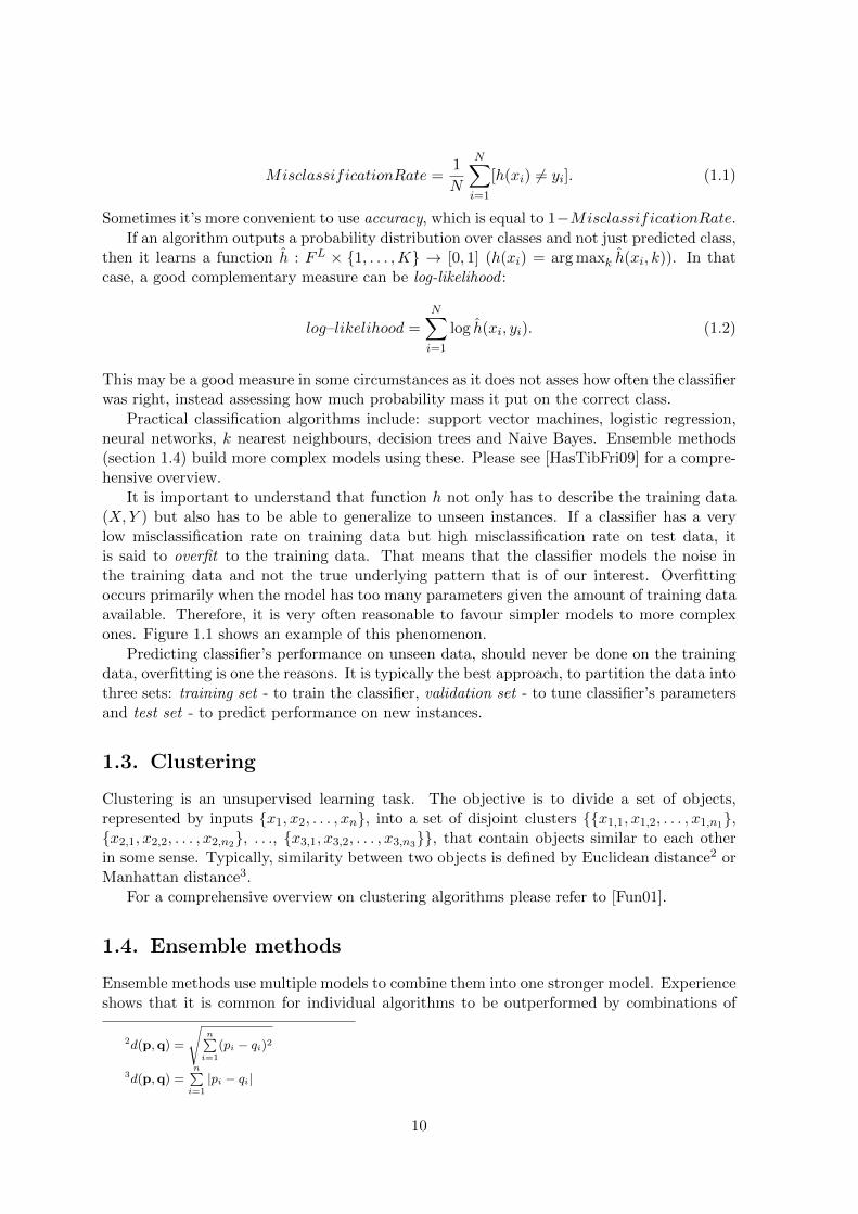
It is important to understand that function h not only has to describe the training data(X,Y ) but also has to be able to generalize to unseen instances. If a classifier has a verylow misclassification rate on training data but high misclassification rate on test data, itis said to overfit to the training data. That means that the classifier models the noise inthe training data and not the true underlying pattern that is of our interest. Overfittingoccurs primarily when the model has too many parameters given the amount of training dataavailable. Therefore, it is very often reasonable to favour simpler models to more complexones. Figure 1.1 shows an example of this phenomenon.

Predicting classifier’s performance on unseen data, should never be done on the trainingdata, overfitting is one the reasons. It is typically the best approach, to partition the data intothree sets: training set - to train the classifier, validation set - to tune classifier’s parametersand test set - to predict performance on new instances.

1.3. Clustering

Clustering is an unsupervised learning task. The objective is to divide a set of objects,represented by inputs {x1, x2, . . . , xn}, into a set of disjoint clusters {{x1,1, x1,2, . . . , x1,n1},{x2,1, x2,2, . . . , x2,n2}, . . ., {x3,1, x3,2, . . . , x3,n3}}, that contain objects similar to each otherin some sense. Typically, similarity between two objects is defined by Euclidean distance2 orManhattan distance3.

For a comprehensive overview on clustering algorithms please refer to [Fun01].

1.4. Ensemble methods

Ensemble methods use multiple models to combine them into one stronger model. Experienceshows that it is common for individual algorithms to be outperformed by combinations of

2d(p,q) =

√n∑i=1

(pi − qi)2

3d(p,q) =n∑i=1

|pi − qi|

10

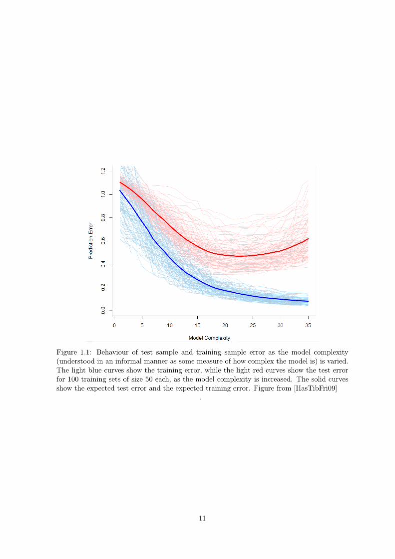
Figure 1.1: Behaviour of test sample and training sample error as the model complexity(understood in an informal manner as some measure of how complex the model is) is varied.The light blue curves show the training error, while the light red curves show the test errorfor 100 training sets of size 50 each, as the model complexity is increased. The solid curvesshow the expected test error and the expected training error. Figure from [HasTibFri09]

.

11

(a) Statistical (b) Representational (c) Computational

Figure 1.2: Reasons why an ensemble of classifiers may work better than a single one.

models and heterogeneous combinations are of special interest ([BelKor07]). As mentionedby [Die00] there are essentially three reasons why ensembles of models perform better thanindividual models: statistical, computational and representational (figure 1.2).

Statistical. One way to look at a learning algorithm is to view it as searching a hypothesisspace H to find the best one. Without enough data the algorithm may find a fewdifferent hypotheses in H that give the same accuracy on the training (or validation)data. By constructing an ensemble, the algorithm can find a point that is, in a certainsense, an average of the members of the ensemble and thus reduces a risk of choosingthe wrong classifier.

Representational. In many cases the true function f cannot be represented within hypoth-esis space H. By combining classifiers into an ensemble it may be possible to expand aset of representable functions. Even though some algorithms, like neural networks (thatactually are universal approximators as shown in [Hor91]), can, in theory, express a lotof functions, it is important to bear in mind that due to the finite amount of trainingdata, they will effectively explore a finite number of hypotheses and will stop when themodel fits the training data well enough.

Computational. Even when there is enough data, an algorithm performing local search forthe best hypothesis may get stuck in local optima. That is the case for neural networksfor example. Therefore, starting from different points and combining obtained modelsin an ensemble may lead to a model that is closer to the true hypothesis.

The most widely used ensemble methods are Random Forest ([Bre01]) and AdaBoost([Sch03]).

1.4.1. Random Forest

Entropy and information gain

Definition 1.4.1 Entropy, is a measure of the uncertainty associated with a random vari-able. For a discrete random variable X with support X , entropy is defined as

12

H(X) =∑x∈X

p(x) log1

p(x)= −

∑x∈X

p(x) log p(x). (1.3)

Definition 1.4.2 Given discrete random variable X with support X and Y with support Y,the conditional entropy of Y given X is defined as

H(Y |X) =∑x∈X

p(x)H(Y |X = x) = −∑x∈X

p(x)∑y∈Y

p(y|x) log p(y|x) (1.4)

Analogous definitions can be formulated for continuous random variables.

Definition 1.4.3 Information gain is the change in entropy of random variable X when avalue of random variable Y is observed, that is

InformationGain(X;Y ) = H(X)−H(X|Y ). (1.5)

Decision trees

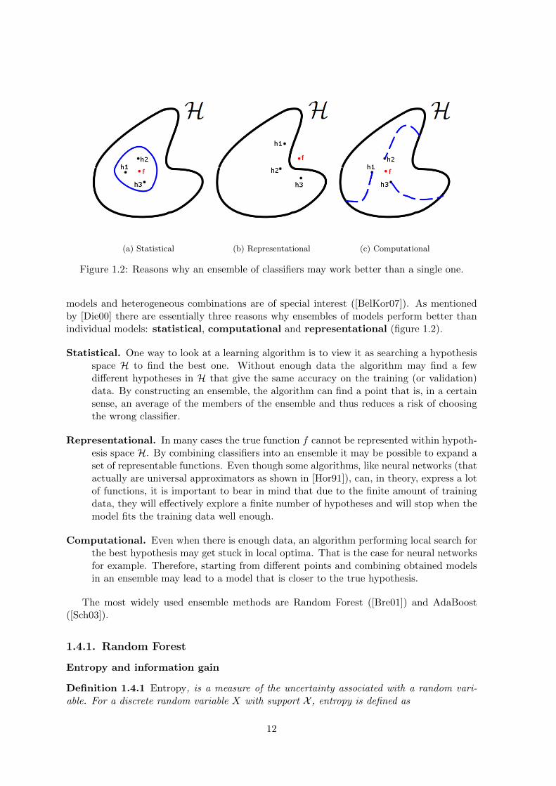
A decision tree partitions the feature space into rectangular regions and assigns a class toevery region. The process of partitioning the space is performed in such a way that thechoice of the variable that will be responsible for current split is done by greedily picking avariable that gives the highest information gain. Decision trees are conceptually very simpleyet accurate. Algorithm 1 gives a precise description on how to build a decision tree.

Algorithm 1 Building a decision tree

BuildTree(D, attributes)beginT ← empty treeif all instances in D have the same class c thenlabel(T )← creturn T

else if attributes = ∅ or no attribute has positive information gain thenlabel(T )← most common class in Dreturn T

elseA← attribute with highest information gainlabel(T )← Afor each value a of A doDa ← instances in D with A = aif Da = ∅ thenTa ← empty treelabel(Ta)← most common class in D

elseTa ← BuildTree(Da, attributes\{A})

end ifadd a branch from T to Ta labelled by a

end forend ifend

13

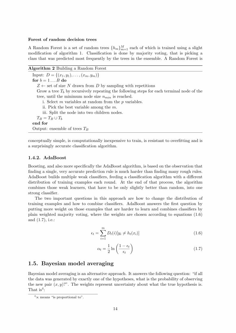
Forest of random decision trees

A Random Forest is a set of random trees {hm}Mm=1 each of which is trained using a slightmodification of algorithm 1. Classification is done by majority voting, that is picking aclass that was predicted most frequently by the trees in the ensemble. A Random Forest is

Algorithm 2 Building a Random Forest

Input: D = {(x1, y1), . . . , (xm, ym)}for b = 1 . . . B doZ ← set of size N drawn from D by sampling with repetitionsGrow a tree Tb by recursively repeating the following steps for each terminal node of thetree, until the minimum node size nmin is reached.

i. Select m variables at random from the p variables.ii. Pick the best variable among the m.iii. Split the node into two children nodes.

TB = TB ∪ Tbend forOutput: ensemble of trees TB

conceptually simple, is computationally inexpensive to train, is resistant to overfitting and isa surprisingly accurate classification algorithm.

1.4.2. AdaBoost

Boosting, and also more specifically the AdaBoost algorithm, is based on the observation thatfinding a single, very accurate prediction rule is much harder than finding many rough rules.AdaBoost builds multiple weak classifiers, feeding a classification algorithm with a differentdistribution of training examples each round. At the end of that process, the algorithmcombines those weak learners, that have to be only slightly better than random, into onestrong classifier.

The two important questions in this approach are how to change the distribution oftraining examples and how to combine classifiers. AdaBoost answers the first question byputting more weight on those examples that are harder to learn and combines classifiers byplain weighted majority voting, where the weights are chosen according to equations (1.6)and (1.7), i.e.:

εt =m∑i=1

Dt(i)[yi 6= ht(xi)] (1.6)

αt =1

2ln

(1− εtεt

)(1.7)

1.5. Bayesian model averaging

Bayesian model averaging is an alternative approach. It answers the following question: “if allthe data was generated by exactly one of the hypotheses, what is the probability of observingthe new pair (x, y)?”. The weights represent uncertainty about what the true hypothesis is.That is4:

4∝ means “is proportional to”.

14

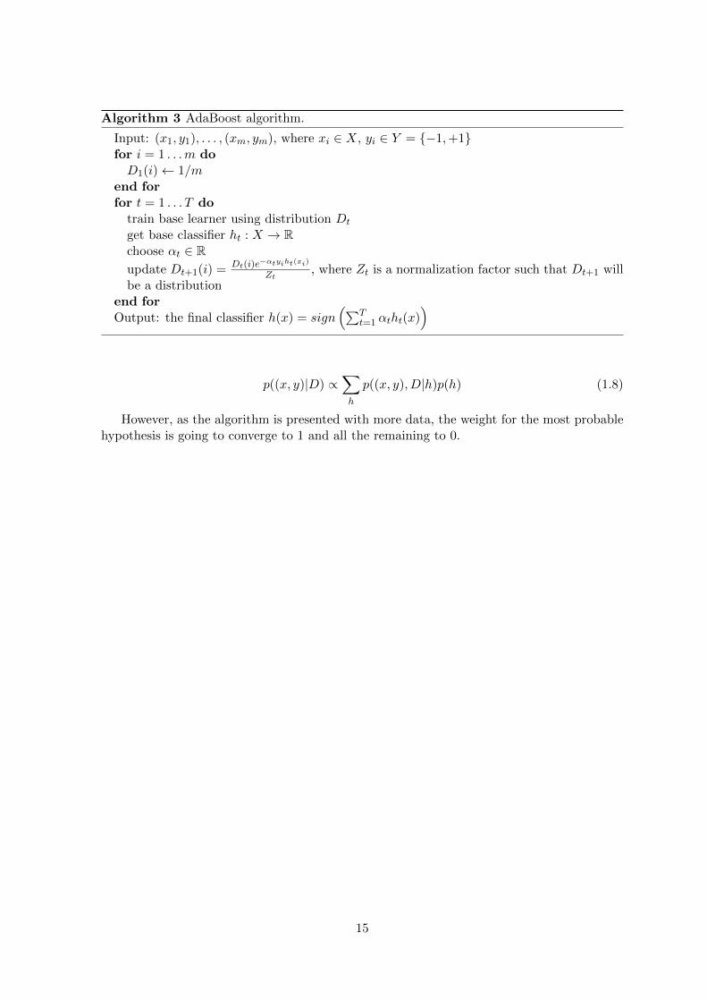
Algorithm 3 AdaBoost algorithm.

Input: (x1, y1), . . . , (xm, ym), where xi ∈ X, yi ∈ Y = {−1,+1}for i = 1 . . .m doD1(i)← 1/m

end forfor t = 1 . . . T do

train base learner using distribution Dt

get base classifier ht : X → Rchoose αt ∈ Rupdate Dt+1(i) = Dt(i)e−αtyiht(xi)

Zt, where Zt is a normalization factor such that Dt+1 will

be a distributionend forOutput: the final classifier h(x) = sign

(∑Tt=1 αtht(x)

)

p((x, y)|D) ∝∑h

p((x, y), D|h)p(h) (1.8)

However, as the algorithm is presented with more data, the weight for the most probablehypothesis is going to converge to 1 and all the remaining to 0.

15

Chapter 2

Basic concepts

2.1. Definitions

Definition 2.1.1 A market is a mechanism for the exchange of goods. The market itself isneutral with respect to the goods or the trades. The market itself cannot acquire or owe goods.Unless explicitly stated otherwise, perfect liquidity1 is assumed and there is no transactionfee. All participants in the market use the same currency for the purposes of trade.

Definition 2.1.2 Prediction market (also predictive market, information market) is a spec-ulative market created for the purpose of making predictions. Market prices in the equilibriumcan be interpreted as predictions of the probability of an event ([Man06], [WolZit04]). In thistype of market one type of good is a bet, and the other is a currency. A bet pays a fixed amountdependent on a particular outcome of a future occurrence, and pays nothing otherwise.

Definition 2.1.3 Artificial prediction market (also machine learning market) is a specialtype of prediction market. Market participants in the artificial prediction market are classifiersthat bet for classes. Equilibrium prices estimate probabilities over classes. The classifiers donot modify their beliefs once they join the market.

Definition 2.1.4 The efficient-market hypothesis asserts that financial markets are infor-mationally efficient. That is, one cannot consistently achieve returns in excess of averagemarket returns on a risk-adjusted basis, given the information publicly available at the timethe investment is made.

Definition 2.1.5 The market equilibrium is a price point for which all agents acting in themarket are satisfied with their trades and do not want to trade any further.

Definition 2.1.6 A homogeneous market is a prediction market such that all the participantsare of the same type, that is, they have the same buying function.

Definition 2.1.7 An inhomogeneous market is a prediction market that aggregates partici-pants who are of different types, that is, they do not all have the same buying function.

Definition 2.1.8 A utility function is a function U : X → R that measures a market par-ticipant’s satisfaction with its current wealth.

1That is, every good can be bought or sold at every point of time.

17

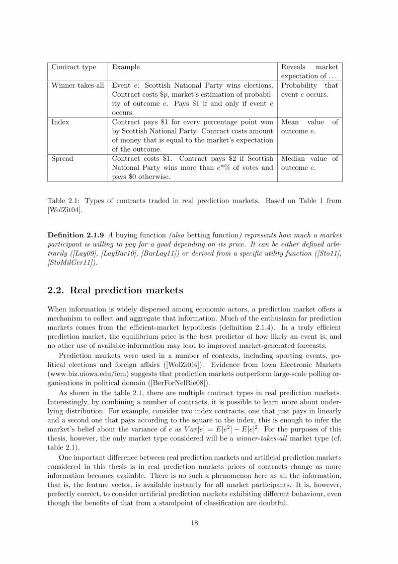
Contract type Example Reveals marketexpectation of . . .

Winner-takes-all Event e: Scottish National Party wins elections.Contract costs $p, market’s estimation of probabil-ity of outcome e. Pays $1 if and only if event eoccurs.

Probability thatevent e occurs.

Index Contract pays $1 for every percentage point wonby Scottish National Party. Contract costs amountof money that is equal to the market’s expectationof the outcome.

Mean value ofoutcome e.

Spread Contract costs $1. Contract pays $2 if ScottishNational Party wins more than e*% of votes andpays $0 otherwise.

Median value ofoutcome e.

Table 2.1: Types of contracts traded in real prediction markets. Based on Table 1 from[WolZit04].

Definition 2.1.9 A buying function (also betting function) represents how much a marketparticipant is willing to pay for a good depending on its price. It can be either defined arbi-trarily ([Lay09], [LayBar10], [BarLay11]) or derived from a specific utility function ([Sto11],[StoMilGer11]).

2.2. Real prediction markets

When information is widely dispersed among economic actors, a prediction market offers amechanism to collect and aggregate that information. Much of the enthusiasm for predictionmarkets comes from the efficient-market hypothesis (definition 2.1.4). In a truly efficientprediction market, the equilibrium price is the best predictor of how likely an event is, andno other use of available information may lead to improved market-generated forecasts.

Prediction markets were used in a number of contexts, including sporting events, po-litical elections and foreign affairs ([WolZit04]). Evidence from Iowa Electronic Markets(www.biz.uiowa.edu/iem) suggests that prediction markets outperform large-scale polling or-ganisations in political domain ([BerForNelRie08]).

As shown in the table 2.1, there are multiple contract types in real prediction markets.Interestingly, by combining a number of contracts, it is possible to learn more about under-lying distribution. For example, consider two index contracts, one that just pays in linearlyand a second one that pays according to the square to the index, this is enough to infer themarket’s belief about the variance of e as V ar[e] = E[e2] − E[e]2. For the purposes of thisthesis, however, the only market type considered will be a winner-takes-all market type (cf.table 2.1).

One important difference between real prediction markets and artificial prediction marketsconsidered in this thesis is in real prediction markets prices of contracts change as moreinformation becomes available. There is no such a phenomenon here as all the information,that is, the feature vector, is available instantly for all market participants. It is, however,perfectly correct, to consider artificial prediction markets exhibiting different behaviour, eventhough the benefits of that from a standpoint of classification are doubtful.

18

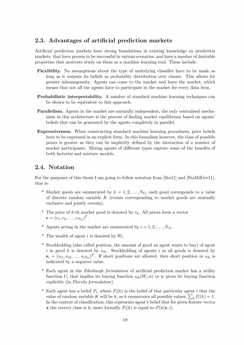
2.3. Advantages of artificial prediction markets

Artificial prediction markets have strong foundations in existing knowledge on predictionmarkets, that have proven to be successful in various scenarios, and have a number of desirableproperties that motivate study on them as a machine learning tool. These include:

Flexibility. No assumptions about the type of underlying classifier have to be made aslong as it outputs its beliefs as probability distribution over classes. This allows forgreater inhomogeneity. Agents can come to the market and leave the market, whichmeans that not all the agents have to participate in the market for every data item.

Probabilistic interpretability. A number of standard machine learning techniques canbe shown to be equivalent to this approach.

Parallelism. Agents in the market are naturally independent, the only centralised mecha-nism in this architecture is the process of finding market equilibrium based on agents’beliefs that can be generated by the agents completely in parallel.

Expressiveness. When constructing standard machine learning procedures, prior beliefshave to be expressed in an explicit form. In this formalism however, the class of possiblepriors is greater as they can be implicitly defined by the interaction of a number ofmarket participants. Mixing agents of different types capture some of the benefits ofboth factorial and mixture models.

2.4. Notation

For the purposes of this thesis I am going to follow notation from [Sto11] and [StoMilGer11],that is:

* Market goods are enumerated by k = 1, 2, . . . , NG, each good corresponds to a valueof discrete random variable K (events corresponding to market goods are mutuallyexclusive and jointly certain).

* The price of k-th market good is denoted by ck. All prices form a vectorc = (c1, c2, . . . , cNG)T .

* Agents acting in the market are enumerated by i = 1, 2, . . . , NA.

* The wealth of agent i is denoted by Wi.

* Stockholding (also called position, the amount of good an agent wants to buy) of agenti in good k is denoted by sik. Stockholding of agents i in all goods is denoted bysi = (si1, ss2, . . . , siNG)T . If short positions are allowed, then short position in sik isindicated by a negative value.

* Each agent in the Edinburgh formulation of artificial prediction market has a utilityfunction Ui that implies its buying function sik(Wi, c) or is given its buying functionexplicitly (in Florida formulation).

* Each agent has a belief Pi, where Pi(k) is the belief of that particular agent i that thevalue of random variable K will be k, as k enumerates all possible values,

∑k Pi(k) = 1.

In the context of classification, this represents agent’s belief that for given feature vectorx the correct class is k, more formally Pi(k) is equal to P (k|x, i).

19

* A sequence of first t data items in data set D is denoted by DT and the tth data itemis denoted by Dt.

20

Chapter 3

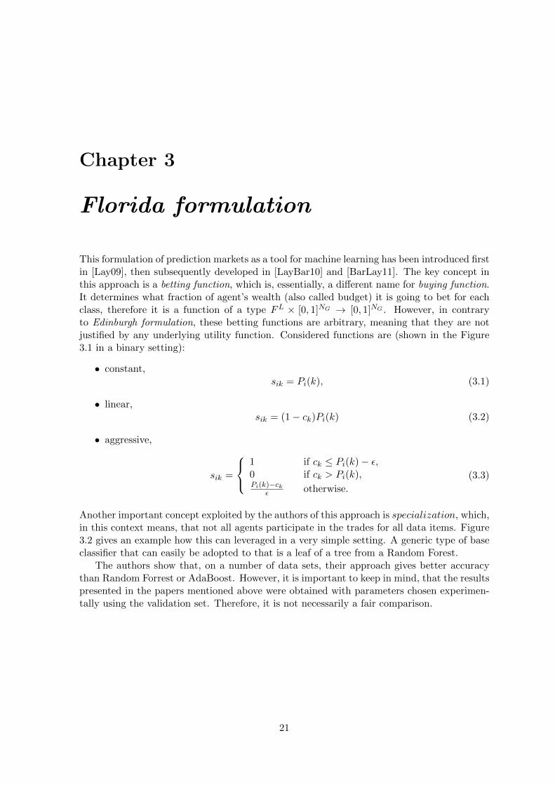
Florida formulation

This formulation of prediction markets as a tool for machine learning has been introduced firstin [Lay09], then subsequently developed in [LayBar10] and [BarLay11]. The key concept inthis approach is a betting function, which is, essentially, a different name for buying function.It determines what fraction of agent’s wealth (also called budget) it is going to bet for eachclass, therefore it is a function of a type FL × [0, 1]NG → [0, 1]NG . However, in contraryto Edinburgh formulation, these betting functions are arbitrary, meaning that they are notjustified by any underlying utility function. Considered functions are (shown in the Figure3.1 in a binary setting):

• constant,sik = Pi(k), (3.1)

• linear,sik = (1− ck)Pi(k) (3.2)

• aggressive,

sik =

1 if ck ≤ Pi(k)− ε,0 if ck > Pi(k),Pi(k)−ck

ε otherwise.

(3.3)

Another important concept exploited by the authors of this approach is specialization, which,in this context means, that not all agents participate in the trades for all data items. Figure3.2 gives an example how this can leveraged in a very simple setting. A generic type of baseclassifier that can easily be adopted to that is a leaf of a tree from a Random Forest.

The authors show that, on a number of data sets, their approach gives better accuracythan Random Forrest or AdaBoost. However, it is important to keep in mind, that the resultspresented in the papers mentioned above were obtained with parameters chosen experimen-tally using the validation set. Therefore, it is not necessarily a fair comparison.

21

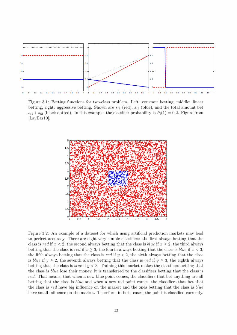
Figure 3.1: Betting functions for two-class problem. Left: constant betting, middle: linearbetting, right: aggressive betting. Shown are si2 (red), si1 (blue), and the total amount betsi1 + si2 (black dotted). In this example, the classifier probability is Pi(1) = 0.2. Figure from[LayBar10].

Figure 3.2: An example of a dataset for which using artificial prediction markets may leadto perfect accuracy. There are eight very simple classifiers: the first always betting that theclass is red if x < 2, the second always betting that the class is blue if x ≥ 2, the third alwaysbetting that the class is red if x ≥ 3, the fourth always betting that the class is blue if x < 3,the fifth always betting that the class is red if y < 2, the sixth always betting that the classis blue if y ≥ 2, the seventh always betting that the class is red if y ≥ 3, the eighth alwaysbetting that the class is blue if y < 3. Training this market makes the classifiers betting thatthe class is blue lose their money, it is transferred to the classifiers betting that the class isred. That means, that when a new blue point comes, the classifiers that bet anything are allbetting that the class is blue and when a new red point comes, the classifiers that bet thatthe class is red have big influence on the market and the ones betting that the class is bluehave small influence on the market. Therefore, in both cases, the point is classified correctly.

22

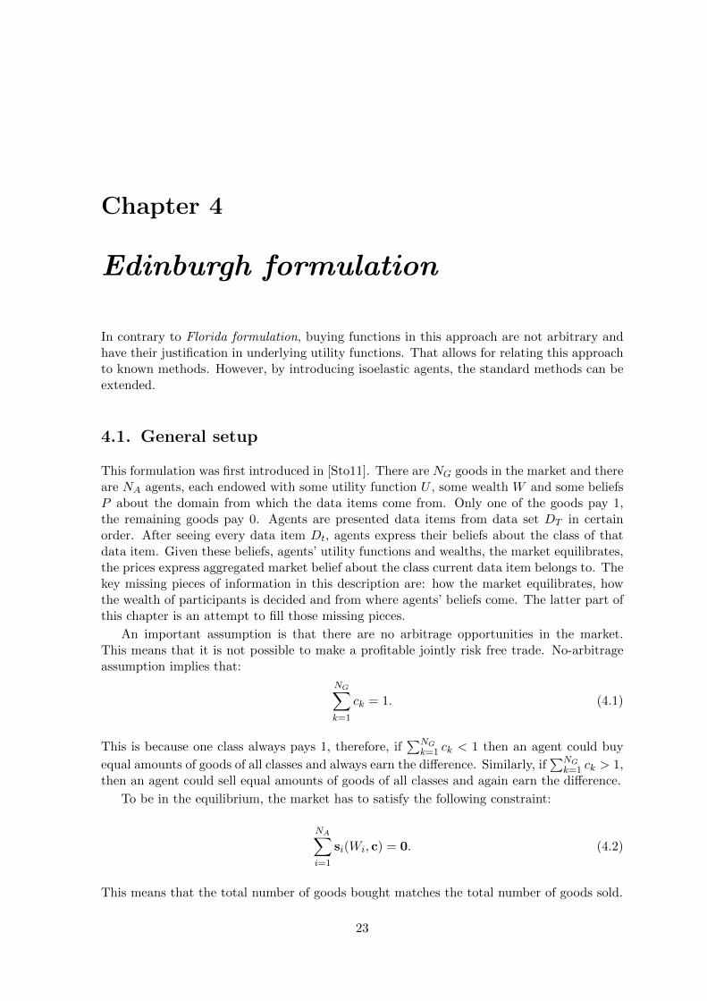
Chapter 4

Edinburgh formulation

In contrary to Florida formulation, buying functions in this approach are not arbitrary andhave their justification in underlying utility functions. That allows for relating this approachto known methods. However, by introducing isoelastic agents, the standard methods can beextended.

4.1. General setup

This formulation was first introduced in [Sto11]. There are NG goods in the market and thereare NA agents, each endowed with some utility function U , some wealth W and some beliefsP about the domain from which the data items come from. Only one of the goods pay 1,the remaining goods pay 0. Agents are presented data items from data set DT in certainorder. After seeing every data item Dt, agents express their beliefs about the class of thatdata item. Given these beliefs, agents’ utility functions and wealths, the market equilibrates,the prices express aggregated market belief about the class current data item belongs to. Thekey missing pieces of information in this description are: how the market equilibrates, howthe wealth of participants is decided and from where agents’ beliefs come. The latter part ofthis chapter is an attempt to fill those missing pieces.

An important assumption is that there are no arbitrage opportunities in the market.This means that it is not possible to make a profitable jointly risk free trade. No-arbitrageassumption implies that:

NG∑k=1

ck = 1. (4.1)

This is because one class always pays 1, therefore, if∑NG

k=1 ck < 1 then an agent could buy

equal amounts of goods of all classes and always earn the difference. Similarly, if∑NG

k=1 ck > 1,then an agent could sell equal amounts of goods of all classes and again earn the difference.

To be in the equilibrium, the market has to satisfy the following constraint:

NA∑i=1

si(Wi, c) = 0. (4.2)

This means that the total number of goods bought matches the total number of goods sold.

23

4.2. Utility functions

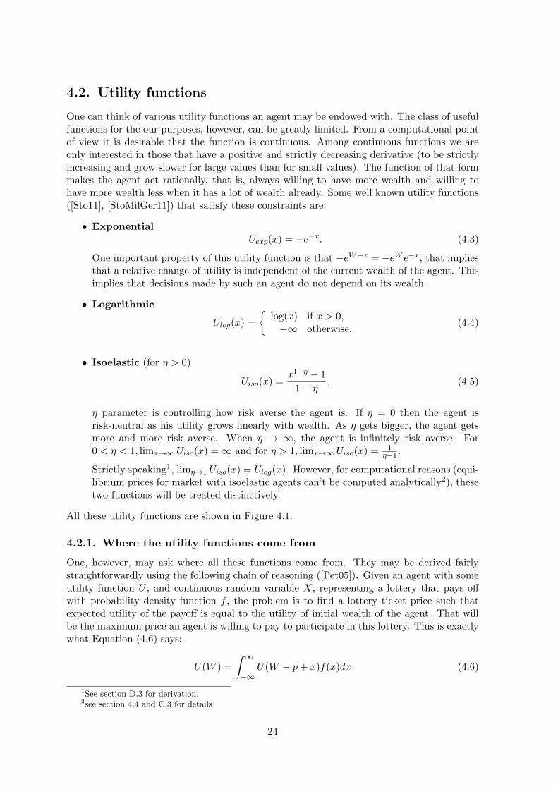
One can think of various utility functions an agent may be endowed with. The class of usefulfunctions for the our purposes, however, can be greatly limited. From a computational pointof view it is desirable that the function is continuous. Among continuous functions we areonly interested in those that have a positive and strictly decreasing derivative (to be strictlyincreasing and grow slower for large values than for small values). The function of that formmakes the agent act rationally, that is, always willing to have more wealth and willing tohave more wealth less when it has a lot of wealth already. Some well known utility functions([Sto11], [StoMilGer11]) that satisfy these constraints are:

• ExponentialUexp(x) = −e−x. (4.3)

One important property of this utility function is that −eW−x = −eW e−x, that impliesthat a relative change of utility is independent of the current wealth of the agent. Thisimplies that decisions made by such an agent do not depend on its wealth.

• Logarithmic

Ulog(x) =

{log(x) if x > 0,−∞ otherwise.

(4.4)

• Isoelastic (for η > 0)

Uiso(x) =x1−η − 1

1− η. (4.5)

η parameter is controlling how risk averse the agent is. If η = 0 then the agent isrisk-neutral as his utility grows linearly with wealth. As η gets bigger, the agent getsmore and more risk averse. When η → ∞, the agent is infinitely risk averse. For0 < η < 1, limx→∞ Uiso(x) =∞ and for η > 1, limx→∞ Uiso(x) = 1

η−1 .

Strictly speaking1, limη→1 Uiso(x) = Ulog(x). However, for computational reasons (equi-librium prices for market with isoelastic agents can’t be computed analytically2), thesetwo functions will be treated distinctively.

All these utility functions are shown in Figure 4.1.

4.2.1. Where the utility functions come from

One, however, may ask where all these functions come from. They may be derived fairlystraightforwardly using the following chain of reasoning ([Pet05]). Given an agent with someutility function U , and continuous random variable X, representing a lottery that pays offwith probability density function f , the problem is to find a lottery ticket price such thatexpected utility of the payoff is equal to the utility of initial wealth of the agent. That willbe the maximum price an agent is willing to pay to participate in this lottery. This is exactlywhat Equation (4.6) says:

U(W ) =

∫ ∞−∞

U(W − p+ x)f(x)dx (4.6)

1See section D.3 for derivation.2see section 4.4 and C.3 for details

24

An approximate simplification of this equation is3:

p =

∫ ∞−∞

xf(x)dx+U ′′(W )

U ′(W )

∫ ∞−∞

(x− p)2

2f(x)dx (4.7)

This expression shows that the maximum amount that an agent is willing to pay for a lotteryticket is equal to the mean of X minus a term consisting of two parts. One part is theintegral (always of positive value) related to the variability of the outcome. The other partdepends only on the agent’s utility function. A few categories of utility functions can be

defined depending on what function the ratio U ′′(W )U ′(W ) is.

Hyperbolic absolute risk aversion (HARA) is the most general class of utility functionsused in practice. A utility function exhibits HARA if its absolute risk aversion A is a hyper-bolic function, namely:

A(c) = −U′′(c)

U ′(c)=

1

ac+ b(4.8)

Special cases of this occur when:

• a = 0, then A(c) = −U ′′(c)U ′(c) = 1

b = const and utility is said to exhibit constant absoluterisk aversion. Then the solution of this differential equation is, up to multiplicative andadditive constant, the exponential utility function.

• b = 0, then A(c) = − cU ′′(c)U ′(c) = 1

a = const and utility is said to exhibit constant relativerisk aversion. Then the solution of this differential equation is, up to multiplicative andadditive constant, the isoelastic utility function.

Therefore, since isoelastic utility generalizes logarithmic utility, I have shown that functionsexhibiting hyperbolic absolute risk aversion generalize all utility functions used in this thesis.

4.3. Buying functions

The next step is to find out what amounts of different stock agents want to buy. As theoutcome is uncertain, a rational agent wants to maximise its expected utility

E[U ] =∑k

Pi(k)U(Wi − sTi c + sik), (4.9)

which leads to equation (4.10).

s∗i = arg maxsi

∑k

Pi(k)U(Wi − sTi c + sik). (4.10)

However, there is more than just one set of parameters maximising expected utility, hencethere is no unique function satisfying this optimisation problem as well. In fact, there is acontinuum of functions that maximise expected utility. The reason for this is that every agentcan make financially-neutral risk-free bets just by buying equal amounts of all goods, utilitiesof s + α1 are equal. The important thing is what the relative amounts of goods bought andsold are, therefore, to deal with this issue, a neutral agent, willing to make only financially-neutral risk-free trades, is introduced. Then it is necessary to specify agent’s position only

3See section D.4 for derivation.

25

up to an equivalence class. To represent each class by one position only, it is necessaryto use some standardization constraint. Some sensible constraints to impose on each agentare sTi c = 0 (agent purchases and sells equal amount of goods) and siNG = 0 (agent doesnot purchase or sell the last good). It is important to understand that those constraintsdo not change agents’ behaviour in the market, they are introduced only for convenience ofrepresenting classes of equivalent positions. It is also correct to switch between constraintsin the calculations.

si(Wi, c) is a smooth function of si if the utility function is a smooth function. Therefore,its maximum with respect to si can be found by simple differentiation. Buying functionscorresponding4 to the utility functions introduced earlier are:

• Exponential

s∗ik = logPi(k)− log ck (4.11)

• Logarithmic

s∗ik =Wi (Pi(k)− ck)

ck(4.12)


s∗ik = Wi

[Pi(k)ck

] 1η

∑j cj

[Pi(j)cj

] 1η

− 1

(4.13)

Again, when η → 1, this becomes equivalent to the buying function derived for loga-rithmic utility.

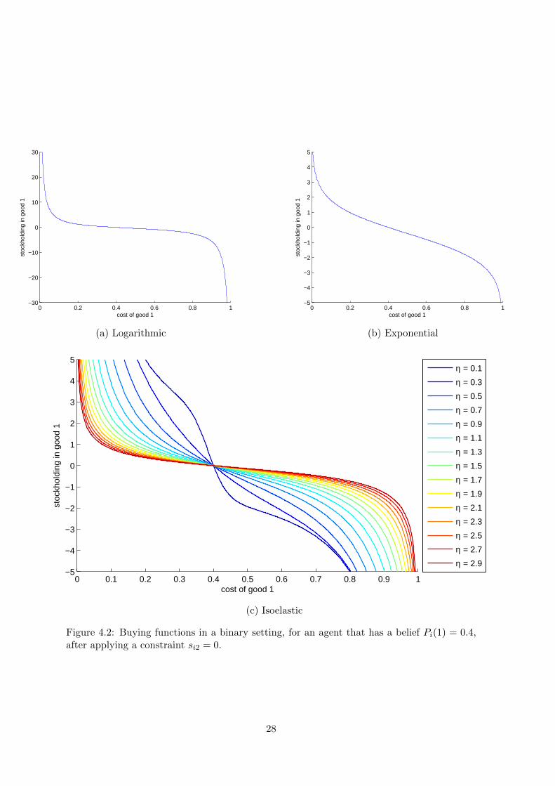
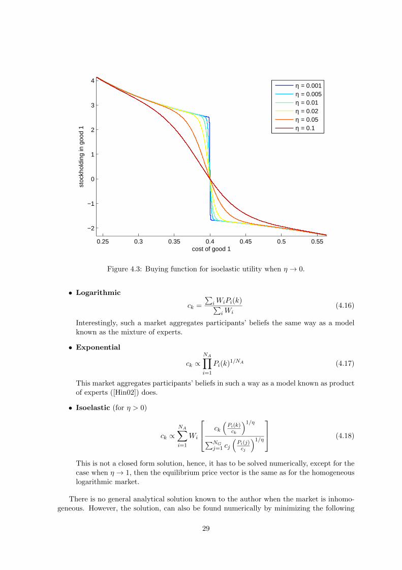
All these buying functions are shown in Figure 4.2. The unexpected change of shape of thefunction in the Figure 4.2(c) and in the Figure 4.3 as η gets closer to 0 is a consequence ofthe fact that, in a binary setting, when η → 0, then5

s∗ik =

Wick

if Pi(k) > ck,

0 if Pi(k) = ck,

− Wi1−ck if Pi(k) < ck.

(4.14)

Also, when η →∞, then

s∗ik = 0 (4.15)

4.4. Finding an equilibrium

The market has to satisfy the market constraint (4.2). All agents simultaneously try to max-imise their utility functions. According to [ArrDeb54], if all individual agents have concaveutility functions, there is a unique market equilibrium. To find this equilibrium in this for-malism, it is necessary to solve equation (4.2). When the market is homogeneous, attemptingto solve market equation analytically gives the following6:

4Please look at appendix A for derivations of buying functions from utility functions.5See section D.5 for details.6See appendix C for details.

26

0 2 4 6 8 10−5

−4

−3

−2

−1

0

1

2

3

wealth

utili

ty

0 2 4 6 8 10−1

−0.9

−0.8

−0.7

−0.6

−0.5

−0.4

−0.3

−0.2

−0.1

0

wealthut

ility

(a) Logarithmic (b) Exponential

0 1 2 3 4 5 6 7−5

−4

−3

−2

−1

0

1

2

3

4

5

wealth

utili

ty

η = 0.1

η = 0.3

η = 0.5

η = 0.7

η = 0.9

η = 1.1

η = 1.3

η = 1.5

η = 1.7

η = 1.9

η = 2.1

η = 2.3

η = 2.5

η = 2.7

η = 2.9

(c) Isoelastic

Figure 4.1: Utility functions in a binary setting.

27

0 0.2 0.4 0.6 0.8 1−30

−20

−10

0

10

20

30

cost of good 1

stoc

khol

ding

in g

ood

1

0 0.2 0.4 0.6 0.8 1−5

−4

−3

−2

−1

0

1

2

3

4

5

cost of good 1

stoc

khol

ding

in g

ood

1

(a) Logarithmic (b) Exponential

0 0.1 0.2 0.3 0.4 0.5 0.6 0.7 0.8 0.9 1−5

−4

−3

−2

−1

0

1

2

3

4

5

cost of good 1

stoc

khol

ding

in g

ood

1

η = 0.1

η = 0.3

η = 0.5

η = 0.7

η = 0.9

η = 1.1

η = 1.3

η = 1.5

η = 1.7

η = 1.9

η = 2.1

η = 2.3

η = 2.5

η = 2.7

η = 2.9

(c) Isoelastic

Figure 4.2: Buying functions in a binary setting, for an agent that has a belief Pi(1) = 0.4,after applying a constraint si2 = 0.

28

0.25 0.3 0.35 0.4 0.45 0.5 0.55

−2

−1

0

1

2

3

4

cost of good 1

stoc

khol

ding

in g

ood

1

η = 0.001η = 0.005η = 0.01η = 0.02η = 0.05η = 0.1

Figure 4.3: Buying function for isoelastic utility when η → 0.

• Logarithmic

ck =

∑iWiPi(k)∑

iWi(4.16)

Interestingly, such a market aggregates participants’ beliefs the same way as a modelknown as the mixture of experts.

• Exponential

ck ∝NA∏i=1

Pi(k)1/NA (4.17)

This market aggregates participants’ beliefs in such a way as a model known as productof experts ([Hin02]) does.


ck ∝NA∑i=1

Wi

ck

(Pi(k)ck

)1/η∑NG

j=1 cj

(Pi(j)cj

)1/η (4.18)

This is not a closed form solution, hence, it has to be solved numerically, except for thecase when η → 1, then the equilibrium price vector is the same as for the homogeneouslogarithmic market.

There is no general analytical solution known to the author when the market is inhomo-geneous. However, the solution, can also be found numerically by minimizing the following

29

function (which will be referred to as market equilibrium function):

E(c) =∑k

(∑i

sik(Wi, c)

)2

(4.19)

If E > 0 there is a mismatch between those who want to sell and those who want to buygoods at a given price. When E = 0, constraint (4.2) is satisfied. Minimizing function (4.19)can, in practice, be done using some variant of Newton’s method7. One good initial valueof c that approximates the solution is just a vector of average belief about classes, that is[

1NA

∑NAi=1 Pi(1), . . . , 1

NA

∑NAi=1 Pi(NG)

].

4.5. Minimizing market equilibrium function

When plugging function (4.19) into an unconstrained optimisation procedure, the solutionfound will not necessarily be a probability distribution (it will not necessarily be a vectorof positive numbers summing up to 1). In order to mitigate against these issues withoutformulating this as constrained optimisation, equation (4.19) can be rewritten as:

E(z) =

NG∑k=1

(NA∑i=1

sik (Wi, c(z))

)2

(4.20)

where c is the softmax function of z:

ck(z) =ezk∑NGj=1 e

zj

Then derivative of E with respect to z can be found using the chain rule:

∂E

∂z=∂E

∂c.∂c

∂z

Starting with

∂c

∂z=

∂c1∂z1

· · · ∂c1∂zj

· · · ∂c1∂zNG

.... . .

...... ∂ci

∂zj

......

. . ....

∂cNG∂z1

· · · ∂cNG∂zj

· · · ∂cNG∂zNG

where8 9

∂ci∂zj

= ci (Iij − cj)

7Experimental work in thesis was done using subspace trust-region method based on the interior-reflectiveNewton method implemented by fminunc function from MATLAB Optimization Toolbox.

8See section D.1 for the derivation.9

Iij =

{1 if i = j,0 if i 6= j.

30

and

∂E

∂c=

[∂E

∂c1· · · ∂E

∂ck· · · ∂E

∂cNG

]where

∂E

∂cq=

NG∑k=1

2

(NA∑i=1

sik(Wi, c)

)(NA∑i=1

∂sik(Wi, c)

∂cq

)

the derivative is equal to:

∂E

∂z=

[∂E

∂c1· · · ∂E

∂ck· · · ∂E

∂cNG

]

∂c1∂z1

· · · ∂c1∂zj

· · · ∂c1∂zNG

.... . .

...... ∂ci

∂zj

......

. . ....

∂cNG∂z1

· · · ∂cNG∂zj

· · · ∂cNG∂zNG

(4.21)

Thus, it is necessary to differentiate the buying functions with respect to the cost vectorin order to use gradient based optimisation methods. Derivatives of the functions introducedearlier can be derived analytically10. If they could not, numerical derivatives can be usedinstead, however, they slow the computations significantly.

4.6. Training the market

4.6.1. Wealth update

Agent i has wealth Wi. Wealth affects agent’s behaviour and, therefore, affects its influenceon the market (except for exponential agents, whose buying function (4.11) does not dependon wealth). For every market training data item agent i gets sTi c for goods that he boughtand sold and gets return of sik∗ for the good that represented the correct class, hence, intotal sTi c + sik∗ . However, because of the constraint sTi c = 0, sTi c + sik∗ = sik∗ .

A number of ways of updating the budgets could be considered. The two most obviousare: online update and batch update. Online update means that budget of every participantof the market changes after every training sample. In that context, W t

i denotes wealth ofagent i after the market saw t data items. Batch update means that agent’s wealth is dividedinto equal pieces, one piece for each training point. In that context W ′i denotes the wealthof agent i after seeing all T data items.

One interesting property of the market that has exclusively isoelastic agents is that thewealths can all be multiplied by the same constant and the prices are going to be exactly thesame as before.

4.6.2. Update for logarithmic agents

The wealths are initialized in such a way that∑NA

i=1Wi = 1.

10See appendix B for derivation of ∂sik∂cq

.

31

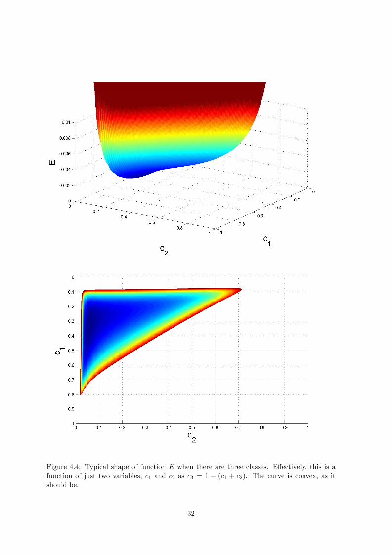
Figure 4.4: Typical shape of function E when there are three classes. Effectively, this is afunction of just two variables, c1 and c2 as c3 = 1 − (c1 + c2). The curve is convex, as itshould be.

32

Online update

W t+1i = W t

i + sikt = W ti +

W ti (Pi(kt)− ckt)

ckt= W t

i

Pi(kt)

ckt(4.22)

Assuming that the distribution of vectors of features x is independent of i, the following chainof equalities holds P (Dt|i)

P (Dt)= P (x,k|i)

P (x,k) = P (k|x,i)P (x|i)P (k|x)P (x) = P (k|x,i)

P (k|x) = Pi(kt)ckt

. Therefore, by equating

W ti to P (i|DT ), budget update takes the form of

W t+1i = P (i|DT+1) =

P (Dt+1|i)P (i|DT )

P (Dt+1)(4.23)

This is Bayesian update rule, initial wealths can be interpreted as a prior distribution. Thenusing the assumption that

∑NAi=1W

ti = 1, it follows that equation (4.16) can be interpreted

in the following way:

ck =

∑NAi=1W

ti Pi(k)∑NA

i=1Wti

=

NA∑i=1

P (i|DT )Pi(k) (4.24)

This is Bayesian averaging procedure mentioned in section 1.5. This is a good method if webelieve that there are many competing hypotheses and only one is correct. However, thisassumption may not always, and, in fact, in most cases is inappropriate ([Min02]). However,it is still an interesting example of how prediction market mechanism is equivalent to standardmachine learning algorithm.

One way of preventing a scenario where all the wealth available on the market goes tothe best player would be to introduce a salary (a fixed income at the beginning of each turnor training epoch) and a tax on wealth. This way no agents would lose all their money andbe completely ignored and the agents who have great wealth would not dominate the markettotally. That idea is in the spirit of a technique known as regularisation.

Batch update

Similarly, an interpretation can be given to batch update.

W ′i =1

T

T∑t=1

(Wi + sikt) = W ti +

1

T

T∑t=1

W ti (Pi(kt)− ckt)

ckt=Wi

T

T∑t=1

Pi(kt)

ckt(4.25)

W ′i = P (i|DT ) =P (i)

T

T∑t=1

P (Dt|i)P (Dt)

=1

T

T∑t=1

P (i|Dt) (4.26)

This is known as maximum posterior mixture model.

33

Chapter 5

Experimental results

5.1. Experimental setup

5.1.1. Data sets

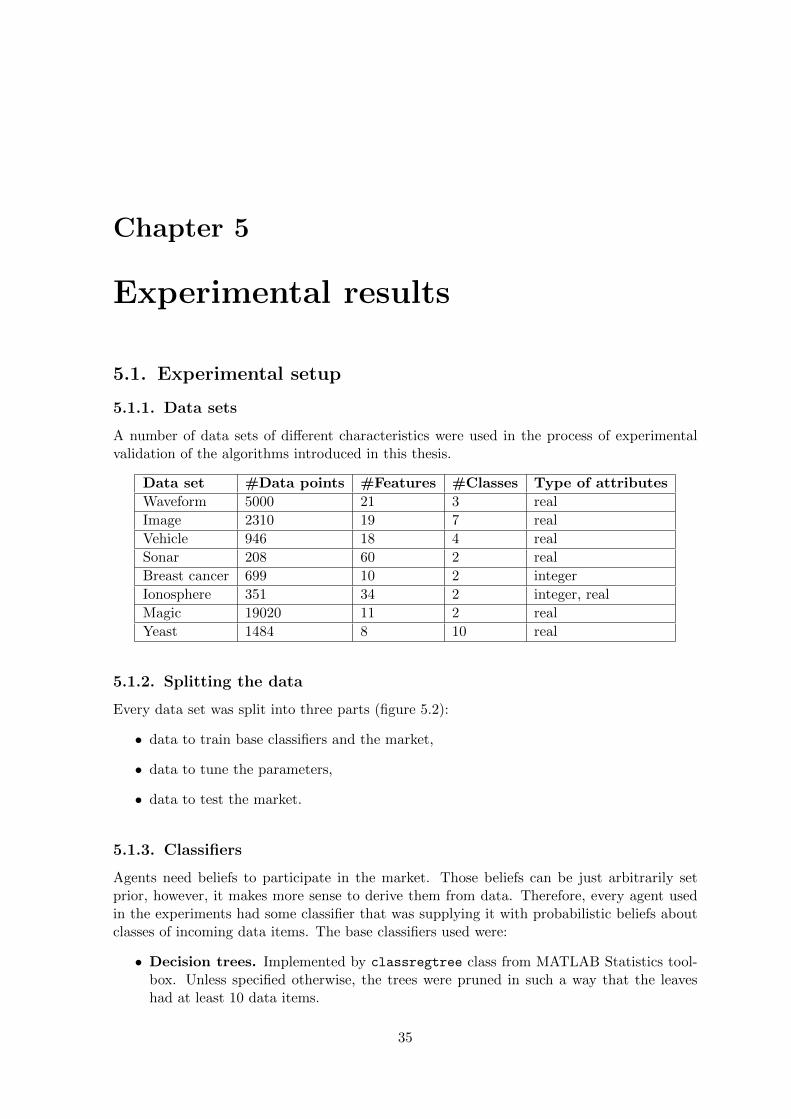
A number of data sets of different characteristics were used in the process of experimentalvalidation of the algorithms introduced in this thesis.

Data set #Data points #Features #Classes Type of attributes

Waveform 5000 21 3 real

Image 2310 19 7 real

Vehicle 946 18 4 real

Sonar 208 60 2 real

Breast cancer 699 10 2 integer

Ionosphere 351 34 2 integer, real

Magic 19020 11 2 real

Yeast 1484 8 10 real

5.1.2. Splitting the data

Every data set was split into three parts (figure 5.2):

• data to train base classifiers and the market,

• data to tune the parameters,

• data to test the market.

5.1.3. Classifiers

Agents need beliefs to participate in the market. Those beliefs can be just arbitrarily setprior, however, it makes more sense to derive them from data. Therefore, every agent usedin the experiments had some classifier that was supplying it with probabilistic beliefs aboutclasses of incoming data items. The base classifiers used were:

• Decision trees. Implemented by classregtree class from MATLAB Statistics tool-box. Unless specified otherwise, the trees were pruned in such a way that the leaveshad at least 10 data items.

35

waveform image sonar vehicle

breast cancer ionosphere magic yeast

Figure 5.1: Class distributions in the data sets. The data sets were chosen in such a way thatthere is a variety in the number of features and classes. Waveform is an artificially generateddata set and the others contain real data.

Figure 5.2: Data split. Base classifiers and the market was trained on the same data set.

• Neural networks. Implemented by mlp class in Netlab ([Netlab]) library. Unlessspecified otherwise, networks had 10 hidden units and were trained in 300 iterations.

• Logistic regression. Implemented by mnrfit and mnrval functions from MATLABStatistics toolbox.

• Naive Bayes. Implemented by NaiveBayes class from MATLAB Statistics toolbox.

• Support Vector Machines. Implemented by svmtrain and svnpredict functionsfrom LIBSVM ([LIBSVM]) library.

To avoid beliefs equal to zero, which may result in prices equal to zero, which maycause division by zero, beliefs have been smoothed in the following way, for all NG classes,Pi(k) := 0.1+Pi(k)T

0.1NG+T, where T denotes the size of the data set.

5.1.4. Sampling methods1

To generate multiple data sets of size n out of one data set of size N , one of the followingsampling methods was applied.

• No sampling. Just permuting the whole data set.

• Bootstrapping. Sampling the original data set n times with replacement.

1Sampling in this context means picking data items from the original data set to create a new data setand should not be confused with sampling as in the context of MCMC methods.

36

• Sample selection bias. This procedure is described by algorithm 42.

Algorithm 4 Sample selection bias

Input: D = ((x1, y1), . . . , (xm, ym)),B - number of biased sets to generate,S - number of training samples in every generated data set,K - number of classes.Generate B probability distributions, such that ∀k∈{1,...,K}

∑Bb=1 Pb(k) = B

Kfor b = 1 . . . B doDb ← ∅while |Db| < S do

(x, y)← random data point from Dif rand(0, 1) ≥ Pb(y) thenDb ← Db ∪ (x, y)

end ifend while

end forOutput: (D1, . . . , DB)

• Subsampling. Sampling the original data set n times without replacement.

5.1.5. Other parameters

Other parameters were:

• number of agents in the market,

• number of iterations of the whole procedure - to have more reliable estimates,

• maximum number of data items - to truncate very large data sets,

• percentages of the data assigned to parts as defined in section 5.1.2.

5.2. Results

Unless specified otherwise, the parameters were set to the following values:

• 10 agents were participating in the market,

• sample selection bias was a sampling method with sample size of 75% of the originalsample,

• experiments were repeated 25 times,

• 60% of the data was used for training, 20% for validation, remaining 20% was left astest data,

• data sets larger than 1000 data items were truncated to 1000 data items,

• there was one training epoch with batch update.

2See section D.2 to see how to generate such probability distributions as mentioned in the algorithm.

37

A number of experiments was executed using this setup:

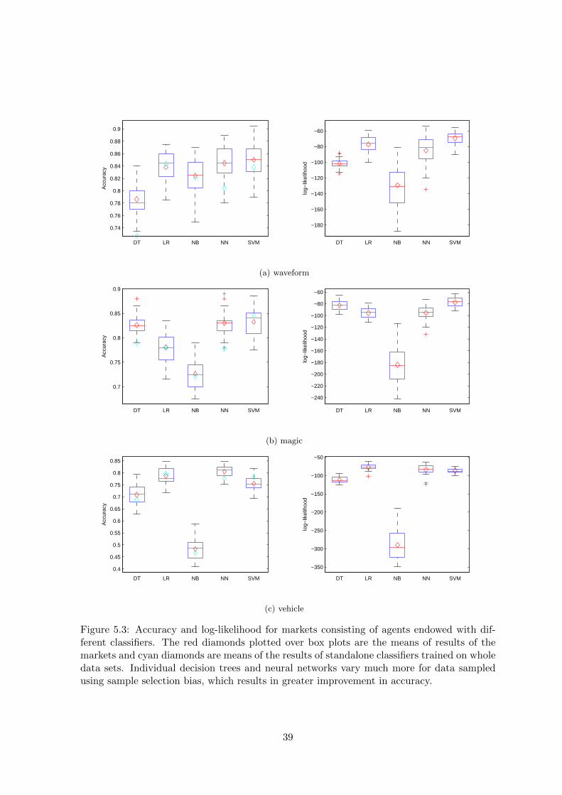
1. Comparison of individual classifiers with markets consisting of agents endowed withthese base classifiers (Figure 5.3).

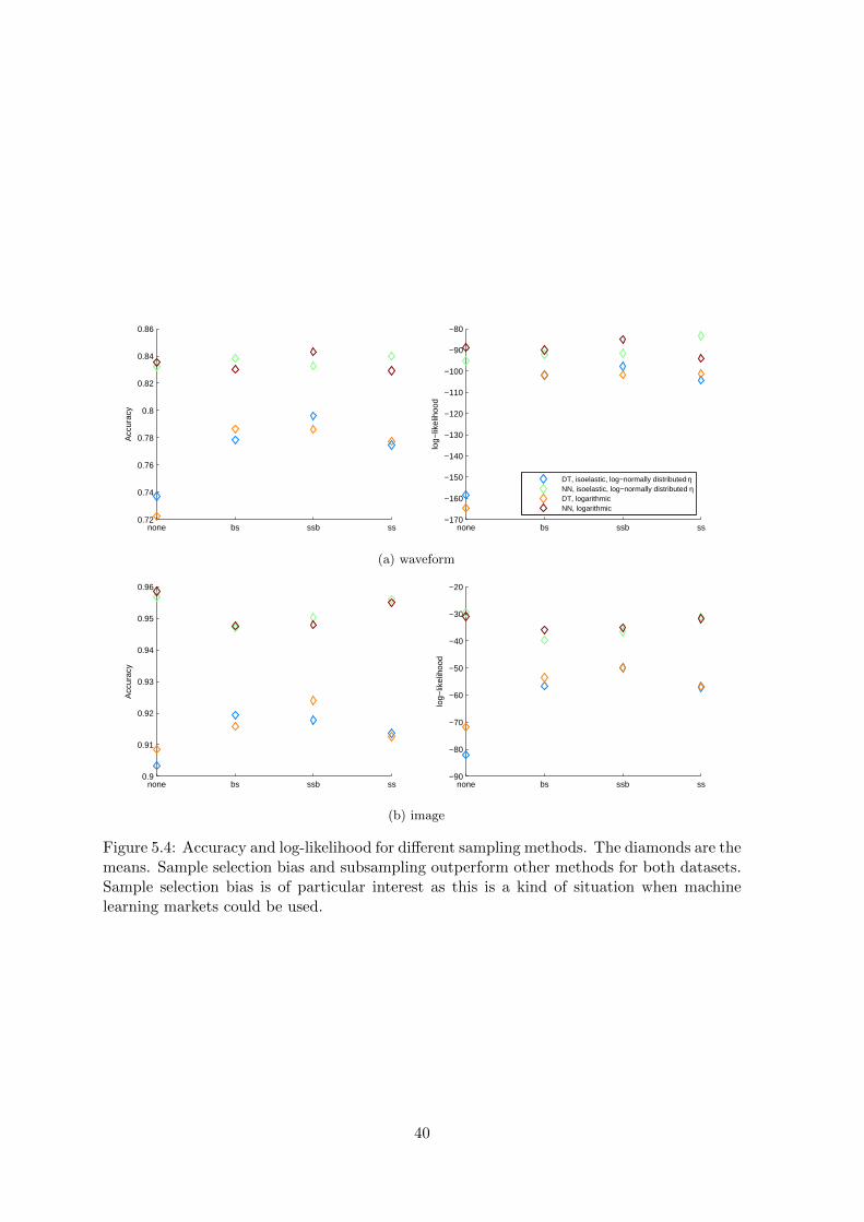
2. Comparison of sampling methods (Figure 5.4).

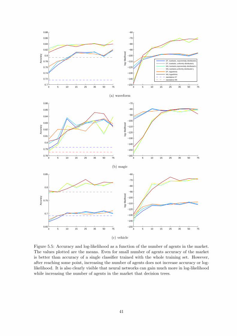
3. Comparison of markets with different number of agents (Figure 5.5).

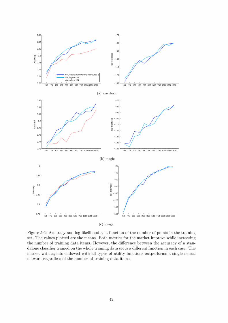
4. Comparison of markets trained using diffent number of data items (Figure 5.6). Forthis experiment only the number of training items was a variable and the number ofvalidation data items was set to 200.

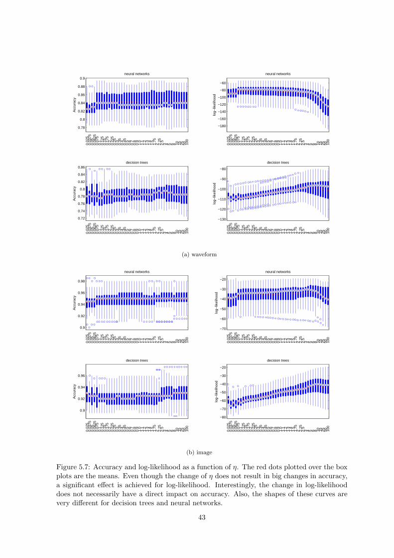
5. Comparison of homogeneous markets of isoelastic agents with different η (Figure 5.7).

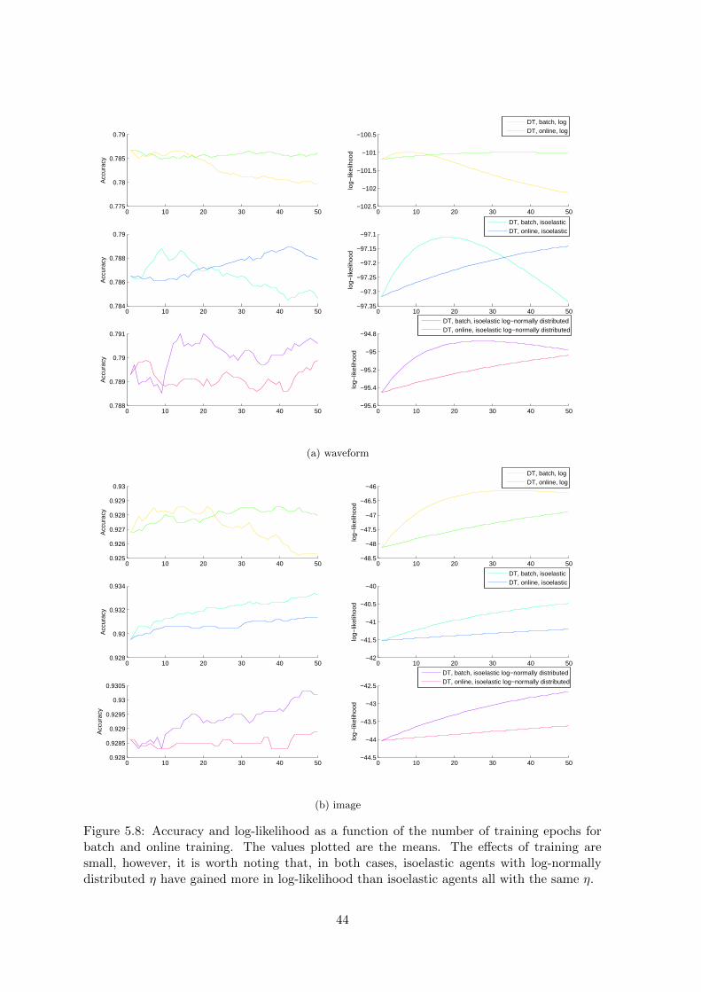
6. Comparison of market training techniques (Figure 5.8). The number of repetitions wasset to 50 for this experiment.

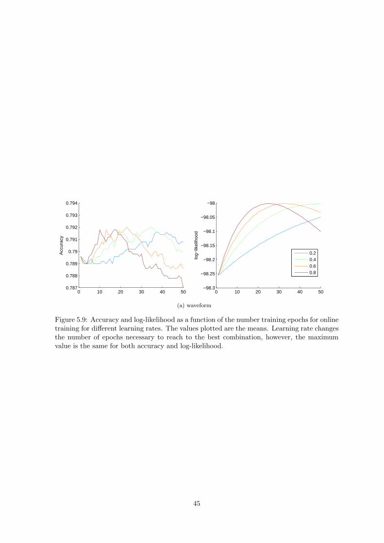
7. Comparison of learning rates for online training (Figure 5.9).

Some additional figures that did not fit in the main part of the thesis, extending thosementioned above, are contained in appendix E.

The seed for random numbers generator was set in such a way that data was split thesame way for every set of parameters in a given iteration.

Two ways of visualising the data was used. Box plot and plotting just the mean. Inthe box plot, the central mark is the median, the edges of the box are the 25th and 75thpercentiles, the whiskers extend to the most extreme data points not considered outliers, andoutliers are plotted individually.

38

0.74

0.76

0.78

0.8

0.82

0.84

0.86

0.88

0.9

DT LR NB NN SVM

Acc

urac

y

−180

−160

−140

−120

−100

−80

−60

DT LR NB NN SVM

log−

likel

ihoo

d

(a) waveform

0.7

0.75

0.8

0.85

0.9

DT LR NB NN SVM

Acc

urac

y

−240

−220

−200

−180

−160

−140

−120

−100

−80

−60

DT LR NB NN SVM

log−

likel

ihoo

d

(b) magic

0.4

0.45

0.5

0.55

0.6

0.65

0.7

0.75

0.8

0.85

DT LR NB NN SVM

Acc

urac

y

−350

−300

−250

−200

−150

−100

−50

DT LR NB NN SVM

log−

likel

ihoo

d

(c) vehicle

Figure 5.3: Accuracy and log-likelihood for markets consisting of agents endowed with dif-ferent classifiers. The red diamonds plotted over box plots are the means of results of themarkets and cyan diamonds are means of the results of standalone classifiers trained on wholedata sets. Individual decision trees and neural networks vary much more for data sampledusing sample selection bias, which results in greater improvement in accuracy.

39

none bs ssb ss0.72

0.74

0.76

0.78

0.8

0.82

0.84

0.86

Acc

urac

y

none bs ssb ss−170

−160

−150

−140

−130

−120

−110

−100

−90

−80

log−

likel

ihoo

d

DT, isoelastic, log−normally distributed ηNN, isoelastic, log−normally distributed ηDT, logarithmicNN, logarithmic

(a) waveform

none bs ssb ss0.9

0.91

0.92

0.93

0.94

0.95

0.96

Acc

urac

y

none bs ssb ss−90

−80

−70

−60

−50

−40

−30

−20

log−

likel

ihoo

d

(b) image

Figure 5.4: Accuracy and log-likelihood for different sampling methods. The diamonds are themeans. Sample selection bias and subsampling outperform other methods for both datasets.Sample selection bias is of particular interest as this is a kind of situation when machinelearning markets could be used.

40

3 5 10 15 25 35 50 75−150

−140

−130

−120

−110

−100

−90

−80

−70

−60

log−

likel

ihoo

d

3 5 10 15 25 35 50 750.7

0.72

0.74

0.76

0.78

0.8

0.82

0.84

0.86

0.88

Acc

urac

y

DT, isoelastic, exponentialy distributed ηDT, isoelastic, uniformly distributed ηNN, isoelastic,exponentialy distributed ηNN, isoelastic,uniformly distributed ηDT, logarithmic

NN, logarithmic

standalone DT

standalone NN

(a) waveform

3 5 10 15 25 35 50 75−160

−150

−140

−130

−120

−110

−100

−90

−80

−70

log−

likel

ihoo

d

3 5 10 15 25 35 50 750.78

0.79

0.8

0.81

0.82

0.83

0.84

0.85

0.86

Acc

urac

y

(b) magic

3 5 10 15 25 35 50 75−150

−140

−130

−120

−110

−100

−90

−80

−70

−60

log−

likel

ihoo

d

3 5 10 15 25 35 50 750.65

0.7

0.75

0.8

0.85

Acc

urac

y

(c) vehicle

Figure 5.5: Accuracy and log-likelihood as a function of the number of agents in the market.The values plotted are the means. Even for small number of agents accuracy of the marketis better than accuracy of a single classifier trained with the whole training set. However,after reaching some point, increasing the number of agents does not increase accuracy or log-likelihood. It is also clearly visible that neural networks can gain much more in log-likelihoodwhile increasing the number of agents in the market that decision trees.

41

50 75 100 150 250 350 500 750 1000125015000.72

0.74

0.76

0.78

0.8

0.82

0.84

0.86A

ccur

acy

NN, isoelastic,uniformly distributed ηNN, logarithmicstandalone NN

50 75 100 150 250 350 500 750 100012501500−130

−120

−110

−100

−90

−80

−70

log−

likel

ihoo

d

(a) waveform

50 75 100 150 250 350 500 750 1000125015000.72

0.74

0.76

0.78

0.8

0.82

0.84

0.86

Acc

urac

y

50 75 100 150 250 350 500 750 100012501500−150

−140

−130

−120

−110

−100

−90

−80

−70

log−

likel

ihoo

d

(b) magic

50 75 100 150 250 350 500 750 1000125015000.75

0.8

0.85

0.9

0.95

1

Acc

urac

y

50 75 100 150 250 350 500 750 100012501500−160

−140

−120

−100

−80

−60

−40

−20

log−

likel

ihoo

d

(c) image

Figure 5.6: Accuracy and log-likelihood as a function of the number of points in the trainingset. The values plotted are the means. Both metrics for the market improve while increasingthe number of training data items. However, the difference between the accuracy of a stan-dalone classifier trained on the whole training data set is a different function in each case. Themarket with agents endowed with all types of utility functions outperforms a single neuralnetwork regardless of the number of training data items.

42

0.78

0.8

0.82

0.84

0.86

0.88

0.9

0.02

50.

0375

0.05

0.06

250.

075

0.1

0.12

50.

150.

175

0.2

0.22

50.

250.

30.

350.

40.

450.

50.

60.

70.

80.

91.

01.

11.

21.

31.

41.

51.

752 2.

252.

53 4 5 6 8 10 15 25 50 10

0

Acc

urac

yneural networks

−180

−160

−140

−120

−100

−80

−60

0.02

50.

0375

0.05

0.06

250.

075

0.1

0.12

50.

150.

175

0.2

0.22

50.

250.

30.

350.

40.

450.

50.

60.

70.

80.

91.

01.

11.

21.

31.

41.

51.

752 2.

252.

53 4 5 6 8 10 15 25 50 10

0

log−

likel

ihoo

d

neural networks

0.72

0.74

0.76

0.78

0.8

0.82

0.84

0.86

0.02

50.

0375

0.05

0.06

250.

075

0.1

0.12

50.

150.

175

0.2

0.22

50.

250.

30.

350.

40.

450.

50.

60.

70.

80.

91.

01.

11.

21.

31.

41.

51.

752 2.

252.

53 4 5 6 8 10 15 25 50 10

0

Acc

urac

y

decision trees

−130

−120

−110

−100

−90

−80

0.02

50.

0375

0.05

0.06

250.

075

0.1

0.12

50.

150.

175

0.2

0.22

50.

250.

30.

350.

40.

450.

50.

60.

70.

80.

91.

01.

11.

21.

31.

41.

51.

752 2.

252.

53 4 5 6 8 10 15 25 50 10

0

log−

likel

ihoo

d

decision trees

(a) waveform

0.9

0.92

0.94

0.96

0.98

0.02

50.

0375

0.05

0.06

250.

075

0.1

0.12

50.

150.

175

0.2

0.22

50.

250.

30.

350.

40.

450.

50.

60.

70.

80.

91.

01.

11.

21.

31.

41.

51.

752 2.

252.

53 4 5 6 8 10 15 25 50 10

0

Acc

urac

y

neural networks

−70

−60

−50

−40

−30

−20

0.02

50.

0375

0.05

0.06

250.

075

0.1

0.12

50.

150.

175

0.2

0.22

50.

250.

30.

350.

40.

450.

50.

60.

70.

80.

91.

01.

11.

21.

31.

41.

51.

752 2.

252.

53 4 5 6 8 10 15 25 50 10

0

log−

likel

ihoo

d

neural networks

0.9

0.92

0.94

0.96

0.02

50.

0375

0.05

0.06

250.

075

0.1

0.12

50.

150.

175

0.2

0.22

50.

250.

30.

350.

40.

450.

50.

60.

70.

80.

91.

01.

11.

21.

31.

41.

51.

752 2.

252.

53 4 5 6 8 10 15 25 50 10

0

Acc

urac

y

decision trees

−80

−70

−60

−50

−40

−30

−20

0.02

50.

0375

0.05

0.06

250.

075

0.1

0.12

50.

150.

175

0.2

0.22

50.

250.

30.

350.

40.

450.

50.

60.

70.

80.

91.

01.

11.

21.

31.

41.

51.

752 2.

252.

53 4 5 6 8 10 15 25 50 10

0

log−

likel

ihoo

d

decision trees

(b) image

Figure 5.7: Accuracy and log-likelihood as a function of η. The red dots plotted over the boxplots are the means. Even though the change of η does not result in big changes in accuracy,a significant effect is achieved for log-likelihood. Interestingly, the change in log-likelihooddoes not necessarily have a direct impact on accuracy. Also, the shapes of these curves arevery different for decision trees and neural networks.

43

0 10 20 30 40 500.775

0.78

0.785

0.79

Acc

urac

y

0 10 20 30 40 50−102.5

−102

−101.5

−101

−100.5

log−

likel

ihoo

d

DT, batch, logDT, online, log

0 10 20 30 40 500.784

0.786

0.788

0.79

Acc

urac

y

0 10 20 30 40 50−97.35

−97.3

−97.25

−97.2

−97.15

−97.1

log−

likel

ihoo

d

DT, batch, isoelasticDT, online, isoelastic

0 10 20 30 40 500.788

0.789

0.79

0.791

Acc

urac

y

0 10 20 30 40 50−95.6

−95.4

−95.2

−95

−94.8

log−

likel

ihoo

d

DT, batch, isoelastic log−normally distributedDT, online, isoelastic log−normally distributed

(a) waveform

0 10 20 30 40 500.925

0.926

0.927

0.928

0.929

0.93

Acc

urac

y

0 10 20 30 40 50−48.5

−48

−47.5

−47

−46.5

−46

log−

likel

ihoo

d

DT, batch, logDT, online, log

0 10 20 30 40 500.928

0.93

0.932

0.934

Acc

urac

y

0 10 20 30 40 50−42

−41.5

−41

−40.5

−40

log−

likel

ihoo

d

DT, batch, isoelasticDT, online, isoelastic

0 10 20 30 40 500.928

0.9285

0.929

0.9295

0.93

0.9305

Acc

urac

y

0 10 20 30 40 50−44.5

−44

−43.5

−43

−42.5

log−

likel

ihoo

d

DT, batch, isoelastic log−normally distributedDT, online, isoelastic log−normally distributed

(b) image

Figure 5.8: Accuracy and log-likelihood as a function of the number of training epochs forbatch and online training. The values plotted are the means. The effects of training aresmall, however, it is worth noting that, in both cases, isoelastic agents with log-normallydistributed η have gained more in log-likelihood than isoelastic agents all with the same η.

44

0 10 20 30 40 500.787

0.788

0.789

0.79

0.791

0.792

0.793

0.794

Acc

urac

y

0 10 20 30 40 50−98.3

−98.25

−98.2

−98.15

−98.1

−98.05

−98

log−

likel

ihoo

d

0.20.40.60.8

(a) waveform

Figure 5.9: Accuracy and log-likelihood as a function of the number training epochs for onlinetraining for different learning rates. The values plotted are the means. Learning rate changesthe number of epochs necessary to reach to the best combination, however, the maximumvalue is the same for both accuracy and log-likelihood.

45

Chapter 6

Summary

A market of agents endowed with classifiers trained on data sampled with sample selectionbias outperforms a single classifier presented with equivalent data. A market consisting oflogarithmic agents is equivalent to a mixture model and a market consisting of exponentialagents is equivalent to a product model. Logarithmic agents can be extended by isoelasticagents. Even though the effects of introducing isoelastic agents are not as dramatic as Iinitially anticipated, there are a couple of important conclusions to make:

• Homogeneous markets of isoelastic agents with η picked using validation data outper-form, especially with respect to log-likelihood, homogeneous markets of logarithmicagents.

• The structure of the market, that is, utility functions and base classifiers agents areendowed with, is much more important parameter of the system influencing accuracyand log-likelihood than the market training procedure. However, when the structure isalready decided, the training procedure may lead to significant improvements in bothmetrics.

Some future research directions in this area may be:

• Using specialized agents that participate in the market only on subspaces of the featurespace like done in [LayBar10]. Such agents could be created for example by clusteringthe feature space and training each agent on the data from one cluster.

• Introducing new agents to the market in the process of training. New agents coming tothe market could be trained only on the instances that are harder or harder instancescould get a higher weight. That would be in the spirit of boosting.

• Adopting this approach to regression. This is especially promising as the marketsexhibit much better behaviour with respect to log-likelihood, which is a continuousquantity, than with respect to accuracy which is discretized.

• Better, more computationally efficient, ways of looking for market equilibrium. Currentmethod does not scale well for problems that have a large number of possible class labels.For batch update the training procedure can also be speeded up by being executed inparallel for individual data items.

• Studying effect of additional inhomogeneity by introducing agents that do not all havethe same base classifier.

47

• Introducing tax on winnings and salary so that no agent goes bankrupt. That wouldresult in a similar effect to a technique known as regularisation.

• Developing better understanding of how updates for isoelastic agents can be interpretedand how they can be related to other methods.

48

Appendix A

Derivations of buying functionsfrom utility functions

In general, the function to be optimised is (4.9) and the constraint that is to be satisfied issTi c = 0. Therefore, Lagrange multiplier λ is introduced and the function to be optimised isnow

UEi (Wi, c, si) =

NG∑k=1

Pi(k)U(Wi − sTi c + sik) + λsTi c (A.1)

Using sTi c = 0 constraint we get:

UEi (Wi, c, si) =

NG∑k=1

Pi(k)U(Wi + sik) + λsTi c (A.2)

Then differentiating with respect to siq (treating all other elements of the vector si as con-stants) and equating the derivative to 0 gives:

0 = Pi(q)U′(Wi + sik) + λcq (A.3)

And finally:

siq = −Wi + (U ′)−1(−λcqPi(q)

)(A.4)

Usually, however, it is easier to start from equation (A.3). It is also very handy to manipulateλ as it remains a constant anyway.

A.1. Exponential utility

Equation (A.3) takes the form:

∂UEi∂siq

= −Pi(q)e(−Wi−siq) + λcq (A.5)

0 = −Pi(q)e(−Wi−siq) + λcq

0 = −Pi(q)e−siq + λ′cq

logPi(q)− siq = log λ′ + log cq

siq = logPi(q)− log λ′ − log cq

49

Then using the constraint s∗iNG = 0 gives:

0 = logPi(NG)− log λ′ − log cNG

log λ′ = logPi(NG)

cNG

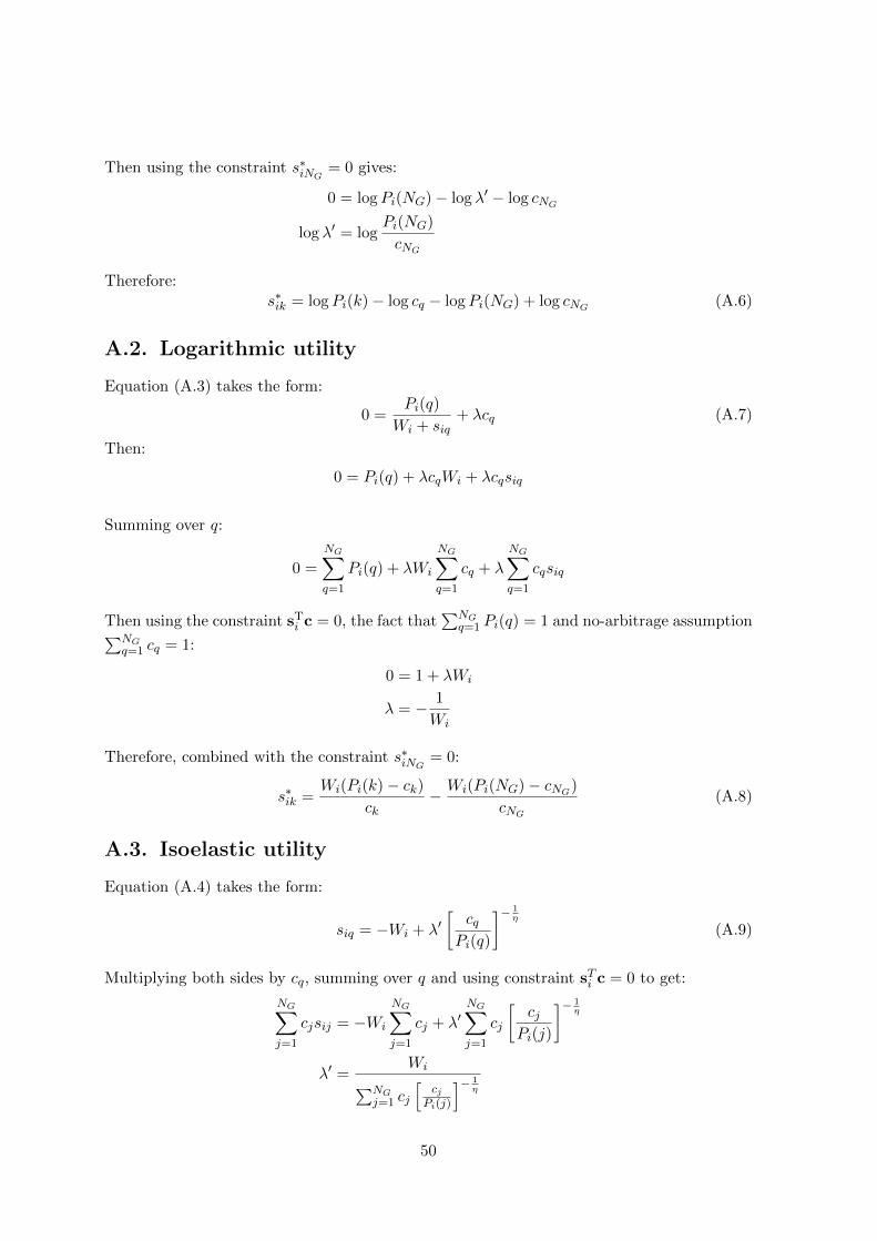
Therefore:s∗ik = logPi(k)− log cq − logPi(NG) + log cNG (A.6)

A.2. Logarithmic utility


0 =Pi(q)

Wi + siq+ λcq (A.7)

Then:

0 = Pi(q) + λcqWi + λcqsiq

Summing over q:

0 =

NG∑q=1

Pi(q) + λWi

NG∑q=1

cq + λ

NG∑q=1

cqsiq

Then using the constraint sTi c = 0, the fact that∑NG

q=1 Pi(q) = 1 and no-arbitrage assumption∑NGq=1 cq = 1:

0 = 1 + λWi

λ = − 1

Wi

Therefore, combined with the constraint s∗iNG = 0:

s∗ik =Wi(Pi(k)− ck)

ck− Wi(Pi(NG)− cNG)

cNG(A.8)

A.3. Isoelastic utility


siq = −Wi + λ′[

cqPi(q)

]− 1η

(A.9)

Multiplying both sides by cq, summing over q and using constraint sTi c = 0 to get:

NG∑j=1

cjsij = −Wi

NG∑j=1

cj + λ′NG∑j=1

cj

[cj

Pi(j)

]− 1η

λ′ =Wi∑NG

j=1 cj

[cj

Pi(j)

]− 1η

50

Which, combined with the constraint s∗iNG = 0, gives the following:

s∗ik = Wi

[Pi(k)ck

] 1η

∑NGj=1 cj

[Pi(j)cj

] 1η

− 1

−Wi

[Pi(NG)cNG

] 1η

∑NGj=1 cj

[Pi(j)cj

] 1η

− 1

= Wi

[Pi(k)ck

] 1η −

[Pi(NG)cNG

] 1η

∑NGj=1 cj

[Pi(j)cj

] 1η

(A.10)

51

Appendix B

Derivatives of buying functions

B.1. Exponential utility

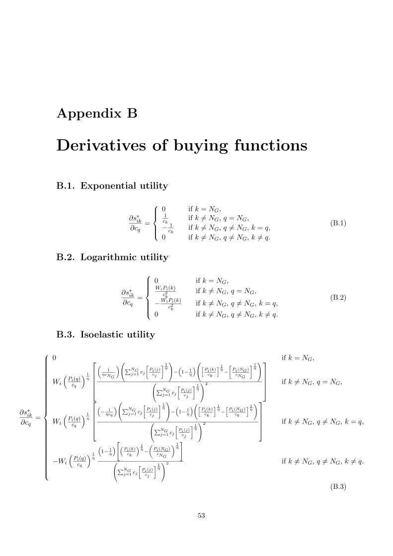
∂s∗ik∂cq

=

0 if k = NG,1ck

if k 6= NG, q = NG,

− 1ck

if k 6= NG, q 6= NG, k = q,

0 if k 6= NG, q 6= NG, k 6= q.

(B.1)

B.2. Logarithmic utility

∂s∗ik∂cq

=

0 if k = NG,WiPi(k)

c2kif k 6= NG, q = NG,

−WiPi(k)c2k

if k 6= NG, q 6= NG, k = q,

0 if k 6= NG, q 6= NG, k 6= q.

(B.2)

B.3. Isoelastic utility

∂s∗ik∂cq

=

0 if k = NG,

Wi

(Pi(q)cq

) 1η

(

1ηcNG

)∑NGj=1 cj

[Pi(j)

cj

] 1η

−(1− 1η

)[Pi(k)ck

] 1η−[Pi(NG)

cNG

] 1η

∑NG

j=1 cj

[Pi(j)

cj

] 1η

2

if k 6= NG, q = NG,

Wi

(Pi(q)cq

) 1η

(− 1ηcq

)∑NGj=1 cj

[Pi(j)

cj

] 1η

−(1− 1η

)([Pi(k)

ck

] 1η−[Pi(NG)

cq

] 1η

)∑NG

j=1 cj

[Pi(j)

cj

] 1η

2

if k 6= NG, q 6= NG, k = q,

−Wi

(Pi(q)cq

) 1η

(1− 1

η

)(Pi(k)ck

) 1η−(Pi(NG)

cNG

) 1η

∑NG

j=1 cj

[Pi(j)

cj

] 1η

2 if k 6= NG, q 6= NG, k 6= q.

(B.3)

53

Appendix C

Derivations of equilibrium prices

C.1. Exponential utility

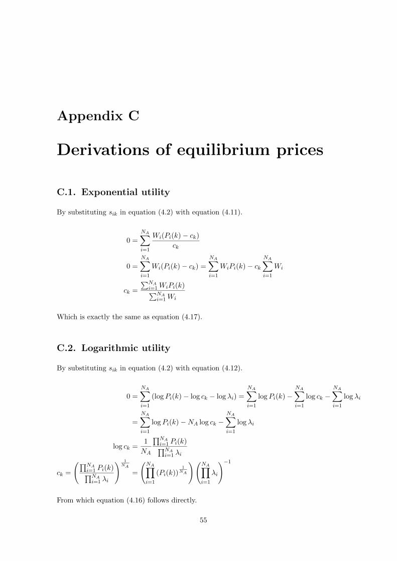
By substituting sik in equation (4.2) with equation (4.11).

0 =

NA∑i=1

Wi(Pi(k)− ck)ck

0 =

NA∑i=1

Wi(Pi(k)− ck) =

NA∑i=1

WiPi(k)− ckNA∑i=1

Wi

ck =

∑NAi=1WiPi(k)∑NA

i=1Wi

Which is exactly the same as equation (4.17).

C.2. Logarithmic utility


0 =

NA∑i=1

(logPi(k)− log ck − log λi) =

NA∑i=1

logPi(k)−NA∑i=1

log ck −NA∑i=1

log λi

=

NA∑i=1

logPi(k)−NA log ck −NA∑i=1

log λi

log ck =1

NA

∏NAi=1 Pi(k)∏NAi=1 λi

ck =

(∏NAi=1 Pi(k)∏NAi=1 λi

) 1NA

=

(NA∏i=1

(Pi(k))1NA

)(NA∏i=1

λi

)−1

From which equation (4.16) follows directly.

55

C.3. Isoelastic utility


0 =

NA∑i=1

Wi

[Pi(k)ck

] 1η

∑j cj

[Pi(j)cj

] 1η

− 1

=

NA∑i=1

Wi

[Pi(k)ck

] 1η

∑j cj

[Pi(j)cj

] 1η

− NA∑i=1

Wi

NA∑i=1

Wi =

NA∑i=1

Wi

[Pi(k)ck

] 1η

∑j cj

[Pi(j)cj

] 1η

ck =

∑NAi=1Wi

ck

[Pi(k)

ck

] 1η

∑j cj

[Pi(j)

cj

] 1η

∑NA

i=1Wi

From which equation (4.18) follows directly. When η = 1, it is equivalent to equation (4.16),as it should be.

56

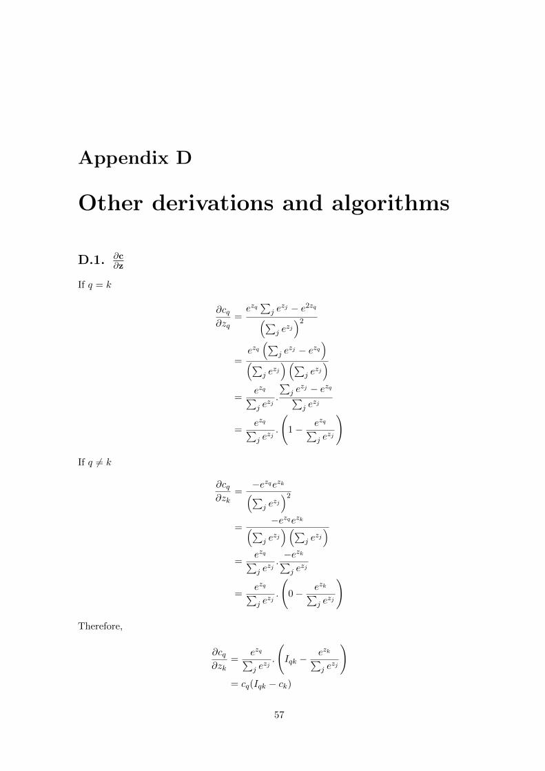
Appendix D

Other derivations and algorithms

D.1. ∂c∂z

If q = k

∂cq∂zq

=ezq∑

j ezj − e2zq(∑

j ezj)2

=ezq(∑

j ezj − ezq

)(∑

j ezj)(∑

j ezj)

=ezq∑j e

zj.

∑j e

zj − ezq∑j e

zj

=ezq∑j e

zj.

(1− ezq∑

j ezj

)

If q 6= k

∂cq∂zk

=−ezqezk(∑

j ezj)2

=−ezqezk(∑

j ezj)(∑

j ezj)

=ezq∑j e

zj.−ezk∑j e

zj

=ezq∑j e

zj.

(0− ezk∑

j ezj

)

Therefore,

∂cq∂zk

=ezq∑j e

zj.

(Iqk −

ezk∑j e

zj

)= cq(Iqk − ck)

57

D.2. Generating random bistochastic matrices

Theoretical justification of correctness of this algorithm known in the literature can be foundin [CapSomBruZyc09].

Algorithm 5 Generating random bistochastic matrices

Input: K,NM ← K-by-N matrix of random numbers between 0 and 1D ← vector of length K filled with oneswhile max(D) > ε do

for k = 1 . . .K doM(k, :)←M(k, :)/sum(M(k, :))

end forfor n = 1 . . . N doM(:, n)←M(:, n)/(sum(M(:, n)) ∗ (N/K))

end forfor k = 1 . . .K doD(k) = |sum(M(k, :))− 1|

end forend whileOutput: M

D.3. limη→1

Uiso(x) = Ulog(x)

Using L’Hopital’s rule:

limη→1

x1−η − 1

1− η=

limη→1

ddη

(x1−η − 1

)ddη (1− η)

=

limη→1

ddη

(eloge x

1−η)

−1=

limη→1

ddη

(e(1−η) loge x

)−1

=

limη→1

−e(1−η) loge x loge x

−1=

limη→1

e(1−η) loge x loge x =

loge x

D.4. Arrow-Pratt measure of absolute risk-aversion

Beginning with equating expected utility to initial utility:

U(W ) =

∫ ∞−∞

U(W − p+ x)f(x)dx.

58

Then using Taylor expansion, approximately:

U(W ) =

∫ ∞−∞

[U(W ) + U ′(W )(x− p) + U ′′(W )

(x− p)2

2

]f(x)dx

U(W ) = U(W ) + U ′(W )

∫ ∞−∞

(x− p)f(x)dx+ U ′′(W )

∫ ∞−∞

(x− p)2

2f(x)dx

0 = U ′(W )

∫ ∞−∞

(x− p)f(x)dx+ U ′′(W )

∫ ∞−∞

(x− p)2

2f(x)dx

p =

∫ ∞−∞

xf(x)dx+U ′′(W )

U ′(W )

∫ ∞−∞

(x− p)2

2f(x)dx

D.5. Buying function for isoelastic utility when η → 0

s∗ik =Wi

[Pi(k)ck

] 1η −

[1−Pi(k)1−ck

] 1η

ck

[Pi(k)ck

] 1η

+ (1− ck)[1−Pi(k)1−ck

] 1η

=Wi

[Pi(k)ck

] 1η

ck

[Pi(k)ck

] 1η

+ (1− ck)[1−Pi(k)1−ck

] 1η

−

[1−Pi(k)1−ck

] 1η

ck

[Pi(k)ck

] 1η

+ (1− ck)[1−Pi(k)1−ck

] 1η

=Wi

1

ck + (1− ck)[

ckPi(k)

1−Pi(k)1−ck

] 1η

− 1

ck

[1

ckPi(k)

1−Pi(k)1−ck

] 1η

+ (1− ck)

Then from the fact that:

limη→0

[ck

Pi(k)

1− Pi(k)

1− ck

] 1η

=

0 if Pi(k) > ck,∞ if Pi(k) < ck,1 if Pi(k) = ck.

It follows that:

limη→0

s∗ik =

Wick

if Pi(k) > ck,

0 if Pi(k) = ck,

− Wi1−ck if Pi(k) < ck.

59

Appendix E

Additional figures

Some figures that did not fit in the main part of the thesis are:

• Figure E.1 extends Figure 5.8.





61

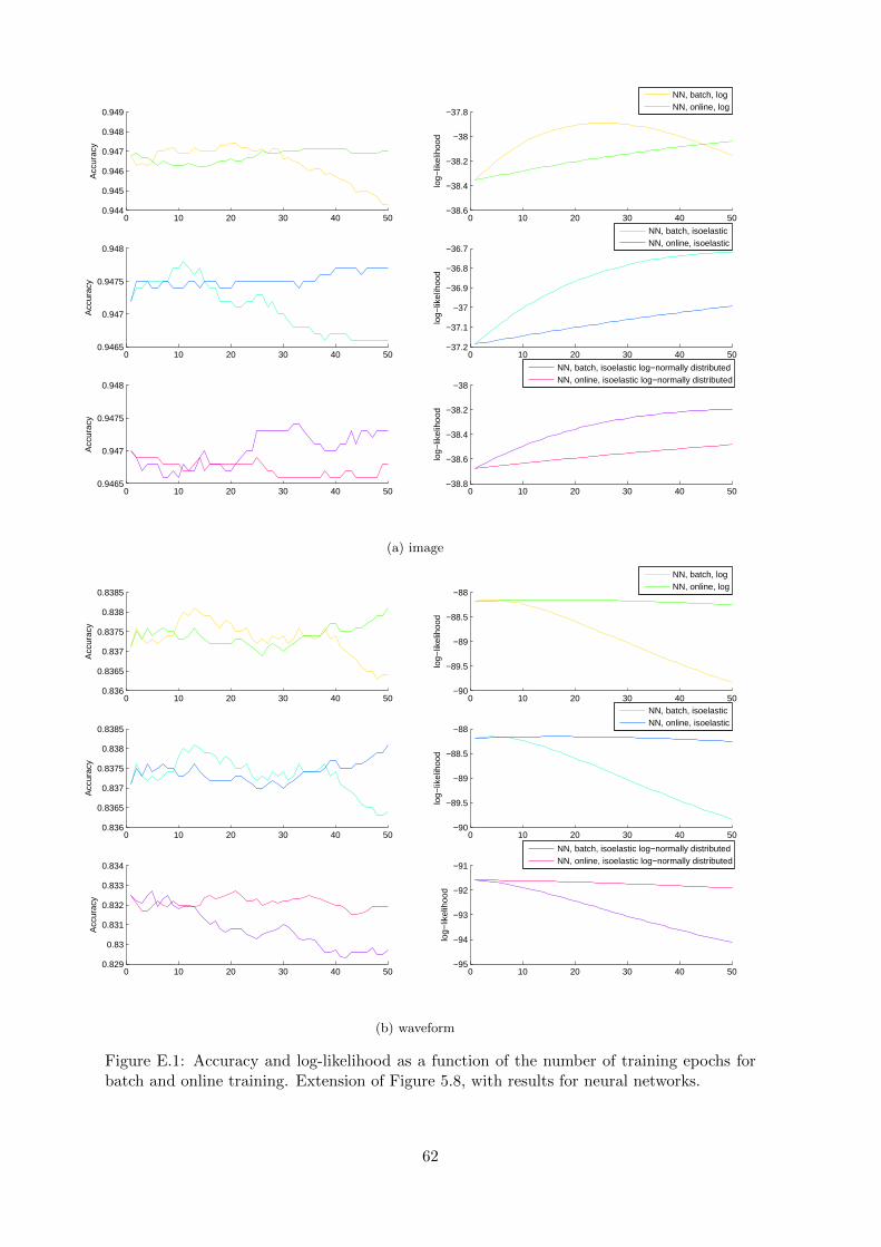
0 10 20 30 40 500.944

0.945

0.946

0.947

0.948

0.949

Acc

urac

y

0 10 20 30 40 50−38.6

−38.4

−38.2

−38

−37.8

log−

likel

ihoo

d

NN, batch, logNN, online, log

0 10 20 30 40 500.9465

0.947

0.9475

0.948

Acc

urac

y

0 10 20 30 40 50−37.2

−37.1

−37

−36.9

−36.8

−36.7

log−

likel

ihoo

d

NN, batch, isoelasticNN, online, isoelastic

0 10 20 30 40 500.9465

0.947

0.9475

0.948

Acc

urac

y

0 10 20 30 40 50−38.8

−38.6

−38.4

−38.2

−38

log−

likel

ihoo

d

NN, batch, isoelastic log−normally distributedNN, online, isoelastic log−normally distributed

(a) image

0 10 20 30 40 500.836

0.8365

0.837

0.8375

0.838

0.8385

Acc

urac

y

0 10 20 30 40 50−90

−89.5

−89

−88.5

−88

log−

likel

ihoo

d

NN, batch, logNN, online, log

0 10 20 30 40 500.836

0.8365

0.837

0.8375

0.838

0.8385

Acc

urac

y

0 10 20 30 40 50−90

−89.5

−89

−88.5

−88

log−

likel

ihoo

d

NN, batch, isoelasticNN, online, isoelastic

0 10 20 30 40 500.829

0.83

0.831

0.832

0.833

0.834

Acc

urac

y

0 10 20 30 40 50−95

−94

−93

−92

−91

log−

likel

ihoo

d

NN, batch, isoelastic log−normally distributedNN, online, isoelastic log−normally distributed

(b) waveform

Figure E.1: Accuracy and log-likelihood as a function of the number of training epochs forbatch and online training. Extension of Figure 5.8, with results for neural networks.

62

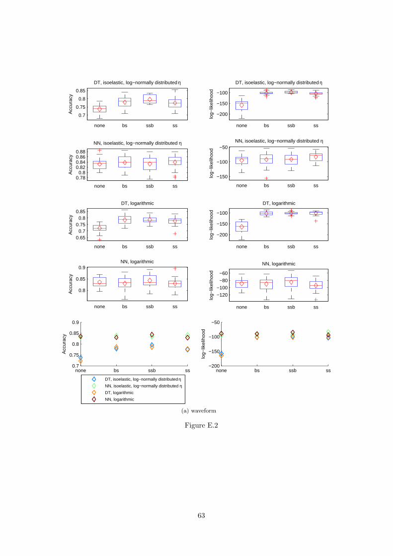
0.7

0.75

0.8

0.85

none bs ssb ss

Acc

urac

y

DT, isoelastic, log−normally distributed η

−200

−150

−100

none bs ssb ss

log−

likel

ihoo

d


0.780.8

0.820.840.860.88

none bs ssb ss

Acc

urac

y

NN, isoelastic, log−normally distributed η

−150

−100

−50

none bs ssb ss

log−

likel

ihoo

d


0.650.7

0.750.8

0.85

none bs ssb ss

Acc

urac

y

DT, logarithmic

−200

−150

−100

none bs ssb ss

log−

likel

ihoo

d

DT, logarithmic

0.8

0.85

0.9

none bs ssb ss

Acc

urac

y

NN, logarithmic

−120

−100

−80

−60

none bs ssb ss

log−

likel

ihoo

d

NN, logarithmic

none bs ssb ss0.7

0.75

0.8

0.85

0.9

Acc

urac

y

DT, isoelastic, log−normally distributed ηNN, isoelastic, log−normally distributed ηDT, logarithmic

NN, logarithmic


−150

−100

−50

log−

likel

ihoo

d

(a) waveform

Figure E.2

63

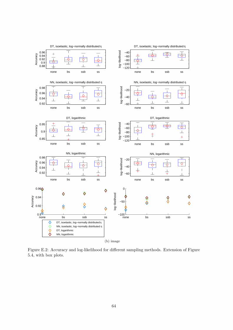
0.880.9

0.920.940.96

none bs ssb ss

Acc

urac

y


−120−100

−80−60−40

none bs ssb ss

log−

likel

ihoo

d


0.92

0.94

0.96

0.98

none bs ssb ss

Acc

urac

y


−60

−40

−20

none bs ssb ss

log−

likel

ihoo

d


0.85

0.9

0.95

none bs ssb ss

Acc

urac

y

DT, logarithmic

−120

−100−80

−60

−40

none bs ssb ss

log−

likel

ihoo

dDT, logarithmic

0.92

0.94

0.96

0.98

none bs ssb ss

Acc

urac

y

NN, logarithmic

−60

−40

−20

none bs ssb ss

log−

likel

ihoo

d

NN, logarithmic

none bs ssb ss0.9

0.92

0.94

0.96

Acc

urac

y

DT, isoelastic, log−normally distributed ηNN, isoelastic, log−normally distributed ηDT, logarithmic

NN, logarithmic


−50

0

log−

likel

ihoo

d

(b) image

Figure E.2: Accuracy and log-likelihood for different sampling methods. Extension of Figure5.4, with box plots.

64

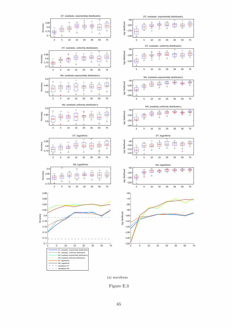
0.7

0.75

0.8

0.85

3 5 10 15 25 35 50 75A

ccur

acy

DT, isoelastic, exponentialy distributed η

−140

−120

−100

−80

3 5 10 15 25 35 50 75

log−

likel

ihoo

d


0.7

0.75

0.8

0.85

3 5 10 15 25 35 50 75

Acc

urac

y

DT, isoelastic, uniformly distributed η

−120

−100

−80

3 5 10 15 25 35 50 75

log−

likel

ihoo

d


0.8

0.85

0.9

3 5 10 15 25 35 50 75

Acc

urac

y

NN, isoelastic,exponentialy distributed η

−200

−150

−100

−50

3 5 10 15 25 35 50 75

log−

likel

ihoo

d


0.8

0.85

0.9

3 5 10 15 25 35 50 75

Acc

urac

y

NN, isoelastic,uniformly distributed η

−200

−150

−100

−50

3 5 10 15 25 35 50 75

log−

likel

ihoo

d


0.75

0.8

0.85

3 5 10 15 25 35 50 75

Acc

urac

y

DT, logarithmic

−120

−110

−100

−90

3 5 10 15 25 35 50 75

log−

likel

ihoo

d

DT, logarithmic

0.75

0.8

0.85

0.9

3 5 10 15 25 35 50 75

Acc

urac

y

NN, logarithmic

−200

−150

−100

−50

3 5 10 15 25 35 50 75

log−

likel

ihoo

d

NN, logarithmic

3 5 10 15 25 35 50 750.7

0.72

0.74

0.76

0.78

0.8

0.82

0.84

0.86

0.88

Acc

urac

y


NN, logarithmic

standalone DT

standalone NN

3 5 10 15 25 35 50 75−150

−140

−130

−120

−110

−100

−90

−80

−70

−60

log−

likel

ihoo

d

(a) waveform

Figure E.3

65

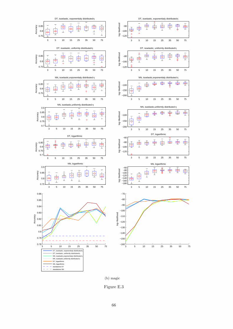
0.75

0.8

0.85

3 5 10 15 25 35 50 75

Acc

urac

y


−120

−100

−80

3 5 10 15 25 35 50 75

log−

likel

ihoo

d


0.75

0.8

0.85

3 5 10 15 25 35 50 75

Acc

urac

y


−120

−100

−80

3 5 10 15 25 35 50 75

log−

likel

ihoo

d


0.75

0.8

0.85

3 5 10 15 25 35 50 75

Acc

urac

y


−200

−150

−100

3 5 10 15 25 35 50 75

log−

likel

ihoo

d


0.7

0.75

0.8

0.85

0.9

3 5 10 15 25 35 50 75

Acc

urac

y


−200

−150

−100

3 5 10 15 25 35 50 75

log−

likel

ihoo

d


0.7

0.75

0.8

0.85

3 5 10 15 25 35 50 75

Acc

urac

y

DT, logarithmic

−120

−100

−80

−60

3 5 10 15 25 35 50 75

log−

likel

ihoo

d

DT, logarithmic

0.75

0.8

0.85

0.9

3 5 10 15 25 35 50 75

Acc

urac

y

NN, logarithmic

−180−160−140−120−100

−80−60

3 5 10 15 25 35 50 75

log−

likel

ihoo

d

NN, logarithmic

3 5 10 15 25 35 50 750.78

0.79

0.8

0.81

0.82

0.83

0.84

0.85

0.86

Acc

urac

y


NN, logarithmic

standalone DT

standalone NN

3 5 10 15 25 35 50 75−160

−150

−140

−130

−120

−110

−100

−90

−80

−70

log−

likel

ihoo

d

(b) magic

Figure E.3

66

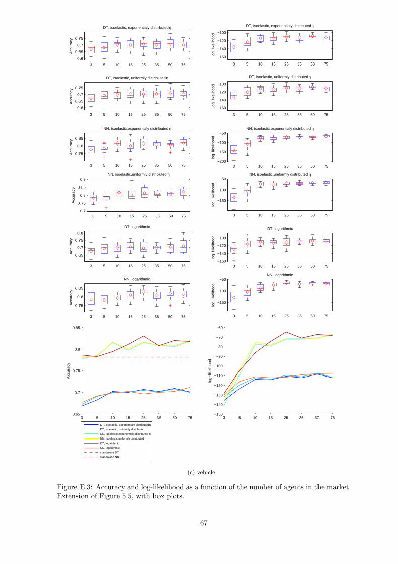
0.6

0.65

0.7

0.75

3 5 10 15 25 35 50 75

Acc

urac

y


−160

−140

−120

−100

3 5 10 15 25 35 50 75

log−

likel

ihoo

d


0.6

0.65

0.7

0.75

3 5 10 15 25 35 50 75

Acc

urac

y


−160

−140

−120

−100

3 5 10 15 25 35 50 75

log−

likel

ihoo

d


0.75

0.8

0.85

3 5 10 15 25 35 50 75

Acc

urac

y


−200

−150

−100

−50

3 5 10 15 25 35 50 75

log−

likel

ihoo

d


0.7

0.75

0.8

0.85

0.9

3 5 10 15 25 35 50 75

Acc

urac

y


−150

−100

−50

3 5 10 15 25 35 50 75lo

g−lik

elih

ood


0.65

0.7

0.75

0.8

3 5 10 15 25 35 50 75

Acc

urac

y

DT, logarithmic

−160

−140

−120

−100

3 5 10 15 25 35 50 75

log−

likel

ihoo

d

DT, logarithmic

0.75

0.8

0.85

3 5 10 15 25 35 50 75

Acc

urac

y

NN, logarithmic

−150

−100

−50

3 5 10 15 25 35 50 75

log−

likel

ihoo

d

NN, logarithmic

3 5 10 15 25 35 50 750.65

0.7

0.75

0.8

0.85

Acc

urac

y


NN, logarithmic

standalone DT

standalone NN

3 5 10 15 25 35 50 75−150

−140

−130

−120

−110

−100

−90

−80

−70

−60

log−

likel

ihoo

d

(c) vehicle

Figure E.3: Accuracy and log-likelihood as a function of the number of agents in the market.Extension of Figure 5.5, with box plots.

67

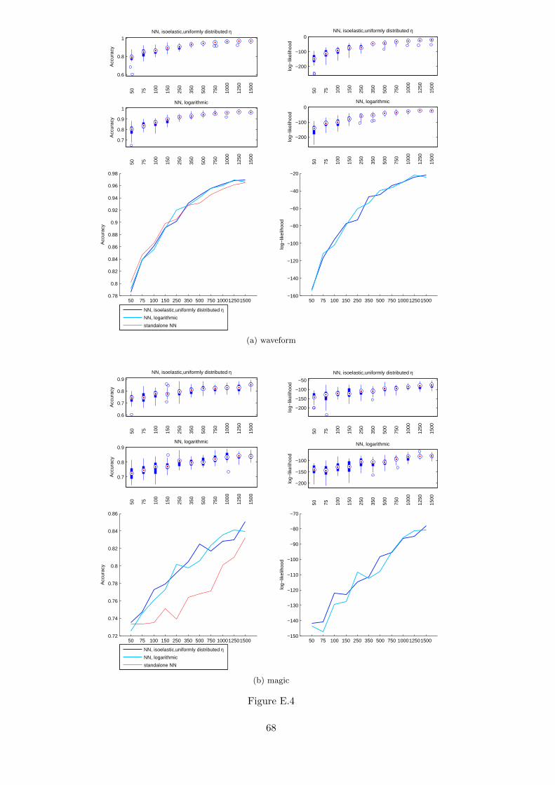
0.6

0.8

1

50 75 100

150

250

350

500

750

1000

1250

1500

Acc

urac

y


−200

−100

0

50 75 100

150

250

350

500

750

1000

1250

1500

log−

likel

ihoo

d


0.7

0.8

0.9

1

50 75 100

150

250

350

500

750

1000

1250

1500

Acc

urac

y

NN, logarithmic

−200

−100

0

50 75 100

150

250

350

500

750

1000

1250

1500

log−

likel

ihoo

d

NN, logarithmic

50 75 100 150 250 350 500 750 1000125015000.78

0.8

0.82

0.84

0.86

0.88

0.9

0.92

0.94

0.96

0.98

Acc

urac

y

NN, isoelastic,uniformly distributed ηNN, logarithmic

standalone NN

50 75 100 150 250 350 500 750 100012501500−160

−140

−120

−100

−80

−60

−40

−20

log−

likel

ihoo

d

(a) waveform

0.6

0.7

0.8

0.9

50 75 100

150

250

350

500

750

1000

1250

1500

Acc

urac

y


−200

−150

−100

−50

50 75 100

150

250

350

500

750

1000

1250

1500

log−

likel

ihoo

d


0.7

0.8

0.9

50 75 100

150

250

350

500

750

1000

1250

1500

Acc

urac

y

NN, logarithmic

−200

−150

−100

50 75 100

150

250

350

500

750

1000

1250

1500

log−

likel

ihoo

d

NN, logarithmic

50 75 100 150 250 350 500 750 1000125015000.72

0.74

0.76

0.78

0.8

0.82

0.84

0.86

Acc

urac

y


standalone NN

50 75 100 150 250 350 500 750 100012501500−150

−140

−130

−120

−110

−100

−90

−80

−70

log−

likel

ihoo

d

(b) magic

Figure E.4

68

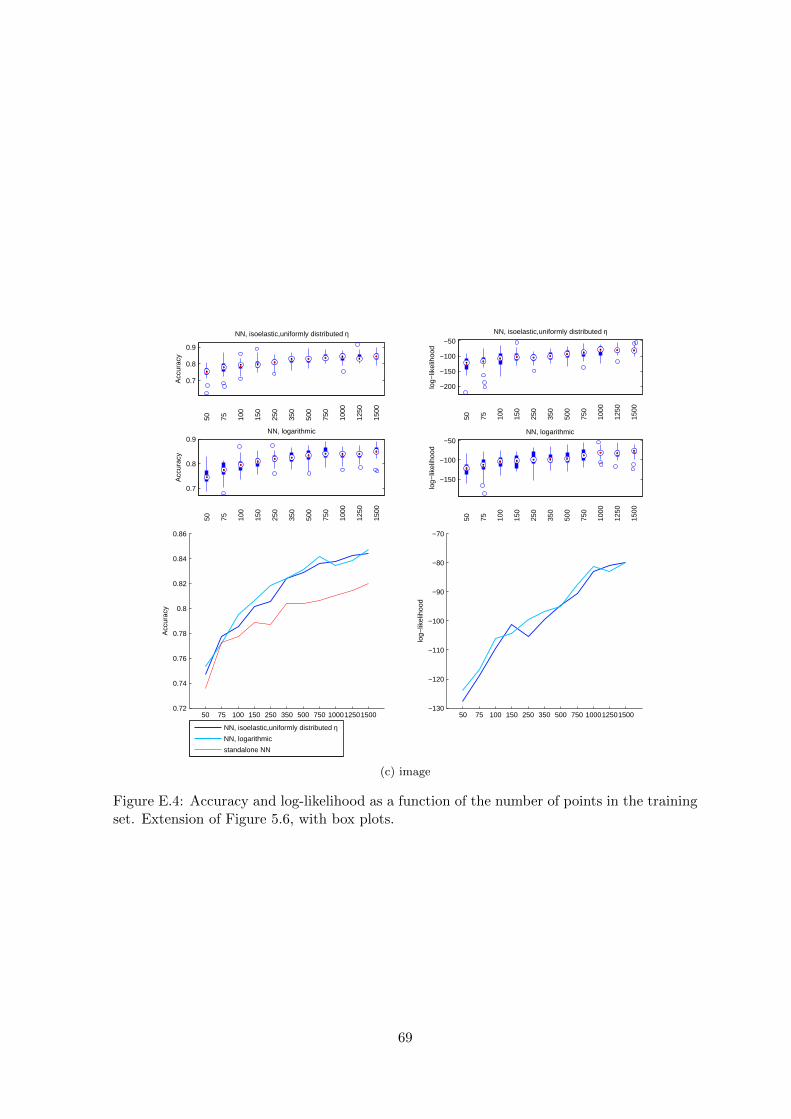
0.7

0.8

0.9

50 75 100

150

250

350

500

750

1000

1250

1500

Acc

urac

y


−200

−150

−100

−50

50 75 100

150

250

350

500

750

1000

1250

1500

log−

likel

ihoo

d


0.7

0.8

0.9

50 75 100

150

250

350

500

750

1000

1250

1500

Acc

urac

y

NN, logarithmic

−150

−100

−50

50 75 100

150

250

350

500

750

1000

1250

1500

log−

likel

ihoo

dNN, logarithmic

50 75 100 150 250 350 500 750 1000125015000.72

0.74

0.76

0.78

0.8

0.82

0.84

0.86

Acc

urac

y


standalone NN

50 75 100 150 250 350 500 750 100012501500−130

−120

−110

−100

−90

−80

−70

log−

likel

ihoo

d

(c) image

Figure E.4: Accuracy and log-likelihood as a function of the number of points in the trainingset. Extension of Figure 5.6, with box plots.

69

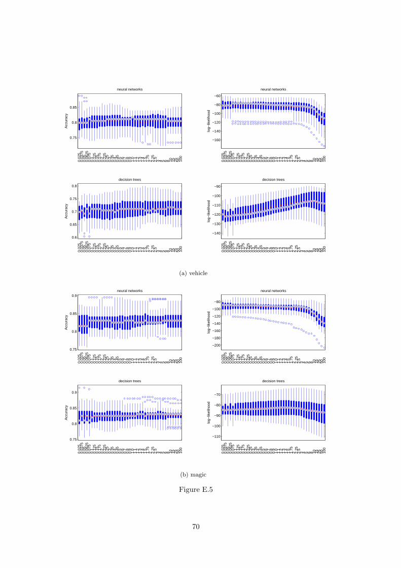
0.75

0.8

0.85

0.02

50.

0375

0.05

0.06

250.

075

0.1

0.12

50.

150.

175

0.2

0.22

50.

250.

30.

350.

40.

450.

50.

60.

70.

80.

91.

01.

11.

21.

31.

41.

51.

752 2.

252.

53 4 5 6 8 10 15 25 50 10

0

Acc

urac

y

neural networks

−160

−140

−120

−100

−80

−60

0.02

50.

0375

0.05

0.06

250.

075

0.1

0.12

50.

150.

175

0.2

0.22

50.

250.

30.

350.

40.

450.

50.

60.

70.

80.

91.

01.

11.

21.

31.

41.

51.

752 2.

252.

53 4 5 6 8 10 15 25 50 10

0

log−

likel

ihoo

d

neural networks

0.6

0.65

0.7

0.75

0.8

0.02

50.

0375

0.05

0.06

250.

075

0.1

0.12

50.

150.

175

0.2

0.22

50.

250.

30.

350.

40.

450.

50.

60.

70.

80.

91.

01.

11.

21.

31.

41.

51.

752 2.

252.

53 4 5 6 8 10 15 25 50 10

0

Acc

urac

y

decision trees

−140

−130

−120

−110

−100

−90

0.02

50.

0375

0.05

0.06

250.

075

0.1

0.12

50.

150.

175

0.2

0.22

50.

250.

30.

350.

40.

450.

50.

60.

70.

80.

91.

01.

11.

21.

31.

41.

51.

752 2.

252.

53 4 5 6 8 10 15 25 50 10

0

log−

likel

ihoo

d

decision trees

(a) vehicle

0.75

0.8

0.85

0.9

0.02

50.

0375

0.05

0.06

250.

075

0.1

0.12

50.

150.

175

0.2

0.22

50.

250.

30.

350.

40.

450.

50.

60.

70.

80.

91.

01.

11.

21.

31.

41.

51.

752 2.

252.

53 4 5 6 8 10 15 25 50 10

0

Acc

urac

y

neural networks

−200

−180

−160

−140

−120

−100

−80

0.02

50.

0375

0.05

0.06

250.

075

0.1

0.12

50.

150.

175

0.2

0.22

50.

250.

30.

350.

40.

450.

50.

60.

70.

80.

91.

01.

11.

21.

31.

41.

51.

752 2.

252.

53 4 5 6 8 10 15 25 50 10

0

log−

likel

ihoo

d

neural networks

0.75

0.8

0.85

0.9

0.02

50.

0375

0.05

0.06

250.

075

0.1

0.12

50.

150.

175

0.2

0.22

50.

250.

30.

350.

40.

450.

50.

60.

70.

80.

91.

01.

11.

21.

31.

41.

51.

752 2.

252.

53 4 5 6 8 10 15 25 50 10

0

Acc

urac

y

decision trees

−110

−100

−90

−80

−70

0.02

50.

0375

0.05

0.06

250.

075

0.1

0.12

50.

150.

175

0.2

0.22

50.

250.

30.

350.

40.

450.

50.

60.

70.

80.

91.

01.

11.

21.

31.

41.

51.

752 2.

252.

53 4 5 6 8 10 15 25 50 10

0

log−

likel

ihoo

d

decision trees

(b) magic

Figure E.5

70

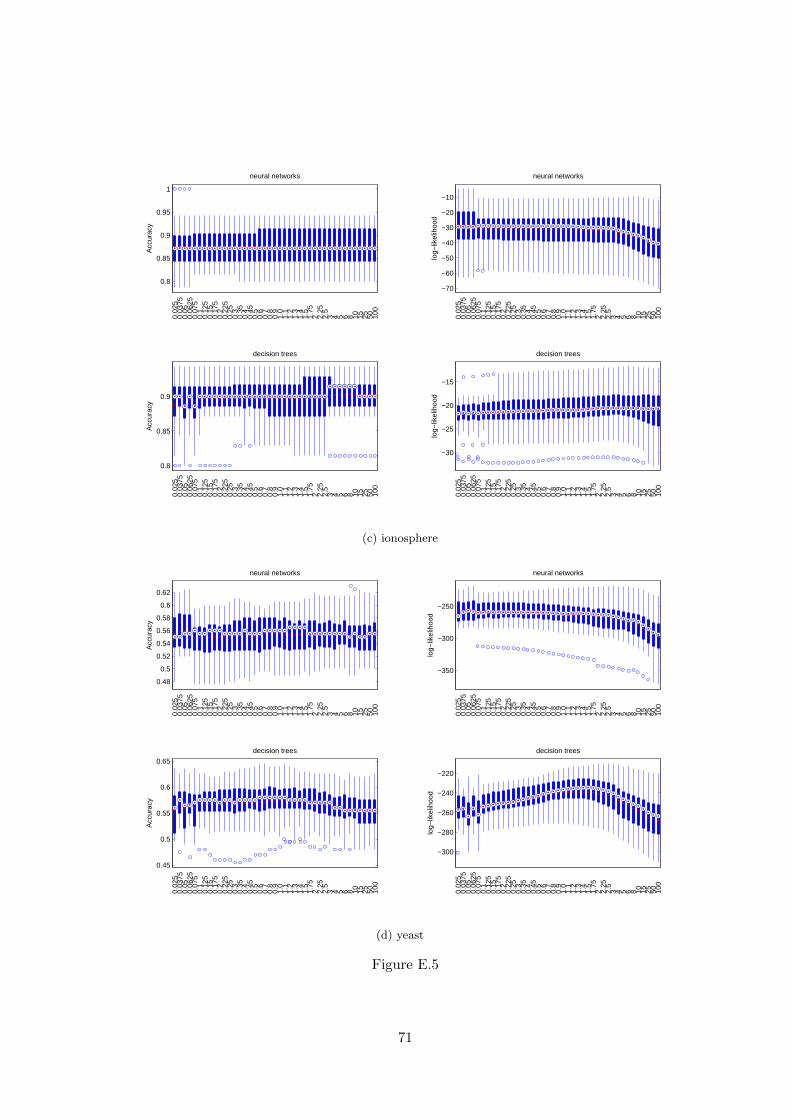
0.8

0.85

0.9

0.95

1

0.02

50.

0375

0.05

0.06

250.

075

0.1

0.12

50.

150.

175

0.2

0.22

50.

250.

30.

350.

40.

450.

50.

60.

70.

80.

91.

01.

11.

21.

31.

41.

51.

752 2.

252.

53 4 5 6 8 10 15 25 50 10

0

Acc

urac

y

neural networks

−70

−60

−50

−40

−30

−20

−10

0.02

50.

0375

0.05

0.06

250.

075

0.1

0.12

50.

150.

175

0.2

0.22

50.

250.

30.

350.

40.

450.

50.

60.

70.

80.

91.

01.

11.

21.

31.

41.

51.

752 2.

252.

53 4 5 6 8 10 15 25 50 10

0

log−

likel

ihoo

d

neural networks

0.8

0.85

0.9

0.02

50.

0375

0.05

0.06

250.

075

0.1

0.12

50.

150.

175

0.2

0.22

50.

250.

30.

350.

40.

450.

50.

60.

70.

80.

91.

01.

11.

21.

31.

41.

51.

752 2.

252.

53 4 5 6 8 10 15 25 50 10

0

Acc

urac

y

decision trees

−30

−25

−20

−15

0.02

50.

0375

0.05

0.06

250.

075

0.1

0.12

50.

150.

175

0.2

0.22

50.

250.

30.

350.

40.

450.

50.

60.

70.

80.

91.

01.

11.

21.

31.

41.

51.

752 2.

252.

53 4 5 6 8 10 15 25 50 10

0

log−

likel

ihoo

d

decision trees

(c) ionosphere

0.48

0.5

0.52

0.54

0.56

0.58

0.6

0.62

0.02

50.

0375

0.05

0.06

250.

075

0.1

0.12

50.

150.

175

0.2

0.22

50.

250.

30.

350.

40.

450.

50.

60.

70.

80.

91.

01.

11.

21.

31.

41.

51.

752 2.

252.

53 4 5 6 8 10 15 25 50 10

0

Acc

urac

y

neural networks

−350

−300

−250

0.02

50.

0375

0.05

0.06

250.

075

0.1

0.12

50.

150.

175

0.2

0.22

50.

250.

30.

350.

40.

450.

50.

60.

70.

80.

91.

01.

11.

21.

31.

41.

51.

752 2.

252.

53 4 5 6 8 10 15 25 50 10

0

log−

likel

ihoo

d

neural networks

0.45

0.5

0.55

0.6

0.65

0.02

50.

0375

0.05

0.06

250.

075

0.1

0.12

50.

150.

175

0.2

0.22

50.

250.

30.

350.

40.

450.

50.

60.

70.

80.

91.

01.

11.

21.

31.

41.

51.

752 2.

252.

53 4 5 6 8 10 15 25 50 10

0

Acc

urac

y

decision trees

−300

−280

−260

−240

−220

0.02

50.

0375

0.05

0.06

250.

075

0.1

0.12

50.

150.

175

0.2

0.22

50.

250.

30.

350.

40.

450.

50.

60.

70.

80.

91.

01.

11.

21.

31.

41.

51.

752 2.

252.

53 4 5 6 8 10 15 25 50 10

0

log−

likel

ihoo

d

decision trees

(d) yeast

Figure E.5

71

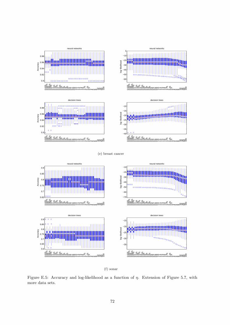
0.9

0.92

0.94

0.96

0.98

0.02

50.

0375

0.05

0.06

250.

075

0.1

0.12

50.

150.

175

0.2

0.22

50.

250.

30.

350.

40.

450.

50.

60.

70.

80.

91.

01.

11.

21.

31.

41.

51.

752 2.

252.

53 4 5 6 8 10 15 25 50 10

0

Acc

urac

y

neural networks

−60

−50

−40

−30

−20

−10

0

0.02

50.

0375

0.05

0.06

250.

075

0.1

0.12

50.

150.

175

0.2

0.22

50.

250.

30.

350.

40.

450.

50.

60.

70.

80.

91.

01.

11.

21.

31.

41.

51.

752 2.

252.

53 4 5 6 8 10 15 25 50 10

0

log−

likel

ihoo

d

neural networks

0.9

0.92

0.94

0.96

0.98

0.02

50.

0375

0.05

0.06

250.

075

0.1

0.12

50.

150.

175

0.2

0.22

50.

250.

30.

350.

40.

450.

50.

60.

70.

80.

91.

01.

11.

21.

31.

41.

51.

752 2.

252.

53 4 5 6 8 10 15 25 50 10

0

Acc

urac

y

decision trees

−40

−35

−30

−25

−20

−15

−10

0.02

50.

0375

0.05

0.06

250.

075

0.1

0.12

50.

150.

175

0.2

0.22

50.

250.

30.

350.

40.

450.

50.

60.

70.

80.

91.

01.

11.

21.

31.

41.

51.

752 2.

252.

53 4 5 6 8 10 15 25 50 10

0

log−

likel

ihoo

d

decision trees

(e) breast cancer

0.65

0.7

0.75

0.8

0.85

0.9

0.02

50.

0375

0.05

0.06

250.

075

0.1

0.12

50.

150.

175

0.2

0.22

50.

250.

30.

350.

40.

450.

50.

60.

70.

80.

91.

01.

11.

21.

31.

41.

51.

752 2.

252.

53 4 5 6 8 10 15 25 50 10

0

Acc

urac

y

neural networks

−70

−60

−50

−40

−30

−20

−10

0.02

50.

0375

0.05

0.06

250.

075

0.1

0.12

50.

150.

175

0.2

0.22

50.

250.

30.

350.

40.

450.

50.

60.

70.

80.

91.

01.

11.

21.

31.

41.

51.

752 2.

252.

53 4 5 6 8 10 15 25 50 10

0

log−

likel

ihoo

d

neural networks

0.6

0.65

0.7

0.75

0.8

0.85

0.9

0.02

50.

0375

0.05

0.06

250.

075

0.1

0.12

50.

150.

175

0.2

0.22

50.

250.

30.

350.

40.

450.

50.

60.

70.

80.

91.

01.

11.

21.

31.

41.

51.

752 2.

252.

53 4 5 6 8 10 15 25 50 10

0

Acc

urac

y

decision trees

−35

−30

−25

−20

−15

0.02

50.

0375

0.05

0.06

250.

075

0.1

0.12

50.

150.

175

0.2

0.22

50.

250.

30.

350.

40.

450.

50.

60.

70.

80.

91.

01.

11.

21.

31.

41.

51.

752 2.

252.

53 4 5 6 8 10 15 25 50 10

0

log−

likel

ihoo

d

decision trees

(f) sonar

Figure E.5: Accuracy and log-likelihood as a function of η. Extension of Figure 5.7, withmore data sets.

72

Bibliography

[ArrDeb54] Kenneth J. Arrow, Gerard Debreu, Existence of an equilibrium for a competitiveeconomy, Econometrica: Journal of the Econometric Society, 22(3):265290, 1954.

[BarLay11] Adrian Barbu, Nathan Lay, An Introduction to Artificial Prediction Markets,arXiv:1102.1465v3 [stat.ML].

[BelKor07] Robert M. Bell, Yehuda Koren, Lessons from the Netflix prize challenge, ACMSIGKDD Explorations Newsletter, 9(2):7579, 2007.

[BerForNelRie08] Joyce Berg, Robert Forsythe, Forrest Nelson, Thomas Rietz, Results froma Dozen Years of Election Futures Markets Research, Handbook of Experimental Eco-nomics Results, 2008, vol. 1, pages 742-751.

[Bis06] Christopher M. Bishop, Pattern Recognition and Machine Learning, Springer, 2006.

[Bre01] Leo Breiman, Random Forests, Machine Learning 45(1): 5-32, 2001.

[CapSomBruZyc09] Valerio Cappellini, Hans-Jurgen Sommers, Wojciech Bruzda, KarolZyczkowski, Random bistochastic matrices, Journal of Physics A-mathematical and The-oretical, vol. 42, no. 36, 2009.

[Die00] Thomas G. Dietterich, Ensemble Methods in Machine Learning, MCS 2000.

[Fun01] Glenn Fung, A Comprehensive Overview of Basic Clustering Algorithms.

[HasTibFri09] Trevor Hastie, Robert Tibshirani, Jerome Friedman, The Elements of Statis-tical Learning: Data Mining, Inference, and Prediction, 2009.

[Hin02] Goffrey E. Hinton, Training products of experts by minimizing contrastive divergence,Neural Computation, 14:1771-1800, 2002.

[Hor91] Kurt Hornik, Approximation capabilities of multilayer feedforward networks, NeuralNetworks, vol. 4(2), 1991.

[Lay09] Nathan Lay, Supervised Aggregation of Classifiers using Artificial Prediction Markets.MSc Thesis, buying State University, 2009.

[LayBar10] Nathan Lay, Adrian Barbu, Supervised Aggregation of Classifiers using ArtificialPrediction Markets, ICML 2010.

[LIBSVM] Machine Learning and Data Mining Group at National Taiwan University,www.csie.ntu.edu.tw/∼cjlin/libsvm/.

[Man06] Charles F. Manski, Interpreting the predictions of prediction markets, EconomicsLetters, Elsevier, vol. 91(3), pages 425-429, June.

73

[Min02] Thomas P. Minka, Bayesian model averaging is not model combination, MIT MediaLab note, 2002.

[Netlab] Non-linearity and Complexity Research Group at Aston University,www.aston.ac.uk/ncrg.

[Pet05] Michael Peters, Lecture notes to Econ304 - Honours Microeconomics at the Universityof British Columbia, 2005.

[Sch03] Robert E. Schapire, The boosting approach to machine learning: An overview, Non-linear Estimation and Classification, Springer, 2003.

[Sto11] Amos Storkey, Machine Learning Markets, AISTATS 2011.

[StoMilGer11] Amos Storkey, Jonathan Millin, Krzysztof Geras, Inhomogeneous Agents inMachine Learning Markets, submitted to NIPS 2011.

[WolZit04] Justin Wolfers, Eric Zitzewitz, Prediction markets, Journal of Economic Perspec-tives, pages 107-126, 2004.

[WolZit07] Justin Wolfers, Eric Zitzewitz, Interpreting Prediction Market Prices as Probabil-ities, 2007.

74

prediction markets for machine learning - new york …kgeras/files/thesis.pdf · prediction markets...

Documents