predicting the presence of historic and prehistoric...
TRANSCRIPT
Predicting the Presence of Historic and Prehistoric Campsites in Virginia’s
Chesapeake Bay Counties
by
Patricia Noela Wright
A Thesis Presented to the
Faculty of the USC Graduate School
University of Southern California
In Partial Fulfillment of the
Requirements for the Degree
Master of Science
(Geographic Information Science and Technology)
August 2016

ii
Copyright © 2016 Patricia N. Wright

iii
To Opa for always inspiring me to persevere
iv
Table of Contents
List of Figures ............................................................................................................................... vii
List of Tables ................................................................................................................................. ix
Acknowledgements ......................................................................................................................... x
List of Abbreviations ..................................................................................................................... xi
Abstract ........................................................................................................................................ xiii
Chapter 1 Introduction .................................................................................................................... 1
1.1 Motivation ............................................................................................................................3
1.2 Predicting Archaeological Sites in the Chesapeake Bay Region .........................................4
1.3 Objectives of this Research ..................................................................................................6
Chapter 2 Background and Related Literature................................................................................ 8
2.1 Predictive Modeling in Archaeology ...................................................................................8
2.1.1. Inductive and deductive predictive models ..............................................................10
2.2 A Framework for Predictive Modeling ..............................................................................12
2.2.1. Unit of study ............................................................................................................13
2.2.2. Model result classes .................................................................................................13
2.2.3. Decision rules...........................................................................................................14
2.3 Fuzzy Overlay Modeling ...................................................................................................14

v
2.3.1. Related Literature.....................................................................................................15
2.4 Maximum Entropy Modeling ............................................................................................16
2.4.1. Related Literature.....................................................................................................17
2.5 Environmental Variables for Modeling Campsite Locations ............................................18
2.6 Summary ............................................................................................................................20
Chapter 3 Data and Methodology ................................................................................................. 21
3.1 Study Area .........................................................................................................................21
3.2 Archaeological Campsites Data .........................................................................................22
3.3 Environmental Data ...........................................................................................................24
3.3.1. Elevation ..................................................................................................................25
3.3.2. Chesapeake Bay waterbody .....................................................................................26
3.3.3. Land Cover...............................................................................................................27
3.3.4. Wetlands ..................................................................................................................28
3.3.5. Soils..........................................................................................................................29
3.3.6. Virginia Major Roads ..............................................................................................30
3.4 Data preparation .................................................................................................................31
3.4.1. Preliminary data manipulation .................................................................................31
3.4.2. Data preparation for fuzzy overlay ..........................................................................32
3.4.3. Preparation of data for Maxent ................................................................................37
3.5 Model Implementation .......................................................................................................38
3.5.1. Running Fuzzy Overlay ...........................................................................................38
3.5.2. Running Maxent.......................................................................................................38
3.6 Risk Analysis .....................................................................................................................39
vi
Chapter 4 Results .......................................................................................................................... 41
4.1 Fuzzy Overlay Results .......................................................................................................42
4.2 Maxent Results...................................................................................................................46
4.3 Comparison of Model Results ...........................................................................................52
4.4 Risk Analysis Results ........................................................................................................57
4.5 Summary ............................................................................................................................62
Chapter 5 Summary and Conclusions ........................................................................................... 63
5.1 Model evaluations ..............................................................................................................63
5.2 Modeling for Risk Analysis ...............................................................................................64
5.3 Limitations and Observations ............................................................................................65
5.4 Future work ........................................................................................................................66
5.5 Conclusion .........................................................................................................................66
REFERENCES ............................................................................................................................. 67
vii
List of Figures
Figure 1 Project study area within state of Virginia ....................................................................... 2
Figure 2 Close-up of study area with counties................................................................................ 3
Figure 3 Virginia’s physical regions and the Fall Line separation ............................................... 22
Figure 4 Archaeological campsites ............................................................................................... 23
Figure 5 Elevation data (meters) ................................................................................................... 26
Figure 6 Waterbody data ............................................................................................................... 27
Figure 7 Land cover data .............................................................................................................. 28
Figure 8 Virginia wetlands data .................................................................................................... 29
Figure 9 Watersheds used to acquire soils data ............................................................................ 30
Figure 10 Virginia’s major roads data .......................................................................................... 31
Figure 11 Illustration of the Gaussian function in Fuzzy Membership. Source: Esri Desktop Help
....................................................................................................................................................... 34
Figure 12 Illustration of the Near function in Fuzzy Membership Source: Esri Desktop Help ... 35
Figure 13 Illustration of Small function in Fuzzy Membership Source: Esri Desktop Help ........ 36
Figure 14 Fuzzy overlay results indicating site suitability ........................................................... 43
Figure 15 Fuzzy overlay results with archaeological camps ........................................................ 45
Figure 16 Maxent results indicating site probability .................................................................... 47
Figure 17 Marginal response curve ............................................................................................... 48
Figure 18 Average omission and predicted area for campsites .................................................... 49
Figure 19 Maxent model sensitivity ............................................................................................. 50
Figure 20 Jackknife of regularized training gain .......................................................................... 52
viii
Figure 21 Comparison of areas with 0-25% site potential results of models ............................... 54
Figure 22 Comparison of areas with 25-50% site potential results of models ............................. 55
Figure 23 Comparison of areas with 25-50% site potential results of models ............................. 56
Figure 24 Comparison of areas with over 75% site potential results of models........................... 57
Figure 25 Risk of sea-level rise to highly suitable locations from the fuzzy overlay analysis ..... 59
Figure 26 Risk of sea-level rise for Maxent results ...................................................................... 60
Figure 27 Risk of urbanization for fuzzy overlay results ............................................................. 61
Figure 28 Risk of human degradation for Maxent results ............................................................ 62

ix
List of Tables
Table 1 Known Sites within Suitability Locations ....................................................................... 46
Table 2 Permutation of importance of each environmental variable ............................................ 51
Table 3 Count of grid cells from comparative analysis ................................................................ 57

x
Acknowledgements
I am grateful for a number of people whose wisdom and support have guided me through this
project. First and foremost, I extend my gratitude to my thesis committee, Dr. Karen Kemp, for
your patience and invaluable guidance as I produced my thesis, and to Dr. Su Jin Lee and Dr.
Steven Fleming for your support and passion for GIS. This thesis would not be possible without
the support of my family and friends throughout this process.

xi
List of Abbreviations
APM Archaeological predictive model
ASCII American Standard Code for Information Interchange
AUC Area under the receiver operator curve
BLM Bureau of Land Management
DEM Digital Elevation Model
CBP Chesapeake Bay Program
CRM Cultural resource management
.csv Comma separated value file
GIA Graphical intuitive approach
GIS Geographic Information System
NAD83 North American Datum 1983
NLCD National Land Cover Database
NOAA National Oceanic and Atmospheric Association
NRCS Natural Resources Conservation Service
NWI National Wetlands Inventory
RCL Road Center Line Program
ROC Receiver operating characteristic
SSI Spatial Sciences Institute
USC University of Southern California
UTM Universal Transverse Mercator
USGS United States Geological Survey
V-CRIS Virginia Cultural Resource Information System

xii
VDOT Virginia Department of Transportation
VGIN Virginia Geographic Information Network
xiii
Abstract
Geographic Information Systems (GIS) have been widely used for archaeological predictive
modeling since the 1960s. For coastal archaeology, predictive modeling, which is the practice of
using mathematical models to indicate the likelihood of archaeological site locations, cultural
resources, or settlement patterns, is especially helpful in locating sites potentially endangered by
coastline erosion and destructive forces. The purpose of this project was to determine if it is
possible to predict the presence of unknown archaeological sites along Virginia’s Chesapeake
coast to aid in their preservation and site management. In order to predict the presence of sites, a
baseline of favorable environmental conditions was determined from known coastline
archaeological sites. Environmental variables considered include elevation, slope, wetland type,
land type, and distance to the Chesapeake Bay. In order to explore if these environmental
variables can be used to determine locations favorable to the establishment of campsites, spatial
data about these environmental variables were used in two predictive modeling methods: fuzzy
overlay analysis and maximum entropy. Each model’s outcomes were compared with known site
locations in order to determine their success. The results of each model successfully indicated
areas of site location suitability. Although results for each model varied, the trends produced
were similar. Finally, in order to better prioritize site management, a risk analysis was also
conducted of perceived threats compared to areas in which the models predicted site presence.
These risk areas were calculated using data on human degradation and coastal sea-rise threat. As
this study demonstrates, using models to predict where potential sites can allow archaeologists to
prioritize areas to study for resource management purposes.

1
Chapter 1 Introduction
Virginia’s Chesapeake Bay region is an area well known for its rich cultural past and is an active
study area for archaeologists. Known archaeological sites vary from prehistoric to historic
cultural areas—from the Paleo-Indian inhabitants from 9000 years ago, to the slave trade and
piracy in the 1600s, followed by the American Revolution, and eventually the Civil War era. As
this thesis shows, the Chesapeake Bay region is dotted with notable battle sites, dwelling areas,
and shipwrecks. The dynamic environment of the shoreline, caused by natural wind and wave
forces, erodes these cultural resources. Shoreline erosion often contributes to the exposure of
archaeology sites and destruction of artifacts and features.
Geographic Information Systems (GIS) have been widely used for archaeological
predictive modeling since the 1960s (Wescott and Kuiper 2006). For coastal archaeology,
predictive modeling, which is the practice of using mathematical models to indicate the
likelihood of archaeological site locations, cultural resources, or settlement patterns, is especially
helpful in locating sites potentially endangered by coastline erosion and destructive forces. In
order to address the problem of potential destruction of archaeological sites, this project explores
two GIS modeling methods, fuzzy overlay and maximum entropy, to predict the presence of
unfound archaeology sites. As this study demonstrates, using models to predict where potential
sites may be can allow archaeologists to prioritize areas to study for resource management
purposes.
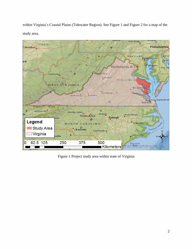
The study area for this project includes seven counties in the Chesapeake Bay area. These
counties are: Gloucester, Essex, Lancaster, Middlesex, Richmond, Westmoreland, and
Northumberland. The study area encompasses approximately 117 by 84 kilometers of land
2
within Virginia’s Coastal Plains (Tidewater Region). See Figure 1 and Figure 2 for a map of the
study area.
Figure 1 Project study area within state of Virginia

3
Figure 2 Close-up of study area with counties
1.1 Motivation
Cultural environments change over time and sequences of human deposits are left behind
in stratified layers of soil. In order to understand and evaluate cultural environments,
archaeologists examine the materials and deposits left behind at prehistoric and historic sites to
gain insight on a past society. It is the archaeologist’s challenge to obtain as much information
about a culture before this information is lost forever due to inevitable destruction over time.

4
In particular, Virginia’s Chesapeake Bay watershed has a bounteous cultural heritage,
and numerous archaeological sites. Known for its historical and cultural richness, coastal
Chesapeake Virginia is rife with cultural history. The Chesapeake watershed includes many
types of archaeology sites including Native American, Civil War, shipwrecks, and colonial
explorer sites. According to the Chesapeake Bay Program (CBP)1, a regional partnership focused
on Chesapeake Bay restoration and protection, there are estimated to be at least 100,000
archaeology sites within the Chesapeake Bay watershed, with only a small percentage of these
sites documented.
Now, these sites are buried under layers of sediment and shell middens hiding stone tools,
artifacts, and dwellings. As sea levels rise, these sites are being flooded by water and becoming
difficult and sometimes impossible to study. The slow rise in sea level results in the gradual
input of sediment and organic matter into depressed land areas, creating tidal marshes.
According to Lowery et. al (2012), sulfidization created in these tidal marshes will destroy or
alter artifacts and shift site materials around, making it hard to identify cultural materials. These
erosive processes are slowly destroying sites, making it difficult to excavate them. Lowery et. al
determined that at least 281 of 17,230 known archaeological sites in the Chesapeake Bay area are
being impacted by geologic processes associated with sea level rise.
1.2 Predicting Archaeological Sites in the Chesapeake Bay Region
According to V-CRIS (Virginia Cultural Resources Information System)2, within this
study area there are 1,717 known, recorded archaeology sites of different types. In order to
reduce the sample size and enhance the success of the predictive models, this project focuses on
1 Information found at http://www.chesapeakebay.net/ 2 Data available with permission at https://vcris.dhr.virginia.gov/vcris/

5
the 216 known historic and prehistoric campsites. Campsite locations were chosen for several
reasons. While the time range of settlement periods is vast for these known sites (from
approximately 5000 B.C.E. through the 1920s), campsites contain relatively similar features
throughout time, making all campsites comparable for this kind of study, even with wide time
gaps. All prehistoric and historic campsites structures were either semi-permanent or temporary.
Typically, campsites are classified by the amount and type of artifact fragments found at a
location. Campsites are characterized by: low artifact concentration, presence of fire pits, and
lack of dwelling structures (Judge and Sebastian 1988). Due to the scarcity of permanent floor
structures and artifact fragments, campsite locations are more susceptible to erosive and
destructive forces, making them particularly an appropriate focus for this study.
Focusing on predicting the location of campsites, the study began by determining a set of
environmental conditions observed in known archaeological sites and discussed in previous
research. Environmental variables considered include elevation, slope, wetland type, land type,
and distance to the Chesapeake Bay. Then, to explore if these environmental variables can be
used to determine locations favorable to the establishment of campsites, spatial data about these
environmental variables were used in two predictive modeling methods: fuzzy overlay analysis
and maximum entropy. After inputting the environmental data into each model, the models’
output shows locations where sites are likely to be found.
Each model uses different techniques of prediction. The maximum entropy modeling
tool, Maxent, finds the maximum entropy (largest spread) of site presence in relation to the input
environmental variables. Maxent builds models of site distribution occurrences starting with a
uniform probability of distribution values over background locations, and then iterates the
process to improve model fit.

6
In fuzzy overlay analysis, each environmental variable is assigned a fuzzy membership
value based on the role of that variable in determining the suitability of a location for use. For
instance, slope might be given a fuzzy membership based on slope percentage. Assuming that
low slopes would be more favorable to the location of sites, lower slope profiles (5% and under)
are given a high membership value, and high slope profiles (60% and above) are given low
membership values. These fuzzy layers are then input into a fuzzy overlay tool, which calculates
the product of each fuzzy layer and determines which locations are likely locations for
archaeology sites based on high fuzzy membership values.
Finally, to demonstrate how predictive models such as these can be used to prioritize site
management, a risk analysis of potential threats was conducted. Risks examined were potential
human degradation determined by nearness to major roads and sea level rise based on nearness
to the shoreline in areas where elevation was less than three meters above sea level. These risk
factors were overlaid onto the predicted site locations created by each model to show how they
may be used to suggest areas of highest priority for survey.
1.3 Objectives of this Research
The purpose of this project was to determine if it is possible to predict the presence of
unknown archaeological sites along Virginia’s Chesapeake coast to aid in their preservation and
site management. In order to achieve this, the research addressed the following questions:
1. Can the potential location of archeological campsites be modeled successfully using
the deductive fuzzy overlay approach?
2. Can the potential location of archaeological campsites be modeled successfully using
the inductive maximum entropy approach?
3. How do the results of these different modeling approaches differ in results?

7
4. How can these predictions be used to assist in risk management for cultural resource
management agencies?
The remainder of this document is composed of four additional chapters. Chapter 2
discusses relevant literature and previous work that were used as resources for this project.
Chapter 3 outlines the data compiled and describes the modeling processes used in the project.
Chapter 4 reviews the results of the two modeling processes and examines the differences
between the two. Chapter 4 also includes the results of the risk analysis. Lastly, Chapter 5
discusses model performance and the risk analysis as an illustration of the value of the prediction
models.
8
Chapter 2 Background and Related Literature
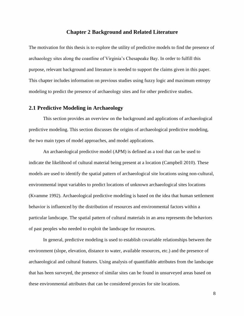
The motivation for this thesis is to explore the utility of predictive models to find the presence of
archaeology sites along the coastline of Virginia’s Chesapeake Bay. In order to fulfill this
purpose, relevant background and literature is needed to support the claims given in this paper.
This chapter includes information on previous studies using fuzzy logic and maximum entropy
modeling to predict the presence of archaeology sites and for other predictive studies.
2.1 Predictive Modeling in Archaeology
This section provides an overview on the background and applications of archaeological
predictive modeling. This section discusses the origins of archaeological predictive modeling,
the two main types of model approaches, and model applications.
An archaeological predictive model (APM) is defined as a tool that can be used to
indicate the likelihood of cultural material being present at a location (Campbell 2010). These
models are used to identify the spatial pattern of archaeological site locations using non-cultural,
environmental input variables to predict locations of unknown archaeological sites locations
(Kvamme 1992). Archaeological predictive modeling is based on the idea that human settlement
behavior is influenced by the distribution of resources and environmental factors within a
particular landscape. The spatial pattern of cultural materials in an area represents the behaviors
of past peoples who needed to exploit the landscape for resources.
In general, predictive modeling is used to establish covariable relationships between the
environment (slope, elevation, distance to water, available resources, etc.) and the presence of
archaeological and cultural features. Using analysis of quantifiable attributes from the landscape
that has been surveyed, the presence of similar sites can be found in unsurveyed areas based on
these environmental attributes that can be considered proxies for site locations.
9
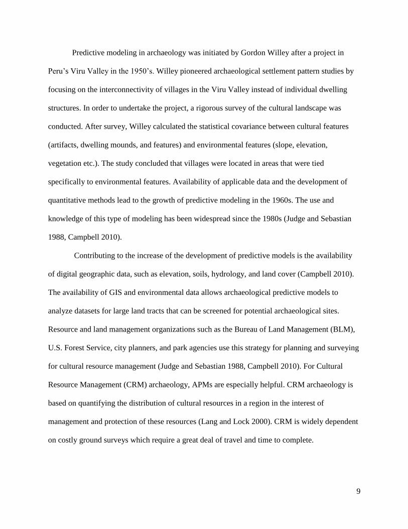
Predictive modeling in archaeology was initiated by Gordon Willey after a project in
Peru’s Viru Valley in the 1950’s. Willey pioneered archaeological settlement pattern studies by
focusing on the interconnectivity of villages in the Viru Valley instead of individual dwelling
structures. In order to undertake the project, a rigorous survey of the cultural landscape was
conducted. After survey, Willey calculated the statistical covariance between cultural features
(artifacts, dwelling mounds, and features) and environmental features (slope, elevation,
vegetation etc.). The study concluded that villages were located in areas that were tied
specifically to environmental features. Availability of applicable data and the development of
quantitative methods lead to the growth of predictive modeling in the 1960s. The use and
knowledge of this type of modeling has been widespread since the 1980s (Judge and Sebastian
1988, Campbell 2010).
Contributing to the increase of the development of predictive models is the availability
of digital geographic data, such as elevation, soils, hydrology, and land cover (Campbell 2010).
The availability of GIS and environmental data allows archaeological predictive models to
analyze datasets for large land tracts that can be screened for potential archaeological sites.
Resource and land management organizations such as the Bureau of Land Management (BLM),
U.S. Forest Service, city planners, and park agencies use this strategy for planning and surveying
for cultural resource management (Judge and Sebastian 1988, Campbell 2010). For Cultural
Resource Management (CRM) archaeology, APMs are especially helpful. CRM archaeology is
based on quantifying the distribution of cultural resources in a region in the interest of
management and protection of these resources (Lang and Lock 2000). CRM is widely dependent
on costly ground surveys which require a great deal of travel and time to complete.
10
Archaeological prediction models make CRM survey more efficient by providing a picture of
potential site distribution, allowing survey resources to be efficiently deployed.
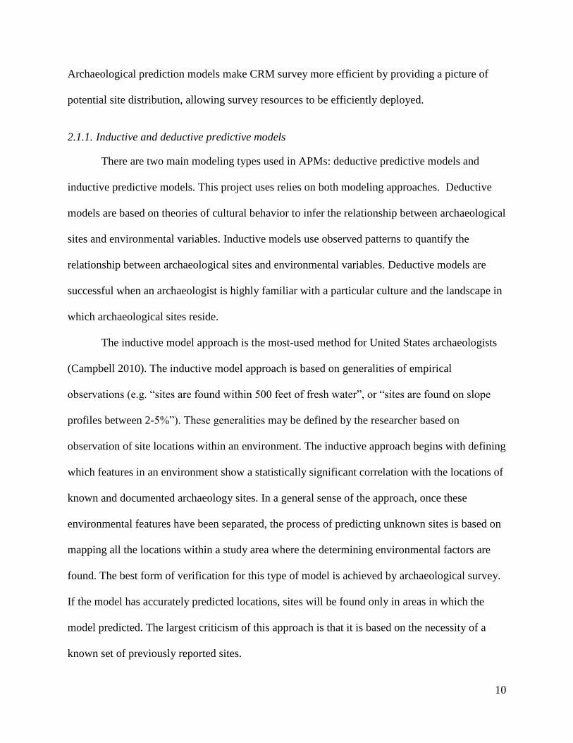
2.1.1. Inductive and deductive predictive models
There are two main modeling types used in APMs: deductive predictive models and
inductive predictive models. This project uses relies on both modeling approaches. Deductive
models are based on theories of cultural behavior to infer the relationship between archaeological
sites and environmental variables. Inductive models use observed patterns to quantify the
relationship between archaeological sites and environmental variables. Deductive models are
successful when an archaeologist is highly familiar with a particular culture and the landscape in
which archaeological sites reside.
The inductive model approach is the most-used method for United States archaeologists
(Campbell 2010). The inductive model approach is based on generalities of empirical
observations (e.g. “sites are found within 500 feet of fresh water”, or “sites are found on slope
profiles between 2-5%”). These generalities may be defined by the researcher based on
observation of site locations within an environment. The inductive approach begins with defining
which features in an environment show a statistically significant correlation with the locations of
known and documented archaeology sites. In a general sense of the approach, once these
environmental features have been separated, the process of predicting unknown sites is based on
mapping all the locations within a study area where the determining environmental factors are
found. The best form of verification for this type of model is achieved by archaeological survey.
If the model has accurately predicted locations, sites will be found only in areas in which the
model predicted. The largest criticism of this approach is that it is based on the necessity of a
known set of previously reported sites.
11
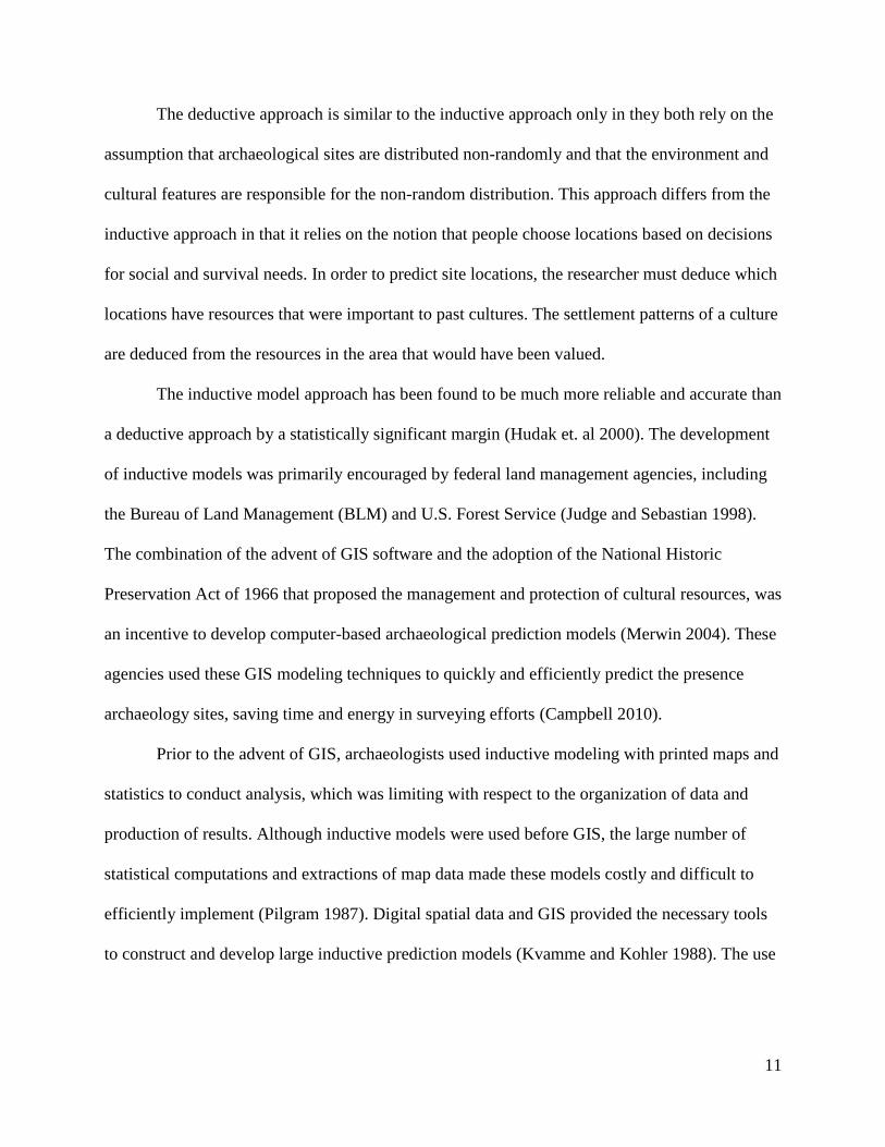
The deductive approach is similar to the inductive approach only in they both rely on the
assumption that archaeological sites are distributed non-randomly and that the environment and
cultural features are responsible for the non-random distribution. This approach differs from the
inductive approach in that it relies on the notion that people choose locations based on decisions
for social and survival needs. In order to predict site locations, the researcher must deduce which
locations have resources that were important to past cultures. The settlement patterns of a culture
are deduced from the resources in the area that would have been valued.
The inductive model approach has been found to be much more reliable and accurate than
a deductive approach by a statistically significant margin (Hudak et. al 2000). The development
of inductive models was primarily encouraged by federal land management agencies, including
the Bureau of Land Management (BLM) and U.S. Forest Service (Judge and Sebastian 1998).
The combination of the advent of GIS software and the adoption of the National Historic
Preservation Act of 1966 that proposed the management and protection of cultural resources, was
an incentive to develop computer-based archaeological prediction models (Merwin 2004). These
agencies used these GIS modeling techniques to quickly and efficiently predict the presence
archaeology sites, saving time and energy in surveying efforts (Campbell 2010).
Prior to the advent of GIS, archaeologists used inductive modeling with printed maps and
statistics to conduct analysis, which was limiting with respect to the organization of data and
production of results. Although inductive models were used before GIS, the large number of
statistical computations and extractions of map data made these models costly and difficult to
efficiently implement (Pilgram 1987). Digital spatial data and GIS provided the necessary tools
to construct and develop large inductive prediction models (Kvamme and Kohler 1988). The use
12
of GIS modeling in archaeology has increased as GIS software became more sophisticated and
cost efficient (Wescott and Brandon 2002).
This paper is inspired by the inductive and deductive approach as well. Maxent employs
an inductive approach analysis, whereas fuzzy overlay is deductive. Maxent employs the
inductive modeling approach by finding the probability of suitability of site locations based on
the presence of environmental data. Fuzzy overlay is deductive in that environmental variables
are used to predict the probability of suitable sites based on presumptions made by the
researcher.
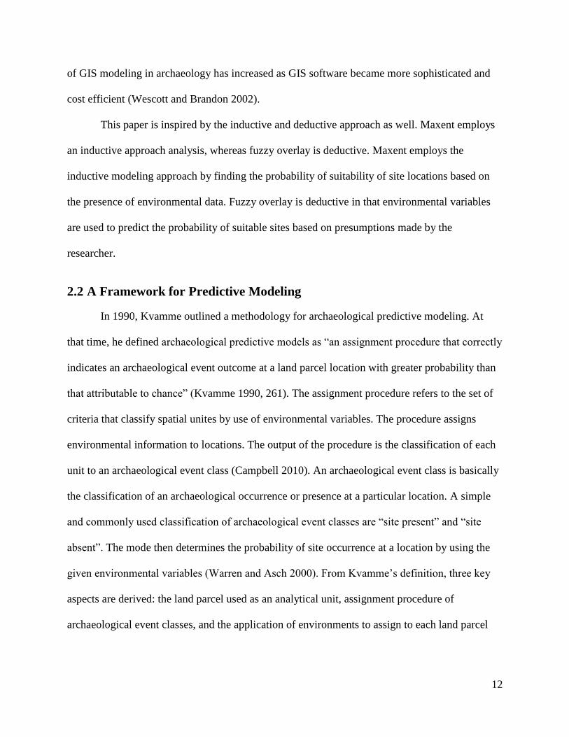
2.2 A Framework for Predictive Modeling
In 1990, Kvamme outlined a methodology for archaeological predictive modeling. At
that time, he defined archaeological predictive models as “an assignment procedure that correctly
indicates an archaeological event outcome at a land parcel location with greater probability than
that attributable to chance” (Kvamme 1990, 261). The assignment procedure refers to the set of
criteria that classify spatial unites by use of environmental variables. The procedure assigns
environmental information to locations. The output of the procedure is the classification of each
unit to an archaeological event class (Campbell 2010). An archaeological event class is basically
the classification of an archaeological occurrence or presence at a particular location. A simple
and commonly used classification of archaeological event classes are “site present” and “site
absent”. The mode then determines the probability of site occurrence at a location by using the
given environmental variables (Warren and Asch 2000). From Kvamme’s definition, three key
aspects are derived: the land parcel used as an analytical unit, assignment procedure of
archaeological event classes, and the application of environments to assign to each land parcel
13
(Campbell 2010). By generalizing these aspects and taking into account current modeling
environments, each of these aspects is further explored below.
2.2.1. Unit of study
An important aspect of archaeological predictive modeling is the unit used to measure the
presence of archaeological sites. Often the unit used is the archaeological site itself. For instance,
as used in this study, known archaeological sites can be represented as points. However, when
predicting areas of archaeological site presence, Kvamme (1998) suggests that the unit of
investigation used should be represented by land parcels or grid cells, the latter allowing the
entire study area to be divided into discrete units of uniform size. In the case of the research
reported here, uniform square grid cells are necessary for both fuzzy overlay and Maxent models,
as both use standard rasters for data analysis.
The grid cell chosen for analysis should capture the variability of the real-life landscape
but should not be at a finer scale than the available data (Hudek et al. 2000). In order to reduce
the margin of error, the consideration of the scale of available data is highly important. Because
data is collected at certain levels of positional and attribute accuracy, the cell size should be
based on the characteristics of the available environmental data. Using a cell size for the unit of
study that is at a finer resolution than the mapping scale of the environmental data could
introduce errors in model precision (Clark et al 2002).
2.2.2. Model result classes
The outputs of an archaeological prediction model are represented by the assignment of a
grid cell to an archaeological event class that is defined prior to model construction (Campbell
2010). In this project, as discussed in the next chapter, the nature of the modeling tools allowed
multiple archaeological event classes to be used, ranging from most suitable to least suitable.

14
2.2.3. Decision rules
Lastly, decision rules must be created on how to predict archaeological site locations
using environmental variables (Kvamme 1998). These decision rules are based on whether a
deductive or inductive model type is used. When using inductive analysis decision rules can be
made using statistical techniques to find site patterns. When using deductive analysis, the
archaeologist creates rules based on knowledge of cultural patterns and their relationship to the
environment. This study relies on both inductive analysis using statistical methods for Maxent,
and fuzzy overlay requires some deductive reasoning when choosing environmental parameters.
For instance, determining which types of land cover are most likely to contain a campsite
involves some deductive reasoning based on information provided by previous studies.
2.3 Fuzzy Overlay Modeling
Fuzzy logic modeling in archaeology became popular in the 1980s (Judge and Sebastian
1998). The fuzzy logic concept is used to simulate real-world conditions in which environmental
conditions are either suitable, not suitable, or along a spectrum of being partially suitable to
partially not suitable for a particular outcome. Fuzzy logic is based on the idea that an
archaeological event class could have infinite options, instead of the Boolean logic of “true” and
“false” or “site-present” and “site-absent”.
Fuzzy logic was introduced by L.A. Zadeh in 1965. Zadeh’s key idea was that it is
possible to represent the similarity an entity shares to other members of a group with a
membership function whose values (memberships) are between 0 and 1. Zadeh defines a fuzzy
set as “a class of objects with a continuum of grades of membership…such a set is characterized
by a membership (characteristic) function which assigns to each object a grade of membership
ranging between zero and one” (Zadeh 1965, 261).
15
Solving a problem with the fuzzy logic system requires four steps to be followed. The
first is fuzzification that assigns a membership function to every variable in the problem. The
second step includes a knowledge base defining the rules of logic. Rules follow an “if…then…”
sequence and express logical assumptions. Third is inference, the processing of the rules.
Boolean algebra operations (intersection, union, negation, etc.) are often used at this step in the
fuzzy-set operations. Lastly is reversing the fuzziness or the procedure of transforming the result
of rules processing into a value indicating the final object outcome.
2.3.1. Related Literature
Mink (2009) discusses using the fuzzy logic approach in ArcMap to model the likelihood
of prehistoric settlement locations in Woodford County, Kentucky. His study was used to create
a predictive model for the Environmental Division of Kentucky Transportation Cabinet to better
spatially estimate the probability of encountering prehistoric lithics. In Mink’s study, he used the
classic deductive modeling approach in determining the significant factors that would influence
the likelihood of prehistoric settlements. Mink used slope, minutes to water source, and elevation
above water as his environmental variables. The result of his study concludes that sites were
more likely to be within a short walking distance of water, and at low elevations.
Vaughn (2012) explains the use of fuzzy overlay as an archaeological predictive model to
find archaeological sites in the Pisgah National Forest. Vaughn explains that the results of fuzzy
overlay analysis is based on the experience of different archaeologists. In her study, Vaughn
explores two different models based on methods presented by two different archaeologists. She
tests these methods using fuzzy overlay for both. One model is based on methods by Mink et. al
(2009) (mentioned above) and one model is based on methods provided by National Forest
Service (NFS). She compares the models using fuzzy overlay in order to determine whether or
16
not fuzzy overlay is an effective tool for predicting archaeology sites in the Pisgah National
Forest. Vaughn compares the effectiveness of each model using Kvamme’s gain statistic which
measures the accuracy and precision of a model’s findings. Specifically, the gain statistic
measures the percent of area covered by each part of the map divided by the percent of sites in
each part of the map. Her results showed that the NFS Model provided a smaller range of
possibility, and the Mink model had a higher range due to the greater number of parameters.
However, results for the NFS model provided more results of probable site areas, whereas the
Mink model was more restricted in its results.
2.4 Maximum Entropy Modeling
Maximum modeling entropy works by finding the largest spread (maximum entropy) in a
geographic dataset of known site presences in relation to a set of background environmental
variables. According to Berger (1996) the concept of maximum entropy can be traced to biblical
times but the introduction of computers in the 21st century has allowed its wide scale application
for modeling in statistical recognition and pattern recognition. Berger explains that the concept
of maximum entropy is based modeling the behavior of a random, incomplete process. To
construct the model, one must use a sample of outputs of the real world process (e.g. using
known archaeological site locations in a river valley, to find the probability of unknown sites).
From the sample output, the model must construe an accurate representation of the real world
process.
The widely used implementation of this technique, Maxent3, is designed to integrate with
GIS software making data input and predicted mapped output more efficient. Maxent is a
program originally designed for modeling species distributions from presence-only species data
3 Program can be downloaded at http://www.cs.princeton.edu/~schapire/maxent

17
(Elith et. al 2010, Phillips, Dudík, and Schapire 2004; Phillips, Anderson, and Schapire 2005;
Phillips and Dudík 2008).
The Maxent software was created by Phillips, Dudik, and Shapire in 2004 as a species
modeling program. Using maximum entropy, the program uses presence-only data to create a
probability distribution using environmental variables as constraints. In this project, the
presence-only data is implemented as archaeological campsite locations instead of species data.
Instead of species modeling, this project explores cultural modeling to find the probability
distribution of campsite locations along the Chesapeake Bay.
2.4.1. Related Literature
Bevan and Wilson (2013) explain the use of maximum entropy modeling to understand
the human settlement of Bronze Age towns on the island of Crete. Using Maxent, the authors
relied on patchy and incomplete data to predict the networks of past settlements. The data used
for these models included spatial site point data for the settlement. The model predicted for
missing archaeological data by characterizing the locations of known settlements using presence-
only data. The Maxent model was able to determine which site characteristics were sufficiently
robust to be considered reliable indicators to predict unknown settlement areas.
Galletti et. al (2013) created a predictive model in Maxent to estimate probability
distributions of ancient and modern terraces in the Troodos Foothills of Cyprus. The article
explains how the Maxent model is effective in predicting potential terrace distributions whose
locations are strongly influenced by topography. The study concludes that Maxent is effective in
assessing environmental constraints and terrace locations and would be useful for archaeological
modeling based on human-environment interactions.
18
2.5 Environmental Variables for Modeling Campsite Locations
Choosing the best environmental variables to support predictive modeling in archaeology
is critical. This section outlines previous research that identifies environmental conditions that
have been found to be related to the location of archaeological sites. This knowledge is used to
inform the set of environmental variables chosen for inclusion in this research.
In Kuiper’s and Wescott’s (1999) paper, the authors explain how GIS was used for
predictive modeling to locate unrecorded prehistoric midden sites in Maryland’s Aberdeen
Proving Ground in the Chesapeake Bay region. The predictive model was created using both a
deductive model (based on theories of cultural behavior) and an inductive model (based on
observed patterns). In order to run the model, the authors created an archaeological site database,
produced environmental GIS data layers, and used descriptive statistical analysis to calibrate the
model. Archaeological site data was a polygon location and included the following data: site
type, distance to water, type of water source (brackish or fresh), soil type, topographic setting,
slope, elevation, aspect, geomorphic setting, time period, dimensions, and contents. Each of
these environmental factors was created as a layer in the GIS using a variety of sources and GIS
tools. The paper successfully demonstrated that midden locations were located within 500 feet of
water, and at an elevation between 0-20 feet.
Merwin (2002) summarizes the environmental conditions in which most coastal
archaeological campsites were found in her study in the New York’s Harbor area. Her research
showed that most sites are found in areas of well-drained soil, in relatively flat topography, on
the shores of protected harbors, estuaries or streams, and adjacent to wetland areas. More
specifically her spatial analysis revealed that most sites are found in elevations less than 20
meters above sea level, with an average level of 10 meters above sea-level. Her study also

19
reveals that campsites are generally located on slope profiles less than 20%, with a mean slope of
10%. Regarding proximity to water resources, including both fresh and brackish, her report
concludes that most sites are found within 2 kilometers of waterbodies and adjacent to wetland
areas.
Lock and Harris (2006) explain that many sites near waterbodies are found near fertile,
silty-loam texture soils in their predictive modeling study in West Virginia and Virginia. The
authors conducted an environmental assessment impact study associated with the proposal to
install a high-power transmission line between the WV and VA border. To comply with CRM
legislation, a predictive model was created to identify the spatial probability of prehistoric and
historic sites in the project area. For each site, they set parameters related to distance to water,
elevation, slope, and soil type. Using exploratory data analysis, the environmental variables
associated with known archaeology sites were explored using a graphical intuitive approach
(GIA). The GIA drew on the review of the parameter distributions and relationships to
understand the threshold boundaries for archaeology sites. The authors concluded that areas with
fertile vegetation, such as forested areas, are more likely to appeal as a place for settlement than
barren or wetland areas.
Kvamme (1992) explains the difficulty of finding reliable data that accurately depicts the
landscapes of the past and he notes that often archaeologists are forced to use modern maps as a
guide. Even so, he claims that using modern maps for environmental variables are relatively
reliable in that even though landscapes change overtime, their settings remain reasonably stable
over a period of 15,000 years. For the purpose of this study, modern environmental variables are
used due to lack of access to relevant representative past data, and under the assumption that
time does not completely alter a landscape.
20
2.6 Summary
Using archaeological predictive models is necessary to predict the probability of campsite
locations in Virginia’s Chesapeake Bay region. As described in chapter 2, this study utilizes both
a deductive model approach in fuzzy overlay, and an inductive approach in Maxent. In order to
succeed in creating a predictive model to find unknown sites in Virginia, this report uses similar
data and techniques that were implemented by Kuiper’s and Wescott (1999) Merwin (2002),
Mehrer and Wescott, and Kvamme (1992) due to similarities in type of analysis and region of
study. Environmental variables chosen include: distance to water, slope percentage, elevation,
land cover, wetlands, and soils. The next chapter explains the methodology and data used to
carry out this project.
21
Chapter 3 Data and Methodology
While they use the same input data, the Maxent and fuzzy overlay modeling undertaken in this
research required different methods of data preparation. This chapter discusses the spatial extent
of the study area and the preparation of the archaeological campsite data and the environmental
variable data that was acquired. It concludes by describing the specific model parameters needed
for the fuzzy overlay and Maxent modeling conducted.
3.1 Study Area
As explained in Chapter 1, the study area encompasses seven counties in the coastal
plains region of Virginia, bordering the Chesapeake Bay. These counties include: Essex,
Gloucester, Lancaster, Middlesex, Northumberland, Richmond and Westmoreland counties. The
study area, shown above in Figure 1, encompasses an area 117 by 84 kilometers.
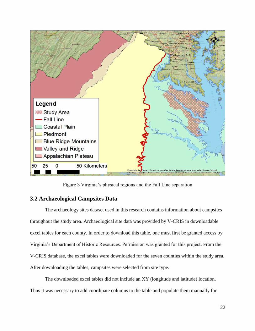
The study area boundary was determined by the political boundaries of each county. The
easternmost counties extend to the Chesapeake Bay. Each county lies within Virginia’s Coastal
Plain (Tidewater) region, an area characterized by low, flat land adjacent to the Atlantic Ocean
(McGlone 2008). The Tidewater gets its name from the daily tides that affect the coastal regions
within the area (McGlone 2008). The Tidewater region lies east of the Fall Line, a natural
boundary caused by a line of crystalline rocks, separating the Tidewater region from the
Piedmont region (Figure 3).
22
Figure 3 Virginia’s physical regions and the Fall Line separation
3.2 Archaeological Campsites Data
The archaeology sites dataset used in this research contains information about campsites
throughout the study area. Archaeological site data was provided by V-CRIS in downloadable
excel tables for each county. In order to download this table, one must first be granted access by
Virginia’s Department of Historic Resources. Permission was granted for this project. From the
V-CRIS database, the excel tables were downloaded for the seven counties within the study area.
After downloading the tables, campsites were selected from site type.
The downloaded excel tables did not include an XY (longitude and latitude) location.
Thus it was necessary to add coordinate columns to the table and populate them manually for
23
each site individually using the V-CRIS database map viewer. This required zooming to each site
to be included, extracting the coordinates in decimal degrees and inputting them into the table.
Once this was completed, the attributes became associated with a location and could be input
into ArcMap as a vector point dataset.
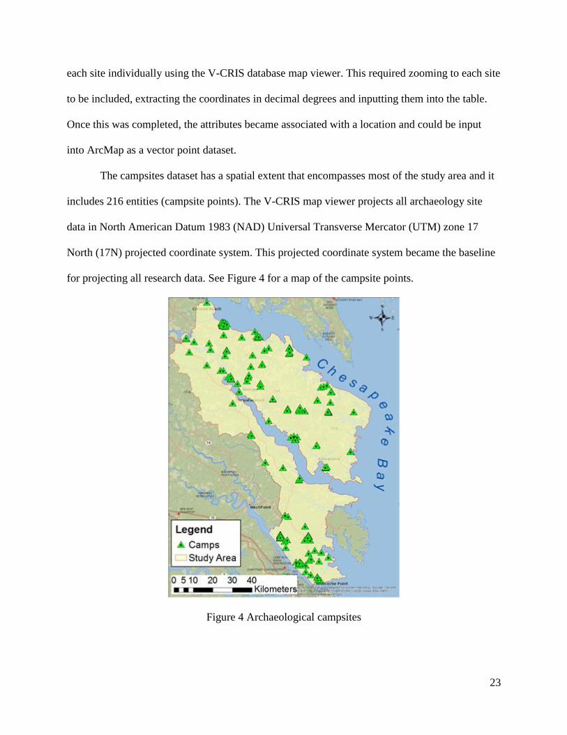
The campsites dataset has a spatial extent that encompasses most of the study area and it
includes 216 entities (campsite points). The V-CRIS map viewer projects all archaeology site
data in North American Datum 1983 (NAD) Universal Transverse Mercator (UTM) zone 17
North (17N) projected coordinate system. This projected coordinate system became the baseline
for projecting all research data. See Figure 4 for a map of the campsite points.
Figure 4 Archaeological campsites

24
Although the original data includes numerous attributes that could be useful for analysis,
there are several issues hindering their use. For example, data completeness is dependent on the
individual who originally entered the information about each site. Therefore, some sites have
missing data for some attributes. Also, the “time period” attribute is problematic for analysis
since precise dates are difficult to determine for archaeological sites. Thus, many of the time
periods entered are approximate. However, since the objective was simply to predict locations of
campsites, these limitations in the source data were easily disregarded in this study.
This dataset was used for two purposes in this study. It was used in Maxent as the input
file from which to predict the presence of unknown sites. This dataset was also used to validate
the fuzzy overlay model by comparing the predicted sites to known sites.
3.3 Environmental Data
Environmental data used in the models were obtained from the National Wetlands
Inventory (NWI), the National Oceanic and Atmospheric Administration (NOAA), the
Chesapeake Bay Program (CBP), and the U.S. Geological Survey (USGS). Slope was derived
from the DEM file using the Slope tool in ArcToolbox. Datasets were acquired for the
Chesapeake Bay counties of Essex, Richmond, Westmoreland, Middlesex, Gloucester,
Lancaster, Northumberland and Westmoreland.
For the purpose of this study, a 30 m by 30 m analysis grid was used that is aligned to the
USGS DEMs of similar dimension. The appropriateness of this grid size for this analysis is
supported by Campbell and Johnson (2004) who explain that the 30 m2 cell size has been used in
many similar predictive models. The area of 30 m2 is assumed to be a good representation of the
footprint of a campsite. All environmental attributes were generalized to this resolution.

25
In order to understand the breadth and meaning of each dataset, this section provides a
description of each dataset used in this project, including what the data represents, dataset size,
scale, a brief attribute description, and any issues or errors encountered. As previously
mentioned, each dataset was projected to NAD 1983 UTM zone 17N.
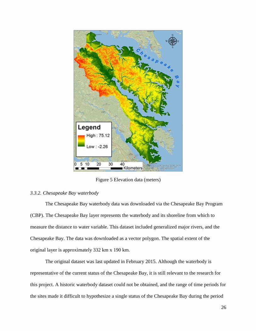
3.3.1. Elevation
Elevation data was downloaded as a Digital Elevation Model (DEM) from USGS in
raster format. The original USGS elevation data was created in 2001. Data was downloaded for
the seven counties within the study area to create the elevation layer. The elevation layer
indicates a representative elevation for the land surface included within each 30 x 30 m cell. The
unit of elevation for this data is meters. As noted above, this cell resolution of 30 x 30 m with a
vertical accuracy of 1 m became the analysis grid for all raster dataset conversions in this project.
The spatial extent for this layer is the same as the study area. See Figure 5 for a representation of
the Elevation layer.
26
Figure 5 Elevation data (meters)
3.3.2. Chesapeake Bay waterbody
The Chesapeake Bay waterbody data was downloaded via the Chesapeake Bay Program
(CBP). The Chesapeake Bay layer represents the waterbody and its shoreline from which to
measure the distance to water variable. This dataset included generalized major rivers, and the
Chesapeake Bay. The data was downloaded as a vector polygon. The spatial extent of the
original layer is approximately 332 km x 190 km.
The original dataset was last updated in February 2015. Although the waterbody is
representative of the current status of the Chesapeake Bay, it is still relevant to the research for
this project. A historic waterbody dataset could not be obtained, and the range of time periods for
the sites made it difficult to hypothesize a single status of the Chesapeake Bay during the period

27
of analysis. For the sake of terrestrial archaeology, the current waterbody is most relevant for
predicting the location of sites inland. Predicting the location of sites within the waterbody
would be useful for marine archaeology, which is not the focus of this research. The boundary is
represented by the mean tide level. This dataset was chosen as a general representation of the
waterbody layer. Because of the ever-changing nature of the tides and water level, the layer was
chosen to represent the mean tide level. The representation of this layer is visible in Figure 6.
Figure 6 Waterbody data
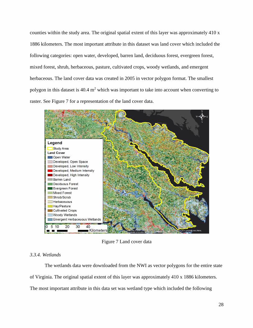
3.3.3. Land Cover
Land cover data for the state of Virginia was downloaded as a vector polygon from the
USGS National Land Cover Database (NLCD). The data was later extracted for the seven
28
counties within the study area. The original spatial extent of this layer was approximately 410 x
1886 kilometers. The most important attribute in this dataset was land cover which included the
following categories: open water, developed, barren land, deciduous forest, evergreen forest,
mixed forest, shrub, herbaceous, pasture, cultivated crops, woody wetlands, and emergent
herbaceous. The land cover data was created in 2005 in vector polygon format. The smallest
polygon in this dataset is 40.4 m2 which was important to take into account when converting to
raster. See Figure 7 for a representation of the land cover data.
Figure 7 Land cover data
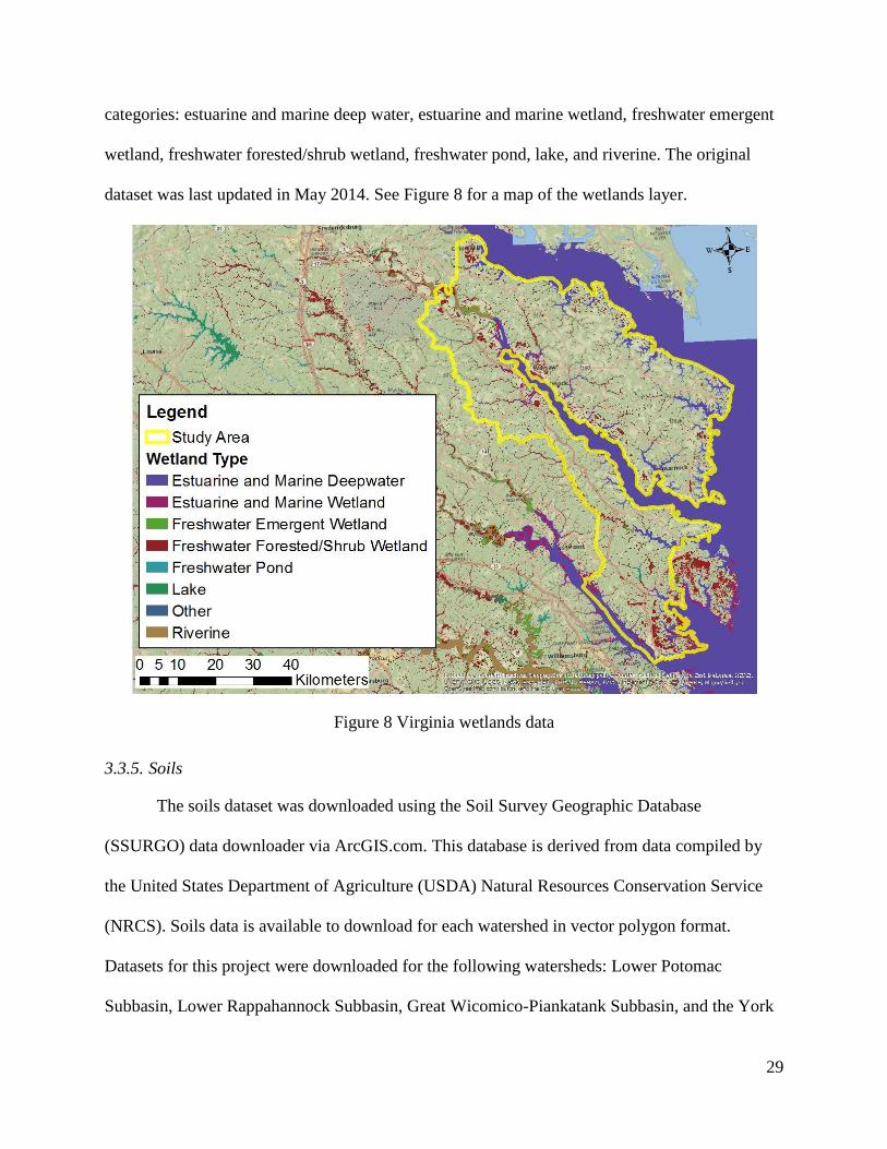
3.3.4. Wetlands
The wetlands data were downloaded from the NWI as vector polygons for the entire state
of Virginia. The original spatial extent of this layer was approximately 410 x 1886 kilometers.
The most important attribute in this data set was wetland type which included the following
29
categories: estuarine and marine deep water, estuarine and marine wetland, freshwater emergent
wetland, freshwater forested/shrub wetland, freshwater pond, lake, and riverine. The original
dataset was last updated in May 2014. See Figure 8 for a map of the wetlands layer.
Figure 8 Virginia wetlands data
3.3.5. Soils
The soils dataset was downloaded using the Soil Survey Geographic Database
(SSURGO) data downloader via ArcGIS.com. This database is derived from data compiled by
the United States Department of Agriculture (USDA) Natural Resources Conservation Service
(NRCS). Soils data is available to download for each watershed in vector polygon format.
Datasets for this project were downloaded for the following watersheds: Lower Potomac
Subbasin, Lower Rappahannock Subbasin, Great Wicomico-Piankatank Subbasin, and the York

30
Subbasin. The spatial extent for this layer is approximately 243 X 239 kilometers. Key attributes
included in these datasets are map unit name, flood frequency, drainage class, runoff, and erosion
class. The map depicted below shows the soil regions downloaded for this project. The soil type
attribute used for the environmental layer was too fine to depict in graphical form, as the value
indicated for a legend exceeded 200 rows. This data was last updated in February 2014. See
Figure 9 for a map of the watersheds used to acquire data for the soils layer.
Figure 9 Watersheds used to acquire soils data
3.3.6. Virginia Major Roads
This dataset was used in the risk analysis portion of this project. The dataset was created
by The Virginia Geographic Information Network (VGIN). VGIN coordinates and manages the
development of the statewide digital road centerline data which includes: address, road name,
and state route number. The dataset is a part of The Road Centerline Program (RCL) which is
focused on creating a single statewide, consistent digital road file. The RCL data layer is

31
supported and maintained by Virginia's local governments, the Virginia Department of
Transportation (VDOT), and VGIN. The RCL dataset is updated every four months for major
roads in Virginia.
Figure 10 Virginia’s major roads data
3.4 Data preparation
Preparation for modeling began with data collection and conversion. Data were converted
into forms suitable for fuzzy overlay analysis and Maxent in ArcMap 10.3. Based on the
previous research discussed in Chapter 2, it was determined that the location of potential sites
should be modeled from the environmental variables of: distance from water, percent slope, land
cover type, wetland type, soil type and elevation.
3.4.1. Preliminary data manipulation
The data used for both models are the same, however, they are utilized by the models in
different formats. The initial preparation is relevant for both models. Additional preparation
32
needed for each model is explained in the following subsections. First, each data layer was
projected to the NAD1983 UTM zone 17N projected coordinate system.
Secondly, a slope layer was derived from the elevation DEM using the Slope tool in
ArcMap 10.3. The slope was determined using percent rise rather than degree of slope. Percent
rise is used because it most commonly used in previous archaeological research studies.
Next, the wetlands layer, the Chesapeake Bay layer, the soils layer, and the land cover
layer were converted from vector polygon to raster format. The new raster layers were snapped
to the elevation layer to ensure all layers had the same cell size of 30 meters, the same spatial
extent, were projected to the same coordinate system, and were co-registered spatially.
Next, each layer was extracted to encompass only the study area using the Extract by
Mask tool. Each layer was extracted to the mask of the elevation layer, and assigned the same
environments. The next steps for each layer are explained in the following subsections for each
model.
3.4.2. Data preparation for fuzzy overlay
In order to prepare the data for fuzzy overlay analysis, a number of ArcMap tools were
used to convert the variables into the proper format. A large part of the fuzzy logic analysis
involved use of the Fuzzy Membership tool. The Fuzzy Membership tool reclassifies data to a
scale of 0 to 1 based on membership possibility for possible archaeological campsite locations.
In the tool, 1 is assigned to locations that are positively a member of an archaeological campsite
location set, and 0 is assigned to locations that are definitely not part of the set of campsite
locations. Values between 1 and 0 indicate the strength of membership such that locations with
higher numbers (closer to 1) are more likely to contain an archaeology site and locations with
lower numbers are less likely contain a site. The Fuzzy Membership tool reclassifies continuous
33
raster data depending on the fuzzy function used within the tool. However categorical raster data
(e.g. wetland type) must first be reclassified using the Reclassify tool. This tool reclassifies data
on a 1 to 10 scale. These reclassified numbers are then input into Fuzzy Membership to correct
the values from 0 to 1, in order to undergo fuzzy overlay analysis. Other important tools in data
preparation were Euclidean Distance and Fuzzy Overlay which are explained later in this
chapter.
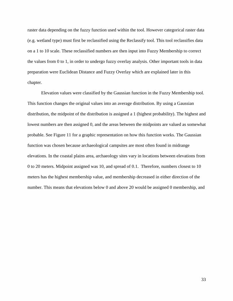
Elevation values were classified by the Gaussian function in the Fuzzy Membership tool.
This function changes the original values into an average distribution. By using a Gaussian
distribution, the midpoint of the distribution is assigned a 1 (highest probability). The highest and
lowest numbers are then assigned 0, and the areas between the midpoints are valued as somewhat
probable. See Figure 11 for a graphic representation on how this function works. The Gaussian
function was chosen because archaeological campsites are most often found in midrange
elevations. In the coastal plains area, archaeology sites vary in locations between elevations from
0 to 20 meters. Midpoint assigned was 10, and spread of 0.1. Therefore, numbers closest to 10
meters has the highest membership value, and membership decreased in either direction of the
number. This means that elevations below 0 and above 20 would be assigned 0 membership, and

34
all elevations beyond 20 up to the highest elevation of 77.5 would be assigned 0 membership as
well.
Figure 11 Illustration of the Gaussian function in Fuzzy Membership. Source: Esri Desktop Help
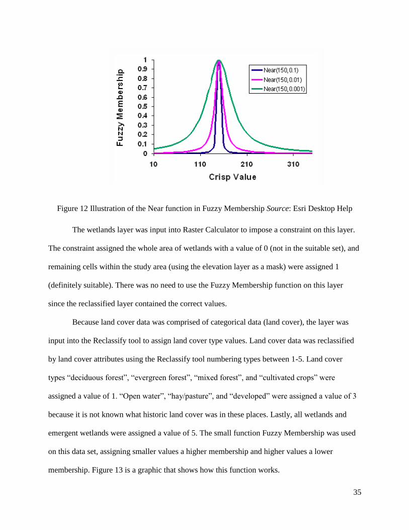
Slope values were classified in Fuzzy Membership using the near function. The near
function specifies a midpoint near a specified number that is assigned the highest membership.
The further from this specified number (in positive and negative directions), it is deemed less fit.
Figure 12 shows a graphic on how this function works. Sites are most likely found in areas with
a 3-7 slope percentage, and 5 was used as the “near” number. The near function was used rather
than the Gaussian because of the specific number in which sites are likely to be found. The gap
between 3-7 slope percentage is small, and so a 5 was deemed the near number.
35
Figure 12 Illustration of the Near function in Fuzzy Membership Source: Esri Desktop Help
The wetlands layer was input into Raster Calculator to impose a constraint on this layer.
The constraint assigned the whole area of wetlands with a value of 0 (not in the suitable set), and
remaining cells within the study area (using the elevation layer as a mask) were assigned 1
(definitely suitable). There was no need to use the Fuzzy Membership function on this layer
since the reclassified layer contained the correct values.
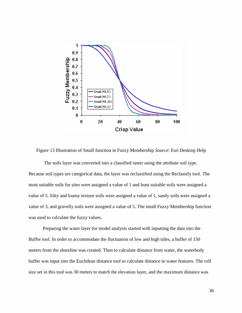
Because land cover data was comprised of categorical data (land cover), the layer was
input into the Reclassify tool to assign land cover type values. Land cover data was reclassified
by land cover attributes using the Reclassify tool numbering types between 1-5. Land cover
types “deciduous forest”, “evergreen forest”, “mixed forest”, and “cultivated crops” were
assigned a value of 1. “Open water”, “hay/pasture”, and “developed” were assigned a value of 3
because it is not known what historic land cover was in these places. Lastly, all wetlands and
emergent wetlands were assigned a value of 5. The small function Fuzzy Membership was used
on this data set, assigning smaller values a higher membership and higher values a lower
membership. Figure 13 is a graphic that shows how this function works.
36
Figure 13 Illustration of Small function in Fuzzy Membership Source: Esri Desktop Help
The soils layer was converted into a classified raster using the attribute soil type.
Because soil types are categorical data, the layer was reclassified using the Reclassify tool. The
most suitable soils for sites were assigned a value of 1 and least suitable soils were assigned a
value of 5. Silty and loamy texture soils were assigned a value of 1, sandy soils were assigned a
value of 3, and gravelly soils were assigned a value of 5. The small Fuzzy Membership function
was used to calculate the fuzzy values.
Preparing the water layer for model analysis started with inputting the data into the
Buffer tool. In order to accommodate the fluctuation of low and high tides, a buffer of 150
meters from the shoreline was created. Then to calculate distance from water, the waterbody
buffer was input into the Euclidean distance tool to calculate distance to water features. The cell
size set in this tool was 30 meters to match the elevation layer, and the maximum distance was
37
set to 2000 meters to accommodate the walkability to a water source. The resulting water
distance layer was input into the Fuzzy Membership tool using the small function, indicating
areas closer to the water were more suitable than areas further away.
3.4.3. Preparation of data for Maxent
Three kinds of data files are required for Maxent: several co-registered ASCII format
raster environmental layers, a .csv file of site locations and, optionally, a bias file indicating the
extent of the model processes. Preparing data to input into Maxent was done in ArcMap 10.3 and
Microsoft Excel.
The environmental layers used in the Maxent model were wetlands, slope, elevation,
soils, and landcover. For processing in Maxent, it was necessary simply to convert the raster
layers described in Section 3.4.1 into ASCII format.
The required .csv file indicates the known site locations from which the model derives
suitable location conditions to predict where possible unknown sites are located. Based on that
information, the model uses the environmental variables (soils, water, wetlands, land cover,
elevation and slope) to determine other areas that are suitable. The bias file indicates the
boundary extent for the model, and the area in which sites are suitable.
As mentioned previously, the campsite points Excel file was converted into a comma
separated values (.csv) file to be input into Maxent. The extent of the study area was earlier
created by selecting Essex, Richmond, Lancaster, Middlesex, Gloucester, Northumberland, and
Westmoreland counties from the US Counties file, then merging this into a single polygon. The
bias file was created by converting the study area polygon feature into raster format using the
Polygon to Raster tool, using the DEM raster template to ensure the layer was coregistered with

38
all the others. Lastly, the file was converted into ASCII (.asc) format to be input into the Maxent
model.
3.5 Model Implementation
This section explains how the fuzzy overlay and Maxent models were implemented. In
order to run the models, different parameters need to be set as explained below.
3.5.1. Running Fuzzy Overlay
The fuzzy membership layers (fuzzy elevation, soils, fuzzy slope, fuzzy wetlands, fuzzy,
water distance, fuzzy land type) are simultaneously input into the Fuzzy Overlay tool. In this
case, the Fuzzy Overlay type used was AND. The fuzzy AND overlay type returns the minimum
value of all the sets for each cell. This technique is useful in identifying the least common
denominator for the membership of all the input criteria The result was an output producing
possible archaeological campsite locations.
In order to ensure successful model results, the model was run several times with slightly
different fuzzy values in order to achieve a result indicating a good fit. The process of iteration
was utilized mainly on the distance to water parameter and the fuzzy overlay operator.
3.5.2. Running Maxent
Maxent builds models by beginning with a uniform distribution of probability of
occurrence over the entire environmental extent. According to the user manual (Phillips 2011),
this distribution uses the environmental layers and presence sites input into the model. Then, the
model conducts an optimization routine that iteratively improves model fit by iteratively running
analyses. Fit is measured as gain. The gain is the deviance statistic that maximizes the
probability of the site presence in relation to environmental data. Gain increases with each
39
iteration. The final probability distribution produces the output showing the probability of the
presence at any location.
In the Maxent interface, the comma separated values campsites file was input as the
‘Samples’ file to indicate known site locations. The slope, elevation, land cover, soils, water, and
wetlands files were input into the ‘Environmental Layers’ path. The counties bias file was input
into the bias file input. The model was set to run with a random seed, subsample type model with
a random test percentage of 25%, and 50 replications. These parameters allowed the model to
withhold a random 25% of the archaeology site samples in each of the 50 replications in order to
calculate probability values and gain. The model was also set to test 80% of the sample size
using the “default prevalence” parameter which indicates the probability that an individual is
observed at a suitable location. At the completion of the processing, the model creates outputs
into a user specified folder with graphs, and ASCII versions of the maps. These results are
explored in the next chapter.
3.6 Risk Analysis
In order to display the value of using models to predict campsite locations, a risk analysis
was conducted. The risk analysis shows which areas within the study region are at potential risk
of human degradation and sea-level rise. The process of risk analysis was conducted using binary
overlay using the Raster Calculator tool in ArcMap. For this analysis, the major road layer was
used to calculate one aspect of human degradation. The waterbody layer was used to represent
distance to water and DEM was used to indicate elevation and used to calculate sea-level rise.
In order to calculate the threat of sea-level rise, several parameters were set to indicate
risk areas, which were input into Raster Calculator. The Euclidean distance from water layer was
used to set the distance to water parameter. Arbitrary distances were used to limit the boundary

40
of the results. Using the elevation layer, areas with an elevation rise of three meters above sea-
level were extracted to indicate water rise. The elevation of three meters above sea-level was
chosen because this is regarded as the projected maximum sea-level rise by 2100 (Lowery 2012).
These data layers were created using raster calculator using a constraint equation to limit the
results to these parameters.
After the variables were created, the sea-level rise layer, water distance layer, and model
results were overlaid to indicate areas at potential risk. Using a binary overlay method, the fuzzy
overlay model results with potential site locations above 0.75 were overlaid with each distinct
water distance, and with the sea-level rise to indicate areas where potential archaeological camp
sites were at risk. The same binary overlay method was used with the Maxent results to
determine risk to high probability sites.
For the purpose of this demonstration, calculating potential threat from human
degradation was indicated by nearness to major roads. The major roads layer was used to
indicate areas of potential development because zoning data, although preferable for analysis,
was unavailable for each county. The major roads layer was deemed a suitable, general measure
of human degradation because of the concept of transit-oriented development. According to
Belzer and Autler (2002), transit-oriented development is based on the principle of businesses,
and residential areas being constructed close to major roadways for more efficient travel to work,
goods, and services. Areas within two-kilometers of a major road were deemed “at risk”. In
order to calculate urbanization risks, the same overlay method described above was used. The
single buffer layer was overlaid with each model result to indicate potential risk areas.
Having outlined the data used for this study and the methods applied, the next chapter
explores the results.
41
Chapter 4 Results
This chapter explains the results of each modeling process. Although the desired outcome for
each model is similar, the manner in which these methods are implemented are unalike. The
process of fuzzy overlay analysis is produced by an organized, deductive workflow, inputting
features into a process, and receiving an outcome to input into another process until the final
outcome. The inductive process of maximum entropy inputs variables into a machine learning
algorithm and iterates the model process, to receive the outcome.
The fuzzy overlay analysis produced results by overlaying the fuzzy environmental
layers. The output from fuzzy overlay is a raster layer with high and low values in which higher
values indicate areas that are more suitable and low values indicating areas that are less suitable.
Maxent produced results through a probability distribution using presence point data (campsites)
and background environmental variables. Maxent outputs a map in ASCII grid format that can be
imported into ArcMap to produce a raster layer. The raster layer shows high and low values,
similar in appearance to those produced in fuzzy overlay, with high values indicating areas with
a high probability of being suitable for sites, and low values indicating areas of less probability.
Maxent also outputs several plots and tables indicating the reliability of the model and how each
environmental variable functioned in the model. These outputs include: jack-knife testing
determining the importance of each environmental layer, response curves indicating how the
model responded to each environmental variable, and the area under the receiver operator curve
(AUC) indicating the fitness of the model. The results of each model are further explained
below.
42
4.1 Fuzzy Overlay Results
Calculation of fuzzy overlay analysis results was determined using fuzzy logic. Fuzzy
logic uses a continuum of logical values between 0 (completely false/unsuitable) and 1
(completely true/suitable). Values in between are conditions that are “partly true” and “partly
false”. This logic was applied to campsites due to the elements of uncertainty in finding them,
and the lack of discrete variables. Concrete variables cannot be calculated because strict
boundaries for archaeology sites are hard to define, and sites are susceptible to their
environment. In this project, fuzzy overlay analysis was used to predict the possible site locations
for unknown archaeological campsites locations. Fuzzy membership for layers is determined by
known suitable environmental conditions, as proposed in prior research. As mentioned above,
each factor (elevation, slope, soils, distance to water, wetland type, and land cover) was assigned
a fuzzy membership based on suitable attribute conditions. These features were then overlaid on
top of each other with the AND fuzzy overlay operator to determine the locations that are most
suitable for sites.
As mentioned above, the combination of fuzzy membership layers used the AND
operator. The AND operator determines the minimum value for each cell of all input fuzzy layers
to create the output layer. In doing so, the operation determines the least common denominator
for membership criteria. Figure 14 shows the site suitability map that resulted from fuzzy overlay
analysis. Suitability values range from 0 to 1 and are classified into 4 equal classes plus None for
values of 0 (shown in dark green). Values from .76 to 1 are represented by red (high suitability),
from .51 to .75 by orange-red (moderate suitability), from .26-.5 by yellow (slight suitability)
and from .1 to .25 by green (low suitability).
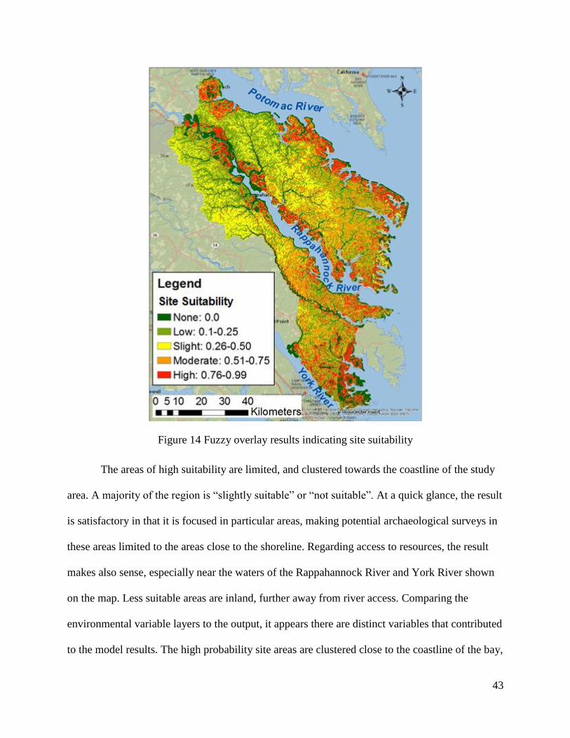
43
Figure 14 Fuzzy overlay results indicating site suitability
The areas of high suitability are limited, and clustered towards the coastline of the study
area. A majority of the region is “slightly suitable” or “not suitable”. At a quick glance, the result
is satisfactory in that it is focused in particular areas, making potential archaeological surveys in
these areas limited to the areas close to the shoreline. Regarding access to resources, the result
makes also sense, especially near the waters of the Rappahannock River and York River shown
on the map. Less suitable areas are inland, further away from river access. Comparing the
environmental variable layers to the output, it appears there are distinct variables that contributed
to the model results. The high probability site areas are clustered close to the coastline of the bay,
44
and near river inlets. Two main environmental factors would contribute to this trend: elevation
and distance to water. Closer to the shoreline, the elevation is lower and would lie between the
predicted range of between 0-20 feet. The distance to water also appears to be a high
contributing factor which reflects the parameter that a water source should be within reasonable
walking distance (2000 meters).
In order to assess the accuracy of the model, the results of the fuzzy overlay prediction
were compared to known archaeological campsite locations. Figure 15 below shows the location
of campsites over the fuzzy overlay suitability map. Clusters of known archaeological sites
appear along the Chesapeake Bay in the predicted high suitability areas. However, the
relationship between these distributions is not immediately apparent given the cell size at which
the analysis was conducted.

45
Figure 15 Fuzzy overlay results with archaeological camps
To explore this relationship further, Table 1 below shows the number and percentage of
each known archaeological sites found within each suitability area displayed in the map. In total,
approximately 122 archaeological sites (out of the total 216) are found in high suitability areas,
38 are found in moderately suitability areas, 25 are found in slightly suitable areas, 23 are found
in low suitably areas, and 8 are found in none suitability areas. Thus, 56% of known archaeology
sites are found in high suitability areas. A chi-square test was also performed on the values
output for each category. After running the chi-square test, the probability of the distributed sites
was 0.0015, indicating the models nonrandom distribution of results.
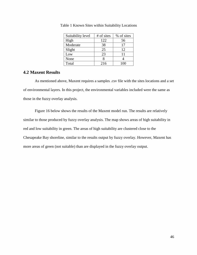
46
Table 1 Known Sites within Suitability Locations
Suitability level # of sites % of sites
High 122 56
Moderate 38 17
Slight 25 12
Low 23 11
None 8 4
Total 216 100
4.2 Maxent Results
As mentioned above, Maxent requires a samples .csv file with the sites locations and a set
of environmental layers. In this project, the environmental variables included were the same as
those in the fuzzy overlay analysis.
Figure 16 below shows the results of the Maxent model run. The results are relatively
similar to those produced by fuzzy overlay analysis. The map shows areas of high suitability in
red and low suitability in green. The areas of high suitability are clustered close to the
Chesapeake Bay shoreline, similar to the results output by fuzzy overlay. However, Maxent has
more areas of green (not suitable) than are displayed in the fuzzy overlay output.
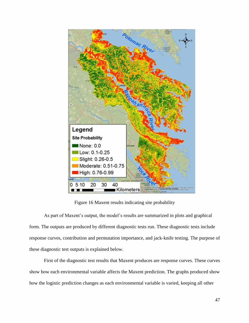
47
Figure 16 Maxent results indicating site probability
As part of Maxent’s output, the model’s results are summarized in plots and graphical
form. The outputs are produced by different diagnostic tests run. These diagnostic tests include
response curves, contribution and permutation importance, and jack-knife testing. The purpose of
these diagnostic test outputs is explained below.
First of the diagnostic test results that Maxent produces are response curves. These curves
show how each environmental variable affects the Maxent prediction. The graphs produced show
how the logistic prediction changes as each environmental variable is varied, keeping all other
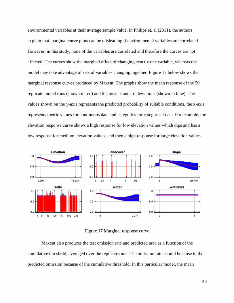
48
environmental variables at their average sample value. In Philips et. al (2011), the authors
explain that marginal curve plots can be misleading if environmental variables are correlated.
However, in this study, none of the variables are correlated and therefore the curves are not
affected. The curves show the marginal effect of changing exactly one variable, whereas the
model may take advantage of sets of variables changing together. Figure 17 below shows the
marginal response curves produced by Maxent. The graphs show the mean response of the 50
replicate model runs (shown in red) and the mean standard deviations (shown in blue). The
values shown on the y-axis represents the predicted probability of suitable conditions, the x-axis
represents metric values for continuous data and categories for categorical data. For example, the
elevation response curve shows a high response for low elevation values which dips and has a
low response for medium elevation values, and then a high response for large elevation values.
Figure 17 Marginal response curve
Maxent also produces the test omission rate and predicted area as a function of the
cumulative threshold, averaged over the replicate runs. The omission rate should be close to the
predicted omission because of the cumulative threshold. In this particular model, the mean
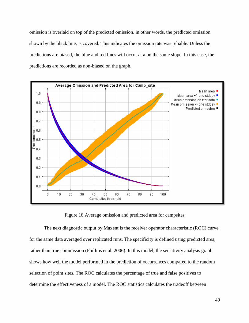
49
omission is overlaid on top of the predicted omission, in other words, the predicted omission
shown by the black line, is covered. This indicates the omission rate was reliable. Unless the
predictions are biased, the blue and red lines will occur at a on the same slope. In this case, the
predictions are recorded as non-biased on the graph.
Figure 18 Average omission and predicted area for campsites
The next diagnostic output by Maxent is the receiver operator characteristic (ROC) curve
for the same data averaged over replicated runs. The specificity is defined using predicted area,
rather than true commission (Phillips et al. 2006). In this model, the sensitivity analysis graph
shows how well the model performed in the prediction of occurrences compared to the random
selection of point sites. The ROC calculates the percentage of true and false positives to
determine the effectiveness of a model. The ROC statistics calculates the tradeoff between
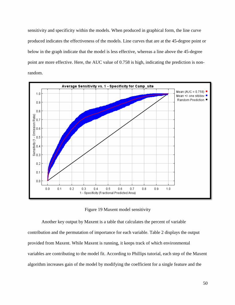
50
sensitivity and specificity within the models. When produced in graphical form, the line curve
produced indicates the effectiveness of the models. Line curves that are at the 45-degree point or
below in the graph indicate that the model is less effective, whereas a line above the 45-degree
point are more effective. Here, the AUC value of 0.758 is high, indicating the prediction is non-
random.
Figure 19 Maxent model sensitivity
Another key output by Maxent is a table that calculates the percent of variable
contribution and the permutation of importance for each variable. Table 2 displays the output
provided from Maxent. While Maxent is running, it keeps track of which environmental
variables are contributing to the model fit. According to Phillips tutorial, each step of the Maxent
algorithm increases gain of the model by modifying the coefficient for a single feature and the

51
program assigns the increase in gain to the environmental variables that these features depend
on. This is converted into percentages at the end of the model processes, providing the table
below. The table provides estimates of the relative contributions of the environmental variables
to the model. In the table below, it shows that Maxent used the elevation, soils, and water
variables the most in its model process. The right hand column displays the permutation of
importance. These values are calculated only in the final Maxent model that is iterated. The
contribution for each variable is determined by randomly permuting the values of that variable
among the training points (both presence and background) and measuring the resulting decrease
in training AUC. A large decrease indicates that the model depends heavily on that variable.
Values are normalized to give percentages.
Table 2 Permutation of importance of each environmental variable
Lastly, Maxent provides a graph of the Jackknife of Regularized Training Gain. The
graph shows the training gain of each variable if the model ran the variable alone, and compares
it to the training gain of the rest of the variables. This graph is especially useful in identifying
which variables contribute the most individually to the model. Figure 20 shows the regularized
training gain for the variables run in this model. The jackknife graph supports the table above in
displaying the elevation, distance to water, and soils variables as the highest contributing
variables to the model.
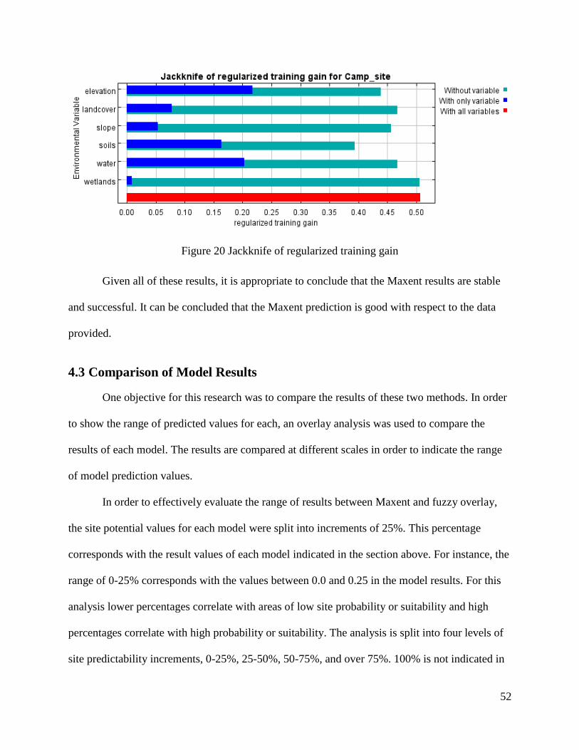
52
Figure 20 Jackknife of regularized training gain
Given all of these results, it is appropriate to conclude that the Maxent results are stable
and successful. It can be concluded that the Maxent prediction is good with respect to the data
provided.
4.3 Comparison of Model Results
One objective for this research was to compare the results of these two methods. In order
to show the range of predicted values for each, an overlay analysis was used to compare the
results of each model. The results are compared at different scales in order to indicate the range
of model prediction values.
In order to effectively evaluate the range of results between Maxent and fuzzy overlay,
the site potential values for each model were split into increments of 25%. This percentage
corresponds with the result values of each model indicated in the section above. For instance, the
range of 0-25% corresponds with the values between 0.0 and 0.25 in the model results. For this
analysis lower percentages correlate with areas of low site probability or suitability and high
percentages correlate with high probability or suitability. The analysis is split into four levels of
site predictability increments, 0-25%, 25-50%, 50-75%, and over 75%. 100% is not indicated in
53
this analysis because neither of the models resulted in a 100% values. For each increment of
suitability/probability, the results were compared to indicate in which areas the models produced
the same results and which areas the model differed in predictions.
The results for each increment are illustrated below. Figure 21 displays the comparative
results of each models predictions with a 0-25% probability/suitability of an archaeological
campsite presence. The red sections in the map indicate areas where both models predicted a 0-
25% probability of site presence. Areas indicated in yellow display where only fuzzy overlay
indicated suitability for sites. The purple areas indicate areas where Maxent predicted the given
range of probability of sites. The green areas indicate areas out of the range of probability (over
0-25%). Consecutively, Figure 22 compares the results of 25-50% range of predictability for
each model, Figure 23 compares the results of 50-75%, and Figure 24 compares the results of
predictions over the 75% range. These maps show that the lowest and highest range of
probability/suitability areas have a greater area of matching results. This conclusion is supported
by a visual comparison of the results of each model and by the calculation of the count of grid
cells for each comparative map category shown in Table 3. It is also evident that both models
produced a much more limited area for highly likely/suitable potential site locations. The lower
values cover a more expansive part of the study area in both sets of results.
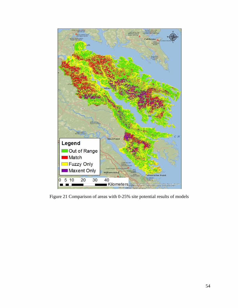
54
Figure 21 Comparison of areas with 0-25% site potential results of models
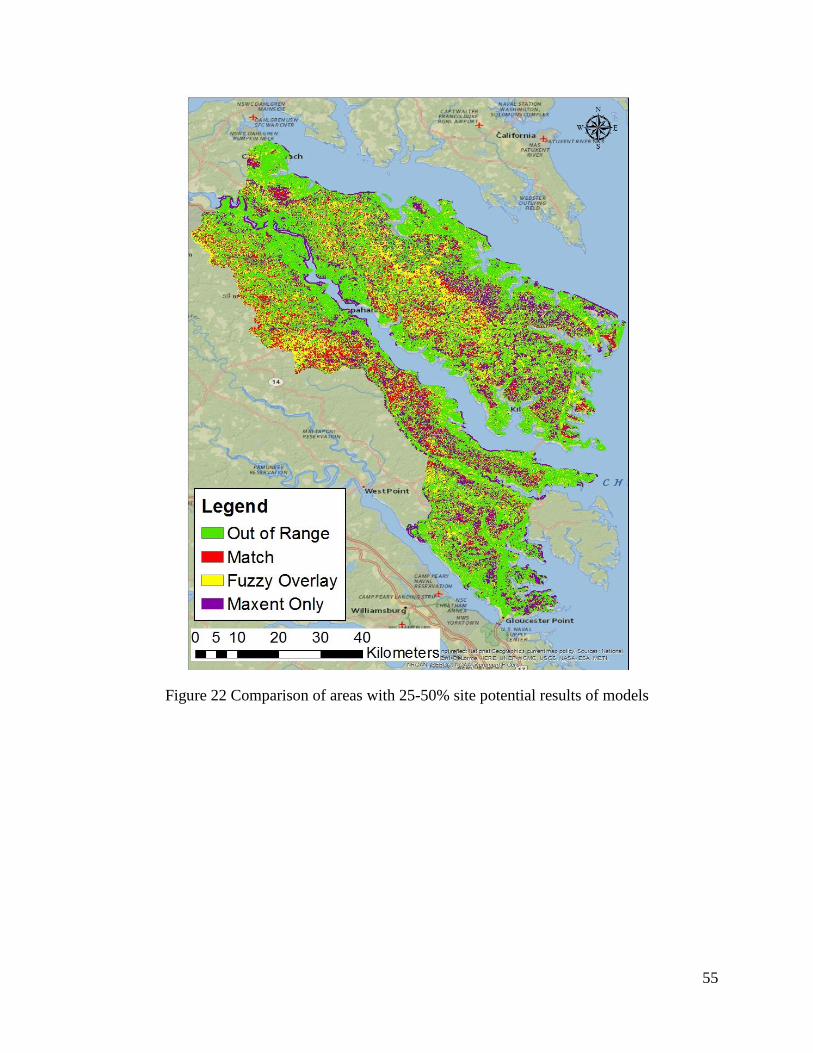
55
Figure 22 Comparison of areas with 25-50% site potential results of models
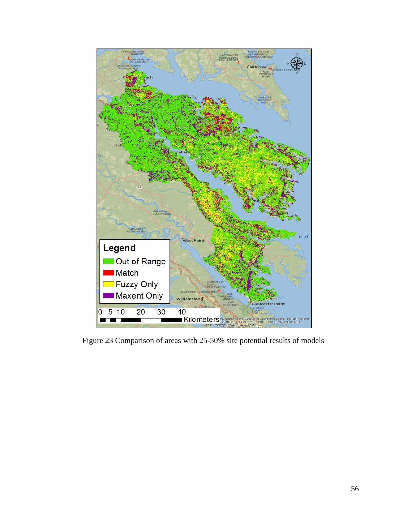
56
Figure 23 Comparison of areas with 25-50% site potential results of models
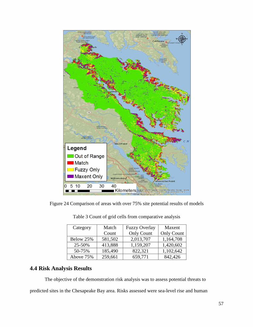
57
Figure 24 Comparison of areas with over 75% site potential results of models
Table 3 Count of grid cells from comparative analysis
Category Match
Count
Fuzzy Overlay
Only Count
Maxent
Only Count
Below 25% 581,502 2,013,707 1,164,708
25-50% 413,888 1,159,207 1,420,602
50-75% 185,490 822,321 1,102,642
Above 75% 259,661 659,771 842,426
4.4 Risk Analysis Results
The objective of the demonstration risk analysis was to assess potential threats to
predicted sites in the Chesapeake Bay area. Risks assessed were sea-level rise and human

58
degradation resulting from nearness to major roads. This overlay analysis for the risk assessment
was kept simple as it was not the primary goal of this project. Rather it is included as a
supplement to the research, showing how modeled results can be used in threat analysis for
cultural resource management purposes. The figures below display the relationship between
areas of each potential threat and each of the model results: the fuzzy overlay suitability
locations and the Maxent high probability locations.
Calculating the sea-level rise results involved overlaying three layers: the model result
layer, the meters above sea-level layer, and the distance to water layer. The model result layer
only includes area of high probability (above 0.75). The results for the risk of sea-level rise risk
overlaid on the fuzzy overlay site suitability is displayed in Figure 25. Red represents high risk
of destruction from sea-level rise, yellow represents a moderate risk, and blue represents a low
risk of destruction. Figure 26 displays the risk analysis of sea-level rise for the Maxent results.
Calculating the risk analysis for threat of human degradation involved overlaying the
distance to roads layer and the model results layer. The results of the human degradation risk
analysis for fuzzy overlay is displayed in Figure 27 and the results of the risk of human
degradation risk for Maxent results is displayed in Figure 28.

59
Figure 25 Risk of sea-level rise to highly suitable locations from the fuzzy overlay analysis
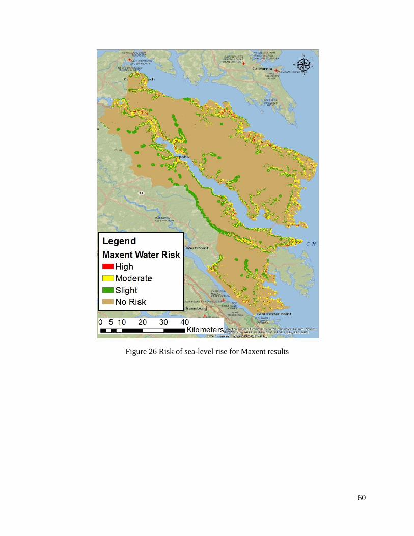
60
Figure 26 Risk of sea-level rise for Maxent results

61
Figure 27 Risk of urbanization for fuzzy overlay results
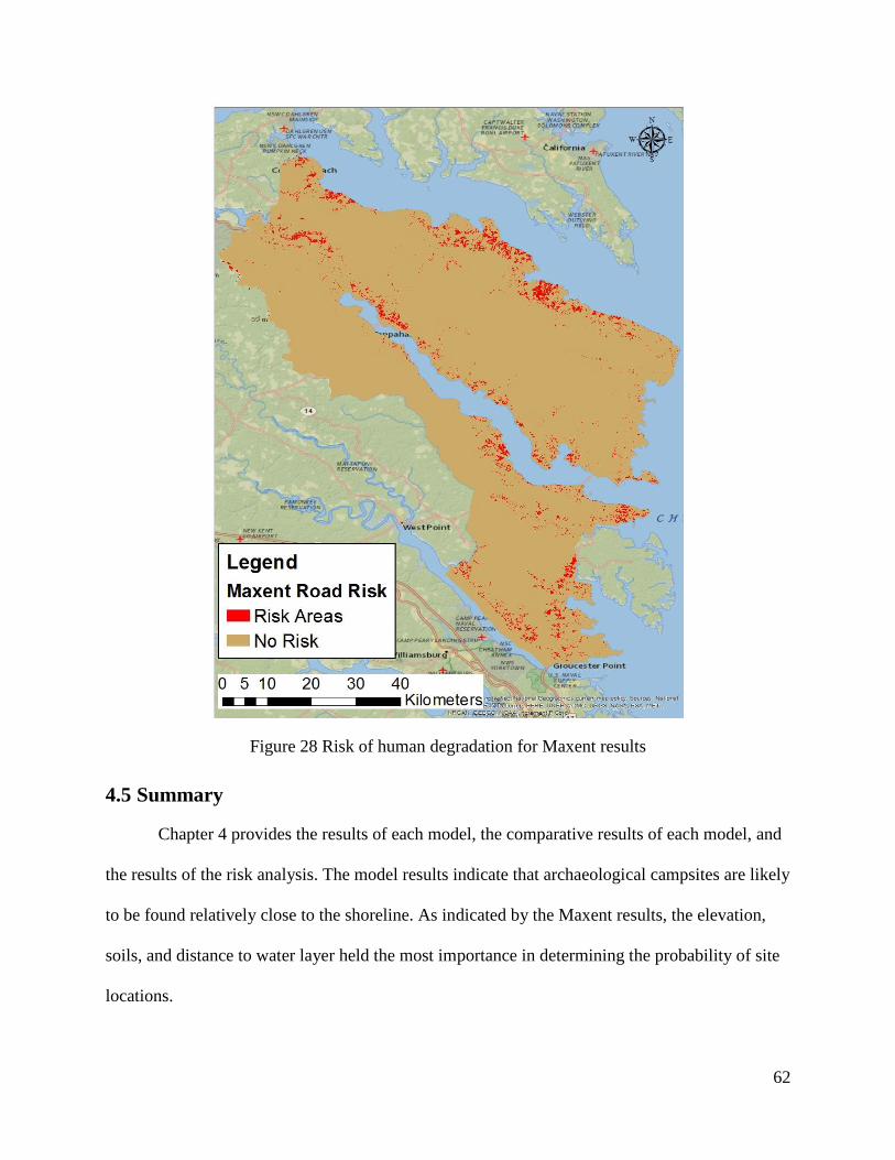
62
Figure 28 Risk of human degradation for Maxent results
4.5 Summary
Chapter 4 provides the results of each model, the comparative results of each model, and
the results of the risk analysis. The model results indicate that archaeological campsites are likely
to be found relatively close to the shoreline. As indicated by the Maxent results, the elevation,
soils, and distance to water layer held the most importance in determining the probability of site
locations.
63
Chapter 5 Summary and Conclusions
The purpose of this project was to evaluate the effectiveness of the fuzzy overlay model and
Maxent model for predicting the presence of unknown archaeological sites along Virginia’s
Chesapeake coast to aid in their preservation and site management. This chapter discusses and
compares the results of each model, evaluates model effectiveness and addresses the results of
the risk analysis.
5.1 Model evaluations
Because the way in which each model runs is different, the evaluation for each is also
different. While Maxent has diagnostic tools included in the program to ensure the best possible
model fit for the environmental variables given, fuzzy overlay requires manual evaluation.
Although the results of each model are relatively different, the performance of each model are
good.
For Maxent, model performance is indicated by the test omission rate and predicted area.
In the model, the mean omission is overlaid on top of the predicted omission, indicating the
omission rate was reliable (see Figure 18). The performance of the Maxent model is also
diagnosed by the receiver operator characteristic (ROC) curve. The ROC calculates the
percentage of true and false positives to determine the effectiveness of a model. In Maxent, the
ROC is produced in graphical form. Line curves that are at the 45-degree point or below in the
graph indicate that the model is less effective, whereas a line above the 45-degree point are more
effective. In this model, the AUC value of 0.758 is high, indicating the prediction is non-random
(Figure 19).

64
For the fuzzy overlay model, Model results were also compared to known archaeological
site point data. In this instance, 56% of sites fell within the high predicted ranges and a chi-
square test determined the distribution of results was nonrandom.
In order to assess the results, the outcome for the Maxent model and for the fuzzy overlay
model were compared. Comparing the models visually, it appears that the areas of prediction are
relatively similar, with Maxent producing a more limited area of prediction. However, when
comparing the results together in one map, it is evident that each model produced moderately
different results. The differences in each models results are due to the different methods by
which each model evaluates the environmental variables to produce results.
In fuzzy overlay, a deductive approach, variable parameters are set by the researcher and
then undergo fuzzy membership and overlay to produce a result. Maxent, an inductive machine
learning method, finds the largest spread of potential site presence based on correlations between
the site point data and the input environmental variables. Maxent output provides information
regarding which environmental factors have the highest importance to the model. In this case,
elevation had the highest impact while soils and wetlands had low impact on the model.
However, the fact that the models did have some prediction overlap for the most likely or
suitable areas for sites indicates that the models were effective.
5.2 Modeling for Risk Analysis
The risk analysis portion of this project demonstrated how the presence of threat can be
related to the location of highly likely or suitable sites as predicted by the models. Such a process
shows how such archaeological prediction models can be used in cultural resource management,
urban planning and site preservation. The results of the risk management show that areas with a
high probability of predicted sites (over 75%) are threatened by sea-level rise and urbanization.

65
The simple analysis shows that there is a large area within the study region that poses a risk of
urbanization to the predicted sites (see Figure 27 and Figure 28). The risk of sea-level rise in the
study area is also prevalent at varying degrees (see Figure 25 and Figure 26). The risk analysis
outlines critical areas for CRM archaeologists and land management agencies to survey for
preservation of sites. In conjunction with archaeological prediction models, risk analysis is a
great way to prioritize cultural areas for preservation and management.
5.3 Limitations and Observations
This study was conducted in order to determine whether a deductive model approach and
an inductive model approach could be used to predict the probability of campsite locations and to
establish whether or not these sites are at risk of human degradation and sea-level rise. Although
the models appear to be successful, there are limits to the analysis of results. Ideally, in order to
justify whether or not these models were successful, archaeological survey would need to be
conducted in these areas to ensure that sites exist in the areas that models produced a high
probability of sites. Due to time constraints and lack of resources, a large-scale survey was not
conducted.
The study was also limited by available data to conduct risk analysis. As mentioned in
Chapter 3, county zoning data would have been ideal for calculating risk of human degradation.
However, instead, the major roads layer was used to indicate proximity to urban zones with
heavy human traffic, and represent the potential for growth.
Lastly, in order to improve this study, a comparison of the permutation of importance of
environmental variables could be used to check the fuzzy overlay analysis. As indicated by
Maxent, the soils, elevation, and distance to water variables carried the most importance in
predicting the probability of site locations.

66
5.4 Future work
For future work, using inductive and deductive models together could help determine the
probability of site locations. This could especially be helpful in the continuation of CRM projects
to help cut costs and efficiently find site locations. Maps and graphical output produced by these
models allow CRM archaeologists find areas of the greatest probable importance when presented
with a road proposal, or building construction. In conjunction with a sophisticated risk analysis,
CRM archaeologists could focus resources and survey time to areas that hold the highest
probable risk of destruction and the highest probability of a site location.
Perhaps in future studies, Maxent could be used to distinguish how to use environmental
variables for other models such as fuzzy overlay. Because of its inductive approach in which it
uses environmental variables to determine the presence of sites, it could aid in better deductive
reasoning when searching for archaeological sites. The Maxent model provides the necessary
input needed to make decisions on where to find sites. If the environmental parameters in fuzzy
overlay mirrored those in Maxent, it could improve the fit of the model.
5.5 Conclusion
This study demonstrates the effectiveness and importance of APMs in predicting the
probability of site locations. Both inductive and deductive APMs prove to be successful and with
similar trended results. The research presented in this thesis provides the basic methodology to
be carried out for future projects to use and improve. The results of the models are especially
helpful for CRM archaeology in finding the probability of site locations for survey areas when
building roads, buildings, businesses etc. Combined with the risk analysis, the model results also
show the importance of APMs in finding possible site locations for historic and prehistoric
preservation.
67
REFERENCES
Belzer, Dena, and Gerard Autler. 2002. Transit Oriented Development: Moving from Rhetoric to
Reality. Technical Report, Brookings Institution Center on Urban and Metropolitan
Policy.
Berger, Adam. 1996. “A Brief Maxent Tutorial.” Accessed November 27, 2015.
http://www.cs.cmu.edu/afs/cs/user/aberger/www/html/tutorial/tutorial.html
Bevan, Andrew, and Alan Wilson. 2013. "Models of Settlement Hierarchy Based on Partial
Evidence." Accessed April 3, 2015. Journal of Archaeological Science, 1-28.
Brown, K. L. 1977. “Late Prehistoric Settlement Patterns in Southwestern Kansas: A Model.”
Master’s Thesis, Anthropology, University of Kansas, Lawrence.
Campbell, Joshua S. 2012. "Archaeological Predictive Model of Southwestern Kansas." PhD
diss., University of Kansas.
Campbell, Joshua, and W. C. Johnson. 2004. Temporal Predictive Model for Fort Hood, Texas:
A Pilot Study in the Cowhouse Creek Drainage. Fort Hood: United States Army.
Clark, W. A. V., and P. L. Hosking. 1986. Statistical Methods for Geographers. New York:
Wiley & Sons.
Galletti, Christopher S., Elizabeth Ridder, Steven E. Falconer, and Patricia L. Fall. 2013.
"Maxent Modeling of Ancient and Modern Agricultural Terraces in the Troodos
Foothills, Cyprus." Applied Geography (39): 46-56
Hudak, G. J., E. Hobbs, A. Brooks, C. A. Sersland, and C. Phillips. 2000. A Predictive Model of
Precontact Archaeological Site Location for The State of Minnesota. St. Paul: Minnesota
Department of Transportation.
Judge, W. J., and L. Sebastian, eds. 1988. Quantifying the Present and Predicting the Past:
Theory, Method, and Application of Archaeological Predictive Modeling. Denver: U.S.
Bureau of Land Management, Department of Interior.
Kuiper, James A., and Konnie L. Wescott. 1999. “A GIS Approach for Predicting Prehistoric
Site Locations.” The Review of Economic Studies 72: 1-18.
Kvamme, K. L. 1988. Development and Testing of Quantitative Models. In Quantifying the
Present and Predicting the Past: Theory, Method, and Application of Archaeological
Predictive Modeling, eds. W. J. Judge and L. Sebastian, 325-428. Washington, D.C.: U.S.
Government Printing Office.
———. 1990. The Fundamental Principles and Practice of Predictive Archaeological Modeling.
In Mathematics and Information Science in Archaeology: A Flexible Framework, ed. A.
Voorrips, 257-295. Bonn: Holos.
68
———. 1992. A Predictive Site Location Model on the High Plains: An Example with an
Independent Test. Plains Anthropologist 37:19-40.
Lang, N. 2000. “Harmonising Research and Cultural Resource Management.” In Beyond the
Map: Archaeology and Spatial Technologies, by Gary Lock, 214-228. Amsterdam: IOS
Press.
Lock, Gary, and Trevor Harris. 2006."Modeling Applications in Progress." In GIS and
Archaeological Site Location Modeling, by Mark Mehrer and Konnie Wescott, 403-11.
Boca Raton, FL: Taylor & Francis.
Lowery, Darrin L., Michael A. O'Neal, Sebastian Carisio, and Tessa Montini. 2012. Sea Level
Rise in Coastal Virginia: Understanding Impacts to Archaeological Resources. Rep.
Newport News: Virginia Department of Historic Resources.
McGlone, Tim. 2008. “What’s in a Name?” Accessed November 27, 2015.
http://pilotonline.com/news/local/history/what-s-in-a-name-hampton-
roads/article_099f6b90-aa5e-5853-9194-420aae51cea0.html
Mink, Philip B., John Ripy, Keiron Baily, and Ted Grossardt. 2009. “Predictive Archaeological
Modeling using GIS-based Fuzzy Set Estimation.” Paper presented at the Transportation
Research Board Annual Meeting, Washington, D.C. January 11-15.
Mehrer, Mark, and Konnie Wescott. 2006. GIS and Archaeological Site Location Modeling.
Boca Raton, FL: Taylor & Francis.
Merwin, Daria. 2003. "The Potential for Submerged Prehistoric Archaeological Sites off Sandy
Hook." Bulletin of the Archaeological Society of New Jersey, 57 (2003): 1-24.
Phillips, Steven J. n.d. "A Brief Tutorial on Maxent." Unpublished tutorial distributed with
software.
Phillips, Steven J., Robert P. Anderson, and Robert E. Schapire. 2005. "Maximum Entropy
Modeling of Species Geographic Distributions." Ecological Modelling 190 (2006): 231-
259.
Phillips, Steven J. and Miroslav Dudík. 2008. "Modeling of Species Distributions with Maxent:
New Extensions and a Comprehensive Evaluation." Ecography (31): 161-175.
Phillips, Steven J., Miroslav Dudík, and Robert E. Schapire. 2004. "A Maximum Entropy
Approach to Species Distribution Modeling." Proceedings of the Twenty-First
International Conference on Machine Learning: 655-662.
Pilgram, T. 1987. Predicting Archaeological Sites from Environmental Variables, A
Mathematical Model for the Sierra Nevada Foothills, California. Oxford: BAR
International Series 320.

69
Vaughn, Maureen. 2012. “Calculating the Presence of Archaeological Sites in the Pisgah
National Forest.” Master’s Thesis, Anthropology, Warren Wilson College, Pennsylvania.
Warren, R. E., and D. L. Asch. 2000. “A Predictive Model of Archaeological Site Location in the
Eastern Prairie Peninsula. In Practical Applications of GIS for Archaeologists: A
Predictive Modeling Kit, by Kuiper Wescott & R.J. Brandon. London: Taylor & Francis.
Wescott, Kuiper, and R. J. Brandon. 2000. Practical Applications of GIS for Archaeologists: A
Predictive Modeling Kit. London: Taylor & Francis.
Zadeh, L. A. 1965. “Fuzzy Sets.” Information and Control (8): 338-353.