Predicting the outcome of rouletteMichael Small and Chi Kong Tse Citation: Chaos 22, 033150 (2012); doi: 10.1063/1.4753920 View online: http://dx.doi.org/10.1063/1.4753920 View Table of Contents: http://chaos.aip.org/resource/1/CHAOEH/v22/i3 Published by the American Institute of Physics. Related ArticlesStability of discrete breathers in nonlinear Klein-Gordon type lattices with pure anharmonic couplings J. Math. Phys. 53, 102701 (2012) Secondary nontwist phenomena in area-preserving maps Chaos 22, 033142 (2012) Delay induced bifurcation of dominant transition pathways Chaos 22, 033141 (2012) Clocking convergence to a stable limit cycle of a periodically driven nonlinear pendulum Chaos 22, 033138 (2012) Characterizing the dynamics of higher dimensional nonintegrable conservative systems Chaos 22, 033137 (2012) Additional information on ChaosJournal Homepage: http://chaos.aip.org/ Journal Information: http://chaos.aip.org/about/about_the_journal Top downloads: http://chaos.aip.org/features/most_downloaded Information for Authors: http://chaos.aip.org/authors

Predicting the outcome of roulette

Michael Small1,2,a) and Chi Kong Tse2

1School of Mathematics and Statistics, The University of Western Australia, Perth, Australia2Department of Electronic and Information Engineering, Hong Kong Polytechnic University, Hong Kong

(Received 30 April 2012; accepted 4 September 2012; published online 26 September 2012)

There have been several popular reports of various groups exploiting the deterministic nature of the

game of roulette for profit. Moreover, through its history, the inherent determinism in the game of

roulette has attracted the attention of many luminaries of chaos theory. In this paper, we provide a

short review of that history and then set out to determine to what extent that determinism can really

be exploited for profit. To do this, we provide a very simple model for the motion of a roulette

wheel and ball and demonstrate that knowledge of initial position, velocity, and acceleration is

sufficient to predict the outcome with adequate certainty to achieve a positive expected return. We

describe two physically realizable systems to obtain this knowledge both incognito and in situ. The

first system relies only on a mechanical count of rotation of the ball and the wheel to measure the

relevant parameters. By applying these techniques to a standard casino-grade European roulette

wheel, we demonstrate an expected return of at least 18%, well above the �2.7% expected of a

random bet. With a more sophisticated, albeit more intrusive, system (mounting a digital camera

above the wheel), we demonstrate a range of systematic and statistically significant biases which

can be exploited to provide an improved guess of the outcome. Finally, our analysis demonstrates

that even a very slight slant in the roulette table leads to a very pronounced bias which

could be further exploited to substantially enhance returns. VC 2012 American Institute of Physics.

[http://dx.doi.org/10.1063/1.4753920]

“No one can possibly win at roulette unless he steals

money from the table when the croupier isn’t

looking” (Attributed to Albert Einstein in Ref. 1)

Among the various gaming systems, both current

and historical, roulette is uniquely deterministic. Rela-

tively simple laws of motion allow one, in principle, to

forecast the path of the ball on the roulette wheel and to

its final destination. Perhaps because of this appealing

deterministic nature, many notable figures from the early

development of chaos theory have leant their hand to

exploiting this determinism and undermining the pre-

sumed randomness of the outcome. In this paper, we aim

only to establish whether the determinism in this system

really can be profitably exploited. We find that this is def-

initely possible and propose several systems which could

be used to gain an edge over the house in a game of rou-

lette. While none of these systems are optimal, they all

demonstrate positive expected return.

I. A HISTORY OF ROULETTE

The game of roulette has a long, glamorous, inglorious

history, and has been connected with several notable men of

science. The origin of the game has been attributed,2 perhaps

erroneously,1 to the mathematician Blaise Pascal.3 Despite

the roulette wheel becoming a staple of probability theory,

the alleged motivation for Pascal’s interest in the device was

not solely to torment undergraduate students, but rather as

part of a vain search for perpetual motion. Alternative stories

have attributed the origin of the game to the ancient Chinese,

a French monk or an Italian mathematician.2,4 In any case,

the device was introduced to Parisian gamblers in the mid-

eighteenth century to provide a fairer game than those cur-

rently in circulation. By the turn of the century, the game

was popular and wide-spread. Its popularity bolstered by its

apparent randomness and inherent (perceived) honesty.

The game of roulette consists of a heavy wheel,

machined and balanced to have very low friction, and

designed to spin for a relatively long time with a slowly

decaying angular velocity. The wheel is spun in one direc-

tion, while a small ball is spun in the opposite direction on

the rim of a fixed circularly inclined surface surrounding and

abutting the wheel. As the ball loses momentum, it drops to-

ward the wheel and eventually will come to rest in one of 37

numbered pockets arranged around the outer edge of the

spinning wheel. Various wagers can be made on which

pocket, or group of pockets, the ball will eventually fall into.

It is accepted practice that, on a successful wager on a single

pocket, the casino will pay 35 to 1. Thus, the expected return

from a single wager on a fair wheel is ð35þ 1Þ � 137

þð�1Þ � �2:7%.5 In the long-run, the house will, naturally,

win. In the eighteenth century, the game was fair and con-

sisted of only 36 pockets. Conversely, an American roulette

wheel is even less fair and consists of 38 pockets. We con-

sider the European, 37 pocket, version as this is of more im-

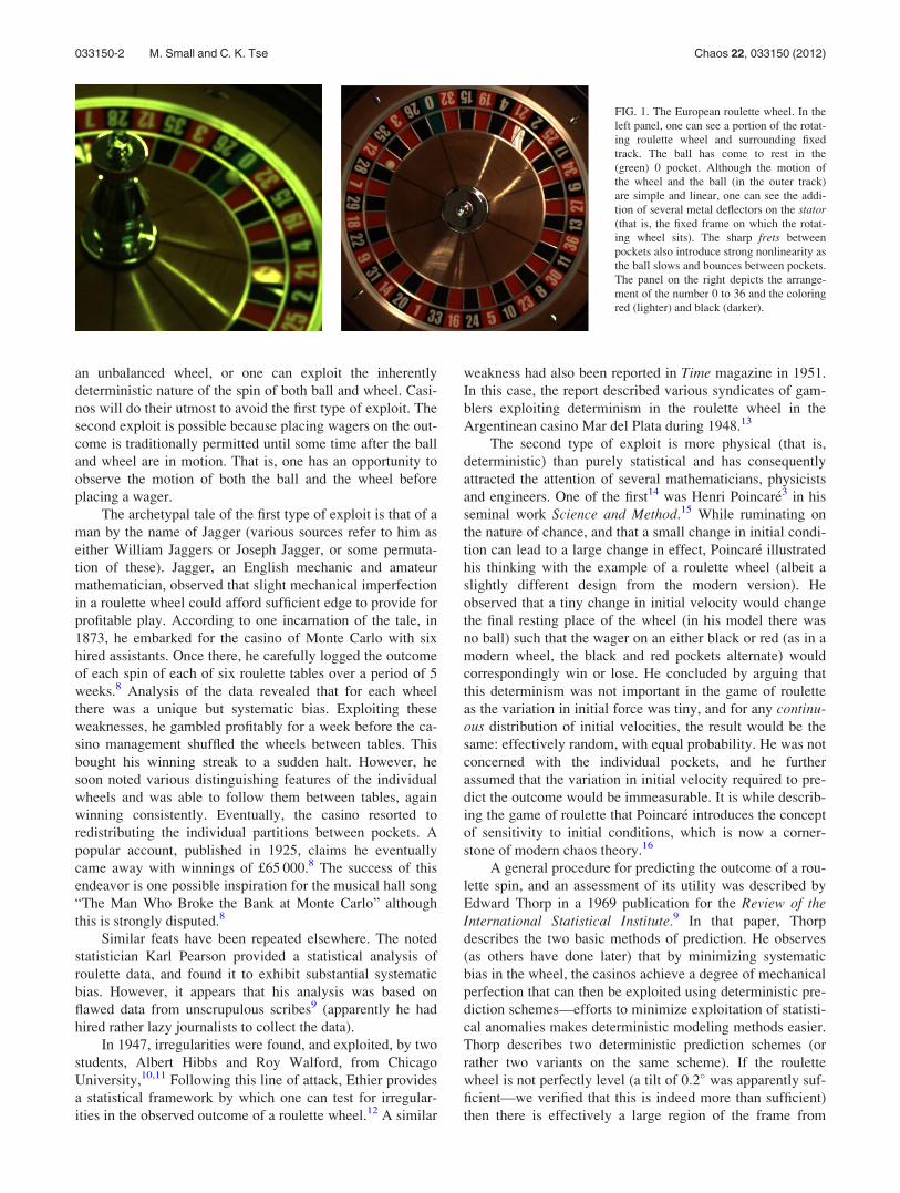
mediate interest to us.6 Figure 1 illustrates the general

structure, as well as the layout of pockets, on a standard

European roulette wheel.

Despite many proposed “systems,” there are only two

profitable ways to play roulette.7 One can either exploita)Electronic mail: michael.small@uwa.edu.au.

1054-1500/2012/22(3)/033150/9/$30.00 VC 2012 American Institute of Physics22, 033150-1

CHAOS 22, 033150 (2012)

an unbalanced wheel, or one can exploit the inherently

deterministic nature of the spin of both ball and wheel. Casi-

nos will do their utmost to avoid the first type of exploit. The

second exploit is possible because placing wagers on the out-

come is traditionally permitted until some time after the ball

and wheel are in motion. That is, one has an opportunity to

observe the motion of both the ball and the wheel before

placing a wager.

The archetypal tale of the first type of exploit is that of a

man by the name of Jagger (various sources refer to him as

either William Jaggers or Joseph Jagger, or some permuta-

tion of these). Jagger, an English mechanic and amateur

mathematician, observed that slight mechanical imperfection

in a roulette wheel could afford sufficient edge to provide for

profitable play. According to one incarnation of the tale, in

1873, he embarked for the casino of Monte Carlo with six

hired assistants. Once there, he carefully logged the outcome

of each spin of each of six roulette tables over a period of 5

weeks.8 Analysis of the data revealed that for each wheel

there was a unique but systematic bias. Exploiting these

weaknesses, he gambled profitably for a week before the ca-

sino management shuffled the wheels between tables. This

bought his winning streak to a sudden halt. However, he

soon noted various distinguishing features of the individual

wheels and was able to follow them between tables, again

winning consistently. Eventually, the casino resorted to

redistributing the individual partitions between pockets. A

popular account, published in 1925, claims he eventually

came away with winnings of £65 000.8 The success of this

endeavor is one possible inspiration for the musical hall song

“The Man Who Broke the Bank at Monte Carlo” although

this is strongly disputed.8

Similar feats have been repeated elsewhere. The noted

statistician Karl Pearson provided a statistical analysis of

roulette data, and found it to exhibit substantial systematic

bias. However, it appears that his analysis was based on

flawed data from unscrupulous scribes9 (apparently he had

hired rather lazy journalists to collect the data).

In 1947, irregularities were found, and exploited, by two

students, Albert Hibbs and Roy Walford, from Chicago

University,10,11 Following this line of attack, Ethier provides

a statistical framework by which one can test for irregular-

ities in the observed outcome of a roulette wheel.12 A similar

weakness had also been reported in Time magazine in 1951.

In this case, the report described various syndicates of gam-

blers exploiting determinism in the roulette wheel in the

Argentinean casino Mar del Plata during 1948.13

The second type of exploit is more physical (that is,

deterministic) than purely statistical and has consequently

attracted the attention of several mathematicians, physicists

and engineers. One of the first14 was Henri Poincar�e3 in his

seminal work Science and Method.15 While ruminating on

the nature of chance, and that a small change in initial condi-

tion can lead to a large change in effect, Poincar�e illustrated

his thinking with the example of a roulette wheel (albeit a

slightly different design from the modern version). He

observed that a tiny change in initial velocity would change

the final resting place of the wheel (in his model there was

no ball) such that the wager on an either black or red (as in a

modern wheel, the black and red pockets alternate) would

correspondingly win or lose. He concluded by arguing that

this determinism was not important in the game of roulette

as the variation in initial force was tiny, and for any continu-ous distribution of initial velocities, the result would be the

same: effectively random, with equal probability. He was not

concerned with the individual pockets, and he further

assumed that the variation in initial velocity required to pre-

dict the outcome would be immeasurable. It is while describ-

ing the game of roulette that Poincar�e introduces the concept

of sensitivity to initial conditions, which is now a corner-

stone of modern chaos theory.16

A general procedure for predicting the outcome of a rou-

lette spin, and an assessment of its utility was described by

Edward Thorp in a 1969 publication for the Review of theInternational Statistical Institute.9 In that paper, Thorp

describes the two basic methods of prediction. He observes

(as others have done later) that by minimizing systematic

bias in the wheel, the casinos achieve a degree of mechanical

perfection that can then be exploited using deterministic pre-

diction schemes—efforts to minimize exploitation of statisti-

cal anomalies makes deterministic modeling methods easier.

Thorp describes two deterministic prediction schemes (or

rather two variants on the same scheme). If the roulette

wheel is not perfectly level (a tilt of 0:2� was apparently suf-

ficient—we verified that this is indeed more than sufficient)

then there is effectively a large region of the frame from

FIG. 1. The European roulette wheel. In the

left panel, one can see a portion of the rotat-

ing roulette wheel and surrounding fixed

track. The ball has come to rest in the

(green) 0 pocket. Although the motion of

the wheel and the ball (in the outer track)

are simple and linear, one can see the addi-

tion of several metal deflectors on the stator(that is, the fixed frame on which the rotat-

ing wheel sits). The sharp frets between

pockets also introduce strong nonlinearity as

the ball slows and bounces between pockets.

The panel on the right depicts the arrange-

ment of the number 0 to 36 and the coloring

red (lighter) and black (darker).

033150-2 M. Small and C. K. Tse Chaos 22, 033150 (2012)

which the ball will not fall onto the spinning wheel. By

studying Las Vegas wheels, he observes this condition is met

in approximately one third of wheels. He claims that in such

cases it is possible to garner a expected return of þ15%,

which increased to þ44% with the aid of a “pocket-sized”

computer. Some time later, Thorp revealed that his collabo-

rator in this endeavor was Claude Shannon,17 the founding

father of information theory.18

In his 1967 book,2 the mathematician Richard A.

Epstein describes his earlier (undated) experiments with a

private roulette wheel. By measuring the angular velocity of

the ball relative to the wheel, he was able to predict correctly

the half of the wheel into which the ball would fall. Impor-

tantly, he noted that the initial velocity (momentum) of the

ball was not critical. Moreover, the problem is simply one of

predicting when the ball will leave the outer (fixed) rim as

this will always occur at a fixed velocity. However, a lack of

sufficient computational resources meant that his experi-

ments were not done in real time, and certainly not attempted

within a casino.

Subsequent to, and inspired by, the work of Thorp and

Shannon, another widely described attempt to beat the casi-

nos of Las Vegas was made in 1977–1978 by Doyne Farmer,

Norman Packard, and colleagues.1 It is supposed that

Thorp’s 1969 paper had let the cat out of the bag regarding

profitable betting on roulette. However, despite the assertions

of Bass,1 Thorp’s paper9 is not mathematically detailed

(there is in fact no equations given in the description of rou-

lette). Thorp is sufficiently detailed to leave the reader in no

doubt that the scheme could work, but also vague enough so

that one could not replicate his effort without considerable

knowledge and skill. Farmer, Packard, and colleagues imple-

mented the system on a 6502 microprocessor hidden in a

shoe, and proceeded to apply their method to the various

casinos of the Las Vegas Strip. The exploits of this group are

described in detail in Bass.1 The same group of physicists

went on to apply their skills to the study of chaotic dynami-

cal systems19 and also for profitable trading on the financial

markets.20 In Farmer and Sidorowich’s landmark paper on

predicting chaotic time series21 the authors attribute the in-

spiration for that work to their earlier efforts to beat the

game of roulette.

Less exalted individuals have also been employing sim-

ilar schemes, in some cases fairly recently. In 2004, the

BBC carried the report of three gamblers22 arrested by

police after winning £1 300 000 at the Ritz Casino in Lon-

don. The trio had apparently been using a laser scanner and

their mobile phones to predict the likely resting place of the

ball. Happily, for the trio but not the casino, they were

judged to have broken no laws and allowed to keep their

winnings.23 The scheme we describe in Sec. II and imple-

ment in Sec. III is certainly compatible with the equipment

and results reported in this case. In Sec. IV, we conclude

with some remarks concerning the practicality of applying

these methods in a modern casino, and what steps casinos

could take (or perhaps have taken) to circumvent these

exploits. A preliminary version of these results was pre-

sented at a conference in Macau.24 An independent and

much more detailed model of dynamics of the roulette

wheel is discussed in Strzalko et al.25 Since our preliminary

publication,24 private communication with several individu-

als indicates that these methods have now progressed to the

point of at least four instances of independent in situ field

trials.

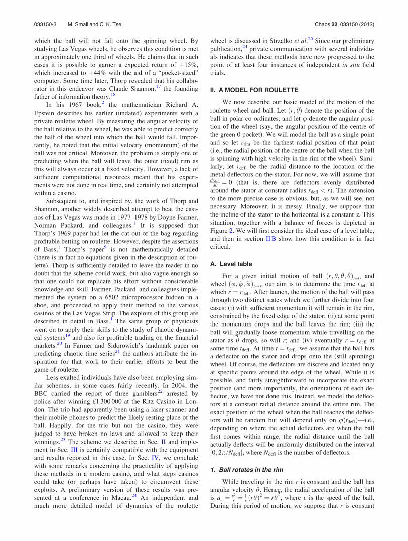
II. A MODEL FOR ROULETTE

We now describe our basic model of the motion of the

roulette wheel and ball. Let ðr; hÞ denote the position of the

ball in polar co-ordinates, and let u denote the angular posi-

tion of the wheel (say, the angular position of the centre of

the green 0 pocket). We will model the ball as a single point

and so let rrim be the farthest radial position of that point

(i.e., the radial position of the centre of the ball when the ball

is spinning with high velocity in the rim of the wheel). Simi-

larly, let rdefl be the radial distance to the location of the

metal deflectors on the stator. For now, we will assume thatdrdefl

dh ¼ 0 (that is, there are deflectors evenly distributed

around the stator at constant radius rdefl < r). The extension

to the more precise case is obvious, but, as we will see, not

necessary. Moreover, it is messy. Finally, we suppose that

the incline of the stator to the horizontal is a constant a. This

situation, together with a balance of forces is depicted in

Figure 2. We will first consider the ideal case of a level table,

and then in section II B show how this condition is in fact

critical.

A. Level table

For a given initial motion of ball ðr; h; _h; €hÞt¼0 and

wheel ðu; _u; €uÞt¼0, our aim is to determine the time tdefl at

which r ¼ rdefl. After launch, the motion of the ball will pass

through two distinct states which we further divide into four

cases: (i) with sufficient momentum it will remain in the rim,

constrained by the fixed edge of the stator; (ii) at some point

the momentum drops and the ball leaves the rim; (iii) the

ball will gradually loose momentum while travelling on the

stator as _h drops, so will r; and (iv) eventually r ¼ rdefl at

some time tdefl. At time t ¼ tdefl, we assume that the ball hits

a deflector on the stator and drops onto the (still spinning)

wheel. Of course, the deflectors are discrete and located only

at specific points around the edge of the wheel. While it is

possible, and fairly straightforward to incorporate the exact

position (and more importantly, the orientation) of each de-

flector, we have not done this. Instead, we model the deflec-

tors at a constant radial distance around the entire rim. The

exact position of the wheel when the ball reaches the deflec-

tors will be random but will depend only on uðtdeflÞ—i.e.,

depending on where the actual deflectors are when the ball

first comes within range, the radial distance until the ball

actually deflects will be uniformly distributed on the interval

½0; 2p=Ndefl�, where Ndefl is the number of deflectors.

1. Ball rotates in the rim

While traveling in the rim r is constant and the ball has

angular velocity _h. Hence, the radial acceleration of the ball

is ac ¼ v2

r ¼ 1r ðr _hÞ2 ¼ r _h

2, where v is the speed of the ball.

During this period of motion, we suppose that r is constant

033150-3 M. Small and C. K. Tse Chaos 22, 033150 (2012)

and that h decays only due to constant rolling friction: hence

_r ¼ 0 and €h ¼ €hð0Þ, a constant. This phase of motion will

continue provided the centripetal force of the ball on the rim

exceeds the force of gravity maccos a > mgsin a (m is the

mass of the ball). Hence, at this stage

_h2>

g

rtan a: (1)

2. Ball leaves the rim

Gradually the speed on the ball decays until eventually_h

2 ¼ gr tana. Given the initial acceleration €hð0Þ, velocity

_hð0Þ, and position hð0Þ, it is trivial to compute the time at

which the ball leaves the rim, trim to be

trim ¼ �1

€hð0Þ_hð0Þ �

ffiffiffiffiffiffiffiffiffiffiffiffiffiffig

rtan a

r� �: (2)

To do so, we assume that the angular acceleration is constant

and so the angular velocity at any time is given by _hðtÞ¼ _hð0Þ þ €hð0Þt and substitute into Eq. (1). That is, we are

assuming that the force acting on the ball is independent of

velocity—this is a simplifying assumption for the naive

model we describe here, more sophisticated alternatives are

possible, but in all cases this will involve the estimation of

additional parameters. The position at which the ball leaves

the rim is given by

hð0Þ þðgr tan aÞ � _hð0Þ2

2€hð0Þ

����������2p

where j � j2p denotes modulo 2p.

3. Ball rotates freely on the stator

After leaving the rim, the ball will continue (in practice,

for only a short while) to rotate freely on the stator until it

eventually reaches the various deflectors at r ¼ rdefl. The

angular velocity continues to be governed by

_hðtÞ ¼ _hð0Þ þ €hð0Þt;

but now that

r _h2< g tan a

the radial position is going to gradually decrease too. The

difference between the force of gravity mgsina and the

(lesser) centripetal force mr _h2cos a provides inward acceler-

ation of the ball

€r ¼ r _h2cos a� g sin a: (3)

Integrating Eq. (3) yields the position of the ball on the

stator.

4. Ball reaches the deflectors

Finally, we find the time t ¼ tdefl for which r(t), computed

as the definite second integral of Eq. (3), is equal to rdefl. We

can then compute the instantaneous angular position of the ball

hðtdeflÞ ¼ hð0Þ þ _hð0Þtdefl þ 12€hð0Þt2

defl and the wheel uðtdeflÞ¼ uð0Þ þ _uð0Þtdefl þ 1

2€uð0Þt2

defl to give the salient value

c ¼ jhðtdeflÞ � uðtdeflÞj2p (4)

denoting the angular location on the wheel directly below

the point at which the ball strikes a deflector. Assuming the

constant distribution of deflectors around the rim, some (still

to be estimated) distribution of resting place of the ball will

depend only on that value c. Note that, although we have

described ðh; _h; €hÞt¼0 and ðu; _u; €uÞt¼0 separately, it is possi-

ble to adopt the rotating frame of reference of the wheel and

treat h� u as a single variable. The analysis is equivalent,

estimating the required parameters may become simpler.

FIG. 2. The dynamic model of ball and wheel. On the

left, we show a top view of the roulette wheel (shaded

region) and the stator (outer circles). The ball is mov-

ing on the stator with instantaneous position ðr; hÞwhile the wheel is rotating with angular velocity _u(note that the direction of the arrows here are for illus-

tration only, the analysis in the text assume the same

convention, clockwise positive, for both ball and

wheel). The deflectors on the stator are modelled as a

circle, concentric with the wheel, of radius rdefl. On

the right, we show a cross section and examination of

the forces acting on the ball in the incline plane of the

stator. The angle a is the incline of the stator, m is

the mass of the ball, ac is the radial acceleration of

the ball, and g is gravity.

033150-4 M. Small and C. K. Tse Chaos 22, 033150 (2012)

We note that for a level table, each spin of the ball alters

only the time spent in the rim, the ball will leave the rim of

the stator with exactly the same velocity _h each time. The

descent from this point to the deflectors will therefore be

identical. There will, in fact, be some characteristic duration

which could be easily computed for a given table. Doing this

would circumvent the need to integrate Eq. (3).

B. The crooked table

Suppose, now that the table is not perfectly level. This is

the situation discussed and exploited by Thorp.9 Without

loss of generality (it is only an affine change of co-ordinates

for any other orientation) suppose that the table is tilted by

an angle d such that the origin u ¼ 0 is the lowest point on

the rim. Just as with the case of a level table, the time which

the ball spends in the rim is variable and the time at which it

leaves the rim depends on a stability criterion similar to

Eq. (1). But now that the table is not level, that equilibrium

becomes

r _h2 ¼ g tanðaþ d cos hÞ: (5)

If d ¼ 0 then it is clear that the distribution of angular posi-

tions for which this condition is first met will be uniform.

Suppose instead that d > 0, then there is now a range of criti-

cal angular velocities _h2

crit 2 ½gr tanða� dÞ; g

r tanðaþ dÞ�.Once _h

2< g

r tanðaþ dÞ, the position at which the ball leaves

the rim will be dictated by the point of intersection in ðh; _hÞ-space of

_h ¼ffiffiffiffiffiffiffiffiffiffiffiffiffiffiffiffiffiffiffiffiffiffiffiffiffiffiffiffiffiffiffiffiffiffig

rtanðaþ d cos hÞ

r(6)

and the ball trajectory as a function of t (modulo 2p)

_hðtÞ ¼ _hð0Þ þ €hð0Þt; (7)

hðtÞ ¼ hð0Þ þ _hð0Þtþ 1

2€hð0Þt2: (8)

If the angular velocity of the ball is large enough, then the

ball will leave the rim at some point on the half circle prior

to the low point (u ¼ 0). Moreover, suppose that in one rev-

olution (i.e., hðt1Þ þ 2p ¼ hðt2Þ), the velocity changes by_hðt1Þ � _hðt2Þ. Furthermore, suppose that this is the first

revolution during which _h2< g

r tanðaþ dÞ (that is, _hðt1Þ2

� gr tanðaþ dÞ but _hðt2Þ2 < g

r tanðaþ dÞ). Then, the point

at which the ball will leave the rim will (in ðh; _hÞ-space)

be the intersection of Eq. (6) and

_h ¼ _hðt1Þ �1

2p

�_hðt2Þ � _hðt1Þ

�h: (9)

The situation is depicted in Figure 3. One can expect for a

tilted roulette wheel, the ball will systematically favor leav-

ing the rim on one half of the wheel. Moreover, to a good

approximation, the point at which the ball will leave the rim

follows a uniform distribution over significantly less than

half the wheel circumference. In this situation, the problem

of predicting the final resting place is significantly simplified

to the problem of predicting the position of the wheel at the

time the ball leaves the rim.

We will pursue this particular case no further here. The

situation (5) may be considered as a generalisation of the

ideal d ¼ 0 case. This generalisation makes the task of pre-

diction significantly easier, but we will continue to work

under the assumption that the casino will be doing its utmost

to avoid the problems of an improperly levelled wheel.

Moreover, this generalisation is messy, but otherwise unin-

teresting. In Sec. III, we consider the problem of implement-

ing a prediction scheme for a perfectly level wheel.

III. EXPERIMENTAL RESULTS

In Sec. II, we introduced the basic mathematical model

which we utilize for the prediction of the trajectory of the

ball within the roulette wheel. We ignore (or rather treat as

essentially stochastic) the trajectory of the ball after hitting

the deflectors—charting the distribution of final outcome

from deflector to individual pocket in the roulette wheel is a

tractable probabilistic problem, and one for which we will

sketch a solution later. However, the details are perhaps only

of interest to the professional gambler and not to most physi-

cists. Hence, we are reduced to predicting the location of the

wheel and the ball when the ball first reaches one of the

deflectors. The model described in Sec. II is sufficient to

achieve this—provided one has adequate measurements of

the physical dimensions of the wheel and all initial positions,

FIG. 3. The case of the crooked table. The blue curve denotes the stability

criterion (6), while the red solid line is the (approximate) trajectory of the ball

with hðt1Þ þ 2p ¼ hðt2Þ indicating two successive times of complete revolu-

tions. The point at which the ball leaves the rim will therefore be the first

intersection of this stability criterion and the trajectory. This will necessarily

be in the region to the left of the point at which the ball’s trajectory is tangent

to Eq. (6), and this is highlighted in the figure as a green solid. Typically a

crooked table will only be slightly crooked and hence this region will be close

to h ¼ 0 but biased toward the approaching ball. The width of that region

depends on _hðt1Þ � _hðt2Þ, which in turn can be determined from Eq. (6).

033150-5 M. Small and C. K. Tse Chaos 22, 033150 (2012)

velocities, and accelerations (as a further approximation we

assume deceleration of both the ball and wheel to be constant

over the interval which we predict).

Hence, the problem of prediction is essentially two-

fold. First, the various velocities must be estimated accu-

rately. Given these estimates, it is a trivial problem to then

determine the point at which the ball will intersect with one

of the deflectors on the stator. Second, one must then have

an estimate of the scatter imposed on the ball by both the

deflectors and possible collision with the individual frets. To

apply this method in situ, one has the further complication

of estimating the parameters r, rdefl; rrim; a, and possibly dwithout attracting undue attention. We will ignore this addi-

tional complication as it is essentially a problem of data col-

lection and statistical estimation. Rather, we will assume

that these quantities can be reliably estimated and restrict

our attention to the problem of prediction of the motion.

To estimate the relevant positions, velocities, and accelera-

tions ðh; _h; €h;u; _u; €uÞt¼0 (or perhaps just ðh� u; _h � _u;€h � €uÞt¼0), we employ two distinct techniques.

In Secs. III A–III C, we describe these methods. In

Sec. III A, we introduce a manual measurement scheme, and

in Sec. III B, we describe our implementation of a more so-

phisticated digital system. The purpose of Sec. III A is to

demonstrate that a rather simple “clicker” type of device—

along the lines of that utilized by the Doyne Farmer, Norman

Packard, and collaborators1—can be employed to make suf-

ficiently accurate measurements. Nonetheless, this system is

far from optimal: we conduct only limited experiments with

this apparatus: sufficient to demonstrate that, in principle,

the method could work. In Sec. III B, we describe a more so-

phisticated system. This system relies on a digital camera

mounted directly above a roulette wheel and is therefore

unlikely to be employed in practice (although alternative,

more subtle, devices could be imagined). Nonetheless, our

aim here is to demonstrate how well this system could work

in an optimal environment.

Of course, the degree to which the model in Sec. II is

able to provide a useful prediction will depend critically on

how well the parameters are estimated. Sensitivity analysis

shows that the predicted outcome (Eq. (4)) depends only lin-

early or quadratically (in the case of physical parameters of

the wheel) on our initial estimates. More important however,

and more difficult to estimate, is to what extent each of these

parameters can be reliably estimated. For this reason, we first

take a strictly experimental approach and show that even

with the various imperfections inherent in experimental mea-

surement, and in our model, sufficiently accurate predictions

are realizable. Later, in Sec. III C, we provide a brief compu-

tational analysis of how model prediction will be affected by

uncertainty in each of the parameters.

A. A manual implementation

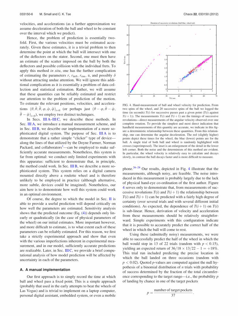
Our first approach is to simply record the time at which

ball and wheel pass a fixed point. This is a simple approach

(probably that used in the early attempts to beat the wheels of

Las Vegas) and is trivial to implement on a laptop computer,

personal digital assistant, embedded system, or even a mobile

phone.26–28 Our results, depicted in Fig. 4 illustrate that the

measurements, although noisy, are feasible. The noise intro-

duced in this measurement is probably largely due to the lack

of physical hand-eye co-ordination of the first author. Figure

4 serves only to demonstrate that, from measurements of suc-

cessive revolutions T(i) and T(iþ 1) the relationship between

T(i) and T(iþ 1) can be predicted with a fairly high degree of

certainty (over several trials and with several different initial

conditions). As expected, the dependence of T(iþ 1) on T(i)is sub-linear. Hence, derivation of velocity and acceleration

from these measurements should be relatively straightfor-

ward. Simple experiments with this configuration indicate

that it is possible to accurately predict the correct half of the

wheel in which the ball will come to rest.

Using these (admittedly noisy) measurements, we were

able to successfully predict the half of the wheel in which the

ball would stop in 13 of 22 trials (random with p < 0:15),

yielding an expected return of 36=18� 13=22� 1 ¼ þ18%.

This trial run included predicting the precise location in

which the ball landed on three occasions (random with

p < 0:02). Quoted p-values are computed against the null hy-

pothesis of a binomial distribution of n trials with probability

of success determined by the fraction of the total circumfer-

ence corresponding to the target range—i.e., the probability pof landing by chance in one of the target pockets

p ¼ number of target pockets

37:

FIG. 4. Hand-measurement of ball and wheel velocity for prediction. From

two spins of the wheel, and 20 successive spins of the ball we logged the

time (in seconds) T(i) for successive passes past a given point (T(i) against

T(iþ 1)). The measurements T(i) and T(iþ 1) are the timings of successive

revolutions—direct measurements of the angular velocity observed over one

complete rotation. To provide the simplest and most direct indication that

handheld measurements of this quantity are accurate, we indicate in this fig-

ure a deterministic relationship between these quantities. From this relation-

ship, one can determine the angular deceleration. The red (slightly higher)

points depict these times for the wheel, the blue (lower) points are for the

ball. A single trial of both ball and wheel is randomly highlighted with

crosses (superimposed). The inset is an enlargement of the detail in the lower

left corner. Both the noise and the determinism of this method are evident.

In particular, the wheel velocity is relatively easy to calculate and decays

slowly, in contrast the ball decays faster and is more difficult to measure.

033150-6 M. Small and C. K. Tse Chaos 22, 033150 (2012)

B. Automated digital image capture

Alternatively, we employ a digital camera mounted

directly above the wheel to accurately and instantaneously

measure the various physical parameters. This second

approach is obviously a little more difficult to implement in-

cognito. Here, we are more interested in determining how

much of an edge can be achieved under ideal conditions,

rather than the various implementation issues associated

with realizing this scheme for personal gain. In all our trials,

we use a regulation casino-grade roulette wheel (a 32”

“President Revolution” roulette wheel manufactured by Mat-

sui Gaming Machine Co. Ltd., Tokyo). The wheel has 37

numbered slots (1 to 36 and 0) in the configuration shown in

Figure 1 and has a radius of 820 mm (spindle to rim). For the

purposes of data collection, we employ a Prosilica EC650C

IEEE-1394 digital camera (1/3” CCD, 659� 493 pixels at

90 frames per second). Data collection software was written

and coded in Cþþ using the OpenCV library.

The camera provides approximately (slightly less due to

issues with data transfer) 90 images per second of the posi-

tion of the roulette wheel and the ball. Artifacts in the image

due to lighting had to be managed and filtered. From the re-

sultant image, the position of the wheel was easily deter-

mined by locating the only green pocket (“0”) in the wheel,

and the position of the ball was located by differencing suc-

cessive frames (searching for the ball shape or color was not

sufficient due to the reflective surface of the wheel and ambi-

ent lighting conditions).

From these time series of Cartesian coordinates for the

position of both the wheel (green “0” pocket) and ball, we

computed the centre of rotation and hence derived angular

position time series. Polynomial fits to these angular position

data (modulo 2p) provided estimates of angular velocity and

acceleration (deceleration). From this data, we found that,

for out apparatus, the acceleration terms where very close to

being constant over the observation time period—and hence

modeling the forces acting on the ball as constant provided a

reasonable approximation. With these parameters, we

directly applied the model of Sec. II to predict the point at

which the ball came into contact with the deflectors.

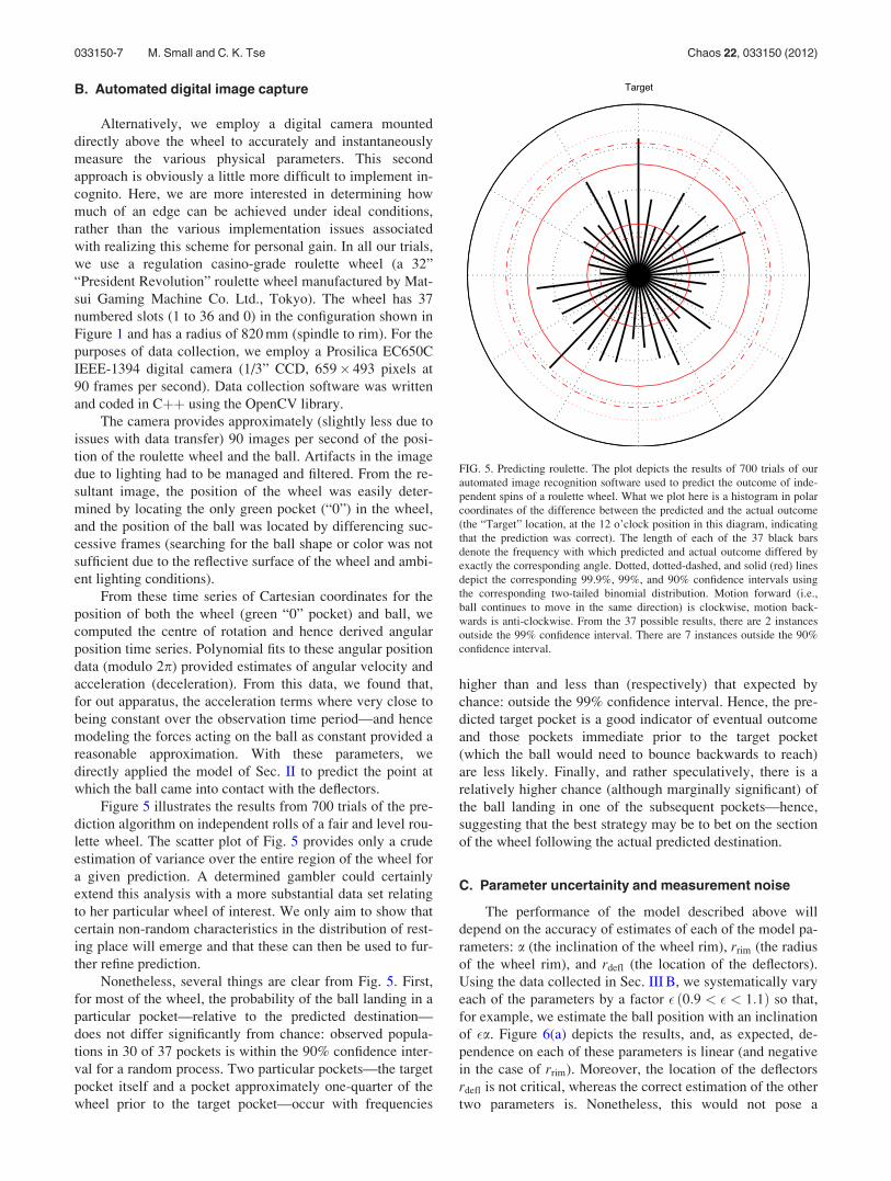
Figure 5 illustrates the results from 700 trials of the pre-

diction algorithm on independent rolls of a fair and level rou-

lette wheel. The scatter plot of Fig. 5 provides only a crude

estimation of variance over the entire region of the wheel for

a given prediction. A determined gambler could certainly

extend this analysis with a more substantial data set relating

to her particular wheel of interest. We only aim to show that

certain non-random characteristics in the distribution of rest-

ing place will emerge and that these can then be used to fur-

ther refine prediction.

Nonetheless, several things are clear from Fig. 5. First,

for most of the wheel, the probability of the ball landing in a

particular pocket—relative to the predicted destination—

does not differ significantly from chance: observed popula-

tions in 30 of 37 pockets is within the 90% confidence inter-

val for a random process. Two particular pockets—the target

pocket itself and a pocket approximately one-quarter of the

wheel prior to the target pocket—occur with frequencies

higher than and less than (respectively) that expected by

chance: outside the 99% confidence interval. Hence, the pre-

dicted target pocket is a good indicator of eventual outcome

and those pockets immediate prior to the target pocket

(which the ball would need to bounce backwards to reach)

are less likely. Finally, and rather speculatively, there is a

relatively higher chance (although marginally significant) of

the ball landing in one of the subsequent pockets—hence,

suggesting that the best strategy may be to bet on the section

of the wheel following the actual predicted destination.

C. Parameter uncertainity and measurement noise

The performance of the model described above will

depend on the accuracy of estimates of each of the model pa-

rameters: a (the inclination of the wheel rim), rrim (the radius

of the wheel rim), and rdefl (the location of the deflectors).

Using the data collected in Sec. III B, we systematically vary

each of the parameters by a factor � ð0:9 < � < 1:1Þ so that,

for example, we estimate the ball position with an inclination

of �a. Figure 6(a) depicts the results, and, as expected, de-

pendence on each of these parameters is linear (and negative

in the case of rrim). Moreover, the location of the deflectors

rdefl is not critical, whereas the correct estimation of the other

two parameters is. Nonetheless, this would not pose a

FIG. 5. Predicting roulette. The plot depicts the results of 700 trials of our

automated image recognition software used to predict the outcome of inde-

pendent spins of a roulette wheel. What we plot here is a histogram in polar

coordinates of the difference between the predicted and the actual outcome

(the “Target” location, at the 12 o’clock position in this diagram, indicating

that the prediction was correct). The length of each of the 37 black bars

denote the frequency with which predicted and actual outcome differed by

exactly the corresponding angle. Dotted, dotted-dashed, and solid (red) lines

depict the corresponding 99.9%, 99%, and 90% confidence intervals using

the corresponding two-tailed binomial distribution. Motion forward (i.e.,

ball continues to move in the same direction) is clockwise, motion back-

wards is anti-clockwise. From the 37 possible results, there are 2 instances

outside the 99% confidence interval. There are 7 instances outside the 90%

confidence interval.

033150-7 M. Small and C. K. Tse Chaos 22, 033150 (2012)

significant problem for prediction as in all case the variation

in these parameters introduces a systematic bias which could

easily be corrected for, or even used to estimate the true

value.

What is more striking is the effect of measurement noise

depicted in Fig. 6(b). We add Gaussian noise to each timing

measurement (each frame, recording at 90 frames per sec-

ond) over the duration of the observation period (25 frames)

used to estimate initial velocity and deceleration of the ball

and velocity of the wheel. The added noise has an effect of

increasing the variation in the predicted resting place of the

ball (since the noise is unbiased) and the strength of this

effect is linear with the level of noise. As independent noise

realizations are added to 50 measurements (25 each for the

ball and wheel), this is a substantial amount of error—even

at a fairly low amplitude. Nonetheless, the final results are

still within 2–3 pockets of the original prediction for noise of

up to 2% on every scalar observation.

IV. EXPLOITS AND COUNTER-MEASURES

The essence of the method presented here is to predict

the location of the ball and wheel at the point when the ball

will first come into contact with the deflectors. Hence, we

only require knowledge of initial conditions of each aspect

of the system (or more concisely, their relative positions,

velocities and accelerations). In addition to this, certain pa-

rameters derived from the physical dimensions of the wheel

are required—these could either be estimated directly, or

inferred from observational trajectory data. Finally, we note

that while anecdotal evidence suggests that (the height of

the) frets plays an important role in the final resting place of

the ball, this does not enter into our model of the more deter-

ministic phase of the system dynamics. It will affect the dis-

tribution of final resting places—and hence this is going to

depend rather sensitively on a particular wheel.

We would like to draw two simple conclusions from this

work. First, deterministic predictions of the outcome of a

game of roulette can be made, and can probably be done

in situ. Hence, the tales of various exploits in this arena are

likely to be based on fact. Second, the margin for profit is

quite slim. Minor manipulation with the frictional resistance

or level of the wheel and/or the manner in which the croupier

actually plays the ball (the force with which the ball is rolled

and the effect, for example, of axial spin of the ball) have

not been explored here and would likely affect the results

significantly. Hence, for the casino the news is mostly

good—minor adjustments will ameliorate the advantage of

the physicist-gambler. For the gambler, one can rest assured

that the game is on some level predictable and therefore

inherently honest.

Of course, the model we have used here is extremely

simple. In Strzalko et al.,25 much more sophisticated model-

ing methodologies have been independently developed and

presented. Certainly, since the entire system is a physical dy-

namical system, computational modeling of the entire system

may provide an even greater advantage.25 Nonetheless, the

methods presented in this paper would certainly be within

the capabilities of a 1970s “shoe-computer.”

ACKNOWLEDGMENTS

The first author would like to thank Marius Gerber for

introducing him to the dynamical systems aspects of the

game of roulette. Funding for this project, including the rou-

lette wheel, was provided by the Hong Kong Polytechnic

University. The labors of final year project students, Yung

Chun Ting and Chung Kin Shing, in performing many of the

mechanical simulations describe herein are gratefully

acknowledged. M.S. is supported by an Australian Research

Council Future Fellowship (FT110100896).

FIG. 6. Parameter uncertainty. We explore the

effect of error in the model parameters on the out-

come by varying the three physical parameters of

the wheel (a) and introducing uncertainty in the

measurement of timing events used to obtain

estimates of velocity and deceleration (b). In (a), we

depict the effect of perturbing the estimated

values of a (green—affine, increasing steeply) rrim

(red—affine, decreasing) and rdefl (blue—affine and

increasing slowly) from 90% to 110% of the true

value. In (b), we add Gaussian noise of magnitude

between 0.5% and 10% the variance of the true

measurements to initial estimates of all positions

and velocities. Horizontal dotted lines in both plots

depict error corresponding to one whole pocket in

the wheel. The vertical axis is in radians and covers

6 p2—half the wheel. In the upper panel, least varia-

tion in outcome is observed with errors in estima-

tion of rdefl.

033150-8 M. Small and C. K. Tse Chaos 22, 033150 (2012)

1T. A. Bass, The Newtonian Casino (Penguin, London, 1990).2R. A. Epstein, The Theory of Gambling and Statistical Logic (Academic,

New York, 1967).3E. T. Bell, Men of Mathematics (Simon and Schuster, New York, 1937).4The Italian mathematician, confusingly, was named Don Pasquale2, a sur-

name phonetically similar to Pascal. Moreover, as Don Pasquale is also

the name of a 19th century opera buff, this attribution is possibly fanciful.5F. Downton and R. L. Holder, “Banker’s games and the gambling act

1968,” J. R. Stat. Soc. Ser. A 135, 336–364 (1972).6B. Okuley and F. King-Poole, Gamblers Guide to Macao (South China

Morning Post, Hong Kong, 1979).7Three, if one has sufficient finances to assume the role of the house.8C. Kingston, The Romance of Monte Carlo (John Lane The Bodley Head

Ltd., London, 1925).9E. O. Thorp, “Optimal gambling systems for favorable games,” Rev. Int.

Stat. Inst. 37, 273–293 (1969).10Life Magazine Publication, “How to Win $6,500,” Life, 46, December 8,

1947.11Alternatively, and apparently erroneously, reported to be from Californian

Institute of Technology in Ref. 2.12S. N. Ethier, “Testing for favorable numbers on a roulette wheel,” J. Am.

Stat. Assoc. 77, 660–665 (1982).13Time Magazine Publication, “Argentina—Bank breakers,” Time 135, 34,

February 12, 1951.14The first, to the best of our knowledge.15H. Poincar�e, Science and Method (Nelson, London, 1914). English transla-

tion by Francis Maitland, preface by Bertrand Russell. Facsimile reprint in

1996 by Routledge/Thoemmes, London.

16J. P. Crutchfield, J. Doyne Farmer, N. H. Packard, and R. S. Shaw,

“Chaos,” Sci. Am. 255, 46–57 (1986).17E. O. Thorp, The Mathematics of Gambling (Gambling Times, 1985).18C. E. Shannon, “A mathematical theory of communication,” Bell Syst.

Techn. J. 27, 379–423, 623–656 (1948).19N. H. Packard, J. P. Crutchfield, J. D. Farmer, and R. S. Shaw, “Geometry

from a time series,” Phys. Rev. Lett. 45, 712–716 (1980).20T. A. Bass, The Predictors, edited by A. Lane (Penguin, London, 1999).21J. D. Farmer and J. J. Sidorowich, “Predicting chaotic time series,” Phys.

Rev. Lett. 59, 845–848 (1987).22BBC Online, “Arrests follow £1m roulette win,” BBC News March 22,

2004.23BBC Online, “Laser scam” gamblers to keep £1m,” BBC News December

5, 2004.24M. Small and C. K. Tse, “Feasible implementation of a prediction algo-

rithm for the game of roulette,” in Asia-Pacific Conference on Circuitsand Systems (IEEE, 2008).

25J. Strzalko, J. Grabski, P. Perlikowksi, A. Stefanski, and T. Kapitaniak,

Dynamics of gambling, Vol. 792 of Lecture Notes in Physics (Springer,

2009).26Implementation on a “shoe-computer” should be relatively straightforward

too.27C. T. Yung, “Predicting roulette,” Final Year Project Report, Hong Kong

Polytechnic University, Department of Electronic and Information Engi-

neering, April 2011.28K. S. Chung, “Predicting roulette II: Implementation,” Final Year Project

Report, Hong Kong Polytechnic University, Department of Electronic and

Information Engineering, April 2010.

033150-9 M. Small and C. K. Tse Chaos 22, 033150 (2012)