predicting periphyton cover frequency … · predicting periphyton cover frequency distributions...

PREDICTING PERIPHYTON COVER FREQUENCY DISTRIBUTIONS

ACROSS NEW ZEALAND’S RIVERS1

Ton H. Snelder, Doug J. Booker, John M. Quinn, and Cathy Kilroy2

ABSTRACT: Regression models of mean and mean annual maximum (MAM) cover were derived for two catego-ries of periphyton cover (filaments and mats) using 22 years of monthly monitoring data from 78 river sitesacross New Zealand. Explanatory variables were derived from observations of water quality variables, hydrol-ogy, shade, bed sediment grain size, temperature, and solar radiation. The root mean square errors of thesemodels were large (75-95% of the mean of the estimated values). The at-site frequency distributions of periphy-ton cover were approximated by the exponential distribution, which has the mean cover as its single parameter.Independent predictions of cover distributions at all sites were calculated using the mean predicted by theregression model and the theoretical exponential distribution. The probability that cover exceeds specifiedthresholds and estimates of MAM cover, based on the predicted distributions, had large uncertainties (~80-100%) at the site scale. However, predictions aggregated by classes of an environmental classification accuratelypredicted the proportion of sites for which cover exceeded nominated criteria in the classes. The models are use-ful for assessing broad-scale patterns in periphyton cover and for estimating changes in cover with changes innutrients, hydrological regime, and light.

(KEY TERMS: periphyton; model; flow regime; nutrients; New Zealand; cover; frequency distribution; probabil-ity.)

Snelder, Ton H., Doug J. Booker, John M. Quinn, and Cathy Kilroy, 2013. Predicting Periphyton Cover Fre-quency Distributions Across New Zealand’s Rivers. Journal of the American Water Resources Association(JAWRA) 50(1): 111-127. DOI: 10.1111/jawr.12120

INTRODUCTION

Healthy river ecosystems are characterized by thepresence of periphyton (primarily algae attached to thesurface of the riverbed), but at relatively low levels ofabundance (measured as areal cover, biomass, or bio-volume) (Biggs, 2000). Periphyton in rivers providesbasal resources for food webs (Kiffney et al., 2001; Fin-lay et al., 2002; Liess and Hillebrand, 2006). However,high abundance of periphyton can have negative

effects on habitat quality, water chemistry, and biodi-versity, and can reduce recreation and aesthetic values(Biggs, 2000; Suren et al., 2003; Suplee et al., 2009).Two key factors that are influenced by human activi-ties affect periphyton abundance in rivers: flowregimes (Biggs et al., 1998b) and nutrient concentra-tions (Dodds et al., 1997; Biggs, 2000). In addition,light exerts a strong influence on periphyton in riversand is affected by human activities such as deforesta-tion and management of riparian vegetation (Davies-Colley and Quinn, 1998; Boothroyd et al., 2004).

1Paper No. JAWRA-12-0262-P of the Journal of the American Water Resources Association (JAWRA). Received December 12, 2012; acceptedJune 10, 2013. © 2013 American Water Resources Association. Discussions are open until six months from print publication.

2Senior Principal (Snelder), Aqualinc Research Limited, P.O. Box 20462, Bishopdale, Christchurch, New Zealand; Scientist (Booker andKilroy), National Institute for Water and Atmospheric Research, Christchurch, New Zealand; and Principal Scientist (Quinn), National Insti-tute of Water and Atmospheric Research, Hamilton, New Zealand (E-Mail/Snelder: [email protected]).

JOURNAL OF THE AMERICAN WATER RESOURCES ASSOCIATION JAWRA111

JOURNAL OF THE AMERICAN WATER RESOURCES ASSOCIATION

Vol. 50, No. 1 AMERICAN WATER RESOURCES ASSOCIATIONFebruary 2014

Establishing quantitative relationships betweenperiphyton abundance and these factors has proven tobe difficult, but remains an urgent priority due to theneed to manage the ecological impacts of water with-drawal, change in flow regimes, and eutrophication ofrivers worldwide (Dodds and Welch, 2000; Lewis et al.,2010). This need is particularly strong in New Zealand,where there is intensification of land use as well asincreasing demand for water for industry, powergeneration, and agriculture (Ministry for the Environ-ment, 2007).

Guidelines for the management of periphyton inNew Zealand (Ministry for the Environment, 2000)recommend that maximum periphyton abundanceshould not exceed between 50 and 200 mg chlorophylla m�2 depending on the specific instream values tobe protected, including benthic biodiversity, contactrecreation, aesthetics, and angling. These guidelinesare within the range that periphyton biomass is con-sidered to constitute a nuisance (Suplee et al., 2009).The New Zealand guidelines also recommend a maxi-mum cover of the beds of rivers by filamentous algaeof 30% and mats of 60% (Ministry for the Environ-ment, 2000). Studies have linked these cover thresh-olds to biomass in the range 100-150 mg chlorophylla m�2 (Welch et al., 1988).

Several studies have linked nutrient concentrationsto mean biomass, mean summer biomass, or biomassduring periods of low flow (e.g., Welch et al., 1988;Heatherly et al., 2008). Biggs (2000) linked meanannual maximum (MAM) biomass in 30 sites in 25 hill-country, gravel-bed rivers in New Zealand, to meanmonthly concentrations of dissolved inorganic nitrogen(DIN) and dissolved reactive phosphorus (DRP) and asingle hydrological index (the mean days of accrual).Mean days of accrual was defined as the mean timebetween flows exceeding three times the median(FRE3), which was found in an earlier study to be thehydrological index most closely related to periphytonbiomass (Clausen and Biggs, 1997). Although thismodel is widely applied (e.g., Ministry for the Environ-ment, 2000), it was fitted to only a subset of the riverenvironments of New Zealand, albeit those with highsusceptibility to periphyton proliferations. Water man-agers are concerned with not only maximum periphy-ton abundance but also the percentage of the time thatany given threshold, such as a guideline, is exceeded.Thus, more generally applicable models that predictthe frequency distribution of periphyton abundancewould provide useful tools for water management.

Periphyton abundance is often low in rivers thathave frequent large floods, but may be high after longperiods without floods and with favorable growingconditions (Suren et al., 2003; Suren and Jowett,2006). This suggests that the theoretical exponentialdistribution may be an adequate approximation for

the distribution of periphyton abundance at sites.Zero is the most frequently occurring value of theexponential distribution and the frequency of largervalues descend asymptotically to zero. If periphytonabundance is exponentially distributed, the probabil-ity that cover is equal to or greater than zero is one(or 100% of the time) and decreases asymptotically tozero for large values of cover. The exponential distri-bution has the mean as its single parameter andwould, therefore, provide a method for estimating theprobability that cover exceeds a given threshold or,conversely, the cover that is equaled or exceededgiven any probability.

The objective of this study was to develop modelsthat could be used to estimate periphyton abundancein rivers and changes in abundance associated withchanges in conditions caused by human activities. Weaimed to develop models that could predict the fre-quency distribution of periphyton cover for thisdomain as a function of relevant and easily obtainedexplanatory variables, and also to estimate the uncer-tainty of these models for predictions made at indi-vidual sites and across regions.

METHODS AND MATERIALS

Study Sites

The National Rivers Water Quality Network(NRWQN) comprises 77 sites located on 48 of NewZealand’s rivers (Figure 1) and was specificallydesigned to broadly represent variation in main-stemrivers across New Zealand (Smith and Maasdam,1994; Davies-Colley et al., 2011). Since 1989, a rangeof water quality variables and a visual assessment ofthe cover of filamentous and mat-forming algae hasbeen carried out monthly at NRWQN sites and flowsare monitored continuously (Smith and McBride,1990; Davies-Colley et al., 2011). More intensive bio-monitoring is carried out annually at all sites andincludes an assessment of substrate size class compo-sition. This includes a visual assessment of substratesize class composition reported as the percentage ofbed covered by the following size classes: silt andsand (<2 mm), small gravel (2-32 mm), large gravel(32-64 mm), small cobbles (64-128 mm), large cobbles(128-256 mm), and boulders (256-330 mm).

In this study we analyzed data for the time period1989-2010 (22 years), but excluded several NRWQNsites for various reasons. The sites AK1, AK2, andGS1 (see Figure 1 for site codes) were excludedbecause they are located on deep rivers with siltybeds that lack periphyton. RO2 and RO6 were

JAWRA JOURNAL OF THE AMERICAN WATER RESOURCES ASSOCIATION112

SNELDER, BOOKER, QUINN, AND KILROY

excluded due to a large number of missing periphytonobservations. Sites WH3 and WH4 were excludedbecause they are dominated by macrophytes. Threesites on large rivers including the Waikato (HM2,HM4, and HM5) and the Clutha (DN4) rivers wereexcluded due to logistical difficulties in samplingperiphyton and artificially fluctuating water levels.

We split the records for some sites into two por-tions to account for significant changes that hadoccurred at the site through the period of operation ofthe NRWQN. The two portions of the record weretreated as separate sites in the analyses that follow.Five sites (HM1, RO4, WA6, WN3, and DN2) weresplit due to changes in site locations that wererequired for operational reasons. Five sites (includingRO3, HV5, WN2, TK2, and DN1) were split due tovery obvious changes in mean water quality. Thirteensites in the South Island (NN3, NN5, GY1, CH1,TK3, TK4, TK6, AX1, AX2, AX3, AX4, DN4, andDN9) were split because they were colonized by theinvasive alga Didymosphenia geminata (Kilroy et al.,2009). The abundance of D. geminata responds tovery different factors to the other bloom forming taxain New Zealand rivers (Kilroy et al., 2009). For thisreason, we retained the portion of the record prior tothe establishment of D. geminata but did not includethe second portion. Site TK1 was split due to the pre-commissioning failure of the Opuha Dam and thesubsequent establishment of D. geminata. Afterexcluding some sites and splitting others, we had atotal of 78 sites comprising either the entire record of

the NRWQN site (designated “All”) or parts of therecord were designated as “Part 1” or “Part 2”depending on the period covered.

Periphyton Data

Periphyton abundance was measured each monthat the NRWQN sites by visual assessment. The coverof two categories; filaments (>2 cm long) and mats(>2 mm thick) were measured as continuous vari-ables. In the field, mats were distinguished from thinfilms when the texture of the underlying substratecould not been seen and the layer could be scraped orpeeled. These two periphyton categories are consid-ered to be at problematic levels if they exceed 30 and60% of the visible stream bed (generally <0.75 mdeep), respectively (Ministry for the Environment,2000). Where possible, ten replicate observations of0.5-m radius patches of riverbed were made atequally spaced points across a wadeable cross sectionof the river using an underwater viewer. However,because the NRWQN rivers are medium to large,some observations were confined to the wadeablemargin from one bank or, at 10% of sites, to observa-tions from bridges or cableways (see Quinn and Raa-phorst (2009) for details).

For each site and sample date, we calculated themean of the ten replicate observations to produce atime series of monthly proportion of the bed coveredby filaments and mats. For each site, we then calcu-lated the mean of these monthly cover estimates overthe entire time series for both the filament and matcover categories. In addition, we calculated the maxi-mum cover in both categories in each year. We calcu-lated the MAM cover from these data for each site.

Approach to Modeling Distribution of PeriphytonCover

Our approaches to modeling periphyton cover atthe sites are summarized in Figure 2. We primarilyaimed to predict the frequency distribution of periph-yton cover using the exponential distribution as theunderlying theoretical distribution. The cumulativefrequency distribution (CFD) gives the probability (orthe expected proportion of the time) that cover isequal to, or greater than, a given value. The theoreti-cal CFD is as follows:

Pr ¼ e�C=l ð1Þ

where Pr (0 ≤ Pr < 1) is the probability of cover Cbeing equaled or exceeded given the mean value(l > 0). The quantile function (inverse CFD) gives the

FIGURE. 1. Location of the Study Sites Coded by TopographyCategory. Note that records for some sites were split and the twoportions of record were treated as separate sites in the analysis.


PREDICTING PERIPHYTON COVER FREQUENCY DISTRIBUTIONS ACROSS NEW ZEALAND’S RIVERS

cover that is expected to be equaled or exceeded witha given probability (or proportion of the time). Thequantile function for the exponential distribution isas follows:

C ¼ �lnðPrÞ � l ð2Þ

where Pr (0 ≤ Pr < 1) is the probability that cover Cis exceeded given the mean (l > 0). The quantilefunction (Equation 2) can be used to estimate theexpected value of the MAM cover based on monthlyobservations by setting probability to 0.083.

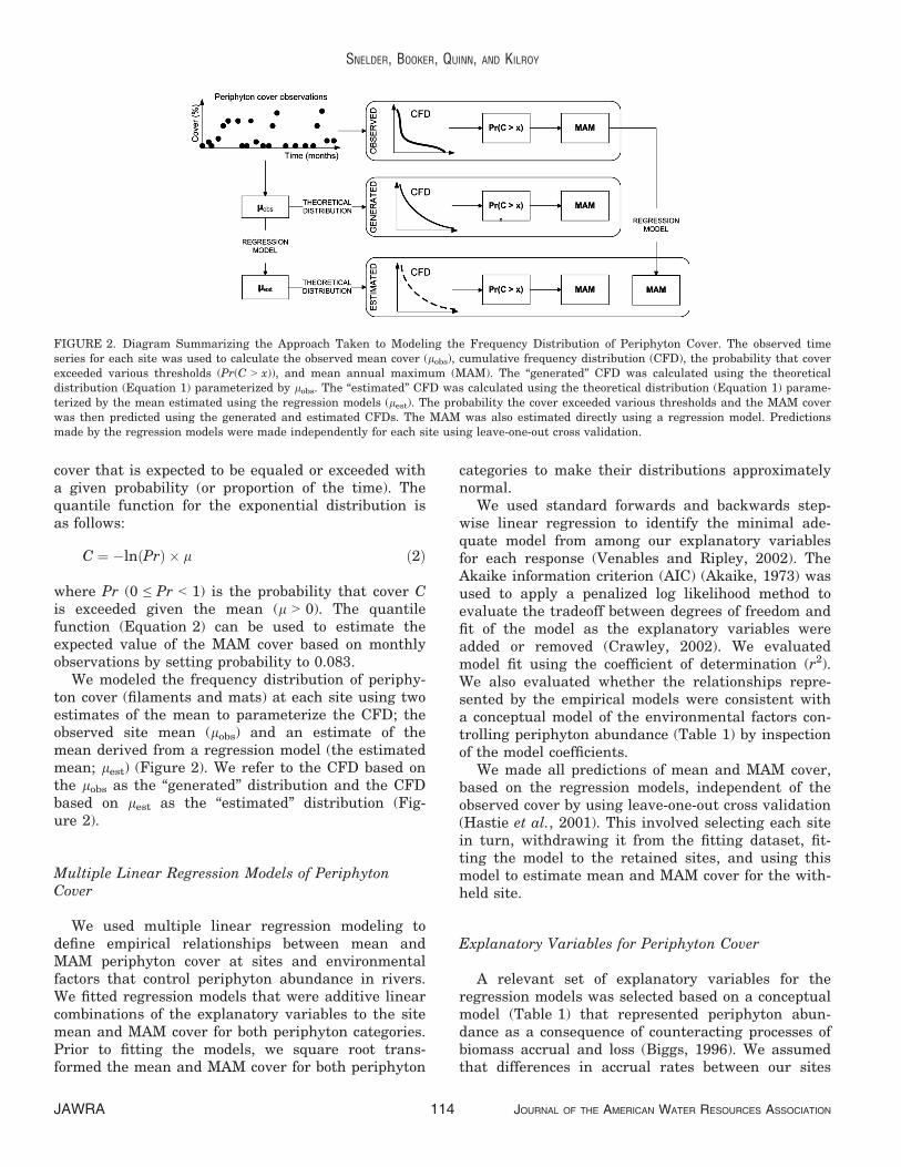
We modeled the frequency distribution of periphy-ton cover (filaments and mats) at each site using twoestimates of the mean to parameterize the CFD; theobserved site mean (lobs) and an estimate of themean derived from a regression model (the estimatedmean; lest) (Figure 2). We refer to the CFD based onthe lobs as the “generated” distribution and the CFDbased on lest as the “estimated” distribution (Fig-ure 2).

Multiple Linear Regression Models of PeriphytonCover

We used multiple linear regression modeling todefine empirical relationships between mean andMAM periphyton cover at sites and environmentalfactors that control periphyton abundance in rivers.We fitted regression models that were additive linearcombinations of the explanatory variables to the sitemean and MAM cover for both periphyton categories.Prior to fitting the models, we square root trans-formed the mean and MAM cover for both periphyton

categories to make their distributions approximatelynormal.

We used standard forwards and backwards step-wise linear regression to identify the minimal ade-quate model from among our explanatory variablesfor each response (Venables and Ripley, 2002). TheAkaike information criterion (AIC) (Akaike, 1973) wasused to apply a penalized log likelihood method toevaluate the tradeoff between degrees of freedom andfit of the model as the explanatory variables wereadded or removed (Crawley, 2002). We evaluatedmodel fit using the coefficient of determination (r2).We also evaluated whether the relationships repre-sented by the empirical models were consistent witha conceptual model of the environmental factors con-trolling periphyton abundance (Table 1) by inspectionof the model coefficients.

We made all predictions of mean and MAM cover,based on the regression models, independent of theobserved cover by using leave-one-out cross validation(Hastie et al., 2001). This involved selecting each sitein turn, withdrawing it from the fitting dataset, fit-ting the model to the retained sites, and using thismodel to estimate mean and MAM cover for the with-held site.

Explanatory Variables for Periphyton Cover

A relevant set of explanatory variables for theregression models was selected based on a conceptualmodel (Table 1) that represented periphyton abun-dance as a consequence of counteracting processes ofbiomass accrual and loss (Biggs, 1996). We assumedthat differences in accrual rates between our sites

FIGURE 2. Diagram Summarizing the Approach Taken to Modeling the Frequency Distribution of Periphyton Cover. The observed timeseries for each site was used to calculate the observed mean cover (lobs), cumulative frequency distribution (CFD), the probability that coverexceeded various thresholds (Pr(C > x)), and mean annual maximum (MAM). The “generated” CFD was calculated using the theoreticaldistribution (Equation 1) parameterized by lobs. The “estimated” CFD was calculated using the theoretical distribution (Equation 1) parame-terized by the mean estimated using the regression models (lest). The probability the cover exceeded various thresholds and the MAM coverwas then predicted using the generated and estimated CFDs. The MAM was also estimated directly using a regression model. Predictionsmade by the regression models were made independently for each site using leave-one-out cross validation.



were determined by the rate of growth and that thisis controlled primarily by nutrient supply, light, andtemperature. We assumed that biomass loss is deter-mined primarily by hydrological disturbance (i.e.,high flows, and changes of flows) (Biggs, 1996). Highflows remove periphyton when shear stress is suffi-cient to tear periphyton from the bed (Biggs, 1996;Biggs et al., 1998a, b). Biomass loss is increased ifchanges in flows are also associated with abrasiondue to sediment movement and may be enhancedwhen rates of increase in flows are high (Horneret al., 1990; Uehlinger, 1991). We expected biomassloss processes due to hydrological disturbance to bemediated by channel morphology with loss ratesbeing lower where stream substrates are stable andconsist of larger substrata (i.e., gravels, cobbles, andboulders) (Uehlinger, 1991; Doyle and Stanley, 2006).We also anticipated that biomass accrual would berelated to hydrological conditions, particularly themagnitude of base or low flows. Sites with small lowflows are likely to have periods of low water velocitythat favors the development of some filamentous taxa(Suren et al., 2003; Flinders and Hart, 2009).

Differences in loss rates between sites may alsoarise due to differences in invertebrate grazer abun-dance and grazing rates (Dodds and Welch, 2000;Rutherford et al., 2000). Our environmental data didnot include invertebrate grazers explicitly. However,we assumed that some differences in grazer densitybetween sites may be accounted for by the combina-tion of substrate size and hydrological indices (Quinnand Hickey, 1990).

We derived a set of candidate explanatory vari-ables for the sites using data available from theNRWQN and other sources (Table 2). For each site,we evaluated the median concentration of total phos-phorus (TP) (mg/m3), DRP (mg/m3), total nitrogen(TN) (mg/m3), and DIN (mg/m3). We calculated theratio of TN to TP and the ratio of DIN to DRP to

define the explanatory variables TN:TP and DIN:DRP. We log (base 10) transformed all the nutrientvariables to make their distributions approximatelynormal and their relationship with site mean periph-yton cover more linear.

Following similar methods to Olden and Poff(2003), we computed several hydrological indices fromthe mean daily flow time series for each site to charac-terize the flow regime components represented by theconceptual model (Table 2). The frequency of largefloods was represented by the number of events peryear that exceeded a multiple (n) times the long-termmedian flow (FREn) where n = 2, 3, and 4. If the timeinterval between an event dropping below the thresh-old and the next event rising above the threshold wasless than five days, only a single event was counted.We used the mean of the yearly values (FREn) afterhaving discarded years with more than 30 days ofmissing data to represent the frequency of largefloods. The frequency of changes of flows was repre-sented by hydrological reversals (Reversals). Rever-sals are occasions on which the direction of dailychange in flows reverses (i.e., the number of occasionson which increasing flows (rising hydrograph limbs)changed to falling limbs) and vice versa (Olden andPoff, 2003). Sites with frequent reversals have manyhydrograph peaks. Rates of increase in flow were rep-resented by the number of days on which flow was lessthan that of the previous day (nNeg). We estimatednNeg for each site by first counting the number ofdays in each year for which the flow reduced on thesubsequent day. nNeg for each site was the mean ofthese values over years. Sites with steep rising limbshave large values of nNeg. We used the mean annualseven-day low flow divided by the mean flow to repre-sent the low flow magnitude (LowFlow). We derivedthis explanatory variable for each site by first estimat-ing the minimum of a seven-day moving average flowin each year of record. LowFlow was the mean of these

TABLE 1. Summary of the Conceptual Model of the Environmental Factors that Control Mean Periphyton Cover.

Environmental Factor

Expected Response ofMean Cover to Increase

in the Factor Explanation of Expected Response

Light at the stream bed ↑ Increases growth rateWater temperature ↑ Increases growth rateNutrients ↑ Increases growth rateRatio of N to P ↑ or � High values reduce growth rate at sites with high N; low values

reduce growth rate at sites with high PFrequency of large floods ↓ Increases loss rateLow flow magnitude ↓ Small low flow magnitude may be associated with higher rates of

accrual due to low water velocityRates of change in flow ↓ High rates of change in flow may be associated with high loss ratesReversals ↓ Frequent reversals may be associated with high loss ratesBed sediment grain size ↑ Larger grains provide favorable habitat, are more stable, and decrease loss rate



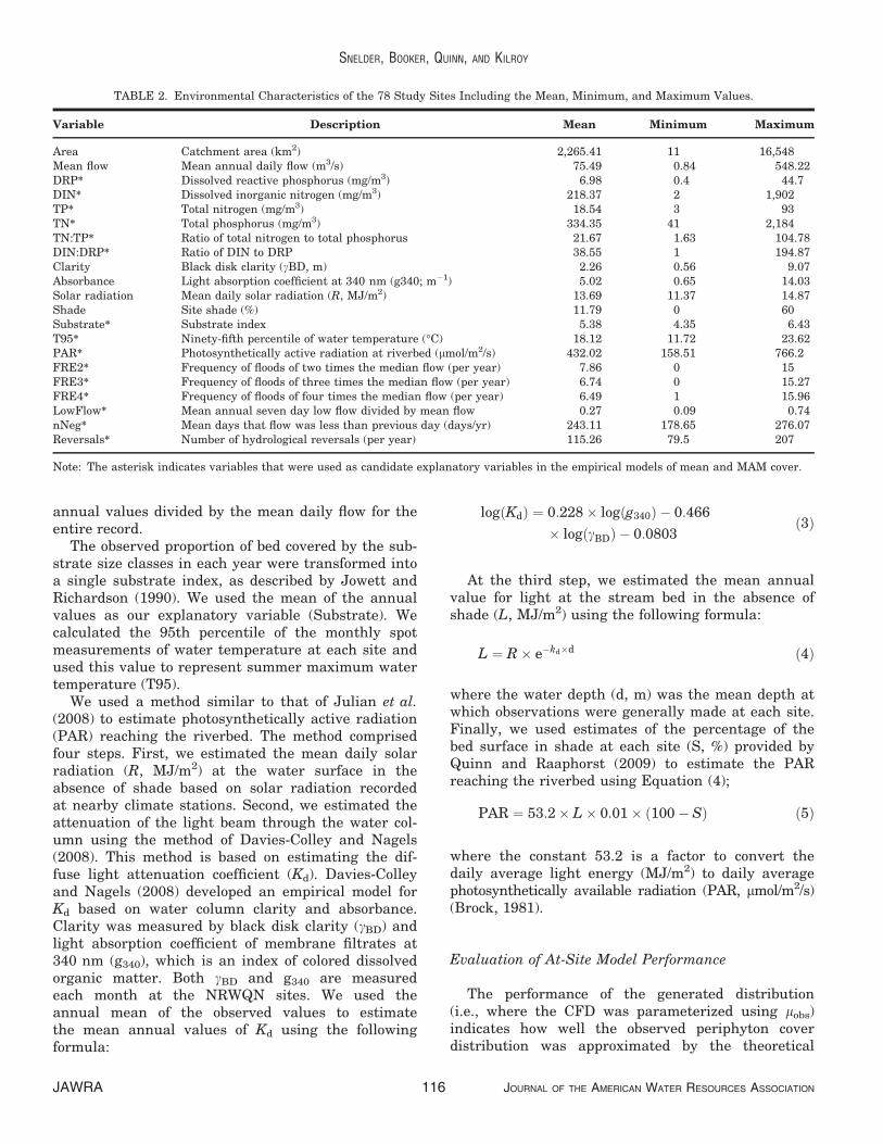
annual values divided by the mean daily flow for theentire record.

The observed proportion of bed covered by the sub-strate size classes in each year were transformed intoa single substrate index, as described by Jowett andRichardson (1990). We used the mean of the annualvalues as our explanatory variable (Substrate). Wecalculated the 95th percentile of the monthly spotmeasurements of water temperature at each site andused this value to represent summer maximum watertemperature (T95).

We used a method similar to that of Julian et al.(2008) to estimate photosynthetically active radiation(PAR) reaching the riverbed. The method comprisedfour steps. First, we estimated the mean daily solarradiation (R, MJ/m2) at the water surface in theabsence of shade based on solar radiation recordedat nearby climate stations. Second, we estimated theattenuation of the light beam through the water col-umn using the method of Davies-Colley and Nagels(2008). This method is based on estimating the dif-fuse light attenuation coefficient (Kd). Davies-Colleyand Nagels (2008) developed an empirical model forKd based on water column clarity and absorbance.Clarity was measured by black disk clarity (cBD) andlight absorption coefficient of membrane filtrates at340 nm (g340), which is an index of colored dissolvedorganic matter. Both cBD and g340 are measuredeach month at the NRWQN sites. We used theannual mean of the observed values to estimatethe mean annual values of Kd using the followingformula:

logðKdÞ ¼ 0:228� logðg340Þ � 0:466

� logðcBDÞ � 0:0803ð3Þ

At the third step, we estimated the mean annualvalue for light at the stream bed in the absence ofshade (L, MJ/m2) using the following formula:

L ¼ R� e�kd�d ð4Þ

where the water depth (d, m) was the mean depth atwhich observations were generally made at each site.Finally, we used estimates of the percentage of thebed surface in shade at each site (S, %) provided byQuinn and Raaphorst (2009) to estimate the PARreaching the riverbed using Equation (4);

PAR ¼ 53:2� L� 0:01� ð100� SÞ ð5Þ

where the constant 53.2 is a factor to convert thedaily average light energy (MJ/m2) to daily averagephotosynthetically available radiation (PAR, lmol/m2/s)(Brock, 1981).

Evaluation of At-Site Model Performance

The performance of the generated distribution(i.e., where the CFD was parameterized using lobs)indicates how well the observed periphyton coverdistribution was approximated by the theoretical

TABLE 2. Environmental Characteristics of the 78 Study Sites Including the Mean, Minimum, and Maximum Values.

Variable Description Mean Minimum Maximum

Area Catchment area (km2) 2,265.41 11 16,548Mean flow Mean annual daily flow (m3/s) 75.49 0.84 548.22DRP* Dissolved reactive phosphorus (mg/m3) 6.98 0.4 44.7DIN* Dissolved inorganic nitrogen (mg/m3) 218.37 2 1,902TP* Total nitrogen (mg/m3) 18.54 3 93TN* Total phosphorus (mg/m3) 334.35 41 2,184TN:TP* Ratio of total nitrogen to total phosphorus 21.67 1.63 104.78DIN:DRP* Ratio of DIN to DRP 38.55 1 194.87Clarity Black disk clarity (cBD, m) 2.26 0.56 9.07Absorbance Light absorption coefficient at 340 nm (g340; m�1) 5.02 0.65 14.03Solar radiation Mean daily solar radiation (R, MJ/m2) 13.69 11.37 14.87Shade Site shade (%) 11.79 0 60Substrate* Substrate index 5.38 4.35 6.43T95* Ninety-fifth percentile of water temperature (°C) 18.12 11.72 23.62PAR* Photosynthetically active radiation at riverbed (lmol/m2/s) 432.02 158.51 766.2FRE2* Frequency of floods of two times the median flow (per year) 7.86 0 15FRE3* Frequency of floods of three times the median flow (per year) 6.74 0 15.27FRE4* Frequency of floods of four times the median flow (per year) 6.49 1 15.96LowFlow* Mean annual seven day low flow divided by mean flow 0.27 0.09 0.74nNeg* Mean days that flow was less than previous day (days/yr) 243.11 178.65 276.07Reversals* Number of hydrological reversals (per year) 115.26 79.5 207

Note: The asterisk indicates variables that were used as candidate explanatory variables in the empirical models of mean and MAM cover.



empirical distribution. We evaluated the performanceof the generated distributions by comparing theobserved probability that cover exceeded six coverthresholds: 10, 20, 30, 40, 50, and 60%, with predic-tions of the same probabilities made from the gener-ated CFD. In addition, we compared the observedMAM cover with that predicted from the generatedCFD.

The performance of the estimated distribution(i.e., where the CFD was parameterized using lest)indicates how well our models predict periphytoncover at a new site or the response of cover tochanges in the explanatory variables. We evaluatedthe performance of the estimated distribution bycomparing the observed probability that coverexceeded the six cover thresholds and the observedMAM cover with that predicted from the estimatedCFD. The performance of the regression models ofMAM cover indicates how well these models predictMAM cover at a new site or the response of MAMcover to changes in the explanatory variables. Weevaluated the performance of the regression modelsof MAM cover by comparing the observed and pre-dicted estimates.

We quantified the overall performance of all mod-els (i.e., predicted mean and MAM cover, predictedprobability the cover thresholds were exceeded, andpredicted MAM) using the Nash-Sutcliffe efficiency(NSE) statistic (Moriasi et al., 2007). NSE expressesthe magnitude of the prediction error relative to thevariance of the observations and is therefore a nor-malized statistic that could be used to compare theperformance of our various models. The statistic wascomputed from paired observed and predicted datafor all sites as follows:

NSE ¼ 1�Pn

i¼1ðYi � bY Þ2Pni¼1ðYi � �YÞ2 ð6Þ

where Yi was the observation for the ith site, bY wasthe prediction for the ith site, and �Y was the overallmean of the observations. NSE ranges between �∞and 1.0, with values of 1 representing perfect agree-ment between predictions and observations. Values ofNSE larger than 0 indicate acceptable levels of per-formance and larger than 0.5 is regarded as satisfac-tory for hydrological simulation models (Moriasiet al., 2007). Negative NSE values indicate unaccept-able performance and that the mean of the observedvalues provides a better prediction (Moriasi et al.,2007). We note that outside the hydrological literature,NSE has been referred to as r2 (e.g., Pi~neiro et al.,2008). We used NSE to avoid confusion with the coeffi-cient of determination that we report for our regres-sion models.

We quantified model uncertainties by the root meansquared deviation (RMSD) (Pi~neiro et al., 2008) as

RMSD ¼ffiffiffiffiffiffiffiffiffiffiffiffi1

n� 1

r Xni¼1

ð bYl � YiÞ2 ð7Þ

As the back-transformed errors (i.e., bYl � Yi) werenot normally distributed, we also characterized theuncertainty by the median absolute deviation (MAD).Model bias was described by the mean of the pre-dicted minus observed values (Kobayashi and Salam,2000; Pi~neiro et al., 2008). We also tested if the slopeand intercept of regressions of the observed vs. pre-dicted values differed significantly from 1 and 0,respectively (a = 5%).

Evaluation of Model Performance at Regional Scales

To evaluate the performance of our models forbroad-scale (rather than site) predictions, we aggre-gated predictions for the individual study sites intoenvironmental classes. We considered that the riverenvironment classification (REC) (Snelder and Biggs,2002) would provide a rigorous test of the regional-scale predictions because it has been shown to dis-criminate variation in the factors that our conceptualmodel (Table 2) suggests control periphyton includinghydrology (Snelder et al., 2005), water quality (Larnedet al., 2004), and geomorphology (Booker, 2010). Thesecond level of the REC discriminates classes of riversbased on differences in catchment climate and topo-graphy (Snelder and Biggs, 2002). However, becausethere are many classes at the second level of the REC,compared to the total number of sites, we defined asimilar but simpler classification comprising the com-bination of the geographic categories defined by theNorth and South Islands and two topography catego-ries defined by catchment slope. We used the RECdatabase to determine the mean catchment slope ofour study sites and divided the sites into “Lowland”and “Hill” catchment slope categories using the med-ian value of the site catchment slopes (i.e., 15°) todefine the category threshold. This resulted in fourenvironmental classes comprising the combination ofthe two sets of categories: Northern Lowland, North-ern Hill, Southern Lowland, Southern Hill (Figure 1).

We evaluated the performance of both methods forestimating the MAM cover for making regional pre-dictions: using the regression model of MAM cover,and prediction of MAM cover from the estimated dis-tribution (i.e., where the CFD was parameterizedusing lest). For both sets of predictions, we evaluatedthe observed proportion of sites in each class forwhich the MAM cover by filaments and matsexceeded each of the nominated cover thresholds and



compared this to the equivalent predictions. We eval-uated the aggregate performance by plotting theobserved vs. predicted proportions within each classand quantified this using the NSE statistic.

RESULTS

Observations of Periphyton Cover

The observed site mean cover by filaments and matswas variable across sites with mean cover by filamentstending to be higher than mats (Table 3). The observedsite MAM cover by filaments and mats were also vari-able and filaments tended to have larger values thanmats. The Pearson correlation for site mean and MAMcover were high within each of the periphyton covercategories (Table 4), but correlations between theperiphyton cover categories were lower (Table 4).

The mean of the observed probability of exceedingthe cover thresholds by filaments and mats was vari-able and there were only small differences betweenthe periphyton categories in the probability of exceed-ing any given cover threshold. The mean probabilityof exceeding the cover thresholds decreased as thecover threshold increased and for 60% cover was verylow for both periphyton categories (Table 3).

Generated Frequency Distributions of PeriphytonCover

The observed CFDs were approximated by the gen-erated CFDs (i.e., where the CFD was parameterizedusing lobs) for both cover categories at most sites(Figure 3). However, the observed CFDs tended todecrease more rapidly at low cover values than thegenerated CFDs and the tails of the observed CFDswere thicker than the generated CFDs (Figure 3).

The NSE statistic for the predicted probabilitiesthat cover exceeded the thresholds derived from thegenerated CFDs were high (between 0.44 and 0.80;Table 5). The RMSD and MAD for these predictionswere correspondingly low (Table 5), but relativeRMSD (i.e., compared with the mean of the valuesbeing estimated, Table 3) was between 50 and 113%for filaments and 49 and 130% for mats. The MADfor the predicted probability that cover exceeded allthresholds was smaller than the equivalent RMSDvalues (with relative MAD ranging from 10 to 53%)indicating the errors were not normally distributed(Table 5).

The predicted probability that cover exceeded allthresholds derived from the generated CFDs wasbiased (intercept significantly different from 0;Table 5). The bias was negative (i.e., the values wereoverestimated) for the 10% cover threshold and werepositive for the subsequent thresholds (i.e., the valueswere underestimated). This is consistent with theobservation that the observed CFDs tend to decreasemore rapidly at low cover values than the generatedCFD and the tails of the observed distributions arethicker than the generated CFD (Figure 3).

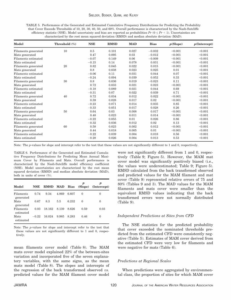
The NSE values for the MAM cover predicted fromthe generated CFDs were high (Table 6; Figure 4).The RMSD and MAD for the MAM filament coverpredictions were correspondingly low and representedrelative errors of 44 and 23%, respectively (Table 3).The RMSD and MAD for the MAM mats cover pre-dictions made from the generated CFDs were alsolow and represented relative errors of 45 and 30%,respectively (Table 3). However, the MAM valuespredicted from the generated CFD were positivelybiased (i.e., the values were underestimated) (Table 6;Figure 4).

TABLE 3. Periphyton Cover Characteristics of the 78 Study SitesIncluding the Mean, Minimum, and Maximum of: the Mean SiteCover, Mean Annual Maximum (MAM) Cover, and the Probabilitythat Cover in Both Categories (filaments and mats) ExceededThresholds of 10, 20, 30, 40, 50, and 60%.

Characteristic Mean Minimum Maximum

Mean filamentous cover (%) 6 0 26Mean mats cover (%) 5 0 24MAM filamentous cover (%) 21 0 67MAM mats cover (%) 18 0 59Probability (filaments > 10%) 0.14 0 0.6Probability (filaments > 20%) 0.09 0 0.4Probability (filaments > 30%) 0.06 0 0.4Probability (filaments > 40%) 0.04 0 0.3Probability (filaments > 50%) 0.03 0 0.3Probability (filaments > 60%) 0.02 0 0.2Probability (mats > 10%) 0.13 0 0.5Probability (mats > 20%) 0.08 0 0.3Probability (mats > 30%) 0.05 0 0.3Probability (mats > 40%) 0.03 0 0.3Probability (mats > 50%) 0.02 0 0.2Probability (mats > 60%) 0.01 0 0.2

TABLE 4. Pearson Correlation Coefficients betweenMean and Mean Annual Maximum (MAM) Coverby Filaments and Mats at the 78 Study Sites.

MeanFilaments

MeanMats

MAMFilaments

Mean mats 0.57MAM filaments 0.94 0.46MAM mats 0.51 0.94 0.44

Note: All correlations were significant (p < 0.001).



Regression Models

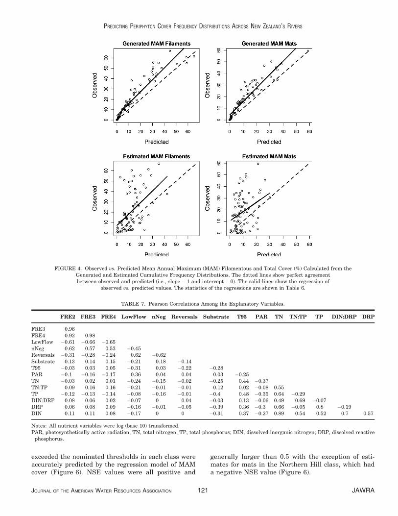
Most pairs of the candidate explanatory variableshad low correlation (Table 7). However, many ofthe nutrient variables were moderately correlated(0.5 < r < 0.7) and TN was highly correlated withDRP and TP. With the exception of FRE2, 3, and 4,which were highly correlated, the hydrological indiceswere only moderately correlated indicating that theycomprised unique information about the hydrologicalregimes at the sites.

The mean filament cover model explained 42% ofthe between-sites variation (Table 8). The fitted coeffi-cients were consistent with the conceptual model offactors controlling periphyton cover (Tables 1 and 8).The mean mats cover model explained 32% of thebetween-sites variation (Table 8). The fitted coeffi-cients were consistent with the conceptual model of

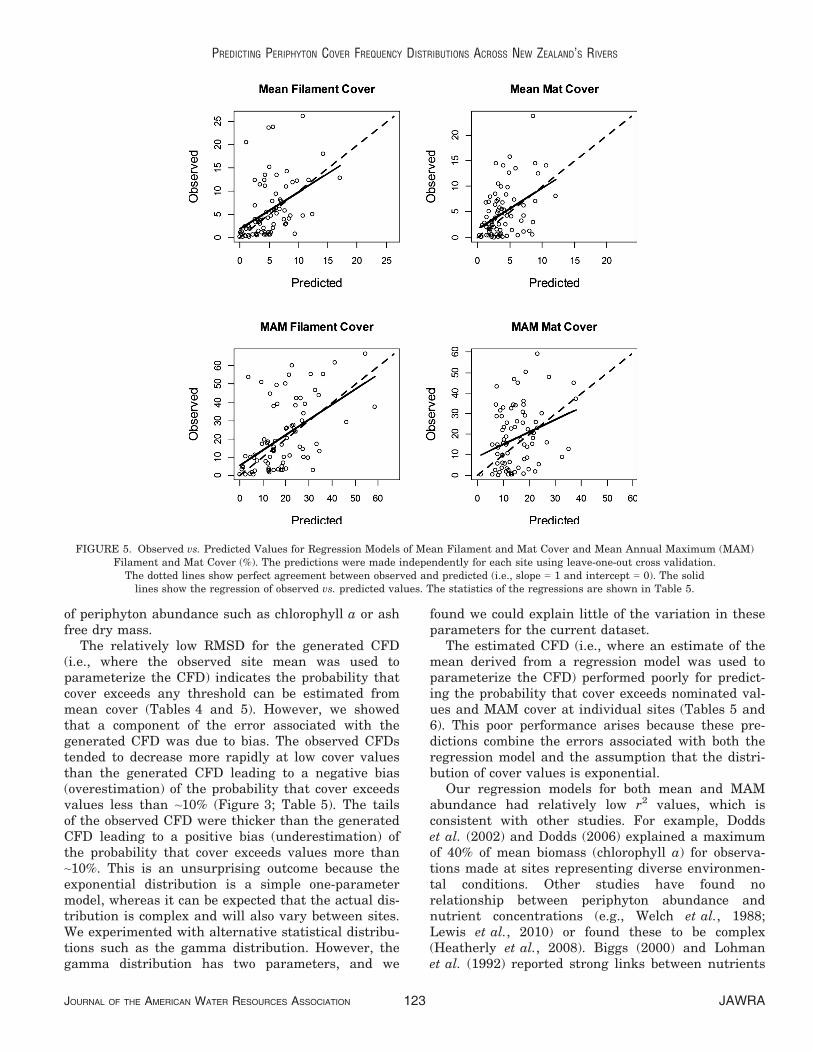
factors controlling periphyton cover except for Rever-sals, which were positively related to cover (Tables 1and 8). For the mean cover models, the slopes andintercepts of the regressions of the back-transformedobserved vs. predicted values were not significantly dif-ferent to 1 and 0, respectively, indicating the modelswere consistent and unbiased (Table 9; Figure 4).RMSD calculated from the back-transformed observedand predicted mean filaments and mats cover repre-sented relative errors of 95 and 91%, respectively(Tables 9 and 3). The MAD values for the mean fila-mentous and mats cover models were smaller than theequivalent RMSD values indicating that the back-transformed errors were not normally distributed(Table 9).

The MAM filament cover model explained 45% ofthe variation between sites and included the sameexplanatory variables, with the same signs, as the

FIGURE 3. Examples of Observed, Generated, and Estimated Cumulative Frequency Distributions (CFDs) for Cover by Filaments(top two rows) and Mats (lower two rows) for Eight Randomly Selected Sites. The generated CFDs were calculated using the

theoretical distribution parameterized with the observed mean (lobs). The estimated CFDs were calculated usingthe theoretical distribution parameterized with the mean estimated by regression model (lest).



mean filaments cover model (Table 8). The MAMmats cover model explained 22% of the between-sitesvariation and incorporated five of the seven explana-tory variables, with the same signs, as the meanmats model (Table 8). The slopes and intercepts ofthe regression of the back transformed observed vs.predicted values for the MAM filament cover model

were not significantly different from 1 and 0, respec-tively (Table 9; Figure 5). However, the MAM matcover model was significantly positively biased (i.e.,the values were underestimated; Table 9; Figure 5).RMSD calculated from the back transformed observedand predicted values for the MAM filament and matcover (Table 9) represented relative errors of 75 and80% (Tables 9 and 3). The MAD values for the MAMfilaments and mats cover were smaller than theequivalent RMSD values indicating that the backtransformed errors were not normally distributed(Table 9).

Independent Predictions at Sites from CFD

The NSE statistics for the predicted probabilitythat cover exceeded the nominated thresholds pre-dicted from the estimated CFD were consistently neg-ative (Table 5). Estimates of MAM cover derived fromthe estimated CFD were very low for filaments andwere negative for mats (Table 6).

Predictions at Regional Scales

When predictions were aggregated by environmen-tal class, the proportion of sites for which MAM cover

TABLE 5. Performance of the Generated and Estimated Cumulative Frequency Distributions for Predicting the Probabilitythat Cover Exceeds Thresholds of 10, 20, 30, 40, 50, and 60%. Overall performance is characterized by the Nash-Sutcliffe

efficiency statistic (NSE). Model uncertainty and bias are reported as probabilities Pr (0 ≤ Pr < 1). Uncertainties arecharacterized by the root mean squared deviation (RMSD) and median absolute deviation (MAD).

Model Threshold (%) NSE RMSD MAD Bias p(Slope) p(Intercept)

Filaments generated 10 0.5 0.101 0.027 �0.032 <0.001 <0.001Mats generated 0.47 0.095 0.03 �0.012 <0.001 <0.001Filaments estimated �0.07 0.149 0.06 �0.009 <0.001 <0.001Mats estimated �0.15 0.14 0.078 0.031 <0.001 <0.001Filaments generated 20 0.82 0.045 0.022 0.015 <0.001 <0.001Mats generated 0.8 0.038 0.023 0.025 0.01 <0.001Filaments estimated �0.06 0.11 0.031 0.044 0.07 <0.001Mats estimated �0.24 0.094 0.039 0.052 0.33 <0.001Filaments generated 30 0.8 0.036 0.019 �0.023 0.11 <0.001Mats generated 0.72 0.033 0.021 0.023 <0.001 <0.001Filaments estimated �0.18 0.089 0.021 0.044 0.69 <0.001Mats estimated �0.31 0.07 0.022 0.039 0.71 <0.001Filaments generated 40 0.72 0.034 0.012 0.022 <0.001 <0.001Mats generated 0.59 0.028 0.017 0.02 <0.001 <0.001Filaments estimated �0.23 0.071 0.014 0.035 0.85 <0.001Mats estimated �0.33 0.051 0.017 0.028 0.26 <0.001Filaments generated 50 0.64 0.03 0.008 0.017 <0.001 <0.001Mats generated 0.48 0.023 0.011 0.014 <0.001 <0.001Filaments estimated �0.22 0.055 0.01 0.026 0.86 <0.001Mats estimated �0.32 0.036 0.012 0.02 0.13 <0.001Filaments generated 60 0.58 0.023 0.002 0.012 <0.001 <0.001Mats generated 0.44 0.018 0.005 0.01 <0.001 <0.001Filaments estimated �0.22 0.039 0.004 0.018 0.56 <0.001Mats estimated �0.28 0.026 0.004 0.013 0.53 <0.001

Note: The p-values for slope and intercept refer to the test that these values are not significantly different to 1 and 0, respectively.

TABLE 6. Performance of the Generated and Estimated Cumula-tive Frequency Distributions for Predicting Mean Annual Maxi-mum Cover by Filaments and Mats. Overall performance ischaracterized by the Nash-Sutcliffe model efficiency coefficient(NSE). Model uncertainties are characterized by the root meansquared deviation (RMSD) and median absolute deviation (MAD),both in units of cover (%).

Model NSE RMSD MAD Biasp

(Slope)p

(Intercept)

Filamentsgenerated

0.74 9.34 4.869 6.607 0 0

Matsgenerated

0.67 8.3 5.5 6.232 0 0

Filamentsestimated

0.03 18.162 8.139 8.626 0.59 0.03

Matsestimated

�0.22 16.024 9.985 8.283 0.46 0

Note: The p-values for slope and intercept refer to the test thatthese values are not significantly different to 1 and 0, respec-tively.



exceeded the nominated thresholds in each class wereaccurately predicted by the regression model of MAMcover (Figure 6). NSE values were all positive and

generally larger than 0.5 with the exception of esti-mates for mats in the Northern Hill class, which hada negative NSE value (Figure 6).

FIGURE 4. Observed vs. Predicted Mean Annual Maximum (MAM) Filamentous and Total Cover (%) Calculated from theGenerated and Estimated Cumulative Frequency Distributions. The dotted lines show perfect agreementbetween observed and predicted (i.e., slope = 1 and intercept = 0). The solid lines show the regression of

observed vs. predicted values. The statistics of the regressions are shown in Table 6.

TABLE 7. Pearson Correlations Among the Explanatory Variables.

FRE2 FRE3 FRE4 LowFlow nNeg Reversals Substrate T95 PAR TN TN:TP TP DIN:DRP DRP

FRE3 0.96FRE4 0.92 0.98LowFlow �0.61 �0.66 �0.65nNeg 0.62 0.57 0.53 �0.45Reversals �0.31 �0.28 �0.24 0.62 �0.62Substrate 0.13 0.14 0.15 �0.21 0.18 �0.14T95 �0.03 0.03 0.05 �0.31 0.03 �0.22 �0.28PAR �0.1 �0.16 �0.17 0.36 0.04 0.04 0.03 �0.25TN �0.03 0.02 0.01 �0.24 �0.15 �0.02 �0.25 0.44 �0.37TN:TP 0.09 0.16 0.16 �0.21 �0.01 �0.01 0.12 0.02 �0.08 0.55TP �0.12 �0.13 �0.14 �0.08 �0.16 �0.01 �0.4 0.48 �0.35 0.64 �0.29DIN:DRP 0.08 0.06 0.02 �0.07 0 0.04 �0.03 0.13 �0.06 0.49 0.69 �0.07DRP 0.06 0.08 0.09 �0.16 �0.01 �0.05 �0.39 0.36 �0.3 0.66 �0.05 0.8 �0.19DIN 0.11 0.11 0.08 �0.17 0 0 �0.31 0.37 �0.27 0.89 0.54 0.52 0.7 0.57

Notes: All nutrient variables were log (base 10) transformed.PAR, photosynthetically active radiation; TN, total nitrogen; TP, total phosphorus; DIN, dissolved inorganic nitrogen; DRP, dissolved reactivephosphorus.



Predictions of MAM cover made from the esti-mated CFD were adjusted by the model bias (Table 6)before aggregating the predictions by environmentalclass. When predictions were aggregated by environ-mental class, the proportion of sites for which MAM

cover exceeded the nominated thresholds was accu-rately predicted for some classes (Figure 7). NSEvalues were positive for three of the four classes forboth filaments and mats. The NSE values for the pre-dicted proportion of sites for which filamentsexceeded the thresholds were negative for the South-ern Hill class but were larger than 0.2 for the otherclasses (Figure 7). The predictions for mats were neg-ative for the Northern Hill class, but were largerthan 0.45 for the other classes (Figure 7).

DISCUSSION

In this study, we derived empirical models of meanand MAM periphyton cover for two categories (fila-ments and mats) that are relevant to establishedguidelines for New Zealand rivers (Ministry for theEnvironment, 2000). We found that filaments wereonly moderately correlated with mats and that sepa-rate models were required to best predict the two cat-egories. We also showed that the frequencydistribution for the cover categories is approximatedby the exponential distribution and quantified theerrors associated with this approximation. Our studywas based on periphyton cover observations, but themethod may be equally applicable to other measures

TABLE 8. Statistics of the Regression Models of Mean and Mean Annual Maximum (MAM) Cover by Filamentsand Mats Including the r2 Values, Coefficients, Standard Errors, and p Values for the Explanatory Variables.

Explanatory Variable

Periphyton Category

Mean Filaments (r2 = 0.42) MAM Filaments (r2 = 0.45)

Coefficient SE Pr(>|t|) Coefficient SE Pr(>|t|)

Intercept 1.056 1.966 0.593 0.413 3.347 0.902FRE2 �0.097 0.044 0.031 �0.177 0.075 0.021nNeg �0.012 0.006 0.052 �0.016 0.01 0.13LowFlow �3.126 1.048 0.004 �5.908 1.784 0.001T95 0.114 0.053 0.035 0.244 0.09 0.009PAR 0.004 0.001 0 0.008 0.002 0log10TN 0.884 0.385 0.025 1.594 0.656 0.018log10DIN:DRP �0.393 0.259 0.135 �0.73 0.442 0.103

Mean Mats (r2 = 0.32) MAM Mats (r2 = 0.22)

Intercept �5.324 2.142 0.015 �0.61 1.629 0.709FRE4 �0.117 0.042 0.007 �0.206 0.079 0.011Reversals 0.023 0.006 0 0.033 0.012 0.007LowFlow �3.062 1.323 0.024 �6.607 2.453 0.009Substrate 0.65 0.338 0.058 NA NA NAPAR 0.003 0.001 0.002 0.005 0.002 0.009log10TN:TP 0.542 0.358 0.134 1.235 0.667 0.068log10DRP 0.738 0.292 0.014 NA NA NA

Notes: NA indicates the explanatory variable was not included in the model.PAR, photosynthetically active radiation; TN, total nitrogen; TP, total phosphorus; DIN, dissolved inorganic nitrogen; DRP, dissolved reactivephosphorus.

TABLE 9. Performance of the Regression Models of Mean andMean Annual Maximum (MAM) Cover by Filaments and Mats.Model predictions were independent of the models (i.e., for sites notused in fitting the models) using leave-one-out cross validation.Overall performance is characterized by the Nash-Sutcliffe modelefficiency coefficient (NSE). NSE and RMSD1 values are for theregression of square root transformed observed and predicted val-ues. The values RMSD2, bias, and p values for slope and interceptwere calculated from the back-transformed data.

NSE RMSD1 RMSD2 Biasp

(Slope)p

(Intercept)

Meanfilaments

0.25 1.04 5.55 0.00 0.14 0.17

Meanmats

0.16 1.01 4.38 �0.83 0.34 0.09

MAMfilaments

0.30 1.2 15.9 �2.3 0.28 0.22

MAMmats

0.08 1.87 14.5 �2.95 0.07 0.02

Notes: The p values for slope and intercept refer to the nullhypothesis that these values are not significantly different from 1and 0, respectively. Details of the explanatory variables are pro-vided in Table 1.

RMSD, root mean squared deviation.



of periphyton abundance such as chlorophyll a or ashfree dry mass.

The relatively low RMSD for the generated CFD(i.e., where the observed site mean was used toparameterize the CFD) indicates the probability thatcover exceeds any threshold can be estimated frommean cover (Tables 4 and 5). However, we showedthat a component of the error associated with thegenerated CFD was due to bias. The observed CFDstended to decrease more rapidly at low cover valuesthan the generated CFD leading to a negative bias(overestimation) of the probability that cover exceedsvalues less than ~10% (Figure 3; Table 5). The tailsof the observed CFD were thicker than the generatedCFD leading to a positive bias (underestimation) ofthe probability that cover exceeds values more than~10%. This is an unsurprising outcome because theexponential distribution is a simple one-parametermodel, whereas it can be expected that the actual dis-tribution is complex and will also vary between sites.We experimented with alternative statistical distribu-tions such as the gamma distribution. However, thegamma distribution has two parameters, and we

found we could explain little of the variation in theseparameters for the current dataset.

The estimated CFD (i.e., where an estimate of themean derived from a regression model was used toparameterize the CFD) performed poorly for predict-ing the probability that cover exceeds nominated val-ues and MAM cover at individual sites (Tables 5 and6). This poor performance arises because these pre-dictions combine the errors associated with both theregression model and the assumption that the distri-bution of cover values is exponential.

Our regression models for both mean and MAMabundance had relatively low r2 values, which isconsistent with other studies. For example, Doddset al. (2002) and Dodds (2006) explained a maximumof 40% of mean biomass (chlorophyll a) for observa-tions made at sites representing diverse environmen-tal conditions. Other studies have found norelationship between periphyton abundance andnutrient concentrations (e.g., Welch et al., 1988;Lewis et al., 2010) or found these to be complex(Heatherly et al., 2008). Biggs (2000) and Lohmanet al. (1992) reported strong links between nutrients

FIGURE 5. Observed vs. Predicted Values for Regression Models of Mean Filament and Mat Cover and Mean Annual Maximum (MAM)Filament and Mat Cover (%). The predictions were made independently for each site using leave-one-out cross validation.

The dotted lines show perfect agreement between observed and predicted (i.e., slope = 1 and intercept = 0). The solidlines show the regression of observed vs. predicted values. The statistics of the regressions are shown in Table 5.



and periphyton abundance. However, the sites inthese studies comprised a limited range of environ-mental conditions and the locale was more restrictedthan this study. This suggests that regional relation-ships may provide greater predictive ability, but atthe expense of generality (Dodds et al., 2002).

The prediction uncertainties were derived fromcross-validation of the regression models of the meanand MAM cover for both periphyton categories andwere small in absolute terms (Table 9). However, con-sistent with the low r2 values, the relative uncertain-ties (i.e., compared with the mean of the values beingestimated) were quite large (75-95%; Tables 9 and 3).The errors calculated from the back-transformed pre-dictions were not normally distributed and the MAD(i.e., the error exceeded by half of the sites) was con-sistently smaller than the RMSD. Thus, the majorityof sites had relatively low errors, but there were largeerrors at a small number of sites.

The low r2 values and large uncertainties may bepartly due to sources of variation in periphyton coverthat were not represented by our explanatory vari-ables. For example, we did not include variables thataccount for differences in periphyton communitiesbetween sites or differences in the intensity of inver-

tebrate grazing. Inconsistent relationships betweenperiphyton cover and nutrients may be due to theconfounding effects of uptake from the water columnby the standing crop and the mediation of uptake byhydraulic conditions (Hall et al., 2002). It is likelythat our regression models have revealed only thestrongest patterns between periphyton cover andenvironment and their explanatory power was limitedby the number of sites and availability of potentialexplanatory variables in our dataset.

The predictions of the proportion of sites thatexceed nominated thresholds within environmentalclasses, made using both the estimated CFD and theregression model of MAM, were more accurate thanthe site-scale predictions (Figures 6 and 7). The clas-sification provided a strong test of the broad-scalepredictions because the classes themselves discrimi-nate variation in the correlates of periphyton cover.The North and South Islands discriminate variationin climatic factors and catchment topography discrim-inates differences in hydrology and water quality(Snelder and Biggs, 2002; Larned et al., 2004). Thus,we are confident that, despite large site-scale uncer-tainties, the models provide a useful representationof the broad-scale pattern of periphyton cover across

FIGURE 6. Observed vs. Predicted Values for the Proportion of Sites in Each Environmental Class for Which Mean AnnualMaximum (MAM) Cover Exceeds Nominated Thresholds. The MAM predictions were made using the regression model

and were made independently for each site using leave-one-out cross validation.



New Zealand. In addition, the regression models ofmean and MAM periphyton cover included severalhydrological indices, nutrient status, and light regime(PAR) as explanatory variables. Thus, the models arepotentially useful for assessing the broad-scale effectsof changes of these factors on periphyton cover.

Our models should be used cautiously and predic-tions should not be made outside the range of the fit-ting dataset (Table 1). It should also be recognizedthat our models describe differences between sites.Using the models to infer changes at a site assumesthat the modeled relationships are transferable andgeneral. We did not test the validity of this space-for-time-substitution in this study.

The relationships between the explanatory vari-ables and periphyton cover were consistent with ourunderstanding of the factors controlling periphytonabundance and relationships found by other studies.Periphyton cover was generally positively related toeither nitrogen or phosphorus concentrations (thatwere strongly intercorrelated). In accord with ourconceptual model (Table 2), models that included TNas a significant predictor also included DIN:DRP as anegative influence. In addition, models that includedDRP also included TN:TP as a positive influence.These combinations of variables reflect the combined

influences of these key nutrients on periphytongrowth rates and suggest both nitrogen and phospho-rus should be considered as potentially limiting nutri-ents (Dodds et al., 2002). Dodds et al. (2002) foundthat periphyton biomass (chlorophyll a) was nega-tively correlated with latitude, which they consideredwas associated with increased light. This is consistentwith the inclusion of PAR in our models. We alsofound that periphyton cover was positively correlatedwith temperature, which is also consistent withDodds et al. (2002).

Our models suggest that several independentaspects of the hydrological regime are associated withperiphyton cover (Table 8). Cover decreased withincreasing values of LowFlow and FREn, indicatingthat cover is lower at sites that have high base flowsand frequent floods. Mean filamentous cover was alsonegatively related to rates of change in flow (nNeg). Ingeneral, the consequence of water abstraction, dams,or diversions is to reduce base flows, flood flows, andthe rates of change in flows at a site and this is consis-tent with the observation that abstraction tends toincrease periphyton abundance (Lowe, 1979; Biggsand Price, 1987). We found that mean and MAM matcover was positively related to hydrological reversals(Reversals). The positive relationship between mat

FIGURE 7. Observed vs. Predicted Values for the Proportion of Sites in Each Environmental Class for Which Mean AnnualMaximum (MAM) Cover Exceeds Nominated Thresholds. The MAM predictions for each site were made using theestimated cumulative frequency distributions (CFDs) and were adjusted by the estimated model bias (Table 6).



cover and hydrological reversals may be associatedwith the higher resistance of mat-forming taxa and thetendency for mats to be the dominant growth form athydrologically disturbed sites (Biggs et al., 1998a, b).

We tested a variety of other regression model for-mulations, including models with nonlinear termsand interactions between various explanatory vari-ables. While some of these formulations increased theexplained variation, they generally did not improvethe predictive performance. Biggs (2000) and Doddset al. (2002) suggest that regionalized regressionmodels, such as those often applied to predictinghydrological indices (e.g., Laaha and Bl€oschl, 2006),could improve periphyton–environment relationships.The prerequisite for this, however, is a sufficientnumber of sites within each region and thereforeongoing monitoring of periphyton abundance andenvironmental characteristics such as that under-taken by the NRWQN would be necessary to advancethis approach.

CONCLUSION

While the uncertainty of our models is large at thesite scale, we showed that they produce accurate pre-dictions of broad-scale patterns. We conclude that themodels are potentially useful for making broad-scaleassessments of mean and MAM periphyton cover andcover frequency distributions in rivers and for esti-mating the strength and direction of changes in coverin response to changes in nutrients, hydrologicalregime, and light. Estimates of several of the explan-atory variables required by our models are availablefor all river locations in New Zealand including med-ian nutrient concentrations (Unwin et al., 2010) andestimates of the hydrological indices (Booker andSnelder, 2012). Future research could develop esti-mates of PAR, T95, and the substrate index for allriver locations in New Zealand using methods similarto Unwin et al. (2010) and Snelder et al. (2011).These data would allow mean cover to be estimatedat new sites without the need to make observationsof water quality and hydrology.

ACKNOWLEDGMENTS

This research was funded by the New Zealand Ministry forBusiness, Innovation and Enterprise, Environmental Flows Pro-gram (C01X0308), and Wheel of Water Program (ALNC1102). Wethank the field and laboratory teams who helped to collect datarelated to the NRWQN, without which this study would not havebeen possible. Thanks in particular to Graham Bryers who checkedand collated the data over the life of the NRWQN programme. We

thank two anonymous reviewers whose comments improved ouroriginal manuscript.

LITERATURE CITED

Akaike, H., 1973. Information Theory and an Extension of theMaximum Likelihood Principle. In: Second InternationalSymposium on Information Theory, B.N. Petrov and F. Csaki(Editors). Akademiai Kiado, Budapest, pp. 267-281.

Biggs, B.J.F., 1996. Hydraulic Habitat of Plants in Streams. Regu-lated Rivers: Research and Management 12:131-144.

Biggs, B.J.F., 2000. Eutrophication of Streams and Rivers: Dis-solved Nutrient-Chlorophyll Relationships. Journal of the NorthAmerican Benthological Society 19:17-31.

Biggs, B.J.F., D.G. Goring, and V.I. Nikora, 1998a. Subsidy andStress Responses of Stream Periphyton to Gradients in WaterVelocity as a Function of Community Growth Form. Journal ofPhycology 34:598-607.

Biggs, B.J.F. and G.M. Price, 1987. A Survey of Filamentous AlgalProliferations in New Zealand Rivers. New Zealand Journal ofMarine and Freshwater Research 21:175-191.

Biggs, B.J., F.R.J. Stevenson, and R.L. Lowe, 1998b. A HabitatMatrix Conceptual Model for Stream Periphyton. Archiv F€urHydrobiologie 143:25-56.

Booker, D.J., 2010. Predicting Wetted Width in Any River at AnyDischarge. Earth Surface Processes and Landforms 35:828-841.

Booker, D.J. and T.H. Snelder, 2012. Comparing Methods for Esti-mating Flow Duration Curves at Ungauged Sites. Journal ofHydrology 438:78-94.

Boothroyd, I.K.G., J.M. Quinn, E.R. Langer, K.J. Costley, and G.Steward, 2004. Riparian Buffers Mitigate Effects of Pine Planta-tion Logging on New Zealand Streams: 1. Riparian VegetationStructure, Stream Geomorphology and Periphyton. Forest Ecol-ogy and Management 194:199-213.

Brock, T.D., 1981. Calculating Solar Radiation for Ecological Stud-ies. Ecological Modelling 14:1-19.

Clausen, B. and B.J.F. Biggs, 1997. Relationships Between BenthicBiota and Hydrological Indices in New Zealand Streams. Fresh-water Biology 38:327-342.

Crawley, M.J., 2002. Statistical Computing: An Introduction toData Analysis Using S-Plus. John Wiley & Sons, Inc., Hoboken,New Jersey.

Davies-Colley, R.J. and J.W. Nagels, 2008. Predicting Light Pene-tration into River Waters. Journal of Geophysical Research 113:G03028.

Davies-Colley, R.J. and J.M. Quinn, 1998. Stream Lighting in FiveRegions of North Island, New Zealand: Control by Channel Sizeand Riparian Vegetation. New Zealand Journal of Marine andFreshwater Research 32:591-605.

Davies-Colley, R.J., D.G. Smith, R.C. Ward, G.G. Bryers, G.B.McBride, J.M. Quinn, and M.R. Scarsbrook, 2011. Twenty Yearsof New Zealand’s National Rivers Water Quality Network: Ben-efits of Careful Design and Consistent Operation. Journal of theAmerican Water Resources Association 47:750-771.

Dodds, W.K., 2006. Eutrophication and Trophic State in Rivers andStreams. Limnology and Oceanography 51(1):671-680.

Dodds, W.K., V.H. Smith, and K. Lohman, 2002. Nitrogen andPhosphorus Relationships to Benthic Algal Biomass in Temper-ate Streams. Canadian Journal of Fisheries and Aquatic Sci-ences 59(5):865-874.

Dodds, W.K., V.H. Smith, and B. Zander, 1997. Developing NutrientTargets to Control Benthic Chlorophyll Levels in Streams: A CaseStudy of the Clark Fork River. Water Research 31:1738-1750.

Dodds, W.K.K. and E.B. Welch, 2000. Establishing Nutrient Crite-ria in Streams. Journal of the North American BenthologicalSociety 19:186-196.



Doyle, M.W. and E.H. Stanley, 2006. Exploring Potential Spatial-Temporal Links Between Fluvial Geomorphology and Nutrient-Periphyton Dynamics in Streams Using Simulation Models.Annals of the Association of American Geographers 96:687-698.

Finlay, J.C., S. Khandwala, and M.E. Power, 2002. Spatial Scalesof Carbon Flow in a River Food Web. Ecology 83:1845-1859.

Flinders, C.A. and D.D. Hart, 2009. Effects of Pulsed Flows on Nui-sance Periphyton Growths in Rivers: A Mesocosm Study. RiverResearch and Applications 25:1320-1330.

Hall, Jr., R.O., E.S. Bernhardt, and G.E. Likens, 2002. RelatingNutrient Uptake with Transient Storage in Forested MountainStreams. Limnology and Oceanography 47(1):255-265.

Hastie, T., R. Tibshirani, and J.H. Friedman, 2001. The Elementsof Statistical Learning: Data Mining, Inference, and Prediction.Springer-Verlag, New York City, New York.

Heatherly, T., M.B. David, C.A. Mitchell, T.V. Royer, K.M. Starks,M.R. Whiles, and L.E. Gentry, 2008. Assessment of Chlorophyll-asa Criterion for Establishing Nutrient Standards in the Streams andRivers of Illinois. Journal of EnvironmentalQuality 37:437-447.

Horner, R.R., E.B. Welch, M.R. Seeley, and J.M. Jacoby, 1990.Responses of Periphyton to Changes in Current Velocity, Sus-pended Sediment and Phosphorus Concentration. FreshwaterBiology 24(2):215-232.

Jowett, I.G. and J. Richardson, 1990. Microhabitat Preferences ofBenthic Invertebrates in a New Zealand River and the Develop-ment of In-Stream Flow-Habitat Models for Deleatidium spp.New Zealand Journal of Marine and Freshwater Research24:19-30.

Julian, J.P., M.W. Doyle, and E.H. Stanley, 2008. Empirical Model-ing of Light Availability in Rivers. Journal of GeophysicalResearch 113:G03022.

Kiffney, P.M., J.S. Richardson, and W.L. Montgomery, 2001. Inter-actions Among Nutrients, Periphyton, and Invertebrate andVertebrate (Ascaphus Truei) Grazers in Experimental Channels.Copeia 2001:422-429.

Kilroy, C., S.T. Larned, and B.J.F. Biggs, 2009. The Non-Indige-nous Diatom Didymosphenia Geminata Alters Benthic Commu-nities in New Zealand Rivers. Freshwater Biology 54:1990-2002.

Kobayashi, K. and M. Salam, 2000. Comparing Simulated andMeasured Values Using Mean Squared Deviation and ItsComponents. Agronomy Journal 92:345.

Laaha, G. and G. Bl€oschl, 2006. A Comparison of Low Flow Region-alisation Methods—Catchment Grouping. Journal of Hydrology323:193-214.

Larned, S.T., M.R. Scarsbrook, T. Snelder, N.J. Norton, and B.J.F.Biggs, 2004. Water Quality in Low-Elevation Streams andRivers of New Zealand. New Zealand Journal of Marine &Freshwater Research 38:347-366.

Lewis, J.R., M. William, J.R. Mccutchan, and H. James, 2010.Ecological Responses to Nutrients in Streams and Rivers of theColorado Mountains and Foothills. Freshwater Biology 55:1973-1983.

Liess, A. and H. Hillebrand, 2006. Role of Nutrient Supply in Gra-zer-Periphyton Interactions: Reciprocal Influences of Periphytonand Grazer Nutrient Stoichiometry. Journal of the North Ameri-can Benthological Society 25:632-642.

Lohman, K., J.R. Jones, and B.D. Perkins, 1992. Effects of NutrientEnrichment and Flood Frequency on Periphyton Biomass inNorthern Ozark Streams. Canadian Journal of Fisheries andAquatic Sciences 49(6):1198-1205.

Lowe, R.L., 1979. Phytobenthic Ecology and Regulated Streams.The Ecology of Regulated Streams. Plenum Press, New YorkCity, New York, pp. 25-34.

Ministry for the Environment, 2000. New Zealand PeriphytonGuideline: Detecting, Monitoring and Managing Enrichment ofStreams. Ministry for the Environment, Wellington, New Zea-land.

Ministry for the Environment, 2007. Environment New Zealand.Ministry for the Environment, Wellington, New Zealand.

Moriasi, D.N., J.G. Arnold, M.W. Van Liew, R.L. Bingner, R.D.Harmel, and T.L. Veith, 2007. Model Evaluation Guidelines forSystematic Quantification of Accuracy in Watershed Simula-tions. Transactions of the ASABE 50:885-900.

Olden, J.D. and N.L. Poff, 2003. Redundancy and the Choice ofHydrologic Indices for Characterizing Streamflow Regimes.River Research and Applications 19:101-121.

Pi~neiro, G., S. Perelman, J. Guerschman, and J. Paruelo, 2008.How to Evaluate Models: Observed vs. Predicted or Predictedvs. Observed? Ecological Modelling 216:316-322.

Quinn, J.M. and C.W. Hickey, 1990. Characterisation and Classifi-cation of Benthic Invertebrate Communities in 88 New ZealandRivers in Relation to Environmental Factors. New ZealandJournal of Marine and Freshwater Research 24:387-410.

Quinn, J.M. and E. Raaphorst, 2009. Trends in Nuisance Periphy-ton Cover at New Zealand National River Water Quality Net-work Sites 1990-2006. NIWA Client Report HAM2008-194,National Institute of Water and Atmospheric Research Ltd.,Hamilton, New Zealand.

Rutherford, J.C., M.R. Scarsbrook, and N. Broekhuizen, 2000.Grazer Control of Stream Algae: Modeling Temperature andFlood Effects. Journal of Environmental Engineering 126:331-339.

Smith, D.G. and R. Maasdam, 1994. New Zealand’s National WaterQuality Network. 1. Design and Physio-Chemical Characterisa-tion. New Zealand Journal of Marine & Freshwater Research28:19-35.

Smith, D.G. and G.B. McBride, 1990. New Zealand’s NationalWater Quality Monitoring Network — Design and First Year’sOperation. Water Resources Bulletin 26:767-775.

Snelder, T.H. and B.J.F. Biggs, 2002. Multi-Scale River Environ-ment Classification for Water Resources Management. Journalof the American Water Resources Association 38:1225-1240.

Snelder, T.H., N. Lamouroux, and H. Pella, 2011. Empirical Model-ling of Large Scale Patterns in River Bed-Surface Grain-Size.Geomorphology 127:189-197.

Snelder, T.H., R. Woods, and B.J.F. Biggs, 2005. Improved Eco-Hydrological Classification of Rivers. River Research and Appli-cations 21:609-628.

Suplee, M.W., V. Watson, M. Teply, and H. McKee, 2009. HowGreen Is Too Green? Public Opinion of What Constitutes Unde-sirable Algae Levels in Streams. Journal of the American WaterResources Association 45:123-140.

Suren, A.M., B.J.F. Biggs, M.J. Duncan, L. Bergey, and P.Lambert, 2003. Benthic Community Dynamics During SummerLow-Flows in Two Rivers of Contrasting Enrichment 2. Inverte-brates. New Zealand Journal of Marine and FreshwaterResearch 37:71-83.

Suren, A.M. and I.G. Jowett, 2006. Effects of Floods Versus LowFlows on Invertebrates in a New Zealand Gravel-Bed River.Freshwater Biology 51:2207-2227.

Uehlinger, U.E., 1991. Spatial and Temporal Variability of thePeriphyton Biomass in a Prealpine River (Necker, Switzerland).Archiv fur Hydrobiologie 123:219-237.

Unwin, M., T. Snelder, D. Booker, D. Ballantine, and J. Lessard,2010. Predicting Water Quality in New Zealand Rivers fromCatchment-Scale Physical, Hydrological and Land CoverDescriptors Using Random Forest Models. NIWA Client ReportCHC2010-0, National Institute of Water and AtmosphericResearch Ltd., Christchurch, New Zealand.

Venables, W.N. and B.D. Ripley, 2002. Modern Applied Statisticswith S (Fourth Edition). Springer, New York City, New York.

Welch, E.B., J.M. Jacoby, R.R. Horner, and M.R. Seeley, 1988.Nuisance Biomass Levels of Periphytic Algae in Streams.Hydrobiologia 157:161-168.



predicting periphyton cover frequency … · predicting periphyton cover frequency distributions...

Documents